Three-dimensional analysis of reinforced concrete frames based on lumped damage mechanics

International Journal of Solids and Structures 40 (2003) 5109–5123

www.elsevier.com/locate/ijsolstr

Three-dimensional analysis of reinforced concreteframes based on lumped damage mechanics

Maria Eugenia Marante a,b, Julio Fl�oorez-L�oopez a,*

a Department of Structural Engineering, University of Los Andes, M�eerida 5101, Venezuelab Department of Structural Engineering, Lisandro Alvarado University, Barquisimeto 3002, Venezuela

Received 30 July 2002; received in revised form 30 December 2002

Abstract

This paper presents a general formulation for the analysis of reinforced concrete frames. The model has been de-

veloped within the framework of lumped damage mechanics. This is a theory based on the methods of continuum

damage mechanics, fracture mechanics and the concept of plastic hinge. The paper also describes the numerical im-

plementation of the model in the finite element programs. The model is evaluated by the numerical simulation of three

tests reported in the literature. Two of them deal with a column subjected to variable axial loads and biaxial flexure. The

third is a two-story three-dimensional frame subjected to earthquake loadings outside the principal directions of the

frame.

� 2003 Elsevier Ltd. All rights reserved.

Keywords: Fracture mechanics; Damage mechanics; Structural analysis; Biaxial bending; Reinforced concrete

1. Introduction

The inelastic analysis of RC framed structures can be carried out in two ways. The first approach, which

is called the fiber beam theory, represents the cross section of each frame member as a set of small filaments

with finite length and in series along the element. Each filament is characterized by the uniaxial constitutive

law that represents the behavior of concrete or steel. Oliva and Clough (1987) list the following references

for the fiber beam theory: Aktan et al. (1973), Okada et al. (1976), Takizawa and Aoyama (1976). The

models proposed by Roufaiel and Meyer (1987), Zeris and Mahin (1991), Anthoine et al. (1997), Oller et al.

(1992) and Bahn and Hsu (2000) can also be included in this category. For very large three-dimensionalstructures, the fiber beam theory is computationally expensive. The second approach, which is called the

frame theory, is based on the formulation of interaction plasticity surfaces and flow rules to define the

flexure-rotational behavior of the element (Nigam, 1967; Padilla-Mora and Schnobrich, 1974; Selna and

Lawder, 1977; Chen and Powell, 1982; Lai et al., 1984). The frame theory is computationally much cheaper

* Corresponding author. Tel./fax: +58-274-2402867.

E-mail addresses: [email protected] (M.E. Marante), [email protected] (J. Fl�oorez-L�oopez).

0020-7683/$ - see front matter � 2003 Elsevier Ltd. All rights reserved.

doi:10.1016/S0020-7683(03)00258-0

mail to: [email protected]

5110 M.E. Marante, J. Fl�oorez-L�oopez / International Journal of Solids and Structures 40 (2003) 5109–5123

than the fiber beam theory. The model in the present paper belongs to the frame theory. While all the

previous models in the frame theory have used the lumped plasticity, we propose a new model based on the

lumped damage mechanics as introduced below.

The basic idea in the lumped damage mechanics is the combination of the methods of continuumdamage and fracture mechanics with the concept of plastic hinge. It provides a general framework for the

analysis of framed structures under severe overloads (typically earthquake loadings), high cycle fatigue,

impacts or blasts. It can be widely applied to civil engineering structures (buildings, bridges) and some

offshore and industrial structures. Cipollina et al. (1995), Bolzon (1996), Fl�oorez-L�oopez (1998), Mazza

(1998), Perdomo et al. (1999) and Perera et al. (2000) have used the lumped damage mechanics to planar

frames. The present work and a previous one by the authors (Marante and Fl�oorez-L�oopez, 2002) attempt to

deal with three-dimensional space frames. A model that describes the process of damage due to biaxial

flexure is presented by taking into account the possibility of variable axial forces and torques. The paperalso describes the finite element implementation of the model. Three test results reported in the literature

(Bousias et al., 1995; Oliva, 1980; Oliva and Clough, 1987) are simulated to validate the model.

2. Kinematics of spatial frames

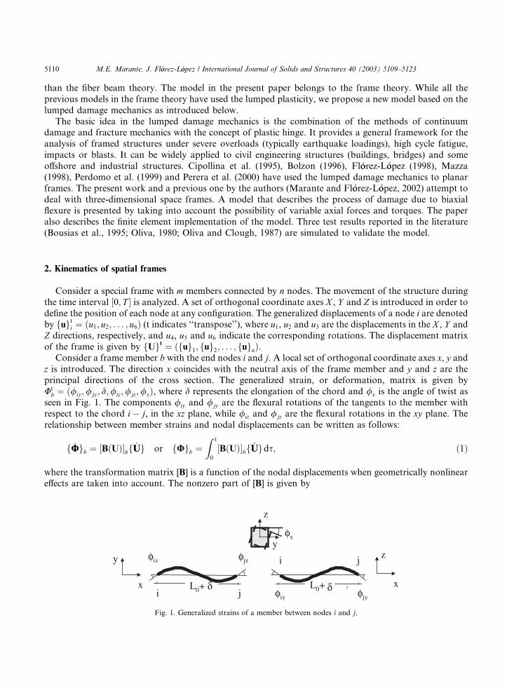
Consider a special frame with m members connected by n nodes. The movement of the structure during

the time interval ½0; T � is analyzed. A set of orthogonal coordinate axes X , Y and Z is introduced in order to

define the position of each node at any configuration. The generalized displacements of a node i are denotedby fugti ¼ ðu1; u2; . . . ; u6Þ (t indicates ‘‘transpose’’), where u1, u2 and u3 are the displacements in the X , Y and

Z directions, respectively, and u4, u5 and u6 indicate the corresponding rotations. The displacement matrix

of the frame is given by fUgt ¼ ðfug1; fug2; . . . ; fugnÞ.Consider a frame member b with the end nodes i and j. A local set of orthogonal coordinate axes x, y and

z is introduced. The direction x coincides with the neutral axis of the frame member and y and z are the

principal directions of the cross section. The generalized strain, or deformation, matrix is given by

Utb ¼ ð/iy ;/jy ; d;/iz;/jz;/xÞ, where d represents the elongation of the chord and /x is the angle of twist as

seen in Fig. 1. The components /iy and /jy are the flexural rotations of the tangents to the member withrespect to the chord i� j, in the xz plane, while /iz and /jz are the flexural rotations in the xy plane. The

relationship between member strains and nodal displacements can be written as follows:

f _UUgb ¼ ½BðUÞ�bf _UUg or fUgb ¼Z t

0

½BðUÞ�bf _UUgds; ð1Þ

where the transformation matrix [B] is a function of the nodal displacements when geometrically nonlineareffects are taken into account. The nonzero part of [B] is given by

y

x

z

φjy

i j

L0+ δ

φjzφiz

i jL0+ δ

z

φiy

φxy

x

Fig. 1. Generalized strains of a member between nodes i and j.

M.E. Marante, J. Fl�oorez-L�oopez / International Journal of Solids and Structures 40 (2003) 5109–5123 5111

½B� ¼

�m1

L�m2

L�m3

Ln1 n2 n3

m1

Lm2

Lm3

L0 0 0

�m1

L�m2

L�m3

L0 0 0

m1

Lm2

Lm3

Ln1 n2 n3

�t1 �t2 �t3 0 0 0 t1 t2 t3 0 0 0n1L

n2L

n3L

m1 m2 m3 � n1L

� n2L

� n3L

0 0 0

n1L

n2L

n3L

0 0 0 � n1L

� n2L

� n3L

m1 m2 m3

0 0 0 �t1 �t2 �t3 0 0 0 t1 t2 t3

26666666666664

37777777777775

; ð2Þ

where t, n, and m are the unit vectors in the x, y, and z directions, respectively. Note that the zeros must beadded to the columns and the lines that do not correspond to any of the degrees of freedom of the element.

The components of these vectors are expressed with respect to the global system of reference.

3. Dynamics of spatial frames

The equilibrium equation for the spatial frames can be obtained via the principle of virtual power,

P �i þ P �

a ¼ P �e 8fU�g; ð3Þ

where P �i is the deformation power (or internal power), P �

a the inertial forces power and P �e the external

nodal forces power. The deformation power is obtained by the introduction of the generalized stresses

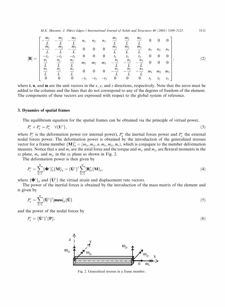
vector for a frame member fMgtb ¼ ðmiy ;mjy ; n;miz;mjz;mxÞ, which is conjugate to the member deformation

measure. Notice that n and mx are the axial force and the torque and miy and mjy are flexural moments in the

xz plane, miz and mjz in the xy plane as shown in Fig. 2.

The deformation power is then given by

P �i ¼

Xmb¼1

f _UU�gtbfMgb ¼ f _UU�gtXmb¼1

½B�tbfMgb; ð4Þ

where f _UU�gb and f _UU�g the virtual strain and displacement rate vectors.

The power of the inertial forces is obtained by the introduction of the mass matrix of the element and

is given by

P �a ¼

Xmb¼1

f _UU�gt½mass�bf€UUg ð5Þ

and the power of the nodal forces by

P �e ¼ f _UU�gtfPg; ð6Þ

Fig. 2. Generalized stresses in a frame member.


where {P} is the nodal external force vector. The principle of virtual power for a framed structure results in

f _UU�gtXmb¼1

½B�tbfMgb þ f _UU�gtXmb¼1

½mass�bf€UUg ¼ f _UU�gtfPg; 8f _UU�g: ð7Þ

Eliminate the virtual displacement rate vector in (7) to obtain the following equilibrium equation:

Xmb¼1

½B�tbfMgb þXmb¼1

½mass�bf€UUg ¼ fPg: ð8Þ

4. Lumped damage mechanics

4.1. Complementary elastic energy and state laws

A generalized constitutive law for a frame member can be obtained by using the lumped dissipation

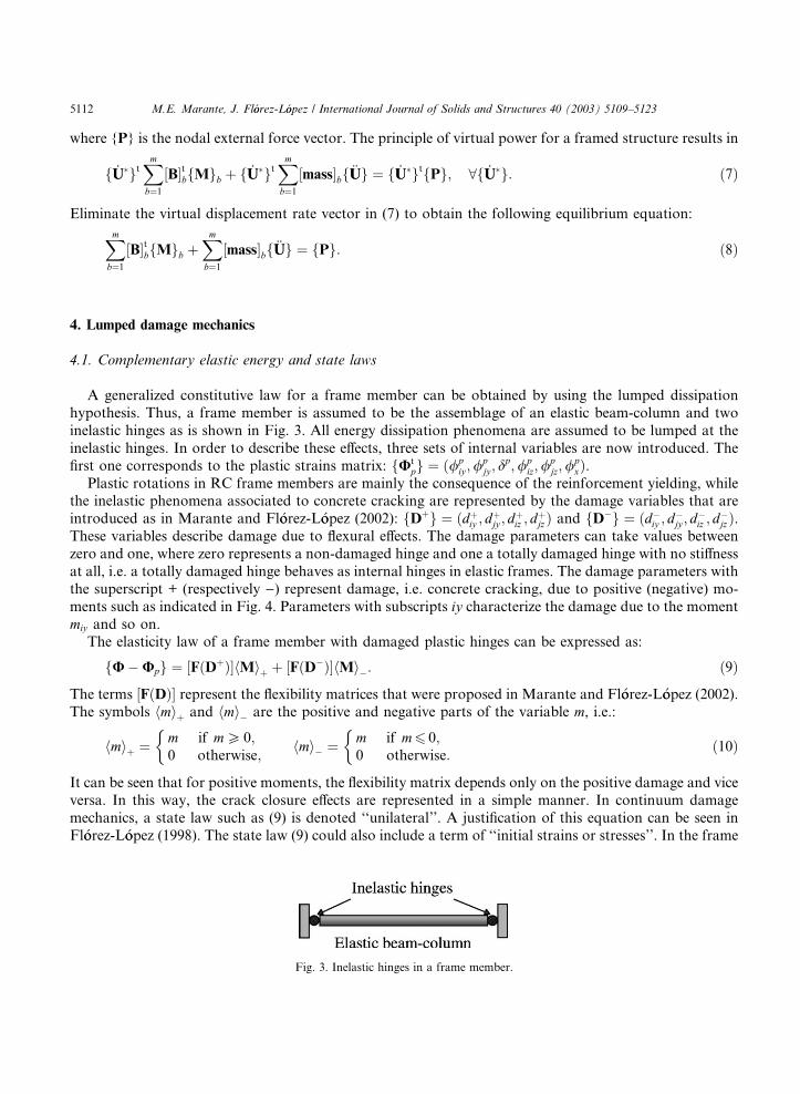
hypothesis. Thus, a frame member is assumed to be the assemblage of an elastic beam-column and two

inelastic hinges as is shown in Fig. 3. All energy dissipation phenomena are assumed to be lumped at the

inelastic hinges. In order to describe these effects, three sets of internal variables are now introduced. The

first one corresponds to the plastic strains matrix: fUtpg ¼ ð/p

iy ;/pjy ; d

p;/piz;/

pjz;/

pxÞ.

Plastic rotations in RC frame members are mainly the consequence of the reinforcement yielding, whilethe inelastic phenomena associated to concrete cracking are represented by the damage variables that are

introduced as in Marante and Fl�oorez-L�oopez (2002): fDþg ¼ ðdþiy ; d

þjy ; d

þiz ; d

þjz Þ and fD�g ¼ ðd�

iy ; d�jy ; d

�iz ; d

�jz Þ.

These variables describe damage due to flexural effects. The damage parameters can take values between

zero and one, where zero represents a non-damaged hinge and one a totally damaged hinge with no stiffness

at all, i.e. a totally damaged hinge behaves as internal hinges in elastic frames. The damage parameters with

the superscript + (respectively )) represent damage, i.e. concrete cracking, due to positive (negative) mo-

ments such as indicated in Fig. 4. Parameters with subscripts iy characterize the damage due to the moment

miy and so on.The elasticity law of a frame member with damaged plastic hinges can be expressed as:

fU�Upg ¼ ½FðDþÞ�hMiþ þ ½FðD�Þ�hMi�: ð9Þ

The terms ½FðDÞ� represent the flexibility matrices that were proposed in Marante and Fl�oorez-L�oopez (2002).The symbols hmiþ and hmi� are the positive and negative parts of the variable m, i.e.:

hmiþ ¼ m if mP 0;0 otherwise;

�hmi� ¼ m if m6 0;

0 otherwise:

�ð10Þ

It can be seen that for positive moments, the flexibility matrix depends only on the positive damage and vice

versa. In this way, the crack closure effects are represented in a simple manner. In continuum damage

mechanics, a state law such as (9) is denoted ‘‘unilateral’’. A justification of this equation can be seen in

Fl�oorez-L�oopez (1998). The state law (9) could also include a term of ‘‘initial strains or stresses’’. In the frame

Fig. 3. Inelastic hinges in a frame member.

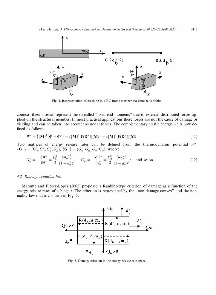
Fig. 4. Representation of cracking in a RC frame member via damage variables.


context, these stresses represent the so called ‘‘fixed end moments’’ due to external distributed forces ap-

plied on the structural member. In most practical applications these forces are not the cause of damage or

yielding and can be taken into account as nodal forces. The complementary elastic energy W � is now de-

fined as follows:

W � ¼ 12fMgtfU�Upg ¼ 1

2fMgt½FðDþÞ�hMiþ þ 1

2fMgt½FðD�Þ�hMi�: ð11Þ

Two matrices of energy release rates can be defined from the thermodynamic potential W �:fGþg ¼ ðGþ

iy ;Gþjy ;G

þiz ;G

þjzÞ, fG

�g ¼ ðG�iy ;G

�jy ;G

�iz ;G

�jzÞ, where:

Gþiy ¼ � oW �

odþiy

¼ F 011

2

hmiyi2þð1� dþ

iy Þ2; G�

iy ¼ � oW �

od�iy

¼ F 011

2

hmiyi2�ð1� d�

iy Þ2; and so on: ð12Þ

4.2. Damage evolution law

Marante and Fl�oorez-L�oopez (2002) proposed a Rankine-type criterion of damage as a function of theenergy release rates of a hinge i. The criterion is represented by the ‘‘non-damage convex’’ and the nor-

mality law that are shown in Fig. 5.

Fig. 5. Damage criterion in the energy release rate space.


Therefore, the ‘‘non-damage zone’’ is limited by the lines:

Gþiy ¼ Rþ

iyðdþiy ; n;mxÞ; G�

iy ¼ R�iyðd�

iy ; n;mxÞ;Gþ

iz ¼ Rþiz ðdþ

iz ; n;mxÞ; G�iz ¼ R�

iz ðd�iz ; n;mxÞ:

ð13Þ

The functions R are denoted crack resistance functions of the inelastic hinge i. It can be noticed that in the

particular case of loadings in only one plane, the damage criterion becomes a generalized form of the

Griffith criterion for a plastic hinge. Crack resistance functions have been identified from experimental

results and depend on the axial force, the torque and the corresponding damage variable. An expression of

R derived from the one proposed in Cipollina et al. (1995) is

R ¼ Gcrðn;mxÞ þ qðn;mxÞlnð1� dÞ1� d

: ð14Þ

The term Gcr represents the crack resistance of the plastic hinge when there is no cracking (d ¼ 0). Thisvalue can be expressed as a function of the first cracking moment of the cross section mcr:

Gcr ¼ 12F0m2

crðn;mxÞ: ð15Þ

The first cracking moment can be computed by the standard methods of the classic reinforced concrete

theory. Notice that the cracking moment depends on the level of axial force and torque, therefore the term

Gcr does too.The other parameter of the crack resistance, the term qðn;mxÞ can also be computed in a similar way, but

this time as function of the ultimate moment of the cross section mu. Indeed, the expression G ¼ R defines

a relationship between the moment and the damage:

F0m2

2¼ ð1� dÞ2Gcr þ qð1� dÞ lnð1� dÞ: ð16Þ

With the help of the expression (16), the ultimate moment mu can be related with a damage value du. It canbe noticed again that the ultimate moment also depends on the axial force and the torque. For these values

the function F0m2=2 reaches a maximum:

F0m2uðn;mxÞ2

¼ ð1� duÞ2Gcr þ qð1� duÞ lnð1� duÞ

� 2ð1� duÞGcr þ q½lnð1� duÞ þ 1� ¼ 0: ð17Þ

From Eq. (17), the value of q (and that of du) can be computed. Again, the ultimate moment can be

computed via the classic theory of reinforced concrete structures.

4.3. Yield function

The plastic behavior of a damaged plastic hinge can be obtained by the introduction of an ‘‘effectivemoment on a plastic hinge’’ and the strain equivalence hypothesis. By analogy with the effective stress of

continuum damage mechanics, the effective moments miy and miz on a plastic hinge i are introduced as follows:

miy ¼

miy

1� dþiy

if dþiy is active;

miy

1� d�iy

if d�iy is active;

8><>: miz ¼

miz

1� dþiz

if dþiz is active;

miz

1� d�iz

if d�iz is active:

8><>: ð18Þ

Now, the yield function of a plastic hinge with damage can be obtained from any of the expressionsproposed in the literature for reinforced concrete frame members by substitution of the moments with the

effective moments. The plastic strains evolution law can be obtained via normality rule:


fi ¼ fiðmiy ;miz;mx; n;/piy ;/

piz;/

pix; d

pi Þ; _//p

iy ¼ _kkiofiomiy

; _//piz ¼ _kki

ofiomiz

; _//pix ¼ _kki

ofiomx

; _ddpi ¼ _kkiofion

;

ð19Þ

the plastic axial deformation and twist of the frame member, are obtained by adding the contribution of

both hinges:

_//px ¼ _kki

ofiomx

þ _kkjofjomx

; _ddp ¼ _kkiofion

þ _kkjofjon

: ð20Þ

In Marante and Fl�oorez-L�oopez (2002), a classical criterion, the Bresler interaction function (Bresler, 1960),

was chosen as a point of departure. A more general criterion (the Bresler function does not consider plastictwist) could also be used.

5. Time-discrete solution algorithm

The strain–displacement equation (1) and the constitutive law (9)–(20) define a relationship between the

generalized stresses in an element b and the nodal displacements: fMgb ¼ fMðUÞgb. The nodal accelera-

tions can also be expressed as a function of the nodal displacements, after time discretization by finite

differences and the use of the Newmark method. Therefore, the time interval ½0; T � is substituted by a

discrete set of instants ð0; t1; t2; . . . ; T Þ. The frame is analyzed only for these times by using a conventional

step-by-step method. The difference between two consecutive instants ðDt ¼ ts � ts�1Þ is called ‘‘global

step’’. Then, the equilibrium equation (8) at a given time ts can be written as:

fLðUÞg ¼Xmb¼1

½B�tbfMðUÞgb þ ½mass�f€UUðUÞg � fPg ¼ 0: ð21Þ

This equation, with the boundary conditions, defines the so called ‘‘global problem’’.

The global problem is solved via the Newton–Raphson method. Each iteration of the global problem for

a given time ts requires the solution of the following linear problem:

fLðUÞg ffi fLðU0Þg þoL

oU

� �fUg¼fU0g

fU�U0g ¼ 0; ð22Þ

where fU0g represents the displacement matrix at the time tn obtained during the precedent iteration and

{U} is the displacement at the present iteration. It can be noticed that in order to build the residual matrix

fLðU0Þg and its Jacobian, the computation of all the matrices fMðU0Þgb and its derivatives is needed. This

calculation is called ‘‘local problem’’. This problem is in general non-linear and requires the use of the

Newton–Raphson method again.

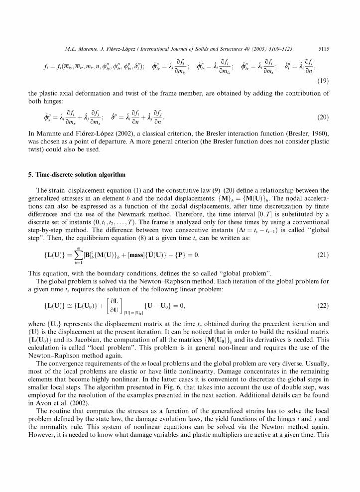
The convergence requirements of the m local problems and the global problem are very diverse. Usually,most of the local problems are elastic or have little nonlinearity. Damage concentrates in the remaining

elements that become highly nonlinear. In the latter cases it is convenient to discretize the global steps in

smaller local steps. The algorithm presented in Fig. 6, that takes into account the use of double step, was

employed for the resolution of the examples presented in the next section. Additional details can be found

in Avon et al. (2002).

The routine that computes the stresses as a function of the generalized strains has to solve the local

problem defined by the state law, the damage evolution laws, the yield functions of the hinges i and j andthe normality rule. This system of nonlinear equations can be solved via the Newton method again.However, it is needed to know what damage variables and plastic multipliers are active at a given time. This

Step-by-step loop

Convergence?

Computation of the displacementmatrix (iteration of the global

problem)

Printing

yes

no

end

Do while notconvergence or α ≠ 1

Computation of the intermediatestress (local problem)

Computation of the value of α

Loop on b

Assemblage

{Φ} at the endof the step

{Φ}b =[B]b{U}α = 1

intermediatestrainInt {Φ}k = (α−1) {Φ0}k + {Φ}k

Resolution of the linearequation: [∂L/ ∂U]{∆U}=-{L}

α = α/2

Return

Noconvergence ?

α = 1 ?

Return

No

YesYes

{Φ0}k = Int {Φ}k

α= 1Convergence = FALSE

Fig. 6. Computational algorithm for the numerical resolution.


is done by using an elastic predictor, inelastic corrector and projection algorithm as the one described in

Simo et al. (1988).

6. Examples

Bousias et al. (1995) carried out an experimental program on the behavior of reinforced concrete ele-

ments under biaxial bending and axial forces. The specimens consisted of square columns built as cantilever

into a heavy foundation. The columns were subjected to axial forces and lateral displacements. In the firstexample of this section, the column was subjected to displacement-controlled lateral actions as the one

shown in Fig. 7(a). The experimental results are shown in Fig. 7(b) and (d). The results of the numerical

simulation are presented in Fig. 7(c) and (e). The data for the simulation consist in the interaction diagrams

of the first cracking, yielding and ultimate moments, the interaction diagram of the ultimate plastic cur-

vature (see Fig. 8), and the elastic stiffness coefficients (elastic modulus, equivalent inertia and area). Ad-

ditionally, the geometry and the loading history must also be defined. The geometry was represented by

only one finite element that was fixed (nil displacements) at one extreme while the other one was subjected

to the imposed displacements indicated in Fig. 7(a). The axial forces were included as force-controlledloadings on the axis of the column.

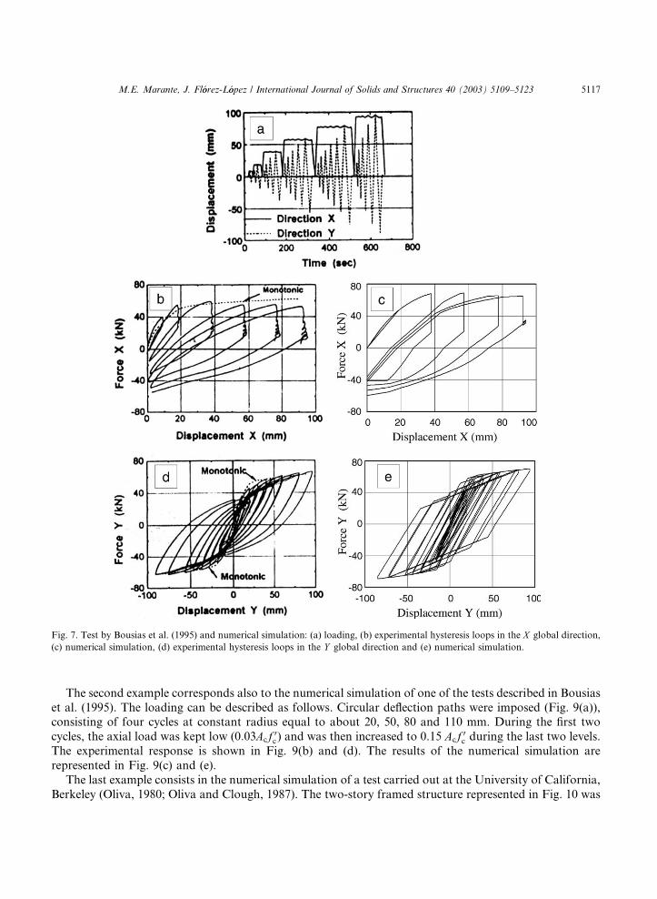
Fig. 7. Test by Bousias et al. (1995) and numerical simulation: (a) loading, (b) experimental hysteresis loops in the X global direction,

(c) numerical simulation, (d) experimental hysteresis loops in the Y global direction and (e) numerical simulation.


The second example corresponds also to the numerical simulation of one of the tests described in Bousias

et al. (1995). The loading can be described as follows. Circular deflection paths were imposed (Fig. 9(a)),consisting of four cycles at constant radius equal to about 20, 50, 80 and 110 mm. During the first two

cycles, the axial load was kept low (0:03Acf 0c ) and was then increased to 0.15 Acf 0

c during the last two levels.

The experimental response is shown in Fig. 9(b) and (d). The results of the numerical simulation are

represented in Fig. 9(c) and (e).

The last example consists in the numerical simulation of a test carried out at the University of California,

Berkeley (Oliva, 1980; Oliva and Clough, 1987). The two-story framed structure represented in Fig. 10 was

0 375 750 1125 15000

-875

-1750

-2625

-3500

Moment (kN-m)

Axi

alfo

rce

(kN

)

0 1.5 3.0 4.5 6.00

-875

-1750

-2625

-3500

Ultimate plastic curvature x 10-3

Axi

alfo

rce

(kN

)

Fig. 8. Data for the simulation presented in Fig. 7.


subjected several times to ground displacements histories derived from the Taft earthquake record. The

structure was placed with an angle of 25� with respect to the axis of the shaking table motion. Thus, thestructure was subjected to biaxial solicitations. First two low intensity shakes, with peak acceleration

amplitude of 0.06 g, were applied on the structure. The goal of this loading was to induce minor cracking in

the virgin frame to replicate the condition of a real structure which has been under service loading. Then the

structure was subjected to a severe shaking with a peak acceleration of 0.685 g.

The beams and columns of the structure were represented by the finite element described in this paper

(one element for frame member). Standard elastic plate elements (Kirchoff theory) were used to represent

the first and second floor slabs. The entire structure was represented by 16 inelastic elements (beams and

columns) and eight elastic elements (slabs). The data for the numerical simulation was obtained from thecross section properties of the frame indicated in Oliva (1980). The loading input for the analysis consisted

in the actual Taft earthquake record obtained from the PEER strong motion data base (web version). The

real loading applied on the structure, although derived from this record, is not exactly the same and some

differences can be appreciated between both records.

The damage state after the first low intensity shake obtained with the computer program can be seen in

Fig. 11(a). In the figure, the maximum values of damage of each hinge (there are four values per hinge) are

shown. It can be noticed that no value exceeded 0.26. This corresponds indeed to minor cracking that does

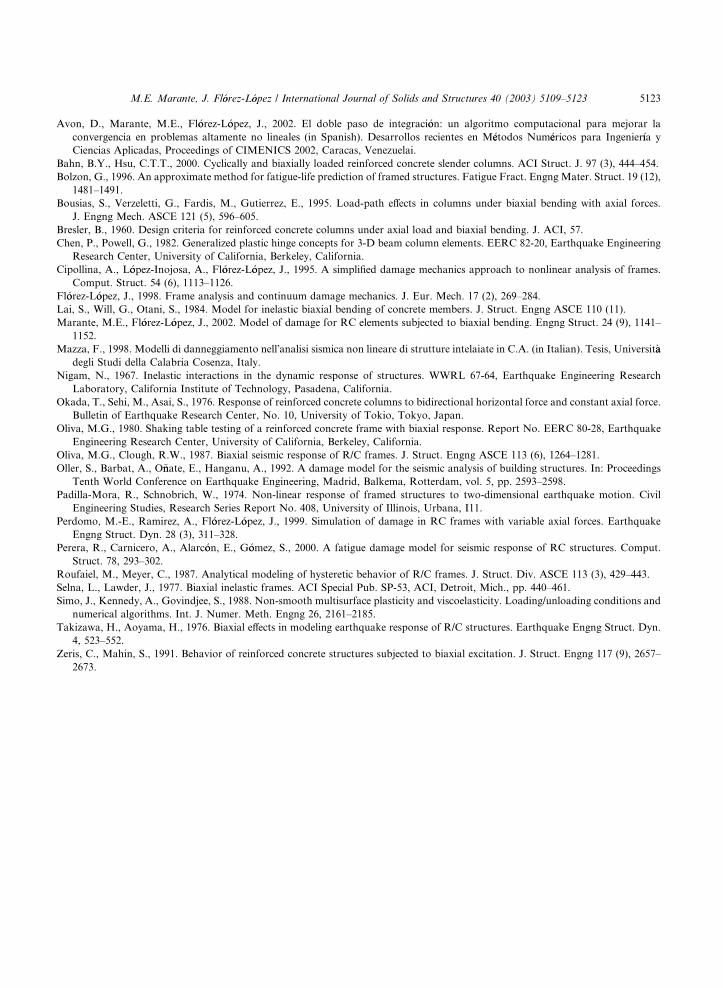
not need reparation, as indicated in Alarc�oon et al. (2001).The numerical results obtained after the severe shake are shown in Figs. 11(b), 12 and 13. In Fig. 12, the

experimental and computed displacements of the first floor are presented (there is no information of the

second floor displacements in Oliva, 1980). Fig. 13 shows the computed and observed local behavior of one

of the columns of the first floor. Fig. 11(b) indicates the final state of damage after the numerical simu-

lation. Very high values of damage can be observed in this figure. Structures with values of damage that

high should not, after conventional engineering criteria, be repaired (see Alarc�oon et al., 2001). The structure

was nonetheless repaired and tested again (Oliva, 1980), and its behavior does not seem bad.

7. Limitations of the proposed model

The limitations of the model can be grouped into two different categories. The first one includes the

restrictions due to the general framework of the model, i.e. lumped damage mechanics. It is clear that the

model may be used only in the situations where cracking and plasticity are limited to restricted areas of

the frame member. Often, this is the case under earthquake loadings, but if extensive cracking of variabledensity develops across the elements, fiber beam theories are more adequate. On the other hand, fiber beam

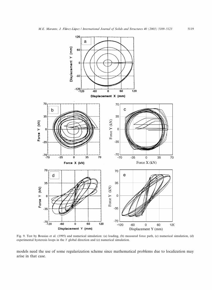
Fig. 9. Test by Bousias et al. (1995) and numerical simulation: (a) loading, (b) measured force path, (c) numerical simulation, (d)

experimental hysteresis loops in the Y global direction and (e) numerical simulation.


models need the use of some regularization scheme since mathematical problems due to localization may

arise in that case.

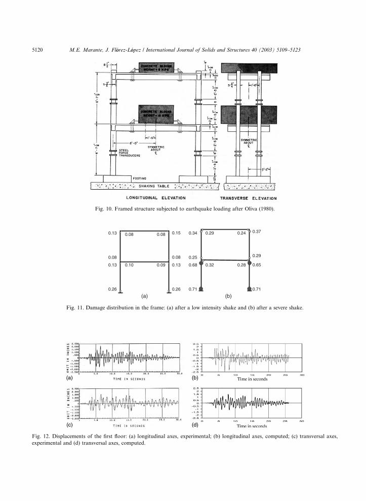
Fig. 10. Framed structure subjected to earthquake loading after Oliva (1980).

0.71 0.71

0.68 0.65

0.25 0.29

0.34 0.37

0.32 0.28

0.29 0.24

0.26 0.26

0.13 0.13

0.08 0.08

0.13 0.15

0.10 0.09

0.08 0.08

(a) (b)

Fig. 11. Damage distribution in the frame: (a) after a low intensity shake and (b) after a severe shake.

Fig. 12. Displacements of the first floor: (a) longitudinal axes, experimental; (b) longitudinal axes, computed; (c) transversal axes,

experimental and (d) transversal axes, computed.


Fig. 13. Local behavior of a first floor column: (a) longitudinal axes, experimental; (b) longitudinal axes, computed; (c) transversal

axes, experimental and (d) transversal axes, computed.


Localization is not a problem in lumped damage mechanics. In fact, lumped damage mechanics can be

seen as a regularization procedure valid in the case of beams. The use of regularization methods in strain-

softening problems involves the introduction of ‘‘internal length scales’’ that are essential for the proper

description of the localization phenomenon. The concept of ‘‘internal length scale’’ in lumped damage

mechanics can be related with two characteristics of the method. In the first place, the fact that energy

dissipation is assumed to be lumped into locations of zero length: the inelastic hinges. It must be em-

phasized that although concentrated into zero length zones, this energy dissipation is no nil. The secondaspect related with the internal length scale, is the fact that the user defines the number and locations of the

inelastic hinge when she or he discretizes the structure into finite elements. The structural response is in-

dependent of the number or the size of the finite elements as far as the position of the inelastic hinges is not

changed. Therefore, this constitutes a second limitation of the model: the position of the inelastic hinges is

part of the data of the problem. However, in most earthquake engineering applications, this is not an

important restriction since the user has almost always an accurate idea of where these inelastic hinges can

appear, as it can be seen, for instance, in the last example of Section 6.

The second category of limitations is related with the model itself. For instance, the damage evolutionlaw (13) becomes a sort of Griffith criterion in the case of monotonic loadings in only one plane. The

Griffith criterion does not take into account low or high cycle fatigue effects and therefore, neither does the

proposed model. In this sense, the model could be improved by the use of generalized forms of the Griffith

criteria that are available in the continuum damage and fracture mechanics literature. Additionally, a

Rankine-like criterion of damage for general biaxial loadings was assumed. This criterion has the merit of

simplicity but implies an uncoupling between crack evolution in the different faces of the element. The


limitations of this hypothesis have not been evaluated yet and, probably, better criteria are possible without

implying a significant increment in the complexity of the model.

The model only includes damage variables related to flexural effects. The influence that torsion and axial

forces may have on the flexural behavior has been taken into account in a simplified way. However, nospecific torsion or axial related damage has been introduced. Therefore the model should be used only in

cases of flexural dominated behavior.

Some discrepancies can be appreciated between model and test in the examples of the previous section,

for instance in the case of Fig. 9. In addition to the aforementioned limitations of the model, it must be

added the uncertainty of the data for the simulation. Specifically that related with the variation of the axial

loads during the test. The interaction diagrams needed for the simulation (see Fig. 8) also introduce some

uncertainty since these properties can be computed with errors that are almost always larger than 10% or

15%. The same remarks apply for the last example of Section 6. For instance, the data related with theearthquake records that are used as input are not the same for test and simulation. On the other hand the

results of the first example of Section 6 (Fig. 7) were excellent.

8. Final remarks and conclusions

The common philosophy of most codes (perhaps all of them) for building design is that buildings should

be able to resist minor earthquakes without damage, to resist moderate earthquake with some, repairable,damage and to resist mayor earthquakes without collapse, although with damage that might be non-

repairable. It is then obvious that quantitative damage analysis of building structures should be a mayor

subject of the structural engineering.

However, in practice, damage analyses are not very often carried out. In the cases where such analyses

are needed, the common procedure consists in inelastic analyses based on plasticity theories. However,

these results are of little use for the practical engineer. Thus, a damage analysis is then accomplished via

semi-empirical rules by post-processing. The coupled damage/structural analysis of the structure constitutes

a more rational approach to the problem. Concepts from fracture mechanics and continuum damagemechanics can be adapted to the analysis of framed structures with plastic hinges and the resulting theory

constitutes a good compromise between simplicity, rationality and accuracy, for engineering purposes, even

for complex three-dimensional problems.

Acknowledgements

The results presented in this paper were obtained in the course of an investigation sponsored by

FONACIT, CDCHT-ULA, and CDCHT-UCLA. The authors express their gratitude to the ASCE for

granting the use of Figs. 7(a), (b), (d), 9(a), (b), (d) and to the Earthquake Engineering Research Center,

University of California for granting the use of Figs. 10, 12(a), (c), 13(a) and (c).

References

Aktan, A., Pecknold, D., Sozen, M., 1973. Effects of two-dimensional earthquake motion on a reinforced concrete column. Civil

Engineering Studies, Structural Research Series Report No. 399, University of Illinois, Urbana, I11.

Alarc�oon, E., Recuero, A., Perera, R., Lopez, C., Gutierrez, J.P., De Diego, A., Picon, R., Florez Lopez, J., 2001. A reparability index

for reinforced concrete members based on fracture mechanics. Engng Struct. 23 (6), 687–697.

Anthoine, A., Guedes, J., Pegon, P., 1997. Non-linear behavior of reinforced concrete beams: from 3D continuum to 1D member

modeling. Comput. Struct. 65 (6), 949–963.


Avon, D., Marante, M.E., Fl�oorez-L�oopez, J., 2002. El doble paso de integraci�oon: un algoritmo computacional para mejorar la

convergencia en problemas altamente no lineales (in Spanish). Desarrollos recientes en M�eetodos Num�eericos para Ingenier�ııa y

Ciencias Aplicadas, Proceedings of CIMENICS 2002, Caracas, Venezuelai.

Bahn, B.Y., Hsu, C.T.T., 2000. Cyclically and biaxially loaded reinforced concrete slender columns. ACI Struct. J. 97 (3), 444–454.

Bolzon, G., 1996. An approximate method for fatigue-life prediction of framed structures. Fatigue Fract. Engng Mater. Struct. 19 (12),

1481–1491.

Bousias, S., Verzeletti, G., Fardis, M., Gutierrez, E., 1995. Load-path effects in columns under biaxial bending with axial forces.

J. Engng Mech. ASCE 121 (5), 596–605.

Bresler, B., 1960. Design criteria for reinforced concrete columns under axial load and biaxial bending. J. ACI, 57.

Chen, P., Powell, G., 1982. Generalized plastic hinge concepts for 3-D beam column elements. EERC 82-20, Earthquake Engineering

Research Center, University of California, Berkeley, California.

Cipollina, A., L�oopez-Inojosa, A., Fl�oorez-L�oopez, J., 1995. A simplified damage mechanics approach to nonlinear analysis of frames.

Comput. Struct. 54 (6), 1113–1126.

Fl�oorez-L�oopez, J., 1998. Frame analysis and continuum damage mechanics. J. Eur. Mech. 17 (2), 269–284.

Lai, S., Will, G., Otani, S., 1984. Model for inelastic biaxial bending of concrete members. J. Struct. Engng ASCE 110 (11).

Marante, M.E., Fl�oorez-L�oopez, J., 2002. Model of damage for RC elements subjected to biaxial bending. Engng Struct. 24 (9), 1141–

1152.

Mazza, F., 1998. Modelli di danneggiamento nell�analisi sismica non lineare di strutture intelaiate in C.A. (in Italian). Tesis, Universit�aa

degli Studi della Calabria Cosenza, Italy.

Nigam, N., 1967. Inelastic interactions in the dynamic response of structures. WWRL 67-64, Earthquake Engineering Research

Laboratory, California Institute of Technology, Pasadena, California.

Okada, T., Sehi, M., Asai, S., 1976. Response of reinforced concrete columns to bidirectional horizontal force and constant axial force.

Bulletin of Earthquake Research Center, No. 10, University of Tokio, Tokyo, Japan.

Oliva, M.G., 1980. Shaking table testing of a reinforced concrete frame with biaxial response. Report No. EERC 80-28, Earthquake

Engineering Research Center, University of California, Berkeley, California.

Oliva, M.G., Clough, R.W., 1987. Biaxial seismic response of R/C frames. J. Struct. Engng ASCE 113 (6), 1264–1281.

Oller, S., Barbat, A., O~nnate, E., Hanganu, A., 1992. A damage model for the seismic analysis of building structures. In: Proceedings

Tenth World Conference on Earthquake Engineering, Madrid, Balkema, Rotterdam, vol. 5, pp. 2593–2598.

Padilla-Mora, R., Schnobrich, W., 1974. Non-linear response of framed structures to two-dimensional earthquake motion. Civil

Engineering Studies, Research Series Report No. 408, University of Illinois, Urbana, I11.

Perdomo, M.-E., Ramirez, A., Fl�oorez-L�oopez, J., 1999. Simulation of damage in RC frames with variable axial forces. Earthquake

Engng Struct. Dyn. 28 (3), 311–328.

Perera, R., Carnicero, A., Alarc�oon, E., G�oomez, S., 2000. A fatigue damage model for seismic response of RC structures. Comput.

Struct. 78, 293–302.

Roufaiel, M., Meyer, C., 1987. Analytical modeling of hysteretic behavior of R/C frames. J. Struct. Div. ASCE 113 (3), 429–443.

Selna, L., Lawder, J., 1977. Biaxial inelastic frames. ACI Special Pub. SP-53, ACI, Detroit, Mich., pp. 440–461.

Simo, J., Kennedy, A., Govindjee, S., 1988. Non-smooth multisurface plasticity and viscoelasticity. Loading/unloading conditions and

numerical algorithms. Int. J. Numer. Meth. Engng 26, 2161–2185.

Takizawa, H., Aoyama, H., 1976. Biaxial effects in modeling earthquake response of R/C structures. Earthquake Engng Struct. Dyn.

4, 523–552.

Zeris, C., Mahin, S., 1991. Behavior of reinforced concrete structures subjected to biaxial excitation. J. Struct. Engng 117 (9), 2657–

2673.

Three-dimensional analysis of reinforced concrete frames based on lumped damage mechanics

Documents

Transcript of Three-dimensional analysis of reinforced concrete frames based on lumped damage mechanics