arX

iv:p

hysi

cs/0

6112

74v1

[ph

ysic

s.pl

asm

-ph]

28

Nov

200

6

Thomson scattering from near–solid density

plasmas using soft x–ray free electron lasers

A. Holl a Th. Bornath a L. Cao b T. Doppner a S. Dusterer c

E. Forster b C. Fortmann a S.H. Glenzer d G. Gregori e

T. Laarmann f K.-H. Meiwes-Broer a A. Przystawik a

P. Radcliffe c R. Redmer a H. Reinholz a G. Ropke a R. Thiele a

J. Tiggesbaumker a S. Toleikis c N.X. Truong a T. Tschentscher c

I. Uschmann b U. Zastrau b

aInstitut fur Physik, Universitat Rostock, Universitatsplatz 3, 18051 Rostock,

Germany

bInstitut fur Optik und Quantenelektronik, Friedrich-Schiller-Universitat Jena

Max-Wien-Platz 1, 07743 Jena, Germany

cDeutsches Elektron-Synchrotron DESY, Notkestr. 85, 22607 Hamburg, Germany

dL-399, Lawrence Livermore National Laboratory, University of California, P.O.

Box 808, Livermore, CA 94551, USA

eCCLRC, Rutherford Appleton Laboratory, Chilton, Didcot OX11 0QX, Great

Britain and Clarendon Laboratory, University of Oxford, Parks Road, Oxford,

OX1 3PU, Great Britain

fMax-Born-Institut, Max-Born-Strasse 2a, 12489 Berlin, Germany

Abstract

We propose a collective Thomson scattering experiment at the VUV free electronlaser facility at DESY (FLASH) which aims to diagnose warm dense matter atnear–solid density. The plasma region of interest marks the transition from an idealplasma to a correlated and degenerate many–particle system and is of current inter-est, e.g. in ICF experiments or laboratory astrophysics. Plasma diagnostic of suchplasmas is a longstanding issue. The collective electron plasma mode (plasmon) isrevealed in a pump–probe scattering experiment using the high–brilliant radiationto probe the plasma. The distinctive scattering features allow to infer basic plasmaproperties. For plasmas in thermal equilibrium the electron density and temperatureis determined from scattering off the plasmon mode.

Key words: warm dense matter, plasma diagnostic, Thomson scattering, plasmonsPACS: 52.25.Os, 52.35.Fp, 71.45.Gm, 71.10.Ca

Preprint submitted to Elsevier 2 February 2008

1 Introduction

Accurate measurements of plasma temperatures and densities are importantfor understanding and modeling contemporary plasma experiments in thewarm dense matter (WDM) regime [1]. WDM is characterized by a free elec-tron density of ne = 1021 − 1026 cm−3 and temperatures of several eV. In thisregime bound and free electrons become strongly correlated and medium andlong–range order are built up. Of special interest is WDM at near–solid den-sity (ne = 1021 − 1022cm−3, Te = 1 − 20 eV) where the transition from anideal plasma to a degenerate, strongly coupled plasma occurs. In particular,transient plasma behavior at these conditions is observed in dynamical exper-iments, like laser shock–wave or Z–pinch experiments and are of particularimportance for inertial confinement fusion (ICF) experiments. In such appli-cations the plasma evolution follows its path through the largely unknowndomain of WDM. Further applications of this plasma domain are found, e.g.,in high–energy density physics, astrophysics and material sciences.

A rigorous understanding of highly correlated plasmas is a long–standing andpresently unresolved problem. Only recently, with the availability of high–brilliant and coherent VUV and x-ray radiation at a frequency larger thanthe density dependent electronic plasma frequency ωpe, it became feasible topenetrate through dense plasmas and study basic plasma properties from scat-tered spectra [2,3,4,5,6]. The recent effort to develop diagnostic methods usingThomson scattering is an important first step towards a systematic under-standing of WDM. Available radiation sources to probe such plasmas arebacklighter systems in the x-ray regime as well as free electron laser (FEL)radiation currently available in the VUV. Backlighters have been developedin ICF related research [7] and have been applied to solid density plasmas.The first experiment to measure the spectrally resolved x-ray Thomson scat-tering spectrum in solid density Be plasma has been reported in [8]. Using the4.75 keV titanium He-α backlighter, the non–collective Thomson scatteringspectrum from the thermally distributed electrons allowed the measurementof the Compton–shifted electron distribution function, which was used to de-termine the plasma density, temperature and ionization degree. A pioneeringscattering experiment from the collective electron plasma mode (plasmon) atsolid density using a Cl Ly-α backlighter at 2.96 keV has been performed re-cently [9]. A new type of radiation sources for WDM studies became availablewith the advances of FELs. For instance, the FLASH facility at DESY, hassuccessfully started user experiments in the VUV range 13 − 50 nm [10,11,12]using the SASE 1 principle [13,14]. A proof–of–principle collective Thomsonscattering experiment at FLASH (25 nm) will be performed in March 2007.

Email address: arne.hoell@uni-rostock.de (A. Holl).1 SASE: self amplification of stimulated emission

2

This experiment aims to demonstrate Thomson scattering with FEL radia-tion at near–solid density plasmas as a diagnostic method which is describedin this paper in detail. With further advance in FEL technology with respectto bandwidth, photon energy and brilliance, the method presented here canbe developed to a standard diagnostic tool for WDM research.

Scattering from ideal plasmas has much been studied [15,16,17] and can bedescribed theoretically within the random phase approximation (RPA). It hasbeen shown [5,6] that in the region of near–solid density collisions significantlymodify the scattering spectrum and a theory beyond the RPA is needed. Theelaboration of such theories of non–ideal plasmas [18] is more complicated anddifferent ways have been followed in the past. Local field corrections [19], in-corporated by Ichimaru [20,21] using a general density–response formalism,consistently improve the RPA. Alternatively, a theory based on the dielec-tric function which can be expressed in terms of correlation functions hasbeen studied. For their calculation perturbative methods have been devel-oped [22,23]. Applications for optical and transport properties in WDM arestudied [24,25,26].

The paper is organized as follows. In section 2 we outline the theoretical basisfor Thomson scattering in WDM, introduce the dynamical structure factoras a central quantity and describe its calculation. Results of the calculationsand estimations are used to discuss the applicability of collective Thomsonscattering for plasma diagnostics in section 3. In section 4 we describe theplanned experiment at FLASH. Based on the results of section 3, we specifyout requirements and restrictions relevant for the experiment. In section 5 wegive a summary and address future extensions of the method.

2 Theory

2.1 Scattering Geometry

In this section we will outline the theory needed to describe the scatteringof coherent radiation from an equilibrium plasma at near–solid density. Thescattering geometry is shown in Fig. 1. The plasma is irradiated by the linearlypolarized FEL probe–beam in z–direction with the polarization pointing intothe x–direction. The detector is located in the direction of the scattered wavevector kf at the distance R much larger than the plasma extension. Thedirection of kf is characterized by the scattering angle θ and the azimuthalangle ϕ as shown in Fig. 1. The momentum transfer of the scattered photonis given by k = kf − ki and its energy transfer by ω = ωf − ωi. The modulusof the initial and final wave vector is given by

3

Fig. 1. Scattering geometry

ki = |ki| =ωi

c

√√√√1 − ω2pe

ω2i

(1)

kf = |kf | =ωf

c

√√√√1 − ω2pe

ω2f

≈ ωf

c

√√√√1 − ω2pe

ω2i

. (2)

The square root terms in Eq. (1) and (2) account for the dispersion of incomingand scattered wave. In the density region of 1021 − 1022 cm−3 the electron

plasma frequency is of the order of ωpe =√

nee2/ǫ0me ≈ 1 − 4 eV and theprobe radiation in the VUV–region is of the order of ωi ≈ ωf = 50 − 100 eV.Therefore, we have |ω| . ωpe ≪ ωi ≈ ωf , and the approximation in Eq. (2)is well justified. From the scattering geometry given in Fig. 1 one finds for

the modulus of the momentum transfer k =√

k2i + k2

f − 2kikf cos θ and using

Eqs. (1) and (2)

k =4π

λ0

sin(θ/2)

√√√√1 +ω

ωi

+ω2

ω2i

1

4 sin2(θ/2)

√√√√1 − ω2pe

ω2i

, ωi =2πc

λ0

. (3)

As pointed out, |ω|/ωi and ωpe/ωi are small quantities, and it is easily ob-served from Eq. (3) that the momentum transfer k is well approximated bythe relation k = 4π

λ0

sin(θ/2) for elastic scattering. This, however, is only validfor θ > |ω|/ωi, a condition fulfilled in most scattering experiment.

The scattered power Ps from the electrons into a frequency interval dω andsolid angle dΩ is given by [16]

Ps(R, ω)dΩdω =Pir

20dΩ

2πA

∣∣∣kf × (kf × E0i)∣∣∣2NS(k, ω)dω . (4)

In Eq. (4) Pi denotes the incident FEL power, r0 = e2/mec2 = 2.8 × 10−15 m

the classical electron radius, A the plasma area irradiated by the FEL, N thenumber of nuclei and S(k, ω) the total electron dynamical structure factor. Thepolarization term |kf × (kf × E0i)|2 reflects the dependence of the scatteredpower on the incident laser polarization with the hat denoting unit vectors. For

4

linear polarization and for unpolarized light, respectively, this term is givenby

∣∣∣kf ×(kf × E0i

)∣∣∣2

=

(1 − sin2 θ cos2 ϕ) lin. polarized

(1 − 12sin2 θ) = 1

2(1 + cos2 θ) unpolarized

(5)

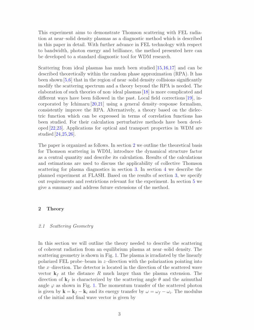
In the case of linear polarization the dependence on the scattering angle θ isshown in Fig. 2. The strongest dependence on θ is observed for ϕ = 0, whereasat ϕ = 90 the polarization term is independent of the scattering angle θ. As

∣∣∣kf ×(kf × E0i

)∣∣∣2

Fig. 2. Dependence of the scattered light on laser polarization, scattering angle θand azimuthal angle ϕ.

seen from Eq. (4), the scattered power depends on the setup of the scatteringexperiment (initial probe power, scattering angle, probe wavelength, probe po-larization), the density and plasma length, and on the total electron dynamicalstructure factor S(k, ω). The dynamical structure factor is the Fourier trans-form of the electron–electron density fluctuations. It is a central quantity sinceit contains the details of the correlated many–particle system [21,27]. The def-inition and calculation of S(k, ω) are given in section 2.2.

2.2 Thomson Scattering in WDM

A characterization of plasmas in equilibrium at different densities and temper-atures can be performed by simple estimations of dimensionless parameters.The coupling parameter Γ is defined as the ratio of the Coulomb energy be-tween two charged particles at a mean particle distance d and the thermalenergy. Using the Wigner–Seitz radius for d, we find an expression for theelectron coupling parameter

5

Γ =e2

4πε0dkBTe

, d =(

4πne

3

)−1/3

. (6)

If Γ < 1 the plasma is weakly coupled, and Γ ≪ 1 denotes the ideal plasmaregime. Correlations become more important in the coupled plasma regime,where Γ & 1. The degeneracy parameter Θ estimates the role of quantumstatistical effects in the system and is given by the ratio of the thermal energyand the Fermi energy EF

Θ =kBTe

EF

, EF =~

2

2me

(3π2ne

)2/3. (7)

In a degenerate plasma, the Fermi energy is larger than the thermal energy,i.e. Θ < 1, and most electrons populate states inside the Fermi sea wherequantum effects are of importance. Contrary to that, for Θ > 1 the role ofquantum effects decreases.

The dimensionless scattering parameter α compares the length scale of elec-tron density fluctuations ℓ ≈ 2π/k measured in the scattering experiment tothe screening length λsc in the plasma. The scattering parameter is defined as

α =1

kλsc

, λ−2sc → λ−2

sc,e = κ2sc,e =

e2m3/2e√

2π2ǫ0~3

∞∫

0

dE E−1/2f e(E) , (8)

where we used the electron screening length λsc,e which is written in terms ofthe Fermi–Dirac distribution function f e(E) of the electrons and accounts forquantum effects [25]. In the case of a classical Maxwell–Boltzmann electrondistribution function, the screening length in Eq. (8) reduces to the Debyescreening length κ2

sc,e → κ2D,e = nee

2/(ǫ0kBTe). For α > 1, i.e. in the collectivescattering regime, only density fluctuations larger than the screening lengthare observed, while at α < 1, i.e. in the non-collective scattering regime, thedensity fluctuations of individual electrons are resolved. As seen from Eq. (3),ℓ = 2π/k is mainly determined by the probe wavelength and the scattering an-gle (i.e. by the setup of the scattering experiment) while λsc,e is determined bythe plasma properties like density and temperature (see Eq. (8)). The density–temperature plot in Fig. 3 shows different plasma regions. In particular, theregion of moderate temperature and near–solid density (gray region), overlapswith the ideal plasma, coupled plasma and degenerate plasma region. Depend-ing on the scattering geometry conditions and probing wavelength, this plasmaregion is accessible applying both, collective and non–collective scattering. Ata wavelength λ0 = 25 nm, however, there is only collective scattering (α > 0)for arbitrary scattering angle observable from this plasma region.

As outlined in conjunction with Eq. (4), the scattering from the plasma is

6

1019

1020

1021

1022

ne [cm

-3]

10-2

10-1

100

101

102

103

104

Te [

eV]

α=1

α=2

α=0.5

Γ=1

Θ=1

near-soliddensityplasma

idealplasma

coupleddegenerateplasma

plasma

collective

non-collectivescattering

scattering

Fig. 3. Plasma parameters in the density–temperature plane. The region of moder-ate temperature, near–solid density plasmas is shown. Also, the electron couplingparameter Γ, degeneracy parameter Θ as well as the scattering parameter α is shownas defined in Eqs. (6), (7) and (8). Assumed are the scattering angle θ = 90 andprobe laser wavelength λ0 = 25nm.

determined by the mean electron–electron density fluctuations per nucleuswhich is expressed by the dynamical structure factor S(k, ω). The structurefactor is defined in terms of the electron density response function χtot

ee via afluctuation–dissipation theorem (FDT) [28]

S(k, ω) =~

n

1

1 − e−β~ωIm χtot

ee (k, ω) , (9)

with n the number density of the nuclei (atoms and ions). The density responsefunction χtot

ee is given as [29]

χtotee (k, ω) = Ω0

i

~

+∞∫

0

dt ei(ω+iη)t⟨[

δntote (k, t), δntot

e (−k, 0)]⟩

, (10)

with δntote = ntot

e − 〈ntote 〉 being the density fluctuations of all electrons from

the average density and the brackets denoting the ensemble average. The nor-malization volume is denoted by Ω0. The limit η → 0 has to be taken after thethermodynamic limit. The solution of Eq. (10) accounting for bound states isa nontrivial problem. Here we follow the idea of Chihara [30,31] who applied achemical picture and decomposed the electrons into free and bound electronsof density ne and nb

e respectively. With Zf free and Zb bound electrons pernucleus, ne and nb

e are related to the ion density ni according to ne = Zfni andnb

e = Zbni. Writing the total electron density ntote = ne +nb

e, we can decomposethe total density response function in Eq. (10) according to

7

χtotee = χff + χbb + χbf + χfb = χff + χbb + 2χbf , (11)

with the electron density response functions of the free–free, bound–bound,bound–free and free-bound system χff , χbb, χbf and χfb, respectively. Theresponse function are defined as in Eq. (10) with the corresponding electrondensities. We also used χbf = χfb. Chihara showed that for a classical systemthe total electron dynamical structure factor can be written in the followingdecomposed form

S(k, ω)=ZfS0ee(k, ω) + |fI(k) + q(k)|2 Sii(k, ω)

+Zb

∫dω′Sce(k, ω − ω′)SS(k, ω′) . (12)

The first term is due to the free electron fluctuations with Zf the number offree electrons per atom. The second term describes number fluctuations of theweakly and tightly bound electrons, with fI(k) the ion form factor, q(k) theelectron screening cloud and Sii the ion–ion structure factor. The last term inEq. (12) is attributed to inelastic Raman transitions of core electrons into thecontinuum Sce, modulated with the ion self–motion SS.

Under the condition Eb ≫ ~2k2/(2m) [4], where Eb is the ionization potential

of the bound states, the first two terms in Eq. (12) are most important. Forthe experimental conditions, specified in section 4, the ionization potentialfor hydrogen and helium is Eb = 13.6 eV and 24 eV, respectively. The energytransferred by the x–ray photons to the bound electrons is only ∼ 0.02 eV.Therefore, bound–free transitions can be neglected.

2.3 Density Response Function

To shortly review the calculation of the electron density response functionwe follow [29]. We consider a plasma consisting of free electrons and ions.The electron and the ion response functions in a collision–free one–componentplasma (OCP) model are given by the well–known Lindhard expressions

χ0cc′(k, ω) = δcc′

1

Ω0

∑

p

f cp+k/2 − f c

p−k/2

∆Ecp,k − ~(ω + iη)

= χ0c(k, ω)δcc′ , (13)

with ∆Ecp,k = Ec

p+k/2 − Ecp−k/2 = ~

2k · p/mc, and the Fermi function f cp =

[exp(βEcp − βµc) + 1]−1 with β = 1/(kBT ). The pole appearing in Eq. (13) is

shifted by η off the real axis and the limit η → 0+ has to be taken after thethermodynamic limit. Eq. (13) is written in matrix form for the plasma speciesdenoted by the indices c and c′. The matrix is diagonal, i.e. by definition, there

8

are no density fluctuations between different plasma species within the OCPdescription.

In RPA the plasma interacts via a screened interaction V sccc′ obtained self–

consistently from the “ring summation” according to

V sccc′(k, ω) = Vcc′(k) +

∑

d

Vcd(k)χ0d(k, ω)Ω0V

scdc′(k, ω) , (14)

which is solved by

V sccc′(k, ω) =

Vcc′(k)

1 − χ0eΩ0Vee − χ0

i Ω0Vii

(15)

in the case of a Coulomb bare potential 2 , Vcc′(k) = ecec′/(ǫ0Ω0k2), considered

in this paper only. The screened interaction contains mutual screening con-tribution from both plasma species (electrons and ions). The RPA responsetensor is given by solving

χRPAcc′ (k, ω) = χ0

c(k, ω)δcc′ + χ0c(k, ω)Ω0V

sccc′(k, ω)χ0

c′(k, ω) (16)

with the matrix elements written as

χRPAee (k, ω)=

χ0e − χ0

eΩ0Viiχ0i

1 − χ0eΩ0Vee − χ0

i Ω0Vii, (17)

χRPAei (k, ω)=

χ0eΩ0Veiχ

0i

1 − χ0eΩ0Vee − χ0

i Ω0Vii

. (18)

The remaining two matrix elements are obtained by interchanging e ↔ i.

To take into account the density fluctuations from the bound electrons, notpresent in Eqs. (17) and (18), one has to solve the dielectric plasma responseincluding bound states [32]. This goes beyond the scope of this paper, andwe follow the idea of Chihara [31] by considering the plasma in a chemicalpicture and decompose the electrons as free, weakly bound and tightly boundelectrons. From Eq. (3) we find a maximal momentum transfer at ω ≈ ωpe

for θ = 180. Therefore, the smallest length scale ℓ = 2π/k at which densityfluctuations can be resolved in the scattering process is ℓ ≥ 12 nm for a probewavelength λ0 = 25 nm. The electron and ion size is much smaller than ℓ and,consequently, details of the atomic structure of the ion enter only in integratedform. This allows to treat the bound electrons in a frozen core approximation.

2 Note, in [29] arbitrary potentials are considered. The simplified expressions hereare obtained by using VeeVii − VeiVie = 0 valid for Coulomb interactions.

9

This implies that χff , χbb and χbf for the free–free, bound–bound and bound–free electron density response function respectively can be written as

χRPAff (k, ω)=χRPA

ee (k, ω) , (19)

χRPAbb (k, ω)=Z2

b χRPAii (k, ω) , (20)

χRPAbf (k, ω)=Zbχ

RPAie (k, ω) , (21)

where all density fluctuations are referred to the total number of nuclei. FromEq. (11) and (19)–(21) the total electron density response function is writtenas

χtotee (k, ω) = χRPA

ee + Z2b χ

RPAii + 2Zbχ

RPAie . (22)

Upon introduction of the partial dynamical structure factors following Eq. (9)

See =Cne

ImχRPAee , Sii =

Cni

ImχRPAii , Sei =

C√neni

ImχRPAei (23)

with C−1 = (1 − exp[−β~ω])/~, we find

S = ZfSee + Z2b Sii + 2Zb

√ZfSei . (24)

We made the assumption that the number of nuclei n equals the number ofions ni, i.e., there are no neutral atoms in the plasma. Eq. (24) correspondsto the first two terms in Eq. (12). In (12), however, the contribution from theelectrons screening the ion charge is separated from See. This can be donerewriting

χRPAee = χRPA

ee + ∆χRPAee

=χ0

e

1 − χ0eΩ0Vee

+Ω2

0VeeVii(χ0e)

2χ0i

(1 − χ0eΩ0Vee − χ0

i Ω0Vii) (1 − χ0eΩ0Vee)

=χ0

e

1 − χ0eΩ0Vee

+(χRPA

ei )2

χRPAii

. (25)

In Eq. (25) χRPAee contains the contributions from the free electrons, whereas

∆χRPAee describes the quasi–free electrons which screen the ions. From the

Eqs. (20)–(25) we find for the total response function

χtotee (k, ω) = χRPA

ee +

(Zb +

χRPAei

χRPAii

)2

χRPAii . (26)

10

Eq. (26) is a simple model for the total electron response function with tightlyand weakly bound electrons “frozen” to the ions. Since we are interested incollective Thomson scattering, i.e. the scattering off electron fluctuations overa distance much larger than the ion size, all atomic details are integratedout. In RPA, Eq. (26) is equivalent to the first two terms in Eq. (12) withZb = limk→0 fI(k) the integrated charge of the tightly bound electrons.

Beyond the RPA, collisions are considered in the response functions χ byutilizing the Mermin ansatz [33] which makes use of a relaxation time τ . Asoutlined in [29,34] the inclusion of local particle number conservation leads toa generalization of the Mermin ansatz in terms of a complex valued dynam-ical collision frequency τ → 1/ν(ω). The collisional response function χν,0

c ofplasma species c is then given by

χν,0c (k, ω) =

(1 − iω

ν(ω)

)

χ0c(k, z)χ0

c(k, 0)

χ0c(k, z) − iω

ν(ω)χ0

c(k, 0)

(27)

and z = ω− Im ν(ω)+ iRe ν(ω). Eq. (27) is exact in the long wavelength limitand serves as a good approximation for finite k. The details of the microscopiccalculation of the dynamical collision frequency are reviewed in section 2.4.Having introduced electron–ion collisions for the OCP plasma according toEq. (27), the equations (17) – (26) can be generalized accordingly and weobtain the total collisional response function χν,tot

cc′ by simply replacing χ0c →

χν,0c in these equations.

2.4 Collision Frequency

As outlined, e.g. in [29,34], the original Ansatz for the dielectric plasma re-sponse made by Mermin [33], can be generalized by calculating the dynamiccollisions frequency. In the long–wavelength limit, the dynamical collision fre-quency can be expressed in terms of the inverse response function via a gener-alized Drude expression. This inverse response function can be obtained by aperturbative evaluation of the corresponding force–force correlation functionwith respect to the plasma interaction. The result for the collision frequencyin Born approximation can be written as (see [29,34] for further details)

νBorn(ω) = −iK ni

neω

∞∫

0

dq q6V 2D(q)Sii(q)[ǫRPA(q, ω) − ǫRPA(q, 0)] (28)

with K = (ǫ0Ω20)/(6π2e2me), and Sii(q) the static ion–ion structure factor and

VD(q) = −Ze2/(ǫ0Ω0(q2 + κ2

sc,e)) the statically screened Debye potential. The

11

electronic screening length κsc,e is defined in Eq. (8). The electron RPA dielec-tric function ǫRPA in Eq. (28) is related to the Lindhard response function,Eq. (13), according to ǫ−1

RPA = 1 + χ0ee

2/(ǫ0k2). It should be pointed out that

the electron screening is accounted for in the Debye potential, whereas ionscreening is treated in the ion–ion structure factor according to

Sii(q) =q2

q2 + κ2D,i

, (29)

with the ion Debye screening length κ2D,i = Z2

fnie2/(ǫ0kBTi). Improvements of

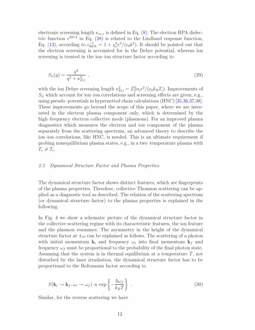
Sii which account for ion–ion correlations and screening effects are given, e.g.,using pseudo–potentials in hypernetted chain calculations (HNC) [35,36,37,38].These improvements go beyond the scope of this paper, where we are inter-ested in the electron plasma component only, which is determined by thehigh–frequency electron collective mode (plasmons). For an improved plasmadiagnostics which measures the electron and ion component of the plasmaseparately from the scattering spectrum, an advanced theory to describe theion–ion correlations, like HNC, is needed. This is an ultimate requirement ifprobing nonequilibrium plasma states, e.g., in a two–temperature plasma withTe 6= Ti.

2.5 Dynamical Structure Factor and Plasma Properties

The dynamical structure factor shows distinct features, which are fingerprintsof the plasma properties. Therefore, collective Thomson scattering can be ap-plied as a diagnostic tool as described. The relation of the scattering spectrum(or dynamical structure factor) to the plasma properties is explained in thefollowing.

In Fig. 4 we show a schematic picture of the dynamical structure factor inthe collective scattering regime with its characteristic features, the ion featureand the plasmon resonance. The asymmetry in the height of the dynamicalstructure factor at ±ω can be explained as follows. The scattering of a photonwith initial momentum ki and frequency ωi into final momentum kf andfrequency ωf must be proportional to the probability of the final photon state.Assuming that the system is in thermal equilibrium at a temperature T , notdisturbed by the laser irradiation, the dynamical structure factor has to beproportional to the Boltzmann factor according to

S(ki → kf , ωi → ωf) ∝ exp

− ~ωf

kBT

. (30)

Similar, for the reverse scattering we have

12

-2 -1 0 1 2ω

0

0.2

0.4

0.6

0.8

1

S(k,

ω)

[a.

u.]

-0.05 0 0.050

0.2

0.4

0.6

0.8

1

-2 -1 0 1 20

0.01

0.02

0.03

plasmonresonance

ion feature

temperatureasymmetry

ωres ωresωac

ωac

ωresωres

free

and

electrons

weakly

tightlybound

electrons

Fig. 4. Schematic view of the dynamical structure factor S(k, ω) as a function of thefrequency shift ω in the collective scattering regime (color online). The high reso-nance collective mode (plasmons) is shown as a red hatched region. At low frequencyshifts, the ion feature due to weakly and tightly bound electrons is shown as theblue dotted region. The plasmon and ion acoustic resonance frequency, ωres and ωac,respectively, are shown. The insets on the upper left and right show magnificationsof the plasmon resonance and the ion feature respectively.

S(kf → ki, ωf → ωi) ∝ exp

− ~ωi

kBT

. (31)

For a homogeneous and stationary system, the scattering process is describedby k ≡ kf−ki and ω ≡ ωf−ωi, the momentum and energy transfer, only. Fromthe general property [39] χ(k, ω) = χ∗(−k,−ω) 3 , we find via the equilibriumFDT (9) and the relations (30), (31)

S(−k,−ω)

S(k, ω)= exp

(− ~ω

kBT

). (32)

Eq. (32) is known as detailed balance relation, and it is a general propertyfollowing from first principles. As seen, the ratio defined in (32) at any par-ticular energy transfer ~ω depends only on the equilibrium temperature ofthe system. This makes the detailed balance relation a highly suitable tool tomeasure the temperature of the plasma, independent of any model assump-tions other than thermodynamic equilibrium. In Fig. 4 the asymmetry in thedynamical structure factor, denoted as temperature asymmetry, is due to thedetailed balance relation.

3 This is a general requirement due to the reality of the induced current j and thevector potential A acting as the external perturbation.

13

Scattering from electrons which are weakly or tightly bound to the ions, seediscussion in connection with Eq. (12), leads to the low frequency resonance,the ion feature. As shown in Fig. 4, due to the large ion mass, the ion fea-ture shows a very narrow spectral width. Currently, there is no x–ray or VUVradiation available that would allow to spectrally resolve the ion feature. Inthe future this could be possible with FEL seeding [40] and in recently pro-posed FELs based on a energy recovery linac scheme with very narrow XUVbandwidth [41].

The high–frequency mode, known as plasmon, is due to the collective scat-tering from free electrons. In Fig. 4, a red (ω < 0) and blue (ω > 0) shiftedplasmon feature appear due to the creation and annihilation of a plasmon, re-spectively. Neglecting the plasmon collisional and Landau damping, the plas-mon resonance ωres is approximately given by the plasmon dispersion relation.For a classical collisionless plasma an expression for the plasmon dispersionhas been given by Gross and Bohm [42], valid in the long wavelength limit~k2/(2meω) ≪ 1

ω2res ≈ ω2

pe +3kBTe

mek2 , (33)

with the density dependent plasma frequency ωpe. The dispersion relation iscalculated from the condition Re ǫ(k, ω) = 0. Eq. (33) follows for a classicalMaxwell Boltzmann plasma and the dielectric function ǫ expanded to orderO(k2). An inspection of Eq. (33) reveals immediately that the plasmon reso-nance position is mainly determined by the plasma frequency and, therefore,by the electron density. The second term in the dispersion relation contains atemperature dependence. Having determined the temperature via the detailedbalance relation as explained, the measurement of the plasmon position ωres

provides the free electron density in the plasma.

An improvement of the classical dispersion relation (33) including quantumdiffraction is obtained if the electron Lindhard expression for the dielectricfunction is solved for Re ǫ(k, ω) = 0. The second moments of the Fermi func-tion are given by Fermi integrals, which can be expressed using an approxi-mate solution [43] to the lowest order in y = neΛ

3e/ge. Here we have defined

the electron thermal wavelength Λe = h/√

2πmekBTe and ge the electron spindegeneracy factor. With these approximations an improved dispersion relation(IDR) can be obtained

ω2res(k

2) ≈ ω2pe +

3kBTe

mek2(1 + 0.088neΛ

3e + . . .

)+

(~k2

2me

)2

, (34)

and the ellipsis denoting higher order terms in y. This expansion is valid for

14

y < 5.5 [43]. At the order O(k4) only the leading term is kept. Other termsof the order O(k4) [44] are suppressed by higher moments of the distributionfunction. It is a simple observation from Eq. (34) that in the limit ~ → 0 andneΛ

3e → 0 the Gross–Bohm dispersion relation, Eq. (33) is recovered. Further,

it must be pointed out that both dispersion relations assume Im ǫ(k, ω) = 0and, consequently, neglect the effect of collisional damping.

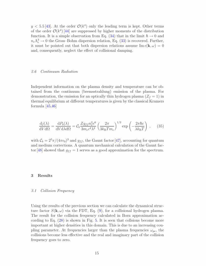
2.6 Continuum Radiation

Independent information on the plasma density and temperature can be ob-tained from the continuum (bremsstrahlung) emission of the plasma. Fordemonstration, the emission for an optically thin hydrogen plasma (Zf = 1) inthermal equilibrium at different temperatures is given by the classical Kramersformula [45,46]

dj(λ)

dV dΩ=

dPb(λ)

dV dλdΩ= Cb

Zgffn2ee

6

3mec2λ2

(2π

3kBTme

)1/2

exp

(− 2π~c

λkBT

), (35)

with Cb = 25π/(4πǫ0)3 and gff , the Gaunt factor [47], accounting for quantum

and medium corrections. A quantum mechanical calculation of the Gaunt fac-tor [48] showed that gff = 1 serves as a good approximation for the spectrum.

3 Results

3.1 Collision Frequency

Using the results of the previous section we can calculate the dynamical struc-ture factor S(k, ω) via the FDT, Eq. (9), for a collisional hydrogen plasma.The result for the collision frequency calculated in Born approximation ac-cording to Eq. (28) is shown in Fig. 5. It is seen that collsions become moreimportant at higher densities in this domain. This is due to an increasing cou-pling parameter. At frequencies larger than the plasma frequencies ωpe, thecollisions become less effective and the real and imaginary part of the collisionfrequency goes to zero.

15

0.0

1.0

2.0

3.0

4.0

0.01 0.1 1 10 1000.0

0.5

1.0

1.5

ω / ωpe

ν [

1014

1/s

]

ne=1.0

ne=2.5

ne=5.0

ne=7.5

ne=10

ne=1.0ne=2.5

ne=7.5

ne=5.0

ne=10

Re ν(ω)

Im ν(ω)

Fig. 5. Real and imaginary part of the electron ion dynamical collision frequency inhydrogen as a function of the energy transfer (upper and lower panel respectively).The collision frequency is calculated in Born approximation, Eq. (28), with respectto a statically screened Debye potential. The electron and ion temperature is 12 eVand the free electron density ne is given in units of 1021 cm−3.

3.2 Dynamical Structure Factor

From the collision frequencies we have calculated the dynamical structure fac-tor using Eqs. (26) with the replacement χ0

c → χν,0c for an equilibrium plasma

at Te = Ti = 12 eV. The results are plotted in Fig. 6 as a function of thefrequency shift ω. Three different FEL probe wavelengths 15 nm, 25 nm and35 nm are shown in the upper, middle and lower panel, respectively. The cor-responding momentum transfer k is calculated from Eq. (3) for a scatteringangle of 90. The structure factor is calculated for the same electron densitiesas in Fig. 5. In order to account for the FEL bandwidth and the final spec-trometer resolution, we convoluted the structure factor with a Gaussian profileof δω/ω = 0.01 full width half maximum (FWHM). In Fig. 6 elastic scatteringof the bound electrons at ω = 0 contributes to the ion feature. Its spectralwidth is given by the bandwidth and spectrometer resolution. Therefore, theion feature serves as a measure of the FEL bandwidth. Beside the ion fea-ture we observe the blue and red shifted plasmon resonance. Both resonancesare different in height, attributed to the detailed balance relation, Eq. (32).This asymmetry increases with decreasing temperature. In accordance withthe Gross–Bohm and the improved dispersion relation, Eqs. (33) and (34),one can observe that the plasmon resonance is shifted to larger resonance fre-quencies with increasing densities due to an increase of the plasma frequency.

16

0.00

0.02

0.04

0.06

0.08

0.00

0.02

0.04

0.06

-5 -4 -3 -2 -1 0 1 2 3 4 5ω [eV]

0.00

0.02

0.04

0.06

ne=1.0

ne=2.5ne=5.0

ne=7.5 ne=10

ne=1.0

ne=2.5

ne=7.5ne=5.0ne=10

ne=1.0

ne=2.5ne=5.0ne=7.5 ne=10

δω=0.83eV

λ0=25nm

λ0=35nm

λ0=15nm

δω=0.50eV

δω=0.35eV

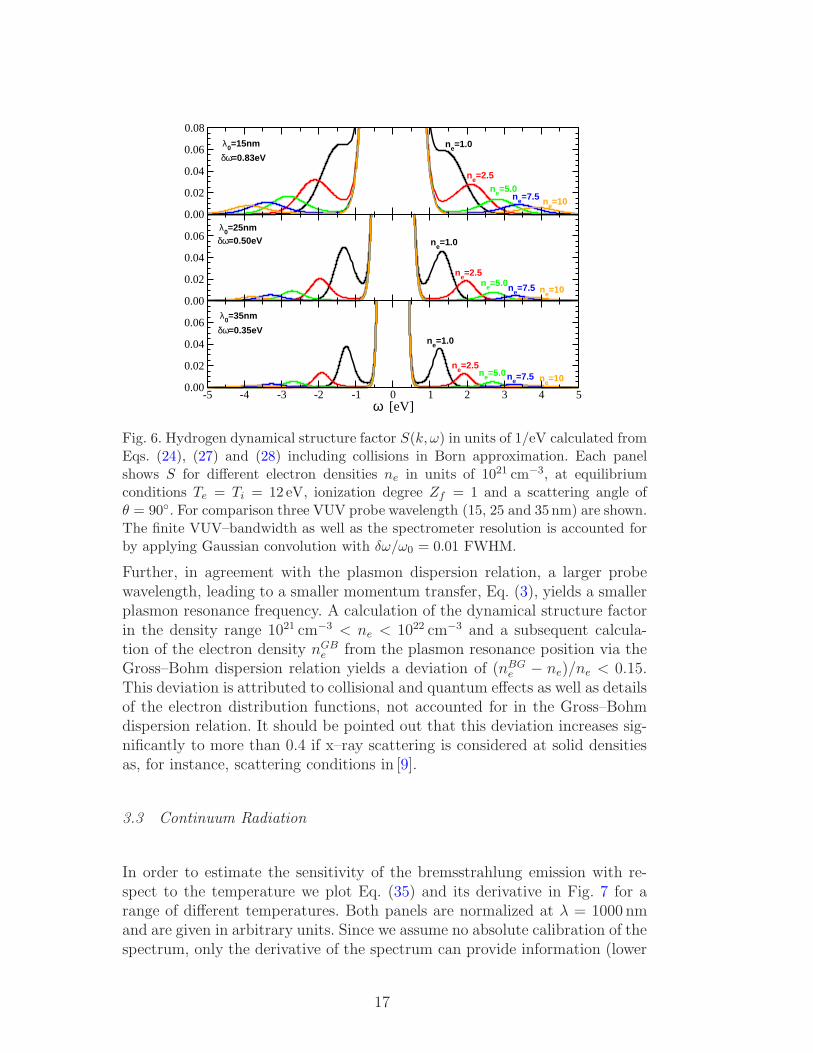
Fig. 6. Hydrogen dynamical structure factor S(k, ω) in units of 1/eV calculated fromEqs. (24), (27) and (28) including collisions in Born approximation. Each panelshows S for different electron densities ne in units of 1021 cm−3, at equilibriumconditions Te = Ti = 12 eV, ionization degree Zf = 1 and a scattering angle ofθ = 90. For comparison three VUV probe wavelength (15, 25 and 35 nm) are shown.The finite VUV–bandwidth as well as the spectrometer resolution is accounted forby applying Gaussian convolution with δω/ω0 = 0.01 FWHM.

Further, in agreement with the plasmon dispersion relation, a larger probewavelength, leading to a smaller momentum transfer, Eq. (3), yields a smallerplasmon resonance frequency. A calculation of the dynamical structure factorin the density range 1021 cm−3 < ne < 1022 cm−3 and a subsequent calcula-tion of the electron density nGB

e from the plasmon resonance position via theGross–Bohm dispersion relation yields a deviation of (nBG

e − ne)/ne < 0.15.This deviation is attributed to collisional and quantum effects as well as detailsof the electron distribution functions, not accounted for in the Gross–Bohmdispersion relation. It should be pointed out that this deviation increases sig-nificantly to more than 0.4 if x–ray scattering is considered at solid densitiesas, for instance, scattering conditions in [9].

3.3 Continuum Radiation

In order to estimate the sensitivity of the bremsstrahlung emission with re-spect to the temperature we plot Eq. (35) and its derivative in Fig. 7 for arange of different temperatures. Both panels are normalized at λ = 1000 nmand are given in arbitrary units. Since we assume no absolute calibration of thespectrum, only the derivative of the spectrum can provide information (lower

17

j(λ)

[a.

u.] T = 3 eV

T = 6 eVT = 9 eVT = 12 eV

200 400 600 800 1000λ [nm]

- d

j(λ)

/ d

λ [

a.u.

]

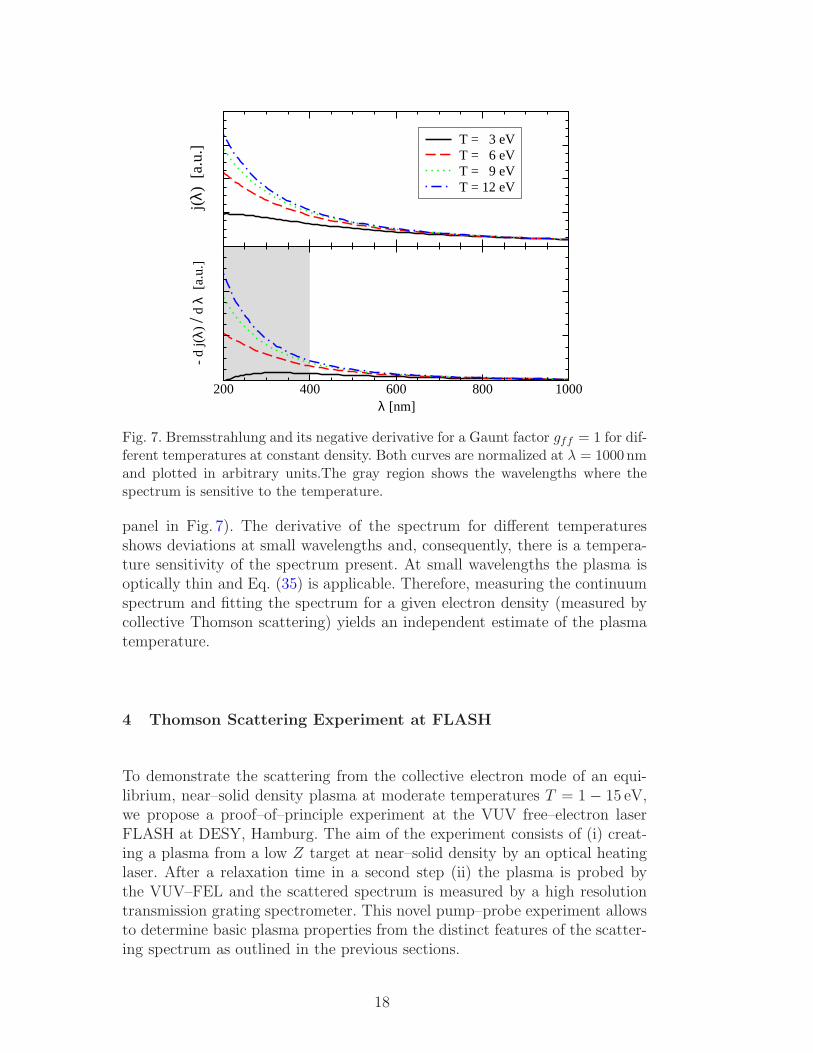
Fig. 7. Bremsstrahlung and its negative derivative for a Gaunt factor gff = 1 for dif-ferent temperatures at constant density. Both curves are normalized at λ = 1000nmand plotted in arbitrary units.The gray region shows the wavelengths where thespectrum is sensitive to the temperature.

panel in Fig. 7). The derivative of the spectrum for different temperaturesshows deviations at small wavelengths and, consequently, there is a tempera-ture sensitivity of the spectrum present. At small wavelengths the plasma isoptically thin and Eq. (35) is applicable. Therefore, measuring the continuumspectrum and fitting the spectrum for a given electron density (measured bycollective Thomson scattering) yields an independent estimate of the plasmatemperature.

4 Thomson Scattering Experiment at FLASH

To demonstrate the scattering from the collective electron mode of an equi-librium, near–solid density plasma at moderate temperatures T = 1 − 15 eV,we propose a proof–of–principle experiment at the VUV free–electron laserFLASH at DESY, Hamburg. The aim of the experiment consists of (i) creat-ing a plasma from a low Z target at near–solid density by an optical heatinglaser. After a relaxation time in a second step (ii) the plasma is probed bythe VUV–FEL and the scattered spectrum is measured by a high resolutiontransmission grating spectrometer. This novel pump–probe experiment allowsto determine basic plasma properties from the distinct features of the scatter-ing spectrum as outlined in the previous sections.

18

4.1 Experimental Requirements

Based on our results described in section 3, we have analyzed the realizationof such an experiment and list some of its most important features:

(1) In order to obtain a strong plasmon scattering signal resulting from freeelectrons and a preferably weak signal from the bound electrons, a low Ztarget material is used.

(2) As the target we employ a cryogenic hydrogen beam which, upon fullionization, provides a free electron density of ne = (2.2−2.4)×1022 cm−3.After a relaxation time of about 1 ps we expect a plasma density of aboutne = 1021 − 1022 cm−3.

(3) Making use of a scattering geometry ϕ = 90, θ = 90 as shown in Fig. 1and 8, the linear polarization of the FEL pulse does not decrease thescattering spectrum (see Fig. 2). In a temperature range Te = 1−15 eV acollective scattering spectrum is expected, as exemplarily shown in Fig. 6for a temperature of Te = 12 eV and various electron densities.

(4) Given that the electron density is in the range ne = 1021 − 1022 cm−3,FEL radiation at a wavelength of λ0 = 25 nm (≈ 50 eV) is chosen inorder to fully separate the plasmons from the ion feature. Due to thebandwidth characteristics of the FEL, this cannot be achieved at a smallerwavelength at, e.g. λ0 = 15 nm (see Fig. 6).

(5) The application of the detailed balance relation, Eq. (32), for the temper-ature measurement restricts the plasma temperature to Te . 15 eV. Atlarger temperatures the asymmetry in the scattering spectrum becomesless than 10% and cannot be resolved experimentally.

(6) The number of photons scattered from the plasmons has to be sufficientlyhigh. For a FLASH pulse of energy EFLASH and wavelength λ0 focusedonto the target, one obtains the total number of photons N tot

ph by

N totph = 5.03 × 109 EFLASH[µJ]λ0[nm] . (36)

The scattered fraction for a plasma length L and the scattering crosssection σ = σT /(1+α2) ≈ σT /α2 (note: α > 3) with σT = 6.65×10−25 cm2

the total Thomson cross section, is given by σneL. Neglecting the densitycorrection in the momentum transfer, Eq. (3), we find with Eq. (8) forthe scattering parameter α

α2 = 0.1146λ2

0[nm2]ne[1021cm−3]

Te[eV] sin2 θ/2. (37)

Therefore, the number of scattered photons N scph into the acceptance solid

angle of the detector ∆Ω = 6 × 10−4 sr is given by

19

N scph ≈ 1.753

EFLASH [µJ]L[µm]Te[eV]

λ0[nm] sin2 θ/2. (38)

For a plasma length L = 40 µm, a wavelength λ0 = 25 nm, a pulse energyEFLASH = 30 µJ, and a scattering angle of θ = 90 we find the numberof photons collected with the spectrometer N sc

ph ≈ 170 Te[eV].

4.2 Experimental Setup

The vacuum chamber with its main connections being used for the Thom-son scattering experiment at DESY and the alignment of the laser beams areshown in Fig. 8 and Fig. 9, respectively. The plasma is generated by 100 fs

Fig. 8. Vacuum chamber with the main connections.

Fig. 9. Adjustment of the space and time overlap of the FEL and optical laser.

pulses with up to 10 mJ energy at 800 nm which are focused to a spot size of50 µm in the interaction region where the cryogenic hydrogen beam crossesperpendicularly to the laser beams. For probing the plasma, the FEL beamenters the interaction region through a hole in the parabola mirror, having a

20

beam waist diameter of 20 µm in the interaction region. Important for the suc-cess of the experiment is a good control of the pump–probe–delay between theoptical pump laser and the FEL. A parallel alignment of the beams, as shownin Fig. 9, is chosen in order to simplify the coarse adjustment of the temporaloverlap using a fast photodiode. For the fine adjustment, the photoelectron(PE) sideband generation technique is applied, which has been successfullydemonstrated at FLASH [49] at a helium gas jet. We will use the same laserbeam alignment (note: Fig. 9 is taken from [49]) and a similar PE sidebandgeneration setup. In contrast to [49] we apply the technique to the hydrogengas jet at 100 K and record the PE spectrum by a field free electron time–of–flight (TOF) spectrometer. Once the temporal overlap between the opticallaser and the FEL has been determined, the the pump–probe delay can beadjusted up to several nanoseconds by a motorized translation stage. The sta-bility of the laser pulse timing is monitored by a streak camera and can bemeasured on a shot to shot basis by electro–optical sampling [50] with an ac-curacy of 200 fs. The repetition rate of the experiment is 5 Hz, determined bythe repetition rate of the FEL.

The hydrogen beam runs perpendicular to the optical laser and the FELthrough their joint focus. A cryogenic source similar to the one used here hasbeen characterized for helium at beam diameters of 30−100 µm[51]. Prepara-tory tests aiming at a continuous hydrogen beam have been performed at theUniversity of Rostock. Depending on the pressure and temperature conditions,the source provides: a spray of hydrogen droplets, a well collimated beam ofdroplets or a slow moving filament of solid hydrogen. For the experiment wewill make use of the collimated beam consisting of droplets 40 µm in diameter.It operates stable at a temperature of T ≈ 15 K and a pressure of p ≈ 15 barfor a nozzle diameter of dnozzle = 20 µm. Similar studies on cryogenic argonbeams [52] and piezo-driven hydrogen droplets [53] have been reported.

As shown in Fig. 8, the scattered photons are measured by a high resolutiontransmission grating EUV spectrometer, mounted perpendicular on top of theinteraction region at a scattering angle of θ = 90. The spectrometer layoutis schematically shown in Fig. 10, details are reported in [54]. A large area

Fig. 10. Schematic view of the EUV spectrometer.

transmission grating with a line density of 1000 lines/mm will be used. Thespectral range is λ = 0.5 − 50 nm and the expected spectrum is optimally

21

distributed on the CCD surface (size: 27× 13.5 mm2). The spectral resolutionof the spectrometer is mainly limited by the dimension of the plasma andthe pixel size of the soft x–ray CCD (13.5 × 13.5 µm2). At the wavelengthλ = 25 nm we expect a resolution of ∆λ/λ ≈ 8 × 10−3. The acceptance solidangle is ∆Ω = 6 × 10−4 sr.

As additional diagnostics an optical spectrometer for the detection of con-tinuum radiation and a CCD–based microscope pointing to the focus will beemployed. The microscope is used for characterization of the hydrogen beamin terms of droplet number, size and speed and for initial alignment.

5 Summary

We have shown that x–ray Thomson scattering can be applied as a diagnostictool to elaborate correlated plasmas in the WDM regime. In particular, we pro-pose a proof–of–principle experiment at the VUV FLASH facility at DESYto measure equilibrium properties of a near–solid density hydrogen plasma.High–brilliant coherent VUV FEL radiation at a wavelength of λ0 = 25 nmwill be used to scatter off the dense plasma. The collective Thomson scatter-ing spectrum will be measured using a high resolution, high sensitivity trans-mission grating EUV-spectrometer. As our theoretical calculations show, thedistinctive plasmon features expected in the spectrum, will allow to measurethe electron density and temperature. The plasma regime considered in thispaper lies in the range of ne = 1021 − 1022 cm−3 for the free electron densityand Te = 1 − 15 eV for the temperature. A plasma under these conditions isgenerated by laser irradiation of a cryogenic hydrogen droplet beam. A timedelay between the pump and probe laser of the order of the relaxation time(≈ 1 ps) will allow to probe the plasma at equilibrium condition.

The electron temperature will be determined by the asymmetry between thered and blue shifted part of the spectrum. This property is directly relatedto the detailed balance relation which is based on first principles. Therefore,the method provides a reliable measure of the equilibrium temperature. Theposition of the plasmon resonance is determined by the density. A calculationof the dynamical structure factor for different electron densities allows to iden-tify the plasmon resonance position by the maximum of the plasmon feature.This method provides a reliable electron density measurement if collisional andLandau damping as well as quantum statistical effects are accounted for in thecalculations. Estimations for the density can be obtained based on the plasmondispersion relation with a systematic error of less than 15% in the consideredplasma regime. Limiting factors of the proposed measurement have been esti-mated. The spectral resolution, resulting from the finite FEL bandwidth andEUV–spectrometer resolution, is sufficiently large to spectrally separate the

22

plasmon from the Rayleigh peak. The number of scattered photons off theplasmons has been estimated. More information will be obtained from addi-tional diagnostics. For instance, the measurement of the continuum radiationprovides independent information on the plasma density and temperature.

The proposed plasma diagnostic method can be developed into a standardtool for WDM research. Due to the unique features of x-ray and VUV FELradiation concerning brilliance and coherence, they are favorable sources forThomson scattering diagnostics which has the potential to be extended tononequilibrium plasmas in the future. This will need a time–resolved scatter-ing experiment which will reveal the plasma dynamics in WDM and experi-ments are currently proposed, e.g. at FLASH [55]. The experiment proposedin this paper serves as a precursor to a systematic elaboration of the widelyunexplored regime of WDM.

6 Acknowledgments

This work was supported by the virtual institute VH-VI-104 of the Helmholtzassociation and the Sonderforschungsbereich SFB 652. The work of SHG wasperformed under the auspices of the U.S. Department of Energy by the Uni-versity of California Lawrence Livermore National Laboratory under contractnumber No. W-7405-ENG-48 and the Alexander–von–Humboldt foundation.The work of GG was supported by the Council for the Central Laboratory ofthe Research Councils (UK).

References

[1] R.W. Lee, et al., J. Opt. Soc. Am. B 20, 770 (2003).

[2] D. Riley, et al., Phys. Rev. Lett. 84, 1704 (2000).

[3] O.L. Landen, et al., J. Quant. Spectrosc. Radiat. Transfer 71, 465 (2001).

[4] G. Gregori, et al., Phys. Rev. E 67, 026412 (2003).

[5] A. Holl, et al., Eur. Phys. J. D 29, 159 (2004).

[6] R. Redmer, et al., IEEE Trans. Plasma Science 33 , 77 (2005).

[7] O.L. Landen, et al., Rev. Sci. Inst. 72, 627 (2001).

[8] S.H. Glenzer, et al., Phys. Rev. Lett. 90, 175002 (2003).

[9] S.H. Glenzer, et al., Phys. Rev. Lett. (2006), submitted.

23

[10] V. Ayvazyan, et al., Eur. Phys. J. D. 37, 297 (2006).

[11] N. Stojanovic, et al., Appl. Phys. Lett., accepted for publication (2006).

[12] H.N. Chapman et al., Nature Physics Letters, Nov. (2006).

[13] A. Kondratenko, E. Saldin, Part. Accel. 10, 207 (1980).

[14] R. Bonifacio, C. Pellegrini, Opt. Commun. 50, 373 (1984).

[15] T.P. Hughes, Plasma and Laser Light, John Wiley & Sons, NY. (1975).

[16] J. Sheffield, Plasma Scattering of Electromagnetic Radiation, Academic Press,N.Y. (1975).

[17] G. Bekefi, Radiation Processes in Plasmas, John Wiley, New York (1966).

[18] Yu.L. Klimontovich, Kinetic Theory of Nonideal Gases and Nonideal Plasmas,Pergamon, Oxford (1982).

[19] G. Gregori, et al., J. Phys. A 36 , 5971 (2003).

[20] S. Ichimaru, et al., Phys. Rev. A32 , 1768 (1985).

[21] S. Ichimaru, Statistical Plasma Physics, vol. II: Condensed Plasmas, Addison–Wesley (1994).

[22] G. Ropke, Phys. Rev. E 57, 4673 (1998).

[23] G. Ropke, A. Wierling, Phys. Rev. E 57, 7075 (1998).

[24] A. Wierling, et al., Physics of Plasmas 8, 3810 (2001).

[25] H. Reinholz, Ann. Phys. (Fr) 30, 1 (2005).

[26] M.W.C. Darma-Wardana, Phys. Rev. E 73, 036401 (2006).

[27] S. Ichimaru, Plasma Physics: An Introduction to Statistical Physics of Charged

Particles, Addison–Wesley (1988).

[28] R. Kubo, Rep. Prog. Phys. 29, 255 (1966).

[29] A. Selchow, et al., Phys. Rev. E 64, 056410 (2001).

[30] J. Chihara, J. Phys. F 17, 295 (1987).

[31] J. Chihara, J. Phys.: Cond. Matter 12, 231 (2000).

[32] G. Ropke, R. Der, Phys. Stat. Sol. B 92, 510 (1979).

[33] N.D. Mermin, Phys. Rev. B 1, 2362 (1970).

[34] H. Reinholz et al., Phys. Rev. E 62, 5648 (2000).

[35] P. Seuferling et al., Phys. Rev. A40, 323 (1989).

[36] Y.V. Arkhipov, A.E. Davletov, Phys. Lett. A 247, 339 (1998).

24

[37] G. Gregori, et al., Phys. Rev. E 74, 026402 (2006).

[38] V. Schwarz, et al., Hypernetted chain calculations for two–component plasmas,Cont. Plasma Phys (2006) submitted.

[39] A. Sitenko, V. Malnev, Plasma Physics Theory, Chapman & Hall, London(1995).

[40] J. Feldhaus, et al., Opt. Commun. 140, 341 (1997).

[41] http://www.4gls.ac.uk

[42] D. Bohm, E.P. Gross, Phys. Rev. 75, 1851 (1949).

[43] R. Zimmermann, Many–Particle Theory of Highly Excited Semiconductors,Teubner, Leipzig (1998).

[44] W.-D. Kraeft, et al., Quantum Statistics of Charged Particle Systems,Akademie-Verlag, Berlin (1986).

[45] H.A. Kramers, Philos. Mag. 46, 836 (1923).

[46] G.B. Rybicki, A.P. Lightman, Radiative Processes in Astrophysics, J. Wiley &Sons, New York (1975).

[47] J.A. Gaunt, Proc. R. Soc. A 126, 654 (1930).

[48] C. Fortmann, et al., High Energy Density Physics 2, 57 (2006).

[49] M. Meyer, et al., Phys. Rev A 74, 011401(R) (2006).

[50] G. Berden, et al., Phys. Rev. Lett. 93, 114802 (2004).

[51] M.N. Slipchenko, et al., Rev. Sci. Instrum. 73, 3600 (2002).

[52] M. Grams, et al., Rev. Sci. Instrum. 76, 123904 (2005).

[53] B. Trostell, Nucl. Instr. Meth. in Phys. Res. A 362, 41 (1995).

[54] J. Jasny, et al., Rev. Sci. Instrum. 65, 1631 (1994).

[55] A. Holl, et al., Thomson Scattering Measurements of Plasma Dynamics, FLASHproposal (2006).

[56] D.N. Zubarev, V. Morozov, G. Ropke, Statistical Mechanics of Nonequilibrium

Processes, Akademie Verlag, Berlin (1997).

25