Thin Plates And Shells Theory Analysis And Applications

TM

Marcel Dekker, Inc. New York • Basel

Eduard VentselTheodor KrauthammerThe Pennsylvania State UniversityUniversity Park, Pennsylvania

Thin Plates and ShellsTheory, Analysis, and Applications

Copyright 2001 by Marcel Dekker, Inc. All Rights Reserved.

ISBN: 0-8247-0575-0

This book is printed on acid-free paper.

Headquarters

Marcel Dekker, Inc.

270 Madison Avenue, New York, NY 10016

tel: 212-696-9000; fax: 212-685-4540

Eastern Hemisphere Distribution

Marcel Dekker AG

Hutgasse 4, Postfach 812, CH-4001 Basel, Switzerland

tel: 41-61-261-8482; fax: 41-61-261-8896

World Wide Web

http://www.dekker.com

The publisher offers discounts on this book when ordered in bulk quantities. For more

information, write to Special Sales/Professional Marketing at the headquarters address above.

Neither this book nor any part may be reproduced or transmitted in any form or by any

means, electronic or mechanical, including photocopying, microfilming, and recording, or by

any information storage and retrieval system without permission in writing from the publisher.

Current printing (last digit):

10 9 8 7 6 5 4 3 2 1

PRINTED IN THE UNITED STATES OF AMERICA


http://www.dekker.com

To:

Liliya, Irina, and Masha

and

Nina, Yoaav, Adi, and Alon


Preface

Thin-walled structures in the form of plates and shells are encountered in many

branches of technology, such as civil, mechanical, aeronautical, marine, and chemi-

cal engineering. Such a widespread use of plate and shell structures arises from their

intrinsic properties. When suitably designed, even very thin plates, and especially

shells, can support large loads. Thus, they are utilized in structures such as aerospace

vehicles in which light weight is essential.

In preparing this book, we had three main objectives: first, to offer a compre-

hensive and methodical presentation of the fundamentals of thin plate and shell

theories, based on a strong foundation of mathematics and mechanics with emphasis

on engineering aspects. Second, we wanted to acquaint readers with the most useful

and contemporary analytical and numerical methods for solving linear and non-

linear plate and shell problems. Our third goal was to apply the theories and methods

developed in the book to the analysis and design of thin plate-shell structures in

engineering. This book is intended as a text for graduate and postgraduate students

in civil, architectural, mechanical, chemical, aeronautical, aerospace, and ocean

engineering, and engineering mechanics. It can also serve as a reference book for

practicing engineers, designers, and stress analysts who are involved in the analysis

and design of thin-walled structures.

As a textbook, it contains enough materal for a two-semester senior or grad-

uate course on the theory and applications of thin plates and shells. Also, a special

effort has been made to have the chapters as independent from one another as

possible, so that a course can be taught in one semester by selecting appropriate

chapters, or through equivalent self-study.

The textbook is divided into two parts. Part I (Chapters 1–9) presents plate

bending theory and its application and Part II (Chapters 10–20) covers the theory,

analysis, and principles of shell structures.


jiao

Highlight

jiao

Highlight

The book is organized in the following manner. First, the general linear the-ories of thin elastic plates and shells of an arbitrary geometry are developed by usingthe basic classical assumptions. Deriving the general relationships and equations ofthe linear shell theory requires some familiarity with topics of advanced mathe-matics, including vector calculus, theory of differential equations, and theory ofsurfaces. We tried to keep a necessary rigorous treatment of shell theory and itsprinciples and, at the same time, to make the book more readable for graduatestudents and engineers. Therefore, we presented the fundamental kinematic andstatic relationships, and elements of the theory of surfaces, which are necessaryfor constructing the shell theory, without proof and verification. The detailed deri-vation and proof of the above relationships and equations are given in AppendicesA–E so that the interested reader can refer to them.

Later on, governing differential equations of the linear general theory areapplied to plates and shells of particular geometrical forms. In doing so, variousapproximate engineering shell theories are presented by introducing some supple-mentary assumptions to the general shell theory. The mathematical formulation ofthe above shell theories leads, as a rule, to a system of partial differential equations.A solution of these equations is the focus of attention of the book. Emphasis is givento computer-oriented methods, such as the finite difference and finite element meth-ods, boundary element and boundary collocation methods, and to their applicationto plate and shell problems. Nevertheless, the emphasis placed on numerical methodsis not intended to deny the merit of classical analytical methods that are also pre-sented in the book, for example, the Galerkin and Ritz methods.

A great attempt has been made to emphasize the physical meanings of engi-neering shell theories, mathematical relationships, and adapted basic and supple-mentary assumptions. The accuracy of numerical results obtained with the use of theabove theories, and possible areas of their application, are discussed. The main goalis to help the reader to understand how plate and shell structures resist the appliedloads and to express this understanding in the language of physical rather thanpurely mathematical aspects. To this end, the basic ideas of the considered plateand shell models are demonstrated by comparisons with more simple models such asbeams and arches, for which the main ideas are understandable for readers familiarwith strength of materials. We believe that understanding the behavior of plate andshell structures enables designers or stress analysts to verify the accuracy of numer-ical structural analysis results for such structures obtained by available computercode, and to interpret these results correctly.

Postgraduate students, stress analysts, and engineers will be interested in theadvanced topics on plate and shell structures, including the refined theory of thinplates, orthotropic and multilayered plates and shells, sandwich plate and shellstructures, geometrically nonlinear plate, and shell theories. Much attention is alsogiven to orthotropic and stiffened plates and shells, as well as to multishell structuresthat are commonly encountered in engineering applications. The peculiarities of thebehavior and states of stress of the above thin-walled structures are analyzed indetail.

Since the failure of thin-walled structures is more often caused by buckling, theissue of the linear and nonlinear buckling analysis of plates and shells is given muchattention in the book. Particular emphasis is placed on the formulation of elasticstability criteria and on the analysis of peculiarities of the buckling process for thin


jiao

Highlight

shells. Buckling analysis of orthtropic, stiffened, and sandwich plates and shells is

presented. The important issues of postbuckling behavior of plates and shells—in

paticular, the load-carrying capacity of stiffened plates and shells—are discussed in

detail. Some considerations of design stability analysis for thin shell structures is also

provided in the book.

An introduction to the vibration of plates and shells is given in condensed form

and the fundamental concepts of dynamic analysis for free and forced vibrations of

unstiffened and stiffened plate and shell structures are discussed. The book empha-

sizes the understanding of basic phenomena in shell and plate vibrations. We hope

that this materal will be useful for engineers in preventing failures and for acousti-

cians in controlling noise.

Each chapter contains fully worked out examples and homework problems

that are primarily drawn from engineering practice. The sample problems serve a

double purpose: to help readers understand the basic principles and methods used in

plate and shell theories and to show application of the above theories and methods

to engineering design.

The selection, arrangement, and presentation of the material have been made

with the greatest care, based on lecture notes for a course taught by the first author

at The Pennsylvania State University for many years and also earlier at the Kharkov

Technical University of Civil Engineering, Ukraine. The research, practical design,

and consulting experiences of both authors have also contributed to the presented

material.

The first author wishes to express his gratitude to Dr. R. McNitt for his

encouragement, unwavering support, and valuable advice in bringing this book to

its final form. Thanks are also due to the many graduate students who offered

constructive suggestions when drafts of this book were used as a text. A special

thanks is extended to Dr. I. Ginsburg for spending long hours reviewing and criti-

quing the manuscript. We thank Ms. J. Fennema for her excellence in sketching the

numerous figures. Finally, we thank Marcel Dekker, Inc., and especially, Mr. B. J.

Clark, for extraordinary dedication and assistance in the preparation of this book.

Eduard Ventsel

Theodor Krauthammer


Contents

Preface

PART I. THIN PLATES

1 Introduction1.1 General1.2 History of Plate Theory Development1.3 General Behavior of Plates1.4 Survey of Elasticity Theory

References

2 The Fundamentals of the Small-Deflection Plate Bending Theory2.1 Introduction2.2 Strain–Curvature Relations (Kinematic Equations)2.3 Stresses, Stress Resultants, and Stress Couples2.4 The Governing Equation for Deflections of Plates in

Cartesian Coordinates2.5 Boundary Conditions2.6 Variational Formulation of Plate Bending Problems

ProblemsReferences

3 Rectangular Plates3.1 Introduction3.2 The Elementary Cases of Plate Bending3.3 Navier’s Method (Double Series Solution)


3.4 Rectangular Plates Subjected to a Concentrated Lateral Force P3.5 Levy’s Solution (Single Series Solution)3.6 Continuous Plates3.7 Plates on an Elastic Foundation3.8 Plates with Variable Stiffness3.9 Rectangular Plates Under Combined Lateral and Direct Loads

3.10 Bending of Plates with Small Initial CurvatureProblemsReferences

4 Circular Plates4.1 Introduction4.2 Basic Relations in Polar Coordinates4.3 Axisymmetric Bending of Circular Plates4.4 The Use of Superposition for the Axisymmetric Analysis of

Circular Plates4.5 Circular Plates on Elastic Foundation4.6 Asymmetric Bending of Circular Plates4.7 Circular Plates Loaded by an Eccentric Lateral Concentrated Forc4.8 Circular Plates of Variable Thickness

ProblemsReferences

5 Bending of Plates of Various Shapes5.1 Introduction5.2 Elliptical Plates5.3 Sector-Shaped Plates5.4 Triangular Plates5.5 Skew Plates

ProblemsReferences

6 Plate Bending by Approximate and Numerical Methods6.1 Introduction6.2 The Finite Difference Method (FDM)6.3 The Boundary Collocation Method (BCM)6.4 The Boundary Element Method (BEM)6.5 The Galerkin Method6.6 The Ritz Method6.7 The Finite Element Method (FEM)

ProblemsReferences

7 Advanced Topics7.1 Thermal Stresses in Plates7.2 Orthotropic and Stiffened Plates7.3 The Effect of Transverse Shear Deformation on the Bending of

Elastic Plates


7.4 Large-Deflection Theory of Thin Plates7.5 Multilayered Plates7.6 Sandwich Plates

ProblemsReferences

8 Buckling of Plates8.1 Introduction8.2 General Postulations of the Theory of Stability of Plates8.3 The Equilibrium Method8.4 The Energy Method8.5 Buckling Analysis of Orthotropic and Stiffened Plates8.6 Postbuckling Behavior of Plates8.7 Buckling of Sandwich Plates

ProblemsReferences

9 Vibration of Plates9.1 Introduction9.2 Free Flexural Vibrations of Rectangular Plates9.3 Approximate Methods in Vibration Analysis9.4 Free Flexural Vibrations of Circular Plates9.5 Forced Flexural Vibrations of Plates

ProblemsReferences

PART II. THIN SHELLS

10 Introduction to the General Linear Shell Theory10.1 Shells in Engineering Structures10.2 General Definitions and Fundamentals of Shells10.3 Brief Outline of the Linear Shell Theories10.4 Loading-Carrying Mechanism of ShellsReferences

11 Geometry of the Middle Surface11.1 Coordinate System of the Surface11.2 Principal Directions and Lines of Curvature11.3 The First and Second Quadratic Forms of Surfaces11.4 Principal Curvatures11.5 Unit Vectors11.6 Equations of Codazzi and Gauss. Gaussian Curvature.11.7 Classification of Shell Surfaces11.8 Specialization of Shell GeometryProblemsReferences


12 The General Linear Theory of Shells12.1 Basic Assumptions12.2 Kinematics of Shells12.3 Statics of Shells12.4 Strain Energy of Shells12.5 Boundary Conditions12.6 Discussion of the Governing Equations of the General

Linear Shell Theory12.7 Types of State of Stress for Thin ShellsProblemsReferences

13 The Membrane Theory of Shells13.1 Preliminary Remarks13.2 The Fundamental Equations of the Membrane Theory of Thin

Shells13.3 Applicability of the Membrane Theory13.4 The Membrane Theory of Shells of Revolution13.5 Symmetrically Loaded Shells of Revolution13.6 Membrane Analysis of Cylindrical and Conical Shells13.7 The Membrane Theory of Shells of an Arbitrary Shape in

Cartesian CoordinatesProblemsReferences

14 Application of the Membrane Theory to the Analysis of ShellStructures14.1 Membrane Analysis of Roof Shell Structures14.2 Membrane Analysis of Liquid Storage Facilities14.3 Axisymmetric Pressure VesselsProblemsReferences

15 Moment Theory of Circular Cylindrical Shells15.1 Introduction15.2 Circular Cylindrical Shells Under General Loads15.3 Axisymmetrically Loaded Circular Cylindrical Shells15.4 Circular Cylindrical Shell of Variable Thickness Under

Axisymmetric LoadingProblemsReferences

16 The Moment Theory of Shells of Revolution16.1 Introduction16.2 Governing Equations16.3 Shells of Revolution Under Axisymmetrical Loads16.4 Approximate Method for Solution of the Governing Equations

(16.30)


16.5 Axisymmetric Spherical Shells, Analysis of the State of Stressat the Spherical-to-Cylindrical Junction

16.6 Axisymmetrically Loaded Conical Shells16.7 Axisymmetric Deformation of Toroidal Shells

ProblemsReferences

17 Approximate Theories of Shell Analysis and Their Applications17.1 Introduction17.2 The Semi-Membrane Theory of Cylindrical Shells17.3 The Donnel–Mushtari–Vlasov Theory of Thin Shells17.4 Theory of Shallow Shells17.5 The Theory of Edge Effect

ProblemsReferences

18 Advanced Topics18.1 Thermal Stresses in Thin Shells18.2 The Geometrically Nonlinear Shell Theory18.3 Orthotropic and Stiffened Shells18.4 Multilayered Shells18.5 Sandwich Shells18.6 The Finite Element Representations of Shells18.7 Approximate and Numerical Methods for Solution of Nonlinear

EquationsProblemsReferences

19 Buckling of Shells19.1 Introduction19.2 Basic Concepts of Thin Shells Stability19.3 Linear Buckling Analysis of Circular Cylindrical Shells19.4 Postbuckling Analysis of Circular Cylindrical Shells19.5 Buckling of Orthotropic and Stiffened Cylindrical Shells19.6 Stability of Cylindrical Sandwich Shells19.7 Stability of Shallow Shells Under External Normal Pressure19.8 Buckling of Conical Shells19.9 Buckling of Spherical Shells

19.10 Design Stability AnalysisProblemsReferences

20 Vibrations of Shells20.1 Introduction20.2 Free Vibrations of Cylindrical Shells20.3 Free Vibrations of Conical Shells20.4 Free Vibrations of Shallow Shells20.5 Free Vibrations of Stiffened Shells


20.6 Forced Vibrations of ShellsProblemsReferences

Appendix A. Some Reference DataA.1 Typical Properties of Selected Engineering Materials at

Room Temperatures (U.S. Customary Units)A.2 Typical Properties of Selected Engineering Materials at

Room Temperatures (International System (SI) Units)A.3 Units and Conversion FactorsA.4 Some Useful DataA.5 Typical Values of Allowable LoadsA.6 Failure Criteria

Appendix B. Fourier Series ExpansionB.1 Dirichlet’s ConditionsB.2 The Series SumB.3 Coefficients of the Fourier SeriesB.4 Modification of Relations for the Coefficients of Fourier’s SeriesB.5 The Order of the Fourier Series CoefficientsB.6 Double Fourier SeriesB.7 Sharpening of Convergence of the Fourier SeriesReferences

Appendix C. Verification of Relations of the Theory of SurfacesC.1 Geometry of Space CurvesC.2 Geometry of a SurfaceC.3 Derivatives of Unit Coordinate VectorsC.4 Verification of Codazzi and Gauss Equations

Appendix D. Derivation of the Strain–Displacement RelationsD.1 Variation of the Displacements Across the Shell ThicknessD.2 Strain Components of the Shell

Appendix E. Verification of Equilibrium Equations


1

Introduction

1.1 GENERAL

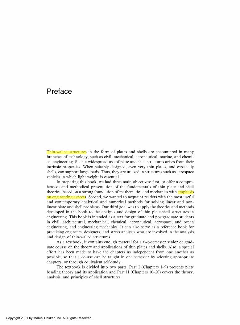
Thin plates are initially flat structural members bounded by two parallel planes,called faces, and a cylindrical surface, called an edge or boundary. The generatorsof the cylindrical surface are perpendicular to the plane faces. The distance betweenthe plane faces is called the thickness (h) of the plate. It will be assumed that the platethickness is small compared with other characteristic dimensions of the faces (length,width, diameter, etc.). Geometrically, plates are bounded either by straight or curvedboundaries (Fig. 1.1). The static or dynamic loads carried by plates are predomi-nantly perpendicular to the plate faces.

The load-carrying action of a plate is similar, to a certain extent, to that ofbeams or cables; thus, plates can be approximated by a gridwork of an infinitenumber of beams or by a network of an infinite number of cables, depending onthe flexural rigidity of the structures. This two-dimensional structural action ofplates results in lighter structures, and therefore offers numerous economic advan-tages. The plate, being originally flat, develops shear forces, bending and twistingmoments to resist transverse loads. Because the loads are generally carried in bothdirections and because the twisting rigidity in isotropic plates is quite significant, aplate is considerably stiffer than a beam of comparable span and thickness. So, thinplates combine light weight and a form efficiency with high load-carrying capacity,economy, and technological effectiveness.

Because of the distinct advantages discussed above, thin plates are extensivelyused in all fields of engineering. Plates are used in architectural structures, bridges,hydraulic structures, pavements, containers, airplanes, missiles, ships, instruments,machine parts, etc. (Fig. 1.2).

We consider a plate, for which it is common to divide the thickness h into equalhalves by a plane parallel to its faces. This plane is called the middle plane (or simply,

Part I

Thin Plates


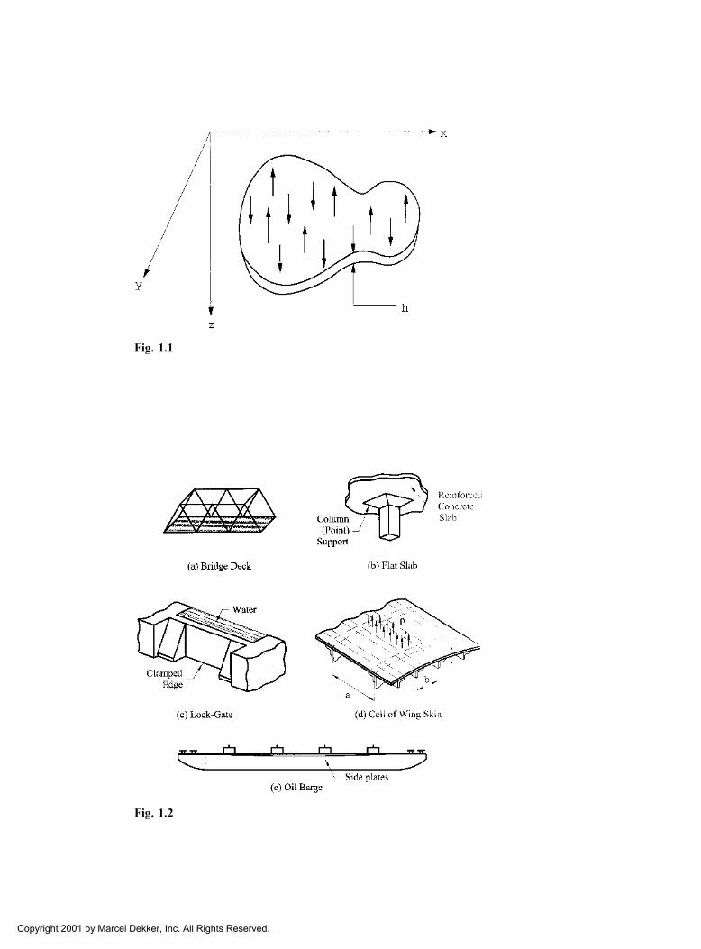
Fig. 1.1

Fig. 1.2


the midplane) of the plate (Fig. 1.3). Being subjected to transverse loads, an initiallyflat plate deforms and the midplane passes into some curvilinear surface, which isreferred to as the middle surface. With the exception of Secs 3.8 and 4.8, we willconsider only plates of constant thickness. For such plates, the shape of a plate isadequately defined by describing the geometry of its middle plane. Depending on theshape of this midplane, we will distinguish between rectangular, circular, elliptic, etc.,plates.

A plate resists transverse loads by means of bending, exclusively. The flexuralproperties of a plate depend greatly upon its thickness in comparison with otherdimensions. Plates may be classified into three groups according to the ratio a=h,where a is a typical dimension of a plate in a plane and h is a plate thickness. Thesegroups are

1. The first group is presented by thick plates having ratios a=h � 8 . . . 10. Theanalysis of such bodies includes all the components of stresses, strains, and displace-ments as for solid bodies using the general equations of three-dimensional elasticity.

2. The second group refers to plates with ratios a=h � 80 . . . 100. These platesare referred to as membranes and they are devoid of flexural rigidity. Membranescarry the lateral loads by axial tensile forces N (and shear forces) acting in the platemiddle surface as shown in Fig. 1.7. These forces are called membrane forces; theyproduce projection on a vertical axis and thus balance a lateral load applied to theplate-membrane.

3. The most extensive group represents an intermediate type of plate, so-called thin plate with 8 . . . 10 � a=h � 80 . . . 100. Depending on the value of theratio w=h, the ratio of the maximum deflection of the plate to its thickness, thepart of flexural and membrane forces here may be different. Therefore, this group,in turn, may also be subdivided into two different classes.

a. Stiff plates. A plate can be classified as a stiff plate if w=h � 0:2. Stiff platesare flexurally rigid thin plates. They carry loads two dimensionally, mostly by inter-nal bending and twisting moments and by transverse shear forces. The middle planedeformations and the membrane forces are negligible. In engineering practice, theterm plate is understood to mean a stiff plate, unless otherwise specified. The conceptof stiff plates introduces serious simplifications that are discussed later. A funda-

Fig. 1.3


mental feature of stiff plates is that the equations of static equilibrium for a plateelement may be set up for an original (undeformed) configuration of the plate.

b. Flexible plates. If the plate deflections are beyond a certain level,w=h � 0:3, then, the lateral deflections will be accompanied by stretching of themiddle surface. Such plates are referred to as flexible plates. These plates repre-sent a combination of stiff plates and membranes and carry external loads by thecombined action of internal moments, shear forces, and membrane (axial) forces.Such plates, because of their favorable weight-to-load ratio, are widely used bythe aerospace industry. When the magnitude of the maximum deflection is con-siderably greater than the plate thickness, the membrane action predominates. So,if w=h > 5, the flexural stress can be neglected compared with the membranestress. Consequently, the load-carrying mechanism of such plates becomes ofthe membrane type, i.e., the stress is uniformly distributed over the platethickness.

The above classification is, of course, conditional because the reference of theplate to one or another group depends on the accuracy of analysis, type of loading,boundary conditions, etc.

With the exception of Sec. 7.4, we consider only small deflections of thin plates,a simplification consistent with the magnitude of deformation commonly found inplate structures.

1.2 HISTORY OF PLATE THEORY DEVELOPMENT

The first impetus to a mathematical statement of plate problems, was probably doneby Euler, who in 1776 performed a free vibration analysis of plate problems [1].

Chladni, a German physicist, discovered the various modes of free vibrations[2]. In experiments on horizontal plates, he used evenly distributed powder, whichformed regular patterns after induction of vibration. The powder accumulated alongthe nodal lines, where no vertical displacements occurred. J. Bernoulli [3] attemptedto justify theoretically the results of these acoustic experiments. Bernoulli’s solutionwas based on the previous work resulting in the Euler–D.Bernoulli’s bending beamtheory. J. Bernoulli presented a plate as a system of mutually perpendicular strips atright angles to one another, each strip regarded as functioning as a beam. But thegoverning differential equation, as distinct from current approaches, did not containthe middle term.

Fig. 1.4


The French mathematician Germain developed a plate differential equationthat lacked the warping term [4]; by the way, she was awarded a prize by the ParisianAcademy in 1816 for this work. Lagrange, being one of the reviewers of this work,corrected Germain’s results (1813) by adding the missing term [5]; thus, he was thefirst person to present the general plate equation properly.

Cauchy [6] and Poisson [7] were first to formulate the problem of plate bendingon the basis of general equations of theory of elasticity. Expanding all the character-istic quantities into series in powers of distance from a middle surface, they retainedonly terms of the first order of smallness. In such a way they obtained the governingdifferential equation for deflections that coincides completely with the well-knownGermain–Lagrange equation. In 1829 Poisson expanded successfully the Germain–Lagrange plate equation to the solution of a plate under static loading. In thissolution, however, the plate flexural rigidity D was set equal to a constant term.Poisson also suggested setting up three boundary conditions for any point on a freeboundary. The boundary conditions derived by Poisson and a question about thenumber and nature of these conditions had been the subject of much controversyand were the subject of further investigations.

The first satisfactory theory of bending of plates is associated with Navier [8],who considered the plate thickness in the general plate equation as a function ofrigidity D. He also introduced an ‘‘exact’’ method which transformed the differentialequation into algebraic expressions by use of Fourier trigonometric series.

In 1850 Kirchhoff published an important thesis on the theory of thin plates[9]. In this thesis, Kirchhoff stated two independent basic assumptions that are nowwidely accepted in the plate-bending theory and are known as ‘‘Kirchhoff’s hypoth-eses.’’ Using these assumptions, Kirchhoff simplified the energy functional of 3Delasticity theory for bent plates. By requiring that it be stationary he obtained theGermain-Lagrange equation as the Euler equation. He also pointed out that thereexist only two boundary conditions on a plate edge. Kirchhoff’s other significantcontributions are the discovery of the frequency equation of plates and the intro-duction of virtual displacement methods in the solution of plate problems.Kirchhoff’s theory contributed to the physical clarity of the plate bending theoryand promoted its widespread use in practice.

Lord Kelvin (Thomson) and Tait [10] provided an additional insight relative tothe condition of boundary equations by converting twisting moments along the edgeof a plate into shearing forces. Thus, the edges are subject to only two forces: shearand moment.

Kirchhoff’s book was translated by Clebsh [11]. That translation containsnumerous valuable comments by de Saint-Venant: the most important being theextension of Kirchhoff’s differential equation of thin plates, which considered, in amathematically correct manner, the combined action of bending and stretching.Saint-Venant also pointed out that the series proposed by Cauchy and Poissons asa rule, are divergent.

The solution of rectangular plates, with two parallel simple supports and theother two supports arbitrary, was successfully solved by Levy [12] in the late 19thcentury.

At the end of the 19th and the beginning of the 20th centuries, shipbuilderschanged their construction methods by replacing wood with structural steel. Thischange in structural materials was extremely fruitful in the development of various


plate theories. Russian scientists made a significant contribution to naval architec-ture by being the first to replace the ancient trade traditions with solid mathematicaltheories. In particular, Krylov [13] and his student Bubnov [14] contributed exten-sively to the theory of thin plates with flexural and extensional rigidities. Bubnov laidthe groundwork for the theory of flexible plates and he was the first to introduce amodern plate classification. Bubnov proposed a new method of integration of differ-ential equations of elasticity and he composed tables of maximum deflections andmaximum bending moments for plates of various properties. Then, Galerkin devel-oped this method and applied it to plate bending analysis. Galerkin collected numer-ous bending problems for plates of arbitrary shape in a monograph [15].

Timoshenko made a significant contribution to the theory and application ofplate bending analysis. Among Timoshenko’s numerous important contributions aresolutions of circular plates considering large deflections and the formulation ofelastic stability problems [16,17]. Timoshenko and Woinowsky-Krieger publisheda fundamental monograph [18] that represented a profound analysis of variousplate bending problems.

Extensive studies in the area of plate bending theory and its various applica-tions were carried out by such outstanding scientists as Hencky [19], Huber [20], vonKarman [21,22], Nadai [23], Foppl [24].

Hencky [19] made a contribution to the theory of large deformations and thegeneral theory of elastic stability of thin plates. Nadai made extensive theoretical andexperimental investigations associated with a check of the accuracy of Kirchhoff’splate theory. He treated different types of singularities in plates due to a concen-trated force application, point support effects, etc. The general equations for thelarge deflections of very thin plates were simplified by Foppl who used the stressfunction acting in the middle plane of the plate. The final form of the differentialequation of the large-deflection theory, however, was developed by von Karman. Healso investigated the postbuckling behavior of plates.

Huber, developed an approximate theory of orthotropic plates and solvedplates subjected to nonsymmetrical distributed loads and edge moments. Thebases of the general theory of anisotropic plates were developed by Gehring [25]and Boussinesq [26]. Lekhnitskii [27] made an essential contribution to the develop-ment of the theory and application of anisotropic linear and nonlinear plate analysis.He also developed the method of complex variables as applied to the analysis ofanisotropic plates.

The development of the modern aircraft industry provided another strongimpetus toward more rigorous analytical investigations of plate problems. Platessubjected to in-plane forces, postbuckling behavior, and vibration problems (flutter),stiffened plates, etc., were analyzed by various scientists and engineers.

E. Reissner [28] developed a rigorous plate theory which considers the defor-mations caused by the transverse shear forces. In the former Soviet Union the worksof Volmir [29] and Panov [30] were devoted mostly to solution of nonlinear platebending problems.

The governing equation for a thin rectangular plate subjected to direct com-pressive forces Nx was first derived by Navier [8]. The buckling problem for a simplysupported plate subjected to the direct, constant compressive forces acting in oneand two directions was first solved by Bryan [31] using the energy method. Cox [32],Hartmann [33], etc., presented solutions of various buckling problems for thin


rectangular plates in compression, while Dinnik [34], Nadai [35], Meissner [36], etc.,completed the buckling problem for circular compressed plates. An effect of thedirect shear forces on the buckling of a rectangular simply supported plate wasfirst studied by Southwell and Skan [37]. The buckling behavior of a rectangularplate under nonuniform direct compressive forces was studied by Timoshenko andGere [38] and Bubnov [14]. The postbuckling behavior of plates of various shapeswas analyzed by Karman et al. [39], Levy [40], Marguerre [41], etc. A comprehensiveanalysis of linear and nonlinear buckling problems for thin plates of various shapesunder various types of loads, as well as a considerable presentation of availableresults for critical forces and buckling modes, which can be used in engineeringdesign, were presented by Timoshenko and Gere [38], Gerard and Becker [42],Volmir [43], Cox [44], etc.

A differential equation of motion of thin plates may be obtained by applyingeither the D’Alambert principle or work formulation based on the conservation ofenergy. The first exact solution of the free vibration problem for rectangular plates,whose two opposite sides are simply supported, was achieved by Voight [45]. Ritz[46] used the problem of free vibration of a rectangular plate with free edges todemonstrate his famous method for extending the Rayleigh principle for obtainingupper bounds on vibration frequencies. Poisson [7] analyzed the free vibration equa-tion for circular plates. The monographs by Timoshenko and Young [47], DenHartog [48], Thompson [49], etc., contain a comprehensive analysis and design con-siderations of free and forced vibrations of plates of various shapes. A referencebook by Leissa [50] presents a considerable set of available results for the frequenciesand mode shapes of free vibrations of plates could be provided for the design and fora researcher in the field of plate vibrations.

The recent trend in the development of plate theories is characterized by aheavy reliance on modern high-speed computers and the development of the mostcomplete computer-oriented numerical methods, as well as by introduction of morerigorous theories with regard to various physical effects, types of loading, etc.

The above summary is a very brief survey of the historical background of theplate bending theory and its application. The interested reader is referred to specialmonographs [51,52] where this historical development of plates is presented in detail.

1.3 GENERAL BEHAVIOR OF PLATES

Consider a load-free plate, shown in Fig.1.3, in which the xy plane coincides with theplate’s midplane and the z coordinate is perpendicular to it and is directed down-wards. The fundamental assumptions of the linear, elastic, small-deflection theory ofbending for thin plates may be stated as follows:

1. The material of the plate is elastic, homogeneous, and isotropic.2. The plate is initially flat.3. The deflection (the normal component of the displacement vector) of the

midplane is small compared with the thickness of the plate. The slope ofthe deflected surface is therefore very small and the square of the slope isa negligible quantity in comparison with unity.

4. The straight lines, initially normal to the middle plane before bending,remain straight and normal to the middle surface during the deformation,


and the length of such elements is not altered. This means that the verticalshear strains �xz and �yz are negligible and the normal strain "z may alsobe omitted. This assumption is referred to as the ‘‘hypothesis of straightnormals.’’

5. The stress normal to the middle plane, �z, is small compared with theother stress components and may be neglected in the stress–strain rela-tions.

6. Since the displacements of a plate are small, it is assumed that the middlesurface remains unstrained after bending.

Many of these assumptions, known as Kirchhoff’s hypotheses, are analogous tothose associated with the simple bending theory of beams. These assumptions resultin the reduction of a three-dimensional plate problem to a two-dimensional one.Consequently, the governing plate equation can be derived in a concise and straight-forward manner. The plate bending theory based on the above assumptions isreferred to as the classical or Kirchhoff’s plate theory. Unless otherwise stated, thevalidity of the Kirchhoff plate theory is assumed throughout this book.

1.4 SURVEY OF ELASTICITY THEORY

The classical theories of plates and shells are an important application of the theoryof elasticity, which deals with relationships of forces, displacements, stresses, andstrains in an elastic body. When a solid body is subjected to external forces, itdeforms, producing internal strains and stresses. The deformation depends on thegeometrical configuration of the body, on applied loading, and on the mechanicalproperties of its material. In the theory of elasticity we restrict our attention to linearelastic materials; i.e., the relationships between stress and strain are linear, and thedeformations and stresses disappear when the external forces are removed. Theclassical theory of elasticity assumes the material is homogeneous and isotropic,i.e., its mechanical properties are the same in all directions and at all points.

The present section contains only a brief survey of the elasticity theory that willbe useful for the development of the plate theory. All equations and relations will begiven without derivation. The reader who desires to review details is urged to refer toany book on elasticity theory – for example [53–55].

1.4.1 Stress at a point: stress tensor

Consider an elastic body of any general shape subjected to external loads which arein equilibrium. Then, consider a material point anywhere in the interior of the body.If we assign a Cartesian coordinate frame with axes x, y, and z, as shown in Fig. 1.5,it is convenient to assign an infinitesimal element in the form of parallelepiped(dx; dy; dz), with faces parallel to the coordinate planes. Stresses acting on thefaces of this element describe the intensity of the internal forces at a point on aparticular face. These stresses can be broken down into a normal component (normalstress) and tangent component (shear stress) to the particular face. As a result, thethree stress components, denoted by �xx; �xy; �xz; . . . ; will act on each face of theelement. The subscript notation for the stress components is interpreted as follows:the first subscript indicates the direction of an outer normal to the face on which thestress component acts; the second subscript relates to the direction of the stress itself.


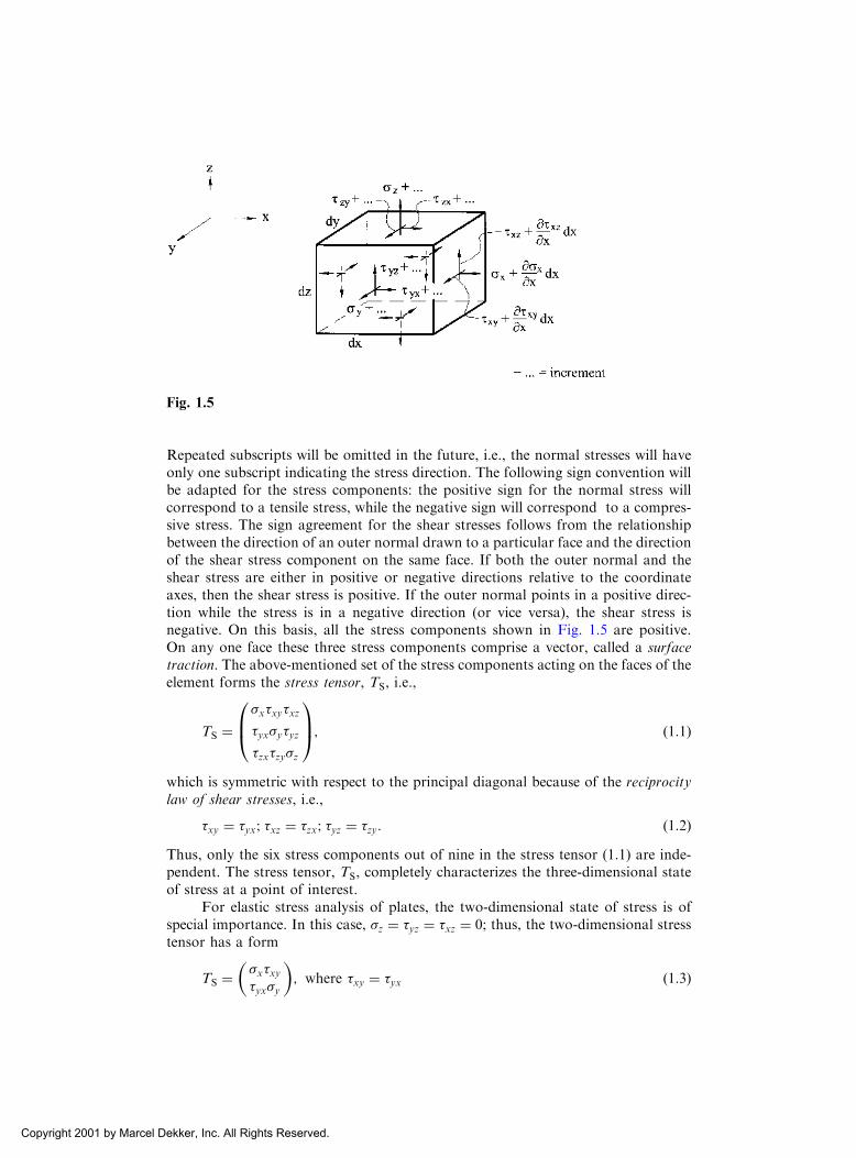
Repeated subscripts will be omitted in the future, i.e., the normal stresses will haveonly one subscript indicating the stress direction. The following sign convention willbe adapted for the stress components: the positive sign for the normal stress willcorrespond to a tensile stress, while the negative sign will correspond to a compres-sive stress. The sign agreement for the shear stresses follows from the relationshipbetween the direction of an outer normal drawn to a particular face and the directionof the shear stress component on the same face. If both the outer normal and theshear stress are either in positive or negative directions relative to the coordinateaxes, then the shear stress is positive. If the outer normal points in a positive direc-tion while the stress is in a negative direction (or vice versa), the shear stress isnegative. On this basis, all the stress components shown in Fig. 1.5 are positive.On any one face these three stress components comprise a vector, called a surfacetraction. The above-mentioned set of the stress components acting on the faces of theelement forms the stress tensor, TS, i.e.,

TS ¼�x�xy�xz

�yx�y�yz

�zx�zy�z

0B@

1CA; ð1:1Þ

which is symmetric with respect to the principal diagonal because of the reciprocitylaw of shear stresses, i.e.,

�xy ¼ �yx; �xz ¼ �zx; �yz ¼ �zy: ð1:2ÞThus, only the six stress components out of nine in the stress tensor (1.1) are inde-pendent. The stress tensor, TS, completely characterizes the three-dimensional stateof stress at a point of interest.

For elastic stress analysis of plates, the two-dimensional state of stress is ofspecial importance. In this case, �z ¼ �yz ¼ �xz ¼ 0; thus, the two-dimensional stresstensor has a form

TS ¼ �x�xy�yx�y

� �; where �xy ¼ �yx ð1:3Þ

Fig. 1.5


1.4.2 Strains and displacements

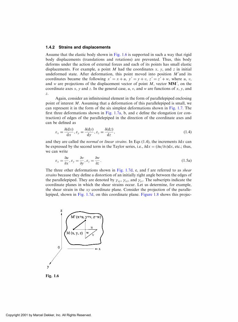
Assume that the elastic body shown in Fig. 1.6 is supported in such a way that rigidbody displacements (translations and rotations) are prevented. Thus, this bodydeforms under the action of external forces and each of its points has small elasticdisplacements. For example, a point M had the coordinates x; y, and z in initialundeformed state. After deformation, this point moved into position M 0and itscoordinates became the following x 0 ¼ xþ u; y 0 ¼ yþ v, z 0 ¼ z 0 þ w, where u, v,and w are projections of the displacement vector of point M, vector MM

0, on thecoordinate axes x, y and z. In the general case, u, v, and w are functions of x, y, andz.

Again, consider an infinitesimal element in the form of parallelepiped enclosingpoint of interest M. Assuming that a deformation of this parallelepiped is small, wecan represent it in the form of the six simplest deformations shown in Fig. 1.7. Thefirst three deformations shown in Fig. 1.7a, b, and c define the elongation (or con-traction) of edges of the parallelepiped in the direction of the coordinate axes andcan be defined as

"x ¼ �ðdxÞdx

; "y ¼�ðdyÞdy

; "z ¼�ðdzÞdz

; ð1:4Þ

and they are called the normal or linear strains. In Eqs (1.4), the increments �dx canbe expressed by the second term in the Taylor series, i.e., �dx ¼ ð@u=@xÞdx, etc.; thus,we can write

"x ¼ @u

@x; "y ¼

@v

@y; "z ¼

@w

@z: ð1:5aÞ

The three other deformations shown in Fig. 1.7d, e, and f are referred to as shearstrains because they define a distortion of an initially right angle between the edges ofthe parallelepiped. They are denoted by �xy, �xz, and �yz. The subscripts indicate thecoordinate planes in which the shear strains occur. Let us determine, for example,the shear strain in the xy coordinate plane. Consider the projection of the paralle-lepiped, shown in Fig. 1.7d, on this coordinate plane. Figure 1.8 shows this projec-

Fig. 1.6


tion in the form of the rectangle before deformation (ABCD) and after deformation(A 0B 0C 0D 0). The angle BAD in Fig. 1.8 deforms to the angle B 0A 0D 0, the deforma-tion being the angle � 0 þ � 00; thus, the shear strain is

�xy ¼ � 0 þ � 00 ðaÞor it can be determined in terms of the in-plane displacements, u and v, as follows:

�xy ¼@v@xdx

dxþ @u@x dx

þ@u@y dy

dyþ @v@y dy

¼@v@x

1þ @u@x

þ@u@y

1þ @v@y

:

Since we have confined ourselves to the case of very small deformations, we mayomit the quantities @u=@x and @v=@y in the denominator of the last expression, asbeing negligibly small compared with unity. Finally, we obtain

Fig. 1.7

Fig. 1.8


�xy ¼@v

@xþ @u@y: ðbÞ

Similarly, we can obtain �xz and �yz. Thus, the shear strains are given by

�xy ¼@u

@yþ @v

@x; �xz ¼

@u

@zþ @w@x; �yz ¼

@v

@zþ @w@y: ð1:5bÞ

Similar to the stress tensor (1.1) at a given point, we can define a strain tensor as

TD ¼

"x1

2�xy

1

2�xz

1

2�yx "y

1

2�yz

1

2�zx

1

2�zy "z

0BBBBB@

1CCCCCA: ð1:6Þ

It is evident that the strain tensor is also symmetric because of

�xy ¼ �yx; �xz ¼ �zx; �yz ¼ �zy ð1:7Þ

1.4.3 Constitutive equations

The constitutive equations relate the stress components to strain components. Forthe linear elastic range, these equations represent the generalized Hooke’s law. In thecase of a three-dimensional isotropic body, the constitutive equations are given by[53].

"x ¼ 1

E�x � � �y þ �z

� �� ; "y ¼

1

E�y � � �x þ �zð Þ� �

; "z ¼1

2�z � � �y þ �x

� �� ;

ð1:8aÞ

�xy ¼1

G�xy; �xz ¼

1

G�xz; �yz ¼

1

G�yz; ð1:8bÞ

where E, �, and G are the modulus of elasticity, Poisson’s ratio, and the shearmodulus, respectively. The following relationship exists between E and G:

G ¼ E

2ð1þ �Þ ð1:9Þ

1.4.4 Equilibrium equations

The stress components introduced previously must satisfy the following differentialequations of equilibrium:

@�x@x

þ @�xy@y

þ @�xz@z

þ Fx ¼ 0;

@�y@y

þ @�yx@x

þ @�yz@z

þ Fy ¼ 0;

@�z@z

þ @�zx@x

þ @�zy@y

þ Fz ¼ 0;

ð1:10Þ


where Fx; Fy; and Fz are the body forces (e.g., gravitational, magnetic forces). Inderiving these equations, the reciprocity of the shear stresses, Eqs (1.7), has beenused.

1.4.5 Compatibility equations

Since the three equations (1.10) for six unknowns are not sufficient to obtain asolution, three-dimensional stress problems of elasticity are internally statically inde-terminate. Additional equations are obtained to express the continuity of a body.These additional equations are referred to as compatibility equations. In Eqs (1.5) wehave related the six strain components to the three displacement components.Eliminating the displacement components by successive differentiation, the follow-ing compatibility equations are obtained [53–55]:

@2"x@y2

þ @2"y

@x2¼ @2�xy@x@y

;

@2"y

@z2þ @

2"z@y2

¼ @2�yz@y@z

; ð1:11aÞ

@2"z@x2

þ @2"x@z2

¼ @2�xz@x@z

;

@

@z

@�yz@x

þ @�xz@y

� @�xy@z

� �¼ 2

@2"z@x@y

;

@

@x

@�xz@y

þ @�xy@z

� @�yz@x

� �¼ 2

@2"x@y@z

; ð1:11bÞ

@

@y

@�xy@z

þ @�yz@x

� @�xz@y

� �¼ 2

@2"y@x@z

:

For a two-dimensional state of stress (�z ¼ 0, �xz ¼ �yz ¼ 0), the equilibrium condi-tions (1.10) become

@�x@x

þ @�xy@y

þ Fx ¼ 0;

@�y@y

þ @�yx@x

þ Fy ¼ 0;

ð1:12Þ

and the compatibility equation is

@2"x@y2

þ @2"y

@x2¼ @2�xy@x@y

�xz ¼ �yz ¼ "z ¼ 0� �

: ð1:13Þ

We can rewrite Eq. (1.13) in terms of the stress components as follows

@2

@x2þ @2

@y2

!�x þ �y� � ¼ 0: ð1:14Þ


This equation is called Levy’s equation. By introducing Airy’s stress function � x; yð Þwhich satisfies

�x ¼@2�

@y2; �y ¼

@2�

@x2; �xy ¼ � @2�

@x@y; ð1:15Þ

Eq. (1.14) becomes

r2r2� ¼ 0; ð1:16Þwhere

r2 � @2

@x2þ @2

@y2ð1:17Þ

is the two-dimensional Laplace operator.

SUMMARY

For an elastic solid there are 15 independent variables: six stress components, sixstrain components, and three displacements. In the case where compatibility is satis-fied, there are 15 equations: three equilibrium equations, six constitutive relations,and six strain-displacement equations.

REFERENCES

1. Euler, L., De motu vibratorio tympanorum, Novi Commentari Acad Petropolit, vol. 10,

pp. 243–260 (1766).

2. Chladni, E.F., Die Akustik, Leipzig, 1802.

3. Bernoulli, J., Jr., Essai theorique sur les vibrations de plaques elastiques rectangularies et

libers, Nova Acta Acad Petropolit, vol. 5, pp. 197–219 (1789).

4. Germain, S., Remarques sur la nature, les bornes et l’etendue de la question des surfaces

elastiques et equation general de ces surfaces, Paris, 1826.

5. Lagrange, J.L., Ann Chim, vol. 39, pp. 149–207 (1828).

6. Cauchy, A.L., Sur l’equilibre le mouvement d’une plaque solide, Exercises Math, vol. 3,

p. 328 (1828).

7. Poisson, S.D., Memoire sur l’equilibre et le mouvement des corps elastique, Mem Acad

Sci, vol. 8, p. 357 (1829).

8. Navier, C.L.M.H., Bulletin des Sciences de la Societe Philomathique de Paris, 1823.

9. Kirchhoff, G.R., Uber das gleichgewichi und die bewegung einer elastishem scheibe, J

Fuer die Reine und Angewandte Mathematik, vol. 40, pp. 51–88 (1850).

10. Lord Kelvin and Tait, P.G., Treatise on Natural Philosophy, vol. 1, Clarendon Press,

Oxford, 1883.

11. Clebsch, A. Theorie de l’Elasticite des Corps Solids, Avec des Notes Entendues de Saint-

Venant, Dunod, Paris, pp. 687–706 (1883).

12. Levy, M., Memoire sur la theorie des plaques elastiques planes, J Math Pure Appl, vol 3,

p. 219 (1899).

13. Krylov, A.N., On stresses experienced by a ship in a sea way, Trans Inst Naval Architects,

vol. 40, London, pp. 197–209, 1898.

14. Bubnov, I.G., Theory of Structures of Ships, vol. 2, St . Petersburg, 1914.

15. Galerkin, B.G., Thin Elastic Plates, Gostrojisdat, Leningrad, 1933 (in Russian).

16. Timoshenko, S.P., On large deflections of circular plates, Mem Inst Ways Commun, 89,

1915.


17. Timoshenko, S.P., Sur la stabilite des systemes elastiques, Ann des Points et Chaussees,

vol. 13, pp. 496–566; vol. 16, pp. 73–132 (1913).

18. Timoshenko, S.P. and Woinowsky-Krieger, S., Theory of Plates and Shells, 2nd edn,

McGraw-Hill, New York, 1959.

19. Hencky, H., Der spanngszustand in rechteckigen platten (Diss.), Z Andew Math und

Mech, vol. 1 (1921).

20. Huber, M.T., Probleme der Static Techish Wichtiger Orthotroper Platten, Warsawa,

1929.

21. von Karman, T., Fesigkeitsprobleme in Maschinenbau, Encycl der Math Wiss, vol. 4, pp.

348–351 (1910).

22. von Karman,T., Ef Sechler and Donnel, L.H. The strength of thin plates in compression,

Trans ASME, vol. 54, pp. 53–57 (1932).

23. Nadai, A. Die formanderungen und die spannungen von rechteckigen elastischen platten,

Forsch a.d. Gebiete d Ingeineurwesens, Berlin, Nos. 170 and 171 (1915).

24. Foppl, A., Vorlesungen uber technische Mechanik, vols 1 and 2, 14th and 15th edns,

Verlag R., Oldenburg, Munich, 1944, 1951.

25. Gehring, F., Vorlesungen uber Mathematieche Physik, Mechanik, 2nd edn, Berlin,1877.

26. Boussinesq, J., Complements anne etude sur la theorie de l’equilibre et du mouvement

des solides elastiques, J de Math Pures et Appl , vol. 3, ses. t.5 (1879).

27. Leknitskii, S.G., Anisotropic Plates (English translation of the original Russian work),

Gordon and Breach, New York, 1968.

28. Reissner, E., The effect of transverse shear deformation on the bending of elastic plates, J

Appl Mech Trans ASME, vol. 12, pp. A69–A77 (1945).

29. Volmir, A.S., Flexible Plates and Shells, Gos. Izd-vo Techn.-Teoret. Lit-ry, Moscow,

1956 (in Russian).

30. Panov, D.Yu., On large deflections of circular plates, Prikl Matem Mech, vol. 5, No. 2,

pp. 45–56 (1941) (in Russian).

31. Bryan, G.N., On the stability of a plane plate under thrusts in its own plane, Proc London

Math Soc, 22, 54–67 (1981)

32. Cox, H.L, Buckling of Thin Plates in Compression, Rep. and Memor., No. 1553,1554,

(1933).

33. Hartmann, F., Knickung, Kippung, Beulung, Springer-Verlag, Berlin, 1933.

34. Dinnik, A.N., A stability of compressed circular plate, Izv Kiev Polyt In-ta, 1911 (in

Russian).

35. Nadai, A., Uber das ausbeulen von kreisfoormigen platten, Zeitschr VDJ, No. 9,10 (1915).

36. Meissner, E., Uber das knicken kreisfoormigen scheiben, Schweiz Bauzeitung, 101, pp. 87–

89 (1933).

37. Southwell, R.V. and Scan, S., On the stability under shearing forces of a flat elastic strip,

Proc Roy Soc, A105, 582 (1924).

38. Timoshenko, S.P. and Gere, J.M., Theory of Elastic Stability, 2nd edn, McGraw-Hill,

New York, 1961.

39. Karman, Th., Sechler, E.E. and Donnel, L.H., The strength of thin plates in compres-

sion, Trans ASME, 54, 53–57 (1952).

40. Levy, S., Bending of Rectangular Plates with Large Deflections, NACA, Rep. No.737,

1942.

41. Marguerre, K., Die mittragende briete des gedruckten plattenstreifens,

Luftfahrtforschung, 14, No. 3, 1937.

42. Gerard, G. and Becker, H., Handbook of Structural Stability, Part1 – Buckling of Flat

Plates, NACA TN 3781, 1957.

43. Volmir, A.S., Stability of Elastic Systems, Gos Izd-vo Fiz-Mat. Lit-ry, Moscow, 1963 (in

Russian).

44. Cox, H.l., The Buckling of Plates and Shells. Macmillan, New York, 1963.


45. Voight, W, Bemerkungen zu dem problem der transversalem schwingungen rechteckiger

platten, Nachr. Ges (Gottingen), No. 6, pp. 225–230 (1893).

46. Ritz, W., Theorie der transversalschwingungen, einer quadratischen platte mit frein

randern, Ann Physic, Bd., 28, pp. 737–786 (1909).

47. Timoshenko, S.P. and Young, D.H., Vibration Problems in Engineering, John Wiley and

Sons., New York, 1963.

48. Den Hartog, J.P., Mechanical Vibrations, 4th edn, McGraw-Hill, New York, 1958.

49. Thompson, W.T., Theory of Vibrations and Applications, Prentice-Hill, Englewood Cliffs,

New Jersey, 1973.

50. Leissa, A.W., Vibration of Plates, National Aeronautics and Space Administration,

Washington, D.C., 1969.

51. Timoshenko, S.P., History of Strength of Materials, McGraw-Hill, New York, 1953.

52. Truesdell, C., Essays in the History of Mechanic., Springer-Verlag, Berlin, 1968.

53. Timoshenko, S.P. and Goodier, J.N., Theory of Elasticity, 3rd edn, McGraw-Hill, New

York, 1970.

54. Prescott, J.J., Applied Elasticity, Dover, New York, 1946.

55. Sokolnikoff, I.S., Mathematical Theory of Elasticity, 2nd edn, McGraw-Hill, New York,

1956.


2

The Fundamentals of the Small-Deflection P late Bending Theory

2.1 INTRODUCTION

The foregoing assumptions introduced in Sec. 1.3 make it possible to derive the basicequations of the classical or Kirchhoff’s bending theory for stiff plates. It is conve-nient to solve plate bending problems in terms of displacements. In order to derivethe governing equation of the classical plate bending theory, we will invoke the threesets of equations of elasticity discussed in Sec. 1.4.

2.2 STRAIN–CURVATURE RELATIONS (KINEMATIC EQUATIONS)

We will use common notations for displacement, stress, and strain componentsadapted in elasticity (see Sec. 1.4). Let u; v; and w be components of the displacementvector of points in the middle surface of the plate occurring in the x; y, and zdirections, respectively. The normal component of the displacement vector, w (calledthe deflection), and the lateral distributed load p are positive in the downwarddirection. As it follows from the assumption (4) of Sec. 1.3

"z ¼ 0; �yz ¼ 0; �xz ¼ 0: ð2:1ÞIntegrating the expressions (1.5) for "z; �yz; and �xz and taking into account Eq.(2.1), we obtain

wz ¼ w x; yð Þ; uz ¼ �z@w

@xþ u x; yð Þ; vz ¼ �z

@w

@yþ v x; yð Þ; ð2:2Þ

where uz; vz, and wz are displacements of points at a distance z from the middlesurface. Based upon assumption (6) of Sec. 1.3, we conclude that u ¼ v ¼ 0. Thus,Eqs (2.2) have the following form in the context of Kirchhoff’s theory:


wz ¼ w x; yð Þ; uz ¼ �z@w

@x; vz ¼ �z

@w

@y: ð2:3Þ

As it follows from the above, the displacements uz and vz of an arbitrary horizontallayer vary linearly over a plate thickness while the deflection does not vary over thethickness.

Figure 2.1 shows a section of the plate by a plane parallel to Oxz; y ¼ const:,before and after deformation. Consider a segment AB in the positive z direction. Wefocus on an arbitrary point B which initially lies at a distance z from the undeformedmiddle plane (from the point A). During the deformation, point A displaces a dis-tance w parallel to the original z direction to point A1. Since the transverse sheardeformations are neglected, the deformed position of point B must lie on the normalto the deformed middle plane erected at point A1(assumption (4)). Its final position isdenoted by B1. Due to the assumptions (4) and (5), the distance z between the above-mentioned points during deformation remains unchanged and is also equal to z.

We can also represent the displacement components uz and vz, Eqs (2.2), in theform

uz ¼ �z#x; vz ¼ �z#y; ð2:4Þ

where

#x ¼ @w

@x; #y ¼

@w

@yð2:5Þ

are the angles of rotation of the normal (normal I–I in Fig. 2.1) to the middle surfacein the Oxz and Oyz plane, respectively. Owing to the assumption (4) of Sec. 1.3, #xand #y are also slopes of the tangents to the traces of the middle surface in the above-mentioned planes.

Substitution of Eqs (2.3) into the first two Eqs (1.5a) and into the first Eq.(1.5b), yields

"zx ¼ �z@2w

@x2; "zy ¼ �z

@2w

@y2; �zxy ¼ �2z

@2w

@x@y; ð2:6Þ

Fig. 2.1


where the superscript z refers to the in-plane strain components at a point of theplate located at a distance z from the middle surface. Since the middle surfacedeformations are neglected due to the assumption (6), from here on, this superscriptwill be omitted for all the strain and stress components at points across the platethickness.

The second derivatives of the deflection on the right-hand side of Eqs. (2.6)have a certain geometrical meaning. Let a section MNP represent some plane curvein which the middle surface of the deflected plate is intersected by a plane y ¼ const.(Fig. 2.2).

Due to the assumption 3 (Sec. 1.3), this curve is shallow and the square of theslope angle may be regarded as negligible compared with unity, i.e., (@w=@xÞ2 � 1.Then, the second derivative of the deflection, @2w=@x2 will define approximately thecurvature of the section along the x axis, �x. Similarly, @2w=@y2 defines the curvatureof the middle surface �y along the y axis. The curvatures �x and �y characterize thephenomenon of bending of the middle surface in planes parallel to the Oxz and Oyzcoordinate planes, respectively. They are referred to as bending curvature and aredefined by

�x ¼1

�x¼ � @

2w

@x2; �y ¼

1

�y¼ � @

2w

@y2ð2:7aÞ

We consider a bending curvature positive if it is convex downward, i.e., in thepositive direction of the z axis. The negative sign is taken in Eqs. (2.7a) since, forexample, for the deflection convex downward curve MNP (Fig. 2.2), the secondderivative, @2w=@x2 is negative.

The curvature @2w=@x2 can be also defined as the rate of change of the angle#x ¼ @w=@x with respect to distance x along this curve. However, the above anglecan vary in the y direction also. It is seen from comparison of the curves MNP andM1N1P1 (Fig. 2.2), separated by a distance dy. If the slope for the curve MNPis @w=@x then for the curve M1N1P1 this angle becomes equal to@w

@x� @

@y

@w

@x

� �dy

� �or

@w

@x� @2w

@x@ydy

!. The rate of change of the angle @w=@x per

unit length will be ð�@2w=@x@y). The negative sign is taken here because it is assumed

Fig. 2.2


that when y increases, the slope angle of the tangent to the curve decreases (byanalogy with the sign convention for the bending curvatures �x and �y). Similarly,can be convinced that in the perpendicular section (for the variable x), the rate ofchange of the angle @w=@y is characterized by the same mixed derivativeð�@2w=@x@yÞ. By analogy with the torsion theory of rods, the derivative @2w=@x@ydefines the warping of the middle surface at a point with coordinates x and y is calledthe twisting curvature with respect to the x and y axes and is denotes by �xy. Thus,

�xy ¼ �yx ¼ 1

�xy¼ � @2w

@x@yð2:7bÞ

Taking into account Eqs (2.7) we can rewrite Eqs (2.6) as follows

"x ¼ z�x; "y ¼ z�y; �xy ¼ 2z�xy: ð2:8Þ

2.3 STRESSES, STRESS RESULTANTS, AND STRESS COUPLES

In the case of a three-dimensional state of stress, stress and strain are related by theEqs (1.8) of the generalized Hooke’s law. As was mentioned earlier, Kirchhoff’sassumptions of Sec. 1.3 brought us to Eqs (2.1). From a mathematical standpoint,this means that the three new equations (2.1) are added to the system of governingequations of the theory of elasticity. So, the latter becomes overdetermined and,therefore, it is necessary to also drop three equations. As a result, the three relationsout of six of Hookes’ law (see Eqs (1.8)) for strains (2.1) are discarded. Moreover, thenormal stress component �z ¼ 0: Solving Eqs (1.8) for stress components �x, �y, and�xy, yields

�x ¼E

1� �2 "x þ �"y� �

; �y ¼E

1� �2 "y þ �"x� �

; �xy ¼ G�xy: ð2:9Þ

The stress components are shown in Fig. 2.3a. The subscript notation and signconvention for the stresses were given in Sec. 1.4.

Fig. 2.3


Introducing the plate curvatures, Eqs (2.7) and using Eqs (2.8), the aboveequations appear as follows:

�x ¼ Ez

1� �2 ð�x þ ��yÞ ¼ � Ez

1� �2@2w

@x2þ � @

2w

@y2

!;

�y ¼Ez

1� �2 ð�y þ ��xÞ ¼ � Ez

1� �2@2w

@y2þ � @

2w

@x2

!;

�xy ¼Ez

1þ � �xy ¼ � Ez

1þ �@2w

@x@y:

ð2:10Þ

It is seen from Eqs. (2.10) that Kirchhoff’s assumptions have led to a completelydefined law of variation of the stresses through the thickness of the plate. Therefore,as in the theory of beams, it is convenient to introduce, instead of the stress compo-nents at a point problem, the total statically equivalent forces and moments appliedto the middle surface, which are known as the stress resultants and stress couples. Thestress resultants and stress couples are referred to as the shear forces, Qx and Qy, aswell as the bending and twisting moments Mx; My, and Mxy, respectively. Thus,Kirchhoff’s assumptions have reduced the three-dimensional plate straining problemto the two-dimensional problem of straining the middle surface of the plate.Referring to Fig. 2.3, we can express the bending and twisting moments, as wellas the shear forces, in terms of the stress components, i.e.,

Mx

My

Mxy

8><>:

9>=>; ¼

ðh=2�h=2

�x

�y

�xy

8><>:

9>=>;zdz ð2:11Þ

and

Qx

Qy

( )¼

ðh=2�h=2

�xz

�yz

( )dz: ð2:12Þ

Because of the reciprocity law of shear stresses (�xy ¼ �yx), the twisting moments onperpendicular faces of an infinitesimal plate element are identical, i.e., Myx ¼ Mxy.

The sign convention for the shear forces and the twisting moments is the sameas that for the shear stresses (see Sec. 1.4). A positive bending moment is one whichresults in positive (tensile) stresses in the bottom half of the plate. Accordingly, allthe moments and the shear forces acting on the element in Fig. 2.4 are positive.

Note that the relations (2.11) and (2.12) determine the intensities of momentsand shear forces, i.e., moments and forces per unit length of the plate midplane.Therefore, they have dimensional units as [force � length=length� or simply ½force� formoments and ½force=length� for shear forces, respectively.

It is important to mention that while the theory of thin plates omits the effectof the strain components �xz ¼ �xz=G and �yz ¼ �yz=G on bending, the vertical shearforces Qx and Qy are not negligible. In fact, they are necessary for equilibrium of theplate element.


Substituting Eqs (2.10) into Eqs (2.11) and integrating over the plate thickness,we derive the following formulas for the stress resultants and couples in terms of thecurvatures and the deflection:

Mx ¼ D �x þ ��y� � ¼ �D

@2w

@x2þ � @

2w

@y2

!;

My ¼ D �y þ ��x� � ¼ �D

@2w

@y2þ � @

2w

@x2

!;

Mxy ¼ Myx ¼ Dð1� �Þ�xy ¼ �Dð1� �Þ @2w

@x@y;

ð2:13Þ

where

D ¼ Eh3

12ð1� �2Þ ð2:14Þ

is the flexural rigidity of the plate. It plays the same role as the flexural rigidity EI inbeam bending. Note that D > EI ; hence, a plate is always stiffer than a beam of thesame span and thickness. The quantities �x; �y and �xy are given by Eqs (2.7).

Solving Eqs (2.13) for the second derivatives of the deflection and substitutingthe above into Eqs (2.10), we get the following expressions for stresses

�x ¼ � 12Mx

h3z; �y ¼ � 12My

h3z; �xy ¼

12Mxy

h3z: ð2:15Þ

Determination of the remaining three stress components �xz; �yz; and �zthrough the use of Hooke’s law is not possible due to the fourth and fifth assump-tions (Sec. 1.3), since these stresses are not related to strains. The differential equa-

Fig. 2.4


tions of equilibrium for a plate element under a general state of stress (1.10) (assum-ing that the body forces are zero) serve well for this purpose, however. If the faces ofthe plate are free of any tangent external loads, then �xz and �yz are zero forz ¼ �h=2. From the first two Eqs (1.10) and Eqs (2.9) and (2.10), the shear stresses�xz (Fig. 2.3(b)) and �yz are

�xz ¼ �ðh=2

�h=2

@�x@x

þ @�xy@y

� �dz ¼ E z2 � h2=4

� �2 1� �2� � @

@xr2w;

�yz ¼ �ðh=2

�h=2

@�y@y

þ @�yx@x

� �dz ¼ E z2 � h2=4

� �2 1� �2� � @

@yr2w;

ð2:16Þ

where r2ð Þ is the Laplace operator, given by

r2w ¼ @2w

@x2þ @

2w

@y2: ð2:17Þ

It is observed from Eqs (2.15) and (2.16) that the stress components �x; �y;and �xy (in-plane stresses) vary linearly over the plate thickness, whereas the shearstresses �xz and �yz vary according to a parabolic law, as shown in Fig. 2.5.

The component �z is determined by using the third of Eqs (1.10), upon sub-stitution of �xz and �yz from Eqs (2.16) and integration. As a result, we obtain

�z ¼ � E

2ð1� �2Þh3

12� h2z

4þ z3

3

!r2r2w: ð2:18Þ

Fig. 2.5


2.4 GOVERNING EQUATION FOR DEFLECTION OF PLATES INCARTESIAN COORDINATES

The components of stress (and, thus, the stress resultants and stress couples) gen-erally vary from point to point in a loaded plate. These variations are governed bythe static conditions of equilibrium.

Consider equilibrium of an element dx dy of the plate subject to a verticaldistributed load of intensity pðx; yÞ applied to an upper surface of the plate, as shownin Fig. 2.4. Since the stress resultants and stress couples are assumed to be applied tothe middle plane of this element, a distributed load p x; yð Þ is transferred to themidplane. Note that as the element is very small, the force and moment componentsmay be considered to be distributed uniformly over the midplane of the plate ele-ment: in Fig. 2.4 they are shown, for the sake of simplicity, by a single vector. Asshown in Fig. 2.4, in passing from the section x to the section xþ dx an intensity ofstress resultants changes by a value of partial differential, for example, by@Mx ¼ @Mx

@x dx. The same is true for the sections y and yþ dy. For the system offorces and moments shown in Fig. 2.4 , the following three independent conditionsof equilibrium may be set up:

(a) The force summation in the z axis gives

@Qx

@xdxdyþ @Qy

@ydxdyþ pdxdy ¼ 0;

from which

@Qx

@xþ @Qy

@yþ p ¼ 0: ð2:19Þ

(b) The moment summation about the x axis leads to

@Mxy

@xdxdyþ @My

@ydxdy�Qydxdy ¼ 0

or

@Mxy

@xþ @My

@y�Qy ¼ 0: ð2:20Þ

Note that products of infinitesimal terms, such as the moment of the loadp and the moment due to the change in Qy have been omitted in Eq.(2.20) as terms with a higher order of smallness.

(c) The moment summation about the y axis results in

@Myx

@yþ @Mx

@x�Qx ¼ 0: ð2:21Þ

It follows from the expressions (2.20) and (2.21), that the shear forces Qx and Qy canbe expressed in terms of the moments, as follows:

Qx ¼ @Mx

@xþ @Mxy

@yð2:22aÞ


Qy ¼@Mxy

@xþ @My

@yð2:22bÞ

Here it has been taken into account thatMxy ¼ Myx: Substituting Eqs (2.22) into Eq.(2.19), one finds the following:

@2Mx

@x2þ 2

@2Mxy

@x@yþ @

2My

@y2¼ �pðx; yÞ: ð2:23Þ

Finally, introduction of the expressions for Mx; My; and Mxy from Eqs (2.13) intoEq. (2.23) yields

@4w

@x4þ 2

@4w

@x2@y2þ @

4w

@y4¼ p

D: ð2:24Þ

This is the governing differential equation for the deflections for thin plate bendinganalysis based on Kirchhoff’s assumptions. This equation was obtained by Lagrangein 1811. Mathematically, the differential equation (2.24) can be classified as a linearpartial differential equation of the fourth order having constant coefficients [1,2].

Equation (2.24) may be rewritten, as follows:

r2ðr2wÞ ¼ r4w ¼ p

D; ð2:25Þ

where

r4ð Þ � @4

@x4þ 2

@4

@x2@y2þ @4

@y4ð2:26Þ

is commonly called the biharmonic operator.Once a deflection function wðx; yÞ has been determined from Eq. (2.24), the

stress resultants and the stresses can be evaluated by using Eqs (2.13) and (2.15). Inorder to determine the deflection function, it is required to integrate Eq. (2.24) withthe constants of integration dependent upon the appropriate boundary conditions.We will discuss this procedure later.

Expressions for the vertical forces Qx and Qy, may now be written in terms ofthe deflection w from Eqs (2.22) together with Eqs (2.13), as follows:

Qx ¼ �D@

@x

@2w

@x2þ @

2w

@y2

!¼ �D

@

@xðr2wÞ;

Qy ¼ �D@

@y

@2w

@x2þ @

2w

@y2

!¼ �D

@

@yðr2wÞ:

ð2:27Þ

Using Eqs (2.27) and (2.25), we can rewrite the expressions for the stress components�xz; �yz; and �z, Eqs (2.16) and (2.18), as follows

�xz ¼3Qx

2h1� 2z

h

� �2" #

; �yz ¼3Qy

2h1� 2z

h

� �2" #

;


�z ¼ � 3p

4

2

3� 2z

hþ 1

3

2z

h

� �3" #

: ð2:28Þ

The maximum shear stress, as in the case of a beam of rectangular cross section,occurs at z ¼ 0 (see Fig. 2.5), and is represented by the formula

max :�xz ¼3

2

Qx

h; max :�yz ¼

3

2

Qy

h:

It is significant that the sum of the bending moments defined by Eqs (2.13) isinvariant; i.e.,

Mx þMy ¼ �Dð1þ �Þ @2w

@x2þ @

2w

@y2

!¼ �Dð1þ �Þr2w

or

Mx þMy

1þ � ¼ �Dr2w ð2:29Þ

Letting M denote the moment function or the so-called moment sum,

M ¼ Mx þMy

1þ � ¼ �Dr2w; ð2:30Þ

the expressions for the shear forces can be written as

Qx ¼ @M

@x; Qy ¼

@M

@yð2:31Þ

and we can represent Eq. (2.24) in the form

@2M

@x2þ @

2M

@y2¼ �p;

@2w

@x2þ @

2w

@y2¼ �M

D:

ð2:32Þ

Thus, the plate bending equation r4w ¼ p=D is reduced to two second-order partialdifferential equations which are sometimes preferred, depending upon the method ofsolution to be employed.

Summarizing the arguments set forth in this section, we come to the conclusionthat the deformation of a plate under the action of the transverse load pðx; yÞ appliedto its upper plane is determined by the differential equation (2.24). This deformationresults from:

(a) bending produced by bending moments Mx and My, as well as by theshear forces Qx and Qy;

(b) torsion produced by the twisting moments Mxy ¼ Myz.

Both of these phenomena are generally inseparable in a plate. Indeed, let us replacethe plate by a flooring composed of separate rods, each of which will bend under the


action of the load acting on it irrespective of the neighboring rods. Let them now betied together in a solid slab (plate). If we load only one rod, then, deflecting, it willcarry along the adjacent rods, applying to their faces those shear forces which wehave designated here by Qx and Qy. These forces will cause rotation of the crosssection, i.e., twisting of the rod. This approximation of a plate with a grillage of rods(or beams) is known as the ‘‘grillage, or gridwork analogy’’ [3].

2.5 BOUNDARY CONDITIONS

As pointed out earlier, the boundary conditions are the known conditions on thesurfaces of the plate which must be prescribed in advance in order to obtain thesolution of Eq. (2.24) corresponding to a particular problem. Such conditionsinclude the load pðx; yÞ on the upper and lower faces of the plate; however, theload has been taken into account in the formulation of the general problem ofbending of plates and it enters in the right-hand side of Eq. (2.24). It remains toclarify the conditions on the cylindrical surface, i.e., at the edges of the plate,depending on the fastening or supporting conditions. For a plate, the solution ofEq. (2.24) requires that two boundary conditions be satisfied at each edge. Thesemay be a given deflection and slope, or force and moment, or some combination ofthese.

For the sake of simplicity, let us begin with the case of rectangular plate whoseedges are parallel to the axes Ox and Oy. Figure 2.6 shows the rectangular plate oneedge of which (y ¼ 0) is built-in, the edge x ¼ a is simply supported, the edge x ¼ 0 issupported by a beam, and the edge y ¼ b is free.

We consider below all the above-mentioned boundary conditions:(1) Clamped, or built-in, or fixed edge y ¼ 0At the clamped edge y ¼ 0 the deflection and slope are zero, i.e.,

w ¼ 0jy¼0 and #y �@w

@y¼ 0

y¼0

: ð2:33Þ

(2) Simply supported edge x ¼ aAt these edges the deflection and bending moment Mx are both zero, i.e.,

w ¼ 0jx¼a; Mx ¼ �D@2w

@x2þ � @

2w

@y2

!¼ 0

x¼a

: ð2:34Þ

The first of these equations implies that along the edge x ¼ a all the derivativesof w with respect to y are zero, i.e., if x ¼ a and w ¼ 0, then @w

@y ¼ @2w@y2

¼ 0.It follows that conditions expressed by Eqs (2.34) may appear in the following

equivalent form:

w ¼ 0jx¼a;@2w

@x2¼ 0

x¼a

: ð2:35Þ

(3) Free edge y ¼ bSuppose that the edge y ¼ b is perfectly free. Since no stresses act over this

edge, then it is reasonable to equate all the stress resultants and stress couplesoccurring at points of this edge to zero, i.e.,


My ¼ 0y¼b; Qy ¼ 0

y¼b; Myx ¼ 0

y¼b

ð2:36Þ

and this gives three boundary conditions. These conditions were formulated byPoisson.

It has been mentioned earlier that three boundary conditions are too many tobe accommodated in the governing differential equation (2.24). Kirchhoff suggestedthe following way to overcome this difficulty. He showed that conditions imposed onthe twisting moment and shear force are not independent for the presented small-deflection plate bending theory and may be reduced to one condition only. It shouldbe noted that Lord Kelvin (Thomson) gave a physical explanation of this reduction[4].

Figure 2.7a shows two adjacent elements, each of length dx belonging to theedge y ¼ b. It is seen that, a twisting moment Myxdx acts on the left-hand element,while the right-hand element is subjected to Myx þ @Myx=@x

� �dx

� �dx. These

moments are resultant couples produced by a system of horizontal shear stresses�yx. Replace them by couples of vertical forces Myx and Myx þ @Myx

@x dx with the

Fig. 2.6


moment arm dx having the same moment (Fig. 2.7b), i.e., as if rotating the above-mentioned couples of horizontal forces through 90.

Such statically equivalent replacement of couples of horizontal forces by cou-ples of vertical forces is well tolerable in the context of Kirchhoff’s plate bendingtheory. Indeed, small elements to which they are applied can be considered as abso-lutely rigid bodies (owing to assumption (4)). It is known that the above-mentionedreplacement is quite legal for such a body because it does not disturb the equilibriumconditions, and any moment may be considered as a free vector.

Forces Myx and Myx þ @Myx

@x dx act along the line mn (Fig. 2.7b) in oppositedirections. Having done this for all elements of the edge y ¼ b we see that at theboundaries of two neighboring elements a single unbalanced force ð@Myx=@xÞdx isapplied at points of the middle plane (Fig. 2.7c).

Thus, we have established that the twisting momentMyx is statically equivalentto a distributed shear force of an intensity @Myx=@x along the edge y ¼ b, for asmooth boundary. Proceeding from this, Kirchhoff proposed that the three bound-ary conditions at the free edge be combined into two by equating to zero the bendingmoment My and the so-called effective shear force per unit length Vy. The latter isequal to the sum of the shear force Qy plus an unbalanced force @Myx=@x, whichreflects the influence of the twisting moment Myx (for the edge y ¼ b). Now we arriveat the following two conditions at the free edge:

My ¼ 0y¼b; Vy ¼ 0

y¼b

ð2:37Þ

where

Vy ¼ Qy þ@Mxy

@x: ð2:38Þ

The effective shear force Vy can be expressed in terms of the deflection w using Eqs(2.13) and (2.27). As a result, we obtain

Fig. 2.7


Vy ¼ �D@

@y

@2w

@y2þ ð2� �Þ @

2w

@x2

" #: ð2:39aÞ

In a similar manner, we can obtain the effective shear force at the edge parallelto the x axis, i.e.,

Vx ¼ �D@

@x

@2w

@x2þ ð2� �Þ @

2w

@y2

" #ð2:39bÞ

Finally, the boundary conditions (2.37) may be rewritten in terms of the deflec-tion as follows

@2w

@y2þ � @

2w

@x2¼ 0

y¼b

and� @

@y

@2w

@y2þ ð2� �Þ @

2w

@x2

" #¼ 0

y¼b

: ð2:40Þ

Similarly, the boundary conditions for the free edge parallel to the x axis can beformulated. This form of the boundary conditions for a free edge is conventional.

It should be noted that transforming the twisting moments – as it was men-tioned above – we obtain not only continuously distributed edge forces Vx and Vy

but, in addition, also nonvanishing, finite concentrated forces at corner points (oneach side of a corner) of a rectangular plate. These are numerically equal to the valueof the corresponding twisting moment (Fig. 2.8). The direction and the total magni-tude of the corner forces can be established by analyzing boundary conditions of aplate and the deflection surface produced by a given loading.

The concept of the corner forces is not limited to the intersection of two freeboundaries, where they obviously must vanish. In general, any right angle cornerwhere at least one of the intersecting boundaries can develop Mxy and Myx will havea corner force. Consider, as an example, the case of symmetrically loaded, simplysupported rectangular plate, as shown in Fig. 2.9.

At the corners, x ¼ a and y ¼ b, the above-discussed action of the twistingmoments (because Mxy ¼ Myx) results in

Fig. 2.8


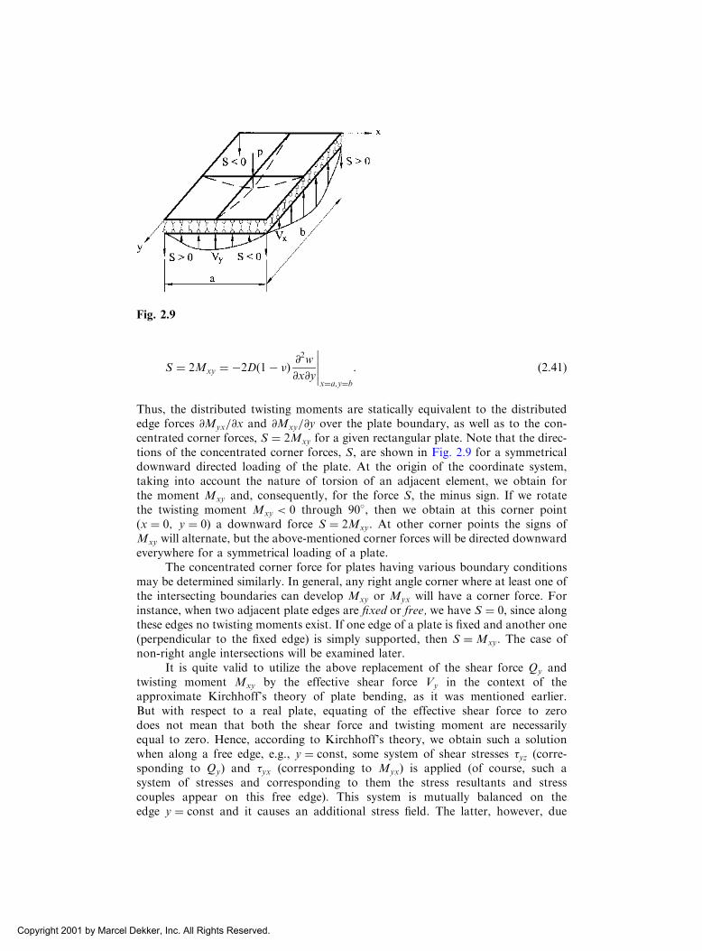
S ¼ 2Mxy ¼ �2D 1� �ð Þ @2w

@x@y

x¼a;y¼b

: ð2:41Þ

Thus, the distributed twisting moments are statically equivalent to the distributededge forces @Myx=@x and @Mxy=@y over the plate boundary, as well as to the con-centrated corner forces, S ¼ 2Mxy for a given rectangular plate. Note that the direc-tions of the concentrated corner forces, S, are shown in Fig. 2.9 for a symmetricaldownward directed loading of the plate. At the origin of the coordinate system,taking into account the nature of torsion of an adjacent element, we obtain forthe moment Mxy and, consequently, for the force S, the minus sign. If we rotatethe twisting moment Mxy < 0 through 90, then we obtain at this corner point(x ¼ 0; y ¼ 0) a downward force S ¼ 2Mxy. At other corner points the signs ofMxy will alternate, but the above-mentioned corner forces will be directed downwardeverywhere for a symmetrical loading of a plate.

The concentrated corner force for plates having various boundary conditionsmay be determined similarly. In general, any right angle corner where at least one ofthe intersecting boundaries can develop Mxy or Myx will have a corner force. Forinstance, when two adjacent plate edges are fixed or free, we have S ¼ 0, since alongthese edges no twisting moments exist. If one edge of a plate is fixed and another one(perpendicular to the fixed edge) is simply supported, then S ¼ Mxy. The case ofnon-right angle intersections will be examined later.

It is quite valid to utilize the above replacement of the shear force Qy andtwisting moment Mxy by the effective shear force Vy in the context of theapproximate Kirchhoff’s theory of plate bending, as it was mentioned earlier.But with respect to a real plate, equating of the effective shear force to zerodoes not mean that both the shear force and twisting moment are necessarilyequal to zero. Hence, according to Kirchhoff’s theory, we obtain such a solutionwhen along a free edge, e.g., y ¼ const, some system of shear stresses �yz (corre-sponding to Qy) and �yx (corresponding to Myx) is applied (of course, such asystem of stresses and corresponding to them the stress resultants and stresscouples appear on this free edge). This system is mutually balanced on theedge y ¼ const and it causes an additional stress field. The latter, however, due

Fig. 2.9


to Saint-Venant’s principle, decays rapidly as we move away from this edge intothe interior of the plate. The above-mentioned additional stress field cannot bedetermined by using the governing differential equation (2.24). Corrections can beobtained using the plate bending equations with regard to the shear strains �xzand �yz and will be discussed in Sec. 7.3. These corrections, as a rule, are neg-ligible for solid isotropic plates.

(4) Edge x ¼ 0 supported by a beamThe boundary conditions of the type (2.33), (2.35), and (2.37) are called homogeneousboundary conditions. Nonhomogeneous boundary conditions are commonly used inmany important engineering structures – for example, when a plate is supported byan edge beam.

Assume that the cross section of the edge beam is symmetrical with respect tothe middle surface of the plate and the edge beam has flexural and torsional rigid-ities. Since the edge beam and the plate are built monotonically (Fig. 2.10), they musthave the same displacements and slopes.

wb ¼ wx¼0

and #b ¼ #x¼0

or@w

@x

� �b

¼ @w

@x

x¼0

; ð2:42Þ

where the subscript b refers to the edge beam, and quantities relating to the platehave no subscripts.

Consider an element dy of the edge beam as a free body, as shown in Fig. 2.10.Equilibrium conditions of this element result in the following equations:X

Fz ¼ 0:�Qb � VxdyþQb þdQb

dydy ¼ 0

XMy ¼ 0:þ T þMxdy� T þ dT

dydy

� �¼ 0 or

Vx ¼dQb

dyð0; yÞ; Mx ¼

dT

dyð0; yÞ ðaÞ

where T is the twisting moment in the beam.As it follows from the beam theory [5]

Fig. 2.10


dQb

dyð0; yÞ ¼ � EIð Þb

@4wb

@y4ð0; yÞ and ðbÞ

Tð0; yÞ ¼ � GJð Þbd#bdy

ð0; yÞ ¼ � GJð Þb@2wb

@x@yð0; yÞ; ðcÞ

where ðEIÞb and ðGJÞb are the flexural rigidity and the torsional stiffness of the beamcross section, respectively.

Substituting (b) and (c) into Eq. (a) and taking into account the compatibilityconditions (2.42), gives the boundary conditions for the plate edge x ¼ 0 supportedby the beam:

Vx ¼ � EIð Þb@4wb

@y4

x¼0

; Mx ¼ � GJð Þb@3wb

@x@y2

x¼0

ð2:43aÞ

Using the expressions for Mx and Vx, Eqs. (2.13), (2.39b), and Eqs (2.42), we canrewrite the boundary conditions (2.43a) in terms of w, as follows:

D@3w

@x3þ ð2� �Þ @

3w

@x@y2

" #¼ EIð Þb

@4w

@y4

x¼0

; D@2w

@x2þ � @

2w

@y2

" #¼ GJð Þb

@3w

@x@y2

x¼0

:

ð2:43bÞSimilar expressions can be written for edges y ¼ 0; b.

Let us study the boundary conditions on skew edges. Consider a vertical sec-tion of the plate whose normal n makes an angle with the x axis (Fig. 2.11a). Takethe origin of the Cartesian coordinate system n (outward normal to the edge) and t(tangent to the edge) at some point of the edge. In a general case, the normal bendingMn and twisting Mnt moments, as well the transverse shear force Qn will act at thissection. Figure 2.11b shows the state of stress of a layer of the plate with thecoordinate z > 0. The above moments at any point of the skew edge are

Fig. 2.11


Mn ¼ðh=2

�h=2

�nzdz; Mnt ¼ðh=2

�h=2

�ntzdz: ð2:44Þ

The relationship between the stress components shown in Fig. 2.11b is given by [6,7]

�n ¼ �x cos2 þ �y sin2 þ 2�xy cos sin ;

�nt ¼ �xy cos 2� ð�x � �yÞ sin cos:

Substituting the above into Eqs (2.44), integrating over the plate thickness andtaking into account Eqs (2.11), one obtains the following relationships

Mn ¼ Mx cos2 þMy sin

2 þMxy sin 2;

Mnt ¼ Mxy cos 2� ðMx �MyÞ sin cos:ð2:45Þ

The shear force Qn acting at a section of the edge having a normal n can be evaluatedfrom condition of equilibrium of the plate element shown in Fig. 2.11a, as follows:

Qnds�Qxdy�Qydx ¼ 0; from which

Qn ¼ Qx cosþQy sin :ð2:46Þ

The effective shear force at a point of the skew edge can be determined similarly to(2.38), i.e.,

Vn ¼ Qn þ@Mnt

@t; ð2:47Þ

where @=@t denotes a differentiation with respect to the tangent of the skew edge.The boundary conditions discussed above for rectilinear edge can be general-

ized to some curvilinear edge. Let n and t be the outward normal making the angle with the x axis and tangent to the curvilinear edge at a point of interest (Fig. 2.12).Then the prescribed boundary conditions (2.33), (2.35), and (2.37), taking intoaccount (2.47), can be rewritten at an arbitrary point of the above curvilinearedge, as follows:

Fig. 2.12


(1) Built-in curvilinear edge

w ¼ 0;@w

@n¼ 0: ð2:48aÞ

(2) Simply supported edge

w ¼ 0; Mn ¼ 0: ð2:48bÞ

(3) Free curvilinear edge

Mn ¼ 0;Vn ¼ Qn þ@Mnt

@s¼ 0: ð2:48cÞ

(4) Curvilinear edge is elastically fixed

wþ 1Vn ¼ 0;@w

@nþ 2Mn ¼ 0; ð2:48dÞ

where Mn and Vn are the normal bending moment and the normal effective shearforce, respectively, defined by expressions (2.45) and (2.47). They can also beexpressed in terms of the deflection w using Eqs (2.45)–(2.47) and Eqs (2.13) and(2.27). In Eqs (2.48) 1 and 2 are some coefficients that characterize a supportcompliance.

If adjacent edges of a plate have slopes of the normals 1 and 2 (Fig. 2.13),then the concentrated force S at a common corner point will be equal to

S ¼ Mntð Þ1� Mntð Þ2 : ð2:49Þ

When 1 ¼ 0 and 2 ¼ �=2 we will obtain the expression (2.41).It is observed from the above that the boundary conditions are of the two basic

kinds: geometric or kinematic boundary conditions describe edge constraint pertainingto deflection or slope; static or natural boundary conditions impose some restrictionson the internal forces and moments at the edges of the plate. Accordingly, in Eq.(2.48a) both conditions are kinematic; in Eq. (2.48c) they are both static; and in Eq.(2.48b) the boundary conditions are mixed.

Fig. 2.13


2.6 VARIATIONAL FORMULATION OF PLATE BENDING PROBLEMS

It is known from the theory of elasticity that governing equations for stresses,strains, and displacements can be represented in the differential form. However,this is not a unique possible formulation of the problem for finding the stress–strainfield of an elastic body. The problem of determining stresses, strains, and displace-ments can be reduced to some definite integral of one or another type of thesefunctions called functionals. Then, the functions themselves (stresses, strains, anddisplacements) reflecting a real state of a body can be found from conditions ofextremum for this functional. The mathematical techniques of such an approach isstudied in the division of mathematics called the calculus of variation. Therefore,some postulates and statements that formulate properties of these functionals in thetheory of elasticity are referred to as variational principles. The latter represent somebasic theorems expressed in the form of integral equalities connecting stresses,strains, and displacements throughout the volume of a body and based on theproperties of the work done by external and internal forces. A variety of powerfuland efficient approximate methods for analysis of various linear and nonlinear pro-blems of solid mechanics are based on the variational principles. Some of thesemethods will be described further in Chapter 6.

2.6.1 Strain energy of plates

A functional is a scalar quantity depending on some function or several functions, asfrom independent variables. The functional can be treated as a function of an infinitenumber of independent variables. The subject matter of the calculus of variation issearching of unknown functions fiðx; y; zÞ that give a maximum (minimum) or sta-tionary value of a functional. For example,

� ¼ð ðV

ðF f1ðx; y; zÞ; f2ðx; y; zÞ; . . . ; fnðx; y; zÞ; f 0

1 ðx; y; zÞ; . . . ;�

f 0n ðx; y; zÞ; x; y; z

�dV:

The above-mentioned functions for which the functional is maximum (minimum) orstationary are referred to as extremals of the given functional [8–11].

Let us consider a functional expressing the total potential energy of a deformedelastic body and the loads acting on it. The total potential energy, �, consists of thestrain energy of deformation (the potential of internal forces), U, and the potentialenergy of external forces (the potential of external forces), �, i.e.,

� ¼ U þ�: ð2:50Þ

By convention, let us assume that the potential energy at the initial, undeformedstate, �0, is zero. Hence, the total energy � presents a variation of the energy ofinternal and external forces in the transition from initial to deformed states. Thepotential energy of a body is measured by the work done by external and internalforces when this body returns from its final to an initial position (where it wasmentioned above, �0 ¼ 0).

Our study is mainly limited to linearly elastic bodies that dissipate no energyand have only one equilibrium configuration. We also require that loads keep the


same orientation in space as they move. Such loads are called conservative. Amechanical system is called conservative if zero net work is done in carrying thesystem around any closed path: that is, in arbitrary changing a configuration andthen restoring it. An extension of this study to nonlinear, or nonconservative, pro-blems is possible.

First, let us set up an expression for the potential of the internal forces (strainenergy of deformation). This potential is equal to the negative work of the internalforces, i.e., U ¼ �Wi. Since the work done by the internal forces, Wi, is alwaysnegative (because displacements always occur in the opposite direction with respectto applied internal forces), the strain energy is positive.

The strain energy stored in an elastic body for a general state of stress is givenby [6,7]

U ¼ 1

2

ð ð ðV

�x"x þ �y"y þ �z"z þ �xy�xy þ �xz�xz þ �yz�yz� �

dV: ð2:51Þ

The integration extends over the entire body volume V . Based upon the assumptionsof Kirchhoff’s small-deflection plate bending theory, the stress components �z; �xz;and �yz may be omitted. Thus, introducing the generalized Hooke’s law, the aboveexpression reduces to the following form, involving only stresses and elastic con-stants,

U ¼ð ð ðV

1

2E�2x þ �2y � 2��x�y� �þ 1þ �

E�2xy

� �dV : ð2:52Þ

Substituting for the stress components from Eq. (2.10) into Eq. (2.52) and integrat-ing it over the thickness of the plate, we obtain

U ¼ 1

2

ð ðA

D@2w

@x2

!2

þ @2w

@y2

!2

þ 2�@2w

@x2@2w

@y2þ 2ð1� �Þ @2w

@x@y

!224

35dA ð2:53Þ

or alternatively

U ¼ 1

2

ð ðA

D@2w

@x2þ @

2w

@y2

!2

� 2ð1� �Þ @2w

@x2@2w

@y2� @2w

@x@y

!224

35

8<:

9=;dA ð2:54Þ

where A is the area of the plate middle surface.We can also rewrite the expression (2.53) for the strain energy in terms of the

bending and twisting moments, and the corresponding curvatures by the use of Eqs(2.13). As a result, for plates of a constant thickness the strain energy is

U ¼ 1

2

ð ðA

Mx�x þMy�y þ 2Mxy�xy� �

dA: ð2:55Þ


We observe from Eqs (2.53) and (2.54) that the strain energy is a nonlinear (quad-ratic) function of deformations. Hence, the principle of superposition is therefore notvalid for the strain energy.

The expressions (2.53) and (2.54) are valid for plates of constant and variablethickness. It should be noted that the following integral

ð ðA

@2w

@x2@2w

@y2� @2w

@x@y

!224

35dA ð2:56Þ

entering in Eq (2.54) is equal to zero for fixed supports and for simply supportededges of plates, whose contour is traced by straight lines. This statement can be easilyproven by transforming the integral (2.56) over the plate surface into the line integralover the plate boundary [3].

The potential of external forces, �, is defined as the work done by externalforces through the corresponding displacements, assuming that these forces remainunchanged during the deformation. Further, when a positive displacement occurs, �decreases, so the potential of the external forces is always negative and may beevaluated as the product of these forces and the corresponding final displacementcomponents. Determine the potential, �p, of the distributed load pðx; yÞ and con-centrated Pi andMj forces and moments applied to the middle surface of the plate asfollows:

�p ¼ �ð ðA

pðx; yÞwdA þXi

Piwi þXj

Mj#j

24

35; ð2:57Þ

where wi and #j are the deflection and the slope of the normal at the point ofapplication of the ith force and jth moment in the plane of the action of this moment,respectively.

In the expression (2.57) the potential of edge loads, ��, is not included. Theseloads have potentials only if compatible boundary displacements are permitted. Insuch cases, the potentials of the edge moments mn;mt and the transverse edge forcesVn can be expressed as

�� ¼ �þ�

Vnwþmn

@w

@nþmnt

@w

@t

� �ds; ð2:58Þ

where @w=@n and @w=@t are the derivatives of w with respect to the outward normaland the tangent directions, respectively, along the plate boundary to the boundary �.

The total potential of the external loads applied to the plate surface and to itsboundary is

� ¼ �p þ��; ð2:59Þ

where �p and �� are given by the expressions (2.57) and (2.58).Using expressions (2.50), (2.54), (2.57) and (2.58), we can write the total poten-

tial energy of the plate in bending in the Cartesian coordinates as follows


� ¼ 1

2

ð ðA

D@2w

@x2þ @

2w

@y2

!2

� 2ð1� �Þ @2w

@x2@2w

@y2� @2w

@x@y

!224

35

8<:

9=;dA

�ð ðA

pðx; yÞwdAþXi

Pwi þXj

Mj#jþ24

þ�

Vnwn þmn

@w

@nþmnt

@w

@t

� �ds

35;

ð2:60Þ

or alternatively

� ¼ 1

2

ð ðA

Mx�x þMy�y þ 2Mxy�xy� �

dA

�ð ðA

pðx; yÞwdAþXi

Piwi þXj

Mj#jþ24

þ�

Vnwn þmn

@w

@nþmnt

@w

@t

� �ds

35:

ð2:61Þ

As is seen from Eq. (2.58) that the value of the total potential energy ofbending of plates is determined by an assignment of deflection w as a function ofindependent variables (x and y in the Cartesian coordinate system).

2.6.2 Variational principles

Let us consider some general concepts of the calculus of variation. A variation meansan infinitesimal increment of a function for fixed values of its independent variables.The variation is designated by the symbol �. The variational symbol � may be treatedas the differential operator d. The only difference between them lies in the fact thatthe symbol � refers to some possible variations of a given function while the symbol dis associated with real variations of the same function. In what follows, only thefollowing three operations are needed:

dð�wÞdx

¼ �dw

dx

� �; �ðw2Þ ¼ 2wð�wÞ;

ðð�wÞdx ¼ �

ðwdx:

Consider an elastic body in equilibrium. This means that the body subjectedto the maximum values of static (i.e., slowly piled-up) external forces has alreadyreached its final state of deformation. Now we disturb this equilibrium conditionby introducing small, arbitrary, but kinematically compatible, displacements.These displacements need not actually take place and need not be infinitesimal.Only one restriction is imposed on these displacements: they must be compatiblewith the support conditions (as discussed later, there are cases when satisfactionof geometric (or kinematic) boundary conditions is sufficient) and internal com-patibility of the body. These displacements are called admissible virtual, because


they are imagined to take place (i.e., hypothetical), with the actual loads acting attheir fixed values. The admissible virtual displacement produces an admissibleconfiguration of the body. It follows from the above that virtual displacementscannot affect the equilibrium of the given system, when the full loads have beenapplied. Neither external loads nor internal forces and moments are altered by avirtual displacement [8–12, 14].

Now we can introduce the general variational principles of solid mechanics.

(a) The Principle of Conservation of Energy

This principle states that the strain energy stored in an elastic body is equal to the workdone by the applied external loads during the loading process, if we assume that thereare no thermal or inertial effects.

(b) The Principle of Virtual Work

The work done by actual forces through a virtual displacement of the actual con-figuration is called virtual work. It is assumed that during the virtual displacementsall forces are held constant. The virtual work is designated by �W .

The principle of virtual work is formulated as follows:

An elastic body is in equilibrium if and only if the total virtual work done by external

and internal forces is zero for any admissible virtual displacements, i.e.,

�W ¼ �Wi þ �We ¼ 0 (2.62)

where �Wi and �We are the virtual works done by internal and external forces,respectively. As mentioned earlier, �Wi is negative. This principle was first pro-posed by J. Bernoulli in 1771. It can be interpreted as follows: if a body is inequilibrium then its resultant force and resultant couple are both zero; so, theyproduce no work.

(c) The Principle of Minimum Potential Energy

The principle of minimum potential energy may be looked upon as a specializationof the principle of virtual work (2.62). Indeed, the potential energy of the internalforces is equal to the negative work of the internal forces, i.e., U ¼ �Wi. On theother hand, We ¼ ��. Therefore, we can write the equality (2.62), as follows:

�W ¼ ��U � �� ¼ 0; ð2:63Þwhere �U þ �� ¼ �ðU þ�Þ ¼ �� (because � can be treated as a differential of afunction) and �� is the variation in the total potential energy due to introducingcompatible virtual displacements and is given by Eq. (2.60) or Eq. (2.61). Finally, theequality (2.63) can be written as

�� ¼ 0: ð2:64ÞThis equality expresses the principle of minimum potential energy proposed byLagrange.

From calculus, an equality df ¼ 0 means that the function f has an extremum(or a value corresponding to a point of inflection). It can be shown [9,10] that avariation of the total potential energy during any admissible virtual displacement(variation of the displacement) is positive for any stable configuration of equili-


brium. Hence, in this case, the total potential energy of a given system has a mini-mum. From the uniqueness theorem [6,7], the problem of the theory of elasticity,based on assumptions of small displacements and deformations defines only oneequilibrium configuration, and this configuration of equilibrium is stable. Thus, ifthe small-deflection theory of an elastic body is being studied, then the potentialenergy is a minimum in an equilibrium state. So, the principle of minimum potentialenergy, proposed by Lagrange, can be formulated, as follows:

Among all admissible configurations of an elastic body, the actual configuration (that

satisfies static equilibrium conditions) makes the total potential energy, �, stationary

with respect to all small admissible virtual displacements. For stable equilibrium, � is a

minimum.

Notice that the above principle applies to a conservative system only.It can be shown that the governing differential equation (2.24) and the bound-

ary conditions (2.48) can be deduced from Lagrange’s variational principle (2.64)[3,8–12]. However, the key importance of the variational principles discussed aboveis that they can be used to obtain approximate solutions of complicated problems ofsolid mechanics, in particular, plate-shell bending problems. These are obtainedwhile avoiding mathematical difficulties associated with integration of differentialequations in partial derivatives. The corresponding methods, called variational meth-ods and based on the above-mentioned principles, are discussed further in Chapter 6.More complete information on the variational principles and their application inmechanics is available in the literature [8–12].

PROBLEMS

2.1 Verify the result given by Eq. (2.18).

2.2 Derive the governing differential equation for deflections of a plate subjected to a

distributed moment load mxðx; yÞ and myðx; yÞ applied to the middle surface.

2.3 Show that at the corner of a polygonal simply supported plate, Mxy ¼ 0 unless the

corner is 90.2.4 If a lateral deflection w is a known function of x and y, what are the maximum slope

@w=@n and the direction of axis n with respect to the x axis in terms of @w=@x and

@w=@y?2.5 Show that the sum of bending curvatures in any two mutually perpendicular directions,

n and t, at any point of the middle surface, is a constant, i.e.,

�x þ �y ¼ �n þ �t ¼ const:

2.6 Verify the expression given by Eq. (2.61).

2.7 Derive the expressions for the boundary quantities Mn;Mnt; and Vn in terms of the

deflection w at a regular (smooth) point of the curvilinear contour of the plate using:

(a) the local coordinates n and t where the coordinate n coincides with the direction of

the outward normal and t – with the tangent direction to the boundary; (b) the intrinsic

coordinates n and s, where s, is the arc length over the boundary.

Hint: use the following relations for part (b)

@n

@s¼ 1

�t;@t

@s¼ � 1

�n

where n and t are the unit vectors of the intrinsic coordinate system directed along the

outward normal and tangent to the boundary, respectively.


2.8 Derive Eq. (2.24) directly from the third equation of (1.10) by using the relations (2.16)

and (2.17).

2.9 Assume that shear stresses in the plate are distributed according to the parabolic law

for �h=2 � z � h=2. Show that when the expression �xz ¼ 6Qx=h3

� �h=2ð Þ2�z2

� �is sub-

stituted into the first relation (2.12) an identity is obtained.

2.10 Prove that the integral (2.56) is equal to zero for fixed supports and for simply sup-

ported edges.

REFERENCES

1. Webster, A.G., Partial Differential Equations of Mathematical Physics, Dover, New

York, 1955.

2. Sommerfeld, A., Partial Differential Equations in Physics, Academic Press, New York,

1948.



4. Thomson, W. and Tait, P.G., Treatise on Natural Philosophy, Cambridge University

Press, Cambridge, 1890.

5. Timoshenko, S.P., Strength of Materials, 3rd edn, Van Nostrand Company, New York,

1956.


York, 1970.

7. Prescott, J.J., Applied Elasticity, Dover, New York, 1946.

8. Forray, M.J., Variational Calculus in Science and Engineering, McGraw-Hill, New York,

1968.

9. Lanczos, C., The Variational Principles of Mechanics, The University of Toronto Press,

Toronto, 1964.

10. Hoff, H.I., The Analysis of Structures Based on the Minimal Principles and Principle of

Virtual Displacements, John Wiley and Sons, New York, 1956.

11. Reddy, J.N., Energy and Variational Methods in Applied Mechanics, John Wiley and

Sons, New York, 1984.

12. Washizy, K., Variational Methods in Elasticity and Plasticity, 3rd edn, Pergamon Press,

New York, 1982.

FURTHER READING

Gould, P.L., Analysis of Shells and Plates, Springer-Verlag, New York, Berlin, 1988.

Heins, C.P., Applied Plate Theory for the Engineer, Lexington Books, Lexington,

Massachusetts, 1976.

McFarland, D.E., Smith, B.L. and Bernhart, W.D., Analysis of Plates, Spartan Books, New

York, 1972.

Mansfield, E.H., The Bending and Stretching of Plates, Macmillan, New York, 1964.

Szilard, R., Theory and Analysis of Plates, Prentice-Hall, Inc., Englewood Cliffs, New York,

1974.

Ugural, A.C., Stresses in Plates and Shells, McGraw-Hill, New York, 1981.

Vinson, J.R., The Behavior of Plates and Shells, John Wiley and Sons, New York, 1974.


3

Rectangular Plates

3.1 INTRODUCTION

We begin the application of the developed plate bending theory with thin rectangularplates. These plates represent an excellent model for development and as a check ofvarious methods for solving the governing differential equation (2.24).

In this chapter we consider some mathematically ‘‘exact’’ solutions in the formof double and single trigonometric series applied to rectangular plates with varioustypes of supports and transverse loads, plates on an elastic foundation, continuousplates, etc.

3.2 THE ELEMENTARY CASES OF PLATE BENDING

Let us consider some elementary examples of plate bending of great importance forunderstanding how a plate resists the applied loads in bending. In addition, theseelementary examples enable one to obtain closed-form solutions of the governingdifferential equation (2.24).

3.2.1 Cylindrical bending of a plate

Consider an infinitely long plate in the y axis direction. Assume that the plate issubjected to a transverse load which is a function of the variable x only, i.e., p ¼ pðxÞ(Fig. 3.1a). In this case all the strips of a unit width parallel to the x axis and isolatedfrom the plate will bend identically. The plate as a whole is found to be bent over thecylindrical surface w ¼ wðxÞ. Setting all the derivatives with respect to y equal zero inEq. (2.24), we obtain the following equation for the deflection:

d4w

dx4¼ pðxÞ

D: ð3:1Þ


We have applied here the ordinary derivative notation since w depends nowonly on the variable x. Equation (3.1) describes a cylindrical bending of thin plates. Itis seen that this equation coincides with the corresponding equation of bending of abeam if we replace the flexural rigidity of the beam, EI , by the flexural rigidity of aplate, D. Since D > EI , the strip of the unit width within the plate (it is cross-hatchedin Fig. 3.1a) is always stiffer than an isolated beam having the same span andthickness.

An integration of Eq. (3.1) should present no problems. Let, for example,p ¼ p0

xa, then the general solution of Eq. (3.1) is of the following form:

w ¼ wh þ wp ¼ C1 þ C2xþ C3x2 þ C4x

3 þ p0x5

120aD; ð3:2Þ

where wh is a solution of homogeneous equation (3.1) and wp is a particular solutiondepending on the right-hand side of Eq. (3.1), i.e., on a given type of the appliedloading.

The boundary conditions for the plate-strip can be written as follows (Fig.3.1a)

w ¼ 0jx¼0;dw

dx¼ 0

x¼0

and w ¼ 0jx¼a;Mx ¼ �Dd2w

dx2¼ 0

x¼a

: ð3:3Þ

The constants of integration Ci ði ¼ 1; 2; 3; 4Þ can be evaluated from theboundary conditions (3.3). Substituting for w from (3.2) into (3.3), we obtain thefollowing:

C1 ¼ C2 ¼ 0;C3 ¼7p0a

2

240D; C4 ¼

9p0a

240D:

Substituting the above into Eq. (3.2), yields Eq. (3.4), as shown below:

w ¼ p0a4

240D7x2

a2� 9

x3

a3þ 2

x5

a5

!ð3:4Þ

This is the equation for the deflection of the plate in cylindrical bending.The bending moments Mx and My may be obtained from Eqs (2.13) making

all the derivatives of w with respect to y equal zero, i.e.,

Fig. 3.1


Mx ¼ �Dd2w

dx2; My ¼ ��Dd2w

dx2¼ �Mx; Mxy ¼ 0: ð3:5Þ

Substituting Eq. (3.4) into Eq. (3.5), we obtain

Mx ¼ � p0a2

1207� 27

x

aþ 20

x3

a3

!: ð3:6Þ

The moment My ¼ �Mx is proportional to Mx.A cylindrical bending of a plate with a finite size in the y direction is possible

only if the moment My will be applied to edges that are parallel to the x axis, asshown for the strip isolated from an infinite plate of Fig. 3.1b. In the absence of thesemoments, the surface of deflections will deviate from the cylindrical one over part ofthe length along the y axis.

3.2.2 Pure bending of plates

Consider a rectangular plate with a free boundary and assume that this plate issubjected to distributed bending moments over its edgesMx ¼ m1 ¼ const andMy ¼m2 ¼ const (Fig. 3.2). In this particular case, the governing differential equation(2.24) becomes

@4w

@x4þ 2

@4w

@x2@y2þ @

4w

@y4¼ 0: ð3:7Þ

This equation will be satisfied if we make

w ¼ 0:5 C1x2 þ C2y

2� �

: ð3:8ÞThe constants of integration C1 and C2 may be evaluated from the following bound-ary conditions:

Mx ¼ m1 and My ¼ m2: ð3:9Þ

Fig. 3.2


Using Eqs (2.13), (3.8), and (3.9), we obtain

C1 ¼�m2 �m1

Dð1� �2Þ ; C2 ¼�m1 �m2

Dð1� �2Þ :

Substituting the above into Eq. (3.8) yields the deflection surface, as shown below:

w ¼ 1

2Dð1� �2Þ ð�m2 �m1Þx2 þ ð�m1 �m2Þy2� � ð3:10Þ

Hence, in all sections of the plate parallel to the x and y axes, only the constantbending moments Mx ¼ m1 and My ¼ m2 will act. Other stress resultants and stresscouples are zero, i.e.,

Mxy ¼ Qx ¼ Qy ¼ 0:

This case of bending of plates may be referred to as a pure bending.Let us consider some particular cases of pure bending of plates.

(a) Let m1 ¼ m2 ¼ m.Then,

w ¼ � m

2Dð1þ �Þ ðx2 þ y2Þ: ð3:11Þ

This is an equation of the elliptic paraboloid of revolution. The curved plate in thiscase represents a part of a sphere because the radii of curvature are the same at allthe planes and all the points of the plate.

(b) Let m1 ¼ m;m2 ¼ 0 (Fig. 3.3).Then,

w ¼ m

2Dð1� �2Þ �x2 þ �y2� �: ð3:12Þ

A surface described by this equation has a saddle shape and is called the hyperbolicparaboloid of revolution (Fig. 3.3). Horizontals of this surface are hyperbolas, asymp-totes of which are given by the straight lines x

y¼ � ffiffiffi

�p

. As is seen, due to the Poissoneffect the plate bends not only in the plane of the applied bending moment Mx ¼m1 ¼ m but it also has an opposite bending in the perpendicular plane.

Fig. 3.3


(c) Let m1 ¼ m;m2 ¼ �m (Fig. 3.4a).Then

w ¼ m

2Dð1� �Þ ð�x2 þ y2Þ: ð3:13Þ

This is an equation of an hyperbolic paraboloid with asymptotes inclined at 45 to thex and y axes.

Let us determine the moments Mn and Mnt from Eqs (2.45) in skew sectionsthat are parallel to the asymptotes. Letting ¼ 45, we obtain

Mn ¼ 0; Mnt ¼ �m:

Thus, a part of the plate isolated from the whole plate and equally inclined to the xand y axes will be loaded along its boundary by uniform twisting moments ofintensity m. Hence, this part of the plate is subjected to pure twisting (Fig. 3.4b).Let us replace the twisting moments by the effective shear forces V, rotating thesemoments through 90 (see Sec. 2.4). Along the whole sides of the isolated part weobtain V ¼ 0, but at the corner points the concentrated forces S ¼ 2m are applied.Thus, for the model of Kirchhoff’s plate, an application of self-balanced concen-trated forces at corners of a rectangular plate produces a deformation of pure torsionbecause over the whole surface of the plate Mnt ¼ m ¼ const:

Remark

Since the plate described above in pure bending has no supports, its deflectionshave been determined with an accuracy of the displacements of an absolutely rigidbody.

3.3 NAVIER’S METHOD (DOUBLE SERIES SOLUTION)

In 1820, Navier presented a paper to the French Academy of Sciences on the solu-tion of bending of simply supported plates by double trigonometric series [1].

Fig. 3.4


Consider a rectangular plate of sides a and b, simply supported on all edges andsubjected to a uniform load pðx; yÞ: The origin of the coordinates is placed at theupper left corner as shown in Fig. 3.5.

The boundary conditions for a simply supported plate are the following (seeEqs (2.35):

w ¼ 0jx¼0;a;@2w

@x2¼ 0

x¼0;a

and w ¼ 0jy¼0;b;@2w

@y2¼ 0

y¼0;b

: ð3:14Þ

In this case, the solution of the governing differential equation (2.24), i.e., the expres-sions of the deflection surface, wðx; yÞ, and the distributed surface load, pðx; yÞ, haveto be sought in the form of an infinite Fourier series (see Appendix B), as follows:

wðx; yÞ ¼X1m¼1

X1n�1

wmn sinm�x

asin

n�y

b; ð3:15aÞ

pðx; yÞ ¼X1m¼1

X1n¼1

pmn sinm�x

asin

n�y

b; ð3:15bÞ

where wmn and pmn represent coefficients to be determined. It can be easily verifiedthat the expression for deflections (3.15a) automatically satisfies the prescribedboundary conditions (3.14).

Let us consider a general load configuration. To determine the Fourier coeffi-cients pmn, each side of Eq. (3.15b) is multiplied by sin l�x

asin k�y

band integrated twice

between the limits 0;a and 0;b, as follows (see Appendix B):

ða0

ðb0

pðx; yÞ sin l�xa

sink�y

bdxdy ¼

X1m¼1

X1n¼1

pmn

ða0

ðb0

sinm�x

asin

n�y

bsin

l�x

asin

k�y

bdxdy:

ðaÞ

Fig. 3.5


It can be shown by direct integration that

ða0

sinm�x

asin

l�x

adx ¼

0 ifm 6¼ l

a=2 if m ¼ l

8<:

and

ðb0

sinn�y

bsin

k�y

bdy ¼

0 if n 6¼ k

b=2 if n ¼ k:

8<:

ð3:16Þ

The coefficients of the double Fourier expansion are therefore the following:

pmn ¼4

ab

ða0

ðb0

pðx; yÞ sinm�xa

sinn�y

bdxdy: ð3:17Þ

Since the representation of the deflection (3.15a) satisfies the boundary conditions(3.14), then the coefficients wmn must satisfy Eq. (2.24). Substitution of Eqs (3.15)into Eq. (2.24) results in the following equation:

X1m¼1

X1n¼1

wmn

m�

a

� �4þ 2

m�

a

� �2 n�

b

� �2þ n�

b

� �4� �� pmn

D

�sin

m�x

asin

n�y

b¼ 0:

This equation must apply for all values of x and y. We conclude therefore that

wmn�4 m2

a2þ n2

b2

!2

� pmn

D¼ 0;

from which

wmn ¼1

�4D

pmn

ðm=aÞ2 þ ðn=bÞ2� �2 : ð3:18Þ

Substituting the above into Eq. (3.15a), one obtains the equation of the deflectedsurface, as follows:

wðx; yÞ ¼ 1

�4D

X1m¼1

X1n¼1

pmn

ðm=aÞ2 þ ðn=bÞ2� �2 sinm�xa sinn�y

b; ð3:19Þ

where pmn is given by Eq. (3.17). It can be shown, by noting that sinm�x=aj � 1 and

jsin n�y=bj � 1 for every x and y and for every m and n, that the series (3.19) isconvergent.

Substituting wðx; yÞ into the Eqs (2.13) and (2.27), we can find the bendingmoments and the shear forces in the plate, and then using the expressions (2.15),determine the stress components. For the moments in the plate, for instance, weobtain the following:


Mx ¼ 1

�2

X1m¼1

X1n¼1

pmn

½ðm=aÞ2 þ �ðn=bÞ2�½ðm=aÞ2 þ ðn=bÞ2�2 sin

m�x

asin

n�y

b;

My ¼1

�2

X1m¼1

X1n¼1

pmn

½ðn=bÞ2 þ �ðm=aÞ2�½ðm=aÞ2 þ ðn=bÞ2�2 sin

m�x

asin

n�y

b;

Mxy ¼ � 1��2

X1m¼1

X1n¼1

pmn

mn

ab½ðm=aÞ2 þ ðn=bÞ2�2 cosm�x

acos

n�y

b:

ð3:20Þ

The infinite series solution for the deflection (3.19) generally converges quickly; thus,satisfactory accuracy can be obtained by considering only a few terms. Since thestress resultants and couples are obtained from the second and third derivatives ofthe deflection wðx; yÞ, the convergence of the infinite series expressions of the internalforces and moments is less rapid, especially in the vicinity of the plate edges. Thisslow convergence is also accompanied by some loss of accuracy in the process ofcalculation. The accuracy of solutions and the convergence of series expressions ofstress resultants and couples can be improved by considering more terms in theexpansions and by using a special technique for an improvement of the convergenceof Fourier’s series (see Appendix B and Ref. [2]).

Example 3.1

A rectangular plate of sides a and b is simply supported on all edges and subjected toa uniform pressure p x; yð Þ ¼ p0, as shown in Fig 3.5. Determine the maximum deflec-tion, moments, and stresses.

Solution

The coefficients pmn of the double Fourier expansion of the load are obtained fromEq. (3.17). Substituting pðx; yÞ ¼ p0 ¼ const and integrating, yields the following

pmn ¼4p0�2mn

ð1� cosm�Þð1� cos n�Þ or pmn ¼16p0�2mn

ðm; n ¼ 1; 3; 5; . . .Þ: ðaÞ

It is observed that because pmn ¼ 0 for even values of m and n, these integers assumeonly for odd values.

Substituting for pmn from (a) into Eqs (3.19) and (3.20), we can obtain theexpressions for deflections and moments. We obtain the following:

w ¼ 16p0D�6

X1m¼1;3;...

X1n¼1;3;...

sinm�x

asin

n�y

b

mn ðm=aÞ2 þ ðn=bÞ2� �2; ð3:21aÞ

Mx ¼ 16p0�4

X1m¼1;3;...

X1n¼1;3;...

ðm=aÞ2 þ �ðn=bÞ2mn ðm=aÞ2 þ ðn=bÞ2� �2 sinm�xa sin

n�y

b; ð3:21bÞ

My ¼16p0�4

X1m¼1;3;...

X1n¼1;3;...

�ðm=aÞ2 þ ðn=bÞ2

mn ðm=aÞ2 þ ðn=bÞ2� �2 sinm�xa sinn�y

b; ð3:21cÞ

Mxy ¼ � 16ð1� �Þ�4ab

X1m

X1n

1

½ðm=aÞ2 þ ðn=bÞ2�2 cosm�x

acos

m�y

b: ð3:21dÞ


Based upon physical considerations and due to the symmetry of the plate andboundary conditions, the maximum deflection occurs at the center of the plate(x ¼ a=2; y ¼ b=2) and its value is shown next:

wmax ¼16p0�6D

X1m¼1;3;...

X1n¼1;3;...

ð�1Þmþn2 �1

mn ðm=aÞ2 þ ðn=bÞ2� �2: ðbÞ

Here, sinm�=2 and sin n�=2 are replaced by ð�1Þm�1=2 and ð�1Þn�1=2, respectively. Itcan be observed that this series converges very rapidly, and the consideration of twoterms gives an accuracy sufficient for all practical purposes. In particular, for thecase of a square plate (a ¼ b), we obtain

wmax ¼16p0a

4

�6D

1

4þ 1

100þ 1

100þ . . .

� �� 4a4p0�6D

¼ 0:00416p0a

4

D;

or substituting for D ¼ Eh3

12ð1��2Þ and making � ¼ 0:3, we obtain

wmax � 0:0454p0a

4

Eh3:

The error of this result compared with an exact solution is about 2.5% [3].It is observed that the series for the bending and twisting moments given by

Eqs (3.21) do not converge as rapidly as that of the series for the deflections. Themaximum bending moments, found at the center of the plate, are determined byapplying Eqs (3.21b) and (3.21c). The first term of this series for a square plate for� ¼ 0:3 yields

Mx;max ¼ My;max ¼ 0:0534p0a2: ðcÞ

The exact solution for the bending moments at the center of the square plate for � ¼0:3 is the following [3]:

Mx;max ¼ My;max ¼ 0:0479p0a2: ðdÞ

The error of solution (c) is about 11.5 per;, and that is worse than that for thedeflections.

The maximum normal stress at the center of the square plate produced by themoments of Eq. (d), by application of Eqs (2.15) is determined to be �x;max ¼ �y;max

¼ 0:287 p0a2

h2.

Let us study the essential characteristics of the transverse shear forces asapplied to the simply supported rectangular plate of Example 3.1. To simplify ouranalysis, we use only a single harmonic approximation of a uniformly distributedloading and solution also. However, the general conclusions will be valid for anyharmonic approximations of the solution. From Eq. (a), we compute the followingfor m ¼ n ¼ 1:

p11 ¼16p0�2

and p ¼ 16p0�2

sin�x

asin�y

b:

Retaining also only one term in the series (a), we obtain the following expression forthe deflection:


w ¼ 16p0D�6

sin�x

asin�y

b

1=a2 þ 1=b2� �2 : ðeÞ

The transverse shear forces, Qx and Qy, and effective shear forces, Vx and Vy, may befound by substituting for w from Eq. (e) into Eqs (2.27) and (2.39). We obtain

Qx ¼ 16p0�3

cos�x

asin�y

ba 1=að Þ2þ 1=bð Þ2� � ; Qy ¼

16p0�3

sin�x

acos

�y

bb 1=að Þ2þ 1=bð Þ2� �

Vx ¼ 16p0�3

1=a2 þ 2� �ð Þ1=b2� �a 1=a2 þ 1=b2� �2 cos

�x

asin�y

b;

Vy ¼16p0�3

2� �ð Þ1=a2 þ 1=b2� �b 1=a2 þ 1=b2� �2 sin

�x

acos

�y

b

ðfÞ

The resultant of the external distributed load carrying by the plate is

Rp ¼ða0

ðb0

pdxdy ¼ 16p0�2

ða0

ðb0

sin�x

asin�y

bdxdy or Rp ¼ 64p0

�4ab: ðgÞ

which acts in the positive z direction (downward). Determine the resultant of thetransverse effective shear forces, RV, acting on the plate edges, as follows

RV ¼ �ðb0

Vx 0; yð Þ þ Vx a; yð Þ � �dy�

ða0

Vy x; 0ð Þ þ Vy x; bð Þ � �dx: ðhÞ

The negative sign on the right-hand side of Eq. (h) indicates that the resultant of theeffective shear forces points in the negative z direction. Evaluating these integralsyields

RV ¼ � 64p0�4

ab

a2 þ b2� �2 a4 þ 2 2� �Þa2b2 þ b4

� �:

� ðiÞ

Adding Rp and RV given by Eqs (g) and (i), results in the following:

Rp þ RV ¼ �128p0 1� �ð Þ�4

a3b3

a2 þ b2� �2 ðjÞ

as an apparently unbalanced force. However, we must include the corner forcesgiven by Eqs (2.41) in the total equilibrium condition according to the classicalplate theory. From Eq. (3.21d) for m ¼ n ¼ 1, we have the following

Mxy ¼ � 16 1� �ð Þ�4ab

cos�x

acos

�y

b

1=a2 þ 1=b2� �2 : ðkÞ


As explained in Sec. 2.4, all the corner concentrated forces, S, for the simply sup-ported rectangular plate that is subjected to a downward directed uniform load p0,act downward also, i.e., in the positive z direction. Each such a force is given by Eq.(2.41), i.e.,

S ¼ 2 Mxy

¼ 216 1� �ð Þ�4ab

a3b3

a2 þ b2� �2

" #:

Thus, a total force due to the corner forces acts in the positive z direction and is givenby the following:

RS ¼ 4S ¼ 128p0 1� �ð Þ�4

a3b3

a2 þ b2� �2 : ðlÞ

Now, adding Eqs (j) and (l), we get

Rp þ RV þ RS ¼ 0:

The effective shear force distributions and concentrated corner forces are shown inFig. 2.9. Thus, we have demonstrated the contribution of the corner forces to theoverall equilibrium of the rectangular simply supported plate.

It is interesting to note that the boundary transverse shear forces, Qx and Qy,balance the external distributed load p0. Indeed, let us compute the resultant RQ ofthe shear forces on the boundary of the plate, as follows:

RQ ¼ �ðb0

Qx 0; yð Þ þ Qx a; yð Þ � �dy�

ða0

Qy x; 0ð Þ þ Qy x; bð Þ � �dx:

Substituting for Qx and Qy from the first two equations (f) into the above, we obtain

RQ ¼ � 64p0�4

ab; ðmÞ

where the negative sign indicates that RQ points in the negative z direction, i.e., in theupward direction. Adding Eqs (g) and (m) results in

Rp þ RQ ¼ 0:

However, following the logic of Kirchhoff’s plate theory, the transverse shear forcealone cannot be treated as the edge supporting reaction. Only the effective shearforce may represent such a reaction. This result will also be discussed in detail later,in Sec. 7.3.

Example 3.2

A rectangular wall panel is taken to be simply supported on all edges and subjectedto a patch load of intensity p0 ¼ const: as shown in Fig. 3.6. Determine the deflectedsurface.

Solution

The constants of the Fourier expansion of the load are


pmn ¼4p0uv

ð�þu=2

��u=2

ð þv=2

�v=2

sinm�x

asin

n�y

bdxdy

¼ 16p0�2mn

sinm��

asin

n�

bsin

m�u

2asin

n�v

2b:

ð3:22Þ

Inserting the above into Eqs (3.19), yields the double series expression of the follow-ing deflected surface

wðx; yÞ ¼ 16p0�6D

X1m¼1

X1n¼1

sinm��

asin

n�

bsin

m�u

2asin

n�v

2bsin

m�x

asin

n�y

b

mn ðm=aÞ2 þ ðn=bÞ2� �2 : ð3:23Þ

The convergence of this solution is relatively fast if the dimensions u and v are nottoo small. The deflection can be obtained with sufficient accuracy by taking the firstfour terms of the series.

3.4 RECTANGULAR PLATES SUBJECTED TO A CONCENTRATEDLATERAL FORCE P

Let us consider a rectangular plate simply supported on all edges of sides a and b andsubjected to concentrated lateral force P applied at x ¼ � and y ¼ , as shown in Fig.3.7.

Assume first that this force is uniformly distributed over the contact area ofsides u and v (Fig. 3.6) i.e., its load intensity is defined as

p0 ¼P

uv:

Substituting the above into Eq. (3.22), one obtains

pmn ¼16P

�2mnuvsin

m��

asin

n�

bsin

m�u

2asin

n�v

2b: ð3:24Þ

Fig. 3.6


Now we must let the contact area approach zero by permitting u ! 0 and v ! 0. Inorder to be able to use the limit approach first, Eq. (3.24) must be put in a moresuitable form. For this purpose, the right-hand side is multiplied and divided by ab,giving the following:

pmn ¼ limu!0;v!0

4P

absin

m��

asin

n�

b

sinm�u

2asin

n�v

2bðm�u=2aÞðn�v=2bÞ

24

35 : ð3:25Þ

Knowing that lim!0

sin

¼ 1, Eq. (3.25) becomes

pmn ¼4P

absin

m��

asin

n�

b; ð3:26Þ

and the deflection of the plate subjected to a concentrated force is obtained from Eq.(3.19), as follows:

wðx; yÞ ¼ 4P

�4Dab

X1m¼1

X1n¼1

sinm��

asin

n�

b

ðm=aÞ2 þ ðn=bÞ2� �2 sinm�xa sinn�y

b: ð3:27Þ

The convergence of this series is fairly rapid. Let � ¼ a=2 and ¼ b=2; then for evenm and n, all the numbers pmn are zero. For odd numbers, we derive the followingfrom (3.27):

pmn ¼4P

absin

m�

2sin

n�

2:

The deflected middle surface equation (3.27) in this case becomes

wðx; yÞ ¼ 4P

�4Dab

X1m¼1;3;...

X1n¼1;3;...

sinm�

2sin

n�

2ðm=aÞ2 þ ðn=bÞ2� � sinm�x

asin

n�y

b: ð3:28Þ

Furthermore, if the plate is square (a ¼ b), the maximum deflection, which occurs atthe center, is obtained from Eq. (3.28), as follows:

wmax ¼4Pa2

�4D

X1m¼1;3;...

Xn¼1;3;...

1

ðm2 þ n2Þ2:

Fig. 3.7


Retaining the first nine terms of this series (m ¼ 1, n ¼ 1; 3; 5; m ¼ 3, n ¼ 1; 3; 5;m ¼ 5, n ¼ 1; 3; 5) we obtain

wmax ¼4Pa2

�4D

1

4þ 2

100þ 1

324þ 2

625þ 2

1156þ 1

2500

� �¼ 0:01142

Pa2

D:

The ‘‘exact’’ value is wmax ¼ 0:01159Pa2

Dand the error is thus 1.5% [3].

This very simple Navier’s solution, Eq. (3.28), converges sufficiently rapidly forcalculating the deflections. However, it is unsuitable for calculating the bendingmoments and stresses because the series for the second derivatives @2w=@x2 and@2w=@y2 obtained by differentiating the series (3.28) converge extremely slowly.These series for bending moment, and consequently for stresses as well as for theshear forces, diverge directly at a point of application of a concentrated force, calleda singular point. Thus, to calculate stress components in the vicinity of a concen-trated force, it is necessary to use a more efficient technique, especially since themaximum stresses occur in the immediate vicinity of the singular point. Therefore,the problem of determining a correct stress distribution near such types of singularpoints is of practical interest.

We now consider one approach for determining the bending moment distribu-tion near the above-mentioned singular point. Let us write the solution (3.27) in theform

w ¼ 4Pb3

�4a

X1m¼1

Sm sinm��

asin

m�x

a; ð3:29aÞ

where

Sm ¼ 1

2

X1n¼1

cosn�

bðy� Þ � cos

n�

bðyþ Þ

m2b2=a2 þ n2� �2 : ð3:29bÞ

The series (3.29b) can be summed using the formula [4]:

X1n¼1

cos nz

ð2 þ n2Þ2 ¼� 1

24þ �

43coshð�� zÞ

sin�� ð�� zÞ

42� sinh ð�� zÞ

sinh�

þ �2

42coshð�� zÞ cosh�

sin h2�:

ðaÞ

Using the above formula, we can represent the deflection surface (3.28) as

wðx; yÞ ¼ Pa2

�3D

X1m¼1

1þ m coth m � my1b

cothmy1b

� m b

cothm

b

� �

sinh

m

bsin h

my1b

sinm��

asin

m�x

am3 sinh m

;

ð3:30Þ

where m ¼ m�ba; y1 ¼ b� y; and y � . If y < , then the values y1 and must be

replaced by y and 1 ¼ b� , respectively.Let us use an infinitely long (in the y-direction) plate loaded by a concentrated

force P applied at x ¼ � and y ¼ 0, as shown in Fig. 3.8, to illustrate the above-


mentioned approach. The deflection of such a plate-strip can be easily obtained fromEq. (3.30) by letting b ! 1. Then, taking into account the following approximateequalities,

tanh m � 1; cosh m � 1

2em ; sinh

mbðb� 2yÞ � cosh

mbðb� 2yÞ

� 1

2e m=bð Þ b�2yð Þ;

ð3:31Þ

we obtain the following expression for the deflection surface of the above-mentionedplate-strip:

w ¼ Pa2

2�3D

X1m¼1

1

m3sin

m��

asin

m�x

a1þm�y

a

� �e�

m�ya : ð3:32Þ

Differentiating the above expression twice in accordance with Eqs (2.13), we obtainthe following expressions for the bending moments

Mx ¼ P

2�

X1m¼1

1

msin

m��

asin

m�x

a1þ �þ ð1� �Þm�y

a

h ie�

m�ya ; ð3:33aÞ

My ¼P

2�

X1m¼1

1

msin

m��

asin

m�x

a1þ �� ð1� �Þm�y

a

h ie�

m�ya : ð3:33bÞ

Series in Eqs (3.33) can be summed up by using the formula [4]:

X1m¼1

1

msin

m�x

asin

m��

ae�

m�ya ¼ 1

4�lncosh

�y

a� cosh

�

aðxþ �Þ

cosh�y

a� cos

�

aðx� �Þ

: ð3:34Þ

Fig. 3.8


Let us present the equations for the bending and twisting moments for points thatare in the immediate vicinity from the point of application of force P but necessarilylying on the x axis. In this case, the values ðx� �Þ and y are very small and thefollowing approximate equalities hold:

cos�ðx� �Þ

a� 1� �

2ðx� �Þ22a2

; cosh�y

a� 1þ �

2y2

2a2: ð3:35Þ

Applying the expression (3.34) and the above approximate equalities to Eqs (3.33),we obtain the following equations for the bending moments:

Mx

My

�¼ P

4�ð1þ �Þ ln

2a sin��

a�r

� ð1� �Þy2r2

8><>:

9>=>;; r2 ¼ ðx� �Þ2 þ y2: ð3:36Þ

As seen from Eqs (3.36), the bending moments and, consequently, shear forcesare unbounded at r ¼ 0, i.e., at a point where a concentrated force is applied. This isan evident reason of divergence of the Fourier series at the singular points. Anoccurrence of infinite stress resultants and stress couples can be physically explained.First, in reality there is no concentrated force. A load is always distributed over somefinite area. It can be easily shown that a finite value of a concentrated force cannotbalance the intensities of the shear forces and bending moments in the vicinity of apoint of application of P. Indeed, let us cut from the square plate subjected to acenter force P, a differential element of sides �x and �y surrounding this singularpoint (Fig. 3.9). Then, from a static equilibrium condition – namely, the forcesummation into the z direction is zero – we obtain

P� 2Qx�x� 2Qy�y ¼ 0;

Fig. 3.9


or for square plates loaded by a centrally applied concentrated force, Qx ¼ Qy in thevicinity of the singular point, and for �x ¼ �y, we have Qx ¼ P

4�x. If �x ! 0; the

intensity of Qx ! 1:Secondly, if a concentrated force P is replaced by a distributed load over a

small area of radius c, surrounding a point of application of the above force, then itwas shown that if c < h, the Kirchhoff hypotheses do not hold. A more accuratestress analysis in the vicinity of the above-mentioned loaded zone can be carried outwith the use of three-dimensional (3D) elasticity theory (i.e., without Kirchhoff’sassumptions). Such a rigorous treatment of stress distribution showed [3] that theclassical plate bending theory based on Kirchhoff’s assumptions determines stresseswith sufficient high degree of accuracy if c � 2h. However, if c < h, then, near theloaded plate surface, the high local compressive vertical normal and transverse shearstresses occur. Both the above stresses were assumed to be negligible in the Kirchhoffplate theory.

Thus, the ‘‘defect’’ of the Kirchhoff theory can be removed if we replace aconcentrated force by a distributed load over some small but finite area, say, over acircular region of radius c and c � 2h. It should also be noted that a replacement of areal load distributed over a small area by a concentrated force, or by a moment (theresultants of this load) represents a very suitable idealization.

The deflection surface of a plate due to the concentrated force can be used forcalculating the deflections and stresses caused by an arbitrary load pðx; yÞ, as dis-cussed later. Such singular solutions may also be convenient in analyzing the stressdistribution near stress raisers of various nature. However, in the case of concen-trated loads, the solutions in the form of series should be avoided for calculatingstresses. Here, the closed-form solutions are desirable.

The expressions for bending moments in the long plate-strip loaded uniformlyover a circular area of small radius c are given in [5]. Neglecting small terms of orderc2=a2 for points near the center of a circular loading zone, these expressions have thefollowing form

Mx¼P

4��ð1þ �Þ ln c

a0þ 1

� �� Pð1� �Þ

4�; My ¼

P

4��ð1þ �Þ ln c

a0þ 1

� �; ð3:37Þ

where a0 ¼ 2a� sin

��a .

Now we can consider the expressions for bending moments in the vicinity ofthe point of application of a concentrated force P for rectangular plates of finitelength. These solutions can be obtained by adding the boundary moments whichsatisfy new boundary conditions: namely,

w ¼ 0jy¼�b=2; Mx ¼ 0y¼�b=2

:

Adding the solution obtained above for a long plate-strip with a new one, we obtainthe following expressions of bending moments for points in the vicinity of an appli-cation of concentrated force P:

Mx ¼ � 1þ �4�

P lnr

a0þ �1

P

4�þ 1� �

4�Py2

r2;

My ¼ � 1þ �4�

P lnr

a0þ �2

P

4�þ 1� �

4�Py2

r2;

ð3:38Þ


where �1 and �2 are some coefficients depending on the plate dimensions. They arepresented below in Table 3.1 [3].

Let us turn back to the expression (3.27) and write it in the following form

w ¼ Gðx; y; �; Þ ¼ 4

�4abD

X1m¼1

X1n¼1

sinm��a sin

n� b

sinm�xa sinn�yb

ðm=aÞ2 þ ðn=bÞ2� �2 : ð3:39Þ

This is the equation of the deflected surface of the plate produced by a unit con-centrated force P ¼ 1 and it is denoted by Gðx; y; �; Þ. It is seen that Gðx; y; �; Þdepends on two sets of coordinates: (a) the point of observation, ðx; yÞ and (b) thepoint of application of the applied unit force, ð�; Þ. This function is defined asGreen’s function and represents a deflection at the point of observation, ðx; yÞ, dueto a unit force at the point of application, ð�; Þ or vice versa, because this function issymmetrical with respect to these coordinate sets, i.e., Gðx; y; �; Þ ¼ Gð�; ; x; yÞ.The latter immediately follows from the well-known reciprocity theorem.Sometimes, Gðx; y; �; Þ is referred to as an influence function. Once Green’s functionis established for a plate, one can determine readily the deflection at any point ofobservation due to prescribed surface loading pð�; Þ. Then, by superposition, wehave the following:

wðx; yÞ ¼ð ð

S

pð�; ÞGðx; y; �; Þd�d :

The Green’s function approach is widely used in mechanics [6,7].

3.5 LEVY’S SOLUTION (SINGLE SERIES SOLUTION)

In the preceding sections it was shown that the calculation of bending moments andshear forces using Navier’s solution is not very satisfactory because of slow conver-gence of the series.

In 1900 Levy developed a method for solving rectangular plate bending pro-blems with simply supported two opposite edges and with arbitrary conditions ofsupports on the two remaining opposite edges using single Fourier series [8]. Thismethod is more practical because it is easier to perform numerical calculations forsingle series that for double series and it is also applicable to plates with variousboundary conditions.

Levy suggested the solution of Eq. (2.24) be expressed in terms of complemen-tary, wh; and particular, wp, parts, each of which consists of a single Fourier serieswhere unknown functions are determined from the prescribed boundary conditions.Thus, the solution is expressed as follows:

Table 3.1

b=a 1.0 1.2 1.4 1.6 1.8 2.0 1

�1 �0:565 �0:350 �0:211 �0:125 �0:073 �0:042 0

�2 0.135 0.115 0.085 0.057 0.037 0.023 0


w ¼ wh þ wp: ð3:40ÞConsider a plate with opposite edges, x ¼ 0 and x ¼ a, simply supported, and tworemaining opposite edges, y ¼ 0 and y ¼ b, which may have arbitrary supports.

The boundary conditions on the simply supported edges are

w ¼ 0jx¼0;x¼a and Mx ¼ �D@2w

@x2þ � @

2w

@y2

!¼ 0

x¼0;x¼a

: ð3:41aÞ

As mentioned earlier, the second boundary condition can be reduced to the follow-ing form:

@2w

@x2¼ 0

x¼0;x¼a

ð3:41bÞ

The complementary solution is taken to be

wh ¼X1m¼1

fmðyÞ sinm�x

a; ð3:42Þ

where fmðyÞ is a function of y only; wh also satisfies the simply supported boundaryconditions (3.41). Substituting (3.42) into the following homogeneous differentialequation

r2r2w ¼ 0 ð3:43Þgives

m�

a

� �4fmðyÞ � 2

m�

a

� �2d2fmðyÞdy2

þ d4fmðyÞdy4

" #sin

m�x

a¼ 0;

which is satisfied when the bracketed term is equal to zero. Thus,

d4fmðyÞdy4

� 2m�

a

� �2d2fmðyÞdy2

þ m�

a

� �4fmðyÞ ¼ 0 ð3:44Þ

The solution of this ordinary differential equation can be expressed as

fmðyÞ ¼ e�y: ð3:45ÞSubstituting the above into Eq. (3.44), gives the following characteristic equation:

�4 � 2m2�2

a2�2 þm4�4

a4¼ 0; ð3:46Þ

which has the two following two double roots

�1;2 ¼m�

a; �3;4 ¼ �m�

a: ð3:47Þ

According to the obtained values of the characteristic exponents, the solution of thehomogeneous equation can be expressed in terms of either exponential functions

fmðyÞ ¼ A 0me

m�y=a þ B 0me

�m�y=a þm�y

aC 0

mem�y=a þD 0

me�m�y=a

� � ð3:48Þ

or hyperbolic functions


fmðyÞ ¼ Am sinhm�y

aþ Bm cosh

m�y

aþm�y

aCm sinh

m�y

aþDm cosh

m�y

a

� �:

ð3:49Þ

The second form, Eq. (3.49), is more convenient for calculations.The complementary solution given by Eq. (3.42) becomes

wh ¼X1m¼1

Am sinhm�y

aþ Bm cosh

m�y

a

h

þm�y

aCm sinh

m�y

aþDm cosh

m�y

a

� �isin

m�x

a;

ð3:50Þ

where the constants Am;Bm;Cm; and Dm are obtained from the boundary conditionson the edges y ¼ 0 and y ¼ b:

The particular solution, wp, in Eq. (3.40), can also be expressed in a singleFourier series as

wpðx; yÞ ¼X1m¼1

gmðyÞ sinm�x

a: ð3:51Þ

The lateral distributed load pðx; yÞ is taken to be the following (see Appendix B):

pðx; yÞ ¼X1m¼1

pmðyÞ sinm�x

a; ð3:52Þ

where

pmðyÞ ¼2

a

ða0

pðx; yÞ sinm�xa

dx: ð3:53Þ

Substituting Eqs (3.51) and (3.52) into Eq. (3.44), gives

d4gmðyÞdy4

� 2m�

a

� �2d2gmðyÞdy2

þ m�

a

� �4gmðyÞ ¼

pmðyÞD

: ð3:54Þ

Solving this equation, we can determine gmðyÞ and, finally, find the particular solu-tion, wpðx; yÞ.

The complementary components of the stress resultants and stress couples,Mxh;Myh;Mxyh; and Vxh;Vyh; can be expressed in terms of fmðyÞ by substitutingEq. (3.50) into Eqs (2.13) and (2.39), as follows:


Mxh ¼ DX1m¼1

m2�2

a2fm � � d

2fmdy2

!sin

m�x

a;

Myh ¼ DX1m¼1

�m2�2

a2fm � d2fm

dy2

!sin

m�x

a;

Mxyh ¼ �Dð1� �ÞX1m¼1

m�

a

dfmdy

cosm�x

a;

Vxh ¼ DX1m¼1

m�

a

� �3fm �m�

að2� �Þ d

2fmdy2

" #cos

m�x

a;

Vyh ¼ DX1m¼1

� d3fmdy3

þ ð2� �Þ m�

a

� �2dfmdy

" #sin

m�x

a:

ð3:55Þ

These homogeneous stress resultants and stress couple components must be com-plemented with particular ones.

Example 3.3

The rectangular simply supported plate on all edges and having dimensions a and b(Fig. 3.10) is subjected to a uniform load p0. Determine the deflections and bendingmoments.

Solution

Since the boundary conditions are identical for all the edges of the plate and the loadis constant, then we make the x axis coincident with the axis of symmetry of theplate. It will be shown later that this location of the x axis simplifies considerably thecomputational procedure.

For pðx; yÞ ¼ p0, Eq. (3.53) upon integration, becomes

pm ¼ 2p0a

ða0

sinm�x

adx ¼ 4p0

m�ðm ¼ 1; 3; 5; . . .Þ: ðaÞ

Substituting the above into Eq. (3.54), one obtains

Fig. 3.10


d4gmdy4

� 2m�

a

� �2d2gmdy2

þ m�

a

� �4gm ¼ 4p0

m�D: ðbÞ

Since the right-hand side of this equation is a constant, the particular solutionof Eq. (b) will also be a constant. Setting, for example,

gm ¼ A; ðcÞand substituting the above into Eq. (b), gives

A ¼ a

m�

� �4 4p0m�D

: ðdÞ

So, using Eqs (c), (d), and (3.51), the particular solution is of the following form:

wpðx; yÞ ¼4p0a

4

�5D

X1m¼1;3;5;...

1

m5sin

m�x

a: ð3:56aÞ

This series can be summed, and we obtain

wpðx; yÞ ¼4p0a

4

�5D

X1m¼1;3;5;...

1

m5sin

m�x

a¼ p0

24Dx4 � 2ax3 þ a3x� �

: ð3:56bÞ

The expression (3.56b) represents the equation for deflections of a uniformly loadedsimply supported strip of unit width parallel to the x axis.

Due to the symmetry of the boundary conditions and applied loading, we canconclude that the plate deflection will be also symmetrical about the x axis, i.e.,wðx; yÞ ¼ wðx;�yÞ. This condition is satisfied by Eq. (3.50) if we let Am ¼ Bm ¼ 0.Then, combining Eqs (3.50) and (3.56), we obtain

w ¼X1

m¼1;3;5;...

Bm coshm�y

aþ Cm

m�y

asinh

m�y

aþ 4p0a

4

m5�5D

!sin

m�x

a; ð3:57aÞ

or alternatively, using expression (3.56b),

w ¼ p024D

x4 � 2ax3 þ a3x� �

þX1

m¼1;3;5;...

Bm coshm�y

aþ Cm

m�y

asinh

m�y

a

� �sin

m�x

a:

ð3:57bÞ

Equations (3.57) exactly satisfy Eq. (2.24) and the boundary conditions (3.41) atx ¼ 0 and x ¼ a. The remaining boundary conditions are, as follows:

w ¼ 0jy¼�b2;@2w

@y2¼ 0

y¼�b

2

: ð3:58Þ

Application of the above to w leads to two equations for determining Bm and Cm.Solving these equations, one obtains

Bm ¼ � 2p0a4 m sinh m þ 2 coshmð Þ�5m5D cosh2 m

; Cm ¼ 2p0a4

�5m5D coshm; ðeÞ


where m ¼ m�b=2a.The deflection of the plate surface, Eq. (3.57a), may thus be expressed

w ¼ 4p0a4

�5D

X1m¼1;3;::

1

m51� m tanhm þ 2

2 coshmcosh

2my

bþ m2 cosh m

2y

b

�

sinh2my

b

�sin

m�x

a:

ð3:59Þ

The maximum deflection is obtained at the plate center (x ¼ a=2; y ¼ 0), where

wmax ¼4p0a

4

�5D

X1m¼1;3;...

ð�1Þm�12

m51� m tanhm þ 2

2 cosh m

� �:

Since

X1m¼1;3;...

ð�1Þm�12

m5¼ 5�5

29ð3Þ :

we can write the following expression for the maximum deflection of the plate:

wmax ¼5p0a

4

384D� 4p0a

4

�5D

X1m¼1;3;...

ð�1Þm�12 m tanhm þ 2ð Þ2 coshm m5

: ð3:60Þ

The first term above represents the deflection wmax of the middle of a uniformlyloaded, simply supported strip. The second term is a very rapidly converging series.For example, in the case of a square plate (a ¼ b and m ¼ m�=2), the maximumdeflection is given as

wmax ¼5p0a

4

384D� 4p0a

4

�5D0:68562� 0:00025 þ . . .ð Þ ¼ 0:00406

p0a4

D:

It is seen that the second term of the series in parentheses is negligible and that bytaking only the first term (m ¼ 1), the formula for deflection is obtained correct tothree significant figures.

Substituting the expression (3.57b) into the first and second equations (3.55),we obtain the following expressions for bending moments:

Mx ¼p0xða� xÞ

2þ ð1� �Þp0a2�2

X1m¼1;3;...

m2 Bm coshm�y

a

h

þCm

m�y

asinh

m�y

a� 2�

1� � coshm�y

a

� ��sin

m�x

a;

My ¼ �p0xða� xÞ

2� ð1� �Þp0a2�2

X1m¼1;3;...

m2 Bm coshm�y

a

h

þCm

m�y

asinh

m�y

aþ 2

1� � coshm�y

a

� ��sin

m�x

a;

ð3:61Þ

where Bm and Cm are given by Eqs (e).Both series in Eqs (3.61) converge rapidly. At the center (x ¼ a=2; y ¼ 0) of the

square plate the bending moments are given as


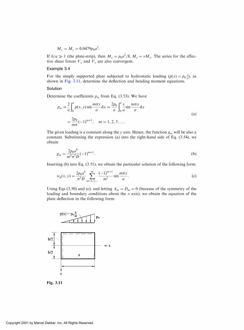
Mx ¼ My ¼ 0:0479p0a2:

If b=a � 1 (the plate-strip), then Mx ¼ p0a2=8;My ¼ �Mx. The series for the effec-

tive shear forces Vx and Vy are also convergent.

Example 3.4

For the simply supported plate subjected to hydrostatic loading (pðxÞ ¼ p0xa), as

shown in Fig. 3.11, determine the deflection and bending moment equations.

Solution

Determine the coefficients pm from Eq. (3.53). We have

pm ¼ 2

a

ða0

pðx; yÞ sinm�xa

dx ¼ 2p0a

ða0

x

asin

m�x

adx

¼ 2p0m�

ð�1Þmþ1; m ¼ 1; 2; 3 . . . :

ðaÞ

The given loading is a constant along the y axis. Hence, the function gm will be also aconstant. Substituting the expression (a) into the right-hand side of Eq. (3.54), weobtain

gm ¼ 2p0a4

m5�5Dð�1Þmþ1: ðbÞ

Inserting (b) into Eq. (3.51), we obtain the particular solution of the following form:

wpðx; yÞ ¼2p0a

4

�5D

X1m¼1;2;...

ð�1Þmþ1

m5sin

m�x

a: ðcÞ

Using Eqs (3.50) and (c), and letting Am ¼ Dm ¼ 0 (because of the symmetry of theloading and boundary conditions about the x axis), we obtain the equation of theplate deflection in the following form:

Fig. 3.11


wðx; yÞ ¼X1

m¼1;2;...

Bm coshm�y

aþ Cm

m�y

asinh

m�y

aþ 2p0a

4

�5D

ð�1Þmþ1

m5

!sin

m�x

a;

ðdÞwhere the constants of integration Bm and Cm are evaluated from the boundaryconditions on edges y ¼ �b=2: namely,

w ¼ 0jy¼�b=2 and@2w

@y2¼ 0

y¼�b=2

: ðeÞ

Application of the above to w, Eq. (d), leads to two equations. Solving them for Bm

and Cm yields

Bm ¼ � 2þ m tanh mð Þ �1ð Þmþ1

�5m5 cosh m; Cm ¼ �1ð Þmþ1

�5m5 cosh m; ðfÞ

where m ¼ m�b=2a.The deflection of the plate along the x axis is

wð Þy¼0 ¼ p0a4

D

X1m¼1

2 �1ð Þmþ1

�5m5þ Am

" #sin

m�x

a:

For a square plate we have a ¼ b, from which one obtains the following:

wð Þy¼0¼p0a

4

D0:002055 sin

�x

a� 0:000177 sin

2�x

aþ 0:000025 sin

3�x

a� . . .

� �:

ðgÞThe center deflection is given as

wð Þx¼a=2;y¼0 ¼ 0:00203p0a

4

D: ðhÞ

As expected, this result is about one-half of the deflection of a uniformly laded plate(see Example 3.1). Equating the first derivative of the expression (g) to zero, we canfind that the maximum deflection occurs at a point x ¼ 0:557a and thatwmax ¼ 0:00206ðp0a4=DÞ.

The bending moments can be found by substitution of Eq. (d) for deflectioninto Eq. (2.13). For example, the bending moment equation Mx along the x axis, i.e.,for y ¼ 0, has the form

Mxð Þy¼0 ¼ p0a2X1m¼1

2ð�1Þmþ1

�3m3sin

m�x

a

þ p0a2�2

X1m¼1

m2 ð1� �ÞBm � 2�Cm½ � sinm�xa;

where the constants Bm and Cm are given by the expressions (f). These series con-verge rapidly and several first terms give a sufficiently accurate result for Mx:


Example 3.5

Derive expressions for the deflected surface and the bending moments in a floorplate-strip subjected to a uniformly distributed load q0 along line y ¼ 0, as shownin Fig. 3.12a. Assume the edges x ¼ 0 and x ¼ a are simply supported.

Solution

If a plate is strongly lengthened in one direction – for example, in the y direction –then such a plate in some problems can be considered as an infinite one in thisdirection. Levy’s solution can be applied advantageously with some modificationsto obtain the expressions for the deflections and bending moments.

The solution of the governing differential equation (2.24) is sought in the formof Eq. (3.48). At the same time, since for y ! 1 deflections cannot approach infi-nity, then the terms containing em�y=a should be equated to zero because these termsand their derivatives do not vanish at y ! 1. Hence, wh can be represented asfollows:

wh ¼X1m¼1

B 0m þm�y

aD 0

m

� �e�m�y=a sin

m�x

a: ðaÞ

The above satisfies Eq. (2.24) and the boundary conditions on the edges x ¼ 0 andx ¼ a.

Let us consider the lower part of the plate where y � 0. The constants B 0m and

D 0m can be evaluated from the conditions of symmetry of the plate and loading at

y ¼ 0. First, due to the symmetry of the deflected middle surface of the plate withrespect to the x axis, the derivative @w=@y is zero at y ¼ 0; this condition is satisfied ifB 0m ¼ D 0

m. Therefore, Eq. (a) becomes (for the lower part of the plate)

Fig. 3.12


wh ¼X1m¼1

B 0m 1þm�y

a


m�x

a: ðbÞ

Secondly, the effective (Kirchhoff’s) shear force at the section just below the xaxis is numerically equal to one-half the line load qðxÞ. Taking into account the sign,this condition leads to the following:

Vy

y¼þ0

¼ � 1

2qðxÞ: ðcÞ

If the line load is uniformly distributed along the x axis, it can be expanded into asine series in accordance with Eq. (3.52). The coefficients qm of the single Fourierexpansion are obtained from Eq. (3.53), as follows (for a uniformly distributed loadq0)

qm ¼ 2

a

ða0

qðxÞ sinm�xa

dx ¼ 4q0m�

for m ¼ 1; 3; 5; . . . : ðdÞ

Thus, the load is expressed as

q ¼ 4q0�

X1m¼1;3;...

1

msin

m�x

a: ðeÞ

Now using the expression (c) and Eqs (3.55) and (e), we obtain

Vy

� �y¼0

¼ �D@

@yr2wh ¼ � 2q0

�

X1m¼1;3;...

1

msin

m�x

a: ðfÞ

Substitution of Eq. (b) in the left-hand side of Eq. (f) gives

B 0m ¼ q0a

3

�4m4Dðm ¼ 1; 3; 5; . . .Þ: ðgÞ

Since the plate at y > 0 and y < 0 carries no load, the particular solution of Eq.(2.24) is zero. Thus, the expression of the deflection surface of the plate becomes

w ¼ wh ¼ q0a3

�4D

X1m¼1;3;...

1

m41þm�y

a


m�x

a: ðhÞ

When the above is inserted into Eqs (3.55), the expressions for bending moments willbe obtained in the following form:

Mx ¼q0a

�2

X1m¼1;3;...

1

m21þ �þ ð1� �Þm�y

a

h ie�m�y=a sin

m�x

a;

My ¼q0a

�2

X1m¼1;3;...

1

m21þ �� ð1� �Þm�y

a

h ie�m�y=a sin

m�x

a:

ðiÞ

The maximum values of the deflections and bending moments occur at the platecenter, i.e., at y ¼ 0 and x ¼ a=2


wmax ¼q0a

3

�4D

X1m¼1;3;...

ð�1Þm�12

m4¼ 5q0�a

3

1536D;

Mx;max ¼ My;max ¼q0að1þ �Þ

�2

X1m¼1;3;::

ð�1Þm�12

m2¼ 0:91853q0að1þ �Þ

�2:

For y ¼ a the factor e�y=a ¼ e�� 0:045 and it is possible to consider that thebending moments and deflections vanish practically at a distance y � a. The deflec-tion and bending moment diagrams are shown in Fig. 3.12b.

Example 3.6

A simply supported rectangular plate shown in Fig. 3.13 is loaded by an edgemoment mx ¼ f ðxÞ along edge x ¼ 0: Determine the equation for deflections ofthe plate middle surface.

Solution

We expand the given moment function f ðxÞ into the following Fourier series:

mx ¼ f ðxÞ ¼X1n¼1

Fn sinn�y

b; ðaÞ

where Fn are the constants of the Fourier expansion. Since a lateral load pðx; yÞ iszero, the solution must satisfy the homogeneous differential equation (3.43). Thesolution of this homogeneous equation may be taken in the form

w ¼X1n¼1

1

2nC1n coshnxþ C2nnx sinh nxð

þ C3n sinh nxþ C4nnx coshnxÞ sin ny;ðbÞ

where n ¼ n�=b. The constants of integration Cin ði ¼ 1; 2; 3; 4Þ can be evaluatedfrom the prescribed boundary conditions on edges of the plate: namely,

w ¼ 0jx¼0;a; Mx ¼ mx

x¼0; Mx ¼ 0

x¼a; ðcÞ

w ¼ 0jy¼0;b; My ¼ 0y¼0;b

; ðdÞ

Fig. 3.13


w in the form of Eq. (b) satisfies Eq. (3.43) and the boundary conditions (d) exactly.Using the relations (2.12) and Eq. (a), the boundary conditions (c) can be rewritten,as follows

w ¼ 0jx¼0;a; �D@2w

@x2þ � @

2w

@y2

!" #x¼0

¼ Fn sin ny and@2w

@x2þ � @

2w

@y2

!x¼a

¼ 0:

ðeÞSubstitution of Eqs (b) into (e) and solving the obtained equations for Cin, oneobtains

C1n ¼ 0;C2n ¼ � Fn

2D;C3n ¼

Fn

2D1� coth2 na� �

na;C4n ¼Fn

2Dcothna: ðfÞ

Inserting the above into Eq. (f) yields the following:

w ¼X1n¼1

Fn

2D2n sinh nanx cosh nða� xÞ � na

sinh nx

sinh na

� �sin ny: ð3:62Þ

As it follows from the above, in order to obtain a particular solution for platessubjected to various types of load distribution pðx; yÞ ¼ p0 � f ðxÞ it is necessary todetermine the coefficients pm (see Eq. (3.53)). Table 3.2 furnishes the values of pm forvarious types of load distributions.

3.6 CONTINUOUS PLATES

When a uniform plate extends over a support and has more than one span along itslength or width, it is termed continuous. Such plates are of considerable practicalinterest.

Continuous plates are externally statically indeterminate members (note that aplate itself is also internally statically indeterminate). So, the well-known methodsdeveloped in structural mechanics can be used for the analysis of continuous plates.In this section, we consider the force method which is commonly used for the analysisof statically indeterminate systems. According to this method, the continuous plate issubdivided into individual, simple-span panels between intermediate supports byremoving all redundant restraints. It can be established, for example, by introducingsome fictitious hinges above the intermediate supports. In this way, the redundantmoments acting along the intermediate supports are eliminated. Similar fictitioushinges can be used at the ends if those are fixed. The simple-span panel obtainedin such a way is referred to as a primary plate. In order to restore the rejectedrestraints, the unknown redundant moments are applied to the primary plate.These moments can be determined from the solution of simultaneous algebraicequations expressing the compatibility of the slopes between the adjoining panelsproduced by both external loads and unknown redundant moments.

In our further discussion we assume that the supports are unyielding. For thesake of simplicity, we confine ourselves to a rectangular plate continuous in onedirection only and having the same flexural rigidity. Obviously, the general proce-dure of the force method discussed below can be applied to plates continuous in bothdirections.


Table 3.2

No.

Load Geometry

pðx; yÞ ¼Pm pm sin m�x

a

Expansion coefficient pm[determined from Eq. (3.53)]

1 Uniform loading, p0 ¼ const

pm ¼ 4p0m�

ðm ¼ 1; 3; 5; . . .Þ

2 Hydrostatic loading,

pðxÞ ¼ p0x

a

pm ¼ 2p0m�

ð�1Þmþ1

ðm ¼ 1; 2; . . .Þ

3 Line load p0 at x ¼ �

pm ¼ 2p0a

sinm��

a

ðm ¼ 1; 2; 3; . . .Þ

4 Uniform load from ð� � eÞ toð� þ eÞ

pm ¼ 4p0m�

sinm��

asin

m�e

a

ðm ¼ 1; 2; . . .Þ

5 Triangular load

pðxÞ ¼ 2p0x

aif x � a=2

pðxÞ ¼ 2p0a� x

aif x � a=2

pm ¼ 8p0m2�2

ð�1Þm�12

ðm ¼ 1; 3; . . .Þ


Consider the three-span simply supported continuous plate. The plate is sub-jected to a uniform load of intensities p1; p2, and p3 as shown in Fig. 3.14a. Figure3.14b illustrates the primary plate obtained by introducing the fictitious hinges abovethe intermediate supports; �1ðyÞ and �2ðyÞ are the redundant, unknown distributedmoments replacing the removed restraints at the intermediate supports. Theseunknown bending moments may be represented by the following Fourier series:

�1ðyÞ ¼X1

m¼1;3;...

�1m sin �my; �2ðyÞ ¼X1

m¼1;3;...

�2m sin �my; �m ¼ m�

b: ð3:63Þ

Since the deflection is symmetric with respect to the line y ¼ b=2, the numbersm in the expansions (3.63) must be odd only. It is seen from Fig. 3.14b that the

Fig. 3.14


primary plate consists of individual simple-span panels subjected to a given loadingand the distributed edge moments �1ðyÞ and �2ðyÞ, as shown in Fig. 3.14c.

The deflected surface of each simply supported individual panel may beobtained by application of Levy’s method. The general solution for individual panelssimply supported on all edges is given by Eqs (3.50) and (3.56a) if y is replaced by xi,x by y, and a by b. We have the following:

wi ¼X1

m¼1;3;...

AðiÞm sinh �mxi þ BðiÞ

m cosh �mxi þ CðiÞm �mxi sinh �mxi

�

þDðiÞm �mxi cosh �mxi þ

4pib4

m5�5D

!sin �my; i ¼ 1; 2; 3:

ð3:64Þ

The boundary conditions of each panel as well as the compatibility of deformationsbetween any two panels across a common boundary (slopes continuity at the inter-mediate supports) are used to determine the constants in the solution (3.64) and thecoefficients in the Fourier series (3.63). The boundary conditions for the plates 1, 2,and 3 are represented as follows:

w1 ¼ 0jx1¼0;c1 ;@2w1

@x21¼ 0

x1¼0

; �D@2w1

@x21¼

X1m¼1;3;...

�1m sin �my

x1¼c1

; ðaÞ

w2 ¼ 0jx2¼0;c2 ;�D@2w2

@x22¼

X1m¼1;3;...

�1m sin �my

x2¼0

;

�D@2w2

@x22¼

X1m¼1;3;...

�2m sin �my

x2¼c2

ðbÞ

w3 ¼ 0jx3¼0;c3 ;@2w3

@x23¼ 0

x3¼c3

; �D@2w3

@x23¼

X1m¼1;3;...

�2m sin �my

x3¼0

: ðcÞ

The compatibility conditions are expressed as follows

@w1

@x1

� �x1¼c1

¼ @w2

@x2

� �x2¼0

;@w2

@x2

� �x2¼c2

¼ @w3

@x3

� �x3¼0

: ðdÞ

Let us consider the middle panel 2 (Fig. 3.14c). Application of the edge conditions(b) to Eq. (3.64) for i ¼ 2 leads to the following values of the constants

Að2Þm ¼ 1

D sinh �mc2

4p2b4

m5�5cosh �mc2 � 1ð Þ 1þ 0:5�m csch �mc2ð Þ

"

þ c22�m

�1m csch �mc2 � �2m coth �mc2ð Þ�;

Bð2Þm ¼ � 4p2b

4

m5�5D;Cð2Þ

m ¼ 2p2b4

m5�5D� �1m

2D�2m;

Dð2Þm ¼ 1

2D sinh �mc2

4p2b4

m5�51� cosh �mc2ð Þ � 1

�2m�2m � �1m cosh �mc2ð Þ

" #:

ðeÞ


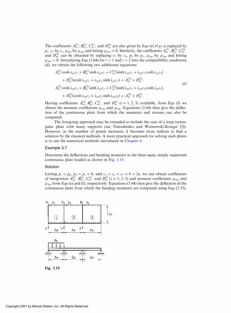
The coefficients Að1Þm ;B

ð1Þm ;C

ð1Þm ; and Dð1Þ

m are also given by Eqs (e) if p2 is replaced byp1; c2 by c1; �2m by �1m and letting �1m ¼ 0. Similarly, the coefficients Að3Þ

m ;Bð3Þm ;C

ð3Þm ;

and Dð3Þm can be obtained by replacing c2 by c3, p2 by p3, �1m by �2m and letting

�2m ¼ 0. Introducing Eqs (3.64) for i ¼ 1 and i ¼ 2 into the compatibility conditions(d), we obtain the following two additional equations:

Að1Þm cosh �mc1 þ Bð1Þ

m sinh �mc1 þ Cð1Þm sinh �mc1 þ �mc1 cosh �mc1ð Þ

þDð1Þm cosh �mc1 þ �mc1 sinh �mc1ð Þ ¼ Að2Þ

m þDð2Þm ;

Að2Þm cosh �mc2 þ Bð2Þ

m sinh �mc2 þ Cð2Þm sinh �mc2 þ �mc2 cosh �mc2ð Þ

þDð2Þm cosh �mc2 þ �mc2 sinh �mc2ð Þ ¼ Að3Þ

m þDð3Þm :

ðfÞ

Having coefficients AðiÞm ;B

ðiÞm ;C

ðiÞm ; and DðiÞ

m ði ¼ 1; 2; 3Þ available, from Eqs (f) weobtain the moment coefficients �1m and �2m. Equations (3.64) then give the deflec-tion of the continuous plate from which the moments and stresses can also becomputed.

The foregoing approach may be extended to include the case of a long rectan-gular plate with many supports (see Timoshenko and Woinowski-Krieger [3]).However, as the number of panels increases, it becomes more tedious to find asolution by the classical methods. A more practical approach for solving such platesis to use the numerical methods introduced in Chapter 6.

Example 3.7

Determine the deflections and bending moments in the three-span, simply supportedcontinuous plate loaded as shown in Fig. 3.15.

Solution

Letting p1 ¼ p0; p2 ¼ p3 ¼ 0; and c1 ¼ c2 ¼ c3 ¼ b ¼ 2a, we can obtain coefficientsof integration AðiÞ

m ; BðiÞm ; C

ðiÞm ; and DðiÞ

m ði ¼ 1; 2; 3Þ and moment coefficients �1m and�2m from Eqs (e) and (f), respectively. Equations (3.64) then give the deflection of thecontinuous plate from which the bending moments are computed using Eqs (3.55).

Fig. 3.15


The deflection w and bending moments Mx and My diagrams along the centralsection y ¼ a of the three-span plate are shown in Fig. 3.16 for � ¼ 0:3:The max-imum values of the deflection and bending moment are

wmax ¼ 0:64ð1� �2Þ p0a4

Eh3and Mxmax ¼ 0:177pa2:

3.7 PLATES ON AN ELASTIC FOUNDATION

Many problems of considerable practical importance can be related to the solutionof plates resting on an elastic foundation. Reinforced concrete pavements of high-ways and airport runways, foundation slabs of buildings, etc., are well-known directapplication. However, an indirect application of this type of plate bending problemis of equal importance. For example, the shallow shell bending problems may bereduced to the solution of the problem for a plate on an elastic foundation; i.e., ananalogy exists between the governing differential equation of a shallow shell and thatof a plate on elastic foundation.

The key difficulty of this type of problem is in the correct mathematicaldescription of a real elastic foundation. There exist a lot of various hypotheses –models of elastic foundations. The simplest of them has been suggested by Winkler[11]. It is based on the assumption that the foundation’s reaction qðx; yÞ can bedescribed by the following relationship:

qðx; yÞ ¼ kw; ð3:65Þwhere k is a constant termed the foundation modulus, which has the dimensions offorce per unit surface area of the plate per unit deflection, e.g. ðlb=in2Þð1=inÞ in USunits or ðN=m2Þð1=mÞ in SI units. Values of k for various soils are given in numerousreferences such as [9,12]. In Eq. (3.65) qðx; yÞ is the resisting pressure of the founda-tion and w is the deflection of the plate.

When the plate is supported by a continuous elastic foundation, the externalload acting in the lateral direction consists of the surface load pðx; yÞ and of the

Fig. 3.16


reaction of the elastic foundation qðx; yÞ. Thus, the differential equation of the plate(2.24) becomes the following:

@4w

@x4þ 2

@4w

@x2@y2þ @

4w

@y4¼ 1

Dpðx; yÞ � qðx; yÞ½ �: ð3:66Þ

In this differential equation, the reactive force, qðx; yÞ, exerted by the elastic founda-tion is also unknown, because it depends on the deflection, wðx; yÞ, of the plate.Substituting Eq. (3.65) into (3.66), the governing differential equation of the plateon an elastic foundation, given by the Winkler model, can be written as

Dr2r2wþ kw ¼ p: ð3:67ÞThis equation can be solved for rectangular plates by the classical methods discussedearlier.

3.7.1 Application of Navier’s solution

Let us consider a simply supported rectangular plate of sides a b on an elasticfoundation (Fig. 3.17). The deflection wðx; yÞ and a given loading pðx; yÞ can beexpressed in the form of a double trigonometric series in the form of the expressions(3.15), as follows. Substituting the above expressions into the governing differentialequation of the problem (3.67), we obtain the unknown amplitudes of the deflec-tions, wmn, for a specific set of m and n values, as follows:

wmn ¼pmn

D�4 m2=a2 þ n2=b2� �2þk

; ð3:68Þ

Fig. 3.17


which substituted into Eq. (3.15a) yields

wðx; yÞ ¼X1n¼1

X1m¼1

pmn sinm�x

asin

n�y

b

D�4 m2=a2 þ n2=b2� �2þk

: ð3:69Þ

If a plate is subjected to a uniform load of intensity p0, then Eq. (3.69) becomes

w ¼ 16p0�2

X1n¼1

X1m¼1

sinm�x

asin

n�y

b

mn �4Dðm2=a2 þ n2=b2Þ2 þ k� �: ð3:70Þ

If a plate is loaded by a concentrated force P applied at a point (�; ), then thedeflected surface equation of the plate can be represented by the following form:

w ¼ 4P

ab

X1n¼1

X1m¼1

sinm��

asin

n�

b�4Dðm2=a2 þ n2=b2Þ2 þ k

sinm�x

asin

n�y

b: ð3:71Þ

Having the deflection of the plate produced by a concentrated force, the deflectionproduced by any kind of lateral loading is obtained by the method of superposition.

3.7.2 Application of Levy’s method

If any two opposite edges of the plate on an elastic foundation are simply supported,say, the edges x ¼ 0 and x ¼ a, then Levy’s solution presented earlier in Sec. 3.5 canbe applied advantageously. The general solution of the governing differential equa-tion of the plate on an elastic foundation, Eq. (3.67), may be represented again in theform of the sum of particular and complementary solutions, i.e.,

w ¼ wp þ wh: ð3:72ÞExpressing the complementary solution by the Fourier series, yields

wh ¼X1m¼1

fmðyÞ sinm�x

a: ð3:73Þ

Substituting the above into the homogeneous part of Eq. (3.66) and solving it forfmðyÞ, we obtain

fmðyÞ ¼ Am sinh my sin myþ Bm sinh my cosmyþ Cm cosh my sin my

þDm coshmy cosmy;

ð3:74Þwhere

m ¼

ffiffiffiffiffiffiffiffiffiffiffiffiffiffiffiffiffiffiffiffiffiffiffiffiffiffiffiffiffiffiffiffiffiffiffiffiffiffiffiffiffiffiffiffiffiffiffiffiffiffiffi1

2

m2�2

a2þ

ffiffiffiffiffiffiffiffiffiffiffiffiffiffiffiffiffiffiffiffim4�4

a4þ k

D

s0@

1A

vuuut ; m ¼

ffiffiffiffiffiffiffiffiffiffiffiffiffiffiffiffiffiffiffiffiffiffiffiffiffiffiffiffiffiffiffiffiffiffiffiffiffiffiffiffiffiffiffiffiffiffiffiffiffiffiffiffiffiffiffiffi1

2�m2�2

a2þ

ffiffiffiffiffiffiffiffiffiffiffiffiffiffiffiffiffiffiffiffim4�4

a4þ k

D

s0@

1A

vuuut :

ð3:75ÞSubstituting (3.74) into (3.73), we can obtain the expression for complementarysolution wh. Similarly, if we express the particular solution as


wp ¼X1m¼1

gmðyÞ sinm�x

a; ð3:76Þ

and the applied load as

p ¼X1m¼1

pmðyÞ sinm�x

a; ð3:77Þ

and then we substitute these equations into Eq. (3.66), we obtain

d4gmdy4

� 2m�

a

� �2d2gmdy2

þ m4�4

a4þ k

D

!gm ¼ pmðyÞ

D: ð3:78Þ

Solving Eq. (3.78) for gm, we can find the particular solution wp. Therefore, Eq.(3.76) together with Eqs (3.73) and (3.74) describes the deflected surface of the plate.

Example 3.8

Find the equation for the deflection of a rectangular plate, resting on a Winklerfoundation of modulus k and subjected to a uniform loading of intensity p0. Assumethat edges x ¼ 0 and x ¼ a are simply supported while edges y ¼ �b=2 are fixed.

Solution

For a uniform loading p, the right-hand side of Eq. (3.66) is constant. Thus, theparticular solution is also a constant and may be taken in the following form:

gm ¼ B; ðaÞand the expression for pm is given by (see Table 3.2)

pm ¼ 4p0m�

: ðbÞ

Substitution of (a) and (b) into Eq. (3.78) results in the following particular solution:

gm ¼ 4p0Dm�

1

m4�4

a4þ kD

� � : ðcÞ

Due to the symmetry of the deflection around the x axis, we can take Bm ¼ Cm ¼ 0in Eq. (3.74) and the general solution for deflection becomes

w ¼X1m¼1

Am sinh my sin myþDm cosh my cosmyþ gmð Þ sinm�xa; ð3:79Þ

where Am and Bmare constants of integration. They have to be evaluated from theboundary conditions on the edges y ¼ �b=2; namely,

w ¼ 0jy¼�b=2;@w

@y¼ 0

y¼�b=2

: ðdÞ

Substituting the expressions (3.79) into these boundary conditions, gives


Am ¼ gm

�1 cosh mb

2cosm

b

2

� � ; Dm ¼ �Am tanhmb

2tanhm

b

2

� gm

coshmb

2cosm

b

2

ðeÞ

where

�1 ¼�2 þ �3�4 � �5

� tanhmb

2tanhm

b

2;

�2 ¼ m coshmb

2sin m

b

2; �3 ¼ m sinh m

b

2cosm

b

2;

�4 ¼ m sinh mb

2cosm

b

2; �5 ¼ m cosh m

b

2sin m

b

2:

ðfÞ

Substituting the above into expression (3.79), we can obtain the deflection equationfor the plate under consideration.

The Winkler model introduced above is the simplest model of an elastic foun-dation. It was based on the assumption that the subgrade of a foundation at somepoint of its surface is proportional to the pressure between the plate and the sub-grade at the same point. This is correct in the case of a floating plate, but in the caseof a coherent subgrade such a hypothesis approximates crudely the actual behaviorof the subgrade. A better approximation can be obtained using the model of a semi-infinite elastic space, as shown in Fig. 3.18; the deflection of a semi-infinite spacesurface due to the distributed loads can be determined with the use of Boussinesq’ssolution [13]. So, the deflection at a point ðxi; yiÞ of the semi-infinite space surfacecaused by an elementary distributed load qdxdy applied at point ðx; yÞ using theBoussinesq solution can be represented in the following form:

dwi ¼ K ðx� xiÞ; ðy� yiÞ½ �qdxdy;where K½ � is an influence function (or Green’s function). It represents a deflection atpoint ðxi; yiÞ of a semi-infinite space caused by a unit force P ¼ 1 applied at pointðx; yÞ. This function K ½. . .� can be derived from Boussinesq’s solution. Then, an

Fig. 3.18


arbitrary reaction load qðx; yÞ occurring over a plate base causes the followingdeflection at point ðxi; yiÞ:

wðxi; yiÞ ¼ða0

ðb0

K ðx� xiÞ; ðy� yiÞ½ �qðx; yÞdxdy: ð3:80Þ

The above-mentioned function K ½. . .� is given by the following [13]:

K ½. . .� ¼ 1� �2�E

1

r; ð3:81Þ

where r is the distance between the point of load application ðx; yÞ and point ofobservation (xi; yi), r

2 ¼ ðx� xiÞ2 þ ðy� yiÞ2. With regard to expression (3.81) andreplacing a unit force by qdxdy, Eq. (3.80) may be rewritten as

wðxi; yiÞ ¼1� �2�E

ða0

ðb0

qðx; yÞdxdyffiffiffiffiffiffiffiffiffiffiffiffiffiffiffiffiffiffiffiffiffiffiffiffiffiffiffiffiffiffiffiffiffiffiffiffiffiffiffiffiffiðx� xiÞ2 þ ðy� yiÞ2

q : ð3:82Þ

For this model, the relationship between the deflection of the foundation w and thefoundation reaction q is much more complicated than for the Winkler model. Thus,the problem of bending of a plate resting on a semi-infinite space becomes moredifficult. In the majority of cases, such plate bending problems can be solved numeri-cally only.

3.8 PLATES WITH VARIABLE STIFFNESS

Let us consider bending of a rectangular plate having a variable thickness,h ¼ hðx; yÞ. We assume that the above thickness varies gradually and there is noabrupt variation in thickness so that the expressions for the bending and twistingmoments derived earlier for plates of constant thickness, Eqs (2.13), apply withsufficient accuracy to this case also. Substituting the above equations for the bendingand twisting moments into the equation of static equilibrium (2.23) and taking intoaccount that D ¼ Dðx; yÞ. One obtains the following:

Dr2r2wþ 2@D

@x

@

@xðr2wÞ þ 2

@D

@y

@

@yðr2wÞ þ r2Dðr2wÞ

� ð1� �Þ @2D

@x2@2w

@y2� 2

@2D

@x@y

@2w

@x@yþ @

2D

@y2@2w

@x2

!¼ p:

ð3:83Þ

This is the governing fourth-order partial differential equation with variable coeffi-cients in w describing the bending of thin plates with variable thickness. A closed-form solution of this equation is possible in very special cases only. Practically, platesof variable thickness can be treated by approximate and numerical methods intro-duced in Chapter 6. Among them, the variational (the Ritz method) and finiteelement methods are widely used in practice. Analysis of plates with variable thick-ness can be efficiently carried out by the small parameter method [3]. Let us illustratean application of this method to rectangular plates of variable stiffness.


For simplicity, assume that the plate stiffness varies in one direction only, say,in the y direction. So, the plate thickness, h, varies according to the law

h ¼ h0 1þ ��ðyÞ½ �; ð3:84Þwhere � is a constant and is in the range 0 < � < 1, �ðyÞ is a given function describ-ing a variation of the plate thickness over the y cordinate, and h0 is some referenceplate thickness.

Thus,

D ¼ E hðyÞ½ �312ð1� �2Þ ¼ D0 1þ ��ðyÞ½ �3; D0 ¼

Eh3012ð1� �2Þ : ð3:85Þ

The small parameter method introduces the value � as a parameter of a solution ofthe given problem. Considering the deflection as a function of x; y; and �, representwðx; y; �) in the form

w ¼X1m¼0

wm�m; ð3:86Þ

where wm ¼ wmðx; yÞ: Substituting the expressions (3.85) and (3.86) into Eq. (3.83)and equating the coefficients for identical powers of � to zero, we obtain the follow-ing sequence of differential equations:

r2r2w0 ¼p

D0

;

r2r2w1 ¼ �3 �ðyÞr2r2w0 þ 2� 0ðyÞ @@y

r2w0 þ� 00ðyÞ r2w0 � ð1� �Þ @2w0

@x2

" #( );

r2r2w2 ¼ �3 �ðyÞr2r2w1 þ 2� 0ðyÞ @@y

r2w1 þ� 00ðyÞ r2w1 � ð1� �Þ @2w1

@x2

" #( )

� 3 �ðyÞ½ �2r2r2w0 þ 4�ðyÞ� 0ðyÞ @@y

r2w0 þ 2

� 0ðyÞ� �2þ�ðyÞ� 00ðyÞh i

r2w0 � ð1� �Þ @2w0

@x2

" #);

etc:

ð3:87Þ

where the prime notations indicate the derivatives of the function �ðyÞ with respectto y. Assume for simplicity that the plate edges x ¼ 0 and x ¼ a are simply sup-ported. Then, following the Levy method, solutions of Eqs (3.87) are sought in theform of the following series:


w0 ¼X1n¼1

w0n sinn�x

a;

w1 ¼X1n¼1

w1n sinn�x

a;

w2 ¼X1n¼1

w2n sinn�x

a

etc . . . . . . . . . . . . . . .

ð3:88Þ

where the coefficients wmn ðm ¼ 0; 1; 2; . . .Þ are functions of the y only. Expand thegiven loading in the series also, as follows:

pðx; yÞ ¼X1n¼1

pnðyÞ sinn�x

a: ð3:89Þ

Substituting the first expression (3.88) and Eq. (3.89) into the first equation (3.87)and satisfying the boundary conditions prescribed on the plate edges y ¼ 0 andy ¼ b, we can determine w0n. Then, substitution of the first and second expressions(3.88) into the second equation (3.87) gives w1n. Similarly, each of the functions wm

can be found by substitution of w0;w1; . . . ;wm�1 into the corresponding differentialequation of the system (3.87) involving wm into the left-hand side. Finally, thedeflection surface of the plate is obtained by substituting for w0;w1;w2; . . . ;wm

from Eqs (3.88) into Eq. (3.86). The interested reader can find an application ofthis and other methods to plates of variable thickness in Ref. [14].

Example 3.9

A rectangular plate of variable thickness in the y direction is simply supported onedges x ¼ 0 and x ¼ a and is fixed on edges y ¼ 0 and y ¼ b. The plate thicknessvaries according to the law h ¼ h0ð1þ �yÞ. The plate is subjected to a loadp ¼ p0 sin

n�xasin m�y

b. Find the deflections and bending moments in the plate.

Solution

This problem was solved numerically by using the above-presented general proce-dure of the small-parameter method. The boundary conditions are found to be asfollows:

w ¼ @2w

@x2¼ 0

x¼0;a

;w ¼ @w

@y¼ 0

y¼0;b

:

For the plate under consideration, �ðyÞ � y. The values of the deflection and bend-ing moment My at a plate section x ¼ a=2 are given in Table 3.3. These results wereobtained by using the three terms in the expansion (3.86) for a plate with the follow-ing geometric and mechanical parameters: a ¼ b ¼ 1m; h0 ¼ 0:0625m; � ¼ 0:5; and� ¼ 0:3.


3.9 RECTANGULAR PLATES UNDER COMBINED LATERAL ANDDIRECT LOADS

To this point, it was assumed that a plate is bent by lateral load only and deflectionsare so small that the plate middle surface was assumed to be unstrained. Thus, thelatter was considered as a neutral surface. Occasionally, however, direct forces (act-ing in the plane of the middle surface of the plate) are applied directly at the bound-aries or they arise due to temperature changes (Chapter 7). The latter forces and thecorresponding stresses are also referred to as the membrane or in-plane forces and themembrane or in-plane stresses, respectively.

Attention will now be directed to situations in which lateral and direct forcesact on the plate simultaneously. We will distinguish two possible cases:

1. Stresses in the middle surface are small and, therefore, their influence onthe plate bending is negligible. So, the total stress may be obtained byadding stresses caused by stretching and by bending of the plate middlesurface.

2. Direct stresses are not small and their effect on the plate bendingshould be taken into account. These stresses may have a considerableeffect on the bending of the plate and must be considered in derivingthe corresponding differential equation of the deflection surface. Themidsurface is strained subsequent to combined loading and assumption6 of the Kirchhoff theory (see Sec. 1.3) is no longer valid. However, wis still regarded as small so that remaining assumptions of Sec. 1.3hold, and yet large enough so that the products of the direct forcesor their derivatives and the derivatives of w are of the same order ofmagnitude as the derivatives of the shear forces, Qx and Qy. Thus, asbefore, the internal forces and moments are given by Eqs (2.13) and(2.27).

We consider below the second case in detail. Let a plate element of sides dx anddy be subjected to direct forces Nx;Ny; and Nxy ¼ Nyx which are functions of x andy. The top and front views of such an element are shown in Fig. 3.19a and b,respectively. The lateral load of intensity pðx; yÞ is applied to the element and themoments, due to this load, acting on the element are shown in Fig. 2.4. We willderive the differential equation of the plate straining due to the combined effect ofdirect and lateral loads.

Table 3.3

yðmÞw

p0=EMy

1

�0

� �

0 0 �0:035100.2 15.851 0.00561

0.4 30.156 0.02321

0.6 26.04 0.02065

0.8 10.3432 �0:0060251.0 0 �0:05646


Consider the equilibrium of the element shown in Fig. 3.19, which is subjectedto the in-plane forces Nx;Ny; and Nxy, as well as to the lateral load pðx; yÞ. First, weapply the condition

PFx ¼ 0. Referring to Fig. 3.19a, from the equilibrium of Nxdy

forces into the x-direction, we obtain the following:

Nx þ@Nx

@xdx

� �dy cos 0 �Nxdy cos; ðaÞ

where 0 ¼ þ d ¼ þ @@x dx. Noting that deflections are assumed to be very small

and, hence, for small cos � 1, and that likewise, cos 0 � 1, Eq. (a) reduces to@Nx

@x dxdy. The sum of the x components of Nxydx is treated in a similar way. Thus,the force summation in the x direction leads to

@Nx

@xþ @Nxy

@y¼ 0: ð3:90aÞ

Furthermore, the conditionP

Fy ¼ 0 results in the following:

@Nxy

@xþ @Ny

@y¼ 0: ð3:90bÞ

Equations (3.90) are independent from the equilibrium equations of Sec. 2.3 and maybe studied separately.

Considering the projection of all the forces (direct and lateral) on the z axis, theplate deflection must be taken into account. Due to the bending of the plate in the xzplane, the z component of the normal force Nx is equal to (Fig. 3.19b)

�Nxdy sin þ Nx þ@Nx

@xdx

� �dy sin 0 ðbÞ

Inasmuch as and 0 are small, sin � � @w=@x and sin 0 � 0, where 0 ¼ þ d. The latter can be represented as

0 � þ @@x

dx ¼ @w

@xþ @

2w

@x2dx;

Fig. 3.19


substituting the above into Eq. (b) gives

�Nxdy@w

@xþ Nx þ

@Nx

@xdx

� �@w

@xþ @

2w

@x2dx

!dy:

Neglecting higher-order terms in this equation yields

Nx

@2w

@x2dxdyþ @Nx

@x

@w

@xdxdy:

The z components of the in-plane shear forces Nxy on the x edges of the element aredetermined as follows. The slopes of the deflection surface in the y direction on the xedges are equal to @w=@y and @w=@yþ ð@2w=@x@yÞdx, respectively. The z directedcomponent of Nxyi s then

Nxy

@2w

@y@xdxdyþ @Nxy

@x

@w

@ydxdy:

An expression identical to the above is found for the z projection of the in-planeshear forces Nyx acting on the y edges:

Nyx

@2w

@x@ydxdyþ @Nyx

@y

@w

@xdxdy:

Finally, for the forces in Figs 3.19 and 2.4, fromP

Fz ¼ 0, we have the following:

@Qx

@xþ @Qy

@yþ pþNx

@2w

@x2þNy

@2w

@y2þ 2Nxy

@2w

@x@y

þ @Nx

@xþ @Nyx

@y

� �@w

@xþ @Nxy

@xþ @Ny

@y

� �@w

@y¼ 0:

As is seen from Eqs (3.90), the terms within the parentheses in the above expressionvanish and we finally obtain the above equation in the following form:

@Qx

@xþ @Qy

@yþ pþNx

@2w

@x2þNy

@2w

@y2þ 2Nxy

@2w

@x@y¼ 0: ð3:91Þ

As the direct forces do not result in any moment along the edges of the element, Eqs(2.20) and (2.21), and, hence Eqs (2.27) are unchanged. Introduction of Eqs. (2.27)into Eq. (3.91), yields

@4w

@x4þ 2

@4w

@x2@y2þ @

4w

@y4¼ 1

DpþNx

@2w

@x2þNy

@2w

@y2þ 2Nxy

@2w

@x@y

!: ð3:92Þ

Expressions (3.91) and (3.92) are governing differential equations for a thin platesubjected to combined lateral and direct loads. It is observed that Eq. (2.24) is nowreplaced by Eq. (3.92) to determine the deflection surface of the plate if the directloads Nx;Ny; and Nxy are not small. Either Navier’s or Levy’s methods may beapplied to obtain a solution.


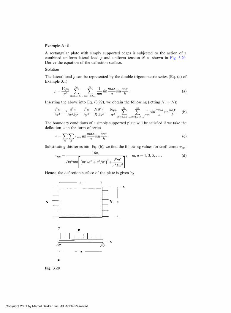
Example 3.10

A rectangular plate with simply supported edges is subjected to the action of acombined uniform lateral load p and uniform tension N as shown in Fig. 3.20.Derive the equation of the deflection surface.

Solution

The lateral load p can be represented by the double trigonometric series (Eq. (a) ofExample 3.1)

p ¼ 16p0�2

X1m¼1;3;5;...

X1n¼1;3;5;...

1

mnsin

m�x

asin

n�y

b: ðaÞ

Inserting the above into Eq. (3.92), we obtain the following (letting Nx ¼ N):

@4w

@x4þ 2

@4w

@x2@y2þ @

4w

@y4�N

D

@2w

@x2¼ 16p0

�2

X1m¼1;3;5;...

X1n¼1;3;5;...

1

mnsin

m�x

asin

n�y

b: ðbÞ

The boundary conditions of a simply supported plate will be satisfied if we take thedeflection w in the form of series

w ¼Xm

Xn

wmn sinm�x

asin

n�y

b: ðcÞ

Substituting this series into Eq. (b), we find the following values for coefficients wmn:

wmn ¼16p0

D�6mn m2=a2 þ n2=b2� �2þ Nm2

�2Da2

" # ; m; n ¼ 1; 3; 5; . . . : ðdÞ

Hence, the deflection surface of the plate is given by

Fig. 3.20


w ¼ 16p0�6D

X1m¼1;3;5;...

X1n¼1;3;5;...

sinm�x

asin

n�y

b

mn m2=a2 þ n2=b2� �2þ Nm2

�2Da2

" #: ðeÞ

Comparing this result with the solution (3.21a), we conclude from the presence of theterm Nm2=�2Da2 in the brackets of the denominator that the deflection of the plate issomewhat diminished by the action of the tensile forces N. This is as would beexpected.

3.10 BENDING OF PLATES WITH SMALL INITIAL CURVATURE

Let us assume that a plate has an initial curvature of its middle surface, i.e., there isan initial deflection w0 at any point of the above surface. It is assumed that w0 issmall compared with the plate thickness. If the plate is subject to lateral load andthen an additional deflection w1 occurs, the total deflection is thus

w ¼ w0 þ w1: ð3:93ÞHere w1 is the solution of Eq. (2.24) set up for the flat plate, i.e., without the above-mentioned initial deflection. It will be valid if the small initial deflection, w0, isconsidered as a result of the action of some fictitious lateral load. Then, applyingthe superposition principle (recall that the above principle cannot be applied forlarge deflections), it is possible to determine the total deflection.

If besides the lateral load, the direct forces are also applied to an initiallycurved plate, then these forces produce bending also, which depends not only onw1 but also on w0. In order to determine the total deflection, w, we introduce w ¼w0 þ w1 into the right hand side of Eq. (3.92). The left-hand side of this equationtakes into account a change in curvature from the initial curved state due to thegiven lateral load. Therefore, w1 has to be substituted for w on the left-hand sideof Eq. (3.92). Thus, Eq. (3.92) for the initially curved plate is of the followingform:

@4w1

@x4þ 2

@4w1

@x2@y2þ @

4w1

@y4¼ 1

DpþNx

@2ðw0 þ w1Þ@x2

þNy

@2ðw0 þ w1Þ@y2

"

þ2Nxy

@2ðw0 þ w1Þ@x@y

#:

ð3:94Þ

As mentioned previously, the influence of the initial curvature on the total deflectionof the plate is equivalent to the influence of some fictitious lateral load of intensity pfequal to

pf ¼ Nx

@2w0

@x2þNy

@2w0

@y2þ 2Nxy

@2w0

@x@y: ð3:95Þ

Hence, an initially curved plate will experience a bending under action of the directforces, lying in the plate middle surface only.


Example 3.11

Consider a simply supported plate with sides a and b. Assume that the initial deflec-tion is defined by the following equation:

w0 ¼ 11 sin�x

asin�y

b: ðaÞ

The plate edges x ¼ 0 and x ¼ a are subjected to an in-plane uniform compressiveforce Nx ¼ �N, as shown in Fig. 3.21. Find the deflected surface of the plate.

Solution

The differential equation (3.94) together with Eq. (a) will take the following form forthe problem under consideration:

@4w1

@x4þ 2

@4w1

@x2@y2þ @

4w1

@y4¼ N

D

11�2

a2sin�x

asin�y

b� @

2w1

@x2

!: ðbÞ

Let us represent a solution of the above equation in the form

w1 ¼ A sin�x

asin�y

b; ðcÞ

where A is unknown parameter. This solution satisfies exactly the simply supportedboundary conditions. Inserting Eq. (c) into Eq. (b) yields

A ¼ 11N

�2Da2

1þ a2

b2

� �2

�N

: ðdÞ

Substituting for A from Eq. (d) into Eq. (c), one obtains the deflection w1, caused bythe compressive forces N. Adding this deflection to the initial deflection (a), gives thefollowing total deflection of the plate:

w ¼ w0 þ w1 ¼111� sin

�x

asin�y

b; ðeÞ

Fig. 3.21


where

¼ N

�2Da2

1þ a2

b2

� �2: ðfÞ

The maximum deflection occurs at the plate center. Setting x ¼ a=2 and y ¼ b=2, weobtain

wmax ¼111� : ðgÞ

In general case, a given initial deflection of the plate can be expanded into thefollowing Fourier series:

w0 ¼X1

m¼1;3;...

X1n¼1;3;...

mn sinm�x

asin

n�y

bðhÞ

Substituting the above into Eq. (b) and solving yields

w1 ¼X1

m¼1;3;...

X1n¼1;3;...

bmn sinm�x

asin

n�y

b; ðiÞ

where

bmn ¼mnN

�2Da2

mþ n2a2

m2b2

� �2

�N

: ðkÞ

As follows from Eq. (k), the coefficients bmn are increased with an increase of theforce N.

To write the equation for a plate subjected to initial deflection and to in-planeuniform tensile forces, it is required to change the sign of N in Eq. (b) of the fore-going example only. By following the approach described above, the deflection of aninitially curved plate subjected to a simultaneous action of in-plane forces Nx;Ny;and Nxymay also be readily obtained.

PROBLEMS

3.1 A rectangular plate with sides a and b (0 � x � a, 0 � y � b) is bent according to the

following equation w ¼ C sin�x=a sin�y=b. Clarify the type of loading and static

boundary conditions that correspond to the given deflection surface.

3.2 Given the deflection surface of the rectangular plate with sides a and b (0 � x � a,

0 � y � b) in the form w ¼ Axyðx� aÞðy� bÞ, specify the type of loading and kine-

matic boundary conditions corresponding to the given deflection surface of the plate.

3.3 A square plate is subjected to uniformly distributed twisting moments Mxy ¼ Myx

applied to all its four edges. Determine the expression for the deflection surface.

3.4 Formulate the conditions under which a cylindrical bending can occur.

3.5 A rectangular plate of sides a and b is subjected to uniformly distributed bending

moments m applied to all four edges of the plate (see Fig. 3.2, where m1 ¼ m2 ¼ m).

Its curved middle surface should present a portion of a sphere because the radii of

curvature are identical in all planes and at all points of the plate. However, as follows


from Eq. (3.11), the deflection surface of the above plate under the given moment

loading m represents a paraboloid of revolution. Explain this discrepancy.

3.6 Consider a simply supported plate with sides a and b (0 � x � a, 0 � y � b). If the

applied load is represented by Eq. (3.15b) find the expressions for the coefficients pmn

for the following load distributions:

(a) hydrostatic pressure given by the law pðx; yÞ ¼ p0x=a;(b) uniform line load p0 distributed over the line x ¼ �;(c) uniform load p0 distributed over a half of the rectangular plate middle surface,

i.e., 0 � � � a=2 and 0 � � b, where � and are coordinates of a point of

application of applied loading.

3.7 A steel door 2 m long, 1.2 m wide, and 20 mm thick is subjected is subjected to a

uniform pressure p0. The plate is simply supported at all edges. Using the Navier

approach and retaining only the first four terms in the series expansion, determine:

(a) the limiting value of p0 that can be applied to the plate without causing yielding; (b)

the maximum deflection w and bending moments Mx and My that would be produced

when the pressure reaches its limiting value. Use E ¼ 210GPa; � ¼ 0:3; �YS ¼ 240MPa

3.8 A rectangular wall panel is subjected to a uniform patch load of intensity p0. The plate

is regarded as simply supported (Fig. 3.6). Using the Navier approach and retaining the

first four terms in the series solution, determine: (a) the maximum deflection w; (b) the

maximum bending moment Mx. Take a ¼ b ¼ 2m; h ¼ 2 10�2 m; � ¼ ¼ a=2, u ¼v ¼ 0:5m; v ¼ 0:3, E ¼ 200 GPa. Express w and Mx in terms of p0.

3.9 Consider a simply supported square plate with side a and subjected to a concentrated

load P applied at its center (Fig. 3.7). Find the corner points and indicate their direc-

tions.

3.10 Verify Eq. (3.36).

3.11 A semi-infinite plate-strip (0 � y <1) is simply supported on the edges x ¼ 0 and

x ¼ a. The edge y ¼ 0 is given by the following displacement and rotation:

wðx; 0Þ ¼ A sin�x

a;@w

@yðx; 0Þ ¼ B sin

�x

a:

Determine the bending moment My and the effective shear force Vy on the edge y ¼ 0:3.12 An infinite plate-strip (�1 < y <1) is simply supported at x ¼ 0 and x ¼ a. A uni-

form line load q acts along the line y ¼ 0. Determine the deflection w and bending

moment My at the plate center, x ¼ a=2; y ¼ 0.

3.13 Consider a rectangular plate with two opposite sides (x ¼ 0 and x ¼ aÞ simply sup-

ported; the third edge (y ¼ 0) is built-in, and the fourth edge (y ¼ bÞ free. The plate issubjected to a uniform pressure of intensity p0. Retaining only the first two terms of the

Levy’s solution, determine the deflection at the midpoint of the free edges and the

bending moments at the midpoint of the clamped edge. Take a ¼ 2m; b ¼ 3:5m, h ¼0:15m; E ¼ 210GPa; � ¼ 0:3.

3.14 A rectangular plate with two opposite sides y ¼ �b=2 fixed and the sides x ¼ 0 and x ¼a simply supported is subjected to a hydrostatic loading, as shown in row 2 of Table

3.2. Derive the expressions for the deflections w and the reactional bending moments

My along the clamped edges y ¼ �b=2.3.15 Consider a simply supported rectangular plate 0 � x � a and 0 � y � b. The plate is

loaded by the edge moments mx along the edges x ¼ 0 and x ¼ a and the edge moment

my along the edges y ¼ 0 and y ¼ b. Applying the Levy approach, derive the expression

for the deflection surface w.

3.16 Consider a three-span simply supported continuous plate shown in Fig. 3.15. The

second span is subjected to a uniform load of intensity p0. Draw the diagrams of the


deflections and bending moments along the central section y ¼ a. Take a ¼ 1m; h ¼10mm; E ¼ 200GPa; � ¼ 0:3; p0 ¼ 25MPa.

3.17 A rectangular plate with two simply supported edges x ¼ 0 and x ¼ a and two clamped

edges y ¼ �b=2 rests on an elastic foundation of the Winkler type. The plate is sub-

jected to a uniform lateral surface load p0. Determine the maximum deflection, wmax,

and the maximum bending moment, My, at the clamped edges. Take a ¼ 1:5m; b ¼2:0m; h ¼ 12mm; p0 ¼ 20MPa; k ¼ 1:04 MPA/m, E ¼ 210GPa; � ¼ 0:3.

3.18 A rectangular plate has a small initial deviation of the middle surface wiðx; yÞ. The plateis subjected to a lateral surface load p and in-plane forces Nx;Ny; and Nxy. Show that

the governing differential equation of that initially curved plate under the above load

and forces has the form

@4w1

@x4þ 2

@4w1

@x2@y2þ @

4w1

@y4¼ 1

DpþNx:

@2ðwi þ w1Þ@x2

þ 2Nxy

@2ðwi þ w1Þ@x@y

"

þ:Ny

@2ðwi þ w1Þ@y2

# ðP3:1Þ

3.19 A simply supported rectangular plate with sides a and b (0 � x � a, 0 � y � b) has an

initial deflection wi ¼ C sin �xasin �y

band uniform in-plane compression forces Nx

applied to the edges x ¼ 0 and x ¼ a. With reference to Eq. (P3.1), show that the

deflection surface of that plate is given by

w1 ¼ wi þ w1 ¼C

1� sin�x

asin�y

b; where ¼ Nx

�2D=a2 1þ a2=b2� �

x

:

3.20 Verify Eqs (3.87).

3.21 A simply supported rectangular plate with sides a and b has an initial deflection

w0ðx; yÞ, defined by Eq. (a) in Example 3.11. The plate is subject to uniform biaxial

compressive forces Nx and Ny. Determine the maximum deflection for a ¼ b and

Nx ¼ Ny ¼ �N.

3.22 A flat plate is subjected to lateral distributed load p and direct (in-plane) forces Nx;Ny;and Nxy. In addition, body forces Fx and Fy act in the middle plane of the plate. Show

that the governing differential equation for deflections becomes

r2r2w ¼ 1

DpþNx

@2w

@x2þNy

@2w

@y2þ 2Nxy

@2w

@x@y� Fx

@w

@x� Fy

@w

@y

!: ðP3:2Þ

REFERENCES

1. Navier, C.L.M.N., Bulletin des Science de la Societe Philomarhique de Paris, 1823.

2. Kantorovich, L.V. and Krylov, V.I., Approximate Methods of Higher Analysis, John

Wiley and Sons, New York, 1958.

3. Timoshenko, S.P. and Woinowski-Krieger, S., Theory of Plates and Shells, 2nd edn,


4. Gradshtein, I.S. and Ryzhik, I.M., Table of Integrals, Series, and Products, Academic

Press, New York, 1980.

5. Lukasiewitz, S., Local Loads in Plates and Shells, Warszawa Noordhoff International

Publishing, Leyden, 1979.

6. Ventsel, ES., On One Approach of Construction of Green’s Functions for Some Boundary

Value Problems of the Theory of Plates and Shallow Shells, Kharkov State University,

Ukr. NIINTI, No. 2997-Ukr. 89, 1989 (in Russian).


7. Melnikov, Yu.A., Green’s Functions in Applied Mechanics, Computational Mechanics

Publications, Southampton, UK, and Boston, USA, 1995.

8. Levy, M., Memoire sur la theorie des plaques elastiques planes, J Math Pures Appl, vol.

3, p. 219 (1899).

9. Flugge, W. (ed.), Handbook of Engineering Mechanics, McGraw-Hill, New York, 1975.

10. Ponomarev, S.D. (ed.), Stress Analyses in Mechanical Engineering, Gos Nauchno-Tekh

Izd-vo Mashinostr Lit-ry, Moscow, 1958 (in Russian).

11. Winkler, E., Die Lehre von der Elastizitat und Festigkeit, Prague, 1867.

12. Hetenyi, M., Beams on Elastic Foundation, The University of Michigan Press, Ann

Arbor, 1961.

13. Vlasov, V.Z. and Leont’ev, N.N., Beams, Plates, and Shells on Elastic Foundation, NASA

TTF-357, Washington, D.C., 1966.

14. Ventsel, E.S., A solution of some linear boundary value problems of the theory of

elasticity with a complex operator using simple boundary value problems, Dokl Acad

Sci, Ukraine, Ser. E, No. 8, p. 43–47 (1980) (in Russian).


4

Circular Plates

4.1 INTRODUCTION

Circular plates are common in many structures such as nozzle covers, end closures inpressure vessels, pump diaphragms, turbine disks, and bulkheads in submarines andairplanes, etc. When circular plates are analyzed, it is convenient to express thegoverning differential equation (2.24) in polar coordinates. This can be readilyaccomplished by a coordinate transformation. An alternative approach based onthe procedure presented in Chapter 3 for rectangular plates to derive the basicrelationships for the lateral deflections of circular plates may be used also.

4.2 BASIC RELATIONS IN POLAR COORDINATES

As mentioned earlier, we use the polar coordinates r and ’ in solving the bendingproblems for circular plates. If the coordinate transformation technique is used, thefollowing geometrical relations between the Cartesian and polar coordinates areapplicable (see Fig. 4.1a):

x ¼ r cos ’; y ¼ r sin ’ and r2 ¼ x2 þ y2; ’ ¼ tan�1 y

x: ð4:1Þ

Referring to the above

@r

@x¼ x

r¼ cos ’;

@r

@y¼ y

r¼ sin ’;

@’

@x¼ � y

r2¼ � sin ’

r;

@’

@y¼ x

r2¼ cos ’

r:

ð4:2Þ

Inasmuch as the deflection is a function of r and ’, the chain rule together with therelations (4.2) lead to the following


@w

@x¼ @w

@r

@r

@xþ @w@’

@’

@x¼ @w

@rcos ’� 1

r

@w

@’sin ’: ð4:3Þ

To evaluate the expression @2w=@x2, we can repeat the operation (4.3) twice. As aresult, we obtain

@2w

@x2¼ cos ’

@

@r

@w

@x

� �� 1

rsin ’

@

@’

@w

@x

� �

¼ @2w

@r2cos2 ’� @2w

@’@r

sin 2’

rþ @w@r

sin2 ’

rþ @w@’

sin 2’

r2þ @

2w

@’2sin2 ’

r2:

ð4:4aÞ

Similarly,

@2w

@y2¼ @2w

@r2sin2 ’þ @2w

@r@’

sin 2’

rþ @w@r

cos2 ’

r� @w@’

sin 2’

r2þ @

2w

@’2cos2 ’

r2; ð4:4bÞ

@2w

@x@y¼ @2w

@r2sin 2’

2þ @2w

@r@’

cos 2’

r� @w@’

cos 2’

r2� @w@r

sin 2’

2r� @

2w

@’2sin 2’

2r2: ð4:4cÞ

Adding term by term the relations (4.4a) and (4.4b), yields

r2r w � @2w

@x2þ @

2w

@y2¼ @2w

@r2þ 1

r

@w

@rþ 1

r2@2w

@’2: ð4:5Þ

After repeating twice the operation r2r , the governing differential equation for the

plate deflection (2.26) in polar coordinates becomes

r4r w � @2

@r2þ 1

r

@

@rþ 1

r2@2

@’2

!@2w

@r2þ 1

r

@w

@rþ 1

r2@2w

@’2

!¼ p

D; ð4:6aÞ

or in the expended form

@4w

@r4þ 2

r

@3w

@r3� 1

r2@2w

@r2þ 1

r3@w

@rþ 2

r2@4w

@r2@’2� 2

r3@3w

@’2@rþ 4

r4@2w

@’2þ 1

r4@4w

@’4¼ p

D:

ð4:6bÞ

Let us set up the relationships between moments and curvatures. Consider now thestate of moment and shear force on an infinitesimal element of thickness h, describedin polar coordinates, as shown in Fig. 4.1b. Note that, to simplify the derivations, thex axis is taken in the direction of the radius r, at ’ ¼ 0 (Fig. 4.1b). Then, the radialMr, tangential Mt, twisting Mrt moments, and the vertical shear forces Qr;Qt willhave the same values as the moments Mx;My; and Mxy, and shears Qx;Qy at thesame point in the plate. Thus, transforming the expressions for moments (2.13) andshear forces (2.27) into polar coordinates, we can write the following:


Mr ¼ �D@2w

@r2þ � 1

r

@w

@rþ 1

r2@2w

@’2

!" #; Mt ¼ �D

1

r

@w

@rþ 1

r2@2w

@’2þ � @

2w

@r2

" #;

Mrt ¼ Mtr ¼ �Dð1� �Þ 1

r

@2w

@r@’� 1

r2@w

@’

!; ð4:7aÞ

Qr ¼ �D@

@rr2r w

� �;Qt ¼ �D

1

r

@

@’r2r w

� �: ð4:7bÞ

Similarly, the formulas for the plane stress components, from Eqs (2.15), are writtenin the following form:

�r ¼12Mr

h3z; �t ¼

12Mt

h3z; �rt ¼ �tr ¼

12Mtr

h3z; ð4:8Þ

where Mr;Mt and Mtr are determined by Eqs (4.7). Clearly the maximum stressestake place on the surfaces z ¼ �h=2 of the plate.

Similarly, transforming Eqs (2.38) and (2.39) into polar coordinates gives theeffective transverse shear forces. They may be written for an edge with outwardnormal in the r and ’ directions, as follows:

Vr ¼ Qr þ1

r

@Mrt

@’¼ �D

@

@rðr2

r wÞ þ1� �r

@

@’

1

r

@2w

@r@’� 1

r2@w

@’

!" #;

Vt ¼ Qt þ@Mrt

@r¼ �D

1

r

@

@’ðr2

r wÞ þ ð1� �Þ @@r

1

r

@2w

@r@’� 1

r2@w

@’

!" #:

ð4:9Þ

The boundary conditions at the edges of a circular plate of radius a may readily bewritten by referring to Eqs. (2.48), namely:

(a) Clamped edge r ¼ a

w ¼ 0jr¼a;@w

@r¼ 0

r¼a

: ð4:10Þ

(b) Simply supported edge r ¼ a

Fig. 4.1


w ¼ 0jr¼a;Mr ¼ 0r¼a: ð4:11Þ

(c) Free edge r ¼ a

Mr ¼ 0r¼a;Vr ¼ 0

r¼a: ð4:12Þ

If we use the transformations given by Eqs (4.1)–(4.4), the strain energy for a circularplate is

U ¼ 1

2

ð ðS

D@2w

@r2þ 1

r

@w

@rþ 1

r2@2w

@’2

!2

�2ð1� �Þ @2w

@r21

r

@w

@rþ 1

r2@2w

@’2

!24

þ2ð1� �Þ 1

r

@2w

@r@’� 1

r2@w

@’

!235rdrd’:

ð4:13Þ

4.3 AXISYMMETRIC BENDING OF CIRCULAR PLATES

When an applied loading and end restraints of the circular plate are independent ofthe angle ’, then the deflection of the plate and the stress resultants and stresscouples will depend upon the radial position r only. Such a bending of the circularplate is referred to as axially symmetrical and the following simplifications can bemade:

@kð Þ@’k

¼ Mrt ¼ Qt ¼ 0; k ¼ 1; 2; 3; 4:

The previous equations for the bending of a circular plate can therefore be simplifiedto

Mr ¼ �Dd2w

dr2þ �

r

dw

dr

!;Mt ¼ �D

1

r

dw

drþ � d

2w

dr2

!;

Qr ¼ �Dd

dr

d2w

dr2þ 1

r

dw

dr

!¼ �D

d

dr

1

r

d

drrdw

dr

� �� :

ð4:14Þ

The differential equation of the deflected surface of the circular plate, Eq. (4.6a),reduces now to

r4r w � d2

dr2þ 1

r

d

dr

!d2w

dr2þ 1

r

dw

dr

!¼ p

D; ð4:15aÞ

and in the extended form

d4w

dr4þ 2

r

d3w

dr3� 1

r2d2w

dr2þ 1

r3dw

dr¼ p

D: ð4:15bÞ

The formulas for stress components are given by Eq. (4.8), setting �r� ¼ 0, where Mr

and M� can be determined from relations (4.14). Introducing the identity

r2r w � d2w

dr2þ 1

r

dw

dr¼ 1

r

d

drrdw

dr

� �; ð4:16Þ


Eq. (4.15a) appears in the form

1

r

d

drrd

dr

1

r

d

drrdw

dr

� �� ¼ p

D: ð4:17Þ

The rigorous solution of Eqs (4.15) or Eq. (4.17) is obtained as the sum of thecomplementary solution of the homogeneous differential equation, wh, and theparticular solution, wp, i.e.,

w ¼ wh þ wp: ð4:18ÞThe complementary solution of Eqs (4.15) or Eq. (4.17) is given by

wh ¼ C1 ln rþ C2r2 ln rþ C3r

2 þ C4; ð4:19Þ

where Ciði ¼ 1; 2; 3; 4Þ are constants that can be evaluated from the boundary con-ditions.

The particular solution, wp, is obtained by successive integration of Eq. (4.17):

wp ¼ð1

r

ðr

ð1

r

ðrpðrÞD

drdrdrdr: ð4:20Þ

If the plate is under a uniform loading p ¼ p0 ¼ const, the particular solution is

wp ¼p0r

4

64D: ð4:21Þ

For purposes of calculation, the following quantities are given explicitly:

w ¼ C1 ln rþ C2r2 ln rþ C3r

2 þ C4 þp0r

4

64D;

dw

dr¼ C1

1

rþ C2 2r ln rþ rð Þ þ 2C3rþ

p0r3

16D;

Mr ¼ �D �C1

1� �r2

þ 2C2ð1þ �Þ ln rþ C2ð3þ �Þ þ 2C3ð1þ �Þ�

þ p0r2

16Dð3þ �Þ

#;

Mt ¼ �D C1

1� �r2

þ 2C2ð1þ �Þ ln rþ C2ð1þ 3�Þ þ 2C3ð1þ �Þ�

þ p0r2

16Dð1þ 3�Þ

#;

Qr ¼ �4D C2

1

rþ p0r

8D

� �:

ð4:22Þ

Let us consider some solutions for axially symmetrical circular plates.

4.3.1 Solid plates

Consider a solid plate of radius a under an axisymmetric load pðrÞ. Take the origin ofthe coordinate system at a plate center. The solution of the governing differential


equation (4.17) is given by the expressions (4.18)–(4.20). For the solid plate, whichcontains no concentrated loads at r ¼ 0, it is easy to see that the terms involving thelogarithms in Eq. (4.19) yield an infinite displacement and bending moment, and theshear force for all values of C1 and C2, except zero; therefore, C1 ¼ C2 ¼ 0. Thus, fora solid circular plate subjected to an axisymmetric distributed load with arbitraryboundary conditions, the deflection surface is given by

w ¼ C3r2 þ C4 þ wp: ð4:23Þ

The constants of integration C3 and C4 in this equation are determined from bound-ary conditions specified at boundary r ¼ a. Let us consider some particular cases ofplates and loadings that are commonly encountered in practice.

(a) Plate with simply supported edge under a uniform load p0 (Fig. 4.2a).

The boundary conditions are

w ¼ 0jr¼a;Mr ¼ 0r¼a: ðaÞ

Substituting for wp from Eq. (4.21) into Eq. (4.23), we obtain the equation for thedeflected surface:

w ¼ C3r2 þ C4 þ

p0r4

64D; ð4:24Þ

and the expression for Mr may be obtained from Eq. (4.22) by making C1 ¼ C2 ¼ 0:

Mr ¼ �D 2C3ð1þ �Þ þp0r

2

16Dð3þ �Þ

" #: ð4:25Þ

Introducing Eqs (4.24) and (4.25) into the boundary conditions (a), one obtains thesystem of two algebraic equations in C3 and C4. Solving the above system, yields

C3 ¼ � p0a2

32D

3þ �ð Þ1þ �ð Þ ;C4 ¼

p0a4 5þ �ð Þ

64D 1þ �ð Þ : ðbÞ

Substituting the above into Eq. (4.24) gives the plate deflection in the form

Fig. 4.2


w ¼ p0ða2 � r2Þ64D

5þ �1þ � a

2 � r2� �

: ð4:26Þ

The maximum deflection, which occurs at r ¼ 0, is thus

wmax ¼p0a

4

64D

5þ �1þ ��

: ðcÞ

Given the deflection curve w, the moment equation can readily be obtained from Eqs(4.22) by substituting for C3 and C4 from (b) and making C1 ¼ C2 ¼ 0. Thus, weobtain

Mr ¼p016

3þ �ð Þ a2 � r2� �

;Mt ¼p016

3þ �ð Þa2 � 1þ 3�ð Þr2� �: ð4:27Þ

The bending moment diagrams are shown in Fig. 4.2b. The maximum moments alsooccur at the plate center, i.e., at r ¼ 0. Thus, we have

maxMr ¼ maxMt ¼p0a

2

163þ �ð Þ: ð4:28Þ

(b) Plate with clamped edge under a uniform load p0 (Fig. 4.3a)


w ¼ 0jr¼a;dw

dr¼ 0

r¼a

: ðdÞ

Introducing the deflection surface in the form of Eq. (4.24) into the conditions (d),we obtain

C3 ¼ � p0a2

32D;C4 ¼

p0a4

64D: ðeÞ

Similarly to the procedure for the previous case, the deflection is then

w ¼ p064D

a2 � r2� �2

: ð4:29Þ

The maximum deflection occurs at the center of the plate:

Fig. 4.3


wmax ¼p0a

4

64D: ðfÞ

Expressions for the bending moments are calculated by means of Eqs (4.22).Substituting for C3 and C4 from Eqs (e) into Eqs (4.22) and letting C1 ¼ C2 ¼ 0,we obtain

Mr ¼p016

1þ �ð Þa2 � 3þ �ð Þr2� �; Mt ¼

p016

1þ �ð Þa2 � 1þ 3�ð Þr2� �: ð4:30Þ

The bending moment distributions are shown in Fig. 4.3b. The maximum bendingmoment Mr occurs at the edge of the plate (at r ¼ a), where

maxMr ¼ � p0a2

8: ð4:31aÞ

The maximum bending moment Mt takes place at the plate center (at r ¼ 0), where

maxMt ¼p0a

2 1þ �ð Þ16

: ð4:31bÞ

If � ¼ 0:3, comparing Eqs (c) and (f), we see that the maximum deflection for thesimply supported plate is about four times as great as that for the plate with aclamped edge. For the same value of �, the maximum bending moment for a simplysupported plate is about 1.7 times as great as that for the plate with clamped edge.

(c) Circular plate under a concentrated force at its center

When a concentrated or a point load acts at the plate center, one can set p0 ¼ 0and; thus;wp ¼ 0 in Eq. (4.18). Referring to Eq. (4.19), we can conclude that C1 mustbe taken as zero in order that the deflection should be finite at r ¼ 0. The terminvolving C2 must now be retained because of the very high shear stresses presentin the vicinity of the center (see Sec. 3.4). The deflection surface of the plate is thenrepresented, as follows:

w ¼ C2r2 ln rþ C3r

2 þ C4: ð4:32ÞThe constants C2;C3; and C4 are evaluated from the boundary conditions and fromconditions at the point of application of the concentrated force. As an example,consider the plate with clamped edge loaded by a concentrated force P applied atplate center O, as shown in Fig. 4.4a. The boundary conditions (d), when introducedinto Eq. (4.32) lead to

C2a2 ln aþ C3a

2 þ C4 ¼ 0;

C2a 2 ln aþ 1ð Þ þ 2C3 ¼ 0:ðgÞ

The additional condition can be set up from the following consideration. Let usisolate a small cylinder of radius r in the vicinity of the application of P (Fig. 4.5).

From equilibrium of this cylinder, we obtain

XFz ¼ 0: Qr 2�rð Þ þ P ¼ 0 or Qr ¼ � P

2�r:

Substituting for Qr from Eq. (4.22) into the above and letting p0 ¼ 0, we obtain


4DC2

1

r¼ P

2�r: ðhÞ

Solving Eqs (g) and (h), the constants of integration are

C2 ¼P

8�D; C3 ¼ � P

16�D2 ln aþ 1ð Þ; C4 ¼

Pa2

16�D:

Upon substitution of the above into Eq. (4.32), we obtain an expression for thedeflection:

w ¼ P

16�D2r2 ln

r

aþ a2 � r2

� �: ð4:33Þ

The bending moments Mr and Mt may be obtained by inserting the constants ofintegrationC2;C3; andC4 ðC1 ¼ 0Þ into Eqs (4.22) for p0 ¼ 0. We have the following:

Mr ¼P

4�1þ �ð Þ ln a

r� 1

h i; Mt ¼

P


r� �

h i: ð4:34Þ

Applying the same procedure, we can obtain the deflection surface and bendingmoments for a plate with simply supported edges and subjected to a concentratedforce at its center. For this plate, the deflection and bending moments are given by

w ¼ P

16�D2r2 ln

r

aþ 3þ �1þ � a2 � r2

� �� ;

Mr ¼P


r; Mt ¼

P


rþ 1� �

h i:

ð4:35Þ

Fig. 4.4

Fig. 4.5


As seen, the bending moments for both plates approach infinity at the point ofapplication of concentrated force (r ! 0) (see Fig. 4.4b). The appearance here of asingularity in the bending moments has the same nature as that discussed earlier forrectangular plates loaded by a concentrated force. A detailed explanation of thisphenomenon is provided in Sec. 3.4.

(d) Simply supported circular plate subjected to a symmetric lateral loadwhich linearly increases from the center of the edge (Fig. 4.6)

Substituting p ¼ p0rainto Eq. (4.20) for the particular solution gives

wp ¼ð1

r

ðr

ð1

r

ð1

Dr p0

r

a

� �drdrdrdr ¼ p0r

5

225aD: ð4:36Þ

Substituting the above into Eq. (4.23), yields the general solution of the form

w ¼ C3r2 þ C4 þ

p0r5

225aD: ðaÞ

Substituting (a) into the boundary conditions (4.11) leads to the following values ofthe constants of integration:

C3 ¼ � p0a2

90D

4þ �1þ ��

; C4 ¼p0a

4

45D

4þ �2 1þ �ð Þ �

1

5

� �: ðbÞ

Equation (a) with known coefficients C3 and C4 determines the deflected plate sur-face

w ¼ p0a2

45D

r2

2

4þ �1þ ��

þ a24þ �

2ð1þ �Þ �1

5

� �þ r5

5a3

( ): ðcÞ

Example 4.1

A cylindrical tank and flat thin plate bottom are subjected to internal pressure p, asshown in Fig. 4.7a. Determine a required thickness of the bottom, h, and calculate itsmaximum deflection. Use R ¼ 0:25m, p ¼ 2:5MPa, E ¼ 200GPa, and � ¼ 0:3;respectively. The allowable stress �all is 150MPa.

Solution

The cylindrical tank bottom represents a circular solid plate. It is necessary toestablish a type of boundary conditions on the plate edge, which depends on arigidity of the cylinder, and the presence of the gasket at the connection. If the

Fig. 4.6


cylinder itself is sufficiently rigid, the plate of radius is R (Fig. 4.7b) is thin and, inaddition, the bottom is inserted without a soft gasket, then we can assume thecircular plate edge to be clamped over the contour of the bolts arrangement andthe plate. If the cylinder walls are compliant and the soft gaskets are at the connec-tion, one can take the plate edge to be simply supported (Fig. 4.7c). In practice, a realtype of plate support is an intermediate one between the above-mentioned extremecases, i.e., they (the supports) represent an elastic restraint support. In order to gain aclear impression of real stresses and deformations occurring in the bottom, it makessense to consider both extreme cases. The deflection surfaces and bending momentsfor these cases are given by Eqs (4.29), (4.30), and (4.26), (4.27). The bendingmoment, Mr and Mt, diagrams are shown in Figs 4.3 and 4.4 for both extremecases. Referring to these diagrams, we can conclude that the maximum bendingmoment for a simply supported circular plate occurs at the center, while for theplate with clamped edge the maximum bending moment is at the plate edge. Thevalue of the maximum bending moment for a simply supported plate is nearly 1.7times larger than for a plate with a clamped edge (for � ¼ 0:3). However, taking intoaccount that the plate edge is rather clamped than simply supported, one can expectthat the value of the maximum bending moment at the plate center does not exceedp0R

2=8, i.e., the value of the bending moment at the clamped edge. Therefore, thecircular plate with a clamped edge can be taken as the design variant of the tankhead. The maximum normal stress occurs at the clamped edge (i.e., for r ¼ R andz ¼ �h=2). From Eq. (4.8), �max is given by

�r;max ¼Mr;max

h2=6¼ 6pR2

8h2; �t;max ¼

Mt;max

h2=6¼ �

6pR2

8h2:

The third principal stress �3 ¼ �z ¼ 0, according to the general assumptions adoptedin the plate bending theory. Since the material of the plate is assumed to be a ductile,the maximum shear (Tresca) criterion of yielding (see Appendix A.6.2) can beapplied: namely,

Fig. 4.7


�e ¼ �1 � �3 ¼6pR2

8h2� �all:

Solving this for the plate thickness, h, yields

h ¼ffiffiffiffiffiffiffiffiffiffiffi6pR2

8�all

s¼

ffiffiffiffiffiffiffiffiffiffiffiffiffiffiffiffiffiffiffiffiffiffiffiffiffiffiffiffiffiffiffiffiffiffiffiffiffiffiffi6 2:5 106� �

0:25ð Þ28 150 106� �

s� 28mm;

D ¼ Eh3

12 1� �2� � ¼ 40:2 104N �m

Note that if the simply supported plate was chosen as a design variant, then the platethickness was found to be h � 36mm.

The maximum deflection for the selected design variant of the tank head isgiven by Eq. (f) (case (b) in Sec. 4.3.1), as follows:

wmax ¼pR4

64D:

Substituting the given numerical data into the above equation gives

wmax ¼ 0:38mm:

Example 4.2

Find the expression for the deflection of the clamped solid plate shown in Fig. 4.8adue to line load p distributed along a circle with radius r ¼ b.

Solution

To solve this problem, one first divides the plate problem into two parts (Fig. 4.8b):an inner solution for a solid plate 1 extending over the region 0 � r � b, and an outersolution for an annular plate 2 over the region b � r � a. In each case, the governingequation are (for p ¼ 0)

r4r w1 ¼ 0;r4

r w2 ¼ 0:

For the inner plate 1 the solution w1 is of the form (see Eq. (4.23))

w1 ¼ C1ð Þ3 r2 þ C

1ð Þ4 ; ðaÞ

and for plate 2 the corresponding solution is

Fig. 4.8


w2 ¼ C2ð Þ1 ln rþ C

2ð Þ2 r2 ln rþ C

2ð Þ3 r2 þ C

2ð Þ4 : ðbÞ

The six constants in Eqs (a) and (b) are determined from the boundary conditions atr ¼ a, i.e.,

w2 ¼ 0r¼a

dw2

dr¼ 0

r¼a

ðcÞ

and from the continuity conditions at the junction of the two plate segments. Thelatter have the form

w1

r¼b

¼ w2

r¼b

;dw1

dr

r¼b

¼ dw2

dr

r¼b

; M 1ð Þr

r¼b

¼ M 2ð Þr

r¼b

; p ¼ Q 1ð Þr

r¼b

�Q 2ð Þr

r¼b:

ðdÞSince the inner plate is in pure bending (see Eq. (a)), then Qð1Þ

r ¼ 0 and the lastcondition (d) is of the form

p ¼ �Qð2Þr

r¼b: ðeÞ

The last condition (e) is illustrated in Fig. 4.8b. Introducing expressions (a) and (b)into conditions (c), (d), and (e) together with Eqs (4.14), we can find the six constantsof integration. The final solution is, as follows:

– for the inner plate 1, 0 � r � b

w ¼ pb

8a2Da2 � b2� �

a2 þ r2� �� 2a2 b2 þ r2

� �lna

b

h i; ð4:37aÞ

– for the outer annular plate 2, b � r � a

w ¼ pb

8a2Da2 þ b2� �

a2 � r2� �þ 2a2 b2 þ r2

� �ln

r

a

h i: ð4:37bÞ

4.3.2 Annular circular plates

In this section, we discuss the bending of circular plates with concentric circularholes, the so-called annular plates (Fig. 4.9).

Fig. 4.9


The outer and inner radii of a plate are denoted by a and b, respectively. Forannular plates the homogeneous solution is given by Eq. (4.19). The solution of anaxially symmetric bending of circular plates with central holes may follow a proce-dure similar to the one discussed in the foregoing section, but one must consider theboundary conditions at the outer (r ¼ a) as well as the inner (r ¼ b) boundaries. Twotypical cases of loading are illustrated below.

(a) Simply supported annular plate loaded by edge moments (Fig. 4.10)

For this case of loading, wp ¼ 0 and the general solution is given by

w ¼ C1 ln rþ C2r2 ln rþ C3r

2 þ C4: ð4:38Þ


Mr ¼ m1

r¼b

; Qr ¼ 0r¼b

; Mr ¼ m2

r¼a

; w ¼ 0jr¼a: ðaÞ

Introducing Eq. (4.38) into the boundary conditions (a), with the use of Eqs (4.14),yields the following expressions for the constants of integration:

C1 ¼m1 �m2ð Þa2b2

D 1� �ð Þ a2 � b2� � ; C2 ¼ 0;C3 ¼

m1b2 �m2a

2

2D 1þ �ð Þ a2 � b2� � ;

C4 ¼ � m1 �m2ð Þa2b2D 1� �ð Þ a2 � b2

� � ln a� m1b2 �m2a

2� �

2D 1þ �ð Þ a2 � b2� � a2:

ðbÞ

Substituting the above into Eq. (4.38) yields the expression for deflections:

w ¼ m1 �m2ð Þa2b2D 1� �ð Þ a2 � b2

� � ln r

aþ m1b

2 �m2a2

2D 1þ �ð Þ a2 � b2� � r2 � a2

� �: ð4:39Þ

Substituting the above expression into Eqs (4.14) gives the expressions for bendingmoments:

Mr ¼ �m1b2 �m2a

2

a2 � b2þ a2b2 m1 �m2ð Þ

r2 a2 � b2� � ; Mt ¼ �m1b

2 �m2a2

a2 � b2� a2b2 m1 �m2ð Þ

r2 a2 � b2� � :

ð4:40Þ

Fig. 4.10


(b) Simply supported plate under a line load uniformly distributed along theinner edge (Fig. 4.11)

Again, wp ¼ 0, and the general solution is given by Eqs (4.38). The boundary con-ditions are

w ¼ 0jr¼a; Mr ¼ 0r¼a

; Mr ¼ 0r¼b

; Qr ¼ �pr¼b: ð4:41Þ

Substituting expressions (4.14) and (4.38) into boundary conditions (4.41), we find

C1 ¼ pb

4D

2ð1þ �Þ ln bað1� �Þða2 � b2Þ a

2b2; C2 ¼ pb

4D;

C3 ¼ pb

4D

b2 ln baa2 � b2

� ln a� 3þ �2ð1þ �Þ

!;

C4 ¼ �pb

4D

a2b2 ln baa2 � b2

2ð1þ �Þ1� � þ

� �� ð3þ �Þa2

2ð1þ �Þ

( ):

Substitution of the above into Eq. (4.38) gives the following expression for thedeflection:

w ¼ pa2b

4D1� r2

a2

!(3þ #

2 1þ #ð Þ �b2

a2 � b2lnb

a

" #

þ r2

a2ln

r

aþ 2b2

a2 � b21þ #1� # ln

b

aln

r

a

):

ð4:42Þ

It is observed that if b ! 0, b2 ln ðb=aÞ vanishes, and Eq. (4.42), letting p ¼ P=2�b,reduces to the first equation (4.35) for a solid circular plate under a concentratedforce applied at its center.

4.4 THE USE OF SUPERPOSITION FOR THE AXISYMMETRICANALYSIS OF CIRCULAR PLATES

The procedure discussed in Sec. 4.3 for determining the deflections and bendingmoments of symmetrically loaded circular plates is applicable to other cases ofloading and boundary conditions. For complicated configurations of loads andboundary conditions, the method of superposition may be used to good advantage

Fig. 4.11


to simplify the analysis. Superposition is a valid method of solution if the response ofa structure is directly proportional to the load that produces it and deflections aresmall. Then, if a static loading is broken into simpler components, the final responseis independent of whether component loads are applied simultaneously or added inarbitrary sequence. Let us illustrate an application of the method of superposition inthe following examples.

Example 4.3

Find the center deflection, w0, in the solid clamped plate loaded as shown in Fig.4.12a.

Solution

Consider a solid plate with clamped edge loaded by a line load p around a circle ofradius c, as shown in Fig. 4.12b. The center deflection, w0, is given by expression(4.37a). Setting b ¼ c and r ¼ 0, we obtain the center deflection, w0, as follows:

w0 ¼pc

8Da2 � c2 þ 2c2 ln

c

a

� �: ðaÞ

Having the deflection for a load uniformly distributed along a concentric circle, wecan determine the deflection for the given loading using the method of superposition.In fact, consider an infinitesimal line load p0dc around a circle of radius c on a plate,as shown in Fig. 4.12c. Then, the center deflection for the given loading is obtainedfrom Eq. (a), replacing p by p0dc and integrating from 0 to b. We have

wc ¼p08D

ðb0

a2c� c3 þ 2c3 ln c� 2c3 ln a� �

dc

¼ p08D

a2c2

2� c4

4þ 2 ln a � c

4

4þ 2

c4

4ln c� c4

16

!" #b

0

:

Fig. 4.12


Finally, we obtain

wc ¼p0b

2

16Da2 � 3

4b2 þ b2 ln

b

a

� �: ð4:43Þ

Example 4.4

The plate shown in Fig. 4.13a is stepped so that the central disk has twice the flexuralrigidity of the outer annulus. Find the maximum deflection and bending moment Mr

at r ¼ 0:5a, caused by concentrated force P. Use � ¼ 0:3.

Solution

The plate can be separated into two components (Fig. 4.13b): an inner part of theplate of radius a=2 and outer part in the form of an annular plate (a=2 � r � a).Continuity between the inner and outer plates is maintained by applying anunknown moment, Mr, as shown in Fig. 4.13b.

First, consider the solution for the inner plate. The slope at r ¼ a=2 is

dwi

dr¼ dwi

drPð Þ þ dwi

drMrð Þ; ðaÞ

where dwi

drPð Þ and dwi

drMrð Þ are the slopes of the inner plate at r ¼ a=2 produced by an

external concentrated force P and bending moment Mr, respectively. The aboveslopes can be obtained by differentiating the expressions for the deflections givenby the first equation (4.35) and Eq. (4.39) and then setting r ¼ a=2 in the equation fordwi

drðPÞ and r ¼ a=2;m1 ¼ 0; b ¼ 0; and m2 ¼ Mr in the equation for dwi

drðMrÞ. Thus,

we obtain the following:

dwi

drPð Þ ¼ �0:0612

P 0:5að Þ2D

¼ �0:0153Pa

D;

dwi

drMrð Þ ¼ C1

0:5a

2þ C2

1

0:5a¼ 0:5a

2� 2 0:25a2

� �Mr

1:3 0:25a2� �

2D

!¼ �0:1923

Mra

D: ðbÞ

Fig. 4.13


Finally,

dwi

drPð Þ þ dwi

drMrð Þ ¼ �0:0153

Pa

D� 0:1923

Mra

D: ðcÞ

Then we can determine the slopes of the outer annular plate. This plate isloaded by the line shear forces Qr and the line unknown bending moments Mr.The line shear force is

Qr ¼P

2�r¼ P

2� 0:5að Þ ¼ 0:318P

a: ðdÞ

The slope of the outer plate at r ¼ a=2 is

dwo

dr¼ dwo

drQrð Þ þ dwo

drMrð Þ: ðeÞ

The slopes on the right-hand side of Eq. (e) can be obtained by differentiating theexpressions for the deflections given by Eqs (4.39) and (4.42) and then setting m2 ¼0; m1 ¼ Mr, and q ¼ Qr.

We obtain the following:

dwo

drMrð Þ ¼ Mrb

2

Dða2 � b2Þa2

rð1� �Þ þr

1þ �

" #; ðfÞ

dwo

drðQrÞ ¼ Qr

a2b

4D� 2r

a2

� �3þ �

2ð1þ �Þ �b2

a2 � b2lnb

a

" #þ r

a22 ln

r

aþ 1

� �(ðgÞ

þ 2b2

a2 � b21þ �1� � ln

b

a

1

a

):

Making b ¼ a=2 and r ¼ a=2 in Eqs (f) and (g) and using Eq. (d), we obtain thefollowing expressions for slopes at r ¼ a=2:

dwo

drMrð Þ ¼ 1:0806

Mra

D;

dwo

drðQrÞ ¼ �0:1353

Pa

D: ðhÞ

Finally, the total slope at r ¼ a=2 of the outer plate is given by

dwo

dr¼ �0:1353

Pa

Dþ 1:0806

Mra

D: ðiÞ

Equating slopes from Eqs (c) and (i), we find the following:

Mr ¼ 0:094P: ðjÞThe maximum deflection occurs under the point of application of the concentratedforce. This center deflection is the sum of the following four contributions:

w at r ¼ 0in the first equation (4.35);w at r ¼ 0 in Eq (4.39) with m1 ¼ 0 and m2 ¼ Mr; b ¼ 0;w at r ¼ b in Eq. (4.42) with q ¼ Qr; andw at r ¼ b ¼ 0:5a in Eq. (4.39) with m1 ¼ Mr and m2 ¼ 0.


Thus, at the plate center, at r ¼ 0, the maximum deflection is given as

wmax ¼ 0:0505Pð0:25a2Þ

2Dþ Mra

2

4Dð1þ �Þ �Mrb

2

Dða2 � b2Þ2

1þ �b2 � a2

4þ a2

1� � lnb

a

" #þ 0:1934Qr

a3

D:

Substituting here Qr from Eq. (d) for Mr from Eq. (j), we compute the centerdeflection:

wmax ¼ 0:03224Pa2

D

4.5 CIRCULAR PLATES ON ELASTIC FOUNDATION

We consider in this section circular plates loaded symmetrically with respect to theircenter and resting on a Winkler-type foundation, which was discussed earlier inchapter 3. The foundation reaction, q rð Þ, can be described by

qðrÞ ¼ k � wðrÞ; ð4:44Þwhere k k ¼ constÞð is the modulus of the foundation.

Introducing the reaction of the foundation from Eq. (4.44) into Eq. (4.15b), weobtain the governing differential equation of bending of circular plates resting on aWinkler-type foundation:

d2

dr2þ 1

r

d

dr

!d2w

dr2þ 1

r

dw

dr

!¼ 1

Dp� kwð Þ; ð4:45Þ

where p is a given surface load. Denoting

l ¼ffiffiffiffiD

k

4

r; ð4:46Þ

and introducing the dimensionless coordinate � ¼ r=l, one can write Eq. (4.45) in theform

d2

d�2þ 1

�

d

d�

!2

wþ w ¼ pl4

D: ð4:47Þ

Introducing the following notation

r2� ¼

d2

d�2þ 1

�

d

d�; ð4:48Þ

we can rewrite Eq. (4.47) as follows:

r4�wþ w ¼ pl4

D: ð4:49Þ

For p ¼ 0, the homogeneous equation (4.49) is reduced to a system of the followingtwo second-order differential equations:


d2w

d�2þ 1

�

dw

d�� iw ¼ 0; ð4:50Þ

where i is the imaginary unit, i2 ¼ �1.The solution of this system of differential equations is of the form [1]:

w ¼ C1J0 �ffiffii

p� �þ C2J0 �

ffiffiffiffiffiffi�i

p� �þ C3H

1ð Þ0 �

ffiffii

p� �þ C4H

1ð Þ0 �

ffiffiffiffiffiffi�i

p� �; ð4:51Þ

where J0 �ffiffiffiffiffiffi�i

p� �is the Bessel function of the first kind of zero order and H

1ð Þ0 �

ffiffiffiffiffiffi�ip� �

is the Hankel function of the first kind of zero order [2].Since the functions J0 �


and H1ð Þ0 ð� ffiffiffiffiffiffi�i

p) are complex, whereas the solu-

tion w must be real, it is evident that the constants Ci i ¼ 1; 2; 3; 4ð Þ must also becomplex. In order to express the solution in terms of real functions, let us rewrite theexpression (4.51) in the form

w ¼ A1u0 �ð Þ þ A2v0 �ð Þ þ A3f0 �ð Þ þ A4g0 �ð Þ; ð4:52Þwhere the following expressions are the modified Bessel functions [1] tabulated in [3]:

u0 �ð Þ ¼ ReJ0 �ffiffii

p� �¼ J0 �

ffiffii

p� �þ J0 �ffiffiffiffiffiffi�i

p� �2

;

v0 �ð Þ ¼ ImJ0 �ffiffii

p� �¼ J0 �

ffiffii

p� �� J0 �ffiffiffiffiffiffi�i

p� �2i

;

f0 �ð Þ ¼ ReH1ð Þ0 �

ffiffii

p� �¼ H

1ð Þ0 �

ffiffii

p� �þH1ð Þ0 �


2;

g0 �ð Þ ¼ ImH1ð Þ0 �

ffiffii

p� �¼ H

1ð Þ0 �

ffiffii

p� ��H1ð Þ0 �


2i:

ð4:53Þ

Since the functions u0 �ð Þ; v0 �ð Þ; f0 �ð Þ; and g0 �ð Þ are real, then the coefficientsAi i ¼ 1; 2; 3; 4ð Þwill also be real.

It can be shown that the functions u0 and v0, together with all of their deriva-tives, remain finite when � ! 0 and tend toward infinity when �! 1. The functionf0 for �! 0 has a singularity of the �2 ln � type, the function g0 approaches infinity asln � when � ! 0; both these functions approach zero when � ! 1 [1].

The following relationships exist between the functions u0; v0; f0; and g0:

r2�u0 ¼ v0;r2

�v0 ¼ �u0; r2� f0 ¼ g0; r2

�g0 ¼ �f0; ð4:54Þwhere the operator r2

� is given by Eq. (4.48). These relations and Eqs (4.14) enable usto write the expressions for bending moments and shear forces.

Example 4.6

Find the deflection surface equation for an infinite plate resting on an elastic foun-dation, subjected to a concentrated force P.

Solution

The deflection surface is given by Eq. (4.52). Thus, the problem is to evaluate theconstants of integration Ai. The functions u0 �ð Þ and v0 �ð Þ tend toward infinity for� ! 1 whereas the deflections and bending moments for � ! 1 should vanish. Asit follows from the physical sense of the problem, then A1 ¼ A2 ¼ 0. For � ¼ 0; the


deflection should be finite; since g0 �ð Þ approaches infinity for � ! 0; then A4 ¼ 0:Thus,

w ¼ A3f0 �ð Þ: ð4:55ÞNotice that f0 �ð Þ remains finite when �! 0. The constant A3 is determined from theequilibrium condition at the point of application of P: the resultant of the radialshear force Qr distributed over a lateral surface of an infinitesimal circular cylindercut out from the plate at its center must be in the limit equal to a value of the appliedforce P, ie.,

lim�!0

Qr ¼P

2�r¼ � P

2�l�: ð4:56Þ

Substituting for w from Eq. (4.55) into the third Eq. (4.14) and taking into accountthe relations (4.54), we obtain the following expression for the shear force:

Qr ¼ �D

l3A3g0

0 �ð Þ; ð4:57aÞ

where the prime notation indicates the first derivative of the function with respect tothe variable �. From the theory of the Bessel functions [2], when �! 0 theng 00ð�Þ ¼ � 2

��. Thus,

Qr ¼ �A3

D

l32

��: ð4:57bÞ

Equating the right-hand sides of Eqs (4.56) and (4.57b), one obtains A3 ¼ Pl2=4Dand the deflection surface is given by

w ¼ Pl2

4Df0 �ð Þ: ð4:58Þ

Taking into account that the function f0 �ð Þ tends toward 1=2 for � ! 0 [2], wecan determine the maximum deflection (under point of application of P), as follows:

wmax ¼Pl2

8D:

The bending moments may be determined from Eqs (4.14) by inserting Eqs (4.57).They are of the following form:

Mr ¼P

4�1þ �ð Þ ln

2l

r� �

� �� 1

21� �ð Þ

� �;

M� ¼P

4�1þ �ð Þ ln

2l

r� �

� �þ 1

21� �ð Þ

� �;

ð4:59Þ

where � ¼ 0:5772157 . . . is Euler’s constant. These formulas are inapplicable for thepoint of application of the concentrated force.

The function (4.58) can be considered as a Green’s function in polar coordi-nates for plates resting on a Winkler-type elastic foundation, i.e., it enables one todetermine the deflection surface of an infinite plate subjected to any type of axisym-metric loading p ¼ p rð Þ by integrating the solution as a function of r.

Once the solution for an infinite plate on an elastic foundation is available, wecan go to the solution for a circular plate of finite dimensions subjected to an


axisymmetric loading. For example, the deflection surface of solid circular plates ona Winkler-type foundation can be represented by Eq. (4.18), where wp is a particularand wh is a complementary solutions of Eq. (4.45), respectively. The particularsolution can be determined using the superposition principle and Green’s function(4.58). The homogeneous solution for the solid circular plate of finite dimensions isof the form

wh ¼ A1u0 �ð Þ þ A2v0 �ð Þ:The constants of integration A1 and A2 can be evaluated from the prescribed bound-ary conditions on the plate edge.

4.6 ASYMMETRIC BENDING OF CIRCULAR PLATES

In the foregoing sections, our concern was with circular plates loaded axisymmetri-cally. We now turn to asymmetrical loading. For the analysis of deflections andstresses, we must obtain appropriate solutions of the governing differential equation(4.6). The general solution of this equation can also be presented in the form of(4.18). The complementary solution, wh, can be expressed by the following series:

wh ¼ f0ðrÞþX1n¼1

fnðrÞ cos n’þX1n¼1

f n ðrÞ sin n’: ð4:60Þ

Substituting the above into Eq. (4.6), and noting the validity of the resulting expres-sions for all r and ’, leads to two ordinary differential equations with solutions

f0ðrÞ ¼ A0 þ B0r2 þ C0 ln

r

r þD0r

2 lnr

r0;

f1ðrÞ ¼ A1rþ B1r�1 þ C1r

3 þD1r lnr

r0for n ¼ 1;

. . . . . . . . . . . . . . . . . . . . . . . . . . . . . . . . . . . . . . . . . .

fnðrÞ ¼ Anrn þ Bnr

�n þ Cnrnþ2 þDnr

�nþ2 n 6¼ 1ð Þ;

ð4:61Þ

Similar expressions can be written for f n ðrÞ and f 1 ðrÞ. The first term in Eq. (4.61)represents an axisymmetric part of the deflection, discussed in Sec. 4.3. The termscontaining cos n’ in Eq. (4.60) correspond to symmetrical components of the func-tion wh with respect to the plane ’ ¼ 0, while the terms containing sin n’ represent aninversely symmetrical part of wh. The applied surface load p ¼ p r; ’ð Þ can beexpanded into a trigonometric series:

p r; ’ð Þ ¼ p0ðrÞþX1n¼1

pnðrÞ cos n’þX1n¼1

p nðrÞ sin n’; ð4:62Þ

where

pnðrÞ ¼1

�

ð2�0

pðr; ’Þ cos n’d’; p nðrÞ ¼1

�

ð2�0

pðr; ’Þ sin n’d’;

p0ðrÞ ¼1

2�

ð2�0

pðr; ’Þd’:ð4:63Þ


The constants of integration, An; . . . ;Dn, can be determined from boundary condi-tions of the plate. The boundary conditions on curvilinear edges of the circular platesare given by the expressions (4.10)–(4.12). The stress resultants and stress coupleswithin the plate and on its edge are given by Eqs (4.7) and (4.9). Some details of anasymmetrical circular plate analysis are explained by considering the following illus-trative problems.

Example 4.7

The edge of a solid circular plate of radius a is fixed over its boundary and theapplied load is expressed as

p ¼ p0 1þ x

a

� �¼ p0 1þ r

acos ’

� �: ðaÞ

Find an expression for the deflections (Fig. 4.14).

Solution

Comparing Eq. (a) with Eq. (4.62), we can see that only two terms of the series arepresent in the example: an axisymmetric component p0 and component pnðrÞ cos n’for n ¼ 1 i.e., p1ðrÞ ¼ p0

racos ’. The axisymmetric part of the solution, caused by

load p0,w0, has been obtained in Sec. 4.3 and is expressed by formulas (4.29) and(4.30).

Find the asymmetrical part of the solution, w1, that corresponds to the loadcomponent p1ðrÞ. The above part of the solution can also be represented in the formof Eq. (4.18). The homogeneous solution is given by the second equation (4.61), i.e.,

wð1Þh ¼ f1ðrÞ cos ’ ¼ A1rþ B1r

�1 þ C1r3 þD1r ln

r

a

� �cos ’; ðbÞ

Fig. 4.14


where the superscript 1 indicates that this solution is obtained for n ¼ 1. A particularsolution must satisfy Eq. (4.6) with the right-hand side p0r

Dacos ’. We will seek this

particular solution in the following form:

wð1Þp ¼ Ar5 cos ’: ðcÞ

Substituting the above into Eq. (4.6), we can find a constant A, i.e., A ¼ p0=192Da.Thus, the particular solution is

wð1Þp ¼ p0r

5 cos ’

192Da: ðdÞ

Hence, the general solution that corresponds to the asymmetrical part of loading isgiven by

w1 ¼ A1rþ B1r�1 þ C1r

3 þD1r ln rþp0r

5

192Da

!cos ’: ðeÞ

The boundary and continuity conditions are, as follows:

w 6¼ 1r¼0

;@w

@r6¼ 1

r¼0;w ¼ 0jr¼a;

@w

@r¼ 0

r¼a

: ðfÞ

As it follows from the first two boundary conditions (f)

B1 ¼ 0 and D1 ¼ 0:

The third and fourth conditions (f) lead to the following two equations:

A1aþ C1a3 þ p0a

4

192D¼ 0; A1 þ 3C1a

2 þ 5p0a3

192D¼ 0;

from which one derives A1 and C1, as follows:

A1 ¼p0a

3

192D;C1 ¼ � p0a

96D:

Hence, the deflection surface of the plate caused by the asymmetrical part of thegiven loading (a) is of the following form:

w1 r; ’ð Þ ¼ wð1Þh þ wð1Þ

p ¼ p0a4

192D

r

a� 2

r

a

� �3þ r

a

� �5� �cos ’: ðgÞ

Finally, the deflection surface of the plate due to the given loading (a) can beobtained by superposing the solutions given by formulas (4.29) and (g). We have

w r; ’ð Þ ¼ w0 þ w1 ¼p0a

4

64D1� 2

r

a

� �2þ r

a

� �4� �þ p0a

4

192D

r

a� 2

r

a

� �3þ r

a

� �5� �cos ’:

ðhÞThe deflection at the center, wC, can be obtained by setting r ¼ 0. We obtain

wC ¼ p0a4

64D: ðiÞ


The bending moments can be obtained by substitution for w from (g) into Eqs (4.7).Stress analysis of circular plates having various boundary conditions and sub-

jected to asymmetrical loading can be successfully carried out by numerical andapproximate methods introduced in Chapter 6. Among other methods, the recipro-city theorem [4] may enable a simple approach for computation of the center dis-placements in circular plates with symmetrical boundary conditions underasymmetrical loading.

Consider a circular plate that carries two loads PC and PD applied at pointsC and D, respectively. Maxwell’s reciprocal theorem is formulated, as follows [6]:

PC�CD ¼ PD�DC; ð4:64Þwhere �CD is the displacement component at point C in the direction of load PC anddue to load PD; �DC is the displacement component at point D in the direction ofload PD and due to load PC. Equation (4.64) states that work done by the load PC inmoving through displacement produced by the load PD is equal to work done by theload PD in moving through displacement produced by the load PC. The words‘‘load’’ and ‘‘displacement’’ can be given by their general meanings, i.e., concen-trated forces and deflections, couples and their rotations; at last, distributed loadand the corresponding deflections are included.

Let point C be the center of a circular plate and point D be some point locatedat a distance r from that center. Denote �CD ¼ wC and �DC ¼ wðrÞ. Evidently wðrÞ isa deflection at point D due to the unit force applied at the plate center. In the cases offixed and simply supported plates, wðrÞ is given by expressions obtained in Eqs (4.33)and (4.35), respectively. Then, let PC ¼ 1 and PD ¼ pðr; ’Þ. Substituting the aboveinto Eq. (4.64), one obtains

wC ¼ð2�0

ða0

pðr; ’ÞwðrÞrdrd’ ð4:65Þ

where a is the radius of a circular plate.To illustrate the application of Eq. (4.65), reconsider Example 4.7. Upon sub-

stituting pðr; ’Þ ¼ p0 1þ racos ’

� �and Eq. (4.33) into Eq. (4.65), setting P ¼ 1 and

integrating, we obtain

wC ¼ p016�D

ð2�0

ða0

1þ r

acos ’

� �2r2 ln

r

aþ a2 � r2

� �rdrd’ ¼ p0a

4

64D: ð4:66Þ

The above coincides exactly with the value given by Eq. (i) in Example 4.7.

4.7 CIRCULAR PLATES LOADED BY AN ECCENTRIC LATERALCONCENTRATED FORCE

The solution for circular plates under an arbitrary concentrated load can be con-sidered one of the fundamental problems in the theory of plates, because this solu-tion can be used as the Green’s function (see Sec. 3.4) for determining deflections ofthe plate caused by an arbitrary asymmetric loading.


Consider a bending problem for a clamped circular plate of radius R loaded bya concentrated force P applied at a distance b from the center of the plate. Representthe given concentrated force in the following form of series:

P

�b

1

2þX1n¼1

cos n’

!:

This series is quite analogous to the series applied earlier for the case of a rectangularplate loaded by a concentrated force. Then, the deflected surface of the plate, wðr; ’Þ,can be sought also in the form of the trigonometric series corresponding to the givenloading. The next procedure for obtaining a solution of Eq. (4.6) will be quite similarto that discussed in Sec. 4.6. An approach for obtaining the solution of the problemleads to a rapidly convergent series for deflections. However the series in thesolutions for the bending moments and shear forces do not convergent rapidly,and, directly at the point of application of the concentrated force these series aredivergent (see Sec. 3.4). Therefore, a solution of this problem in the closed form is ofa special interest. Such a solution was first obtained by Michell [5]. We presentMichell’s solution below.

At first, let us remind ourselves of one well-known definition of a circle given inanalytical geometry. Let point M0 be any point on the circumference, points O1 andO2 some fixed points on the xy coordinate plane and r01 and r02 some distances frompoint M0 to points O1 and O2 as shown in Fig. 4.15a.

Then, any circle can be defined as a locus of points for which the ratio r01=r02 is a

constant. In fact, as follows from Fig. 4.15a,

r01 ¼ffiffiffiffiffiffiffiffiffiffiffiffiffiffiffiffiffiffiffiffiffiffiffiffiffiffiffiffiffiffiffiffiffiffiffiffiffiffiffiffiffiffiffiffiffiffiffiffiffiffiffiffiffiffiffiffiffiffiffiffiR2 þ ð�RÞ2 � 2R � ð�RÞ cos ’;

qr02 ¼

ffiffiffiffiffiffiffiffiffiffiffiffiffiffiffiffiffiffiffiffiffiffiffiffiffiffiffiffiffiffiffiffiffiffiffiffiffiffiffiffiffiffiffiffiffiffiffiffiffiffiffiffiffiffiffiffiffiffiffiffiffiffiffiR2 þ ðR=�Þ2 � 2R � ðR=�Þ cos ’

q;

ð4:67Þwhere � is some parameter. It can be shown that

r01r02

¼ � ¼ const: ð4:68Þ

Let the concentrated force P be applied at point O1 at a distance �R from the center,as shown in Fig. 4.15b. Locate an arbitrary point M of the plate by coordinates r1and r2; which are the distances from the above point to some fixed points O1 and O2.

Fig. 4.15


The coordinates r1 and r2 are related to Cartesian coordinates by the followingexpressions:

r21 ¼ ðx� �RÞ2 þ y2; r22 ¼ ðx� R=�Þ2 þ y2: ð4:69ÞDetermine the expression for the Laplace operator of some function � in terms ofthe coordinates r1 and r2. For this purpose, first find the following

@�

@x¼ @�

@r1

@r1@x

þ @�

@r2

@r2@x

¼ @�

@r1� x� �R

r1þ @�

@r2� x� R=�

r2;

@2�

@x2¼ @2�

@r21

ðx� �RÞ2r21

þ @2�

@r22

ðx� R=�Þ2r22

þ @�

@r1

1

r1� ðx� �RÞ2

r31

" #

þ @�

@r2

1

r2� ðx� R=�Þ2

r32

" #:

ð4:70Þ

Similarly,

@2�

@y2¼ @2�

@r21

y2

r21þ @

2�

@r22

y

r22þ @�

@r1

1

r1� y2

r31

!þ @�

@r2

1

r2� y2

r32

!: ð4:71Þ

Summing the above equations for the second derivatives, one obtains the expressionfor the Laplace operator. We have the following:

r2� � @2�

@x2þ @

2�

@y2¼ @2�

@r21þ @

2�

@r22þ 1

r1

@�

@r1þ 1

r2

@�

@r2: ð4:72Þ

This expression can be rewritten in the form

r2� ¼ 1

r1

@

@r1r1@�

@r1

� �þ 1

r2

@

@r2r2@�

@r2

� �: ð4:73Þ

Determination of the biharmonic operator r2r2� is reduced to the double imple-mentation of the operator (4.73).

A solution of Eq. (4.6) for the circular plate loaded by a concentrated force Pat point O1 can be represented in the following form:

w ¼ P

8�Dr21 ln r1 þ C1r

21 ln r2 þ C2r

21 þ C3r

32; ð4:74Þ

where the first term on the right-hand side represents the deflection surface of theplate symmetrical about point O1 and having a singularity at that point. The con-stants of integration C1;C2; and C3 are evaluated from the boundary conditions.Since on the boundary, r1 ¼ r01; r2 ¼ r02, and also r01 ¼ �r02, then the boundary con-dition w ¼ 0 will be satisfied if we put

C1 ¼ � P

8�D;C2 ¼ � P

8�Dln �� C3

�2: ð4:75Þ

In this case,


w ¼ P

8�Dr21 ln

r1�r2

þ C3 r22 �r21�2

!: ð4:76Þ

The constant C3 is determined from the condition that on the boundary @w=@n ¼ 0.Since w ¼ 0, then to satisfy this boundary condition it is sufficient that @w=@r1 ¼ 0 onthe boundary, i.e., for r1 ¼ �r2. As it follows from the above, C3 ¼ P

8�D�2

2. Finally, we

obtain

w ¼ P

8�Dr21 ln

r1�r2

þ 1

2ð�2r22 � r21Þ

� �: ð4:77Þ

At the point of application of the concentrated force, i.e., for r1 ¼ 0 and r2 ¼R 1

��

(see Fig. 4.15b), the deflection is

w ¼ PR2

16�Dð1� �2Þ: ð4:78Þ

The closed-form equation for the deflections enables one to determine the bendingmoments in the closed form also. For this purpose, we first find the derivatives of wand the bending moments in the Cartesian coordinate system using Eqs (4.70). Thebending moments at points of the diameter passing through the point of applicationof the force (y ¼ 0Þ are found to be

Mx ¼ Mr ¼P

8�D2ð1þ �Þ ln r1

�r2þ 2þ �2ð1þ �Þ þ r21

r22ð1� �Þ

" #;

My ¼ Mt ¼P

8�D2ð1þ �Þ ln r1

�r2þ 2�þ �2ð1þ �Þ � r21

r22ð1� �Þ

" #:

ð4:79Þ

where r1 ¼ x� �R; r2 ¼ R=�� x.In the particular case of a clamped circular plate loaded by a concentrated

force P applied at its center, �! 0 and Eqs (4.78) and (4.79) will coincide with thoseobtained in Sec. 4.3 for an axisymmetrically loaded circular plate (see Eqs (4.33) and(4.34)).

4.8 CIRCULAR PLATES OF VARIABLE THICKNESS

We limit ourselves to axisymmetric bending, since this is the type most widelyencountered in engineering – for example, in many machine parts, such as turbineblades, bellows, springs, etc. Following Szillard [6], we derive the governing equationof these plates.

Due to the symmetry, Qt and Mrt vanish and only internal forces and momentsshow in Fig. 4.16a act on the plate element, as follows

ðQr þ dQrÞðrþ drÞd’�Qrrd’þ pdsdr ¼ 0; ð4:80Þ

Mr þdMr

drdr

� �rþ drð Þd’�Mrrd’�Qrrd’dr�Mtdrd’ ¼ 0: ð4:81Þ


The last term on the left-hand side of Eq. (4.81) is due to the resultant momentshown in Fig. 4.16b. Replacing ds ¼ rd’, canceling the common factor drd’ andneglecting small quantities of higher order, Eqs (4.80) and (4.81) become

� 1

r

d

drrQrð Þ ¼ p; ð4:82Þ

Qr ¼dMr

drþ 1

rMr �Mtð Þ: ð4:83Þ

Substituting for Mr and Mtfrom Eqs (4.14) into Eq. (4.83) and making D ¼ DðrÞ, weobtain

d3w

dr3þ d2w

dr21

D

dD

drþ 1

r

� �þ dw

dr

�

rD

dD

dr� 1

r2

� �þQr

D¼ 0: ð4:84Þ

If we substitute for Qr from the third equation (4.14) into Eq. (4.82), we obtain

1

r

d

drrD

d

dr

1

r

d

drrdw

dr

� �� ¼ pðrÞ: ð4:85Þ

Either of the two equations, (4.84) or (4.85), can be used as the governing differentialequations of axisymmetrically loaded circular plates of variable thickness.

In order to lower the order of differential equation (4.84), let us introduce anew variable

# ¼ � dw

dr; ð4:86Þ

where # is the angle of rotation of the normal to the plate middle surface. Thenegative sign for # is because, as seen from Fig. 4.17, this angle is counted off inthe direction which is opposite to the rotation from the r axis to the z axis. Theexpressions for bending moments, Eqs (4.14), can be also written in terms of #, asfollows:

Fig. 4.16


Mr ¼ Dd#

drþ � #

r

� �;Mt ¼ D

#

rþ �d#

dr

� �: ð4:87Þ

Finally, introducing # in the form of Eq. (4.86) into Eq. (4.84) yields the following:

d2#

dr2þ 1

rþ 1

D

dD

dr

� �d#

drþ �

D

dD

dr� 1

r

� �#

r¼ Qr

D: ð4:88Þ

If D ¼ const, Eq. (4.88) reduces to

d2#

dr2þ 1

r

d#

dr� 1

r2# ¼ Qr

D: ð4:89Þ

Equation (4.88) can also be considered as the governing differential equation ofbending of an axisymmetrically loaded circular plate having a variable stiffness. Itis assumed that the right-hand side of this equation is a known function of r. Qr canbe obtained from the free-body equilibrium. In a general case, when h is an arbitraryfunction of r, Eq. (4.88) can be solved numerically only using the approximatemethods introduced in Chapter 6. The small-parameter method, introduced inChapter 3 for treating rectangular plates with a variable thickness, can also beapplied to the solution of Eq. (4.88).

However, there is an important particular case when a closed-form solution ofEq. (4.88) is available. This is a case when the plate thickness varies according to thefollowing law:

h ¼ Cr: ð4:90ÞDepending on the exponent , the shape of the plate may be different (Fig. 4.18). Theproblem of an axisymmetric bending of the circular plate having a form that corre-sponds to < 0 is encountered, in particular, in the analysis of turbine disks loadedby an axial load.

Let r1 be the inner radius and h1 the plate thickness on the inner edge of anannular circular plate. Taking into account Eq. (4.90), we can represent the platethickness as

h ¼ h1r

r1

� �: ð4:91Þ

The flexural rigidity of the arbitrary point of the plate for this case is

Fig. 4.17


D ¼ Eh3

12ð1��2Þ ¼ D0

r

ri

� �3

; and ð4:92Þ

D0 ¼Eh31

12ð1� �2Þ is the flexural rigidity on the inner edge. Substituting Eq. (4.92) into

Eq. (4.88), yields

d2�

dr2þ 1þ 3ð Þ

r

d�

dr� 1� 3�ð Þ

r2# ¼ Qr

D0

r1r

� �3: ð4:93Þ

The general solution of this equation can be represented

# ¼ #h þ #p; ð4:94Þwhere the complementary solution #h is sought in the form

#h ¼ Crx: ð4:95ÞSubstituting the above into the homogeneous equation (4.93), we obtain the follow-ing characteristic equation:

x2 þ 3x� ð1� 3�Þ ¼ 0:

The roots of this equation are the following:

x1 ¼ � 3

2þ

ffiffiffiffiffiffiffiffiffiffiffiffiffiffiffiffiffiffiffiffiffiffiffiffiffiffiffiffiffiffiffiffi92

4þ 1� 3�ð Þ

r; x2 ¼ � 3

2�

ffiffiffiffiffiffiffiffiffiffiffiffiffiffiffiffiffiffiffiffiffiffiffiffiffiffiffiffiffiffiffiffi92

4þ 1� 3�ð Þ

r:

Hence, the complementary solution is given by

#h ¼ C1r�3

2þffiffiffiffiffiffiffiffiffiffiffiffiffiffiffiffiffiffiffi92

4 þ 1�3�ð Þph i

þ C2r�3

2�ffiffiffiffiffiffiffiffiffiffiffiffiffiffiffiffiffiffiffi92


: ð4:96ÞThe particular solution, #p, depends on the type of loading. If the circular plate issubjected to a load p0 ¼ const, then the shear force Qr can be calculated from theequilibrium as follows:

Fig. 4.18


Qr ¼ �p0r2 � r212r

:

Substituting the above into the right-hand side of Eq. (4.93), we can seek a particularsolution in the following form #p ¼ Bry. After a simple transformation, we obtain

#p ¼ � p0r31

2D0

r3 1�ð Þ

8� 9þ 3�þ r 1�3ð Þr213 1� �ð Þ

" #: ð4:97Þ

If a concentrated load P is distributed over the inner edge, we can find, by analogy,that

Qr ¼ � P

2�rand #p ¼ Pr31 r 1�3ð Þ

6�D0 1� �ð Þ : ð4:98Þ

The general solution of Eq. (4.93) for a plate subjected to uniform pressure p0 andconcentrated force P distributed over the inner edge of the plate can be representedin the form

# ¼ C1r�3

2þffiffiffiffiffiffiffiffiffiffiffiffiffiffiffiffiffiffiffi92


þ C2r�3

2�ffiffiffiffiffiffiffiffiffiffiffiffiffiffiffiffiffiffiffiffi92

4 þ 1�3�Þð Þph i

:

� p0r31

2D0

r3ð1�Þ

8� 9þ 3�þ rð1�3Þr213ð1� �Þ

" #þ Pr31 rð1�3Þ

6�D0ð1� �Þ:

ð4:99Þ

The bending moments can be determined from Eqs (4.87). The deflection w is deter-mined by integrating the expression (4.86). We have

w ¼ �ð#drþ C3: ð4:100Þ

The constants of integration, C1;C2, and C3, are to be determined from boundaryconditions. The above conditions are of the following form:

if the plate edge is fixed, then # ¼ 0;if the plated edge is simply supported, then Mr ¼ D d#

drþ � #

r

� � ¼ 0;

The third boundary condition is formulated, as follows: the deflection on therestrained edge is zero. One can also take a definite integral instead of indefiniteEq. (4.100), i.e.,

w ¼ �ðrr0

#d �rr; ð4:101Þ

where r0 is the radius on the plate support and r is the radius at a point of interest.

Example 4.9

Find the expressions for stresses and deflections in the circular plate with linearlyvarying thickness. The plate is simply supported on its edges and loaded by lineforces P, as shown in Fig. 4.19a. Given r2 ¼ r1; � ¼ 1=3.


Solution

The parameter in this case is equal to unity. Thus, for ¼ 1 and � ¼ 1=3, Eq.(4.99) becomes

# ¼ C1 þ C2r�3 þ Pr31 r

�2

4�D0

: ðaÞ

Accordingly,

#

r¼ C1r

�1 þ C2r�4 þ Pr31 r

�3

4�D0

;d#

dr¼ �3C2r

�4 � Pr31 r�3

2�D0

: ðbÞ


Mr ¼ 0r¼r1

ord#

drþ 1

3

#

r

� �¼ 0

r¼r1

; Mr ¼ 0r¼r2¼3r1

ord#

drþ 1

3

#

r

� �¼ 0

r¼r2¼r1

:

ðcÞSubstituting for # and d#=dr from Eqs (b) into the boundary conditions (c) leads tothe following system of two algebraic equations:

� 3C2

r41� P

2�D0

þ C1

3r1þ C2

3r41þ P

12�D0

¼ 0;

� 3C2

4r41� P

23�D0

þ C1

3r1þ C2

34r41þ P

123�D0

¼ 0:

Solving these equations for C1 and C2 yields

C1 ¼5

4

P

4�D0

r1 1þ 3 �

1� 3 !

; C2 ¼5

32

P

�D0

r413 � 1� 3 :

Fig. 4.19


Substituting the above into the expression (a) gives the following

# ¼ P

4�D0

r15ð1� Þ1� 3 þ 5ð3 � Þ

8ð1� 3Þr31r3

þ r21r2

" #: ðdÞ

Knowing # we can determine the bending moments Mr and Mt from Eqs (4.87). Wehave

Mr ¼ D0

r3

r31

d#

drþ � #

r

� �¼ 5P

12�

r1ð2 � 1Þrð3 � 1Þ � 1þ � 1

3 � 1

r2

r21

" #;

Mt ¼ D0

r3

r31

#

rþ � d#

dr

� �¼ P

4�

5ð� 1Þ3 � 1

r2

r21þ 1

3

" #:

ðeÞ

The moment diagrams for ¼ 3 are shown in Fig. 4.19b. The maximum stress atr ¼ r1 is

�t;max ¼6Mt

h21¼ 1:08

P

�h21;

and at r ¼ r2

�t;max ¼6Mt

3h1ð Þ2 ¼ 0:63P

�h21:

The maximum deflection for ¼ 3 is found from Eq. (4.101) by substituting for #from Eq. (d) into the above and making r0 ¼ r2 ¼ r1:

wmax ¼ �ðr13r1

#dr ¼ 0:295Pr21�D0

:

Numerical results, given in Fig. 4.19, were taken from Ref. [7].

PROBLEMS

4.1 A circular plate of radius a is bent according to the following equation (the origin of

the coordinate system is at the plate center):

w ¼ Cða2 � r2Þ

Fig. P4.1


How is the plate supported and what is the nature of the loading?

4.2 The equation of the deflected middle surface of the circular plate of radius a is given by

the following equation:

w ¼ C ð5þ �Þa4 � 2ð3þ �Þa2r2 þ ð1þ �Þr4� �How is the plate supported and what is the nature of the loading?

4.3 It is known that at a concentrated load on a beam, the bending moment is finite at the

point of application of the force. However, at a concentrated load on a plate, the

bending moment is infinite at a point of application of the force according to

Kirchhoff’s plate bending theory. Explain physically, why there is this difference.

4.4 At each of the circular plates with the clamped edge and loaded, as shown in Fig. P.4.1,

determine the deflection and bending moments equations. Find wmax; Mr;max; and

Mt;max.

4.5 At each of the circular plates with simply supported edge and loaded, as shown in Fig.

P.4.2, determine the equations for deflections and bending moments. Find wmax;Mr;max, and Mt;max.

Fig. P4.2


4.6 Let a circular plate be subjected to an axially symmetric transverse load of intensity p.

Show that p ¼ Qr

rþ dQr

dr:

4.7 Show that the following relations are valid for the axisymmetrically loaded circular

plate:

d

dr�r þ �tð Þ ¼ �Qr

Dand

d

drMr þMtð Þ ¼ �ð1þ �ÞQr:

4.8 At each of the annular circular plates and loaded, as shown in Fig. P.4.3, determine the

equations for the deflections and bending moments. Find wmax; Mr;max; and Mt;max.

4.9 Calculate the stresses and deflections in a diaphragm intended for measuring the rate of

liquid (see Fig. P.4.3b). The resistance created by the diaphragm in flowing the liquid

Fig. P4.3


causes a pressure drop of intensity p. Given: a ¼ 0:2m; p ¼ 0:4MPa; � ¼ 0:3, E ¼ 220

GPa; and h ¼ 0:02m.

4.10 Calculate the stresses and deflections in the cap of a hatch. The cap is modeled by a

circular plate simply supported on its outer edge and having a rigid cylinder welded to

the plate’s central part, as shown in Fig. P.4.3.e. Use: a ¼ 0:85m; p ¼ 2MPa; E ¼200GPa; � ¼ 0:3, and h ¼ 0:08m:

4.11 Find the deflections and bending moments in the circular stepped plate shown in Fig.

P.4.4. Assume a ¼ 2m; h ¼ 0:2m; h1 ¼ 0:12m; p0 ¼ 1:5MPa; E ¼ 200GPa; and

� ¼ 0:3.4.12 Redo Problem 4.11 for the case of the plate with fixed outer edge.

4.13 Find the expressions for deflections and bending moments in a circular plate subjected

to load p ¼ p0racos ’ (the origin is taken at the plate center) if the plate edge is fixed and

a is the plate radius.

4.14 A circular simply supported plate is subjected to a transverse load p ¼ p0 1þ racos ’

� �(the origin of the coordinate system is taken at the plate center) and a is the plate

radius. Draw the deflection and bending moment diagrams along the diameter for

’ ¼ �=4. Use a ¼ 2:0m; h ¼ 0:15m, p0 ¼ 5MPa; E ¼ 200GPa; and � ¼ 0:3.4.15 Derive expressions for the stress couples Mr, Mt, and Mrt in terms of the deflection,

using the procedure presented in Sec. 2.3 for rectangular plates.

4.16 A concrete circular slab, simply supported on its edge, is subjected to the loading

shown in Fig. P.4.5. Using the reciprocity theorem, determine the center deflection

Fig. P4.4

Fig. P4.5


of the plate due to a concentrated center force. A useful formula for a concentrated

center force P and � ¼ 0 is w ¼ 1

16�D2r2 ln

r

aþ 3ða2 � r2Þ

h i.

4.17 For the circular plate, shown in Fig. P.4.5c, verify Eq. (4.64) using the Michell solution

given by Eq. (4.77) and the solution (P.4.1) for the deflection due to a centrally applied

concentrated force.

4.18 Derive the governing differential equation for a circular plate analogous to Eq. (2.44)

for rectangular plates, using the procedure presented in Sec. 2.4.

REFERENCES

1. Korenev, B.G., Besselevykh Funktsiiakh Nekotorye Zadachi Teorii Uprugosti I

Teploprovodnosti Reshaemye v, Gos Izd Fiz-Mat Literatyru, Moscow, 1960 (in Russian).

2. Watson, G.N., Theory of Bessel Functions, 2nd ed., Cambridge University Press,

Cambridge, 1944.

3. Abramowitz, M. and Stegun, I.A., Handbook of Mathematical Functions, Bureau of

Standards, Series No. 55, US Government Printing Office, Washington, DC, 1965.

4. Cook, R.D. and Young, W.C., Advanced Mechanics of Materials, Macmillan Publishing

Company and Colliear Macmillan Publishers, New York and London, 1985.

5. Michell, J.H., Proc. London Math. Soc., vol. 34, p. 223, 1902.

6. Szillard, R., Theory and Analysis of Plates, Prentice-Hall, Englewood Cliffs, New Jersey,

1974.

7. Boyarshinov, S.V., The Fundamentals of Structural Mechanics of Machines,

Mashinostroenie, Moscow, 1973 (in Russian).


5

Bending of Plates of Various Shapes

5.1 INTRODUCTION

Structural members, common in engineering practice, consist of plates with shapesother than rectangular or circular. The analytical approaches to the solutions of suchplate bending problems, discussed in Chapters 3 and 4, are usually too complicatedto be considered for practical use. The more general forms are discussed in thischapter. We consider possible solutions, which can be obtained analytically withrelative ease for some geometrical forms of plates different from rectangular andcircular.

5.2 ELLIPTICAL PLATES

Elliptical plates with a clamped boundary, subjected to uniformly distributed loads,enable one to obtain an analytical solution. Let us consider the elliptical plate shownin Fig. 5.1. Take the origin of the coordinate system at the center of the plate. Theequation of the contour of the plate (equation of the ellipse) is given by

x2

a2þ y2

b2¼ 1: ðaÞ

The boundary conditions for the clamped edge of the plate are

w ¼ 0;@w

@n¼ 0: ðbÞ

It can be easily shown that these conditions are satisfied if the deflected surface is

w ¼ w0

x2

a2þ y2

b2� 1

!2

; ð5:1Þ


where w0 is the center deflection of the plate. Substituting for w into the governingdifferential equation (2.24), and letting p ¼ p0, gives

w0

24

a4þ 16

a2b2þ 24

b4

� �¼ p0

D;

from which

w0 ¼p0

D 24=a4 þ 24=b4 þ 16=a2b2� � : ð5:2Þ

Substituting the above into Eq. (5.1), gives the following solution:

w0 ¼p08D

a4b4 x2=a2 þ y2=b2 � 1� �23a4 þ 3b4 þ 2a2b2� � : ð5:3Þ

Since the deflection surface w in the form of Eq. (5.1) satisfies Eq. (2.24) and theprescribed boundary conditions (b) exactly, then it is an exact solution of the givenplate bending problem.

The maximum deflection is given by

wmax ¼ wð0; 0Þ ¼ p08D

a4b4

ð3a4 þ 3b4 þ 2a2b2Þ :

Knowing the deflection surface Eq. (5.2), one can determine the bending moments inthe plate using Eqs (2.13). The bending moments My at the end points of the semi-minor axis and at the plate center are

My

x¼0;y¼�b

¼ � 8�w0D

b2; My

x¼0;y¼0

¼ 4w0D1

b2þ �

a2

� �: ð5:4Þ

Fig. 5.1


The bending moments Mx at the end point of the semi-major axis and at the platecenter are given by

Mx

x¼�a;y¼0

¼ � 8w0D

a2; Mx

x¼0;y¼0

¼ 4w0D1

a2þ �

b2

� �: ð5:5Þ

Comparing these values of the bending moments, we can conclude that the end pointof the semi-minor axis of the ellipse is the most stressed point.

In the particular case, for a ¼ b ¼ R, the relation (5.3) gives a value of themaximum deflection for a circular plate with clamped boundary:

w0 ¼p0R

4

64D:

For an elliptical plate with a simply supported boundary, subjected to a uniformlydistributed load, the deflected surface is a more intricate problem. Omitting thesolution of this problem, we give only values of the maximum deflection

w0 ¼ p0b

4

D

and the bending moments at the center of the plate

Mx ¼ p0b3; My ¼ 1p0b

2:

The values of the coefficients ; ; and 1 are given in the Table 5.1 [1] for � ¼ 0:3:

5.3 SECTOR-SHAPED PLATES

The general solution for circular plates (Sec. 4.2) can be used with some modifica-tions for a plate in the form of a sector plate. We consider a uniformly loaded sectorplate subtending the angle and bounded by the lines r ¼ r0 and r ¼ r1. The plate isassumed to be simply supported along the straight edges, as shown in Fig. 5.2.

By expanding the lateral load p ¼ p0 ¼ const into a trigonometric series con-taining the sine terms only, we obtain the following expression for the load:

p ¼ 4p0�

X1m¼1;3;5;...

1

msin

m�’

: ð5:6Þ

The general solution of the problem is sought in the form

w ¼ wh þ wp;

where the particular solution for the deflections, wp, which satisfies the conditions ofsimple supports along the edges ’ ¼ 0; , is given by [2]

Table 5.1

a=b 1.0 1.2 1.5 2.0 3.0 4.0 5.0 1

0.70 0.96 1.26 1.58 1.88 2.02 2.10 2.28

0.206 0.219 0.222 0.210 0.188 0.184 0.17 0.15

1 0.206 0.261 0.321 0.379 0.433 0.465 0.48 0.5


wp ¼4p0r

40

��4

X1m¼1;3;5;...

sinm�’

m 16�m2�2=2� �

4�m2�2=2� �: ð5:7Þ

where � ¼ r=r0The complementary solution, wh, can be taken as

wh ¼ F0 þX1m¼1

Fm sinm�’

; ð5:8Þ

where

F0 ¼ A0 þ B0�2 þ C0 ln �þD0�

2 ln �;

Fm ¼ Am�m�= þ Bm�

�m�= þ Cm�2þm�= þDm�

2�m�=:ð5:9Þ

The coefficients A0;B0;C0;D0; and Am;Bm;Cm;Dm are determined from the bound-ary conditions at r ¼ r0 and r ¼ r1. Some analytical solutions for sector plates withvarious values of the angle ¼ �=2ð and ¼ �Þ are given in Timoshenko andWoinowski-Krieger [1].

If the uniformly loaded and simply supported plate sector takes the form of asemicircle ( ¼ �), as shown in Fig. 5.3, then its solution assumes the form

w ¼X1

m¼1;3;5;...

Amrm þ Cmr

mþ2� �

sinm’þ 4p0r4

�D

X1m¼1;3;5;...

sinm’

m 16�m2� �

4�m2� �:

ð5:10ÞThis solution satisfies the boundary conditions on the straight edge of the semicir-cular plate. The constants Am and Cm are determined from the boundary conditionsalong the curvilinear edge of the semicircle. Determining the above constants andinserting them into Eq. (5.10), one finds

w ¼ por40

D

X1m¼1;3;5;...

4�4

m� 16�m2� �

4�m2� �

(

þ �m 5þmþ �ð Þm� 16�m2� �

2þmð Þ mþ 0:5 1þ �ð Þ½ �

� �mþ2ð3þmþ �Þm�ð4þmÞð4�m2Þ mþ 0:5ð1þ �Þ½ �

)sinm’:

ð5:11Þ

Fig. 5.2


5.4 TRIANGULAR PLATES

5.4.1 Isosceles right triangular plates

Consider a simply supported isosceles right triangular plate AOB, of length a under aconcentrated force P acting at an arbitrary point Cð�; Þ, as shown in Fig. 5.4. Tosolve the given plate bending problem, the method of images, introduced by Nadai[2], may be used. According to this method, the given triangular plate is considered asone-half of a simply supported square plate, as indicated in Fig. 5.4 by dashed lines.

This square plate is subjected to the concentrated forces P (given force actingdownward) and �P (fictitious concentrated force acting upward) at points C �; ð Þand C 0 a� �; a� ð Þ, respectively. Point C 0 is the mirror or image point of C withrespect to diagonal AB. The bending couple due to þP and �P results in a zerobending moment and deflection along diagonal AB of the square plate, i.e., theprescribed simply supported boundary conditions for the given triangular plate

Fig. 5.3

Fig. 5.4


will be satisfied. The deflection owing to the force P can be obtained from Eq. (3.27)by replacing b with a. Finally, we have

wþP ¼ 4Pa2

�4D

X1m¼1

X1n¼1

sinm��

asin

n�

b

m2 þ n2� �2 sin

m�x

asin

n�y

a: ð5:12Þ

Upon substitution of �P for P, a� ð Þ for �, and a� �ð Þ for in Eq. (5.12), weobtain the deflection due to the force �P at C 0:

w�P ¼ � 4Pa2

�4D

X1m¼1

X1n¼1

ð � 1Þmþn sinm�

asin

m��

a

m2 þ n2� �2 sin

m�x

asin

n�y

a: ð5:13Þ

The deflected surface of the triangular plate is obtained from

w ¼ wþP þ w�P; ð5:14Þwhere wþP and w�P are given by Eqs (5.12) and (5.13). Using the function w asGreen’s function, we can obtain the solution of an isosceles triangular, simply sup-ported plate subjected to any type of loading pðx; yÞ. For example, the deflectedsurface of a triangular plate under a uniformly distributed load of intensity p0 ¼P=d�d may be found from Eq. (5.14), after integration over the area of the plate, asfollows:

w ¼ 16p0a4

�6d

X1m¼1;3...

X1n¼2;4...

n sinm�x

asin

n�y

a

m n2 �m2� �

m2 þ n2� �2

24

þX1

m¼2;4...

X1n¼1;3...

m sinm�x

asin

n�y

a

n m2 � n2� �

m2 þ n2� �2

35:

ð5:15Þ

This series converges very rapidly. With the expressions for the deflection of the platedetermined, one can obtain the bending moments and stresses in the plate from Eqs(2.13) and (2.15), respectively.

5.4.2 Equilateral triangular plate

Consider a simply supported equilateral plate ABC shown in Fig. 5.5. The deflectedsurface of the equilateral triangular plate may be represented in the form

w ¼ kFðx; yÞ; ð5:16Þwhere k is a constant and Fðx; yÞ is some function that satisfies the prescribed simplysupported boundary conditions for the plate. In particular, Fðx; yÞ can be repre-sented as the product of the left-hand sides of equations of the three sides of thetriangle. In this case,

Fðx; yÞ ¼ xþ a

3

� � xffiffiffi3

p þ y� 2a

3ffiffiffi3

p� �

xffiffiffi3

p � y� 2a

3ffiffiffi3

p� �

¼ x3 � 3y2x

3� aðx2 þ y2Þ

3þ 4a3

81:

ð5:17Þ


It is evident that Fðx; yÞ is zero at the boundary. In the particular case of auniformly loaded equilateral triangular plate, the deflection surface can be taken as[1]

w ¼ p064aD

x3 � 3y2x� a x2 þ y2� �þ 4

27a3

� �4

9a2 � x2 � y2

� �; ð5:18Þ

where p0 is the load intensity. It can be shown that this expression for w satisfies thegoverning differential equation (2.24) and the boundary conditions for a simplysupported edge. Therefore, Eq. (5.18) is the solution. By employing Eqs (2.13), thebending moments may then be obtained. It can be shown that the center momentsare

Mx ¼ My ¼ ð1þ �Þ p0a2

54: ð5:19Þ

The largest moments occur on the planes bisecting the angles of the triangle. Forexample, at points along the x axis (Fig. 5.5), for � ¼ 0:3, we obtain the followingexpressions:

Mx;max ¼ 0:0248p0a2 x ¼ �0:062a; y ¼ 0ð Þ;

My;max ¼ 0:0259p0a2 x ¼ 0:129a; y ¼ 0ð Þ:

The maximum stress is given by �y;max ¼ 0:155p0a2=h2.

5.5 SKEW PLATES

Skew plates are widely used in modern structures. Swept wings of airplanes andparallelogram slabs in buildings and bridges are examples of the application ofskew plates in engineering. Following Szillard [3], let us derive the governing differ-ential equation of bending of skew plates by introducing an oblique coordinatesystem, �; , as shown in Fig. 5.6. The coordinates of the rectangular (x; y) andoblique (�; ) systems are related by

Fig. 5.5


� ¼ x� y tan ’ and ¼ 1

cos ’y: ð5:20Þ

Substitution of the expressions (5.20) into Eq. (2.17), transforms the Laplacianoperator from the rectangular to oblique coordinate system, r2

o, as follows:

r2o ¼ 1

cos2 ’

@2

@�2� 2 sin ’

@2

@�@ þ @2

@ 2

!ð5:21Þ

Therefore, the governing differential equation of plate bending, expressed in terms ofthe oblique coordinates, is of the form

D

cos4 ’

@4w

@�4þ 2 1þ 2 sin2 ’

� � @4w

@�2@ 2

(� 4 sin ’

@4w

@�3@ þ @4w

@�@ 3

!þ @

4w

@ 4

)¼ p �; ð Þ:

ð5:22Þor, more concisely,

Dr2or2

ow �; ð Þ ¼ p �; ð Þ: ð5:23ÞThe analytical solution of Eq. (5.22) or (5.23) is complicated by the absence of

orthogonal relationships and by the presence of singularities occurring at the obtusecorners. It can be solved only for a few particular cases. Thus, the analysis of theskew plates mentioned above can be carried out, primarily, by numerical methodsdiscussed in Chapter 6. Some numerical solution procedures and the correspondingexamples are discussed in Szillard [3].

PROBLEMS

5.1 Derive the equation for the bending moments, Mx and My, for a clamped elliptical

plate under a uniformly distributed surface load p0.

5.2 Derive the equations for the shear forces, Qx and Qy, for a clamped elliptical plate

under a uniformly distributed surface load p0.

Fig. 5.6


5.3 With reference to Problem 5.2, show that a clamped elliptical plate under a uniformly

distributed load p0 is in a state of equilibrium, i.e., show that Pþ R ¼ 0, where P is the

resultant of distributed load p0 and R is the resultant of the reactive forces on the plate

boundary, R ¼ ÞVxdy� Vydx� �

.

5.4 Determine the required thickness of a fixed elliptical plate with a ¼ 25 in. and b ¼18 in: The plate is loaded by a uniform pressure of 120 psi. Take � ¼ 0:3 and the

allowable stress of 16 ksi.

5.5 Verify Eq. (5.11).

5.7 A simply supported wing panel in the form of an isosceles right triangle is subjected to

a uniform distributed load p0 (Fig. 5.4). By retaining only the first term of the series

solution at point Cðx ¼ a=4; y ¼ a=4Þ, determine (a) the deflection and (b) the bending

moments.

5.8 Consider a simply supported equilateral triangular plate under a uniformly distributed

load p0. With reference to Eqs (2.32), show that

r2M ¼ �p0;M ¼ p04a

xþ a

3

� �x� 2

3aþ y

ffiffiffi3

p� �x� 2

3a� y

ffiffiffi3

p� �:

.

5.9 Verify Eq. (5.22).

5.10 Consider a clamped plate in the form of a parallelogram (Fig. 5.6) subjected to a

uniform surface load p0. Taking a solution of Eq. (5.22) in the form

wð�; Þ ¼ A

41� cos

2��

a

� �1� cos

2�

b

� �

determine at point � ¼ a=2 and ¼ b=2: (a) the deflection, (b) the bending moments.

Use ’ ¼ 15.5.11 Determine the expressions for Mx;My; and Mxy for skew plates by using the geome-

trical relationship (5.20) between the Cartesian and oblique coordinates.

REFERENCES



2. Nadai, A., Die Elastichen Platten, Springer-Verlag, Berlin, 1925.

3. Szillard, R., Theory and Analysis of Plates, Prentice-Hall, Englewood Cliffs, New Jersey,

1974.


6

Plate Bending by Approximate andNumerical Methods

6.1 INTRODUCTION

An exact solution in analytical form (i.e., exact solution formula) of plate bendingproblems using classical methods, discussed in Chapters 3, 4, and 5, is limited torelatively simple plate geometry, load configuration, and boundary supports. If theseconditions are more complicated, the classical analysis methods become increasinglytedious or even impossible. In such cases, approximate methods are the onlyapproaches that can be employed for the solution of practically important platebending problems. Nevertheless, the classical solutions remain very valuable becausethey enable one to gain insight into the variation of stresses and strains with basicshape and property changes, and they provide an understanding of the physical platebehavior under an applied loading. In addition, they can be used as a basis forincisively evaluating the results of approximate solutions through quantitative com-parisons and order-of-magnitude bounds.

In this chapter we consider some approximate methods that are widely used forplate and shell bending analysis. By convention, these approximate methods may bedivided into two groups.

6.1.1 Indirect methods

These methods enable us to obtain numerical values of unknown functions by,primarily, direct discretization of the governing differential equation of the corre-sponding boundary value problem. Also they can be defined as methods for solvingproblems on computers. Note that computers have changed, almost revolutionized,numerical methods. These changes of the field as a whole, as well as many individualmethods, are continuing. Here, we introduce such well-known methods as the finitedifference method, the method of boundary collocations, the boundary elementmethod, and the Galerkin method.


6.1.2 Direct methods

These methods use the variational principles introduced in Sec. 2.6 for determin-ing numerical fields of unknown functions (deflections, internal forces, andmoments), avoiding the differential equations of the plate or shell theory. TheRitz method is considered first and then the most efficient and well-acceptedmethod at the present time – the finite element method – is also be presented.It should be noted that the above-mentioned division is very conventional becausesome approximate methods combine some distinguishing features of both groupsof methods. For instance, the variational difference method is based on varia-tional principles but unknown functions of deflection are represented in a numer-ical form at nodal points of the mesh drawn on the area of a plate midplane. Inthis chapter, all the above-mentioned methods are discussed only with applicationto plate bending problems. Their application to shell problems is considered inPart II.

6.2 THE FINITE DIFFERENCE METHOD (FDM)

6.2.1 General concepts

This is a method of the solution of boundary value problems for differential equa-tions. The essence of the FDM lies in the following:

1. The middle plane of the plate is covered by a rectangular, triangular, orother reference network (Fig. 6.1), depending on the geometry of theplate. This network is called a finite difference mesh and points of inter-section of this mesh are referred to as mesh or nodal points.

2. The governing differential equation inside the plate domain is replaced bythe corresponding finite difference equations at the mesh points using thespecial finite difference operators.

3. Boundary conditions are also formulated with the use of the above-men-tioned finite difference operators at mesh points located on the plateboundary.

As a result of such replacement, we obtain a closed set of linear algebraic equationswritten for every nodal point within the plate. Solving this system of equations, oneobtains a numerical field of the nodal displacements.

6.2.2 Approximation of derivatives by finite differences

The key point of the FDM is the finite difference approximation of derivatives.Consider a development of the above approximations for the derivatives of a one-dimensional, continuous function f ðxÞ. It is known that the derivative of a functionf ðxÞ at point xi is defined, as follows (Fig. 6.2a):

df

dx

� �i

¼ lim�!0

fiþ1 � fi�

ordf

dx

� �i

¼ lim�!0

fi � fi�1

�;


Fig. 6.1

Fig. 6.2


where fi ¼ f ðxiÞ, etc.; � is a finite increment of the variable x. Dropping the symbolof limit in the above equalities, we obtain

df

dx

� �i

� fiþ1 � fi�

; ð6:1aÞ

df

dx

� �i

� fi � fi�1

�: ð6:1bÞ

Expressions (6.1a) and (6.1b) are called the first forward and backward approxima-tions of the first derivative of f ðxÞ at point xi, respectively. In practice, the expressionfor a central difference approximation of (df =dxÞi is often used, as follows:

df

dx

� �i

� fiþ1 � fi�1

2�: ð6:2Þ

Expressions (6.1) and (6.2) are also referred to as the finite difference operators of thefirst derivative. It is clear that expressions (6.1) and (6.2) are more accurate as thevalue of � is smaller. From now on, for simplicity, we use the sign of equality in theabove expressions instead of the sign of approximate equality.

Applying expressions (6.1) and (6.2) as operators we can derive the correspond-ing differential approximations of the second, third, and fourth derivatives of thefunction f ðxÞ. We present below only the central difference approximations of theabove derivatives, as follows:

d2f

dx2

!i

¼ fi�1 � 2fi þ fiþ1

�2; ð6:3Þ

d3f

dx3

!i

¼ fiþ2 � 2fiþ1 þ 2fi�1 � fi�2

2�3; ð6:4Þ

d4f

dx4

!i

¼ fiþ2 � 4fiþ1 þ 6fi � 4fi�1 þ fi�2

�4: ð6:5Þ

The coefficient patterns for the central finite difference operators of a one-dimen-sional function f ðxÞ are given in Fig. 6.2b.

By using the quadratic interpolation, one can obtain the expressions of theabove derivatives for a nonuniformly spaced finite difference mesh shown in Fig. 6.3.

For example,

df

dx

� �i

¼ �2fi�1 � 1� 2� �fi þ fiþ1

1þ ð Þ� ;

d2f

dx2

!i

¼ 2 fi�1 � 1þ ð Þfi þ fiþ1

� � 1þ ð Þ�2

:

ð6:6Þ

We now discuss the case of a continuous function Fðx; yÞ of two variables. Forthis purpose, assume that a plate middle plane is approximated by a mesh withthe mesh widths of �x and �y in the x and y directions, respectively. Let usrestrict our derivation and application to equally spaced square meshes by introdu-cing �x ¼ �y ¼ �. It is evident that @iF=dxi and @jF=@yj (i; j ¼ 1; 2; 3; 4Þ are


approximated by the finite difference operators of the type (6.3)–(6.5). For example,for a central point k, we obtain

@2F

@x2

!k

¼ Fa � 2Fk þ Fc

�2;

@2F

@y2

!k

¼ Fd � 2Fk þ Fb

�2: ð6:7Þ

Adding the equalities (6.7), we obtain the finite difference approximation of theLaplace operator, as follows:

r2F� �

k¼ @2F

@x2þ @

2F

@y2

!¼ Fa þ Fb þ Fc þ Fd � 4Fk

�2: ð6:8Þ

The finite difference approximation of the biharmonic operator can be obtained byapplying the Laplace operator (6.8) twice. We have the following:

r2r2F� �

k¼

20Fk � 8 Fa þ Fb þ Fc þ Fdð Þ þ 2 Fe þ Ff þ Fg þ Fh

� �þ Fl þ Fm þ Fn þ Fið Þ�4

:

ð6:9Þ

The expression for the approximation of the second mixed derivative can beobtained following the pattern shown next:

@2F

@x@y

!k

¼ @

@x

@F

@y

� �k

¼ � @F=@yð Þaþ @F=@yð Þc2�

¼ Fh � Fe þ Ff � Fg

4�2: ð6:10Þ

Applying this operator twice, one obtains the approximation of the fourth derivativeof the function Fðx; yÞ; ð@4F=@x2@y2Þk.

For reference purposes, some useful finite difference operators for a squaremesh are represented in the form of coefficient patterns in Fig. 6.4. Notice that thecenter point in each case is the node about which each operator is written (the abovepoint is outlined by a rectangle). In the case of a rectangular mesh with �x ¼ �x and�y ¼ �y, one needs to replace � with �x, or � with �y. For example,

Fig. 6.3


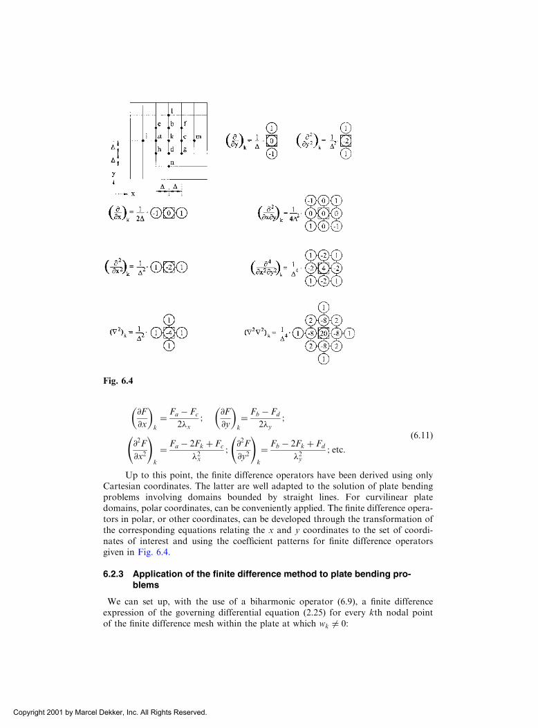
@F

@x

� �k

¼ Fa � Fc

2�x;

@F

@y

� �k

¼ Fb � Fd

2�y;

@2F

@x2

!k

¼ Fa � 2Fk þ Fc

�2x;@2F

@y2

!k

¼ Fb � 2Fk þ Fd

�2y; etc:

ð6:11Þ

Up to this point, the finite difference operators have been derived using onlyCartesian coordinates. The latter are well adapted to the solution of plate bendingproblems involving domains bounded by straight lines. For curvilinear platedomains, polar coordinates, can be conveniently applied. The finite difference opera-tors in polar, or other coordinates, can be developed through the transformation ofthe corresponding equations relating the x and y coordinates to the set of coordi-nates of interest and using the coefficient patterns for finite difference operatorsgiven in Fig. 6.4.

6.2.3 Application of the finite difference method to plate bending pro-blems

We can set up, with the use of a biharmonic operator (6.9), a finite differenceexpression of the governing differential equation (2.25) for every kth nodal pointof the finite difference mesh within the plate at which wk 6¼ 0:

Fig. 6.4


r2r2w� �

k¼ pk

D; k ¼ 1; 2; . . .N; ð6:12Þ

where pk is an average load over an area �� enclosing the nodal point k. If aconcentrated force P is applied at a kth point, then pk ¼ P=�2. The finite differenceoperators for some moments and the effective shear forces are given in Fig. 6.5. Theywere obtained by replacing the partial derivatives in Eqs (2.13) and (2.39b) by thecorresponding finite difference expressions.

Let us consider some finite difference expressions for typical boundary condi-tions for the plate edge x ¼ const:

(a) Simply supported edge (Fig. 6.6a)

According to the boundary conditions for a simply supported edge, we have

wk ¼ 0 and@2w

@x2

!k

¼ 0; ð6:13aÞ

and applying the finite difference operator of the second derivative (see Fig. 6.4)yields

wa � 2wk þ wb

�2¼ 0;

from which, taking into account that wk ¼ 0, we can obtain

wb ¼ �wa: ð6:13bÞ

Fig. 6.5


(b) Clamped edge (Fig. 6.6b)

Boundary conditions for the clamped edge of a plate can be written for the kth pointas follows:

wk ¼ 0 and@w

@x

� �k

¼ 0: ð6:14aÞ

Applying the operator of the first derivative of w, the latter boundary conditionbecomes (see Fig. 6.4)

wb � wa

2�¼ 0;

from which

wb ¼ wa: ð6:14bÞ

(c) Free edge (Fig. 6.6c)

As shown in Sec. 2.4, the boundary conditions for a free edge, for instance,x ¼ const, have the form

Mx ¼ 0 and Vx ¼ 0: ð6:15aÞ

Fig. 6.6


Applying the finite difference operators of forces and moments, given in Fig. 6.5, tothe above boundary conditions, the latter are represented for a kth point on the plateedge as follows:

2 1þ �ð Þwk � wa � wc � � wb þ wdð Þ ¼ 0;

2 3� �ð Þ wc � wað Þ þ 2� �ð Þ we þ wh � wf � wg

� �þ wi � wm ¼ 0:ð6:15bÞ

There will be four fictitious nodes – f ; c; g, and m – when the finite difference analogof the differential equation (6.12), Eq. (6.9) is applied to mesh point k on the freeedge (Fig. 6.6c).

The expressions (6.13b), (6.14b), or (6.15b) are used either for eliminating thefictitious points mentioned above or for joining them to Eq. (6.9) as additionalequations. As a result we obtain the closed system of linear algebraic equationswith a square matrix. Solving this system of equations yields the numerical field ofthe plate deflections wk ðk ¼ 1; 2; . . . ;NÞ.Example 6.1

Find the approximate deflection values for a continuous rectangular plate, withloads and supports as shown in Fig. 6.7 [1].

Solution

The domain of the plate is divided into a number of small squares (28 squares, asshown in Fig. 6.7). We thus have �x ¼ �y ¼ � ¼ 0:25a. In labeling nodal points,the plate and loading symmetry about the x axis has been taken into account. At allthe nodal points on the outer and inner (x ¼ a) boundaries the deflections are zero.At the fictitious nodes, located outside of the outer boundary, we have the following(with regard to the notation of the nodal points of Fig. 6.7):

w100 ¼ w1;w6

00 ¼ w6;w500 ¼ w5;w10

00 ¼ w10;

w10 ¼ �w1;w2

0 ¼ �w2;w30 ¼ �w3:

ðaÞ

Nodal loads on the right field of the plate (just to the right of the line x ¼ a) arep4 ¼ p5 ¼ p9 ¼ p10 ¼ 0; and on the left field of the plate (just to the left of the linex ¼ a) they are p1 ¼ p2 ¼ p3 ¼ p6 ¼ p7 ¼ p8 ¼ p ¼ const.

Fig. 6.7


Using the operator (6.9), we obtain a set of the algebraic equations (6.12) in theexplicit form for the nodal points 1; 2; . . . ; 10. Then, with the use of the relation forcase (a), we can eliminate the deflections at the fictitious points 1 00; 5 00; 6 00; and 10 00 inthe above system of equations. Solving the latter yields the following numericalvalues of the deflections at the nodal points of the mesh shown in Fig. 6.7:

w1 ¼ 0:00129pa4

D; w2 ¼ 0:002047

pa4

D; w3 ¼ 0:001746

pa4

D;

w4 ¼ �0:000246pa4

D; w5 ¼ �0:000133

pa4

D; w6 ¼ 0:001746

pa4

D

w7 ¼ wmax ¼ 0:00278pa4

D; w8 ¼ 0:002019

pa4

D; w9 ¼ �0:0003476

pa4

D;

w10 ¼ �0:0001875pa4

D:

Having determined the numerical values of the deflections and applying the finitedifference operators for moments (see Fig. 6.5), one can determine the bending andtwisting moments, and then the corresponding stresses.

The FDM has become fairly popular in recent years. As mentioned earlier,according to this method the governing differential equation is replaced by a set ofsimultaneous algebraic equations: computers can be used to find the solution to thesealgebraic equations. The FDM has obvious advantages and disadvantages. Amongits advantages, we can mention the following:

(a) it is straightforward in understanding and application;(b) it is sufficiently universal, being applied to both linear and nonlinear

problems; and(c) it is well suited for computer application.

Disadvantages of this method are

(a) it requires (to a certain extent) mathematically trained operators;(b) it requires more work to achieve complete automation of the procedure in

program writing;(c) the matrix of the approximating system of linear algebraic equations is

asymmetric, causing some difficulties in numerical solution of this system;and

(d) an application of the FDM to domains of complicated geometry may runinto serious difficulties.

This section contains only a brief description of the FDM and its application to platebending problems. The interested reader is referred to other works [2,3].

6.3 THE BOUNDARY COLLOCATION METHOD (BCM)

The boundary collocation method (BCM) is among the simplest methods of solvingpartial differential equations, both from a conceptual, as well as a computationalpoint of view. The solution is expressed as a sum of known solutions of the govern-ing differential equation, and boundary conditions are satisfied at selected colloca-


tion points on the boundary. Thus, the obtained solution satisfies the governingdifferential equation exactly and the prescribed boundary conditions only approxi-mately. An estimation of the error of approximation can be found by simply check-ing the boundary conditions at some intermediate points located between thecollocation ones. The method is easily applied to irregular domains (simply or multi-ply connected) with arbitrary boundary conditions. This method can be consideredas a particular case of the more general method, the so-called the weighted residualmethod [4], when the weighting functions are chosen in the form of the Dirac deltafunctions at discrete points of a boundary.

We describe the general procedure of the BCM applied to plate bending pro-blems. The presentation of the method follows the spirit of Hutchinson’s paper [5].Consider a thin plate occupying a two-dimensional domain � with boundary �.When the plate is subjected to transverse loading p, its deflection w must satisfythe governing differential equation (2.24) within the domain and prescribed bound-ary conditions on its boundary, i.e.,

l w x; yð Þ½ � ¼ f x; yð Þ�; ð6:16Þ

where l ¼ ½l1; l2�T is a known two-component, linear differential operator prescribedon the boundary �, whose explicit form is given by Eqs (2.48); f ¼ ½f1; f2�T is also aknown two-component vector-function specified on �. The superscript T indicatesthe symbol of transposition.

In the BCM an unknown deflection w x; yð Þ is approximated by an expansion ofthe form

w x; yð Þ ¼XNj¼1

aj�j x; yð Þ þ wp x; yð Þ ð6:17Þ

where �j x; yð Þ are some prescribed trial (or basis) functions; aj are unknown coeffi-cients, and wp is an appropriate particular solution of the nonhomogeneous equation(2.24). The trial functions �j x; yð Þ are subject to the following conditions [6]:

(a) They must be linearly independent (i.e., any function from the expansion(6.17) can not be linearly expressed through the other functions of thesame expansion);

(b) Every function from the expansion (6.17) satisfies the homogeneous dif-ferential equation (2.24) exactly.

Many possibilities exist for the choice of the basis functions�j in the expansion(6.17). One possible choice is to represent them in polar coordinates for the platebending problems, as follows [7]:

rk

r�k

rkþ2

r�kþ2

8>><>>:

9>>=>>;

sin k’cos k’

�ð6:18Þ

where k ¼ 1; 2; . . . ;1 for sin terms and k ¼ 0; 1; 2; . . . ;1 for cos terms. For k ¼ 0and k ¼ 1 the basis functions are the following:

�0 ¼ 1; r2 ln r; r2 ln r� �T

; �1 ¼ r; r3; r�1; r ln r� �T ð6:19Þ


In the expressions (6.18) r and ’ are polar coordinates of points of interest with theorigin located somewhere within the plate. Each term in the left set of braces timeseach term in the right set of braces in (6.18) represents a solution form and satisfiesthe homogeneous differential equation (2.24). Other forms of the basic functions arediscussed in [5, 8].

In dealing with solid plates with a centrally placed origin, all singular terms inthe expressions (6.18) and (6.19) (lnr; rlnr, and r to any negative power) are omitted.As it follows from the above, w x; yð Þ in the form of (6.17) satisfies Eq. (2.24) exactly.Thus, only the boundary conditions need to be satisfied. Substituting the expressions(6.17) into Eqs. (6.16) and assuming that the boundary conditions will be satisfied atsome discrete points (xi; yi; i ¼ 1; 2; . . . ;M), called collocation points, along bound-ary �, leads to a system of 2M linear algebraic equations for N unknown constantsaj. This system can be written in the following form:

A½ � af g ¼ bf g; ð6:20Þwhere A½ � ¼ ½Aij;AiþM;j�T and fbg ¼ ½bi; biþM �T are the partitioned matrices. Thecoefficients of these matrices are of the form

Aij ¼ l1½�jðxi; yÞ�;AiþM;j ¼ l2½�jðxi; yiÞ�;bi ¼ f1ðxi; yiÞ � l1½wpðxi; yiÞ�; biþM ¼ f2ðxi; yiÞ � l2½wpðxi; yiÞ�

fag is the column matrix of unknown coefficients aj. In order to obtain a squarematrix [A], the number of terms in the expansion (6.17) would have to be twice thenumber of collocation points, that is, N ¼ 2M. Such a variant of the BCM is calledthe straightforward boundary collocation method.

As an alternative to insuring that the matrix A½ � is square by a proper choice ofterms and boundary conditions, one can go to the process known as the over-determined boundary collocation method. In the latter approach, more collocationpoints are chosen than are necessary, i.e., 2M > N, and the system (6.20) containsmore equations than unknowns. This overdetermined system can be solved by theleast squares method [2]. This numerical procedure is quite simple. Let fa g be a trialsolution of Eq. (6.20). fa g does not exactly satisfy Eq. (6.20) but leads to someresidual error feg, so that

½A�fa g � fbg ¼ feg ð6:21ÞIt can be shown the condition for selecting the solution fa g to minimize the

error ei is equivalent to the following matrix equation [5]

A½ �T � A½ � � a � � ¼ A½ �T � bf g ð6:22Þ

The matrix A½ �T � A½ � is square and positive definite. The system of linear algebraicequations (6.22) is called the normal system. The solution steps are the same as for asquare matrix.

In conclusion, notice that the BCM has some advantages and disadvantages.Among the advantages one notes the following:

1. it is easy to understand and program the approach;2. it is easily applied to arbitrary shapes and boundary conditions, and the

solution appears in a closed form for the whole region.


However, the BCM has some disadvantages, among which are

(a) it is limited to linear problems;(b) a complete set of solutions (the basic functions �j) to the differential

equations must be known; and(c) the matrix A½ � is full and sometimes ill-conditioned, and a known arbi-

trariness exists in the selection of the collocation points.

This section contains only a brief survey of the boundary collocation method. Theinterested reader is referred to other works [5,8,9].

Example 6.2

A 90 sectorial plate subjected to a uniform surface load of an intensity p0 is simplysupported along its straight edges. Determine the deflection, bending moments dis-tribution along the x axis for (a) simply supported (Fig. 6.8a) and (b) clamped (Fig.6.8b) conditions along its arc. Assume � ¼ 0:3 (this example is taken from Ref. [9]).

Solution

The deflection wðx; yÞ is approximated by the expression (6.17) and the trial func-tions are taken in polar coordinates according to Eqs (6.18), as follows:

w ¼XNj¼0

ajrj þ bjr

jþ2� �

cos j’þ p0r4

64D; ðaÞ

where the coefficients aj and bj are to be determined from the boundary conditions,and the upper limit of summation N is determined by the accuracy of solutiondesired from the BCM. The simply supported plate (Fig. 6.8a) is analyzed byusing 14 boundary points and the plate simply supported along the straight edgesand clamped along the arc (Fig. 6.8b) by using 12 boundary points. The results of theanalysis are presented in Table 6.1, which shows these results, and in Fig. 6.9, wherethe moment distributions are shown.

In Table 6.1, the numerical results given by the BCM solutions are comparedwith exact solutions obtained in Ref. [7]. This comparison shows that the BCMsolution agrees well with the exact solution both in the interior of the plate and atits boundary.

Fig. 6.8


6.4 THE BOUNDARY ELEMENT METHOD

The boundary element method (BEM) is now used extensively for the analysis oftwo-dimensional (2D) and three-dimensional (3D) elastic, homogeneous, and iso-tropic bodies. It offers important advantages over domain-type methods, such as thefinite element method and the finite difference method, since only the discretizationof the boundary is needed. The BEM is well suited for treating complicated bound-aries, for discontinuous internal actions, mixed boundary conditions, etc. In parti-cular, the BEM has been applied successfully for the solutions of plate bendingproblems, demonstrating its advantages [10–14].

The BEM reduces a given boundary value problem for a plate, in the form ofpartial differential equations to the integral equations over the boundary of the plate.Then, the BEM proceeds to obtain an approximate solution by solving these integralequations. To make such a reduction possible, it is necessary, first, to express thesolution as the sum of a particular integral corresponding to a given loading appliedto the plate and of a complementary solution. That solution satisfies the homoge-neous partial differential equation corresponding to the load-free plate, subject tocertain boundary conditions.

Table 6.1

Simple arc support Clamped arc support

w Mx My w Mx

x=a Exact BCM Exact BCM Exact BCM Exact BCM Exact BCM

0 0 0 — �271 — 271 0 0 — �199

0.25 92 93 36 38 319 322 63 64 68 70

0.50 225 226 353 354 352 353 132 132 272 273

0.75 203 203 381 381 286 287 82 81 113 116

1.00 0 0 0 0 88 88 0 1 �488 �486

Multi. 10�5p0a4=D 10�4p0a

2 10�4p0a2 10�5p0a

4=D 10�4p0a2

Fig. 6.9


Several different boundary element approaches have already been proposed forthe construction of the complementary solution. They are frequently referred to asdirect and indirect BEM formulations [12,13]. In the indirect BEM formulation, thecomplementary function is represented by an integral in terms of some arbitraryfunctions, called source functions, over the boundary of a domain of the plate. Thesesource functions may be visualized, for example, as fictitious force and momentdistributions acting on the boundary of the given plate embedded in an infiniteelastic plate (the term ‘‘fictitious’’ is used here because these loads are not resultingin transverse loads assigned for the plate). Finding these source functions, one candetermine the deflections, bending and twisting moments anywhere within the plateor on its boundary.

In the direct formulation, the partial differential equation of the plate bendingproblem for the complementary function is transformed by the use of the reciprocalwork identity to an integral equation in terms of boundary values of the deflectionsand the stress resultants. Both BEM formulations have certain advantages and dis-advantages that are discussed in detail in Refs [12,13]. It has been established nowthat these two formulations have the same origin and theoretical basis. We discussbelow both approaches, as applied to plate bending problems.

6.4.1 Indirect BEM for plates

The presentation of the indirect BEM below follows the approach of Ventsel [14].Assume that a given plate, originally occupying a 2D domain � with a smoothboundary �, is to be extended infinitely. Then, apply to an infinite plate theabove-mentioned fictitious loads in the form of transverse loads qð�; Þ and momentsmnð�; Þ distributed continuously over �, where ð�; Þ is some point on � (called thesource point). The moments mn act in the direction of the outward normal n to � atthe source point (Fig. 6.10).

In order to determine the deflection surface of the infinite plate caused by theabove-mentioned fictitious loads, find the so-called singular solutions of the bihar-monic equation (2.24). In our case, these singular solutions correspond to the deflec-tion of point ðx; yÞ of the infinite plate (called the observation point) caused by a unitnormal concentrated force, and by a unit concentrated moment; both are applied at

Fig. 6.10


a source point ð�; Þ. The above singular solutions are denoted by Gqðx; y; �; Þ andGmðx; y; �; Þ, respectively.

Mathematically, the fundamental solution Gqðx; y; �; Þ of Eq. (2.25) is definedas

r2r2Gq ¼ �ðx; y; �; Þ; ð6:23aÞwhere �ðx; y; �; Þ is the Dirac delta function. The solution of the above equation hasthe form

Gqðx; y; �; Þ ¼1

8�Dr2 ln r; ð6:23bÞ

where r2 ¼ ðx� �Þ2 þ ðy� Þ2 is a distance between the source and observationpoints. Notice that the observation point may be found either inside the domainof the plate �, or on its boundary; the source point is always located on the bound-ary �.

Now we can assign the singular solution Gmðx; y; �; Þ. Let us consider twonormal and oppositely directed concentrated forces P and �P, applied at a sourcepoint ð�; Þ and at some neighboring point located on the normal n, at a distance �nfrom the former. Then a unit concentrated moment at the above source point andacting in the direction of n can be obtained as follows:

m ¼ limP ��n ¼ 1P!1�n!0

ð6:24aÞ

If one takes a sum of the solutions (6.23) of the above-mentioned concentrated forcesand goes to the limit �n ! 0, then, taking into account Eq. (6.24a), one finds thefollowing expression for Gmðx; y; �; Þ:

Gmðx; y; �; Þ ¼ � @Gqðx; y; �; Þ@n

: ð6:24bÞ

The deflection surface of the infinite plate due to the fictitious and given loadscan be represented in the following form:

w x; yð Þ ¼ wp x; yð Þ þð�

q x; yð ÞGq x; y; �; ð Þ þmn �; ð ÞGm x; y; �; ð Þ� �ds;

x; yð Þ 2 �;

ð6:25Þ

where

wp x; yð Þ ¼ð ð�

p �; �ð ÞGq x; y; �; �ð Þd�dz ð6:26Þ

is a particular solution of Eq. (2.24). Since a point x; yð Þ is inside the domain �whereas a point �; ð Þ is on the boundary �, the deflection function w x; yð Þ as givenby Eq. (6.25) will be a continuous function of x and y, with continuous derivatives ofall orders, in the domain �. We can thus differentiate with respect to x and y, as


required to find the slopes, moments, and shear forces in the plate due to thesefictitious loads applied along �.

Assume that the boundary conditions on � are nonhomogeneous, as follows:

w ¼ w �; #n ;¼ # n

�

(Problem 1);

w ¼ w �; Mn ¼ M

n

�

(Problem 2),

Mn ¼ M n

�; Vn ¼ V

n

�

(Problem 3),

ð6:27Þ

where #n;Mn; and Vn are the slope, bending moment, and the effective shear forceon the boundary with the outer normal n;# n;M

n ; and V

n are given boundaryfunctions specified on �. The boundary quantities #n;Mn; and Vn at a regularpoint on � are expressed in terms of the deflection w by the relations (2.45)–(2.48)and Eq. (2.13). We obtain the following:

#n ¼@w

@n;

Mn ¼ �D@2w

@n2þ � @

2w

@t2

!;

Vn ¼ �D@3w

@n3þ 2� �ð Þ @

3w

@n@t2

" #;

ð6:28Þ

where @=@n and @=@t denote differentiation along the outward normal and tangentialdirections, respectively.

The expression (6.25) satisfies the governing equation (2.24) exactly and doesnot satisfy the prescribed boundary conditions (6.27) for arbitrary chosen fictitiousloads q and mn. Inserting wðx; yÞ in the form of Eq. (6.25) into the boundary con-ditions (6.27) and letting a point ðx;yÞ from inside the domain approach the bound-ary, we obtain the integral representation of the deflection, slope, normal bendingmoment, and the effective shear force on � due to the given and fictitious loads. In sodoing, it is necessary to take the limit as x; y approaches �, and to examine thelimiting values of the above-mentioned integral representations. It can be shown thatthe deflections and slopes remain continuous, whereas the normal bending momentsand effective shear forces undergo a finite jump for a passage through the boundary�. Equating the limiting values of w x; yð Þ; #n x; yð Þ;Mn x; yð Þ; and Vn x; yð Þ on � to theprescribed boundary functions according to Eqs (6.28), we finally obtain the bound-ary integral equations for the unknown fictitious loads q �; ð Þ and mn �; ð Þ. Theseequations can be represented in the general form for solving Problems 1, 2, and 3, asfollows:ð

�

qð�; ÞGqðx; y; �; Þ þmnð�; ÞGmðx; y; �; Þ� �

dsþ wpðx; yÞ ¼ w ðx; yÞ;

ð6:29aÞð�

qð�; Þ @2Gqðx; y; �; Þ

@nþmnð�; Þ

@Gmðx; y; �; Þ@n

" #dsþ @wpðx; yÞ

@n¼ # nðx; yÞ;

ð6:29bÞ


ð�

qð�; nÞ @2Gqðx; y; �; Þ@n2

þ � @2Gqðx; y; �; Þ

@t2

!" #dsþmnðx; yÞ

2

þð�

mnð�; Þ@2Gmðx; y; �; Þ

@n2þ � @

2Gmðx; y; �; Þ@t2

!" #ds

þ @2

@n2þ � @

2

@t2

!wpðx; yÞ ¼ M

n ðx; yÞ; ð6:29cÞ

1

2qðx; yÞ þ

ð�

qð�; Þ @3Gqðx; y; �; Þ

@n3þ ð2� �Þ @

3Gqðx; y; �; Þ@n@t2

" #ds

þð�

mnð�; Þ@3Gmðx; y; �; Þ

@n3þ ð2� �Þ @

3Gmðx; y; �; Þ@n@t2

" #ds

þ @3

@n3þ ð2� �Þ @3

@n@t2

" #wpðx; yÞ ¼ V

n ðx; yÞ: ð6:29dÞ

It can be shown [14] that the kernels of the integrals in Eqs (6.29a)–(6.29c), as wellas the first integral in Eq. (6.29d), are bounded when a point ðx; yÞ from thedomain � approaches �; ð Þ on �: Therefore, the integrals of these equations canbe evaluated by using a standard numerical technique developed for the numericalimplementation of regular integrals. The kernel of the second integral in Eq.(6.29d) behaves like r�2 when a point x; yð Þ ! �; ð Þ on the boundary. This integraldoes not exist neither as an improper nor singular integral and special care must betaken for representation and evaluation of such a type of integral. There are anumber of efficient techniques for dealing with this strongly singular integral [14–16]. The first approach is to cancel out explicitly this higher-order singularity inadvance, before limiting transition to the boundary (for example, by using integra-tion by parts for the expression of the effective shear force when a point x; yð Þ isnot on �). The second possibility is to assign a certain sense to this stronglysingular integral. This is possible because it appears in the expression for theeffective shear force which is finite on the boundary. Hadamard [17] defined thisintegral in the finite part integration sense and it is referred to as a hypersingularintegral. Hypersingular integrals can be evaluated analytically, using either someregularization technique [14–17, etc.], or numerically, by special quadrature for-mulas that avoid any explicit performing of limiting processes [14,18,19].

Solving the boundary integral equations, we obtain the source functions q �; ð Þand mn �; ð Þ distributed over �. Once the fictitious loads q and mn distributed overthe boundary have been established from the numerical solution of the boundaryintegral equations, the values of the deflection and stress resultants anywhere withinthe plate and on its boundary can be calculated by using Eqs (6.25) and (2.13).

6.4.2 Direct BEM

Unlike the indirect BEM, the direct BEM is formulated in terms of the naturalvariables, interpretable as deflection, slope, bending moment, and effective shearforce assigned along the plate boundary �.


The direct BEM can be obtained with the use of the Betti–Maxwell reciprocaltheorem [12, 20]. This theorem states that for any two equilibrium states, say, A andB, of an elastic body, the work that would be done by the forces A if given thedisplacements B is equal to the work that would be done by the forces B if given thedisplacements A. This means that the following expression can be written for anyelastic plate:ð ð

�

pAwBd�þð�

VAwB �MA#Bð Þds ¼ð ð

�

pBwAd�

þð�

VBwA �MB#Að Þds:ð6:30Þ

Again, assume that the plate boundary is smooth. If the boundary has corner points,the expression (6.30) has to be complemented by the terms

PVAwB and

PVBwA on

the left- and right-hand sides, respectively. Here, the summation is made over allcorners.

Let us identify wA with w and pA with p (i.e., an actual deflection field andactual loading are chosen as the state A), while wB is identified with the fundamentalsolution (6.23b) for a unit concentrated force replacing pB and applied at a sourcepoint ð�; Þ of an infinite plate. Taking into account thatð ð

�

wðx; yÞ�ðx; y; �; Þd� ¼ wð�; Þ; ð6:31Þ

one obtains from the expression (6.30), after the usual limiting process when theinterior point (�; ) approach � [11–14], the following integral representation of theplate deflections:

cwð�; Þ ¼ð�

Vn wh iGq �Mn wh i @Gq

@n� Vn Gq

� �wþMn Gq

� �#n

� �dsðx; yÞ

þð ð�

pðx; yÞGqd�ðx; yÞð6:32Þ

In Eq. (6.32), n is the normal at point ðx; yÞ on the boundary � and

c ¼1 ð�; Þ inside �

1

2ð�; Þ on �

0 ð�; Þ outside �

8>><>>: ð6:32Þ

Explicit expressions for the operators Mnh. . .i; and Vnh. . .i at a point ðx; yÞ are givenby Eqs. (6.28); Gq � Gqðx; y; �; Þ is a fundamental (singular) solution of Eq. (6.23a)given by Eq. (6.23b).

For solving well-posed plate bending boundary value problems, given by Eqs.(2.24) and (6.27), an additional equation is required. This can be an integral repre-sentation for the slopes. Let v is an arbitrary direction at point ð�; Þ 2 �. When theabove point approaches the boundary, this direction will coincide with the corre-sponding direction of the outward normal at the source point (�; Þ 2 �. Thus,


differentiating Eq. (6.32) in a fixed direction v, we obtain, through a limiting process,the following integral representation of the slopes:

c#vð�; Þ ¼ð�

Vn wh i @Gq

@v�Mn wh i @

2Gq

@n@v� Vn

@Gq

@v

� �wþMn

@Gq

@v

� �#n

" #dsðx; yÞ

þð ð�

pðx; yÞ @Gq

@vd�ðx; yÞ

ð6:34Þwhere c for a smooth boundary at point (x; yÞ is given by (6.32), #v ¼ @w=@v.

The expressions (6.32) and (6.34) can be used to give the boundary integralequations of the direct BEM. Indeed, placing in the above equations the point ð�; Þon the boundary �, replacing two out of four boundary quantities, w; #n;Mn; andVn, by prescribed boundary functions according to Eqs. (6.27), and noting that theboundary functions on the left sides are the same boundary functions as on the rightsides, we can formulate two coupled boundary integral equations for the two remain-ing boundary quantities.

Comparing the indirect and direct BEM formulations, it is easy to discoverthat the variables ðx; yÞ and ð�; Þ change places in the resulting boundary integralequations (6.29) and (6.32), (6.34).

6.4.3 Numerical treatment of BEM

An analytical solution of the boundary integral equations of either direct or indirectBEM formulation is possible in the exceptional cases of a simple plate geometry,load, and boundary conditions. However, these equations can be solved numericallyby employing the standard boundary element technique developed, for example, inRefs [11–13].

Let us describe briefly a possible numerical procedure for solving these bound-ary integral equations. The boundary of a given domain is divided into N smoothboundary elements (BEs), ��k k ¼ 1; 2; . . .Nð Þ. The geometry of ��k is approxi-mated by a straight line or a parabolic arc. Unknown source functions (either‘‘fictitious’’ loads in the indirect BEM or natural variables in the direct BEM) areassumed to be uniformly or linearly varying along ��k (of course, a higher order ofapproximation of these functions can be also assigned). The nodes of the unknownsource functions and the given boundary functions are assigned either at the centerof ��k or at the interfaces between two adjacent boundary elements. The integralsare evaluated analytically or numerically using standard Gaussian quadrature [21].In the case where the boundary integrals involve the previously mentioned strongsingularities (when a point x; yð Þ 2 � ! ð�; Þ 2 �), it is necessary to consider aneighborhood of such points separately and employ the special regularization for-mulas [14–19] for evaluating these singular integrals. Such an approximation of theboundary integral equations yields a system of algebraic equations with respect tonodal values of the unknown source functions. Once these unknowns have beenestablished, the values of the deflections and stress resultants at any point eitherinside the plate domain or on its boundary can be evaluated from the discretizedform of Eqs (6.25), (6.32), and (2.13).


Example 6.3

A square plate with a square central opening is subjected to a uniform surface load p.The external edges of the plate are simply supported and the internal edges are free,as shown in Fig. 6.11a. Determine the deflection at the points A;B; and C. Assume� ¼ 1=6.

Solution

This problem has been analyzed by Tottenham [10]. He applied the direct andindirect BEM to the analysis of this plate. One-quarter of the plate was consid-ered, with the nodes at the quarter points along each side, giving a total of 24points – shown in Fig. 6.11b. Due to the symmetry, the boundary conditionswere satisfied at 13 points – indicated also in Fig. 6.11b. The 26 algebraic equa-tions for the 26 source functions specified at 13 points of the external and inter-nal edges of the plate boundary have approximated the boundary integralequations of the indirect and direct BEM . The results obtained are comparedwith those using the finite element method (FEM) and variational finite differencemethod (VFDM) in Table 6.2. In both of the comparative cases (for BEM solu-tions) the mesh size was a=16 and the source functions are assumed to be con-stant over BEs along the boundary. In analyzing this problem, the corner pointswere ignored. As follows from Table 6.2, the numerical results obtained by BEMare very close to those obtained by FEM and VFDM (the discrepancy of theresults does not exceed more than 2.5%).

Example 6.4

A quadrangular plate is subjected to a concentrated force P applied at the center ofan inscribed circle, as shown in Fig. 6.12a. The radius of the inscribed circleR ¼ 2=3 m. Poisson’s ratio � ¼ 0:3, the plate thickness h ¼ 2 10�3 m, the mod-ulus of elasticity E ¼ 2 105 Pa. Determine the deflection and bending momentdistributions along section AB and along the boundary.

Fig. 6.11


Solution

This problem was analyzed by Ventsel [14]. He applied the indirect BEM to theanalysis of the plate. The plate boundary was divided into 28 boundary elements(BEs), giving a total of 28 nodes. The boundary conditions were satisfied at thesenodal points. Unknown edge forces, q, and the normal edge moments, mn, wereassumed to be constant over BEs. The two boundary integral equations (Eqs(6.29a) and (6.29b)) were approximated by 56 algebraic equations for the 56 nodalloads, q kð Þ and m kð Þ

n k ¼ 1; 2; . . . ; 28ð Þ. Some results of the numerical analysis areshown in Fig. 6.12a, b in the form of the deflection and bending moment distribu-tions along section AB and the boundary. The deflection and bending momentsordinates are given in Fig. 6.12 to within the following constant multipliers: p=Dfor the w and P for the function M.

In conclusion, it should be noted that the BEM is very powerful and efficient asapplied to various linear plate bending problems. The method has the followingadvantages:

1. It can be easily adapted to any complicated geometry of the domaininvolved and to arbitrary boundary conditions, like the finite elementmethod. However, unlike the FEM, an application of the BEM to bound-ary value problems enables us to reduce the dimensionality of the pro-blem. The latter results in a smaller, than the FEM, system of equationsand considerable reductions in the data required to run a problem.

2. The BEM is easily programmed for arbitrary plate configurations, loads,and boundary conditions.

3. The numerical accuracy of the BEM is generally greater than that of theFEM and other numerical methods. The numerical discretization of themethod leads to a stable system of linear algebraic equations. The error ofan approximate solution introduced by the BEM can be estimated aposteriori when the problem under consideration has been solved [14].

4. The method has been adapted well for the solution of the so-called sin-gular problems, such as plates with crack-like defects, plates having holes,corners, etc.

However, this method has some disadvantages:

1. It can be successfully applied primarily to linear problems.2. The method requires that a fundamental solution of a governing differ-

ential equation or Green’s function be represented in the explicit analy-

Table 6.2

Displacement ðpa4=100DÞBoundary element method

Point Indirect Direct Finite element method Finite difference method

A 0.2188 0.2188 0.2185 0.2174

B 0.3107 0.3141 0.3156 0.3006

C 0.1558 0.1565 — 0.1541


tical form. Note, that for the plate bending problems discussed, the fun-damental solution is of the very simple analytical form. If the above-mentioned fundamental solution is more awkward than for plate bendingproblems, the BEM formulation and numerical approximation becomesless efficient.

3. The matrix of the approximating system of linear algebraic equations iscomplete, unlike the FEM, which causes some difficulties in its numericalimplementation.

This section contains only a brief description of the BEMs and their applicationto plate bending problems. The interested reader is referred to other publications[10–15].

Fig. 6.12


6.5 THE GALERKIN METHOD

The method formulated by Galerkin [22] can be applied successfully to diverse typesof problems of applied elasticity including the plate bending problems. Although themathematical theory behind the Galerkin method is quite complicated, its physicalinterpretation is relatively simple. We consider now the general idea of the Galerkinmethod from the mathematical point of view.

Let a differential equation of a given 2D boundary value problem be of theform

L wðx; yÞ½ � ¼ pðx; yÞ in some 2D domain �; ð6:35Þ

where w ¼ w x; yð Þ is an unknown function of two variables (of course, the methodcan be applied to 3D problems also) and p is a given load term defined also in thedomain �. The symbol L indicates either a linear or nonlinear differential operator.For instance, for plate bending problems, L½. . .� � Dr2r2ð. . .Þ. The function w mustsatisfy the prescribed boundary conditions on the boundary � of that domain. Anapproximate solution of Eq. (6.35) is sought in the following form:

wN x; yð Þ ¼XNi¼1

ifi x; yð Þ; ð6:36Þ

where i are unknown coefficients to be determined and fi x; yð Þ are the linearlyindependent coordinate functions (they are also called trial functions) that satisfyall the prescribed boundary conditions but not necessarily satisfy Eq. (6.35).

From calculus, any two functions f1ðxÞ and f2ðxÞ are called mutually orthogo-nal in the interval ða; bÞ if they satisfy the condition

ðba

f1ðxÞf2ðxÞdx ¼ 0: ðaÞ

For example, a set of functions 1, sin x, cos x; cos 2x, sin 2x; . . . ; cos kx, sin kx; . . .is orthogonal in the interval (0; 2�) because any two functions from the this setsatisfy the condition (a) in the above interval. If one of the functions – for exam-ple, f1ðxÞ – is identically equal to zero, then the condition (a) is satisfied for anyfunction f2ðxÞ:

Thus, if a function wðx; yÞ is an exact solution of the given boundary valueproblem, then the function LðwÞ � p½ � will be orthogonal to any set of functions.Since the deflection function wNðx; yÞ in the form of (6.36) is an approximate solu-tion only of Eq. (6.35), LðwNÞ � p½ � 6¼ 0, and it is no longer orthogonal to any set offunctions. However, we can require that the magnitude of the function LðwNÞ � p½ �be minimum. This requirement is equivalent to the condition that the above functionshould be orthogonal to some bounded set of functions: first of all, to the trialfunctions fiðxÞ. It leads to the following Galerkin equation:ð ð

A

L wNð Þ � p½ �fi x; yð Þdxdy ¼ 0; ð6:37Þ


Substituting for wN from Eq. (6.36), one obtains

ð ðA

LXNi¼1

ifiðx; yÞ !

� p

" #fjðx; yÞdxdy ¼ 0; j ¼ 1; 2; . . . ;N:

Introducing the residual error function EðwNÞ, as follows,

EðwNÞ ¼ LXNi¼1

ifiðx; yÞ !

� p; ð6:38Þ

we can rewrite the above Galerkin equation in the formð ðA

E i; fiðx; yÞ; pð Þfjðx; yÞdxdy ¼ 0; i; j ¼ 1; 2; . . . ;N: ð6:39Þ

The above requirement can be used as a condition for determining the coefficients i.Replacing the integral in Eq. (6.39) by the sum of integrals, we obtain the followingsystem of linear algebraic equations:

a111 þ a122 þ ::::: þ a1NN ¼ b1

. . . . . . . . . . . . . . . . . . . . . . . . . . . . . . . . .

aN11 þ aN22 þ :::::þ aNNN ¼ bN;

ð6:40aÞ

where

aij ¼ð ðA

L fið Þ � fjdxdy; bi ¼ð ðA

p � fjdxdy i; j ¼ 1; 2; . . . ;N: ð6:40bÞ

Solving Eqs (6.40a), we can determine the unknown coefficients i which, in con-junction with Eq. (6.36), gives the N-parameter Galerkin approximation of Eq.(6.35). Notice that if N ! 1, the Galerkin solution approaches the exact solutionif the system of functions f1; f2; . . . is complete and linearly independent [6].

Galerkin equations (6.37) had been derived above from the special mathema-tical condition of orthogonality of two functions, Eq. (a). However, the Galerkinmethod can be derived from the general variational principle of virtual work, intro-duced in Sec. 2.6.2.

As shown in Sec. 2.4, the governing equation of plate bending problems, Eq.(2.24), represents the condition of static equilibrium of an infinitesimal plate element.Then, the operator ½LðwNÞ � p� can be interpreted as an intensity of some unbalancedtotal loading that occurs over the area of integration A (area of the plate) when thedeflection function is sought in the form of Eq. (6.36). Retaining a finite number of Nterms in the expansion (6.36) implies that an actual continual system is replaced by asystem withN degrees of freedom (i.e., a discrete system). In turn, the constant coeffi-cients i (i ¼ 1; 2; . . . ;NÞ can be treated as some generalized displacements, each ofwhich corresponds to a deflected state of the plate defined by a function fiðx; yÞ.

According to the principle of virtual work, any discrete system is in equilibriumif work done by all the elementary forces, i.e., LðwNÞ � p½ �dxdy, acting through someadmissible for this system displacements, i.e., �ifiðx; yÞ, is equal to zero:


�Wi ¼ �j

ð ðA

LðwNÞ � p½ �fiðx; yÞdxdy ¼ 0: ðbÞ

This equality, after discarding the arbitrary variation �i, yields Eqs (6.37).Since the Galerkin equations (6.37) can be treated as an expression of the

principle of virtual work, then, instead of factor fiðx; yÞ, any of its derivatives canalso be set depending on the sense of the operator ½LðwNÞ � p�. For example, in thegoverning differential equation of beam bending, d2v=dx2 ¼ �M=EI , the operator½EIðd2w=dx2Þ þM� represents the bending moments in dimension. Then, assigningthe deflections in the form of the series vN ¼PN

i ifiðxÞ, it is necessary to take fi00ðxÞ,

having the dimension of curvature, as a multiplier in the integrand of Eq. (6.39), butnot fi. In this case, the product EðvNÞ � fj 00dx represents an elementary work and theGalerkin equations appear in the following form:

ðL0

EðvNÞ � fj 00dx ¼ 0; i ¼ 1; 2; . . . ;N:

The above variational interpretation of the method provides a way for justifying theso-called generalized Galerkin method. Let the trial functions fiðx; yÞ, unlike the gen-eral requirements of the Galerkin method, satisfy kinematic boundary conditionsonly. This implies that, if for example, the bending moment Mn and effective shearforce Vn at any point of the boundary � (n is outward normal at a point of theboundary) are equal to zero, then bending of a plate over surface fiðx; yÞ can cause anappearance of some moments Mni 6¼ 0 and Vni 6¼ 0. Then, the following equations,instead of Eqs (6.37), result from the variational principle �Wi ¼ 0:ð ð

A

LðwÞ � p½ �fiðx; yÞdxdy� WWi ¼ 0; ð6:41Þ

where WWi is work done by moments and forces on the boundary of the domain ofintegration A acting through displacements fiðx; yÞ: For plate bending problems,

WWi ¼þ�

�Mn

@fi@ndsþ

þ�

�Vnfids

where �Mn and �Vn are unbalanced portions of the moment and effective shearforce on the boundary � in plate bending over the surface w. For example, on theedge x ¼ 0 of the rectangular plate,

�Mx ¼ mx � �D@2w

@x2þ � @

2w

@y2

!" #;

�Vx ¼ qx � �D@

@x

@2w

@x2þ ð2� �Þ @

2w

@y2

!" #;

where mx and qx are intensities of external load applied to the plate edge.Hence, when the Galerkin method is applied to the solution of the boundary

value problems of solid mechanics and an approximate solution of Eq. (6.35) issought in the form of (6.36), the multiplier in the integrand of Eq. (6.37) should


be chosen in such a way that the operation of orthogonality would correspond to theapplication of the principle of virtual work to the given problem. Such an approachwill result in a more rapid convergence of a solution.

Example 6.5

Find an analytical expression by Galerkin’s method for the deflection of a uniformlyloaded (p ¼ const) rectangular plate with all edges clamped (Fig. 6.13).

Solution

The boundary conditions for the plate are given by

w ¼ 0jx¼�ay¼�b

;@w

@x¼ @w

@y

x¼�ay¼�b

: ðaÞ

Let us take the deflected plate surface in the following form

w ¼ 1f1 x; yð Þ þ 2f2 x; yð Þ þ 3f3 x; yð Þ þ . . . ðbÞwhere

f1 ¼ x2 � a2� �2

y2 � b2� �2

; f2 ¼ x2 � a2� �2

y2 � b2� �3

; etc:

The function (b) satisfies all the prescribed boundary conditions (a) exactly. Tosimplify the solution, let us consider only the first term in Eq. (b). Thus,Galerkin’s equations (6.40) reduce to only one equation of the following type:

a111 ¼ b1; ðcÞwhere

a11 ¼ D

ðA

ðr2r2f1 � f1dxdy; b1 ¼

ðA

ðp � f1dxdy: ðdÞ

We have the following

Fig. 6.13


f1 ¼ x2 � a2� �2

y2 � b2� �2

;@4f1@x4

¼ 24 y2 � b2� �2

;@4f1@y4

¼ 24 x2 � a2� �2

;

@4f1@x2@y2

¼ 16 3x2 � a2� �

3y2 � b2� �

;

a11 ¼ D

ð ðA

@4f1@x4

f1 þ 2@4f1@x4@y4

f1 þ@4f1@y4

f1

!dxdy

¼ 4D

ða0

ðb0

24 x2 � a2� �2h

y2 � b2� �4þ32 3x2 � a2

� �3y2 � b2� �

x2 � a2� �2

y2 � b2� �2þ 24 x2 � a2

� �4y2 � b2� �2i

dxdy

¼ D4 � 128 � 6463 � 25 a5b5 b4 þ 4

7a2b2 þ a4

� �;

b1 ¼ð ð

A

p � f1dxdy ¼ 4p

ða0

ðb0

x2 � a2� �2

y2 � b2� �2

dxdy ¼ 4p64

225a5b5:

Inserting these values of a11 and b1 into Eq. (c) yields the following:

1 ¼b1a11

¼ 7p

128D b4 þ 47a2b2 þ a4

� � :Thus,

w ¼ 1f1 ¼7p

128D b4 þ 47 a

2b2 þ a4� � x2 � a2

� �2y2 � b2� �2

:

The maximum deflection occurs at the plate center or at x ¼ y ¼ 0, as shown below:

wmax ¼7pa4b4

128D b4 þ 47a2b2 þ a4

� � :For a square plate (a ¼ b), we have

w ¼ 0:0213p

Da4x2 � a2� �2

y2 � a2� �2

and wmax ¼ 0:0213pa4

D:

The exact solution obtained by a more rigorous approach is shown next [7]:

wmax ¼ 0:0202pa4

D:

Although, only one term of the series expansion has been retained, the error of theapproximate solution is about 5%. The bending moments can be determined fromEqs (2.13). Let us determine the bending moment Mx along the line y ¼ 0 for asquare plate (a ¼ b). We have the following for this line y ¼ 0:


w ¼ 1 x2 � a2� �2

a4; ðeÞ

Mx ¼ �D@2w

@x2

y¼0

¼ �4D1 3x2 � a2� �

a4: ðfÞ

The maximum bending moment occurs at midpoints of the sides x ¼ �a; y ¼ 0, andMmax is given by

Mmax ¼ �8D1a6 ¼ �0:171pa2:

The exact solution of Mmax found by Galerkin is �0:204pa2 [22]. The error is about16%, which is higher than for the deflection. Taking more terms in the expression(b), we approach the above exact value of the bending moment.

It should be noted that the Galerkin method is more general that the Ritzmethod discussed in Sec. 6.6, because no quadratic functional or virtual work prin-ciple is necessary. If the governing equations are derivable from a variational prin-ciple, then the Galerkin method reduces to the Ritz method and leads to an identicalset of linear algebraic equations produced by the Ritz method. Sometimes, theGalerkin method may be preferable if it is more convenient to work with the govern-ing differential equations rather than with the energy functional. Moreover, there areproblems for which no satisfactory variational principle has been formulated, but forwhich a set of governing differential equations is available. This suggests that theGalerkin method is even broader in application than the Ritz method.

6.6 THE RITZ METHOD

We are now coming to the presentation of the direct methods. We begin with a studyof the Ritz method. The Ritz method belongs among the so-called variational meth-ods that are commonly used as approximate methods for a solution of variousboundary value problems of mechanics. These methods are based on variationalprinciples of mechanics discussed in Sec. 2.6.

The energy method developed by Ritz [23] applies the principle of minimumpotential energy (2.64). According to the Ritz method, the deflection surface of theplate is approximated by series of the form

w x; yð Þ ¼X1i¼1

Cifi x; yð Þ; ð6:42Þ

where fi x; yð Þ are some coordinate functions that satisfy individually, at least, thekinematic boundary conditions (i.e., conditions imposed on the deflections and theirfirst derivatives) and Ci are unknown constants to be determined from the minimumpotential energy principle.

Introducing the expression for w x; yð Þ in the form of (6.42) into Eq. (2.60) forthe total potential energy of a plate, we obtain the following after integrating thetotal potential energy � as a function of the unknown coefficients Ci:

� ¼ � C1;C2; . . .ð Þ: ð6:43Þ


Therefore, the extremum problem of the calculus of variations is transformed intothe maximum–minimum problem of differential calculus, The latter problem, inturn, is solved by satisfying the following:

@�

@C1

¼ 0;@�

@C2

¼ 0; . . . ;@�

@Ci

¼ 0; . . . : ð6:44Þ

Since U is a quadratic and �p is a linear functional of w (see Eqs (2.54) and (2.57)),then Eqs (6.44) represent a system of linear nonhomogeneous algebraic equations forCi. The solution of this system, being substituted into the expression (6.42), yields afinal solution of the problem. It is evident that the accuracy of the Ritz methoddepends considerably on how well the assumed coordinate functions are capable ofdescribing the actual deflection surface. These functions must satisfy the two condi-tions [6,24]:

1. For any i elements f1; f2; . . . ; fn should be linearly independent or, in otherwords, any element fi cannot be expressed by a linear combination ofothers.

2. The sequence of elements (6.42) is a complete in the energy. This meansthat whatever element w and a number " > 0 have been, one can find sucha natural number N and such constants C1;C2; . . . ;CN that the followinginequality could be satisfied:

w�XNi¼1

Cifi

�� < ":

where k k is the norm in the energy space [6].

If the coordinate functions fi x; yð Þ satisfy the above-mentioned requirements (andthe kinematic boundary conditions), then the infinite series (6.42) with the coeffi-cients obtained from Eqs (6.44) represent an exact solution. In most cases, however,only several terms of the series (6.42) are retained. As a result, only an approximatesolution of a problem is available, the accuracy of which depends to a greater degreeon a selection of the coordinate functions fi x; yð Þ and on a number of terms Nretained in the following expression:

w x; yð Þ ¼XNi¼1

Cifi x; yð Þ: ð6:45Þ

Various methods for selecting suitable coordinate functions fi x; yð Þ for bending ana-lysis of plates by the Ritz method are presented in Refs [24,25].

Example 6.6

Determine the deflection of a rectangular plate simply supported on two oppositeedges y ¼ 0 and y ¼ b, clamped on edge x ¼ 0, and free on the edge x ¼ a, as shownin Fig. 6.14. The plate is subjected to a uniform load of intensity p0.

Solution

The geometrical boundary conditions for the plate of Fig. 6.14 are

w ¼ 0jy¼0; w ¼ 0jy¼b; w ¼ 0jx¼0;@w

@x¼ 0

x¼0

: ðaÞ


The coordinate functions fi x; yð Þ must satisfy the boundary conditions (a) onlyand they must not satisfy the natural boundary conditions for the free edge x ¼ aand the second boundary condition (My ¼ 0) for simply supported edges y ¼ 0and y ¼ b. Let us take an approximate solution of the following form (the firstapproximation):

w x; yð Þ ¼ C1

x

a

� �2sin�y

b; ðbÞ

where C1 is an unknown coefficient. It can be easily shown that w x; yð Þ in the form ofEq. (b) satisfies exactly the boundary conditions (a) and does not violate the condi-tions of w 6¼ 0 and @w=@x 6¼ 0 along the free edge, and @w=@y 6¼ 0 along the simplysupported edges. Let us introduce new dimensionless coordinates � and , as follows:

x ¼ a� and y ¼ b : ðcÞThus, we can rewrite the expression for the total potential energy (Eq. (2.60)) in newcoordinates as

� ¼ Db

2a3

ð10

ð10

@2w

@�2

!þ a

b

� �2 @2w

@ 2

!" #28<:

�2 1� �ð Þ a

b

� �2 @2w

@�2@2w

@ 2� @2w

@�@

!224

359=;d�d � ab

ð10

ð10

p � wd�d ;

ðdÞ

and the expression for the deflection surface is

w ¼ C1�2 sin� : ðeÞ

Upon substituting the expression (e) for the deflection into Eq. (d), evaluating theintegrals and taking the derivative @�=@C1 ¼ 0, we can determine coefficient C1. Wehave C1 ¼ a4p=D

� �2=�ð Þ, where � is given by

� ¼ 3� 2þ �4

10

a

b

� �4þ 4

3�2 ð1� �Þ a

b

� �2� 2

3��2

a

b

� �2� �:

"ðfÞ

Fig. 6.14


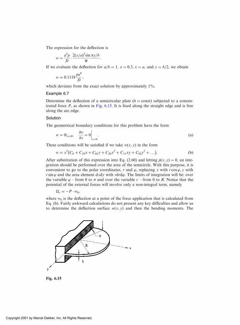
The expression for the deflection is

w ¼ a4p

D� 2 x=að Þ2sin�y=b

�:

If we evaluate the deflection for a=b ¼ 1; � ¼ 0:3; x ¼ a; and y ¼ b=2, we obtain

w ¼ 0:1118pa4

D;

which deviates from the exact solution by approximately 1%.

Example 6.7

Determine the deflection of a semicircular plate (h ¼ constÞ subjected to a concen-trated force P, as shown in Fig. 6.15. It is fixed along the straight edge and is freealong the arc edge.

Solution

The geometrical boundary conditions for this problem have the form

w ¼ 0jx¼0;@w

@x¼ 0

x¼0

: ðaÞ

These conditions will be satisfied if we take w x; yð Þ in the form

w ¼ x2 C0 þ C10xþ C01yþ C20x2 þ C11xyþ C02y

2 þ . . .� �

: ðbÞAfter substitution of this expression into Eq. (2.60) and letting p x; yð Þ ¼ 0, an inte-gration should be performed over the area of the semicircle. With this purpose, it isconvenient to go to the polar coordinates, r and ’, replacing x with r cos ’; y withr sin ’ and the area element dxdy with rdrd’. The limits of integration will be: overthe variable ’ – from 0 to � and over the variable r – from 0 to R. Notice that thepotential of the external forces will involve only a non-integral term, namely

�s ¼ �P � w0;

where w0 is the deflection at a point of the force application that is calculated fromEq. (b). Fairly awkward calculations do not present any key difficulties and allow usto determine the deflection surface w x; yð Þ and then the bending moments. The

Fig. 6.15


accuracy of calculation of the bending moments depends mainly on the number ofterms retained in the expansion (b).

If a plate has openings (Fig. 6.16), then the analysis can be performed similarlybut the area of openings must be eliminated from the area of integration in calculat-ing the total potential energy �.

Let us discuss the advantages of the Ritz method.

(a) The basic advantage lies in the fact that the coordinate functions fi x; yð Þmust satisfy the kinematic (or geometrical) boundary conditions only.Therefore, the area of an application of the method to the plate bendingproblems is wider than of the classical analytical methods discussed inChapter 3. Therefore, the Ritz method is very efficient for the analysis ofplates having free edges, for plates with openings.

(b) The method can be also applied successfully to rectangular plates ofvariable thickness, because there is no difference between the expressionsof � for plates of constant and variable thicknesses.

(c) Another advantage of the method is that the matrix of the linear algebraicequations, following on from Eq. (6.44), is always symmetrical, resultingin stable and powerful logarithms for their numerical solution.

The basic disadvantages of the method are

(a) The Ritz method can be applicable only to simple configurations of plates(rectangular, circular, etc.), because of the complexity of selecting thecoordinate functions for domains of complex geometry.

(b) The Ritz method approximation (6.44) results in the complete matrix oflinear algebraic equations that produces some difficulties in its numericalimplementation.

It should be noted that the Ritz method can serve as a basis for a such popular andpowerful methods as the finite element method, which is discussed in the next section.

6.7 THE FINITE ELEMENT METHOD (FEM)

6.7.1 Introduction

The finite element method (FEM) is based on the concept that one can replace anycontinuum by an assemblage of simply shaped elements with well-defined force–

Fig. 6.16


displacement and material relationships. While one may not be able to derive aclosed-form solution for the continuum, one can derive an approximate solutionfor the element assemblage that replaced it.

According to the FEM, a plate is discretized into a finite number of elements(usually, triangular or rectangular in shape), called finite elements and connected attheir nodes and along interelement boundaries. Unknown functions (deflections,slopes, internal forces, and moments) are assigned in the form of undeterminedparameters at those nodes. The equilibrium and compatibility conditions must besatisfied at each node and along the boundaries between finite elements. To deter-mine the above-mentioned unknown functions at nodal points, one of the variationalprinciples, introduced in Sec. 2.6, is applied. As a result, a system of algebraicequations is obtained. Its solution determines the state of stress and strain in agiven plate.

There are a number of finite element methods. In this section we discussonly the commonly used finite element displacement approach wherein the gov-erning set of algebraic equations is expressed in terms of unknown nodal displa-cements.

The FEM can be treated as some modification of the Ritz method. A differencebetween the classical Ritz approach and the FEM is in the technique of representa-tion of displacements. In the Ritz method, the displacements are assigned in theentire domain occupied by the plate. A governing system of algebraic equationsfor this approach will have a completed, not banded structure. Since in the FEMthe displacements are assigned element by element, the matrix of the system ofalgebraic equations is obtained as partially completed, and usually it has a bandedstructure. This is a profound advantage of the FEM compared with other numericalmethods introduced in the preceding sections of this chapter.

The FEM has gained considerable attention and prominence after the publica-tion of the classic paper by Turner et al. [26] that showed how one can use anassemblage of simple elements as a basis for computerized structural analysis.Courant [27], and later Argyris et al. [28] represent the initial attempts to providethe theoretical investigations of this method. Gallagher [29], Hughes [30],Zienkiewicz [31], and other investigators developed the general procedure of theFEM technique for plate and shell stress analysis.

For every finite plate (or shell) element there is a relationship between thegeneralized displacements at the nodal points and the corresponding forces andmoments at the nodes. This relationship may be presented in the form of a matrixcalled a stiffness matrix. In this section, we discuss the stiffness matrices for rectan-gular and triangular plate elements. Then, we present the general procedure of theFEM for plate bending analysis. The derivations, given below, are based on theclassical (Kirchhoff’s) plate bending theory introduced in Chapter 2.

6.7.2 The rectangular plate element

Consider a flat rectangular plate which is subdivided into rectangular finite elementswith dimensions c and d, as shown in Fig. 6.17. The properties belonging to such afinite element (abbreviated further as FE) is designated e. The geometrical positionof a rectangular FE is determined by the four nodal (corner) points i; j; k; and l, andthe straight line boundaries. At each node q ðq ¼ i; j; k; lÞ we consider the possible


nodal deflection wq and rotations of the normal to the plate middle surface (slopes)about the x and y axes, i.e., @w=@yð Þq and @w=@xð Þq, respectively.

The deflection wq and two rotations @w=@yð Þq and @w=@xð Þq are referred to as aset of nodal displacements.

We assume that the FE is subjected to surface-distributed load pðx; yÞ andexternal concentrated force Pq and moments mxq and myq, applied at each nodalpoint q of the FE, as shown in Fig. 6.17. Do not confuse the external nodal momentsmxq and myq with the stress couples Mx and My introduced in Chapter 2. The nodalforce and two moments are referred to as a set of nodal forces. The nodal displace-ments and nodal forces are assumed to be positive in the directions shown in Fig.6.17. Two coordinate systems are introduced in Fig. 6.17: the coordinate set X;Y;Zis referred to as a global set for the entire structure while the set x; y; z is called thelocal set for the FE of interest.

We develop below a stiffness matrix for a given FE. Let us approximate thedeflection field over the area of the rectangular FE shown in Fig. 6.17. The strainenergy of the plate in bending involves the second derivatives of the deflections (seeEq. (2.60)). Hence, the degree of a polynomial that approximates this deflection fieldcannot be less than two. On the other hand, in order to characterize the shape of theFE by its nodal displacements with reference to Fig. 6.17, it is necessary to have 12degrees of freedom (in the three degrees of freedom, w; @w=@y; @w=@x at each of thefour nodal points i; j; k; l of the above element). Consequently, we need to select apolynomial with 12 parameters. The polynomial selected is

wðx; yÞ ¼ 1 þ 2xþ 3yþ 4x2 þ 5y2 þ 6xyþ 7x2yþ 8xy2 þ 9x3 þ 10y3

þ 11x3yþ 12xy3:ð6:46Þ

Obviously, the above polynomial satisfies exactly the governing differential equation(2.24). However, this deflection function will not result in a fully compatible element.In the FEM formulation, it is required that the compatibility conditions (equality ofthe deflections and slopes) are satisfied at the nodal points. An accuracy of the FEMwill be increased if the selected deflection function involves the compatibility of thedeflections and slopes along a common boundary line of the adjacent FEs. It can beshown that the polynomial (6.46) provides the compatibility of deflections between

Fig. 6.17


elements and some slopes (normal) are continuous while other slopes (tangential)may not be continuous. In order to correct this problem, one needs to define fourdegrees of freedom at each node and, correspondingly, employ a deflection functionwith 16 terms [29,30]. Of course, the above polynomial leads to improved results, butthe analysis becomes more involved than described below. At the same time, numer-ical and theoretical investigations showed that the use of the polynomial (6.46)provides a convergence of the solution by the FEM. So, the polynomial (6.46) isfrequently used in engineering practice.

Let us represent the above polynomial approximating the deflection field overthe FE designated by e in the matrix form as follows:

we ¼ N½ � f g; ð6:47Þwhere

N½ � ¼ 1; x; y; x2; y2; xy; x2y; xy2; x3; y3; x3y; xy3� �

and f g ¼ 1; 2; . . . ; 12½ �T :ð6:48Þ

Here and further, the subscript e refers to a finite element designated by this letter.We introduce the braces . . .f g to indicate a matrix of one column, the brackets . . .½ � torepresent a matrix (both, a square and row matrices); and the superscript T torepresent the transpose of a matrix.

Introduce the element displacement matrix �f ge as follows:�f ge¼ �i; �j; �k; �l

� �T; ð6:49Þ

where

�i� � ¼ wi; @w=@yð Þi; @w=@xð Þi

� �T; �j

� � ¼ wj; @w=@yð Þj; @w=@xð Þj� �T

; etc.

If we express the coefficients mðm ¼ 1; 2; 3; . . . ; 12Þ via the nodal displacements wq,@w=@yð Þq; and @w=@xð Þq ðq ¼ i; j; k; lÞ in the local coordinate system x; y; z, then wecan write the following relationship:

�f ge¼ C½ � f g; ð6:50Þwhere C½ � is 12 12 matrix whose elements depend on the x and y coordinates of thenodal points of the finite element shown in Fig. 6.17.

From the foregoing, the solution for the unknown constants is

f g ¼ C½ ��1 �f ge: ð6:51ÞThe inverse matrix C½ ��1 is given below for the rectangular FE of Fig. 6.17 in theexplicit form in Table 6.3.

Upon substitution of f g from Eq. (6.51) into Eq. (6.47) one obtains

we ¼ L½ � �f ge; ð6:52Þwhere

L½ � ¼ N½ � C½ ��1 ð6:53Þ


is referred to as a shape function for the FE of interest.Define the strain–displacement relationship as follows:

"f ge ¼ z �f ge; ð6:54Þwhere "f ge ¼ "x; "y; �xy

� �Tis the strain matrix and �f ge ¼ �x; �y; 2�xy

� �Tis the curva-

ture matrix. Using Eqs (2.7), one can represent the latter matrix in terms of thedeflections as follows:

�f ge ¼ � @w

@x2;� @

2w

@y2;�2

@2w

@x@y

" #T

: ð6:55Þ

Substituting for we from Eq. (6.52) into Eq. (6.55), one can express the curva-ture matrix in terms of the polynomial (6.46) as follows:

�f ge ¼ B½ � �f ge; ð6:56Þwhere B½ � ¼ B½ �i; B½ �j; B½ �k; B½ �l

� �and

Table 6.3

1 0 0 0 0 0 0 0 0 0 0 0

0 1 0 0 0 0 0 0 0 0 0 0

0 0 1 0 0 0 0 0 0 0 0 0

� 3

a2� 2

a0 3

a2� 1

a0 0 0 0 0 0 0

� 3

b20 � 2

b0 0 0 0 0 0 3

b20 � 1

b

� 1

ab� 1

b� 1

a

1

ab0 1

a� 1

ab0 0 1

ab

1

b0

3

a2b

2

ab0 � 3

a2b

1

ab0 3

a2b� 1

ab0 � 3

a2b� 2

ab0

3

ab20 2

ab� 3

ab20 � 2

ab

3

ab20 � 1

ab� 3

ab20 1

ab

2

a31

a20 � 2

a31

a20 0 0 0 0 0 0

2

b30 1

b20 0 0 0 0 0 � 2

b30 1

b2

� 2

a3b� 1

a2b0 2

a3b� 1

a2b0 � 2

a3b

1

a2b0 2

a3b

1

a2b0

� 2

ab30 � 1

ab22

ab30 1

ab2� 2

ab30 1

ab22

ab30 � 1

ab2

½C ��1 ¼


B½ �i ¼ � @2 L½ �i@x2

;� @2 L½ �i@y2

;�2@2 L½ �i@x@y

" #T

;

B½ �j ¼ � @2 L½ �j@x2

;� @2 L½ �j@y2

;�2@2 L½ �j@x@y

" #T

; etc.

Now. let us introduce the stress resultants and stress couples relationships (see Eqs(2.13)) in the matrix form:

fMge ¼Mx

My

Mxy

8>><>>:

9>>=>>; ¼ D

1 � 0

� 1 0

0 0 ð1� �Þ=2

2664

3775

�x

�y

2�xy

8>><>>:

9>>=>>;; ð6:57aÞ

or symbolically as follows:

Mf ge¼ D½ � �f ge; ð6:57bÞwhere D½ � is the elasticity matrix. The stress–strain relationship, from Eqs (2.10), canbe written in the matrix form as follows:

�f ge¼ z D ½ � �f ge; ð6:58Þwhere the matrix D ½ � is given by

D ½ � ¼ 12

h3D½ �: ð6:59Þ

To continue the development, it is necessary to define the set of discrete nodal forcescorresponding to the prescribed nodal degrees, as shown in Fig. 6.17:

Rf ge¼ Ri;Rj;Rk;Rl

� �T; ð6:60aÞ

where

Rq

� � ¼ Pq;mxq;myq

� �T; q ¼ i; j; k; l: ð6:60bÞ

We now employ the principle of minimum potential energy, introduced in Sec.2.6.2, to derive the element stiffness matrix, k½ �e and the element nodal force matrixRf ge. Toward this end, we write the strain energy in the element as (see Eq. (2.61))

Ue ¼1

2

ð ðAe

�½ �Te Mf gedAe: ð6:61Þ

Substituting for �½ �Te from Eq. (6.56) and for Mf ge from Eq. (6.57b) into the above,we obtain

Ue ¼1

2

ð ðAe

�f gTe B½ �T D½ � B½ � �f gedAe ¼ �f gTe1

2

ð ðAe

B½ �T D½ � B½ �dAe

* +�f ge

or


U ¼ 1

2�f gTe k½ �e �f ge; ð6:62Þ

where Ae is the rectangular area c d of the FE of interest (see Fig. 6.17) and

k½ �e¼ð ðAe

B½ �T D½ � B½ �dAe ð6:63Þ

is the (symmetric) element stiffness matrix.The potential of external forces, �e, acting upon the element is

�e ¼ � �f gTe Rf ge�ð ðAe

pwdAe; ð6:64Þ

where the first term on the right-hand side is the potential of the discrete nodal forcesand the second term is the potential of the distributed load pðx; yÞ: If we substitutefor w from Eq. (6.52) into the above equation, we obtain

�e ¼ � �f gTe Rf ge�ð ðAe

p L½ � �f gedAe:

Since the potential of external forces is a scalar quantity, we may take the transposewithout changing its value

�e ¼ � �f gTe Rf geþð ð

Ae

p L½ �TdAe

* +: ð6:65Þ

It is convenient to write the above equation in the form

�e ¼ � �f gTe Q� �

e; ð6:66Þ

where

Q� �

e¼ Rf geþ

ððAe

p L½ �TdAe ð6:67Þ

is the element nodal force matrix.If �e ¼ Ue þ�e is the total potential energy associated with the element, we

have

�e ¼1

2�f gTe k½ �e �f ge� �f gTe Q

� �e: ð6:68Þ

If we apply the principle of minimum potential energy to Eq. (6.68), we obtain

@�e

@ �f ge¼ 0 or

@�e

@ �q� � ¼ 0; q ¼ i; j; k; l: ð6:69Þ


If we perform the operations prescribed by Eq. (6.69) and rearrange terms, we obtainthe following expression that relates nodal displacements and corresponding nodalforces:

k½ �e �f ge¼ Q� �

e: ð6:70Þ

This 12 12 system of linear algebraic equations characterizes the deformation ofthe rectangular plate element subjected to surface load and nodal forces.

When the elements are assembled, the total potential energy of the entire plateis characterized by the following (see Eq. (6.69):

� ¼XEe¼1

1

2�f gTe k½ �e �f ge� �f gTe Q

� �e

� �; ð6:71Þ

where E refers to the total number of finite elements comprising the given plate. Thisexpression contains 12E unknowns, which is excessive. Since the value of �f ge for twoadjacent elements that share a common nodal point must be the same, the displace-ment vector is reduced and can be represented as

�f g ¼ �1;�2; . . . ;�M½ �T ; ð6:72Þ

where M ¼ 3N and N is the total number of nodal points in the mesh. Thus, theexpression of �in terms of the reduced displacement vector takes the form

� ¼ 1

2�f gT K½ � �f g � �f gT Q

� �; ð6:73Þ

where K½ � is the M M global stiffness matrix of the entire plate and Q� �

is thegeneralized global force matrix.

If we apply the principle of minimum potential energy to Eq. (6.73):

@�

@ �i

� � ¼ 0; i ¼ 1; 2; . . . ;M;

we obtain the following governing equation of the FEM for the entire plate:

K½ � �f g ¼ Q� �

: ð6:74ÞThe global stiffness matrix K½ � and the generalized global force matrix Q

� �can be

assembled from 12 12 element stiffness, k½ �e, and the element force, Q� �

e, matrices.

This assembly process is readily computerized once the individual element propertiesare known.

The matrix K½ � in Eq. (6.74) is singular, because in deriving the above equationpossible rigid body motions of the entire plate have not been prevented. Applyingappropriate kinematic boundary conditions (imposed on the components of thedisplacement vector �f ge), we eliminate the rigid body motion. This results in deletingsome rows and columns of the matrix K½ �, corresponding to vanishing displacements,and the nonsingular stiffness matrix K ½ � is obtained. As a result, Eq. (6.74) can berepresented in the form

K ½ � � � � ¼ Q � �: ð6:75Þ


This set of algebraic equations is then solved for the unknown displacements. Theorder of this system will be equal to the total number of unknown displacements ofthe discretized plate. The matrix K ½ � can always be written in banded, symmetricform.

Once all displacements have been determined, we can utilize Eqs (6.56) and(6.57) to determine the bending and twisting moments. The general procedure forsolving plate (or shell) bending problems by FEM is summarized as follows:

1. For every FE, having a number e and certain nodes numbering anddisplacements, the nodal force Q

� �eand the element stiffness k½ �e matrices

are determined in the local coordinate system. A transition of the abovematrices from the local to global coordinate system is carried out.

2. The governing system of equations (6.74) is set up where the globalmatrices K½ � and Q

� �are simply generated in elements as follows: K½ � ¼P

e k½ �e and Q� � ¼P

e Q� �

e.

3. The prescribed kinematic boundary conditions are inserted in the globalstiffness matrix, as indicated earlier, and the set of equations (6.75) isformed for the entire plate.

4. The set of Eqs (6.75) is solved.5. Output data are calculated. The element deflections, internal forces, and

moments, as well as the stress components, are computed at all nodalpoints.

It should be noted that the procedure described can be efficient only by using power-ful digital computers. At present, new powerful computer programs, based on FEM,have been developed for solving various linear and nonlinear plate (and shell) bend-ing problems.

6.7.3 The triangular plate element

The triangular element can easily accommodate irregular boundaries and can begraduated in size to permit small elements in regions of stress concentration.Consequently, this element is widely used in the finite element technique. Let a flatplate be subdivided into a set of triangular finite elements referred to the localcoordinate system xyz, where one of the coordinate axes (for instance, the y axis,as shown in Fig. 6.18) is directed along a particular side of the FE.

Fig. 6.18


The matrix of the nodal displacements for this FE includes the nodal deflec-tions wq and slopes ð@w=@yÞq; ð@w=@xÞq where q ¼ i; j; k. Thus, the triangular FEposseses nine degrees of freedom.

The problem of selecting a suitable polynomial to describe the displacementfield over the triangular FE of interest is somewhat more difficult than for therectangular element. The simplest expression for the deflection function wðx; yÞthat satisfies all the general requirements, introduced in Sec. 6.7.2, is a cubic poly-nomial. However, a complete cubic polynomial contains 10 terms. Thus, one needsto fit this cubic polynomial to the nine-degree FE under consideration. Severaldifferent possibilities of the presentations of this polynomial were proposed to over-come this difficulty [29–31]. We consider only one of them. It was recommended totake the above cubic polynomial in the form

wðx; yÞ ¼ 1 þ 2xþ 3yþ 4x2 þ 5xyþ 6y2 þ 7x3 þ 8ðx2yþ y2xÞ þ 9y3:ð6:76Þ

The triangular plate bending element, based on the polynomial (6.47), has severallimitations. The continuity of slopes across element lines is not guaranteed. Further,its stiffness matrix may be singular for some orientations of sides of FE with respectto the local coordinate axes [30,31]. Thus, this type of element cannot always provideaccurate results when used for the bending analysis of plates. However, because of itssimplicity, this polynomial is used in engineering practice.

The nodal displacement matrix �f ge is of the form (see Fig. 6.18):

�f ge¼ �i; �j; �k� �

; ð6:77Þwhere

�i� � ¼ wi; ð@w=@yÞi; ð@w=@xÞi

� �; etc.

The matrix representing the deflection field is also given by Eq. (6. 47), but thematrices N½ � and f g now have the following form:

N½ � ¼ 1; x; y; x2; xy; y2; x3; x2yþ y2x; y3� �

; f g ¼ 1; 2; . . . ; 9½ �T : ð6:78ÞNodal displacements, upon introduction of Eq. (6.76) and the first derivatives of wwith respect to x and y into Eq. (6.77), are next found. They are given by Eq. (6.50)in which the matrix C½ � is the 9 9 matrix that depends upon the nodal coordinates.Inversion of the above matrix provides the values of the unknown coefficients 1;2; . . . ; 9 and is given by Eq. (6.51). The displacement function is expressed by Eq.(6.52).

The nodal force matrix Rf ge for the triangular FE represents a three-compo-nent vector of the form

Rf ge¼ Ri;Rj;Rk

� �T; ð6:79Þ

where Rf gqðq ¼ i; j; kÞ is given by Eq. (6.60b). The stiffness matrix, k½ �e, and theexternal nodal force matrix, Q

� �e, for the triangular plate element as well as the

governing equation of the FEM for the entire plate can be obtained by employingthe general procedure introduced in Sec. 6.7.2 for the rectangular plate element.

Let us discuss briefly some advantages of the FEM:


1. The solution by the FEM is obtained without the use of the governingdifferential equation.

2. The method has a clear and straightforward mechanical meaning and canbe formulated in terms of a technique familiar to practicing engineers.

3. The method can be successfully applied to arbitrary boundary and load-ing conditions that can be handled in the same manner as simpler pro-blems.

4. The complete automation of all procedures of the numerical process forsolving boundary value problems by the FEM is permitted.

5. The FEM can be applied to the stress analysis of combined structuresconsisting of various structural elements such as plates, shells, beams,arches, etc.

Among the disadvantages of the FEM, the following can be mentioned:

1. The FEM requires the use of powerful computers of considerable speedand storage capacity.

2. It is difficult to ascertain the accuracy of numerical results when largestructural systems are analyzed.

3. The method is poorly adapted to a solution of the so-called singularproblems (e.g., plates and shells with cracks, corner points, discontinuityinternal actions, etc.), and of problems for unbounded domains.

4. The method presents many difficulties associated with problems of C1

continuity and nonconforming elements in plate (and shell) bendinganalysis.

Since the application of fundamental concepts of the FEM has recently extendedto various linear and nonlinear boundary value problems, it is efficient to combinethe BEM and FEM for the stress analysis of combined plate and shell structures[12,13].

Example 6.8

A square simply supported plate with side a is acted upon by (a) a uniform lateralsurface load p0 and (b) a concentrated force P applied at the plate center. Determinethe deflections and the bending and twisting moments by the FEM. Use � ¼ 0:3

Solution

Calculations are carried out with the use of the rectangular FEs under a variednumber of the plate discretization. The deflection, w; the bending moments, Mx;My, at the plate center, and the twisting moment, Mxy at a corner point of the plateare assigned in the form:

– for a uniformly distributed load p0, as follows:

w ¼ � 10�4 p0a4

D; Mx ¼ My ¼ � 10�2p0; Mxy ¼ � � 10�2p0 and

– for a concentrated force P, as follows:

w ¼ 1 � 10�2 Pa2

D; Mx ¼ My ¼ 1 � 10�2P; Mxy ¼ �1 � 10�2P:


The results of calculations are given in Table 6.4 (taken from Ref. [32]), where thesenumerical results for varied numbers of the FEs are compared with those obtainedfrom Ref. [7]. As seen from Table 6.4, a discrepancy of the corresponding numericaldata is small even for a sufficiently large mesh of the plate discretization. A reductionof mesh dimensions (an increase in the number of the FEs) provides a monotonicconvergence of the obtained results to an exact solution.

This section provides only a brief survey of the FEM and its application toplate bending problems. The literature associated with this method and its applica-tion is voluminous. The interested reader is referred to Refs [28–31].

PROBLEMS

6.1 Derive the finite difference expressions for the effective shear forces Vx and Vy.

Referring to Fig. 6.5 check the correctness of the result for Vx.

6.2 Determine the finite difference expression corresponding to Eq. (2.25) at a pivotal point

k for nonuniform spaced rectangular mesh widths �x and �y in the x and y axes

directions, respectively.

6.3 Verify Eqs (6.15b).

6.4 Consider a clamped plate shown in Fig. P.6.1. The plate is acted upon by a uniformly

distributed load of intensity p0. Find the deflection w at the nodal points 1 through 5

Fig. P6.1

Table 6.4

Discretization

Number of

nodes

A uniform distributed load Concentrated force

� 1 1 �1

2 2 9 34.44 4.427 �3:492 1.378 23.18 �6:5054 4 25 39.45 4.694 �3:317 1.233 24.72 �6:1848 8 81 40.40 4.728 �3:296 1.183 25.18 �6:03216 16 289 40.58 4.781 �3:251 1.167 25.34 �6:085[7] — 40.62 4.789 �3:247 1.160 — —


and estimate the location of the point of maximum deflection and determine its mag-

nitude. Use the method of finite differences.

6.5 With reference to Example 6.1 of Sec. 6.2, determine the bending moments Mx and My

at nodal points of the mesh of the plate shown in Fig. 6.7 by utilizing the deflection

field found at the nodal point in the above example.

6.6 Consider a square clamped plate with side a. The plate is subjected to a uniformly

distributed load of intensity p0. Analyze a convergence of numerical FDM solutions

for the deflections w and the bending moments Mx and My at the plate center for

varied plate mesh widths �. Take � equal to a=2; a=4; and a=8.6.7 Derive Eq. (6.22) from the conditions of minimum of the error ei, given by Eq. (6.21).

6.8 Consider a simply supported square plate (0 � x; y � a) subjected to a uniformly

distributed load p0. Using the approximate representation of the deflection in the

form of (a) in Example 6.2, write out the straightforward BCM governing collocation

equations (6.19) for the collocation points on the plate boundary. Take the three points

for each side of the plate boundary.

6.9 With reference to Fig. 6.10 write the expression for the singular solution Gmðx; y; �; Þin the explicit form.

6.10 Write the boundary integral equations of the direct BEM formulation for a simply

supported rectangular plate ð0 � x � a; 0 � y � bÞ subjected to a lateral surface load

pðx; yÞ. Use the expressions (6.31) and (6.33).

6.11 Consider a square clamped plate with side a subjected to a uniformly distributed load

p0. Applying the indirect BEM approach, write the boundary integral equations in the

explicit form. Use the expressions (6.25) and (6.27).

6.12 With reference to Example 6.5 of Sec. 6.5, find the maximum value of the bending

moment Mx by retaining two and three terms in the expression (b) for the deflection

surface. Compare the obtained value of Mmax with the exact solution given in that

example. Use the Galerkin method.

6.13 With reference to Fig. 6.13, solve the problem of Example 6.5 by taking the deflection

surface of the plate in the following form

w ¼ A cos2�x

2acos2

�y

2b

that satisfies all the boundary conditions of the plate. Applying the Galerkin method,

find the maximum deflection and bending moments at the plate center and at a mid-

point of the clamped edge.

6.14 Consider a rectangular plate under a uniformly distributed surface load p0. The plate

has edges y ¼ �b simply supported and the edges x ¼ �a clamped. Using the Galerkin

method, determine the deflection and bending moments at the plate center and the

bending moment Mx at the midpoint of the clamped edge x ¼ a. Let a ¼ 1m; b ¼1:5m; h ¼ 12mm; p0 ¼ 25MPa; E ¼ 200GPa; and � ¼ 0:3. Assume a solution of the

following form:

w ¼ 1

2C 1� cos

2�x

a

� �cos

�y

2b:

Check that the above solution satisfies all the prescribed boundary conditions of the

plate.

6.15 A rectangular plate with sides a and b (0 � x � a, 0 � y � b) is subjected to a uniformly

distributed load of intensity p0. The plate edges y ¼ 0; b are simply supported, the edge

x ¼ 0 is clamped, while the edge x ¼ a is free. Determine the deflection w and stresses �xand �y at the plate center. Use the Ritz method and solution approximated by

w ¼ Cx

a

� �2sin�y

b:


Check that the above solution satisfies the kinematic boundary conditions on the plate

boundary. Take a ¼ b ¼ 1:5m; h ¼ 15mm; E ¼ 210GPa; p0 ¼ 30MPa; and � ¼ 0:3.6.16 Determine the required thickness h of a rectangular plate platform of sides 2a and 2b

(�a � x � a, �b � y � bÞ. The plate is supported by columns at its corners and the

plate edges are free. The plate is acted upon by a uniform lateral surface load p0. Let

a ¼ b ¼ 2:0m, p0 ¼ 32MPa; E ¼ 210GPa; �YP ¼ 250MPa, and � ¼ 0:3; the factor ofsafety is 2. Assuming that the columns can be considered as point supports at the plate

corners, take a solution in the form

w ¼ C cos�x

2aþ cos

�y

2b

� �:

Use the Ritz method and Tresca criterion.

6.17 A uniformly loaded rectangular plate of sides a and b (0 � x � a; 0 � y � bÞ has thefollowing boundary conditions: the edge x ¼ 0 is fixed, the edge y ¼ 0 is simply sup-

ported, and the edges y ¼ b and x ¼ a are free. Determine the deflections at the mid-

points of the free edges of the plate if a deflection surface of the plate is approximated

by the following expression:

w ¼ Cx

a

� �2sin�y

2b:

Check that the above expression satisfies the kinematic boundary conditions prescribed

on the plate edges. Use the Ritz method and take � ¼ 0:3:6.18 Derive the expression of the nodal force matrix Q

� �efor the squarer finite element of

side c, as shown in Fig. 6.17, subjected to a uniform distributed load p0 only.

6.19 Redo Problem 6.18 for the triangular finite element representing a right isosceles

triangle with legs a and b ðb ¼ 2aÞ. The origin of the Cartesian coordinate system is

taken at the centroid of the triangle.

6.20 A square plate of side a ð0 � x � a; 0 � y � bÞ with two opposite sides x ¼ 0 and x ¼ a

simply supported and the remaining edges clamped is subjected to a uniformly dis-

tributed load p0. If the plate is discretized into four identical rectangular finite elements,

compute the maximum deflection. Take a ¼ 4m; h ¼ 30mm; p0 ¼ 50MPa; E ¼ 210

GPa; and � ¼ 0:3. Analyze only one quarter-plate by the FEM.

REFERENCES

1. Alexandrov, A.V., and Potapov, V.D. The Fundamentals of the Theory of Elasticity and

Plasticity, Izd-vo Vyshaia Shkola, Moscow, 1990 (in Russian).

2. Salvadori, M.G. and Baron, M.L., Numerical Methods in Engineering, Prentice-Hall,

Englewood Cliffs, New Jersey, 1967.

3. Wang, P.Ch., Numerical and Matrix Methods in Structural Mechanics, John Wiley and


4. Finlayson, B.A., The Method of Weighted Residuals and Variational Principles, Academic

Press, New York, 1972.

5. Hutchinson, J.R., Analysis of plates and shells by boundary collocations. In: Boundary

Element Analysis of Plates and Shells (ed. D.E. Beskos), Springer-Verlag, Berlin, pp. 341–

368 (1991).

6. Mikhlin, S.G., Variational Methods in Mathematical Physics, Macmillan, New York,

1964.

7. Timoshenko, S.P, and Woinowsky-Krieger. S., Theory of Plates and Shells, McGraw-

Hill, New York, 1959.

8. Kolodziej, J.A., Review of application of boundary collocation method in mechanics of

continuum media, Solid Mechanics Archives, 12, pp. 187–231 (1987).


9. Johnson, D., Plate bending by a boundary point method, Computers & Structures, vol.

26, No. 4, pp. 673–680 (1987).

10. Tottenham, H., The boundary element method for plates and shells. In: Developments in

Boundary Element Methods – 1 (eds PK Banerjee and R Butterfield), Applied Science

Publishers, London, pp. 173–207 (1979).

11. Hartmann, F., Static analysis of plates. In: Boundary Element Analysis of Plates and

Shells (ed. D.E. Beskos), Springer-Verlag, Berlin, pp. 1–35 (1991).

12. Brebbia, C.A., Telles, J.C.F. and Wrobel, L.C., Boundary Element Techniques. Theory

and Application in Engineering, Springer-Verlag, Berlin, 1984.

13. Banerjee, P.K. and Butterfield, R., Boundary Element Methods in Engineering Science,


14. Ventsel, E.S., An indirect boundary element method for plate bending analysis, Int J

Numer Meth Eng, 9, pp. 1597–1611 (1997).

15. Krishnasamy, G., Schmerr, L.W., Rudolphi, T.J., and Rizzo, F.L., Hypersingular

boundary integral equations: some applications in acoustic and elastic wave scattering,

J Appl Mech, 57, pp. 404–414 (1990).

16. Rudolphi, T.J., Krishnasamy, G., Schmerr, L.W., and Rizzo, F.J., On the use of strongly

singular integral equations for crack problems. In: Boundary Elements X (ed. C.A.

Brebbia), Springer-Verlag, Berlin, pp. 249–263 (1988).

17. Hadamard, J.S., Lectures on Cauch’s Problem in Linear Partial Differential Equations,

Yale University Press, London, 1923.

18. Kutt, R., Quadrature formulas for finite-part integrals, Report WISK, The National

Research Institute for Mathematical Science, 178, Pretoria, 1975.

19. Ioakimidis, N.I. and Pitta, M.S. Remarks on the Gaussian quadrature rule for finite-part

integrals with a second-order singularity, Comput Meth Appl Mech Eng, 69, pp. 325–343

(1988).

20. Fung, Y.C., Foundations of Solid Mechanics, Prentice-Hall, Englewood Cliffs, 1965.

21. Stroud, A.H. and Secrest, D., Gaussian Quadrature Formulas, Prentice-Hall, Englewood

Cliffs, New Jersey, 1966.

22. Galerkin, B.G., Series-solutions of some cases of equilibrium of elastic beams and plates,

Vestn Inshenernov, vol. 1, pp. 897–903 (1915) (in Russian).

23. Ritz, W., Theorie der transversalschwingungen einer quadratischen plattemit freien ran-

dern, Ann Phys, vol. 28, pp. 737–786 (1909).

24. Washizu, K., Variational Methods in Elasticity and Plasticity, Pergamon Press, Oxford,

1968.

25. Szilard, R., Theory and Analysis of Plates. Classical and Numerical Methods, Prentice-

Hall, Englewood Cliffs, New Jersey, 1974.

26. Turner, M.J., Clough, R.W., Martin, H.C., and Topp, L.J. Stiffness and deflection

analysis of complex stuctures, J Aeronaut Sci, vol. 23, no.9, pp. 805–823 (1956).

27. Courant, R. Variational methods for the solution of problems of equilibrium and vibra-

tion, Bulletin of the American Mathematical Society, vol. 49, pp. 1–23 (1943).

28. Argyris, J.N., Kelsey, S., and Kamel, H., Matrix methods of structural analysis. In:

Matrix Methods of Structural analysis (ed. Fraeijs de Veubeke), Pergamon Press,

Oxford, 1964.

29. Gallagher, R.H., Finite Element Analysis, Prentice-Hill, Englewood Cliffs, New Jersey,

1975.

30. Hughes, T.J.R., The Finite Element Method, Prentice-Hill, Englewood Cliffs, New Jersey,

1987.

31. Zienkiewicz, O., The Finite Element Method, McGraw-Hill, London, 1977.

32. Grigorenko, Ia.M. and Mukoed, A.P. Solutions of the Shell Theory Problems by

Computers. Gos. Izd-vo ‘‘Vysha Shkola’’, Kiev, 1974 (in Russian).


7

Advanced Topics

7.1 THERMAL STRESSES IN PLATES

7.1.1 Basic concepts

It was assumed in the foregoing discussions that the temperature of an elastic plateremains constant and has the same value at all points of the plate; hence, tempera-ture effects were not taken into consideration. If the temperature of the plate is raisedor lowered it expands or contracts, respectively. Within a certain temperaturechange, such expansion or contraction, for most structural materials, is directlyproportional to the change in temperature. When a free plate made of homogeneousisotropic material is heated uniformly, there appear normal strains but no thermalstresses. The thermal stresses will occur in the following cases: first, if the plateexperiences a nonuniform temperature field; secondly, if the displacements are pre-vented from occurring freely because of the restrictions placed on the boundary evenwith a uniform temperature; and thirdly, if the material displays anisotropy evenwith uniform heating – for example, if a heated plate consists of several layers ofdifferent materials (e.g., bimetallic plates).

A study of the deformations of an elastic solid in the presence of a temperaturefield is called thermoelasticity. Let us assume that the temperature of an infinitesimalplate element is increased from T0 to T . The initial temperature, T0, is defined as areference state of uniform temperature distribution which does not produce stress orstrain in the plate. The thermal field, T ¼ Tðx; y; zÞ, is assumed to be known from asolution of the heat conduction problem. The thermal strains are expressed for atwo-dimensional body as follows [1,2]:

"zxT ¼ T; "zyT ¼ T; �zxyT ¼ 0; ð7:1Þ


where is the coefficient of thermal expansion. Over a moderate temperaturechange, remains reasonably constant and represents an experimentally determinedmaterial property. In Eqs (7.1), "zxT ; "

zyT ; and �

zxyT are the normal and shear thermal

strain components, respectively, at a distance z from the plate middle surface. FromEqs (7.1) it follows that the temperature field has no effect on the shear straincomponents.

Also, from Eqs (7.1), taking the temperature effects into account, we mustmodify the general plate bending equations. For the sake of simplicity, we assumethat the material properties of the plate are not affected by temperature changes: i.e.,the modulus of elasticity, E, and Poisson’s ratio, �, are assumed to be constant. Ingeneral, a temperature increase or decrease produces changes in a plate’s curvatureand in the dimensions of the plate’s middle surface.

7.1.2 Thermoelastic plate equations

We begin by modifying Hooke’s law relations for Kirchhoff’s plate theory. Theserelations are obtained by adding to strains resulting from external forces, the strainsdue to the thermal effects. The latter are given by Eqs (7.1). We have the following:

"zx ¼ 1

E�zx � ��zy� �þ T; "zy ¼

1

E�zy � ��zx� �þ T; �zxy ¼ 1

G�zxy: ð7:2Þ

Solving these equations for the stress components, yields

�zx ¼ E

1� �2 "zx þ �"zy � 1þ �ð ÞT� �

;

�zy ¼E

1� �2 "zy þ �"zx � 1þ �ð ÞT� �

; �zxy ¼ G�zxy:

ð7:3Þ

The assumptions of Kirchhoff’s plate bending theory, introduced in Sec. 1.3,can be applied to the thermoelastic analysis of plates, with the exception of assump-tion 6. As mentioned earlier, a change in the temperature of a plate may result in achange in the dimensions of the middle surface, i.e., points of the middle surface candisplace not only in the z but also in the x and y directions. Let u and v, as before, bethe displacement components along the x and y axes on the middle surface, respec-tively. Thus, the total strain components for thermoelastic plates can be obtained bysuperimposing the strains due to stretching or contracting of the middle surface (Eqs1.5a) and the strains associated with bending of the middle surface (Eqs 2.6), derivedin Sec. 2.2. As result, the following expressions for the strains in terms of displace-ment components in the middle surface can be written:

"zx ¼ @u

@x� z

@2w

@x2; "zy ¼

@v

@y� z

@2w

@y2; �zxy ¼

@u

@yþ @v

@x

� �� 2z

@2w

@x@y: ð7:4Þ

In the foregoing, the first terms on the right-hand sides of the above equationsrepresent the strain components in the middle surface due to its stretching, andterms with w represent the strain components due to bending.

Owing to the deformation of the plate middle surface, the stresses distributedover the thickness of the plate result in the in-plane forces, Nx;Ny;Nxy and moments,Mx;My;Mxy, per unit length, as shown in Figs 3.19 and 2.4. The in-plane forcecomponents are represented by


Nx

Ny

Nxy

8><>:

9>=>; ¼

ðh=2�h=2

�zx

�zy

�zxy

8><>:

9>=>;dz; ð7:5Þ

and the moments are given by Eqs (2.11). Introducing Eqs (7.3) and (7.4) into Eqs(2.11) and (7.5), the stress resultants are obtained in the form

Nx ¼ Eh

1� �2@u

@xþ � @v

@y

� �� NT

1� � ; Ny ¼Eh

1� �2@v

@yþ � @u

@x

� �� NT

1� � ;

Nxy ¼ Nyx ¼ E

2 1þ �ð Þ@u

@yþ @v

@x

� �; ð7:6Þ

Mx ¼ �D@2w

@x2þ � @

2w

@y2

!� MT

1� � ; My ¼ �D@2w

@y2þ � @

2w

@x2

!� MT

1� � ;

Mxy ¼ Myx ¼ �D 1� �ð Þ @2w

@x@y: ð7:7Þ

Here the quantities

NT ¼ E

ðh=2�h=2

Tðx; y; zÞdz and MT ¼ E

ðh=2�h=2

Tðx; y; zÞzdz ð7:8Þ

are termed the thermal stress resultants, i.e., the thermal equivalent normal force andbending moment, respectively.

The components of the stress tensor may now be derived in terms of the stressresultants by substitution of Eqs (7.4) into (7.3) and elimination of the displacementderivatives through the use of Eqs (7.7) and (7.8), as follows:

�zx ¼ 1

hNx þ

NT

1� ��

þ 12z

h3Mx þ

MT

1� ��

� ET

1� � ;

�zy ¼1

hNy þ

NT

1� ��

þ 12z

h3My þ

MT

1� ��

� ET

1� � ;

�zxy ¼1

hNxy þ

12z

h3Mxy:

ð7:9Þ

Substitution of Eqs (7.7) and the second equation of (7.8) into the plate equilibriumequation (2.25) gives the following:

r2r2w ¼ 1

Dp� 1

1� �r2MT

� �: ð7:10Þ

This is the governing differential equation for the bending of thin elastic Kirchhoff’splates due to the lateral pressure and thermal effects. We observe from Eq. (7.10) thatit is possible to superimpose the temperature-induced deflections with those inducedonly by the transverse load.

From the above, it follows that in addition to the thermal bending stressesresulting from the temperature variation across the thickness of the plate, membranestresses are also produced, if the plate is heated uniformly throughout its thickness


and prescribed boundary conditions prevent free expansion or contraction of themiddle surface of the plate. The equations governing the in-plane (membrane) resul-tants are given by Eqs (3.90). These equations are identically satisfied by introducingthe stress function � x; yð Þ, related to the force resultants, as follows:

Nx ¼ @2�

@y2; Ny ¼

@2�

@x2; Nxy ¼ � @2�

@x@y: ð7:11Þ

For a plate of a constant thickness and negligible weight, the equation of compat-ibility can be obtained by inserting Eqs (7.2) and (7.9) into Eq. (1.13) and makingMx ¼ My ¼ Mxy ¼ MT ¼ 0. We obtain

@2

@y2Nx � �Ny þNT

� �þ @2

@x2Ny � �Nx þNT

� � ¼ 2 1þ �ð Þ @2Nxy

@x@y: ð7:12Þ

Substitution of relations (7.11) into the above yields

r2r2� ¼ �r2NT ð7:13Þwhere NT is given by Eq. (7.8). Equation (7.13) is the governing differential equationfor the two-dimensional thermoelastic problem of plane stress for thin plates. Since wehave assumed the validity of Kirchhoff’s small-deflection theory, the governingequations of thermal bending, Equation (7.10), and thermal stretching or contract-ing, Eq. (7.13), are independent of each other. Equation (7.10) may be solved by themethods discussed in Chapters 3 and 6, while the methods discussed in the theory ofelasticity for plane stress problems are available for solving Eq. (7.13) [1,2]. Wediscuss below some peculiarities associated with the solution of the thermoelasticplate bending problems. We modify the boundary conditions for thermoelasticplates. Let us consider the boundary conditions for rectangular plates again, asfollows:

(a) Simply supported edges x ¼ 0 and x ¼ a

w ¼ 0; Mx ¼ 0

From Eq. (7.7), the condition for the bending moment can be rewritten as

Mx ¼ �D@2w

@x2þ � @

2w

@y2

!� MT

1� � ¼ 0

x¼0;x¼a

: ð7:14Þ

Taking into account that for edges x ¼ 0; a the curvature @2w=@y2 ¼ 0, the aboveconditions can be simplified to the form

w ¼ 0jx¼0;a and D@2w

@x2þ MT

1� � ¼ 0

x¼0;a

: ð7:15Þ

(b) Clamped edges x ¼ 0 and x ¼ a

w ¼ 0jx¼0;a and@w

@x¼ 0jx¼0;x¼a: ð7:16Þ

(c) Free edges x ¼ 0 and x ¼ aThe boundary conditions in this case are (see Chapter 2)


Mx ¼ 0 and Vx ¼ 0: ð7:17ÞThe first condition (for the bending moment) is given by Eq. (7.14). The effectiveshear force is found to be (see Sec. 2.4) Vx ¼ Qx þ @Mxy=@y. Using Eqs (2.22a) and(7.7), we can express Vx in the above equation in terms of the deflections w. Finally,the second equation (7.17) will take the following form:

@3w

@x3þ 2� �ð Þ @

3w

@x@y2þ 1

D 1� �ð Þ@MT

@x¼ 0

x¼0;a

: ð7:18Þ

Similarly, the boundary conditions can be represented for edges y ¼ 0 and y ¼ b. Weobserve from Eqs (7.15)–(7.18) that the boundary conditions for simply supportedand free edges of thermoelasic plates are nonhomogeneous.

Small-deflection thermal bending problems of plates can be readily solved bythe so-called isothermal analogy [1,2]. Let us introduce a fictitious lateral load asfollows:

pT ¼ � 1

1� �r2MT: ð7:19Þ

Then, the thermoelastic plate bending problems can be reduced to the correspondingisothermal problems for a plate subjected to two types of surface lateral loads: anactual surface lateral load of intensity p x; yð Þ and a fictitious load of intensitypT x; yð Þ. It should be noted that the isothermal analogy might also require a mod-ification of the boundary conditions. This means that in the mathematical formula-tion of the static boundary conditions, the thermal equivalent moment MT must beincluded in accordance with Eqs (7.15) and (7.18) for bending problems.

Example 7.1

Consider a simply supported rectangular plate (see Fig. 3.5) that is subjected to anonuniform temperature distribution. Determine the deflection surface of the plate.

Solution

The boundary conditions on the edges x ¼ 0; a of the plate are given by Eqs (7.15).Similar expressions can be written for edges y ¼ 0; b by replacing the variable x withy in the second equation (7.15). In general,MT is a function of x;y; and T . From Eqs(7.15) and (7.7), the following expression applies to the boundary

Dr2w ¼ �MT

1

1� �x¼0;ay¼0;b

: ðaÞ

Equation (7.10), setting p ¼ 0, can be represented in an equivalent form, as follows:

Dr2wþMT

1

1� � ¼ f x; yð Þ;

r2f ¼ 0:

ðbÞ

Equation (a) and the first equation (b) results in

f ¼ 0; ðcÞwhich is an appropriate solution of the second Eq. (b).


Thus, the given thermoelastic problem can be reduced to the solution of thefollowing equation:

Dr2w ¼ �MT

1

1� � ; ð7:20Þ

with the following boundary condition on all edges:

w ¼ 0jx¼0;ay¼0;b

: ðdÞ

We apply Navier’s method for solving the boundary value problem described by Eq.(7.20) and Eq. (d). The solution of Eq. (7.20) is sought in the following form of adouble Fourier series:

w x; yð Þ ¼X1m¼1

X1n¼1

wmn sinm�x

asin

n�y

b: ðeÞ

Each term of this series satisfies the boundary conditions (d). The right-hand side ofEq. (7.20) is expressed in a similar form, i.e.,

MT x; yð Þ ¼X1m¼1

X1n¼1

� Tð Þmn sin

m�x

asin

n�y

b; ðfÞ

where the Fourier coefficients � Tð Þmn are the following:

� Tð Þmn ¼ 4

ab

ða0

ðb0

MT x; yð Þ sinm�xa

sinn�y

bdxdy: ðgÞ

Substituting these two series into Eq. (7.20), and equating coefficients of like terms,we obtain

wmn ¼� Tð Þmn

1� �ð Þ�2D1

m=að Þ2þ n=bð Þ2� �

: ðhÞ

If, for example, the temperature varies through thickness only, i.e., T ¼ T zð Þ, then

� Tð Þmn ¼ 4MT

�2mn1� �1ð Þm½ � 1� �1ð Þn½ �; ðiÞ

and the deflection surface becomes

w x; yð Þ ¼ 16MT

1� �ð Þ�2DX1

m¼1;3;...

X1n¼1;3;...

sinm�xa sinn�yb

mn m=að Þ2þ n=bð Þ2� �: ð7:21Þ

The bending moments and stresses in the plate may be calculated from Eqs (7.7) and(7.9).

The thermoelastic problem above has been considered in Cartesian coordinatesfor rectangular plates. However, all previously introduced thermoelastic analysis canbe applied to circular plates in polar coordinates. This section covers only somegeneral ideas and fundamental concepts of the thermoelastic stress analysis of platesin the context of Kirchhoff’s bending theory. The interested reader is referred to Refs[1,2].


7.2 ORTHOTROPIC AND STIFFENED PLATES

7.2.1 General

Up to this point, all our previous discussions of plates have assumed the platematerial to be isotropic according to assumption 1 in Sec. 1.3. We recall that theassumption of isotropy implies that material properties at a point are the same inall directions. This means, that if an isotropic material is subjected to an axialstress in a principal direction, the major deformation occurs in the direction ofthe applied load. Lateral deformations of smaller magnitude occur in the otherprincipal directions. Also, shear stress causes only shear deformation. So, normalstrains and stresses are not coupled to shear strains and stresses. The deforma-tions are dependent on the two independent elastic constants – for instance, Eand �. Many construction materials such as steel, aluminum, etc., fall into thiscategory.

However, certain materials display direction-dependent properties; conse-quently, these materials are referred to as anisotropic. In anisotropic materialsstressed in one of the principal directions, the lateral deformations in the otherprincipal directions could be smaller or larger than the deformation in the directionof the applied stress depending on the material properties. For a general anisotropicmaterial, the matrix of material constants, because of symmetry, contains 21 inde-pendent material constants. This means that all the strains are coupled to all thestresses. Some materials such as wood, plywood, delta wood, and fiber-reinforcedplastics, etc., fall into this category. These materials possess natural anisotropy.Besides plates made of anisotropic materials, a number of manufactured platesmade of isotropic materials also may fall into the category of anisotropic plates:examples include corrugated and stiffened plates, etc. Such a type of anisotropy isreferred to as structural anisotropy and that of an anisotropic plate can approxi-mately replace their structural behavior. Such an approximation is possible if, forexample, stiffeners are arranged sufficiently close to each other so that the givenstiffened plate can be replaced by an orthotropic homogeneous plate with ‘‘distrib-uted’’ stiffened rigidities along the plate. Experimental data indicate a good agree-ment with this idealization provided that the flexural rigidities are uniformlydistributed in the x and y directions.

If an anisotropic material has three mutually perpendicular planes of symmetrywith respect to its elastic properties, it is called orthotropic (i.e., orthogonally aniso-tropic). Practical applications of orthotropic plates in civil, marine, and aerospaceengineering are numerous and include decks of contemporary steel bridges, compo-site-beam gridworks, plates and reinforced with closely spaced flexible ribs, andreinforced concrete plates.

The fundamental equations for the small-deflection theory of bending of thinorthotropic plates are presented in this section.

7.2.2 Basic relationships

Let us consider bending of plates of constant thickness and made of orthotropicmaterial. Assume that the principal directions of orthotropy coincide with the x andy coordinate axes which, in turn, lie in the middle plane of the plate. The stress–strainrelations (2.9) used for isotropic plates are not valid for orthotropic plates. Thus, we


must obtain a new set of stress–strain relations that reflects the orthotropic proper-ties of a material of the plate. Such a set of relations is shown below [3]:

"x ¼ �xEx

� �y�yEy

; "y ¼�yEy

� �x�xEx

; �xy ¼�xyG; ð7:22Þ

where Ex;Ey; �x; �y; and G are assumed to be elastic constants of an orthotropicmaterial, i.e., Ex;Ey; and �x; �y are the moduli of elasticity and Poisson’s ratios in thex and y directions, respectively. They are independent of one another. G is the shearmodulus, which is the same for both isotropic and orthotropic materials. It can beexpressed in terms of Ex and Ey as follows:

G �ffiffiffiffiffiffiffiffiffiffiffiExEy

p2 1þ ffiffiffiffiffiffiffiffiffi

�x�yp� � : ð7:23Þ

The following relationship exists between independent elastic constants introducedabove:

�xEx

¼ �yEy

: ð7:24Þ

This equality directly results from Betti’s reciprocal theorem. Solving Eqs (7.22) forthe stress components and taking into account (7.24), we obtain

�x ¼ Ex

1� �x�y"x þ �y"y� �

; �y ¼Ey

1� �x�y"y þ �x"x� �

;

�xy ¼ G�xy:

ð7:25Þ

The derivation of the governing differential equation of bending of an orthotropicplate is based on the general hypotheses introduced in Sec. 1.3. The strain-deflectionrelations (2.6) hold for orthotropic plates also. So, substituting the relations (2.6)into Eqs (7.25) gives the following:

�x ¼ � Ex

1� �x�y@2w

@x2þ �y

@2w

@y2

!z; �y ¼ � Ey

1� �x�y@2w

@y2þ �x

@2w

@x2

!z;

�xy ¼ �2Gz@2w

@x@y:

ð7:26ÞSubstituting the above into Eqs (2.11) and integrating over the plate thickness, yieldsthe following bending and twisting moments deflection relations for orthotropicplates:

Mx ¼ � Dx

@2w

@x2þDxy

@2w

@y2

" #; My ¼ � Dy

@2w

@y2þDyx

@2w

@x2

" #;

Mxy ¼ �2Ds

@2w

@x@y;

ð7:27Þ


where Dx;Dy;Dxy;Dyx; and Ds are the flexural and torsional rigidities of an ortho-tropic plate, respectively, and are given as

Dx ¼Ex

1� �x�yh3

12; Dy ¼

Ey

1� �x�yh3

12; Dxy ¼

Ex�y1� �x�y

h3

12;

Dyx ¼ Ey�x1� �x�y

h3

12; Ds ¼

Gh3

12:

ð7:28Þ

In view of the expressions (7.24), one can conclude that Dxy ¼ Dyx. The shear forceexpressions (2.22) become

Qx ¼ � @

@xDx

@2w

@x2þH

@2w

@y2

!; Qy ¼ � @

@yH@2w

@x2þDy

@2w

@y2

!; ð7:29Þ

where

H ¼ Dxy þ 2Ds: ð7:30ÞThe governing differential equation (2.24) for orthotropic plates becomes

Dx

@4w

@x4þ 2H

@4w

@x2@y2þDy

@4w

@y4¼ p x; yð Þ: ð7:31Þ

We give below the expression for the potential energy of bending for orthotropicplates, which follows from Eqs (2.52) and (7.26):

U ¼ 1

2

ð ðA

Dx

@2w

@x2

!2

þ 2Dxy

@2w

@x2@2w

@y2þDy

@2w

@y2

!2

þ 4Ds

@2w

@x@y

!224

35dA:

ð7:32ÞEquations (7.31) and (7.32) are valid for both naturally and structurally orthotropicplates provided structural elements causing orthotropy are arranged sufficiently closetogether, so as to ignore a jump change of elastic properties in a plate.

7.2.3 Determination of rigidities for structurally orthotropic plates

The solution of Eq. (7.31) requires specific values of the flexural and torsionalrigidities of naturally and structurally orthotropic plates and plate structures. Asmentioned earlier, the orthotropic moduli and Poisson’s ratios Ex;Ey; �x; �y; and Gcan be obtained experimentally for naturally orthotropic materials – for example,from tension or shear tests, as in the case of isotropic materials. The plate rigiditiesmay be then calculated from Eqs (7.28) and (7.30).

The flexural and torsional rigidities of structurally ortotropic plates are deter-mined using the following approximate procedure. A structurally orthotropic plate isreduced to a naturally orthotropic plate with elastic properties equal to the averageproperties of components of the original plates [4]. Such a plate is termed an equiva-lent or transformed orthotropic plate. Subsequently, the rigidities (7.28) and (7.30) ofsuch an equivalent orthotropic plate are approximated, depending on the type ofstructural orthotropy. The suitable formulas for the plate rigidities for some com-


monly encountered cases of structurally orthotropic plates, shown in Fig. 7.1 [5], arelisted below [4–6,7]:

(a) Plate reinforced by equidistant stiffeners in one direction (the x-direction) (Fig.7.1a)

Dx ¼ Eh3

12 1� �2� �þ E 0b H31 � h3

� �12t

; Dy ¼ H ¼ Eh3

12 1� �2� � : ðaÞ

(b) Plate reinforced by a set of equidistant ribs in one direction (Fig. 7.1b)

Dx ¼ EI

t;Dy ¼

Eh3

12 1� bt þ bh3

tH31

� � ; Dxy ¼ 0;Ds �Ch3

12þ C

2t; ðbÞ

where I is the moment of inertia of a T-shaped section corresponding to one spacingof the rib location about its center axis (shown as shaded in Fig. 7.1c); C is thetorsional rigidity of one rib about its centroidal axis. In Eqs (a), (b), and (c), E and

Fig. 7.1


E 0 are the elastic moduli of the plating and stiffeners or ribs, respectively; � isPoisson’s ratio of plating.(c) Plate reinforced by equidistant stiffeners in two directions (Fig.7.1c)

Dx ¼ Eh3

12 1� �2� �þ E 0b1 H31 � h3

� �12t1

;

Dy ¼Eh3

12 1� �2� �þ E 0b2 H32 � h3

� �12t2

;H � Eh3

12 1� �2� � ;ðcÞ

(d) Corrugated plate with a sinusoidal corrugation z ¼ H1 sin�yl(Fig. 7.1d)

Dx ¼ EI ; Dy ¼l

s

Eh3

12ð1� �2Þ ; Dxy ¼ 0;H ¼ s

l

Eh3

12ð1þ �Þ ðdÞ

where

I ¼ 0:5H2h 1� 0:81

2:5ðH=2lÞ2� �

is the moment of inertia of one wave of the corrugation, and s ¼ l 1þ �2H21=4l

2� �

isan unfolded length of the one wave.(e) Open gridworks ( Fig. 7.1e)

Dx ¼b1h

3

12t1; Dy ¼

b2h3

12t2; Dxy ffi 0; H ¼ 2Ds ¼

1

2

C1

t1þ C2

t2

� �; ðeÞ

where C1 and C2 are the torsional rigidities of the ribs that are parallel to the x and yaxes.(f) Two-way reinforced concrete slab (Fig. 7.1f)

Dx ¼ Ec

1� �2c� � h3

12� Ixs þ

Es

Ec

Ixs

" #; Dy ¼

Ec

1� �2c� � h3

12� Iys þ

Es

Ec

Iys

" #;

Ds ¼1� �c

2

ffiffiffiffiffiffiffiffiffiffiffiffiDxDy

p;H ¼ ffiffiffiffiffiffiffiffiffiffiffiffi

DxDy

p;Dxy ¼ �c


p;

ðfÞ

where Ec; �c are the modulus of elasticity and Poisson’s ratio for concrete, respec-tively; Es is the modulus of elasticity for steel; and Ixs; Iys are the moments of inertiaof steel bars about the x and y axes, respectively.

Notice when Ex ¼ Ey ¼ E and �x ¼ �y ¼ �, Eqs (7.23), (7.28), and (7.30)become

G ¼ E

2 1þ �ð Þ ; Dx ¼ Dy ¼ D ¼ Eh3

12 1� �2� � ; Dxy ¼ �D ¼ �Eh3

12 1� �2� � ;

Ds ¼Eh3

24 1þ �ð Þ ; H ¼ Dxy þ 2Ds ¼ D ¼ Eh3

12 1� �2� � :and Eq. (7.31) reduces to that of an isotropic plate, Eq. (2.24), for this particularcase.


7.2.4 Rectangular naturally and structurally orthotropic plates

The general procedure for the determination of the deflection, bending moments,and stress components in orthotropic plates is identical with that employed forisotropic plates. The analytical and numerical methods described earlier inChapters 3 and 6 can be used for determining the deflections, stress resultants,and stress couples.

Example 7.2

A rectangular orthotropic plate with principal directions parallel to the sides issimply supported on all four edges (see Fig. 3.5) and bends under a normal loaddistributed according to some arbitrary law, i.e., p ¼ p x; yð Þ. Determine the deflec-tion surface for the plate.

Solution

The simply supported boundary conditions are given by Eqs (3.14). We now applyNavier’s method discussed in Chapter 3 to treat this plate. Introduction of Eqs (3.15)into (7.31) yields the following:

X1m¼1

X1n¼1

wmn

m4�4

a4Dx þ 2

m2n2�4

a2b2H þ n4�4

b4Dy

!� pmn

( )sin

m�x

asin

n�y

b¼ 0:

ðaÞSince the above must be valid for all x and y, the terms in the braces must be zero.We obtain

wmn ¼pmn

Dx m4�4=a4� �þ 2H m2n2�4=a2b2

� �þDy n4�4=b4� � : ðbÞ

Substituting Eqs (b) and (3.17) into Eq. (3.15a), we obtain the expression for thefollowing deflections:

w ¼ 4

ab

X1m¼1

X1n¼1

ða0

ðb0

p x; yð Þ sinm�xa sinn�yb

dxdy

Dx m4�4=a4� �þ 2H m2n2�4=a2b2

� �þDy n4�4=b4� �: ðcÞ

In the particular case of a rectangular plate under a uniformly distributed loadof intensity p0, referring to Sec. 3.3, Eq. (c) is reduced to the following:

w ¼ 16p0�6

X1m¼1;3;...

X1n¼1;3;...

sinm�xa sinn�yb

mn Dx m4=a4� �þ 2H m2n2=a2b2

� �þDy n4=b4� �� : ð7:33Þ

For isotropic materials, letting Dx ¼ Dy ¼ Dxy ¼ D, the above equation will coincidewith Eq. (3.21a).

Example 7.3

An infinitely long (in the y direction) plate is reinforced by equidistant stiffeners in thedirection of the x axis located symmetrically about the middle surface. This plate ismodeled by an equivalent orthotropic plate with elastic properties given by Eqs (a) ofSec. 7.2.3. Assuming that the plate is simply supported on edges x ¼ 0; a and subjectedto a uniform surface load p0 (Fig. 7.2), determine the plate deflection surface.


Solution

We apply Levy’s method discussed in Sec. 3.5 to treat this splate-strip. The deflectioncan be expressed by Eq. (3.40), where the complementary solution wh is given by Eq.(3.42). Substituting the above into the homogeneous differential equation (7.31)gives

Dx

m�

a

� �4fm � 2H

m�

a

� �2d2fmdy2

þDy

d4fmdy4

¼ 0: ðaÞ

The solution of this ordinary differential equation is of the following form:

fm ¼ Cesy:

Then

Dx

m�

a

� �4�2Hs2

m�

a

� �2þDys

4 ¼ 0: ðbÞ

The roots of this equation are

s1;2 ¼ �m�

a


Dy

H þffiffiffiffiffiffiffiffiffiffiffiffiffiffiffiffiffiffiffiffiffiffiffiffiH2 �DxDy

q� �s;

s3;4 ¼ �m�

a


Dy

H �ffiffiffiffiffiffiffiffiffiffiffiffiffiffiffiffiffiffiffiffiffiffiffiffiH2 �DxDy

q� �s:

ðcÞ

The particular solution can be determined by using the procedure discussed in Sec.3.5. Taking the distributed load p x; yð Þ in the form of a single Fourier series (3.52),where pm is given by Eq. (3.53), and for a uniformly distributed load – by Eq. (a) ofExample 3.3:

pm ¼ 4p0m�

; m ¼ 1; 3; 5; . . . : ðdÞ

Fig. 7.2


The particular solution is given by Eq. (3.51). Substituting for wp and p from Eqs(3.51) and (d) into Eq. (7.31), yields the following:

Dx

m�

a

� �2gm � 2H

m�

a

� �2d2gmdy2

þDy

d4gmdy4

¼ pm:

The particular solution of this equation is presented next:

gm ¼ pmDx

a

m�

� �4and

wp ¼X1

m¼1;3;...

pmDx

a

m�

� �4sin

m�x

a¼ 4p0�Dx

a

�

� �4 X1m¼1;3;...

1

m5sin

m�x

a

ðeÞ

The general solution w becomes

w ¼X1

m¼1;3;...

C1mes1y þ C2me

s2y þ C3mes3y þ C4me

s4y þ 4p0�Dx

a

�

� �4 1

m5

� �sin

m�x

a

ð7:34ÞAs y gets larger, the quantities es1y and es3y tend to approach infinity. Thus, we mustset C1m ¼ C3m ¼ 0 and Eq. (7.34) reduces to the following:

w ¼X1

m¼1;3;...

C2mes2y þ C4me

s4y þ 4p0�Dx

a

�

� �4 1

m5

� �sin

m�x

að7:35Þ

7.2.5 Circular structurally orthotropic plates

Circular plates with frequently arranged annular ribs (Fig. 7.3a) or with rectangularcorrugation (Fig. 7.3b) can be considered as examples of structurally orthotropicplates. These plates have a different stiffness in the radial and circumferential direc-tions. In this case, as mentioned in Sec. 7.2.1, an inhomogeneouty of elastic proper-ties of the plate in different directions is explained not by material properties, whichare assumed to be isotropic and homogeneous, but the plate structure only. Strictly

Fig. 7.3


speaking, the flexural rigidity of such plates varies along a radius by some periodicallaw: it has one value between ribs while another value along them. However, if theribs are arranged sufficiently close to one other, then it can be assumed that therigidity in the radial and circumferential directions has some average values, con-stant or smoothly varying along the radius, and the plates themselves are structurallyorthotropic.

We derive the governing differential equation and general relationships forstructurally orthotropic circular plates in the context of Kirchhoff’s theory. As anexample, consider an axisymmetric bending of a circular plate with annular ribs (Fig.7.3a). We assume that the state of stress in the annular rib is uniaxial, i.e.,�z ¼ �r ¼ 0. In deriving this governing equation, we follow the approach discussedin Sec. 4.8. Let # ¼ �dw=dr be the angle of rotation of the normal to the middlesurface (Fig. 4.17). For axisymmetric deformation of the circular plate and uniaxialdeformation of the rib, the following expressions for the strain and stress compo-nents can be set up:

For the plate

"r ¼d#

drz; "t ¼

#

rz;

�r ¼Ez

1� �2d#

drþ � #

r

� �; �t ¼

Ez

1� �2#

rþ d#

dr

� �:

ð7:36aÞ

For the rib

"t ¼#

rz; �t ¼ Ez

#

r; ð7:36bÞ

where the subscripts r and t denote the radial and circumferential strain and stresscomponents, respectively; z is a distance counted from the middle surface.

Integrating the stresses over the plate thickness and over the cross-sectionalarea of the rib, we can obtain the bending moments (per unit length) (see Fig. 7.3c) asfollows:

Mr ¼ðh=2�h=2

�rzdz ¼ Dr

d#

drþ � #

r

� �;

Mt ¼ðh=2�h=2

�tzdzþ1

l

ðA

�tzdA ¼ D#

rþ � d#

dr

� �þ EIx

l

#

r;

ð7:37Þ

or

Mt ¼ Dt

#

rþ �Dr

d#

dr; ð7:38Þ

where l is the spacing of the ribs; D ¼ Eh3=12ð1� �2Þ is the flexural rigidity of anunstiffened plate; Dr ¼ D;Dt ¼ D 1þ EIx=Dlð Þ are transformed rigidities in theradial and circumferential directions, respectively; and Ix ¼ b h31 � h3

� �=12 is the

moment of inertia of the area of the rib.Substituting the expressions for the bending moments, Eqs (7.37) and (7.38),

into the equation of equilibrium of a differential element of a circular axisymmetric


plate, Eq. (4.83), we obtain, after some simple transformations, the following gov-erning differential equation:

d2#

dr2þ 1

r

d#

dr� 1

r2Dt

Dr

# ¼ Qr

Dr

: ð7:39Þ

Note that for isotropic plates, letting Dr ¼ Dt ¼ D, Eq. (7.39) coincides with Eq.(4.89).

A solution of the corresponding homogeneous equation is sought in the fol-lowing form:

#h ¼ Cr :

Substituting the above into Eq. (7.39) for zero right-hand side results in the followingcharacteristic equation:

2 ¼ Dt

Dr

; ð7:40Þ

the roots of which are

1 ¼ffiffiffiffiffiffiDt

Dr

s¼ ; 2 ¼ �

ffiffiffiffiffiffiDt

Dr

s¼ � : ð7:41Þ

Then, the complementary solution, #h, is of the following form:

#h ¼ C1r þ C2r

� : ð7:42ÞThe particular solution of Eq. (7.39) depends on the type of loading. If, for example,a plate is subjected to a uniformly distributed load of intensity p0, then

Qr ¼p0r

2;

and Eq. (7.39) takes the form

d2#

dr2þ 1

r

d#

dr� 2 1

r2# ¼ p0

r

2Dr

: ð7:43Þ

The particular solution of this equation is sought in the following form of powerfunction:

#p ¼ Cr:

Substitution of the above into Eq. (7.43) leads to

Cr �2ð Þð2 þ 2Þ ¼ p0r

2Dr

:

This equality must be satisfied for any value of r; thus, the following is determined:

r �2ð Þ ¼ r; � 2 ¼ 1 and ¼ 3; and C ¼ p0

2Dr 9� 2� � :Therefore, the particular solution of Eq. (7.39) for the case of a uniform loading is

#p ¼ p0r3

2Dr 9� 2� � ; ð7:44Þ

and the general solution is of the form


# ¼ C1r þ C2r

� þ pr3

2Dr 9� DtDr

� � : ð7:45Þ

For the corrugated plate shown in Fig. 7.3b, the governing differential equa-tion is of the same form as Eq. (7.39) but the flexural rigidities will be different –namely

Dr ¼Eh3

12 1� �2� � ls; Dt ¼

EIx

l 1� �2� � ; ð7:46Þ

where l is the spacing of the corrugation; s is an unfolded length of the middle line ofone corrugation; h is a thickness which is assumed to be constant; and Ix is themoment of inertia of the cross section of one corrugation about the axis coincidingwith the middle plane. The expressions for the bending moments and stresses in thecorrugated plate have the form

Mr ¼ Dr

d#

dr; Mt ¼ Dt

#

r;

�r;max ¼6Mr

h2þ �Mtl

Ixzmax; �t;max ¼

Mtl

Ixzmax þ �

6Mr

h2;

ð7:47Þ

where zmax is the largest distance from the plate middle plane.Analysis of circular plates with radial ribs can also be performed using the

above-mentioned scheme of structural orthotropy (for a sufficiently larger number ofstiffeners). However, this case is more complicated because the distances betweensuch ribs vary along the plate radius and, therefore, the flexural rigidity is alsovariable. In addition, for a one-sided arrangement of ribs, stretching of the platemiddle plane becomes significant and must be taken into account. Many referencesare available for orthotropic plate design. An interested reader is referred to otherworks [4–6,7].

7.3 THE EFFECT OF TRANSVERSE SHEAR DEFORMATION ON THEBENDING OF ELASTIC PLATES

7.3.1 Introduction

Kirchhoff’s hypotheses, discussed in Sec. 1.3, permitted the creation of the classical(Kirchhoff’s) bending theory of thin plates which for more than a century has beenthe basis for the calculation and design of structures in various areas of engineeringand has yielded important theoretical and numerical results. However, just as for anyother approximation theory, Kirchhoff’s theory has some obvious drawbacks anddeficiencies, two of which are:

1. A well-known disagreement exists between the order of Eq. (2.24) and thenumber of the boundary conditioners on the plate free edge. As a result,the boundary conditions of the classical theory take into account onlytwo characteristics on the free edge of the plate rather than three char-acteristics corresponding to the reality (see Sec. 2.5). Of the two condi-tions of (2.37), only the first condition (imposed on the bending moment)has a clear physical interpretation. The reduction of the twisting moment


to a transverse shear force is not justified in the general case [8,9]. As aresult of the replacement of the transverse shear force QxðQyÞ and twist-ing moment Mxy by their combination, effective shear force VxðVyÞ, theself-balanced tangential stresses remain at the free edge of a plate and theconcentrated forces arise at the corner points of a rectangular or poly-gonal plate when this reduction is used. The role of the latter forces is stillnot clear [8,9].

2. Certain formal contradictions take place between the Kirchhoff platetheory and the three-dimensional equations of elasticity. The most impor-tant of the above contradictions is associated with Hooke’s law (Eq.(1.8b)) for the transverse shear stresses �xz and �yz. In fact, the deforma-tions �xz and �yz are absent according to the hypotheses of the classicaltheory. However, the stresses �xz and �yz cannot be equal to zero, as itwould be expected from Eqs. (1.8b), because the shear forces Qx and Qy,which are resultants of the above-mentioned stresses, are necessary for anequilibrium of the plate differential element.

Notice that as a result of an inaccuracy of Kirchhoff’s theory, we cannot guaranteethat the stress distribution predicted by this theory will agree well with the actualstresses in the immediate vicinity of the plate edge. The latter statement acquires apractical importance of a refinement of the classical plate theory for plate fieldsneighboring to a boundary or to openings whose diameter (or another typical dimen-sion) is not too large compared with the plate thickness.

Numerous researchers have attempted to refine Kirchhoff’s theory and suchattempts continue to this day. E. Reissner made the most important advance in thisdirection [10,11]. Reissner’s theory takes into account the influence of the transverseshear deformation on the deflection of the plate and leads to a sixth-order system ofgoverning differential equations, and accordingly, to three boundary conditions onthe plate edge. Here it is unnecessary to introduce the effective transverse shear force.Reissner’s theory is free from the drawbacks of Kirchhoff’s theory discussed above.

The correct interpretation of Reissner’s theory is complicated substantially bythe fact that this theory involves the variational procedure to derive the governingequations, which was essentially based on the use of Kirchhoff’s theory to approx-imate the stress distribution over the thickness of the plate. Therefore, anotherapproach is presented below for obtaining the governing differential equations ofthe refined plate bending theory, which takes into account the transverse sheardeformations. According to this approach, the above equations are derived fromthe equations of the theory of elasticity and certain physical hypotheses. Thisapproach was developed by Vasil’ev [12] and we follow the outline given in thisreference.

7.3.2 The governing equations of the refined plate bending theory

Let us introduce again three familiar hypotheses:

1. the straight line normal to the middle plane of the plate does not changeits length and remains rectilinear when the plate is subjected to bending;

2. the transverse normal stress �z is small compared with the stresses �x and�y; and


3. the middle plane remains unstrained subsequent to bending.

The only difference between these hypotheses and Kirchhoff’s hypotheses discussedin Sec. 1.3 is that the former hypotheses do not require the straight line of the plate tobe orthogonal to the bent midsurface of the plate, In this case, the straight linenormal to the midsurface, called also the normal element, acquires three independentdegrees of freedom corresponding to the deflection w x; yð Þ and the angles of rotation#x and #y which are not related to the deflection w as it has taken place inKirchhoff’s theory (see Eqs (2.5)).

It has been shown in Sec. 2.2 that the displacement components over the platethickness, according to the above-mentioned hypotheses, obey the following law (seeEqs (2.3)–(2.5)):

u ¼ �z#x x; yð Þ; v ¼ �z#y x; yð Þ; w ¼ w x; yð Þ: ð7:48ÞBy repeating the derivation of relations (2.13) discussed in Sec. 2.3, we obtain

Mx ¼ �D@#x@x

þ � @#y@y

� �; My ¼ �D

@#y@y

þ � @#x@x

� �;

Mxy ¼ � 1

2D 1� �ð Þ @#x

@yþ @#y@x

� �:

ð7:49Þ

Note that if the angles of rotation are related to the deflections by relations of thetype of (2.5), the bending and twisting moment equations (7.49) will coincide withthe relations (2.13) derived for the classical (Kirchhoff’s) theory.

The stresses �x; �y; and �xy are related to the stress resultants Mx;My; and Mxy

by relations (2.11) and the transverse shear forces, Qx and Qy are resultants of thetransverse shear stresses, �xz and �yz (see Eqs (2.12)). As mentioned previously, thetransverse shear forces cannot be obtained directly by integrating Eqs (2.12) inKirchhoff’s theory because of the hypotheses (2.1) adapted in this theory.However, the refined theory makes it possible to obtain Qx and Qy in terms of thedeflection w and the angles of rotation #x and #y by integrating Eqs (2.12).Substituting for �xz and �yz from Eq. (1.8b) into Eqs (2.12) and using the secondand third relations (1.5b) and (7.48), we obtain the following

Qx ¼ G

ðh=2�h=2

@u

@zþ @w@x

� �dz ¼ Gh �#x þ

@w

@x

� �: ð7:50Þ

Thus, within the framework of the theory, one can obtain the transverse shear forcesas the stress resultants of the shear stress �xz and �yz. We have the following:

Qx ¼ C x; Qy ¼ C y; ð7:51Þwhere

C ¼ Gh; x ¼ �#x þ@w

@x; y ¼ �#y þ

@w

@yð7:52Þ

and C describes the shear stiffness of the plate in the planes xz and yz.Considering the equilibrium of the plate element, as shown in Fig. 2.4, we

obtain Eqs (2.19) and (2.22). Substituting for the stress resultants from the relations(7.49), (7.51) into Eqs (2.19) and (2.22), we arrive at the system of equations for


#x; #y; and w. It is possible to simplify this system. To this end, we use Eq. (2.23). Bysubstituting the moments according Eqs. (7.49) into the above equation, we obtain

Dr2 @#x@x

þ @#y@y

� �� p ¼ 0: ð7:53Þ

Let us introduce the so-called potential function � x; yð Þ of the displacement field in aplane z ¼ const which satisfies the following relations:

#x ¼ @�

@x; #y ¼

@�

@y: ð7:54Þ

Using this function, we can reduce Eq. (7.53) to the form

Dr2r2� ¼ p: ð7:55ÞUsing Eqs (2.22), and substituting there the expressions (7.49) and (7.51) formoments and forces together with relations (7.54), we obtain

@F�@x

¼ 0;@F�@y

¼ 0; F� ¼D

Cr2�� þ w: ð7:56Þ

From the first two Eqs (7.56), it follows that F� ¼ const. The value of this constant isunessential for the potential function and, hence, can be assumed to be equal to zerowithout loss of generality. Then, F� ¼ 0 and we obtain the following from Eq. (7.56):

w ¼ ��D

Cr2�; ð7:57Þ

where the function � is given by Eq. (7.54). This potential is sometimes referred to asthe penetrating potential, because it describes solutions that penetrate into the platedomain. However, this potential cannot describe completely the bending behavior ofthe plate. It does not take into account the rotation of the plate element in its ownplane, which can be described by the so-called stream function . This function maybe introduced as follows:

#x ¼ � @ @y

; #y ¼@

@x;w ¼ 0: ð7:58Þ

It can be easily verified that the relations (7.58) represent the solution of the homo-geneous equation (7.53) (i.e., for p ¼ 0).

Substituting the expressions (7.49) for the moments and expressions (7.51) and(7.52) for the shear forces into Eqs. (2.22) and using Eqs (7.58), we obtain

@F @x

¼ 0;@F @y

¼ 0; F ¼ � � k2 ; ð7:59Þ

where

k2 ¼ 2C

D 1� �ð Þ : ð7:60Þ

By repeating the reasoning that led to Eq. (7.57), we arrive at the Helmholtz equa-tion:

r2 � k2 ¼ 0: ð7:61Þ


Since the plate bending problem is assumed to be linear, we can use the method ofsuperposition and represent the angles of rotation of the normal element of the plateas follows:

#x ¼@�

@x� @ @y

; #y ¼@�

@yþ @ @x; ð7:62Þ

where the functions � and are defined by Eqs (7.54) and (7.58), respectively.Equations (7.55) and (7.61) represent the sixth-order system of governing differentialequations of the plate bending theory by taking into account the transverse sheardeformations. This theory is sometimes referred to as the shear or refined platetheory.

The deflection w is given by Eq. (7.57). Taking into account the relations (7.49)and (7.62), we can express the bending and twisting moments, as well as shear forces,in terms of the following functions � and :

Mx ¼ �D@2�

@x2þ � @

2�

@y2� 1� �ð Þ @

2

@x@y

" #;

My ¼ �D@2�

@y2þ � @

2�

@x2þ 1� �ð Þ @

2

@x@y

" #;

Mxy ¼ �D 1� �ð Þ @2�

@x@yþ 1

2

@2

@x2� @

2

@y2

!" #; ð7:63Þ

Qx ¼ �D@

@x��þ C

@

@y; Qy ¼ �D

@

@y��þ C

@

@x: ð7:64Þ

As C ! 1 (i.e., the transverse shear deformation is ignored) it follows from Eqs(7.57) and (7.61) that ¼ 0 andw ¼ � and the resulting systemof Eqs (7.55) and (7.61)degenerates into the governing differential equation (2.24) of the Kirchhoff theory.

From the above it follows that the effect of the transverse shear strains istwofold. Consider the second term on the right-hand side of Eq. (7.57). It deter-mines the effect of the shear strain on the deflection. The asymptotic analysis,conducted in Ref. [12], showed that the coefficient r2� in Eq. (7.57) contains thefactor of h2=a2, where a is the characteristic length of the plate. Since h2=a2 is avery small value for thin plates, we can set w ¼ � with a high degree of accuracy.The second effect of the shear strains is associated with the existence of theHelmholtz equation (Eq. (7.61)). The key difference between Kirchhoff’s theoryand the refined theory presented is directly related to that equation. It wasestablished [12,13] that the Helmholtz equation determines the state of stress ofthe plate near the plate edge or other perturbation line along which the continuityof the plate geometry is violated, or in the vicinity of the applied load, etc. It isknown that solutions of this equation vary rapidly only when remote from theedge. Therefore, the potential is a function of the boundary layer type, i.e., itdescribes solutions that decay with increasing distance from the boundary. It wasestablished that decays at a distance equal approximately to two thicknessesfrom the boundary. At interior points of the plate domain that are farther than


2h from the boundary, therefore, the solution is described practically exactly bythe penetrating potential �. This, of course, does not mean that the boundarylayer potential can be ignored, because it may influence significantly the pene-trating potential via the boundary conditions.

Let us determine the stress components corresponding to the displacements(7.48). Repeating the derivation of the stress–moments relations (2.15), it can beshown that the stresses �x; �y; and �xy are defined by the same relations (2.15) asin the case for Kirchhoff’s plate bending theory.

Now we can proceed to determining the shear stresses �xz and �yz. If we sub-stitute for the transverse shear strains �xz and �yz from Eq. (1.5b), together with therelations (7.48), into the constitutive equations (1.8b) for the transverse shear stres-ses, we obtain

�xz ¼ G �#x þ@w

@x

� �; �yz ¼ G �#y þ

@w

@y

� �: ð7:65Þ

These stresses do not satisfy the following static boundary conditions

�xz ¼ 0z¼�h

2

; �yz ¼ 0z¼�h

2

ð7:66Þbecause the theory under consideration is based on the displacement approximationin the form of Eq. (7.48). Note that these relations also do not coincide with therelations (2.16), which follow from the equilibrium equations. Kirchhoff’s theory isfree from this contradiction because it does not involve the constitutive relations(1.8b).

Boundary conditions

As mentioned earlier, Eqs (7.55) and (7.61) form a sixth-order system of differentialequations; hence, the corresponding boundary value problem requires three bound-ary conditions. To be specific, we consider the typical boundary conditions for theedge x ¼ const:

(a) The edge x ¼ const is perfectly fixedFor this edge the boundary conditions are

u ¼ 0; v ¼ 0; w ¼ 0: ð7:67ÞUsing Eqs (7.48) and (7.62), we can rewrite these boundary conditions in terms of thefunctions � and , as follows

@�

@x¼ @

@y;

@�

@y¼ � @

@x; ��D

C�� ¼ 0: ð7:68Þ

(b) The edge x ¼ const: is freeThis type of boundary conditions implies that the stresses �x; �xy; and �xz mustvanish. For the bending problems of thin plates described by the refined theorypresented above, these requirements can be reduced to the following conditions:

Mx ¼ 0; Mxy ¼ 0; Qx ¼ 0: ð7:69ÞApplying the relations ((7.63) and (7.64), we can rewrite these boundary conditionsin terms of the functions � and , as follows:


@2�

@x2þ � @

2�

@y2� 1� �ð Þ @

2

@x@y¼ 0;

@2�

@x@yþ 1

2

@2

@x2� @

2

@y2

!¼ 0;

D

C

@

@x�� @

@y¼ 0:

ð7:70Þ

Let us transform the second boundary condition (7.70). Eliminating @2 =@x2 withthe use of (7.61), differentiating with respect to y (along the plate edge), and elim-inating � with the use of the third condition (7.70), we obtain

@

@x

@2�

@xþ 2� �ð Þ @

2�

@y2�D

Cð1� �Þ @

2

@y2��

" #¼ 0: ð7:71Þ

If ¼ 0 andC ! 1, then the third condition (7.71) disappears and the first boundarycondition (7.70) and Eq. (7.70) become equivalent to the conditionsMx ¼ 0 andVx ¼0 in Kirchhoff’s theory. Note that the condition Vx ¼ 0 is obtained without reductionof the twisting moment to a force performed in Kirchhoff’s theory (see Sec. 2.4).(c) The edge x ¼ const is simply supportedThe shear plate bending theory allows two types of boundary conditions for a simplysupported edge in contrast to Kirchhoff’s theory:

– The first case corresponds to a plate whose contour is supported by the diaphragmsthat are absolutely rigid in their own planes. We then have

w ¼ 0; Mx ¼ 0; #y ¼ 0: ð7:72ÞUsing the relations (7.63), we can represent these conditions in terms of functions �and after some transformations, as follows [12]:

� ¼ 0;@2�

@x2¼ 0;

@

@x¼ 0: ð7:73Þ

– The second possible case of a simply supported edge corresponds to a plate free-resting on a supporting contour. The corresponding boundary conditions for thisedge are

w ¼ 0; Mx ¼ 0; Mxy ¼ 0: ð7:74ÞAgain, using Eqs (7.63), we can rewrite these conditions in terms of the followingfunctions � and :

��D

C�� ¼ 0;

@2�

@x2þ � @

2�

@y2� 1� �ð Þ @

2

@x@y¼ 0;

@2�

@x@yþ 1

2

@2

@x2� @

2

@y2

!¼ 0:

ð7:75Þ

Note that the governing differential equations (7.57) and (7.63) can be obtained fromthe following conditions of the minimum for the Lagrange functional:


U ¼ð ð

1

2Mx

@#x@x

þMy

@#y@y

þMxy

@#x@y

þ @#y@x

� ��

þQx x þQy y

�� pw

�dxdy:

ð7:76Þ

7.3.3 Application of the refined theory

In order to illustrate an application of this theory, let us consider the classicalcommonly encountered problem: a simply supported rectangular plate with sides aand b (0 � x � a; 0 � y � bÞ subjected to a uniformly distributed load of intensity p(see Fig. 3.5). This problem has been analyzed comprehensively by Kirchhoff’stheory in Sec. 3.3. The deflected surface of the plate was given by Eq. (3.21a). Wehave ascertained that the edge supporting reactions (Vx and Vy) did not balance thegiven uniform load exerted on the plate (see Example 3.1). Note that the contourtransverse shear forces, Qx and Qy, balance the external load, but according toKirchhoff’s theory they cannot be treated as the edge supporting reactions. Thus,as already discussed in the above example, there will be the concentrated reactions,S, at each corner to satisfy the equilibrium conditions for the plate as a solid.

Let us now consider the solution of this problem using the shear plate bendingtheory discussed above. To satisfy the boundary conditions (7.73), we seek thesolution in the form of the series

� ¼Xm

Xn

�mn sin �mx sin �ny; ¼Xm

Xn

mn cos �mx cos �ny; ð7:77Þ

where

�m ¼ m�

a; �n ¼

n�

b: ð7:78Þ

By substituting the second series into Eq. (7.61), we obtain mn ¼ 0, i.e., ¼ 0.Inserting the first series into Eqs (7.55) and expanding the surface load pðx; yÞ intoa similar series, we find �mn and then, using relation (7.57), we obtain the followingexpression for the plate deflections:

w ¼ 1

D

Xm

Xn

pmn 1þDC �2m þ �2n� �h i

�2m þ �2n� �2 sin �mx sin �ny: ð7:79Þ

For a thin plate, the numerical difference between the solutions (3.21a) and (7.79) issmall, but these solutions are sufficiently different. Unlike Kirchhoff’s theory, in theshear theory the supporting reactions coincide with the contour transverse shearforces, Qx and Qy, given by Eqs (7.64); these forces balance the applied uniformload p exerted on the plate and exclude the existence of any corner forces. Asmentioned earlier, the existence of these corner forces is also not confirmed by thesolution of the three-dimensional theory of elasticity for this problem. Thus,Kirchhoff’s plate bending theory leads to the edge supporting reactions that differsignificantly from the reactions resulting from the refined plate theory discussedabove.


Concluding remarks

The refined plate theory presented above is referred to as a first-order shear theorybecause it deals with the resultant stresses (the forces and moments). There are anumber of first-order shear theories of plate bending developed by E. Reissner[10,11], Timoshenko [4], Vasil’ev [12], Green [14], Mindlin [15], etc. All these theorieswere constructed in a reasonably correct manner and are reducible to a sixth-ordersystem of equations which may be different from Eqs (7.55) and (7.61). However, itis significant that these theories, independently of particular hypotheses on whichthey are based, can be reduced to a biharmonic equation similar to Eq. (7.55) and tothe Helmholtz equation of the type of Eq. (7.61). In essence, all these theories differfrom the classical (Kirchhoff’s) theory.

A refined higher-order theory of plates was developed by Reddy [16]. Thedistinction between the first- and second-order theories is associated with the accu-racy of the shear stress-free conditions (7.66) on the plate surfaces �h=2. Reddy’stheory satisfies the stress-free boundary conditions and accounts for shear rotationsand parabolic variations of the transverse shear stresses.

Concluding our general observations on the influence of shear deformationson the state of stress in plate bending problems, we can note the following. Thenondimensional analysis shows that the stresses �x; �y; and �xy are of orderpa2=h2, whereas �xz and �yz are of the order pa=h, and �z is of order p; wherea is the characteristic length of the plate. Therefore, for thin plates with the ratioa=h > 10, the transverse normal �z and shear stresses �xz and �yz are negligiblewhen compared with the remaining stresses �x; �y; and �xy. Then, as mentionedearlier, the influence of the transverse shear strains on the deflections is also verysmall and can be neglected. Its application gives no practical improvement ofresults obtained by Kirchhoff’s theory for thin plates. Thus, for thin isotropicplates, the refined (shear) plate bending theory is of a fundamental rather thanapplied nature. This theory makes it possible to eliminate the contradictions anddrawbacks of the classical (Kirchhoff’s) theory discussed above. In particular, oneof the significant corrections to the classical plate bending theory is associatedwith the effective shear forces that appear in this theory as a formal quantity formatching the number of the natural boundary conditions on a free edge with theorder of the governing differential equation (2.24).

However, the transverse shear strain correction is of considerable importancefor analyzing the state of stress in plate fields adjacent to the boundary or to variousgeometrical and load discontinuities (cracks, holes whose diameter is so small as tobe of the order of magnitude of the plate thickness, concentrated load, etc.). Also ithas been observed that the effect of the shear strains is more pronounced in ortho-tropic plates than in isotropic plates.

7.4 LARGE-DEFLECTION THEORY OF THIN PLATES

7.4.1 General

The Kirchhoff’s linear plate bending theory discussed in earlier chapters, is validonly for small deflections (w � 0:2h). In this case, the theory gives sufficiently accu-rate results and lateral loads are carried by a bending action of the plate only. Thelinear theory ignores straining of the middle surface of the plate and the correspond-


ing in-plane stresses are neglected. However, if the magnitude of the lateral deflec-tions increases beyond a certain level (w � 0:3h), these deflections are accompaniedby stretching of the middle surface. Coincidentally, the load-carrying mechanism ofa plate is changed: the membrane forces produced by such stretching help appreci-ably in resisting the lateral loads (such a plate is referred to as a flexible plate – seeSec. 1.1). As the ratio w=h increases, the role of the membrane forces becomes morepronounced. When the magnitude of the maximum deflection reaches the order ofthe plate thickness (w � h), the membrane action becomes comparable to that ofbending. Beyond this (w > h), the membrane action predominates (as mentioned inSec. 1.1., such a plate is called a membrane). When constructing the large-deflectionplate bending theory, we use two assumptions: the hypothesis of the straight normals(assumption 4 of Sec. 1.3) and the hypothesis of an absence of reciprocal pressure ofhorizontal layers (assumption 5 of Sec. 1.3). However, the assumption about absenceof membrane deformations of the middle plane (assumption 6 of Sec. 1.3) is dropped.

The large-deflection theory assumes that the deflections w are sufficiently large(they can be comparable with the plate thickness or larger), but they should remainsmall relative to the other dimensions of the plate (except for its thickness). Thus, thebent (deformed) midsurface of the plate may be considered as a shallow surface dueto the smallness of the w=a ratio, where a is some typical dimension of the platemiddle plane. Moreover, the displacement components u and v that were neglected inthe linear theory are taken into account. But these components will be assumed to besmall compared with deflections, i.e., juj � jwj, jvj � jwj. This assumption is quiteunderstandable: the deflection w occurs in the direction of the least rigidity, while thedisplacements u and v occur in the direction of the largest rigidity of the plate. It isalso assumed that the derivatives of the displacements u and v with respect to the xand y coordinates are small compared with the values of @w=@x and @w=@y. It shouldbe also noted that the deflections of the plate are not assumed to be small, comparedwith its thickness, but at the same time still sufficiently small to justify an applicationof the simplified formulas (2.7) for the plate curvatures. Finally, the large-deflectiontheory deals with finite deflections. However, the relative deformations (strains) areassumed to be small quantities (for instance, in steel structures they are of the orderof 1/1000).

Flexible plates and membranes are widely used in engineering. For example, apart of a plane skin of an aircraft wing, reinforced by the longitudinal stiffeners(stringers) and transverse ribs, should be classified as a flexible plate. Flexible platesalso occupy a highly permanent place in shipbuilding. The skin of a ship bottom issubjected to compression and it also participates in the overall bending of the shiphull; in addition, the ship’s bottom undergoes a significant water pressure. As a rule,the deflections of the skin are comparable with its thickness. The theory of flexibleplates can also be applied to the stress analysis of a ship’s deck because for certainpositions of a ship with respect to the crests of waves, the deck is found to be stronglycompressed. Therefore, the stress analysis of such decks requires an application ofthe large-deflection theory.

In designing thin-walled beams with high and thin webs in civil engineeringstructures, the web should be analyzed as a flexible plate: buckling can occur due toshear, with formation of inclined bulgings.

Circular flexible plates and membranes are frequently met in instrument-mak-ing. For example, corrugated membrane plates with initial imperfections are used as


elastic-sensitive elements of manometric devices. They can undergo significantdeflections.

7.4.2 The rectangular flexible plates

In deriving the governing differential equations for large deflections in rectangularplates, the Cartesian coordinate system will be used. We consider all the three sets ofequations: equilibrium of a plate element; compatibility conditions; and constitutiverelations.

We begin our analysis with the equilibrium equations. Note that in the large-deflection force analysis of thin plates, in-plane forces Nx;Ny; and Nxy depend nownot only on external forces applied at the middle plane but also on the stretching ofthe middle surface caused by its bending. A fundamental feature of the large-deflec-tion plate bending problems is that the equations of static equilibrium must be set upfor the deformed (bent) configuration of plates. However, in the case of a shallowbent surface of the plate, this point is of fundamental importance only for analyzingthe force summation in the z direction. Thus, the assumptions adapted in the large-deflection theory, and discussed in Sec. 7.4.1, make it possible to employ the equili-brium equations (3.90) and (3.91) in the force analysis of a plate under transverseloading, resulting in relatively large elastic deflections.

We are coming now to the analysis of deformations of the middle surface of theplate caused by its bending. Let us attach the Cartesian fixed coordinate axes x and yto the middle plane of the plate. Consider three points A x; y; 0ð Þ; B xþ dx; y; 0ð Þ; andC x; yþ dy;0ð Þ on the undeformed midplane of the plate (Fig. 7.4).

After deformation, the coordinates of these points will be

A1 xþ u; yþ v;wð Þ;B1 xþ dxþ uþ @u

@xdx; yþ vþ @v

@xdx;wþ @w

@xdx

� �;

C1 xþ uþ @u@y

dy; yþ vþ @v

@ydy;wþ @w

@ydy

� �;

where u; v; and w are the displacement components of any point of the plate middlesurface along the x; y; and z axes, respectively. Determine the distance betweenpoints A1 and B1:

A1B1 ¼ffiffiffiffiffiffiffiffiffiffiffiffiffiffiffiffiffiffiffiffiffiffiffiffiffiffiffiffiffiffiffiffiffiffiffiffiffiffiffiffiffiffiffiffiffiffiffiffiffiffiffiffiffiffiffiffiffiffiffiffiffiffiffiffiffiffiffiffiffiffiffiffiffiffiffiffiffidxþ @u

@xdx

� �2

þ @v

@xdx

� �2

þ @w

@xdx

� �2s

: ðaÞ

Fig. 7.4


The relative stretching of the line segment AB ¼ dx on the plate middle surface in thedirection of the x axis is

"x ¼ A1B1 � AB

AB¼

ffiffiffiffiffiffiffiffiffiffiffiffiffiffiffiffiffiffiffiffiffiffiffiffiffiffiffiffiffiffiffiffiffiffiffiffiffiffiffiffiffiffiffiffiffiffiffiffiffiffiffiffiffiffiffiffiffiffiffiffiffiffiffiffiffiffiffiffiffiffiffiffiffiffidxþ @u

@xdx� �2

þ @v@x dx� �2

þ @w@x dx� �2r

� dx

dx

¼ffiffiffiffiffiffiffiffiffiffiffiffiffiffiffiffiffiffiffiffiffiffiffiffiffiffiffiffiffiffiffiffiffiffiffiffiffiffiffiffiffiffiffiffiffiffiffiffiffiffiffiffiffiffiffiffiffiffiffiffiffiffiffiffiffiffiffiffiffiffi1þ 2

@u

@xþ @u

@x

� �2

þ @v

@x

� �2

þ @w

@x

� �2s

� 1:

ðbÞ

Due to the smallness of displacements u and v, one can neglect @u=@xð Þ2 and @v=@xð Þ2under the radical sign (if w is comparable with the plate thickness, we can assumethat @u=@x and @v=@y has the same order of smallness as the values @w=@xð Þ2 and@w=@yð Þ2, respectively). Thus, we can rewrite "x as follows:

"x ¼ffiffiffiffiffiffiffiffiffiffiffiffiffiffiffiffiffiffiffiffiffiffiffiffiffiffiffiffiffiffiffiffiffiffiffiffi1þ 2

@u

@xþ @w

@x

� �2s

� 1; ðcÞ

and after approximately taking the root, we obtain

"x ¼ @u

@xþ 1

2

@w

@x

� �2

: ð7:80aÞ

Similarly,

"y ¼@v

@yþ 1

2

@w

@y

� �2

: ð7:80bÞ

Now we can proceed to determining a shear strain at point A (Fig. 7.4). Let usintroduce the following designations:

S1 is the distance A1B1; S2 is the distance A1C1; S is the distance B1C1:

From the triangle A1B1C1 we obtain

S2 ¼ S21 þ S2

2 � 2S1S2 cos ; ðdÞwhere represents the angle between line segments A1B1 and A1C1. Solving theabove equation for cos, yields

cos ¼ �S2 � S21 � S2

2

2S1S2

: ðeÞ

The distance S1 may be found from Eq. (a), as follows:

S21 ¼ 1þ @u

@x

� �2

þ @v

@x

� �2

þ @w

@x

� �2" #

dx2 ¼ 1þ "xð Þ2dx2:

Similarly, we can determine the following

S22 ¼

@u

@x

� �2

þ 1þ @v

@x

� �2

þ @w

@y

� �2" #

dy2 ¼ 1þ "y� �2

dy2;

S2 ¼ 1þ @u

@x

� �dx� @u

@ydy

� �2þ @v

@xdx� 1þ @v

@y

� �dy

� �2þ @w

@xdx� @w

@ydy

� �2:


Substitution of the above into Eq. (e) yields the following:

cos ¼@u

@y1� @u

@x

� �þ @v

@x1þ @v

@y

� �þ @w@x

@w

@y

1þ "xð Þ 1þ "y� � :

Since the strain components are assumed to be small, we can drop "x and "y com-pared with unity and the products

@u

@y

@u

@x;@v

@x

@v

@y

may also be dropped compared with

@w

@x

@w

@y:

Finally, we obtain

cos ¼ @u

@yþ @v

@xþ @w@x

@w

@y:

The shear strain �xy is defined as follows:

�xy ¼�

2� � sin

�

2�

� �¼ cos:

Thus, the shear strain in the plate middle surface is

�xy ¼@u

@yþ @v

@xþ @w@x

@w

@y: ð7:81Þ

Finally, the strain components in the plate middle surface are

"x ¼ @u

@xþ 1

2

@w

@x

� �2

; "y ¼@v

@yþ 1

2

@w

@y

� �2

; �xy ¼@u

@yþ @v

@xþ @w@x

@w

@y: ð7:82Þ

Eliminating the tangential components of displacements u and v from Eqs (7.82), onecan obtain the following equation of the compatibility of deformations in the middlesurface of the plate:

@2"x@y2

þ @2"y

@x2� @

2�xy@x@y

¼ @2w

@x@y

!2

� @2w

@x2@2w

@y2: ð7:83Þ

Consider now the constitutive equations. It should be noted that due to theadapted assumptions in Sec. 7.4.1, the constitutive relations for the large-deflectionplate analysis are of the same form as for the classical plate theory. In particular, thestrain–membrane force relations, according to Hooke’s law, are of the form

"x ¼ 1

EhNx � �Ny

� �; "y ¼

1

EhNy � �Nx

� �; �xy ¼

Nxy

Gh: ð7:84Þ

Upon substitution of Eqs (7.84) into Eqs (7.83), we derive the following:

1

Eh

@2

@y2Nx � �Ny

� �þ @2

@x2Ny � �Nx

� �� 2 1þ �ð Þ @2Nxy

@x@y

" #¼ @2w

@x@y

!2

� @2w

@x2@2w

@y2

ð7:85Þ


Thus, the system of the four equations (Eqs (3.90), (3.91), and (7.85)) is found to beclosed, i.e., it involves the four unknown functions, Nx;Ny;Nxy; and w. However,this system of four equations can be reduced to the corresponding system of twoequations by introducing a stress function � for in-plane stress components, asfollows:

Nx ¼ @2�

@y2; Ny ¼

@2�

@x2; Nxy ¼ � @2�

@x@y; ð7:86Þ

where � ¼ �h. In doing so, as it can be easily verified, Eqs (3.90) are identicallysatisfied. Substituting for � from Eqs (7.86) into Eqs (7.85) and (3.91), we obtain

@4�

@x4þ 2

@4�

@x2@y2þ @

4�

@y4¼ Eh

@2w

@x@y

!2

� @2w

@x2@2w

@y2

24

35;

@4w

@x4þ 2

@4w

@x2@y2þ @

4w

@y4¼ 1

D

�pþ @

2�

@y2@2w

@x2þ @

2�

@x2@2w

@y2�2

@2�

@x@y

@2w

@x@y

�:

ð7:87Þ

These are the governing differential equations for large deflections of thin plates.Equations (7.87) are coupled, nonlinear, partial differential equations, each of fourthorder. The first equation can be interpreted as an equilibrium equation, while thesecond one is a compatibility equation in terms of the stress function. They were firstintroduced in 1910 by von Karman [17].

Once the stress function � and the deflection w have been determined, the in-plane forces Nx;Ny; and Nxy, as well the bendingMx;My and twisting Mxy momentscan be obtained through the use of Eqs (7.86) and (2.13). The functions � and wmust satisfy not only Eqs (7.87) but also the prescribed boundary conditions. If weconsider a rectangular plate, then two conditions must be imposed on the functions� and w separately on each side of the plate. In the large-deflection theory of platebending, the support conditions (simple support, built-in support, etc.) require somecorrection [17]. In particular, for built-in or hinged supports, the boundary condi-tions mentioned above will be similar to those of shallow shells discussed later in Sec.17.4.

Unfortunately, where realistic problems are concerned, solving these coupled,nonlinear, partial differential equations represents a stubborn mathematical task.The usual numerical procedure is to reduce the nonlinear differential equations(7.87) to a system of nonlinear algebraic equations using the variational methods,finite difference methods, or finite element methods. Inasmuch as the analyticalsolution of these nonlinear algebraic equations is possible only in the exceptionalcases, an iterative numerical procedures can be used (see Sec. 18.7). Only as a resultof recent progress in the development of various numerical approaches has the large-deflection analysis of plates been treated satisfactory [17–20].

The governing differential equations (7.87) have been derived assuming thatthe material of the plate was isotropic. For plates made of orthotropic material (inthe case when the axes of elastic symmetry coincide with the coordinate axes x andy), equations analogous to Eqs (7.87) have the following form [3]:


1

hAy

@4�

@x4þ 2Axy

@4�

@x2@y2þ Ax

@4�

@y4

!¼ @2w

@x@y

!2

� @2w

@x2@2w

@y2;

Dx

@4w

@x4þ 2H

@4w

@x2@y2þDy

@4w

@y4¼ pþ @2�

@y2

@2w

@x2� 2

@2�

@x@y

@2w

@x@y

þ @2�

@x2@2w

@y2

!;

ð7:88Þ

where Dx;Dy; and H are given by Eqs (7.28) and (7.30). Ax ¼ 1=Ex;Ay ¼ 1=Ey;Axy

¼ 1=2G� @y=Ey ¼ 1=2G� @x=Ex:Example 7.4

Consider a rectangular plate subjected to a uniformly distributed load of intensity p(Fig. 7.5a). The plate is supported along all the edges by diaphragms that are abso-lutely rigid in their own plane and flexible out of their plane. This corresponds to thefollowing boundary conditions:

w ¼ 0;@2w

@x2¼ 0; Nx ¼ 0; v ¼ 0

x¼0;a

: ðaÞ

Similarly, the boundary conditions can be formulated on edges y ¼ 0 and y ¼ b.Carry out a qualitative bending analysis of the plate.

Solution

The solution of Eqs (7.87) will be sought in the following form:

w ¼Xm;n

fmn sinm�x

asin

n�y

b; � ¼

Xi;j

�ij sini�x

asin

j�y

b; ð7:89Þ

where fmn and �ij are unknown constants. It can be easily verified that the functions wand � in the form of (7.89) satisfy the prescribed boundary conditions (a).

We use the Galerkin method (see Sec. 6.5) to determine constants fmn and �ij .Substitute the expansions (7.89) into Eqs (7.87) and multiply the first equation bysin ði�x=aÞ sin ðj�y=bÞ and the second one by sin ðm�x=aÞ sin ðn�y=bÞ. Integratingeach of the expressions obtained over the plate area and equating the results to

Fig. 7.5


zero, we obtain the system of nonlinear algebraic equations for the constants fmn and�ij.

The numerical procedure is illustrated for the case when only one term isretained in the expansion (7.89), i.e.,

w ¼ f sin�x

asin�y

b; � ¼ � sin

�x

asin�y

b:

Upon substitution of the above into Eqs (7.87), one obtains

Eð1Þ1 ¼ � 1

Eh

�2

a2þ �

2

b2

!2

sin�x

asin�y

b

� f�4

a2b2cos2

�x

acos2

�y

b� sin2

�x

asin2

�y

b

� �;

Eð1Þ2 ¼ fD

�2

a2þ �

2

b2

!2

sin�x

asin�y

b

� 2f ��4

a2b2

!sin2

�x

asin2

�y

b� cos2

�x

acos2

�y

b

� �� p;

where E1ð Þ1 and E

ð1Þ2 are the first term approximation of the residual error functions of

the first and second equations (7.87), respectively. Applying the Galerkin method(see Sec. 6.5), multiply E

1ð Þ1 and E

ð1Þ2 by sin ð�x=aÞ sin ð�y=bÞ and integrate over the

plate area. We have

��2

a2þ �

2

b2

!2

þ f 216�2Eh

3a2b2¼ 0;

fD�2

a2þ �

2

b2

!2

� f �32�2

3a2b2¼ 16

�2p:

ð7:90Þ

This system of two equations can be reduced to one equation for the deflectionamplitude f11. For example, if a=b ¼ 1, we have

f

hþ 128 1� �2� �

3�4f 3

h3¼ B; ð7:91Þ

where

B ¼ 4pa4

�6Dh:

Equation (7.91) enables one to carry out a qualitative large-deflection bendinganalysis of the square plate. In order to obtain a more accurate result, it is neces-sary to retain in the expressions (7.89) a larger number of terms. Figure 7.5billustrates the relationship of f =h versus B corresponding to the bending of squarestiff (curve 1) and flexible (curve 2) plates for � ¼ 0:3. A difference of 10% isalready reached for the stiff plate for f =h � 0:5 in this case. The above exampleis taken from Ref. [21].


7.4.3 Axisymmetric bending of circular flexible plates andmembranes

We use the polar coordinate system for the axisymmetric bending analysis of theflexible circular plates and membranes (see Fig. 4.1). Let u be a radial displacementof points in the middle surface, and "r and "t are the strain components in the radialand tangential (i.e., perpendicular to the radial) directions, respectively. In the ana-lysis of flexible circular plates and membranes subjected to axisymmetric load p wefollow the outline of Ref. [19].

Using the line of reasoning as in Sec. 7.4.2, we can conclude that "r is expressedby the relation similar to Eq. (7.80a) by replacing the partial derivatives in x with theordinary derivatives in r. We have

"r ¼du

drþ 1

2

dw

dr

� �2

: ð7:92aÞ

Since for axisymmetric deformation of circular plates, v ¼ 0 and @kð. . .Þ=@’k ¼ 0ðk ¼ 1; 2; . . .Þ, the in-plane circumferential (or tangential) strain, "t, can occur as aresult of the radial displacements only. So, if points on an infinitesimal arc lengthds ¼ rd’ displace along the plate radius r by an amount u, then, after deformation,the arc length becomes (rþ uÞd’ and the corresponding circumferential strain com-ponent is

"t ¼ðrþ uÞd’� rd’

rd’or

"t ¼u

r:

ð7:92bÞ

The shear deformation is zero in axisymmetric bending. Substituting u ¼ "tr into Eq.(7.92a) results in the following compatibility of deformations equation:

d

drðr"tÞ � "r ¼ � 1

2

dw

dr

� �2

: ð7:93Þ

The middle surface curvatures in the radial, �r, and tangential, �t, directions, can beobtained from Eqs (2.7) using the relations (4.4) and the conditions of axial sym-metry discussed above. Thus, we have

�r ¼ � d2w

dr2; �t ¼ � 1

r

dw

dr: ð7:94aÞ

The twist of the middle surface, �rt ¼ 0.Let # be the angle of rotation of the normal to the plate middle surface (see Fig.

4.17), introduced by Eq. (4.86). Then, Eqs (7.94a) can be rewritten in terms of theabove angle #, as follows:

�r ¼d#

dr; �t ¼

#

r: ð7:94bÞ

Consider now the state of moments and shear forces on an infinitesimal ele-ment of the plate, described in polar coordinates and shown in Fig. 7.6a. The x and yaxes are taken in the radial and tangential directions, respectively, in the middlesurface, as shown in Fig. 7.6a.


The condition that the sum of the x-directed forces equals zero leads to

Nr þ dNrð Þ rþ drð Þd’�Nrrd’� 2Ntdrd’

2¼ 0:

Neglecting the high-order terms in the above equation yields

rdNr þNrdr�Ntdr or

d

drrNrð Þ �Nt ¼ 0:

ð7:95aÞ

The equilibrium of moments about the x axis is governed by the following equation:

Mr þ dMrð Þ rþ drð Þd’�Mrrd’þQrd’dr� 2Mtdrd’

2þ prd’dr

dr

2¼ 0 :

Omitting the higher-order terms yields

dMr

drþMr

r�Mt

r¼ �Q: ð7:95bÞ

Fig. 7.6


To describe equilibrium of the circular plate in the z direction, it is necessary, as wehave seen in Sec. 3.9, to consider the plate in the deflected state. For the forces in Fig.7.6b, acting on the interior part of the circular plate of radius r, from

PFz ¼ 0, we

have

Qð2�rÞ þNrð2�rÞ# ¼;R; ð7:96Þwhere

R ¼ðr0

pð2�rÞdr ð7:97Þ

is the resultant of the external distributed load.Introduce the load function �, as follows:

� ¼ 1

r

R

2�¼ 1

r

ðr0

prdr: ð7:98Þ

Then, the shear force, Q; can be found from Eq. (7.96), as follows:

Q ¼ ��Nr#; ð7:99Þand the load intensity is given by

p ¼ 1

r

d

drðr�Þ: ð7:100Þ

The in-plane force–strain relations can be obtained by transforming Eqs (7.84) fromCartesian to polar coordinates. Solving the above equations for the in-plane forces,we obtain

Nr ¼Eh

1� �2 "r þ �"tð Þ;Nt ¼Eh

1� �2 ð"t þ �"rÞ: ð7:101Þ

The bending moment–curvature relations are given by Eqs (4.14).The equation of equilibrium (7.95a) will be satisfied if one introduces the stress

function � by the following relations:

Nr ¼1

r

d�

dr; Nt ¼

d2�

dr2: ð7:102Þ

Comparing Eqs (7.95b) and (7.99), one finds

dMr

drþMr

r�Mt

r¼ ��þNr#: ð7:103Þ

Substituting for Mr from the first equation of Eq. (4.14) into Eq. (7.103) and usingEqs (7.102) and (4.86), we obtain, after some mathematics,

Dd

dr

1

r

d

drrdw

dr

� �� ¼ �þ 1

r

d�

dr

dw

drð7:104Þ

or in the following form

Dd

drr2w� � ¼ �þ 1

r

d�

dr

dw

dr; ð7:105Þ


where

r2w ¼ 1

r

d

drrdw

dr

� �ð7:106Þ

is the Laplace operator in the polar coordinates for axisymmetric deformation.Let us express the strain components in terms of the stress function �. We

obtain

"r ¼1

Eh

1

r

d�

dr� � d

2�

dr2

!; "t ¼

1

Eh

d2�

dr2� �

r

d�

dr

!: ð7:107Þ

Introducing the above relations into the compatibility equation (7.93), one obtains

d3�

dr3þ 1

r

d2�

dr2� 1

r2d�

dr¼ �Eh

2

dw

dr

� �2

: ð7:108Þ

Applying again the Laplace operator (7.106), we can rewrite the above equation, asfollows:

d

drr2�� ¼ �Eh

2r

dw

dr

� �2

: ð7:109Þ

Thus, the governing differential equations for an axisymmetrically loaded, flexiblecircular plate have the following form

Dd

drr2w� � ¼ �þ 1

r

d�

dr

dw

dr; ð7:110aÞ

d

drr2�� ¼ �Eh

2r

dw

dr

� �2

: ð7:110bÞ

For the small-deflection stiff, axisymmetrically loaded circular plates, Eq. (7.110b) isomitted and Eq. (7.110a) appears in the form

Dd

drr2w� � ¼ �: ð7:111Þ

Differentiating both parts of this equation with respect to r, one obtains Eq. (4.17),as expected. On the contrary, for an absolutely flexible plate (i.e., membrane), theterm containing D should be neglected and we obtain the following system of differ-ential equations:

1

r

d�

dr

dw

dr¼ ��; ð7:112aÞ

d

drr2�� ¼ �Eh

2r

dw

dr

� �2

: ð7:112bÞ

Let us consider now the boundary conditions for flexible circular plates,described by Eqs (7.110). If a circular plate is simply supported along edge r ¼ a,then the boundary conditions are

w ¼ 0jr¼a;d2w

dr2þ �

r

dw

dr

!¼ 0jr¼a: ð7:113aÞ


If a circular plate is fixed along edge r ¼ a, then the boundary conditions are of theform

w ¼ 0jr¼a;dw

dr¼ 0jr¼a: ð7:113bÞ

For solid plates having no concentric circular hole, the above boundary conditionsmust be complemented by the condition of no slope at the plate center, i.e.,

# ¼ � dw

dr¼ 0jr¼a: ð7:114Þ

Let us describe the boundary conditions for the stress function �.In the case when the edge points of the plate cannot displace in the radial

direction, the following condition must be satisfied:

u¼ 0jr¼a: ð7:115ÞUsing the relations (7.92b) and (7.107), one obtains

u

r¼ Eh

d2�

dr2� �

r

d�

dr

!;

and the boundary conditions (7.115) can be written in the form

d2�

dr2� �

r

d�

dr

!¼ 0

r¼a

: ð7:116Þ

If the edge points of the plate are free to displace in the radial direction, then thecorresponding boundary condition is of the form

Nr ¼1

r

d�

dr¼ 0

r¼a

: ð7:117Þ

The conditions (7.116) and (7.117) must be supplemented by the condition of bound-edness of the derivative of the stress function, d�=dr, for the entire plate: in parti-cular, at r ¼ 0. The value of Nr, and hence, �r, should be also bounded. Then, as seenfrom the expression (7.102), the following condition must be satisfied:

d�

dr¼ 0

r¼0

: ð7:118Þ

Example 7.5

Consider a flexible circular plate of radius a with clamped edge under a uniform loadp0, as shown in Fig. 4.3a. Find the bending moments and normal stresses.

Solution

Let us approximate the deflected surface of the flexible circular plate with clampededge by the expression

w ¼ f 1� r2

a2

!2

; ðaÞ


where f is the maximum deflection at the plate center, i.e., at r ¼ 0. Note that thisequation corresponds to the solution of the same problem for stiff circular platesaccording to the small-deflection plate bending theory (see Sec. 4.3).

Substituting for w from Eq. (a) into Eq. (7.110b), gives

d

drr2�� ¼ � 8Ehf 2

a2r

r

a� r3

a3

!2

:

Integrating this equation, one obtains

r2� ¼ � 8Ehf 2

a2r2

2a2� r4

2a4þ r6

6a6

!þ C1:

Multiplying this equation by r and integrating repeatedly, we obtain

d�

dr¼ � 2Ehf 2

a

r3

2a3� r5

3a5þ r7

12a7

!þ C1

r

2þ C2

1

r: ðbÞ

The constant C2 ¼ 0 due to the condition (7.118). The constant C1 is evaluated fromboundary conditions on the plate edge. We consider below two types of possibleboundary conditions for function �.

(a) Points of the plate edge are free to displace in the plane of the middle surfaceUsing the condition (7.117), one finds

C1 ¼Ehf 2

r2: ðcÞ

Then, we obtain

d�

dr¼ Ehf 2

6a3r

a� 6

r3

a3þ 4

r5

a5� r7

a7

!: ðdÞ

Since p ¼ p0 ¼ const, the function � in (7.98) is shown next:

� ¼ p0r

2:

On the other hand,

r2w ¼ � 8f

a21� 2

r2

a2

!:

Hence,

d

drr2w� � ¼ 32fr

a4: ðeÞ

Let us apply the Galerkin method in the form of the principle of virtual work (seeSec. 6.5) to solving Eq. (7.110a). In this case, the differential operator of the problemis of the form

Dd

drðr2wÞ �� 1

r

d�

dr

dw

dr:


It has a sense of bending moments in dimension. Seeking the deflected surface of theplate in the form of the series

w ¼XNi¼1

Ai iðrÞ; ðfÞ

we can represent the Galerkin equation (6.39), according to the principle of virtualwork for solving Eq. (7.110a), as follows

ða0

EðwNÞd jdr

rdr ¼ 0; j ¼ 1; 2; . . . ;N: ðgÞ

Retaining only one term in the expansion (f) and setting according to (a),

1 ¼ 1� r2

a2

!2

:

Hence, the function Eðw1Þ is equal to

E1ðwÞ ¼ D32fr

a4� p0r

2þ 2

3

Eh

rf 3

5� 3�

1� �r

a

�� 6

r3

a3þ 4

r5

a5� r7

a7

!r

a� r3

a3

!:

Introducing the dimensionless variable

� ¼ r

a;

and substituting for E and 1 from the above equations into Eq. (g), one obtains

ð10

32Df �� 1

2p0�a

4 þ 2

3

Eh

�f 3

5� 3�

1� � �� 6�3 þ 4�5 � �7� �

�� 3� �� d� ¼ 0:

Evaluating this integral, we obtain the following equation:

6

7�3 þ 16

3ð1� �2Þ � ¼ p ; ðhÞ

where

� ¼ f

h; p ¼ p0

E

a

h

� �4: ðiÞ

For � ¼ 0:3, the above equation appears in the form

0:857�3 þ 5:862� ¼ p :

Solving this equation, gives �. Having determined �, we can determine the deflec-tions, bending moments, and normal stresses. The bending moments can be deter-mined from Eqs (4.14) by substituting for w from Eq. (a). We have

Mr ¼ 4Df

a2ð1þ �Þ � ð3þ �Þ�2� �

; ðjÞ

Mt ¼ 4D ð1þ �Þ � ð1þ 3�Þ�2� �: ðkÞ


The in-plane normal stresses, �r0 and �t0, are given by

�r0 ¼Nr

h¼ 1

hr

d�

dr; �t0 ¼

Nt

h¼ 1

h

d2�

dr2;

or substituting for d�=dr from Eq. (b), and (c), and determining d2�=dr2, we obtain

�r0 ¼Ef 2

6a23� 6�2 þ 4�4 � �6� �

;

�t0 ¼Ef 2

6a23� 18�2 þ 20�4 � 7�6� �

:

ðlÞ

It is seen from the above equations that, near the plate edge, the tangential stresses�t0 are compressive.

The bending normal stresses, �rb and �tb, are shown next:

�rb ¼6Mr

h2; �tb ¼

6Mt

h2:

At the plate center, the bending normal stresses are (for � ¼ 0:3Þ� rb ¼ � tb ¼ 2:86�; ðmÞ

and near the plate edge the above stresses are

� rb ¼ 4:4�; � tb ¼ 1:32�; ðnÞwhere

� rb ¼�rbE

a

h

� �2; � tb ¼

�tbE

a

h

� �2: ðoÞ

(b) The edge points are not displaced in the radial directionFrom Eq. (7.116), it follows that the constant C1 in Eq. (b) is equal to

C1 ¼Ehf 2

3a25� 3�

1� � ;

from which

d�

dr¼ Ehf 2

6a

5� 3�

1� � �� 6�3 þ 4�5 � �7� �

:

In this case of the boundary conditions, the Galerkin equation (6.39) is of the form

ð10

32Df �� 1

2p0�a

4 þ 2

3

Ehf 3

�

5� 3�

1� � �� 6�3 þ 4�5 � �7� �

ð�� 3Þ" #

ð�� 3Þ�d� ¼ 0:

Evaluating this integral, yields the following equation:

2

21

23� 9�

1� � �3 þ 16

3ð1� �2Þ � ¼ p ; ðpÞ

or for � ¼ 0:3;


2:762�3 þ 5:862� ¼ p : ðqÞThe in-plane normal stresses are

�r0 ¼Ef 2

6a25� 3�

1� � � 6�2 þ 4�4 � �6� �

;

�t0 ¼Ef 2

6a25� 3�

1� � � 18�2 þ 20�4 � 7�6� �

:

ðrÞ

At the plate center these stresses are

� r0 ¼ � t0 ¼5� 3�

6ð1� �Þ �2;

and near the plate edge the in-plane normal stresses are given by

� r0 ¼1

3ð1� �Þ �2; � t0 ¼

�

3ð1� �Þ �2:

The bending normal stresses are determined by the previous equations (m)and (n).

7.5 MULTILAYERED PLATES

Plates composed of two or more thin bonded layers of isotropic or anisotropicmaterials are called multilayered plates. Such plates offer certain advantages overhomogeneous plates. When suitably designed, they combine a moderate weight witha sufficient strength. Such multilayered plates are used extensively for flight struc-tures, in plywood laminates, and ‘‘sandwich’’ structural assemblies; each layer maypossess a different thickness orientation of the principal axes, and anisotropic prop-erties. In formulating the governing differential equations within the frame of theclassical plate bending theory, we assume that the individual layers are isotropic andthat sliding between them is prevented. So, the strain–displacement relations for thekth layer (Fig. 7.7) can be written as follows:

Fig. 7.7


" kð Þx ¼ �zk

@2w

@x2; " kð Þ

y ¼ �zk@2w

@y2; � kð Þ

xy ¼ �2zk@2w

@x@yð7:119Þ

From Hooke’s law, Eqs (2.9), we obtain

� kð Þx ¼ Ek

1� �2k" kð Þx þ �k" kð Þ

y

� �; � kð Þ

y ¼ Ek

1� � kð Þk

" kð Þy þ �k" kð Þ

x

� �;

� kð Þxy ¼ Ek

2 1þ �kð Þ �kð Þxy :

ð7:120Þ

Substituting the strains defined by Eqs (7.119) into the above, integrating over eachlayer and summing the results, we obtain the following bending and twistingmoments:

Mx

My

Mxy

8><>:

9>=>; ¼

Xk

ðzkzk�1

�x

�y

�xy

8><>:

9>=>;

kð Þ

zdz: ð7:121Þ

The stress components defined in the kth layer can be calculated from

� kð Þx ¼ �zk

Ek

1� �2k@2w

@x2þ �k

@2w

@y2

!; � kð Þ

y ¼ �zkEk

1� �2k@2w

@y2þ �k

@2w

@x2

!;

� kð Þxy ¼ �zk

Ek

1þ �k@2w

@x@y:

ð7:122ÞThe governing differential equation for multilayered plates can be derived similarly,as described in Sec. 2.4. This equation will be similar to that for homogeneous plates,but replacing the rigidity D by the so-called transformed rigidity, Dt, of the multi-layered plates, as follows [22,23]:

Dtr2r2w x; yð Þ ¼ p x; yð Þ; ð7:123Þwhere Dt is given by Pister and Dong in the form [22]

Dt ¼AC � B2

A; ð7:124Þ

and the constants A;B; and C are given by

A ¼Xk

Ek

1� �2kzk � zk�1ð Þ;B ¼

Xk

Ek

1� �2kz2k � z2k�1

2

!;

C ¼Xk

Ek

1� �2kz3k � z3k�1

3

!:

ð7:125Þ

The deflected surface of the multilayered plates can be determined by the sameanalytical and numerical methods as those discussed for homogeneous plates inChapters 3, 4, and 6.


If multilayered plates are composed from 2nþ 1 symmetrical isotropic layers,about the midplane then the transformed flexural rigidity Dt and Poisson’s ratio �tcan be determined from [21]

Dt ¼2

3

Xnk¼1

Ek

1� �2kh3k � h3kþ1

� �þ Enþ1h3nþ1

1� �2nþ1

" #;

�t ¼2

3Dt

Xnk¼1

Ek�k1� �2k

h3k � h3kþ1

� �þ Enþ1�nþ1h3nþ1

1� �2nþ1

" #:

ð7:126Þ

Lekhnitskii [3] and Ambartsumyan [23] gave similar expressions for multilayeredorthotropic plates.

7.6 SANDWICH PLATES

Sandwich plates are frequently used in aerospace structures, shipbuilding, buildingstructures, etc. There are many varieties of sandwich construction, but the basicnotion is to separate two thin flat sheets (skins or faces) of strong material (metalor fiber composite) by a core material that is lightweight and comparatively weak.The latter is a hardened foam or has a honeycomb or corrugated construction.

Figure 7.8 shows a rectangular sandwich plate of dimensions a b. The middleplane of the plate lies in the xy plane. The faces are each of thickness t and the core isof thickness c. The small-deflection theory of the sandwich plates was first developedby Libove and Batdorf [24]. The difference between the sandwich and classical platebending theories is the low transverse shear stiffness of the core, which can no longerbe neglected and must be included in all sandwich calculations.

Following Libove and Batdorf [24], we present below the small-deflection platebending theory. It is based on the following assumptions:

(a) The faces are made from different orthotropic materials and they areassumed to be thin in comparison with the thickness of the core, i.e.,t � c. Thus, the flexural rigidity of the faces can be neglected.

(b) The faces carry all the bending and twisting moments. The core makes nocontribution to the bending stiffness of the sandwich plate.

(c) The core may also be orthotropic. The material of the core is assumed tobe absolutely rigid in the direction perpendicular to the middle surface of

Fig. 7.8


the plate and quite compliant in the tangential direction. Therefore, onlythe transverse shear stresses �xz and �yz arise in the core material. They arenearly uniform throughout the thickness of the core.

(d) The x and y axes are the principal axes of orthotropy.(e) A general small-deflection theory for flat orthotropic plates, in which

deflections due to shear are taken into account, is applied to the sandwichplate. It is assumed that the sandwich behaves essentially as a plate,provided certain physical constants serve to describe the sandwich plateflexural behavior and they may be regarded as the fundamental propertiesof the plate.

These constants are:– flexural and twisting stiffnesses, Dx, Dy, and Dxy:

Dx ¼ � Mx

@2w=@x2; Dy ¼ � My

@2w=@y2; Dxy �

Mxy

@2w=@x@y:

– the two transverse stiffnesses, DQx and DQy:

DQx ¼ Qx

�xz; DQy ¼

Qy

�yz: ð7:127Þ

– the two Poisson’s ratios, �x and �y:

�x ¼@2w=@y2

@2w=@x2; �y ¼ � @

2w=@x2

@2w=@y2:

The four constants, Dx;Dy; �x; and �y are not independent of each other. If three ofthem are known, the fourth can be determined from the following relation:

�xDy ¼ �yDx;

which can be derived from Betti’s reciprocal theorem [4]. For simpler types ofsandwich construction the physical constants can be evaluated theoretically fromthe geometry and physical properties of the material used. For more complicatedtypes of construction, these constants can be evaluated experimentally only. In thegeneral case of the orthotropic faces and core, the expressions for the rigiditiesintroduced above are presented for some practically important cases in Refs [26,27].

Let w be the deflection of the middle surface of the sandwich plate; the stressresultants and stress couples are also associated with the plate middle surface. Weapply the same sign convention for the bending moments, and shear and in-planeforces as for homogeneous plates in Chapter 2. The deflection of the sandwich platesis produced by bending in the faces and by shear in the core. Thus, the curvatures inthe xz and yz directions are made up of the components that are due to the bendingmoments, Mx and My, and that are due to the variation of the shear forces, Qx andQy. The differential equations for the bending curvatures @2w=@x2 can be representedin the form

@2w

@x2¼ �Mx

Dx

þ �yMy

Dy

þ 1

DQx

@Qx

@x;

@2w

@y2¼ �x

Mx

Dx

�My

Dy

þ 1

DQy

@Qy

@y: ð7:128aÞ


The twist, @2w=@x@y, is also made up of the components due to the twisting moment,Mxy, and that due to the variation of the shear forces, Qx and Qy. The differentialequation of the twist curvature is given by

@2w

@x@y¼ �Mxy

Dxy

þ 1

2

1

DQx

@Qx

@yþ 1

2

1

DQy

@Qy

@x: ð7:128bÞ

It is convenient to invert Eqs (7.128) as follows:

Mx ¼ �D x

@

@x

@w

@x� Qx

DQx

� �þ �y

@

@y

@w

@y� Qy

DQy

!" #;

My ¼ �D y

@

@y

@w

@y� Qy

DQy

!þ �x

@

@x

@w

@x� Qx

DQx

� �" #;

Mxy ¼ �Dxy

2

@

@x

@w

@y� Qy

DQy

!þ @

@y

@w

@x� Qx

DQX

� �" #;

ð7:129Þ

where

D x ¼

Dx

1� �x�y; D

y ¼Dy

1� �x�y: ð7:130Þ

Substituting the relations (7.129) into the equilibrium equations, Eqs (2.19)–(2.22),one finds

ðDxy þ �yD xÞ@3w

@x@y2þD

x

@3w

@x3¼ D

x

DQx

@2Qx

@x2þ 1

2

Dxy

DQx

@2Qx

@y2

þ 1

2

Dxy

DQy

þ �yD x

DQy

!@2Qy

@x@y�Qx; ð7:131aÞ

Dxy þ �xD y

� � @3w@x2@y

þD y

@3w

@y3¼ D

y

DQy

@2Qy

@y2þ 1

2

Dxy

DQy

@2Qy

@x2

þ 1

2

Dxy

DQx

þ �xD y

DQx

� �@2Qx

@x@y�Qy; ð7:131bÞ

@Qx

@xþ @Qy

@y¼ �p: ð7:131cÞ

This is the system of the governing differential equations in w;Qx; and Qy for thesmall-deflection theory of sandwich plate bending problems based on the assumptionsintroduced earlier.

Assuming general values for the middle surface deflection w and the shearforces Qx and Qy, which satisfy Eqs (7.131) and the relevant boundary conditions,it is possible to solve a number of bending problems of sandwich plates. The bound-ary conditions on the edges of the sandwich plate should be consistent with Eqs(7.131). We present below a simplified variant of the boundary conditions: namely,


(a) Simply supported edge (y ¼ const) in which all points in the boundary are pre-vented from moving parallel to the edge.

w ¼ 0; My ¼ 0;Qx

DQx

¼ 0: ð7:132aÞ

(b) Free edge (y ¼ constÞMy ¼ 0; Mxy ¼ 0; Qy ¼ 0: ð7:132bÞ

(c) Clamped edge (y ¼ const) in which the points in the boundary are prevented frommoving parallel to the edge.

w ¼ 0;Qx

DQx

¼ 0;@w

@y� Qy

DQy

¼ 0: ð7:132cÞ

Similarly, the boundary conditions may be formulated on edges x ¼ const.Let us consider a special case of the sandwich plate having isotropic faces of

equal thicknesses and an isotropic non-direct stress-carrying core. For this special case,assuming that t � c, we have

D x ¼ D

y ¼ Ds ¼Ef td

2

2ð1� �2f Þ; �x ¼ �y ¼ �f ;

DQx¼ DQy

¼ DQ ¼ Gc

d2

c; Dxy ¼ Dsð1� �f Þ;

ð7:133Þ

where Ef and �f are the modulus of elasticity and Poisson’s ratio, respectively, ofisotropic sandwich plate faces; Gc is the modulus of rigidity of the isotropic core; d ¼cþ t is the distance between the centerlines of the faces; Ds and DQ are the flexuraland transverse shear stiffnesses of the isotropic sandwich plate.

For this special case, the system of the three governing differential equations(7.131) can be reduced to a single equation. In fact, the equations of equilibrium (Eqs(2.19)–(2.22)) are reduced to Eq. (2.23). Substituting for Mx;My; and Mxy from Eqs(7.129) into Eq. (2.23) and taking into account the relations (7.133), one obtains

Dsr2r2w� Ds

DQ

@3Qx

@x3þ @

3Qy

@y3þ @3Qx

@x@y2þ @3Qy

@x2@y

!¼ p: ð7:134Þ

It can be easily verified that the following equality takes place:

@3Qx

@x3þ @

3Qy

@y3þ @3Qx

@x@y2þ @3Qy

@x2@y¼ r2 @Qx

@xþ @Qy

@y

� �¼ �r2p:

Thus, Eq. (7.134) finally can be rewritten in the following form:

Dsr2r2w ¼ 1� Ds

DQ

r2

� �p: ð7:135Þ

This is the governing differential equation of the isotropic sandwich plate. In the limit-ing case when Gc ! 1, Eq. (7.135) is reduced to the governing differential equationof isotropic homogeneous plate bending, Eq. (2.24) with the flexural stiffness Ds, i.e.,with the stiffness of the composed section consisting of the two layers of thickness teach and separated by a distance c. In another limiting case when Gc ! 0, Eq.(7.135) is reduced to the corresponding equation for the separated faces.

Here only basic concepts have been given of the theory of sandwich plates. Theinterested reader is referred to Refs [24–28].


PROBLEMS

7.1 Calculate the maximum deflection and maximum moments in Example 7.1 of Sec. 7.1.

Take m ¼ n ¼ 1, T ¼ T0z=h; b ¼ 2a; � ¼ 0:3:7.2 Redo Problem 7.1 for the temperature field given by T ¼ T0 2z=hð Þ.7.3 With reference to Eqs. (7.8), derive the additional potential energy for the thermal

bending and thermal stretching into the total potential energy of the plate (Eq.

(2.60)).

7.4 Consider a built-in edge, rectangular plate (�a=2 � x � a=2, �b=2 � y � b=2) under atransverse temperature field T ¼ T0 z2=h

� �. Find the expression for the deflection sur-

face of the plate. Use the Ritz method and results of the Problem 7.3. Assume that w is

given by

w ¼ 1

4w0 1þ cos

2�x

a

� �1þ cos

2�y

b

� �:

7.5 A simply supported plate with sides a ¼ 35 in: and b ¼ 45 in: and having a thickness of

3 in. is heated from both top and bottom such that, at a certain time, three thermo-

couples read Tðþh=2Þ ¼ 350F; Tð0Þ ¼ 100F, and Tð�h=2Þ ¼ 350F. If the stress-freetemperature is 80F, calculate the maximum deflection of the plate. Retain only one

term (m ¼ n ¼ 1Þ in the series solution. Assume that the plate is made of aluminum

with the following mechanical parameters: Eal ¼ 10 106 psi, al ¼ 10 10�6in:=in:F; and � ¼ 0:3.

7.6 Verify Eq. (7.32).

7.7 A rectangular, simply supported plate with sides a and b (b ¼ 1:5aÞ is reinforced by

single equidistant stiffeners (Fig. 7.1a). Compute the maximum deflection, wmax. The

plate and stiffeners are made of steel with E ¼ 200GPa; � ¼ 0:3. Take a ¼ 1280mm;t ¼ 180mm; h ¼ 40mm; and H1 ¼ 80mm.

7.8 Determine the rigidities of a steel bridge deck that may be approximated as a steel plate

reinforced by a set of equidistant ribs in one direction (Fig. 7.1b). Take h ¼ 12 mm,

H1 ¼ 36 mm, t ¼ 120 mm, E ¼ 210 GPa, � ¼ 0:3, and the torsional rigidity of one rib

is C ¼ JG ¼ 0:246b3ðH1 � hÞG.7.9 A rectangular, simply supported building floor slab with sides a and b is made of

reinforced concrete. It is subjected to a uniformly distributed load of intensity p0.

Determine the expressions for (a) the deflection surface and (b) the bending moments.

Take b ¼ 2a, m ¼ n ¼ 1, t1 ¼ a=10, t2 ¼ a=8, h ¼ a=15, d2 ¼ d1 ¼ h=10,Ec ¼ 21:4GPa, �c ¼ 0:15, Es ¼ 200 GPa, �s ¼ 0:28.

7.10 Find the maximum stresses in a simply supported rectangular plate with sides a and b.

The plate is subjected to a uniformly applied load of intensity p0. It is constructed of a

alumina/epoxy laminate with Ex ¼ 33; 000 ksi; Ey ¼ 3000 ksi; G ¼ 1000 ksi; �x ¼ 0:28,and �y ¼ 0:3. Let a ¼ 35 in:; b ¼ 20 in:; and h ¼ 0:20 in: Compare the result with that

of an equivalent isotropic plate of E ¼ 17400 ksi and � ¼ 0:35:7.11 An infinitely long plate of Example 7.3 of Sec. 7.2 is reinforced by a set of equidistant

ribs in the x direction (Fig. 7.1b). The plate is subjected to a uniformly distributed load

of intensity p0. Determine the deflections and bending moments in the plate if a ¼12 ft:; t ¼ 12 in:; h ¼ 0:2 in:; H1 ¼ 2:5 in:; and b ¼ 1:5 in: Assume that the plate and

ribs are made of the same material with E ¼ 30,000 ksi and � ¼ 0:3. Retain only one

term in the series solution.

7.12 Verify Eq. (7.39).

7.13 Determine the particular solution of Eq. (7.39) for an orthotropic circular plate sub-

jected to a concentrated force P applied at its center.

7.14 A circular, simply supported plate of radius R is reinforced by equidistant annular ribs

(Fig. 7.3a). The plate is subjected to a uniform load p0. Determine the maximum

allowable value of p0 if wmax ¼ 0:2 in. Take R ¼ 10 ft; h ¼ 1 in:; t ¼ 10 in:; b ¼ 4 in:;


and h1 ¼ 6 in: Assume that the plate and ribs are made of the same material with E ¼29,000 ksi and � ¼ 0:29.

7.15 Verify Eqs (7.55) and (7.56).

7.16 Verify the boundary conditions for the free edge given by Eqs (7.70).

7.17 Solve the problem of Example 3.1 within the framework of the refined (shear) plate

bending theory. Determine the deflection surface w and the bending moments Mx and

My. Check the overall equilibrium of the plate.

7.18 Verify Eq. (7.87).

7.19 Transform Eqs (7.86) to plane polar coordinates r and ’. Show that in this case

Nr ¼1

r

@�

@rþ 1

r2@2�

@’2; Nt ¼

@2�

@r2; Nrt ¼ � @

@r

1

r

@�

@’

� �; and ðP7:1Þ

r2r2� ¼ � 1

2EhLðw;wÞ;

r2r2w ¼ 1

Dpþ Lðw;�Þ½ �; ðP7:2Þ

where

Lðw;�Þ ¼ @2w

@r21

r

@�

@rþ 1

r2@2�

@’2

!þ 1

r

@w

@rþ 1

r2@2w

@’2

!@2�

@r2

� 2@

@r

1

r

@�

@’

� �@

@r

1

r

@w

@’

� � ðP:7:3Þ

and Lðw;wÞ is obtained by replacing � with w in the above equation.

7.20 Consider a rectangular isotropic, sandwich plate shown in Fig. 7.8. Following

Plantema [28], introduce wb and ws as follows

w ¼ wb þ ws; �xz ¼@ws

@x; �yz ¼

@ws

@y; ðP:7:4Þ

where wb and ws are the deflections of the above plate due to bending and shear,

respectively. Show that Eqs (7.127), (7.129), and (7.135) will be transformed in terms

of the partial deflections to the following relations and equations

Mx ¼ �Ds

@2wb

@x2þ � @

2wb

@y2

!; My ¼ �Ds

@2wb

@y2þ � @

2wb

@x2

!;

Mxy ¼ �Dsð1� �Þ@2wb

@x@y;

Qx ¼ DQ

@ws

@x; Qy ¼ DQ

@ws

@y; ðP7:5Þ

r2r2wb ¼1

Ds

pðx; yÞ: ðP7:6Þ

Verify also that the relationship between the partial deflections is of the form

ws ¼ � Ds

DQ

r2wb þ C; ðP7:7Þ

where C is an arbitrary integration constant which is to be determined from boundary

conditions prescribed for ws on the plate edges (see [27] for more detail). For a ver-

ification of Eq. (P7.7), use Eqs (2.22) together with Eqs (P7.2).


REFERENCES

1. Boley, B.A. and Weiner, J.H., Theory of Thermal Stresses, John Wiley and Sons, New

York, 1960.

2. Johns, D.J., Thermal Stress Analysis, Pergamon Press, Elmsford, New York, 1965.

3. Lekhnitskii, S.G., Anisotropic Plates, Gordon and Breach, New York, 1968.

4. Timoshenko, S.P and Woinowski-Krieger S., Theory of Plates and Shells, 2nd. edn,


5. Boyarshinov SV., The Fundamentals of Structural Mechanics of Machines,


6. Troitsky, M.S., Orthotropic Bridges – Theory and Design, The James Lincoln Arc

Welding Foundation, Cleveland, 1987.

7. Huffington, H.J., Theoretical determination of rigidity properties of orthotropic stiffened

plates, J Appl Mech, vol. 23, No. 1, pp. 15–20 (1956).

8. Donnel, L.H., Beams, Plates, and Shells, McGraw-Hill, New York, 1976.

9. Alfutov, N.A., On paradoxes of the theory of thin elastic plates,Mechanics of Solids, No.

3, pp. 65–72 (1992).

10. Reissner, E., On the theory of bending of elastic plates, J Math Phys, vol. 23, 184–191

(1944).

11. Reissner, E., The effect of transverse shear deformation on the bending of elastic plates, J

Appl Mech, vol. 12, pp A69–A77 (1945).

12. Vasil’ev, V.V., Classical theory of plates: historical perspective and state-of-the-art,

Mechanics of Solids, vol. 33, No. 3, pp. 35–45 (1998).

13. Zihlin, P.A., On Poisson’s and Kirchhoff’s theories of plates from the point of view of

the modern theory of plates, Mechanics of Solids, No. 3, pp. 65–72 (1992).

14. Green, A., On Reissner’s theory of bending of elastic plates, Quart Appl Math, vol. 7,

No. 2, pp. 223–228 (1949).

15. Mindlin, R.D., Influence of rotary inertia and shear on flexural motions of isotropic

elastic plates, J Appl Mech, vol. 18, No.1, pp. 31–38 (1951).

16. Reddy, J.N., Energy and Variational Methods in Applied Mechanics, John Wiley and


17. Von Karman, Th., Encyklop. die der Mathematischen, Wissenschaften, vol .IV, 1910.

18. Levy, S., Large deflection theory for rectangular plates, Proc. Symp. on Non-Linear

Problems, Symp Appl Math., I, pp. 197–210 (1947).

19. Volmir, A.S., Flexible Plates and Shells, AFFDL-TR-66-216, Air Force Flight Dynamics

Laboratory, Wright-Patterson Air Force Base, Ohio, 1967.

20. Zienkiewitcz, D.C., The Finite Element Method, McGraw-Hill, New York, 1977.

21. Alexandrov, A.P. and Potapov, V.D., The Fundamentals of the Theory of Elasticity and

Plasticity, Izd-vo ‘‘Vyshaia Shkola,’’ Moscow, 1990 (in Russian).

22. Pister, K.S. and Dong, S.B., Elastic bending of layered plates, Proc ASCE J Eng Mech

Div, October, 84, pp. 1–10 (1950).

23. Ambartsumyan, S.A., Theory of Anisotropic Plates (translation from the Russian),

Technomic, Stamford, CT, 1970.

24. Libove, C. and Butdorf, S.B., A General Small-Deflection Theory for Flat Sandwich

Plates, NACA TN 1526, 1948.

25. Robinson, J.R., The buckling and bending of orthotropic sandwich plates with all edges

simply supported, Aeronautical Quart, vol. 6, No. 2, pp. 125–148 (1955).

26. Libove, C. and Hubka, R.E., Elastic Constants for Corrugated Core Sandwich Plates,

NACA TN 2289, 1951.

27. Allen, H.G., Analysis and Design of Structural Sandwich Panels, Pergamon Press,

London, 1969.

28. Plantema, F.J., Sandwich Construction, John Wiley and Sons, New York, 1966.


8

Buckling of Plates

8.1 INTRODUCTION

Thin plates of various shapes used in naval and aeronautical structures are oftensubjected to normal compressive and shearing loads acting in the middle plane of theplate (in-plane loads). Under certain conditions such loads can result in a platebuckling. Buckling or elastic instability of plates is of great practical importance.The buckling load depends on the plate thickness: the thinner the plate, the lower isthe buckling load. In many cases, a failure of thin plate elements may be attributedto an elastic instability and not to the lack of their strength. Therefore, plate buck-ling analysis presents an integral part of the general analysis of a structure.

In this chapter, we consider a systematic but simplified analysis of plate buck-ling and obtain some useful relations between the critical loads and plate parameters.

8.2 GENERAL POSTULATIONS OF THE THEORY OF STABILITY OFPLATES

This section contains some fundamentals of classical stability analysis of thin elasticplates. It should be noted that the stability analysis of plates is qualitatively similarto the Euler stability analysis of columns [1].

Consider an ideal thin, elastic plate which is assumed initially to be perfectlyflat and subjected to external in-plane compressive and shear loads acting strictly inthe middle plane of the plate. The resulting deformations of this plate are character-ized by the absence of deflections (u 6¼ 0; v 6¼ 0; and w ¼ 0) and, consequently, of thebending and twisting moments, as well as the transverse shear forces. Such a planestress condition of the plate is referred to as an initial or flat configuration of equili-brium, assuming the equilibrium conditions between applied external loads and thecorresponding in-plane stress resultants.


Depending mainly on values of the applied in-plane loads, an initial, flatconfiguration of a plate equilibrium may be stable or unstable. The initial config-uration of elastic equilibrium is stable, if when the plate is displaced from thisequilibrium state by an infinitesimal disturbance, say a small lateral force, thedeflected plate will tend to come back to its initial, flat configuration when thedisturbance is removed. The initial configuration of equilibrium is said to beunstable if, when the plate is displaced from this equilibrium position by a smalllateral load, it will tend to displace still further when the load is removed. Theunstable plate will find other (new) equilibrium state(s), which may be in thevicinity of the initial state or may be far away from the initial equilibrium config-uration. If the plate remains at the displaced position even after the small lateralload is removed, it is said to be in neutral equilibrium; thus, the plate in neutralequilibrium is neither stable nor unstable.

The transition of the plate from the stable state of equilibrium to the unstableone is referred to as buckling or structural instability. The smallest value of the loadproducing buckling is called the critical or buckling load.

The importance of buckling is the initiation of a deflection pattern, which if theloads are further increased above their critical values, rapidly leads to very largelateral deflections. Consequently, it leads to large bending stresses, and eventually tocomplete failure of the plate.

It is important to note that a plate leading from the stable to unstable config-uration of equilibrium always passes through the neutral state of equilibrium, whichthus can be considered as a bordering state between the stable and unstable config-urations. In the mathematical formulation of elastic stability problems, neutral equi-librium is associated with the existence of bifurcation of the deformations. Accordingto this formulation, the critical load can be identified with the load corresponding tothe bifurcation of the equilibrium states, or in other words, the critical load is thesmallest load at which both the flat equilibrium configuration of the plate and slightlydeflected configuration are possible.

The goal of the buckling analysis of plates is to determine the critical bucklingloads and the corresponding buckled configuration of equilibrium. We considerbelow the linear buckling analysis of plates based on the following assumptions:

(a) Prior to loading, a plate is ideally flat and all the applied external loadsact strictly in the middle plane of the plate.

(b) States of stress is described by equations of the linear plane elasticity. Anychanges in the plate dimensions are neglected prior to buckling.

(c) All the loads applied to the plate are dead loads; that is, they are notchanged either in magnitude or in direction when the plate deforms.

(d) The plate bending is described by Kirchhoff’s plate bending theory dis-cussed in Chapter 2.

The linear buckling analysis of plates based on these assumptions makes it possibleto determine accurately the critical loads, which are of practical importance in thestability analysis of thin plates. However, this analysis gives no way of describing thebehavior of plates after buckling, which is also of considerable interest. The post-buckling analysis of plates is usually difficult because it is basically a nonlinearproblem. Some postbuckling plate problems will be discussed in Sec. 8.5. Classical


buckling problems of plates can be formulated using (1) the equilibrium method, (2)the energy method, and (3) the dynamic method.

The equilibrium method

Consider an initial state of equilibrium of a plate subjected to the external edge loadsacting in the middle plane of the plate. Let the corresponding in-plane stress resul-tants in this initial state be Nx;Ny; and Nxy. They may be found from the solution ofthe plane stress problem for the given plate geometry and in-plane external loading.However, for a complex plate geometry and complex in-plane load configurations,such a problem may involve sufficient difficulties. We confine the bucking analysis inthis chapter by considering such load configurations and plate geometry, whendetermining the above-mentioned in-plane resultants presents no difficulties, andthey can be directly expressed via the given external forces. Note that such problemsare of a practical importance. Next, assume that for certain values of the externalforces, the plate has buckled slightly. We formulate the differential equation ofequilibrium for this neighboring state assuming that the latter represents a slightlybent configuration of equilibrium. For the plate, the in-plane external edge loads thatresult in an elastic instability as in the case of a beam column, are independent of thelateral loads. Thus, the governing differential equation of the linear buckling analysisof plates is obtained from Eq. (3.92) by making p equal zero. We have the following:

@4w

@x4þ 2

@4w

@x2@y2þ @

4w

@y4¼ 1

DNx

@2w

@x2þ 2Nxy

@2w

@x@yþNy

@2w

@y2

!; ð8:1Þ

where Nx;Ny; and Nxy are the internal forces acting in the middle surface of the platedue to the applied in-plane loading. The right-hand side of Eq. (8.1) can be inter-preted as some fictitious, transverse surface load, pf , created by the normal projec-tions of the in-plane internal forces acting in the slightly curved configuration of theplate.

Equation (8.1) is a homogeneous, partial differential equation. The mathema-tical problem is to solve this equation with appropriate homogeneous boundaryconditions. In general, such a problem has only a trivial solution corresponding tothe initial, flat configuration of equilibrium (i.e., w ¼ 0). However, the coefficients ofthe governing equation depend on the magnitudes of the stress resultants, which are,in turn, connected with the applied in-plane external forces, and we can find values ofthese loads for which a nontrivial solution is possible. The smallest value of theseloads will correspond to a critical load.

A more general formulation of the equilibrium method transforms the stabilityproblem into an eigenvalue problem. For this purpose, we multiply a reference valueof the stress resultants ( �NNx; �NNy; and �NNxy) by a load parameter �, i.e.,

Nx ¼ �� NNx; Ny ¼ �� NNy;Nxy ¼ �� NNxy: ð8:2ÞSubstituting Eqs (8.2) into Eq. (8.1), we obtain an alternative form of the governingdifferential equation of plate buckling problems:

r4wþ �

D�NNx

@2w

@x2þ �NNy

@2w

@y2þ 2 �NNxy

@2w

@x@y

!¼ 0: ð8:3Þ


The solution of Eq. (8.3), w x; yð Þ, obtained by some analytical or numericalmethods, introduced in Chapters 3 and 6, involves arbitrary constant coefficients Ci

i ¼ 1; 2; . . . ; nð Þ to be determined from the prescribed boundary conditions.Consequently, Eq. (8.3) is reduced to a system of homogeneous, linear algebraicequations in Ci. For an existence of a nontrivial solution of the system, its determi-nant must be equal to zero. This results in the so-called characteristic equation in �.Solving this characteristic equation, we obtain some specific values �1; �2; . . . ; �n (thecharacteristic numbers or eigenvalues) and the corresponding nonzero solutions,called characteristic functions or eigenfunctions. The smallest of the characteristicnumbers or eigenvalues not equal to zero will be the critical value, �cr, and thecorresponding eigenfunctions will be the buckling modes. Then, the critical load iscalculated by multiplying �cr and the corresponding reference value of the load.

The energy method

The energy method is based on the general theorems and principles of the equili-brium of mechanical systems discussed in Sec. 2.6. As mentioned in Sec. 2.6, thepotential energy of a system has an extremum at equilibrium. Based on this state-ment, we can reformulate the concepts of stability and instability presented earlier.The equilibrium will be stable if the potential energy in that state has a minimumvalue in comparison with values corresponding to any possible states close to thestate of equilibrium, unstable if the potential energy is a maximum, and neutral if thepotential energy in the equilibrium state is neither a maximum nor a minimum.

Let us apply this potential energy criterion to the buckling analysis of plates.Two states of the plate are considered: an initial state of equilibrium under the givenin-plane edge loads, in which the middle surface remains flat; a neighboring state, inwhich the middle surface is slightly curved due to small virtual displacements appliedto the plate. Let �0 and � be the potential energies in the flat and neighboring statesof equilibrium, respectively. The equilibrium will be stable if for all possible smalldeflections �0 < �; unstable if �0 > �, and neutral if �0 ¼ �.

The increment in the total potential energy of the plate loaded by the edge in-plane external loads, after the transition of this plate from an initial configuration ofequilibrium to the above-mentioned neighboring configuration of equilibrium isgiven by the following relationship:

�� ¼ ��0 ¼ �U0 þUb þ��; ð8:4Þwhere �U0 is the increment of the strain energy of the plate middle surface inbuckling; Ub is the strain energy of bending and twisting of the plate; and �� isthe increment in the potential of the in-plane external edge forces applied to theplate. Bifurcation of an initial configuration of equilibrium (corresponding to theneutral equilibrium) occurs when

�� ¼ 0: ð8:5aÞThis is the general energy criterion for the buckling analysis of plates (and shells also).The critical loads may be determined from this criterion at an additional condition ofthe minimum of the load parameter �.

It can be shown [1,2] that the governing differential equation (8.1) can beobtained from the condition (8.5a). The latter can also be employed for constructingan approximate solution of the plate buckling problems, in particular for determin-


ing the critical loads, by the Ritz method (see Sec. 6.6). In this case, the deflectionsurface of the plate, w x; yð Þ, in the neighboring state of equilibrium is sought in theform of Eq. (6.42). If all external forces acting on the plate vary in the proportion toa load parameter �, then substituting Eq. (6.42) into the condition (8.5a) yields

�� ¼ �� ;C1;C2; . . . ;Cnð Þ ¼ 0; ð8:5bÞ

where Ci i ¼ 1; 2; . . . ;Cnð Þ are undetermined coefficients. Numerical implementationof the conditions (8.5) requires the usual minimization process (Eq. (6.44)). Thelatter also leads to a system of linear algebraic, homogeneous equations. So, apply-ing the procedure discussed earlier for determining a nontrivial solution in the equi-librium method, we can find all the characteristic numbers �i, and their smallestvalue corresponding to the critical eigenvalue, �cr.

Dynamic or kinematic method

This method is the most general and universal and is associated with the mathema-tical problem of the stability of motion. The method is based on examining trans-verse oscillations of a thin plate subjected to in-plane edge loads. The smallest valueof the load that results in unbounded growth of the amplitude of these oscillations intime is considered as a critical value of the applied loads.

The equilibrium and energy methods are now discussed in more detail.

8.3 THE EQUILIBRIUM METHOD

8.3.1 Buckling of rectangular plates

According to the equilibrium method, the critical values of applied in-plane forcesmay be found from the solution of the governing differential equation (8.1) or itsequivalent analog (8.3). As mentioned in Sec. 8.2, this equation is a homogeneous,linear partial differential equation with, generally speaking, variable coefficients. It isimpossible to find its analytical solution in the general case. However, for someparticular but practically important cases this equation makes it possible to obtainan exact solution. The following examples illustrate the equilibrium method forobtaining the exact solutions associated with determining the critical forces in rec-tangular plates.

Example 8.1

Determine the critical buckling load for a simply supported plate subjected to auniformly distributed compressive edge load qx acting in the x direction, as shownin Fig. 8.1.

Solution

For this particular case Nx ¼ �qx and Ny ¼ Nxy ¼ 0. The differential equation (8.1)becomes

Dr2r2wþNx

@2w

@x2¼ 0: ð8:6Þ


We seek the solution of this equation in the form of Eq. (3.15a) that satisfies thesimply supported boundary conditions. Inserting this solution into Eq. (8.1) leads tothe following equation:

X1m¼1

X1n¼1

D�4m2

a2þ n2

b2

!2

�qx�2 m

2

a2

24

35wmn sin

m�x

asin

n�y

b¼ 0:

One possible solution is wmn ¼ 0; however, this represents the trivial solution,w x; yð Þ ¼ 0, and corresponds to an equilibrium in the unbuckled, flat state of theplate and is of no interest. Another possible solution is obtained by setting thequantity in square brackets to zero, or

�4Dm2

a2þ n2

b2

!2

�qx�2 m

2

a2¼ 0;

from which

qx ¼ �2D

b2mb

aþ n2a

mb

!2

: ðaÞ

The constants wmn remain undetermined. Expression (a) gives all values of qx corre-sponding to m ¼ 1; 2; 3; . . . ; n ¼ 1; 2; 3; . . . as possible forms of the defected surface(Eq. (3.15a)). From all of these values one must select the smallest, which will be thecritical value. Evidently the smallest value of qx is obtained for n ¼ 1. For n ¼ 1 theformula for qx takes the form

Nx ¼ �2D

b2mb

aþ a

mb

� �2

ð8:7aÞ

or, in an equivalent form,

qx ¼ K�2D

b2; ð8:7bÞ

where

K ¼ mb

aþ a

mb

� �2

ð8:8Þ

Fig. 8.1


is the buckling load parameter. For a given value of m; the parameter K depends onlyon the ratio a=b, called the aspect ratio of the plate. As follows from Eqs (8.7) and(8.8), the smallest value of qx, and consequently, the value of the critical force qx;cr,depends on the number of half-sine waves in the longitudinal direction, m. For agiven aspect ratio the critical load is obtained by selecting m so that it makes Eq.(8.7b) a minimum. Since only K depends on m, we have the following:

dK

dm¼ 2

mb

aþ a

mb

� �b

a� a

m2b

� �¼ 0:

Since the first factor in parentheses of the above is nonzero, we obtain

m ¼ a

b: ð8:9Þ

This provides the following minimum values of the critical load:

min qx ¼ qx;cr ¼4�2D

b2: ð8:10Þ

The corresponding value of the buckling load parameter is K ¼ 4. The correspond-ing critical stress is found to be

�x;cr ¼Nx;cr

h¼ qx;cr

h¼ 4�2D

b2h¼ �2E

3 1� v2� � h

b

� �2

: ð8:11Þ

Thus, the critical values of qx and �x correspond to such plate dimensions when itswidth, b, fits in its length, a, by whole numbers. In this case a bent plate is subdividedinto square cells of side dimensions b. In the general case, qx;cr may be determinedfrom Eqs (8.7) and (8.8).

The variation of the buckling load parameter K as a function of the aspectratio a=b for m ¼ 1; 2; 3; 4 is shown in Fig. 8.2. Referring to this figure, the magni-tude of qx;cr and the number of half-waves m (in the direction of the applied com-pressive forces) for any value of the aspect ratio can readily be found. For example, ifa=b ¼ 1:5, we can find that K ¼ 4:34 and m ¼ 2. The corresponding critical load forthis particular case is

Fig. 8.2


qx;cr ¼ 4:34�2D

b2:

The plate will buckle under this load into two half-waves in the direction of theapplied compressive loads and one-half in the perpendicular direction.

An analysis of the curves in Fig. 8.2 shows that for short and broad plates (fora=b < 1) a minimum value of the critical force is obtained for m ¼ 1. For a=b � 1,that is for very short and broad plates, the ratio a=b can be neglected compared withthe ratio b=a in Eq. (8.8). As a result, min.K ffi b2=a2 and the value of the criticalforce for this particular case is

qx;cr ¼�2D

a2:

Thus, in this case, the critical force does not depend on the plate width and dependsonly upon its length. The above expression represents the Euler critical load for astrip of unit width and of length a whose smallest value of flexural rigidity, EI , isreplaced with the flexural rigidity of the plate, D.

Example 8.2

Determine the buckling critical load for a plate subjected to a uniformly distributedcompressive edge load acting in the x direction. Assume that the edges x ¼ 0 andx ¼ a are simply supported, the edge y ¼ 0 is fixed, and the edge y ¼ b is free, asshown in Fig. 8.3.

Solution

It is convenient for this problem to employ Levy’s method (see Sec. 3.5) for thesolution. The boundary conditions at the edges x ¼ 0 and x ¼ a will be automati-cally satisfied by setting

w x; yð Þ ¼X1m¼1

fm yð Þ sinm�xa: ðaÞ

For this case, we also can set Nx ¼ �qx and Ny ¼ Nxy ¼ 0. Substituting theabove into Eq. (8.1) and imposing the condition that at least one of the termsmultiplying sin m�x=að Þ must vanish, we determine for fm yð Þ the following ordinarydifferential equation:

Fig. 8.3


d4fmdy4

� 2m�

a

� �2d2fdy2

þ m�

a

� �4� qx

D

m�

a

� �2� �fm ¼ 0: ð8:12Þ

The solution of Eq. (8.12) is shown below:

fm yð Þ ¼ C1e�y þ C2e

y þ C3 cos yþ C4 sin y; ð8:13Þwhere

; ¼ � m�

a

� �2þ

ffiffiffiffiffiffiffiffiffiffiffiffiffiffiffiffiffiffiffiqxD

m�

a

� �2r" #1=2

: ð8:14Þ

The constants Ci i ¼ 1; 2; 3; 4ð Þ are evaluated from the boundary conditions pre-scribed on the edges y ¼ 0 and y ¼ b, i.e.,

w ¼ 0jy¼0;@w

@y¼ 0

y¼0

ð8:15aÞ

My ¼ �D@2w

@y2þ � @

2w

@x2

!¼ 0

y¼b

;Vy ¼ �D@3w

@y3þ ð2� �Þ @

3w

@x@y2

" #¼ 0

y¼b

:

ð8:15bÞIntroducing (a) with (8.13) into the boundary conditions (8.15a), we obtain two alge-braic equations for the unknown constants. Solving the above equations, one finds

C1 ¼ �C3

2þ C4

2; C2 ¼ �C3

2� C4

2: ðbÞ

Substituting the above into Eq. (8.13), gives

fm yð Þ ¼ C3 cosy� coshyð Þ þ C4 sin y� sinh y

� �: ð8:16Þ

Introducing wðx; yÞ with fm yð Þ in the form of Eq. (8.16) into the boundary conditions(8.15b) results in two simultaneous homogeneous algebraic equations. In order toobtain a nontrivial solution, we equate the determinant of these equations to zero,and obtain

2gh g2 þ �2� �cosb cosh b ¼ 1

2�2 � 2g2� �

sin b sinh b; ð8:17Þ

where

g ¼ 2 � � m�

a

� �2; � ¼ 2 þ � m�

a

� �2:

For m ¼ 1, the minimum eigenvalue of Eq. (8.17), i.e., the critical value of theapplied force is

qx;cr ¼ K�2D

b2; ð8:18Þ

where for � ¼ 0:25, K ¼ 1:328.It can be observed that a type of the plate boundary support has an effect on

values of critical forces and buckling modes. For example, fixed supports increase aplates stability compared with hinged supports; the presence of a free edge leads to a


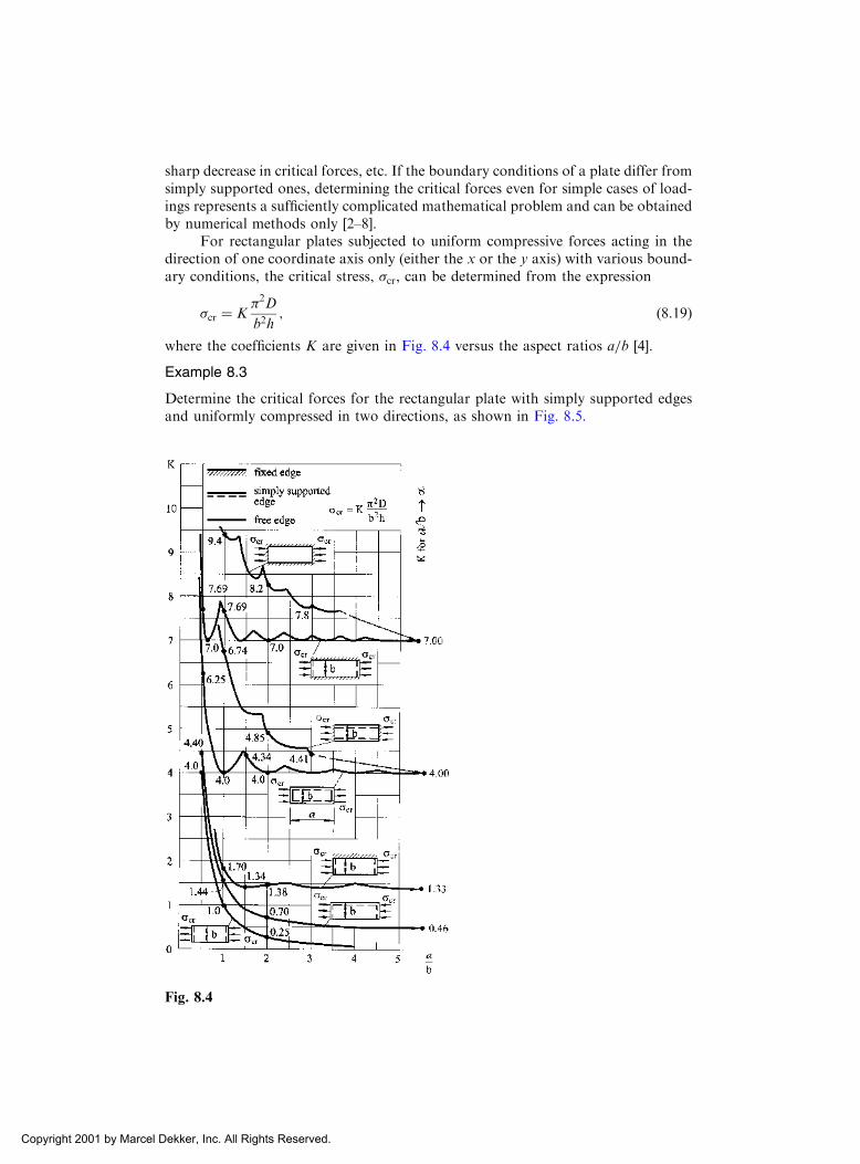
sharp decrease in critical forces, etc. If the boundary conditions of a plate differ fromsimply supported ones, determining the critical forces even for simple cases of load-ings represents a sufficiently complicated mathematical problem and can be obtainedby numerical methods only [2–8].

For rectangular plates subjected to uniform compressive forces acting in thedirection of one coordinate axis only (either the x or the y axis) with various bound-ary conditions, the critical stress, �cr, can be determined from the expression

�cr ¼ K�2D

b2h; ð8:19Þ

where the coefficients K are given in Fig. 8.4 versus the aspect ratios a=b [4].

Example 8.3

Determine the critical forces for the rectangular plate with simply supported edgesand uniformly compressed in two directions, as shown in Fig. 8.5.

Fig. 8.4


Solution

For this problem, first analyzed by Bryan [9] in 1861, the stress resultants may beeasily found: they are Nx ¼ �qx; Ny ¼ �qy; Nxy ¼ 0. Equation (8.1) for this type ofloading becomes

@4w

@x4þ 2

@4w

@x2@y2þ @

4w

@y4þ 1

DNx

@2w

@x2þNy

@2w

@y2

!¼ 0: ð8:20Þ

Let us take w in the form of the expression (3.15a). The deflection surface equation inthis form satisfies the simply supported boundary conditions. Substituting the aboveinto Eq. (8.20) gives

wmn

m2

a2þ n2

b2

!2

� 1

�2Dqx

m2

a2þ qy

n2

b2

" #8<:

9=; ¼ 0: ð8:21Þ

The trivial solution of this equation is wmn ¼ 0. As mentioned earlier, this solutioncorresponds to unbuckled, i.e., flat, configuration of equilibrium of the plate and isof no interest for buckling analysis. A nontrivial solution can be obtained by equat-ing the term in braces in Eq. (8.21) to zero, i.e.,

qx

�m

a

�2

þ qy

�n

b

�2

¼ D�2�m

a

�2

þ�n

b

�2" #2

: ð8:22Þ

Let us consider several particular cases:1. Assume, first, that qx ¼ qy ¼ q ¼ const (a uniform all-round compression).

In this case, it follows from Eq. (8.22) that

q ¼ �2D

b2n2 þ mb

a

� �2" #

:

Fig. 8.5


It can be easily shown that the minimum value of q; qcr, corresponds to m ¼ n ¼ 1.Thus,

qcr ¼�2D

b21þ b

a

� �2" #

: ð8:23Þ

In particular, for the square plate (a ¼ b), the above expression appears, as follows:

qcr ¼ 2�2D

b2:

Hence, if the square plate is compressed in two directions by the two equal system offorces, q, the critical value of these forces is two times less than that for the squareplate compressed by the same force acting in one direction only (see Example 8.1).

2. Assume now that the compressive forces qx and qy applied to the plate ofFig. 8.5 will increase in the proportion to one parameter. For example, qx ¼ � andqy ¼ �, where > 0 is some fixed known parameter. Then, from Eq. (8.22), weobtain

� ¼ �2D

b2

mba

� �2þn2

� �mba

� �2þn2

: ð8:24Þ

For a > b, the minimum value of � may be reached for n ¼ 1 only. Thus,

�cr ¼ K�2D

b2; ð8:25Þ

where

K ¼ mb=að Þ2þ1� �mb=að Þ2þ : ð8:26Þ

For each ratio of a=b and each value of it should be selected a number of the half-sine waves m from the condition of minimum of K as discussed in Example 8.1.

8.3.2 Buckling of circular plates

Circular plates in some measuring instruments are used as sensitive elements react-ing to a change in the lateral pressure. In some cases – in temperature changes, in theprocess of their assembly – these elements are subjected to the action of radialcompressive forces from a supporting structure. As a result, buckling of the circularplates can take place.

Let us consider a circular solid plate subjected to uniformly distributed in-plane compressive radial forces qr, as shown in Fig. 8.6. We confine our bucklinganalysis to considering only axisymmetric configurations of equilibrium for the plate.

We can use the polar coordinates r and ’ to transfer the governing differentialequation of plate buckling (Eq. (8.1)), derived for a rectangular plate, to a circularplate. For the particular case of axisymmetric loading and equilibrium configura-tions, we have

Nx ¼ Ny ¼ Nr ¼ �qr; Nxy ¼ 0: ð8:27Þ


Denoting

�2 ¼ qrD; ð8:28Þ

and using the relations between the polar and Cartesian coordinates, Eqs (4.1)–(4.4),we obtain the following differential equation of the axisymmetrically loaded circularplate subjected to in-plane compressive forces qr:

d4w

dr4þ 2

r

d3w

dr3� 1

r2d2w

dr2þ 1

r3dw

drþ �2 d2w

dr2þ 1

r

dw

dr

" #¼ 0: ð8:29Þ

Let us introduce the following new variable:

� ¼ �r; ð8:30Þwhich represents a dimensionless polar radius. Using the new variable �, we canrewrite Eq. (8.29), as follows:

d4w

d�4þ 2

�

d3w

d�3þ 1� 1

�2

� �d2w

d�2þ 1

�1þ 1

�2

� �dw

d�¼ 0: ð8:31Þ

This is a fourth-order linear, homogeneous differential equation. The general solu-tion of this equation is given by [1] as

w �ð Þ ¼ C1 þ C2 ln �þ C3J0 �ð Þ þ C4Y0 �ð Þ; ð8:32Þwhere J0 �ð Þ and Y0 �ð Þ are the Bessel functions of the first and second kind of zeroorders, respectively. They are tabulated in Ref. [10]. In Eq. (8.32), Ci i ¼ 1; . . . ; 4ð Þare constants of integration. Since w �ð Þ must be finite for all values of �; including�¼ 0, then the two terms ln � and Y0 �ð Þ, having singularities at � ¼ 0, must bedropped for the solid plate because they approach an infinity when �! 1. Thus,for the solid circular plate, Eq. (8.32) must be taken in the form

w �ð Þ ¼ C1 þ C3J0 �ð Þ: ð8:33ÞDetermine the critical values of the radial compressive forces, qr, applied to themiddle plane of solid circular plates for two types of boundary supports.

Fig. 8.6


(1) Circular plate with fixed edge

Let the radius of the plate be R. We denote the corresponding value of �R by , i.e., ¼ �R: The boundary conditions are

w ð Þ ¼ 0�¼; # ð Þ ¼ 0

�¼; ðaÞ

where the slope of the plate midsurface, #ð�Þ, is given by

# �ð Þ ¼ �dw

d�¼ �C3

d

d�J0 �ð Þ: ðbÞ

From the Bessel function theory [10], that it follows

J1 �ð Þ ¼ � d

d�J0 �ð Þ: ðcÞ

Thus, we can write the following representations for the slope

# �ð Þ ¼ ��C3J1 �ð Þ; ð8:34Þand

# ð Þ ¼ ��C3J1 ð Þ on the boundary; ð8:35Þwhere J1ð Þ is the Bessel function of the first kind of the first order.

Substituting the expressions (8.34) and (8.35) into the boundary conditions (a)yields the following system of two linear homogeneous equations:

C1 þ C3J0 ð Þ ¼ 0;

��C3J1 ð Þ ¼ 0:

For a nontrivial solution of these equations:

J1 ð Þ ¼ 0:

From the tables of roots of the Bessel functions [10] it follows that the smallest rootof the function J1 ð Þ is min ¼ 3:8317.

Noting that 2 ¼ �Rð Þ2¼ qr=DR2, we obtain the critical value of the compres-sive forces as

qr;cr ¼ 3:8317ð Þ2 DR2

¼ 14:68D

R2: ð8:36Þ

(2) Circular plate with simply supported edge

The boundary conditions for this type of support are

w ð Þ ¼ 0j�¼;Mr ð Þ ¼ 0j�¼: ðdÞThe radial bending moment, Mr, for an axisymmetrically loaded circular plate isgiven by Eq. (4.14). When passing from variable r to the variable �, the expressionfor Mr becomes

Mr ¼ �D�2 d2w

d�2þ �

�

dw

d�

!: ð8:37Þ


Using Eq. (8.33) for the deflections and Eq. (8.37) for the radial bending moments,we can represent the second boundary condition (d) in the form

�D�2 d2

d�2J0 �ð Þ þ �

�

d

d�J0 �ð Þ

" #¼ 0

�¼: ð8:38Þ

Using the relationships between the Bessel functions of the first kind [10], we have

d2

d�2J0 �ð Þ ¼ �J0 �ð Þ þ 1

�J1 �ð Þ: ðeÞ

Substituting the expression for the deflections (8.33) into the boundary conditions (d)and taking into account Eqs (8.38) and (e), we arrive at the following system of linearhomogeneous equations:

C1 þ C3J0 ð Þ ¼ 0

�D�2C3 J0 ð Þ � 1� �ð ÞJ1 ð Þ½ � ¼ 0ðfÞ

A nontrivial solution of this system of equations leads to the following:

J0 ð Þ � 1� �ð ÞJ1 ð Þ ¼ 0: ðgÞLetting � ¼ 0:3 and using the tables of the Bessel function [10], we can determine thesmallest nonzero root of Eq. (g). We have

min ¼ 2:0485;

and the critical value of an intensity of the radial compressive forces is

qr;cr ¼ 4:196D

R2: ð8:39Þ

Comparing the values of the critical compressive forces for the clamped and simplysupported circular solid plates, we can conclude that the replacement of the sup-ported edges with clamped ones increases the critical force by a factor of 3.5.

8.4 THE ENERGY METHOD

Practical application of the equilibrium method runs into serious mathematicalobstacles when determining the buckling loads of the plates with complex geometryand mixed boundary conditions. Under these circumstances a possibility for obtain-ing a rigorous solution of the differential equation (8.1) becomes very doubtful and,practically, impossible. Therefore, the use of the energy method can be very advan-tageous.

We will apply the energy criterion (8.5) to the buckling analysis of plates. Theincrement in the total potential energy of the plate upon buckling is given by Eq.(8.4). Let us derive the expression for the increment in the strain energy of the middlesurface of the plate. In deriving this expression, we assume that the in-plane stressresultants are entirely due to external edge loading in the plane of the plate, in whichcase they are unchanged during bending (created by buckling). The increment of thestrain energy of the plate middle surface due to buckling can be obtained from thegeneral expression of the potential energy of an elastic body given by Eq. (2.51).Based on the assumptions 4 and 5 of the classical plate theory, the above expression


is simplified and has the following form for the above-mentioned increment of themiddle surface:

�U ¼ 1

2

ð ðV

ð�x"x þ �y"y þ �xy�xy� �

dV : ðaÞ

This increment of the strain energy can also be expressed in terms of the in-planestress resultants. The latter are related to the stress components as follows:

�x ¼Nx

h; �y ¼

Ny

h; and �xy ¼

Nxy

h: ðbÞ

Substituting the above into Eq. (a) and integrating over the plate thickness, h, resultsin the following expression for the increment in the strain energy of the plate middlesurface:

�U0 ¼ð ð

A

Nx"x þNy"y þNxy�xy� �

dxdy: ð8:40Þ

Note that there is no 1/2 coefficient in Eq. (8.40), since the in-plane stress resultantsare already acting when additional middle surface strains (due to the buckling)occur. For the sake of simplicity, we derive the expression for �U0 for a rectangularplate of dimensions a b. Inserting Eqs (7.82) into Eq. (8.40) results in the followingexpression for the increment of the strain energy of the plate middle surface:

�U0 ¼ðb0

ða0

Nx

@u

@xþNy

@v

@yþNxy

@u

@yþ @v

@x

� �� dxdy

þ 1

2

ðb0

ðb0

Nx

@w

@x

� �2

þNy

@w

@y

� �2

þ2Nxy

@w

@x

@w

@y

" #dxdy:

ð8:41Þ

We transform the first integral of the right-hand side of Eq. (8.41). Integrating thisexpression term-by-term, we obtain

ðb0

ða0

Nx

@u

@xþNy

@v

@yþNxY

@u

@yþ @v

@x

� �� dxdy ¼

ðb0

Nxu a

0þ Nxyv a

0

h idy

þðb0

Nyv b

0þ Nxyu b

0

h idx�

ðb0

ða0

u@Nx

@xþ @Nxy

@y

� �dxdy

�ðb0

ða0

v@Nxy

@xþ @Ny

@y

� �dxdy:

ð8:42Þ

Using Eqs (3.90a) and (3.90b), we can conclude that the two last integrals onthe right-hand side in the above expression vanish. The first two integrals on theright-hand side of Eq. (8.42) represent the work, We, done by the in-plane externalforces applied to the middle surface of the plate. Thus, the expression (8.42) can berepresented in the form


�U0 ¼ We þ1

2

ðb0

ða0

Nx

@w

@x

� �2

þNy

@w

@y

� �2

þ2Nxy

@w

@x

@w

@y

" #dxdy: ð8:43Þ

It can be shown that the expression for �U0 in the form of Eq. (8.43) is valid(replacing the limits of integration) for a plate of any geometry, not necessarily,rectangular.

The increment in the potential of the external, in-plane forces applied to theplate is equal to the negative value of the work done by these forces, i.e.,

�� ¼ �We: ð8:44ÞThe strain energy of the bending and twisting of a plate, Ub, is given by Eq. (2.53).Therefore, the increment in the total potential energy of the plate upon buckling,��, can be obtained by substituting Eqs (2.53) and (8.43) with taking into accountEq. (8.44) on the right-hand side of Eq. (8.4).

�� ¼ 1

2

ð ðA

D@2w

@x2þ @

2w

@y2

!2

þ2 1� �ð Þ @2w

@x@y

!2

� @2w

@x2@2w

@y2

24

35

8<:

9=;dxdy

þ 1

2

ð ðA

Nx

@w

@x

� �2

þNy

@w

@y

� �2

þ2Nxy

@w

@x

@w

@y

" #dxdy

ð8:45Þ

As mentioned in Sec. 8.2, the energy criterion (8.5) may be employed be obtain theexact and approximate solutions of the plate buckling problems. In the latter case,this criterion may be combined with, for instance, the Ritz method together with theeigenvalue technique introduced in Sec. 8.2.

Note that in practice �� ¼ 0 only if the form chosen for the deflection is exact.Any approximation form, when Eq. (8.45) is applied, will give a value of the criticalforce higher than the true value. Let us demonstrate the advantages of the energycriterion in illustrative examples.

Example 8.4

Using the Ritz method, determine the critical buckling load for the plate with threesimply supported edges x ¼ 0; a and y ¼ 0 and one free edge y ¼ b, as shown in Fig.8.7. The plate is loaded by linearly distributed compressive in-plane forcesqx ¼ q 1þ y

b

� �along the simply supported edges x ¼ 0; a, where > 0 is some fixed

parameter.

Solution

The deflection surface of the plate can be approximated, as follows:

w ¼ sinn�x

a

XNi¼1

Ciyi: ðaÞ

This approximate solution satisfies exactly the prescribed geometric boundary con-ditions, i.e.,

w ¼ 0jx¼0;a; w ¼ 0jy¼0: ðbÞ

Retaining only one term (i ¼ 1) in the series (a), we can find the following:


@w

@x¼ C1y

n�

acos

n�x

a

� �;@2w

@x2¼ �C1y

n�

a

� �2sin

n�x

a;

@2w

@x@y¼ C1

n�

acos

n�x

a

� �;@2w

@y2¼ 0:

For this type of loading, the solution of the plane stress problem is Nx ¼ �qx,Ny ¼ Nxy ¼ 0. Substituting the above into Eq. (8.45), and performing the operationsof integration, we obtain

�� ¼ C21

ab

4D

b2

3

n�

a

� �4þ2 1� �ð Þ n�

a

� �2" #� q

n�

a

� �2b2

1

3þ

4

� �( ):

The eigenvalues of the load qx can be found from equation @�=@C1 ¼ 0. We have

qn ¼n2�2D

b2b2=a2 þ 6 1� �ð Þ=n2�2

1þ 3 =4

" #:

For n ¼ 1, the smallest eigenvalue is approximately equal to the critical value, i.e.,

qcr ¼b2=a2 þ 6 1� �ð Þ=�2

1� 3 =4� �

2D

b2: ð8:46Þ

Example 8.5

Determine the critical value of uniformly distributed in-plane shear forces qxy for thesimply supported rectangular plate shown in Fig. 8.8.

Solution

We assume that the deflection surface is adequately approximated as follows:

w ¼ C1 sin�x

asin�y

bþ C2 sin

2�x

asin

2�y

b; ðaÞ

where C1 and C2 are two unknown coefficients. It is obvious that w in the form of (a)satisfies exactly the prescribed geometrical boundary conditions (w ¼ 0 on theboundary).

Fig. 8.7


Substituting for w from (a) into the potential energy expression �� given byEq. (8.45) and setting Nxy ¼ �qxy; Nx ¼ Ny ¼ 0, we obtain

�� ¼ ��4

8Dab

1

a2þ 1

b2

� �2

C21 þ 16C2

2

� �� 32

9qxyC1C2: ðbÞ

Applying the conditions for a stationary value of �� – namely, @ð��Þ=�C1 and@ ��ð Þ=@C2 ¼ 0 – results in the following two homogeneous linear equations:

�4

4Dab

1

a2þ 1

b2

� �2

C1 �32

9qxyC2 ¼ 0;

� 32

9SC1 þ 4�4Dab

1

a2þ 1

b2

� �2

C2 ¼ 0:

A nontrivial solution can be obtained by equating the determinant of these equationsto zero. Consequently, we have

�8D2a2b2 a�2 þ b�2� �4� 32qxy

9

� �2

¼ 0;

which gives the following approximation for the critical shear forces:

qxy;cr ¼ � 9

32�4Dab

1

a2þ 1

b2

� �2

: ð8:47Þ

This result, which is larger by 15% than an exact solution for a square plate (a ¼ b)[1], can be improved by retaining more terms in the expression (a) [1–3].

8.5 BUCKLING ANALYSIS OF ORTHOTROPIC AND STIFFENEDPLATES

8.5.1 Orthotropic plates

Consider a rectangular orthotropic plate whose elastic properties are characterizedby four independent constants: the moduli of elasticity Ex and Ey in the two

Fig. 8.8


mutually perpendicular principal directions x and y; the shear modulus G; andPoisson’s ratio �x. The second Poisson’s ratio �y is related to �x by the expression(7.24). The constitutive equations, stress resultants–curvature equations, and thegoverning differential equation for the orthotropic plate in the framework ofsmall-deflection plate bending theory have been derived in Sec. 7.2. Repeating thederivation of Eq. (3.92), we can represent the governing differential equation of theorthotropic plate buckling, as follows:

Dx

@4w

@x4þ 2H

@4w

@x2@y2þDy

@4w

@y4þNx

@2w

@x2þNy

@2w

@y2þ 2Nxy

@2w

@x@y¼ 0: ð8:48Þ

Let us analyze the stability of a rectangular, simply supported orthotropic platesubjected to in-plane compressive forces qx, as shown in Fig. 8.1. The boundaryconditions for simply supported edges of the orthotropic plate are

w ¼ 0jx¼0;ay¼0;b

;@2w

@x2þ �y

@2w

@y2¼ 0

x¼0;a

;@2w

@y2þ �x

@2w

@x2¼ 0

y¼0;b

: ðaÞ

We take the deflection surface of the plate in the form

w ¼ w11 sinm�x

asin

n�y

b: ðbÞ

The deflection surface in the form of (b) satisfies exactly the boundary conditions (a).Substituting (b) into Eq. (8.48) and letting Nx ¼ �qx; Ny ¼ Nxy ¼ 0, we obtain fromthe solution of this equation the following expression for the compressive forces qx:

qx ¼ �2ffiffiffiffiffiffiffiffiffiffiffiffiDxDy

pb2

ffiffiffiffiffiffiDx

Dy

smb

a

� �2

þ 2HffiffiffiffiffiffiffiffiffiffiffiffiDxDy

p n2 þffiffiffiffiffiffiDy

Dx

sa

mb

� �2" #

: ð8:49Þ

It is evident that a minimum value of qx is reached for n ¼ 1. The critical value of thecompressive force can be obtained by varying a number of half-waves m. For a platethat is lengthened along the x axis (a � b), we have the following:

qx;cr ¼2�2


pb2

1þ HffiffiffiffiffiffiffiffiffiffiffiffiDxDy

p !

: ð8:50Þ

For a plate with a finite ratio of sides, it should be taken [4], that

m ¼ 1 for 0 <a

b<

ffiffiffiffiffiffiffiffiffi4Dx

Dy

4

s;

m ¼ 2 for

ffiffiffiffiffiffiffiffiffi4Dx

Dy

4

s<

a

b<

ffiffiffiffiffiffiffiffiffiffiffiffi36

Dx

Dy

4

s;

m ¼ 3 for

ffiffiffiffiffiffiffiffiffiffiffiffi36

Dx

Dy

4

s<

a

b<

ffiffiffiffiffiffiffiffiffiffiffiffiffiffi144

Dx

Dy

4

s; and so on:


Making Dx ¼ Dy ¼ H ¼ D, we obtain the expression (8.10) for qx;cr in a rectangular,simply supported isotropic plate.

8.5.2 Stiffened plates

In the stability analysis of stiffened plates, two modes of buckling are usually con-sidered. One possible mode is the local buckling of the plate between the stiffeners,provided that the plate is reinforced with strong stiffeners. In the second case, anoverall buckling of the plate–stiffener combination occurs. The latter is called pri-mary buckling in the pertinent literature.

A more economical design can be obtained if we permit simultaneous local andprimary buckling at about the same stress level. Consequently, in the elastic stabilityanalysis of stiffened plates, the structural interaction of plate and stiffeners should betaken into account.

Two approaches to the stability analysis of stiffened plates are possible. If aplate is reinforced with many equally spaced parallel stiffeners of the same size (orwith a grid-stiffening arrangement), such an assembly can effectively be approxi-mated by the orthotropic (structurally orthotropic) plate theory. This approachmakes it possible to consider Eq. (8.48) for the buckling analysis of structurallyorthotropic plates, and the rigidities on the left-hand side of this equation are deter-mined according to the procedure introduced in Sec. 7.2.3. Evidently, this approachis applicable only in the case when the stiffeners are located close to one another: thevalue 1=n (n is the number of stiffeners or ribs taken over all the width of the plate)should be small compared with unity.

Another approach involves the buckling analysis of a plate which is reinforcedwith few stiffeners. For such a type of stiffened plates, the convenient orthotropicplate idealization cannot be used to obtain reliable values for the critical loads. Sincethe stiffeners are rigidly fastened to the plate, we should treat the plate and stiffenersas a structural unit; consequently, at mutual points, the stiffener deflects and twists inthe same way as the plate. Since the numerical procedure of the first approach isquite similar to the one discussed in Sec. 8.5.1 and involves no new ideas andprinciples, the second approach will be introduced below only. The critical loadmay be determined by the equilibrium or energy methods. The following examplesillustrate the application of both methods for the buckling analysis of the stiffenedplate.

Example 8.6

This problem was analyzed by Timoshe [1]. Determine the critical load for a simplysupported rectangular plate which is reinforced by a single longitudinal rib locatedalong its centerline, as shown in Fig. 8.9. The plate is subjected to the in-planecompressive forces qx uniformly distributed along the edges x ¼ 0; a.

Solution

In our buckling analysis, we take into account only the bending stiffness of the rib inthe plane perpendicular to the middle plane of the plate. We apply the differentialequation (8.6) to one of the halves of the plate. Its integral is represented in the form

w x; yð Þ ¼ F yð Þ sinm�xa: ð8:51Þ


Substituting the above into Eq. (8.6) and letting Nx ¼ �qx; Ny ¼ 0;Nxy ¼ 0, gives

d4F yð Þdy4

� 2m�

a

� �2d2F yð Þdy2

þ m�

a

� �2 m�

a

� �2� qx

D

� �F yð Þ ¼ 0: ð8:52Þ

Its solution is of the form

F yð Þ ¼ C1 coshyþ C2 sinh yþ C3 cosyþ C4 sin y; ð8:53Þwhere

¼ffiffiffiffiffiffiffiffiffiffiffiffiffiffiffiffiffiffiffiffiffiffiffiffiffiffiffiffi� �þ

ffiffiffiffiffiqxD

r� �s; ¼

ffiffiffiffiffiffiffiffiffiffiffiffiffiffiffiffiffiffiffiffiffiffiffiffiffiffiffiffi�

ffiffiffiffiffiqxD

r� �

� �sand � ¼ m�

a: ð8:54Þ

The boundary conditions on the edge y ¼ b=2 are

w ¼ 0;@2w

@y2¼ 0

y¼b=2

: ð8:55Þ

Assume that the plate is buckled together with the rib; then the bent surface of theplate must be symmetric about the line y ¼ 0. This results in the following condition:

@w

@y¼ 0

y¼0

: ð8:56Þ

The difference in the reaction forces from the two strips of the plate given by theexpression

Ry ¼ �D@3w

@y3þ 2� �ð Þ @

3w

@y@x2

" #ð8:57Þ

will be transmitted to the rib. Assume that the plate and rib are made of one and thesame material. Due to the assumption adopted above for deformations of the rib, itcan be easily shown that only the first term in the brackets of Eq. (8.57) should betaken into account. If we assume that the rib together with the plate is subjected to

Fig. 8.9


the compressive forces qx, then the equation for the elastic curve of the rib may berepresented in the form

EIi@4w

@x4þ qx

@2w

@x2þ 2D

@3w

@y3

!y¼0

¼ 0;

or replacing qx ¼ Nx ¼ �xAi for the rib, we obtain

EIi@4w

@x4þ �xAi

@2w

@x2þ 2D

@3w

@y3

!y¼0

¼ 0; ð8:58Þ

where Ii and Ai are the second moment of inertia and area of the rib cross section,respectively.

Let us introduce the following parameters:

� ¼ a

b; � ¼ EIi

Db; � ¼ Ai

bh: ð8:59Þ

Introducing Eq. (8.53) into the conditions (8.55), (8.56), and (8.58), we obtain asystem of linear algebraic homogeneous equations for C1; . . . ;C4. Equating thedeterminant of this system to zero, yields the following equation:

1

btanh

b

2� 1

btan

b

2

� ��m2

2� K�

!m2�2

2� 4

m

ffiffiffiffiK

p¼ 0; ð8:60Þ

where

K ¼ �x;cr�x;E

ð8:61Þ

and

�x;cr ¼qx;crh; �x;E ¼ 4

�2D

b2hð8:62Þ

where �x;E is the critical stress for a rectangular, simply supported, unstiffened platewith the dimensions of Fig. 8.9 (see Eq. (8.11)). Equation (8.60) may be solved by themethod of trial and errors. For m ¼ 1 and � > 2, its solution, using the parametersintroduced in Eqs (8.59), gives the following expression for �x;cr:

�x;cr ¼�2D

b2h

1þ �2� �2þ2�

�2 1þ 2�ð Þ : ð8:63Þ

Now we analyze the stability problems for stiffened plates by the energy method.

Example 8.7

Determine the critical value of the in-plane compressive forces qx acting on the platereinforced by two equally spaced stiffeners, as shown in Fig. 8.10. The plate is simplysupported on all edges. Let Ai and Bi (Bi ¼ EIi) be the area of the cross section andthe bending stiffness of a stiffener, and ci be spacing of the stiffeners.


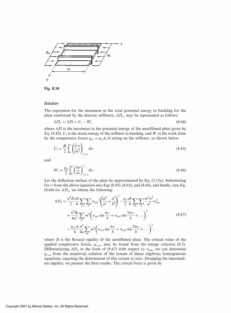
Solution

The expression for the increment in the total potential energy in buckling for theplate reinforced by the discrete stiffeners, ��s, may be represented as follows:

��s ¼ ��þUi �Wi; ð8:64Þwhere �� is the increment in the potential energy of the unstiffened plate given byEq. (8.45), Ui is the strain energy of the stiffener in bending, andWi is the work doneby the compressive forces qxi ¼ qxAi=h acting on the stiffener, as shown below:

Ui ¼Bi

2

ða0

@2w

@x2

!y¼ci

dx ð8:65Þ

and

Wi ¼qxi2

ða0

@w

@x

� �2

y¼ci

dx: ð8:66Þ

Let the deflection surface of the plate be approximated by Eq. (3.15a). Substitutingfor w from the above equation into Eqs (8.45), (8.65), and (8.66), and finally, into Eq.(8.64) for ��s, we obtain the following:

��s ¼�4D

2

ab

4

Xm

Xn

wmn2 m2

a2þ n2

b2

!2

� qx2

ab

4

Xm

Xn

m2�2

a2w2mn

þ �4Bi

4a3

Xm

m4 wm1 sin�cib

þ wm2 sin2�cib

þ . . .

� �2

� qxiAi

h

�2

4a

Xm

m2 wm1 sin�cib

þ wm2 sin2�cib

þ . . .

� �2

;

ð8:67Þ

where D is the flexural rigidity of the unstiffened plate. The critical value of theapplied compressive forces, qx;cr, may be found from the energy criterion (8.5).Differentiating ��s in the form of (8.67) with respect to wmn, we can determineqx;cr from the nontrivial solution of the system of linear algebraic homogeneousequations, equating the determinant of this system to zero. Dropping the intermedi-ate algebra, we present the final results. The critical force is given by

Fig. 8.10


qx;cr ¼�4D

b21þ �2� �þ 3�

�2 1� 3�ð Þ ; ð8:68Þ

where �; �; and � are given by formulas (8.59). The solution (8.68) is done in the firstapproximation, i.e., for m ¼ n ¼ 1. If a rectangular, simply supported plate is rein-forced by i equally spaced stiffeners then the critical value of the compressive forcesis the following:

qx;cr ¼�2D

b2

1þ �2� �2þ2Pi

�i sin2 �ci=bð Þ

�2 1þ 2Pi

�i sin2 �ci=bð Þ

� � : ð8:69Þ

8.6 POSTBUCKLING BEHAVIOR OF PLATES

8.6.1 Large deflections of plates in compression

Using the linearized buckling analysis introduced in Sec. 8.2, we have consideredonly the initial elastic buckling of flat plates and the critical forces and stresses havebeen found for some typical loadings and boundary conditions. The critical force isthe force at which bifurcation of equilibrium states occurs and is of fundamentalsignificance to the designer. So, the critical loads found in the previous sectionsrepresent merely the loads at which buckling begins. It should be noted that thepostbuckling behavior of plates is markedly different from that of thin rods. While asmall increase in the critical load for rods will produce a complete collapse, the load-carrying capacity of the plate is not exhausted and elastic plate can carry stresseshigher than �cr. It can be explained, first of all, by the effect of large deflections in thepostbuckling stage and, then, by the fact that the longitudinal edges of the plate areusually constrained to remain straight. Thus, the postbuckling mechanism of elasticplates is characterized not only by bending but also by the direct (or in-plane)stresses. It is important that the latter become comparable in magnitude with theformer stresses.

The use of an additional strength due to the postbuckling effects is of greatpractical importance in the design of ship and aerospace structures. By consideringthe postbuckling behavior of plates, considerable weight savings can be achieved. Inthese structures, the edges of the plates are usually supported by stringers in such away that they remain straight during buckling. After buckling, the central part of theplate bulges out, and an increasingly larger portion of the load is carried by thematerial close to the supported edges (stringers) of the plate.

The nonlinear, large-deflection plate bending theory, discussed in Sec. 7.4, canbe used for the analysis of the postbuckling behavior of plates. Because of a non-linearity of the governing differential equations of this analysis, the resulting math-ematical difficulties are considerable and exact solutions can very seldom beobtained. The most generally used techniques for the treatment of postbuckling ofplates are based on numerical methods [11,12].

For some simple cases an analytical solution can be obtained under someassumptions regarding the plate behavior, boundary conditions, etc. Consider arectangular, simply supported plate, as shown in Fig. 8.1. The plate is subjected to


the in-plane compressive forces qx. An approximate expression for the buckledmiddle surface of the plate is taken in the following form (m ¼ n ¼ 1):

w ¼ w11 sin�x

asin�y

b: ð8:70Þ

The governing differential equations for the investigation of the postbuckling beha-vior of thin plates of a constant thickness are von Karman’s large-deflection equa-tions (7.87), derived in Sec. 7.4. Assuming that the lateral load p is zero, we canrewrite these equations in terms of the stress function � (� ¼ �=hÞ, as follows:

1

Er4� ¼ @2w

@x@y

!2

� @2w

@x2@2w

@y2; ð8:71aÞ

D

hr4w ¼ @2�

@y2@2w

@x2þ @

2�

@x2@2w

@y2� 2

@2�

@x@y

@2w

@x@y: ð8:71bÞ

Substituting for w from Eq. (8.70) into Eq. (8.71a), we obtain

1

Er4� ¼ 1

2w211

�4

a2b2cos

2�x

aþ cos

2�y

b

� �: ð8:72Þ

Assume that the edge supports do not prevent the in-plane motions of the plate inthe y direction or, in other words, the in-plane shear stresses are zero. A particularintegral of Eq. (8.72) is taken, as follows:

�p ¼ A cos2�x

aþ B cos

2�y

b:

Determine the unknown coefficients A and B by calculating r4�p and comparing theleft- and right-hand sides of Eq. (8.72). We obtain the following:

�p ¼ Ew211

32

�a

b

�2

cos2�x

aþ b

a

� �2

cos2�y

b

" #: ð8:73Þ

Assuming that the edge supports do not prevent the in-plane motions of the plate inthe y direction, we take the solution of the homogeneous Eq. (8.72) in the form

�h ¼ � qxy2

2h: ð8:74Þ

Finally, the general solution of Eq. (8.72) is

� ¼ �p þ �h ¼ Ew211

32

a

b

� �2cos

2�x

aþ b

a

� �2

cos2�y

b

" #� qxy

2

2h: ð8:75Þ

In-plane stresses in the plate middle surface are

�x ¼@2�

@y2¼ �E

�2

8

w11

a

� �2cos

2�y

b� qx

h; �y ¼

@2�

@x2¼ �E

�2

8

w11

b

� �2cos

2�x

a;

�xy ¼ � @2�

@x@y¼ 0:

ð8:76Þ


As seen, the in-plane shear stresses are zero. Let us apply the Galerkin method tosolve Eq. (8.71b). Using the general procedure of the method discussed in Sec. 6.5,we obtainða

0

ðb0

E sin�x

asin�y

bdxdy ¼ 0; ð8:77Þ

where

E � D

hr4w� @

2�

@y2@2w

@x2� @

2�

@x2@2w

@y2þ 2

@2�

@x@y

@2w

@x@y: ð8:78Þ

Substituting for w and � from Eqs (8.70) and (8.75) into (8.77) and performingthe corresponding operations of differentiation and integration, yields thefollowing:

D�4ab

4w11

1

a2þ 1

b2

� �2

� qxw11

�2

a2ab

4þ E

�4w311

64h

1

a4þ 1

b4

� �ab ¼ 0: ð8:79Þ

Assuming that w11 6¼ 0, we obtain

qx ¼ Nx ¼ �xh ¼ D�2

b2b

aþ a

b

� �2

þE�2h

16b2w211

b2

a2þ a2

b2

!: ð8:80Þ

Since the first term on the right-hand side of the above equation represents thecritical force of the linear buckling analysis, qx;cr, introduced in Sec. 8.3, it is evidentthat the plate can sustain a compression load greater than the linear buckling. Itshould be noted that the load-carrying capacity is more pronounced when theunloaded edges are constrained to remain straight (Ny 6¼ 0).

The first detailed analysis of the postbuckling behavior of plates loaded bycompressive loads was conducted by von Karman et al. [13], who suggested a sim-plified approach to obtain an estimate for the ultimate load carried by the buckledplate. Based on experimental observations, this simplified method assumes that theultimate buckling load of the plate is carried exclusively by two strips of equal width(the so-called effective width), located along the unloaded edges, and the stringers,jointly with the effective width portion of the plate, act as columns. A detailednumerical analysis of the postbuckling behavior of thin plates with various boundaryconditions using the simplified method based on the effective width concept incompression for routine design purposes was developed by Marguerre [14], Cox[2], Schade [15], etc. The interested reader is referred to these references and toRefs [1,3].

8.6.2 Load-carrying capacity of plates in compression

We have seen that a plate after buckling may carry in some cases a compressive forcethat is many times higher than the critical load at which buckling begins. So, in caseswhen issues of weight economy are of fundamental importance, as for example in theaircraft industry, it is expedient to determine not only the critical load but also theultimate load which the plate can carry without failure, which corresponds to theplate load-carrying capacity in compression.


We consider below a rectangular plate that is pin-connected along its edgeswith rigid stiffeners. The plate is subjected to compressive forces in one direction, asshown in Fig. 8.11a.

Prior to buckling of the plate, the compressive stresses are uniformly distrib-uted over its width, b, but after buckling the distribution of stresses along the loadededges becomes progressively nonlinear: they increase more intensively in the vicinityof the plate edges and the stresses differ little from their critical values in the centralpart of the plate. A typical compressive stress distribution along the plate crosssection is shown in Fig. 8.11b. The actual distribution of the compressive stressesdepends on the boundary conditions and on the length-to-width ratio, a=b, providedthat this ratio is less than 3.

When failure of the plate is impending, almost the total compressive load iscarried by two strips, located along the unloaded edges.

Following the simplified approach proposed by von Karman et al. [13], wedetermine the ultimate load carried by the compressed plate. This approach is basedon the following assumptions:

Fig. 8.11


(a) The initial (unloaded) plate is perfectly flat.(b) The ultimate buckling load is carried exclusively by two strips of equal

width, be, located along the unloaded edges.(c) The maximum stress in the edge fiber of the plate, located in the middle

surface, �u, is uniformly distributed over the two plate strips, be, as shownin Fig. 8.11c.

(d) The supporting stiffeners remain straight during the buckling and, jointlywith the effective width portion of the plate, be, they act as columns.

Since the normal compressive stress is not uniform along the plate cross section, letus introduce the mean compressive stress, �m. From the above assumptions, it fol-lows that the effective width, be, is

be ¼1

�u

ðb0

�mdy: ð8:81Þ

Now we can determine the effective width of the bunched plate by using the referencevalue of the critical stress, �cr, in the following form:

�cr ¼N1cr

h¼ K

D

h

�

b

� �2: ð8:82Þ

Due to the assumption (b), an expression similar to Eq. (8.82) can be written for theequivalent plate of width be:

�u ¼ KD

h

�

be

� �2

: ð8:83Þ

Comparing Eqs (8.82) and (8.83) yields the following:

be ¼ b

ffiffiffiffiffiffi�cr�u

r: ð8:84Þ

A more accurate postbuckling analysis estimates be as follows [16]:

be ¼ b �ffiffiffiffiffiffi�cr�u

3

r: ð8:85aÞ

Koiter [17] received the expressions for the effective width of flat plate in the form

be ¼ b 1:2�cr�u

� �0:4

� 0:65�cr�u

� �0:8

þ0:45�cr�u

� �1:2" #

: ð8:85bÞ

The ultimate load carried by the compressed plate is

Pu ¼ �ubeh: ð8:86ÞTo obtain estimates for the maximum edge stresses, �u, two cases are considered:

1. If the supporting stiffeners are relatively strong, the yield criterion can beconveniently used, in connection with the effective width concept, todetermine �u the plate is able to carry. In this case, �u is simply equalto the yield stress �y, provided that the stiffeners and the adjacent plate


strips reach the yield stresses simultaneously without buckling. The ulti-mate load carried by the plate in this case is

Pu ¼ �ybeh: ð8:87Þ2. If the supporting stiffeners are relatively weak, they may fail by buckling

before yield stress is developed. In this case, a trial and error procedureshould be used to obtain an estimate for the maximum edge stresses, �u.First, we assign an effective width be in the first approximation asbe ¼ ð0:3� 0:6Þb, and determine �ð1Þu , considering that the longitudinalsupporting stiffener and the effective width portion of the plate act as acolumn. Using the �ð1Þu value obtained, a new estimate for bð2Þe can becalculated, etc. The procedure is repeated until the interrelationshipbetween these two variables is satisfied.

8.7 BUCKLING OF SANDWICH PLATES

The stability analysis of sandwich plate structure has to be taken with regard tovarious types of its buckling modes as a whole and its separate elements. Let asandwich plate be loaded by the external in-plane edge loads (compressive and/orshear) symmetrically with respect to its middle plane. Two possible modes of buck-ling should be distinguished: a general, resulting from bending of the middle surfaceof the sandwich plate; a local, manifested as bending (wrinkling) of the upper andlower sheets and occurring without bending of the plate as a whole. In this book weconsider only the buckling analysis of the general stability of sandwich plates. Thelocal stability problems for sandwich plates were studied in Ref. [18].

The governing differential equations of the small-deflection bending theory oforthotropic and isotropic sandwich plates were derived in Sec. 7.6. The above equa-tions will be valid for the buckling analysis if, according to the general procedureintroduced in Sec. 8.2 for plate stability problems, instead of the transverse surfaceload p, a fictitious load pf (see Sec. 8.2) is inserted in Eqs (7.131) for orthotropicsandwich plates or in Eq. (7.135) for isotropic ones:

pf ¼ Nx

@2w

@x2þNy

@2w

@y2þ 2Nxy

@2w

@x@y; ð8:88Þ

where Nx;Ny; and Nxy are the internal forces acting in the middle plane of the platecorresponding to the applied in-plane loading. Thus, the stability problem of thesandwich orthotropic plate is described by a system of governing equations consistingof Eqs (7.131a) and (7.131b), and (7.131c), where the latter equation is of the form

@Qx

@xþ @Qy

@y¼ �pf ; ð8:89Þ

pf is given by Eq. (8.88). In a special case, substituting for pf from Eq. (8.88) into Eq.(7.135), we obtain the following governing differential stability equation for isotropicsandwich shells:

Dsr2r2w ¼ 1� Ds

DQ

r2

� �Nx

@2w

@x2þNy

@2w

@y2þ 2Nxy

@2w

@x@y

!ð8:90Þ


Example 8.8

A rectangular simply supported isotropic sandwich plate of Fig. 7.8 is subjected toan in-plane edge compressive load of intensity qx, as shown in Fig. 8.1. Determinethe critical value of this load if a ¼ 20 in:; b ¼ 10 in:; t ¼ 0:02 in:; c ¼ 0:2 in:, Ef ¼10 106 psi; Gc ¼ 12,000 psi, � ¼ 0:3.

Solution

The simply supported boundary conditions in terms of the deflections are given byEqs (3.14). For the problem under consideration, Nx ¼ �qx and pf ¼ �qx@

[email protected], Eq. (8.90) simplifies to the following form:

Dsr2r2wþ qx 1� Ds

DQ

r2

� �@2w

@x2¼ 0: ðaÞ

Equation (a) is a constant-coefficient equation. A solution of the form

w ¼ C1 sinm�x

asin

n�y

b; m; n ¼ 1; 2; 3; . . . ; ðbÞ

where C1 is a constant, is seen to satisfy the boundary conditions (3.14). Introductionof that expression for w into Eq. (a) and rearrangement gives

qx ¼ �2Ds

b2ðmb=aÞ þ ðn2a=mbÞ� �21þ ðmb=aÞ2 þ n2

� � ; ðcÞ

where m and n are positive integers and

¼ �2Ds

b2DQ

: ðdÞ

Equation (c) may now be written in the following alternative form:

qx ¼ Ks

�2Ds

b2; ðeÞ

where the nondimensional buckling coefficient Ks for sandwich plates is defined as

Ks ¼½mb=aþ n2a=mbÞ�21þ n2 þ ðmb=aÞ2� � : ðfÞ

For given values of the plate aspect ratio a=b and the shear stiffness parameter , thevalue of the wave–length parameters m and n may be chosen by trial to give thesmallest value of qx; i:e:; qx;cr.

It is seen that for Gc ! 1; ¼ 0 and the buckling parameter Ks ! K givenby Eq. (8.8) (for n ¼ 1). Thus, for this particular case when the transverse sheardeformation is neglected, Eq. (c) reduces to the corresponding expression (8.7b)derived for buckling of homogeneous plates.

Using the numerical data of the problem, let us compute the rigidities. We have


Ds ¼Estðcþ tÞ22ð1� �2Þ ¼ 5318 lb-in; DQ ¼ Gc

ðcþ tÞ2c

¼ 2904 lb/in,

¼ �2Ds

b2DQ

¼ 1:831:

Introduction of these data into Eq. (f) reveals that the smallest value of the coefficientKs corresponds to n ¼ 1 and m ¼ 3. For this value Eq. (g) gives qx;cr ¼ 973:2 lb/in.

If the core were omitted and the two face sheets bonded together to form a thinhomogeneous plate 0.04 in. thick, the corresponding critical load would be only23.4 lb.

PROBLEMS

8.1 Figure 8.2 shows the variation of the buckling load parameter K as a function of aspect

ratio a=b for m ¼ 1; 2; 3; 4: Based on this figure, determine the condition at which a

transition from m to mþ 1 half-sine waves across the span of the plate, compressed in

the x direction by a uniform edge loads.

8.2 Calculate the critical value of the uniform compressive edge loads qx applied over two

simply supported edges of length b if two opposite edges of the length a are fixed. Use

a ¼ 2m; b ¼ 1m; h ¼ 0:1m; E ¼ 210GPa; and � ¼ 0:3.8.3 Calculate the critical value of the uniformly applied compressive edge loads for a

rectangular plate of sides a and b with two simply supported opposite edges and two

other opposite edges free. Assume that the load is applied over the free edges. Take

a ¼ 10m; b ¼ 5m; h ¼ 0:15m; E ¼ 220GPa; and � ¼ 0:3.8.4 Let a rectangular, simply supported plate of sides a and b be loaded by uniformly

distributed compressive qx and tensile qy forces. The qx forces are applied parallel to

the side a and qy forces act in the direction parallel to the side b. Find the nontrivial

solution of Eq. (8.20) for this type of loading and calculate the critical value of the

parameter � if qy ¼ �qx and a ¼ b. Compare this result with the case when the above

plate is compressed in two directions (see Fig. 8.5).

8.5 Consider a circular plate uniformly compressed by in-plane radial forces qr. Compare

the critical values of qr for two types of plate supports: (a) simply supported edge and

(b) fixed edge. Use the radius of the plate a ¼ 40 in:; h ¼ 2:5 in:; E ¼ 25,000 ksi; and� ¼ 0:3.

8.6 Consider a rectangular plate of sides 2a and 2b. The origin of the Cartesian coordinate

system is taken at the plate center. The plate rests at its center upon columns and is

compressed by uniformly distributed forces qx applied parallel to the side 2a. Assuming

that the column support can be approximated by a point support, determine the critical

value of qx. Use the Ritz method and the approximate expression for the deflection in

the form

w ¼ C cos�x

2aþ cos

�y

2b

h i:

8.7 Let a rectangular plate of sides a and b (a > bÞ with fixed edges be subjected to

compressive linearly varying loads qx ¼ q0ð1� y=bÞð < 1Þ. The load is applied to

short plate edges. The origin of the Cartesian coordinate system is attached at the

left upper corner of the plate. Determine the critical value of the applied compressive

load by the Ritz method. Assume that a ¼ 3m; b ¼ 1:5m; h ¼ 0:15m; ¼ 0:5; E ¼200GPa; and � ¼ 0:28, and the approximate expression for deflections is

w ¼ C x2 � a2� �2

y2 � b2� �2

:


8.8 Derive Eq. (8.48).

8.9 Consider an unstiffened, simply supported rectangular plate of sides a and b and a

plate of the same geometry and boundary conditions but reinforced by a single long-

itudinal rib located along its centerline, as shown in Fig. 8.9. Compare the critical

values of the compressive forces qx uniformly distributed along the edges x ¼ 0; afor the above two plates. Assume that a ¼ b ¼ 2m, h ¼ 0:15m, E ¼ 220GPa; and� ¼ 0:3, and the rib has a cross section in the form of a channel section C75 6. In

the buckling analysis, take into account the buckling stiffness of the rib in the plane

that is perpendicular to the plate middle plane.

8.10 A simply supported square plate is reinforced by three equally spaced stiffeners of

rectangular cross section of depth h1 and of width t. The plate is subjected to in-

plane uniform compressive forces qx that act parallel to the stiffeners. Determine the

critical value of the applied forces. Assume that the stiffeners and plate are made of the

same material and stiffeners are symmetrical about the plate middle plane. Use a ¼5m; h ¼ 0:2m; h1 ¼ 0:4m; t ¼ 0:1m; E ¼ 210GPa; and � ¼ 0:3.

8.11 A long, simply supported rectangular plate (a=b ¼ 3Þ, subjected to uniform compres-

sive forces qx acting parallel to the long side a was reinforced by stiffeners symmetri-

cally placed about the plate middle surface. Three variants of locations of the stiffeners

had been discussed:

(a) First, the equally spaced transverse stiffeners (i.e., located in the perpendicular

direction with respect to qx) were suggested to locate at a distance equal to b;

(b) Secondly, the equally spaced transverse stiffeners were suggested to locate at a

distance b=2;(c) Thirdly, only one longitudinal stiffener located along the plate centerline (i.e., in

the direction of the applied load) was suggested to apply.

Assuming buckling of the reinforced plate as a whole, determine the critical values of

the applied forces qx for all the above cases. If the geometrical and mechanical proper-

ties of the plate and stiffeners are known, draw conclusions about the efficient arrange-

ment of stiffeners for the problem under consideration from the point of view of the

buckling analysis.

8.12 Estimate the ultimate edge load of a rectangular plate, stiffened along both longitu-

dinal edges and uniformly compressed in the x direction. Assume that the plate is

simply supported along its edges and that the stiffeners and adjacent plate strips

simultaneously approach the compressive yield strength. Let a ¼ 900mm; b ¼ 450

mm; h ¼ 1mm; E ¼ 73GPa; � ¼ 0:3, and �y ¼ 415MPa:

REFERENCES

1. Timoshenko, S.P. and Gere, J.M., Theory of Elastic Stability, McGraw-Hill, New York,

1961.

2. Cox, H.L., The Buckling of Plates and Shells, The Macmillan Company, New York,

1963.

3. Bulson, P.S., The Stability of Plates, American Elsevier Publishing Company, New York,

1969.

4. Volmir, A.S., Stability of Elastic Systems, Gos. Izd-vo Fiz.-Mat. Lit-ry, Moscow, 1963

(in Russian).

5. Carson, W.G. and Newton, R.E., Plate buckling analysis using a fully compatible finite

elements, AIAAJ, vol. 7, No. 3, pp. 527–529, (1969).

6. Kapur, K.K. and Hartz, B.J., Stability of plates using the finite element method, J Engng

Mech Div, Proc ASCE, vol. 92, pp. 177–195, 1966.


7. Costa, J.A. and Brebbia, C.A. Elastic buckling of plates using the boundary element

methods. In Boundary Elements, VII (eds C.A. Brebbia and G. Maier), Springer-Verlag,

Berlin, 4-29–4-43 (1985).

8. Manolis, G.D., Beskos, D.E. and Pineros, M.F. Beam and plate stability by boundary

elements, Comput Struct, vol. 22, pp. 917–923, (1986).

9. Bryan, G.N., On the stability of a plane plate under thrusts in its own plane with

application to the buckling of the sides of a ship, Proc Lond Math Soc, vol. 22, pp.

54–67, (1891).

10. Watson, G.N., Theory of Bessel Functions, 2nd edn, Cambridge University Press,

Cambridge, 1944.

11. Murray, D.W. and Wilson, E.L., Finite-element large-deflection analysis of plates, Proc.

ASCE, J Engng Mech, Div EMI, p. 143 (1969).

12. Yang, T. J., Elastic postbuckling prediction of plates using discrete elements, AIAAJ,

vol. 9, No. 9, pp. 1665–1666 (1971).

13. von Karman, T., Sechler, E.E., and Donnel, L.H., The strength of thin plates in com-

pression, Trans ASME, vo. 54, pp. 53–57 (1932).

14. Marguerre, K., Die mittragende breite der gedruckten platte, Luftfahrtforschung, vol. 14,

no. 3, pp. 121–128 (1937).

15. Schade, H.A., Larguer effective de toles reinforcees travaillant sous l’action de forces de

flexion, Bulletin Technique du Bureau Veritas, pp. 215–227 (1953).

16. Marguerre, K., The apparent width of the plate in compression, Tech Memo No. 833,

NACA, Washington, D.C, 1937.

17. Koiter, W.T., The effective width of flat plates for various longitudinal edge conditions

at loads far beyond the buckling load, Rep. No. 5287, National Luchtvaart Laboratorium

(The Netherlands).

18. Yusuff, S., Theory of wrinkling in sandwich construction, J Roy Aeron Soc, vol. 59, No.

529 (1955).


9

The Vibration of Plates

9.1 INTRODUCTION

In the preceding chapters, we have assumed that all external forces are appliedslowly: so slowly that the loads and the resulting stresses and deformations areindependent of time. In engineering practice, however, many components ofmachines and structures are subjected to dynamic effects, produced by time-depen-dent external forces or displacements. Dynamic loads may be created by movingvehicles, wind gusts, seismic disturbances, unbalanced machine vibrations, flightloads, sound, etc. Dynamic effects of time-dependent loads on structures are studiedin structural dynamics. Structural dynamics deals with time-dependent motions ofstructures, primarily, with vibration of structures, and analyses of the internal forcesassociated with them. Thus, its objective is to determine the effect of vibrations onthe performance of the structure or machine.

The dynamics of plates, which are continuous elastic systems, can be modeledmathematically by partial differential equations based on Newton’s laws or by inte-gral equations based on the considerations of virtual work. In practical applicationsonly the lateral vibration is of interest, and the effects of extensional vibrations in themiddle plane may be neglected. Therefore, the inertia forces, associated with thelateral translation of the plate, are considered. In this chapter only the simplifiedtheory of plate vibrations is introduced; some physical phenomena, associated with,for instance, damping effects, are not considered.

Damping effects are caused either by internal friction or by the surroundingmedia. Although structural damping is theoretically present in all plate vibrations, ithas usually little or no effect on (a) the natural frequencies and (b) the steady-stateamplitudes; consequently, it can be safely ignored in the initial treatment of theproblem. We follow the same pattern, as used in earlier chapters, of looking first


for exact solutions by solving the differential equations, then looking for approx-imate solutions.

The derivation of the governing differential equation of motion of plates is, inmost cases, a simple extension of the static case by adding effective forces to the platethat result from accelerations of the mass of the plate. These are the inertia forces.For the most part, we take advantage of D’Alambert’s principle to add the inertiaforces as reversed effective forces. Other time-dependent forces may also be consid-ered. The most common of these are damping forces.

We consider various kinds of motion of plates. There is a free vibration, whichoccurs in the absence of applied loads but may be initiated by applying initialconditions to the plate. The free vibration deals with natural characteristics of theplates, and these natural vibrations occur at discrete frequencies, depending only onthe geometry and material of the plates. Then, there is a forced vibration, whichresults from an application of time-dependent loads. Forced vibrations come intwo kinds: a harmonic response, when a periodic force is applied to the plate; anda transient response, when the applied force is not a periodic force.

In deriving the governing differential equation of motion, we use the generalassumptions of Kirchhoff’s plate bending theory introduced in Sec. 1.3. To adapt theelastic static equations derived for thin plates in Chapter 2, to model undampedstructural dynamics, we need to consider only the dependent variables (the deflec-tions, strains, and stresses) as functions of time. Let the applied loads be somefunctions of time, and explicitly include inertia forces in the surface lateral loadsaccording to D’Alambert’s principle. In this case, the forcing function appearing onthe right-hand side of the governing differential equation (2.24) for the bending ofthin plates becomes

p x; y; tð Þ � �h @2w

@t2x; y; tð Þ; ð9:1Þ

where both p and w are functions of time, as well as space; � is the mass density ofthe material, and h is the plate thickness. In the forced vibrations p x; y; tð Þ causes thedynamic response.

Thus, the differential equation of forced, undamped motion of plates has theform

Dr2r2w x; y; tð Þ ¼ p x; y; tð Þ � �h @2w

@t2x; y; tð Þ: ð9:2Þ

9.2 FREE FLEXURAL VIBRATIONS OF RECTANGULAR PLATES

Consider a rectangular plate with arbitrary supports. Let us assume that certaintransverse surface loads distributed on the surface cause the particles, located inthe middle surface, to attain the deflections and velocities directed perpendicularlyto the initial (undeformed) middle surface. At a certain time, which is assumed tobe the initial, the plate is suddenly released from all external loads. The unloadedplate, which has initial deflection and velocity, begins to vibrate. The particleslocated in the middle surface move in the direction perpendicular to the plateand, as a result, the plate becomes curved. Such vibrations are called free ornatural transverse vibrations. The plate will execute free or natural lateral vibrations.


As stated previously, natural vibrations are functions of the material propertiesand the plate geometry only, and are inherent properties of the elastic plate,independent of any load. Thus, for natural or free vibrations, p x; y; tð Þ is setequal to zero, and Eq. (9.2) becomes

Dr2r2w x; y; tð Þ þ �h @2w

@t2x; y; tð Þ ¼ 0: ð9:3Þ

Deflection w must satisfy the boundary conditions at the plate edge (these conditionspractically do not differ from those in the case of static equilibrium) and the follow-ing initial conditions:

when t ¼ 0 : w ¼ w0 x; yð Þ; @w

@t¼ v0 x; yð Þ; ð9:4Þ

where w0 and v0 are the initial deflection and initial velocity for point (x; y).Equation (9.3) is the governing, fourth-order homogeneous partial differential

equation of the undamped, free, linear vibrations of plates. A complete solution of theproblem of a freely vibrating plate is reduced to determining the deflections at anypoint for any moment of time. However, the most important part of the problem offree flexural vibrations of plates is to determine the natural frequencies and the modeshapes of the vibration (deflection surfaces in two dimensions) associated with eachnatural frequency. For such a problem (like in buckling), Eq. (9.3) is an eigenvalueproblem. The natural frequencies are the eigenvalues and associated shape functionsare the eigenfunctions. Values of these parameters are necessary for establishing thedynamic stresses caused by a variable load. A solution of Eq. (9.3) can be obtainedby applying the classical analytical and approximate methods discussed in Chapters3, 4, and 6 for static plate bending problems.

Let us describe a general analytical method (the Fourier method) for determin-ing the natural frequencies of a freely vibrating plate. To solve Eq. (9.3) and obtainw x; y; tð Þ in general, one can assume the following solution:

w x; y; tð Þ ¼ A cos!tþ B sin!tð ÞW x; yð Þ; ð9:5Þwhich is a separable solution of the shape function W x; yð Þ describing the modes ofthe vibration and some harmonic function of a time; ! is the natural frequency of theplate vibration which is related to vibration period T by the relationship ! ¼ 2�=T .

Introducing Eq. (9.5) into Eq. (9.3), we have

Dr2r2W x; yð Þ � !2�hW ¼ 0: ð9:6ÞLet us represent a solution of this equation in the form of a Fourier series. Requiringthe functionW to satisfy the boundary conditions and to be the solution of Eq. (9.6),we obtain a system of homogeneous equations for the unknown constants. Thissystem has solutions that differ from zero only in the case when its determinant� !ð Þ is equal to zero; therefore we obtain the frequency or characteristic equation,which is

� !ð Þ ¼ 0: ð9:7ÞThis equation will have an infinite number of solutions which constitute the fre-quency spectrum for a given plate. In general, the frequencies will depend on twoparameters: m and n (m ¼ 1; 2; . . . ; n ¼ 1; 2; . . .). The lowest frequency is called the


frequency of the fundamental mode or the fundamental natural frequency and all otherfrequencies are called the frequencies of higher harmonics, or overtones. For eachfrequency !mn, there is a corresponding shape function Wmn x; yð Þ that, on the basisof the homogeneous equations, is determined by a constant multiplier (which can beassumed as being equal to unity). For example, in the case of a rectangular, simplysupported plate, the shape function may be taken as

W x; yð Þ ¼X1m¼1

X1n¼1

Cmn sinm�x

asin

n�y

b; ð9:8Þ

where a and b are the plate dimensions and Cmn is the vibration amplitude for eachvalue of m and n. Substitution of Eq. (9.8) into Eq. (9.6) results in the homogeneousalgebraic equation

m4�4

a4þ 2

m2�2

a2n2�2

b2þ n4�4

b4� !

2�h

D¼ 0: ð9:9Þ

Solving this equation for ! gives the natural frequencies

!mn ¼ �2m2

a2þ n2

b2

! ffiffiffiffiffiffiD

�h

s: ð9:10Þ

The fundamental natural frequency can be obtained by letting m ¼ 1; n ¼ 1. Notethat, again (as in the buckling analysis), the amplitude Cmn cannot be determinedfrom the linear eigenvalue problem.

For a square plate of dimension a, Eq. (9.10) becomes

!mn ¼�2

a2

ffiffiffiffiffiffiD

�h

sm2 þ n2� �

; ð9:11Þ

and the fundamental natural frequency is

!11 ¼2�2

a2

ffiffiffiffiffiffiD

�h

s: ð9:12Þ

The fundamental mode of the flexural vibration is a single sine wave in the x and ydirections. Figure 9.1a shows a plate view executing the vibrations of the fundamen-tal tone with the natural frequency !11. The maximum deflection is at the platecenter. The deflected surfaces that correspond to the natural frequencies !21 and!12 are depicted in Fig. 9.1b and c; in each case there are the two maximum deflec-tions and one of the axes of symmetry is a nodal line.

9.3 APPROXIMATE METHODS IN VIBRATION ANALYSIS

9.3.1 Variational methods

An exact solution of the governing differential equation (9.3) in closed form ispossible only for a limited number of cases regarding a plate’s geometry and itsboundary conditions. As mentioned previously, the natural fundamental frequenciesare of the greatest importance in practice. Therefore, one has to determine thesefrequencies by the approximate methods discussed in Chapter 6.


Here, we consider some variational methods for determining natural frequen-cies of freely vibrating plates. First we apply Rayleigh’s principle for finding thelowest natural frequency of a vibrating plate, which is of great interest in appliedvibration analysis. This principle is based on the following statement: if the vibratingsystem is conservative (no energy is added or lost), then the maximum kinetic energy,Kmax, must be equal to the maximum potential (strain) energy, Umax. Applying thisprinciple, we consider an elastic plate undergoing free vibrations with the funda-mental mode as a system with one degree of freedom. Taking into account that onlyfree flexural vibrations are of interest, we can present the above principle as follows:

Umax ¼ Kmax: ð9:13ÞThis principle is essentially a restatement of the principle of conservation of energy(see Sec. 2.6). The strain energy of the plate is described in detail in Sec. 2.6. Thekinetic energy of the plate is

K ¼ 1

2

ð ðA

�h@wðx; y; tÞ

@t

� �2dxdy: ð9:14Þ

Assuming that the plate is undergoing harmonic vibrations, we can approximate thevibrating middle surface of the plate by the equation

wðx; y; tÞ ¼ Wðx; yÞ sin!t; ð9:15Þwhere W x; yð Þ is a given continuous function that approximately represents theshape of the plate’s deflected middle surface and satisfies at least the kinematicboundary conditions and ! represents the unknown natural frequency of the platepertinent to the assumed shape function. Substituting the expression (9.15) into Eq.(9.14) for the kinetic energy, we obtain

K ¼ !2

2cos2 !t

ð ðA

�hW2ðx; yÞdxdy: ð9:16Þ

It is evident, that the kinetic energy is a maximum when cos!t ¼ 1. Thus, we have

Fig. 9.1


Kmax ¼!2

2

ð ðA

�hW2ðx; yÞdxdy ð9:17Þ

The strain energy is a maximum when the deflection is a maximum. For the deflectedmiddle surface, which is approximated by Eq. (9.15), Umax occurs when sin!t ¼ 1. Itcan be easily shown that under this condition the maximum strain energy of thevibrating plate is identical to Eq. (2.54), derived in Sec. 2.6 for the static case.

Substituting the expressions (2.54) and (9.17) for the maximum values of thestrain and kinetic energies, respectively, into Rayleigh’s principle (9.13), we obtain

!2 ¼ 2UmaxÐ ÐA�hW2ðx; yÞdxdy ; ð9:18Þ

where

Umax ¼1

2

ð ðA

D r2W� �2þ2 1� �ð Þ @2W

@x@y

!2

� @2W

@x2@2W

@y2

24

35

8<:

9=;dxdy: ð9:19Þ

The accuracy of determining the natural frequencies by Eq. (9.18) depends to aconsiderable extent on the successful selection of the expression for W . Frequently,the function W is chosen as an expression that is proportional to a static deflectionof a plate of interest with the same boundary conditions as for the plate of interestunder a uniformly distributed lateral surface load p. This is equivalent to the assump-tion that the plate surface that corresponds to the fundamental mode is identical tothat deflected by a uniform distributed load. The approximate lowest or fundamentalfrequency calculated from Rayleigh’s principle is always higher than the ‘‘exact’’values, since we have arbitrarily stiffened the plate by assuming a modal shape,thus increasing its frequency.

Equation (9.18) determines a frequency ! only in the first approximation. Amore accurate frequency value can be obtained by using the Ritz method discussed inSec. 6.6 for static plate problems. Being applied to the plate vibration problems, thismethod represents a generalization of Rayleigh’s principle by including more thanone parameter in the expression of the shape function. In this way, not only a moreaccurate value for the lowest natural frequency can be obtained but also additionalinformation concerning the higher frequencies and pertinent mode shapes is gained.

Assuming the shape function Wðx; yÞ in the form of a series, we can write

Wðx; yÞ ¼Xni¼1

CiWiðx; yÞ: ð9:20Þ

The unknown coefficients Ci are obtained from the minimum total energy principle(see Secs 2.6 and 6.6). Thus, based on Eq. (6.44), we may write

@ðUmax � KmaxÞ@Ci

¼ 0 ði ¼ 1; 2; 3; . . . ; nÞ: ð9:21Þ

Inserting Eq. (9.20) into Eqs (9.17), (9.19) and performing the Ritz procedure,described by Eq. (9.21), we obtain, after integration of the definite integrals, the setof homogeneous linear algebraic equations in Ci. In order that at least one coefficientbe different from zero, we equate the determinant of this system to zero and obtain


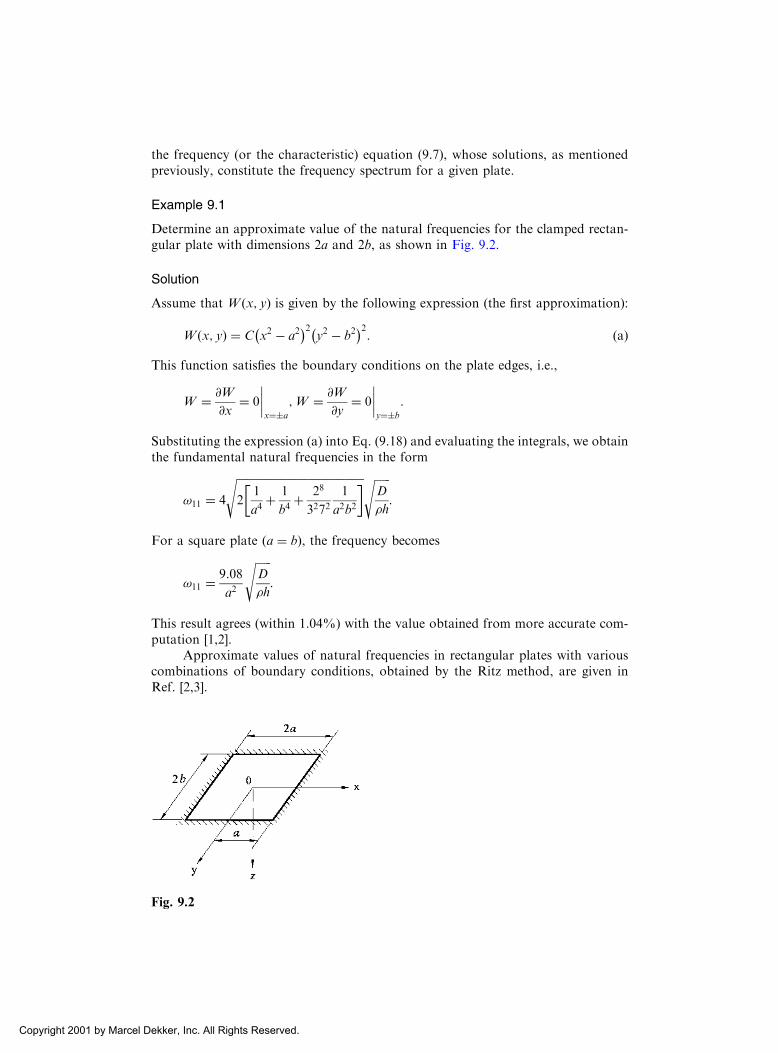
the frequency (or the characteristic) equation (9.7), whose solutions, as mentionedpreviously, constitute the frequency spectrum for a given plate.

Example 9.1

Determine an approximate value of the natural frequencies for the clamped rectan-gular plate with dimensions 2a and 2b, as shown in Fig. 9.2.

Solution

Assume that W x; yð Þ is given by the following expression (the first approximation):

W x; yð Þ ¼ C x2 � a2� �2

y2 � b2� �2

: ðaÞ

This function satisfies the boundary conditions on the plate edges, i.e.,

W ¼ @W

@x¼ 0

x¼�a

;W ¼ @W

@y¼ 0

y¼�b

:

Substituting the expression (a) into Eq. (9.18) and evaluating the integrals, we obtainthe fundamental natural frequencies in the form

!11 ¼ 4

ffiffiffiffiffiffiffiffiffiffiffiffiffiffiffiffiffiffiffiffiffiffiffiffiffiffiffiffiffiffiffiffiffiffiffiffiffiffiffiffiffiffiffiffiffiffi2

1

a4þ 1

b4þ 28

32721

a2b2

� �s ffiffiffiffiffiffiD

�h

s:

For a square plate a ¼ bð Þ, the frequency becomes

!11 ¼9:08

a2

ffiffiffiffiffiffiD

�h

s:

This result agrees (within 1.04%) with the value obtained from more accurate com-putation [1,2].

Approximate values of natural frequencies in rectangular plates with variouscombinations of boundary conditions, obtained by the Ritz method, are given inRef. [2,3].

Fig. 9.2


9.3.2 The Galerkin method

The Galerkin method, introduced in Sec. 6.5, also may be used for determining thenatural frequencies in vibrating plates. Assume again that a shape function for theplate is approximated by a series (9.20), which satisfies, term by term, all boundaryconditions. Then, following the general procedure of the Galerkin method (see Sec.6.5), the unknown coefficients Ci can be determined from the orthogonality con-ditions (6.37). For the vibration plate problems described by Eq. (9.6), the ortho-gonality conditions together with the expansion (9.20) result in the followingequation:

ð ðA

DXni¼1

Cir2r2Wi � �h!2Xni¼1

CiWi

!Wkdxdy ¼ 0; k ¼ 1; 2; . . . ; n:

ð9:22ÞThe numerical implementation of the above condition leads to the Galerkin

system of linear algebraic homogeneous equations of the form

a11C1 þ a12C2 þ . . . . . . . . . . . . . . . ¼ 0

. . . . . . . . . . . . . . . . . . . . . . . . . . . . . . . . . . . .

an1C1 þ an2C2 þ . . . . . . . . . . . . . . . ¼ 0;

ð9:23Þ

where

aik ¼ aki ¼ð ð

A

Dr2r2Wi � �h!2Wi

� �Wkdxdy: ð9:24Þ

This system of homogeneous equations has a nontrivial solution if its determinantmade up of the coefficients aik is equal to zero. The latter results in the nth ordercharacteristic equation (9.7) for determining the natural frequencies.

Let us represent the shape function Wðx; yÞ for a rectangular plate with dimen-sions a and b in the form

Wðx; yÞ ¼Xi

Xk

CikWikðx; yÞ; ð9:25Þ

where Cik are unknown coefficients representing the amplitudes of the free vibrationmodes and Wikðx; yÞ is the product of the pertinent eigenfunctions of lateral beamvibrations,

Wikðx; yÞ ¼ FiðxÞFkðyÞ; ð9:26Þwhich satisfy the prescribed boundary conditions on the edges x ¼ 0; x ¼ a; and y ¼0; y ¼ b. In Eq. (9.26), FiðxÞ and FkðyÞ represent the ith and kth modes of freelyvibrating beams with spans a and b, respectively.

Example 9.2

Determine the natural frequencies of the rectangular, simply supported plate of sidesa and b with a uniformly distributed mass m and with four concentrated masses M,as shown in Fig. 9.3.


Solution

We apply the Galerkin method for the solution of this problem. We modify slightlyEq. (9.24) for the coefficients aik of Galerkin’s system of equations, to the presentproblem, as follows:

aik ¼ aki ¼ð ð

A

Dr2r2Wi �m!2Wi

� �Wkdxdy�

XM!2WiWk; ð9:27Þ

where m andM are uniformly distributed and concentrated masses, respectively. Thedeflected surface of the vibrating plate is approximated by the series

W x; yð Þ ¼X1i¼1

X1k¼1

Cik sini�x

asin

k�y

b; ðaÞ

which satisfies the simply supported boundary conditions.

The first approximation

Retaining only the first term in the expansion (a), we obtain

a11 ¼ð ð

A

D@4W1

@x4þ 2

@4W1

@x2@y2þ @

4W1

@y4

!�m!2W1

" #W1dxdy� 4M!2W1:

ð9:28ÞIntroducing in the above W1 ¼ sinð�x=aÞ sinð�y=bÞ and substituting for a11 from(9.28) into the Galerkin equation (9.24), we obtain, after some operations, thisequation in the following form:

D�41

a2þ 1

b2

� �2

�m!2

" # ða0

ðb0

sin2�x

asin2

�y

bdxdy� 4M!2 1

4¼ 0: ðfÞ

Integrating Eq. (f) yields the following expression for the natural frequency:

! ¼ �21

a2þ 1

b2

� � ffiffiffiffiffiffiffiffiffiffiffiffiffiffiffiffiffiD

mþ 4Mab

vuut : ð9:29Þ

Fig. 9.3


Using more additional terms in Eq. (a), the ‘‘exact’’ value of the natural frequencymay be obtained. The application of the fourth approximation to this problem forthe square plate (a ¼ b) has shown that the refinement over the first approximationdoes not exceed 1.2%. Thus, the accuracy of the first approximation may be con-sidered as quite satisfactory.

9.4 FREE FLEXURAL VIBRATIONS OF CIRCULAR PLATES

Let us consider a freely vibrating, solid, circular plate of radius a, having a constantthickness h. Using the polar coordinates, r and ’, with the origin at the center of theplate, we can rewrite the governing differential equation of the free vibration ofplates, Eq. (9.3), as follows:

Dr2rr2

r wþ �h @2w

@t2¼ 0; ð9:30Þ

where r2r is the Laplace operator given by Eq. (4.5). Assume that the deflection of the

middle surface of the plate can be approximated as

w r; ’; tð Þ ¼ W r; ’ð ÞF tð Þ: ð9:31ÞIntroducing the above into Eq. (9.30), yields

DF tð Þr2rr2

rW þ �hW d2F

dt2¼ 0 or

Dr2rr2

rW

�hW¼ �

d2Fdt2

F: ð9:32Þ

Since the left-hand side of this equation is a function of variables r and ’ whereas theright-hand side depends only on time variable t, we can conclude that the ratios inthe left- and right-hand sides of Eq. (9.32) must be constant. Denote the afore-mentioned constant ratio on the right-hand side of Eq. (9.32) by !2, i.e.,

d2F

dt2¼ �!2F; ð9:33Þ

where ! is the natural frequency of vibrations. Solving this for F , yields

F ¼ A sin !tþ ’0ð Þ; ð9:34Þwhere ’0 is an arbitrary constant. The shape functionW r; ’ð Þ satisfies the differentialequation

Dr2rr2

rW

�hW¼ !2 or r2

rr2rW � �4W ¼ 0; ð9:35Þ

where

�4 ¼ !2�h

D: ð9:36Þ

Let us go from the variable r to the dimensionless variable � ¼ �r. Then, Eq. (9.35)becomes

@2

@�2þ 1

�

@

@�þ 1

�2@2

@’2

!2

W �W ¼ 0: ð9:37Þ


Its solution is of the following form [4,5]:

W r; ’ð Þ ¼ C1Jn �ð Þ þ C2In �ð Þ þ C3Yn �ð Þ þ C4Kn �ð Þ½ � sin n’þ ð Þ; ð9:38Þwhere n ¼ 0; 1; . . . ;1; C1; . . . ;C4 are constants of integration; and JnðÞ; InðÞ; YnðÞ;and KnðÞ are Bessel functions of the first and second kind of the real and imaginaryarguments, respectively [4,5], and is a constant. Since the origin of the polarcoordinate system is taken to coincide with the center of the circular plate havingno internal holes or supports at the center, the terms Yn �ð Þ and Kn �ð Þ must bediscarded ito avoid infinite deflections and stresses at r ¼ 0. When these simplifica-tions are employed, Eq. (9.38) becomes, for a typical mode,

W ¼ C1Jn �ð Þ þ C2In �ð Þ½ � sin n’þ ð Þ: ð9:39ÞAssume that the plate is clamped along its contour. The boundary conditions are

W ¼ @W

@r¼ 0

r¼a

ð9:40Þ

When Eq. (9.39) is substituted into the above boundary conditions, the existence of anontrivial solution yields the following characteristic determinant:

Jnð�Þ Inð�ÞJ 0nð�Þ I 0

nð�Þ

¼ 0; ð9:41Þ

where the primes are used to indicate a differentiation with respect to the argument,in this case to �. Using the following recursion relationships [4,5]:

�J 0n �ð Þ ¼ nJn �ð Þ � �Jnþ1 �ð Þ

�I 0n �ð Þ ¼ nIn �ð Þ þ �Inþ1 �ð Þ;

ð9:42Þ

and expanding Eq. (9.41) gives

Jn �ð ÞInþ1 �ð Þ þ In �ð ÞJnþ1 �ð Þ ¼ 0: ð9:43aÞThe eigenvalues � determining the frequencies ! are the roots of Eq. (9.43a). TheBessel functions are widely tabulated for small values of n [4].

For circular plates simply supported all around (w ¼ 0 and Mr ¼ 0), the fre-quency equation is of the form

Jnþ1ð�ÞJnð�Þ

þ Inþ1ð�ÞInð�Þ

¼ 2�

1� � : ð9:43bÞ

If a plate edge is completely free (Mr ¼ 0 and Vr ¼ 0), then the frequency equationcan be represented as follows (for � � n) [3]:

Jnð�ÞJ 0nð�Þ

ffi �2 þ 2ð1� �Þn2� �Inð�Þ=I 0

nð�Þ� �� 2�ð1� �Þ

�2 � 2ð1� �Þn2 ð9:43cÞ

For more information concerning the above problems, see Ref. [3].The natural frequencies and pertinent mode shapes for solid circular plates can

be also calculated by using the Ritz or Galerkin methods, as indicated in Sec. 9.3. Letus illustrate this procedure.


Example 9.3

Determine the fundamental natural frequency of axisymmetric vibrations of a solidcircular plate with radius R. The plate is clamped along its boundary.

Solution

We take the shape function in the first approximation as follows:

W ¼ C R2 � r2� �

:2 ðaÞEvidently, the above expression satisfies the given boundary conditions (w ¼ 0 and@w=@r ¼ 0) exactly. We apply the Ritz method. It can be shown that for circularplates with a fastened edge the expression for the potential energy (4.13) becomessimplified:

Umax ¼ð ð

A

D

2

@2W

@r2þ 1

r

@W

@rþ 1

r2@2W

@’2

!2

rdrd’: ð9:44aÞ

The corresponding expression for the kinetic energy in polar coordinates has theform

Kmax ¼!2

2

ð ðA

�hW2ðr; ’Þrdrd’: ð9:44bÞ

Substituting for W from Eq. (a) into expressions (9.44) and evaluating the corre-sponding integrals, one obtains

Umax ¼ C2D�

2R6 32

3and Kmax ¼

!2

2C2�R10 1

10�h: ðbÞ

Then, the fundamental natural frequency (the first approximation) may be foundfrom Eq. (9.18), as follows:

!11 ¼10:33

R2

ffiffiffiffiffiffiD

�h

s:

Notice that the second approximation of this frequency differs from the above valueby 1.175% only.

9.5 FORCED FLEXURAL VIBRATIONS OF PLATES

The equation of motion of plates under a variable, time-dependent, transverse loadp x; y; tð Þ is given by Eq. (9.2). A solution of the above nonhomogeneous, partialdifferential equation must satisfy the prescribed boundary and initial conditions. Anexact solution can be obtained by using the following procedure. First, let us solvethe problem of free vibrations of a plate, and determine the natural frequencies !mn

and the corresponding mode shapes Wmn. Then, let us introduce a load p x; y; tð Þ inthe form of series extended in eigenfunctions (the mode shapes), i.e.,

p ¼X1m¼1

X1n¼1

fmn tð ÞWmn x; yð Þ: ð9:45Þ


We seek a solution of Eq. (9.2) in the form

w ¼X1m¼1

X1n¼1

Fmn tð ÞWmn x; yð Þ: ð9:46Þ

The following equation takes place for the function Fmn:

€FFmn þ !2mnFmn ¼

1

�hfmn tð Þ; ð9:47Þ

from which

Fmn ¼ Amn cos!mntþ Bmn sin!mntþ F ðpÞmn tð Þ ð9:48Þ

and

w ¼X1m¼1

X1n¼1

Amn cos!mntþ Bmn sin!mntþ F ðpÞmn tð Þ

h iWmnðx; yÞ ð9:49Þ

where F ðpÞmn is a particular solution of Eq. (9.2); its form depends on fmn, i.e., how a

given load p varies with time. The constants Amn and Bmn are determined from initialconditions: namely, at t ¼ 0

w ¼ w0 x; yð Þ and@w

@t¼ v0 x; yð Þ: ð9:50Þ

Example 9.4

Determine the vibration modes for a simply supported rectangular plate with dimen-sions a and b. The plate is subjected to a surface transverse load varying asp ¼ p0 x; yð Þ cos�t, where � is the frequency of forced vibrations, which is equalto the frequency of a disturbing loading.

Solution

Let us expand an applied load into the series

pðx; y; tÞ ¼ cos�po x; yð Þ ¼ cos�tX1m

X1n

Amn sin mx sin ny; ð9:51Þ

where

Amn ¼4

ab

ða0

ðb0

p0ðx; yÞ sin mx sin nydxdy; m ¼ m�

a; n ¼

n�

b: ð9:52Þ

The deflected surface of the vibrating plate can be approximated by the series (9.46)where

Wmmðx; yÞ ¼ sin mx sin ny ð9:53ÞThe particular solution, F ðpÞ

mnðtÞ, may be found from Eq. (9.47) by letting fmnðtÞ ¼cos�t:

We obtain

F ðtÞmn ¼

1

�h

cos�t

!2mn ��2

ð9:54Þ


Substituting the above into Eq. (9.49) and evaluating the constants Amn and Bmn

from the assumption that the plate is at rest at the initial moment (i.e., att ¼ 0 w ¼ 0 and @!=@t ¼ 0), we obtain the following expression for the deflectedsurface of the vibrating plate:

w ¼ 1

�h

X1m¼1

X1n¼1

Amn

!2mn ��2

ðcos�t� cos!mntÞ sin mx sin ny ð9:55Þ

In the case when the load frequency � will coincide with any natural frequen-cies of the plate, the plate will vibrate in the resonance state. In fact, if for any m andn, � ¼ !mn, then the corresponding term of the series (9.55) becomes indetermined ofthe type 0=0. Evaluating this indeterminate form yields

wmn ¼1

�h

Amn

2!mn

t sin!mnt sin mx sin ny: ð9:56Þ

This expression represents a vibration with an amplitude that indefinitely increaseswith time.

If p0 ¼ const, then Amn ¼ 16p0=mn�2 for m ¼ 1; 3; 5 . . . ; n ¼ 1; 3; 5; . . .Eq. (9.55) will be of the form:

w ¼ 16p0�h�2

X1m¼1;3;...

X1n¼1;3;...

cos�t� cos!mnt

mnð!2mn ��2Þ sin mx sin ny ð9:57Þ

Here, we did not take into account the resistance of surrounding media andinternal friction. These factors can have a pronounced effect on the vibration pro-cess. As a result, the vibrations will have a gradually diminishing amplitude.

This chapter can serve only as introduction to the dynamic behavior of plates;for further analysis, the interested reader is referred to other works [1,3,6,7].

PROBLEMS

9.1 Consider free harmonic vibrations of a rectangular plate with simply supported edges

x ¼ 0 and x ¼ a. Determine the natural frequencies and associated mode shapes if

(a) the edges y ¼ 0 and y ¼ b are free, (b) the edges y ¼ 0 and y ¼ b are clamped,

(c) the edge y ¼ 0 is simply supported and the edge y ¼ b is free, and (d) the edge y ¼0 is simply supported and the edge y ¼ b is clamped. Use wðx; y; tÞ ¼ FðyÞsinðm�x=aÞ cos!t.

9.2 Determine an approximate value of the lowest natural frequency of a rectangular plate.

The edges x ¼ 0 and x ¼ a are built-in and the edges y ¼ 0 and y ¼ b are simply

supported. Use the Galerkin method. Take the shape function, Wðx; yÞ, in the form

of Eq. (9.25), where

FiðxÞ ¼ sin �ix� sinh �ix� aðcos �ix� cosh �ixÞ;FkðyÞ ¼ sin�ky; and �i ¼ i�=a; �k ¼ k�=b; i ¼ ð2nþ 1Þ=2; ðn ¼ 1; 2; . . .Þ

9.3 Redo Problem 9.1 by employing the Ritz method. Take Wðx; yÞ in the form

Wðx; yÞ ¼X1m¼1

X1n¼1

Amn 1� cos2m�x

a

� �sin

n�y

b:


9.4 Determine an approximate value of the fundamental natural frequency for a rectan-

gular plate. The edges y ¼ 0 and y ¼ b are simply supported while the edge x ¼ 0 is

clamped at the edge.

9.5 Consider free, axisymmetric harmonic vibrations of a circular solid plate with radius R.

Calculate the three lowest natural frequencies if (a) the plate edge r ¼ R is simply

supported and (b) the plate edge r ¼ R is clamped.

9.6 Determine the lowest natural frequency of the rectangular, simply supported plate of

sides a and b with a uniformly distributed mass m and with a concentrated mass M

applied at the plate center (x ¼ a=2 and y ¼ b=2).9.7 Determine the amplitude of the forced vibrations of a rectangular simply supported

plate of sides a and b. The plate is subjected to the following time-dependent, trans-

verse surface load:

p ¼ p0 sin�x

asin2

�y

asin �t:

.

9.8 For approximate description of elastic vibrations of a rectangular plate (0 � x � a;0 � y � b) with thickness h, this plate is replaced by a single degree of freedom system.

The mass of the plate is concentrated at the plate center. Determine the corresponding

reduction coefficient (mass factor), ensuring such an equivalent replacement if the plate

is simply supported and its deflection surface is approximated by the following expres-

sion that satisfies all the boundary conditions:

W ¼ A cos�x

2acos

�y

2b

(the origin of the coordinate system is taken at the plate center).

9.9 Redo Problem 9.8 for the plate clamped along edges x ¼ �a and y ¼ �b. Take W in

the form:

W ¼ A

a4b4x2 � a2� �2

y2 � b2� �2

:

REFERENCES

1. Nowacki, W., Dynamics of Elastic Systems, John Wiley and Sons, New York, 1963.

2. Warburton, G., The vibration of rectangular plates, Proc J Mech Engrs, vol. 168, No. 12,

pp. 371–384 (1954).

3. Leissa, A.W., Vibrations of Plates, National Aeronautics and Space Administration,

Washington, D.C., 1969.

4. Watson, G.N., Theory of Bessel Functions, 2nd. edn, Cambridge University Press,

Cambridge, 1944.

5. McLachlan, N., Bessel Functions for Engineers, Oxford Eng Sci Ser, Oxford University

Press, London, 1948.

6. Thomson, W.T., Vibration Theory and Applications, Prentice-Hall, Englewood Cliffs, New

Jersey, 1973.

7. Dill, E.N. and Pister, K.S., Vibration of rectangular plates and plate systems, Proc 3rd US

Natl Congr Appl Mech, pp. 123–132 (1958).


10

Introduction to the General ShellTheory

10.1 SHELLS IN ENGINEERING STRUCTURES

Thin shells as structural elements occupy a leadership position in engineering and, inparticular, in civil, mechanical, architectural, aeronautical, and marine engineering(Fig. 10.1). Examples of shell structures in civil and architectural engineering arelarge-span roofs, liquid-retaining structures and water tanks, containment shells ofnuclear power plants, and concrete arch domes. In mechanical engineering, shellforms are used in piping systems, turbine disks, and pressure vessels technology.Aircrafts, missiles, rockets, ships, and submarines are examples of the use of shellsin aeronautical and marine engineering. Another application of shell engineering isin the field of biomechanics: shells are found in various biological forms, such as theeye and the skull, and plant and animal shapes. This is only a small list of shell formsin engineering and nature.

The wide application of shell structures in engineering is conditioned by theirfollowing advantages:

1. Efficiency of load-carrying behavior.2. High degree of reserved strength and structural integrity.3. High strength : weight ratio. This criterion is commonly used to estimate a

structural component efficiency: the larger this ratio, the more optimal isa structure. According to this criterion, shell structures are much superiorto other structural systems having the same span and overall dimensions.

4. Very high stiffness.5. Containment of space.

In addition to these mechanical advantages, shell structures enjoy the unique posi-tion of having extremely high aesthetic value in various architectural designs.

Part II

Thin Shells


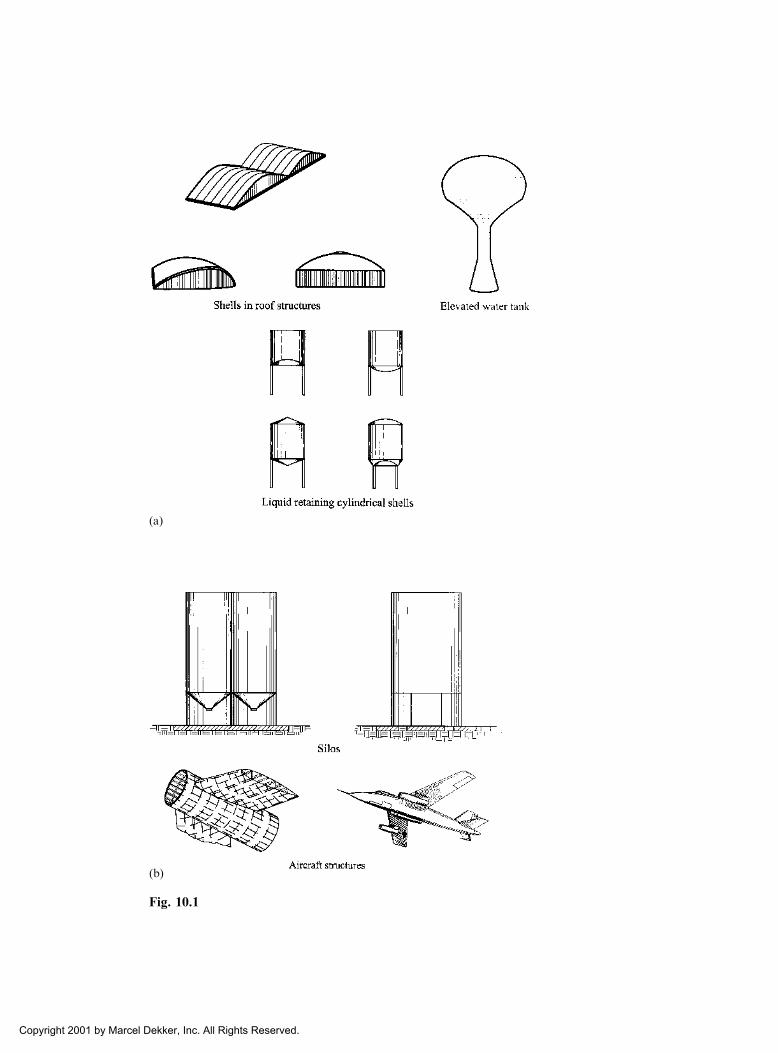
(a)

(b)

Fig. 10.1


Contemporary engineers using scientifically justified methods of design tend todevelop a structure that combines maximum strength, functional perfection, andeconomy during its lifetime. In addition, it is important that the best engineeringsolution ensues, other things being equal, at the expense of the selection of structuralform and by not increasing the strength properties of the structure, e.g., by increas-ing its cross section. Note that the latter approach is easier. Shell structures supportapplied external forces efficiently by virtue of their geometrical form, i.e., spatialcurvatures; as a result, shells are much stronger and stiffer than other structuralforms.

10.2 GENERAL DEFINITIONS AND FUNDAMENTALS OF SHELLS

We now formulate some definitions and principles in shell theory. The term shell isapplied to bodies bounded by two curved surfaces, where the distance between thesurfaces is small in comparison with other body dimensions (Fig. 10.2).

The locus of points that lie at equal distances from these two curved surfacesdefines the middle surface of the shell. The length of the segment, which is perpendi-cular to the curved surfaces, is called the thickness of the shell and is denoted by h.The geometry of a shell is entirely defined by specifying the form of the middlesurface and thickness of the shell at each point. In this book we consider mainlyshells of a constant thickness.

Shells have all the characteristics of plates, along with an additional one –curvature. The curvature could be chosen as the primary classifier of a shell becausea shell’s behavior under an applied loading is primarily governed by curvature (seeSec. 10.4). Depending on the curvature of the surface, shells are divided into cylind-rical (noncircular and circular), conical, spherical, ellipsoidal, paraboloidal, toroidal,and hyperbolic paraboloidal shells. Owing to the curvature of the surface, shells aremore complicated than flat plates because their bending cannot, in general, be sepa-rated from their stretching. On the other hand, a plate may be considered as a speciallimiting case of a shell that has no curvature; consequently, shells are sometimesreferred to as curved plates. This is the basis for the adoption of methods from thetheory of plates, discussed in Part I, into the theory of shells.

There are two different classes of shells: thick shells and thin shells. A shell iscalled thin if the maximum value of the ratio h=R (where R is the radius of curvatureof the middle surface) can be neglected in comparison with unity. For an engineeringaccuracy, a shell may be regarded as thin if [1] the following condition is satisfied:

Fig. 10.2


maxh

R

� �� 1

20: ð10:1Þ

Hence, shells for which this inequality is violated are referred to as thick shells. For alarge number of practical applications, the thickness of shells lies in the range

1

1000� h

R� 1

20;

i.e., in the range of thin shells, and therefore the theory of thin shells presented in thisbook is of great practical importance.

Note also that the inequality (10.1) defines very roughly the boundary betweenthin and thick shells. In reality, it depends also upon other geometrical parameters ofshells, the character of their boundary conditions, smoothness of a variation ofexternal loads over the shell surface, etc.

10.3 BRIEF OUTLINE OF THE LINEAR SHELL THEORIES

The most common shell theories are those based on linear elasticity concepts. Linearshell theories predict adequately stresses and deformations for shells exhibiting smallelastic deformations; i.e., deformations for which it is assumed that the equilibriumequation conditions for deformed shell surfaces are the same as if they were notdeformed, and Hooke’s law applies.

For the purpose of analysis, a shell may be considered as a three-dimensionalbody, and the methods of the theory of linear elasticity may then be applied.However, a calculation based on these methods will generally be very difficult andcomplicated. In the theory of shells, an alternative simplified method is thereforeemployed. According to this method and adapting some hypotheses (see Sec. 12.1),the 3D problem of shell equilibrium and straining may be reduced to the analysis ofits middle surface only, i.e. the given shell, as discussed earlier as a thin plate, may beregarded as some 2D body. In the development of thin shell theories, simplification isaccomplished by reducing the shell problems to the study of deformations of themiddle surface.

Shell theories of varying degrees of accuracy were derived, depending on thedegree to which the elasticity equations were simplified. The approximations neces-sary for the development of an adequate theory of shells have been the subject ofconsiderable discussions among investigators in the field. We present below a briefoutline of elastic shell theories in an historical context.

Love was the first investigator to present a successful approximation shelltheory based on classical linear elasticity [2]. To simplify the strain–displacementrelationships and, consequently, the constitutive relations, Love applied, to the shelltheory, the Kirchhoff hypotheses developed originally for the plate bending theory,together with the small deflection and thinness of the shell assumptions. This set ofassumptions is commonly called the Kirchhoff–Love assumptions. The Love theory ofthin elastic shells is also referred to as the first-order approximation shell theory. Inspite of its popularity and common character, Love’s theory was not free from somedeficiencies, including its inconsistent treatment of small terms, where some wereretained and others were rejected, although they were of the same order. This meantthat, for certain shells, Love’s differential operator matrix on the displacements, in


the equations of equilibrium, became unsymmetric. Obviously, this violated Betti’stheorem of reciprocity. Love’s theory also contained some other inconsistencies. Theneed for a mathematically rigorous two-dimensional set of the shell equationsemploying the Kirchhoff–Love assumptions led to different versions of the first-order approximation theories.

E. Reissner [3] developed the linear theory of thin shells (also the first-orderapproximation theory) where some inadequacies of Love’s theory were eliminated.He derived equations of equilibrium, strain–displacement relations, and stress resul-tants expressions for thin shells directly from the three-dimensional theory of elas-ticity, by applying the Love–Kirchhoff hypotheses and neglecting small terms oforder z=Ri (where Ri i ¼ 1; 2ð Þ are the radii of the curvature of the middle surface)compared with unity in the corresponding expressions.

Sanders [4] also developed the first-order-approximation shell theory from theprinciple of virtual work and by applying the Kirchhoff–Love assumptions. Sanders’theory of thin shells has removed successfully the inconsistencies of the Love theory.A version that retains terms of magnitude compatible with those retained byE. Reissner and resolves the inconsistency in the expression for twist was developedby Koiter [5].

Timoshenko’s theory of thin shells [6] was very close to the Love theory.General relations and equations were obtained by applying the Kirchhoff–Lovehypotheses and neglecting terms z=Ri in comparison with unity. Naghdi [7,8] ana-lyzed the accuracy of the Love–Kirchhoff theory of thin elastic shells.

A second class of thin elastic shells, which is commonly referred to as higher-order approximation, has also been developed. To this grouping it is possible toassign all linear shell theories in which one or another of the Kirchhoff–Lovehypotheses are suspended. First, we consider some representative theories in whichthe thinness assumption is delayed in derivation while the rest of the postulates areretained. In this case, the order of a particular approximate theory will be establishedby the order of the terms in the thickness coordinate that is retained in the strain andconstitutive equations.

Lur’ye [9], Flugge [10], and Byrne [11] independently developed the second-order approximation theory of shells. The general relations and equations of thistheory are the direct result of the application of the Kirchhoff hypotheses togetherwith the small-deflection assumption to the corresponding equations of the three-dimensional theory of elasticity. The second-order approximation theory attempts amore careful discard of terms z=Ri. It retains these terms in comparison with unity inthe strain–displacement relations and stress resultant equations. Applications of thistheory have generally been restricted to circular cylindrical shells. In addition, thegeneral relations and equations of this second-order approximation shell theory arefound to be cumbersome for application.

Novozhilov [1] developed another version of the second-order approximationtheory. Just as Lur’ye–Flugge–Byrne theory, he obtained the strain–displacementrelations from the three-dimensional theory of elasticity by applying Kirchhoff’sassumptions. Then, he made use of the strain energy expression to derive the for-mulas for the stress resultants and couples (again by applying the Kirchhoff hypoth-eses) and for determining the terms to be disregarded. Novozhilov developed thecriterion for simplifying the governing equations and relations of the general theoryof thin shells based on Kirchhoff’s hypotheses. He proved that the errors introduced


by Kirchhoff’s assumptions into the small-deflection shell theory were of the orderh=Ri in comparison with unity [12].

Valuable contributions to the general theory of thin shells were given byGol’denveizer [13]. He was the first to formulate the conditions for compatibilityof strain components in the general theory of shells.

The second-order approximation equations were derived by Vlasov [14]directly from the general three-dimensional linear elasticity equations for a thickshell. The assumption that the transverse normal and shear strain componentsmay be neglected for thin shells was made, and the remaining strains were repre-sented by the first three terms of their series expansion. The assumption of zerotransverse normal strain as well as zero transverse shear strains permits a rapidtransition from the three-dimensional theory to the two-dimensional equations ofthe thin shell theory.

Another class of second-order approximation theories appeared in which theassumptions on the vanishing of the transverse normal strain and on the preserva-tion of the normals was abandoned. Such theories, which incorporated the trans-verse shear and normal stress effects, were proposed by E. Reissner [15,16], Naghdi[17], and others. A comprehensive analysis of the first- and higher-order approxima-tion theories and of the corresponding governing equations for elastic shells wasmade by Kraus [18], Leissa [19], etc.

The small-defection shell theories discussed above were formulated from theclassical linear theory of elasticity. It is known that the equations of these theories,which are based on Hooke’s law and the omission of nonlinear terms in both theequations for strain components and equilibrium equations, have a unique solutionin every case. In other words, a linear shell theory determines a unique position ofequilibrium for every shell with prescribed load and constraints. In reality, however,a solution of physical shell problems is not always unique. A shell under identicalconditions of loading and constraints may have several possible positions of equili-brium. A theory that takes into account finite or large deformations is referred to asa geometrically nonlinear theory of thin shells. Additionally, a shell may be physicallynonlinear with respect to the stress–strain relations.

E. Reissner [20] derived a nonlinear theory of symmetrically loaded shells ofrevolution. In this theory, the small-deflection assumption was abandoned while theremaining assumptions of the general higher-order approximation theories wereretained. Derivations of a more general geometrically nonlinear theory of thin shellshave been carried out by Naghdi and Nordgren [21], Sanders [22], and Koiter [23].Vlasov [14] derived a set of equations for nonlinear shallow shells. From theseequations, as a particular case, von Karman equations describing finite deformationsfor plates, discussed in Sec. 7.4, followed. A subsequent development of the generalnonlinear theory of thin shells has been made by Mushtari and Galimov [24],Simmonds and Danielson [25], etc.

A number of specialized shell theories were developed to include features ofspecial types of shells, in parallel with the evolution of the general theories of thinshells discussed above. The factors influencing the assumptions and domains ofapplications of these specialized shell theories have been a shell geometry, the defor-mation ranges, the loading and stress conditions, the particular shell behaviordesired, etc. Most of these theories are based on Love’s first-order approximation.


The membrane theory of thin shells may be presented as the first example ofsuch a type of the specialized shell theory. The general form of the governing equa-tions of the membrane theory of thin shells was established by Beltrami [26] andLecornu [27] in the last century. The membrane theory of shells was intensivelyevolving. H. Reissner [28] developed the membrane theory of thin shells of revolu-tion under unsymmetric loads. Sokolovskii [29] reduced the equations of the mem-brane theory to canonical form and revealed a number of their characteristicproperties. Pucher [30] discovered the usefulness of Airy’s stress function for thesolution of membrane problems in shells of an arbitrary form.

Another example of the specialized shell theory is the theory of shallow shells.Donnel [31], Vlasov [14], and Mushtari [32] independently developed a simplifiedengineering theory of thin shells of a general form. Due to their simplicity, thegoverning equations of this theory were found to be extremely convenient for solvingmany engineering shell problems. Apart from the Kirchhoff–Love hypotheses, someadditional assumptions that simplify the strain–displacement relations, equilibrium,and compatibility equations were used in deriving these equations. It turned out thatthe Donnel–Vlasov–Mushtari theory could be applied with sufficient accuracy toshallow shells. Shallow shells have geometries that are close to that of a thinplate. Such shells have a wide application in engineering, for example in roof struc-tures, which have a relatively small rise compared with their span. Notice that theabove-mentioned theory may also be applied to non-shallow shells whose state ofstress is characterized by rapidly varying stress components along the coordinates ofthe middle surface. Shallow shells are commonly referred to as curved plates.Marguerre established the governing equations for plates having an initial curvature[33].

Shells of revolution, a very important class of thin shells, have many technicalapplications in engineering. The theory of thin shells of revolution may serve as onemore example of the specialized shell theories. H. Reissner presented a classicalformulation of the bending problems for a shell of revolution [28] and studied aspherical shell under axisymmetric bending. He reduced the differential equations ofthe spherical shell to a convenient form and then applied the asymptotic method fortheir integration. Meissner [34] was able to generalize Reissner’s results to symme-trical deformation of shells of revolution of an arbitrary shape and having a variablethickness. Hoff [35] analyzed circular conical shells under an arbitrary loading.Flugge gave general solutions for spherical and conical shells subjected to asymme-trical loading [36]. His approach was based on the classical displacement method.

Wissler analyzed toroidal shells [37]. By convention, cylindrical shells are fre-quently considered apart from the shells of revolution, although they technically fallinto this class of shells. The analysis of cylindrical shells for general surface loadingoccupies a prominent place in the literature because of their wide practical signifi-cance and the relative simplicity of the theory. We should mention that Fluggederived the governing differential equations for circular cylindrical shells in termsof displacements [36]. Parkus derived the equations for a cylinder of an arbitrarycross section [38]. It should be noted that radical simplifications underlying therelations and equations of the general theory of cylindrical shells were introducedby Donnel [31], Dishinger [39], Hoff [40], and Vlasov [14]. Novozhilov [1] derived thegoverning differential of the general theory of cylindrical shells of an arbitrary shape


using complex variables and pointed out some possible simplifications of these equa-tions.

The concept of the edge effect, introduced first by Love [2], applied to shells ofrevolution, is of greatest importance in an engineering analysis of thin shells. Loveshowed that a first approximation to a general solution might be obtained in theform of the sum of the solutions of the membrane equations and the equations forthe edge effect. Integrals of the latter equations are expressed in terms of rapidlyvarying functions. Gol’denveizer [13] defined the conditions for which the rapidlydecaying solutions of the equations of the general shell theory may be obtained, andanalyzed a number of possible special cases. Geckeler [41] applied this concept tosymmetrically loaded spherical shells. His approximate method was based on thereduction of the system of the two-coupled differential equations to two independentdifferential equations, assuming that for very thin shells the derivatives of the givenfunctions will be greater than the functions themselves.

Shell buckling problems have been a subject of investigations by many scien-tists and engineers. For a circular cylindrical shell subjected to a uniform compres-sive axial load, the differential equations have been formulated and solutions havebeen found by Lorentz [42] and Timoshenko [43]. Mises [44] and Mushtari andSachenkov [45] treated a linear buckling problem for cylindrical shells subjected tocombined loading (external pressure and axially applied compressive forces). Thecombined effect of axial and internal pressure was studied by Flugge [36] for cylind-rical shells. It should be noted that, unlike the plate bending problems, a theoreti-cally determined buckling load, calculated by the small-deflection theory, is rarelyattained or even approached in experiment. It was shown that initial imperfectionswere the most influential contributor to the discrepancy between theoretical andexperimental results in determining the buckling loads. Donnel and Wan [46] derivedthe general equations and analyzed the effect of imperfections on the buckling of thincylindrical shells under uniform, axial compressive forces.

The buckling problem for a spherical shell under an external pressure waspresented by Zoelly [47] in linear and by von Karman and Tsien [48] in nonlinearformulations, respectively. Koiter [49] analyzed the postbuckling behavior of acylindrical shell under axial compression. Buckling of shallow shells under normalsurface load was studied by Budansky [50] (linear problem) and Kaplan and Fung[51] (nonlinear problem).

Equations of motion for the vibration analysis of shells may be derived as asimple extension of the static case by adding the inertia forces to body forces andbody moment terms that result from accelerations of the mass of the shell accordingto the D’Alambert principle. The equations of free vibrations of thin elastic shellswere first derived by Love [2]. Then, the equations of motion for shells of variousshape according to the first- and higher-order approximations were presented byKraus [18], Flugge [52], Epstein [53], etc. Analysis of various equations of motionof thin elastic shells, as well as a comprehensive presentation of available results forfree vibration frequencies and mode shapes which can be used for design was madeby Leissa [19].

This historical survey is aimed at only providing a brief background on theformation of the shell theory. The interested reader who wants to be moreacquainted with the shell’s history in more details is referred to other works[1,18,19,36].


10.4 LOADING-CARRYING MECHANISM OF SHELLS

The general theories of beams, arches, plates, and shells are usually based upon theunified set of assumptions. However, the load–resistance mechanisms of these mem-bers do not resemble one another. The load–resistance mechanism of flat plates wasdiscussed in Secs 1.1 and 1.3. We can say that shells fall into a class of plates asarches relate to straight beams under the action of transverse loading. It is knownthat the efficiency of the arch form lies primarily in resisting the transverse load witha thrust N, thus minimizing the shear force V and bending moment M. It is possibleto specify the arch shape and the manner of its loading in such a way that the archdoes not experience bending at all. In this case, the arch is in the so-called moment-less state of stress. For example, for a parabolic arch, bending will not be induced bya vertical load uniformly distributed over its chord. Thus, the ability of arches tosupport certain transverse loads without bending is the reason for their structuraladvantage over straight beams.

A shell mainly balances an applied transverse load, much like an arch, bymeans of tensile and compressive stresses, referred to as the membrane or directstresses. These stresses are uniformly distributed over the shell thickness. Such astate of stress is called the momentless or membrane state of stress. Although theshear force and bending and twisting moments are still present in the general case ofloading, the efficiency of the shell form rests with the presence of the membranestresses, as the primary means of resistance with the bending stress resultants andcouples are minimized. Thus, shells, like arches over beams, possess an analogousadvantage over plates; however, with the following essential difference – while anarch of a given form will support only one completely determined load without bending,a shell of a given shape has, provided its edges are suitably supported, as a rule, thesame property for a wide range of loads which satisfy only very general requirements.

The membrane stress condition is an ideal state at which a designer should aim.It should be noted that structural materials are generally far more efficient in anextensional rather in a flexural mode because:

1. Strength properties of all materials can be used completely in tension (orcompression), since all fibers over the cross section are equally strainedand load-carrying capacity may simultaneously reach the limit for thewhole section of the component.

2. The membrane stresses are always less than the corresponding bendingstresses for thin shells under the same loading conditions.

Thus, the momentless or membrane stress conditions determine the basic advantagesof shells compared with beams, plates, etc.

The highest efficiency of a shell, as a structural member, is associated with itscurvature and thinness. Owing to the shell curvature, the projections of the directforces on the normal to the middle surface develop an analog of an ‘‘elastic founda-tion’’ under the shell. So, it can be said that a shell resists an applied transverseloading as a flat plate resting on an elastic foundation. This phenomenon can explainan essential increase in strength and stiffness of a shell compared with a plate. Thus,as a result of the curvature of the surface, a shell acquires a spatial stiffness that givesto it a larger load-carrying capacity and develops the direct stresses. Owing to its


thinness, a shell may balance an applied transverse loading at the expense of themembrane stresses mainly, with bending actions minimized.

Note that the pure bending conditions have no advantages and should beavoided because shells, in view of their small thickness, possess a low strength forthis deformation. However, sometimes bending conditions cannot be avoided. Itturns out that strong severe bending conditions are localized only in a small domainnear some discontinuities in loading and geometrical conditions, as well as nearsupports, etc. As we move away from such a disturbance zone, the bending stresseswill diminish rapidly and a considerable part of the shell will be in the momentlessstress condition. Therewith, the thinner the shell the faster this decrease of bendingstresses.

As mentioned above, shell thinness demonstrates the high efficiency of shells. Itis associated with the shell’s low weight and simultaneously its high strength.However, a shell’s thinness is, at the same time, a weak point because all the advan-tages mentioned earlier hold for a tensile state of stress. In this case, a shell materialis stretched and its strength properties are used completely. On the other hand, athinness of shells manifests itself in compression. External forces, as before, areeffectively transformed in the constant membrane stresses over the shell thickness.However, the trouble is that the level of the critical stresses at buckling be sufficientlylow. This level is just determined by the shell thickness. The thinner the shell, thelower is the level of the critical stresses. The latter can be many factors smaller thanthe proportional limit of the shell material. In this case, the efficiency of thin shellscan be reduced considerably. To avoid the possibility of buckling, a shell structureshould be designed in such a way that a dominant part of the structure is in tension.

REFERENCES

1. Novozhilov, V.V., Theory of Thin Elastic Shells, 2nd edn, P. Noordhoff, Groningen,

1964.

2. Love, A.E.H., A Treatise on the Mathematical Theory of Elasticity, 1st edn, Cambridge

University Press, 1892; 4th. edn, Dover, New York, 1944.

3. Reissner, E., A new derivation of the equations of the deformation of elastic shells, Am J

Math, vol. 63, No.1, pp. 177–184 (1941).

4. Sanders, J.L., An Improved First Approximation Theory for Thin Shells, NASA TR-R24,

1959.

5. Koiter, W.T., A consistent first approximation in the general theory of thin elastic shells,

Proc. Symp. on Theory of Thin Elastic Shells (Delft, August 1959), North-Holland,

Amsterdam, pp. 12–33 (1960).

6. Timoshenko, S. and Woinowsky-Krieger, S., Theory of Plates and Shells, McGraw-Hill,

New York, 1959.

7. Naghdi, P.M., A survey on resent progress in the theory of thin elastic shells, Appl Mech

Revs, vol, 9, pp. 365–368 (1956).

8. Naghdi, P.M., Foundations of elastic shell theory. In: Progress in Solid Mechanics (eds

I.N. Sneedon and R. Hill), North-Holland, Amsterdam, IV, Chapter 1, 1963.

9. Lur’ye, A.I., General theory of elastic shells, Prikl Mat Mekh, vol. 4, No. 4, pp. 7–34

(1940) (in Russian).

10. Flugge, W., Stresses in Shells, 2nd edn, Springer-Verlag, Berlin, 1962.

11. Byrne, R., Theory of small deformations of a thin elastic shell, Seminar Reports in Math,

University of California, Publ in Math, N.S., vol. 2, No. 1, pp. 103–152 (1944).


12. Novozhilov, V.V. and Finkelshtein, R.O., On the error in Kirchhoff’s hypothesis in the

theory of shells, Prikl Mat Mekh, vol. 7, No. 5, pp. 35–46 (1943) (in Russian).

13. Gol’denveizer, A.L., Theory of Thin Shells, Pergamon Press, New York, 1961.

14. Vlasov, V.Z., General Theory of Shells and its Applications in Engineering, NASA TT F-

99, 1964.

15. Reissner, E., Stress strain relations in the theory of thin elastic shells, J Math Phys, vol.

31, pp. 109–119 (1952).

16. Reissner, E., On the theory of thin elastic shells, H. Reissner Anniv Vol, J.W. Edwards,

Ann Arbor, pp. 231–247 (1949).

17. Naghdi, P.M., On the theory of thin elastic shells, Q Appl Math, vol. 14, pp. 369–380

(1957).

18. Kraus, H., Thin Elastic Shells, John Wiley and Sons, New York, 1967.

19. Leissa, A.W., Vibrations of Shells, NASA SP-288, Washington, DC, 1973.

20. Reissner, E., On axisymmetrical deformation of thin shells of revolution, Proc Symp

Appl Math, vol. 3, pp. 27–52 (1950).

21. Naghdi, P.M. and Nordgren, R.P., On the nonlinear theory of shells under the Kirchhoff

hypothesis, Q Appl Math, vol. 21, pp. 49–60 (1963).

22. Sanders, J.L., Nonlinear theories for thin shells, Q Appl Math, vol. 21, pp. 21–36 (1963).

23. Koiter, W.T., The stability of elastic equilibrium (Chapter 5: Shell theory for finite

deflections), Diss, Tech Rept, AFFDL-TR-70-25, Air Force System Command, Wright-

Patterson AFB, 1970.

24. Mushtari, Kh.M. and Galimov, K.Z., Nonlinear Theory of Thin Shells, The Israel

Program for Scientific Translations, Jerusalem, 1961.

25. Simmonds, J.G. and Danielson, D.A., Nonlinear shell theory with finite rotation and

stress-function vectors, J Appl Mech, vol. 39, pp. 1085–1090 (1972).

26. Beltrami, E., Sull’equilibrio delle supperficial flessibili ed inestendibili, Mem R, Acad Sci

di Bologna, 1881.

27. Lecornu, L., Sur l’equilibre des surfaces flexible et inextendibles, J de L’Ecole

Polytechnique, c. XLVIII.

28. Reissner, H., Spaunnungen in Kugelschalen, Muller-Breslau-Festschrift, Leipzig, 1912.

29. Sokolovskii, V.V., Momentless shells of revolution, Prikl Mat Mekh, vol. 1, No. 3, pp.

81–88 (1938) (in Russian).

30. Pucher, A., Uber den spannungszustand in gekrummten flachen, Beton u Eisen, vol. 33,

pp. 298–304 (1934).

31. Donnel, L.H., Beams, Plates, and Shells, McGraw-Hill, New York, 1976.

32. Mushtari, Kh.M., Certain generalizations of the theory of thin shells, Izv Fiz Mat O-va

pri Kazan Un-te, vol. 11, No. 8 (1938) (in Russian).

33. Marguerre, K., Zur theorie der gekrummten platten grosser formanderung, Proc 5th Int

Congr Appl Mech, Cambridge, Mass., pp. 93–101 (1939).

34. Meissner, E., Das elastizitatsproblem fur dunne schalen von ringflachen, Kugel-und

Kegelvj-Schr Naturf Ges, Zurich, vol. 60, pp. 23–47 (1915).

35. Hoff, N.J., Thin circular conical shells under arbitrary loads, J Appl Mech, vol. 22, pp.

557–562 (1955).

36. Flugge, W., Die Stabilitat der Kreiszylinderschale, Ing-Arch, vol. 3, pp. 463–506 (1932).

37. Wissler, H., Festigkeitsberechnung von Ringflachenschalen, Diss, Zurich, 1916.

38. Parkus, H., Die Grundleichungen der allegemeinen zylinderschale, Osterr Ing-Arch, vol.

6, pp. 30–35 (1951).

39. Dishinger, F., Die strenge berechnung der kreiszylinderschale in ihrer anwendung auf die

Zeics-Dywidag-Schalen, Beton u. Eisen, vol. 34, pp. 257–264, 283–294 (1935).

40. Hoff, N.J., Boundary value problems of thin-walled circular cylinders, J Appl Mech, vol.

21, pp. 343–350 (1954).

41. Geckeler, J., Die festigkeit achsensymmetrischer schalen, Ing Arch, Bd. 1, 1930.


42. Lorentz, R., Die nichtachsensymmetrische knickung dunnwandiger hohlzylinder, Phys

Z, vol. 12, pp. 241–260 (1911).

43. Timoshenko, S.P. and Gere, J., Theory of Elastic Stability, McGraw-Hill, New York,

1961.

44. Mises, R., Der kritische aubendruck fur alldeits belastete cylindrischer rohre, Festschr

Zum 70 Geburtstag von prof A Stodola, Zurich, pp. 418–432 (1929).

45. Mushtari, Kh.M. and Sachenkov, A.V., A stability of cylindrical and conical shells of

circular cross sections under axial compression and external normal pressure, Prikl Mat

Mekh, vol. 18, No. 6, pp. 667–674 (1954).

46. Donnel, L.H. and Wan, C.C., Effect of imperfection on the buckling of thin cylinders

and columns under axial compression, J Appl Mech, vol. 17, No. 1, pp. 73–83 (1950).

47. Zoelly, R., Uber ein Knickungsproblem an der Kugelschale, Diss, Zurich, 1915.

48. Von Karman, T. and Tsien, H.S., The buckling of thin cylindrical shells under elastic

compression, J Aeronaut Sci, vol. 8, pp. 303–312 (1941).

49. Koiter, W.T., Buckling and Postbuckling Behavior of a Cylindrical Panel under Axial

Compression, Nat Luchtvaart Laboratory, Report No. 476, Amsterdam, 1956.

50. Budansky, B., Buckling of clamped shallow spherical shells, Proc IUTAM Symposium on

the Theory of Thin Elastic Shells, Amsterdam, pp. 64–94 (1960).

51. Kaplan, A. and Fung, Y.C., A Nonlinear Theory of Bending and Buckling of Thin Elastic

Shallow Spherical Shells, NASA TN 3212, 1954.

52. Flugge, W., Static und Dynamik der Schalen, Julius Springer, Berlin, 1934.

53. Epstein, P.S., On the theory of elastic vibrations in plates and shells, J Math Phys, vol.

21, pp. 198–209 (1942).


11

Geometry of the Middle Surface

11.1 COORDINATE SYSTEM OF THE SURFACE

A surface � can be defined as a locus of points whose position vector, r, directedfrom the origin 0 of the global coordinate system, OXYZ, is a function of twoindependent parameters and (see Fig. 11.1).

The parametric representation of the surface can be given, as follows:

in vector form as r ¼ r ; ð Þ; ð11:1Þor

in scalar form as X ¼ X ; ð Þ; Y ¼ Y ; ð Þ; Z ¼ Z ; ð Þ; ð11:2Þwhere X ; ð Þ; Y ; ð Þ; and Z ; ð Þ are some definite, continuous, and single-valuedfunctions of two variable coordinates and . If we eliminate the parameters and from Eqs (11.2), then the equation of the surface becomes

F X;Y;Zð Þ ¼ 0: ð11:3ÞThe parametric equation (11.1) may also be written in the form

r ¼ X ; ð Þiþ Y ; ð Þjþ Z ; ð Þk; ð11:4Þin which i; j; and k are unit vectors along the X;Y; and Z axes, respectively.

We assume that there is a one-to-one correspondence between the pairs ofnumbers (; ) belonging to � and points of the surface. Therefore these parameters, and , can be called curvilinear coordinates of a given surface. If one of the coordi-nates, e.g., , is incremented ¼ 1; ¼ 2; . . . ; ¼ n, we define a series of para-metric curves on the surface, along which only a parameter varies. These curves aretermed the -coordinate lines. Similarly, if a parameter takes on the values ¼ 1; ¼ 2; . . . ; ¼ n, we obtain the -coordinate lines.


If the - and -coordinate lines are mutually perpendicular at all points on asurface � (i.e., the angles between the tangents to these lines are equal to 90), thecurvilinear coordinates are said to be orthogonal. Orthogonal curvilinear coordinatesare used extensively in this book.

The derivatives of the position vector r with respect to the curvilinear coordi-nates and are given by the following:

@r

@¼ r; and

@r

@¼ r; ; ð11:5Þ

where we have introduced the comma notation to denote partial derivatives withrespect to and ; r; and r; are the tangent vectors at any point of the surface tothe - and -coordinate lines, respectively (Fig. 11.1). Indeed, since and are scalarquantities, the directions of vectors r; and r; coincide with directions of the vectordr. This vector dr points to the chords joining pointsM and N for r;, andM and N1

for r;. In the limit, as �! 0 and �! 0, these chords approach the tangents at apointM along the coordinate lines and , respectively. Since the latter are assumedto be orthogonal, then

r; �r;¼ 0: ð11:6Þ

11.2 PRINCIPAL DIRECTIONS AND LINES OF CURVATURE

Consider a small region of a smooth surface � near a typical point M. By ‘‘smooth’’we mean that the surface is continuous, and contains no discontinuities of slope, i.e.,creases or vertices. If we draw various curves along the surface � through point M,then the tangents to these curves are placed on one plane called the tangent plane tothe surface at M (plane P in Fig. 11.2). A line that is perpendicular to the tangentplane and passes through point M is called the normal to the surface � at point M,and it is denoted by n. Since the surface is smooth (as defined above), the tangentplane and, hence, the normal are uniquely determined.

A normal section of the surface � at point M can be defined as the section bysome plane containing a normal to the surface at that point. Such a section repre-

Fig. 11.1


sents a plane curve. Obviously, an infinite number of different normal sections maybe drawn through point M of surface � (sections aa; bb; cc; etc., in Fig. 11.3)

Consider one of such normal sections as a plane curve, as shown in Fig. 11.4.The position of a point M on the curve is determined by a single arc length coordi-nate s, measured from a suitable datum point. Let M and M1 be two neighboringpoints defining a short arc of length ds. At M and M1 the normals OM and OM1 aredrawn to the curve (there is only one normal at each point, since the curve is smooth)and they are inclined with respect to a suitable datum direction at angles � and�þd�, respectively. Assume that the two normals intersect at a point O (the centerof curvature of the arc). The center of curvature is defined strictly in terms of alimiting process in which ds ! 0. The length OM (i.e., the distance from the centerof curvature to point M) is called the radius of curvature, �, of the given curve atpoint M.

It follows by simple trigonometry from the above description that

� ¼ ds

d�: ð11:7aÞ

Fig. 11.2

Fig. 11.3


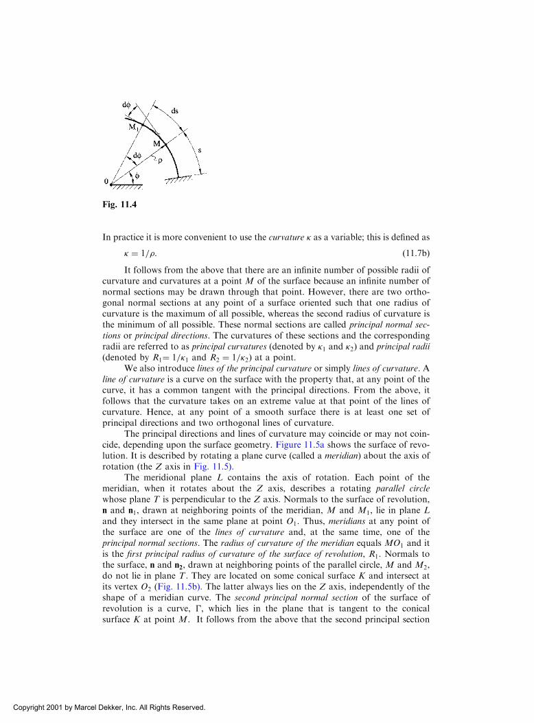
In practice it is more convenient to use the curvature � as a variable; this is defined as

� ¼ 1=�: ð11:7bÞIt follows from the above that there are an infinite number of possible radii of

curvature and curvatures at a point M of the surface because an infinite number ofnormal sections may be drawn through that point. However, there are two ortho-gonal normal sections at any point of a surface oriented such that one radius ofcurvature is the maximum of all possible, whereas the second radius of curvature isthe minimum of all possible. These normal sections are called principal normal sec-tions or principal directions. The curvatures of these sections and the correspondingradii are referred to as principal curvatures (denoted by �1 and �2) and principal radii(denoted by R1¼ 1=�1 and R2 ¼ 1=�2) at a point.

We also introduce lines of the principal curvature or simply lines of curvature. Aline of curvature is a curve on the surface with the property that, at any point of thecurve, it has a common tangent with the principal directions. From the above, itfollows that the curvature takes on an extreme value at that point of the lines ofcurvature. Hence, at any point of a smooth surface there is at least one set ofprincipal directions and two orthogonal lines of curvature.

The principal directions and lines of curvature may coincide or may not coin-cide, depending upon the surface geometry. Figure 11.5a shows the surface of revo-lution. It is described by rotating a plane curve (called a meridian) about the axis ofrotation (the Z axis in Fig. 11.5).

The meridional plane L contains the axis of rotation. Each point of themeridian, when it rotates about the Z axis, describes a rotating parallel circlewhose plane T is perpendicular to the Z axis. Normals to the surface of revolution,n and n1, drawn at neighboring points of the meridian, M and M1, lie in plane Land they intersect in the same plane at point O1. Thus, meridians at any point ofthe surface are one of the lines of curvature and, at the same time, one of theprincipal normal sections. The radius of curvature of the meridian equals MO1 and itis the first principal radius of curvature of the surface of revolution, R1. Normals tothe surface, n and n2, drawn at neighboring points of the parallel circle, M and M2,do not lie in plane T . They are located on some conical surface K and intersect atits vertex O2 (Fig. 11.5b). The latter always lies on the Z axis, independently of theshape of a meridian curve. The second principal normal section of the surface ofrevolution is a curve, �, which lies in the plane that is tangent to the conicalsurface K at point M. It follows from the above that the second principal section

Fig. 11.4


and parallel circle have a common tangent at point M. Thus, the parallel circles ofthe surface of revolution represent the second lines of curvature but they are not thesecond principal normal sections or principal directions. The generator MO2 of theconical surface K is the second principal radius of curvature of the surface ofrevolution, R2. This radius is numerically equal to the distance along a normalto the meridian curve from a point of interest of this curve to the axis of rotation(the Z axis).

In Sec. 11.1 we made no special assumptions about the curvilinear coordinatesof a shell middle surface. However, from now on we assume that the coordinate lines and are the lines of curvature. This system of the coordinate lines has particularlysimple properties, so that the equations of the theory of shells acquire a relativelysimple form in this system. To be able to use the corresponding formulas of thegeneral theory of shells, knowledge of the lines of curvature is required, and thedetermination of these curves for a given surface is, in general, a fairly complicatedproblem. However, for many of types of shells used in practice, the geometry of themiddle surface is of a simple nature (e.g., surfaces of revolution, cylindrical surfaces,etc.), so that the lines of curvature are already known.

11.3 THE FIRST AND SECOND QUADRATIC FORMS OF SURFACES

Let us study a surface � of an arbitrary geometry near typical point M, as shown inFig. 11.6. Consider two points Mð; Þ and M1ðþ d; þ dÞ arbitrarily near toeach other and both lying on the surface. Let their position vectors be r and rþ dr,respectively.

Determine the length of the arc ds joining the points M and M1 on the surface.In the limit, ds approaches drj j, where drj j is the modulus of the increment in thevector r going from point M to point M1, as defined by

dr ¼ r; dþ r; d: ð11:8Þ

Fig. 11.5


The square of this differential of the arc length is

ds2 ¼ drj j2¼ dr � dr ¼ r; �r; dð Þ2þ2r; �r; ddþ r; �r; dð Þ2: ð11:9ÞDenoting

a11 ¼ ðr; �r; Þ; a12 ¼ ðr; �r; Þ; a22 ¼ ðr; �r; Þ; ð11:10Þwe can rewrite Eq. (11.9), as follows:

ds2 ¼ a11ðdÞ2 þ 2a12ddþ a22ðdÞ2: ð11:11ÞThe expression on the right-hand side of this equation is called the first quadraticform of the surface defined by the vector rð; Þ and aik ði; k ¼ 1; 2Þ are the coefficientsof that form.

If the coordinate lines and form an orthogonal net, then r; �r;¼ 0 and,hence, a12 ¼ 0. Denoting

A ¼ ða11Þ1=2; B ¼ ðb11Þ1=2; ð11:12Þwe can rewrite the first quadratic form (Eq. (11.11)) for this particular case as

ds2 ¼ A2 dð Þ2þB2 dð Þ2: ð11:13ÞThe quantities A and B are termed the Lame parameters. To interpret the meaning ofA and B geometrically, we rewrite Eq. (11.13), as follows:

ds2 ¼ ds21 þ ds22; ð11:14aÞwhere ds1 and ds2 are the lengths of linear arc elements corresponding to the incre-ments in the curvilinear coordinates and , respectively (Fig.11.6), and

ds1 ¼ Ad and ds2 ¼ Bd: ð11:14bÞWe can see that the Lame parameters are quantities which relate a change in arclength on the surface to the corresponding change in curvilinear coordinate or, inother words, they may be treated as some distortion coefficients transforming thechange in curvilinear coordinates (dimensional or dimensionless) into the change inarc length of linear segments, ds1 and ds2.

The coefficients of the first quadratic form can also be computed in terms of theCartesian coordinates by substituting Eq. (11.4) into the relations (11.10). We obtain

Fig. 11.6


a11 ¼ X;ð Þ2þ Y;ð Þ2þ Z;ð Þ2; a12 ¼ X; X;þY; Y;þZ; Z; ;

a22 ¼ X;� �2þ Y;

� �2þ Z;� �2

:ð11:15Þ

The first quadratic form generally pertains to the measurement of distancesalong an arc between two points on a surface, to areas on the surface, and to anglesbetween any two curves passing through a point (i.e., the angle between the tangentsto these curves), etc. Thus, the first quadratic form defines the intrinsic geometry ofthe surface. However, it does not involve the specific shape of the surface. Forinstance, this form cannot be a measure of curvature of curves lying on a surfaceor if we change a curvature of the surface (say, by its bending) without its stretchingor contracting, the first quadratic form remains unchanged. So, the representation ofthe surface by the Lame parameters only is not sufficient and the first quadratic formmust be complemented with the second quadratic form to describe uniquely theintrinsic and extrinsic geometries of a surface.

The second quadratic form describes a shape of the surface, given by Eq. (11.1).This problem is associated with finding a curvature of the surface at a point. Thenotion of curvature of the surface is an extension of the notion of curvature of aplane curve, discussed in Sec. 11.2.

Consider a normal section which traces a plane curve with a unit inwardnormal e3 directed toward the center of curvature of the curve. The curvature ofthat normal section, called the normal curvature and denoted by �n, is of the follow-ing form (a detailed derivation of this expression is given in Appendix C.2):

�n ¼ II

I¼ b11 dð Þ2þ2b12ddþ b22 dð Þ2

a11 dð Þ2þ2a12ddþ a22 dð Þ2 ; ð11:16Þ

where

b11 ¼ e3 �@2r

@2; b12 ¼ e3 �

@2r

@@; b22 ¼ e3 �

@2r

@2; ð11:17Þ

and the coefficients aik ði; k ¼ 1; 2Þ are given by Eqs (11.10). It can be seen thatexpression I in the denominator of Eq. (11.16) represents the first quadratic formof the surface for any coordinate curves that are not orthogonal (see Eq. (11.11)).

Expression II is called the second quadratic form of surfaces:

II ¼ b11 dð Þ2þ2b12ddþ b22 dð Þ2; ð11:18Þand the quantities b11; b12; and b22 are referred to as the coefficients of the secondquadratic form of surfaces. The coefficients b11 and b22 characterize the normalcurvature of lines ¼ const: and ¼ const, respectively, whereas the coefficientb12 describes the twisting of the surface. Thus, the second quadratic form definescompletely a curved shape of a surface in the neighborhood of a point of interest.

The coefficients of the second quadratic form bik ði; k ¼ 1; 2Þ were given interms of the curvilinear coordinates and . They can also be expressed in termsof the Cartesian coordinates X;Y; and Z (see Eqs (C.11) in the Appendix C.2).

As mentioned previously, the simultaneous use of the first and second quad-ratic forms define completely and uniquely a surface with the accuracy of its locationin the space. This means that two surfaces having the same first and second quadratic


forms coincide in their configuration and can be different only by their location inthe space.

11.4 PRINCIPAL CURVATURES

As mentioned in Sec. 11.2, through every point M of a smooth surface the normalcurvature, �n, in general varies with the direction through the point. However, thereare two orthogonal directions on which �n is extremal (�max ¼ �1 and �min ¼ �2) andthese are what have been named in Sec. 11.2 the principal directions. It is seen fromEq. (11.16) that the normal curvature at point M of a surface depends on a directionof the section, � ¼ d=d. Determine the values of � that correspond to the extremalvalues of �n. For this purpose, transform Eq. (11.16), by inserting the parameter �, tothe form

�nð�Þ ¼b11 þ 2b12�þ b22�

2

a11 þ 2a12�þ a22�2: ð11:19Þ

The desired values of � are evaluated from the condition d�n=d� ¼ 0. The latterresults in the following equation:

ðb12a22 � b22a12Þ�2 þ ðb11a22 � b22a11Þ�þ ðb11a12 � b12a11Þ ¼ 0:

This equation defines the two roots, �1 and �2, corresponding to the two principaldirections, i.e.,

�1;2 ¼�ðb11a22�b22a11Þ�

ffiffiffiffiffiffiffiffiffiffiffiffiffiffiffiffiffiffiffiffiffiffiffiffiffiffiffiffiffiffiffiffiffiffiffiffiffiffiffiffiffiffiffiffiffiffiffiffiffiffiffiffiffiffiffiffiffiffiffiffiffiffiffiffiffiffiffiffiffiffiffiffiffiffiffiffiffiffiffiffiffiffiffiffiffiffiffiffiffiffiffiffiffiffiffiffiffiffiffiffiffiffiffiffiffiffiðb11a22� a11b22Þ2�4ðb12a22�b22a12Þðb11a12�b12a11Þ

q2ðb12a22 � b22a12Þ

:

ð11:20ÞOne of the roots, �1, being substituted into Eq. (11.19), corresponds to the maximumvalue of the normal curvature, �1, while the second one, �2, corresponds to theminimum value, �2.

We have postulated in Sec. 11.2 that the curvilinear coordinate lines and are to be the principal directions. It can be shown (see Appendix C.2) that theprincipal directions are mutually orthogonal. From the orthogonality condition(C.13) or (C.14) (see Appendix C.2), and from Eqs (11.10), we obtain that

a12 ¼ b12 ¼ 0 ð11:21Þif the curvilinear coordinate lines and are chosen to coincide with the principaldirections. The values of the principal curvature can be immediately determinedfrom Eq. (11.16) by setting a12 ¼ b12 ¼ 0 and then letting d ¼ 0 and d ¼ 0, inturn, to give

�1 ¼1

R1

¼ b11a11

; �2 ¼1

R2

¼ b22a22

: ð11:22Þ

The expression of the second quadratic form, Eq. (11.18), when the principal direc-tions (or the lines of curvature) are used as the curvilinear coordinate curves, sim-plifies to the form

II ¼ b11ðdÞ2 þ b22ðdÞ2: ð11:23Þ


11.5 UNIT VECTORS

As mentioned previously, all vector quantities in the theory of shells, which arefunctions of points on the middle surface, will be given in terms of their projectionson the directions of the tangents to some reference axes (the coordinate lines and ,and normal to the surface at a point of interest). Since these reference axes changetheir directions when passing from one point of the surface to another one, it isnecessary to investigate the differentiation of these vector quantities with respect to and .

A triad of the unit orthogonal vectors composed at a point on the middlesurface of tangent vectors e1 and e2 to the coordinate lines and , and an inwardnormal vector e3 directed toward the center of curvature of the shell, represent alocal vectorial basis to which the displacements, stress resultants, and stress couplesare assigned. This basis defines a right-hand system, as shown in Fig. 11.7. Takinginto account the expressions (11.5), (11.10), and (11.12), we can introduce the unitvectors as follows:

e1 ¼r;r; ¼ r;

A; e2 ¼

r;

r; ¼ r;

B; e3 ¼ e1 e2 ¼

1

ABr; r;� � ð11:24Þ

Any vector T may be represented in terms of the introduced orthogonal unit vectors,as follows:

T ¼ T1e1 þ T2e2 þ T3e3;

where T1;T2; and T3 are components of the vector in the coordinate basis (Eq.(11.24)). A partial derivative of the above vector T with respect to any coordinatemay be represented as

@T

@¼ @T1

@e1 þ

@T2

@e2 þ

@T3

@e3 þ T1

@e1@

þ T2

@e2@

þ T3

@e3@: ð11:25Þ

The laws of differentiating the vectors, represented by Eq. (11.25), are reduced to thefollowing form (a detailed derivation of these expressions is given in Appendix C.3):

@e1@

¼ � 1

B

@A

@e2 þ

A

R1

e3;@e1@

¼ 1

A

@B

@e2;

@e2@

¼ 1

B

@A

@e1;

@e2@

¼ � 1

A

@B

@e1 þ

B

R2

e3;

@e3@

¼ � A

R1

e1;@e3@

¼ � B

R2

e2:

ð11:26Þ

Fig. 11.7


11.6 EQUATIONS OF CODAZZI AND GAUSS. GAUSSIANCURVATURE.

We present some important relations between the Lame parameters A and B and theprincipal curvatures k1 ¼ 1=R1 and k2 ¼ 1=R2. These relations will be given belowwithout proof (a detailed derivation is given in Appendix C.4), as follows:

@

@

A

R1

� �¼ 1

R2

@A

@;

@

@

B

R2

� �¼ 1

R1

@B

@ð11:27aÞ

and

@

@

1

A

@B

@

� �þ @

@

1

B

@A

@

� �¼ � AB

R1R2

: ð11:27bÞ

Equations (11.27a) are referred to as the conditions of Codazzi, whereas Eq. (11.27b)is known as the condition of Gauss.

Thus, the four functions A;B;R1, and R2 of the two parameters and are theLame parameters and principal radii of curvature of any surface only in the casewhen they are related to one another by the conditions of Codazzi and Gauss(11.27). From the above, it follows that the latter equations constitute necessaryconditions for the existence of a surface.

Let us determine the product and semi-sum of the principal curvatures basedon Eq. (11.19), as follows:

� ¼ k1k2 ¼b11b22 � b212a11a22 � a212

; ð11:28Þ

K ¼ k1 þ k22

¼ � 2a12b12 � a11b22 � a22b11

2 a11a22 � a212� � : ð11:29Þ

The first of these quantities is called the Gaussian curvature and the second is themean curvature of a surface. The concept of Gaussian curvature is fundamental inthe theory of surfaces. If the coordinate curves are lines of curvature, then theexpression for �, Eq. (11.28), is reduced to the following equation (because a12 ¼b12 ¼ 0Þ :

� ¼ k1k2 ¼b11b22A2B2

; ð11:30Þ

where b11 and b22 are given by Eqs (11.17).From the algebraic sign of the Gaussian curvature, the form of a surface in the

neighborhood of a given point can be inferred. If � > 0, then, as follows from Eq.(11.28), the principal curvatures have the same sign. This means that both centers ofprincipal curvature (O1 and O2 in Fig.11.8a) lie on the same side of the surface. Thecenters of curvature of all other normal sections will also lie on the segment O1 O2.Point M of a surface whose centers of a curvature are located in such a way, calledthe elliptic point. On the contrary, for the centers of curvature O1 and O2 lie onopposite sides of the surface, as shown in Fig. 11.8b. The corresponding point of thesurface is called hyperbolic. At last, if � ¼ 0, then one of the two principal curvaturesis zero, and the corresponding center of curvature (Fig.11.8c) is on an infinity. PointM of the surface in this case is called a parabolic.


For example, a sphere and an ellipsoid are examples of surfaces with positiveGaussian curvature. The so-called pseudo-sphere has a negative � that is a constantfor all points. Cylindrical and conical surfaces have zero Gaussian curvatures.

The above sections contain only a brief survey of the geometry of surfaces. Theinterested reader is referred to Appendix C of the book and to Refs [1–3].

11.7 CLASSIFICATION OF SHELL SURFACES

We define here some of the surfaces that are commonly used for shell structures inengineering practice. There are several possible classifications of these surfaces. Onesuch classification, associated with the Gaussian curvature, was discussed in Sec.11.6. Following Ref. [4], we now discuss other categories of shell surfaces associatedwith their shape and geometric developability.

11.7.1 Classification based on geometric form

(a) Surfaces of revolution (Fig. 11.9)

As mentioned previously, surfaces of revolution are generated by rotating a planecurve, called the meridian, about an axis that is not necessarily intersecting themeridian. Circular cylinders, cones, spherical or elliptical domes, hyperboloids ofrevolution, and toroids (see Fig. 11.9) are some examples of surfaces of revolution. Itcan be seen that for the circular cylinder and cone (Fig. 11.9a and b), the meridian isa straight line, and hence, k1 ¼ 0, which gives �¼ 0. These are shells of zeroGaussian curvature. For ellipsoids and paraboloids of revolution and spheres(Fig. 11.9c, d, and e), both the principal curvatures are in the same direction and,thus, these surfaces have a positive Gaussian curvature (� > 0). They are synclasticsurfaces. For the hyperboloid of revolution (Fig. 11.9f), the curvatures of the mer-idian and the second line of curvature are in opposite directions (i.e., the principalradii R1 and R2 lie on opposite sides of the surface for all points on the surface). Forthe toroid (Fig. 11.9g), the Gaussian curvature changes from positive to negative aswe move along the surface.

(b) Surfaces of translation (Fig. 11.10)

A surface of translation is defined as the surface generated by keeping a plane curveparallel to its initial plane as we move it along another plane curve. The two planescontaining the two curves are at right angles to each other. An elliptic paraboloid is

Fig. 11.8


Fig. 11.9


shown in Fig. 11.10 as an example of such a type of surfaces. It is obtained bytranslation of a parabola on another parabola; both parabolas have their curvaturesin the same direction. Therefore, this shell has a positive Gaussian curvature. Forthis surface sections x ¼ const and y ¼ const are parabolas, whereas a section z ¼const represents an ellipse: hence its name, ‘‘elliptic paraboloid.’’

(c) Ruled surfaces (Fig. 11.11)

Ruled surfaces are obtained by the translation of straight lines over two end curves(Fig. 11.11). The straight lines are not necessarily at right angles to the planescontaining the end curves. The frustum of a cone can thus be considered as aruled surface, since it can be generated by translation of a straight line (the genera-tor) over two curves at its ends. It is also, of course, a shell of revolution. Thehyperboloid of revolution of one sheet, shown in Fig. 11.11a, represents anotherexample of ruled surfaces. It can be generated also by the translation of a straightline over two circles at its ends. Figure 11.11b shows a surface generated by atranslation of a straight line on a circular curve at one end and on a straight lineat the other end. Such surfaces are referred to as conoids. Both surfaces shown inFig. 11.11 have negative Gaussian curvatures.

11.7.2 Classification based on shell curvature

(a) Singly curved shells

These shells have a zero Gaussian curvature. Some shells of revolution (circularcylinders, cones), shells of translation, or ruled surfaces (circular or noncircularcylinders and cones) are examples of singly curved shells.

Fig. 11.10

Fig. 11.11


(b) Doubly curved shells of positive Gaussian curvature

Some shells of revolution (circular domes, ellipsoids and paraboloids of revolution)and shells of translation and ruled surfaces (elliptic paraboloids, paraboloids ofrevolution) can be assigned to this category of surfaces.

(c) Doubly curved shells of negative Gaussian curvature

This category of surfaces consists of some shells of revolution (hyperboloids ofrevolution of one sheet) and shells of translation or ruled surfaces (paraboloids,conoids, hyperboloids of revolution of one sheet).

It is seen from this classification that the same type of shell may appear in morethan one category.

11.7.3 Classification based on geometrical developability

(a) Developable surfaces

Developable surfaces are defined as surfaces that can be ‘‘developed’’ into a planeform without cutting and/or stretching their middle surface. All singly curved sur-faces are examples of developable surfaces.

(b) Non-developable surfaces

A non-developable surface is a surface that has to be cut and/or stretched in order tobe developed into a planar form. Surfaces with double curvature are usually non-developable.

The classification of shell surfaces into developable and non-developable has acertain mechanical meaning. From a physical point of view, shells with non-devel-opable surfaces require more external energy to be deformed than do developableshells, i.e., to collapse into a plane form. Hence, one may conclude that non-devel-opable shells are, in general, stronger and more stable than the corresponding devel-opable shells having the same overall dimensions. On the other hand, developableshells have some advantages associated with their technological effectiveness.

11.8 SPECIALIZATION OF SHELL GEOMETRY

It is shown in the next chapter that the governing equations and relations of thegeneral theory of thin shells are formulated in terms of the Lame parameters A and Bas well as of the principal curvatures �1 ¼ 1=R1 and �2 ¼ 1=R2. In the general case ofshells having an arbitrary geometry of the middle surface, the coefficients of the firstand second quadratic forms and the principal curvatures are some functions of thecurvilinear coordinates. We determine the Lame parameters for some shell geome-tries that are commonly encountered in engineering practice.

11.8.1 Shells of revolution

The shells of revolution were discussed in Secs 11.2 and 11.7. As for the curvilinearcoordinate lines and , the meridians and parallels may be chosen: they are thelines of principal curvatures and form an orthogonal mesh on the shell middle sur-face. Figure 11.12a shows a surface of revolution where R1 is the principal radius ofthe meridian, R2 is the principal radius of the parallel circle (as shown in Sec.11.2, R2


is the distance along a normal to the meridional curve drawn from a point of interestto the axis of revolution of the surface), and r is the radius of the parallel circle.

There are several possibilities for a choice of the curvilinear coordinates and .

(a) First, consider the cylindrical coordinate system, taking

¼ Z; ¼ �; ð11:31Þwhere Z indicates the vertical position of a point M and � denotes an angularposition of the point along the parallel circle from some arbitrary origin. The latterangle may be referred to as the circumferential angle.

Consider a differential element isolated by two neighboring meridional sectionsand two parallel circles (the cross-hatched element in Fig. 11.12a). Let the arc lengthsof sidesMM1 and MM2 be ds1 and ds2, respectively. From the triangle AMM1 ofFig. 11.12b, we have

cos�

2� ’

� �¼ dZ

ds1; ð11:32Þ

from which

ds1 ¼dZ

sin ’¼ dZ

ffiffiffiffiffiffiffiffiffiffiffiffiffiffiffiffiffiffiffiffi1þ cot2 ’

q; ð11:33Þ

where ’ is the angle formed by the extended normal to the surface at pointM and theaxis of rotation. This angle is referred to as the meridional angle.

For shells of revolution the radius of a parallel circle, r, is a function of Z, i.e.,r ¼ r Zð Þ. By inspection of Fig. 11.12b, we have the following:

ds1 ¼ffiffiffiffiffiffiffiffiffiffiffiffiffiffiffiffiffiffiffiffiffiffiffiffiffidZ2 þ AM2

1

q¼

ffiffiffiffiffiffiffiffiffiffiffiffiffiffiffiffiffiffiffiffiffiffiffiffidZ2 þ drð Þ2

q¼ dZ

ffiffiffiffiffiffiffiffiffiffiffiffiffiffi1þ r;2z

q: ð11:34Þ

On the other hand, as follows from Fig. 11.12a, we have

MM2 ¼ ds2 ¼ rd�: ð11:35Þ

Fig. 11.12


Using the general expressions (11.14b), and taking into account that for the cylind-rical coordinates given by the expression (11.31), d ¼ dZ and d ¼ d�, we canfinally determine the Lame parameters in the following form:

A ¼ffiffiffiffiffiffiffiffiffiffiffiffiffiffiffiffiffiffiffiffiffiffiffi1þ dr

dZ

� �2s

; B ¼ r: ð11:36Þ

(b) Next, consider the spherical coordinate system, taking

¼ ’; ¼ �: ð11:37ÞIt can be easily shown that the spherical coordinates (Eqs (11.37)) also defineuniquely a point M on the surface of revolution. By inspection of Fig. 11.12, thefollowing obvious relations hold:

ds1 ¼ R1d’ ¼ R1d and ds2 ¼ rd� ¼ rd: ð11:38ÞComparing the above with the expressions (11.14), we obtain the Lame parametersin the form

A ¼ R1; B ¼ r; ð11:39Þor noting that r ¼ R2 sin ’ (see Fig. 11.12b), we can rewrite the expressions (11.39) asfollows:

A ¼ R1; B ¼ R2 sin ’: ð11:40ÞThe first two of the relations of the Codazzi–Gauss equations (Eqs (11.27a)) areidentically satisfied in this case, whereas the third equation (Eq. (11.27b)) gives thefollowing:

d R2 sin ’ð Þd’

¼ R1 cos ’: ð11:41Þ

Determine the principal curvatures and principal radii of curvatures for shells ofrevolution. Let a shell of revolution be assigned in the global coordinate system bythe following equations:

X ¼ rðZÞ cos �; Y ¼ rðZÞ sin �; Z ¼ Z; ð11:42Þwhere r is the radius of the parallel circle at a section Z ¼ const and � is the angle ofrotation of the meridional plane. Substituting Eqs (11.42) into Eqs (11.15) and(C.12), we obtain, after some mathematics, the following:

a11 ¼ 1þ r;2Z ; a12 ¼ 0; a22 ¼ r2; ! ¼ r

ffiffiffiffiffiffiffiffiffiffiffiffiffiffiffi1þ r;2Z

q;

b11 ¼ � r;ZZffiffiffiffiffiffiffiffiffiffiffiffiffiffiffiffi1þ r;2:Z

p ; b12 ¼ 0; b22 ¼rffiffiffiffiffiffiffiffiffiffiffiffiffiffiffi

1þ r;2Zp : ð11:43Þ

Substituting the above into Eqs (11.22), yields the following expressions for theprincipal curvatures:

�1 ¼1

R1

¼ � r;ZZ

1þ r;2Z� �3=2 ; �2 ¼

1

r 1þ r;2Z� �1=2 : ð11:44Þ


It can be seen from Eqs (11.44) that �2 is always positive, whereas �1 may be eitherpositive or negative depending upon the sign of the value of r;ZZ. If a convexity ofthe meridian curve is directed to the Z axis, as in Fig. 11.9f, then, r;ZZ > 0, and �1 forsuch a shell is negative.

Hence, if the equation of the meridional curve, i.e., r ¼ r Zð Þ, is known, one candetermine the principal curvatures and principal radii of shells of revolution usingEqs (11.44).

We consider below some specific forms of shells of revolution that are com-monly used in applications and present the principal curvatures and principal radiifor them.

(a) Ellipsoid of revolution (Fig. 11.9c)

The equation of the meridian of an ellipsoid has the form

b2r2 þ a2Z2 ¼ a2b2; ðaÞwhere a and b are lengths of the major and minor semi-axes, respectively. So, Eq. (a)can be written as

r2

a2þ Z2

b2¼ 1;

which gives us r as a function of Z, as follows:

r ¼ a

b

ffiffiffiffiffiffiffiffiffiffiffiffiffiffiffiffib2 � Z2

p: ðbÞ

Upon determining r;Z and r;ZZ, and substituting into Eqs (11.44), we can readilyobtain the expressions for the principal radii of curvature, as follows:

R1 ¼1

�1¼ a2b2

r2

a4þ Z2

b4

!3=2

; R2 ¼1

�2¼ 1

b2b4r2 þ Z2a4� �1=2

: ð11:45Þ

We would prefer to have R1 and R2 as functions of ’ (see Fig. 11.12a), and hence, wemust eliminate Z and r from the above. To do this, we consider a triangle formed bythe sides ds1 (along the meridian), dr; and dZ (see Fig. 11.12b). We can write thefollowing:

tan ’ ¼ dZ

dr:

Using this equation and Eq. (b), we can express r and Z as functions of ’ and thelengths of ellipse axes, a and b. We have the following:

r ¼ a2 sin ’

a2 sin2 ’þ b2 cos2 ’� �1=2 and Z ¼ � b2 cos ’

a2 sin2 ’þ b2 cos2 ’� �1=2 : ðcÞ

Substituting for r and Z from Eqs (c) into the expressions for R1 and R2, Eqs (11.45),gives

R1 ¼a2b2

a2 sin2 ’þ b2 cos2 ’� �3=2 ; R2 ¼

a2

a2 sin2 ’þ b2 cos2 ’� �1=2 : ð11:46Þ


(b) Paraboloid of revolution (Fig. 11.9d)

The equation of the meridional curve is given by

r2 � 2pZ ¼ 0 or r2 ¼ a2

bZ; ðdÞ

where p is a parameter of the parabola. Using the technique considered above for theellipsoid of revolution, we present below the final expressions for the principal radiiof curvature for the paraboloid, dropping the intermediate mathematics,

R1 ¼a2

2b

1

cos2 ’� �3=2 ; R2 ¼

a2

2b

1

cos ’; ð11:47Þ

where b is the height of the paraboloid and a is one-half the length of the paraboloidbase.

(c) Sphere (Fig. 11.9e)

Consider a spherical shell of radius a. It can be easily shown that the principal radiusof the meridian is equal to the radius of the generating circle a. Indeed, the equationof the meridian is

Z2 þ r2 ¼ a2:

With r;Z ¼ �Z=r and r;ZZ ¼ � 1=rð Þ 1þ Z2=r2� �

, we find from Eq. (11.45) that theprincipal radii of the sphere are

R1 ¼1þ Z=rð Þ2� �3=21=rð Þ 1þ Z2=r2

� � ¼ ffiffiffiffiffiffiffiffiffiffiffiffiffiffiffiffiZ2 þ r2

q¼ a and R2 ¼ r 1þ z2

r2

!1=2

¼ffiffiffiffiffiffiffiffiffiffiffiffiffiffiffiffir2 þ Z2

p¼ a:

Thus, for a spherical shell, both the principal radii of curvature are equal to theradius of the generating circle a.

(d) Hyperboloid of revolution (Fig. 11.9f)

The equation of the generating curve (hyperbola) is

r2

a2� Z2

b2¼ 1; ðeÞ

where a is one-half the length of the reference section of the hyperboloid and b issome characteristic dimension of the hyperboloid. The latter may be evaluated bysubstituting the base coordinates s;Sð Þ and the top coordinates ðt;TÞ into the equa-tion of the hyperbola, i.e.,

b ¼ aTffiffiffiffiffiffiffiffiffiffiffiffiffiffit2 � a2

p ¼ aSffiffiffiffiffiffiffiffiffiffiffiffiffiffis2 � a2

p :

For the radii of curvature we have to use the same formulas as for the ellipsoid (i.e.,Eqs (11.46)), replacing b2 by �b2. Thus, we obtain

R1 ¼ � a2b2

a2 sin2 ’� b2 cos2 ’� �3=2 ; R2 ¼

a2

a2 sin2 ’� b2 cos2 ’� �1=2 : ð11:48Þ


The principal radii of curvature for convex shells of revolution formed byrotating curves of the second order about their axes of symmetry can also be com-puted from the following equations [5]:

R1 ¼R0

1þ � sin2 ’� �3=2 ; R2 ¼R0

1þ � sin2 ’� �1=2 ; ð11:49Þ

where the parameter R0 equals the value of the radii of curvature at ’ ¼ 0, i.e., at thevertex of the corresponding shell, and the parameter � takes on the following values:

� ¼ 0 for a spherical shell;

� ¼ �1 for paraboloids;

� > �1 for ellipsoids; and

� < �1 for hyperboloids:

11.8.2 Cylindrical shells

A cylinder is generated by moving a straight line along a curve while maintaining itparallel to its original position. It follows from this definition that through everypoint of the cylinder one may pass a straight line that lies entirely on this surface.These lines are called the generators. All planes that are normal to the generatorsintersect the cylinder in identical curves, which are called profiles. The cylinder isnamed after the shape of the profile, i.e., a circular, elliptical, or parabolic cylinder.Of these shells, only the circular cylinder is a shell of revolution, whereas the othersrepresent shells of translation (see Sec. 11.7.1(b)) since they can be generated by thetranslation of a straight line.

Let us consider a cylindrical shell of a general shape, as shown in Fig. 11.13.We use the cylindrical coordinate system to describe the position of a reference

point on a cylindrical shell middle surface. Thus, the curvilinear coordinates of thereference point may be taken as

¼ x; ¼ �; ð11:50Þ

Fig. 11.13


where x is the distance measured from some reference profile to the point of interestand � is the angle between the normal to the shell at a point and a reference normalat a chosen origin.

Consider an element of the shell, bounded by sections x; xþ dx and �; � þ d�(Fig. 11.13). The first quadratic form of the surface will be here, as follows:

ds2 ¼ dx2 þ R22d�

2; ð11:51Þwhere R2 is the second principal radius of curvature, while the first principal radius isinfinite, i.e., R1 ¼ 1: Comparing the above with the relation (11.12), one can obtainthe Lame parameters for the cylindrical shell of a general shape, as follows:

A ¼ 1; B ¼ R2: ð11:52ÞFor a circular cylindrical shell, R2 ¼ const ¼ R, where R is the radius of the circularcylinder. So, the Lame parameters for the circular cylindrical shell are

A ¼ 1; B ¼ R ¼ const: ð11:53Þ

11.8.3 Conical shells

In a conical shell, the meridional angle ’ is a constant and can no longer serve as acoordinate of the meridian. The location of a point on the middle surface will bedefined by the radius vector r taken from the top of the cone (point O in Fig. 11.14)along its generator, and angle � formed by a meridional plane passing through thatpoint with some reference meridional plane. Let the length of the vector r be s andthe slope of the generator to the cone base be . The projections of r on the globalcoordinate axes, X;Y; and Z (see Fig. 11.14) are

X ¼ s cos cos �; Y ¼ s cos sin �; Z ¼ s sin : ð11:54ÞThe vector r can be resolved along the unit vectors i; j; and k, as follows:

r ¼ s i cos cos � þ j cos sin � þ k sin ð Þ: ð11:55Þ

Fig. 11.14


The values s and � will be considered as the curvilinear coordinates on the middlesurface, as follows:

¼ s and ¼�: ð11:56ÞThe coefficients of the first quadratic form are determined from Eqs (11.12) and(11.10), i.e.,

A2 ¼ @r

@

� �2

and B2 ¼ @r

@

� �2

:

Substituting for r from Eq. (11.55), then differentiating with respect to and andtaking into account relations (11.56), we obtain the Lame parameters for a conicalshell in the form

A ¼ 1 and B ¼ s cos: ð11:57Þ

11.8.4 Shallow shells

A shallow shell is defined as a shell having a relatively small raise as compared to itsspans (Fig. 11.15).

A shell is said to be a shallow if at any point of its middle surface the followinginequalities hold:

@z

@x

� �2

� 1;@z

@y

� �2

� 1 ð11:58Þ

where z ¼ z x; yð Þ represents the equation of the shell middle surface. Referring toFig. 11.15b, one sees the effect of this simplification. Consider a differential elementof the middle surface bounded by the intersections with two planes parallel to theOyz coordinate plane and separated by a distance dx, and two planes parallel to theOxz coordinate plane separated by a distance dy. From Fig. 11.15b, it follows that

ds1 ffi dx 1þ z; xð Þ2� �1=2 ð11:59aÞ

Fig. 11.15


Similarly, we can write

ds2 ffi dy 1þ z; yð Þ2� �1=2: ð11:59bÞ

These expressions, due to the geometric simplification (Eq. (11.58)), may be writtensimply as

ds2 � dy and ds1 � dx: ð11:60ÞPractically, the above imply that the curvilinear coordinates and may be selectedas the Cartesian coordinates x and y with the following Lame parameters:

A ¼ B ¼ 1: ð11:61Þ

PROBLEMS

11.1 Verify Eqs (11.28) and (11.29).

11.2 Draw sketches of the following meridians and calculate the principal curvatures �1 and�2 in each case: (a) Z ¼ Ar2; and (b) ðr=aÞ2 � ðz=bÞ2 ¼ 1.

11.3 Explain the difference between the first and second quadratic forms from the geometric

point of view.

11.4 Roof shell structures often have a shape of surfaces of translation (see Sec. 11.7.1(b)).

The equation of such a surface can be assigned as Z ¼ ’ðXÞ þ ðYÞ. Assuming that a

location of a point on this surface is given by the Cartesian coordinates ¼ x and

¼ y, determine the coefficients of the first quadratic form for the nonshallow shell of

translation.

11.5 Verify Eqs. (11.45) and (11.47).

11.6 Verify that the Gauss–Codazzi relations are satisfied for a shell of revolution with the

parameter A given by equation A ¼ ½1þ ðr;ZÞ2�1=2.11.7 Verify Eqs (11.48).

11.8 Calculate the Lame parameters for a conical shell in terms of the coordinates Z and �(see Fig. 11.15), i.e., for ¼ Z and ¼ �:

11.9 Prove that surfaces possessing the same Lame parameters will have the same Gaussian

curvature.

REFERENCES

1. Louis, A., Differential Geometry, Harper and Row, New York, 1967.

2. Stoker, J.J., Differential Geometry, Wiley-Interscience, New York, 1969.

3. Kreyszig, E., Differential Geometry, University of Toronto, Toronto, 1959.

4. Kelkar, V.S. and Sewell, R.T., Analysis & Design of Shell Structures, Prentice-Hall,


5. Novozhilov, V.V., Thin Shell Theory, P. Noordholf, Groningen, The Netherlands, 1964.


12

The General Linear Theory of Shells

12.1 BASIC ASSUMPTIONS

The linear theory of thin elastic shells with arbitrary shape of the middle surface isderived on the basis of Kirchhoff’s assumptions that were used in the development ofthe plate bending theory introduced in Part I. These assumptions are formulated forthe linear theory of thin shells of an arbitrary shape, as follows:

1. Normals to the undeformed middle surface remain straight and normal tothe deformed middle surface and undergo no extension. This assumptionimplies that all the strain components (normal and shear) in the directionof the normal to the middle surface vanish.

2. The transverse normal stress is small compared with other normal stresscomponents and may be neglected.

Novozhilov showed [1] that the error introduced by the Kirchhoff hypotheses in thetheory of thin shells is of the order h=R in comparison with unity, in which h andR arethe shell thickness and radius of curvature of the middle surface, respectively. It isassumed that the thickness of the shell is small compared with other dimensions, forexample, the smallest radius of the middle surface of the shell (see the inequality(10.1)).

We also assume that the displacements of an arbitrary point of a shell are smallin comparison to its thickness. As a consequence of this assumption, the products ofthe displacements and their partial derivatives will be neglected as second-orderquantities of smallness. Furthermore, we can refer all calculations to the originalconfiguration of the shell and ensure the differential equations will be linear.

From here on we assume that the material of the shells is homogeneous, iso-tropic and that it obeys Hooke’s law.


jiao

Highlight

jiao

Highlight

jiao

Highlight

jiao

Highlight

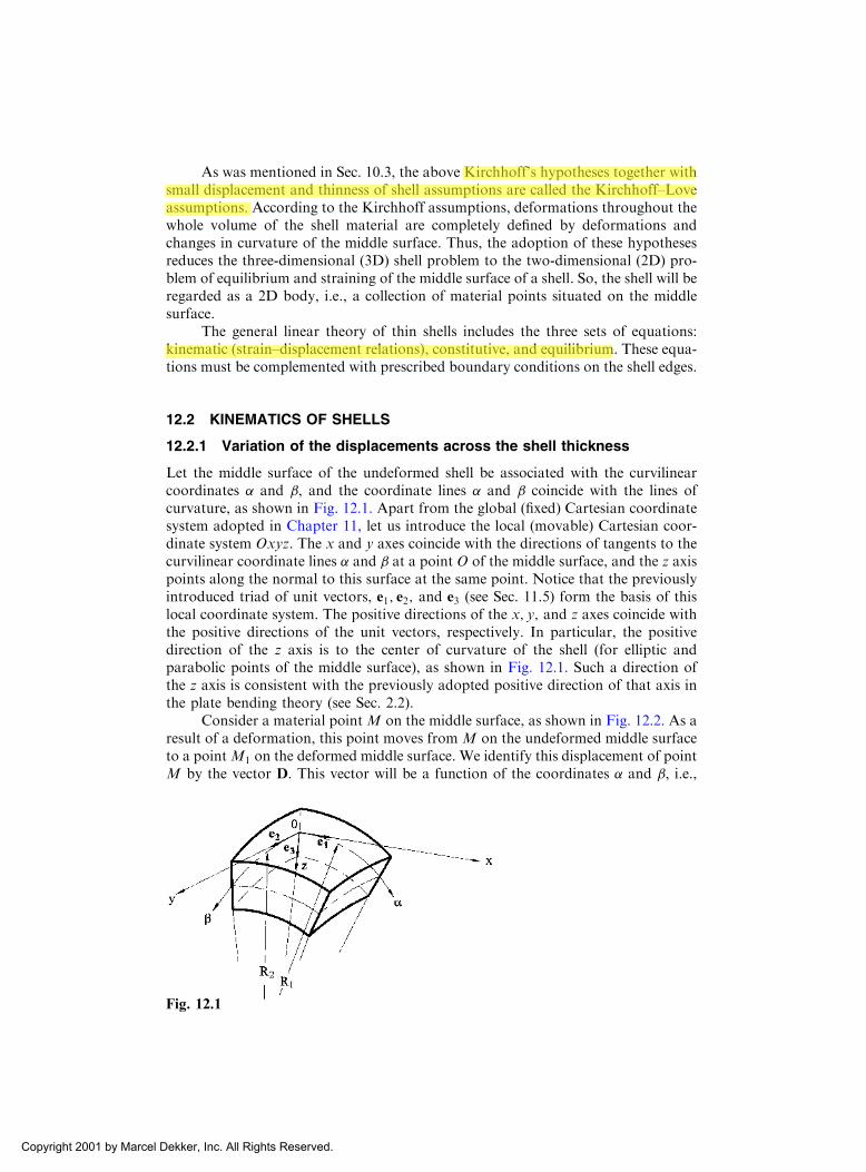
As was mentioned in Sec. 10.3, the above Kirchhoff’s hypotheses together withsmall displacement and thinness of shell assumptions are called the Kirchhoff–Loveassumptions. According to the Kirchhoff assumptions, deformations throughout thewhole volume of the shell material are completely defined by deformations andchanges in curvature of the middle surface. Thus, the adoption of these hypothesesreduces the three-dimensional (3D) shell problem to the two-dimensional (2D) pro-blem of equilibrium and straining of the middle surface of a shell. So, the shell will beregarded as a 2D body, i.e., a collection of material points situated on the middlesurface.

The general linear theory of thin shells includes the three sets of equations:kinematic (strain–displacement relations), constitutive, and equilibrium. These equa-tions must be complemented with prescribed boundary conditions on the shell edges.

12.2 KINEMATICS OF SHELLS

12.2.1 Variation of the displacements across the shell thickness

Let the middle surface of the undeformed shell be associated with the curvilinearcoordinates and , and the coordinate lines and coincide with the lines ofcurvature, as shown in Fig. 12.1. Apart from the global (fixed) Cartesian coordinatesystem adopted in Chapter 11, let us introduce the local (movable) Cartesian coor-dinate system Oxyz. The x and y axes coincide with the directions of tangents to thecurvilinear coordinate lines and at a point O of the middle surface, and the z axispoints along the normal to this surface at the same point. Notice that the previouslyintroduced triad of unit vectors, e1; e2; and e3 (see Sec. 11.5) form the basis of thislocal coordinate system. The positive directions of the x; y; and z axes coincide withthe positive directions of the unit vectors, respectively. In particular, the positivedirection of the z axis is to the center of curvature of the shell (for elliptic andparabolic points of the middle surface), as shown in Fig. 12.1. Such a direction ofthe z axis is consistent with the previously adopted positive direction of that axis inthe plate bending theory (see Sec. 2.2).

Consider a material point M on the middle surface, as shown in Fig. 12.2. As aresult of a deformation, this point moves from M on the undeformed middle surfaceto a pointM1 on the deformed middle surface. We identify this displacement of pointM by the vector D. This vector will be a function of the coordinates and , i.e.,

Fig. 12.1


jiao

Highlight

jiao

Highlight

points of the middle surface and, hence, it will completely define the deformedposition of the middle surface.

Denote the projections of the displacement vector D on the directions of the x; y;and z axes of the local coordinate system by u; v; and w, respectively. Here u and v aretangential displacements and w is the normal displacement or deflection. The positivedirections of the displacement components u; v; and w coincide with the positivedirections of the local coordinate axes x; y; and z at a point of the middle surface. LetpointMz be within the shell, at a distance z from point M on the middle surface, andits displacement vector be D

z. The components of this vector along the coordinateaxes x; y; and z uz; vz; and wz, can be expressed in terms the displacement compo-nents of the point M, as follows (the detailed derivation of these equations is given inAppendix D.):

uz ¼ u� z#1; vz ¼ v� z#2; wz ¼ w; ð12:1Þwhere #1 and #2 are the angles of rotation of the normal to the middle surface abouttangents to the coordinate lines and , respectively. They are given by the following(for derivation of these equations see Appendix D):

#1 ¼u

R1

þ 1

A

@w

@; #2 ¼

v

R2

þ 1

B

@w

@: ð12:2Þ

12.2.2 Strain–displacement relations

First, let us introduce the strain components at a point of the middle surface. Wedenote by "1 and "2 the linear strain components in the and directions, respectively,and by �12 the shear strain component in the middle surface. These strain componentscan be expressed in terms of the displacement components, u; v; and w, introducedearlier, as follows (the detailed derivation of these expressions is given inAppendixD):

"1 ¼1

A

@u

@þ 1

AB

@A

@v� w

R1

; ð12:3Þ

"2 ¼1

B

@v

@þ 1

AB

@B

@u� w

R2

; ð12:4Þ

�12 ¼B

A

@

@

v

B

� �þ A

B

@

@

u

A

� �: ð12:5Þ

Fig. 12.2


Let us examine a variation of the strain components across the shell thickness. Forthis purpose, we pass within the shell an equidistant surface located at a distance zfrom the middle surface, where �h=2 � z � h=2. Locate a point on this surface bythe same coordinates and that were used for the middle surface. According toKirchhoff’s assumptions, points lying on one normal to the middle surface remainon the same normal after deformation. Therefore, the above coordinates remainvalid for the equidistant surface too. It can be proven (see Appendix D) that if the- and -coordinate lines coincide with the lines of curvature on the middle surface,then they are orthogonal, and may also serve as lines of curvature for the equidistantsurface.

Figure 12.3 shows a section of the shell by a plane normal to the middle sur-face. Consider two pairs of neighboring points, M and N, lying along line ¼ const:on the middle surface, and their counterparts Mz and Nz on the equidistant surface,located at a distance z from the middle surface. In virtue of Kirchhoff’s assumptions,adopted in the general shell theory, all these points will be located on the samenormals after deformation and the distance between them in the normal direction(in the z direction) remains unchanged.

If the radius of curvature of arc MN on the middle surface is R1, then thecorresponding radius of curvature of arcMzNz on the equidistant surface (by inspec-tion of Fig. 12.3) is

Rz1 ¼ R1 � z: ð12:6Þ

It follows from the above that Rz1 is the first principal radius of curvature of the

equidistant surface. Moreover, if the length of arc MN is ds1 ¼ Ad, then the lengthof the corresponding arc MzNz of the equidistant surface and its Lame parameterare determined as follows:

dsz1 ¼ Azd ¼ A 1� z

R1

� �d; ð12:7Þ

Az ¼ A 1� z

R1

� �: ð12:8Þ

Fig. 12.3


Similarly, the formulas for determining the second principal radius of curvature, Rz2,

and the second Lame parameter of the equidistant surface, Bz, can be obtained asfollows:

Bz ¼ B 1� z

R2

� �; Rz

2 ¼ R2 � z: ð12:9Þ

When points of the middle surface undergo displacements u; v; and w, then, accord-ing to the adapted assumptions, the corresponding points of the equidistant surfaceundergo displacements uz; vz; and wz given by Eqs (12.1). Therefore, we can obtainthe relationships for determining the strain components in the equidistant surface,"z1; "

z2; and �

z12 by replacing in Eqs (12.3)–(12.5) the quantities R1;R2;A;B; and u; v;

w with Rz1;R

z2;A

z;Bz; and uz; vz;wz according to Eqs (12.1), (12.6), (12.8), and (12.9).After some algebra, we obtain

"z1 ¼1

1� zR1

"1 þ z�1ð Þ; "z2 ¼1

1� zR2

"2 þ z�2ð Þ; ð12:10Þ

�z12 ¼1

1� zR1

!1 þ z�1ð Þ þ 1

1� zR2

!2 þ z�2ð Þ; ð12:11Þ

where

�1 ¼ � 1

A

@#1@

þ 1

AB

@A

@B#2

� �¼ � 1

A

@

@

u

R1

þ 1

A

@w

@

� �þ 1

AB

@A

@

v

R2

þ 1

B

@w

@

� �� ;

ð12:12Þ

�2 ¼ � 1

B

@#2@

þ 1

AB

@B

@#1

� �¼ � 1

B

@

@

v

R2

þ 1

B

@w

@

� �þ 1

AB

@B

@

u

R1

þ 1

A

@w

@

� �� ;

ð12:13Þ

!1 ¼1

A

@v

@� 1

AB

@A

@u; !2 ¼

1

B

@u

@� 1

AB

@B

@v; ð12:14Þ

�1 ¼ � 1

A

@#2@

� 1

AB

@A

@#1

� �; �2 ¼ � 1

B

@#1@

� 1

AB

@B

@#2

� �: ð12:15Þ

In Eqs (12.15), the angles of rotation, #1 and #2, are given by Eqs (12.2); !1 and !2

can be identified with the angles of rotation of the unit vectors e1 and e2, respectively,about the normal direction to the middle surface given by the unit vector e3 (seeAppendix D.1). The terms �1 and �2 correspond to the familiar bending curvaturesintroduced in the plate bending theory (see Sec. 2.2). However, for shells they aremore properly called the changes in curvatures of the middle surface in the directions ofthe - and -coordinate lines, since shells, by definition, are initially curved.

Equation (12.11) contains four different functions (!1; !2; �1; and �2).However, one can bring it to a form consisting of only two different functions ofthe curvilinear coordinates of the middle surface. With this purpose, first of all, notethat the following identity holds:

�1 �!2

R1

¼ �2 �!1

R2

: ð12:16Þ


The validity of this identity can be easily verified if we substitute for �1; �2; !1; and !2

from Eqs (12.15) and (12.14) in terms of u; v; and w, and perform a differentiationwith regard to the Codazzi relations (11.27a). Then, comparing Eqs (12.5) and(12.14), it is easily verified that

�12 ¼ !1 þ !2: ð12:17ÞLet us introduce the following geometric quantity:

�12 ¼ �1 �!2

R1

¼ �2 �!1

R2

: ð12:18Þ

The term �12 represents the twist of a differential element of the middle surface due tothe shell bending. It can be defined as the limit of the ratio of the relative angle ofrotation of two opposite sides of the above element, caused by shell straining, and adistance between these sides, as the element shrinks to zero. The twist has thedimensions of reciprocal of length and is thereby analogous to curvature.

Substituting for �1 and !2 or for �2 and !1 from Eqs (12.14) and (12.15) intothe above, yields

�12 ¼ � 1

R1

u

AB

@A

@� 1

B

@u

@

� �þ 1

R2

v

AB

@B

@� 1

A

@v

@

� �

� 1

AB

@2w

@@� 1

B

@B

@

@w

@� 1

A

@A

@

@w

@

!:

ð12:19Þ

Finally, reducing terms of Eq. (12.11) to the common denominator and using Eqs(12.17) and (12.18), we can rewrite the above equation in the form

�z12 ¼1

1� zR1

� �1� z

R2

� � �12 þ 2z�12 �z2

R1R2

�1R1 þ �2R2ð Þ" #

: ð12:20Þ

It follows from Eq. (12.18) and (12.17) that

�1R1 þ �2R2 ¼ �12 R1 þ R2ð Þ þ �12:Substituting the above into Eq. (12.20), after some algebra, we obtain

�z12 ¼1

1� zR1

� �1� z

R2

� � �12 1� z2

R1R2

!þ 2z�12 1� z

2

1

R1

þ 1

R2

� �� ( ):

ð12:21ÞEquations (12.10) and (12.21) determine the strain components variation

across the shell thickness according to the second-order approximation of the gen-eral, linear shell theory. However, for thin shells used in engineering practice, theratio h=Rmin (where Rmin is the smallest radius of curvature of the middle surface) isless than 1/50. Therefore, the ratio z=Rmin does not exceed 1%. It should be kept inmind that as mentioned previously, the Kirchhoff assumptions stipulate the error ofthe linear theory of the order of h=Rmin. So, retaining in the expressions (12.10) and(12.21) the terms of the order h=Ri ði ¼ 1; 2Þ in comparison with unity is not justified.Hence, the above expressions for the strain components at an arbitrary point of the


shell may be simplified to the form (neglecting here the value of z=Ri in comparisonwith unity)

"z1 ¼ "1 þ z�1; ð12:22aÞ"z2 ¼ "2 þ z�2; ð12:22bÞ�z12 ¼ �12 þ 2z�12: ð12:22cÞ

In so doing, it cannot be stated that the linear in z Eqs (12.22) are less accurate thanEqs (12.10) and (12.21).

The relations (12.22) are of primary importance in the theory of shells. Theyexpress the normal and shear strain components at any point across the shell thick-nesses as a linear combination of the following two terms:

(a) the in-plane strain components on the middle surface that are expressedin terms of the middle surface displacements by Eqs (12.3)–(12.5);

(b) the changes in curvature and twist that are also given in terms of themiddle surface displacements by Eqs (12.12), (12.13), and (12.19).

Therefore, as mentioned previously, the relations (12.22) enable one to reduce the 3Dproblem of the shell straining to the 2D problem of the deformation of the shellmiddle surface. The relationships between the in-plane strains, changes in curvature,and twist on the one hand, and the displacements of the middle surface on the other,are called the generalized strain–displacement or kinematic equations. They establishthe conditions of compatibility of the strains and displacements, suitably specializedfor the shell theory under consideration. Let us summarize these equations, asfollows:

"1 ¼1

A

@u

@þ 1

AB

@A

@v� w

R1

;

"2 ¼1

B

@v

@þ 1

AB

@B

@u� w

R2

;

�12 ¼B

A

@

@

v

B

� �þ A

B

@

@

u

A

� �; ð12:23Þ

�1 ¼ � 1

A

@

@

u

R1

þ 1

A

@w

@

� �þ 1

AB

@A

@

v

R2

þ 1

B

@w

@

� �� ;

�2 ¼ � 1

B

@

@

v

R2

þ 1

B

@w

@

� �þ 1

AB

@B

@

u

R1

þ 1

A

@w

@

� �� ;

�12 ¼ � 1

AB� 1

A

@A

@

@w

@� 1

B

@B

@

@w

@þ @2w

@@

!þ 1

R1

A

B

@

@

u

A

� �þ 1

R2

B

A

@

@

v

B

� �" #;

ð12:24Þ"3 ¼ �13 ¼ �23 ¼ 0: ð12:25Þ

It follows from the above equations that a deformation of the shell middle surface iscompletely defined by the six strain parameters, "1; "2; �12;�1; �2; and �12 that are


called the strain components. The first three strain components characterize thechanges in linear and angular dimensions of a differential element of the middlesurface, while the last three strain components are associated with the change inspace shape of the above element, i.e., with its bending and twisting. It is pertinent todraw the analogy between shells and curved beams. It is known from the strength ofmaterials [2] that any change in linear dimensions of a curved bar is accompanied bya change in its curvature and vice versa.

Taking in Eqs (12.22)–(12.24) A ¼ B ¼ 1; R1 ¼ R2 ¼ 1; and ¼ x; ¼ y, weobtain the strain–displacement relationships for the bending theory of flat plates:

"1 ¼ �z@2w

@x2; "2 ¼ �z

@2w

@y2; �12 ¼ �2z

@2w

@x@y: ð12:26Þ

These are identified with the x- and y-coordinate axes, respectively.It can be seen from Eqs (12.22)–(12.24) that the six quantities determining

deformations of the middle surface of the shell and changes in its curvature("1; "2; �12; �1:�2; and �12) are expressed in terms of the three displacement compo-nents (u; v; and w). Therefore, there are some identical relationships between the sixparameters. The meaning of these relationships, called the compatibility equations,lies in the fact that elements of the middle surface obtaining the linear deformations,"1; "2; and �12, as well as changes in curvature and twist, �1; �2; and �12, must form aunique and continuous surface. The simplest way to obtain these equations is todemand that the coefficients that characterize the first and second quadratic forms ofthe deformed surface would satisfy the Codazzi and Gauss equations (11.27). Thecompatibility equations were derived by Gol’denveizer [3], accordingly; they arepresented below without derivation:

@

@�2Bð Þ � 1

A

@

@�12A

2� �� @B

@�1 þ

1

R2

@A

@�12

þ 1

R1

� @

@ð"2BÞ þ

@B

@"1 þ

@

@ð�12AÞ

� �¼ 0;

@

@�1Að Þ � 1

B

@

@�12B

2� �� @A

@�2 þ

1

R1

@B

@�12

þ 1

R2

� @

@"1Að Þ þ @A

@"2 þ

@

@�12Bð Þ

� �¼ 0;

1

AB

@

@

1

A� @

@"2Bð Þ þ @B

@"1 þ

1

2A

@

@�12A

2� ��

þ 1

AB

@

@

1

B� @

@"1Að Þ þ @A

@"2 þ

1

2B

@

@�12B

2� ��

� �1R2

þ �2R1

� �¼ 0:

ð12:27ÞAs in problems of the theory of elasticity, the compatibility equations (12.27) areused in the theory of shells for solving problems formulated in terms of the stressresultants and stress couples. When we solve problems in displacements, these equa-tions are identically satisfied. This can be proven by substituting the expressions fordeformations and parameters of a change in curvature from Eqs (12.23) and (12.24)


into Eqs (12.27) and performing the transformations of these equations with the useof the Codazzi and Gauss relationships.

12.3 STATICS OF SHELLS

In the previous section we dealt with geometrical description of the shell (deforma-tions and displacements). In the present section we consider the equilibrium condi-tions of the shell.

12.3.1 Hooke’s law for thin shells

The constitutive equations for a 3D homogeneous isotropic body are given by Eqs(1.8). Applying the same system of notations as that adapted above for the straincomponents in Sec. 12.2.2, we can rewrite the above equations, as follows:

"z1 ¼1

E�z1 � � �z2 þ �z3ð Þ½ �; "z2 ¼

1

E�z2 � � �z1 þ �z3ð Þ½ �; "z3 ¼

1

E�z3 � � �z2 þ �z1ð Þ½ �;

ð12:28Þ

�z12 ¼�z12G; �z13 ¼

�z13G; �z23 ¼

�z23G; ð12:29Þ

where �z1; �z2; and �

z3 are the normal stresses acting on planes whose normals are

parallel to the directions ; , and z axes, respectively; "z1; "z2; and "

z3 are the linear

strains along the same directions; �z12; �z13; and �

z23 are shear stresses; and �

z12; �

z13; and

�z23 are the corresponding shear strains.Returning to Kirchhoff’s postulates, note that the assumption of the preserva-

tion of the normal implies that all of the strain components in the direction of thenormal to the middle surface (hypothesis 1) vanish. This means that

"z3 ¼ �z13 ¼ �z23 ¼ 0; ð12:30Þand, in view of Eqs (12.29), the shear stress components �z13 and �

z23 also vanish. The

next Kirchhoff’s assumption for thin shells states that the transverse normal stress isnegligible compared with the in-plane normal stresses (hypothesis 2), so we can set

�z3 ¼ 0: ð12:31ÞThis assumption proves itself because the normal stress �z3 on the external andinternal shell surfaces is equal to the intensity of the applied transverse externalload. It can be shown that the in-plane normal stresses, �z1 and �z2, are, at least,R=h times greater than �z3 [1]. Due to the shell thinness, we can conclude that �z3 willalso be small at interior points of the shell.

Solving Eqs (12.28) and (12.29) for the stress components and taking intoaccount the relation (12.31), we can obtain the following expressions for determiningthe stress components in terms of the strain components:

�z1 ¼E

1� �2 ð"z1 þ �"z2Þ; �z2 ¼

E

1� �2 ð"z2 þ �"z1Þ; �z12 ¼ G�z12 ¼

E

2ð1þ �Þ �z12:

ð12:32Þ


Substituting for the strain components from Eqs (12.22) into the above, we expressthe stress components at any point across the thickness of the shell in terms of themiddle surface strain components, changes in curvature, and twist, as follows:

�z1 ¼E

1� �2 "1 þ �"2 þ z �1 þ ��2ð Þ½ �; �z2 ¼E

1� �2 "2 þ �"1 þ z �2 þ ��1ð Þ½ �;

�z12 ¼E

1þ �1

2�12 þ z�12

� �: ð12:33Þ

Figure 12.4 shows a space differential element isolated from a shell by means of foursections normal to its middle surface and tangential to the lines and þ d; andþ d. The height of this element is finite and equals the shell thickness h. In thisfigure, the stresses acting on the volume element are indicated. The sign conventionand subscript notation of the stress components are that of the theory of elasticity(see Sec. 1.4) and adapted in the treatment of thin shells, where the subscripts 1, 2,and 3 correspond to the axes ; ; and z, respectively. So, all stresses are shownpositive in Fig. 12.4. For any orthogonal coordinates, the condition of equilibrium ofmoments on a differential element requires that

�z12 ¼ �z21; �z13 ¼ �z31; and �z23 ¼ �z32: :

12.3.2 The stress resultants and stress couples in shells

It follows from Eq. (12.33) that the stress components are linearly distributed acrossthe thickness of the elastic shell; therefore, it is convenient to integrate the stressdistribution through the shell thickness, and then to replace the usual considerationof stresses by a consideration of statically equivalent stress resultants and stresscouples applied to the middle surface, just as was done in the plate bending theory(see Sec. 2.3). These stress resultants and stress couples are also referred to as theinternal forces and moments, respectively. By performing such integrations, the var-iations with respect to z are completely eliminated to give a 2D theory of thin shells.The elements of area of the cross sections (shaded in Fig.12.4) are

dsz1 ¼ Azddz ¼ A 1� z

R1

� �ddz; dsz2 ¼ Bzddz ¼ B 1� z

R2

� �ddz:

ð12:34Þ

Fig. 12.4


jiao

Highlight

Let us define the in-plane normal force N1 as the resultant of the normal stresses �1acting on plane face yz per unit length of the element. Thus, we have the following:

N1Bd ¼ðh=2�h=2

�z1dsz2 ¼

ðh=2�h=2

�z1B 1� z

R2

� �ddz;

from which

N1 ¼1

Bd

ðh=2�h=2

�z1Bd 1� z

R2

� �dz or N1 ¼

ðh=2�h=2

�z1 1� z

R2

� �dz: ð12:35aÞ

Similarly, we can define the in-plane shear force N12 and the transverse shear forceQ1, which are the resultants of the shear stress components �12 and �13, respectively,and act on the same yz plane face:

N12 ¼ðh=2�h=2

�z12 1� z

R2

� �dz ð12:35bÞ

Q1 ¼ðh=2�h=2

�z13 1� z

R2

� �dz: ð12:35cÞ

Expression for the remaining stress resultants per unit length are derived in a similarmanner. They are given by the following:

N2 ¼ðh=2�h=2

�z2 1� z

R1

� �dz; ð13:35dÞ

N21 ¼ðh=2�h=2

�z21 1� z

R1

� �dz; ð12:35eÞ

Q2 ¼ðh=2�h=2

�z23 1� z

R1

� �dz: ð12:35fÞ

Taking, next, the moments of the stress components �z1 and �z12 about the y and xaxes, we will arrive to the following two new quantities:

M1 ¼ðh=2�h=2

�z1z 1� z

R2

� �dz ð12:36aÞ

and

M12 ¼ðh=2�h=2

�z12z 1� z

R2

� �dz; ð12:36bÞ

which are referred to, as mentioned previously, as the stress couples or the bendingand twisting moments, respectively, acting on plane face yz. These moments are givento per unit length of the element of Fig. 12.4. Similarly, we can define the stresscouples or the bending and twisting moments assigned on plane face xz, as follows:

M2 ¼ðh=2�h=2

�z2z 1� z

R1

� �dz; ð12:36cÞ

M21 ¼ðh=2�h=2

�z21z 1� z

R1

� �dz: ð12:36dÞ


The positive senses of the stress resultants and stress couples are shown in Fig. 12.5;the sign convention adopted in this figure is the same as for thin plates (see Sec. 2.3).

Notice in the above definitions of the stress resultants and stress couples thatthe symmetry of the stress tensor (�12 ¼ �21) does not necessarily imply that N12 andN21 are either equal or that M12 and M21 are equal for a thin shell of an arbitraryshape, except for a spherical shell.

In the general linear theory of thin shells presented above, six internal forces,N1, N12, N21, N2;Q1, and Q2, and four moments,M1,M2,M12 andM21, characterizecompletely the state of stress of the shell, because the knowledge of these quantitiesenables one to determine the stress components at any point of the shell, as follows:

�z1 ¼N1

hþ 12M1

h3z

� �1

1� zR2

� N1

hþ 12M1

h3z;

�z2 ¼N2

hþ 12M2

h3z

� �1

1� zR1

� N2

hþ 12M2

h3z;

�z12 ¼1

2hN12 þN21ð Þ þ 6

h3M12 þM21ð Þz:

ð12:37Þ

The determination of the transverse shear stresses �13 and �23 from their resultants Q1

and Q2 is not as precise, even within the framework of the present theory, as is thedetermination of �1, �2, and �12. In this case, it is reasoned, as in the theory of beamsand thin plates, that the transverse shear stresses are parabolically distributed acrossthe thickness of the shell. Assuming that the shear stresses are lacking on the outerand inner surfaces of the shell, we obtain the following expression for the transverseshear stresses:

�zi3 ¼6

5

Qi

h1� 2z

h

� �2" #

; i ¼ 1; 2; ð12:38Þ

where, for the sake of convenience, a ‘‘form factor’’ of 6/5 is introduced. It representsthe ratio of peak shear stress to average shear stress across the thickness of the shell.

As mentioned previously, general theory of thin shells presented was based onthe Kirchhoff–Love assumptions. Now is the time to discuss these assumptionsapplied to the preceding derivations of the stress resultants and stress couples.

Fig. 12.5


1. We have found that, as a result of the first Kirchhoff assumption, �13 ¼�23 ¼ 0 and therefore �13 ¼ �23 ¼ 0 from Hooke’s law (Eqs 12.29). Nevertheless, wehave defined the nonvanishing shear stress resultants Q1 and Q2 as integrals of �13and �23 over the shell thickness. A similar situation has been observed in the platebending theory (see Sec. 2.3), as well as in the elementary theory of beams. Here,as in the plate bending theory, the Q1 and Q2 resultants must be retained forpurposes of equilibrium. However, they cannot be determined directly by integrat-ing the shear stresses �13 and �23 over the shell thickness as was done for otherstress resultants. As in the plate bending theory, the transverse shear forces Q1 andQ2 may be found from equilibrium conditions set up for a differential element; thisis shown later.

2. We have also found that, as a result of the first and second Kirchhoff’sassumptions, "3 ¼ �3 ¼ 0. If only �3 were assumed to vanish, then the followingexpression for the normal strain "3 could be obtained from Eqs (12.28) by setting�3 ¼ 0. We have

"3 ¼ � �

1� � ð"1 þ "2Þ: ð12:39Þ

From this expression it would appear that the simultaneous vanishing of both thetransverse normal stress and normal strain is inconsistent. These inconsistencies anddeficiencies specify an approximate character of the general linear thin shell theory.However, as mentioned previously, the error introduced by Kirchhoff’s assumptionsinto the shell theory is of the order of h=Ri in comparison with unity.

12.3.3 Equilibrium of the shell element

Consider a differential element isolated from a shell and bounded by two pairs of thenormal sections passing through the - and -coordinate lines (Fig. 12.4) and specifyits equilibrium under all external and internal forces. The external forces will com-prise some surface loads applied to the upper and lower surfaces of the element. Asmentioned previously, the stress components, continuously distributed across theshell thickness, are replaced by statically equivalent internal forces and momentsand applied to the middle surface (Fig. 12.5). An analogous operation can be exe-cuted for the external loads by replacing them by statically equivalent forces dis-tributed over the middle surface. Let us resolve the surface load p into components inthe directions of e1; e2; and e3 are denoted by p1; p2; and p3. Thus,

p ¼ p1e1 þ p2e2 þ p3e3: ð12:40Þ

Hence, instead of considering the equilibrium of the 3D element of the shell shown inFig. 12.4, one can study the equilibrium of the 2D element of the middle surfaceshown in Fig. 12.5.

Let us consider the equilibrium conditions of this element of the middle surfaceloaded by the external and internal forces and moments. The force and momentequilibrium for the shell element (the resultant force and resultant moment of all theexternal and internal forces applied to the middle surface are zero) results in thefollowing scalar equations:


@

@N1Bð Þ þ @

@N21Að Þ þN12

@A

@�N2

@B

@�Q1

AB

R1

þ p1AB ¼ 0;

@

@N2Að Þ þ @

@N12Bð Þ þN21

@B

@�N1

@A

@�Q2

AB

R2

þ p2AB ¼ 0;

@

@Q1Bð Þ þ @

@Q2Að Þ þN1

AB

R1

þN2

AB

R2

þ p3AB ¼ 0; ð12:41Þ

@

@BM12ð Þ þ @

@AM2ð Þ �M1

@A

@þM21

@B

@�Q2AB ¼ 0;

@

@AM21ð Þ þ @

@BM1ð Þ �M2

@B

@þM12

@A

@�Q1AB ¼ 0;

N12 �N21 �M12

R1

þM21

R2

¼ 0: ð12:42Þ

The detailed derivations of Eqs (12.41) and (12.42) are given in Appendix E. Theabove equations represent a set of the differential equations of static equilibrium of ashell element of the general theory of thin elastic shells.

It can be easily shown that the third Eq. (12.42) is identically satisfied. Toprove that, one needs to substitute for N12;N21; and M12;M21 from Eqs (12.35) and(12.36) into the third Eq. (12.42). We obtain the following:

ðh=2�h=2

�z12 1� z

R2

� �dz�

ðh=2�h=2

�z21 1� z

R1

� �dz�

ðh=2�h=2

�z12z

R1

1� z

R2

� �dz

¼ðh=2�h=2

�z21z

R2

1� z

R1

� �dz ¼

ðh=2�h=2

1� z

R2

� �1� z

R1

� ��z12 � �z21ð Þdz � 0

because �z12 ¼ �z21:

Hence, the system of three equations (Eqs (12.42)) can be reduced to twoequations and the third equation may be disregarded, although we may mention itfrom time to time.

Novozhilov [1] suggested that we reduce the number of unknowns in the aboveequations by setting

M12 ¼ M21 ¼ H; S ¼ N12 þH

R2

¼ N21 þH

R1

: ð12:43Þ

It can be shown that the substitution of these expressions for N12;N21;M12; and M21

from Eqs (12.43) into the third Eq. (12.42) results in the identity, 0 � 0. Thus, takinginto account relations (12.43), the equilibrium equations (12.41) and (12.42) arefinally reduced to the system of five partial differential equations for eight unknownstress resultants and couples: i.e., N1;N2;S;M1;M2;H;Q1; and Q2.

Determining the transverse shear forces Q1 and Q2 from the first and secondEqs (12.42) and substituting them into Eqs (12.41) with the replacement N12 ¼ S �H=R2 and N21 ¼ S �H=R1, we arrive at three equations of equilibrium in the fol-lowing form:


@

@N1Bð Þ þ 1

A

@

@SA2� �� 2

R2

@A

@H � 1

R1

@

@M1Bð Þ �M2

@B

@þ 2

@

@HAð Þ

� �

�N2

@B

@þ ABp1 ¼ 0;

@

@N2Að Þ þ 1

B

@

@SB2� �� 2

R1

@B

@H � 1

R2

@

@M2Að Þ �M1

@A

@þ 2

@

@HBð Þ

� �

�N1

@A

@þ ABp2 ¼ 0;

N1

AB

R1

þN2

AB

R2

þ @

@

1

A

1

A

@

@HA2� �þ @

@M1Bð Þ �M2

@B

@

� � �

þ @

@

1

B

1

B

@

@HB2� �þ @

@AM2ð Þ �M1

@A

@

� � �þ ABp3 ¼ 0:

ð12:44Þ

12.3.4 Constitutive equations (stress resultants–strain and stresscouple–curvature relations)

In shell problems, the constitutive equations are required to relate the stress resul-tants and stress couples, instead of merely stresses, to the corresponding strains andcurvatures.

Since we have already neglected the terms of order z=Ri (i ¼ 1; 2) in determin-ing deformations (hence, also stresses), then the factor (1� z=Ri) can be dropped.Thus, substituting for �z1; �

z2; and �

z12 from Eqs (12.33) into Eqs (12.35) and (12.36),

as well as taking into account expressions (12.43) and integrating over the thicknessof the shell, we obtain the following stress resultant–strain and stress couple–curva-ture relations:

N1 ¼Eh

1� �2 "1 þ �"2ð Þ; N2 ¼Eh

1� �2 "2 þ �"1ð Þ;

N12 ¼ S � H

R2

; N21 ¼ S � H

R1

; S ¼ Eh

2 1þ �ð Þ �12; ð12:45Þ

M1 ¼ D �1 þ ��2ð Þ; M2 ¼ D �2 þ ��1ð Þ;

M12 ¼ M21 ¼ H; H ¼ D 1� �ð Þ�12; ð12:46Þwhere

D ¼ Eh3

12ð1� �2Þ ð12:47Þ

is the flexural rigidity (or stiffness) of the shell. Equations (12.45) and (12.46) arereferred to as the constitutive equations or stress resultants–strain and stress couple–curvature relations of the general linear theory of thin shells. As for the transverseshear forces, Q1 and Q2 – as mentioned previously, they can be determined from theequations of static equilibrium only, Eqs (12.42).


In the first-order approximation shell theory, the constitutive relations for N12

and N21 are usually simplified to the form

N12 ¼ N21 ¼ S ¼ Eh

2 1þ �ð Þ �12: ð12:48Þ

In this form, the constitutive equations (12.45), (12.46), and (12.48) remind us of thecorresponding stress resultants–strains and stress couple–curvatures relations dis-cussed previously in the plate bending theory (Sec. 2.3). The difference betweenthe two constitutive equations is that the strain–displacement relations in the generalshell theory have a more complex form than in the plate theory. However, as men-tioned in Ref. [1], although the error introduced by the simplified relation (12.48)does not exceed the corresponding errors of the general assumptions adopted in theshell theory, the application of the above equation brings some contradictions. Butthese contradictions do not practically influence the accuracy of the calculations ofthe stress and displacement components.

12.4 STRAIN ENERGY OF SHELLS

The strain energy of the shell can be determined by means of Kirchhoff’s assump-tions discussed previously, i.e., the transverse normal, �3, and shear, �13 and �23,stress components are neglected. Therefore, the strain energy density (strain energyper unit volume) uu is given by [1]:

uu ¼ 1

2Eð�z1Þ2 þ ð�z2Þ2 � 2��z1�

z2

� �þ 1

2Gð�z12Þ2

or

uu ¼ E

2 1� �2� � "z1ð Þ2þ "z2ð Þ2þ2�"z1"z2

h iþ G

2�z12ð Þ2: ð12:49aÞ

Since G ¼ E=2 1þ �ð Þ, the last equation may be rewritten as

uu ¼ E

2 1� �2� � "z1 þ "z2ð Þ2þ2 1� �ð Þ 1

4�z12ð Þ2� "z1"

z2

� �� : ð12:49bÞ

Substituting for "z1; "z2; and �

z12 from Eqs (12.22) into the above:

uu ¼ E

2 ð1� �2 Þ "1 þ "2 þ zð�1 þ �2½ Þ�2

þ 2ð1� �Þ 1

4ð�12 þ 2�12zÞ2 � ð"1 þ �1zÞð"2 þ �2zÞ

� ��:

ð12:50Þ

To calculate the total strain energy of the shell, it is necessary to multiply the straindensity uu by an elementary volume of the layer of the shell, as follows:

dV ¼ AzBzdddz ¼ 1� z

R1

� �1� z

R2

� �ABdddz;

and to integrate over the shell thickness (�h=2 � z � h=2) and over the area of itsmiddle surface.


Accepting the same accuracy that has been used to derive the values of thestrain components, neglecting the small terms of the order z=Ri in the expressions forthe volume of shell, element and integrating over the shell thickness, we obtain thefollowing expression for the strain energy of the shell:

U ¼ð

ð

Eh

2 1� �2� � "1 þ "2ð Þ2þ2 1� �ð Þ �2124

� "1"2 !" #

ABdd

þð

ð

D

2�1 þ �2ð Þ2þ2ð1� �Þ �212 � �1�2

� �� ABdd:

ð12:51Þ

The first integral in the expression (12.51) represents the membrane strain energy ofthe shell, whereas the second term expresses its bending strain energy. Using Eqs(12.45) and (12.46), one can express the strain energy of the shell in terms of theinternal forces and moments, as follows:

U ¼ð

ð

1

2EhN1 þN2ð Þ2þ2ð1þ �Þ S2 �N1N2

� �� ABdd

þð

ð

12

2Eh3M1 þM2ð Þ2þ2ð1þ �Þ H2 �M1M2

� �� ABdd:

ð12:52Þ

At last, the strain energy can be calculated using the following equation:

U ¼ 1

2

ð

ð

N1"1 þN2"2 þ S�12 þM1�1 þM2�2 þ 2H�12½ �ABdd: ð12:53Þ

The expressions (12.51)–(12.53) are valid for shells with both constant andvariable thicknesses.

12.5 BOUNDARY CONDITIONS

In the previous sections we have derived a set of differential equations (kinematic,equilibrium, and constitutive), which must be satisfied everywhere on the middlesurface. However, the solutions of the above equations, naturally, do not yet deter-mine completely the state of stress and strain in a shell, as long as they are not subjectto boundary conditions. We now clarify how many boundary conditions must beimposed on the shell edges and set up their formulation for the general linear theoryof thin shells. We consider three cases.

1. A shell has no boundaries, i.e., it is completely closed. The coordinate lines and on the middle surface of the closed shell will be, in turn, also closed. It isevident that in this case the concept of the boundary conditions loses its meaning.However, it does not follow from this that any solution satisfying the previouslymentioned governing differential equations of the general linear shell theory is in thiscase a solution of the shell problem under consideration. A true solution must be aperiodic function of the coordinates and for a passage through the shell alongthese closed coordinate lines, and hence, in moving along any closed curve belongingto the middle surface. Thus, in the case of complete or closed shells, the boundaryconditions are replaced by the conditions of periodicity.

2. A shell is closed with respect to one coordinate and open with respect toanother, as is, for example, the case for cylindrical shells. It is evident that in the


direction of the closed coordinate the conditions of periodicity must be formulatedas the boundary conditions. Along the other, the open coordinate, it is necessary toset up the boundary conditions, which are to be satisfied in solving the governingdifferential equations of the general shell theory.

3. A shell is open with regard to both coordinate lines and . In this case, it isrequired to set up certain boundary conditions in the directions of both principaldirections. Proceeding now to this general case, we confine ourselves to the simplestcase where the boundaries coincide with the lines of principal curvature of the middlesurface (the - and - coordinate lines), since this case is encountered most frequentlyin practice.

Let, for example, the line ¼ be a boundary of the shell. The stresses actingon the boundary can be reduced to the three internal forces N2;N21; and Q2 and twomomentsM2 andM21. The deformations on the same boundary are characterized bythe three displacement components u; v; and w and two slopes #1 and #2. Thus, atfirst glance, five boundary conditions must be prescribed on the edge line ¼ .However, this is not true: due to the Kirchhoff kinematic hypothesis (the firstKirchhoff assumption), not all the above-mentioned quantities are independent.The slope of the normal to the shell boundary, #2, is connected with the displace-ments w and v on this boundary by the condition of the preservation of the normal.Therefore, the number of independent displacements (and hence, the correspondinggeneralized forces) equals four, and only the four boundary conditions can beassigned on each edge of the shell. By the way, as follows from the above, such anumber of independent boundary conditions corresponds to the eighth order of thegoverning differential equations of the general linear theory of thin shells.

Thus, the five forces and moments assigned for the static boundary conditionson the shell boundary (i.e., the boundary conditions expressed in terms of the inter-nal forces and moments) can be reduced to four quantities in accordance withKirchhoff’s postulates. This can be carried out in a similar manner to that done inthe plate theory (Sec. 2.5): namely, the three boundary quantities, N2;N21; and M21,may be replaced with the two boundary quantities with an acceptable accuracy.

Figure 12.6 shows two adjacent differential segments of the boundary ¼

of the middle surface, each of length ds1, near some point m1. The boundary curvemm1m2 may be approximated by a polygon formed by two small segments of equallength. The length of each such segment with a high order of accuracy may be setequal to the length of the arc spanning, i.e., mm1 ¼ m1m2 � ds1. Let points n1 and n2be halfway between the points m and m1;m1 and m2, respectively. It is evident thatn1n2 � ds1. Let M21ds1 and

M21 þ@M21

@s1ds1

� �ds1

be the resultants of the twisting moments distributed over segments mm1 and m1m2,respectively. These act at the midpoints n1 and n2. Further, we replace each of theabove resultant couples by a pair of equal and opposite forces with the moment armsds1 and applied at end points of the corresponding segments. So, at end points mand m1 the forces M21ds1ð Þ=ds1 ¼ M21, acting normal to the chord mm1, are applied.Similarly, the forces M21 þ @M21=@s1ð Þds1, acting normal to the chord m1m2, will beapplied at end points m1 and m2. Thus at each point of the corners of the polygon,


two concentrated forces from twisting moments distributed over the adjacent seg-ments are applied, as shown in Fig. 12.6b for corner point m1.

Projecting both these forces, acting at a point m1, on the direction of thenormal to the middle surface (the direction of the transverse shear force Q2) andon the direction of the tangent to the middle surface (the direction of the in-planeshear force N21), we obtain:

(a) in the first case

þM21

@M21

@s1ds1 �M21 ¼

@M21

@s1ds1; ðaÞ

(b) in the second case

� 2M21 þ@M21

@s1ds1

� �’; ðbÞ

where 2’ is the angle between the normals to the middle surface at points n1 and n2,i.e., 2’ ¼ ds1=R1. Substituting this value for ’ into the expression (b) and retainingonly the first-order quantities, one finds �ðM21=R1Þds1. Thus, along the shell edge ¼ , the twisting moment can be replaced by the distributed normal (transverse)shear forces @M21=@s1 and distributed tangential (in-plane) shear forces �M21=R1.

As mentioned previously (see Sec. 2.5), the replacement of the twisting momentby statically equivalent forces results in a certain redistribution of the stresses overthe thickness of the shell along its boundaries. By the St.Venant principle, the effectof this approximation cannot be significant; it can only be noticeable within theimmediate neighborhood of the boundaries (at distances of the order of the shellthickness).

It follows from the above that the boundary conditions on the edge ¼ canbe formulated in terms of the following four quantities:

Fig. 12.6


N2; T2 ¼ N21 �M21

R1

; V2 ¼ Q2 þ1

A

@M21

@; M2; ð12:54Þ

where T2 and V2 are referred to as the in-plane and transverse effective shear forces,respectively. These boundary quantities define completely the state of stress on theabove-mentioned shell edge; therefore, the number of boundary conditions on theedge must be equal to four, and not five.

Note that the static boundary conditions (12.54) can also be expressed in termsof functions S and H by using the relations (12.43). In this case, the boundaryquantities on the edge ¼ are of the form

N2; T2 ¼ S � 2H

R1

; V2 ¼ Q2 þ1

A

@H

@; M2: ð12:55Þ

Using the above results, it is not difficult to deduce, similarly, the boundary quan-tities assigned for the edge ¼ .

We have considered the so-called static boundary conditions expressed in termsof the four generalized force and moment quantities prescribed on the shell edges. Ofcourse, the boundary conditions of the shell can be expressed in terms of the pre-scribed displacements or slopes on its edges (the so-called kinematic boundary con-ditions). Sometimes, the mixed boundary conditions expressed in terms of thedisplacements and forces prescribed on the shell boundaries are also encounteredin practice.

Let us list some typical boundary conditions that are frequently encountered inengineering applications. These conditions are formulated below for a boundary ofthe shell, which is a part of the curve, i.e., for the boundary ¼ :

(1) Free edge

N2 ¼ 0; T2 ¼ N21 �M21

R1

¼ 0; V2 ¼ Q2 þ1

A

@M21

@¼ 0; M2 ¼ 0 ð12:56Þ

(2) Clamped edge

u ¼ 0; v ¼ 0; w ¼ 0; #2 ¼ 0; ð12:57Þwhere #2 is given by Eq. (12.2).

(3) Hinged edge with the support free to move in the normal direction

M2 ¼ 0; V2 ¼ Q2 þ1

A

@M21

@¼ 0; u ¼ 0; v ¼ 0: ð12:58Þ

(4) Hinged edge with fixed support

M2 ¼ 0; u ¼ 0; v ¼ 0; w ¼ 0: ð12:59ÞSimilarly, the boundary conditions for the shell edge ¼ can be assigned.

12.6 DISCUSSION OF THE GOVERNING EQUATIONS OF THEGENERAL LINEAR SHELL THEORY

At this point, the governing equations of the general linear theory of thin shells arenow complete. They can be classified in the following manner:


(1) The strain–displacement relations

Six strain–displacement equations are summarized for the general linear shell theoryby Eqs (12.23) and (12.24). They involve six components of strain, "1; "2; �12; �1; �2;and �12, which are given explicitly in terms of the three displacement componentsu; v; and w. Note that the six strain components must satisfy the equations ofcompatibility (Eqs (12.27)). The latter equations are used only for solving the shellproblems in forces–strain components. If the problem under consideration is solvedin terms of the displacement components, then these conditions are satisfiedautomatically.

(2) The constitutive equations

The eight equations are summarized in the general case by Eqs (12.45) and (12.46).They express the eight stress resultants and stress couples, N1; N2; N12; N21;M1;M2;M21; and M12, as explicit functions of the six strain components, "1; "2; �12; �1; �2;and �12. The number of these constitutive equations can be reduced for a practicalstress analysis of shells to six by accepting the assumption (12.43).

(3) Equations of equilibrium

Five equations of equilibrium must be satisfied. They are given by Eqs (12.41) and(12.42). These five equations involve the 10 stress resultants and couple resultants,N1; N2;N12; N21;M1; M2; M12; M21; Q1; and Q2. The number of the these forcesand moments can be reduced to eight by using Eqs (12.43).

(4) Boundary conditions

Boundary conditions relate the stress resultants and stress couples or displacementcomponents specified on the shell boundaries to prescribed boundary quantities (in aparticular case, the latter may be equal to zero). These boundary conditions aresummarized by Eqs (12.56)–(12.59).

Thus, in general, there are 19 equations relating 19 unknowns, u; v; w; "1; "2;�12; �1; �12; N1; N2; N12; N21; M1 ;M2; M12; M21;Q1, and Q2. For a simplifiedgeneral linear theory of shells, one can take N12 ¼ N21 and M12 ¼ M21, therebyreducing the number of equations and unknowns to 17.

As for the theory of elasticity, shell problems may be solved either in terms ofdisplacements or in terms of the internal forces and moments. According to the firsttechnique, the internal forces and moments are replaced in the equilibrium equations(12.41) and (12.42) by the displacement components u; v; and w, using the constitu-tive and strain–displacement relations (12.45), (12.46) and (12.23), (12.24), respec-tively. As a result, the eight-order system of the three governing partial differentialequations for displacements is obtained. The second technique consists of simulta-neous treatment of equations of equilibrium (12.41) and (12.42) or (12.44) andcompatibility relations (12.27). In so doing, the eight-order system of six governingdifferential equations for N1; N2; S; M1; M2; and H will be obtained.


12.7 TYPES OF STATE OF STRESS FOR THIN SHELLS

All equations mentioned in Sec. 12.6 are linear for both techniques, which, of course,greatly simplifies their study and solution. However, shell problems associated withcalculations of the stress and strain components remain very difficult. As a rule, thegoverning, eight-order partial differential equations of the general shell theory havevariable coefficients. Mathematical difficulties associated with integration of such atype of differential equations are evident. Even for the simplest circular cylindricalshells for which the governing equations have constant coefficients, cumbersomecomputations remain involved and,by far, not all problems of practical interestfor such shells have been solved. Consequently, attempts of scientists and engineersengaged in the practical stress analysis of shell structures were directed towards thesearch for possibilities of simplifying the above governing differential equations ofthe general shell theory and shell problems themselves. Several approximate methodsand the corresponding shell models based upon some additional assumptions andupon simplified governing equations are considered in Chapter 17.

Previously, in presenting the general linear shell theory, it was assumed that theflexural stresses are values of the same order as the stresses caused by in-plane(membrane) stresses. If one of the above-mentioned types of stresses is negligiblein comparison with another one, then it is possible to introduce considerable sim-plifications in the general linear shell theory. Consider some possible types of state ofstress for thin shells.

1. If the flexural stresses are negligible compared with the membrane stressesthen such a type of state of stress is called a membrane or momentless state of stress.The governing equations of the membrane theory can be obtained directly from theequations of the general shell theory by neglecting the effect of the bending andtwisting moments, as well as the transverse shear forces, on the state of stress andstrain of thin shells. In some cases, the membrane theory describes the state of stressand strain with reasonable accuracy, since the bending and twisting moments are ofnegligible magnitudes: for example, hollow spherical shells subjected to inside andoutside uniform pressure are in the pure membrane state of stress.

2. If, to the contrary, the membrane stresses are negligible in comparison withthe flexural stresses, then such a type of state of stress is referred to as a pure flexuralor moment state of stress. Note that the definitions of the ‘‘membrane’’ and ‘‘pureflexural’’ states of stress are not quite correct because the membrane state of stressadmits an existence of small flexural stresses and, in turn, small membrane stressesmay occur in a pure flexural state of stress. It was mentioned previously that shells,due to their small thickness, possess a relatively small flexural stiffness and, there-fore, they are poorly adapted to resisting in bending. Even relatively small bendingmoments may cause considerable flexural stresses and displacements in shells.Therefore, a pure flexural type of the state of stress is dangerous and technicallydisadvantageous for thin shells. It should be avoided by introducing some intermedi-ate reinforcements, by selecting the corresponding shape of the shell, by choosing thetype of supports, etc. Conversely, the membrane state of stress, at which the shell isuniformly stressed across its thickness, is technically the most advantageous. So,engineers designing a shell should aim at such a state of stress.

3. If the flexural and membrane stresses are of the same order, then such astate of stress is called a mixed state of stress, or edge effect. The term ‘‘edge effect’’ is


associated with the fact that the above-mentioned mixed state of stress often occursnear edges of the shell. Note that all attempts to generate the membrane state ofstress throughout the shell surface were not successful, except for a few particularcases. At the main portion of a shell the state of stress, which is close to the mem-brane, can be generated. However, near the shell edges or some reinforcing stiffeners,the mixed state of stress takes place. This edge effect is, as a rule, localized in acomparatively small area. The latter circumstance is commonly used for the decom-position of a given state of stress into the membrane and edge effect. As shown inSec. 17.5, such decomposition results in considerable simplifications in solving theshell problems.

PROBLEMS

12.1 Verify Eqs (12.10)–(12.15).

12.2 Verify Eq. (12.16).

12.3 Explain and show the physical meaning of the twist of a differential element of the

middle surface, �12.12.4 Equations (12.22) are not unique linear relations in the general linear theory of thin

shells. Using the expansions of the type

1

1� z=Ri

¼ 1þ z

Ri

þ z

Ri

� �2

þ . . . ði ¼ 1; 2Þ

and Eqs (12.10) and (12.11), derive the corresponding strain relations in the equidistant

surface. Compare the accuracy of the above equations with the relations (12.22).

12.5 Would the accuracy of Eqs (12.24) be changed if the terms of the order "i=Ri ði ¼ 1; 2Þwere added to the right-hand sides?

12.6 Give the physical explanation of the assumption �z ¼ 0 adopted in the general linear

theory of thin shells. Compare the orders of the direct stresses �1 and �2 with the above

stress �3.12.7 Generalize the equilibrium equations (12.41) to include surface loading that consists of

distributed moments m1ðx; yÞ and m2ðx; yÞ.12.8 Verify Eqs (12.44).

12.9 What are the formal contradictions, brought by the approximate relations (12.48), in

the general linear shell theory?

12.10 Verify Eqs. (12.52) and (12.53).

12.11 Derive the boundary conditions of the type (12.56)–(12.59) for the shell boundary

¼ .

REFERENCES

1. Novozhilov, V.V., Thin Shell Theory (translated from 2nd Russian ed. by P.G. Lowe),

Groningen, Noordholf, The Netherlands, 1964.

2. Cook, R.D. and Young, W.C., Advanced Mechanics of Materials, Prentice-Hall, New

Jersey, 1964.

3. Gol’denveizer, A.L., Theory Of Elastic Shells (translated from Russian by G. Herrmann),

Pergamon Press, New York, 1961.


13

The Membrane Theory of Shells

13.1 PRELIMINARY REMARKS

It was shown in Chapter 12 that a thin elastic shell supports an arbitrary externalloading by means of stress resultants (internal forces) and stress couples (bendingand twisting moments). Under appropriate loading and boundary conditions, how-ever, the resulting bending and twisting moments are either zero, or so small thatthey may be neglected. Such a state of stress is referred to as the membrane state ofstress because of the analogy to membranes that cannot support bending and twist-ing moments. The corresponding theory of thin shells that deals with this state ofstress is called the membrane theory of shells. It follows from the above that themembrane theory neglects all moments, i.e.,

M1 ¼ M2 ¼ H ¼ 0: ð13:1ÞIn turn, it follows from the corresponding moment relations

M1 ¼ D �1 þ ��2ð Þ; M2 ¼ D �2 þ ��1ð Þ; H ¼ Dð1� �Þ�12; ð13:2Þthat neglecting the moments will be justified either when the shell has a very smallflexural stiffness, D, or when the changes in curvature and in twist of the middlesurface, �1; �2; and �12, are very small. In the first case, we deal with an absolutelyflexible shell, the membrane; in the second case, with the momentless or the mem-brane state of stress of a shell that has a finite flexural stiffness. Although, both theseproblems are described by one and the same theory, a distinction must be madebetween them because they resist the applied loading differently. An absolutelyflexible shell (for instance, made from cloth) is not able to sustain compressive forcessince any small compression forces will cause the loss of stability of its shape.Therefore, these shells may resist the applied loads only in tension.

Shells with finite flexural stiffness, in contrast to absolutely flexible shells, mayresist in both the membrane states of compressive as well as tensile forces. They lose


jiao

Highlight

jiao

Highlight

jiao

Highlight

jiao

Highlight

jiao

Highlight

stability only when the compressive forces exceed a certain critical value. For abso-lutely flexible shells, since they do not possess a resistance to bending, only themembrane state of stress is possible, while for shells with finite stiffness such astate of stress is only one of the possible stress conditions. In this chapter we consideronly shells with a finite flexural stiffness.

13.2 THE FUNDAMENTAL EQUATIONS OF THE MEMBRANETHEORY OF THIN SHELLS

The governing equations of the membrane theory can be obtained directly from theequations of the general theory of thin shells derived in Chapter 12. For this purpose,it is assumed that, in view of the smallness of the changes of curvature and twist, themoment terms in the equations of equilibrium for a shell element are unimportant,although in principle the shell may resist the external loads in bending. Note thatneglecting the moments leads to neglecting the normal shear forces. Thus, for themembrane theory of thin shells, we can assume that

M1 ¼ M2 ¼ H ¼ Q1 ¼ Q2 ¼ 0: ð13:3ÞIntroducing Eq. (13.3) into Eqs (12.44) and taking into account Eq. (12.43), onearrives at the following system of differential equations:

@

@N1Bð Þ þ 1

A

@

@A2S� ��N2

@B

@þ ABp1 ¼ 0;

@

@N2Að Þ þ 1

B

@

@B2S� ��N1

@A

@þ ABp2 ¼ 0;

N1

1

R1

þN2

1

R2

þ p3 ¼ 0;

ð13:4Þ

where N12 ¼ N21 ¼ S (since H ¼ 0Þ.In this system, the number of unknowns is equal to the number of equations, so

the problem of the membrane theory of shells is statically determinate (that is truefor the equilibrium of an infinitely small shell element but is not always true for theequilibrium of the entire shell). This means that if the external load components,p1; p2; and p3, are known, then the membrane forces and stresses for such a shell areuniquely determined from Eqs (13.4).

Having determined the membrane forces, the shell displacements may befound. Solving the constitutive equations (12.45) for strains, and substituting theminto Eqs (12.23), yields the following system of the three partial differential equationsfor the displacements:

"1 ¼1

A

@u

@þ v

AB

@A

@� w

R1

¼ 1

EhN1 � �N2ð Þ;

"2 ¼1

B

@v

@þ u

AB

@B

@� w

R2

¼ 1


�12 ¼B

A

@

@

v

B

� �þ A

B

@

@

u

A

� �¼ 2ð1þ �Þ

EhS:

ð13:5Þ


jiao

Highlight

jiao

Highlight

The system of the differential equations (13.4) in the membrane theory for determin-ing the membrane internal forces (and stresses) is of the second order. Accordingly,the system (13.5) for the displacements is also of the second order. However, thestress resultants (N1;N2; and S) on the right-hand sides of Eqs (13.5) are themselvessolutions of the second-order equations. Hence, the displacements in the membranetheory must satisfy a fourth-order system of differential equations. The latter can beobtained by substituting into Eqs (13.4) for the stress resultants from the corre-sponding expressions in terms of the strains.

The mathematical formulation of the theory of membrane shells is completedby adding appropriate boundary conditions. In the membrane theory, it followsfrom the above that only two boundary conditions may be specified on each edgeof the shell. If the boundary conditions are given in terms of the stress resultants,then only the membrane (or in-plane) forces (N1;N2; and S) are specified on edges ofthe shell. If the boundary conditions are formulated in terms of displacements, thenonly displacement components that are tangent to the middle surface, i.e., u and v,must be prescribed on the shell boundary. In the membrane theory it is impossible tospecify the edge displacements w and slopes #, since their assignment may result inthe appearance of the corresponding boundary transverse shear forces and bendingmoments. This is in a conflict with the general postulates of the membrane theory ofthin shells introduced above.

Since the differential equations of the membrane theory for the stress resultants(13.4) and for the displacements (13.5) have different orders (the second and fourth,respectively), the boundary conditions cannot be prescribed in terms of forces onlyfor membrane shells: half of the boundary conditions should be assigned in terms ofdisplacements.

13.3 APPLICABILITY OF THE MEMBRANE THEORY

As mentioned previously (see Sec. 10.1), the advantages of a shell as a structuralmember can be only completely realized when its wall resists the applied loads intension (or compression) under membrane state of stress conditions. We now expresssome considerations which provide a good insight into the range of applicability ofthe membrane theory.

Membrane strains are associated with deformations of line elements that lie inthe middle surface of the shell. If a shell is bent without straining of the middlesurface, it is said to be bent inextensionally. For example, if we roll a sheet of paperinto a cone or a cylinder, we bend it inextensionally. It is known that shells offer highresistance to membrane strains. In fact, we can bend a piece of thin sheet metal easilywith our fingers, but we cannot stretch it noticeably.

However, there are many cases in which inextensional bending is impossible.There is Lagrange’s theorem (see, for instance [1]), which asserts that a convex closedsurface cannot be deformed inextensionally. For example, a Ping-Pong ball cannotbe bent inextensionally. Cones, cylinders, and convex domes cannot be bent inex-tensionally if their edges are reinforced by rigid rings. Since shells offer high resis-tance to membrane stresses, those that cannot be bent inextensionally are usuallyvery stiff. Generally, the membrane theory is permissible only for shells that cannotbe bent inextensionally, or for shells that experience only very small bendingmoments.


jiao

Highlight

Now we present, without proof, the general conditions under which the mem-brane theory is valid. It can be shown that these conditions are necessary andsufficient for an existence of the momentless state of stress in thin shells and thatthey correspond to the minimum of strain energy stored by a shell during its strain-ing. These conditions are [2]:

(a) The boundaries of a shell are free from transverse shear forces andmoments. Loads applied to the shell boundaries must lie in planes thatare tangent to the middle surface of the shell.

(b) The normal displacements and rotations at the shell edges are uncon-strained: that is, these edges can displace freely in the direction of thenormal to the middle surface.

(c) A shell must have a smoothly varying and continuous surface.(d) The components of the surface and edge loads must be also smooth and

continuous functions of the coordinates.

If these conditions are violated, fully or partially, flexural stresses occur. If designersdo not succeed in eliminating these stresses completely, they must aim at localizingthem and limiting their magnitude. Thus, the solutions given by the membranetheory must, in many cases, be supplemented by a solution of the equations of thebending theory in those parts of the shell where bending proves to be important.Such a combination of the bending and membrane theories is one of the importantideas on the basis of which the majority of problems of the shell theory are beingsolved at present. It should be also noted that even if the membrane stresses aresometimes combined with flexural stresses, the membrane theory does not lose itssignificance because already at a small distance from a bending zone, the state ofstress may be usually considered as momentless.

13.4 THE MEMBRANE THEORY OF SHELLS OF REVOLUTION

Consider a particular case of a shell described by a surface of revolution (Fig. 11.12).The midsurface of such a shell of revolution, as mentioned in Sec. 11.8, is generatedby rotating a meridian curve about an axis lying in the plane of this curve (the Zaxis).

The geometry of shells of revolution is addressed in Sec. 11.8. There it ismentioned that meridians and parallel circles can be chosen as the curvilinear coor-dinate lines for such a shell because they are lines of curvature, and form an ortho-gonal mesh on its midsurface. Let us locate a point on the middle surface by thespherical coordinates � and ’ (see Sec. 11.8), where � is the circumferential anglecharacterizing a position of a point along the parallel circle, whereas the angle ’ isthe meridional angle, defining a position of that point along the meridian. The latterrepresents the angle between the normal to the middle surface and the shell axis (Fig.11.12a). As before, R1;R2 are the principal radii of curvature of the meridian andparallel circle, respectively, and r is the radius of the parallel circle. The Lameparameters for shells of revolution in the above-mentioned spherical coordinatesystem are given by Eqs (11.39). Notice that, due to the symmetry of shells ofrevolution about the Z axis, these parameters are functions of ’ only and do notdepend upon �. Referring to Fig. 11.12a and b, we can obtain by inspection thefollowing relations:


jiao

Highlight

jiao

Highlight

jiao

Highlight

r ¼ R2 sin ’;

AM1 ¼ dr ¼ dr

d’d’ � MM1 cos ’ ¼ R1d’ cos ’

ð13:6aÞ

or

dr

d’¼ d

d’R2 sin ’ð Þ ¼ R1 cos ’: ð13:6bÞ

Finally from Eqs (13.6a) and (13.6b) we obtain

1

r

dr

d’¼ R1

R2

cot ’: ð13:6cÞ

Substituting for A and B from Eqs (11.39) into the system of differential equations(13.4) and taking into account the relations (13.6), yields

R1

@S

@�þ @

@’rN1ð Þ �N2R1 cos ’þ rR1p1 ¼ 0;

R1

@N2

@�þ 1

r

@

@’r2S� �þ rR1p2 ¼ 0;

�1N1 þ �2N2 þ p3 ¼ 0;

ð13:7Þ

where

�1 ¼1

R1

and �2 ¼1

R2

:

The last equation in the above system is known as the Laplace equation. Note thatthe membrane forces N1;N2; and S are, in a general case of loading, some functionsof � and ’.

Equations (13.7) can be reduced to one single, second-order differential equa-tion for some function U: For this purpose, rewrite the above equations using therelations (13.6), as follows

1

R1

@N1

@’þN1 �N2

R2

cot ’þ 1

R2 sin ’

@S

@�þ p1 ¼ 0; ð13:8aÞ

1

R2 sin ’

@N2

@�þ 1

R1

@S

@’þ 2 cot ’

R2

S þ p2 ¼ 0; ð13:8bÞ

N1

R1

þN2

R2

þ p3 ¼ 0: ð13:8cÞ

Solving Eq. (13.8c) for N2 and substituting this into Eqs (13.8a) and (13.8b), onefinds the following:

1

R1

@N1

@’þN1

1

R1

þ 1

R2

� �cot ’þ 1

R2 sin ’

@S

@�¼ �p1 � p3 cot ’

� 1

R1 sin ’

@N1

@�þ 1

R1

@S

@’þ 2

cot ’

R2

S ¼ 1

sin ’

@p3@�

� p2:

ð13:9Þ


We introduce new variables, U and V instead of N1 and S, as follows:

N1 ¼U

R2 sin2 ’; S ¼ V

R22 sin

2 ’: ð13:10Þ

Substituting the above into Eqs (13.9), we obtain, after some simple transformations,the following system of equations:

R22 sin ’

R1

@U

@’þ @V@�

¼ �ðp3 cos ’þ p1 sin ’ÞR32 sin

2 ’;

� R2

sin ’

@U

@�þ @V@’

¼ @p3@�

� p2 sin ’

� �R1R

22 sin ’:

ð13:11Þ

Differentiating then the first equation (13.11) with respect to ’ and the second onewith respect to �, and subtracting the second equation from the first, we obtain thefollowing second-order differential equation for U:

1

R1R2 sin ’

@

@’

R22 sin ’

R1

@U

@’

!þ 1

R1 sin2 ’

@2U

@�2¼ Fð�; ’Þ; ð13:12Þ

where

Fð�; ’Þ ¼ � 1

R1R2 sin ’

@

@’R3

2 sin2 ’ðp3 cos ’þ p1 sin ’Þ

� �þ R2

@p2@�

sin ’� @2p3@�2

!:

ð13:13ÞEquation (13.12) may be written in the operator form

LU ¼ Fð�; ’Þ; ð13:14Þwhere the differential operator L is of the form

Lð. . .Þ � 1

R1R2 sin ’

@

@’

R22 sin ’

R1

@ð. . .Þ@’

!þ 1

R1 sin2 ’

@2

@�2ð. . .Þ: ð13:15Þ

The kinematic equations for displacements of shells of revolution in sphericalcoordinates are

1

R1

@u

@’� w

R1

¼ 1

EhN1 � �N2ð Þ ¼ "1;

1

r

@v

@�þ u

rcos ’� w

R2

¼ 1

EhN2 � �N1ð Þ ¼ "2;

r

R1

@

@’

v

r

� �þ 1

r

@u

@�¼ S

Gh¼ �12:

ð13:16Þ

Now transform the above kinematic equations. Introducing the functions

� ¼ u

sin ’; ¼ v

R2 sin ’; ð13:17Þ


and making subsequent transformations associated with an elimination of deflectionw and then �, the system of equations (Eqs (13.16)) may be reduced to one second-order differential equation for the unknown function . In the operator form, thisequation has the form

L ¼ f ð�; ’Þ; ð13:18Þwhere

f ð�; ’Þ ¼ 1

R1R2 sin ’

1

Gh

@ðR2SÞ@’

� 1

EhR1

R21 þ R2

2 þ 2�R1R2

� � @N1

@�

� R2

EhR2 þ �R1ð Þ @p3

@�

�;

ð13:19Þ

and the operator L is given by Eq. (13.15). Thus, the governing differential equationsfor determining the membrane forces, Eq. (13.14), and displacements, Eq. (13.18),have an identical form. These equations can be solved by using the well-knownmethod of separation of variables.

Let us represent the load components p1; p2; and p3 in the form of the Fourierseries

p1 ¼X1n¼0

p1ncos n� þX1n¼1

p1 n sin n�; p2 ¼

X1n¼1

p2n sin n� þX1n¼0

p2 n cos n�;

p3 ¼X1n¼0

p3n cos n� þX1n¼1

p3 n sin n�

;

ð13:20Þwhere p1n; . . . ; p3

n are functions of ’ only. The first of the two sums in each line

represents that part of the load that is symmetric in � and the second sum representsthe antisymmetric part. The coefficients pin and pi

n ði ¼ 1; 2; 3Þ are evaluated from

well-known formulas (see, for example, Appendix B). For the shell analysis, it issufficient to consider only one harmonic of the load, say, p

ðnÞi , i.e.,

pðnÞ1 ¼ p1n cos n�; p

ðnÞ2 ¼ p2n sin n�; p

ðnÞ3 ¼ p3n cos n� ð13:21Þ

and then a solution may be obtained by summing the membrane forces, displace-ments, etc., due to individual load components. Inserting Eq. (13.21) into Eq. (13.12)and introducing the expression

U ¼ Un cos n�; ð13:22Þwe obtain, in the general case, the following ordinary differential equations withvariable coefficients:

1

R1R2 sin ’

d

d’

R22 sin ’

R1

dUn

d’

!� n2

R1 sin2 ’

Un ¼ Fnð’Þ; ð13:23Þ

where

Fnð’Þ ¼ � 1

R1R2 sin ’

d

d’ðp3n cos ’þ p1n sin ’ÞR3

2 sin2 ’

� �þ R2nðp2n sin ’þ np3nÞ:ð13:24Þ


In turn, the expression for V can be introduced in the form

V ¼ Vn sin n�: ð13:25ÞOnce the expression Un has been determined by solving Eq. (13.23), we can introduceEqs (13.21), (13.22), and (13.25) into the first equation (Eq. (13.11)). Solving thisequation, we obtain Vn as follows:

Vn ¼ �R22 sin ’

nR1

dUn

d’� ðp3n cos ’þ p1n sin ’ÞR3

2 sin2 ’: ð13:26Þ

Finally, using the expressions (13.10) and Eq. (13.8c), the membrane forces for theconsidered harmonic of load can be determined in the following form

NðnÞ1 ¼ N1n cos n�; N

ðnÞ2 ¼ N2n cos n�; SðnÞ ¼ Sn sin n�: ð13:27Þ

Then, we can come to determining the displacements. For this purpose, we representthe previously introduced function in the form

ðnÞ ¼ n sin n�: ð13:28ÞSubstituting the expressions (13.28), (13.21), and (13.27) into Eq. (13.18), we obtainan ordinary differential equation for n. The latter will be identical to Eq. (13.23), ifwe replace in it Un with n and Fnð’Þ with fnð’Þ, as follows:

fnð’Þ ¼1

R1R2 sin ’

1

Gh

dR2Sn

d’þ n

N1n

EhR1

R21 þ R2

2 þ 2#R1R2

� ��

þR2

EhR2 þ �R1ð Þnp3n

�:

ð13:29Þ

A solution of the differential equation for n involves four constants of integration:two constants from Eq. (13.23) for the forces and the remaining two constants fromthe equation for displacements. These constants are evaluated from the boundaryconditions discussed in Sec. 13.2.

Using the solution obtained for n, as well as Eqs (13.17) and (13.16), andintroducing the displacements in the form

uðnÞ ¼ un cos n�; vðnÞ ¼ vn sin n�; wðnÞ ¼ wn cos n�; ð13:30Þwe can determine the expressions for un; vn; and wn, and then the displacementsthemselves.

13.5 SYMMETRICALLY LOADED SHELLS OF REVOLUTION

Let us assume that the shell of revolution is subjected to loading that is symmetricalabout the shell axis, i.e., the Z axis. A self-weight of a shell and a uniformly dis-tributed snow load are examples of such a type of loading. In this case, the governingdifferential equations of the membrane theory of shells of revolution will be simpli-fied considerably. All the derivatives with respect to � will vanish because a givenload, and hence all the membrane forces and displacements, does not change in thecircumferential direction. The externally applied loads per unit area of the middlesurface are represented at any point by the components p1 and p3 acting in thedirections of the y and z axes of the local coordinate system at the above point


(see Sec. 12.2), respectively, where the y axis points in the tangent direction along themeridian and the z axis is a normal to the middle surface at that point (Fig. 13.1).The load component p2 (acting along the x axis) is assumed to be absent. Thepresence of this component implies that the shell is twisted about its axis. If p2 ¼0 and edge forces in the circumferential direction are also zero, then, as follows fromthe second Eq. (13.7), in the case of axisymmmetrical loading,

S ¼ N12 ¼ N21 ¼ 0: ð13:31ÞThe nonzero membrane forces are shown in Fig. 13.1.The first and third equations of the system (13.7) after some algebra transfor-

mations, eliminating N2, and taking into account Eqs (13.6), may be reduced to thefollowing equation:

d

d’N1r sin ’ð Þ þ rR1 p1 sin ’þ p3 cos ’ð Þ ¼ 0: ð13:32Þ

Integrating this equation from ’0 to ’, one finds

N1r sin ’½ �’’0 ¼ �ð’’0

rR1ðp1 sin �’’þ p3 cos �’’Þd �’’ or

N1r sin ’ ¼ �ð’’0

rR1 p1 sin �’’þ p3 cos �’’ð Þd �’’þNð0Þ1 b sin ’0;

ð13:33aÞ

where ’0 is the angle corresponding to the shell edge (for instance, at the top) wherethe boundary conditions are specified; N

ð0Þ1 and r0 ¼ b are the meridional force, and

the radius of the parallel circle, respectively, at the shell edge ’ ¼ ’0 (Fig. 13.2); and�’’ is a dummy variable.

Solving Eq. (13.33a) for N1 and taking into account Eq. (13.6a), yields

N1 ¼ � 1

R2 sin2 ’

ð’’0

R1R2 p1 sin �’’þ p3 cos �’’ð Þ sin �’’d �’’þNð0Þ1 R

ð0Þ2 sin2 ’0

R2 sin2 ’

ð13:33bÞwhere b ¼ R

ð0Þ2 sin ’0. R

ð0Þ2 is the principal radius of curvature at the shell edge ’ ¼ ’0.

Fig. 13.1


Let a shell, in addition to the surface load components p1 and p3, be subjectedto some line load q per unit length of the top parallel circle, ’ ¼ ’0. This may be, forexample, the weight of a skylight of a dome. From Fig. 13.2, N

ð0Þ1 ¼ �q= sin ’0;

substituting into Eq. (13.33a) gives

N1r sin ’ ¼ �ð’’e

rR1 p1 sin �’’þ p3 cos �’’ð Þd �’’þ qb

� �: ð13:34Þ

This equation may be easily interpreted if we multiply both sides of Eq. (13.34) by2�. We have

N1 2�rð Þ sin ’ ¼ �2�

ð’’0

rR1 p1 sin �’’þ p3 cos �’’ð Þd �’’� 2�bq: ð13:35Þ

Referring to Fig. 13.2, one can conclude that the left-hand side of this equation is thevertical component of the resultant of meridional forces N1over a parallel circledetermined by angle ’. As seen from Fig.13.2, 2�rR1d’ is the area of an elementaryring corresponding to an infinitesimal angle d’; and p1 sin ’ and p3 cos ’ are thevertical components of the surface load. Hence, the integrand function of Eq.(13.35) represents a vertical component of the surface load corresponding to theelementary ring. Integrating over ’, we obtain the vertical component of the resul-tant of all surface loads acting on the shell above the parallel circle ’ where N1is tobe determined. So, we can rewrite Eq. (13.35), as follows:

N1 2�rð Þ sin ’ ¼ �F;

from which

N1 ¼ � F

2�r sin ’; ð13:36Þ

where

F ¼ 2�½ð’’0

rR1 p1 sin �’’þ p3 cos �’’ð Þd �’’þ qb� ð13:37Þ

Fig. 13.2


is the vertical component of all external loading applied above the parallel circle ’ ofthe shell where N1 is desired. Thus, Eq. (13.35) represents the static equilibriumcondition: i.e., the force summation in the direction of the shell axis (the Z axis) iszero. Note that in the case of a shell closed at its apex, ’0 ¼ 0 and N1 becomes

N1 ¼ � 1

r sin ’

ð’0

rR1 p1 sin �’’þ p3 cos �’’ð Þd �’’: ð13:38Þ

Having determined N1 from Eq. (13.34) or Eq. (13.36), or Eq. (13.38), we cancalculate N2 from the third Eq. (13.7), as follows:

N2 ¼ �R2 p3 þN1

R1

� �: ð13:39Þ

Now we can discuss the displacements in symmetrically loaded shells of revolu-tion. For this particular case, v ¼ 0 and �12 ¼ 0 and the system of Eqs (13.16) may besimplified to the following:

1

R1

du

d’� w

R1

¼ 1

EhN1 � �N2ð Þ ¼ "1;

u

R2

cot ’� w

R2

¼ 1

EhN2 � �N1ð Þ ¼ "2;

ð13:40Þ

where u and w are displacements along the tangent and normal to the meridian curve(or along the y and z axes, as shown in Fig. 13.1), respectively. Knowing N1 and N2

for a given shell problem, we can evaluate the strain components, "1 and "2, andthen, u and w from Eqs. (13.40). For this purpose, eliminating w from Eqs (13.40),one finds that

1

R2

du

d’� u cot ’

� �¼ R1

R2

� �"1 � "2: ð13:41Þ

Multiplying both sides of the above equation by R2 csc ’, we have, after some mathe-matics,

d

d’u csc ’ð Þ ¼ f1ð’Þ; ð13:42aÞ

where

f1ð’Þ ¼R2

sin ’

R1

R2

"1 � "2� �

: ð13:42bÞ

The function f1ð’Þ can be found when N1 and N2 have been determined. IntegratingEq. (13.42a), we obtain the following expression for u:

u ¼ sin ’

ðf1ð’Þd’þ C1 sin ’; ð13:43Þ

where C1 is a constant of integration. Substituting for u from Eq. (13.43) into thesecond Eq. (13.40), one finds the following expression for w:

w ¼ cos ’

ðf1ð’Þd’þ C1 cos ’� "2R2: ð13:44Þ


The constant of integration is evaluated from the boundary condition at either thetop or the bottom of the shell, i.e., for ’ ¼ ’0 or ’¼’1.

Note that the normal displacements w for various points of a shell, including itsedges, are related to tangential displacements u. Thus, for a membrane shell, theboundary conditions must not be simultaneously imposed on u and w. If a displace-ment component is given along one of parallels, then the constant C1 can be eval-uated from Eqs (13.43) or (13.44). Thus, we have the freedom of prescribing u or w atonly one of the shell boundaries, and we must permit only other displacementsyielded by our analysis; otherwise, incompatibility problems will arise.

In analysis of shell structures consisting of thin shells of revolution and otherstructural members (ring beams, flat or curved plates, supports, etc.), the horizontaldisplacements and rotation of the tangent to the meridian at the shell boundaries areof considerable interest. These quantities are required for satisfying the compatibilityconditions at the junction of a thin shell and the structural members.

First, determine the horizontal expansion or contraction of the membrane shellat its edge, �. We have the following conditions for the rings:

� ¼ r"2 ¼r

EhN2 � �N1ð Þ; ð13:45aÞ

or

� ¼ R2 sin ’

EhN2 � �N1ð Þ: ð13:45bÞ

For a spherical shell, letting R1 ¼ R2 ¼ R, Eq. (13.45b) becomes

� ¼ R sin ’

EhN2 � �N1ð Þ: ð13:45cÞ

For example, determine the horizontal expansion of the sphere edge ’ ¼ ’1 underthe internal pressure p. Taking into account that due to the symmetry of the shell andloading, N1 ¼ N2 ¼ N, and making p3 ¼ �p (for internal pressure), one can bringthe third Eq. (13.7) to the form 2N=R ¼ p, from which one derives N ¼ pR=2.Substituting the above into Eq. (13.45c) gives

� ¼ pR2 sin ’12Eh

ð1� �Þ: ð13:46aÞ

For a hemisphere, ’1 ¼ �=2 and � becomes

� ¼ pR2

2Eh1� �ð Þ: ð13:46bÞ

Now, we can proceed to determine the rotation of the tangent to the meridian.It can be easily shown that it is equal to the rotation of the normal to the middlesurface during deformation about the axis which is tangent to the parallel circle. Thelatter expression was introduced in Sec. 12.2.1 as #1, given by the first Eq. (12.2).Setting A ¼ R1 and ¼’, we obtain

#1 ¼1

R1

uþ @w@’

� �: ð13:47aÞ

By differentiating Eq. (13.44), we have


dw

d’¼ cos ’ � f1ð’Þ � sin ’

ðf1ð’Þd’� C1 sin ’� "2

dR2

d’� R2

d"2d’

: ð13:47bÞ

The displacement u is given by Eq. (13.43). Adding the right-hand sides of Eqs(13.47b) and (13.43), we obtain #1, as follows:

#1 ¼1

R1

cos ’ � f1ð’Þ � "2dR2

d’� R2

d"2d’

� �;

or substituting for f1ð’Þ from Eq. (13.42b) results in the following:

#1 ¼ cot ’ "1 �R2

R1

"2

� �� "2R1

dR2

d’� R2

R1

d"2d’

: ð13:48aÞ

Let us present this expression in the explicit form for a special case of spherical shellsonly. Substituting R1 ¼ R2 ¼ R into the above equation, we obtain

#1 ¼ cot ’ "1 � "2ð Þ � d"2d’

: ð13:48bÞ

Inserting the strains in terms of N1 and N2 into this equation, we obtain the follow-ing expression of #1 for a sphere:

Eh#1 ¼ cot ’ð1þ �ÞðN1 �N2Þ �dN2

d’þ �dN1

d’: ð13:48cÞ

13.6 MEMBRANE ANALYSIS OF CYLINDRICAL AND CONICALSHELLS

Cylindrical and conical shells have straight generators and, therefore, the radius ofthe curvature in the meridional direction is infinite. It will be shown that thevanishing one out of the two principal curvatures leads to a great simplification inthe analysis of such a type of shells. For this reason, we treat these shells as aseparate category of membrane shells.

13.6.1 General cylindrical shells

We consider cylindrical shells with an arbitrary shape of the cross section (or profile):e.g., circular, elliptical, parabolic, and cylinders of open or closed types. The pecu-liarities of the geometry of these shells were analyzed in Sec. 11.8. Since the gen-erators of cylindrical shells are straight, such shells have zero Gaussian curvaturesand, hence, have developable surfaces (see Sec. 11.7).

Using the cylindrical coordinates x and � to describe the position of a referencepoint on the cylindrical shell middle surface (Fig. 11.13), the Lame parameters aregiven by the relations (11.52), i.e.,

A ¼ 1; B ¼ R2; ð13:49Þwhere R2 ¼ R2ð�Þ is the second principal radius of curvature, while the first radius ofcurvature R1 ¼ 1. Notice that for a circular cylindrical shell R2 ¼ const ¼ R, where


R is the radius of the circular cross section of the shell. With the cylindrical coordi-nates defined above and the Lame parameters given by Eqs (13.49), the equilibriumEqs (13.4) are significantly simplified and become (making ¼ x and ¼� in theabove equations):

@N1

@xþ 1

R2

@S

@�þ p1 ¼ 0;

@S

@xþ 1

R2

@N2

@�þ p2 ¼ 0;

N2 þ R2p3 ¼ 0;

ð13:50Þ

where p1; p2; and p3 are the load components in the directions of the shell generator,tangent to its profile, and the normal to the middle surface, respectively.

The strain–displacement relations for cylindrical shells can be obtained fromEqs (13.5) by substituting for the Lame parameters from Eqs (13.49) and making R1

¼ 1 and ¼ x and ¼ �. As a result, we obtain these relations in the followingform:

"1 ¼@u

@x¼ 1


"2 ¼1

R2

@v

@�� w

R2

¼ 1


�12 ¼1

R2

@u

@�þ @v

@x¼ 1

GhS:

ð13:51Þ

A general solution of Eqs (13.50) may be obtained in the following manner. Fromthe third Eq. (13.50), we obtain the circumferential force N2, i.e.,

N2 ¼ �R2p3: ð13:52aÞ

The other two Eqs (13.50) may be solved by simple integration in the x direction, i.e.,

S ¼ �ð

p2 þ1

R2

@N2

@�

� �dxþ f1ð�Þ; ð13:52bÞ

N1 ¼ �ð

p1 þ1

R2

@S

@�

� �dxþ f2ð�Þ; ð13:52cÞ

where f1ð�Þ and f2ð�Þ are unknown functions of �, to be determined from two bound-ary conditions. Each must be of the kind that on a profile x ¼ const (one end of theshell or a plane of symmetry) one of the forces S or N1 will be given as an arbitraryfunction of �.


Similarly, the general solution of Eqs (13.51) may be found once the membraneforces have been determined. For h ¼ const; this solution is given by

Ehu ¼ðN1 � �N2ð Þdxþ f3ð�Þ; ð13:53aÞ

Ehv ¼ 2ð1þ �ÞðSdx� Eh

R2

ð@u

@�dxþ f4ð�Þ; ð13:53bÞ

Ehw ¼ Eh@v

@�� R2 N2 � �N1ð Þ; ð13:53cÞ

where f3ð�Þ and f4ð�Þ are two additional arbitrary functions which may be used tofulfill two boundary conditions on the edges x ¼ const of the shell. Equations (13.52)and (13.53) represent a complete general solution of the cylindrical membrane shellproblem.

It should be noted that since the arbitrary functions fið�Þ ði ¼ 1; 2; 3; 4Þ dependupon �, boundary conditions can only be assigned for edges x ¼ const: As a rule, wecannot satisfy boundary conditions on the longitudinal edges (� ¼ const) of an opencylindrical shell, when, for example, a segment of a cylindrical membrane shell isunder consideration. These must, therefore, be abandoned, which represents a severelimitation of the theory of the membrane shells as applied to open cylindrical shells.This limitation can only be remedied by including the bending resistance of the shell.However, such difficulties do not arise if a shell is closed with respect to the coordi-nate �,

For most practical problems, we will have p1 ¼ 0 and p2 and p3 will be inde-pendent of x. Thus, from Eqs (13.52), one finds that

N2 ¼ �p3R2; ð13:54aÞ

S ¼ � p2 þ1

R2

@N2

@�

� �xþ f1ð�Þ or S ¼ �xFð�Þ þ f1ð�Þ; ð13:54bÞ

where

Fð�Þ ¼ p2 þ1

R2

@N2

@�¼ p2 �

1

R2

d

d�p3R2ð Þ: ð13:54cÞ

Hence, taking the partial derivative of S with respect to � and integrating, we obtain

@S

@�¼ �x

dF

d�þ df1ð�Þ

d�:

Substituting this expression and p1 ¼ 0 into Eq. (13.52c), we find that

N1 ¼x2

2R2

!dF

d�� x

R2

df1d�

þ f2ð�Þ: ð13:54dÞ


Substituting next for the membrane forces from Eqs (13.54) into Eqs (13.53) andevaluating the integrals, we can represent the displacement components in terms ofthe introduced function Fð�Þ, as follows

Ehu ¼ x3

6R2

dF

d�� ðxÞN2 �

x2

2R2

df1d�

þ x � f2 þ f3;

Ehv ¼ � x4

24R2

d

d�

1

R2

dF

d�

� �� ð1þ �Þx2F þ � � x

2

2R2

dN2

d�

þ x3

6R2

d

d�

1

R2

df1d�

� �� x2

2R2

df2d�

þ x 2ð1þ �Þf1 �1

R2

df3d�

� �þ f4;

Ehw ¼ x4

24

d

d�

1

R2

d

d�

1

R2

dF

d�

� �� þ x2

2ð2þ �Þ dF

d�� d

d�

1

R2

dN2

d�

� ��

þ R2N2 �x3

6

d

d�

1

R2

d

d�

1

R2

df1d�

� �� þ x2

2

d

d�

1

R2

df2d�

� �

� x ð2þ �Þ df1d�

� d

d�

1

R2

df3d�

� �� ðR2Þf2 �

df4d�:

ð13:55Þ

For a circular cylindrical shell R2 ¼ R ¼ const and Eqs (13.54) and (13.55) may besimplified.

Consider the boundary conditions for a closed cylindrical shell. For staticallydeterminate shells, the two conditions should be assigned for determining arbitraryfunctions f1ð�Þ and f2ð�Þ: These conditions should be imposed on the membraneforces N1 and S on the shell edges. In so doing, since the expression for S containsonly one function f1ð�Þ, the shear force can be prescribed on one edge of the shellonly. The functions f3ð�Þ and f4ð�Þ are evaluated from the two kinematic boundaryconditions assigned for the displacement components u and v on the shell edges –e.g., x ¼ 0 and x ¼ L, where L is the length of the cylindrical shell.

For statically indeterminate cylindrical shells the number of kinematic bound-ary conditions increases at the expense of static boundary conditions. For example, ifboth ends of the shell, x ¼ 0 and x ¼ L, are built-in, all the boundary functionsmentioned previously are evaluated from the following conditions:

ujx¼0 ¼ ujx¼L ¼ vjx¼0 ¼ vjx¼L;¼ 0:

Comparing the flexural deformations at surface layers in the shell, "ðfÞ1 ¼ �1h=2 and"ðfÞ2 ¼ �2h=2; with the membrane deformations, "1 and "2, one can establish that theformer deformations are small compared with the latter only in the case whenarbitrary functions fið�Þ ði ¼ 1; 2; 3; 4Þ satisfy the limitations

h

R

d2fid�2

!� fi:

These inequalities express the general requirement of slowly varying deformations inthe direction of �. The above requirements impose additional limitations on admis-sible character of distribution of boundary loads N

ð0Þ1 and Sð0Þ.

It follows from Eqs (13.55) that the continuous expressions for the displace-ment components in the membrane theory can only be obtained in the case when


arbitrary functions f1ð�Þ and f2ð�Þ, which arise in integrating the equilibrium equa-tions, are continuous together with their derivatives up to the second and thirdderivatives. This also imposes certain limitations on admissible types of loadingand boundary conditions in order that membrane theory can be applied.

One important comment should be mentioned. It follows from Eqs (13.54) and(13.55) that the membrane forces and displacements increase without limit with anincrease of the shell length. This is a natural result of the membrane analysis of acylindrical shell in which th flexural rigidity of the circumferential cross sections ofthe shell is neglected and all loading is directly transmitted to the shell ends.Therefore, the area of application of the membrane theory of cylindrical shells isrestricted by fairly short shells (l=R �

ffiffiffiffiffiffiffiffiffiR=h

p) [2]. So, there is a variety of require-

ments that govern the applicability of the membrane theory of cylindrical shells.These requirements are concerned with the type of shell supports, type of loading,and length of the shell.

An impression may be formed that the membrane theory of cylindrical shellsis practically of no use because of the limitations mentioned above. However, thisis not true. In some cases, the membrane theory of cylindrical shells allows one toobtain simple and, at the same time, sufficiently accurate solutions. In particular, itis applicable to the analysis of cylindrical shells reinforced by stiffeners. In thiscase, the external loading applied to the closely spaced at equal distances stiffenersis distributed by the stiffener elements in such a way that the condition of slowlyvarying deformation in the circumferential direction is satisfied.

13.6.2 Conical shells

Figure 13.3a shows a conical shell in the form of a frustum of a cone. The meridianof the shell has zero curvature, while the radius of the second principal curve is R2.The radius of the parallel circle is denoted by r. In this typical case, the angle ’ is aconstant and can no longer serve as a coordinate on the meridian. Instead, weintroduce the coordinate s, the distance of a point of the middle surface, usuallymeasured from the vertex, along the generator, i.e., ¼ s. Another coordinate is the

Fig. 13.3


circumferential angle � in the horizontal plane measured on the parallel circle, i.e., ¼ �:

For such a shell, a length of the element along the meridian is ds1 and along theparallel circle is ds2 ¼ rd�. It follows from Fig. 13.3a and b that

R2 ¼ s cot ’; r ¼ s cos ’: ð13:56Þ

Thus, the Lame parameters for the given coordinate system are

A ¼ 1 and B ¼ r ¼ s cos ’: ð13:57Þ

Substituting the above into Eqs (13.4) and (13.5), we obtain the equilibrium andkinematic equations, respectively. The equilibrium equations for the conical shell aregiven by

@

@sN1sð Þ þ 1

cos ’

@S

@��N2 þ sp1 ¼ 0;

1

cos ’

@N2

@�þ 1

s

@

@sSs2� �þ sp2 ¼ 0;

1

stan ’N2 þ p3 ¼ 0:

ð13:58Þ

The kinematic equations for displacement components have the form

@u

@s¼ "1

1

cos ’

@v

@�þ u� w tan ’ ¼ "2s

s@

@s

v

s

� �þ 1

s cos ’

@u

@�¼ �12

ð13:59Þ

We come now to determining the membrane forces and displacements for conicalshells. From the last Eq. (13.58), we have

N2 ¼ �p3s � cot ’: ð13:60Þ

Substituting the above into the second Eq. (13.58), one finds that

@

@sSs2� � ¼ �s2 p2 �

1

sin ’

@p3@�

� �:

Integrating this expression over s, we obtain

S ¼ 1

s2f1ð�Þ �

Zs

s2 p2 �1

sin ’

@p3@�

� �ds

� �: ð13:61Þ


Substituting for N2 and S from Eqs (13.60) and (13.61) into the first Eq. (13.58), andintegrating over s, gives the following expression:

N1 ¼1

s2 cos ’f

01 ð�Þ þ

1

sf2ð�Þ �

1

s sin ’

ðs

sðp3 cos ’þ p1 sin ’Þds

þ 1

s cos ’

ðs

1

s2

ðs

@p2@�

� 1

sin ’

@2p3@�2

!s2ds

" #ds:

ð13:62Þ

Let us determine the displacements. From the first Eq. (13.59), we have

u ¼ðs

"1dsþ f3ð�Þ: ð13:63Þ

Substituting for u from Eq. (13.63) into the third Eq. (13.59) and integrating over s,one finds that

v ¼ 1

cos ’f

03ð�Þ þ sf4ð�Þ þ s

ðs

�12sds� s

cos ’

@

@�

ðs

ðs

"1ds

� �ds

s2: ð13:64Þ

The displacement w is determined from the second Eq. (13.59), i.e.,

w ¼ u cot ’þ 1

sin ’

@v

@�� "2s cot ’: ð13:65Þ

As for the case of the cylindrical shell, four arbitrary functions depend only upon theangular coordinate �; therefore, the boundary conditions on edges � ¼ const of openshells cannot be satisfied.

A continuity and slowly varying of loads with respect to the angular coordinateare necessary conditions of applicability of the membrane theory to a conical shell.

Let us pay attention to one peculiarity of conical shells: a closed at a vertexconical shell is not capable of carrying a self-balanced load applied to its free edgeaccording to the membrane theory. The reason for that is an unlimited increase offorces, and hence, deformations in the vicinity of the vertex, i.e., for s ¼ 0 (seeformulas (13.60)–(13.62)). In so doing, the displacements determined from Eqs(13.64) and (13.65) become also unlimited: a moment state of stresses will occurnear the vertex of a closed conical shell.

For an axisymmetrically (with respect to the shell axis) loaded conical shell, thesystem of equations (13.58) may be simplified. Putting the derivatives of all functionswith respect to � equal zero and S ¼ 0 together with p2 ¼ 0, we obtain the above-mentioned system in the following form:

d

dsðN1sÞ �N2 ¼ �p1s;

N2 ¼ �p3s cot ’:

ð13:66Þ

Adding these equations member by member, we obtain the following first-orderdifferential equation for N1:

d

dsðN1sÞ ¼ �sðp1 þ p3 cot ’Þ: ð13:67Þ


Integrating the above, yields

N1 ¼ � 1

s

Zðp1 þ p3 cot ’Þsdsþ

C

s

� �; ð13:68Þ

where C is a constant of integration.

13.7 THE MEMBRANE THEORY OF SHELLS OF AN ARBITRARYSHAPE IN CARTESIAN COORDINATES

The boundary contour of shells of an arbitrary shape does not usually coincide withthe lines of curvature. As an example, one can mention shells of double curvaturewhich are commonly used for roofs of buildings. A membrane analysis of such shellsis more conveniently performed using Cartesian coordinates whose x and y axes liein a horizontal plane with the z axis pointing in the vertical direction to the planeabove. The middle surface of the shell can be assigned by the following equation inthe Cartesian coordinate system:

z ¼ f ðx; yÞ: ð13:69ÞIn this coordinate system, we consider an element ABCD of the shell obtained bymaking sections at the locations x; xþ dx; and y; yþ dy (Fig. 13.4).

These sections are not necessarily the lines of curvature in a general case (theexceptions are cylindrical surfaces for which the x axis is directed along generators).They are not mutually perpendicular. Hence, angle ! between sides AB and AD isnot necessarily a right angle and element ABCD is a skew quadrilateral with sides ds1and ds2 in space. Its projection in the xy plane is a rectangle �AA �BB �CC �DD with sides dx anddy. Let ’ and � be the angles which sides AD and AB make with the xy plane.Correspondingly, the lengths AD and AB of the shell element are ðdx= cos ’Þ andðdy= cos �Þ, respectively. The midsurface area of the element ABCD becomesðdx= cos ’Þðdy= cos�Þ sin!.

Fig. 13.4


The curves x ¼ const and y ¼ const on the shell midsurface can be used ascoordinate curves, and we denote by N1;N2; and S the membrane stress resultants atany point on the shell. It should be noted that the directions of these forces make upnon-right angles with the corresponding sides of the element. These membrane forcesare shown in Fig. 13.4. Two out of all unknown forces (N1 and S) are parallel to theplane Oxz, and, therefore, have no components in the direction of the y axis. Twoothers (N2 and S on sides AD and BC) have no components in the x direction. Theseconsiderations simplify setting up the equation of equilibrium.

Figure 13.4 also shows the surface load components, where p1 and p2 areparallel to the x and y axes, respectively, and p3 acts in the z direction. These loadcomponents are defined per unit are of the shell midsurface.

We set up the equation of equilibrium in the direction of the x axis. Consider aside AB. The membrane force per unit length acting on this side is N1ðdy= cos�Þ andits component in the x direction is N1ðdy= cos�Þ cos ’. The in-plane shear force S ofthe same direction has a component in the x direction of the form Sðdx= cos ’Þ cos ’.By analogy, the components of the membrane forces acting on the opposite side CDcan be represented, as follows:

N1 þ@N1

@xdx

� �dy

cos �þ @�@x dx� � cos ’þ @’

@xdx

� �;

S þ @S@y

dy

� �cos ’þ @’

@ydy

� �dx

cos ’þ @’@y dy� � :

Summing these forces with the corresponding signs, taking into account that theresultant force due to the loading p1 is obtained by multiplying p1 by the area of theelement ABCD; and canceling out the common factor dxdy, we obtain the followingafter some simplifications and assuming that the angles ’ and � are small:

@

@xN1

cos ’

cos�

� �þ @S@y

þ p1sin!

cos� cos ’¼ 0: ð13:70aÞ

Similarly, we can obtain the following equilibrium equation for the components ofthe membrane forces in the y direction:

@

@yN2

cos�

cos ’

� �þ @S@x

þ p2sin!

cos� cos ’¼ 0: ð13:70bÞ

Let us set up an equation of equilibrium for all the membrane forces in the zdirection. The component of the force N1 in the z direction is N1ðdy= cos�Þ sin ’ andthe component of the in-plane shear force S in the same direction referred to thesame side of the element ABCD is Sðdy= cos�Þ sin ’. The corresponding expressionscan be obtained for the two other components of the membrane forces. So, theequation of equilibrium for the membrane forces in the z direction is derived aftersome simplifications, as follows:

@

@xN1

sin ’

cos�

� �þ @

@yN2

sin�

cos ’

� �þ @

@yS tan ’ð Þ þ @

@xS tan�ð Þ þ p3

sin!

cos� cos ’¼ 0:

ð13:70cÞ


The values of the trigonometric functions entering into Eqs (13.70) can be expressedin terms of the partial derivatives of the equation of a surface given by Eq. (13.69),i.e.,

tan ’ ¼ dz

dx; tan� ¼ dz

dy; ð13:71aÞ

hence,

cos ’ ¼ 1ffiffiffiffiffiffiffiffiffiffiffiffiffiffiffiffiffiffiffiffiffi1þ @z

@x

� �2r ; sin ’ ¼ @z=@xffiffiffiffiffiffiffiffiffiffiffiffiffiffiffiffiffiffiffiffiffi1þ @z

@x

� �2r ; etc. ð13:71bÞ

It can be easily noted that the expressions

N1

dy

cos�

� �cos ’; N2

dx

cos ’

� �cos�; S

dy

cos�

� �cos�; S

dx

cos ’

� �cos ’

represent projections of the membrane forces acting on sides of the shell skewquadrilateral element ABCD on the coordinate plane xy or the membrane forcesacting on sides of the rectangle �AA �BB �CC �DD, as shown in Fig. 13.4. Let us denote theseprojections by �NN1dy; �NN2dx; and �SSdx, i.e.,

�NN1 ¼ N1

cos ’

cos�; �NN2 ¼ N2

cos�

cos ’; �SS ¼ S: ð13:72Þ

Using these notations, we can rewrite equations of equilibrium, Eqs (13.70), asfollows

@ �NN1

@xþ @

�SS

@yþ �pp1 ¼ 0; ð13:73aÞ

@ �SS

@xþ @

�NN2

@yþ �pp2 ¼ 0; ð13:73bÞ

@

@x�NN1 tan ’

� �þ @

@y�NN2 tan�

� �þ @

@y�SS tan ’� �þ @

@x�SS tan�� þ �pp3 ¼ 0: ð13:73cÞ

where

�pp1 ¼ p1sin!

cos� cos ’; �pp2 ¼ p2

sin!

cos� cos ’; �pp3 ¼ p3

sin!

cos� cos ’ð13:74Þ

are the surface load components per unit area of the projection of the shell elementon the xy plane in the x; y; and z directions, respectively.

Equation (13.73c) can be rewritten by substituting for the tangents from Eqs(13.71a), as follows:

�NN1

@2z

@x2þ 2 �SS

@2z

@x@yþ �NN2

@2z

@y2¼ � �pp3 �

@ �NN1

@xþ @

�SS

@y

� �@z

@x� @ �SS

@xþ @

�NN2

@y

� �@z

@y:

ð13:75Þ


Taking into account Eqs (13.73a) and (13.73b), this equation may be represented inthe form

�NN1

@2z

@x2þ 2 �SS

@2z

@x@yþ �NN2

@2z

@y2¼ � �pp3 þ �pp1

@z

@xþ �pp2

@z

@y: ð13:76Þ

For a given shell surface z ¼ f ðx; yÞ and given loading, Eqs (13.73a), (13.73b), and(13.76) govern the membrane forces in the shell under consideration. This system ofequations can be reduced to one differential equation. In fact, Eqs (13.73a) and(13.73b) coincide with the corresponding equations of the plane elasticity [3]. Wenow introduce the Pucher stress function � [4], which is defined by the following

�NN1 ¼@2�

@y2�ð�pp1dx; �NN2 ¼

@2�

@x2�ð�pp2dy; �SS ¼ � @2�

@x@y: ð13:77Þ

It is easily verified by substitution that if � is a continuous function with continuouspartial derivatives, Eqs (13.73a) and (13.73b) are identically satisfied. Introducing therelations (13.77) into Eq. (13.76), yields the following:

@2�

@x2@2z

@y2� 2

@2�

@x@y

@2z

@x@yþ @

2�

@y2@2z

@x2¼� �pp3 þ �pp1

@z

@x

þ �pp2@z

@yþ @2z

@x2

ð�pp1dxþ @2z

@y2

ð�pp2dy:

ð13:78ÞEquation (13.78) represents the governing differential equation for a membrane shellof an arbitrary shape in Cartesian coordinates.

Solving this equation and satisfying the boundary conditions, we obtain thefunction � and, then, the membrane forces from Eqs (13.77) and (13.72), i.e.,

N1 ¼ �NN1

ffiffiffiffiffiffiffiffiffiffiffiffiffiffiffiffiffiffiffiffiffiffiffiffiffi1þ ð@z=@xÞ21þ ð@z=@yÞ2

s; N2 ¼ �NN2

ffiffiffiffiffiffiffiffiffiffiffiffiffiffiffiffiffiffiffiffiffiffiffiffiffi1þ ð@z=@yÞ21þ ð@z=@xÞ2

s; S ¼ �SS: ð13:79Þ

For most practical problems, loadings �pp1 and �pp2 are zero. Substituting �pp1 ¼ �pp2 ¼ 0into Eq. (13.76), we obtain the following expression:

�NN1

@2z

@x2þ 2 �SS

@2z

@x@yþ �NN2

@2z

@y2¼ � �pp3: ð13:80Þ

PROBLEMS

13.1 Derive Eq. (13.18).

13.2 Derive Eqs (13.33) and (13.39) in cylindrical coordinates z and r (see Eqs (11.31)).

13.3 Using the nondimensional analysis procedure, it can be shown that the membrane

forces, strain components, and displacements obtained by the membrane theory are

of the order

N1;N2;S� � � ~LLp;� "1; "2; �12

� � ~Lp

Eh

Lp

Eh; u; v;wf g � L2p

Eh; ðaÞ

on other hand, the changes in curvature and in twist and the moments in the frame-

work of the membrane theory have the order


jiao

Highlight

�1; �2; �12� � � p

Eh; M1;M2;H

� � � h2p; ðbÞ

where L is some typical linear dimension of a shell (for example, radius of curvature of

the shell midsurface), p is a loading parameter, h is the shell thickness, and the symbol

� means that the quantities on the left- and right-hand sides have the same order.

Estimate the order of the membrane and bending stresses in the framework of applic-

ability of the membrane theory.

13.4 Consider a circular plate and hemispherical shell having the same radii R and thick-

nesses h. Assume that the plate and shell carry the same uniform normal pressure p (the

resultant of this pressure, F ¼ �R2p, is the same for both plate and shell). However, the

plate carries p by bending and the shell carries p by membrane action. Compare the

maximum normal stresses in the plate and shell.

13.5 Using the expressions (a) and (b) of Problem 13.3, verify that the membrane theory

satisfies the equilibrium equations of the general linear theory of thin shells (Eqs

(12.44)) with the error of the order of h2=C2 compared with unity.

13.6 Formulate a complete set of boundary conditions for a shell of revolution according to

the membrane shell theory.

13.7 Compare the flexural and membrane stresses in a circular, closed cylindrical shell under

a uniform internal pressure of intensity p0. Take R=h ¼ 30; � ¼ 0.

13.8 Formulate the restrictions imposed by the membrane theory on the stress analysis of

closed and open cylindrical shells.

13.9 Verify Eq. (13.65).

13.10 Derive Eq. (13.70c).

13.11 Based on Eq. (13.80), derive the governing equations of:

(a) a cable structure lying in the xz plane and subjected to a ‘‘live load’’ p and self-

weight q;

(b) a thin membrane.

13.12 Specify Eq. (13.76) for shells with surfaces defined by the following equations:

(a) dome: z2 þ x2 þ y2 ¼ a2;

(b) cone: z2 ¼ ðx2 þ y2Þ tan2 ;(c) elliptic paraboloid: z ¼ x2=2h1 þ y2=2h2;(d) hyperbolic paraboloid: z ¼ x2=2h1 � y2=2h2; and(e) hypar with the coordinate axes along straight-line generators: z ¼ Cxy:

Assume that all shells are subjected to a normal uniform pressure p0.

13.13 Derive the governing differential equations of the membrane theory in displacements.

REFERENCES

1. Calladine, C.R., Theory of Shell Structures, Cambridge University Press, Cambridge,

1983.

2. Novozhilov, V.V., The Shell Theory [translated from 2nd Russian edn. by P.G. Lowe],

Noordhoff, Groningen, The Netherlands, 1964.

3. Timoshenko, S.P. and Goodier, J.N., Theory of Elasticity, 2nd edn, McGraw-Hill, New

York, 1951.

4. Pucher, A., Uber den spannungszustand in gekrummten flachen, Beton u Eisen, vol. 33

(1934).


14

Application of the Membrane Theoryto the Analysis of Shell Structures

We consider below an application of the membrane theory of thin shells, developedin Chapter 13, to the analysis of various shell structures. The membrane theory canbe applied with various levels of accuracy to the stress analysis of two kinds of shellstructures: facilities for storage of water, gas, oil, etc. (elevated water towers, silos,pressure vessels, tanks, closures, etc.) and long-span roofs of buildings or domes.

14.1 MEMBRANE ANALYSIS OF ROOF SHELL STRUCTURES

14.1.1 Axisymmetrically loaded dome roofs

(a) Spherical domes: self-weight

First, we consider a dome closed at its apex and subjected to a dead load of p per unitarea of the middle surface (e.g., own weight, weight of cladding, etc.), as shown inFig. 14.1a.

Resolving the dead load p into components along the normal, p3, and meri-dional, p1, directions, with respect to the middle surface of the dome, we obtain thefollowing relationships:

p3 ¼ p cos ’; p1 ¼ p sin ’: ð14:1ÞSubstituting the above into Eq. (13.38), taking into account Eq. (13.6a) and notingthat for a sphere R1 ¼ R2 ¼ R, we obtain the following expression for the meridionalforce:

N1 ¼ � 1

R sin2 ’

ð’0

R2 sin �’’ðp sin2 �’’þ p cos2 �’’Þd �’’;

or


N1 ¼ �pR1� cos ’

1� cos2 ’¼ � pR

1þ cos ’: ð14:2Þ

Then, substituting Eq. (14.2) into Eq. (13.39) gives the expression for the circum-ferential force, as follows:

N2 ¼ �pR cos ’þ pR

1þ cos ’¼ �pR cos ’� 1

1þ cos ’

� �: ð14:3Þ

At the crown of the dome where ’ ¼ 0, we have the following:

N1 ¼ N2 ¼ � pR

2:

The meridional force, N1, is compressive along the meridian of the dome, increasingfrom the apex to the bottom of the dome. The circumferential compressive force N2,near the crown, decreases gradually with the increase of ’ and changes sign.Diagrams of the distribution of the membrane forces N1 and N2 are shown in Fig.14.1b.

Denote by ’ the coordinate of the parallel circle on which N2 ¼ 0. Thisparallel circle is called the line of transition. Below this line, the circumferentialforce,N2, is tensile only under the loading shown in Fig. 14.1a. The coordinate ’

of the line of transition may be found from Eq. (14.3), equating the term in theparenthesis to zero and putting ’ ¼ ’ . We have

cos ’ � 1

1þ cos ’ ¼ 0;

from which ’ ¼ 51490.

Spherical domes whose opening angle is less then 2’ are free from tensilestresses. At the base of a semi-sphere (’ ¼ ’1 ¼ 90), N2 ¼ pR; N1 ¼ �pR.

The presence of the line of transition enables one to avoid considerable bendingnear the base of a dome. Let us consider this statement in detail. Resolve themembrane force N

ð1Þ1 , acting at the base of the dome (’ ¼ ’1), into two components:

the vertical V and horizontal H, as shown in Fig. 14.2a. The vertical component V

Fig. 14.1


will be transmitted to the wall on which the dome rests, while the assimilation of thehorizontal component H requires a special structural element called a thrust (orsupporting) ring. A half-plan of the ring is shown in Fig. 14.2b. The shell is assumedto extend to the centroid of the ring to eliminate the introduction of eccentricity.

The vertical and horizontal components of the membrane force N1 are foundto be

V ¼ Nð1Þ1 sin ’1; H ¼ �N

ð1Þ1 cos ’1: ð14:4Þ

The horizontal component, H, being applied to the thrust ring produces its tensionin the circumferential direction. Let T be the circumferential tension in the ring. Wecan evaluate T by summing forces in the x direction on Fig. 14.2b and assuming thatthe radius of the ring is approximately equal to a, i.e., to the radius of the parallelcircle at the shell base (’ ¼ ’1), as follows:

2T ¼ð�=2��=2

�Nð1Þ1 cos ’1 cos �ðad�Þ or T ¼ �N

ð1Þ1 a cos ’1: ð14:5Þ

For the spherical shell we have a ¼ R sin ’1. So that

T ¼ �Nð1Þ1 R cos ’1 sin ’1: ð14:6Þ

For the self-weight case, we find by substituting Eq. (14.2) into Eq. (14.6) that

T ¼ pR2 cos ’1 sin ’11þ cos ’1

: ð14:7Þ

Comparing Eq. (14.7) and the graph for N2 in Fig. 14.1b, we can conclude that therecould be a strain incompatibility at the junction between the shell edge and the thrustring. For ’1 < 5149

0, the circumferential force N2 is compressive while the ring

force T is tensile for all ’1 < 90. Thus, the dome, which has been shown to be ina state of compression through the membrane stress analysis, must accommodatesomewhat the circumferential expansion of the base ring accompanying the tensile

Fig. 14.2


force T . Clearly, this cannot be accomplished with membrane action alone, andbending must be considered to satisfy deformational continuity. It should benoted that the bending effects introduced are usually confined to a relatively smallportion of the shell adjacent to the base, and membrane action will still predominatethroughout most of the shell.

However, if ’ > 51490the circumferential force N2 will be tensile and, hence,

will coincide with the sign of the circumferential tension in the ring. So, the possi-bility arises of selecting the cross-sectional area of the thrust ring in such a way thatthe elongation of the shell edge would be equal to stretching the ring. The circum-ferential strains of the shell edge, "ðsÞ2 , and the thrust ring, "ðrÞ2 , are found to be

"ðsÞ2 ¼ 1

EshN

ð1Þ2 � �sNð1Þ

1

� �; "ðrÞ2 ¼ �ðrÞ2

Er

¼ T

ErAr

¼ �Nð1Þ1 a

ErAr

cos ’1: ð14:8Þ

In Eqs (14.8), Nð1Þ1 and N

ð1Þ2 are the meridional and circumferential forces at the shell

base, respectively, i.e., at ’ ¼ ’1; Es and �s are the modulus of elasticity andPoisson’s ratio, respectively, of the shell material; Er and Ar are the modulus ofelasticity and cross-sectional area of the thrust ring, respectively. The requiredcross-sectional area of the thrust ring can be determined from the following compat-ibility condition:

"ðsÞ2 ¼ "ðrÞ2 : ð14:9ÞSubstituting Eqs (14.8) into Eq. (14.9) yields the required area of the cross section ofthe thrust ring, as follows:

Ar ¼cos ’1

Nð1Þ2

Nð1Þ1

� �s

Es

Er

ah; ð14:10Þ

where Nð1Þ1 and N

ð1Þ2 are given by Eqs (14.2) and (14.3) by substituting ’1 for ’.

Having determined the internal forces, we can calculate the meridional, �1, andcircumferential, �2, membrane stress components, as follows:

�1 ¼N1

h¼ � p

h

R

1þ cos ’; �2 ¼

N2

h¼ � p

hR cos ’� 1

1þ cos ’

� �: ð14:11Þ

Let us now determine the displacements of the spherical dome supporting itsown weight (Fig. 14.1a). Substituting for the membrane forces N1 and N2 from Eqs(14.2) and (14.3) into the right-hand sides of Eqs (13.5) gives the strains "1 and "2.Introducing the latter into Eqs (13.42b) results in the following expressions for f1ð’Þ:

f ð’Þ ¼ R2pð1þ �ÞEh

cos ’� 2

1þ cos ’

� �: ð14:12Þ

Inserting the above expression into Eq. (13.43), and evaluating the integrals, yieldsthe following expression for u:

u ¼ pR2ð1þ �ÞEh

sin ’ lnð1þ cos ’Þ � sin ’

1þ cos ’

� �þ C1 sin ’; ð14:13Þ


where C1 is a constant of integration that can be evaluated from boundary condi-tions on the dome base, i.e., Fig.14.2a, u ¼ 0j’¼’1 . It follows from the above that

C1 ¼pR2ð1þ �Þ

Eh

1

1þ cos ’1� lnð1þ cos ’1Þ

� �:

Upon substitution of this value into Eq. (14.13), the deflection u is obtained in theform

u ¼ pR2ð1þ �ÞEh

sin ’ ln1þ cos ’

1þ cos ’1þ cos ’� cos ’1ð1þ cos ’Þð1þ cos ’1Þ

� �: ð14:14Þ

Then Eq. (13.44) yields w.Up to this point, we have assumed that domes were closed at their apex. Now

let us analyze the membrane forces distribution in a spherical dome under self-weight, which has a skylight at its top (Fig. 14.3).

In this case, the dome has the form of a truncated sphere with a reinforcing ringused to support the upper structure (skylight). We assume that p is the weight of theshell surface per unit area and there is a line load q per unit length at the top of thedome, due to the weight of the skylight, hood, etc. To find N1; we substitute R1 ¼R2 ¼ R; and p3 ¼ p cos ’; p1 ¼ p sin ’, and r ¼ R sin ’ into Eq. (13.34). We have thefollowing:

N1 ¼ � 1

R sin2 ’

ð’’0

R2 sin2 �’’ p sin2 �’’þ p cos2 �’’� �

sin �’’d �’’þ qb

� �

¼ pRcos ’� cos ’0

sin2 ’� q

b

R sin2 ’;

where b is the radius of the parallel circle at the dome top. Since b ¼ R sin ’0, weobtain

N1 ¼1

sin2 ’pR cos ’� cos ’0ð Þ � q sin ’0½ �: ð14:15Þ

Substituting the above into Eq. (13.39), we obtain

N2 ¼1

sin2 ’�pR cos ’ sin2 ’� cos ’0 þ cos ’

� �þ q sin ’0� �

: ð14:16Þ

Fig. 14.3


(b) Spherical domes: live or snow loads

Live or snow loads are applied in such a way that they are uniformly distributed overthe plan area of the shell surface as opposed to self-weight loading, which is uni-formly distributed over the surface area. If q is the loading defined on the plan area,then referring to Fig. 14.4a, we can obtain an equivalent load p defined on thesurface area from the following relationship (ds ¼ Rd’):

pRd’ ¼ ðqRd’Þ cos ’ or p ¼ q cos ’: ð14:17ÞThus, from Eqs (14.1), we obtain

p3 ¼ q cos2 ’; p1 ¼ q sin ’ cos ’: ð14:18ÞSubstituting these values into Eq. (13.38) and again setting R1 ¼ R2 ¼ R andr ¼ R sin ’, we have

N1 ¼ � 1

R sin2 ’

ð’0

qR2 sin2 �’’ cos �’’þ cos3 �’’� �

sin �’’d �’’:

Evaluating this integral yields the following expression for the meridional force:

N1 ¼ � qR

2: ð14:19Þ

Substituting this into Eq. (13.39) we obtain the circumferential force:

N2 ¼ � qR

2cos 2’: ð14:20Þ

The meridional and circumferential forces distributions are shown in Fig. 14.4b.Referring to these diagrams, we can see that N1 is compressive throughout thedome, from ’ ¼ 0 to ’¼ 90; while N2 is a tensile force beyond ’ ¼ 45.

Fig. 14.4


14.1.2 Conic roofs: axisymmetric loading

Consider a planetarium dome that may be approximated as an edge-supportedtruncated cone. We derive expressions for the circumferential and meridional forcesfor two conditions of loading: (a) self-weight of the shell per unit area of its middlesurface (Fig. 14.5a) and (b) snow load uniformly distributed over the shell plan (Fig.14.5b). Both types of loading are axisymmetric.

For the analysis of this dome under its self-weight, we use the equationsderived in Sec. 13.6.2 for conical shells. For the axisymmetric loading, these equa-tions are simplified – namely, S ¼ 0 – and the remaining membrane forces arefunctions of the s coordinate only. The circumferential force N2 is given by Eq.(13.60). We have the following:

N2 ¼ �p3s cot ’; ð14:21Þwhere the coordinate s defines the distance of a point of the middle surface measuredfrom the vertex along the generator of the shell, as shown in Fig. 14.5a.

Substituting for N2 from Eq. (14.21) into the first Eq. (13.58) and setting S ¼ 0,we obtain the following expression for the meridional force N1:

N1 ¼ � 1

s

ðp1 þ p3 cot ’ð Þsdsþ C

� �; ð14:22Þ

where C is a constant of integration. Substituting for p1 and p3 from Eq. (14.1) intoEq. (14.22), yields the following:

N1 ¼ � p

s

ðss0

sin ’þ cos ’ cot’ð Þ�ssd �ssþ C

s: ð14:23Þ

As no force acts at the top edge of the shell, C ¼ 0 and we obtain

N1 ¼ � p

s

ðss0

�ss

sin ’d �ss:

and, finally,

Fig. 14.5


N1 ¼ � p

2s

s2 � s20sin ’

: ð14:24Þ

The circumferential force N2 may be determined from Eq. (14.21) by substitutingp3 ¼ p cos ’. We have

N2 ¼ �pscos2 ’

sin ’: ð14:25Þ

To analyze the force components due to the snow load q, defined on the planarea, we use the relations (14.18) to determine the equivalent load componentsdefined on the surface area. Substituting the above relations into Eq. (14.22) yields

N1 ¼ � 1

s

ððq sin ’ cos ’þ q cos2 ’ cot ’Þsdsþ C

s: ð14:26Þ

Evaluating this integral gives the following expression for the meridional force:

N1 ¼ � qs

2cot ’þ C

s:

The condition that N1 ¼ 0 at s ¼ s0 leads to the following expression for C:

C ¼ 0:5qs0 cot ’:

Hence,

N1 ¼ � q

2ss2 � s20� �

cot ’: ð14:27ÞThe circumferential force N2 may be found from Eq. (13.60) by substituting for p3from the first relation (14.18), as follows:

N2 ¼ �qscos3 ’

sin ’: ð14:28Þ

The membrane stresses are obtained by dividing the membrane forces given by Eqs(14.27) and (14.28) by the shell thickness h.

14.1.3 Cylindrical shell roofs

Circular cylindrical shells, or ‘‘barrel’’ shells, are frequently used for roof structures.Such a roof structure represents an open cylindrical shell having two curvilinear andtwo straight edges, as shown in Fig. 14.6a. Cylindrical shell roofs may be supportedalong curvilinear edges by rigid arches, frames, or solid wall supports that are stiffagainst deformations in their own planes but that are nearly perfectly flexible fordeformations perpendicular to their planes; such supports are called diaphragms.Along the rectilinear edges, these cylindrical shells are supported by the edge beams.The shell roof may be either dome-type convex or suspended membrane-type con-cave: the former is made of reinforced concrete and is used for relatively small spans,while membrane shell roofs are made of metal (e.g., steel, aluminum alloys) and cancover large span structures.

Consider a circular cylindrical barrel shell of length L under its self-weight(Fig. 14.6a). If p is the dead load per unit area of the shell surface, we can resolveit into components along the normal and circumferential directions.

We have


p3 ¼ p cos �; p2 ¼ p sin �: ð14:29ÞSubstituting this loading and R2 ¼ R into Eqs (13.54), we obtain

N2 ¼ �pR cos �; S ¼ �xFð�Þ þ f1ð�Þ;

N1 ¼x2

2R

dF

d�� x

R

df1d�

þ f2ð�Þ;ð14:30Þ

where

Fð�Þ ¼ p2 �1

R

d

d�ðp3RÞ: ð14:31Þ

The unknown functions f1ð�Þ and f2ð�Þ may be evaluated from the prescribed bound-ary conditions on the shell edges x ¼ 0 and x ¼ L. The above conditions for thebarrel shells supported by the diaphragms at the edges x ¼ 0, L can be formulated,as follows:

N1 ¼ 0x¼ox¼L

: ð14:32aÞ

Substituting these into the third Eq. (14.30), we have at x ¼ 0 and x ¼ L:

N1ð0Þ ¼ f2ð�Þ ¼ 0; N1ðLÞ ¼L2

2R

dF

d�� L

R

df1d�

¼ 0:

Fig. 14.6


Thus,

f1ð�Þ ¼L

2Fð�Þ þ C: ð14:33Þ

For a given constant loading along x, we expect that the membrane forces N1 and N2

will be symmetrical, while S will be inversely symmetrical about the shell midspan,i.e., at x ¼ L=2. Thus,

S ¼ 0jx¼L=2 ð14:32bÞSubstituting for p3 and p2 from Eq. (14.29) into Eq. (14.31), we obtain

Fð�Þ ¼ p sin � þ p

RR sin � ¼ 2p sin �; ð14:34Þ

and inserting the above together with Eq. (14.33) into the second Eq. of (14.30), wecan write the expression for S in the following explicit form:

S ¼ �2px sin � þ L

22p sin � þ C ¼ 2p sin �

L

2� x

� �þ C: ð14:35Þ

Applying the condition (14.32b), we obtain

C ¼ 0:

Finally, all the membrane forces for the given loading may be represented in theform

N1 ¼ � px

RðL� xÞ cos �; N2 ¼ �pR cos �; S ¼ 2p

L

2� x

� �sin �: ð14:36Þ

The variation of N1;N2; and S over the depth of the cross section x=L/4of thesemicircular barrel shell under self-weight is shown in Fig. 14.6b.

It follows from Eqs (14.36) that N2 ¼ 0 at � ¼ ��=2. However, the shear forceS does not vanish on the straight edges of the shell, as it is required there for the freeedges. Figure 14.6a shows the variation of the membrane shear forces S from x ¼ 0to x ¼ L at the edge � ¼ �=2. From this diagram, it is seen that these edge forces areself-equilibrating. To resist these forces, the edge members are employed. The latterare loaded by forces equal and opposite to the edge forces on the shell, i.e., S. Sincethe edge shell is compressed by the shear forces S, the edge member is stressed intension only (Fig. 14.6a). Thus, the edge members are subjected to tensile axial loads2pðL=2� xÞ (for � ¼ �=2Þ and they have free ends at the diaphragm supports. Thistensile loading is balanced by the internal axial forces TðxÞ, which are zero at x ¼ 0,L and may be found from the free-body diagram of the part of this edge member. Weobtain from equilibrium the following expressions:

TðxÞ ¼ðx0

2pL

2� x

� �dx ¼ 2p

L

2x� x2

� �:

This force has a maximum at x ¼ L=2, which is given by

Tmax ¼pL2

4:

The total compressive force on the cross section of the shell at x ¼ L=2 may beobtained by substituting x ¼ L=2 into the first Eq. (14.36) and integrating over thecross section. We have, at x ¼ L=2,


R ¼ 2

ð�=20

N1Rd� ¼ � pL2

2

ð�=20

cos �d� ¼ � pL2

2:

It is seen that this unbalanced compressive force on the shell cross section is balancedby the tensile forces Tmax in the two edge beams, which must be provided. Similarly,equilibrium will be satisfied on any other section along the shell span. Thus, asemicircular barrel shell can support dead load under membrane conditions if thetension edge members are provided at their bottom edges. However, the membraneconditions are not satisfied because of the incompatibility of deformations at theshell edges. Indeed, as follows from the first Eq. (14.36), N1 ¼ 0 at �¼� �=2. On theother hand, the edge member has tensile forces TðxÞ, which will cause it to extend inthe axial direction. Moreover, due to its own weight, the edge member will tend todeflect vertically. These deflections will be different from the vertical deformations ofthe shell and edge members. The membrane theory alone cannot eliminate theseincompatibilities of deformations and must be complemented by the bending theory(see Chapter 15).

When a cylindrical shell cross section has edges with an angle � different from90 (e.g., less than 90), there arise further complications associated with an applica-tion of the membrane theory. In fact, in this case, N2 (see the second Eq. of (14.36))will now be nonzero at the longitudinal edges. Thus, the edge member has to resistboth N2 and S forces from the shell edges. This gives rise to further incompatibilitiesof deformation and requires an application of the bending theory of shells.

The procedure for the membrane analysis of cylindrical shells under self-weightdescribed above is a particular case of a more general approach based on a Fourierseries expansion. The governing differential equations for the membrane forces incylindrical shells are given by Eqs (13.50). These equations have constant coefficientsin x and, hence, they can be solved by representing solutions in the form of cosineand sine functions in x.

For barrel shells having simply supported edges x ¼ 0 and x ¼ L, which arecommonly constructed as roof structures, the solutions of Eqs (13.50) can be repre-sented as follows:

N1 ¼X1n¼1

N1n sinn�x

L; S ¼

X1n¼0

Sn cosn�x

L; N2 ¼

X1n¼1

N2n sinn�x

L: ð14:37Þ

It can be shown that the above solutions satisfy the simply supported boundaryconditions. The load components are also expanded into Fourier series in x. Thiscan be done by assuming odd extensions of the loads in the interval (0;L) (refer toAppendix B). Introducing Eqs (14.37) and the load expansions into Eqs (13.50),solutions for membrane stress resultants can be obtained (after solving the resultingordinary differential equations).

14.1.4 Shell roofs in the form of an elliptic or hyperbolic paraboloidcovering rectangular areas

Such a type of roof is commonly used for covering public and sports buildings.Elliptic and hyperbolic paraboloids, considered in this section, fall into the categoryof shells of translation introduced in Sec. 11.7.


At first, assume that an elliptic paraboloid covers a rectangular area with thedimensions 2a 2b and that it is subjected to a uniform vertical surface load ofintensity p3 ¼ p (Fig. 14.7a). The equation of the shell middle surface in this case canbe represented as

z ¼ fx2

2a2þ x2

2a2y2

2b2

!y2: ð14:38Þ

Taking into account, we obtain

@2z

@x2¼ f

a2;@2z

@y2¼ f

b2; and

@2z

@x@y¼ 0:

Assume, for simplicity, that �pp3 � p3 ¼ p, i.e., the vertical surface load per unit area ofthe middle surface is approximately equal to the vertical load of the horizontalprojection of the middle surface. Then, substituting the above into Eq. (13.78), yieldsthe following:

1

b2@2�

@x2þ 1

a2@2�

@y2¼ � p

f: ð14:39Þ

Assume then that the shell edges are attached to supporting arches, so that themembrane forces N1 and N2 are zero and the vertical load is transmitted to thesupports by means of the membrane shear forces. Express these boundary conditionsin terms of the function �. Taking into account the relations (13.77) and (13.72), wecan write the boundary conditions on the shell edges as follows:

Fig. 14.7


N1 ¼ 0 and@2�

@y2¼ 0

x¼�a

; ð14:40aÞ

N2 ¼ 0 and@2�

@x2¼ 0

y¼�b

: ð14:40bÞ

The solution of Eq. (14.39) is sought in the form

� ¼Xn

Cn cosnx coshny�p

2fb2x2; ð14:41Þ

where

n ¼n�

2a; n ¼

n�

2b; n ¼ 1; 3; 5; . . . :

It can be easily shown that � in the form of Eq. (14.41) satisfies exactly the homo-geneous equation (14.39) and the boundary conditions (14.40a). The constants ofintegration Cn are evaluated from the boundary conditions (14.40b). We have

@2�

@x2

y¼�b

¼ � �2

4a2

Xn

n2Cn cosnx coshny�pb2

f¼ 0:

Next, expand the value �pb2=f� �

into the Fourier series

� pb2

f¼Xn

An cosnx; ð14:42aÞ

where

An ¼2

a

ða0

� pb2

f

!cos

n�x

2adx ¼ � 4pb2

�f

1

nsin

n�

2: ð14:42bÞ

Then,

@2�

@x2

y¼�b

¼Xn

� �2

4a2n2 cosh nbCn �

4pb2

�f

1

nsin

n�

2

!cosnx: ð14:43Þ

This expression is equal to zero if

Cn ¼ �16pa2b2 sin n�

2n3�3f coshðn�=2Þ : ð14:44Þ

Introducing Cn from Eq. (14.44) into Eq. (14.41), we obtain the expression for �,that satisfies the differential equation (14.39) and the prescribed boundary conditions(14.40).

Knowing the function �, we can determine �NN1; �NN2; and �SS using the relations(13.55) as follows:


�NN1 ¼ � 4pa2

�f

Xn

sinðn�=2Þn coshðn�=2Þ cosnx coshny;

�NN2 ¼4pb2

�f

Xn

sinðn�=2Þn coshðn�=2Þ cosnx coshny�

pb2

f;

�SS ¼ � 4pab

�f

Xn

sinðn�=2Þn coshðn�=2Þ sin nx sinh ny:

ð14:45Þ

Having determined the components of the horizontal projections of the mem-brane forces, we can calculate the membrane forces themselves using the relations(13.72).

Figures 14.7b and c show the membrane force diagrams for a shell with thefollowing dimensions: a ¼ 25m; b ¼ 20m; and fx ¼ fy ¼ 5m (from Ref. [1]). It fol-lows from these diagrams that the membrane shear forces increase very rapidlyapproaching infinity at the corner points. This testifies that the membrane theoryalone cannot be applied near the corner points. However, the given formulas andrelations describe quite accurately the stress state throughout the shell, except forcomparatively small areas near the corner points. In addition, they indicate thatthese areas should be reinforced due to the presence of the bending and twistingmoments.

A roof in the form of a hyperbolic paraboloid, covering the rectangular area,can be analyzed similarly. The equation of such surface is given by

z ¼ fx2

2a2� y2

2b2

!ð14:46Þ

The governing differential equation for the function � will differ from Eq. (14.39) bythe sign for the first term only, i.e.,

� 1

b2@2�

@x2þ 1

a2@2�

@y2¼ � p

f: ð14:47Þ

Its solution can be represented in the form

� ¼Xn

Cn sin n�1x cos n�1y�pb2

2fx2; ð14:48Þ

where

n�1 ¼�ðn� 1Þ

2a; n�1 ¼

�ðn� 1Þ2b

; n ¼ 1; 3; 5; . . . :

Here

Cn ¼ �16pa2b2ð1� cos n� 1

2�Þ

ðn� 1Þ3�3f cos n� 12

�:


Having determined �, we can calculate �NN1; �NN2; and �NN12 as follows:

�NN1 ¼ �Xn

Cn2n�1 sin n�1x cosn�1y;

�NN2 ¼ �Xn

Cn2n�1 sin n�1x cosn�1y�

pb2

f

�NN12 ¼Xn

Cnn�1n�1 cos n�1x sin n�1y

: ð14:49Þ

Roofs with hyperbolic paraboloid surfaces are commonly made as suspended shells,because in this shape the roof’s state of stress is in good agreement with the moment-less scheme of the analysis.

14.1.5 Asymmetrically loaded domes: wind loading

In the general case of asymmetrically loaded domes, the governing equations of themembrane theory of shells of revolution must be solved without the simplificationsprovided by the axisymmetric membrane theory. As an example of the application ofthe general membrane theory, we consider shells subjected to wind loads.

The value and distribution of the wind loading can be established by testingmodels of structures in wind tunnels. There are special standard relationships thatallow us to determine the value and distribution of wind loading for commonly usedtypes of structures.

It is usual to represent dynamic loading, such as wind and earthquake effects,by statically equivalent for the purposes of design. The wind load on shell struc-tures is composed of pressure on the wind side and suction on the leeward side.Here the load component acting perpendicular to the middle surface p3 is takeninto account. The components p1 and p2 are due to the friction forces and are ofnegligible magnitude. Assuming, for the sake of simplicity, that the wind acts inthe direction of the meridian plane � ¼ 0, the components of the wind pressure areof the form [2]

p1 ¼ p2 ¼ 0; p3 ¼ p sin ’ cos �; ð14:50Þ

where p represents the static wind pressure intensity. Figure 14.8 shows the distribu-tion of the wind load given by Eq. (14.50) on a spherical dome.

The differential equation (13.23) for the wind loading, given by Eq. (14.50), hasthe following form (making n ¼ 1):

1

R1R2 sin ’

d

d’

R22 sin ’

R1

dU1

d’

!� U1

R1 sin2 ’

¼ F1ð’Þ; ð14:51Þ

where

F1ð’Þ ¼ �p1

R1R2 sin ’

d

d’R3

2 sin3 ’ cos ’

� �� R2 sin ’

� �: ð14:52Þ


Let us introduce some additional function

U 1 ¼ U1R2 sin ’: ð14:53Þ

The replacement of U1 with U 1 changes Eq. (14.51) to the form

d

d’

1

R1 sin ’

dU 1

d’

� �¼ R1F1ð’Þ: ð14:54Þ

The function U 1 can be evaluated as a result of two successive integrations and using

the integration by parts formula. Dropping intermediate mathematics, one obtainsthe following final result:

U 1 ¼ �p C1

ð’’0

R1 sin �’’d �’’þð’’0

�ð �’’ÞR1 sin �’’d �’’þ C2

� �; ð14:55Þ

where ’0 can be chosen arbitrarily. Further, it will be identified with the angledetermining the upper edge of a shell (for truncated shells). The function �ð’Þ isgiven by

�ð’Þ ¼ R22 sin

2 ’ cos ’�ð’’0

R1R2 sin3 �’’’d �’’: ð14:56Þ

In Eq. (14.55), C1 and C2 are the constants of integration. Using Eq. (14.53), wedetermine U1 as follows:

U1 ¼U

1

R2 sin ’¼ � p

R2 sin ’C1

ð’’0

R1 sin �’’d �’’þð’’0

�ð �’’ÞR1 sin �’’d �’’þ C2

� �;

ð14:57ÞUsing the relations (13.10), (13.8c), and (13.22), we find the membrane forces N1 andN2, as follows (for simplicity, the superscripts 1, corresponding to the first term in theexpansion (13.27), are dropped below):

Fig. 14.8


N1 ¼ � p

R22 sin

3 ’C1

ð’’0

R1 sin �’’d �’’þð’’0

�ð �’’ÞR1 sin �’’d �’’þ C2

� �cos �; ð14:58Þ

N2 ¼ �p R2 sin ’�1

R1R2 sin3 ’

C1

ð’’0

R1 sin �’’d �’’

�

þð’’0

�ð �’’ÞR1 sin �’’d �’’þ C2

��cos �: ð14:59Þ

Knowing U1, we can determine V1 from the first Eq. (13.11). We have the following

@V

@�¼ �p3R

32 sin

2 ’ cos ’� R22 sin ’

R1

@U

@’¼ �p

R3

2 sin3 ’ cos ’

� C1 R2 sin ’� cot ’

ð’’0

R1 sin �’’d �’’

� ��þ�ð’ÞR2 sin ’

� cot ’

ð’’0

�ð �’’ÞR1 sin �’’d �’’� C2 cot ’

��cos �:

Taking into account the second relation (13.10), we obtain the following (againdropping the superscript 1 for the membrane shear force):

S ¼ V

R22 sin

2 ’¼ �p R2 sin ’� C1

1

R2 sin ’� cos ’

R22 sin

3 ’

ð’’0

R1 sin �’’d �’’

!"

� �ð’ÞR2 sin ’

þ cos ’

R22 sin

3 ’

ð’’0

�ð �’’ÞR1 sin �’’d �’’þ C2 cos ’

R22 sin

3 ’

#sin �:

ð14:60Þ

The constants of integration, C1 and C2, are to be evaluated by assigning the mem-brane forces N1 and N2 on the upper edge of the shell, i.e., at ’ ¼ ’0. Denoting theseforces by N

ð0Þ1 and Sð0Þ, and letting ’ ¼ ’0 in Eqs (14.58) and (14.60), we obtain the

following expressions:

C1 ¼ � 1

pN

ð0Þ1 R

ð0Þ2

� �2sin ’0 cos ’0 � Sð0ÞRð0Þ

2 sin ’0

� �;

C2 ¼ �R

ð0Þ2

� �2sin3 ’0

� �p

Nð0Þ1 :

ð14:61Þ

For domes closed at the vertex, we have ’0 ¼ 0 and C1 ¼ C2 ¼ 0.As an example, let us determine the expressions for the membrane forces for a

spherical dome of radius R (see Fig. 14.8). For this particular case, R1 ¼ R2 ¼ R;’0 ¼ 0 and


�ð’Þ ¼ R2 sin2 ’ cos ’�ð’0

sin3 �’’d �’’

� �¼ R2½sin2 ’ cos ’� ð1� cos ’Þ

þ 1

3ð1� cos3 ’Þ�

N1 ¼ � pR

sin3 ’

ð’0

sin3 �’’ cos �’’� ð1� cos �’’Þ sin �’’þ 1

3ð1� cos3 �’’Þ sin �’’

� �d �’’ cos �

¼ � pR

3 sin3 ’sin2 ’ð1þ sin2 ’Þ � 2ð1� cos ’Þ� �

cos �;

S ¼ � pR

3 sin3 ’2� cos ’ð2þ sin2 ’Þ� �

sin �;

N2 ¼ � pR

3 sin3 ’sin2 ’ð2 sin2 ’� 1Þ þ 2ð1� cos ’Þ� �

cos �:

ð14:62ÞIt is seen from Eqs (14.62) that the maximum values of the membrane forces occur asfollows:

. for the meridional forces, N1, at ’ � �=4 and �¼ 0;�;

. for the circumferential forces, N2 at ’¼�=2 and �¼0;�; and

. for the shear forces, S; at ’¼�=2 and �¼�=2; 3�=2.At the top of the dome (’ ¼ 0), all the membrane forces are zero. Figure 14.9 depictsthe variations of N1 and N2 along the meridian � ¼ 0 and the variation of S along themeridian � ¼ 90.

14.2 MEMBRANE ANALYSIS OF LIQUID STORAGE FACILITIES

14.2.1 Introduction

Liquid storage facilities in the form of tanks, elevated water towers, cooling towers,etc., are widely used. They are made of steel or concrete and represent multishellstructures, i.e., a combination of spherical, cylindrical, and conical shells, and

Fig. 14.9


circular plate, and circular rings located axisymmetrically. They are loaded axisym-metrically, to withstand water or gas pressure, dead or live loads, etc., or asymme-trically, for example, to withstand wind pressure. First, we consider theaxisymmetric-type loading.

The walls of closed tanks designed for carrying liquids and gases are subjectedto normal pressure forces p3 (see Fig. 14.10). These forces consist of an excesspressure of gases p and the hydrostatic liquid pressure. The law of varying of thehydrostatic pressure over the tank depth can be expressed as

p3 ¼ � p þ �lðx� x Þ½ �; ð14:63Þwhere �l is the specific weight of the liquid; x and x are the coordinates of parallelscorresponding to the cross section of interest and the upper level of liquid, respec-tively. These coordinates are measured from a vertex of the tank or from its upperedge (Fig. 14.10).

Let us go from the x coordinate to the angular coordinate ’. Using therelationships

dx

dr¼ tan ’;

dr

d’¼ R1 cos ’; ð14:64Þ

we find

dx ¼ tan ’dr; x ¼ð’’0

tan �’’dr ¼ð’’0

R1 sin �’’d �’’ ð14:65Þ

and

x� x ¼ð’’0

R1 sin �’’d �’’�ð’ ’0

R1 sin �’’d �’’ ¼ð’’ R1 sin �’’d �’’: ð14:66Þ

Substituting the above into Eq. (14.63), we obtain

p3 ¼ � p þ �lð’’ R1 sin �’’d �’’

� �; ð14:67Þ

where ’0 and ’ are the meridional angles corresponding to the coordinates x ¼ 0and x ¼ x , respectively.

Fig. 14.10


The meridional forces for tanks can be determined from Eq. (13.33b) and Eq.(13.39). The former equation can be rewritten for tanks, taking into account Eq.(14.67) and noting that p1 ¼ 0, as follows:

N1 ¼1

R2 sin2 ’

p ð’’0

R1R2 cos �’’ sin �’’d �’’

�

þ�lð’’0

R1R2 cos �’’ sin �’’d �’’

ð’’ R1 sin �’’d �’’

�þN

ð0Þ1 R

ð0Þ2 sin2 ’0

R2 sin2 ’

ð14:68Þ

If we take into account relation (13.6b), then the first integral in the square bracketscan be represented as follows:ð’

’0

R2 sin �’’ � dðR2 sin �’’Þ ¼ 1

2R2

2 sin2 ’� ðRð0Þ

2 Þ2 sin2 ’0� �

:

Then, Eq. (14.68) appears as

N1 ¼p R2

2þ �l

R2 sin2 ’

ð’’ R1R2 cos �’’ sin �’’d �’’

ð’’ R1 sin �’’d �’’

þ Nð0Þ1 � p Rð0Þ

2

2

!R

ð0Þ2 sin2 ’0

R2 sin2 ’

:

ð14:69Þ

In the second term of Eq. (14.69), the lower limit of the first integral is ’ ; becausefor ’ < ’ the hydrostatic pressure of the liquid is zero.

Below we consider the membrane analysis of liquid storage facilities made ofvarious forms of shells of revolution under axisymmetric and asymmetric loads.

14.2.2 Spherical storage tank with supports in its diametrical plane:axisymmetric loading

For a closed spherical shell R1 ¼ R2 ¼ Rð0Þ1 ¼ R

ð0Þ2 ¼ R and ’0 ¼ 0. Then, it follows

from Eq. (14.69) that

N1 ¼p R2

þ �lR2

6 sin2 ’cos3 ’ � cos2 ’ 3 cos ’ � 2 cos ’ð Þ� �

: ð14:70Þ

Since the meridional forces N1 have an obvious abrupt change at the support(’ ¼ �=2), Eq. (14.70) is valid for ’ < �=2.

The circumferential force can be found from Eq. (13.39) as follows:

N2 ¼ �ðp3RþN1Þ; ð14:71Þwhere

p3 ¼ p þ �lRð’’ sin �’’d �’’ ¼ p þ �lRðcos ’ � cos ’Þ:

Let us determine the meridional forces in the lower portion of the sphere tank, i.e.,for ’ > �=2. Taking the lower vertex of the sphere as a reference point for thereading of the meridional angles ’, we replace the lower limit in the first integralof Eq. (14.69) with �, i.e., ’0 ¼ �. We obtain the following:


N1 ¼p R2

þ �lR2

sin2 ’

ð’�

cos �’’ sin �’’d �’’

ð’’ sin �’’d �’’ ¼ p R

2

þ �lR2

63 cos ’ þ 2

1þ cos3 ’

sin2 ’

! ð14:72Þ

It follows from Eq. (14.70) that, at the support, for ’ ¼ �=2, we derive

N01 ¼

p R2

þ �lR2

6cos3 ’ :

On the other hand, from Eq. (14.72), for ’ ¼ �=2, the meridional force is

N001 ¼ p R

2þ �lR

2

6ð3 cos ’ þ 2Þ:

Thus, the value of the abrupt change in the meridional force at the support level inthe diametrical plane is

�N1 ¼ N001 �N

01 ¼

�lR2

6ð3 cos ’ þ 2� cos3 ’ Þ: ð14:73Þ

In particular, if the spherical tank is completely filled by a liquid only, i.e., p ¼ 0and ’ ¼ 0, then

�N1 ¼2

3�lR

2: ð14:74aÞ

Recalling that the volume of the sphere is V ¼ 4

3�R3, we can rewrite Eq. (14.74a), as

follows:

�N1 ¼V�l2�R

: ð14:74bÞ

The above represents the meridional force, which balances the liquid weight fillingthe spherical tank. Thus, the meridional forces N1 at the sphere portion 0 � ’ < �=2are to be determined from Eq. (14.70) and at the portion �=2 � ’ � � from Eq.(14.72). The circumferential force N2 is determined from Eq. (14.71) for both por-tions of the sphere, taking into account that N1 for the upper and lower portions aregiven by Eqs (14.70) and (14.72), respectively. It is seen from the above equationsthat the maximum values of the meridional forces take place when the sphericalstorage tank is completely filled by a liquid.

Determine the limit of the second term in parentheses of Eq. (14.72) when’! �. Using the L’Hospital’s rule, we obtain

N1

’¼�¼

p R2

þ �lR2

2ð1þ cos ’ Þ: ð14:75Þ

With the use of Eq. (14.71), it will be easily established that

N1j’¼� ¼ N2j’¼�:The meridional and circumferential force, N1 and N2, diagrams for the sphericalstorage tank filled completely by a liquid of a specific weight �l are shown in Fig.14.11.


Determination of the meridional and circumferential forces in the sphericaltank caused by a self-weight and snow loading should present no problems. Wedenote the load intensity due to the self-weight and snow cover by q1 and q2,respectively. The latter will be assumed to be uniform at the portion from thetank vertex to the parallel that corresponds to some value ’ ¼ ’2.

It follows from Eq. (14.1) and Eq. (14.10) that

p1 ¼ q sin ’ and p3 ¼ q cos ’:

Substituting the above into Eq. (13.33b) and taking into account that for a closedspherical tank R1 ¼ R2 ¼ R and ’0 ¼ 0 and N

ð0Þ1 ¼ 0, we obtain

N1q ¼ � qR

sin2 ’

ð’0

sin �’’d �’’ ¼ � qR

sin2 ’ð1� cos ’Þ: ð14:76Þ

Here, by q it is meant that q ¼ q1 þ q2 for 0 � ’ � ’2 and q1 for ’2 � ’ � �=2.The meridional force at the lower portion of the tank is derived from Eq.

(14.76). Assuming again that the reference point for angles ’ is taken at the lowersphere vertex, we obtain

N1q ¼ � qR

sin2 ’

ð’�

sin �’’d �’’ ¼ qR

sin2 ’ð1þ cos ’Þ: ð14:77Þ

Referring to Eqs (14.76) and (14.77) we can conclude that the meridional forces dueto the self-weight are compressive over the sphere portion 0 � ’ � �=2, i.e., they areopposite in sign to the forces due to the internal excessive pressure. Over the sphereportion �=2 � ’ � �, the meridional forces load the shell. It can be shown that thevalues of N1 change abruptly for ’ ¼ �=2 and the amount of this change is equal tothe weight of the sphere and snow load per unit the perimeter of the diametricalsection of the sphere.

14.2.3 Cylindrical tank with bottom in the form of ellipsoid ofrevolution: axisymmetric loading

Assume that a cylindrical tank is filled by a liquid with a specific weight �l to the levelx from the top of its cylindrical part, as shown in Fig. 14.12a. In addition, it is

Fig. 14.11


subjected to the gas vapor pressure p . Hence, the total normal pressure is deter-mined, as before, by Eq. (14.63). The origin of the coordinate x is taken at the top ofthe cylinder.

At first, we consider the cylindrical portion of the tank. For the cylinder, R1 ¼1; R2 ¼ R and from the third Eq. (13.7) and Eq. (14.63), it follows that

N2 ¼ R p þ �lðx� x Þ½ � for x � x : ð14:78ÞThe distribution of N2 for the cylindrical portion of the tank is shown in Fig. 4.12b.As seen from this diagram, N2 is constant and it equals p R over the cylindricalportion where the hydrostatic pressure of the liquid is absent. Then, this force variesaccording to the linear law of the rise of the hydrostatic pressure and reaches itsmaximum value at the lower edge of the cylinder. The value of the meridional forceN1 depends on the location of the tank supports. In any case, this force can bedirectly found from equilibrium of the portion of the cylinder intersected by aplane, perpendicular to the axis of the tank. So, if the tank is suspended at theupper edge of its cylinder, the meridional force is expressed

N1 ¼p R2

þ G�

2�Rð14:79Þ

where, G� ¼ Gq þ Gl; Gq ¼Ð Lx qtdx is the self-weight of a portion of the tank located

below the section of the interest; qt is the self-weight of the tank per unit length; andGl is the self-weight of a liquid filling the cylinder. If the tank is supported at thejunction with the lower bottom, then

N1 ¼p R2

� 1

2�R

ðx0

qtd �xx: ð14:80Þ

If qt¼ const, then the meridional force is

N1 ¼p R2

� qtx

2�R: ð14:81Þ

Fig. 14.12


It should be noted that if a tank is filled by a gas only, then the circumferential forceN2 is always greater than the meridional force N1(twice as large if the self-weight ofthe tank is ignored in the formulas (14.79) and (14.80)). Therefore, a wall thicknessshould be selected, as a rule, corresponding to the maximum value of the circum-ferential forces.

We proceed now to determining the membrane forces for the bottom. The totalpressure on the surface of the bottom is

p3 ¼ p þ �lðLþð’�=2

R1 sin �’’d �’’Þ; ð14:82Þ

where L is the height of the cylindrical part of the liquid column. The principal radiiof curvature for the ellipsoid of revolution are given by Eqs (11.49). We rewrite theseformulas as follows:

R1 ¼Rð1þ �Þ1=2

ð1þ � sin2 ’Þ3=2 ; R2 ¼Rð1þ �Þ1=2

ð1þ � sin2 ’Þ1=2 ; ð14:83Þ

where � ¼ R2

b2� 1; b is the length of the semiaxis of the ellipse (the bottom depth),

and R is the radius of the cylindrical portion of the tank. Substituting the expressionfor R1 from Eq. (14.83) into Eq. (14.82) and integrating, we obtain after some algebra

p3 ¼ p þ �l L� bcos ’

ð1þ � sin2 ’Þ1=2� �

: ð14:84Þ

Introducing the above into Eq. (14.69) and integrating, we obtain the followingexpression for the meridional force:

N1 ¼p R2

2þ �l

R2 sin2 ’

ð’�=2

R1R2 cos �’’ sin �’’ L� bcos �’’

ð1þ � sin2 �’’Þ1=2� �

d �’’

þ Nð0Þ1 � p Rð0Þ

2

2

!R

ð0Þ2 sin2 ’0

R2 sin2 ’

:

ð14:85Þ

Near the bottom edge,

Nð0Þ1 ¼ Rðp þ �lLÞ

2þ �lV

2�R¼ Rðp þ �lLÞ

2þ �l

3Rb; R

ð0Þ2 ¼ R; ’0 ¼ �=2;

where V ¼ 2

3�R2b is the volume of the liquid filling the bottom. Substituting R1; R2;

Nð0Þ1 ; R

ð0Þ2 ; into Eq. (14.85) and integrating, one obtains

N1 ¼R2ðp þ �lLÞ

2þ �lR

2b

3R2 sin2 ’

1þ cos3 ’

ð1þ � sin2 ’Þ3=2" #

: ð14:86Þ

With the use of Eq. (13.39) the circumferential force, N2, can be found, as follows:

N2 ¼ �R2 p þ �l L� bcos ’

ð1þ � sin2 ’Þ1=2� ��

�N1

R2

R1

: ð14:87Þ

The maximum values of the meridional and circumferential forces occur at the poleof the bottom (for ’ ¼ �). Using the L’Hospital rule, we can determine N1max andN2max from Eqs. (14.86) and (14.87), as follows:


N1max ¼ N2max

’¼�=2¼

R2

bp þ �lðLþ bÞ½ �:

The meridional force, N1, for the bottom is tensile. The circumferential force, N2,for shallow bottoms changes its sign as it approaches the junction with the cylind-rical portion of the tank, i.e., from a tensile force it becomes compressive. Themeridional and circumferential force diagrams for a shallow bottom are shown inFig. 14.13.

It should be kept in mind that at the transition from the cylindrical part ofthe tank to its bottom, the meridional curvature changes abruptly. The compat-ibility of deformations is achieved here owing to the occurrence of additionalcircumferential forces and bending moments. In this zone, called also ‘‘the edgeeffect zone,’’ the membrane shell theory can give significant errors. However, themoment state of stress will diminish quickly, as we go away from the junction.Therefore, the thickness of the wall for both the cylindrical portion of the tank andits bottom can be selected from the membrane shell theory. However, at the edgeeffect zone, the corresponding reinforcement of the tank is needed (e.g., this rein-forcement can be provided by setting up a ring beam or sheets of larger thickness,etc.).

14.2.4 The axisymmetrically loaded Intze tank

Elevated tanks of different forms of shells of revolution serve for water storage in acity or town. These water tanks are made of steel or concrete. An economical form ofthese tanks that is commonly constructed is the Intze tank, which is shownschematically in Fig. 14.14a.

The Intze tank consists of a roof shell, cylindrical wall, conical shell, ring beam,bottom shell, and supporting structure. The tank is filled with a liquid up to the topof the cylindrical wall. We consider below the membrane analysis of the Intze tankmade of concrete and shown in Fig. 14.14a. The Intze tank can be separated into theelementary shell components as mentioned above, shown in Fig. 14.14b. Each shellcomponent will be treated as a membrane shell according to the general procedureintroduced in Chapter 13.

Fig. 14.13


Roof shell

The roof shell is subjected to a dead load (e.g., the weight of the roof) and live orsnow loading. The membrane analysis of this shell is quite similar to that given inSec. 14.1 for a spherical dome. At the base of the shell, the compressive membraneforces (if ’1 < 5149

0), N

ðdÞ1 and N

ðdÞ2 will act.

Cylindrical wall

The cylindrical wall at its top, from the shell roof, is loaded by the vertical membraneforce V1 ¼ N

ðdÞ1 sin and the horizontal forceH1 ¼ N

ðdÞ1 cos. Since we restricted our

analysis to the membrane theory only, the above horizontal force will be resisted

Fig. 14.14


jointly by the edge zones of the roof and the wall near the junction. A more accuratestress analysis of such a junction, including the moment shell theory, is given in thenext chapter.

The water load acting on the cylindrical part of the tank causes the circumfer-ential membrane forces only, N

ðsÞ2 . It is equal to

NðsÞ2 ¼ �lax; ð14:88aÞ

where �l is the water density. The maximum compressive meridional force NðsÞ1

occurs at the base of the cylinder and is

NðsÞ1max ¼ V1 þ �chsL; ð14:88bÞ

where �c and hs are the concrete density and the wall thickness of the cylinder,respectively. The maximum circumferential force acts at the base of the cylinder.It is equal to

NðsÞ2max ¼ �laL: ð14:88cÞ

Ring beam

At the top of the cone, the meridional compressive force NðsÞ1max is given by Eq.

(14.88b). Neglecting the self-weight of the ring, this force is directly applied to thetop of the cone, as shown in Fig. 14.14b. The above force can be resolved into acomponent along the cone, N

ðcÞ1 ¼ N

ðsÞ1max= sin , and the horizontal component,

H2 ¼ NðsÞ1max cot . The latter component is resisted by the ring beam. The hoop

tension in the ring beam is given by

T ðrÞ ¼ H2ðaþ d=2Þ:

Conical shell

The conical shell is subjected to dead and water loads. The dead load consists of theself-weight of the conical frustum, Wc, and the total vertical load carried on top ofthe cone, which comes from the roof shell and the cylindrical wall, Ws. The aboveload components are

Wc ¼ Uchc�c

where Uc ¼ �ðaþ rÞ x2 þ a� rð Þ2� �1=2 ð0 � � l) is the volume of the frustum, hc isthe cone thickness, and r is the radius of the cone parallel circle of interest;

Ws ¼ NðsÞ1max2�ðaÞ:

Then, the meridional force due to dead load and carried by the cone, NðcÞ1D, is given by

NðcÞ1D ¼ � Wc þWs

2�rðsin Þ : ð14:89aÞ

The circumferential force in the cone shell, NðcÞ2D due to the dead load, can be obtained

from the third Eq. (13.7) by letting R1 ¼ 1 and p3 ¼ �chc cos.The water load components are (using the coordinates s and where s is

measured along line OB starting from point O, as shown in Fig. 14.14b)

p1 ¼ 0; p3 ¼ ��l Lþ ðS � sÞ sin ½ �: ð14:90Þ


Substituting the above into Eq. (13.68), integrating, and using the boundary condi-tions for the case of water loading

NðcÞ1W ¼ 0js¼S;

we obtain

NðcÞ1W ¼ � �l cot

6s2s3 sin � 3s2ðLþ S sin Þ þ S2ð3Lþ S sin Þ� �

: ð14:89bÞ

The circumferential membrane force due to the water loading can be again obtainedfrom Eq. (13.39) by letting R1 ¼ 1 and substituting for p3 from Eq. (14.90).

Bottom shell

The membrane forces, NðbÞ1D and N

ðbÞ2D, due to dead load (the self-weight of the bottom

shell) are readily obtained from Eqs (14.2) and (14.3).Referring to Fig. 14.14b, we can find water load components, as follows:

p1 ¼ 0; p3 ¼ �l HW þ Rð1� cos ’Þ½ �;where HW ¼ Lþ f2 is the height of water above the top of the bottom shell.Substituting the above into Eq. (13.38), setting R1 ¼ R and r ¼ R sin ’, and evaluat-ing the integral, one obtains

NðbÞ1W ¼ �lR

6 sin2 ’�3HW sin2 ’þ Rð3 cos2 ’� 2 cos3 ’� 1Þ� �

: ð14:91Þ

The circumferential force due to water load, NðbÞ2W , can be obtained then from Eq.

(13.39).Finally the resultant membrane forces N1 and N2 from the cone and bottom

shell are transmitted to the tank supports. The latter may have a variety of struc-tures. For example, the tank may be supported on a circular ring beam (resisting thehorizontal components of the cone meridional membrane force) that spans over arow of columns (resisting the vertical components of the membrane resultants). Themembrane analysis of a supporting circular ring beam is quite similar to the analysisof the ring beam between conical and cylindrical shells given above.

14.2.5 Asymmetrically loaded liquid storage facilities: wind loading

In the operating conditions, liquid storage facilities (tanks, reservoirs, containers,etc.) and high-rise structures (chimneys, etc.) are subjected to unsymmetric, primar-ily, wind loading. In such facilities, which are not filled by liquid, as well as in high-rise structures, the wind loads can cause significant stresses and strains. If the mate-rial of these structures behaves elastically, then stresses and strains can be repre-sented as a sum of two components. The first component corresponds to the beamstate of stress of a shell with undistorted contour of its cross section. It is figured outusing the well-known formulas of strength of materials [3]. The second term accountsfor an additional state of stress due to the distortion of the shell cross-section con-tour. The ratio of these two terms depends on the geometric and rigidity parametersof a shell structure.

Wind loading is characterized by a little variation, which makes it possible tobreak down the general state of stress associated with a deformation of the contour


of the shell cross section into pure membrane and moment (of the edge effect type)stress states. The former usually governs over the considerable part of the shell.Moreover, it determines particular solutions of the governing differential equationsfor the moment state of stress also. Therefore, a study of the character and value ofthe membrane stresses and strains due to static wind loading is of considerableinterest in engineering practice. As mentioned previously, the value and law of dis-tribution of the wind loading over the shell surface can be established by testing somemodels of circular cylindrical shells in wind tunnels. The experimental resultsobtained showed that the wind loading can be taken as a normal pressure to theshell at all points and it can be approximated by the following truncated Fourierseries:

p1 ¼ p2 ¼ 0; p3 ¼ p Xn

pn cos n�; ð14:92Þ

where p is the maximum value of the face pressure. Wind tunnel experimentalinvestigations showed that it is possible to be restricted by the three terms in theexpansion (14.92), taking p0 ¼ �0:7; p1 ¼ 0:5; and p2 ¼ 1:2.

The distribution of the normal pressure p3, based on the trinomial approxima-tion mentioned above is shown in Fig. 14.15a. For not-too-high shells, one canassume the pressure to be constant along their generators. For high-level cylindricalshell structures, a variation of the wind pressure over the shell depth may be takeninto account by replacing the given variable wind load with some equivalent constantload over the shell depth.

Let us consider a circular cylindrical reservoir of radius R and depth H.Assume that it is fixed at the base and is free from the shear and meridional forceat the top. Then, taking the origin of the coordinate system at the shell top, we canwrite the above boundary conditions as follows:

Sð�Þ ¼ N1ð�Þ ¼ 0x¼0: ð14:93Þ

Directly from Eq. (13.52a) we obtain the expression for the membrane circumfer-ential forces by letting R2 ¼ R:

Fig. 14.15


N2 ¼ �p3R ¼ �p RXn

pn cos n�: ð14:94aÞ

Then, taking into account that R2 ¼ R; p2 ¼ 0; and f1ð�Þ ¼ 0 (due to theboundary conditions described above), we obtain from Eq. (13.52b) the following:

S ¼ �ðx0

dð�p3RÞRd�

d �xx ¼ �p � xXn

pnn sin n� ð14:94bÞ

From Eq. (13.52c) it follows that (letting f2ð�Þ ¼ 0 and p1 ¼ 0)

N1 ¼ �ðx0

1

R

@S

@�d �xx ¼ p x2

2R

Xn

pnn2 cos n�: ð14:94cÞ

In Eqs (14.94b) and (14.94c), the unknown functions f1ð�Þ and f2ð�Þ are equal to zerodue to the prescribed boundary conditions (14.93). The diagrams of the membraneforces N1;N2; and S are shown in Fig. 14.15b at a section x ¼ H. The circumfer-ential force N2 is a constant over the shell depth in the membrane theory. However,it should be noted that when we approach the supporting cross section, the bendingaffects the state of stress significantly. Consequently, the membrane forces N1;N2;and S are redistributed over the length and cross sections of the shell.

14.3 AXISYMMETRIC PRESSURE VESSELS

Pressure vessels are commonly used to resist internal pressure (pressurized liquids orgases). They are usually made of metals or composite materials. In such construc-tions, the stresses due to the self-weight of the vessel are negligible compared with thestresses due to the internal pressure.

Let us consider a pressure vessel in the form of a shell of revolution with anarbitrary shape of the meridian, which intersects the axis of revolution at a rightangle (Fig. 14.16).

In this section, we determine the membrane forces due to the axisymmetricinternal pressure, p. Thus, the applied load components are

p1 ¼ 0; p2 ¼ 0; and p3 ¼ �p:

Fig. 14.16


Substituting the above into Eq. (13.38) and noting that r ¼ R2 sin ’ anddr ¼ ds cos ’=R1d’ cos ’, we obtain the following expression for the meridionalforce:

N1 ¼1

R2 sin2 ’

ðr0r0¼0

p�rrd�rr ¼ pr2

2R2 sin2 ’;

or upon substituting r ¼ R2 sin ’, we can simplify this expression, as follows:

N1 ¼pR2

2; ð14:95aÞ

which is valid for any shape of meridian. Now, using Eq. (13.39), we can determineN2 as follows:

N2 ¼ pR2 1� R2

2R1

� �: ð14:95bÞ

Let us now consider a cylindrical pressure vessel with hemispherical heads under aninternal pressure p, as shown in Fig. 14.17.

For the spherical head with R1 ¼ R2 ¼ R, we obtain from the above

N1 ¼ N2 ¼pR

2:

For the cylinder, we have N2 ¼ pR and N1 ¼ pR=2. Determine the radial displace-ments of the two neighboring points A and B at the junction of the cylinder andsphere (see Fig. 14.17a). We have

�c ¼ R"ðCÞ2 ¼ R

EtCðNðCÞ

2 � �NðCÞ1 Þ ¼ pR2

2EtCð2� �Þ: ð14:96aÞ

�s ¼ R"ðSÞ2 ¼ R

EtSðNðSÞ

2 � �NðSÞ1 Þ ¼ pR2

2EtSð1� �Þ ð14:96bÞ

Fig. 14.17


where �c and �s are the radial displacements of the cylinder and sphere, respectively,at the above-mentioned neighboring points.

It follows from Eqs (14.96), that the radial displacement of the cylinder isgreater than that of the sphere. Hence, in order to provide the compatibility ofthe radial displacements at the junction of the two shells, the shear forces, V , andbending moments,M, are to be applied at this junction, as shown in Fig. 14.17b. Thesituation becomes more complicated if we have a shallow spherical shell instead of ahemispherical shell as a head. In this case, the radial membrane force N1 in thesphere, at the junction with the cylinder, has to be restricted by the cylinder as anedge load. Consequently, the displacement of the two shells is much greater and aring beam needs to be provided at the junction to resist the radial membrane forceN1. The actual state of stress at the above junction will be discussed in detail in thenext chapter.

A toroidal shell is also used for pressure vessels. A toroid is generated by therotation of a closed curve about an axis passing outside. Figure 14.18a shows a shellin the shape of a toroid or doughut of circular section subjected to internal pressurep. The membrane force N1 may be found from conditions of equilibrium of a shellsegment shown in Fig. 14.18b, i.e.,

N1ð2�rÞ sin ’ ¼ p�ðr2 � b2Þ;

from which

N1 ¼p

2� r

2 � b2

r sin ’:

Taking into account that r ¼ bþ a sin ’, we represent N1 in the form

N1 ¼pa

2

2bþ a sin ’

bþ a sin ’: ð14:97aÞ

Fig. 14.18


The circumferential membrane force N2 may be found from Eq. (13.39); substituting

there R1 ¼ a;R2 ¼ aþ b

sin ’and p3 ¼ �p, we have

N2 ¼ � p3R2 þN1

R2

R1

� �¼ pR2 �N1

R2

R1

¼ 1

2pa: ð14:97bÞ

The radial displacement w can be determined in the usual fashion, i.e.,

w ¼ r"2 ¼r

EhðN2 � #N1Þ:

However, if we try to calculate the longitudinal component of the displacement,which is parallel to the axis of the shell, u, one can show that the integral in theexpression (13.43) diverges, since its integrand approaches infinity as ’ goes to zero.It follows from the above that in the domain of the shell near a point ’ ¼ 0, themembrane theory does not describe the state of stress and strain of the toroidal shell,even loaded by a uniform pressure.

PROBLEMS

14.1 A hemispherical roof dome in Fig. 14.1 is subjected to its own weight. Assume that the

dome is constructed of masonry having a radius of curvature R ¼ 40m. Determine the

required thickness of the dome according to the maximum principal stress theory if the

compressive ultimate stress �u ¼ 22MPa and the factor of safety is 1.9.

14.2 A spherical roof dome in Fig. 14.2 is subjected to its own weight. Determine the

required cross-sectional area of the thrust ring. Take R ¼ 35m; ’1 ¼ 55; and hs ¼10 cm (thickness of the dome). Assume that the dome and the thrust ring are con-

structed of concrete with � ¼ 0:15.14.3 A planetarium dome may be approximated as an edge-supported truncated cone, as

shown in Fig. 14.5b. It is subjected to a snow load with a maximum accumulation over

the dome q ¼ 2:5 kPa. Assume that the dome is constructed of 12 cm thick concrete

having the radii of the parallel circles equal to 40 m at the base and 25 m at the top,

respectively. Determine the membrane stresses in the dome.

14.4 A cooling tower may be approximated by a one-sheet hyperboloid of revolution (see

Fig. 11.9f). The equation of its meridian is r ¼a

b

ffiffiffiffiffiffiffiffiffiffiffiffiffiffiffib2 þ z2

p, where a and b are the

parameters of the hyperbola. Determine the membrane forces, N1 and N2, distribution

over the depth of the cooling tower under its own weight. Assume that the tower is

made of concrete and T ¼ 22:0m; S ¼ 116:0m; a ¼ 51:5m; b ¼ 73:42m; and

h ¼ 0:2m.

Hint: use cylindrical coordinates for the solution.

14.5 The four different dome configurations of the same height, H ¼ 0:5a, are shown in Fig.

P.14.1. The first dome is spherical with R0 ¼ R ¼ 1:25a; the second dome is parabolic

with R0 ¼ a; the third dome has the form of a semiellipsoid with R0 ¼ 2a and �¼ 3;

and the fourth dome represents a segment of ellipsoid (the tangents of the dome

meridian at its edges are not vertical) with R0 ¼ 1:625a and � ¼ 1:5. All the four

domes cover the same areas (of radius a) and they are made of concrete. (a) Find

the meridional and circumferential forces distribution over the height of the above

domes under their self-weight p in terms of a and p. (b) Determine the cross-sectional

area of the thrust ring for all domes if the ring is assumed to be also made of the

reinforced concrete. Take the thickness of the shell h ¼ a=50 and �c ¼ 0:15. (c) Analyze


and compare the states of stress of the four domes and on this basis select a more

appropriate configuration of the dome. Justify your decision.

14.6 A circular cylindrical barrel shell of semicircular cross section is simply supported at

x ¼ 0 and x ¼ L (Fig. 14.6a). The shell is subjected to its self-weight p. The edge beams

are employed along the rectilinear edges of the barrel shell to resist the membrane shear

forces S. (a) Determine the membrane forces N1;N2; and S. (b) Select the required

cross-sectional area of the edge beam if the shell and the above beam are made of an

aluminum with �y ¼ 414MPa; � ¼ 0:3, and factor of safety is 2.0. Take a ¼ 10m; L ¼30m; and h ¼ a=100. (c) Discuss the applicability of the membrane theory for the

above barrel shell.

14.7 A horizontal circular pipe of radius a; length L; and thickness h, supporting its own

weight, is made of concrete. (a) Determine the membrane forces distribution over the

pipe length and over its cross section. (b) Determine the deflections u; v; and w for

section x ¼ L=2. (c) Analyze the applicability of the membrane theory for the above

shell. Take p1 ¼ 0; p2 ¼ p sin �; p3 ¼ p cos �, and � ¼ 0. The boundary conditions are of

the form: N1 ¼ 0; v ¼ 0jx¼0;x¼L.

14.8 A simply supported at ðx ¼ 0 and x ¼ LÞ semicircular cylindrical shell (Fig. 14.6) is

subjected to a snow load q which is uniformly distributed over its plane area. Given the

radius of the shell is a, thickness is h, modulus of elasticity and Poisson’s ratio are E

and �, respectively, determine the membrane stresses in the shell.

14.9 Show that the governing equation of the membrane theory for an elliptic paraboloid

under the action of a symmetric normal surface loading p, Eq. (14.39), can be reduced

to the following governing equation of torsion of the prismatic rod:

@2�

@�2þ @

2�

@ 2¼ �2; ðP14:1Þ

where � is the stress function, � ¼ x=a, and ¼ y=b.14.10 Using the results of Problem 14.9, determine the membrane forces in the shell roof

approximated by an elliptic paraboloid of revolution on an equilateral triangular plan

Fig. P14.1


(Fig P.14.2) due to a dead load p: Assume reasonable values for any additional proper-

ties and parameters required.

Hint: it is known from the theory of elasticity that the stress function � for the torsion

of the rod having a cross section in the form of an equilateral triangle is expressed in

the following form:

� ¼ � 1

6ax3 � 3xy2� �� 2

3a2 þ 1

2ðx2 þ y2Þ

� �: ðP:14:2Þ

14.11 An auditorium dome of span 350 ft is approximated by a spherical shell of radius

280 ft. The dome is simply supported at its ends. Determine the maximum membrane

forces in the dome under the action of a wind pressure. The components of the wind

pressure are given by Eqs (14.50) and p ¼ 15 psf. Assume reasonable values for any

additional properties required.

14.12 A circular cylindrical chimney shell of height L and radius R is subjected to a wind

pressure p3. The chimney shell is fixed at its base and free at the top. Assuming that the

wind pressure is constant over the height of the chimney and in the circumferential

direction is approximated by the polynomial p3 ¼ pð�0:7þ 0:5 cos � þ 1:2 cos 2�Þ,determine the membrane forces in the shell.

14.13 A steel cylindrical pressure vessel with conical end caps is subjected to an internal

pressure of p ¼ 1:5 MPa, as shown in Fig. P.14.3. Using the membrane theory

alone, determine the required thickness of the cylinder if the yield stress of the steel

is 250 MPa. Where may additional strengthening be required?

14.14 The tank shown in Fig. P.14.4 has a cylindrical top and a conical bottom. The tank is

supported by a structure (not shown) that applies only vertical forces around the

parallel AB. The tank is filled to depth H ¼ 2:5R with water of weight density �l .Determine the expressions for the membrane forces just above and just below the

parallel AB.

14.15 Redo Problem 14.14 replacing the conical bottom with a hemispherical bottom of

radius R. Consider two cases: (a) the bottom convexity is directed down and (b) the

bottom convexity is directed up.

14.16 The spherical tank is filled with water at a distance H from the top, as shown in Fig.

P.14.5a. The tank is supported by the outlet pipe. Determine the expressions for the

membrane forces if the radius of the tank is R and water density is �l

Hint: the volume of a spherical segment is U ¼ �l

6ð3r2A þ 3r2B þ l2Þ; 0 < l < 2R.

Fig. P14.2


14.17 A horizontal circular pipe of radius R; length l; and thickness h is subjected to internal

gas pressure p. Determine the membrane stresses in the pipe if its ends are assumed to

be built-in.

14.18 The Intze tank, shown in Fig. 14.14a, is filled with water up to the top of the cylindrical

wall. The tank is made of concrete. The total load on the roof shell is taken as p ¼ 3:5kPa over its surface area. Determine (a) the membrane stresses in the roof shell,

cylindrical wall, conical shell, and bottom shell; (b) the tension forces in the ring

beam at the junction of the wall and cone, and in the supporting ring beam. Let a ¼7:6m; L ¼ 7:2m, b ¼ 4:8m; f1 ¼ 2:0m; f2 ¼ 1:3m; hr ¼ 95mm, hs ¼ 250mm; and hb¼ 280mm

Fig. P14.3

Fig. P14.4

Fig. P14.5


14.19 A circular toroidal shell is subjected to internal pressure p ¼ 2:5MPa, as shown in Fig.

14.18. The dimensions of the toroid are a ¼ 0:09m; b ¼ 0:60m; and h ¼ 1:8mm.

Determine the membrane stresses in the shell.

14.20 A spherical concrete dome having a span of 2a and height H (H ¼ 0:5aÞ supports itsown weight p. The ends of the dome have roller supports (they can freely displace in the

horizontal direction). Determine (a) the horizontal displacements at the dome base and

(b) the vertical displacement at its apex.

14.21 Redo Problem 14.20, except now assume that the dome is subjected to snow loading q.

REFERENCES

1. Novozhilov, V.V., The Shell Theory [translated from 2nd Russian edn by P.G. Lowe],




3. Gere, J.M. and Timoshenko, S.P., Mechanics of Materials, 4th edn, PWS Publishing

Company, Boston, 1997.


15

Moment Theory of Circular CylindricalShells

15.1 INTRODUCTION

The membrane theory of thin shells, discussed in previous chapters, is sufficient toanalyze with a high degree of accuracy many commonly encountered loading con-ditions. However, at locations where the deflections are restricted, or there is achange in geometry, such as the cylindrical-to-spherical shell junction (see Sec.14.7), the membrane theory is inadequate to maintain deflection and rotation com-patibility between the shells. At these locations, discontinuity forces and momentsare developed that result in bending and shear stresses in the shell. It should be notedthat these bending and shear stresses are localized over a small area of the shell, andthey dissipate rapidly along the shell. Many structures, such as shell roof structures,storage tanks, pressure vessels, missiles, etc., are designed according to the mem-brane theory and the total stress at discontinuities is determined from the membraneand moment theories. Thus, a complete analysis of various thin shell forms wouldrequire an appropriate moment theory, which is to be combined with the previouslydiscussed membrane theory.

It should be noted that, due to the small thickness of the shell, even smallbending moments cause large stresses in the shell. Therefore, it is very importantto determine the bending stress–strain field correctly to insure a design reliability.The complete moment theory of thin shells is mathematically intricate. The govern-ing differential equations of the moment theory of shells enable analytical or exactsolutions only for some particular cases. Therefore, approximate shell theories weredeveloped (see Chapter 17). The numerical methods, usually the finite elementmethod (FEM), discussed in Chapters 6 and 18, were also applied for the momentanalysis of thin shells.

We begin the moment analysis of thin shells with cylindrical shells. A cylind-rical shell presents one of the most generally acceptable and optimal structural form


of shells employed in engineering. A cylindrical shell, as mentioned previously, issuccessful in combining simplicity, compactness, and almost an ideal technologicaleffectiveness. The latter enables one to develop items by usual rolling-up a givensheet skelps. Therefore, pattern cutting of a material and the subsequent process ofmanufacturing of a given structural form requires a minimum of technologicaleffort. On the other hand, unlike the other shell forms – say, noncircular shells ofrevolution – the governing differential equations of the moment theory of a circularcylindrical shell of constant thickness represent a system of equations with constantcoefficients, which gives us the possibility to analyzing their solutions in the generalform.

15.2 CIRCULAR CYLINDRICAL SHELLS UNDER GENERAL LOADS

Here we will use the same coordinates x and � as we did for the membrane theory ofcylindrical shells (Fig. 11.13), where x is the distance of a point of interest from adatum plane normal to the generators (this plane usually coincide with one edge ofthe shell) and � measures the angular distance of the point from a datum generator.In this case, the Lame parameters are given by Eqs (11.53) and the principal radii ofcurvature are

R1 ¼ 1; R2 ¼ R: ð15:1Þ

The equilibrium equations of the general classical shell theory, Eqs.(12.41) and(12.42), and the relations (12.43), appear in the following form:

R@N1

@xþ @S@�

þ p1R ¼ 0;

@N2

@�þ R

@S

@x�Q2 �

@H

@xþ p2R ¼ 0;

@Q2

@�þ R

@Q1

@xþN2 þ p3R ¼ 0; ð15:2Þ

@M2

@�þ R

@H

@x� RQ2 ¼ 0;

R@M1

@xþ @H@�

� RQ1 ¼ 0: ð15:3Þ

This system of five differential equations of equilibrium can be reduced to the fol-lowing system of three equations, by eliminating the shear forces, Q1 and Q2, fromEqs (15.3):

R@N1

@xþ @S@�

þ p1R ¼ 0;

@N2

@�þ R

@S

@x� 1

R

@M2

@�� 2

@H

@xþ p2R ¼ 0;

1

R

@2M2

@�2þ 2

@2H

@x@�þ R

@2M1

@x2þN2 þ p3R ¼ 0:

ð15:4Þ


The kinematic relations for thin cylindrical shells may be obtained from the corre-sponding equations of the general shell theory, Eqs (12.23) and (12.24), by using Eqs(15.1) and (15.2). We have the following:

"1 ¼@u

@x; "2 ¼

1

R

@v

@�� w

R; �12 ¼

1

R

@u

@�þ @v

@x; ð15:5aÞ

�1 ¼ � @2w

@x2; �2 ¼ � 1

R2

@v

@�þ @

2w

@�2

!; �12 ¼ � 1

R

@v

@xþ @2w

@x@�

!: ð15:5bÞ

Substituting the above into Eqs (12.45) and (12.46), we obtain the following stressresultant – and stress couples – displacements relations for circular cylindrical shells

N1 ¼Eh

1� �2@u

@xþ �

R

@v

@�� w

� �� ; N2 ¼

Eh

1� �21

R

@v

@�� w

� �þ � @u

@x

� �;

S ¼ Eh

2ð1þ �Þ@v

@xþ 1

R

@u

@�

� �; ð15:6a--cÞ

M1 ¼ �D@2w

@x2þ �

R2

@v

@�þ @

2w

@�2

!" #; M2 ¼ �D

1

R2

@v

@�þ @

2w

@�2

!þ � @

2w

@x2

" #;

H ¼ �Dð1� �Þ @v

@xþ @2w

@x@�

!1

Rð15:6d--fÞ

Then, upon substituting Eqs (15.6) into Eqs (15.4) and introducing the dimensionlesscoordinate � ¼ x=R in place of x, one derives a set of three expressions in the threedisplacements u; v; and w. It is convenient to write this system of equations in thematrix form

Lu ¼ g; ð15:7Þwhere

u ¼u

v

w

8><>:

9>=>;; L ¼

l11 l12 l13

l21 l22 l23

l31 l32 l33

264

375; g ¼ 1� �2

EhR2

�p1

�p2

p3

8><>:

9>=>;; ð15:8Þ

and elements of the differential matrix L are

l11 ¼@2

@�2þ 1� �

2

@2

@�2; l12 ¼ l21 ¼

1þ �2

@2

@�@�; l13 ¼ l31 ¼ �� @

@�;

l22 ¼1� �2

@2

@�2þ @2

@�2þ a2 2ð1� �Þ @

2

@�2þ @2

@�2

" #;

l23 ¼ l32 ¼ � @

@�þ a2 ð2� �Þ @3

@�2@�þ @3

@�3

" #; l33 ¼ 1þ a2

@2

@�2þ @2

@�2

!2

;

ð15:9Þwhere


a2 ¼ h2=12R2 ð15:10ÞFor thin shells the values of a2 are very small (10�4–10�6). These are the

governing differential equations for the displacements in circular cylindrical shellsunder general loading.

Following Gol’denveizer [1] the problem of solving Eqs (15.7) is reduced to theintegration of a single differential equation for some potential function. For thispurpose, it is convenient to use the operator method introduced in [1]. Noting thatthe coefficients of Eqs. (15.7) are constants; we will consider those relations, accordingto the above method, as algebraic equations in u; v; and w. These have coefficients inwhich the symbols of differentiation, @k=@�k and @k=@�k ðk ¼ 1; 2; 3; 4Þ occur togetherwith other quantities (the symbol of multiple differentiation is to be considered as theproduct of appropriate degrees of @=@� and @=@�). Let us set these as follows:

u ¼ 11�1 þ12�2 þ13�3; v ¼ 21�þ22�2 þ23�3;

w ¼ 31�1 þ32�2 þ33�31;ð15:11Þ

where

¼l11 l12 l13l21 l22 l23l31 l32 l33

24

35 ð15:12Þ

is the determinant made up of the operators given by Eq. (15.7) and ik ði; k ¼1; 2; 3Þ are the minors of the above determinant, i.e., the determinants obtainedby excluding the ith and the kth column from ik.

Substituting the expressions (15.11) into Eqs (15.7) and using the well-knowntheorems of the theory of linear algebraic equations, one finds the following rela-tions:

�1 þ g1 ¼ 0; �2 þ g2 ¼ 0; �3 þ g3 ¼ 0: ð15:13ÞEquations (15.13) are nonhomogeneous. Their solutions can be represented in theform

�1 ¼ �10 þ�11; �2 ¼ �20 þ�21; �3 ¼ �30 þ�31; ð15:14Þwhere the second subscript 0 refers to the solutions of the homogeneous equations(complementary solutions) and the second subscript 1 stands for particular solu-tions. The former solutions of Eqs (15.13) are found from the following equations:

�10 ¼ 0; �20 ¼ 0; �30 ¼ 0: ð15:15ÞThus, the functions u0; v0; and w0 are defined as

u0 ¼ 11�10 þ12�20 þ13�30; v0 ¼ 21�10 þ22�20 þ23�30;

w0 ¼ 31�10 þ32�20 þ33�30

ð15:16ÞThey correspond to solutions of the homogeneous equations (15.7) for any �10;�20;and �30 that satisfy Eqs (15.15). In particular, we can let

�10 ¼ 0; �20 ¼ 0; �30 ¼2

1� �F : ð15:17Þ


Then, each solution of the equation

F ¼ 0 ð15:18Þcorresponds to an integral of the homogeneous equations (15.7), given by the expres-sions

u0 ¼2

1� �13F; v0 ¼2

1� �23F; w0 ¼2

1� �33F; ð15:19Þ

or using the explicit form of the symbols 13;23; and 33 from Eqs (15.9) and(15.12), we obtain

u0 ¼ � @3

@�@�2:þ � @

3

@�3þ a2

ð1þ �Þð2� �Þ1� � :

@5

@�3@�2þ 1þ �1� �

@5

@�@�4þ 4�

@3

@�3

"(

þ 2�

1� �@3

@�@�2

#)F;

v0 ¼ ð2þ �Þ @3

@�2@�þ @3

@�3� a2

2ð2� �Þ1� �

@5

@�4@�þ 4� 3�þ �2

1� �@5

@�2@�3þ @5

@�5

" #( )F;

w0 ¼@4

@�4þ 2

@4

@�2@�2þ @4

@�4þ a2 4

@4

@�4þ 2ð2� 2�þ �2Þ

1� �@4

@�2@�2þ @4

@�4

" #( )F :

ð15:20ÞSubstituting for the operators lik from the relations (15.9) into (15.12) and (15.18), weobtain the latter equation in the explicit form, as follows:

ð1þ 4a2Þ @8F

@�8þ 4ð1þ a2Þ @8F

@�6@�2þ 6þ a2ð1� �2Þ� � @8F

@�4@�4þ 4

@8F

@�2@�6þ @

8F

@�8

þ ð8� 2�2Þ @6F

@�4@�2þ 8

@6F

@�2@�4þ 2

@6F

@�6þ ð1� �2Þ 1

a2þ 4

� �@4F

@�4

þ 4@4F

@�2@�2þ @

4F

@�4¼ 0:

ð15:21ÞThus, the problem is reduced to funding solutions of one single eighth-order dif-ferential equation (15.21) and the function F can be considered as a potentialfunction for the integration of the homogeneous equations (15.7). Solving Eq.(15.21), we can determine the function F and then, using the relations (15.20),find the complementary solutions, u0; v0; and w0. The particular solutions fornonhomogeneous equations (15.7), u1; v1; and w1, can be reduced to determiningthe particular integrals for the nonhomogeneous equations (15.13). In many cases,the particular solutions can be obtained from the membrane theory introduced inChapter 13.


Thus, the analysis of arbitrarily loaded cylindrical shells is reduced to theintegration of differential equations (15.7) with operators (15.9) or equivalentequations (15.13). In the general case of loading and boundary conditions, solu-tions of the above equations can be obtained only by numerical methods, such asthe FEM and the finite difference method (FDM), etc. However, in some parti-cular cases, it is possible to obtain closed-form solutions. Such solutions, even ifapproximate, are of great theoretical importance because they provide the possi-bility of carrying out a comprehensive analysis of a shell’s state of stress andstrain under general loads. As a result, one can introduce various simplificationsinto the governing equations. In particular, it was shown in Refs [1–3] that acomplete state of stress of cylindrical shells under general loads can be repre-sented as a sum of the following elementary stress states, based on fulfillment ofsome assumptions about the variation of the stress and strain components or thepotential function:

. the beam state that provides a static equilibrium of a shell as a rigidbody;

. the membrane state, corresponding to a particular solution of the govern-ing equations of a shell carrying surface loads;

. the so-called basic state, corresponding to the stress and strain compo-nents varying slightly along the shell generator;

. the edge effect state, corresponding to rapidly varying the stress and straincomponents along the shell generator.

We now discuss briefly the stress analysis of cylindrical shells based on the closed-form solutions of the governing equations and possible simplifications that can beintroduced from this analysis.

15.2.1 Analysis of closed cylindrical shells

For closed cylindrical shells, it is convenient to seek a solution of Eq. (15.21) in theform of the trigonometric series in the variable �, as follows:

F ¼X1n¼2

Fn cos n� þ F n sin n�ð Þ; ð15:22Þ

in which n ¼ 0 and n ¼ 1, the terms corresponding to axisymmetric and beam statesof stress, are eliminated. The axisymmetric state of stress of cylindrical shells isstudied in detail in Sec. 15.3, while the state of stress of a beam type is presentedin Mechanics of Materials (see, for example, [4]). The first term in the parenthesis ofEq. (15.22) refers to symmetric states and the second term refers to skew-symmetricstates of stress about the reference meridional plane � ¼ 0. Substituting Eq. (15.22)into the differential equation (15.21), yields

X1n¼2

dnðFnÞ cos n� þ dnðF n Þ sin n�½ � ¼ 0; ð15:23Þ

where dnis a differential operator to be defined below. By requiring that each term onthe left-hand side of this equality be zero, we obtain for Fn and F

n one and the same


ordinary linear differential equation with constant coefficients. We present thisequation for the function Fn:

dnðFnÞ � ð1þ 4a2Þ d8Fn

d�8� 4ð1þ a2Þn2 d

6Fn

d�6þ�6n4 þ a2ð1� �2Þn4:� ð8� 2�2Þn2

þ ð1� �2Þ 1

a2þ 4

� ��d4Fn

d�4� 4n2ðn2 � 1Þ2 d

2Fn

d�2þ n4ðn2 � 1Þ2Fn ¼ 0:

ð15:24ÞIts solution can be represented in the form

Fn ¼ Ae�� ðA¼ constÞ:Inserting the above into Eq. (15.24) and neglecting small quantities of the order of a2

in comparison with those of order unity in its coefficients, yields the followingcharacteristic equation for determining roots �:

�8 � 4n2�6 þ 6n4�4 � ð8� 2�2Þn2�4 þ ð1� �2Þa�2�4 � 4n2ðn2 � 1Þ2�2

þ n4ðn2 � 1Þ2 ¼ 0:ð15:25Þ

The detailed investigation of the roots of this equation and the corresponding ana-lysis of the state of stress and strain of closed cylindrical shells has been carried outby Gol’denveizer [1]. In particular, it was shown in the above reference that ifn � a�1=2 ¼ ffiffiffiffiffi

12p

R=h, the roots of the characteristic equation are broken downinto small ( �j j � a1=2n2) and large ( �j j � a�1=2) roots. The above inequality holdsfor closed cylindrical shells having a large and an intermediate relative reducedlengths, L=R. The small roots correspond to the basic state of stress for the shell,described by the simplified equations of the semi-membrane theory of shells (Sec.

17.2). By the way, if the relative length is not too large, so that L=R <0:8

n2

ffiffiffiffiR

h

r, the

membrane theory can also be applied to describe a slowly varying state of stress. Thelarge roots correspond to the edge effect state of stress described by simplifiedequations introduced in Sec. 17.5. Both the approximate theories mentioned aboveare introduced and analyzed in Chapter 17.

If n � a�1=2, the above division of the roots into the small and large is impos-sible. The above inequality holds for closed cylindrical shells having a small and verysmall reduced length L=R. These shells are in a complete state of stress, which cannotbe uncoupled into the previously introduced elementary stress states. However, foran analysis of these shells under general loading, the Donnell–Mushtari–Vlasovapproximate theory, introduced in Sec. 17.3, can be applied. According to thattheory, the characteristic equation (15.25) may be simplified significantly. It haseight mutually complex conjugate roots of the form

�1�4 ¼ �p1 � iq1; �5�8 ¼ �p2 � iq2;

where p1; q1; p2; and q2 are real positive numbers. To eliminate the complexquantities, the arbitrary constants are replaced according to the followingexpressions:


A1 ¼1

2iðC1 þ iC2Þ; A2 ¼ � 1

2iðC1 � iC2Þ; A3 ¼

1

2ið�C3 þ iC4Þ;

A4 ¼1

2iðC3 þ iC4Þ;

A5 ¼1

2iðC5 þ iC6Þ; A6 ¼ � 1

2iðC5 � iC6Þ; A7 ¼

1

2ið�C7 þ iC8Þ;

A8 ¼1

2iðC7 þ iC8Þ:

ð15:26Þ

Then, a solution of the homogeneous equation (15.24) can be represented, as follows

Fn ¼ ep1�ðC1 sin q1� þ C2 cos q1�Þ þ e�p1�ðC3 sin q1� þ C4 cos q1�Þ

þ ep2�ðC5 sin q2� þ C6 cos q2�Þ þ e�p2�ðC7 sin q2� þ C8 cos q2�Þ:ð15:27Þ

Equation (15.27) involves eight constants of integration. They are evaluated from theboundary conditions on the curvilinear shell edges for the expression of the potentialfunction, including the complementary (Eq. (15.27) and particular solutions. Asmentioned previously, the latter can be obtained from the membrane shell theory.The boundary conditions (four on each curvilinear shell edge) are formulated interms of the three displacements u; v;w, slope #2, internal forces N1; T1; V1; andmoment M1. Having determined these constants, we can then calculate the potentialfunction, the displacements and, finally, using Eqs (15.6), the stress resultants andstress couples for a closed cylindrical shell under general loads. The problem of ananalysis of the shell is completed if an axisymmetric and beam states of stress,corresponding to the harmonics n ¼ 0 and n ¼ 1 (previously eliminated from theconsideration) are added.

15.2.2 Analysis of open cylindrical shells

Open circular cylindrical shells are commonly used in civil engineering for roofstructures. The curvilinear edges of these shells rest upon some supporting elementsin the form of solid diaphragms, tied arches, elevated gridwork, arched truss, etc.These supports are rigid for deformations in their own planes but are flexible fordeformations outside their planes (Fig. 15.1).

Such cylindrical shells are sometimes referred to as barrel shells (see also Sec.14.1.3). If the length of such a barrel shell (along its meridian) is L, the aboveboundary conditions are of the form

w ¼ 0; v ¼ 0; N1 ¼ 0; and M1 ¼ 0�¼0:�¼L=R

; ð15:28aÞ

or in terms of the displacement components,

w ¼ 0; v ¼ 0;@u

@�¼ 0; and

@2w

@�2¼ 0

�¼0;�¼L=R

: ð15:28bÞ


The boundary conditions on the rectilinear shell edges, � ¼ const, can be arbitrary.These edges are usually supported by edge beams. In the case of a multiwave shellstructure, neighboring shells are joined by their longitudinal edges.

For open cylindrical shells, the boundary conditions (15.28) on the curvilinearedges will be satisfied if the potential function, F , is represented in the form of thetrigonometric series

F ¼X1m¼1

Fmð�Þ sin m�; ð15:29Þ

where,

m ¼ m�R

L: ð15:30Þ

The problem of determining the complementary solution of the partial differentialequation then leads to the integration of a sequence of ordinary differentialequations of the form (see Eq. (15.21):

d8Fm

d�8� ð42m � 2Þ d

6Fm

d�6þ 64m þ a2ð1� �2Þ4m � 82m þ 1� � d4Fm

d�4

� 4ð1þ a2Þ6m � ð8� 2�2Þ4m þ 42m� � d2Fm

d�2

þ ð1þ 4a2Þ8m þ ð1� �2Þ 1

a2þ 4

� �4m

� �Fm ¼ 0:

ð15:31Þ

We seek a solution of the above equation in the form

Fm ¼ Ae��::

Inserting the above into Eq. (15.31) and again neglecting the quantities of the orderof a2 in comparison with those of order unity in the coefficients of the equation,yields the following characteristic equation:

�8 � ð42m � 2Þ�6 þ ð64m � 82m þ 1Þ�4 � 46m � ð8� 2�2Þ4m þ 42m� �

�2

þ 8m þ 1� �2a2

4m

!¼ 0:

ð15:32Þ

Fig. 15.1


The eight roots of this characteristic equation can be expressed as

�1--4 ¼ ��1 � i�2; �5--8 ¼ �&1 � i&2; ð15:33Þ

where �1; �2; &1; and &2 are real and positive numbers. As mentioned in Sec. 15.2.1,for a closed cylindrical shell, the eight roots of the characteristic equation can bedivided into the small and large roots. For an open shell, that cannot be achieved.Thus, a solution of the homogeneous equation (15.31), after replacing the complexquantities with real constants Ci by using Eqs (15.26), is of the form

Fm ¼ e�1�ðC1 sin�2� þ C2 cos�2�Þ þ e��1�ðC3 sin�2� þ C4 cos�2�Þ

þ e&1�ðC5 sin &2� þ C6 cos &2�Þ þ e�&1�ðC7 sin &2� þ C8 cos &2�Þ: ð15:34Þ

The eight constants of integration are evaluated from the boundary conditions onthe shell edges � ¼ 0 and �¼L=R for the summarized expression of Fm, including aparticular and complementary solution (Eq. (15.34)).

As for closed cylindrical shells, open cylindrical shells may also be classified,depending on the parameter m. Following Gol’denveizer [1], the classification hasthe following form:

1. shells of very large relative reduced length, for which m � a1=2;2. shells of large relative reduced length, for which m � a1=2;3. shells of an intermediate relative reduced length, for which a1=2 � m

� a�1=2;4. shells of small relative reduced length, for which m � a�1=2;5. shells of very small relative reduced length, for which m � a�1=2.

Let us analyze the states of stress for the above classes of open cylindrical shellsunder general loads and discuss the corresponding approximate methods for deter-mining the stress and strain components for those shells.

The shells of the Class 1 can be treated as thin-walled bars, because defor-mations of these shells are only slightly constrained in the circumferential direc-tion. The shells of the Class 2 are in the basic state of stress, because the stressand strain components (or the potential function) are characterized by a smallvariation along the shell generator. Such shells can be analyzed using the approx-imate semi-membrane theory of thin shells (Sec. 17.2). The shells of the Class 3are in the simplified basic state of stress, which is characterized by a smallvariation of the potential function along the generator and by a rapid variationin the circumferential direction. So, further simplifications of the semi-membranetheory are possible for such shells (see, for example Ref. [2]). The complete stateof stress for Class 4 of open cylindrical shells cannot be broken down into theelementary states of stress. However, such shells can be treated by the Donnell–Mushtari–Vlasov approximate theory (see Sec. 17.3). Finally, the shells of theClass 5 can be considered as cylindrical plates [2]. The equilibrium equationsfor such plates may be broken down as follows: two of them represent theplane stress problem and the third equation is the biharmonic equation of theplate bending problem.


15.3 AXISYMMETRICALLY LOADED CIRCULAR CYLINDRICALSHELLS

Pipes, tanks, boilers, and various other vessels subjected to internal pressure can beclassified as axisymmetrically loaded cylindrical shells.

A closed circular cylindrical shell of radius R will be deformed axisymmetri-cally if its external load and boundary conditions on ends are symmetrical about theaxis of the shell, i.e., p1 ¼ p1ðxÞ; p2 ¼ 0; and p3 ¼ p3ðxÞ and the boundary conditionsdo not depend upon the angular coordinate �. Under these conditions, the displace-ments, strains, internal forces, and moments will be functions of the coordinate xonly, and the tangential displacement v ¼ 0, because the displacement v, being inde-pendent of �, will cause a skew-symmetric deformation of the shell about its axis.

Subject to the foregoing simplifications, the terms S;H;Q2; �12; �2 and �12drop out. Correspondingly, only three out of the five equilibrium equations (15.2)and (15.3) remain to be satisfied. These remaining equations of static equilibrium areof the following form:

dN1

dxþ p1 ¼ 0; ð15:35a

dQ1

dxþN2

1

Rþ p3 ¼ 0; ð15:35bÞ

dM1

dx�Q1 ¼ 0: ð15:35cÞ

From Eq. (15.35a), the meridional force N1 is

N1 ¼ �Z

p1dxþ C; ð15:36Þ

where C is a constant of integration. It may be expressed via the meridional forceN

ð0Þ1 in a reference cross section of the shell, x ¼ 0, N

ð0Þ1 . We have

N1 ¼ �ðp1dxþN

ð0Þ1 : ð15:37Þ

The kinematic relations (Eqs (15.5)), from symmetry, are of the form

"1 ¼du

dx; "2 ¼ �w

R; �1 ¼ � d2w

dx2: ð15:38Þ

The corresponding stress resultant and stress couples-displacement relations (Eqs(15.6)) take the form

N1 ¼Eh

1� �2du

dx� �w

R

� �; N2 ¼

Eh

1� �2 �du

dx� w

R

� �; ð15:39Þ

M1 ¼ �Dd2w

dx2; M2 ¼ �D�

d2w

dx2¼ �M1: ð15:40Þ

Eliminating Q1 from Eqs (15.35b) and (15.35c), yields

d2M1

dx2þN2

1

Rþ p3 ¼ 0: ð15:41Þ


Then, using the first and second of Eqs (15.39), we can express N2 in terms of N1 andw:

N2 ¼ �Eh

Rwþ �N1: ð15:42Þ

Substituting Eq. (15.42) and Eq. (15.39) into Eq. (15.41), and assuming thath ¼ const, we obtain the following equation:

Dd4w

dx4þ Eh

R2w ¼ p3 þ

�

RN1: ð15:43Þ

A more convenient form of this equation is shown below:

d4w

dx4þ 44w ¼ 1

Dp3 þ

�

RN1

� �; ð15:44Þ

where,

4 ¼ Eh

4R2D¼ 3ð1� �2Þ

R2h2ð15:45Þ

is a geometric parameter of the dimension [length]�1. Equation (15.44) or Eq.(15.43) represent the governing differential equation of an axsymmetrically loadedcircular cylindrical shell.

It can be easily shown that Eq. (15.44) coincides with the governing differentialequation of bending of a strip-beam cut off from the shell by two neighboringlongitudinal sections � and � þ d� and resting on an elastic Winkler foundation [5](shaded in Fig. 15.2). The elastic foundation for the strip-beam is the support part ofthe shell (not shaded in Fig. 15.2), resisting its deflections at the expense of thecircumferential membrane forces N2. These forces produce a projection in thenormal direction that equals N2d�, which can be interpreted as the reactive forcesof the foundation.

The shear force Q1 is given by

Fig. 15.2


Q1 ¼dM1

dx¼ �D

d3w

dx3: ð15:46Þ

The general solution of Eq. (15.44) can be represented in the form

w ¼ wh þ wp ð15:47Þwhere wh is a complementary solution of the homogeneous equation (15.44) and wp

is a particular solution of the above equation with the right-hand side. wh is sought inthe form

wh ¼ Cekx:

Substituting the above into Eq. (15.44), yields the following characteristic equation:

k4 þ 44 ¼ 0:

The roots of this equation are

k1;2 ¼ ð1� iÞ; k3;4 ¼ �ð1� iÞ:Therefore, the complementary solution of Eq. (15.44) is of the form

wh ¼ exðC1eix þ C2e

�ixÞ þ e�xðC3eix þ C4e

�ixÞ; ð15:48Þwhere Ci ði ¼ 1; 2; 3; 4Þ are constants of integration (complex). Applying Euler’sformula

ei’ ¼ cos ’þ i sin ’; e�i’ ¼ cos ’� i sin ’;

we can replace the exponential functions (15.48) with trigonometric functions. Wehave the following:

wh ¼ e�xðA1 sin xþ A2 cos xÞ þ exðA3 sin xþ A4 cosxÞ; ð15:49Þwhere Ai (i ¼ 1; 2; 3; 4) are new, real arbitrary constants of integration.

The particular solution of Eq. (15.44), wp, depends upon the law of distributionof the surface loads p1 and p3. If the latter vary along the longitudinal coordinate xas a power law with an exponent not more than three, then the particular solutionhas the form

wp ¼p3R

2

Ehþ �N1R

Eh: ð15:50Þ

If the surface loads mentioned above vary according to another law, but fairlysmoothly, then the expression (15.50) may also be used as an approximate particularsolution of the equation. The following strong inequality is a necessary condition forthe validity of the last statement:

d4wp

dx4

� 4wp

:It is possible to write the exact expression for the particular solution of Eq. (15.44)for arbitrary surface loads p1 and p3, by using the well-known method of variation ofparameters [6], i.e.,


wp ¼ 4

ðx0

K½ðx� �Þ��ð�Þd�; ð15:51Þ

where

KðxÞ ¼ 1

4ðcosh x sin x� sinh x cosxÞ and �ðxÞ ¼ p3R

2

Ehþ �N1R

Eh:

The particular, wp, and the complementary solutions of Eq. (15.44) can beinterpreted as follows. The particular solution is the solution obtained by assumingthe membrane action for the shell. This solution may not satisfy the prescribedboundary conditions of the shell. The complementary solution expresses the correc-tion to the particular one, i.e., membrane solution, so that the prescribed boundaryconditions can be satisfied for the sum of wp and wh.

The constants of integration, Ai, are evaluated from the boundary conditionsassigned on the edges of a shell. Two boundary conditions are usually prescribed onany edge. Let us consider some typical boundary conditions for the closed cylindricalshell shown in Fig. 15.3.

(a) The shell edge is built-in.In this case the boundary conditions are (Fig. 15.3a)

w ¼ 0;dw

dx¼ 0: ð15:52aÞ

(b) The shell edge is simply supported.In this case the boundary conditions are (Fig. 15.3b)

w ¼ 0;d2w

dx2¼ 0 ðsince M1 ¼ 0Þ; ð15:52bÞ

(c) The shell edge is free.The boundary conditions are, for this case (Fig. 15.3c),

Fig. 15.3


d2w

dx2¼ 0 ðsince M1 ¼ 0Þ; d

3w

dx3¼ 0 ðsince Q1 ¼ 0Þ: ð15:52cÞ

(d) The shell edge is loaded by a given force Q0 and moment M0 (Fig. 15.3d)The boundary conditions for this case are of the following form:

�Dd2w

dx2¼ M0;�D

d3w

dx3¼ Q0: ð15:52dÞ

In the case of joining a cylindrical shell with a shell of another geometry (Fig.15.3e), it is necessary to satisfy the following four boundary conditions (two condi-tions are required for each edge of the joining shells): equality of the deflections w orcircumferential strains "2; equality of slopes dw=dx; equality of moments M1; andequality of thrusts, i.e.,

ð�N1 cos ’þQ1 sin ’Þh ¼ ðQ0Þc; ð15:52eÞwhere the subscripts h and c refer to the head shell and cylindrical shell,respectively.

If a cylindrical shell is joined with the flat bottom (Fig. 15.3f), then the bound-ary conditions are somewhat simplified because the first condition of joining, due tothe assumption of nonstretching the middle surface of the plate, has a form w0 ¼ 0,the fourth condition, (15.52e), is not needed.

15.3.1 Analysis of long cylindrical shells

To evaluate the constants of integration it is necessary to solve a system of fourlinear algebraic equations for four unknowns Ai ði ¼ 1; 2; 3; 4Þ. However, forsome practically important cases this procedure may be simplified. Consider along thin cylindrical shell. Take the origin of the x axis at one of the shell edges.It is seen from Eq. (15.49) that the first two terms, which are multiplied by e�x

will diminish quickly as we go away from the edge x ¼ 0. Hence, for a longcylinder, these first two terms have a negligible effect at the edge x ¼ L (where Lis the length of the shell). The second two terms involving ex, in contrast,increase quickly. Taking into account that the deflections w for large values ofx should be finite and small quantities, one can conclude that the constants A3

and A4 should be very small for the above-mentioned long shell. Thus, in thefield located near the origin of the coordinates, the second two terms may beneglected, i.e., it is possible to set A3 ¼ A4 ¼ 0. Then, the solution becomes thefollowing:

w ¼ e�xðA1 sin xþ A2 cosxÞ þ wp; ð15:53Þwhere A1 and A2 are constants of integration, to be determined from the boundaryconditions at x ¼ 0. The function w in the form of Eq. (15.53) is applicable for theshell field near its edge x ¼ 0. For the field located near the opposite edge of the shell,x ¼ L, the second two terms in Eq. (15.49) cannot be dropped because the factor ex

takes very large values. However, one can take a new origin of the coordinatesystem, locating it at the second edge of the shell and pointing the x axis out tothe opposite side. Then, we can again employ the expression (15.53) and, evaluating


new constants of integration A1 and A2, obtain the function w for the field locatednear the second edge of the shell.

Let us define more precisely the conditions under which a shell can be regardedas long. Assume that the permissible error of the shell stress analysis is, say, 5%. Itcan be easily shown that this requirement will be achieved if the following inequal-ities hold in this case (for � ¼ 0:3):

L � 3 or ð15:54Þ

L � 3

¼ 3ffiffiffiffiffiffiffiffiffiffiffiffiffiffiffiffiffiffi

3ð1� �2Þ4p ffiffiffiffiffiffi

Rhp

� 2:3ffiffiffiffiffiffiRh

p; i:e:; L � 2:3

ffiffiffiffiffiffiRh

p: ð15:55Þ

Shells satisfying the above inequality will be referred to as long, or semi-infinite shells,and the error of approximate solutions, by using Eq. (15.53), will not be more than5%.

Consider a long shell loaded by a uniform internal pressure p3 ¼ �p ¼ const,an axial force N

ð0Þ1 ; and p1, as well as the edge loads M0 and Q0, as shown in Fig.

15.4.The boundary conditions for the shell edge x ¼ 0 are of the form

�Dd2w

dx2¼ M0

x¼0

; �Dd3w

dx3¼ Q0

x¼0

: ð15:56Þ

The general solution for the semi-infinite shell is taken in the form of Eq. (15.53).Substituting this solution into the conditions (15.56) yields the following values ofthe constants of integration:

A1 ¼M0

22D; A2 ¼ � 1

23DðQ0 þ M0Þ:

Substituting the above constants into Eq. (15.53) yields the following equation forthe deflections:

w ¼ M0

2D2e�xðsin x� cosxÞ � Q0

2D3e�x cosxþ wp: ð15:57aÞ

Inserting the above into Eqs (15.39), (15.40), and (15.46), and letting p3 ¼ �p, weobtain

Fig. 15.4


# ¼ dw

dx¼ M0

De�x cosxþ Q0

2D2e�xðcos xþ sin xÞ þ dwp

dx; ð15:57bÞ

M1 ¼ �Dd2w

dx2¼ M0e

�xðcosxþ sin xÞ þQ0

e�x sin x�D

d2wp

dx2; ð15:57cÞ

M1 ¼ �Dd2w

dx2¼ M0e

�xðcosxþ sin xÞ þQ0

e�x sin x�D

d2wp

dx2; ð15:57dÞ

Q1 ¼ �Dd3w

dx3¼ �2M0e

�x sin xþQ0e�xðcos x� sin xÞ �D

d3wp

dx3;

ð15:57eÞ

N2 ¼ �Ehw

Rþ �N1 ¼ 2R � e�x2 M0ðcosx� sin xÞ þQ0

cosx

� �þ p0R:

ð15:57fÞThe normal stress components are given by

�1 ¼N1

hþ 12M1

h3z; �2 ¼

N2

hþ 12M2

h3z: ð15:58Þ

Example 15.1

A long cylindrical shell is subjected to end moment m, as shown in Fig. 15.5a. Deriveand plot the values of w and M1 along the x axis.

Solution

From Eqs (15.57), setting M0 ¼ �m, we have the following:

w ¼ � m

2D2e�xðsin x� cosxÞ; M1 ¼ �me�xðcosxþ sin xÞ:

On the loaded edge of the shell, x ¼ 0, we obtain the following:

Fig. 15.5


wjx¼0 ¼ wmax ¼m

2D2; M1

x¼0

¼ M1max ¼ �m:

Figure 15.5b shows the plots of the deflections and moments in a dimensionless formover the shell length. It is seen that all these values practically diminish at a distancex ¼ 2:3


pfrom the loaded edge of the shell. Such a sharp decrease of the moment

state components, as we move away from the loaded shell edge, is called the edgeeffect. It will be discussed in more detail later, in Sec. 17.5.

Example 15.2

Determine the stresses and deformations in a long thin-walled cylinder with a rigidend, as shown in Fig. 15.6a. The cylinder is subjected to an internal pressure ofintensity p. Assume that R ¼ 1:2m; h ¼ 0:01m; p3 ¼ �p ¼ const; and � ¼ 0:3.

Fig. 15.6


Solution

Since the end is absolutely rigid, the shell edge may be assumed to be built-in with theend, and the boundary conditions are given by Eqs (15.52a). Making p1 ¼ 0, we canfind the meridional force at the edge x ¼ 0 from the equilibrium of part of the shellcut off along the circle x ¼ const. We have the following:

Nð0Þ1 ð2�RÞ ¼ pð�R2Þ; from which N

ð0Þ1 ¼ pR

2:

Thus N1 ¼ Nð0Þ1 ¼ pR=2 ¼ const and the particular solution (Eq. (15.50)) is of the

form

wp ¼ � pR2

Ehð1� �=2Þ:

The geometric parameter is

¼ffiffiffiffiffiffiffiffiffiffiffiffiffiffiffiffiffiffi3ð1� �2ÞR2h2

4

s¼ 11:73ð1=mÞ:

Substituting for w and # ¼ dw=dx from Eqs (15.57a) and (15.57b) into the boundaryconditions (15.52a), we obtain the two following equations:

� M0

2D2� Q0

2D3� p

R2

Eh1� �

2

� �¼ 0;

M0

Dþ Q0

22D¼ 0:

Solving these equations for M0 and Q0 gives

M0 ¼p

221� �

2

� �; Q0 ¼ � p

1� �

2

� �:

Then, using Eqs (15.57), we can determine the following deflections, internal forces,and moments:

w ¼ pR2

Eh1� �

2

� �e�xðsin xþ cos xÞ � 1� �

;

N2 ¼ pR 1� 1� �

2

� �he�xðcosxþ sin xÞ

�;

M1 ¼p

221� �

2

� �e�xðcosx� sin xÞ;M2 ¼ �M1:

Figure 15.6b shows the diagrams of w;M1; and N2 along the shell length. Themaximum bending moments occur at the junction of the shell and the head (at x ¼0Þ and they are, as follows:

M1max ¼p

221� �

2

� �¼ 3:08 10�3p ðNm=mÞ;

M2max ¼ �M1max ¼ 0:924 10�3p ðNm=mÞ:The tensile membrane forces at x ¼ 0 are

N1 ¼pR

2¼ 0:6p; N2 ¼ pR 1� ð1� �=2Þð Þ ¼ 0:18p ðN=mÞ:


The maximum normal stresses at outside points of the shell section located at thejunction of the shell and head (x ¼ 0) are the following:

�1 ¼6M1

h2þN1

h¼ 184:8pþ 60p ¼ 244:8p ðN=m2Þ;

�2 ¼6M2

h2þN2

h¼ 55:4pþ 18p ¼ 73:4p ðN=m2Þ:

At sections of the cylinder remote from the end, the bending moments vanish and thetensile membrane forces take the following values:

N1 ¼pR

2¼ 0:6p; N2 ¼ pR ¼ 1:2p ðN=mÞ:

The zone of the bending stresses is very small and at a distance of R=16 from thehead, the bending stresses vanish.

Example 15.3

Determine the normal stresses in the cylinder of Example 15.2, (Fig. 15.6a), assum-ing that the flat end has a thickness comparable with the thickness of cylinder wall.Given: h (thickness of the cylinder wallÞ ¼ 0:01m; h1 (thickness of theheadÞ ¼ 0:04m, R ¼ 1:2m, � ¼ 0:3; E ¼ 200GPa; and p ¼ const.

Solution

Separate mentally the cylinder and end into two independent components by takinga section at the point of intersection of the middle surfaces of the cylinder and end.This point may be regarded as a junction. Since the deformations of the independentcomponents (cylinder and end) do not match each other at the junction, we have toapply unknown forces and couples, Q0;M0; and N

ð0Þ1 , as shown in Fig. 15.7. These

unknown forces and couples are to be determined from the compatibility conditionsat the junction of the cylinder and end. We make the following reasonable assump-tion that stretching of the flat end may be neglected, i.e., the end is infinitely rigid forany in-plane deformations. Then, the compatibility conditions can be formulated asfollows:

Fig. 15.7


wc ¼ 0x¼0

ðaÞ and #cx¼0

¼ #hr¼R

ðbÞ; ð15:59Þ

i.e., the deflection of the cylinder at the junction is zero and the relative rotation ofthe wall of cylinder, #c, and flat end, #h, at the junction is also zero. The positivedirections of the rotations are shown in Fig. 15.7. We have two equations and threeunknowns. However, the meridional membrane force can be directly determinedfrom the equilibrium conditions of the head, i.e.,

pð�R2Þ ¼ N1ð2�RÞ; from which N1 ¼pR

2: ðaÞ

Deflections and slopes of the edge of the cylinder may be determined from Eqs(15.57) and (15.50) with regard to Eq. (a), as follows:

wc

x¼0

¼ � M0

2D2þ Q0

2D3þ pR2

Eh1� �

2

� �" #; #c

x¼0

¼ M0

Dþ Q0

2D2: ðbÞ

The angle of rotation of a normal of the end edge, #h, due to p and M0 can beobtained by differentiating Eqs (4.26) and (4.38) with respect to r. Letting p0 ¼ �pand a ¼ R in Eq. (4.26) and b ¼ 0, m2 ¼ 0, and m1 ¼ M0 in Eq. (4.39), yields, afterdifferentiation the following expression for #h,

#hr¼R

¼ #hðpÞr¼R

þ #hðM0Þr¼R

¼ pR3

8D1ð1þ �Þ� M0R

D1ð1þ �Þ: ðcÞ

In writing this equation, it has been taken into account that the angles of rotation ofnormals to the end middle surface produced by p and M0 have different signs (seeFig. 15.7) at the junction.

Substituting for wc; #c; and #h from Eqs (b) and (c) into Eq. (15.59) yields thefollowing equations for the unknowns M0 and Q0:

M0

2D2þ Q0

2D3þ pR2

Eh1� �

2

� �¼ 0;

M0

Dþ Q0

2D2¼ � M0R

D1ð1þ �Þþ pR3

8D1ð1þ �ÞðdÞ

where

¼ 11:734 ð1=mÞ (see Example 15:2Þ;

D ¼ Eh3

12ð1� �2Þ ¼ 18:315 103ðNmÞ; and

D1 ¼Eh31

12ð1� �2Þ ¼ 1172 103ðNmÞ:

Using the above numerical data, and solving Eqs (d) for M0 and Q0, yields thefollowing:

M0 ¼ 0:04783p ðNm=mÞ; Q0 ¼ �0:5972 10�2p ðN=mÞ:


Note that for an absolutely rigid end, the bending moment at the junction was

M1 ¼ 0:00308p ðNm=mÞ:Thus, because of the compliance of the flat end, the bending moment at the cylinderedge increases more than 10 times. This can be explained by the fact that the end isdeflected as if it turns the edge of the cylinder inside out. The bending momentdiagrams are shown in Fig. 15.8.

The maximum stresses at the center of the head are

�r ¼ �t ¼6M1

h21¼ 0:252pð6Þ

42ð10�4Þ ¼ 945p ðN=m2Þ:

The maximum stresses in the cylinder occur in the neighborhood of the edge. Theyare

�1 ¼pR

2hþ 6M1

h2¼ 2930p N=m2Þ; �2 ¼ �

pR

2hþ 6M1

h2

� �¼ 879p ðN=m2Þ:

The tensile stresses in the cylinder away from the edge are

�1 ¼pR

2h¼ 60p; �2 ¼

pR

h¼ 120p ðN=m2Þ:

Example 15.4

A long thin-walled cylindrical shell is subjected to a circumferential line load P(force/length), as shown in Fig. 15.9. Determine the expressions for the deflections,internal forces, and bending moments.

Solution

Consider a free-body diagram of the small ring cut from the shell and enclosingthe line load P, as shown in Fig. 15.10. For the right half of the cylinder, thefollowing boundary conditions may be formulated from the symmetry of theloading:

Fig. 15.8


:dw

dx¼ 0

x¼0

; ð15:60aÞ

Q0 ¼ �P

2

x¼0

(see Fig. 15.10). ð15:60bÞ

Substituting for dw=dx from Eq. (15.57b) into Eq. (15.60a) yields

M0

Dþ Q0

22D¼ 0;

or taking into account Eq. (15.60b), we obtain from the above M0 ¼P

4.

Inserting the above into Eqs (15.57), we obtain the following expressions forthe deflections, internal forces, and bending moments:

w ¼ P

83De�xðsin xþ cosxÞ; ð15:61aÞ

M1 ¼P

4e�xðcosx� sin xÞ;M2 ¼ �M1; ð15:61bÞ

N2 ¼ � EhP

83RDe�xðsin xþ cos xÞ;N1 ¼ 0: ð15:61cÞ

Fig. 15.9

Fig. 15.10


The deflection, bending moment, and circumferential force diagrams are shown inFig. 15.9b.

Expressions (15.61) may be used as Green’s functions for determining thedeflections, internal forces, and bending moments in long cylindrical shells subjectedto radial loading uniformly distributed around the circumference of a shell, butarbitrarily distributed along the x axis (along the shell meridian), as shown in Fig.15.11. For the use of w in the form of Eq. (15.61a) as Green’s function, we rewrite itas follows:

wðxÞ ¼ P

83D� FðxÞ; ð15:62aÞ

where

FðxÞ ¼ e�xðsin xþ cosxÞ: ð15:62bÞFirst, we assume that a point of observation A (point where the deflection is to

be determined) is located outside the loaded region pð�Þ, as shown in Fig. 15.11a.Take the origin of the Cartesian coordinate system at a point A. The elementarydeflection at point A caused by an elementary radial line load pð�Þd� applied at adistance � from the origin is given by Eq. (15.62a), replacing P with pd�, and x with �:

dwA ¼ pð�ÞdxFð�Þ83D

:

The deflection at point A produced by the entire load is derived as follows:

wA ¼ 1

83D

ðaþL

a

pð�ÞFð�Þd�; ð15:63Þ

which can be calculated once pð�Þ is specified. Consider a particular case, p ¼ const.Inserting Eq. (15.62b) into the above and letting p ¼ const, we obtain the followingafter integration:

Fig. 15.11


wA ¼ pR2

2Ehe�a cosa� e�L cosðaþ LÞ� �

: ð15:64Þ

Secondly, locate the point of observation, A, within the loaded region, as shown inFig. 15.11b. Let us take the origin of the Cartesian coordinates again at point A. Anelementary deflection at that point owing to load pd� is given by Eq. (15.62). Thus,the resulting deflection at point A produced by the entire load can be again obtainedby integration of Eq. (15.62). We have

wA ¼ 1

83D

ðb0

pð�ÞFð�Þd� þðc0

pð�ÞFð�Þd��

: ð15:65Þ

If p ¼ const, then inserting Eq. (15.62b) into the above and putting p ¼ const, weobtain the following after integration:

wA ¼ pR2

2Eh2� e�b cosb� e�c cosch i

: ð15:66Þ

Note that if the distance a is large and L is finite, then, as follows from Eq. (15.64),wA � 0. This agrees well with the physical meaning. If b and c are large in Eq.(15.66), then the deflection will be approximately equal to pR2=Eh, which representsthe deflection of a long cylindrical shell subjected to an axisymmetrical uniform loadof intensity p ¼ const:

Example 15.5

A stiffening ring is placed around a long cylinder at a distance remote from theends, as shown in Fig. 15.12a. The cylinder is subjected to an internal pressureof intensity p. The radius of the shell middle surface is R and the wall thicknessis h. The ring dimensions are hi (thickness of the ring) and bi (the width of thering). Determine the stresses at the ring attachment. Assume that the ring doesnot resist rotation, the dimensions of the ring cross section are small comparedwith the shell radius, and the shell and ring are made of one and the samematerial.

Fig. 15.12


Solution

Figure 15.12b shows the free-body diagram of the ring and adjacent parts of thecylinder walls. The contact forces and moments between the cylinder and ring are theshear force Q0 and the bending moment M0. Compatibility of the deflections for theshell, ws, and for the ring, wr, require that

ws ¼ wr: ðaÞFrom symmetry, the angle of rotation of the shell, #s, due to the pressure and contactforces, Q0, and moments, M0, must be zero. So, the second compatibility equation isthe following:

#s ¼ 0: ðbÞThe deflection of the ring due to 2Q0 is

wr ¼ð2Q0RÞR

AiE; ðcÞ

where Ai ¼ bi � hi is the cross-sectional area of the ring. The deflection of the shelldue to the pressure and contact forces and moments is determined by Eq. (15.57a), asfollows:

ws ¼ � M0

2D2þ Q0

2D3þ pR2

Eh1� �

2

� �" #: ðdÞ

The signs for wr and ws due to the internal pressure and contact forces and momentsare in an agreement with the general sign convention adopted in this book for thedeflections w in thin shells. The angle of rotation of the shell due to the pressure andcontact forces and moments at the ring attachment is determined by Eq. (15.57b) asfollows:

#s ¼dws

dx¼ M0

Dþ Q0

22DðeÞ

(it can be easily shown by inspection that M0 and Q0 produce rotation of the samesigns).

Substituting for ws and #s from Eqs (d) and (e) into Eqs (a) and (b), results inthe following equations:

2Q0R2

AiE¼ � M0

2D2þ Q0

2D3þ pR2

Eh1� �

2

� �" #;

M0

Dþ Q0

22D

ðfÞ

Solving this system of equations for M0 and Q0 gives the following:

M0 ¼p

2h

1� �=22=Ai þ =hð Þ ; Q0 ¼ � p

h

1� �=22=Ai þ =hð Þ : ð15:67Þ


Stress in the ring is

�r ¼2Q0R

Ai

¼ � 2pRð1� �=2Þh 2þ Ai=hð Þ : ð15:68Þ

The maximum longitudinal stress in the shell occurs at the ring attachment and isgiven by

�ðsÞ1 ¼ pR

2hþ 6M1

h2¼ pR

2hþ 3pð1� �=2Þh3ð2=Ai þ =hÞ

: ð15:69Þ

The deflection of the shell at the ring junction is

ws ¼ � 2pR2ð1� �=2ÞEð2hþ AiÞ

: ð15:70Þ

The circumferential membrane force is given by Eq. (15.57e). Substituting for M0

and Q0 from Eqs (15.67) into the above, and letting x ¼ 0, gives the following:

N2 ¼ pR � ð1� �=2Þhð2=Ai þ =hÞ

þ 1

� �: ð15:71Þ

The circumferential bending moment is

M2 ¼ �M1 ¼�p

2h

1� �=2ð2=Ai þ =hÞ

:

Finally, the circumferential stress in the shell is given by

�ðsÞ2 ¼ N2

hþ 6M2

h2¼ p

hRþ ð1� �=2Þ

hð2=Ai þ =hÞ3�

h� R

� �� : ð15:72Þ

15.3.2 Analysis of short cylindrical shells

It was shown in the above analysis of long cylindrical shells that the deflection andstress components due to the applied edge shear forces and bending moments dis-sipate rapidly as x increases and it becomes larger than 2:3


p. This rapid reduction

in deflections and stresses, as x increases, simplifies the solution (15.49) by lettingA3 ¼ A4 ¼ 0. When the length of the cylinder, L, is less than about 2.3


p, A3 and

A4 cannot be ignored and all four constants in Eq. (15.49) must be evaluated. Thus,when the length of the shell is comparatively small, a mutual effect of the shell edgesis so considerable that the constants of integration in Eq. (15.49) cannot be deter-mined separately. Shells whose length does not satisfy the inequality (15.55) arereferred to as short shells. A solution for short shells involves all the four constantsof integration.

To simplify the procedure of evaluating the constants Ai ði ¼ 1; 2; 3; 4Þ, weintroduce the so-called Krylov’s functions [7], as follows:


V1ðxÞ ¼ coshx cosx;V2ðxÞ ¼1

2coshx sin xþ sinh x cosx½ �;

V3ðxÞ ¼1

2sinh x sin x;V4ðxÞ ¼

1

4½coshx sin x� sinh x cosx�:

ð15:73ÞA transition from the exponential functions to Krylov’s functions is implementedwith the use of Euler’s expression, as follows:

ei’ ¼ cos ’þ i sin ’; e’ ¼ cosh ’þ sinh ’:

As a result, the general solution (15.47) may be transformed to the following form:

w ¼ C1V1ðxÞ þ C2V2ðxÞ þ C3V3ðxÞ þ C4V4ðxÞ þ wp; ð15:74Þwhere C1; . . . ;C4 are new constants of integration.

Krylov’s functions possess the following properties. First, they are related toone another by the following simple differential relationships:

d

dxV1ðxÞ ¼ �4V4ðxÞ;

d

dxV2ðxÞ ¼ V1ðxÞ;

d

dxV3ðxÞ ¼ V2ðxÞ;

d

dxV4ðxÞ ¼ V3ðxÞ:

ð15:75Þ

Secondly, when x ¼ 0, all these functions vanish except for the function V1, which isequal to unity, i.e.,

V1ð0Þ ¼ 1; V2ð0Þ ¼ 0; V3ð0Þ ¼ 0; V4ð0Þ ¼ 0: ð15:76ÞThese properties of Krylov’s functions enable one to express the constants ofintegration Ci ði ¼ 1; 2; 3; 4Þ in terms of the so-called initial parametersw0; #0;M10, and Q10, i.e., the deflection, slope, bending moment, and shear forceprescribed at the shell edge x ¼ 0: Taking into account Eqs (15.57) and (15.74)–(15.76), one can write the following:

w0 ¼ C1 þ wp0 0 ; ð15:77aÞ#0 ¼ C2 þ w 0

p0; ð15:77bÞM10 ¼ �Dð2C3 þ wp0

00 Þ; ð15:77cÞQ10 ¼ �Dð3C4 þ wp0Þ: ð15:77dÞ

where wp0; w0p0; wp0

00 ; and wp0000 are the particular solution and its derivatives with

respect to x at the shell edge x ¼ 0: Evaluating C1; . . . ;C4 from Eqs (15.77) interms of the initial parameters and inserting them into Eq. (15.74), we obtain thefollowing expressions for the deflections in terms of the initial parameters:

w ¼ ðw0 � wp0ÞV1ðxÞ þ1

#0 � w 0

p0

� �V2ðxÞ �

1

2M10

Dþ wp0

00� �

V3ðxÞ

� 1

3Q10

Dþ wp0

000� �

V4ðxÞ þ wp:

ð15:78Þ


Differentiating the above and using relations (15.75) leads to the following expres-sions for #;M1; and Q1

# ¼ �4ðw0 � wp0ÞV4ðxÞ þ ð#0 � w 0p0ÞV1ðxÞ �

1

M10

Dþ wp0

00� �

V2ðxÞ

� 1

2Q10

Dþ wp0

000� �

V3ðxÞ þ w 0p; ð15:79Þ

M1 ¼ 4D2ðw0 � wp0ÞV3ðxÞ þ 4Dð#0 � w 0p0ÞV4ðxÞ þ ðM10 þDwp0

00 ÞV1ðxÞ

þ 1

ðQ10 þDwp0

000ÞV2ðxÞ �Dwp00; ð15:80Þ

Q1 ¼ 4D3ðw0 � wp0ÞV2ðxÞ þ 4D2ð#0 � w0p0ÞV3ðxÞ � 4ðM10 þDw

00p0ÞV4ðxÞ

þ ðQ10 þDwp0000ÞV1ðxÞ �Dwp

000: ð15:81Þ

The particular solution is determined by Eq. (15.50). If p3 ¼ const and N1 ¼ const;then w 0

p ¼ wp00 ¼ wp

000 ¼ 0.Since two out of the four initial parameters are usually known from the bound-

ary conditions on the shell edge x ¼ 0, then the problem of evaluating the constantsof integration is reduced to a solution of a system of algebraic equations for twounknowns. The latter is set up from the boundary conditions at the shell edge x ¼ L(where L is the shell length).

Example 15.6

Determine the equation of the deflected surface of a short cylindrical shell of radiusR loaded by uniformly distributed moments m along the edge x ¼ L, as shown inFig. 15.13.

Fig. 15.13


Solution

Since for the edge x ¼ 0, M1 ¼ 0; Q1 ¼ 0, and no transverse load is applied to theshell, then the deflection surface of the shell is of the form

w ¼ w0V1ðxÞ þ1

#0V2ðxÞ: ðaÞ

The initial parameters, w0 and #0, may be evaluated from the boundary conditionson the edge x ¼ L. The boundary conditions are

M1 ¼ mx¼L

; Q1 ¼ 0x¼L

: ðbÞ

Inserting the expressions for the bending moment and shear force, Eqs (15.80) and(15.81), into the above, yields the following equations:

4D2w0V3ðLÞ þ 4D#0V4ðLÞ ¼ m;

4D3w0V2ðLÞ þ 4D2#0V3ðLÞ ¼ 0:ðcÞ

Solving these equations for w0 and #0 gives

w0 ¼ � mV3ð�Þ4D2½V4ð�ÞV2ð�Þ � V2

3 ð�Þ�; #0 ¼

mV2ð�Þ4D½V4ð�ÞV2ð�Þ � V2

3 ð�Þ�;

where � ¼ L. Substituting the above into Eq. (15.78) gives the deflection surface ofthe short cylindrical shell loaded by a uniformly distributed moment m applied alongthe edge x ¼ L:

wðxÞ ¼ m

4D2½V4ð�ÞV2ð�Þ � V23 ð�Þ

½�V3ð�ÞV1ðxÞ þ V2ð�ÞV2ðxÞ�: ð15:82Þ

In a general case of loading, a cylindrical shell may be subjected to circumfer-ential axisymmetric line loads P and moments m, respectively, as well as to uniformpressure p distributed over some shell length, as shown in Fig. 15.14. This shell canbe divided into several segments (I, II, III, etc.) between sections where the loadingconditions change. For each such segment, the function w will be different. To avoidthe determination of a large number of constants of integration, it is convenient toset up a general-purpose equation of the middle surface of the shell which is contin-uous function of x throughout a shell in spite of the discontinuity of the loadingdiagram.

In setting up the general-purpose equation of the deflection surface of the shell,it should be taken into account that the function w and its first derivative should becontinuous everywhere. The second derivative changes abruptly at sections wherethe radial moments m are applied, the third derivative may have a jump at sectionswhere the radial forces P are applied, etc.

Dropping intermediate mathematics, we present below the general-purposeequation of the deflections for a cylindrical shell subjected to discontinuous loads,as shown in Fig.15.14:


wðxÞ ¼ ðw0 � wp0ÞV1ðxÞ þ1

ð#0 � w 0

p0ÞV2ðxÞ �1

2M10

Dþ wp0

00� �

V3ðxÞ

� 1

2Q10

Dþ wp0

000� �

V4ðxÞ þ wp1

I

� P

D3V4½ðx� lPÞ�

II

� m

D2V3½ðx� lmÞ�

III

þ�� pþ �N1

R

�R2

Eh1� V1½ðx� lNÞ��

IV

;

ð15:83Þwhere wp1 is a particular solution for the first segment; lP; lm; and lN are the coordi-nates of an application of the applied line forces P, moments m, and meridionalforces N1, respectively. In a general case, a number of terms in Eq. (15.83) depend ona number of discontinuous loads applied to the shell. The signs of the terms adoptedin this equation correspond to directions of loads indicated in Fig. 15.14 and to thesign convention for deflections used in this book. The initial parameters w0; #0;M10;and Q10 are determined, as usual, from the boundary conditions. Two of them areknown for x ¼ 0, the remaining two parameters are evaluated from the boundaryconditions at the shell edge x ¼ L.

Example 15.7

A short cylinder is loaded by two moments m uniformly distributed along circularsections x ¼ 2:5 in: and x ¼ 7:5 in:, respectively, as shown in Fig. 15.15. Assumingthat R ¼ 20 in:; h ¼ 1 in:; � ¼ 0:3; and L ¼ 10 in:, determine the equation of thedeflected midsurface of the cylinder.

Solution

For the given data,

¼ffiffiffiffiffiffiffiffiffiffiffiffiffiffiffiffiffiffi3ð1� �2Þh2R2

4

s¼

ffiffiffiffiffiffiffiffiffiffiffiffiffiffiffiffiffiffiffiffiffiffi3ð1� 0:32Þð1Þ2ð20Þ2

4

s¼ 0:28741=in:

Taking the origin of the coordinate system at the left edge of the shell, we can writethe general-purpose equation (Eq. (15.83)) for the problem under consideration:

Fig. 15.14


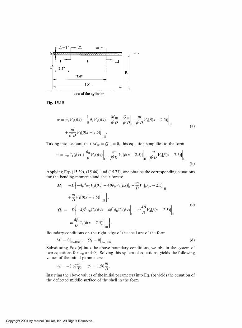
w ¼ w0V1ðxÞ þ1

#0V2ðxÞ �

M10

2D� Q10

3D

I

� m

2DV3½ðx� 2:5Þ�

II

þ m

2DV3½ðx� 7:5Þ�

III

:

ðaÞ

Taking into account that M10 ¼ Q10 ¼ 0, this equation simplifies to the form

w ¼ w0V1ðxÞ þ#0V2ðxÞ

I

� m

2DV3½ðx� 2:5Þ�

II

þ m

2DV3½ðx� 7:5Þ�

III

ðbÞApplying Eqs (15.39), (15.46), and (15.73), one obtains the corresponding equationsfor the bending moments and shear forces:

M1 ¼ �D �42w0V3ðxÞ � 4#0V4ðxÞI�m

DV1½ðx� 2:5�

n II

þm

DV1½ðx� 7:5Þ�

III

�;

Q1 ¼ �D �43w0V2ðxÞ � 42#0V3ðxÞI

þm4

DV4½ðx� 2:5Þ�

II

�m4

DV4½ðx� 7:5Þ�

III

�:

ðcÞ

Boundary conditions on the right edge of the shell are of the form

M1 ¼ 0x¼10 in:

; Q1 ¼ 0x¼10 in:

ðdÞSubstituting Eqs (c) into the above boundary conditions, we obtain the system oftwo equations for w0 and #0. Solving this system of equations, yields the followingvalues of the initial parameters:

w0 ¼ �3:67m

D; #0 ¼ 1:56

m

D:

Inserting the above values of the initial parameters into Eq. (b) yields the equation ofthe deflected middle surface of the shell in the form

Fig. 15.15


w ¼ m

D�3:67V1ð0:2874xÞ þ 5:428V2ð0:2874xÞ

Iþ12:107V3½0:2874ðx� 2:5Þ�

II

�þ 12:107V3½0:2874ðx� 7:5Þ�

III

�:

15.4 CIRCULAR CYLINDRICAL SHELL OF VARIABLE THICKNESSUNDER AXISYMMETRIC LOADING

Consider a state of stress and strain of circular cylindrical shells whose thicknessvaries only along the shell generator, i.e., h ¼ hðxÞ, and remains symmetrical withrespect to the middle surface. This shell is subjected to axisymmetrically applied edgeand distributed loads. It follows from the preceding sections that in this case adeformation of the shell does not depend on the circumferential angle �.

The governing differential equation for bending of an axisymmetrically loadedcircular cylindrical shell, Eq. (15.43), can be generalized to the case of the above-mentioned shell with variable thickness, as follows:

d2

dx2DðxÞ d

2w

dx2

" #þ Eh

R2w ¼ p3 þ

�

RN1; ð15:84Þ

where

DðxÞ ¼ Eh3ðxÞ12ð1� �2Þ : ð15:85Þ

is the flexural stiffness of the shell with variable thickness h ¼ hðxÞ. Equation (15.84)is a fourth-order ordinary differential equation with variable coefficients. It may besolved analytically for some particular laws of D ¼ DðxÞ only. For instance,Timoshenko provided an analytical solution of this equation when h ¼ x ð > 0Þusing the Bessel functions [8]. In a general case, when DðxÞ is an arbitrary function ofx, a solution of Eq. (15.84) can be obtained only numerically. For this purpose, onehas to transform Eq. (15.84) in the following way. Using Eqs (15.39), (15.41), and(15.46), one can reduce the fourth-order differential equation to the system of fourfirst-order differential equations, as follows:

dw

dx¼ #1;

d#1dx

¼ d2w

dx2¼ �M1

D;

dM1

dx¼ Q1;

dQ1

dx¼ � p3 þ

N2

R

� �¼ �p3 � �

N1

Rþ Eh

R2w:

ð15:86Þ

Let us introduce a dimensionless variable � and dimensionless parameters of the stateof stress and strain at any section of the cylinder Xi ði ¼ 1; 2; 3; 4Þ, as follows:

� ¼ x

R; X1 ¼

w

R; X2 ¼ #1 ¼

dw

dx;

X3 ¼R

D0

M1 ¼ �RD

D0

d2w

dx2; X4 ¼

R2

D0

Q1 ¼ �R2 D

D0

d3w

dx3

ð15:87Þ


where D0 ¼ const is the flexural stiffness of the shell at some reference section, say, at� ¼ 0; D ¼ DðxÞ is the flexural stiffness at a section of interest.

Applying the above-introduced dimensionless variables and parameters (Eqs(15.87)), one can represent Eqs (15.86) in the form

1

d�¼ X2;

dX2

d�¼ �D1

DX3;

dX3

d�¼ X4;

dX4

d�¼ EhR2

D0

X1 �R3

D0

p3 þ �N1

R

� �:

ð15:88Þ

This system of first-order ordinary differential equations is equivalent to the fourth-order single differential equation (15.84). In turn, the former system may be writtenin the following matrix form:

dX

d�¼ Að�ÞXþ f; ð15:89Þ

where

X ¼

X1

X2

X3

X4

2666664

3777775 ð15:90Þ

is the column vector that characterizes the parameters of the state of stress and strainat a section of interest and

A ¼

0 1 0 0

0 0 �D0=D 0

0 0 0 1

EhR2

D00 0 0

266666664

377777775; f ¼

0

0

0

�R3

D0p3 þ �N1

R

� �

266666664

377777775

ð15:91Þ

are the square matrix (4 4) and the column vector of the right-hand sides, res-pectively. The system of differential equations (15.89) may be efficiently solvednumerically using, for example, the sweep method [9] or Godunov’s method ofdiscrete orthogonalization [10].

Example 15.8

Consider a circular cylindrical shell of variable thickness under the action of pressurep. Two cases of variation of the shell thickness are analyzed: (a)

h1 ¼ h0 � 1

c2x2 þ 4

3

� �and (b) h2 ¼ h0 ¼ const, as shown in Fig. 15.16a and b, respec-


tively. As this takes place, the area of an axial cross section for all the three shells isidentical in the interval �c � x � c, i.e., the above shells are of the same weight. Theparallel edges of the shells are simply supported. Assuming that h0 ¼ 0:5; c ¼ 20; R¼ 15; and � ¼ 0:3, determine the deflections, internal forces, and moments in theshell.

Solution

Since the shells and loading are symmetrical about x ¼ 0, all the above problems aresolved for the interval 0 � x � c. Boundary conditions of the simply supported typefor the shell edge x ¼ c and the symmetry conditions for the section x ¼ 0 areprescribed. The numerical values of the components of the state of stress and strainare given in Table 15.1 for h ¼ h1. Analogous results are given in Table 15.2 forh ¼ h2. The system of ordinary differential equations (15.89) was solved byGodunov’s method of discrete orthogonalization. From these tables it is seen howthe thickness redistribution of the shell influences the state of stress and strain underthe condition of the conservation of the shell weight. It makes it possible to select themost efficient parameters of shell structures.

Fig. 15.16

Table 15.1

x ðM1=pÞ 10 ðN1=pÞ 10�1 Q1=p ðw= pEÞ 10�3

0 �0:31633 0.40996 0 0.30976

2 �0:32035 0.40996 �0:39650 10�3 0.31210

4 �0:33230 0.40996 �0:82848 10�3 0.31931

6 �0:35740 0.40996 �1:18812 10�2 0.33193

8 �0:42139 0.40996 �0:50151 10�2 0.35117

10 �0:58015 0.40996 �0:11284 10�1 0.37985

12 �0:86017 0.40996 �0:14980 10�1 0.42531

14 �0:99610 0.40996 �0:97754 10�2 0.50433

16 0:1056 10�1 0.40996 0.10333 0.63605

18 0.29781 0.40996 0.14807 0.71609

20 0 0.40996 �0:73044 0


PROBLEMS

15.1 Indicate cases when the membrane theory alone cannot describe adequately the state of

stress of cylindrical shells under applied transverse loading.

15.2 Verify Eqs (15.21) and (15.24).

15.3 What are the conditions at which a complete state of stress in open and closed cylind-

rical shells can be broken down into elementary states of stress? Characterize these

elementary stress states.

15.4 A long steel pipe is subjected to the edge line load Q0 that is applied uniformly around

the circumference x ¼ 0. The radius and thickness of the pipe are R ¼ 0:5m and

h ¼ 5mm, respectively. (a) Derive and plot the values of w and M vs. x. (b)

Determine the distance x at which the deflections and moments are 5% of their abso-

lute maximum values. Take E ¼ 200GPa; and � ¼ 0:3.15.5 A very long cylinder of radius R and of thickness h is subjected to uniform loading

p0 over L of its length (Fig. 15.11) (a) Determine the ratio of maximum bending

stress to maximum magnitude of membrane stress. (b) Calculate the deflections and

bending moments at a point A for two cases of location of that point, as shown in

Figs 15.11a and b. Take R ¼ 1:5m; h ¼ 6mm; p0 ¼ 5 kPa; E ¼ 200GPa; and

� ¼ 0:3.15.6 Verify Eqs (15.57).

15.7 The infinite circular cylinder of radius R is subjected to a uniformly distributed around

a circumference moment m, as shown in Fig. P.15.1. Assuming that the moment is

applied near the center of the cylinder, find the expressions for w; #;M1; and Q1 as

functions of m and x:15.8 A stiffening ring is placed around a long steel cylindrical shell at a distance remote

from the ends, as shown in Fig. 15.12a. The cylinder is loaded by an internal pressure

p0. Determine stress at the ring attachment if: (a) the ring is assumed to be infinitely

rigid and (b) the ring is assumed to be 100 mm wide and 10 mm thick. Take the radius

of the cylinder as 1.25 m and its thickness as 6 mm, p0 ¼ 10 kPa; E ¼ 200GPa; and� ¼ 0:3:

15.9 Determine stresses in a cylindrical component reinforced by a ring and subjected to

internal pressure p ¼ 4 MPa (Fig. P.15.2). All dimensions in Fig. P.15.2 are given in

mm. Take E ¼ 200GPa; and � ¼ 0:3.

Table 15.2

x M1=p N1=p Q1=p ðw= pEÞ 10�3

0 0:13028 10�4 0:42808 10 0 0.41154

2 0:31492 10�3 0:42808 10 0:29494 10�3 0.41153

4 0:10442 10�2 0:42808 10 0:33756 10�3 0.41140

6 0:82148 10�3 0:42808 10 �0:91417 10�3 0.41095

8 �0:44991 10�2 0:42808 10 �0:48864 10�2 0.41030

10 �0:18990 10�1 0:42808 10 �0:97479 10�2 0.41154

12 �0:27954 10�1 0:42808 10 0:55193 10�2 0.41935

14 0:39696 10�1 0:42808 10 0:73855 10�1 0.43480

16 0.30266 0:42808 10 0.18704 0.43047

18 0.65488 0:42808 10 0:82290 10�1 0.31639

20 0 0:42808 10 �0:97407 0

This example has been taken from Ref. [10]


15.10 A long cylindrical shell is reinforced by two equal stiffening rings at a distance 5 cm

from one another. Both stiffening rings are placed far from the shell ends. The shell is

loaded by an internal pressure p0. Determine the deflections and stresses at the ring

attachments if each ring has a rectangular cross section 2.5 cm wide and 0.5 cm thick.

The parameters of the shell are R ¼ 1:5m. h ¼ 5mm. Take p0 ¼ 500 kPa;E ¼ 200GPa; and � ¼ 0:3.

15.11 A long cylindrical pipe of diameter D ¼ 1:0 m and of wall thickness h ¼ 6 mm is

subjected to load P, uniformly distributed along a circular cross section (Fig. 15.9).

Determine the value of P required according to the Tresca criterion. Use �ys ¼ 220

MPa; E ¼ 200GPa; and � ¼ 0:3.15.12 Consider a semi-infinite cylindrical shell of radius R and thickness h loaded by an

internal pressure p0 ¼ const. Compare the maximum values of bending stresses, �1,for two types of boundary conditions, prescribed on the shell edge x ¼ 0: built-in and

simply supported edges. Indicate in the solution the locations of these maximum

stresses.

15.13 A stepped water tower, shown in Fig. P.15.3, is filled to capacity with a liquid of

specific weight �. Determine the values of the discontinuity moments and shear forces

along the joint and at the base of the tower. Assume that the water tower is built-in at

its base. The self-weight of the tower can be neglected. TakeH ¼ 4:0m; R ¼ 1m;H1 ¼1:0m; h1 ¼ 25mm; h2 ¼ 15mm; E ¼ 30GPa; � ¼ 9800N=m3; and � ¼ 0:15.

15.14 Solve a problem of Example 15.7 (see Fig. 15.15) replacing the two moments applied to

the short shell by two equal line forces P distributed along circular sections of a shell

x ¼ 2:5 in: and x ¼ 7:5 in:15.15 Verify the general-purpose equation of the middle surface deflections, Eq. (15.83).

Fig. P15.1

Fig. P15.2


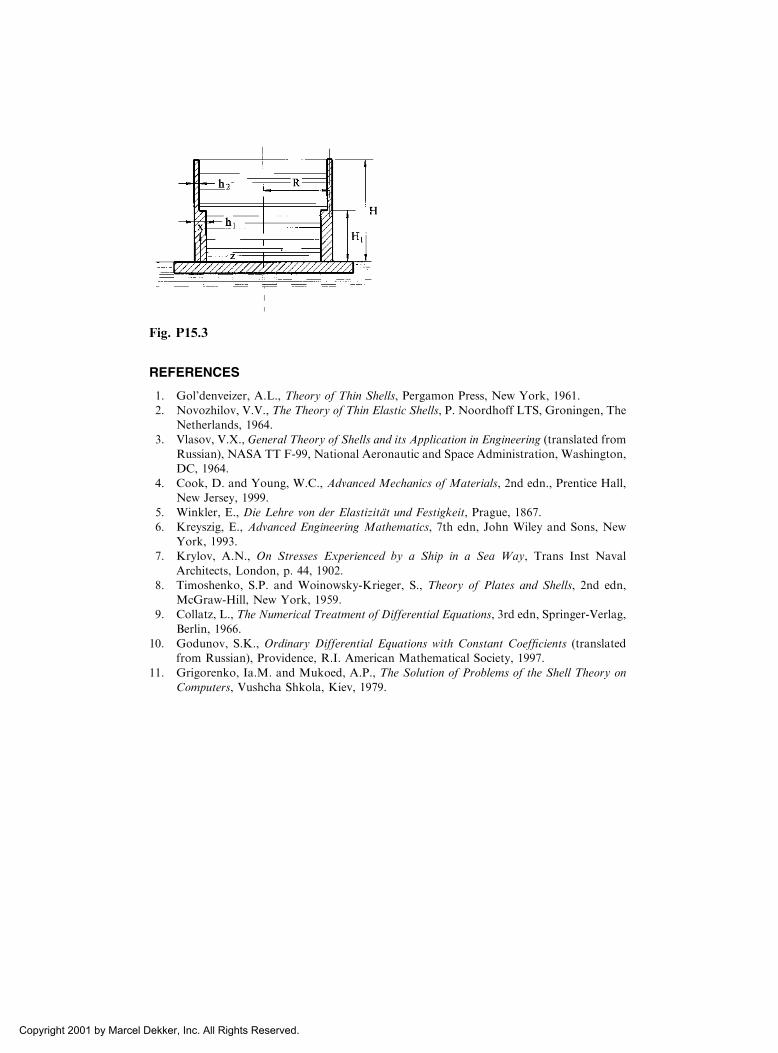
REFERENCES

1. Gol’denveizer, A.L., Theory of Thin Shells, Pergamon Press, New York, 1961.

2. Novozhilov, V.V., The Theory of Thin Elastic Shells, P. Noordhoff LTS, Groningen, The

Netherlands, 1964.

3. Vlasov, V.X., General Theory of Shells and its Application in Engineering (translated from

Russian), NASA TT F-99, National Aeronautic and Space Administration, Washington,

DC, 1964.

4. Cook, D. and Young, W.C., Advanced Mechanics of Materials, 2nd edn., Prentice Hall,

New Jersey, 1999.

5. Winkler, E., Die Lehre von der Elastizitat und Festigkeit, Prague, 1867.

6. Kreyszig, E., Advanced Engineering Mathematics, 7th edn, John Wiley and Sons, New

York, 1993.

7. Krylov, A.N., On Stresses Experienced by a Ship in a Sea Way, Trans Inst Naval

Architects, London, p. 44, 1902.



9. Collatz, L., The Numerical Treatment of Differential Equations, 3rd edn, Springer-Verlag,

Berlin, 1966.

10. Godunov, S.K., Ordinary Differential Equations with Constant Coefficients (translated

from Russian), Providence, R.I. American Mathematical Society, 1997.

11. Grigorenko, Ia.M. and Mukoed, A.P., The Solution of Problems of the Shell Theory on

Computers, Vushcha Shkola, Kiev, 1979.

Fig. P15.3


16

The Moment Theory of Shells ofRevolution

16.1 INTRODUCTION

As mentioned, shells of revolution belong to a highly general class of shells fre-quently used in engineering. One representative of this class, cylindrical shells, wasconsidered in Chapter 15, and we will not dwell on these shells. The shell typesanalyzed in this chapter are subclasses of shells of revolution having non-zeroGaussian curvature. As mentioned in Sec. 11.7, such shells have non-developablesurfaces. Hence, they are stronger, stiffer, and more stable than shells with zeroGaussian curvature. These shells are frequently used to cover the roofs of sporthalls and large liquid storage tanks. The containment shield structures of nuclearpower plants also have dome-like roofs. Various pressure vessels are either com-pletely composed of a single rotational shell or have shells of revolution at their endcaps. Conical shells with zero Gaussian curvature are also representative of thisclass of shells: they are used to cover liquid storage tanks and the nose cones ofmissiles and rockets.

In the membrane analysis of shells of revolution considered in Chapters 13 and14, we saw that the membrane theory alone cannot accommodate all the loads,support conditions, and geometries in actual shells. Thus, in a general case, shellsof revolution experience both stretching and bending to resist an applied loading,which distinguishes significantly the bending of shells from the elementary behaviorof plates (see also Sec. 10.4).

However, the character of bending deformation may be different. If a shell ofrevolution is subjected to a concentrated force (Fig. 16.1a), bending exerts a crucialeffect on its strength, because, in this case, the bending deformation increases with agrowth of the forces until the load-carrying capacity of the shell structure is exhausted.In places of junction of a shell with its supports (Fig. 16.1b) or other structuralmembers (shell of another geometry, ring beam, etc.), or in places of jump change in


the radii of curvature (Fig. 16.1c), the bending has another character; here, bendingpropagates only if it is needed to eliminate the discrepancies between the membranedisplacements or to satisfy the conditions of statics. If a shell material is ductile, thebending deformations of the latter type are usually decreased and do not practicallyinfluence the load-carrying capacity of shell structures. If the material of the shell isbrittle, the bending deformations remain proportional to the applied loads until failureand can result in a significant decrease in the strength of the shell structure

In this chapter we consider the bending theory of shells of revolution. It shouldbe noted that the solutions of the governing differential equations involve manydifficulties for a general shell of revolution, and therefore, we solve these equationsfor some particular shell geometries and load configurations that are frequently usedin engineering practice.

16.2 GOVERNING EQUATIONS

We present below the governing differential equations of the moment theory of shellsof revolution of an arbitrary shape. As curvilinear coordinates and of a point onthe shell middle surface, it is convenient to take the spherical coordinates, introducedin Sec. 11.8, and used in the membrane theory of shells of revolution in Chapters 13and 14. Thus, we take ¼ ’ and ¼ �. As before, the angle ’ defines the location ofa point along the meridian, whereas � characterizes the location of a point along theparallel circle (see Fig. 11.12). Let R1 and R2 be the principal radii of curvature of themeridian and parallel circle, respectively. Obviously, R1 and R2 will be functions of ’only, i.e., R1 ¼ R1ð’Þ and R2 ¼ R2ð’Þ. The Lame parameters in this case are deter-mined by the following formulas (see Sec. 11.8):

A ¼ R1ð’Þ; B ¼ R2ð’Þ sin ’; r ¼ R2 sin ’: ð16:1ÞThe Codazzi and Gauss conditions are given by Eqs (11.41).

Let us consider the kinematic relations of the moment theory of shells ofrevolution. Displacement components of the middle surface along the given coordi-

Fig. 16.1


nate axes are u (in the meridional direction), v (in the circumferential direction), andw (in the normal direction to the middle surface). The strain–displacement relations(12.23) and (12.24) of the general shell theory – taking into account Eqs (16.1) and(11.41) – take the following form for shells of revolution:

"1 ¼1

R1

@u

@’� w

� �;

"2 ¼1

R2 sin ’

@v

@�þ u cos ’� w sin ’

� �;

�12 ¼1

R1

@v

@’� cos ’

R2 sin ’vþ 1

R2 sin ’

@u

@�; ð16:2Þ

�1 ¼ � 1

R1

@

@’

1

R1

uþ @w@’

� �� ;

�2 ¼ � 1

R2 sin ’ð Þ2@v

@�sin ’þ @

2w

@�2

!� cos ’

R1R2 sin ’uþ @w

@’

� �;

�12 ¼1

R2 sin ’

cos ’

R2 sin ’

@w

@�� 1

R1

@2w

@�@’� 1

R1

@u

@�� sin ’

R1

@v

@’þ cos ’

R2

v

" #; ð16:3Þ

where "1 and "2 are in-plane meridional and circumferential strain components in themiddle surface, �12 characterizes a shear of the middle surface; �1 and �2 representthe changes in curvature of the coordinate lines in the middle surface due to itsbending, and �12 characterizes a twist of the middle surface. The rotations of theshell edges that coincide with the coordinate lines � and ’, respectively, can beobtained from Eqs (12.2) using the relations (16.1) and (11.41). We obtain

#1 ¼u

R1

þ 1

R1

@w

@’; #2 ¼

1

R2 sin ’

@w

@�þ v sin ’

� �: ð16:4Þ

Equations of static equilibrium (12.41) and (12.42) with regard to relations (12.43),(11.41), and (16.2) take the form

@

@’N1R2 sin ’ð Þ þ R1

@

@�S � H

R1

� ��N2R1 cos ’�Q1R2 sin ’

þ p1R1R2 sin ’ ¼ 0;

R1

@N2

@�þ @

@’R2 sin ’ S � H

R2

� �� þ S � H

R1

� �R1 cos ’

�Q2R1 sin ’þ p2R1R2 sin ’ ¼ 0;

@

@’ðQ1R2 sin ’Þ þ

@

@�ðQ2R1Þ þN1R2 sin ’þN2R1 sin ’þ p3R1R2 sin ’ ¼ 0;

@

@’ðHR2 sin ’Þ þ R1

@M2

@�þHR1 cos ’�Q2R1R2 sin ’ ¼ 0;

R1

@H

@�þ @

@’ðM1R2 sin ’Þ �M2R1 cos ’�Q1R1R2 sin ’ ¼ 0:

ð16:5Þ


Taking into account the relations for the effective shear forces (in-plane andout-of-plane) introduced in Sec. 12.5, the following static quantities can be assignedon a boundary coinciding with the edge parallel circle ’ ¼ ’e:

N1;T1 ¼ S � 2H

R2

; M1; and V1

where

V1 ¼ Q1 þ1

R2 sin ’

@H

@�¼ 1

R2 sin ’2@H

@�þ @ðM1R2 sin ’Þ

R1@’�M2 cos ’

� �: ð16:6Þ

The constitutive relations are found to be in the form of Eqs (12.45) and(12.46).

The governing equations and relations introduced above allow one to deter-mine the stress and displacement components that occur in a shell of revolutionsupported along its edges and subjected to given external loads. The unknownfunctions characterizing the state of stress and strain (deformations and stressresultants and couples) depend upon variables � and ’ in Eqs (16.3), (16.5), and(12.45), (12.46). These unknowns are periodic functions of variable � for shells ofrevolution. Thus, one can apply the separation of variables method for solving thegoverning differential equations of shells of revolution. This method implies thatall loads, displacements, and stress resultants and couples may be represented inthe form

fið�; ’Þ ¼X1k¼0

fðsÞik cos k� þ

X1k¼1

fðaÞik sin k�;

�ið�; ’Þ ¼X1k¼1

�ðsÞik sin k� �X1k¼0

�ðaÞik cos k�;

ð16:7Þ

where by functions fi are meant the functions p1; p3; u;w; "1; "2; #1; �1; �2;N1;N2;M1; M2; and Q1, and by functions �i are meant the functions p2; v; �12; #2;S;H;and Q2. It can be seen that the functions having the superscripts s and a corre-spond to symmetric and skew-symmetric of the above-mentioned functions abouta zero meridian, respectively. It is easily verified that the symmetric and skew-symmetric components of the displacements, stress resultants, etc., determined bythe same system of equations. Therefore, we present the corresponding relationsand equations for functions having the superscript s only, without using thisindex. So, substituting the expressions (16.7) into the kinematic relations (16.2)and (16.3), equilibrium equations (16.5), and eliminating the shear forces, Q1 andQ2, we obtain some systems of ordinary differential equations for unknownfunctions of deformations, and stress resultants and couples. Note that the con-stitutive equations (12.45) and (12.46) remain unchanged. It is required only toprovide all the quantities involving in these equations with the index k. Let uspresent these equations:


Kinematic equations (strain–displacement relations)

"1k ¼1

R1

dukd’

� wk

� �;

"2k ¼1

R2 sin ’ðkvk þ uk cos ’� wk sin ’Þ;

�12k ¼1

R1

dvkd’

� cos ’

R2 sin ’vk �

kukR2 sin ’

;

�1k ¼ � 1

R1

d

d’

ukR1

þ 1

R1

dwk

d’

� �;

�2k ¼ � 1

ðR2 sin ’Þ2kvk sin ’� k2wk

� �� cos ’

R1R2 sin ’uk þ

dwk

d’

� �;

�12k ¼1

R2 sin ’� cos ’

R2 sin ’kwk þ

k

R1

dwk

d’þ k

R1

uk �sin ’

R1

dvkd’

þ cos ’

R2

vk

� �;

#1k ¼1

R1

uk þdwk

d’

� �; #2k ¼

1

R2 sin ’ð�kwk þ vk sin ’Þ

ð16:8ÞEquations of static equilibrium

d

d’N1kR2 sin ’ð Þ þ R1kSk �

1

R1

d

d’ðM1kR2 sin ’Þ þM2k cos ’

� 2kHk �N2kR1 cos ’þ p1kR1R2 sin ’ ¼ 0

� R1kN2k þ1

R2 sin ’

d

d’SkðR2 sin ’Þ2� �

� 1

R2

R1ð�kÞM2k þ 2R2 sin ’dHk

d’

�þ2 cos ’HkðR1 þ R2Þ

�

þ p2kR1R2 sin ’ ¼ 0:

N1k

R1

þN2k

R2

þ 1

R1R2 sin ’

d

d’

Hkkþ 1

R1

d

d’ðM1kR2 sin ’Þ �M2k cos ’

� �

þ 1

R2 sin ’

k

R2 sin ’

d

d’ðR2 sin ’Þ2Hk

� �� k2R1M2k

� ��þ p3k ¼ 0:

ð16:9Þ

Equations (16.8) and (16.9), together with the constitutive equations (12.45) and(12.46) and proper boundary conditions, form the closed eight-order system of theordinary differential equations for each kth harmonic of the expansion (16.7). Thissystem of the governing equations describes the state of stress and strain for thegeneral moment theory of shells of revolution having a meridian of an arbitraryshape. This system of ordinary equations may be solved by applying the standardnumerical methods intended for a solution of ordinary differential equations andintroduced, for example, in Refs. [1,2]. The finite element method can also be appliedto the analysis of the state of stress and strain for shells of revolution of a generalshape [3,4].


It should be noted that numerical difficulties associated with a solution of thedifferential equations (16.8) and (16.9) may be partially eliminated for some specificshapes of shells of revolution and loading.

16.3 SHELLS OF REVOLUTION UNDER AXISYMMETRICAL LOADS

When a shell of revolution is subjected to rotationally symmetrical loads (p2 ¼ 0), itsdeformations and stress resultants and couples do not depend upon the variable �.The conditions of symmetry dictate that

S ¼ Q2 ¼ H ¼ 0 and v ¼ �12 ¼ �12 ¼ 0: ð16:10ÞFor this particular case of loading, the strain–displacement relations (16.2) and(16.3) and equilibrium equations (16.5) and constitutive equations (12.45) and(12.46) take the following form:

Strain–displacement relations

"1 ¼1

R1

du

d’� w

� �; "2 ¼

1

R2

ðu cot ’� wÞ;

�1 ¼ � 1

R1

d

d’

1

R1

uþ dw

d’

� �� ; �2 ¼ � cot ’

1

R1R2

uþ dw

d’

� �;

#1 ¼u

R1

þ 1

R1

dw

d’;

ð16:11Þ

where #1 is the angle of rotation of the tangent to the shell meridian.

Equilibrium equations

d

d’ðN1R2 sin ’Þ �N2R1 cos ’�Q1R2 sin ’þ p1R1R2 sin ’ ¼ 0;

d

d’ðQ1R2 sin ’Þ þN1R2 sin ’þN2R1 sin ’þ p3R1R2 sin ’ ¼ 0;

d

d’ðM1R2 sin ’Þ �M2R1 cos ’�Q1R1R2 sin ’ ¼ 0:

ð16:12Þ

Constitutive equations

N1 ¼Eh

1� �2 ð"1 þ �"2Þ; N2 ¼Eh

1� �2 ð"2 þ �"1Þ;

M1 ¼ Dð�1 þ ��2Þ; M2 ¼ Dð�2 þ ��1Þ:ð16:13Þ

It is convenient to express the fourth and fifth Eqs (16.11) in terms of #1. So,inserting the fifth Eq. (16.11) into the above equations, one obtains the following

�1 ¼ � 1

R1

d#1d’

; �2 ¼ � cot ’1

R2

#1: ð16:14Þ

Substituting for the strain components from the first two Eqs (16.11) and Eqs (16.14)into Eqs (16.13), gives the following stress resultants and couples–displacementrelations


N1 ¼ B1

R1

du

d’� w

� �þ �

R2

ðu cot ’� wÞ� �

; ð16:15aÞ

N2 ¼ B1

R2

ðu cot ’� wÞ þ �

R1

du

d’� w

� �� ; ð16:15bÞ

M1 ¼ �D1

R1

d#1d’

þ �

R2

#1 cot ’

� �; ð16:15cÞ

M2 ¼ �D1

R2

#1 cot ’þ�

R1

d#1d’

� �; ð16:15dÞ

where

B ¼ Eh

1� �2 ;D ¼ Eh3

12ð1� �2Þ : ð16:16Þ

Equations (16.11), (16.12), and (16.13) or (16.15) form a closed system of 12ordinary differential equations for 12 unknowns (strains, stress resultants andcouples). Solving this system of equations, one obtains the internal forces, moments,and displacements. The stress components are calculated by the following formulas:

�1max ¼N1

hþ 6M1

h2; �2max ¼

N2

hþ 6M2

h2: ð16:17Þ

Let us bring the above system of equations to two symmetric governing equa-tions for two unknowns. Following Meissner [5], we introduce the new variables

#1 and U ¼ R2Q1ð’Þ: ð16:18ÞWe now express the internal forces and moments in terms of the new variables.Canceling the circumferential force N2 from the first and second Eqs (16.12), weobtain the following equation:

1

R1

d

d’ðN1 sin ’þQ1 cos ’Þr½ � þ ðp1 sin ’þ p3 cos ’Þr ¼ 0: ð16:19Þ

Integrating this equation over ’, we obtain

ðN1 sin ’þQ1 cos ’Þr ¼ �Fð’Þ; ð16:20Þwhere

Fð’Þ ¼ð’’e

R1rðp1 sin �’’þ p3 cos �’’Þd �’’þ C; ð16:21Þ

here �’’ is a dummy variable; ’e is the angular coordinate of one of the shell edges –say, the top edge; Fð’Þ represents the resultant of all external surface loads applied toan isolated part of the shell per unit ’; and C takes into account an axial componentof the external loads applied to the top edge of the shell.

Comparing Eqs (16.21) and (13.37), we can conclude that a particular solutionof Eq. (16.19), corresponding to the integral Fð’Þ; represents a membrane solution ofthe general bending theory of axisymmetrically loaded shells of revolution.

Taking into account Eq. (16.18), we can express the meridional force N1 interms of U from Eq. (16.20), as follows:


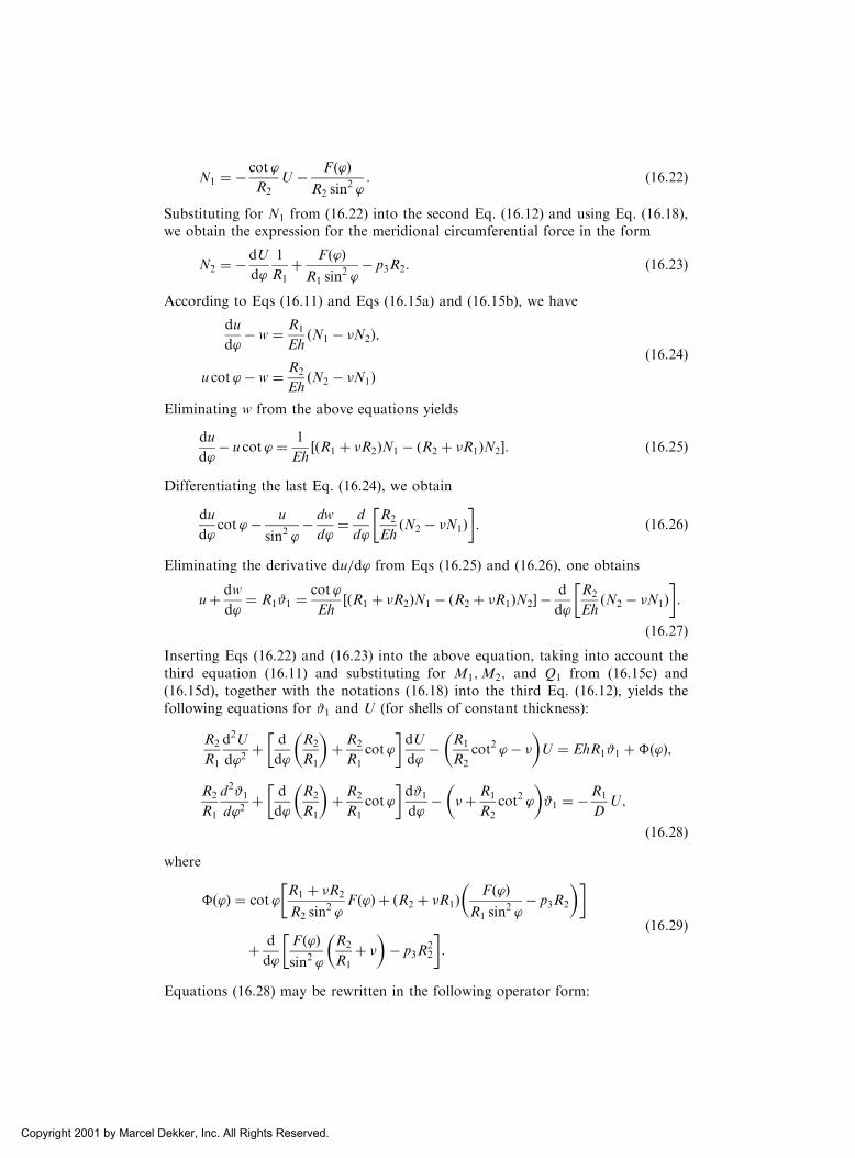
N1 ¼ � cot ’

R2

U � Fð’ÞR2 sin

2 ’: ð16:22Þ

Substituting for N1 from (16.22) into the second Eq. (16.12) and using Eq. (16.18),we obtain the expression for the meridional circumferential force in the form

N2 ¼ � dU

d’

1

R1

þ Fð’ÞR1 sin

2 ’� p3R2: ð16:23Þ

According to Eqs (16.11) and Eqs (16.15a) and (16.15b), we have

du

d’� w ¼ R1

EhðN1 � �N2Þ;

u cot ’� w ¼ R2

EhðN2 � �N1Þ

ð16:24Þ

Eliminating w from the above equations yields

du

d’� u cot ’ ¼ 1

EhðR1 þ �R2ÞN1 � ðR2 þ �R1ÞN2½ �: ð16:25Þ

Differentiating the last Eq. (16.24), we obtain

du

d’cot ’� u

sin2 ’� dw

d’¼ d

d’

R2

EhðN2 � �N1Þ

� �: ð16:26Þ

Eliminating the derivative du=d’ from Eqs (16.25) and (16.26), one obtains

uþ dw

d’¼ R1#1 ¼

cot ’

EhðR1 þ �R2ÞN1 � ðR2 þ �R1ÞN2½ � � d

d’

R2

EhðN2 � �N1Þ

� �:

ð16:27ÞInserting Eqs (16.22) and (16.23) into the above equation, taking into account thethird equation (16.11) and substituting for M1;M2; and Q1 from (16.15c) and(16.15d), together with the notations (16.18) into the third Eq. (16.12), yields thefollowing equations for #1 and U (for shells of constant thickness):

R2

R1

d2U

d’2þ d

d’

R2

R1

� �þ R2

R1

cot ’

� �dU

d’� R1

R2

cot2 ’� ��

U ¼ EhR1#1 þ�ð’Þ;

R2

R1

d2#1d’2

þ d

d’

R2

R1

� �þ R2

R1

cot ’

� �d#1d’

� �þ R1

R2

cot2 ’

� �#1 ¼ �R1

DU;

ð16:28Þwhere

�ð’Þ ¼ cot ’R1 þ �R2

R2 sin2 ’

Fð’Þ þ ðR2 þ �R1ÞFð’Þ

R1 sin2 ’

� p3R2

� ��

þ d

d’

Fð’Þsin2 ’

R2

R1

þ ��

� p3R22

� �:

ð16:29Þ

Equations (16.28) may be rewritten in the following operator form:


LðUÞ þ �U ¼ EhR1#1 þ�ð’Þ;

Lð#1Þ � �#1 ¼ �R1

DU:

ð16:30Þ

where

Lð::Þ ¼ R2

R1

d2ð::Þd’2

þ d

d’

R2

R1

� �þ R2

R1

cot ’

� �dð::Þd’

� cot2 ’ð::Þ R1

R2

� �ð16:31Þ

Equations (16.30) are the governing differential equations of the axisymmetric bend-ing of shells of revolution of constant thickness. A particular solution of the systemof ordinary differential equations (16.30) can be found from the membrane theory ofaxisymmetrically loaded shells of revolution (see Sec. 13.5).

Setting

U ¼ 1

R1

Lð Þ � � ð Þ; #1 ¼ � 1

D ; ð16:32Þ

where is some function of forces and displacements. We identically satisfy thesecond Eq. (16.30). Inserting Eqs (16.32) into the first Eq. (16.30), we obtain

L1

R1

Lð Þ� �

� �L

R1

� �þ �

R1

Lð Þ þ EhR1

D� �2

R1

! ¼ �ð’Þ: ð16:33Þ

If the radius of the shell curvature R1 ¼ const (sphere, cone, toroid), then Eq. (16.33)takes the following form:

LLð Þ þ �2 ¼ R1�ð’Þ; ð16:34Þwhere

�2 ¼ EhR21

D� �2 � b2 ð16:35Þ

and b2 ¼ 12ð1� �2ÞR21=h

2 is the basic characteristic of a shell. Equation (16.34) canbe represented in the form

Lþ i�½ � Lð Þ � i� ½ � ¼ R1�ð’Þ; ð16:36Þand its general solution can be obtained in a complex form.

It is convenient to express the boundary conditions of the shell of revolutionvia the horizontal, �, and vertical, , displacements of a point of the middle surface,as shown in Fig. 16.2. The formulas that relate the displacement components u and vto the displacements � and can be directly obtained from Fig, 16.2, i.e.,

� ¼ w sin ’� u cos ’; ¼ w cos ’þ u sin ’: ð16:37ÞLet us consider some typical boundary conditions for the shells of revolution

shown in Fig. 16.3.

(a) The edge of a shell is built-in (Fig. 16.3a)The boundary conditions are of the form

#1 ¼ � ¼ 0j’¼’e : ð16:38aÞ


The relative stretching in the circumferential direction is

"2 ¼�

r¼ �

R2 sin ’; from which � ¼ "2R2 sin ’: ðaÞ

Using the above relation (a) and Eqs (16.13), the second boundary condition (Eq.(16.38a)) can be rewritten as follows:

Fig. 16.2

Fig. 16.3


"2 ¼ 0j’¼’e or N2 � �N1 ¼ 0j’¼’e ð16:38bÞ(b) The edge of a shell is pinned (Fig. 16.3b)In this case

� ¼ 0j’¼’e or "2 ¼ 0; N2 � �N1 ¼ 0j’¼’e and

M1 ¼ 0j’¼’e or1

R1

d#1d’

þ � cot ’R2

#1 ¼ 0j’¼’e :ð16:38cÞ

(c) The edge of a shell is simply supported (Fig. 16.3c)In this case the boundary conditions are of the form

M1 ¼ 0

’¼’e

or1

R1

d#

d’þ � cot’

R2

#1 ¼’¼’e and

N1 cos ’e þQ1 sin ’e ¼ 0’¼’e :

ð16:38dÞ

(d) The edge of a shell is free (Fig. 16.3d)Here the boundary conditions are

M1 ¼ 0j’¼’e or1

R1

d#1d’

þ � cot ’R2

#1 ¼ 0j’¼’eQ1 ¼ 0j’¼’e or U ¼ 0j’¼’e:

ð16:38eÞ

(e) The edge of a shell is loaded by edge forces Ne;Qe; and Me (Fig. 16.3e)In this case the boundary conditions are

M1 ¼ Me

’¼’e or

1

R1

d#1d’

þ � cot ’R2

#1 ¼ Me

’¼’e

Q1 ¼ Qe

’¼’e or U ¼ QeR2

’¼’e :

ð16:38f Þ

(f) A shell is built-in from both sides (Fig. 16.3f)Since such a shell is statically indeterminate, we must impose the following fiveconditions:

#1 ¼ 0j’¼’e1 ; "2 ¼ 0j’¼’e1 ; #1 ¼ 0j’¼’e2 ; "2 ¼ 0j’¼’e2 ;

A=B ¼ 0 or

ð’¼’e2’¼’e1

ð"1 sin ’þ #1 cos ’ÞR1d’ ¼ 0:ð16:38gÞ

(g) Two joined shells (Fig. 16.3g)It is necessary for this case to satisfy the four boundary conditions, namely,

�ð1Þe ¼ �ð2Þe or "ð1Þ2e ¼ "ð2Þ2e ;

#ð1Þ1e ¼ #ð2Þ1e ; Mð1Þ1e ¼ M

ð2Þ1e ;

Nð1Þ1e cos ’e1 þQ

ð1Þ1e sin ’e1 ¼ N

ð2Þ1e cos ’e2 �Q

ð2Þ1 sin ’e2 :

ð16:38hÞ

The last condition expresses the equality of the radial forces (thrusts).(h) If a shell is closed at its vertex, for ’ ¼ 0, then the following conditions must besatisfied:

#1 ¼ 0j’¼0 and Q1 ¼ 0j’¼0: ð16:39Þ


16.4 APPROXIMATE METHOD FOR SOLUTION OF THE GOVERNINGEQUATIONS (16.30)

The solution of the governing differential equations (16.30) is quite complicated. Inthe present section, we introduce one approximate method for the bending analysisof shells of revolution under axisymmetric edge loads.

Figure 16.4 shows two shells of revolution subjected to distributed over theedge loads N1e, Me and Qe. The first shell (Fig. 16.4a) is a shallow one. In axisym-metric bending of such a shell, the radial displacements and the correspondingcircumferential tensile deformations are small near the loaded edge. Therefore,deformations caused by the bending moments diminish slowly and their influencemay extend over, practically, the entire shell.

In the second case, shown in Fig. 16.4b, the slope of the normal, #1, is large.Here, considerable circumferential tension occurs near the loaded edge as the shellbends axisymmetrically. As a consequence, the bending deformations diminishrapidly and they practically vanish at a small distance from the edge.

The effect of the circumferential tension in an axisymmetric bending of a shellwith large angle of rise is similar to that of an elastic foundation. A similar effect ofrapid decrease of the bending deformations near the loaded edge was observed in theaxisymmetrically loaded cylindrical shells in Sec. 15.5. Based on this analogy, a veryefficient approximate method may be developed for shells of revolution with largeangle of a rise and subjected to edge loading. This method uses the followingassumptions:

(a) All functions characterizing the stress and strain components in a shell near its edge,as well as their first derivatives, are small compared with their higher derivatives.This assumption is based on that fact that all the considered functions willcontain multipliers of the type e�’; where ’ is the angle measured from theshell edge of interest and is some parameter. In differentiating these functions,the parameter appears every time in the form of the multiplier. Since thesefunctions are rapidly decaying, the value of the parameter is large. Therefore,values of the first derivative are sufficiently greater than the values of the func-tions themselves, and values of the second derivatives are greater than the firstderivatives, etc., i.e.,

dnUn

d’n� dðn�1ÞUn

d’n�1and

dn#1d’n

� dðn�1Þ#1d’n�1

:

Fig. 16.4


On this basis, terms containing the functions themselves and their first derivatives onthe left-hand side of Eqs (16.30) are dropped. The function �ð’Þ on the right-handside of Eqs (16.30) is zero for loads applied to the edge of the shell. As a result, thegoverning differential equations (16.30) take the form

R2

R1

d2U

d’2¼ EhR1#1; ð16:40aÞ

R2

R1

d2#1d’2

¼ �R1

DU: ð16:40bÞ

(b) The radii of curvature, R1 and R2, are assumed to be constant near the shell edge.This is true for spherical shells only. For shells of other shapes this assumption iscarried out the more precisely the closer the shape of a shell approaches a sphericalone.

The approximate method for the bending analysis of axisymmetrically loadedspherical shells of revolution based on the above-mentioned assumptions was firstintroduced by H. Reissner [6] and Geckeler [7]; it was then generalized to shells ofrevolution of an arbitrary shape of a meridian by Meissner [5,8]. Equations (16.40)can be reduced to a single differential equation with one unknown. DifferentiatingEq. (16.40a) twice with regard to the second assumption, and inserting d2#1=d’

2 intoEq. (16.40b), we obtain the following fourth-order governing differential equation:

d4U

d’4þ 44U ¼ 0; ð16:41Þ

where

¼ R1

ffiffiffiffiffiffiffiffiffiffiffiffiffiffiffiffiffiffi3ð1� �2ÞR2

2h2

4

s: ð16:42Þ

Note that it is impossible to neglect the function U compared with its fourth deri-vative in Eq. (16.41) because the multiplier 44 is sufficiently large.

Equation (16.41) is referred to as the edge effect differential equation because itssolution is expressed in terms of rapidly damped functions. The edge effect governingequation and the corresponding numerical procedure for the general theory of thinshells is discussed in more detail in Sec. 17.5. Equation (16.41) is analogous to that ofan axisymmetric deformation of a circular cylindrical shell (see Eq. (15.44)). Hence,we can apply the edge effect technique developed in Sec. 15.3 to axisymmetricbending analysis of shells of revolution. The general solution of Eq. (16.41) for Ucan be written in the form

U ¼ e�’ðB1 sin ’þ B2 cos’Þ þ e’ðB3 sin ’þ B4 cos ’Þ: ð16:43Þ

It is convenient to introduce a new independent variable !, representing also theangular coordinate and counting off from the shell edge, as shown in Fig. 16.5.

If the lower shell edge is of interest (Fig. 16.5a), then

! ¼ ’e � ’: ð16:44aÞ


If the upper shell edge is of interest (Fig. 16.5b), then the angle ! is counted offoppositely and

! ¼ ’� ’e: ð16:44bÞSince, in both the above-mentioned cases,

d4U

d’4¼ d4U

d!4;

in the transition to a new variable, the differential equation remains unchanged, i.e.,

d4U

d!4þ 44U ¼ 0: ð16:45Þ

The solution of this equation can be written in the form

U ¼ e�!ðC1 sin !þ C2 cos!Þ þ e!ðC3 sin !þ C4 cos!Þ; ð16:46Þwhere C1; . . . ;C4 are constants to be determined from the boundary conditions.Since the function U has to die down as the angle ! increases, the second term inEq. (16.46), involving the multiplier e!, must vanish as we move away from theloaded edge of the shell. Therefore, the constants C3 and C4 should be equal to zeroand the above solution takes the form

U ¼ e�!ðC1 sin !þ C2 cos!Þ: ð16:47ÞThis solution describes the moment state of stress and strain near a loaded edge(either bottom or top). However, in differentiating Eq. (16.47), it should be takeninto account that on the top edge of the shell angle ! is counted off in the side of anincrease of angle ’; therefore, dU=d’ ¼ dU=d!. On the bottom edge, referencedirections of angles ’ and ! are opposite, therefore, dU=d’ ¼ �dU=d!. Let usdetermine the derivatives of the function U with respect to ’, as follows:

dU

d’¼ �e�! C1ðcos!� sin !Þ � C2ðcos!þ sin !Þ½ �;

d2U

d’2¼ 22e�! �C1 cos!þ C2 sin !½ �;

d3U

d’3¼ �23e�! C1ðcos !þ sin !Þ þ C2ðcos!� sin !Þ½ �:

Fig. 16.5


Signs indicated at the top of the right-hand sides of these expressions stand for theupper edge of the shell; signs indicated at the bottom stand for the lower edge. Since,for this case, only the edge loads are of interest, we can put p1 ¼ 0; p3 ¼ 0; andFð’Þ ¼ 0;�ð’Þ ¼ 0 (see Eq. (16.28) and (16.29)). The stress resultants and couplesand the displacement components are related to function U, as follows:

N1 ¼ � cot ’

R2

U; N2 ¼ � 1

R1

dU

d’; Q1 ¼

U

R2

;

#1 ¼R2

EhR21

d2U

d’2; M1 ¼ � D

R1

d#1d’

¼ � DR2

R31Eh

d3U

d’3;

M2 ffi �M1; "2 ¼1

EhðN2 � �N1Þ; � ¼ "2r:

ð16:48Þ

Based on the smallness of #1 compared with its first derivative, the terms containing#1 in the expressions for bending moments (see Eqs (16.15c and d)) have beendropped in the above equations.

Let us consider a shell of revolution subjected to the edge loads in the form ofthe shear force Qe and bending moment Me applied either to the top or to thebottom edges of the shell. The boundary conditions for these types of loading are

M1 ¼ Me

!¼0

;Q1 ¼ Qe

!¼0

: ð16:49Þ

Substituting for U from Eq. (16.47) into Eqs (16.48) for M1 and Q1 and thenthe latter equations into the above boundary conditions, results in the followingalgebraic equations:

Me ¼ � R1

2R2ðC1 þ C2Þ; Qe ¼

1

R2

C2;

from which

C1 ¼ � 2MeR2

R1

�QeR2; C2 ¼ QeR2:

Substituting the above into Eqs (16.47) and (16.48), gives the following expressionsfor the internal forces, moments, and deformations:

N1 ¼ cot ’ �Me

2

R1

e�! sin !�Qee�!ðcos!� sin !Þ

� �;

N2 ¼2R2

R1

Me

R1

e�!ðcos!� sin !Þ �Qee�! cos!

� �;

M1 ¼ Mee�!ðcos!þ sin !Þ �QeR1

e�! sin !;M2 ¼ �M1;

#1 ¼ �Me

R1

De�! cos!þQe

R21

22De�!ðcos!þ sin !Þ:

ð16:50Þ

On the shell edge, for ! ¼ 0, one obtains the following:


#1e ¼ �Me

DR1 þ

QeR21

22D;

N1e ¼ �Qe cot ’e;N2e ¼ Me

2R22

R21

�Qe

2R2

R1

;

"2e ¼1

EhMe

2R22

R21

�Qe

2R2

R1

þ �Qe cot ’e

" #; �e ¼ "2ere ¼ "2eR2e sin ’e:

ð16:51ÞThe upper signs in all the above equations refer to the top edge of the shell, whereasthe lower signs refer to the bottom edge. If a shell of revolution is loaded by thehorizontal force (thrust) He per unit length applied to the shell edge ’ ¼ ’e, then theinternal forces and deformations can also be determined from Eqs (16.50) and(16.51) by substituting for Qe from the following equation:

Qe ¼ �He sin ’e: ð16:52ÞIf an arbitrary surface load is applied to the shell of revolution, then the solutions(16.48) must be complemented by a particular solution of the nonhomogeneousequations. This particular solution in most cases is determined from the membranetheory of shells introduced in Chapter 13 .

The accuracy of the introduced approximate Geckeler’s analysis was analyzedin Refs [5–9]. It has been established that for thin shells with fairly big angle of rise,these formulas give satisfactory accurate results. The error of approximate formulasof the edge effect theory has an order of

ffiffiffiffiffiffiffiffiffiffiffiffiffiffiffiffiffiffiffiffiffih cot2 ’=R

p. Practically, this method can be

used if the angle of the shell edge ’e > 35.In the next section we apply the approximate solution procedure discussed

above to the analysis of some specific geometric forms of shells of revolution usedin practical application. We assume that for the geometry of the shells under con-sideration all requirements about accuracy of applicability of the approximatemethod introduced above are satisfied.

16.5 AXISYMMETRIC SPHERICAL SHELLS, ANALYSIS OF THESTATE OF STRESS AT THE SPHERICAL-TO-CYLINDRICALJUNCTION

For spherical shells, R1 ¼ R2 ¼ R, and the governing equations of axisymmetricbending of shells of revolution, Eqs (16.40) are simplified. The solution procedurebased on the approximate method introduced in Sec. 16.4, as applied to the bendinganalysis of axisymmetrically loaded spherical shells, is illustrated below by the fol-lowing examples.

Example 16.1

Calculate stresses in the hemispherical shell stiffened on its edge by a flange andloaded by an internal pressure p which is balanced by a force P, as shown in Fig.16.6a. Given R ¼ 50 cm; h ¼ 0:3 cm; r1 ¼ 49:85 cm; r2 ¼ 53 cm; r3 ¼ 51:6 cm; b ¼3:15 cm; h1 ¼ 0:8 cm; � ¼ 0:3, and E ¼ 20GPa.


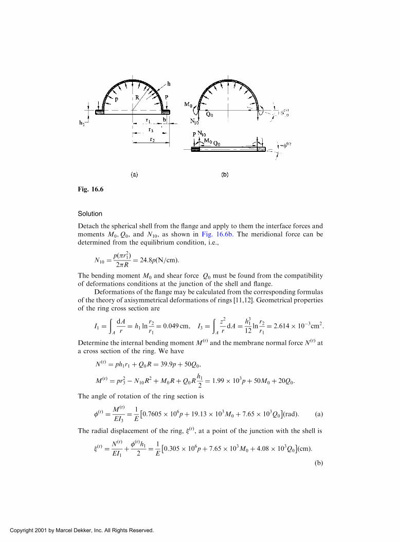
Solution

Detach the spherical shell from the flange and apply to them the interface forces andmoments M0;Q0, and N10, as shown in Fig. 16.6b. The meridional force can bedetermined from the equilibrium condition, i.e.,

N10 ¼pð�r21Þ2�R

¼ 24:8pðN=cmÞ:

The bending moment M0 and shear force Q0 must be found from the compatibilityof deformations conditions at the junction of the shell and flange.

Deformations of the flange may be calculated from the corresponding formulasof the theory of axisymmetrical deformations of rings [11,12]. Geometrical propertiesof the ring cross section are

I1 ¼ðA

dA

r¼ h1 ln

r2r1

¼ 0:049 cm; I3 ¼ðA

z2

rdA ¼ h31

12lnr2r1

¼ 2:614 10�3cm2:

Determine the internal bending moment MðrÞ and the membrane normal force NðrÞ ata cross section of the ring. We have

NðrÞ ¼ ph1r1 þQ0R ¼ 39:9pþ 50Q0;

MðrÞ ¼ pr23 �N10R2 þM0RþQ0R

h12¼ 1:99 103pþ 50M0 þ 20Q0:

The angle of rotation of the ring section is

�ðrÞ ¼ MðrÞ

EI3¼ 1

E0:7605 106pþ 19:13 103M0 þ 7:65 103Q0

� �ðradÞ: ðaÞ

The radial displacement of the ring, �ðrÞ, at a point of the junction with the shell is

�ðrÞ ¼ NðrÞ

EI1þ �

ðrÞh12

¼ 1

E0:305 106pþ 7:65 103M0 þ 4:08 103Q0

� �ðcmÞ:ðbÞ

Fig. 16.6


The state of stress of the shell can be represented as a sum of the membrane statecaused by the internal pressure p and membrane force N10, and the moment statecaused by the edge loads M0 and Q0.

For the membrane state of stress of the shell corresponding to a particularsolution of the governing equations, we have

#ðsÞ1p ¼ 0; Up ¼ 0; N1p ¼ N2p ¼ pr212R

¼ N10 ¼ 24:8p;

where the subscript p refers to the quantities associated with the membrane state. Itcan also be assumed that r1 � R; then

N1p ¼ N2p ¼ pR

2¼ 25p:

The radial (horizontal) displacement of the shell edge, �ðsÞp , corresponding to themembrane state of stress, is given by

�ðsÞp ¼ R

EhN2p � �N1p

� � ¼ 50 24:8pð1� 0:3Þ0:3ðEÞ ¼ 2:9 103

p

EðcmÞ: ðcÞ

Now, we can calculate the linear and angular displacements on the shell edge causedby the edge loads, M0 and Q0. These displacement components are determined withthe use of the approximate solution procedure introduced in Sec. 16.4. In this case, aparticular solution is zero. The general solution of the governing equations of theedge effect is given by Eqs (16.49). First, let us compute the parameter (see Eq.(16.42)) and the flexural stiffness. We have

¼ R

ffiffiffiffiffiffiffiffiffiffiffiffiffiffiffiffiffiffi3ð1� �2ÞR2h2

4

s¼ 16:6ðcmÞ; D ¼ Eh3

12ð1� �2Þ ¼ 2:475 10�3EðN � cmÞ:

Substituting R1 ¼ R2 ¼ R into Eq. (16.51), determine #ðsÞ10; "ðsÞ20; and �

ðsÞ0 at the junction

of the shell and ring which are caused by the above-mentioned edge loads. Takingthe bottom signs in the above equations and letting ’ ¼ 90, one obtains

#ðsÞ10 ¼ �M0R

DþQ0R

2

22D¼ � 1220M0

Eþ 1840Q0

E; ðdÞ

�ðsÞ0’¼90

¼ R"ðsÞ ¼ R

Eh

M022

R�Q02

" #¼ 1835M0

E� 5330Q0

E: ðeÞ

Let us set up the compatibility equations at the junction of the shell and ring:

�ðsÞp þ �ðsÞ0 ¼ �ðrÞ;

#ðsÞ10 ¼ �ðrÞðfÞ

Substituting for all the components on the left- and right-hand sides of Eqs (f) fromEqs (a), (b), (c), (d), and (e), we obtain the following system of algebraic equations:

2:90 103p

E� 5530

Q0

Eþ 1835

M0

E¼ 305 103

p

Eþ 4080

Q0

Eþ 7650

M0

E;

1840Q0

E� 1220

M0

E¼ 760:5 103

p

Eþ 7650

Q0

Eþ 19130

M0

E


Solving these equations, yields

M0 ¼ �33:8pðN � cm=cmÞ; Q0 ¼ �10:7pðN=cmÞ:The maximum stresses occur at an outside point of the shell at ’ ¼ 90. They are

�1max ¼N1

h� 6M1

h2; �2max ¼

N2

h� 6M2

h2; ðgÞ

where

N1 ¼ N10 ¼ 24:8pðN=cmÞ; M1 ¼ M0 ¼ �33:8pðN � cm=cmÞ;

N2 ¼ N20 þN2pðN=cmÞ; M2 ¼ �M1 ¼ �10:1pðN � cm=cmÞ;and N20 is given by Eq. (16.49), i.e.,

N20 ¼ M0

22

R�Q0ð2Þ ¼ �17:32p (N/cm):

Finally, N2 can be determined as follows:

N2 ¼ N2p þN20 ¼ 24:8p� 17:32p ¼ 7:48p (N/cm).

Substituting all the above data into Eqs (g) yields the following values of the max-imum stresses:

�1max ¼24:8p

0:3þ 6ð33:8pÞ

ð0:3Þ2 ¼ 2336pðN=cm2Þ;

�2max ¼7:48p

0:3þ 6ð10:1pÞ

ð0:3Þ2 ¼ 698:2ðN=cm2Þ:

These values of the normal stresses coincide with the numerical data obtained in Ref.[12], where the same problem had been solved using the exact governing equations(16.30). The above-mentioned coincidence for this case can be explained by the factthat the meridional angle at the shell edge, ’e, is equal to 90 and the radii ofcurvature had constant values throughout the shell.

Example 16.2

Consider a cylindrical vessel, made of steel, with a hemispherical head, as shown inFig. 16.7a, under an internal pressure p. Determine the internal forces, moments, andstresses at the junction of the cylindrical and spherical shells. Given the radii of thecylinder and sphere are assumed to be the same and equal R ¼ 1:5 m, the thicknessof the cylinder and shell is h ¼ 0:01m; E ¼ 200GPa, and � ¼ 0:3.

Solution

First, consider the membrane state of stress of the cylinder and head separately (Fig.16.7b). In the spherical shell (at the junction):

NðsÞ1p ¼ N

ðsÞ2p ¼ pR

2; �ðsÞp ¼ � pR2

2Ehð1� �Þ:


In the cylindrical shell (at the junction):

NðcÞ1p ¼ pR

2; N

ðcÞ2p ¼ pR; �ðcÞp ¼ � R

EhN

ðcÞ2p � �NðcÞ

1p

� �¼ � pR2

Ehð2� �Þ:

In the above equations �ðsÞp and �ðcÞp refer to the membrane radial (horizontal) dis-placements at the juncture of the hemisphere and cylinder, respectively. Since at thejunction of two shells N

ðsÞ1p ¼ N

ðcÞ1p , then the membrane state of stress satisfies the

static conditions of joint operation of the two shells. However, conditions of defor-mations’ compatibility are not satisfied because the radial displacements of thecylindrical shell at the juncture are greater than the corresponding radial displace-ments of the spherical shell. Therefore, at the junction of the two shells, the interfaceforce Q0 and momentM0 occur (Fig. 16.7c). These interface force and moment causethe moment stress of the edge effect type in the vicinity of the joint (see also Sec. 17.5).The values of the interface force and moment may be found from the conditions ofcompatibility of deformations at the junction of the spherical and cylindrical shells.Equating the total (i.e., caused by both the membrane state and edge effect) radialdisplacements and the angles of rotation at the juncture of the shells (the positivedirections for displacements and angles of rotation are shown on the right part ofFig. 16.6c), we obtain the following:

� �ðsÞp �Q0�ðsÞQ �M0�

ðsÞM ¼ ��ðcÞp þQ0�

ðcÞQ �M0�

ðcÞM

�M0#ðsÞ1M �Q0#

ðsÞ1Q ¼ M0#

ðcÞ1M �Q0#

ðcÞ1Q;

ðaÞ

where �Q; �M and #1Q; #1M refer to the radial displacements and slopes at the junc-ture caused by the unit interface shear force, Q0 ¼ 1, and unit bending moment,M0 ¼ 1; superscripts s and c stand for the hemisphere and cylinder, respectively. Thedeformation components at the junction for both cylindrical and spherical shellsmay be determined from Eqs (16.51) by setting ’e ¼ �=2 and making R1 ¼ 1; R2 ¼R and ¼ R for the cylindrical shell and letting R1 ¼ R2 ¼ R and ’ ¼ �=2 for thespherical shell. Consequently, we obtain

Fig. 16.7


�ðsÞQ ¼ �ðcÞQ ¼ 1

2D3; �ðsÞM ¼ �ðcÞM ¼ 1

2D2; #ðsÞ1M ¼ #ðcÞ1M ¼ 1

D; #ðsÞ1Q ¼ #ðsÞ1Q ¼ 1

2D2;

where

¼

R¼

ffiffiffiffiffiffiffiffiffiffiffiffiffiffiffiffiffiffi3ð1� �2Þ4

pffiffiffiffiffiffiRh

p ¼ 10:4931 ð1=mÞ:

Then, it follows from the compatibility equations (a) that

M0 ¼ 0;Q0 ¼�ðcÞp � �ðsÞp�ðsÞQ þ �ðcÞQ

¼ pR2ðD3Þ2Eh

¼ pffiffiffiffiffiffiRh

p

8ffiffiffiffiffiffiffiffiffiffiffiffiffiffiffiffiffiffi3ð1� �2Þ4

p ¼ 0:01191p (N � m/m).

Using Eqs (16.48) and (15.57), we can obtain the displacements and stress resultantsand couples caused by the edge loads and the given internal pressure in both thecylindrical and spherical shells.

Figure 16.8a and b shows the bending moment M1 and circumferential forceN2m diagrams, where N2M is due to the edge loads only.

The maximum values ofM1 and N2M at the junction of the two shells are foundto be

M1max ¼pR2

2EhD2e��=4

ffiffiffi2

p

2¼ 3:6 10�4p ðN �m=mÞ;

N2M

¼ Q02 ¼ 0:375p ðN=mÞ:Note that N2M has different signs for the cylindrical and spherical shells at thejuncture (see Fig. 16.8b).

The normal stresses due to the bending edge effect are

�1M ¼ 6M1max

h2¼ 0:146

pR

h¼ 21:9p; �2M ¼ 0:1�1M ¼ 2:19p:

The circumferential force N2M eliminates a discontinuity in the forces of the mem-brane state. It can be easily shown that the total membrane force N2 ¼ N2p þN2M isidentical for both shells at the junction and equal N2 ¼ 1:125p. Thus, the totalcircumferential force N2 varies continuously in the compound shell, as shown inFig. 16.8c.

Fig. 16.8


It is seen that the stresses due to the edge effect have a magnitude of the sameorder ðpR=hÞ as the membrane stresses in the shells under consideration. This istypical for shells at which the edge effect occurs, because the compatibility of defor-mations is not satisfied by the membrane state only.

Example 16.3

A compound steel shell consists of a cylinder (radius R and wall thickness h) and of ahead in the form of a spherical segment (radius Rs ¼ 2R and thickness h), as shownin Fig. 16.9a. This compound shell is subjected to an internal pressure p. Determinethe internal forces and moments in the compound shell if R ¼ 1:5m; h ¼ 0:02m; � ¼0:3; E ¼ 200GPa, and ’1 ¼ 30.

Solution

First, consider the membrane state of the head and cylinder separately, as shown inFig. 16.9b. From the membrane shell theory, it follows that

NðsÞ1p ¼ N

ðsÞ2p ¼ pRs

2¼ pR; N

ðcÞ1p ¼ pR

2;NðcÞ

2p ¼ pR ðaÞ

where, again, the subscript p refers to the membrane solution and superscripts s andc stand for the sphere and cylinder, respectively. It is seen from Fig. 16.9b that, apartfrom the latter example, the membrane state alone does not satisfy the conditions ofstatic equilibrium in the head and cylinder. Therefore, the edge effect occurs at thejunction of the compound shell to satisfy both the statics and compatibility ofdeformations conditions.

Consider the edge effect procedure being applied to the given compound shell.The membrane force N

ðsÞ1p at the edge of the head has a horizontal component, which

is equal to

Fig. 16.9


T0 ¼ NðsÞ1p cos ’1 ¼ pR

ffiffiffi3

p

2: ðbÞ

To ensure that the shell loading by the membrane scheme (Fig. 16.9b), together withthe edge effect, would be equivalent to the given loading applied to the compoundshell, it is necessary to include the thrust that is equal and oppositely directed to T0

among the edge effect forces, as shown in Fig. 16.8c. Thus, in applying the edgeeffect solution procedure, we should assume that the cylindrical shell is loaded by theedge moment M0 and shear force H0, whereas the spherical shell is loaded by theedge moment M0 and thrust ðH0 � T0Þ, as shown in Fig. 16.9c. The unknown quan-tities M0 and H0 are evaluated from the compatibility of deformations’ conditions,i.e., the radial (horizontal) displacements and angles of rotation of normals shouldbe identical at the juncture of both shells. Equating the edge radial displacements ofthe sphere and cylinder at the juncture, we obtain

�ðsÞ ¼ �ðcÞ ðcÞ

where,

�ðsÞ ¼ � R

EhðNðsÞ

2p � �NðsÞ1p Þ þ ðT0 �H0Þ�ðsÞH �M0�

ðsÞM

�ðcÞ ¼ � R

EhN

ðcÞ2p � �NðcÞ

1p Þ þH0�ðcÞH �M0�

ðcÞM :

� ðdÞ

In Eqs (c) and (d), the first terms on the right-hand sides correspond to the mem-brane solution.

The conditions of compatibility for the slopes (the positive direction of theslopes is shown in Fig. 16.9c to the right) has the form

ðT0 �H0Þ#ðsÞ1H �M0#ðsÞ1M ¼ �H0#

ðcÞ1H þM0#

ðcÞ1M : ðeÞ

In Eqs. (d) and (e), the subscripts H and M indicate the cause of the correspondingdisplacements. The coefficients �ðsÞH ; �

ðsÞM ; #

ðsÞ1H; #

ðsÞM and �ðcÞH ; �

ðcÞM ; #

ðcÞ1H; #

ðcÞ1M can be

calculated from Eqs (16.51) by setting R1 ¼ R2 ¼ Rs ¼ 2R; ’e ¼ ’1; and replacingQ0 with H0 sin ’1 or T0 sin ’1) according to Eq. (16.50) for the spherical shell, andby setting R1 ¼ 1; R2 ¼ R; and ’e ¼ ’1 for the cylindrical shell. As a result, weobtain

�ðsÞH ¼ sin2 ’12D3s

; �ðsÞM ¼ sin ’12D2s

; #ðsÞ1M ¼ 1

Ds; #ðsÞ1H ¼ �ðsÞM ;

�ðcÞH ¼ 1

2D3c; �ðcÞM ¼ 1

2D2c; #ðcÞM ¼ 1

Dc; #ðcÞ1H ¼ �ðcÞM ;

s ¼ffiffiffiffiffiffiffiffiffiffiffiffiffiffiffiffiffiffi3ð1� �2Þ4

pffiffiffiffiffiffiffiffiffi2Rh

p ; c ¼ffiffiffiffiffiffiffiffiffiffiffiffiffiffiffiffiffiffi3ð1� �2Þ4

pffiffiffiffiffiffiRh

p :

ðfÞ


Substituting the numerical data into the relations (a), (b), (d), and (f), one obtains thefollowing:

D ¼ Eh3

12ð1� �2Þ ¼ 146:52 103ðNmÞ; c ¼ 7:4213ð1=mÞ; s ¼ 5:2477ð1=mÞ;

NðsÞ1p ¼ N

ðsÞ2p ¼ 1:5p ðN=mÞ; N

ðcÞ1p ¼ 0:75p ðN=mÞ; N

ðcÞ2p ¼ 1:5p; T0 ¼ 1:3p ðN=mÞ;

�ðsÞH ¼ 0:005903 10�6ðm2=NÞ; �ðsÞM ¼ 0:06196 10�6ðm=NÞ;#ðsÞM ¼ 1:301 10�6ð1=NÞ;

�ðcÞH ¼ 0:008362 10�6ðm2=NÞ; �ðcÞM ¼ 0:06196 10�6ðm=NÞ;#ðcÞM ¼ 0:9196 10�6ð1=NÞ:

Substituting the above into the compatibility equations (c) and (e) and taking intoaccount the relations (d), we can calculate H0 and M0. We have

H0 ¼ 0:5401p ðN=mÞ; M0 ¼ 0:03627p ðN �m=mÞ:Using Eqs (16.48) for a spherical shell and Eqs (15.57) for the cylindrical shell, wecan determine the membrane forces N2;N1 and bending moments M1;M2 in thespherical and cylindrical parts of the given compound shell. The equations for themembrane forces and bending moments are of the following form:

– for the cylindrical shell

NðcÞ2 ¼ 1:5p 1� 4:0075e�cxðcoscxþ sin cxÞ

� �; N

ðcÞ1 ¼ 0:75p;

MðcÞ1 ¼ 0:03627pe�cxðcoscx� sin cxÞ;

ðgÞ

where the coordinate x is counted off from the juncture of the spherical and cylind-rical shells.–for the spherical shell

NðsÞ2 ¼ 1:5p 1� 4:0075e�!ðcos!þ sin !Þ½ �;

NðsÞ1 ¼ 1:5p 1� 0:44e�! cos!½ �;

MðsÞ1 ¼ 0:03627pe�!ðcos!� sin !Þ;

ðhÞ

where ¼ Rss and ! ¼ ’1 � ’ ¼ 30 � ’.The diagrams of the membrane force N2 and bending momentM1 are shown in

Fig. 16.10.The maximum normal stresses occur in the cylindrical shell at points in its

inner surface at the junction with the sphere segment. The total meridional stressis tensile at the above points and is equals to

�1 ¼N1

hþ 6M1

h2¼ 37:5pþ 544p ¼ 581:5p: ðiÞ

The circumferential stress at the same points is compressive and is given by

�2 ¼N2

hþ � 6M1

h2¼ �61:8p: ðjÞ


It can be shown that in the given compound shell the edge effect normal stress islarger by an order of magnitude

ffiffiffiffiffiffiffiffiffiffiffiffiðR=hÞpthan the corresponding membrane stress.

Therefore, the compound shell, like that analyzed in this example, is inefficient.However, it is possible to essentially decrease the stresses at the junction of

compound shell structures. Figure 16.11a shows two shells, cylindrical and spherical,joined by a ring. The latter is supposed to support the thrust T0 (Fig. (16.11a)). In theanalysis of such shell structures, one can assume that the bending stiffness of the ringin the direction perpendicular to its plane is negligible. Thus, the ring resists only theradial load in its own plane. The free-body diagrams of the shells and ring are shownin Fig. 16.11b.

Let us determine the stress components at the junction of the two shells, shownin Fig. 16.11. The geometrical and mechanical parameters of the shells are takenfrom Example 16.3.

The values of the unknown interface forces, H1 and H2, as well the momentM0, are evaluated from the conditions of deformations, compatibility of the shellparts and ring. Let the shell and ring be made of the same material. Assume that the

Fig. 16.10

Fig. 16.11


cross-sectional area of the ring, Ar, has an order of magnitude Rh and the terms ofthe order of magnitude

ffiffiffiffiffiffiffiffiffih=R

pcan be neglected compared with unity. In this case, the

radial compliance of the ring, R2=ArE, will be significantly lower than the radialcompliance of the shells, i.e.,

�ðcÞH ¼ 1

2D3c¼ 2

ffiffiffiffiffiffiffiffiffiffiffiffiffiffiffiffiffiffi3ð1� �2Þ4

qR

Eh

ffiffiffiffiR

h

r:

Therefore, one can assume that the thrust T0 is completely carried by the ring andthe ring’s horizontal displacement, T0R

2=EAr, determines the corresponding dis-placements of the shell parts (cylindrical and spherical shells). Thus, the above-mentioned compatibility equations can be represented in the following form:

� R

EhðNðsÞ

2p � �NðsÞ1p Þ þH1�

ðsÞH �M0�

ðsÞM ¼ T0R

2

EAr

;

� R

EhðNðcÞ

2p � �Nðc1pÞ þH2�

ðcÞH �M0�

ðcÞM ¼ T0R

2

EAr

;

M0#ðcÞM �H2#

ðcÞH ¼ �M0#

ðsÞM þH1#

ðsÞH :

ðkÞ

Let us select the cross-sectional area of the ring, Ar, from the condition

�r ¼ �2p ðlÞwhere

�r ¼T0R

Ar

¼ pR2ffiffiffi3

p

2Ar

;

is the compressive stress in the ring and

�2p ¼ pR

h

is the maximum tensile stress in the shell by the membrane theory. Thus, we have

Ar ¼ffiffiffi3

p

2Rh ¼ 0:02598ðm2Þ: ðmÞ

Substituting for the coefficients �H; �M; #H; and #M from Eqs (f) and taking intoaccount Eq. (k), we can solve Eqs (p) for H1;H2; and M0. We obtain

M0 ¼ 0:01605p; H1 ¼ 0:2434p; H2 ¼ 0:3308p:

Having determined the edge effect forces and moments, we can calculate theinternal forces and bending moments in the spherical and cylindrical parts of thegiven compound shell by using Eqs (16.48) and (15.57), respectively. It can be seenthat for this compound shell reinforced by the ring, the maximum edge effect bend-ing stresses will have the same order of magnitude as the membrane stresses. Inparticular, the maximum edge effect bending stress in the zone of the junction ofthe two shells is given by

�1 ¼6M1

h2¼ 240:75p:


Comparing this bending stress due to the edge effect with the corresponding stressfrom the previous example, we can conclude that the setup of the ring allows one todecrease the edge effect maximum stress by more than two times, although the abovestress remains quite considerable.

16.6 AXISYMMETRICALLY LOADED CONICAL SHELLS

For a conical shell, a distance s measured from the vertex of the cone along thestraight meridian may be conveniently taken as a meridional coordinate of a pointon the middle surface (see Sec. 13.6.2). Replacing the variable ’ with a new variables, we use the following obvious relationships

ds ¼ R1d’;dð. . .Þd’

¼ R1

dð. . .Þds

ð16:53aÞ

For conical shells R1 is a constant at infinity and does not vary with s, so thatdR1=ds ¼ 0; hence,

d2ð. . .Þd’2

¼ R21

d2ð. . .Þds2

and R2 ¼ s cot ’;dR2

ds¼ cot ’: ð16:53bÞ

where ’ is the constant value for all points on the straight meridian (Fig. 13.3).In this section, we are concerned with the bending theory of a conical shell

subjected to axisymmetrically applied edge loads. Therefore, we seek only solutionsof the homogeneous bending theory equations (the edge effect solutions), becausethe membrane solution may be used as a particular integral of the general theoryequations for conical shells. Using the relationships (16.53), we can rewrite thegoverning equation (16.28) in terms of the variable s, setting R1 ¼ 1 for conicalshells and �ð’Þ ¼ 0, as follows:

d2#1ds2

þ 1

s

d#1ds

� 1

s2#1 ¼ � 1

DR2

U;

d2U

ds2þ 1

s

dU

ds� 1

s2U ¼ Eh

R2

#1;

ð16:54aÞ

or in the following operator form

L1ð#1Þ þ1

DU ¼ 0

L1ðUÞ � Eh#1 ¼ 0

ð16:54bÞ

where the operator L1ð::Þ is given by

L1ð. . .Þ � cot ’ sd2ð. . .Þds2

þ dð. . .Þds

� 1

sð. . .Þ

" #:

The solution of the governing differential equations (16.54b) can be expressed interms of the Bessel functions or their modifications [13]. However, this rigorousapproach is not suited to practical engineering calculations, as it is too lengthyeven when tables of the Bessel functions are available. The problem of strainingthe conical shells may be solved by using the numerical methods introduced inChapter 6 or by the finite element method technique [3,4].


A simpler solution for the conical shell problems, analogous to the Geckelerapproximation, (see Sec. 16.4) is now introduced. Dropping terms with #1 andd#1=ds and the terms U and dU=ds from the left-hand sides of Eqs (16.54a), yieldsthe following approximate equations:

d2#1ds2

� � U

DR2

;

d2U

ds2� Eh

R2

#1:

ð16:55Þ

Differentiating the second equation twice with respect to s and substituting it into thefirst equation, gives the following governing differential equation of the edge effectfor conical shells:

d4U

ds4þ Eh

R22D

U ¼ 0 or

d4U

ds4þ 44U ¼ 0;

ð16:56Þ

where

¼ffiffiffiffiffiffiffiffiffiffiffiffiffiffiffiffiffiffi3ð1� �2ÞR2

2h2

4

s: ð16:57Þ

Remember that in deriving the governing differential equation of the edge effectthe following assumptions have been adopted: the lower derivatives of functionsand functions themselves are small compared with the higher derivatives and theradius R2 varies slightly near the shell edge. It has been shown that these assump-tions are fairly fulfilled if

ffiffiffiffiffiffiffiffiffiffiffiffiffiffiffiffiffiffiffiffih=ðr sin ’Þp � 1 (r is the radius of the parallel circle)

[14] or for conical shells with a considerable slope of the meridian(’ > 35 � 40).

Let x be the coordinate measured from the edge of interest. Then we have

– for the top edge x ¼ s� s0,– for the bottom edge x ¼ s0 � s,

where s0 is some coordinate that corresponds to the given edge of the shell. Intransition to the variable x, Eq. (16.56) remains unchanged, i.e.,

d4U

dx4þ 44U ¼ 0: ð16:58Þ

Using the edge effect procedure, developed in Sec. 16.4, we can obtain thesolution of Eq. (16.58) and the following expressions for the deformations, internalforces, and moments in a conical shell subjected to the edge loadsMe and Qe in termsof the variable x, as follows:


U ¼ �Me2R2e�x sin xþQeR2e

�xðcosx� sin xÞ;

N1 ¼ cot ’ �Me2e�x sin x�Qee

�xðcosx� sin xÞ� �;

N2 ¼ 2R2 Mee�xðcos x� sin xÞ �Qee

�x cos x� �

;

M1 ¼ Mee�xðcos xþ sin xÞ �Qe

1

e�x sin x;M2 ¼ �M1;

#1 ¼ �Me

1

De�x cosxþQe

1

22De�xðcosxþ sin xÞ;

� ¼ "2r ¼ R2 sin ’1

EhðN2 � �N1Þ:

ð16:59Þ

The positive directions of the edge force Qe and moment Me are shown in Fig. 16.12.The upper sign in Eqs (16.59) refers to the top edge (at ’ ¼ ’e1Þ and the lower signrefers to the bottom edge (at ’ ¼ ’e2Þ of the shell.

Example 16.4

Determine the internal forces in a conical shell subjected to the edge loads m andH, as shown in Fig. 16.13. Given h ¼ 0:5 in; ’ ¼ 60; s1 ¼ 10 in:; s2 ¼ 30 in:; R2 ¼s2 cot ’ ¼ 17:3 in:; and � ¼ 0:3.

Solution

The parameter for the bottom edge is obtained from Eq. (16.57):

¼ffiffiffiffiffiffiffiffiffiffiffiffiffiffiffiffiffiffi3ð1� �2ÞR2

2h2

4

s¼ 0:4371 ð1=in:Þ:

The edge loads on the bottom edge are

Me ¼ m; Qe ¼ H sin 60 ¼ 0:866H:

Fig. 16.12


Using Eqs (16.59) and setting x ¼ 0, we can calculate the angle of rotation of thenormal to the meridian, #1, and the internal forces at the bottom edge. We have

#1 ¼ � m

Dþ Qe

22D¼ �2:29

m

Dþ 2:28

H

D;

N1 ¼ �Qe cot ’ ¼ �0:5H;

N2 ¼ 2R2ðm�QeÞ ¼ 6:58m� 13:1H:

Comparing these numerical data with those obtained by using the exact edge effectprocedure based on the use of the Bessel functions [12], we can conclude that theerror of this approximate analysis does not exceed 1% for the given case.

16.7 AXISYMMETRIC DEFORMATION OF TOROIDAL SHELLS

Structural components having a form of toroidal shells are commonly used inmechanical engineering. Housings of pumps, hydraulic clutches, tanks, bellows,etc., are examples of such shape of a shell. The shape of a toroidal shell is character-ized by the radii R and a and by the following parameters (Fig.16.14):

Fig. 16.13

Fig. 16.14


¼ a

R; ¼ a

h: ð16:60Þ

For a toroidal shell, the principal radii of curvature are (Fig. 16.13)

O1A ¼ R1 ¼ a ¼ const; O2A ¼ R2 ¼ R1þ sin ’

sin ’; ð16:61Þ

where ’ is the angular coordinate varying in the range �180 < ’ < 180. Toroidalshells, except for shallow part near ’ ¼ 0, can be successfully analyzed by the meth-ods of the theory of edge effect (see Sec. 16.4).

For shells including the shallow part near ’ ¼ 0, the problem becomes morecomplicated. Considerable difficulties are associated with determining a particularsolution of the nonhomogeneous governing differential equations, because the mem-brane solution near ’ ¼ 0 becomes invalid. Thus, toroidal shells must be analyzed byusing the governing equations of the general moment theory of axisymmetric shellsof revolution. Substituting for the principal radii of curvature from the relations(16.61) into Eqs (16.30), we obtain the following governing differential equations ofthe axisymmetric deformation of toroidal shells:

L2ðUÞ þ �L2ðUÞ ¼ Eha#1ð’Þ þ� ð’Þ;

L2ð#1Þ � �#1 ¼ � a

DU;

ð16:62Þ

where

L2ð. . .Þ ¼1þ sin ’

sin ’

d2ð. . .Þd’2

þ cot ’dð. . .Þd’

� cot ’ cos ’1þ sin ’ ð. . .Þ;

� ð’Þ ¼ a2d

d’p3

1þ sin ’ð Þ22 sin2 ’

" #þ p1a

2 ð1þ sin ’Þ sin ’

1þ sin ’ sin ’

þ ��

þ Fð’Þ cos ’ð2þ 3 sin ’Þ sin4 ’ð1þ sin ’Þ :

ð16:63ÞThe solution of Eqs (16.62) can be obtained by numerical methods introduced inChapter 6 – in particular, by the finite element method.

PROBLEMS

16.1 Derive Eqs (16.5).

16.2 Derive Eqs (16.9).

16.3 Show that the vertical displacement of a point in the middle surface of shell of revolu-

tion, (see Fig. 16.1) are governed by the following equation

¼ð’’0

ð"1 sin �’’þ #1 cos �’’ÞR1d �’’:

16.4 Verify Eqs (16.50).

16.5 Consider a spherical dome supporting its own weight and described in Sec. 14.1.1.

Assume that the supports are as shown in Fig. 14.2a. (a) Determine the bending

stresses and (b) compare the bending and membrane stresses. Assume reasonable

values for any additional properties and parameters required.


16.6 A dome in the form of a spherical segment is clamped around its base and is loaded by

an external pressure p ¼ 1:5 MPa. Determine the force and moment applied to the base

of the shell by support. Take ’1 (the meridional angle at the shell base)=55, E ¼200GPa; � ¼ 0:3; h ¼ 20 mm, and R ¼ 1500 mm.

16.7 A cylindrical tank is capped by a hemispherical shell, as shown in Fig. 16.6. The tank is

loaded by an internal pressure p ¼ 1:4 MPa. Determine the discontinuity stresses at the

junction. Take the allowable membrane stress �all ¼ 120 Mpa, E ¼ 200GPa � ¼ 0:3,R ¼ 1000mm, hc ¼ hs ¼ 12mm, where hc and hs are the thicknesses of the cylindrical

tank and hemispherical shell, respectively.

16.8 A hemispherical cap of radius R and thickness h is loaded by uniformly applied to the

free edge of the cap moments M0. Determine the length L, measured along the mer-

idian from the loaded edge of the cap, where the internal momentM1 diminishes to 1%

of moment M0. How does this length compare with that in Example 15.1 for a cylind-

rical shell?

16.9 Redo Problem 16.8 replacing the moments M0 with uniformly applied horizontal

forces Q0 to the free edge of the cap.

16.10 What is the maximum stress at the junction of the flat circular plate and (a) hemi-

spherical shell (Fig. P.16.1a) and (b) conical shell with ¼ 37 (Fig. P.16.1b)? Both

shells are subject to an internal pressure of p ¼ 1:5 MPa. Let E ¼ 200GPa; and

� ¼ 0:27.16.11 A conical frustum has a free edge at its top and it is built-in at the base. The shell is

subject to internal pressure p. Determine the internal forces and bending moments in

the shell. Let the radii of the parallel circles at the shell top and its base be 5.5 m and

8.5m, respectively, h ¼ 60mm; E ¼ 200GPa; and � ¼ 0:3. Employ the approximate

method of Sec. 16.4 to determine the bending stress resultants and couples.

16.12 Calculate the displacements of the edge of the hemispherical shell shown in Fig. 16.5a.

For your calculations use the numerical data in Example 16.1.

16.13 Compare the values of the normal stresses in the spherical shell segment for four

variants of boundary conditions at its base: (a) the shell is loaded by a normal mer-

idional force Ne applied to its free edge; (b) the shell is built-in; (c) the shell has roller

supports at its free edge; and (d) the shell is simply supported. The shell is subjected to

an external normal pressure p. Let R ¼ 30h and ’1 ¼ 35(meridional angle at the shell

base) for all the above-mentioned shells. Employ the approximate method of Sec. 16.4

for the solution.

16.14 Consider the Intze-type water tank of Problem 14.18 (Fig. 14.14a). (a) Find the bend-

ing stress resultants and couples in the wall and the roof and plot their diagrams.

(b) Assume that there is no ring beam at B. Find the final value of N2 in the cone

at B using the moment theory. Neglect the effects of discontinuities at C on the stresses

Fig. P16.1


at B. In your calculations assume that the modulus of elasticity of the wall and the roof

are the same and Poisson’s ratios are zero. Use the numerical data in Problem 14.18 for

the solution.

16.15 Find the bending field in the intersection of the cylindrical wall and its conical end caps

in the cylindrical pressure vessel shown in Fig. P.14.4. Take H ¼ 2R ¼ 2m, h1 ¼ 10

mm, h2 ¼ 12mm, E ¼ 200 GPa, � ¼ 0:3.16.16 Consider the water tank shown in Fig. P.14.3. Perform a complete analysis of this tank.

Let R ¼ 500mm; H ¼ 2R; and h1 ¼ h2 ¼ 5mm. Assume reasonable values for any

additional properties required.

16.17 Consider a conical shell with a central angle , the base radius a, and thickness h. The

lower edge of this cone is fixed against rotation and translation. The shell is subjected

to its own weight with intensity p. Perform a complete analysis of this shell.

16.18 Verify Eqs 16.62.

REFERENCES

1. Collatz, L., The Numerical Treatment of Differential Equations, 3rd edn, Springer-Verlag,

Berlin, 1966.

2. Godunov, S.K., Ordinary Differential Equations with Constant Coefficients (translated

from Russian), Providence, R.I. American Mathematical Society, 1997.

3. Zienkiewicz, O.C., The Finite Element Method, McGraw-Hill, New York, 1977.

4. Ashwell, D.G. and Gallagher, R.H. (eds) Finite Elements for Thin Shells and Curved

Members, Wiley, London, 1976.

5. Meissner, E., Das elastizitatsproblem fur dunne schalen von ringflachen, kugel-, and

kegelform, Physik Zeit., vol. 14, pp. 343–349 (1913).

6. Reissner, H., Spannungen in Kugelschalen , Muller, Breslau-Festscher, 1912.

7. Geckeler, J., Uber die Festigkeit Achsensymmetrischer Schalen, Forschg.-Arb. Ingwes, p.

276, Berlin, 1926.

8. Meissner, E., Uber elastizitat und festigkeit dunner schalen, Viertelschr d Natur, Ges, Bd.

60, Zurich, 1915.

9. Novozhilov, V.V., The Theory of Thin Elastic Shells, P. Noordhoff Ltd, Groningen, the

Netherlands, 1964.


York, 1970.

11. Feodosyev, V., Strength of Materials, Izdatelstvo Mir, Moscow, 1968.

12. Boyarshinov, S.V., The Fundamentals of Structural Mechanics of Machines, Izdatelstvo


13. Watson, G.N., Theory of Bessel Functions, 2nd edn, Cambridge University Press,

Cambridge, 1944.

14. Biderman, V.L., Mechanics of Thin-Walled Structures, Izdatelstvo Mashinostroenie,

Moscow, 1977 (in Russian).


17

Approximate Theories of ShellAnalysis and Their Applications

17.1 INTRODUCTION

The complexity of the governing equations of the general linear theory of thin shellsmotivated the development of a wide range of approximate theories associated withsimplifications of these equations.

There are two principal avenues in developing these approximate theories. Thefirst avenue is based on introducing some additional hypotheses (except for thegeneral Kirchhoff–Love assumptions) that follow from the mechanical analysis ofshell straining under applied loading, numerical results of solving various particularshell problems, and from experimental investigations [1–4, etc.]. The second avenueis based on the asymptotic analysis of the governing differential equations of thegeneral linear theory of thin shells having a small parameter a (see Sec. 15.2) [5].Both avenues arrive at the same results. However, the second avenue provides a wayfor an error estimation of the corresponding approximate equations. Note that thepossibility of introducing one or other simplification is determined by the characterof loading (its variation), boundary conditions, and the shell stiffness and its othergeometric parameters.

In this chapter we consider only the first avenue of simplifications and thecorresponding approximate theories.

17.2 THE SEMI-MEMBRANE THEORY OF CYLINDRICAL SHELLS

In the analysis of long closed and open cylindrical shells, the so-called semi-mem-brane theory has enabled a wide range of applications. It enables one to analyze theabove-mentioned shells with the use of simple (and well-known for engineers) math-ematical technique in situations when the membrane theory is not applicable.


17.2.1 The governing differential equations of the semi-membranetheory

It was mentioned previously that the membrane theory is inapplicable for the stressanalysis of long cylindrical shells. Another deficiency of the membrane theory is theimpossibility of satisfying the prescribed boundary conditions on the longitudinaledges of an open cylindrical shell. Vlasov [1] proposed an approximate approach, theso-called semi-membrane theory of cylindrical shells, which is free of those draw-backs. Moreover, this theory is significantly simpler than the general theory ofcylindrical shells. As a result, Vlasov’s theory has been widely adapted in engineeringpractice for the analysis of cylindrical shell structures.

The semi-membrane theory is based on the following assumptions (along withthe general Kirchhoff–Love hypotheses):

1. The bending, M1, and twisting, H, moments at sections normal to the shellgenerator are insignificant and may be neglected. This means that thenormal stresses are assumed to be uniformly distributed across the shellthickness at a section, perpendicular to the longitudinal axis of the shell.

2. The circumferential strain "2 and shear strain �12 in the middle surface areneglected.

3. Poisson’s ratio is zero, i.e., � ¼ 0:

Introducing these assumptions implies that a real shell is replaced by the modeldepicted in Fig. 17.1a. According to this model, a shell consists of innumerablesets of transverse elementary curvilinear strips connected by hinged bonds. Eachsuch strip works in bending in the plane of the shell cross section. Forces are trans-mitted from strip to strip by means of rods. The latter can transmit only in-planenormal and shear forces, N1 and S, respectively. Non-zero stress resultants andcouples are shown in Fig. 17.1b.

The assumptions introduced above are justified by some physical considera-tions. Gol’denveizer [5] and Novozhilov [2] showed that these assumptions are math-ematically equivalent to the inequality

@2f

@x2

� @2f

@�2

; ð17:1Þ

Fig. 17.1


which states that the second derivative of any function (displacement, strain, stressresultant or couple) in the longitudinal direction is negligible compared with itssecond derivative in the circumferential direction. As mentioned in Sec. 15.2, sucha state of stress and strain is referred to as the basic one.

The equations of equilibrium (Eqs (15.4)) with regard to the introduced assump-tions (M1 ¼ Q1 ¼ H ¼ 0) are of the following form (for circular cylindrical shells):

R@N1

@xþ @S@�

þ p1R ¼ 0;

@N2

@�þ R

@S

@x� 1

R

@M2

@�þ p2R ¼ 0;

1

R

@2M2

@�2þN2 þ p3R ¼ 0:

ð17:2Þ

Eliminating from the above equations the membrane forces S and N2 results in thefollowing equation that relates N1 to M2:

@2N1

@x2þ 1

R3�ðM2Þ ¼ � @p1

@xþ 1

R

@p2@�

� 1

R

@2p3@�2

; ð17:3Þ

where the operator �, called Vlasov’s operator, is given as follows:

�ð. . .Þ � @4ð. . .Þ@�4

þ @2ð. . .Þ@�2

: ð17:4Þ

We come now to the derivation of equations for strains and displacements. Takinginto account the assumptions of the semi-membrane theory ("2 ¼ �12 ¼ 0; �1 ¼ 0),the kinematic relations (15.5) take the form

"1 ¼@u

@x; "2 ¼

1

R

@v

@�� w

R¼ 0; �12 ¼

@v

@xþ 1

R

@u

@�¼ 0; ð17:5aÞ

�1 ¼ 0; �2 ¼ � 1

R2

@v

@�þ @

2w

@�2

!and �12 ¼ � 1

R

@v

@xþ @2!

@x@�

" #¼ 0 ð17:5bÞ

The angles of rotations of the normal to the middle surface in the circumferential andmeridional directions, #1 and #2 respectively, can be obtained from Eqs (12.2) bysetting ¼ x; ¼ �, A ¼ 1 and B ¼ R. We have

#1 ¼@w

@x; #2 ¼

v

Rþ 1

R

@w

@�: ð17:5cÞ

Using the relations (17.5a) and (17.5b), express the displacements u; w; and curva-ture �2 in terms of the circumferential displacement v. We obtain

w ¼ @v

@�; u ¼ �

ð�

@v

@xRd�; �2 ¼ � 1

R2

@v

@�þ @

3v

@�3

!: ð17:6Þ

The constitutive equations (15.6), with regard to the adopted assumptions, canbe represented in the form

N1 ¼ Eh@u

@x; M2 ¼ D�2 ¼

Eh3

12�2: ð17:7Þ


Let us write the expressions for N1 and M2 in terms of the circumferentialdisplacement v. From Eqs. (17.6) it follows that

N1 ¼ �Eh

ð�

@2v

@x2Rd�; ð17:8aÞ

M2 ¼ � Eh3

12R2

@v

@�þ @

3v

@�3

!: ð17:8bÞ

The remaining stress resultants and couples are not equal to zero, as this seeminglyfollows from the adopted assumptions, and they can be also expressed in terms of vusing the equations of equilibrium (Eqs (17.2) and (15.3)). We have

Q2 ¼1

R

@M2

@�¼ � Eh3

12R3

@2v

@�2þ @

4v

@�4

!¼ � Eh3

12R2�ðvÞ; ð17:9Þ

S ¼ �ð�

@N1

@xRd� �

ð�

p1Rd� ¼ Eh

ð�

ð�

@2v

@x2R2d�

" #d� �

ð�

p1Rd�; ð17:10Þ

N2 ¼ � 1

R

@2M2

@�2� p3R ¼ Eh3

12R3

@

@�

@2v

@�2þ @

4v

@�4

!� p3R ¼ Eh3

12R3

@

@��ðvÞ � p3R:

ð17:11ÞIndeterminate functions in � resulting in integrating over x were dropped because theabove functions must be periodical.

Now all the stress resultants and couples, as well as the displacements, havebeen expressed in terms of the circumferential displacement v. To determine thisfunction, we can apply Eq. (17.3). Substituting for N1 and M2 from Eqs (17.8)into Eq. (17.3) and, then, differentiating it with respect to �, we obtain the followinggoverning equation of the semi-membrane theory:

Eh@4v

@x4þ Eh3

12R6��ðvÞ ¼ Pðx; �Þ; ð17:12Þ

where

Pðx; �Þ ¼ 1

R

@2p1@x@�

� 1

R2

@2p2@�2

þ 1

R2

@3p3@�3

ð17:13Þ

is a function of a given surface loading. Equation (17.12) can be integrated in series;the given loads are expanded into a Fourier series and the function v is sought in theform of a Fourier series also. The constants of integration are evaluated from theboundary conditions on the shell edges.

Having determined the function v, it is possible to calculate all the stressresultants and couples from Eqs (17.8)–(17.11). The displacement components aregiven by Eqs (17.6). The stress components can be determined by using the relations

�1 ¼N1

h; �2 ¼

N2

h� 6M2

h2; �12 ¼

S

h:


We can also present the governing differential equation of the semi-membranetheory in terms of the displacement function F , introduced as follows:

u ¼ � @F@x; v ¼ 1

R

@F

@�; w ¼ @2F

R@�2: ð17:14Þ

Substituting the above into Eqs (17.5a), it is easily shown that the second assumptionof the semi-membrane theory ("2 ¼ �12 ¼ 0) will be automatically satisfied. Then,inserting Eq. (17.14) into Eqs (15.6a) and (15.6e) and using the above-introducedassumptions, leads to the following:

N1 ¼ �Eh@2F

@x2; M2 ¼ � Eh3

12R3

@2F

@�2þ @

4F

@�4

!: ð17:15Þ

Finally, substituting the above into Eq. (17.3), one obtains the following alternativegoverning equation of the semi-membrane theory of cylindrical shells:

B@4F

@x4þ D

R6

@8F

@�8þ 2

@6F

@�6þ @

4F

@�4

!¼ @p1@x

� 1

R

@p2@�

þ 1

R

@2p3@�2

; ð17:16Þ

where B ¼ Eh is the shell stiffness in tension; D ¼ Eh3=12 is the flexural shell stiffness(� ¼ 0 due to the third assumption of the semi-membrane theory).

17.2.2 Analysis of cylindrical shells by the semi-membrane theory

Assume that a surface load is symmetrical about the plane � ¼ 0. In this case, theload components p1; p2; and p3 may be expended into a Fourier series, as follows:

p1 ¼ p10 þX1k¼1

p1k cos k�; p2 ¼ p20 þX1k¼1

p2k sin k�; p3 ¼ p30 þX1k¼1

p3k cos k�:

ð17:17ÞSubstituting Eq. (17.17) into the expression (17.13), yields the load function Pðx; �Þ,as follows:

Pðx; �Þ ¼X1k¼1

� k

R

dp1kdx

þ k2

R2p2k þ

k3

R2p3k

" #sin k� or

Pðx; �Þ ¼X1k¼1

Pk sin k�;

ð17:18aÞ

where

Pk ¼ � k

R

dp1kdx

þ k2

R2p2k þ

k3

R2p3k: ð17:18bÞ

The circumferential displacement v is sought in the form of the series

v ¼X1k¼1

Vk sin k�; ð17:19Þ

where Vk ¼ VkðxÞ. Substituting for v and P from Eqs (17.18) and (17.19) into Eq.(17.12), yields


EhX1k¼1

d4Vk

dx4þ h2

12R6Vkk

4ðk2 � 1Þ2" #

sin k� ¼X1k¼1

Pk sin k�: ð17:20aÞ

The above results in the following system of ordinary differential equations of thefollowing type:

d4V1

dx4¼ 1

EhP1;

d4V2

dx4þ h2

12R624ð22 � 1Þ2V2 ¼

1

EhP2;

. . . . . . . . . . . . . . . . . . . . . . . . . . . . . . . . . . . .

d4Vk

dx4þ h2

12R6k4ðk2 � 1Þ2Vk ¼

1

EhPk;

. . . . . . . . . . . . . . . . . . . . . . . . . . . . . . . . . . . .

ð17:20bÞ

The first equation of the above system characterizes a bending deformation of theshell with no distortion of the circumference shape. It can be easily shown thatstresses and displacements corresponding to the first equation completely coincidewith those obtained by the elementary beam bending theory. The second and sub-sequent equations of the system (17.20b) represent deformation of the shell asso-ciated with a distortion of the shape of its cross section.

Let us consider the kth equation of the system (17.20b). We represent thisequation in the form

d4Vk

dx4þ 44kVk ¼

1

EhPkðxÞ; ð17:21Þ

where

44k ¼h2k4ðk2 � 1Þ2

12R6and k ¼

ffiffiffiffiffiffiffiffiffiffiffiffiffiffiffiffiffiffiffiffiffiffiffiffiffiffiffih2k4ðk2 � 1Þ2

48R6

4

s: ð17:22Þ

Equation (17.21) is analogous to that treated previously for the axisymmetric defor-mation of a circular cylindrical shell (see Eq. (15.44)). Its integral is of the form

Vk ¼ Vkh þ Vkp; ð17:23Þwhere Vk0 is a solution of the homogeneous equation (17.21) and Vkp represents itsparticular solution. As discussed in Sec. 15.3, Vkh may be represented in the form

Vkh ¼ A1k cosh kx sin kxþ A2k coshkx coskxþ A3k sinh kx cos kx

þ A4k sinh kx sin kx: ð17:24aÞThe particular solution of the nonhomogeneous equation (17.21) depends upon thetype of surface loading. In the case when @4

@x4PkðxÞ ¼ 0, the particular solution is of

the form

Vkp ¼ PkðxÞ4Eh4k

: ð17:24bÞ


The constants of integration are evaluated from boundary conditions prescribed onthe edges of a shell for the total solution (Eq. (17.23)).

For a very long shell that satisfies the following condition

kL � 3 or L � 2:5R

ffiffiffiffiR

h

rðk � 2Þ ð17:25Þ

it is advantageous to represent the total solution in the following form, analogous tothe expression (15.53):

Vk ¼ C1ke�kx sin kxþ C2ke

�kx coskxþ Vkp: ð17:26ÞThe constants C1k and C2k are evaluated from boundary conditions prescribed at theshell edge x ¼ 0:

Example 17.1

A simply supported thin-walled cylindrical tube with flat ends is filled by water up tothe level H, as shown in Fig. 17.2. Determine the deformations and stresses due tothe water pressure. Given L ¼ 40m; 2R ¼ 3:2m; and H ¼ 0:516m.

Solution

The water pressure on the cylindrical wall of the tube and on its ends is given by thefollowing:

for� �0 � � � �0 p3 ¼ ��lRðcos � � cos �0Þ; ðaÞfor �0 � � � ð2�� 0Þ p3 ¼ 0; ðbÞ

where �l is the specific weight of water. The negative sign in Eq. (a) is taken becausep3 is assumed to be positive in the inward direction.

The pressure on the bottoms and on the cylindrical surface may be consideredindependent from one another. Since the ends have a significant stiffness againstdeformations in their own planes that excludes the possibility of distortion of theshape of the circumference near the tube edge, the pressure on the bottom will causean eccentric tension of the tube.

Determine the deformation of the tube caused by the water pressure on thecylindrical surface of the tube. Let us expend the pressure into the following seriesin �:

Fig. 17.2


p3 ¼ p30 þX1k¼1

p3k cos k�: ðcÞ

Integrating the right- and left-hand sides of the expression (c) together with (a) from0 to 2�, one finds p30 as follows:

��lRð�0��0

ðcos � � cos �0Þd� ¼ 2�ðp30Þ;

from which

p30 ¼ � �lR�

ðsin �0 � �0 cos �0Þ: ðdÞ

To determine the coefficient p3k, we multiply the left- and right-hand sides of theexpression (c) by cos k� and integrate from 0 to 2 �. We obtain

��lRð�0��0

ðcos � � cos �0Þ cos k�d� ¼ð2�0

p3k cos2 k�d�;

from which

p3k ¼ � 2�lR

�fk: ðeÞ

where

fk ¼sin ðkþ 1Þ�0½ �

2ðkþ 1Þ þ sin ðk� 1Þ�0½ �2ðk� 1Þ � sin k�0 cos k�0

kfor k 6¼ 1 and

fk ¼�02� 1

4sin �0 for k ¼ 1:

ðfÞ

The component of pressure p30, causing an axisymmetric deformation of the tube,has no significant meaning and it will not be considered in what follows. Determinethe function of the surface load, P. According to Eq. (17.18), for p1 ¼ p2 ¼ 0 andp3 ¼ p3k;

Pk ¼k3

R2p3k ¼ � 2�lk

3

�Rfk;

and one has the following:

P ¼ �X1k¼1

2�l fkk3

�Rsin k�: ðgÞ

Hence, the kth equation (Eq. (17.20b)) takes the form

d4Vk

dx4þ 44kVk ¼ � 2�lk

3fk�EhR

; ðhÞ

where k is given by Eq. (17.22). The solution of this fourth-order differential equa-tion can be obtained in the form of the sum of a complementary solution of thehomogeneous equation, and of a particular solution. However, there is a goodreason to choose another way for solving Eq. (h). The boundary conditions forthis problem are symmetrical, i.e.,


v ¼ 0jx¼0;L and N1 ¼ 0x¼0;L

: ðiÞ

(It is assumed that the shell ends offer no resistance to the displacements that areperpendicular to the end planes. The water pressure is of no concern here; it may betaken into account separately.) Using Eqs (17.8a) and (17.19), we can rewrite theboundary conditions (k) in terms of the function Vk as follows:

V ¼ 0kx¼0;L

andd2Vk

dx2

!¼ 0

x¼0;L

: ðjÞ

Due to the symmetry of the boundary conditions, the general solution of the differ-ential equation (h) can be conveniently represented in the form of the followingtrigonometric series:

Vk ¼X1

m¼1;3;5;...

Akm sinm�x

L: ðkÞ

It can be easily shown that Vk in the form of the series (k) satisfies all the boundaryconditions (i). Inserting the series (m) into the differential equation (h) results in theequality

X1m¼1;3;5;...

Akm

m�

L

� �4sin

m�x

Lþ 44k

X1m¼1;3;5;...

Akm sinm�x

L¼ � 2k3�l fk

�EhR: ðlÞ

To determine the coefficients Akm, we multiply both sides of the above equation bysinm�x=L and integrate from 0 to L. As a result, we obtain

Akm ¼ � 8k3�l fkL4

m�2REhðm4�4 þ 44kL4Þ : ðmÞ

Inserting the above into Eqs (k) and (17.19), yields the following trigonometric seriesfor v:

v ¼ �X1

k¼1;2;...

X1m¼1;3;5;...

8k3�l fkL4

m�2REhðm4�4 þ 44kL4Þ sin

m�x

Lsin k�: ðnÞ

These series converge very rapidly. Knowing v, we can calculate the remainingdisplacement components u and w (see Eqs (17.6)) and the stress resultants andcouples (see Eqs (17.7)–(17.11)). For k ¼ 1, the parameter k ¼ 0 and the corre-sponding solution will coincide with the elementary solution of the bending theoryof a beam.

Let us present the solution of the same problem assuming that the tube issupported by a rigid collar at its midspan, as shown in Fig. 17.3. It is assumedthat the collar prevents completely a distortion of the circular cross section of thetube.

In this case, the shell has two segments. Taking the origin of the coordinatesystem at a middle point of the shell length, one can write the following boundaryconditions for function Vk ðk � 2Þ :


u ¼ 0; v ¼ 0; Vk ¼ 0;dVk

dx¼ 0

x¼0

and

v ¼ 0; N1 ¼ 0; Vk ¼ 0;d2Vk

dx2¼ 0

x¼L=2

:

ðoÞ

Since these boundary conditions are asymmetric, the solution should be sought inthe form of Eq. (17.23), (17.24) i.e., as the sum of Vkc and Vkp. Evaluating theconstants of integration Aik ði ¼ 1; 2; 3; 4Þ in the above solution from the boundaryconditions (o), we can determine the circumferential displacement v from Eq. (17.19)and then can calculate all the displacement and stress components. Figure 17.4depicts the diagrams of the meridional normal stresses �1over the middle crosssection of the tube:

(a) according to the elementary beam bending theory (Fig. 17.4a);(b) based on Vlasov’s theory, in the absence of the reinforcing collar (Fig.

17.4b); and(c) based on Vlasov’s theory but with the rigid collar at the tube midspan

(Fig. 17.4c).

Figure 17.5 shows the diagrams of the meridional normal stresses �1 in the lowerstretched fiber along the tube length for the above-mentioned three cases.

Fig. 17.3

Fig. 17.4


The last two solutions (for Cases b and c) were obtained by retaining fourterms in the expansion (m).

Comparing the bending stress diagrams depicted in Figs 17.4 and 17.5, oneconcludes that:

(a) Stresses in the shell for the given loading differ significantly from thosecalculated by the elementary beam bending theory.

(b) The bending stresses are noticeably reduced if a rigid collar, preventing adistortion of the tube cross section, is present. The character of the stressdistribution is also changed.

This example was taken from Ref. [6].If a large number of rigid collars were placed over the shell length in such a way

that all its cross sections remained circular and undistorted, the deformations andstresses would not be different from those calculated by the beam bending theory.Based on the above, one can conclude that the most efficient way of decreasingstresses in shell structures is to attach rigid collars to the shells. If a shell is loadedby a concentrated force, normal to the shell middle surface, then it is sufficient to setup only one rigid collar at a place of the force application. In this case, the shell willdeform as a beam, i.e., without distortion of its cross section.

In conclusion, let us discuss some issues regarding accuracy and area ofapplication of the semi-membrane theory. It was indicated earlier (see Chapter 13)that the accuracy of solutions given by the membrane theory depends on the smooth-ness of a shell geometry, the smoothness of an applied loading, and on the formula-tion of boundary conditions. However, for a cylindrical shell, in addition to theserequirements, one more requirement is added – namely, a shell length (see Sec. 13.6).It was shown in that section that the accuracy of the membrane solution decreaseswith an increase in the shell length, even if the other requirements of the existence ofthe membrane state of stress are satisfied. From a physical point of view, this meansthat for a long cylindrical shell the boundary conditions have little effect on thestresses and deformations in its middle part and these boundary conditions cannotprevent the appearance of significant bending stresses in this part of the shell (if anexternal loading is capable of causing the bending stresses).

Thus, the semi-membrane theory holds an intermediate place between themembrane theory and the general theory of thin shells (see Chapter 12). It can beapplied to relatively long open and closed cylindrical shells with an arbitrary shapeof the cross section if the variation of the displacement and stress components in thedirection of the shell generator is smoother than their variation in the circumferential

Fig. 17.5


direction. It follows from the above that a simple criterion for an estimate of theaccuracy of solutions of the semi-membrane theory can be established. This criterionlies in the comparison of @2f =@x2 and @2f =@�2 (where f is any displacement, strain,internal force, or stress component), according to the inequality (17.1).

It should be noted, however, that for very long shells, subjected to smoothlyvarying loads along their generator, distortions of the shell cross section can beneglected. Such shells may be treated as thin-walled bars. On other hand, forsmall values of L=R, the membrane theory is more accurate than the semi-membranetheory because the former theory takes into account the in-plane cross-section defor-mations "2 and �12. However, for very small values of L=R ðL=R < 3


p) [7], both

the theories are inapplicable because, in this case, the deformations vary rapidly inthe shell longitudinal direction. Finally, the semi-membrane theory can be recom-mended for medium-length cylindrical shells (L=2R ¼ 2� 8)

17.3 THE DONNELL–MUSHTARI–VLASOV THEORY OF THIN SHELLS

This section will continue the discussion about simplified theories of thin shells. Weintroduce below the Donnell [3], Mushtari [4], and Vlasov [1] theory (abbreviated asthe DMV theory). Conceptually, the DMV theory represents a simplified variant ofthe general linear theory of thin shells. Usually, this theory is based on the followingphysical assumptions (along with the Kirchhoff–Love hypotheses):

(a) the effect of the transverse shear forces Q1 and Q2 in the in-plane equili-brium equations is negligible (the static assumption);

(b) the influence of the deflections, w, will predominate over the influences of thein-plane displacements u and v in the bending response of the shell (thegeometric assumption).

It should be noted that the static and geometric assumptions agree well with eachother as predicted by the static–geometric analogy established for thin shells byGol’denveizer [5]. Further, it was shown by Novozhilov [2] that the above physicalassumptions are well justified in the following two cases:

1. A shell is shallow ( see Sec. 11.8.4).2. The state of stress is of such a type that displacements, and hence, stresses,

are rapidly varying functions at least in the direction of one of the coordi-nates and . As a result, the derivatives of these functions are signifi-cantly greater than the functions themselves – the second derivatives aregreater than the first derivatives, etc.

The second case is more general than the first case because it is applied not only toopen but also to closed shells, i.e., to essentially non-shallow shells.

A variation of any function f ðsÞ can be characterized by the order of the value

1

f ðsÞ df ðsÞds

� 1

b; ð17:27Þ

where b is a typical linear dimension of the shell and the symbol � indicates theidentity of the values order. It is assumed that the state of stress and strain of a shellis rapidly varying, say in the direction, if for any functions f ð; Þ (displacements,stress resultants, and and couples) the following strong inequality holds [2,5]:


Rj jmin

f @f

A@

� 1: ð17:28Þ

Based on the physical assumptions of the DMV theory, the kinematic relations(12.24) and the first two (the in-plane) equilibrium Eqs (12.41) are simplified to thefollowing form:

The kinematic relations

�1 ¼ � 1

A

@

@

1

A

@w

@

� �þ 1

AB2

@A

@B

@w

@

� �;

�2 ¼ � 1

B

@

@

1

B

@w

@

� �þ 1

A2B

@B

@

@w

@

� �;

�12 ¼ � 1

AB

@2w

@@� 1

B

@B

@

@w

@� 1

A

@A

@

@w

@

" #:

ð17:29Þ

(the terms containing the in-plane displacements u and v for the changes in thecurvature and twist of the middle surface were dropped in the above equations);

The in-plane equilibrium equations

@

@ðBN1Þ þ

@

@ðASÞ þ @A

@S � @B

@N2 þ ABp1 ¼ 0;

@

@ðAN2Þ þ

@

@ðBSÞ þ @B

@S � @A

@N1 þ ABp2 ¼ 0

ð17:30Þ

(the transverse shear forces Q1 and Q2 were neglected here, and N12 ¼ N21 ¼ S). Thethird Eq. (12.41) and Eqs (12.42) remain unchanged. Taking into account theapproximate nature of the DMV theory, we also can set M12 ¼ M21 ¼ H. The con-stitutive equations (12.45) and (12.46) will also remain unchanged.

Vlasov [1] introduced a scalar function of stresses �ð; Þ as follows:

N1 ¼1

B

@

@

1

B

@�

@

� �þ 1

A2B

@B

@

@�

@;

N2 ¼1

A

@

@

1

A

@�

@

� �þ 1

AB2

@A

@

@�

@;

S ¼ � 1

AB

@2�

@@� 1

B

@B

@

@�

@� 1

A

@A

@

@�

@

!:

ð17:31Þ

Substituting for N1;N2; and S from Eqs (17.31) into Eqs (17.30), taking into accountthe Codazzi–Gauss relations (11.27), and setting p1 ¼ p2 ¼ 0, it can be establishedthat the latter equations will not be satisfied identically. The left-hand sides of theseequations do not turn out to equal zero; they are equal to

� @�

A@

AB

R1R2

and � @�

B@

AB

R1R2

;

respectively. Thus, an exact realization of the homogeneous equations of equilibrium(17.30) is reached only for shells of zero Gaussian curvature. However, these equa-tions are satisfied approximately also in the case when the state of stress is rapidlyvarying in the direction of the coordinate lines and . It can be shown that in this


case, the non-zero terms may be disregarded because of their smallness, even if theGaussian curvature differs from zero. Therefore, it can be concluded that for asufficiently rapid variability of the state of stress, the expressions (17.31) satisfyapproximately Eqs (17.30) (for p1 ¼ p2 ¼ 0Þ for an arbitrary shell geometry withan accuracy comparable to neglecting the first derivatives of � compared with itssecond and third derivatives.

Substituting for Q1 and Q2 from Eqs (12.42) into the third Eq. (12.41), andusing the relations (12.46) and (17.29), we obtain the following equation:

�Dr2r2wþN1

R1

þN2

R2

þ p3 ¼ 0: ð17:32Þ

Finally, substituting for N1 and N2 from the first two Eqs (17.31) into the aboveequation, after some manipulations and taking into account the Codazzi–Gaussrelations (11.27), yields the following equation:

Dr2r2w� r2k� ¼ p3; ð17:33aÞ

where

r2ð. . .Þ � 1

AB

@

@

B

A

@ð. . .Þ@

� �þ @

@

A

B

@ð. . .Þ@

� �� ð17:34aÞ

is the Laplace elliptic operator and,

r2kð. . .Þ ¼

1

AB

@

@

B

A�2@ð. . .Þ@

� �þ @

@

A

B�1@ð. . .Þ@

� �� ð17:34bÞ

is the Vlasov’s operator [1]; �1 ¼ 1=R1; �2 ¼ 1=R2 are the principal curvatures in thedirections of the coordinate lines and , respectively.

Equation (17.33a) involves two unknown functions, w and �. The seconddifferential equation, connecting the same two functions, can be obtained fromthe compatibility equations (12.27). The parameters �1; �2; and �12 are expressedin terms of w and the in-plane components of deformation. The latter componentsare connected with in-plane forces, and hence, by Hooke’s law, with the function �.However, the in-plane deformations appear in the first two Eqs (12.27) only assecondary terms of the form "=R, but the terms of the same order compared with� (changes in curvature and twist) have been already disregarded. Thus, according tothe DMV theory, the compatibility equations (12.27) can be also simplified to theform

@

@ðB�2Þ �

@B

@�1 �

1

A

@

@ðA2�12Þ ¼ 0;

@

@ðA�1Þ �

@A

@�2 �

1

B

@

@ðB2�12Þ ¼ 0;

1

AB

@

@

1

A� @

@ð"2BÞ þ

@B

@"1 þ

1

2A

@

@ð�12A2Þ

� � �

þ 1

AB

@

@

1

B� @

@ð"1AÞ þ

@A

@"2 þ

1

2B

@

@ð�12B2Þ

� � �� 2

R1

þ �1R2

� �¼ 0:

ð17:35Þ


It can be shown that the first two equations of the above system are automaticallysatisfied if we substitute for �1; �2; and �12 from the kinematic relations (17.29).The third equation of the system (17.35), after substituting for "1; "2; and �12 fromEqs (12.45) together with Eqs (17.31), and for �1; �2; and �12 from Eqs (17.29),and after some transformations with the use of the Codazzi–Gauss relations, takesthe form

r2r2�þ Ehr2kw ¼ 0: ð17:33bÞ

Thus, the system of the governing differential equations of the approximate DMVtheory of thin shells have the following form:

�r2k�þDr2r2w ¼ p3;

r2r2�þ Ehr2kw ¼ 0:

ð17:36Þ

The first equation of the above system is the equilibrium equation, whereas thesecond one represents the compatibility equation. For a flat plate, �1 ¼ 0 and�2 ¼ 0, and therefore, r2

kð. . .Þ ¼ 0. Hence, for flat plates, the first and second Eqs(17.36) are uncoupled. The second equation, r2r2� ¼ 0, determines the Airy stressfunction of the plane stress problem, and the second one, Dr2r2w ¼ p3, describesthe plate bending problem, as discussed in Part I of the book. The operator r2

k,depending upon the shell curvatures, characterizes in Eqs (17.36) the coupled effectbetween the bending and membrane stress resultants.

In conclusion, let us briefly discuss a practical application of the DMV theoryof thin shells. As mentioned previously, it can be applied to closed or open shells ofany geometry if the state of stress is rapidly varying, at least, in one direction. Itshould be noted that solutions of the membrane shell problem and problem of purebending are given by slowly varying functions. Therefore, the DMV theory can givea serious error in the stress analysis of such shell problems only if a shell area underconsideration is not small compared with the radius Rj jmin. The DMV theory can beapplied successfully to the analysis of thin shells whose state of stress is described byrapidly varying functions as, for instance, in the edge effect state of stress, discussedin detail in Sec. 17.5 for thin shells of any geometry. The DMV theory can also becorrectly applied to the stress analysis of the shallow shells introduced in the next

section. Lur’e [8] showed that the analysis of not too long LR� 0:75

ffiffiffiRh

q� �cylindrical

shells, based on the DMV theory, gives sufficiently accurate results even for slowlyvarying loads.

17.4 THEORY OF SHALLOW SHELLS

Shallow shells are frequently used for roof structures of industrial and public build-ings. They are also used in mechanical and aerospace engineering applications. Thetheory of shallow shells can be also used to analyze shells that become locallyshallow when the original shell is divided into finite segments or elements (see, forinstance, Chapter 19).

Shallow shells were introduced in Sec. 11.8.4. Let us define a shallow shell in amore rigorous manner. Take the Cartesian coordinates x and y of the projections ofpoints of the shell’s middle surface on the coordinate plane Oxy as curvilinear


coordinates and of that surface, i.e., define the middle surface of the shell by thefollowing equation:

z ¼ zðx; yÞ: ð17:37ÞThis can be done because of the single-valued correspondence of points of the middlesurface and their rectangular projections on the plane Oxy.

A shell may be called shallow if at any point of its middle surface the inequalities(11.58) hold.

If we confine our analysis to the accuracy of the theory of thin shells (seeinequality (10.1)), i.e., consider a shell as shallow for

@z

@x

� �2

< 0:05;@z

@y

� �2

< 0:05; ð17:38Þ

then the angle of 0.224 rad or � 13 may be taken as the limiting angle between thetangent plane to the shell’s middle surface and the coordinate plane Oxy. Notice thatVlasov [1] defined a shallow shell as a shell whose rise does not exceed 1/5 of thesmallest dimension of the shell in its plane (projection on the coordinate plane Oxy).However, it can be shown [2] that this practical limitation of the applicability of theshallow shell theory corresponds to the error noticeably exceeding the above-men-tioned error of 5%.

Consider an element of the middle surface ABCD (Fig. 11.15a). Let its projec-tion on the coordinate plane Oxy be the rectangle with sides dx and dy, as shown inFig. 11.15a. The sides of the element ABCD are the following:

ds1 ¼ffiffiffiffiffiffiffiffiffiffiffiffiffiffiffiffiffiffiffiffiffiffi1þ @z

@x

� �2s

dx; ds2 ¼ffiffiffiffiffiffiffiffiffiffiffiffiffiffiffiffiffiffiffiffiffiffi1þ @z

@y

� �2s

dy:

However, by virtue of the assumption (17.38), one can use the following approxima-tions:

ds1 � dx; ds2 � dy; ð17:39Þi.e., one can identify the increments of arcs of the coordinate lines on the shell’smiddle surface with the increments of the corresponding rectangular coordinates.The cosine of angle between the lines x and y is equal to

cosðds1^; ds2Þ ¼@z@x@z@yffiffiffiffiffiffiffiffiffiffiffiffiffiffiffiffiffiffiffiffiffi

1þ @z@x

� �2r ffiffiffiffiffiffiffiffiffiffiffiffiffiffiffiffiffiffiffiffi1þ @z

@y

� �2r :

It follows from the above that for shallow shells, again because of the inequalities(17.38), one can assume that

cosðds1^; ds2Þ � 0; ð17:40Þi.e., it is possible to consider the curvilinear system x; y as approximately orthogonal.The curvatures of the coordinate lines x and y, �1 and �2, and ‘‘twist,’’ �12, of theundeformed middle surface at any point of the middle surface of the shallow shellcan be identified with the second derivatives of Eq. (17.37), i.e.,


�1 ¼1

R1

� @2z

@x2; �2 ¼

1

R2

� @2z

@y2; �12 �

@2z

@x@y: ð17:41Þ

Taking Eqs (17.39) and (17.40) as exact equalities, we obtain that the followingLame parameters for a shallow shell of any geometry:

A ¼ 1; B ¼ 1; ð17:42Þi.e., the intrinsic geometry of a shallow shell is identical to the geometry of a plane of itsprojection. This actually represents the first basic assumption of the theory of shallowshells. It follows from the above that the shallow shell has the Gaussian curvature� ¼ 1

R1R2� 0 because the latter is an exact zero only for flat plates. In particular cases

the Gaussian curvature of shallow shells is also exactly equal to zero (for instance, ifa shallow shell is a cylindrical or conical shell).

As mentioned in Sec. 17.3, the DMV theory can be applied to the analysis ofshallow shells. Hence, the next, second basic assumption of the theory of shallow shellsis the basic assumption of the more general DMV theory of neglecting the tangential(membrane) displacements u and v in the kinematic expressions for the changes incurvature and twist, Eqs (12.24) and the transverse shear forces Q1 and Q2 in the twofirst equations of equilibrium (12.41) (see Sec. 17.3).

The DMV theory, as the general theory of thin shells, was constructed in termsof the lines of curvature as curvilinear coordinate lines. Therefore, from now on,assume that the coordinate lines x and y coincide with the lines of curvature of theshell’s middle surface. The error of this assumption is not beyond the limits of theaccuracy of the shallow shell theory.

The shallowness of shells makes it possible to make further simplifications tothe DMV theory. Making ¼ x; ¼ y; and A ¼ B ¼ 1, we obtain the followingrelations for the strain components (Eqs (12.23)) and changes in curvature (Eqs(12.24)):

"1 ¼@u

@x� w

R1

; "2 ¼@v

@y� w

R2

; �12 ¼@v

@xþ @u@y;

�1 ¼ � @2w

@x2; �2 ¼ � @

2w

@y2; �12 ¼ � @2w

@x@y:

ð17:43Þ

The Laplace operator (17.34a) is easily simplified to the form

r2ð. . .Þ � @2ð. . .Þ@x2

þ @2ð. . .Þ@y2

: ð17:44aÞ

The Codazzi conditions (11.27a) for shallow shells, and taking into account Eqs(17.42), are

@

@

1

R1

� �¼ 0 and

@

@

1

R2

� �¼ 0:

Also, the Vlasov operator r2k, introduced in Sec. 17.3 (see Eq.(17.34b)), taking into

account the above relations, can be simplified to the following form:

r2kð. . .Þ �

1

R2

@2ð. . .Þ@x2

þ 1

R1

@2ð. . .Þ@y2

¼ �1@2ð. . .Þ@x2

þ �2@2ð. . .Þ@y2

: ð17:44bÞ


Although the operators r2 and r2k were notably simplified, the system of governing

equations for the theory of shallow shells will be of the same form as the system ofequations (17.36) derived in Sec. 17.3 for the general DMV approximate theory ofthin shells.

Solving the system of differential equations (17.36), gives � and w. Havingdetermined the above functions, we can then determine the internal forces andmoments using Eqs (17.31), (17.29) and (12.46). Let us present below all theseequations for shallow shells, as follows:

N1 ¼@2�

@y2; N2 ¼

@2�

@x2; S ¼ � @2�

@x@y; ð17:45aÞ

M1 ¼ �D@2w

@x2þ � @

2w

@y2

!; M2 ¼ �D

@2w

@y2þ � @

2w

@x2

!;

H ¼ �ð1� �Þ @2w

@x@y; ð17:45bÞ

Q1 ¼ �D@

@xðr2wÞ; Q2 ¼ �D

@

@yðr2wÞ:

The solution of Eqs (17.36) must satisfy the boundary conditions prescribedon the shell edges. We present below some typical boundary conditions for ashallow shell of an arbitrary geometry whose boundaries form a rectangularplane. For the sake of simplicity, assume that the shell edges coincide with thex- and y-coordinate lines and these lines are the lines of curvature. As mentionedpreviously, Eqs (17.36) have the eighth order, so the four boundary conditionsmust be prescribed on each edge of the shell (by two conditions on each of thefunctions � and w). Let us consider the boundary conditions for the shell edge x ¼const: Note that the boundary conditions, depending on the shell deflections, havethe same form as that for flat plates (see Eqs (2.48)). Therefore, we introducebelow some typical boundary conditions imposed on the function � (or on thein-plane displacements in the directions of the x and y axes, u and v). We have (forexample, for the shell edge x ¼ const.)

(a) Points of the shell edge can freely displace in the direction of the x axis.This means that

N1 ¼ 0 or@2�

@y2¼ 0: ð17:46aÞ

(b) Points of the shell edge can freely displace in the direction of the y axis.Then, we have

�12 ¼ 0 or@2�

@x@y¼ 0: ð17:46bÞ

(c) No displacements of the shell edge are allowed in the x direction, i.e.,

u ¼ 0: ð17:47aÞ


(d) No displacements of the shell edge are allowed in the y direction, i.e.,

v ¼ 0: ð17:47bÞ

In solving real design problems, various combinations of these boundary conditionscan be met. For example, for a clamped shell edge that is parallel to the y axis, theboundary conditions are given by

u ¼ v ¼ w ¼ @w

@x¼ 0: ð17:48Þ

If a shell edge rests on a diaphragm that is absolutely rigid in its own plane andflexible out of the plane, the boundary conditions have the form

@2�

@y2¼ 0; v ¼ w ¼ @2w

@x2¼ 0: ð17:49aÞ

If a shell edge can displace freely along this diaphragm, then we have

@2�

@y2¼ @2�

@x@y¼ 0; w ¼ @2w

@x2¼ 0: ð17:49bÞ

Similarly, the boundary conditions can be presented for the shell edge y ¼ const:For the analysis of shallow shells it is necessary to solve the system of equations

(17.36), satisfying the above boundary conditions for the functions w and �. For asolution of these equations, some analytical and numerical methods, introduced inChapter 6, may be applied. One of the most adapted analytical methods for solvingthis system of linear differential equations for a shallow shell with constant curva-tures whose edges form a rectangular plane is the Fourier method of double series,which is similar to the Navier method discussed in Sec. 3.3 for bending of rectangularplates. Variational methods are frequently used for analyses of shallow shells. Inorder to apply the variational methods introduced in Chapter 6, let us set up theexpression for the strain energy of shallow shells. Substituting for N1;N2; and Sfrom Eqs (17.45a) and for M1;M2; and H from Eqs (17.45b) into Eq. (12.52) andsetting A ¼ B ¼ 1, we obtain the following expression for the strain energy of shal-low shells:

U ¼ 1

2Eh

ð ðA

@2�

@x2þ @

2�

@y2

!( 2

� 2ð1þ �Þ @2�

@x2@2�

@y2� @2�

@x@y

!224

359=;dA

þð ð

A

D

2

@2w

@x2þ @

2w

@y2

!2

�2ð1� �Þ @2w

@x2@2w

@y2� @2w

@x@y

!224

35

8<:

9=;dA;

ð17:50Þwhere A is the area of the middle surface of the shallow shell.

Writing the corresponding expressions for work done by external loads, We,and the total potential energy, �, we can apply the Ritz method (see Sec. 6.6) forsolving various problems of shallow shell analysis.


Example 17.2

A shallow, rectangular in a plane, shell of sides a and b, is subjected to a normaluniform surface load p0 ¼ const directed downward. The middle surface of the shellhas the form of an elliptic paraboloid:

z ¼ ff1f

2x

a� 1

� �2þ f2

f2y

b� 1

� �2�1

� �; ðaÞ

where f ¼ f1 þ f2 is the rise of the shell (Fig. 17.6). The shell rests on the diaphragmsalong its edges. These diaphragms are absolutely rigid in their planes and flexible outof the planes. Determine the deflections, internal forces, and moments.

Solution

Determine the principal curvatures of the shell. It follows from Eqs (17.41) that wehave

�1 ¼ 8f1a2; �2 ¼ 8

f2b2; �12 ¼ 0: ðaÞ

Substituting the above into the expressions (17.44), we can write the system ofequations (17.36), as follows (making p3 ¼ p0):

Dr2r2w� 8f1a2@2�

@y2� 8

f2b2@2�

@x2¼ p0;

1

Ehr2r2�þ 8

f1a2@2w

@y2þ 8

f2b2@2w

@x2¼ 0:

ðbÞ

The boundary conditions on the shell edges have a form of Eqs (17.49a). Taking intoaccount the expressions (17.45), these boundary conditions can be represented, asfollows:

w ¼0x¼0;a

;@2w

@x2¼ 0

x¼0;a

;@2�

@y2¼ 0

x¼0;a

; v ¼ 0jx¼0:a; ðcÞ

w ¼ 0y¼0;b

;@2w

@y2¼ 0

y¼0;b

;@2�

@x2¼ 0

y¼0;b

; u ¼ 0jy¼0;b: ðdÞ

Fig. 17.6


A solution of Eqs (b) is sought in the following form of the Fourier series in twovariables:

w ¼X1m¼1

X1n¼1

wmn sinm�x

asin

n�y

b; ðeÞ

� ¼X1m¼1

X1n¼1

’mn sinm�x

asin

n�y

b: ðfÞ

It can be shown that the expressions (e) and (f) satisfy exactly the three first condi-tions in (c) and (d). Let us check the fulfillment of the fourth conditions. Find thestrain, as follows:

"2 ¼1

EhðN2 � �N1Þ ¼

1

Eh

@2�

@x2� � @

2�

@y2

!:

Substituting for � from Eq. (f) into the above, results in the following:

"2 ¼ � 1

Eh

X1m¼1

X1n¼1

’mn

m2�2

a2� � n

2�2

b2

!sin

m�x

asin

n�y

b:

It is evident, that "2 ¼ 0 for x ¼ 0 and x ¼ a. Taking into account the second rela-tion (17.43), we can conclude that v is a constant along the shell edges x ¼ 0 andx ¼ a. So, we can put it equal to zero. Similarly, it is possible to show that thedisplacement u ¼ 0 along edges y ¼ 0 and y ¼ b:

Next, represent the given load p0 in the form of the Fourier series too, asfollows:

pðx; yÞ ¼X1m¼1

X1n¼1

pmn sinm�x

asin

n�y

b;

where

pmn ¼4

ab

ða0

ðb0

pðx; yÞ sinm�xa

sinn�y

bdxdy:

Since

pðx; yÞ ¼ p0 ¼ const; then pmn ¼16p0�2mn

; m; n ¼ 1; 3; 5; . . . : ðgÞ

Inserting the expressions (e), (f), and (g) into Eqs (b), we obtain the following systemof linear algebraic equations:

1

Eh

m2�2

a2þ n2�2

b2

!2

’mn �8�2

a2b2ðn2f1 þm2f2Þwmn ¼ 0;

8�2

a2b2ðn2f1 þm2f2Þ’mn þD

m2�2

a2þ n2�2

b2

!2

wmn ¼ pmn: ðhÞ


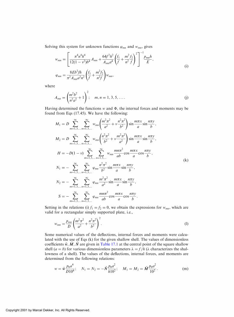
Solving this system for unknown functions ’mn and wmn, gives

wmn ¼�4n4h4

12ð1� �2Þb4 Amn þ64f 2h2

Amna4

f1fþm2

n2f2f

!224

35

�1

pmnh

E;

’mn ¼8Eb2fh

�2Amna2n2

f1fþm2f2

n2f

!wmn;

ðiÞ

where

Amn ¼m2b2

n2a2þ 1

!2

; m; n ¼ 1; 3; 5; . . . : ðjÞ

Having determined the functions w and �, the internal forces and moments may befound from Eqs (17.45). We have the following:

M1 ¼ DX1

m¼1;3;...

X1n¼1;3;...

wmn

m2�2

a2þ � n

2�2

b2

!sin

m�x

asin

n�y

b;

M2 ¼ DX1

m¼1;3;...

X1n¼1;3;...

wmn

n2�2

b2þ �m

2�2

a2

!sin

m�x

asin

n�y

b;

H ¼ �Dð1� �ÞX1

m¼1;3;...

X1n¼1;3;...

wmn

mn�2

abcos

m�x

acos

n�y

b;

N1 ¼ �X1

m¼1;3;...

X1n¼1;3;...

’mn

n2�2

b2sin

m�x

asin

n�y

b;

N2 ¼ �X1

m¼1;3;...

X1n¼1;3;...

’mn

m2�2

a2sin

m�x

asin

n�y

b;

S ¼ �X1

m¼1;3;...

X1n¼1;3;...

’mn

mn�2

abcos

m�x

acos

n�y

b:

ðkÞ

Setting in the relations (i) f1 ¼ f2 ¼ 0, we obtain the expressions for wmn, which arevalid for a rectangular simply supported plate, i.e.,

wmn ¼pmn

D

m2�2

a2þ n2�2

b2

!2

: ðlÞ

Some numerical values of the deflections, internal forces and moments were calcu-lated with the use of Eqs (k) for the given shallow shell. The values of dimensionlesscoefficients �ww; �MM; �NN are given in Table 17.1 at the central point of the square shallowshell (a ¼ bÞ for various dimensionless parameters � ¼ f =h (� characterizes the shal-lowness of a shell). The values of the deflections, internal forces, and moments aredetermined from the following relations:

w ¼ �wwp0a

4

D104; N1 ¼ N2 ¼ � �NN

p0a2

h102; M1 ¼ M2 ¼ �MM

p0a2

102: ðmÞ


The given numerical data for the shallow shell are compared in the table withthe values of the deflections and bending moments in a rectangular simply sup-ported plate having the same linear dimensions (a and bÞ as the shallow shell andsubjected to the same load p0. It follows from Table 17.1 that with an increase inthe parameter �, the load-carrying mechanism of the shallow shell changes: itsstiffness increases and bending moments are diminished, i.e., for large values of� the shallow shell supports a given normal surface load p3 practically due to themembrane action only. Of course, this qualitative conclusion is valid not only forthe considered shell but also for all of the classes of shallow shells. Comparisonof the ordinates of bending moments (and deflections) in shallow shells and flatplates shows that the above-mentioned values are significantly greater (by oneorder) in flat plates than in shallow shells for certain values of the parameter� ¼ f =h ðf ¼ f1 þ f2Þ.

To analyze the load-carrying mechanism of shallow shells subjected to a nor-mal surface load, Fig. 17.7 illustrates some numerical results of the analysis of theshallow shell with the following geometrical and mechanical characteristics: a ¼ b ¼10m; h ¼ 0:1m, f1 ¼ f2 ¼ 0:5 m, E ¼ 40GPa, � ¼ 0:17, and p3 ¼ p0 ¼ const. For

this shell D ¼ Eh3

12ð1��2Þ ¼ 3:4326 106 N �m.

Figure 17.7 shows the diagrams of the deflection, w, membrane force, N1, andbending moment, M1, along the central section (x ¼ a=2) of the shell. It should benoted that the location of the maximum deflection in the shallow shell shifts from thecenter (as it was in a flat plate) towards the supports. The bending moment distribu-tions in the shell, both qualitatively and quantitatively, differ from those in flatplates. The numerical results in Fig. 17.7 and in Table 17.1 were obtained by retain-ing the six terms in the series (e), and eight and 10 terms in the series (k) for thedeflections, membrane forces, and bending moments, respectively. In conclusion, letus make some comments.

1. When a shallow shell rise, f , increases, the shell geometry will differ notice-ably from plane geometry, i.e., the first basic assumption of the shallow shell theory

Table 17.1

Parameter �

Values of the dimensionless coefficients at the central point of the shell

Shallow shell Plate (� ¼ 0)

�ww �NN �MM �ww �MM

0.5 36.2101 4.2401 3.7985 39.4215 4.250

1.0 27.2112 6.3618 2.7911 39.4215 4.250

1.5 19.200 6.7200 1.9396 39.4215 4.250

2.0 13.4115 6.2501 1.1988 39.4215 4.250

3.0 7.0851 4.9501 0.5066 39.4215 4.250

4.0 4.1200 3.8102 0.2106 39.4215 4.250

5.0 2.6100 3.0115 0.07086 39.4215 4.250

6.0 1.7511 2.4510 0.01398 39.4215 4.250

10.0 0.5601 1.3102 �0:02180 39.4215 4.250

20.0 0.1364 0.6201 �0:00021 39.4215 4.250


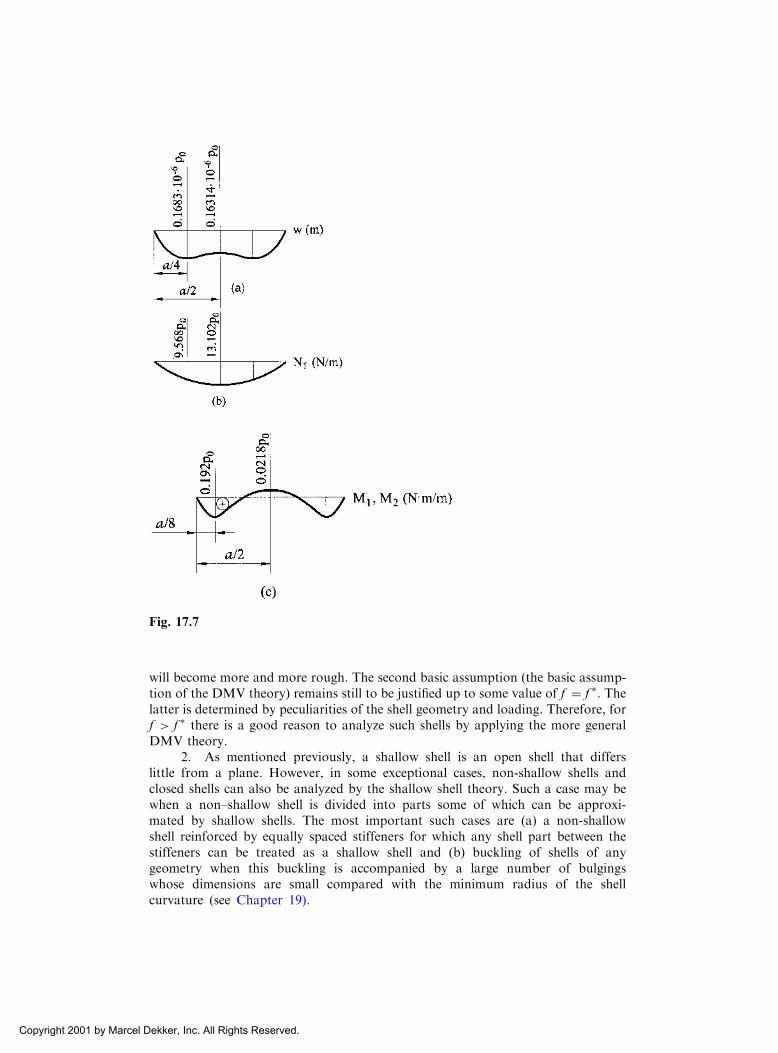
will become more and more rough. The second basic assumption (the basic assump-tion of the DMV theory) remains still to be justified up to some value of f ¼ f . Thelatter is determined by peculiarities of the shell geometry and loading. Therefore, forf > f there is a good reason to analyze such shells by applying the more generalDMV theory.

2. As mentioned previously, a shallow shell is an open shell that differslittle from a plane. However, in some exceptional cases, non-shallow shells andclosed shells can also be analyzed by the shallow shell theory. Such a case may bewhen a non–shallow shell is divided into parts some of which can be approxi-mated by shallow shells. The most important such cases are (a) a non-shallowshell reinforced by equally spaced stiffeners for which any shell part between thestiffeners can be treated as a shallow shell and (b) buckling of shells of anygeometry when this buckling is accompanied by a large number of bulgingswhose dimensions are small compared with the minimum radius of the shellcurvature (see Chapter 19).

Fig. 17.7


17.5 THE THEORY OF EDGE EFFECT

In this section we introduce one more approximate theory of thin shells. As men-tioned in Sec. 17.3, a thin shell can be found in the basic state of stress that ischaracterized by slowly varying deformations and stresses. The membrane (seeChapters 13 and 14) and pure bending stress states fall into the category of thebasic state of stress. The pure bending state rarely occurs. It is possible for nonrigidshells only whose constraints allow such a type of bending. In some cases, the state ofstress in thin shells can be separated into the following two components: the basic(mainly, membrane) for the entire shell and the mixed, mostly, a moment state, callededge effect, localizing near shell boundaries or near other sites at which the membranetheory does not apply. The latter state of stress can be superimposed on the basic statethat essentially simplifies the obtaining of the general state of stress in a shell. It wasindicated in Chapters 13–16 that the membrane solution alone for some shell geome-tries, loadings, and supports cannot satisfy the prescribed boundary conditions at theshell edges, the known conditions of continuity, equilibrium and/or kinematic con-straints at the edge effect zones. Gol’denveizer termed the sources of edge effects‘‘lines of distortion.’’ To facilitate their identification, Gol’denveizer listed these as [5]:

(a) the physical edges of a shell;(b) lines along which discontinuities of the components of external loads or

of certain their derivatives occur;(c) lines along which the middle surface of a shell has a break or the curva-

ture of the middle surface changes abruptly; and(d) lines along which the rigidity of a shell or its thickness undergoes sudden

changes.

The edge effect can be defined as such a state of stress and strain at which stresses anddisplacements vary slightly along the lines of distortion, but decay rapidly in the normaldirection to those lines.

The edge effect concept was demonstrated in Chapters 15 and 16 for axisym-metrically loaded circular cylindrical shells and shells of revolution, respectively.This section is concerned with constructing the general theory of the edge effectfor shells of any geometry subjected to asymmetric loading.

In deriving the governing differential equations of the theory of edge effect, wemake the following assumptions:

1. The lines of distortion coincide with one of the lines of curvature (fordefiniteness sake, with the -coordinate line).

Let us introduce the so-called asymptotic line as a line along which thenormal curvature of the surface, 1=Ri, is zero. For example, a generatorof a cylindrical surface can be considered as an asymptotic line. In thetheory of edge effect, it is assumed that the lines of distortion at any pointof the middle surface do not touch the asymptotic line. In this case, theedge effect always takes place and it is called simple edge effect. If thedistortion line touches an asymptotic line, then such an edge effect isreferred to as a complex one. In this section we analyze only the simpleedge effect.

2. The normal component of displacement, w, in zones of the edge effect issignificantly greater than the in-plane components, u and v.


3. Functions f that characterize the state of stress and strain (displacements,internal forces, and moments) vary significantly more rapidly in the direc-tion of the -coordinate line than in the direction of the -coordinate line,i.e.,

@f

A@

� @f

B@

: ð17:51Þ

(4) The Lame parameters, A and B, as well as the radii of curvature, have asmall variation in the direction of the -coordinate line, i.e.,

@A

@� A;

@B

@� B;

@R1

@� R1;

@R2

@� R2:

ð17:52Þ

A rapid decay of the edge effect state of stress, as we move away along the normal tothe line of distortion is a very important characteristic of a shell. It is caused by theshell thinness and by the curvilinearity of its surface. Let us explain this phenomenonin more detail in the following simple example.

Figure 17.8 shows a flat cantilever plate and an open circular cylindrical shellloaded by uniformly distributed bending moments, m ¼ const, applied to the freeedges of the plate and shell.

It is evident, that the cantilever plate will resist the external moment load bymeans of bending only (producing the bending and twisting moments, and shearforces); no membrane forces occur in its middle surface (Fig. 17.8a). The cantilevershell will support the applied distributed moments m not only by means of the bend-ing but also by straining the middle surface. The latter is accompanied by an appear-ance of the circumferential membrane forces N2 in the longitudinal sections of theshell ’ ¼ const, i.e., in the sections perpendicular to the edge x ¼ a (Fig. 17.8b). Thelarger the shell curvature 1=R, the stiffer is the shell in its middle surface and thegreater is the role of the membrane forces N2 in resisting the applied bending load.The availability of the circumferential forces N2 will cause the internal bendingmoment to decrease rapidly as we move away from the loaded edge in the normaldirection to the edge. This phenomenon is quite understandable if we recall the

Fig. 17.8


analogy between a shell and a flat plate resting on an elastic Winkler-type foundation.The normal projections of the circumferential forces N2 are interpreted as the reac-tions of the Winkler-type foundation (see Fig. 15.2 and the corresponding explana-tions in Sec. 15.3). Thus, the cylindrical shell shown in Fig. 17.8b acts as a flatcantilever plate resting on some elastic foundation. It is well known that stressesand displacements in such a flat cantilever plate, loaded by the distributed momentsm applied along its free edge, decay rapidly as we move away from this loaded edgedue to the distributed character of the elastic foundation.

For a more complete insight into the physical nature of the edge effect phe-nomenon, it is instructive to turn our attention to the general principles ofmechanics: in particular, to the principle of minimum potential energy (see Sec.2.6.2). It is easy to verify that the potential energy caused by bending moments isconsiderably larger than the potential energy due to the membrane forces. Hence, ifwe move away from a loaded zone that causes bending (for example, from a fixedshell edge) then, based on the principle of minimum potential energy, the process ofthe moment and shear force damping should begin. This a reason for the occurrenceof rapidly decaying state of stress-edge effects.

Another situation occurs near the straight edges and other lines of disturbanceof the state of stress and strain of a shell (the asymptotic lines). Assume, for example,that the edge ’ ¼ 0 is fixed and the other edges are free to displace. If the externalmoment m is applied to the edge ’ ¼ ’1 then the circumferential forces N2 are notneeded for equilibrium. Therefore, the bending moments decrease slightly as wemove away from the line of disturbance (in this case ’ ¼ ’1Þ and a given state ofstress cannot be separated into the membrane type and edge effect. Thus, nearstraight edges of open cylindrical shells, the simple edge effect concept cannot beapplicable. The possibilities of simplifying the governing differential equations aremore restricted here than in the case of the simple edge effect.

Now we derive the governing differential equation of the simple edge effectassuming the -coordinate line is the distortion line. Due to the adopted assumptions(see assumptions 3 and 4), the Laplace operator, r2f ; and the operator r2

kf can besimplified to the form

r2f � @

A@

@f

A@

� �; r2

kf � 1

R2

@

A@

@f

A@

� �: ð17:53Þ

Since all functions describing the state of stress and strain in the zone of the simpleedge effect represent some rapidly varying functions, we can use the differentialequations of the DMV theory introduced in Sec. 17.3. These equations will behomogeneous for the edge effect problems. Taking into account the relations(17.53), the differential equations (17.36) for the edge effect analysis can be writtenin the following form:

D@

A@

@

A@

@

A@

@w

A@� 1

R2

@

A@

@�

A@¼ 0;

1

Eh

@

A@

@

A@

@

A@

@�

A@þ 1

R2

@

A@

@w

A@¼ 0:

ð17:54Þ

As mentioned previously, only the rapidly varying functions are of interest in thetheory of the edge effect. Therefore, in integrating Eqs (17.54), arbitrary functionsthat depend linearly upon should be dropped (these functions characterize the


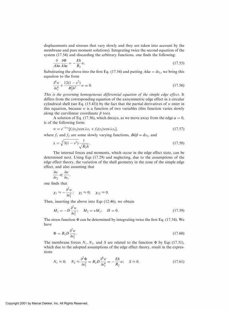
displacements and stresses that vary slowly and they are taken into account by themembrane and pure moment solutions). Integrating twice the second equation of thesystem (17.54) and discarding the arbitrary functions, one finds the following:

@

A@

@�

A@¼ �Eh

R2

w: ð17:55Þ

Substituting the above into the first Eq. (17.54) and putting Ad ¼ ds1, we bring thisequation to the form

@4w

@s41þ 12ð1� �2Þ

R22h

2w ¼ 0: ð17:56Þ

This is the governing homogeneous differential equation of the simple edge effect. Itdiffers from the corresponding equation of the axisymmetric edge effect in a circularcylindrical shell (see Eq. (15.43)) by the fact that the partial derivatives of w enter inthis equation, because w is a function of two variables (this function varies slowlyalong the curvilinear coordinate too).

A solution of Eq. (17.56), which decays, as we move away from the edge ¼ 0,is of the following form:

w ¼ e��s1 ½f1ðs2Þ cos �s1 þ f2ðs2Þ cos �s1�; ð17:57Þwhere f1 and f2 are some slowly varying functions, Bd ¼ ds2, and

� ¼ffiffiffiffiffiffiffiffiffiffiffiffiffiffiffiffiffiffi3ð1� �2Þ4

q1ffiffiffiffiffiffiffiffiR2h

p : ð17:58Þ

The internal forces and moments, which occur in the edge effect state, can bedetermined next. Using Eqs (17.29) and neglecting, due to the assumptions of theedge effect theory, the variation of the shell geometry in the zone of the simple edgeeffect, and also assuming that

@w

@s2� @w

@s1;

one finds that

�1 � � @2w

@s21; �2 � 0; �12 � 0:

Then, inserting the above into Eqs (12.46), we obtain

M1 ¼ �D@2w

@s21; M2 ¼ �M1; H ¼ 0: ð17:59Þ

The stress function � can be determined by integrating twice the first Eq. (17.54). Wehave

� ¼ R2D@2w

@s21: ð17:60Þ

The membrane forces N1;N2; and S are related to the function � by Eqs (17.31),which due to the adopted assumptions of the edge effect theory, result in the expres-sions

N1 � 0; N2 �@2�

@s21¼ R2D

@4w

@s41¼ �Eh

R2

w; S � 0: ð17:61Þ


The transverse shear forces may be found from the corresponding equilibrium equa-tions of the DMV theory, i.e.,

Q1 ¼ �D@

A@ðr2wÞ; Q2 ¼ �D

@

B@ðr2wÞ:

Using the relations (17.53), the above relations appear, as follows:

Q1 ¼ �D@3w

@s31; Q2 � 0: ð17:62Þ

The above relations and equations of the general edge effect theory were introducedfor the case when the distortion line coincides with the -coordinate line. Similarly,the corresponding equations can be presented for the -coordinate line as a distor-tion line and, generally, for the case when the shell edge does not coincide with theline of curvature [5].

In conclusion, one notes the following:

1. The edge effect theory introduced above cannot be applied to the casewhen the shell boundary or another distortion line coincides with theasymptotic line.

2. If a considered state of stress and strain varies rapidly not only in thedirection of the normal to the shell boundary but also along the boundaryitself, the stress analysis of such a shell can be carried out by the DMVtheory introduced in Sec. 17.3.

3. The governing differential equation of the edge effect, Eq. (17.56), is onlyapproximate. The exact solution of the shell problems by the edge effecttheory requires an integration of the system of the partial differentialequations of the general theory of thin shells and therefore has no advan-tages from separation of a given state of stress into the membrane stateand edge effect. Thus, the latter is taken into account only approximately.

4. The solution (17.57) makes it possible to satisfy the two boundary con-ditions on the corresponding shell edge. It is evident that these boundaryconditions must be formulated for the sum of the membrane solution andthe solution given by Eq. (17.56).

PROBLEMS

17.1 Verify Eqs (17.12) and (17.16).

17.2 Specify the area of application of the semi-membrane theory to the analysis of open

and closed cylindrical shells.

17.3 A simply supported, at x ¼ 0 and x ¼ L, cylindrical tube is filled by water up to the

level H (Fig. 17.2). The tube is reinforced by two equally spaced, rigid along the tube

length, collars in such a way that they prevent a distortion of the tube cross sections.

Applying the semi-membrane theory, determine the axial normal stress, �1, distributionover the shell cross section where the collar is attached to the tube. Let L ¼ 30m; R ¼5:5m; h ¼ 5:0 cm; H ¼ 1:2m; E ¼ 210GPa, and � ¼ 0:3.

17.4 A simply supported, at x ¼ 0 and x ¼ L, closed circular cylindrical shell is subjected to

a uniform vertical line load q, as shown in Fig. P.17.1. Determine the axial normal

stress, �1, distribution in the lower stretched fiber along the shell length. Compare this


stress with that obtained by the elementary beam bending theory. Take L ¼ 15:0m;R ¼ 2:0m; h ¼ 1:5 cm; E ¼ 200GPa; and � ¼ 0:3.

17.5 Derive Eqs (17.36).

17.6 Substitute for N1;N2; and S from Eqs (17.31) into Eqs (17.30). Setting p1 ¼ p2 ¼ 0 and

taking into account the Codazzi–Gauss relations (11.27), specify the accuracy of satis-

fying Eqs (17.30) in the framework of the assumptions of the DMV theory.

17.7 Show that the system of the governing equations (17.36) can be reduced to a single,

eight-order differential equation, as follows:

ar2kr2

k�þ r2r2r2r2� ¼ p3D

ðP17:1Þ

where � is some solving function introduced, as follows:

w ¼ r2r2�; � ¼ �Ehr2k� ðP:17:2Þ

and

a ¼ 12ð1� �2Þ=h2: ðP:17:3Þ17.8 Show that for a spherical shallow shell (R1 ¼ R2 ¼ R), the system of equations (17.36)

can be broken down into the following equations:

ðaÞ Dr2r2w þ Eh

R2w ¼ p3 ðP:17:3aÞ

ðbÞ r2w0 ¼ 0 ðP:17:3bÞ

ðcÞ r2� ¼ Eh

Rw ðP:17:3cÞ

where

r2�þ Eh

Rw ¼ Eh

Rw0 and w ¼ w0 þ w ðP:17:3dÞ

Hint: use the spherical coordinates ’ and �.17.9 Give a physical interpretation of Eqs (P.17.3) of the previous problem.

17.10 Verify Eq. (17.50).

17.11 Consider a shallow shell in polar coordinates ¼ r and ; where r is the polar radius

and is the polar angle of a point of the middle surface on the horizontal plane. For

this case, the Lame parameters are A ¼ 1 and B ¼ r. Show that the shallow shell in this

coordinate system is governed by the same equations (17.36) and the differential

operators (17.34) are given by

Fig. P.17.1


r2ð. . .Þ � 1

r

@

@rr@ð. . .Þ@r

� �þ 1

r

@2ð. . .Þ@2

" #;

r2kð. . .Þ �

1

r

@

@rrk2

@ð. . .Þ@r

� �þ @

@

k1r

@ð. . .Þ@

� �� :

ðP:17:4Þ

17.12 Show that the membrane forces N1;N2; and S in the shallow shell theory are expressed

in terms of the displacements, as follows:

N1 ¼ B@u

@xþ � @v

@y� ð�1 þ ��2Þw

� �; N2 ¼ B

@v

@yþ � @u

@x� ð�1 þ ��2Þw

� �;

S ¼ Bð1� �Þ2

@v

@xþ @u@y

� � ðP:17:5Þ

where

B ¼ Eh

1� �2 :

17.13 Using the equations of equilibrium (12.44), Eqs (17.45b), (P.17.5), and the relations

(17.42), show that the governing equations of the shallow shell of double curvature in

Cartesian coordinates are of the following form:

@2u

@x2þ 1� �

2

@2u

@y2þ 1þ �

2

@2v

@x@y� ð�1 þ ��2Þ

@w

@x¼ � p1

B;

1� �2

@2u

@x@yþ @2

@y2þ 1� �

2

@2

@x2

!v� ð�2 þ ��1Þw ¼ � p2

B;

@u

@xð�1 þ ��2Þ þ

@v

@yð�2 þ ��1Þ � ð�21 þ �22 þ 2��1�2Þw� h2

12r2r2w ¼ � p3

B:

ðP:17:6Þ

17.14 The governing equations (17.36) for the shallow shell theory were derived assuming

that p1 ¼ p2 ¼ 0; and p3 6¼ 0. Show that if all the load components are nonzero, the

relations (17.45a) should be replaced with

N1 ¼@2�

@y2�ðp1dx; N2 ¼

@2�

@x2�ðp2dy; S ¼ � @2�

@x@y; ðP:17:7Þ

and Eqs. (17.36) for this case appear as follows:

�r2k�þDr2r2w ¼ p3 � �1

ðp1dx� �2

Zp2dy;

r2r2�þ Ehr2kw ¼

ð@2p1@y2

dxþð@2p2@x2

dy� � @p1@x

þ @p2@y

� �:

ðP:17:8Þ

17.15 Consider a square in a plan shallow shell of double curvature. Let the equation of its

middle surface be given by (the origin of the Cartesian coordinate system is taken at the

center of the projection of the shell on the horizontal plane)

z ¼ f 1� x2 þ y2

2a2

!;

where f ¼ f1 þ f2 is the total rise. The shell edges, x ¼ �a and y ¼ �a, have the same

supports as described in Example 17.1. The shell is subjected to a uniformly distributed

load p. Determine the deflection w, the membrane forces N1;N2; and S, the bending

moments M1 and M2; and the twisting moment H. Take four terms (m ¼ 1; n ¼ 1; m


¼ 1; n ¼ 3; m ¼ 3; n ¼ 1; m ¼ 3; n ¼ 3Þ in the expansions (e) and (f) in Example 17.1.

Let a ¼ 2:0m; h ¼ 20mm; f1 ¼ f2 ¼ 250mm; p ¼ 2 kPa; G ¼ 30GPa; and � ¼ 0.

17.16 A shallow shell of double curvature, shown in Fig. 17.6, is supported by diaphragms at

its edges (the boundary conditions are given by Eqs (c) and (d) in Example 17.1). The

shell is subjected to a uniformly distributed load of intensity p: Determine the deflec-

tions, in-plane forces, and bending moments in the shell. Take four terms in the

expansions (e) and (f) (see problem 17.15). Take a ¼ 10m; b ¼ 12m; �1 ¼ 0:04=l;m;�2 ¼ 0:02781=m, h ¼ 30mm; E ¼ 22GPa; and � ¼ 0:

17.17 Show that if deflection w is a rapidly varying function, at least in one of the coordinate

directions, then the following estimate takes place:

r2w w

R1R2

� C2

where C � 1.

17.18 Based on the results of Problem 17.7, derive Eqs (17.62).

17.19 Specify the area of application of the edge effect theory for open and closed cylindrical

shells loaded asymmetrically.

REFERENCES

1. Vlasov, V.Z., General Theory of Shells and its Applications in Engineering, NASA

Technical Translation TTF-99, Washington DC, 1964.

2. Novozhilov, V.V., Thin Shell Theory (translated from 2nd Russian edn. by P.G. Lowe),


3. Donnell, L.H., Stability of Thin Walled Tubes under Torsion, NACA, Report No. 479,

Washington, DC, 1933.

4. Mushtari, Kh.M., Certain generalizations of the theory of thin shells, Izv Fiz Mat ob-va pri

Kaz Un-te, vol. 11, No. 8 (1938) (in Russian).

5. Gol’denveizer, A.L, Theory of Elastic Shells (translated from Russian by G. Herrmann),

Pergamon Press, New York, 1961.

6. Boyarshinov, S.V., The Fundamentals of Structural Mechanics of Machines,


7. Biderman, V. L., Mechanics of Thin-Walled Structures, Izdatel’stvo ‘‘Mashinostroenie’’,


8. Lur’e, A.L., General theory of elastic shells, Prikl Mat Mekh, vol. 4, No. 1, pp. 7–34

(1940) (in Russian).


18

Advanced Topics

18.1 THERMAL STRESSES IN THIN SHELLS

18.1.1 General

This section is concerned with the influence of high temperature on the state of stressand strain in thin shells. This issue has been studied in Sec. 7.1, as applied to thinplates. It should be noted that the thermal stresses and deformations in thin shells area major factor in the design of structures such as boilers, heat exchangers, pressurevessels, nuclear piping, and supersonic aircraft skin. The basic concepts of the ther-moelastic stress analysis of thin shells are quite similar to those introduced in Sec. 7.1for thin plates. Similarly, the thermoelastic problems require modifying the consti-tutive equations of the general shell theory.

Let a shell be subjected to a nonuniform temperature field Tð; ; zÞ measuredfrom some specified reference value. The temperature distribution T can be obtainedfrom a solution of the equation of heat conduction [1], represented in terms of theshell coordinates. Taking into account the relations (7.1), we can modify the con-stitutive equations (12.28) by taking into account the temperature effects, as follows:

"z1 ¼1

E�z1 � ��z2ð Þ þ T; "z2 ¼

1

E�z2 � ��z1ð Þ þ T; �z12 ¼

1

G�z12; ð18:1Þ

where is the coefficient of thermal expansion (see Sec. 7.1). It is assumed that E; �,and d are constant for a given temperature field. Solving Eqs (18.1) for the stresscomponents yields

�z1 ¼E

1� �2 "z1 þ �"z2 � ð1þ �ÞT½ �; �z2 ¼

E

1� �2 "z2 þ �"z1 � ð1þ �ÞT½ �;

�z12 ¼ G�z12:

18:2


Substituting Eqs (18.2) into Eqs (12.35) and (12.36) with the use of the relations(12.22), and integrating over z from �h=2 to h=2, one obtains

N1 ¼ Bð"1 þ �"2Þ �NT

1� � ; N2 ¼ Bð"2 þ �"1Þ �NT

1� � ;

N12 ¼ N21 ¼ S ¼ B1� �2

�12; ð18:3Þ

M1 ¼ Dð�1 þ ��2Þ �MT

1� � ; M2 ¼ Dð�2 þ ��1Þ �MT

1� � ;

M12 ¼ M21 ¼ H ¼ Dð1� �Þ�12; ð18:4Þwhere

B ¼ Eh=ð1� �2Þ ð18:5Þis the shell stiffness in tension and NT and MT are the thermal stress resultants, asgiven by Eqs (7.8). The equations of static equilibrium, Eqs (12.41) and (12.42), andkinematic equations, Eqs (12.23) and (12.24), of the general shell theory remainunchanged. Thus, a set of thermoelastic governing differential equations withinthe framework of the Kirchhoff–Love postulates consists of Eqs (12.23), (12.24),(12.41), (12.42), and (18.3)–(18.5). As mentioned in Chapter 12, these equations insome cases must be complemented with the equations of compatibility. The solutionsof the above equations must satisfy the prescribed boundary conditions on shelledges.

As for thin plates, the thermal stresses in a shell can occur in the followingcases: in a nonuniform heating; if thermal deformations are restricted by imposedconstraints; in heating of multilayered shells composed of heterogeneous materials,etc. However, not any nonuniform heating causes the thermal stresses. For instance,if the temperature varies linearly over the length of a cylindrical shell and is constantover its circumference and thickness, then the shell’s middle surface becomes aconical surface, but no stresses occur.

The isothermal analogy, introduced in Sec. 7.1 for the thermoelastic platebending problems, can be applied also for solving the thermoelastic governingshell equations together with appropriate boundary conditions. According to thisanalogy, the thermoelastic terms entering on the right-hand side of the governingequations may be treated as some fictitious and known surface loading. In the nextsections, the thermoelastic shell equations will be applied for stress analysis of someparticular shell forms and loadings.

18.1.2 Circular cylindrical shells under axisymmetric nonuniformheating

Assume that the heating of a circular cylindrical shell is axisymmetric and varieslinearly across its thickness according to the following law:

T ¼ T0 þ�Tz

h; ð18:6Þ

where T0 ¼ ðT1 þ T2Þ=2 is an average temperature of the shell wall; �T ¼ T1 � T2 isa temperature change; and T1 and T2 are the temperatures of the lower and uppersurfaces of the shell, respectively.


Derivation of the governing differential equation of the thermoelastic axisym-metric shell analysis is analogous to the derivation described in Sec. 15.3 for thestatic analysis. A distinction lies in the fact that constitutive equations of thisproblem must be complemented with thermal terms, as indicated in Sec. 18.1.1.Taking into account Eqs (12.22) and (15.38), we can rewrite the constitutiveequations (18.2) in terms of the displacement components, as follows:

�z1 ¼E

1� �2du

dx� z

d2w

dx2� �w

R� ð1þ �ÞT

" #;

�z2 ¼E

1� �2 �w

Rþ � du

dx� z

d2w

dx2

!� ð1þ �ÞT

" #:

ð18:7Þ

Then, using Eqs (12.35) and (12.36), and Eqs (15.38), we can rewrite the constitutiveequations (Eqs (18.3)–(18.5)) in terms of the displacement components:

N1 ¼ Bdu

dx� �w

R� ð1þ �ÞT0

� �; ð18:8aÞ

N2 ¼ B �du

dx� w

R� ð1þ �ÞT0

� �¼ �N1 � w

Eh

R� EhT0; ð18:8bÞ

M1 ¼ �Dd2w

dx2þ ð1þ �Þ�T

h

" #; M2 ¼ �D �

d2w

dx2þ ð1þ �Þ�T

h

" #: ð18:9Þ

Accordingly, the expressions of the shear force, Eq. (15.46), and the governingdifferential equation (15.44) are

Q1 ¼dM1

dx¼ �D

d3w

dx3þ ð1þ �Þ

h

dð�TÞdx

" #; ð18:10Þ

d4w

dx4þ 44w ¼ p3

Dþ �N1

DR� ð1þ �Þ

h

d2ð�TÞdx2

� Eh

DRT0; ð18:11Þ

where is given by Eq. (15.45). A solution of Eq. (18.11) is given by the expression(15.53) for long shells and by (15.74) for short shells. The particular solution, wp,depends upon an assigned thermal field and given loading. If the thermal field andloading are such that

d4T0

dx4¼ 0;

d2ð�TÞdx2

¼ 0;

d4p3dx4

¼ 0;d4N1

dx4¼ 0;

then the particular solution is of the following type:

wp ¼R2

Ehp3 þ �

N1

R

� �� RT0: ð18:12Þ


The technique of integrating Eq. (18.11) is not different from that discussed in Sec.15.3.

As mentioned previously, the thermal terms on the right-hand side of Eq.(18.11) can be interpreted as some fictitious surface load, qT . So, we can rewriteEq. (18.11), as follows:

d4w

dx4þ 44w ¼ 1

Dp3 � qT þ �N1

R

� �; ð18:13Þ

where

qT ¼ Dð1þ �Þh

d2ð�TÞdx2

þ Eh

RT0: ð18:14Þ

Using the principle of superposition, the given thermoelastic problem for a circularcylindrical shell can be broken down into two independent problems. The firstproblem involves only thermal effects produced by qT . In this case, only the parti-cular solution is of interest (all constants of integration are assumed to be zero). Thesecond problem deals with external forces, p3 and N1. Its solution was presented inSec. 15.3. The constants of integration are evaluated in such a way that the sum ofthe solutions of these two problems satisfies the prescribed boundary conditions.

Example 18.1

An infinitely long circular cylindrical shell is heated according to Eq. (18.6). Thetemperature is a constant along the shell length. Determine the thermal stresses.

Solution

A given thermal field can be represented as a superposition of a uniform heatingT0 ¼ ðT1 þ T2Þ=2, which produces no stresses, and of the thermal change�T ¼ T1 �T2 (Fig. 18.1).

Let us consider the state of stress corresponding to the thermal jump men-tioned above. Since the temperature does not vary along the shell length, then allvalues are constant over the length, and, hence, a general solution of the thermalhomogeneous equation is nonexistent. The particular solution (Eq. (18.12)) forp3 ¼ 0, N1 ¼ 0, and T0 ¼ 0 is also zero. Thus, the deflections of points of the middlesurface w and the circumferential force N2, according to Eq. (18.8b), are also equal

Fig. 18.1


to zero. However, the bending moments in this case are not equal to zero; it followsfrom Eqs. (18.9) that they are

M1 ¼ M2 ¼ �ð1þ �ÞDh

�T : ð18:15Þ

A special feature of this thermal problem is that, in spite of the presence of thebending moments, the curvature of the middle surface does not change. It can beexplained as follows: change in curvature caused by a nonuniform heating is com-pensated by a curvature change produced by the bending moments given by Eq.(18.15). The values of the bending stresses at the upper and lower points of the shellsurfaces are found to be the following:

�1max ¼ � 6M1

h2¼ � E

2ð1� �Þ�T; �2max ¼ � 6M2

h2¼ � E

2ð1� �Þ�T :

The bending stress diagrams across the shell thickness are shown in Fig. 18.1. Theyalso illustrate the above statement about the lack of a change in curvature for thegiven thermal field.

Example 18.2

A cylindrical stepped shell is shown in Fig. 18.2a. The shell is heated over its lowersurface up to the temperature T1 ¼ 120C and over the upper surface to the tem-perature T2 ¼ 50C. The temperatures are constant over the shell length. GivenR ¼ 0:5m, h1 ¼ 2 10�2 m, h2 ¼ 1 10�2 m; the shell material is a structural steelwith � ¼ 0:3; E ¼ 200GPa, and ¼ 12 10�6=C. Determine the thermal stresses.Assume that the shell is sufficiently long.

Solution

The given thermal field can again be broken down into a uniform heating T0 ¼ ðT1 þT2Þ=2 ¼ 85C and temperature jump �T ¼ T1 � T2 ¼ 70C. Since the uniform heat-ing produces no thermal stresses, it will not be taken into further account. Assumethat the given shell is cut into two parts: the first of constant thickness h1 and thesecond of constant thickness h2: If they were really separated then they would besubjected to the thermal jump �T and, consequently, were additionally loaded by

Fig. 18.2


the bending moments at shell edges, as shown in Fig. 18.2b. These moments can becalculated from Eqs. (18.15):

– for the first part of the shell ðh ¼ h1Þ,

Mð1Þ1ð�TÞ ¼ ��Tð1þ �ÞD1

h1¼ � �TEh21

12ð1� �Þ ¼ �8000 N �m=m;

– for the second part of the shell ðh ¼ h2Þ,

Mð2Þ1ð�TÞ ¼ ��Tð1þ �ÞD2

h2¼ � �TEh22

12ð1� �Þ ¼ �2000 N �m=m:

At a state shown in Fig. 18.2c, the shell is loaded by the interface moments, M0 andshear forces, Q0 at the junction of the two shell parts only, where M0 and Q0 are theinterface bending moment and shear force that actually act at the junction of thestepped shell and M

ð1Þ1ð�TÞ and M

ð2Þ1ð�TÞ have been added to compensate the moments

applied to the shell in the state shown in Fig. 18.2b. To determine the interfacemoment M0 and shear force Q0, it is sufficient to consider only the state shown inFig. 18.2c and set up the conditions of compatibility for deformations at the junctionof the two shell parts. The latter are of the following form:

wð1Þ ¼ wð2Þ; #ð1Þ1 ¼ �#ð2Þ1 ; ðaÞi.e., the deflections and slopes of the normals for the two shell parts at the junctionshould be the same. The negative sign in Eq. (a) is taken because the direction of thex axis for the first and second parts of the shell is opposite. The deflections, wð1Þ andwð2Þ, and slopes, #ð1Þ1 and #ð2Þ1 , may be determined from Eqs (15.57). For the first (left)shell part, setting x ¼ 0 and wp ¼ 0, we obtain

wð1Þ ¼ �M0 þMð1Þ1ð�TÞ

2D121

þ Q0

2D131

; #ð1Þ1 ¼ M0 þMð1Þ1ð�TÞ

D11� Q0

2D121

: ðbÞ

Similarly, for the second shell part, again setting x ¼ 0 and wp ¼ 0, we have thefollowing:

wð2Þ ¼ �M0 þMð2Þ1ð�TÞ

2D222

� Q0

2D232

; #ð2Þ1 ¼ M0 þMð2Þ1ð�TÞ

D22þ Q0

2D222

: ðcÞ

Computing the geometric properties of the stepped shell, we have

D1 ¼Eh31

12ð1� �2Þ ¼ 146:8 kN �m; D2 ¼Eh32

12ð1� �2Þ ¼ 18:33 kN �m

or D2 ¼D1

8;

1 ¼ 4

ffiffiffiffiffiffiffiffiffiffiffiffiffiffiffiffiffi3ð1� �2R2h21

s¼ 12:85

1

m; 2 ¼ 4

ffiffiffiffiffiffiffiffiffiffiffiffiffiffiffiffiffiffi3ð1� �2ÞR2h22

s¼ 18:13

1

m¼ 1

ffiffiffi2

p;

Mð1Þ1ð�TÞ ¼ 8000N �m=m; M

ð2Þ1ð�TÞ ¼ 2000N �m=m ¼ 1

4M

ð1Þ1ð�TÞ:


Substituting Eqs (b) and (c) into the compatibility equations (a), we obtain thefollowing system of two equations:

3M0 þ 0:298Q0 ¼ 0 and 10�3ð3:539M0 þ 0:0623Q0Þ ¼ �10:258:

Solving these equations for M0 and Q0, yields

M0 ¼ �3523 N �m=m; Q0 ¼ 35480 N=m:

Having determined M0 and Q0, we can calculate the deflections, internal forces, andbending moments from Eqs (15.57). Summing them with the corresponding values ofthe state shown in Fig. 18.2b, we obtain the final expressions of the thermoelasticdeflections and stress resultants and couples for the given problem (Fig. 18.2a). Themost stressed point is located at the outside surface of the thinner part of the shell,near the stepped transition. The internal forces, bending moments, and normalstresses in this place are

M1 ¼ �3523 N �m=m; M2 ¼ �2460 N �m=m; N1 ¼ 0;

N2 ¼ 142656 N=m; w ¼ 0:413 10�3 m ¼ 0:413mm;

�1 ¼6M1

h22¼ 211:4MPa; �2 ¼

N2

h2þ 6M2

h22¼ 161:9MPa:

As we move away from the stepped transition, the bending moments, M1ð�TÞ andM2ð�TÞ, occur in the shell wall. These moments induce the normal stresses, which arefound to be

�1 ¼ �2 ¼ 120MPa:

18.1.3 Thermoelastic stress analysis of shallow shells

The general assumptions and governing equations of the shallow shell theory weredeveloped in Sec. 17.4. As mentioned in Sec. 18.1, the equilibrium and kinematicequations of the shell theory remain unchanged, whereas the constitutive relationsshould be changed in the thermoelastic stress analysis.

Solving the first two equations (18.3) for the strain components "1 and "2 yieldsthe following:

"1 ¼1

EhðN1 � �N2 þNT Þ; "2 ¼

1

EhðN2 � �N1 þNT Þ: ð18:16Þ

Now repeating the procedure of deriving the governing differential equations of theshallow shell described in Secs 17.3 and 17.4, with the use of the constitutive equa-tions (18.3), (18.4), and (18.16), yields the following equations:

Dr2r2w� r2k� ¼ p3 �

1

1� �r2MT ;

1

Ehr2r2�þ r2

kw ¼ � 1

Ehr2NT ;

ð18:17Þ

where the stress function � and operator r2k were introduced in Sec. 17.4, and the

quantities NT andMT are given by Eqs (7.8). This system of equations represents thethermoelastic governing differential equations of the shallow shell.Hence, if the values ofNT and MT remain constant or vary linearly along the coordinate lines x and y, thenthe governing differential equations of the thermoelastic shallow shell stress analysisremain of the same type as for a non-thermally affected shell. However, a thermal


effect can influence the stress state of the shallow shell through the boundary condi-tions. Such a case is typical for stiffened shells. If a shell wall is heated faster than itsstiffening ribs, then the thermal deformation of the shell itself will be restrained andsignificant compressive stresses may occur in the shell, causing buckling.

18.2 THE GEOMETRICALLY NONLINEAR SHELL THEORY

18.2.1 Introduction

The general shell theories presented previously were based on linear elasticity con-cepts. Linear shell theories predict adequately stresses and displacements for shellsexhibiting small elastic deformations. The governing differential equations of thesetheories were based on Hooke’s law, and the omission of rotations in the expressionsfor strains and equilibrium. As a result, the above governing equations were linear-ized. A theory of shells in which the small-displacement assumption is abandonedand the remaining assumptions are retained is called the geometrically nonlineartheory. This theory is based on the analysis of large, or finite displacements.Therefore, the geometrically nonlinear theory is also referred to as a large- orfinite-displacement theory. In developing the governing equations of the geometri-cally nonlinear theory of thin shells, rotations are taken into account in both thestrain–displacement and equilibrium equations. Additionally a shell may be a phy-sically nonlinear with respect to constitutive relations. This type of nonlinearityforms the basis of inelastic shell theory and is not discussed in this book.

The large-displacement shell theory is often required when dealing with shal-low shells, highly elastic membranes, and with buckling problems. The reason forthat lies in the following. Shallow shells are less stiff than rising shells: the sametransverse load produces larger displacements in shallow shells than in rising shellshaving the same planar dimensions. Hence, the displacements of the shallow shellcan be beyond the limits of the applicability of the small-displacement theory (thecommonly used criterion of an applicability of the linear shell theory is formulated asfollows: the above theory is applicable if jDj=h � ð0:2� 0:5Þ where D ¼ ½u; v;w�T isthe displacement vector. However, such a classification may be considered as arbi-trary only since here too the decisive influence is that of the preassigned error limitsin the solution of the boundary conditions of the theory of shells. Another approachto the criteria of applicability of the linear shell theory was given in Ref. [5]). Thesmall-displacement theory determines a unique configuration of equilibrium forevery shell with a prescribed load and assigned constraints. However, in reality, asolution of a physical shell problem is not always unique. A shell under identicalconditions of loading and constraints may have several possible equilibrium config-urations. Analyses of possible equilibrium configurations under prescribed loadsprovides a basis for studies of shell buckling problems that will be discussed in thenext chapter. Membranes or flexible thin shells may be defined as shells whosebending stiffness is negligible compared with their in-plane stiffness. Such shellsmay resist applied loads in tension only. Displacements of the membranes, as arule, exceed their thickness. Therefore, the geometrically nonlinear theory must beapplied to characterize adequately the state of stress and strain of membranes.

We present in this section the geometrically nonlinear theory of shallow shellsfor which the displacements by modulus are equal or exceed the shell thickness but are


considerably less than the other linear dimensions of the shell (from now on, the term‘‘geometrically’’ will be dropped because only this type of nonlinearity is discussedherein). The large-displacement theory of thin plates and shells originates from vonKarman’s work [2]. E. Reissner developed the geometrically nonlinear theory of thinshells [3]. Considerable contributions in the nonlinear shell theory were made bySaunders [4], Mushtari [5], etc. We will present here Vlasov’s approach for derivingthe governing differential equations of the nonlinear shallow shell theory [6].

A geometric nonlinearity manifests to the theory in twoways. At first, because ofmoderately large displacements, the strain components are related to these displace-ments by means of nonlinear equations. Secondly, a shell element undergoes so muchchanges in its shape after deformation, i.e., it moves and rotates in space through suchfinite distances and angles, that it is impossible to set up its equilibrium equations basedon an undeformed shell configuration as has been done in the linear shell theory.

18.2.2 Nonlinear theory of shallow shells

As in the classical shell theory, assume that the coordinate lines coincide with thelines of principal curvatures. We start the nonlinear shallow shell analysis with thestrain–displacement relations. In the classical, linear shell theory, it was assumed thatstrains were small and that the rotations were of the same order of magnitude as thestrains. As mentioned earlier, the above rotations should be taken into account indeveloping the kinematic relations of the nonlinear theory of shallow shells.However, it will be assumed that the nonlinear strains of the middle surface remainstill small compared with unity and they are of the order of the rotations squared.

It follows from the above that the nonlinear theory deals with the more compli-cated strain–displacement equations. However, for shallow shells, these equations canbe simplified. Indeed, since the geometry of a shallow shell is close to a flat plate, thestiffness of the shell in the tangent plane is significantly greater than the flexural stiff-ness (see Sec. 7.4.1). Therefore, say, the angle of rotation !1 of the element ds1 in thetangential plane (about the unit vector e3) is much smaller than the angle of rotation #1of the same element in the normal plane (about the unit vector e2). However, althoughthe angles #1 and #2 are larger inmodulus than the angles!1 and !2, the former anglesthemselves remain still small because of the following limitation for the deflectionsadopted in the nonlinear theory of shallow shells: wj j � 5h. Therefore, the squares ofthe angles #1 and #2 can be neglected in comparison with unity.

Thus, the basic assumption of the linear shell theory about the smallness of thesquares of all the angles of rotation compared with unity and about the equivalenceof orders of their values is now reduced and it is postulated that

!21 � #21 � 1;!2

2 � #22 � 1: ð18:18ÞAs a result of the above assumption, the strain–displacement relations of the lineartheory of shallow shells, Eqs (17.43), are complemented by the same nonlinear termsas in the theory of flexible plates (see Eqs (7.82)):

"1 ¼@u

@x� w

R1

þ 1

2

@w

@x

� �2

; "2 ¼@v

@y� w

R2

þ 1

2

@w

@y

� �2

;

�12 ¼@u

@yþ @v

@xþ @w@x

@w

@y:

ð18:19Þ


Notice that the shear strain expression for shallow shells is absolutely identical tothat obtained in the large-deflection theory of thin plates (see the third Eq. (7.82)).Hence, the shell curvature does not affect the shear deformation of the middle sur-face, if the coordinate lines x and y are the lines of the principal curvatures in theframework of the theory of shallow shells.

The expressions for changes in curvature and for twist of the middle surfacealso coincide with those obtained in the small-deflection theory of shallow shells, i.e.,

�1 ¼ � @2w

@x2; �2 ¼ � @

2w

@y2; �12 ¼ � @2w

@x@y: ð18:20Þ

The tangential strain components, "z1; "z2; and �

z12, at points in an equidistant surface

of the shell from the z coordinate, are determined, as previously, by Eqs (12.22).The expressions for the stress resultants and stress couples, as well as the

constitutive equations of the nonlinear shallow shell theory remain identical tothose introduced in Sec. 12.3 for the linear shell theory. Introducing the relations(18.19) into the constitutive equations (12.45) and letting N12 ¼ N21 ¼ S, we obtainthe following relations between the membrane forces and displacements at points ofthe middle surface:

N1 ¼Eh

1� �2@u

@xþ � @v

@yþ 1

2

@w

@x

� �2

þ �2

@w

@y

� �2

� w

R1

� � w

R2

" #;

N2 ¼Eh

1� �2@v

@yþ � @u

@xþ 1

2

@w

@y

� �2

þ �2

@w

@x

� �2

� w

R2

� � w

R1

" #;

S ¼ Eh

2ð1þ �Þ@u

@yþ @v

@xþ @w@x

@w

@y

� �:

ð18:21Þ

Let us eliminate the tangential displacements u and v from Eqs (18.21), and expressthe forces N1;N2; and S in terms of the deflections w. For this purpose, first, trans-form the two first relations (18.21), as follows:

N1 � �N2 ¼ Eh@u

@xþ 1

2

@w

@x

� �2

� w

R1

" #; N2 � �N1 ¼ Eh

@v

@yþ 1

2

@w

@y

� �2

� w

R2

" #:

ð18:22ÞUsing the above relations, set up the following equation:

@2

@y2ðN1 � �N2Þ þ

@2

@x2ðN2 � �N1Þ � 2ð1þ �Þ @

2S

@x@y

¼ Eh@2

@y21

2

@w

@x

� �2" #

þ @2

@x21

2

@w

@y

� �2" #

� @2

@x@y

@w

@x

@w

@y

� �(

� 1

R1

@2w

@y2� 1

R2

@2w

@x2

�:


According to the general rules of differentiating, the following equalities hold:

@2

@y21

2

@w

@x

� �2" #

¼ @2w

@x@y

!2

þ @w@x

@3w

@x@y2;@2

@x21

2

@w

@y

� �2" #

¼ @2w

@x@y

!2

þ @w@y

@3w

@x2@y;

@2

@x@y

@w

@x

@w

@y

� �¼ @3w

@x2@y

@w

@yþ @2w

@x@y

!2

þ @2w

@x2@2w

@y2þ @w@x

@3w

@x@y2:

Inserting these equalities in the above equation yields the following:

@2

@y2ðN1 � �N2Þ þ

@2

@x2ðN2 � �N1Þ � 2ð1þ �Þ @

2S

@x@y

¼ Eh@2w

@x@y

!2

� @2w

@x2@2w

@y2� 1

R1

@2w

@y2� 1

R2

@2w

@x2

24

35:

ð18:23Þ

Equation (18.23) represents the equation of compatibility of deformations of the non-linear shallow shell theory in terms of the membrane forces and deflections.

Let us introduce the stress function � according to the relations (17.45a).Substituting for � from the above relations into Eqs (18.23), results in

r2r2� ¼ Eh@2w

@x@y

!2

� @2w

@x2@2w

@y2� r2

kw

24

35; ð18:24Þ

where the operators r2 and r2k are given by Eqs (17.44).

Now we are coming to constructing the equations of equilibrium for ashallow shell element subjected to a transverse surface load p3. The positivedirections of the internal forces and moments acting on the element are shownin Fig. 12.5. The derivation of the equations of equilibrium in the nonlineartheory of shallow shells has some peculiarities. The force summations in the xand y directions, as well as the moment summations about the above axes, are setup as for the linear shell theory. This involves neglecting the changes in transitionof the shell element from its initial (undeformed) to the deflected state, and theinitial curvatures of the above element are also neglected. However, the forcesummation into the z direction is set up by taking into account both the initialcurvatures of the element and its consequent distortion acquired as a result ofshell straining under action of applied loads. It can be shown that the aboveequation of equilibrium will have the form of the third Eq. (12.41), derived forthe linear shell theory, but complemented by the same terms as for the corre-sponding equilibrium equation of the nonlinear theory of flat plates (see Eq.(3.91). The system of simplifications adopted in the nonlinear shallow shell theoryresults in the following equations of equilibrium:

@N1

@xþ @S@y

¼ 0;

@N2

@yþ @S@x

¼ 0; ð18:25Þ


@Q1

@xþ @Q2

@y¼ �p3 �

N1

R1

�N2

R2

�N1

@2w

@x2�N2

@2w

@y2� 2S

@2w

@x@y; ð18:26Þ

Q1 ¼@M1

@xþ @H@y

; ð18:27aÞ

Q2 ¼@M2

@yþ @H@x: ð18:27bÞ

Using the relations (18.27), it is possible to eliminate the shear forces Q1 andQ2 from Eq. (18.26). As a result, the equations of static equilibrium of theelement of a shallow shell in the nonlinear theory are reduced to the followingequations:

@N1

@xþ @S@y

¼ 0;

@N2

@yþ @S@x

¼ 0;

@2M1

@x2þ 2

@2H

@x@yþ @

2M2

@y2þN1

1

R1

þ @2w

@x2

!þN2

1

R2

þ @2w

@y2

!þ 2S

@2w

@x@yþ p3 ¼ 0:

ð18:28ÞSubstituting for the bending and twisting moments from Eqs (17.45b) into the thirdEq. (18.28) and introducing again the stress function � from Eq. (17.45a), we obtainthat the first two equations of (18.28) will be identically satisfied and the thirdequation becomes

Dr2r2w� r2k�þ @2�

@y2@2w

@x2þ @

2�

@x2@2w

@y2� 2

@2�

@x@y

@2w

@x@y

!" #¼ p3: ð18:29Þ

Eqsuations (18.24) and (18.29) are the governing differential equations of the non-linear theory of shallow shells. By introducing the operator

LðU;VÞ � @2U

@x2@2V

@y2� 2

@2U

@x@y

@2V

@x@yþ @

2U

@y2@2V

@x2; ð18:30Þ

we can rewrite the governing equations (18.24) and (18.29), as follows:

r2r2� ¼ �Eh1

2Lðw;wÞ þ r2

kw

� �;

Dr2r2w� r2k�þ Lð�;wÞ� � ¼ p3:

ð18:31Þ

Letting in Eqs (18.31) �1 ¼ 1=R1 ¼ 0 and �2 ¼ 1=R2 ¼ 0, we obtain Eqs (7.87) forthe large-deflection theory of plates. Boundary conditions on edges of the large-deflection shallow shell are formulated in a similar manner to those of the small-deflection shallow shell or of the large-deflection plate (see Secs 17.4 and 7.4, respec-tively).


In conclusion, let us formulate some qualitative considerations about themechanical behavior of a geometrically nonlinear shell under applied loading. Forsimplicity, consider a flexible spherical shallow shell. Such a shell is governed by Eqs(18.31), if we let R1 ¼ R2 ¼ R. We obtain the following system of equations:

1

Ehr2r2�þ 1

2Lðw;wÞ þ 1

Rr2w

� �¼ 0;

Dr2r2w� 1

Rr2�þ Lð�;wÞ

� �¼ p3:

ðaÞ

Assume that the stress function � is assigned in the first approximation, as follows:

� ¼ Aðp3Þ � w; ðbÞwhere Aðp3Þ is a function of loading only. Substituting for � from Eq. (b) into Eq.(a), one obtains

A

Ehr2r2wþ 1

Rr2wþ 1

2Lðw;wÞ ¼ 0;

Dr2r2w� A

Rr2w� ALðw;wÞ ¼ p3:

Eliminating the nonlinear term Lðw;wÞ from the above equations, we obtain thefollowing equation:

D r2r2wþ 1

Rr2w ¼ p 3; ðcÞ

where

D ðp3Þ ¼2A

EhþD

A; p 3 ¼

p3A: ðdÞ

The quantity D ðp3Þ is made up of the extensional stiffness Eh and the flexuralstiffness D. Therefore, it can be called the composite stiffness of the shell.Obviously, the latter depends on the loading p3.

For a flexible plate, R ¼ 1, and Eq. (c) becomes

D r2r2w ¼ p 3: ðeÞEquations (c) and (e) are linear equations. Thus, a geometrically nonlinear shell orplate can be considered as a linear system whose flexural and extensional stiffnessesare replaced with some variable composite stiffness, D, given by the first Eq (d) anddepending on the applied loading. The above consideration can be used for anapproximate shell or plate analysis.

Example 18.3

Analyze the state of stress and strain in a cylindrical shallow shell of radius R havinga rectangular configuration in a plan (see Fig. 18.3a). Assume that the shell islengthened in the y direction (b � a) and is subjected to a uniform transverse surfaceload of intensity p. The straight edges of the shell are hinged and the displacementalong the x axis is eliminated.


Solution

Let us confine our study to the analysis of the middle part of the shell that issufficiently remote from the short curvilinear edges. A curved surface of this partof the shell can be considered as a cylindrical surface. Just as has been done for thecylindrical bending of flat plates (see Sec. 3.2.1), the bending of the given part of theshell will be identical to the bending of a unit curvilinear, simply supported at x ¼ 0and x ¼ a, shallow strip, isolated from the shell. For such a strip, w ¼ wðxÞ. Since thedeformations in the y direction of such a strip are restrained because of an interac-tion of neighboring strips, then it can be assumed that the relative deformation in they direction is zero, i.e., "2 ¼ 0. It can also be shown that the membrane force N1 ¼const over the shell width. The latter can be checked by considering the equilibriumof a shell element detached from the transverse shell strip, which is subjected to themembrane forces and given loading p, as shown in Fig. 18.3b. For a shallow shelland assumptions adopted in the nonlinear theory, the tangent to the curved axis ofthe shell strip can be neglected, i.e., it is possible to assume that N1 is a constant overthe shell width.

Thus, the equation of equilibrium (18.29) of the nonlinear shallow shell theoryacquires, in this particular case, the following form (taking into account thatN1 ¼ @2�=@y2Þ:

Dd4w

dx4�N1

d2w

dx2�N1

R¼ p: ð18:32Þ

The solution of this equation is sought in the form of the following series:

wðxÞ ¼X1m¼1

fm sinm�x

a: ð18:33Þ

It is evident that wðxÞ in the form of Eq. (18.33) satisfies the prescribed boundaryconditions for the deflections.

We solve the above problem in the first approximation, retaining the first termin the expansion (18.33) only. We apply the Galerkin method (see Sec. 6.5) for thesolution of Eq. (18.32). Let us introduce

(a) (b)

Fig. 18.3


E � Dd4w

dx4�N1

d2w

dx2þ 1

R

!� p ¼ 0: ð18:34Þ

Write the Galerkin equation (6.38) in the formða0

E sin�x

adx ¼ 0: ð18:35Þ

Substituting for w from Eq. (18.33) into the above and retaining only one term in theexpansion, one finds the following after integration:

Df1�5

4a4þN1 f1

�3

a3� 1

R

!� p ¼ 0: ð18:36Þ

Determine the expression for the constant membrane force N1. From the first Eq.(18.19), one obtains

@u

@x¼ "1 þ

w

R� 1

2

@w

@x

� �2

: ð18:37Þ

Integrating the above over the width of the shell, yields the following:

uðaÞ � uð0Þ ¼ða0

"1 þw

R� 1

2

@w

@x

� �2" #

dx: ð18:38Þ

The given boundary conditions prescribed along the straight edges of the shell are ofthe form

w ¼ 0jx¼0;a;@2w

@x2¼ 0

x¼0;a

; u ¼ 0jx¼0;a:

Taking into account that "2 ¼ 0, we can obtain from the constitutive equations(12.45):

"1 ¼1� �2Eh

N1:

Substituting for "1 from the above relation into Eq. (18.38) and taking into accountthe boundary conditions, we can express the membrane force N1, as follows:

N1 ¼ � Eh

ð1� �2Þaða0

w

R� 1

2

@w

@x

� �2" #

dx:

Substituting for w from Eq. (18.33) into the above and integrating, we obtain (form ¼ 1Þ

N1 ¼Eh

1� �2f 21 �

2

4a2� 2f1�R

!: ð18:39Þ

Substituting the above expression into Eq. (18.36), we obtain the following cubicequation for the amplitude of deflections:


�5

16

f 31h3

� 3�2

4

f 21Rh3

þ �5

48þ 2a4

4R2h2

!f1h¼ ð1� �2Þ pa

4

Eh4: ð18:40Þ

The relationship between the dimensionless parameters p ¼ ð1� �2Þpa4=Eh4 andf1=h is illustrated in Fig. 18.4 (taken from Ref. [7]). The curves of this figure aregiven for various values of k ¼ a2=Rh. Figure 18.4 shows the four different plots;the straight line 1 indicates the relationship p of f1=h due to the linear theory ofshallow shells, whereas the three other curves describe the relationship in the large-deflection theory for various values of the parameter k .

It is seen that for a relatively small parameter k , the relationship p of f1=h issingle-valued (curve 2 refers to a flexible flat plate with k ¼ 0; and curve 3 stands fork ¼ 4:475). However, for larger values of this parameter (curve 4 stands fork ¼ 40) the above relationship is not uniquely defined, i.e., the three real roots ofEq. (18.40) correspond to one and the same value of p . This is a consequence ofsome peculiarities of straining the large-deflection shallow shell in the process ofincreasing the applied loading. As long as the parameter p increases from zero tothe value of 1025 (the ordinate of point A on the curve), the deflection amplitudegrows continuously up to the value � 2:2h, as is indicated by the branch OA of thecurve. However, as soon as the load parameter p becomes larger than a certainvalue (about 1025), the given cylindrical shallow shell undergoes the so-called snapthrough, i.e., the deflection changes its value by jumping from approximately 2:2h(the abscissa of point A on the curve) to approximately 11:1h (the abscissa of point Don the curve). Upon unloading after this snap through, the shell does not return toits initial configuration of equilibrium. The permanent deflection measured by theabscissa of point E remains in the shell. To return the panel to its initial configura-tion it is necessary to apply to it a load of another sign whose dimensional parameterp ¼ �959:7 (the ordinate of point B on the curve 4). At this load, an inverse snapthrough of the panel occurs. This snap through corresponds to the transition frompoint B to point F on curve 4.

Fig. 18.4


It is clear that the linear relationship between p and f1=h presented by thestraight line 1 leads to incorrect quantitative and qualitative results of the stress andstrain analysis of the given shell.

18.3 ORTHOTROPIC AND STIFFENED SHELLS

18.3.1 Introduction

In the previous chapters of Part II, only homogeneous and isotropic shells wereconsidered. This permitted the study of the effects of different types of a shellgeometry, edge constraints, loading, etc., upon stress and strain components usingvarious shell theories. In this section, the complicated effects associated with materialanisotropy and geometric nonhomogeneity, e.g., shell reinforcement, are considered.Obviously, each such effect causes complications in the governing differential equa-tions of the general shell theory. We present below the general equations and rela-tions for orthotropic and stiffened (structurally orthotropic) shells in the frameworkof the linear (classical) shell theory. It should be noted that the governing differentialequations of the theory of orthotropic and stiffened shells may be derived in muchthe same way as was done for the theory of isotropic and homogeneous shells inChapter 12. In fact, as mentioned in Sec. 12.5, the general linear theory of thinisotropic shells consists of the three sets of equations: the strain–displacement rela-tions, Eqs (12.22)–(12.24); equations of equilibrium (or motion for dynamic pro-blems), Eqs (12.41) and (12.42); and the constitutive equations (12.32) or (12.45) and(12.46). These three sets of equations are to be completed by appropriate boundaryconditions. The first two sets of equations, without changes, are carried over into thetheory of the orthotropic shells, whereas the constitutive equations (12.32) or (12.45)and (12.46), used for isotropic shells, are not valid for the above orthotropic shellsand must be modified. First, we consider the stress–strain relations for orthotropicshells and then generalize them for stiffened shells.

18.3.2 Orthotropic shells

A material is orthotropic if its mechanical characteristics are specified along twomutually orthogonal directions (for a two-dimensional space). Such a material hasdifferent values for E;G; and � for each direction (see Sec. 7.2). For instance, shellsmade of delta wood, plywood, fiberglass, metallic composites, and other compositematerials fall into the category of orthotropic shells. We assume that the orthotropicmaterial of the shell is so arranged that at each point of the shell its mutuallyorthogonal directions of elastic symmetry coincide with the principal lines of curva-ture on the shell’s middle surface. For such orthotropic material of a shell, the stresscomponents are related to strain components at any point located at a distance zfrom the middle surface, as follows:

�z1 ¼E1

1� �1�2ð"z1 þ �2"z2Þ; "z2 ¼

E2

1� �1�2ð"z2 þ �1"z1Þ; �z12 ¼ G�z12; ð18:41Þ

where E1 and E2 are the moduli of elasticity in the directions of the - and -coordinate axes, respectively; �1 and �2 are the Poisson’s ratios corresponding tothe above axes; and G is the shear modulus. It should be noted that the moduli of


elasticity and Poisson’s ratios are not independent and are related by the followingexpression (see Eq. (7.24)):

�1E2 ¼ �2E1:

Substituting for the strain components from Eqs (12.22) into Eqs (18.41), oneobtains

�z1 ¼E1

1� �1�2"1 þ �2"2 þ zð�1 þ �2�2Þ½ �;

�z2 ¼E2

1� �1�2"2 þ �1"1 þ zð�2 þ �1�1Þ½ �;

�z12 ¼ Gð�12 þ 2z�12Þ:

ð18:42Þ

These are the general constitutive relations of the linear theory of orthotropic shellsbased on the Kirchhoff–Love postulates. They relate the stress components at a pointof the shell located at a distance z from the middle surface to the in-plane straincomponents and changes in curvature and twist of the middle surface.

Substituting Eqs (18.41) into the stress and couple resultants’ expressions(12.35) and (12.36), integrating over the shell thickness, and neglecting the termsof order z=Ri compared with unity, yields the following:

N1 ¼ B1ð"1 þ �2"2Þ; N2 ¼ B2ð"2 þ �1"1Þ; N12 ¼ N21 ¼ S ¼ BG�12; ð18:43ÞM1 ¼ D1ð�1 þ �2�2Þ; M2 ¼ D2ð�2 þ �1�1Þ; M12 ¼ M21 ¼ H ¼ DG�12;

ð18:44Þwhere B1;B2; and BG are the extensional and shear stiffnesses, respectively, definedas

B1 ¼E1h

1� �1�2; B2 ¼

E2h

1� �1�2; BG ¼ Gh; ð18:45aÞ

and D1;D2; and DG are the flexural and torsional stiffnesses, respectively, defined as

D1 ¼E1h

3

12ð1� �1�2Þ; D2 ¼

E2h3

12ð1� �1�2Þ; DG ¼ Gh3

6: ð18:45bÞ

Equations (18.43) and (18.44) represent the stress resultant–in-plane strain and stresscouple–curvature relations for the orthotropic linear shell theory based on theKirchhoff–Love postulates.

18.3.3 Stiffened shells

Stiffened shells are commonly used in the aerospace and civil engineering fields. Forexample, a stiffened circular cylindrical shell is a widely used structural configurationfor an aircraft fuselage or a launch vehicle fuel tank. Being suitably designed, thestiffened shells are more efficient and economical configurations than the corre-sponding unstiffened shells. They correspond, to a great extent, to specificationsfor low-weight structural configurations that are very important for aerospacestructures.


Basically, two approaches are possible for the analysis of stiffened shells. If thedistance between the stiffeners is too large, then the shell structure must be presentedas a combination of shell and stiffener elements, each having its own governingequations and coupled to one another by equations of continuity. However, if thestiffening elements are relatively closely spaced, then a shell structure can be con-sidered as orthotropic, the structurally orthotropic shell (see Sec. 7.2). In the lattercase, the rigidities of the stiffeners can be ‘‘smeared’’ along the shell middle surface toyield an equivalent homogeneous orthotropic shell. Only the second approach isconsidered in this book.

Consider a thin shell, reinforced by closely spaced stiffeners, in two mutuallyperpendicular directions, attached to the inside of the shell skin, as illustrated in Fig.18.5. Assume that the depth of the stiffeners is small compared with the principalradii of curvature of the shell middle surface and that the stiffeners, unlike the shellskin, undergo a uniaxial state of stress. For the sake of simplicity, assume that thestiffeners and skin are made of the same isotropic material. As mentioned previously,such a gird-stiffened shell is replaced by a structurally orthotropic unstiffened(homogeneous) shell. Let us set up the constitutive equations for the above shellby modifying the expressions (12.45) and (12.46). For the shell wall construction thatis not symmetrical relative to the shell middle surface (see Fig. 18.5b), there iscoupling between extensional forces and curvature change and between bendingmoments and extensional strain. Taking into account the above considerationsand neglecting the terms of order z=Ri with respect to unity in Eqs (12.35) andsubstituting for the stress components from Eqs. (12.33), one can write the aboveexpressions for the stress resultants for the structurally orthotropic shells. The mem-brane force N1 is given by

N1d ¼ d

ðh=2�h=2

�z1dzþðA

�z1dA ¼ dEh

1� �2 ð"1 þ �"2Þ þ "1EA þ �1EF:

ð18:46ÞDividing both sides of the above equation by d, one obtains the following expres-sion for N1:

N1 ¼ "1B11 þ "2B12 þ �1K11: ð18:47aÞIn a similar manner, the expressions for the membrane force N2 and S are given by

Fig. 18.5


N2 ¼ "2B22 þ "1B21 þ �2K22: ð18:47bÞS ¼ B33�12: ð18:47cÞ

In Eqs (18.47)

B11 ¼ Bþ EAd

; B12 ¼ B21 ¼ B�; K11 ¼EFd

;

B22 ¼ Bþ EA

d; K22 ¼

EF

d; B33 ¼

1� �2

B; B ¼ Eh

1� �2 ;ð18:48Þ

A and A are the cross-sectional areas of the stiffeners in the - and -directions,respectively; F ¼

ÐA

zdA and F ¼ÐA

zdA are the first moments of area of thestiffeners about the tangents to the middle surface.

Note that K11 > 0;K22 > 0 for internally spaced stiffeners and K11 < 0,K22 < 0 for externally spaced stiffeners; K11 ¼ K22 ¼ 0 if the stiffeners are locatedsymmetrically with respect to the shell middle surface.

Analogously, we can introduce the expressions for the bending moments in thestructurally orthotropic shells. We have the following:

M1d ¼ d

ðh=2�h=2

�z1zdzþðA

�z1zdA;

or

M1 ¼ "1K11 þ �1D11 þ �2D12: ð18:49aÞSimilarly, the bending moment M2 is given by

M2 ¼ D22�2 þD21�1 þ K22"2 ð18:49bÞand

H ¼ �12D33; ð18:49cÞwhere

D11 ¼ Dþ EId

; D12 ¼ D21 ¼ �D;D22 ¼ Dþ EI

d;

D33 ¼ Dð1� �Þ þ 1

2

GJd

þ GJ

d

� �; D ¼ Eh3

12ð1� �2Þ ;ð18:50Þ

where I ¼ÐA

z2dA and I ¼ÐA

z2dA are the moments of inertia of the stiffenersabout the tangents to the middle surface; J and J are the torsional constants for the- and -directed stiffeners. For thin-walled open cross sections, the torsional con-stant is given approximately by the following relation [8]:

J ¼ 1

3

Xlih

3i ;

whereP

li is the developed length of the middle line of the cross section of thestiffener and hi is its wall thickness. Note that the twisting rigidity of stiffened shellsreinforced by thin-walled members with open cross sections differs little from thecorreponding rigidity of unstiffened shells. Therefore, in the analysis of the abovestiffened shells, one can take


D33 � Dð1� �Þ: ð18:51ÞBy way of illustration of the above theory of orthotropic and stiffened shells,

let us now derive the governing differential equation for some shell problems.

1. Axisymmetrically loaded stiffened circular cylindrical shell subjected tointernal pressure p

Assume that the shell is stiffened by closely spaced circular circumferential rings.According to the above theory, first replace the given naturally orthotropic andstiffened circular shell by a structurally orthotropic shell having the extensionaland flexural rigidities given by Eqs (18.48) and (18.50). Inserting the expressions(15.38) into Eqs (18.47a and b) and (18.49a) yields the following stress resultants–displacement relations:

N1 ¼ B11

du

dx� B12

w

R� K11

d2w

dx2; N2 ¼ �B22

w

Rþ B21

du

dx;

M1 ¼ �D11

d2w

dx2þ K11

du

dx:

ð18:52Þ

Using the first Eq. (18.52), express du=dx in terms of N1 and w, and then substitutethe result into the second and third Eq. (18.52). We obtain the following:

N2 ¼1

B11

B21N1 þw

RB221 � B22B11

� �þ B21K11

d2w

dx2

" #;

M1 ¼1

B11

K11N1 þw

RK11B12 þ K2

11 � B11D11

� � d2wdx2

" #:

ð18:53Þ

Inserting the above equations into the equilibrium equation (15.41) results in thefollowing governing differential equation for an axisymmetrically loaded, structu-rally orthotropic circular cylindrical shell (stiffened by circumferential rings):

d4w

dx4� 2�2

d2w

dx2þ 44sw ¼ f ðp3;N1Þ; ð18:54Þ

where

�2 ¼ K11B12

2RDs

; 4s ¼Bs

4DsR2; Ds ¼ B11D11 � K2

11; Bs ¼ B11B22 � B212;

f ðp3;N1Þ ¼1

Ds

B11p3 þ K11

d2N1

dx2þ B21

RN1

!:

ð18:55ÞThe membrane meridional force N1 may be found from Eq. (15.36), i.e.,

N1 ¼ �ðp1dxþN

ð0Þ1 ; ð18:56Þ

where Nð0Þ1 is the meridional force in a reference section of the shell, x ¼ 0.

For an unstiffened, isotropic, circular cylindrical shell, axisymmetrically loadedby a pressure p3, one obtains the following:


K11 ¼ 0; B11 ¼ B22 ¼ B; B21 ¼ �B; Bs ¼ B2ð1� �2Þ;

D11 ¼ D ¼ Eh3

12ð1� �2Þ ; � ¼ 0; 4s ¼ 4

Ds ¼ BD; f ðp3;N1Þ ¼1

BDp3 þ

�B

RN1

� �;

and Eqs (18.55) will be reduced to Eq. (15.43) derived in Sec. 15.3 for an isotropiccircular cylindrical shell loaded axisymmetrically by a pressure p3 (if p1 ¼ 0 thenN1 ¼ const, and d2N1=dx

2 ¼ 0).

2. Shallow structurally orthotropic shells with unsymmetrical over-the-shellthickness composition

Assume that all the assumptions adopted for the theory of shallow shells and intro-duced in Sec. 17.4 hold. Thus, the equations of equilibrium of a differential shellelement of the middle surface and compatibility equations presented in Sec. 17.4remain unchanged. Only the constitutive equations will be changed, which results innew governing differential equations.

The equations of static equilibrium of the linear shallow shell theory can beobtained either from the equilibrium equations of the general linear shell theory, Eqs(12.41) and (12.42), using the assumptions adopted in the shallow shell theory (seeSec. 17.4), or from Eqs (18.28) by making all the nonlinear terms equal to zero. Inany case, the equations of equilibrium of the linear shallow shell theory, using theCartesian coordinates as the lines of curvature of the shallow shell middle surface,are of the following form (assuming that p1 ¼ p2 ¼ 0Þ:

@N1

@xþ @S@y

¼ 0;

@S

@xþ @N2

@y¼ 0; ð18:57Þ

@2M1

@x2þ 2

@2H

@x@yþ @

2M2

@y2þN1

R1

þN2

R2

¼ �p3 ð18:58Þ

The compatibility equations for the linear shallow shell theory are given by Eqs(17.35). In particular, the third equation of this system can be represented in thefollowing form for the shallow shell (making ¼ x; ¼ y; and A ¼ B ¼ 1):

@2"1@y2

þ @2"2@x2

� @2�12@x@y

¼ � @2w

@y21

R1

� @2w

@x21

R2

: ð18:59Þ

The constitutive equations for shallow shells, reinforced in both directions by stiffen-ers, may be presented in the form of Eqs (18.47) and (18.49). The strain–displace-ment relations and the curvature changes–displacement expressions for the shallowcomposite shells are given by Eqs (17.43).

Solving Eq. (18.47) for the strain components yields the following:


"1 ¼1

Bs

ðN1B22 �N2B12 � �1K11B22 þ �2K22B12Þ;

"2 ¼1

Bs

ðN2B11 �N1B12 þ �1K11B12 � �2K22B11Þ;

�12 ¼S

B33

:

ð18:60Þ

Substituting the above expressions into Eqs (18.49), one obtains

M1 ¼K11B22

Bs

N1 �K11B12

Bs

N2 þ D11 �K2

11B22

Bs

!�1 þ D12

K11K22B12

Bc

� ��2;

M2 ¼K22B11

Bs

N2 �K22B21

Bs

N1 þ D21 þK11K22B21

Bs

� ��1 þ D22 �

K222B11

Bs

!�2;

H ¼ D33�12: ð18:61ÞInserting the above expressions into Eq. (18.58) yields

K11B22

Bs

@2N1

@x2� K11B12

Bs

@2N2

@x2þ D11 �

K211B22

Bs

!@2�1@x2

þ D12 þK11K22B12

Bs

� �@2�2@x2

þ 2D33

@2�12@x@y

þ K22B11

Bs

@2N2

@y2� K22B12

Bs

@2N1

@y2

þ D21 þK11K22B21

Bs

� �@2�1@y2

þ D22 �K2

22B11

Bs

!@2�2@y2

¼ �p3 �N1

R1

þN2

R2

� �:

ð18:62ÞIntroduce again the stress function � by Eqs (17.45a). Substituting for the changes incurvature and twist from Eqs (17.43) and for the membrane forces from Eqs (17.45a)into Eq. (18.62), we obtain the following:

LK�þ r41sw ¼ p3; ð18:63Þ

where

LK ð. . .Þ �@4

@x4ð. . .ÞK11B12

Bs

þ @4

@y4ð. . .ÞK22B12

Bs

� @4

@x2@y2ð. . .Þ ðK11B22 þ K22B11Þ

Bs

� r2kð. . .Þ;

r41s �

@4

@x4ð. . .Þ D11 �

K211B22

Bs

!þ 2

@4

@x2@y2ð. . .Þ D21 þD33 þ

K11B12K22

Bs

� �

þ @4

@y4ð. . .Þ D22 �

K222B11

Bs

!; r2

kð. . .Þ �1

R1

@2

@y2ð. . .Þ þ 1

R2

@2

@x2ð. . .Þ:

ð18:64ÞThen, let us use the compatibility equations (17.35). As mentioned in Sec. 17.3, thefirst two equations of the above system (17.35) will be automatically satisfied if one


substitutes for �1; �2; and �3 from the kinematic relations (17.29). Substituting forthe in-plane strain components from Eqs (18.60) into the third compatibility equa-tion (18.59) yields

1

Bs

B22

@2N1

@y2� B12

@2N2

@y2� K11B22

@2�1@y2

þ K22B12

@2�2@y2

þ B11

@2N2

@x2� B12

@2N1

@x2

"

þK11B12

@2�1@x2

� K22B11

@2�2@x2

#� 1

B33

@2S

@x@y¼ r2

kw ð18:65Þ

or, using the strain–displacement relations (17.43) and Eqs (17.45), we obtain

r42s�� LKw ¼ 0; ð18:66Þ

where

r42sð. . .Þ �

B11

Bs

@4

@x4ð. . .Þ þ 2

1

2B33

� B12

Bs

� �@4

@x2@y2þ B22

Bs

@4

@y4ð. . .Þ: ð18:67Þ

Equations (18.63) and (18.66) form the system of governing differential equations forthe shallow structurally orthotropic shells.

It can be shown that for shallow unstiffened and isotropic shells, the operators(18.64) and (18.67) become

LK ð. . .Þ ¼ �r2kð. . .Þ; r4

1sð. . .Þ ¼ Dr4ð. . .Þ; r42sð. . .Þ ¼

1

Ehr4ð. . .Þ; ð18:68Þ

where r4ð. . .Þ is the biharmonic operator given by Eq. (2.26). Equations (18.63) and(18.66) will be reduced to the system of equations (17.36) introduced in Secs 17.3 and17.4.

18.4 MULTILAYERED SHELLS

Consider a thin multilayered shell of revolution of a constant thickness, composed ofn isotropic and orthotropic layers of variable thickness, whose mechanical parametersvary along the meridian only (see Fig. 18.6). Many of structures made of compositematerials can be presented as multilayered orthotropic shells of revolution.

It is supposed that the above layers deform without slipping and separation.The stress components on planes, that are tangent to the contact surface, have nodiscontinuities and the material of the shell layers obeys Hooke’s law.

The coordinate surface does not necessarily coincide with the contact surface oftwo adjacent layers. If a shell is composed of layers of identical thickness, then thecoordinate surface is chosen to be parallel to the contact surfaces. It is also assumedthat the deformations are small, the Kirchhoff–Love hypotheses are valid for theentire shell packet, and the mechanical parameters of each layer are not too differentfrom one another, i.e., the shell is not significantly nonhomogeneous across itsthickness. The axes of orthotropy in all layers of the shell packet are assumed tobe parallel to the coordinate lines. Let the coordinate surface of the multilayeredshell, chosen from some considerations, be referred to the curvilinear orthogonalcoordinate system ¼ s and ¼�, where s is the length of the meridian arc, measured


from some reference shell cross section and � is the circumferential angle measuredfrom some reference meridian. For this coordinate system, the Lame parameters are

A ¼ 1 and B ¼ r; ð18:69Þwhere r is the radius of the parallel circle.

There exists an obvious relationship between the spherical coordinates adoptedin Sec. 11.8 and the coordinates mentioned above, i.e.,

cos �ds ¼ dr: ð18:70ÞThe entire shell is referred to the coordinate system z; �; s. Then, the equations zi ¼ziðs; �Þ ði ¼ 1; 2; . . . ; n� 1Þ assign the contact surfaces for the i and i þ 1 layers, andbounding (lower and upper ) surfaces are given by the equations z0 ¼ z0ðs; �Þ and zn¼ znðs; �Þ (Fig. 18.6). Due to the above-mentioned assumptions adopted in the multi-layered shell theory, it is possible to replace the usual consideration of stresses overthe entire shell packet by a consideration of statically equivalent stress resultants andstress couples, just as has been done for isotropic shells in Sec. 12.3.2. So, by analogywith Eqs (12.35) and (12.36), we obtain the following expressions for the internalforces and moments:

N1 ¼Xni¼1

ðzizi�1

�i1 1� z

R2

� �dz; N2 ¼

Xni¼1

ðzizi�1

�i2 1� z

R1

� �dz;

N12 ¼Xni¼1

ðzizi�1

�i12 1� z

R1

� �dz; N21 ¼

Xni¼1

ðzizi�1

�i21 1� z

R2

� �dz;

Q1 ¼Xi¼n

i¼1

ðzizi�1

�i1z 1� z

R2

� �dz; Q2 ¼

Xni¼1

ðzizi�1

�i2z 1� z

R1

� �dz;

M1 ¼Xni¼1

ðzizi�1

�i1 1� z

R2

� �zdz; M2 ¼

Xni¼1

ðzizi�1

�i2 1� z

R1

� �zdz;

M12 ¼Xni¼1

ðzizi�1

�i12 1� z

R1

� �zdz; M21 ¼

Xni¼1

ðzizi�1

�i21 1� z

R2

� �zdz:

ð18:71Þ

Fig. 18.6


It should be noted that these stress resultants and stress couples are referred to thecoordinate surface, unlike a single-layered isotropic shell, when they were referred tothe middle surface. It is assumed that the stress resultants, N12 and N21, and stresscouples, M12 and M21, can be reduced by using Novozhilov’s suggestion (Eq.(12.43)).

Equations of static equilibrium and kinematic relations for the multilayeredshells of revolution are coincident with those obtained in Sec. 16.2 for isotropic shellsof revolution, taking into account that the internal forces and moments are given bythe relations (18.71). Following a procedure similar to the one described in Sec.12.3.4, we can obtain the constitutive equations for the multilayered orthotropicshells of revolution under axisymmetrical loading. We have

N1 ¼ C11"1 þ C12"2 þ K11�1 þ K12�2;

N2 ¼ C12"1 þ C22"2 þ K12�1 þ K22�2;

S ¼ C66�12 þ 2K66�12; ð18:72ÞM1 ¼ K11"1 þ K12"2 þD11�1 þD12�2;

M2 ¼ K12"1 þ K22"2 þD12�1 þD22�2;

H ¼ K66�12 þ 2D66�12; ð18:73Þwhere S andH are given by Eqs (12.43) and the constants Cmp;Kmp; and Dmp dependupon the mechanical characteristics of layers and are of the following form:

Cmp ¼Xni¼1

ðzizi�1

Bimpdz; Kmp ¼

Xni¼1

ðzizi�1

Bimpzdz; Dmp ¼

Xni¼1

ðzizi�1

Bimpz

2dz:

ð18:74ÞThe expressions of Bi

mp for the ith ayer have the following form:

– for orthotropic shells

B11 ¼E1

1� �1�2; B12 ¼

�1E2

1� �1�2¼ �2E1

1� �1�2; B22 ¼

E2

1� �1�2; B66 ¼ G;

ð18:75Þ– for homogeneous isotropic shells

C11 ¼ C22 ¼Eh

1� �2 ; C12 ¼ �C11; C66 ¼Eh

2ð1þ �Þ ;

D11 ¼ D22 ¼Eh3

12ð1� �2Þ ; D12 ¼ �D11; D66 ¼Eh3

24ð1þ �Þ ;

K11 ¼ K22 ¼ K12 ¼ K66 ¼ 0:

ð18:76Þ

In Eqs (18.75), E1 and E2 are the moduli of elasticity in the direction of the meridianand parallel, respectively; �1 and �2 are Poisson’s ratios in those directions, respec-tively; and G is the shear modulus in a plane that is parallel to the coordinate surface.In Eqs (18.76), E and � are the modulus of elasticity and Poisson’s ratio for theisotropic shell material.


The equations of equilibrium, kinematic relations, and constitutive equations(18.73) can be reduced to the eight-order system of 12 governing differential equa-tions involving 12 unknown functions of the displacements, internal forces, andmoments for the multilayered orthotropic shells of revolution. The higher order ofthis system and large number of equations and unknown functions present majorproblems for its solving. So, only numerical and approximate methods discussed inChapter 6 can be employed for the analysis of the state of stress and strain ofmultilayered orthotropic shells.

18.5 SANDWICH SHELLS

Sandwich shells are commonly used in aircraft construction, shipbuilding, industrialbuilding, etc., because they are quite efficient constructions: high strength is success-fully combined with low weight. In this section we present a small-deflection elastictheory of orthotropic sandwich shallow shells that takes into account deformationsdue to the transverse shear. This theory represents a natural extension of the small-deflection theory of orthotropic sandwich plates introduced in Sec. 7.6.

The sandwich shell construction is quite similar to the sandwich plate intro-duced in Sec. 7.6 (see Fig. 7.8). The load-carrying flexural mechanism of a sandwichshell is also analogous to that of a sandwich plate. Assume that all the sandwichconstruction notations introduced in the plate sandwich theory in Sec. 7.6 are alsoadopted in the shell sandwich.

The basic theory of orthotropic sandwich cylindrical shells was developed byStein and Mayers [9]. We present this theory as applied to shallow sandwich shells. Itis assumed that a sandwich shell – just as discussed previously for a sandwich plate –behaves elastically as a homogeneous orthotropic shell with some mechanical prop-erties, which characterize its mechanical behavior and peculiarities of its load-carry-ing mechanism under applied loads. The seven physical constants that characterizethe flexural mechanism of flat plates have been presented in Sec. 7.6 (the subscripts xand y adopted in the sandwich plate theory are replaced by the subscripts 1 and 2 forthe sandwich shell). These constants were the flexural stiffnesses D1 and D2, theflexural Poisson’s ratios �1 and �2, the twisting stiffness D12, and the shear stiffnessesDQ1

and DQ2. Four of constants are related to each other by the following equality

(see Sec. 7.6):

�1D2 ¼ �2D1:

As mentioned previously, the behavior of a shell under applied loading differs essen-tially from the behavior of a flat plate. The applied loading is resisted predominantlyby the in-plane stressing of the shell (see Chapter 10). Thus, the seven physical con-stants characterizing the flexural mechanism must be complemented by some physicalconstants that represent the membrane actions of a sandwich shell. The five addi-tional constants appearing in the sandwich shell theory were introduced in Ref. [9]and are the extensional stiffnesses,1 and2, the extensional Poisson’s ratios, �

01 and

� 02, and the in-plane shear stiffness 12. They can be introduced as follows:

1 ¼N1

"1; 2 ¼

N2

"2; � 01 ¼ � "2

"1; � 02 ¼ � "1

"2; 12 ¼

N12

�12¼ N21

�21¼ S

�12:

ð18:77Þ


These physical constants can be determined either theoretically in some simple casesor experimentally [9,10].

The equilibrium and strain–displacement relations for the small-deflectionorthotropic shallow shell theory will coincide with the corresponding equationsderived in Sec. 17.3 and 17.4 for the homogeneous isotropic shallow shells. Theequilibrium equations of the small-deflection theory of shallow shells can beobtained from Eqs (12.41) and (12.42), letting ¼ x; ¼ y; and A ¼ B ¼ 1. Theabove equations have the following form (for p1 ¼ p2 ¼ 0):

@N1

@xþ @S@y

¼ 0;@N2

@yþ @S@x

¼ 0;

@Q1

@xþ @Q2

@yþN1

R1

þN2

R2

þ p3 ¼ 0;

Q1 �@M1

@x� @H@y

¼ 0; Q2 �@M2

@y� @H@x

¼ 0

ð18:78a-eÞ

where all the stress resultants and stress couples are referred to the middle surface ofthe sandwich shell. The sign convention for the internal forces and moments coin-cides with that adopted for the general shell theory of a homogeneous shell. It is alsoassumed that, due to the assumptions adopted in the general shallow shell theory,N12 ¼ N21 ¼ S and M12 ¼ M21 ¼ H.

Now, we can turn our attention to the constitutive relations. The bending andtwisting moments, changes in curvature, and twist relations remain analogous tothose derived in the sandwich plate theory (see Eqs (7.129)). The relations betweenthe elastic membrane strains and the membrane forces, taking into account Eqs(18.77), can be represented in the form

"1 ¼N1

1

� � 02N2

2

; "2 ¼N2

2

� � 01N1

1

; �12 ¼S

12

: ð18:79Þ

Solving these equations for the membrane forces yields the following:

N1 ¼1

1� � 01� 02ð"1 þ � 02"2Þ; N2 ¼

2

1� � 01� 02ð"2 þ � 01Þ; S ¼ 12�12: ð18:80Þ

Substituting the expressions for the middle surface strains from Eqs (17.43) into theabove equations, one obtains

N1 ¼1

1� � 01� 02@u

@x� w

R1

þ � 02@v

@Y� w

R2

� �� ;

N2 ¼2

1� � 01� 02@v

@y� w

R2

þ � 01@u

@x� w

R1

� �� ;

S ¼ 12

@v

@xþ @u@y

� �:

ð18:81Þ

Equations (18.78), (7.129), and (18.81) represent the 11 basic equations that arenecessary for determining the internal forces, moments, and displacements actingin the sandwich shallow shell. The number of the governing equations can bereduced to five by substituting Eqs (7.129) and (18.81) into Eqs (18.78). As a result,the five differential equations with five unknowns – the shear forces Q1 and Q2 and


displacements u; v; and w – are obtained. Because of the awkwardness of these fivedifferential equations for the orthotropic sandwich shallow shell, they are not givenhere. The interested reader is referred to Refs [9–11], where these equations arepresented.

For a special case of an isotropic sandwich shallow shell with non-direct-stress-carrying core, the physical constants are simplified to the following form:

DQ1¼ DQ2

¼ DQ ¼ d2

cGc; �1 ¼ �2 ¼ � 01 ¼ � 02 ¼ �;

D 1 ¼ D

2 ¼ Ds ¼Ef td

2

2ð1� �2f Þ; D12 ¼ Dsð1� �Þ;

1 ¼ 2 ¼ 2Ef t; 12 ¼Ef t

1þ � ; d ¼ cþ t;

ð18:82Þ

where all the above notations are explained in Sec.7.6. For this special case, thesystem of the five governing differential equations for an orthotropic sandwichshallow shell can be reduced to a single eight-order differential equation in w.Dropping the intermediate and lengthy mathematical manipulations associatedwith deriving this equation, we present below only the final result:

Dsr4r4wþ 1� Ds

DQ

r2

� �2Ef t

1

R2

@2

@x2þ 1

R1

@2

@y2

!2

w� r4p3

24

35 ¼ 0; ð18:83Þ

where

r4ð. . .Þ � @4ð. . .Þ@x4

þ 2@4ð. . .Þ@x2@y2

þ @4ð. . .Þ@y4

is a biharmonic operator.It can be easily shown that if R1 ! 1 and R2 ! 1, this equation is equivalent

to Eq. (7.135) derived in Sec. 7.5.1 for isotropic sandwich flat plates. Note that in thelimiting case when the shear modulus approaches infinity, Eq. (18.83) is reduced tothe governing differential equation of the homogeneous isotropic shallow shell the-ory with the flexural stiffness Df , i.e., with the stiffness of a composite sectioncomposed from two facings separated by a distance which is equal to the depth ofthe core.

18.6 THE FINITE ELEMENT REPRESENTATIONS OF SHELLS

18.6.1 Introduction

We have seen in previous chapters of Part II that the shell problems associated withdetermining displacements, internal forces, and moments are described by high-order partial differential equations with variable coefficients. Only in very specialcases of shell geometry, boundary conditions, and loadings is it possible to obtainreasonably accurate closed-form solutions and to develop relatively general analy-tical expressions for deformations and stresses (see Chapters 14–17). Such closed-form expressions, obtained in terms of arbitrary parameters defining a shell geome-try, boundary conditions, and loading, are of considerable interest for a designer. In


fact, the analytical solutions permit any desired parametric studies to be conducted,rapid calculation of actual stresses and deformations in shell structures, and theyprovide a basis for error estimates of numerical solutions obtained by approximatemethods.

However, available analytical solutions of shell structural problems are, never-theless, limited in scope and, in general, do not apply to arbitrary shapes, loading,irregular stiffening, cutouts, support conditions, and many other aspects of practicaldesign. Therefore, not surprisingly, the development of numerical formulations overthe past 50 years, notably the finite element method (FEM), has enabled one toanalyze thin shell structures. As mentioned in Sec. 6.7, the FEM is a general numer-ical procedure that can be used to tackle any problem of structural stress analysis,including shell problems, to any desired degree of accuracy. However, initially, oneneeds to understand the response of the basic individual elements making up a shellstructure, and then to assemble such elements by enforcing compatibility of defor-mations between elements at their common nodes, and equilibrium of forces andmoments at all nodes, as well as constraint conditions at the boundary nodes of thestructure. Then, the overall response of the complete shell structure can be predicted.

The general procedure of an application of the FEM to thin shell structures isquite similar to that discussed in Sec. 6.7 for plate bending problems. We discuss inthis section some issues regarding the peculiarities of the FEM representation andformulation for thin shell structural analysis.

There are three distinct approaches to the finite element representation of thinshell structures [12]:

(a) in ‘‘faceted’’ form with flat elements;(b) via curved elements formulated on the basis of thin shell theory; and(c) by means of the three-dimensional (solid) elements.

This section is concerned with the flat and curved shell elements only. Various appli-cations of the solid finite elements to the stress analysis are given in Refs [12,13,14,etc.]. We consider below several applications of the FEM to some shell geometries.

18.6.2 The finite element solutions of axisymmetrically loaded shellsof revolution

The axisymmetric bending of shells of revolution was studied in Sec. 16.3. It wasshown in the above section that the state of stress and strain of such shells isgoverned by the ordinary differential equations: i.e., the displacements, internalforces, moments, and stresses are functions of one variable (meridional coordinate)only. Let us take the length of the meridian arc, s, measured from some referencepoint of the shell, as the meridional coordinate of a point in the middle surface.

If we apply the FEM to the bending analysis of axisymmetrically loaded shellsof revolution, then the finite element should be one dimensional. Such an elementmay be represented in the form of a frustum: i.e., as a ring, generated by the straightline segment between two parallel circles or ‘‘nodes’’, say, i and j, as shown in Fig.18.7. The thickness may vary from element to element. To increase the accuracy of asolution, finite elements with curved generators are employed in some cases.

The displacement vector of a point in the midsurface is specified by two com-ponents u and w in the meridional and normal directions, respectively (see Sec. 16.3).


Using the relationships r ¼ R2 sin ’ and ds ¼ R1d’, we can rewrite the strain–dis-placement equations (16.11) in terms of variable s, as follows:

"1 ¼du

ds� w

R1

; "2 ¼1

ru cos ’� w sin ’ð Þ;

�1 ¼ � d#1ds

; �2 ¼ � cos ’

r#1;

#1 ¼u

R1

þ dw

ds

ð18:84Þ

(for simplicity from hereon the subscript 1 in the notation for the angle of rotation #is omitted).

The Codazzi–Gauss condition for shells of revolution is

dr

ds¼ cos ’: ð18:85Þ

Introduce the displacement f� �

and strain "f g vectors, respectively, as follows:f� �T ¼ u;w½ �; ð18:86aÞ"f gT ¼ "1; "2; �1; �2½ �: ð18:86bÞ

Using the above notations, we can rewrite the kinematic relationships (18.84) for thefinite element shown in Fig. 18.7 in the following matrix form:

"f g ¼ R½ � f� �

; ð18:87Þwhere

R½ � ¼

d

ds� 1

R1cos ’

r� sin ’

r

� d

ds

1

r1

� �� d2

ds2

� cos ’

rR1

� cos ’

r

d

ds

266666666664

377777777775

ð18:88Þ

Fig. 18.7


The stress resultant and couples–strain relations, Eqs. (16.13), can also bepresented in the matrix form, as follows:

�f g ¼ D½ � "f g; ð18:89Þwhere

�f gT¼ N1;N2;M1;M2½ � ð18:90Þis the stress resultants and couples vector and

D½ � ¼ Eh

1� �2

1 � 0 0� 1 0 00 0 h2=12 �h2=120 0 �h2=12 h2=12

2664

3775 ð18:91Þ

is the elasticity matrix.The strain energy, stored by an axisymmetrically loaded shell of revolution in

bending, can be obtained from Eq. (12.53) by letting S ¼ H ¼ 0 and replacingABdd with dA. We have

U ¼ 1

2

ð ðA

N1"1 þN2"2 þM1�1 þM2�2ð ÞdA: ð18:92Þ

Using the vector notations introduced above for the strains and stress resultants andcouples, and noting that the area of the element dA ¼ rdsd� and integrating (18.92)over � from 0 to 2�, we can represent Eq. (18.92) for the one-dimensional finiteelement in Fig. 18.7, as follows:

U ¼ 2�

ðs1s0

"f gT Tf grds; ð18:93Þ

where s0 and s1 are the end points of the s arc.The vector of external forces can be represented in the form

Pf gT¼ px; pz½ �; ð18:94Þwhere px and pz are the horizontal (or radial) and vertical (or axial) components ofan applied loading, respectively. If a shell is subjected to an external normal pressureq, then

pz ¼ q cos ’; px ¼ q sin ’: ð18:95ÞThe work done by external loads applied along the displacements given by the vectorf� �

can be represented as follows:

We ¼ 2�

ðs1s0

f� �T

Pf grds: ð18:96Þ

Next, let us introduce the two nodal displacement vectors that characterize thedegrees of freedom of the finite element in the form of a frustum with a straightgenerator (see Fig. 18.7) and designated by e, as follows:


fgge ¼fgigfgjg

( ); fgigT ¼ ui;wi; #i½ �; ði ! jÞ; ð18:97Þ

f�ge ¼f�iff�jg

( ); f�igT ¼ �i; i; #i½ �; ði ! jÞ; ð18:98Þ

where #i ¼ ðdw=dsÞi and �iðjÞ and iðjÞ are the horizontal (or radial) and vertical (oraxial) displacements at the nodal point iðjÞ. The nodal displacement vectors intro-duced above are related to one another, as follows (see Eq. (16.37)):

gi� � ¼ �½ � �i

� �; ði ! jÞ ð18:99Þ

where

�½ � ¼� cos ’ sin ’ 0sin ’ cos ’ 00 0 1

24

35: ð18:100Þ

Let us approximate the displacement field across the given finite element by thefollowing polynomials:

u ¼ 1 þ 2s;w ¼ 3 þ 4sþ 5s2 þ 6s3:

ð18:101Þ

To determine the values of the coefficients k ðk ¼ 1; 2; . . . ; 6Þ, the coordinate s of thenodal points is substituted in the displacement functions (18.101). This will generatesix equations in which the only unknowns are the above coefficients. By so doing, wecan solve for k in terms of the nodal displacements ui;wi; . . . ; #j and finally obtainthe following:

f� � ¼ NN

h ig� �

eð18:102Þ

where {f} is given by Eq. (18.86a)and

NNh i

¼ 1� l 0 0 l 0 00 1� 3l2 þ 2l3 Lðl � 2l þ l2Þ 0 3l2 � 2l3 Lð�l þ l2Þ

� �;

ð18:103Þhere l ¼ s=L, where L is the length of the frustum meridian for the given finiteelement (see Fig. 18.7).

Substituting for the vector g� �

from Eq. (18.99) into Eq. (18.102), yields

f� � ¼ NN

h i ��½ 0

0 �½ �

" #�f ge ¼ NNi

h i�½ �; NNj

h i�½ �

h i�f ge¼ N½ � �f ge: ð18:104Þ

Equation (18.87) then leads to

"f g ¼ R½ � N½ � �f ge ¼ B½ � �f ge; ð18:105Þwhere

B½ � ¼ Bi� �½ �; Bj

� ��½ �� ð18:106Þ


and

Bi½ � ¼ R½ � NNi

h iði ! jÞ: ð18:107Þ

Substituting for �f g from Eq. (18.89) into Eq. (18.93) and taking into accountEq. (18.105), we obtain the expression of the strain energy stored by the finiteelement designated by e in the following form

U ¼ �f gTe ð�ðs1s0

B½ �T D½ � B½ �rds� �

�f ge: ð18:108Þ

Using the notations adopted in Sec. 6.7, and letting dA ¼ rdsd� ¼ rd�ðLdlÞ integrat-ing over � from 0 to 2�, we obtain from Eq. (6.63) the stiffness matrix for the finiteelement e, as follows:

k½ �e¼ 2�L

ð10

B½ �T D½ � B½ �rdl: ð18:109Þ

The explicit expressions for the matrices B½ � and k½ �e are given in Ref. [14–16].Prior to integration of the above expression, the radius of the parallel circle r must beexpressed as a function of s.

Steps 1 to 5 of the general FEM procedure, described in Sec. 6.7, may now beapplied to obtain the solution of the shell nodal displacements. Then, the strains,stress resultants and couples, and finally, the stress components can be determinedfrom Eqs (18.87), (18.89), and (16.17).

In conclusion, note that the finite elements in the form of the frustum can bealso applied to the analysis of asymmetrically loaded shells of revolution. If only themembrane solution is required, the quantities �1; �2;M1; and M2 are ignored andthe expressions developed in this section are considerably reduced in complexity.

18.6.3 Analysis of shallow shells of double curvature by the FEM

The theory of thin shallow shells was presented in Sec. 17.4. Let us introduce thestrain vector "f g and the vector of stress resultants and couples �f g for shallow shells,as follows:

"f gT ¼ "1; "2; �12; �1; �2; �12½ �;�f gT ¼ N1;N2;S;M1;M2;H½ �;

ð18:110Þ

where the strain components, internal forces, and moments are given by Eqs (17.43),(12.45), and (12.46), respectively.

The total potential energy of a shallow shell in bending, �, can be defined as asum of the strain energy U (Eq. 12.53) and the potential energy of the applied loads.Letting dA ¼ ABdd, we obtain:

� ¼ 1

2

ð ðA

N1"1 þN2"2 þ S�12 þM1�1 þM2�2 þ 2H�12ð ÞdA

�ð ð

A

p1uþ p2vþ p3wð ÞdA:ð18:111Þ


As mentioned previously, a midsurface of a shallow shell can be approximated byflat or by curved finite elements when applying the FEM technique. We considerbelow both two approximations of the shell geometry.

1. A curved finite element in the form of a shallow shell of double curvature

Let us consider a finite element in the form of a shallow shell of double curvaturehaving a rectangular projection on the Oxy coordinate plane, as shown in Fig. 18.8.At each nodal (corner) point of this finite element, designated by 1, 2, 3, and 4, weconsider the possible three displacement components u; v; and w in the directions ofthe coordinate axes x; y; and z, respectively; two angles of rotations, � #1 and � #2, about the y and x axes, respectively; and the value ! modeling a twist at anodal point of interest. Thus, the curved finite element of the shallow shell shown inFig. 18.8, has 24 degrees of freedom.

To approximate the displacement fields in the above finite element, we makethe following assumptions:

(a) The displacements uðx; yÞ and vðx; yÞ depend only on the in-plane displa-cements of the nodal points and they are distributed linearly across thefinite element area. So, for example, all points of the finite element willreceive only the horizontal (in the coordinate plane Oxy) displacementsdue to a unit displacement of the nodal point 4 along the x axis (i.e.,u4 ¼ 1). The above horizontal displacements will be distributed along line2–4, according to the relationship y=b, along line 3–4, according to x=a,and over the entire area of the finite element, according to the relationshipuðx; yÞ ¼ x

a; yb.

(b) The deflections wðx; yÞ do not depend on the in-plane (horizontal) dis-placements of the nodal points, and they can be approximated by apolynomial with 16 degrees of freedom.

These assumptions provide a way of presenting an approximation of displacementsin the explicit form that avoids a very cumbersome operation of inverting the matrixC½ � (see Sec. 6.7.2):

The approximation of the displacements across the finite element can be givenin the following compact form:

Fig. 18.8


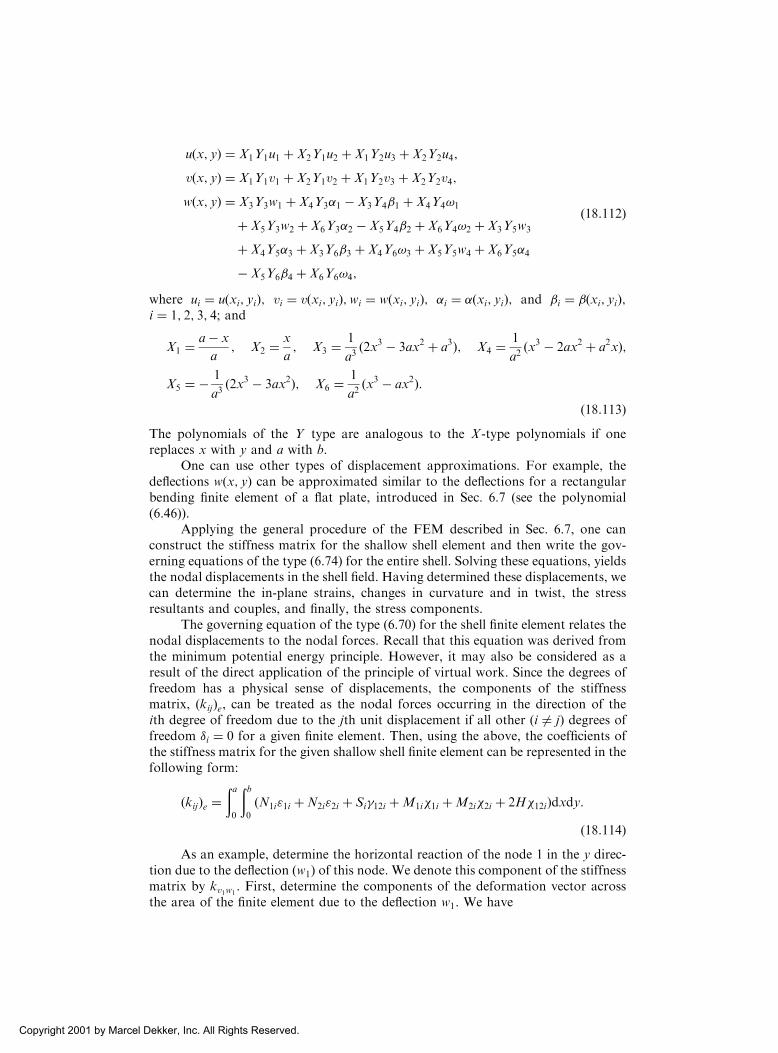
uðx; yÞ ¼ X1Y1u1 þ X2Y1u2 þ X1Y2u3 þ X2Y2u4;

vðx; yÞ ¼ X1Y1v1 þ X2Y1v2 þ X1Y2v3 þ X2Y2v4;

wðx; yÞ ¼ X3Y3w1 þ X4Y31 � X3Y41 þ X4Y4!1

þ X5Y3w2 þ X6Y32 � X5Y42 þ X6Y4!2 þ X3Y5w3

þ X4Y53 þ X3Y63 þ X4Y6!3 þ X5Y5w4 þ X6Y54

� X5Y64 þ X6Y6!4;

ð18:112Þ

where ui ¼ uðxi; yiÞ; vi ¼ vðxi; yiÞ;wi ¼ wðxi; yiÞ; i ¼ ðxi; yiÞ; and i ¼ ðxi; yiÞ;i ¼ 1; 2; 3; 4; and

X1 ¼a� x

a; X2 ¼

x

a; X3 ¼

1

a3ð2x3 � 3ax2 þ a3Þ; X4 ¼

1

a2ðx3 � 2ax2 þ a2xÞ;

X5 ¼ � 1

a3ð2x3 � 3ax2Þ; X6 ¼

1

a2ðx3 � ax2Þ:

ð18:113ÞThe polynomials of the Y type are analogous to the X-type polynomials if onereplaces x with y and a with b.

One can use other types of displacement approximations. For example, thedeflections wðx; yÞ can be approximated similar to the deflections for a rectangularbending finite element of a flat plate, introduced in Sec. 6.7 (see the polynomial(6.46)).

Applying the general procedure of the FEM described in Sec. 6.7, one canconstruct the stiffness matrix for the shallow shell element and then write the gov-erning equations of the type (6.74) for the entire shell. Solving these equations, yieldsthe nodal displacements in the shell field. Having determined these displacements, wecan determine the in-plane strains, changes in curvature and in twist, the stressresultants and couples, and finally, the stress components.

The governing equation of the type (6.70) for the shell finite element relates thenodal displacements to the nodal forces. Recall that this equation was derived fromthe minimum potential energy principle. However, it may also be considered as aresult of the direct application of the principle of virtual work. Since the degrees offreedom has a physical sense of displacements, the components of the stiffnessmatrix, ðkijÞe, can be treated as the nodal forces occurring in the direction of theith degree of freedom due to the jth unit displacement if all other (i 6¼ j) degrees offreedom �i ¼ 0 for a given finite element. Then, using the above, the coefficients ofthe stiffness matrix for the given shallow shell finite element can be represented in thefollowing form:

ðkijÞe ¼ða0

ðb0

N1i"1i þN2i"2i þ Si�12i þM1i�1i þM2i�2i þ 2H�12ið Þdxdy:ð18:114Þ

As an example, determine the horizontal reaction of the node 1 in the y direc-tion due to the deflection (w1) of this node. We denote this component of the stiffnessmatrix by kv1w1

. First, determine the components of the deformation vector acrossthe area of the finite element due to the deflection w1. We have


"ð1Þ1w1¼ � 1

R1

X3Y3w1; "ð1Þ2w1¼ 1

R2

X3Y3w1; �ð1Þ12w1¼ 0;

�ð1Þ1w1¼ �X3;XXY3w1; �ð1Þ2w1

¼ �X3Y3;YYw1; �ð1Þ12w1¼ �X3;XY3;Yw1;

ð18:115Þwhere the superscript 1 denotes the number of the nodal point of interest. Then, wecan find the components of the stress resultant vector due to v1. We have

Nð1Þ1v1

¼ Eh�

1� �2 X1Y1;Yv1; Nð1Þ2v1

¼ Eh

1� �2 X1Y1;Yv1; Sð1Þv1

¼ Eh

2ð1þ �ÞX1;XY1v1:

ð18:116ÞIn Eqs (18.115) and (18.116), the comma notation denotes a partial differentiation ofthe polynomials Xi and Yi, i.e.,

X3;XX ¼ @2X3

@x2¼ 12x� 6a

a3; Y3;YY ¼ @2Y3

dy2¼ 12y� 6b

b3;

X3;X ¼ @X3

@x¼ 6x2 � 6ax

a3; Y3;Y ¼ @Y3

@y¼ 6y2 � 6yb

b3;

X1;X ¼ @X1

@x¼ � 1

a; Y1;Y ¼ @Y1

@y¼ � 1

b:

Substituting the components of vectors �f gv1 and "f gw1into Eqs (18.115), (18.116),

and (18.114) yields the following:

kv1w1¼ða0

ðb0

Nð1Þ1v1"ð1Þ1w1

þNð1Þ2v1"ð1Þ2w1

þ Sð1Þv1�ð1Þ12w1

� �dxdy;

¼ða0

ðb0

Eh�

1� �2 X1Y1;Y � 1

R1

� �X3Y3 þ

Eh

1� �2 X1Y1;Y � 1

R2

� �X3Y3

� �dxdy;

¼ 7

40

Eh

1� �2 a�

R1

þ 1

R2

� �� :

ð18:117ÞSimilarly, the rest of the components of the stiffness matrix ðkijÞe can be obtained. Inthis example, it was assumed that �1 ¼ const and �2 ¼ const:

2. A flat finite element for the analysis of shallow shells

We considered above a curved shallow shell finite element whose surface is consistentto the surface of the entire shallow shell. However, the stiffness matrix constructedabove has a serious drawback associated with the presence of rigid body motions.This means that if such a finite element is subjected to some displacement modeling itstransfer in a space without straining (for example, w1 ¼ w2 ¼ w3 ¼ w4 ¼ t while allthe rest of the degrees of freedom are equal to zero), then some stresses occur in thatelement, resulting in an obvious contradiction. An appearance of such a phenomenonessentially decreases the accuracy of the analysis and sometimes can result in diver-gence of a solution. An elimination of this phenomenon can be carried out at theexpense of a special treatment of the obtained stiffness matrix. However, this treat-ment may result in violation of the matrix symmetry, compatibility of its components,


and completeness of approximating functions. Therefore, the problem of the devel-opment of finite elements for shallow shells of double curvature is very complicated.

From a physical point of view, it is advantageous to employ flat finite elementsfor the analysis of shallow shells of double curvature. In this case, a shell element canbe obtained as a simple combination of the corresponding elements for plane stressand for plate bending by satisfying all the necessary requirements. Geometric fea-tures of the shell are taken into account by the geometry of an inscribed polyhedron.Since the approximation accuracy of the shell surface is increased with a finer ele-ment mesh, it is possible to state that the FEM convergence will be achieved in thiscase.

When assigning an assemblage of flat finite elements for a shallow shell, onemust inscribe the elements into the shell geometry. Therefore, one can use rectan-gular elements for developable surfaces on a plane (e.g., cylindrical surfaces) andtriangular elements for undevelopable surfaces (e.g., spherical shells). The stiffnessmatrix of a rectangular (or triangular) flat shell finite element can be obtained as asimple superposition of the stiffness matrices of that element for plane stress and forplate bending. The stiffness matrix for a flat plate bending finite element was intro-duced in Sec. 6.7.

Consider the derivation of the stiffness matrix for the rectangular plane stressfinite element 1–2–3–4 shown in Fig. 18.8 (the projection of a shallow shell curvedelement on the Oxy coordinate plane). Assume that the in-plane displacement pat-tern is defined by the following polynomials:

uðx; yÞ ¼ 1 þ 2xþ 3yþ 4xy;vðx; yÞ ¼ 5 þ 6xþ 7yþ 8xy:

ð18:118Þ

Thus, the generalized displacements of a node of the flat rectangular finite element ina matrix form are the following

uv

�¼ 1 x y xy 0 0 0 0

0 0 0 0 1 x y xy

� � 12. . .8

8>><>>:

9>>=>>; ¼ N½ � f g: ð18:119Þ

Let us introduce the nodal displacement vector of the above-mentioned element, asfollows:

�f gTe ¼ u1; v1; u2; v2; . . . ; u4; v4½ �: ð18:120ÞIt is seen that the displacement functions (18.118) contain the same number ofunknown parameters k ðk ¼ 1; 2; . . . ; 8Þ as the number of the nodal displacementsui and viði ¼ 1; . . . ; 4Þ and yield the linear displacements along the element sides. Ifwe express the above coefficients k via nodal displacements, i.e., via the componentsof the element displacement vector �f ge, we obtain

�f ge¼ C½ � f g; ð18:121Þwhere C½ � is an 88 matrix whose terms depend on the x and y coordinates of thenodal points of the given finite element. From Eq. (18.121), the vector f g can beexpressed as a function of the finite element nodal displacement vector, as follows:

f g ¼ C½ ��1 �f ge: ð18:122Þ


Since the displacement functions are now expressed in terms of the nodal displace-ments in the explicit form, we can follow the same procedure as described in Sec. 6.7for evaluating the components of the stiffness matrix of the plane stress finite ele-ment.

Here, only the general information about the FEM analysis and its applicationto shell structures has been presented. It should be noted that many books haveappeared during the last four decades and they contain extensive discussions of FEMapproaches and the related numerical procedures, for example [Refs 12–17].

18.7 APPROXIMATE AND NUMERICAL METHODS FOR SOLUTIONOF NONLINEAR EQUATIONS

Analysis of flexible plates and shells is reduced to a solution of nonlinear differentialequations for the stress function and deflection, Eqs (7.87) and (18.31), respectively.The solution of these equations via the classical analytical route can be obtained inexceptional cases only. Therefore, approximate and numerical methods acquire agreat importance for the nonlinear plate and shell analysis. These methods, based onsome iterative procedures, are usually combined with other well-known variationaland numerical methods, introduced in Chapter 6 and Sec. 18.6, to obtain the solu-tion of Eqs (7.87) and (18.31) with a reasonable accuracy.

We introduce below some approximate methods specially adapted to the ana-lysis of flexible plates and shells under external loads.

18.7.1 The method of successive approximations

Let us use the flexible plate problem to illustrate the method of successive approx-imations. We rewrite Eqs (7.87), as follows

1

Ehr2r2� ¼ � 1

2Lðw;wÞ;

Dr2r2w ¼ Lð�;wÞ þ p;

ð18:123Þ

where the operator Lð. . .Þ is given by Eq. (18.30).In the first approximation, the above system of equations is taken in the form

r2r2�1 ¼ 0;

Dr2r2w1 ¼ p:ð18:124aÞ

In the second approximation, the functions �1 and w1 are substituted into the right-hand sides of Eqs (18.122). We obtain

1

Ehr2r2�2 ¼ � 1

2Lðw1;w1Þ;

Dr2r2w21 ¼ Lð�1;w1Þ þ p;

ð18:124bÞ

and equations of the ðnþ 1Þth approximation will have the form

1

Ehr2r2�nþ1 ¼ � 1

2L wn;wnð Þ;

Dr2r2wnþ1 ¼ L wn;�nð Þ þ p;

ð18:124cÞ


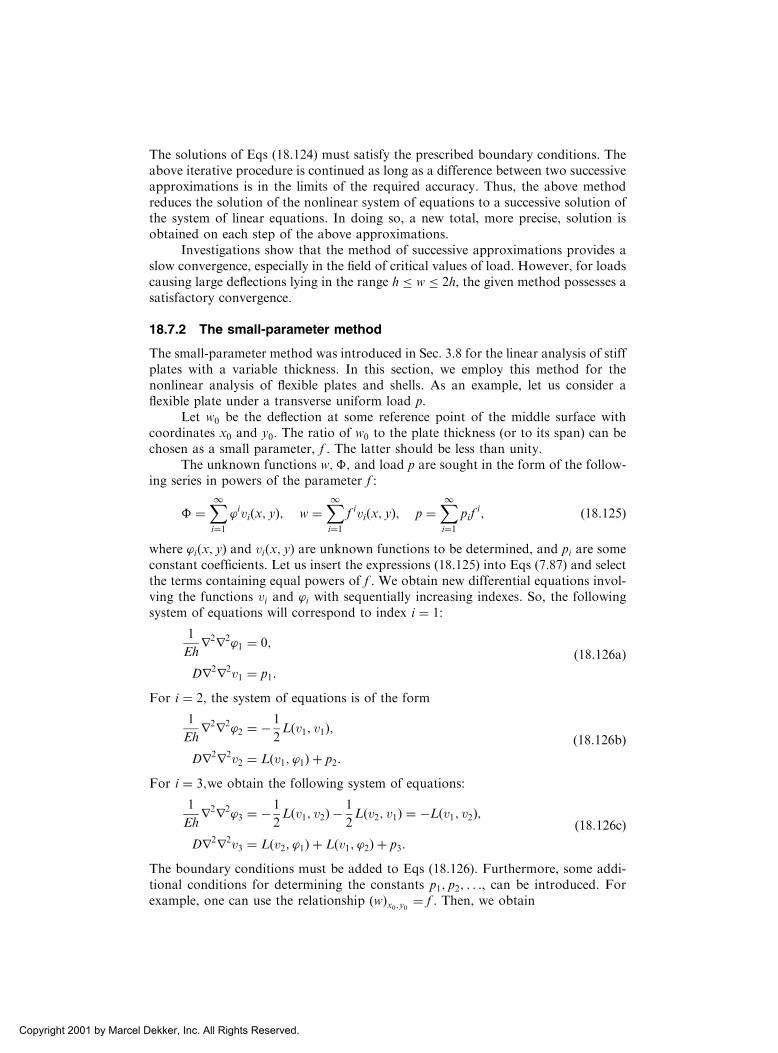
The solutions of Eqs (18.124) must satisfy the prescribed boundary conditions. Theabove iterative procedure is continued as long as a difference between two successiveapproximations is in the limits of the required accuracy. Thus, the above methodreduces the solution of the nonlinear system of equations to a successive solution ofthe system of linear equations. In doing so, a new total, more precise, solution isobtained on each step of the above approximations.

Investigations show that the method of successive approximations provides aslow convergence, especially in the field of critical values of load. However, for loadscausing large deflections lying in the range h � w � 2h, the given method possesses asatisfactory convergence.

18.7.2 The small-parameter method

The small-parameter method was introduced in Sec. 3.8 for the linear analysis of stiffplates with a variable thickness. In this section, we employ this method for thenonlinear analysis of flexible plates and shells. As an example, let us consider aflexible plate under a transverse uniform load p.

Let w0 be the deflection at some reference point of the middle surface withcoordinates x0 and y0. The ratio of w0 to the plate thickness (or to its span) can bechosen as a small parameter, f . The latter should be less than unity.

The unknown functions w;�; and load p are sought in the form of the follow-ing series in powers of the parameter f :

� ¼X1i¼1

’iviðx; yÞ; w ¼X1i¼1

f iviðx; yÞ; p ¼X1i¼1

pifi; ð18:125Þ

where ’iðx; yÞ and viðx; yÞ are unknown functions to be determined, and pi are someconstant coefficients. Let us insert the expressions (18.125) into Eqs (7.87) and selectthe terms containing equal powers of f . We obtain new differential equations invol-ving the functions vi and ’i with sequentially increasing indexes. So, the followingsystem of equations will correspond to index i ¼ 1:

1

Ehr2r2’1 ¼ 0;

Dr2r2v1 ¼ p1:

ð18:126aÞ

For i ¼ 2, the system of equations is of the form

1

Ehr2r2’2 ¼ � 1

2Lðv1; v1Þ;

Dr2r2v2 ¼ Lðv1; ’1Þ þ p2:

ð18:126bÞ

For i ¼ 3;we obtain the following system of equations:

1

Ehr2r2’3 ¼ � 1

2Lðv1; v2Þ �

1

2Lðv2; v1Þ ¼ �Lðv1; v2Þ;

Dr2r2v3 ¼ Lðv2; ’1Þ þ Lðv1; ’2Þ þ p3:

ð18:126cÞ

The boundary conditions must be added to Eqs (18.126). Furthermore, some addi-tional conditions for determining the constants p1; p2; . . ., can be introduced. Forexample, one can use the relationship wð Þx0;y0 ¼ f . Then, we obtain


ðv1Þx0;y0 ¼ 1; ð18:127aÞðv2Þx0;y0 ¼ ðv3Þx0;y0: ¼ . . . ¼ 0: ð18:127bÞ

Equations (18.126a) are linear equations describing the bending problem of stiffplates. If there are no in-plane forces in the middle surface, then the stress function’1 can be taken identically equal to zero, i.e., ’1 � 0. From the second Eq. (18.126a)and the relations (18.127a), taking into account the boundary conditions, the con-stant p1 and function v1ðx; yÞ are determined. Further, the function v1ðx; yÞ is sub-stituted into the right-hand side of Eqs (18.126b); in this case, Lðv1; ’1Þ ¼ 0, so thatthe second Eq. (18.126b) will repeat the second Eq. (18.126a). The first Eq. (18.126b)will provide a way of determining ’2ðx; yÞ: At the third step, let us substitute v1, v2,and ’2 into the right-hand sides of Eqs (18.126c). As a result, the constant p3 andfunction v3ðx; yÞ will be found. Once, the constants p1; p2; p3; . . . have been found,the value of f is approximately determined from the last relation (18.125) for thegiven load p.

This method, like the method of successive approximations, allows one toreduce the given nonlinear problem to a subsequent solution of the system of linearequations. In so doing, one obtains on each step of approximations, a more precise –but not a new, more correct, as in the method of successive approximations –solution.

Apparently, the small-parameter method will converge rapidly for reasonablysmall deviations from linear solutions. However, confidence limits of the applicationof the method so far have not been defined.

18.7.3 The method of successive loadings [18]

According to this method, a given load p is applied to a shell (or plate) by smallportions. It is assumed that each such a portion of loading causes insignificantchanges in the state of stress and strain (in order to neglect the nonlinear terms inthe corresponding governing equations), so that a flexible plate or shell, subjected tothe above-mentioned portion loading, can be analyzed with the use of linear differ-ential equations.

Following the outline of Ref. [19], let us illustrate the use of this method for thesolution of the nonlinear equations of a flexible shallow shell. After application ofthe first portion of loading p0, the shell deflections are assumed to be small, so theycan be determined from the linear equations (17.36). The latter have the followingform (in the zero approximation):

1

Ehr2r2�0 þ r2

�0w0 ¼ 0;

Dr2r2w0 � r2�0�0 ¼ p0;

ð18:128Þ

where

r2�0w0 ¼ �1

@2w0

@y2þ �2

@2w0

@x2;

r2�0�0 ¼ �1

@2�0

@y2þ �2

@2�0

@x2:

ð18:129Þ


Then, the next small portion of loading, �p1, is applied to the shell. The deflectionand stress function will take the increments �w1 and ��1, respectively; therefore,they can be represented in the form

w1 ¼ w0 þ�w1; �1 ¼ �0 þ��1: ð18:130ÞSubstituting the expressions (18.130) into Eqs (17.36), one obtains

1

Ehr2r2 �0 þ��1ð Þ þ r2

�0 w0 þ�w1ð Þ ¼ �L1 w0 þ�w1ð Þ; w0 þ�w1ð Þ½ �;

Dr2r2 w0 þ�w1ð Þ � r2�0 �0 þ��1ð Þ ¼ L2 �0 þ��1ð Þ; w0 þ�w1ð Þ½ �

þ p0 þ�p1:

ð18:131Þwhere the operators L1ð. . .Þ and L2ð. . .Þ are given by Eq. (18.30).

Subtracting Eqs (18.131) and (18.128) member by member, we obtain

1

Ehr2r2��1 þ r2

�1�w1 ¼ �L1 �w1;�w1ð Þ;

Dr2r2�w1 � r2�1 ��1ð Þ � r2

1 �w1ð Þ ¼ L2 ��1;�w1ð Þ þ�p1;

ð18:132Þ

where

r2�1 �w1ð Þ ¼ �1 þ

@2w0

@x2

!@2 �w1ð Þ@y2

� 2@2w0

@x@y

@2 �w1ð Þ@x@y

þ �2 þ@2w0

@y2

!@2 �w1ð Þ@x2

;

r2�1 ��1ð Þ ¼ �1 þ

@2w0

@x2

!@2 ��1ð Þ@y2

� 2@2w0

@x@y

@2 ��1ð Þ@x@y

þ �2 þ@2w0

@y2

!@2ð��1Þ@x2

;

r21 �w1ð Þ ¼ @2�0

@y2@2 �w1ð Þ@x2

� 2@2�0

@x@y

@2 �w1ð Þ@x@y

þ @2�0

@x2@2 �w1ð Þ@y2

:

ð18:133ÞSince the load portions are assumed to be small, it can be expected that the incre-ments of the deflection and stress function will also be sufficiently small. Then, all thenonlinear terms, L1 �w1;�w1ð Þ and L2 ��1;�w1ð Þ can be omitted on the right-handsides of Eqs (18.132). As a result, �w1 and ��1 can be found from the followingsystem of linear differential equations:

1

Ehr2r2 ��1ð Þ þ r2

�1 �w1ð Þ ¼ 0;

Dr2r2 �w1ð Þ � r2�1 ��1ð Þ � r2

1 �w1ð Þ ¼ �p1:

ð18:134Þ

Repeating this procedure for the consequent small load portions, �pi, oneobtains the equations for the increments �w2;��2;�w3;��3; . . .. For an arbi-trary load portion �pi, one can write the following system of linear differentialequations:


1

Ehr2r2 ��ið Þ þ r2

�i �wið Þ ¼ 0;

Dr2r2 �wið Þ � r2�i ��ið Þ � r2

i ð�wiÞ ¼ �pi;

ð18:135Þ

where

r2�i �wnð Þ ¼ �1 þ

@2wi�1

@x2

!@2 �wið Þ@y2

� 2@2wi�1

@x@y

@2 �wið Þ@x@y

þ �2 þ@2wi�1

@y2

!@2 �wið Þ@x2

;

r2�i ��ið Þ ¼ �1 þ

@2 �wi�1ð Þ@x2

!@2 ��ið Þ@y2

� 2@2wi�1

@x@y

@2 ��ið Þ@x@y

þ �2 þ@2wi�1

@y2

!@2 ��ið Þ@x2

;

r2i �wið Þ ¼ @2�i�1

@y2@2 �wið Þ@x2

� 2@2�i�1

@x@y

@2 �wið Þ@x@y

þ @2�i�1

@x2@2 �wið Þ@y2

:

ð18:136Þ

The total values of the deflection and stress function are determined, after the ithiterative step, as follows:

wn ¼ w0 þXni¼1

�wi; �n ¼ �0 þX1i¼1

��i: ð18:137Þ

Note that the above iterative process assumes that some transformations that hadbeen done with the differential equations (18.128), (18.132), and (18.135) should beperformed with the corresponding boundary conditions, if that is necessary.

It should be noted that in the multiple repetition of the successive approxima-tions, the error of determining the functions w and �, caused by omitting the non-linear terms, can be accumulated. To increase the accuracy of determining thedeflections and stress function, the method of successive loading can be combinedwith the Newton method, which is introduced next. The latter can correct a givensolution obtained at each step of loading.

18.7.4 The Newton method

Using the variational methods, finite element or finite difference methods, etc., thenonlinear differential equations (7.87) and (18.31) are reduced to a system of non-linear algebraic equations. An exact solution of these equations is practically impos-sible. We introduce below one more approximate method, the Newton method,which is highly efficient for the solution of nonlinear algebraic equations.

Consider the following system of nonlinear equations


F1ðx1; x2; . . . ; xnÞ ¼ 0;

F2ðx1; x2; . . . ; xnÞ ¼ 0;

. . . . . . . . . . . . . . . . . . . . .

Fnðx1; x2; . . . ; xnÞ ¼ 0:

ð18:138Þ

Assume that the functions FiðxÞði ¼ 1; 2; . . . ; nÞ have continuous derivatives withrespect to all variables x1; x2; . . . ; xk. Let us represent the system of equations(18.138) in the following matrix form:

FðxÞ ¼ 0; ð18:139Þwhere

F ¼ F1;F2; . . . ;Fn½ �T ; x ¼ x1; x2; . . . ; xn½ �T ð18:140Þare the n-dimensional vectors of functions Fi and independent variables xi.

Assume that the kth approximation of the solution of Eqs (18.139) has beenfound in the form

xðkÞ ¼ x

ðkÞ1 ; x

ðkÞ2 ; . . . ; x

ðkÞn

h i:

Then, the exact solution of Eqs (18.139) can be represented in the following form:

x ¼ xðxÞ þ e

ðkÞ; ð18:141Þwhere e

ðkÞ ¼ ½eðkÞ1 ; eðkÞ2 ; . . . ; e

ðkÞn � are some corrections (the solution errors). Let us

introduce the Jacobi matrix of the functions F1;F2; . . . ;Fn with respect to theindependent variables x1; x2; . . . ; xn, as follows:

WðxÞ ¼

@F1@x1

@F1@x2

. . .@F1@xn

@F2@x1

@F2@x2

. . .@F2@xn

. . . . . . . . . . . .@Fn@x1

@Fn@x2

. . .@Fn@xn

26666664

37777775: ð18:142Þ

If this matrix is nonsingular, i.e., if detWðxÞ 6¼ 0, then the correction eðkÞ can be

expressed as follows:

eðkÞ ¼ �W

�1ðxðkÞÞ � FðxðkÞÞ; ð18:143Þwhere W�1ðxðkÞÞ is the inverse Jacobi matrix. Thus, the successive approximations ofthe solution of Eqs (18.139) are obtained according to the following numericalprocedure:

xðkþ1Þ ¼ x

ðkÞ �W�1ðxðkÞÞ � FðxðkÞÞ ðk ¼ 0; 1; 2; . . .Þ: ð18:144Þ

As zero approximation of the solution, xð0Þ, any rough approximation (for example,a graphical approximation) may be taken. The numerical procedure, described byEq. (18.144), will stop when the following inequality is satisfied:

xðkþ1Þ � x

ðkÞ � ";


where " is the required level of a permissible level of calculations.

Example 18.4

Find an approximate positive solution of the system of equations by the Newtonmethod.

x2 þ y2 þ z2 � 1 ¼ 0; 2x2 þ y2 � 4z ¼ 0; 3x2 � 4yþ z2 ¼ 0: ðaÞ

Solution

We have

FðxÞ ¼x2 þ y2 þ z2 � 1

2x2 þ y2 � 4z

3x2 � 4yþ z2

8><>:

9>=>;: ðbÞ

Take the zero approximation of the solution as x0 ¼ y0 ¼ z0 ¼ 0:5. Then,

Fðxð0ÞÞ ¼0:25þ 0:25þ 0:25� 1

0:50þ 0:25� 2:0

0:75� 2:0þ 0:25

8><>:

9>=>; ¼

�0:25

�1:25

�1:0

8><>:

9>=>;: ðcÞ

Let us make up the Jacobi matrix:

WðxÞ ¼2x 2y 2z

4x 2y �4

6x �4 2z

264

375: ðdÞ

Substituting for x the zero approximation solution into the above, gives

Wðxð0ÞÞ ¼1 1 1

2 1 �4

3 �4 1

264

375:

Calculate the determinant of the zero approximation Jacobi matrix. We obtain

det Wðxð0ÞÞ ¼1 1 1

2 1 �4

3 �4 1

¼ �40:

Compute the inverse Jacobi matrix in the zero approximation. We obtain

W�1ðxð0ÞÞ ¼ � 1

40

�15 �5 �5

�14 �2 6

�11 7 �1

264

375 ¼

0:375 0:125 0:125

0:35 0:05 �0:15

0:275 �0:175 0:025

264

375:

Applying Eq. (18.144), we obtain the first approximation of the solution of Eqs (a),as follows:


xð1Þ ¼ x

ð0Þ �W�1ðxð0ÞÞ � Fðxð0ÞÞ

¼0:5

0:5

0:5

8>><>>:

9>>=>>;�

0:375 0:125 0:125

0:35 0:05 �0:15

0:275 �0:175 0:025

2664

3775

�0:25

�1:25

�1:00

8>><>>:

9>>=>>; ¼

0:875

0:500

0:375

8>><>>:

9>>=>>;:

Then, the second approximation, xð2Þ can be calculated. We have

Fðxð1ÞÞ ¼

ð0:875Þ2 þ ð0:500Þ2 þ ð0:375Þ2 � 1

2 � ð0:875Þ2 þ ð0:500Þ2 � 4 � 0:3753 � ð0:875Þ2 � 4 � 0:500þ 0:375

3 � ð0:875Þ2 � 4 � 0:500þ ð0:375Þ2

8>>><>>>:

9>>>=>>>;

¼0:15625

0:28125

0:43750

8><>:

9>=>;:

Find the first approximation Jacobi matrix. We have

Wðxð1ÞÞ ¼2 � 0:875 2 � 0:500 2 � 0:3754 � 0:875 2 � 0:500 �4

6 � 0:875 � 4 2 � 0:375

2664

3775 ¼

1:750 1 0:750

3:500 1 �4

5:250 �4 0:750

2664

3775:

Computing the determinant of the above matrix gives

det Wðxð1ÞÞ ¼1:750 1 0:750

3:500 1 �4

5:250 �4 0:750

¼ �64:750;

and the corresponding inverse matrix is given by

W�1ðxð1ÞÞ ¼ � 1

64:75

�15:25 �3:75 �4:75

�23:625 �2:625 9:625

�19:25 12:25 �1:75

264

375:

The second approximation of the solution is obtained from Eq. (18.144), as follows:

xð2Þ ¼ x

ð1Þ �W�1ðxð1ÞÞ � Fðxð1ÞÞz

¼0:875

0:500

0:375

8>><>>:

9>>=>>;þ 1

64:75

�15:25 �3:75 �4:75

�23:625 �2:625 9:625

�19:25 12:25 �1:75

2664

3775

0:15625

0:28125

0:43750

8>><>>:

9>>=>>;

¼0:78981

0:49662

0:36993

8>><>>:

9>>=>>;:

Similarly, the consequent approximations can be found. In the third approximationwe have

xð3Þ ¼

0:785210:496620:36992

8<:

9=;; Fðxð3ÞÞ ¼

0:000010:000040:00005

8<:

9=;:


If we confine ourselves to the third approximation, then the solution of Eqs (a) is ofthe form

x ¼ 0:7852; y ¼ 0:4966; z ¼ 0:3699:

Example 18.5

Find a solution of the differential equation

dy

dx¼ x2 þ y2 for xj j � 1ffiffiffi

2p ; ðaÞ

with the boundary conditions

y ¼ 0x¼0: ðbÞ

Use the method of successive approximations.

Solution

Equation (a) with the boundary conditions (b) represent the Cauchy problem. It isevident that the solution of the above problem is also in the interval jyj � 1ffiffi

2p .

Applying the method of successive approximations, let us take y0 ¼ yð0Þ ¼ 0 asthe zero approximation. Then, the iterative procedure of the method (See Sec.18.7.1) can be represented, as follows

y1ðxÞ ¼ðx0

t2dt ¼ 1

3x3;

y2ðxÞ ¼ðx0

t2 þ 1

9t6

� �dt ¼ 1

3x3 þ 1

63x7;

y3ðxÞ ¼ðx0

t2 þ 1

9t6 þ 2

189t10 þ 1

3969t14

� �dt

¼ 1

3x3 þ 1

63x7 þ 2

2079x11 þ 1

59535x15:

For jxj � 1ffiffi2

p the difference between y2ðxÞ and y3ðxÞ does not exceed the value of

2

2079

1ffiffiffi2

p� �11

þ 1

59535

1ffiffiffi2

p� �15

� 0:000022;

and one can approximately put

yðxÞ � y2ðxÞ ¼1

3x3 þ 1

63x7:

This example was taken from Ref. [20].

PROBLEMS

18.1 A long thin-walled steel tube is heated to 250C above the room temperature 22C.Assume that the ends of the tube are simply supported. Let the mean radius of the tube

R ¼ 1:2m and its thickness h ¼ 10mm. Determine the maximum thermal stresses in

the tube if Es ¼ 200GPa, �s ¼ 0:3, and s ¼ 25:2 10�6=C.


18.2 A long thin-walled aluminum tube has free ends and is subjected to uniform tempera-

tures T1 ¼ 150C and T2 ¼ 350C at the inner and outer surfaces, respectively. Let the

mean radius of the tube be 0.8 m and its thickness h ¼ 10mm. Calculate the maximum

thermal stresses in the tube if Ea ¼ 70GPa; a ¼ 23 10�6=C; and �a ¼ 0:3.18.3 Compute the discontinuity stresses at the junction of the cylindrical shell and hemi-

spherical head, as shown in Fig. 16.6, for the uniform temperature change

�T ¼ 120C. Use the geometric and mechanical parameters of the compound shell

structure given in Example 16.2 and s ¼ 25 10�6=C. Apply the approximate

method of Sec. 16.4 for the problem solution.

18.4 Compute the stresses in the hemispherical shell stiffened on its edge by a flange, as

shown in Fig. 16.5. Assume that the shell and flange are made of steel with

Es ¼ 210GPa, �s ¼ 0:3; and s ¼ 25 10�6=C. Take the geometric parameters of

the shell and flange from Example 16.1. Apply the approximate method of Sec. 16.4

for the problem solution.

18.5 Derive Eqs (18.17).

18.6 Verify Eqs (18.24) and (18.29).

18.7 Derive Eq. (18.54).

18.8 A closed, circular cylindrical shell of length L and radius R is stiffened by equally

spaced collars, at a distance L=10, located inside the shell. The shell is simply supported

at x ¼ 0 and x ¼ L and is subjected to a uniform internal pressure p. Calculate the

normal stresses in the stiffened shell in terms of p if the shell and collars are made of

steel with Es ¼ 210GPa and �s ¼ 0:3. Assume also that the collars have a form of the

equal angle section 25 25 5 mm and R ¼ 0:8m; L ¼ 4m; and h¼ 1mm. In your

calculations, consider the stiffened shell as a structurally orthotropic homogeneous

shell.

18.9 Verify Eqs (18.63) and (18.66).

18.10 Derive Eqs (18.82).

18.11 Consider two extreme cases for a sandwich shallow shell given by Eqs (18.82): (a) let

R1 ! 1 and R2 ! 1 and (b) let Gc ! 1. Transform the above governing equation

for these two cases and explain their physical sense.

18.12 Based on the representations (18.106) and (18.107), write the matrices Bi½ � and Bj

� �in

the explicit form.

18.13 Write a computer code for calculating the components of the stiffness matrix for the

finite element in the form of a frustum (Fig. 18.7) for an axisymmetrically loaded shell

of revolution. Use the relations introduced in Sec. 18.6.2. Assume reasonable values for

any shell properties required.

18.14 Using the Newton method, find a solution of the equation

4x3 � 2x2 � 4x� 3 ¼ 0:

18.15 Find a solution of the differential equation for the bending moments in a simply

supported beam with a variable cross section:

d2y

dx2þ ð1þ x2Þy ¼ 0;

y ¼ 0x¼�1

and y ¼ 0x¼1

Use the method of successive approximations.

REFERENCES

1. Carslaw, H.S. and Jaeger, J.C., Conduction of Heat in Solids, 2nd edn, Oxford University

Press, London, 1959.


2. Von Karman, Th., Encyklopadie der Mathematischen, Wissenschaften, vol. IV, 1910.

3. Reissner, E., On the theory of thin elastic plates. In: H. Reissner Anniversary Volume, pp.

231–247 (1949). Ann Arbor, J. W. Edwards.

4. Sanders, L, Jr., Nonlinear Theories for Thin Shells, Contract NONR 1866(02), Office of

Naval Research, Tech. Report No. 10, Harvard Press, Cambridge, Massachusetts, 1961.

5. Mushtari, Kh.M. and Galimov, K.Z., Nonlinear Theory of Thin Elastic Shells, Russian

translational series, NASA TT-F-62, Washington, DC, US Department of Commerce,

1957.

6. Vlasov, V.Z., General Theory of Shells and Its Application in Engineering, NASA TTF-99,

Washington, DC, 1964.

7. Alexandrov, A.V. and Potapov, V.D., The Fundamentals of the Theory of Elasticity and

Plasticity, Izd-vo ‘‘Vyshaya Shkola,’’ Moscow, 1990 (in Russian).

8. Cook, R.D. and Young, W.C., Advanced Mechanics of Materials, 2nd edn, Prentice Hall,


9. Stein, M. and Mayers, J.A., A Small Deflection Theory for Curved Sandwich Plates,

NACA, Washington, DC, 1950.

10. Plantema, F., Sandwich Construction, John Wiley and Sons, New York, 1966.

11. Baker, E.H., Cappelly, A.P., Lovalevsky, L., Risb, F.L., and Verette, R.M., Shell

Analysis Manual, NASA CR-912, Washington, DC, April 1968.

12. Gallagher, R.H., Problems and progress in thin shell finite element analysis, In: Finite

Element for Thin Shells and Curved Members (eds D.G. Ashwell and R.H. Gallagher),

John Wiley and Sons, London, 1976.

13. Hughes, T.J.R., The Finite Element Method, Prentice-Hall, Englewood Cliffs, New

Jersey, 1987.

14. Hughes, T.J.R. and Hinton, E., Finite element method for plate and shell structures, Vol

1: Finite Element Technology, Pineridge Press International, Swansea, UK, 1986.

15. Zienkiewitcz, D.C., The Finite Element Method in Engineering Science, McGraw-Hill,

New York, 1969.

16. Gallagher, R.H., Finite Element Analysis:Fundamentals, Prentice-Hall, Englewood Cliffs,

New Jersey, 1976.

17. Segerlind, L.J., Applied Finite Element Analysis, John Wiley, London, 1975.

18. Petrov, V.V., The Method of Successive Loadings in the Nonlinear Theory of Plates and

Shells, Izd-vo Saratov University, Saratov, 1975 (in Russian).

19. Alexandrov, A.V. and Potapov, V.D., The Fundamentals of the Theory of Elasticity and

Plasticity, Izd-vo ‘‘Vyshaya Shkola,’’ Moscow, 1990 (in Russian).

20. Krylov, A.N., Lectures on Approximate Calculations, Izd-vo Academy of Sciences of

USSR, Moscow, 1949 (in Russian).


19

Buckling of Shells

19.1 INTRODUCTION

An efficiency of the membrane stress state, based on the strength conditions only,enables one to employ a very small shell thickness, as discussed in the precedingchapters of Part II. However, a possibility of the shell buckling impedes that, causingus either to increase the shell thickness or to reinforce the shell by stiffeners. It shouldbe noted that the shell buckling is always disastrous, unlike, for example, a columnor plate buckling. Therefore, the problem of the stability in designing shell structuresis extremely vital. This problem is made worse because of some specific difficultiesassociated with determining correctly the critical values of loads applied to thinshells. Note that these difficulties are much greater than in the buckling analysisof columns, frames, and flat plates. They are associated with a complicated mathe-matical description of the deformed state of shells, and with a diversity of situationsat which a shell can buckle.

General postulations, definitions, and fundamentals of the structural stabilitytheory, introduced in Chapter 8 for the plate buckling problems, can be applied alsoto the shell buckling analysis. In this chapter, we present a systematic but simplifiedanalysis of shell buckling, and obtain some useful relationships between the criticalvalues of applied loads and shell parameters. We limit ourselves to the considerationof thin shells for which elastic buckling without plastic deformation is possible.

19.2 BASIC CONCEPTS OF THIN SHELLS STABILITY

Let us compare qualitatively the buckling behavior of columns, flat plates, andshells. For the sake of simplicity, we treat a column, plate, and shell as one degreeof freedom systems and consider typical diagrams of the relationship between theapplied load p and some deflection parameter f in the buckling problems. We assume


that the deflections are small compared with the overall dimensions of the structuralmember, but of the same order of magnitude as the depth of the column crosssection, or the wall thickness of the plate or shell.

The representative ‘‘load–deflection’’ diagram for columns and plates of per-fect geometric form and loaded by in-plane compressive forces p is shown in Fig.19.1a. Each position plotted in this figure represents an equilibrium configuration ofthe member – stable, neutral, or unstable – depending upon whether the slope of thepath at that point is positive, zero, or negative, respectively. Points not lying on thisdiagram, of course, correspond to nonequilibrium configurations. The equilibriumpath consists of the three branches: (a) branch OA refers to an initial, unbuckledconfiguration of equilibrium that is assumed to be momentless; (b) two ‘‘rising’’branches CA and AD refer to buckled configurations of equilibrium. Note thatthe curve CAD is symmetrical about the p axis. For the equilibrium path, shownin Fig. 19.1a, at the transition point A, a bifurcation of equilibrium is said to occur,since there are at least two possible states of equilibrium, f ¼ 0 and f ! 1. Such a

Fig. 19.1


transition point A, as mentioned in Sec. 8.2, is referred to as a bifurcation point, andthe load at that point is called the critical load, pcr. As shownin Fig. 19.1a, there arenew and stable, buckled configurations of equilibrium in the immediate vicinity ofthe bifurcation point. Therefore, with the slight and smooth increase in the appliedload above pcr, the initial configuration of equilibrium of the structural member(column or plate) ceases to be stable, and smoothly, without any jumps, it goesover to an adjacent buckled, stable configuration of equilibrium. It follows fromthe above that the critical values of an applied load can be determined with the use oflinear differential equations of the structural stability theory, introduced in Sec. 8.2.A geometrically nonlinear theory can be used only for describing the postbucklingbehavior of the member.

Lets turn our attention to the analysis of a shell buckling process. The repre-sentative paths of equilibrium for a simply supported shallow cylindrical shell undera uniform axial loading p (Fig. 19.1b) are shown in Fig. 19.1c. The solid curve OABDrefers to the shell whose initial configuration is assumed to be perfect, i.e., withoutany geometric and other imperfections. The load p is applied statically such that theinitial configuration of equilibrium of the shell is in the membrane state of stress, andthus, f ¼ 0. The equilibrium path OABD consists of the ‘‘rising’’ branches OA andBD, corresponding to stable equilibrium states, and the ‘‘descending’’ branch ABthat corresponds to an unstable equilibrium configuration.

Point A on the curve OABD can also be interpreted as a bifurcation point.However, unlike the equilibrium path, shown in Fig. 19.1a, for columns and flatplates, there are no new stable buckled configurations in the immediate vicinity ofthe bifurcation point A. The stable, buckled configurations of equilibrium are offfrom the initial ones at some finite distances (on the branch BD). Therefore, atransition from the initial configuration of equilibrium (branch OA) to a new,buckled and stable configuration of equilibrium (branch BD) occurs by a jump,i.e., the shell ‘‘jumps’’ from a stable state at A through the statically unstablestate, given by the branch AB, to the stable state at F on the branch BD, asshown in Fig. 19.1c. This sudden transition from the initial configuration of equili-brium to the next, stable and buckled configuration of equilibrium, with the corre-sponding jump in f , is termed as snap-through buckling. As a result, the shell bucklinganalysis, in a general case, must be based on the geometrically nonlinear shell theory.

The curve OABD has been analyzed above for the buckling model of someperfect shell. However, a real shell typically has some geometric and other imperfec-tions due to manufacturing. Such irregularities of the shell geometric form areequivalent to prebuckling deformations imposed on the original shell configuration.Note, that experiments performed on columns and flat plates under in-plane com-pressive forces showed that they are relatively insensitive to slight geometric imper-fections. This is not the case in a shell buckling process. Buckling experiments carriedout on shells showed that some shells are very sensitive to geometric and loadingimperfections. For instance, for the shallow cylindrical shell under consideration(Fig. 19.1b), such an elevated sensitivity to slight imperfections can be explainedby the closeness of the unstable branch AB to the initial shell configuration ofequilibrium given by straight line OA.

The path of shell instability for the given real shell with geometric and otherimperfections is given by the dashed curve shown in Fig. 19.1c. It is seen that,due to the above-mentioned irregularities, the real shell begins to deviate from its


initial configuration at the beginning of loading, and thus, the latter cannot beassumed to be in a membrane state of stress. The branch OA

0for increasing

loading will no longer coincide with the p axis. A transition from one stablestate to another will also occur by a jump at the level of the limit point A

0(the

snap-through buckling).It follows from the above that there are three distinct values of the critical loads

that characterize the buckling behavior of thin shells:

1. pð1Þcr is the ‘‘upper’’ critical load – it can be defined as the largest load up towhich the initial configuration of equilibrium of the perfect shell remainsstable with respect to infinitesimal disturbances;

2. pð2Þcr is the ‘‘lower’’ critical load – it can be defined as the largest load up towhich the initial configuration of equilibrium of the perfect shell remainsstable with respect to both infinitesimal and finite disturbances;

3. pbis the critical load of a real shell, also referred to as the buckling load – itcan be defined as some load for which the jump (or snap-through buck-ling) of a real shell occurs, i.e., such a critical value of the load for whichthe initial state of equilibrium of a real shell ceases to be stable.

It will be shown later that the values of pð1Þcr are determined with the use of lineardifferential equations. In determining pð2Þcr , it is necessary to solve extremely compli-cated problems of the geometrically nonlinear theory of shells. It is impossible toobtain an exact and analytical solution of the latter problems. Therefore, all avail-able results are obtained by numerical methods.

For real shells, the critical load, pb, is somewhere between the values of pð1Þcr andpð2Þcr , obtained for perfect shells. The more precisely a shell is manufactured, the closeris value of pb to pð1Þcr . The value of pb is extremely sensitive to geometric and loadingimperfections and to small deviations in boundary conditions. On the one hand, itresults in a large scatter of the experimental results of pb. On the other hand, someconceptual difficulties occur in the theoretical determination of pb because of theimpossibility of taking into account, with a high degree of accuracy, all the imper-fections and irregularities during the design stage. As a result, a severe discrepancywas noted between the theoretical and experimental results in determining the shellcritical loads.

In summary, it should be noted that the linear stability theory is not sufficientto predict completely the buckling and postbuckling behavior of thin shells. Thestability equations of shells can be derived successfully, based on the nonlinearequilibrium equations. The nonlinear theory can also be used to consider theinfluence of initial imperfections and other effects in the shell buckling analysis.It was believed that an accurate formulation of the buckling problem, in theframework of the nonlinear theory and exact solution of the corresponding equa-tions, would result in a close agreement between the theoretical and numericalresults in determining the critical loads. However, at present, in practice, thisprocedure has turned out to be prohibitively difficult and, so far, it has notlived up to the expectations placed on the geometrically nonlinear shell theory.The latter theory serves to broaden our knowledge of shell buckling analysis and toclarify the meaning and limitations of the linear stability theory. But, at present, itis not a design tool for directly determining the buckling load. Some details of thebuckling design procedure for thin shells will be given in Sec. 19.8. At the same


time, the buckling analysis of thin shells by means of the linear theory yields someuseful information about the buckling behavior of shells. Particularly, closed-formanalytical expressions, obtained by the linear stability theory, demonstrate theinterplay of various parameters that affect stability when combined with appro-priate correction and statistical coefficients. One could complement those relationsso that reliable design expressions would be obtained (see Sec. 19.8). In the nextsections, we perform linear and nonlinear stability analyses of shells of variousgeometries, and compare the corresponding results.

The basic problem in the buckling analysis of shells, as for thin plates, is indetermining the critical values of applied loads. Such a problem can be solved byusing the equilibrium, energy, and dynamic methods introduced in Sec. 8.2 for theplate buckling problems. We discuss below some details of application of the equili-brium and energy methods to the elastic shell buckling analysis.

19.2.1 Equilibrium method

The equilibrium method is adequately applicable to only conservative systems (seeSec. 2.6). A perfect shell loaded by potential external forces is a particular case of aconservative system.

As mentioned in Sec. 8.2, the equilibrium method is based on the observationthat at a critical load, a deformed state of a shell exists that is assumed to be aninfinitesimally, close to its initial, unbuckled configuration of equilibrium. Thus, theappearance of a possible bifurcation in the solution corresponds to the critical load.This criterion for determining critical loads can be used to obtain the governingdifferential equations of the shell buckling analysis. As we have seen, the structureof the governing differential equations of the general, even linear, theory of thinshells is sufficiently complicated. Therefore, a solution of practical shell problemsinvolves considerable difficulties. Fortunately, many shell stability problems, havinggreat practical importance, can be simplified. For example, this is particularly truefor such cases when a shell bucking is accompanied by an appearance of compara-tively small-sized deformation waves (i.e., such waves whose dimensions are, at leastin one direction, small compared with the radii of curvature of the middle surface orwith the overall shell dimensions). In this case, a buckled shell in the neighborhoodof the formed bulges can be treated as a shallow shell. In many cases that enables oneto apply the theory of shallow shells, introduced in Sec. 17.4, for the shell bucklingproblems

Now, we derive the stability equations for shallow shells by the equilibriummethod. Let w0 and �0 be the prebuckled values of the deflection and stress function,respectively. They correspond to the initial equilibrium position. The values of w and�, corresponding to the deformed adjacent position that occurs at buckling, wouldthen be represented by the following:

w ¼ w0 þ w1; � ¼ �0 þ�1; ð19:1Þwhere w1 and �1 represent some increments in values of the deflection and stressfunction in transition from the initial position of equilibrium to an infinitesimallyclose adjacent configuration of equilibrium. Applying the governing differentialequations of the geometrically nonlinear shallow shell theory, Eqs (18.31), to the


initial, prebuckled state of equilibrium, one obtains the following system of equa-tions:

r2r2�0 ¼ �Eh1

2Lðw0;w0Þ þ r2

kw0

� �;

Dr2r2w0 � r2k�0 þ Lð�0;w0Þ

� � ¼ p3:

ð19:2Þ

Now, let us apply Eqs (18.31) to the adjacent buckled configuration of equilibrium.Substituting for w and � from Eqs (19.1) into Eqs (18.31), we obtain the modifiednonlinear differential equations of the shallow shell theory. Subtracting Eqs (19.2)from these modified equations gives the following equations that will be applied tothe shell buckling problems:

1

Ehr2r2�1 ¼ �r2

kw1 �@2w0

@x2@2w1

@y2þ 2

@2w0

@x@y

@2w1

@x@y� @

2w1

@x2@2w0

@y2;

Dr2r2w1 ¼ r2k�1 þ

@2�0

@x2@2w1

@y2� 2

@2�0

@x@y

@2w1

@x@yþ @

2�0

@y2@2w1

@x2

!

þ @2�1

@x2@2w0

@y2� 2

@2�1

@x@y

@2w0

@x@yþ @

2�1

@y2@2w0

@x2

!:

ð19:3Þ

In deriving these equations, the terms

@2w1

@x2@2w1

@y2;

@2w1

@x@y

!2

;@2�1

@x2@2w1

@y2; 2

@2�1

@x@y

@2w1

@x@y;

and

@2�1

@y2@2w1

@x2

were neglected, since they are small compared with the corresponding remainingterms. Equations (19.3) represent a system of two linear differential equations inw1and�1with variable coefficients corresponding to w0 and �0.

Thus, the procedure introduced above results in the replacement of nonlineardifferential equations by the linear differential equations of shell stability. In sodoing, the deflection w0 and stress function �0 can be determined from either linearor nonlinear equations, which are set up for the initial equilibrium path. The mostcommon simplification is to apply the equations of the linear shell theory to theinitial position of equilibrium, such that w0 and �0 are given by the solutions of thelinear governing equations. A further simplification is usually introduced in thelinear stability analysis. Since it is assumed that the classical linear shell theory isapplicable to the prebuckled state, then, for consistency, all the terms containingprebuckled rotations can be omitted from Eqs (19.3). If these terms are neglected thestability equations (19.3) reduce to the form


1

Ehr2r2�1 ¼ �r2

kw1;

Dr2r2w1 ¼ r2k�1 þ

@2�0

@x2@2w1

@y2� 2

@2�0

@x@y

@2w1

@x@yþ @

2�0

@y2@2w1

@x2:

ð19:4Þ

Using Eqs (17.31) and letting ¼ x; ¼ y; and A ¼ B ¼ 1, we can express theprebuckled stress function �0 in terms of the membrane internal forces acting in themiddle surface of the shallow shell prior to buckling, N10;N20; and S0. We have thefollowing:

N10 ¼@2�0

@y2; N20 ¼

@2�0

@x2; S0 ¼ � @

2�0

@x@yð19:5Þ

Applying these relations to the second Eq. (19.4), we can rewrite the system of thestability equations (19.4) in the following alternative form:

1

Ehr2r2�1 ¼ �r2

kw1; ð19:6aÞ

Dr2r2w1 ¼ r2k�1 þ N10

@2w1

@x2þ 2S0

@2w1

@x@yþN20

@2w1

@y2

!: ð19:6bÞ

As for the plate buckling analysis (see Sec. 8.2), the terms in parentheses on the right-hand side of Eq. (19.6b) can be treated as some fictitious transverse surface load p

ðfÞ3 .

So, we can rewrite Eqs (19.6) in terms of this fictitious load, pðfÞ3 , as follows:

1

Ehr2r2�1 ¼ �r2

kw1;

Dr2r2w1 ¼ r2k�1 þ p

ðfÞ3 ;

ð19:7Þ

where

pðfÞ3 ¼ N10

@2w1

@x2þ 2S0

@2w1

@x@yþN20

@2w1

@y2: ð19:8Þ

The coupled equations (19.4) or (19.6), or (19.7) are referred to as the stabilityequations for shallow shells. They are homogeneous partial differential equations inwhich the critical load appears as an unknown parameter. Equations (19.7) can beconveniently reduced to one uncoupled equation in w1. Applying the operator r4 tothe second equation and the operator r2

k to the first equation of the above system,and adding these equations, one obtains the following governing stability equation:

Dr4r4w1 þ Ehr2kr2

kw1 ¼ r4ðpðfÞs Þ: ð19:9ÞThe linear governing stability equations (19.7) or (19.9) can be applied to variousstability problems of shallow and cylindrical shells. The general procedure of theequilibrium method, based on the above-mentioned governing equations, for deter-mining the critical loads in shell buckling problems is quite similar to that of dis-cussed in Sec. 8.2 for the plate bending problems. The application of this procedurewill be illustrated in the next sections.


19.2.2 Energy method

The energy method of the buckling shell analysis is based on the observation that thetotal potential energy of a loaded shell is a relative minimum for a stable configura-tion along the equilibrium path, but is only stationary for unstable configurations.

We apply the energy criterion (8.5a) derived in Sec. 8.2 to the linear shellbuckling problems. Applying this criterion, we assume that: (a) there is no bendingprior to buckling, so that the initial shell is in the membrane state of stress only, and(b) at the onset of buckling, there are additional contributions to the strain energydue to the middle surface straining and bending.

We present the energy criterion (8.5a), as follows:

�� ¼ �U þ�� ¼ 0; ð19:10Þwhere

�U ¼ U �U0 ð19:11Þis the change in the shell strain energy during buckling; U is the total strain energy ofthe shell after it has buckled; U0 is the strain energy of the shell just before buckling;and �� is the increment in the potential of the external loading owing to stretchingof the middle surface and bending as the shell deflects due to the buckling action. Thecomponents of �� in Eq. (19.10) can be obtained by using either Eqs (12.51)–(12.53)in the general case, or Eqs (17.50) if the shallow shell theory is of interest. We presentbelow the expressions of the components U;U0; and �� for the shell bucklingproblems based on Eqs (12.51)–(12.53). We have the following:

U ¼ Eh

2ð1� �2Þð ð

A

ð"1 þ "2Þ2 þ 2ð1� �Þ ð�12Þ24

� "1"2" #( )

ABdd

þD

2

ð ðA

½ð�1 þ �2Þ2 þ 2ð1� �Þð�212 � �1�2Þ�ABdd; ð19:12aÞ

U0 ¼Eh

2ð1� �2Þð ð

A

ð"10 þ "20Þ2 þ 2ð1� �Þ ð�012Þ24

� "10"20 !" #

ABdd;

ð19:12bÞwhere

"1 ¼ "10 þ "11; "2 ¼ "20 þ "21; �12 ¼ �012 þ �112: ð19:13ÞAssuming that all loads applied to the shell remain unchanged during buckling,

we obtain the following expression for ��:

�� ¼ �ð ð

A

ðp1u1 þ p2v1 þ p3w1ÞABdd: ð19:14Þ

In the expressions (19.12)–(19.14), "10; "20; and �012 refer to prebuckled strain com-

ponents corresponding to the initial position of equilibrium; u1; v1;w1 are the incre-mental displacements due to the buckling, and "11; "21; �

112, and �1; �2; �12 represent

the in-plane strain components, changes in curvature and twist corresponding tothese incremental displacements, respectively; and p1; p2; and p3 are in-plane com-pressive edge loads and normal surface load, respectively, applied to the shell. Since


the initial configuration of equilibrium is assumed to be momentless, the changes incurvature and twist may occur as a result of buckling only. Therefore, the index 1 forthese components will be omitted from here on.

The general procedure of the energy method in the shell buckling analysis fordetermining the critical values of applied loading is analogous to that discussed inSec. 8.4 for the plate bending problems.

19.3 LINEAR BUCKLING ANALYSIS OF CIRCULAR CYLINDRICALSHELLS

19.3.1 General

Buckling of cylindrical shells can occur in those cases when they are subjected to theaction of axial compression, transverse pressure, torsion, etc. These loads can beapplied either separately or in various combinations. We present below the simplifiedlinear buckling analysis of circular cylindrical shells based on the Donnel–Mushtari–Vlasov (DMV) theory, which is assumed to be applicable with reasonable accuracyto this analysis. It has been shown (see, for instance Ref. [1]) that the simplified linearequations of the DMV theory can be applicable to the local instability shell problemsif the dimensions of bulging, formed in buckling, are small compared with the shelltypical dimensions, at least in one direction.

19.3.2 Critical load for an axially compressed cylinder

Consider the stability problem of a closed cylindrical shell of radius R and of lengthL, simply supported on its edges and subjected to uniform compressive forces q1.This case of loading is of a great practical importance. For example, an aircraftfuselage is subjected to compressive forces transmitted from the engine at the accel-eration path. Some other problems including the buckling of shells in bending, canalso be reduced to application of results obtained from the case of axially symme-trical compression. Along with that, the circular cylindrical shell compressed alongits generator can serve as some standard for comparing the theoretical and experi-mental data to check various approaches in shell stability analysis.

The boundary conditions for the deflections, w, in buckling of the shell underconsideration are of the following form:

w ¼ 0jx¼0;L;@2w

@x2¼ 0

x¼0;L

: ð19:15Þ

The x and y coordinates can be chosen as coordinates that determine the location ofa point on the middle surface. They define the position of a point along the shellgenerator and over the arc of its cross section, respectively, as shown in Fig. 19.2.

As a first variant of the solution of this buckling problem, let us assume thatthe deflected surface of the shell after buckling is axisymmetric, i.e., the shell crosssection remains circular, as shown in Fig. 19.2. Assuming that the initial, prebuckledconfiguration of equilibrium of the cylindrical shell is momentless, take the equationfor deflections w in buckling in the form

w ¼ �f sinm�x

L: ð19:16Þ


The index 1 for w will be omitted since no confusion is possible when the initial stateof equilibrium is momentless. It is evident that the deflections in the form of Eq.(19.16) satisfy the boundary conditions (Eqs (19.15)). We apply the energy method todetermine the critical forces in the considered symmetrical buckling.

First, determine the strain components prior to buckling, i.e., in the pre-buckled, membrane state. Since there is no acting normal load, one obtains fromEq. (15.40) that N20 ¼ 0. The applied compressive load is constant over the shellcircumference, thus, we have N10 ¼ �q1. The axial strain, just before buckling, isfound from Eq. (12.45), as follows:

"10 ¼N10

Eh¼ � q1

Eh: ð19:17aÞ

The corresponding circumferential strain follows also from Eqs. (12.45), as shownbelow:

"20 ¼ ��"10: ð19:17bÞ

As a result of buckling, the deflection w occurs, producing the circumferential strain"21. Assuming that w is given by Eq. (19.16), we can determine "21 from Eq. (15.38),as follows:

"21 ¼ �w

R¼ f

Rsin

m�x

a: ð19:18Þ

Therefore, the total circumferential strain after the shell has buckled is

"2 ¼ "20 þ "21 ¼ ��"10 �w

R¼ ��"10 þ

f

Rsin

m�x

L: ð19:19Þ

To find the corresponding total meridional strain, "1, we now refer to the first Eq.(12.45), with N1 ¼ N10 ¼ �q1, as follows:

N10 ¼ �q1 ¼Eh

1� �2 ð"1 þ �"2Þ;

from which,

"1 ¼ � ð1� �2ÞEh

q1 � �"2:

Fig. 19.2


Substituting for q1=Eh from Eq. (19.17a) into the above yields

"1 ¼ ð1� �2Þ"10 þ �w

Rþ �"10

� �¼ "10 þ �

w

R¼ "10 �

�

Rf sin

m�x

L: ð19:20Þ

Note that, owing to the axisymmetric deformation, the shear strain is zero. Now wecan analyze the buckled axisymmetric configuration of the shell equilibrium. Let usdetermine the changes in curvature. Due to axisymmetric bending deformation, wehave the following:

�1 ¼ � d2w

dx2¼ f

m�

L

� �2sin

m�x

L; �2 ¼ �12 ¼ 0 ð19:21Þ

The increase in strain energy during buckling, �U, can be determined. For thispurpose, Eqs (19.19), (19.20), and (19.17) are introduced into Eqs (19.12a) and(19.12b), respectively. Then, subtracting U and U0, we finally obtain �U, as follows:

�U ¼ 2��q1

ðL0

f sinm�x

Ldxþ f 2

�EhL

2Rþ f 2

DR�5m4

2L3: ð19:22Þ

Let us determine the increment in the potential of the external loading, ��. In thecase of axisymmetric loading, we have the following:

�N10 ¼ q1;N2 ¼ 0; and S ¼ 0; pðfÞ3 ¼ N10

@2w

@x2¼ q1f

m�

L

� �2sin

m�x

L:

ð19:23ÞTo evaluate ��, we use Eq. (19.14), setting p2 ¼ p3 ¼ 0. Determine the increment inthe potential produced by the compressive forces q1. As discussed in Sec. 2.5,�� ¼ ��We, where, We is the work done by external loading. Let us first evaluatethe elementary work done by the compressive forces during the buckling. We have(for dead load q1) the following:

�ðdWeÞ ¼ ðq1dyÞdu1 ¼ ðq1dyÞdu1dx

dx ¼ q1"11dxdy:

Thus,

��1 ¼ �ð ð

A

q1"11dxdy ¼ �ð ð

A

q1ð"1 � "10Þdxdy: ð19:24Þ

Substituting for "1 and "10 from Eqs (19.20) and (19.17a) into the above integral,utilized for the circular cylindrical shell, yields the following:

��1 ¼ 2��q1

ðL0

wdx ¼ �2��q1f

ðL0

sinm�x

Ldx: ð19:25aÞ

The increment in the potential of the normal component of the in-plane forces, ��2

– refer to the loading pðfÞ3 given by Eq. (19.8) – can be evaluated from Eq. (19.14) by

replacing p3 with pðf Þ3 and letting N10 ¼ �q1;N20 ¼ S0 ¼ 0. This integral, utilized for

the given cylindrical shell, has the form

��2 ¼ � 1

2

ðL0

ðpðfÞ3 wÞ2�Rdx


or

��2 ¼ � 1

2q1ð2�RÞf 2

ðL0

m�

L

� �2sin

m�x

L

� �2dx: ð19:25bÞ

Finally, adding ��1 and ��2, we obtain the following:

�� ¼ �2�q1 �

ðL0

f sinm�x

Ldxþ R

4

m2�2

Lf 2

!: ð19:26Þ

Introducing the expressions for �U and �� from Eqs (19.22) and (19.26), respec-tively, into the energy criterion (19.10), yields the following equation for determiningthe critical value of q1:

�EhL

2Rþ �

5Rm4D

2L3� �

3Rm2q12L

!f 2 ¼ 0:

For the above to be valid for any f , it is required that

q1 ¼D�2

R2þ Eh

�2; ð19:27Þ

where

� ¼ m�R

L: ð19:28Þ

Determine the minimum value of q1 by equating the first derivative of q1 with respectto � to zero. In so doing, we assume that m � 1. Then, we obtain the following:

�cr ¼ffiffiffiffiffiffiffiffiffiffiffiEhR2

D

4

r: ð19:29Þ

Substituting for �cr from the above into Eq. (19.27) results in the critical value of theapplied compressive load, q1;cr, corresponding to the bifurcation point in the frame-work of the linearized buckling analysis of the shell. We have the following expres-sion:

q1;cr ¼1ffiffiffiffiffiffiffiffiffiffiffiffiffiffiffiffiffiffi

3ð1� �2Þp Eh2

R: ð19:30Þ

For � ¼ 0:3, we obtain

q1;cr ¼ 0:605Eh2

R; ð19:31aÞ

and the corresponding critical stress is

�1;cr ¼q1crh

¼ 0:605Eh

R: ð19:31bÞ

This formula is of fundamental importance in the structural theory of shell stability.It follows from Sec. 19.2 that Eqs (19.30) and (19.31) determine the upper value ofthe critical loads, i.e., q

ð1Þ1;cr. However, hereafter, the superscript 1 is dropped because

the linear buckling analysis of shells is of interest in this section. Determine the


length of half sine waves into which the shell buckles, lw ¼ L=m. It follows from Eqs(19.28) and (19.29) that one can show the following:

lw ¼ �ffiffiffiffiffiffiRh

pffiffiffiffiffiffiffiffiffiffiffiffiffiffiffiffiffiffiffiffiffi12ð1� �2Þ4

p : ð19:32Þ

In the case of very short shells, if ðL=RÞ2 � 1, one should set m ¼ 1 and the differ-entiation of Eq. (19.27) becomes invalid. However, in this case, � will be so muchlarger that the second term in the above equation becomes negligible compared withthe first term. As a result, we obtain the following:

q1;cr ¼�2D

L2and �1;cr ¼

�2D

hL2:

This is the well-known Euler’s formula for a strip column [2] cut from the shell in thedirection of its generator.

Now, let us turn our attention to a more general variant of the solution of thebuckling problem under consideration and assume that the shell buckled surface isasymmetric. For this general case, we apply the equilibrium method introduced in Sec.19.2. The stability equation (Eq. (19.9)) for an axially loaded, by uniform compres-sive forces q1, cylindrical shell takes the form (assuming N10 ¼ �q1)

Dr4r4wþ Eh

R2

@4w

@x4þ q1r4 @2w

@x2

!¼ 0: ð19:33Þ

We solve this equation in the manner outlined by Batdorf [3]. The general solutionsatisfying the boundary conditions (19.15) will be sought in the following form:

w ¼ f sinm�x

Lsin

ny

R; ð19:34Þ

where m and n are the numbers of half-waves in the longitudinal and circumferentialdirections, respectively. We also introduce the following dimensionless parameter ,where

¼ nL

�R; ð19:35Þ

and rewrite Eq. (19.34) as follows:

w ¼ f sinm�x

Lsin�y

L: ð19:36Þ

Substitution of Eq. (19.36) into Eq. (19.33), gives the following:

D�

L

� �8ðm2 þ 2Þ4 þ Eh

R2m4 �

L

� �4�q1

�

L

� �6m2ðm2 þ 2Þ2 ¼ 0: ð19:37Þ

Dividing Eq. (19.37) by Dð�=LÞ8, one obtains the following equation:

ðm2 þ 2Þ4 þ 12m4Z2

�4� K1m

2ðm2 þ 2Þ2 ¼ 0; ð19:38Þ

where

Z ¼ L2

Rhð1� �2Þ1=2


and

K1 ¼q1L

2

D�2: ð19:40Þ

The nondimensional parameter Z is a shape factor. It is a measure of the ratio of theshell length to its radius and is useful for distinguishing between short and longcylinders. The parameter K1 is the buckling coefficient similar to the one that appearsin the plate buckling analysis (see Eq. (8.8)). It is a measure of the ratio of the shelllength to its radius and is useful for distinguishing between short and long cylinders.Solving Eq. (19.38) for K1, one obtains

K1 ¼ðm2 þ 2Þ2

m2þ 12Z2m2

�4ðm2 þ 2Þ2 : ð19:41Þ

Differentiating the above expression with respect to ðm2 þ 2Þ2=m2 and setting theresult equal to zero, shows that K1 has a minimum value when

ðm2 þ 2Þ2m2

¼ 12Z2

�4

!1=2

: ð19:42Þ

Substitution of (19.42) into (19.41), gives

K1 ¼4ffiffiffi3

p

�2Z; ð19:43Þ

from which

q1;cr ¼1ffiffiffiffiffiffiffiffiffiffiffiffiffiffiffiffiffiffi

3ð1� �2Þp Eh2

R: ð19:44Þ

The corresponding critical stress is given by

�1;cr ¼q1;crh

¼ Eh

R

1ffiffiffiffiffiffiffiffiffiffiffiffiffiffiffiffiffiffi3ð1� �2Þ

p : ð19:45Þ

If � ¼ 0:3, then

q1;cr ¼ 0:605Eh2

Rand �1;cr ¼ 0:605

Eh

R: ð19:46Þ

Comparing Eqs (19.44) or (19.46) and Eqs (19.30) and (19.31), it is seen that thecritical loads for asymmetric and axisymmetric buckling modes coincide exactly. Wereturn now to Eq. (19.42) to establish the range of validity of Eqs (19.43) and (19.46).Solving Eq. (1942) for , we have

¼ ð12Z2Þ1=4�

m�m2

" #1=2

: ð19:47Þ

Since, as a minimum, m ¼ 1, it is apparent that for real values of one obtains thefollowing:

Z � �2

121=2� 2:85: ð19:48Þ


Thus, the expressions (19.43) and (19.46) can be applied to cylinders for which Z �2:85 or whose length L > 1:69


p=ffiffiffiffiffiffiffiffiffiffiffiffiffi1� �24

p. Such cylinders are classified as moder-

ate-length cylinders. For short cylinders, for Z less than 2.85, the values of ¼ 0 andm ¼ 1 are to be substituted into Eq. (19.41). For a short and simply supportedcylinder, we obtain

K1 ¼ 1þ 12Z2

�4: ð19:49Þ

The critical stress for cylinders with Z < 2:85 is thus given by

�1;cr ¼K1�

2D

hL2; ð19:50Þ

where K1 is defined by Eq. (19.49). Expression (19.50) indicates that the critical stressof a short cylinder approaches that of a wide laterally unsupported plate as Zapproaches zero or as a simply supported column.

In the foregoing analysis, it was assumed that failure would occur as a result oflocal surface buckling. This assumption is valid only as long as the cylinder is notextremely slender. Long narrow cylinders may become unstable as a result of Euler’scolumn buckling (general or global instability) before the local instability stress isreached, and must therefore be checked for both modes of failure. It has thus beenshown that the buckling mode of an axially loaded cylinder depends on the ratio ofits length to its radius. The local instability occurs for short and moderate-lengthcylinders, whereas a long cylinder buckles as a column. There is a big differencebetween local and general bucklings of short and long cylinders. The buckling of avery long cylinder (Euler’s buckling mode) does not involve surface distortion of thecircular cross section at all. Instead, the member simply behaves like Euler’s column.The local instability largely involves a surface distortion for short cylinders.Intermediate-length cylinders are to be found between these two extremes and repre-sent the majority of actual cylinders. Cylinders of this type buckle by developingsurface distortions in both the longitudinal and circumferential directions, and theircritical stress is given by Eq. (19.46).

19.3.3 Buckling of cylindrical shells under external pressure

Consider the case when a shell is subjected to uniform external pressure of intensity p(Fig. 19.3). Such a type of loading is typical for submarine hulls and shell aircraftengine housings. Also tanks in chemical plants often experience an excessive externalpressure.

The external uniform pressure causes the membrane longitudinal stress �1 andcircumferential stress �2, as well as the bending stresses in a cylindrical shell. Inanalyzing the shell buckling, the circumferential compressive stresses are of greatimportance. If a shell is sufficiently long, then the critical values of the externalpressure p only slightly affect the boundary conditions prescribed on the shelledges. This means that a distortion of the circular cross section will be identicalthroughout the length of the shell. Hence, the buckling analysis of long cylindricalshells can be replaced (for the sake of simplicity) by the analysis of the stability of aring of unit length with the same radius and thickness as for the given shell. Such a


buckling problem was analyzed, for example, in Ref. [2]. The critical value of theexternal pressure is given by

pcr ¼ðn2 � 1ÞEI

R3; ð19:51Þ

where n is the number of half-waves in the circumferential direction. The minimumvalue of pcr is reached when n ¼ 2, i.e.,

pcr:min ¼ 3EI

R3: ð19:52Þ

For long shells, pcr is also given by Eq. (19.52), replacing EI by the flexural rigidity,D ¼ Eh3=12ð1� �2Þ.

If a cylindrical shell subjected to a uniform external pressure is not too long,then its buckling analysis should be carried out with the use of equations of thestructural stability theory, discussed in Sec. 19.2. Assume that the shell edges aresimply supported and there is no bending of the shell. The circumferential stress is�2 ¼ �pR=h. Hence, the action of the transverse pressure p is equivalent to the actionof the compressive circumferential forces, equal to pR. Making use of the homoge-neous equation (19.9) and setting N10 ¼ 0; N20 ¼ �pr; and S ¼ 0 and dividing bothsides by h, one obtains the following equation for the problem under consideration:

D

hr8wþ E

R2

@4w

@x4þ pR

hr4 @2w

@y2

!¼ 0: ð19:53Þ

where r8 � r4ð. . .Þr4ð. . .Þ.One can take the solution of this equation in the form of Eq. (19.34) that

satisfies the prescribed boundary conditions. Substituting the above expression forw into Eq. (19.53), one obtains the following:

D

h

m2�2

L2þ n2

R2

!4

þ E

R2

m4�4

L4� pR

h

m2�2

L2þ n2

R2

!2n2

R2¼ 0; ð19:54Þ

from which

Fig. 19.3


pmn ¼ DRm2�2

L2nþ n

R2

!2

þ Eh

Rn21

1þ n2L2

R2m2�2

� �2: ð19:55Þ

It is evident that in determining the critical pressure we have to take m ¼ 1. Thismeans that the cylindrical shell subjected to external pressure has to buckle along theshell generator over one half-wave. Then we obtain the following from Eq. (19.55):

pn ¼Dn2

R31þ 1

n2�R

L

� �2" #2

þEh

R

�RL

� �4n6 1þ 1

n2�RL

� �2� �2 : ð19:56Þ

Determine from Eq. (19.56) the number of half-waves in the circumferential direc-tion, ncr, which provides a minimum value of pn, i.e., the value of pcr. In the generalcase, this problem can be solved only numerically; however, for some importantpractical cases, it may be simplified. For example, for intermediate-length shellswhen 0:3

ffiffiffiffiffiffiffiffiffiR=h

p> L=R >


p, the expression (19.56) is simplified significantly; it

is possible to assume n2 � ð�R=LÞ2. Then, instead of Eq. (19.56), one obtains

pn ¼D

R3n2 þ Eh

R

ð�R=LÞ4n6

:

Minimizing the above expression in n from the condition dpn=dn ¼ 0, we can find(for � ¼ 0:3Þ

n2cr ¼�R

L

ffiffiffiffiffiffiffiffiffiffiffiffiffiffiffiffiffiffiffiffiffi36ð1� �2Þ4

q ffiffiffiffiR

h

r� 7:5

R

L

ffiffiffiffiR

h

rð19:57Þ

and

pcr ¼�

ffiffiffi6

p

9ð1� �2Þ3=4 ER

L

� �h

R

� �5=2

¼ 0:92Eh2

RL

ffiffiffiffih

R

r: ð19:58Þ

For short shells, when L=R <ffiffiffiffiffiffiffiffiffih=R

p, the expression (19.56) can be also simplified.

Investigations showed that buckling of such shells is accompanied by a large numberof half-waves in the circumferential direction [4]. Consequently, the second term inthe expression (19.56) can be neglected and we obtain

pn ¼Dn2

R31þ 1

n2�R

L

� �2" #2

:

The minimum value of pn is reached for ncr ¼ �R=L. Thus, the critical value of theexternal pressure for the short shells is

pcr ¼4D�2

RL2: ð19:59Þ

This value of the critical pressure corresponds to the following value of the circum-ferential force, N2;cr

N2;cr ¼ pcrR ¼ 4D�2

L2: ð19:60Þ


This expression is analogous to that obtained in Sec. 8.3 for the critical load of asimply supported rectangular plate compressed uniformly in one direction. Thus, ashort cylindrical shell with simply supported edges under external pressure buckles asa simply supported plate, compressed in the longitudinal direction, whose width b isequal to L, and the number of half-waves is equal to 2n.

It should be noted that expression (19.51) for long cylindrical shells cannot beobtained from Eq. (19.56) as a limiting case when L=R ! 1. This can be explainedas follows. Expression (19.56) was obtained on the basis of the simplified equationsof the shallow shell theory, Eqs (19.53). It has been shown [4] that the assumptions ofthe shallow shell theory, introduced in Secs 17.3 and 17.4, are equivalent to thecondition n2 � 1 (assume that this inequality holds for n � 4Þ for the bucklingproblem under consideration. Thus, expression (19.56) is valid only if the aboveinequality holds. Cases n ¼ 2; 3 that are typical for buckling of long cylindrical shellsshould be considered using a more refined shell theory: in particular, a more refinedexpression for a change of curvature of the deflected middle surface along the shellcircumference. The latter can be obtained, for instance, by using the semi-membranetheory of the cylindrical shell, introduced in Sec. 17.2. Omitting the details of deriv-ing the buckling governing equation based on this refined curvature expression, wepresent only the final result for the upper critical value of the external pressure forlong shells, as follows [4]:

pcr ¼DR

n2 � 1

�2

L2þ n2

R2

!2

þ 1

R41� 2 �

�2R2

L2þ n2

!" #8<:

9=;

þ Eh

R

�4

L4

1

�2

L2 þ n2

R2

� �2

ðn2 � 1Þ; n > 1:

ð19:61Þ

For a very long cylindrical shell, when L � R, this equation reduces to Eq. (19.51),i.e., the critical value of the external pressure for a ring of unit length.

19.3.4 Buckling of circular cylindrical shells under axial loads andexternal pressure

A combination of axial loads and external pressure is typical, for example, forelevated tower-shaped reservoirs or tanks used in chemical engineering. For thesestructures, the compressive stresses due to their self-weight occur at the bottom oftanks, whereas some vacuum may occur inside the tank.

Applying the linear buckling analysis, let us combine Eqs (19.33) (dividing it byh) and (19.53). As a result, we obtain the buckling governing equation for inter-mediate-length cylindrical shells subjected to axial compressive loads, q1, and auniform internal pressure, p, in the following form [4]:

D

hr4r4wþ E

R2

@4w

@x4þ q1

hr4 @2w

@x2

!þ pR

hr4 @2w

@y2

!¼ 0: ð19:62Þ

Introducing the expression for w from Eq. (19.34) into the above, one obtains

qq1 þp

�2¼ 1

12ð1� �2Þð1þ �2Þ2

�2 þ �2

ð1þ �2Þ ; ð19:63Þ


where

qq1 ¼q1R

Eh; pp ¼ p

E

R

h

� �2

; � ¼ m�R

nL; ¼ n2h

R: ð19:64Þ

It is seen that the critical combinations of values qq1 and pp are related to one anotherby a linear relationship. The plot of qq1 vs pp represents some polygon ACDB, asshown in Fig. 19.4. This figure is taken from Ref. [4].

Note that points A and B in this figure correspond to the upper critical valuesof axial compressive load, qq1cr, and external pressure, ppcr, respectively, applied sepa-rately from one another. If we join these points by a straight line, we obtain someintermediate values of qq1 and pp corresponding to the following equation:

qq1qq1cr

þ pp

ppcr¼ 1

or

q1q1cr

þ p

pcr¼ 1 ð19:65Þ

(the superscript 1 that refers to the upper critical loads is omitted in the above andfurther equations, because in the linear buckling analysis only such a critical load canbe obtained).

It is easily seen that Eq. (19.65) determines the critical combination of the axialloads and external pressure conservatively with respect to the polygon. Therefore,this equation can be used as a first approximation in a practical design.

Theoretical investigations and experiments showed that an axial compressiondecreases the value of the external critical pressure, compared with the case when thiscompression is absent. An axial tension increases the value of the external criticalpressure. In turn, an internal pressure increases the value of the axial compressivecritical force.

Also it should be noted that in the shell buckling problems introduced above,the solutions were obtained by assigning the boundary conditions for the deflectionsof the type of Eqs (19.15) on the shell edges, ignoring the in-plane displacementsprescribed also on these edges. The investigations associated with the effect of the in-

Fig. 19.4


plane boundary conditions on the values of the critical loads for simply supportedshells showed that the critical stress is reduced drastically if the edges are permittedto move freely in the tangential direction [5,6].

19.3.5 Buckling analysis of cylindrical shells subjected to torsion

Let us consider a cylindrical shell of radius R and length L subjected to the twistingcouples T applied to its ends. The unbuckled (initial) state of stress in such shells isdetermined by the shear stresses, �. For thin cylindrical shells, such stresses are

� ¼ T

2�R2h: ð19:66Þ

Buckling of cylindrical shells under twisting couples occurs when these couples reachsome critical values Tcr. Such a type of buckling can take place under certain con-ditions in shells of aircraft structures and aircraft engines.

We consider here the linear buckling analysis only. Assume that the intermedi-ate-length cylindrical shell, loaded by twisting couples T , is simply supported on itsends. Then, the stability equation (Eq. (19.9)) for this particular case of the shellgeometry and loading will have the following form (after dividing both sides of theabove equation by h):

D

hr4r4wþ E

R2

@4w

@x4þ 2�r4 @2w

@x@y

!¼ 0: ð19:67Þ

By analogy with the stability problem of flat plates in shear, one can assume that theshell buckling in torsion will be followed by the formation of regularly located over acircumference waves, which are inclined under some angle to the shell generator.

A solution of Eq. (19.67) will be sought in the following form [4]:

w ¼ f cos�x

Lcos

n

Rðyþ �xÞ; ð19:68Þ

where the origin of the x axis is taken at the shell midspan, n is the number of wavesalong a circumference, and � is the slope of the crest of waves to the shell generator.Equation (19.68) satisfies the boundary conditions for x ¼ �L=2.

After intermediate lengthy and cumbersome manipulation, we obtain someapproximate expressions for the critical values of the twisting moment, Tcr. We have

Tcr ¼ 2�E

1� �2R2h3

L22:8þ

ffiffiffiffiffiffiffiffiffiffiffiffiffiffiffiffiffiffiffiffiffiffiffiffiffiffiffiffiffiffiffiffiffiffiffiffiffiffiffiffiffiffiffiffiffiffiffiffiffiffiffiffiffiffiffi2:6þ 1:4

L2

2Rh

ffiffiffiffiffiffiffiffiffiffiffiffiffi1� �2

p� �1:5s2

435: ð19:69aÞ

If the shell ends are fixed, then Tcr can be found from the following approximateequation:

Tcr ¼ 2�E

1� �2R2h3

L24:6þ

ffiffiffiffiffiffiffiffiffiffiffiffiffiffiffiffiffiffiffiffiffiffiffiffiffiffiffiffiffiffiffiffiffiffiffiffiffiffiffiffiffiffiffiffiffiffiffiffiffiffiffiffiffiffiffiffiffi7:8þ 1:67

L2

2Rh


p� �1:5s2

435: ð19:69bÞ


All the above equations were given for the intermediate-length cylindrical shells (theintermediate-length shell criterion was introduced in Sec. 19.3.4). For long-lengthshells when

L2h

ð2RÞ31ffiffiffiffiffiffiffiffiffiffiffiffiffi

1� �2p > 7:8

for fixed shell ends, and

L2h

ð2RÞ21ffiffiffiffiffiffiffiffiffiffiffiffiffi

1� �2p > 5:5

for simply supported shell ends, it had been established that Tcr does not depend onthe shell boundary conditions and can be approximated by the following equation:

Tcr ¼1:5E

1� �2� �0:75 ffiffiffiffiffiffiRh

p: ð19:70Þ

The detailed buckling analysis of cylindrical shells in torsion is given in Ref. [4].

19.4 POSTBUCKLING ANALYSIS OF CIRCULAR CYLINDRICALSHELLS

It was mentioned previously that the critical stress, given by the solution based onthe linear buckling analysis, is not supported by test data. Experiments to validatethe theoretical results inevitably indicated that the actual cylinders buckle at loadsconsiderably below that those predicted by the linear stability theory. For instance,buckling loads for axially compressed cylinders were as low as 30% of the load givenby the linear stability theory solution. Furthermore, the test results exhibited anunusually large degree of scatter.

Donnel [7,8] was the first to propose the use of the nonlinear or finite-deflectiontheory of cylindrical shells in an attempt to explain the existing discrepancy betweenthe theoretical and experimental results. Then, von Karman and Tsien [9], usingDonnel’s large-deflection stability equations, obtained the first accurate descriptionof the postbuckling behavior of an axially compressed cylinder. The next step in thestudy of the stability of cylindrical shells was made when Donnel and Wan [10]introduced in 1950 an initial imperfection into the buckling analysis. They showedthat the initial imperfections can reduce appreciably the maximum load that anaxially compressed cylinder can support. The next investigations supported theview that the discrepancy between the linear stability theory and test results wasdue mainly due to the presence of initial geometric and loading imperfections. Forexample, some investigators were be able to manufacture near-perfect shell speci-mens and thus minimize the effects of initial imperfections. For these near-perfectspecimens, the observed buckling load was closer to the theoretically obtained cri-tical load.

The governing equations of the large-deflection theory (Eqs (18.31)) are applic-able for an initially perfect shallow shell. Several minor modifications must be intro-duced to make these equations valid also for a shallow shell with initial imperfectionsof shape. Assume that the lateral deflection consists of an initial deflection (compar-able with the shell thickness), wi, in addition to the deflection w produced by the


applied loads. Let us rewrite the strain–displacement relations (18.19) to include theeffects of the initial imperfections. If in the derivation of these expressions given inSec. 18.2.2 the lateral deflection w is replaced by wþ wi, then Eqs (18.19) take theform

"1 ¼@u

@x� �1ðwþ wiÞ þ

1

2

@w

@x

� �2

þ @w@x

@wi

@x;

"2 ¼@v

@y� �2ðwþ wiÞ þ

1

2

@w

@y

� �2

þ @w@y

@wi

@y;

�xy ¼@u

@yþ @v

@xþ @w@x

@w

@yþ @wi

@x

@w

@yþ @w@x

@wi

@y:

ð19:71Þ

Following the procedure for the derivation of the differential equations of the large-deflection theory, given in Sec. 18.2, we obtain the following

D

hr2r2w� Lðwþ wi;�Þ � r2

k� ¼ p3h;

1

Er2r2� ¼ � 1

2Lðwþ 2wi;wÞ � r2

kw

ð19:72Þ

where � ¼ �=h and the operator LðU;VÞ is given by Eqs. (18.30). The above equa-tions are the nonlinear governing equations of an initially imperfect shallow shells.

We analyze below the postbuckling behavior of a shallow square cylindricalpanel of side a, subjected to uniform compressive forces q1 applied along the curvi-linear edges of the panel, as shown in Fig. 19.5. The radius of curvature of the panelis R, and its thickness is h. The postbuckling behavior of such a panel is very similarto that of the entire cylinder, however, the calculation of the critical values of thecompressive loads for this panel is less lengthy and less complicated than for theentire cylinder. The analysis presented here follows the general outline of that givenby Volmir [4].

As far as the boundary conditions are concerned, it is assumed that (1) theedges are simply supported, (2) the shear force S vanishes along each edge, (3) theedges y ¼ 0 and y ¼ a are free to move in the y direction, and (4) the panel retains itsrectangular shape (in a plane) during buckling. These conditions are satisfied if we let

Fig. 19.5


w ¼ f sin�x

asin�y

a: ð19:73Þ

The panel is also assumed to have an initial deflection, given by

wi ¼ fi sin�x

asin�y

a: ð19:74Þ

It was shown [10] that the effect of initial imperfections is found to be stronger iftheir shape corresponds to the wave-like behavior of a perfect shell in buckling.

Let us substitute for w and wi from Eqs (19.73) and (19.74) into the second Eq.(19.72). Making in the above equation �2 ¼ 1=R; �1 ¼ 0, one obtains the following:

r2r2� ¼ E ðf 2 þ 2f � f1Þ�4

2a4cos

2�x

aþ cos

2�y

a

� �þ f�2

Ra2sin�x

asin�y

a

" #:

ð19:75ÞA particular solution of this equation, obtained by the method of undeterminedcoefficients, is

�p ¼ Eðf 2 þ 2f � fiÞ32

cos2�x

aþ cos

2�y

a

� �þ Efa2

4�2Rsin�x

asin�y

a: ð19:76Þ

Determine the complementary solution of Eq. (19.75), �h. This solution shouldsatisfy the homogeneous equation r2r2� ¼ 0 and also has to correspond to theprimary membrane forces that exist prior to buckling and are caused by the givenloading q1. We have that N1 ¼ �q1;and N2 ¼ S ¼ 0. Noting that

q1h¼ @2�

@y2;

one obtains the following:

�h ¼ � q1y2

2h: ð19:77Þ

Thus, the general solution of the second Eq. (19.72) is obtained, as follows:

� ¼ Eðf 2 þ 2f � fiÞ32

cos2�x

aþ cos

2�y

a

� �þ Efa2

4R�2sin�x

asin�y

a� q1y

2

2h: ð19:78Þ

Now, let us return to the first Eq. (19.72). We satisfy this equation approximatelyonly in Galerkin’s procedure sense. So, setting p3 ¼ 0; �1 ¼ 0; and �2 ¼ 1=R, weobtainða ða

0

D

hr2r2w� Lðw;wi;�Þ �

1

R

@2�

@x2

" #sin�x

asin�y

adxdy ¼ 0: ð19:79Þ

Substituting for w;wi; and � from Eqs (19.73), (19.74), and (19.78) into the aboveand integrating, we obtain, after some mathematics, the following equation:

Df�4

a2� q1�

2

4ðf þ fiÞ þ

Efha2

16R2� 5

6f þ fi

� �Eh

Rf þ Eh�4

32a2ðf 2 þ 3ffi þ 2f 2i Þf ¼ 0;

ð19:80Þ


from which

qq1 ¼�2

3ð1� �2Þ þk2

4�2þ �

2

8�2 þ 3��i þ 2�2i� �� 4k

�25

6�þ �i

� �" #�

�þ �i; ð19:81Þ

where

qq1 ¼q1a

2

Eh3; k ¼ a2

Rh; � ¼ f

h; �i ¼

fih: ð19:82Þ

For � ¼ 0:3, the relation (19.81) becomes

qq1 ¼ 3:6þ k2

39:5þ 1:23ð�2 þ 3��i þ 2�2i Þ � 0:405kð0:83�þ �iÞ

" #�

�þ �i: ð19:83Þ

Setting �i ¼ 0, we obtain the nonlinear load–deflection relationship for the perfect,axially compressed square shallow cylindrical shell, as follows:

qq1 ¼�2

3ð1� �2Þ þk2

4�2þ �

2

8�2 � 10

3�2k�: ð19:84Þ

If we set k ¼ 0 (the curvature parameter), we derive the following nonlinear load–deflection relationship:

qq1 ¼�2

3ð1� �2Þ þ�2

8�2; ð19:85Þ

which coincides with the corresponding nonlinear relationship for a square, simplysupported flat plate.

Comparing Eqs (19.84) and (19.85), we can conclude that the presence of anadditional linear term on the right-hand side of Eq. (19.84) indicates some peculia-rities in the buckling behavior of a cylindrical panel compared with that of a flatplate. As buckling occurs, the applied compressive load drops, reaches a knownminimum and only then is starting to increase. The minimum value of qq1 can beobtained from the following:

dqq1d�

¼ �2

4�� 10

3�2k ¼ 0; ð19:86Þ

from which

� ¼ 40k

3�4� 0:14k: ð19:87Þ

The following critical load parameter corresponds to this definition:

qqð2Þ1;cr ¼

�2

3ð1� �2Þ þk2

4�2� 200

9�6k2; ð19:88Þ

which represents the lower critical load parameter qq1 for the perfect shallow cylind-rical panel (see Sec. 19.2).

Approaching �! 0 in Eq. (19.84), one obtains the following equation for theupper value of the critical load parameter qq1 in a simply supported, axially com-pressed perfect square cylindrical panel by the linear buckling analysis:


qqð1Þ1;cr ¼

�2

3ð1� �2Þ þk2

�2: ð19:89Þ

Thus, we can represent the nonlinear load–deflection relationship for the givenperfect cylindrical panel as

qq1 ¼ qqð1Þ1 þ �

2

8�2 � 10

3�2k�: ð19:90Þ

Inserting Eq. (19.89) into Eq. (19.88) leads to the following:

qqð2Þ1;cr ¼ qq

ð1Þ1;cr �

200

9�6k2: ð19:91Þ

Let us turn to Eq. (19.83). As mentioned in Sec.19.2, there is a good reason tobelieve that the initial imperfections of a shell geometry have a great effect on thescatter of experimental data of the critical loads and on the discrepancies between thetheoretical and experimental results. Figure 19.6 (taken from Ref. [11]) shows theload–deflection relationships for a flat plate with k ¼ 0 (Fig. 19.6a) and for a cylind-rical panel with k ¼ 24 (Fig. 19.6b).

The curves in each figure depict the variation of the load parameter qq1 with thetotal lateral deflection parameter �þ �i. The curves for several different values of theinitial imperfection �i are presented. It follows from Fig. 19.6a, that small initialdeformations practically do not affect the buckling behavior of flat plates and thebehavior of the flat plate is similar to that of a column. In fact, as in the case of theperfect plate (�i ¼ 0), the critical load does not represent the maximum carryingcapacity of the imperfect plate. Instead, as the deflection continues to grow, theimperfect plate is able to resist increasing loads. Furthermore, as the deflectionsincrease, the curves of the initially imperfect plates approach that of the perfect plate.

The cylindrical panels demonstrate another behavior. A strong dependence ofthe maximum axial compressive load on the magnitude of the initial imperfection isseen from Fig. 19.6b. As long as the axial load is small, bending increases verygradually with an increase in the load. Then, suddenly, at a certain load whosemagnitude appears to depend on the magnitude of the initial imperfection, thebending deflections begin to grow rapidly and the load drops. The important con-clusion that can be drawn from this figure is that the maximum load, i.e., the buck-ling load, q1b as introduced in Sec. 19.2, the initially imperfect panel can support, isconsiderably less that the upper critical load given by the linear stability theory. Evenfor very small imperfections, such as �i ¼ 0:05, the maximum buckling load is only75% of the upper critical load. Thus, small initial imperfections have a very signifi-cant effect on the buckling characteristics of cylindrical panels. The failure of themoderate-length cylinders in axial compression should be influenced profoundly bythe magnitude of initial imperfections in the cylinder.

It should be noted that the general conclusions made above on the effect of theinitial imperfections on the buckling characteristics of axially compressed panels arevalid also for closed axially compressed cylinders. However, they are not typical forthe buckling behavior of cylindrical shells under other loads.

Let us discuss briefly some important theoretical results available on the post-buckling behavior of cylinders subject to external pressure whose linear bucklinganalysis was presented in Sec. 19.3.3. It was shown [4,8] that the effect of nonlinear-


ity in the case of the external pressure is significantly weaker than for the case of axialcompression. The level of qq

ð2Þ1;cr is about 70–75% of qq

ð1Þ1;cr, while for axial compression

the above level lowered to 30–35%. Experimental data obtained by various investi-gators showed that the influence of the geometric imperfections on the critical valueof applied loads depends essentially upon R=h. For instance, for very thin shells, thecritical value of the transverse pressure drops significantly due to the presence ofinitial imperfections in the shell geometry.

19.5 BUCKLING OF ORTHOTROPIC AND STIFFENED CYLINDRICALSHELLS

19.5.1 Orthotropic cylindrical shells under external pressure

Consider the stability problem for an orthotropic cylindrical shell of length L andradius R. The shell is simply supported on its ends and is subjected to an external

Fig. 19.6


pressure p. Assume that the material of the shell is so arranged that at each point ofthe shell its mutual orthogonal directions of elastic symmetry coincide with theprincipal lines of curvature of the shell midsurface.

The differential equation of stability for orthotropic cylindrical shells underexternal pressure can be derived in much the same way as for isotropic shells (see Sec.19.3.3). The solution of this equation can also be sought in the form of Eq. (19.34).Omitting the lengthy and cumbersome mathematics, we present below the followingfinal expression for the critical value of external pressure, pcr:

pcr ¼ minDn

R3þ hn

2

Rtn

" #1

�n

( ); ð19:92Þ

where,

Dn ¼ D14 þ 2D3

2ðn2 � 1Þ þD2ðn2 � 1Þ2 þ ðD3 � �1D2Þ2;

n ¼ 2 þ ð2 � �2n2Þ D32 þD2ðn2 � 1Þ� � 1

E2R2h;

tn ¼ 4�2 þ 2�32n2 þ �1n4; �n ¼ 0:52 þ n2 � 1;

�1 ¼1

E1

; �2 ¼1

E2

; �3 ¼1

2G� �1E1

; ¼ �R

L:

ð19:93Þ

The rigidities D1;D2; and DG are given by Eqs (18.45b) and D3 ¼ D1�2 þDG. Itfollows from Eq. (19.92), that the critical value of pressure, pcr, is obtained byselecting the number of half-waves in the circumferential direction, n, so that itmakes Eq. (19.92) a minimum.

19.5.2 Stability of stiffened cylindrical shells

As mentioned previously, cylinders are frequently manufactured with longitudinal(stringers) and circumferential (ribs or collars) stiffeners. An aircraft fuselage and asubmarine hull are examples of stiffened shells. As a rule, stiffened shells are moreefficient than unstiffened shells. In addition, they are less sensitive to initial imper-fections. Therefore, the critical values of applied loads for such shells are closer tothe theoretically determined values of the upper critical loads predicted by the linearstability theory.

The buckling analysis of stiffened shells, just as the corresponding analysis ofstiffened plates, requires several steps. The first step in this analysis is to assess theoverall or primary buckling response of the stiffened shell. The second step is todetermine the local skin buckling response for skin segments located between stiffen-ers. The third step is to determine whether stiffener buckling has occurred at thegiven buckling load level. Our main concern in this book is with the primary buck-ling analysis of stiffened shells.

The primary buckling analysis of thin shells reinforced by closely spaced ortho-gonal stiffeners can be addressed conveniently with the use of the orthotropic shelltheory, introduced in Sec. 18.3. In this case, the rigidities of the stiffeners are smear-ing along the shell middle surface, and a gird-stiffened shell is replaced by a structu-rally orthotropic unstiffened shell. We locate a point on the shell midsurface by the xand y coordinates (see Fig. 19.2). Following the simplified DMV theory of thin


shells, introduced in Sec. 17.3, let us derive the governing differential equations forthe structurally orthotropic circular cylindrical shell. Assume that the stiffeners andshell skin are made of the same isotropic material having the modulus of elasticity Eand Poisson’s ratio �, and that the stiffeners are symmetric with respect to the middlesurface (i.e., K11 ¼ K22 ¼ 0). For this particular case, setting R1 ! 1 and R2 ¼ R,the governing equations of the stiffened cylindrical shells, Eqs (18.63) and (18.66),are reduced to the following form:

D11

@4w

@x4þ 2ðD21 þD33Þ

@4w

@x2@y2þD22

@4w

@y4� 1

R

@2�

@x2¼ p3;

B11

Bs

@4�

@x4þ 1

B33

� 2B12

Bs

� �@4�

@x2@y2þ B22

Bs

@4�

@y4þ 1

R

@2w

@x2¼ 0:

ð19:94Þ

It can be shown that for an unstiffened circular cylindrical shell, D11 ¼ D22 ¼ D;D12 ¼ �D; D33 ¼ Dð1� �Þ; B11 ¼ B22 ¼ B; B12 ¼ �B; B33 ¼ Bð1� �Þ=2;Bs ¼ B2ð1� �2Þ, Eqs (19.94) are reduced to the governing equations of an isotropiccircular cylindrical shells according to the DMV theory. If R ! 1, the first Eq. of(19.94) transforms into Eq. (7.31), derived in Sec. 7.2 for the structurally orthotropicflat plates. Introducing the operators

r4Dð::Þ � D11

@4ð::Þ@x4

þ 2ðD12 þD33Þ@4ð::Þ@x2@y2

þD22

@4ð::Þ@y4

;

r4Bð::Þ �

B11

Bs

@4ð::Þ@x4

þ 1

B33

� 2B12

Bs

� �@4ð::Þ@x2@y2

þ B22

Bs

@4ð::Þ@y4

;

ð19:95Þ

we can rewrite Eqs (19.94) as follows:

r4Dw� 1

R

@2�

@x2¼ p3; r4

B�þ 1

R

@2w

@x2¼ 0: ð19:96Þ

In the buckling analysis problems, p3 is replaced by pðfÞ3 from Eq. (19.8); then the first

Eq. (19.96) becomes

r4Dw� 1

R

@2�

@x2¼ N10

@2w

@x2þN20

@2w

@y2þ 2S0

@2w

@x@y: ð19:97Þ

Consider a structurally orthotropic circular cylindrical shell subjected to uniformaxial compression forces q1. Using Eqs (19.96) and (19.97) and setting N10 ¼ �q1;N20 ¼ S0 ¼ 0, one obtains the following:

r4Dw� 1

R

@2�

@x2þ q1

@2w

@x2¼ 0;

r4B�þ 1

R

@2w

@x2¼ 0:

ð19:98Þ

The Galerkin method can be applied to solving Eqs (19.98). Let us approximate thedeflection w by the following series (the first-order approximation):

w ¼ f sin�x

lxsin�y

ly; ð19:99Þ


where lx and ly are the lengths of the half-waves in the longitudinal and circumfer-ential directions, respectively. Dropping intermediate and lengthy manipulations, wepresent below, following Volmir [4], the final result for the upper critical forcescorresponding to the axisymmetric mode of buckling, when only circumferentialaxisymmetric bulges take place. In this particular case, w ¼ f sin�x=lx and theabove-mentioned critical forces are

qð1Þ1;cr ¼

2

R

ffiffiffiffiffiffiffiffiffiffiffiffiffiD11Bs

B11

s: ð19:100Þ

For an isotropic circular cylindrical shell subjected to compressive forces q1 in thelongitudinal direction, the above expression passes into Eq. (19.30).

Similarly, the stability problem for a cylindrical shell simply supported on itsends and reinforced by closely spaced (at equal distances lx stiffening rings underexternal pressure, can be considered. Assume that the rings are symmetrically placedwith respect to the shell midsurface and that the shell and rings are made of the sameisotropic material, having the modulus of elasticity E and Poisson’s ratio �. For thisparticular case, Eqs (18.48) and (18.50) are simplified to the following form:

B11 ¼ B ¼ Eh

1� �2 ; B12 ¼ B21 ¼ B; K11 ¼ K22 ¼ 0;

B22 ¼ Bþ EAc

lx; B33 ¼ B

1� �2

;

D11 ¼ D ¼ Eh3

12ð1� �2Þ ; D12 ¼ D21 ¼ �D; D22 ¼ Dþ EIclx; D33 ¼ Dð1� �Þ;

ð19:101aÞ

where Ac and Ic are the cross-sectional area and moment of inertia of the ringsabout the tangent to the middle surface. Comparing the rigidities of the cylind-rical shell reinforced by rings (Eqs (19.101a)) and the rigidities of the orthotropiccylindrical shell (Eqs (18.44) and (18.45b)), we can derive the following approx-imate relations for the elastic constants in the reduced structurally orthotropicshell:

E1 ¼ E;E2 ¼ E 1þ Ac

lxh

� �;D1 ¼ D;D2 ¼ Dþ EIc

lx;

�2 ¼ �; �1 ¼�E

E2

;D3 ¼ DG þ �D1 ¼ D;

�1 ¼1

E; �2 ¼

1

E2

; �3 ¼1þ �� E=E2

E:

ð19:101bÞ

Substituting these values into Eqs (19.92) and (19.93) leads to the followingexpression for the critical value of external pressure:


pcr ¼ min1

0:52 þ n2 � 1

EIcR3lx

ðn2 � 1Þ2 þ 2

�n

ðn2 � 1Þð2 � �n2Þ" #

þ Eh

R

ð1þ �Þ4�n

þ D

R3

2

�n

"ð2 � �n2Þð2 þ n2 � 1Þ þ ð1� �Þ2

þð2 þ n2 � 1Þ2��

ð19:102Þ

where

� ¼ Ac

lxh; �n ¼ ð2 þ n2Þ2 þ �n2 2ð1þ �Þ2 þ n2

� �:

For thin stiffened shells of aircraft and marine structures, the value of � ismuch less than unity and the flexural rigidity of rings, EIc, is much larger than thestiffness of the shell between the rings, Dlx. Therefore, with a small error, one canassume that � ¼ 0 and D ¼ 0. If, in addition, the small terms in the first brackets ofEq. (19.102) are omitted, then the above equation is simplified to the form

pcr ¼ minE

0:52 þ n2 � 1

IcR3lx

ðn2 � 1Þ2 þ h

R

4

ð2 þ n2Þ2" #( )

: ð19:103Þ

The critical value of the external pressure is obtained by selecting n so that it makesEq. (19.102) or Eq. (19.103) a minimum. Conducted investigations have shown thata minimum is obtained, as a rule, if n ¼ 2; 3.

If we take ¼ 0 in Eq. (19.103), i.e., consider an infinitely long cylindrical shellreinforced by rings, one obtains, by setting q ¼ plx, for n ¼ 2; the expression for thecritical value of external pressure in a closed circular ring in the form

qcr ¼3EIcR3

:

As expected, the above equation coincides with Eq. (19.52).For stiffened cylindrical shells subjected to axial compressive loads and exter-

nal pressure, Eq. (19.65) is generalized to the following form [4]:

q1q1;cr

� �þ p

pcr¼ 1; ð19:104Þ

where > 0 is some parameter. The recommended value of is determined by thelevel of designed limiting state in combined loading. For example, for waffle shells, ¼ 1:7. The values of this coefficient are given for some stiffened shells in Ref. [4].

Comprehensive theoretical and numerical investigations of stiffened shells sub-jected to global and local buckling, as well as the design strategy for optimal designof the above shells, are given in Refs [4,12,13]. In particular, it was shown that awaffle-type cylindrical shell with closely placed stringers and rings meets minimumweight requirements. Terebushko showed [14] that with typical geometric parametersfor stiffeners and the distances between them, one can design a stiffened cylindricalshell that will be about 1.5 times lighter than the corresponding unstiffened isotropiccylindrical shell of the same overall geometry.


19.6 STABILITY OF CYLINDRICAL SANDWICH SHELLS

Consider a closed cylindrical sandwich shell loaded symmetrically about its middlesurface. The buckling analysis of the sandwich shells includes two modes of buck-ling: a global (or general), associated with bending of the middle surface of the shell;and a local, which is manifested in bending of facing sheets without bending of theshell as a whole. The local bending of face sheets can be modeled by a shell resting onan elastic foundation. In this book, we consider only the global buckling of a sand-wich shell.

The small-deflection theory of the shallow sandwich shells was introduced inSec. 18.4. The governing differential equations (18.78), (7.129), and (18.81) derivedfor the shallow sandwich shells may also be applied to a circular cylindrical sandwichshell if its middle surface is referred to the coordinates x and y measured along theshell generator and arc of its cross section. To apply the above-mentioned equationsfor the stability problems, they should be modified. The value of the transversesurface load p3 in the fifth equation of equilibrium (Eq. 18.78e)) has to be replacedby the value of p

ðfÞ3 according to Eq. (19.8). Thus, Eqs (18.78a–d) remain unchanged,

while Eq. (18.78e), for the buckling problems of the sandwich cylindrical shell, takesthe form

@Q1

@xþ @Q2

@yþN10

@2w

@x2þN20

1

Rþ @

2w

@y2

!þ 2S0

@2w

@x@y¼ 0: ð19:105Þ

The stress resultants–displacements relations have the form of Eqs (18.81). Theconstitutive equations in terms of the moments, shear forces, and deflections are,as follows (see Eqs. (7.129)):

M1 ¼ �D 1

@2w

@x2þ �2

@2w

@y2

!� 1

DQ1

@Q1

@xþ �2DQ2

@Q2

@y

� �" #;

M2 ¼ �D 2

@2w

@y2þ �1

@2w

@x2

!� 1

DQ2

@Q2

@yþ �1DQ1

@Q1

@x

� �" #;

H ¼ �D12

@2w

@x@y� 1

2

1

DQ1

@Q1

@yþ 1

DQ2

@Q2

@x

� �" #;

ð19:106Þ

where

D 1 ¼

D1

1� �1�2; D

2 ¼D2

1� �1�2; ð19:107Þ

and �1; �2;D1;D2; and D12 are the flexural Poisson’s ratios, flexural and twistingstiffness, respectively; DQ1

and DQ2are the transverse shear stiffnesses (see Sec. 7.6).

Let us analyze the compressive buckling of an isotropic, sandwich circularcylindrical shell. For this special case, the above governing differential equationsof the small-deflection sandwich shell theory can be reduced to a single eight-orderdifferential equation in w in the form of Eq. (18.83). Modifying the above equationsto the stability analysis of the sandwich circular plate, we obtain


Dsr4r4wþ 1� Ds

DQ

r2

� �2Ef t

R2

@4w

@x4

!� r4 N10

@2w

@x2þN20

@2w

@y2

"

þ2S0

@2w

@x@y

!#¼ 0;

ð19:108Þ

where Ds and DQ are given by Eqs (18.82).Following Plantema [17], consider the axisymmetric buckling of an infinitely

long, axially compressed isotropic sandwich cylinder. Let the axial compressive loadper unit run be q1. Then, N10 ¼ �q1, N20 ¼ S0 ¼ 0. For axisymmetric buckling, it isobserved that all derivatives of the deflection w with respect to the y coordinatevanish. Thus, Eq. (19.108) is simplified to the following:

Ds

@8w

@x8þ 1� Ds

DQ

@2

@x2

!@4

@x42Ef t

R2wþ q1

@2w

@x2

!¼ 0: ð19:109Þ

A solution of this equation may be represented in the form

w ¼ A sin�x

l; ð19:110Þ

where l is the half-wave length in the axial direction. Substituting the above into Eq.(19.109), we obtain, after some mathematics, the following:

q1 ¼�2Ds

l21þ �

2Ds

l2DQ

!�1

þ 2Ef tl2

�2R2:

With

Ds ¼Ef td

2

2ð1� �2Þthis equation becomes

q1 ¼ Ds

�2

l21þ �

2Ds

l2DQ

!�1

þ 4ð1� �2Þl2�2R2d2

24

35: ð19:111Þ

Find the minimum value of q1 as a function of the continuous variable l. Thecondition @q1=@l ¼ 0 leads to the following relationship:

l2

�2¼ Rd

2ffiffiffiffiffiffiffiffiffiffiffiffiffi1� �2

p � Ds

DQ

: ð19:112Þ

Substitution of the above into Eq. (19.111) gives the following expression for thecritical load:

q1;cr ¼4Ds


p

Rd1�Ds


p

DQRd

!: ð19:113Þ


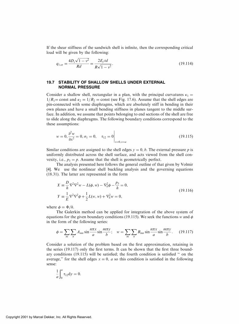
If the shear stiffness of the sandwich shell is infinite, then the corresponding criticalload will be given by the following:

q1;cr ¼4Ds


p

Rd¼ 2Ef td

Rffiffiffiffiffiffiffiffiffiffiffiffiffi1� �2

p : ð19:114Þ

19.7 STABILITY OF SHALLOW SHELLS UNDER EXTERNALNORMAL PRESSURE

Consider a shallow shell, rectangular in a plan, with the principal curvatures �1 ¼1=R1¼ const and �2 ¼ 1=R2 ¼ const (see Fig. 17.6). Assume that the shell edges arepin-connected with some diaphragms, which are absolutely stiff in bending in theirown planes and have a small bending stiffness in planes tangent to the middle sur-face. In addition, we assume that points belonging to end sections of the shell are freeto slide along the diaphragms. The following boundary conditions correspond to thethese assumptions:

w ¼ 0;@2w

@x2¼ 0; �1 ¼ 0; �12 ¼ 0

x¼0;x¼a

ð19:115Þ

Similar conditions are assigned to the shell edges y ¼ 0; b. The external pressure p isuniformly distributed across the shell surface, and acts viewed from the shell con-vexity, i.e., p3 ¼ p. Assume that the shell is geometrically perfect.

The analysis presented here follows the general outline of that given by Volmir[4]. We use the nonlinear shell buckling analysis and the governing equations(18.31). The latter are represented in the form

X � D

hr2r2w� Lð�;wÞ � r2

k��p3h¼ 0;

Y � 1

Er2r2�þ 1

2Lðw;wÞ þ r2

kw ¼ 0;

ð19:116Þ

where � ¼ �=h.The Galerkin method can be applied for integration of the above system of

equations for the given boundary conditions (19.115). We seek the functions w and �in the form of the following series:

� ¼Xm

Xn

Amn sinn�x

asin

m�y

b; w ¼

Xm

Xn

Bmn sinn�x

asin

m�y

b: ð19:117Þ

Consider a solution of the problem based on the first approximation, retaining inthe series (19.117) only the first terms. It can be shown that the first three bound-ary conditions (19.115) will be satisfied; the fourth condition is satisfied ‘‘ on theaverage,’’ for the shell edges x ¼ 0; a so this condition is satisfied in the followingsense:

1

a

ða0

�12dy ¼ 0:


The Galerkin method equations (see Sec. 6.5) are the following:

ða0

ðb0

X sin�x

asin�y

bdxdy ¼ 0;

ða0

ðb0

Y sin�x

asin�y

bdxdy ¼ 0: ð19:118Þ

Substituting expressions (19.116) together with the approximations (19.117) into theabove and integrating, one obtains

D

hB1

�6

16

1

a2þ 1

b2

� �2

�A1B1

2

3

�4

a2b2þ A

�4

16

k1b2

þ k2a2

� �� p

h¼ 0;

A1

Eþ 16B2

1

3�2 baþ a

b

� �2 � k1b2

þ k2a2

� �B1

�21

1a2

þ 1b2

� �2¼ 0:

ð19:119Þ

Introduce the following dimensionless parameters:

k 1 ¼k1a

2

h; k 2 ¼

k2b2

h; k ¼ k 1 þ k 2; � ¼ a

b; � ¼ B1

h; pp ¼ p

E

ab

h2

� �2

:

ð19:120ÞUsing the above-introduced parameters, we can represent a solution of Eqs (19.119),in the following load–deflection relationship:

pp ¼ 32�2

9

�3

1þ 1�

� �2 � k �2�2

1þ 1�

� �2 þ ðk Þ2�2

16 1þ 1�

� �2 þ �6 1�þ �� 2

192ð1� �2Þ

264

375�: ð19:121Þ

For a square shallow shell panel and � ¼ 0:3, the above equation simplifies to theform

pp ¼ 8:77�3 � 2:46k �2 þ ½0:154ðk Þ2 þ 22��: ð19:122ÞFor a cylindrical shallow shell panel, �1 ¼ 0 and �2 ¼ 1=R, then k ¼ b2=Rh.

Figure 19.7 illustrates the diagrams of pp vs :� for various values of k and for� ¼ 1. These diagrams are shown by dashed lines. The numerical data presented inthe Fig. 19.7 are taken from Ref. [4]. It is seen that for small values of k the value ofpp increases continuously, just as for flat plates; for large values of k , the diagramppð�Þ has a descending branch. To find the value of k at which jumping occurs fromone stable configuration of equilibrium to another, it is necessary to analyze dpp=d�.Equating it to zero, one finds the values of � corresponding to the upper and lowervalues of the critical pressure previously introduced in Sec. 19.2. We have thefollowing:

� ¼ 3

32k � 1

32

ffiffiffiffiffiffiffiffiffiffiffiffiffiffiffiffiffiffiffiffiffiffiffiffiffiffiffiffiffiffiffiffiffiffiffiffiffiffiffiffiffi3ðk Þ2 �

�4 1þ 1�

� �42ð1� �2Þ

vuut: ð19:123Þ


The boundary of the domain of this jump corresponds to the case when the diagramppð�Þ has a point of inflection with a horizontal tangent. In so doing, the expressionunder the radical sign must vanish. Thus, a limiting value of k will be of the form

k ¼�2 1þ 1

�

� �2ffiffiffiffiffiffiffiffiffiffiffiffiffiffiffiffiffiffi6ð1� �2Þ

p for � ¼ 3

32k : ð19:124Þ

If we retain four terms in series (19.177), the refined solutions will be obtained. Theyare shown by solid lines in Fig.19.7. It is seen from this figure that the distinctions ofthe refined diagrams from the first-approximation diagrams become perceptible onlyfor ‘‘elevating’’ shells, starting with k ¼ 36, and the refined diagrams give slightlylower upper critical values of pressure. However, the refined diagrams illustrate thechanges in the lower critical loads: in some cases, the loads change sign.

19.8 BUCKLING OF CONICAL SHELLS

Thin conical shells find wide applications in the structures of jet engines, aircrafts,liquid storages, reservoirs, etc. Buckling analysis of conical shells is more compli-cated than the corresponding analysis of cylindrical shells, because of the complexityof the stability governing equations.

We consider below some final results of the linear buckling analysis of inter-mediate-length conical shells subjected to uniform external pressure p, as shown inFig. 19.8. Assume that the shell ends cannot displace at their ends in the directionnormal to the shell midsurface. The criterion of the ‘‘intermediate-length cylindricalshell’’ was introduced in Sec. 19.3. This criterion can be employed for conical shells,too, by replacing R with the mean radius of the parallel circle rm ¼ ðr1 þ r2Þ=2, andby setting L equal to the length of the longitudinal axis of the shell (Fig. 19.8). Forthe above-mentioned shells, n2 > �2, where n is the number of half-waves in thecircumferential direction of the shell and � ¼ �rm=L. Then, the approximate relationfor determining the critical value of the external pressure in a conical shell is

Fig. 19.7


pcr ¼0:855

ð1� �2Þ0:75Eh

L

h

rm

� �1:5

ðcosÞ1:5: ð19:125Þ

For � ¼ 0:3, this relation appears in the form

pcr ¼ 0:92Eh

L

h

rm

� �1:5

ðcosÞ1:5: ð19:126Þ

This expression differs from the corresponding value of critical pressure in cylind-rical shells, Eq. (19.58), by the factor ðcosÞ1:5. Hence, for angles of conicity of2 < 408, pcr, given by Eqs (19.125) or (19.126), will differ from the critical valueof the external pressure, determined for a mean cylinder of length L and havingR ¼ rm, not more than 10%.

The critical values of other loads (axial forces, twisting moments, etc.) appliedto conical shells with an angle not more than 20, can be approximately found fromthe corresponding relations for cylindrical shells by replacing R with rm and settingthe cylindrical shell length equal to the length of the longitudinal axis of the conicalshell.

19.9 BUCKLING OF SPHERICAL SHELLS

The most important stability problem for thin spherical shells is referred to the casewhen they are loaded by external pressure. Such a type of problem is met in radarantenna caps in aircrafts, submarine bulkheads, bottoms of reservoirs, etc. We con-sider here the linear buckling analysis of spherical segments whose rise is comparablewith their radius and closed spherical shells under external pressure. The stabilityanalysis of shallow spherical shells under external pressure was considered in Sec.19.7.

We determine the critical load for a closed spherical shell. It was shown that thecritical stresses for the above shell and for elevated spherical segments under externalpressure are identical [4]. We assume that within the limits of area of local initialbulging, the shell can be considered as a shallow one: therefore, Eqs (17.36) areapplicable. For a spherical shell, the operator r2

kð::Þ ¼ r2ð::Þð1=RÞ, where R is theradius of the middle surface. Thus, Eqs (17.36) for the spherical shell take the form

Fig. 19.8


Dr2r2w ¼ 1

Rr2�þ p3;

1

Ehr2r2� ¼ � 1

Rr2w:

ð19:127Þ

Eliminating � from the above equations results in the following sixth-order differ-ential equation for w:

Dr6wþ Eh

R2r2w ¼ r2p3; ð19:128Þ

where r6ð::Þ ¼ r2r2r2ð::Þ. If an external pressure is applied to the spherical shell,then initial direct forces in all normal sections of the unbuckled shell are (see Sec.14.3) the following:

N1 ¼ N2 ¼ � pR

2: ð19:129Þ

It should be noted that the uniform external pressure does not appear directly in Eq.(19.128) but indirectly only, in terms of the fictitious load p

ðfÞ3 . The latter load is

expressed through the direct internal forces (19.129) and can be found from Eq.(19.8). We have (setting p3 ¼ p)

pðfÞ3 ¼ � pR

2r2w: ð19:130Þ

Therefore, Eq. (19.128) appears in the form

Dr6wþ pR

2r4wþ Eh

R2r2w ¼ 0: ð19:131Þ

Following the approach of Ref. [4], assume that the solution of Eq. (19.131) mustsatisfy the relation

r2w ¼ ��2w; ð19:132Þwhere � is some undetermined parameter. Substituting the above relation into Eq.(19.131) yields the following equation (for � 6¼ 0):

D�4 � pR

2�2 þ Eh

R2

� ��2w ¼ 0; ð19:133Þ

and solving this equation for p yields

p ¼ 2Eh

R3�2þ 2D

R�2: ð19:134Þ

Taking the limit of p with respect to �2, one obtains

�2 ¼ffiffiffiffiffiffiffiffiffiffiEh

DR2

r¼ 1

Rh

ffiffiffiffiffiffiffiffiffiffiffiffiffiffiffiffiffiffiffiffiffi12ð1� �2Þ

q:

Substituting the above into Eq. (19.134) gives the following value of the criticalpressure:

pcr ¼2Eh2

R2ffiffiffiffiffiffiffiffiffiffiffiffiffiffiffiffiffiffi3ð1� �2Þ

p ¼ 2Effiffiffiffiffiffiffiffiffiffiffiffiffiffiffiffiffiffi3ð1� �2Þ

p h

R

� �2

: ð19:135Þ


For � ¼ 0:3, we obtain

pcr ffi 1:21Eh

R

� �2

:

The corresponding value of the critical stress, �cr, is

�cr ¼N1;cr

h¼ Eh

R

1ffiffiffiffiffiffiffiffiffiffiffiffiffiffiffiffiffiffi3ð1� �2Þ

p : ð19:136aÞ

or, for � ¼ 0:3

�cr ffi 0:605Eh

R: ð19:136bÞ

Thus, the critical stress of a spherical shell under external pressure is the same as thecritical stress of a closed cylindrical shell under axial uniform compression (see Eq.(19.31b)).

The critical stress given by Eqs (19.136) can be classified as the upper criticalstress, pð1Þcr , for the shell and loading under consideration (see Sec. 19.2). However,numerous experimental investigations showed that the actual critical stresses ofspherical shells under external pressure are far below the values given by Eqs(19.136), obtained on the basis of the linear stability theory. It can be explainedby the fact that the real spherical shells are found to be sensitive to the lightest initialimperfections, just as compressed cylindrical shells discussed in Sec. 19.3.2.Therefore, the buckling analysis of spherical shells should be performed in the frame-work of the nonlinear stability theory. Such a buckling analysis is more complicatedfrom the mathematical and mechanical points of view (for details, see for exampleRef. [4]). We present below only the final results of the nonlinear stability problemfor the spherical shells under external pressure, associated with determining thelower value of the critical pressure, pð2Þcr , which is [4]

pð2Þcr ¼ 0:31Eh

R

� �2

: ð19:137Þ

It is seen that this value is four times less than pð1Þcr .

19.10 DESIGN STABILITY ANALYSIS

Let us summarize the basic theoretical and experimental results of buckling shellanalysis, discussed in the preceding sections. As mentioned previously, there is alarge discrepancy between the analytical predictions of the shell buckling behaviorand the corresponding experimental results. In addition, the scatter of the test datamay be quite large. The major reason for the above discrepancy is the sensitivity ofshell buckling to the initial geometric and loading imperfections, and to deviation inboundary conditions. As a result of these imperfections, as well as the inelasticbehavior of shells in buckling, the critical load of real shells, called the bucklingload in Sec. 19.2, for some shell configurations and loads can be much less than pð1Þcr ,predicted by the linear buckling analysis. It should be noted that application of thegeometrically nonlinear stability theory for determining pð2Þcr , in order to eliminate thediscrepancy between the theoretical and experimental data in the buckling of thin


shells, is associated with very cumbersome and difficult computations, and theresults, obtained by this theory, did not justify such efforts [16].

Since the load-carrying capability of thin shells is mostly determined by thebuckling load, it is very important to determine a reliable and accurate value ofthis load for design purposes. Because the effects of initial imperfections men-tioned above are extremely difficult to determine at the design stage, manytheoretical and experimental investigations have been directed toward the evalua-tion of an alternative to, or at least a modification of, the classical, linearstability theory. Now, the buckling design analysis of thin shells is based onthe classical, linear stability theory applied to initially perfect elastic shell, pro-vided one accounts for the reduction in critical load resulting from initial imper-fections and inelastic behavior. On this basis, several approaches were developedfor determining the allowable design buckling loads.

When sufficient experimental data exist for a given shell and loading, a statis-tical method of design curves may be useful in determining the allowable designbuckling load. Each such design curve was obtained at a certain probability level.The load at which a shell may be expected to buckle is the load which corresponds tothe curve best fit. This approach is described in Refs [12,13, 19, 22, 23, etc].

Whenever sufficient experimental data do not exist to obtain a statisticalallowable design buckling load, design recommendations have been based onallowable behavior of a shell structure. In general, this involves empirical reductionfactors to decrease the theoretical upper critical load [4,12,15, 24, etc.]. Due to thelack of test data for some types of shells and loads, the recommendations may beconservative for some cases. We consider here only the second approach andpresent below a small selection of the empirical equations for determining theallowable buckling loads for cylindrical shells that incorporate the above-men-tioned correction factors.

19.10.1 Buckling of unstiffened cylindrical shells

(a) Axial compression

The classical critical stress formula (19.31b) can be used to predict buckling ofinitially imperfect cylindrical shells, provided it is written in the following form:

�cr ¼ �Eh

R; ð19:138Þ

where � is the so-called buckling coefficient that varies with R=h. For high-qualitymanufactured shells the above coefficient is determined from the following relation-ship, which agrees well with experimental data (for R=h ¼ 100 . . . 1500Þ [4]:

� ¼ 1

�8

ffiffiffiffiffiffiffiffiffiffiffiffiffiffiffiffiffiffi100h

R

� �3s

: ð19:139Þ

If shells are manufactured under insufficient quality controls and the initial imper-fections are comparable to the shell thickness, the design values of the bucklingcoefficient have to be divided by approximately two. Initial imperfections that exceedthe shell thickness noticeably are absolutely inadmissible because they decrease thestiffness of shell structure appreciably.


The critical stress for a short and thin cylinder with length L � 1:22ffiffiffiffiffiffiRh

pfor

simply supported edges, and with L � 2:5ffiffiffiffiffiffiRh

pfor fixed edges, can be determined

from the buckling formula derived previously for a wide flat plate, as follows:

�cr ¼ �Eh2

L2; ð19:140Þ

where � ¼ 0:9 for simply supported and � ¼ 3:6 for fixed shell edges.The alternative buckling stress equations were derived by Donnel and Wan

[10]. They are in good agreement with the relations (19.138) and (19.140).The following approximate equation for the allowable axial compressive stress

in cylindrical shells for elastic buckling was developed in the ASME Code [22] byusing a factor of safety of 10 in Eq. (19.31b):

� ¼ 0:0625Eh

R: ð19:141Þ

For structural steel cylinders, inelastic buckling cannot be readily dealt withusing a plasticity reduction factor. Instead, it is customary to use some empiricalformulas, such as those listed in Refs [22,23].

(b) External pressure

The critical value of external pressure for simply supported cylindrical shells (besidesvery short and very long shells) is given by [4]

pcr ¼ ð0:855Þ Eh2

RLð1� �2Þ0:75ffiffiffiffih

R

r; ð19:142Þ

where the coefficient depends on the ratio R=h, as follows:

R=h . . . . . . . . . 250 500 1000 1500

. . . . . . . . . . . . 0:7 0:6 0:5 0:4

In designing short L � 2:5ffiffiffiffiffiffiRh

p� �, simply supported cylindrical shells under external

pressure, the value of pcr is given by [4]

pcr ¼ 1Eh2

RL; ð19:143Þ

where 1 ¼ 1:8 for all-around pressure and 1 ¼ 3:6 for side pressure.For long, simply supported cylindrical shells ðL > 3:35R

ffiffiffiRh

qÞ, the critical value

of the pressure can be determined from the following relationship:

pcr ¼ 0:275Eh3

R3: ð19:144Þ

The boundary conditions exert some effect on the critical value of the externalpressure. For example, for a cylindrical shell having one pin-connected edge andthe second one fixed, the critical value of external pressure, p cr, is given by [4]

p cr ¼ 0:6pcr; ð19:145Þwhere pcr is the critical value of external pressure for the previously introducedsimply supported cylindrical shell.


An empirical equation developed by the U.S. Navy [20] for the buckling ofcylindrical shells under lateral and axial pressure in the elastic range is given by

pcr ¼2:42E

ð1� �2Þ3=4ðh=2RÞ2:5

L=2R� 0:45ðh=2RÞ0:5� � : ð19:146Þ

For cylindrical shells with large R=h ratios, the above equation can be simplified to

pcr ¼2:42E

ð1� �2Þ3=4ðh=2RÞ2:5L=2R

: ð19:147Þ

19.10.2 Buckling of unstiffened spherical shells under externalpressure

The critical value of external pressure and critical stress is shown below [4]

pcr ¼ Eh2

R2; �cr ¼

Eh

2R; ð19:148Þ

where the coefficient for high-quality manufactured shells and for 250 � R=h �800 is determined by the following formula:

¼ 1

2:368

ffiffiffiffiffiffiffiffiffiffiffiffiffiffiffiffiffiffi100h

R

� �3s

: ð19:149Þ

For the range R=h � 250, according to the recommendations of Ref. [4], ¼ 0:3. If aspherical shell is not manufactured with sufficient accuracy and initial imperfectionsare comparable with its thickness, the coefficient is reduced by about 1.5–2 times.

The following empirical equations for determining the critical stress and thecritical pressure were developed in Refs [17]:

�cr ¼ 0:125Eh

R; pcr ¼ 0:25

Eh2

R2: ð19:150Þ

19.10.3 Buckling of unstiffened conical shells

Conical shells subjected to external pressure can be designed as cylindrical shells withthe effective thickness, he; and efffective length, Le, determined from the followingrelations [24]:

he ¼ h cos; Le ¼L

21þ r1

r2

� �; ð19:151Þ

where h is thickness of the cone, L is the height of the conical shell, and r1 and r2 arethe radii of parallel circles at the top and bottom sections of the truncated cone,respectively.

19.10.4 Stiffened shells

Experimental investigations showed that stiffened shells are less sensitive to overalland local imperfections [12]. Therefore, the critical values of applied loads for suchshells are closer to the theoretically determined values of the upper critical loads


predicted by the linear stability theory. Some empirical equations were developed fordetermining the critical stresses and loads for stiffened shells of various configurationunder axial compression, external pressure, torsion, shear, as well as various loadingcombinations [12,14,19,21]. For example, for the spherical shell with closely andequally spaced stiffeners in two mutually orthogonal directions under external pres-sure, the buckling value of the above pressure is given by [21]

pcr ¼ 0:366EhmR

� �2hbhm

� �3=2

; ð19:152Þ

where hm ¼ hþ A=s is the effective membrane thickness and hb ¼ 12I=sð Þ1=3is theeffective bending thickness; A and I are the area and moment of inertia of thestiffener, s is the spacing between stiffeners.

Local buckling of the spherical shells between the stiffeners must also becon-sidered for large-diameter shells. One such equation is given by

pcr ¼ 7:42Eh3

Rs2: ð19:153Þ

Only a small selection of the recommended design relations for determiningthe critical loads in thin shells has been introduced above. The interested reader isreferred to Refs [4,12,13,14,19–24].

In conclusion, note that in practice one must tend to designing the shell struc-tures whose stability would not depend on occasional and not easily controlledfactors. The basic avenues of designing such shell structures is the use of stiffenedshells, sandwich shells, corrugated shells, etc. In some, the most important cases,sharpened shells are applied.

PROBLEMS

19.1 It follows from Fig. 19.1a that the path of equilibrium for a flat plate is symmetric

about the vertical, p axis, whereas the corresponding path for a shallow shell is non-

symmetrical. Explain the above difference in the buckling behavior of plates and shells.

19.2 Provide a detailed deviation of Eqs (19.3).

19.3 Derive Eqs (19.4) from (19.3) by neglecting all the terms containing prebuckled rota-

tions.

19.4 Derive Eqs (19.9) from Eqs (19.7).

19.5 A water tower support constructed of a long steel piping of 1.0 m diameter is to carry

an axial compression load of 520 kN. Assuming that the supports ends are pin-con-

nected, determine the required thickness of the shell that will prevent this tower sup-

port from buckling. Use L ¼ 2:0m; E ¼ 200GPa; � ¼ 0:3, and a factor of safety (FS)

of 3.5.

19.6 Verify Eq. (19.22)

19.7 A thin steel pipe is subjected to a vacuum pressure of 150 psi. Assuming that the pipe

edges are simply supported, determine the required thickness of the pipe, preventing

the pipe from buckling. Given E ¼ 29,000 psi, � ¼ 0:3, L ¼ 10 ft, R ¼ 2:5 ft, and the

factor of safety (FS) is 3.0.

19.8 Determine the critical stress in a simply supported circular cylindrical panel subjected

to a uniformly distributed compressive forces q1, as shown in Fig. P.19.1. Assume that

the shell edges are simply supported.

Hint: take the deflection w in the form


w ¼ f sinm�x

L� sinm��

�0:

19.9 Determine the critical value of the external pressure p acting on a spherical shell of

radius R.

Hint: eliminating � from Eqs (19.7) and letting R1 ¼ R2 ¼ R and p ¼ �hr2w, yields

the following equation:

Dr6wþ pr4wþ Eh

R2r2w ¼ 0: ðaÞ

The solution of this equation satisfies the condition r2w ¼ ��2w; where � is some

indeterminate parameter. Substituting r2w into Eq. (a) minimizing over �2, yields pcr.19.10 Determine the critical stress for an axially compressed unstiffened closed cylindrical

shell of radius R ¼ 2:0m and of thickness h ¼ 0:01m. The shell length is L ¼ 0:6m.

Assume that the shell manufactured is of insufficient quality. Use also E ¼ 220GPa;and � ¼ 0:3.

19.11 Determine the critical value of the external pressure p in an unstiffened cylinder having

the radius R ¼ 2:5m; thickness h ¼ 8mm, and length L ¼ 0:5m. Assume that one end

of the cylinder is fixed and the other one is free. Take E ¼ 210GPa; and � ¼ 0:3:19.12 A thin-walled cylinder is used to support a reactor of weight W . Find the maximum

value of W that can be applied to the cylinder without causing it to buckle. Take L ¼10ft; R ¼ 2 ft; E ¼ 29,000 ksi, h ¼ 0:2 in:; � ¼ 0:25, and the factor of safety (FS) is 2.5.

REFERENCES

1. Volmir, A.S. Flexible Plates and Shells (translated from Russian), Air Force Flight

Dynamics Laboratory, Technical Report No. 66-216, Ohio, Wright-Patterson Air

Force Base, 1967.

2. Brush, D.O. and Almroth, B.O., Buckling of Bars, Plates, and Shells, McGraw-Hill, New

York, 1975.

3. Batdorf, S.B., A Simplified Method of Elastic Stability Analysis for Thin Cylindrical

Shells, NACA, Technical Report, No. 874, Washington, DC, 1947.

4. Volmir, A.S., Stability of Elastic Systems, Gos. Izd-vo Fiz.-Mat. Lit., Moscow, 1963 (in

Russian).

Fig. P19.1


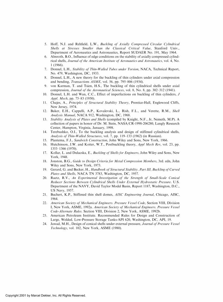
5. Hoff, N.J. and Rehfield, L.W., Buckling of Axially Compressed Circular Cylindrical

Shells at Stresses Smaller than the Classical Critical Value, Stanford Univ.,

Department of Aeronautics and Astronautics, Report SUDAER No. 191, May 1964.

6. Almroth, B.O., Influence of edge conditions on the stability of axially compressed cylind-

rical shells, Journal of the American Institute of Aeronautics and Astronautics, vol. 4, No.

1 (1966).

7. Donnel, L.H., Stability of Thin-Walled Tubes under Torsion, NACA, Technical Report,

No. 479, Washington, DC, 1933.

8. Donnel, L.H., A new theory for the buckling of thin cylinders under axial compression

and bending, Transactions ASME, vol. 56, pp. 795–806 (1934).

9. von Karman, T. and Tsien, H.S., The buckling of thin cylindrical shells under axial

compression, Journal of the Aeronautical Sciences, vol. 8, No. 8, pp. 302–312 (1941).

10. Donnel, L.H. and Wan, C.C., Effect of imperfections on buckling of thin cylinders, J

Appl. Mech, pp. 75–83 (1950).

11. Chajes, A., Principles of Structural Stability Theory, Prentice-Hall, Englewood Cliffs,

New Jersey, 1974.

12. Baker, E.H., Cappelli, A.P., Kovalevski, L., Rish, F.L., and Verette, R.M., Shell

Analysis Manual, NACA 912, Washington, DC, 1968.

13. Stability Analysis of Plates and Shells (compiled by Knight, N.F., Jr, Nemeth, M.P). A

collection of papers in honor of Dr. M. Stein, NASA/CR-1998-206280, Langly Research

Center, Hampton, Virginia, January, 1998.

14. Terebushko, O.I., To the buckling analysis and design of stiffened cylindrical shells,

Analysis of Thin-Walled Structures, vol. 7, pp. 119–133 (1962) (in Russian).

15. Plantema, F.J., Sandwich Construction, John Wiley and Sons, New York, 1966.

16. Hutchinson, J.W. and Koiter, W.T., Postbuckling theory, Appl Mech Rev, vol. 23, pp.

1353–1366 (1970).

17. Kollar, L. and Dulacska, E., Buckling of Shells for Engineers, John Wiley and Sons, New

York, 1948.

18. Jonston, B.G., Guide to Design Criteria for Metal Compression Members, 3rd. edn, John


19. Gerard, G. and Becker, H.,Handbook of Structural Stability, Part III, Buckling of Curved

Plates and Shells, NACA TN 3783, Washington, DC, 1957.

20. Raetz, R.V., An Experimental Investigation of the Strength of Small-Scale Conical

Reducer Sections Between Cylindrical Shells Under External Hydrostatic Pressure. U.S.

Department of the NAVY, David Taylor Model Basin, Report 1187, Washington, D.C.,

US Navy, 1957.

21. Buchert, K.P., Stiffened thin shell domes, AISC Engineering Journal, Chicago, AISC,

1964.

22. American Society of Mechanical Engineers. Pressure Vessel Code, Section VIII, Division

I, New York, ASME, 1992a. American Society of Mechanical Engineers. Pressure Vessel

Code-Alternate Rules. Section VIII, Division 2, New York, ASME, 1992b.

23. American Petroleum Institute. Recommended Rules for Design and Construction of

Large, Welded, Low-Pressure Storage Tanks-API 620, Washington, DC, API, 19.

24. Jawad, M.H., Design of conical shells under external pressure, Journal of Pressure Vessel

Technology, vol. 102, New York, ASME (1980).


20

Vibrations of Shells

20.1 INTRODUCTION

The dynamic effects of time-dependent loads on shell structures are quite similarto those discussed in Chapter 9 for plates. Thus, the objectives of the vibrationanalysis of shells, as well the general approach for deriving the shell equationsof motion, remain analogous to the plate vibration analysis introduced in Sec.9.1.

Assume that the state of stress within a shell during vibrations has a char-acter determined by the equations of equilibrium, and the shell middle surfacedeforms according to the same law during vibrations as in the static equilibriumstate. Based on the above, the equations of motion of the vibrating shell can beobtained by applying the D’Alambert principle, just as it was done for vibratingplates – i.e., by adding the inertia forces to given external loads, assigned bycomponents p1; p2; and p3, namely (damping forces are not considered here):

p1 ! p1 � �h@2u

@t2; p2 ! p2 � �h

@2v

@t2; p3 ! p3 � �h

@2w

@t2; ð20:1Þ

where p1; p2; p3; and u; v;w are functions of the Cartesian coordinates of the mid-dle surface and time, � is the mass density of the material, and h is the shellthickness. As for vibrating plates, we distinguish between free vibrations of shells,which occur in the absence of applied loads but are initiated by some initialconditions imposed on the shell, and forced vibrations of shells, which resultfrom the application of time-dependent loads. We consider in this chapter bothtypes of vibrations.


20.2 FREE VIBRATIONS OF CYLINDRICAL SHELLS

20.2.1 General

As mentioned in Sec. 9.1, free vibrations deal with some natural characteristics ofshells. These natural vibrations occur at discrete frequencies, depending only on thegeometry and material of the shell. A knowledge of the free-vibration characteristicsof thin elastic shells is important both for our general understanding of the funda-mentals of the shell behavior and for industrial applications of shell structures. Inconnection with the latter, the natural frequencies of shell structures must be knownto avoid the destructive effect of resonance with adjacent rotating or oscillatingequipment (such as jet and reciprocating aircraft engines, electrical machinery, mar-ine turbines and propulsors, etc.).

Since the free vibrations occur in the absence of all external forces(p1 ¼ p2 ¼ p3 ¼ 0), we address the free-vibration analysis of shells with the solutionof homogeneous partial differential equations with homogeneous boundary condi-tions. Let us derive the equations of the free vibrations of thin elastic cylindrical andshallow shells.

20.2.2 Axisymmetric free flexural vibrations of cylindrical shells

Consider the free flexural vibrations of a circular cylindrical shell when the radial wand longitudinal u displacements do not depend on the angular coordinate �, and thecircumferential displacement v is zero. Any cross section of such a shell will be acircular ring, and several half-waves can be placed throughout the shell length, asshown in Fig. 20.1.

The equation of axisymmetrical free vibrations can be obtained from the gov-erning differential equation of the axisymmetrically loaded circular cylindrical shell,Eq. (15.44). One replaces, due to Eq. (20.1), the normal component of the externalloading p3 by the normal component of the inertia forces, and neglects the long-itudinal component of the above forces. Thus, the differential equation of the axi-symmetrically vibrating circular cylindrical shell is found to be

@4w

@x4þ 44w ¼ � �h

D

@2w

@t2; ð20:2Þ

Fig. 20.1


where the deflection w ¼ wðx; tÞ is a function of the x coordinate and time t.The solution of Eq. (20.2) for a simply supported shell of length L, assuming

harmonic equations in time, is sought in the following form:

wðx; tÞ ¼X1n¼1

An sinn�x

Lsin!t; ð20:3Þ

where ! is the frequency of natural vibrations (or natural frequency) of the given shell.It is related to the vibration period T by the relationship ! ¼ 2�=T . Substituting forw from Eq. (20.3) into Eq. (20.2), one obtains

Dn�

L

� �4þEh

R2¼ �h!2;

and the natural frequency ! is given by

!2 ¼ E

�R2ð1þ ��4Þ; ð20:4Þ

where

� ¼ h2

12R2ð1� �2Þ ; � ¼ n�R

L: ð20:5Þ

The value of � for thin shells is small compared with unity. For shells that are notshort, when �4 < 1, the product ��4 can be neglected. Then, the natural frequency ofaxisymmetrical vibrations for all numbers n will coincide with the natural frequencyof axisymmetrical vibrations of a ring or an infinitely long shell. For other shells, notsimply supported at their ends, a solution of Eq. (20.2) will be sought in the follow-ing general form:

wðx; tÞ ¼ WðxÞ sin!t: ð20:6ÞSubstituting the above into Eq. (20.2), we obtain an ordinary fourth-order differ-ential equation inWðxÞ. Its solution will have an analogous form to that discussed inSec. 15.3 if axisymmetrical deformations of a statically loaded circular cylindricalshell are of interest. Satisfying the given boundary conditions, one can obtain – fromthe condition of nontriviality of the above solution – the expression for the naturalfrequencies in axisymmetrically vibrating cylindrical shells. For example, for fixedshell edges, the natural frequency of the first mode of axisymmetrical vibrations (thefundamental natural frequency) is determined from the following equation:

!21 ¼

E

�R21þ � 4:73

R

L

� �4" #

: ð20:7aÞ

The frequency of the second harmonics for the above shell is

!22 ¼

E

�R21þ � 7:83

R

L

� �4" #

: ð20:7bÞ

Since the value of � for thin shells is small, then, as follows from Eqs (20.7), the fixededges of the shell have a low effect on the natural frequencies of vibrations ascompared with the simply supported edges. Similar results will be obtained forother boundary conditions. Hence, the natural frequency of axisymmetrical (long-


itudinally-radial) vibrations of thin and not-short circular cylindrical shells dependsa little on boundary conditions and on the mode of vibrations (for the first mode).

To determine the frequencies of axisymmetric vibrations, the energy method,based on the variational principles (see Sec. 2.6), can also be applied. As shown inSec. 15.3, the axisymmetric bending of a circular cylindrical shell is quite similar tothe bending of a strip-beam of unit width cut off the shell and resting on an elasticfoundation with the foundation modulus k ¼ Eh=R2. The strain energy of such astrip-beam, deflecting by wðxÞ; will be of the form

U ¼ EI

2

ðL0

d2w

dx2

!2

dxþ k

2

ðL0

w2dx; ð20:8Þ

where L denotes the span of the strip-beam. It follows from the above that the strainenergy consists of the strain energy of the strip-beam itself, which is proportional toh3, and the energy of the elastic foundation, which is proportional to h (the shellthickness). If the small value of the strain bending energy (the first term in Eq. (20.8))is neglected, then the maximum value of the strain energy will be equal to thefollowing:

Umax ¼Eh

R2

ðL0

w2dx: ð20:9Þ

The maximum value of the kinetic energy for any mode of free vibrations is given by

Kmax ¼�h!2

2

ðL0

w2dx:

Equating Umax and Kmax, we obtain the following expression for the frequency offree vibrations:

!2 ¼ E

�R2: ð20:10Þ

Hence, under the assumption introduced above (neglecting the bending potentialenergy of a strip-beam in Eq. (20.8)), the frequency of natural radial vibrationsdoes not depend on wmax, i.e., on the vibration mode and boundary conditions. Itis necessary only that a circular cross section is preserved on the shell ends.

In increasing the shell thickness and decreasing its length, the dependence ofvibration frequencies on the mode and boundary conditions becomes more signifi-cant. For cylindrical shells, such a mode of axisymmetric vibrations is possible whenu ¼ w ¼ 0. In this case, points of such shells are displaced in the circumferentialdirection only (i.e., v 6¼ 0); these are torsional vibrations.

20.2.3 Free asymmetric flexural vibrations of circular cylindricalshells

1. Closed cylindrical shells

The differential equations of equilibrium in terms of the displacement componentsfor a circular cylindrical shell are given by Eqs (15.7)–(15.9). According to theDonnel–Mushtari–Vlasov (DMV) theory, they can be simplified by dropping thebending terms in the operators l23 and l32 that are proportional to h2=R2 (see Eqs


(15.9)). Taking into account the relations (20.1), we can write the differential equa-tions of motion for a freely vibrating circular cylindrical shell in the framework ofthe DMV theory in terms of the x and � coordinates, as follows:

@2u

@x2þ 1� �

2R2

@2u

@�2þ 1þ �

2R

@2v

@x@��

R

@w

@x¼ 1� �2

E�@2u

@t2;

1þ �2R

@2u

@x@�þ 1� �

2

@2v

@x2þ 1

R2

@2v

@�2� 1

R2

@w

@�¼ 1� �2

E�@2v

@t2;

�

R

@u

@xþ 1

R2

@v

@�� w

R2� h2

12

@4w

@x4þ 2

R2

@4w

@x2@�2þ 1

R4

@4w

@�4

!¼ 1� �2

E�@2w

@t2:

ð20:11Þ

Assume that the given closed cylindrical shell of length L is simply supported on itsedges. Then, the solutions of Eqs (20.11) can be sought in the following form:

u ¼Xm

Xn

Amn cosm� cosn�x

Lsin!t;

v ¼Xm

Xn

Bmn sinm� sinn�x

Lsin!t;

w ¼Xm

Xn

Cmn cosm� sinn�x

Lsin!t;

ð20:12Þ

where Amn;Bmn; and Cmn are some constants; m refers to the number of half-waves inthe circumferential direction of the shell, whereas n characterizes the number of half-waves of displacements placed on the shell length L. The displacement componentsu; v; and w in the form of Eqs (20.12) satisfy the prescribed boundary conditions onthe shell edges x ¼ 0 and x ¼ L and the periodicity conditions with respect to thevariable �.

Inserting Eqs (20.12) into Eqs (20.11), we obtain the following system ofhomogeneous algebraic equations in Amn;Bmn; and Cmn :

��2 � 1� �2

m2 þ�

� �Amn þ

1þ �2

m�Bmn � ��Cmn ¼ 0;

1þ �2

m�Amn þ �m2 � 1� �2

�2 þ�

� �Bmn þmCmn ¼ 0;

��Amn þmBmn þ �1� a2ð�2 þm2Þ2 þ��

Cmn ¼ 0;

ð20:13Þ

where

� ¼ n�R

L; � ¼ ð1� �2ÞR2

E�!2; a2 ¼ h2

12R2:

The constants Amn;Bmn; and Cmn cannot be simultaneously equal to zero. To deter-mine nontrivial solutions of the above system of homogeneous equations, it is neces-sary to equate its determinant to zero. We have the following:

��2 � 1� �2

m2 þ� 1þ �2

m� ��1þ �2

m� �m2 � 1� �2

�2 þ��

m

�� m � 1þ a2ð�2 þm2Þ2 ��

¼ 0:


The resulting equation of the third power in �, or of the sixth power in ! determinesthe natural frequencies of vibrations of the given cylindrical shell corresponding tocertain numbers of m and n. The above equation can also be written in the form

T1!6 þ T2!

4 þ T3!2 þ T4 ¼ 0; ð20:14Þ

where T1;T2;T3; and T4 are some coefficients depending on m and n, as well asgeometric and mechanical parameters of the shell. It can be shown that all the rootsof the characteristic equation (20.14) are always real, and three values of the naturalfrequencies ! correspond to each pair of numbers m and n. The negative values of !,which are the roots of Eq. (20.14) but have no physical meaning, are dropped.

Having determined any of the three frequencies, the ratios between the ampli-tudes, for instance Amn=Cmn; Bmn=Cmn can be calculated from the homogeneousequations (20.13). Each value of ! corresponds to a certain ratio between the ampli-tudes of the longitudinal, tangential, and normal displacements.

Conducted investigations showed that for mostly transverse (or normal) vibra-tions of circular cylindrical shells, the value !2 will be small and their degrees higherthan second can be neglected. In this case, we obtain the following from Eq. (20.14):

!2 ¼ �T4

T3

or !2 ¼ E

�R2ð1� �2Þð1� �2Þ�4 þ a2ð�2 þm2Þ4

m2 þ ð�2 þm2Þ2 : ð20:15Þ

It is of great practical importance to determine the values of m and n for whichthe natural frequency of predominantly transverse vibrations, given by Eq. (20.15),will be the smallest. The analysis shows that the lowest natural frequency will be forn ¼ 1, i.e., for one half-wave located over the shell length, and, hence, � ¼ �R=L.The natural frequency, as a function of m, has a minimum. It can be shown that forintermediate-length shells, the value of m2, corresponding to the smallest frequency,can be neglected compared with ð�2 þm2Þ2. Then, Eq. (20.15) can be rewritten forthe above-mentioned shells, as follows:

� ¼ T1

ð�2 þm2Þ2 þ a2ð�2 þm2Þ2;

where T1 ¼ ð1� �2Þ�4. Denoting X ¼ ð�2 þm2Þ2, we can rewrite the above equationas follows:

� ¼ T1

Xþ a2X : ð20:16Þ

To determine the value of X (or m) corresponding to the minimum of �, we differ-entiate Eq. (20.16) with respect to X and equate this derivative to zero. We have thefollowing:

@�

@X¼ � T1

X2þ a2 ¼ 0;

from which

X ¼ffiffiffiffiffiffiT1

a2

r¼ ð�2 þm2Þ2 or m2 ¼

ffiffiffiffiffiffiT1

a24

r� �2: ð20:17Þ


Since the number of m may be an integer only, then, after determining m from Eq.(20.17), it should be taken to be equal to the nearest integer. The smallest naturalfrequency corresponds to this integer. The second derivative of � with respect to mwill be positive; therefore, Eq. (20.17) defines a minimum.

Example 20.1

For a simply supported closed cylindrical shell of radius R ¼ 17 cm and of lengthL ¼ 54 cm, find the number of half-waves in the circumferential direction and theminimum natural frequency. Use the following geometric and mechanical para-meters of the shell: h ¼ 0:08 cm; � ¼ 0:3; E ¼ 200GPa, and � ¼ 0:3:

Solution

For the given geometric and mechanical shell parameters, we can find thata2 ¼ 0:18 10�5, � ¼ 1, and T1 ¼ 0:9. Substituting the above data into Eq.(20.17), gives m ¼ 5:1. Hence, the minimum natural frequency of predominantlytransverse vibrations, !min, takes place for five half-waves or for 10 nodal pointsplaced over the circumference of the shell cross section. The value of ! is found fromEq. (20.15) for m ¼ 5. The relationship between the frequency and m is shown inFig. 20.2.

Figure 20.3 illustrates the relationship of the frequency for any fixed value of mfrom the shell length, L. It is seen that the frequency decreases as the length of theshell increases. However, starting from some length L , the frequency becomes aconstant and practically coincides with the frequency determined for a shell havingfree edges or for a shell of an infinite length when the shell experiences only bendingwithout stretching of the middle surface.

If a shell is not too short (L > R), then the natural frequency is virtuallyindependent of the boundary conditions and it is possible to determine this fre-quency for a shell with any, say simply supported, boundary conditions.

The strain energy of a shell of any geometry is given by Eq. (12.51). The kineticenergy of a vibrating shell is of the following form:

K ¼ �h

2

ð ðA

@u

@t

� �2

þ @v

@t

� �2

þ @w

@t

� �2" #

ABdd: ð20:18Þ

Fig. 20.2


Assuming, again, the harmonic vibrations in time, we can approximate the displace-ments of a cylindrical shell midsurface as follows:

u ¼ u0ðx; �Þ sin!t;v ¼ v0ðx; �Þ sin!t;w ¼ w0ðx; �Þ sin!t;

where u0;w0; and w0 are the maximum displacements. Substituting the derivatives ofu; v; and w with respect to time into Eq. (20.18), we can find the maximum value ofthe kinetic energy:

Kmax ¼�h

2!2

ð ðA

u20 þ v20 þ w20

� �Rdxd�: ð20:19Þ

Equating Kmax and Umax and letting, A ¼ 1;B ¼ R; ¼ x; and ¼ �, we obtain thefollowing expression for the frequency of asymmetric flexural free vibrations of acylindrical shell in terms of its strain and kinetic energies:

!2 ¼ 2Umax

�hÐ Ð

Au20 þ v20 þ w2

0

� �Rdxd�

: ð20:20Þ

2. Open cylindrical shells (panels)

The vibration analysis of cylindrical shells can be conveniently carried out with theuse of Eqs (17.36) in terms of the stress function � and deflection w. Assuming thatthe stiffness of the shell in the middle surface is much greater than its stiffness in thenormal direction with respect to the middle surface, we can use the following con-ditions according to Eqs (20.1):

p1 ¼ p2 ¼ 0 and p3 ¼ ��h @2w

@t2:

Substituting the above into Eqs (17.36) and taking ¼ � ¼ x=R; ¼ � ¼ s=R,�1 ¼ 0, and �2 ¼ 1=R, one obtains the following system of equations:

Fig. 20.3


� @2�

@�2RþDr2r2wþ �hR4 @

2w

@t2¼ 0;

r2r2�þ REh@2w

@�2¼ 0:

ð20:21Þ

The above is a set of the governing differential equations of the undamped, free linear,transverse vibrations of circular cylindrical shells. The details of determining thenatural frequencies of cylindrical shells is explained in the illustrative problem thatfollows.

Example 20.2

Determine the natural frequency of free vibrations of the circular cylindrical, simplysupported shell shown in Fig. 20.4. Calculate the fundamental natural frequency forthe shell made of reinforced concrete and having the following geometric andmechanical parameters: L ¼ 55m, l ¼ 21m; f ¼ 4:0m; R ¼ 15:0m; h ¼ 0:1m; �0 ¼1:6 rad; E ¼ 6GPa; � ¼ 1:6 103 kg=m3, and � ¼ 0.

Solution

The simply supported boundary conditions in the adapted coordinate system are ofthe form

w ¼ v ¼ M1 ¼ N1 ¼ 0�¼0;�¼L=R

;

w ¼ u ¼ M2 ¼ N2 ¼ 0�¼0:�¼�0 :

A solution of Eqs (20.15) is sought in the form of the following series:

� ¼X1m¼1

X1n¼1

Amn sin �n� sin�m� � sin !t;

w ¼X1m¼1

X1n¼1

Bmn sin �n� sin�m� � sin!t;ðaÞ

where

Fig. 20.4


�n ¼n�R

L; �m ¼ m�

�0:

Substituting the above into Eqs (20.21), one obtains the following:

AmnR�2n þ BmnDð�2n þ �2

mÞ2 � Bmnð�hÞR4!2 ¼ 0;

Amn

Ehð�2n þ �2

mÞ2 � BmnR�2n ¼ 0:

From the condition of nontriviality of the solution of the above system of thehomogeneous algebraic equations, we obtain the following characteristic equation:

!2 ¼ 1

�hR4

EhR2�4n

ð�2n þ �2mÞ2

þDð�2n þ �2mÞ2

" #: ðbÞ

To determine the fundamental natural frequency of free vibrations, it is necessary tocalculate the values of m and n (values of �n and �m) corresponding to the lowestfrequency. Analysis of Eq. (b) shows that the fundamental mode of the vibrationscorresponds to �1 (for n ¼ 1, one half-wave in the longitudinal direction). Let uscalculate the number m (the number of circumferential half-waves) that correspondsto the fundamental natural frequency of the given shell. For this purpose, take thefirst derivative of the expression (b) with respect to �m and equate it to zero for�1 ¼ const. We have

@ð!2mnÞ

@�m

¼ 0:

After some simple manipulations, one obtains

�m ¼

ffiffiffiffiffiffiffiffiffiffiffiffiffiffiffiffiffiffiffiffiffiffiffiffiffiffiffiffiffiffiffiffiffiffiffiffiffiffiffiffiffiffiffiffiffiffiffiffiffiffiffiffiffi�1

ffiffiffiffiffiffiffiffiffiffiffiffiffiffiffiffiffiffiffiffiffiffiffiffiffiffi12R2ð1� �2Þ

h24

s� �1

0@

1A

vuuut :

It can be easily shown that for long and intermediate-length shells, the fundamentalnatural frequency occurs for n ¼ 1 and m ¼ 2 (one half-wave in the longitudinal andtwo half-waves in the circumferential directions, respectively). The shell under con-sideration, having 4 < L=l ¼ 2:64 > 1, can be classified as an intermediate-lengthshell. So, we obtain the following:

�1 ¼�ð15:0Þ55:0

¼ 0:856; �2 ¼�ð2Þ1:6

¼ 3:927:

Substituting the above data into Eq. (b), we obtain !12 ¼ 7:151=s.

20.3 FREE VIBRATIONS OF CONICAL SHELLS

The governing equations of free vibrations of conical shells can be derived from Eqs(12.23), (12.24), and (12.41), (12.42), (12.45), (1246) of the general linear shell theoryby introducing the curvilinear coordinates ¼ s and ¼ � (where s is the distance ofa point of the midsurface, measured from some reference point, e.g., from the shellvertex, and � is the circumferential angle determining the location of the meridian),substituting the corresponding Lame parameters, and replacing the distributed sur-


face loads p1; p2; and p3 with the inertia forces according to Eqs (20.1). The govern-ing equations of free vibrations in displacements obtained represent the partialdifferential equations with variable coefficients. Their solution represents a verycomplicated mathematical problem.

Conducted analyses and tests showed that for small angles of conicity 2(about 30–40Þ (see Fig. 19.8), the frequency of axisymmetric, free radial vibrationscan be approximately calculated by Eqs (20.4) and (20.7) by replacing R in theseequations with rm ¼ ðr1 þ r2Þ=2 and setting the length of the longitudinal axis of theconical shell equal to L (cylindrical shell length). It should be noted that conicalshells with these angles of conicity are met in nozzle structures of jet engines. Thevibration shell analyses showed that the error introduced by the above approximateprocedure was not more than 5–10%. For larger angles of conicity, refined solutions,based on the governing differential equations of free vibrations mentioned above,should be employed.

The dependence of the frequency of free radial vibrations on the number ofwaves along the shell cross section has a minimum, just as for a cylindrical shell (seeFig. 20.2). The above minimum is explained by relations between the strain energydue to elongation and the strain energy due to bending in various undulations.

A conical shell can have longitudinal and torsional vibrations but they are ofless importance than the bending and normal axisymmetric vibrations.

20.4 FREE VIBRATIONS OF SHALLOW SHELLS

The governing differential equations of free vibrations of shallow shells can beobtained from Eqs (17.36) by using the relations (20.1), setting p1 ¼ p2 ¼ p3 ¼ 0,and assuming that stiffness of the shell in the middle surface is much greater than itsstiffness in the direction normal to the middle surface. Therefore, putting ¼ x and ¼ y and neglecting the in-plane inertia forces, we obtain the following differentialequations of free vibrations of shallow shells:

Dr2r2w� r2k�þ �h @

2w

@t2¼ 0;

r2r2�þ Ehr2kw ¼ 0;

ð20:22Þ

where the operators r2 and r2k are given by Eqs (17.44), respectively.

To determine the natural frequencies of shallow shells having arbitrary bound-ary conditions, the approximate and numerical methods introduced in Chapter 6may be used. Let us consider an application of some methods to the free-vibrationproblems of a shallow shell given by Eqs (20.22). Assume that the projection of theshell into the Oxy coordinate plane is a rectangle with sides a and b.

1. Galerkin method

The stress function � and deflection w are sought in the form of the following series:

� ¼Xm

Xn

Amn�mnðx; yÞ sin!t;

w ¼Xm

Xn

BmnWmnðx; yÞ sin!t:ð20:23Þ


The functions �mn andWmn must satisfy the prescribed boundary conditions on shelledges x ¼ 0; a and y ¼ 0; b. It is convenient to assign the above functions in the formof the product of two functions, each of which depends upon only one independentvariable, i.e.,

�mn ¼ XnðxÞYmðyÞ; Wmn ¼ �nðxÞmðyÞ:The functions Xn;Ym;�n; and m are chosen such that they would satisfy the givenboundary conditions on the corresponding shell edges. It is convenient to employ theso-called fundamental beam functions [1] as the above-mentioned approximatingfunctions. The Galerkin equations (Eqs (6.39)) for free-vibration analysis of shallowshells can be represented in the following form:ð ð

A


2w

@t2

!Wijdxdy ¼ 0;

ð ðA

r2r2�þ Ehr2kw

� ��ijdxdy ¼ 0:

ð20:24Þ

Substituting for w and � from Eqs (20.23) into the above and evaluating the inte-grals, we obtain a system of homogeneous algebraic equations in Amn and Bmn.Equating the determinant of the above system of equations to zero results in thefollowing characteristic equation for determining the natural frequencies:

!2mn ¼

1

�hDJ4J5

þ EhJ2J3J1J5

� �; ð20:25Þ

where,

J1 ¼ð ð

A

XnYmr2r2ðXnYm

� �dxdy;

J2 ¼ð ð

A

XnYm m

@

@xð�2� 0

nÞ þ�n

@

@y�1

0m

� �� dxdy;

J3 ¼ð ð

A

�nm Ym

@

@xð�2X 0

nÞ þ Xn

@

@yð�1Y 0

mÞ� �

dxdy;

J4 ¼ð ð

A

�nmr2r2�nmdxdy; J5 ¼ð ð

A

�2n

2mdxdy:

ð20:26Þ

In choosing Xn;Ym;�n; and m, it is important to assign orthogonal function,whose second and fourth derivatives also possess orthogonality properties. In thiscase, an infinite system of the homogeneous linear algebraic equations with aninfinite number of equations is separated down into a system consisting of thepair of equations in Amn and Bmn for each pair of the numbers m and n.

2. The Rayleigh–Ritz method

According to the Rayleigh–Ritz method, natural frequencies of free vibrations ofshallow shells are determined from the condition of a minimum of the sum of thepotential and kinetic energies of the shell. The strain energy of a shallow shell is givenby Eq. (17.50) and the kinetic energy for the above shallow shell can be representedby Eq. (20.18), if we put A ¼ B ¼ 1; ¼ x; and ¼ y. If the membrane inertia forces


are neglected compared with the transverse inertia forces, then we obtain, from Eq.(20.18), the following expression for the kinetic energy of a shallow shell:

K ¼ �h

2

ð ðA

@w

@t

� �2

dxdy: ð20:27Þ

If a shell is undergoing harmonic vibrations, then a maximum value of the kineticenergy is given by the following expression:

Kmax ¼�h!2

2

ð ðA

w2dxdy: ð20:28Þ

Assume that the stress function � and deflection w of the shell are approximated bythe expressions (20.23). The conditions of the minimum of the Rayleigh’s fractiongives

@

@Amn

Umax � !2Kmax

� � ¼ 0;@

@Bmn

Umax � !2Kmax

� � ¼ 0; ð20:29Þ

from which the characteristic equation for determining the natural frequencies isobtained.

Example 20.3

Determine the natural frequency of free vibrations of a shallow, simply supportedshell of a double positive curvature. Assume that the shell is a rectangular in a plane,as shown in Fig. 17.6, and �1 ¼ 1=R1 ¼ const; �2 ¼ 1=R2 ¼ const.

Solution

The simply supported boundary conditions on the shell edges are of the form

w ¼ v ¼ M1 ¼ N1 ¼ 0x¼0;a

; w ¼ u ¼ M2 ¼ N2 ¼ 0y¼0;b

: ðaÞLet us approximate the stress function � and deflection surface w by the followingseries:

� ¼X1m¼1

X1n¼1

Amn sin �nx sin�my sin!t;

w ¼X1m¼1

X1n¼1

Bmn sin �nx sin�my sin!t;

ðbÞ

where �n ¼ n�=a; �m ¼ m�=b. It can be shown that the expressions for � and w inthe form of Eqs (b) satisfy the boundary conditions (a). Substituting the expressions(b) into Eqs (20.22), we obtain the homogeneous system of linear algebraic equationsin Amn and Bmn. To obtain a nontrivial solution of this system, it is necessary toequate its denominator to zero. Expanding the above determinant, one obtains

!2mn ¼

1

�hDð�2n þ �2

mÞ2 þEh

�2nR2

þ �2m

R1

� �2

ð�2n þ �2mÞ2

26664

37775: ðcÞ


For a cylindrical, simply supported shallow shell, Eq. (c) takes the following form(R1 ¼ 1;R2 ¼ R ¼ const):

!2mn ¼

1

�hDð�2n þ �2

mÞ2 þEh

R2

�4n

ð�2n þ �2mÞ2

" #: ðdÞ

Equations of a minimum @!2mn=@�n ¼ 0 for a fixed value of �m and @!2

mn=@�m ¼ 0 fora fixed value of �n have no real roots, which shows the monotonic character of thevariation of !2

mn as a function of �n and �m. Thus, the frequency of the fundamentalmode, or the lowest natural frequency of free vibrations of a given shallow, simplysupported shell, corresponds to one half-wave in the x and y directions, i.e.,m ¼ n ¼ 1.

20.5 FREE VIBRATIONS OF STIFFENED SHELLS

The analytical solution of free-vibration problems of stiffened shells presents con-siderable difficulties. Consider the free vibrations of a cylindrical shell reinforced bytransverse rings (collars). The method of an approximate analysis of flexural vibra-tions of such a shell depends on the ratio between the flexural stiffnesses of the ring(in its own plane) and the shell itself. If the shell stiffness Dmultiplied by the distancebetween the rings, lx, is significantly less than the flexural stiffness of the ring, EIr,then the natural frequencies can be found from Eqs (20.4) and (20.15), assumingL ¼ lx. If the value of D � lx is significantly larger than EIr then to determine thenatural frequency of flexural vibrations of the stiffened shell, the stiffness of the ringscan be uniformly distributed over the shell and the latter is considered as structurallyorthotropic, i.e., having different flexural stiffnesses in the longitudinal and trans-verse directions (see Sec. 18.3.2). In the circumferential direction, such a shell willhave the flexural stiffness equals to Dþ EIr=lx, where Ir is the moment of inertia ofthe ring cross section with joined segment of the shell (of length lx) about thecommon axis x of bending of this combined section.

Expression (20.15), for the structurally orthotropic cylindrical shell, can bewritten in the following form:

!2 ¼ 1

�hR2

�4Ehþ ðDþ EIr=lxÞR2 ð�2 þm2Þ4

ð�2 þm2Þ2 þm2: ð20:30Þ

The relation (20.30) is valid if the modulus of elasticity of the shell material differsslightly from the modulus of elasticity of the ring material. If the moduli of elasticityof the shell and ring differ significantly, then the relation (20.15) must be trans-formed, as follows:

!2 ¼ B

MMR2

ð1� �2Þ�4 þ ðDþ ErIr=lxÞBR2 ð�2 þm2Þ4

m2 þ ð�2 þm2Þ2 ; ð20:31Þ

where

B ¼ Esh

1� �2sis the extensional stiffness of the shell at a section of unitlength;


Es and �s are the modulus of elasticity and Poisson’s ratio of theshell material;

MM ¼ �shþAr�rlx

is a shell mass referred to an area of the shell middlesurface;

Ar is the ring’s cross-sectional area;�s and �r are the mass densities of the shell and ring materials,

respectively;

D ¼ Esh3

12ð1� �2s Þþ ErIr

lx

is the flexural stiffness of the stiffened shell (see Eqs(18.50)); and

Er is the modulus of elasticity of the ring material.

All the above relations and equations of free vibrations have been derived forunloaded shells. However, it is known that the natural frequencies of free vibrationsdepend on the character and value of applied static loading, such as the normalsurface pressure, axial force, torque, etc. Let us discuss first an influence of thesestatic loads on the natural frequencies of closed unstiffened circular cylindrical shells.Assume that the shell is simply supported on its edges. The governing differentialequations of free vibrations of such shells will be analogous to those of Eqs (20.11),with an addition of terms depending on the given static loading. Dropping theintermediate mathematics associated with deriving the above equations (these deri-vations are quite similar to those carried out in Sec. 20.2.3), we give only the finalresults. The natural frequency of free vibrations of a circular, simply supportedcylindrical shell subjected to a combined static loading is

� ¼ �0 þð�2 þm2Þ2 1ðm2 � 1Þ þ 2�

2 � 2 3�m� �m2 þ ð�2 þm2Þ2 ; ð20:32Þ

where

�0 ¼ð1� �2Þ�R2

E!20 ¼

ð1� �2Þ�4 þ a2ð�2 þm2Þ4m2 þ ð�2 þm2Þ2 ; ð20:33Þ

!0 is the natural frequency of free vibrations of the unloaded shell, and

1 ¼pRð1� �2Þ

Eh; 2 ¼

N1ð1� �2ÞEh

; 3 ¼Hð1� �2Þ2�R2Eh

; ð20:34Þ

where p is the difference between the normal internal and external pressure, N1 is anaxial tension force, and H is a torque. Thus, it is seen from the expression (20.32)that the presence of the internal pressure and axial tensile force increases the naturalfrequencies of free vibrations in comparison with the corresponding natural frequen-cies of an unloaded shell. An application of the torque decreases the natural fre-quencies of free vibrations corresponding to certain wave numbers m and n.

If the value of m2 in the denominator of Eq. (20.32) is neglected (which corre-sponds to neglecting the membrane internal forces in the vibration equations), thenthe expression for determining the natural frequencies in statically loaded shells issimplified to the following:

� ¼ �0 þ 1ðm2 � 1Þ þ 2�2 � 2 3�m: ð20:35Þ


Such a simplification is absolutely coincident with the accuracy of the general shelltheory for m > 3. If no torque and axial force are applied to the shell and only anormal internal pressure acts on the shell, then

3 ¼ 0; 2 ¼ 1

2:

Thus, in this case of loading, Eq. (20.32) becomes

� ¼ ð1� �2Þ�4 þ a2ð�2 þm2Þ4 þ 1ð�2 þm2Þ2ðm2 � 1Þm2 þ ð�2 þm2Þ2 : ð20:36Þ

This expression can be applied to the case of external pressure by replacing 1 with(� 1). As seen from Eq. (20.32), for m ¼ 1, i.e., for vibrations of a beam type whencircumferences of the shell cross sections do not deform, the natural frequency offree vibrations does not depend on a normal pressure. The latter also does notinfluence the natural frequencies of axisymmetrical vibrations of cylindrical shells.

If a static load acts on the stiffened cylindrical shell reinforced by the transverserings, then the natural frequency will also be determined by Eq. (20.32) in which �0

is figured out for an unloaded structurally orthotropic shell, i.e.,

�0 ¼ð1� �2Þ�R2

E!20s; ð20:37Þ

where !0s is given by the expression (20.25).

20.6 FORCED VIBRATIONS OF SHELLS

In this section, we are concerned with determining the response of thin elastic shellsto external time-dependent loads. Consider a problem of forced transverse vibrationsof a simply supported shallow shell subjected to the action of an arbitrary loadp3ðx; y; tÞ. Assume that the latter varies in time according to the harmonic law, i.e.,

p3ðx; y; tÞ ¼ p3ðx; yÞ sin�t; ð20:38Þwhere � is the frequency of the applied load. The equations of forced transversevibrations of a shallow shell can be represented in the form

1

Ehr2r2�þ r2

kw ¼ 0;


2w

@t2� p3 ¼ 0:

ð20:39Þ

If the shallow shell projection on the xy-coordinate plane is a rectangle with sides aand b, then a solution of Eqs (20.39) is sought in the following form:

� ¼ sin�tX1m¼1

X1n¼1

Amn sin �nx sin�my;

w ¼ sin�tX1m¼1

X1n¼1

Bmn sin �nx sin�my:

ð20:40Þ


The external load applied to the shell is also extended into the following series:

p3ðx; y; tÞ ¼ sin�tX1m¼1

X1n¼1

Cmn sin �nx sin�my; ð20:41Þ

where

Cmn ¼4

ab

ð ðA

p3ðx; yÞ sin �nx sin�mydxdy

and

�n ¼n�

a; �m ¼ m�

b: ð20:42Þ

Substituting Eqs (20.40) and (20.41) into Eqs (20.39), we obtain, after some mathe-matics, the following:

Bmn

Ehðk2�2n þ k1�2mÞ2

ð�2n þ �2mÞ2

þDð�2n þ �2mÞ2 � �h�2

" #¼ Cmn: ð20:43Þ

Taking into account expression (c) of Example 20.3 for determining the naturalfrequencies of free vibrations, Eq. (20.43) can be rewritten as follows:

Bmn ¼1

�h

Cmn

ð!2mn ��2Þ : ð20:44Þ

Then, the amplitude of the forced vibrations is determined as follows:

w ¼ 1

�h

X1m¼1

X1n¼1

Cmn

!2mn ��2

; ð20:45Þ

where !mn, the frequency of the natural vibrations of the shallow shell, is given byEq. (c) of Example 20.3.

When the frequency of the forced vibrations, �, coincides with one of thenatural frequencies, a resonance occurs (w ! 1). If � is small compared with!mn, then the deflections will correspond to the case of static loading, i.e.,

BBmn ¼1

�h

Cmn

!2mn

: ð20:46Þ

Let us introduce the dynamic coefficient �, as the ratio of Bmn=BBmn. Using theexpressions (20.44) and (20.46) for the coefficients in the above ratio, we obtain

� ¼ 1

1��2=!2mn

: ð20:47Þ

Let us now consider some special classes of dynamic loading applied to the shallowshell.

1. Uniform surface loading p sin�tFor this type of dynamic loading,

Cmn ¼16p

�2mn; m ¼ 1; 3; 5; . . . ;1; n ¼ 1; 3; 5; . . . ;1;


and the amplitude of the forced vibrations is given by

w ¼ 16p

�2�h

X1m¼1;3;...

X1n¼1;3;...

sin �nx sin�my

mnð!2mn ��2Þ : ð20:48Þ

2. Concentrated force P sin�t applied at a point �; For this case of dynamic loading,

Cmn ¼4P

absin �n� sin�m ; m; n ¼ 1:2; 3; . . . ;1;

and the amplitude of the forced vibrations is

w ¼ 4P

�hab

X1m¼1

X1n¼1

sin �n� sin�m

!2mn ��2

sin �nx sin�my: ð20:49Þ

Example 20.4

Determine the amplitude of forced vibrations in a simply supported cylindrical shellhaving the dimensions of Example 20.2. The shell is subjected to a uniformly dis-tributed surface loading varying with time as p3 ¼ p sin�t, where p ¼ 0:5 kN=m2 and� ¼ 20=s.

Solution

We can use all the expressions derived in this section for cylindrical shells, replacingthe coordinates x and y by ¼ x=R and � ¼ s=R, respectively, where s is the arc ofthe circumference of the shell cross section. Expanding the load p into the trigono-metric series in and , determine from Eq. (20.42) the coefficients Cmn. We have thefollowing:

Cmn ¼4pR

�0L

ð�00

ðL=R0

sin �n sin�m�dd� ¼16p

�2mn; m; n ¼ 1; 3; 5; . . . ;1:

The amplitude of the forced vibrations is given by Eq. (20.49), where the naturalfrequencies can be calculated from Eq. (b) of Example 20.2. Calculating the firstthree natural frequencies from the above equations, corresponding to m ¼ 1; n ¼ 1;m ¼ 3; n ¼ 1; and m ¼ 5; n ¼ 1, we obtain

!11 ¼ 18:841=s; !31 ¼ 9:6081=s; !51 ¼ 25:5911=s

(here only the frequencies for odd numbers of m and n are given). For these values of!mn, the value of w calculated from Eq. (20.49) is w ¼ 1:931 10�2 m.

The case considered above of the transverse vibrations eliminating the defor-mations of the middle surface is approximate. It has been assumed that the exten-sional stiffness of a shell is infinitely large. Since a real shell has a finite stiffness intension, the natural frequencies must be lower than those given above. It is impor-tant to note that, in some cases, vibrations without stretching of the middle surfaceare impossible (for instance, for closed spherical shells). However, the investigationsof equations of motion of shells conducted show that stretching of the shell middlesurface is significantly small for a larger part of the shell surface and it may play asignificant role only near the shell edges.


This chapter contains only some general information about the dynamicresponse of thin shells. The interested reader is referred to Refs [2–5] for additionalreading.

PROBLEMS

20.1 Determine the fundamental natural frequency of the axisymmetric radial free vibra-

tions of a circular cylindrical shell of length L and radius R for the two types of

boundary conditions at the shell ends x ¼ 0 and x ¼ L: (a) the fixed edges and (b)

the simply supported edges. Let R ¼ 0:5m; h ¼ 8mm; L ¼ 4R. The shell is made of

steel.

20.2 Investigate the variation of frequency of free radial vibrations of a simply supported

open circular cylindrical shell (see Fig. 20.4) from its length L. Take the geometric

parameters of the shell in the transverse direction from Example 20.2. Let the shell

length L ¼ 6:0; 10:0; . . . ; 54m with the step of 4.0 m.

Hint: Use Eq. (b) in Example 20.2 for your calculations and take n ¼ 1;

m ¼ 1; 2:3; 4; 5.20.3 Consider a shallow cylindrical shell having a square plan with sides a a. Investigate

an influence of the shell shallowness f =a on the frequencies of free vibrations. Take in

your calculations n ¼ 1;m ¼ 1; 2 in the series expansions. Use the following geometric

and mechanical parameters of the shell: a ¼ 16m; h ¼ 6 cm; E ¼ 15GPa; � ¼ 0:15;and � ¼ 2400 kg=m3. Confine your analysis to the following range: 1/20� f =a � 1=8.

20.4 Calculate the lowest frequency of free vibrations of a spherical shallow shell on a

square plan. Assume that the shell is simply supported on its edges. Let a ¼ 10m; f ¼0:3m; E ¼ 210GPa, � ¼ 2300 kg=m3; � ¼ 0:3; h ¼ 0:1m; and R ¼ 85m.

20.5 Calculate the lowest frequency of free vibrations of a shallow shell of double curvature

on a rectangular plane (Fig. 17.6). The shell is simply supported on its ends. Let a ¼20m; b ¼ 20m, h ¼ 10 cm; f ¼ 4m; R1 ¼ 25m; R2 ¼ 42m; E ¼ 22GPa; and

� ¼ 0:15.20.6 Determine the amplitude of forced vibrations of a cylindrical shell loaded by a con-

centrated harmonic force P sin�t applied at a point with the coordinates 1 and 1.Assume reasonable values for any additional properties and parameters required.

Hint: Replace the given concentrated force by a uniform load q distributed over a small

portion of a cylindrical surface with sides � and , so that q ¼ P=4R2� .20.7 Calculate the amplitude of the forced vibrations of a spherical shallow shell subjected

to a uniformly distributed load p ¼ p0 sin�t. Take as the dimensions of the shell the

frequencies of free vibrations from Problem 20.5. Use p0 ¼ 0:8 kN=m2 and � ¼ 60 s�1.

REFERENCES

1. Vlasov,V.Z., General Theory of Shells and Its Application in Engineering (English trans),

NASA TT F-99, Washington, DC, April 1964.

2. Kraus, H., Thin Elastic Shells, John Wiley and Sons, New York, 1967.

3. Flugge, W., Statik and Dynamik der Schalen, Springer-Verlag, Berlin, 1962.

4. Nowacki, W., Dynamics of Elastic Systems, John Wiley and Sons, New York, 1963.

5. Leissa, A.W., Vibration of Shells, NASA SP-288, Washington, DC, 1973.


Appendix A

Some Reference Data


A.1 Typical properties of selected engineering materials at room temperaturesa (U.S. Customary Units)

Material

Specific weight

(lb/in3)

Ultimate strength (ksi) Yield strengthb

0.2% offset

tension (ksi)

Modulus of

elasticity

(106 psi)

Coefficient of

thermal

expansion

10�6=FPoisson’s

ratioTensile Compressionb

Steel:

Structural, ASTM-A36 0.284 58 — 36 29 6.5 0.32

Tool L2 0.295 116 — 102 29 6.5 0.32

Stainless (304) 0.284 75 — 30 28 9.6 0.27

Cast iron:

Gray, ASTM A-48 0.260 25 97 — 10 6.7 0.28

Malleable, ASTM A-47 0.264 40 83 33 24 6.7 0.28

Aluminum:

Alloy 2014-T6 0.101 68 — 60 10.6 12.8 0.35

Alloy 6061-T6 0.098 42 — 38 10.0 13.1 0.35

Brass, yellow, cold-rolled 0.306 78 — 63 15 11.3 0.35

Bronze, cold-rolled 0.320 81 — 75 16 9.9 0.31

Magnesium alloys 0.065 40 — 22 6.5 14.3 0.30

Concrete:

Medium strength 0.084 — 4 — 3.5 5.5 0.15

High strength 0.084 — 6 — 4.3 5.5 0.15

Timber (air dry):

Douglas fir 0.017 0.30c 3.76d — 1.9 — 0.29c

White spruce 0.130 0.36c 5.18d — 1.4 — 0.31c

Glass, 98% silica 0.079 — 7 — 9.6 44 0.17

Plastic reinforced:

Kevlar 0.0524 104 70 — 19 — 0.34

30% glass 0.0524 13 19 10.5 0.34

Rubber 0.033 2 — — — 90 0.5

a Properties may vary widely with changes in composition, heat treatment, and method of manufacture.b The yield and ultimate strength for ductile metals are generally assumed to be equal for both tension and compression.c Measured perpendicular to the grain.d Measured parallel to the grain.


A.2 Typical properties of selected engineering materials at room temperaturea(International System (SI) Units)

Material

Density

(mg/m3)

Ultimate strength (MPa) Yield strengthb

0.2% Offset

tension (MPa)

Modulus of

elasticity

(GPA)

Coefficient of

thermal

expansion

10�6=CPoisson’s

ratioTensile Compressionb

Steel:

Structural, ASTM-A36 7.86 400 — 250 200 11.7 0.32

Tool L2 8.16 800 — 703 200 11.7 0.32

Stainless (304), cold-rolled 7.86 517 — 207 193 17.3 0.27

Cast iron:

Gray, ASTM A-48 7.2 179 689 — 67 12.1 0.28

Malleable, ASTM A-47 7.3 276 572 — 172 12.1 0.28

Aluminum:

Alloy 2014-T6 2.8 469 — 414 73 23 0.35

Alloy 6061-T6 2.71 290 — 255 69 23.6 0.35

Brass, yellow, cold-rolled 8.47 540 — 435 105 20 0.35

Bronze, cold-rolled 8.86 560 — 520 110 17.8 0.31

Magnesium alloys 1.83 276 — 80–280 45 27 0.35

Concrete

Medium strength 2.32 — 28 — 24 10 0.15

High strength 2.32 — 40 — 30 10 0.15

Timber (air dry):

Douglas fir 0.47 2.1c 26d — 13.1 4 0.29c

White spruce 3.60 2.5c 36d — 9.65 4 0.31c

Glass, 98% silica 2.19 — 50 — 65 80 0.17

Plastic reinforced:

Kevlar 1.45 717 483 — 131 — 0.34

30% glass 1.45 90 131 72.4 — 0.34

Rubber 0.91 14 — — — 162 0.5

a Properties may vary widely with changes in composition, heat treatment, and method of manufacture.b The yield and ultimate strength for ductile metals are generally assumed to be equal for both tension and compression.c Measured perpendicular to the grain.d Measured parallel to the grain.


A.3 UNITS AND CONVERSION FACTORS

Quantity International system (SI) units Conversions of US customary

units to SI units

Area m2 1 in:2 ¼ 645:2 10�6 m2

Density kg=m3 1 slug=in:3 ¼ 890,600 kg=m3

Force N (newton) 1 lb ¼ 4:448NFrequency 1/2 (Hz, hertz)

Length m (meter) 1 in: ¼ 0:0254mMass kg (kilogram) 1 slug ¼ 14:59 kgMoment N �m 1 in � lb ¼ 0:1130N �mMoment of inertia m4 1 in:4 ¼ 416:2 10�9 m4

Power N �m=s ¼ J=s (W, watt) 1 in: � lb=sec ¼ 0:1130WPressure, stress N=m2 (Pa, pascal) 1 psi ¼ 6895 Pa

Time s (second)

Velocity m/s 1 in:=sec ¼ 0:0254m=sVolume m3 1 in:3 ¼ 16:39 10�6 m3

Work, energy N �m (J, joule) 1 in: � lb ¼ 0:1130N �m

A.4 SOME USEFUL DATA

Atmospheric pressure p � 100 kPa

Acceleration of gravity g � 9:8ms=s=sMass density of water � � 1000 kg=m3

Weight density of water � � 9800 kN=m3

Mass to weight conversion w ¼ mg

A.5 TYPICAL VALUES OF ALLOWABLE LOADS

Quantity US customary units International system

(SI) units

Soil:

Ordinary clay and sand mixture 2–3 tons/ft2 200–300 kPa

Hard clay and firm coarse sand 4–6 tons/ft2 400–600 kPa

Bed rock > 15 tons=ft2 > 1400 kPa

Wood, yellow pine 1600 psi 11 MPa

Concrete 1000 psi 7 MPa

Steel 20,000 psi 140 MPa

A.6 FAILURE CRITERIA

Failure criteria are associated with failure of materials, not failure of structure.Commonly used failure criteria are employed to predict whether a given state ofstress will cause (a) the material to yield (for ductile materials) or (b) the material tofracture (for brittle materials).


We consider briefly some failure criteria for isotropic materials. Let the algeb-raically largest and smallest principal stresses be designated �1 and �3, respectively.

A.6.1 Brittle failure criteria

1. Maximum normal stress criterion

This criterion predicts that a material fails when the maximum principal stressreaches or exceeds a limiting value. For the case in which this principal stress isthe tensile stress, this criterion has the following form:

failure predicted when �1 � �tf ; ðA:1Þwhere �tf is the limiting tensile stress for a given material determined from a failuretest in uniaxial tension.

If the criterion is applied to a compressive state of stress, then the inequality(A.1) is of the form

Failure predicted when �3 � �cf ; ðA:2Þ

where �3 is the magnitude of the minimum principal stress (�3 < 0) and �cf is the

strength determined by testing a specimen in uniaxial compression.

2. Mohr criterion

Failure is predicted when

�1�tf

� �3�cf

� 1: ðA:3Þ

A.6.2 Ductile failure criteria (yield criteria)

1. Maximum shear stress criterion (or Tresca criterion)

This criterion states that yielding will begin when the maximum shear stress reachesor exceeds limiting value �y, i.e.,

yielding predicted when �max � �y;

where �y is determined from a tension test. In terms of the principal stresses, theabove inequality can be rewritten as follows (�max ¼ ð�1 � �3=2Þ; �y ¼ �y=2):

�1 � �3 � �y; ðA:4Þwhere �y is 0.2% tension offset yield strength. It is assumed here that a ductilematerial possesses the same yield strength �y in tension and compression.

2. Von Mises criterion (maximum distortion energy criterion)

This criterion postulates that failure by yielding occurs when the distortion energyper unit volume reaches or exceeds some limiting value associated with yielding in asimple tension test, i.e.,

yielding predicted when

ffiffiffiffiffiffiffiffiffiffiffiffiffiffiffiffiffiffiffiffiffiffiffiffiffiffiffiffiffiffiffiffiffiffiffiffiffiffiffiffiffiffiffiffiffiffiffiffiffiffiffiffiffiffiffiffiffiffiffiffiffiffiffiffiffiffiffiffiffiffiffiffiffiffiffiffiffiffi1

2�1 � �2ð Þ2þ �2 � �3ð Þ2þ �1 � �3ð Þ2� �r

� �y: ðA:5Þ


Appendix B

Fourier Series Expansion

B.1 DIRICHLET’S CONDITIONS

A function f ðxÞ defined in the interval �� x � � can be expanded into a trigono-metric series of the type

f ðxÞ ¼ a02þX1k¼0

ak cos kxþ bk sin kxð Þ; ðB:1Þ

provided that:

(a) f ðxÞ has a finite number of jumps discontinuity points in the given inter-val and the limiting finite values of the function exist from the right,f ðx1 þ 0Þ, and from the left, f ðx1 � 0Þ at the above points;

(b) the finite limiting values of f ðxÞ exist at the interval ends, i.e., at pointsf ð�� 0Þ and f ð�þ 0Þ; and

(c) f ðxÞ has a finite number of maximum and minimum in the given intervalð��; �Þ.

B.2 THE SERIES SUM

If Dirichlet’s conditions are satisfied and the coefficients a0; ak; and bk are found (seebelow), then the Fourier series have a sum that is equal to

(a) the given function f ðxÞ at any point of continuity inside the interval��;þ�;

(b) the arithmetic mean of limiting values of f ðxÞ from the right and from theleft from points of the discontinuity jump, i.e., 1

2f ðx1 þ 0Þ þ f ðx1 � 0Þ½ � at

discontinuity points; and(c) the arithmetic mean of limiting values, i.e., 1

2f ð�� 0Þ þ f ð�þ 0Þ½ � on both

end points of the interval (i.e., at points ��;þ�).


B.3 COEFFICIENTS OF THE FOURIER SERIES

These coefficients are evaluated by multiplying both parts of the equality (B.1) bycos kxdx and sin kxdx sequentially, and integrating in the limits ��;þ�, i.e.,

a0 ¼1

�

ð��

f ðxÞdx; ak ¼1

�

ð��

f ðxÞ cos kx; bk ¼1

�

ð��

f ðxÞ sin kxdx: ðB:2Þ

If f ðxÞ has discontinuity jumps for x1; x2; . . . ; xs then calculating the above coeffi-cients,

ak ¼1

�

ðx1��

f ðxÞ cos kxdxþ 1

�

ðx2x1

f ðxÞ cos kxdxþ . . .þ 1

�

ð�xs

f ðxÞ cos kxdx;

bk ¼1

�

ðx1��

f ðxÞ sin kxdxþ 1

�

ðx2x1

f ðxÞ sin kxdxþ . . .þ 1

�

ð�xs

f ðxÞ sin kxdx:

B.4 MODIFICATION OF RELATIONS FOR THE COEFFICIENTS OFFOURIER’S SERIES

(a) A given function f ðx Þ is either even or odd

For even function f ðxÞ; the Fourier expansion coefficients are

ak ¼2

�

ð�0

f ðxÞ cos kxdx; bk ¼ 0:

For odd function f ðxÞ; the Fourier expansion coefficients are given by

ak ¼ 0; bk ¼2

�

ð�0

f ðxÞ sin kxdx:

The Fourier expansions for the above two cases will be of the following form:

– for even function (f ð�xÞ ¼ f ðxÞÞ:a02þX1k¼1

ak cos kx:

– for odd function (f ð�xÞ ¼ �f ðxÞ)X1k¼1

bk sin kx:

(b) A function f ðx Þ is defined in the interval �l;þl .

Then,

ak ¼1

l

ðl�l

f ðxÞ cos k�xldx; bk ¼

1

l

ðl�l

f ðxÞ sin k�xl

dx: ðB:3Þ

(c) A given function f ðx Þ is defined in the interval from 0 to 2� (half-rangeexpansion)

Then, in this case, the Fourier expansion coefficients are given by:


a0 ¼1

2�

ð2�0

f ðxÞdx; ak ¼1

�

ð2�0

f ðxÞ cos kxdx; bk ¼1

�

ð2�0

f ðxÞ sin kxdx:

(d) A function f ðx Þ is defined in the interval 0; l

Such a function can be expanded into the Fourier series either in sine or cosine. Theexpansions and their coefficients in these cases are:

– expansions in cosines (for even functions)

f ðxÞ ¼ a02þX1k¼1

ak cosk�x

l; ak ¼

2

l

ðl0

f ðxÞ cos k�xldx: ðB:4aÞ

– expansions in sines (for odd functions)

f ðxÞ ¼X1k¼1

bk sink�x

l; bk ¼

2

l

ðl0

f ðxÞ sin k�xl

dx: ðB:4bÞ

B.5 THE ORDER OF THE FOURIER SERIES COEFFICIENTS

Let a function f ðxÞ, defined on the interval ��;þ�, have discontinuities at pointsx01; x

02; . . . ; x

0s . One of the end points, for instance �, should be referred to disconti-

nuity points if the limiting values f ð�þ 0Þ and f ð�� 0Þ are different. For the sake ofnotation symmetry, we designate that latter point by x0sþ1 ¼ �. Let �0i denote a jumpof f ðxÞ at point x0i , so that

�0i ¼ f ðx0i þ 0Þ � f ðx0i�0Þ:The coefficients of the Fourier series will be of the form

an ¼1

�

ðx0i��

f ðxÞ cos nxdxþ 1

�

ðx02x01

f ðxÞ cos nxdxþ . . .þ 1

�

ð�x0s

f ðxÞ cos nxdx:

ðB:5ÞFor example, let f ðxÞ be defined in the form (Fig. B.1)

f ðxÞ ¼ 0 �� x � 0;

f ðxÞ ¼ 1 0 � x � �:

In this case, we have two discontinuities, as follows:

x ¼ 0 �01 ¼ 1

x ¼ � �02 ¼ �1

Fig. B.1


Integrating Eq. (B.5) by parts, yields the following:

an ¼ � 1

n�

Xi¼sþ1

i¼1

�0i sin�x0i �

1

n�

ð��

f 0ðxÞ sin nxdx ðB:6Þ

where the prime notation indicates the first derivative of f ðxÞ with respect to x.Rewrite Eq. (B.6) as follows:

an ¼ �B0

n� b 0

n

nðB:7Þ

where

B0 ¼1

�

Xi¼sþ1

i¼1

�0i sin�x0i ; b 0

n ¼1

�

ð��

f0 ðxÞ sin nxdx: ðB:8Þ

Similarly, the coefficient bk is given by

bn ¼A0

nþ a

0n

n; ðB:9Þ

where

A0 ¼1

�

Xi¼sþ1

i¼1

�0i cos�x0i ; a

0n ¼

1

�

ð��

f0 ðxÞ cos nxdx ðB:10Þ

Applying these relations for the derivative of the given function f 0ðxÞ, one obtainsthe following:

a 0n ¼ �B1

n� b 00

n

n; b 0

n ¼A1

nþ a 00

n

n;

where

A1 ¼1

�

Xi¼s1þ1

i¼1

� 0i cos kx0i ;B1 ¼

1

�

Xi¼s1þ1

i¼1

� 0i sin kx;

x0i are discontinuity points of f 0ðxÞ and � 0i are jumps of f 0ðxÞ at those points.

Extending this operation further and inserting the obtained values into the relations(B.7) and (B.9) gives the following:

an ¼ �B0

n� A1

n2þ B2

n3þ A3

n4� . . . ;

bn ¼A0

n� B1

n2� A2

n3þ B3

n4þ . . . ;

ðB:11Þ

where

Aj ¼1

�

Xi¼sjþ1

i¼1

�ðjÞi cos nxðjÞi ; Bj ¼

1

�

Xi¼sjþ1

i¼1

�ðjÞi sin nxðjÞi ;

xðjÞi are discontinuity points of the jth derivative of the given function f ðxÞ; �ðjÞi are

jumps of f ðjÞðxÞ at those points.


All the above relations will hold for the interval �l;þl also, but in this case it isnecessary to set

Aj ¼l

�

� �j1

�

Xi¼sjþ1

i¼1

�ðjÞi cos�xðjÞil

; Bj ¼l

�

� �j1

�

Xi¼sjþ1

i¼1

�ðjÞi sin�xðjÞil: ðB:12Þ

It follows from Eqs (B.11) that the order of the Fourier expansion coefficients isdetermined by the presence of discontinuities in a function itself and in its sequentialderivatives. If f ðxÞ has at least one discontinuity, for instance, on the interval end,then Eqs (B.11) involve the terms A0 and B0 and, hence, the coefficients an and bn willbe of the order of 1=n. If no discontinuities exist, then A0 ¼ B0 ¼ 0 and the order ofthe Fourier coefficients will be of 1=n2. If the first derivative of the given function hasno discontinuity, then the order of the Fourier coefficients is increased by a unity1=n3, etc.

It should be noted that the differentiation of the Fourier series makes worse itsconvergence, so that if for f ðxÞ the order of the coefficients is 1=n2, then for f 0ðxÞ itbecomes 1=n, and for f 00ðxÞ this series ceases to be the Fourier series because itscoefficients will not approach zero as k increases; such a series fails for calculations.

B.6 DOUBLE FOURIER SERIES

The concept of a Fourier series expansion for a function of a single variable can beextended to the case of a function of two or more variables. For instance, we canexpand f ðx; yÞ into a double Fourier series as follows:

f ðx; yÞ ¼X1m¼1

X1n¼1

fmn sinm�x

asin

n�y

b: ðB:13Þ

The above represents a half-range sine series in x multiplied by a half-range sineseries in y, using for the period of expansions 2a and 2b, respectively. That is

f ðx; yÞ ¼X1m¼1

fmðyÞ sinm�x

a; ðB:14aÞ

with

fmðyÞ ¼X1n¼1

fmn sinn�y

b: ðB:14bÞ

Treating Eq. (B.14a) as a Fourier series wherein y is kept constant, Eq. (B.14b) isapplied to give

fmðyÞ ¼2

a

ða0

f ðx; yÞ sinm�xa

dx: ðB:15Þ

Similarly, for Eq. (B.14b),

fmn ¼2

b

ðb0

fmðyÞ sinn�y

bdx: ðB:16Þ

Equation (B.16), together with Eq. (B.15), then leads to


fmn ¼4

ab

ða0

ðb0

f ðx; yÞ sinm�xa

sinn�y

bdxdy: ðB:17Þ

This agrees with Eq. (3.17) of Sec. 3.3, which was derived differently. Similarly, theresults can be obtained for cosine series or for series having both cosines and sines.

B.7 SHARPENING OF CONVERGENCE OF THE FOURIER SERIES

The following efficient method for sharpening of the convergence of the Fourierseries was proposed by Krylov [A.1].

Let a function f ðxÞ have some discontinuity points in a defined interval. Weselect such a function F0ðxÞ that has the same discontinuity points and jumps as thegiven function. Then, the difference f1ðxÞ ¼ f ðxÞ � F0ðxÞ will have no jumps and,hence, f1ðxÞ will have the Fourier coefficients of the order of 1=n2. Similarly, afunction f 0ðxÞ (the prime notation indicates here the first derivative of the functionwith respect to x) can be treated by letting

f 0ðxÞ ¼ f 01 ðxÞ þ F 0

0ðxÞ ¼ f2ðxÞ þ F1ðxÞwhere F1ðxÞ is some linear function with the same jumps as f 0ðxÞ. Analogously,

f 00ðxÞ ¼ f 02 ðxÞ þ F 0

1ðxÞ ¼ f3ðxÞ þ F2ðxÞ:Expanding this process as long as desired, one can obtain in remainder a Fourierseries with coefficients of any order of smallness.

The present section contains only general information about the Fourier series.The interested reader is referred to Refs [A.2–A.4].

REFERENCES

A.1 Krylov, A.N., Collected Works, vol. 3, parts 1 and 2, Academy of Sciences of the USSR,


A.2 Churchill, R.V., Fourier Series and Boundary Value Problems, McGraw-Hill, New York,

1960.

A.3 Wylie, C.R., Advanced Engineering Mathematics, McGraw-Hill, New York, 1960.

A.4 Kantorovich, L.V., and Krylov, V.I., Approximate Methods of Higher Analysis, John



Appendix C

Verification of Relations of the Theoryof Surfaces

C.1 GEOMETRY OF SPACE CURVES

The equation of a three-dimensional curve l can be represented in the Cartesiancoordinate system (X;Y; and Z) by the following one vector equation:

rð�Þ ¼ Xð�Þiþ Yð�Þjþ Zð�Þk; ðC:1Þwhere r is a position vector from the origin of the coordinate system to a point ofinterest and � is some parameter. If Xð�Þ;Yð�Þ; and Zð�Þ are single-valued andcontinuous functions of the parameter �, then we will insure that a given value ofthat parameter defines only one point on the space curve. For example, an arc lengths, measured along the space curve from some origin, can be chosen as such a para-meter. In this case, the vectorial equation (C.1) can be written in the following form:

r ¼ rðsÞ: ðC:2ÞConsider a typical point M and a neighboring point N on the curve l. The positionvectors of those points are r and rþ�r, respectively (Fig. C.1). It is seen from thisfigure that the difference of the two vectors, �r, is depicted by a vector whosemagnitude and direction coincide with the chord, joining the points M and N.When N ! M, the direction of �r approaches the direction of the tangent to thecurve at point M and its length to the arc length between the above points, �s.Hence, in the limit (when �s ! 0), we have

dr ¼ tds;

where t is the unit tangent vector directed along the tangent to the curve l at pointM.Thus, the unit tangent vector to the curve at a point of interest is given by

t ¼ dr

ds; ðC:3Þ

The definition of a curvature of a plane curve was given in Sec. 11.2. Now we reworkthis definition in a vector form for a space curve.


Let tM and tN be the two unit tangent vectors at neighboring points M and N,respectively. A change �t in the vector t as we move from point M to point N on thesurface is shown in Fig. C.2.

The vector �t lies in a plane passing through point M and the vectors tM andtN . This plane is called the osculating plane. The length of the vector �t approachesthe value

�tj j ¼ �� ¼ �s

�:

As one goes to the limit, for �s ! 0, one obtains

dt

ds¼ v

�¼ �v; ðC:4Þ

where � is the radius of curvature and �v (� ¼ 1=�) is the curvature vector at point Mof the curve l. Differentiating the identity t

2 ¼ 1 with respect to s, one obtains

Fig. C.1

Fig. C.2


dt

ds� t ¼ 0:

Thus, dt=ds, and hence, the unit vector v, is perpendicular to the unit tangentvector tM . Let us introduce a principal normal to the curve l at a point M. Itcan be defined as that vector in the osculating plane at point M that is perpendi-cular to the tangent tM to the curve at the point of interest. Thus, v represents theunit vector of the principal normal and it points in the direction of the curveconvexity. Figure C.3 illustrates a curve l on the surface �, the osculating planeS passing through point M lying on this curve, and the principal normal given bythe unit normal vector v.

Taking into account the relation (C.3), we can represent (C.4) as follows:

d2r

ds2¼ v

�¼ �v: ðC:5Þ

The relationship (C.5) is referred to as the Frenet formula.

C.2 GEOMETRY OF A SURFACE

Assume that a surface � is assigned by the vector equation (11.1) and the parameters and are considered as the curvilinear coordinates of a point on the surface. Then,let the triad of the unit vectors, e1; e2; and e3, given by Eqs (11.24) form a localvectorial basis to which the displacements and internal forces are referred (see Fig.11.7).

Consider an arbitrary curve l on the surface given by the following vectorialequation:

r ¼ rð; Þ; ¼ ðsÞ; ¼ ðsÞ; ðC:6Þwhere s is the arc length of that curve, measured from some origin. We use theproperties of the curvature vector �v to derive the expression of the second quadratic

Fig. C.3


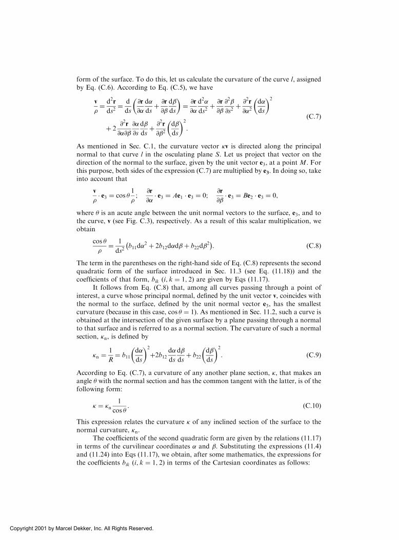
form of the surface. To do this, let us calculate the curvature of the curve l, assignedby Eq. (C.6). According to Eq. (C.5), we have

v

�¼ d2r

ds2¼ d

ds

@r

@

d

dsþ @r

@

d

ds

� �¼ @r

@

d2

ds2þ @r

@

@2

@s2þ @2r

@2d

ds

� �2

þ 2@2r

@@

@

@s

d

dsþ @2r

@2d

ds

� �2

:

ðC:7Þ

As mentioned in Sec. C.1, the curvature vector �v is directed along the principalnormal to that curve l in the osculating plane S. Let us project that vector on thedirection of the normal to the surface, given by the unit vector e3, at a point M. Forthis purpose, both sides of the expression (C.7) are multiplied by e3. In doing so, takeinto account that

v

�� e3 ¼ cos �

1

�;

@r

@� e3 ¼ Ae1 � e3 ¼ 0;

@r

@� e3 ¼ Be2 � e3 ¼ 0;

where � is an acute angle between the unit normal vectors to the surface, e3, and tothe curve, v (see Fig. C.3), respectively. As a result of this scalar multiplication, weobtain

cos �

�¼ 1

ds2b11d

2 þ 2b12ddþ b22d2

� �: ðC:8Þ

The term in the parentheses on the right-hand side of Eq. (C.8) represents the secondquadratic form of the surface introduced in Sec. 11.3 (see Eq. (11.18)) and thecoefficients of that form, bik ði; k ¼ 1; 2Þ are given by Eqs (11.17).

It follows from Eq. (C.8) that, among all curves passing through a point ofinterest, a curve whose principal normal, defined by the unit vector v, coincides withthe normal to the surface, defined by the unit normal vector e3, has the smallestcurvature (because in this case, cos � ¼ 1). As mentioned in Sec. 11.2, such a curve isobtained at the intersection of the given surface by a plane passing through a normalto that surface and is referred to as a normal section. The curvature of such a normalsection, �n, is defined by

�n ¼ 1

R¼ b11

d

ds

� �2

þ2b12d

ds

d

dsþ b22

d

ds

� �2

: ðC:9Þ

According to Eq. (C.7), a curvature of any another plane section, �, that makes anangle � with the normal section and has the common tangent with the latter, is of thefollowing form:

� ¼ �n1

cos �: ðC:10Þ

This expression relates the curvature � of any inclined section of the surface to thenormal curvature, �n.

The coefficients of the second quadratic form are given by the relations (11.17)in terms of the curvilinear coordinates and . Substituting the expressions (11.4)and (11.24) into Eqs (11.17), we obtain, after some mathematics, the expressions forthe coefficients bik ði; k ¼ 1; 2Þ in terms of the Cartesian coordinates as follows:


b11 ¼1

!

@2X@2

@2Y@2

@2Z@2

@X@

@Y@

@Z@

@X@

@Y@

@Z@

; b22 ¼

1

!

@2X@2

@2Y@2

@2Z@2

@X@

@Y@

@Z@

@X@

@Y@

@Z@

;

b12 ¼1

!

@2X@@

@2Y@@

@2Z@@

@X@

@Y@

@Z@

@X@

@Y@

@Z@

; ðC:11Þ

where

! ¼ffiffiffiffiffiffiffiffiffiffiffiffiffiffiffiffiffiffiffiffiffiffiffiffia11a22 � a212

q: ðC:12Þ

It was mentioned in Sec. 11.3 that the directions of principal curvatures areorthogonal. To prove this, it is sufficient to verify that an angle between the twoprincipal directions is equal to �=2 at any point of the surface. Assume that thesedirections have been found and that they are characterized by the following quan-tities:

�1 ¼d

dand �2 ¼

�

�:

The increments of the position vector r along each of these two directions can bewritten in the following form:

dr ¼ r;dþ r;d; �r ¼ r;�þ r;�:

If these two directions are orthogonal, then

ðdr � �rÞ ¼ ðr; � r;Þd�þ ðr; � r;Þd�þ ðr; � r;Þðd�þ �dÞ ¼ 0; ðC:13Þor dividing the above equality by d�, and taking into account the notations of Eqs(11.10),

a11 þ a12ð�1 þ �2Þ þ a22ð��2Þ ¼ 0: ðC:14ÞSubstituting for �1 and �2 from Eq. (11.20) into Eq. (C.14), we find that the ortho-gonality condition is identically satisfied. Thus, the directions of the principal cur-vatures are orthogonal.

C.3 DERIVATIVES OF UNIT COORDINATE VECTORS

Consider two neighboring points M and M1 on the coordinate line , separated by asmall distance �s. Let e3 and e3 þ�e3 be the inward normal unit vectors at thosepoints, directed toward the center of curvature O, as shown in Fig. C.4. The corre-sponding principal radius of curvature of the surface is denoted by R1.

It is seen from the above figure that an increment vector �e3, obtained bymoving e3 from point M to point M1, is parallel to the chord MM1, and in the limit


when M ! M1; this increment becomes parallel to the tangent vector e1. Thus, �e3can be represented in the form

�e3 ¼ � �e3 e1: ðC:15Þ

The negative sign in the above equation indicates that the vector �e3 points in thenegative direction of the -coordinate axis (see Fig. 11.7).

The magnitude of this increment can be found from similarity of the triangles(Fig. C.4), i.e.,

�e3 e3 ¼ MM1

R1

: ðC:16Þ

Substituting Eq. (C.15) into Eq. (C.16), and noting that e3 ¼ 1 and

MM1 ¼ �s ¼ A�, yields

�e3

�¼ � A

R1

e1: ðC:17Þ

Taking the limit of both sides of the above relation as �! 0, one obtains

de3d

¼ � A

R1

e1: ðC:18Þ

Similarly,

de3d

¼ � B

R2

e2: ðC:19Þ

Now we can proceed to determine the derivatives of the tangent unit vectors, e1 ande2, with respect to and . Obviously the following equality holds:

@r;@

¼ @r;@

;

because it is equivalent to the following identity:

Fig. C.4


@2r

@@¼ @2r

@@:

From the above, and taking into account the relations (11.10) and (11.12), we obtain

@

@Ae1ð Þ ¼ @

@Be2ð Þ: ðC:20aÞ

The derivatives of the unit tangent vectors can be expressed in terms of their com-ponents along the triad of the unit vectors e1; e2; and e3. Notice that the derivative ofany unit tangent vector is normal to the vector itself, so that there are no componentsin the direction of the vector being differentiated. Let us prove this statement.Consider the following scalar product of the two unit tangent vectors in the curvi-linear coordinate system:

ei � ej ¼ �ij�ij ¼ 1 if i ¼ j;�ij ¼ 0 if i 6¼ j;

where i; j ¼ 1; 2; and 3. Differentiating the scalar product of the two unit vectorswith respect to k (k ¼ 1 or 2) yields

ei � ej� �

;k¼ 0;

from which

ej � ei;k þ ei � ej;k ¼ 0:

Setting i ¼ j yields

2 ei � ei;k� � ¼ 0;

as was to be shown.First, determine the derivative @e1=@. As follows from the above, this deriva-

tive can be represented in terms of its components in the directions of e2 and e3 only.We have

@e1@

¼ qe2 þ te3; ðC:20bÞ

where unknown components q and t represent the projections of the vector @e1=@on the directions of e2 and e3, respectively. It is known from the vector algebra thatthe projection of any vector a on the direction of a vector b is equal to the scalarproduct of a � b. Therefore, the component q is given by

q ¼ e2 �@e1@

� �¼ @

@e2 � e1ð Þ � e1 �

@e2@

� �¼ �e1 �

@e2@

ðC:21Þ

@

@e2 � e1ð Þ ¼ 0 because e2 is normal to e1

� �:

It follows from Eq. (C.20a) that

@

@ðBe2Þ ¼ B

@e2@

þ e2@B

@¼ @

@ðAe1Þ: ðC:22Þ

Thus,


@e2@

¼ 1

B

@ðAe1Þ@

� 1

B

@B

@e2: ðC:23Þ

From Eqs (C.21) and (C.22), one obtains the following:

q ¼ �A

Be1 �

@e1@

� �� 1

B

@A

@e1 � e1ð Þ:

Since e1 � e1 ¼ 1 and e1 � @e1@ ¼ 0, the above equation becomes

q ¼ � 1

B

@A

@: ðC:24Þ

Let us proceed to determining the component t in Eq. (C.20b). We have

t ¼ e3 �@e1@

¼ @

@ðe3 � e1Þ � e1 �

@e3@

� �¼ �e1 �

@e3@

ðC:25Þ

(because e3 � e1 ¼ 0). Using Eq. (C.18), we obtain

t ¼ �e1 � � A

R1

e1

� �¼ A

R1

: ðC:26Þ

Finally, substituting for q and t from Eqs (C.24) and (C.26), we obtain the follow-ing expression for the derivative @e1=@:

@e1@

¼ � 1

B

@A

@e2 þ

A

R1

e3: ðC:27Þ

Determine the derivative @e1=@. Again, we can represent the above derivativein terms of its components along the unit vectors e2 and e3:

@e1@

¼ qe2 þ te3; ðC:28Þ

where q and t are the unknown projections of @e1=@ on the directions of the unitvectors e2 and e3, respectively (as mentioned previously, the projection of @e1=@ one1 is zero).

By analogy with Eq. (C.21), we can write

q ¼ e2 �@e1@:

Using the identity (C.20), the above relation appears as follows:

q ¼ � 1

A

@A

@e1 � e2ð Þ þ 1

Ae2 �

@ Be2ð Þ@

� �¼ 1

A

@B

@:

Thus

q ¼1

A

@B

@: ðC:29Þ

Similarly,

t ¼ e3 �@e1@

� �¼ @

@e1 � e3ð Þ � e1 �

@e3@

¼ �e1 �@e3@:


Using Eq. (C.19), we can rewrite the above relation as follows:

t ¼ �e1 � � B

R1

e2

� �¼ B

R1

e1 � e2ð Þ ¼ 0:

Finally, substituting t ¼ 0 and for q, from Eq. (C.29) into Eq. (C.28), we obtain thefollowing expression for the derivative @e1=@:

@e1@

¼ 1

A

@B

@e2: ðC:30Þ

In a similar manner, one can determine the derivatives @e2=@ and @e2=@. The finalexpressions for the derivatives of the unit vectors with respect to and are given byEqs (11.26).

C.4 VERIFICATION OF CODAZZI AND GAUSS EQUATIONS

Using the evident identity

@2e3@@

¼ @2e3@@

;

and substituting the expressions (11.26) for e3; and e3; into the above, we obtain thefollowing:

@

@

A

R1

e1

� �¼ @

@

B

R2

e2

� �or

@

@

A

R1

� �e1 þ

A

R1

@e1@

¼ @

@

B

R2

� �e2 þ

B

R2

@e2@:

ðC:31Þ

Replacing @e1=@ and @e2=@ in the above by their values from Eqs (11.26) andtransferring all the terms in Eq. (C.31) to the left-hand side, one finds the followingequation:

@

@

A

R1

� �� 1

R2

@A

@

� �� e1 �

@

@

B

R2

� �� 1

R1

@B

@

� �e2 ¼ 0: ðC:32Þ

This vector equation is equivalent to the two scalar equations (11.27a), called theconditions of Codazzi.

Next, consider another identity

@2e1@@

¼ @2e1@@

:

This identity, using the relations (11.26), can be reduced to the following:

@

@

1

A

@B

@

� �þ @

@

1

B

@A

@

� �þ AB

R1R2

� �e2 þ

@

@

A

R1

� �� 1

R2

@A

@

� �e3 ¼ 0: ðC:33Þ

The above vector equation may only be satisfied if the terms in the square bracketsare equal to zero. This gives the two scalar equations, but only the first of these isnew, while the second equation coincides with one of the relationships (Eq. (11.27a)).So, equating the first term in the square brackets to zero, one obtains Eq. (11.27b),known as the condition of Gauss.


Similarly, it is found that the identity

@2e2@@

¼ @2e2@@

involves no new relationships between the parameters A;B;R1; and R2.


Thin Plates And Shells Theory Analysis And Applications

Documents

Transcript of Thin Plates And Shells Theory Analysis And Applications