MODULE TITLE: FURTHER AERODYNAMICS AND PROPULSION ANDCOMPUTATIONAL TECHNIQUE

ASSIGNMENT TITLE: AEROFOIL THEORY

NAME OF LECTURER: P.E. BARRINGTON

DATE: 14TH NOVEMBER 2013

NAME OF STUDENT: CHRIS CHIKADIBIA ESIONWU

COURSE: AEROSPACE ENGINEERING, ASTRONAUTICS AND SPACETECHNOLOGY

ROUTE: NUEAS

STUDENT 1D: K1114745

1 | C h r i s E s i o n w u - K 1 1 1 4 7 4 5

TASKS

1. Use thin aerofoil theory to determine the zero lift angle of attack and the moment coefficient about the aerodynamic centrefor a NACA 23012 aerofoil. Clearly show how your results wereobtained.

solution

Fig.1: a diagram of NACA 23012 aerofoil.9

NACA 23012 is a cambered aerofoil. Its first integer is the amount of camber in items of relative magnitude of design lift coefficient1, design lift coefficient = 0.3.

The second and third integer is the distance from the leading edge to the location of the maximum camber1, which is 30/2 % = 15% of chord. The last two integers is the section thickness in percentage of chord1, that is, maximum thickness = 12%.

For a NACA 23012 aerofoil, the mean camber line is given below:

zc={

k16 {x3−3mx2+m2 (3−m)x },0<x<m,m<x<1(equ.1)

2 | C h r i s E s i o n w u - K 1 1 1 4 7 4 5

zc=

k1m3

6(1−x )(equ.2)

In figure 1, where the chord location x and y are normalised by the chord, m is chosen so that maximum camber occurs at x = p, that is p= 0.3/2 = 0.15 and m = 0.2025.

(K1 is the desired lift coefficient, for NACA 23012, k1 = 15.957).4

Therefore, substituting p = 15.957, x = x/c and m = 0.2025 in equ.1 and equ.2

zc=2.6595 [3(xc )

3

−0.6075(xc )2

+0.1147(xc )]for0≤xc ≤0.2025

zc=0.02208(1−

xc )for0.2025≤ xc ≤1.0

In figure 1, differentiating z with respect to x, dz/dx is thus:

dzdx=2.6595[3(xc )

2

−1.215(xc )+0.1147 ]for0≤ xc ≤0.2025

dz=−0.0228for0.2025≤ x

c≤1.0

converting¿xθandtakingx=(c2)¿

dzdx

=2.6595¿

3 | C h r i s E s i o n w u - K 1 1 1 4 7 4 5

= 0.6840−2.3736cosθ+1.995cos2θfor0≤θ≤0.9335rad

¿=−0.02208for0.9335≤θ≤π

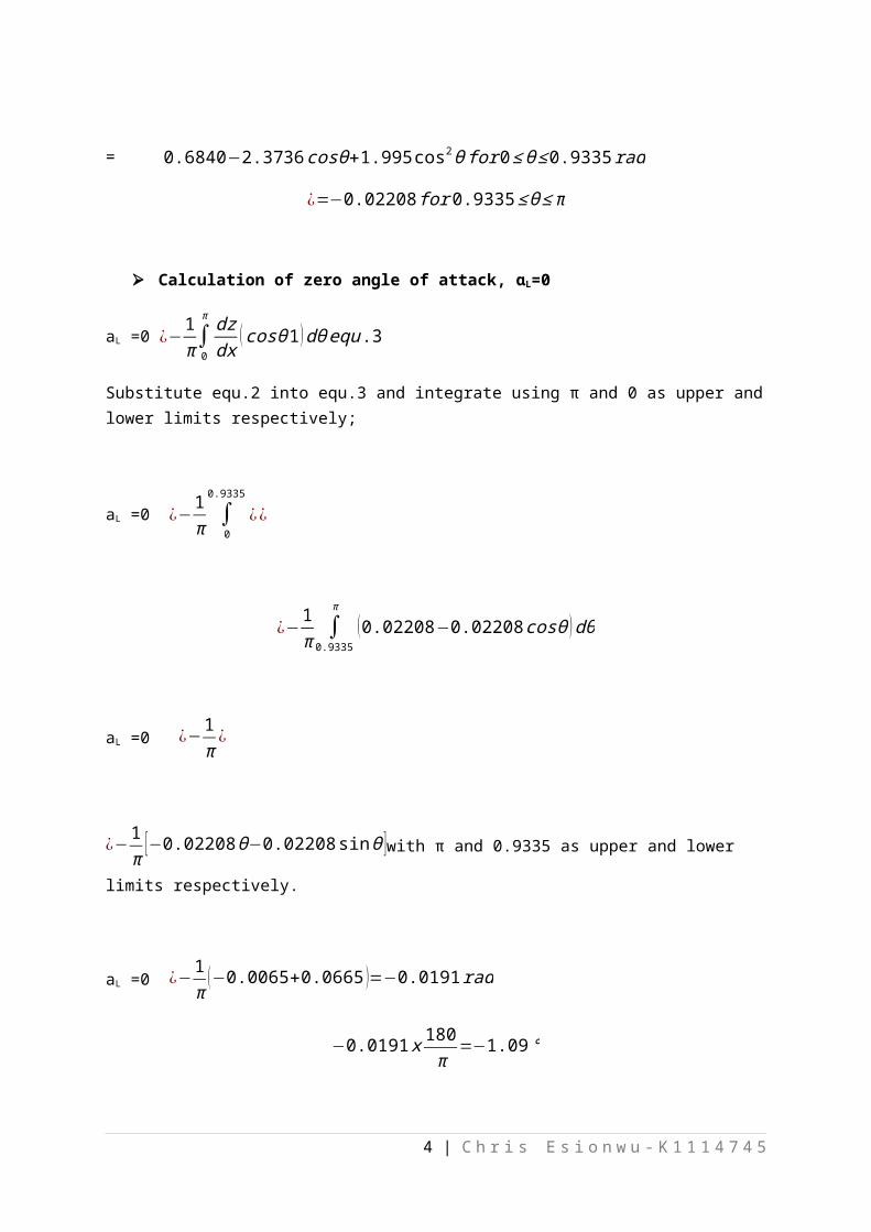
Calculation of zero angle of attack, ɑL=0

aL =0 ¿−1π∫0

π dzdx (cosθ1)dθequ.3

Substitute equ.2 into equ.3 and integrate using π and 0 as upper andlower limits respectively;

aL =0 ¿−1π ∫

0

0.9335

¿¿

¿−1π ∫

0.9335

π

(0.02208−0.02208cosθ )dθ

aL =0 ¿−1π

¿

¿−1π [−0.02208θ−0.02208sinθ ]with π and 0.9335 as upper and lower

limits respectively.

aL =0 ¿−1π (−0.0065+0.0665 )=−0.0191rad

−0.0191x 180π

=−1.09°

4 | C h r i s E s i o n w u - K 1 1 1 4 7 4 5

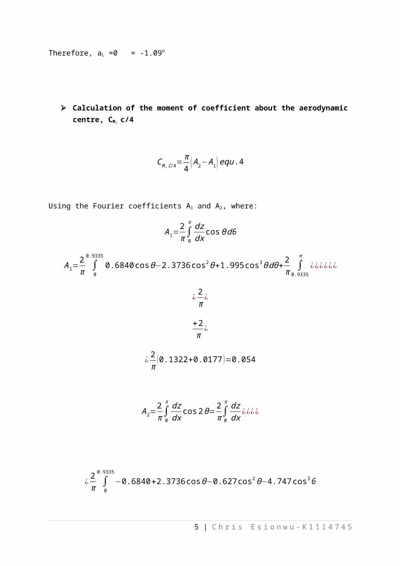
Therefore, aL =0 = -1.09o

Calculation of the moment of coefficient about the aerodynamiccentre, CM, c/4

CM,C/4=π4 (A2−A1)equ.4

Using the Fourier coefficients A1 and A2, where:

A1=2π∫0

π dzdx cosθdθ

A1=2π ∫

0

0.9335

0.6840cosθ−2.3736cos2θ+1.995cos3θdθ+2π ∫

0.9335

π

¿¿¿¿¿¿

¿2π

¿

+2π

¿

¿ 2π (0.1322+0.0177 )=0.054

A2=2π∫0

π dzdx cos2θ=

2π∫0

π dzdx ¿¿¿¿

¿2π ∫

0

0.9335

−0.6840+2.3736cosθ−0.627cos2θ−4.747cos3θ

5 | C h r i s E s i o n w u - K 1 1 1 4 7 4 5

+3.99cos4θ¿dθ¿+2π ∫

0.9335

π

¿¿

recallthat∫cos4θdθ=14cos3θsinθ+

38

¿¿¿¿¿

Therefore, A2=2π

{−0.6840θ+2.373sinθ−0.628(12 )¿−4.747(13)sinθ ¿¿

+2π

¿

¿2π (0.11384+0.01056 )=0.0792

Thus, A1 = 0.0954 and A2 = 0.0792

Substitute A1 and A2 into equ.4

CM,C/4=π4

(0.092−0.0954 )

CM,C/4=−0.0127

6 | C h r i s E s i o n w u - K 1 1 1 4 7 4 5

2. Compare your results for question 1 with results obtained using Javafoil and experimental results published in Theory ofWing Sections. Comment on any discrepancy.

A graph of CL, CM plotted against the angle of attack (α) found in page 498, appendix 1V of the Theory of Wing Sections by I L Abbott and A.E. Von Doenhoff; figure 2, CL versus α shows that at zero lift, a0 = - 1.10o.

Also looking at the lower part of the graph, CM, C/4 versus α, figure 2, the little constant dots indicates the point where CM does not vary with a (i.e. the aerodynamic centre, AC), this point reads thatCM, C/4 at AC = -0.01.

7 | C h r i s E s i o n w u - K 1 1 1 4 7 4 5

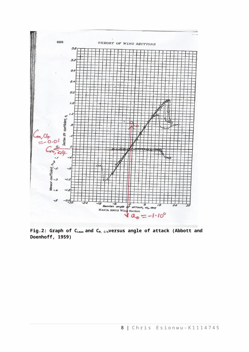
Fig.2: Graph of CLmax and CM, C/4versus angle of attack (Abbott and Doenhoff, 1959)

8 | C h r i s E s i o n w u - K 1 1 1 4 7 4 5

Fig.3: Print Screen of a Javafoil reading showing a table of aerodynamic characteristics of NACA 23012 aerofoil.

According to fig.3 above, at zero lift, α 0 = -1.60 and CM, C/4 = -0.22 because the reading for CM did not change even after angle of attackincreased from -1.6 to -1.5 degrees.The table below shows the values of a0 and CM, C/4 , from the thin theory, javafoil result and experimental result as given in the book; Theory of Wing Sections, pages 129and 179 (Abott, ibid).

Source of Result α0 (degrees) CM at ACThin aerofoil theory -1.09 -0.0127Javafoil -1.60 -0.2200Experimental -1.10 -0.01

Fig.4: a table showing the values for angle of attack and CM, C/4

9 | C h r i s E s i o n w u - K 1 1 1 4 7 4 5

According to the table above, there is no discrepancy between the thin aerofoil theory and experimental results, that is, these data are concurrent. This is a proof that the analytical process of swapping the chord line with a vortex sheet, with the flow tangency condition evaluated along the camber line is correct.2 These resultsare different from the one of javafoil because of human error; such as rounding error during calculations and parallax error during experiment.

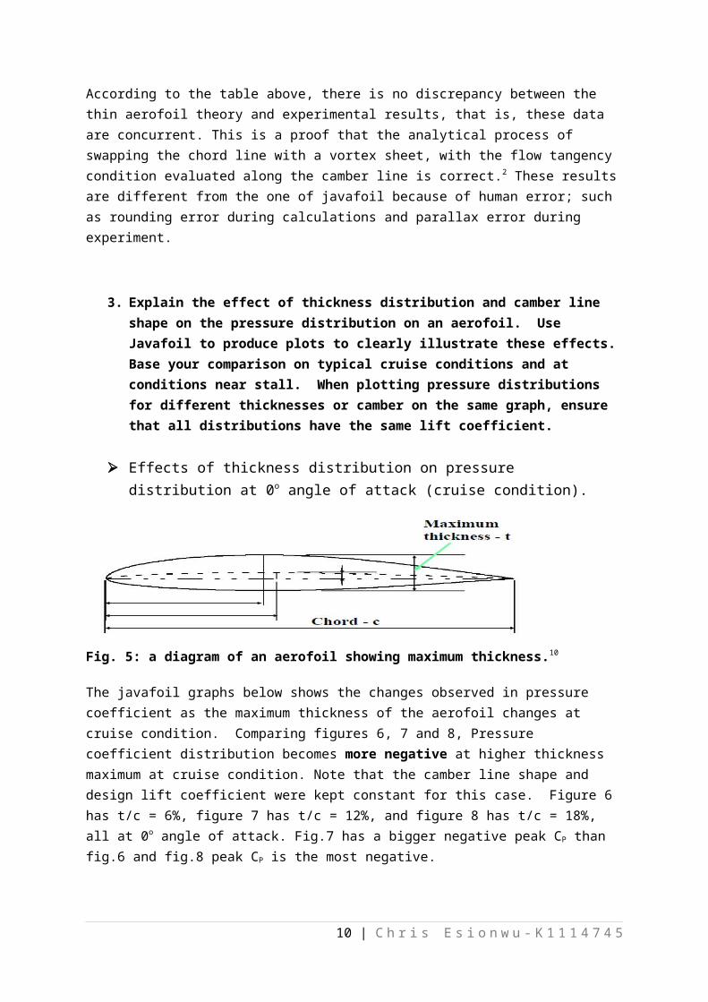
3. Explain the effect of thickness distribution and camber line shape on the pressure distribution on an aerofoil. Use Javafoil to produce plots to clearly illustrate these effects.Base your comparison on typical cruise conditions and at conditions near stall. When plotting pressure distributions for different thicknesses or camber on the same graph, ensure that all distributions have the same lift coefficient.

Effects of thickness distribution on pressure distribution at 0o angle of attack (cruise condition).

Fig. 5: a diagram of an aerofoil showing maximum thickness.10

The javafoil graphs below shows the changes observed in pressure coefficient as the maximum thickness of the aerofoil changes at cruise condition. Comparing figures 6, 7 and 8, Pressure coefficient distribution becomes more negative at higher thickness maximum at cruise condition. Note that the camber line shape and design lift coefficient were kept constant for this case. Figure 6 has t/c = 6%, figure 7 has t/c = 12%, and figure 8 has t/c = 18%, all at 0o angle of attack. Fig.7 has a bigger negative peak CP than fig.6 and fig.8 peak CP is the most negative.

10 | C h r i s E s i o n w u - K 1 1 1 4 7 4 5

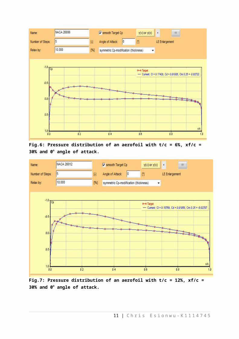
Fig.6: Pressure distribution of an aerofoil with t/c = 6%, xf/c = 30% and 0o angle of attack.

Fig.7: Pressure distribution of an aerofoil with t/c = 12%, xf/c = 30% and 0o angle of attack.

11 | C h r i s E s i o n w u - K 1 1 1 4 7 4 5

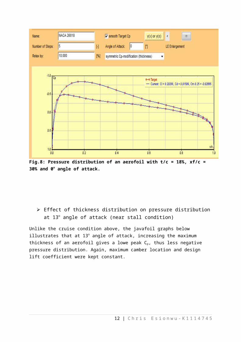
Fig.8: Pressure distribution of an aerofoil with t/c = 18%, xf/c = 30% and 0o angle of attack.

Effect of thickness distribution on pressure distributionat 13o angle of attack (near stall condition)

Unlike the cruise condition above, the javafoil graphs below illustrates that at 13o angle of attack, increasing the maximum thickness of an aerofoil gives a lowe peak Cp, thus less negative pressure distribution. Again, maximum camber location and design lift coefficient were kept constant.

12 | C h r i s E s i o n w u - K 1 1 1 4 7 4 5

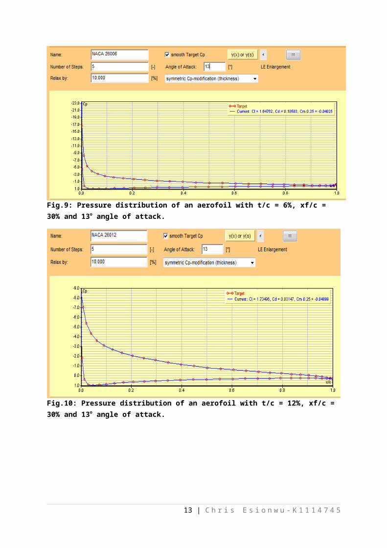
Fig.9: Pressure distribution of an aerofoil with t/c = 6%, xf/c = 30% and 13o angle of attack.

Fig.10: Pressure distribution of an aerofoil with t/c = 12%, xf/c = 30% and 13o angle of attack.

13 | C h r i s E s i o n w u - K 1 1 1 4 7 4 5

Fig.11: Pressure distribution of an aerofoil with t/c = 18%, xf/c = 30% and 13o angle of attack.

Effects of chamber line shape on pressure distribution at 0o angle of attack (cruise condition)

Fig. 12: a diagram of an aerofoil showing camber line shape.10

14 | C h r i s E s i o n w u - K 1 1 1 4 7 4 5

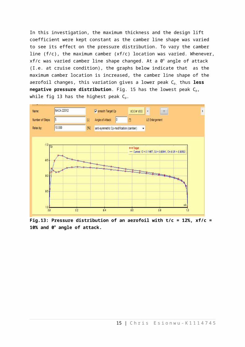
In this investigation, the maximum thickness and the design lift coefficient were kept constant as the camber line shape was varied to see its effect on the pressure distribution. To vary the camber line (f/c), the maximum camber (xf/c) location was varied. Whenever,xf/c was varied camber line shape changed. At a 0o angle of attack (I.e. at cruise condition), the graphs below indicate that as the maximum camber location is increased, the camber line shape of the aerofoil changes, this variation gives a lower peak Cp, thus less negative pressure distribution. Fig. 15 has the lowest peak Cp, while fig 13 has the highest peak Cp.

Fig.13: Pressure distribution of an aerofoil with t/c = 12%, xf/c = 10% and 0o angle of attack.

15 | C h r i s E s i o n w u - K 1 1 1 4 7 4 5

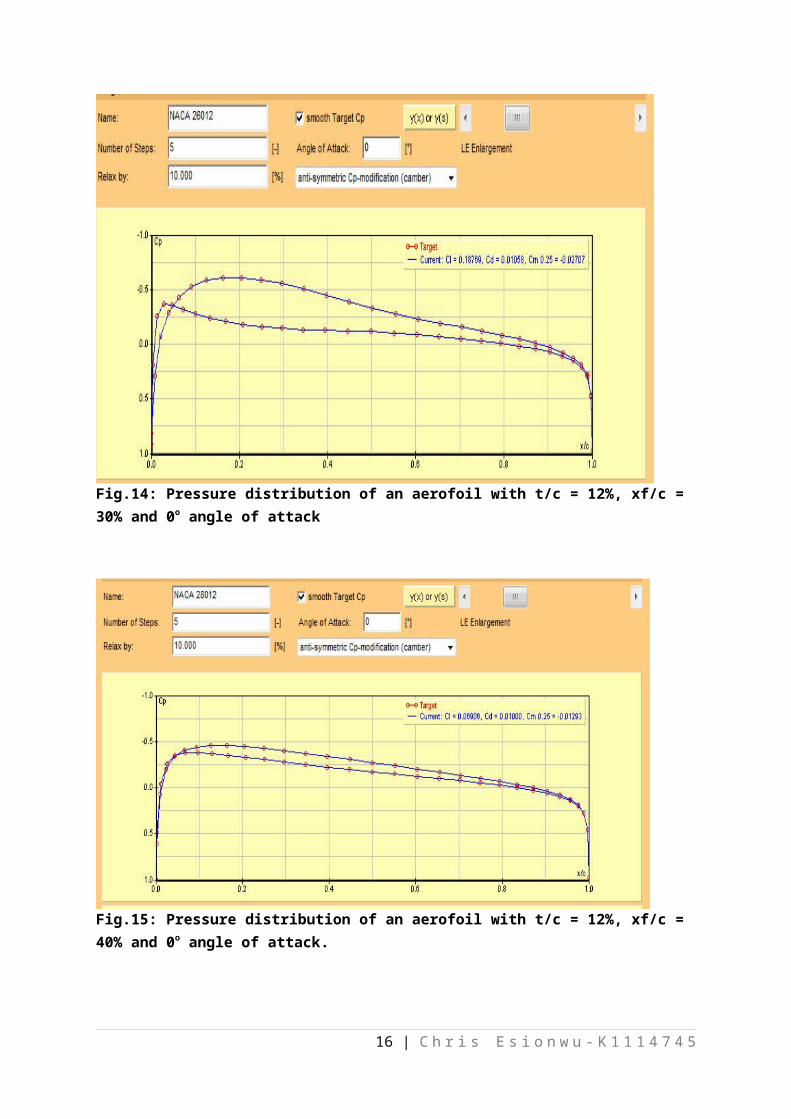
Fig.14: Pressure distribution of an aerofoil with t/c = 12%, xf/c = 30% and 0o angle of attack

Fig.15: Pressure distribution of an aerofoil with t/c = 12%, xf/c = 40% and 0o angle of attack.

16 | C h r i s E s i o n w u - K 1 1 1 4 7 4 5

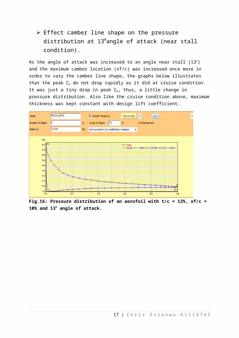
Effect camber line shape on the pressure distribution at 130angle of attack (near stall condition).

As the angle of attack was increased to an angle near stall (13o) and the maximum camber location (xf/c) was increased once more in order to vary the camber line shape, the graphs below illustrates that the peak Cp do not drop rapidly as it did at cruise condition. It was just a tiny drop in peak Cp, thus, a little change in pressure distribution. Also like the cruise condition above, maximumthickness was kept constant with design lift coefficient.

Fig.16: Pressure distribution of an aerofoil with t/c = 12%, xf/c = 10% and 13o angle of attack.

17 | C h r i s E s i o n w u - K 1 1 1 4 7 4 5

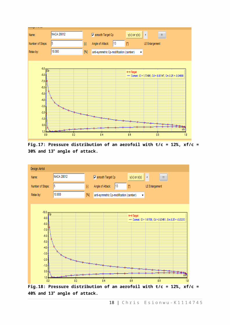
Fig.17: Pressure distribution of an aerofoil with t/c = 12%, xf/c = 30% and 13o angle of attack.

Fig.18: Pressure distribution of an aerofoil with t/c = 12%, xf/c = 40% and 13o angle of attack.

18 | C h r i s E s i o n w u - K 1 1 1 4 7 4 5

4. In no more the 500 words, discuss the key desirable characteristics of an aerofoil for a low speed general aviation aircraft and how these are achieved. Please ensure that you cite any references correctly.

A good aerofoil at low speed should have a minimum lift-to-drag ratio and a high maximum lift coefficient. This can be achieved with following ways:

1. An aerofoil with a flattened peak pressure coefficient near the nose: This kind of aerofoil is designed to have a large leading-edge radius.2 For example, the LS (1)-0417 aerofoil; 0.08c standard has this desired feature compared to the 0.02c standard which does not.2

The aerofoil is designed to have a high aerodynamic loading inthe bottom surface. This is achieved by designing a cusped trailing edge which increases the camber, and as such, an increase in the aerodynamic loading in that location.2 A cusped trailing edge and a large leading-edge radius design on an aerofoil, do not allow flow separation above the top surface at a high angle of attack, therefore achieving a higher value of maximum lift coefficient. Also, since there isno flow separation, stall is reduced, and there will be a significant decrease in drag due to pressure drag.2

A typical example is the NASA LS (1)-0417 which as a higher CLmax than NACA 2412. When NASA noticed this feature they designed more of NASA LS (1) 04xx series which all have an approximate 30% increase in Clmax. There is a 50% increase Lift/Drag (L/D) ratio at a CL of 1.0; a typical climb lift for general aviation aircraft. This resulted to highly improved climb performance.2

2. Another way of increasing maximum lift coefficient is to design the aerofoil with split flaps instead using plain flaps. Split flaps are formed by deflecting the aft portion ofthe lower surface about a hinge point on the surface at the forward edge of the deflected location (Abbott, ibid).

19 | C h r i s E s i o n w u - K 1 1 1 4 7 4 5

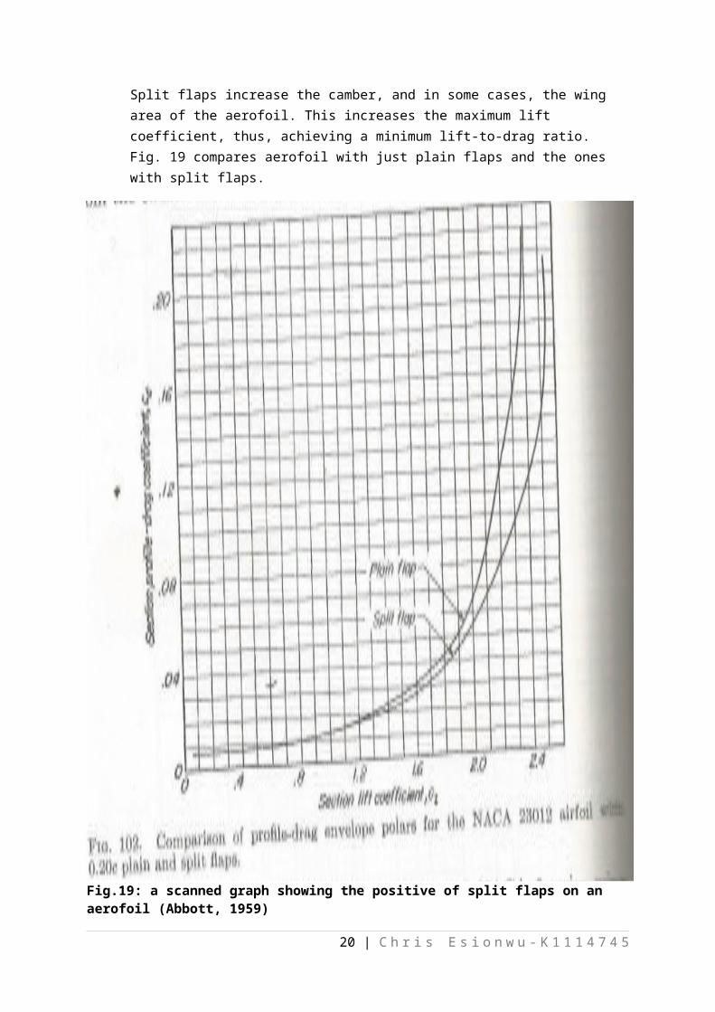
Split flaps increase the camber, and in some cases, the wing area of the aerofoil. This increases the maximum lift coefficient, thus, achieving a minimum lift-to-drag ratio. Fig. 19 compares aerofoil with just plain flaps and the ones with split flaps.

Fig.19: a scanned graph showing the positive of split flaps on an aerofoil (Abbott, 1959)

20 | C h r i s E s i o n w u - K 1 1 1 4 7 4 5

3. Including slotted flaps on an aerofoil will also reduce L/D ratioand increase CLmax. This process adds slots between the main portion of the wing section and the deflected flap; this increases the camber, and in most cases increases the chord of the section. The result of this design delays low separation over the flap, and so provides boundary layer control, thus, reducing L/D ratio and increasing CLmax. Figure 20 has a table showing the positive effects of slotted flaps on the L/D ratio and CLmax.

Fig.20: a scanned table showing the positive effects of slots on an aerofoil (Abbott, 1959)

21 | C h r i s E s i o n w u - K 1 1 1 4 7 4 5

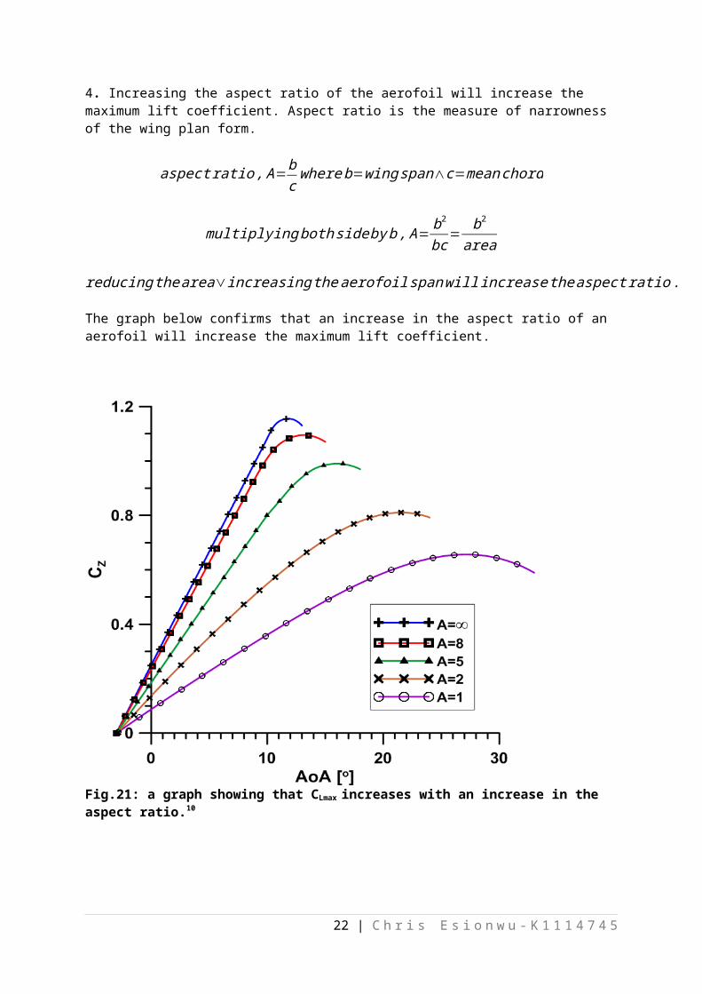
4. Increasing the aspect ratio of the aerofoil will increase the maximum lift coefficient. Aspect ratio is the measure of narrowness of the wing plan form.

aspectratio,A=bcwhereb=wingspan∧c=meanchord

multiplyingbothsidebyb,A=b2

bc=b2

area

reducingthearea∨increasingtheaerofoilspanwillincreasetheaspectratio.

The graph below confirms that an increase in the aspect ratio of an aerofoil will increase the maximum lift coefficient.

Fig.21: a graph showing that CLmax increases with an increase in the aspect ratio.10

22 | C h r i s E s i o n w u - K 1 1 1 4 7 4 5

REFERENCES

1. Abbott, I.H. and Von Doenhoff, A.E. (1959) Theory of Wing Section. USA: Courier Corporation. ISBN-13: 978-0-486-60586-9

2. Anderson, J.D. (2011) Fundamentals of Aerodynamics. 5th Edition. USA: McGraw Hill. ISBN: 978-0-07-339810-5

3. Houghton, E.L. and Carpenter, P.W. (2003) Aerodynamics for Engineering Students. 5th Edition. Great Britain: Butterworth-Heinemann.

4. .,(2012) features of NACA 23012 aerofoil {online}. Last accessed on 12th November 2013 at http://en.wikipedia.org/wiki/NACA_23012

5. ,.(1995) Javafoil Applet {online}. Last accessed on 12th November 2013 at http://www.mh-aerotools.de/airfoils/javafoil.htm

6. ,.(2003) Thin Aerofoil Theory {online}. Last accessed on 12th November 2013 at http://www.dept.aoe.vt.edu/~devenpor/aoe5104/19.%20ThinAirfoilTheory.pdf

7. ,.(1998) Applied Aerodynamics, thin aerofoil theory results {online}. Last accessed on 12th November 2013 at http://www.desktop.aero/appliedaero/airfoils1/tatresults.html

8. ,.(2001) Aerofoil Naming Convention {online}. Last accessed on12th November 2013 at http://www.desktopaero.com/appliedaero/appliedaero.html

9. ,.(2010) Aerofoil Tools {online}. Last accessed 13th November 2013 at https://www.google.co.uk/search?

23 | C h r i s E s i o n w u - K 1 1 1 4 7 4 5

q=naca+23012+airfoil&source=lnms&tbm=isch&sa=X&ei=SYCDUsfmEI2Y1AXfpYCQDw&ved=0CAcQ_AUoAQ&biw=1170&bih=850

10. ,.( 2009) Aircraft Wing {online}. Last accessed on 13th November 2013 at http://itlims.meil.pw.edu.pl/zsis/pomoce/BIPOL/BIPOL_1_handout_8A.pdf

24 | C h r i s E s i o n w u - K 1 1 1 4 7 4 5