NETWORK THEORY

Ms. Manjushree Jena

Dept:-Electronics and Telecommunication

MODULE -I

NETWORK TOPOLOGY

1. Introduction: When all the elements in a network are replaces by lines with circles or dots at both ends, configuration is called the graph of the network.

A. Terminology used in network graph:- (i) Path:- A sequence of branches traversed in going from one node to another is

called a path. (ii) Node:- A node point is defined as an end point of a line segment and exits at the

junction between two branches or at the end of an isolated branch. (iii) Degree of a node:- It is the no. of branches incident to it.

2-degree 3-degree

(iv) Tree:- It is an interconnected open set of branches which include all the nodes of the given graph. In a tree of the graph there can‟t be any closed loop.

(v) Tree branch(Twig):- It is the branch of a tree. It is also named as twig. (vi) Tree link(or chord):- It is the branch of a graph that does not belong to the

particular tree. (vii) Loop:- This is the closed contour selected in a graph. (viii) Cut-Set:- It is that set of elements or branches of a graph that separated two parts

of a network. If any branch of the cut-set is not removed, the network remains connected. The term cut-set is derived from the property designated by the way by which the network can be divided in to two parts.

(ix) Tie-Set:- It is a unique set with respect to a given tree at a connected graph containing on chord and all of the free branches contained in the free path formed between two vertices of the chord.

(x) Network variables:- A network consists of passive elements as well as sources of energy . In order to find out the response of the network the through current and voltages across each branch of the network are to be obtained.

(xi) Directed(or Oriented) graph:- A graph is said to be directed (or oriented ) when all the nodes and branches are numbered or direction assigned to the branches by arrow.

(xii) Sub graph:- A graph said to be sub-graph of a graph G if every node of is a node of G and every branch of is also a branch of G.

(xiii) Connected Graph:- When at least one path along branches between every pair of a graph exits , it is called a connected graph.

(xiv) Incidence matrix:- Any oriented graph can be described completely in a compact matrix form. Here we specify the orientation of each branch in the graph and the nodes at which this branch is incident. This branch is called incident matrix.

When one row is completely deleted from the matrix the remaining matrix is called a reduced incidence matrix.

(xv) Isomorphism:- It is the property between two graphs so that both have got same incidence matrix.

B. Relation between twigs and links- Let N=no. of nodes L= total no. of links B= total no. of branches No. of twigs= N-1 Then, L= B-(N-1)

C. Properties of a Tree- (i) It consists of all the nodes of the graph. (ii) If the graph has N nodes, then the tree has (N-1) branch. (iii) There will be no closed path in a tree. (iv) There can be many possible different trees for a given graph depending on the no.

of nodes and branches.

1. FORMATION OF INCIDENCE MATRIX:- This matrix shows which branch is incident to which node. Each row of the matrix being representing the corresponding node of the

graph. Each column corresponds to a branch.

If a graph contain N- nodes and B branches then the size of the incidence matrix [A] will be NXB.

A. Procedure:- (i) If the branch j is incident at the node I and oriented away from the node, =1. In

other words, when =1, branch j leaves away node i.

(ii) If branch j is incident at node j and is oriented towards node i, =-1. In other

words j enters node i. (iii) If branch j is not incident at node i. =0.

The complete set of incidence matrix is called augmented incidence matrix.

Ex-1:- Obtain the incidence matrix of the following graph. a 1 b 2 c

5 4 3

Node-a:- Branches connected are 1& 5 and both are away from the node. Node-b:- Branches incident at this node are 1,2 &4. Here branch is oriented towards the node whereas branches 2 &4 are directed away from the node. Node-c:- Branches 2 &3 are incident on this node. Here, branch 2 is oriented towards the node whereas the branch 3 is directed away from the node. Node-d:- Branch 3,4 &5 are incident on the node. Here all the branches are directed towards the node. So, branch Node 1 2 3 4 5

1 1 0 0 0 1

[ ]= 2 -1 1 0 1 0

3 0 -1 1 0 0

4 0 0 -1 -1 -1

B. Properties:- (i) Algebraic sum of the column entries of an incidence matrix is zero. (ii) Determinant of the incidence matrix of a closed loop is zero.

C. Reduced Incidence Matrix :-

If any row of a matrix is completely deleted, then the remaining matrix is known as reduced Incidence matrix. For the above example, after deleting row, we get

[Ai’]=[

]

Ai’ is the reduced matrix of Ai .

Ex-2: Draw the directed graph for the following incidence matrix. Branch Node 1 2 3 4 5 6 7 1 -1 0 -1 1 0 0 1 2 0 -1 0 -1 0 -1 0 3 1 1 0 0 -1 1 0 4 0 0 1 0 1 0 -1

Solution:- From node

From branch

Tie-set Matrix: Branch 1 2 3 4 5 Loop currents I1 1 0 0 1 1 I2 -1 -1 1 0 -1 Bi= 1 0 0 1 1 = 1 0 0 1 1 -1 -1 1 0 -1 1 1 -1 0 1 Let V1, V2, V3, V4 & V5 be the voltage of branch 1,2,3,4,5 respectively and j1, j2, j3, j4, j5 are current through the branch 1,2,3,4,5 respectively.

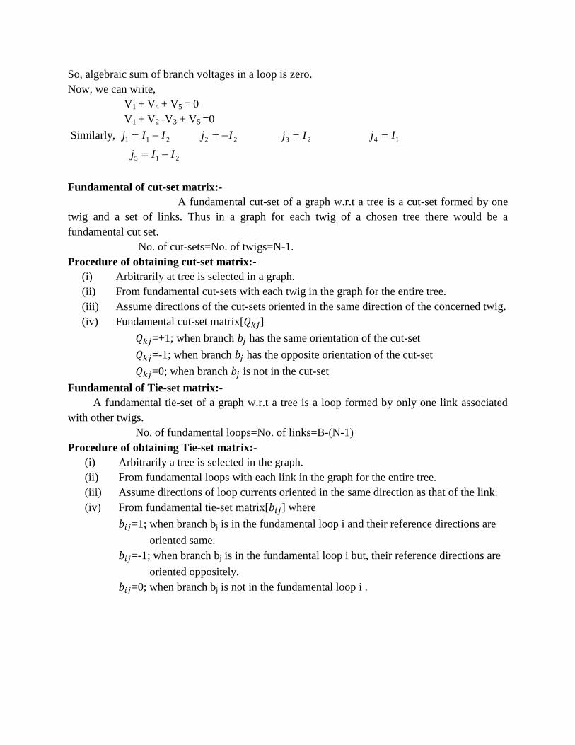
So, algebraic sum of branch voltages in a loop is zero. Now, we can write, V1 + V4 + V5 = 0 V1 + V2 -V3 + V5 =0

Similarly, 211 IIj 22 Ij 23 Ij 14 Ij

215 IIj

Fundamental of cut-set matrix:- A fundamental cut-set of a graph w.r.t a tree is a cut-set formed by one twig and a set of links. Thus in a graph for each twig of a chosen tree there would be a fundamental cut set. No. of cut-sets=No. of twigs=N-1. Procedure of obtaining cut-set matrix:-

(i) Arbitrarily at tree is selected in a graph. (ii) From fundamental cut-sets with each twig in the graph for the entire tree. (iii) Assume directions of the cut-sets oriented in the same direction of the concerned twig. (iv) Fundamental cut-set matrix[ ]

=+1; when branch has the same orientation of the cut-set

=-1; when branch has the opposite orientation of the cut-set

=0; when branch is not in the cut-set

Fundamental of Tie-set matrix:- A fundamental tie-set of a graph w.r.t a tree is a loop formed by only one link associated with other twigs. No. of fundamental loops=No. of links=B-(N-1) Procedure of obtaining Tie-set matrix:-

(i) Arbitrarily a tree is selected in the graph. (ii) From fundamental loops with each link in the graph for the entire tree. (iii) Assume directions of loop currents oriented in the same direction as that of the link. (iv) From fundamental tie-set matrix[ ] where

=1; when branch bj is in the fundamental loop i and their reference directions are

oriented same. =-1; when branch bj is in the fundamental loop i but, their reference directions are

oriented oppositely. =0; when branch bj is not in the fundamental loop i .

Ex-3: Determine the tie set matrix of the following graph. Also find the equation of branch current and voltages.

Solution Tree No. of loops= No. of links= 2 Loop 1 Loop 2 Q1. Draw the graph and write down the tie-set matrix. Obtain the network equilibrium

equations in matrix form using KVL.

Solution

Tie-set 1 2 3 4 5 6 I1 1 0 0 1 -1 0 I2 0 1 0 0 1 -1 I3 0 0 1 -1 0 1

0541 VVV 11 Ij

0652 VVV 22 Ij

0643 VVV 33 Ij

Again, V1= e2 – e2 i4= I1- I3 V2= e3-e2 i5=I2- I1

V4= e4 – e1 i6 = I3- I2 V5=e2- e4

V6= e3- e4

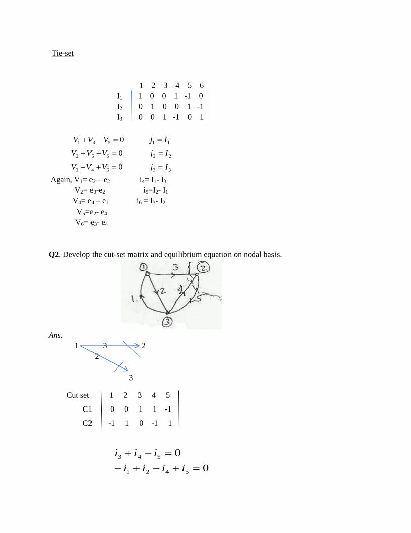
Q2. Develop the cut-set matrix and equilibrium equation on nodal basis.

Ans. 1 3 2 2 3

Cut set 1 2 3 4 5

C1 0 0 1 1 -1

C2 -1 1 0 -1 1

0

0

5421

543

iiii

iii

Ex- Determine the cut-set matrix and the current balance equation of the following graph?

Solution:

Tree

No of twigs=1, 2, 5

Cut-set matrix

branch

cut-set 1 2 3 4 5

C1 0 1 1 0 0

C2 0 0 1 -1 1

C3 1 0 1 -1 0

0

0

0

431

543

32

iii

iii

ii

where, 54321 ,,,, iiiii are respective branch currents.

MODULE- II

LAPLACE TRANSFORM

Definition:

Given a function f (t), its Laplace transform, denoted by F(s) or L[f (t)], is given by,

[ ( )] ( ) ∫ ( )

where, s is a complex variable given by,

* The Laplace transform is an integral transformation of a function f (t) from the time domain

into the complex frequency domain, giving F(s).

Properties of L.T.

(i) Multiplication by a constant:-

Let, K be a constant

F(s) be the L.T. of f(t)

Then; [ ( )] ∫ ( )

∫ ( )

( )

(ii) Sum and Difference:-

Let ( ) & ( ) are the L.T. of the functions ( ) ( ) respectively.

[ ( ) ( )] ( ) ( )

(iii) Differentiation w.r.t. time [Time – differentiation]

[ ( )

] ( ) ( )

Proof

F(S)= [ ( )] ∫ ( )

Let, f(t)=u; then, ( )

&

So, ∫ ( )

= - ∫

( ) (

)

=>F(s)= ( )

+

∫ *

( )

+

=>F(s)= ( )

*

( )

+

=> * ( )

+ s F(s) ( )

(iv) Integration by time “t”:-

[∫ ( )

] ∫ [∫ ( )

]

dt

U=∫ ( )

=> ( )

( )

dv = dt => v=

So, [∫ ( )

] ∫ [ ]

∫

=

∫ ∫ ( )

∫ ( )

[∫ ( )

]

+ ( )

(v) . Differentiation w.r.to S [frequency differentiation]:-

( )

[ ( )

Proof: ( )

∫ ( ) ∫ ( ) *

+ ∫ ( ) ( )

∫ ( )

[ ( )]

(vi) . Integration by „S‟:-

∫ ( )

[ ( )

]

Proof; ∫ ( )

∫ ∫ ( )

∫ ( ) *

+

=∫ ( ) *

+

∫

( )

*

( )

+

(vii). Shifting Theorem:-

(a) L[f(t-1).U(t-a)] = ( )

(b) F(s+a) =L[ ( )]

Proof: L [ ( )] ( ) ( ) ( )

(viii). Initial Value Theorem:-

f( )

( )

[ ( )

proof : sF(s) - f( ) ∫ ( )

=>s(s) = f( ) ∫ ( )

=>

( ) f( )

∫ ( )

( )

(ix). Final Value Theorem:-

F( )

( )

[ ( )]

Proof :- [sf(s) - f( )]

∫ ( )

∫

( )

∫ ( )

( )

=f( ) ( )= ( )

( )

(x). Theorem of periodic functions:-

Let ( ) ( ) ( ) the functions described by 1st ,2nd & 3rd ...cycles of the periodic

function ( ) whose time periods is T.

( ) ( ) ( ) ( ) ( ) ( ) ( )

[ ( )] ( ) ( )

( )

= ( ) [1+ ] = ( )

(xi). Convolution Theorem:

dftftftfsFsFLt

)(0

12121'

(xii). Time Scaling:

a

sF

aatfL

1

MODULE- III

NETWORK THEORY

Documents

Transcript of NETWORK THEORY