Thesis Ambient air quality and human health in India - White ...

1

Thesis

Ambient air quality and human health in India

Luke Alexander Conibear

Supervisors

Dominick V. Spracklen, Stephen R. Arnold, Christoph Knote (external), Alan Williams

Submitted in accordance with the requirements for the degree of Doctor of Philosophy as part of

the integrated PhD/MSc in Bioenergy

Engineering and Physical Sciences Research Council (EPSRC)

Centre for Doctoral Training (CDT) in Bioenergy,

School of Chemical and Process Engineering, Faculty of Engineering, University of Leeds

Institute for Climate and Atmospheric Science,

School of Earth and Environment, Faculty of Environment, University of Leeds

December 2018

2

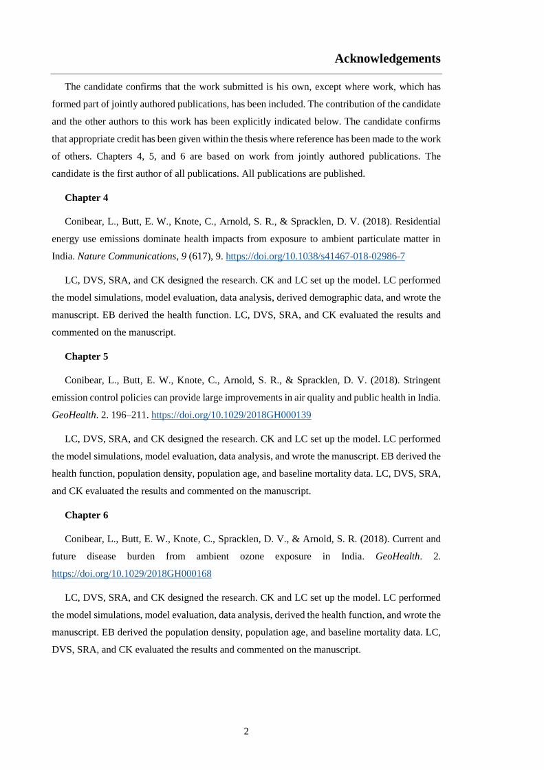
Acknowledgements

The candidate confirms that the work submitted is his own, except where work, which has

formed part of jointly authored publications, has been included. The contribution of the candidate

and the other authors to this work has been explicitly indicated below. The candidate confirms

that appropriate credit has been given within the thesis where reference has been made to the work

of others. Chapters 4, 5, and 6 are based on work from jointly authored publications. The

candidate is the first author of all publications. All publications are published.

Chapter 4

Conibear, L., Butt, E. W., Knote, C., Arnold, S. R., & Spracklen, D. V. (2018). Residential

energy use emissions dominate health impacts from exposure to ambient particulate matter in

India. Nature Communications, 9 (617), 9. https://doi.org/10.1038/s41467-018-02986-7

LC, DVS, SRA, and CK designed the research. CK and LC set up the model. LC performed

the model simulations, model evaluation, data analysis, derived demographic data, and wrote the

manuscript. EB derived the health function. LC, DVS, SRA, and CK evaluated the results and

commented on the manuscript.

Chapter 5

Conibear, L., Butt, E. W., Knote, C., Arnold, S. R., & Spracklen, D. V. (2018). Stringent

emission control policies can provide large improvements in air quality and public health in India.

GeoHealth. 2. 196–211. https://doi.org/10.1029/2018GH000139


the model simulations, model evaluation, data analysis, and wrote the manuscript. EB derived the

health function, population density, population age, and baseline mortality data. LC, DVS, SRA,

and CK evaluated the results and commented on the manuscript.

Chapter 6

Conibear, L., Butt, E. W., Knote, C., Spracklen, D. V., & Arnold, S. R. (2018). Current and

future disease burden from ambient ozone exposure in India. GeoHealth. 2.

https://doi.org/10.1029/2018GH000168


the model simulations, model evaluation, data analysis, derived the health function, and wrote the

manuscript. EB derived the population density, population age, and baseline mortality data. LC,

DVS, SRA, and CK evaluated the results and commented on the manuscript.

https://doi.org/10.1038/s41467-018-02986-7

https://doi.org/10.1029/2018GH000139

https://doi.org/10.1029/2018GH000168

3

I am grateful to my supervisors Dominick V. Spracklen, Stephen R. Arnold, Christoph Knote,

and Alan Williams. I am especially thankful to Dom, Steve, and Christoph for their guidance,

support, and expertise throughout this process. My questions were always answered quickly,

cheerfully, and comprehensively. It has been a pleasure working together. I sincerely appreciate

the support from the EPSRC CDT in Bioenergy (Grant No.EP/L014912/1). I am very grateful to

all in the Bioenergy CDT for the opportunity to have undertaken this PhD.

I acknowledge the use of the many tools and facilities that were fundamental to completing

this thesis. The facilities of the N8 High-Performance Computing Centre of Excellence provided

and funded by the N8 consortium and EPSRC (Grant No.EP/K000225/1), coordinated by the

Universities of Leeds and Manchester. Christoph Knote for helping set up and run the Weather

Research and Forecasting model coupled with Chemistry (WRF-Chem) and his WRFotron scripts

to automate WRF-Chem runs with re-initialised meteorology. Edward W. Butt for deriving health

functions, demographic, and epidemiological data, and the many discussions. The WRF-Chem

preprocessor tools (mozbc, fire_emiss, anthro_emiss, and bio_emiss) provided by the

Atmospheric Chemistry Observations and Modeling (ACOM) laboratory of the National Center

for Atmospheric Research (NCAR). The global model output from Model for Ozone and Related

Chemical Tracers, version 4 (MOZART-4) (http://www.acom.ucar.edu/wrf-chem/mozart.shtml).

The post-processing script wrfout_to_cf.ncl created by Mark Seefeldt at the University of

Colorado (http://foehn.colorado.edu/wrfout_to_cf/). The Aerosol Network (AERONET) staff for

establishing and maintaining the observation sites. The Central Pollution Control Board (CPCB),

Ministry of Environment and Forests, Government of India for the observational data. The

European Centre for Medium-Range Weather Forecasts (ECMWF) for their global reanalyses

(http://apps.ecmwf.int/datasets/). The International Energy Agency (IEA) for the scenario data

from the Energy and Air Pollution, World Energy Outlook Special Report. The boundaries shown

on any maps in this work do not imply any judgement concerning the legal status of any territory

or the endorsement or acceptance of such boundaries.

This copy has been supplied on the understanding that it is copyright material and that no

quotation from the thesis may be published without proper acknowledgement.

http://www.acom.ucar.edu/wrf-chem/mozart.shtml

http://foehn.colorado.edu/wrfout_to_cf/

http://apps.ecmwf.int/datasets/

4

Abstract

700 million Indians have used solid fuels in their homes for the last 30 years, contributing

substantially to air pollutant emissions. The Indian economy and industrial, power generation,

and transport sectors have grown considerably over the last decade, increasing emissions of air

pollutants. These air pollutant emissions have caused present-day concentrations of ambient PM2.5

and O3 in India to be amongst the highest in the world. Exposure to this air pollution is the second

leading risk factor in India, contributing one-quarter of the global disease burden attributable to

air pollution exposure. Air pollutant emissions are predicted to grow extensively over the coming

years in India. Despite the importance of air quality in India, it remains relatively understudied,

and knowledge of the sources and processes causing air pollution is limited.

This thesis aims to understand the contribution of different pollution sources to the attributable

disease burden from ambient air pollution exposure in India and the effects of future air pollution

control pathways. The attributable disease burden from ambient PM2.5 exposure in India is

substantial, where large reductions in emissions will be required to reduce the health burden due

to the non-linear exposure-response relationship. The attributable disease burden from ambient

O3 exposure is larger than previously thought and is of similar magnitude to that from PM2.5 in

the future. Key sources contributing to the present day disease burden from ambient PM2.5 and O3

exposure are the emissions from the residential combustion of solid fuels, land transport, and coal

combustion in power plants. The attributable disease burden is estimated to increase in the future

due to population ageing and growth. Stringent air pollution control pathways are required to

provide critical public health benefits in India in a challenging environment. A key focus should

be to reduce the combustion of solid fuels.

5

Table of Contents

Acknowledgements ...................................................................................................................... 2

Abstract ......................................................................................................................................... 4

Table of Contents ......................................................................................................................... 5

List of Tables ................................................................................................................................ 8

List of Figures ............................................................................................................................. 10

List of Equations ........................................................................................................................ 19

1. Ambient air quality and human health in India ..................................................... 20

1.1. Air pollution pathway ......................................................................................... 20

1.1.1. Fundamentals of ambient air pollution ........................................................ 21

1.1.1.1. Aerosols ..................................................................................................... 21

1.1.1.2. Ozone ......................................................................................................... 23

1.1.2. Air pollution sources .................................................................................... 25

1.1.2.1. Sectors ........................................................................................................ 25

1.1.2.2. Residential emissions and solid fuel use .................................................... 26

1.1.3. Emissions ..................................................................................................... 31

1.1.3.1. Indian emissions ......................................................................................... 31

1.1.3.2. Air pollution control policies in India ........................................................ 32

1.1.4. Concentrations ............................................................................................. 37

1.1.4.1. Present day air pollutant concentrations in India ....................................... 37

1.1.4.2. Meteorological and geographical impacts on Indian air pollution ............. 40

1.1.5. Exposures ..................................................................................................... 42

1.1.5.1. Association and causation .......................................................................... 42

1.1.5.2. Intake fraction ............................................................................................ 43

1.1.6. Doses ............................................................................................................ 44

1.1.7. Health impacts .............................................................................................. 45

1.1.7.1. Health impacts of PM2.5 exposure .............................................................. 46

1.1.7.2. Health impacts of O3 exposure ................................................................... 51

1.1.7.3. Risk assessments to estimate the burden of disease ................................... 53

1.1.7.4. Disease burden from air pollution exposure at the global scale ................. 55

1.1.7.5. Disease burden from air pollution exposure within India .......................... 61

1.1.7.6. Source contributions to the burden of disease from air pollution .............. 64

1.1.7.7. Future disease burden from air pollution in India ...................................... 66

1.2. Summary and Aims ............................................................................................. 67

1.3. Outline ................................................................................................................. 68

2. Methods ....................................................................................................................... 69

6

2.1. Air quality modelling .......................................................................................... 69

2.2. Weather Research and Forecasting Model with Chemistry................................ 70

2.2.1. Model setup ................................................................................................. 72

2.2.2. Physics ......................................................................................................... 72

2.2.3. Chemistry..................................................................................................... 75

2.2.4. Emissions ..................................................................................................... 77

2.3. Exposure-response function for long-term ambient PM2.5 exposure .................. 79

2.4. Exposure-response function for long-term ambient O3 exposure ....................... 84

2.5. Current and future population of India ............................................................... 86

2.6. Sector-specific disease burden ............................................................................ 90

2.7. Uncertainties ....................................................................................................... 90

3. Model evaluation ....................................................................................................... 92

3.1. Metrics ................................................................................................................ 92

3.2. Meteorology........................................................................................................ 93

3.3. Ambient surface PM2.5 concentrations ............................................................... 97

3.4. Aerosol optical depth ........................................................................................ 100

3.5. Ambient surface O3 concentrations .................................................................. 102

4. Residential energy use emissions dominate health impacts from exposure to

ambient particulate matter in India ....................................................................................... 105

4.1. Abstract ............................................................................................................. 105

4.2. Introduction ...................................................................................................... 105

4.3. Results .............................................................................................................. 106

4.3.1. The contribution of emission sectors to ambient PM2.5 concentrations ..... 106

4.3.2. Premature mortality due to ambient PM2.5 exposure ................................. 109

4.3.3. The contribution of emission sectors to the disease burden ...................... 111

4.4. Conclusion ........................................................................................................ 114

5. Stringent emission control policies can provide large improvements in air quality

and public health in India ....................................................................................................... 115

5.1. Abstract ............................................................................................................. 115

5.2. Introduction ...................................................................................................... 115

5.3. Specific methods............................................................................................... 117

5.3.1. Air pollution control pathways .................................................................. 117

5.3.2. Health impact estimates ............................................................................. 119

5.4. Results .............................................................................................................. 119

5.4.1. Impact of scenarios on ambient PM2.5 concentrations in India .................. 119

5.4.2. Indian disease burden under air pollution control pathways ..................... 121

5.4.3. Sensitivities to demography and baseline mortality rates .......................... 124

7

5.4.4. Comparison to previous studies ................................................................. 126

5.5. Conclusion ........................................................................................................ 130

6. Current and future disease burden from ambient ozone exposure in India ...... 131

6.1. Abstract ............................................................................................................. 131

6.2. Introduction ....................................................................................................... 131

6.3. Precursor emissions........................................................................................... 133

6.4. Results ............................................................................................................... 135

6.4.1. Comparison of disease burden using earlier and updated risks ................. 135

6.4.2. Reduction in O3 concentrations and disease burden per source removal ... 137

6.4.3. Impact of emission mitigation scenarios on O3 and the disease burden .... 139

6.4.4. Sensitivities to demography and baseline mortality rates .......................... 145

6.5. Discussion ......................................................................................................... 146

6.6. Conclusion ........................................................................................................ 150

7. Discussion and Conclusion ...................................................................................... 152

7.1. Summary of work.............................................................................................. 152

7.2. Critical discussion of work ............................................................................... 155

7.3. Future work ....................................................................................................... 158

7.4. Conclusion ........................................................................................................ 160

References ................................................................................................................................. 161

Appendices ................................................................................................................................ 202

Appendix A: Acronyms and Abbreviations ........................................................................... 202

Appendix B: Supplementary information for “Residential energy use emissions dominate

health impacts from exposure to ambient particulate matter in India” .................................. 209

Appendix C: Supplementary information for “Stringent emission control policies can provide

large improvements in air quality and public health in India” ............................................... 214

Appendix D: Supplementary information for “Current and future disease burden from ambient

ozone exposure in India” ....................................................................................................... 215

8

List of Tables

Table 1: Recent air pollution related policies in place or discussed within Indian ministries and

agencies (Sagar et al 2016, Ministry of Finance 2016, Global Alliance for Clean Cookstoves and

Dalberg Global Development Advisors 2013, Ministry of Petroleum and Natural Gas 2018c,

Smith 2017b, Ministry of Petroleum and Natural Gas 2018a, Ministry of Environment and Forests

2009, 2018, Forest Survey of India 2017, Nain Gill 2010, Ministry of Environment Forests and

Climate Change 2015a, Ministry of Road Transport and Highways 2016a, Government of India

2015, Ministry of Environment Forests and Climate Change 2015b, National Transport

Development Policy Committee 2014, National Institution for Transforming India 2015, Ministry

of Road Transport and Highways 2016b, Government of India 2014, Ministry of Power 2015,

Ministry of New and Renewable Energy 2010, National Institution for Transforming India 2017,

Ministry of Environment Forests and Climate Change 2018). .................................................... 35

Table 2: Health impacts of PM2.5 exposure (U.S. Environmental Protection Agency 2012, 2009b,

Brook et al 2010, Newby et al 2015, Loomis et al 2013, Gordon et al 2014, Anderson et al 2012,

Pope III and Dockery 2006, Naeher et al 2007, Edwards et al 2014, Bruce et al 2015b, Smith et

al 2004, Bruce et al 2015a, Krewski et al 2009, Cohen et al 2017, Pope III 2007, Bell et al 2004,

Stieb et al 2003, World Health Organization 2013, World Health Organization Regional Office

for Europe 2013, Bell et al 2013, Achilleos et al 2017, Li et al 2016b, Atkinson et al 2012, Héroux

et al 2015, Atkinson et al 2014, Levy et al 2012). ....................................................................... 48

Table 3: Health impacts of O3 exposure (World Health Organization 2013, U.S. Environmental

Protection Agency 2013b, Jerrett et al 2009, Zanobetti and Schwartz 2011, Smith et al 2009b,

Turner et al 2016, Atkinson et al 2016). ...................................................................................... 52

Table 4: Model setup and parameterisation used in the WRF-Chem model............................... 72

Table 5: Reduction in population-weighted annual-mean PM2.5 concentrations in India caused

by removing different emission sectors. Sectors are agriculture (AGR), biomass burning (BBU),

dust (DUS), power generation (ENE), industrial non-power (IND), residential energy use (RES),

and land transport (TRA). ......................................................................................................... 107

Table 6: Estimated premature mortality associated with ambient PM2.5 exposure in India. Results

for different emission sectors (both absolute and fractional) for both subtraction and attribution

methods. Values in parentheses represent the 95% uncertainty intervals (95UI). Sectors are

agriculture (AGR), biomass burning (BBU), dust (DUS), power generation (ENE), industrial non-

power (IND), residential energy use (RES), and land transport (TRA). ................................... 110

Table 7: Reduction in population-weighted surface O3 concentrations in India associated with

removing different sources. Two different O3 metrics (3mDMA1 and ADM8h) are shown. Sources

are biomass burning (BBU), power generation (ENE), industrial non-power (IND), residential

energy use (RES), and land transport (TRA). Absolute (ppbv) and relative (%) reductions are

shown. ........................................................................................................................................ 138

9

Table 8: Source contributions to the annual premature mortalities associated with ambient O3

exposure in India in 2015 calculated using Turner et al (2016) risks and LCCmin, including source

contributions to the annual premature mortalities associated with ambient PM2.5 exposure from

Conibear et al (2018a) (Chapter 4). The absolute number and percentage of total premature

mortalities associated with O3 exposure in India are shown for two different methods (attribution

and subtraction), and for the subtraction method for PM2.5 exposure. Sources are biomass

burning (BBU), power generation (ENE), industrial non-power (IND), residential energy use

(RES), and land transport (TRA). Values in parentheses represent the 95% uncertainty intervals

(95UI). ....................................................................................................................................... 139

Table 9: Estimated premature mortality associated with ambient PM2.5 exposure in India per

disease from both subtraction and attribution methods. Values in parentheses represent the 95%

uncertainty intervals (95UI). Sectors are agriculture (AGR), biomass burning (BBU), dust (DUS),

power generation (ENE), industrial non-power (IND), residential energy use (RES), and land

transport (TRA). ........................................................................................................................ 210

Table 10: Estimated years of life lost (YLL) associated with ambient PM2.5 exposure in India per

sector from both subtraction and attribution methods. Values in parentheses represent the 95%



transport (TRA). ........................................................................................................................ 211

Table 11: Ground measurement air quality stations. ............................................................... 212

Table 12: AERONET stations. .................................................................................................. 213

Table 13: Scaling factors per emission sector and air pollutant in India (International Energy

Agency 2016a). ......................................................................................................................... 214

Table 14: Ambient surface O3 observation site details. ............................................................ 215

10

List of Figures

Figure 1: Air pollution pathway (Smith 1993, McGranahan and Murray 2003, U.S.

Environmental Protection Agency 2009a). ................................................................................. 21

Figure 2: The size of particulate matter (Guarnieri and Balmes 2014). .................................... 22

Figure 3: The energy ladder (World Health Organization 2006b, Gordon et al 2014). ............ 27

Figure 4: Solid fuel use in India. (a) Primary fuel use in India in 2011 in urban areas, rural

areas, and overall. (b) Solid fuel use overall and in the top ten contributing states. (c) Solid fuel

use per state as a percentage. (d) Number of households primarily using solid fuels. Change in

primary fuel use between 1994 and 2010 in (e) rural areas and (f) urban areas (Energy Sector

Management Assistance Program and Global Alliance for Clean Cookstoves 2015, International

Energy Agency 2016a, Global Alliance for Clean Cookstoves and Dalberg Global Development

Advisors 2013, Jain et al 2015, Government of India 2011). ...................................................... 29

Figure 5: Indian emissions of PM and precursor gases for 2015 by sector (Mt yr-1)

(Venkataraman et al 2018). Emissions of NOx are NO. .............................................................. 31

Figure 6: Annual-mean ambient PM2.5 concentrations from the Global Burden of Diseases,

Injuries, and Risk Factors Study (GBD) 2016 using the data integration model for air quality

(DIMAQ) (Shaddick et al 2018b, Cohen et al 2017, GBD 2016 Risk Factors Collaborators 2017).

(a) 2016. (b) 2015. (c) 2014. (d) 2013. (e) 2012. (f) 2011. (g) 2010. (h) 2005. (i) 2000. (j) 1995.

(k) 1990. ....................................................................................................................................... 38

Figure 7: Seasonal ambient O3 concentrations from the GBD2013 (GBD 2013 Risk Factors

Collaborators 2015, Brauer et al 2016). Calculated as the maximum running 3-month average of

daily 1-hour maximum values...................................................................................................... 38

Figure 8: Size-dependent deposition of particulate matter (Guarnieri and Balmes 2014). ....... 45

Figure 9: Global premature mortalities by major risk factor and cause in 2015. Plot from

Landrigan et al (2017) using data from GBD2016 (GBD 2016 Risk Factors Collaborators 2017).

..................................................................................................................................................... 46

Figure 10: Overview of diseases, conditions, and biomarkers affected by ambient air pollution

(Thurston et al 2017). .................................................................................................................. 50

Figure 11: The global burden of disease from ambient PM2.5 exposure in 2016. (a) Number of

premature mortalities per country. (b) Mortality rate per 100,000 population per country

(Institute for Health Metrics and Evaluation 2018). ................................................................... 56

Figure 12: Drivers of changes in estimated premature mortality associated with ambient PM2.5

exposure by country from 1990 to 2015 (Cohen et al 2017). ...................................................... 57

Figure 13: The global burden of disease from ambient O3 exposure in 2016. (a) Number of



11

Figure 14: The disease burden from air pollution. (a) Annual premature mortality estimates in

1990. (b) Mortality rate per 100,000 population in 1990. (c) Annual premature mortality

estimates in 2016. (d) Mortality rate per 100,000 population in 2016. Data from GBD2016


Figure 15: Environmental risk transition estimates for India from GBD2016 for ambient PM2.5,

O3, and household solid fuels from 1990–2016 (Institute for Health Metrics and Evaluation 2018).

(a) Number of deaths per year. (b) Number of DALYs per year. (c) Mortality rate per 100,000 per

year. (d) DALYs rate per 100,000 per year. ............................................................................... 60

Figure 16: The Indian burden of disease from ambient PM2.5 exposure in 2016. (a) Number of

premature mortalities per state. (b) Mortality rate per 100,000 population per state (Indian

Council of Medical Research et al 2017a). ................................................................................. 62

Figure 17: The Indian burden of disease from ambient O3 exposure in 2016. (a) Number of


Council of Medical Research et al 2017a). ................................................................................. 63

Figure 18: Source categories responsible for the largest impact on premature mortality

associated with ambient air pollution in 2010 (Lelieveld et al 2015). Source categories are

industry (IND), land transport (TRA), residential (RCO), biomass burning (BB), power

generation (PG), agriculture (AGR), and natural (NAT). The white areas are where annual-mean

PM2.5 concentrations are below the theoretical minimum risk exposure level. .......................... 65

Figure 19: Increase in premature mortality associated with ambient air pollution exposure from

2010 to 2050 under a business-as-usual scenario (Lelieveld et al 2015). .................................. 66

Figure 20: Model domain used in this thesis. Background colour shows terrain height from WRF-

Chem simulated domain on a Lambert conformal conical projection. ....................................... 73

Figure 21: International geosphere-biosphere programme (IGBP) modified moderate resolution

imaging spectroradiometer (MODIS) based land use classifications in India. .......................... 74

Figure 22: Integrated-exposure response (IER) functions estimating the relative risk (RR) of

mortality from ambient PM2.5 concentrations from Global Burden of Diseases, Injuries, and Risk

Factors Study (GBD) 2015 (GBD 2015 Risk Factors Collaborators 2016b) and GBD2016 (GBD

2016 Risk Factors Collaborators 2017). Mean exposure-response shown in bold line for

ischaemic heart disease (IHD), cerebrovascular disease (CEV), chronic obstructive pulmonary

disease (COPD), lower respiratory infections (LRI), and lung cancer (LC). IHD and CEV have

shaded regions representing the variation between age groups. ................................................ 81

Figure 23: Short-term PM and PM10 exposure excess risk estimates in India. .......................... 84

Figure 24: Attributable fractions as a function of ambient O3 concentrations for chronic

obstructive pulmonary disease (COPD) from both the earlier American Cancer Society Cancer

Prevention Study II (CPS-II) (Jerrett et al 2009) and the updated CPS-II study (Turner et al 2016).

12

Mean (solid line) as well as upper and lower 95% confidence intervals (shading) shown for both

low-concentration cut-offs (LCCmin and LCCfifth). ....................................................................... 85

Figure 25: Change in baseline mortality, population age distribution, and population density for

India between 2015 and 2050 from the International Futures (IFs) integrated modelling system

(Hughes et al 2011) baseline scenario. Baseline mortality rates for (a) lower respiratory

infections (LRI), (b) chronic obstructive pulmonary disease (COPD), (c) ischaemic heart disease

(IHD), (d) cerebrovascular disease (CEV), and (e) lung cancer (LC) in 2015 and 2050. (f)

Population age distribution. (g) Spatial distribution of population density in 2015 for South Asia.

(h) Change in population density for South Asia between 2050 and 2015. ................................. 88

Figure 26: Variation in baseline mortality, population age distribution, and population density

for India in 2015 between the International Futures (IFs) integrated modelling system (Hughes

et al 2011) baseline scenario and data used in GBD2016 (GBD 2016 Risk Factors Collaborators

2017). Baseline mortality rates for (a) lower respiratory infections (LRI), (b) chronic obstructive

pulmonary disease (COPD), (c) ischaemic heart disease (IHD), (d) cerebrovascular disease

(CEV), and (e) lung cancer (LC) in 2015 from IFs and GBD2016 (Institute for Health Metrics

and Evaluation 2018). Note that for LRI, IFs provides age group 0–4 while GBD2016 provides

age group 0–5. (f) Population age distribution in 2015 from IFs and GBD2016 (Global Burden

of Disease Study 2016 2017a). (g) The difference in population density for South Asia in 2015

from IFs and Gridded Population of the World, Version 4 (GPWv4) (Center for International

Earth Science Information Network and NASA Socioeconomic Data and Applications Center

2016b). ......................................................................................................................................... 89

Figure 27: Spatial distribution of seasonal-mean total precipitation for 2014. (a–d) WRF-Chem.

(e–h) ECMWF global reanalyses. (i–l) The difference (WRF-Chem minus ECMWF). Results

shown for winter through autumn, see labels at the top of the figure. ........................................ 94

Figure 28: Spatial distribution of seasonal-mean boundary layer height for 2014. (a–d) WRF-

Chem. (e–h) ECMWF global reanalyses. (i–l) The difference (WRF-Chem minus ECMWF).

Results shown for winter through autumn, see labels at the top of the figure. ............................ 95

Figure 29: Spatial distribution of seasonal-mean wind speed and direction for 2014. (a–d) WRF-


Results shown for winter through autumn, see labels at the top of the figure. ............................ 95

Figure 30: Spatial distribution of seasonal-mean temperature for 2014. (a–d) WRF-Chem. (e–h)

ECMWF global reanalyses. (i–l) The difference (WRF-Chem minus ECMWF). Results shown for

winter through autumn, see labels at the top of the figure. ......................................................... 96

Figure 31: Annual-mean meteorology correlations between model and ECMWF global

reanalyses at each grid cell. (a) Boundary layer height, (b) total precipitation, (c) wind speed,

and (d) temperature for 2014. ..................................................................................................... 97

13

Figure 32: Model domain showing ground measurement sites for PM2.5 and AERONET

measuring AOD. The Delhi region is expanded in the bottom left. ............................................ 98

Figure 33: Comparison of observed and simulated PM2.5 concentrations. (a) Annual-mean

surface PM2.5 concentrations. Model results for 2014 (background) are compared with surface

measurements from 2016 (filled circles). (b) Comparison of annual and seasonal-mean surface

PM2.5 concentrations. The best-fit line (green), 1:1, 2:1, and 1:2 lines are shown (black). Annual,

winter (DJF), spring (MAM), summer (JJA), and autumn (SON) NMB are -0.10, -0.24, -0.07,

0.69, and -0.10, respectively. The best-fit line for annual data has slope = 0.70 and Pearson’s

correlation coefficient (r) = 0.19. ............................................................................................... 99

Figure 34: Seasonal-mean PM2.5 concentrations for 2014. (a–d) model results (background) for

2014 for all sources are compared with ground-measurements (filled circles) from 2016, winter

to autumn. ................................................................................................................................. 100

Figure 35: Evaluation of annual and seasonal-mean model AOD at 550 nm. (a) Comparison of

model and satellite (MODIS Aqua C6) at AERONET locations. (b) Comparison of model and

measured (AERONET). The best-fit line (green), 1:1, 2:1, and 1:2 lines are shown (black). NMB

and slope of the best-fit line are given inset. ............................................................................. 101

Figure 36: Comparison of observed and simulated O3 concentrations. (a) Annual mean surface

O3 concentrations from the model for 2014 (background) compared with observations (filled

circles, with text showing site abbreviation and measured annual mean). (b) Comparison of

annual and monthly-mean surface O3 concentrations (colours of filled circles are grouped per

site for annual and monthly values). The overall best-fit line is solid, and the 1:1, 2:1, and 1:2

lines are dashed lines. Comparison of annual mean observed and simulated values: normalised

mean bias (NMB) = 0.35; the best-fit line has slope = 1.21, and Pearson’s correlation coefficient

(r) = 0.55. .................................................................................................................................. 103

Figure 37: Comparison of rural and urban observed and simulated O3 concentrations. (a)

Comparison of annual and monthly-mean ambient surface O3 concentrations from rural

observation sites. The rural site best-fit line (solid), 1:1, 2:1, and 1:2 lines are shown (dashed).

Rural site NMB is 0.28, the rural site best-fit line has slope = 1.18, and rural site r = 0.67. (b)

Comparison of annual and monthly-mean ambient surface O3 concentrations from urban

observation sites. The urban site best-fit line (solid), 1:1, 2:1, and 1:2 lines are shown (dashed).

Urban site NMB is 0.41, the urban site best-fit line has slope = 1.24, and urban site r = 0.47.

Colours of filled circles grouped by site. .................................................................................. 104

Figure 38: Fractional contribution of residential energy use to annual-mean PM2.5. (a)

Concentrations. (b) Anthropogenic emissions. Emissions are from EDGAR-HTAP v2.2 (Section

2.2.4). ........................................................................................................................................ 108

14

Figure 39: Seasonal-mean anthropogenic PM2.5 emissions. Anthropogenic PM2.5 emissions in (a)

winter and (b) summer. Fractional contributions from the residential sector for (c) winter and (d)

summer. Emissions are from EDGAR-HTAP v2.2 (Section 2.2.4). ........................................... 108

Figure 40: Seasonal-mean PM2.5 concentrations for 2014. (a–d) Residential sector PM2.5

concentrations, winter to summer. (e–h) The fraction from the residential sector, winter to

summer. ..................................................................................................................................... 109

Figure 41: Disease burden due to exposure to ambient PM2.5 across India. (a) Estimate of annual

premature mortality due to exposure to PM2.5 in India. (b) Attributable fraction of premature

mortalities from residential energy use emissions (attribution method). (c) The averted fraction

of premature mortalities from removing residential energy use emissions (subtraction method).

................................................................................................................................................... 110

Figure 42: Comparison of annual premature mortality estimates for India due to exposure to

ambient PM2.5. (a) Total annual premature mortality from exposure to ambient PM2.5 from all

emission sources. This study (green) and sensitivity studies (purple) comparing varying model

spatial resolution, population year, exposure-response function, baseline mortality rates, and

PM2.5 concentrations are compared with previous studies (orange). (b) Attributed sector-specific

estimates from the attribution method from this study compared to previous studies. (c) Averted

sector-specific estimates from the subtraction method from this study compared to previous

studies. Error bars for this study and sensitivity analyses represent 95% uncertainty intervals

(95UI) calculated by combining fractional errors in quadrature (see Methods). Error bars for

previous studies given at the 95% uncertainty level where provided. ....................................... 113

Figure 43: Cumulative emissions per source within India in 2015 and projected emissions in

2040 under the NPS and CAS (International Energy Agency 2016a). ...................................... 119

Figure 44: The impact of scenarios on annual-mean ambient PM2.5 concentrations in India. (a)

Annual-mean ambient PM2.5 concentrations in India in 2015 from the control scenario. (b)

National-mean changes in 2015 population-weighted annual-mean ambient PM2.5 concentrations

for each scenario. (c–h) Difference in annual-mean ambient PM2.5 concentrations for IEA New

Policy Scenario (NPS), IEA Clean Air Scenario (CAS), removal of power generation emissions

(ENE 0%), removal of industry emissions (IND 0%), removal of residential energy use emissions

(RES 0%), and removal of land transport emissions (TRA 0%) scenarios. .............................. 120

Figure 45: The impact of scenarios on air quality metrics in India. (a) Percentage of the

population and (b) total population in 2015 (1st bar) and 2050 (2nd bar) exposed to annual-mean

ambient PM2.5 concentrations exceeding 10 g m-3 (WHO AQG), 35 g m-3 (WHO IT-1), and 40

g m-3 (NAAQS) in each scenario. ............................................................................................ 121

Figure 46: The impact of scenarios on annual premature mortality from exposure to ambient

PM2.5 in India. (a) Annual premature mortality from exposure to ambient PM2.5 in India in 2015

from the control scenario. (b) National-mean changes in annual premature mortality estimates

15

from ambient PM2.5 exposure per scenario, for both emissions only changes in 2015 and overall

changes in 2050. The dashed horizontal line represents the change in annual premature mortality

in 2050 if emissions remain at 2015 levels. (c–h) Difference in the annual premature mortality

from ambient PM2.5 exposure in 2050 for IEA New Policy Scenario (NPS), IEA Clean Air Scenario

(CAS), removal of power generation emissions (ENE 0%), removal of industry emissions (IND

0%), removal of residential energy use emissions (RES 0%), and removal of land transport

emissions (TRA 0%) scenarios relative to the control scenario in 2015. ................................. 122

Figure 47: The impact of scenarios on annual mortality rate per 100,000 population from

exposure to ambient PM2.5 in India. (a) Annual mortality rate per 100,000 population from

exposure to ambient PM2.5 in India in 2015 from the control scenario. (b) National-mean changes

in annual mortality rate per 100,000 population estimates from ambient PM2.5 exposure per

scenario, for both emissions only changes in 2015 and overall changes in 2050. The dashed

horizontal line represents the change in annual mortality rate per 100,000 population in 2050 if

emissions remain at 2015 levels. (c–h) Difference in the annual mortality rate per 100,000

population from ambient PM2.5 exposure in 2050 for IEA New Policy Scenario (NPS), IEA Clean

Air Scenario (CAS), removal of power generation emissions (ENE 0%), removal of industry

emissions (IND 0%), removal of residential energy use emissions (RES 0%), and removal of land

transport emissions (TRA 0%) scenarios relative to the control scenario in 2015. ................. 123

Figure 48: (a) The impact of emission scaling on population-weighted annual-mean ambient

PM2.5 concentrations. (b) The impact of emission scaling on total annual premature mortality

from exposure to ambient PM2.5 concentrations in India. ........................................................ 124

Figure 49: The impact of scenarios on the disease burden from exposure to ambient PM2.5 in

India. (a) National-mean annual premature mortality rate per 100,000 population due to ambient

exposure to PM2.5 in India. (b) Disease breakdown of health burden from ambient PM2.5 exposure

in India. For each panel, the bars show estimates for 2015, 2050, 2050 with population density

from 2015, 2050 with population age grouping from 2015, and 2050 with baseline mortality rates

from 2015 (1st to 5th bars per scenario). The vertical error bars show 95% uncertainty intervals

(95UI) calculated by combining fractional errors in quadrature (see Methods). .................... 126

Figure 50: Comparison of the impacts of different scenarios on ambient PM2.5 concentrations

and the associated disease burden in India from this study with previous studies. (a) Comparison

of population-weighted annual-mean ambient PM2.5 concentrations. (b) Comparison of

percentage of the population exposed to various metrics of annual-mean ambient PM2.5

concentrations in India. (c) Comparison of total premature mortality estimates due to exposure

to ambient PM2.5 per year in India from different scenarios. ................................................... 128

Figure 51: Fractional contribution per sector to total annual anthropogenic emissions. The

fractional contribution of land transport (TRA), power generation (ENE), residential energy use

16

(RES), and industry (IND) to anthropogenic emissions of (a–d) nitrogen oxides (NOx), (e–h) non-

methane volatile organic compounds (NMVOC), and (i–l) carbon monoxide (CO). ................ 134

Figure 52: Fractional contribution per season to total anthropogenic emissions. The fractional

contribution to total anthropogenic emissions of NOx from winter (DJF), spring (MAM), summer

(JJA), and autumn (SON) to anthropogenic emissions of (a–d) nitrogen oxides (NOx), (e–h) non-

methane volatile organic compounds (NMVOC), and (i–l) carbon monoxide (CO). ................ 135

Figure 53: Estimates of (a) premature mortality, (b) mortality rate per 100,000 population, and

(c) years of life lost (YLL) in 2015 from ambient O3 exposure in India using the earlier CPS-II

study risks from Jerrett et al (2009) (solid bars) and the updated CPS-II study risks from Turner

et al (2016) (dashed bars). Error bars represent 95% uncertainty intervals. ........................... 136

Figure 54: Premature mortality estimates due to O3 exposure across India in 2015. All

calculations for the control scenario. (a, d) Annual mean surface O3 concentrations. (b, e) Annual

premature mortality. (c, f) Annual mortality rate per 100,000 population. (a–c) Calculated

following Jerrett et al (2009). (d–f) Calculated following Turner et al (2016). (a) Shows the

3mDMA1 O3 metric. (d) Shows the ADM8h O3 metric. See text for details. ............................. 137

Figure 55: Impacts of air pollution control pathways on surface O3 concentrations in India. (a)

National-mean relative changes in population-weighted ADM8h surface O3 concentrations for

different emission scenarios relative to the control scenario in 2015. (b–g) Absolute change in

ADM8h O3 concentrations for different emission scenarios relative to the control (CTL) scenario.

Emission scenarios are New Policy Scenario (NPS), Clean Air Scenario (CAS), and when

individual emission sectors are switched off: power generation (ENE 0%), industrial non-power

(IND 0%), residential energy use (RES 0%), and land transport (TRA 0%). ........................... 140

Figure 56: Impacts of air pollution control pathways on annual premature mortality from

ambient O3 exposure in India. (a) National-mean changes in annual premature mortality

estimates from ambient O3 exposure per scenario, for both emissions only changes between 2015

and 2050 (solid bars) and overall changes in 2050 including 2015 to 2050 changes in emissions

as well as population growth, population ageing, and baseline mortality rates (POP/AGE/BM,

dashed bars). The dashed horizontal line represents the change in annual premature mortality in

2050 if emissions remain at 2015 levels. (b–g) Change in annual premature mortality from

ambient O3 exposure in 2050 from different emission scenarios (see Figure 55) relative to the

control scenario in 2015 accounting for emission changes and POP/AGE/BM changes. All health

impacts are calculated using Turner et al (2016) RR and LCCmin. ........................................... 142

Figure 57: Impacts of air pollution control pathways on annual mortality rate per 100,000

population from ambient O3 exposure in India. (a) National-mean changes in annual mortality

rate per 100,000 population estimates from ambient O3 exposure per scenario, for both emissions

only changes between 2015 and 2050 (solid bars) and overall changes in 2050 including 2015 to

2050 changes in emissions as well as population ageing and baseline mortality rates

17

(POP/AGE/BM, dashed bars). The dashed horizontal line represents the change in annual

mortality rate per 100,000 population in 2050 if emissions remain at 2015 levels. (b–g) Annual

change in mortality rate per 100,000 population from ambient O3 exposure in 2050 from different

emission scenarios (see Figure 55) relative to the control scenario in 2015 accounting for

emission changes and POP/AGE/BM changes. All health impacts are calculated using Turner et

al (2016) RR and LCCmin........................................................................................................... 143

Figure 58: The impact of emission scaling on (a) population-weighted ADM8h surface O3

concentrations, and (b) annual premature mortality estimates from O3 exposure using Turner et

al (2016) risks and LCCmin for emissions only changes between 2015 and 2050. For each source

sector, a control scenario (CTL, 100%) is compared against scenarios where emission sectors

are individually increased by 10% (110% of emissions), decreased by 10% (90% of emissions),

and completely removed (0% of emissions). A solid line joins the data points from the idealised

simulations (0%, -10%, and +10%) and is added to guide the eye. Linear scaling was applied to

the 10% emission reduction scenarios per sector (10 × -10%, dashed lines) following a similar

approach to Wild et al (2012) and Turnock et al (2018). ......................................................... 145

Figure 59: Comparison of premature mortality estimates for India due to ambient O3 exposure.

Estimates are shown using relative risks from either the earlier CPS-II study from Jerrett et al

(2009) (solid bars) or the updated CPS-II study from Turner et al (2016) (dashed bars). (a) Total

premature mortality from O3 exposure from all sources. Estimates are shown for both lower

concentration cut-offs (LCCmin and LCCfifth). This study (green) is compared with previous studies

(orange). (b) Estimates of premature mortality from different emission sectors (see key) using

either the attribution or the subtraction method. Estimates are shown for LCCmin. Error bars

represent 95% uncertainty intervals. ........................................................................................ 148

Figure 60: Comparison of (a) premature mortality and (b) mortality rate estimates for India due

to PM2.5 and O3 exposure. Estimates are shown for the 2015 control (CTL) scenario, the New

Policy Scenario (NPS) in 2050, and the Clean Air Scenario (CAS) in 2050. Estimates of the

disease burden for O3 exposure (green) are from this study using relative risks from the updated

CPS-II study from Turner et al (2016) and LCCmin. Estimates of the disease burden for PM2.5

exposure (orange) are from Conibear et al (2018b) (Chapter 5) using the IER function (Burnett

et al 2014) updated for GBD2016 (GBD 2016 Risk Factors Collaborators 2017). Estimates for

O3 exposure are from COPD only. Estimates for PM2.5 exposure are from COPD, LRI, CEV, LC,

and IHD combined. Error bars represent 95% uncertainty intervals. ..................................... 150

Figure 61: Comparison of annual-mean PM2.5 concentrations. (a) Model (WRF-Chem). (b)

GBD2015 (2016) (Shaddick et al 2018b) DIMAQ. (c) Model minus GBD2015. ..................... 209

Figure 62: Premature mortality estimates from exposure to ambient PM2.5 in India. (a) Premature

mortality rate per 100,000 population. (b) Premature mortality estimate using Indian state-

18

specific baseline mortality rates (Chowdhury and Dey 2016), where white space represents where

there was no state-specific baseline mortality rate data available. .......................................... 209

Figure 63: Fractional contribution per source to total annual-mean ambient O3 surface

concentrations. (a) Total annual-mean ambient O3 surface concentrations. (b–f) Fractional

contribution from biomass burning (BBU), power generation (ENE), industrial non-power (IND),

residential energy use (RES), and land transport (TRA). .......................................................... 216

Figure 64: Dominant source contributions to premature mortality burden due to O3 exposure

across India in 2015. (a) Attributable fraction of premature mortalities from land transport

emissions (attribution method). (b) Averted fraction of premature mortalities from removing land

transport emissions (subtraction method). (c) Attributable fraction of premature mortalities from

energy emissions (attribution method). (d) Averted fraction of premature mortalities from

removing energy emissions (subtraction method). All health impacts are calculated using Turner

et al (2016) RR and LCCmin. ...................................................................................................... 217

Figure 65: The impact of scenarios on O3 metrics. (a) Percentage of population in 2015 (1st bar)

and 2050 (2nd bar) exposed to population-weighted ambient surface O3 concentrations above 50

ppb (WHO AQG, Indian NAAQS) in each scenario. (b) Absolute population in 2015 (1st bar) and

2050 (2nd bar) exposed to population-weighted ambient surface O3 concentrations above 50 ppb

(WHO AQG, Indian NAAQS) in each scenario. ........................................................................ 218

Figure 66: Sensitivities of health impacts due to O3 exposure in India to demography and baseline

mortality rates. (a) Mortality rate per 100,000 population. (b) Total annual premature mortality.

Impacts are estimated using either Jerrett et al (2009) (red) and Turner et al (2016) (purple)

relative risks with LCCmin. For each panel, the control (CTL) scenario is compared against the

NPS and CAS scenarios. For each panel, the five bars (left to right) show estimates for 2015 with

2015 population, age, and baseline mortality, 2050 with 2050 population, age, and baseline

mortality, and 2050 with population from 2015 (POP2015), population age grouping from 2015

(AGE2015), and baseline mortality rates from 2015 (BM2015). .............................................. 219

19

List of Equations

Equation 1: Integrated exposure-response (IER) functions to estimate long-term relative risk

from PM2.5 exposure (Burnett et al 2014). .................................................................................. 80

Equation 2: Long-term premature mortality from PM2.5 exposure. ........................................... 82

Equation 3: Long-term years of life lost from PM2.5 exposure. .................................................. 82

Equation 4: Long-term premature mortality from O3 exposure. ................................................ 86

Equation 5: Long-term attributable fraction from O3 exposure................................................. 86

Equation 6: Long-term hazard ratio from O3 exposure. ............................................................ 86

Equation 7: Sector-specific premature mortality following the subtraction method. ................ 90

Equation 8: Sector-specific premature mortality following the attribution method. ................. 90

Equation 9: Mean bias. .............................................................................................................. 92

Equation 10: Normalised mean bias. ......................................................................................... 93

Equation 11: Root mean squared error. .................................................................................... 93

Equation 12: Normalised mean absolute error. ......................................................................... 93

Equation 13: Pearson’s correlation coefficient. ........................................................................ 93

Equation 14: The non-linear O3 response. ............................................................................... 144

Equation 15: The percentage contribution of the non-linear O3 response. ............................. 144

20

1. Ambient air quality and human health in India

Air pollution exposure is a leading global risk factor (Cohen et al 2017, GBD 2016 Risk

Factors Collaborators 2017, Indian Council of Medical Research et al 2017b, India State-Level

Disease Burden Initiative Collaborators 2017). Exposure to air pollution is the second leading risk

factor in India, contributing one-quarter of the global disease burden attributable to air pollution

exposure (Cohen et al 2017, GBD 2016 Risk Factors Collaborators 2017, Indian Council of

Medical Research et al 2017b, India State-Level Disease Burden Initiative Collaborators 2017).

The disease burden from air pollution is costly, worsening, and disproportionally falls on

susceptible populations (Landrigan et al 2017). Despite this importance, research on air pollution

in India is limited and little is known about the sources and processes that contribute to air

pollution in this region. Understanding the causes and processes behind the health impacts of air

pollution exposure across a range of scales is critical to reduce the substantial and growing disease

burden in India.

1.1. Air pollution pathway

Exposure to air pollution is a risk factor that causes health impacts (Smith 1993, McGranahan

and Murray 2003, U.S. Environmental Protection Agency 2009a). Epidemiological risk is the

probability that a disease, injury, or infection will occur. The risk assessment of air pollution

follows the air pollution pathway (Figure 1) from sources through emissions, concentrations,

exposures, doses, to health impacts (Smith 1993, McGranahan and Murray 2003, U.S.

Environmental Protection Agency 2009a). Sources are the origin of the pollutant, generally the

quantity and quality of fuel used. Emissions are air pollutants released from the source and are

characterised by the environment, transported, and transformed. Concentrations are the amount

of an air pollutant in space and time. Exposures are concentrations of air pollutants that are

breathed in and depend on pathways, durations, intensities, and frequencies of contact with the

pollutant. Doses are how much of the exposure is deposited in the body. Health impacts accrue

from doses, can be acute (short-term) or chronic (long-term), and are non-specific in that they

have many risk factors. Monitoring and intervention can occur at any stage along this pathway.

Health impacts are the primary risk indicators, though control measures at this stage are often too

late and complicated due to their non-specific nature. Doses are also too late in the air pollution

pathway and are poorly understood for many pollutants. Control measures and standards

generally focus on sources, emissions, and concentrations, with recent efforts targeting exposures.

21

Figure 1: Air pollution pathway (Smith 1993, McGranahan and Murray 2003, U.S.

Environmental Protection Agency 2009a).

1.1.1. Fundamentals of ambient air pollution

Ambient air pollution is a complex mixture of many particles and gases. Air quality is

generally measured by a small subset of these particles and gases. Fine particles with aerodynamic

diameters less than or equal to 2.5 micrometres (PM2.5) and tropospheric ozone (O3) are two

important indicators of air quality. PM2.5 is the most consistent and robust predictor of health

effects from studies of long-term exposure to air pollution (Health Effects Institute 2018). O3 has

been associated with increased respiratory mortality (Health Effects Institute 2018). This thesis is

consistent with the Global Burden of Diseases, Injuries, and Risk Factors Study (GBD) when

quantifying exposure to ambient air pollution using PM2.5 and O3 as indicators. The air quality

community often refers to aerosol mass as particulate matter (PM).

1.1.1.1. Aerosols

An aerosol is a solid or a liquid suspended in a gas. Aerosol matter are characterised by their

size, shape, and composition (Brasseur and Jacob 2016, Seinfeld and Pandis 2016). Aerosols span

three orders of magnitude in size, generally categorised into modes. The nucleation mode are

particles with a diameter less than 0.01 m, the Aitken mode are particles sized between 0.01–

0.1 m, the accumulation mode are particles with diameters between 0.1–2.5 m, and the coarse

mode are particles with diameter between 2.5–10 m. Particles less than 0.1 m are ultrafine

particles, less than 2.5 m in diameter are fine particulate matter (PM2.5), and particles less than

10 m (PM10) combine fine and coarse particles. Figure 2 shows the size of fine and coarse PM

relative to human hair (Guarnieri and Balmes 2014). Fine and coarse particles vary in their origin,

transformation, removal, composition, optical properties, and health impacts (Brasseur and Jacob

2016, Seinfeld and Pandis 2016). Aerosols are physically intricate in shape becoming more

spherical when dissolved or aged. However, they are often assumed spherical for simplicity

(Brasseur and Jacob 2016, Seinfeld and Pandis 2016).

22

Figure 2: The size of particulate matter (Guarnieri and Balmes 2014).

Aerosols are chemically complex (Brasseur and Jacob 2016, Seinfeld and Pandis 2016).

Primary aerosols are directly emitted to the atmosphere, including sea salt (NaCl), mineral dust,

sulphate (SO4), organic carbon (OC), black carbon (BC), metals, and bio-aerosols. Primary SO4

are from sea spray and fossil fuel combustion. Primary OC and BC are from mobile exhausts,

wildfires, agricultural combustion, and solid fuel burning. Primary metals are from volcanoes and

industrial processes. Primary bio-aerosols are from viruses and bacteria. Primary organic aerosol

(POA) are directly emitted organic matter (OM). Organic aerosol (OA) reacts in the gas, particle,

and aqueous phase.

Secondary aerosols are formed in the atmosphere. Secondary inorganic aerosols (SIA) include

SO4, nitrate (NO3), ammonium (NH4), ammonium sulphate (NH4)2SO4, and ammonium nitrate

(NH4NO3). Secondary SO4 are from the oxidation of sulphur gases, e.g. sulphur dioxide (SO2)

oxidises to sulphuric acid (H2SO4) and is neutralised by ammonia (NH3) to form (NH4)2SO4.

Secondary NO3 are from the oxidation of nitrogen oxides (NOx) partitioning to the particle phase,

forming NH4NO3. Secondary NH4 are from NH3 emissions from agriculture or industry.

Secondary organic aerosols (SOA) are formed from the oxidation of volatile organic compounds

(VOC) and semi-volatile and intermediate volatility organic compounds (S/IVOCs) to low-

volatility products that condense into the particle phase (Brasseur and Jacob 2016, Seinfeld and

Pandis 2016). SOA formation depends on volatility, hygroscopicity, and reactivity of the VOCs

and the reacted products. Many different organic species contribute to SOA. POA can dilute and

evaporate forming vapours, which can react and recondense to SOA (Brasseur and Jacob 2016,

Seinfeld and Pandis 2016).

Important aerosol chemical and microphysical processes include nucleation, coagulation,

condensation, gas-phase chemistry, heterogeneous chemistry, cloud interactions, dry deposition,

23

and wet removal (Brasseur and Jacob 2016, Seinfeld and Pandis 2016). Nucleation describes new

aerosol formation from gases. Coagulation is the process by which two particles collide to form

one larger particle. Condensation (evaporation) is the mass exchange between gases and particles.

Chemistry differs by phase, where heterogeneous chemistry involves the liquid- and solid-phase

(Brasseur and Jacob 2016, Seinfeld and Pandis 2016). Cloud interactions depend on aerosol

activation forming cloud condensation nuclei in the presence of supersaturated water vapour. Dry

deposition is direct exchange with the surface. Wet removal is through washout below clouds and

rainout within clouds, where particles that have activated to form cloud condensation nuclei are

removed.

Aerosols have a lifetime of minutes to a week, depending on particle size, and is affected by

deposition, transport, dispersion, and chemistry. Aerosol hygroscopicity is the uptake of water, is

affected by the composition, and has a considerable influence on optical properties (Brasseur and

Jacob 2016, Seinfeld and Pandis 2016). Aerosols deliquesce at a relative humidity where particles

transition from non-aqueous to aqueous (Brasseur and Jacob 2016, Seinfeld and Pandis 2016).

Nucleation and Aitken mode aerosol are formed from condensed gas and nucleated aerosols,

are lost through coagulation, dominate the total aerosol number, and contribute little to the total

aerosol mass due to their small size (Brasseur and Jacob 2016, Seinfeld and Pandis 2016).

Accumulation mode aerosol are formed from condensation and coagulation, dominating the total

aerosol surface area and mass (Brasseur and Jacob 2016, Seinfeld and Pandis 2016).

Accumulation aerosols are primarily lost through rainout and dry deposition. Accumulation mode

aerosols are largely soluble, hygroscopic, and deliquescent. Accumulation mode aerosols have a

longer lifetime and transport further distances, than ultrafine and coarse aerosols. Coarse particles

are mainly of primary origin through mechanical or natural processes. Coarse aerosols are lost

through dry deposition and washout (Brasseur and Jacob 2016, Seinfeld and Pandis 2016).

Aerosols scatter and absorb radiation, primarily in the visible wavelength range, influenced by

their size, chemical composition, and shape (Brasseur and Jacob 2016, Seinfeld and Pandis 2016).

This interaction with radiation means aerosols cause visibility impairment and means aerosol can

affect the climate through aerosol radiation interactions (ARI) (Intergovernmental Panel on

Climate Change 2013). Aerosols also alter the climate indirectly by interacting with clouds,

known as aerosol-cloud interactions (ACI) (Intergovernmental Panel on Climate Change 2013).

Aerosol radiation interactions can lead to warming through absorption of radiation (e.g. BC) or

cooling through scattering (e.g. OC, SO4) (Intergovernmental Panel on Climate Change 2013).

1.1.1.2. Ozone

O3 is a secondary gaseous pollutant produced in the atmosphere. O3 production and loss are

controlled by different mechanisms in the stratosphere and troposphere. Photolysis of O2 controls

stratospheric O3 production following the Chapman mechanism (Brasseur and Jacob 2016,

24

Seinfeld and Pandis 2016). In the troposphere, where ultra-violet (UV) radiation is not energetic

enough to photolyse oxygen (O2) directly, production of tropospheric O3 is driven by

photochemical oxidation of VOCs and carbon monoxide (CO) in the presence of NOx. O3

production is complex and non-linearly dependant on temperature, radiation intensity, spectral

distribution, precursor concentrations, among many other factors (Brasseur and Jacob 2016,

Seinfeld and Pandis 2016). NOx is emitted mainly as nitric oxide (NO). NO is oxidised to NO2 by

organic-peroxy (RO2) or hydro-peroxy (HO2) radicals released during VOC oxidation. VOC

oxidation is initiated mostly by reaction with hydroxyl (OH) radicals. NO2 photolysis produces

NO and a ground-state oxygen atom, O(3P), which reacts with O2 to form O3. O3 photolysis

produces electronically excited oxygen atoms, O(1D), which react with water vapour to produce

the OH radical, which can then further oxidise VOCs. O3 can react with NO to produce NO2,

which is an important O3 sink in urban areas, where NO concentrations are very high, leading to

low O3 abundances. VOCs are biogenic and anthropogenic, including methane (CH4), alkanes,

alkenes, aromatic hydrocarbons, carbonyl compounds, alcohols, organic peroxides, and

halogenated organic compounds. VOC lifetime can vary from an hour to a decade (Brasseur and

Jacob 2016, Seinfeld and Pandis 2016).

Chemical production and loss of O3 show complex dependencies on O3 precursor

concentrations. Isopleths are used to illustrate the dependency of O3 production of NOx and VOC

concentrations, depicting lines of constant O3 production rate and regimes where O3 is insensitive

to VOC abundance (NOx-limited) and relatively insensitive or inversely related to NOx abundance

(VOC-limited) (Brasseur and Jacob 2016, Seinfeld and Pandis 2016). The majority of the

troposphere is NOx-limited. Biogenic and anthropogenic VOCs are important precursors in rural

and urban areas, respectively, though O3 and precursors of O3 can be transported long distances.

Transport of stratospheric O3 is an additional minor source to tropospheric O3. The dominant sinks

of tropospheric O3 are photochemical loss, dry deposition, as well as direct reactions with HO2

and OH (Brasseur and Jacob 2016, Seinfeld and Pandis 2016).

O3 lifetime varies with altitude, latitude, and season (Brasseur and Jacob 2016, Seinfeld and

Pandis 2016). The global-mean lifetime of O3 is 19 days, though O3 lifetime is only a few days at

the surface of the boundary layer and a few months in the upper troposphere (Brasseur and Jacob

2016, Seinfeld and Pandis 2016). The gradient of O3 lifetime with altitude drives increasing O3

concentrations at higher altitudes. The air quality community is primarily concerned with O3 at

the surface. The diurnal cycles of rural O3 concentrations are less variable as rural O3 persists

longer than in urban areas due to less chemical scavenging from other primary pollutants. Urban

O3 diurnal cycles have a night-time decrease relative to day-time. O3 has low aqueous solubility

(Brasseur and Jacob 2016, Seinfeld and Pandis 2016).

25

1.1.2. Air pollution sources

1.1.2.1. Sectors

Throughout the year in India, there are air pollutant emissions from transport (on- and off-

road), residential (cooking, lighting, and water heating), industry, power generation, diesel

generators (including agricultural pumps and tractors), open waste burning, natural and

anthropogenic dust (combustion, industry, and resuspended road). In winter, there are additional

emissions from residential heating, commercial heating, and agricultural burning. There are also

emissions from informal industrial activities including brick kilns, food operations, and

agricultural processing (Venkataraman et al 2018).

Residential, industrial, and power generation sectors in India all primarily combust solid fuels

(wood, crop residue, dung, and coal). Emission factors from solid fuel use are often three orders

of magnitude larger in residential uses relative to those in a large-scale facility, due to advanced

combustion control, fuel quality control, post-combustion emission control systems, and

legislative and reporting requirements (Shen et al 2010, Wang et al 2012). Power generation and

industrial activities are key in eastern and southern India. The majority (57%) of electricity is

produced by coal (Global Alliance for Clean Cookstoves and Dalberg Global Development

Advisors 2013). Indian coal has low sulphur contents, high ash and moisture contents, and low

net calorific values, with implications for SO2 and PM emissions. Approximately one-quarter of

coal is imported into India (Sahu et al 2017). The majority of India’s thermal power plants do not

adhere to regulations, do not use flue-gas desulphurisation, and have low energy efficiencies,

leading to high air pollutant emissions (Venkataraman et al 2018). India’s brick kilns use

predominantly traditional technologies, such as Bull’s trench kilns (76%) and clamp kilns (21%),

using fired-brick walling materials and coal (Venkataraman et al 2018). Agricultural burning of

solid fuels is primarily in the northwest (Punjab and Haryana). Natural dust is a strong source of

PM in the northwest near the Thar Desert.

The total vehicle fleet in India is currently approximately 150 million, where between 67–82%

are two-wheelers including scooters, motorcycles, and mopeds due to their low cost (Pandey and

Venkataraman 2014, Guttikunda and Mohan 2014). Approximately one-sixth is from four-

wheelers including cars and jeeps, and small shares are from other modes of transport (Pandey

and Venkataraman 2014, Guttikunda and Mohan 2014). The vehicle fleet is predominately in

urban areas (Pandey and Venkataraman 2014, Guttikunda and Mohan 2014). There is little use of

public vehicles, largely due to a lack of infrastructure (Venkataraman et al 2018). Between 2000

and 2015, the number of households grew by a 1.39% per year, installed capacity of electricity

generation grew by 6.89% per year, industrial cement production grew by 5.06% per year,

passenger-kilometres increased by 6.54% per year, and freight-kilometres increased by 3.61% per

year (Venkataraman et al 2018). The next section focuses on residential emissions and solid fuel

use in detail.

26

1.1.2.2. Residential emissions and solid fuel use

Using solid fuels to create fire is arguably the defining task in human history (Wrangham

2010). Until approximately 1850, everyone used solid fuels for cooking (Smith 2017b). The

fraction of the global population using solid fuels decreased to 62% in 1980 and further decreased

to 41% in 2010 (Bonjour et al 2013). The majority of the global population now use clean fuels,

gas and electricity, which is a sign of substantial development (Smith 2017b). However, the

absolute number of solid fuel users has remained the same between 1980 and 2010 (approximately

3 billion globally, with 700 million in India) (World Health Organization 2015, Bonjour et al

2013). The absolute number of solid fuel users is important when considering absolute emissions.

Substantial development between 1990 and 2010 halved the number of extremely poor people

(Gapminder 2018) and many in India now have mobile phones and motorbikes (Smith and Sagar

2014). However, most of the Indian population earn between 2 and 8 dollars per day (Gapminder

2018), still using traditional Indian stoves (Chulhas) with solid biomass (primarily brushwood)

(Smith and Sagar 2014). Energy consumption per capita in India is 25% of the global average.

This poverty is a fundamental reason for solid fuel use.

As the absolute number of solid fuel users has remained the same for the last 30 years, globally

and in India, waiting for people to come out of poverty has not solved the issue of solid fuel use.

Solid fuel interventions are implemented to address the ongoing issue of solid fuel use. The goal

of solid fuel interventions is to either make the available clean i.e. to combust biomass cleanly in

advanced stoves (move from the bottom left to the top left of the energy ladder, Figure 3), or to

make the clean available i.e. to make clean fuels affordable (move from the top right to the top

left of the energy ladder, Figure 3) (Smith and Sagar 2014). Both types of solid fuel intervention

aim to improve population health before they become wealthy.

27

Figure 3: The energy ladder (World Health Organization 2006b, Gordon et al 2014).

India’s National Programme on Improved Chulha (NPIC) introduced 32 million improved

cookstoves into rural areas between 1984 and 2001, 27% of the programmes aim (Hanbar and

Karve 2002, Smith et al 1993). The Indian NPIC focused on fuel efficiency, as the benefits of

clean combustion were not fully understood, and is cited as failing due to a top-down approach,

with little feedback, and poor quality materials (Gifford 2010, Venkataraman et al 2010). The

NPIC improved cookstoves often had higher air pollutant emissions and similar efficiencies to

the traditional stoves they were replacing (Smith 1989).

Two recent cross-sectional studies (defined population at a single point in time) evaluating the

health benefits of clean fuels and improved stoves in India found improved respiratory and

cardiovascular effects (Lewis et al 2017, Sukhsohale et al 2013). Randomised control trials

(RCT), the gold standard of epidemiological evidence, have been used to study the impacts of

solid fuel interventions on reducing air pollutant exposures, mostly the instances of lower

respiratory infection (LRI) in young children (Gordon et al 2017, Jack et al 2015, Chen et al 2016,

Schilmann et al 2015, Smith et al 2011, Mortimer et al 2017, Tielsch et al 2016, Hanna et al

2016, Alexander et al 2017, Aung et al 2018). Hanna et al (2016) found no effect of improved

cookstove use in India on any health indicators measured, due to irregular and inappropriate stove

use, failed maintenance, and declined usage over time. Aung et al (2018) found improved

cookstoves lowered systolic and diastolic blood pressure among exclusive users of the improved

cookstove in India, while the confidence intervals included zero. Cookstove stacking (using

multiple fuels or stoves at once) worsened systolic and diastolic blood pressure (Aung et al 2018).

Stove stacking can lead to higher emissions than before the intervention, worsening the health

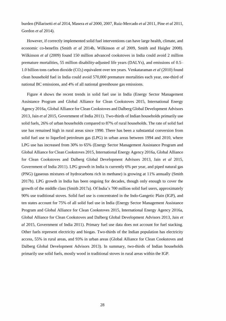
28

burden (Pillarisetti et al 2014, Masera et al 2000, 2007, Ruiz-Mercado et al 2011, Pine et al 2011,

Gordon et al 2014).

However, if correctly implemented solid fuel interventions can have large health, climate, and

economic co-benefits (Smith et al 2014b, Wilkinson et al 2009, Smith and Haigler 2008).

Wilkinson et al (2009) found 150 million advanced cookstoves in India could avoid 2 million

premature mortalities, 55 million disability-adjusted life years (DALYs), and emissions of 0.5–

1.0 billion tons carbon dioxide (CO2) equivalent over ten years. Venkataraman et al (2010) found

clean household fuel in India could avoid 570,000 premature mortalities each year, one-third of

national BC emissions, and 4% of all national greenhouse gas emissions.

Figure 4 shows the recent trends in solid fuel use in India (Energy Sector Management

Assistance Program and Global Alliance for Clean Cookstoves 2015, International Energy

Agency 2016a, Global Alliance for Clean Cookstoves and Dalberg Global Development Advisors

2013, Jain et al 2015, Government of India 2011). Two-thirds of Indian households primarily use

solid fuels, 26% of urban households compared to 87% of rural households. The rate of solid fuel

use has remained high in rural areas since 1990. There has been a substantial conversion from

solid fuel use to liquefied petroleum gas (LPG) in urban areas between 1994 and 2010, where

LPG use has increased from 30% to 65% (Energy Sector Management Assistance Program and

Global Alliance for Clean Cookstoves 2015, International Energy Agency 2016a, Global Alliance

for Clean Cookstoves and Dalberg Global Development Advisors 2013, Jain et al 2015,

Government of India 2011). LPG growth in India is currently 6% per year, and piped natural gas

(PNG) (gaseous mixtures of hydrocarbons rich in methane) is growing at 11% annually (Smith

2017b). LPG growth in India has been ongoing for decades, though only enough to cover the

growth of the middle class (Smith 2017a). Of India’s 700 million solid fuel users, approximately

90% use traditional stoves. Solid fuel use is concentrated in the Indo-Gangetic Plain (IGP), and

ten states account for 75% of all solid fuel use in India (Energy Sector Management Assistance

Program and Global Alliance for Clean Cookstoves 2015, International Energy Agency 2016a,

Global Alliance for Clean Cookstoves and Dalberg Global Development Advisors 2013, Jain et

al 2015, Government of India 2011). Primary fuel use data does not account for fuel stacking.

Other fuels represent electricity and biogas. Two-thirds of the Indian population has electricity

access, 55% in rural areas, and 93% in urban areas (Global Alliance for Clean Cookstoves and

Dalberg Global Development Advisors 2013). In summary, two-thirds of Indian households

primarily use solid fuels, mostly wood in traditional stoves in rural areas within the IGP.

29

Figure 4: Solid fuel use in India. (a) Primary fuel use in India in 2011 in urban areas, rural

areas, and overall. (b) Solid fuel use overall and in the top ten contributing states. (c) Solid fuel

use per state as a percentage. (d) Number of households primarily using solid fuels. Change in

primary fuel use between 1994 and 2010 in (e) rural areas and (f) urban areas (Energy Sector

Management Assistance Program and Global Alliance for Clean Cookstoves 2015, International

Energy Agency 2016a, Global Alliance for Clean Cookstoves and Dalberg Global Development

Advisors 2013, Jain et al 2015, Government of India 2011).

30

The combustion of solid fuels is incomplete, leading to substantial emissions of air pollutants

(Chafe et al 2014a, Lelieveld et al 2015, Silva et al 2016a, Butt et al 2016, Gordon et al 2014,

Naeher et al 2007, Smith et al 2000b). The incomplete combustion is due to low combustion

efficiencies, low-temperature combustion, and that the combustion gases are not within the

combustion chamber long enough for complete combustion to occur (Jetter and Kariher 2009,

Jetter et al 2012a, Grieshop et al 2011, Huang et al 2015, Reddy and Venkataraman 2002, Fuzzi

et al 2015, Fleming et al 2018a). These air pollutants impact human health (Edwards et al 2014,

Smith 2013, Gordon et al 2014), climate (Unger et al 2010, Butt et al 2016, Aunan et al 2009,

Huang et al 2018), environment (Bailis et al 2015, Sovacool 2012, Mwampamba 2007), and

human well-being (World Health Organization 2016b, Pachauri et al 2013, Rosenthal et al 2018).

Solid fuels mark a fundamental divide on the energy ladder, representing a large difference in

emissions of incomplete combustion pollutants (Smith et al 2000a, Jetter et al 2012a).

Many people use improved cookstoves as opposed, or in addition, to traditional cookstoves.

Globally, one-third of solid fuel users have improved cookstoves, with higher use in China

(~85%) and lower use in India (~10%) (Energy Sector Management Assistance Program and

Global Alliance for Clean Cookstoves 2015). Improved cookstoves encompass a wide variety of

physical characteristics and performances, including combustion chamber insulation, chimneys,

and fans. Many improved designs were developed before technical standards were in place,

leading to high emissions (Hutton et al 2006, Energy Sector Management Assistance Program

and Global Alliance for Clean Cookstoves 2015, Roden et al 2009, Kar et al 2012, Jetter and

Kariher 2009, Smith et al 2000b, Winijkul et al 2016). Some improved cookstoves have been

found to increase BC emissions relative to traditional stoves (Grieshop et al 2017), and these BC

differences are not currently accounted for within carbon market accounts (Aung et al 2016). The

increase in BC could potentially worsen health impacts if BC is found to be more toxic than total

PM mass, as suggested by Smith et al (2009a) and Baumgartner et al (2014), coupled to

worsening climate impacts through BC absorbing solar radiation. Chimneys and fans temporarily

reduce household exposures by moving air pollutants outside (Sambandam et al 2015, Martin et

al 2013, Venkataraman et al 2010). The majority (95%) of improved cookstoves in India are

improved chimney Chulha stoves (Energy Sector Management Assistance Program and Global

Alliance for Clean Cookstoves 2015). Field studies of improved cookstoves vary considerably to

laboratory studies (Edwards et al 2014, Smith et al 2007, Roden et al 2009, Sambandam et al

2015, Grieshop et al 2017, Kar et al 2012, Patange et al 2015, Muralidharan et al 2015). The

variability is due to non-ideal user behaviour, variations in fuel composition, type, size, moisture,

and combinations, cooking patterns, situational and measurement variabilities, seasonal patterns,

and stove deterioration (Edwards et al 2014, Venkataraman et al 2010, L’Orange et al 2015). It

is very difficult to burn biomass in small, low-cost cookstoves cleanly enough to meet the required

reductions in emissions to improve health (see non-linear health response to pollution in Section

2.3).

31

Kerosene, a liquid fuel, is often used in India for lighting by rural populations and those in the

lowest socioeconomic decile (Klimont et al 2017). Kerosene can increase specific pollutant

emissions relative to solid fuels (Bates and Bruce 2014). Gas fuels, in particular LPG, are the

primary alternative to traditional solid fuels in India, which improve combustion efficiencies and

reduce emissions, though are limited by the high upfront connection cost, high recurring fuel cost,

and lack of local fuel distribution (Smith 2015, S. Mehta 2003, Smith et al 2000b, Edwards et al

2014, Ryu et al 2006, Smith et al 2000a, Smith and Sagar 2014, Jetter et al 2012b, Williams et al

2015, Jain et al 2015). High fuel costs are often overcome by government subsidies

(Venkataraman et al 2010), though only 7% of fossil fuel subsidies have been historically

distributed to the lowest household income quintile groups (Arze del Granado et al 2012, Smith

and Sagar 2015). Many people use more than one fuel depending on price, season, and availability

(Sinton et al 2004). Efficient, cheap, and portable electric induction cookstoves are promoted in

India (Smith 2014).

1.1.3. Emissions

1.1.3.1. Indian emissions

Many studies have analysed the sectoral contributions to emissions in India (Venkataraman et

al 2018, Kumar et al 2012b, Sahu et al 2017, Saikawa et al 2017, Vadrevu et al 2017, Mittal et

al 2015). The most comprehensive emission inventory for India, by Venkataraman et al (2018),

found present-day PM2.5, BC, OC, and NMVOC emissions are primarily from residential solid

fuel, industries, and agricultural burning, while SO2 and NOx emissions are primarily from

industries and power generation using coal and land transport (Figure 5).

Figure 5: Indian emissions of PM and precursor gases for 2015 by sector (Mt yr-1)

(Venkataraman et al 2018). Emissions of NOx are NO.

32

Residential emissions only account for 10% of global energy use (Chum et al 2011) but

contribute 25–55% of BC and 72–78% of OC emissions globally (Bond et al 2013, Lu et al 2011,

Huang et al 2015). In India, residential emissions account for 45–86% of BC emissions and 68–

97% of OC emissions (Bond et al 2013, Lu et al 2011, Huang et al 2015, Paliwal et al 2016). All

species had increased emissions in India over the last decade (Sahu et al 2017, Saikawa et al 2017,

Sadavarte and Venkataraman 2014, Pandey et al 2014). Over the last two decades, anthropogenic

emissions of BC and OC in India have been rapidly increasing (Lu et al 2011), with emissions

factors for BC from residential combustion remaining the same (Masera et al 2000, Huang et al

2015).

Emissions in India are particularly uncertain (Saikawa et al 2017). Residential emissions are

generally based on a combination of fuel consumption rates and emissions factors (Butt et al

2016, Smith et al 2014a), which are uncertain primarily due to emissions factors varying up to

three orders of magnitude from fuel type, stove, fuel quality, combustion, and operating

conditions (Roden et al 2009, Kodros et al 2015, Bond et al 2004, Jetter et al 2012b, Li et al

2009, L’Orange et al 2012, Junker and Liousse 2008). The fuel type and activity data within

residential emission inventories can also vary widely (Tao et al 2018). The uncertainty in

published estimates for regional scale BC and OC emissions is typically a factor of two to five

(Lu et al 2011, Kulkarni et al 2015, Winijkul et al 2016, Li et al 2016a). Aerosol optical depth

(AOD), BC, and OC are often underestimated by models in regions with high residential

emissions, such as India (Bond et al 2013, Butt et al 2016, Pan et al 2015). The uncertainty is

potentially due to discrepancies in activity levels, technologies in use, and emission factors

(Ramachandran et al 2015, Zhong et al 2016a). SOA precursor emissions are uncertain in India

due to a lack of speciation measurements (Roden et al 2006, Martinsson et al 2015, Jayarathne et

al 2018). The emission inventory uncertainty is important considering India is rapidly developing.

The large uncertainty in residential emissions, particularly the relative emissions of BC and OC,

leads to uncertainty in the net radiative forcing from residential emissions, where the sign of the

net forcing is unknown (Butt et al 2016, Unger et al 2010, Kodros et al 2015, Aunan et al 2009,

Bauer et al 2010, Bond et al 2013, Jacobson 2010). The uncertainty in sign poses doubt over the

extent of climate co-benefits achieved through changes in this sector (Shindell et al 2012, Huang

et al 2015, Fuzzi et al 2015, Gao et al 2018).

1.1.3.2. Air pollution control policies in India

India has many national and sub-national policies aimed at addressing the health burden from

air pollution (Sagar et al 2016). Table 1 is a non-exhaustive list of policies in place or being

discussed within Indian ministries and agencies relating to air pollution control in India. For the

first time, many of these policies are due to be unified within the upcoming National Clean Air

Programme (NCAP) (Ministry of Environment Forests and Climate Change 2018). The NCAP

provides a framework for air quality management with the aim of attaining Indian air quality

33

standards throughout the country. The NCAP identifies 100 non-attainment cities that will be

required to create their own action plans. The NCAP specifies the need to increase the number of

manual and continuous monitoring stations, especially in rural areas, with PM2.5 monitoring

increasing from 67 to 1,000 stations in 2 years. This thesis will directly compliment the NCAP

by providing source-specific estimates of ambient air quality and the exposure-associated health

affects at high-resolution in India.

The Ministry of Health and Family Welfare plays a key role with new targets based on the air

pollution pathway aimed at providing the most significant exposure reductions, instead of only

reducing pollutant concentrations (Ministry of Health and Family Welfare 2015a). The focus on

exposures is important as it considers both ambient and household air pollution, and accounts for

the large variations in intake fraction (U.S. National Research Council 2012). The Ministry of

Finance has committed to provide clean gas for cooking to 50 million households by 2019

(Ministry of Finance 2016). The Ministry of New and Renewable Energy launched the National

Biomass Cookstove Initiative (NBCI) in 2009 to promote improved cookstoves utilising carbon-

finance to scale (Global Alliance for Clean Cookstoves and Dalberg Global Development

Advisors 2013). NBCI aims to provide 10.5 million improved cookstoves by 2022, primarily to

rural households. A range of 41 improved cookstoves approved by the Ministry of New and

Renewable Energy have been distributed since 2013. However, many homes remain using

traditional stoves post-intervention resulting in unrealised air pollutant reductions (Aung et al

2016, Pope et al 2017). In 2009, the Rajiv Gandhi Gramin LPG Vitran Yojana (RGGLVY) was

initiated by the Government of India to increase LPG coverage in rural areas. The RGGLVY

scheme commissioned 10,000 connections by late 2014 but was discontinued in 2015 (Tripathi et

al 2015).

Since 2015, the Ministry of Petroleum and Natural Gas alongside three major oil companies

have initiated three programmes to promote LPG to the poor (Mittal et al 2017), addressing the

700 million solid fuel users caught in the Chulha trap (Smith 2017a). The Pratyaksh Hanstantrit

Labh (PAHAL) (Ministry of Petroleum and Natural Gas 2018c) scheme directly pays fuel

subsidies into people’s bank accounts, meaning that all LPG is now sold at international rates,

substantially reducing diversion of LPG to the non-household sector (Smith 2017b). The Pradhan

Mantri Ujjwala Yojana (Ujjwala) (Ministry of Petroleum and Natural Gas 2018a) scheme

launched in 2016 aims to provide gas connections to 80 million poor households by March 2020

and has already provided 50 million connections as of August 2018 (Dabadge et al 2018, Ministry

of Petroleum and Natural Gas 2018b). Connections here specifically mean a formal account with

a distributor covering a deposit to then access the subsidised LPG (Goldemberg et al 2018). There

is uncertainty regarding the continued use of LPG post connection due to higher fuel prices

(Kishore 2017). The Give it Up scheme was designed to persuade middle-class households to give

up their fuel subsidies to redirect them to poor households, reaching over 10 million households

34

by late 2017 (Government of India 2018). The LPG growth rate in India continues to be 6%,

though for the poor populations too, which is twice the previous rate (Smith 2017a). The Indian

government aims to provide 10 million PNG connections by 2019, to free up LPG connections

for the poor (Smith 2017a). India aims to provide clean cooking to 80% of all households by 2019,

and 90% by the early 2020’s (Goldemberg et al 2018). To emphasise, clean here refers to

exposure-associated health impacts, however, replacing solid fuels with LPG results in minor CO2

emissions (Haines et al 2017, Smith 2014). The Ministry of Power launched the Deen Dayal

Upadhyaya Gram Jyoti Yojana (DDUGJY) in 2015 to provide electricity to rural households.

India is involved in many global policies and commitments to reduce the disease burden from

air pollution. The main aims of India’s Intended Nationally Defined Contribution (INDC) under

the United Nations Framework Convention on Climate Change is to achieve a 40% share of

electricity generation from renewable sources by 2030, with 175 GW of renewable energy by

2022, and to reduce PM emission intensity by 33–35% by 2030 (Government of India 2015).

India’s INDCs include stricter emission standards for desulphurisation (Ministry of Environment

Forests and Climate Change 2015b), de-NOx technologies in power generation (Ministry of

Environment Forests and Climate Change 2015b), growth in public transport (National Transport

Development Policy Committee 2014, National Institution for Transforming India 2015), tighter

vehicle emission standards (Ministry of Road Transport and Highways 2016b, Government of

India 2014), and improved energy efficiency in industry (Ministry of Environment Forests and

Climate Change 2015b) and power generation (Ministry of Power 2015).

Key global policies including India are the air pollution-related sustainable development goals

(SDGs) (World Health Organization 2016c), including aiming to eradicate extreme poverty for

all people everywhere (target 1.1), to end preventable deaths of children under 5 years of age

(targets 1.4 and 3.2), to reduce hunger and increase agricultural productivity (target 2.3), to reduce

premature mortality from non-communicable diseases (NCDs) by one third through prevention

(target 3.4), to reduce the disease burden from air pollution (target 3.9), to provide universal

access to clean household energy (target 7.1), to clean industrial and technological processes

(target 9.4), to provide safe, affordable, accessible, and sustainable transport (target 11.2), to

improve urban air quality (target 11.6), to provide benefits from reduced climate forcing (goal

13), and reducing deforestation by eliminating domestic solid fuel use (target 15.2) (United

Nations 2015, Haines et al 2017). India is part of the WHO South-East Asia Region who has the

target of a 50% reduction in the proportion of households primarily using solid fuels by 2025

(World Health Organization South East Asia Region 2013).

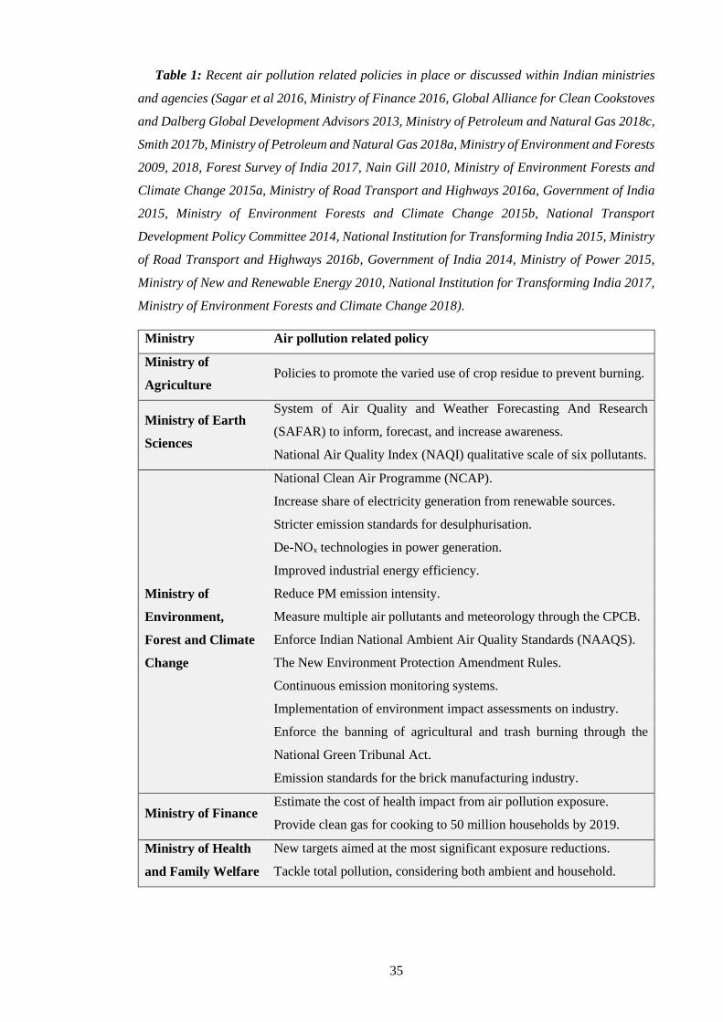
35

Table 1: Recent air pollution related policies in place or discussed within Indian ministries

and agencies (Sagar et al 2016, Ministry of Finance 2016, Global Alliance for Clean Cookstoves

and Dalberg Global Development Advisors 2013, Ministry of Petroleum and Natural Gas 2018c,

Smith 2017b, Ministry of Petroleum and Natural Gas 2018a, Ministry of Environment and Forests

2009, 2018, Forest Survey of India 2017, Nain Gill 2010, Ministry of Environment Forests and

Climate Change 2015a, Ministry of Road Transport and Highways 2016a, Government of India

2015, Ministry of Environment Forests and Climate Change 2015b, National Transport

Development Policy Committee 2014, National Institution for Transforming India 2015, Ministry

of Road Transport and Highways 2016b, Government of India 2014, Ministry of Power 2015,

Ministry of New and Renewable Energy 2010, National Institution for Transforming India 2017,

Ministry of Environment Forests and Climate Change 2018).

Ministry Air pollution related policy

Ministry of

Agriculture Policies to promote the varied use of crop residue to prevent burning.

Ministry of Earth

Sciences

System of Air Quality and Weather Forecasting And Research

(SAFAR) to inform, forecast, and increase awareness.

National Air Quality Index (NAQI) qualitative scale of six pollutants.

Ministry of

Environment,

Forest and Climate

Change

National Clean Air Programme (NCAP).

Increase share of electricity generation from renewable sources.

Stricter emission standards for desulphurisation.

De-NOx technologies in power generation.

Improved industrial energy efficiency.

Reduce PM emission intensity.

Measure multiple air pollutants and meteorology through the CPCB.

Enforce Indian National Ambient Air Quality Standards (NAAQS).

The New Environment Protection Amendment Rules.

Continuous emission monitoring systems.

Implementation of environment impact assessments on industry.

Enforce the banning of agricultural and trash burning through the

National Green Tribunal Act.

Emission standards for the brick manufacturing industry.

Ministry of Finance Estimate the cost of health impact from air pollution exposure.

Provide clean gas for cooking to 50 million households by 2019.

Ministry of Health

and Family Welfare

New targets aimed at the most significant exposure reductions.

Tackle total pollution, considering both ambient and household.

36

Ministry of Heavy

Industries and

Public Enterprises

Faster adoption and manufacturing of hybrid and electric vehicles.

Ministry of Human

Resource

Development

Ensure regular check-ups for non-communicable diseases of children.

Include the health impacts of air pollution in the school curriculum.

Ministry of Labour

and Employment

Ensure regular check-ups for non-communicable diseases of workers.

Strengthen hospital capacity to cater for non-communicable diseases.

Ministry of Micro,

Small and Medium

Enterprises

Zero Effect, Zero Defect campaign to increase efficiency, pollution

control, and use of renewable energy.

Ministry of New

and Renewable

Energy

Launched the NBCI in 2009 to provide 10.5 million improved

cookstoves by 2022, primarily to rural households.

Increase in solar and electric lighting.

Support Integrated Rural Energy Programme on household pollution.

Develop a national policy for clean biofuels.

Ministry of

Petroleum and

Natural Gas

PAHAL scheme directly pays subsidies into people’s banks.

Ujjwala to provide gas connections.

The Give it Up scheme to persuade middle-class households to give up

their fuel subsidies to redirect them to poor households.

Provide 10 million PNG connections by 2019.

Ministry of Power

National Mission for Enhanced Energy Efficiency.

DDUGJY to provide electricity to rural households

Improved energy efficiency through Perform, Achieve, and Trade.

The Fly Ash Utilisation Policy.

Promote improved cookstoves.

Ministry of Road

Transport and

Highways

Growth in public and electric transport.

Tighter vehicle emission standards.

Bharat VI standards reducing emissions from buses and trucks.

Ministry of Rural

Development Promote clean air guidelines.

Ministry of Steel Reduce anthropogenic dust emissions.

Ministry of Urban

Development

Disincentives for diesel generators.

Enforcement of the ban on trash burning.

Ministry of Women

and Child

Development

Promote awareness of air pollution from solid fuel use.

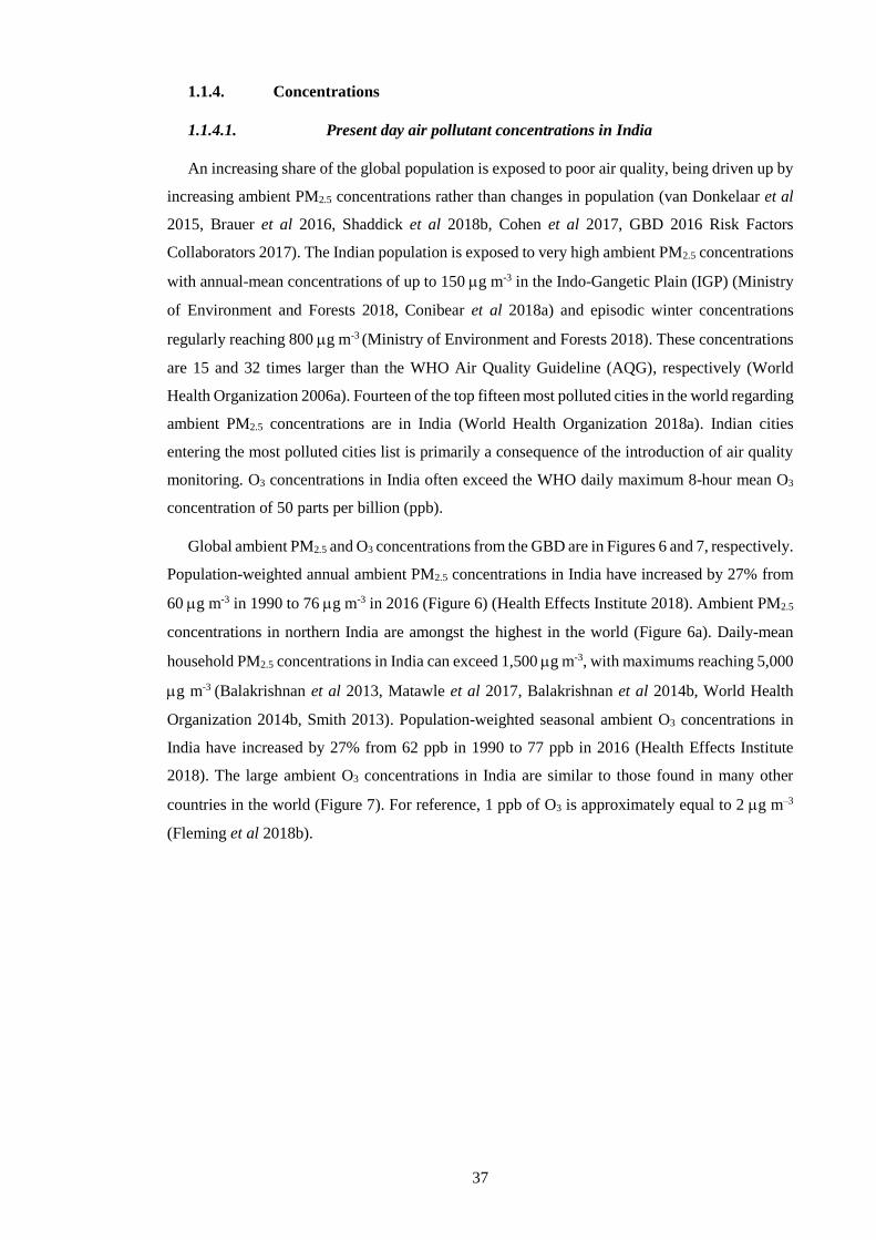
37

1.1.4. Concentrations

1.1.4.1. Present day air pollutant concentrations in India

An increasing share of the global population is exposed to poor air quality, being driven up by

increasing ambient PM2.5 concentrations rather than changes in population (van Donkelaar et al

2015, Brauer et al 2016, Shaddick et al 2018b, Cohen et al 2017, GBD 2016 Risk Factors

Collaborators 2017). The Indian population is exposed to very high ambient PM2.5 concentrations

with annual-mean concentrations of up to 150 g m-3 in the Indo-Gangetic Plain (IGP) (Ministry

of Environment and Forests 2018, Conibear et al 2018a) and episodic winter concentrations

regularly reaching 800 g m-3 (Ministry of Environment and Forests 2018). These concentrations

are 15 and 32 times larger than the WHO Air Quality Guideline (AQG), respectively (World

Health Organization 2006a). Fourteen of the top fifteen most polluted cities in the world regarding

ambient PM2.5 concentrations are in India (World Health Organization 2018a). Indian cities

entering the most polluted cities list is primarily a consequence of the introduction of air quality

monitoring. O3 concentrations in India often exceed the WHO daily maximum 8-hour mean O3

concentration of 50 parts per billion (ppb).

Global ambient PM2.5 and O3 concentrations from the GBD are in Figures 6 and 7, respectively.

Population-weighted annual ambient PM2.5 concentrations in India have increased by 27% from

60 g m-3 in 1990 to 76 g m-3 in 2016 (Figure 6) (Health Effects Institute 2018). Ambient PM2.5

concentrations in northern India are amongst the highest in the world (Figure 6a). Daily-mean

household PM2.5 concentrations in India can exceed 1,500 g m-3, with maximums reaching 5,000

g m-3 (Balakrishnan et al 2013, Matawle et al 2017, Balakrishnan et al 2014b, World Health

Organization 2014b, Smith 2013). Population-weighted seasonal ambient O3 concentrations in

India have increased by 27% from 62 ppb in 1990 to 77 ppb in 2016 (Health Effects Institute

2018). The large ambient O3 concentrations in India are similar to those found in many other

countries in the world (Figure 7). For reference, 1 ppb of O3 is approximately equal to 2 g m–3

(Fleming et al 2018b).

38

Figure 6: Annual-mean ambient PM2.5 concentrations from the Global Burden of Diseases,

Injuries, and Risk Factors Study (GBD) 2016 using the data integration model for air quality

(DIMAQ) (Shaddick et al 2018b, Cohen et al 2017, GBD 2016 Risk Factors Collaborators 2017).

(a) 2016. (b) 2015. (c) 2014. (d) 2013. (e) 2012. (f) 2011. (g) 2010. (h) 2005. (i) 2000. (j) 1995.

(k) 1990.

Figure 7: Seasonal ambient O3 concentrations from the GBD2013 (GBD 2013 Risk Factors

Collaborators 2015, Brauer et al 2016). Calculated as the maximum running 3-month average of

daily 1-hour maximum values.

PM2.5 concentrations within India are highest in the IGP (Henriksson et al 2011, David et al

2018). The IGP, also known as the northern India river plain, is a huge fertile plain encompassing

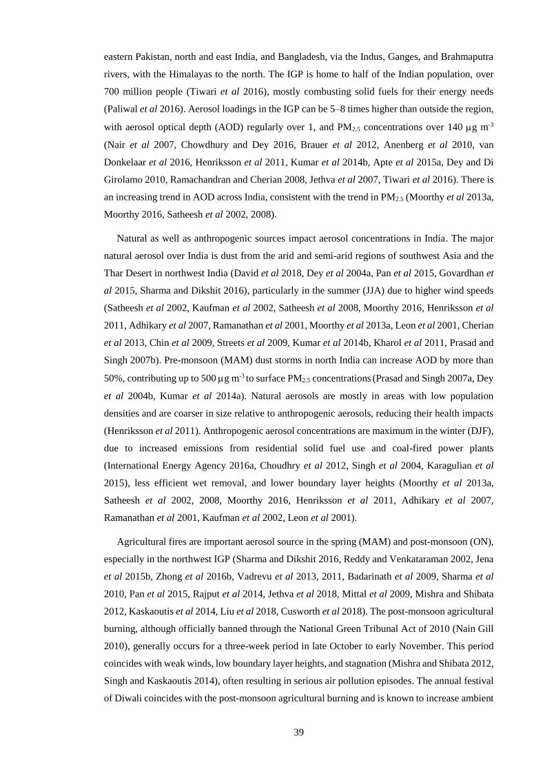
39

eastern Pakistan, north and east India, and Bangladesh, via the Indus, Ganges, and Brahmaputra

rivers, with the Himalayas to the north. The IGP is home to half of the Indian population, over

700 million people (Tiwari et al 2016), mostly combusting solid fuels for their energy needs

(Paliwal et al 2016). Aerosol loadings in the IGP can be 5–8 times higher than outside the region,

with aerosol optical depth (AOD) regularly over 1, and PM2.5 concentrations over 140 g m-3

(Nair et al 2007, Chowdhury and Dey 2016, Brauer et al 2012, Anenberg et al 2010, van

Donkelaar et al 2016, Henriksson et al 2011, Kumar et al 2014b, Apte et al 2015a, Dey and Di

Girolamo 2010, Ramachandran and Cherian 2008, Jethva et al 2007, Tiwari et al 2016). There is

an increasing trend in AOD across India, consistent with the trend in PM2.5 (Moorthy et al 2013a,

Moorthy 2016, Satheesh et al 2002, 2008).

Natural as well as anthropogenic sources impact aerosol concentrations in India. The major

natural aerosol over India is dust from the arid and semi-arid regions of southwest Asia and the

Thar Desert in northwest India (David et al 2018, Dey et al 2004a, Pan et al 2015, Govardhan et

al 2015, Sharma and Dikshit 2016), particularly in the summer (JJA) due to higher wind speeds

(Satheesh et al 2002, Kaufman et al 2002, Satheesh et al 2008, Moorthy 2016, Henriksson et al

2011, Adhikary et al 2007, Ramanathan et al 2001, Moorthy et al 2013a, Leon et al 2001, Cherian

et al 2013, Chin et al 2009, Streets et al 2009, Kumar et al 2014b, Kharol et al 2011, Prasad and

Singh 2007b). Pre-monsoon (MAM) dust storms in north India can increase AOD by more than

50%, contributing up to 500 g m-3 to surface PM2.5 concentrations (Prasad and Singh 2007a, Dey

et al 2004b, Kumar et al 2014a). Natural aerosols are mostly in areas with low population

densities and are coarser in size relative to anthropogenic aerosols, reducing their health impacts

(Henriksson et al 2011). Anthropogenic aerosol concentrations are maximum in the winter (DJF),

due to increased emissions from residential solid fuel use and coal-fired power plants

(International Energy Agency 2016a, Choudhry et al 2012, Singh et al 2004, Karagulian et al

2015), less efficient wet removal, and lower boundary layer heights (Moorthy et al 2013a,

Satheesh et al 2002, 2008, Moorthy 2016, Henriksson et al 2011, Adhikary et al 2007,

Ramanathan et al 2001, Kaufman et al 2002, Leon et al 2001).

Agricultural fires are important aerosol source in the spring (MAM) and post-monsoon (ON),

especially in the northwest IGP (Sharma and Dikshit 2016, Reddy and Venkataraman 2002, Jena

et al 2015b, Zhong et al 2016b, Vadrevu et al 2013, 2011, Badarinath et al 2009, Sharma et al

2010, Pan et al 2015, Rajput et al 2014, Jethva et al 2018, Mittal et al 2009, Mishra and Shibata

2012, Kaskaoutis et al 2014, Liu et al 2018, Cusworth et al 2018). The post-monsoon agricultural

burning, although officially banned through the National Green Tribunal Act of 2010 (Nain Gill

2010), generally occurs for a three-week period in late October to early November. This period

coincides with weak winds, low boundary layer heights, and stagnation (Mishra and Shibata 2012,

Singh and Kaskaoutis 2014), often resulting in serious air pollution episodes. The annual festival

of Diwali coincides with the post-monsoon agricultural burning and is known to increase ambient

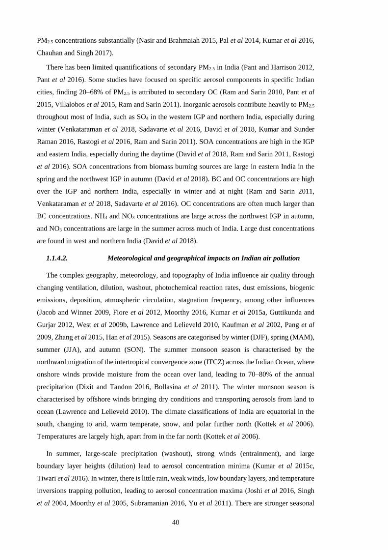
40

PM2.5 concentrations substantially (Nasir and Brahmaiah 2015, Pal et al 2014, Kumar et al 2016,

Chauhan and Singh 2017).

There has been limited quantifications of secondary PM2.5 in India (Pant and Harrison 2012,

Pant et al 2016). Some studies have focused on specific aerosol components in specific Indian

cities, finding 20–68% of PM2.5 is attributed to secondary OC (Ram and Sarin 2010, Pant et al

2015, Villalobos et al 2015, Ram and Sarin 2011). Inorganic aerosols contribute heavily to PM2.5

throughout most of India, such as SO4 in the western IGP and northern India, especially during

winter (Venkataraman et al 2018, Sadavarte et al 2016, David et al 2018, Kumar and Sunder

Raman 2016, Rastogi et al 2016, Ram and Sarin 2011). SOA concentrations are high in the IGP

and eastern India, especially during the daytime (David et al 2018, Ram and Sarin 2011, Rastogi

et al 2016). SOA concentrations from biomass burning sources are large in eastern India in the

spring and the northwest IGP in autumn (David et al 2018). BC and OC concentrations are high

over the IGP and northern India, especially in winter and at night (Ram and Sarin 2011,

Venkataraman et al 2018, Sadavarte et al 2016). OC concentrations are often much larger than

BC concentrations. NH4 and NO3 concentrations are large across the northwest IGP in autumn,

and NO3 concentrations are large in the summer across much of India. Large dust concentrations

are found in west and northern India (David et al 2018).

1.1.4.2. Meteorological and geographical impacts on Indian air pollution

The complex geography, meteorology, and topography of India influence air quality through

changing ventilation, dilution, washout, photochemical reaction rates, dust emissions, biogenic

emissions, deposition, atmospheric circulation, stagnation frequency, among other influences

(Jacob and Winner 2009, Fiore et al 2012, Moorthy 2016, Kumar et al 2015a, Guttikunda and

Gurjar 2012, West et al 2009b, Lawrence and Lelieveld 2010, Kaufman et al 2002, Pang et al

2009, Zhang et al 2015, Han et al 2015). Seasons are categorised by winter (DJF), spring (MAM),

summer (JJA), and autumn (SON). The summer monsoon season is characterised by the

northward migration of the intertropical convergence zone (ITCZ) across the Indian Ocean, where

onshore winds provide moisture from the ocean over land, leading to 70–80% of the annual

precipitation (Dixit and Tandon 2016, Bollasina et al 2011). The winter monsoon season is

characterised by offshore winds bringing dry conditions and transporting aerosols from land to

ocean (Lawrence and Lelieveld 2010). The climate classifications of India are equatorial in the

south, changing to arid, warm temperate, snow, and polar further north (Kottek et al 2006).

Temperatures are largely high, apart from in the far north (Kottek et al 2006).

In summer, large-scale precipitation (washout), strong winds (entrainment), and large

boundary layer heights (dilution) lead to aerosol concentration minima (Kumar et al 2015c,

Tiwari et al 2016). In winter, there is little rain, weak winds, low boundary layers, and temperature

inversions trapping pollution, leading to aerosol concentration maxima (Joshi et al 2016, Singh

et al 2004, Moorthy et al 2005, Subramanian 2016, Yu et al 2011). There are stronger seasonal

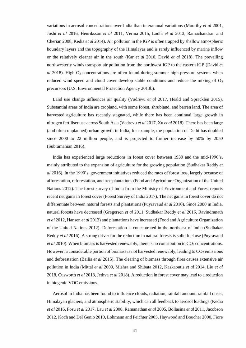
41

variations in aerosol concentrations over India than interannual variations (Moorthy et al 2001,

Joshi et al 2016, Henriksson et al 2011, Verma 2015, Lodhi et al 2013, Ramachandran and

Cherian 2008, Kedia et al 2014). Air pollution in the IGP is often trapped by shallow atmospheric

boundary layers and the topography of the Himalayas and is rarely influenced by marine inflow

or the relatively cleaner air in the south (Kar et al 2010, David et al 2018). The prevailing

northwesterly winds transport air pollution from the northwest IGP to the eastern IGP (David et

al 2018). High O3 concentrations are often found during summer high-pressure systems when

reduced wind speed and cloud cover develop stable conditions and reduce the mixing of O3

precursors (U.S. Environmental Protection Agency 2013b).

Land use change influences air quality (Vadrevu et al 2017, Heald and Spracklen 2015).

Substantial areas of India are cropland, with some forest, shrubland, and barren land. The area of

harvested agriculture has recently stagnated, while there has been continual large growth in

nitrogen fertiliser use across South Asia (Vadrevu et al 2017, Xu et al 2018). There has been large

(and often unplanned) urban growth in India, for example, the population of Delhi has doubled

since 2000 to 22 million people, and is projected to further increase by 50% by 2050

(Subramanian 2016).

India has experienced large reductions in forest cover between 1930 and the mid-1990’s,

mainly attributed to the expansion of agriculture for the growing population (Sudhakar Reddy et

al 2016). In the 1990’s, government initiatives reduced the rates of forest loss, largely because of

afforestation, reforestation, and tree plantations (Food and Agriculture Organization of the United

Nations 2012). The forest survey of India from the Ministry of Environment and Forest reports

recent net gains in forest cover (Forest Survey of India 2017). The net gains in forest cover do not

differentiate between natural forests and plantations (Puyravaud et al 2010). Since 2000 in India,

natural forests have decreased (Gregersen et al 2011, Sudhakar Reddy et al 2016, Ravindranath

et al 2012, Hansen et al 2013) and plantations have increased (Food and Agriculture Organization

of the United Nations 2012). Deforestation is concentrated in the northeast of India (Sudhakar

Reddy et al 2016). A strong driver for the reduction in natural forests is solid fuel use (Puyravaud

et al 2010). When biomass is harvested renewably, there is no contribution to CO2 concentrations.

However, a considerable portion of biomass is not harvested renewably, leading to CO2 emissions

and deforestation (Bailis et al 2015). The clearing of biomass through fires causes extensive air

pollution in India (Mittal et al 2009, Mishra and Shibata 2012, Kaskaoutis et al 2014, Liu et al

2018, Cusworth et al 2018, Jethva et al 2018). A reduction in forest cover may lead to a reduction

in biogenic VOC emissions.

Aerosol in India has been found to influence clouds, radiation, rainfall amount, rainfall onset,

Himalayan glaciers, and atmospheric stability, which can all feedback to aerosol loadings (Kedia

et al 2016, Fosu et al 2017, Lau et al 2008, Ramanathan et al 2005, Bollasina et al 2011, Jacobson

2012, Koch and Del Genio 2010, Lohmann and Feichter 2005, Haywood and Boucher 2000, Fiore

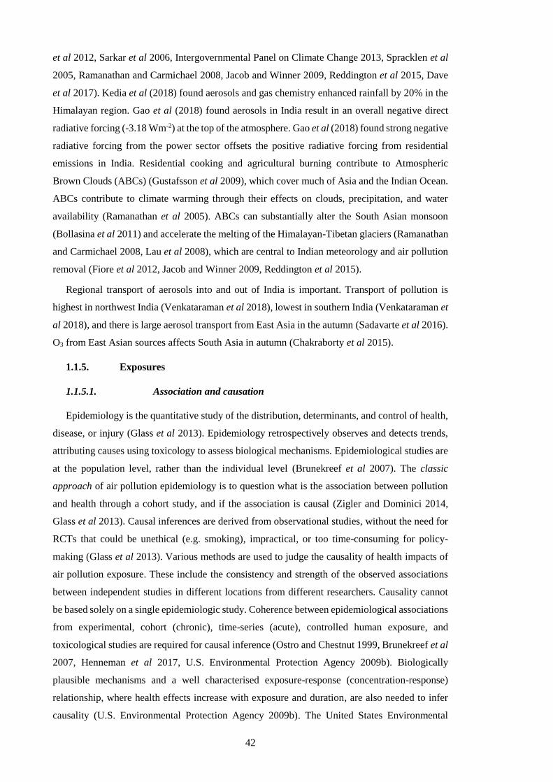
42

et al 2012, Sarkar et al 2006, Intergovernmental Panel on Climate Change 2013, Spracklen et al

2005, Ramanathan and Carmichael 2008, Jacob and Winner 2009, Reddington et al 2015, Dave

et al 2017). Kedia et al (2018) found aerosols and gas chemistry enhanced rainfall by 20% in the

Himalayan region. Gao et al (2018) found aerosols in India result in an overall negative direct

radiative forcing (-3.18 Wm-2) at the top of the atmosphere. Gao et al (2018) found strong negative

radiative forcing from the power sector offsets the positive radiative forcing from residential

emissions in India. Residential cooking and agricultural burning contribute to Atmospheric

Brown Clouds (ABCs) (Gustafsson et al 2009), which cover much of Asia and the Indian Ocean.

ABCs contribute to climate warming through their effects on clouds, precipitation, and water

availability (Ramanathan et al 2005). ABCs can substantially alter the South Asian monsoon

(Bollasina et al 2011) and accelerate the melting of the Himalayan-Tibetan glaciers (Ramanathan

and Carmichael 2008, Lau et al 2008), which are central to Indian meteorology and air pollution

removal (Fiore et al 2012, Jacob and Winner 2009, Reddington et al 2015).

Regional transport of aerosols into and out of India is important. Transport of pollution is

highest in northwest India (Venkataraman et al 2018), lowest in southern India (Venkataraman et

al 2018), and there is large aerosol transport from East Asia in the autumn (Sadavarte et al 2016).

O3 from East Asian sources affects South Asia in autumn (Chakraborty et al 2015).

1.1.5. Exposures

1.1.5.1. Association and causation

Epidemiology is the quantitative study of the distribution, determinants, and control of health,

disease, or injury (Glass et al 2013). Epidemiology retrospectively observes and detects trends,

attributing causes using toxicology to assess biological mechanisms. Epidemiological studies are

at the population level, rather than the individual level (Brunekreef et al 2007). The classic

approach of air pollution epidemiology is to question what is the association between pollution

and health through a cohort study, and if the association is causal (Zigler and Dominici 2014,

Glass et al 2013). Causal inferences are derived from observational studies, without the need for

RCTs that could be unethical (e.g. smoking), impractical, or too time-consuming for policy-

making (Glass et al 2013). Various methods are used to judge the causality of health impacts of

air pollution exposure. These include the consistency and strength of the observed associations

between independent studies in different locations from different researchers. Causality cannot

be based solely on a single epidemiologic study. Coherence between epidemiological associations

from experimental, cohort (chronic), time-series (acute), controlled human exposure, and

toxicological studies are required for causal inference (Ostro and Chestnut 1999, Brunekreef et al

2007, Henneman et al 2017, U.S. Environmental Protection Agency 2009b). Biologically

plausible mechanisms and a well characterised exposure-response (concentration-response)

relationship, where health effects increase with exposure and duration, are also needed to infer

causality (U.S. Environmental Protection Agency 2009b). The United States Environmental

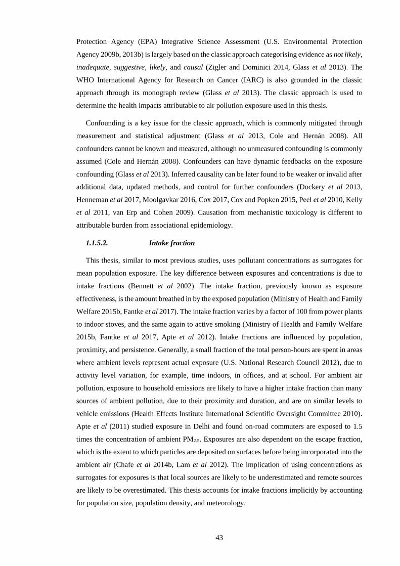
43

Protection Agency (EPA) Integrative Science Assessment (U.S. Environmental Protection

Agency 2009b, 2013b) is largely based on the classic approach categorising evidence as not likely,

inadequate, suggestive, likely, and causal (Zigler and Dominici 2014, Glass et al 2013). The

WHO International Agency for Research on Cancer (IARC) is also grounded in the classic

approach through its monograph review (Glass et al 2013). The classic approach is used to

determine the health impacts attributable to air pollution exposure used in this thesis.

Confounding is a key issue for the classic approach, which is commonly mitigated through

measurement and statistical adjustment (Glass et al 2013, Cole and Hernán 2008). All

confounders cannot be known and measured, although no unmeasured confounding is commonly

assumed (Cole and Hernán 2008). Confounders can have dynamic feedbacks on the exposure

confounding (Glass et al 2013). Inferred causality can be later found to be weaker or invalid after

additional data, updated methods, and control for further confounders (Dockery et al 2013,

Henneman et al 2017, Moolgavkar 2016, Cox 2017, Cox and Popken 2015, Peel et al 2010, Kelly

et al 2011, van Erp and Cohen 2009). Causation from mechanistic toxicology is different to

attributable burden from associational epidemiology.

1.1.5.2. Intake fraction

This thesis, similar to most previous studies, uses pollutant concentrations as surrogates for

mean population exposure. The key difference between exposures and concentrations is due to

intake fractions (Bennett et al 2002). The intake fraction, previously known as exposure

effectiveness, is the amount breathed in by the exposed population (Ministry of Health and Family

Welfare 2015b, Fantke et al 2017). The intake fraction varies by a factor of 100 from power plants

to indoor stoves, and the same again to active smoking (Ministry of Health and Family Welfare

2015b, Fantke et al 2017, Apte et al 2012). Intake fractions are influenced by population,

proximity, and persistence. Generally, a small fraction of the total person-hours are spent in areas

where ambient levels represent actual exposure (U.S. National Research Council 2012), due to

activity level variation, for example, time indoors, in offices, and at school. For ambient air

pollution, exposure to household emissions are likely to have a higher intake fraction than many

sources of ambient pollution, due to their proximity and duration, and are on similar levels to

vehicle emissions (Health Effects Institute International Scientific Oversight Committee 2010).

Apte et al (2011) studied exposure in Delhi and found on-road commuters are exposed to 1.5

times the concentration of ambient PM2.5. Exposures are also dependent on the escape fraction,

which is the extent to which particles are deposited on surfaces before being incorporated into the

ambient air (Chafe et al 2014b, Lam et al 2012). The implication of using concentrations as

surrogates for exposures is that local sources are likely to be underestimated and remote sources

are likely to be overestimated. This thesis accounts for intake fractions implicitly by accounting

for population size, population density, and meteorology.

44

For household air pollution, exposure levels are mostly lower than household concentrations

due to stove location, cooking duration, a division of tasks, the presence of a flue, the ventilation

rate, the volume of the home, and the proximity of the home to other households and sources

(Balakrishnan et al 2014b, Smith et al 2014a, Bruce et al 2015b, Edwards et al 2014, Ruiz-

Mercado et al 2011). Household air pollutant exposures have been measured in India since 1981

(Smith et al 1983). Solid fuel combustion in traditional stoves leads to exposures between that

experienced by second-hand smoking and active smoking (Pope III et al 2011, Smith and Peel

2010). Traditional cooking with solid fuels is approximately equivalent to 400 cigarettes per hour

in terms of PM2.5 exposure from second-hand smoke (Smith 1987). Household air pollution is a

severe health issue in India (Balakrishnan et al 2014a, 2013). Household air pollution is not

directly quantified in this thesis, though the contribution from household air pollution (residential

emissions) to ambient air pollution is quantified. Ambient and household air pollution interact

and exchange (Zhou et al 2015, Han et al 2015, Gordon et al 2014, Rehman et al 2011,

Balakrishnan et al 2011, Chafe et al 2014b).

1.1.6. Doses

The dose is the pollutant concentration in body tissues, such as the lung, after repeated

exposure. PM dosimetry is the deposition, translocation, clearance, and retention of particles

within the respiratory tract (U.S. Environmental Protection Agency 2009b). The dose of PM

depends on the concentration, duration, ventilation, and particle characteristics. PM size is a key

characteristic controlling deposition, translocation, and clearance of particles after exposure

(Figure 8). PM deposition is primarily by diffusion, impaction, and sedimentation. Diffusion is

the dominant mechanism for ultrafine PM (0.01–0.1 m), and sedimentation and impaction

dominate coarse PM (2.5–10 m). Thoracic particles are coarse particles that reach the lung

airways past the larynx. Respirable particles are fine particles those that reach the gas-exchange

region of the lungs. The IER makes assumptions about the dosing rates between ambient air

pollution, household air pollution, second hand smoking, and active smoking. For example, the

dose from one cigarette is equivalent to an exposure to 667 g m-3 of ambient PM2.5 for 24-hours

(Burnett et al 2018, 2014).

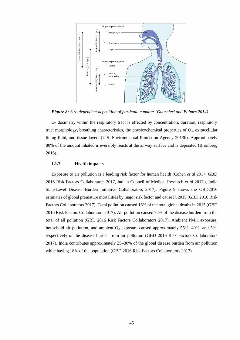
45

Figure 8: Size-dependent deposition of particulate matter (Guarnieri and Balmes 2014).

O3 dosimetry within the respiratory tract is affected by concentration, duration, respiratory

tract morphology, breathing characteristics, the physicochemical properties of O3, extracellular

lining fluid, and tissue layers (U.S. Environmental Protection Agency 2013b). Approximately

80% of the amount inhaled irreversibly reacts at the airway surface and is deposited (Bromberg

2016).

1.1.7. Health impacts

Exposure to air pollution is a leading risk factor for human health (Cohen et al 2017, GBD

2016 Risk Factors Collaborators 2017, Indian Council of Medical Research et al 2017b, India

State-Level Disease Burden Initiative Collaborators 2017). Figure 9 shows the GBD2016

estimates of global premature mortalities by major risk factor and cause in 2015 (GBD 2016 Risk

Factors Collaborators 2017). Total pollution caused 16% of the total global deaths in 2015 (GBD

2016 Risk Factors Collaborators 2017). Air pollution caused 72% of the disease burden from the

total of all pollution (GBD 2016 Risk Factors Collaborators 2017). Ambient PM2.5 exposure,

household air pollution, and ambient O3 exposure caused approximately 55%, 40%, and 5%,

respectively of the disease burden from air pollution (GBD 2016 Risk Factors Collaborators

2017). India contributes approximately 25–30% of the global disease burden from air pollution

while having 18% of the population (GBD 2016 Risk Factors Collaborators 2017).

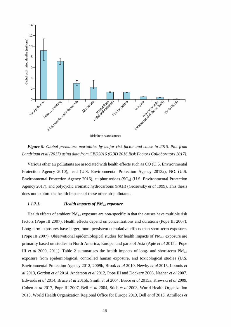
46

Figure 9: Global premature mortalities by major risk factor and cause in 2015. Plot from

Landrigan et al (2017) using data from GBD2016 (GBD 2016 Risk Factors Collaborators 2017).

Various other air pollutants are associated with health effects such as CO (U.S. Environmental

Protection Agency 2010), lead (U.S. Environmental Protection Agency 2013a), NOx (U.S.

Environmental Protection Agency 2016), sulphur oxides (SOx) (U.S. Environmental Protection

Agency 2017), and polycyclic aromatic hydrocarbons (PAH) (Grosovsky et al 1999). This thesis

does not explore the health impacts of these other air pollutants.

1.1.7.1. Health impacts of PM2.5 exposure

Health effects of ambient PM2.5 exposure are non-specific in that the causes have multiple risk

factors (Pope III 2007). Health effects depend on concentrations and durations (Pope III 2007).

Long-term exposures have larger, more persistent cumulative effects than short-term exposures

(Pope III 2007). Observational epidemiological studies for health impacts of PM2.5 exposure are

primarily based on studies in North America, Europe, and parts of Asia (Apte et al 2015a, Pope

III et al 2009, 2011). Table 2 summarises the health impacts of long- and short-term PM2.5

exposure from epidemiological, controlled human exposure, and toxicological studies (U.S.

Environmental Protection Agency 2012, 2009b, Brook et al 2010, Newby et al 2015, Loomis et

al 2013, Gordon et al 2014, Anderson et al 2012, Pope III and Dockery 2006, Naeher et al 2007,

Edwards et al 2014, Bruce et al 2015b, Smith et al 2004, Bruce et al 2015a, Krewski et al 2009,

Cohen et al 2017, Pope III 2007, Bell et al 2004, Stieb et al 2003, World Health Organization

2013, World Health Organization Regional Office for Europe 2013, Bell et al 2013, Achilleos et

47

al 2017, Li et al 2016b, Atkinson et al 2012, Héroux et al 2015, Atkinson et al 2014, Levy et al

2012).

Long-term PM2.5 exposure is a cause of all-cause mortality, cardiovascular mortality, and

cardiovascular morbidity, a likely cause of respiratory effects, and a suggestive cause of

reproductive and developmental outcomes. Short-term PM2.5 exposure is a cause of mortality and

cardiovascular effects, and a likely cause of respiratory effects. PM is an IARC group 1

carcinogen. The classifications likely and suggestive causes are due to limited consistency and

coherence across studies, and the lack of size-resolved PM exposure cancer studies. Susceptible

populations to the health effects of PM exposure are those with underlying cardiovascular and

respiratory illnesses, older adults for cardiovascular morbidity, children for respiratory effects,

and those with lower socioeconomic status including reduced access to health care, low

educational attainment, and residential location (U.S. Environmental Protection Agency 2009b).

There is no clear evidence of a low safe threshold or specific lag period from short-term PM2.5

exposure for cardiovascular or respiratory effects (U.S. Environmental Protection Agency

2009b).

48

Table 2: Health impacts of PM2.5 exposure (U.S. Environmental Protection Agency 2012,

2009b, Brook et al 2010, Newby et al 2015, Loomis et al 2013, Gordon et al 2014, Anderson et

al 2012, Pope III and Dockery 2006, Naeher et al 2007, Edwards et al 2014, Bruce et al 2015b,

Smith et al 2004, Bruce et al 2015a, Krewski et al 2009, Cohen et al 2017, Pope III 2007, Bell et

al 2004, Stieb et al 2003, World Health Organization 2013, World Health Organization Regional

Office for Europe 2013, Bell et al 2013, Achilleos et al 2017, Li et al 2016b, Atkinson et al 2012,

Héroux et al 2015, Atkinson et al 2014, Levy et al 2012).

PM2.5

Duration Effect Evidence

strength Mechanism

Long-

term,

chronic

(months

to years)

All-cause

mortality Causal All-cause.

Cardiovascular

morbidity and

mortality

Causal

Ischaemic heart disease (IHD), cerebrovascular

disease (CEV), atherosclerosis, coagulation,

hypertension, and vascular reactivity.

Respiratory

effects

Likely

cause

Chronic obstructive pulmonary disease (COPD),

lower respiratory infection (LRI), impaired lung

function, impaired lung growth, increased

respiratory symptoms, asthma, altered pulmonary

function, mild inflammation, oxidative

responses, immune suppression,

histopathological changes, and exacerbated

allergic responses.

Reproductive

and

developmental

outcomes

Suggestive

cause Low birth weight and infant mortality.

Cancer Causal

Lung cancer (LC).

Limited evidence for bladder cancer, lung

adenoma, enhanced frequencies of chromosome

aberrations and micronuclei in lymphocytes,

genetic and DNA damage, genetic mutations,

altered gene expression, and DNA methylation.

Short-

term,

acute

All-cause

mortality Causal All-cause.

Cardiovascular

effects Causal

Hospital admissions from IHD and congestive

heart failure, cardiovascular disease, altered

49

(hours to

weeks)

vasomotor function, altered vessel tone,

microvascular reactivity, myocardial ischemia

(reduced blood flow), heart rate variability,

systemic oxidative stress, altered blood pressure,

blood coagulation, and systemic inflammation.

Respiratory

effects

Likely

cause

Hospital admissions from COPD and respiratory

infections, asthma, altered pulmonary function,

pulmonary inflammation, oxidative responses,

exacerbations of allergic responses, allergic

sensitisation, and airway hyper-responsiveness.

The biological mechanisms of ambient PM2.5 exposure are complex, vary with the duration of

exposure, and are yet to be fully explained. Further biologically plausible mechanisms have been

observed including modulated host defence and immunity, hypoxemia, the sequestration of red

blood cells, vascular thrombogenic effects, altered endothelial function, among many others

(Seaton et al 1999, 1995, U.S. Environmental Protection Agency 2009b, Pope III and Dockery

2006, Health Effects Institute Review Panel on Ultrafine Particles 2013). Multiple mechanisms

can overlay the patterns of response and can interact with other risk factors. The health effects of

air pollution exposure are considered to be systematic (throughout the whole body) and consistent

with accelerated ageing.

New diseases and conditions are continually being associated with exposure to air pollution

(Grandjean and Landrigan 2006, Landrigan et al 2017). Figure 10 shows the diseases and

conditions plausibly affected by air pollution, where the ones in bold type are currently included

in GBD categories (Thurston et al 2017). The GBD estimates the health impacts PM2.5 exposure

for four non-communicable diseases (IHD, CEV, COPD, and LC) and one communicable disease

(LRI). IHD is associated with a reduction of blood supply to the heart, potentially leading to a

heart attack (Global Burden of Disease Collaborative Network 2017, World Health Organization

2018c, Thurston et al 2016). CEV is a group of brain dysfunctions related to disease of the blood

vessels supplying the brain, including stroke (Global Burden of Disease Collaborative Network

2017, World Health Organization 2018c). COPD is the incompletely reversible obstruction of the

airways, defined by three main characteristics; small airways obstruction (thickening cell walls),

emphysema (inflammation), and chronic bronchitis (cough and phlegm) (Global Burden of

Disease Collaborative Network 2017, World Health Organization 2018c, Postma et al 2015). LC

is the abnormal change of cells in the lung, categorised as primary or secondary, and non-small

cell or small cell (Global Burden of Disease Collaborative Network 2017, World Health

Organization 2018c). LRI are a broad group of infections in the airways and lungs, such as

pneumonia (Global Burden of Disease Collaborative Network 2017, World Health Organization

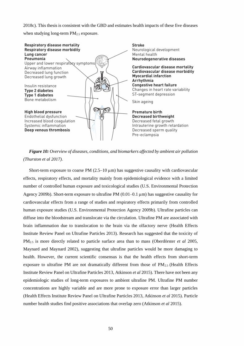
50

2018c). This thesis is consistent with the GBD and estimates health impacts of these five diseases

when studying long-term PM2.5 exposure.

Figure 10: Overview of diseases, conditions, and biomarkers affected by ambient air pollution

(Thurston et al 2017).

Short-term exposure to coarse PM (2.5–10 m) has suggestive causality with cardiovascular

effects, respiratory effects, and mortality mainly from epidemiological evidence with a limited

number of controlled human exposure and toxicological studies (U.S. Environmental Protection

Agency 2009b). Short-term exposure to ultrafine PM (0.01–0.1 m) has suggestive causality for

cardiovascular effects from a range of studies and respiratory effects primarily from controlled

human exposure studies (U.S. Environmental Protection Agency 2009b). Ultrafine particles can

diffuse into the bloodstream and translocate via the circulation. Ultrafine PM are associated with

brain inflammation due to translocation to the brain via the olfactory nerve (Health Effects

Institute Review Panel on Ultrafine Particles 2013). Research has suggested that the toxicity of

PM2.5 is more directly related to particle surface area than to mass (Oberdörster et al 2005,

Maynard and Maynard 2002), suggesting that ultrafine particles would be more damaging to

health. However, the current scientific consensus is that the health effects from short-term

exposure to ultrafine PM are not dramatically different from those of PM2.5 (Health Effects

Institute Review Panel on Ultrafine Particles 2013, Atkinson et al 2015). There have not been any

epidemiologic studies of long-term exposures to ambient ultrafine PM. Ultrafine PM number

concentrations are highly variable and are more prone to exposure error than larger particles

(Health Effects Institute Review Panel on Ultrafine Particles 2013, Atkinson et al 2015). Particle

number health studies find positive associations that overlap zero (Atkinson et al 2015).

51

Epidemiological evidence is limited in resolving what specific characteristics, components,

and sources of air pollution cause specific health effects (West et al 2016). Currently, the scientific

consensus treats all fine particles as equally toxic without regard to their source, shape, volatility,

and chemical composition (Lelieveld et al 2015, World Health Organization 2006a, Burnett et al

2014, U.S. Environmental Protection Agency 2009b). Previous studies suggest that carbonaceous

aerosol have strong associations with health impacts (Tuomisto et al 2008, Atkinson et al 2015)

and that particles from fossil fuel combustion are more toxic than particles from other sources

such as biomass burning (Thurston et al 2016). Secondary sulphates, nitrates, and crustal

materials have been found to be less toxic than average PM2.5 (Tuomisto et al 2008, Kelly and

Fussell 2012). There is insufficient evidence on the toxicity of metals (Atkinson et al 2015). Many

previous studies use a single pollutant approach for single diseases, providing limited insight into

the toxicity of particle constituents (Levy et al 2012, Atkinson et al 2015). There are no

epidemiological studies that estimate the joint effects of ambient and household air pollution.

1.1.7.2. Health impacts of O3 exposure

Table 3 summarises the long- and short-term health impacts of O3 exposure from controlled

human exposure, epidemiological, and toxicological studies (World Health Organization 2013,

U.S. Environmental Protection Agency 2013b, Jerrett et al 2009, Zanobetti and Schwartz 2011,

Smith et al 2009b, Turner et al 2016, Atkinson et al 2016). Short-term O3 exposure is a cause of

respiratory effects, a likely cause of cardiovascular effects and all-cause mortality, with

suggestive causality for central nervous system effects. Long-term O3 exposure is a likely cause

of respiratory effects, with suggestive causality of cardiovascular, reproductive and

developmental effects, central nervous system effects, and all-cause mortality. Previous studies

have highlighted the limited and confounded evidence for short-term cardiovascular effects

(Goodman et al 2014), conflicting evidence for long-term health impacts (Committee on the

Medical Effects of Air Pollutants 2015, Atkinson et al 2016, U.S. Environmental Protection

Agency 2013b), and the limited evidence for use of low concentration thresholds (Committee on

the Medical Effects of Air Pollutants 2015). There have been three, recent, major studies of long-

term O3 exposure and human health adding to the original American Cancer Society Cancer

Prevention Study II (CPS-II) by Jerrett et al (2009); the updated CPS-II study by Turner et al

(2016), the Harvard Medicare study (Di et al 2017), and the Canadian Census Health and

Environment Cohort (CanCHEC) study (Crouse et al 2015). All studies found O3 health effects

on all-cause mortality, unconfounded by PM2.5 or NO2, with some finding health effects for

cardiovascular, diabetes, and respiratory mortality (Jerrett et al 2009, Turner et al 2016, Di et al

2017, Crouse et al 2015).

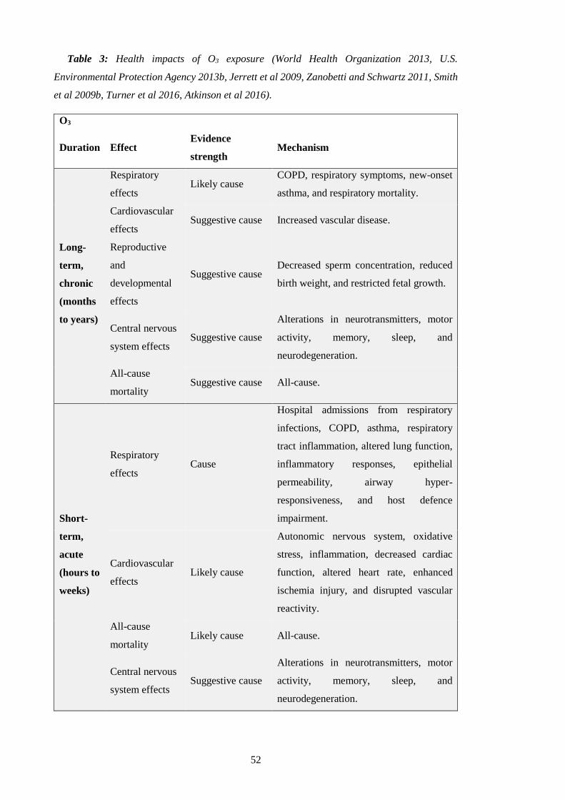
52

Table 3: Health impacts of O3 exposure (World Health Organization 2013, U.S.

Environmental Protection Agency 2013b, Jerrett et al 2009, Zanobetti and Schwartz 2011, Smith

et al 2009b, Turner et al 2016, Atkinson et al 2016).

O3

Duration Effect Evidence

strength Mechanism

Long-

term,

chronic

(months

to years)

Respiratory

effects Likely cause

COPD, respiratory symptoms, new-onset

asthma, and respiratory mortality.

Cardiovascular

effects Suggestive cause Increased vascular disease.

Reproductive

and

developmental

effects

Suggestive cause Decreased sperm concentration, reduced

birth weight, and restricted fetal growth.

Central nervous

system effects Suggestive cause

Alterations in neurotransmitters, motor

activity, memory, sleep, and

neurodegeneration.

All-cause

mortality Suggestive cause All-cause.

Short-

term,

acute

(hours to

weeks)

Respiratory

effects Cause

Hospital admissions from respiratory

infections, COPD, asthma, respiratory

tract inflammation, altered lung function,

inflammatory responses, epithelial

permeability, airway hyper-

responsiveness, and host defence

impairment.

Cardiovascular

effects Likely cause

Autonomic nervous system, oxidative

stress, inflammation, decreased cardiac

function, altered heart rate, enhanced

ischemia injury, and disrupted vascular

reactivity.

All-cause

mortality Likely cause All-cause.

Central nervous

system effects Suggestive cause

Alterations in neurotransmitters, motor

activity, memory, sleep, and

neurodegeneration.

53

Biologically plausible mechanisms for the adverse health effects of O3 exposure include

pulmonary function decrement, lung permeability, and many others. Susceptible populations to

the health effects from O3 exposure are those with asthma, children, elderly, individuals lacking

certain nutrients (e.g. vitamins C and E), outdoor workers, and individuals with gene variations

(U.S. Environmental Protection Agency 2013b). The lag of health effects relative to exposure to

O3 is dependent on age and pre-existing conditions and is consistently found to be within the first

few days for morbidity and mortality endpoints (U.S. Environmental Protection Agency 2013b).

The health effects of O3 exposure are confounded by temperature (Wilson et al 2014, Pattenden

et al 2010) and other pollutants (Committee on the Medical Effects of Air Pollutants 2015).

1.1.7.3. Risk assessments to estimate the burden of disease

Risk assessments quantify the disease burden of air pollution in terms of mortality and

morbidity. This thesis follows the methodology of the comparative risk assessment from the GBD.

The first GBD study was in 1993, commissioned by the World Bank (The World Bank 1993).

The first comprehensive ambient air pollution study was for 2000 published in 2004 through the

WHO and the World Bank (Cohen et al 2004, Pandey 2000), which was updated in 2009 by the

WHO (World Health Organization 2009). The GBD progressed in 2010 through funding by the

Bill & Melinda Gates Foundation and support from the WHO to study a huge scope of risk factors

and causes throughout the world. This led to the publications of GBD2010 in 2012 (GBD 2010

Risk Factors Collaborators 2012), GBD2013 in 2015 (GBD 2013 Risk Factors Collaborators

2015), GBD2015 in 2016 (GBD 2015 Risk Factors Collaborators 2016a), and GBD2016 in 2017

(GBD 2016 Risk Factors Collaborators 2017).

There are five key inputs to risk assessments to estimate the burden of disease from air

pollution exposure: pollutant concentrations, the counterfactual level, the population exposure,

baseline mortality rates, and an exposure-response function (Ostro et al 2018). The input methods

vary with approach, e.g. improvements to the exposure-response function. The input data vary in

time, e.g. the age and size of the population exposed or the pollutant concentration.

Accurate representation of air pollution concentrations is critical. The pollutant concentrations

are estimated through chemical transport models (Fang et al 2013, Lelieveld et al 2013, Silva et

al 2013, Ghude et al 2016, Butt et al 2016, Chafe et al 2014a, Lelieveld et al 2015, Anenberg et

al 2010), satellite observations (Apte et al 2015a, Brauer et al 2012, van Donkelaar et al 2010,

2016, Evans et al 2013), and ground measurements (Cohen et al 2004, Nagpure et al 2014,

Guttikunda and Goel 2013, Chate et al 2013). Models allow for air pollutant estimations where

ground measurements are limited in space and satellite observations are limited in time. Many

ground measurements within the WHO ambient air pollution database, used by the GBD, derived

PM2.5 from PM10 using conversion factors (World Health Organization 2018a). Recent GBD

studies (GBD2015 and GBD2016) have combined all the above sources within a Bayesian

hierarchical model, the data integration model for air quality (DIMAQ), along with land use

54

regression models, population, monitor type, PM2.5 to PM10 conversion factors, land use elevation,

and the concentrations of SO4, NO3, OC, and NH3 (Shaddick et al 2018b). The error in predicted

PM2.5 concentrations was greatly reduced through the addition of the local population as a

covariate (Ostro et al 2018).

The counterfactual level, also known as the theoretical minimum risk exposure level or the

low-concentration cut-off, is a minimum pollutant concentration where no health effects occur.

For long-term PM2.5 exposure, the disease-specific counterfactual in the GBD2010 and GBD2013

ranged from 5.8–8.9 g m-3, and in the GBD2015 and GBD2016 ranged from 2.4–5.9 g m-3. For

long-term O3 exposure, the counterfactual varied per study and percentile applied between 26.7–

41.9 ppb. The population exposure is the specific group exposed to the pollutant concentration.

Baseline mortality rates are the occurrence of the cause already present in that specific group. The

exposure-response functions use epidemiological data to relate a specific pollutant concentration

to a relative risk of disease. A significant advance in exposure-response function was the

development of the integrated-exposure response (IER) functions (Burnett et al 2014) as part of

the GBD2010 project (GBD 2010 Risk Factors Collaborators 2012) for long-term exposure to

ambient PM2.5 concentrations. The IER functions combine epidemiological evidence from

ambient air pollution, household air pollution, second-hand smoking, and active smoking to

estimate the health response to exposures across a widened range of pollutant concentrations.

Exposures to PM2.5 from air pollution and second-hand smoking are substantially smaller than

those from active smoking (Pope III et al 2018). The IER functions are a pragmatic approach,

including additional epidemiological evidence with each GBD study. The IER functions are

detailed in Section 2.3 and used in Chapters 4 and 5. The exposure-response functions for long-

term O3 exposure (detailed in Section 2.4 and used in Chapter 6) use risk estimates per increment

in pollutant concentration.

Mortality is measured by the number of premature mortalities, which are considered

preventable if the risk were to have been eliminated. The estimates are specifically for premature

mortality, as death is postponed or brought forward rather than avoided (Brunekreef et al 2007).

Morbidity is measured by years of life lost (YLL) due to the age-specific premature mortality

relative to a healthy life expectancy. Years lost due to disability (YLD) account for the incidence

and prevalence of disease, which can be added to YLL per cause to give the total disease burden,

known as DALYs (World Health Organization 2018b).

The economic impact of air pollution burden is difficult to assess as evaluation methods vary

dramatically in the literature, including metrics of a lost healthy life year, willingness to pay, and

ones based on income (World Health Organization 2003). A recent study by The World Bank and

the Institute for Health Metrics and Evaluation (IHME) estimated the cost of air pollution

following a willingness to pay approach and an income-based approach (The World Bank and

Institute for Health Metrics and Evaluation 2016). For the willingness to pay approach, total air

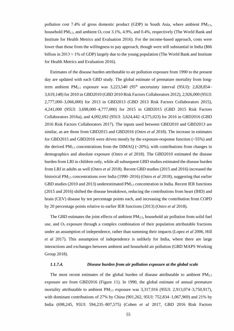
55

pollution cost 7.4% of gross domestic product (GDP) in South Asia, where ambient PM2.5,

household PM2.5, and ambient O3 cost 3.1%, 4.9%, and 0.4%, respectively (The World Bank and

Institute for Health Metrics and Evaluation 2016). For the income-based approach, costs were

lower than those from the willingness to pay approach, though were still substantial in India ($66

billion in 2013 ≈ 1% of GDP) largely due to the young population (The World Bank and Institute

for Health Metrics and Evaluation 2016).

Estimates of the disease burden attributable to air pollution exposure from 1990 to the present

day are updated with each GBD study. The global estimate of premature mortality from long-

term ambient PM2.5 exposure was 3,223,540 (95th uncertainty interval (95UI): 2,828,854–

3,619,148) for 2010 in GBD2010 (GBD 2010 Risk Factors Collaborators 2012), 2,926,000 (95UI:

2,777,000–3,066,000) for 2013 in GBD2013 (GBD 2013 Risk Factors Collaborators 2015),

4,241,000 (95UI: 3,698,000–4,777,000) for 2015 in GBD2015 (GBD 2015 Risk Factors

Collaborators 2016a), and 4,092,692 (95UI: 3,624,442–4,575,023) for 2016 in GBD2016 (GBD

2016 Risk Factors Collaborators 2017). The inputs used between GBD2010 and GBD2013 are

similar, as are those from GBD2015 and GBD2016 (Ostro et al 2018). The increase in estimates

for GBD2015 and GBD2016 were driven mostly by the exposure-response function (~55%) and

the derived PM2.5 concentrations from the DIMAQ (~20%), with contributions from changes in

demographics and absolute exposure (Ostro et al 2018). The GBD2010 estimated the disease

burden from LRI in children only, while all subsequent GBD studies estimated the disease burden

from LRI in adults as well (Ostro et al 2018). Recent GBD studies (2015 and 2016) increased the

historical PM2.5 concentrations over India (1990–2016) (Ostro et al 2018), suggesting that earlier

GBD studies (2010 and 2013) underestimated PM2.5 concentration in India. Recent IER functions

(2015 and 2016) shifted the disease breakdown, reducing the contributions from heart (IHD) and

brain (CEV) disease by ten percentage points each, and increasing the contribution from COPD

by 20 percentage points relative to earlier IER functions (2013) (Ostro et al 2018).

The GBD estimates the joint effects of ambient PM2.5, household air pollution from solid fuel

use, and O3 exposure through a complex combination of their population attributable fractions

under an assumption of independence, rather than summing their impacts (Lopez et al 2006, Hill

et al 2017). This assumption of independence is unlikely for India, where there are large

interactions and exchanges between ambient and household air pollution (GBD MAPS Working

Group 2018).

1.1.7.4. Disease burden from air pollution exposure at the global scale

The most recent estimates of the global burden of disease attributable to ambient PM2.5

exposure are from GBD2016 (Figure 11). In 1990, the global estimate of annual premature

mortality attributable to ambient PM2.5 exposure was 3,317,916 (95UI: 2,913,074–3,750,917),

with dominant contributions of 27% by China (901,262, 95UI: 752,834–1,067,969) and 21% by

India (698,245, 95UI: 594,235–807,575) (Cohen et al 2017, GBD 2016 Risk Factors

56

Collaborators 2017). In 2016, the estimates of annual premature mortality from exposure to

ambient PM2.5 increased globally by 23% to 4,092,692 (95UI: 3,624,442–4,575,023), in China by

19% to 1,075,039 (95UI: 940,395–1,221,813), and in India by 48% to 1,034,420 (95UI: 893,676–

1,176,954) (Cohen et al 2017, GBD 2016 Risk Factors Collaborators 2017). The large increase

in the burden of disease in India between 1990 and 2016 means that China and India both

dominate the contribution to the global burden, each contributing one-quarter. The large

populations of India and China are important factors to their large disease burdens. For the

mortality rate per 100,000 population, which is independent of population size, the Eastern

European countries of Bulgaria (126) and Ukraine (118) stand out relative to the rates in India

(79) and China (79) in 2016 (Cohen et al 2017, GBD 2016 Risk Factors Collaborators 2017). The

decrement in life expectancy from ambient PM2.5 in South Asia is 1.56 years (Apte et al 2018).

Figure 11: The global burden of disease from ambient PM2.5 exposure in 2016. (a) Number of


(Institute for Health Metrics and Evaluation 2018).

57

Figure 12 shows the drivers of the changes in premature mortality attributable to ambient PM2.5

exposure by country from 1990 to 2015 (Cohen et al 2017). The 23% increase in the global disease

burden between 1990 and 2015 was driven by population ageing (+41%) and population growth

(+26%), partially offset by improvements in baseline mortality rates (-54%). There are substantial

variations in the drivers between countries, where India experienced more substantial impacts of

population growth (+50%) and China had strong opposing influences between population ageing

(+69%) and improving baseline mortality rates (-79%). The strong roles of the demographic and

epidemiological transitions are clear, and often dominate the changes due to variations in

exposure.

Figure 12: Drivers of changes in estimated premature mortality associated with ambient

PM2.5 exposure by country from 1990 to 2015 (Cohen et al 2017).

Figure 13 shows the global burden of disease from exposure to ambient O3 in 2016. In 1990,

the global estimate of annual premature mortality attributable to ambient O3 exposure was

153,732 (95UI: 54,522–267,745), with dominant contributions of 44% by China (68,395, 95UI:

24,740–120,304) and 27% by India (41,709, 95UI: 15,172–70,285) (Cohen et al 2017, GBD 2016

Risk Factors Collaborators 2017). By 2016, the global estimate of annual premature mortality

from exposure to ambient O3 increased by 52% to 233,628 (95UI: 90,109–385,303), increasing

substantially by 116% in India to 90,253 (95UI: 34,556–145,570), while only increasing by 2%

in China to 69,707 (95UI: 26,763–115,134) (Cohen et al 2017, GBD 2016 Risk Factors

Collaborators 2017). The large increase in the disease burden from O3 exposure in India between

1990 and 2016 means that India dominates the contribution to the global burden (39%). The

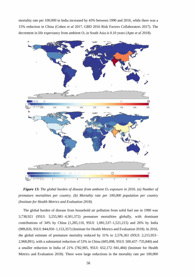
58

mortality rate per 100,000 in India increased by 43% between 1990 and 2016, while there was a

15% reduction in China (Cohen et al 2017, GBD 2016 Risk Factors Collaborators 2017). The

decrement in life expectancy from ambient O3 in South Asia is 0.10 years (Apte et al 2018).

Figure 13: The global burden of disease from ambient O3 exposure in 2016. (a) Number of



The global burden of disease from household air pollution from solid fuel use in 1990 was

3,738,921 (95UI: 3,255,981–4,301,372) premature mortalities globally, with dominant

contributions of 34% by China (1,285,110, 95UI: 1,081,537–1,521,215) and 26% by India

(989,826, 95UI: 844,050–1,153,357) (Institute for Health Metrics and Evaluation 2018). In 2016,

the global estimate of premature mortality reduced by 31% to 2,576,361 (95UI: 2,215,953–

2,968,891), with a substantial reduction of 53% in China (605,098, 95UI: 500,437–735,840) and

a smaller reduction in India of 21% (782,905, 95UI: 652,172–941,484) (Institute for Health

Metrics and Evaluation 2018). There were large reductions in the mortality rate per 100,000

59

population of 51% globally, 49% in India, and 61% in China (Institute for Health Metrics and

Evaluation 2018). The decrement in life expectancy from household air pollution in South Asia

is 1.22 years (Apte et al 2018).

Overall, the main trends from 1990 (Figure 14a) to 2016 (Figure 14c) are that the number of

premature mortalities from ambient PM2.5 exposure increased globally, and especially in India.

The mortality rate per 100,000 population for ambient PM2.5 exposure remained stable (Figure

14b and 14d), indicating that the growth in the number of premature mortalities was primarily

driven by population characteristics. There were large decreases in the number of premature

mortalities and the mortality rate from household air pollution from solid fuels, highlighting the

important development relating to this issue that has occurred between 1990 and 2016, although

a substantial burden remains globally and in India. The burden of disease from exposure to

ambient O3 has remained relatively small compared to exposure to ambient PM2.5 and household

air pollution.

Figure 14: The disease burden from air pollution. (a) Annual premature mortality estimates

in 1990. (b) Mortality rate per 100,000 population in 1990. (c) Annual premature mortality

estimates in 2016. (d) Mortality rate per 100,000 population in 2016. Data from GBD2016


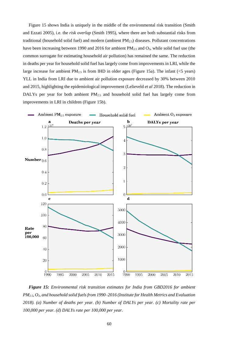
60

Figure 15 shows India is uniquely in the middle of the environmental risk transition (Smith

and Ezzati 2005), i.e. the risk overlap (Smith 1995), where there are both substantial risks from

traditional (household solid fuel) and modern (ambient PM2.5) diseases. Pollutant concentrations

have been increasing between 1990 and 2016 for ambient PM2.5 and O3, while solid fuel use (the

common surrogate for estimating household air pollution) has remained the same. The reduction

in deaths per year for household solid fuel has largely come from improvements in LRI, while the

large increase for ambient PM2.5 is from IHD in older ages (Figure 15a). The infant (<5 years)

YLL in India from LRI due to ambient air pollution exposure decreased by 30% between 2010

and 2015, highlighting the epidemiological improvement (Lelieveld et al 2018). The reduction in

DALYs per year for both ambient PM2.5 and household solid fuel has largely come from

improvements in LRI in children (Figure 15b).

Figure 15: Environmental risk transition estimates for India from GBD2016 for ambient

PM2.5, O3, and household solid fuels from 1990–2016 (Institute for Health Metrics and Evaluation

2018). (a) Number of deaths per year. (b) Number of DALYs per year. (c) Mortality rate per

100,000 per year. (d) DALYs rate per 100,000 per year.

61

1.1.7.5. Disease burden from air pollution exposure within India

In 2016, air pollution was the second leading risk factor in India, behind child and maternal

malnutrition, and up from third in 1990 (India State-Level Disease Burden Initiative Collaborators

2017). Four out of the top five leading causes of disease in India are caused in part by air pollution

exposure (India State-Level Disease Burden Initiative Collaborators 2017). Figure 16 shows the

Indian burden of disease from exposure to ambient PM2.5 in 2016. Within India in 2016, the

densely populated state of Uttar Pradesh in the central IGP dominates the contribution (21%) to

the national burden of disease from ambient PM2.5 exposure, ahead of West Bengal, Maharashtra,

and Bihar all contributing 9% each (Indian Council of Medical Research et al 2017a). Regarding

the mortality rate per 100,000 population, states throughout the IGP have massive burdens,

especially Punjab (105), Haryana (103), Uttar Pradesh (99), and West Bengal (95) (Indian Council

of Medical Research et al 2017a). The disease burden in Delhi from exposure to ambient PM2.5

is 11,517 (95UI: 9,757–13,331) premature mortalities per year with a mortality rate of 57 (95UI:

48–66) (Indian Council of Medical Research et al 2017a).

62

Figure 16: The Indian burden of disease from ambient PM2.5 exposure in 2016. (a) Number

of premature mortalities per state. (b) Mortality rate per 100,000 population per state (Indian

Council of Medical Research et al 2017a).

Figure 17 shows the Indian burden of disease from exposure to ambient O3 in 2016. Uttar

Pradesh dominates the contribution to ambient O3 with 27% of the national burden (Indian

Council of Medical Research et al 2017a). States in the western IGP have the highest mortality

rate per 100,000 population with Uttarakhand (12) and Himachal Pradesh (11), followed by Uttar

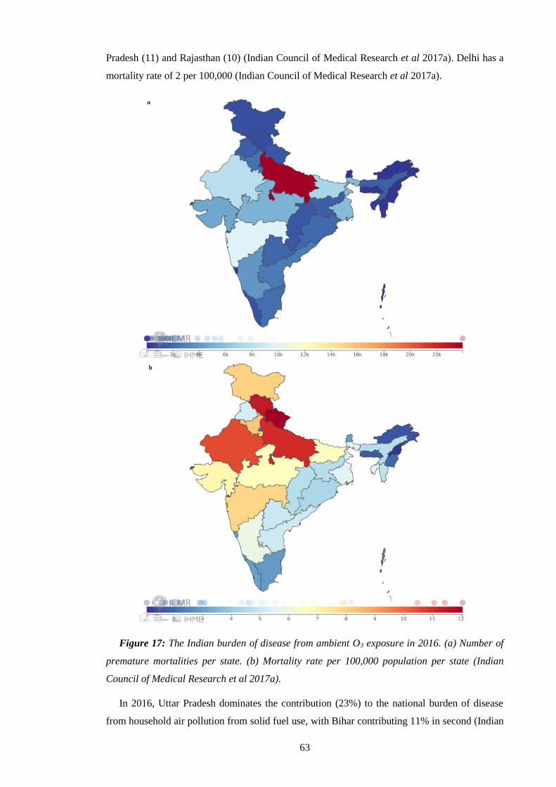
63

Pradesh (11) and Rajasthan (10) (Indian Council of Medical Research et al 2017a). Delhi has a

mortality rate of 2 per 100,000 (Indian Council of Medical Research et al 2017a).

Figure 17: The Indian burden of disease from ambient O3 exposure in 2016. (a) Number of


Council of Medical Research et al 2017a).

In 2016, Uttar Pradesh dominates the contribution (23%) to the national burden of disease

from household air pollution from solid fuel use, with Bihar contributing 11% in second (Indian

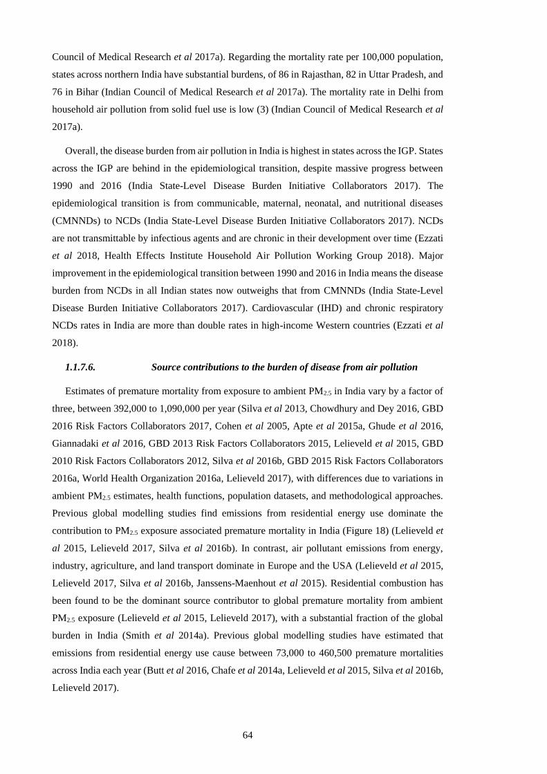
64

Council of Medical Research et al 2017a). Regarding the mortality rate per 100,000 population,

states across northern India have substantial burdens, of 86 in Rajasthan, 82 in Uttar Pradesh, and

76 in Bihar (Indian Council of Medical Research et al 2017a). The mortality rate in Delhi from

household air pollution from solid fuel use is low (3) (Indian Council of Medical Research et al

2017a).

Overall, the disease burden from air pollution in India is highest in states across the IGP. States

across the IGP are behind in the epidemiological transition, despite massive progress between

1990 and 2016 (India State-Level Disease Burden Initiative Collaborators 2017). The

epidemiological transition is from communicable, maternal, neonatal, and nutritional diseases

(CMNNDs) to NCDs (India State-Level Disease Burden Initiative Collaborators 2017). NCDs

are not transmittable by infectious agents and are chronic in their development over time (Ezzati

et al 2018, Health Effects Institute Household Air Pollution Working Group 2018). Major

improvement in the epidemiological transition between 1990 and 2016 in India means the disease

burden from NCDs in all Indian states now outweighs that from CMNNDs (India State-Level

Disease Burden Initiative Collaborators 2017). Cardiovascular (IHD) and chronic respiratory

NCDs rates in India are more than double rates in high-income Western countries (Ezzati et al

2018).

1.1.7.6. Source contributions to the burden of disease from air pollution

Estimates of premature mortality from exposure to ambient PM2.5 in India vary by a factor of

three, between 392,000 to 1,090,000 per year (Silva et al 2013, Chowdhury and Dey 2016, GBD

2016 Risk Factors Collaborators 2017, Cohen et al 2005, Apte et al 2015a, Ghude et al 2016,

Giannadaki et al 2016, GBD 2013 Risk Factors Collaborators 2015, Lelieveld et al 2015, GBD

2010 Risk Factors Collaborators 2012, Silva et al 2016b, GBD 2015 Risk Factors Collaborators

2016a, World Health Organization 2016a, Lelieveld 2017), with differences due to variations in

ambient PM2.5 estimates, health functions, population datasets, and methodological approaches.

Previous global modelling studies find emissions from residential energy use dominate the

contribution to PM2.5 exposure associated premature mortality in India (Figure 18) (Lelieveld et

al 2015, Lelieveld 2017, Silva et al 2016b). In contrast, air pollutant emissions from energy,

industry, agriculture, and land transport dominate in Europe and the USA (Lelieveld et al 2015,

Lelieveld 2017, Silva et al 2016b, Janssens-Maenhout et al 2015). Residential combustion has

been found to be the dominant source contributor to global premature mortality from ambient

PM2.5 exposure (Lelieveld et al 2015, Lelieveld 2017), with a substantial fraction of the global

burden in India (Smith et al 2014a). Previous global modelling studies have estimated that

emissions from residential energy use cause between 73,000 to 460,500 premature mortalities

across India each year (Butt et al 2016, Chafe et al 2014a, Lelieveld et al 2015, Silva et al 2016b,

Lelieveld 2017).

65

Figure 18: Source categories responsible for the largest impact on premature mortality

associated with ambient air pollution in 2010 (Lelieveld et al 2015). Source categories are

industry (IND), land transport (TRA), residential (RCO), biomass burning (BB), power

generation (PG), agriculture (AGR), and natural (NAT). The white areas are where annual-mean

PM2.5 concentrations are below the theoretical minimum risk exposure level.

All previous global modelling studies estimating the source contributions to the disease burden

(Lelieveld et al 2015, Lelieveld 2017, Silva et al 2016b) used global models with relatively coarse

resolution, which may not resolve the high PM2.5 concentrations in India, and were limited by

lack of ground measurements before 2016. Chapter 4 is the first study to use high-resolution

simulations, evaluated by new ground measurements, to estimate the contribution of different

emission sectors to ambient PM2.5 concentrations and the attributable disease burden from

exposure across India.

Previous global modelling studies have estimated the contribution of sources to the disease

burden from ambient O3 exposure in India using the earlier CPS-II risk estimates (Malley et al

2017, Silva et al 2016b, Lelieveld et al 2015). These risk estimates have been recently updated

(Turner et al 2016). Substantial contributions were found to be from power generation, land

transport, and residential emissions (Malley et al 2017, Silva et al 2016b, Lelieveld et al 2015).

Previous studies of the total and source-specific disease burden associated with O3 exposure have

used global, offline chemical transport models at relatively coarse spatial resolution (between 0.5°

× 0.67° and 2.0° × 2.5°) (Malley et al 2017, Silva et al 2016b, Lelieveld et al 2015). Tropospheric

O3 has a non-linear dependence on precursors concentrations, with production on short timescales

(Liang and Jacobson 2000, Carey Jang et al 1995, Wild and Prather 2006, Sharma et al 2017b).

Coarse spatial resolution models dilute O3 precursors, causing simulated concentrations to diverge

from observations (Liang and Jacobson 2000, Carey Jang et al 1995, Wild and Prather 2006,

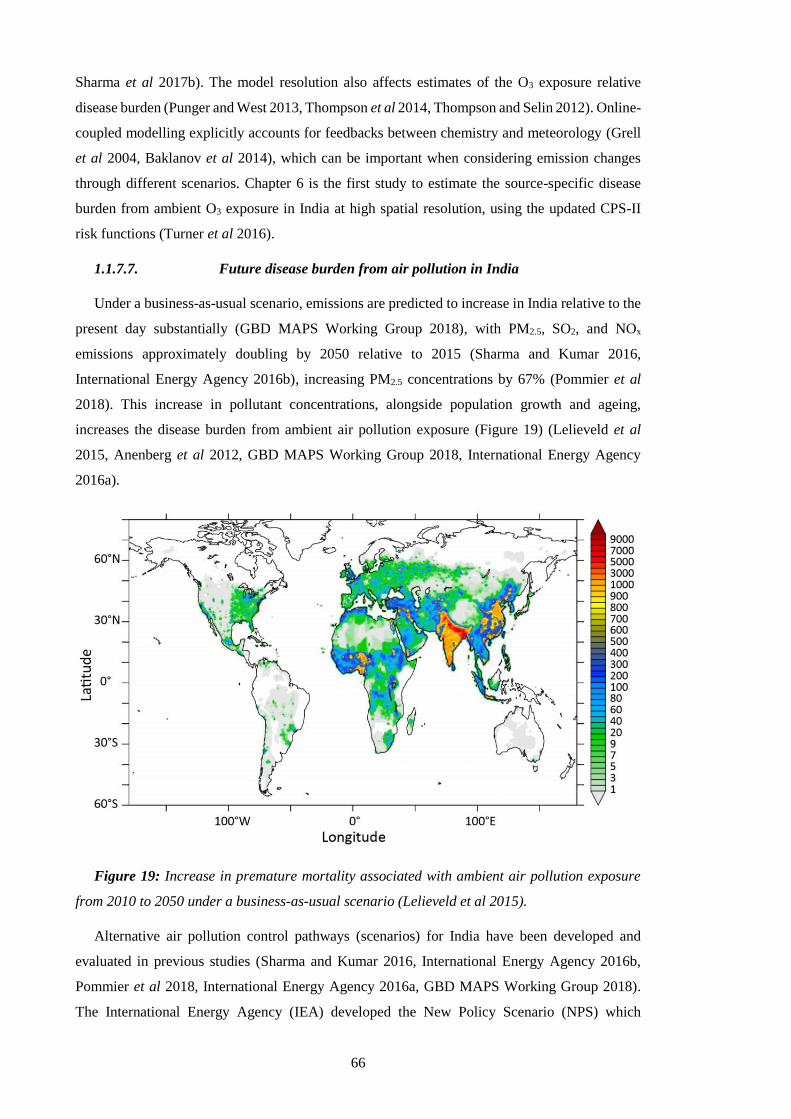
66

Sharma et al 2017b). The model resolution also affects estimates of the O3 exposure relative

disease burden (Punger and West 2013, Thompson et al 2014, Thompson and Selin 2012). Online-

coupled modelling explicitly accounts for feedbacks between chemistry and meteorology (Grell

et al 2004, Baklanov et al 2014), which can be important when considering emission changes

through different scenarios. Chapter 6 is the first study to estimate the source-specific disease

burden from ambient O3 exposure in India at high spatial resolution, using the updated CPS-II

risk functions (Turner et al 2016).

1.1.7.7. Future disease burden from air pollution in India

Under a business-as-usual scenario, emissions are predicted to increase in India relative to the

present day substantially (GBD MAPS Working Group 2018), with PM2.5, SO2, and NOx

emissions approximately doubling by 2050 relative to 2015 (Sharma and Kumar 2016,

International Energy Agency 2016b), increasing PM2.5 concentrations by 67% (Pommier et al

2018). This increase in pollutant concentrations, alongside population growth and ageing,

increases the disease burden from ambient air pollution exposure (Figure 19) (Lelieveld et al

2015, Anenberg et al 2012, GBD MAPS Working Group 2018, International Energy Agency

2016a).

Figure 19: Increase in premature mortality associated with ambient air pollution exposure

from 2010 to 2050 under a business-as-usual scenario (Lelieveld et al 2015).

Alternative air pollution control pathways (scenarios) for India have been developed and

evaluated in previous studies (Sharma and Kumar 2016, International Energy Agency 2016b,

Pommier et al 2018, International Energy Agency 2016a, GBD MAPS Working Group 2018).

The International Energy Agency (IEA) developed the New Policy Scenario (NPS) which

67

considers all relevant existing and planned policies as of 2016 and the Clean Air Scenario (CAS)

which represents aggressive policy action using proven energy policies and technologies tailored

to national circumstances (International Energy Agency 2016b, 2016a). Emissions of SO2, NOx,

and PM2.5 under the NPS increased on average by 9% by 2040 relative to 2015, while the

premature mortality estimate increased by 53% (International Energy Agency 2016b, 2016a).

Emissions of SO2, NOx, and PM2.5 under the CAS decreased on average by 65% by 2040 relative

to 2015, while the premature mortality estimate decreased by 5% (International Energy Agency

2016b, 2016a). The GBD MAPS Working Group studied a business-as-usual reference scenario,

an ambitious scenario reflecting stringent emission standards, and an aspirational scenario all

through to 2050 (Venkataraman et al 2018, GBD MAPS Working Group 2018). Population-

weighted ambient PM2.5 concentrations across India in 2050 under the reference, ambitious, and

aspirational scenarios changed by +43%, +10%, and -35%, respectively relative to the reference

scenario in 2015 (Venkataraman et al 2018, GBD MAPS Working Group 2018). Premature

mortality from ambient PM2.5 exposure would increase under the reference, ambitious, and

aspirational scenarios by 234%, 194%, and 125% in 2050 relative to 2015 (Venkataraman et al

2018, GBD MAPS Working Group 2018). Both the IEA and GBD MAPS Working Group studies

highlight the substantial impact of the demographic transition in India.

The previous studies that evaluated Indian scenarios (International Energy Agency 2016b,

2016a, Pommier et al 2018, GBD MAPS Working Group 2018) used relatively coarse spatial

resolution (0.5° × 0.5° or 0.5° × 0.67°) chemical transport models to estimate the impacts on PM2.5

concentrations per scenario, which may not resolve the high PM2.5 concentrations in India. No

previous studies have analysed the impacts of future air pollution control pathways on ambient

O3 and the associated disease burden.

Chapter 5 and 6 analyse the impacts of multiple air pollution control pathways (scenarios) in

India on ambient PM2.5 and O3 concentrations and associated disease burdens, respectively. Both

chapters use a higher resolution (30 km, 0.3° horizontal) regional numerical weather prediction

model online-coupled with atmospheric chemistry, with the latest exposure-response functions,

and disease-specific baseline mortality rates for 2015 and 2050. Both chapters are individually

the first high-resolution analyses of the impacts of future scenarios on ambient PM2.5 and O3

concentrations and resulting disease burden in India, respectively.

1.2. Summary and Aims

Two-thirds of Indian households primarily use solid fuels, mostly wood in polluting traditional

stoves in rural areas within the IGP. The absolute number of solid fuel users has remained stable

for the last 30 years, contributing substantially to air pollutant emissions. India experienced large

growth in the economy, industry, power generation, and transport sectors over the last decade

leading to a large growth in emissions of air pollutants. Emissions of air pollutants are predicted

to grow substantially over the coming years in India. These air pollutant emissions have caused

68

very high concentrations of ambient PM2.5 and O3 in India. Exposure to these air pollutants is the

second leading risk factor in India (GBD 2016 Risk Factors Collaborators 2017, India State-Level

Disease Burden Initiative Collaborators 2017). India contributes one-quarter and one-third of the

present-day global disease burden attributable to ambient PM2.5 and O3 exposure, respectively

(GBD 2016 Risk Factors Collaborators 2017, India State-Level Disease Burden Initiative

Collaborators 2017). India is uniquely in the middle of the environmental risk transition, where

there is both substantial risk from household air pollution and ambient air pollution (GBD 2016

Risk Factors Collaborators 2017, India State-Level Disease Burden Initiative Collaborators

2017).

Despite the importance of air quality in India, it remains relatively understudied, and

knowledge of the sources and processes causing air pollution is limited. It is critical to understand

the contribution of different emission sources to ambient air pollution to design effective policies

to reduce this substantial disease burden. This thesis aims to understand the source contributions

to the attributable disease burden from ambient air pollution exposure in India and the effects of

future air pollution control pathways.

The thesis has three main objectives. Firstly, quantify the contributions of different emission

sources to ambient PM2.5 concentrations and the related disease burden across India in the present

day. Secondly, estimate the impact from different future air pollution control pathways on ambient

PM2.5 concentrations and human health in India. Thirdly, understand the current and future disease

burden from ambient O3 exposure in India, identifying critical contributing emission sources and

the impacts of future policy scenarios. These objectives are achieved by combining high-

resolution computer simulations, new and extensive observations, and the latest exposure-

response relationships. The high-resolution, online-coupled, regional numerical weather

prediction (NWP) model, Weather Research and Forecasting Model with Chemistry (WRF-

Chem), is used throughout these chapters.

1.3. Outline

Chapter 1 introduces the research topic, aim, objectives, and outline. Chapter 2 discusses the

methods. Chapter 3 discusses the model evaluation. Chapter 4 estimates the contribution of

different emission sources to ambient PM2.5 concentrations and the related disease burden across

India. Chapter 5 estimates the impacts of different air pollution control pathways on ambient

PM2.5 and human health in India. Chapter 6 studies the source contributions of ambient O3

concentrations in India, the exposure-related disease burden, and the changes under future policy

scenarios. Chapter 7 summarises and discusses the work undertaken, highlighting areas of future

work.

69

2. Methods

This chapter describes the methods and models used in this thesis. Section 2.1 summarises the

background of air quality modelling. Section 2.2 describes the air quality model used in the thesis.

Section 2.3 and 2.4 describe the exposure-response functions for PM2.5 and O3, respectively.

Section 2.5 describes the population data used. Section 2.6 explains the methods used to estimate

the sector-specific disease burden. Section 2.7 discusses uncertainties in the methods.

2.1. Air quality modelling

Satellite observations are limited in either space or time. Ground measurements are limited in

space, especially over India. Models can address these gaps in space and time, giving insight into

driving processes and mechanisms of air quality. The main purpose of the model used in this

thesis was to simulate total PM2.5 and O3 concentrations accurately and to attribute total

concentrations to different emission sectors. There are a wide variety of models. The discussion

here, and the term model used subsequently, applies to three-dimensional, mathematical

(describing fundamental atmospheric processes), Eulerian (fixed grid), atmospheric models

(Seinfeld and Pandis 2016).

The essential components of a model are emissions, transport, and physiochemical

transformations (Brasseur and Jacob 2016). Models are based on the non-linear primitive

equations including the momentum equation, thermodynamic equation, continuity equation, and

the ideal gas law (Brasseur and Jacob 2016). The primitive equations have no analytical solution,

and numerical methods are required (Brasseur and Jacob 2016).

Aerosol schemes are required to resolve the large aerosol size range for the chemical and

microphysical processes through individual modules (Brasseur and Jacob 2016). Aerosol schemes

represent aerosol size, mass, and number (Brasseur and Jacob 2016). Bulk aerosol schemes

resolve aerosol mass, assume the size distribution, are numerically efficient, and are useful when

focusing on gas-phase chemistry (Brasseur and Jacob 2016). Modal aerosol schemes carry aerosol

mass and number, representing aerosol size by overlapping intervals assuming a lognormal

distribution (Brasseur and Jacob 2016). Sectional aerosol schemes discretise aerosol size into bins

carrying mass and number (Brasseur and Jacob 2016). Aerosol schemes can interact with

radiation, photolysis, and clouds (Brasseur and Jacob 2016). The continuity equations solved for

aerosol mechanisms are the same as for gas mechanisms (Brasseur and Jacob 2016).

Models use gas-phase mechanisms to simulate chemical production and loss (Brasseur and

Jacob 2016, Seinfeld and Pandis 2016). Gas-phase mechanisms use an ensemble of chemical

reactions to calculate chemical production and loss using rate laws, aqueous chemistry using

cloud type, and phase equilibrium using Henry’s law coefficients (Brasseur and Jacob 2016,

Seinfeld and Pandis 2016). Gas-phase mechanisms simplify large, complex organic compounds

by classifying them by functionality or volatility, which are then represented by a surrogate

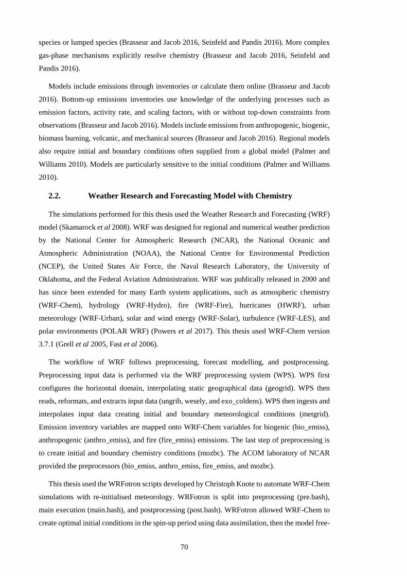
70

species or lumped species (Brasseur and Jacob 2016, Seinfeld and Pandis 2016). More complex

gas-phase mechanisms explicitly resolve chemistry (Brasseur and Jacob 2016, Seinfeld and

Pandis 2016).

Models include emissions through inventories or calculate them online (Brasseur and Jacob

2016). Bottom-up emissions inventories use knowledge of the underlying processes such as

emission factors, activity rate, and scaling factors, with or without top-down constraints from

observations (Brasseur and Jacob 2016). Models include emissions from anthropogenic, biogenic,

biomass burning, volcanic, and mechanical sources (Brasseur and Jacob 2016). Regional models

also require initial and boundary conditions often supplied from a global model (Palmer and

Williams 2010). Models are particularly sensitive to the initial conditions (Palmer and Williams

2010).

2.2. Weather Research and Forecasting Model with Chemistry

The simulations performed for this thesis used the Weather Research and Forecasting (WRF)

model (Skamarock et al 2008). WRF was designed for regional and numerical weather prediction

by the National Center for Atmospheric Research (NCAR), the National Oceanic and

Atmospheric Administration (NOAA), the National Centre for Environmental Prediction

(NCEP), the United States Air Force, the Naval Research Laboratory, the University of

Oklahoma, and the Federal Aviation Administration. WRF was publically released in 2000 and

has since been extended for many Earth system applications, such as atmospheric chemistry

(WRF-Chem), hydrology (WRF-Hydro), fire (WRF-Fire), hurricanes (HWRF), urban

meteorology (WRF-Urban), solar and wind energy (WRF-Solar), turbulence (WRF-LES), and

polar environments (POLAR WRF) (Powers et al 2017). This thesis used WRF-Chem version

3.7.1 (Grell et al 2005, Fast et al 2006).

The workflow of WRF follows preprocessing, forecast modelling, and postprocessing.

Preprocessing input data is performed via the WRF preprocessing system (WPS). WPS first

configures the horizontal domain, interpolating static geographical data (geogrid). WPS then

reads, reformats, and extracts input data (ungrib, wesely, and exo_coldens). WPS then ingests and

interpolates input data creating initial and boundary meteorological conditions (metgrid).

Emission inventory variables are mapped onto WRF-Chem variables for biogenic (bio_emiss),

anthropogenic (anthro_emiss), and fire (fire_emiss) emissions. The last step of preprocessing is

to create initial and boundary chemistry conditions (mozbc). The ACOM laboratory of NCAR

provided the preprocessors (bio_emiss, anthro_emiss, fire_emiss, and mozbc).

This thesis used the WRFotron scripts developed by Christoph Knote to automate WRF-Chem

simulations with re-initialised meteorology. WRFotron is split into preprocessing (pre.bash),

main execution (main.bash), and postprocessing (post.bash). WRFotron allowed WRF-Chem to

create optimal initial conditions in the spin-up period using data assimilation, then the model free-

71

runs for a set period to allow for sophisticated physics without drifting. The input data for nudging

has a 3-hour update interval, and values were interpolated in-between. Nudging was only applied

to selected variables (horizontal wind, vertical wind, potential temperature, and water vapour

mixing ratio) and with a nudging coefficient that still allows for WRF-Chem to create its own

dynamic, fine-scale, meteorology.

WRF-Chem is fully online-coupled (Grell et al 2005). Online-coupled models account for

interactions and feedbacks between air quality and meteorology (Grell et al 2005). These

interactions can include impacts on radiation, cloud condensation nuclei, removal processes, and

transport (Grell et al 2005). Offline models treat air quality and meteorology independently using

archived meteorology, losing valuable information about atmospheric processes (Grell et al

2005). WRF-Chem uses the Advanced Research WRF (ARW) fluid flow solver to calculate air

quality and meteorology components using the same transport, grid coordinates, sub-grid scale

physics, and timestep (Skamarock and Klemp 2008). ARW is fully compressible, allowing for

significant changes in fluid density (Skamarock and Klemp 2008). ARW is non-hydrostatic,

calculating the full vertical momentum equation (Skamarock and Klemp 2008). Fully

compressible, non-hydrostatic, numerical solvers allow explicit representation of structures

previously parameterised (Skamarock and Klemp 2008). ARW has a Eulerian mass conserving

dynamical core (Skamarock et al 2008). The driving equations of ARW have been derived in full

in Skamarock and Klemp (2008). The timestep of ARW is limited by the Courant-Friedrichs-

Levy (CFL) stability criterion (Courant et al 1928) and is suitable for regional NWP applications

not influenced by the pole problem (Brasseur and Jacob 2016). ARW uses terrain-following,

hydrostatic, pressure coordinates to account for surface topography (Laprise 1992).

WRF-Chem allows users to select mechanisms, schemes, and parameterisations, including

numerous options for physics, chemistry, and dynamics. The application of WRF-Chem over

South Asia was first documented in 2012 with two key papers evaluating the model's performance

for meteorology (Kumar et al 2012a) and chemistry (Kumar et al 2012b), establishing its

credibility for future use. Since then WRF-Chem has been used extensively over South Asia,

including papers using more complex sectional aerosol schemes (Kumar et al 2015b), higher

resolution simulations (Kumar et al 2015c), and exploring the impacts of dust (Kumar et al 2014a,

2014b).

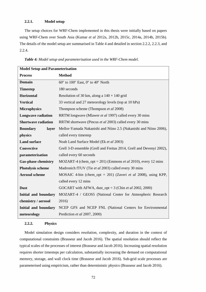
72

2.2.1. Model setup

The setup choices for WRF-Chem implemented in this thesis were initially based on papers

using WRF-Chem over South Asia (Kumar et al 2012a, 2012b, 2015c, 2014a, 2014b, 2015b).

The details of the model setup are summarised in Table 4 and detailed in section 2.2.2, 2.2.3, and

2.2.4.

Table 4: Model setup and parameterisation used in the WRF-Chem model.

Model Setup and Parameterisation

Process Method

Domain 60 to 100 East, 0 to 40 North

Timestep 180 seconds

Horizontal Resolution of 30 km, along a 140 × 140 grid

Vertical 33 vertical and 27 meteorology levels (top at 10 hPa)

Microphysics Thompson scheme (Thompson et al 2008)

Longwave radiation RRTM longwave (Mlawer et al 1997) called every 30 mins

Shortwave radiation RRTM shortwave (Pincus et al 2003) called every 30 mins

Boundary layer

physics

Mellor-Yamada Nakanishi and Niino 2.5 (Nakanishi and Niino 2006),

called every timestep

Land surface Noah Land Surface Model (Ek et al 2003)

Convective

parameterisation

Grell 3-D ensemble (Grell and Freitas 2014, Grell and Devenyi 2002),

called every 60 seconds

Gas-phase chemistry MOZART-4 (chem_opt = 201) (Emmons et al 2010), every 12 mins

Photolysis scheme Madronich fTUV (Tie et al 2003) called every 30 mins

Aerosol scheme MOSAIC 4-bin (chem_opt = 201) (Zaveri et al 2008), using KPP,

called every 12 mins

Dust GOCART with AFWA, dust_opt = 3 (Chin et al 2002, 2000)

Initial and boundary

chemistry / aerosol

MOZART-4 / GEOS5 (National Center for Atmospheric Research

2016)

Initial and boundary

meteorology

NCEP GFS and NCEP FNL (National Centers for Environmental

Prediction et al 2007, 2000)

2.2.2. Physics

Model simulation design considers resolution, complexity, and duration in the context of

computational constraints (Brasseur and Jacob 2016). The spatial resolution should reflect the

typical scales of the processes of interest (Brasseur and Jacob 2016). Increasing spatial resolution

requires shorter timesteps per calculation, substantially increasing the demand on computational

memory, storage, and wall clock time (Brasseur and Jacob 2016). Sub-grid scale processes are

parameterised using empiricism, rather than deterministic physics (Brasseur and Jacob 2016).

73

The model domain was a 140 × 140 cell grid, with a horizontal resolution of 30 km, 33 vertical

levels up to 10 hPa, and a timestep of 180 seconds. The resolution of 30 km was chosen as

adequate to resolve fine gradients in air pollutant concentrations while remaining computationally

feasible to perform 15 years of simulations. The relatively low vertical resolution has been used

in previous high horizontal resolution (10 km) simulations for air quality applications due to

computational constraints (Kumar et al 2015c). The time-step of the model simulation was taken

as 6 × grid spacing to ensure that the model does not violate the CFL stability criterion (Courant

et al 1928). Figure 20 shows the model domain used within all WRF-Chem simulations in this

thesis, using a Lambert conformal conical projection, with terrain height displayed.

Figure 20: Model domain used in this thesis. Background colour shows terrain height from

WRF-Chem simulated domain on a Lambert conformal conical projection.

Static geography fields were interpolated from the 20 category international geosphere-

biosphere programme (IGBP) modified moderate resolution imaging spectroradiometer

(MODIS) based land use classifications at 30 arc-second resolution by the WPS (Figure 21).

Substantial areas of India are cropland, with some forest, shrubland, and barren land. MODIS-

based categories should only be used with the Noah Land Surface Model (Ek et al 2003), which

was used to parameterise heat and moisture fluxes in four soil layers to 2 m. A single layer urban

canopy model was implemented with surface effects for roofs, walls, and streets.

74

Figure 21: International geosphere-biosphere programme (IGBP) modified moderate

resolution imaging spectroradiometer (MODIS) based land use classifications in India.

The Thompson scheme was used for cloud microphysics including cloud formation, phase

conversion, and precipitation (Thompson et al 2008). The Thompson scheme has been found to

accurately simulate Himalayan precipitation (Karki et al 2018, Reshmi Mohan et al 2018,

Rajeevan et al 2010). The Grell 3-D scheme (Grell and Freitas 2014) was used for convective

parameterisation, which is a development of the Grell-Devenyi scheme (Grell and Devenyi 2002).

The Grell scheme has been found to have improved skill at simulating the South Asian monsoon

relative to other cumulus schemes (Dash et al 2006, Yu et al 2011).

The Rapid Radiative Transfer Model (RRTM) option was used for downward and upward

fluxes of absorption, scattering, and emission from both shortwave radiation due to solar activity

and longwave radiation due to water vapour, clouds, and trace gases (e.g. CO2 and O3) (Iacono et

al 2008). The Mellor-Yamada Nakanishi and Niino 2.5 (Nakanishi and Niino 2006) boundary

layer scheme was called every timestep. WRF-Chem has been used to skillfully simulate air

pollution episodes over China with the Mellor-Yamada Nakanishi and Niino 2.5 boundary layer

scheme and the RRTM radiation schemes (Chen et al 2017a).

NCEP Global Forecast System (GFS) 6-hourly analyses initialised meteorological conditions

at 0.5 resolution. These, together with GFS 3-hour forecasts in between were also used for

boundary conditions and grid analysis nudging (National Centers for Environmental Prediction

et al 2007, 2000). Simulated mesoscale meteorology was kept in line with analysed meteorology

through grid nudging to the NCEP GFS analyses to limit errors in mesoscale transport (National

Centers for Environmental Prediction et al 2007, 2000). Kumar et al (2014b) used WRF-Chem

75

over South Asia and found nudging improved model skill in simulating meteorology. In this

thesis, model meteorology was reinitialised every month to avoid drifting of WRF-Chem, while

chemistry and aerosol fields were kept to allow for pollution build up and mesoscale transport

phenomena to be captured. During the simulations, horizontal and vertical wind, potential

temperature, and water vapour mixing ratio were nudged to GFS analyses in all model layers

above the planetary boundary layer using four-dimensional data assimilation (FDDA) (Liu et al

2006, 2005). FDDA in WRF-Chem does not use the analyses fields for its values. Instead, it uses

them as initial conditions, and then uses the primitive atmospheric equations, affecting chemicals

through transport. One-week spin-up was implemented based on previous studies (Berge et al

2001, Kumar et al 2015c, Knote et al 2015). The immediate model results were outputted every

hour.

2.2.3. Chemistry

Gas-phase chemical reactions were calculated using the chemical mechanism Model for

Ozone and Related Chemical Tracers, version 4 (MOZART-4) (Emmons et al 2010). Several

updates to photochemistry of aromatics, biogenic hydrocarbons, and other species relevant to

regional air quality were applied including a detailed treatment of VOCs (Knote et al 2014,

Hodzic and Jimenez 2011, Hodzic and Knote 2014). The MOZART-4 scheme has been used in

other studies over India using WRF-Chem and captured critical observed features of gas-phase

species (Kumar et al 2014b, Ghude et al 2016). The updated MOZART-4 gas-phase mechanism

should be used with either the Tropospheric Ultraviolet-Visible (TUV) (Tie et al 2005) or the Fast

Tropospheric Ultraviolet-Visible (fTUV) module to calculate photolysis rates (Tie et al 2003).

The fTUV scheme was implemented as it is a simplified version of the TUV model (Madronich

and Weller 1990), reducing computational costs of using the full TUV scheme (Hodzic and Knote

2014). The fTUV code was updated to include aerosol feedbacks on photolysis (Hodzic and Knote

2014). Gas wet deposition was a combination of resolved (Neu and Prather 2012) and convective

washout (Grell and Freitas 2014), updated to use Henry’s law constants in gas-droplet partitioning

(Knote et al 2015). Gas dry deposition was based on aerodynamic, transport, and surface

resistances (Wesely 1989). The updated version of MOZART-4 has been used in many previous

studies (Knote et al 2014, 2015, Hodzic et al n.d., Campbell et al 2015, Im et al 2015, Wang et

al 2015).

Aerosol physics and chemistry were represented by the MOSAIC 4-bin scheme without

subgrid convective aqueous chemistry (Hodzic and Knote 2014, Zaveri et al 2008). The Kinetic

PreProcessor (KPP) (Damian et al 2002) was used to convert the underlying chemistry into

ordinary differential equations. Four sectional discrete size bins were used within MOSAIC based

on dry aerosol diameter; 0.039–0.156 m, 0.156–0.625 m, 0.625–2.5 m, 2.5–10 m (Hodzic

and Knote 2014, Zaveri et al 2008). Water uptake and loss do not transfer aerosols between the

size bins (Hodzic and Knote 2014, Zaveri et al 2008). MOSAIC carries sulphate (SO4), nitrate

76

(NO3), ammonium (NH4), calcium (Ca), carbonate (CO3), black carbon (BC), primary organic

mass (OM), liquid water (H2O), sea salt (NaCl), methanesulfonate (CH3SO3), and other inorganic

mass such as minerals and trace metals (Hodzic and Knote 2014, Zaveri et al 2008). The aerosol

number was carried separately, and both aerosol mass and number were calculated for each size

bin (Hodzic and Knote 2014, Zaveri et al 2008). MOSAIC assumes aerosols are spherical,

internally mixed within the same size bin and externally mixed with other size bins, implying that

per size bin there is no ageing time for emissions to transfer from hydrophobic to hydrophilic

(Kumar et al 2015c). Wet deposition of aerosols was a mixture of resolved (Neu and Prather

2012) and convective washout (Grell and Freitas 2014). Dry deposition was based on the

resistances approach (Wesely 1989) as a function of friction velocity and the boundary layer

height (Walcek et al 1986). The thermodynamic module in MOSAIC was designed for dynamic

gas-particle partitioning, reliably predicting particle deliquescence (moisture absorption until

dissolution), water content, and solid-liquid phase equilibrium in multicomponent aerosols, and

is computationally efficient (Hodzic and Knote 2014, Zaveri et al 2008). MOSAIC removes

aerosols via grid-scale precipitation (Chapman et al 2009, Easter et al 2004).

The SOA formation mechanism varies with or without the use of aqueous chemistry in the

MOSAIC aerosol scheme (Hodzic and Knote 2014). For MOSAIC without aqueous chemistry,

as used in this thesis, the SOA formation mechanism was from Hodzic and Knote (2014), based

work by Hodzic and Jimenez (2011). SOA calculations use a lumped surrogate VOC for

anthropogenic (VOCA) and biomass burning (VOCBB) co-emitted with CO that oxidises with OH

and condenses into SOA (Hodzic and Jimenez 2011). The ratio of VOCA (or VOCBB) to CO

emissions was parameterised as being proportional to the ratio of SOA formed to the change in

CO in very aged air (Hodzic and Jimenez 2011). CO is typically well produced by models, can

be measured by satellites, has similar or collocated emissions sources as anthropogenic SOA

precursors, and is approximately inert with regard to SOA timescales (Hodzic and Jimenez 2011).

Simulated SOA accuracy from this CO proxy approach is similar to volatility basis set (VBS)

parameterisations (Robinson et al 2007), while being much less computationally expensive and

can be used in regions where the emissions of SOA precursors are not yet available (e.g. India)

(Hodzic and Jimenez 2011). Hodzic and Knote (2014) updated the SOA calculations from Hodzic

and Jimenez (2011) to use ambient ageing measurements of OA that produce reasonable and

efficient simulated SOA precursors. Hodzic and Knote (2014) calculate biogenic SOA via a two-

product approach (partitioning coefficient and a proportionality constant for each specie oxidising

VOCs) (Odum et al 1997, Odum Jay et al 1996), with updated yields (Hodzic and Knote 2014).

Glyoxal SOA, a product of isoprene oxidation, formation and partitioning were included using a

simple surface uptake mechanism (Knote et al 2014).

Simulations over India comparing the bulk scheme from Georgia Tech / Goddard Global

Ozone Chemistry Aerosol Radiation and Transport (GOCART) (Chin et al 2000) and the

77

MOSAIC 8-bin sectional schemes have shown the MOSAIC scheme more accurately represents

aerosol observations (Kumar et al 2015b). MOSAIC accounts for many aerosol processes (e.g.,

aerosol thermodynamics, SOA formation, in-cloud, and impaction scavenging) not included in

the GOCART bulk aerosol scheme. The 8-bin MOSAIC sectional aerosol scheme is 1.8 times

slower than the 3-mode Modal Aerosol Dynamics Model for Europe (MADE) (Ackermann et al

1998) modal aerosol scheme while containing 2.7 times more prognostic chemical species (Fast

et al 2011). The MOSAIC 4-bin aerosol scheme is less computationally demanding relative to the

8-bin scheme, while still skilfully simulating PM2.5 mass over India (Sarangi et al 2015, Kumar

et al 2015b). In this thesis, the MOZART-MOSAIC 4-bin without subgrid convective aqueous

chemistry was implemented throughout, due to the balance of detailed aerosol and trace gas

processes with computational efficiency. There are uncertainties within MOSAIC, such as aerosol

shape and morphology, assumed chemical species density, assumed refractive indices, and the

conversion factor between OM and OC (Barnard et al 2010).

2.2.4. Emissions

Anthropogenic emissions for 2010 were taken from the Emission Database for Global

Atmospheric Research with Task Force on Hemispheric Transport of Air Pollution (EDGAR-

HTAP) version 2.2 at 0.1 × 0.1 horizontal resolution (Janssens-Maenhout et al 2015). EDGAR-

HTAP v2.2 uses the Model Intercomparison Study for Asia Phase III (MIX), which is a mosaic

of Asian anthropogenic emission inventory (Li et al 2017b). For India, MIX uses the Indian

emission inventory provided by the Argonne National Laboratory (Lu et al 2011, Lu and Streets

2012) for SO2, BC, and OC for all sectors, as well as NOx for power plants, and Regional Emission

inventory in Asia (REAS) version 2.1 (Kurokawa et al 2013) for other species. The bottom-up

global emission inventory EDGAR v4.3 filled gaps in EDGAR-HTAP v2.2 (Janssens-Maenhout

et al 2015). Emissions include PM2.5, PM10, SO2, NOx, CO, NMVOC, NH3, BC, and OC

(Janssens-Maenhout et al 2015). Emissions are classified by source sector: aviation, shipping,

power generation (ENE), industrial non-power (IND), land transport (TRA), residential energy

use (RES), and agriculture (AGR) (Janssens-Maenhout et al 2015). Power generation emissions

for the energy sector are from electricity and heat production. Industrial non-power emissions

include large-scale combustion and industrial processes. Emissions from residential energy use

categorised in EDGAR-HTAP v2.2 comprise small-scale combustion devices for heating,

cooking, lighting, and cooling in addition to supplementary engines for residential, commercial,

agricultural, solid waste, and wastewater treatment (Janssens-Maenhout et al 2015). In India,

residential emissions are primarily from cooking. Residential energy use emissions of PM2.5, BC,

and OC, were qualitatively classified as highly uncertain within EDGAR-HTAP v2.2 (Janssens-

Maenhout et al 2015). Seasonal cycles were derived from monthly activity data for power

generation, industrial non-power, and all transport sectors, while residential energy use depends

on regional monthly-mean temperature (Lu et al 2011). EDGAR has been found to simulate air

78

quality well over South Asia using WRF-Chem relative to other anthropogenic emission

inventories (Saikawa et al 2017). Emissions from EDGAR-HTAP v2.2 were chosen over

ECLIPSE due to higher spatial resolution in EDGAR-HTAP v2.2 (0.1 × 0.1relative to 0.5 ×

0.5), that ECLIPSE underestimated BC and trace gas emission magnitudes and had inaccuracies

in their spatial distribution over India (Stohl et al 2015, Klimont et al 2017), and that simulations

using EDGAR emissions estimate PM closer to observations over India (Saikawa et al 2017).

Biomass burning emissions were taken from the Fire Inventory from NCAR (FINN) version

1.5 bottom-up inventory using burned area estimates (Wiedinmyer et al 2011). Biomass burning

emissions are from the open burning of biomass including wildfires, agricultural fires, and

prescribed fires, and not biofuel use and trash burning (Wiedinmyer et al 2011). FINN uses daily,

1 km resolution, global estimates of gas and aerosol emissions from satellite observations of active

fires and land cover with updated emission factors and estimated fuel loadings (Akagi et al 2011).

FINN fire emissions were used over the Global Fire Emissions Database (GFED) fire emissions

as FINN has higher spatial resolution and better captures small fires (Reddington et al 2016,

Randerson et al 2012). However, it is likely that emissions from agricultural fires are still

underestimated (Cusworth et al 2018).

Biogenic emissions were calculated online by the Model of Emissions of Gases and Aerosol

from Nature (MEGAN) (Guenther et al 2006) online canopy model. MEGAN is driven by 1 km

satellite measurements of land use (Guenther et al 2006). MEGAN estimates the net emission of

134 gases and aerosols from terrestrial ecosystems (Guenther et al 2006). MEGAN is

recommended to be used with the updated gas-phase mechanism of MOZART-4 as it speciates

biogenic VOCs online (Hodzic and Knote 2014).

Dust emissions were calculated online through GOCART with Air Force Weather Agency

(AFWA) modifications based on wind speed and land surface characteristics (Legrand et al 2018,

Chin et al 2000, Ginoux et al 2001, Jones et al 2012, 2010, Su and Fung 2015, Kok 2011). The

AFWA modifications are based on dust emission parameterisations from Marticorena and

Bergametti (1995) with ten saltation size bins and five dust size bins (0–2 m, 2–3.6 m, 3.6–6

m, 6–12 m, and 12–20 m) (Legrand et al 2018). GOCART AFWA dust emissions were

chosen over GOCART dust emissions due to updated physics, over the MOSAIC and

MADE/SORGAM dust emissions option due to errors, and over the GOCART dust emissions

with University of Cologne (UOC) modifications due to lack of testing (Legrand et al 2018).

MOZART-4 / Goddard Earth Observing System Model version 5 (GEOS5) 6-hourly

simulation data were used for chemical and aerosol boundary conditions (National Center for

Atmospheric Research 2016), which were interpolated onto the WRF-Chem domain using the

mozbc preprocessor. The species map within mozbc defines the speciation of initial and boundary

79

chemistry conditions from MOZART-4 with an assumed size distribution, as MOZART-4 used a

bulk scheme for 12 aerosol compounds.

Monthly files were concatenated to annual files for use with the preprocessor anthro_emiss.

Within anthro_emiss, emissions preprocessing was set up for a modal aerosol scheme, MADE

(Ackermann et al 1998), and mapping splits these to the appropriate size bin. The anthro_emiss

preprocessor outputs two datasets per domain for 00 and 12 hours Coordinated Universal Time

(UTC). Preprocessors map unspeciated PM2.5 from emission input files to other inorganics after

subtracting all known aerosol. A similar process happens for PM10, where the mass is the

difference between PM10 and PM2.5 only. Within the fire_emiss preprocessor, emissions were

mapped directly onto WRF-Chem MOSAIC aerosol bins, avoiding double counting, and the size

distribution were calculated online.

2.3. Exposure-response function for long-term ambient PM2.5 exposure

Long-term (annual) average exposures to ambient PM2.5 concentrations were associated with

a relative risk of disease estimated through the integrated exposure-response (IER) functions

(Burnett et al 2014). The IER functions (Burnett et al 2014), developed as part of GBD2010

(GBD 2010 Risk Factors Collaborators 2012), represent a significant advance in estimating risk

from PM2.5 exposure. The IER functions combine epidemiological evidence from ambient air

pollution, household air pollution, second-hand smoking, and active smoking to estimate the

health response to exposures across a widened range of pollutant concentrations (Burnett et al

2014). Exposures to PM2.5 increase from ambient air pollution to second-hand smoking,

household air pollution from solid fuel combustion, and active smoking (Pope III et al 2018). The

IER functions enable the estimation of risk factor across the global concentration range of ambient

PM2.5 (Burnett et al 2014). The IER functions assume that PM2.5 is an appropriate indicator of risk

and that epidemiological data is valid across populations (Ostro et al 2018). There are individual

IER functions per cause of COPD, IHD, CEV, LRI, and LC. The IER functions primarily use

epidemiological data from cohort studies from the United States, Europe, and parts of Asia.

Relative risks (RR) are the ratio of the probability of a health endpoint occurring in a

population exposed to a level of pollution, to the probability of that same health endpoint

occurring in a population that is not exposed. An RR of one represents no increase in risk. RRs

for individual health conditions vary due to differences in approach, exposure estimates, and the

mechanisms linking exposures to the health condition (Burnett et al 2014, Pope III et al 2011).

The IER functions use age-specific modifiers for each disease to estimate the RR of mortality

associated with ambient PM2.5 concentrations (z), as shown in Equation 1. The maximum risk is

1 + α, the ratio of the IER at low to high concentrations is β, and the power of the PM2.5

concentration is γ. Parameter distributions of α, β, and γ were sampled for 1,000 simulations to

derive the mean IER function with 95% uncertainty intervals.

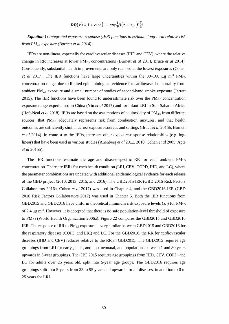
80

cfzzzRR exp11

Equation 1: Integrated exposure-response (IER) functions to estimate long-term relative risk

from PM2.5 exposure (Burnett et al 2014).

IERs are non-linear, especially for cardiovascular diseases (IHD and CEV), where the relative

change in RR increases at lower PM2.5 concentrations (Burnett et al 2014, Bruce et al 2014).

Consequently, substantial health improvements are only realised at the lowest exposures (Cohen

et al 2017). The IER functions have large uncertainties within the 30–100 g m-3 PM2.5

concentration range, due to limited epidemiological evidence for cardiovascular mortality from

ambient PM2.5 exposure and a small number of studies of second-hand smoke exposure (Jerrett

2015). The IER functions have been found to underestimate risk over the PM2.5 concentration

exposure range experienced in China (Yin et al 2017) and for infant LRI in Sub-Saharan Africa

(Heft-Neal et al 2018). IERs are based on the assumptions of equitoxicity of PM2.5 from different

sources, that PM2.5 adequately represents risk from combustion mixtures, and that health

outcomes are sufficiently similar across exposure sources and settings (Bruce et al 2015b, Burnett

et al 2014). In contrast to the IERs, there are other exposure-response relationships (e.g. log-

linear) that have been used in various studies (Anenberg et al 2011, 2010, Cohen et al 2005, Apte

et al 2015b).

The IER functions estimate the age and disease-specific RR for each ambient PM2.5

concentration. There are IERs for each health condition (LRI, CEV, COPD, IHD, and LC), where

the parameter combinations are updated with additional epidemiological evidence for each release

of the GBD project (2010, 2013, 2015, and 2016). The GBD2015 IER (GBD 2015 Risk Factors

Collaborators 2016a, Cohen et al 2017) was used in Chapter 4, and the GBD2016 IER (GBD

2016 Risk Factors Collaborators 2017) was used in Chapter 5. Both the IER functions from

GBD2015 and GBD2016 have uniform theoretical minimum risk exposure levels (zcf) for PM2.5

of 2.4 g m-3. However, it is accepted that there is no safe population-level threshold of exposure

to PM2.5 (World Health Organization 2006a). Figure 22 compares the GBD2015 and GBD2016

IER. The response of RR to PM2.5 exposure is very similar between GBD2015 and GBD2016 for

the respiratory diseases (COPD and LRI) and LC. For the GBD2016, the RR for cardiovascular

diseases (IHD and CEV) reduces relative to the RR in GBD2015. The GBD2015 requires age

groupings from LRI for early-, late-, and post-neonatal, and populations between 1 and 80 years

upwards in 5-year groupings. The GBD2015 requires age groupings from IHD, CEV, COPD, and

LC for adults over 25 years old, split into 5-year age groups. The GBD2016 requires age

groupings split into 5-years from 25 to 95 years and upwards for all diseases, in addition to 0 to

25 years for LRI.

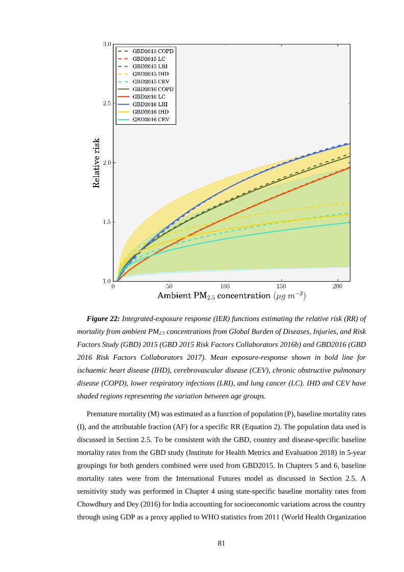
81

Figure 22: Integrated-exposure response (IER) functions estimating the relative risk (RR) of

mortality from ambient PM2.5 concentrations from Global Burden of Diseases, Injuries, and Risk

Factors Study (GBD) 2015 (GBD 2015 Risk Factors Collaborators 2016b) and GBD2016 (GBD

2016 Risk Factors Collaborators 2017). Mean exposure-response shown in bold line for

ischaemic heart disease (IHD), cerebrovascular disease (CEV), chronic obstructive pulmonary

disease (COPD), lower respiratory infections (LRI), and lung cancer (LC). IHD and CEV have

shaded regions representing the variation between age groups.

Premature mortality (M) was estimated as a function of population (P), baseline mortality rates

(I), and the attributable fraction (AF) for a specific RR (Equation 2). The population data used is

discussed in Section 2.5. To be consistent with the GBD, country and disease-specific baseline

mortality rates from the GBD study (Institute for Health Metrics and Evaluation 2018) in 5-year

groupings for both genders combined were used from GBD2015. In Chapters 5 and 6, baseline

mortality rates were from the International Futures model as discussed in Section 2.5. A

sensitivity study was performed in Chapter 4 using state-specific baseline mortality rates from

Chowdhury and Dey (2016) for India accounting for socioeconomic variations across the country

through using GDP as a proxy applied to WHO statistics from 2011 (World Health Organization

82

2011). The sensitivity study applied the state-to-nation ratios from the state-specific baseline

mortality rates to the GBD2015 baseline mortalities for COPD, IHD, and CEV. Baseline mortality

for LC did not exhibit any relation with GDP, and they did not study LRI. Accordingly, the

GBD2015 values were directly used for these diseases. This was done for mean, upper, and lower

confidence intervals.

RRRRIPAFIPM 1

Equation 2: Long-term premature mortality from PM2.5 exposure.

Years of life lost (YLL) for each age and disease were estimated as a function of premature

mortality and age-specific life expectancy (LE) from the standard reference life table from the

GBD (Equation 3). The standard reference life table was used from GBD2015 (Global Burden of

Disease Study 2015 2016b) in Chapter 4 and GBD2016 in Chapters 5 and 6 (Global Burden of

Disease Study 2016 2017b). Applying country-specific life expectancy values (Ministry of

Statistics and Programme Implementation 2016) from the Government of India in 2014 reduced

YLL by 60% relative to using the GBD2015 LE values. The GBD normative standard life table

was used for the main YLL results to be consistent with the extensive work done on this issue by

the GBD project. The GBD project in 2010 developed the normative standard life table after

consultation with philosophers, ethicists, and economists to compute YLL at each age by

identifying the lowest observed death rate for any age group in countries of more than 5 million

in population (Murray et al 2012). Two principles behind the decision were that the only

differences in the rating of death or disability should be due to age and that everyone in the world

has the right to best life expectancy in the world. The GBD India-specific study used the same

GBD normative standard life table (India State-Level Disease Burden Initiative Collaborators

2017).

LEMYLL

Equation 3: Long-term years of life lost from PM2.5 exposure.

The GBD meta-analyses estimates for PM2.5 risks include studies from India for household air

pollution, but no epidemiologic studies exist for long-term ambient PM2.5 exposure in India.

Recent epidemiological studies in India, supported by the Indian Council of Medical Research

(ICMR) and the European Research Council, are underway to analyse the health impacts of long-

term exposure to ambient and household air pollution (Tonne et al 2017, Balakrishnan et al 2015).

The IER functions are required for risk assessments in locations where the risk of exposure to air

pollution is high, and there are little data on long-term epidemiological studies, such as India. The

lack of locally-derived exposure-response functions has impeded previous risk assessment

attempts to impact local policy in India (The World Bank 1995, Health Effects Institute Public

Health and Air Pollution in Asia Program 2011).

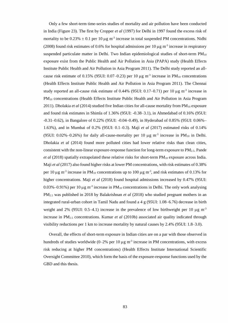
83

Only a few short-term time-series studies of mortality and air pollution have been conducted

in India (Figure 23). The first by Cropper et al (1997) for Delhi in 1997 found the excess risk of

mortality to be 0.23% ± 0.1 per 10 g m-3 increase in total suspended PM concentrations. Nidhi

(2008) found risk estimates of 0.6% for hospital admissions per 10 g m-3 increase in respiratory

suspended particulate matter in Delhi. Two Indian epidemiological studies of short-term PM10

exposure exist from the Public Health and Air Pollution in Asia (PAPA) study (Health Effects

Institute Public Health and Air Pollution in Asia Program 2011). The Delhi study reported an all-

cause risk estimate of 0.15% (95UI: 0.07–0.23) per 10 g m-3 increase in PM10 concentrations

(Health Effects Institute Public Health and Air Pollution in Asia Program 2011). The Chennai

study reported an all-cause risk estimate of 0.44% (95UI: 0.17–0.71) per 10 g m-3 increase in

PM10 concentrations (Health Effects Institute Public Health and Air Pollution in Asia Program

2011). Dholakia et al (2014) studied five Indian cities for all-cause mortality from PM10 exposure

and found risk estimates in Shimla of 1.36% (95UI: -0.38–3.1), in Ahmedabad of 0.16% (95UI:

-0.31–0.62), in Bangalore of 0.22% (95UI: -0.04–0.49), in Hyderabad of 0.85% (95UI: 0.06%–

1.63%), and in Mumbai of 0.2% (95UI: 0.1–0.3). Maji et al (2017) estimated risks of 0.14%

(95UI: 0.02%–0.26%) for daily all-cause-mortality per 10 g m-3 increase in PM10 in Delhi.

Dholakia et al (2014) found more polluted cities had lower relative risks than clean cities,

consistent with the non-linear exposure-response function for long-term exposure to PM2.5. Pande

et al (2018) spatially extrapolated these relative risks for short-term PM10 exposure across India.

Maji et al (2017) also found higher risks at lower PM concentrations, with risk estimates of 0.38%

per 10 g m-3 increase in PM10 concentrations up to 100 g m-3, and risk estimates of 0.13% for

higher concentrations. Maji et al (2018) found hospital admissions increased by 0.47% (95UI:

0.03%–0.91%) per 10 g m-3 increase in PM10 concentrations in Delhi. The only work analysing

PM2.5 was published in 2018 by Balakrishnan et al (2018) who studied pregnant mothers in an

integrated rural-urban cohort in Tamil Nadu and found a 4 g (95UI: 1.08–6.76) decrease in birth

weight and 2% (95UI: 0.5–4.1) increase in the prevalence of low birthweight per 10 g m-3

increase in PM2.5 concentrations. Kumar et al (2010b) associated air quality indicated through

visibility reductions per 1 km to increase mortality by natural causes by 2.4% (95UI: 1.8–3.0).

Overall, the effects of short-term exposure in Indian cities are on a par with those observed in

hundreds of studies worldwide (0–2% per 10 g m-3 increase in PM concentrations, with excess

risk reducing at higher PM concentrations) (Health Effects Institute International Scientific

Oversight Committee 2010), which form the basis of the exposure-response functions used by the

GBD and this thesis.

84

Figure 23: Short-term PM and PM10 exposure excess risk estimates in India.

2.4. Exposure-response function for long-term ambient O3 exposure

The disease burden associated with COPD from ambient O3 exposure was estimated using

relative risk (RR) estimates from the earlier American Cancer Society Cancer Prevention Study

II (CPS-II) study from Jerrett et al (2009), in addition to the updated CPS-II study from Turner et

al (2016). The updated CPS-II study derived RR estimates from a larger study population (+49%),

studying twice as many deaths during a longer follow up period (+22%). The updated CPS-II

study used improved exposure estimates and found the hazard ratios (HR) for respiratory

mortality increased. The earlier CPS-II study found HR per 10 ppb for respiratory mortality after

adjusting for PM2.5 confounding of 1.04 (95UI: 1.01–1.07), while the updated CPS-II study found

HR for COPD mortality after adjusting for PM2.5 and NO2 confounding of 1.14 (95UI: 1.08–1.21).

The updated CPS-II study found through sensitivity analyses that the long-term O3 health impacts

are not confounded by socioeconomic status or modelling approach. To be consistent with the

GBD, premature mortality was estimated from the risk of ambient O3 exposure from the cause of

COPD only. The GBD used the earlier CPS-II study risks with 3-month average daily maximum

1-hour O3 concentrations (3mDMA1), while the updated CPS-II study used annual average daily

maximum 8-hour O3 concentrations (ADM8h). Both the earlier (Jerrett et al 2009) and updated

(Turner et al 2016) RR estimates were used, with the corresponding O3 metric. No epidemiologic

studies exist for long-term O3 exposure in India.

Premature mortality associated with O3 exposure (M) was estimated for COPD for adults over

25 years of age (as per GBD) following Equation 4. Mortality was a function of the baseline

mortality rate (I), attributable fraction (AF), and the exposed population (P) per age group. The

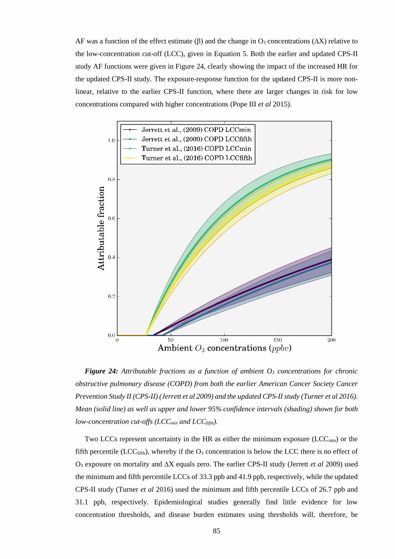
85

AF was a function of the effect estimate (β) and the change in O3 concentrations (∆X) relative to

the low-concentration cut-off (LCC), given in Equation 5. Both the earlier and updated CPS-II

study AF functions were given in Figure 24, clearly showing the impact of the increased HR for

the updated CPS-II study. The exposure-response function for the updated CPS-II is more non-

linear, relative to the earlier CPS-II function, where there are larger changes in risk for low

concentrations compared with higher concentrations (Pope III et al 2015).

Figure 24: Attributable fractions as a function of ambient O3 concentrations for chronic

obstructive pulmonary disease (COPD) from both the earlier American Cancer Society Cancer

Prevention Study II (CPS-II) (Jerrett et al 2009) and the updated CPS-II study (Turner et al 2016).

Mean (solid line) as well as upper and lower 95% confidence intervals (shading) shown for both

low-concentration cut-offs (LCCmin and LCCfifth).

Two LCCs represent uncertainty in the HR as either the minimum exposure (LCCmin) or the

fifth percentile (LCCfifth), whereby if the O3 concentration is below the LCC there is no effect of

O3 exposure on mortality and ∆X equals zero. The earlier CPS-II study (Jerrett et al 2009) used

the minimum and fifth percentile LCCs of 33.3 ppb and 41.9 ppb, respectively, while the updated

CPS-II study (Turner et al 2016) used the minimum and fifth percentile LCCs of 26.7 ppb and

31.1 ppb, respectively. Epidemiological studies generally find little evidence for low

concentration thresholds, and disease burden estimates using thresholds will, therefore, be

86

conservative (U.S. Environmental Protection Agency 2013b). β is the natural log of the HR for a

10 ppb increase in long-term O3 exposure (Equation 6). To account for uncertainty in the RR

estimates, 1,000 estimates of β were sampled from normal distributions of β using 95%

uncertainty intervals to derive a distribution of the AF. YLL were estimated in the same way as

detailed in Section 2.3, using the standard reference life table from GBD2016 (Global Burden of

Disease Study 2016 2017b).

PAFIM

Equation 4: Long-term premature mortality from O3 exposure.

XeAF 1

Equation 5: Long-term attributable fraction from O3 exposure.

10

)ln(HR

Equation 6: Long-term hazard ratio from O3 exposure.

A couple of previous epidemiological studies have researched the health impacts of short-term

O3 exposure in Delhi, India. Nidhi (2008) and Maji et al (2018) found short-term risk estimates

of 3.3% and 3.41% (95UI: 0.02%–6.83%), respectively, for hospital admissions per 10 g m-3

increase in O3 in Delhi. Maji et al (2017) estimated risks of 0.31% (95UI: 0.05%–0.57%) for daily

all-cause-mortality per 10 g m-3 increase in O3 concentrations in Delhi. These mortality risks,

although for all-cause and Delhi only, are larger than corresponding risks recommended by the

WHO (0.29%) (Héroux et al 2015) and Turner et al (2016) (0.2%) which are in line with the

estimates used in this thesis. This suggests the estimates in this thesis are conservative.

2.5. Current and future population of India

For Chapter 4, present-day population density data for 2015 was obtained at 0.25 ×

resolution from the Gridded Population of the World, Version 4 (GPWv4), created by the Centre

for International Earth Science Information Network (CIESIN) and accessed from the National

Aeronautics and Space Administration (NASA) Socioeconomic Data and Applications Centre

(SEDAC) (Center for International Earth Science Information Network and NASA

Socioeconomic Data and Applications Center 2016b). The United Nations adjusted version was

implemented for 2015 with a total population of 1.302 billion in India. Shapefiles were used to

split data per state within India from Spatial Data Repository, The Demographic and Health

Surveys Program (ICF International n.d.) and the GADM database of Global Administrative

Areas version 2.8 (Hijmans et al 2016). Chapter 4 includes rural and urban splits, where urban

areas were defined as having a population density of at least 400 persons’ km-2, as used in previous

studies (Lelieveld et al 2015). Population age composition was taken from the GBD2015

population estimates for 2015 for Chapter 4 (Global Burden of Disease Study 2015 2016a). The

87

GPWv4 national identifier grid (Center for International Earth Science Information Network and

NASA Socioeconomic Data and Applications Center 2016a) was used to allocate data by country.

For Chapters 5 and 6, present day (2015) and future (2050) population density, population age

structure, and baseline mortality rates for COPD, IHD, CEV, LC, and LRI were obtained from

the International Futures (IFs) integrated modelling system (Hughes et al 2011) base case scenario

(Hughes et al 2012). The IFs base case scenario forecasts a range of global transitions in human

development including increasing incomes, education, health, infrastructure, governance, and

productivity that are continuous with historical patterns, include non-linear relationships, and

exclude large disruptive changes (Hughes et al 2012). Figure 25 shows the variation in baseline

mortality, population age distribution, and population density for India between 2015 and 2050.

Baseline mortality rates for all diseases in India show reductions in 2050 relative to 2015,

primarily for LRI, CEV, and IHD where there are substantial decreases. The baseline mortality

rate for COPD reduces slightly in 2050 relative to 2015 for age groupings 60 years and older. The

population age distribution shifts towards older ages (40 years and older), and there is

considerable population growth, particularly across the IGP.

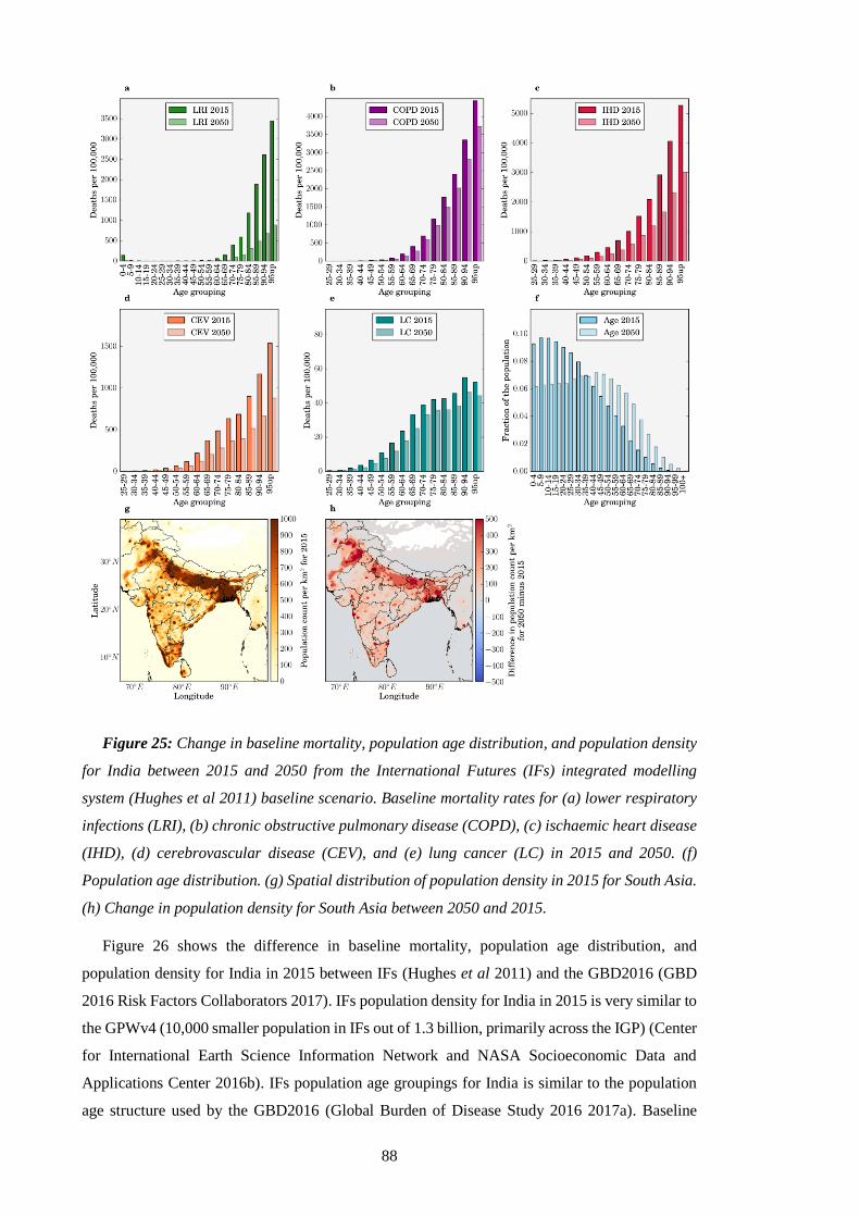
88

Figure 25: Change in baseline mortality, population age distribution, and population density

for India between 2015 and 2050 from the International Futures (IFs) integrated modelling

system (Hughes et al 2011) baseline scenario. Baseline mortality rates for (a) lower respiratory

infections (LRI), (b) chronic obstructive pulmonary disease (COPD), (c) ischaemic heart disease

(IHD), (d) cerebrovascular disease (CEV), and (e) lung cancer (LC) in 2015 and 2050. (f)

Population age distribution. (g) Spatial distribution of population density in 2015 for South Asia.

(h) Change in population density for South Asia between 2050 and 2015.

Figure 26 shows the difference in baseline mortality, population age distribution, and

population density for India in 2015 between IFs (Hughes et al 2011) and the GBD2016 (GBD

2016 Risk Factors Collaborators 2017). IFs population density for India in 2015 is very similar to

the GPWv4 (10,000 smaller population in IFs out of 1.3 billion, primarily across the IGP) (Center

for International Earth Science Information Network and NASA Socioeconomic Data and

Applications Center 2016b). IFs population age groupings for India is similar to the population

age structure used by the GBD2016 (Global Burden of Disease Study 2016 2017a). Baseline

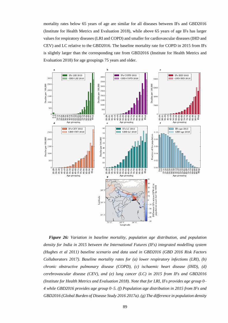
89

mortality rates below 65 years of age are similar for all diseases between IFs and GBD2016

(Institute for Health Metrics and Evaluation 2018), while above 65 years of age IFs has larger

values for respiratory diseases (LRI and COPD) and smaller for cardiovascular diseases (IHD and

CEV) and LC relative to the GBD2016. The baseline mortality rate for COPD in 2015 from IFs

is slightly larger than the corresponding rate from GBD2016 (Institute for Health Metrics and

Evaluation 2018) for age groupings 75 years and older.

Figure 26: Variation in baseline mortality, population age distribution, and population

density for India in 2015 between the International Futures (IFs) integrated modelling system

(Hughes et al 2011) baseline scenario and data used in GBD2016 (GBD 2016 Risk Factors

Collaborators 2017). Baseline mortality rates for (a) lower respiratory infections (LRI), (b)

chronic obstructive pulmonary disease (COPD), (c) ischaemic heart disease (IHD), (d)

cerebrovascular disease (CEV), and (e) lung cancer (LC) in 2015 from IFs and GBD2016

(Institute for Health Metrics and Evaluation 2018). Note that for LRI, IFs provides age group 0–

4 while GBD2016 provides age group 0–5. (f) Population age distribution in 2015 from IFs and

GBD2016 (Global Burden of Disease Study 2016 2017a). (g) The difference in population density

90

for South Asia in 2015 from IFs and Gridded Population of the World, Version 4 (GPWv4)

(Center for International Earth Science Information Network and NASA Socioeconomic Data and

Applications Center 2016b).

2.6. Sector-specific disease burden

There are two main methods for estimating the sectoral contributions to premature mortality

from ambient air pollution exposure, each giving greatly different results (Kodros et al 2016).

The subtraction (or zero-out) method calculates the sector-specific mortality (MSECTOR) as the

difference between the all-source premature mortality estimate from all sources (MALL) and the

premature mortality estimate based on a model simulation where the emission sector has been

removed (MSECTOR_OFF) as in Equation 7 (Silva et al 2016b, Kodros et al 2016, Chambliss et al

2014).

OFFSECTORALLSECTOR MMM _

Equation 7: Sector-specific premature mortality following the subtraction method.

Alternatively, the attribution method first calculates the fractional sectoral reduction in PM2.5

concentrations from removing an emission sector (PM2.5_SECTOR_OFF) and then uses this fraction to

scale the total premature mortality estimate (Equation 8) (GBD MAPS Working Group 2016,

Lelieveld et al 2015, Chafe et al 2014a, Kodros et al 2016, Archer-Nicholls et al 2016, Lelieveld

2017).

ALLOFFSECTORALLALLSECTOR PMPMPMMM _5.2__5.2_5.2

Equation 8: Sector-specific premature mortality following the attribution method.

The two methods answer different questions: the attribution method estimates the number of

premature mortalities that could be attributed to a sectors’ emissions, while the subtraction

method estimates the reduction in premature mortalities that could be achieved by removing the

sectors’ emissions. The non-linear exposure-response relationships mean these two methods give

different estimates. Chapters 4 and 6 use and compare both methods when estimating sector-

specific disease burdens.

2.7. Uncertainties

Uncertainty intervals at the 95% level (95UI) were estimated through combining fractional

errors in quadrature (i.e. square root of the sum of squares) from two standard deviations of

weekly PM2.5 or daily O3 concentrations per grid cell, the derived uncertainty intervals for the

exposure-response functions, and the provided uncertainties in baseline mortality rates (Institute

for Health Metrics and Evaluation 2018). Applying uncertainties in quadrature results in similar

uncertainty ranges (±50%) as when using Monte Carlo analysis (Chen et al 2017b, Jain et al 2017,

Silva et al 2016b, Liu et al 2009). Uncertainty ranges are only noticeably reduced when using

91

Bayesian Hierarchical modelling as performed by recent updates to the GBD project (GBD 2015

Risk Factors Collaborators 2016a, GBD 2016 Risk Factors Collaborators 2017, Cohen et al 2017).

However, the relative uncertainty range for India in the GBD is larger than that for many other

countries, due to the lack of ground measurements in India (Ostro et al 2018).

Model errors arise through limited physical understanding, parameterisations, numerical

errors, and model implementation (Brasseur and Jacob 2016). Model uncertainty arises from

stochastic, unresolved processes, and parameter uncertainty (Brasseur and Jacob 2016).

Emissions inventories for India have significant uncertainties, especially across the IGP

(Janssens-Maenhout et al 2015, Saikawa et al 2017, Monks et al 2015, Jena et al 2015a,

Karambelas et al 2018a, 2018b). Monitoring stations are limited in India and are especially scarce

in rural areas (Karambelas et al 2018b). Consistent with the GBD project, the toxicity of PM2.5

were treated as homogenous regarding source, shape, and chemical composition, due to the lack

of composition-dependent exposure-response functions. Disease burden estimates do not account

for multiple exposure cases or multipollutant scenarios.

Chapter 5 and 6 estimate future air pollution and associated health impacts using the same

meteorology inputs and parameterisations, and hence do not include the impacts of climate

changes on air quality, although these changes are likely smaller relative to those driven by

emission changes for PM2.5 (Pommier et al 2018, Silva et al 2017, Fang et al 2013, Jacobson

2008, Kumar et al 2018) and O3 (Pommier et al 2018, Kumar et al 2018, Silva et al 2017).

Consequently, the validity of results is limited to the impacts of projected emission changes in

India and do not include impacts of future climate change or impacts of emission changes outside

India. Reductions in O3 precursors in India may reduce O3 concentrations outside of India,

providing public health benefits not accounted for (West et al 2009a). Reduced O3 concentrations

will also reduce damage to crops and the economic cost associated with premature mortalities

(Ghude et al 2014, 2016, Sinha et al 2015), as well as providing substantial climate co-benefits

(Shindell et al 2012).

92

3. Model evaluation

Model evaluation is critical to validate, verify, and estimate model skill in simulating reality

(Brasseur and Jacob 2016). Model evaluations use observations as reality (Brasseur and Jacob

2016). Observations are either in-situ or remote, short- or long-term, active or passive, and can be

systematically- or randomly-biased relative to reality (Brasseur and Jacob 2016). This section

evaluates a WRF-Chem model simulation for 2014. In Section 3.1, the metrics are defined. In

Section 3.2, the meteorology is evaluated. In section 3.3, surface PM2.5 concentrations are

evaluated. In Section 3.4, aerosol optical depth is evaluated. In Section 3.5, surface O3

concentrations are evaluated.

3.1. Metrics

Statistical metrics recommended for evaluating air quality models (Yu et al 2006) include

mean bias (MB), normalised mean bias (NMB), root mean square error (RMSE), normalised

mean absolute error (NMAE), and Pearson’s correlation coefficient (r). These have been used in

previous studies for evaluating regional, air quality models (Emery et al 2001, Kumar et al 2012b,

2012a, Zhang et al 2006). The MB indicates the level of overestimation (positive values) or

underestimation (negative values) by the model (Equation 9). N represents the total number of

model-observation pair values while Mi and Oi represent the ith model and observed values,

respectively. The NMB represents the model bias relative to the observations without being overly

influenced by small numbers in the denominator (Equation 10). The RMSE captures the average

error produced by the model (Equation 11). The NMAE represents the mean absolute difference

between the model and observations relative to the observations (Equation 12). The extent of the

linear relationship between model and observations is given by the Pearson’s correlation

coefficient (Equation 13). The over bars represent the respective mean. MB has the same units as

the variable being evaluated, while all other metrics are unit-less. The gradient of best fit is

determined using least-squares solution to a linear matrix equation. Model performance

benchmarks in simulating meteorology for air quality for temperature are < ± 0.5 K for MB and

< 2 K for NMAE, while for wind speed are < ± 0.5 m s-1 for MB and < 2 m s-1 for RMSE (Emery

et al 2001).

N

iii OM

NMB

0

1

Equation 9: Mean bias.

N

ii

N

iii

O

OM

NMB

1

1

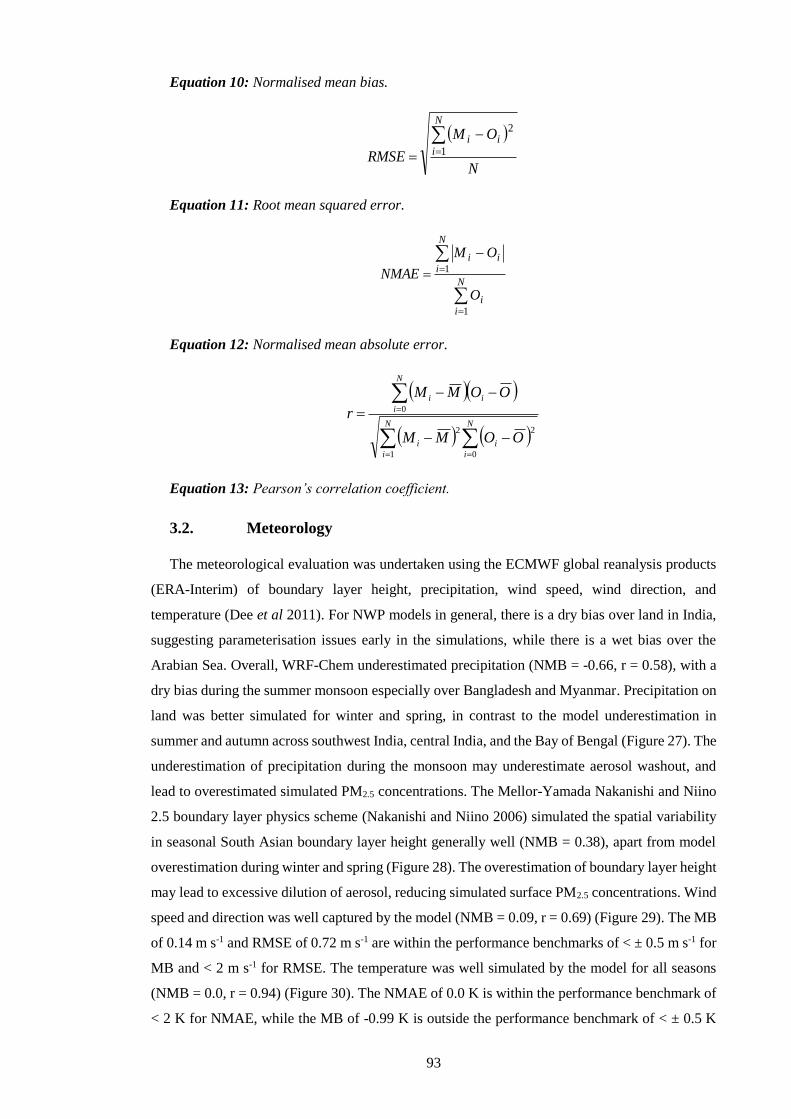
93

Equation 10: Normalised mean bias.

N

OM

RMSE

N

iii

1

2

Equation 11: Root mean squared error.

N

ii

N

iii

O

OM

NMAE

1

1

Equation 12: Normalised mean absolute error.

N

i

N

i

ii

N

i

ii

OOMM

OOMM

r

1 0

22

0

Equation 13: Pearson’s correlation coefficient.

3.2. Meteorology

The meteorological evaluation was undertaken using the ECMWF global reanalysis products

(ERA-Interim) of boundary layer height, precipitation, wind speed, wind direction, and

temperature (Dee et al 2011). For NWP models in general, there is a dry bias over land in India,

suggesting parameterisation issues early in the simulations, while there is a wet bias over the

Arabian Sea. Overall, WRF-Chem underestimated precipitation (NMB = -0.66, r = 0.58), with a

dry bias during the summer monsoon especially over Bangladesh and Myanmar. Precipitation on

land was better simulated for winter and spring, in contrast to the model underestimation in

summer and autumn across southwest India, central India, and the Bay of Bengal (Figure 27). The

underestimation of precipitation during the monsoon may underestimate aerosol washout, and

lead to overestimated simulated PM2.5 concentrations. The Mellor-Yamada Nakanishi and Niino

2.5 boundary layer physics scheme (Nakanishi and Niino 2006) simulated the spatial variability

in seasonal South Asian boundary layer height generally well (NMB = 0.38), apart from model

overestimation during winter and spring (Figure 28). The overestimation of boundary layer height

may lead to excessive dilution of aerosol, reducing simulated surface PM2.5 concentrations. Wind

speed and direction was well captured by the model (NMB = 0.09, r = 0.69) (Figure 29). The MB

of 0.14 m s-1 and RMSE of 0.72 m s-1 are within the performance benchmarks of < ± 0.5 m s-1 for

MB and < 2 m s-1 for RMSE. The temperature was well simulated by the model for all seasons

(NMB = 0.0, r = 0.94) (Figure 30). The NMAE of 0.0 K is within the performance benchmark of

< 2 K for NMAE, while the MB of -0.99 K is outside the performance benchmark of < ± 0.5 K

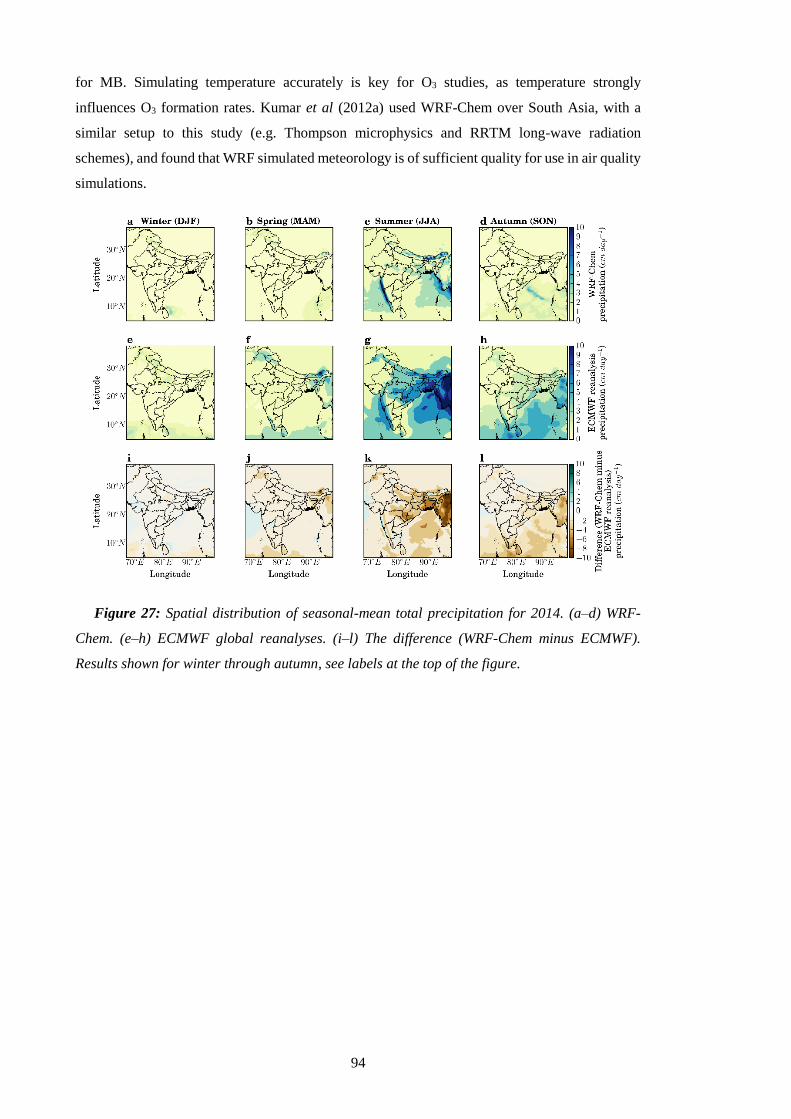
94

for MB. Simulating temperature accurately is key for O3 studies, as temperature strongly

influences O3 formation rates. Kumar et al (2012a) used WRF-Chem over South Asia, with a

similar setup to this study (e.g. Thompson microphysics and RRTM long-wave radiation

schemes), and found that WRF simulated meteorology is of sufficient quality for use in air quality

simulations.

Figure 27: Spatial distribution of seasonal-mean total precipitation for 2014. (a–d) WRF-


Results shown for winter through autumn, see labels at the top of the figure.

95

Figure 28: Spatial distribution of seasonal-mean boundary layer height for 2014. (a–d) WRF-



Figure 29: Spatial distribution of seasonal-mean wind speed and direction for 2014. (a–d)

WRF-Chem. (e–h) ECMWF global reanalyses. (i–l) The difference (WRF-Chem minus ECMWF).


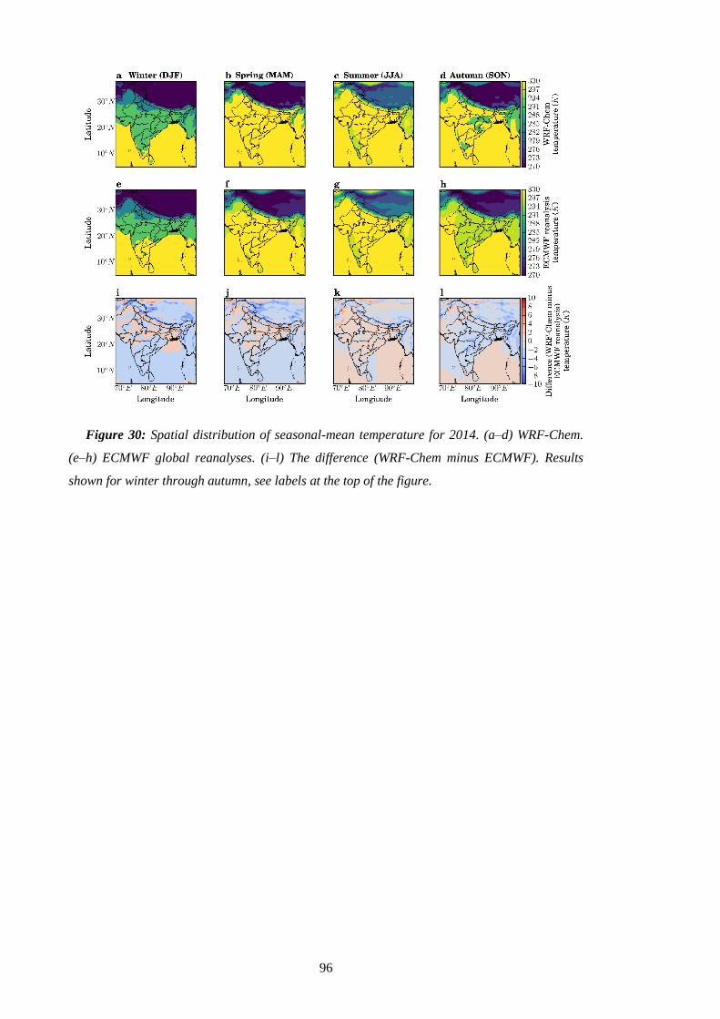
96

Figure 30: Spatial distribution of seasonal-mean temperature for 2014. (a–d) WRF-Chem.

(e–h) ECMWF global reanalyses. (i–l) The difference (WRF-Chem minus ECMWF). Results

shown for winter through autumn, see labels at the top of the figure.

97

Figure 31: Annual-mean meteorology correlations between model and ECMWF global

reanalyses at each grid cell. (a) Boundary layer height, (b) total precipitation, (c) wind speed,

and (d) temperature for 2014.

3.3. Ambient surface PM2.5 concentrations

Surface measurements of PM2.5 were obtained from the National Air Quality Monitoring

Program (NAMP) by the Central Pollution Control Board (CPCB), Ministry of Environment and

Forests, Government of India (Ministry of Environment and Forests 2018). CPCB measurements

used the automatic beta attenuation method (Ministry of Environment and Forests 2013).

Environmental data collection in India has primarily been focused on compliance with India’s

NAAQS (Health Effects Institute Public Health and Air Pollution in Asia Program 2011). Most

of the sites are in urban areas. The monitoring sites are shown spatially in Figure 32 and detailed

in Table 11 (Appendix B). The network of sites reporting PM2.5 has expanded substantially in the

last few years, with only four sites reporting in 2014, compared to 45 in 2016. India has strong

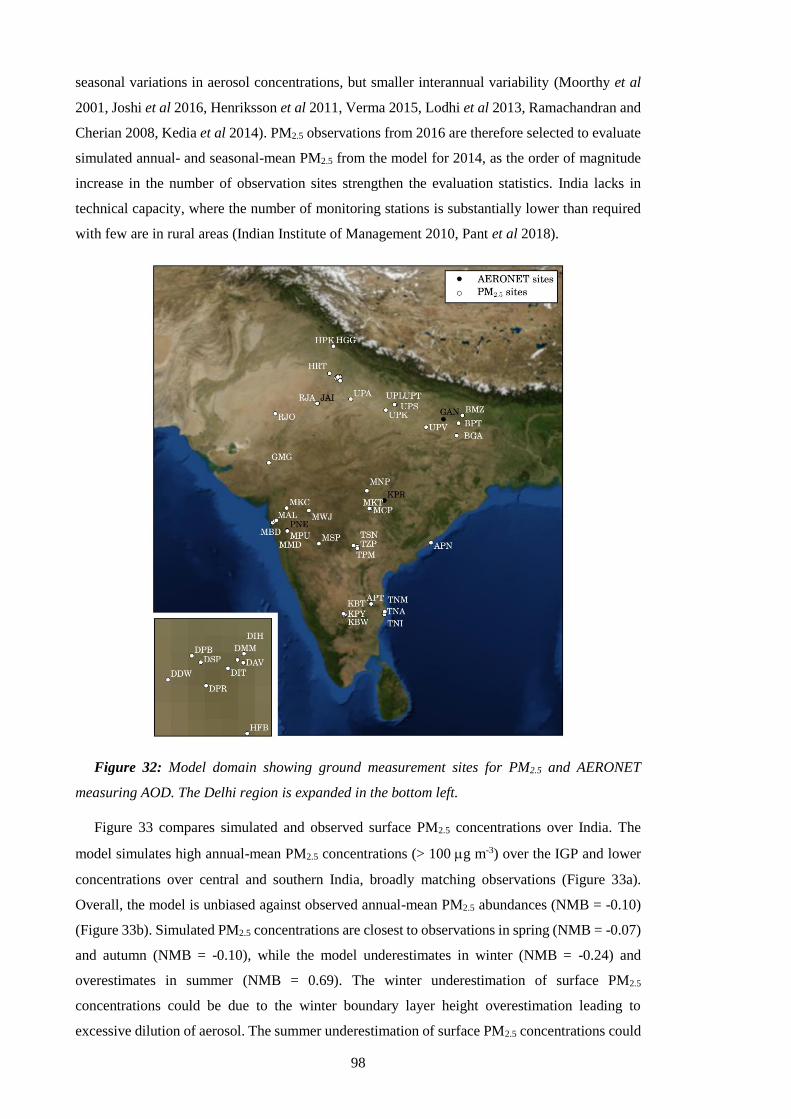
98

seasonal variations in aerosol concentrations, but smaller interannual variability (Moorthy et al

2001, Joshi et al 2016, Henriksson et al 2011, Verma 2015, Lodhi et al 2013, Ramachandran and

Cherian 2008, Kedia et al 2014). PM2.5 observations from 2016 are therefore selected to evaluate

simulated annual- and seasonal-mean PM2.5 from the model for 2014, as the order of magnitude

increase in the number of observation sites strengthen the evaluation statistics. India lacks in

technical capacity, where the number of monitoring stations is substantially lower than required

with few are in rural areas (Indian Institute of Management 2010, Pant et al 2018).

Figure 32: Model domain showing ground measurement sites for PM2.5 and AERONET

measuring AOD. The Delhi region is expanded in the bottom left.

Figure 33 compares simulated and observed surface PM2.5 concentrations over India. The

model simulates high annual-mean PM2.5 concentrations (> 100 g m-3) over the IGP and lower

concentrations over central and southern India, broadly matching observations (Figure 33a).

Overall, the model is unbiased against observed annual-mean PM2.5 abundances (NMB = -0.10)

(Figure 33b). Simulated PM2.5 concentrations are closest to observations in spring (NMB = -0.07)

and autumn (NMB = -0.10), while the model underestimates in winter (NMB = -0.24) and

overestimates in summer (NMB = 0.69). The winter underestimation of surface PM2.5

concentrations could be due to the winter boundary layer height overestimation leading to

excessive dilution of aerosol. The summer underestimation of surface PM2.5 concentrations could

99

be due to the summer monsoon precipitation dry bias underestimating aerosol washout. The

model has limited success in reproducing the spatial variability of PM2.5, underestimating near

the Thar Desert and in the central IGP. Underestimation of dust in the western IGP has been

identified previously (Kumar et al 2014b) and likely contributes to model underestimation of

PM2.5 in this region. Simulated PM2.5 concentrations are greatest in winter (DJF) and autumn

(SON), and lowest in spring (MAM) and summer (JJA), matching observations (Figure 34a–d).

Figure 33: Comparison of observed and simulated PM2.5 concentrations. (a) Annual-mean

surface PM2.5 concentrations. Model results for 2014 (background) are compared with surface

measurements from 2016 (filled circles). (b) Comparison of annual and seasonal-mean surface

PM2.5 concentrations. The best-fit line (green), 1:1, 2:1, and 1:2 lines are shown (black). Annual,

winter (DJF), spring (MAM), summer (JJA), and autumn (SON) NMB are -0.10, -0.24, -0.07,

0.69, and -0.10, respectively. The best-fit line for annual data has slope = 0.70 and Pearson’s

correlation coefficient (r) = 0.19.

100

Figure 34: Seasonal-mean PM2.5 concentrations for 2014. (a–d) model results (background)

for 2014 for all sources are compared with ground-measurements (filled circles) from 2016,

winter to autumn.

3.4. Aerosol optical depth

Aerosol optical depth (AOD) is the columnar aerosol estimated as the partial depletion of

radiance per unit path length (km-1) due to absorbing or scattering through the atmospheric column

determined by aerosol loading, size distribution, and refractive index (Levy et al 2009, Remer et

al 2008). An AOD of 0.01 corresponds to a clean atmosphere, 0.4 to a hazy atmosphere, and 1.0

means 37% of the sunlight is prevented from reaching the surface (Seinfeld 2004). Simulated

AOD was evaluated against ground measurements (aerosol robotic network, AERONET) and

satellite (MODIS). Level 2 (version 2) AERONET data was used, which are cloud-screened and

quality assured with a low uncertainty of 0.01–0.02 at 500 nm. AERONET AOD was obtained at

wavelengths between 340 nm and 1640 nm and was interpolated to obtain AOD at 550 nm from

the closest neighbouring wavelengths. The model evaluation used AOD from the MODIS Aqua

(MYD) satellite. Collection 6 (C6) level 2 (L2) AOD at 0.55 m with the scientific data set optical

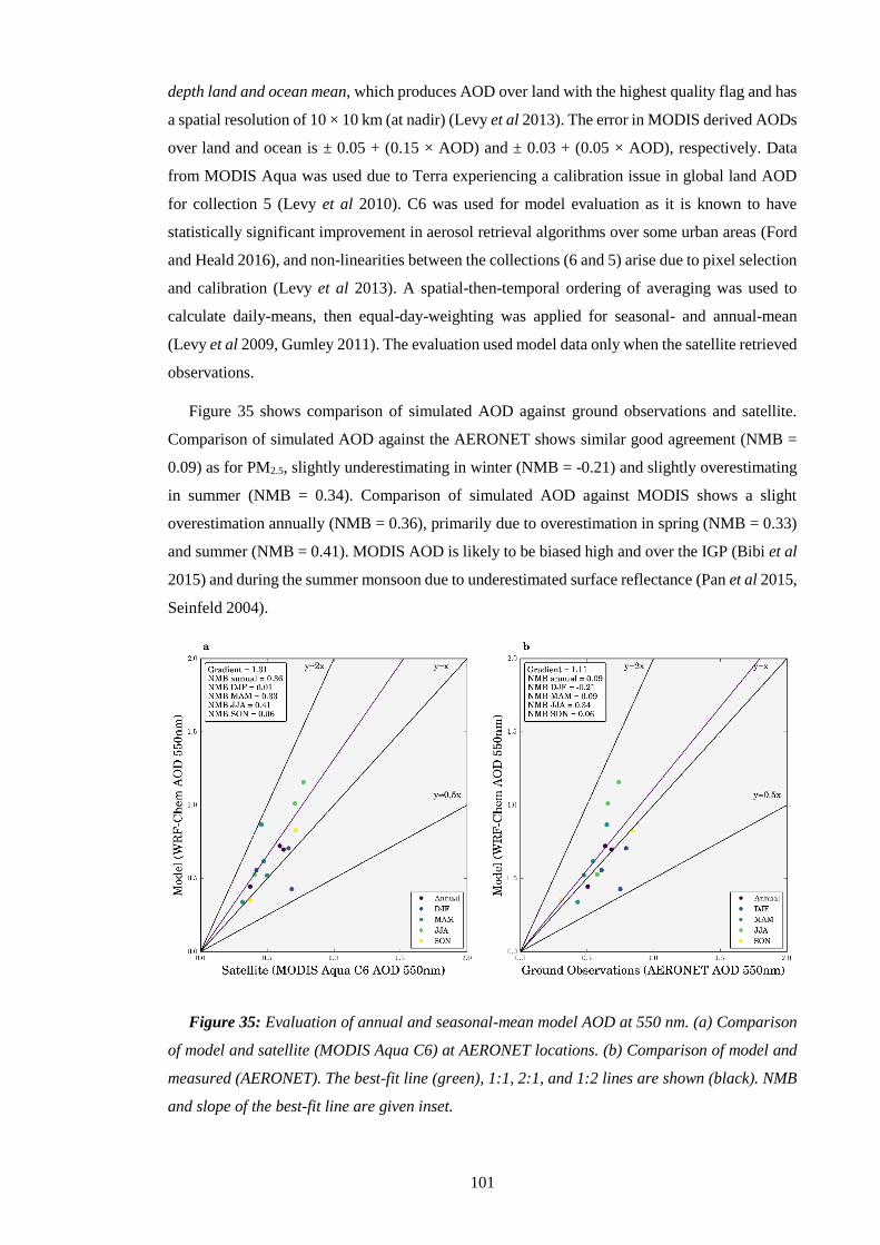
101

depth land and ocean mean, which produces AOD over land with the highest quality flag and has

a spatial resolution of 10 × 10 km (at nadir) (Levy et al 2013). The error in MODIS derived AODs

over land and ocean is ± 0.05 + (0.15 × AOD) and ± 0.03 + (0.05 × AOD), respectively. Data

from MODIS Aqua was used due to Terra experiencing a calibration issue in global land AOD

for collection 5 (Levy et al 2010). C6 was used for model evaluation as it is known to have

statistically significant improvement in aerosol retrieval algorithms over some urban areas (Ford

and Heald 2016), and non-linearities between the collections (6 and 5) arise due to pixel selection

and calibration (Levy et al 2013). A spatial-then-temporal ordering of averaging was used to

calculate daily-means, then equal-day-weighting was applied for seasonal- and annual-mean

(Levy et al 2009, Gumley 2011). The evaluation used model data only when the satellite retrieved

observations.

Figure 35 shows comparison of simulated AOD against ground observations and satellite.

Comparison of simulated AOD against the AERONET shows similar good agreement (NMB =

0.09) as for PM2.5, slightly underestimating in winter (NMB = -0.21) and slightly overestimating

in summer (NMB = 0.34). Comparison of simulated AOD against MODIS shows a slight

overestimation annually (NMB = 0.36), primarily due to overestimation in spring (NMB = 0.33)

and summer (NMB = 0.41). MODIS AOD is likely to be biased high and over the IGP (Bibi et al

2015) and during the summer monsoon due to underestimated surface reflectance (Pan et al 2015,

Seinfeld 2004).

Figure 35: Evaluation of annual and seasonal-mean model AOD at 550 nm. (a) Comparison

of model and satellite (MODIS Aqua C6) at AERONET locations. (b) Comparison of model and

measured (AERONET). The best-fit line (green), 1:1, 2:1, and 1:2 lines are shown (black). NMB

and slope of the best-fit line are given inset.

102

3.5. Ambient surface O3 concentrations

Model evaluation for O3 used ambient surface measurements from previous measurement

studies over India representative of different chemical environments. Details of the monitoring

sites are given in Table 14 (Appendix D). Surface O3 observations used ultraviolet photometry

online analysers with a 5% accuracy (Kleinman et al 1994). Similar to previous studies, the model

evaluation used observational data of a different year to the simulation due to the paucity of O3

observations over India (Kumar et al 2012b, 2015c, Ojha et al 2016, Sharma et al 2017a, Kumar

et al 2018).

Figure 36 shows the comparison of observed and simulated O3 concentrations. Simulated O3

concentrations were highest in northern and eastern India. Simulated O3 concentrations were

lowest in summer (JJA), as seen in previous studies (Chatani et al 2014, Ojha et al 2016, Roy et

al 2008, Lu et al 2018). The low O3 concentrations in summer are likely due to the monsoon cloud

cover reducing solar radiation and wet scavenging of O3 precursors suppressing O3 production

(Lu et al 2018). Model simulations overestimated surface O3 concentrations relative to

observations with an overall NMB of 0.35. Previous modelling studies over India also mostly

overestimated O3 relative to observations (Kota et al 2018, Surendran et al 2015, Sharma et al

2017a, 2016, Marrapu et al 2014, Kumar et al 2012b, 2010a, Chatani et al 2014, Engardt 2008,

Gupta and Mohan 2015, Lu et al 2018, Ojha et al 2012, 2016, Pommier et al 2018, Roy et al

2008, Karambelas et al 2018b).

Models have been found to have limited success in simulating local scale titration chemistry

of O3 with NO, causing O3 concentrations to be overestimated (Chatani et al 2014, Sharma et al

2016, Engardt 2008, Sharma and Khare 2017, Pommier et al 2018). Urban observations close to

large NOx emission sources tend to have low O3 concentrations due to this titration effect (Clapp

and Jenkin 2001). To examine this effect, the model is separately evaluated against rural

(including semi-rural, coastal, and high altitude) and urban (including semi-urban) observations

(Figure 37). The model simulates O3 concentrations closer to observations for rural sites (NMB

= 0.28) than for urban sites (NMB = 0.41). This suggests that the titration of O3 with large NO

concentrations may be causing the model to overestimate O3 where high NO concentrations are

likely not captured by the model. Previous studies have found Indian O3 concentrations to be

larger downwind of heavily populated regions relative to urban areas (Lal et al 2008, Lawrence

and Lelieveld 2010). The combination of EDGAR-HTAP with MOZART has also been found to

enhance surface O3 mixing ratios due to vertical mixing of enhanced O3 that has been produced

aloft (Sharma et al 2017a). The overestimation of O3 could also be due to the underestimation of

dust aerosols (Conibear et al 2018a). Heterogeneous reactions on dust surfaces have been found

to reduce O3 concentrations (Li et al 2017a, Kumar et al 2014a). Accurate simulation of dust

emissions and the inclusion of these heterogeneous reactions reduced the difference between

observed and simulated O3 concentrations in India from 16 ppbv to 2 ppbv (Kumar et al 2014a).

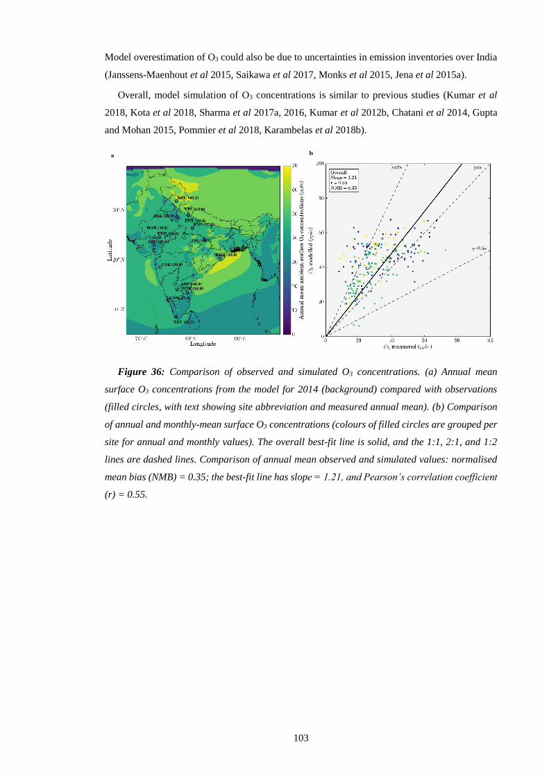
103

Model overestimation of O3 could also be due to uncertainties in emission inventories over India

(Janssens-Maenhout et al 2015, Saikawa et al 2017, Monks et al 2015, Jena et al 2015a).

Overall, model simulation of O3 concentrations is similar to previous studies (Kumar et al

2018, Kota et al 2018, Sharma et al 2017a, 2016, Kumar et al 2012b, Chatani et al 2014, Gupta

and Mohan 2015, Pommier et al 2018, Karambelas et al 2018b).

Figure 36: Comparison of observed and simulated O3 concentrations. (a) Annual mean

surface O3 concentrations from the model for 2014 (background) compared with observations

(filled circles, with text showing site abbreviation and measured annual mean). (b) Comparison

of annual and monthly-mean surface O3 concentrations (colours of filled circles are grouped per

site for annual and monthly values). The overall best-fit line is solid, and the 1:1, 2:1, and 1:2

lines are dashed lines. Comparison of annual mean observed and simulated values: normalised

mean bias (NMB) = 0.35; the best-fit line has slope = 1.21, and Pearson’s correlation coefficient

(r) = 0.55.

104

Figure 37: Comparison of rural and urban observed and simulated O3 concentrations. (a)

Comparison of annual and monthly-mean ambient surface O3 concentrations from rural

observation sites. The rural site best-fit line (solid), 1:1, 2:1, and 1:2 lines are shown (dashed).

Rural site NMB is 0.28, the rural site best-fit line has slope = 1.18, and rural site r = 0.67. (b)

Comparison of annual and monthly-mean ambient surface O3 concentrations from urban

observation sites. The urban site best-fit line (solid), 1:1, 2:1, and 1:2 lines are shown (dashed).

Urban site NMB is 0.41, the urban site best-fit line has slope = 1.24, and urban site r = 0.47.

Colours of filled circles grouped by site.

105

4. Residential energy use emissions dominate health impacts from

exposure to ambient particulate matter in India

4.1. Abstract

Exposure to ambient PM2.5 is a leading contributor to disease in India. Previous studies

analysing emission source attributions were restricted by coarse model resolution and limited

PM2.5 observations. A regional model informed by new observations is used to make the first

high-resolution study of the sector-specific disease burden from ambient PM2.5 exposure in India.

Observed annual-mean PM2.5 concentrations exceed 100 g m-3 and are well simulated by the

model. Emissions from residential energy use dominate (52%) population-weighted annual-mean

PM2.5 concentrations, and are attributed to 511,000 (95UI: 340,000–697,000) premature

mortalities annually. However, removing residential energy use emissions would avert only

256,000 (95UI: 162,000–340,000), due to the non-linear exposure-response relationship causing

health effects to saturate at high PM2.5 concentrations. Consequently, large reductions in

emissions will be required to reduce the health burden from ambient PM2.5 exposure in India.

4.2. Introduction

Estimates of premature mortality from exposure to ambient PM2.5 in India vary by a factor of

three, between 392,000 to 1,090,000 per year (GBD 2013 Risk Factors Collaborators 2015, Silva

et al 2013, GBD 2016 Risk Factors Collaborators 2017, Cohen et al 2005, Apte et al 2015a,

Ghude et al 2016, Giannadaki et al 2016, Chowdhury and Dey 2016, Lelieveld et al 2015, GBD

2010 Risk Factors Collaborators 2012, Silva et al 2016b, GBD 2015 Risk Factors Collaborators

2016a, World Health Organization 2016a, Lelieveld 2017), with differences due to variations in

ambient PM2.5 estimates, health functions, population datasets, and methodological approaches.

Previous global modelling studies find emissions from residential energy use dominate the

contribution to PM2.5 exposure associated premature mortality in India (Lelieveld et al 2015,

Lelieveld 2017, Silva et al 2016b), with estimates between 73,000 to 460,500 premature

mortalities per year (Butt et al 2016, Chafe et al 2014a, Lelieveld et al 2015, Silva et al 2016b,

Lelieveld 2017).

Previous studies used global models at relatively coarse resolution (Lelieveld et al 2015,

Lelieveld 2017, Silva et al 2016b). Coarse resolution may underestimate PM2.5 concentrations

over polluted areas and regional transport due to the short atmospheric lifetime of PM2.5 (Li et al

2016c, Punger and West 2013, Thompson and Selin 2012, Thompson et al 2014).

Underestimating PM2.5 concentrations will underestimate air pollution-related premature

mortality (Punger and West 2013). Model simulations using emissions at coarse spatial

resolutions have been shown to have discrepancies relative to observations (Moorthy et al 2013b,

Pan et al 2015, Pommier et al 2018, Karambelas et al 2018a), while higher resolution models

106

have been found to produce PM2.5 concentrations in closer agreement to observations (Kumar et

al 2015c, Conibear et al 2018a, Saikawa et al 2017). Modelling air pollution at high spatial

resolution is important as concentrations can vary substantially across small scales where

population density and exposures are high (Punger and West 2013, Crippa et al 2017). Spatial

variation differs with aerosol size (U.S. Environmental Protection Agency 2009b), where

secondary PM2.5 generally has smaller spatial gradients than primary PM2.5 and is, therefore, less

likely to be sensitive to spatial resolution (U.S. Environmental Protection Agency 2007).

Resolution directly changes the resolved space, in addition to indirectly influencing

parameterisation choices important for secondary pollutants (Wild and Prather 2006, Punger and

West 2013).

This work is the first study to use high-resolution simulations to estimate the contribution of

different emission sectors to ambient PM2.5 concentrations and the related disease burden from

exposure across India. A regional numerical weather prediction model online-coupled with

atmospheric chemistry at 30 km horizontal resolution is used to study the disease burden due to

ambient PM2.5 exposure in India from seven emission sources. A control simulation is performed

with all emission sources for the year of 2014. Then annual sensitivity simulations are performed

removing the respective emissions from each source individually. The sources studies are

agriculture (AGR), biomass burning (BBU), dust (DUS), power generation (ENE), industrial non-

power (IND), residential energy use (RES) and land transport (TRA). The contribution of specific

emission sources to PM2.5 concentrations is calculated by switching off the emission sources one

at a time. The disease burden is then calculated using the exposure-response function from the

GBD2015. Understanding the contribution of different emission sectors to ambient air pollution

is essential to reduce the air pollution exposure associated disease burden.

4.3. Results

Annual mean PM2.5 concentrations were evaluated against observations (Section 3.3), where

the model was found to be unbiased against observed annual-mean PM2.5 abundances (NMB = -

0.10). Simulated population-weighted (country-scale exposure) annual-mean PM2.5 concentration

across India was 57.2 g m-3. Model simulations show that in 2014, 99% of the Indian population

are exposed to annual-mean PM2.5 concentrations that exceeded the WHO AQG of 10 g m-3 and

81% above the WHO Level 1 Interim Target (IT-1) of 35 g m-3.

4.3.1. The contribution of emission sectors to ambient PM2.5 concentrations

To investigate the contribution of different emission sectors to ambient PM2.5 over India,

emissions from different sectors are switched off one at a time in individual annual simulations.

Table 5 shows the contribution of the different emission sectors to annual-mean PM2.5

concentrations across India.

107

Table 5: Reduction in population-weighted annual-mean PM2.5 concentrations in India caused

by removing different emission sectors. Sectors are agriculture (AGR), biomass burning (BBU),

dust (DUS), power generation (ENE), industrial non-power (IND), residential energy use (RES),

and land transport (TRA).

AGR BBU DUS ENE IND RES TRA

Reduction to

population weighted

PM2.5 (PM2.5_SECTOR_OFF)

g m-3 0.2 1.6 0.0 12.0 9.3 29.5 5.9

% 0 3 0 21 16 52 10

The largest reductions in population-weighted ambient PM2.5 concentrations are achieved

through the removal of emissions from residential energy use (52%) followed by power

generation (21%), industry (16%), and land transport (10%). Removing emissions from

residential energy use reduces ambient PM2.5 concentrations by as much as 70% over the IGP,

with reductions of 30–50% over southern India (Figure 38a). Figure 38b shows residential energy

use contributes 67% of annual anthropogenic PM2.5 emissions across India, with contributions as

great as 90% over the IGP. Figure 39 shows that the contributions from residential energy use

emissions to annual anthropogenic PM2.5 emissions across India are 62% in summer and 70% in

winter. The concentration and fractional contribution of residential emissions to PM2.5

concentrations are largest in the winter (Figure 40). Emissions from residential energy use

contribute a larger fraction of anthropogenic PM2.5 emissions than to ambient PM2.5

concentrations due to non-anthropogenic sources of PM2.5, including dust and biomass burning,

and due to the contribution of aerosol precursors such as SO2 and NOx, for which industry and

power generation dominate emissions. Source apportionment suggests that 46–73% of BC

concentrations in India are from non-fossil source (residential biofuel and biomass burning) (Butt

et al 2016), which broadly matches this estimate of the contribution of residential emissions to

PM2.5 concentrations.

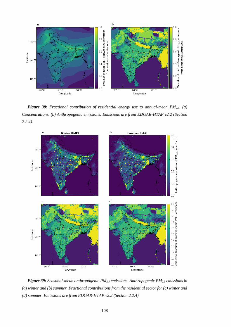
108

Figure 38: Fractional contribution of residential energy use to annual-mean PM2.5. (a)

Concentrations. (b) Anthropogenic emissions. Emissions are from EDGAR-HTAP v2.2 (Section

2.2.4).

Figure 39: Seasonal-mean anthropogenic PM2.5 emissions. Anthropogenic PM2.5 emissions in

(a) winter and (b) summer. Fractional contributions from the residential sector for (c) winter and

(d) summer. Emissions are from EDGAR-HTAP v2.2 (Section 2.2.4).

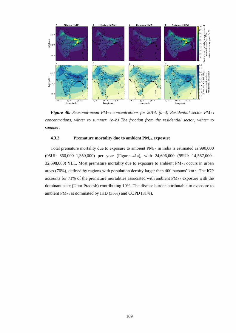
109

Figure 40: Seasonal-mean PM2.5 concentrations for 2014. (a–d) Residential sector PM2.5

concentrations, winter to summer. (e–h) The fraction from the residential sector, winter to

summer.

4.3.2. Premature mortality due to ambient PM2.5 exposure

Total premature mortality due to exposure to ambient PM2.5 in India is estimated as 990,000

(95UI: 660,000–1,350,000) per year (Figure 41a), with 24,606,000 (95UI: 14,567,000–

32,698,000) YLL. Most premature mortality due to exposure to ambient PM2.5 occurs in urban

areas (76%), defined by regions with population density larger than 400 persons’ km-2. The IGP

accounts for 71% of the premature mortalities associated with ambient PM2.5 exposure with the

dominant state (Uttar Pradesh) contributing 19%. The disease burden attributable to exposure to

ambient PM2.5 is dominated by IHD (35%) and COPD (31%).

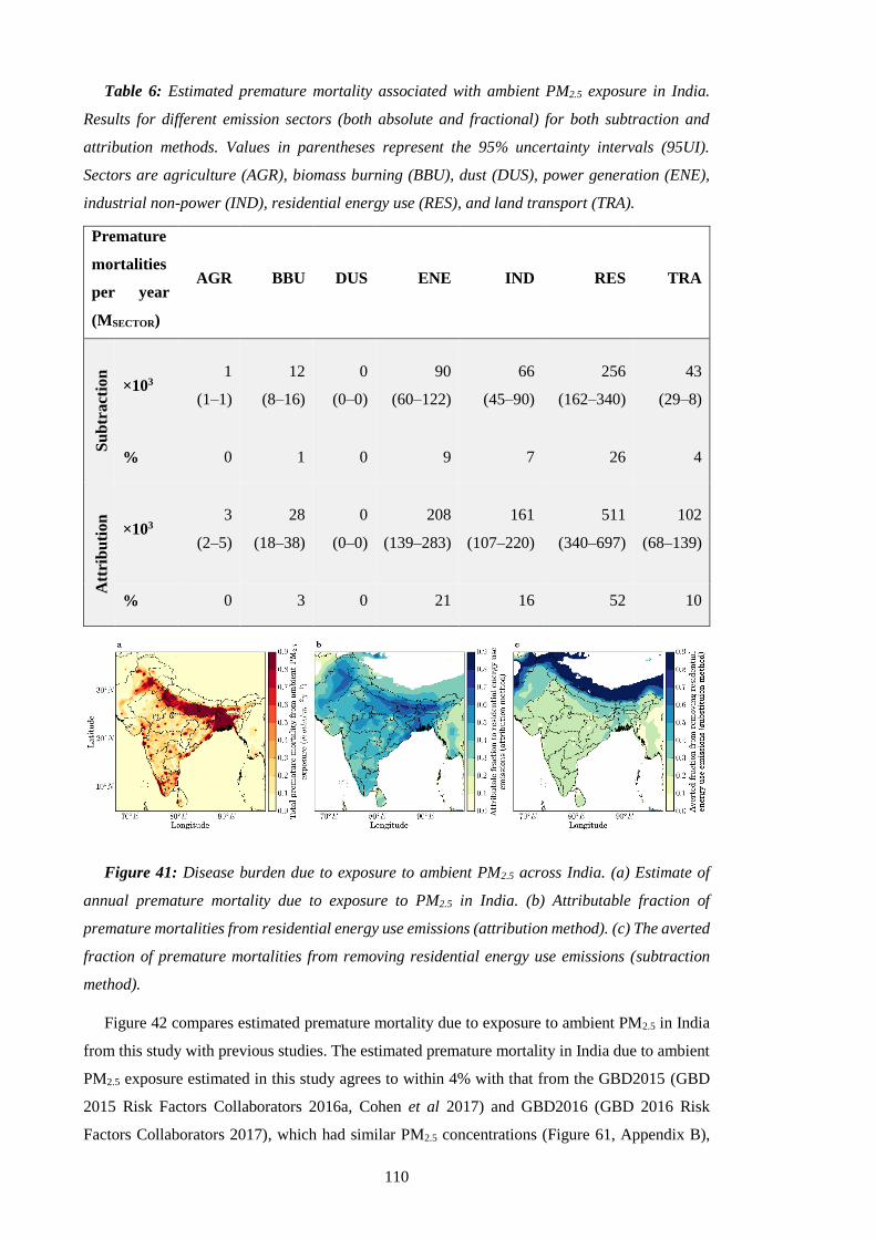
110

Table 6: Estimated premature mortality associated with ambient PM2.5 exposure in India.

Results for different emission sectors (both absolute and fractional) for both subtraction and

attribution methods. Values in parentheses represent the 95% uncertainty intervals (95UI).

Sectors are agriculture (AGR), biomass burning (BBU), dust (DUS), power generation (ENE),

industrial non-power (IND), residential energy use (RES), and land transport (TRA).

Premature

mortalities

per year

(MSECTOR)


Su

btr

act

ion

×103 1

(1–1)

12

(8–16)

0

(0–0)

90

(60–122)

66

(45–90)

256

(162–340)

43

(29–8)

% 0 1 0 9 7 26 4

Att

rib

uti

on

×103 3

(2–5)

28

(18–38)

0

(0–0)

208

(139–283)

161

(107–220)

511

(340–697)

102

(68–139)

% 0 3 0 21 16 52 10

Figure 41: Disease burden due to exposure to ambient PM2.5 across India. (a) Estimate of

annual premature mortality due to exposure to PM2.5 in India. (b) Attributable fraction of

premature mortalities from residential energy use emissions (attribution method). (c) The averted

fraction of premature mortalities from removing residential energy use emissions (subtraction

method).

Figure 42 compares estimated premature mortality due to exposure to ambient PM2.5 in India

from this study with previous studies. The estimated premature mortality in India due to ambient

PM2.5 exposure estimated in this study agrees to within 4% with that from the GBD2015 (GBD

2015 Risk Factors Collaborators 2016a, Cohen et al 2017) and GBD2016 (GBD 2016 Risk

Factors Collaborators 2017), which had similar PM2.5 concentrations (Figure 61, Appendix B),

111

but is up to a factor of two greater than in many other studies. These previous studies applied

different PM2.5 concentrations at a range of spatial resolutions (0.1 to 2.8), as well as different

population datasets, exposure-response functions, and baseline mortalities, all of which may play

a role in the different premature mortality estimates. Likely reasons for lower premature mortality

estimates in many previous studies are explored and summarised in Figure 42. Using lower

resolution PM2.5 data (3 in place of 0.3), reduced population-weighted PM2.5 concentrations by

20%, but reduced this study’s premature mortality estimate by only 7%, due to the non-linear

exposure-response relationship (Section 2.3). This approach does not account for the effect of

resolution on the representation of atmospheric processes within the model (Punger and West

2013). Using population data for 2010 (SEDAC GPWv4 UN-adjusted), when the Indian

population was 7% lower than in 2015, reduced this study’s premature mortality estimates by

14%. Using the RR from the GBD2010 IER function (Apte et al 2015a, Burnett et al 2014) as in

some previous studies (Giannadaki et al 2016, Apte et al 2015a, Ghude et al 2016, Lelieveld et

al 2015, Silva et al 2016b, Chowdhury and Dey 2016), increased this study’s premature mortality

estimates by 22%. In contrast, applying RR from GBD2013 (GBD 2013 Risk Factors

Collaborators 2015) reduced this study’s mortality estimate by 31%. Using the GBD2015 baseline

mortality estimates for 2010 (Institute for Health Metrics and Evaluation 2018), increased this

study’s premature mortality estimates by 7%. Applying state-specific baseline mortality values

(Chowdhury and Dey 2016) (see Methods) reduced this study’s estimate of premature mortality

by 3%, while increasing impacts over the IGP due to the higher baseline mortality rates in this

region (Figure 62, Appendix B). Many previous studies (Silva et al 2016b, 2016c, World Health

Organization 2014a, Giannadaki et al 2016, Apte et al 2015a, GBD 2013 Risk Factors

Collaborators 2015, Chafe et al 2014a, Brauer et al 2016) estimated maximum annual-mean PM2.5

concentrations across the IGP to be between 50–80 g m-3, but lacked widespread measurements

of PM2.5 for model evaluation. New observations suggest annual-mean PM2.5 concentrations of at

least 120 g m-3 across the IGP, which is well simulated by this study’s model (Section 3.3).

Scaling this study’s PM2.5 concentrations so that annual-mean concentrations do not exceed 80

g m-3 and 50 g m-3 reduced this study’s premature mortality estimates by 25% and 39%,

respectively. Overall, this study suggests that different exposure-response relationships and

different PM2.5 concentrations cause the largest differences in premature mortality estimates for

India and are likely driving the majority of the difference between previous estimates.

4.3.3. The contribution of emission sectors to the disease burden

Table 6 shows the premature mortality estimates per emission sector for both the subtraction

and attribution methods (Section 2.6), Table 9 (Appendix B) shows disease-specific results, and

Table 10 (Appendix C) shows sector-specific YLL. The premature mortality estimates from the

subtraction method (Figure 41c) are a factor of 2–2.5 smaller than the attribution method (Figure

41b). The difference is due to the non-linear exposure-response relationship, where health effects

112

saturate at high PM2.5 concentrations (Kodros et al 2016, Pope III et al 2015). The estimate of the

reduction in premature mortality through removing an emission sector (subtraction method) is a

factor 2–2.5 times less than the estimate of the premature mortality attributed to that sector

(attribution method). Consequently, the summation of sector contributions from the subtraction

method is 469,000 (95UI: 304,000–626,000) premature mortalities per year (47% of control),

which is substantially lower than the sector summation from the attribution method of 1,012,000

(95UI: 675,000–1,381,000) premature mortalities per year (102% of control). Overall, this has

implications for attempts to reduce air pollution mortality in regions with high PM2.5

concentrations.

For both methods, residential energy use is the dominant contributor to premature mortalities

due to exposure to ambient PM2.5 across all states in India, except for Delhi where emissions from

land transport are dominant. Emissions from residential energy use cause 511,000 (95UI:

340,000–697,000) premature mortalities per year, 52% of the total premature mortalities due to

ambient PM2.5 exposure (attribution method). Removing emissions from residential energy use

would prevent 256,000 (95UI: 162,000–340,000) premature mortalities per year, 26% of the total

premature mortalities due to ambient PM2.5 exposure (subtraction method). After residential

energy use, the next largest contributions are from power generation (9% of total premature

mortalities for subtraction method and 21% for attribution method), industry (7% for subtraction

and 16% for attribution), and land transport (4% for subtraction and 10% for attribution).

Figure 42 compares estimates of the source-specific premature mortality from ambient PM2.5

exposure in India. Previous studies also find emissions from residential energy use to dominate

the contribution to PM2.5 exposure associated premature mortality in India (Lelieveld et al 2015,

Lelieveld 2017, Silva et al 2016b). Power generation was the next largest contributor in all studies

(Lelieveld et al 2015, Lelieveld 2017, Silva et al 2016b), while the percentage contribution in this

study is approximately a factor of two larger. Industrial emissions are third largest in both this

study and Silva et al (2016a) using the subtraction method, while dust was third for Lelieveld et

al (2015, 2017) using the attribution method. The percentage contribution from land transport

was double that of all previous studies (Lelieveld et al 2015, Lelieveld 2017, Silva et al 2016b).

The two previous studies (Lelieveld et al 2015, Silva et al 2016b) that used the GBD2010 RR

(which increased this study’s estimates by 22%) obtained substantially lower total premature

mortality than this study’s estimates, likely due to lower PM2.5 concentrations. More recent

previous studies (GBD 2015 Risk Factors Collaborators 2016a, Cohen et al 2017, GBD 2016

Risk Factors Collaborators 2017, Lelieveld 2017) using the GBD2015 RR, estimate similar total

premature mortality to this study. Other studies estimating the contribution from residential

energy use emissions to premature mortality are lower than this study due to a combination of

using a log-linear exposure-response function with lower PM2.5 concentrations (Butt et al 2016)

or only estimating the contribution from residential cooking (Chafe et al 2014a). This study’s

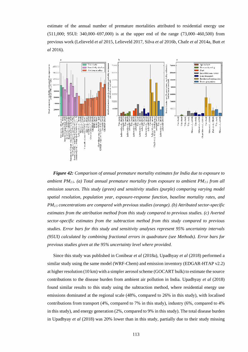
113

estimate of the annual number of premature mortalities attributed to residential energy use

(511,000; 95UI: 340,000–697,000) is at the upper end of the range (73,000–460,500) from

previous work (Lelieveld et al 2015, Lelieveld 2017, Silva et al 2016b, Chafe et al 2014a, Butt et

al 2016).

Figure 42: Comparison of annual premature mortality estimates for India due to exposure to

ambient PM2.5. (a) Total annual premature mortality from exposure to ambient PM2.5 from all

emission sources. This study (green) and sensitivity studies (purple) comparing varying model

spatial resolution, population year, exposure-response function, baseline mortality rates, and

PM2.5 concentrations are compared with previous studies (orange). (b) Attributed sector-specific

estimates from the attribution method from this study compared to previous studies. (c) Averted

sector-specific estimates from the subtraction method from this study compared to previous

studies. Error bars for this study and sensitivity analyses represent 95% uncertainty intervals

(95UI) calculated by combining fractional errors in quadrature (see Methods). Error bars for

previous studies given at the 95% uncertainty level where provided.

Since this study was published in Conibear et al (2018a), Upadhyay et al (2018) performed a

similar study using the same model (WRF-Chem) and emission inventory (EDGAR-HTAP v2.2)

at higher resolution (10 km) with a simpler aerosol scheme (GOCART bulk) to estimate the source

contributions to the disease burden from ambient air pollution in India. Upadhyay et al (2018)

found similar results to this study using the subtraction method, where residential energy use

emissions dominated at the regional scale (48%, compared to 26% in this study), with localised

contributions from transport (4%, compared to 7% in this study), industry (6%, compared to 4%

in this study), and energy generation (2%, compared to 9% in this study). The total disease burden

in Upadhyay et al (2018) was 20% lower than in this study, partially due to their study missing

114

agricultural burning emissions, increasing the relative contributions from other sources. Another

study from Venkataraman et al (2018) was subsequently published detailing the emission

inventories used in the GBD MAPS Working Group (2018) study of present and future ambient

air pollution in India. They found solid fuel use (biomass and coal) combustion dominates the

contributions to ambient PM2.5 concentrations and the associated disease burden, from residential

use in the present day and industry and power generation in the future (GBD MAPS Working

Group 2018, Venkataraman et al 2018). The key findings from Upadhyay et al (2018),

Venkataraman et al (2018), and GBD MAPS Working Group (2018) are coherent with this study

in that residential emissions from solid fuel use dominate the present day disease burden from

ambient air pollution exposure.

4.4. Conclusion

In this study, a regional numerical weather prediction model online-coupled with chemistry is

used to make the first high-resolution study of the contributions of seven emission sources to the

disease burden associated with ambient PM2.5 exposure in India. New observations suggest

annual-mean PM2.5 concentrations exceed 100 g m-3 across northern India, matching

concentrations simulated by the model and confirming the conclusions of recent studies with

similar PM2.5 concentrations (Cohen et al 2017). Sensitivity studies suggest that different

exposure-response relationships and PM2.5 concentrations drive the largest differences in

estimates of premature mortality for previous studies. Residential energy use contributed 52% of

population-weighted annual-mean PM2.5 concentrations resulting in an estimated 511,000 (95UI:

340,000–697,000) premature mortalities per year. Completely removing residential emissions

would prevent 256,000 (95UI: 162,000–340,000) premature mortalities each year, 26% of the

total premature mortalities due to exposure to ambient PM2.5. The smaller relative reduction in

premature mortality compared to the reduction in PM2.5 concentration is due to the non-linear

exposure-response relationship, where the mortality response to PM2.5 concentrations is sub-linear

at the high PM2.5 concentrations over India. Consequently, large reductions in emissions and PM2.5

concentrations will be required to reduce the substantial health burden. Information on the source

contributions to the burden of disease attributable to ambient PM2.5 exposure is critical to support

the national and sub-national control of air pollution.

115

5. Stringent emission control policies can provide large

improvements in air quality and public health in India

5.1. Abstract

Exposure to high concentrations of ambient PM2.5 is a leading risk factor for public health in

India causing a substantial burden of disease. Business-as-usual economic and industrial growth

in India is predicted to increase emissions, worsen air quality, and increase the associated disease

burden in future decades. A high-resolution online-coupled model is used to estimate the impacts

of different air pollution control pathways on ambient PM2.5 concentrations and human health in

India. With no change in emissions, the disease burden from exposure to ambient PM2.5 in 2050

will increase by 75% relative to 2015, due to population ageing and growth increasing the number

of people susceptible to air pollution. The International Energy Agencies (IEA) New Policy

Scenario (NPS) and Clean Air Scenario (CAS) in 2050 can reduce ambient PM2.5 concentrations

below 2015 levels by 9% and 68%, respectively, offsetting 61,000 and 610,000 premature

mortalities a year, which is 9% and 91% of the projected increase in premature mortalities due to

population growth and ageing. Throughout India, the CAS stands out as the most effective

scenario to reduce ambient PM2.5 concentrations and the associated disease burden, reducing the

2050 mortality rate per 100,000 below 2015 control levels by 15%. However, even under such

stringent emission control policies, population growth and ageing results in premature mortality

estimates from exposure to particulate air pollution to increase by 7% compared to 2015,

highlighting the challenge facing efforts to improve public health in India.

5.2. Introduction

Emissions are predicted to substantially increase under a business-as-usual scenario relative

to the present day (GBD MAPS Working Group 2018), with PM2.5, SO2, and NOx emissions

approximately doubling by 2050 relative to 2015 (Sharma and Kumar 2016, International Energy

Agency 2016b), increasing PM2.5 concentrations by 67% (Pommier et al 2018). Climate change

is also predicted to alter ambient PM2.5 concentrations in India; however, these changes are

smaller relative to emission changes (Pommier et al 2018, Silva et al 2017, Fang et al 2013,

Jacobson 2008, Kumar et al 2018). In addition to changing concentrations, the disease burden

from air pollution exposure is affected by population growth, population ageing, and changes in

baseline mortality rates (Lelieveld et al 2015, Hughes et al 2011). These other drivers vary the

number of people susceptible to air pollution, and their effects can outweigh the impact from

emission changes (GBD MAPS Working Group 2016, Chowdhury et al 2018, GBD MAPS

Working Group 2018). The business-as-usual scenario in India is predicted to increase estimates

of premature mortality from ambient PM2.5 exposure (Lelieveld et al 2015, Anenberg et al 2012,

GBD MAPS Working Group 2018, International Energy Agency 2016a).

116

Alternative air pollution control pathways (scenarios) for India have been developed and

evaluated in previous studies (Sharma and Kumar 2016, International Energy Agency 2016b,

Pommier et al 2018, International Energy Agency 2016a, GBD MAPS Working Group 2018).

The International Energy Agency (IEA) developed the New Policy Scenario (NPS) which

considers all relevant existing and planned policies as of 2016 and the Clean Air Scenario (CAS)

which represents aggressive policy action using proven energy policies and technologies tailored

to national circumstances (International Energy Agency 2016b, 2016a). The NPS in 2040 was

found to offset most of the growth in emissions of SO2, NOx, and PM2.5 relative to 2015 bringing

the mean total growth per pollutant down to 9%, while under the CAS in 2040 emissions were

reduced below 2015 levels by an average of 65% (International Energy Agency 2016b, 2016a).

The IEA found the associated disease burden due to the NPS and the CAS scenarios changed by

+53% and -5%, respectively, where population growth and ageing to 2040 substantially increased

the number of people susceptible to air pollution (International Energy Agency 2016a).

The GBD MAPS Working Group studied a business-as-usual reference scenario, an ambitious

scenario reflecting stringent emission standards, and an aspirational scenario all through to 2050

(Venkataraman et al 2018, GBD MAPS Working Group 2018). Population-weighted ambient

PM2.5 concentrations across India in 2050 under the reference, ambitious, and aspirational

scenarios will change by +43%, +10%, and -35%, respectively relative to the reference scenario

in 2015 (Venkataraman et al 2018, GBD MAPS Working Group 2018). Total annual premature

mortality from ambient PM2.5 exposure in 2050 relative to 2015 would increase under the

reference, ambitious, and aspirational scenarios by 234%, 194%, and 125%, respectively,

highlighting the substantial impact of the demographic transition in India (Venkataraman et al

2018, GBD MAPS Working Group 2018). The ambitious and aspirational scenarios reduced the

2050 reference population-weighted ambient PM2.5 concentrations by 23% and 54% in 2050,

respectively in 2050, offsetting the increase in annual deaths by 0.34 and 1.2 million, respectively

(Venkataraman et al 2018, GBD MAPS Working Group 2018).

Previous work using the ECLIPSE current legislation scenario found the estimate of premature

mortalities from ambient PM2.5 exposure in India to increase by 125% in 2030 relative to 2010

for the reference case, and then increase again by 95% in 2050 relative to 2030 (Stohl et al 2015).

The ECLIPSE short-lived climate pollutant mitigation scenario could offset 20% of the premature

mortality from ambient PM2.5 exposure in India (Stohl et al 2015). CH4 and BC mitigation

measures have been found to lower future PM2.5 concentrations in India, reducing the exposure

related associated disease burden (Anenberg et al 2012). Alternative scenarios for land transport

has been studied in India, where air quality co-benefits are possible (Mittal et al 2015).

Previous studies that evaluated Indian scenarios (International Energy Agency 2016b, 2016a,

Pommier et al 2018, GBD MAPS Working Group 2018) used relatively coarse spatial resolution

(0.5° × 0.5° or 0.5° × 0.67°) chemical transport models to estimate the impacts on PM2.5

117

concentrations per scenario, which may not resolve the high PM2.5 concentrations in India. The

GBD MAPS Working Group then applied the fractional impacts on higher resolution ambient

PM2.5 concentrations to estimate the impacts on health (GBD MAPS Working Group 2018). In

this study, multiple air pollution control pathways (scenarios) in India are analysed using a higher

resolution (30 km, 0.3° horizontal) regional numerical weather prediction model online-coupled

with atmospheric chemistry, with the latest exposure-response functions (GBD2016), and

disease-specific baseline mortality rates for 2015 and 2050. This study is the first high-resolution

analysis of the impacts of scenarios on ambient PM2.5 concentrations and resulting disease burden

in India. The impacts of both the NPS and CAS scenarios from the IEA are studied (International

Energy Agency 2016a). Idealised simulations are performed applying individual emission

changes to the four emission sectors that contribute most to ambient PM2.5 concentrations in India

(RES, ENE, IND, and TRA) to help interpret the impacts of the scenarios. For each sector,

simulations with small (-10% and +10%) emission changes are undertaken as well as simulations

where the emission sector has been completely removed. It is assumed that both climate and

emissions from countries outside India remain unchanged, allowing us to isolate the impacts of

changing Indian emissions. Sensitivity studies are conducted to explore the impacts of the Indian

demographic and epidemiologic transition through to 2050 on the public health burden associated

with air pollution exposure. Conducting a large ensemble of simulations across sectors and

scenarios, and estimating resulting ambient PM2.5 concentrations and human health impacts,

produces a valuable resource to help inform environmental policy decisions at the state and

national levels.

5.3. Specific methods

5.3.1. Air pollution control pathways

The NPS considers all relevant existing and planned policies as of 2016, including India’s

INDC to greenhouse gases under the United Nations Framework Convention on Climate Change.

In the NPS SO2, NOx, and PM2.5 emissions increase overall by 10%, 10%, and 7% in 2040 relative

to 2015, respectively. SO2 emissions from the power sector are largely reduced by air quality

policies, such as The New Environment Protection Amendment Rules (Ministry of Environment

Forests and Climate Change 2015a). Transport NOx emissions decrease due to the Bharat VI

standards, due to be introduced in 2020, reducing emissions from buses and trucks (Ministry of

Road Transport and Highways 2016a). Residential PM2.5 emissions decrease due to the expansion

of LPG promotion policies, such as Ujjwala (Ministry of Petroleum and Natural Gas 2018a) and

PAHAL (Ministry of Petroleum and Natural Gas 2018c). Substantial industrial growth offsets

these reductions, mainly due to increases in iron and steel production using coal with low emission

standards, despite Indian coal and imported Indonesian coal having low sulphur contents. The

high growth rates from 2000 to 2015 in the number of household, electricity generation, cement

production, land transport distance travelled are projected to continue between 2015 and 2030,

118

slowing after 2030 (Venkataraman et al 2018). Power generation is expected to increase by a

factor of two over the next ten years, primarily fuelled by coal (Sahu et al 2017).

The CAS represents aggressive pollution abatement using proven energy policies and

technologies. In the CAS SO2, NOx, and PM2.5 emissions decrease overall by 69%, 50%, and 76%

in 2040 relative to 2015, respectively. SO2 and NOx emissions are lowered primarily due to

industrial controls on iron, steel, and cement production and stricter standards for heavy-duty

vehicles. PM2.5 emission reductions benefit from tight standards in iron and steel manufacturing,

in addition to universal access to clean cooking facilities, such as modern fuels and clean

cookstoves. Both the NPS and CAS suggest that the industrial sector will dominate anthropogenic

emissions of SO2, NOx, and PM2.5 in the future.

The NPS and CAS are applied to anthropogenic emissions by scaling emissions by factors

from the IEA (International Energy Agency 2016a), which are in Figure 43 and Table 13

(Appendix D). Sector-specific SO2, NOx, and PM2.5 emissions are scaled by factors from the IEA

(International Energy Agency 2016a). Sector-specific BC and OC emissions are scaled by the

same factor as PM2.5, while CO and all VOCs are scaled by the mean of total factors across all

sectors (1.09 and 0.35 for the NPS and CAS, respectively). NH3 emissions are not scaled,

consistent with the GBD MAPS Working Group (GBD MAPS Working Group 2018). This is due

to the low contribution of NH3 to ambient PM2.5 concentrations through the agricultural sector in

India (Conibear et al 2018a, Pozzer et al 2017), that secondary nitrate contributes less than 5% of

PM2.5 mass (Rastogi et al 2016, Kumar and Sunder Raman 2016, Ram and Sarin 2011), the low

mortality response from NH3 changes in India (Lee et al 2015, Pozzer et al 2017), that there are

large uncertainties in future NH3 emissions in India (Venkataraman et al 2018), and that the level

of NH3 emissions is relatively stable with no control measures applied (GBD MAPS Working

Group 2018). Despite these reasons, fertiliser use is increasing across South Asia (Xu et al 2018).

To help interpret the results for the CAS and NPS simulations, idealised simulations are

performed where each of the leading four emission sources to ambient PM2.5 concentrations (RES,

ENE, IND, and TRA) previously identified (Chapter 4) have emissions increased or decreased by

10% in addition to simulations where emissions from that sector are completely removed. All

simulations are annual simulations using meteorology and boundary conditions for the year 2014.

119

Figure 43: Cumulative emissions per source within India in 2015 and projected emissions in

2040 under the NPS and CAS (International Energy Agency 2016a).

5.3.2. Health impact estimates

Under the control scenario, total premature mortality due to exposure to ambient PM2.5 in India

in 2015 is estimated as 900,000 (95UI: 683,000–1,252,000) per year, the mortality rate as 62

deaths per 100,000 population, with 21,528,000 (95UI: 15,997,000–30,268,000) YLL. This

premature mortality estimate total is 9% lower than reported in Chapter 4 primarily due to the

slightly lower risk estimates for cardiovascular diseases from the GBD2016 exposure-response

function relative to the GBD2015. This study’s mortality estimate is 13% lower than the estimate

from the GBD2016 (GBD 2016 Risk Factors Collaborators 2017), where the difference results

from a combination of slightly lower population density from IFs, lower baseline mortality rates

at higher ages for cardiovascular diseases, and this study’s slightly lower PM2.5 concentrations

over the central and western IGP (Conibear et al 2018a, Shaddick et al 2018b).

5.4. Results

5.4.1. Impact of scenarios on ambient PM2.5 concentrations in India

Figure 44 shows the impacts of the scenarios on annual-mean PM2.5 concentrations across

India. The NPS and CAS scenarios reduce population-weighted ambient PM2.5 concentrations by

9% and 68%, respectively, relative to the control scenario in 2015. In the CAS scenario, large

reductions in ambient PM2.5 concentrations are simulated across the IGP, spatially matching the

changes simulated by the scenario removing residential energy use emissions (RES 0%). The

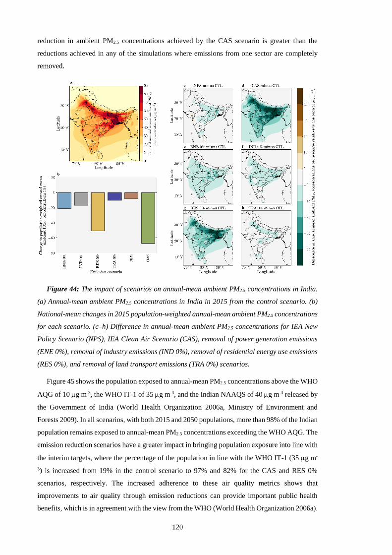
120

reduction in ambient PM2.5 concentrations achieved by the CAS scenario is greater than the

reductions achieved in any of the simulations where emissions from one sector are completely

removed.

Figure 44: The impact of scenarios on annual-mean ambient PM2.5 concentrations in India.

(a) Annual-mean ambient PM2.5 concentrations in India in 2015 from the control scenario. (b)

National-mean changes in 2015 population-weighted annual-mean ambient PM2.5 concentrations

for each scenario. (c–h) Difference in annual-mean ambient PM2.5 concentrations for IEA New

Policy Scenario (NPS), IEA Clean Air Scenario (CAS), removal of power generation emissions

(ENE 0%), removal of industry emissions (IND 0%), removal of residential energy use emissions

(RES 0%), and removal of land transport emissions (TRA 0%) scenarios.

Figure 45 shows the population exposed to annual-mean PM2.5 concentrations above the WHO

AQG of 10 g m-3, the WHO IT-1 of 35 g m-3, and the Indian NAAQS of 40 g m-3 released by

the Government of India (World Health Organization 2006a, Ministry of Environment and

Forests 2009). In all scenarios, with both 2015 and 2050 populations, more than 98% of the Indian

population remains exposed to annual-mean PM2.5 concentrations exceeding the WHO AQG. The

emission reduction scenarios have a greater impact in bringing population exposure into line with

the interim targets, where the percentage of the population in line with the WHO IT-1 (35 g m-

3) is increased from 19% in the control scenario to 97% and 82% for the CAS and RES 0%

scenarios, respectively. The increased adherence to these air quality metrics shows that

improvements to air quality through emission reductions can provide important public health

benefits, which is in agreement with the view from the WHO (World Health Organization 2006a).

121

Figure 45: The impact of scenarios on air quality metrics in India. (a) Percentage of the

population and (b) total population in 2015 (1st bar) and 2050 (2nd bar) exposed to annual-mean

ambient PM2.5 concentrations exceeding 10 g m-3 (WHO AQG), 35 g m-3 (WHO IT-1), and 40

g m-3 (NAAQS) in each scenario.

5.4.2. Indian disease burden under air pollution control pathways

The impacts of the scenarios on premature mortality estimates from ambient PM2.5 exposure

across India is shown in Figure 46. Total premature mortality across India is shown assuming

population and underlying health data appropriate for both 2015 and 2050 (Figure 46b). Reduced

ambient PM2.5 concentrations for the NPS and CAS reduce estimates of annual premature

mortality for 2015 by 4% and 39%, respectively relative to the control scenario of 900,000 (95UI:

683,000–1,252,000) annual premature mortalities. Assuming no change in emissions, total annual

premature mortality for the control scenario in 2050 is estimated to be 1,577,000 (95UI:

1,210,000–2,209,000). This estimate of premature mortality in 2050 is 75% greater than in 2015

due to population growth and ageing, partly offset by reducing baseline mortality rates. Under the

NPS and CAS, total premature mortality in 2050 changes by +68% and +7%, respectively relative

to the control scenario estimate for 2015. The NPS and CAS can therefore potentially reduce the

annual premature mortality estimate in 2050 by 61,000 and 610,000 deaths relative to the 2015

control, equivalent to offsetting 9% and 91% of the increase in 2050 caused by population ageing

and growth. Despite the small national increase in premature mortalities (7%), the disease burden

is reduced in some states (Jammu and Kashmir, Himachal Pradesh, Uttaranchal, and Sikkim)

(Figure 46d).

Figure 47 shows the impacts of the scenarios on the mortality rate per 100,000 population from

exposure to ambient PM2.5 across India. Under no change in emissions to 2050, the mortality rate

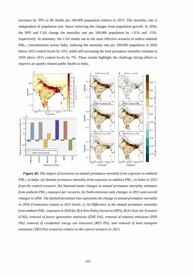
122

increases by 39% to 86 deaths per 100,000 population relative to 2015. The mortality rate is

independent of population size, hence removing the changes from population growth. In 2050,

the NPS and CAS change the mortality rate per 100,000 population by +31% and -15%,

respectively. In summary, the CAS stands out as the most effective scenario to reduce ambient

PM2.5 concentrations across India, reducing the mortality rate per 100,000 population in 2050

below 2015 control levels by 15%, while still increasing the total premature mortality estimate in

2050 above 2015 control levels by 7%. These results highlight the challenge facing efforts to

improve air quality related public health in India.

Figure 46: The impact of scenarios on annual premature mortality from exposure to ambient

PM2.5 in India. (a) Annual premature mortality from exposure to ambient PM2.5 in India in 2015

from the control scenario. (b) National-mean changes in annual premature mortality estimates

from ambient PM2.5 exposure per scenario, for both emissions only changes in 2015 and overall

changes in 2050. The dashed horizontal line represents the change in annual premature mortality

in 2050 if emissions remain at 2015 levels. (c–h) Difference in the annual premature mortality

from ambient PM2.5 exposure in 2050 for IEA New Policy Scenario (NPS), IEA Clean Air Scenario

(CAS), removal of power generation emissions (ENE 0%), removal of industry emissions (IND

0%), removal of residential energy use emissions (RES 0%), and removal of land transport

emissions (TRA 0%) scenarios relative to the control scenario in 2015.

123

Figure 47: The impact of scenarios on annual mortality rate per 100,000 population from

exposure to ambient PM2.5 in India. (a) Annual mortality rate per 100,000 population from

exposure to ambient PM2.5 in India in 2015 from the control scenario. (b) National-mean changes

in annual mortality rate per 100,000 population estimates from ambient PM2.5 exposure per

scenario, for both emissions only changes in 2015 and overall changes in 2050. The dashed

horizontal line represents the change in annual mortality rate per 100,000 population in 2050 if

emissions remain at 2015 levels. (c–h) Difference in the annual mortality rate per 100,000

population from ambient PM2.5 exposure in 2050 for IEA New Policy Scenario (NPS), IEA Clean

Air Scenario (CAS), removal of power generation emissions (ENE 0%), removal of industry

emissions (IND 0%), removal of residential energy use emissions (RES 0%), and removal of land

transport emissions (TRA 0%) scenarios relative to the control scenario in 2015.

In all states except Delhi, residential energy use is the dominant sectoral contributor to ambient

PM2.5 concentrations in the 2015 control scenario. In simulations where emissions from RES,

ENE, IND, and TRA sectors are removed in 2050, the total premature mortality increases by 30%,

59%, 64%, and 68%, respectively relative to the control scenario estimate for 2015 (Figure 46b).

The increase in the total premature mortality estimate in 2050 due to population ageing and

growth can be offset by 407,000 (60%), 142,000 (21%), 105,000 (16%), and 68,000 (10%)

premature mortalities by removing RES, ENE, IND, and TRA, respectively. The mean mortality

rate per 100,000 population across India in 2050 relative to 2015 increases by 3%, 24%, 29%,

and 31% by removing RES, ENE, IND, and TRA, respectively (Figure 47b). In Delhi, multiple

emission sources contribute strongly to the very high annual-mean ambient PM2.5 concentrations

of 122 g m-3 in the 2015 control scenario. Emissions from TRA dominate (36%), and emissions

124

from RES (27%), ENE (26%), and IND (13%) also contribute substantially. In West Bengal

annual-mean ambient PM2.5 concentrations are also very high at 94 g m-3, however RES

emissions heavily dominate the source contribution (62%), and the scenario removing these is

equivalent to 75% of the potential health benefits from the CAS. In West Bengal, annual

premature mortality for the NPS and CAS in 2050 relative to the control scenario for 2015 are

increased in line with the national averages of 68% and 7%, respectively. While for Delhi, both

scenarios are less effective at reducing the disease burden where there is a 70% increase for the

NPS and 22% increase for the CAS.

Figure 48 shows the impact of emission scaling from the idealised simulations (0%, -10%, and

+10%) on population-weighted annual-mean ambient PM2.5 concentrations and the associated

disease burden. There is an approximately linear reduction in population-weighted ambient PM2.5

concentrations relative to individual source emission changes. However, there is a non-linear

reduction in premature mortality from the individual source change scenarios, due to the non-

linear exposure-response function. Reductions in population-weighted ambient PM2.5

concentrations are relatively larger than reductions in the associated disease burden.

Figure 48: (a) The impact of emission scaling on population-weighted annual-mean ambient

PM2.5 concentrations. (b) The impact of emission scaling on total annual premature mortality

from exposure to ambient PM2.5 concentrations in India.

5.4.3. Sensitivities to demography and baseline mortality rates

Sensitivity studies are performed estimating the disease burden from emission only changes

in 2015, and then for 2050 individually using population density from 2015 (POP2015),

population age groupings from 2015 (AGE2015), or baseline mortality rates from 2015

(BM2015) to explore the impact of each variable in turn. Figure 49a shows the change in the

national-mean premature mortality rate per 100,000 population in India due to ambient PM2.5

exposure from each scenario. Figure 49b shows the disease breakdown of the total premature

125

mortality estimates per scenario. Figure 49a and 49b do not show results from the -10% and +10%

emission change scenarios as premature mortality estimates and mortality rates only change by

±2% for these scenarios. For emission only changes in 2015, the NPS and CAS reduced premature

mortality estimates by 4% and 39%, respectively, while the individual removal of RES, ENE,

IND, and TRA emissions reduced premature mortality estimates by 26%, 9%, 7%, and 4%,

respectively (Figure 49b). Emissions reductions have a larger impact through reducing respiratory

diseases (LRI and COPD), which respond more linearly, rather than the cardiovascular diseases

(IHD and CEV), which have a more non-linear response to changes in PM2.5 concentrations. The

non-linearity was also found in previous studies (Apte et al 2015a, Kodros et al 2016, Conibear

et al 2018a). These scenarios in which only emissions are modified highlight the need for stringent

air quality management to reduce the disease burden in the highly polluted country of India due

to the non-linear exposure-response function.

Each sensitivity (POP2015, AGE2015, and BM2015) uses 2015 data for that specific variable

with 2050 data for the other variables. Each sensitivity shows the influence of the other parameters

in combination in 2050, compared with 2015. The difference between each sensitivity mortality

estimate for 2050 and the control mortality estimate for 2015 is the impact of the temporal change

(2050 minus 2015) in that specific variable. For the control scenario, premature mortality

estimates in 2050 for POP2015, AGE2015, and BM2015 changed by -22%, -60%, and +74%,

respectively, relative to control scenario estimates for 2050 (Figure 49). Consequently, population

ageing and growth together through to 2050 in India increase the number of people susceptible to

air pollution, while a decrease in baseline mortality rates offsets a large part of this increase. The

considerable sensitivity of premature mortality estimates to population ageing and baseline

mortality rates illustrates the importance of demographic and epidemiological transitions in the

future disease burden from exposure to ambient PM2.5, which was also found in recent previous

studies (Chowdhury et al 2018, GBD MAPS Working Group 2018).

126

Figure 49: The impact of scenarios on the disease burden from exposure to ambient PM2.5 in

India. (a) National-mean annual premature mortality rate per 100,000 population due to ambient

exposure to PM2.5 in India. (b) Disease breakdown of health burden from ambient PM2.5 exposure

in India. For each panel, the bars show estimates for 2015, 2050, 2050 with population density

from 2015, 2050 with population age grouping from 2015, and 2050 with baseline mortality rates

from 2015 (1st to 5th bars per scenario). The vertical error bars show 95% uncertainty intervals

(95UI) calculated by combining fractional errors in quadrature (see Methods).

5.4.4. Comparison to previous studies

Figure 50 compares this study’s simulated impacts of the different scenarios on ambient PM2.5

concentrations and the associated disease burden in India with previous studies (GBD MAPS

Working Group 2018, International Energy Agency 2016a). This study estimates a larger

percentage of the population exposed to ambient PM2.5 concentrations exceeding the WHO IT-1

compared to the IEA study (International Energy Agency 2016a) (Figure 50b). This could

potentially be a reflection of lower spatial resolution used in the IEA study underestimating the

high ambient PM2.5 concentrations in India, in addition to the different modelling choices. The

IEA study used the Greenhouse gas–Air pollution Interactions and Synergies (GAINS) model

(Amann et al 2011) driven by the European Monitoring and Evaluation Programme (EMEP)

chemical transport model (Simpson et al 2012). The control scenario estimate of total premature

mortality in 2015 from the IEA study was 34% smaller than this study (Figure 50c). This is likely

due to the combination of lower ambient PM2.5 concentrations, older baseline mortality rates

(2011 versus 2016 in this study) corrected for risk but not cause of mortality, and the use of older

exposure-response functions from the GBD2013 (GBD 2013 Risk Factors Collaborators 2015).

The GBD2013 exposure-response functions have weaker relationships between risk and ambient

127

PM2.5 concentrations relative to the updated exposure-response functions from the GBD2016

(GBD 2016 Risk Factors Collaborators 2017, Cohen et al 2017) as used by this study and the

GBD MAPS Working Group study. The IEA study estimated slightly smaller changes in

premature mortality of +53% and -5% for the NPS and CAS, respectively relative to control

scenario in 2015 compared to this study’s estimates of +68% and +7%, primarily due to an earlier

year of estimation (2040 versus 2050 in this study) reducing the impacts of population growth

and ageing.

The control scenario population-weighted annual-mean ambient PM2.5 concentrations from the

GBD MAPS Working Group study (GBD MAPS Working Group 2018) are 24% larger than those

in this study (Figure 50a), potentially due to their use of higher resolution (0.1° × 0.1°) modelling

and data assimilation within a Bayesian hierarchical model in the control scenario. The fractional

impacts of the scenarios on ambient PM2.5 concentrations are then derived using the South Asia

nested version of the GEOS-Chem chemical transport model at coarser resolution (0.5° × 0.67°)

to scale the higher resolution ambient PM2.5 concentrations.

Present day emissions from this study are from EDGAR-HTAP v2.2 (Janssens-Maenhout et

al 2015), and future emissions are scaled according to factors from the IEA NPS and CAS

(International Energy Agency 2016a). Present day emissions of PM2.5, BC, and OC from

EDGAR-HTAP v2.2 (Janssens-Maenhout et al 2015) agree well with those from the GBD MAPS

Working Group (Venkataraman et al 2018, GBD MAPS Working Group 2018). Present day

emissions of SO2, NOx, and NMVOC from EDGAR-HTAP v2.2 (Janssens-Maenhout et al 2015)

are a factor 1.5–2 larger than those from the GBD MAPS Working Group (Venkataraman et al

2018, GBD MAPS Working Group 2018), due largely to differences in the power sector.

The ambitious and aspirational scenarios analysed in the GBD MAPS Working Group study

are different from the NPS and CAS scenarios analysed in this study. Both the IEA NPS and GBD

MAPS Working Group ambitious scenarios are based on relevant existing and planned policies

as of 2016 including India’s INDCs. However, the technology shifts and sectoral growth rates

vary between the different scenarios. In the NPS, SO2, NOx, and PM2.5 emissions increase by

10%, 10%, and 7% in 2040 relative to 2015, respectively, while in the GBD MAPS Working

Group ambitious scenario SO2, NOx, and PM2.5 emissions increase by 156%, 96%, and 26% in

2050 relative to 2015, respectively. Similarly, while both the IEA CAS and the GBD MAPS

Working Group aspirational scenario represent stringent air quality management, the specific

realisations of these scenarios varies between the studies. In the CAS, SO2, NOx, and PM2.5

emissions change by -69%, -50%, and -76% in 2040 relative to 2015, respectively, while in the

GBD MAPS Working Group aspirational scenario SO2, NOx, and PM2.5 emissions change by -

6%, +13%, and -67% in 2050 relative to 2015, respectively. The GBD MAPS Working Group

found larger resulting ambient PM2.5 concentrations from their scenarios (Figure 50a) and

consequent increases in premature mortality in 2050 (Figure 50c). The NPS emissions of BC, OC,

128

SO2, and NOx are more similar to the GBD MAPS Working Group aspirational scenario

(Venkataraman et al 2018, GBD MAPS Working Group 2018). NPS emissions of PM2.5 show a

similar but lower (-30%) trend to the GBD MAPS Working Group ambitious scenario due to

lower emissions from residential biomass and agricultural burning. NMVOC emissions are

similar to the NPS and the GBD MAPS Working Group ambitious scenario (Venkataraman et al

2018, GBD MAPS Working Group 2018). This study, the GBD MAPS Working Group study,

and the IEA study all find substantial potential public health benefits from stringent air quality

management relative to a business-as-usual scenario.

Figure 50: Comparison of the impacts of different scenarios on ambient PM2.5 concentrations

and the associated disease burden in India from this study with previous studies. (a) Comparison

of population-weighted annual-mean ambient PM2.5 concentrations. (b) Comparison of

percentage of the population exposed to various metrics of annual-mean ambient PM2.5

concentrations in India. (c) Comparison of total premature mortality estimates due to exposure

to ambient PM2.5 per year in India from different scenarios.

The influence of climate change on Indian PM2.5 concentrations is uncertain (Jacob and

Winner 2009, Fiore et al 2012, Fang et al 2013). Climate changes are projected to be smaller than

emission changes (Pommier et al 2018, Silva et al 2017, Fang et al 2013, Jacobson 2008, Kumar

129

et al 2018). Two recent studies analysed the combined impacts of climate change and emission

scenarios on future air quality in South Asia by 2050 (Kumar et al 2018, Pommier et al 2018).

The massive increase in anthropogenic emissions in India by 2050 has been found to have an

order of magnitude larger impact on PM2.5 concentrations than climate change (Pommier et al

2018). Kumar et al (2018) found South Asian PM2.5 concentrations to change by +13 g m-3 and

+1 g m-3 by 2050 relative to 2015 under Representative Concentration Pathways (RCP) 8.5 and

RCP6.0, respectively. Kumar et al (2018) qualitatively related changes in meteorological

variables with those in air quality, due to the limited number of simulations conducted relative to

the large ensemble of simulations required to quantify the impacts of climate change. The health

impacts of climate changes on PM2.5 concentrations in India were estimated to be 80,200 deaths

per year by 2100 (Silva et al 2017). This is 3% of the increase in PM2.5 exposure associated

mortality in India by 2050 due to emission changes under a reference scenario (GBD MAPS

Working Group 2018). Both previous studies estimating the future health impacts of air pollution

in India under different scenarios also used fixed meteorology to focus on the impacts of different

air pollution control pathways (GBD MAPS Working Group 2018, International Energy Agency

2016a).

Regional transport of pollution from distant sources impacts local ambient PM2.5

concentrations (Task Force on Hemispheric Transport of Air Pollution 2010). In 2007, PM2.5

produced inside India was associated with 75,000 premature deaths outside of India, while PM2.5

produced outside India was associated with 67,000 premature deaths inside India (Zhang et al

2017). Aerosol transport from Africa and the Middle East is associated with 83,000 and 77,000

premature mortalities in India, respectively, primarily from dust (Liu et al 2009). Regional

transport of PM2.5 into South Asia contributes 7% of the total mortality impact (Anenberg et al

2014).

This study, in agreement with previous studies (GBD MAPS Working Group 2018,

International Energy Agency 2016a), finds substantial increases in the future disease burden

associated with ambient PM2.5 exposure in India due to population growth and ageing. New

policies as of 2016 or small (-10%) changes in emissions provide only small improvements in air

quality and public health, with the impacts being heavily outweighed by the demographic

transition. Stringent air quality management, such as under the IEA CAS, removing residential

energy use emissions or the GBD MAPS Working Group aspirational scenario, will be required

to provide vast improvements in air quality and essential public health benefits. The removal of

residential energy use and land transport emissions might have further health benefits if exposures

are studied at finer scales due to the collocation of emissions with exposures. The changes in

disease burden estimates from ambient PM2.5 exposure do not consider that for some scenarios

there is a sizeable accompanying reduction in the disease burden from reducing household air

pollution from solid fuel use (e.g. the CAS and RES 0%).

130

5.5. Conclusion

Exposure to ambient particulate matter is a leading risk factor for public health in India.

Business-as-usual economic and industrial growth in India in 2050 is predicted to increase

emissions and further worsen ambient PM2.5 concentrations. Previous studies of alternative air

pollution control scenarios in India have used relatively coarse spatial resolution models to

estimate the impacts of the scenarios on ambient PM2.5 concentrations. In this study, a high-

resolution online-coupled model was used with the latest exposure-response function to estimate

the impacts of multiple Indian emission scenarios on ambient PM2.5 concentrations and human

health in India. The impacts of climate change and the impacts of changing emissions from

outside India are not included in this study. With no emissions growth in India, the disease burden

from exposure to ambient PM2.5 in 2050 will increase by 75% relative to 2015, due to population

ageing and growth increasing the number of people susceptible to air pollution, partly offset by

decreasing baseline mortality rates. The IEA NPS and CAS in 2050 can reduce population-

weighted ambient PM2.5 concentrations below 2015 levels by 9% and 68%, respectively. These

reductions in ambient PM2.5 concentrations reduce the annual premature mortality estimate by

61,000 and 610,000 deaths, which is 9% and 91% of the projected increase in premature

mortalities due to population growth and ageing, respectively. Throughout India, the CAS stands

out as the most effective scenario to reduce ambient PM2.5 concentrations and the associated

disease burden, reducing the 2050 mortality rate per 100,000 below 2015 control levels by 15%.

However, even under the strong emission reductions in the CAS, population growth and ageing

means that the annual premature mortality in 2050 will be 7% greater than in 2015. Small

emission changes bring small improvements to air quality and human health, where the

demographic transition to 2050 heavily outweighs the impacts. Strict implementation of air

quality management, such as under the IEA CAS or removing residential energy use emissions

from solid fuel use, can reduce the substantial and increasing health impacts of air pollution

exposure in India bringing crucial public health benefits.

131

6. Current and future disease burden from ambient ozone exposure

in India

6.1. Abstract

Long-term ambient O3 exposure is a risk factor for human health. This study estimates the

source-specific disease burden associated with long-term O3 exposure in India at high spatial

resolution using updated risk functions from the CPS-II. This study estimates 374,000 (95UI:

140,000–554,000) annual premature mortalities using the updated risk function in India in 2015,

200% larger than estimates using the earlier CPS-II risk function. This study finds land transport

emissions dominate the source contribution to this disease burden (35%), followed by emissions

from power generation (23%). With no change in emissions by 2050, this study estimates

1,126,000 (95UI: 421,000–1,667,000) annual premature mortalities, an increase of 200% relative

to 2015 due to population ageing and growth increasing the number of people susceptible to air

pollution. This study finds that the IEA NPS provides small changes (+1%) to this increasing

disease burden from the demographic transition. Under the IEA CAS, this study estimates

791,000 (95UI: 202,000–1,336,000) annual premature mortalities in 2050, avoiding 335,000

annual premature mortalities (45% of the increase) compared to the scenario of no emission

change. This study highlights that critical public health benefits are possible with stringent

emission reductions, despite population growth and ageing increasing the attributable disease

burden from O3 exposure even under such strong emission reductions. The disease burden

attributable to ambient PM2.5 exposure dominates that from ambient O3 exposure in the present

day, while in the future they may be similar in magnitude.

6.2. Introduction

The GBD2016 attributed 233,638 (95UI: 90,109–385,303) annual premature mortalities to

ambient O3 exposure globally, with 39% of the disease burden in India (GBD 2016 Risk Factors

Collaborators 2017, Cohen et al 2017). The GBD2016 used the earlier CPS-II risk estimates

(Jerrett et al 2009) for the cause of COPD only. These risk estimates have been updated for the

same CPS-II cohort through an extended follow-up with an expanded study population (Turner

et al 2016). Hazard ratios were found to increase (Turner et al 2016). The updated risks have been

used to estimate global premature mortality from long-term ambient O3 exposure, resulting in

substantial mortality increases, including in India (Malley et al 2017). This increased public health

burden due to O3 exposure has implications for air quality management strategies.

Ambient surface O3 concentrations have been increasing in India due to increasing emissions

of O3 precursors (Roy et al 2017, Ghude et al 2013). A business-as-usual scenario in India is

projected to increase O3 precursor emissions and future O3 concentrations (Pommier et al 2018,

Pozzer et al 2012, Chatani et al 2014, Fiore et al 2012, Wild et al 2012), with associated

projections increasing the disease burden from O3 exposure in India (Lelieveld et al 2015).

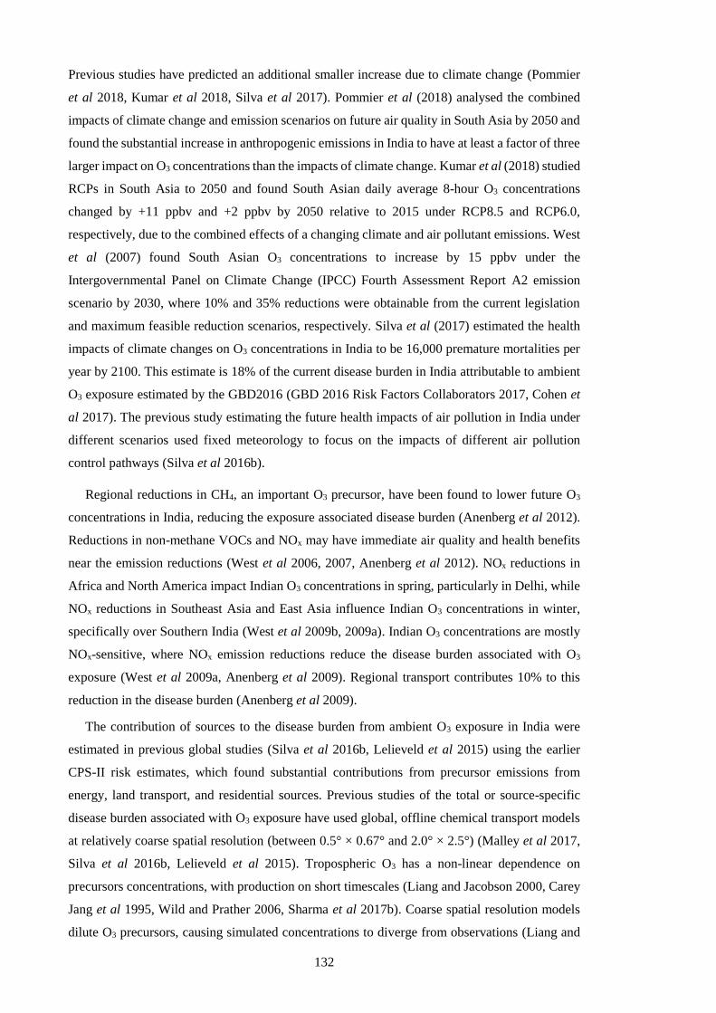
132

Previous studies have predicted an additional smaller increase due to climate change (Pommier

et al 2018, Kumar et al 2018, Silva et al 2017). Pommier et al (2018) analysed the combined

impacts of climate change and emission scenarios on future air quality in South Asia by 2050 and

found the substantial increase in anthropogenic emissions in India to have at least a factor of three

larger impact on O3 concentrations than the impacts of climate change. Kumar et al (2018) studied

RCPs in South Asia to 2050 and found South Asian daily average 8-hour O3 concentrations

changed by +11 ppbv and +2 ppbv by 2050 relative to 2015 under RCP8.5 and RCP6.0,

respectively, due to the combined effects of a changing climate and air pollutant emissions. West

et al (2007) found South Asian O3 concentrations to increase by 15 ppbv under the

Intergovernmental Panel on Climate Change (IPCC) Fourth Assessment Report A2 emission

scenario by 2030, where 10% and 35% reductions were obtainable from the current legislation

and maximum feasible reduction scenarios, respectively. Silva et al (2017) estimated the health

impacts of climate changes on O3 concentrations in India to be 16,000 premature mortalities per

year by 2100. This estimate is 18% of the current disease burden in India attributable to ambient

O3 exposure estimated by the GBD2016 (GBD 2016 Risk Factors Collaborators 2017, Cohen et

al 2017). The previous study estimating the future health impacts of air pollution in India under

different scenarios used fixed meteorology to focus on the impacts of different air pollution

control pathways (Silva et al 2016b).

Regional reductions in CH4, an important O3 precursor, have been found to lower future O3

concentrations in India, reducing the exposure associated disease burden (Anenberg et al 2012).

Reductions in non-methane VOCs and NOx may have immediate air quality and health benefits

near the emission reductions (West et al 2006, 2007, Anenberg et al 2012). NOx reductions in

Africa and North America impact Indian O3 concentrations in spring, particularly in Delhi, while

NOx reductions in Southeast Asia and East Asia influence Indian O3 concentrations in winter,

specifically over Southern India (West et al 2009b, 2009a). Indian O3 concentrations are mostly

NOx-sensitive, where NOx emission reductions reduce the disease burden associated with O3

exposure (West et al 2009a, Anenberg et al 2009). Regional transport contributes 10% to this

reduction in the disease burden (Anenberg et al 2009).

The contribution of sources to the disease burden from ambient O3 exposure in India were

estimated in previous global studies (Silva et al 2016b, Lelieveld et al 2015) using the earlier

CPS-II risk estimates, which found substantial contributions from precursor emissions from

energy, land transport, and residential sources. Previous studies of the total or source-specific

disease burden associated with O3 exposure have used global, offline chemical transport models

at relatively coarse spatial resolution (between 0.5° × 0.67° and 2.0° × 2.5°) (Malley et al 2017,

Silva et al 2016b, Lelieveld et al 2015). Tropospheric O3 has a non-linear dependence on

precursors concentrations, with production on short timescales (Liang and Jacobson 2000, Carey

Jang et al 1995, Wild and Prather 2006, Sharma et al 2017b). Coarse spatial resolution models

dilute O3 precursors, causing simulated concentrations to diverge from observations (Liang and

133

Jacobson 2000, Carey Jang et al 1995, Wild and Prather 2006, Sharma et al 2017b, Li et al 2016c,

Punger and West 2013, Thompson and Selin 2012, Thompson et al 2014). Resolution directly

changes the resolved space, in addition to indirectly influencing parameterisation choices

important for secondary pollutants (Wild and Prather 2006, Punger and West 2013). The model

resolution also affects estimates of the O3 exposure related disease burden (Punger and West 2013,

Thompson et al 2014, Thompson and Selin 2012). O3 has greater regional transport efficiency

relative to PM2.5, and studies focusing on both O3 and PM2.5 found health impacts of PM2.5 to be

more localised (Anenberg et al 2010, Ghude et al 2016, Anenberg et al 2014, 2009). Online-

coupled modelling explicitly accounts for feedbacks between chemistry and meteorology (Grell

et al 2004, Baklanov et al 2014), which can be important to consider when emissions are

changing.

This study makes the first estimate of the source-specific disease burden due to O3 exposure

at high spatial resolution, using the updated CPS-II risk functions from Turner et al (2016), in

addition to analysing the impacts of future air pollution control pathways. High-resolution (30km,

0.3° spatial resolution) numerical weather prediction, online-coupled with chemistry, model

simulations are used to estimate the present-day reductions in surface O3 concentrations in India

resulting from the removal of different O3 precursor source sectors. An annual control simulation

was performed for the year 2014 and evaluated against surface observations; then annual

sensitivity simulations are performed individually removing biomass burning (BBU), power

generation (ENE), industrial non-power (IND), residential energy use (RES), and land transport

(TRA). The impact of scenarios is conducted in line with the IEA NPS and CAS (International

Energy Agency 2016a). To help interpret the impacts of these emission scenarios, idealised

simulations individually changing emissions (-10% and +10%) are conducted for the four

anthropogenic emission sectors (ENE, IND, RES, and TRA). The associated disease burden per

risk estimate, per simulation, is estimated. Further sensitivity studies are performed to explore the

impacts of the Indian demographic and epidemiologic transition through to 2050 on the public

health burden associated with O3 exposure. It is assumed that both climate and emissions from

countries outside India remain unchanged, allowing the isolation of the impacts of changing

Indian emissions. The aim is to produce a valuable resource to help inform environmental policy

decisions at the state and national levels regarding O3 precursor emission controls.

6.3. Precursor emissions

Figure 51 shows the spatial contributions of land transport, power generation, residential

energy use, and industry to total annual anthropogenic emissions of NOx, NMVOC, and CO. Land

transport dominates anthropogenic emissions of NOx, while residential energy use is the leading

contributor to anthropogenic emissions of CO and NMVOC. Figure 52 shows the fractional

contribution of each season (winter DJF, spring MAM, summer JJA, and autumn SON) to total

anthropogenic emissions of NOx, NMVOC, and CO. Anthropogenic emissions of NOx, NMVOC,

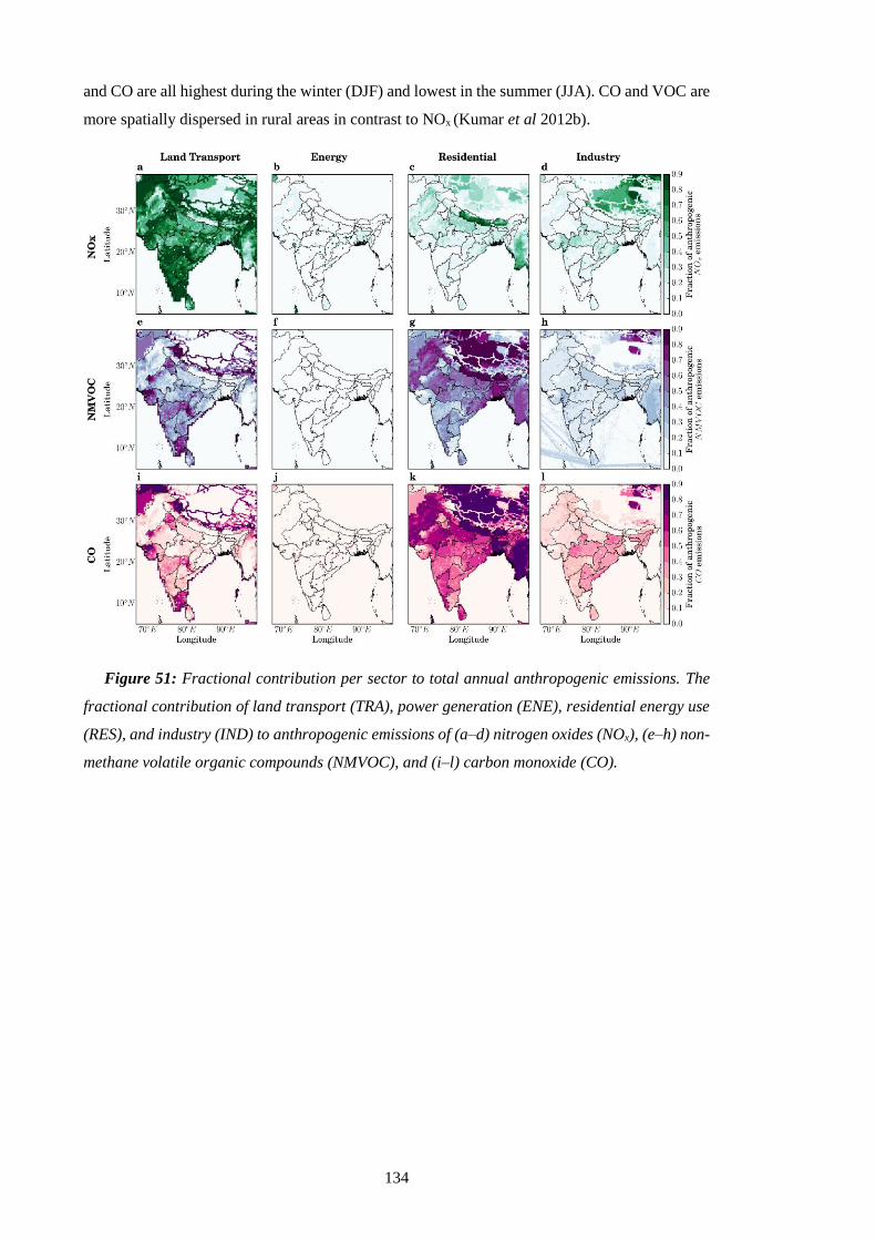
134

and CO are all highest during the winter (DJF) and lowest in the summer (JJA). CO and VOC are

more spatially dispersed in rural areas in contrast to NOx (Kumar et al 2012b).

Figure 51: Fractional contribution per sector to total annual anthropogenic emissions. The

fractional contribution of land transport (TRA), power generation (ENE), residential energy use

(RES), and industry (IND) to anthropogenic emissions of (a–d) nitrogen oxides (NOx), (e–h) non-

methane volatile organic compounds (NMVOC), and (i–l) carbon monoxide (CO).

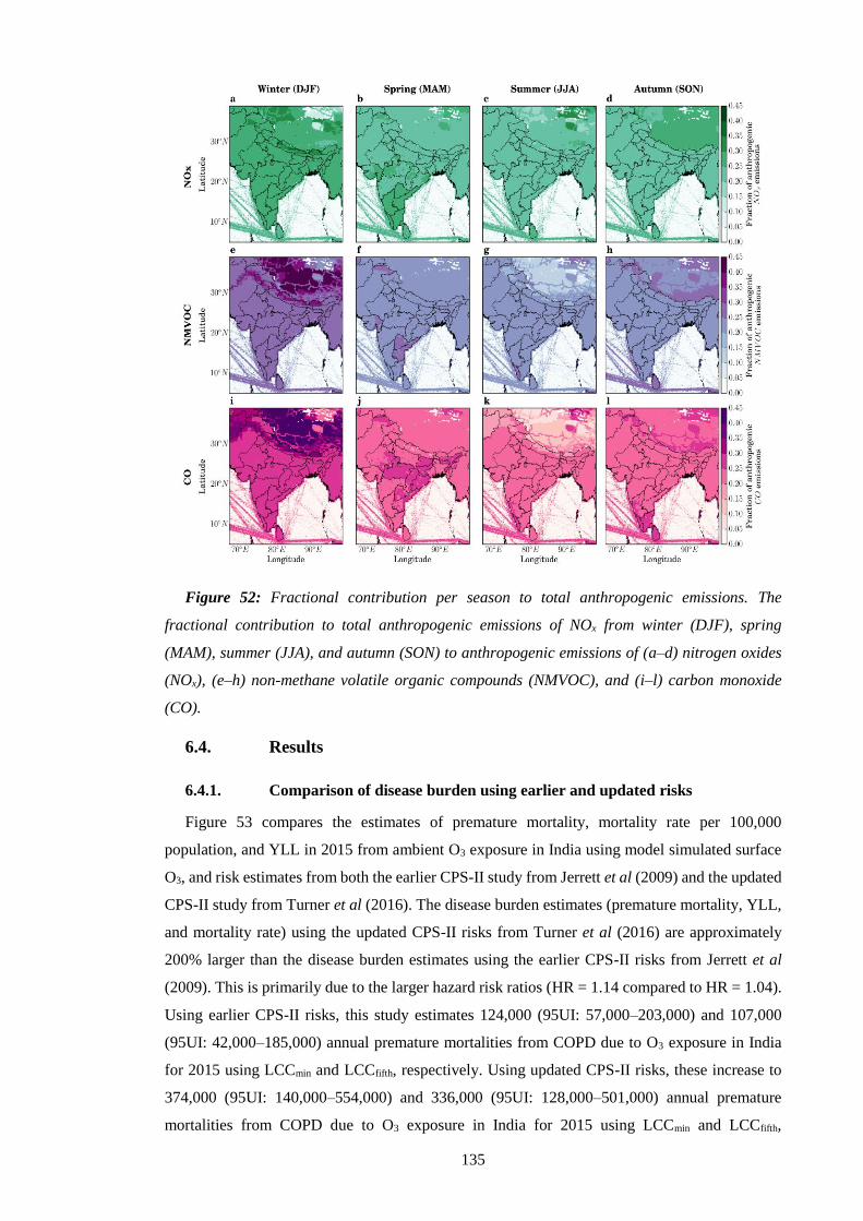
135

Figure 52: Fractional contribution per season to total anthropogenic emissions. The

fractional contribution to total anthropogenic emissions of NOx from winter (DJF), spring

(MAM), summer (JJA), and autumn (SON) to anthropogenic emissions of (a–d) nitrogen oxides

(NOx), (e–h) non-methane volatile organic compounds (NMVOC), and (i–l) carbon monoxide

(CO).

6.4. Results

6.4.1. Comparison of disease burden using earlier and updated risks

Figure 53 compares the estimates of premature mortality, mortality rate per 100,000

population, and YLL in 2015 from ambient O3 exposure in India using model simulated surface

O3, and risk estimates from both the earlier CPS-II study from Jerrett et al (2009) and the updated

CPS-II study from Turner et al (2016). The disease burden estimates (premature mortality, YLL,

and mortality rate) using the updated CPS-II risks from Turner et al (2016) are approximately

200% larger than the disease burden estimates using the earlier CPS-II risks from Jerrett et al

(2009). This is primarily due to the larger hazard risk ratios (HR = 1.14 compared to HR = 1.04).

Using earlier CPS-II risks, this study estimates 124,000 (95UI: 57,000–203,000) and 107,000

(95UI: 42,000–185,000) annual premature mortalities from COPD due to O3 exposure in India

for 2015 using LCCmin and LCCfifth, respectively. Using updated CPS-II risks, these increase to

374,000 (95UI: 140,000–554,000) and 336,000 (95UI: 128,000–501,000) annual premature

mortalities from COPD due to O3 exposure in India for 2015 using LCCmin and LCCfifth,

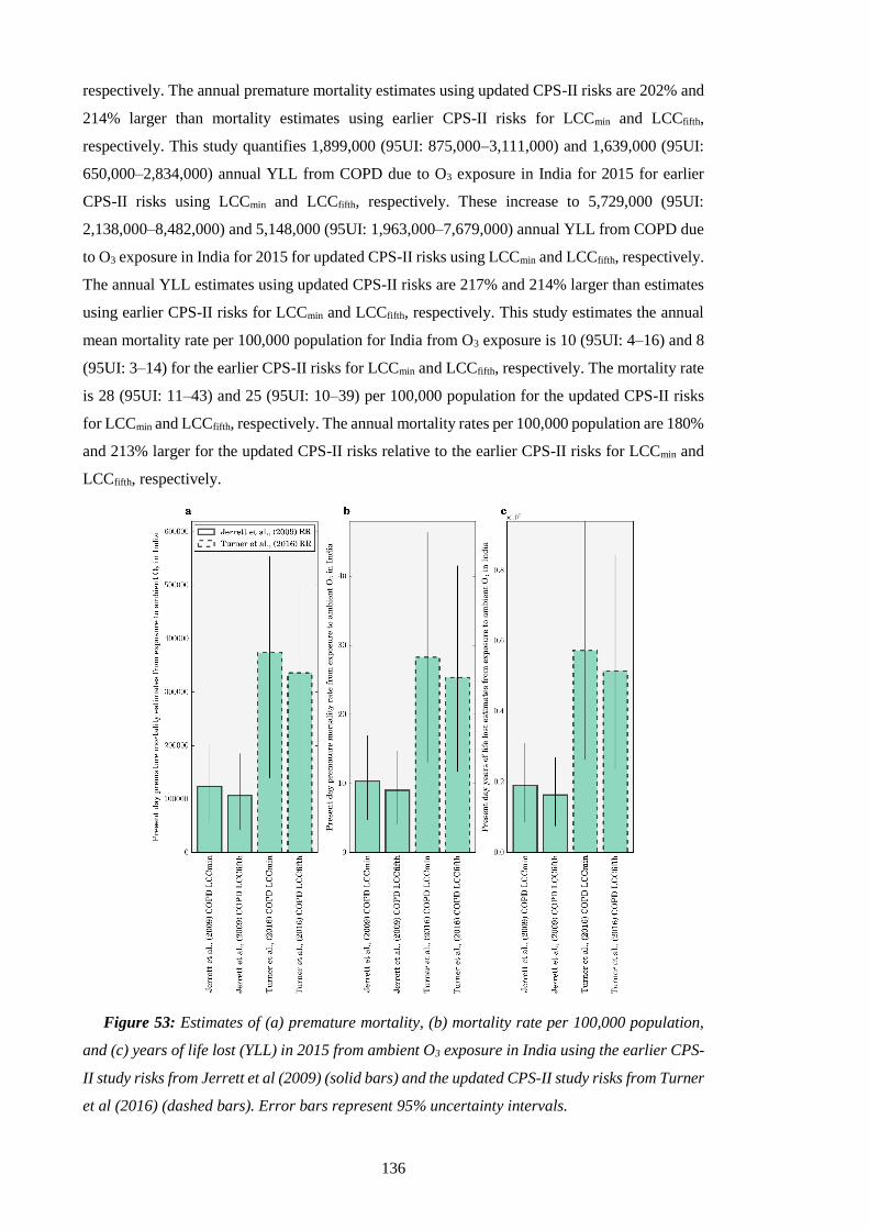
136

respectively. The annual premature mortality estimates using updated CPS-II risks are 202% and

214% larger than mortality estimates using earlier CPS-II risks for LCCmin and LCCfifth,

respectively. This study quantifies 1,899,000 (95UI: 875,000–3,111,000) and 1,639,000 (95UI:

650,000–2,834,000) annual YLL from COPD due to O3 exposure in India for 2015 for earlier

CPS-II risks using LCCmin and LCCfifth, respectively. These increase to 5,729,000 (95UI:

2,138,000–8,482,000) and 5,148,000 (95UI: 1,963,000–7,679,000) annual YLL from COPD due

to O3 exposure in India for 2015 for updated CPS-II risks using LCCmin and LCCfifth, respectively.

The annual YLL estimates using updated CPS-II risks are 217% and 214% larger than estimates

using earlier CPS-II risks for LCCmin and LCCfifth, respectively. This study estimates the annual

mean mortality rate per 100,000 population for India from O3 exposure is 10 (95UI: 4–16) and 8

(95UI: 3–14) for the earlier CPS-II risks for LCCmin and LCCfifth, respectively. The mortality rate

is 28 (95UI: 11–43) and 25 (95UI: 10–39) per 100,000 population for the updated CPS-II risks

for LCCmin and LCCfifth, respectively. The annual mortality rates per 100,000 population are 180%

and 213% larger for the updated CPS-II risks relative to the earlier CPS-II risks for LCCmin and

LCCfifth, respectively.

Figure 53: Estimates of (a) premature mortality, (b) mortality rate per 100,000 population,

and (c) years of life lost (YLL) in 2015 from ambient O3 exposure in India using the earlier CPS-

II study risks from Jerrett et al (2009) (solid bars) and the updated CPS-II study risks from Turner

et al (2016) (dashed bars). Error bars represent 95% uncertainty intervals.

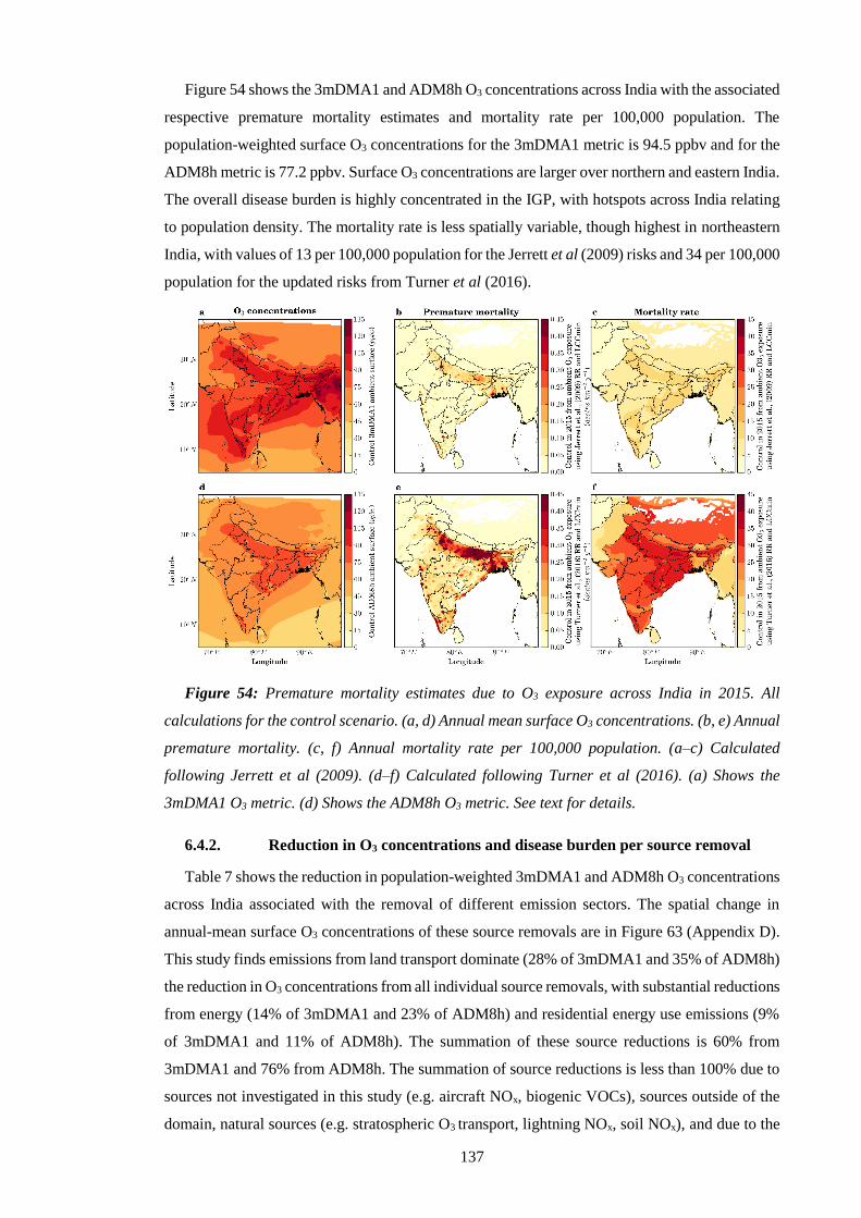
137

Figure 54 shows the 3mDMA1 and ADM8h O3 concentrations across India with the associated

respective premature mortality estimates and mortality rate per 100,000 population. The

population-weighted surface O3 concentrations for the 3mDMA1 metric is 94.5 ppbv and for the

ADM8h metric is 77.2 ppbv. Surface O3 concentrations are larger over northern and eastern India.

The overall disease burden is highly concentrated in the IGP, with hotspots across India relating

to population density. The mortality rate is less spatially variable, though highest in northeastern

India, with values of 13 per 100,000 population for the Jerrett et al (2009) risks and 34 per 100,000

population for the updated risks from Turner et al (2016).

Figure 54: Premature mortality estimates due to O3 exposure across India in 2015. All

calculations for the control scenario. (a, d) Annual mean surface O3 concentrations. (b, e) Annual

premature mortality. (c, f) Annual mortality rate per 100,000 population. (a–c) Calculated

following Jerrett et al (2009). (d–f) Calculated following Turner et al (2016). (a) Shows the

3mDMA1 O3 metric. (d) Shows the ADM8h O3 metric. See text for details.

6.4.2. Reduction in O3 concentrations and disease burden per source removal

Table 7 shows the reduction in population-weighted 3mDMA1 and ADM8h O3 concentrations

across India associated with the removal of different emission sectors. The spatial change in

annual-mean surface O3 concentrations of these source removals are in Figure 63 (Appendix D).

This study finds emissions from land transport dominate (28% of 3mDMA1 and 35% of ADM8h)

the reduction in O3 concentrations from all individual source removals, with substantial reductions

from energy (14% of 3mDMA1 and 23% of ADM8h) and residential energy use emissions (9%

of 3mDMA1 and 11% of ADM8h). The summation of these source reductions is 60% from

3mDMA1 and 76% from ADM8h. The summation of source reductions is less than 100% due to

sources not investigated in this study (e.g. aircraft NOx, biogenic VOCs), sources outside of the

domain, natural sources (e.g. stratospheric O3 transport, lightning NOx, soil NOx), and due to the

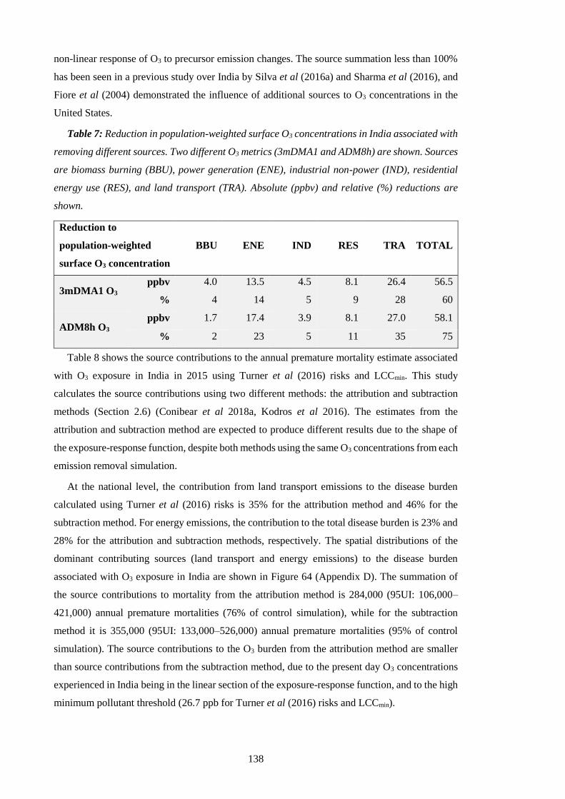
138

non-linear response of O3 to precursor emission changes. The source summation less than 100%

has been seen in a previous study over India by Silva et al (2016a) and Sharma et al (2016), and

Fiore et al (2004) demonstrated the influence of additional sources to O3 concentrations in the

United States.

Table 7: Reduction in population-weighted surface O3 concentrations in India associated with

removing different sources. Two different O3 metrics (3mDMA1 and ADM8h) are shown. Sources

are biomass burning (BBU), power generation (ENE), industrial non-power (IND), residential

energy use (RES), and land transport (TRA). Absolute (ppbv) and relative (%) reductions are

shown.

Reduction to

population-weighted

surface O3 concentration

BBU ENE IND RES TRA TOTAL

3mDMA1 O3 ppbv 4.0 13.5 4.5 8.1 26.4 56.5

% 4 14 5 9 28 60

ADM8h O3 ppbv 1.7 17.4 3.9 8.1 27.0 58.1

% 2 23 5 11 35 75

Table 8 shows the source contributions to the annual premature mortality estimate associated

with O3 exposure in India in 2015 using Turner et al (2016) risks and LCCmin. This study

calculates the source contributions using two different methods: the attribution and subtraction

methods (Section 2.6) (Conibear et al 2018a, Kodros et al 2016). The estimates from the

attribution and subtraction method are expected to produce different results due to the shape of

the exposure-response function, despite both methods using the same O3 concentrations from each

emission removal simulation.

At the national level, the contribution from land transport emissions to the disease burden

calculated using Turner et al (2016) risks is 35% for the attribution method and 46% for the

subtraction method. For energy emissions, the contribution to the total disease burden is 23% and

28% for the attribution and subtraction methods, respectively. The spatial distributions of the

dominant contributing sources (land transport and energy emissions) to the disease burden

associated with O3 exposure in India are shown in Figure 64 (Appendix D). The summation of

the source contributions to mortality from the attribution method is 284,000 (95UI: 106,000–

421,000) annual premature mortalities (76% of control simulation), while for the subtraction

method it is 355,000 (95UI: 133,000–526,000) annual premature mortalities (95% of control

simulation). The source contributions to the O3 burden from the attribution method are smaller

than source contributions from the subtraction method, due to the present day O3 concentrations

experienced in India being in the linear section of the exposure-response function, and to the high

minimum pollutant threshold (26.7 ppb for Turner et al (2016) risks and LCCmin).

139

Table 8: Source contributions to the annual premature mortalities associated with ambient O3

exposure in India in 2015 calculated using Turner et al (2016) risks and LCCmin, including source

contributions to the annual premature mortalities associated with ambient PM2.5 exposure from

Conibear et al (2018a) (Chapter 4). The absolute number and percentage of total premature

mortalities associated with O3 exposure in India are shown for two different methods (attribution

and subtraction), and for the subtraction method for PM2.5 exposure. Sources are biomass

burning (BBU), power generation (ENE), industrial non-power (IND), residential energy use

(RES), and land transport (TRA). Values in parentheses represent the 95% uncertainty intervals

(95UI).

Source

contribution

to annual

premature

mortalities

BBU ENE IND RES TRA TOTAL

O3,a

ttri

bu

tion

×103 7

(3–11)

86

(32–127)

19

(7–28)

41

(15–61)

131

(49–194)

284

(106–421)

% 2 23 5 11 35 76

O3,s

ub

tract

ion

×103 10

(4–15)

105

(39–156)

22

(8–33)

45

(17–67)

173

(65–256)

355

(133–527)

% 3 28 6 12 46 95

PM

2.5,s

ub

tract

ion

(Ch

ap

ter

4) ×103

12

(8–16)

90

(60–122)

66

(45–90)

256

(162–340)

43

(29–58)

467

(304–626)

% 1 9 7 26 4 47

6.4.3. Impact of emission mitigation scenarios on O3 and the disease burden

Figure 55 shows the impact of different emission scenarios on surface O3 concentrations. The

NPS increased the population-weighted ADM8h O3 concentrations by 1%, while the CAS

reduced them by 24%. The removal of land transport emissions reduces population-weighted

ADM8h O3 concentrations by 35%, and the removal of energy emissions reduces them by 23%.

These results show that the removal of land transport emissions produces greater reductions in O3

concentrations than the CAS. The larger reduction of O3 via removing land transport emissions

may be due to land transport emissions heavily dominating contributions to anthropogenic NOx

emissions, coupled to many population regions of India being NOx limited. O3 production in India

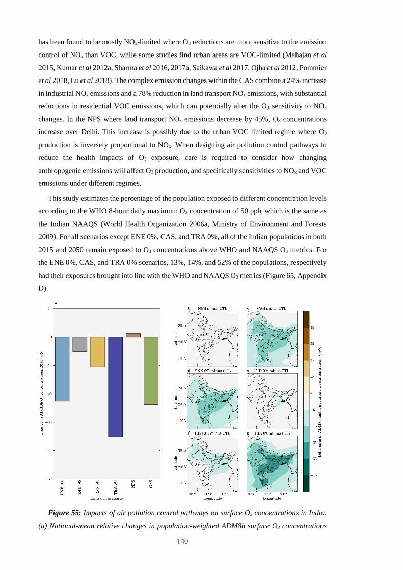
140

has been found to be mostly NOx-limited where O3 reductions are more sensitive to the emission

control of NOx than VOC, while some studies find urban areas are VOC-limited (Mahajan et al

2015, Kumar et al 2012a, Sharma et al 2016, 2017a, Saikawa et al 2017, Ojha et al 2012, Pommier

et al 2018, Lu et al 2018). The complex emission changes within the CAS combine a 24% increase

in industrial NOx emissions and a 78% reduction in land transport NOx emissions, with substantial

reductions in residential VOC emissions, which can potentially alter the O3 sensitivity to NOx

changes. In the NPS where land transport NOx emissions decrease by 45%, O3 concentrations

increase over Delhi. This increase is possibly due to the urban VOC limited regime where O3

production is inversely proportional to NOx. When designing air pollution control pathways to

reduce the health impacts of O3 exposure, care is required to consider how changing

anthropogenic emissions will affect O3 production, and specifically sensitivities to NOx and VOC

emissions under different regimes.

This study estimates the percentage of the population exposed to different concentration levels

according to the WHO 8-hour daily maximum O3 concentration of 50 ppb, which is the same as

the Indian NAAQS (World Health Organization 2006a, Ministry of Environment and Forests

2009). For all scenarios except ENE 0%, CAS, and TRA 0%, all of the Indian populations in both

2015 and 2050 remain exposed to O3 concentrations above WHO and NAAQS O3 metrics. For

the ENE 0%, CAS, and TRA 0% scenarios, 13%, 14%, and 52% of the populations, respectively

had their exposures brought into line with the WHO and NAAQS O3 metrics (Figure 65, Appendix

D).

Figure 55: Impacts of air pollution control pathways on surface O3 concentrations in India.

(a) National-mean relative changes in population-weighted ADM8h surface O3 concentrations

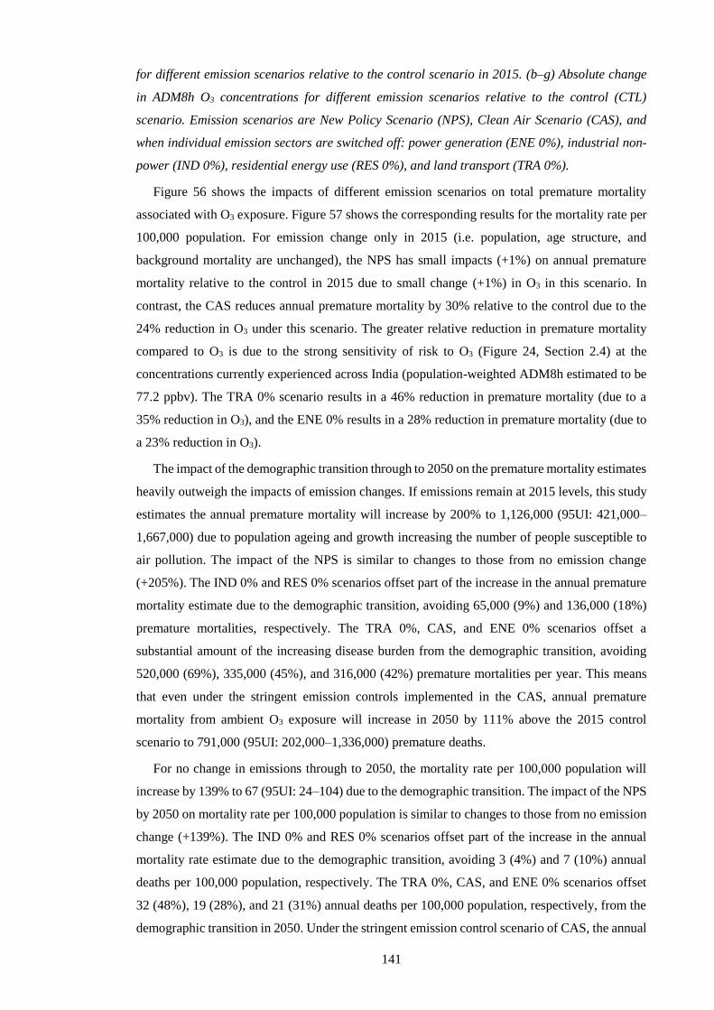
141

for different emission scenarios relative to the control scenario in 2015. (b–g) Absolute change

in ADM8h O3 concentrations for different emission scenarios relative to the control (CTL)

scenario. Emission scenarios are New Policy Scenario (NPS), Clean Air Scenario (CAS), and

when individual emission sectors are switched off: power generation (ENE 0%), industrial non-

power (IND 0%), residential energy use (RES 0%), and land transport (TRA 0%).

Figure 56 shows the impacts of different emission scenarios on total premature mortality

associated with O3 exposure. Figure 57 shows the corresponding results for the mortality rate per

100,000 population. For emission change only in 2015 (i.e. population, age structure, and

background mortality are unchanged), the NPS has small impacts (+1%) on annual premature

mortality relative to the control in 2015 due to small change (+1%) in O3 in this scenario. In

contrast, the CAS reduces annual premature mortality by 30% relative to the control due to the

24% reduction in O3 under this scenario. The greater relative reduction in premature mortality

compared to O3 is due to the strong sensitivity of risk to O3 (Figure 24, Section 2.4) at the

concentrations currently experienced across India (population-weighted ADM8h estimated to be

77.2 ppbv). The TRA 0% scenario results in a 46% reduction in premature mortality (due to a

35% reduction in O3), and the ENE 0% results in a 28% reduction in premature mortality (due to

a 23% reduction in O3).

The impact of the demographic transition through to 2050 on the premature mortality estimates

heavily outweigh the impacts of emission changes. If emissions remain at 2015 levels, this study

estimates the annual premature mortality will increase by 200% to 1,126,000 (95UI: 421,000–

1,667,000) due to population ageing and growth increasing the number of people susceptible to

air pollution. The impact of the NPS is similar to changes to those from no emission change

(+205%). The IND 0% and RES 0% scenarios offset part of the increase in the annual premature

mortality estimate due to the demographic transition, avoiding 65,000 (9%) and 136,000 (18%)

premature mortalities, respectively. The TRA 0%, CAS, and ENE 0% scenarios offset a

substantial amount of the increasing disease burden from the demographic transition, avoiding

520,000 (69%), 335,000 (45%), and 316,000 (42%) premature mortalities per year. This means

that even under the stringent emission controls implemented in the CAS, annual premature

mortality from ambient O3 exposure will increase in 2050 by 111% above the 2015 control

scenario to 791,000 (95UI: 202,000–1,336,000) premature deaths.

For no change in emissions through to 2050, the mortality rate per 100,000 population will

increase by 139% to 67 (95UI: 24–104) due to the demographic transition. The impact of the NPS

by 2050 on mortality rate per 100,000 population is similar to changes to those from no emission

change (+139%). The IND 0% and RES 0% scenarios offset part of the increase in the annual

mortality rate estimate due to the demographic transition, avoiding 3 (4%) and 7 (10%) annual

deaths per 100,000 population, respectively. The TRA 0%, CAS, and ENE 0% scenarios offset

32 (48%), 19 (28%), and 21 (31%) annual deaths per 100,000 population, respectively, from the

demographic transition in 2050. Under the stringent emission control scenario of CAS, the annual

142

mortality rate from exposure to O3 in 2050 will increase by 71% above the 2015 control scenario

to 48 (95UI: 13–86) deaths per 100,000 population.

These results highlight the dominant role of the demographic transition by 2050 in controlling

the susceptibility of the Indian population to air pollution, leading to a substantial mortality

increase. Stringent air pollution control pathways can provide essential public health benefits

offsetting part of the disease burden from O3 exposure.

Figure 56: Impacts of air pollution control pathways on annual premature mortality from

ambient O3 exposure in India. (a) National-mean changes in annual premature mortality

estimates from ambient O3 exposure per scenario, for both emissions only changes between 2015

and 2050 (solid bars) and overall changes in 2050 including 2015 to 2050 changes in emissions

as well as population growth, population ageing, and baseline mortality rates (POP/AGE/BM,

dashed bars). The dashed horizontal line represents the change in annual premature mortality in

2050 if emissions remain at 2015 levels. (b–g) Change in annual premature mortality from

ambient O3 exposure in 2050 from different emission scenarios (see Figure 55) relative to the

control scenario in 2015 accounting for emission changes and POP/AGE/BM changes. All health

impacts are calculated using Turner et al (2016) RR and LCCmin.

143

Figure 57: Impacts of air pollution control pathways on annual mortality rate per 100,000

population from ambient O3 exposure in India. (a) National-mean changes in annual mortality

rate per 100,000 population estimates from ambient O3 exposure per scenario, for both emissions

only changes between 2015 and 2050 (solid bars) and overall changes in 2050 including 2015 to

2050 changes in emissions as well as population ageing and baseline mortality rates

(POP/AGE/BM, dashed bars). The dashed horizontal line represents the change in annual

mortality rate per 100,000 population in 2050 if emissions remain at 2015 levels. (b–g) Annual

change in mortality rate per 100,000 population from ambient O3 exposure in 2050 from different

emission scenarios (see Figure 55) relative to the control scenario in 2015 accounting for

emission changes and POP/AGE/BM changes. All health impacts are calculated using Turner et

al (2016) RR and LCCmin.

Figure 58 shows the impact of emission scaling from the idealised simulations (0%, -10%, and

+10%) on surface O3 concentrations and the associated disease burden. This study applied linear

scaling to illustrate the influence of the non-linear response of O3 concentrations to changes in O3

precursors. Wild et al (2012), later developed by Turnock et al (2018), used simulations from

20% emission reductions of O3 precursors to scale surface O3 changes and found this

parameterised approach worked well for small emission perturbations. The parameterised

approach also works well for CO and NMVOC, while the O3 response to NOx was more non-

linear (Wu et al 2009). The parameterisation was not expected to perform well for large emission

perturbations (> ±60%) or source regions under titration regimes (emission reductions may lead

to O3 increases) (Wild et al 2012, Turnock et al 2018). This study used a similar approach here.

144

However, the scaling was applied to a -10% emission change, per sector instead of per precursor,

up to complete removal to illustrate the difference of the non-linear O3 response.

This study estimates the non-linear O3 response (O3,non-linear) as a function of the O3 from the

control simulation (O3,CTL), the 0% idealised simulation (O3,sim0%), and the -10% idealised

simulation (O3,sim-10%) following Equation 14. The percentage contribution of non-linear O3

response (O3,non-linear,%) is then estimated relative to the change in O3 from the 0% idealised

simulation following Equation 15. Calculations are performed for both population-weighted

ADM8h O3 concentrations and the premature mortality estimates from O3 exposure following

Turner et al (2016) risks and LCCmin.

%10,3,3%0,3,3,3 10 simCTLsimCTLlinearnon OOOOO

Equation 14: The non-linear O3 response.

%0,3,3,3,%,3 100 simCTLlinearnonlinearnon OOOO

Equation 15: The percentage contribution of the non-linear O3 response.

For population-weighted ADM8h O3 concentrations, this study finds that the non-linear O3

response accounts for 69%, 61%, 104%, and 43% of the change from the 0% idealised simulations

for TRA, IND, ENE, and RES, respectively (Figure 58a). This means that the non-linear O3

response plays a strong role for O3 changes from TRA, IND, and ENE emission removal, although

the absolute change for the IND simulations is small. The strong non-linear O3 response for TRA

and ENE may be due to the large, heterogeneous NOx emissions across India (Figure 51, Section

6.3), and other precursors co-emitted with these sectors. For premature mortality estimates from

O3 exposure following Turner et al (2016) risks and LCCmin, this study finds that the non-linear

O3 response accounts for 73%, 65%, 103%, and 48% of the change from the 0% idealised

simulations for TRA, IND, ENE, and RES, respectively (Figure 58b). The similar contributions

of the non-linear O3 response to O3 concentrations and the associated premature mortality

estimates suggest that the changes in O3 concentrations are in the linear section of the exposure-

response function (i.e. below approximately 100 ppb). Although these estimates are illustrative,

they suggest a strongly non-linear chemical regime over India under large emission changes,

which was also found in Turnock et al (2018), where the non-linear response of O3 concentrations

to changes in O3 precursors plays a large role on surface O3 concentrations and the exposure

associated disease burden.

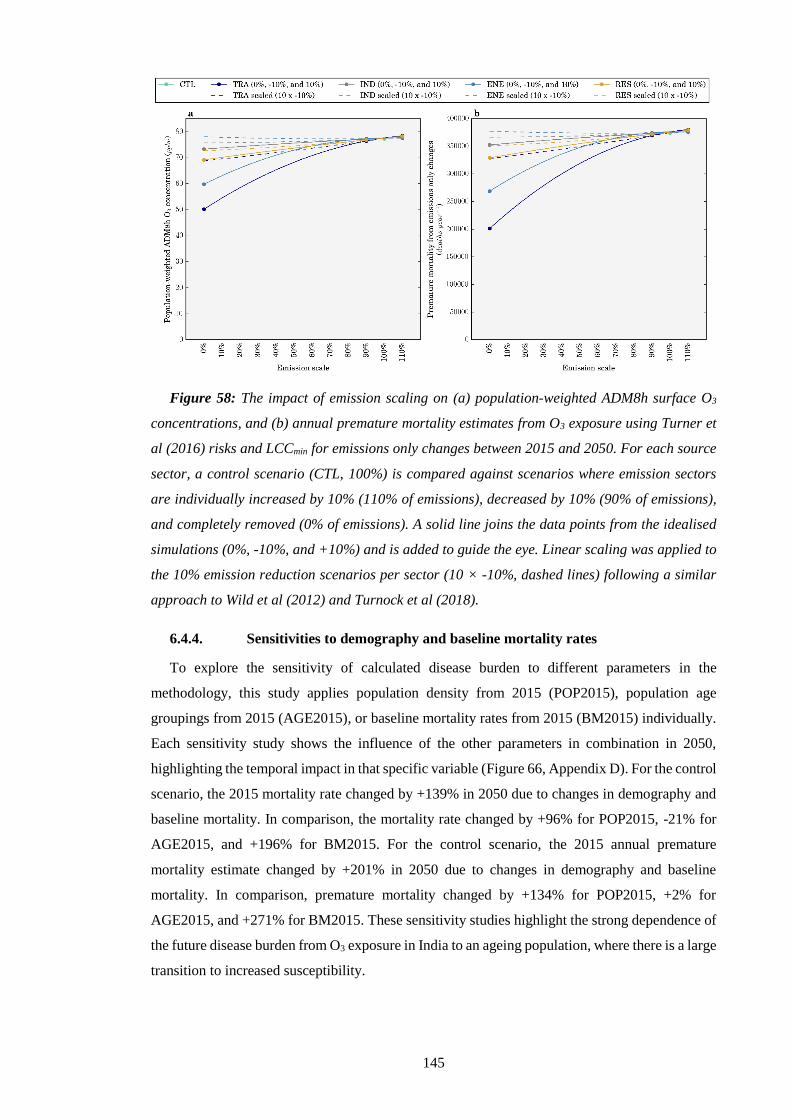
145

Figure 58: The impact of emission scaling on (a) population-weighted ADM8h surface O3

concentrations, and (b) annual premature mortality estimates from O3 exposure using Turner et

al (2016) risks and LCCmin for emissions only changes between 2015 and 2050. For each source

sector, a control scenario (CTL, 100%) is compared against scenarios where emission sectors

are individually increased by 10% (110% of emissions), decreased by 10% (90% of emissions),

and completely removed (0% of emissions). A solid line joins the data points from the idealised

simulations (0%, -10%, and +10%) and is added to guide the eye. Linear scaling was applied to

the 10% emission reduction scenarios per sector (10 × -10%, dashed lines) following a similar

approach to Wild et al (2012) and Turnock et al (2018).

6.4.4. Sensitivities to demography and baseline mortality rates

To explore the sensitivity of calculated disease burden to different parameters in the

methodology, this study applies population density from 2015 (POP2015), population age

groupings from 2015 (AGE2015), or baseline mortality rates from 2015 (BM2015) individually.

Each sensitivity study shows the influence of the other parameters in combination in 2050,

highlighting the temporal impact in that specific variable (Figure 66, Appendix D). For the control

scenario, the 2015 mortality rate changed by +139% in 2050 due to changes in demography and

baseline mortality. In comparison, the mortality rate changed by +96% for POP2015, -21% for

AGE2015, and +196% for BM2015. For the control scenario, the 2015 annual premature

mortality estimate changed by +201% in 2050 due to changes in demography and baseline

mortality. In comparison, premature mortality changed by +134% for POP2015, +2% for

AGE2015, and +271% for BM2015. These sensitivity studies highlight the strong dependence of

the future disease burden from O3 exposure in India to an ageing population, where there is a large

transition to increased susceptibility.

146

6.5. Discussion

Figure 59 compares this study’s total and source-specific premature mortality estimates for

India from O3 exposure with previous studies (GBD 2016 Risk Factors Collaborators 2017, Cohen

et al 2017, GBD 2010 Risk Factors Collaborators 2012, GBD 2013 Risk Factors Collaborators

2015, GBD 2015 Risk Factors Collaborators 2016a, Ghude et al 2016, Lelieveld et al 2015,

Malley et al 2017, Silva et al 2016b, 2013).

For calculations using Jerrett et al (2009) risks, estimates of the total annual premature

mortality from O3 exposure in India in the present day vary from 78,000 to 190,000 (GBD 2015

Risk Factors Collaborators 2016a, GBD 2016 Risk Factors Collaborators 2017, Silva et al 2013,

Lelieveld et al 2015, Silva et al 2016b, Malley et al 2017), between -36% smaller and +55%

larger than this study’s estimates. This study’s estimates of premature mortality are +15%

(LCCmin) and -1% (LCCfifth) of the estimate from GBD2015 (GBD 2015 Risk Factors

Collaborators 2016a) and +38% (LCCmin) and +19% (LCCfifth) of the estimate from GBD2016

(GBD 2016 Risk Factors Collaborators 2017). The slightly larger estimates in this study are

primarily due to higher estimates of O3 concentrations combined with higher (lower) COPD

baseline mortality rates from the IFs model relative to GBD2016 (GBD2015). For calculations

using Turner et al (2016) risks, this study estimates annual premature mortality to be 12% higher

than Malley et al (2017), the only other study that has applied these risks, due to higher O3

concentrations across India in this study. Turner et al (2016) found significant positive

associations between O3 and all-cause, circulatory, and respiratory mortality, suggesting that our

estimates from COPD only may be conservative. Overall, this study’s estimates of annual

premature mortality in India for the present day from O3 exposure are in general agreement with

previous key studies.

In terms of source contributions, Silva et al (2016a) calculated the disease burden from O3

exposure in India for 2005 using Jerrett et al (2009) risks and the subtraction method. For seasonal

O3 concentrations, they found approximately equal leading contributions from energy (9%), land

transport (9%), and residential (9%) emissions. They found premature mortality fractional

contributions were approximately double the fractional contributions to O3 concentrations, with

17% from energy, 16% from land transport, and 16% from residential emissions. In contrast, this

study finds land transport to dominate the fractional source contributions to seasonal O3

concentrations (28%) over energy (14%) and residential (9%) emissions (Table 7, 3mDMA1

metric). Our larger contribution from land transport may be due to the growth in land transport

emissions between 2005 and 2010, where Indian passenger and freight kilometres increased by

6.54% and 3.61% per year, respectively (Venkataraman et al 2018). In agreement with Silva et

al (2016a), this study finds the fractional source contributions to premature mortality were

approximately double the fractional contributions to O3 concentrations due to the low

concentration cutoffs, with land transport again dominating (46%) over energy (28%) and

residential (12%) emissions (Table 8, subtraction method).

147

Another study estimated the source contributions to present day annual-mean surface O3

concentrations and found land transport emissions to dominate (8%, 3.3 ppb) above those from

industry (5%, 2.1 ppb), energy (4%, 1.9 ppb), and residential (3%, 1.4 ppb) sources (Sharma et al

2016). The main difference in corresponding source contributions to annual-mean O3

concentrations here are that this study estimates larger contributions from land transport (30%,

13.6 ppb) and energy (24%, 11.0 ppb) emissions (Figure 63, Appendix D). This is likely due to

lower emissions of O3 precursors from land transport and energy in the emission inventory used

in Sharma et al (2016), relative to that used in our study (EDGAR-HTAP version 2.2).

Overall, this study agrees with these previous studies that a number of emission sectors are

important, though this study finds larger contributions from land transport and energy emissions.

Future work needs to better constrain the sensitivity of O3 concentrations to different emission

sectors.

This study’s results show that decreasing land transport emissions reduces O3 concentrations

across India. Though in the future with decreasing VOC emissions from the residential sector and

increasing the number of vehicles, this trend could change the future sensitivity of O3 production

to precursor emission changes, which was also found in previous studies (Sharma et al 2016,

Chatani et al 2014).

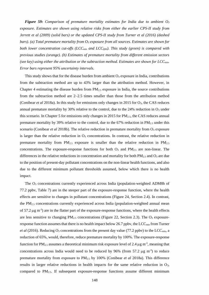
148

Figure 59: Comparison of premature mortality estimates for India due to ambient O3

exposure. Estimates are shown using relative risks from either the earlier CPS-II study from

Jerrett et al (2009) (solid bars) or the updated CPS-II study from Turner et al (2016) (dashed

bars). (a) Total premature mortality from O3 exposure from all sources. Estimates are shown for

both lower concentration cut-offs (LCCmin and LCCfifth). This study (green) is compared with

previous studies (orange). (b) Estimates of premature mortality from different emission sectors

(see key) using either the attribution or the subtraction method. Estimates are shown for LCCmin.

Error bars represent 95% uncertainty intervals.

This study shows that for the disease burden from ambient O3 exposure in India, contributions

from the subtraction method are up to 43% larger than the attribution method. However, in

Chapter 4 estimating the disease burden from PM2.5 exposure in India, the source contributions

from the subtraction method are 2–2.5 times smaller than those from the attribution method

(Conibear et al 2018a). In this study for emissions only changes in 2015 for O3, the CAS reduces

annual premature mortality by 30% relative to the control, due to the 24% reduction in O3 under

this scenario. In Chapter 5 for emissions only changes in 2015 for PM2.5, the CAS reduces annual

premature mortality by 39% relative to the control, due to the 67% reduction in PM2.5 under this

scenario (Conibear et al 2018b). The relative reduction in premature mortality from O3 exposure

is larger than the relative reduction in O3 concentrations. In contrast, the relative reduction in

premature mortality from PM2.5 exposure is smaller than the relative reduction in PM2.5

concentrations. The exposure-response functions for both O3 and PM2.5 are non-linear. The

differences in the relative reductions in concentration and mortality for both PM2.5 and O3 are due

to the position of present-day pollutant concentrations on the non-linear health functions, and also

due to the different minimum pollutant thresholds assumed, below which there is no health

impact.

The O3 concentrations currently experienced across India (population-weighted ADM8h of

77.2 ppbv, Table 7) are in the steeper part of the exposure-response function, where the health

effects are sensitive to changes in pollutant concentrations (Figure 24, Section 2.4). In contrast,

the PM2.5 concentrations currently experienced across India (population-weighted annual mean

of 57.2 g m-3) are in the flatter part of the exposure-response functions, where the health effects

are less sensitive to changing PM2.5 concentrations (Figure 22, Section 2.3). The O3 exposure-

response function assumes that there is no health impact below 26.7 ppbv, the LCCmin from Turner

et al (2016). Reducing O3 concentrations from the present day value (77.2 ppbv) to the LCCmin, a

reduction of 65%, would, therefore, reduce premature mortality by 100%. The exposure-response

function for PM2.5 assumes a theoretical minimum risk exposure level of 2.4 g m-3, meaning that

concentrations across India would need to be reduced by 96% (from 57.2 g m-3) to reduce

premature mortality from exposure to PM2.5 by 100% (Conibear et al 2018a). This difference

results in larger relative reductions in health impacts for the same relative reduction in O3,

compared to PM2.5. If subsequent exposure-response functions assume different minimum

149

pollutant thresholds (or lower concentration cut-offs, LCC), the calculated sensitivity of health

impacts to changes in O3 concentrations will also change.

This study finds that with no emissions change to 2050, the demographic and epidemiological

transitions increase the annual premature mortality due to O3 exposure by 200% and the mortality

rate per 100,000 population by 139%, while the corresponding impacts of PM2.5 exposure in India

are 75% and 39%, respectively (Conibear et al 2018b). The larger increase for the O3 burden

under constant emissions is due to the limited improvement in baseline mortality rate for COPD,

while for the PM2.5 exposure burden there are substantial reductions in baseline mortality rates

for LRI, IHD, and CEV.

Figure 60 compares the disease burden from PM2.5 and O3 exposure in India in 2015 and 2050

due to changes in emissions, demography, and baseline mortality. Chapter 5 estimated the present

day disease burden from ambient PM2.5 exposure in India to be 900,000 (95UI: 683,000–

1,252,000) premature mortalities per year, increasing to 967,000 (95UI: 820,000–1,194,000)

under the CAS in 2050, for a 67% reduction in population-weighted annual mean PM2.5

concentrations (Conibear et al 2018b). This study estimates the present day disease burden from

ambient O3 exposure in India to be 374,000 (95UI: 140,000–554,000) premature mortalities per

year, increasing to 791,000 (95UI: 202,000–1,336,000) under the CAS in 2050, for a 24%

reduction in population-weighted annual mean O3 concentrations. This suggests that the future

disease burden from PM2.5 and O3 exposures in India may be similar in magnitude, in contrast to

the present day where the disease burden from PM2.5 dominates that from O3 exposure. This is

due to the combination of the smaller reduction in O3 (24%) compared to PM2.5 (67%) under the

CAS and because the COPD baseline mortality rates are predicted to remain high through to 2050,

whereas there are substantial reductions in the baseline mortality rates for other diseases that are

related to PM2.5 exposure (LRI, IHD, and CEV). The predicted increase in health affects both

from PM2.5 and O3 exposure due to the demographic and epidemiologic changes highlight the

challenge facing Indian efforts to reduce the public health risks from exposure to poor air quality

in India.

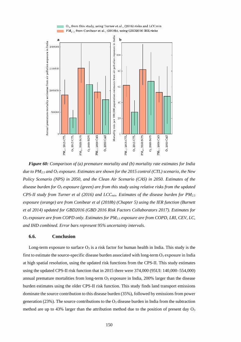
150

Figure 60: Comparison of (a) premature mortality and (b) mortality rate estimates for India

due to PM2.5 and O3 exposure. Estimates are shown for the 2015 control (CTL) scenario, the New

Policy Scenario (NPS) in 2050, and the Clean Air Scenario (CAS) in 2050. Estimates of the

disease burden for O3 exposure (green) are from this study using relative risks from the updated

CPS-II study from Turner et al (2016) and LCCmin. Estimates of the disease burden for PM2.5

exposure (orange) are from Conibear et al (2018b) (Chapter 5) using the IER function (Burnett

et al 2014) updated for GBD2016 (GBD 2016 Risk Factors Collaborators 2017). Estimates for

O3 exposure are from COPD only. Estimates for PM2.5 exposure are from COPD, LRI, CEV, LC,

and IHD combined. Error bars represent 95% uncertainty intervals.

6.6. Conclusion

Long-term exposure to surface O3 is a risk factor for human health in India. This study is the

first to estimate the source-specific disease burden associated with long-term O3 exposure in India

at high spatial resolution, using the updated risk functions from the CPS-II. This study estimates

using the updated CPS-II risk function that in 2015 there were 374,000 (95UI: 140,000–554,000)

annual premature mortalities from long-term O3 exposure in India, 200% larger than the disease

burden estimates using the older CPS-II risk function. This study finds land transport emissions

dominate the source contribution to this disease burden (35%), followed by emissions from power

generation (23%). The source contributions to the O3 disease burden in India from the subtraction

method are up to 43% larger than the attribution method due to the position of present day O3

151

concentrations on the steeper part of the non-linear health function and the relatively high

minimum pollutant threshold. This is in contrast to the PM2.5 disease burden in India where the

source contributions from the subtraction method are 2–2.5 times smaller than those from the

attribution method due to the position of present day PM2.5 concentrations on the flatter part of

the non-linear health function and the relatively low minimum pollutant threshold.

With no change in emissions by 2050, this study estimates 1,126,000 (95UI: 421,000–

1,667,000) annual premature mortalities, an increase of 200% relative to the control in 2015 due

to population ageing and growth increasing the number of people susceptible to air pollution. This

study finds the IEA New Policy Scenario provides small changes (+1%) to this increasing disease

burden from the demographic transition. Under a stringent air pollution control pathway, the IEA

Clean Air Scenario, this study estimates 791,000 (95UI: 202,000–1,336,000) annual premature

mortalities in 2050. This represents an avoidance of 335,000 premature mortalities a year

compared to the scenario of no emission change, offsetting 45% of the increase in premature

mortalities due to the demographic transition. However, this shows that even under a scenario of

strong emission reductions leading to a 24% reduction in O3 concentrations across India,

population growth and ageing are likely to lead to increasing premature mortality from O3

exposure. This study does not include impacts of climate change or the impacts of changing

emissions from outside India on O3 concentrations or the disease burden. This study finds that the

future disease burden from PM2.5 and O3 exposures in India may be similar in magnitude, in

contrast to the present day where the disease burden from PM2.5 dominates that from O3 exposure.

This study highlights the challenge facing efforts to improve air quality related public health in

India, but that critical public health benefits are possible with stringent emission reductions.

152

7. Discussion and Conclusion

7.1. Summary of work

700 million Indians have used solid fuels in their homes for the last 30 years, contributing

substantially to air pollutant emissions (Smith and Sagar 2014). India experienced large growth

in its economy, industry, power generation, and transport sectors over the last decade leading to

a large growth in emissions of air pollutants. Emissions of air pollutants are predicted to grow

substantially over the coming years in India. These air pollutant emissions have caused present-

day concentrations of ambient PM2.5 and O3 in India to be amongst the highest in the world (World

Health Organization 2018a). Exposure to this air pollution is the second leading risk factor in

India, contributing one-quarter of the global disease burden attributable to air pollution exposure

(GBD 2016 Risk Factors Collaborators 2017, India State-Level Disease Burden Initiative

Collaborators 2017).




to reduce this substantial disease burden. This thesis aimed to understand the present day

contribution of different pollution sources to the ambient air pollution associated disease burden

in India and the effects of future air pollution control pathways.

The thesis had three main objectives. The first objective was to quantify the contribution of

different emission sources to ambient PM2.5 concentrations and the related disease burden across

India in the present day. This study combined high-resolution computer simulations with new

observations, as previous studies used coarse model resolution with limited observations. The

second objective studied different future air pollution control pathways in India, estimating the

impacts on ambient PM2.5 concentrations and human health. Poor air quality in India is predicted

to worsen in the future, and limited air pollution control pathways have been studied at high

resolution. Thirdly, the current and future disease burden from ambient O3 exposure in India was

studied, identifying critical contributing emission sources and the impacts of future policy

scenarios. This study combined high-resolution computer simulations with the latest exposure-

response relationships.

This thesis found ambient PM2.5 and O3 concentrations were high across India, especially in

the IGP. Almost everyone in India is exposed to ambient PM2.5 and O3 concentrations above the

WHO recommended guidelines. This thesis estimated that present-day exposure to ambient PM2.5

in India caused 990,000 (95UI: 660,000–1,350,000) premature mortalities per year. Present day

exposure to ambient O3 in India caused 124,000 (95UI: 57,000–203,000) premature mortalities

per year using old risk functions, increasing by 200% to 374,000 (95UI: 140,000–554,000)

premature mortalities per year using updated risk functions. This suggests that the present-day

153

attributable disease burden from ambient PM2.5 exposure dominates that from ambient O3

exposure in India.

Emissions from residential energy use contributed 52% of the population-weighted annual-

mean PM2.5 concentrations, attributed to 511,000 (95UI: 340,000–697,000) premature mortalities

each year. Removing residential energy use emissions would avert only 256,000 (95UI: 162,000–

340,000) premature mortalities annually, due to the non-linear exposure-response relationship

causing health effects to saturate at high PM2.5 concentrations. For ambient O3 exposure, land

transport emissions dominated the source contribution to the disease burden (35% attribution and

46% subtraction), followed by emissions from power generation (23% attribution and 28%

subtraction). For ambient PM2.5 exposure, the summation of source contributions from the

attribution method was 1,012,000 (95UI: 675,000–1,381,000) premature mortalities per year

(102% of control), which is substantially higher than the sector summation from the subtraction

method of 469,000 (95UI: 304,000–626,000) premature mortalities per year (47% of control). For

ambient O3 exposure, the summation of source contributions from the attribution method was

284,000 (95UI: 106,000–421,000) annual premature mortalities (76% of control), while for the

subtraction method was 355,000 (95UI: 133,000–526,000) annual premature mortalities (95% of

control). This difference of the attribution method estimates being larger than those from the

subtraction method for PM2.5, and smaller for O3, is due to the shape of the exposure-response

functions and the present day concentrations experienced. The exposure-response functions for

both O3 and PM2.5 are non-linear. However, the present day O3 concentrations experienced in

India are in the linear section (steeper) of the exposure-response function and the minimum

pollutant threshold is relatively high (below which there is no health impact). The present-day

PM2.5 concentrations experienced in India are in the non-linear section (flatter) of the exposure-

response function and the minimum pollutant threshold is relatively low. This difference suggests

that there are larger relative reductions in health impacts for the same relative reduction in O3

compared to PM2.5. This implication is dependent on the shape of the exposure-response function

and the assumed minimum pollutant threshold.

This study avoided summing the disease burden from ambient O3 and PM2.5 exposure in the

main results as similar diseases (e.g. COPD) cause them both, although the risk estimates account

for confounding. However, for illustrative purposes, the combined annual disease burden

contributions from ambient PM2.5 and O3 exposure for the subtraction method suggest that

residential emissions dominate with 301,000 (95UI: 179,000–407,000) premature mortalities,

followed by land transport emissions with 216,000 (95UI: 94,000–314,000) premature

mortalities, then energy emissions with 195,000 (95UI: 99,000–278,000) premature mortalities.

Overall, this highlights the need to control emissions from the residential sector.

With emissions remaining at 2015 levels, premature mortality from exposure to ambient PM2.5

in 2050 will increase by 75% relative to 2015, and the mortality rate will increase by 39%. For

154

ambient O3 exposure under constant emissions from 2015, the number of premature mortalities

in 2050 will increase by 201% relative to 2015, and the mortality rate will increase by 140%. The

increase in disease burden from exposure to ambient PM2.5 and O3 in 2050 relative to 2015 under

constant emissions is due to population ageing and growth increasing the number of people

susceptible to air pollution. The larger increase for the O3 burden under constant emissions is due

to the limited improvement in baseline mortality rate for COPD, while for the PM2.5 exposure

burden there are substantial reductions in baseline mortality rates for LRI, IHD, and CEV.

This thesis also explored the impact of different future emission scenarios. In particular, two

scenarios were compared, the NPS considering all relevant existing and planned policies as of

2016, and the CAS representing aggressive policy action using proven energy policies and

technologies tailored to national circumstances. The IEA NPS in 2050 reduces population-

weighted annual-mean ambient PM2.5 concentrations below 2015 levels by 9%, while population-

weighted ADM8h O3 concentrations increase by 1%. The IEA CAS in 2050 reduces population-

weighted annual-mean ambient PM2.5 concentrations below 2015 levels by 68% and reduces

population-weighted ADM8h O3 concentrations by 24%. Under both the NPS and the CAS, the

total number of premature mortalities in 2050 still increases relative to 2015 due to the strong

drivers from population ageing and growth. The NPS offsets the rising number of premature

mortalities from population ageing and growth by 9% (61,000 deaths) for PM2.5 exposure, while

increasing the number of premature mortalities by 1% (13,000 deaths) for O3 exposure. The CAS

offsets the rising number of premature mortalities from population ageing and growth by 91%

(610,000 deaths) for PM2.5 and 45% (335,000 deaths) for O3. The CAS can reduce the mortality

rate by 15% for PM2.5 in 2050 relative to 2015, while for O3 the CAS in 2050 can offset 28% of

the increase from population ageing and growth.

In the present day, the annual disease burden in India from ambient PM2.5 exposure (900,000

premature mortalities and mortality rate of 62 per 100,000) dominates that from O3 exposure

(374,000 premature mortalities and mortality rate of 28 per 100,000). In contrast, the future

disease burden from ambient exposure to PM2.5 (under the CAS, 967,000 premature mortalities

and mortality rate of 53 per 100,000) and O3 (under the CAS, 791,000 premature mortalities and

mortality rate of 48 per 100,000) may be similar in magnitude.

In summary, this thesis aimed to understand the source contributions to the ambient air

pollution associated disease burden in India and the effects of future air pollution control

pathways. The attributable disease burden from ambient PM2.5 exposure in India is substantial,

where large reductions in emissions will be required to reduce the health burden due to the non-

linear exposure-response relationship. The attributable disease burden from ambient O3 exposure

is larger than previously thought. Key sources contributing to the present day disease burden from

ambient PM2.5 and O3 exposure are the emissions from the residential combustion of solid fuels,

land transport, and coal combustion in power plants. The attributable disease burden is estimated

155

to increase in the future due to population ageing and growth. Stringent air pollution control

pathways are required to provide critical public health benefits in India. A key focus should be to

reduce the burning of solid fuels. The attributable disease burden to ambient PM2.5 exposure

dominates ambient O3 exposure in the present day, while in the future they are of similar

magnitudes. This thesis highlights the challenge facing efforts to improve air quality related

public health in India.

7.2. Critical discussion of work

All health effects in this thesis were estimated as attributable burdens from associational

epidemiology, rather than causations from mechanistic toxicology. A key criticism here is that

the exposure-response functions used to estimate the attributable burdens are causal and reversible

based on the classic approach to causal inference, using historical exposure-response functions

to predict future changes in pollution and health (Dominici and Zigler 2017). The potential

outcomes approach addresses this critique, where causal effects are explicitly defined as

consequences of specific actions, as oppose to inferring causality (Zigler and Dominici 2014).

However, the potential outcomes causal effect can be complicated by interference, for example

from the regional transport of pollution, other policies, air quality trends, and meteorology

(Tchetgen and Vanderweele 2012). Potential outcomes studies require prospective planning

regarding what to measure, what control to use, and how to consider intended effects versus actual

effects, so maybe more suitable for specific policy changes rather than source contributions

(Hubbell and Greenbaum 2014).

The current standard in the literature is to use concentrations as surrogates for exposures.

Recent advances in exposure assessment include the estimation of individual exposures based on

household addresses (Beckerman et al 2013), the integration of personal exposure assessments

between models and measurements (Shaddick et al 2018a), including household air pollution and

second hand smoking (Kodros et al 2018, Hill et al 2017), and including time-activity data

between household and ambient pollution (Hill et al 2017). This additional complexity in future

work will improve the accuracy of health impact estimates.

The horizontal spatial resolution (30 km) used in this thesis was unable to resolve the very fine

concentration gradients in different microenvironments (Beelen et al 2008). Risk assessments

resolving microenvironments may capture the collocation of emissions and exposures, e.g.

populations are nearer emissions from residential solid fuel use, land transport, and diesel

generators, as opposed to larger stationary sources (GBD MAPS Working Group 2018).

The work in Chapter 4 found that ambient PM2.5 concentrations (influenced by model spatial

resolution) and the exposure-response function were both strong drivers of the differences

between disease burden estimates attributable to air pollution in India. Similar, recent work by

Kushta et al (2018) over Europe found that in this domain, the exposure-response function is the

156

main source of uncertainty in the health impact assessments. This difference may be due to the

use of the 95% uncertainty levels within a specific exposure-response function for the sensitivity

estimates, rather than between different realisations of the exposure-response functions, and to

the lower PM2.5 concentrations found over Europe (maximum of 40 g m-3, compared to 120 g

m-3 over India). This difference for Europe suggests that uncertainty is driven by different causes

in different countries, as found by Kodros et al (2018).

The source contribution estimates were for one model setup, not accounting for interannual

variations in emissions and meteorology or sensitivity to model choices. There were additional

emission sources not included, such as emissions from waste burning (Kodros et al 2016), bagasse

combustion (Sahu et al 2015), and anthropogenic dust (GBD MAPS Working Group 2018).

Different emission inventories would produce different results, for example, the Regional

Emission inventory in Asia (REAS) more closely matched South Asian AOD from satellite

relative to EDGAR, likely due to EDGAR underestimating SO2, NOx, and NH3 emissions and

hence producing less secondary aerosol (Saikawa et al 2017). Previous studies have highlighted

the importance of using an ensemble of estimates (Post et al 2012, Silva et al 2016c), as variability

among models is large for O3 (Silva et al 2013, Post et al 2012). To account for these variabilities

and limitations, an ensemble of model simulations would be suitable, changing emission

inventories, year of simulation, and model parameterisations. However, this was beyond the time

and computational constraints of this work.

The urban and rural splits were based on population density (400 persons’ km-2), which did

not capture the type of work undertaken. A recent study included the type of work (e.g.

agricultural) undertaken and estimated larger rural contributions to the disease burden in India,

relative to Chapter 4 (Karambelas et al 2018b).

The response of O3 concentrations to changes in emissions is non-linear, meaning an emission

removal approach to quantify attributions can differ from a source tracking approach (Silva et al

2016b, Grewe et al 2010, 2012, Mertens et al 2018, Koo et al 2009, Clappier et al 2017). The

response of PM2.5 concentrations to changes in emissions is largely linear, which was also found

in previous work (Dedoussi and Barrett 2014). Source tracking within chemical transport models

also find residential emissions to dominate PM2.5 concentrations in North India, followed by

industrial emissions (Guo et al 2017). The source tracking approach had not yet been used for

health impact assessments at the time of these studies. Since the publication of this work, Guo et

al (2018) used the source tracking approach to estimate the source-specific disease burden from

ambient PM2.5 exposure in India and found similar results to this work where residential emissions

contributed 56% to the 1 million premature mortalities per year. Source apportionment analyses

of PM into source categories based on chemical composition are mixed in India, with widely

varying results even for the same city (Pant and Harrison 2012). Source apportionment analyses

157

are limited by the availability of locally derived emissions source profiles (Pant and Harrison

2012).

Dust emissions were found to be low in Chapter 4 using the GOCART dust scheme with

AFWA modifications. Previous studies have also found WRF-Chem to underestimate dust

emissions in India (Dipu et al 2013, Kumar et al 2014b). This finding has led WRF-Chem studies

over India to increase the dimensional proportionality constant within the GOCART AFWA dust

emission online flux calculation. The dimensional proportionality constant was initially 1 × 10-9

kg m-5 s2 (Legrand et al 2018). Previous studies increased this constant by a factor of 22 to 2.2 ×

10-8 kg m-5 s2 when using FDDA and by a factor of 9 to 9 × 10-9 kg m-5 s2 when not using FDDA,

based on most closely matching observed and simulated AOD and Angström exponent (Kumar

et al 2014b). After correcting the underestimation of dust emissions in WRF-Chem, Kumar et al

(2014a) added heterogeneous chemical reactions between dust and O3 photochemistry and found

these heterogeneous reactions reduced the difference between observed and simulated O3

concentrations in India from 16 ppbv to 2 ppbv.

The simulation of meteorology could be improved, especially the summer monsoon

precipitation dry bias and the winter boundary layer height overestimation. The Indian monsoon

is better simulated at resolutions that explicitly resolve convection (Chen et al 2018, Chang et al

2009, Srinivas et al 2018), however, this requires substantial computational resources. Recent air

quality studies over India using WRF found improved meteorological simulation of precipitation

and relative humidity using ECMWF, rather than NCEP, initial and boundary conditions (Kumar

et al 2017, Chatani and Sharma 2018). There are mixed results for different convection

parameterisation schemes over India using WRF (Mukhopadhyay et al 2010, Srinivas et al 2013,

Rotach and Zardi 2007, Chang et al 2009). Mukhopadhyay et al (2010) and Srinivas et al (2013)

both found the Betts-Miller-Janjic convection parameterisation scheme simulated Indian

monsoon precipitation with the lowest bias, while Rotach and Zardi (2007) and Chang et al (2009)

found the best performance for the Grell-Devenyi scheme. Previous studies evaluating different

boundary layer schemes (with tied land surface schemes) using WRF over India have found

performance varies widely where the best choices may be application specific (Mohan and Gupta

2018, Gunwani and Mohan 2017, Hari Prasad et al 2016, Sonia et al 2014, Mohan and Bhati

2011, Panda and Sharan 2012, Madala et al 2014, Hariprasad et al 2014). Srinivas et al (2018)

recently found the Mellor-Yamada Nakanishi and Niino 2.5 boundary layer scheme performed

better than alternative schemes, while still underestimating heavy rainfall. The meteorological

evaluation could have used data from the India Meteorological Department, as opposed to

ECMWF reanalysis products.

The part of the IER functions with the largest uncertainty (30–100 µg m-3) coincides with

PM2.5 concentrations often found in India and China. Despite this, a recent study of long-term

PM2.5 exposures in China found the health response to be similar to the IER functions (Zheng et

158

al 2017). The exposure-response functions did not include epidemiological studies from long-

term ambient air pollution studies in India, as they do not exist. The exposure estimates focused

on single pollutants individually, rather than multipollutant approaches combining effects from

PM2.5 and O3 (Greenbaum and Shaikh 2010).

Future air pollution control pathways were applied through scaling factors to the

anthropogenic emission inventory, which assumes changes are homogeneous across the model

domain and do not consider changes in other countries over the same timeframe. The future

scenarios did not include changes in land use or land cover. The future scenarios had a timing

mismatch between emissions (2040) and demographic and epidemiological changes (2050).

These studies did not estimate DALYs (which account for YLD), economic costs, the impacts

of Indian emissions on the disease burden in other countries (Zhang et al 2017), population effect

modifiers (e.g. gender, socioeconomics, genes), crop impacts of O3 (Ghude et al 2014, 2016,

Sinha et al 2015), or the climate impacts (Shindell et al 2012).

7.3. Future work

Future estimates of the disease burden from ambient air pollution exposure can be more

accurately estimated when epidemiological evidence resolves the specific characteristics,

components, and sources of air pollution that cause the specific health effects (West et al 2016).

The IERs are based on assumptions of equal toxicity and include data from household air

pollution, second hand smoking, and active smoking. Recent work by Burnett et al (2018) relaxed

these assumptions to develop the Global Exposure Mortality Model (GEMM), covering almost

all of the global PM2.5 concentration range (2.5–84 gm-3) from cohort studies of ambient air

pollution only. GEMM hazard ratios are larger than those from the GBD2015 IER and are closer

to linear, especially for high PM2.5 concentrations (Burnett et al 2018). The attributable disease

burden from ambient PM2.5 exposure in India using the GEMM for the five causes of deaths used

in this study (COPD, IHD, CEV, LC, and LRI) is 1,867,342 (95UI: 1,355,715–2,240,783)

premature mortalities per year, approximately 70% larger than the GBD2015 estimates using the

IER functions of 1,090,391 (95UI: 936,588–1,254,784) premature mortalities per year (Burnett

et al 2018). Burnett et al (2018) also found that the disease burden from all NCD and LRI were

20% larger than those based on the five causes of death (COPD, IHD, CEV, LC, and LRI),

suggesting that other diseases also contribute beyond the five causes studied here and in the GBD

(Grandjean and Landrigan 2006, Landrigan et al 2017). These findings suggests the health impact

from ambient PM2.5 exposure could be substantially larger than previously thought, the non-linear

implications of emission changes would alter, and the future balance of disease burdens from

PM2.5 and O3 would change. The GEMM exposure-response function would be further suitable

for India when it includes cohort studies of ambient air pollution from India, as only one study is

available from a country with similar air pollution concentrations (China). The simulated

159

components of PM2.5 concentrations in India can be evaluated against measurements when they

become publically available.

The total exposure to air pollution from ambient, household, and smoking sources could be

investigated, as performed by Hill et al (2017) for Mongolia. This could include multiple air

pollutants together, rather than the single pollutant approach, although the implementation

challenge is vast (Dominici et al 2010). Risk assessments could also include DALYs and the

economic costs from the health impacts attributable to air pollution.

Short-term drivers to pollution episodes could be explored in terms of the impact on human

health. For example, in November 2016, daily-mean PM2.5 concentrations in Delhi were over 900

g m-3, many times higher than the WHO AQG of 25 g m-3. This pollution episode coincided

with large agricultural burning of rice residues across northwest India, though the impact on PM2.5

concentrations and human health has not been quantified. Another study could analyse the

impacts of the Indian solid fuel intervention to promote LPG to over 90% of households by early

2020’s (Section 1.1.3.2) on air quality and human health, considering stove stacking and stove

usage patterns.

The emission inventories used in this thesis could be improved by including additional

emission sources, such as anthropogenic dust (Venkataraman et al 2018, GBD MAPS Working

Group 2018), waste burning (Kodros et al 2016), and bagasse combustion (Sahu et al 2015). The

emissions inventories from Venkataraman et al (2018) for 2015, 2030, and 2050 are now available

upon request and would improve future scenario estimates of air pollution relative to using scaling

factors (Chapters 5 and 6). Upcoming emission inventories plan to split residential emissions into

cooking, heating, and lighting and by fuel, which will provide insights into the drivers behind this

sectors large contributing disease burden. Sensitivity simulations could be conducted by applying

an Indian-specific diurnal cycle to the anthropogenic emissions when data becomes available. The

air pollution estimates could be improved by changing the dimensional proportionality constant

for dust emissions and adding the heterogeneous chemical reactions between dust and O3

photochemistry (Section 7.2). These changes were implemented into WRF-Chem for the

GOCART bulk aerosol scheme and work is currently being undertaken to accommodate for these

changes within the MOSAIC sectional scheme.

Simulations could be performed using WRF-Chem with chemical data assimilation, especially

for AOD and PM2.5, to improve the accuracy of simulated particulate air quality. Previous studies

have developed and explored the use of chemical data assimilation in WRF-Chem (Li et al 2013,

Peng et al 2017, Liu et al 2011, Saide et al 2013, Pagowski and Grell 2012, Bocquet et al 2015,

Liu et al 2017, Mizzi et al 2016).

160

7.4. Conclusion

Since 1980, 700 million Indians have used solid fuels in their homes in poor quality stoves

that produce substantial emissions of air pollutants (Smith and Sagar 2014). The Indian economy

and industrial, power generation, and transport sectors have grown considerably over the last

decade. These increasing emissions of air pollutants have caused present-day concentrations of

ambient PM2.5 and O3 in India to be amongst the highest in the world (World Health Organization

2018a). Exposure to this air pollution is the second leading risk factor in India, contributing one-

quarter of the global disease burden attributable to air pollution exposure (GBD 2016 Risk Factors

Collaborators 2017, India State-Level Disease Burden Initiative Collaborators 2017). Air

pollutant emissions are predicted to grow extensively over the coming years in India.




to reduce this substantial disease burden. This thesis aimed to understand the contribution of

different pollution sources to the ambient air pollution associated disease burden in India and the

effects of future air pollution control pathways.

The thesis had three main objectives. Firstly, the contribution of different emission sources to

ambient PM2.5 concentrations and the related disease burden across India in the present day was

studied. Secondly, different future air pollution control pathways in India were analysed,

estimating the impacts on ambient PM2.5 concentrations and human health. Thirdly, the current

and future disease burden from ambient O3 exposure in India was studied, identifying critical

contributing emission sources and the impacts of future policy scenarios. This thesis combined

high-resolution computer simulations with new observations and the latest exposure-response

relationships.

The attributable disease burden from ambient PM2.5 exposure in India is substantial, where

large reductions in emissions will be required to reduce the health burden due to the non-linear

exposure-response relationship. The attributable disease burden from ambient O3 exposure is

larger than previously thought. Key sources contributing to the present day disease burden from

ambient PM2.5 and O3 exposure are the emissions from the residential combustion of solid fuels,

land transport, and coal combustion in power plants. The attributable disease burden is estimated

to increase in the future due to population ageing and growth. Stringent air pollution control

pathways are required to provide critical public health benefits in India in a challenging

environment. A key focus should be to reduce the burning of solid fuels. The attributable disease

burden to ambient PM2.5 exposure dominates ambient O3 exposure in the present day, while in the

future they are of similar magnitudes. This thesis highlights the challenge facing efforts to

improve air quality related public health in India.

161

References

Achilleos S, Kioumourtzoglou M A, Wu C Da, Schwartz J D, Koutrakis P and Papatheodorou S

I 2017 Acute effects of fine particulate matter constituents on mortality: A systematic review

and meta-regression analysis Environ. Int. 109 89–100

Ackermann I J, Hass H, Memmesheimer M, Ebel A, Binkowski F S and Shankar U 1998 Modal

Aerosol Dynamics model for Europe: Development and first applications Atmos. Environ.

32 2981–99

Adhikary B, Carmichael G R, Tang Y, Leung L R, Qian Y, Schauer J J, Stone E A, Ramanathan

V and Ramana M V. 2007 Characterization of the seasonal cycle of south Asian aerosols:

A regional-scale modeling analysis J. Geophys. Res. Atmos. 112 1–22

Akagi S K, Yokelson R J, Wiedinmyer C, Alvarado M J, Reid J S, Karl T, Crounse J D and

Wennberg P O 2011 Emission factors for open and domestic biomass burning for use in

atmospheric models Atmos. Chem. Phys. 11 4039–72

Alexander D, Northcross A, Wilson N, Dutta A, Pandya R, Ibigbami T, Adu D, Olamijulo J,

Morhason-Bello O, Karrison T, Ojengbede O and Olopade C O 2017 Randomized

controlled ethanol cookstove intervention and blood pressure in pregnant nigerian women

Am. J. Respir. Crit. Care Med. 195 1629–39

Amann M, Bertok I, Borken-Kleefeld J, Cofala J, Heyes C, Höglund-Isaksson L, Klimont Z,

Nguyen B, Posch M, Rafaj P, Sandler R, Schöpp W, Wagner F and Winiwarter W 2011

Cost-effective control of air quality and greenhouse gases in Europe: Modeling and policy

applications Environ. Model. Softw. 26 1489–501

Anderson G B, Krall J R, Peng R D and Bell M L 2012 Is the relation between ozone and mortality

confounded by chemical components of particulate matter? Analysis of 7 components in 57

US communities Am. J. Epidemiol. 176 726–32

Anenberg S C, Horowitz L W, Tong D Q and West J J 2010 An estimate of the global burden of

anthropogenic ozone and fine particulate matter on premature human mortality using

atmospheric modeling Environ. Health Perspect. 118 1189–95

Anenberg S C, Schwartz J, Shindell D, Amann M, Faluvegi G, Klimont Z, Janssens-maenhout G,

Pozzoli L, Dingenen R Van, Vignati E, Emberson L, Muller N Z, West J J, Williams M,

Demkine V, Hicks W K, Kuylenstierna J, Raes F and Ramanathan V 2012 Global Air

Quality and Health Co-benefits of Mitigation Near-Term Climate Change through Methane

and Black Carbon Emissions Controls Environ. Heal. Perspect. 120 831–9

Anenberg S C, Talgo K, Arunachalam S, Dolwick P, Jang C and West J J 2011 Impacts of global,

regional, and sectoral black carbon emission reductions on surface air quality and human

mortality Atmos. Chem. Phys. 11 7253–67

Anenberg S C, West J J, Fiore A M, Jaffe D A, Prather M J, Bergmann D, Cuvelier K, Dentener

F J, Duncan B N, Gauss M, Hess P, Jonson J E, Lupu A, MacKenzie I A, Marmer E, Park

R J, Sanderson M G, Schultz M, Shindell D T, Szopa S, Vivanco M G, Wild O and Zeng G

2009 Intercontinental Impacts of Ozone Pollution on Human Mortality Environ. Sci.

Technol. 43 6482–7

Anenberg S C, West J J, Yu H, Chin M, Schulz M, Bergmann D, Bey I, Bian H, Diehl T, Fiore

A, Hess P, Marmer E, Montanaro V, Park R, Shindell D, Takemura T and Dentener F 2014

Impacts of intercontinental transport of anthropogenic fine particulate matter on human

mortality Air Qual. Atmos. Heal. 7 369–79

Apte J S, Bombrun E, Marshall J D and Nazaroff W W 2012 Global intraurban intake fractions

for primary air pollutants from vehicles and other distributed sources Environ. Sci. Technol.

46 3415–23

Apte J S, Brauer M, Cohen A J, Ezzati M and Pope C A 2018 Ambient PM2.5 Reduces Global

162

and Regional Life Expectancy Environ. Sci. Technol. Lett. 5 546–51

Apte J S, Kirchstetter T W, Reich A H, Deshpande S J, Kaushik G, Chel A, Marshall J D and

Nazaroff W W 2011 Concentrations of fine, ultrafine, and black carbon particles in auto-

rickshaws in New Delhi, India Atmos. Environ. 45 4470–80

Apte J S, Marshall J D, Cohen A J and Brauer M 2015a Addressing Global Mortality from

Ambient PM2.5 Environ. Sci. Technol. 49 8057–66

Apte J S, Marshall J D, Cohen A J and Brauer M 2015b Addressing Global Mortality from

Ambient PM2.5 - Supplementary Information Environ. Sci. Technol. 49 8057–66

Archer-Nicholls S, Carter E, Kumar R, Xiao Q, Baumgartner J, Wiedinmyer C, Liu Y, Frostad J,

Forouzanfar M H, Cohen A, Brauer M, Baumgartner J and Wiedinmyer C 2016 The

Regional Impacts of Cooking and Heating Emissions on Air Quality and Disease Burden in

China Environ. Sci. Technol. 50 9416–23

Arze del Granado F J, Coady D and Gillingham R 2012 The Unequal Benefits of Fuel Subsidies:

A Review of Evidence for Developing Countries Int. Monet. Fund 10 1–24

Atkinson R W, Butland B K, Dimitroulopoulou C, Heal M R, Stedman J R, Carslaw N, Jarvis D,

Heaviside C, Vardoulakis S, Walton H and Anderson H R 2016 Long-term exposure to

ambient ozone and mortality: a quantitative systematic review and meta-analysis of

evidence from cohort studies. BMJ Open 6 e009493

Atkinson R W, Cohen A, Mehta S and Anderson H R 2012 Systematic review and meta-analysis

of epidemiological time-series studies on outdoor air pollution and health in Asia Air Qual.

Atmos. Heal. 5 383–91

Atkinson R W, Kang S, Anderson H R, Mills I C and Walton H A 2014 Epidemiological time

series studies of PM2.5 and daily mortality and hospital admissions: a systematic review

and meta-analysis. Thorax 69 660–5

Atkinson R W, Mills I C, Walton H A and Anderson H R 2015 Fine particle components and

health—a systematic review and meta-analysis of epidemiological time series studies of

daily mortality and hospital admissions J. Expo. Sci. Environ. Epidemiol. 25 208–14

Aunan K, Berntsen T K, Myhre G, Rypdal K, Streets D G, Woo J H and Smith K R 2009 Radiative

forcing from household fuel burning in Asia Atmos. Environ. 43 5674–81

Aung T, Baumgartner J, Jain G, Sethuraman K, Reynolds C, Marshall J and Brauer M 2018 Blood

pressure and eye health symptoms from a randomized cookstove intervention in rural India

Environ. Res. 166 658–67

Aung T W, Jain G, Sethuraman K, Baumgartner J, Reynolds C C O, Grieshop A P, Marshall J D

and Brauer M 2016 Health and Climate-relevant Pollutant Concentrations from a Carbon-

finance Approved Cookstove Intervention in Rural India Environ. Sci. Technol. 50 7228–

38

Badarinath K V S, Kumar Kharol S and Rani Sharma A 2009 Long-range transport of aerosols

from agriculture crop residue burning in Indo-Gangetic Plains-A study using LIDAR,

ground measurements and satellite data J. Atmos. Solar-Terrestrial Phys. 71 112–20

Bailis R, Drigo R, Ghilardi A and Masera O 2015 The carbon footprint of traditional woodfuels

Nat. Clim. Chang. 5 266–72

Baklanov A, Schlünzen K, Suppan P, Baldasano J, Brunner D, Aksoyoglu S, Carmichael G,

Douros J, Flemming J, Forkel R, Galmarini S, Gauss M, Grell G, Hirtl M, Joffre S, Jorba O,

Kaas E, Kaasik M, Kallos G, Kong X, Korsholm U, Kurganskiy A, Kushta J, Lohmann U,

Mahura A, Manders-Groot A, Maurizi A, Moussiopoulos N, Rao S T, Savage N, Seigneur

C, Sokhi R S, Solazzo E, Solomos S, Sørensen B, Tsegas G, Vignati E, Vogel B and Zhang

Y 2014 Online coupled regional meteorology chemistry models in Europe: Current status

and prospects Atmos. Chem. Phys. 14 317–98

163

Balakrishnan K, Cohen A and Kirk R. Smith 2014a Addressing the Burden of Disease

Attributable to Air Pollution in India: The Need to Integrate across Household and Ambient

Air Pollution Exposures Environ. Health Perspect. 122 6–7

Balakrishnan K, Dhaliwal R S and Shah B 2011 Integrated Urban–Rural Frameworks for Air

Pollution and Health-Related Research in India: The Way Forward Environ. Health

Perspect. 119 a12–3

Balakrishnan K, Ghosh S, Ganguli B, Sambandam S, Bruce N, Barnes D F and Smith K R 2013

State and national household concentrations of PM2.5 from solid cookfuel use: results from

measurements and modeling in India for estimation of the global burden of disease. Environ.

Heal. 12 1–14

Balakrishnan K, Ghosh S, Thangavel G, Sambandam S, Mukhopadhyay K, Puttaswamy N,

Sadasivam A, Ramaswamy P, Johnson P, Kuppuswamy R, Natesan D, Maheshwari U,

Natarajan A, Rajendran G, Ramasami R, Madhav S, Manivannan S, Nargunanadan S,

Natarajan S, Saidam S, Chakraborty M, Balakrishnan L and Thanasekaraan V 2018

Exposures to fine particulate matter (PM2.5) and birthweight in a rural-urban, mother-child

cohort in Tamil Nadu, India Environ. Res. 161 524–31

Balakrishnan K, Mehta S, Ghosh S, Johnson M, Brauer M, Zhang J, Naeher L and Smith K R

2014b WHO Indoor Air Quality Guidelines: Household Fuel Combustion - Review 5:

Population levels of household air pollution and exposures

Balakrishnan K, Sambandam S, Ramaswamy P, Ghosh S, Venkatesan V, Thangavel G,

Mukhopadhyay K, Johnson P, Paul S, Puttaswamy N, Dhaliwal R S and Shukla D K 2015

Establishing integrated rural-urban cohorts to assess air pollution-related health effects in

pregnant women, children and adults in Southern India: an overview of objectives, design

and methods in the Tamil Nadu Air Pollution and Health Effects (TAPHE) s BMJ Open 5

e008090

Barnard J C, Fast J D, Paredes-Miranda G, Arnott W P and Laskin A 2010 Technical note:

Evaluation of the WRF-Chem “Aerosol chemical to aerosol optical properties” module

using data from the MILAGRO campaign Atmos. Chem. Phys. 10 7325–40

Bates M N and Bruce N 2014 WHO Indoor Air Quality Guidelines: Household Fuel Combustion

- Review 9: Summary of systematic review of household kerosene use 1–13

Bauer S E, Menon S, Koch D, Bond T C and Tsigaridis K 2010 A global modeling study on

carbonaceous aerosol microphysical characteristics and radiative effects Atmos. Chem.

Phys. 10 7439–56

Baumgartner J, Zhang Y, Schauer J J, Huang W, Wang Y and Ezzati M 2014 Highway proximity

and black carbon from cookstoves as a risk factor for higher blood pressure in rural China

Proc. Natl. Acad. Sci. 111 13229–34

Beckerman B S, Jerrett M, Serre M, Martin R V, Lee S-J, van Donkelaar A, Ross ev Z, Su J and

Burnett R T 2013 A Hybrid Approach to Estimating National Scale Spatiotemporal

Variability of PM2.5 in the Contiguous United States Environ. Sci. Technol. 47 7233–41

Beelen R, Hoek G, Brandt P A Van Den, Goldbohm R A, Fischer P, Schouten L J, Jerrett M,

Hughes E, Armstrong B and Brunekreef B 2008 Long-Term Effects of Traffic-Related Air

Pollution on Mortality in a Dutch Cohort (NLCS-AIR Study) Environ. Health Perspect. 116

196–202

Beig G, Gunthe S and Jadhav D B 2007 Simultaneous measurements of ozone and its precursors

on a diurnal scale at a semi urban site in India J. Atmos. Chem. 57 239–53

Bell M L, Samet J M and Dominici F 2004 Time-Series Studies of Particulate Matter Annu. Rev.

Public Health 25 247–80

Bell M L, Zanobetti A and Dominici F 2013 Evidence on Vulnerability and Susceptibility to

Health Risks Associated With Short-Term Exposure to Particulate Matter: A Systematic

164

Review and Meta-Analysis Am. J. Epidemiol. 178 865–76

Bennett D H, McKone T E, Evans J S, William W N, Margni M D, Jolliet O and Smith K R 2002

Defining Intake Fraction Environ. Sci. Technol. 206–11

Berge E, Huang H-C, Chang J and Liu T-H 2001 A study of the importance of initial conditions

for photochemical oxidant modeling J. Geophys. Res. 106 1347

Bibi H, Alam K, Chishtie F, Bibi S, Shahid I and Blaschke T 2015 Intercomparison of MODIS,

MISR, OMI, and CALIPSO aerosol optical depth retrievals for four locations on the Indo-

Gangetic plains and validation against AERONET data Atmos. Environ. 111 113–26

Bocquet M, Elbern H, Eskes H, Hirtl M, Aabkar R, Carmichael G R, Flemming J, Inness A,

Pagowski M, Pérez Camaño J L, Saide P E, San Jose R, Sofiev M, Vira J, Baklanov A,

Carnevale C, Grell G and Seigneur C 2015 Data assimilation in atmospheric chemistry

models: Current status and future prospects for coupled chemistry meteorology models

Atmos. Chem. Phys. 15 5325–58

Bollasina M A, Ming Y and Ramaswamy V 2011 Anthropogenic Aerosols and the Summer

Monsoon Science 334 502–5

Bond T C, S. J. Doherty, Fahey D W, Forster P M, Berntsen T, DeAngelo B J, Flanner M G, Ghan

S, Kärcher B, Koch D, Kinne S, Kondo Y, Quinn P K, Sarofim M C, Schultz M G, Schulz

M, Venkataraman C, Zhang H, Zhang S, Bellouin N, Guttikunda S K, Hopke P K, Jacobson

M Z, Kaiser J W, Klimont Z, Lohmann U, Schwarz J P, Shindell D, Storelvmo T, Warren S

G and Zender C S 2013 Bounding the role of black carbon in the climate system: A scientific

assessment J. Geophys. Res. Atmos. 118 5380–552

Bond T, Venkataraman C and Masera O 2004 Global atmospheric impacts of residential fuels

Energy Sustain. Dev. 8 20–32

Bonjour S, Adair-Rohani H, Wolf J, Bruce N G, Mehta S, Pruss-Usten A, Lahiff M, Rehfuess E

A, Mishra V and Smith K R 2013 Solid Fuel Use for Household Cooking: Country and

Regional Estimates for 1980–2010 Environ. Health Perspect. 121 784–90

Brasseur G P and Jacob D J 2016 Modeling of Atmospheric Chemistry (Cambridge University

Press)

Brauer M, Amann M, Burnett R T, Cohen A, Dentener F, Ezzati M, Henderson S B,

Krzyzanowski M, Martin R V, Van Dingenen R, van Donkelaar A and Thurston G D 2012

Exposure assessment for estimation of the global burden of disease attributable to outdoor

air pollution. Environ. Sci. Technol. 46 652–60

Brauer M, Freedman G, Frostad J, van Donkelaar A, Martin R V., Dentener F, Dingenen R van,

Estep K, Amini H, Apte J S, Balakrishnan K, Barregard L, Broday D, Feigin V, Ghosh S,

Hopke P K, Knibbs L D, Kokubo Y, Liu Y, Ma S, Morawska L, Sangrador J L T, Shaddick

G, Anderson H R, Vos T, Forouzanfar M H, Burnett R T and Cohen A 2016 Ambient Air

Pollution Exposure Estimation for the Global Burden of Disease 2013 Environ. Sci. Technol.

50 79–88

Bromberg P A 2016 Mechanisms of the acute effects of inhaled ozone in humans Biochim.

Biophys. Acta 1860 2771–81

Brook R D, Rajagopalan S, Pope C A, Brook J R, Bhatnagar A, Diez-Roux A V., Holguin F,

Hong Y, Luepker R V., Mittleman M A, Peters A, Siscovick D, Smith S C, Whitsel L and

Kaufman J D 2010 Particulate matter air pollution and cardiovascular disease: An update to

the scientific statement from the American heart association Circulation 121 2331–78

Bruce N, Dherani M, Liu R, Hosgood H D, Sapkota A, Smith K R, Straif K, Lan Q and Pope D

2015a Does household use of biomass fuel cause lung cancer? A systematic review and

evaluation of the evidence for the GBD 2010 study. Thorax 70 433–41

Bruce N, Pope D, Rehfuess E, Balakrishnan K, Adair-Rohani H and Dora C 2015b WHO indoor

air quality guidelines on household fuel combustion: Strategy implications of new evidence

165

on interventions and exposure–risk functions Atmos. Environ. 106 451–7

Bruce N, Smith K R, Balmes J, Pope D, Dherani M, Zhang J, Duan X, Bates M, Lin W, Adair-

Rohani H, Mehta S and Cohen A 2014 WHO Indoor Air Quality Guidelines: Household

Fuel Combustion - Review 4: Health effects of household air pollution (HAP) exposure

Brunekreef B, Miller B G and Hurley J F 2007 The brave new world of lives sacrificed and saved,

deaths attributed and avoided Epidemiol. Soc. 18 785–8

Burnett R, Chen H, Szyszkowicz M, Fann N, Hubbell B, Pope C A, Apte J S, Brauer M, Cohen

A, Weichenthal S, Coggins J, Di Q, Brunekreef B, Frostad J, Lim S S, Kan H, Walker K D,

Thurston G D, Hayes R B, Lim C C, Turner M C, Jerrett M, Krewski D, Gapstur S M, Diver

W R, Ostro B, Goldberg D, Crouse D L, Martin R V., Peters P, Pinault L, Tjepkema M, van

Donkelaar A, Villeneuve P J, Miller A B, Yin P, Zhou M, Wang L, Janssen N A H, Marra

M, Atkinson R W, Tsang H, Quoc Thach T, Cannon J B, Allen R T, Hart J E, Laden F,

Cesaroni G, Forastiere F, Weinmayr G, Jaensch A, Nagel G, Concin H and Spadaro J V.

2018 Global estimates of mortality associated with long-term exposure to outdoor fine

particulate matter Proc. Natl. Acad. Sci. 1–6

Burnett R T, Arden Pope C, Ezzati M, Olives C, Lim S S, Mehta S, Shin H H, Singh G, Hubbell

B, Brauer M, Ross Anderson H, Smith K R, Balmes J R, Bruce N G, Kan H, Laden F, Prüss-

Ustün A, Turner M C, Gapstur S M, Diver W R and Cohen A 2014 An integrated risk

function for estimating the global burden of disease attributable to ambient fine particulate

matter exposure Environ. Health Perspect. 122 397–403

Butt E W, Rap A, Schmidt A, Scott C, Pringle K, Reddington C, Richards N, Woodhouse M,

Ramirez-villegas J, Yang H, Vakkari V, Stone E A, Rupakheti M, Praveen P S, Zyl P G

Van, Beukes J P, Josipovic M, Mitchell E J S, Sallu S, Forster P and Spracklen D V 2016

The impact of emissions from residential combustion on atmospheric aerosol, human health

and climate Atmos. Chem. Phys. 16 873–905

Campbell P, Zhang Y, Yahya K, Wang K, Hogrefe C, Pouliot G, Knote C, Hodzic A, San Jose

R, Perez J L, Jimenez Guerrero P, Baro R and Makar P 2015 A multi-model assessment for

the 2006 and 2010 simulations under the Air Quality Model Evaluation International

Initiative (AQMEII) phase 2 over North America: Part I. Indicators of the sensitivity of O3

and PM2.5 formation regimes Atmos. Environ. 115 569–86

Carey Jang J C, Jeffries H E, Byun D and Pleim J E 1995 Sensitivity of ozone to model grid

resolution-I. Application of high-resolution regional acid deposition model Atmos. Environ.

29 3085–100

Center for International Earth Science Information Network and NASA Socioeconomic Data and

Applications Center 2016a Gridded Population of the World, Version 4 (GPWv4): National

Identifier Grid (Palisades, NY)

Center for International Earth Science Information Network and NASA Socioeconomic Data and

Applications Center 2016b Gridded Population of the World, Version 4 (GPWv4):

Population Density Columbia Univ.

Chafe Z A, Brauer M, Klimont Z, Dingenen R Van, Mehta S and Rao S 2014a Household Cooking

with Solid Fuels Contributes to Ambient PM2.5 Air Pollution and the Burden of Disease

Environ. Health Perspect. 122 1314–20

Chafe Z a, Brauer M, Klimont Z, Van Dingenen R, Mehta S, Rao S, Riahi K, Dentener F and

Smith K R 2014b Household Cooking with Solid Fuels Contributes to Ambient PM2.5 Air

Pollution and the Burden of Disease - Supplementary Material Environ. Health Perspect.

122 1314–20

Chakraborty T, Beig G, Dentener F J and Wild O 2015 Atmospheric transport of ozone between

Southern and Eastern Asia Sci. Total Environ. 523 28–39

Chambliss S E, Silva R, West J J, Zeinali M and Minjares R 2014 Estimating source-attributable

health impacts of ambient fine particulate matter exposure: global premature mortality from

166

surface transportation emissions in 2005 Environ. Res. Lett. 9 104009, 1–10

Chang H I, Kumar A, Niyogi D, Mohanty U C, Chen F and Dudhia J 2009 The role of land surface

processes on the mesoscale simulation of the July 26, 2005 heavy rain event over Mumbai,

India Glob. Planet. Change 67 87–103

Chapman E G, Gustafson, W I, Easter R C, Barnard J C, Ghan S J, Pekour M S and Fast J D 2009

Coupling aerosol-cloud-radiative processes in the WRF-Chem model: investigating the

radiative impact of elevated point sources Atmos. Chem. Phys. 9 945–64

Chatani S, Amann M, Goel A, Hao J, Klimont Z, Kumar A, Mishra A, Sharma S, Wang S X,

Wang Y X and Zhao B 2014 Photochemical roles of rapid economic growth and potential

abatement strategies on tropospheric ozone over South and East Asia in 2030 Atmos. Chem.

Phys. 14 9259–77

Chatani S and Sharma S 2018 Uncertainties Caused by Major Meteorological Analysis Data Sets

in Simulating Air Quality Over India J. Geophys. Res. Atmos. 123 1–18

Chate D, Beig G, Satpute T, Sahu S K, Ali K, Parkhi N and Ghude S 2013 Assessments of

population exposure to environmental pollutants using air quality measurements during

Commonwealth Games-2010. Inhal. Toxicol. 25 333–40

Chauhan A and Singh R P 2017 POOR AIR QUALITY AND DENSE HAZE/SMOG DURING

2016 IN THE INDO-GANGETIC PLAINS ASSOCIATED WITH THE CROP RESIDUE

BURNING AND DIWALI FESTIVAL Geosci. Remote Sens. Symp. 6048–51

Chen C, Zeger S, Breysse P, Katz J, Checkley W, Curriero F C and Tielsch J M 2016 Estimating

indoor PM2.5 and CO concentrations in households in southern Nepal: The Nepal cookstove

intervention trials PLoS One 11 1–17

Chen D, Xie X, Zhou Y, Lang J, Xu T, Yang N, Zhao Y and Liu X 2017a Performance Evaluation

of the WRF-Chem Model with Different Physical Parameterization Schemes during an

Extremely High PM2.5 Pollution Episode in Beijing Aerosol Air Qual. Res. 7 262–77

Chen L, Shi M, Gao S, Li S, Mao J, Zhang H, Sun Y, Bai Z and Wang Z 2017b Assessment of

population exposure to PM2.5 for mortality in China and its public health benefit based on

BenMAP Environ. Pollut. 221 311–7

Chen X, Pauluis O and Zhang F 2018 Regional simulation of Indian summer monsoon

intraseasonal oscillations at gray-zone resolution Atmos. Chem. Phys. 18 1003–22

Cherian R, Venkataraman C, Quaas J and Ramachandran S 2013 GCM simulations of

anthropogenic aerosol-induced changes in aerosol extinction, atmospheric heating and

precipitation over India J. Geophys. Res. Atmos. 118 2938–55

Chin M, Diehl T, Dubovik O, Eck T F, Holben B N, Sinyuk A and Streets D G 2009 Light

absorption by pollution, dust, and biomass burning aerosols: A global model study and

evaluation with AERONET measurements Ann. Geophys. 27 3439–64

Chin M, Ginoux P, Kinne S, Torres O, Holben B N, Duncan B N, Martin R V., Logan J a.,

Higurashi A and Nakajima T 2002 Tropospheric Aerosol Optical Thickness from the

GOCART Model and Comparisons with Satellite and Sun Photometer Measurements J.

Atmos. Sci. 59 461–83

Chin M, Rood R B, Lin S-J, Müller J-F and Thompson A M 2000 Atmospheric sulfur cycle

simulated in the global model GOCART: Model description and global properties J.

Geophys. Res. 105 24671–87

Choudhry P, Misra A and Tripathi S N 2012 Study of MODIS derived AOD at three different

locations in the Indo Gangetic Plain: Kanpur, Gandhi College and Nainital Ann. Geophys.

30 1479–93

Chowdhury S and Dey S 2016 Cause-specific premature death from ambient PM2.5 exposure in

India: Estimate adjusted for baseline mortality Environ. Int. 91 283–90

167

Chowdhury S, Dey S and Smith K R 2018 Ambient PM2.5 exposure and expected premature

mortality to 2100 in India under climate change scenarios Nat. Commun. 9 1–10

Chum H, Faaij A, Moreira J, Berndes G, Dhamija P, Dong H, Gabrielle B, Goss Eng A, Lucht

W, Mapako M, Masera Cerutti O, McIntyre T, Minowa T, Pingoud K, Edenhofer O, Pichs-

Madruga R, Sokona Y, Seyboth K, Matschoss P, Kadner S, Zwickel T, Eickemeier P,

Hansen G, Schlomer S and von Stechow C 2011 Bioenergy IPCC Spec. Rep. Renew. Energy

Sources Clim. Chang. Mitig. 332

Clapp L J and Jenkin M E 2001 Analysis of the relationship between ambient levels of O3, NO2

and NO as a function of NOx in the UK Atmos. Environ. 35 6391–405

Clappier A, Belis C A, Pernigotti D and Thunis P 2017 Source apportionment and sensitivity

analysis: Two methodologies with two different purposes Geosci. Model Dev. 10 4245–56

Cohen A J, Anderson H R, Ostro B, Pandey K D, Krzyzanowski M, Künzli N, Gutschmidt K, Iii

C A P, Romieu I, Samet J M and Smith K R 2004 Urban Air Pollution Comp. Quantif. Heal.

Risks Glob. Reg. Burd. Dis. Attrib. to Sel. Major Risk Factors. WHO 1353–433

Cohen A J, Brauer M, Burnett R, Anderson H R, Frostad J, Estep K, Balakrishnan K, Brunekreef

B, Dandona L, Dandona R, Feigin V, Freedman G, Hubbell B, Jobling A, Kan H, Knibbs L,

Liu Y, Martin R, Morawska L, III C A P, Shin H, Straif K, Shaddick G, Thomas M,

Dingenen R van, Donkelaar A van, Vos T, Murray C J L and Forouzanfar M H 2017

Estimates and 25-year trends of the global burden of disease attributable to ambient air

pollution: An analysis of data from the Global Burden of Diseases Study 2015 Lancet 389

1907–18

Cohen A J, Ross Anderson H, Ostro B, Pandey K D, Krzyzanowski M, Künzli N, Gutschmidt K,

Pope A, Romieu I, Samet J M and Smith K 2005 The global burden of disease due to outdoor

air pollution. J. Toxicol. Environ. Health 68 1301–7

Cole S R and Hernán M A 2008 Constructing inverse probability weights for marginal structural

models Am. J. Epidemiol. 168 656–64

Committee on the Medical Effects of Air Pollutants 2015 Quantification of Mortality and Hospital

Admissions Associated with Ground-level Ozone A Rep. by Comm. Med. Eff. Air Pollut.

132

Conibear L, Butt E W, Knote C, Arnold S R and Spracklen D V. 2018a Residential energy use

emissions dominate health impacts from exposure to ambient particulate matter in India Nat.

Commun. 9 1–9

Conibear L, Butt E W, Knote C, Arnold S R and Spracklen D V. 2018b Stringent emission control

policies can provide large improvements in air quality and public health in India GeoHealth

2 196–211

Courant R, Friedrichs K and H L 1928 Uber die partiellen Differenzengleichungen der

mathematischen Physik Math. Ann. 100 32–74

Cox L A T and Popken D A 2015 Has reducing fine particulate matter and ozone caused reduced

mortality rates in the United States? Ann. Epidemiol. 25 162–73

Cox L J 2017 Do causal concentration–response functions exist? A critical review of associational

and causal relations between fine particulate matter and mortality Crit. Rev. Toxicol. 47

609–37

Crippa P, Sullivan R C, Thota A and Pryor S C 2017 The impact of resolution on meteorological,

chemical and aerosol properties in regional simulations with WRF-Chem Atmos. Chem.

Phys. 17 1511–28

Cropper M L, Simon N B, Alberini A, Arora S and Sharma P K 1997 The Health Benefits of Air

Pollution Control in Delhi Am. J. Agric. Econ. 79 1625–9

Crouse D L, Peters P A, Hystad P, Brook J R, van Donkelaar A, Martin R V., Villeneuve P J,

168

Jerrett M, Goldberg M S, Arden Pope C, Brauer M, Brook R D, Robichaud A, Menard R

and Burnett R T 2015 Ambient PM2.5, O3, and NO2 exposures and associations with

mortality over 16 years of follow-up in the Canadian census health and environment cohort

(CanCHEC) Environ. Health Perspect. 123 1180–6

Cusworth D H, Mickley L J, Sulprizio M P, Liu T, Marlier M E, DeFries R S, Guttikunda S K

and Gupta P 2018 Quantifying the influence of agricultural fires in northwest India on urban

air pollution in Delhi, India Environ. Res. Lett. 13

Dabadge A, Sreenivas A and Josey A 2018 What Has the Pradhan Mantri Ujjwala Yojana

Achieved So Far? Econ. Polit. Wkly. LIII 69–75

Damian V, Sandu A, Damian M, Potra F and Carmichael G R 2002 The kinetic preprocessor

KPP-a software environment for solving chemical kinetics Comput. Chem. Eng. 26 1567–

79

Dash S K, Shekhar M S and Singh G P 2006 Simulation of Indian summer monsoon circulation

and rainfall using RegCM3 Theor. Appl. Climatol. 86 161–72

Dave P, Bhushan M and Venkataraman C 2017 Aerosols cause intraseasonal short-term

suppression of Indian monsoon rainfall Sci. Rep. 7 17347

David L M and Nair P R 2011 Diurnal and seasonal variability of surface ozone and NOx at a

tropical coastal site: Association with mesoscale and synoptic meteorological conditions J.

Geophys. Res. 116 D10303

David L M, Ravishankara A R, Kodros J K, Venkataraman C, Sadavarte P, Pierce J R,

Chaliyakunnel S and Millet D B 2018 Aerosol Optical Depth Over India J. Geophys. Res.

Atmos. 123 3688–703

Dedoussi I C and Barrett S R H 2014 Air pollution and early deaths in the United States. Part II:

Attribution of PM2.5 exposure to emissions species, time, location and sector Atmos.

Environ. 99 610–7

Dee D P, Uppala S M, Simmons A J, Berrisford P, Poli P, Kobayashi S, Andrae U, Balmaseda M

A, Balsamo G, Bauer P, Bechtold P, Beljaars A C M, van de Berg L, Bidlot J, Bormann N,

Delsol C, Dragani R, Fuentes M, Geer A J, Haimberger L, Healy S B, Hersbach H, Holm E

V., Isaksen L, Kallberg P, Kohler M, Matricardi M, Mcnally A P, Monge-Sanz B M,

Morcrette J J, Park B K, Peubey C, de Rosnay P, Tavolato C, Thapaut J N and Vitart F 2011

The ERA-Interim reanalysis: Configuration and performance of the data assimilation system

Q. J. R. Meteorol. Soc. 137 553–97

Dey S and Di Girolamo L 2010 A climatology of aerosol optical and microphysical properties

over the Indian subcontinent from 9 years (2000-2008) of Multiangle Imaging

Spectroradiometer (MISR) data J. Geophys. Res. Atmos. 115 1–22

Dey S, Sarkar S and Singh R P 2004a Comparison of aerosol radiative forcing over the Arabian

Sea and the Bay of Bengal Adv. Sp. Res. 33 1104–8

Dey S, Tripathi S N, Singh R P and Holben B N 2004b Influence of dust storms on the aerosol

optical properties over the Indo-Gangetic basin J. Geophys. Res. 109 1–13

Dholakia H H, Bhadra D and Garg A 2014 Short term association between ambient air pollution

and mortality and modification by temperature in five Indian cities Atmos. Environ. 99 168–

74

Di Q, Wang Y, Zanobetti A, Wang Y, Koutrakis P, Choirat C, Dominici F and Schwartz J D 2017

Air Pollution and Mortality in the Medicare Population N. Engl. J. Med. 376 2513–22

Dipu S, Prabha T V., Pandithurai G, Dudhia J, Pfister G, Rajesh K and Goswami B N 2013 Impact

of elevated aerosol layer on the cloud macrophysical properties prior to monsoon onset

Atmos. Environ. 70 454–67

Dixit Y and Tandon S K 2016 Hydroclimatic variability on the Indian subcontinent in the past

169

millennium: Review and assessment Earth-Science Rev. 161 1–15

Dockery D, Rich D, George P, Goodman P, Ohman-Strickland P, Clancy L and Kotlov T 2013

Effect of Air Pollution Control on Mortality and Hospital Admissions in Ireland Heal. Eff.

Institute, Res. Report. Boston, MA. 176 152

Dominici F, Peng R D, Barr C D and Bell M L 2010 Protecting human health from air pollution:

Shifting from a single-pollutant to a multipollutant approach Epidemiology 21 187–94

Dominici F and Zigler C 2017 Best practices for gauging evidence of causality in air pollution

epidemiology Am. J. Epidemiol. 186 1303–9

van Donkelaar A, Martin R V., Brauer M and Boys B L 2015 Use of Satellite Observations for

Long-Term Exposure Assessment of Global Concentrations of Fine Particulate Matter


van Donkelaar A, Martin R V., Brauer M, Kahn R, Levy R, Verduzco C and Villeneuve P J 2010

Global estimates of ambient fine particulate matter concentrations from satellite-based

aerosol optical depth: Development and application Environ. Health Perspect. 118 847–55

van Donkelaar A, Martin R V, Brauer M, Hsu N C, Kahn R A, Levy R C, Lyapustin A, Sayer A

M and Winker D M 2016 Global Estimates of Fine Particulate Matter using a Combined

Geophysical-Statistical Method with Information from Satellites, Models, and Monitors

Environ. Sci. Technol. 50 3762–72

Easter R C, Ghan S J, Zhang Y, Saylor R D, Chapman E G, Laulainen N S, Abdul-Razzak H,

Leung L R, Bian X and Zaveri R A 2004 MIRAGE: Model description and evaluation of

aerosols and trace gases J. Geophys. Res. Atmos. 109 D20210

Edwards R, Karnani S, Fisher E M, Johnson M, Naeher L, Smith K R and Morawska L 2014

WHO Indoor Air Quality Guidelines: Household fuel Combustion - Review 2: Emissions

of Health-Damaging Pollutants from Household Stoves 1–42

Ek M B, Mitchell K E, Lin Y, Rogers E, Grunmann P, Koren V, Gayno G and Tarpley J D 2003

Implementation of Noah land surface model advances in the National Centers for

Environmental Prediction operational mesoscale Eta model J. Geophys. Res. Atmos. 108

8851–67

Emery C, Tai E and Yarwood G 2001 Enhanced Meteorological Modeling and Performance

Evaluation for Two Texas Ozone Episodes Air Sci. 1–235

Emmons L K, Walters S, Hess P G, Lamarque J-F, Pfister G G, Fillmore D, Granier C, Guenther

A, Kinnison D, Laepple T, Orlando J, Tie X, Tyndall G, Wiedinmyer C, Baughcum S L and

Kloster S 2010 Description and evaluation of the Model for Ozone and Related chemical

Tracers, version 4 (MOZART-4) Geosci. Model Dev. 3 43–67

Energy Sector Management Assistance Program and Global Alliance for Clean Cookstoves 2015

The state of the global clean and improved cooking sector 179

Engardt M 2008 Modelling of near-surface ozone over South Asia J. Atmos. Chem. 59 61–80

van Erp A M and Cohen A J 2009 HEI’s Research Program on the Impact of Actions to Improve

Air Quality: Interim Evaluation and Future Directions Heal. Eff. Institute, Commun. Boston,

MA. 14 34

Evans J, van Donkelaar A, Martin R V., Burnett R, Rainham D G, Birkett N J and Krewski D

2013 Estimates of global mortality attributable to particulate air pollution using satellite

imagery Environ. Res. 120 33–42

Ezzati M, Pearson-Stuttard J, Bennett J E and Mathers C D 2018 Acting on non-communicable

diseases in low- and middle-income tropical countries Nature 559 507–16

Fang Y, Mauzerall D L, Liu J, Fiore A M and Horowitz L W 2013 Impacts of 21st-century climate

change on global air pollution-related premature mortality Clim. Change 121 239–53

170

Fantke P, Jolliet O, Apte J S, Hodas N, Evans J S, Weschler C J, Stylianou K, Jantunen M and

McKone T E 2017 Characterizing Aggregated Exposure to Primary Particulate Matter:

Recommended Intake Fractions for Indoor and Outdoor Sources Environ. Sci. Technol. 51

9089–100

Fast J D, Gustafson W I, Chapman E G, Easter R C, Rishel J P, Zaveri R A, Grell G A and Barth

M C 2011 The aerosol modeling testbed: A community tool to objectively evaluate aerosol

process modules Bull. Am. Meteorol. Soc. 92 343–60

Fast J D, Gustafson W I, Easter R C, Zaveri R A, Barnard J C, Chapman E G, Grell G A and

Peckham S E 2006 Evolution of ozone, particulates, and aerosol direct radiative forcing in

the vicinity of Houston using a fully coupled meteorology-chemistry-aerosol model J.

Geophys. Res. Atmos. 111 1–29

Fiore A, Jacob D J, Liu H, Yantosca R M, Fairlie T D and Li Q 2004 Variability in surface ozone

background over the United States: Implications for air quality policy J. Geophys. Res.

Atmos. 108 4787

Fiore A M, Naik V, Spracklen D V., Steiner A, Unger N, Prather M, Bergmann D, Cameron-

Smith P J, Cionni I, Collins W J, Dalsøren S, Eyring V, Folberth G A, Ginoux P, Horowitz

L W, Josse B, Lamarque J-F, MacKenzie I A, Nagashima T, O’Connor F M, Righi M,

Rumbold S, Shindell D T, Skeie R B, Sudo K, Szopa S, Takemura T and Zeng G 2012

Global Air Quality and Climate Chem. Soc. Rev. 41 6663–83

Fleming L T, Weltman R, Yadav A, Edwards R D, Arora N K, Pillarisetti A, Meinardi S, Smith

K R, Blake D R and Nizkorodov S A 2018a Emissions from village cookstoves in Haryana,

India and their potential impacts on air quality Atmos. Chem. Phys. Discuss. 1–21

Fleming Z L, Doherty R M, Von Schneidemesser E, Malley C S, Cooper O R, Pinto J P, Colette

A, Xu X, Simpson D, Schultz M G, Lefohn A S, Hamad S, Moolla R, Solberg S and Feng

Z 2018b Tropospheric ozone assessment report: Present-day ozone distribution and trends

relevant to human health Elem. Sci. Anthr. 6 41

Food and Agriculture Organization of the United Nations 2012 State of the World’s Forests

Ford B and Heald C L 2016 Exploring the uncertainty associated with satellite-based estimates

of premature mortality due to exposure to fine particulate matter Atmos. Chem. Phys. 156

3499–523

Forest Survey of India 2017 Forest Cover State For. Rep. 2017. Minist. Environ. For. Gov. India.

36

Fosu B O, Wang S-Y S, Wang S-H, Gillies R R and Zhao L 2017 Greenhouse gases stabilizing

winter atmosphere in the Indo-Gangetic plains may increase aerosol loading Atmos. Sci.

Lett. 18 168–74

Fuzzi S, Baltensperger U, Carslaw K, Decesari S, Denier van der Gon H, Facchini M C, Fowler

D, Koren I, Langford B, Lohmann U, Nemitz E, Pandis S, Riipinen I, Rudich Y, Schaap M,

Slowik J G, Spracklen D V., Vignati E, Wild M, Williams M and Gilardoni S 2015

Particulate matter, air quality and climate: lessons learned and future needs Atmos. Chem.

Phys. 15 8217–99

Gao M, Ji D, Liang F and Liu Y 2018 Attribution of aerosol direct radiative forcing in China and

India to emitting sectors Atmos. Environ. 190 35–42

Gapminder 2018 Income Mountain. Version 2.

Gaur A, Tripathi S N, Kanawade V P, Tare V and Shukla S P 2014 Four-year measurements of

trace gases (SO2, NOx, CO, and O3) at an urban location, Kanpur, in Northern India J.

Atmos. Chem. 71 283–301

GBD 2010 Risk Factors Collaborators 2012 A comparative risk assessment of burden of disease

and injury attributable to 67 risk factors and risk factor clusters in 21 regions, 1990-2010: a

systematic analysis for the Global Burden of Disease Study 2010. Lancet 380 2224–60

171

GBD 2013 Risk Factors Collaborators 2015 Global, regional, and national comparative risk

assessment of 79 behavioural, environmental and occupational, and metabolic risks or

clusters of risks in 188 countries, 1990-2013: A systematic analysis for the Global Burden

of Disease Study 2013 Lancet 386 2287–323

GBD 2015 Risk Factors Collaborators 2016a Global, regional, and national comparative risk


clusters of risks, 1990-2015: a systematic analysis for the Global Burden of Disease Study

2015 Lancet 388 1659–724

GBD 2015 Risk Factors Collaborators 2016b Supplement to: GBD 2015 Risk Factors

Collaborators. Global, regional, and national comparative risk assessment of 79 behavioural,

environmental and occupational, and metabolic risks or clusters of risks, 1990–2015: a

systematic analysis for the Global Bur Lancet 388 1659–724

GBD 2016 Risk Factors Collaborators 2017 Global, regional, and national comparative risk


clusters of risks, 1990–2016: a systematic analysis for the Global Burden of Disease Study

2016 Lancet 390 1345–422

GBD MAPS Working Group 2016 Burden of Disease Attributable to Coal-Burning and Other

Air Pollution Sources in China

GBD MAPS Working Group 2018 Burden of Disease Attributable to Major Air Pollution Sources

in India

Ghude S D, Chate D M, Jena C, Beig G, Kumar R, Barth M C, Pfister G G, Fadnavis S and Pithani

P 2016 Premature mortality in India due to PM2.5 and ozone exposure Geophys. Res. Lett.

43 1–9

Ghude S D, Jena C, Chate D M, Beig G, G. G. Pfister, Kumar R and Ramanathan V 2014

Reductions in India’s crop yield due to ozone Geophys. Res. Lett. 41 5685–91

Ghude S D, Kulkarni S H, Jena C, Pfister G G, Beig G, Fadnavis S and Van Der R J 2013

Application of satellite observations for identifying regions of dominant sources of nitrogen

oxides over the Indian subcontinent J. Geophys. Res. Atmos. 118 1075–89

Giannadaki D, Lelieveld J, Pozzer A, Lim S, Vos T, Flaxman A, Danaei G, Shibuya K, Cohen A,

Anderson H, Ostra B, Pandey K, Krzyzanowski M, Künzli N, Gutschmidt K, Pope A,

Romieu I, Samet J, Smith K, Ezzati M, Lopez A, Rodgers A, Hoorn S, Murray C, Laden F,

Schwartz J, Speizer F, Dockery D, Pope C, Ezzati M, Dockery D, Lelieveld J, Evans J, Fnais

M, Giannadaki D, Pozzer A, Pinault L, Tjepkema M, Crouse D, Weichenthal S, Donkelaar

A, Martin R, Brauer M, Chen H, Burnett R, Bell M, Morgenstern R, Harrington W,

Giannadaki D, Pozzer A, Lelieveld J, Anenberg S, Horowitz L, Tong D, West J, Jöckel P,

Tost H, Pozzer A, Brühl C, Buchholz J, Ganzeveld L, Hoor P, Kerkweg A, Lawrence M,

Sander R, Steil B, Stiller G, Tanarhte M, Taraborelli D, Aardenne J, Lelieveld J, Pozzer A,

Meij A, Yoon J, Tost H, Georgoulias A, Astitha M, Lelieveld J, Barlas C, Giannadaki D,

Pozzer A, Green J, Sánchez S, Zheng S, Pozzer A, Cao C, Lelieveld J, Krzyzanowski M,

Cohen A, Cooke R, Wilson A, Tuomisto J, Morales O, Tainio M, Evans J, Kinney P, Roman

H, Walker K, et al 2016 Implementing the US air quality standard for PM2.5 worldwide can

prevent millions of premature deaths per year Environ. Heal. 15 1–11

Gifford M L 2010 A Global Review of Cookstove Programs 34

Ginoux P, Chin M, Tegen I, Prospero J M, Holben B, Dubovik O and Lin S J 2001 Sources and

distributions of dust aerosols simulated with the GOCART model J. Geophys. Res. 106

20255–73

Glass T A, Goodman S N, Hernán M A and Samet J M 2013 Causal Inference in Public Health

Annu. Rev. Public Health 34 61–75

Global Alliance for Clean Cookstoves and Dalberg Global Development Advisors 2013 India

Cookstoves and Fuels Market Assessment

172

Global Burden of Disease Collaborative Network 2017 Global Burden of Disease Study 2016

(GBD 2016) Causes of Death and Nonfatal Causes Mapped to ICD Codes Inst. Heal.

Metrics Eval. (IHME). Seattle, United States. Online:

http://ghdx.healthdata.org/record/global-burden-disease-study-2016-gbd-2016-causes-

death-and-nonfatal-causes-mapped-icd-codes

Global Burden of Disease Study 2015 2016a Global Burden of Disease Study 2015 (GBD 2015)

Population Estimates 1970-2015 Seattle, United States Inst. Heal. Metrics Eval. Online:

http://ghdx.healthdata.org/record/global-burden-disease-study-2015-gbd-2015-population-

estimates-1970-2015

Global Burden of Disease Study 2015 2016b Global Burden of Disease Study 2015 (GBD 2015)

Reference Life Table Seattle, United States Inst. Heal. Metrics Eval. Online:

http://ghdx.healthdata.org/record/global-burden-disease-study-2015-gbd-2015-reference-

life-table

Global Burden of Disease Study 2016 2017a Global Burden of Disease Study 2016 (GBD 2016)

Population Estimates 1950-2016 Seattle, United States Inst. Heal. Metrics Eval. Online:

http://ghdx.healthdata.org/record/global-burden-disease-study-2016-gbd-2016-population-

estimates-1950-2016

Global Burden of Disease Study 2016 2017b Global Burden of Disease Study 2016 (GBD 2016)

Reference Life Table Seattle, United States Inst. Heal. Metrics Eval. Online:

http://ghdx.healthdata.org/record/global-burden-disease-study-2016-gbd-2016-reference-

life-table

Goldemberg J, Martinez-Gomez J, Sagar A and Smith K R 2018 Household air pollution, health,

and climate change: cleaning the air Environ. Res. Lett. 13 030201

Goodman J E, Prueitt R L, Sax S N, Lynch H N, Zu K, Lemay J C, King J M and Venditti F J

2014 Weight-of-evidence evaluation of short-term ozone exposure and cardiovascular

effects Crit. Rev. Toxicol. 44 725–90

Gordon S B, Bruce N G, Grigg J, Hibberd P L, Kurmi O P, Lam K H, Mortimer K, Asante K P,

Balakrishnan K, Balmes J, Bar-Zeev N, Bates M N, Breysse P N, Buist S, Chen Z, Havens

D, Jack D, Jindal S, Kan H, Mehta S, Moschovis P, Naeher L, Patel A, Perez-Padilla R,

Pope D, Rylance J, Semple S and Martin W J 2014 Respiratory risks from household air

pollution in low and middle income countries. Lancet 2 823–60

Gordon S, Mortimer K, Grigg J and Balmes J 2017 In control of ambient and household air

pollution — how low should we go? Lancet Respir. Med. 5 918–20

Govardhan G R, Nanjundiah R S, Satheesh S K, Moorthy K K and Kotamarthi V R 2015

Performance of WRF-Chem over Indian region: Comparison with measurements. J. Earth

Syst. Sci. 124 875–96

Government of India 2014 Auto Fuel Vision & Policy 2025 Gov. India 294

Government of India 2011 Census of India 2011

Government of India 2018 Give it Up LPG Scheme Online: http://mylpg.in/index.aspx

Government of India 2015 India’s Intended Nationally Determined Contribution

Grandjean P and Landrigan P 2006 Developmental neurotoxicity of industrial chemicals Lancet

368 2167–78

Greenbaum D and Shaikh R 2010 First steps toward multipollutant science for air quality

decisions Epidemiology 21 195–7

Gregersen H, El Lakany H, Bailey L and White A 2011 The greener side of REDD+: Lessons for

REDD+ from countries where forest area is increasing

Grell G A and Devenyi D 2002 A generalized approach to parameterizing convection combining

ensemble and data assimilation techniques Geophys. Res. Lett. 29 10–3

173

Grell G A and Freitas S R 2014 A scale and aerosol aware stochastic convective parameterization

for weather and air quality modeling Atmos. Chem. Phys. 14 5233–50

Grell G A, Knoche R, Peckham S E and McKeen S A 2004 Online versus offline air quality

modeling on cloud-resolving scales Geophys. Res. Lett. 31 6–9

Grell G A, Peckham S E, Schmitz R, McKeen S A, Frost G, Skamarock W C and Eder B 2005

Fully coupled “online” chemistry within the WRF model Atmos. Environ. 39 6957–75

Grewe V, Dahlmann K, Matthes S and Steinbrecht W 2012 Attributing ozone to NOx emissions:

Implications for climate mitigation measures Atmos. Environ. 59 102–7

Grewe V, Tsati E and Hoor P 2010 On the attribution of contributions of atmospheric trace gases

to emissions in atmospheric model applications Geosci. Model Dev. 3 487–99

Grieshop A P, Jain G, Sethuraman K and Marshall J D 2017 Emission factors of health- and

climate-relevant pollutants measured in home during a carbon-finance-approved cookstove

intervention in rural India GeoHealth 1 222–36

Grieshop A P, Marshall J D and Kandlikar M 2011 Health and climate benefits of cookstove

replacement options Energy Policy 39 7530–42

Grosovsky A J, Sasaki J C, Arey J, Eastmond D A, Parks K K and Atkinson R 1999 Evaluation

of the potential health effects of the atmospheric reaction products of polycyclic aromatic

hydrocarbons HEI Res. Rep. 84. Boston, MAHealth Eff. Inst. 40

Guarnieri M and Balmes J R 2014 Outdoor air pollution and asthma Lancet 383 1581–92

Guenther A, Karl T, Harley P, Wiedinmyer C, Palmer P I and Geron C 2006 Estimates of global

terrestrial isoprene emissions using MEGAN (Model of Emissions of Gases and Aerosols

from Nature) Atmos. Chem. Phys. 6 3181–210

Gumley L 2011 ECNU IMAPP WORKSHOP LAB FIVE: MODIS AOD Analysis

Gunwani P and Mohan M 2017 Sensitivity of WRF model estimates to various PBL

parameterizations in different climatic zones over India Atmos. Res. 194 43–65

Guo H, Kota S H, Chen K, Sahu S K, Hu J and Ying Q 2018 Source contributions and potential

reductions to health effects of particulate matter in India Atmos. Chem. Phys. 18 15219–29

Guo H, Kota S H, Sahu S K, Hu J, Ying Q, Gao A and Zhang H 2017 Source apportionment of

PM2.5 in North India using source-oriented air quality models Environ. Pollut. 231 426–36

Gupta M and Mohan M 2015 Validation of WRF/Chem model and sensitivity of chemical

mechanisms to ozone simulation over megacity Delhi Atmos. Environ. 122 220–9

Gustafsson Ö, Kruså M, Zencak Z, Sheesley R J, Granat L, Engström E, Praveen P S, Rao P S P,

Leck C and Rodhe H 2009 Brown Clouds over South Asia: Biomass or Fossil Fuel

Combustion? Science 323 495–9

Guttikunda S K and Goel R 2013 Health impacts of particulate pollution in a megacity - Delhi,

India Environ. Dev. 6 8–20

Guttikunda S K and Gurjar B R 2012 Role of meteorology in seasonality of air pollution in

megacity Delhi, India Environ. Monit. Assess. 184 3199–211

Guttikunda S K and Mohan D 2014 Re-fueling road transport for better air quality in India Energy

Policy 68 556–61

Haines A, Amann M, Borgford-Parnell N, Leonard S, Kuylenstierna J and Shindell D 2017 Short-

lived climate pollutant mitigation and the Sustainable Development Goals Nat. Clim.

Chang. 7 863–9

Han Y, Qi M, Chen Y, Shen H, Liu J, Huang Y, Chen H, Liu W, Wang X, Liu J, Xing B and Tao

S 2015 Influences of ambient air PM2.5 concentration and meteorological condition on the

indoor PM2.5 concentrations in a residential apartment in Beijing using a new approach

174

Environ. Pollut. 205 307–14

Hanbar R D and Karve P 2002 National Programme on Improved Chulha (NPIC) of the

Government of India: an overview Energy Sustain. Dev. 6 49–55

Hanna R, Duflo E and Greenstone M 2016 Up in Smoke: The Influence of Household Behavior

on the Long-Run Impact of Improved Cooking Stoves Am. Econ. J. Econ. Policy 8 80–114

Hansen M C, Potapov P V., Moore R, Hancher M, Turubanova S A, Tyukavina A, Thau D,

Stehman S V., Goetz S J, Loveland T R, Kommareddy A, Egorov A, Chini L, Justice C O

and Townshend J R G 2013 High-Resolution Global Maps of 21st-Century Forest Cover

Change Science 342 850–3

Hari Prasad K B R R, Venkata Srinivas C, Venkateswara Naidu C, Baskaran R and Venkatraman

B 2016 Assessment of surface layer parameterizations in ARW using micro-meteorological

observations from a tropical station Meteorol. Appl. 23 191–208

Hariprasad K B R R, Srinivas C V., Singh A B, Vijaya Bhaskara Rao S, Baskaran R and

Venkatraman B 2014 Numerical simulation and intercomparison of boundary layer structure

with different PBL schemes in WRF using experimental observations at a tropical site

Atmos. Res. 145–146 27–44

Haywood J and Boucher O 2000 Estimates of the direct and indirect radiative forcing due to

tropospheric aerosols: A review Rev. Geophys. 38 513–43

Heald C L and Spracklen D V. 2015 Land Use Change Impacts on Air Quality and Climate Chem.

Rev. 115 4476–96

Health Effects Institute 2018 State of Global Air 2018 Heal. Eff. Institute, Spec. Report. Boston,

MA.

Health Effects Institute Household Air Pollution Working Group 2018 Household Air Pollution

and Noncommunicable Disease Heal. Eff. Institute, Commun. Boston, MA. 18 86

Health Effects Institute International Scientific Oversight Committee 2010 Outdoor Air Pollution

and Health in the Developing Countries of Asia: A Comprehensive Review Heal. Eff.

Institute, Spec. Report. Boston, MA. 18 284

Health Effects Institute Public Health and Air Pollution in Asia Program 2011 Public Health and

Air Pollution in Asia (PAPA): Coordinated Studies of Short-Term Exposure to Air Pollution

and Daily Mortality in Two Indian Cities vol 157

Health Effects Institute Review Panel on Ultrafine Particles 2013 Understanding the Health

Effects of Ambient Ultrafine Particles Heal. Eff. Institute, Perspect. Boston, MA. 3

Heft-Neal S, Burney J, Bendavid E and Burke M 2018 Robust relationship between air quality

and infant mortality in Africa Nature 559 254–8

Henneman L R F, Liu C, Mulholland J A and Russell A G 2017 Evaluating the effectiveness of

air quality regulations: A review of accountability studies and frameworks J. Air Waste

Manag. Assoc. 67 144–72

Henriksson S V., Laaksonen A, Kerminen V M, Räisänen P, Järvinen H, Sundstrom A M and De

Leeuw G 2011 Spatial distributions and seasonal cycles of aerosols in India and China seen

in global climate-aerosol model Atmos. Chem. Phys. 11 7975–90

Héroux M E, Anderson H R, Atkinson R, Brunekreef B, Cohen A, Forastiere F, Hurley F,

Katsouyanni K, Krewski D, Krzyzanowski M, Künzli N, Mills I, Querol X, Ostro B and

Walton H 2015 Quantifying the health impacts of ambient air pollutants: recommendations

of a WHO/Europe project Int. J. Public Health 60 619–27

Hijmans R, University of California, Berkeley Museum of Vertebrate Zoology, Kapoor J,

Wieczorek J, International Rice Research Institute, Garcia N, Maunahan A, Rala A and

Davis A M 2016 Global Administrative Areas (GADM): Boundaries without limits. Version

2.8.

175

Hill L D, Edwards R, Turner J R, Argo Y D, Olkhanud P B, Odsuren M, Guttikunda S, Ochir C

and Smith K R 2017 Health assessment of future PM2.5 exposures from indoor, outdoor,

and secondhand tobacco smoke concentrations under alternative policy pathways in

Ulaanbaatar, Mongolia PLoS One 12 1–26

Hodzic A, D. G and Cui Y Meteorological conditions, emissions and transport of anthropogenic

pollutants over the Central Rocky Mountains during the 2011 BEACHON-RoMBAS field

study In prep.

Hodzic A and Jimenez J L 2011 Modeling anthropogenically controlled secondary organic

aerosols in a megacity: a simplified framework for global and climate models Geosci. Model

Dev. 4 901–17

Hodzic A and Knote C 2014 WRF-Chem 3.6.1: MOZART gas-phase chemistry with MOSAIC

aerosols Atmos. Chem. Div. (ACD), Natl. Cent. Atmos. Res. 7

Huang Y, Shen H, Chen Y, Zhong Q, Chen H, Wang R, Shen G, Liu J, Li B and Tao S 2015

Global organic carbon emissions from primary sources from 1960 to 2009 Atmos. Environ.

122 505–12

Huang Y, Unger N, Storelvmo T, Harper K, Zheng Y and Heyes C 2018 Global radiative effects

of solid fuel cookstove aerosol emissions Atmos. Chem. Phys. 18 5219–33

Hubbell B and Greenbaum D 2014 Counterpoint: Moving from potential-outcomes thinking to

doing-changing research planning to enable successful health outcomes research Am. J.

Epidemiol. 180 1141–4

Hughes B B, Irfan M T, Moyer J D, Rothman D S and Solórzano J R 2012 Exploring Future

Impacts of Environmental Constraints on Human Development Sustainability 4 958–94

Hughes B B, Kuhn R, Peterson C M, Rothman D S, Solórzano J R, Mathers C D and Dickson J

R 2011 Projections of global health outcomes from 2005 to 2060 using the International

Futures integrated forecasting model Bull. World Health Organ. 89 478–86

Hutton G, Rehfuess E, Tedioso F and Weiss S 2006 Evaluation of the costs and benefits of

household energy and health interventions at global and regional levels World Heal. Organ.

109

Iacono M J, Delamere J S, Mlawer E J, Shephard M W, Clough S A and Collins W D 2008

Radiative forcing by long-lived greenhouse gases: Calculations with the AER radiative

transfer models J. Geophys. Res. Atmos. 113 2–9

ICF International Spatial Data Repository, The Demographic and Health Surveys Program

Online: spatialdata.dhsprogram.com

Im U, Bianconi R, Solazzo E, Kioutsioukis I, Badia A, Balzarini A, Baró R, Bellasio R, Brunner

D, Chemel C, Curci G, Flemming J, Forkel R, Giordano L, Jiménez-Guerrero P, Hirtl M,

Hodzic A, Honzak L, Jorba O, Knote C, Kuenen J J P, Makar P A, Manders-Groot A, Neal

L, Pérez J L, Pirovano G, Pouliot G, San Jose R, Savage N, Schroder W, Sokhi R S, Syrakov

D, Torian A, Tuccella P, Werhahn J, Wolke R, Yahya K, Zabkar R, Zhang Y, Zhang J,

Hogrefe C and Galmarini S 2015 Evaluation of operational on-line-coupled regional air

quality models over Europe and North America in the context of AQMEII phase 2. Part I:

Ozone Atmos. Environ. 115 404–20

India State-Level Disease Burden Initiative Collaborators 2017 Nations within a nation:

variations in epidemiological transition across the states of India, 1990–2016 in the Global

Burden of Disease Study Lancet 390 2437–60

Indian Council of Medical Research, Public Health Foundation of India and Institute for Health

Metrics and Evaluation 2017a GBD India Compare Data Visualization. ICMR, PHFI, IHME

Online: vizhub.healthdata.org/gbd-compare/india

Indian Council of Medical Research, Public Health Foundation of India and Institute for Health

Metrics and Evaluation 2017b India: Health of the Nation’s States. The India State-Level

176

Disease Burden Initiative vol New Delhi

Indian Institute of Management 2010 Evaluation of Central Pollution Control Board (CPCB)

Institute for Health Metrics and Evaluation 2018 GBD Compare Data Visualization. Seattle, WA

IHME, Univ. Washingt. Online: vizhub.healthdata.org/gbd-compare

Intergovernmental Panel on Climate Change 2013 Contribution of Working Group I to the Fifth

Assessment Report of the Intergovernmental Panel on Climate Change - Summary for

Policymakers in Climate Change 2013: the Physical Science Basis 27

International Energy Agency 2016a Energy and Air Pollution. World Energy Outlook Special

Report (Paris, France)

International Energy Agency 2016b World Energy Outlook 2016 (Paris, France)

Jack D W, Asante K P, Wylie B J, Chillrud S N, Whyatt R M, Ae-Ngibise K A, Quinn A K,

Yawson A K, Boamah E A, Agyei O, Mujtaba M, Kaali S, Kinney P and Owusu-Agyei S

2015 Ghana randomized air pollution and health study (GRAPHS): Study protocol for a

randomized controlled trial Trials 16 1–10

Jacob D J and Winner D A 2009 Effect of climate change on air quality Atmos. Environ. 43 51–

63

Jacobson M Z 2012 Investigating cloud absorption effects: Global absorption properties of black

carbon, tar balls, and soil dust in clouds and aerosols J. Geophys. Res. Atmos. 117 1–25

Jacobson M Z 2008 On the causal link between carbon dioxide and air pollution mortality

Geophys. Res. Lett. 35 1–5

Jacobson M Z 2010 Short-term effects of controlling fossil-fuel soot, biofuel soot and gases, and

methane on climate, Arctic ice, and air pollution health J. Geophys. Res. Atmos. 115

D14209:1-24

Jain A, Ray S, Ganesan K, Aklin M, Cheng C and Urpelainen J 2015 ACCESS TO CLEAN

COOKING ENERGY AND ELECTRICITY: Survey of States Columbia Univ. Counc.

Energy, Environ. Water Shakti Sustain. Energy Found. 98

Jain S L, Arya B C, Kumar A, Ghude S D and Kulkarni P S 2005 Observational study of surface

ozone at New Delhi, India Int. J. Remote Sens. 26 3515–24

Jain V, Dey S and Chowdhury S 2017 Ambient PM2.5 exposure and premature mortality burden

in the holy city Varanasi, India Environ. Pollut. 226 182–9

Janssens-Maenhout G, Crippa M, Guizzardi D, Dentener F, Muntean M, Pouliot G, Keating T,

Zhang Q, Kurokawa J, Wankmüller R, Denier Van Der Gon H, Kuenen J J P, Klimont Z,

Frost G, Darras S, Koffi B and Li M 2015 HTAP-v2.2: A mosaic of regional and global

emission grid maps for 2008 and 2010 to study hemispheric transport of air pollution Atmos.

Chem. Phys. 15 11411–32

Jayarathne T, Stockwell C E, Bhave P V., Praveen P S, Rathnayake C M, Md Islam R, Panday A

K, Adhikari S, Maharjan R, Douglas Goetz J, Decarlo P F, Saikawa E, Yokelson R J and

Stone E A 2018 Nepal Ambient Monitoring and Source Testing Experiment (NAMaSTE):

Emissions of particulate matter from wood-and dung-fueled cooking fires, garbage and crop

residue burning, brick kilns, and other sources Atmos. Chem. Phys. 18 2259–86

Jena C, Ghude S D, Beig G, Chate D M, Kumar R, Pfister G G, Lal D M, Surendran D E, Fadnavis

S and van der A R J 2015a Inter-comparison of different NOx emission inventories and

associated variation in simulated surface ozone in Indian region Atmos. Environ. 117 61–73

Jena C, Ghude S D, Pfister G G, Chate D M, Kumar R, Beig G, Surendran D E, Fadnavis S and

Lal D M 2015b Influence of springtime biomass burning in South Asia on regional ozone

(O3): A model based case study Atmos. Environ. 100 37–47

Jerrett M 2015 The death toll from air-pollution sources Nature 525 330–1

177

Jerrett M, Burnett R T, Pope C A, Ito K, Thurston G, Krewski D, Shi Y, Calle E and Thun M

2009 Long-Term Ozone Exposure and Mortality N. Engl. J. Med. 360 1085–95

Jethva H, Chand D, Torres O, Gupta P, Lyapustin A and Patadia F 2018 Agricultural Burning and

Air Quality over Northern India: A Synergistic Analysis using NASA’s A-train Satellite

Data and Ground Measurements Aerosol Air Qual. Res.

Jethva H, Satheesh S K and Srinivasan J 2007 Evaluation of Moderate-Resolution Imaging

Spectroradiometer (MODIS) Collection 004 (C004) aerosol retrievals at Kanpur, Indo-

Gangetic Basin J. Geophys. Res. Atmos. 112 1–9

Jetter J J and Kariher P 2009 Solid-fuel household cook stoves: Characterization of performance

and emissions Biomass and Bioenergy 33 294–305

Jetter J, Zhao Y, Smith K R, Khan B, Yelverton T, Decarlo P and Hays M D 2012a Pollutant

emissions and energy efficiency under controlled conditions for household biomass

cookstoves and implications for metrics useful in setting international test standards


Jetter J, Zhao Y, Smith K R, Khan B, Yelverton T, DeCarlo P and Hays M D 2012b Pollutant

emissions and energy efficiency under controlled conditions for household biomass

cookstoves and implications for metrics useful in setting international test standards


Jones S L, Adams-Selin R, Hunt E D, Creighton G A and Cetola J D 2010 Adapting WRFCHEM

GOCART for Fine-Scale Dust Forecasting AGU Fall Meet. Abstr. Vol. 1

Jones S L, Adams-Selin R, Hunt E D, Creighton G A and Cetola J D 2012 Update on

modifications to WRF-CHEM GOCART for fine-scale dust forecasting at AFWA Am.

Geophys. Union, Fall Meet. 2012 A33D–0188

Joshi H, Naja M, Singh K P, Kumar R, Bhardwaj P, Babu S S, Satheesh S K, Moorthy K K and

Chandola H C 2016 Investigations of aerosol black carbon from a semi-urban site in the

Indo-Gangetic Plain region Atmos. Environ. 125 346–59

Junker C and Liousse C 2008 A global emission inventory of carbonaceous aerosol from historic

records of fossil fuel and biofuel consumption for the period 1860-1997 Atmos. Chem. Phys.

8 1195–207

Kar A, Rehman I H, Burney J, Puppala S P, Suresh R, Singh L, Singh V K, Ahmed T, Ramanathan

N and Ramanathan V 2012 Real-time assessment of black carbon pollution in Indian

households due to traditional and improved biomass cookstoves Environ. Sci. Technol. 46

2993–3000

Kar J, Deeter M N, Fishman J, Liu Z, Omar A, Creilson J K, Trepte C R, Vaughan M A and

Winker D M 2010 Wintertime pollution over the Eastern Indo-Gangetic Plains as observed

from MOPITT, CALIPSO and tropospheric ozone residual data Atmos. Chem. Phys. 10

12273–83

Karagulian F, Dora C F C, Prüss-Ustün A M, Bonjour S, Adair-Rohani H and Amann M 2015

Contributions to cities’ ambient particulate matter (PM): a systematic review of local source

contributions at global level Atmos. Environ. 120 475–83

Karambelas A, Holloway T, Kiesewetter G and Heyes C 2018a Constraining the uncertainty in

emissions over India with a regional air quality model evaluation Atmos. Environ. 174 194–

203

Karambelas A, Holloway T, Kinney P L, Fiore A M, Fries R De, Kiesewetter G and Heyes C

2018b Urban versus rural health impacts attributable to PM2.5 and O3 in northern India

Environ. Res. Lett. 13 064010

Karki R, Hasson S ul, Gerlitz L, Talchabhadel R, Schenk E, Schickhoff U, Scholten T and Böhner

J 2018 WRF-based simulation of an extreme precipitation event over the Central Himalayas:

Atmospheric mechanisms and their representation by microphysics parameterization

178

schemes Atmos. Res. 214 21–35

Kaskaoutis D G, Kumar S, Sharma D, Singh R P, Kharol S K, Sharma M, Singh A K, Singh S,

Singh A and Singh D 2014 Effects of crop residue burning on aerosol properties, plume

characteristics, and long-range transport over northern India J. Geophys. Res. Atmos. 119

5424–44

Kaufman Y J, Tanré D and Boucher O 2002 A satellite view of aerosols in the Climate System

Nature 419 215–23

Kedia S, Cherian R, Islam S, Das S K and Kaginalkar A 2016 Regional simulation of aerosol

radiative effects and their influence on rainfall over India using WRFChem model Atmos.

Res. 182 232–42

Kedia S, Ramachandran S, Holben B N and Tripathi S N 2014 Quantification of aerosol type, and

sources of aerosols over the Indo-Gangetic Plain Atmos. Environ. 98 607–19

Kedia S, Vellore R K, Islam S and Kaginalkar A 2018 A study of Himalayan extreme rainfall

events using WRF-Chem Meteorol. Atmos. Phys. 1–11

Kelly F, Armstrong B, Atkinson R, Anderson H R, Barratt B, Beevers S, Cook D, Green D,

Derwent D, Mudway I and Wilkinson P 2011 The London low emission zone baseline study

Heal. Eff. Institute, Res. Report. Boston, MA. 163 116

Kelly F J and Fussell J C 2012 Size, source and chemical composition as determinants of toxicity

attributable to ambient particulate matter Atmos. Environ. 60 504–26

Kharol S K, Badarinath K V S, Sharma A R, Kaskaoutis D G and Kambezidis H D 2011 Multiyear

analysis of Terra/Aqua MODIS aerosol optical depth and ground observations over tropical

urban region of Hyderabad, India Atmos. Environ. 45 1532–42

Kishore R 2017 India’s poor are not using LPG cylinders they got under Ujjwala scheme LiveMint

Online: https://www.livemint.com/Politics/oqLQDFKNuMdbmLEVL88krN/Indias-poor-

are-not-using-LPG-cylinders-they-got-under-Ujjw.html

Kleinman L, Lee Y, Springston S R, Nunnermacker L, Zhou X, Brown R, Hallock K, Klotz P,

Leahy D, Lee J H and Newman L 1994 Ozone formation at a rural site in the southeastern

United States J. Geophys. Res. 99 3469–82

Klimont Z, Kupiainen K, Heyes C, Purohit P, Cofala J, Rafaj P, Borken-Kleefeld J and Schöpp

W 2017 Global anthropogenic emissions of particulate matter including black carbon Atmos.

Chem. Phys. 17 8681–723

Knote C, Hodzic A and Jimenez J L 2015 The effect of dry and wet deposition of condensable

vapors on secondary organic aerosols concentrations over the continental US Atmos. Chem.

Phys. 15 1–18

Knote C, Hodzic A, Jimenez J L, Volkamer R, Orlando J J, Baidar S, Brioude J, Fast J, Gentner

D R, Goldstein A H, Hayes P L, Knighton W B, Oetjen H, Setyan A, Stark H, Thalman R,

Tyndall G, Washenfelder R, Waxman E and Zhang Q 2014 Simulation of semi-explicit

mechanisms of SOA formation from glyoxal in aerosol in a 3-D model Atmos. Chem. Phys.

14 6213–39

Koch D and Del Genio A D 2010 Black carbon semi-direct effects on cloud cover: Review and

synthesis Atmos. Chem. Phys. 10 7685–96

Kodros J K, Carter E, Brauer M, Volckens J, Bilsback K R, L’Orange C, Johnson M and Pierce

J R 2018 Quantifying the Contribution to Uncertainty in Mortality Attributed to Household,

Ambient, and Joint Exposure to PM2.5 From Residential Solid Fuel Use GeoHealth 2 1–15

Kodros J K, Scott C E, Farina S C, Lee Y H, L’Orange C, Volckens J and Pierce J R 2015

Uncertainties in global aerosols and climate effects due to biofuel emissions Atmos. Chem.

Phys. 15 8577–96

Kodros J K, Wiedinmyer C, Ford B, Cucinotta R, Gan R, Magzamen S and Pierce J R 2016 Global

179

burden of mortalities due to chronic exposure to ambient PM2.5 from open combustion of

domestic waste Environ. Res. Lett. 11 1–9

Kok J F 2011 A scaling theory for the size distribution of emitted dust aerosols suggests climate

models underestimate the size of the global dust cycle Proc. Natl. Acad. Sci. 108 1016–21

Koo B, Wilson G M, Morris R E, Dunker A M and Yarwood G 2009 Comparison of Source

Apportionment and Sensitivity Analysis in a Particulate Matter Air Quality Model Environ.

Sci. Technol. 43 6669–75

Kota S H, Guo H, Myllyvirta L, Hu J, Sahu S K, Garaga R, Ying Q, Gao A, Dahiya S, Wang Y

and Zhang H 2018 Year-long simulation of gaseous and particulate air pollutants in India


Kottek M, Grieser J, Beck C, Rudolf B and Rubel F 2006 World map of the Köppen-Geiger

climate classification updated Meteorol. Zeitschrift 15 259–63

Krewski D, Jerrett M, Burnett R T, Ma R, Hughes E, Shi Y, Turner M C, Pope 3rd C A, Thurston

G, Calle E E, Thun M J, Beckerman B, DeLuca P, Finkelstein N, Ito K, Moore D K,

Newbold K B, Ramsay T, Ross Z, Shin H and Tempalski B 2009 Extended follow-up and

spatial analysis of the American Cancer Society study linking particulate air pollution and

mortality HEI Res. Report. Boston, MA 140

Kulkarni S, Sobhani N, Miller-Schulze J P, Shafer M M, Schauer J J, Solomon P a., Saide P E,

Spak S N, Cheng Y F, Denier van der Gon H a. C, Lu Z, Streets D G, Janssens-Maenhout

G, Wiedinmyer C, Lantz J, Artamonova M, Chen B, Imashev S, Sverdlik L, Deminter J T,

Adhikary B, D’Allura A, Wei C and Carmichael G R 2015 Source sector and region

contributions to BC and PM2.5 in Central Asia Atmos. Chem. Phys. 15 1683–705

Kumar M, Singh R K, Murari V, Singh A K, Singh R S and Banerjee T 2016 Fireworks induced

particle pollution: A spatio-temporal analysis Atmos. Res. 180 78–91

Kumar P, Khare M, Harrison R M, Bloss W J, Lewis A C, Coe H and Morawska L 2015a New

Directions: Air pollution challenges for developing megacities like Delhi Atmos. Environ.

122 657–661

Kumar P, Kishtawal C M and Pal P K 2017 Impact of ECMWF, NCEP, and NCMRWF global

model analysis on the WRF model forecast over Indian Region Theor. Appl. Climatol. 127

143–51

Kumar R, Barth M C, Madronich S, Naja M, Carmichael G R, Pfister G G, Knote C, Brasseur G

P, Ojha N and Sarangi T 2014a Effects of dust aerosols on tropospheric chemistry during a

typical pre-monsoon season dust storm in northern India Atmos. Chem. Phys. 14 6813–34

Kumar R, Barth M C, Nair V S, Pfister G G, Suresh Babu S, Satheesh S K, Krishna Moorthy K,

Carmichael G R, Lu Z and Streets D G 2015b Sources of black carbon aerosols in South

Asia and surrounding regions during the Integrated Campaign for Aerosols, Gases and

Radiation Budget (ICARB) Atmos. Chem. Phys. 15 5415–28

Kumar R, Barth M C, Pfister G G, Monache L D, Lamarque J F, Archer-Nicholls S, Tilmes S,

Ghude S D, Wiedinmyer C, Naja M and Walters S 2018 How will air quality change in

South Asia by 2050? J. Geophys. Res. Atmos. 123 1–25

Kumar R, Barth M C, Pfister G G, Nair V S, Ghude S D and Ojha N 2015c What controls the

seasonal cycle of black carbon aerosols in India? J. Geophys. Res. Atmos. 120 7788–812

Kumar R, Barth M C, Pfister G G, Naja M and Brasseur G P 2014b WRF-Chem simulations of a

typical pre-monsoon dust storm in northern India: Influences on aerosol optical properties

and radiation budget Atmos. Chem. Phys. 14 2431–46

Kumar R, Naja M, Pfister G G, Barth M C and Brasseur G P 2012a Simulations over South Asia

using the Weather Research and Forecasting model with Chemistry (WRF-Chem): Set-up

and meteorological evaluation Geosci. Model Dev. 5 321–43

180

Kumar R, Naja M, Pfister G G, Barth M C, Wiedinmyer C and Brasseur G P 2012b Simulations

over South Asia using the Weather Research and Forecasting model with Chemistry (WRF-

Chem): chemistry evaluation and initial results Geosci. Model Dev. 5 321–43

Kumar R, Naja M, Venkataramani S and Wild O 2010a Variations in surface ozone at Nainital:

A high-altitude site in the central Himalayas J. Geophys. Res. Atmos. 115 1–12

Kumar R, Sharma S K, Thakur J S, Lakshmi P V M, Sharma M K and Singh T 2010b Association

of air pollution and mortality in the ludhiana city of India: A time-series study Indian J.

Public Health 54 98–103

Kumar S and Sunder Raman R 2016 Inorganic ions in ambient fine particles over a National Park

in central India: Seasonality, dependencies between SO42−, NO3−, and NH4+, and

neutralization of aerosol acidity Atmos. Environ. 143 152–63

Kurokawa J, Ohara T, Morikawa T, Hanayama S, Janssens-Maenhout G, Fukui T, Kawashima K

and Akimoto H 2013 Emissions of air pollutants and greenhouse gases over Asian regions

during 2000-2008: Regional Emission inventory in ASia (REAS) version 2 Atmos. Chem.

Phys. 13 11019–58

Kushta J, Pozzer A and Lelieveld J 2018 Uncertainties in estimates of mortality attributable to

ambient PM2.5 in Europe. Environ. Res. Lett. 13 064029

L’Orange C, DeFoort M and Willson B 2012 Influence of testing parameters on biomass stove

performance and development of an improved testing protocol Energy Sustain. Dev. 16 3–

12

L’Orange C, Leith D, Volckens J and DeFoort M 2015 A quantitative model of cookstove

variability and field performance: Implications for sample size Biomass and Bioenergy 72

233–41

Lal S, Naja M and Subbaraya B H 2000 Seasonal variations in surface ozone and its precursors

over an urban site in India Atmos. Environ. 34 2713–24

Lal S, Sahu L K, Venkataramani S, Rajesh T A and Modh K S 2008 Distributions of O3, CO and

NMHCs over the rural sites in central India J. Atmos. Chem. 61 73–84

Lam N L, Chen Y, Weyant C, Venkataraman C, Sadavarte P, Johnson M a, Smith K R, Brem B

T, Arineitwe J, Ellis J E and Bond T C 2012 Household light makes global heat: high black

carbon emissions from kerosene wick lamps Environ. Sci. Technol. 46 13531–8

Landrigan P J, Fuller R, Acosta N J R, Adeyi O, Arnold R, Basu N (Nil), Baldé A B, Bertollini

R, Bose-O’Reilly S, Boufford J I, Breysse P N, Chiles T, Mahidol C, Coll-Seck A M,

Cropper M L, Fobil J, Fuster V, Greenstone M, Haines A, Hanrahan D, Hunter D, Khare M,

Krupnick A, Lanphear B, Lohani B, Martin K, Mathiasen K V, McTeer M A, Murray C J

L, Ndahimananjara J D, Perera F, Potočnik J, Preker A S, Ramesh J, Rockstrom J, Salinas

C, Samson L D, Sandilya K, Sly P D, Smith K R, Steiner A, Stewart R B, Suk W A, van

Schayck O C P, Yadama G N, Yumkella K and Zhong M 2017 The Lancet Commission on

pollution and health Lancet 6736

Laprise R 1992 The Euler Equations of Motion with Hydrostatic Pressure as an Independent

Variable Mon. Weather Rev. 120 197–207

Lau K M, Ramanathan V, Wu G X, Li Z, Tsay S C, Hsu C, Sikka R, Holben B, Lu D, Tartari G,

Chin M, Koudelova P, Chen H, Ma Y, Huang J, Taniguchi K and Zhang R 2008 The joint

aerosol-monsoon experiment: A new challenge for monoon climate research Bull. Am.

Meteorol. Soc. 89 369–83

Lawrence M G and Lelieveld J 2010 Atmospheric pollutant outflow from southern Asia: A review


Lee C J, Martin R V., Henze D K, Brauer M, Cohen A and Donkelaar A Van 2015 Response of

global particulate-matter-related mortality to changes in local precursor emissions Environ.


181

Legrand S L, Polashenski C, Letcher T W, Creighton G A, Peckham E and Cetola J D 2018 The

AFWA Dust Emissions Scheme for the GOCART Aerosol Model in WRF-Chem Geosci.

Model Dev. Discuss. 1–57

Lelieveld J 2017 Clean air in the Anthropocene Faraday Discuss. 200 693–703

Lelieveld J, Barlas C, Giannadaki D and Pozzer A 2013 Model calculated global, regional and

megacity premature mortality due to air pollution Atmos. Chem. Phys. 13 7023–37

Lelieveld J, Evans J S, Fnais M, Giannadaki D and Pozzer A 2015 The contribution of outdoor

air pollution sources to premature mortality on a global scale Nature 525 367–71

Lelieveld J, Haines A and Pozzer A 2018 Age-dependent health risk from ambient air pollution:

a modelling and data analysis of childhood mortality in middle-income and low-income

countries Lancet Planet. Heal. 2 e292–300

Leon J-F, Chazette P, Dulac F, Pelon J, Flamant C, Bonazzola M, Foret G, Alfaro S C, Cachier

H, Cautenet S, Hamonou E, Gaudichet A, Gomes L, Rajot J-L, Lavenu F, Inamdar R, Sarode

P R and Kadadevarmath J S 2001 Large-scale advection of continental aerosols during

INDOEX J. Geophys. Res. 106 28427–39

Levy J I, Diez D, Dou Y, Barr C D and Dominici F 2012 A meta-analysis and multisite time-

series analysis of the differential toxicity of major fine particulate matter constituents Am.

J. Epidemiol. 175 1091–9

Levy R C, Leptoukh G G, Kahn R, Zubko V, Gopalan A and Remer L A 2009 A Critical Look at

Deriving Monthly Aerosol Optical Depth From Satellite Data IEEE Trans. Geosci. Remote

Sens. 47 2942–56

Levy R C, Mattoo S, Munchak L A, Remer L A, Sayer A M, Patadia F and Hsu N C 2013 The

Collection 6 MODIS aerosol products over land and ocean Atmos. Meas. Tech. 6 2989–3034

Levy R C, Remer L A, Kleidman R G, Mattoo S, Ichoku C, Kahn R and Eck T F 2010 Global

evaluation of the Collection 5 MODIS dark-target aerosol products over land Atmos. Chem.

Phys. 10 10399–420

Lewis J J, Hollingsworth J W, Chartier R T, Cooper E M, Foster W M, Gomes G L, Kussin P S,

MacInnis J J, Padhi B K, Panigrahi P, Rodes C E, Ryde I T, Singha A K, Stapleton H M,

Thornburg J, Young C J, Meyer J N and Pattanayak S K 2017 Biogas Stoves Reduce

Firewood Use, Household Air Pollution, and Hospital Visits in Odisha, India Environ. Sci.

Technol. 51 560–9

Li K, Liao H, Mao Y and Ridley D A 2016a Source sector and region contributions to

concentration and direct radiative forcing of black carbon in China Atmos. Environ. 124

351–66

Li M H, Fan L C, Mao B, Yang J W, Choi A M K, Cao W J and Xu J F 2016b Short-term exposure

to ambient fine particulate matter increases hospitalizations and mortality in COPD: A

systematic review and meta-analysis Chest 149 447–58

Li M, Wang T, Han Y, Xie M, Li S, Zhuang B and Chen P 2017a Modeling of a severe dust event

and its impacts on ozone photochemistry over the downstream Nanjing megacity of eastern

China Atmos. Environ. 160 107–23

Li M, Zhang Q, Kurokawa J, Woo J-H, He K, Lu Z, Ohara T, Song Y, Streets D G, Carmichael

G R, Cheng Y, Hong C, Huo H, Jiang X, Kang S, Liu F, Su H and Zheng B 2017b MIX: a

mosaic Asian anthropogenic emission inventory under the international collaboration

framework of the MICS-Asia and HTAP Atmos. Chem. Phys. 17 935–63

Li X, Wang S, Duan L, Hao J and Nie Y 2009 Carbonaceous aerosol emissions from household

biofuel combustion in China Environ. Sci. Technol. 43 6076–81

Li Y, Henze D K, Jack D and Kinney P L 2016c The influence of air quality model resolution on

health impact assessment for fine particulate matter and its components Air Qual. Atmos.

182

Heal. 9 51–68

Li Z, Zang Z, Li Q B, Chao Y, Chen D, Ye Z, Liu Y and Liou K N 2013 A three-dimensional

variational data assimilation system for multiple aerosol species with WRF/Chem and an

application to PM2.5 prediction Atmos. Chem. Phys. 13 4265–78

Liang J and Jacobson M Z 2000 Effects of subgrid segregation on ozone production efficiency in

a chemical model Atmos. Environ. 34 2975–82

Liu J, Mauzerall D L and Horowitz L W 2009 Evaluating inter-continental transport of fine

aerosols:(2) Global health impact Atmos. Environ. 43 4339–47

Liu T, Marlier M E, DeFries R S, Westervelt D M, Xia K R, Fiore A M, Mickley L J, Cusworth

D H and Milly G 2018 Seasonal impact of regional outdoor biomass burning on air pollution

in three Indian cities: Delhi, Bengaluru, and Pune Atmos. Environ. 172 83–92

Liu X, Mizzi A P, Anderson J L, Fung I Y and Cohen R C 2017 Assimilation of satellite NO2

observations at high spatial resolution using OSSEs Atmos. Chem. Phys. 17 7067–81

Liu Y, Bourgeois A, Warner T, Swerdlin S and Hacker J 2005 Implementation of observation-

nudging based on FDDA into WRF for supporting AFEC test operations WRF Users Work.

Liu Y, Bourgeois A, Warner T, Swerdlin S and Yu W 2006 An update on “observation nudging”-

based FDDA for WRF-ARW: Verification using OSSE and performance of real-time

forecasts WRF Users Work.

Liu Z, Liu Q, Lin H C, Schwartz C S, Lee Y H and Wang T 2011 Three-dimensional variational

assimilation of MODIS aerosol optical depth: Implementation and application to a dust

storm over East Asia J. Geophys. Res. 116 1–19

Lodhi N K, Beegum S N, Singh S and Kumar K 2013 Aerosol climatology at Delhi in the western

Indo-Gangetic Plain: Microphysics, long-term trends, and source strengths J. Geophys. Res.

Atmos. 118 1361–75

Lohmann U and Feichter J 2005 Global indirect aerosol effects: a review Atmos. Chem. Phys. 5

715–37

Loomis D, Grosse Y, Lauby-Secretan B, Ghissassi F El, Bouvard V, Benbrahim-Tallaa L, Guha

N, Baan R, Mattock H, Straif K and International Agency for Research on Cancer

Monograph Working Group IARC 2013 The carcinogenicity of outdoor air pollution Lancet

Oncol. 14 1262–3

Lopez A D, Mathers C D, Ezzati M, Jamison D T and Murray C J L 2006 Global Burden of

Disease and Risk Factors ed Disease Control Priorities Project (The World Bank and Oxford

University Press)

Lu X, Zhang L, Liu X, Gao M, Zhao Y and Shao J 2018 Lower tropospheric ozone over India

and its linkage to the South Asian monsoon Atmos. Chem. Phys. 18 3101–18

Lu Z and Streets D G 2012 Increase in NOx Emissions from Indian Thermal Power Plants during

1996−2010: Unit-Based Inventories and Multisatellite Observations Environ. Sci. Technol.

46 7463–70

Lu Z, Zhang Q and Streets D G 2011 Sulfur dioxide and primary carbonaceous aerosol emissions

in China and India, 1996–2010 Atmos. Chem. Phys. 11 9839–64

Madala S, Satyanarayana A N V and Rao T N 2014 Performance evaluation of PBL and cumulus

parameterization schemes of WRF ARW model in simulating severe thunderstorm events

over Gadanki MST radar facility - Case study Atmos. Res. 139 1–17

Madronich S and Weller G 1990 Numerical integration errors in calculated tropospheric

photodissociation rate coefficients J. Atmos. Chem. 10 289–300

Mahajan A S, De Smedt I, Biswas M S, Ghude S, Fadnavis S, Roy C and van Roozendael M 2015

Inter-annual variations in satellite observations of nitrogen dioxide and formaldehyde over

183

India Atmos. Environ. 116 194–201

Mahapatra P S, Panda S, Walvekar P P, Kumar R, Das T and Gurjar B R 2014 Seasonal trends,

meteorological impacts, and associated health risks with atmospheric concentrations of

gaseous pollutants at an Indian coastal city Environ. Sci. Pollut. Res. 21 11418–32

Maji S, Ahmed S, Siddiqui W A and Ghosh S 2017 Short term effects of criteria air pollutants on

daily mortality in Delhi, India Atmos. Environ. 150 210–9

Maji S, Ghosh S and Ahmed S 2018 Association of air quality with respiratory and cardiovascular

morbidity rate in Delhi, India Int. J. Environ. Health Res. 00 1–20

Malley C S, Henze D K, Kuylenstierna J C I, Vallack H W, Davila Y, Anenberg S C, Turner M

C and Ashmore M R 2017 Updated Global Estimates of Respiratory Mortality in Adults

≥30Years of Age Attributable to Long-Term Ozone Exposure Environ. Health Perspect.

125 1–9

Mallik C, Lal S and Venkataramani S 2015 Trace gases at a semi-arid urban site in western India:

Variability and inter-correlations J. Atmos. Chem. 72 143–64

Marrapu P, Cheng Y, Beig G, Sahu S, Srinivas R and Carmichael G R 2014 Air quality in Delhi

during the Commonwealth Games Atmos. Chem. Phys. 14 10619–30

Marticorena B and Bergametti G 1995 Modeling the atmospheric dust cycle: 1. Design of a soil-

derived dust emission scheme J. Geophys. Res. 100 16415–30

Martin W J, Glass R I, Araj H, Balbus J, Collins F S, Curtis S, Diette G B, Elwood W N, Falk H,

Hibberd P L, Keown S E J, Mehta S, Patrick E, Rosenbaum J, Sapkota A, Tolunay H E and

Bruce N G 2013 Household air pollution in low- and middle-income countries: health risks

and research priorities PLoS Med. 10 e1001455

Martinsson J, Eriksson A C, Nielsen I E, Malmborg V B, Ahlberg E, Andersen C, Lindgren R,

Nyström R, Nordin E Z, Brune W H, Svenningsson B, Swietlicki E, Boman C and Pagels J

H 2015 Impacts of Combustion Conditions and Photochemical Processing on the Light

Absorption of Biomass Combustion Aerosol Environ. Sci. Technol. 49 14663–71

Masera O, Edwards R, Arnez C A, Berrueta V, Johnson M, Bracho L R, Riojas-Rodríguez H and

Smith K R 2007 Impact of Patsari improved cookstoves on indoor air quality in Michoacán,

Mexico Energy Sustain. Dev. 11 45–56

Masera O R, Saatkamp B D and Kammen D M 2000 From linear fuel switching to multiple

cooking strategies: A critique and alternative to the energy ladder model World Dev. 28

2083–103

Matawle J L, Pervez S, Shrivastava A, Tiwari S, Pant P, Deb M K, Bisht D S and Pervez Y F

2017 PM2.5 pollution from household solid fuel burning practices in central India: 1. Impact

on indoor air quality and associated health risks Environ. Geochem. Health 39 1045–1058

Maynard A D and Maynard R L 2002 A derived association between ambient aerosol surface area

and excess mortality using historic time series data Atmos. Environ. 36 5561–7

McGranahan G and Murray F 2003 Air Pollution and Health in Developing Countries vol 41, ed

Stockholm Environment Institute (London, Sterling VA: Earthscan Publications Ltd)

Mertens M, Grewe V, Rieger V S and Jöckel P 2018 Revisiting the contribution of land transport

and shipping emissions to tropospheric ozone Atmos. Chem. Phys. 18 5567–88

Ministry of Environment and Forests 2018 Continuous Ambient Air Quality Monitoring

(CAAQM). Central Pollution Control Board (CPCB). Government of India. Gov. India

Online: http://www.cpcb.gov.in/CAAQM/

Ministry of Environment and Forests 2013 Guidelines for Manual Sampling & Analyses. National

Ambient Air Quality Standards (NAAQS) Guidelines for the Measurement of Ambient Air

Pollutants - Volume II

184

Ministry of Environment and Forests 2009 National Ambient Air Quality Standards

Ministry of Environment Forests and Climate Change 2015a Environment (Protection)

Amendment Rules

Ministry of Environment Forests and Climate Change 2018 National Clean Air Programme

(NCAP) India Gov. India Online: http://www.moef.gov.in/sites/default/files/NCAP with

annex-ilovepdf-compressed.pdf

Ministry of Environment Forests and Climate Change 2015b Press Information Bureau:

Environment Ministry Notifies Stricter Standards for Coal Based Thermal Power Plants to

Minimise Pollution Gov. India Online:

http://pib.nic.in/newsite/PrintRelease.aspx?relid=133726

Ministry of Finance 2016 Union Budget 2016–2017 Gov. India

Ministry of Health and Family Welfare 2015a Report of the Steering Committee on Air Pollution

and Health-Related Issues. Gov. India New Delhi

Ministry of Health and Family Welfare 2015b Report of the Steering Committee on Air Pollution

and Health Related Issues

Ministry of New and Renewable Energy 2010 National Solar Mission: Jawaharlal Nehru

National Solar Mission. Towards Building SOLAR INDIA.

Ministry of Petroleum and Natural Gas 2018a Pradhan Mantri Ujjwala Yojana (PMUY).

Government of India. Gov. India Online: http://www.pmujjwalayojana.com/

Ministry of Petroleum and Natural Gas 2018b Pradhan Mantri Ujjwala Yojana achieves 5 core

mark Press Inf. Bur. Gov. India Online: pib.nic.in/Pressreleaseshare.aspx?PRID=1541545

Ministry of Petroleum and Natural Gas 2018c Pratyaksh Hanstantrit Labh (PAHAL) - Direct

Benefits Transfer for LPG (DBTL) Consumers Scheme. Government of India. Gov. India

Online: http://petroleum.nic.in/dbt/index.php

Ministry of Power 2015 Press Information Bureau: Energy Efficient Norms For Power Plants

Gov. India Online: http://pib.nic.in/newsite/PrintRelease.aspx?relid=117384

Ministry of Road Transport and Highways 2016a Central Motor Vehicles (Amendment) Rules

Ministry of Road Transport and Highways 2016b Press Information Bureau: Government decides

to directly shift from BS-IV to BS-VI Emission norms Gov. India Online:

http://pib.nic.in/newsite/PrintRelease.aspx?relid=134232

Ministry of Statistics and Programme Implementation 2016 Life expectancy at birth - 2014

Mishra A K and Shibata T 2012 Synergistic analyses of optical and microphysical properties of

agricultural crop residue burning aerosols over the Indo-Gangetic Basin (IGB) Atmos.

Environ. 57 205–18

Mittal N, Mukherjee A and Gelb A 2017 Fuel Subsidy Reform in Developing Countries: Direct

Benefit Transfer of LPG Cooking Gas Subsidy in India

Mittal S, Hanaoka T, Shukla P R and Masui T 2015 Air pollution co-benefits of low carbon

policies in road transport: A sub-national assessment for India Environ. Res. Lett. 10 1–10

Mittal S K, Singh N, Agarwal R, Awasthi A and Gupta P K 2009 Ambient air quality during

wheat and rice crop stubble burning episodes in Patiala Atmos. Environ. 43 238–44

Mizzi A P, Arellano A F, Edwards D P, Anderson J L and Pfister G G 2016 Assimilating compact

phase space retrievals of atmospheric composition with WRF-Chem/DART: A regional

chemical transport/ensemble Kalman filter data assimilation system Geosci. Model Dev. 9

965–78

Mlawer E J, Taubman S J, Brown P D, Iacono M J and Clough S A 1997 Radiative transfer for

inhomogeneous atmospheres: RRTM, a validated correlated-k model for the longwave J.

185

Geophys. Res. 102 16663–82

Mohan M and Bhati S 2011 Analysis of WRF Model Performance over Subtropical Region of

Delhi, India Adv. Meteorol. 2011 1–13

Mohan M and Gupta M 2018 Sensitivity of PBL parameterizations on PM10 and ozone

simulation using chemical transport model WRF-Chem over a sub-tropical urban airshed in

India Atmos. Environ. 185 53–63

Monks P S, Archibald A T, Colette A, Cooper O, Coyle M, Derwent R, Fowler D, Granier C,

Law K S, Mills G E, Stevenson D S, Tarasova O, Thouret V, von Schneidemesser E,

Sommariva R, Wild O and Williams M L 2015 Tropospheric ozone and its precursors from

the urban to the global scale from air quality to short-lived climate forcer Atmos. Chem.

Phys. 15 8889–973

Moolgavkar S H 2016 Fine Particulate Matter Pollution and Mortality Risk Anal. 36 1766–9

Moorthy K K 2016 South Asian aerosols in perspective: Preface to the special issue Atmos.

Environ. 125 307–11

Moorthy K K, Babu S, Manoj M R and Satheesh S K 2013a Buildup of aerosols over the Indian

Region Geophys. Res. Lett. 40 1011–4

Moorthy K K, Beegum S N, Srivastava N, Satheesh S K, Chin M, Blond N, Babu S S and Singh

S 2013b Performance evaluation of chemistry transport models over India Atmos. Environ.

71 210–25

Moorthy K K, Saha A, Prasad B S N, Niranjan K, Jhurry D and Pillai P S 2001 Aerosol optical

depths over peninsular India and adjoining oceans during the INDOEX campaigns: Spatial,

temporal, and spectral characteristics J. Geophys. Res. 106 28539–54

Moorthy K K, Sunilkumar S V., Pillai P S, Parameswaran K, Nair P R, Ahmed Y N, Ramgopal

K, Narasimhulu K, Reddy R R, Vinoj V, Satheesh S K, Niranjan K, Rao B M,

Brahmanandam P S, Saha A, Badarinath K V S, Kiranchand T R and Latha K M 2005

Wintertime spatial characteristics of boundary layer aerosols over peninsular India J.


Mortimer K, Ndamala C B, Naunje A W, Malava J, Katundu C, Weston W, Havens D, Pope D,

Bruce N G, Nyirenda M, Wang D, Crampin A, Grigg J, Balmes J and Gordon S B 2017 A

cleaner burning biomass-fuelled cookstove intervention to prevent pneumonia in children

under 5 years old in rural Malawi (the Cooking and Pneumonia Study): a cluster randomised

controlled trial Lancet 389 167–75

Mukhopadhyay P, Taraphdar S, Goswami B N and Krishnakumar K 2010 Indian Summer

Monsoon Precipitation Climatology in a High-Resolution Regional Climate Model: Impacts

of Convective Parameterization on Systematic Biases Weather Forecast. 25 369–87

Muralidharan V, Sussan T E, Limaye S, Koehler K, Williams D L, Rule A M, Juvekar S, Breysse

P N, Salvi S and Biswal S 2015 Field testing of alternative cookstove performance in a rural

setting of Western India Int. J. Environ. Res. Public Health 12 1773–87

Murray C J L, Ezzati M, Flaxman A D, Lim S, Lozano R, Michaud C, Naghavi M, Salomon J A,

Shibuya K, Vos T, Wikler D and Lopez A D 2012 GBD 2010: Design, definitions, and

metrics Lancet 380 2063–6

Mwampamba T H 2007 Has the woodfuel crisis returned? Urban charcoal consumption in

Tanzania and its implications to present and future forest availability Energy Policy 35

4221–34

Naeher L P, Brauer M, Lipsett M, Zelikoff J T, Simpson C D, Koenig J Q and Smith K R 2007

Woodsmoke health effects: a review. Inhal. Toxicol. 19 67–106

Nagpure A S, Gurjar am B R and Martel c J 2014 Human health risks in national capital territory

of Delhi due to air pollution Atmos. Pollut. Res. 5 371–80

186

Nain Gill G 2010 A green tribunal for India J. Environ. Law 22 461–74

Nair V S, Moorthy K K, Alappattu D P, Kunhikrishnan P K, George S, Nair P R, Babu S S, Abish

B, Satheesh S K, Tripathi S N, Niranjan K, Madhavan B L, Srikant V, Dutt C B S,

Badarinath K V S and Reddy R R 2007 Wintertime aerosol characteristics over the Indo-

Gangetic Plain (IGP): Impacts of local boundary layer processes and long-range transport J.


Naja M and Lal S 2002 Surface ozone and precursor gases at Gadanki (13.5°N, 79.2°E), a tropical

rural site in India J. Geophys. Res. Atmos. 107

Naja M, Lal S and Chand D 2003 Diurnal and seasonal variabilities in surface ozone at a high

altitude site Mt Abu (24.6°N, 72.7°E, 1680 m asl) in India Atmos. Environ. 37 4205–15

Nakanishi M and Niino H 2006 An improved Mellor-Yamada Level-3 model: Its numerical

stability and application to a regional prediction of advection fog Boundary-Layer Meteorol.

119 397–407

Nasir U P and Brahmaiah D 2015 Impact of fireworks on ambient air quality: a case study Int. J.


National Center for Atmospheric Research 2016 ACOM MOZART-4/GEOS-5 global model

output UCAR

National Centers for Environmental Prediction, National Weather Service, National Oceanic and

Atmospheric Administration and U.S. Department of Commerce 2000 NCEP Final (FNL)

Operational Model Global Tropospheric Analyses, continuing from July 1999. Research

Data Archive at the National Center for Atmospheric Research, Computational and

Information Systems Laboratory.

National Centers for Environmental Prediction, National Weather Service, National Oceanic and

Atmospheric Administration and U.S. Department of Commerce 2007 NCEP Global

Forecast System (GFS) Analyses and Forecasts. Research Data Archive at the National

Center for Atmospheric Research, Computational and Information Systems Laboratory.

National Institution for Transforming India 2015 India Energy Security Scenarios (IESS) 2047

Gov. India Online: http://indiaenergy.gov.in/

National Institution for Transforming India 2017 Three-year action agenda, 2017–18 to 2019–20

National Transport Development Policy Committee 2014 India Transport Report: Moving India

to 2032 vol I (New Delhi, India)

Neu J L and Prather M J 2012 Toward a more physical representation of precipitation scavenging

in global chemistry models: Cloud overlap and ice physics and their impact on tropospheric

ozone Atmos. Chem. Phys. 12 3289–310

Newby D E, Mannucci P M, Tell G S, Baccarelli A A, Brook R D, Donaldson K, Forastiere F,

Franchini M, Franco O H, Graham I, Hoek G, Hoffmann B, Hoylaerts M F, Künzli N, Mills

N, Pekkanen J, Peters A, Piepoli M F, Rajagopalan S and Storey R F 2015 Expert position

paper on air pollution and cardiovascular disease Eur. Heart J. 36 83–93

Nidhi J G 2008 Air pollution and associated respiratory morbidity in Delhi Health Care Manag.

Sci. 11 132–8

Nishanth T, Satheesh Kumar M K and Valsaraj K T 2012 Variations in surface ozone and NOx

at Kannur: a tropical, coastal site in India J. Atmos. Chem. 69 101–26

Oberdörster G, Oberdörster E and Oberdörster J 2005 Nanotoxicology: An Emerging Discipline

Evolving from Studies of Ultrafine Particles Environ. Health Perspect. 113 823–39

Odum J R, Jungkamp T P W, Griffin R J, Forstner H J L, Flagan R C and Seinfeld J H 1997

Aromatics, reformulated gasoline, and atmospheric organic aerosol formation Environ. Sci.

Technol. 31 1890–7

187

Odum Jay R, Hoffmann T, Bowman F, Collins D, Flagan Richard C and Seinfeld John H 1996

Gas particle partitioning and secondary organic aerosol yields Environ. Sci. Technol. 30

2580–5

Ojha N, Naja M, Singh K P, Sarangi T, Kumar R, Lal S, Lawrence M G, Butler T M and Chandola

H C 2012 Variabilities in ozone at a semi-urban site in the Indo-Gangetic Plain region:

Association with the meteorology and regional processes J. Geophys. Res. Atmos. 117 1–19

Ojha N, Pozzer A, Rauthe-Schöch A, Baker A K, Yoon J, Brenninkmeijer C A M and Lelieveld

J 2016 Ozone and carbon monoxide over India during the summer monsoon: Regional

emissions and transport Atmos. Chem. Phys. 16 3013–32

Ostro B D and Chestnut L G 1999 Letters to the Editor Int. Epidemiol. Assoc. 28 990–2

Ostro B, Spadaro J V., Gumy S, Mudu P, Awe Y, Forastiere F and Peters A 2018 Assessing the

recent estimates of the global burden of disease for ambient air pollution: Methodological

changes and implications for low- and middle-income countries Environ. Res. 1–13

Pachauri S, van Ruijven B J, Nagai Y, Riahi K, van Vuuren D P, Brew-Hammond A and

Nakicenovic N 2013 Pathways to achieve universal household access to modern energy by

2030 Environ. Res. Lett. 8 8

Pagowski M and Grell G A 2012 Experiments with the assimilation of fine aerosols using an

ensemble Kalman filter J. Geophys. Res. 117 1–15

Pal R, Mahima G, Singh C, Tripathi A and Singh R 2014 The effects of fireworks on ambient air

and possible impact on cardiac health, during Deepawali festival in north India World Heart

J. 5 21–32

Paliwal U, Sharma M and Burkhart J F 2016 Monthly and Spatially Resolved Black Carbon

Emission Inventory of India: Uncertainty Analyses Atmos. Chem. Phys. 16 12457–76

Palmer T and Williams P 2010 Stochastic Physics and Climate Modelling (Cambridge University

Press)

Pan X, Chin M, Gautam R, Bian H, Kim D, Colarco P R, Diehl T L, Takemura T, Pozzoli L,

Tsigaridis K, Bauer S and Bellouin N 2015 A multi-model evaluation of aerosols over South

Asia: common problems and possible causes Atmos. Chem. Phys. 15 5903–28

Panda J and Sharan M 2012 Influence of land-surface and turbulent parameterization schemes on

regional-scale boundary layer characteristics over northern India Atmos. Res. 112 89–111

Pande P, Dey S, Chowdhury S, Choudhary P, Ghosh S, Srivastava P and Sengupta B 2018

Seasonal transition in PM10 exposure and associated all-cause mortality risks in India


Pandey A, Sadavarte P, Rao A B and Venkataraman C 2014 Trends in multi-pollutant emissions

from a technology-linked inventory for India: II. Residential, agricultural and informal

industry sectors Atmos. Environ. 99 341–52

Pandey A and Venkataraman C 2014 Estimating emissions from the Indian transport sector with

on-road fleet composition and traffic volume Atmos. Environ. 98 123–33

Pandey K 2000 Ambient particulate matter concentrations in residential areas of world cities: new

estimates based on global model of ambient particulates (GMAPS) Dev. Res. Gr. Environ.

Dep. World Bank, Washington, DC

Pang X, Mu Y, Lee X, Zhang Y and Xu Z 2009 Influences of characteristic meteorological

conditions on atmospheric carbonyls in Beijing, China Atmos. Res. 93 913–9

Pant P, Guttikunda S K and Peltier R E 2016 Exposure to particulate matter in India: A synthesis

of findings and future directions Environ. Res. 147 480–96

Pant P and Harrison R M 2012 Critical review of receptor modelling for particulate matter: A

case study of India Atmos. Environ. 49 1–12

188

Pant P, Lal R M, Guttikunda S K, Russell A G, Nagpure A S, Ramaswami A and Peltier R E 2018

Monitoring particulate matter in India: recent trends and future outlook Air Qual. Atmos.

Heal.

Pant P, Shukla A, Kohl S D, Chow J C, Watson J G and Harrison R M 2015 Characterization of

ambient PM2.5 at a pollution hotspot in New Delhi, India and inference of sources Atmos.

Environ. 109 178–89

Patange O S, Ramanathan N, Rehman I H, Tripathi S N, Misra A, Kar A, Graham E, Singh L,

Bahadur R and Ramanathan V 2015 Reductions in indoor black carbon concentrations from

improved biomass stoves in rural India Environ. Sci. Technol. 49 4749–56

Pattenden S, Armstrong B, Milojevic A, Heal M R, Chalabi Z, Doherty R, Barratt B, Kovats R S

and Wilkinson P 2010 Ozone, heat and mortality: Acute effects in 15 British conurbations

Occup. Environ. Med. 67 699–707

Peel J L, Klein M, Flanders W D, Mulholland J A and Tolbert P E 2010 Impact of improved air

quality during the 1996 Summer Olympic Games in Atlanta on multiple cardiovascular and

respiratory outcomes Heal. Eff. Institute, Res. Report. Boston, MA. 148 56

Peng Z, Liu Z, Chen D and Ban J 2017 Improving PM2.5 forecast over China by the joint

adjustment of initial conditions and source emissions with an ensemble Kalman filter Atmos.

Chem. Phys. 17 4837–55

Pillarisetti A, Vaswani M, Jack D, Balakrishnan K, Bates M N, Arora N K and Smith K R 2014

Patterns of stove usage after introduction of an advanced cookstove: the long-term

application of household sensors. Environ. Sci. Technol. 48 14525–33

Pincus R, Barker H W and Morcrette J-J 2003 A fast, flexible, approximate technique for

computing radiative transfer in inhomogeneous cloud fields J. Geophys. Res. 108 1–5

Pine K, Edwards R, Masera O, Schilmann A, Marren-Mares A and Riojas-Rodriguez H 2011

Adoption and use of improved biomass stoves in Rural Mexico Energy Sustain. Dev. 15

176–83

Pommier M, Fagerli H, Gauss M, Simpson D, Sharma S, Sinha V, Ghude S D, Landgren O, Nyiri

A and Wind P 2018 Impact of regional climate change and future emission scenarios on

surface O3 and PM2.5 over India Atmos. Chem. Phys. 18 103–27

Pope D, Bruce N, Dherani M, Jagoe K and Rehfuess E 2017 Real-life effectiveness of ‘improved’

stoves and clean fuels in reducing PM2.5 and CO: Systematic review and meta-analysis

Environ. Int. 101 7–18

Pope III C A 2007 Mortality effects of longer term exposures to fine particulate air pollution:

review of recent epidemiological evidence Inhal. Toxicol. 19 33–8

Pope III C A, Burnett R T, Krewski D, Jerrett M, Shi Y, Calle E E and Thun M J 2009

Cardiovascular mortality and exposure to airborne fine particulate matter and cigarette

smoke: Shape of the exposure-response relationship Circulation 120 941–8

Pope III C A, Burnett R T, Turner M C, Cohen A, Krewski D, Jerrett M, Gapstur S M and Thun

M J 2011 Lung Cancer and Cardiovascular Disease Mortality Associated with Ambient Air

Pollution and Cigarette Smoke: Shape of the Exposure – Response Relationships Environ.

Health Perspect. 119 1616–21

Pope III C A, Cohen A J and Burnett R T 2018 Cardiovascular Disease and Fine Particulate

Matter. Lessons and Limitations of an Integrated Exposure–Response Approach Circ. Res.

122 1645–7

Pope III C A, Cropper M, Coggins J and Cohen A 2015 Health Benefits of Air Pollution

Abatement Policy: Role of the Shape of the Concentration-Response Function J. Air Waste

Manage. Assoc. 65 516–22

Pope III C A and Dockery D W 2006 Health Effects of Fine Particulate Air Pollution: Lines that

189

Connect J. Air Waste Manage. Assoc. 56 709–42

Post E S, Grambsch A, Weaver C, Morefield P, Huang J, Leung L Y, Nolte C G, Adams P, Liang

X Z, Zhu J H and Mahoney H 2012 Variation in estimated ozone-related health impacts of

climate change due to modeling choices and assumptions Environ. Health Perspect. 120

1559–64

Postma D S, Bush A and Van Den Berge M 2015 Risk factors and early origins of chronic

obstructive pulmonary disease Lancet 385 899–909

Powers J G, Klemp J B, Skamarock W C, Davis C A, Dudhia J, Gill D O, Coen J L, Gochis D J,

Ahmadov R, Peckham S E, Grell G A, Michalakes J, Trahan S, Benjamin S G, Alexander

C R, Dimego G J, Wang W, Schwartz C S, Romine G S, Liu Z, Snyder C, Chen F, Barlage

M J, Yu W and Duda M G 2017 The weather research and forecasting model: Overview,

system efforts, and future directions Bull. Am. Meteorol. Soc. 98 1717–37

Pozzer A, Tsimpidi A P, Karydis V A, Meij A De and Lelieveld J 2017 Impact of agricultural

emission reductions on fine-particulate matter and public health Atmos. Chem. Phys. 17

12813–26

Pozzer A, Zimmermann P, Doering U M, Van Aardenne J, Tost H, Dentener F, Janssens-

Maenhout G and Lelieveld J 2012 Effects of business-as-usual anthropogenic emissions on

air quality Atmos. Chem. Phys. 12 6915–37

Prasad A K and Singh R P 2007a Changes in aerosol parameters during major dust storm events

(2001-2005) over the Indo-Gangetic Plains using AERONET and MODIS data J. Geophys.

Res. 112 1–18

Prasad A K and Singh R P 2007b Comparison of MISR-MODIS aerosol optical depth over the

Indo-Gangetic basin during the winter and summer seasons (2000-2005) Remote Sens.

Environ. 107 109–19

Punger E M and West J J 2013 The effect of grid resolution on estimates of the burden of ozone

and fine particulate matter on premature mortality in the United States Air Qual. Atmos.

Heal. 6 1–22

Puyravaud J P, Davidar P and Laurance W F 2010 Cryptic Loss of India’s Native Forests Science

329 32

Rajeevan M, Kesarkar A, Thampi S B, Rao T N, Radhakrishna B and Rajasekhar M 2010

Sensitivity of WRF cloud microphysics to simulations of a severe thunderstorm event over

Southeast India Ann. Geophys. 28 603–19

Rajput P, Sarin M, Sharma D and Singh D 2014 Characteristics and emission budget of

carbonaceous species from post-harvest agricultural-waste burning in source region of the

Indo-Gangetic plain Tellus, Ser. B Chem. Phys. Meteorol. 66

Ram K and Sarin M M 2011 Day-night variability of EC, OC, WSOC and inorganic ions in urban

environment of Indo-Gangetic Plain: Implications to secondary aerosol formation Atmos.

Environ. 45 460–8

Ram K and Sarin M M 2010 Spatio-temporal variability in atmospheric abundances of EC, OC

and WSOC over Northern India J. Aerosol Sci. 41 88–98

Ramachandran S and Cherian R 2008 Regional and seasonal variations in aerosol optical

characteristics and their frequency distributions over India during 2001–2005 J. Geophys.

Res. 113 D08207

Ramachandran S, Kedia S and Sheel V 2015 Spatiotemporal characteristics of aerosols in India:

Observations and model simulations Atmos. Environ. 116 225–44

Ramanathan V and Carmichael G 2008 Global and regional climate changes due to black carbon

Nat. Geosci. 1 221–7

Ramanathan V, Chung C, Kim D, Bettge T, Buja L, Kiehl J T, Washington W M, Fu Q, Sikka D

190

R and Wild M 2005 Atmospheric brown clouds: impacts on South Asian climate and

hydrological cycle. Proc. Natl. Acad. Sci. 102 5326–33

Ramanathan V, Crutzen P J, Lelieveld J, Mitra a. P, Althausen D, Anderson J, Andreae M O,

Cantrell W, Cass G R, Chung C E, Clarke a. D, Coakley J a., Collins W D, Conant W C,

Dulac F, Heintzenberg J, Heymsfield a. J, Holben B, Howell S, Hudson J, Jayaraman A,

Kiehl J T, Krishnamurti T N, Lubin D, McFarquhar G, Novakov T, Ogren J a., Podgorny I

a., Prather K, Priestley K, Prospero J M, Quinn P K, Rajeev K, Rasch P, Rupert S, Sadourny

R, Satheesh S K, Shaw G E, Sheridan P and Valero F P J 2001 Indian Ocean Experiment:

An integrated analysis of the climate forcing and effects of the great Indo-Asian haze J.

Geophys. Res. 106 28371

Randerson J T, Chen Y, Van Der Werf G R, Rogers B M and Morton D C 2012 Global burned

area and biomass burning emissions from small fires J. Geophys. Res. G Biogeosciences

117

Rastogi N, Singh A, Sarin M M and Singh D 2016 Temporal variability of primary and secondary

aerosols over northern India: Impact of biomass burning emissions Atmos. Environ. 125

396–403

Ravindranath N, Srivastava N, Murthy I K, Malaviya S, Munsi M and Sharma N 2012

Deforestation and Forest Degradation in India: Implications for REDD+ Curr. Sci. 102

1117–25

Reddington C L, Butt E W, Ridley D a., Artaxo P, Morgan W T, Coe H and Spracklen D V. 2015

Air quality and human health improvements from reductions in deforestation-related fire in

Brazil Nat. Geosci. 8 768–71

Reddington C L, Spracklen D V, Artaxo P, Ridley D and Rizzo L V 2016 Analysis of particulate

emissions from tropical biomass burning using a global aerosol model and long-term surface

observations Atmos. Chem. Phys. 16 11083–106

Reddy B S K, Kumar K R, Balakrishnaiah G, Gopal K R, Reddy R R, Ahammed Y N,

Narasimhulu K, Reddy L S S and Lal S 2010 Observational studies on the variations in

surface ozone concentration at Anantapur in southern India Atmos. Res. 98 125–39

Reddy M S and Venkataraman C 2002 Inventory of aerosol and sulphur dioxide emissions from

India. Part II—biomass combustion Atmos. Environ. 36 699–712

Reddy R R, Gopal K R, Reddy L S S, Narasimhulu K, Kumar K R, Ahammed Y N and Reddy C

V K 2008 Measurements of surface ozone at semi-arid site Anantapur (14.62 degrees N,

77.65 degrees E, 331 m asl) in India J. Atmos. Chem. 59 47–59

Rehman I H, Ahmed T, Praveen P S, Kar A and Ramanathan V 2011 Black carbon emissions

from biomass and fossil fuels in rural India Atmos. Chem. Phys. 11 7289–99

Remer L a., Kleidman R G, Levy R C, Kaufman Y J, Tanré D, Mattoo S, Martins J V, Ichoku C,

Koren I, Yu H and Holben B N 2008 Global aerosol climatology from the MODIS satellite

sensors J. Geophys. Res. 113 1–18

Reshmi Mohan P, Srinivas C V., Yesubabu V, Baskaran R and Venkatraman B 2018 Simulation

of a heavy rainfall event over Chennai in Southeast India using WRF: Sensitivity to

microphysics parameterization Atmos. Res. 210 83–99

Robinson A L, Donahue N M, Shrivastava M K, Weitkamp E a, Sage A M, Grieshop A P, Lane

T E, Pierce J R and Pandis S N 2007 Rethinking Organic Aerosols: Semivolatile Emissions

and Photochemical Aging Science 315 1259–62

Roden C A, Bond T C, Conway S and Osorto Pinel A B 2006 Emission factors and real-time

optical properties of particles emitted from traditional wood burning cookstoves Environ.


Roden C A, Bond T C, Conway S, Osorto Pinel A B, MacCarty N and Still D 2009 Laboratory

and field investigations of particulate and carbon monoxide emissions from traditional and

191

improved cookstoves Atmos. Environ. 43 1170–81

Rosenthal J, Quinn A, Grieshop A P, Pillarisetti A and Glass R I 2018 Clean cooking and the

SDGs: Integrated analytical approaches to guide energy interventions for health and

environment goals Energy Sustain. Dev. 42 152–9

Rotach M W and Zardi D 2007 On the boundary‐layer structure over highly complex terrain: Key

findings from MAP Q. J. R. Meteorol. Soc. 133 937–48

Roy C, Fadnavis S, Müller R, Chaudhary A D, Ploeger F and Rap A 2017 Influence of enhanced

Asian NOx emissions on ozone in the Upper Troposphere and Lower Stratosphere (UTLS)

in chemistry climate model simulations Atmos. Chem. Phys. 17 1279–311

Roy S, Beig G and Jacob D 2008 Seasonal distribution of ozone and its precursors over the

tropical Indian region using regional chemistry-transport model J. Geophys. Res. Atmos. 113

1–15

Ruiz-Mercado I, Masera O, Zamora H and Smith K R 2011 Adoption and sustained use of

improved cookstoves Energy Policy 39 7557–66

Ryu C, Yang Y Bin, Khor A, Yates N E, Sharifi V N and Swithenbank J 2006 Effect of fuel

properties on biomass combustion: Part I. Experiments—fuel type, equivalence ratio and

particle size Fuel 85 1039–46

S. Mehta 2003 Characterizing exposures to indoor air pollution from household solid fuel use

Sadavarte P and Venkataraman C 2014 Trends in multi-pollutant emissions from a technology-

linked inventory for India: I. Industry and transport sectors Atmos. Environ. 99 353–64

Sadavarte P, Venkataraman C, Cherian R, Patil N, Madhavan B L, Gupta T, Kulkarni S,

Carmichael G R and Adhikary B 2016 Seasonal differences in aerosol abundance and

radiative forcing in months of contrasting emissions and rainfall over northern South Asia


Sagar A, Balakrishnan K, Guttikunda S, Roychowdhury A and Smith K R 2016 India leads the

way: A health-centered strategy for air pollution Environ. Health Perspect. 124 116–7

Sahu L K and Lal S 2006 Distributions of C2-C5 NMHCs and related trace gases at a tropical

urban site in India Atmos. Environ. 40 880–91

Sahu S K, Ohara T and Beig G 2017 The role of coal technology in redefining India’s climate

change agents and other pollutants Environ. Res. Lett. 12 1–10

Sahu S K, Ohara T, Beig G, Kurokawa J and Nagashima T 2015 Rising critical emission of air

pollutants from renewable biomass based cogeneration from the sugar industry in India

Environ. Res. Lett. 10 1–8

Saide P E, Carmichael G R, Liu Z, Schwartz C S, Lin H C, Da Silva A M and Hyer E 2013

Aerosol optical depth assimilation for a size-resolved sectional model: Impacts of

observationally constrained, multi-wavelength and fine mode retrievals on regional scale

analyses and forecasts Atmos. Chem. Phys. 13 10425–44

Saikawa E, Trail M, Zhong M, Wu Q, Young C L, Janssens-Maenhout G, Klimont Z, Wagner F,

Kurokawa J, Nagpure A S, Ram B and Gurjar 2017 Uncertainties in emissions estimates of

greenhouse gases and air pollutants in India and their impacts on regional air quality

Environ. Res. Lett. 12

Sambandam S, Balakrishnan K, Ghosh S, Sadasivam A, Madhav S, Ramasamy R, Samanta M,

Mukhopadhyay K, Rehman H and Ramanathan V 2015 Can currently available advanced

combustion biomass cook-stoves provide health relevant exposure reductions? Results from

initial assessment of select commercial models in India. Ecohealth 12 25–41

Sarangi C, Tripathi S N, Tripathi S and Barth M C 2015 Aerosol-cloud associations over Gangetic

Basin during a typical monsoon depression event using WRF-Chem simulation J. Geophys.

Res. Atmos. 120 10,974-10,995

192

Sarangi T, Naja M, Ojha N, Kumar R, Lal S, Venkataramani S, Kumar A, Sagar R and Chandola

H C 2014 First simultaneous measurements of ozone, CO, and NOy at a high-altitude

regional representative site in the central Himalayas J. Geophys. Res. Atmos. 19 1592–611

Sarkar S, Chokngamwong R, Cervone G, Singh R P and Kafatos M 2006 Variability of aerosol

optical depth and aerosol forcing over India Adv. Sp. Res. 37 2153–9

Sarkar S, Srivastava R K and Sagar K 2015 Diurnal Monitoring Of Surface Ozone And PM2.5

Concentration And Its Correlation With Temperature Int. J. Technol. Enhanc. Emerg. Eng.

Res. 3 121–9

Satheesh S K, Krishna Moorthy K, Suresh Babu S, Vinoj V and Dutt C B S 2008 Climate

implications of large warming by elevated aerosol over India Geophys. Res. Lett. 35 1–6

Satheesh S K, Ramanathan V, Holben B N, Krishna Moorthy K, Loeb N G, Mating H, Prospero

J M and Savoie D 2002 Chemical, microphysical, and radiative effects of Indian Ocean

aerosols J. Geophys. Res. Atmos. 107

Schilmann A, Riojas-Rodriguez H, Ramirez-Sedeno K, Berrueta V M, Perez-Padilla R and

Romieu I 2015 Children’s Respiratory Health After an Efficient Biomass Stove (Patsari)

Intervention Ecohealth 12 68–76

Seaton A, MacNee W, Donaldson K and Godden D 1995 Particulate air pollution and acute health

effects. Lancet 345 176–8

Seaton A, Soutar A, Crawford V, Elton R, McNerlan S, Cherrie J, Watt M, Agius R and Stout R

1999 Particulate air pollution and the blood Thorax 54 1027–32

Seinfeld J H 2004 Black carbon and brown clouds Geochemistry, Geophys. Geosystems 1 15–6

Seinfeld J H and Pandis S N 2016 Atmospheric Chemistry and Physics. From Air Pollution to

Climate Change. (John Wiley & Sons, Inc.)

Shaddick G, Thomas M, Amini H, Broday D M, Cohen A, Frostad J, Green A, Gumy S, Liu Y,

Martin R V, Prüss-Üstün A, Simpson D, van Donkelaar A and Brauer M 2018a Data

Integration for the Assessment of Population Exposure to Ambient Air Pollution for Global

Burden of Disease Assessment Environ. Sci. Technol. 52 9069–78

Shaddick G, Thomas M L, Green A, Brauer M, Donkelaar A Van, Burnett R, Chang H H, Cohen

A, Dingenen R Van, Dora C, Gumy S, Liu Y, Martin R, Waller L A, West J, Zidek J V and

Pruss-Ustun A 2018b Data integration model for air quality: a hierarchical approach to the

global estimation of exposures to ambient air pollution J. R. Stat. Soc. Appl. Stat. Ser. C 67

231–53

Sharma A, Ojha N, Pozzer A, Mar K A, Beig G, Lelieveld J and Gunthe S S 2017a WRF-Chem

simulated surface ozone over South Asia during the pre-monsoon: Effects of emission

inventories and chemical mechanisms Atmos. Chem. Phys. 17 14393–413

Sharma A R, Kharol S K, Badarinath K V S and Singh D 2010 Impact of agriculture crop residue

burning on atmospheric aerosol loading - A study over Punjab State, India Ann. Geophys.

28 367–79

Sharma M and Dikshit O 2016 Comprehensive Study on Air Pollution and Green House Gases

(GHGs) in Delhi Indian Inst. Technol. Kanpur 334

Sharma P, Kuniyal J C, Chand K, Guleria R P, Dhyani P P and Chauhan C 2013 Surface ozone

concentration and its behaviour with aerosols in the northwestern Himalaya, India Atmos.

Environ. 71 44–53

Sharma S, Chatani S, Mahtta R, Goel A and Kumar A 2016 Sensitivity analysis of ground level

ozone in India using WRF-CMAQ models Atmos. Environ. 131 29–40

Sharma S and Khare M 2017 Simulating ozone concentrations using precursor emission

inventories in Delhi – National Capital Region of India Atmos. Environ. 151 117–32

193

Sharma S and Kumar A 2016 Air pollutant emissions scenario for India - Version 1

Sharma S, Sharma P and Khare M 2017b Photo-chemical transport modelling of tropospheric

ozone: A review Atmos. Environ. 159 34–54

Shen G, Yang Y, Wang B I N, Wang R and Russell A G 2010 Emission Factors of Particulate

Matter and Elemental Carbon for Crop Residues and Coals Burned in Typical Household

Stoves in China Environ. Sci. Technol. 44 7157–62

Shindell D, Kuylenstierna J C I, Vignati E, Dingenen R Van, Amann M, Klimont Z, Anenberg S

C, Muller N, Janssens-Maenhout G, Raes F, Schwartz J, Faluvegi G, Pozzoli L, Kupiainen

K, Höglund-isaksson L, Emberson L, Streets D, Ramanathan V, Hicks K, Oanh N T K,

Milly G, Williams M, van Dingenen R, Amann M, Klimont Z, Anenberg S C, Muller N,

Janssens-Maenhout G, Raes F, Schwartz J, Faluvegi G, Pozzoli L, Kupiainen K, Hoglund-

Isaksson L, Emberson L, Streets D, Ramanathan V, Hicks K, Oanh N T K, Milly G,

Williams M, Demkine V and Fowler D 2012 Simultaneously Mitigating Near-Term Climate

Change and Improving Human Health and Food Security Science 335 183–90

Silva R A, Adelman Z, Fry M M and West J J 2016a The Impact of Individual Anthropogenic

Emissions Sectors on the Global Burden of Human Mortality due to Ambient Air Pollution.

Supplementary Information. Environ. Health Perspect. 124 1776–84

Silva R A, Adelman Z, Fry M M and West J J 2016b The Impact of Individual Anthropogenic

Emissions Sectors on the Global Burden of Human Mortality due to Ambient Air Pollution


Silva R A, West J J, Lamarque J-F, Shindell D T, Collins W J, Dalsoren S, Faluvegi G, Folberth

G, Horowitz L W, Nagashima T, Naik V, Rumbold S T, Sudo K, Takemura T, Bergmann

D, Cameron-Smith P, Cionni I, Doherty R M, Eyring V, Josse B, MacKenzie I A, Plummer

D S, Righi M, Stevenson D S, Strode S, Szopa S and Zengast G 2016c The effect of future

ambient air pollution on human premature mortality to 2100 using output from the ACCMIP

model ensemble Atmos. Chem. Phys. 16 9847–62

Silva R A, West J J, Lamarque J-F, Shindell D T, Collins W J, Faluvegi G, Folberth G A, Horowitz

L W, Nagashima T, Naik V, Rumbold S T, Sudo K, Takemura T, Bergmann D, Cameron-

Smith P, Doherty R M, Josse B, Mackenzie I A, Stevenson D S and Zeng G 2017 Future

global mortality from changes in air pollution attributable to climate change Nat. Clim.

Chang. 7 647–651

Silva R A, West J J, Zhang Y, Anenberg S C, Lamarque J-F, Shindell D T, Collins W J, Dalsoren

S, Faluvegi G, Folberth G, Horowitz L W, Nagashima T, Naik V, Rumbold S, Skeie R, Sudo

K, Takemura T, Bergmann D, Cameron-Smith P, Cionni I, Doherty R M, Eyring V, Josse

B, MacKenzie I a, Plummer D, Righi M, Stevenson D S, Strode S, Szopa S and Zeng G

2013 Global premature mortality due to anthropogenic outdoor air pollution and the

contribution of past climate change Environ. Res. Lett. 8 1–11

Simpson D, Benedictow A, Berge H, Bergström R, Emberson L D, Fagerli H, Flechard C R,

Hayman G D, Gauss M, Jonson J E, Jenkin M E, Nyúri A, Richter C, Semeena V S, Tsyro

S, Tuovinen J P, Valdebenito A and Wind P 2012 The EMEP MSC-W chemical transport

model - technical description Atmos. Chem. Phys. 12 7825–65

Singh R P, Dey S, Tripathi S N, Tare V and Holben B 2004 Variability of aerosol parameters over

Kanpur, northern India J. Geophys. Res. Atmos. 109 1–14

Singh R P and Kaskaoutis D G 2014 Crop residue burning: A threat to South Asian air quality

Eos (Washington. DC). 95 333–4

Sinha B, Singh Sangwan K, Maurya Y, Kumar V, Sarkar C, Chandra B P and Sinha V 2015

Assessment of crop yield losses in Punjab and Haryana using 2 years of continuous in situ

ozone measurements Atmos. Chem. Phys. 15 9555–76

Sinton J E, Smith K R, Peabody J W, Yaping L, Xiliang Z, Edwards R and Quan G 2004 An

assessment of programs to promote improved household stoves in China Energy Sustain.

194

Dev. 8 33–52

Skamarock W C and Klemp J B 2008 A time-split nonhydrostatic atmospheric model for weather

research and forecasting applications J. Comput. Phys. 227 3465–85

Skamarock W C, Klemp J B, Dudhi J, Gill D O, Barker D M, Duda M G, Huang X-Y, Wang W

and Powers J G 2008 A Description of the Advanced Research WRF Version 3 NCAR Tech.

Rep. June 1–113

Smith K R 1987 Biofuels, Air Pollution, and Health: A Global Review 480

Smith K R 2015 Changing paradigms in clean cooking. Ecohealth 12 196–9

Smith K R 1989 Dialectics of Improved Stoves Econ. Polit. Wkly. 24 517–22

Smith K R 1995 Environmental hazards during economic development: the risk transition and

overlap Assess. Manag. Heal. Risks from Drink. Water Contam. Approaches Appl.

(Proceedings Rome Symp. 3–13

Smith K R 1993 Fuel Combustion, Air Pollution Exposure, and Health: The Situation In

Developing Countries Annu. Rev. Energy Environ. 18 529–66

Smith K R 2014 In praise of power Science 345 603

Smith K R 2013 One million premature deaths from cooking fuels in India: How estimated and

what does it mean? First VPCI Honour Lect. Vallabhbhai Patel Chest Institute, Delhi 47

Smith K R 2017a The Indian LPG programmes: globally pioneering initiatives

Smith K R 2017b Why both gas and biomass are needed today to address the solid fuel cooking

problem in India: A challenge to the biomass stove community Energy Sustain. Dev. 38

102–3

Smith K R, Aggarwal A L and Dave R M 1983 Air pollution and rural biomass fuels in developing

countries: A pilot village study in India and implications for research and policy Atmos.

Environ. 17 2343–62

Smith K R, Bruce N, Balakrishnan K, Adair-Rohani H, Balmes J, Chafe Z, Dherani M, Hosgood

H D, Mehta S, Pope D and Rehfuess E 2014a Millions dead: how do we know and what

does it mean? Methods used in the comparative risk assessment of household air pollution.

Annu. Rev. Public Health 35 185–206

Smith K R, Dutta K, Chengappa C, Gusain P P S, Berrueta O M and V, Edwards R, Bailis R and

Shields K N 2007 Monitoring and evaluation of improved biomass cookstove programs for

indoor air quality and stove performance: conclusions from the Household Energy and

Health Project Energy Sustain. Dev. 11 5–18

Smith K R and Ezzati M 2005 HOW ENVIRONMENTAL HEALTH RISKS CHANGE WITH

DEVELOPMENT: The Epidemiologic and Environmental Risk Transitions Revisited Annu.

Rev. Environ. Resour. 30 291–333

Smith K R and Haigler E 2008 Co-benefits of climate mitigation and health protection in energy

systems: scoping methods Annu. Rev. Public Health 29 11–25

Smith K R, Jerrett M, Anderson H R, Burnett R T, Stone V, Derwent R, Atkinson R W, Cohen

A, Shonkoff S B, Krewski D, Pope C A, Thun M J and Thurston G 2009a Public health

benefits of strategies to reduce greenhouse-gas emissions: health implications of short-lived

greenhouse pollutants Lancet 374 2091–103

Smith K R, McCracken J P, Weber M W, Hubbard A, Jenny A, Thompson L M, Balmes J, Diaz

A, Arana B and Bruce N 2011 Effect of reduction in household air pollution on childhood

pneumonia in Guatemala (RESPIRE): A randomised controlled trial Lancet 378 1717–26

Smith K R, Mehta S and Maeusezahl-Feuz M 2004 Chapter 18 - Indoor air pollution from

household use of solid fuels Comp. Quantif. Heal. Risks Glob. Reg. Burd. Dis. due to Sel.

Major Risk Factors 1435–94

195

Smith K R and Peel J L 2010 Mind the Gap Environ. Health Perspect. 118 1643–5

Smith K R and Sagar A 2015 Fossil fuel subsidies and health. Lancet 3 e674

Smith K R and Sagar A 2014 Making the clean available: Escaping India’s Chulha Trap Energy

Policy 75 410–4

Smith K R, Shuhua G, Kun H and Daxiong Q 1993 One hundred million improved cookstoves in

China: How was it done? World Dev. 21 941–61

Smith K R, Uma R, Kishore V V N, Lata K, Joshi V, Zhang J, Rasmussen R A and Khalil M A .

2000a GREENHOUSE GASES FROM SMALL-SCALE COMBUSTION DEVICES IN

DEVELOPING COUNTRIES: PHASE IIA Household Stoves in India U.S. Environ. Prot.

Agency R-00-052 98

Smith K R, Uma R, Kishore V V N, Zhang J, Joshi V and Khalil M A K 2000b GREENHOUSE

IMPLICATIONS OF HOUSEHOLD STOVES: An Analysis for India Annu. Rev. Energy

Environ. 25 741–63

Smith K R, Woodward A, Campbell-Lendrum D, Chadee D, Honda Y, Liu Q, Olwoch J, Revich

B and Sauerborn R 2014b Human Health: Impacts, Adaptation, and Co-Benefit. Clim.

Chang. 2014 Impacts, Adapt. Vulnerability. Part A Glob. Sect. Asp. Contrib. Work. Gr. II

to Fifth Assess. Rep. Intergov. Panel Clim. Chang. 709–54

Smith R L, Xu B and Switzer P 2009b Reassessing the relationship between ozone and short-term

mortality in U.S. urban communities Inhal. Toxicol. 21 37–61

Sonia M, Payraa S, Sinhab P and Vermaa S 2014 A Performance Evaluation of WRF Model

Using Different Physical Parameterization Scheme during Winter Season over a Semi-Arid

Region, India Int. J. 1 104–14

Sovacool B K 2012 The political economy of energy poverty: A review of key challenges Energy

Sustain. Dev. 16 272–82

Spracklen D V, Pringle K J, Carslaw K S, Chipperfield M P and Mann G W 2005 A global off-

line model of size-resolved aerosol microphysics: I. Model development and prediction of

aerosol properties Atmos. Chem. Phys. 5 2227–52

Srinivas C V., Hariprasad D, Bhaskar Rao D V., Anjaneyulu Y, Baskaran R and Venkatraman B

2013 Simulation of the Indian summer monsoon regional climate using advanced research

WRF model Int. J. Climatol. 33 1195–210

Srinivas C V., Yesubabu V, Hari Prasad D, Hari Prasad K B R R, Greeshma M M, Baskaran R

and Venkatraman B 2018 Simulation of an extreme heavy rainfall event over Chennai, India

using WRF: Sensitivity to grid resolution and boundary layer physics Atmos. Res. 210 66–

82

Stieb D M, Judek S and Burnett R T 2003 Meta-Analysis of Time-Series Studies of Air Pollution

and Mortality: Update in Relation to the Use of Generalized Additive Models J. Air Waste

Manage. Assoc. 53 258–61

Stohl A, Aamaas B, Amann M, Baker L H, Bellouin N, Berntsen T K, Boucher O, Cherian R,

Collins W, Daskalakis N, Dusinska M, Eckhardt S, Fuglestvedt J S, Harju M, Heyes C,

Hodnebrog, Hao J, Im U, Kanakidou M, Klimont Z, Kupiainen K, Law K S, Lund M T,

Maas R, MacIntosh C R, Myhre G, Myriokefalitakis S, Olivie D, Quaas J, Quennehen B,

Raut J C, Rumbold S T, Samset B H, Schulz M, Seland, Shine K P, Skeie R B, Wang S,

Yttri K E and Zhu T 2015 Evaluating the climate and air quality impacts of short-lived

pollutants Atmos. Chem. Phys. 15 10529–66

Streets D G, Yan F, Chin M, Diehl T, Mahowald N, Schultz M, Wild M, Wu Y and Yu C 2009

Anthropogenic and natural contributions to regional trends in aerosol optical depth, 1980-

2006 J. Geophys. Res. Atmos. 114 1–16

Su L and Fung J C H 2015 Sensitivities of WRF-chem to dust emission schemes and land surface

196

properties in simulating dust cycles during springtime over East Asia J. Geophys. Res.

Atmos. 120 11,215-11,230

Subramanian B Y M 2016 Can Delhi save itself from its toxic air? Nature 534 166–9

Sudhakar Reddy C, Jha C S, Dadhwal V K, Hari Krishna P, Vazeed Pasha S, Satish K V., Dutta

K, Saranya K R L, Rakesh F, Rajashekar G and Diwakar P G 2016 Quantification and

monitoring of deforestation in India over eight decades (1930–2013) Biodivers. Conserv. 25

93–116

Sukhsohale N D, Narlawar U W, Phatak M S, Agrawal S B and Ughade S N 2013 Effect of indoor

air pollution during cooking on peak expiratory flow rate and its association with exposure

index in rural women Indian J. Physiol. Pharmacol. 57 184–8

Surendran D E, Ghude S D, Beig G, Emmons L K, Jena C, Kumar R, Pfister G G and Chate D M

2015 Air quality simulation over South Asia using Hemispheric Transport of Air Pollution

version-2 (HTAP-v2) emission inventory and Model for Ozone and Related chemical

Tracers (MOZART-4) Atmos. Environ. 122 357–72

Tao S, Ru M Y, Du W, Zhu X, Zhong Q R, Li B G, Shen G F, Pan X L, Meng W J, Chen Y L,

Shen H Z, Lin N, Su S, Zhuo S J, Huang T B, Xu Y, Yun X, Liu J F, Wang X L, Liu W X,

Cheng H F and Zhu D Q 2018 Quantifying the rural residential energy transition in China

from 1992 to 2012 through a representative national survey Nat. Energy 3 567–73

Task Force on Hemispheric Transport of Air Pollution 2010 Hemispheric Transport of Air

Pollution 2010. Part A: Ozone and Particulate Matter. Air Pollution Studies No. 17 United

Nations Econ. Comm. Eur.

Tchetgen E J T and Vanderweele T J 2012 On causal inference in the presence of interference

Stat. Methods Med. Res. 21 55–75

The World Bank 1995 Annual World Bank Conference on Development Economics

The World Bank 1993 World Development Report 1993: Investing in Health vol June

The World Bank and Institute for Health Metrics and Evaluation 2016 The Cost of Air Pollution:

Strengthening the Economic Case for Action. (Washington, DC)

Thompson G, Rasmussen R M and Manning K 2008 Explicit Forecasts of Winter Precipitation

Using an Improved Bulk Microphysics Scheme. Part II: Implementation of a New Snow

Parameterization Am. Meteorol. Soc. 136 5095–115

Thompson T M, Saari R K and Selin N E 2014 Air quality resolution for health impact assessment:

Influence of regional characteristics Atmos. Chem. Phys. 14 969–78

Thompson T M and Selin N E 2012 Influence of air quality model resolution on uncertainty

associated with health impacts Atmos. Chem. Phys. 12 9753–62

Thurston G D, Burnett R T, Turner M C, Shi Y, Krewski D, Lall R, Ito K, Jerrett M, Gapstur S

M, Ryan Diver W and Arden Pope C 2016 Ischemic heart disease mortality and long-term

exposure to source-related components of U.S. fine particle air pollution Environ. Health

Perspect. 124 785–94

Thurston G D, Kipen H, Annesi-Maesano I, Balmes J, Brook R D, Cromar K, De Matteis S,

Forastiere F, Forsberg B, Frampton M W, Grigg J, Heederik D, Kelly F J, Kuenzli N,

Laumbach R, Peters A, Rajagopalan S T, Rich D, Ritz B, Samet J M, Sandstrom T,

Sigsgaard T, Sunyer J and Brunekreef B 2017 A joint ERS/ATS policy statement: what

constitutes an adverse health effect of air pollution? An analytical framework Eur. Respir.

J. 49 1600419

Tie X, Madronich S, Walters S, Edwards D P, Ginoux P, Mahowald N, Zhang R Y, Lou C and

Brasseur G 2005 Assessment of the global impact of aerosols on tropospheric oxidants J.


Tie X, Madronich S, Walters S, Zhang R, Rasch P and Collins W 2003 Effect of clouds on

197

photolysis and oxidants in the troposphere J. Geophys. Res. 108 4642, 1–11

Tielsch J M, Katz J, Khatry S K, Shrestha L, Breysse P, Zeger S, Checkley W, Mullany L C,

Kozuki N, LeClerq S C and Adhikari R 2016 Effect of an improved biomass stove on acute

lower respiratory infections in young children in rural Nepal: a cluster-randomised, step-

wedge trial Lancet Glob. Heal. 4

Tiwari S, Tiwari S, Hopke P K, Attri S D, Soni V K and Singh A K 2016 Variability in optical

properties of atmospheric aerosols and their frequency distribution over a mega city New

Delhi, India Environ. Sci. Pollut. Res. 23 8781–93

Tonne C, Salmon M, Sanchez M, Sreekanth V, Bhogadi S, Sambandam S, Balakrishnan K, Kinra

S and Marshall J D 2017 Integrated assessment of exposure to PM2.5 in South India and its

relation with cardiovascular risk: Design of the CHAI observational cohort study Int. J. Hyg.

Environ. Health 220 1081–8

Tripathi A, Sagar A D and Smith K R 2015 PROMOTING CLEAN AND AFFORDABLE

COOKING: SMARTER SUBSIDIES FOR LPG Work. Pap. July 1–10

Tuomisto J T, Wilson A, Evans J S and Tainio M 2008 Uncertainty in mortality response to

airborne fine particulate matter: Combining European air pollution experts Reliab. Eng. Syst.

Saf. 93 732–44

Turner M C, Jerrett M, Pope III C A, Krewski D, Gapstur S M, Diver R W, Beckerman B S,

Marshall J D, Su J G, Crouse D L and Burnett R T 2016 Long-Term Ozone Exposure and

Mortality in a Large Prospective Study Am. J. Respir. Crit. Care Med. 193 1134–42

Turnock S, Wild O, Dentener F, Davila Y, Emmons L, Flemming J, Folberth G, Henze D, Jonson

J, Keating T, Kengo S, Lin M, Lund M, Tilmes S and O’Connor F 2018 The Impact of

Future Emission Policies on Tropospheric Ozone using a Parameterised Approach Atmos.

Chem. Phys. 18 8952–78

U.S. Environmental Protection Agency 2009a A Conceptual Framework for U.S. EPA’s National

Exposure Research Laboratory Washington, DC. EPA/600/R-09/003. Final Report. 52

U.S. Environmental Protection Agency 2007 Guidance on the Use of Models and Other Analyses

for Demonstrating Attainment of Air Quality Goals for Guidance on the Use of Models and

Other Air Quality Goals for Ozone, PM2.5, and Regional Haze Washington, DC. EPA -

454/B-07-002 262

U.S. Environmental Protection Agency 2010 Integrated Science Assessment for Carbon

Monoxide Washington, DC. EPA/600/R-09/019F. Final Report. 593

U.S. Environmental Protection Agency 2013a Integrated Science Assessment for Lead

Washington, DC. EPA/600/R-10/075F. Final Report. 1886

U.S. Environmental Protection Agency 2016 Integrated Science Assessment for Oxides of

Nitrogen – Health Criteria Washington, DC. EPA/600/R-15/068. 1148

U.S. Environmental Protection Agency 2013b Integrated Science Assessment for Ozone and

Related Photochemical Oxidants Washington, DC. EPA/600/R-10/076F. Final Report. 1251

U.S. Environmental Protection Agency 2009b Integrated Science Assessment for Particulate

Matter Washington, DC. EPA/600/R-08/139F. Final Report. 1071

U.S. Environmental Protection Agency 2017 Integrated Science Assessment for Sulfur Oxides –

Health Criteria Washington, DC. EPA/600/R-17/451.

U.S. Environmental Protection Agency 2012 Provisional Assessment of Recent Studies on Health

Effects of Particulate Matter Exposure Washington, DC. EPA/600/R-12/056F. Final Report.

75

U.S. National Research Council 2012 Exposure Science in the 21st Century: A Vision and a

Strategy (Washington DC: National Academy of Sciences)

198

Unger N, Bond T C, Wang J S, Koch D M, Menon S, Shindell D T and Bauer S 2010 Attribution

of climate forcing to economic sectors. Proc. Natl. Acad. Sci. 107 3382–7

United Nations 2015 Transforming our world: the 2030 Agenda for Sustainable Development

Upadhyay A, Dey S, Chowdhury S and Goyal P 2018 Expected health benefits from mitigation

of emissions from major anthropogenic PM2.5 sources in India: Statistics at state level

Environ. Pollut. 242 1817–26

Vadrevu K, Ohara T and Justice C 2017 Land cover, land use changes and air pollution in Asia:

A synthesis Environ. Res. Lett. 12 1–18

Vadrevu K P, Ellicott E, Badarinath K V S and Vermote E 2011 MODIS derived fire

characteristics and aerosol optical depth variations during the agricultural residue burning

season, north India Environ. Pollut. 159 1560–9

Vadrevu K P, Giglio L and Justice C 2013 Satellite based analysis of fire-carbon monoxide

relationships from forest and agricultural residue burning (2003-2011) Atmos. Environ. 64

179–91

Venkataraman C, Brauer M, Tibrewal K, Sadavarte P, Ma Q, Cohen A, Chaliyakunnel S, Frostad

J, Klimont Z, Martin R V., Millet D B, Philip S, Walker K and Wang S 2018 Source

influence on emission pathways and ambient PM2.5 pollution over India (2015–2050)


Venkataraman C, Sagar A D, Habib G, Lam N and Smith K R 2010 The Indian National Initiative

for Advanced Biomass Cookstoves: The benefits of clean combustion Energy Sustain. Dev.

14 63–72

Verma S 2015 A New Classification of Aerosol Sources and Types as Measured over Jaipur,

India Aerosol Air Qual. Res. 2015 985–93

Villalobos A M, Amonov M O, Shafer M M, Devi J J, Gupta T, Tripathi S N, Rana K S, Mckenzie

M, Bergin M H and Schauer J J 2015 Source apportionment of carbonaceous fine particulate

matter (PM2.5) in two contrasting cities across the Indo–Gangetic Plain Atmos. Pollut. Res.

6 398–405

Walcek C J, Brost R A, Chang J S and Wesely M L 1986 SO2, sulfate and HNO3 deposition

velocities computed using regional landuse and meteorological data Atmos. Environ. 20

949–64

Wang K, Yahya K, Zhang Y, Hogrefe C, Pouliot G, Knote C, Hodzic A, San Jose R, Perez J L,

Jimenez-Guerrero P, Baro R, Makar P and Bennartz R 2015 A multi-model assessment for

the 2006 and 2010 simulations under the Air Quality Model Evaluation International

Initiative (AQMEII) Phase 2 over North America: Part II. Evaluation of column variable

predictions using satellite data Atmos. Environ. 115 587–603

Wang R, Tao S, Wang W, Liu J, Shen H, Shen G, Wang B, Liu X, Li W, Huang Y, Zhang Y, Lu

Y, Chen H, Chen Y, Wang C, Zhu D, Wang X, Li B, Liu W and Ma J 2012 Black carbon

emissions in China from 1949 to 2050 Environ. Sci. Technol. 46 7595–603

Wesely M L 1989 PARAMETERIZATION OF SURFACE RESISTANCES TO GASEOUS

DRY DEPOSITION IN REGIONAL-SCALE NUMERICAL MODELS Atmos. Environ.

23 1293–304

West J, Cohen A, Dentener F, Brunekreef B, Zhu T, Armstrong B, Bell M, Brauer M, Carmichael

G R, Costa D, Dockery D, Kleeman M J, Krzyzanowski M, Kunzli N, Liousse C, Lung S-

C, Martin R V, Pöschl U, Pope C A, Roberts J M, Russell A G and Wiedinmyer C 2016

What we breathe impacts our health: improving understanding of the link between air

pollution and health Environ. Sci. Technol. 50 4895–904

West J J, Fiore A M, Horowitz L W and Mauzerall D L 2006 Global health benefits of mitigating

ozone pollution with methane emission controls. Proc. Natl. Acad. Sci. U. S. A. 103 3988–

93

199

West J J, Naik V, Horowitz L W and Fiore A M 2009a Effect of regional precursor emission

controls on long-range ozone transport - Part 2: Steady-state changes in ozone air quality

and impacts on human mortality Atmos. Chem. Phys. 9 6095–107

West J J, Naik V, Horowitz L W and Fiore A M 2009b Effect of regional precursor emission

controls on long-range ozone transport – Part 1: Short-term changes in ozone air quality


West J J, Szopa S and Hauglustaine D A 2007 Human mortality effects of future concentrations

of tropospheric ozone Comptes Rendus - Geosci. 339 775–83

Wiedinmyer C, Akagi S K, Yokelson R J, Emmons L K, Al-Saadi J A, Orlando J J and Soja A J

2011 The Fire INventory from NCAR (FINN) – a high resolution global model to estimate

the emissions from open burning Geosci. Model Dev. 4 624–41

Wild O, Fiore A M, Shindell D T, Doherty R M, Collins W J, Dentener F J, Schultz M G, Gong

S, Mackenzie I A, Zeng G, Hess P, Duncan B N, Bergmann D J, Szopa S, Jonson J E,

Keating T J and Zuber A 2012 Modelling future changes in surface ozone: A parameterized

approach Atmos. Chem. Phys. 12 2037–54

Wild O and Prather M J 2006 Global tropospheric ozone modeling: Quantifying errors due to grid

resolution J. Geophys. Res. Atmos. 111 1–14

Wilkinson P, Smith K R, Davies M, Adair H, Armstrong B G, Barrett M, Bruce N, Haines A,

Hamilton I, Oreszczyn T, Ridley I, Tonne C and Chalabi Z 2009 Public health benefits of

strategies to reduce greenhouse-gas emissions: household energy Lancet 374 1917–29

Williams K N, Northcross L and Graham J P 2015 Health impacts of household energy use:

indicators of exposure to air pollution and other risks Bull. World Health Organ. 93 507–8

Wilson A, Rappold A G, Neas L M and Reich B J 2014 Modeling the effect of temperature on

ozone-related mortality Ann. Appl. Stat. 8 1728–49

Winijkul E, Fierce L and Bond T C 2016 Emissions from Residential Combustion Considering

End-Uses and Spatial Constraints: Part I, Methods and Spatial Distribution Atmos. Environ.

125 126–39

World Health Organization 2006a Air Quality Guidelines for Particulate Matter, Ozone, Nitrogen

Dioxide and Sulfur Dioxide: Global Update 2005. 22

World Health Organization 2016a Ambient air pollution: A global assessment of exposure and

burden of disease 121

World Health Organization 2014a Burden of disease from Ambient Air Pollution for 2012 -

Results 2014

World Health Organization 2016b Burning Opportunity: Clean Household Energy for Health,

Sustainable Development, and Wellbeing of Women and Children 129

World Health Organization 2006b Fuel for Life: Household Energy and Health

World Health Organization 2018a Global Ambient Air Quality Database (update 2018) [website]

Online: www.who.int/airpollution/data/cities/en/

World Health Organization 2018b Global Health Estimates 2016: Deaths by Cause, Age, Sex, by

Country and by Region, 2000-2016 Online:

http://www.who.int/healthinfo/global_burden_disease/en/

World Health Organization 2009 Global Health Risks: Mortality and burden of disease

attributable to selected major risks

World Health Organization 2003 Guide to Cost-Effectiveness Analysis ed and C J L M Tan-

Torres Edejer, T., R. Baltussem, T. Adam, R. Hutubessy, A. Acharya, D.B. Evans (Geneva,

Switzerland)

World Health Organization 2016c Health and the environment. Draft road map for an enhanced

200

global response to the adverse health effects of air pollution. A69/18. Provisional agenda

item 13.5.

World Health Organization 2018c ICD-11 (International Statistical Classification of Diseases and

Related Health Problems) for Mortality and Morbidity Statistics (ICD-11 MMS). 2018

version. Geneva, Switz. Online: https://icd.who.int

World Health Organization 2015 Population using solid fuels (%), 2013 Public Heal. Environ.

Househ. air Pollut.

World Health Organization 2013 Review of evidence on health aspects of air pollution –

REVIHAAP Project. Technical Report.

World Health Organization 2014b WHO Guidelines for Indoor Air Quality: Household Fuel

Combustion 172

World Health Organization 2011 World Health Statistics 174

World Health Organization Regional Office for Europe 2013 Health risks of air pollution in

Europe – HRAPIE project: Recommendations for concentration–response functions for

cost–benefit analysis of particulate matter, ozone and nitrogen dioxide. 60

World Health Organization South East Asia Region 2013 Action Plan for The Prevention and

Control of Noncommunicable Diseases in South-East Asia, 2013–2020. SEA-NCD-89.

Wrangham R 2010 Catching Fire: How Cooking Made Us Human

Wu S, Duncan B N, Jacob D J, Fiore A M and Wild O 2009 Chemical nonlinearities in relating

intercontinental ozone pollution to anthropogenic emissions Geophys. Res. Lett. 36 1–5

Xu R T, Pan S F, Chen J, Chen G S, Yang J, Dangal S R S, Shepard J P and Tian H Q 2018 Half-

Century Ammonia Emissions From Agricultural Systems in Southern Asia: Magnitude,

Spatiotemporal Patterns, and Implications for Human Health GeoHealth 2 40–53

Yadav R, Sahu L K, Jaaffrey S N A and Beig G 2014 Distributions of ozone and related trace

gases at an urban site in western India J. Atmos. Chem. 71 125–44

Yin P, Brauer M, Cohen A, Burnett R T, Liu J, Liu Y, Liang R, Wang W, Qi J, Wang L and Zhou

M 2017 Long-term Fine Particulate Matter Exposure and Nonaccidental and Cause-specific

Mortality in a Large National Cohort of Chinese Men Environ. Health Perspect. 125

117002:1-11

Yu E, Wang H, Gao Y and Sun J 2011 Impacts of cumulus convective parameterization schemes

on summer monsoon precipitation simulation over China Acta Meteorol. Sin. 25 581–92

Yu S, Eder B, Dennis R, Chu S-H and Schwartz S E 2006 New unbiased symmetric metrics for

evaluation of air quality models Atmos. Sci. Lett. 7 26–34

Zanobetti A and Schwartz J 2011 Ozone and survival in four cohorts with potentially predisposing

diseases Am. J. Respir. Crit. Care Med. 184 836–41

Zaveri R A, Easter R C, Fast J D and Peters L K 2008 Model for Simulating Aerosol Interactions

and Chemistry (MOSAIC) J. Geophys. Res. 113 1–29

Zhang M, Uno I, Zhang R, Han Z, Wang Z and Pu Y 2006 Evaluation of the Models-3 Community

Multi-scale Air Quality (CMAQ) modeling system with observations obtained during the

TRACE-P experiment: Comparison of ozone and its related species Atmos. Environ. 40

4874–82

Zhang Q, Jiang X, Tong D, Davis S J, Zhao H, Geng G, Feng T, Zheng B, Lu Z, Streets D G, Ni

R, Brauer M, van Donkelaar A, Martin R V., Huo H, Liu Z, Pan D, Kan H, Yan Y, Lin J,

He K and Guan D 2017 Transboundary health impacts of transported global air pollution

and international trade Nature 543 705–9

Zhang X Y, Wang J Z, Wang Y Q, Liu H L, Sun J Y and Zhang Y M 2015 Changes in chemical

components of aerosol particles in different haze regions in China from 2006 to 2013 and

201

contribution of meteorological factors Atmos. Chem. Phys. 15 12935–52

Zheng Y, Xue T, Zhang Q, Geng G, Tong D, Li X and He K 2017 Air quality improvements and

health benefits from China’s clean air action since 2013 Environ. Res. 12 114020

Zhong M, Saikawa E, Liu Y, Naik V, Horowitz L W, Takigawa M, Zhao Y, Lin N-H and Stone

E A 2016a Air Quality Modeling with WRF-Chem v3.5 in East and South Asia: sensitivity

to emissions and evaluation of simulated air quality Geosci. Model Dev. 9 1201–18

Zhong M, Saikawa E, Liu Y, Naik V, Horowitz L W, Takigawa M, Zhao Y, Lin N-H and Stone

E A 2016b Air Quality Modeling with WRF-Chem v3.5 in East and South Asia: sensitivity

to emissions and evaluation of simulated air quality Geosci. Model Dev. 9 1201–18

Zhou B, Shen H, Huang Y, Li W, Chen H, Zhang Y, Su S, Chen Y, Lin N, Zhuo S, Zhong Q, Liu

J, Li B and Tao S 2015 Daily variations of size-segregated ambient particulate matter in

Beijing Environ. Pollut. 197 36–42

Zigler C M and Dominici F 2014 Point: Clarifying policy evidence with potential-outcomes

thinking-beyond exposure-response estimation in air pollution epidemiology Am. J.

Epidemiol. 180 1133–40

202

Appendices

Appendix A: Acronyms and Abbreviations

3mDMA1 3-month average daily maximum 1-hour O3 concentrations

95UI 95th uncertainty interval

ACI Aerosol-Cloud Interaction

ACOM Atmospheric Chemistry Observations and Modelling Lab

ADM8h Annual average daily maximum 8-hour O3 concentrations

AERONET Aerosol Robotic Network

AGE2015 Population age groupings from 2015

AGR Agriculture

AOD Aerosol Optical Depth

AQG Air Quality Guideline

ARI Aerosol Radiation Interaction

ARW Advanced Research WRF

BBU Biomass Burning

BC Black Carbon

BM2015 Baseline mortality rates from 2015

Ca Calcium

CanCHEC Canadian Census Health and Environment Cohort

CAS Clean Air Scenario

CEV Cerebrovascular Disease

CFL Courant-Friedrichs-Levy

CH3SO3 Methanesulfonate

CH4 Methane

CIESIN Centre for International Earth Science Information Network

CMNND Communicable, Maternal, Neonatal, and Nutritional Diseases

CO Carbon Monoxide

CO2 Carbon Dioxide

203

CO3 Carbonate

COPD Chronic Obstructive Pulmonary Disease

CPS-II American Cancer Society Cancer Prevention Study II

CTM Chemical Transport Model

DALYs Disability-Adjusted Life Years

DBTL Direct Benefit Transfer of LPG

DDUGJY Deen Dayal Upadhyaya Gram Jyoti Yojana

DIMAQ Data Integration Model for Air Quality

DUS Dust

ECLIPSE Evaluating the Climate and Air Quality Impacts of Short-Lived

Pollutants

ECMWF European Centre for Medium-range Weather Forecasts

EF Emission Factor

EDGAR Emissions Database for Global Atmospheric Research

EMEP European Monitoring and Evaluation Programme

ENE Energy

EPSRC Engineering and Physical Sciences Research Council

ERA ECMWF Re-Analysis

EPA Environmental Protection Agency

FDDA Four-Dimensional Data Assimilation

FINN Fire Inventory from NCAR

FNL Final

fTUV Fast Tropospheric Ultraviolet-Visible photolysis scheme

GACC Global Alliance for Clean Cookstoves

GAINS Greenhouse gas–Air pollution Interactions and Synergies

GBD Global Burden of Disease

GDP Gross Domestic Product

GEMM Global Exposure Mortality Model

204

GFS Global Forecast System

GOCART Global Ozone Chemistry Aerosol Radiation and Transport

GPWv4 Gridded Population of the World, Version 4

H2O Water

H2SO4 Sulphuric acid

HO2 Hydro-peroxy radical

HEI Health Effects Institute

HPC High Performance Computing

HR Hazard Ratios

HTAP Task Force on Hemispheric Transport of Air Pollution

HWRF Hurricane WRF

IARC International Agency for Research on Cancer

ICMR Indian Council of Medical Research

ICS Improved Cookstoves

IEA International Energy Agency

IER Integrated Exposure-Response

IGBP International Geosphere-Biosphere Programme

IGP Indo-Gangetic Plain

IHD Ischaemic Heart Disease

IHME Institute for Health Metrics and Evaluation

IND Industry

INDC Intended Nationally Defined Contribution

IPCC Intergovernmental Panel on Climate Change

IT-1 Interim Target 1



KPP Kinetic PreProcessor

LC Lung Cancer

205

LCC Low-Concentration Cut-off

LPG Liquefied Petroleum Gas

LRI Lower Respiratory Infections

MADE Modal Aerosol Dynamics Model for Europe

MBE Mean Bias Error

MIX Model Intercomparison Study for Asia Phase III

MODIS Moderate Resolution Imaging Spectroradiometer

MOSAIC Model for Simulating Aerosol Interactions and Chemistry

MOZART-4 Model for Ozone and Related chemical Tracers, version 4

N Nitrogen

NAAQS National Ambient Air Quality Standards

NAQI National Air Quality Index

NaCl Sea salt

NAMP National Air Quality Monitoring Program

NASA National Aeronautics and Space Administration

NBCI National Biomass Cookstove Initiative

NCAP National Clean Air Programme

NCAR National Centre for Atmospheric Research

NCD Non-Communicable Diseases

NCEP National Centres for Environmental Prediction

NH3 Ammonia

NH4 Ammonium

NH4NO3 Ammonium nitrate

(NH4)2SO4 Ammonium sulphate

NITI Aayog National Institution for Transforming India

NMBF Normalised Mean Bias Factor

NMVOC Non-Methane Volatile Organic Compound

NO Nitric oxide

206

NO2 Nitrogen dioxide

NO3 Nitrate

NOx Nitrogen oxides

NOAA National Oceanic and Atmospheric Administration

NPS New Policy Scenario

NWP Numerical Weather Prediction

O(3P) Ground-state oxygen atom

O2 Oxygen

O3 Ozone

OA Organic Aerosol

OC Organic Carbon

OM Primary Organic Mass

PAHAL Pratyaksh Hanstantrit Labh

PAPA Public Health and Air Pollution in Asia

PM Particulate Matter

PM2.5 Fine particulate matter, under 2.5 m in size

PM10 Coarse and fine particulate matter, under 10 m in size

PNG Piped Natural Gas

POA Primary Organic Aerosol

POP2015 Population density from 2015

r Pearson’s’ Correlation Coefficient

RCP Representative Concentration Pathways

RCT Randomised Control Trial

REAS Regional Emission inventory in Asia

RES Residential

RGGLVY Rajiv Gandhi Gramin LPG Vitran Yojana

RMSE Root Mean Square Error

RO2 Organic-peroxy radical

207

RR Relative Risk

RRTM Rapid Radiative Transfer Model

SAFAR System of Air Quality and Weather Forecasting and Research

SDG Sustainable Development Goals

SEDAC Socioeconomic Data and Applications Centre

SIA Secondary Inorganic Aerosol

SFU Solid Fuel Use

SO2 Sulphur dioxide

SO4 Sulphate

SOx Sulphur oxides

SOA Secondary Organic Aerosol

SORGAM Secondary Organic Aerosol Model

SVOC Semi-Volatile Organic Compounds

S/IVOC Semi- and Intermediate-Volatility Organic Compounds

TF HTAP Task Force Hemispheric Transport of Air Pollution

TMREL Theoretical Minimum-Risk Exposure Level

TRA Land transport

TUV Tropospheric Ultraviolet-Visible

Ujjwala Pradhan Mantri Ujjwala Yojana

UTC Coordinated Universal Time

UV Ultra-Violet

VBS Volatility Basis Set

VOC Volatile Organic Compounds

VOCA Volatile Organic Compounds from anthropogenic origin

VOCBB Volatile Organic Compounds from biomass burning origin

WEO World Energy Outlook

WHA World Health Assembly

WHO World Health Organization

208

WRF Weather Research and Forecasting Model

WRF-Chem WRF with Chemistry

WRF-Fire Fire WRF

WRF-Hydro WRF with hydrology

WRF-LES WRF with turbulence

WRF-POLAR WRF with polar environments

WRF-Solar WRF with solar and wind energy

WRF-Urban WRF with urban meteorology

WPS WRF preprocessing system

YLL Years of Life Lost

YLD Years Lost due to Disability

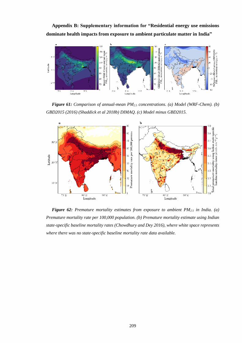
209

Appendix B: Supplementary information for “Residential energy use emissions

dominate health impacts from exposure to ambient particulate matter in India”

Figure 61: Comparison of annual-mean PM2.5 concentrations. (a) Model (WRF-Chem). (b)

GBD2015 (2016) (Shaddick et al 2018b) DIMAQ. (c) Model minus GBD2015.

Figure 62: Premature mortality estimates from exposure to ambient PM2.5 in India. (a)

Premature mortality rate per 100,000 population. (b) Premature mortality estimate using Indian

state-specific baseline mortality rates (Chowdhury and Dey 2016), where white space represents

where there was no state-specific baseline mortality rate data available.

210

Table 9: Estimated premature mortality associated with ambient PM2.5 exposure in India per

disease from both subtraction and attribution methods. Values in parentheses represent the 95%



transport (TRA).


Pre

matu

re m

ort

ali

ty p

er y

ear, su

btr

act

ion

met

ho

d

COPD

(×103)

0

(0–1)

4

(3–7)

0

(0–0)

33

(21–49)

24

(16–36)

92

(56–135)

16

(10–24)

IHD

(×103)

0

(0–0)

3

(3–4)

0

(0–0)

22

(19–28)

16

(14–20)

64

(53–79)

11

(9–13)

LC

(×103)

0

(0–0)

0

(0–0)

0

(0–0)

3

(2–4)

2

(1–3)

8

(5–10)

1

(1–2)

CEV

(×103)

0

(0–0)

2

(1–2)

0

(0–0)

12

(9–15)

9

(7–11)

34

(25–42)

6

(4–7)

LRI

(×103)

0

(0–0)

3

(1–4)

0

(0–0)

21

(9–26)

15

(7–19)

58

(23–74)

10

(4–12)

Pre

matu

re m

ort

ali

ty p

er y

ear,

att

rib

uti

on

met

hod

COPD

(×103)

1

(1–2)

9

(6–13)

0

(0–0)

65

(43–97)

51

(33–75)

161

(105–238)

32

(21–48)

IHD

(×103)

1

(1–2)

10

(7–13)

0

(0–0)

73

(55–96)

57

(43–74)

180

(135–236)

36

(27–47)

LC

(×103)

0

(0–0)

1

(0–1)

0

(0–0)

4

(3–6)

3

(2–4)

10

(7–14)

2

(1–3)

CEV

(×103)

0

(0–1)

4

(3–5)

0

(0–0)

30

(22–38)

23

(17–30)

73

(55–94)

15

(11–19)

LRI

(×103)

1

(0–1)

5

(2–6)

0

(0–0)

35

(15–47)

27

(12–36)

87

(38–12)

17

(8–23)

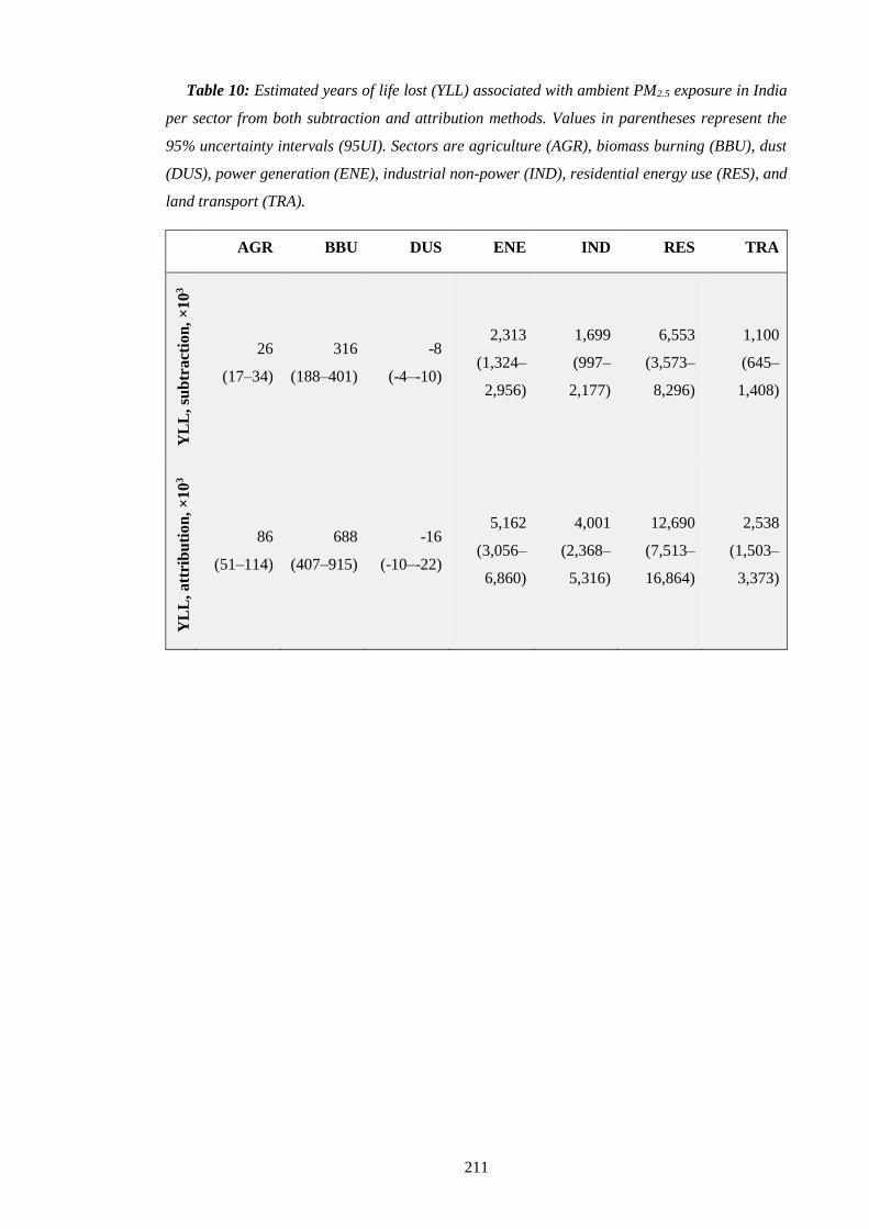
211

Table 10: Estimated years of life lost (YLL) associated with ambient PM2.5 exposure in India

per sector from both subtraction and attribution methods. Values in parentheses represent the

95% uncertainty intervals (95UI). Sectors are agriculture (AGR), biomass burning (BBU), dust

(DUS), power generation (ENE), industrial non-power (IND), residential energy use (RES), and

land transport (TRA).


YL

L,

sub

tra

ctio

n,

×1

03

26

(17–34)

316

(188–401)

-8

(-4–-10)

2,313

(1,324–

2,956)

1,699

(997–

2,177)

6,553

(3,573–

8,296)

1,100

(645–

1,408)

YL

L,

att

rib

uti

on

, ×

10

3

86

(51–114)

688

(407–915)

-16

(-10–-22)

5,162

(3,056–

6,860)

4,001

(2,368–

5,316)

12,690

(7,513–

16,864)

2,538

(1,503–

3,373)

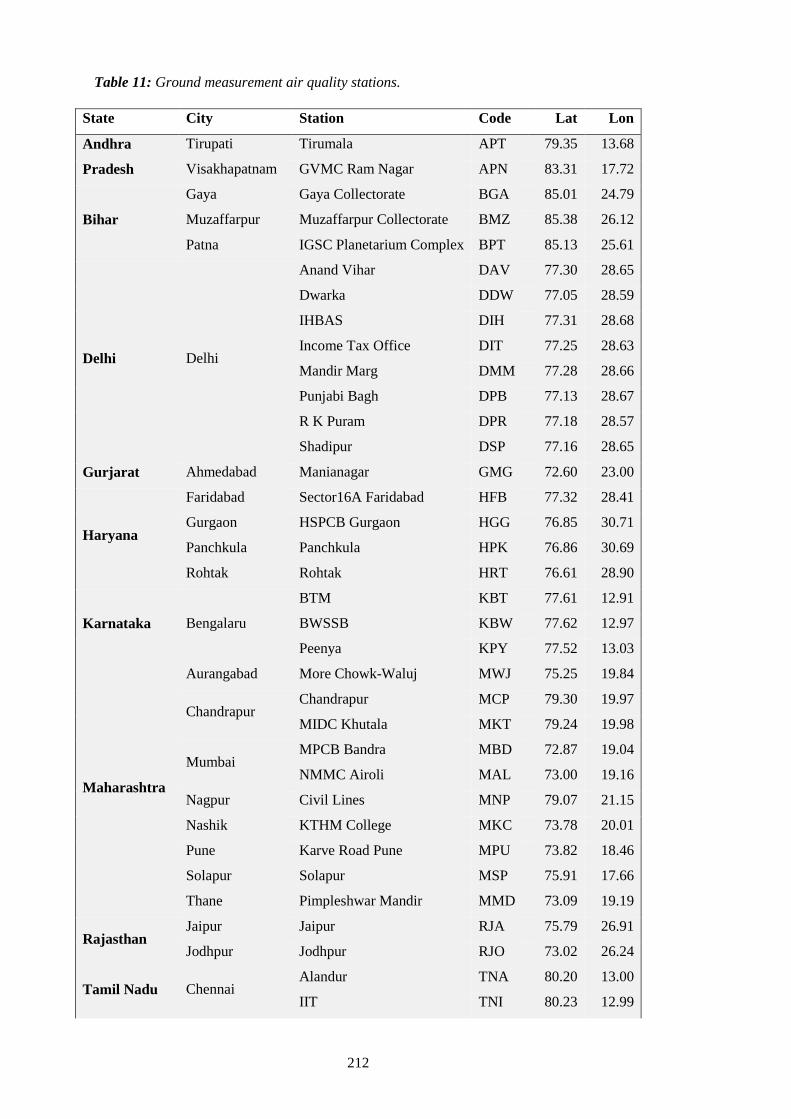
212

Table 11: Ground measurement air quality stations.

State City Station Code Lat Lon

Andhra

Pradesh

Tirupati Tirumala APT 79.35 13.68

Visakhapatnam GVMC Ram Nagar APN 83.31 17.72

Bihar

Gaya Gaya Collectorate BGA 85.01 24.79

Muzaffarpur Muzaffarpur Collectorate BMZ 85.38 26.12

Patna IGSC Planetarium Complex BPT 85.13 25.61

Delhi Delhi

Anand Vihar DAV 77.30 28.65

Dwarka DDW 77.05 28.59

IHBAS DIH 77.31 28.68

Income Tax Office DIT 77.25 28.63

Mandir Marg DMM 77.28 28.66

Punjabi Bagh DPB 77.13 28.67

R K Puram DPR 77.18 28.57

Shadipur DSP 77.16 28.65

Gurjarat Ahmedabad Manianagar GMG 72.60 23.00

Haryana

Faridabad Sector16A Faridabad HFB 77.32 28.41

Gurgaon HSPCB Gurgaon HGG 76.85 30.71

Panchkula Panchkula HPK 76.86 30.69

Rohtak Rohtak HRT 76.61 28.90

Karnataka Bengalaru

BTM KBT 77.61 12.91

BWSSB KBW 77.62 12.97

Peenya KPY 77.52 13.03

Maharashtra

Aurangabad More Chowk-Waluj MWJ 75.25 19.84

Chandrapur Chandrapur MCP 79.30 19.97

MIDC Khutala MKT 79.24 19.98

Mumbai MPCB Bandra MBD 72.87 19.04

NMMC Airoli MAL 73.00 19.16

Nagpur Civil Lines MNP 79.07 21.15

Nashik KTHM College MKC 73.78 20.01

Pune Karve Road Pune MPU 73.82 18.46

Solapur Solapur MSP 75.91 17.66

Thane Pimpleshwar Mandir MMD 73.09 19.19

Rajasthan Jaipur Jaipur RJA 75.79 26.91

Jodhpur Jodhpur RJO 73.02 26.24

Tamil Nadu Chennai Alandur TNA 80.20 13.00

IIT TNI 80.23 12.99

213

Manali TNM 80.26 13.16

Telangana Hyderabad

IDA Pashamylaram TPM 78.18 17.53

Sanathnagar TSN 78.44 17.45

Zoo Park TZP 78.45 17.35

Uttar Pradesh

Agra Sanjay Palace UPA 78.01 27.20

Kanpur Nehru Nagar UPK 80.32 26.47

Lucknow

Central School UPS 80.90 26.83

Lalbagh UPL 80.94 26.85

Talkatora UPT 80.90 26.83

Varanasi Ardhali Bazar UPZ 82.98 25.35

Table 12: AERONET stations.

State City Station Code Lat Lon

Rajasthan Jaipur Jaipur JAI 26.90 75.80

Uttar Pradesh Kanpur Kanpur KPR 26.51 80.23

Maharashtra Pune Pune PNE 18.52 73.85

Jharkhand Bokaro Gandhi College GAN 25.87 84.13

214

Appendix C: Supplementary information for “Stringent emission control policies

can provide large improvements in air quality and public health in India”

Table 13: Scaling factors per emission sector and air pollutant in India (International Energy

Agency 2016a).

New Policy Scenario (NPS) Clean Air Scenario (CAS)

SO2 NOx PM2.5 SO2 NOx PM2.5

Industry (IND) 2.46 2.75 2.52 0.61 1.24 0.48

Power (ENE) 0.11 0.73 0.21 0.05 0.40 0.07

Residential (RES) 0.55 1.10 0.61 0.37 0.54 0.15

Transport (TRA) 2.20 0.55 0.53 1.12 0.22 0.43

Other 1.84 1.10 1.07 0.75 0.27 0.00

Total 1.10 1.10 1.07 0.31 0.50 0.24

215

Appendix D: Supplementary information for “Current and future disease burden

from ambient ozone exposure in India”

Table 14: Ambient surface O3 observation site details.

Site Type Lat.

(°N)

Lon.

(°E)

Alt.

(m) Data period Ref.

Ahmedabad

(ABD)

Semi-

arid,

urban

23.00 72.60 49 1993–1996 (Lal et al 2000)

2002–2003 (Sahu and Lal 2006)

23.03 72.58 53 2011 (Mallik et al 2015)

Anantapur

(ANP)

Semi-

arid

rural site

14.62 77.65 331

2002–2003 (Reddy et al 2008)

2008–2009 (Reddy et al 2010)

Bhubaneswar

(BHB) Coastal 20.30 85.83 45 2010–2012

(Mahapatra et al

2014)

Delhi (DEL) Urban 28.65 77.27 220 1997–2004 (Jain et al 2005)

Gadanki

(GDK) Rural 13.50 79.20 375 1993–1996 (Naja and Lal 2002)

Jabalpur

(JBL)

Semi-

urban 23.17 79.92 411 2013–2014 (Sarkar et al 2015)

Kannur

(KNN)

Semi-

rural 11.90 75.40 5 2009–2010 (Nishanth et al 2012)

Kanpur (KNP) Urban 26.46 80.33 125 2009–2013 (Gaur et al 2014)

Kullu (KLU) Semi-

urban 31.90 77.12 1154 2010 (Sharma et al 2013)

Mt. Abu

(MAB)

High

altitude 24.60 72.70 1680 1993–2000 (Naja et al 2003)

Nainital

(NTL)

High

altitude 29.37 79.45 1958

2006–2008 (Kumar et al 2010a)

2009–2011 (Sarangi et al 2014)

Pune

(PNE)

Semi-

urban 18.54 73.81 600 2003–2004 (Beig et al 2007)

Pantnagar

(PNT)

Semi-

urban 29.00 79.50 231 2009–2011 (Ojha et al 2012)

Trivandrum

(TRV) Coastal 8.55 77.00 5 2007–2009

(David and Nair

2011)

Udaipur

(UDP) Urban 24.58 73.68 598 2010–2011 (Yadav et al 2014)

216

Figure 63: Fractional contribution per source to total annual-mean ambient O3 surface

concentrations. (a) Total annual-mean ambient O3 surface concentrations. (b–f) Fractional

contribution from biomass burning (BBU), power generation (ENE), industrial non-power (IND),

residential energy use (RES), and land transport (TRA).

217

Figure 64: Dominant source contributions to premature mortality burden due to O3 exposure

across India in 2015. (a) Attributable fraction of premature mortalities from land transport

emissions (attribution method). (b) Averted fraction of premature mortalities from removing land

transport emissions (subtraction method). (c) Attributable fraction of premature mortalities from

energy emissions (attribution method). (d) Averted fraction of premature mortalities from

removing energy emissions (subtraction method). All health impacts are calculated using Turner

et al (2016) RR and LCCmin.

218

Figure 65: The impact of scenarios on O3 metrics. (a) Percentage of population in 2015 (1st

bar) and 2050 (2nd bar) exposed to population-weighted ambient surface O3 concentrations above

50 ppb (WHO AQG, Indian NAAQS) in each scenario. (b) Absolute population in 2015 (1st bar)

and 2050 (2nd bar) exposed to population-weighted ambient surface O3 concentrations above 50

ppb (WHO AQG, Indian NAAQS) in each scenario.

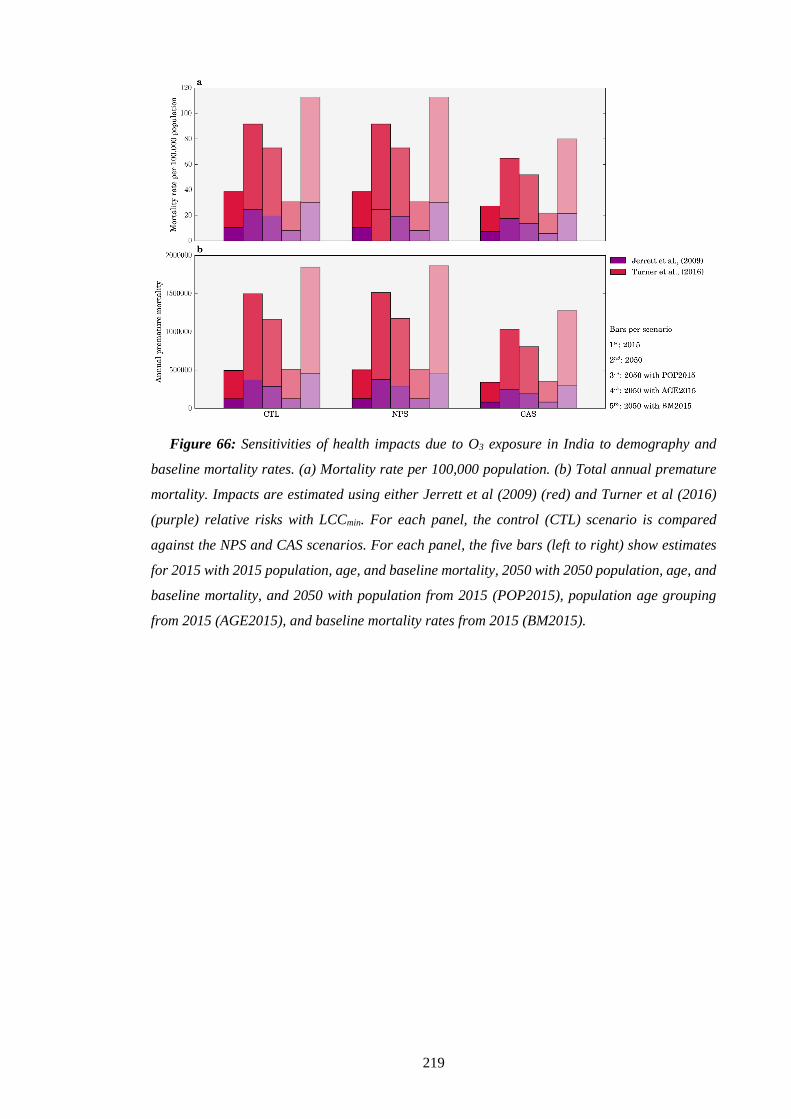
219

Figure 66: Sensitivities of health impacts due to O3 exposure in India to demography and

baseline mortality rates. (a) Mortality rate per 100,000 population. (b) Total annual premature

mortality. Impacts are estimated using either Jerrett et al (2009) (red) and Turner et al (2016)

(purple) relative risks with LCCmin. For each panel, the control (CTL) scenario is compared

against the NPS and CAS scenarios. For each panel, the five bars (left to right) show estimates

for 2015 with 2015 population, age, and baseline mortality, 2050 with 2050 population, age, and

baseline mortality, and 2050 with population from 2015 (POP2015), population age grouping

from 2015 (AGE2015), and baseline mortality rates from 2015 (BM2015).

Thesis Ambient air quality and human health in India - White ...

Documents

Transcript of Thesis Ambient air quality and human health in India - White ...