- 1 -

The Layers of Meteoric Nickel and Aluminium in the Earth's

Upper Atmosphere

Shane Marcus Daly

Submitted in accordance with the requirements for the degree of Doctor of

Philosophy

The University of Leeds

School of Chemistry

May 2020

- 2 -

The candidate confirms that the work submitted is his own, except where work

which has formed part of jointly authored publications has been included. The

contribution of the candidate and the other authors to this work has been

explicitly indicated below. The candidate confirms that appropriate credit has

been given within the thesis where reference has been made to the work of

others.

Please see the contributions section for full details of the contributions of the

candidate and other authors.

This copy has been supplied on the understanding that it is copyright material

and that no quotation from the thesis may be published without proper

acknowledgement.

The right of Shane M Daly to be identified as Author of this work has been

asserted by him in accordance with the Copyright, Designs and Patents Act

1988.

© 2020 The University of Leeds and Shane M Daly

- 3 -

Acknowledgements

First and foremost, I would like to thank my primary supervisor Prof John

Plane, for giving me the opportunity in April 2016 to undertake such an

interesting and challenging PhD about a part of the atmosphere I knew little

about initially. The research environment created within the Plane group has

been excellent and encompasses a wide understanding of different

backgrounds which has always been useful during my study. John also has

great taste in whiskey which for me as an Irishman is very important to have.

I would also like to thank my second supervisor Dr Wuhu Feng, for all the help

he provided with modelling work and patience while dealing with my initial

incompetence; and my third supervisor Prof. Martyn Chipperfield, for his

advice and always offering a welcome outlet during his weekly meetings. I

would also like to thank NERC for funding the project and supporting me with

the opportunity to talk about my research around the world. A further thanks

to the NERC DTP administration for their support, including Nigel.

Thanks are extended to all researchers who I have worked with and helped

me at Leeds during my PhD: Sandy, Tom, David, Tasha, Kevin, Tom, JD,

Wuhu, JC, Chris, James, Nat, the NERC Cohort I was part of and to everyone

else I have not named here. A noted thanks to the D&D group (Aidan, Anthony,

Jamie, Phil, Anthony) for keeping me sane throughout the PhD.

An extended thanks goes to my bachelor and master’s degree supervisor,

Prof. John Sodeau, for putting me back on track in 2016 with a great project

that ultimately lead to my study in Leeds.

Many thanks to Michael at IAP for his assistance and knowledge during the

two visits to the IAP in 2017 along with the rest of the department (Josef,

- 4 -

Franz, Marwa etc) for their immense hospitality. Many thanks to David and

Tom also for helping me throughout the flow tube experiments as well as JC

for taking me under his wing during the initial period of the PhD.

Finally, a special thanks go out to my family, particularly my Parents for

keeping me focused and supported throughout my life, as well as extended

family members that have offered guidance to me and close friends at home

and abroad.

- 5 -

Contributions

My own contributions and those of other researchers, fully and explicitly

indicated in the thesis and associated publications, have been:

In developing experimental methods (Chapter 2):

• Modification and maintenance of the Laser Ablation-Fast flow

tube/Time-of-Flight Mass Spectrometer system for use in experiments

in Chapter 3 (developed by Dr. Juan Carlos Gómez Martín).

• Modification and maintenance of the Ion Fast flow tube/Quadrupole

Mass Spectrometry system for use in experiments in Chapter 3 and 4

(assisted initially by Dr. David Bones and Dr. Thomas Mangan).

• Development of the flow tube calibration cell for use in lidar

observations in Chapter 6.

• The metal resonance and Rayleigh-Mie-Raman lidar systems were

developed at the Leibniz Institute of Atmospheric Physics,

Kühlungsborn, Germany. Dr. Michael Gerding assisted me in the setup

for each instrument for the observations (Chapter 5 & 6).

• Development of the Whole Atmospheric Community Climate Model for

mesospheric metals was done by Dr. Wuhu Feng. I was later deployed

to maintain the updates for WACCM in relation to Ni and to analyse the

output from those model runs (see Chapter 5).

In an investigation of the absorption cross sections and kinetics of AlO

(Chapter 3, Section 3.1) and associated publication:

- 6 -

“Gómez Martín, J. C., Daly, S. M., Plane, J. M. C., (2017), Absorption cross

sections and kinetics of formation of AlO at 298 K., Chemical Physics Letters.,

675, 56-62.”

• I assisted Dr. Juan Carlos Gómez Martín for the majority of all the

kinetic experiments in this Chapter and jointly analysed the data output.

• The theoretical calculations were performed by Prof. John Plane while

the theoretical simulations using PGOPHER were performed by Dr.

James Brooke.

In an investigation of the kinetics of Al+ (Chapter 3, Section 3.2) and

associated publication:

“Daly, S. M., Bones, D. L., Plane, J. M. C., (2019), A study of the reactions of

Al+ ions with O3, N2, O2, CO2 and H2O: influence on Al+ chemistry in planetary

ionospheres., Physical Chemistry Chemical Physics., 21, 14080-14089.”

• I performed the majority of the laboratory experiments for the kinetics

of Al+ and AlO+ while assisting Dr. David Bones with the measurement

of Al+ + O3.

• The data analysis was done by me while David operated the kinetic

model used to measure Al+ and AlO+ + O3.

In an investigation of the kinetics of Ni+ and NiO+ (Chapter 4) and associated

publication:

“Bones, D. L., Daly, S. M., Mangan, T. P., Plane, J. M. C., (2020), A study of

the reactions of Ni+ and NiO+ ions relevant to planetary upper atmospheres.,

Physical Chemistry Chemical Physics., 22, 8940-8951.”

- 7 -

• I performed all laboratory flow tube experiments for Ni+ and NiO+

• The data analysis was jointly done by me, Dr. David Bones and Dr.

Thomas Mangan with the kinetic model developed by David.

In an investigation of the mesospheric Ni layer using lidar (Chapter 5, Section

5.1) and associated publication:

“Gerding, M., Daly, S. M., Plane, J. M. C., (2019), Lidar Soundings of the

Mesospheric Nickel Layer Using Ni(3F) and Ni(3D) Transitions., Geophysical

Research Letters., 46, 408-415.”

• I assisted Dr. Michael Gerding in Kühlungsborn in setting up the lidar

system for Ni observations and took part in the initial observations for

Ni. Michael performed the observations from January – March 2018

since I had to return to Leeds, but we recommended applying the Ni(3D)

transition for observations. The data output was jointly analysed by me

and Michael. I further investigated the relative transitions of Ni using

the NIST spectroscopic database.

In an investigation of the Ni in the upper atmosphere by model simulations,

neutral kinetics of NiO and NiO2 (Chapter 5, Section 5.2 and Chapter 3, Section

3.3) and the associated publication:

“Daly, S. M., Feng, W., Gerding, M., Mangan, T. P., Plane, J. M. C., (2020),

The Meteoric Ni Layer in the Upper Atmosphere., Journal of Geophysical

Research – in press.”

- 8 -

• I performed all the laboratory flow tube kinetics for NiO with CO and O

along with NiO2 and O.

• The model, WACCM-Ni, was initially set up by Dr. Wuhu Feng, with a

number of model runs operated by him. I updated the model with Ni

chemistry every time a new measurement was made in the laboratory.

I also analysed the WACCM output and did the comparisons with Ni

and Fe observations for the paper.

• Theoretical calculations for the paper were performed by Prof. John

Plane.

In investigation of Al in the upper atmosphere (Chapter 6):

• I performed the majority of lidar observations at Kühlungsborn,

Germany, with the assistance of Dr. Michael Gerding while the initial

observations in 2016 performed by Michael.

• I analysed the lidar and rocket data respectively, where the upper limit

for AlO was determined from the lidar observations and Al+ was

compared with Fe+ in the rocket data.

• Theoretical calculations for the paper were performed by Prof. John

Plane.

Throughout the studies detailed here I was supervised, managed, and

directed by Prof John Plane, Dr. Wuhu Feng and Prof Martyn Chipperfield.

- 9 -

Abstract

The major source of metals in the upper atmosphere is the ablation of the

roughly 28 tonnes of interplanetary dust that enters each day from space. This

gives rise to the layers of metal atoms and ions that occur globally in the upper

mesosphere/lower thermosphere (MLT) region between about 70 and 110

km. Metal species in the upper atmosphere offer a unique way of observing

this region and of testing the accuracy of climate models in this domain. The

overarching objective of this project will be to explore the MLT chemistry of

two elements - Ni and Al. Specific objectives of the thesis will include

conducting a laboratory study of the reaction kinetics of Ni and Al species,

both neutral and ionized, that are relevant to understanding and modelling the

contrasting chemistry of these elements in the MLT; extend lidar observations

of the recently discovered Ni layer, which appears to be significantly broader

than the well-known Na and Fe layers, with a Ni density that is roughly an

order of magnitude higher than expected; attempt the first lidar observations

of the AlO layer in the upper atmosphere where if successful, would be the

first time that a molecular metallic species had been observed in the

atmosphere; and develop the first global models of Ni by inserting the

chemistry and the Meteoric Input Function (MIF) of Ni into a whole atmosphere

chemistry-climate model and validating the resulting model simulations

against lidar and rocket-borne mass spectrometric data of metallic ions.

- 10 -

Table of Contents

Acknowledgements .......................................................................................... 3

Contributions .................................................................................................... 5

Abstract ............................................................................................................. 9

Table of Contents ............................................................................................ 10

List of Tables ................................................................................................... 13

List of Figures ................................................................................................. 14

1 Introduction to cosmic dust in the upper atmosphere of Earth.......... 30

1.1 The Mesosphere and Lower Thermosphere .................................. 30

1.2 Ablation of cosmic dust .................................................................. 36

1.3 Observations of metal species in the Mesosphere Lower

Thermosphere .......................................................................................... 44

1.3.1 Remote sensing methods ...................................................... 44

1.3.2 Satellite observations and remote-sensing ............................ 45

1.3.3 Rocket-borne sounding with mass spectrometry ................... 48

1.4 Atmospheric modelling of meteoric metals .................................... 49

1.4.1 Meteoric input function and the chemical ablation model ...... 50

1.4.2 The Whole Atmosphere Community Climate Model .............. 52

1.5 Ni and Al ........................................................................................ 57

1.5.1 Ni ........................................................................................... 57

1.5.2 Al ........................................................................................... 61

1.6 Thesis Overview ............................................................................ 63

2 Materials & Methods ............................................................................... 65

2.1 Laboratory Kinetic instruments ...................................................... 65

2.1.1 Laser Ablation-Fast Flow Tube/Time-of-Flight Mass

Spectrometry for Al + O2 kinetics ...................................................... 65

2.1.2 Ion-Fast flow tube/Quadrupole Mass Spectrometry for Ni+

and Al+ kinetics ................................................................................. 70

2.1.3 Ion-Fast flow tube/Quadrupole Mass Spectrometry for

molecular metal kinetics of NiO+, AlO+ and NiO ................................ 75

2.1.4 Neutral kinetics of NiO ........................................................... 79

2.1.5 Materials ................................................................................ 81

2.2 Lidar Observations ........................................................................ 82

2.2.1 Monitoring site ....................................................................... 82

2.2.2 Rayleigh-Mie-Raman lidar ..................................................... 84

2.2.3 Metal Resonance lidar ........................................................... 86

- 11 -

2.2.4 Flow Tube Calibration Cell for use in observations at 484 nm

90

2.3 Atmospheric Modelling .................................................................. 95

3 The neutral and ion kinetics of Al........................................................ 100

3.1 Neutral kinetics and cross section of Al + O2 ............................... 101

3.1.1 Further reactions of AlO with O2 .......................................... 104

LIF Growth and decay ............................................................................. 104

Al decay – Atomic Resonance Absorption Spectroscopy ........................ 108

Weighted average rate constant ............................................................. 110

3.1.2 Absorption cross section of AlO ........................................... 111

3.1.3 Modelled AlO spectra .......................................................... 114

3.2 Kinetics of Al+ and AlO+ ............................................................... 117

3.2.1 Diffusion of Al+ ..................................................................... 119

3.2.2 Al+ + O3 ................................................................................ 121

3.2.3 Al+ + CO2, N2, O2 and H2O ................................................... 124

3.2.4 AlO+ + O3 and H2O .............................................................. 128

3.2.5 AlO+ + CO ............................................................................ 130

3.2.6 AlO+ + O .............................................................................. 132

3.2.7 Discussion ........................................................................... 134

3.2.8 Atmospheric Implications ..................................................... 137

3.3 Conclusion ................................................................................... 141

4 Neutral and ion-molecule kinetics of Ni .............................................. 144

4.1 Kinetics of Ni+ .............................................................................. 147

4.1.1 Recombination reactions of Ni+ with N2, O2, CO2 and H2O .. 147

4.1.2 Ni+ + O3 ................................................................................ 151

4.2 Kinetics of NiO+ ........................................................................... 154

4.2.1 Flow tube model .................................................................. 154

4.2.2 Reaction of NiO+ with CO .................................................... 157

4.2.3 Reaction of NiO+ with O ....................................................... 158

4.3 Neutral kinetics of NiO and NiO2 ................................................. 161

4.3.1 Reaction of NiO with CO ...................................................... 161

4.3.2 Reactions of NiO and NiO2 with O ....................................... 163

4.4 Discussion ................................................................................... 167

4.4.1 Ni+ + O3, NiO+ + O3, NiO+ + CO, and NiO+ + O .................... 167

4.4.2 NiO + O, NiO + CO, and NiO2 + O ....................................... 171

- 12 -

4.4.3 Ni+ + N2, O2, CO2 and H2O .................................................. 172

4.5 Atmospheric Implications ............................................................. 174

4.6 Conclusion ................................................................................... 178

5 Lidar observations of Ni and model simulations from WACCM-Ni .. 180

5.1 LIDAR observations of Ni ............................................................ 180

5.1.1 Initial observation attempts of Ni – Kühlungsborn 2017 ....... 182

5.1.2 Observations at 341 nm ....................................................... 183

5.1.3 Observations at 337 nm and 341 nm ................................... 190

5.2 WACCM-Ni development ............................................................. 197

5.2.1 A Ni chemistry scheme for atmospheric modelling .............. 197

5.2.2 Whole Atmosphere Community Climate Model for Ni .......... 202

5.2.3 Observational Data for comparison ..................................... 206

5.3 WACCM-Ni results and comparison with observations ............... 207

5.3.1 Mean profiles of Ni and Ni+ WACCM-Ni output .................... 207

5.3.2 Diurnal variation of Ni and Ni+ simulated by WACCM-Ni ..... 210

5.3.3 Global column abundances of Ni and Fe ............................. 212

5.3.4 Comparison between the Ni and Fe layer profiles ............... 215

5.3.5 Nightglow emission from NiO* and FeO* ............................. 217

5.4 Conclusion ................................................................................... 219

6 Observations of Al species in the upper atmosphere ....................... 221

6.1 Lidar soundings of AlO at 484 nm ............................................... 221

6.1.1 Backscatter observations at 484 nm .................................... 223

6.1.2 Statistical analysis of backscatter at 484 nm ....................... 225

6.1.3 Metal dye backscatter vs Rayleigh-Mie-Raman backscatter

signal 227

6.1.4 Calculating the upper limit to the AlO concentration ............ 228

6.1.5 Estimating the AlO concentration from rocket releases of tri-

methyl-aluminium ............................................................................ 231

6.2 Ion measurements ....................................................................... 233

6.3 Discussion ................................................................................... 236

6.4 Conclusion ................................................................................... 237

7 Conclusions and future work .............................................................. 239

7.1 Ni ................................................................................................. 239

7.2 Al ................................................................................................. 241

References ..................................................................................................... 245

- 13 -

List of Tables

Table 2.1: Dates when Ni and AlO lidar measurements were made at the IAP,

Kühlungsborn……………………………………………………………………..82

Table 2.2: The 8 rocket flights used for metal ion measurements………….95

Table 3.1. Low-pressure limiting rate coefficients for the addition of a single

ligand to an Al+ ion using RRKM theory………………………………………131

Table 4.1. Summary of reaction ion molecule (R4.1 – R4.11) and neutral

(R4.12 – R4.14) rate coefficients measured in the present study (T = 294

K)………………………………………………………………………………….161

Table 4.2. Low-pressure limiting rate coefficients for the addition of a single

ligand to an Ni+ ion with He as third body, using RRKM theory …………...168

Table 5.1. Ni chemistry in the MLT……………………………………………195

- 14 -

List of Figures

Figure 1.1: Contour plot of the temperature profile (colour) as a function of

latitude (bottom-ordinate) and height (left-ordinate) in the MLT for January (a)

and July (b) from WACCM. [Plane et al., 2015] ………………………………31

Figure 1.2: Relative abundance output of atmospheric constituents in the MLT

as a function of altitude (km) and mixing ratio, calculated using the UEA 1-

dimensional mesospheric model [Plane, 2003]……………………………….34

Figure 1.3: Injection profiles for the metal constituents that are injected into

Earth’s atmosphere where (a) represents the dust source from JFCs; (b) AST;

(c) HTC sources; and (d) the global ablation rates for Earth’s atmosphere

which is a summation of all 3. Source: [Carrillo-Sánchez et al.,

2020]……………………………………………………………………………….39

Figure 1.4: Schematic of the chemistry of Fe in the mesosphere and lower

thermosphere [Feng et al., 2013]. The blue, green and orange boxes indicate

the ion molecule, neutral and polymerization chemistry, respectively……...41

Figure 1.5: Scan taken from MAVEN (10-15 hr local time) in the northern

hemisphere (50o-70oN) of Mars on April 22nd, where (a) represents the

averaged spectrum and 1σ uncertainties of the Poisson noise of the data with

(b) showing the residual from (a) as the black line along with the Mg+ peak

(red line) and expected Mg peak at 285 nm (orange line). Source: [Crismani

et al., 2017]………………………………………………………………………..48

Figure 1.6: Comparison between the observed and modelled profiles of Ca

and Na vertical column abundances where (a) located at Kühlungsborn (54oN)

and (b) located at Arecibo (18oN). The data points are monthly averages from

- 15 -

January to December. The Na observations are taken from the OSIRIS

spectrometer on the ODIN satellite [Fan et al., 2007], with the Ca lidar data

taken from Kühlungsborn between 1996 – 2000 [Gerding et al., 2000] and

Arecibo Observatory from 2002 – 2003. Source: [Plane et al., 2018b]…….55

Figure 1.7: A comparison between the vertical profiles of the Ni and Fe atom

layers. Adapted from Collins et al. [2015] with Fe lidar measurements from the

same location……………………………………………………………………..59

Figure 2.1: The LA-FFT schematic diagram for the Al + O2 kinetics reaction.

The flip mirror allowed for alteration between the Al and AlO measurements.

The O2 and N2 flows were introduced using calibration mass flow

controllers…………………………………………………………………………65

Figure 2.2: Schematic diagram of the fast flow tube with a laser ablation ion

source, coupled to a differentially pumped quadrupole mass spectrometer.

Reagents were admitted via a sliding injector and kinetics were measured by

either altering the contact time between the sliding injector and the detection

point or by adjusting the reagent concentration at a fixed contact time. The

cooling jacket allowed for solid CO2 pellets to be packed in for low temperature

experiments………………………………………………………………………70

Figure 2.3 Schematic diagram of the modified LAFFT/QMS system with

additional port for the LIF detection of the metal, microwave discharge

connection to the sliding injector, fixed O3 side arm port and secondary PMT

for measurement of O chemiluminescence. Neutral Ni atoms were probed at

341.476 nm [Ni(z3F40−a3D3)] by using a frequency-doubled dye laser (Sirah

Cobra Stretch) pumped with a Nd:YAG laser. The QMS was used to quantify

- 16 -

Ni+ and NiO+ ions but was also used for NO calibration at mass 30 in all the

experiments of this section………………………………………………………75

Figure 2.4: The microwave discharge cavity. Compressed air was used to

prevent the cavity from overheating. This was especially important when the

cavity was glass and not quartz, as glass softens at 427 K and melts at 727

K [Karazi et al., 2017] compared with quartz at 1127K [Ainslie et al., 1961].

Forward wattage of the frequency generator was between 192 – 194 W.

Reflected wattage for the majority of the experiments remained < 5 W. A low

reflected wattage was vital to ensure a more efficient conversion of N2 to

excited N atoms………………………………………………………………….77

Figure 2.5: The receiver system for the RMR and dye lidar in the telescope

bay of the IAP. Both systems were in operation for all the measurements

made. Instead of 7 parabolic mirrors of 500 mm diameter to reduce losses

from the optic connections between the mirrors, a single 30 in. (760 mm)

mirror was applied for the dye lidar observations……………………………..86

Figure 2.6: Schematic diagram of the calibration cell in the RMR-lidar bay (A)

and the cell during operation (B). During operation, the mirror directing the

532 nm laser light to the calibration cell had to be removed from the path of

the lidar beam. The YAG was set to a low pulse energy and beam-splitted for

the calibration since the maximum pulse energy would likely damage the flow

tube window and rod. The bellows connecting the cell to the pump was placed

in a fixed position to avoid contact with telescope and subsequent

misalignment of the lidar beam…………………………………………………90

Figure 3.1: A LIF profile of AlO growth, where the LIF intensity was plotted

against the O2 concentration multiplied by a fixed reaction time of 3.4 ms

- 17 -

(molecule cm-3 s). The growth was fitted with a ‘monomolecular’ exponential

model to measure the rate constant. …………………………………………101

Figure 3.2: Rate plots of the Al decay (red line) and the AlO growths (blue

line) for increasing O2 concentration at a fixed contact time of 1.5 ms. The plot

shows the subsequent Al and AlO atom concentrations (cm-3) against O2

concentration (molecule cm-3). The AlO LIF signal is faster than the Al decay

rate, as the former is measured at the well mixed centre point of the laminar

flow, whereas the latter covers a larger area and thus includes unreacted Al

atoms. The solid blue line shows the bi-exponential fit of the AlO decay

whereas the red dashed line follows the same fit but with kdecay = 0. The

dashed blue line is an evaluation of the bi-exponential expression, using the

estimated AlO decay rate constant of AlO + O2 at 0.8 [Belyung and Fontijn,

1995]……………………………………………………………………………..103

Figure 3.3: Measurements of AlO decay for increasing O2 concentrations at

varying contact times, showing the AlO density (molecule cm-3) against the O2

concentration (molecule cm-3). At longer contact times, the decay of the AlO

signal was more pronounced………………………………………………….105

Figure 3.4: AlO growth rates (blue) and the Al decay rates (red). The

individual points were derived from the LIF growth and ARAS decay plots in

cm3 molecule-1 against contact time (ms). The LIF intercept is within the Origin

but the non-zero of the Al scatterplot intercept is reflective of the radial mixing

time of O2 in the laminar flow………………………………………………….109

Figure 3.5: Absorption in flow tube as a function of wavelength around the

band head of the B(0)-X(0) band of AlO with the reference LIF spectrum. The

- 18 -

absorption insert in the top right corner shows the drop in transmitted intensity

at the AlO fixed wavelength……………………………………………………110

Figure 3.6: Cross section (cm2 molecule-1) against wavenumber (cm-1) for the

observable spectra of the 0-0 and 1-0 bands with their corresponding

simulations from PGOPHER…………………………………………………...113

Figure 3.7: Cross section (cm2 molecule-1) against wavenumber (cm-1) for

simulated spectra of the B(0) ← X(0) band of AlO at 200 and 298 K……...114

Figure 3.8: Al+ ion pulses (left-hand axis) in arbitrary units against flight time

in ms, altered for five different flow velocities (shown as numbers above each

peak, each number in m s-1) at 3 Torr pressure of He. Each point represents

the ratio of each pulse area to that of the largest pulse area measured in the

plot at 26 m s-1 (right-hand log scale). The line was a linear regression fit

through the points. The 1σ error bars were determined from recording 3

repeated measurements at same flow………………………………………...119

Figure 3.9. Plot of k' versus [O3] for the study of R3. The data-points shown

with open triangles were measured with a fixed [H2O] at 3.5 1012 molecule

cm-3. The data-points depicted with solid circles are measured in the absence

of H2O. The effect of the addition of H2O was shown by the intercept

differences between the two fits, with the line fit without H2O having a non-

zero intercept. This was a result of a back reaction between AlO+ and O3 to

retrieve Al+……………………………………………………………………….121

Figure 3.10. k' plotted against [H2O] at three fixed [O3] (see figure legend).

The vertical line indicates the point (H2O = 2 x 1012 molecule cm-3) whereby

R11 dominates R10a so that k' reaches a plateau and no longer increases

with H2O concentration. Therefore, for the final measurements of Al+ + O3, a

- 19 -

concentration of 3.5 x 1012 molecule cm-3 was chosen as it was a safe margin

after the plateau…………………………………………………………………122

Figure 3.11. First-order decays of Al+ in the presence of CO2 (CO2

concentration of 6.0 1014 molecule cm-3) at 293 K, at three different

pressures of He. The y-axis represented the signal ratio of reacted Al+ to initial

Al+ against reaction time t (ms) in the x-axis…………………………………123

Figure 3.12. Second-order rate coefficients krec versus He concentration for

the recombination of Al+ with H2O, CO2 and N2 (note the right-hand axis for

the N2 reaction). The rate of Al+ + N2 was notably slow at 200 K therefore no

temperature dependence was experimentally retrieved since reaction was not

observed at 293 K. Reaction with H2O was limited to 293 K since it would likely

condense to the flow tube walls at lower temperatures……………………..124

Figure 3.13. A plot showing the log scale of ([Al

+]O3

𝑡

[Al+]0𝑡 ) as a function of t, with

an O3 concentration = 1.2 1012 cm-3 at 1.0 Torr and 293 K. The model fit was

represented as the solid black line, with upper and lower error limits illustrated

by the dashed lines. Four experimental data sets were shown here with their

own individual symbols…………………………………………………………126

Figure 3.14: Ratio of signal recovery plotted against [CO] / [O3], where the

CO concentration was varied against a fixed concentration of O3. The dashed

lines represent the ± 1σ of the fit, calculated by individually fitting the rate fit

to each data point. Signal recovery of Al+ was plateauing at ~75% at [CO] /

[O3] ratios greater than 80……………………………………………………...128

Figure 3.15: Reaction of AlO+ + O at 294 K, using the 27 m/z channel for Al+.

The solid circles are the experimental points of Al+ in the presence of O3 and

- 20 -

absence of a fixed [O] = 1.36 1013 molecule cm-3, with the solid line through

the points representing the modelled fit. The open circles with solid line are

the experimental and modelled data for Al+ in the presence of O. The dashed

lines represent the uncertainty………………………………………………...130

Figure 3.16: RRKM fits through the experimental data points (solid circles) for

the recombination reactions of Al+ with N2, CO2 and H2O over a temperature

range form 100 – 600 K. Note the log scale applied for k on the left hand axis

to properly illustrate the 3 reactions separated by up to 3 orders of

magnitude………………………………………………………………………..133

Figure 3.17: Removal rates of Al+ ions in Earth and Mars’ atmosphere. Earth:

Latitude at 40oN, time at local midnight, April (top panel); Mars at local noon

with latitude = 0o, solar longitude Ls = 85o (bottom panel)………………….135

Figure 3.18: Ion Removal rates of AlO+ in planetary atmospheres of Earth and

Mars: Earth, 40oN, at local midnight (top panel); Mars, local noon, latitude =

0o, solar longitude Ls = 85o (bottom panel). The species addressed are

reaction with O, CO, O3 and O2. At >80 km in Earth’s atmosphere, both the O

and CO densities were the dominant sources of AlO+ removal and dominant

for the whole plotted range on Mars’s atmosphere………………………….137

Figure 4.1. Plot of ln ([Ni+]X

𝑡

[Ni+]0𝑡) against reaction time, where [O2] = 1.5 × 1014

molecule cm-3 (dark grey squares), 5.5 × 1014 molecule cm-3 (grey triangles),

1.1 × 1015 molecule cm-3 (light grey circles), 2.2 × 1015 molecule cm-3 (black

diamonds). Experimental conditions: P = 2.5 Torr, T = 294 K. The lines fitted

through the experimental data are exponential fits where the slope yields

k′…………………………………………………………………………………..145

- 21 -

Figure 4.2. Recombination rate coefficients plotted as a function of pressure,

in relation to [He]. Dark grey squares: R4.6 (Ni+ + H2O); black diamonds: R4.9

(Ni+ + CO2); Grey circles: R4.8 (Ni+ + N2); grey triangles: R4.7 (Ni+ + O2). Note

there are two different ordinates: the left-hand ordinate scales for reactions

R4.6 and R4.9; while the right-hand ordinate scales for R4.7 and R4.8

(indicated with arrows). The fitted lines through the experimental points are

linear regression fits, where the slopes of each fit provide the 3rd order rate

coefficients. Experimental conditions: T = 294 K……………………………146

Figure 4.3. Plot of k for R4.1 as a function of [O3], for 3 separate cases: a)

Ni+ + O3 with full recycling of NiO+ by reaction R4.2a (measurements shown

as grey diamonds, with the dotted line as the model fit, extrapolated to [O3] =

0 with the sparse dotted line and 1σ error illustrated as dashed lines); b) Ni+

+ O3 with a fixed [H2O] = 3 × 1012 cm-3, which helped reduce the recycling of

NiO+) (experimental data shown as black triangles, with the black solid line as

the model fit); and finally c) the limiting case of Ni+ + O3 if no recycling back to

Ni via R4.2a took place (black dashed line). Experimental conditions: pressure

= 1.0 Torr, T = 294 K……………………………………………………………149

Figure 4.4. Plot of the fractional recovery in [Ni+] against ratio of [CO]/[O3].

The solid points are the measured experimental points, and the solid black

line is the model fit with the ±1σ uncertainty shown by the shaded region.

Experimental conditions: P = 1 Torr; T = 294 K……………………………...154

Figure 4.5. [Ni+] as a function of increasing [O3], showing the increased

recycling of Ni+ when [O] is present. The experimental points (black triangles)

and model fit (black line) show the [Ni+] amount in the presence of fixed [O] =

9.2 × 1012 molecule cm-3. This was then compared to the experimental points

- 22 -

(grey diamonds) and model fit (grey line) with no [O]. The shades envelopes

(thick grey lines for [Ni+] with no O present and thin light grey lines for [Ni+] in

the presence of [O]) depict the ±1σ uncertainties of the model fits.

Experimental conditions: 1 Torr; T = 294 K; [N2] = 3 × 1015 cm-3………….156

Figure 4.6. Fractional recovery of [Ni] plotted against [CO]/[O3], where [O3] is

fixed at 1.8 × 1012 cm-3. The solid black points are the experimental data with

their individual error bars, while the solid black line is the model fit with ±1σ

uncertainty (shaded region). Conditions: P: 1 Torr; T = 294 K…………….159

Figure 4.7. (a) Plot of [Ni] (arbitrary units) against [O2], where the [O2] was

varied from 2 – 7 × 1014 cm-3, while (b) shows a plot of [Ni] as a function of

[O3], ranging from ~4 – 13 × 1011 cm-3. The symbols indicate the same

treatment in both plots, with the solid black points as the experimental data

with a fixed addition of atomic O ([O] = 9.2 × 1012 molecule cm-3 at injection

point); while the open triangles show data in the absence of O. The solid black

lines represent the model fits through each dataset while the shaded area of

the model fit in the presence of O represents the ±1σ limits. Conditions: 1 Torr,

T = 294 K…………………………………………………………………………161

Figure 4.8. Kinetic plot of experimental data from this study of R4.1, compared

with the flow tube kinetic model with the rate coefficients from McDonald et al.

[2018] substituted in (original fitted rate coefficients shown in Figure 4.3).

Lower grey line indicates the model fit with no [H2O] added; upper grey line

illustrates the fit with [H2O] added. The shaded envelopes represent the

possible range in the modelled values if the uncertainties for the R4.1 and

R4.2 coefficients plus that of the branching ratio for R4.2 are included. See

Figure 4.3 for further details of the plot.………………………………………166

- 23 -

Figure 4.9. Plots of the RRKM fits (thick lines) through the experimentally

measured data points (solid circles) for the recombination reactions of Ni+ with

N2 (green), O2 (blue), CO2 (red) and H2O (black) over a temperature range of

100 – 600 K. The faint lines indicate the sensitivity limits of each fit. Note that

the left-hand ordinate is in log scale to better illustrate the separation of the 4

reactions by nearly 2 orders of magnitude……………………………………170

Figure 4.10. Plots of removal rates of Ni+ and NiO+ ions in planetary

atmospheres from 60 – 140 km: (a) Ni+ and (b) NiO+ on Earth, 40oN, local

midnight, April (top panel); (c) Ni+ and (d) NiO+ on Mars, local noon, latitude

= 0o, solar longitude Ls = 85o (bottom panel). Note the log scale used for the

bottom ordinate to highlight the large differences in Ni+ removal rate between

each species…………………………………………………………………….173

Figure 5.1. Energy level diagram for Ni with the most important transitions

[Kramida et al., 2018]. Wavelengths are given with respect to air. From the

Einstein coefficients we get branching fractions (i.e. relative emission

intensities) for pumping at 341 nm of 11% and 89% at 339nm and 341nm,

respectively. For pumping at 337nm the relative emission intensities are 31%,

41%, 20% and 7% at 337nm, 339nm, 347nm and 381nm, respectively….179

Figure 5.2. Integrated raw profile recorded by the resonance lidar at 341 nm

for the evening of the 8th January 2018, before and after subtraction of the

background, as a function of altitude. The altitude resolution was set to 1 km

bins……………………………………………………………………………….180

Figure 5.3. Nickel density profiles as a function of altitude (km) at the Ni(3D)

transition at 341 nm. The uncertainties are represented as either dotted lines

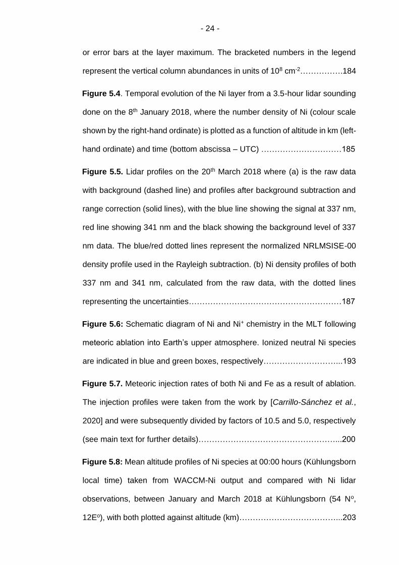
- 24 -

or error bars at the layer maximum. The bracketed numbers in the legend

represent the vertical column abundances in units of 108 cm-2…………….184

Figure 5.4. Temporal evolution of the Ni layer from a 3.5-hour lidar sounding

done on the 8th January 2018, where the number density of Ni (colour scale

shown by the right-hand ordinate) is plotted as a function of altitude in km (left-

hand ordinate) and time (bottom abscissa – UTC) …………………………185

Figure 5.5. Lidar profiles on the 20th March 2018 where (a) is the raw data

with background (dashed line) and profiles after background subtraction and

range correction (solid lines), with the blue line showing the signal at 337 nm,

red line showing 341 nm and the black showing the background level of 337

nm data. The blue/red dotted lines represent the normalized NRLMSISE-00

density profile used in the Rayleigh subtraction. (b) Ni density profiles of both

337 nm and 341 nm, calculated from the raw data, with the dotted lines

representing the uncertainties…………………………………………………187

Figure 5.6: Schematic diagram of Ni and Ni+ chemistry in the MLT following

meteoric ablation into Earth’s upper atmosphere. Ionized neutral Ni species

are indicated in blue and green boxes, respectively………………………...193

Figure 5.7. Meteoric injection rates of both Ni and Fe as a result of ablation.

The injection profiles were taken from the work by [Carrillo-Sánchez et al.,

2020] and were subsequently divided by factors of 10.5 and 5.0, respectively

(see main text for further details)……………………………………………...200

Figure 5.8: Mean altitude profiles of Ni species at 00:00 hours (Kühlungsborn

local time) taken from WACCM-Ni output and compared with Ni lidar

observations, between January and March 2018 at Kühlungsborn (54 No,

12Eo), with both plotted against altitude (km)………………………………...203

- 25 -

Figure 5.9: Mean altitude profiles of modelled Ni+ species at 00:00 hours

(Kühlungsborn local time) between January and March at Kühlungsborn (54

No, 12Eo). The density (log scale) was plotted as a function of altitude. The

solid black line with open pink circles represents geometric mean profile of

observed Ni+, with the geometric 1σ error limits denoted by the gray dotted

lines, for the eight rocket flights described in Table 5.1…………………….204

Figure 5.10: Plots showing the hourly average profiles of the (a) Ni and (b)

Ni+ densities (in cm-3), as a function of altitude, simulated by WACCM-Ni for

the whole month of April at 54o N, 12o E (Kühlungsborn)…………………...207

Figure 5.11: Monthly averaged column abundances as a function of season

and month, simulated by WACCM-Ni and WACCM-Fe: (a) Ni, (b) Ni+, (c) Fe:Ni

ratio and (d) Fe+:Ni+ ratio. Note that (c) and (d) are plotted with the same

contour colour scale…………………………………………………………….209

Figure 5.12: Night-time Ni and Fe layer profiles at mid-latitudes, averaged

from January and March: (a) lidar observations from Kühlungsborn and

Urbana; (b) WACCM output at the same lidar latitudes. The layer peak

densities are scaled separately to effectively overlap the densities for Ni

density (lower ordinate) and Fe density (upper ordinate)…………………...212

Figure 5.13. Plot of the vertical profiles for NiO* and FeO* chemiluminescence

emission rates as a function of altitude. A 100% quantum efficiency was

assumed for both the reactions of Ni and Fe with O3………………………..214

Figure 6.1: The lidar backscatter profile at 484.3646 nm for both the January

2016 and April 2017 periods, where the altitude (km) is plotted against

backscattered photon counts (log scale). The signal below 30 km was reduced

by using a chopper and the Rayleigh scatter from 30 km decreases

- 26 -

exponentially with atmospheric density until ~90 km. No observable

resonance signal for AlO was observed………………………………………219

Figure 6.2: Statistical analysis of the backscatter at 484.3646 nm. The altitude

(km) is plotted against the observed backscatter (photon counts). The zero

line is shown to help identify any specific deviation of the signal. A linear rather

than logarithmic scale is used, as it is easier to compare the statistical

treatment of the resonant backscatter. Note that the Rayleigh scatter begins

close to the altitude where an expected resonance signal might be. An AlO

resonance signal is not present statistically at the 3 level………………...221

Figure 6.3: Comparison of the backscatter signal between the metal

resonance lidar and the RMR lidar, showing altitude against photon counts on

a log scale. The RMR backscatter counts were less than the resonance lidar

signal as this RMR backscatter was recorded by the lowest Rayleigh channel

(5% of the detected light). The Rayleigh scatter of both profiles decay in a

similar way……………………………………………………………………….223

Figure 6.4: Resonance backscatter with background removed (dark blue line)

and the extrapolated Rayleigh signal (purple line), showing altitude (km)

against the recorded photon counts. The signal was extrapolated from the

average counts of the 80-90 km altitude range. The remaining background

scatter after subtraction of the extrapolated Rayleigh line (light blue) did not

show any distinguishing resonance signal…………………………………...225

Figure 6.5: Vertical profile of the upper limit to the AlO number density. A fitted

Gaussian was applied to create the layer profile, with the peak of the layer at

90 km. The upper limit at the peak is 57 molecule cm-3 and the column density

is 4.1 107 molecule cm-2……………………………………………………227

- 27 -

Figure 6.6: Comparison between the AlO trails [Roberts and Larsen, 2014]

and resonance signal upper limit, where the lifetime (s) was plotted against

concentration (cm-3). The maximum observation time for an AlO trail was

about 30 minutes. The measured upper limit of 57 cm-3 from the resonance

lidar would require the AlO trace to have a lifetime of ~8 hours in the MLT.

This comparison indicates that the lidar detection limit would need to decrease

by a factor of 60 for AlO to be measurable…………………………………...229

Figure 6.7: Al+ and Fe+ density profiles on a log scale (measured by mass

spectrometry from 8 rocket flights excluding the ‘Ue06’ flight). The solid black

line represents the geometric mean calculated from the flight rockets for each

species, with the shaded dashed regions indicating the 1σ upper and lower

limits………………………………………………………………………………230

Figure 6.8: Ratio of the geometric means for Fe+:Al+ ion density, against

altitude (km). Ratio shown in log scale. The chondritic (CI) ratio and modelled

ablation ratio are represented as the black solid line and dashed line

respectively. The average Fe+:Al+ ratio from 85 – 115 km for the rocket flights

is 24 ± 10, which is similar to the modelled ablation ratio of 27 [Carrillo-

Sánchez et al., 2020]…………………………………………………………...231

- 28 -

List of Abbreviations

ARAS Atomic Resonance Absorption Spectrometry

AST ASTeroid belt

BUV Nimbus-4 Backscatter UltraViolet

CABMOD Chemical ABlation MODel

CESM Community Earth System Model

FWHM Full Width at Half Maximum

FTCC Flow-Tube Calibration Cell

GLO Arizona Airglow Instrument

GOMOS Global Ozone Measurement by Occulation of Stars

HTC Halley-Type Comet

HTFFR High Temperature Fast Flow Reactor

IAP Leibniz Institute of Atmospheric Physics

IDP Interplanetary Dust Particle

IFFT Ion-Fast Flow Tube

JFC Jupiter-Family Comet

LAFFT Laser Ablation-Fast Flow Tube

LIF Laser Induced Fluorescence

MASI Meteoric Ablation Simulator

MAVEN Mars Atmosphere and Volatile Evolution

MFC Mass Flow Controller

MIF Meteoric Input Function

MLT Mesosphere Lower Thermosphere

MOZART Model for OZone And Related chemical Tracers

MSP Meteoric Smoke Particle

Nd-YAG Neodymium-doped Yttrium Aluminium Garnet

NLC NoctiLucent Cloud

OCC Oort Cloud Comets

- 29 -

OSIRIS Optical Spectrograph and InfraRed Imager System

PLP Pulse Laser Photolysis

PMC Polar Mesospheric Cloud

PMT Photo-Multiplier Tube

PTP p-Terphenyl

QMS Quadrupole Mass Spectrometer

RMR Rayleigh-Mie-Raman

RRKM Rice-Ramsperger-Kassell-Markus

SCCM Standard Cubic Centimetres Per Minute

SLM Standard litres per minute

SCIAMACHY Scanning Imaging Absorption Spectrometer for

Atmospheric CHartographY

TMA Tri-methyl aluminium

TOF-MS Time-Of-Flight Mass Spectrometer

WACCM Whole Atmospheric Community Climate Model

ZoDY Zodiacal Cloud Model

- 30 -

1 Introduction to cosmic dust in the upper atmosphere of

Earth

This chapter gives a general introduction to the mesosphere lower

thermosphere (MLT), the meteoric metals that ablate in this region and the

subsequent metal layers that form between 70 – 110 km. As well as this, the

techniques used to measure these species will be discussed along with the

atmospheric models used to simulate the meteoric input and metal layers; the

two metals specific to this thesis, Ni and Al; and the aims of the research.

1.1 The Mesosphere and Lower Thermosphere

The Earth’s atmosphere consists of several ‘layers’ segregated by altitude and

temperature profile. Each area, spanning from the troposphere to the

exosphere consists of a unique set of atmospheric conditions. The region of

interest in this project is the mesosphere and lower thermosphere layer.

Within this area resides the turbopause at 105 km which represents the

boundary between the atmosphere and space. This region receives high-

energy inputs from space such as solar electro-magnetic radiation and the

solar wind [Marsh et al., 2007] as well as the daily injection of extra-terrestrial

cosmic dust. The MLT also exhibits a similar energetic impact from the lower

atmosphere in the form of gravity waves, tides and planetary waves [Fritts and

Alexander, 2003].

The beginning of the mesosphere is expressed by a local temperature

maximum at the stratopause at ~50 km, which results from stratospheric

ozone absorbing incident radiation above 200 nm, leading to a heating effect

- 31 -

[Barnett et al., 1975; Hiroshi, 1989]. Figure 1.1 shows the temperature

variation during the January (a) and July (b) period of this region from 50 –

110 km. The data used in this Figure consists of an average output from the

Whole Atmosphere Community Climate Model (WACCM) from 2004 to 2011,

a total averaging period of 8 years [Marsh et al., 2013b; Plane et al., 2015]:

Figure 1.1: Temperature profile (colour) as a function of latitude (bottom-

ordinate) and height (left-ordinate) in the MLT for January (a) and July (b) from

WACCM. [Plane et al., 2015]

The profile of figure 1.1 illustrates the temperature decrease with altitude from

the mesosphere (orange region) to the mesopause (purple-green region). The

mesopause height varies seasonally, residing at ~85 km in summer and ~100

km during the winter period. From there, the thermosphere begins and leads

to a rapid warming with increasing altitude, because of extreme UV radiation

- 32 -

absorption, mostly by O2, at wavelengths below 180 nm. These temperatures

in the thermosphere can exceed 1000 K during solar storms [Brasseur and

Solomon, 2005]. It should be noted that because pressure in this region is

extremely low (<10-7 bar above 110 km), the vibrational and rotational modes

of the molecules residing there are generally not in thermodynamic equilibrium

[Brasseur and Solomon, 2005].

The MLT resides between 70 and 110 km in the atmosphere [Portnyagin,

2006]. The turbopause, which can be defined as the boundary between the

atmosphere and space, occurs at an altitude of 105 km, therefore residing in

the MLT [Teitelbaum and Blamont, 1977]. At this boundary point, pressures

fall to less than 5 × 10-7 bar and the mean free path of air molecules there

approaches 1 m. The result is that bulk turbulent motion and thus eddy

diffusion is limited, leaving molecular diffusion as the primary influence on

transport of chemical species. Gravitational separation of molecules by mass

now occurs, leaving heavier species such as Ar and CO2 to reside in the lower

thermosphere while lighter species such as H, H2 and He occur in higher

concentrations above 500 km [Brasseur and Solomon, 2005].

The MLT receives high-energy inputs from space, in the form of solar

electromagnetic radiation and energetic particles i.e. protons and electrons

from solar activity [Marsh et al., 2007]. The result is the generation of radical

and ion species due to photo-dissociation, photoionization, and high-energy

collisions of species in the MLT. The most important of these processes is the

photodissociation of O2 through absorption of incident radiation in the

Schumann-Runge continuum (130-175 nm) as well as the Schumann-Runge

bands (175-195 nm) [Nee and Lee, 1997]. A small contribution is also made

- 33 -

through the photolysis of O3 [Mlynczak et al., 2013]. The O atoms released by

photolysis are a major influence in the MLT since they drive much of the

chemistry in this region, as shown in Figure 1.2 below, controlling the

concentrations of various species such as H, OH and HO2 and being

responsible for the formation of the metal layers.

Atomic oxygen is principally removed through the following reaction

sequence, R1.1 to R1.4:

O + O2 (+M) → O3 (where M = third body, N2 and O2) (R1.1)

H + O3 → OH + O2 (R1.2)

H + O2 (+M) → HO2 + M (R1.3)

O + HO2 → OH + O2 (R1.4)

H + HO2 → H2 + O2 (R1.5)

These reactions control the concentrations of various species in the upper

atmosphere. The direct reaction of O + O (+M) is very slow [Plane et al., 2015]

hence it is not included here. Figure 1.2 below illustrates the modelled mixing

ratios of atmospheric constituents in a vertical profile of the MLT. As stated

previously, atomic O in Figure 1.2(b) is the dominate species. However, there

is a considerable difference in the estimated levels of O below 82 km during

daytime and night-time, with over three orders of magnitude difference

between the night-time atomic O (blue-dashed line in Figure 1.2(b)) and the

daytime estimates (solid-blue line). The recombination of atomic O with O2 to

form O3 in R1.1 contributes to this reduction in atomic oxygen. Above 82 km,

the diurnal variation is less pronounced as the chemical energy from solar UV

- 34 -

absorption during the day builds up and is stored, being slowly released

throughout the night.

Figure 1.2: Vertical profiles of atmospheric constituents in the MLT as a

function of altitude (km) and mixing ratio, calculated using the UEA 1-

dimensional mesospheric model [Plane, 2003].

- 35 -

Methane that propagates up from the stratosphere undergoes oxidation to

H2O in the lower mesosphere. This is followed by photolysis of the water

molecule (by Lyman-alpha radiation at 121.6 nm which penetrates to as low

as 80 km) leading to the production of atomic H [Chandra et al., 1997; Plane,

2003]. In Figure 1.2(a) this reduction in H2O can be observed as a result of

photolysis and subsequent increase in atomic H [Solomon et al., 1982]. With

a similar upper atmospheric profile to O, H has a pronounced diurnal variation

below 82 km as shown in figure 1.2(b). Up at higher altitudes (>90 km) there

is a decrease in H due to formation of H2 as a result of reaction with the

hydroperoxyl radical (R1.5) [Solomon et al., 1982]. This in turn leads to an

increase in H2 mixing ratio up to ~90 km. O3 exhibits a night-time maximum

above 80 km according to figure 1.2(b) but from altitudes above >95 km, its

mixing ratio decreases due to catalytic loss from atomic H (R1.2). Figure

1.2(a) shows that nitric oxide (NO) increases significantly from the

mesosphere to the lower thermosphere, by ~3 orders of magnitude. The

reason for this sharp increase is mainly due to reaction R1.6 [Duff et al., 2003]:

N(2D) + O2 → NO + O (R1.6)

N2+ + O → N(2D) + NO+ (R1.7)

The N(2D) is formed from a variety of exothermic ion-molecule reactions such

as interaction between the N2+ ion and atomic oxygen (R1.7) [Brown, Brown,

1973]. The presence of ionized species in the upper atmosphere is due to the

region receiving high exposure from solar photons which are energetic

enough to ionize molecules and atoms. This leads to increased plasma

concentrations above 70 km, marking the beginning of the ionosphere [Plane,

- 36 -

2003]. This area of atmospheric space has historically been divided into three

regions with distinctly different plasma characteristics. In the D region (70 - 95

km), proton hydrates and negative ions are most prevalent. In the E region

(95 – 170 km) O2+ and NO+ ions are the dominant species along with free

electrons [Monro, 1970]. Finally, in the F region (170 - 500 km), O+ and N+

ions are the positive ions with the highest concentration [Pavlov, 2012].

1.2 Ablation of cosmic dust

The main sources of cosmic dust that enters the terrestrial atmosphere are

the dust trails formed by the sublimation of comets orbiting the sun. These

events are the origin of the well-known meteor showers such as the Leonids

and Perseids. The second input relates to fragments that travel from the

asteroid belt between Mars and Jupiter, as well as dust particles from

cometary trails that have long since decayed [Ceplecha et al., 1998]. All

planets in the solar system encounter interplanetary dust (IDP) as they move

in their respective orbits [Borin et al., 2017]. When these dust particles enter

a planetary atmosphere at orbital velocity, they undergo rapid frictional

heating due to collision with air molecules of that atmosphere, leading to flash

vaporization of the particle. For example, in Earth’s atmosphere, the dust

particles enter at extremely high velocities (11 – 72 km s-1) and ablate, leading

to the formation of the meteoric neutral metal atom layers (Na, Fe, Mg, etc.)

residing from 75 – 110 km, and metal ion layers which reside between 85 –

130 km. The average daily input of cosmic dust into the terrestrial atmosphere

has been debated for decades. The primary reason for this is that no single

technique is available to observe particles over the mass range of 10-12 – 1 g

- 37 -

(bulk of the incoming material) [Ceplecha et al., 1998; Vondrak et al., 2008].

Up until the 1990’s, the mostly accepted figure for daily mass input was in the

region of 44 t d-1, an estimate averaged over the entire planet [Vondrak et al.,

2008]. This value was evaluated through extrapolating between visual

meteoric records with masses > 10 mg as well as satellite impact data,

masses <1µg. Using conventional meteor radar measurements to monitor

specular reflections from the ion trails caused by ablating meteoroids was

ignored as the measurements were regarded as a lower limit to the flux

[Hughes, 1997]. New methods for estimating the cosmic dust flux were then

developed such as the Long Duration Exposure Facility (an orbital impact

detector), an orbital facility with a number of exposed panels on which particle

impact craters could be measured after its return to Earth. The estimate from

this technique was 110 ± 55 t d-1 [Love and Brownlee, 1993; McBride et al.,

1999]. Following the turn of the Millennium, further studies led to an increase

in the range of estimates of the cosmic flux input rate. Single-particle analyses

of stratospheric sulfate aerosol have shown that up to half of the particles in

the lower stratosphere consist of 0.5 - 1% weight of meteoric Fe, from which

a flux between 22 – 104 t d-1 was deduced [Cziczo et al., 2001]. Measurement

of the accumulation of Ir and Pt in polar ice cores in Greenland indicated an

input of 214 ± 82 t d-1 [Gabrielli et al., 2004]. Depending on the method used

to make the estimate, the mass influx of metallic cosmic dust entering the

atmosphere ranges from 5 to 270 t d-1 [Plane, 2012]. Work by Carrillo-

Sánchez et al. [2016] yielded a value of the order of 43 ± 14 t d-1, a value close

to estimates prior to the 1990’s. This was evaluated by applying the mass,

velocity and radiant distributions of the cosmic dust populations from four

known sources: Jupiter family comets (JFCs), asteroid belt (AST), Halley-

- 38 -

Type comets (HTCs) and the Oort Cloud comets (OOCs), constrained by lidar

measurements of the vertical fluxes of Na and Fe atoms in the upper

mesosphere and accumulation rate of cosmic spherules at the South Pole.

Borin et al. [2017] evaluated a mass input of 15.3 ± 2.6 t d-1 through the use

of an astronomical dust model which numerically integrated asteroidal dust

particles. The most recent estimate for the mass input was calculated by

Carrillo-Sánchez et al. [2020], which is an updated study from the work done

by Carrillo-Sánchez et al. [2016], where the new version of the Chemical

ABlation MODel (CABMOD) (see Section 1.4.1) was used to provide the input

for Earth (28 ± 16 t d-1), Mars (2 ± 1 t d-1) and Venus (31 ± 18 t d-1).

Initially when the input of meteoric metals into the atmosphere was estimated,

the relative metallic abundances in the ablated vapour were assumed to

match their meteoric abundances in chondritic meteorites [Fegley Jr and

Cameron, 1987; Vondrak et al., 2008]. In recent years, a more realistic method

has been applied which considers the thermodynamics of a silicate melt, and

explicitly describes the evaporation kinetics of the individual elements by

applying Langmuir evaporation. This shows that the more volatile elements

such as Na evaporate first, followed by the major elements Fe, Mg and Si and

leaving the most refractory elements such as Ca and Al to evaporate last. This

process is known as differential ablation [Carrillo-Sánchez et al., 2015;

Vondrak et al., 2008]. CABMOD has been deployed to investigate this

phenomena by including a series of ablative processes, such as sputtering,

particle melting and vaporization [Carrillo-Sánchez et al., 2020; Carrillo-

Sánchez et al., 2015]. Details of the model are described in Section 1.4.1.

Figure 1.3 is an example of the ablation profile output for all major metal

constituents entering Earth’s atmosphere from three main cosmic dust

- 39 -

sources: JFCs, AST and HTCs, along with the combined total input [Carrillo-

Sánchez et al., 2020].

Figure 1.3: Injection profiles for the metal constituents that are injected into

Earth’s atmosphere where (a) represents the dust source from JFCs; (b) AST;

(c) HTC sources; and (d) the global ablation rates for Earth’s atmosphere

which is a summation of all 3. Source: [Carrillo-Sánchez et al., 2020]

According to Figure 1.3(d), Na (blue line) and K (black dashed line) are the

first elements to ablate between 75 - 130 km, since both are relatively volatile.

Mg, Fe and Si are more distributed throughout the MLT, starting just below

100 km and finishing at ~75-80 km, due to the elements being more resistant

to vaporisation. Ca, Al and Ti are the most refractory elements, and therefore

start to ablate below the main elements.

- 40 -

Once the metals have vaporized into the atmosphere, their interactions with

air molecules in the atmosphere lead to a variety of ion molecule and neutral

reactions. Note that the chemistry of each species is significantly different,

with K behaving more similarly to Na, Mg behaving like Fe, and Ca acting

somewhere in-between. Silicon on the other hand reacts quite differently to

the other meteoric elements, since it is a metalloid (both metal and non-metal)

[Plane et al., 2015]. The majority of the individual reactions for Na, K, Mg, Fe

and Ca have been studied in the laboratory under pressures that are higher

than the pressures of the MLT (<10-5 bar), since those conditions are

extremely difficult to reproduce. The method entails measuring the reactions

over a range of pressures and temperatures so that their rate coefficients can

then be extrapolated to the pressures of the MLT [Broadley et al., 2007;

Vondrak et al., 2006; Whalley et al., 2011], with termolecular reactions being

pressure-independent. Measurements of the rate coefficients for these

meteoric metals can then be compiled in a chemistry scheme reflective of the

expected reactions in the MLT. From there they can be inserted into global

chemistry climate models (see Section 1.4.2), to better understand the

chemical behaviour of the metallic species in the MLT [Feng et al., 2013;

Plane and Whalley, 2012]. Figure 1.4 illustrates the reaction scheme for Fe,

one of the meteoric metals that has been studied most extensively.

- 41 -

Figure 1.4: Schematic of the chemistry of Fe in the mesosphere and lower

thermosphere [Feng et al., 2013]. The blue, green and orange boxes indicate

the ion molecule, neutral and polymerization chemistry, respectively.

Ionized metallic species (blue shaded boxes in Figure 1.4) are species that

tend to dominate above 100 km i.e. in the lower E region. During meteoric

ablation, the metal atoms which evaporate initially travel at high velocities

similar to that of the parent meteoroid, resulting in hyperthermal collisions with

air molecules which may ionize them. Applying the Fe chemistry of Figure 1.4

for example, the following metal ions can form through photoionization of Fe

- 42 -

or charge transfer with the important ambient E region ions (Fe = Mt) [Bones

et al., 2016b; Brown, 1973]:

Mt + hv → Mt+ + e- R1.8

Mt + NO+ → Mt+ + NO R1.9

Mt + O2+ → Mt+ + O2 R1.10

According to Figure 1.4, these charged Fe atoms can further react with O3, to

form MtO+ [Woodcock et al., 2006]. Neutralization of atomic metal ions (Mt+)

such as Fe+ takes place through the formation of a molecular ion, which is

then followed by dissociative recombination with electrons [Bones et al.,

2016b]. Neutralization of Mt+ can also take place through the process of

radiative recombination, whereby the metal ion absorbs an incoming electron

and releases a photon, thereby stabilizing the resulting neutral atom.

Dielectronic recombination, through which a free electron is captured by the

metal ion and this simultaneously excites a core electron in the ion, only

applies to high temperatures above 10,000 K. The exception is for ground

states that have fine-structure splitting such as Si+ and Fe+ [Bryans et al.,

2009]. This may explain why small concentrations of neutral Fe have been

measured up to ~155 km [Chu et al., 2011], an area of very low pressure and

high kinetic temperature.

For the neutral chemistry (green-shaded boxes in figure 1.4), all metal atoms

that have been measured to this point, react rapidly with O3:

Mt + O3 → MtO + O2 R1.11

It is also possible for superoxides (MtO2) to form through recombination

between the metal, O2 and a third body; however, this is restricted to Na, K

- 43 -

and Ca. This reaction is pressure-dependent, however, and therefore only

becomes a competing reaction with R1.11 below 85 km. Once the metal oxide

is formed, it can react with an array of molecules such as CO2 to form metal

bicarbonates (MtCO3) [Gómez Martín et al., 2016], H2O to form metal

hydroxides (Mt(OH)x) [Broadley and Plane, 2010] and O3 to produce higher

oxides (MtOx, x > 1) [Self and Plane, 2003].

Silicon chemistry is quite different from the other metals such as Fe, Ca and

Na. The main reason for this is the very strong SiO bond, which enables rapid

oxidation of ablated Si atoms by O2 [Gómez Martín et al., 2009]. Silicon is a

highly abundant (~20%) element [Gómez Martín et al., 2009] in cosmic dust

and is injected through ablation into the atmosphere above 80 km. A number

of silicon species have been studied recently (SiO, SiO2, Si+, etc) and these

have been implemented into a new model for silicon chemistry in the MLT

[Plane et al., 2016].

The brown-shaded boxes in Figure 1.4 indicate the formation of Meteoric

Smoke Particles (MSPs) through polymerization of Fe- and other metal-

containing species and SiO2 [Aylett et al., 2019]. MSPs are regarded as sinks

for the metallic species below the atom metal layers. First proposed by

Rosinski and Snow [1961], subsequent growth of the particle would take place

by coagulation [Saunders and Plane, 2006]. Experimental studies have

illustrated that they quickly polymerize, especially if the molecules contain Fe

so that the collisions are controlled by long-range magnetic dipole forces

[Saunders and Plane, 2006]. These particles are too small to sediment

gravitationally, therefore are transported downwards through residual

atmospheric circulation [Dhomse et al., 2013]. Because of their small size

- 44 -

range and low concentration, detecting MSPs in the MLT is very challenging

and it is even more difficult to measure their composition. Measuring their

interactions is vital as they potentially play an important role in the formation

of Polar Mesospheric Clouds (PMCs), acting as ice nuclei [Plane et al., 2015].

They may also affect the balance of odd oxygen and hydrogen through

heterogeneous chemistry as well as influencing the mesospheric charge

balance [Murray and Plane, 2003]. Another potentially important impact of

MSPs involves transport into the stratosphere where the particles act as

condensation nuclei for sulfate aerosol and affect the freezing properties of

polar stratospheric clouds, thus affecting stratospheric ozone levels [James et

al., 2018].

1.3 Observations of metal species in the Mesosphere

Lower Thermosphere

1.3.1 Remote sensing methods

Metal species in the upper atmosphere have been observed for decades. The

earliest work can be traced back to Slipher [1929] where the Na layer was

observed through radiation at 589 nm in the night sky spectrum. Quantitative

metal atom measurements in the MLT were first made in the 1950’s using

ground-based photometers. Using this technique, resonance fluorescence

measurements are made from spectroscopic transitions of the metal atoms,

through excitation by solar radiation. By applying this technique, emission

lines from Na, Fe, K and Ca+ in the MLT were categorized due to these metals

having very large resonant scattering cross-sections [Baggaley, 1980;

Hunten, 1967]. From there use of tuneable laser sources allowed for the

- 45 -

development of a resonance technique known as ‘light imaging, detection and

ranging’ (lidar). The Na layer was the first to be measured using this new lidar

detected by Bowman et al. [1969] due to its large effective backscatter cross

section as well as large column abundance. From there on photometry-based

operations were disbanded in the 1970’s due to the rapid introduction of

tuneable laser sources [Gardner et al., 2005; Plane et al., 2015]. The method

entails tuning the wavelength of a pulsed laser beam to correspond to an

intense spectroscopic transition of the species being analysed. This beam is

then transmitted upward to the mesosphere to the metal analyte of interest,

followed by resonant scattering of the pulse by the metal atoms. Most of the

scattering is lost; however, a small fraction resonantly scattered light returns

to the surface. From here it can be collected by a telescope and quantified by

time-resolved photon counting. The recorded altitude of the incoming signal

is determined by the time it spent in the atmosphere before returning. The

absolute metal density is then calculated through calibration with a Raleigh-

scattered signal at a lower altitude of known density [Abo, 2005].

1.3.2 Satellite observations and remote-sensing

The dawning of the space age led to numerous satellite launch and rocket

sounding campaigns. Some of the earliest satellite launches for atmospheric

observations include Ariel I, launched in April 1962, which was designed to

measure various properties of the ionosphere including electron density, ion

concentrations, as well the intensity of the solar spectrum near the Lyman-α

line at 1216 Å [Willmore, 1965]; Explorer 12 launched in August 1961 and

designed to measure cosmic-ray particles, solar wind protons and

- 46 -

magnetospheric magnetic fields [Bryant et al., 1962; Sonnerup and Cahill Jr.,

1968]; OGO-6 which launched in June 1969 and detected Mg+ and Fe+ ion

species [Kumar and Hanson, 1980]; and the Nimbus-4 Backscatter Ultraviolet

(BUV) satellite that was placed into orbit in April 1970 for the purpose of global

atmospheric ozone measurements [Heath et al., 1973].

The introduction of an analytical device in spatial orbit has helped to provide

an extra dimension for analysis of the MLT by downward detection, compared

to the usual lidar measurements upwards from the Earth’s surface. Over the

last two decades, substantial progress in monitoring the MLT using satellites

have been made. In particular, the determination of the vertical profiles of

metal atoms and ions in the upper atmosphere through the deployment of

space-borne limb-scanning spectrometers. Two satellites in particular have

been used for terrestrial upper atmosphere observations of meteoric metals,

Odin and Envisat. The Odin satellite was equipped with the Optical

Spectrograph and Infrared Imager System (OSIRIS) spectrometer designed

for the detection of Na [Fan et al., 2007] and K [Dawkins et al., 2014]. Envisat

includes both the Scanning Imaging Absorption Spectrometer for Atmospheric

Cartography (SCIAMACHY) for measuring Mg and Mg+ [Langowski et al.,

2014; Langowski et al., 2015] and the Global Ozone Measurement by

Occultation of Stars (GOMOS) spectrometer for Na [Fussen et al., 2010]. Both

the OSIRIS and SCIAMACHY instruments measure dayglow radiance profiles

that are produced by solar-excited resonance fluorescence.

More recently, the Mars Atmosphere and Volatile Evolution (MAVEN) mission

was developed to analyse the upper atmosphere of Mars [Crismani et al.,

2017]. The spacecraft launched in November 2013, arrived at the Martian

- 47 -

atmosphere in September 2014 and initiated its one-year mission in

November 2014. The objectives of the study were as follows: Investigate the

interactions between the Sun and solar wind with the magnetosphere and

upper atmosphere of Mars; to analyse the upper atmosphere and ionosphere

composition as well as the dictating processes involved; to evaluate the

escape rates from the Martian upper atmosphere to space; and to use these

escape rates to extrapolate the total atmospheric gaseous loss to space from

past to present [Jakosky et al., 2015]. The most notable discovery during the

campaign in relation to IDPs was the detection of a Mg+ ion layer near an

altitude of 90 km. The Mg+ emission at 280 nm (Figure 1.5) is a result of

resonant scattering of solar UV photon excitation rather than direct excitation

as a result of ablation. The surprising lack of a detectable Mg layer was later

investigated (see Section 1.4.2).

- 48 -

Figure 1.5: Scan taken from MAVEN (10-15 hr local time) in the northern

hemisphere (50o-70oN) of Mars on April 22nd, where (a) represents the

averaged spectrum and 1σ uncertainties of the Poisson noise of the data with

(b) showing the residual from (a) as the black line along with the Mg+ peak

(red line) and expected Mg peak at 285 nm (orange line). Source: [Crismani

et al., 2017]

1.3.3 Rocket-borne sounding with mass spectrometry

During the same period as the early observational satellite launches, rocket-

borne soundings began operation [Krankowsky et al., 1972] and would

continue throughout the 1970’s and 1980’s [Kopp, 1997]. The objectives of

these soundings were to measure the positive and negative ion composition

- 49 -

in the upper atmosphere, specifically the lower E-region. The main difficulty

with the initial measurements was designing a mass spectrometer that could:

meet the requirements for a small payload in a rocket; include a high speed

pump with a large capacity; fast mass sweep; ability to detect positive and

negative ions; better sensitivity than 10 ion cm-3; and a mass range that would

extend up to 150 a.m.u [Krankowsky et al., 1972]. The recorded species

varied from meteoric metals (e.g. Na+, Mg+, Al+, Ca+, Fe+, Co+, Ni+) to metal

containing compounds (e.g. Fe+.(H2O), CaOH+, MgO+). The rocket soundings

also recorded several non-metallic species such as O2+, NO+, O+ and N+

[Grebowsky and Aikin, 2002; Kopp et al., 1985a]. These flights have been

very useful in ion metal comparison studies done at the University of Leeds in

recent years for Si [Plane et al., 2016], Ca [Plane et al., 2018b] and Fe [Feng

et al., 2013]. Further details of rocket flights used in this study are described

in Chapter 5.

1.4 Atmospheric modelling of meteoric metals

For modelling the metallic layers in the MLT, three components are required

for an atmospheric model. First, the meteoric input function (MIF) describes

the injection rate into the atmosphere of each element (e.g. Na or Fe) as a

function of time and latitude [Carrillo-Sánchez et al., 2020]. From there, a

meteoric metal chemistry module needs to be incorporated into the general

atmospheric chemistry scheme in the model [Feng et al., 2013; Marsh et al.,

2013a]. The final component entails insertion of a gas-phase species removal

function through the formation of MSPs. Model outputs can then be compared

- 50 -

to observations and the chemical scheme iterated, if necessary [Plane et al.,

2015].

1.4.1 Meteoric input function and the chemical ablation model

The main purpose of the Chemical Ablation MODel (CABMOD), developed at

the University of Leeds, is to predict the thermal heating of a meteoric particles

from collisions with air molecules in the terrestrial atmosphere [Vondrak et al.,

2008]. With the assumption of Langmuir evaporation, the model applies the

vapour pressure calculated by the MAGMA thermodynamic code [Fegley Jr

and Cameron, 1987; Schaefer and Fegley, 2004] to yield an evaporation rate

of each element as a function of altitude, taking account of changes in the

particle mass and composition changes as ablation occurs. At the melting

range of the particle (since they contain multiple heterogeneous components),

the micrometeoroid begins the process of ablation as the metals and metals

oxide quickly evaporate. The early versions of CABMOD (CABMOD-1 and 2)

assumed that all micrometeoroids were of a homogeneous oxide composition.

The rate of evaporation was determined with the use of the Hertz-Knudsen

equation:

dmi

dt=f(T)γ

ip

iS√

Mi

2πkBT E1.1

where T is the temperature, S the particle surface area, pi the gas-liquid

equilibrium vapour pressure, γi denotes the evaporation coefficient, kB the

Boltzmann constant and f(T) represents the phase transition factor which

accounts for any non-instantaneous melting. γi is assumed to be 1, to maintain

- 51 -

simplicity since there is a lack of experimental data. The phase transition

factor, f(T), is presented as a sigmoidal function:

𝑓(𝑇) = 1

1 + exp (-(T -Tmp)

τ) E1.2

with Tmp representing the mean melting point of the assumed homogeneous

phase, with τ as the width of sigmoid profile. This function allows for melting

to occur over a temperature range, with the most immediate melting occurring

at Tmp. τ was determined to be 51 K for Allende and carbonaceous chondrites

similar to that type, and 108 K for ordinary chondrites (Chergach) [Gómez

Martín et al., 2017].

The latest version of CABMOD (CABMOD-3) assumes that the cosmic dust

particles have two components, silicate bulk and metal grains, which is

supported by the density differences between the phases: the silicate bulk

density at 2200 kg m-3 and a density of 4710 kg m-3 for the sulfide grains

[Bones et al., 2019]. Previous studies relating to Na, Fe and Ca ablation also

supported this update, since it was concluded that a pure metal phase

separate to the bulk silicate phase would explain the observed early release

of Fe during the heating process, particularly in Chergach where a high

metallic Fe abundance lead to doubly peaked profiles [Bones et al., 2019;

Gómez Martín et al., 2017]. Since this update also addresses Ni in these

phases, further details will be discussed in Section 1.5.1.

CABMOD is combined with the astronomical Zodiacal Cloud Model (ZoDY) to

produce the MIF. The ZoDy is a dynamical model which describes both the

temporal and orbital evolution of dust particles in the sub-mm range from the

respective sources: Jupiter Family Comets, Asteroids, Halley Type Comets,

- 52 -

and Oort Type Comets. It also specifies the sinks for these particles, such as

collisional fragmentation, exiting the solar system due to solar photon

pressure, or atmospheric entry [Nesvorný et al., 2011; Nesvorný et al., 2010].

ZoDy provides to CABMOD the meteoric mass (10-8-103 µg) [Ceplecha et al.,

1998], entry velocity (11-72 km s-1) and radiant distributions (0 – 90°) for Earth

[Carrillo-Sánchez et al., 2015; Nesvorný et al., 2011]. CABMOD then predicts

the ablation rate for the meteoric metals of interest. Figure 1.3 above is an

example of the ablation profile output for Na, K, Mg, Fe, Ni, Si, Ca, Al and Ti.

1.4.2 The Whole Atmosphere Community Climate Model

After determination of the MIF for the metal of interest, it is then combined with

a list of potential reactions the metal is expected to have in the MLT and further

added to an atmospheric model. Over the last decade, the research group at

the University of Leeds has used WACCM, with altitudes ranging from the

Earth’s surface to the thermosphere at ~140 km [Feng et al., 2013; Plane et

al., 2018b] and uses the framework developed from the fully coupled

Community Earth System Model (CESM) [Hurrell et al., 2013]. The standard

horizontal resolution of the model is 1.9o x 2.5o (latitude x longitude) and 88

vertical model layers (with a height resolution of ~3.5 km in the MLT). WACCM

provides a detailed description of atmospheric processes in the mesosphere

and lower thermosphere. These include auroral processes, non-local

thermodynamic equilibrium, ion drag, radiative transfer, molecular diffusion of

major and minor species as well as an interactive chemistry module [Marsh et

al., 2007]. Iterations 1 to 4 of WACCM employed the standard model

chemistry Model for OZone And Related chemical Tracers-version 3

- 53 -

(MOZART-3) package [Kinnison et al., 2007], which has 59 chemical species

and 217 gas-phase reactions including the E region ion chemistry for O+, O2+,

N+, N2+, NO+ and electrons [Marsh et al., 2013a]. For altitudes below 60 km,

WACCM has a specified dynamics option where the temperature and wind

field at each time step is nudged with meteorological reanalysis data. Above

60 km, the model is free-running. Several improvements have been made in

recent years since the WACCM4 version described by [Marsh et al., 2013b].

WACCM5 [Gettelman et al., 2019; Mills et al., 2017] applies WACCM4

chemistry WACCM5 also operates at a higher vertical and horizontal

resolution. The latest version of WACCM used for metal chemistry is

WACCM6 which is part of the second iteration of the coupled Earth System

Model, CESM2 [Gettelman et al., 2019]. A lower resolution of WACCM6 is still

available which can run metal layer simulations that are consistent with

previous iterations of WACCM [Plane et al., 2015]. WACCM-X is a separate

development of WACCM which incorporates the same features but extends

up to ~500 km in altitude, covering the majority of thermosphere [Liu et al.,

2010].

In terms of meteoric metals, the neutral and ion chemical reactions of Na

[Marsh et al., 2013a], K [Plane et al., 2014], Mg [Langowski et al., 2015], Fe

[Feng et al., 2013] and Ca [Plane et al., 2018b] have been added to WACCM.

The Fe chemistry scheme illustrated in Figure 1.4 above is an example of how

extensive the reaction catalogue added to WACCM is. WACCM-Ca is the

most recent work relating to modelling work chemistry. For this model the MIF

profiles (see Section 1.4.1) for Ca and Na used in the study were initially

reduced by a factor of 5 [Plane et al., 2018b]. This factor compensates for the

fact that global models such as WACCM underestimate the vertical transport

- 54 -

of minor species in the MLT, because short wavelength gravity waves are not

resolved on the model horizontal grid scale (~150 km). These sub-grid waves

contribute to chemical and dynamical transport while dissipating, and this can

exceed transport driven along mixing ratio gradients by the turbulent eddy

diffusion produced once the waves break [Gardner et al., 2017]. Since these

additional vertical transport mechanisms are underestimated, the MIF needs

to be reduced in order to simulate the observed metal density [Plane et al.,

2018b]. Figure 1.6 shows a monthly comparison example between the

observations and model simulations of Ca and Na using WACCM-Ca, with

both metals showing satisfactory agreement each month.

- 55 -

Figure 1.6: Comparison between the observed and modelled profiles of Ca

and Na vertical column abundances where (a) located at Kühlungsborn (54oN)

and (b) located at Arecibo (18oN). The data points are monthly averages from

January to December. The Na observations are taken from the OSIRIS

spectrometer on the ODIN satellite [Fan et al., 2007], with the Ca lidar data

taken from Kühlungsborn between 1996 – 2000 [Gerding et al., 2000] and

Arecibo Observatory from 2002 – 2003. Source: [Plane et al., 2018b]

- 56 -

The formation of MSPs through the polymerization of metal reservoir species

is currently represented in WACCM by a “dimerization” reaction representing

permanent removal. The dimerization rate constants are estimated using

dipole-dipole capture theory [Feng et al., 2013; Plane, 2004]. For minor metal

species such as K, the dimerization process of the KHCO3 species increases

by a factor of 270, due to the ability of KHCO3 to polymerize with any of the

major metallic species such as NaHCO3 and FeOH [Plane et al., 2014].

Most observations of meteoric metals are done on Earth but the recent

deployment of MAVEN to Mars [McClintock et al., 2015] enabled the detection

of a Mg+ ion layer at ~90 km (though no Mg layer was observed) [Crismani et

al., 2017]. A 1-D model was constructed to investigate this, which used

CABMOD and ZoDy to estimate the Mg MIF for Mars [Plane et al., 2018a].

This study suggested that the absence of a detectable Mg layer is attributed

to ~50% of the ablated Mg atoms ionizing with CO2 molecules in the Martian

atmosphere due to hyperthermal collisions, as well as MgO+ ions forming

cluster ions with CO2 which dissociatively recombine with electrons to form

MgCO3 rather than Mg. Future versions of WACCM – e.g. for Mars - could be

developed to describe other planetary atmospheres once the appropriate

chemistry scheme and atmospheric conditions are achieved.

- 57 -

1.5 Ni and Al

Both species represent part of the total cosmic dust input into Earth’s

atmosphere and are the specific focus of this thesis. Therefore, it is important

to identify what is currently known about the two meteoric metals.

1.5.1 Ni

Techniques for isolating Ni in Fe meteorites have been developed since the

1940’s e.g. breaking off and powdering a fragment of the impacted sample,

dissolving it in dilute HNO3 and adding NH4OH. This results in the precipitation

of the Fe component in the meteorite in the form of ferric hydroxide.

Decantation of the clear liquid mixture from the precipitate followed by addition

of ethanol and dimethylglyoxime leads to the isolation of a scarlet-red

precipitate. This was indicative of Ni and the probability that the specimen was

a meteorite [Ashbrook., 1945]. In terms of atmospheric measurements of Ni

in the upper atmosphere, Ni+ ions (58Ni+ & 60Ni+) were first observed with the

use of a quadrupole mass spectrometer flown from a sounding rocket at the

Andoya Rocket Range, Norway, on 26th November 1969 [Krankowsky et al.,

1972]. Following this, several measurements were carried out during the

1970’s and 1980’s [Grebowsky and Aikin, 2002; Kopp, 1997]. From there,

chemiluminescence from the electronically excited NiO molecule, formed from

the reaction between Ni and O3, was detected by Evans et al. [2011] as a

broad continuum in the visible section of the nightglow spectrum, ranging from

440 – 670 nm. This detection was done using the OSIRIS spectrograph on

the Odin satellite [Llewellyn et al., 2004] and the Arizona Airglow Instrument

(GLO-1) spectrograph on the Space Shuttle [Broadfoot and Bellaire Jr., 1999].

- 58 -

The first observations of the Ni layer were made at the Poker Flat Research

Range at Chatanika. Alaska (65oN, 147oW) by Collins et al. [2015], on two

nights during midwinter (27 - 28th Nov & 20 - 21st Dec 2012) by probing the

Ni(3F4 – 3D) transition at λair = 336.96 nm. The Ni resonance lidar consisted of

an excimer-pumped dye laser and a 1.04 m diameter telescope that was

previously used for Na and Fe mesospheric layer measurements [Gelinas et

al., 2005]. The concentration of Ni atoms was determined by applying

resonance absorption at one wavelength (λ1 = 337.054 nm) following by

measuring emissions at two wavelengths (λ1 = 337.054 nm and λ2 = 339.396

nm). E.13 was applied to determine the ratio of the Ni resonance signal at

altitude z (NNi (z)) to the Rayleigh scattering signal at altitude zR (NRZR):

𝑁𝑁𝑖(𝑧)

𝑁𝑅(𝑧𝑅)=

𝜎𝑎𝑏𝑠(𝜆1)𝜌𝑁𝑖(𝑧)

𝜎𝜋𝑅(𝜆1)𝜌(𝑧𝑅)[𝛾1𝜂1𝑇1+𝛾2𝜂2𝑇2]

[𝜂1𝑇1]

1

4𝜋𝑧𝑅

2

𝑧2 (E1.3)

where σabs is the resonance cross section at wavelength (λ1), ρNi the

concentration of Ni, σπR the Rayleigh backscatter cross section at λ1, ρ is the

concentration of air at altitude (zR), γ1,2 as the branching ratios of each

wavelength transition, η1,2 the receiver efficiencies and T1 and T2 are the one-

way atmospheric transmission coefficient at wavelengths λ1 and λ2. Equation

1.4 can be rearranged to calculate the concentration of Ni:

𝜌𝑁𝑖(𝑧) = 𝑁𝑁𝑖(𝑧)

𝑁𝑅(𝑧𝑅)

𝜎𝜋𝑅(𝜆1)𝜌(𝑧𝑅)

𝜎𝑎𝑏𝑠(𝜆1)

1

[𝛾1+𝛾2[𝜂2𝑇2

𝜂1𝑇1]]4𝜋

𝑧2

𝑧𝑅2 (E1.4)

One challenge with measuring the Ni concentrations was that the element has

several isotopes: 58Ni (68%), 60Ni (26%), 62Ni (4%), 61Ni (1%) and 64Ni (1%).

However, since the isotope shift in the spectral lines was smaller than the

linewidth of the laser [Schroeder and Mack, 1961], it was possible to designate

Ni as a single isotope for retrieving the Ni concentrations.

- 59 -

The peak density was 1.6 104 cm-3 at 87 km, with a column abundance of

2.7 × 1010 cm-2. Figure 1.7 illustrates the Ni layer profile measured by Collins

et al. [2015], compared against Fe layer lidar soundings during the same

period.

Figure 1.7: A comparison between the vertical profiles of the Ni and Fe atom

layers. Adapted from Collins et al. [2015] with Fe lidar measurements from the

same location.

When compared to Fe, another transition metal that should be injected into

Earth’s atmosphere through meteoric ablation over a similar altitude range

[Carrillo-Sánchez et al., 2020], the Fe:Ni column abundance interpreted from

Figure 1.7 is only 1.2 which is much smaller than the carbonaceous Ivuna (CI)

chondritic ratio of 18 [Asplund et al., 2009]. The CI ratio is chosen here as it

is regarded as the closest in composition to IDPs [Jessberger et al., 2001].

- 60 -

Recently, the ablation of Ni from meteoric fragments using the Meteoric

Ablation Simulator (MASI) at the University of Leeds, which has been

previously used to study Fe, Na and Ca meteoric fragments [Bones et al.,

2016a]. In the recent work, the evaporation of Ni and Na were measured

through laser induced fluorescence (LIF) as meteoric fragments in several

different size ranges were heated at a rate that would simulate atmospheric

entry [Bones et al., 2019]. The experimental results from this study were then

applied to the new version of CABMOD (CABMOD-3) (see Section 1.4.1). In

this new iteration, the Ni is treated as part of the Ni-Fe-S metallic grain

composition, but absent from the bulk Fe-Mg-SiO4 phase [Carrillo-Sánchez et

al., 2020]. The experimental data from MASI and the CABMOD-3 simulations

showed that the ablation of Ni occurs rapidly at a relatively low temperature

(~2200 K), with the same observed for metallic or sulfide Fe, before the bulk

silicate of Fe eventually ablates.

The MIF ratio of Fe:Ni predicted by the CABMOD-ZoDy coupled model was

16:1, which is in close agreement with the CI ratio of 18. However, this is still

~13 times larger than the ratio determined from the lidar soundings of Collins

et al. [2015]. This would indicate a large Ni enrichment in cosmic dust particles

entering Earth’s atmosphere, although this would also contradict recent

meteoric fragment analysis done in the laboratory at Leeds [Bones et al.,

2019] as well as the Fe:Ni ratio from cosmic dust particles which survived

atmospheric entry, measured by Arndt et al. [1996]. Further examination of

Figure 1.7 shows that that the Ni layer exhibits a much broader layer profile

than Fe, both top-side and bottom-side, ranging from 70 – 115 km. This may

suggest that the neutral and ion-molecule chemistry of Ni is different to that of

Fe, despite the elements being first row transition metals.

- 61 -

In terms of kinetic measurements, Ni + O2 has been measured previously with

Ar as the carrier gas and acting third body [Brown et al., 1991], yielding a rate

coefficient of k(Ni + O2, T = 296 K) = (1.7 ± 0.3) × 10-30 cm6 molecule-2 s-1. The

reaction of Ni+ + O3 has been studied previously by McDonald et al. [2018]

with the use of a selected-ion flow tube, with a rate coefficient of k(Ni+ + O3, T

= 300 - 500 K) = (11 ± 2) × 10-10 cm3 molecule-1 s-1. The subsequent higher

oxide reactions, NiO+ + O3 and NiO2+ + O3, were measured to be (9.5 ± 3.0)

× 10-10 cm3 molecule-1 s-1 and (10 ± 7) × 10-10 cm3 molecule-1 s-1, respectively.

1.5.2 Al

Al+ ions have been in the MLT by mass spectrometry from sounding rockets,

similar to Ni+ (see section 1.3.3) [Kopp, 1997; Krankowsky et al., 1972] and

have also been detected in the Martian atmosphere using the Neutral Gas Ion

Mass Spectrometer which was part of the MAVEN satellite [Benna et al.,

2015]. Solar-induced fluorescence of the B2Σ+ ← X2Σ+ transition for AlO has

been observed during atmospheric turbulence experiments during twilight

hours involving the release of tri-methyl-aluminium (TMA) [Golomb et al.,

1967; Johnson, 1965], with observed lifetimes ranging from seconds to 30

minutes [Golomb et al., 1967; Roberts and Larsen, 2014]. It is likely that Al

atoms from degraded TMA react with atmospheric O2, leading to this AlO

formation. FeO and NiO have also been measured in the airglow spectrum

[Evans et al., 2011] but no meteoric metal molecular species has been actively

detected (i.e. by resonance lidar) since the transition probabilities between

molecular states are orders of magnitude less than fully allowed atomic

transitions.

- 62 -

Three measurements of the Al + O2 rate constant have been previously made,

with two of the rate coefficients measured by Pulsed Laser Photolysis – Laser

Induced Fluorescence (PLP-LIF) agreeing with each other [Garland and

Nelson, 1992; Le Picard et al., 1997] at k(Al + O2) = ~1.7 × 10-10 cm3 molecule

-1 s-1, but disagreeing with the first published value of k(Al + O2) [Fontijn et al.,

1977]. The work done by Fontijn et al. [1977] entailed using absorption and

resonance fluorescence detection of Al in a High Temperature Fast Flow

Reactor (HTFFR), reporting their value for k(Al + O2) = 3.2 × 10-10 cm3

molecule-1 s-1. The reason why the reaction proceeds so rapidly is due to the

formation of a strong Al-O bond, similar to what is seen for two other meteoric

species Ti [Ritter and Weisshaar, 1990] and Si [Gómez Martín et al., 2009].

Other neutral reactions of Al that have been studied include Al + CO2 [Fontijn

and Felder, 1977; Garland, 1992]; AlO + O2 [Belyung and Fontijn, 1995]; and

AlO + CO2, along with the back reactions of AlO with CO [Parnis et al., 1989]

and O [Cohen and Westberg, 1983]. The atom abstraction reaction of k(AlO

+ H2, 296 K) was measured to have an upper limit of 5.0 × 10-14 cm3 molecule

-1 s-1 by Parnis et al. [1989] in a static pressure gas cell with LIF detection.

The ionization energy of AlO has also been determined previously by Weber

et al. [1986] to be ≤ 9.75 eV, using a guided-ion beam setup. This value is

further supported with a recently calculated value of 9.70 eV using ab initio

theory [Sghaier et al., 2016]. Considering the ionization energies of NO and

O2 to be to be 9.26 and 12.07 eV [Lide, 2006], respectively, it seems likely

that AlO will only charge transfer with O2+ and not NO+ to form AlO+.

- 63 -

1.6 Thesis Overview

The primary objectives of this thesis study are as follows:

A two-month campaign at the Leibniz-Institute of Atmospheric Physics,

Kühlungsborn, Germany (54oN, 12oE) to operate a metal resonance lidar in

an attempt to observe the AlO layer. The cross section for AlO at the

bandhead of the B(0)-X(0) transition will be measured initially in the laboratory

at the University of Leeds. The flow tube for this measurement will be

downscaled for transport to Kühlungsborn to act as a calibration cell for the

lidar so that the observations are done at the bandhead peak.

The Ni layer column abundance observed by Collins et al. [2015] was

surprisingly high, giving an Fe:Ni ratio of only 1.2:1 compared to the CI ratio

of 18:1. This would require a factor of 15 increase in enrichment of Ni which

is highly unlikely. Therefore, further observations are required to verify the

densities observed at Alaska. These lidar soundings will also take place at

Kühlungsborn.

Several neutral and ion-molecule reactions of Ni and Al will be measured in

this study, using a fast flow tube system. Metal atoms and ions are produced

by ablation of a metal rod using a 532 nm Nd-YAG laser [Self and Plane, 2003;

Whalley et al., 2011]. The reactants are later injected into the flow tube with

the products detected by either Laser Induced Fluorescence (LIF) for neutral

species [Gómez Martín and Plane, 2017] or by Mass Spectrometry (MS)

[Broadley et al., 2007] for ion species.

Finally, the complete set of measured Ni kinetics will be inserted into a global

chemistry-climate model along with an experimentally-derived MIF for Ni,

- 64 -

similar to what was done for previous metals [Feng et al., 2013; Marsh et al.,

2013a]. The purpose of this model would be to simulate the expected

densities and profile of the Ni layer to see how they compare with the

measurements made in Alaska and Kühlungsborn.

- 65 -

2 Materials & Methods

This chapter details the range of experimental apparatus used throughout this

thesis study, to help achieve the objectives detailed in Chapter 1.

2.1 Laboratory Kinetic instruments

As stated in chapter 1, the reaction kinetics of several Ni and Al species were

studied and then later applied to a global climate model to simulate both

metals in the MLT. A series of techniques have been developed over the last

few decades for studying these types of reactions. These methods are varied

in terms of the species under study (charged or neutral), the mode of injection

and the detection of the reactants/products. One of the aims of this study was

to attempt lidar observations of AlO. A molecular metal layer has never been

detected previously, so to ensure the possibility of detection, the optical

absorption cross section of AlO needed to be established since a molecular

metal would exhibit a band emission rather than a line emission. To get an

accurate measurement of this, a Laser Ablation-Fast Flow Tube (LA-FFT)

setup was used. The results of these kinetic experiments using this instrument

will be discussed in Chapter 4.

2.1.1 Laser Ablation-Fast Flow Tube/Time-of-Flight Mass

Spectrometry for Al + O2 kinetics

The system has remained largely unchanged for over a decade [Gómez

Martín and Plane, 2011; Self and Plane, 2003] with the exception of the

- 66 -

introduction of the Time-of-Flight Mass Spectrometer (ToF-MS) [Gómez

Martín et al., 2016] and a number of minor modifications. The tube itself is

made from stainless steel, with an internal diameter of 37.5 mm. To allow for

a stable low vacuum in the tube, different sections of the tube were fitted with

70 mm conflat flanges and sealed with copper gaskets. Figure 2.1 below

illustrates the schematic for the LA-FFT:

Figure 2.1: The LA-FFT schematic diagram for the Al + O2 kinetics reaction.

The flip mirror allowed for alteration between the Al and AlO measurements.

The O2 and N2 flows were introduced using calibration mass flow controllers.

A pulsed 532 nm Nd-YAG laser (Continuum Minilite) was used for the ablation

of the rotating cylindrical Al metal target. This laser emits fundamental 1064

nm light in the infrared [Continuum, 1996] but was frequency-doubled to 532

nm (repetition rate = 10 Hz, pulse energies = ~25 mJ). The importance of

- 67 -

mounting the metal target on a rotary feedthrough powered by a DC motor

was to allow for a fresh surface for each laser pulse [Self and Plane, 2003].

An external power supply was used to power the rotating motor. A flow of O2

was then added via a ¼ in. (6 mm) glass sliding injector downstream of the

ablation source. A modified ConFlat flange with a Cajon vacuum fitting was

used to allow the movable injector to be inserted into the flow tube. The O2

concentration was adjusted through balancing the flow with addition of N2.

Adjustment of the sliding injector changes the contact time between O2 and

the Al ablated atoms. If the species were injected too soon, the AlO would not

be detected due to further reaction of AlO with O2. The contact times between

the ablated Al atoms and O2 was varied between 0.5 – 2.5 ms during the

experiment. Typical carrier flows of N2 during the experiment were 3-4

standard litres a minute (slm) at a pressure of 0.7 Torr. Two MKS baratron

units were installed during the experiment, with one operating up to 10 Torr

and the other up to 1000 Torr. Pressure control was maintained with a throttle

valve connected to a 80 m3 hr-1 rotary pump (Edwards, Model E2M80) backed

by a roots blower (Edwards, Model EH500A). This produced the high flow

speeds required in the tube.

Once the pulse of Al/AlO passed down the flow tube and reached the

spectroscopic cell, the Al atoms and AlO molecules were quantified

separately. First, Al atoms were measured using Atomic Resonance

Absorption Spectrometry (ARAS), to measure the absolute concentration of

Al atoms, through absorption of the 396.15 line of Al (2S1/2 ← 2Po3/2), emitted

by a hollow cathode lamp (HCL) (Perkin Elmer). The non-absorbed light

exiting the spectroscopic cell was measured using a monochromator

- 68 -

(resolution of 1.9 nm Full Width at Half Maximum [FWHM]) and a

photomultiplier tube (PMT) (Hamamatsu H7710-12).

For the measurement of AlO absorption and fluorescence, pulsed laser

radiation was generated through a combination of Sirah Cobra Stretch dye

laser pumped by a Continuum Surelite Nd-YAG laser (λ = 532 nm; 10 Hz).

For this experiment, the dye laser used a solution of Coumarin 102 in ethanol,

spanning a spectral range of 455 – 495 nm. The width of the laser pulse was

6 ns and had a linewidth of 0.003 nm. A wavemeter (Coherent Wavemaster)

was used to monitor the wavelength of the dye laser beam during spectral

scans. A HeNe laser was used to calibrate the wavemeter to 3 decimal places

as an extra check.

The AlO fluorescence in the optical port was collected perpendicular to the

dye laser beam, though a set of lenses and interference filters (depending on

whether the measurement was resonance or off-resonance) by a photo-

multiplier tube (PMT) (Electron Tubes, 9816QB). For measurement of the

resonance fluorescence from the B(0)-X(0) and B(1)-X(1) bands, a band-pass

filter centred at 482 nm (Ealing 35-3441, 10 nm FWHM) was installed before

the PMT. To check the transmission curve of the filter before use, a UV-Vis

absorption spectrometer (Perkin Elmer, Lambda 900) was used. Off-

resonance fluorescence was also observed by applying a yellow high pass

filter (Comar 495GY25, with a cut-on wavelength of 495 nm) and by pumping

the B(1)-X(0) or B(2)-X(1) transitions. The better signal was observed with the

resonance detection of AlO at the B(0)-X(0) band, with the signal at least two

orders of magnitude larger than the scattered light from the laser. Therefore,

this band was used for the kinetics studies. Care had to be taken to avoid

- 69 -

saturating the PMT at the bandhead of the 0-0 transition due to intense

fluorescence release. This was achieved by reducing the PMT voltage from

the usual voltage of 1 kV to ~800 V, as well as reducing the pulse laser

energies of the dye laser to ~0.5 mJ.

The dye laser radiation passed through the same optical port as the Al

absorption lamp. Two glass tubes were attached to either side of the

spectroscopic cell with each edge cut to fit a fused silica window at Brewster’s

angle (57o), to ensure that the incident light entering was transmitted to

through the spectroscopic cell with minimal reflections causing scattered light.

Black tape was applied to the glass tubes to limit scattered room light affecting

the PMT. Since the LIF PMT was positioned above the cell and the absorption

PMT was directed to one side of the cell, opposite to the lamp and laser, a flip

mirror was deployed to alternate between each measurement. This way, the

methods did not interfere with each other. The AlO absorption from its B-X

electronic transition was quantified using a multi-pass arrangement. This

entailed passing the dye laser beam back and forth several times through the

cell using mirrors to compensate for the small diameter of the flow tube by

increasing the AlO absorption pathlength, in accordance with the Beer-

Lambert law. The resulting laser pulse energy from this multi-pass system was

monitored on exit by a PMT through a stacking of neutral density filters.

Downstream of the 6-way crossing spectroscopic cell was a TOF-MS with

electron impact ionization (Kore Technology). This was coupled to the end of

the flow tube and was used to identify Al reaction products and to measure

the purity of the N2. The signals from the internal detector of the TOF-MS were

quantified using a digital oscilloscope (LeCroy LT342), followed by

- 70 -

interpretation of the data with the instrument’s software. From there,

subsequent data collection and analysis was carried out. All laser triggering

and acquisition of oscilloscope data were synchronized by a Quantum digital

delay pulse generator (model 9518). The TOF-MS had its own backing pump

(Edwards XDS 35 Dry Pump, 44 m3 hr-1) which operated continuously, even

when the flow tube was not in operation.

For the lidar measurements discussed later in section 2.2, this flow tube was

re-purposed and condensed to a smaller portable system to act as a

calibration cell for AlO to ensure the lidar wavelength was measured

accurately. Details of this cell are discussed in section 2.2.4.

Materials

Oxygen-free-nitrogen (OFN, 99.998%, BOC) cylinder was used to supply the

main carrier gas. For the O2 supply for the sliding injector, an Ultra-High-

Purity (UHP) O2 (BOC) cylinder was used, either directly or in a diluted bulb

mixture with N2. For the metal ablation target, a cylindrical rod (diameter = 6

mm) of industrial grade Al was manufactured. Calibration of the OFN N2

cylinder was made with the TOF-MS to check the purity. This was done by

investigating the relative abundance of other m/z ratios, such as O2 at 32

m/z.

2.1.2 Ion-Fast flow tube/Quadrupole Mass Spectrometry for Ni+ and

Al+ kinetics

The schematic diagram of the IFT/QMS system used to study the reactions of

Al+ is shown in figure 2.2 below. Although this setup is similar in some respects

to that of the LA-FFT used for the Al + O2 kinetics discussed earlier in this

- 71 -

chapter, the ion-molecule version was based on previous studies of the

reactions of Fe+ [Vondrak et al., 2006], Ca+ [Broadley et al., 2008] and Mg+

ions [Whalley et al., 2011]. The stainless-steel flow tube length from ablation

to detection was 972.5 mm, with 111 mm separating the entry to the flow tube

and the ablation point. The flow tube consisted of cross-pieces and nipple

sections, which were all connected by ConFlat flanges and then were sealed

with Viton or copper gaskets, depending on vacuum requirements. The flow

tube had an internal diameter of 350 mm. A roots blower (Edwards, Model

EH500A) which was backed up by an 80 m3 hr-1 rotary pump (Edwards, Model

E2M80), allowed for the high gas flow velocities required in the flow tube.

Figure 2.2: Schematic diagram of the fast flow tube with a laser ablation ion

source, coupled to a differentially pumped quadrupole mass spectrometer.

Reagents were admitted via a sliding injector and kinetics were measured by

either altering the contact time between the sliding injector and the detection

point or by adjusting the reagent concentration at a fixed contact time. The

cooling jacket allowed for solid CO2 pellets to be packed in for low temperature

experiments.

- 72 -

Al+ and Ni+ ions for the reaction were produced through laser ablation of a

solid Al or Ni rod using a 532 nm Nd:YAG laser, which operated at a repetition

rate of 10 Hz with a pulse energy of ~25 mJ per pulse. Both rods were 5 mm

in diameter with varying lengths. Rubber gloves were worn when the Ni rod

was handled to avoid any skin contact. The laser beam was loosely focused

onto the target rod using a quartz lens with a focal length of 150 mm. A beam

dump was positioned after the ablation cell to remove the residual 532 nm

laser light. The metal rod was mounted on an adjustable rotary feedthrough

which was powered by a DC motor. The rod was positioned into the centre of

the cylindrical axis of the flow tube as shown in figure 2.2. The rotation rate of

the rod was at of 2 – 4 Hz to ensure the laser was always hitting a fresh metal

surface, maintaining a uniform M+ signal [Vondrak et al., 2006]. In terms of

signal counts, Ni+ ions were 3-4 times less abundant than Al+ ions under the

same ablation conditions which indicated that the Al rod was much easier to

ablate/ionize.

The metal ion pulses were carried in a flow of He which entered the flow tube

upstream of the ablation target. Reactants for both ions (N2, O2, H2O, CO2,

O3) were injected into the flow tube through a sliding glass injector positioned

along the floor of the tube (Figure 2.2). A 5 slm Mass Flow Controller (MFC)

was used for the main carrier flow (He), with a 100 Standard Cubic Per

Minute (sccm) MFC installed for the O3/O2 mixture and a 200 sccm MFC for

addition of another reactant (H2O, CO2, etc), with an extra 200 sccm MFC to

balance the amount of H2O or CO2 put in with a flow of He. The typical gas

flow rate overall used was ~4200 sccm per experiment. This was divided into

- 73 -

increments of 4000 - 4200 sccm of carrier gas He, 10 - 20 sccm O3/O2 mixture

and 0-200 sccm ratio for the balanced CO2/H2O with He flows. Pressures were

of the order of 1 - 4 torr, which was controlled by a throttle valve situated on

the exhaust. This yielded flow velocities that ranged from 55 - 14 m s-1 with

the Reynolds number always less than 80, ensuring laminar flow conditions

[Gómez Martín et al., 2016].

To generate the O3 required for reaction with M+, O2 was flowed through the

high voltage corona in a commercial ozoniser (Fischer Technology Ozone

Generator 500 Series). This produced a 5-8 % mixture of O3 in O2. The O3

flow was then passed through the MFC and the O3 concentration was

monitored in a 300 mm pathlength optical cell downstream of the ozoniser,

by optical absorption of the 253.7 nm emission line from a Hg lamp [Broadley

et al., 2007; Whalley et al., 2011]. Both the lamp and cell were covered in thick

black cloth to avoid any interference from room lighting. Voltage settings for

the ozoniser were set in the range of 30-41 V, depending on the

O3 concentration required. At the end of each experiment, 100 sccm of

O2 was passed through the system with the ozoniser off to purge the flow tube

of O3. For pressure monitoring, two pressure transducers (MKS Baratron)

were attached adjacent to the gate valve, with upper limits of 10 Torr and 1000

Torr.

The metal ions and their molecular products were detected using a

differentially pumped 2-stage quadrupole mass spectrometer (QMS) which

was run in positive ion mode (Hiden Analytical, HPR60). Since the metal

atoms were already ionized, there was no need for electron impact or

photoionization. The QMS was backed up with an Edwards RV5 (5.8 m3 hr-1)

- 74 -

which kept the system at low pressure when the flow tube was not operating.

If the QMS suddenly was exposed to atmospheric pressure, the turbo and

backing pumps automatically shut down, stabilizing the sytem for restart. The

sample or skimmer cone that was between the flow tube and the first stage of

the MS had a 0.4 mm orifice biased at −17 V. These skimmer cones were

designed to admit the ions from the flow tube into the quadrupole. The

skimmer cone that was between the first and second stage of the MS had a

1.8 mm orifice biased at −86 V. Time-resolved ion pulses were then recorded

with a multichannel scaler (ORTEC) that was synchronized to the Q switch of

the YAG laser by using a digital delay generator (Quantum model 9518). For

each experiment, 500 - 1000 laser shots of Al+ and Ni+ pulses were then

signal-averaged and saved in the ‘.mcs’ format. MS software supplied

from Hiden (MASsoft) was also used in conjunction with the multichannel

scaler. This program allows for a real-time measurement from the MS of a

specific mass of interest during the experiment. It also has a scanning

functionality, allowing for a set range of masses to be scanned for over a

designated time. This is essential for identifying the products that were

detected and from there focusing solely on specific individual masses for long

duration scans. During this study, the desktop computer that operated the

multichannel scaler software stopped working and was too old to be replaced

easily, so MASsoft was then primarily used. Signal was then recorded from 3-

minute averaged intervals.

Materials

He (99.995%, BOC gases) was used as the main carrier flow. To avoid

contamination with H2O and CO2, it was purified by passing through a liquid

- 75 -

N2 molecular sieve maintained at 63 - 77K (4 Å, 1 – 2 mm, Alfa Aesar). H2O

(Milli-Q pure) and CO2 vapour was prepared by purification through three

freeze-pump-thaw cycles. These were then made up into 10% bulbs in a glass

vacuum line, with He as the diluting factor. The initial CO2 added for the bulb

before the purification was from a CO2 (99.995%, BOC gases) cylinder. N2

(99.995%, BOC gases) and O2 (99.999%, BOC gases) were used without

purification.

2.1.3 Ion-Fast flow tube/Quadrupole Mass Spectrometry for

molecular metal kinetics of NiO+, AlO+ and NiO

After measuring the metal atomic ion reaction rates with CO2, N2, O2, H2O and

O3, the next step was to investigate the reactivity of their metal oxide ions with

O, CO and O3. When the metal oxide ion (MO+) is formed in the lower

thermosphere, it can undergo dissociative recombination to form the neutral

metal [Bones et al., 2016b]. The rate at which the metal is neutralized plays

an important role in the top-side layer shape and abundance. However,

reactions that compete with dissociative recombination by reducing MO+ back

to M+ can play an important role in slowing the rate of neutralization. O and

CO react with MO+ to form M+ and O2 or CO2, respectively. O3 can react in a

forward direction to form higher oxides (MO2+) or in a backward direction to

form M+ + 2O2 [Broadley et al., 2007]. For neutral NiO, its reactions with O

and CO were examined to try to explain the broad bottomside of the Ni layer

profile measured by Collins et al. [2015] at Poker Flat, Alaska, compared with

Fe.

- 76 -

The reactions of neutral Ni were performed by [Mangan et al., 2019]

separately to the ion studies done in this thesis. However, the kinetics of NiO

with O and CO and NiO2 with O were not addressed in that study and were

instead determined in this work. Figure 2.3 below shows the series of

modifications that were made to the flow tube discussed earlier in figure 2.2,

to construct the Ion Molecule Fast flow tube/Quadrupole Mass Spectrometry

(IMFT/QMS) system. The colour scheme indicates the distinctions between

the neutral and ion molecule experiments.

Figure 2.3 Schematic diagram of the modified LAFFT/QMS system with

additional port for the LIF detection of the metal, microwave discharge

connection to the sliding injector, fixed O3 side arm port and secondary PMT

for measurement of O chemiluminescence. Neutral Ni atoms were probed at

341.476 nm [Ni(z3F40−a3D3)] by using a frequency-doubled dye laser (Sirah

Cobra Stretch) pumped with a Nd:YAG laser. The QMS was used to quantify

Ni+ and NiO+ ions but was also used for NO calibration at mass 30 in all the

experiments of this section.

- 77 -

O3 was fixed at an injection point 70 mm downstream of the ablation cell. The

sliding injector was still the primary entry point for the reactants (O and CO).

The main difference with this setup from the previously described flow tubes

was the addition of a microwave discharge cavity (McCarroll cavity - Opthos).

The purpose of the cavity was to generate N atoms by discharging N2 that

was flowed through it. These excited atoms were then titrated with NO (N +

NO → O + N2 [Self and Plane, 2003]) The cavity consisted of a 150 mm quartz

tube that was connected to the sliding injector used in previous experiments,

by a Teflon fitting. Teflon was used instead of a standard metal cajon fitting

as the newly formed O would have adsorbed and then recombined on the

metal surface. The quartz tube was mounted on an adjustable stand to allow

for a level of flexibility to the sliding injector and avoid breakage while changing

the length to the flow tube.

- 78 -

Figure 2.4: The microwave discharge cavity. Compressed air was used to

prevent the cavity from overheating. This was especially important when the

cavity was glass and not quartz, as glass softens at 427 K and melts at 727

K [Karazi et al., 2017] compared with quartz at 1127K [Ainslie et al., 1961].

Forward wattage of the frequency generator was between 192 – 194 W.

Reflected wattage for the majority of the experiments remained < 5 W. A low

reflected wattage was vital to ensure a more efficient conversion of N2 to

excited N atoms.

The forward wattage of the discharge was maintained between 192 - 194 W.

A Tesla coil was used to initiate the spark for the discharge. Once the cavity

- 79 -

was tuned, the reflected wattage for the majority of the experiments remained

< 5 W. A low reflected wattage was vital to ensure a more efficient conversion

of N2 to excited N atoms. The O concentration was measured by titration with

NO2 [Self and Plane, 2003]. Reaction of NO with O leads to formation of

excited NO2*; the chemiluminescence was measured through a PMT

(Hamamatsu Type H9306-13) with an interference filter at 590 ± 5 nm. The

PMT was situated upstream of the QMS for the ion experiments, and the LIF

PMT for the neutral component.

O diffusion to the flow tube walls and subsequent removal was an important

factor to account for. The first-order loss of O to the walls of the flow tube was

measured by measuring [O] at differing flow times, achieved by changing the

flow velocity while maintaining a constant pressure. This was done by varying

the total carrier flow and adjusting the pressure accordingly. A secondary

addition of NO was made just upstream of the detection point to measure the

relative intensity of the NO2* chemiluminescence, and from this the change in

relative [O] could be determined.

2.1.4 Neutral kinetics of NiO

For studying the kinetics of NiO, LIF was reintroduced (see section 2.1.1). Ni

atoms were probed at 341.476 nm [Ni(z3F40−a3D3)] through the use of a

frequency-doubled dye laser (Sirah Cobra Stretch) that was pumped with a

Nd:YAG laser (Continuum Surelite). The dye solution used was pyridine 1

which was then doubled using a Beta barium borate (BBO) crystal. A Nd:YAG

laser (Continuum Minilite) was used for the ablation of the Ni metal rod. A

focusing lens (250 mm) was used for the ablation. The Ni LIF signal was

- 80 -

collected using a PMT (Electron tubes, PM30D) with an interference filter (λmax

= 340 nm, fwhm = 10 nm). The distance from ablation to detection by LIF was

455 mm. The QMS was still deployed for calibration of NO before the O was

made to react with NiO.

The main carrier gas was changed from He to N2, as clustering reactions with

the neutral Ni was not an issue. N2 was more readily accessible and

economical, and diffusional loss to the flow tubes walls is also reduced. Flows

of 3000 sccm for the N2 carrier MFC, and 300 sccm for the MFC flowing

through the discharge, were used for all the experiments.

Initially Teflon tubing was used to connect the N2 flow to the microwave cavity.

However, there was some evidence of air contamination leaking into the N2,

and so the Teflon was replaced with copper tubing and a flexible stainless-

steel bellows. The copper tubing was placed in a Dewar and filled with a solid

CO2 pellet/acetone mixture to freeze out any H2O or CO2 contaminants. Liquid

N2 was not used to avoid the possibility of freezing down N2 in the line.

The analogue output from the PMT was sent to a gated boxcar averager (SRS

– Model SR 280) and converted to a digital output. A CompactRIO controller

(National Instruments interpreted the signal for the desktop LabVIEW software

to record the output).

O, CO and O3 were prepared and admitted to the flow tube in the same way

as the NiO+ kinetic study, apart from making up CO and NO bulb mixtures in

N2 rather than He. O diffusion was also measured the same way

(chemiluminescence of NO2* after reaction NO and O) but the PMT measuring

the chemiluminescence of NO2* was placed upstream of the LIF detection

point.

- 81 -

Diffusion of Ni in the flow (kdiff) was measured by varying the total flow of N2

and adjusting the delay between ablation and downstream LIF detection.

2.1.5 Materials

He (99.995%, BOC Gases) was supplied for the ion molecule kinetics with N2

(99.9999%, N6.0, BOC Gases) used for the neutral experiments. O2

(99.999%, BOC gases) was used without purification. CO bulbs were

prepared from a CO (99.5% pure, Argo International) lecture bottle without

any further purification and diluted to 10% mixtures using He or N2.

Atomic O was prepared by reacting discharged N atoms with NO. The NO

bulb was prepared from a NO cylinder mixture (99.95%, air products). The

cylinder had both an O2 and NO2 impurity so purification was needed. The

following degassing method was applied to purify the NO in three steps. First,

just under 1 atm from the cylinder was admitted to the gas line and frozen

down in a glass cold finger held at 77 K (liquid N2). Both the NO (Freezing

point = 109 K) and NO2 (Freezing point = 262 K) froze down, with a trace

amount of O2 also. The liquid oxygen was indicated by a pale blue colour in

the cold finger. The pump was closed off during this process. Second, the

sample was then warmed back to room temperature. The O2 came off first

since it has a similar boiling point to N2. The cold finger was open to vacuum

during this time to pump off the O2 impurity but was closed off before the NO

evaporated. This cycle was repeated 2 to 3 times. The final step was to

remove the NO from the NO2. After freezing down the last time, the liquid N2

Dewar was swapped with a container filled with solid CO2 pellets mixed with

acetone to slightly liquify the pellets and allow for better surface contact with

- 82 -

the cold finger since the pellets alone did not sufficiently cool the glass finger.

The temperature of dry ice (Boiling point ~195 K) was low enough to keep the

NO2 in liquid form but not the NO. The NO was then transferred to another

evacuated bulb. The purification was successful if the final bulb was

colourless. The NO that was transferred was then made into a 5-10% bulb

mixture using N2 or He.

2.2 Lidar Observations

2.2.1 Monitoring site

For all lidar systems, the essential components are a transmitter (i.e. a pulsed

nanosecond laser) and a receiver. Many of these systems apply the use of a

beam expander in the transmitter unit to reduce the divergence of the laser

beam in the atmosphere. If the laser is tuned to a strong atomic resonance

line of the species of interest, the laser light will be resonantly scattered.

Photons will also be backscattered by aerosols (Mie scattering) and molecules

(Rayleigh scattering), and a small fraction of the scattered light can be

detected in a ground-based telescope adjacent to the transmitter. The elapsed

time from the outgoing laser trigger to collection provides the altitude from

which the photons are scattered. Following collection in the telescope, the

photons can be detected by a PMT and recorded with a multichannel scalar

i.e. time-resolved photon counting [Wandinger, 2005].

A collaboration was established with Dr Michael Gerding at the Leibniz

Institute of Atmospheric Physics (IAP), Germany, to perform lidar

observations of Ni and AlO. The IAP is a world leader in lidar observations of

- 83 -

metallic species including Fe, Ca and Ca+ in the MLT [Alpers et al., 1996;

Alpers et al., 1990; Gerding et al., 2000]. The institute is located ~4 km south-

east of the town of Kühlungsborn (54°N, 12°E), a tourist seaside resort on the

Baltic sea and ~24 km west of the closest city, Rostock. The institute was

strategically located because of the very low light pollution levels from the

nearby town of Kühlungsborn. This ensured the lowest possible interference

to atmospheric measurements that are sensitive to external light sources. The

institute is also an active weather station, therefore most of the meteorological

data required during observations was acquired on-site.

Two lidar systems at the IAP were deployed for this study, a metal resonance

lidar and a Rayleigh/Mie/Raman (RMR) lidar. Table 2.1 below shows the

dates the lidar operated on for each metal:

- 84 -

Table 2.1: Dates when Ni and AlO lidar measurements were made at the IAP,

Kühlungsborn

Metal Date Comments

AlO January 2016 Initial observation attempt

April 2017 AlO calibration cell and attempted

monitoring

Ni April/May 2017 Attempted lasing at 337 nm for Ni

September-October

2017

Change in laser and attempted

observations at 337 nm

January-March 2018 Observations of Ni at 337 nm and

341 nm

2.2.2 Rayleigh-Mie-Raman lidar

A Rayleigh-Mie-Raman (RMR) lidar was operated in conjunction with the

resonance lidar system. Since 2009/2010, a new RMR lidar (with a Quanta-

Ray PRO290-30 Nd-YAG laser) was installed on site for the purpose of

soundings of middle atmospheric temperatures and NoctiLucent Cloud

(NLCs) during both daytime and night-time periods, with initial operations in

summer 2010 [Gerding et al., 2013a; Gerding et al., 2016; Kopp et al., 2011].

For this experiment, the RMR lidar was utilized as a reference instrument for

the resonance dye lidar as it could provide an off-resonance measurement of

the atmospheric background. Since it was the most important lidar system at

- 85 -

the institute due to the necessity of quantifying upper atmospheric

temperatures and NLCs, it was operated frequently and had constant

maintenance.

During operation, the YAG reached pulse energies of 650-700 mJ per pulse

at 532 nm and 30 Hz. One fixed mirror and two steering mirrors were used to

guide the laser light into atmosphere and were co-axial with the receiving

telescope. Backscattered light from the atmosphere is now collected by a 32

inch (812.8 mm) parabolic f/4 mirror with a focal length of 3.25 m, compared

to the previous 5 telescopes of 500 mm diameter [Gerding et al., 2013b;

Gerding et al., 2016]. During operation, 90% of the received photons are for

lidar detection, with the latter 10% used for beam stabilization. A chopper was

installed to prevent unwanted entry of large photon quantities scattered from

the lower atmosphere, through specific timing with the fired laser pulse. The

measured photon counts are recorded by transient recorders and were

accumulated over 1000 laser pulses (equates to ~30 s). A new function known

as ‘cloud mode’ allows for lidar operation during periods of ‘broken clouds’.

During this mode, the data would be pre-integrated over 50 laser pulses and

only used for final integration if the observed SNR was at a satisfactory level.

Just a few seconds of increased background from cloud interference would

contaminate the entire measurement. With cloud mode, operation can

continue even during periods of fast cloud travel, without the issue of

recording that data [Gerding et al., 2016]. Generally, 30 minutes of high

background from cloud passage was the institute standard during lidar

practice before operations were terminated.

- 86 -

2.2.3 Metal Resonance lidar

For assessing metal species in the MLT, more flexibility was required as each

metal is detected by a specific wavelength. Operating the metal dye lidar was

similar to that of the RMR-lidar with the main exception of dye changes every

1.5/2 hours during operation.

The original setup in the lidar bay consisted of two dye lasers, each with their

own oscillator and two amplifier stages. Rather than both setups having their

own pumping source, an excimer laser beam was split 50:50% to each dye

laser [Alpers et al., 1996; Gerding et al., 2000]. The system was quite robust,

maintaining functionality even after being shut down for several months. For

this reason, the dye lidar has remained mostly unchanged over the years. The

system was first deployed for atmospheric observations of Ca at 423 nm and

Ca+ at 393 nm in the MLT [Alpers et al., 1996]. This was the reason for having

a dual dye laser setup as both species could be measured simultaneously.

Since 1997, the backscattered photons from the upper atmosphere were

collected in the receiver system consisting of 7 parabolic mirrors, each of 500

mm diameter [Gerding et al., 2000].

For this study, a few modifications were made to the system. A 308 nm XeCl

Lambda Physik LPX 300 excimer laser was the pumping source for the dye

laser, with pulse energies between 400-500 mJ per pulse. Both dye lasers

could not be used as one had deteriorated to the extent that conversion

efficiency of the pumping laser light to the dye beam was very low. Therefore,

only one dye laser was required, allowing 100% of the pumping energy to

pump the one dye and increase the overall lidar pulse energy. This way,

following the fundamental principle of the Power-Aperture product, PavA,

- 87 -

which relates the received signal to the laser power and the area of the

receiving telescope, a larger backscatter signal should be observed [She,

2005].

For Ni, p-Terphenyl (PTP) in propylene carbonate was used first, covering a

spectral range of 330 – 349 nm. The solvent was chosen as a less toxic

alternative to p-Dioxane, the dye solvent used by Collins et al. [2015] but

eventually the solvent had to be changed back to the original p-Dioxane as

the propylene carbonate was not efficient enough [Brackmann, 1994; Gerding

et al., 2019]. Concentrations were of the order of ~0.2 g/L for the PTP. The

initial wavelength that was considered for observations was λair = 336.9563

nm, since this was previously used for the initial observations of Ni (Collins et

al., 2015) for pumping ground state Ni(3F). In late 2017, laboratory kinetics of

Ni showed a more favourable transition at λair = 341.4764 nm probing the low-

lying Ni(3D) state [Ni(z3F40−a3D3)] (Mangan et al., 2019). This wavelength was

closer to the PTP laser dye’s emission maximum than the ground state

transition Ni(3F) at 337 nm. As a result, this yielded a larger laser power, less

broadband emission, and more wavelength stability. For AlO, Coumarin 102

in ethanol was used as the laser dye, spanning a spectral range of 455 to 495

nm, which is within range of the bandhead of the B(0)-X(0) band of AlO at 484

nm.

For the receiver, instead of 7 parabolic mirrors of 500 mm diameter to reduce

losses from the optic connections between the mirrors, a single 30 in. (760

mm) mirror was used for the observations, shown in figure 2.5 below. A quartz

fibre was then used to guide the backscattered light to the detection point.

- 88 -

Figure 2.5: The receiver system for the RMR and dye lidar in the telescope

bay of the IAP. Both systems were in operation for all the measurements

made. Instead of 7 parabolic mirrors of 500 mm diameter to reduce losses

from the optic connections between the mirrors, a single 30 in. (760 mm)

mirror was applied for the dye lidar observations.

The quartz fibre used was an Optran UV with a transmission of ~90% for both

states of Ni and AlO. The wavemeter deployed for the wavelength calibration

and adjustment was the High Finesse WSU-30-MC, with a spectral range of

330-1180 nm. This range ensured that the laser could be tuned to both Ni at

337 nm and AlO at 484 nm. The detector was equipped with a 29-nm (full

width at half maximum) Interference filter (IF) that had ~85% transmission at

both wavelengths observed, and a Hamamatsu R7600U-200 PMT that was

cooled to achieve ~40% quantum efficiency. The wideband IF had the

potential issue of large background noise, so the lidar soundings required

- 89 -

moonless nights; however, with high transmission and the PMT specification,

a larger signal-to-noise ratio was achieved. For the AlO soundings, a 10 nm

interference filter was used, as the higher laser power achieved at 484 nm

was enough to compensate for the signal.

The operating software for the system is unique to the IAP, although it has

remained largely unchanged for over two decades. Therefore, the saved

matrix format for the lidar data were less user friendly than data recorded from

the institute’s more modern equipment, such as the RMR-lidar. Extraction of

the appropriate dataset required written scripts from the program’s designer.

The data was then recorded into altitude bins of 200 m, with each bin

corresponding to 4000 laser pulses at 30 Hz. During analysis, only datasets

with low noise were used to give a stronger profile. Background scans of the

noise were run during the lidar observations. The noise was then quantified in

Hz against the time measured along with an indication of sunset and sunrise

using solar elevation in degrees.

For metal resonance dye lidar monitoring, a set number of atmospheric

conditions were required. During lidar operation, these weather parameters

needed to be monitored as they could interfere with the signal. Sudden drops

in outside temperature can cause thermal small shifts in the beam-steering

mirrors and hence slight misalignment of the laser. Higher relative humidity

with cold temperatures produced a similar effect to cloud coverage, with

enhanced laser scattering in the boundary layer. The automated weather

station at the institute provided real-time measurements of the temperature,

pressure, humidity and wind speed. Once a potential clear day was predicted

by weather reports, on-line satellite data was required during a lidar run to

- 90 -

provide a close to real-time profile of cloud movements near the area, as

clouds were the primary potential interference. Unfortunately, this method

lacks consistency for more low-lying cloud formations, a common issue

around coastal regions. To resolve this, multiple high-resolution cameras were

installed around and on top of the institute to provide detailed coverage of low-

lying cloud movements in the general vicinity. There were further problems

with this as the four main cameras on-site were each delayed by a set number

of minutes, with the most responsive delayed by 5 minutes. This made

immediate response to cloud interference difficult. However, the employment

of the near instantaneous RMR-lidar reading in conjunction with the satellite

data and high-resolution cameras resolved this issue.

Since the institute is located in mainland Europe, numerous aircraft fly through

the general area. To ensure the safety of pilots and passengers, a radar

monitoring system was set up in the lidar bay to detect incoming airplanes.

Upon detection, the lidar was programmed to self-terminate operation.

2.2.4 Flow Tube Calibration Cell for use in observations at 484 nm

For measuring a metal species, the standard metal lidar operation entailed

firing the laser at the wavelength of interest (either calculated theoretically or

measured experimentally) without a constant point of reference. From there,

a wavelength scan over a set number of picometers was applied and

appropriate wavelength tuning of the dye laser would follow until the desired

signal was observed, assuming that signal was even the species of interest in

the first place. With this method, there was high uncertainty in the efficiency

of detection. This issue was less severe with atomic layer species such as Na

- 91 -

and Fe, as they yield specific line emissions and all the currently discovered

metal layers are in atomic form around their layer peak [Plane, 2003]. Even Ni

exhibited a line emission and was already observed for reference [Collins et

al., 2015]. But if a metal molecular layer were to reside in the MLT, the level

of difficulty would increase, as the line spectrum would instead be a band

spectrum. This was the justification behind experimentally measuring the

cross section of AlO (see section 2.1) to find the most suitable wavelength for

performing lidar observations. To assist the measurement of AlO by lidar, a

Flow-tube calibration cell (FTCC) was built and deployed at Kühlungsborn to

reference the wavelength output before attempted observations of AlO were

performed. The setup represented a small-scale flow tube based on that used

for the kinetic studies of Al + O2 (section 2.1.1). Viton gaskets were used

instead of copper caskets, as the ultimate vacuum required for the small-scale

did not need to be as good, since the focus was detection of the species rather

than measuring kinetics. The method allowed a near real time reference for

the AlO band to maintain the ideal wavelength for measuring AlO, and to avoid

drift. The system was also tested before being transported to Germany. This

was to check the minimum requirements needed to see an AlO signal. Figure

2.6 (A) below illustrates a schematic diagram of the FTCC:

- 92 -

Figure 2.6: Schematic diagram of the calibration cell in the RMR-lidar bay (A)

and the cell during operation (B). During operation, the mirror directing the

532 nm laser light to the calibration cell had to be removed from the path of

the lidar beam. The YAG was set to a low pulse energy and beam-splitted for

the calibration since the maximum pulse energy would likely damage the flow

tube window and rod. The bellows connecting the cell to the pump was placed

in a fixed position to avoid contact with telescope and subsequent

misalignment of the lidar beam.

A

B

- 93 -

As shown in figure 2.6, the cell was small enough to be positioned in the centre

of the RMR-lidar bay. The system was initially pumped with an EcoDry M20

pump (15 m3/hr-1, with an ultimate pressure 5.5 x 10-2 mbar) but unfortunately

this was not capable of creating a sufficient vacuum, compared to the

Edwards M28 used in the initial testing (ultimate pressure of 1 x 10-3 mbar).

Following this, a Leybold Trivac D65B pump was borrowed from the University

of Rostock which had the suitable specifications to achieve adequate vacuum

(volume flow rate of 65 m3 hr-1 and an ultimate pressure of <1 x 10-4 mbar).

Further pressure control was achieved with an angle valve, as illustrated in

figure 2.6 (B). The metal target rotation motor was powered at 1V by an

external power supply. To align with the lidar beam, the cell centre line was

elevated to a height of 225 mm. Since the cell required a 532 nm YAG laser

for ablation of the Al rod, a fraction of the total lidar light was diverted to the

ablation cell. Three beam dumps were installed in the system, one to remove

the fundamental 1064 nm light from the Nd-YAG and the second dump

removes the majority of the 532 nm light. The third was for residual light from

the 532 nm laser after it passed through the cell. With the laser operating at

extremely high pulse energies (~650 mJ, 20W at 30 Hz), the YAG was set to

a low pulse energy to avoid damaging the metal rod and flow tube windows.

This along with three mirrors to guide the beam to the cell, reduced the total

output to 20 mJ per pulse. A 150 mm lens was applied to the 532 nm laser to

focus the beam to the rotating metal target. However, due to space

constraints, only one of the two systems could be activated at once.

Therefore, when the lidar required operation, part of the calibration cell

needed to be removed temporally. Overall, it was not an issue changing the

- 94 -

optics for checking the wavelength of the dye laser before and after lidar

measurements, to ensure it was maintained on the most intense Al-O band

down to the nearest picometer.

Unfortunately, since the dye laser was in the room next door, an optic fibre

was required to pass the dye laser light through to the calibration cell. This

initially caused a number of issues as the required pulse laser energies led to

the fibres burning out. ~5 mJ of laser pulse energy was measured before the

fibre, with 2 mJ per pulse after the fibre. Since there was a risk of damaging

the fibre with this pulse and only 0.2 mJ was required to successfully see a

signal (measured at the University of Leeds before departure), the input into

the fibre was reduced using 50% density filters which were installed in front of

the fibre. Combining the optical density filter after the fibre, the total energy

pulse was in the range of 0.2 - 0.5 mJ. The N2 and O2 cylinders were provided

by the IAP’s rocket department.

The cell was operated under the following conditions during wavelength

scanning around the band head of the AlO B(0) – X(0) band. The pressure in

the cell was typically 2.1 Torr, with a N2 flow of 2000 sccm and an O2 flow of

4 sccm. Since Al was very reactive with O2, k = (1.68 ± 0.24) x 10-10 cm3

molecule-1 s-1 [Le Picard et al., 1997]) only a trace concentration was required.

The contact length of the sliding injector after ablation was 80 mm and the

time delay from ablation to the LIF cell was 5.1 ms. After a series of scans, λ

= 484.3646 nm yielded the maximum signal intensity with a signal:scatter ratio

of 9:1.

- 95 -

2.3 Atmospheric Modelling

Once the laboratory kinetics of Ni and Al were completed and observations of

the species by lidar sounding were performed, the final objective was to

investigate if the measurements were reproducible in a global climate model.

For this work, a 3-D global model of meteoric Ni was developed by adding the

measured reaction rates of both Ni and Ni+ into the Whole Atmospheric

Community Climate Model (WACCM) described in Chapter 1. The horizontal

resolution of the model was 1.9o latitude x 2.5o longitude [Feng et al., 2013;

Marsh et al., 2013a; Plane et al., 2018b]. The global model of meteoric Al was

still in development during the writing of this thesis, therefore will not be

included in the study.

Injection profiles, also known as meteoric input functions (MIFs), specify the

temporal and geographical input of meteoric metals into the MLT. The Ni was

added to WACCM-Ni. This MIF were calculated from three sources of cosmic

dust particles that enter Earth’s atmosphere: Jupiter family comets (JFCs), the

asteroid belt (ASTs) and long-period comets (here treated as Halley type

comets, HTCs) [Carrillo-Sánchez et al., 2020; Carrillo-Sánchez et al., 2016].

The mean injection profiles of Ni (dash/dot blue line) into the Earth’s

atmosphere, along with the other major meteoric metals is illustrated in

Chapter 1 (Figure 1.3). Applying the MIFs shown in Figure 1.3 for global

models such as WACCM leads to a large overestimation of all the metal layers

in the MLT [Plane et al., 2018b]. This is most likely due to WACCM

underestimating the vertical transport of minor species through the MLT

[Gardner et al., 2017]. Models with coarse horizontal grid scales such as

WACCM (~200 km resolution) are unable to resolve short wavelength gravity

- 96 -

waves. Therefore, the model does not capture much of the wave spectrum

that causes dynamical or chemical transport [Plane et al., 2018b]. Since

WACCM does not account for these vertical transport components, the MIF

need to be reduced by a factor of ~5 to reproduce the observed metal

densities. Since this has already been applied for Fe [Feng et al., 2013], Ca

[Plane et al., 2018b] and Na [Marsh et al., 2013a], both Al and Ni were given

the same correction.

For each metal, a metal layer that was previously studied was chosen for

comparison. For Ni, a WACCM-Fe simulation was used, as Fe is well studied

both by observation and modelling [Alpers et al., 1990; Feng et al., 2013]. Fe

and Ni are both transition metals that reside next to each other in the periodic

table (atomic numbers 26 and 28, respectively), so a comparison of these

metals is of particular interest. The chondritic ratio of Fe:Ni is 18:1 [Lodders

and Fegley, 2011], and the modelled ablation ratio is 16:1 [Bones et al., 2019;

Carrillo-Sánchez et al., 2020]. WACCM-Ca was the preferred comparison for

WACCM-Al, as both metals are highly refractory. They also have similar

abundances, with a chondritic and ablation ratios of Ca:Al of 1.4:1 [Lodders

and Fegley, 2011] and 0.9:1 [Carrillo-Sánchez et al., 2020], respectively.

Details of the reaction list for Ni and Al are discussed later in Chapters 5 & 6.

The modelled neutral and ion profiles of Ni and Al were then compared to

observational data. For the neutral metals, all data was taken from the lidar

soundings at Kühlungsborn (54°N), which were discussed earlier in this

chapter. Therefore, the modelled output that was analysed was focused at 54o

N. Further analysis was done for output at the Arecibo and Beijing locations

- 97 -

as both are in the process of executing or developing the infrastructure for

lidar soundings for Ni.

For the ion observations, mass spectrometry data were collected from 8 rocket

flights detailed in Table 2.2 below:

Table 2.2: The 8 rocket flights used for metal ion measurements. All the flights

were used in the analysis despite differences in the mean vertical wind in

summer and winter. Since each flight is just a ‘snapshot’ measurement, such

sensitivities did not affect the observed profiles.

Payload Location Latitude Date & Time (UTC) Reference

Ue06

Wallops

Islands, USA 37.8oN 12/08/1976 16:58

[Herrmann et al.,

1978]

Ue08

Wallops

Islands, USA 37.8oN 01/01/1977 19:03

[Meister et al.,

1977]

S261

Kiruna,

Sweden 68oN 30/07/1978 00:32

[Kopp et al.,

1985b]

S262

Kiruna,

Sweden 68oN 13/08/1978 00:38

[Kopp et al.,

1985b]

Ue20

Red Lake,

Canada 51oN 25/02/1979 11:44

[Kopp and

Herrmann, 1984]

Ue21

Red Lake,

Canada 51oN 27/02/1979 11:50 [Kopp, 1997]

Ue10

Kiruna,

Sweden 68oN 16/11/1980 03:50

[Kopp et al.,

1985a]

Ue09

Kiruna,

Sweden 68oN 30/11/1980 00:44

[Kopp et al.,

1985a]

There were ~150 text files for flight with masses ranging from 14 to 176 a.m.u.

Each text file had a list of altitudes and masses but the altitudes were not

- 98 -

evenly spaced between each other and do not match from file to file.

Therefore, an R script was used to extract the data corresponding to the

masses needed (m/z – Al: 27; Fe: 56; Ni: 58) and to interpolate the data gaps

so they could be compared with each other. The geometric mean and

standard deviation were then calculated for each density and Fe+:Al+/Fe+:Ni+

ratios were determined for comparison with WACCM output. Flights were

initially compared individually to identify and remove any outlining dataset that

would affect the overall average.

Running the model

To initiate a model run, a case was first setup using the using the MobaXterm

terminal software. A number of parameters were edited before the case was

configured and the job was built: reaction list source mods; number of cores

required for the run; length of the model (days, months, years) and the

recorded timestamp lengths; whether the run was nudged or free-running.

Once the job was successfully built, it was then submitted to the High-

Performance Computing resource cluster in the University of Leeds known as

the Advanced Research Computing (ARC) cluster. The second iteration,

ARC2 was used from 2017-2019 and was followed by ARC3 from 2019

onwards. For the majority of model runs, any errors present would lead to a

crash of the run at the building stage before submission. Free-running global

climate models were allowed to freely develop atmospheric structures as they

are not constrained but take longer to run. The first few days in the run would

then be dedicated to the growth of the species before useable data was

recorded. This was to reduce the risk of crashing the model while it was in the

- 99 -

preliminary stage of development. Later the model runs could be nudged by

starting from an initialization file making use of all the data in the model run

from day 1. Nudging, which is also known as Newtonian relaxation, is a form

of data assimilation that allows adjustment to the dynamical variables of free

running Global Climate Models. The use of nudging gave a more realistic

representation of the atmosphere at a specific time as they can align a climate

model to real meteorology to compare with observations [Feng et al., 2013;

Smith et al., 2017].

GEOV [NCAR, 2020] was used for immediate viewing of WACCM output as

data did not need to be extracted from the server. However, its functionality

was limited to plotting only the variables output from the model and plotted

pressure on the y-axis rather than altitude. For offline analysis, Panoply

(Version 4.11.2) [Schmunk, 2020] was used. Unfortunately, the program was

only capable of reading one NETCDF4 (Network Commom Data Form) file at

a time, therefore the files required concatenation before been opened. A script

in the IDL language (Interactive Data Language) was created for this task and

to specifically extract the variables wanted from the WACCM run, since the

output ranged from CO2 concentration to e density. The script also included a

function to convert the atmospheric pressure output into altitude in km so it

could be plotted against rocket and lidar data.

- 100 -

3 The neutral and ion kinetics of Al

The only observed Al species in Earth’s upper atmosphere have been Al+ ions

by rocket borne mass spectrometry, with a neutral Al layer yet to be quantified.

Therefore, a catalogue of neutral and ion-molecule Al reactions required

measurement, similar to those used in WACCM-Ca [Plane et al., 2018b] and

WACCM-Fe [Feng et al., 2013], if an Al iteration of WACCM is to be developed

to simulate the potential densities of Al, AlO and Al+. In this chapter, the neutral

kinetics for Al + O2 are examined along with the absorption cross section of

AlO (the energetics of R3.1 – R3.12 were calculated using CBS-QB3 theory

[Frisch et al., 2016]):

Al + O2 → AlO + O Ho = -14 ± 9 kJ mol-1 (R3.1)

AlO + AlO → Al2O + O Ho = -81 kJ mol-1 (R3.2a)

AlO + AlO + M → Al2O2 + M Ho = -516 kJ mol-1 (R3.2b)

Probable reactions of Al+ and AlO+, in the Mesosphere Lower Thermosphere

(MLT) were also investigated:

Al+ + O3 → AlO+ + O2 Ho = -17 kJ mol-1 (R3.3)

Al+ + N2 + M → Al.N2+ + M Ho = -19 kJ mol-1 (R3.4)

Al+ + O2 + M → Al.O2+ + M Ho = -12 kJ mol-1 (R3.5)

Al+ + CO2 + M → Al.CO2+ + M Ho = -45 kJ mol-1 (R3.6)

- 101 -

Al+ + H2O + M → Al.H2O+ + M Ho = -111 kJ mol-1 (R3.7)

AlO+ + O → Al+ + O2 Ho = -17 kJ mol-1 (R3.8)

AlO+ + CO → Al+ + CO2 Ho = -17 kJ mol-1 (R3.9)

AlO+ + O3 → Al+ + 2O2 Ho = -226 kJ mol-1 (R3.10a)

AlO2+ + O2 Ho = -273 kJ mol-1 (R3.10b)

AlO+ + H2O → AlOH+ + OH Ho = -65 kJ mol-1 (R3.11)

AlO+ + O2 → AlO3+ Ho = -521 kJ mol-1 (R3.12)

A similar set of reactions measured for Al+ were also applied to the neutral Al

atom. Those were measured by Dr. Thomas Mangan. All electronic structure

calculations (CBS-QB3 theory [Frisch et al., 2016]) along with Rice-

Ramsperger-Kassell-Markus (RRKM) theory [De Avillez Pereira et al., 1997]

were carried out by Prof. John Plane. Work involving the PGOPHER

spectroscopy program was performed by Dr. James Brooke.

3.1 Neutral kinetics and cross section of Al + O2

Before observations of neutral Al could be attempted in the MLT, it was

important to understand what species were likely to be present (e.g. Al, AlO,

AlOH). The following section presents the kinetics of Al reacting with O2 using

both the Laser Induced Fluorescence (LIF) and Atomic Resonance Absorption

Spectroscopy (ARAS) techniques, which measured the growth of AlO

molecules and the decay of Al atoms, respectively. R1 has been measured

previously [Fontijn et al., 1977; Garland and Nelson, 1992; Le Picard et al.,

1997]. The three measurements indicate a rate coefficient between 1.7 × 10

- 102 -

-10 cm3 molecule-1 s-1 to 3.2 × 10-10 cm3 molecule-1 s-1. Since the rate of

formation of AlO is fast, the species is potentially more abundant than Al in

the upper atmosphere, in contrast to previously measured metals and their

oxides in the MLT (e.g. Fe, Ca, Na). Therefore, it was necessary to know the

cross-section of the resonance band of AlO if ground-based lidar operations

were to take place. For the Al + O2 experiments (experimental details in

chapter 2), the contact time was fixed and the change in concentration of O2

yielded both the growth and decay profiles by LIF and ARAS, respectively.

The contact time for each experiment was adjusted by placing the sliding

injector at different contact lengths between the ablation cell and the

spectroscopic cell. The signal intensity for each concentration was calculated

by taking a mean of recorded points (15-20 points). The mean intensities of

AlO production were then referenced to the chamber conditions during the

specific measurement (flows, pressure, etc.) to calculate the O2 concentration.

The AlO profile was then plotted against [O2] multiplied by the contact time

(molecule cm-3 s) to retrieve the growth rate (kgrowth) (Figure 3.1 is one

example of a LIF measured AlO signal growth):

- 103 -

Figure 3.1: A LIF profile of AlO growth, where the LIF intensity was plotted

against the O2 concentration multiplied by a fixed reaction time of 3.4 ms

(molecule cm-3 s). The growth was fitted with a ‘monomolecular’ exponential

function to measure the rate constant.

The contact length was set to x = 10 cm, giving a reaction time between

ablation and O2 injection of 3.4 ms at 0.8 Torr and a total flow of 3 slm. The

profile of Figure 3.1 shows a clear exponential growth and could be fitted with

the following exponential ‘monomolecular‘ growth model (Matlab) to give

kgrowth:

[AlO] = [Al](1 – exp(-k*([O2]-xc)) (E3.1)

where [AlO] and [Al] represent the concentrations at the detection region and

xc is a center parameter showing the initial concentration of [O2] when

- 104 -

exponential growth takes place. This fit was not applicable at all fixed lengths.

If the O2 was injected too soon, the AlO species would reside in the flow tube

for longer, allowing for further reactions to occur and the LIF signal to

decrease. A similar pattern was also observed for higher O2 concentrations.

3.1.1 Further reactions of AlO with O2

LIF Growth and decay

To account for further product formation in the flow tube and therefore loss of

AlO, the model fit was modified to a bi-exponential expression with psuedo-

first order growth and decay terms:

[AlO] = [Al] (exp(-k'AlO decay [O2] - exp(-k' AlO growth [O2])) (E3.2)

For this fit, it was assumed that Al and AlO showed a similar diffusion rate in

N2. The diffusion rate of Al was measured separately and was of the order of

300 s-1 at 0.8 Torr.

For the AlO datasets showing decay, only the first section of the decay was

included in the fits. The reason for this was that the whole trace did not exhibit

single exponential behaviour as indicated in equation (E3.2). With only the

first section taken into the account, the kdecay was set to 0 and the bi-

exponential expression of E3.2 was simplified back to the monomolecular

growth model (equation 3.1). Figure 3.2 shows the fitted AlO growth:

- 105 -

Figure 3.2: Rate plots of the Al decay (red line) and the AlO growths (blue

line) for increasing O2 concentration at a fixed contact time of 1.5 ms. The plot

shows the subsequent Al and AlO atom concentrations (cm-3) against O2

concentration (molecule cm-3). The AlO LIF signal is faster than the Al decay

rate, as the former is measured at the well mixed centre point of the laminar

flow, whereas the latter covers a larger area and thus includes unreacted Al

atoms. The solid blue line shows the bi-exponential fit of the AlO decay

whereas the red dashed line follows the same fit but with kdecay = 0. The

dashed blue line is an evaluation of the bi-exponential expression, using the

estimated AlO decay rate constant of AlO + O2 at 0.8 Torr [Belyung and

Fontijn, 1995].

- 106 -

The AlO growth rate constant was then determined by linear regression of the

growth rates against the contact time t, as shown in E3.3:

k' = (k1 × t) + c (E3.3)

The contact time was calculated from the injection distance, flow and

pressure, and accounts for parabolic flow correction in the flow tube. The

calculated contact times were in close agreement (within 5%) with the

observed flight time of the Al and AlO pulses between ablation and detection

in spectroscopic cell. The LIF plot of k'growth vs t (blue symbols) is illustrated in

Figure 3.4. Applying the linear fit (blue line) showed that the line goes through

the origin, within error, and has a slope of k1 = (1.73 ± 0.26) × 10-10 cm3

molecule-1 s-1.

With the LIF rate constant now measured, the decay of the LIF signal required

investigation. Figure 4.3 below shows each experimental run that had a trace

of AlO decay against increasing O2 concentration at different contact times.

The AlO dataset has been scaled to the Al concentration, which was

determined by ARAS (further details below), and have been multiplied by the

average correction factor for the laminar flow parabolic profile (0.63) [Gómez

Martín et al., 2016]. This was because the AlO at the core of the laminar flow

was detected by the LIF laser. The solid line fits in Figure 3.3 show the

numerical solutions of the system of differential equations (zero-dimensional)

from a kinetic model [Gómez Martín et al., 2016; Gómez Martín and Plane,

2011], through which “X” (See equations in Figure 3.3) can be defined as a

species in excess over AlO. O2 can react with AlO, illustrated in R3.13 below.

The electronic structure calculations carried out for each reaction were done

at the CBS-QB3 level of theory [Frisch et al., 2016]:

- 107 -

AlO + O2 + M → AlO3 + M ΔH = -217.8 kJ mol-1 (R3.13)

Figure 3.3: Measurements of AlO decay for increasing O2 concentrations at

varying contact times, showing the AlO density (molecule cm-3) against the O2

concentration (molecule cm-3). At longer contact times, the decay of the AlO

signal was more pronounced.

The rate constant for R3.13 at 0.8 Torr and 298 K had been determined by

Belyung and Fontijn [1995] using the Troe expression to be k3.13 = 1×10-13 cm3

molecule-1 s-1 (indicated in Figure 3.2). Comparing this to the observed

removal of AlO in Figure 3.3 above, it is apparent that this rate constant does

not account for the total removal of AlO. The observed rates are contact time

dependent, with the decay more pronounced at longer times. Another

possibility relates to the X (Figure 3.3) variable, suggestive that it could be an

- 108 -

impurity in the introduced O2 supply. However, the gas lines were leak tested,

the O2 supply was UHP and there was no measurable evidence of an impurity

detected from the mass spectra measured. To validate this, X should be of

the same order as O2 but the sum of several higher aluminium oxides does

not account for the fast removal. Therefore, an AlO self-reaction was

considered (see R3.2a and R3.2b above). Both R3.2a and R3.2b are

energetically favourable, with the third body reaction being highly exothermic.

However, Al2O2 was not measured in the mass spectrometer but the Al2O

product was detected at m/z 70, which suggests that R3.2a is the dominant

pathway. Investigation of the potential energy surface of the AlO self-reaction

(using CBS-QB3 theory) [Frisch et al., 2016] was made, with no energy barrier

found between the linear AlO dimer and the Al-O-Al + O exit channel.

Therefore, both R3.2a and R3.2b could be addressed together as they

ultimately result in the same product. An assumed rate constant of ~ 3 × 10-10

cm3 molecule-1 s-1 was applied to the combined reactions, which can explain

the AlO decays observed for [O2] < 5 × 1013 molecule cm-3. For larger O2

concentrations, however, this value was not sufficient, so a secondary AlO

loss process needed consideration. Species clustering was considered as

suggested in the mass spectra, where a m/z 97 peak was observed,

potentially indicative of Al3O+. The clusters may be initiated by the AlO self-

reaction and therefore need a longer contact time. However, insufficient

evidence was available to support this theory.

Al decay – Atomic Resonance Absorption Spectroscopy

By applying the same data treatment to the ARAS data that was used to plot

the LIF intensities, , the calculated k′decay for each contact time was found to

- 109 -

be significantly slower than the LIF counterpart. Figure 3.2 above gives an

example of the Al atom decay corresponding to opposing AlO growth. For

suitable comparison, the column density measured by absorbance across the

flow tube was scaled to concentration using the flow tube diameter. Although

the Al decays appear to be well fitted by single exponential decays, the decay

constants are a factor of 2 smaller than the corresponding AlO growth

constants. This difference relates to the radiation from the Al Hallow Cathode

Lamp (HCL) passing through the laminar flow profile. The Al absorption from

the HCL lamp samples a large area of the spectroscopic cell and averages

the Al concentration at the core and outer laminae of the flow, where

unreacted Al resides due to lower O2 concentration. In contrast, the focused

beam of the LIF laser collects fluorescence at the core of the laminar flow,

where adequate mixing between Al and O2 has been achieved after injection,

leaving the AlO growth rate unaffected by diffusion.

To resolve this issue, the ARAS data were analysed by equating the observed

relative absorptions (I0-I)/I0 to the difference of integrated absorption and

emission lines profiles, where the exponential dependence of the absorption

coefficient was approximated through use of a Taylor series [Laimer et al.,

1996; Laimer et al., 1995; Spietz et al., 2001]. The temperature of the emission

lamp and the detected gas were important for the correction as this

determines the level of broadening of the emitted radiation and the absorption

losses at the detector. The ratio between the temperature of absorption and

emission is λ, illustrated in E3.4:

γ = 𝑇𝐴

𝑇𝐸 (E3.4)

- 110 -

A 1-D box model was created relating the observed relative absorptions at

varying γ against the Al column density (L x [Al] in cm-2) where L (~ 3.75 cm)

is the optical path. This model then functioned as a reference table for the

measured relative absorptions, whereby the absorption intensities are

computed into the model to a corresponding to retrieve the Al column

density. The Doppler temperature of the Al HCL was assumed to be of the

order of 600 K (γ = 2), as indicated in previous studies [L'Vov et al., 1976;

Wagenaar et al., 1974].

Weighted average rate constant

With the ARAS temperature correction applied, the resulting column density

values can be plotted against [O2] to obtain the Al decay rate (kdecay). The

individual decay rates from each experiment were then plotted against contact

time, as indicated in Figure 3.4 below (red points). Applying the linear

regression fit (Equation III) to the plotted points gave a measured rate

constant k4.1 = (1.63 ± 0.22) × 10-10 cm3 molecule-1 s-1, very close to the

measured rate constant for the LIF kinetics of AlO growth (blue points of

Figure 3.4) of (1.73 ± 0.26) × 10-10 cm3 molecule-1 s-1. However, the intercept

for the Al decay was 0.75 ms. This result reflects the mixing time of O2 in the

laminar flow to the walls, as discussed above. Hence, the radial diffusion time

of O2 is of the same order as the contact time. However, the k' vs t plot allowed

for correction of the radial mixing and an average rate constant was calculated

to be k1(298 K) = (1.68 ± 0.24) × 10-10 cm3 molecule-1 s-1 using the LIF and

ARAS datasets.

- 111 -

Figure 3.4: AlO growth rates (blue) and the Al decay rates (red). The

individual points were derived from the LIF growth and ARAS decay plots in

cm3 molecule-1 against contact time (ms). The LIF intercept is within the Origin

but the non-zero of the Al scatterplot intercept is reflective of the radial mixing

time of O2 in the laminar flow.

3.1.2 Absorption cross section of AlO

With the kinetics completed, the next task was to measure an experimental

cross section of AlO for use in future lidar observations. Resonance

fluorescence of the AlO B2Σ+(v′ = 0) ← X2Σ+(v′′ = 0) transition was recorded

as a function of excitation laser wavelength, illustrated in Figure 3.5:

- 112 -

Figure 3.5: Absorption in flow tube as a function of wavelength around the

band head of the B(0)-X(0) band of AlO with the reference LIF spectrum. The

absorption insert in the top right corner shows the drop in transmitted intensity

at the AlO fixed wavelength.

The fluorescence spectrum was also normalized to the measured dye

efficiency and filter transmission curves. Since the measured spectrum was

limited to a small range, the spectral efficiency of the PMT detector did not

change significantly. The absorption spectrum (black line) in Figure 3.5 was

measured under the same conditions as the absorption experiments indicated

previously in Figure 3.3, with 5 laser passes through the flow tube to increase

the absorption pathlength.

- 113 -

Eventually a measurable band was retrieved from the noise at the desired

wavelength, with reference to the measured LIF spectrum and was recorded

with sufficient signal-to-noise. To add more weight to these observations,

further measurements were taken whereby the dye laser was fixed at the 0-0

bandhead and under continuous flow, the ablation laser was switched on and

off to see if any observable change occurred. The observed change is shown

in the top right corner of Figure 3.5. It was clear that the transmission intensity

was unchanged (transmission = ~1) when the ablation laser was off, but when

ablation commenced, the intensity decreased (transmission = 0.96), indicative

of absorbing AlO.

To determine the absorption cross section of AlO, a modified Beer-Lambert

Law was applied. Consideration of the near to stoichiometric conversion of Al

into AlO gives E3.5:

σAlO = 𝑂𝐷

𝑛𝑥𝐿𝑥[𝐴𝑙𝑂]=

ln(𝐼𝑜𝐼)

𝑛𝑥𝐿𝑥[𝐴𝑙]𝑥ϕ (E3.5)

where the optical density of AlO (OD) = ln (I0/I), with I0 and I as the laser

intensities transmitted through the tube without and with AlO respectively, n

represents the number of beam passes through the tube, L × [Al] is the column

density of ground state Al atoms in the absence of O2 measured by ARAS,

and ϕ is a correction factor encompassing the AlO losses through reactions

R2a,b and R14. It also accounted for the incomplete conversion of Al into AlO

due to the slow diffusion of O2 towards the outer area of the laminar flow.

Through this method, the optical path length was the same for both species.

First, the column density of Al(2P3/2) measured at 392.15 nm with no addition

of O2 and under the same conditions (flow, pressure) as the absorption

- 114 -

experiments, was calculated to be L × [Al (2P3/2)] = (8.0 ± 1.4) × 1011 atom cm

-3. The equilibrium populations of the Al ground state doublet (at 298 K) were

of the order of the 0.46 for J=1/2 and 0.54 for J=3/2. Therefore, the L × [Al]

(where L × [Al] = L × [Al (2P1/2) + Al (2P3/2)]) was calculated to be (1.47 ± 0.25)

× 1012 atom cm-3. The added uncertainty was to accommodate the scatter in

the atomic absorption observations and the estimated Doppler temperature

range (450 – 750 K). ϕ was calculated using the kinetics plots by estimating

the fraction of Al in the absorption path that did not convert to AlO and the AlO

loss by secondary processes, yielding a value of 0.76 ± 0.06. With OD at air

wavelength (λair = 484.23 nm) = 0.037 ± 0.005 (as obtained from Figure 3.7)

and constant path length, the absorption cross section for AlO σ(λair=484.23

nm) = (6.7 ± 1.6) × 10-15 cm2 molecule-1 at 0.0027 nm resolution.

3.1.3 Modelled AlO spectra

Theoretical spectra of the 0-0 and 1-0 absorption bands were simulated using

PGOPHER, a general purpose program for simulating and fitting molecular

spectra [Western, 2016; 2017]. The resulting output was then compared with

the observed measurements of the bands in figure 3.6 below, to investigate

for correlation:

- 115 -

Figure 3.6: Cross section (cm2 molecule-1) against wavenumber (cm-1) for the

observable spectra of the 0-0 and 1-0 bands with their corresponding

simulations from PGOPHER

The ideal match with the observed spectra was made by convolving the

simulated spectra with a 0.18 cm-1 Gaussian, accounting for both pressure

broadening and the spectral resolution. The residual component (blue line)

represents the difference between both the modelled and the observed

spectra. The trace features in the residual are the result of imprecision in

calibration of the experimental wavelength and how a simple Gaussian

function is limited in its description of pressure broadening. In terms of the

cross section, the calculation for the bandhead of the 0-0 band was of the

order of 8.5 10-15 cm2 molecule-1 (see Figure 3.7). This was in close

agreement with the experimentally measured absorption cross section of (6.7

± 1.6) × 10-15 cm2 molecule-1. The 0-0 bandhead of the measured LIF

- 116 -

spectrum appears to be saturated compared to the modelled form, but the rest

of the resolved rotational lines outside the bandhead are simulated correctly.

In contrast, the simulated 1-0 band (bottom of Figure 3.6) using PGOPHER

fits very well with the measured spectra. Although there was a significant

difference in the measured and simulated bandhead of the 0-0 band, the very

good agreement with the relative intensities of 1-0 band shows the extensive

capability of PGOPHER in generating spectra for molecular species.

Further analysis with PGOPHER was performed to estimate the change in the

rotational level populations in relation to temperature. Figure 3.7 below shows

the simulated spectra of the B(0) ← X(0) band of AlO at two temperatures,

298 and 200 K.

Figure 3.7: Cross section (cm2 molecule-1) against wavenumber (cm-1) for

simulated spectra of the B(0) ← X(0) band of AlO at 200 and 298 K

- 117 -

It was clear that there was a change in population of the rotational levels at

the different temperatures. This is due to the higher population densities

occupying the lower J levels at lower temperatures (as expected from the

Boltzmann distribution), and thus the peak branch transitions at lower J levels

are larger. In contrast to the rest of the spectra, the cross section at the

bandhead does not change much. This is because of the turn-over of the R

branch which occurs around J = 15, where de-population of higher J levels

compensates for the populations of lower levels as well as the heavy band

overlap contributing to minimize the spectral effect of changing populations

[Kraus et al., 2002]. This is convenient for the atmospheric retrieval of absolute

AlO densities, since the low temperatures of the MLT (< 220 K) should not

interfere with observed intensity at the band-head.

3.2 Kinetics of Al+ and AlO+

Laser ablation of an Al rod using a 532 nm laser (discussed earlier in this

chapter) produces Al atoms and Al+ ions. The kinetics of Al+ and AlO+ were

measured using the Ion-Fast flow tube/Quadrupole Mass Spectrometry

technique described in Section 2.1.3. One concern is that if metastable

excited states of Al+ were produced and were sufficiently long-lived, they

would potentially interfere with the kinetic measurements (and would also be

recorded by the mass spectrometer at m/z 27). The metastable state that

would potentially be most problematic is the Al+(33P) state, which is 4.64 eV

above the Al+(31S) ground state. However, the radiative lifetime of the excited

state is 304 s (0.3 ms) [Kramida et al., 2018]. This was more than an order

of magnitude shorter than the flow time from the metal rod where ablation

- 118 -

occurs to the point where the other reactants are injected into the flow tube,

which ranged from 5 – 40 ms, depending on total flow and reaction distance.

Therefore, by the time the other reactants entered the flow tube, all the Al+ in

the higher metastable state would have radiated or been quenched to the

ground state Al+(1S).

The kinetics measurements of Al+ were made by adjusting the injector length

in the flow tube, which allowed reactants to be injected between 11 and 43 cm

upstream of the skimmer cone of the mass spectrometer. The AlO+ kinetics

was measured at fixed contact lengths with varied concentration of the

reactant (CO, O3 etc). The loss of Al+ by R3.3 – R3.7 was described by a

pseudo first-order decay coefficient, k', since the concentrations of the

reactants, as well as the carrier gas in the case of R3.4 – R3.7, were in large

excess of the Al+ concentration. The diffusional loss of Al+ to the flow tube

walls, 𝑘diff,Al+, was also first-order. Therefore, the total removal of Al+ when

studying R3.3 is given by E3.6:

𝑘𝑡𝑜𝑡𝑎𝑙′ = (𝑘diff,Al+ + 𝑘3[O3] + 𝑘5[O2][M]) (E3.6)

and for R3.4 to R3.7:

𝑘𝑡𝑜𝑡𝑎𝑙′ = (𝑘diff,Al+ + 𝑘X[X]) (E3.7)

where kX represented the pressure-dependent rate coefficient for the

recombination of Al+ with X = N2, O2, CO2 or H2O. Equation E3.6 accounts for

the recombination of Al+ with O2 since this species was always present in the

O3 flow. However, in this case k5 was extremely slow (see below) and so in

practice could be ignored. In the absence of reactants, Al+ concentration at

the skimmer cone, [Al+]0

𝑡 , was given by:

- 119 -

𝑙𝑛[Al+]0𝑡 = 𝑙𝑛[Al

+]𝑡=0 − 𝑡. 𝑘diff,Al+ (E3.8)

where [Al+]𝑋

𝑡=0 was the Al+ concentration up until the injection point of reagent

X, a flow time t upstream of the skimmer cone. When reactant X was added

to the flow tube, the Al+ density at the skimmer cone was then given by:

𝑙𝑛[Al+]X𝑡 = 𝑙𝑛[Al

+]𝑡=0 − 𝑡(𝑘diff,Al+ + 𝑘X[X]) (E3.9)

Subtracting E3.8 from E3.9 generates an expression for k' which describes

the reactive loss of Al+ only:

𝑘′ = 𝑘X[X] =𝑙𝑛(

[Al+]X𝑡

[Al+]0𝑡)

𝑡 (E3.10)

The main advantage of using E3.10 is that the diffusion rate of Al+ was not

required to obtain k'. Note that the flow times t referred to below have been

corrected for the parabolic velocity profile in the flow tube [Brown, 1978]. The

velocity along the axis of the flow tube, which was where the ions were

sampled, was 1.6 times the uniform plug flow velocity – confirmed in the

present experiment by measuring the arrival time of the pulse at the skimmer

cone, shown in Figure 3.8 below.

3.2.1 Diffusion of Al+

Before the kinetics of reactions of R3 - R12 were measured, the diffusional

loss of Al+ to the walls of the flow tube was determined. Figure 3.8 below

shows a series of Al+ pulses detected by the mass spectrometer at different

flight times. This was done by varying the flow times but maintaining constant

pressure.

- 120 -

Note that the time in the x-axis of Figure 3.8 was between 30 – 70 ms, which

is different to the reaction times of the experiment (5 – 40 ms). The time

difference accounts for the distance from the ablation source to the skimmer

cone, which is longer than the reaction time which started from the point of

injection of the reagent to mass spectrometer. The flight time was dependent

on the flow velocity. At the longer flight times, the pulse widths would increase

due to axial diffusion, and the pulse height and integrated area of the ion

pulses decreased due to radial diffusion and loss on the flow tube walls.

Applying a log-plot of the integrated pulse area against flight time gives a

linear trend (Figure 3.8) with a measured slope equal to the first-order loss on

the flow tube walls, 𝑘diff,Al+. This was then applied to the diffusion coefficient

of Al+ in He by the expression for diffusion out of a cylinder [Crank, 1986]:

𝐷𝐴𝑙+−𝐻𝑒 ≥ 𝑘diff,𝐴𝑙+ 𝑃𝑟2

5.81 (E3.11)

where P was the pressure of the flow tube and r was the radius of the tube.

The inequality applies if the metal ion was not removed with 100% collision

efficiency with the flow tube walls. The value for 𝐷𝐴𝑙+−𝐻𝑒was 146

Torr cm2 s-1 using E3.11. For comparison, 𝐷𝐴𝑙+−𝐻𝑒 was also estimated to be

221 Torr cm2 s-1 at 298 K from the following E3.12 [Rees, 1989]:

𝐷𝐴𝑙+−𝐻𝑒 =𝑘𝐵𝑇

2.21𝑛𝜋𝜇√

𝜇

𝛼𝑒2 (E3.12)

where n is the concentration of He, kB is the Boltzmann constant, µ is the

reduced mass of the Al+ -He collision, α the polarizability of He (0.205 Å3) and

e the elemental charge. The experimental lower limit was close to this

estimate, indicative of efficient removal on the electrically earthed flow tube

- 121 -

walls. Over time the probability of removal may become reduced due to

coating of the flow tube walls with a partially insulting metal oxide layer.

Figure 3.8: Al+ ion pulses (left-hand axis) in arbitrary units against flight time

in ms, altered for five different flow velocities (shown as numbers above each

peak, each number in m s-1) at 3 Torr pressure of He. Each point represents

the ratio of each pulse area to that of the largest pulse area measured in the

plot at 26 m s-1 (right-hand log scale). The line was a linear regression fit

through the points. The 1σ error bars were determined from recording 3

repeated measurements at same flow.

3.2.2 Al+ + O3

The solid circle data-points in figure 3.9 were the initial measurement of R3

with k3 = (1.6 ± 0.9) 10-10 cm3 molecule-1 s-1. However, the linear regression

- 122 -

line through these points did not pass through the origin as shown by equation

E3.10. This was the result of a reaction between AlO+ and O3 which recycles

AlO+ to Al+ (reaction R10a), and thus hinders the overall removal of Al+ at

higher O3 concentrations. This phenomenon has also been discussed recently

for the analogous reaction Fe+ + O3 [Melko et al., 2017]. The solution was

addition of H2O along with the O3 to remove AlO+ via reaction R11. This then

inhibited recycling of AlO+ to Al+ through reaction R10a. Figure 3.10 shows

the effect on k' with increasing H2O concentration at three different fixed O3

concentrations. k' initially increases with increased H2O but reaches a plateau

when more than ~2 1012 molecule cm-3 of H2O was added to the flow tube.

The measurement of k1 as a function of [O3] was now repeated at a higher

[H2O] fixed at 3.5 1012 cm-3. The resulting k' values were plotted as the open

triangle points shown in Figure 3.9. A regression fit through these points was

reapplied and now passed through the origin as expected, yielding k1 = (1.4 ±

0.1) × 10-9 cm3 molecule-1 s-1.

- 123 -

Figure 3.9. Plot of k' versus [O3] for the study of R3. The data-points shown

with open triangles were measured with a fixed [H2O] at 3.5 1012 molecule

cm-3. The data-points depicted with solid circles are measured in the absence

of H2O. The effect of the addition of H2O was shown by the intercept

differences between the two fits, with the line fit without H2O having a non-

zero intercept. This was a result of a back reaction between AlO+ and O3 to

retrieve Al+.

- 124 -

Figure 3.10. k' plotted against [H2O] at three fixed [O3] (see figure legend).

The vertical line indicates the point (H2O = 2 x 1012 molecule cm-3) whereby

R11 dominates R10a so that k' reaches a plateau and no longer increases

with H2O concentration. Therefore, for the final measurements of Al+ + O3, a

concentration of 3.5 x 1012 molecule cm-3 was chosen as it was a safe margin

after the plateau.

3.2.3 Al+ + CO2, N2, O2 and H2O

Figure 3.11 shows plots of 𝑙𝑛 ([Al

+]X𝑡

[Al+]0𝑡) versus t (ms) at three different He

pressures from 3 – 4 Torr for reaction R6. The plot fits were both linear and

pass through the origin, as expected from E3.10. The measured slope of each

plot gave the second-order recombination rate coefficient, krec, which showed

an increasing relationship with pressure. R6 was measured at two different

- 125 -

temperatures (206 K and 293 K) and figure 3.12 shows the fitted slopes of krec

versus [He] for R6 at each temperature. The calculated slopes of these plots

gave rates of k6 (206 K) = (1.5 ± 0.2) 10-29 cm6 molecule-2 s-1 and k6 (293 K)

= (5.0 ± 0.6) 10-30 cm6 molecule-2 s-1.

Figure 3.11. First-order decays of Al+ in the presence of CO2 (CO2

concentration of 6.0 1014 molecule cm-3) at 293 K, at three different

pressures of He. The y-axis represented the signal ratio of reacted Al+ to initial

Al+ against reaction time t (ms) in the x-axis.

The reaction of Al+ + H2O (R7) was only measured at 293K because of the

hindrance of H2O condensing on the flow tube walls at lower temperatures.

As illustrated in Figure 3.12, R7 has the largest rate coefficient of the four

recombination reactions, with k7 (293 K) = (2.36 0.32) 10-29

cm6 molecule-2 s-1. This trend with H2O has been observed with previously

- 126 -

measured metals. The reaction of Al+ + N2 (R4) was very slow and could only

be observed at 200 K giving k4 (200 K) = (8.4 ± 0.9) 10-32

cm6 molecule-2 s-1 removing the possibility of measuring an experimental

temperature dependence for the reaction. The right-hand axis of figure 3.12

corresponds to R4 in this case. The reaction of Al+ + O2 (R5) was too slow to

measure even at low temperatures, so an upper limit of k5(205 K)

< 2.8 10-32 cm6 molecule-2 s-1 was obtained from the experimental data. This

was a marked contrast with previous measurements of metal ions with O2,

such as Fe+ (8.3 x 10-30 (T/300)-1.52 cm3 molecule-1 s-1) [Feng et al., 2013;

Vondrak et al., 2006] and Ca+ (4.2 x 10-29(T/200)-2.37 cm3 molecule-1 s-1)

[Broadley et al., 2007; Plane et al., 2018b].

- 127 -

Figure 3.12. Second-order rate coefficients krec versus He concentration for

the recombination of Al+ with H2O, CO2 and N2 (note the right-hand axis for

the N2 reaction). The rate of Al+ + N2 was notably slow at 200 K therefore no

temperature dependence was experimentally retrieved since reaction was not

observed at 293 K. Reaction with H2O was limited to 293 K since it would likely

condense to the flow tube walls at lower temperatures.

- 128 -

3.2.4 AlO+ + O3 and H2O

Removal of Al+ in the presence of O3 was examined (R3.3, R3.10a/b, R3.11)

as a function of t at 293 K. Figure 3.13 below shows the four data-sets of

([Al

+]O3

𝑡

[Al+]0𝑡 ) versus t that were obtained. A model of the flow tube kinetics was

developed, which had included k3.3, the wall loss of Al+, and the two unknowns,

k3.10 and the branching ratio f3.10a (where f3.10a = k3.10a/k3.10 i.e. the fraction

representing the total removal rate that was a result of recycling back to Al+).

This was then used to fit each dataset by minimizing the χ2 residual between

the experimental and modelled points. This analysis lead to weighted means

of k3.10 (293 K) at (1.3 0.6) 10-9 cm3 molecule-1 s-1 and f3.10a at (63 ± 9)%.

The fitting procedure proved to be far more sensitive to f3.10a than k3.10,

because it was the branching ratio that influenced the amount of Al+ present

rather than the absolute rate of reaction of AlO+ with O3. This was shown by

the relative uncertainties of the two parameters represented as dashed lines

in Figure 3.13.

- 129 -

Figure 3.13. A plot showing the log scale of ([Al

+]O3

𝑡

[Al+]0𝑡 ) as a function of t, with

an O3 concentration = 1.2 1012 cm-3 at 1.0 Torr and 293 K. The model fit was

represented as the solid black line, with upper and lower error limits illustrated

by the dashed lines. Four experimental data sets were shown here with their

own individual symbols.

The reaction between AlO+ and H2O (R3.11) was then studied by monitoring

the AlO+ ion with the mass spectrometer (m/z = 43), as a function of [H2O] at

a fixed [O3] of 1.2 x 1012 molecule cm-3. Plots of ([AlO

+]H2O𝑡

[AlO+]0𝑡 ) versus t (ms) were

then fitted with the kinetic model using the now measured k3.3, k3.10a and k3.10b.

Fitting each of the four data sets with 5 to 10 data-points resulted in a value

of k3.11 (293 K) = (9 ± 4) × 10-10 cm3 molecule-1 s-1. The successful

- 130 -

measurement of Al+ + O3 and the branching ratios of AlO+ + O3 were later

essential for further reaction involving CO and O.

3.2.5 AlO+ + CO

The AlO+ ions were produced by reaction R3.3 through addition of O3

downstream of the ablation point at a fixed point. The rate coefficient, k3.9, for

this reaction was determined earlier in this chapter. CO was diluted in He (10%

bulb) and was injected 35.5 cm downstream of the metal rod. This gave a

reaction time of 7.5 ms from the sliding injector to the mass spectrometer. The

rate coefficient, k3.9, for R3.9 was studied by varying the ratio of CO

concentration to O3 concentration and observing the change in ratio

[Al+]/[Al+]0, where [Al+]0 represents the Al+ signal with no CO present. The

experimental data were then fitted with a modified form of E3.6 to account for

regeneration of Al+ from AlO+ by O3 and CO:

𝑑[𝐴𝑙+]

𝑑𝑡= 𝑘𝑑𝑖𝑓𝑓,𝐴𝑙+[𝐴𝑙

+] − 𝑘𝑂3[𝐴𝑙+][𝑂3] − 𝑘𝑂2[𝐴𝑙

+][𝑂2][𝑀] +𝑘3[𝐴𝑙𝑂+][𝑂3]

+𝑘16[𝐴𝑙𝑂+][𝐶𝑂] (E3.13)

In the model run, the Al+ concentration was initially simulation over the

reaction time of 7.5 ms using 𝑘diff,Al+, followed by addition of O3 at 2.73 x 1011

molecule cm-3 with the remaining Al+ trace acting as [Al+]0 before increments

of CO were added. Reaction R11 between AlO+ + H2O was included for the

modelled fit since there was a trace leak in the system (~30 mTorr min-1) and

the rate of R3.11 was very fast (measured earlier in this chapter). However,

the estimated concentration was low (5 109 molecule cm-3) therefore, the

effect on the model fit was minimal overall.

- 131 -

Figure 3.14: Ratio of signal recovery plotted against [CO] / [O3], where the

CO concentration was varied against a fixed concentration of O3. The dashed

lines represent the ± 1σ of the fit, calculated by individually fitting the rate fit

to each data point. Signal recovery of Al+ plateaued at ~75% at [CO] / [O3]

ratios greater than 80.

As shown in figure 3.14, the fitted value of k represented by the solid line gives

an acceptable fit to the experimental data. The error of the fit was determined

by fitting to each individual experimental point, giving a series of k values from

which, the standard deviation was calculated. The percentage recovery of the

27Al+ signal in both the experimental data and modelled fit plateaued between

70-75%, when the ratio of [CO] / [O3] was greater than 80. The calculated rate

for k9 from the model was [3.7 ± 1.1] 10-10 cm3 molecule-1 s-1, more than a

factor of 2 times the rate of FeO+ + CO at [1.59 ± 0.34] 10-10 cm3 molecule-

- 132 -

1 s-1 [Woodcock et al., 2006] and 25% more than CaO+ + CO at [2.8 ± 1.5]

10-10 cm3 molecule-1 s-1 [Broadley et al., 2008].

3.2.6 AlO+ + O

Initially varying the O concentration at a fixed O3 was attempted. However,

both the large diffusion of O and the lack of consistent conversion of NO to O

made it difficult to vary. Therefore, [O] was fixed to 1.36 x 1013 molecule cm-3

against a range of [O3] (0.4 – 3.5 1011 molecule cm-3), following the method

applied in [Whalley and Plane, 2010]. The solid circle points of figure 3.15 are

Al+ ions with only O3 present at a fixed reaction distance, with the rates of k3.3,

k3.10a and k3.10b included. k3.11 was also included but the H2O concentration

from the system leak was too low to affect measurements. The open circles

were the Al+ ions in the presence of O3 and fixed O. The rate of Al+ recovery

was fitted using a modified form of E3.13 to incorporate O instead of CO.

Similar to R3.9, the error of the fit was determined by fitting to each individual

experimental point measured.

- 133 -

Figure 3.15: Reaction of AlO+ + O at 294 K, using the 27 m/z channel for Al+.

The solid circles are the experimental points of Al+ in the presence of O3 and

absence of a fixed [O] = 1.36 1013 molecule cm-3, with the solid line through

the points representing the modelled fit. The open circles with solid line are

the experimental and modelled data for Al+ in the presence of O. The dashed

lines represent the uncertainty.

The O3 was varied from 0.5 – 3.5 1011 molecule cm-3 but the O concentration

was fixed at 1.36 × 1013. The rate of k3.8 = [1.7 ± 0.7] 10-10 cm3 molecule-1 s

-1. Nearly the same as the recorded value for NiO+ + O discussed in Chapter

3. This was a factor of 4 times larger than the measured rate of CaO+ + O at

4.2 × 10-11 cm3 molecule-1 s-1 [Broadley et al., 2008; Plane et al., 2018b] and

nearly 6 times larger than FeO+ + O at 3.0 × 10-11 cm3 molecule-1 s-1 [Feng et

- 134 -

al., 2013; Woodcock et al., 2006]. The rate of AlO+ + O2 was retrieved from

the model runs of AlO+ with CO and O and calculated to be 6 1012

cm3 molecule-1 s-1. The reaction of Al+.N2 + O was not included in the model

since the formation of Al+.N2 by R3.4 was very slow.

3.2.7 Discussion

The rate of Al+ + O3 (R3.3) was found to be ~40% faster than the calculated

Langevin capture rate constant of 1.0 10-9 cm3 molecule-1 s-1. It may be

indicative that the reasonable dipole moment of O3 (0.53 D [Lide, 2006] was

enough to promote Al+ capture. Applying the statistical adiabatic channel

model (SACM) of Troe [Troe, 1985] with a rotational constant for O3 of 0.428

cm-1, estimated by applying a geometric mean of the rotation constants for

rotation orthogonal to the point group C2v axis of the molecule along which the

dipole lies, yielded a value of k1(293 K) = 1.39 10-9 cm3 molecule-1 s-1, which

showed better agreement with the experimental measurement. Finally, the

temperature dependence of the reaction was then theoretically estimated to

be k3.1(100 – 300 K) = 1.48 × 10-9 (T/200)-0.164 cm3 molecule-1 s-1.

Applying SACM for the reaction between AlO+ + O3 (R3.10) yielded a value of

k10(100 - 300 K) = 1.20 10-9 (T/293)-0.175 cm3 molecule-1 s-1, agreeing with

the measured value within error. For R3.11, the larger dipole moment of H2O

of 1.85 D [Clough et al., 1973] increased the SACM estimate to

k3.11(100 - 300 K) = 2.30 10-9 (T/293)-0.309 cm3 molecule-1 s-1, nearly double

the experimental rate.

- 135 -

The cluster reactions of Al+ with N2, CO2 and H2O required extrapolation to the

temperatures and pressures of the MLT which were not possible experimentally.

To do this RRKM theory was applied using a solution of the Master Equation

based on the inverse Laplace transform method [De Avillez Pereira et al., 1997].

This method has been applied previously to recombination reactions of metallic

species [Broadley et al., 2007; Vondrak et al., 2006; Whalley et al., 2011]. The

low-pressure limiting rate coefficients calculated using this method, krec,0, were

then fitted through the experimentally measured data points, followed by

extrapolation between 100 and 600 K, shown in Figure 3.16 below. R3.5 was

nearly 3 orders of magnitude faster than R3.2 (at the same temperature). Table

3.1 below shows the expressions for the low-pressure limit rates. It is noted that

low-pressure limiting rate coefficients are suitable for the meteoric ablation region

in planetary atmospheres where the pressure is ˂ 10-5 bar.

Table 3.1. Low-pressure limiting rate coefficients for the addition of a single

ligand to an Al+ ion using RRKM theory

Reaction log10(krec,0/ cm6 molecule-2 s-1) T = 100 – 600 K

Al+ + N2 -27.9739 + 0.05036log10(T) - 0.60987(log10(T))2

Al+ + CO2 -33.6387 + 7.0522log10(T) - 2.1467(log10(T))2

Al+ + H2O -24.7835 + 0.018833log10(T) - 0.6436(log10(T))2

- 136 -

Figure 3.16: RRKM fits through the experimental data points (solid circles) for

the recombination reactions of Al+ with N2, CO2 and H2O over a temperature

range form 100 – 600 K. Note the log scale applied for k on the left hand axis

to properly illustrate the 3 reactions separated by up to 3 orders of magnitude.

Some of the ion reactions addressed in this chapter have been measured

previously. Leuchtner et al. [1991] found an upper limit of k3.3(300 K) 1.3

10-32 cm6 molecule-2 s-1 for Al+ + O2 in a selected ion flow tube at 0.25 Torr

pressure, which was consistent with the upper limit of 2.8 10-32 cm6

molecule-2 s-1 achieved in this study. For Al+ + CO2, work by Clemmer et al.

[1992] reported a k3.6(300 K) 2.0 10-27 cm6 molecule-2 s-1 in a guided ion

beam instrument with a maximum pressure of 0.3 mTorr. Although the actual

measurement here of k3.5(293 K) = (5.0 ± 0.6) 10-30 cm6 molecule-2 s-1 is 3

orders of magnitude less, it is still less than the upper limit.

- 137 -

3.2.8 Atmospheric Implications

To be able to apply the cluster reaction rate coefficients for modelling in

planetary atmospheres, a level of adjustment is required to account for the

relative efficiency of the main species of each atmosphere instead of He,

which was used as the main carrier and third body source in the kinetic

measurements. If N2 and O2 are the third body in an ion-molecule

recombination reaction, as in the case of the Earth’s atmosphere, the rate

coefficients k3.4, k3.6 and k3.7 would require an increase by a factor of 3 [Plane

et al., 2015]. For Mars’ atmosphere, CO2 is the dominant species and would

require a factor of 8 increase [Whalley and Plane, 2010]. Figure 3.17 below

demonstrates the vertical profiles for removal of Al+ ions in the atmospheres

of Earth and Mars. For Earth, the vertical profiles of T, pressure and the mixing

ratios of O3, N2, CO2, H2O, CO and O were taken from the Whole Atmosphere

Community Climate Model (WACCM4) [Garcia, 2007; Marsh et al., 2013a].

They are represented as monthly zonal averages at 40oN in April, at local

midnight. The top panel of Figure 3.17 below shows that reaction R3.3 with

O3 dominated between the altitudes of 80 and 140 km. During daytime the O3

concentration would decrease by around 1 order of magnitude due to

photolysis [Plane et al., 2015] but R3.3 will still dominate as the rate was still

~5 orders of magnitude higher than the N2 equivalent (R3.4). R3.5 was the

least important removal process because of the low mixing ratio of H2O, less

than a few ppm above 80 km [Plane, 2003; Plane et al., 2015]

- 138 -

Figure 3.17: Removal rates of Al+ ions in Earth and Mars’ atmosphere. Earth:

Latitude at 40oN, time at local midnight, April (top panel); Mars at local noon

with latitude = 0o, solar longitude Ls = 85o (bottom panel).

The vertical profiles of the CO2, O3, N2 and H2O (O2, CO and O in figure 3.18

below) species and T for Mars’ atmosphere were taken from the Mars Climate

- 139 -

Database v.5.3 (http://www-mars.lmd.jussieu.fr/mcd_python/)[Forget et al.,

1999] for the conditions at latitude = 0o, with time at local noon and solar

longitude set to Ls = 85o (northern hemisphere summer). The O3 concentration

was much lower than in Mars compared to Earth’s atmosphere (e.g. 500 times

lower at 80 km) because the Martian atmosphere consists of ~95% CO2.

Therefore, R6 dominates by ~3 orders of magnitude.

On Earth, the metallic ion layers (i.e. Fe+ [Feng et al., 2013] and Mg+

[Langowski et al., 2015] peak at ~95 km, where Figure 3.17 (top panel) shows

that the e-folding lifetime of Al+ was only ~10 s. Recent measurements by the

MAVEN spacecraft on Mars show that the Mg+ layer peaks around 90 km

[Crismani et al., 2017]. At this altitude, the e-folding lifetime of Al+ ions will be

around 1 minute. Al+ would thus rapidly disappear on either planet. However,

since the R3.8 (AlO+ + O → Al+ + O2) was measured to be quite fast ([1.7 ±

0.7] 10-10 cm3 molecule-1 s-1), AlO+ was much more likely to recycle to the

Al+ ion rather than undergo dissociative recombination with an electron [Bones

et al., 2016b]. CO may also play a similar role to O in reducing AlO+ back to

Al+ as suggested by R9 [Woodcock et al., 2006]. To test this a similar plot of

removal rates was prepared for AlO+, as shown in Figure 3.18 below:

- 140 -

Figure 3.18: Ion Removal rates of AlO+ in planetary atmospheres of Earth and

Mars: Earth, 40oN, at local midnight (top panel); Mars, local noon, latitude =

0o, solar longitude Ls = 85o (bottom panel). The species addressed are

reaction with O, CO, O3 and O2. At >80 km in Earth’s atmosphere, both the O

and CO densities were the dominant sources of AlO+ removal and dominant

for the whole plotted range on Mars’s atmosphere.

For both atmospheres in figure 3.18, loss by CO and O dominates the AlO+

removal process above 80 km on Earth, and 60 km on Mars. Therefore,

- 141 -

recycling to Al+ is very likely, reducing the amount of AlO+ available to undergo

dissociative recombination to Al. In Mars, removal by O3 was ~5 orders of

magnitude less than O and O2 drops more than 9 orders of magnitude by 80

km due to the low concentrations of the species.

In Mars’ atmosphere, AlO+ could potentially be formed from the CO2 cluster

ion by the reaction with atomic O. Since the concentrations of O3 are much

less on the Martian atmosphere as indicated earlier, CO2 would represent a

likely pathway.

Al+.CO2 + O → AlO+ + CO2 Hº = -81 kJ mol-1 (R3.13)

Currently the already established metal models (WACCM-Na, WACCM-Ca,

WACCM-Fe) do not account for the ion molecule metal reaction with CO,

since CO is much less abundant than O at the ion altitudes. Figure 3.18

however, suggests that AlO+ removal by CO is significant and should be

included.

3.3 Conclusion

The first measurement of the rate constant for Al + O2 over a range of

temperatures was carried out using absorption and resonance fluorescence

detection of Al in a high temperature fast flow reactor [Fontijn et al., 1977].

The literature value was of the order of k1= 3.2 × 10-10 cm3 molecule-1 s-1 at

298 K. It was later agreed that this value of AlO formation (k1) was in error

[Garland and Nelson, 1992]. Following this, two subsequent measurements

with application of the PLP-LIF technique in a conventional slow flow reactor

[Garland and Nelson, 1992] and in a CRESU apparatus [Le Picard et al., 1997]

- 142 -

were carried out. The reported rate constant in this instance at 298 K was ~1.7

× 10-10 cm3 molecule-1 s-1. The result presented here was in excellent

agreement with the two PLP-LIF experimental determinations, firmly

establishing the rate constant of Al + O2. As well as this, newly found evidence

for the AlO self-reaction was made, whereby the reaction appears to proceed

via the Al2O + O product channel. The first experimental determination of the

absorption cross section (σ) of AlO was made, with a value of (6.7 ± 1.6) × 10

-15 cm2 molecule-1 at 298 K and 0.8 Torr (0.003 nm resolution). The

experimentally measured cross section at the 0-0 band head was compared

with the ro-vibrational spectral model PGOPHER, showing very good

agreement between the two. As well as this, PGOPHER excellently

reproduces the intensities of the J-level rotational lines, even with varying

temperature. Therefore, the program holds credibility for generating reference

spectra of various molecular species as well as gaining understanding of the

cross-section’s temperature dependence. With the newly measured cross

section of AlO, the first attempted lidar observations of a molecular species in

the MLT could be made.

The reaction kinetics of Al+ with O3, N2, CO2 and H2O (R3.3, R3.4, R3.6, R3.7)

have been measured for the first time using a laser ablation fast flow tube

technique, and an upper limit obtained to recombination with O2 (R3.5).

Further reactions with the oxide form, AlO+, were also investigated with CO,

O and O3 (R3.8, R3.9, R3.10a, R3.10b). Al+ was particularly slow at reacting

with the main constituents of Earth’s atmosphere (N2, O2, CO2). The

recombination reaction with CO2 was measured at room temperature,

however, the N2 reaction could only be observed at lower temperatures.

Reaction between Al+ and O3 was close to the ion-molecule capture rate which

- 143 -

was also enhanced by the small dipole moment of O3. This reaction then

dominated removal of Al+ in the terrestrial atmosphere because of the

reasonably high concentrations of O3 in the MLT. However, in the Martian

atmosphere, recombination with CO2 was about 3 orders of magnitude faster.

Reaction of AlO+ with CO had the highest observed reaction rate compared

to other previously measured metal analogues. The fast rates of AlO+ with O

and CO would affect the levels of neutralization to Al by dissociative

recombination since the species would be recycled to Al+.

- 144 -

4 Neutral and ion-molecule kinetics of Ni

In 2015, the mesospheric Ni layer was observed for the first time by resonance

lidar near Fairbanks, Alaska [Collins et al., 2015], reporting a peak density of

~16,000 atoms cm-3 at a height of 87 km, which is within a factor of 2 of the

Fe layer peak at the same location/season. The low ratio of Fe and Ni was

unexpected because the relative Fe to Ni ratio quantified in carbonaceous

chondrites is 18:1. [Asplund et al., 2009]. Metallic Ni+ ions in the Mesosphere-

Lower Thermosphere (MLT) have mostly been observed by mass

spectrometry from rocket soundings [Kopp, 1997] and have been compared

to the most recent ablation ratio estimate predicted by Carrillo-Sánchez et al.

[2020], yielding Fe+/Ni+ ratios of 20−8+13 and 16 respectively which is very close

to the chondritic ratio. To explore the highly contrasting neutral ratio measured

by lidar soundings, kinetic studies of neutral (Ni, NiO, NiO2) and ion-molecule

(Ni+, NiO+) species were carried out in this chapter. The kinetics would also

provide an insight into the upper atmosphere of Mars, where Ni+ ion have been

measured using the MAVEN spacecraft [Carrillo-Sánchez et al., 2020;

Grebowsky et al., 2017].

Based on the chemistry of other meteoric metals such as Fe+, Mg+ and Ca+

[Plane et al., 2015], Ni+ ions are initially produced in the MLT through either

charge transfer of Ni atoms with ambient NO+ and O2+ ions, photo-ionization,

or by direct ionization through atmospheric entry when the freshly ablated Ni

can ionize through hyperthermal collisions with air molecules residing in the

upper atmosphere [Plane et al., 2015]. NiO+ can also be formed directly

through the reaction of Ni with ambient O2+ ions [Schlemmer et al., 2003].

- 145 -

Note that all electronic structure calculations (B3LYP/aug-cc-pVQZ theory

[Frisch et al., 2016]; statistical adiabatic channel model (SACM) [Troe, 1985],

etc); trajectory calculations [Su and Chesnavich, 1982] along with Rice-

Ramsperger-Kassell-Markus (RRKM) theory [De Avillez Pereira et al., 1997]

were carried out by Prof. John Plane in this chapter.

The oxidation of Ni+ to NiO+ would proceed via reaction with O3:

Ni+ + O3 → NiO+ + O2 Ho = -125 [-157 ± 19] kJ mol-1 (R4.1)

The NiO+ ion can then react further with O3 to create higher oxides, or be

recycled back to the Ni+ ion by reaction with O3, CO or O:

NiO+ + O3 → Ni+ + 2O2 Ho = -184 [-136 ± 19] kJ mol-1 (R4.2a)

→ NiO2+ + O2 ` Ho = -259 kJ mol-1 (R4.2b)

NiO2+ + O3 → NiO+ + 2O2 Ho = -61 kJ mol-1 (R4.3a)

→ ONiO2+ + O2 Ho = -142 kJ mol-1 (R4.3b)

NiO+ + O → Ni+ + O2 Ho = -284 [-237 ± 19] kJ mol-1 (R4.4)

NiO+ + CO → Ni+ + CO2 Ho = -195 [-269 ± 19] kJ mol-1 (R4.5)

with the reaction enthalpies been calculated at the B3LYP/aug-cc-pVQZ level

of theory (at 0 K), where the enthalpies shown in parentheses apply the

experimental bond energies of D0(Ni+-OH) = 235 19 kJ mol-1 and D0(Ni+-O)

= 257 19 kJ mol-1 [Armentrout et al., 1982; Vardhan et al., 2003]. As well as

this, Ni+ can undergo recombination reactions with several atmospherically

relevant species:

Ni+ + N2 (+ M) → Ni+.N2 Ho = -112 kJ mol-1 (R4.6)

- 146 -

Ni+ + O2 (+ M) → NiO2+ Ho = -74 kJ mol-1 (R4.7)

Ni+ + CO2 (+ M) → Ni+.CO2 Ho = -109 kJ mol-1 (R4.8)

Ni+ + H2O (+ M) → Ni+.H2O Ho = -168 kJ mol-1 (R4.9)

NiO+ + H2O (+ M) → NiO+.H2O Ho = -212 kJ mol-1 (R4.10a)

NiO+ + H2O → NiOH+ + OH Ho = +22 kJ mol-1 (R4.10b)

NiO+.H2O → Ni(OH)2+ Ho = +13 kJ mol-1 (R4.10c)

Ni+.N2 + O → NiO+ + N2 Ho = -112 kJ mol-1 (R4.11)

where M represents a third body, and the dot notation is to signify a cluster

ion. The Ni+ bond in this regard is electrostatic in nature (i.e. ion-induced

dipole) rather than a chemical one. From there, molecular ion products can

undergo dissociative recombination with electrons, which will lead to

production of neutral Ni atoms. It is noted that radiative (or dielectronic)

recombination of Ni+ with electrons should only be significant in the

thermosphere above 120 km where the atmospheric pressure is very low,

based off the work done with Fe+ [Chu et al., 2011; Plane et al., 2015].

In addition to the ion molecule kinetics, several neutral reactions for NiO and

NiO2 were examined:

NiO + O → Ni + O2 Ho = -102 kJ mol-1 (R4.12)

NiO + CO → Ni + CO2 Ho = -136 kJ mol-1 (R4.13)

NiO2 + O → NiO + O2 Ho = -185 kJ mol-1 (R4.14)

NiO and NiO2 can undergo reaction with O3, O2, CO2 and H2O to form further

higher oxides, carbonates as well as hydroxides [Mangan et al., 2019]. R4.12

– R4.14 reaction pathways play an important role in hindering the formation

- 147 -

of ONiO2, NiCO3 and Ni(OH)2, therefore play a central role in controlling the

shape of the neutral Ni layer. R4.13 has been studied previously by Mangan

et al. [2019] using a pulsed laser photolysis-laser-induced fluorescence (PLP-

LIF) technique in a slow flow reactor cell.

In this chapter we report the experimental kinetics of reactions R4.1 – R4.14,

with additional theory to extrapolate the measured rates to temperature and

pressure conditions of the upper atmosphere. Finally, the relative importance

of these reactions in the upper atmospheres of Earth and Mars was examined.

4.1 Kinetics of Ni+

4.1.1 Recombination reactions of Ni+ with N2, O2, CO2 and H2O

As described in Chapter 2, laser ablation of a Ni metal rod produces Ni atoms

and Ni+ ions and this became the active source for Ni molecular ion species

in the flow tube, to be later detected downstream using a Quadruple Mass

Spectrometer. The kinetics of Ni+ were measured by adjusting the sliding

injector length in the flow tube which carried the reactant, yielding reaction

times of 8 – 40 ms at 294 K. In contrast, for NiO+, the sliding injector was fixed

to certain contact lengths with the concentration of the reactants varied (O2,

O3, O, CO). The depletion in Ni+ was measured in the presence and absence

of the reactant of interest, which is designated here as X. For R4.6 – R4.9, the

generalized three body reaction is represented as:

Ni+ + X (+M) → Ni+.X (R4.16)

- 148 -

a plot of ln ([Ni+]X

𝑡

[Ni+]0𝑡) vs. reaction time t yields the pseudo first-order rate

coefficient k, as shown in E4.1, since the reactant concentrations and the

carrier gas were in large excess of the Ni+ concentration coming from the rod:

𝑘′ = 𝑘X[X] =𝑙𝑛(

[Ni+]X𝑡

[Ni+]0𝑡)

𝑡 (E4.1)

Generation of the expression for k′ has been detailed in Chapter 3, where the

kinetics of Al+ were examined. Here, [Ni+]X𝑡 is the Ni+ signal at the detector at

time t in the presence of reactant X, and [Ni+]0𝑡 represents the Ni+ signal in

the absence of X. Note that the contact time t is measured directly from the

arrival time of the Ni+ pulses at the skimmer cone of the mass spectrometer

(see Figure 3.8 in Chapter 3).

Figure 4.1 shows examples of pseudo first order kinetic plots for R4.7 (Ni+ +

O2). Typical Ni+ concentrations in the upstream section of the tube are

estimated at ~5 × 106 cm-3, whereas [X] is > 1 × 1011 molecule cm-3, giving the

excess required to achieve the pseudo first order conditions with the linearity

of these kinetics plots confirming this assumption. The advantage of using this

method is that k could be determined without needing to know the rate of loss

of Ni+ to the tube walls (kdiff) (discussed in Chapter 3) [Vondrak et al., 2006].

- 149 -

Figure 4.1. Plot of ln ([Ni+]X

𝑡

[Ni+]0𝑡) against reaction time, where [O2] = 1.5 × 1014

molecule cm-3 (dark grey squares), 5.5 × 1014 molecule cm-3 (grey triangles),

1.1 × 1015 molecule cm-3 (light grey circles), 2.2 × 1015 molecule cm-3 (black

diamonds). Experimental conditions: P = 2.5 Torr, T = 294 K. The lines fitted

through the experimental data are exponential fits where the slope yields k′.

When k is plotted against [X], the second-order rate coefficients can then be

determined. These are then plotted further as a function of [He] as shown in

Figure 4.2, with the fitted slopes of these plots (R4.6 – R4.9) yielding the third-

order rate coefficients. The 1 uncertainties are determined from the standard

errors of the slopes of the regression lines, combined with the additional

uncertainty in [X].

- 150 -

Figure 4.2. Recombination rate coefficients plotted as a function of pressure,

in relation to [He]. Dark grey squares: R4.6 (Ni+ + H2O); black diamonds: R4.9

(Ni+ + CO2); Grey circles: R4.8 (Ni+ + N2); grey triangles: R4.7 (Ni+ + O2). Note

there are two different ordinates: the left-hand ordinate scales for reactions

R4.6 and R4.9; while the right-hand ordinate scales for R4.7 and R4.8

(indicated with arrows). The fitted lines through the experimental points are

linear regression fits, where the slopes of each fit provide the 3rd order rate

coefficients. Experimental conditions: T = 294 K.

The measured rate coefficients for the 4 reactions addressed in Figure 4.2

were as follows (cm6 molecule-2 s-1): k4.6(Ni+ + N2) = (3.5 ± 0.5) × 10-30; k4.7(Ni+

+ O2) = (2.8 ± 0.5) × 10-30; k4.8(Ni+ + CO2) = (7.7 ± 1.0) × 10-29; k4.9(Ni+ + H2O)

= (1.3 ± 0.2) × 10-28.

- 151 -

4.1.2 Ni+ + O3

Initial measurements of the pseudo first-order reaction of Ni+ with O3 (R4.1)

gave a lower than expected rate coefficient of ~3 × 10-10 cm3 molecules-1 s-1,

illustrated in Figure 4.3 below (the experimental points shown as diamonds).

A similar issue was observed for the analogous reaction of Al+ + O3 (described

in Chapter 3) as well as the Fe counterpart (Fe+ + O3) measured by Melko et

al. [2017]. In both those studies, significant recycling of the metal oxide ion

back to the atomic ion through reaction with O3 was discovered. Therefore, it

was highly likely that the recycling was repeating here via NiO+ + O3 (reaction

R4.2a). To account for this, a constant concentration of H2O was added into

the flow tube, since the recombination reaction shown as follows:

NiO+ + H2O (+ M) → NiO+.H2O Ho = -212 kJ mol-1 (R4.10a)

would remove the formed NiO+ ions and inhibit it from recycling back to Ni+. It

is also noted that the bimolecular reaction pathway is as follows using

B3LYP/aug-cc-pVQZ level of theory:

NiO+ + H2O → NiOH+ + OH Ho = +22 kJ mol-1 (R4.10b)

which is too endothermic. If the experimental values for both D0(Ni+-OH) = 235

19 kJ mol-1 and D0(Ni+-O) = 257 19 kJ mol-1 [Vardhan et al., 2003] are

taken into account, the reaction may be even more endothermic, HO = +(92

27) kJ mol-1. The rearrangement of the NiO+.H2O to produce the di-

hydroxide ion Ni(OH)2+:

NiO+.H2O → Ni(OH)2+ Ho = +13 kJ mol-1 (R4.10c)

has a barrier of 128 kJ mol-1 with respect to NiO+ + H2O. Therefore, only

reaction channel R4.10a would be the primary pathway for removal of NiO+,

- 152 -

preventing its reaction with O3. As illustrated in Figure 4.3 (black triangles),

the measured k increased significantly in the presence of H2O, suggesting

inhibition of the O3 recycling. However, even with the addition of H2O and

subsequent increase in k, applying a linear fit of k vs. [O3] does not go

through the origin with clear curvature observed past [O3] > 1 × 1012 molecule

cm-3 in Figure 4.3. It was clear that the H2O does not completely prevent

recycling of NiO+ to Ni+ when [O3] was greater than this limit. However, this

could not be resolved experimentally since the upper limit of [H2O] we could

add to the flow tube was constrained by the vapour pressure of the molecule

at 294 K. Therefore, a full kinetic model was developed to fit k4.1, k4.2, k4.3 and

k4.11 to the measurements from different experiments. Since R4.4 and R4.5

also required these reactions, a compromise was established for the rate

coefficients used in the kinetic models for each of these reactions. The final

rate for R4.1 came to value of k4.1(294 K) = (9.7 2.1) 10-10 cm3 molecule-1

s-1. Note that the converted [O3] from [O2] during the experiments ranged from

1.5 to 4% when passed through the high voltage corona in the commercial

ozoniser.

- 153 -

Figure 4.3. Plot of k for R4.1 as a function of [O3], for 3 separate cases: a)

Ni+ + O3 with full recycling of NiO+ by reaction R4.2a (measurements shown

as grey diamonds, with the dotted line as the model fit, extrapolated to [O3] =

0 with the sparse dotted line and 1σ error illustrated as dashed lines); b) Ni+

+ O3 with a fixed [H2O] = 3 × 1012 cm-3, which helped reduce the recycling of

NiO+) (experimental data shown as black triangles, with the black solid line as

the model fit); and finally c) the limiting case of Ni+ + O3 if no recycling back to

Ni via R4.2a took place (black dashed line). Experimental conditions: pressure

= 1.0 Torr, T = 294 K.

- 154 -

4.2 Kinetics of NiO+

4.2.1 Flow tube model

The kinetic model was constructed to detail both the gas-phase reactions of

the ions (and the neutral atom equivalent) as well as their loss on the flow

tube walls. The wall loss rate for each ion was computed from its diffusion

coefficient (kdiff) in He [Rees, 1989]:

𝐷 =𝑘𝐵𝑇

2.21𝑛𝜋𝜇√

𝜇

𝛼𝑒2 (E4.2)

with the wall loss rate then given by

𝑘diff = 𝐷5.81

𝑃𝑟2 (E4.3)

where in E4.2, T is temperature of the system, µ is the reduced mass of the

ion and He, α represents the polarizability of He, e is the charge, n is the He

concentration, and in E4.3, P is the pressure in the tube and r is the radius of

the flow tube [Woodcock et al., 2006]. The wall losses for Ni+, NiO+ and NiO2+

(kdiff) were 661, 656 and 653 s-1, respectively, at conditions of 1 Torr and 294

K. The Ordinary Differential Equations (ODEs) (E4.4 – 4.6) which describe the

wall loss processes and reactions R4.1 - R4.3 were solved numerically with

the use of a 4th-order Runge-Kutta algorithm.

𝑑[𝑁𝑖+]

𝑑𝑡= −𝑘1[𝑁𝑖

+][𝑂3] + 𝑘2𝑎[𝑁𝑖𝑂+][𝑂3] − 𝑘𝑑𝑖𝑓𝑓[𝑁𝑖+][𝑁𝑖

+] − 𝑘9[𝑁𝑖+][𝐻2𝑂] −

𝑘7[𝑁𝑖+][𝑂2] (E4.4)

𝑑[𝑁𝑖𝑂+]

𝑑𝑡= +𝑘1[𝑁𝑖

+][𝑂3] − (𝑘2𝑎 + 𝑘2𝑏)[𝑁𝑖𝑂+][𝑂3] − 𝑘𝑑𝑖𝑓𝑓[𝑁𝑖𝑂+][𝑁𝑖𝑂

+] −

𝑘11[𝑁𝑖𝑂+][𝐻2𝑂] + 𝑘14[𝑁𝑖𝑂

+][𝑂2] (E4.5)

- 155 -

𝑑[𝑁𝑖𝑂2+]

𝑑𝑡= +𝑘2𝑏[𝑁𝑖𝑂

+][𝑂3] − (𝑘3𝑎 + 𝑘3𝑏)[𝑁𝑖𝑂2+][𝑂3] − 𝑘𝑑𝑖𝑓𝑓[𝑁𝑖𝑂2+][𝑁𝑖𝑂2

+] +

𝑘7[𝑁𝑖+][𝑂2] (E4.6)

E4.4 – E4.6 represent the key coupled rate coefficients deployed in the kinetic

model. The complete model also includes coupled rate equations for all the

reagents studied. This was allowed because the concentrations of the

reagents are orders of magnitude higher than the ablated Ni+ (and Ni for the

neutral kinetics). Therefore, they can be considered constant and their

corresponding coupled equations are excluded here.

To adequately replicate the conditions of the experiment as closely as

possible (i.e. sampling over a set range of times, several ms after injection of

O3 into the Ni+/He flow) the slope of 𝑙𝑛 ([Ni𝑡

+]𝑋

[Ni𝑡+]

0

) against t was applied to retrieve

k for each measured [O3]. k was determined from model output sampled at t

= 3.75 and 5.00 ms, which were the reaction times of the experiment by

varying the sliding injector distance in relation to the skimmer cone of the mass

spectrometer. The reason for choosing these times was that over this time

interval the Ni+ decay was observed to be first-order, except for when low [O3]

(<1012 cm-3) was present in the absence of H2O. From there a comparison

was made between the modelled k values and the experimental data, for

experiments measured both with and without H2O (shown as the solid and

dotted lines in Figure 4.3). A third fit in (dashed straight line) Figure 4.3 was

also included where the only reaction is Ni+ + O3 → products i.e. there is no

recycling effect by reaction R4.2a. This fit passes through the steepest part of

the curve of the experimental data with added H2O, at [O3] less than 1 × 1012

molecule cm-3.

- 156 -

The kinetic model was fitted to the experimental data both manually and

through use of a Monte Carlo method. The rate coefficient for reaction Ni+ +

O3, k1, was first increased until the initial steep part of the model curve

matched up with the experimental data. In this range, R4.11 with H2O shuts

down the recycling process of NiO+. To help reinforce the fitted rate of k1, it

was combined with similar fits obtained in experiments that also use k1, NiO+

+ CO (R4.4) and NiO+ + O (R4.5) (Sections 4.3.2 and 4.3.4). The combination

of all 3 experiments yielded a k4.1(294 K) = (9.7 ± 2.1) × 10-10 cm3 molecule-1

s-1. As well as this, the second-order rate coefficient for NiO+ + H2O at 1 Torr

was determined to be (6.2 3.0) 10-10 cm3 molecule-1 s-1 (close agreement

to the theoretical estimate of this reaction discussed in Section 4.6).

If there was significant recycling of the higher oxides, NiOx+ (x = 2, 3 …),

occurring through reaction with O3, then the model fits would lose all

correlation to the data with and without H2O. To allow the model to fit the data,

only (16 9%) of NiO2+ recycling to NiO+ through R4.3 was allowed, and (29

20%) of NiO+ recycling to Ni+ through R4.2 was used. The final uncertainties

for the rate coefficients k4.2a, k4.2b, k4.3a and k4.3b were determined by fitting

each individual data point and from there calculating the mean and standard

deviation of the fitted values (final value shown in Table 4.1).

The model examining the neutral kinetics of NiO has largely a similar structure

to the NiO+ model discussed here. The main difference for the neutral species

is the lack of clustering that is present for the Ni+ and NiO+ ions. For example,

with the Ni+ model involving atomic O, formation of Ni+.N2 ion and reaction of

this species with O needs to be accounted for since N2 is required for the

- 157 -

discharge. However, this reaction is not an issue for neutral Ni, therefore this

reaction is not included in the model list.

4.2.2 Reaction of NiO+ with CO

R4.5 was studied by injecting CO using the sliding injector 0.5 cm upstream

of the fixed O3 injection into the carrier gas flow. In order to measure k4.5, the

ratio of [CO]/[O3] was varied against each other, a similar methodology to that

done for FeO+ + CO and CaO+ + CO, with the N2O substituted for O3 in this

experiment [Broadley et al., 2008; Woodcock et al., 2006]. The recycling of

Ni+ was modelled with the use of the rate coefficients and branching ratios for

R4.1 – R4.3 that were fitted in Section 4.2 of this Chapter. Figure 4.4 below

illustrates the fractional recovery in Ni+ signal (where 0 represents the Ni+

signal when [CO] = 0) against the ratio of [CO]/[O3]. With the ratio increasing

>50, the percentage recovery starts to plateau around 75-80%, evident in the

experimental data and was reproducible in the modelled data. k4.5(NiO + CO)

was then obtained by fitting the model rate to each individual data point in

Figure 4.4. After the model fits to each data point, the average and standard

deviation of the fitted values was calculated, yielding k4.5(NiO + CO, T = 294

K) = (7.4 ± 1.3) × 10-11 cm3 molecule-1 s-1. For the kinetics of NiO+ and NiO in

this chapter, there was a trace leak of H2O in the system of ~30 mTorr min-1.

Therefore, an additional reaction step between the metal oxide and H2O was

included in each model to view its effect but the computed leak was too low

(5 × 109 molecule cm-3) to affect the model fit.

- 158 -

Figure 4.4. Plot of the fractional recovery in [Ni+] against ratio of [CO]/[O3].

The solid points are the measured experimental points, and the solid black

line is the model fit with the ±1σ uncertainty shown by the shaded region.

Experimental conditions: P = 1 Torr; T = 294 K.

4.2.3 Reaction of NiO+ with O

Reacting NiO+ with atomic O recycles the molecular ion back to Ni+. The NiO+

ions are first created in the presence of O3 via R4.1, leading to depletion of

[Ni+] which is then followed by an increase in [Ni+] when O is injected. This

difference can be used to obtain k4.4(NiO + O). Following previous work done

by Whalley and Plane [2010], it is much easier to maintain a constant [O],

accurately measuring the set concentration and wall loss rate (discussed in

Chapter 2) the change in Ni+ signal was measured for a range of [O3]. Applying

- 159 -

a fixed [O3] with varied [O] would prove more difficult as there is much less

control in varying atomic O. The [O3] is largely stable 2 - 3 minutes after the

O2 flow is changed. The O concentration in Figure 4.5 was maintained at 9.2

× 1012 molecules cm-3. Similar to NiO + CO, the recycling of Ni+ was modelled

using the both rate coefficients and branching ratios for R4.1 – R4.3, but also

accounting for the measured wall loss of O (470 65 s-1).

As discussed in Chapter 2, the atomic O is generated from the microwave

discharge of N2 in a glass/quartz cavity and addition of NO to lead to the N +

NO reaction. The amount passed through the discharge tube was ~300 sccm

which is 8-11% of the total flow. Ni+ ions do undergo recombination reaction

with N2 to form Ni+.N2 through reaction R6. This ion can then react further with

atomic O:

Ni+.N2 + O → NiO+ + N2 Ho = -112 kJ mol-1 (R4.11)

The contribution of R4.11 is significant enough, that at the low end [O3] range

in Figure 4.5, the Ni+ + N2 reaction was faster than Ni+ + O3, with the Ni+.N2

ion becoming a significant reservoir species. The flow tube model described

in Section 4.3.1 was modified to accommodate the rate of R4.4 (NiO+ + O) to

the ODE’s of E4.4 and E4.5, followed by addition of another ODE to detail the

formation and removal of the Ni+.N2 ion reactions R4.6 and R4.11. To be able

to measure both rates, k4.4 and k4.12 were fitted to each data point in Figure

4.5 separately using the flow tube kinetic model. The mean and standard

deviation of the fitted data points was calculated, yielding k4.4(NiO+ + O, 294

K) = (1.7 ± 1.2) × 10-10 cm3 molecule-1 s-1, and k4.11(Ni+.N2 + O, 294 K) = (7 ±

4) × 10-12 cm3 molecule-1 s-1.

- 160 -

Figure 4.5. [Ni+] as a function of increasing [O3], showing the increased

recycling of Ni+ when [O] is present. The experimental points (black triangles)

and model fit (black line) show the [Ni+] amount in the presence of fixed [O] =

9.2 × 1012 molecule cm-3. This was then compared to the experimental points

(grey diamonds) and model fit (grey line) with no [O]. The shaded envelopes

(thick grey lines for [Ni+] with no O present and thin light grey lines for [Ni+] in

the presence of [O]) depict the ±1σ uncertainties of the model fits.

Experimental conditions: 1 Torr; T = 294 K; [N2] = 3 × 1015 cm-3

- 161 -

4.3 Neutral kinetics of NiO and NiO2

A similar kinetic model to that used for the NiO+ kinetics was deployed here

for NiO. As discussed in Section 4.3.1, clustering with N2 is not an issue with

neutral Ni, therefore N2 was used as a carrier flow for the experiment instead

of He. The Ni first-order wall loss rate was quantified to be 150 ± 22 s-1. For

the oxides, NiO and NiO2, an estimated loss rate of 130 s-1 was calculated

based from the long-range capture forces between these oxides and N2, a

method described by Self and Plane [2003]. The atomic O wall loss rate for

these experiments was measured to be (231 ± 31 s-1), taken from 7 separate

O diffusion measurements (see Chapter 2). Determination of the rate

coefficient here was done similarly to the molecule ion reactions (see Section

4.3), by evaluating the average value and uncertainty of each reaction rate

coefficient through independently fitting to each experimental data point in the

reaction, and then calculating the mean and standard deviation.

4.3.1 Reaction of NiO with CO

Ni atoms were initially ablated from a Ni rod, followed by addition of O3 at a

point 7 cm downstream of the metal rod to form the NiO molecule through

reaction between Ni and O3 [Mangan et al., 2019]. CO was then added 0.5

cm upstream of the O3 point of injection via the sliding injector. This resulted

in a reaction time of 5 ms from the sliding injector to the LIF detection point.

The same method used to measure k4.5 is used here to measure k4.13, by

varying [CO] at a fixed [O3] and observing the resulting change in fractional

recovery of [Ni+]. The experimental points with model line fit and uncertainty

- 162 -

envelope are shown in Figure 4.6 below. The recycling of Ni was modelled

out by using the rate coefficients and branching ratios for Ni and NiO reacting

with O2 and O3 determined previously by Mangan et al. [2019] (in cm3

molecule-1 s-1): k(Ni + O3, 294 K) = (6.5 ± 0.7) × 10-10; k(NiO + O3 → Ni + 2O2,

294 K) = (1.4 ± 0.5) × 10-10; k(NiO + O3 → NiO2 + O2, 294 K) = (2.5 ± 0.7) ×

10-10; k(Ni + O2 + N2, 1 Torr, 294 K) = (1.2 ± 0.1) × 10-13; k(NiO + O2 + N2, 1

Torr, 294K) = (4.0 ± 0.9) × 10-14. The model fit accurately fits to the

experimental data, yielding a value k4.13(NiO + CO, 294 K) = (3.0 ± 0.5) ×

10-11 cm3 molecule-1 s-1, shown in Figure 4.6. This measured rate is also in

very good agreement with the only previous study of R4.13 done using a

pulsed laser photolysis-laser induced fluorescence (PLP-LIF) technique in a

slow flow reactor [Mangan et al., 2019]. The value reported there was

k4.13(NiO + CO, 190−377 K) = (3.2 ± 0.6) × 10−11 (T/200)−0.19±0.05 cm3 molecule-

1 s-1. When applying the same temperature for both rate coefficients, k4.13(NiO

+ CO, 294 K) = (3.0 0.6) × 10-11 cm3 molecule-1 s-1, the same number

measured in the fast flow tube here, with slightly larger uncertainty.

- 163 -

Figure 4.6. Fractional recovery of [Ni] plotted against [CO]/[O3], where [O3] is

fixed at 1.8 × 1012 cm-3. The solid black points are the experimental data with

their individual error bars, while the solid black line is the model fit with ±1σ

uncertainty (shaded region). Conditions: P: 1 Torr; T = 294 K.

4.3.2 Reactions of NiO and NiO2 with O

Following a similar reaction method to NiO+ + O (section 4.3.3), a constant [O]

was injected against a range of [O3], illustrated in Figure 4.7 below. NiO was

formed first by reaction of the ablated Ni and O3, with the open triangles in

Figure 4.7(b) indicating the Ni signal decay with O3 (varied from (0.3 – 1.3) ×

1012 molecule cm-3 with an uncertainty of ~±10%). Figure 4.7(a) shows the Ni

decay (open triangles) over a range of [O2] to form NiO2 [Mangan et al., 2019].

The solid black points of both Figure 4.7 (a) and (b) are the experimental

points with a fixed value of 9.2 × 1012 molecule cm-3 added at the point of

- 164 -

injection, with both plots showing a level of Ni signal recovery. NiO2 is also

formed through reaction of NiO with O3, therefore the rate, k4.14(NiO2 + O),

needing measuring first in order to fit k4.12(NiO + O) in the flow tube model.

Since the O3 was injected through a side port of the flow tube, a mixing time

of 1.5 ms was accounted for in the model, which was estimated as the time it

took for O3 to diffuse 1 cm across the flow tube with D(O3-N2 = 134 cm2 s-1 at

1 Torr [Langenberg et al., 2019]. The model fit through the experimental points

of Figure 4.7(a) yielded a rate of k4.14(NiO2 + O, 294 K) = (2.5 ± 1.2) × 10-11

cm-3 molecule s-1. For Figure 4.7(b), the model fit computed a value of

k4.12(NiO + O, 294 K) = (4.6 ± 1.4) × 10-11 cm3 molecule-1 s-1.

- 165 -

Figure 4.7. (a) Plot of [Ni]/[Ni]0 against [O2], where [Ni]0 is the concentration

at [O2] = 0. The [O2] was varied from 2 – 7 × 1014 cm-3, while (b) shows a plot

of [Ni] as a function of [O3], ranging from ~4 – 13 × 1011 cm-3. The symbols

indicate the same treatment in both plots, with the solid black points as the

experimental data with a fixed addition of atomic O ([O] = 9.2 × 1012 molecule

cm-3 at injection point); while the open triangles show data in the absence of

O. The solid black lines represent the model fits through each dataset while

the shaded area of the model fit in the presence of O represents the ±1σ limits.

Conditions: 1 Torr, T = 294 K.

- 166 -

Table 4.1 below summarizes all the reactions measured in this study which

will subsequently be added into the WACCM-Ni model.

Table 4.1. Summary of reaction ion molecule (R4.1 – R4.11) and neutral

(R4.12 – R4.14) rate coefficients measured in the present study (T = 294 K).

No. Reaction Rate coefficient a

R4.1 Ni+ + O3 → NiO+ + O2 (9.7 ± 2.1) × 10-10

R4.2a NiO+ + O3 → Ni+ + 2O2 (7.8 2.9) ×10-11

R4.2b NiO+ + O3 → NiO2+ + O2 (1.9 0.7) × 10-10

R4.3a NiO2+ + O3 → NiO+ + 2O2 (4.6 2.2) × 10-11

R4.3b NiO2+ + O3 → ONiO2

+ + O2 (2.4 ± 1.2) 10-10

R4.4 NiO+ + O → Ni+ + O2 (1.7 ± 1.2) × 10-10

R4.5 NiO+ + CO → Ni+ + CO2 (7.4 ± 1.3) × 10-11

R4.6 Ni+ + N2 (+He) → Ni+.N2 (3.5 ± 0.5) × 10-30

R4.7 Ni+ + O2 (+He) → Ni+.O2 (2.8 ± 0.5) × 10-30

R4.8 Ni+ + CO2 (+He) → Ni+.CO2 (7.7 ± 1.0) × 10-29

R4.9 Ni+ + H2O (+He) → Ni+.H2O (1.3 ± 0.2) × 10-28

R4.10 NiO+ + H2O → NiO+.H2O (6.2 3.0) 10-10

R4.11 Ni+.N2 + O → NiO+ + N2 (7 4) 10-12

R4.12 NiO + O → Ni + O2 (4.6 ± 1.4) × 10-11

R4.13 NiO + CO → Ni + CO2 (3.0 0.5) 10-11

R4.14 NiO2 + O → NiO + O2 (2.5 1.2) 10-11

a Units for bimolecular reactions: cm3 molecule-1 s-1. Units for termolecular

reactions: cm6 molecule-2 s-1. The stated uncertainties are 1σ.

- 167 -

4.4 Discussion

To help better under the experimental results and extrapolate to the conditions

of both Earth and Mars’ atmospheres, a series of electronic structure

calculations were performed with the use of b3lyp/aug-cc-pVQZ theory within

the Gaussian 16 suite of programs [Frisch et al., 2016].

4.4.1 Ni+ + O3, NiO+ + O3, NiO+ + CO, and NiO+ + O

The measured rate of R4.1 (Ni+ + O3) in this chapter was very fast, with

k4.1(294 K) = (9.7 2.1) 10-10 cm3 molecule-1 s-1. The reaction is ~20% faster

than the Langevin capture rate of 8.1 10-10 cm3 molecule-1 s-1, but within the

experimental uncertainty recorded. The modest dipole moment of O3 of 0.53

D [Lide, 2006] may have helped enhanced its capture by Ni+ leading to a value

faster than the capture rate. This effect was also observed for Al+ + O3 in

Chapter 3. Two methods have been used to try predict this higher rate

coefficient. Firstly, the effect of the charge-permanent dipole interaction could

be estimated using the method formulated by [Su and Chesnavich, 1982],

based on trajectory calculations, yielding a k4.1(Ni+ + O3, 294 K) = 9.8 10-10

cm3 molecule-1 s-1, which closely agrees with the measured value. The

statistical adiabatic channel model of Troe [1985] with application of the

rotational constant for O3 of 0.428 cm-1 (estimation of this discussed in

Chapter 3), gave a value of k4.1(294 K) = 1.1 10-9 cm3 molecule-1 s-1, which

was slightly higher than the measured rate but still within the uncertainty. Both

methods also predict a slight negative temperature dependence for the

- 168 -

reaction. Combining that with the experimental value measured at 294 K

yielded a rate of: k4.1(100 – 300 K) = 9.7 10-10 (T/200)-0.16

cm3 molecule-1 s-1.

R4.1 is very exothermic at 125 kJ mol-1, with the NiO+ product potentially being

produced in 9 low-lying electronic states, in addition to the its ground state

[Sakellaris and Mavridis, 2013]. When determining the rate coefficients for the

NiO+ reactions, the kinetic model had to assume that the NiO+ is largely

ablated in the ground state or the alternative was rapidly quenching of the

higher electronic states in 1 Torr of N2. The rate coefficient, k4.2(NiO+ + O3)

was determined to be about 35% of the Langevin capture rate for that reaction.

Both branching ratios of the reaction are exothermic (see bond energy

calculations in Section 4.1); with the higher exothermic channel of R4.2b

yielding the NiO2+ + O2 product and producing a larger branching ratio (f4.2b =

71%). When compared to other metal analogues, the branching ratio

producing FeO2+ from FeO+ + O3 is the least dominant of the two channels at

39% [Melko et al., 2017], and for MgO2+ formed from the reaction of MgO+ +

O3, the ratio measures in at 65% [Whalley et al., 2011]. For the higher oxides,

the more exothermic channel of the NiO2+ and O3 reaction (R4.3) produced

ONiO2+ + O2 (Section 4.1 again) with an even higher branching ratio (f3b =

84%). This is highly contrasting to the Fe counterpart, where the FeO3+ + O2

product from the analogues reaction is close to thermoneutral, with the

resulting branching ratio as only 21% [Melko et al., 2017]. The rate coefficients

and branching ratios of R4.1 – 4.3 been studied previously in a selected-ion

flow tube by McDonald et al. [2018]. In their study, a measured rate of k4.1(300

– 500 K) = (11 ± 2) × 10-10 cm3 molecule-1 s-1 was achieved, which is in close

agreement with the measured rate of k4.1 in this chapter. An earlier study by

- 169 -

Božović et al. [2010] stated that k4.1 proceeded at 40% of the collisional rate

at room temperature but further examination by McDonald et al. [2018]

showed that the other group did not account for the recycling of NiO+ with O3

(R4.2a) which is accounted for in this study, justifying the difference in rate.

The branching ratio for R4.2a in this work was f4.2a = (29 ± 14%), which is in

the range of the uncertainty determined by McDonald et al. [2018] at (40 ±

20)%. For the higher oxide rates however, there are differences between the

two experimental works. The combined rate of k4.2 in this work is (2.7 ± 0.8) ×

10-10 cm3 molecule-1 s-1 which is outside the uncertainty range of the very fast

rate of (9.5 ± 3.0) × 10-10 cm3 molecule-1 s-1 measured by McDonald et al.

[2018]. For R4.3, the rate k4.3 = (2.9 ± 1.2) × 10-10 cm3 molecule-1 s-1 just about

agrees with the lower limit of (10 ± 7) × 10-10 cm3 molecule-1 s-1 measured by

McDonald et al. [2018], however the branching ratios of that reaction do not,

with their NiO+ + 2O2 product channel, f4.3a = 85−40+10, whereas the same

channel f4.3a in this study is much lower at (16 ± 10)% but with a much lower

uncertainty.

If the rate coefficients and branching ratios for R4.1 – 4.3 are taken from the

study by McDonald et al. [2018] and applied to the kinetic model used in this

study (see Figure 4.8 below), the newly k′ modelled values do achieve a fit to

the experimental data when [H2O] is added (black triangle symbols of Figure

4.3), largely down to the similar k4.1 values and the near inhibition of R4.2 –

R4.3. However, when [H2O] is absent (diamond symbols of Figure 4.3), no

match between the modelled and experimental data is achieved since the new

k′ modelled values in relation to O3 are much higher in rate than the

experimental points due to the differences in rate of the higher oxides

reactions in both studies.

- 170 -

Figure 4.8. Kinetic plot of experimental data from this study of R4.1, compared

with the flow tube kinetic model with the rate coefficients from McDonald et al.

[2018] substituted in (original fitted rate coefficients shown in Figure 4.3).

Lower line indicates the model fit with no [H2O] added; upper line illustrates

the fit with [H2O] added. The shaded envelopes represent the possible range

in the modelled values if the uncertainties for the R4.1 and R4.2 coefficients

plus that of the branching ratio for R4.2 are included. See Figure 4.3 for further

details of the plot.

The rate coefficient for NiO+ + CO measured in this study came to k4.5(294 K)

= (7.4 ± 1.3) × 10-11 cm3 molecule-1 s-1. When compared to other measured

metallic ions: ~2.2 times slower than FeO+ equivalent at k(FeO+ + CO) = (1.59

0.34) × 10-10 cm3 molecule-1 s-1 [Woodcock et al., 2006] and ~3.8 times

- 171 -

slower than k(CaO+ + CO) = (2.8 ± 1.5) × 10-10 cm3 molecule-1 s-1 [Broadley

et al., 2008]. It is also 5 times slower than k(AlO+ + CO) = (3.7 ± 1.1) × 10-10

cm3 molecule-1 s-1 measured in Chapter 3.

The reaction of NiO+ + O was measured at a rate of k4.4(294 K) = (1.7 ± 1.2)

× 10-10 cm3 molecule-1 s-1., which is almost exactly the same as the rate

coefficient measured k(AlO+ + O) in Chapter 3. This was 5.3 times faster the

FeO+ equivalent where k(FeO+ + O) = ((3.2 1.5) 10-11 cm3 molecule-1 s-1)

[Woodcock et al., 2006] and ~4 times the rate of CaO+ with k(CaO+ + O) =

(4.2 2.8) 10-11 cm3 molecule-1 s-1 [Broadley et al., 2008]. Only the MgO+

analogue achieves a faster rate, with k(MgO+ + O) = (5.9 2.4) 10-10 cm3

molecule-1 s-1 [Whalley and Plane, 2010].

4.4.2 NiO + O, NiO + CO, and NiO2 + O

The reaction of k4.13(NiO + CO) = (3.0 ± 0.5) × 10-11 cm3 molecule-1 s-1 is ~210

times faster than the analogues reaction of FeO + CO with a k(FeO + CO, 294

K) = 1.5 × 10-13 cm3 molecule-1 s-1. The result is in very good agreement with

the only previous study of R4.13 measured by Mangan et al. [2019], where

k4.13(190 − 377 K) = (3.2 ± 0.6) × 10−11 (T/200)−0.19±0.05 cm3 molecule-1 s-1, i.e.

at k4.13(294 K) = (3.0 0.6) × 10-11 cm3 molecule-1 s-1.

The reduction of NiO to Ni via atomic O yielded a rate, k4.12(NiO + O, 294 K)

= (4.6 ± 1.4) × 10-11 cm3 molecule-1 s-1 is one of the slowest measured rates

recorded from the meteoric metal range to date. It is ~3 times slower than the

Fe equivalent at k(FeO + O, 294 K) = 1.4 × 10-10 cm3 molecule-1 s-1 [Self and

Plane, 2003], ~3.5 times slower than k(NaO + O) = 1.6 × 10-10

- 172 -

cm3 molecule-1 s-1, ~7 times slower than k(CaO + O) = 3.1 × 10-10

cm3 molecule-1 s-1 [Broadley and Plane, 2010] and more than an order of

magnitude slower than k(MgO + O) = 6.2 × 10-10 cm3 molecule-1 s-1 measured

by Whalley and Plane [2010]. In contrast, R4.14 yielded a rate of k4.14(NiO2 +

O, 294 K) = (2.5 ± 1.2) × 10-11 cm-3 molecule s-1. which is 24%, 20% and 12%

faster than the respective analogue rates of Fe (1.9 × 10-11 cm3 molecule-1 s-

1), Na (k(NaO2 + O) = 2.0 × 10-11 cm3 molecule-1 s-1) and Ca (k(CaO2 + O) =

2.2 × 10-11 cm3 molecule-1 s-1), only the Mg equivalent is faster, k(MgO2 + O)

= 7.9 × 10-11 cm3 molecule-1 s-1, ~3 times faster than R4.14.

4.4.3 Ni+ + N2, O2, CO2 and H2O

The recombination of Ni+ with N2 (k4.6) does not appear to have a previously

reported rate coefficient. However, the formation of the product ion (Ni+.N2)

has been reported in a separate study involving a ring electrode trap

[Schlemmer et al., 2003]. The equivalent reaction with O2 has been studied

however, with the use of a selected ion flow tube setup [Koyanagi et al., 2002].

There, a bimolecular rate coefficient of 2.0 × 10-13 cm3 molecule-1 s-1 was

measured under conditions of 0.35 Torr of He. Converting the 2nd-order to a

3rd-order rate coefficient provided a value of k4.7 = 1.7 × 10-29

cm6 molecule-2 s-1, ~6 times faster than the value from the study in this chapter

of (2.8 ± 0.5) × 10-30 cm6 molecule-2 s-1. It is not clear why there is such a large

difference between the two rates, however for the study by [Koyanagi et al.,

2002], no pressure-dependence was reported.

There is no previous study found for the cluster reactions of Ni+ with CO2 or

H2O. However, the reaction between Ni+ and D2O was studied by Cheng et

- 173 -

al. [2007]. In their study, the measured rate of 1.7 × 10-12 cm3 molecule-1 s-1

in 0.35 Torr He yields a 3rd-order rate coefficient of 1.5 × 10-28 cm6 molecule-2

s-1. This reported value is ~13% higher than the value for H2O in this study,

k4.9(Ni+ + H2O) = (1.3 ± 0.2) × 10-28 cm6 molecules-2 s-1.

The cluster reactions of Ni+ (R4.6 – R4.9) could only be measured at (294 K),

the rate required extrapolation to the temperatures and pressures in the MLT

that are outside the experimental range. This was done using RRKM theory,

which was also done for the Al+ cluster reactions in Chapter 3, using a solution

of the Master Equation (ME) based on the inverse Laplace transform method

[De Avillez Pereira et al., 1997] This has been done for the recombination

reactions of previous metallic ions studied, including Ca+ [Broadley et al.,

2007], Fe+ [Vondrak et al., 2006] and Mg+ [Whalley et al., 2011].

Table 4.2. Low-pressure limiting rate coefficients for the addition of a single

ligand to an Ni+ ion with He as third body, using RRKM theory

Reaction

log10(krec,0/ cm6 molecule-2 s-1)

T = 100 – 600 K

Ni+ + N2 -27.5009 + 1.0667log10(T) - 0.74741(log10(T))2

Ni+ + O2 -27.8098 + 1.3065log10(T) - 0.81136(log10(T))2

Ni+ + CO2 -29.805 + 4.2282log10(T) - 1.4303(log10(T))2

Ni+ + H2O -24.318 + 0.20448log10(T) - 0.66676(log10(T))2

- 174 -

Figure 4.9. Plots of the RRKM fits (thick lines) through the experimentally

measured data points (solid circles) for the recombination reactions of Ni+ with

N2 (green), O2 (blue), CO2 (red) and H2O (black) over a temperature range of

100 – 600 K. The faint lines indicate the sensitivity limits of each fit. Note that

the left-hand ordinate is in log scale to better illustrate the separation of the 4

reactions by nearly 2 orders of magnitude.

4.5 Atmospheric Implications

Before the cluster reaction rate coefficients can be applied to a model in a

planetary atmosphere, the krec,0 values require adjustment to account for the

relative third body efficiencies of the major atmospheric species compared

with the He used here in the kinetic measurements. For Earth’s atmosphere,

N2 and O2 are the primary atmospheric species, therefore acting as the third

- 175 -

body in an ion-molecule recombination reaction. To account for those species,

the rate coefficients k6, k7, k8 and k9 require an increase by a factor of 3 [Plane

et al., 2015]. For Mars, the primary constituent is CO2, which requires a rate

factor increase of 8 [Whalley and Plane, 2010].

Before the NiO+ rate of removal in both atmospheres was examined, the rate

coefficients of the molecular ion reacting with expected atmospheric species

was estimated using the RRKM method. The molecular parameters for

ONiO2+, ONi+.N2, ONi+.CO2 and ONi+.H2O were determined separately using

electronic structure calculations. The calculated rate coefficients in the range

from 120 - 300 K were as follows:

krec,0(NiO+ + N2 + He) = 3.4 10-30 (T/300)-3.38 cm6 molecule-2 s-1

krec,0(NiO+ + O2 + He) = 1.1 10-29 (T/300)-3.39 cm6 molecule-2 s-1

krec,0(NiO+ + CO2 + He) = 1.2 10-27 (T/300)-3.42 cm6 molecule-2 s-1

krec,0(NiO+ + H2O + He) = 2.0 10-26 (T/300)-2.90 cm6 molecule-2 s-1

where the expected uncertainty is ~3 at 300 K. It is also noted that the

calculated rate for NiO+ + H2O here at 1 Torr and 294 K is 7.2 × 10-10 cm3

molecule-1 s-1, has close agreement with the experimental fit (see Table 4.1 in

Section 4.4).

Figure 4.10 below illustrates the computed vertical profiles for the removal

rates of Ni+ and NiO+ ions in both the atmosphere of Earth and Mars. The

vertical profiles of T, pressure and the mixing ratios of O3, N2, CO2 and H2O

for Earth’s atmosphere are taken out of output from the Whole Atmosphere

Community Climate Model (WACCM4) [Garcia, 2007; Marsh et al., 2013b].

The latitude taken for these conditions was 40oN in April, at 00:00 L.T. In

- 176 -

Figure 4.10a, the dominant removal process of Ni+ appears to be from O3

between the altitude range of 83-110 km. Mass spectrometric measurements

from rocket soundings show that the peak of the Ni+ ion density occurs

between 95-105 km [Carrillo-Sánchez et al., 2020]. During daytime, when the

O3 concentration decreases by ~1 order of magnitude to photolysis [Plane et

al., 2015], the reaction with O3 is fast enough that it will still dominate over this

altitude range. Outside of this altitude range (above 110 km and below 83 km)

clustering with N2 dominates the Ni+ removal, with the recombination with O2

~7 times slower. Loss of Ni+ by CO2 should not be important for two reasons.

Firstly, in Figure 4.10a, formation of the Ni+.CO2 ion in the terrestrial

atmosphere is less competitive than O2, O3 and N2 for the whole altitude

range. Secondly, bond energies of the ion clusters were examined using

B3LYP/aug-cc-pVQZ level of theory and was found that the Ni+.N2 cluster ion

has a high bond energy of 112 kJ mol-1 (reasonably higher than the value of

99 kJ mol-1 measured by Bauschlicher et al. [1989]). Therefore it is unlikely to

undergo ligand switching with CO2, which contradicts behaviour seen from

other metallic ions such as Fe+ [Vondrak et al., 2006], Ca+ [Broadley et al.,

2008] and Mg+ [Whalley et al., 2011]. Despite having a faster rate than N2, O2,

CO2, the reaction of Ni+ with H2O has the least impact in Earth’s atmosphere

because the mixing ratio of H2O is very low, i.e. less than a few ppm above

80 km [Plane et al., 2015].

- 177 -

Figure 4.10. Plots of removal rates of Ni+ and NiO+ ions in planetary

atmospheres from 60 – 140 km: (a) Ni+ and (b) NiO+ on Earth, 40oN, local

midnight, April (top panel); (c) Ni+ and (d) NiO+ on Mars, local noon, latitude

= 0o, solar longitude Ls = 85o (bottom panel). Note the log scale used for the

bottom ordinate to highlight the large differences in Ni+ removal rate between

each species.

The vertical profiles of the plotted species and T (K) for Mars’ atmosphere are

taken from the Mars Climate Database v.5.2 (http://www-

mars.lmd.jussieu.fr/mcd_python/) [Forget et al., 1999], under the following

conditions: latitude = 0o, local noon and solar longitude Ls = 85o (northern

hemisphere summer). Mars’ atmosphere largely consists of CO2 (~95%),

while the O3 concentration is much lower than in Earth’s atmosphere (e.g. a

- 178 -

factor of 0.002 at 80 km). Therefore, in Figure 4.10b, recombination of Ni+ with

CO2 dominates by more than 2 orders of magnitude across the entire plotted

range of altitude from 60 to 140 km.

On Earth’s atmosphere, the fast reaction of NiO+ with O is the most dominant

loss process above 85 km, according to Figure 4.10c, giving the NiO+ ions a

turnover lifetime of around 10 ms. However, below the 85 km mark,

recombination with N2 and O2 can produce NiO+.N2 and ONiO2+ ions, which

then can further ligand-switch with CO2 or H2O which are both more strongly

bound cluster ions to Ni+ (Calculated at the B3LYP/aug-cc-pVQZ level of

theory). From there, any of these cluster ions can then react directly with

atomic O e.g. for NiO+.H2O

NiO+.H2O + O → NiO2+ + H2O Ho = -136 kJ mol-1 (R4.17a)

→ Ni+.H2O + O2 Ho = -240 kJ mol-1 (R4.17b)

For the loss of NiO+ in Figure 4.10d, the reactions with O and CO dominate

above 90 km, with the NiO+ ion having a lifetime of ~100 ms. Below 90 km.

clustering with CO2 becomes more dominant, but the resulting NiO+.CO2

cluster ion will likely go on to react with O, CO, or H2O.

4.6 Conclusion

The rate coefficients for the reactions of Ni+ with O3, N2, O2, CO2 and H2O, the

reactions of NiO and NiO+ with O, CO and O3 and NiO2 with O have been

measured in this chapter. Only the reactions of Ni+ with O3, O2, NiO+ with O3

and NiO with CO have been measured previously. The reaction of Ni+ with O3

to form NiO+ is quite exothermic allowing it to react at the ion-molecule capture

- 179 -

rate, with slight enhancement from the small dipole moment of O3. This

reaction dominates removal of Ni+ in the terrestrial atmosphere because of

the relatively high concentration of O3 in the tertiary ozone maximum residing

at ~87 km. However, NiO+ is more likely to be quickly recycled by O atoms to

Ni+ since it ~5 times faster the Fe analogue of FeO+, interrupting the

dissociative recombination of NiO+ by electrons to produce Ni. In contrast, on

Mars’ atmosphere the recombination of Ni+ with CO2 is the most rapid removal

process by over 2 orders of magnitude, throughout Mars’ mesosphere since

CO2 is the most abundance species there. For the neutral species in this

study, k(NiO + CO) was measured at a rate of 3 × 10-11 molecule cm-3 s-1,

which was the same rate coefficient as the only previously made

measurement of it in a PLP-LIF slow flow tube reactor system. The reaction

with CO is also ~210 times faster than the FeO counterpart, which will likely

influence the bottomside of the Ni layer. NiO and NiO2 with O were also

measured, with the NiO + O rate coefficient being ~3 times smaller than the

Fe counterpart. These rate coefficients will now be added to the Whole

Atmospheric Community Climate Model (WACCM) to simulate Ni and Ni+ in

the upper atmosphere.

- 180 -

5 Lidar observations of Ni and model simulations from

WACCM-Ni

This chapter presents lidar observations of Ni made at Kühlungsborn,

Germany in collaboration with Dr Michael Gerding of the Leibniz Institute of

Atmospheric Physics. These measurements will be compared with previous

measurements of Ni and Fe, and of Ni+ ions from rocket-borne mass

spectrometry. This chapter also describes the new iteration of the Whole

Atmospheric Community Climate Model (WACCM) for Ni, incorporating the

chemistry of Ni and Ni+ (discussed in chapter 4) and a new meteoric input

function for Ni. The model output is then compared with the lidar observations

and rocket sounding measurements. Theoretical calculations (B3LYP/6-

311+g(2d,p) level of theory [Frisch et al., 2016] and time-dependent density

function theory (TD-DFT) [Bauernschmitt and Ahlrichs, 1996]) made in this

chapter were performed by Prof. John Plane.

5.1 LIDAR observations of Ni

For this chapter, lidar observations at Kühlungsborn will be used for

comparison with the model output, as there was a much larger recorded

dataset (~16 hours) compared to the integration time measured in Chatanika,

Alaska (65oN, 147oW) (<1 hour over two days). The lidar system in

Kühlungsborn used an excimer-pumped (XeCl) dye laser with a repetition rate

of 30 Hz [Gerding et al., 2000] with p-Terphenyl dye in p-Dioxane (the same

dye used by Collins et al. [2015]) to operate at 337 nm to access the ground

state Ni(3F) transition [Ni(z3F40−a3F4)] and 341 nm to access the metastable

- 181 -

state Ni(3D) transition [Ni(z3F40−a3D3)]. The lidar system here made

successful soundings of Ni for six nights from January to March 2018 with off-

resonance soundings made beforehand for initial tests. Observations at 341

nm were taken on January 7th, 8th, 14th and February 8th; with March 20th, 2018

as a comparative sounding between 341 nm and 337 nm. The other remaining

date was the first test at 337 nm on the 18th March 2018.

For Fe lidar comparison, observational data was taken from Urbana (40oN,

272oE) from October 1989 to June 1992 [Feng et al., 2013; Helmer et al.,

1998]. The data was collected with 41 vertical levels from 80 km at 0.5 km

intervals. There was no adequate Fe lidar data available from Kühlungsborn

for the comparison.

For comparison with the Ni+ and Fe+ densities from the model output, 8 vertical

profiles of Ni+ (m/z = 58) and Fe+ (m/z = 56). The sounding rocket launches

used for this study are discussed in Table 2.2 (see Chapter 2). A geometric

mean and standard deviation of all the flights was determined for comparison

with the Ni+ model output.

- 182 -

5.1.1 Initial observation attempts of Ni – Kühlungsborn 2017

During the initial trip from March to May 2017, there was difficulty getting the

dye laser to output at 337 nm, which was the wavelength used by Collins et

al. [2015] to probe the ground state Ni(3F) transition at λair = 336.9563 nm. The

broadband light pulse before the etalon (wavelength filter) was measured at

~4 mJ, but after the etalon was applied, there was no detectable light. The

main difference between this setup and the one in Alaska was the choice of

solvent, with propylene carbonate used as a non-toxic solvent as an

alternative to p-Dioxane to dissolve the p-Terphenyl (PTP) dye. Since this

mixture was not producing adequate laser light, the solvent was returned to

p-Dioxane for the return expedition from September to October 2017.

Observations were attempted during this period at 337 nm but there was no

metal layer detected. At the same time, the kinetics of Ni were been

investigated with the research group back in Leeds. It was discovered that the

first excited state of Ni (Ni(3D)) probed at λair = 341.4764 nm gave a higher

signal intensity, and this transition was not used by Collins et al. [2015]. Ni(3D)

is a low-lying metastable state (<500 cm-1) close to the ground state and has

an Einstein coefficient 3 times larger than the corresponding transition at 337

nm (see Figure 5.1).

- 183 -

Figure 5.1. Energy level diagram for Ni with the most important transitions

[Kramida et al., 2018]. Wavelengths are given with respect to air. From the

Einstein coefficients (shown horizontally at units of s-1) we get branching

fractions (i.e. relative emission intensities) for pumping at 341 nm of 11% and

89% at 339nm and 341nm, respectively. For pumping at 337nm the relative

emission intensities are 31%, 41%, 20% and 7% at 337nm, 339nm, 347nm

and 381nm, respectively.

5.1.2 Observations at 341 nm

Lidar operations were then resumed in January 2018 probing the Ni(3D)

transition at 341 nm and a layer was successfully observed on the 7th/8th

January. This was then observed for another six nights from January to March

(with successful observations in March at both 341 nm and 337 nm). In Leeds,

the wavelength was produced by doubling 682 nm light from a pyridine 1 dye

- 184 -

but for the PTP dye, 341.476 nm was closer to the emission maximum. This

provided more stability to the wavelength, with larger laser power and less

broadband emission. The laser had operated on the night of the 7th for 40

minutes with a total 72,000 laser pulses. Photon counts were collected in 200-

m altitude bins, which later were integrated to 1 km to improve signal-to-noise.

The following night, the Ni layer was observed for ~2.5 hr with the same

transition. Figure 5.2 illustrates the integrated raw profile from the night of the

8th January with the background count rate included (dashed line) and

subtracted (solid blue line). The molecular backscatter (Rayleigh signal) is still

visible above 50 km but decreasing with altitude with decreasing air density

(indicated with the purple arrow of Figure 5.2).

Figure 5.2. Integrated raw profile recorded by the resonance lidar at 341 nm

for the evening of the 8th January 2018, before and after subtraction of the

background, as a function of altitude. The altitude resolution was set to 1 km

bins.

- 185 -

Above ~78 km there is a clear Ni signal increase due to the present of

resonance backscatter extending out from the Rayleigh scatter, with the layer

being observed up to ~100 km. At altitudes higher than 100 km, the constant

background counts are a result of detector noise and sky background, at

~1,400 counts / km. The background level is determined by averaging the

signal at an altitude range above the Rayleigh signal (in this case from 120 –

140 km). Subtracting the layer in Figure 2 gives a much clearer view of the

profile. At the altitude of the layer maximum, ~200 photon counts were

recorded from Rayleigh signal, with 2,400 photon counts per kilometre

attributed to the resonance signal. The signal requires further correction by

removing the Rayleigh scatter before the layer peak density and abundance

could be determined. The range-corrected Rayleigh scatter was extrapolated

above 76 km with a normalized nightly density profile from the NRLMSISE-00

[Picone et al., 2002], then was subtracted to get solely resonance counts.

The Rayleigh-subtracted backscatter profiles were then used to calculate the

mean Ni density profiles. The Ni densities, 𝜌Ni, at altitude z were calculated

using the equation E5.1:

ρNi (z) = ρair(zR) · σRay/σres · 𝑁𝑟𝑒𝑠𝑐𝑜𝑟𝑟 (z) / 𝑁𝑅𝑎𝑦

𝑐𝑜𝑟𝑟 (zR) (E5.1)

with 𝜌air(zR) as the air density of the reference altitude taken from the

NRLMSISE-00 atmospheric model [Picone et al., 2002], with zr set to the

reference altitude of 50 km. At that altitude, there was no correction for

stratospheric aerosol backscatter and ozone absorption required. The 𝜎Ra𝑦

and 𝜎res are the Rayleigh and effective backscatter cross sections,

respectively, and are calculated as described by Chu and Papen [2005] and

- 186 -

Fricke and von Zahn [1985], with oscillator strengths of 0.12 for Ni(3D) and

0.024 for Ni(3F) [Kramida et al., 2018]. This yielded a calculated resonance

cross section of 341 nm and 337 nm at σres = 1.08 × 10-17 m2/sr and σres =

2.12 × 10-18 m2/sr respectively. Note that the Ni(3D) resonance cross section

is ~5 times larger than the one measured for Ni(3F), hence why this transition

provided a much better signal in the kinetics experiments. The Rayleigh

backscatter cross section, σRay = 3.57 × 10-31 m2/sr was the same for both 337

and 341 nm. The numbers are calculated for a 0.4 pm laser full width at half

maximum (assuming Lorentz shape) and at ~90-km altitude in winter with an

atmospheric temperature of 200 K.

Nrescorr (z) represented the range-corrected resonance photon counts with NRay

corr

(zR) as the range-corrected Rayleigh count rate at the reference altitude of 50

km. An additional factor was applied to the resonance photon counts to

account for the thermal populations of the 3D3 and 3F4 states used, with the

relative population of the Ni(3D) state between 100 and 240 K varying from

3.9% to 18.5%. The temperature-dependent fraction of Ni in the 3D3 state can

calculated assuming a thermal population by E5.2:

0.570 × exp(-265.8/T) (E5.2)

The temperatures were retrieved from the Rayleigh-Mie-Raman lidar system

(discussed in detail in Chapter 2) which operated in conjunction with the

resonance lidar to provide both temperature measurements and real-time

feedback from cloud interference [Gerding et al., 2016]. The measured

temperatures varied from 180 – 220 K at the peak of the Ni layer from 85-86

km. Referencing climatological data that was published for higher altitudes by

Gerding et al. [2008] showed that similar were expected for the entire altitude

- 187 -

range of the Ni layer during the January to March period. The fraction of

Ni(3D3) varied from 13.1% to 17% based off direct temperature

measurements. Direct temperature measurements were not available for the

whole altitude range therefore an average constant fraction of 15.1% was

used. Further corrections for the density relating to the probability of relaxation

at other wavelengths was then required, with the relaxation of the 3F transition

via emission at 380.7 nm given a 7% probability (illustrated in Figure 5.1),

which was outside the interference filter range. All the major contributors were

in the transmission range of the interference filter, with 339.1 nm for the

excitation of the Ni(3D) state and 339.3 and 347.3 nm for the Ni(3F) state

[Kramida et al., 2018].

For the statistical uncertainty of the calculated density, the square root of the

original count rate at 1 km resolution was taken through the use of Poisson

statistics. Figure 5.3 below illustrates the Ni density profile from both the

observations done on the 7th and 8th January, with the additional nights

included during the January to March period (January 14th, February 8th,

March 20th, 2018). All the nights examined here were measurements at 341

nm, with the same statistical analysis, range correction and Rayleigh-

subtraction discussed previously.

- 188 -

Figure 5.3. Correction Ni density profiles (Boltzmann populations accounted

for) as a function of altitude (km) at the Ni(3D) transition at 341 nm. The

uncertainties are represented as either dotted lines or error bars at the layer

maximum. The bracketed numbers in the legend represent the vertical column

abundances in units of 108 cm-2.

The layer peak varies from 84 – 87 km with observed nightly mean Ni peak

densities ranging from ~280 to 450 cm-3. The column abundance (cm-2) can

also be determined by retrieving the integrated area under the peak, by

calculating the sum of resonance photon counts with altitude and applying the

correction for the 1 km altitude bins (×1 km in cm). This gave column

abundances ranging from 3.1 × 108 to 4.9 × 108 cm-2. The bottom-side of the

Ni layer showed a variance of as much as 5 km between the sounding nights,

with the shape of the layer often differing from an ideal Gaussian.

- 189 -

The longer period of lidar sounding on the 8th/9th January provided a temporal

evolution of the Ni layer, illustrated in Figure 5.4 below. This is the first

temporal view of the Ni layer documented to date, even if it was only for a few

hours. During the 3.5 hr sounding the layer was highly variable, with the peak

density varying by up to 55% and the altitude of the peak changing by ~2 km

within ~15 min timestamps. The bottom-side of the layer gradually ascends

by 2 km over the period of the observations from ~18:30 to 22:00 UTC,

bringing it from 78 – 80 km. The layer topside showed larger variability on

much shorter timescales (~4 km over 15-30 min timestamps). Although this is

only a single observation, the Ni layer appears to show a larger variability

compared to the Fe layer [Feng et al., 2013; Kane and Gardner, 1993]. Fe

observations by [Bills and Gardner, 1990] showed typical Fe densities varying

from 15,000 – 25,000 cm-3 (45% variance) over the course of 6 hr.

- 190 -

Figure 5.4. Temporal evolution of the Ni layer from a 3.5-hour lidar sounding

done on the 8th January 2018, where the number density of Ni (colour scale

shown by the right-hand ordinate) is plotted as a function of altitude in km (left-

hand ordinate) and time (bottom abscissa – UTC)

5.1.3 Observations at 337 nm and 341 nm

After successful lidar soundings of Ni probing the Ni(3D) transition at 341 nm,

the laser was also tuned to 337 nm to try to observe the Ni(3F) state which

was measured by Collins et al. [2015], since this would add more credibility to

these measurements. Since the dye laser had a much lower pulse energy at

this wavelength, the Rayleigh signal was also weaker. The backscatter cross

section of the Ni(3F) transition is also smaller, but the fraction of atoms

occupying the ground state is larger. Through the use of a WS6-200

wavemeter received in March 2018, it was possible to adjust the laser to the

- 191 -

Ni(3F) transition at 337 nm and successfully observe a resonance signal at

this wavelength. The first soundings of Ni(3F) were carried out for 2.5 hr during

the 18th / 19th March 2018. The measured Ni densities from the sounding were

found to be lower than the observations done at 341 nm during the

January/February observations. Following this, comparative soundings were

made at both wavelengths on the 20th/21st March 2018. The laser was first set

to 337 nm and collected Ni(3F) resonance data from 19:04 – 21:22 UTC. The

laser was then tuned back to 341 nm and operated from 21:41-22:43 UTC.

The integrated raw data of both profiles is illustrated in Figure 5.5 with

background subtraction and range correction included along with the

uncorrected profile of 337 nm (background included).

- 192 -

Figure 5.5. Lidar profiles on the 20th March 2018 where (a) is the raw data

with background (dashed line) and profiles after background subtraction and

range correction (solid lines), with the blue line showing the signal at 337 nm,

red line showing 341 nm and the black showing the background level of 337

nm data. The blue/red dotted lines represent the normalized NRLMSISE-00

density profile used in the Rayleigh subtraction. (b) Ni density profiles of both

the Ni(3F) state 337 nm and Ni(3D) state (341 nm), calculated from the raw

data, with the dotted lines representing the uncertainties.

- 193 -

The uncorrected profile at 337 nm has a weak resonance backscatter, similar

to what was observed by Collins et al. [2015]. It is noted that the observations

in Alaska applied a stronger smoothing of their profile. However, for the Ni(3D)

observation on the night of 20th/21st March, the 341-nm resonance signal was

like that measured on the 8th January 2018. The Rayleigh scatter for both 337

and 341 nm reflect the differences in laser pulse energy (1:3) as well as

integration time (2:1) but the resonance signal at 337 nm is still smaller than

expected compared to the 341 nm counterpart. There were several technical

limitations at 337 nm that would have contributed to this result. Since 337 nm

was further from the dye fluorescent maximum than 341 nm, it was more

sensitive to misalignment. At this wavelength, there was also a poorer contrast

of the ring system generated from the external monitoring etalon which is

generally the final laser check done before the dye laser is emitted into the

atmosphere. The spectral resolution of the WS6-200 wavemeter was 0.2 pm

(at 337 nm) and the minimum manual scan steps that could be achieved

based on atmosphere return was also 0.2 nm. Therefore, potential systematic

error of the laser to the center of the Ni resonance line at 337 nm could be

~0.1 pm, resulting in a possible underestimation of the true measured density

at the very most 25%. There was also a larger fraction of broadband emission

at 337 nm indicated by the wavemeter used. This could include Amplified

Spontaneous Emission (ASE) (spontaneously emitted photons that are

amplified and adversely affects gain, efficiency and noise performance of the

laser) [Saifi, 2001] and other broadband emission that contributed to the

Rayleigh signal but not the resonance signal. However, a quantitative analysis

of the broadband emission percentage was not possible with the wavemeter.

- 194 -

Therefore a 33% fraction of amplified spontaneous emission was assumed.

Taking both factors into accounts i.e. the 0.1 pm offset and 33% broadband

emission, the effective backscatter cross section at 337 nm was estimated to

be 1.42 × 10-18 m2/sr. (Already accounted for in the density calculations of

Figure 5.5).

In terms of the wavelength reading for the majority of the observations, an

absolute wavelength reading was not available, a similar situation to the

soundings done by Collins et al. [2015]. It was only in March 2018 that an

accurate measurement of the pulsed laser light was retrieved through the use

of the WS6-200 wavelength meter, with an accuracy of 0.2 pm in the

wavelength range examined (in the range of the pulsed laser bandwidth). This

was then cross-checked with the atmospheric return for both observations of

the Ni(3D) transition at 341 nm and Ni(3F) transition at 337 nm.

To compensate for this in January when the first successful observations were

made, the dye laser was rapidly scanned over a wavelength range of ~100

pm while continuously monitoring the backscatter signal. After initial coarse

adjustment, the final wavelength was found through a detailed scanning

across ~1 pm based on the post-analysis of the normalized resonance

backscatter through integration of 4,000 laser pulses (~2.5 min) and 0.2 pm

wavelength steps per profile. The following soundings night required only fine-

tuning of the laser wavelength since the laser electronics was kept running

continuously and the laser rooms were temperature stabilized. During lidar

operations, the wavelength was re-examined hourly to avoid wavelength drifts

that can be caused by thermal adjustment of the laser resonator. The

- 195 -

bandwidth of the laser was also checked hourly by inspection of the

transmission from an external monitoring etalon.

The metastable 3D state at 341 nm which produced a much better lidar

resonance signal (as shown in Figure 5.5) than the 3F ground state at 337 nm,

was an unexpected result and the first example of a metal resonance lidar

sounding where this is the case. Therefore, it was worth investigating if both

states were existing in thermal equilibrium, which was assumed when the

relative populations were calculated (see Section 5.2.2). Ni should be in a fast

chemical steady state with its oxide form NiO, controlled specifically by the

reactions of Ni with O3 and NiO with O, as seen with other meteoric metals

[Plane et al., 2015]. The latter reaction with atomic O could initially produce Ni

in a non-Boltzmann population which would support the non-thermal

equilibrium case. But recent measurements by Mangan et al. [2019] included

the rate coefficient for k(Ni + O3 → NiO + O2) = (6.5 ± 0.7) × 10−10 cm3

molecule-1 s-1. Taking the O3 concentration at 85 km near the Ni layer peak of

5 × 108 cm-3 [Plane et al., 2015], the e-folding time for conversion of Ni to NiO

is ~3.1 s, with the Ni atom experiencing an order of 105 collisions with air

molecules. This number of collisions, combined with the low energy

separation between the 3D and 3F states (204.8 cm-1), makes it highly likely

that both states are in equilibrium.

Finally, an important issue to address with the new measurements is how they

compare to the well-studied mesospheric Fe layer and the CI chondritic ratio

of Fe:Ni. CI chondrites are chosen here as they are regarded as the closest

in composition to interplanetary dust [Jessberger et al., 2001]. Taking a

standard Fe column abundance during the same January – March period at

- 196 -

midlatitudes yields a value of 1.5 × 1010 cm-2 [Kane and Gardner, 1993]. This

gives a Fe:Ni ratio of 38 ± 11. This ratio is 2.1 and 2.4 times larger than the

ablation ratio calculated by the CABMOD-ZoDy (15.9) [Carrillo-Sánchez et al.,

2020] and the chondritic ratio (18) [Asplund et al., 2009], respectively. This

may suggest that Ni is converted to long-term atmospheric sinks more

efficiently than Fe, or that the Ni in cometary dust particles is sub-chondritic.

Accounting for the measurements made by Collins et al. [2015], the Fe:Ni ratio

is 1.2 which is a factor of 13 and 15 times smaller than the ablation and CI

ratio, which is an even larger difference. This would suggest that Ni is highly

enriched in cosmic dust particles which contradicts the analysis of meteoric

fragments done by Bones et al. [2019], as well as Fe:Ni ratio measured by

Arndt et al. [1996] in cosmic dust particles which had survived atmospheric

entry.

Unfortunately, there is no clear reason as to why there is a 50 – 70 factor

difference between the lidar results in Kühlungsborn and the measurements

made by Collins et al. [2015] in Alaska. Latitudinal differences could be

considered, but this variance with latitude would be surprisingly large. Other

metals typically exhibit abundance increases by no more than a factor of 2

when ranging from middle to high latitudes [Feng et al., 2013; Langowski et

al., 2015]. Therefore, future soundings would be the logical way forward to

resolve this discrepancy. Since the transition at 341 nm is comparatively

easier to reach than 337 nm, it would be suggested to focus on this

wavelength.

- 197 -

5.2 WACCM-Ni development

5.2.1 A Ni chemistry scheme for atmospheric modelling

Following the successful observations of Ni, the next objective entailed

combining a global chemistry-climate model with the recently measured

catalogue of Ni and Ni+ reaction kinetics as well as addition of the

experimentally supported meteoric input function (MIF) for Ni. The model

simulations could then be compared to the lidar observations and ion

measurements from rocket soundings. Additional objectives were to explain

why the Ni layer exhibits a broader profile than Fe on the bottom side, and

why the ratio of neutral Fe:Ni from the observations of Section 5.2 is more

than double the chondritic and modelled ablation ratio. The reaction pathways

for both the neutral and ion-molecule set of Ni reactions are illustrated by the

schematic diagram in Figure 5.6 below with the assigned rate coefficients for

each reaction in Table 5.1. The kinetics of many of the reactions discussed in

Table 5.1 have now been measured, whether from the Ni kinetics of Chapter

4 or the work done by Mangan et al. [2019]. Rate coefficients to those for the

analogous reactions of Fe were applied for the reactions that have not been

yet measured for Ni. This is somewhat arbitrary, of course, since it has already

been demonstrated how different both transitions metal behave kinetically in

Chapter 4. It is noted that the important Ni reactions which have been set to

their Fe analogues are all reasonably exothermic and the rates are quite fast

(R5.10, R5.13, R5.16, R5.17, R5.36 and R5.42). Since this is the first reported

iteration for WACCM-Ni, these rates will likely be revised in future studies in

terms of sensitivity studies and kinetic measurements.

- 198 -

Figure 5.6: Schematic diagram of Ni and Ni+ chemistry in the MLT following

meteoric ablation into Earth’s upper atmosphere. Ionized neutral Ni species

are indicated in blue and green boxes, respectively.

R5.18 – R5.20 from Table 5.1 are polymerization reactions which detail the

permanent loss of the important neutral reservoir species NiOH, Ni(OH)2 and

NiCO3 which can react further to form meteoric smoke particles. This type of

- 199 -

reaction has been used previously for modelling the Fe, Na, Fe, Mg and Ca

layers [Feng et al., 2013; Langowski et al., 2015; Marsh et al., 2013a; Plane

et al., 2014; Plane et al., 2018b]. The polymerization rates k5.18-5.20 are set to

7 10-8 cm3 s-1 for Ni, a factor of 80 times larger than a standard dipole-dipole

capture rate for these metallic species. This is to account for the fact that the

Ni reservoir species are not restricted to Ni-containing molecules and,

therefore, can further polymerize with non-Ni containing meteoric molecules

(e.g., FeOH, Mg(OH)2 and NaHCO3). There is also a large excess of the other

ablated metals when compared to Ni (the elemental ablation ratio of Ni atoms

to the summed amount of Na, Fe, Mg, Si, Al and K atoms is ~ 1/80) [Carrillo-

Sánchez et al., 2020]. This has been done previously for other minor meteoric

metals i.e. Ca and K, with their respective dipole-dipole capture rates been

increased by factors of 100 [Plane et al., 2018b] and 270 [Plane et al., 2014].

Table 5.2. Ni chemistry in the MLT

No. Reaction Rate coefficient a

Neutral reactions

R5.1 Ni + O3 → NiO + O2 k1 = 6.5 × 10-10(T/293)0.167 b

R5.2 Ni + O2 (+M) → NiO2 log10(k2) = -37.592 + 7.168log10(T) -

1.565(log10(T))2 b

R5.3a NiO + O3 → NiO2 + O2 k3a = 2.5 × 10-10 (T/293)0.167 b

R5.3b NiO + O3 → Ni + 2O2 k3b = 1.4 × 10-10 (T/293)0.167 b

R5.4 NiO + O → Ni + O2 k4 = 1.5 × 10-10 exp(-337/T) c

R5.5 NiO + CO → Ni + CO2 k5 = 3.2 × 10-11 (T/200)-0.194 b, c

- 200 -

R5.6 NiO2 + O → NiO + O2 k6 = 7.9 × 10-11 exp(-337/T) c

R5.7 NiO + O2 (+M) → ONiO2 log10(k7) = -41.0913 + 10.1064log10(T)

- 2.2610(log10(T))2 b

R5.8 NiO + CO2 (+M) → NiCO3 log10(k8) = -41.4265 + 10.9640log10(T)

- 2.5287(log10(T))2 b

R5.9 NiO + H2O (+M) → Ni(OH)2 log10(k9) = -29.7651 + 5.2064log10(T) -

1.7118(log10(T))2 b

R5.10 NiO2 + O3 → ONiO2 + O2 k10 = 3.4 × 10-10 exp(-337/T) d

R5.11 ONiO2 + O → NiO2 + O2 k11 = 2.3 × 10-10 exp(-2310/T) d

R5.12 NiCO3 + O → NiO2 + CO2 k12 = 2.3 × 10-10 exp(-2310/T) d

R5.13 ONiO2 + H2O → Ni(OH)2 + O2 k13 = 5 × 10-12 d

R5.14 Ni(OH)2 + H → NiOH + H2O k14 = 3 × 10-10 exp(-796/T) d

R5.15 NiCO3 + H → NiOH + CO2 k15 = 3 × 10-10 exp(-796/T) d

R5.16 ONiO2 + H → NiOH + O2 k16 = 3 × 10-10 exp(-302/T) d

R5.17 NiOH + H → Ni + H2O k17 = 5 × 10-11 exp(-337/T) d

R5.18 NiOH + NiOH → (NiOH)2 k18 = 7 × 10-8 e

R5.19 Ni(OH)2 + Ni(OH)2 →

(Ni(OH)2)2 k19 = 7 × 10-8 e

R5.20 NiCO3 + NiCO3 → (NiCO3)2 k20 = 7 × 10-8 e

R5.21 NiOH + hv → Ni + OH k21 = 1.8 × 10-2 f

Ion-molecule reactions

- 201 -

R22 Ni+ + O3 → NiO+ + O2 k22 = 9.8 × 10-10 (T/294)-0.16 c

R23 Ni+ + N2 (+M) → Ni+.N2 log10(k23) = -27.5009 + 1.0667log10(T)

- 0.74741(log10(T))2 c

R24 Ni+ + O2 (+M) → NiO2+

log10(k24) = -27.8098 + 1.3065log10(T)

- 0.81136(log10(T))2 c

R25 Ni+ + CO2 (+M) → Ni+.CO2 log10(k25) = -29.805 + 4.2282log10(T) -

1.4303(log10(T))2 c

R26 Ni+ + H2O (+M) → Ni+.H2O log10(k26) = -24.318 + 0.20448log10(T)

-0.66676(log10(T))2 c

R27 NiO+ + O → Ni+ + O2 k27 = 1.7 × 10-10 c

R28 NiO+ + CO → Ni+ + CO2 k28 = 7.4 × 10-11 c

R29a NiO+ + O3 → Ni+ + 2O2 k29a = 7.8 × 10-11 c

R29b NiO+ + O3 → NiO2+ + O2 k29b = 1.9 × 10-10 c

R30 NiO2+ + O3 → NiO+ + 2O2 k30 = 4.6 × 10-11 c

R31 Ni+.N2 + O → NiO+ + N2 k31 = 7 × 10-12 c

R32 NiO2+ + O → NiO+ + O2 k32 = 5 × 10-11 d

R33 Ni+.CO2 + O → NiO+ + CO2 k33 = 2 × 10-10 d

R34 Ni+.H2O + O → NiO+ + H2O k34 = 2 × 10-10 d

R35 Ni+ + e- → Ni + hv k35 = 8 × 10-12(T/300)-0.51 d

R36 NiO+ + e- → Ni + O k36 = 5.5 × 10-7(300/T)0.5 d

R37 NiO2+ + e- → Ni + O2 k37 = 3 × 10-7(T/200)-0.5 d

R38 Ni+.CO2 + e- → Ni + CO2 k38 = 3 × 10-7(T/200)-0.5 d

R39 Ni+.H2O + e- → Ni + H2O k39 = 3 × 10-7(T/200)-0.5 d

R40 Ni+.N2 + e- → Ni + N2 k40 = 3 × 10-7(T/200)-0.5 d

R41a Ni + O2+ → Ni+ + O2 k42a = 3.1 × 10-10 g

- 202 -

R41b Ni + O2+ → NiO+ + O k42b = 8.0 × 10-10 g

R42 Ni + NO+ → Ni+ + NO k43 = 9.2 × 10-10 d

R43 Ni + hv → Ni+ + e- k44 = 6.8 × 10-8 h

a Units: s-1 for photolysis reactions; cm3 molecule-1 s-1 for bimolecular

reactions; cm6 molecule-2 s-1 for termolecular reactions. b Mangan et al. [2019].

c Measured, Chapter 4 kinetics. d set to the analogous reaction for Fe [Feng

et al., 2013]. e See text. f Calculated for this study. g Schlemmer et al. [2003]

measured the reaction channel producing NiO+ + O; the channel to Ni+ + O2

is then set so the overall rate coefficient is at the Langevin capture rate. h

Photoionization rate at 100 km, utilizing the photoionization cross sections

from Heays et al. [2017].

5.2.2 Whole Atmosphere Community Climate Model for Ni

The Ni reaction list of Table 5.2 was then imported into the Whole Atmosphere

Community Climate Model (WACCM6), where the framework of the model is

taken from the fully coupled Community Earth System Model (CESM)

[Gettelman et al., 2019]. WACCM6 extends over a large altitude range, going

vertically from the Earth’s surface to the lower thermosphere at ~140 km,

which more than adequate for the 70 – 120 km requirements needed to

simulate the Ni and Ni+ densities. The same horizontal resolution (1.9o latitude

2.5o longitude) and 88 vertical model layers (height resolution ~3.5 km in the

MLT) was used similar to the earlier work on global meteoric metals discussed

in Chapter 1 & 2 [Plane et al., 2015], involving WACCM4 in CESM1 [Hurrell

et al., 2013]. The combination of WACCM6 with Ni chemistry is termed

- 203 -

WACCM-Ni, based from the nomenclature of previous meteoric WACCM

iterations. WACCM-Ni also uses a specific dynamics (SD) version of WACCM

[Feng et al., 2013; Plane et al., 2018b], which is nudged with NASA’s Modern-

Era Retrospective Analysis for Research and Applications (MERRA2) [Molod

et al., 2015]. Since Fe and Fe+ are well characterized from extensive

observations in the MLT, the full set of Fe reactions in WACCM-Fe [Bones et

al., 2016b; Feng et al., 2013; Viehl et al., 2016] were included in the model

run, to act a suitable comparison for Ni and Ni+.

Figure 5.7 below illustrates the meteoric input functions (MIF) of meteoric Ni

and Fe taken from the Chemical Ablation MODel-Zodiacal Cloud Model

(CABMOD-ZoDy) complex (see Chapter 1) [Carrillo-Sánchez et al., 2020].

Both the Ni and Fe profiles were initially reduced by a factor of 5 to

compensate for the fact that global models like WACCM have underestimated

the vertical transport of minor species in MLT [Plane et al., 2018b] because

short wavelength gravity waves are not resolved on the models horizontal grid

scale (~150 km). These waves that are lower than the grid scale help

contribute to chemical and dynamical transport while dissipating, and this can

then surpass transport driven along mixing ratio gradients by the turbulent

eddy diffusion produced once these waves break [Gardner et al., 2017]. This

is why the MIF needs to be reduced in order to simulate the observed metal

density because of the underestimation of these additional vertical transport

mechanisms [Plane et al., 2018b].

In CABMOD-3, the cosmic dust particles are parameterized to have 90 wt%

Fe-Mg-SiO4 phase and a 10 wt% metallic Fe-Ni phase, so that ~70% of the

total Fe is embedded inside the silicate bulk phase [Bones et al., 2019;

- 204 -

Carrillo-Sánchez et al., 2020]. From there, the elemental metallic phase Fe:Ni

ratio is then set to 5.5, which then gives an overall Fe:Ni abundance ratio in

the particle of 18:1, the same as the CI ratio [Asplund et al., 2009]. The goal

of this study was to scale the Ni MIF which in turn would optimise the WACCM-

Ni modelled layer to the measured Ni layer by lidar. If the model output were

to compare to the Ni measurements done at Chatanika, Alaska by Collins et

al. [2015], the Ni MIF would have required an increase, relative to Fe, of up to

a factor of 15 compared to the CI ratio [Carrillo-Sánchez et al., 2020] which is

an extremely large increase and therefore, unlikely to be valid. The

measurements done in Kühlungsborn (Section 5.2) still require a change to

the Ni MIF, but the amount is only a 2.1 decrease relative to the Fe MIF. This

would be explicable if the Fe:Ni ratio in the metallic phase was ~12 rather than

5.5, or the Fe-Ni phase was ~5 wt% of the cosmic dust particles. A similar

discrepancy was observed between the Fe+:Ni+ measurements recorded by

MAVEN in the Martian thermosphere and the CABMOD-ZoDy prediction

[Carrillo-Sánchez et al., 2020]. The relative Ni MIF is not finalized, however,

and will be revised following future lidar measurements. The seasonal and

geographical variation of the Ni MIF was set to the variation determined for

the Fe MIF using an astronomical dust model [Feng et al., 2013; Fentzke and

Janches, 2008].

- 205 -

Figure 5.7. Meteoric injection rates of both Ni and Fe as a result of ablation.

The injection profiles were taken from the work by [Carrillo-Sánchez et al.,

2020] and were subsequently divided by factors of 10.5 and 5.0, respectively

(see main text for further details).

After setting the optimal Ni MIF during 2 years of model spin up, the WACCM-

Ni model was run for a full year simulation from January to December 2012.

The Ni observations in Section 5.2 were performed from January to March

2018, therefore performing the model simulation during the same time period

would be ideal. However, several input files (solar input, CMIP6 emissions,

chemical species at the surface) in the released CESM2_1_1 model have not

been made available for that particular year. Therefore, the choice of using

2012 output does not hold any significance, but the main aim of this study was

- 206 -

to present the first atmospheric model of Ni and then compare the output to

the very limited observational data currently available. As further observations

are made in different monitoring sites worldwide, a deeper examination can

be made into the latitudinal and seasonal dependence of the metal layer.

5.2.3 Observational Data for comparison

To explain the Ni layer measurements recorded by Collins et al. [2015], a very

large Ni enrichment in cosmic dust would be required (see Section 5.3.2). As

well as this, the measured Fe+:Ni+ ion ratio in the MLT was determined to be

~20:1 [Carrillo-Sánchez et al., 2020], meaning that the neutral ratio cannot be

explained by stating that most of the nickel is partitioned into Ni rather than

Ni+. Therefore, the Kühlungsborn observations were chosen for the model

comparison (described in Section 5.2). The observation dates using the

stronger Ni(a3D3 - 3F4) transition at 341.48 nm (details in Section 5.2) were

used averaged to give a single profile for comparison. Since Fe was also used

for comparison, lidar observations from Urbana-Champaign (40oN, 272oE)

between October 1989 and June 1992 were used [Feng et al., 2013; Helmer

et al., 1998]. The fact this was another mid-latitude location with an extensive

array of Fe lidar measurements made it a justified comparison. Rocket-borne

mass spectrometric measurements of Ni+ (m/z = 58) and Fe+ (m/z = 56)

density profiles (including a correction for their isotopic abundances) were

taken from the 8 flights (see Table 2.2). A geometric mean and standard

deviation were applied to the 8 flights before comparison with the Ni+ and Fe+

model output.

- 207 -

5.3 WACCM-Ni results and comparison with observations

5.3.1 Mean profiles of Ni and Ni+ WACCM-Ni output

Figure 5.8 denotes the profiles of the modelled Ni species around midnight,

which were averaged over the same period (January – March) as the

observations measured in Section 5.2. The observations and model

simulations of Ni show a very good agreement, with both profiles peaking at

an altitude of 86 km with peak densities at ~350 cm-3. The profiles also have

very similar top-side and bottom-side scale heights (75 – 102 km). The total

concentration for Ni is mainly dictated by varying the Fe:Ni ratio in the metallic

grain phase described in CABMOD-3 (see Section 5.3.2). However, factors

such as the height of the layer peak and the scale heights provide a good test

of the measured neutral and ion-molecule chemistry. Figure 5.8 also

illustrates the major neutral reservoirs which are the hydroxides NiOH and

Ni(OH)2, and the sink for Ni is the (NiOH)2 dimer which is acting as a surrogate

for meteoric smoke. The metal oxides (NiO, NiO2, ONiO2) appear in narrow

layers peaking at ~10 cm-3 between 78 and 83 km. This is due to conversion

to the more stable hydroxides by reaction of NiO with H2O (R5.9), and ONiO2

with H and H2O (R5.13 & R5.16) [Plane et al., 2015]. NiCO3 is only a minor

reservoir also because it is converted to NiOH by reaction with H (R5.15) with

CO2 as the by-product.

- 208 -

Figure 5.8: Mean altitude profiles of Ni species at 00:00 hours (Kühlungsborn

local time) taken from WACCM-Ni output and compared with Ni lidar

observations, between January and March 2018 at Kühlungsborn (54 No,

12Eo), with both plotted against altitude (km).

Figure 5.9 shows the mean vertical profiles of modelled Ni+ species from

WACCM-Ni in comparison with the geometric mean and standard deviation

profile from the mass spectrometry measurements of Ni+ by sounding rockets

(Table 5.1). The modelled density shows reasonable agreement with the

measurements, fitting to the upper limit of the rocket average at the peak

around 94 km. The modelled Ni+ peak density is 95 cm-3, compared with the

observed peak of 70 cm-3, with the upper limit at ~104 cm-3. Calculating the

column abundance between 80 and 110 km yielded a value of 1.5 × 108 cm-2

- 209 -

for the modelled Ni+, compared with 9.7 × 107 cm-2 for the observed

abundance. The molecular ions NiO+, NiO2+ and Ni+.N2 (R5.23 – R5.24) are

predicted to have much lower number densities than the Ni+ ion (<1 cm-3),

with essentially no Ni+.H2O and Ni+.CO2 species formed (see reactions R5.23

– R5.26 in Table 5.2).

Figure 5.9: Mean altitude profiles of modelled Ni+ species at 00:00 hours

(Kühlungsborn local time) between January and March at Kühlungsborn (54

No, 12Eo). The density (log scale) was plotted as a function of altitude. The

solid black line with open pink circles represents the geometric mean profile

of observed Ni+, with the geometric 1σ error limits denoted by the gray dotted

lines, for the eight rocket flights described in Table 5.1

- 210 -

5.3.2 Diurnal variation of Ni and Ni+ simulated by WACCM-Ni

Figure 5.10 illustrates Ni and Ni+ densities as a function of time (in hours) and

altitude (km), where the output from WACCM-Ni is sampled hourly and

averaged for the whole month of April located at Kühlungsborn (54oN, 12oE).

The Ni peak density in Figure 5.10a varies by ~30% throughout the averaged

24-hour period, with the peak altitude decreasing from 86 km at 00:00 to 84

km at 16:30 hrs. From 04:00 and 19:00 hrs an increase of Ni on the bottom-

side of the layer was observed, whereby the density increases to 150 cm-3 at

80 km, and to 0.1 cm-3 at 72 km. These variances are a result of photolysis of

NiOH (R5.21), as well as an increase of atomic O and H, and decrease of O3,

during daylight hours [Plane et al., 2015].

The Ni+ layer (Figure 5.10b) in contrast does not show any significant diurnal

variation on the top- or bottom-sides. The main difference is a factor of 2

increase in the Ni+ peak density between night and daytime hours (0900 –

1900 hrs). This can be attributed to the increase of ambient NO+ and O2+ in

the region due to photo-ionization; where these ions can then charge transfer

with Ni (R5.41 and R5.42). It is also noted that R5.43 involving the photo-

ionization of Ni is not competitive. Atomic O also increases during daytime

hours by photolysis of O2, therefore, efficiently recycling the NiO+ molecular

ion back to Ni+ (R5.27). This leads to the prevention of the dissociative

recombination process of Ni+ molecular ions with electrons to form neutral Ni

(R5.36).

- 211 -

Figure 5.10: Plots showing the hourly average profiles of the (a) Ni and (b)

Ni+ densities (in cm-3), as a function of altitude, simulated by WACCM-Ni for

the whole month of April at 54o N, 12o E (Kühlungsborn).

- 212 -

5.3.3 Global column abundances of Ni and Fe

The contour plots in Figures 5.11a and 5.11b show the seasonal variation of

the diurnally averaged Ni and Ni+ column abundances, respectively, as a

function of latitude and time in months. The Ni column denotes a wintertime

maximum and summertime minimum, with the seasonal variation increasing

with latitude. The highest abundance is observed over Antarctica during the

winter period, which is likely attributed to the convergence of mesospheric air

over the polar vortex [Gardner et al., 2005]. This pattern has also been

observed for other meteoric metals such as Fe [Feng et al., 2013], Mg

[Langowski et al., 2015] and Na [Marsh et al., 2013a]. At the Northern high

latitudes, the increase in column abundance from summer to winter is a factor

of ~7 for Ni, which is in close agreement to the ~6-fold increase observed for

the other metals. However, in the Southern Hemisphere over Antarctica, an

~11-fold increase in Ni column abundance occurs which is quite high

compared to other metals (which show a 6- to 8-fold increase). The column

abundances measured at Kühlungsborn (see earlier in this Chapter) ranged

from (3.1 – 4.9) × 108 cm-2 between January and March and show good

agreement to the WACCM-Ni column abundance of (4.5 ± 1.5) × 108 cm-2

averaged over the same monthly period and location.

The seasonal variation of the simulated Ni+ layer column abundance in Figure

5.11b is less extreme than Ni. The global seasonal Ni+:Ni ratio from the model

output is 0.34. This ratio is lower than both the modelled Fe+:Fe [Feng et al.,

2013] and Na+:Na [Marsh et al., 2013a] ratios, which have modelled seasonal

averages close to unity. As well as this, the Ni+:Ni ratio is far lower than the

- 213 -

modelled Ca+:Ca seasonal average of 11, but this ratio is a result of the

unusually large photo-ionization rate of Ca and its charge transfer rate with

NO+ [Plane et al., 2018b]. However, when these modelled ratios are

compared to the rocket-borne observations, the Fe+:Fe and Na+:Na ratios are

~0.2 [Feng et al., 2013; Marsh et al., 2013a; Plane, 2004], a factor of 5 times

smaller than the WACCM output, with the observed Ca+:Ca ratio being a factor

of ~2 smaller than its modelled equivalent. The observed Ni+:Ni ratio in

contrast (using the average Ni column abundance from Section 5.2, of 4.1 ×

108 cm-2) is 0.24, only 29% smaller than the ratio output from WACCM.

- 214 -

Figure 5.11: Monthly averaged column abundances as a function of season

and month, simulated by WACCM-Ni and WACCM-Fe: (a) Ni, (b) Ni+, (c) Fe:Ni

ratio and (d) Fe+:Ni+ ratio. Note that (c) and (d) are plotted with the same

contour colour scale.

Figure 5.11c denotes the seasonal variation of the Fe:Ni column abundance

ratio with altitude, simulated from WACCM. There is no notable trend, other

than a decrease in late winter/early spring at the latitude of 60oS. It was

suspected that the rate of photolysis of reservoir species NiOH and FeOH

were different, causing this decrease at 60oS. Previous work on the

- 215 -

mesospheric Fe layer has determined FeOH to be a major Fe reservoir on the

bottom-side of the Fe layer [Feng et al., 2013]. The hydroxide also photolyses

quite rapidly with J(FeOH) = (6 ± 3) × 10−3 s−1 [Viehl et al., 2016]. The

quantum chemistry used in that study was also applied here to retrieve

J(NiOH). Using B3LYP/6-311+g(2d,p) theory [Frisch et al., 2016] and the TD-

DFT method for excited states (Section 1) [Bauernschmitt and Ahlrichs, 1996],

a value of J(NiOH) = 0.02 s-1 was determined in the MLT, a factor of 3 larger

than J(FeOH) [Viehl et al., 2016]. Further investigation of the model output

showed that the Ni:NiOH was higher in the August period at 60o S than

Fe:FeOH, which supports the loss of NiOH to Ni by photolysis. The global

average modelled Fe:Ni ratio from Figure 5.11c is 36 ± 3, which agrees with

the observed ratio of 38 ± 11 from the measurements in Kühlungsborn (see

Section 5.2). The Fe+:Ni+ ratio in Figure 5.11d does illustrate a seasonal

variation with a wintertime minimum, although the overall variation is quite

small. The mean value of the Fe+:Ni+ ratio is 33 ± 1, which is at the upper level

of uncertainty of the observed Fe+:Ni+ ratio of 20−8+13 from rocket-borne mass

spectrometry [Carrillo-Sánchez et al., 2020].

5.3.4 Comparison between the Ni and Fe layer profiles

Figure 5.12 below illustrates the neutral metal profiles of night-time Ni and Fe

at mid-latitudes (54oN), averaged from January to March 2018. Figure 5.12a

denotes the lidar observations of the Ni layer at Kühlungsborn (54oN, 12oE)

(Section 5.2) and the Fe layer at Urbana-Champaign (40oN, 88oE). Figure

5.12b shows the night-time layers from the WACCM-Ni and WACCM-Fe

output for the same locations and monthly average. The observed and

- 216 -

modelled layers both peak at ~86 km. The lidar study earlier in this Chapter

(Section 5.2) and the measurements made by Collins et al. [2015] in Alaska,

both showed a distinct extension of the bottom-side of the Ni layer by 1 - 2 km

lower than the Fe layer between 78 and 85 km (Figure 5.12a). This layer

difference has been replicated successfully by WACCM (Figure 5.12b). When

initially comparing the kinetics of both these metals, this result is unexpected

since the oxidation of Ni by O3 (R5.1) is ~2 times faster than the rate for the

Fe analogue, and the reduction of NiO back to Ni by atomic O (R5.4) is ~3

times slower than the Fe equivalent, suggestive of preferred Ni removal over

Fe. However, work by Rollason and Plane [2000] measured the rate

coefficient for the reaction FeO + O3 → Fe + 2O2 which was one order of

magnitude slower than the analogous reaction of NiO (R5.3b). But the largest

difference is seen when comparing both metal oxide reactions with CO. The

reaction FeO + CO measured by Smirnov [2008] is quite slow, k(FeO + CO,

294 K) = 1.5 × 10-13 cm-3. Whereas for NiO (R5.5), k5.5(NiO + CO, 294 K) is

~210 times faster (Section 5.3). Since the atomic O density decreases very

rapidly below 85 km at night [Plane, 2003], R5.4 shows little influence in Ni

recovery but there is still a significant amount of O3 and CO (from CO2

photolysis). As a result, the NiO + CO reaction becomes more important below

84 km than R5.4 for recycling NiO to Ni, with NiO + O3 playing a secondary

role [Mangan et al., 2019]. These two reactions are the main contributors to

the broader lower-side of the Ni layer.

- 217 -

Figure 5.12: Night-time Ni and Fe layer profiles at mid-latitudes, averaged

from January and March: (a) lidar observations from Kühlungsborn and

Urbana; (b) WACCM output at the same lidar latitudes. The layer peak

densities are scaled separately to effectively overlap the densities for Ni

density (lower ordinate) and Fe density (upper ordinate).

5.3.5 Nightglow emission from NiO* and FeO*

As discussed in Chapter 1, NiO* chemiluminescence from the night airglow

near 87 km was identified by Evans et al. [2011] from the GLO-1 [Broadfoot

and Bellaire Jr., 1999] and OSIRIS [Llewellyn et al., 2004] spectrographs. The

modelled Ni density from WACCM in this study can be used to calculate the

emission rate from NiO* for comparison with the observations. Electronically

excited NiO* is produced solely from the reaction between Ni and O3 (R5.1),

which is exothermic enough (Ho = -297 kJ mol-1 as shown by Mangan et al.

- 218 -

[2019]) to produce chemiluminescence at wavelengths longer than 402 nm.

This threshold is consistent with the OSIRIS nightglow measurement of an

onset at 440 nm [Evans et al., 2011]. An upper limit can be applied to the

nightglow emission rate from NiO* by using k1[Ni][O3], which would assume

that a photon is produced from each individual reaction that takes place

between Ni atoms and the O3 molecule i.e. a quantum yield (QY) of 1. The

calculated NiO* emission profile for mid-latitudes between January and March

is illustrated in Figure 5.13 below. The FeO* emission profile is also shown

which was calculated from the WACCM-Fe output. According to Figure 5.13,

the integrated emission intensities from the NiO* and FeO* layers are 54 and

559 R (1010 photons sec-1 (m2 column)-1), respectively. If both analogues have

a similar QY, this would yield NiO*/FeO* = 0.10. The work from Evans et al.

[2011] showed that the NiO*/FeO* ratio analysed from OSIRIS limb spectra

was in the range of 0.05 to 0.3. Since the model estimate falls within this

bracket, it would suggest that the QYs are similar. The most recent value for

QY(FeO*) estimated by Unterguggenberger et al. [2017] is (13 3)%, which

would mean the QY(NiO*) is in the range of 6 - 40%.

The FeO* layer peaks at 84 km in Figure 5.13 and is in excellent agreement

with OSIRIS observations [Evans et al., 2011]. WACCM-Ni also predicts that

the NiO* layer should peak at the same altitude of 84 km. The satellite limb

observations indicate that the peak may be slightly higher (86 - 89 km) [Evans

et al., 2011], but the NiO* emission signal is noisy because it is weak and

overlain by FeO*, Na D, OH Meinel, O2 Herzberg and NO2 emissions,

therefore making it difficult to pinpoint.

- 219 -

Figure 5.13. Plot of the vertical profiles for NiO* and FeO* chemiluminescence

emission rates as a function of altitude. A 100% quantum efficiency was

assumed for both the reactions of Ni and Fe with O3.

5.4 Conclusion

The Ni layer has been successfully observed at a second monitoring location,

Kühlungsborn, Germany (54oN), over six nights from January to March 2018.

The peak densities reported from the observations were between 280 – 450

cm-3, with column abundances ranging from 3.1 × 108 to 4.9 × 108 cm-2. These

densities are in stark contrast to the only previous measurements made in

Chatanika, Alaska in 2012 which reported a peak density of 16,000 cm-3 and

a column abundance of 2.7 × 1010 cm-2, a factor of 50-70 difference. When

- 220 -

compared to the CI Fe:Ni ratio of 18:1 and the ablation ratio of ~16:1, the

observed Fe:Ni ratio at Kühlungsborn was ~2.4 times larger at 38 ± 11, which

is similar to the observed Fe+:Ni+ ratio in Mars’ ionosphere. A possible

explanation for this could be attributed to Ni being converted to long-term

sinks in the MLT more efficiently than Fe or, more likely, the fact that Ni is sub-

chondritic in cometary dust. The first model of meteoric Ni in the MLT was

then developed, incorporating 43 reactions of Ni and Ni+ species and a Ni MIF

produced from a 2-phase chemical ablation model. A WACCM-Ni simulation

with specified dynamics output from the year 2012 was then presented. There

was good agreement between the modelled layer and observations at

Kühlungsborn once the Ni meteoric input function is reduced by a factor of 2.1

when compared with Fe. The simulated Fe:Ni column abundance ratio in the

MLT also showed close correlation, with a value of 36 ± 3, close to the

observed ratio of 38 ± 11. However, the modelled Ni+ peak density shows

slight overestimation but falls within the upper limit of the geometric mean

recorded by a small number of rocket-borne measurements. The Ni layer

observed at the mid-latitudes location was broader on the bottom-side

compared to Fe, similar to what was seen in Alaska. This was explained by

faster Ni recycling reactions of NiO with CO and O3. Finally, the quantum yield

for photon production from the reaction between Ni and O3 (contributor to the

nightglow) is quite large and similar to that for the analogous Fe reaction.

- 221 -

6 Observations of Al species in the upper atmosphere

Following the successful measurement of the AlO absorption cross section,

and the expectation that AlO will dominate over Al because of the fast reaction

between Al + O2 to form AlO (Chapter 3), lidar observations of AlO were

attempted. Reactions of most metal atoms with O2 lead to a MO2 superoxide

species [Plane et al., 2015], but AlO is one of the exceptions because of the

very strong Al-O bond. The Flow Tube Calibration Cell (FTCC) for the lidar

system (described in Chapter 2) was constructed and transported to the

Leibniz Institute of Atmospheric Physics in Germany. The system was tested

to estimate the minimum requirements for an AlO signal to be observed. This

included the maximum pressure the cell could operate with signal as well as

the minimum pulse laser energies and pumping requirements needed.

Theoretical calculations reported in this chapter (CBS-QB3 level of theory

[Frisch et al., 2016]) were done by Prof. John Plane.

6.1 Lidar soundings of AlO at 484 nm

For each night of lidar operation, a wavelength scan of the dye laser was made

at the beginning and end of the observations, to ensure that the dye laser had

not deviated from the selected wavelength. ~5 mJ of dye laser pulse energy

was split off using a beam splitter and directed using an optic fibre (2 mJ per

pulse after the fibre) into the FTCC for several wavelength scans (see Chapter

2). This was to ensure that the wavelength was set to the highest intensity for

- 222 -

fluorescent emission from the AlO(B(0)-X(0)) band. The maximum signal

intensity was found to be at λ = 484.3646 nm, under conditions of 2.8 mbar

(2.1 Torr), 2000 sccm N2, 4 sccm O2 and 5.1 ms reaction time from ablation

of the metal Al rod to detection by Laser Induced Fluorescence at 484 nm in

the FTCC (see Chapter 2 for FTCC setup).

The resonance dye lidar operated for a total of 21.25 hours over six nights of

observations. The three nights of preliminary measurements in 2016 did not

employ an AlO calibration cell. If periods with high noise due to sunset and

sunrise, and breaks in operation due to dye solution changes, are removed

from the data set, this leaves 18.6 hours of operation. The recording times are

indicated below in universal time (UT):

2016:

2nd - 3rd Jan 2016 19:11 – 00:51 UT (5:40 hours)

5th - 6th Jan 2016 21:23 – 01:00 UT (3:37 hours)

6th - 7th Jan 2016 16:50 – 17:38 UT (0:48 hours)

2017:

19th - 20th April 2017 – 20:50 – 00:30 UT (03:40 hours – 2:00 hours of useable

data)

25th - 26th April 2017 – 20:30 – 01:40 UT (5:10 hours – 4:30 hours of useable

data)

26th - 27th April 2017 – 21:15 – 23:40 UT (2:30 hours – 2:15 hours of useable

data)

Cloud interference on the 19th - 20th April forced stoppage of the lidar two hours

earlier than expected. Measurements were terminated early on the 26th - 27th

- 223 -

April as the cuvette for the dye mixture was damaged by the beam and

subsequently caused leakage of the Coumarin 102 in methanol dye solution.

A Rayleigh-Mie-Raman (RMR) lidar [Gerding et al., 2016] was operated in

conjunction with the resonance lidar system. This consisted of green laser

light at 532 nm from a Nd:YAG laser. For this study, the RMR lidar was used

as a reference instrument for the AlO resonance dye lidar as it could provide

an off-resonance measurement of the atmospheric background as well as

providing real-time feedback to any cloud interference in the area (the

recording software for the dye laser was much older than the more recently

installed RMR lidar).

6.1.1 Backscatter observations at 484 nm

Figure 6.1 presents the lidar backscatter with background removed in

logarithm form (x-axis) against altitude (y-axis). The background of the

backscatter signal was calculated by taking a range of the measured signal at

an altitude above the Rayleigh scatter and averaging them. The altitude

increment averaged for all the background backscatter signal was between

120-150 km. Note that the lidar data from 2016 and 2017 in Figure 6.1 are

plotted separately. This is due to different recording software being used, with

the 2016 data logged in 195 m altitude bins (centre altitude = 98 m), and the

April 2017 dataset in 200 m altitude bins (centre altitude = 100 m).

- 224 -

Figure 6.1: The lidar backscatter profile at 484.3646 nm for both the January

2016 and April 2017 periods, where the altitude (km) is plotted against

backscattered photon counts (log scale). The signal below 30 km was reduced

by using a chopper and the Rayleigh scatter from 30 km decreases

exponentially with atmospheric density until ~90 km. No observable

resonance signal for AlO was observed.

A rotating chopper was deployed to remove the high levels of Rayleigh scatter

below 30 km as this can overload and saturate the sensitive photon-counting

photomultiplier tube (PMT). The rotating chopper is synchronized with the

laser trigger so that back-scattered photons which are collected by the lidar

telescope for up to 200 s after the laser fires are blocked from the PMT.

[Alpers et al., 2004; Gerding et al., 2000]. As shown in Figure 6.1, above 30

km the observed backscatter signal decreases roughly exponentially with

- 225 -

height, in accord with the decreasing atmospheric density and the fall off in

collection efficiency with the square of the altitude. The proposed AlO layer

should peak at an altitude around 90 km, by analogy with the modelled SiO

layer [Plane et al., 2016].

6.1.2 Statistical analysis of backscatter at 484 nm

With the Rayleigh scatter reaching an altitude of 88 km before it disappears

into the noise (Figure 6.1), it was difficult to identify whether a small resonant

signal from an AlO layer was present. After subtraction of the background

scatter (see above), the net signal above 88 km consists of a mix of negative

and positive values. To resolve this issue, Poisson statistics were applied to

investigate the possibility of a small signal [Gerrard et al., 2001], as the total

number of photons arriving during a time interval is Poisson distributed [Liu et

al., 2006]. The backscatter photon counts over the three measurement

periods were treated as the mean. From there, the standard deviation (σ) was

calculated by taking the square root of the backscatter signal before removal

of the atmospheric background. This was then compared with the backscatter

after removal of the background, to see if any signal was present at the 2σ

and 3σ (doubled and tripled standard deviation) levels above the Rayleigh

scatter. If a peak occurred at the 3σ level above the Rayleigh scatter, then this

would indicate a possible resonant AlO layer. Figure 6.2 below illustrates the

statistical treatment to the backscatter signal at 484 nm. The scatter is linearly

plotted here and the focus is on the noise between 75 - 150 km.

- 226 -

Figure 6.2: Statistical analysis of the backscatter at 484.3646 nm. The altitude

(km) is plotted against the observed backscatter (photon counts). The zero

line is shown to help identify any specific deviation of the signal. A linear rather

than logarithmic scale is used, as it is easier to compare the statistical

treatment of the resonant backscatter. Note that the Rayleigh scatter begins

close to the altitude where an expected resonance signal might be. An AlO

resonance signal is not present statistically at the 3 level.

As shown in Figure 6.2 no layer profile is larger than σ. The backscatter noise

occasionally exceeds 2σ, and 1 point reaches 3σ at ~90 km, but there is no

evidence for a layer.

- 227 -

6.1.3 Metal dye backscatter vs Rayleigh-Mie-Raman backscatter

signal

The RMR lidar operated in conjunction with the dye lidar during observations.

Since the RMR emitted a different wavelength (532 nm of the Nd:YAG) to that

for AlO, it could also act as an off-resonance measurement for the backscatter

signal at 484.36 nm. Since no off-resonance measurements were taken with

the dye lidar at the time, this proved to be the best reference. Therefore, the

task was to identify any difference at the end of the Rayleigh scatter that could

be attributed to an added resonance signal. Figure 6.3 illustrates the

backscatter plots of both the dye lidar and the RMR lidar.

Figure 6.3: Comparison of the backscatter signal between the metal

resonance lidar and the RMR lidar, showing altitude against photon counts on

a log scale. The RMR backscatter counts were less than the resonance lidar

signal as this RMR backscatter was recorded by the lowest Rayleigh channel

(5% of the detected light). The Rayleigh scatter of both profiles decay in a

similar way.

- 228 -

In Figure 6.3 the backscatter signal from the RMR was substantially less than

the dye laser, even though the laser power of the Nd:YAG was of the order of

~650 mJ compared to the dye laser in the resonance lidar of 25 mJ. The

principle of the ‘power-aperture’ product entails that the received signal,

independent of the optical processes involved, is proportional to the power P

of the lidar transmitter i.e. the laser power, multiplied by the area A of the

receiving telescope [She, 2005]. Following this principle, the RMR-lidar should

have a much larger backscatter. The reason why it is smaller here is that the

Rayleigh channel used only receives 5% of the incoming light. The other

detectors had a larger Rayleigh scatter than the dye lidar as they received

most of the incoming light. Comparing to the metal resonance backscatter

shows that both Rayleigh signals decay monotonically into the noise.

6.1.4 Calculating the upper limit to the AlO concentration

Since there was no discernible AlO signal in the measured lidar profiles, a

detection limit for AlO was determined. This estimate in the future will be

crucial as an upper limit for future model runs predicting Al in the upper

atmosphere.

Before the upper limit of the lidar signal could be calculated, the resonance

signal needed further investigation. After removing the background signal, the

signal was then extrapolated from 80 km to 90 km (the purple line in Figure

6.4). Figure 6.4 also compares the extrapolated line against the observed

residual backscatter (light blue line), to see if any trace layer remained.

- 229 -

Figure 6.4: Resonance backscatter with background removed (dark blue line)

and the extrapolated Rayleigh signal (purple line), showing altitude (km)

against the recorded photon counts. The signal was extrapolated from the

average counts of the 80-90 km altitude range. The remaining background

scatter after subtraction of the extrapolated Rayleigh line (light blue) did not

show any distinguishing resonance signal.

To retrieve an upper limit for AlO, it was assumed to exist in a roughly

Gaussian-shaped layer extending from 80 to 100 km with a peak at 90 km,

analogous to the other metal layers [Plane, 2003; Plane et al., 2015]. With no

trace signal of an AlO layer present, a Gaussian profile was fitted to the

residual to determine an upper limit to the AlO concentration. The upper limit

of the backscatter would then represent the peak concentration at 90 km.

- 230 -

Adapting the work of Tilgner and von Zahn [1988], an upper limit, nz(AlO), was

calculated as follows:

𝑛𝑧(𝐴𝑙𝑂) = 𝑛𝑧𝑟(𝑎𝑖𝑟)𝜎𝑅𝑎𝑦(𝑎𝑖𝑟)

𝜎𝑟𝑒𝑠(𝐴𝑙𝑂)

𝑧2(𝐴𝑙𝑂)

𝑧𝑟2

𝐶(𝐴𝑙𝑂)

𝐶(𝑎𝑖𝑟)

1

𝑇𝑟2(𝑧𝑟,𝑧) (E6.1)

[Tilgner and von Zahn, 1988]

where nzr(air) is the air density at the reference altitude, σRay and σres are the

Rayleigh and resonant AlO cross sections at 484.36 nm, z the altitude taken

for the AlO maximum, zr the reference altitude of 30 km, C(AlO) and C(air)

representing the subsequent AlO and air counts, and Tr (zr, z) is the

transmission of the atmosphere between zr and z at the laser pulse

wavelength. The fit gave an upper limit for AlO at the peak of 57

molecule cm-3. Once the maximum concentration of the postulated layer was

established, equation (II) was applied to convert the lidar counts into AlO

concentration as a function of altitude:

𝑛𝑧(𝐴𝑙𝑂) = 𝑛𝑧0(𝐴𝑙𝑂)

0.5(𝐶01+𝐶02)𝐶𝑘(𝑧)

𝑧2(𝐴𝑙𝑂)

𝑧02(𝐴𝑙𝑂)

(E6.2)

[Tilgner and von Zahn, 1988]

where nzo(AlO) represented the upper limit of AlO at 90 km, C01 and C02 the

neighbouring values, and Ck(z) the lidar counts. Following this, the total

column abundance of the layer can be calculated by integrating over the

proposed altitude range using E6.3:

[𝑥]𝑖𝛥𝑧 (E6.3)

where [x]i represents the summed number densities in cm-3 taken at the 200

m intervals and Δz accounted for the density in-between the altitude intervals.

- 231 -

This yielded a column density value of 4.1 107 molecule cm-2. Figure 6.5

below shows the AlO number density against altitude:

Figure 6.5: Vertical profile of the upper limit to the AlO number density. A fitted

Gaussian was applied to create the layer profile, with the peak of the layer at

90 km. The upper limit at the peak is 57 molecule cm-3 and the column density

is 4.1 107 molecule cm-2.

6.1.5 Estimating the AlO concentration from rocket releases of tri-

methyl-aluminium

To compare with the estimated upper limit of AlO in the MLT from the lidar

observations, luminous trails created from tri-methyl-aluminium (TMA)

releases were examined. Al has been injected into the MLT using TMA

- 232 -

grenades from sounding rockets [Gole and Kolb, 1981; Johnson and Lloyd,

1963]. Chemiluminescence was observed from these trails and it was

suggested that the reaction between AlO and atomic oxygen leads to the

chemiluminescence [Gole and Kolb, 1981]. Earlier work by Johnson and

Lloyd [1963], and quite recently by Roberts and Larsen [2014], also suggest

that the observed luminescence is due to AlO chemiluminescence. Estimates

of the trail lifetimes have been made, ranging from 5 - 15 minutes [Larsen and

Odom, 1997] and 5 - 30 minutes [Roberts and Larsen, 2014].

These AlO lifetimes can be used to estimate the AlO concentration in the

ambient atmosphere. To do this, the rate of injection of Al from meteoric

ablation rate is required. Carrillo-Sánchez et al. [2016] and Carrillo-Sánchez

et al. [2020] estimate a value of 2 10-3 atom cm-3 s-1 at ~90 km. The AlO at

steady-state is then the injection rate multiplied by the lifetime from the TMA.

Conversely, the upper limit of AlO determined from the lidar measurements

(see above – Section 6.1.4) divided by the injection rate gives an upper limit

to the atmospheric lifetime.

Figure 6.6 compares the AlO lifetimes derived from the TMA releases and the

lidar upper limit. Four launches were taken for this comparison, with the

JOULE 2 launch as the longest-lasting AlO trail [Roberts and Larsen, 2014].

An AlO lifetime of 30 minutes corresponds to a steady-state AlO concentration

of 4 cm-3. The deployed resonance lidar would require a detection limit of ~1

cm-3 to observe this, a factor of 60 times lower than what was achieved so far.

This upper limit however will provide a useful reference for the modelled

output of AlO from WACCM-Al once it is developed.

- 233 -

Figure 6.6: Comparison between the AlO trails (a) & (b) [Roberts and Larsen,

2014] and resonance signal upper limit (c), where the lifetime (s) was plotted

against concentration (cm-3). The maximum observation time for an AlO trail

was about 30 minutes. The measured upper limit of 57 cm-3 from the

resonance lidar would require the AlO trace to have a lifetime of ~8 hours in

the MLT. This comparison indicates that the lidar detection limit would need

to decrease by a factor of 60 for AlO to be measurable.

6.2 Ion measurements

In this section the ion species were investigated. Al has 22 known isotopes

ranging from 22Al to 43Al but 27Al is the only naturally occurring isotope

[Kohman, 1997; Wang et al., 2017]. 27Al+ measurements in the MLT were

taken from rocket-borne mass spectrometric measurements at m/z 27 (see

Table 2.2 in Chapter 2).

- 234 -

Figure 6.7: Al+ and Fe+ density profiles on a log scale (measured by mass

spectrometry from 8 rocket flights excluding the ‘Ue06’ flight). The solid black

line represents the geometric mean calculated from the flight rockets for each

species, with the shaded dashed regions indicating the 1σ upper and lower

limits.

The Al+ profile was similar in shape to the observed Ni+ density discussed in

Chapter 5. The main difference is that the Ni+ ions peaks between 91 – 95 km

compared to Al+, which peaks between 88 – 92 km (54 cm-3 at 88 km with an

upper limit of ~100 cm-3, and 62 cm-3 at 92 km with an upper limit of 87 cm-3,

respectively). This difference can also be seen in Figure 6.7 when comparing

to Fe+, which peaks at a similar height to Ni+. The log scale profile was almost

vertical with increasing altitude which suggested that the mixing ratio of Al+

increased with altitude, at least in the range from 85 – 115 km. In contrast,

Fe+ decreases with height (constant mixing ratio). Each rocket flight only

- 235 -

represents a ‘snapshot’ profile, therefore the recorded counts varied from

flight to flight, leading to relatively large 1σ values. This leads to large

fluctuations in the plotted x̄ - σ and x̄ + σ as shown in Figure 6.7. Figure 6.8

below shows the Fe+:Al+ ratio in the same altitude range, and is compared to

both the CI ratio measured by [Lodders and Fegley, 2011] and the Chemical

Ablation MODel-ZoDiacal Cloud Model (CABMOD-ZoDy) ablation ratio

calculated by Carrillo-Sánchez et al. [2020].

Figure 6.8: Ratio of the geometric means for Fe+:Al+ ion density, against

altitude (km). Ratio shown in log scale. The chondritic (CI) ratio and modelled

ablation ratio are represented as the black solid line and dashed line

respectively. The average Fe+:Al+ ratio from 85 – 115 km for the rocket flights

is 24 ± 10, which is similar to the modelled ablation ratio of 27 [Carrillo-

Sánchez et al., 2020].

- 236 -

The average Fe+:Al+ ratio between 85 and 105 km is 24 ± 10, which is similar

to the ablation ratio of 27 (dashed line of Figure 6.8). If compared to the

atmosphere of Mars, the Fe+:Al+ metal ion ratio measured by the Neutral Gas

Ion Mass Spectrometer on the MAVEN satellite at 185 km, yielded a similar

value of 25 ± 4 [Benna et al., 2015].

6.3 Discussion

The analysis above shows that AlO does not have a sufficiently long lifetime

in the MLT for it to build up to concentrations that are detectable by the current

resonance lidar. The potential reaction pathways which remove AlO are now

discussed. First, a recycling reaction to Al was considered. Al was not included

in the lidar measurements as the kinetics study of Al + O2 in chapter 3 justified

the abundance of AlO over Al. However, if a potential back reaction of AlO

with atomic O were to occur, the AlO would be recycled in the MLT. As well

as this, the Al resonance cross section at 394.4 nm (2S1/2 ← 2Pº1/2) was

calculated to be 1.7 10-12 cm2, a factor 253 times larger than the

experimentally measured cross-section of AlO (see chapter 3). The energetics

of this back-reaction was determined using CBS-QB3 theory electronic theory

[Frisch et al., 2016]:

AlO + O → Al + O2 (ΔH° = -14 ± 9 kJ mol-1) (R6.1)

Comparing the energetics with the exothermic formation of AlO at -14 ± 9 kJ

mol-1, if the estimated upper limit of AlO was of the order of 4 cm-3, then the

Al concentration would be considerably less, at 1.3 10-5 cm-3. Even

- 237 -

assuming thermoneutrality of the back reaction to retrieve Al (i.e. ΔH° = 0),

the detection limit would still be 6 10-3 cm-3. Therefore, there was still no

justification for attempting observations of Al in the upper atmosphere. The

alternative was removal of AlO by further reaction routes, until it reached a

stable reservoir species. These potential pathways were predicted using CBS-

QB3 theory:

AlO + O3 → AlO2 + O2 (ΔH = -291 kJ mol-1) (R6.2)

AlO2 + O → AlO + O2 (ΔH = -107 kJ mol-1) (R6.3)

R6.2 and R6.3 are exothermic, with the forward reaction more energetically

favourable. However, this pair of reactions just recycles AlO but trace

concentrations of H2O could break the two-step cycle through:

AlO + H2O → Al(OH)2 (ΔH = -314 kJ mol-1) (R6.4)

From here, there are two potential reaction pathways for Al(OH)2, as shown

in R6.5 – 6.6:

Al(OH)2 + H → AlOH + H2O (ΔH = -168 kJ mol-1) (R6.5)

Al(OH)2 + O → OAl(OH) + OH (R6.6)

The OAl(OH) may potentially be a stable species for Al in the MLT, as Al would

be in its stable +3 oxidation state.

6.4 Conclusion

In conclusion, observations of AlO were attempted at the Leibniz Institute of

Atmospheric Physics during January 2016 and April 2017. A portable flow

tube calibration setup was developed to calibrate the wavelength (accurately

- 238 -

to 4 decimal places) of the dye laser for the resonance lidar during the April

observational period. After ~ 20 hours of measurements, it was established

that there was no discernible AlO resonant signal at the current limit of

detection. An upper limit of the AlO density (57 cm-3) was compared with AlO

lifetimes determined from TMA releases. It was found that the lidar detection

limit would need to decrease by a factor of 60 (i.e., to around 1 cm-3), for the

AlO layer to be detectable. Al+ ion measurements from the rocket flights

(discussed in Chapters 2 and 5) reveal the Al+ layer peaks at ~ 60 cm-3, with

an upper limit of 100 cm-3. The average Fe+/Al+ ratio on Earth from 85 – 105

km was similar to the MAVEN observations of the Martian atmosphere at 185

km.

- 239 -

7 Conclusions and future work

Chapter 1 provided the background on cosmic dust and metal layers in Earth’s

atmosphere as well as the motivation to study two further metals, Ni and Al,

and their interactions in the upper atmosphere. These experimental and

modelling methods deployed to answer these questions were described in

Chapter 2, with the results detailed in Chapter 3 – 6. This chapter provides the

overall conclusions from the result chapters of this thesis along with

suggestions of future work. Research relating to Ni is detailed in Section 7.1

with Al discussed in Section 7.2

7.1 Ni

For the kinetics of Ni, the rate coefficients for 15 reactions were successfully

measured (3 neutral and 12 ion molecule). Notable reactions include k(NiO+

+ O) = 1.7 ± 1.2 × 10-10 cm-3 molecule-1 s-1 which was 5.3 times faster the

FeO+ equivalent where k(FeO+ + O) = (3.2 ± 1.5) × 10-11 cm3 molecule-1 s-1

[Woodcock et al., 2006] and k(NiO + CO, 294 K) = (3.0 ± 0.5) × 10-11 cm-3

molecule-1 s-1 which is ~210 times the rate of the analogues k(FeO + CO, 294

K) = 1.5 × 10-13 cm-3 [Smirnov, 2008].

To verify the surprisingly large Ni densities (16,000 cm-3) measured by Collins

et al. [2015], further lidar soundings of Ni were carried out during January to

March 2018 period Kühlungsborn, Germany (54oN, 12oE) using the same

spectroscopic transition at λair = 336.96 nm as well as the stronger transition

Ni(a3D3 - 3F4) at λair = 341.48 nm, discovered in Leeds [Mangan et al., 2019].

- 240 -

The Ni densities measured were much lower, with peak densities in the 280 –

450 cm-3 range and column abundances ranging from (3.1 – 4.9) × 108 cm-2.

This yielded a Fe:Ni ratio of 38 ± 11, which was a factor of 2.4 ± 0.7 times

larger than the CI ratio, and up to a factor of 32 larger than ratio observed by

[Collins et al., 2015]. Both lidar measurements however reported a broader

lower-side of the layer compared to Fe, indicative of Ni recycling. 43 reactions

of Ni were then imported in the Whole Atmospheric Community Climate Model

(WACCM) with the addition of Ni meteoric input function that was reduced by

a factor of 2.1 compared to Fe to accommodate for the lack of Ni in the bulk

silicate phase [Bones et al., 2019; Carrillo-Sánchez et al., 2020]. There was

decent agreement between the simulated Ni output from WACCM-Ni with the

limited number of lidar measurements made in Kühlungsborn and the Ni+

output when compared to the mass spectrometry rocket soundings [Kopp,

1997], with just a slight overestimation for the ion species. The modelled Fe:Ni

column abundance ratio of 36 ± 3 showed close correlation to the observed

ratio of 38 ± 11 (Chapter 5). The bottom side of the Ni layer was finally

explained through the faster recycling of Ni from NiO with CO and O3.

For future work, further observations of Ni are clearly the first step for the metal

species. With two separate observations reporting vastly different column

abundances, a third party in a separate monitoring location is required to verify

the density. If the next lidar soundings show close correlation to the

measurements at Kühlungsborn (Chapter 5) then the following task would

entail investigating kinetically why the observed Fe:Ni ratio is a factor of 2

larger than the chondritic ratio, specifically the conversion of Ni to long-term

atmospheric sinks compared to Fe. It may also be likely that Ni is depleted in

cometary dust since the Fe+/Ni+ ratio on Mars agrees with the neutral ratio on

- 241 -

Earth [Carrillo-Sánchez et al., 2020]. Reactions of atomic H with the higher

oxides and hydroxides of Ni would also require measurement and importing

into WACCM-Ni later.

7.2 Al

In total, the rate coefficients for 12 reactions of Al- and Al+-containing species

were successfully measured (2 neutral and 10 ion molecule). The rate of k(Al+

+ O3, 293 K) = (1.4 ± 0.1) × 10-9 cm3 molecule-1 s-1 was faster than all the

previous meteoric metal analogues measured (Fe, Ca, Mg, Ni etc). The

absorption cross section of AlO was determined to be σ(λair = 484.23 nm) =

(6.7 ± 1.6) × 10-15 cm2 molecule-1. With a bandwidth peak of the cross section

at 0.003 nm (only 80 times smaller than the cross section of the Fe line used

lidar observations) and showing little temperature dependence when going

from 298 K to the mesospheric temperatures of 200 K, the results showed

promise for potential detection of AlO in the mesosphere-lower thermosphere

(MLT). The measured rate coefficient k(Al + O2) = (1.68 ± 0.24) × 10-10 cm3

molecule-1 s-1 was in close agreement with the two previous measurements

by pulse-laser-photolysis laser-induced-fluorescence technique [Garland and

Nelson, 1992; Le Picard et al., 1997], further supporting the loss of Al to AlO

in the MLT due to the very strong Al-O bond (503 kJ mol-1) which contrasts

with the other meteoric metals which form MO2 (where M = Fe, Ni, Na, Ca

etc). Only titanium (Ti) is the exception, where k(Ti(a3F) + O2 → TiO + O, 300

K) = (1.5 – 1.6) × 10-12 cm-3 molecule-1 s-1 [Clemmer et al., 1993; Ritter and

Weisshaar, 1990]. However, after 21.25 hours of lidar observations at the

lidar sounding site at Kühlungsborn, Germany, there was no discernible

- 242 -

resonant signal of AlO detected. Instead, an upper limit of 57 cm-3 was

retrieved. Investigating AlO chemiluminescence from tri-methyl-aluminium

(TMA) releases in the 1960s and 70s showed that the detection limit required

to observe AlO density would be ~4 cm-3.

Therefore, future work should primarily focus on improving the AlO detection

limit determined in Chapter 6, by improving the power-aperture product (PA).

This is a relative measure of the performance of the lidar system and as a

result, affects the temporal and spatial resolution possible. The received

signal is proportional to the power P of the lidar transmitter i.e. dye laser; and

to the area A of the telescope that receives the signal [She, 2005].

For the AlO observations discussed in Chapter 2 and 6, the pumping source

(XeCl excimer laser) was previously able to produce pulse energies of ~600

mJ at 308 nm [Gerding et al., 2000] but for the measurements made here, 400

– 500 mJ was achieved. Conversion to 484 nm, using the Lambda Physik FL-

series dye laser, produced laser pulse energies ranging from 15 – 25 mJ (3-

7% conversion). From there, the backscattered light was then collected using

a 78 cm diameter telescope (most conventional telescopes are developed

from glass substrates with metallic coatings and can range from 0.25 – 1 m in

size) and after 21.25 hours of integration time at 484 nm an upper limit of 57

cm-3 was achieved.

The Purple Crow Lidar (PCL) at the University of Western Ontario hosts a

2.65-m diameter liquid-mercury mirror as their receiver [Argall et al., 2000;

Sica et al., 1995], which is ~3.4 times larger than the mirror used in the AlO

measurements. Applying this change to the PA product, the aperture (where

A is in units of m2) will increase from 0.64 to 7. If the other parameters were

- 243 -

kept constant (PMT quantum efficiency, interference filter transmission and

wavelength, etc) then by principle of the PA product, the detection limit would

drop to 5 cm-3.

The transmitter system could be further improved to reduce the detection limit.

The laser system used in Kühlungsborn was originally a twin dye laser setup

stationed nearby at Juliusruh (55oN, 13oE) [Alpers et al., 1996] before moving

to the Leibniz Institute of Atmospheric Physics, Kühlungsborn (55oN, 12oE)

[Gerding et al., 2000], with the dye laser built in the 1980s. Although this is a

robust system and produced a reasonable conversion in the present study,

newer dye lasers have been developed over the last 40 years that offer higher

% conversions with their respective dyes. The modern-day Cobra-Stretch and

Precision-Scan pulsed dye laser systems from SIRAH offer ~30% conversion

in the 400 – 920 nm range [SIRAH, 2020]. That would provide a 4 – 10-fold

increase in conversion, which would in principle decrease the detection limit

further from 5 cm-3 down to the 0.5 – 1.3 cm-3 range. This is in the estimate

range of 1 – 4 cm-3 determined from the TMA grenade observations (see

Chapter 6).

However, bringing the detection limit down to a level this low would require

further modification. In Chapter 6, the Rayleigh scatter was already an issue

up to 88 km, with the suspected layer residing potentially at 90 km based on

the modelled SiO layer [Plane et al., 2016]. With a larger receiver, the

Rayleigh and resonance signals would both increase but better signal-to-

noise would make it easier to separate them [Chazette et al., 2016].

A new version of WACCM containing Al chemistry is currently under

development. This will combine the chemistry from Chapter 3 and further

- 244 -

kinetic work on reactions of neutral Al-containing species. The new model will

provide insight into the expected AlO density. The kinetics of AlO + H2O

requires investigation to determine if the hydroxide reservoir is the main

repository for the metal. If the hydroxide undergoes a similar rate of photolysis

by analogy with other metal hydroxides such as FeOH and NaOH, then it is

likely that more Al is recycled during daylight hours, which would once again

react with O2 to form AlO. This would not benefit lidar observations, however,

since resonant metal lidars have much lower signal-to-noise at night without

background interference from sunlight.

Finally, the next most abundant meteoric metal that hasn’t been studied in

detail, Ti, could be investigated kinetically and modelled with WACCM but the

fraction of Ti in interplanetary dust is so small, that the Ni:Ti and Al:Ti ablation

ratios are 56 and 16 respectively [Carrillo-Sánchez et al., 2020].

- 245 -

References

Abo, M. (2005), Resonance Scattering Lidar., Lidar. Springer Series in Optical

Sciences, 102, doi:10.1007/0-387-25101-4_11.

Ainslie, N. G., J. D. Mackenzie, and D. Turnbull (1961), Melting Kinetics of Quartz

and Cristobalite, The Journal of Physical Chemistry, 65(10), 1718-1724,

doi:10.1021/j100827a012.

Alpers, M., R. Eixmann, C. Fricke-Begemann, M. Gerding, and J. Höffner (2004),

Temperature lidar measurements from 1 to 105 km altitude using resonance,

Rayleigh, and Rotational Raman scattering, Atmos. Chem. Phys., 4(3), 793-800,

doi:10.5194/acp-4-793-2004.

Alpers, M., J. Höfffner, and U. von Zahn (1996), Upper atmosphere Ca and Ca+

at mid-latitudes: First simultaneous and common-volume lidar observations,

Geophysical Research Letters, 23(5), 567-570, doi:10.1029/96GL00372.

Alpers, M., J. Höffner, and U. Von Zahn (1990), Iron atom densities in the polar

mesosphere from lidar observations, Geophysical Research Letters, 17(13),

2345-2348, doi:doi:10.1029/GL017i013p02345.

Argall, P. S., O. N. Vassiliev, R. J. Sica, and M. M. Mwangi (2000), Lidar

measurements taken with a large-aperture liquid mirror. 2. Sodium resonance-

fluorescence system, Appl. Opt., 39(15), 2393-2400, doi:10.1364/AO.39.002393.

Armentrout, P. B., L. F. Halle, and J. L. Beauchamp (1982), Reaction of Cr+, Mn+,

Fe+, Co+, and Ni+ with O2 and N2O. Examination of the translational energy

- 246 -

dependence of the cross sections of endothermic reactions, J. Chem. Phys., 76,

2449-2457.

Arndt, P., J. Bohsung, M. M., and E. K. Jessberger (1996), The elemental

abundances in interplanetary dust particles, Meteoritics & Planetary Science,

31(6), 817-833, doi:10.1111/j.1945-5100.1996.tb02116.x.

Ashbrook., J. (1945), A simple test for nickel in Meteorites, Popular Astronomy,

53, 41.

Asplund, M., N. Grevesse, A. J. Sauval, and P. Scott (2009), The Chemical

Composition of the Sun, in Ann. Rev. Astron. Astrophys., edited by R. Blandford,

J. Kormendy and E. van Dishoeck, pp. 481-522, Annual Reviews, Palo Alto,

doi:10.1146/annurev.astro.46.060407.145222.

Aylett, T., J. S. A. Brooke, A. D. James, M. Nachbar, D. Duft, T. Leisner, and J.

M. C. Plane (2019), Optical properties of meteoric smoke analogues, Atmos.

Chem. Phys., 19(19), 12767-12777, doi:10.5194/acp-19-12767-2019.

Baggaley, W. J. (1980), Meteors and Atmospheres, Symposium - International

Astronomical Union, 90, 85-100, doi:10.1017/S0074180900066535.

Barnett, J. J., J. T. Houghton, and J. A. Pyle (1975), The temperature dependence

of the ozone concentration near the stratopause, 101(428), 245-257,

doi:10.1002/qj.49710142808.

Bauernschmitt, R., and R. Ahlrichs (1996), Treatment of electronic excitations

within the adiabatic approximation of time dependent density functional theory,

Chemical Physics Letters, 256(4), 454-464, doi:10.1016/0009-2614(96)00440-X.

- 247 -

Bauschlicher, C. W., S. R. Langhoff, and L. A. Barnes (1989), Bonding in

zerovalent Ni compounds: NiN2 and Ni(N2)4 compared with NiCO and Ni(CO)4,

Chem. Phys., 129(3), 431-437, doi:10.1016/0301-0104(89)85012-8.

Belyung, D. P., and A. Fontijn (1995), The AlO + O2 Reaction System over a Wide

Temperature Range, The Journal of Physical Chemistry, 99(32), 12225-12230,

doi:10.1021/j100032a027.

Benna, M., P. R. Mahaffy, J. M. Grebowsky, J. M. C. Plane, R. V. Yelle, and B. M.

Jakosky (2015), Metallic ions in the upper atmosphere of Mars from the passage

of comet C/2013 A1 (Siding Spring), Geophysical Research Letters, 42(12), 4670

- 4675, doi:10.1002/2015gl064159.

Bills, R. E., and C. S. Gardner (1990), Lidar observations of mesospheric Fe and

sporadic Fe layers at Urbana, Illinois, 17(2), 143-146,

doi:10.1029/GL017i002p00143.

Bones, D. L., J. D. Carrillo-Sánchez, A. N. Kulak, and J. M. C. Plane (2019),

Ablation of Ni from micrometeoroids in the upper atmosphere: Experimental and

computer simulations and implications for Fe ablation, Planetary and Space

Science, 179, 104725, doi:10.1016/j.pss.2019.104725.

Bones, D. L., J. C. G. Martin, C. J. Empson, J. D. C. Sanchez, A. D. James, T. P.

Conroy, and J. M. C. Plane (2016a), A novel instrument to measure differential

ablation of meteorite samples and proxies: The Meteoric Ablation Simulator

(MASI), Review of Scientific Instruments, 87(9), 12, doi:10.1063/1.4962751.

Bones, D. L., J. M. C. Plane, and W. Feng (2016b), Dissociative Recombination

of FeO+ with Electrons: Implications for Plasma Layers in the Ionosphere, The

- 248 -

Journal of Physical Chemistry A, 120(9), 1369-1376,

doi:10.1021/acs.jpca.5b04947.

Borin, P., G. Cremonese, F. Marzari, and A. J. A. Lucchetti (2017), Asteroidal and

cometary dust flux in the inner solar system, 605, A94, doi:10.1051/0004-

6361/201730617.

Bowman, M. R., A. J. Gibson, and M. C. W. Sandford (1969), Atmospheric Sodium

measured by a Tuned Laser Radar, Nature, 221(5179), 456-457,

doi:10.1038/221456a0.

Božović, A., S. Feil, G. K. Koyanagi, A. A. Viggiano, X. Zhang, M. Schlangen, H.

Schwarz, and D. K. Bohme (2010), Conversion of Methane to Methanol: Nickel,

Palladium, and Platinum (d9) Cations as Catalysts for the Oxidation of Methane

by Ozone at Room Temperature, 16(38), 11605-11610,

doi:10.1002/chem.201000627.

Brackmann, U. (1994), Lambdachrome laser dyes, Lambda Physik GmbH.

Brasseur, G. P., and S. Solomon (2005), Aeronomy of the Middle Atmosphere,

The Netherlands.

Broadfoot, A. L., and P. J. Bellaire Jr. (1999), Bridging the gap between ground-

based and space-based observations of the night airglow, Journal of Geophysical

Research: Space Physics, 104(A8), 17127-17138, doi:10.1029/1999ja900135.

Broadley, S. L., and J. M. C. Plane (2010), A kinetic study of reactions of calcium-

containing molecules with O and H atoms: implications for calcium chemistry in

the upper atmosphere, Physical Chemistry Chemical Physics, 12(31), 9094-9106,

doi:10.1039/C004451B.

- 249 -

Broadley, S. L., T. Vondrak, and J. M. C. Plane (2007), A kinetic study of the

reactions of Ca+ ions with O3, O2, N2, CO2 and H2O, Physical Chemistry Chemical

Physics, 9(31), 4357-4369, doi:10.1039/B704920J.

Broadley, S. L., T. Vondrak, T. G. Wright, and J. M. C. Plane (2008), A kinetic

study of Ca-containing ions reacting with O, O2, CO2 and H2O: implications for

calcium ion chemistry in the upper atmosphere, Physical Chemistry Chemical

Physics, 10(34), 5287-5298, doi:10.1039/B805356A.

Brown, C. E., S. A. Mitchell, and P. A. Hackett (1991), Dioxygen complexes of 3d

transition-metal atoms: formation reactions in the gas phase, J. Phys. Chem., 95,

1062-1066, doi:10.1021/j100156a009.

Brown, R. L. (1978), Tubular Flow Reactors With First-Order Kinetics Journal of

Research of the Notional Bureau of Standards 83.

Brown, T. L. (1973), The Chemistry of Metallic Elements in the Ionosphere and

Mesosphere, Chem. Rev., 73(6), 645-667, doi:10.1021/cr60286a003.

Bryans, P., H. Kreckel, E. Roueff, V. Wakelam, and D. W. Savin (2009), Molecular

Cloud Chemistry and the Importance of Dielectronic Recombination,

Astrophysical Journal, 694(1), 286-293, doi:10.1088/0004-637x/694/1/286.

Bryant, D. A., T. L. Cline, U. D. Desai, and F. B. McDonald (1962), Explorer 12

observations of solar cosmic rays and energetic storm particles after the solar

flare of September 28, 1961, 67(13), 4983-5000, doi:10.1029/JZ067i013p04983.

Carrillo-Sánchez, J. D., J. C. Gómez-Martín, D. L. Bones, D. Nesvorný, P.

Pokorný, M. Benna, G. J. Flynn, and J. M. C. Plane (2020), Cosmic dust fluxes in

- 250 -

the atmospheres of Earth, Mars, and Venus, Icarus, 335, 113395,

doi:10.1016/j.icarus.2019.113395.

Carrillo-Sánchez, J. D., D. Nesvorný, P. Pokorný, D. Janches, and J. M. C. Plane

(2016), Sources of cosmic dust in the Earth's atmosphere, Geophysical Research

Letters, 43(23), 11,979-911,986, doi:10.1002/2016GL071697.

Carrillo-Sánchez, J. D., J. M. C. Plane, W. Feng, D. Nesvorný, and D. Janches

(2015), On the size and velocity distribution of cosmic dust particles entering the

atmosphere, Geophysical Research Letters, 42(15), 6518-6525,

doi:10.1002/2015GL065149.

Ceplecha, Z., J. Borovička, W. G. Elford, D. O. ReVelle, R. L. Hawkes, V.

Porubčan, and M. Šimek (1998), Meteor Phenomena and Bodies, Space Science

Reviews, 84(3), 327-471, doi:10.1023/a:1005069928850.

Chandra, S., C. H. Jackman, E. L. Fleming, and J. M. Russell III (1997), The

Seasonal and Long Term Changes in Mesospheric Water Vapor, 24(6), 639-642,

doi:10.1029/97gl00546.

Chazette, P., J. Totems, L. Hespel, and J.-S. Bailly (2016), 5 - Principle and

Physics of the LiDAR Measurement, in Optical Remote Sensing of Land Surface,

edited by N. Baghdadi and M. Zribi, pp. 201-247, Elsevier, doi:10.1016/B978-1-

78548-102-4.50005-3.

Cheng, P., G. K. Koyanagi, and D. K. Bohme (2007), Heavy water reactions with

atomic transition-metal and main-group cations: Gas phase room-temperature

kinetics and periodicities in reactivity, J. Phys. Chem. A, 111(35), 8561-8573,

doi:10.1021/jp072661p.

- 251 -

Chu, X., and G. C. Papen (2005), Resonance fluorescence lidar for

measurements of the middle and upper atmosphere, Laser Remote Sensing.

Chu, X., Z. Yu, C. S. Gardner, C. Chen, and W. Fong (2011), Lidar observations

of neutral Fe layers and fast gravity waves in the thermosphere (110–155 km) at

McMurdo (77.8°S, 166.7°E), Antarctica, Geophysical Research Letters, 38(23),

doi:10.1029/2011GL050016.

Clemmer, D. E., K. Honma, and I. Koyano (1993), Kinetics of excited-state

titanium(a5F) depletion by nitric oxide, oxygen, nitrous oxide, and nitrogen, The

Journal of Physical Chemistry, 97(44), 11480-11488, doi:10.1021/j100146a022.

Clemmer, D. E., M. E. Weber, and P. B. Armentrout (1992), Reactions of Al+(1S)

with NO2, N2O, and CO2: thermochemistry of AlO and AlO+, The Journal of

Physical Chemistry, 96(26), 10888-10893, doi:10.1021/j100205a052.

Clough, S. A., Y. Beers, G. P. Klein, and L. S. Rothman (1973), Dipole moment

of water from Stark measurements of H2O, HDO, and D2O, The Journal of

Chemical Physics, 59(5), 2254-2259, doi:10.1063/1.1680328.

Cohen, N., and K. R. Westberg (1983), Chemical Kinetic Data Sheets for High‐

Temperature Chemical Reactions, 12(3), 531-590, doi:10.1063/1.555692.

Collins, R. L., J. Li, and C. M. Martus (2015), First lidar observation of the

mesospheric nickel layer, Geophysical Research Letters, 42(2), 665-671,

doi:10.1002/2014gl062716.

Continuum (1996), Minilite (Nd:YAG) User Manual, 26 pp.

Crank, J. (1986), The Mathematics of Diffusion, Oxford.

- 252 -

Crismani, M. M. J., et al. (2017), Detection of a persistent meteoric metal layer in

the Martian atmosphere, Nature Geoscience, 10(6), 401-404,

doi:10.1038/ngeo2958.

Cziczo, D. J., D. S. Thomson, and D. M. Murphy (2001), Ablation, Flux, and

Atmospheric Implications of Meteors Inferred from Stratospheric Aerosol,

Science, 291(5509), 1772, doi:10.1126/science.1057737.

Dawkins, E. C. M., J. M. C. Plane, M. P. Chipperfield, W. Feng, J. Gumbel, J.

Hedin, J. Höffner, and J. S. Friedman (2014), First global observations of the

mesospheric potassium layer, Geophysical Research Letters, 41(15), 5653-5661,

doi:10.1002/2014GL060801.

De Avillez Pereira, R., D. L. Baulch, M. J. Pilling, S. H. Robertson, and G. Zeng

(1997), Temperature and Pressure Dependence of the Multichannel Rate

Coefficients for the CH3 + OH System, J. Phys. Chem., 101, 9681.

Dhomse, S. S., R. W. Saunders, W. Tian, M. P. Chipperfield, and J. M. C. Plane

(2013), Plutonium-238 observations as a test of modeled transport and surface

deposition of meteoric smoke particles, 40(16), 4454-4458,

doi:10.1002/grl.50840.

Duff, J. W., H. Dothe, and R. D. Sharma (2003), On the rate coefficient of the

N(2D)+O2→NO+O reaction in the terrestrial thermosphere, 30(5),

doi:10.1029/2002gl016720.

Evans, W. F. J., R. L. Gattinger, A. L. Broadfoot, and E. J. Llewellyn (2011), The

observation of chemiluminescent NiO* emissions in the laboratory and in the night

- 253 -

airglow, Atmos. Chem. Phys., 11(18), 9595-9603, doi:10.5194/acp-11-9595-

2011.

Fan, Z. Y., J. M. C. Plane, J. Gumbel, J. Stegman, and E. J. Llewellyn (2007),

Satellite measurements of the global mesospheric sodium layer, Atmospheric

Chemistry and Physics, 7(15), 4107-4115.

Fegley Jr, B., and A. G. W. Cameron (1987), A vaporization model for iron/silicate

fractionation in the Mercury protoplanet, Earth and Planetary Science Letters,

82(3–4), 207-222, doi:10.1016/0012-821X(87)90196-8.

Feng, W., D. R. Marsh, M. P. Chipperfield, D. Janches, J. Höffner, F. Yi, and J.

M. C. Plane (2013), A global atmospheric model of meteoric iron, Journal of

Geophysical Research: Atmospheres, 118(16), 9456-9474,

doi:10.1002/jgrd.50708.

Fentzke, J. T., and D. Janches (2008), A semi-empirical model of the contribution

from sporadic meteoroid sources on the meteor input function in the MLT

observed at Arecibo, Journal of Geophysical Research: Space Physics, 113(A3),

doi:10.1029/2007ja012531.

Fontijn, A., and W. Felder (1977), HTFFR kinetics studies of Al + CO2→AlO + CO

from 300 to 1900 K, a non‐Arrhenius reaction, 67(4), 1561-1569,

doi:10.1063/1.434986.

Fontijn, A., W. Felder, and J. J. Houghton (1977), Hiffr kinetics studies.

Temperature dependence of Al/O2 and AlO/O2 kinetics from 300 to 1700/1400 K,

Symposium (International) on Combustion, 16(1), 871-879, doi:10.1016/S0082-

0784(77)80380-9.

- 254 -

Forget, F., F. Hourdin, R. Fournier, C. Hourdin, O. Talagrand, M. Collins, S. R.

Lewis, P. L. Read, and J.-P. Huot (1999), Improved general circulation models of

the Martian atmosphere from the surface to above 80 km, J. Geophys. Res., 104,

24155-24176, doi:10.1029/1999JE001025.

Fricke, K. H., and U. von Zahn (1985), Mesopause temperatures derived from

probing the hyperfine structure of the D2 resonance line of sodium by lidar, Journal

of Atmospheric and Terrestrial Physics, 47(5), 499-512, doi:10.1016/0021-

9169(85)90116-3.

Frisch, M. J., et al. (2016), Gaussian 09, Revision A.02.

Fritts, D. C., and M. J. Alexander (2003), Gravity wave dynamics and effects in

the middle atmosphere, Reviews of Geophysics, 41(1),

doi:10.1029/2001RG000106.

Fussen, D., et al. (2010), A global climatology of the mesospheric sodium layer

from GOMOS data during the 2002-2008 period, Atmospheric Chemistry and

Physics, 10(19), 9225-9236, doi:10.5194/acp-10-9225-2010.

Gabrielli, P., et al. (2004), Meteoric smoke fallout over the Holocene epoch

revealed by iridium and platinum in Greenland ice, Nature, 432(7020), 1011-1014,

doi:10.1038/nature03137.

Garcia, R. R., D. Marsh, D. E. Kinnison, B. Boville, and F. Sassi (2007),

Simulations of secular trends in the middle atmosphere, 1950-2003, J. Geophys.

Res., 112, D09301.

Gardner, C. S., A. Z. Liu, and Y. Guo (2017), Vertical and horizontal transport of

mesospheric Na: Implications for the mass influx of cosmic dust, Journal of

- 255 -

Atmospheric and Solar-Terrestrial Physics, 162, 192-202,

doi:10.1016/j.jastp.2016.07.013.

Gardner, C. S., J. M. C. Plane, W. Pan, T. Vondrak, B. J. Murray, and X. Chu

(2005), Seasonal variations of the Na and Fe layers at the South Pole and their

implications for the chemistry and general circulation of the polar mesosphere,

110(D10), doi:10.1029/2004jd005670.

Garland, N. L. (1992), Kinetic Studies of Boron and Aluminum Species, in Gas

Phase Metal Reactions, edited by A. Fontijn, pp. 73-91, Elsevier, Amsterdam,

doi:10.1016/B978-0-444-89070-2.50008-6.

Garland, N. L., and H. H. Nelson (1992), Temperature dependence of the kinetics

of the reaction Al + O2 → AlO + O, Chemical Physics Letters, 191(3), 269-272,

doi:10.1016/0009-2614(92)85299-P.

Gelinas, L. J., K. A. Lynch, M. C. Kelley, R. L. Collins, M. Widholm, E. MacDonald,

J. Ulwick, and P. Mace (2005), Mesospheric charged dust layer: Implications for

neutral chemistry, Journal of Geophysical Research: Space Physics, 110(A1),

doi:10.1029/2004JA010503.

Gerding, M., M. Alpers, U. von Zahn, R. J. Rollason, and J. M. C. Plane (2000),

Atmospheric Ca and Ca+ layers: Midlatitude observations and modeling, Journal

of Geophysical Research: Space Physics, 105(A12), 27131-27146,

doi:10.1029/2000JA900088.

Gerding, M., S. Daly, and J. M. C. Plane (2019), Lidar Soundings of the

Mesospheric Nickel Layer Using Ni(3F) and Ni(3D) Transitions, Geophysical

Research Letters, 46(1), 408-415, doi:10.1029/2018GL080701.

- 256 -

Gerding, M., J. Höffner, P. Hoffmann, M. Kopp, and F. J. Lübken (2013a),

Noctilucent cloud variability and mean parameters from 15 years of lidar

observations at a mid-latitude site (54°N, 12°E), Journal of Geophysical

Research: Atmospheres, 118(2), 317-328, doi:10.1029/2012JD018319.

Gerding, M., J. Höffner, J. Lautenbach, M. Rauthe, and F. J. Lübken (2008),

Seasonal variation of nocturnal temperatures between 1 and 105 km altitude at

54&deg; N observed by lidar, Atmos. Chem. Phys., 8(24), 7465-7482,

doi:10.5194/acp-8-7465-2008.

Gerding, M., M. Kopp, P. Hoffmann, J. Höffner, and F. J. Lübken (2013b), Diurnal

variations of midlatitude NLC parameters observed by daylight-capable lidar and

their relation to ambient parameters, Geophysical Research Letters, 40(24),

6390-6394, doi:10.1002/2013GL057955.

Gerding, M., M. Kopp, J. Höffner, K. Baumgarten, and F. J. Lübken (2016),

Mesospheric temperature soundings with the new, daylight-capable IAP RMR

lidar, Atmos. Meas. Tech., 9(8), 3707-3715, doi:10.5194/amt-9-3707-2016.

Gerrard, A. J., T. J. Kane, J. P. Thayer, C. S. Ruf, and R. L. Collins (2001),

Consideration of non-Poisson distributions for lidar applications, Appl. Opt., 40(9),

1488-1492, doi:10.1364/AO.40.001488.

Gettelman, A., et al. (2019), The Whole Atmosphere Community Climate Model

Version 6 (WACCM6), 124(23), 12380-12403, doi:10.1029/2019jd030943.

Gole, J. L., and C. E. Kolb (1981), On the upper atmospheric chemiluminescent

emission observed upon release of aluminum vapor and its compounds, Journal

- 257 -

of Geophysical Research: Space Physics, 86(A11), 9125-9136,

doi:10.1029/JA086iA11p09125.

Golomb, D., O. Harang, and F. P. DelGreco (1967), Upper atmosphere densities

and temperatures at 105–165 kilometers from diffusion and spectral intensity of

AlO trails, 72(9), 2365-2370, doi:10.1029/JZ072i009p02365.

Gómez Martín, J. C., M. A. Blitz, and J. M. C. Plane (2009), Kinetic studies of

atmospherically relevant silicon chemistry Part I: Silicon atom reactions, Physical

Chemistry Chemical Physics, 11(4), 671-678, doi:10.1039/B812946K.

Gómez Martín, J. C., D. L. Bones, J. D. Carrillo-Sánchez, A. D. James, J. M. Trigo-

Rodríguez, B. Fegley Jr, and J. M. C. Plane (2017), Novel Experimental

Simulations of the Atmospheric Injection of Meteoric Metals, The Astrophysical

Journal, 836(2), 212, doi:10.3847/1538-4357/aa5c8f.

Gómez Martín, J. C., S. A. Garraway, and J. M. C. Plane (2016), Reaction Kinetics

of Meteoric Sodium Reservoirs in the Upper Atmosphere, The Journal of Physical

Chemistry A, 120(9), 1330-1346, doi:10.1021/acs.jpca.5b00622.

Gómez Martín, J. C., and J. M. C. Plane (2011), Kinetic studies of atmospherically

relevant silicon chemistry. Part III: Reactions of Si+ and SiO+ with O3, and Si+ with

O2, Physical Chemistry Chemical Physics, 13(9), 3764-3774,

doi:10.1039/C0CP01380C.

Gómez Martín, J. C., and J. M. C. Plane (2017), Reaction Kinetics of CaOH with

H and O2 and O2CaOH with O: Implications for the Atmospheric Chemistry of

Meteoric Calcium, ACS Earth and Space Chemistry, 1(7), 431-441,

doi:10.1021/acsearthspacechem.7b00072.

- 258 -

Grebowsky, J. M., and A. C. Aikin (2002), In Situ Measurements of Meteoric Ions,

Cambridge University Press.

Grebowsky, J. M., M. Benna, J. M. C. Plane, G. A. Collinson, P. R. Mahaffy, and

B. M. Jakosky (2017), Unique, non-Earthlike, meteoritic ion behavior in upper

atmosphere of Mars, Geophysical Research Letters, 44(7), 3066-3072,

doi:10.1002/2017GL072635.

Heath, D. F., C. L. Mateer, and A. J. Krueger (1973), The Nimbus-4 Backscatter

Ultraviolet (BUV) atmospheric ozone experiment — tow years' operation, Pure

and Applied Geophysics, 106(1), 1238-1253, doi:10.1007/bf00881076.

Heays, A. N., A. D. Bosman, and E. F. van Dishoeck (2017), Photodissociation

and photoionisation of atoms and molecules of astrophysical interest, 602, A105,

doi:10.1051/0004-6361/201628742.

Helmer, M., J. M. C. Plane, J. Qian, and C. S. Gardner (1998), A model of meteoric

iron in the upper atmosphere, Journal of Geophysical Research: Atmospheres,

103(D9), 10913-10925, doi:10.1029/97jd03075.

Herrmann, U., P. Eberhardt, M. A. Hidalgo, E. Kopp, and L. G. Smith (1978), Metal

ions and isotopes in sporatic E-layers during the Perseid meteor shower, Space

Research, 249-252.

Hiroshi, K. (1989), Warm Stratopause in the Antarctic Winter, 46(3), 435-438,

doi:10.1175/1520-0469(1989)046<0435:Wsitaw>2.0.Co;2.

Hughes, D. W. (1997), Meteors and cosmic dust, Endeavour, 21(1), 31-35,

doi:10.1016/s0160-9327(96)10030-2.

- 259 -

Hunten, D. M. (1967), Spectroscopic studies of the twilight airglow, Space Science

Reviews, 6(4), 493-573, doi:10.1007/bf00173704.

Hurrell, J. W., et al. (2013), The Community Earth System Model: A Framework

for Collaborative Research, Bulletin of the American Meteorological Society,

94(9), 1339-1360, doi:10.1175/bams-d-12-00121.1.

Jakosky, B. M., et al. (2015), The Mars Atmosphere and Volatile Evolution

(MAVEN) Mission, Space Science Reviews, 195(1), 3-48, doi:10.1007/s11214-

015-0139-x.

James, A. D., J. S. A. Brooke, T. P. Mangan, T. F. Whale, J. M. C. Plane, and B.

J. Murray (2018), Nucleation of nitric acid hydrates in polar stratospheric clouds

by meteoric material, Atmos. Chem. Phys., 18(7), 4519-4531, doi:10.5194/acp-

18-4519-2018.

Jessberger, E. K., T. Stephan, D. Rost, P. Arndt, M. Maetz, F. J. Stadermann, D.

E. Brownlee, J. P. Bradley, and G. Kurat (2001), Properties of Interplanetary Dust:

Information from Collected Samples, in Interplanetary Dust, edited by E. Grün, B.

Å. S. Gustafson, S. Dermott and H. Fechtig, pp. 253-294, Springer Berlin

Heidelberg, Berlin, Heidelberg, doi:10.1007/978-3-642-56428-4_6.

Johnson, E. R. (1965), Twilight resonance radiation of AlO in the upper

atmosphere, 70(5), 1275-1277, doi:10.1029/JZ070i005p01275.

Johnson, E. R., and K. H. Lloyd (1963), Determination of Diffusion Coefficients

from Observations on Grenade Glow Clouds, Australian Journal of Physics, 16(4),

490-499, doi:10.1071/PH630490.

- 260 -

Kane, T. J., and C. S. Gardner (1993), Structure and seasonal variability of the

nighttime mesospheric Fe layer at midlatitudes, 98(D9), 16875-16886,

doi:10.1029/93jd01225.

Karazi, S. M., I. U. Ahad, and K. Y. Benyounis (2017), Laser Micromachining for

Transparent Materials, in Reference Module in Materials Science and Materials

Engineering, edited, Elsevier, doi:10.1016/B978-0-12-803581-8.04149-7.

Kinnison, D. E., et al. (2007), Sensitivity of chemical tracers to meteorological

parameters in the MOZART-3 chemical transport model, Journal of Geophysical

Research: Atmospheres, 112(D20), doi:10.1029/2006JD007879.

Kohman, T. P. (1997), Aluminum-26: A nuclide for all seasons, Journal of

Radioanalytical and Nuclear Chemistry, 219(2), 165 - 176,

doi:10.1007/BF02038496.

Kopp, E. (1997), On the abundance of metal ions in the lower ionosphere, Journal

of Geophysical Research: Space Physics, 102(A5), 9667-9674,

doi:doi:10.1029/97JA00384.

Kopp, E., L. André, and L. G. Smith (1985a), Positive ion composition and derived

particle heating in the lower auroral ionosphere, Journal of Atmospheric and

Terrestrial Physics, 47(1), 301-308, doi:10.1016/0021-9169(85)90140-0.

Kopp, E., P. Eberhardt, U. Herrmann, and L. G. Björn (1985b), Positive ion

composition of the high-latitude summer D region with noctilucent clouds, Journal

of Geophysical Research: Atmospheres, 90(D7), 13041-13053,

doi:10.1029/JD090iD07p13041.

- 261 -

Kopp, E., and U. Herrmann (1984), Ion composition in the lower ionosphere,

Annales Geophysicae (European Geophysical Society), 2(1), 83-94.

Kopp, M., M. Gerding, J. Hoffner, M. Zecha, and F. J. Lubken (2011), Lidar

Soundings of Noctilucent Clouds and Temperatures during Day and Night in the

Summer Mid-Latitude Middle Atmosphere, in 20th Esa Symposium on European

Rocket and Balloon Programmes and Related Research, edited by L. Ouwehand,

pp. 409-412, Esa Publications Division C/O Estec.

Koyanagi, G. K., D. Caraiman, V. Blagojevic, and D. K. Bohme (2002), Gas-phase

reactions of transition-metal ions with molecular oxygen: Room-temperature

kinetics and periodicities in reactivity, J. Phys. Chem. A, 106(18), 4581-4590,

doi:10.1021/jp014145j.

Kramida, A., Y. Ralchenko, J. Reader, and N. A. Team (2018), NIST atomic

spectra database (ver. 5.5.6), edited, National Institute of Standards and

Technology, Gaithersburg, MD.

Krankowsky, D., F. Arnold, H. Wieder, and J. Kissel (1972), The elemental and

isotopic abundance of metallic ions in the lower E-region as measured by a

cryogenically pumped quadrupole mass spectrometer, International Journal of

Mass Spectrometry and Ion Physics, 8(4), 379-390, doi:10.1016/0020-

7381(72)83024-9.

Kraus, D., R. J. Saykally, and V. E. Bondybey (2002), Cavity-Ringdown

Spectroscopy Studies of the B2Σ+←X2Σ+ System of AlO, ChemPhysChem, 3(4),

364-366, doi:10.1002/1439-7641(20020415)3:4<364::AID-CPHC364>3.0.CO;2-

G.

- 262 -

Kumar, S., and W. B. Hanson (1980), The morphology of metallic ions in the upper

atmosphere, 85(A12), 6783-6801, doi:10.1029/JA085iA12p06783.

L'Vov, B. V., D. A. Katskov, L. P. Kruglikova, and L. K. Polzik (1976), Absolute

analysis by flame atomic absorption spectroscopy: Present status and some

problems, Spectrochimica Acta Part B: Atomic Spectroscopy, 31(2), 49-80,

doi:10.1016/0584-8547(76)80005-5.

Laimer, J., G. Misslinger, C. G. Schwärzler, and H. Störi (1996), Determination of

atomic hydrogen densities in gases by a deuterium based Lyman‐alpha

absorption method, Journal of Applied Physics, 80(4), 2060-2068,

doi:10.1063/1.363099.

Laimer, J., R. Posch, G. Misslinger, C. G. Schwarzler, and H. Stori (1995),

Determination of absolute hydrogen atom densities by Lyman- alpha absorption,

Measurement Science and Technology, 6(9), 1413.

Langenberg, S., C. Carstens, D. Hupperich, S. Schweighoefer, and U. Schurath

(2019), Technical note: Determination of binary gas phase diffusion coefficients

of unstable and adsorbing atmospheric trace gases at low temperature – Arrested

Flow and Twin Tube method Atmos. Chem. Phys., in press.

Langowski, M., M. Sinnhuber, A. C. Aikin, C. von Savigny, and J. P. Burrows

(2014), Retrieval algorithm for densities of mesospheric and lower thermospheric

metal atom and ion species from satellite-borne limb emission signals, Atmos.

Meas. Tech., 7(1), 29-48, doi:10.5194/amt-7-29-2014.

Langowski, M. P., C. von Savigny, J. P. Burrows, W. Feng, J. M. C. Plane, D. R.

Marsh, D. Janches, M. Sinnhuber, A. C. Aikin, and P. Liebing (2015), Global

- 263 -

investigation of the Mg atom and ion layers using SCIAMACHY/Envisat

observations between 70 and 150 km altitude and WACCM-Mg model results,

Atmos. Chem. Phys., 15(1), 273-295, doi:10.5194/acp-15-273-2015.

Larsen, M. F., and C. D. Odom (1997), Observations of altitudinal and latitudinal

E-region neutral wind gradients near sunset at the magnetic equator, Geophysical

Research Letters, 24(13), 1711-1714, doi:10.1029/97GL01469.

Le Picard, S. D., A. Canosa, D. Travers, D. Chastaing, B. R. Rowe, and T.

Stoecklin (1997), Experimental and Theoretical Kinetics for the Reaction of Al with

O2 at Temperatures between 23 and 295 K, The Journal of Physical Chemistry

A, 101(51), 9988-9992, doi:10.1021/jp972122s.

Leuchtner, R. E., A. C. Harms, and A. W. Castleman Jr. (1991), Aluminum cluster

reactions, The Journal of Chemical Physics, 94(2), 1093-1101,

doi:10.1063/1.460716.

Lide, D. R. (2006), Handbook of Physics and Chemistry, CRC Press.

Liu, H.-L., et al. (2010), Thermosphere extension of the Whole Atmosphere

Community Climate Model, 115(A12), doi:10.1029/2010ja015586.

Liu, Z., W. Hunt, M. Vaughan, C. Hostetler, M. McGill, K. Powell, D. Winker, and

Y. Hu (2006), Estimating random errors due to shot noise in backscatter lidar

observations, Appl. Opt., 45(18), 4437-4447, doi:10.1364/AO.45.004437.

Llewellyn, E. J., et al. (2004), The OSIRIS instrument on the Odin spacecraft,

Canadian Journal of Physics, 82(6), 411-422, doi:10.1139/p04-005.

- 264 -

Lodders, K., and B. J. Fegley (2011), Chemistry of the Solar System, Cambridge,

UK.

Love, S. G., and D. E. Brownlee (1993), A Direct Measurment of the Terrestrial

Mass Rate of Cosmic Dust, Science, 262(5133), 550-553,

doi:10.1126/science.262.5133.550.

Mangan, T. P., N. McAdam, S. M. Daly, and J. M. C. Plane (2019), Kinetic Study

of Ni and NiO Reactions Pertinent to the Earth’s Upper Atmosphere, The Journal

of Physical Chemistry A, 123(2), 601-610, doi:10.1021/acs.jpca.8b11382.

Marsh, D. R., R. R. Garcia, D. E. Kinnison, B. A. Boville, F. Sassi, S. C. Solomon,

and K. Matthes (2007), Modeling the whole atmosphere response to solar cycle

changes in radiative and geomagnetic forcing, Journal of Geophysical Research:

Atmospheres, 112(D23), doi:10.1029/2006JD008306.

Marsh, D. R., D. Janches, W. Feng, and J. M. C. Plane (2013a), A global model

of meteoric sodium, Journal of Geophysical Research: Atmospheres, 118(19),

11,442-411,452, doi:10.1002/jgrd.50870.

Marsh, D. R., M. J. Mills, D. E. Kinnison, J.-F. Lamarque, N. Calvo, and L. M.

Polvani (2013b), Climate Change from 1850 to 2005 Simulated in

CESM1(WACCM), Journal of Climate, 26(19), 7372-7391, doi:10.1175/jcli-d-12-

00558.1.

McBride, N., S. F. Green, and J. A. M. McDonnell (1999), Meteoroids and small

sized debris in Low Earth Orbit and at 1 au: Results of recent modelling, in Space

Debris, edited by W. Flury and H. Klinkrad, pp. 73-82, Pergamon Press Ltd,

Oxford, doi:10.1016/s0273-1177(98)00232-4.

- 265 -

McClintock, W. E., N. M. Schneider, G. M. Holsclaw, J. T. Clarke, A. C. Hoskins,

I. Stewart, F. Montmessin, R. V. Yelle, and J. Deighan (2015), The Imaging

Ultraviolet Spectrograph (IUVS) for the MAVEN Mission, Space Science Reviews,

195(1), 75-124, doi:10.1007/s11214-014-0098-7.

McDonald, D. C., B. C. Sweeny, S. G. Ard, J. J. Melko, J. E. Ruliffson, M. C. White,

A. A. Viggiano, and N. S. Shuman (2018), Temperature and Isotope Dependent

Kinetics of Nickel-Catalyzed Oxidation of Methane by Ozone, The Journal of

Physical Chemistry A, 122(33), 6655-6662, doi:10.1021/acs.jpca.8b02513.

Meister, J., P. Eberhardt, U. Herrmann, E. Kopp, M. A. Hidalgo, and C. F. Sechrist,

Jr. (1977), D-region ion composition during the winter anomaly campaign on

January 8, 1977, COSPAR, 20th Plenary Meeting, 20.

Melko, J. J., S. G. Ard, T. Lê, G. S. Miller, O. Martinez, N. S. Shuman, and A. A.

Viggiano (2017), Determining Rate Constants and Mechanisms for Sequential

Reactions of Fe+ with Ozone at 500 K, The Journal of Physical Chemistry A,

121(1), 24-30, doi:10.1021/acs.jpca.6b08971.

Mills, M. J., et al. (2017), Radiative and Chemical Response to Interactive

Stratospheric Sulfate Aerosols in Fully Coupled CESM1(WACCM), 122(23),

13,061-013,078, doi:10.1002/2017jd027006.

Mlynczak, M. G., et al. (2013), Radiative and energetic constraints on the global

annual mean atomic oxygen concentration in the mesopause region, Journal of

Geophysical Research: Atmospheres, 118(11), 5796-5802,

doi:10.1002/jgrd.50400.

- 266 -

Molod, A., L. Takacs, M. Suarez, and J. Bacmeister (2015), Development of the

GEOS-5 atmospheric general circulation model: evolution from MERRA to

MERRA2, Geosci. Model Dev., 8(5), 1339-1356, doi:10.5194/gmd-8-1339-2015.

Monro, P. E. (1970), The diurnal variations of the concentrations of NO+, O2+,

NO and N in the ionospheric E-region, Journal of Atmospheric and Terrestrial

Physics, 32(3), 373-382, doi:10.1016/0021-9169(70)90009-7.

Murray, B. J., and J. M. C. Plane (2003), Atomic oxygen depletion in the vicinity

of noctilucent clouds, Advances in Space Research, 31(9), 2075-2084,

doi:10.1016/S0273-1177(03)00231-X.

NCAR (2020), GEOV - IDL viewer, edited.

Nee, J. B., and P. C. Lee (1997), Detection of O(1D) Produced in the

Photodissociation of O2 in the Schumann−Runge Continuum, The Journal of

Physical Chemistry A, 101(36), 6653-6657, doi:10.1021/jp970439m.

Nesvorný, D., D. Janches, D. Vokrouhlický, P. Pokorný, W. F. Bottke, and P.

Jenniskens (2011), Dynamical Model for the Zodiacal Cloud and Sporadic

Meteors, The Astrophysical Journal, 743(2), 129.

Nesvorný, D., P. Jenniskens, H. F. Levison, W. F. Bottke, D. Vokrouhlický, and

M. Gounelle (2010), Cometary Origin of the Zodiacal Cloud and Carbonaceous

Micrometeorites. Implications for Hot Debris Disks, The Astrophysical Journal,

713(2), 816.

Parnis, J. M., S. A. Mitchell, T. S. Kanigan, and P. A. Hackett (1989), Gas-phase

reactions of aluminum monoxide with small molecules, The Journal of Physical

Chemistry, 93(24), 8045-8052, doi:10.1021/j100361a017.

- 267 -

Pavlov, A. V. (2012), Ion Chemistry of the Ionosphere at E- and F-Region

Altitudes: A Review, Surveys in Geophysics, 33(5), 1133-1172,

doi:10.1007/s10712-012-9189-8.

Picone, J. M., A. E. Hedin, D. P. Drob, and A. C. Aikin (2002), NRLMSISE-00

empirical model of the atmosphere: Statistical comparisons and scientific issues,

Journal of Geophysical Research: Space Physics, 107(A12), SIA 15-11-SIA 15-

16, doi:10.1029/2002JA009430.

Plane, J. M. C. (2003), Atmospheric chemistry of meteoric metals, Chemical

Reviews, 103(12), 4963-4984, doi:10.1021/cr0205309.

Plane, J. M. C. (2004), A time-resolved model of the mesospheric Na layer:

constraints on the meteor input function, Atmos. Chem. Phys., 4(3), 627-638,

doi:10.5194/acp-4-627-2004.

Plane, J. M. C. (2012), Cosmic dust in the earth's atmosphere, Chemical Society

Reviews, 41(19), 6507-6518, doi:10.1039/c2cs35132c.

Plane, J. M. C., J. D. Carrillo-Sanchez, T. P. Mangan, M. M. J. Crismani, N. M.

Schneider, and A. Määttänen (2018a), Meteoric Metal Chemistry in the Martian

Atmosphere, 123(3), 695-707, doi:10.1002/2017je005510.

Plane, J. M. C., W. Feng, E. Dawkins, M. P. Chipperfield, J. Höffner, D. Janches,

and D. R. Marsh (2014), Resolving the strange behavior of extraterrestrial

potassium in the upper atmosphere, Geophysical Research Letters, 41(13), 4753-

4760, doi:10.1002/2014GL060334.

- 268 -

Plane, J. M. C., W. Feng, and E. C. M. Dawkins (2015), The Mesosphere and

Metals: Chemistry and Changes, Chemical Reviews, 115(10), 4497-4541,

doi:10.1021/cr500501m.

Plane, J. M. C., W. Feng, J. C. Gómez Martín, M. Gerding, and S. Raizada

(2018b), A new model of meteoric calcium in the mesosphere and lower

thermosphere, Atmos. Chem. Phys., 18(20), 14799-14811, doi:10.5194/acp-18-

14799-2018.

Plane, J. M. C., J. C. Gomez-Martin, W. H. Feng, and D. Janches (2016), Silicon

chemistry in the mesosphere and lower thermosphere, Journal of Geophysical

Research-Atmospheres, 121(7), 3718-3728, doi:10.1002/2015jd024691.

Plane, J. M. C., and C. L. Whalley (2012), A New Model for Magnesium Chemistry

in the Upper Atmosphere, Journal of Physical Chemistry A, 116(24), 6240-6252,

doi:10.1021/jp211526h.

Portnyagin, Y. (2006), A review of mesospheric and lower thermosphere models,

Advances in Space Research, 38(11), 2452-2460, doi:10.1016/j.asr.2006.04.030.

Rees, M. H. (1989), Physics and Chemistry of the Upper Atmosphere, Cambridge

University Press, Cambridge.

Ritter, D., and J. C. Weisshaar (1990), Kinetics of neutral transition-metal atoms

in the gas phase: oxidation of scandium(a2D), titanium(a3F), and vanadium(a4F)

by nitric oxide, oxygen, and nitrous oxide, The Journal of Physical Chemistry,

94(12), 4907-4913, doi:10.1021/j100375a028.

Roberts, B. C., and M. F. Larsen (2014), Structure function analysis of chemical

tracer trails in the mesosphere-lower thermosphere region, Journal of

- 269 -

Geophysical Research: Atmospheres, 119(11), 6368-6375,

doi:10.1002/2013JD020796.

Rollason, R. J., and J. M. C. Plane (2000), The reactions of FeO with O3, H2 ,

H2O, O2 and CO2, Physical Chemistry Chemical Physics, 2(10), 2335-2343,

doi:10.1039/B000877J.

Rosinski, J., and R. H. Snow (1961), Secondary Particulate Matter from Meteors

Vapors, Journal of Meteorology, 18(6), 736-745, doi:10.1175/1520-

0469(1961)018<0736:spmfmv>2.0.co;2.

Saifi, M. A. (2001), Optical Amplifiers, in Encyclopedia of Materials: Science and

Technology, edited by K. H. J. Buschow, R. W. Cahn, M. C. Flemings, B. Ilschner,

E. J. Kramer, S. Mahajan and P. Veyssière, pp. 6416-6423, Elsevier, Oxford,

doi:10.1016/B0-08-043152-6/01135-9.

Sakellaris, C. N., and A. Mavridis (2013), First principles exploration of NiO and

its ions NiO+ and NiO-, J. Chem. Phys., 138(5), art. no.: 054308,

doi:10.1063/1.4789416.

Saunders, R. W., and J. M. C. Plane (2006), A laboratory study of meteor smoke

analogues: Composition, optical properties and growth kinetics, Journal of

Atmospheric and Solar-Terrestrial Physics, 68(18), 2182-2202,

doi:10.1016/j.jastp.2006.09.006.

Schaefer, L., and B. Fegley (2004), Application of an equilibrium vaporization

model to the ablation of chondritic and achondritic meteoroids, Earth, Moon, and

Planets, 95(1), 413-423, doi:10.1007/s11038-005-9030-1.

- 270 -

Schlemmer, S., A. Luca, and D. Gerlich (2003), Reactions of trapped ions with

metal atoms: O2+ + Ni and NiN2

+ + Ni, Int. J. Mass Spectr., 223(1-3), 291-299,

doi:10.1016/s1387-3806(02)00865-5.

Schmunk, R. B. (2020), Panoply netCDF, HDF and GRIB Data Viewer, edited,

NASA Goddard Institute for Space Studies.

Schroeder, D. J., and J. E. Mack (1961), Isotope Shift in the Arc Spectrum of

Nickel, Physical Review, 121(6), 1726-1731.

Self, D. E., and J. M. C. Plane (2003), A kinetic study of the reactions of iron

oxides and hydroxides relevant to the chemistry of iron in the upper mesosphere,

Physical Chemistry Chemical Physics, 5(7), 1407-1418, doi:10.1039/B211900E.

Sghaier, O., R. Linguerri, M. M. A. Mogren, J. S. Francisco, and M. Hochlaf (2016),

Spectroscopic Constants of the X1Σ+ and 13Π States of AlO+, The Astrophysical

Journal, 826(2), 163, doi:10.3847/0004-637x/826/2/163.

She, C.-Y. (2005), On atmospheric lidar performance comparison: from power–

aperture product to power–aperture–mixing ratio–scattering cross-section

product, Journal of Modern Optics, 52(18), 2723-2729,

doi:10.1080/09500340500352618.

Sica, R. J., S. Sargoytchev, P. S. Argall, E. F. Borra, L. Girard, C. T. Sparrow, and

S. Flatt (1995), Lidar measurements taken with a large-aperture liquid mirror. 1.

Rayleigh-scatter system, Appl. Opt., 34(30), 6925-6936,

doi:10.1364/AO.34.006925.

SIRAH (2020), Cobra-Stretch Dye Laser Datasheet.

- 271 -

Slipher, V. M. (1929), Emission in the spectrum of the light of the night sky, Publ.

Astron. Soc. Pac, 41, 262–263.

Smirnov, V. N. (2008), Rate constant of the gas-phase reaction between Fe atoms

and CO2, Kinetics and Catalysis, 49(5), 607-609,

doi:10.1134/S0023158408050017.

Smith, A. K., N. M. Pedatella, D. R. Marsh, and T. Matsuo (2017), On the

Dynamical Control of the Mesosphere–Lower Thermosphere by the Lower and

Middle Atmosphere, Journal of the Atmospheric Sciences, 74(3), 933-947,

doi:10.1175/JAS-D-16-0226.1.

Solomon, S., E. E. Ferguson, D. W. Fahey, and P. J. Crutzen (1982), On the

chemistry of H2O H2 and meteoritic ions in the mesosphere and lower

thermosphere, Planetary and Space Science, 30(11), 1117-1126,

doi:10.1016/0032-0633(82)90122-2.

Sonnerup, B. U. Ö., and L. J. Cahill Jr. (1968), Explorer 12 observations of the

magnetopause current layer, 73(5), 1757-1770, doi:10.1029/JA073i005p01757.

Spietz, P., U. Gross, E. Smalins, J. Orphal, and J. P. Burrows (2001), Estimation

of the emission temperature of an electrodeless discharge lamp and

determination of the oscillator strength for the I(2P3/2) 183.038 nm resonance

transition, Spectrochimica Acta Part B: Atomic Spectroscopy, 56(12), 2465-2478,

doi:10.1016/S0584-8547(01)00330-5.

Su, T., and W. J. Chesnavich (1982), Paramterization of the ion-polar molecule

collision rate constant by trajectory calculations, J. Chem. Phys., 76, 5183-5185.

- 272 -

Teitelbaum, H., and J. E. Blamont (1977), Variations of the turbopause altitude

during the night, Planetary and Space Science, 25(8), 723-734,

doi:10.1016/0032-0633(77)90124-6.

Tilgner, C., and U. von Zahn (1988), Average properties of the sodium density

distribution as observed at 69°N latitude in winter, Journal of Geophysical

Research: Atmospheres, 93(D7), 8439-8454, doi:10.1029/JD093iD07p08439.

Troe, J. (1985), Statistical adiabatic channel model of ion-neutral dipole capture

rate constants, Chemical Physics Letters, 122(5), 425-430, doi:10.1016/0009-

2614(85)87240-7.

Unterguggenberger, S., S. Noll, W. Feng, J. M. C. Plane, W. Kausch, S.

Kimeswenger, A. Jones, and S. Moehler (2017), Measuring FeO variation using

astronomical spectroscopic observations, Atmos. Chem. Phys., 17(6), 4177-

4187, doi:10.5194/acp-17-4177-2017.

Vardhan, D., R. Liyanage, and P. B. Armentrout (2003), Guided ion beam studies

of the reactions of Nin+ (n=2-18) with O2: Nickel cluster oxide and dioxide bond

energies, J. Chem. Phys., 119(8), 4166-4178, doi:10.1063/1.1592502.

Viehl, T. P., J. M. C. Plane, W. Feng, and J. Höffner (2016), The photolysis of

FeOH and its effect on the bottomside of the mesospheric Fe layer, 43(3), 1373-

1381, doi:10.1002/2015gl067241.

Vondrak, T., J. M. C. Plane, S. Broadley, and D. Janches (2008), A chemical

model of meteoric ablation, Atmos. Chem. Phys., 8(23), 7015-7031,

doi:10.5194/acp-8-7015-2008.

- 273 -

Vondrak, T., K. R. I. Woodcock, and J. M. C. Plane (2006), A kinetic study of the

reactions of Fe+ with N2O, N2, O2, CO2 and H2O, and the ligand-switching

reactions Fe+.X + Y -> Fe+.Y + X (X = N2, O2, CO2; Y = O2, H2O), Physical

Chemistry Chemical Physics, 8(4), 503-512, doi:10.1039/B508922K.

Wagenaar, H. C., I. Novotný, and L. De Galan (1974), The influence of hollow-

cathode lamp line profiles upon analytical curves in atomic absorption

spectroscopy, Spectrochimica Acta Part B: Atomic Spectroscopy, 29(11), 301-

317, doi:10.1016/0584-8547(74)80035-2.

Wandinger, U. (2005), Introduction to Lidar, in Lidar: Range-Resolved Optical

Remote Sensing of the Atmosphere, edited by C. Weitkamp, pp. 1-18, Springer

New York, New York, NY, doi:10.1007/0-387-25101-4_1.

Wang, M., G. Audi, F. G. Kondev, W. J. Huang, S. Naimi, and X. Xu (2017), The

AME2016 atomic mass evaluation (II). Tables, graphs and references, Chinese

Physics C, 41(3), doi:10.1088/1674-1137/41/3/030003.

Weber, M. E., J. L. Elkind, and P. B. Armentrout (1986), Kinetic energy

dependence of Al++O2→AlO++O, 84(3), 1521-1529, doi:10.1063/1.450497.

Western, C. M. (2016), PGOPHER version 9.1, edited, University of Bristol

Research Data.

Western, C. M. (2017), PGOPHER: A program for simulating rotational, vibrational

and electronic spectra, Journal of Quantitative Spectroscopy and Radiative

Transfer, 186, 221-242, doi:10.1016/j.jqsrt.2016.04.010.

Whalley, C. L., J. C. Gómez Martín, T. G. Wright, and J. M. C. Plane (2011), A

kinetic study of Mg+ and Mg-containing ions reacting with O3, O2, N2, CO2, N2O

- 274 -

and H2O: implications for magnesium ion chemistry in the upper atmosphere,

Physical Chemistry Chemical Physics, 13(13), 6352-6364,

doi:10.1039/C0CP02637A.

Whalley, C. L., and J. M. C. Plane (2010), Meteoric ion layers in the Martian

atmosphere, Faraday Discussions, 147(0), 349-368, doi:10.1039/C003726E.

Willmore, A. P. (1965), The Ionospheric Measurements from Ariel I., Springer,

Dordrecht, doi:10.1007/978-94-010-3590-3_40.

Woodcock, K. R. S., T. Vondrak, S. R. Meech, and J. M. C. Plane (2006), A kinetic

study of the reactions FeO+ + O, Fe+.N2 + O, Fe+.O2 + O and FeO+ + CO:

implications for sporadic E layers in the upper atmosphere, Physical Chemistry

Chemical Physics, 8(15), 1812-1821, doi:10.1039/B518155K.