thermodynamic based modeling for - Scholars' Mine

THERMODYNAMIC BASED MODELING FOR

NONLINEAR CONTROL OF

COMBUSTION PHASING IN HCCI ENGINES

by

JOSHUA BRADLEY BETTIS

A THESIS

Presented to the Faculty of the Graduate School of the

MISSOURI UNIVERSITY OF SCIENCE AND TECHNOLOGY

In Partial Fulfillment of the Requirements for the Degree

MASTER OF SCIENCE IN MECHANICAL ENGINEERING

2010

Approved by

James A. Drallmeier, Advisor

Robert G. Landers

Jagannathan Sarangapani

iii

ABSTRACT

Low temperature combustion modes, such as Homogeneous Charge Compression

Ignition (HCCI), represent a promising means to increase the efficiency and significantly

reduce the emissions of internal combustion engines. Implementation and control are

difficult, however, due to the lack of an external combustion trigger. This thesis outlines a

nonlinear control-oriented model of a single cylinder HCCI engine, which is physically based

on a five state thermodynamic cycle. This model is aimed at capturing the behavior of an

engine which utilizes fully vaporized gasoline-type fuels, exhaust gas recirculation and

intake air heating in order to achieve HCCI operation. The onset of combustion, which is

vital for control, is modeled using an Arrhenius Reaction Rate expression which relates the

combustion timing to both charge dilution and temperature. To account for a finite HCCI

combustion event, the point of constant volume combustion is shifted from SOC to a point

of high energy release based on experimental heat release data. The model is validated

against experimental data from a single cylinder CI engine operating under HCCI conditions

at two different fueling rates. Parameters relevant to control such as combustion timing

agree very well with the experiment at both operating conditions. The extension of the

model to other fuels is also investigated via the Octane Index (OI) of several different

gasoline-type fuels. Since this nonlinear model is developed from a controls perspective,

both the output and state update equations are formulated such that they are functions of

only the control inputs and state variables, therefore making them directly applicable to

state space methods for control. The result is a discrete-time nonlinear control model

which provides a platform for developing and validating various nonlinear control strategies.

iv

ACKNOWLEDGEMENTS

First and foremost, I would like to thank my advisor, Dr. James Drallmeier, for all

of his support. Without his encouragement, good teaching, sound advice and direction

along the way, this thesis would not have been possible. I am also indebted to the rest

of my graduate committee, Dr. Jagannathan Sarangpani and Dr. Robert Landers, for all

of their guidance and support. I would also like to extend a special thanks to the

National Science Foundation, whose financial support enabled this research to become

a reality.

I also owe a great deal to many role models and friends that I met along the way:

Jeff Massey, a PhD student at MS&T, who gathered the experimental HCCI engine data

and whose insight into engines was invaluable during my graduate studies; Bruce

Bunting of Oak Ridge National Laboratories, who allowed data collection from the Hatz

research engine; Dr. Jeff Thomas, who provided me the opportunity to work as a

graduate teaching assistant; Dave Barnard, my best friend as an undergraduate and who

taught me how to appreciate a good rear-engine car; Dr. John Singler, who taught me

the finer points of MatLab; and my colleagues in the engines lab, Cory Huck, Avinash

Singh and Shawn Wildhaber, who provided a fun working environment.

Lastly, and most importantly, I would like to thank my family, especially my

parents, Brad and Shirley Bettis. They have provided love and support throughout my

entire life, and without them, nothing I have accomplished would have been possible.

v

TABLE OF CONTENTS

Page

ABSTRACT………………………………………………………………………………………………………………………iii

ACKNOWLEGDEMENTS……………………………………………………………………………………….…….……iv

LIST OF ILLUSTRATIONS.…………………….………………………………………………………………………...viii

LIST OF TABLES………………………………………………………………………………………………………….….xiii

NOMENCLATURE………………………………………………………………………………………………………….xiv

SECTION

1. INTRODUCTION………………………………………………………………………………………….……….1

1.1. HOMOGENEOUS CHARGE COMPRESSION IGNITION………………….…………………1

1.2. CYCLIC COMMUNICATION……………………...…………………………………………………...2

1.3. HCCI MODELING…………………………………………………………….……………………….……3

2. CONTROL MODEL DEVELOPMENT………………………………………………………………..…….6

2.1. THERMODYNAMIC BASED MODELING…………………………………………………..…….6

2.1.1. Modeling Approach……………………………………………………………….…….6

2.1.2. Inputs, Outputs and State Variables…………………………….……………….9

2.2. EQUATION DERIVATION…………………………………………………………………….……….12

2.2.1. Adiabatic Induction at Atmospheric Pressure Instantaneous

Mixing………………..…….....…………………..…………………………………..…..12

2.2.2. Isentropic Compression…………………….…………………………………..…..14

2.2.3. Constant Volume Combustion……………………………………………………15

2.2.4. Isentropic Expansion………………………………………………………………….18

2.2.5. Isentropic Blowdown to Constant Pressure Exhaust….………….……19

2.3. RESIDUAL GAS FRACTION MODEL…………………….…………………………………………19

2.4. DENSITY AND EGR DISPLACEMENT EFFECTS……………………………..….…………….22

vi

2.5. MODELING THE ONSET OF COMBUSTION………………….………………………….……26

2.5.1. Modified Knock Integral Method…………………………………………..…..28

2.5.2. Ignition Delay 1……………………………………………………………………..…..34

2.5.3. Ignition Delay 2…………………………………………………………………….……39

2.5.4. Ignition Delay 3………………………………………………………………………….44

2.5.5. Integrated Arrhenius Rate………………………………………………………….47

2.5.5.1. Prediction of Pressure Evolution…………………………………….52

2.5.5.2. Arrhenius Rate Sensitivity…….…………………………………………54

2.5.5.3. Integrated Arrhenius Rate Simplifications…….…………………60

2.6. VARIABLE Δθ CORRELATION……………………………………………….………………………68

2.7. ARRHENIUS RATE THRESHOLD AS A FUNCTION OF FUEL ONLY……….………….73

2.8. CONTROL MODEL OUTPUTS………………………………………………….……………………75

2.8.1. Angle of Constant Volume Combustion – θ23………..……………………75

2.8.2. Peak Pressure…………………………………………………………………………….78

2.8.3. Pressure Rise Rate……………………………………………………………………..79

2.8.4. Gross Indicated Work…………………………….…………………………………..80

2.8.5. Efficiency……………………………………….…………………………………………..83

2.9. STATE UPDATE EQUATIONS…………………………………………………….………………….84

3. CONTROL MODEL VALIDATION…………………………………………………….……………………88

3.1. BASE STOICHIOMETRY DETERMINATION………………….…………………………………88

3.2. C7H16: 9 G/MIN FUELING RATE……..……………………………………………….……………94

3.3. C7H16: 6 G/MIN FUELING RATE……...…………………………………….…………………….109

3.4. HCCI OPERATING RANGE………………………………………………………………………....121

vii

4. PERTURBATION ANALYSIS……………………………………………………………………………….124

4.1. TEMPERATURE PERTURBATIONS……………………………………………………………..125

4.2. INTERNAL EGR PERTURBATIONS…….…………………………………………………………133

4.3. EXTERNAL EGR INVESTIGATION………….…………………………………………………….141

4.3.1. Low Temperature External EGR…….………………………………………….141

4.3.2. High Temperature External EGR…….…………………………………………147

4.4. COMPARISON TO EXPERIMENTAL DATA….……………………………………………….154

5. EXTENSION TO OTHER FUELS…………………………………………………………….…………….157

5.1. EXPERIMENTAL RELATION TO OI………………………………………………………………157

5.2. CAPTURING OI INFORMATION IN THE MODEL USING RON AND MON….….166

5.3. APPLYING OI CORRELATION TO PREDICT FUEL CHANGES….………………………170

5.4. MULTI-FUEL VALIDATION WITH EXPERIMENTAL DATA……….…………………….175

6. CONCLUSIONS…………………………………………………………………………………………………178

APPENDICES

A. HCCI CONTROL MODEL CODE…………………………………….……………………………..180

B. HCCI TEST CASES……………………………………………………………………………………….190

BIBLIOGRAPHY………….…………………………………………………………………………………………………195

VITA……………….……………………………………………………………………………………………………………198

viii

LIST OF ILLUSTRATIONS

Figure Page

2.1 HCCI cycle modeled as five distinct thermodynamic states…………………………….……………...8

2.2 Graphical integration of the knock integral from intake valve closing………………………..…30

2.3 Modified Knock Integral Method combustion tracking…………………………………………….……33

2.4 Ignition Delay 1 combustion tracking………………………………………………………………………..….38

2.5 Ignition Delay 2 combustion tracking……………………………………………………………………….…..43

2.6 Ignition Delay 3 combustion tracking……………………………………………………………………….…..46

2.7 Integrated Arrhenius Rate combustion tracking……………………………………………………….…..51

2.8 Integrated Arrhenius Rate pressure comparison for an intake

temperature of 190oC……………………………………………………………………………………………….….52


temperature of 185oC………………………………………………………………………………………………..…53


temperature of 180oC………………………………………………………………………………………………..…53

2.11 Integrated Arrhenius Rate sensitivity to α…………………………………………………………………....56

2.12 Integrated Arrhenius Rate sensitivity to χ………………………………………………………………….….57

2.13 Integrated Arrhenius Rate sensitivity to Ea………………………………………………………………..….59

2.14 Arrhenius integrand plots……………………………………………………………………………………….….…62

2.15 Integrated Arrhenius Rate combustion tracking with threshold value calculated

using variable temperatures…………………………………………………………………………….……….….64

2.16 Integrated Arrhenius Rate combustion tracking with variable temperature

threshold value and offset………………………………………………………………………………………..….65

2.17 Integrated Arrhenius Rate combustion tracking with variable temperature

threshold value and offset (varying lower limit of integration)……………………………………..67

2.18 Δθ plotted versus SOC for the fueling rate of 9 grams/minute……………………………………..69

2.19 Δθ plotted versus SOC for the fueling rate of 6 grams/minute………………………………….….69

2.20 Comparison of Δθ between experiment and correlation using UTG96 at

9 grams/minute……………………………………………………………………………………………………………70

2.21 Comparison of Δθ between experiment and correlation using UTG96 at

6 grams/minute…………………………………………………………………………………………….………………71

2.22 Simulation run with variable and constant Δθ for the fueling rate of

9 grams/minute…………………………………………………………………………………………….………………72

ix

Figure Page

2.23 Simulation run with variable and constant Δθ for the fueling rate of

6 grams/minute………………………………………………………………………………………………………….…72

2.24 Arrhenius Rate Integrand for a Fueling Rate of 6 g/min……………………………………………..…74

2.25 Arrhenius Rate Integrand for a Fueling Rate of 9 g/min…………………………………………..…...74

2.26 Pressure-volume diagram for generic HCCI engine cycle………………………………………...….….81

3.1 SOC tracking versus experimental UTG96 using C8H18 and C7H16

stoichiometries for the fueling rate of 9 grams/minute…………………………………….……….…89

3.2 Model θ23 versus experimental UTG96 CA50 using C8H18 and C7H16

stoichiometries for the fueling rate of 9 grams/minute……………………………………………..…90

3.3 Model peak pressure versus experimental UTG96 using C8H18 and C7H16

stoichiometries for the fueling rate of 9 grams/minute……………………………………………....90

3.4 SOC tracking versus experimental UTG96 using C8H18 and C7H16

stoichiometries for the fueling rate of 6 grams/minute…………………………………………….…..92

3.5 Model θ23 versus experimental UTG96 CA50 using C8H18 and C7H16

stoichiometries for the fueling rate of 6 grams/minute…………………………………………….…..92

3.6 Model peak pressure versus experimental UTG96 using C8H18 and C7H16

stoichiometries for the fueling rate of 6 grams/minute………………………………………………..93

3.7 Integrated Arrhenius Rate: Peak Pressure Comparison between Experiment and

Simulation (9 g/min)……………………………………………………………………………………………….…....96

3.8 Integrated Arrhenius Rate: Start of Combustion Comparison between

Experiment and Simulation (9 g/min)…………………………………………………………………………...98

3.9 Integrated Arrhenius Rate: Angle of Peak Pressure Comparison between

Experiment and Simulation (9 g/min)……………………………………………………………………..….…99

3.10 Integrated Arrhenius Rate: Temperature after Induction Comparison between

Experiment and Simulation (9 g/min)…………………………………………………………………….……101

3.11 Integrated Arrhenius Rate: Pressure after Compression Comparison between


3.12 Integrated Arrhenius Rate: Pressure after Expansion Comparison between


3.13 Integrated Arrhenius Rate: Peak Temperature Comparison between

Experiment and Simulation (9 g/min)…………………………………………………………….……………105

3.14 Integrated Arrhenius Rate: Exhaust Temperature Comparison between


3.15 Integrated Arrhenius Rate: Pressure Rise Rate Comparison between


x

Figure Page

3.16 Integrated Arrhenius Rate: Peak Pressure Comparison between

Experiment and Simulation (6 g/min)……………………………………………………….…………………111

3.17 Integrated Arrhenius Rate: Start of Combustion Comparison between

Experiment and Simulation (6 g/min)………………………………………………………………….…..…113

3.18 Integrated Arrhenius Rate: Angle of Peak Pressure Comparison between

Experiment and Simulation (6 g/min)……………………………………………………………………….…114

3.19 Integrated Arrhenius Rate: Temperature after Induction Comparison between


3.20 Integrated Arrhenius Rate: Pressure after Compression Comparison between

Experiment and Simulation (6 g/min)……………………………………………………………….…………116

3.21 Integrated Arrhenius Rate: Pressure after Expansion Comparison between

Experiment and Simulation (6 g/min)……………………………………………………………………..….117

3.22 Integrated Arrhenius Rate: Peak Temperature Comparison between


3.23 Integrated Arrhenius Rate: Exhaust Temperature Comparison between

Experiment and Simulation (6 g/min)……………………………………………………………………...…120

3.24 Integrated Arrhenius Rate: Pressure Rise Rate Comparison between

Experiment and Simulation (6 g/min)………………………………………………………………………...121

3.25 HCCI efficiency and PRR surface plots……………………………………………………………………….…122

4.1 θ23 Return Map for Varying Intake Temperatures: low iEGR (9 gpm fuel rate)………..…..126

4.2 Peak Pressure Return Map for Varying Intake Temperatures: low iEGR

(9 gpm fuel rate)…………………………………………………………………………………………………………126

4.3 θ23 Return Map for Varying Intake Temperatures: high iEGR (9 gpm fuel rate)……..….…128

4.4 Peak Pressure Return Map for Varying Intake Temperatures: high iEGR

(9 gpm fuel rate)…………………………………………………………………………………………………………129

4.5 θ23 Return Map for Varying Intake Temperatures: low iEGR (6 gpm fuel rate)………....…130

4.6 Peak Pressure Return Map for Varying Intake Temperatures: low iEGR

(6 gpm fuel rate)…………………………………………………………………………………………………………131

4.7 θ23 Return Map for Varying Intake Temperatures: high iEGR (6 gpm fuel rate)………...…132

4.8 Peak Pressure Return Map for Varying Intake Temperatures: high iEGR

(6 gpm fuel rate)……………………………………………………………………………………………………….…132

4.9 θ23 Return Map for Varying Internal EGR Rates: high Tin (9 gpm fuel rate)………….…...…134

4.10 Peak Pressure Return Map for Varying Internal EGR Rates: high Tin

(9 gpm fuel rate)………………………………………………………………………………………………..…….….134

4.11 θ23 Return Map for Varying Internal EGR Rates: low Tin (9 gpm fuel rate)……………..…...136

xi

Figure Page

4.12 Peak Pressure Return Map for Varying Internal EGR Rates: low Tin

(9 gpm fuel rate)…………………………………………………………………………………………………………136

4.13 θ23 Return Map for Varying Internal EGR Rates: high Tin (6 gpm fuel rate)…………….…...138

4.14 Peak Pressure Return Map for Varying Internal EGR Rates: high Tin

(6 gpm fuel rate)………………………………………………………………………………………………….….….138

4.15 θ23 Return Map for Varying Internal EGR Rates: low Tin (6 gpm fuel rate)………….……….139

4.16 Peak Pressure Return Map for Varying Internal EGR Rates: low Tin

(6 gpm fuel rate)………………………………………………………………………………………………………...140

4.17 θ23 Return Map for Varying Intake Temperatures: cool eEGR

(9 gpm fuel rate)…………………………………………………………………………………………………..….…142

4.18 Peak Pressure Return Map for Varying Intake Temperatures: cool eEGR

(9 gpm fuel rate)………………………………………………………………………………………………………...143

4.19 θ23 Return Map for Varying External EGR Rates: high Tin (9 gpm fuel rate)…………………144

4.20 Peak Pressure Return Map for Varying External EGR Rates: high Tin

(9 gpm fuel rate)……………………………………………………………………………………………………….…145

4.21 θ23 Return Map for Varying External EGR Rates: low Tin (9 gpm fuel rate)………….……...146

4.22 Peak Pressure Return Map for Varying External EGR Rates: low Tin

(9 gpm fuel rate)………………………………………………………………………………………………….……..147

4.23 θ23 Return Map for Varying Intake Temperatures: hot eEGR (9 gpm fuel rate)……………148

4.24 Peak Pressure Return Map for Varying Intake Temperatures: hot eEGR

(9 gpm fuel rate)………………………………………………………………………………………………….………149

4.25 θ23 Return Map for Varying External EGR Rates: high Tin (9 gpm fuel rate)…………………150

4.26 Peak Pressure Return Map for Varying External EGR Rates: high Tin

(9 gpm fuel rate)………………………………………………………………………………………………………..150

4.27 θ23 Return Map for Varying External EGR Rates: low Tin (9 gpm fuel rate)……………….…152

4.28 Peak Pressure Return Map for Varying External EGR Rates: low Tin

(9 gpm fuel rate)……………………………………………………………………………………………………..….152

4.29 θ23 Return Map for Varying Intake Temperatures (Exp vs Sim)(9 gpm fuel rate)………...155

4.30 Peak Pressure Return Map for Varying Intake Temperatures

(Exp vs Sim)(9 gpm fuel rate)………………………………………………………………………….……………155

5.1 Experimental heat release rate for UTG96 (9 g/min fueling rate)……………………………....158

5.2 Experimental heat release rate for UTG96 (6 g/min fueling rate)…………………………….….159

5.3 Experimental heat release rate for E85 (9 g/min fueling rate)……………………………….…...159

5.4 Experimental heat release rate for E50 (9 g/min fueling rate)…………………………………….159

xii

Figure Page

5.5 Experimental heat release rate for Pump Gas (9 g/min fueling rate)………………………..…160

5.6 Experimental heat release rate for TRF (9 g/min fueling rate)………………………………….....160

5.7 Experimental start of combustion values for various fuels and fueling rates……………....161

5.8 Experimental CA50 values for various fuels and fueling rates……………………………………..161

5.9 Relationship of CA50 to Octane Index at given intake temperatures

for gasoline-type and oxygenated fuels………………………………………………………………………164

5.10 Relationship of intake temperature to Octane Index at given CA50 values

for gasoline-type and oxygenated fuels………………………………………………………………………165

5.11 Correlation between the activation temperature and OI based on

model calibration to match θ23 to experimental CA50……………………………………………..…168

5.12 Predicted SOC values for various activation temperatures corresponding

to the various fuels………………………………………………………………………………………………...…..170

5.13 Evolution of model SOC from gasoline-type to alcohol stoichiometry……………………..….172

5.14 Experimental 10-90% burn data for various fuels in HCCI…………………………………………...174

5.15 Model vs. experimental SOC for gasoline-type and oxygenated fuels……………………..….176

5.16 Model θ23 vs. experimental CA50 for gasoline-type and oxygenated fuels………….……...176

5.17 Model vs. experimental peak pressure for gasoline-type and oxygenated fuels………....176

xiii

LIST OF TABLES

Table Page

2.1 Engine Operating Conditions…………………………………………………………………………………..……..7

2.2 Hatz engine parameters……………………………………………………………………………………....………28

2.3 Combustion Parameters for the Modified Knock Integral Method…………………………..…..32

2.4 Combustion Parameters for Ignition Delay 1…………………………………………………………..……36

2.5 Combustion Parameters for Ignition Delay 2…………………………………………………………….….41

2.6 Combustion Parameters for Ignition Delay 3………………………………………………………….….…45

2.7 Combustion Parameters for the Integrated Arrhenius Rate………………………………………….49

3.1 Integrated Arrhenius Rate: Comparison of Experiment and Simulation I (9gpm)………...94

3.2 Integrated Arrhenius Rate: Comparison of Experiment and Simulation II (9gpm)…….….94

3.3 Integrated Arrhenius Rate: Comparison of Experiment and Simulation III (9gpm)……....95

3.4 Integrated Arrhenius Rate: Comparison of Experiment and Simulation IV (9gpm)…….….95

3.5 Integrated Arrhenius Rate: Comparison of Experiment and Simulation I (6gpm)………..109

3.6 Integrated Arrhenius Rate: Comparison of Experiment and Simulation II (6gpm)……...109

3.7 Integrated Arrhenius Rate: Comparison of Experiment and Simulation III (6gpm)……..110

3.8 Integrated Arrhenius Rate: Comparison of Experiment and Simulation IV (6gpm)….....110

5.1 Fuel properties………………………………….…………………………………………………………….…….……158

5.2 Calculated OI values for various fuels at different engine setpoints………………………….…164

xiv

NOMENCLATURE

Symbol Description

A Pre-exponential factor

a Fuel reaction order

aTDC After top dead center

b Oxidizer reaction order

bTDC Before top dead center

c1 Averaged specific heats for fresh reactants

c2 Averaged specific heat for re-inducted products

c3 Chemical energy available from combustion

cegr Averaged specific heat for external EGR

CI Compression ignition

Ea Activation energy

EVC Exhaust valve closing

EVO Exhaust valve opening

Fdes Arrhenius rate threshold

HCCI Homogeneous charge compression ignition

IVC Intake valve closing

IVO Intake valve opening

LHV Lower heating value of fuel

MON Motored octane number

N2,k Moles before combustion for cycle k

N3,k Moles after combustion for cycle k

OI Octane index

Pi,k In-cylinder pressure at state i for cycle k (i = 1-5)

Patm Atmospheric pressure

RON Research octane number

SI Spark ignition

SOC Start of combustion

xv

TDC Top dead center

Tegr Temperature of the external EGR

Tin,k Intake temperature for cycle k

Ti,k In-cylinder temperature at state i for cycle k (i = 1-5)

Tref Reference temperature corresponding to heat of formation

Ru Universal gas constant

UTG96 Unleaded test gasoline with 96 RON

Vi,k Cylinder volume at state i for cycle k (i = 1-4)

V23,k Cylinder volume at combustion for cycle k

VTDC Cylinder volume at top dead center

Δθ Crank angle between SOC and θ23

θIVC Crank angle at intake valve closing

θoffset Crank angle offset between original and simplified Arrhenius expressions

θ23,k Crank angle where combustion occurs for cycle k

αi,k Residual mole fraction for cycle k

αe,k External EGR mole fraction for cycle k

β Percentage of chemical energy lost to heat transfer during combustion

γ Specific heat ratio

ω Engine speed

φ Equivalence ratio

ξ Percentage change in temperature of trapped residual during induction

1. INTRODUCTION

1.1 HOMOGENEOUS CHARGE COMPRESSION IGNITION

Homogeneous Charge Compression Ignition (HCCI) engines have the potential to

represent the next generation of technology with respect to internal combustion (IC)

engines due to increased thermal efficiency, as well as ultra low NOx and particulate

matter (PM) emissions [1,2,3]. HCCI combustion is realized through the compression

auto-ignition of a homogeneous fuel/air mixture which results in a nearly instantaneous

ignition event with no discernable flame front [1], thus making it a “hybrid” between

conventional spark (SI) and diesel (CI) ignition strategies. HCCI is therefore able to

simultaneously achieve the high thermal efficiency of a diesel engine along with near

zero NOx and PM emissions [1]. In spite of these benefits, implementation is difficult

due to the lack of an external combustion trigger such as a spark or the injection of fuel.

Many different methods have been proposed for achieving HCCI, some of which utilize

exhaust gas recirculation (EGR) in order to increase the sensible energy of the inducted

mixture in a process called residual affected HCCI. One such residual affected strategy is

to delay the closing of the exhaust valve in order to “re-induct” some of the exhaust

from the previous cycle [4]. Another residual affected strategy utilizes an early closing

of the exhaust valve, which acts to trap some of the exhaust in the cylinder and carry it

through to the next cycle [1]. Another method for achieving HCCI utilizes variable boost

pressure in order to effectively increase the energy of the inducted charge [3]. The

2

inducted air can also be directly pre-heated upstream of the cylinder, in order to

increase its energy [1].

1.2 CYCLIC COMMUNICATION

Since HCCI combustion is dependent upon chemical kinetics rather than an external

trigger, there will therefore be some inherent cyclic coupling present due to the

carryover of exhaust gas from one cycle to the next [1]. When HCCI is achieved by

means of trapping or re-inducting residual gases from the previous cycle via residual

affected strategies, successive engine cycles are therefore coupled through the residual

temperature. Since the inducted reactants are heated by the retained residual gases,

the exhaust temperature from the previous cycle therefore has a direct effect on the

kinetics-dominated combustion phasing event of the subsequent cycle. If a large

amount of hot residual is carried over, it will serve to heat up the reactant charge which

will then result in a more advanced (earlier) combustion phasing.

While the exhaust temperature indeed plays a significant role in cycle to cycle

coupling, the heat transfer, which serves to directly affect the temperature, also plays a

crucial role. The temperatures experienced during an HCCI engine cycle are somewhat

determined by the amount of heat that is transferred, or lost, to the surroundings. The

higher the heat transfer, the lower the in-cylinder temperatures, and vice versa. In

addition, there is some supplementary heat transfer associated with the mixing process

involving the reactant charge and the re-inducted exhaust gases. Similar to the in-

cylinder case, the amount of heat transfer during this process will again directly affect

the final temperature of the reactant mixture. In general, the heat transfer, both in-

3

cylinder and during the induction stroke, will have a direct impact on the temperature,

which then has a significant impact on the combustion phasing.

In addition to the heat transfer effects, there is also a slight amount of cyclic

communication which can be introduced through the charge composition. This occurs

when the combustion event approaches the misfire limit, which is defined by large

amounts of cyclic variation [5]. In this region, combustion becomes incomplete which

then results in numerous incomplete products of combustion such as CO, H2, etc. These

extraneous products are then carried over to the next cycle via the residual gases, and

serve to impact the combustion timing slightly through both heat capacity and chemical

kinetic effects. These effects are typically overpowered by the temperature of the

residual, however, due to its dominance of chemical kinetics [1]. Due to their

dominance on chemical kinetics, these heat transfer and temperature effects must

therefore be captured in the model in order to accurately predict the combustion timing

on a cyclic basis.

1.3 HCCI MODELING

Despite the benefits of HCCI, implementation is difficult due to significant

challenges in controlling the combustion event. In typical SI and CI engines, combustion

is initiated via a spark and the injection of fuel, respectively. In HCCI engines, however,

combustion is solely dependent upon chemical kinetics, which rely heavily on mixture

properties such as reactant concentrations and mixture temperature [2,3]. HCCI

engines therefore lack an external combustion trigger, making control more challenging.

Therefore, in order to achieve and maintain HCCI operation, closed loop control

4

strategies must be employed. In order to accomplish this, however, a model of the HCCI

process must first be developed. Numerous modeling techniques have been employed

to accomplish this, each with differing levels of complexity. The models developed vary

widely from simple zero-dimensional models [6,7], to quasi-dimensional models with

detailed chemical kinetics [8,9], to one-dimensional models with single zone detailed

chemical kinetics [10,11], to multi-dimensional CFD models with multi-zone kinetics

[12]. While CFD-based models provide accuracy, model-based controllers require the

model to be as simplistic as possible while still capturing the key dynamics of the

process. A model of this nature was developed in [13], which captured the behavior of a

propane fueled HCCI engine with variable valve timing. While this model is relatively

simple, it is only applicable to residual affected HCCI strategies with complex valve

actuation systems. In order to achieve effective control, this model developed in [13]

employed simplified expressions that ultimately allowed for linearization. The focus of

the work presented in this paper is the development of a nonlinear model of the HCCI

process, which is based on a five state ideal thermodynamic cycle and is useful for

nonlinear controller development. The model presented here captures the behavior of

a gasoline-type fueled engine which utilizes pre-heated intake air along with external

EGR in order to achieve HCCI operation. Since the model focuses on gasoline-type fuels,

the phenomenon of low temperature heat release, which is typically associated with

diesel-type fuels, therefore does not need to be considered. This nonlinear model,

which employs fewer simplifications than the linearized model in [13], is more

representative of the actual HCCI process and will ultimately allow for nonlinear optimal

5

control over a wider range of operating conditions. As HCCI combustion is very sensitive

to mixture temperature and reactant concentrations [2], the amount of trapped residual

(exhaust gases which are retained in the cylinder) from the previous cycle will therefore

impact the next cycle. In order to capture these cycle to cycle dynamics, a residual mass

fraction expression is abstracted from [14] for use in the model. Intake air temperature

and external EGR rate were chosen as inputs to the model due to their direct influence

on mixture temperature and dilution. Combustion timing is calculated using a simplified

Arrhenius reaction rate expression, which is initialized using start of combustion data

from a single cylinder CI engine operating in HCCI mode. In order to create a discrete-

time control model, each cycle in the HCCI process is divided into 5 discrete

thermodynamic states. The result is a discrete-time nonlinear model which can be used

as a platform for controller development. This nonlinear control model is validated

against experimental HCCI engine data from a single cylinder CI engine running on a 96

RON Unleaded Test Gasoline (UTG96), and is able to accurately track, among other

engine output parameters, the start of combustion.

6

2. CONTROL MODEL DEVELOPMENT

2.1 THERMODYNAMIC BASED MODELING

2.1.1 Modeling Approach. An HCCI engine cycle utilizing intake air heating and

external EGR is very similar to that of an SI engine, with the exception being the lack of a

spark to initiate combustion. Prior to the induction stroke, fuel and external EGR are

injected into a pre-heated stream of fresh intake air to form the reactant charge. The

intake valve then opens in order to draw this mixture into the cylinder, which then

mixes with the trapped residual from the previous cycle to form a homogeneous

mixture at intake valve closing, somewhere around bottom dead center. Once the

intake valve closes, the upward stroke of the piston acts to compress this newly formed

mixture. This compression process results in a spontaneous auto-ignition of the

mixture, typically occurring somewhere around top dead center, which is nearly

instantaneous and shows no discernable flame front [1]. This combustion process

initiates the expansion stroke, during which the piston is forced downwards and useful

work is extracted via the crankshaft. The exhaust valve is then opened, typically slightly

before bottom dead center, to allow for the spent exhaust gases to be pushed out of the

cylinder during the upward stroke of the piston, i.e. the exhaust stroke. Due to engine

geometry and valve timings, a fraction of these exhaust gases, known as the residual

fraction, will remain trapped in the cylinder and carried through to the next cycle.

Somewhere around top dead center, the intake valve is opened followed closely by the

7

closing of the exhaust valve, which allows for the induction of another fresh reactant

charge.

The model being discussed is based on a Hatz 1D50Z CI engine operating in HCCI

mode, the experimental setup for which is presented in previous work done by Massey

et al. [15]. The geometry and valve timings of this engine are fundamental to the

aforementioned engine cycle, in that they determine both the behavior and the

duration of the various processes throughout the cycle. These critical engine

parameters, along with other engine operating conditions for the single cylinder CI

engine being modeled, can be seen in Table 2.1.

Table 2.1: Engine Operating Conditions

Based on the above description of the HCCI cycle, this continuous process can be

modeled using an ideal thermodynamic cycle, and therefore divided up into 5 distinct

states. Several assumptions must be made in order to accomplish this, all of which have

some thermodynamic basis. The induction process is assumed to be adiabatic, and at a

constant pressure. This is a reasonable assumption due to the engine being naturally

aspirated along with the small time scale of the induction stroke. The compression

stroke is assumed to be isentropic, which is typical of most thermodynamic cycles. The

8

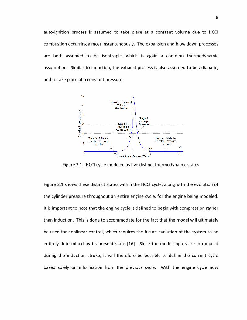
auto-ignition process is assumed to take place at a constant volume due to HCCI

combustion occurring almost instantaneously. The expansion and blow down processes

are both assumed to be isentropic, which is again a common thermodynamic

assumption. Similar to induction, the exhaust process is also assumed to be adiabatic,

and to take place at a constant pressure.

Figure 2.1: HCCI cycle modeled as five distinct thermodynamic states

Figure 2.1 shows these distinct states within the HCCI cycle, along with the evolution of

the cylinder pressure throughout an entire engine cycle, for the engine being modeled.

It is important to note that the engine cycle is defined to begin with compression rather

than induction. This is done to accommodate for the fact that the model will ultimately

be used for nonlinear control, which requires the future evolution of the system to be

entirely determined by its present state [16]. Since the model inputs are introduced

during the induction stroke, it will therefore be possible to define the current cycle

based solely on information from the previous cycle. With the engine cycle now

9

assumed to be a discrete process, we now have the basis to create a discrete-time

control based model.

2.1.2 Inputs, Outputs and State Variables. Since the model being developed will

ultimately be used to synthesize a nonlinear controller, it must therefore be constructed

from a controls perspective. The model presented therefore includes three input

variables, both of which directly affect the combustion process. These inputs are

defined to be the following:

� the pre-heated intake temperature, Tin,k

� the fraction of external EGR, αe,k

� the mass flow rate of fuel, gpmk

These inputs, with k representing the kth

engine cycle, were chosen due to their physical

significance within the HCCI process. Since start of combustion is sensitive to changes in

reactant concentrations and temperature, these inputs therefore directly affect

combustion timing through temperature and dilution effects, respectively. The intake

temperature is controlled using a resistance heater placed in the intake stream, while

the external EGR and fueling rate are controlled using individual solenoids. In addition

to inputs, the model must also include certain output variables which can be used for

feedback to monitor and control the system. The first output chosen for this model was

the combustion phasing. Due to the desire for an actual engine to operate at some

optimal combustion timing, the model must therefore include an output variable which

represents this phenomenon in order to have the ability to control it. Similar to

operating at a desired combustion phasing, engines are also required to produce a

10

desired amount of work. In light of this, the second output was chosen to be the peak

pressure during each cycle, which then gives a basis for the work output from each

engine cycle. This allows the control model to formulate the work being produced, and

then optimize it to some desired value. In order to ensure that the engine remained

within an acceptable operating range, another output was chosen to be the peak

pressure rise rate during each cycle. Since the operating range is typically limited by the

pressure rise rate [17], it must therefore be included as an output in order to properly

control the engine. In addition, an efficiency term was also included as an output. This

efficiency term monitored the work output from the engine based on the amount of

fuel energy input, and therefore gave an indication of how “efficient” the engine was

operating. These outputs are summarized below:

� crank angle where combustion occurs, θ23,k

� peak pressure, P3,k

� pressure rise rate, PRRk

� work output, Wg,k

� efficiency, ηk

where k again denotes the kth

engine cycle.

In order to utilize state-space control methodologies, the model must also define

certain “states” which completely describe the dynamics of the system with respect to

the output variables being controlled. From a modeling perspective, it is preferable if

these “state” variables have some physical meaning so as to gain insight into their

influence on the various outputs from the system. With control of combustion phasing

central to the control effort, these “states” of the system should therefore be physically

11

related to both the reactant concentrations and charge temperature within each cycle,

which are the parameters central to combustion. One such parameter within the model

is the residual mass fraction, which serves to pass information from one cycle to the

next. This residual, or internal EGR, consists of burned gases at the exhaust

temperature of the previous cycle, and acts to simultaneously increase the temperature

and dilute the fresh reactant charge entering the cylinder. Another parameter related

to combustion timing is the temperature in the cylinder at IVC. Intake valve closing is

one of the discrete states within the model, and the corresponding temperature

indicates the charge temperature at the start of compression. Another parameter of

importance is the actual combustion phasing from the previous cycle. As timing is

varied, the exhaust temperature and amount of trapped residual will also vary, thus

having an impact on the phasing during the next cycle through the parameters

mentioned previously. All of these state variables were chosen due to their apparent

physical significance to the combustion process, and are summarized below:

� the amount of trapped residual, αi,k

� the initial mixture temperature at IVC, T1,k

� the crank angle where peak pressure occurs, θ23,k

With the inputs, outputs and state variables of the system defined, the various stages of

the HCCI engine cycle can now be investigated in order to relate each thermodynamic

state back to the inputs and state variables of the system.

12

2.2 EQUATION DERIVATION

2.2.1 Adiabatic Induction at Atmospheric Pressure – Instantaneous Mixing.

Prior to the start of the cycle, fresh reactants must first be inducted into the cylinder

during the induction stroke. This process is assumed to be adiabatic and to take place at

atmospheric pressure. Pre-heated intake air, fuel and external EGR (αe) are all inducted

into the cylinder when the intake valve opens, and are assumed to instantaneously mix

with the trapped residual in the cylinder at the instant of IVC. In order to determine the

thermodynamic state of the mixture at intake valve closing, the chemistry of the

mixture must first be investigated. Since HCCI engines are capable of running on many

different types of fuels, this chemistry will vary depending on the type of fuel being

used. The current model focuses on gasoline-type fuels, and is later validated using data

from an engine running on UTG96, which has a C/H ratio equal to 7.2/15.8. Although

any gasoline-type fuel can be used, one with a C/H ratio equal to 7/16 is chosen as the

fuel in this analysis due to its similarity to the aforementioned validation fuel. As a

check, isooctane (C/H=8/18) was also investigated and it was determined that the

model produced very similar results for both C/H ratios. In order to determine the state

of the mixture, combustion of this gasoline-type fuel (C/H = 7/16) with atmospheric air

is performed under stoichiometric conditions.

( ) ( )1.236.418776.311 22222167 NOHCONOHC ++→++

Now assuming lean combustion (typical of HCCI engines [1]) with stoichiometric air and

both internal and external EGR, the inducted reactant charge becomes:

13

( ) ( )( )( ) ( )2.211136.4187

36.5276.311

2222

222167

ONOHCO

NNOHC

i

e

φφφα

φαφ

−+++

+++++

whereφ is the equivalence ratio, defined as the ratio of moles of fuel to the

stoichiometric amount, αi is the fraction of internal EGR and αe is the fraction of external

EGR added. This external EGR fraction is defined as the molar ratio of external EGR to

reactants, and is initially modeled using the inert gas N2. With the chemistry of the

intake charge now known, the First Law of Thermodynamics can be applied to the

mixing process in order to determine the state of the mixture at IVC, where the

reactants are assumed to instantaneously mix. Assuming the air and external EGR enter

at constant temperatures of Tin and Tegr, respectively, the resulting expression for the

First Law applied to the kth

engine cycle becomes:

( ) ( ) ( ) ( ) ( )3.2EGR mix

,1,,,,,

products reactants

,,,,,, ∑ ∑∑ ∑ =++ kkikikegrkikikinkikikprodkiki ThNThNThNThN

where Ni,k is the number of moles of species i, kih , is the molar enthalpy of species i, Tprod,k

is the temperature of the trapped residual and T1,k is the temperature of the reactants

and products after full mixing. Assuming constant specific heats, the molar enthalpy

becomes:

( ) ( ) ( )4.2,, refipifi TTchTh −+∆=

where ifh ,∆ is the molar heat of formation of species i and Tref is the reference

temperature corresponding to the heat of formation. Applying Equation 2.3 to Equation

2.2 yields the following in-cylinder mixture temperature at intake valve closing (IVC):

14

( )5.2,1,,1,21,1

,1,1,,,1,21,1,1

,1

kekegrkikk

kegrkekegrkprodkikkink

kccc

TcTcTcT

αα

αα

−−−

−−−−−

++

++=

where

( )( ) ( )

( ) ( )8.236.52

7.211136.4187

6.236.4111

2

2222

22167

,

111,2

,1

Npkkegr

OpkNpOHpkCOpkk

NpOpHCpkk

cc

ccccc

cccc

+=

−+++=

++=

−−−

φ

φφφ

φ

represent averaged specific heats for the reactants, trapped residual and external EGR,

respectively. In Equation 2.5, Tprod is the temperature of the residual, which can be

directly related to the exhaust temperature of the previous cycle via the following linear

relationship

( )9.21,5, −= kkprod TT ξ

where ξ represents heat loss during the valve overlap period. This parameter was

determined by synchronizing the model temperatures at IVC with those extracted from

the experimental data. Plugging Equation 2.9 into Equation 2.5 results in the following

expression for the mixture temperature at intake valve closing:

( )10.21,,21

,1,1,5,21,1

,1

−

−−−

++

++=

keegrki

kegrkeegrkkikin

kccc

TcTcTcT

αα

αξα

2.2.2 Isentropic Compression. The engine cycle is defined to start at the

beginning of the compression process at IVC. This compression of the freshly inducted

reactant charge made up of fuel, air and EGR is assumed to be isentropic, which implies

the following relationships:

15

( )

( )12.2

11.2

,1

,23

1,2

,1

1

,23

1,2

k

k

k

k

k

k

PV

VP

TV

VT

γ

γ

=

=

−

State 2 is defined to be at the end of compression just before the onset of combustion.

In these relations, V1, T1 and P1 represent the volume, temperature and pressure at

intake valve closing, respectively. The parameter γ represents the ratio of specific

heats, and is set to 1.3 in this analysis, which is a reasonable approximation for the

working fluid. Also, V23 signifies the volume at which the constant volume combustion

event occurs. This volume can be determined using the simple slider-crank relations

from [18], where θ23,k represents the crank angle at which the constant volume

combustion occurs.

( ) ( ) ( )( )[ ] ( )13.2sincos115.01 ,23

22

,23,23 kkcck RRrVV θθ −−−+−+=

2.2.3 Constant Volume Combustion. The auto-ignition process in HCCI engines

occurs almost instantaneously throughout the cylinder, and is therefore assumed to

take place at a constant volume. It is also assumed that all heat transfer occurs during

the combustion event. A model which utilizes an Integrated Arrhenius Rate to predict

the location of this combustion event is discussed later. Using the chemistry of the lean

intake charge in Equation 2.2, along with the assumption of complete combustion, the

overall combustion reaction becomes:

16

( )( ) ( ) ( )( )

( ) ( ) ( ) ( )( )( ) ( )14.2 111

36.52136.4187

87

36.52136.411111

21,11,

2,1,21,121,1

21,121,1

2,1,211,167

O

NOHCO

OHCO

NOHC

kikkki

kkekikikkkikk

kikkik

kkekikkik

+−+

++−+−

+−+−

+−+

−−+

++++++++

→+

++++++−+

αφφα

φαααφφαφφ

αφαφ

φααφαφ

In order to determine the thermodynamic state of the system after combustion, the

First Law is again applied. Since both the intake and exhaust valves are closed during

the compression stroke, the cylinder is therefore modeled as a closed system and the

First Law takes the form

( )15.2WQU −=∆

Since combustion occurs instantaneously, the cylinder volume does not change and

therefore no work is produced. The heat transfer term in Equation 2.15 can be

approximated to be a certain percentage of the chemical energy available before

combustion. Applying these assumptions to the expression in Equation 2.15, the First

Law now becomes:

( )16.2,167167,3,2 βkHCHCkk NLHVUU +=

where LHVC7H16 and NC7H16 represent the lower heating value and moles of fuel,

respectively. In Equation 2.16, the parameter β represents the percentage of chemical

energy that is lost to heat transfer during combustion. This parameter was set to 0.1,

which represents the approximate energy loss due to heat transfer as given in [18].

Utilizing the definition of internal energy in [18], along with the ideal gas law, the

expression in Equation 2.16 can be rewritten in terms of enthalpy

17

( )17.21671673 ,3,,,,22 ,,, βHCHCkukikikikukikiki NLHVTRNhNTRNhN +−=− ∑∑

Substitution of the combustion reaction parameters from Equation 2.14 into the

expression in Equation 2.17 yields the following expression for the temperature inside

the cylinder immediately after combustion, defined as State 3.

( ) ( ) ( )18.2,31,41,1,,1,2

1,41,1,2,21,1,,1,21,11,3

,3

kukkekegrkik

refkkkkukekegrkikkk

kNRccc

TccTNRccccT

−++

−−−+++=

−−−−

−−−−−−−

αααα

where

( )( )

( ) ( ) ( )( ) ( ) ( ) ( )19.236.52136.524

36.5236.5236.524

11136.4187

1

11,,,11,3

111,2,,2

111,4

1671,3

2222

+++++=

+++++=

−+++=

−=

−−−−

−−−−

−−−

−

kkekikikkk

kkkekkik

OpkNpOHpkCOpkk

HCkk

N

N

ccccc

LHVc

φαααφφ

φφαφα

φφφ

βφ

The parameters N2 and N3 here represent the number of moles in the cylinder before

and after combustion, respectively. In addition, Tref represents the reference

temperature of 298 K corresponding to the heat of formation.

Applying the ideal gas law before and after combustion, and recalling that

combustion occurs at a constant volume, results in the following expression.

( )20.2,2

,3

,2

,2

,3

,3

k

k

k

k

k

kT

TP

N

NP =

In an effort to define P3 solely in terms of temperature, the expression in Equation 2.18

can be rearranged to yield:

18

( ) ( ) ( )21.2,21,1,,1,21,1

1,31,41,1,3,31,41,1,,1,2

,2

kukekegrkikk

krefkkkkukkekegrkik

kNRccc

cTccTNRcccT

−++

−−+−++=

−−−−

−−−−−−−

αααα

Substituting Equations 2.12 and 2.21 into Equation 2.20 results in an expression for the

pressure immediately after combustion which represents the peak pressure seen during

the engine cycle.

( ) ( ) ( )22.2,3

1,31,41,1,3,31,41,1,,1,2

,21,1,,1,21,1

,23

1

,2

,3

,3 katm

krefkkkkukkekegrkik

kukekegrkikk

kk

k

k TPcTccTNRccc

NRccc

V

V

N

NP

−−−−−−−

−−−−

−−+−++

−++

=

αααα

γ

2.2.4 Isentropic Expansion. Following combustion, the piston travels

downwards during the expansion stroke, which produces useful work from the engine.

This expansion process, which takes place until the opening of the exhaust valve, is

assumed to be isentropic, which implies the following relationships:

( )

( )24.2

23.2

,3

4

,23

,4

,3

1

4

,23

,4

k

k

k

k

k

k

PV

VP

TV

VT

γ

γ

=

=

−

Here, State 4 is defined as the end of the expansion stroke at the instant of exhaust

valve opening. In these relations, T3 and P3 represent the temperature and pressure

immediately after combustion, respectively. The parameters V4 and V23 represent the

cylinder volumes at EVO and at which the constant volume combustion event occurs,

respectively. Both of these cylinder volumes can be calculated using the simple slider-

crank relation in Equation 2.13 along with the appropriate crank angle.

19

2.2.5 Isentropic Blowdown to Constant Pressure Exhaust. The exhaust stroke,

which is defined from exhaust valve opening to intake valve opening, is also assumed to

take place at constant pressure. An instantaneous blowdown to atmospheric pressure

is assumed to occur at EVO, which then allows this adiabatic exhaust process to take

place at atmospheric pressure. Under these assumptions, a relation for the

temperature at State 5 (intake valve opening) can be written.

( )25.2,4

1

,4

,5 k

k

atmk T

P

PT

γγ −

=

2.3 RESIDUAL GAS FRACTION MODEL

The amount of residual gas in HCCI engines has a profound effect on emissions,

combustion stability and volumetric efficiency. Residual gas affects the combustion

process in HCCI engines through its influence on both the dilution and temperature of

the overall charge mixture. This becomes particularly important when dealing with HCCI

engines. Since HCCI combustion depends entirely on chemical kinetics in order to occur,

both the dilution and the temperature of the charge mixture will directly affect the

combustion phasing of the engine. According to chemical kinetics models, HCCI

combustion is governed by two main parameters: the concentrations of fuel and

oxygen, and the temperature. This means that changing the concentration and/or the

temperature of the intake charge will cause the combustion phasing to change. The fact

that the residual gas fraction directly affects both the reactant concentrations and the

temperature, makes it an important parameter when trying to model combustion timing

20

in an HCCI engine. Therefore, a practical and accurate model for predicting the residual

gas fraction xr is needed in order to accurately predict the combustion timing.

The predictive model used was taken from [14], which was based on the widely

accepted model developed in [19]. This model predicted the overall residual gas

fraction as a combination of two components: the contribution of back-flow from the

exhaust to the cylinder during valve overlap, and the trapped gas in the cylinder at

exhaust valve closing. The amount of residual trapped in the cylinder at EVC can be

estimated fairly accurately with knowledge of the compression ratio. The flow

processes during the valve overlap period, however, are very complex and are therefore

difficult to model correctly. For most engine speeds, the cylinder contents equilibrate

with the exhaust system during the exhaust stroke and are roughly at atmospheric

pressure. The intake port, on the other hand, is generally below atmospheric pressure,

which results in a net flow of burned gas into the cylinder from the exhaust manifold

[19]. This back-flow contributes significantly to the residual gas fraction for each engine

cycle. The parameter often used to describe this back-flow is the valve overlap factor

(OF). An empirical expression for OF is given in [19] when the valve overlap duration is

known, and can be seen in Equation 2.26 below.

( ) ( )26.28.710745.1

2

max,2

B

DL

BOF vv

ovov θθ ∆+∆+=

In Equation 2.26, OF is the valve overlap factor in degrees/meter, Δθov is the valve

overlap in crank angle degrees, B is the engine bore in mm, Lv,max is the maximum valve

21

lift in mm, and Dv is the valve inner seat diameter in mm. This expression gives a good

estimate of OF for most typical engine geometries.

Once the overlap factor, OF, is known, an expression for the overall residual gas

fraction can be determined. The empirical expression from [14] is given below in

Equation 2.27.

( )27.21

18.153178.4exp1401.0

5.47.0

e

i

i

e

ce

i

i

e

e

i

e

ir

T

T

P

P

rT

T

P

P

P

P

P

P

N

OFx +

−−

−−−=

In Equation 2.27, xr is the residual gas fraction, OF is the valve overlap factor in

degrees/meter, N is the engine speed in rev/sec, Pe and Pi are the exhaust and intake

pressures, respectively, in bar, Te and Ti are the exhaust and intake temperatures,

respectively, in Kelvin, and rc is the compression ratio. This resulting model relates the

residual gas fraction to six independent parameters: engine speed (N), inlet and exhaust

pressures (Pi and Pe), the valve overlap factor (OF), inlet temperature (Ti), and the

compression ratio (rc). The first part of the expression gives the contribution from the

valve overlap period, while the second part relates to the amount of gas trapped in the

cylinder at exhaust valve closing. The sum of these two components gives the total

predicted residual.

This model for predicting the residual gas fraction was abstracted from [14].

This model explicitly accounts for the contributions from both the back-flow of exhaust

gas into the cylinder during the valve overlap period and the gas trapped in the cylinder

at exhaust valve closing. The model correlated well with experiment over a wide range

22

of intake pressures and engine speeds [14], which means that it should provide an

accurate prediction of the residual gas fraction. It is important to note that the residual

fraction will be a small number for most operating conditions. When no external EGR is

implemented on the engine, the residual gas fraction will have a noticeable effect on

the combustion phasing due to the fact that it will dilute and increase the temperature

of the reactant mixture. On the other hand, if there is some external EGR, then the

effect of the residual gas fraction will be minimal. In this case, the amount of EGR will

typically be far greater than that of the residual gases, which will result in the external

EGR having a dominant effect on both the dilution and temperature of the reactant

charge.

2.4 DENSITY AND EGR DISPLACEMENT EFFECTS

When intake temperature is used as an input in order to achieve HCCI, a side

effect is that the density of the intake air also changes as the temperature is varied. This

allows for different amounts of air to be inducted at different intake temperatures,

which will ultimately have a slight effect on the equivalence ratio. Using the ideal gas

law, the moles of air inducted per cycle can be represented by:

( )28.2inu

dinA

TR

VPN =

This relationship assumes that induction occurs at atmospheric pressure, and therefore

allows the moles of air to be calculated based on a given intake temperature. The

displacement volume is used in this case due to the clearance volume being occupied by

23

residual from the previous cycle. For a given fueling rate then, the moles of fuel

inducted per cycle can be determined by

( )29.22

f

f

FMWN

mN

⋅=

&

where fm& is given in grams/min. and N is given in RPM. Once the relative amounts of

fuel and air are known, the next parameter of interest is the amount of fuel required to

achieve stoichiometric conditions within the cylinder. Using the relationship for the

stoichiometric F/A ratio, along with the moles of air calculated using Equation 2.28, the

stoichiometric moles of fuel are given by

( )( )30.2

f

stoicaA

FsMW

AFMWN

N =

Equations 2.28-2.30 allow the amount of air inducted into the cylinder to vary based on

the given intake temperature. This allows the equivalence ratio to vary slightly as

temperature is varied, which is what is observed in the experimental data.

When EGR is introduced into the cylinder during induction, it acts to displace

some of the fresh reactant charge that would otherwise get inducted into the cylinder.

In order to account for this displacement effect, the amount of air inducted into the

cylinder must therefore be reduced as the amount of EGR is increased. In order to

determine the amount of air displaced by this EGR, the total capacity of the overall

cylinder must be determined first. This cylinder capacity can be determined using the

ideal gas law along with the total volume of the cylinder.

24

( ) ( )31.2inu

cdinT

TR

VVPN

+=

The expression in Equation 2.31 allows the total amount of moles inducted to change as

the intake temperature is varied, which is necessary in order to capture the density

effects described previously. Due to valve timings and engine geometry, a small portion

of this total volume is made up of trapped residual gas that is carried over from the

previous cycle. The amount of this residual that is present in the cylinder can be

determined using the residual fraction, αi, along with the expression in Equation 2.31.

( )32.2TiiEGR NN α=

Since we are introducing EGR into the cylinder in this case, another portion of the total

cylinder volume will also be occupied by external EGR. In order to determine the

number of moles inducted into the cylinder, the mole fraction of external EGR must first

be calculated. Using the expression in Equation 2.2

( )( )( ) ( )( )

( )33.215.12471715.59

5.59

φφααφφα

−++++++

=ie

eEGRX

where φ and eα are the equivalence ratio and external EGR fraction which were defined

previously. The expression in Equation 2.33 can then be used to calculate the number

of moles of EGR inducted into the cylinder.

( )34.2TEGREGR NXN =

25

Now that the residual and EGR have been accounted for, the remainder of the cylinder

volume can be filled with fresh air. In order to capture the displacement effect of the

EGR, however, the amount of air inducted must be calculated using partial pressures.

Based on the contents of the cylinder, this partial pressure expression becomes

( )35.2PXPXPXP AiEGREGR ++=

Plugging Equations 2.31, 2.32 and 2.34 into Equation 2.35 results in a partial pressure

expression in terms of moles rather than mole fractions.

( )36.2in

T

Ain

T

iEGRin

T

EGRin P

N

NP

N

NP

N

NP ++=

Rearranging the expression in Equation 2.36 yields:

( )37.2iEGREGRTA NNNN −−=

This expression accounts for the displacement effect by allowing the moles of air

inducted to vary based on the amount of external EGR being introduced. With the

moles of air now known, the moles of fuel required for a stoichiometric mixture can

now be calculated using the expression in Equation 2.30. The density and displacement

effects present for the case of external EGR have been accounted for in Equations 2.31

and 2.37, respectively, which allow the model to accurately predict the amounts of fuel

and air being inducted into the cylinder for each cycle.

26

2.5 MODELING THE ONSET OF COMBUSTION

Unlike conventional spark and compression ignition engines, HCCI engines have

no specific combustion initiator. Instead of being initiated by a spark or the injection of

fuel, HCCI ignition depends entirely on the chemical kinetics [1,2,3]. If the reactant

concentrations and temperature reach sufficient levels during compression, then an

auto-ignition process will occur. Combustion timing is therefore directly linked to the in-

cylinder concentrations of reactants, their temperature and their pressure [1,2,3]. Due

to this dependence on chemical kinetics, ensuring that combustion occurs with

acceptable timing, or even at all, is much more complicated than in the case of either

spark or compression ignition engines. Since the combustion timing plays such a vital

role in the HCCI process, choosing an appropriate model to represent it is therefore

crucial.

Since the goal is to create a control-oriented model, the combustion timing

model chosen must predict both the pressure evolution in the cylinder and, more

importantly, the combustion timing. The pressure evolution directly correlates to the

work output from the engine, while the combustion timing acts to govern this pressure

evolution from cycle to cycle. Therefore, if the combustion timing model can accurately

predict the ignition timing, then it should also be able to predict the pressure evolution

in the cylinder. Since the combustion timing directly controls how the engine will

perform, then choosing a combustion timing model that accurately predicts how the

timing will change from engine cycle to engine cycle is imperative to ensure the validity

of the overall model. Therefore, a great deal of time was spent on choosing an

27

acceptable combustion timing model that would accurately predict the changes in

ignition timing as input conditions were varied. A number of different models were

considered [20-25] throughout the selection process before narrowing the possible

models down to the five most promising. The following sections present these five

different models that were investigated for predicting the onset of combustion. These

models include a modified knock integral [26], three different ignition delay models [27-

29] and an integrated Arrhenius rate model [13]. In each of the five different models, a

lean reaction of air and a gasoline-type fuel is considered. The focus is restricted to

gasoline-type fuels in order to eliminate the complexities of low temperature heat

release that are typically associated with diesel-type fuels. A lean reaction requires that

the equivalence ratio, φ , be less than one. The stoichiometric (φ =1) and rich (φ >1)

cases need not be investigated due to the fact that HCCI is a purely lean strategy by

nature. For the lean case then, with the assumption of complete combustion and no

exhaust gas recirculation, the global combustion reaction used in each model is given

by:

( ) ( )38.211136.418736.4111 222222167 ONOHCONOHC φφφφ −+++⇒++

In order to verify whether or not the combustion timing models were correctly

predicting the ignition timing, the simulation was compared with actual engine data

from a Hatz HCCI engine. The geometry and other engine parameters for the Hatz

engine can be found in Table 2.2.

28

Table 2.2: Hatz engine parameters

In the experiment, the temperature of the incoming air was varied, with the equivalence

ratio being held constant, in order to effectively change the ignition timing from cycle to

cycle. The same thing could then be done in the model by simply changing the intake

temperature. This was done for several different intake temperatures, and the model

results were then compared to the experimental results in order to determine which

model predicted the onset of combustion the best.

2.5.1 Modified Knock Integral Method. The first of the four combustion timing

models investigated was that of a modified knock integral. This was a reasonable model

to look at first, due to its similarities to the original knock integral [30]. In order to

understand why a modified knock integral method is necessary, the original knock

integral must be investigated first. The knock integral method was originally developed

in order to investigate the premature ignition of the fuel and air mixture prior to the

spark, called knock, in spark ignition engines. Since HCCI combustion depends on the

auto-ignition of a fuel and air mixture, the knock integral method would seem to be a

very good way to model it. Livengood and Wu [30] developed the first correlation to

29

predict the auto-ignition of a homogeneous fuel and air mixture, which was later called

the Knock Integral Method. This method is based upon the ignition delay time of the

fuel under consideration, and the resulting empirical relationship is given by:

( ) ( )39.2nPTbAe=τ

where τ is the ignition delay time, T is the mixture temperature as a function of crank

angle, P is the mixture pressure as a function of crank angle, and A, b and n are empirical

constants that are determined experimentally for each fuel.

Livengood and Wu discovered that there is a functional relationship between the

concentrations of the significant species in the reaction and the time it takes to

complete the reaction. When time is replaced by crank angle via the engine speed, the

ignition correlation for the knock integral becomes:

( )( )40.21

11== ∫∫ θ

ωθ

τω

θθd

Aed

knock

n

knock

IVC PTbIVC

where θknock is the crank angle at which knock occurs and IVC is the crank angle of intake

valve closing. The engine speed, denoted as ω, has units of RPM, the pressure has units

of KPa and the temperature has units of degrees Kelvin. The integration is started at

intake valve closing due to the fact that compression, and therefore any type of

appreciable reaction, begins at this point. The value of the integrand continues to

increase as the auto-ignition point is reached, which is shown in Figure 2.2 below.

30

Figure 2.2: Graphical integration of the knock integral from intake valve closing

Once the integral becomes equal to one, the upper limit is said to be the crank angle at

which auto-ignition, or knock, occurs. The integral seen in Equation 2.40, then, is

ultimately able to predict at what crank angle knock, or auto-ignition will occur. This

ability to predict the auto-ignition point of a fuel-air mixture makes the knock integral a

very appealing approach to try and predict the start of combustion in HCCI applications.

In order to make the transition from spark ignition to HCCI, however, the knock integral

must first be modified in order to account for a greater dependence upon chemical

kinetics.

The modified knock integral combustion model that was investigated was

abstracted from previous work done by [26]. In this model, Swan took the original

knock integral and simply added a few terms in order to make it applicable to HCCI

combustion. Since HCCI combustion depends so heavily upon chemical kinetics, terms

were added to the integral in order to account for things such as fuel and oxygen

31

concentrations, and varying EGR rates. The compression process was considered to be

polytropic (PVγ=constant) due to the fact that temperature and pressure as a function of

crank angle are usually unknown on an actual engine. At this point, Swan had

developed a modified knock integral that included species concentrations as well as

simplified temperature and pressure relationships. In order to simplify the model even

further, the concentration terms were replaced by the equivalence ratio since

concentrations as a function of crank angle are also unknown on a real engine. With

these simplifications, the working equation for the Modified Knock Integral Method [26]

becomes:

( )

( )( )( )θ

θ

θφ

ω γ

γ

V

Vvwhere

d

vT

vPbA

IVCc

xSOC

IVC

cIVC

n

cIVC

=

=

∫−

41.2

1

exp

1

1

In Equation 2.41, PIVC is the pressure at intake valve closing and TIVC is the temperature

at intake valve closing. It is evident from Equation 2.41 that the modified knock integral

is very similar to the knock integral, with the exception of a few terms. For the modified

knock integral, the remaining parameters A, b, n, x are constants that must be

determined experimentally for each fuel. These constants were determined for C7H16

using an engine geometry similar to that of the Hatz engine [Swan], and can be seen

below in Table 2.3. The value for A in Table 2 contains an EGR term, which is the

amount of exhaust gas recirculation being used on the engine. In this model, the EGR

32

must be entered in as a percentage of the total intake charge. With these parameters

known, the modified knock integral can now be plugged directly into the control model

in order to approximate the onset of combustion.

Table 2.3: Combustion Parameters for the Modified Knock Integral Method

In order for the modified knock integral to be able to predict the combustion timing at

various inlet conditions, it must first be initialized at some experimental data point. To

accomplish this, the experimental data point corresponding to a combustion timing of

354.1 crank angle degrees was used since it was the most advanced. In order to

initialize the modified knock integral then, this experimental timing value was plugged in

as the upper limit of integration. With the integration limits now known, the engine and

combustion parameters from Tables 2.1 and 2.2 were used in Matlab to numerically

integrate the expression in Equation 2.41. This resulted in an integrated value for the

modified knock integral that correlated with the experiment at one operating point.

This integrated value could now be interpreted as a threshold value for the modified

knock integral, that when held constant at various inlet conditions, would allow for the

33

combustion timing to be tracked by the combustion model. The threshold value which

was calculated for the modified knock integral method can be seen in Equation 2.42.

( )42.23624.0, =MKIMthK

With the threshold now established, the next step was to simply vary the inlet

conditions in the control model by changing the intake temperature from 170oC to

190oC in 5 degree increments, and see how well it tracked the combustion phasing as

compared to the experiment. The results of this comparison can be seen below in

Figure 2.3.

Figure 2.3: Modified Knock Integral Method combustion tracking

Figure 2.3 shows that the modified knock integral fails to capture the

combustion phasing at different operating conditions. This is evident due to the fact

that the slopes of the two lines are different. The experimental timing values vary about

34

6 crank angle degrees, while the values predicted by the modified knock integral only

vary approximately 4 crank angle degrees. The modified knock integral and experiment

both predict the same start of combustion value for the intake temperature of 445oC,

which is due to the fact that this is the experimental data point which was used for

initialization. As the intake temperatures vary from the initialization point, the modified

knock integral becomes less and less accurate. This method accurately predicts the

correct trend for the onset of combustion, but the overall magnitudes differ significantly

from those in the experiment. Even though the modified knock integral accounted for

changes in reactant concentrations, it was still unable to accurately predict the

combustion timing for different inlet conditions. Since accurate prediction of the

combustion phasing is vital to the operation of the overall control model, the Modified

Knock Integral Method was therefore dismissed as a possible combustion timing model.

2.5.2 Ignition Delay 1. The next combustion timing model to be investigated

was that of Ignition Delay 1, which was incorporated from previous work by [27].

Similar to the Modified Knock Integral Method, this method also attempts to utilize the

original knock integral in order to predict the onset of combustion in HCCI applications.

The starting point for this model is the same knock integral introduced above in

Equation 2.40. The limits of integration for this integral remain the same, with the

upper limit being the crank angle at which combustion occurs and the lower limit being

the crank angle of intake valve closing. From the initial integral, it can be seen that the

combustion timing is directly related to both the engine speed and the ignition delay of

the fuel being used. While the Modified Knock Integral Method attempted to add terms

35

to this integral in order to account for reactant concentrations, the Ignition Delay 1

model [27] focuses on formulating a more detailed expression for the ignition delay of

the fuel. Since the ignition delay in compression ignition engines governs when the fuel

will ignite, then the ignition delay in HCCI applications would seem to govern when the

mixture will auto-ignite. Therefore, if a detailed expression for the ignition delay can be

generated, it should be able to track the onset of combustion. How accurately it

predicts the combustion phasing then, will depend solely on the accuracy of the ignition

delay expression itself. To this end, [27] strove to derive an expression for the ignition

delay that would correlate with experimental data that he had collected. In order to

derive this expression, [27] started with a physics based correlation for the ignition

delay that assumed it was a function of temperature and pressure only. This correlation

can be seen below in Equation 2.43:

( )43.2exp 31

2

=T

CPC

Cτ

where C1, C2, and C3 are constants that must be experimentally determined. In order to

make the expression more detailed, various terms were added in order to account for

changes in the air/fuel ratio, the exhaust gas recirculation (EGR) rate and the engine

speed [27]. The addition of these terms is important due to the fact that they will all

directly affect the ignition delay time. The air/fuel ratio is a measure of how much fuel

is injected each cycle, which will have an obvious impact on the ignition delay. The

amount of EGR will also have an impact due to the fact that it effectively dilutes the

reactant charge. Therefore, a high EGR rate should correspond to a longer ignition

36

delay. With the addition of these terms, the new expression for the ignition delay in

[27] becomes:

( ) ( )44.2exp 865

2

42173

++=T

CPCEGRCEGRCCC cC

ccc

C

ccccλτ

In Equation 2.44, λ is the air/fuel ratio, P is the cylinder pressure in (atm) as a function of

crank angle, T is the cylinder temperature in (K) as a function of crank angle and the

remaining values are constants that must be determined experimentally for each fuel.

This ignition delay expression was calibrated using a 97-RON fuel on an engine with

similar geometry to the Hatz [27], and the resulting constants can be seen below in

Table 2.4.

Table 2.4: Combustion Parameters for Ignition Delay 1

The value for the air/fuel ratio in this model was determined from the

equivalence ratio in Table 2.4. Also, the value for the EGR rate in this model is now a

fraction rather than a percentage [27]. With these combustion parameters now known,

the detailed expression for the ignition delay can now be plugged directly into the

37

original knock integral in order to develop the working expression for the Ignition Delay

1 combustion timing model. This expression can be seen below in Equation 2.45.

( )( )45.2

exp

1

865

2

42173

∫

++

SOC

IVC cC

ccc

C

ccT

CPCEGRCEGRCCC ccλω

The expression seen in Equation 2.45 is the final result of [27], and is what will be

plugged into the control model in order to approximate the onset of combustion.

In order to allow the ignition delay expression to predict the combustion timing

at various inlet conditions, it must first be initialized at some experimental data point.

To accomplish this, the experimental data point corresponding to a combustion timing

of 354.1 crank angle degrees was used since it was the most advanced. In order to

initialize the ignition delay expression in Equation 2.45 then, this experimental phasing

value was plugged in as the upper limit of integration. With the integration limits now

known, the engine and combustion parameters from Tables 2.2 and 2.4 could be

plugged into Matlab in order to numerically integrate the expression in Equation 2.45.

This resulted in an integrated value for the knock integral that correlated with the

experiment at one operating point. This integrated value was again interpreted as a

threshold value, that when held constant at various inlet conditions, would allow for the

combustion timing to be tracked by the combustion model. The threshold value which

was calculated for the Ignition Delay 1 model can be seen below in Equation 2.46.

( )46.28567.01, =IgDelthK

38

With the threshold now established, the inlet conditions in the control model could

again be varied by changing the intake temperature in the same manner as stated

previously. The resulting values of combustion phasing could then be compared directly

to the experimental values in order to see how well they correlated. The results of this

comparison can be seen below in Figure 2.4.

Figure 2.4: Ignition Delay 1 combustion tracking

Figure 2.4 shows that Ignition Delay 1 also fails to capture the combustion

phasing at different operating conditions. This is evident due to the fact that the slopes

of the two lines are again significantly different. The experimental timing values vary

about 6 crank angle degrees, while the values predicted by the ignition delay model

don’t show any advance in the phasing whatsoever. The ignition delay and experiment

both predict the same start of combustion value for the intake temperature of 170oC,

which is due to the fact that this is where they were initialized. As the intake

39

temperatures vary from the initialization point, the experimental data shows that the

combustion phasing advances. The Ignition Delay 1 combustion model, however,

predicts constant combustion timing throughout the entire range of input

temperatures. This method does not predict the correct trend for the onset of

combustion, which results in values for the start of combustion that are drastically

different than those in the experiment. The reason that this ignition delay model seems

to predict constant combustion phasing may be due to the fact that the expression for

the ignition delay failed to account for the reactant concentrations explicitly. Since HCCI

combustion depends so heavily on the chemical kinetics, not properly accounting for the

varying concentrations can lead to inaccurate results. Even though the Ignition Delay 1

model accounted for changes in the air/fuel ratio, it was still unable to accurately

predict the combustion timing for different inlet conditions. Once again, since accurate

prediction of the combustion phasing is vital to the operation of the overall control

model, the Ignition Delay 1 model was also dismissed as a possible combustion timing

model.

2.5.3 Ignition Delay 2. Following along with the idea of the knock integral, the

next combustion timing model to be investigated was that of Ignition Delay 2, which

was incorporated from previous work by [28]. Identical to the Ignition Delay 1 model,

this method again attempts to utilize the original knock integral in order to predict the

onset of combustion in HCCI applications. The starting point for this model is again the

same knock integral introduced in Equation 2.40. The limits of integration for this

integral remain the same, with the upper limit being the crank angle at which

40

combustion occurs and the lower limit being the crank angle of intake valve closing.

From the initial integral, it can be seen that the combustion timing is directly related to

both the engine speed and the ignition delay of the fuel being used. Again identical to

Ignition Delay 1 [27], the Ignition Delay 2 [28] model focuses on formulating a detailed

expression for the ignition delay that can then be used with the knock integral. If a

detailed expression for the ignition delay can be generated, it should theoretically be

able to track the onset of combustion. How accurately it predicts the combustion

phasing, however, will again depend solely on the accuracy of the ignition delay

expression itself. To this end, an expression for the ignition delay that would correlate

well with experimental data was formulated [28]. In order to derive this expression,

[28] started with the same physics based correlation for the ignition delay that assumed

it was a function of temperature and pressure only. This correlation can be seen again

in Equation 2.47 below:

( )47.2exp 31

2

=T

CPC

Cτ

where C1, C2, and C3 are constants that must be experimentally determined. In order to

make the expression more detailed, various terms were added in order to account for

changes in both the equivalence ratio and the oxygen mole percentage [28]. The

addition of these terms is important due to the fact that they will both directly affect

the ignition delay time. The equivalence ratio is a measure of how much fuel is injected

each cycle, which will have an obvious impact on the ignition delay. The oxygen mole

percentage accounts for the varying reactant concentrations that the previous ignition

41

delay model left out. With the reactant concentrations now accounted for, this ignition

delay model has the potential to track the onset of combustion more accurately. With

the addition of these terms, the new expression for the ignition delay in [28] becomes:

( )48.2exp21

=

TR

EPC

u

ak

o

mn

c χφτ

In Equation 2.48, P is the cylinder pressure in (atm) as a function of crank angle, T is the

cylinder temperature in (K) as a function of crank angle, φ is the equivalence ratio, χ is

the oxygen mole percentage and the remaining values are constants that must be

determined experimentally for each fuel. This ignition delay expression was calibrated

using isooctane on an engine with similar geometry to the Hatz [28], and the resulting

constants can be seen below in Table 2.5.


With these combustion parameters now known, the detailed expression for the ignition

delay can now be plugged directly into the original knock integral in order to develop

the working expression for the Ignition Delay 2 combustion timing model. This

expression can be seen below in Equation 2.49.

42

( )49.2

exp

1

21

∫

SOC

IVC

u

ak

o

mn

cTR

EPC χφω

The expression seen in Equation 2.49 is the final result of [28], and is what will be

plugged into the control model in order to approximate the onset of combustion.

In order to allow the ignition delay expression to predict the combustion timing


To accomplish this, the same experimental data point as the previous two combustion

models was used. In order to initialize the ignition delay expression in Equation 2.49,

the experimental start of combustion was plugged in as the upper limit of integration.

With the integration limits and combustion parameters now known, Matlab was used to

numerically integrate the expression in Equation 2.49. This resulted in an integrated

value for the knock integral that correlated with the experiment at one operating point.

This integrated value was again interpreted as the threshold value, that when held

constant at various inlet conditions, would allow for the combustion timing to be

tracked by the combustion model. The threshold value which was calculated for the

Ignition Delay 2 model can be seen below in Equation 2.50.

( )50.23475.02, =IgDelthK

With the threshold now established, the inlet conditions in the control model could

again be varied by changing the intake temperature. The resulting values of combustion

43

phasing could then be compared directly to the experimental values in order to see how

well they correlated. The results of this comparison can be seen below in Figure 2.5.


Figure 2.5 shows that Ignition Delay 2 does a good job of predicting the onset of

combustion. Unlike the previous two combustion timing models, the Ignition Delay 2

model produces a line with slope that is very similar to that of the experiment. This

shows that Ignition Delay 2 is accurately predicting both the correct trend in the

combustion phasing as well as the magnitudes. Where as the previous combustion

timing models seemed to be somewhat unaffected by changes in the intake

temperature, this model displays the appropriate sensitivity to changes in the inlet

conditions. While the Ignition Delay 2 model does a very good job of predicting the start

of combustion, there is another aspect of the model that is not very attractive when it

comes to implementation. The Ignition Delay 2 combustion parameters in Table 2.5

were experimentally determined in [28] using isooctane. Therefore, the expression for

44

the ignition delay in [28] is parameterized specifically for isooctane. This means that if a

different operating fuel is chosen, then this combustion model will fail to accurately

predict the start of combustion due to the fact the parameters are no longer valid.

Since the long term goal of the control model is to be able to apply it to different

engines operating on various fuels, this combustion model could lead to obvious

problems in the future. Therefore, due to the fact that the combustion parameters are

only valid for isooctane, the Ignition Delay 2 model was also dismissed as a possible

combustion timing model.

2.5.4 Ignition Delay 3. Continuing on with the concept of the knock integral, the

next combustion timing model to be investigated was that of Ignition Delay 3, which

was previously developed by [29]. This model once again tries to utilize the original

knock integral in order to predict combustion timing for HCCI, and is once again based

on the original knock integral shown in Equation 2.40. Similar to the previous two cases,

the lower and upper limits of integration are once again the crank angle at which

combustion occurs and intake valve closing, respectively. From the initial integral, it can

once again be seen that the combustion timing is directly related to both the engine

speed and the ignition delay of the fuel being used. Also similar to the previous two

cases, the Ignition Delay 3 [29] model tries to utilize a more accurate ignition delay term

within the knock integral in order to accurately predict the onset of combustion. How

accurately it predicts the combustion phasing, however, will again depend solely on the

accuracy of the ignition delay expression itself. Rather than using an experimentally

45

determined ignition delay, this model utilizes an ideal Arrhenius expression which can

be seen in Equation 2.51.

( )51.2exp

= −

TR

EPA

u

aaτ

where A, Ea, and a are empirical parameters that are determined from combustion

kinetics experiments. Since the experimental data available uses a fuel chemically

similar to C7H16, the corresponding Arrhenius rate parameters [29] can be used and can

be seen in Table 2.6 below.


With these parameters known, the ideal Arrhenius ignition delay expression

could now be plugged directly into the knock integral in order to develop the working

expression for the Ignition Delay 3 combustion timing model. Due to the fact that this

model relied on the fact that combustion must occur close to TDC, the knock integral is

therefore evaluated at TDC conditions, which is evident in Equation 2.52 below.

( )52.21

1exp1111

θτω

θτ

ττω

dTTTR

E

P

Pd

SOC

IVC TDCTDCu

a

a

TDCTDC

SOC

IVC

TDC

TDC∫∫

−

=

In order to allow the knock integral expression in Equation 2.52 to predict combustion

timing values, it was initialized using the same experimental data point as in the

46

previous three models. With the start of combustion (354 CAD) and IVC (228 CAD)

known from experiment, the expression in Equation 2.52 was numerically integrated

using Matlab’s quadl function. This resulted in an integrated value for the knock integral

that correlated with the experiment at one operating point. This integrated value was

again interpreted as the threshold value, that when held constant at various inlet

conditions, would allow for the combustion timing to be tracked by the combustion

model. The threshold value which was calculated for the Ignition Delay 3 model can be

seen below in Equation 2.53.

( )53.20.007423, =IgDelthK

With the threshold now established, the intake temperature within the model could

again be varied in order to vary the combustion timing. These values could then be

directly compared to the experimental values in order to see how well they matched.

The results of this comparison can be seen below in Figure 2.6.


47

Figure 2.6 shows that Ignition Delay 3 does a fairly reasonable job of predicting

combustion timing. Unlike the previous models, however, the Ignition Delay 3 model

produces a line with a slightly greater slope than that of the experiment and therefore

over-predicts the onset of combustion for a given intake temperature. Despite this

slight over-prediction, the Ignition Delay 3 model displays an appropriate sensitivity to

changes in the inlet temperature, which make it a reasonable candidate for use in the

overall model. Another advantage over the previous models lay in the utilization of an

Arrhenius type ignition delay. While previous models have required experimentally

determined parameters specific to a given fuel, the Arrhenius expression of Ignition

Delay 3 uses Arrhenius parameters [31] which have been well documented for a number

of different fuels. This suggests that this particular model would be significantly more

robust to changes in fuel type due to the fact that the Arrhenius ignition delay

parameters have been previously calculated. Despite these apparent advantages,

however, the Ignition Delay 3 model stipulates that combustion must occur very close to

TDC. As the ignition timing moves away from TDC, the ignition delay expression in

Equation 2.52 becomes less and less accurate. Therefore, due to the fact that the

ignition delay expression is only valid at or near TDC, the Ignition Delay 3 model was also

dismissed as a possible combustion timing model.

2.5.5 Integrated Arrhenius Rate. The final combustion timing model to be

investigated was called the Integrated Arrhenius Rate model [13]. Rather than trying to

optimize the knock integral, the Arrhenius rate model takes a different approach which

focuses more heavily on the conclusion that both the temperature and the reactant

48

concentrations have the largest effect on HCCI combustion. This fact is again due to the

dependence of HCCI combustion on chemical kinetics. In reality, the combustion

process is made up of numerous sub-reactions that transform the reactants into

products. Due to the fact that these sub-reactions may contain hundreds of different

steps, they are very complex and difficult to model. Due to these complexities, utilizing

these sub-reactions to model combustion in a control oriented model is unrealistic due

to the fact that a control model must remain simple. In an attempt to simplify things

then, the overall combustion reaction is instead modeled by a single global reaction

rate. The reaction rate chosen to represent the overall combustion reaction is that of a

single Arrhenius reaction rate [13]. The Arrhenius rate is a physics based reaction rate

that is used for individual reactions in complex models with detailed chemistry. In the

case of the control model, however, it will act to relate the combustion reaction to both

the temperature and the reactant concentrations in the cylinder. Since these are the

two parameters that most greatly affect HCCI combustion, this single Arrhenius reaction

rate also has the potential of tracking the onset of combustion with a high level of

fidelity. Mathematically, this model involves the integration of a single Arrhenius

reaction rate expression [13]. Similar to the integration of the knock integral, the limits

of integration in this case will again be from the crank angle of intake valve closing to

the crank angle at which combustion occurs. These limits are again chosen due to the

fact that any appreciable reactions will begin with the compression stroke and continue

until the onset of combustion. This Integrated Arrhenius Reaction Rate [13] can be seen

below in Equation 2.54.

49

[ ] [ ]

( )∫

−

SOC

IVC

ba

u

a

d

OfuelTR

EA

54.2

exp 2

θω

The expression in Equation 2.54 contains concentration terms for both the fuel and

oxygen in the reactants, along with the engine speed, ω, in (rad/sec). The reactant

concentrations can be determined using the combustion reaction in Equation 2.38,

along with the cylinder volume. The remaining constants A, Ea/Ru, m and n are empirical

parameters that are determined from combustion kinetics experiments [31] for various

types of fuels. As described previously, the current study focuses on gasoline-type fuels

in order to eliminate the complexities associated with low temperature heat release.

Since the experimental data available uses UTG96 as a fuel, which is chemically similar

to C7H16, the corresponding Arrhenius rate parameters [31] can be used and can be seen

in Table 2.7 below. With the combustion parameters known for C7H16, the Arrhenius

Rate model can now be plugged directly into the control model in order to approximate

the onset of combustion.

Table 2.7: Combustion Parameters for the Integrated Arrhenius Rate

In order to allow the Arrhenius rate expression to predict the combustion timing


This data point was chosen to be the same as in the previous combustion models

50

investigated. In order to initialize the ignition delay expression in Equation 2.54, the

experimental start of combustion was again plugged in as the upper limit of integration.

With the integration limits and combustion parameters now known, Matlab was again

used to numerically integrate the expression in Equation 2.54. This resulted in an

integrated value for the Arrhenius rate that correlated with the experimental start of

combustion point of 354.1 CAD. This integrated value was again the threshold value,

that when held constant at various inlet conditions, would allow for the combustion

timing to be tracked by the combustion model. In other words, the threshold value was

calculated at one operating point and held constant at all others. This threshold value

which was calculated for the Integrated Arrhenius Rate model can be seen below in

Equation 2.55.

( )55.2104625.16

,

−= xK Arrhenth

With the threshold established, the model can now be run at various inlet temperatures

in order to verify whether or not the combustion phasing is being tracked accurately.

The inlet temperatures are again varied from 170oC to 190

oC in 5 degree increments in

order to be consistent with the temperature change in the experiment. The combustion

tracking results for the Arrhenius rate can be found below in Figure 2.7.

51

Figure 2.7: Integrated Arrhenius Rate combustion tracking

Figure 2.7 shows that the Integrated Arrhenius Rate model does an even better

job of predicting the onset of combustion. Just like the Ignition Delay 2 model, this

model also produces a line with a slope very similar to that of the experiment. This

shows that the Arrhenius rate is accurately predicting both the correct trend in the

combustion phasing as well as the magnitudes. Also similar to Ignition Delay 2, the

Arrhenius model also displays the appropriate sensitivity to changes in the inlet

conditions. Unlike the Ignition Delay 2 model, however, the Integrated Arrhenius Rate

model does not contain any shortcomings with respect to the combustion parameters.

Since the Arrhenius rate is a well known expression, there is a collection of combustion

parameters for many different types of fuels. This means that the Integrated Arrhenius

Rate [Shaver] model can be much more robust than the Ignition Delay 2 [28] model

when it comes time to switch fuels. Therefore, the Arrhenius rate model seems to be an

accurate and robust method for predicting the onset of combustion. Since accurate

prediction of the combustion phasing is central to the operation of the control model,

52

the Integrated Arrhenius Rate [13] model seems to be the best choice for the

combustion timing model due to both its simplicity and accuracy.

2.5.5.1 Prediction of Pressure Evolution. One more thing that must be

investigated before choosing the Integrated Arrhenius Rate as the combustion timing

model is whether or not it allows for accurate prediction of the pressure evolution in the

cylinder. As mentioned previously, while the combustion phasing is the most important

aspect of the combustion timing model, it must also be able to predict accurate trends

in the pressure evolution. This will allow the model to accurately predict the work

output from the engine. In order to verify whether the pressure is being tracked, the

same Arrhenius rate expression and parameters used to track the combustion timing

can be utilized. The only difference being that this time the pressure predicted by the

model will be compared to the experiment rather than the combustion phasing values.

These pressure trace comparisons for several different inlet temperatures can be seen

below in Figures 2.8-2.10.

Figure 2.8: Integrated Arrhenius Rate pressure comparison for an intake temperature of 190oC

53



These figures show that the Integrated Arrhenius Rate [13] model does in fact trace the

pressure evolution fairly accurately. As can be seen in the figures above, the pressure

traces basically lie on top of one another at every point throughout the entire cycle. The

only exception to this occurs at the crank angle of peak pressure, where the model

54

seems to slightly over-predict the value for the peak pressure. Even with this slight

over-prediction of the peak pressure, the values predicted by the model are still within

ten percent of the experimental values. Recognizing that the Arrhenius rate is a

somewhat simplified combustion timing model, these percent errors are therefore

within an acceptable tolerance and are surprisingly good. The ability of the Arrhenius

rate to accurately track the pressure evolution in the cylinder for varying inlet

temperatures suggests that it will also be able to track the work output from the engine.

Although this Integrated Arrhenius Rate [13] model is greatly simplified, it manages to

track both the combustion phasing and the pressure evolution with a high level of

accuracy, which can again be seen in Figures 2.7-2.10. With its credibility now verified,

the Integrated Arrhenius Rate model can now be confidently chosen to be the working

combustion timing model for the overall control model.

2.5.5.2 Arrhenius Rate Sensitivity. With the Integrated Arrhenius Rate model

now chosen to be the combustion timing model, a closer inspection is required in order

to fully understand its operation. The first aspect of the model that needs to be

investigated has to do with its sensitivity to the parameters that define it. The three

parameters of interest in this case are the exhaust gas recirculation term, α, the heat

transfer term, χ, and the activation energy term, Ea. The exhaust gas recirculation term

enters the Arrhenius expression in Equation 2.54 through the concentration terms via

the combustion reaction. If EGR is used on the engine, the combustion reaction in

Equation 2.38 will contain additional terms to represent it. These α terms will then

contribute to the species concentrations. The heat transfer term enters into the

55

Arrhenius expression through the ever present residual gas that is trapped in the

cylinder after each cycle. These trapped product gases act to increase the temperature

of the inlet air, which is what the heat transfer term, χ, is meant to represent. The

activation energy term is slightly different in that it is a part of the original Arrhenius

expression itself. This term is meant to represent the energy required for the

combustion reaction to initiate. Since both the EGR and heat transfer terms can change

from cycle to cycle, and the activation energy is an experimentally determined value, it

is important to investigate the effect these changes will have on the ability of the

Arrhenius rate to predict combustion timing.

In order to examine the sensitivity to the EGR rate, the values for α are varied in

the control model with all other parameters being held constant. Since α is the only

parameter changing from case to case, any changes in the combustion timing can then

be attributed directly to the changing internal EGR rate. In order to run the simulation,

the same approach was taken as mentioned previously. The integral was again

initialized at the same experimental data point in order to come up with an integrated

value for the Arrhenius rate expression. This integrated value was again the threshold

value, which was held constant at all inlet conditions in order to predict the onset of

combustion in the control model. Due to the fact that the Arrhenius integral in Equation

2.54 contains an α term, the integrated threshold value will therefore change slightly

with changes in α. These threshold values were calculated for various internal EGR

rates, and the corresponding phasing values were recorded for each case. The results of

this analysis can be seen below in Figure 2.11.

56

Figure 2.11: Integrated Arrhenius Rate sensitivity to α

From Figure 2.11 it is evident that the EGR rate, α, does in fact have an impact on the

ability of the control model to predict the combustion timing. As the value of α is

increased, the Arrhenius rate model seems to get increasingly less sensitive to changes

in the inlet temperature. Even though this trend causes the model to digress slightly

from the experiment, the model can still be used due to the fact that the sensitivity is

fairly low. This does suggest, however, that moderate care need be taken in

determining the EGR fraction, as it will have a slight impact on the overall performance

of the model. Also included in Figure 2.11 is a case for which the threshold value is

calculated at one value of α, and the simulation is run at a different value. This is

represented by the brown line on the plot. The conclusion that can be drawn from this

case is that once a threshold is determined, varying α in the model will have a very

minimal effect on the ability to predict the phasing.

57

The next parameter of interest is the heat transfer term. In order to determine

the sensitivity of the Arrhenius rate expression to this term, the same procedure that

was just carried out for the EGR rate can be repeated. The χ term will now be varied in

the model, while all other parameters are held constant. This will allow for any changes

in the combustion timing to now be directly attributed to changes in the heat transfer

term. The simulation was again run by initializing the Arrhenius integral in Equation

2.54 at the same experimental data point. This resulted in another threshold value, this

time related to the heat transfer term. Since the Arrhenius integral also includes the

heat transfer term, χ, the threshold value will once again change slightly as the

parameter is varied. These threshold values were calculated for several different values

of χ, and were plugged into the control model in order to track the corresponding onset

of combustion. These results are summarized in Figure 2.12 below.

Figure 2.12: Integrated Arrhenius Rate sensitivity to χ

58

From Figure 2.12 it is evident that the heat transfer term has only a slight effect on the

ability of the model to predict the phasing. Even though the Arrhenius rate seems to get

less sensitive to changes in the inlet temperature as the value of χ increases, the change

is very minimal. This proves that the Arrhenius rate expression has a very low sensitivity

to changes in the heat transfer term. Also present in Figure 2.12 is a case for which the

threshold is calculated at one value of χ, and the simulation is run at a different value.

Similar to the previous case, it is evident that varying the χ term in the model will again

have a very minimal effect on its ability to predict the combustion timing.

The final parameter of interest is the activation energy term. In order to

determine the sensitivity for this case, the Ea terms will be varied while the other

parameters are again held constant. This will allow any changes in the combustion

timing to now be attributed directly to changes in the activation energy. The simulation

was once again run by initializing the Arrhenius integral in Equation 2.54 at the same

experimental data point. This resulted in yet another threshold value, this time related

to the activation energy term. Since the activation energy is a part of the original

Arrhenius expression, the threshold value will change slightly as this parameter is varied.

These threshold values were calculated for several different values of Ea, and were again

plugged into the control model in order to track the corresponding combustion timing.

These results can be seen in Figure 2.13 below.

59

Figure 2.13: Integrated Arrhenius Rate sensitivity to Ea

From Figure 2.13 it is evident that the activation energy also slightly affects the ability of

the model to predict the phasing. It appears as though the Arrhenius rate gets more

sensitive to changes in the inlet temperature as the activation energy, Ea, increases.

Even though the sensitivity does increase with inlet temperature, the change is very

small when compared with the overall magnitudes. This now verifies that the Arrhenius

rate expression has a low sensitivity to changes in the activation energy term. Similar to

the previous cases, Figure 2.13 also contains a case for which the threshold value is

calculated at one value of Ea, and the simulation is run at another. Unlike the previous

two cases, Figure 2.13 shows that the simulation must use the activation energy that

corresponds to the threshold value being used. If the activation energy is varied within

the simulation and the threshold value is not, the models’ ability to track the

combustion timing is severely altered. This fact is not detrimental to the model,

however, due to the fact that the activation energy is representative of the fuel being

60

used. Since the type of fuel will remain constant for a given application, the activation

energy used to calculate the threshold value will also be the one used within the model.

It can be concluded then, that the Arrhenius rate model has a low sensitivity to changes

in the activation energy. As long as the same activation energy is used to both calculate

the threshold value and predict the onset of combustion, the particular value chosen

will not drastically affect the overall performance of the model. As a result of this

sensitivity investigation, it was shown that the Arrhenius rate expression has a low

sensitivity to the exhaust gas recirculation term, the heat transfer term and the

activation energy term. The fact that the sensitivity is low, suggests that the exact

determination of these parameters is not crucial to the operation of the overall control

model.

2.5.5.3 Integrated Arrhenius Rate Simplifications. Despite the fact that the

Arrhenius rate combustion timing model is already simplified with respect to the

chemical kinetics, there are still a few aspects which prevent it from being directly

implemented in a control based model. One of these obstacles has to do with the

concentration terms within the Arrhenius integral. As can be seen in Equation 2.54,

these concentrations of fuel and oxygen are functions of crank angle. This means that

the Arrhenius integral must calculate the concentrations of both fuel and oxygen at

every crank angle in order to operate. This requires calculating the moles of reactant

and the volume at each and every crank angle. Therefore, calculating these

concentrations on the fly gives rise to several concerns regarding the performance of

the control model. Firstly, these calculations will effectively increase the computational

61

time of the model due to the fact that they must be made at every crank angle. Since a

control model generally requires that the computational time be kept to a minimum,

these concentration calculations must be simplified in order for the model to operate

efficiently. It is also necessary to simplify these calculations due to the fact that reactant

concentrations as a function of crank angle are unknown on actual engines. A

straightforward approach to simplifying these concentrations is to evaluate them at

some constant crank angle throughout the entire integration. This would eliminate the

need to calculate the concentrations at every single crank angle, which would help to

decrease the computational time and also make the model more applicable to real

engines. While evaluating the concentrations at a constant crank angle acts to simplify

the Arrhenius integral, the actual angle at which to evaluate them must still be chosen.

The most logical crank angle in this respect seems to be top dead center. This choice

seems to make sense due to the fact that combustion is generally going to occur

somewhere around top dead center, which represents the end of the compression

stroke. With this assumption applied, the Integrated Arrhenius Rate integral becomes:

[ ] [ ]( )∫

−

SOC

IVC

TDCb

TDCa

u

a

d

OfuelTR

EA

56.2

exp 2

θω

In order to verify whether or not this simplification is reasonable, the integrands from

Equations 2.54 and 2.56 can be plotted and compared. The integrands were plotted

and can be seen below in Figure 2.14.

62

Figure 2.14: Arrhenius integrand plots

From Figure 2.14 it can be seen that evaluating the concentrations at top dead center

produces almost identical behavior from the Arrhenius expression. Based on this plot, it

was decided that evaluating the concentrations at top dead center was therefore an

acceptable simplification due to the fact that it greatly simplified the combustion timing

model, while still preserving its accuracy.

With the Arrhenius expression concentrations now simplified, the next step is to

verify whether or not it is still capable of predicting the onset of combustion. In order to

accomplish this, the same basic procedure of setting a threshold at one operating point

can be used. In this case, the newly simplified Arrhenius expression in Equation 2.56

was initialized at the same experimental data point corresponding to an intake

temperature of 190oC. This variable temperature Arrhenius expression was integrated

using Matlab in order to establish the new threshold value below.

63

( )57.2103072.2 6−= xKth

At this point, another simplification to the Arrhenius integral must be made in

order to proceed. Similar to the reactant concentrations above, the temperature

relationship within the integral is also a function of crank angle. Since this calculation

will also work to increase the computational time of the model, it would seem

appropriate to simplify it as well. For the same reasons as the concentration terms, this

temperature relationship was simplified by evaluating it at top dead center. This

resulted in an even further simplified Arrhenius expression which can be seen below.

[ ] [ ]( )∫

−

SOC

IVC

TDCb

TDCa

TDCu

a

d

OfuelTR

EA

58.2

exp 2

θω

The threshold value in Equation 2.57 can now be applied to this newly simplified

Arrhenius expression in order to track the combustion timing. First, however, it is

important to recognize how the threshold value was calculated in this instance. The

only reason for the further simplification seen in Equation 2.58 has to do with the

computational time and physical applicability of the combustion timing model. Without

this further simplification, the model would not be physically realizable due to the

inherent complexities of calculating cylinder temperature as a function of crank angle.

The threshold value, on the other hand, is calculated using the variable temperature

Arrhenius expression in Equation 2.56. Since this expression contains fewer

simplifications, the resulting threshold value will be more accurate than if it was

64

calculated using Equation 2.58. This integration is possible due to the fact that the

threshold value need only be determined at one operating point, and is then held

constant at all others. In summary, the threshold value is calculated using the variable

temperature relationship of Equation 2.56, while the simplified expression in Equation

2.58 is used to predict the combustion phasing within the model. The simulation was

run under these conditions, and the results can be seen below.

Figure 2.15: Integrated Arrhenius Rate combustion tracking with threshold value

calculated using variable temperatures

Figure 2.15 shows the Arrhenius expression predicting phasing values that are

offset from those of the experiment. This was expected, however, due to the fact that

the threshold value was calculated using a different expression than the one used in the

model, as described previously. Since the threshold calculation is what correlates the

model with the experiment, the link that was constraining the two is now gone. Despite

this offset, the slope of the line with the integrand evaluated at top dead center appears

65

to be very similar to that of the experiment. In order to utilize the threshold calculated

using variable temperatures in the integral then, some type of offset must be applied to

the start of combustion values predicted by the integrand evaluated at top dead center.

In order to be consistent, the same experimental data point corresponding to an intake

temperature of 190oC is used to determine this offset value. In other words, the offset

value is merely the difference between the model and experiment for the inlet

temperature of 190oC.

( )59.2748.121=offsetθ

This offset value was applied to the phasing values from the model, and the results can

be seen below.

Figure 2.16: Integrated Arrhenius Rate combustion tracking with variable temperature

threshold value and offset

66

The plot in Figure 2.16 displays good agreement between the experiment and

the offset predictions from the model. This suggests that a variable temperature

threshold value can be utilized along with evaluating the Arrhenius expression at top

dead center in the combustion timing model. As long as an offset value is applied, the

constant Arrhenius rate expression seems to still do a reasonable job of tracking the

combustion timing. Also shown in Figure 2.16 are the values from the original Arrhenius

integral without any simplifications. The plot shows that some accuracy is indeed lost in

making all of these assumptions within the integral. However, the simplified Arrhenius

expression still tracks the combustion phasing well enough for the needs of the control

model. The fact that this simplified Arrhenius expression still tracks the onset of

combustion so well leads to the conclusion that it can be implemented in the control

model. This will greatly simplify the combustion timing model, and also act to

significantly decrease its computational time.

Throughout the entire process of making simplifications to the Arrhenius

expression, the lower limit of integration has been held constant at the crank angle of

intake valve closing. This was done due to the fact that significant reactions will not

take place until after the compression stroke has begun [1]. Even though this seems to

be a very reasonable place to start the integration, it would be interesting to observe

the effects of changing this lower limit. Once again using the simplified integral in

Equation 2.58, along with the variable temperature threshold value and the

corresponding offset, this scenario can now be investigated. The only thing necessary in

order to accomplish this is to simply change the value for the lower limit of integration.

67

According to the Arrhenius integrand plot in Figure 2.14, the integrated threshold value

should remain relatively unchanged until a crank angle of approximately 320 degrees.

With this in mind, the lower limit of integration was varied between intake valve closing

and 320 degrees in order to observe the effects on the model’s ability to track the

combustion timing. The results of this analysis can be seen below.

Figure 2.17: Integrated Arrhenius Rate combustion tracking with variable temperature

threshold value and offset (varying lower limit of integration)

The plot in Figure 2.17 shows trends very similar to those in Figure 2.16. The

combustion phasing values from the un-simplified Arrhenius expression are shown for

each lower limit of integration. These lines all lie on top of one another, which suggests

that the original integral is not at all sensitive to changes in the lower limit of

integration. The original integral will track the combustion timing regardless of the

integration limit chosen, provided that the appropriate threshold value is used. The

68

simplified Arrhenius expression evaluated at top dead center, however, is affected by

changes in the lower limit of integration. Although not very much, as the lower limit

moves farther away from top dead center the slope of the line decreases. Even with

this slight decrease in the slope, however, changing the lower limit of integration does

not seem to drastically affect the combustion phasing. For this reason, the lower limit

was therefore returned to its initial crank angle value of intake valve closing. This is also

the most logical place to start the integration due to the fact that most reactions will

begin with compression, as described previously.

2.6 VARIABLE Δθ CORRELATION

Due to the discrete nature of the model being used, a constant volume

combustion event is assumed. This implies that there is an instantaneous energy

release when combustion occurs within the model. Despite the fact that HCCI

combustion is indeed fast, it is not perfectly instantaneous, and therefore requires some

finite amount of time to occur. To account for this phenomenon within the model, a Δθ

term has been added which shifts the point of instantaneous combustion from SOC to a

point of very high energy release based on experimental heat release data. This Δθ is

essentially the crank angle degrees between start of combustion and experimental

CA50. Previous models for HCCI have also included a similar term to account for the fact

that combustion is not actually instantaneous [4,13], and the general method seems to

be to hold this term constant at every engine set point. Experimental combustion data

from the Hatz engine, however, suggests that this Δθ term actually varies with engine

set point. The experiment shows a strong correlation to the location of SOC, which can

69

0

2

4

6

8

10

12

14

16

18

20

350 352 354 356 358 360 362SOC (CAD)

∆θ (

CA

D)

6 gpm fuel rate(UTG96)

0

2

4

6

8

10

12

14

16

18

20

350 352 354 356 358 360 362

SOC (CAD)

∆θ

(C

AD

)

9 gpm fuel rate(UTG96)

be seen in Figures 2.18 and 2.19 for the fueling rates of 9 grams/minute and 6

grams/minute, respectively.

Figure 2.18: Δθ versus SOC for the fueling rate of 9 grams/minute

Figure 2.19: Δθ versus SOC for the fueling rate of 6 grams/minute

Based on this experimental data, it was decided that the inclusion of a variable Δθ was

necessary in order to improve the accuracy of the model. Using the experimental data

70

0

2

4

6

8

10

12

14

16

18

20

350 352 354 356 358 360 362

SOC (CAD)

∆θ (

CA

D)

Experimental

∆θ Correlation

above for UTG96, a multivariable correlation for Δθ was developed based on a similar

model previously developed in the literature [32], which related Δθ to chemical kinetics

through reactant concentrations, SOC and the temperature at SOC. This correlation was

developed using the same parameters, and can be seen in Equation 2.60.

( ) ( )( ) ( )[ ] ( )60.216093521.1992961373.00000351555.0100677.2 1,1,11

1,118

1++

−+−

+ ×=∆ kSOCkkSOCk TVV

k

θφ γ

θ

In order to verify the accuracy of this Δθ correlation, experimental values for the

equivalence ratio, SOC and the temperature at SOC at various operating points were

plugged into the expression in Equation 2.60, and the results were compared against the

experimental Δθ values seen in Figures 2.18 and 2.19. The results of this analysis using

UTG96 as the fuel can be seen in Figures 2.20 and 2.21.

Figure 2.20: Comparison of Δθ between experiment and correlation using UTG96 at 9

grams/minute.

71

0

2

4

6

8

10

12

14

16

18

20

350 352 354 356 358 360 362SOC (CAD)

∆θ (

CA

D)

Experimental

∆θ Correlation

Figure 2.21: Comparison of Δθ between experiment and correlation using UTG96 at 6

grams/minute.

Figures 2.20 and 2.21 reveal that the single correlation in Equation 2.60 does a good job

of predicting Δθ as the intake temperature and/or fueling rate is changed. This variable

Δθ expression is therefore a significant addition to the control model in that it will allow

for more accurate prediction of peak pressure and CA50, which are dependant upon

both the combustion timing and duration.

In order to further validate the use of this variable Δθ correlation, it was included

in the model and compared against the case where Δθ was held constant. The

simulation was therefore run separately using a constant and variable Δθ in order to

observe the effects on the model’s performance. The model outputs were compared

against experimental CA50 values, and the results can be seen below in Figures 2.22 and

2.23.

72

352

357

362

367

372

377

420 430 440 450 460 470 480 490

Intake Temperature (K)

Cra

nk A

ng

le D

eg

rees

Experimental CA50

Variable ∆θ Sim.

Constant ∆θ Sim.

352

357

362

367

372

377

420 430 440 450 460 470 480 490Intake Temperature (K)

Cra

nk A

ng

le D

eg

ree

s

Experimental CA50

Variable ∆θ Sim.

Constant ∆θ Sim.

Figure 2.22: Simulation run with variable and constant Δθ for the fueling rate of 9

grams/minute

Figure 2.23: Simulation run with variable and constant Δθ for the fueling rate of 6

grams/minute

Figures 2.22 and 2.23 show that the variable Δθ correlation indeed has a significant

impact on the performance of the model. When Δθ is held constant, the model is fairly

accurate around the point where that Δθ is chosen, but becomes less accurate as the

engine moves away from that set point. When Δθ is allowed to vary, however, it is

evident that the model is able to track the experimental CA50 values much better as the

73

set point is changed. This improved accuracy, along with the relative simplicity of the

correlation developed, therefore supplies justification for inclusion of this correlation

within the control model being developed.

2.7 ARRHENIUS RATE THRESHOLD AS A FUNCTION OF FUEL ONLY

The ability of the chosen Integrated Arrhenius Rate combustion timing model to

accurately predict the start of combustion relies on the Arrhenius parameters, as well as

the threshold value. While the Arrhenius parameters are given for a type of fuel, the

threshold value must be calculated using experimental start of combustion data via

Equation 2.54. Throughout the process of choosing a combustion timing model, this

threshold value was determined using a single experimental data point corresponding to

the most advanced combustion timing. Once the Integrated Arrhenius Rate model was

chosen, however, the threshold value required a closer examination due to its direct

effect on the model’s ability to predict SOC. Physically, the Arrhenius Rate expression

itself is a global reaction rate which represents the destruction rate of fuel. In order to

account for this reaction taking place within an engine, it was divided by the engine

speed and then integrated over the part of the engine cycle where the most significant

reactions were occurring, i.e. the compression stroke. This resulted in a lower limit of

integration that corresponded to IVC and an upper limit corresponding to SOC. The

overall process of integrating this global Arrhenius rate expression between these limits

resulted in a value which could be physically interpreted as the amount of fuel which

had been destroyed at SOC. This meant that the Arrhenius Rate threshold value could

be interpreted similarly as the concentration of fuel destroyed at SOC for a given

74

experimental set point. In order to obtain a better understanding of how this threshold

varied with set point, it was re-calculated at several different experimental data points.

The same procedure was also carried out at a different fueling rate in order to observe

the effects of equivalence ratio on the aforementioned threshold value. The results of

this analysis can be found in Figures 2.24 and 2.25.

Figure 2.24: Arrhenius Rate Integrand for a Fueling Rate of 6 g/min

Figure 2.25: Arrhenius Rate Integrand for a Fueling Rate of 9 g/min

75

These figures displayed the behavior of the Arrhenius Rate integrand as the intake

temperature is varied between experimental set point for two different fueling rates.

The legend in each figure displayed the threshold values corresponding to each set

point, which were again determined using Matlab’s quadl integration function. Figure

2.24 showed that the threshold value, for the fueling rate of 6 g/min, remained fairly

constant regardless of which experimental data point it was evaluated at. When the

fueling rate was increased to 9 g/min, Figure 2.25 showed that the integrated threshold

value was slightly lower, but again remained fairly constant regardless of the data point

used. The apparent change in threshold magnitude observed between fueling rates was

approximately twelve percent, which was well within the realm of experimental

uncertainty, and therefore not necessarily representative of the change in fueling rate.

These results suggest that the threshold value for a given fuel was insensitive to changes

in both the intake temperature and the fueling rate. Therefore, it was concluded that

the integrated threshold value remained constant for a particular fuel, and could be

determined using any experimental data point available.

2.8 CONTROL MODEL OUTPUTS

2.8.1 Angle of Constant Volume Combustion – θ23. Due to the fact that the

combustion process is one of the most complex parts of an HCCI engine cycle, the

majority of the assumptions in the model were therefore related to the chosen

combustion timing model. As described previously, the combustion timing model was

chosen to be the Integrated Arrhenius Rate, and the simplified equation using

concentrations and temperature evaluated at TDC can be seen below.

76

[ ] [ ]( )∫

−

=SOC

IVC

TDCb

TDCa

TDCu

a

des d

OfuelTR

EA

F 61.2

exp 2

θω

The justification for this simplification can be found in Section 2.5.5.3. Once the pre-

defined threshold value representing the concentration of fuel which must be destroyed

before combustion can begin, Fdes, was reached, the combustion process was assumed

to initiate and to proceed as a function of crank angle. The crank angle where fifty

percent of the mass is destroyed, θ23, could then be related to the crank angle at which

the threshold is crossed, SOC, by SOC = θ23 – Δθ. The Δθ term in this expression has

been previously defined in Section 2.6, and represents the fact that the combustion

event is not entirely instantaneous. Applying this assumption to the integral in Equation

2.61 yielded:

[ ] [ ]

( )∫∆−

−

=θθ

θω

23

62.2

exp 2

IVC

TDCb

TDCa

TDCu

a

des d

OfuelTR

EA

F

This expression successfully captures the dependence of the combustion phasing on

both the reactant concentrations and temperature. Since both of the concentration

terms and the temperature had been evaluated at TDC, the integrand in Equation 2.62

had been reduced to a mere constant that could be pulled out of the integral. Upon

doing this, the expression in Equation 2.62 reduced to:

77

[ ] [ ] ( )

( )63.2

exp 232167

−∆−

−

=ω

θθ IVCOHCTR

EA

F

TDCb

TDCa

TDCu

a

des

The value of the Integrated Arrhenius Rate threshold in Equation 2.63 was evaluated

using experimental combustion timing results as described previously in Section 2.5.5.3.

In order to utilize state-space methods for control, the expression in Equation

2.63 had to be reformulated so that it was a function of only the inputs and state

variables. To accomplish this, the in-cylinder temperature at TDC could be written as:

( )64.2,1

1

,1

k

TDC

k

TDC TV

VT

−

=

γ

The reactant concentrations at TDC could be derived from Equation 2.14 on a molar

basis as:

[ ] [ ] ( )( ) ( )65.21111 ,2,

,2

,1

,167

TDC

kFkki

kTDC

TDC

kFk

kTDCV

NO

V

NHC

+−== −− φαφ

Applying the ideal gas law at IVC results in:

( ) ( )( )[ ] ( )66.2136.5236.524 1,12,,1

11,

−−− ++++=

kekkkiku

kFTR

VPN

αφφα

Substituting Equations 2.64-2.66 into Equation 2.63 applied to the kth

engine cycle

results in the following expression.

78

( ) ( )( )[ ]( )( )

( ) ( )( )[ ] ( )

( )67.2

136.5236.524

1111

136.5236.524exp 23

1,12,,1

112,

1,12,,1

111

1,1

1

1,1

ω

θθαφφα

φααφφα

φγ IVC

TR

VP

TR

VP

TV

VR

EA

F

b

kekkkiku

kki

a

kekkkiku

k

k

TDC

k

u

a

des

−∆−

++++

+−

++++

−

=

−−−

−

−−−

−

+

−

+

Rearranging Equation 2.67 yields the following expression for θ23:

( )( )[ ]( ) ( )( )[ ]

( )68.2

exp

136.5236.524

1111

1,1

1

1,1

1

1,12,,1

12,1

,23 offsetk

k

TDC

k

u

a

ba

kekkkik

ba

uTDC

b

kki

a

k

des

k IVC

TV

VR

E

V

T

P

RV

A

F

θθ

αφφα

φαφω

θ

γ

++∆+

−

++++

+−=

+

−

+

+

−−−

+

−−

Equation 2.68 is a powerful expression, in that it relates the output θ23 to the system

inputs (intake temperature, equivalence ratio and external EGR fraction) as well as the

system states (temperature at the start of compression and residual fraction). This

expression is therefore written in state space form, and represents an output equation

for the control model.

2.8.2 Peak Pressure. Since peak pressure was also defined as an output from

the control model, it must also be defined entirely in terms of both the inputs and state

variables of the system. To this end, plugging Equations 2.11 and 2.18 into Equation

2.22 results in a nonlinear dynamic expression for the peak in-cylinder pressure.

( ) ( )

( )( )69.2

,1,31,41,1,,1,2

1,41,1,1

1

,23

1,21,1,,1,21,11,3

,23

1

,2

,3

,3

kkukkekegrkik

refkkk

k

kukekegrkikkk

k

atm

k

k

kTNRccc

TccTV

VNRcccc

V

VP

N

NP

−++

−−

−+++

=

−−−−

−−

−

−−−−−

αα

ααγ

79

Equation 2.69 is another powerful expression which relates the peak pressure, P3, to the

model inputs and state variables, thus making it another output equation. Note the

dependence on the combustion timing through the V23 term, which represents the

volume at which the constant volume combustion is occurring.

2.8.3 Pressure Rise Rate. Due to the fact that HCCI combustion involves a nearly

instantaneous ignition of a homogenous mixture, there is an inherent risk of extremely

violent combustion if the ignition timing becomes too advanced. Under these

conditions, large amounts of energy are released during the upward motion of the

compression stroke, which oppose the motion of the piston and therefore result in

excessively high pressure rise rates. Since HCCI combustion is a lean strategy, high

levels of noise, rather than engine damage, are generally the issue due to relatively low

combustion temperatures. For this reason, a pressure rise rate threshold is generally

established in an attempt to keep the combustion noise from becoming excessive. A

generally accepted value for this rate of pressure rise is typically around 10 bar/CAD

[17]. In order to incorporate this into the model, a simple correlation was developed

which was based on the peak pressure, P3, along with the combustion duration term Δθ.

( ) ( )70.2,,3

k

kSOCk

k

PPPRR

θ∆

−=

This expression approximates the pressure rise rate as the pressure rise due to

combustion normalized by the time it took for that combustion event to occur. Plugging

Equations 2.12, 2.60 and 2.69 into Equation 2.70 yields:

80

( ) ( )

( )( ) ( )( ) ( )

( )71.2

1609.199296.000003515.0100677.2,18

,

,1,31,41,1,,1,2

1,41,1,1

1

,23

1,21,1,,1,21,11,3

,23

1

,2

,3

,1,11 kSOCTVV

kSOC

kkukkekegrkik

refkkk

k

kukekegrkikkk

k

atm

k

k

kkkSOCk

PTNRccc

TccTV

VNRcccc

V

VP

N

N

PRR−−

−−−−

−−

−

−−−−−

×

−−++

−−

−+++

= φ

γ

αα

αα

Equation 2.71 gives an expression for the pressure rise rate which is written entirely in

terms of inputs and state variables, and is therefore another output equation for the

control model.

2.8.4 Gross Indicated Work. While peak pressure values give a rough estimate

of what the engine is outputting, a more direct indicator of engine performance is the

work output from the engine. In practice, the engine must meet certain power

requirements set by the operator, which demand a certain amount of work output from

the engine. Due to its importance, the work output from the engine was therefore

chosen to be yet another output from the model.

In order to develop a relatively simplistic expression for this output, the gross

indicated work (Wig) was therefore chosen to represent the overall work output from

the engine. This is a reasonable assumption due to the fact that this gross work term

accounted for the work done during both the compression and expansion strokes, which

comprised the large majority of work done during each cycle. A detailed P-V diagram is

provided in Figure 2.26, which displays the compression, expansion and gross indicated

work for a given cycle.

81

Figure 2.26: Pressure-volume diagram for generic HCCI engine cycle

Figure 2.26 displays the pressure-volume history of a typical HCCI engine cycle run on

the Hatz engine. The work for this engine cycle can be approximated using the following

expression:

( )72.22

1

∫=V

V

dVPW

In order to determine the gross indicated work, the compression and expansion

processes from Figure 2.26 were both assumed to be polytropic. This meant that both

processes could be described analytically by:

( )73.2Constant=nPV

82

Assuming that the intake charge is at atmospheric pressure, and that the polytropic

exponent (n) is equal to the ratio of specific heats (γ), Equation 2.73 could be plugged

into Equation 2.72 to determine the compression work. Integrating from V4 to V23:

( )74.21

01157.0 4232, γ−

−=

VVPW kcomp

Due to the valve timing, Figure 2.26 displayed that there is a small amount of additional

compression work which occurs between IVC and EVO. Assuming atmospheric intake

pressure, Equation 2.73 can again be plugged into Equation 2.72 and integrated to

determine the work.

( )( ) ( )75.21

101157.0 4114,2 γ

γ−

−−+−=

VVPVPVW inin

kcomp

Assuming a blowdown to atmospheric pressure, Equation 2.73 was again plugged into

Equation 2.72 in order to determine the expansion work. Integrating from V23 to V4

yields:

( )76.21

23344exp, γ−

−=

VPVPW k

Combining Equations 2.74, 2.75 and 2.76 yields the following expression for the gross

indicated work.

( )( ) ( )77.21

101157.0

1

01157.0 4114423223344, γ

γγ −

−−+−+

−−+−

=VVPVPVVVPVPVP

W ininkig

83

Plugging Equations 2.11, 2.12, 2.18, 2.22 and 2.24 into Equation 2.77 yields the output

equation for the gross indicated work which was used in the control model.

( )( ) ( )[ ]

( ) ( )

( ) ( )

( )78.2

d where

1

1d

1,41,1,1

1

,23

1,21,1,,1,21,11,3

,1,31,41,1,,1,2

,1,31,41,1,,1,2411,23

,23

1

,23

1

,2

,3

,23

4

,23

4

,

refkkk

k

kukekegrkikkk

kkukkekegrkik

kkukkekegrkikk

k

in

k

in

k

k

k

k

kig

TccTV

VNRcccc

TNRccc

TNRcccVVVVV

VP

V

VP

N

NV

V

VV

W

−−

−

−−−−−

−−−−

−−−−

−−

−+++=

−−++

−++

−−+−

+

−

=

γ

γγ

αα

γαα

ααγ

Equation 2.78 gives an expression for the gross indicated work which is written entirely

in terms of inputs and state variables, and is therefore another output equation for the

control model.

2.8.5 Efficiency. In addition to the work output from the engine, it was also

desired to have an additional parameter which gave an indication of how efficient the

engine was operating at a given engine setpoint. To accomplish this, an efficiency term

was introduced which was based on the amount of work output from the engine

normalized by the amount of fuel energy input.

( )79.2,

,

fkf

kig

LHVN

W=η

In order to define this output entirely in terms of system inputs and state variables,

Equation 2.78 was plugged into Equation 2.79 to yield:

84

( )( ) ( )[ ]

( ) ( )( )

( ) ( )

( )80.2

d where

1001

1d

1,41,1,1

1

,23

1,21,1,,1,21,11,3

167,,1,31,41,1,,1,2

,1,31,41,1,,1,2411,23

,23

1

,23

1

,2

,3

,23

4

,23

4

refkkk

k

kukekegrkikkk

HCkfkkukkekegrkik

kkukkekegrkikk

k

in

k

in

k

k

k

k

k

TccTV

VNRcccc

LHVNTNRccc

TNRcccVVVVV

VP

V

VP

N

NV

V

VV

−−

−

−−−−−

−−−−

−−−−

−−

−+++=

−−++

−++

−−+−

+

−

=

γ

γγ

αα

γαα

ααγ

η

Equation 2.80 is another powerful expression which now relates the efficiency, η, to the

model inputs and state variables, thus making it another output equation.

2.9 STATE UPDATE EQUATIONS

State-space methods for control require that the outputs be written entirely in

terms of both the inputs and the state variables of the system. As a result, these

methods also require the state variables in one cycle to be entirely dependent upon the

inputs and state variables of the previous cycle. These expressions are known as state

update equations, and are what allows the controller to “predict” what will happen in a

future cycle, and then choose an appropriate control input for the given conditions. The

state variables of the current system, which have been previously defined, have already

been formulated and presented in Equations 2.10, 2.27 and 2.63. These expressions are

still a step removed from application to control, however, since they are written in

terms of the five state thermodynamic cycle. In order to bridge the gap, these

expressions must therefore be reformulated so that they are functions of only the

inputs and state variables.

The first state variable investigated in this respect is αi, which represents the

trapped residual which is carried over from cycle to cycle. In order to develop an update

85

equation for this parameter, the expression in Equation 2.27 must be redeveloped.

There are several intermediate variables which are functions of engine geometry that

can be evaluated in order to simplify this expression. The geometry of the single

cylinder CI engine being modeled was used to this end, and the corresponding values

can be seen in Table 2.1. In addition to geometry considerations, Equation 2.27 is also

dependent on the difference between intake and exhaust pressure. Since both

pressures are assumed to be atmospheric in the current model, values for these

pressures are taken from averaged experimental data in order to preserve the accuracy

of the residual calculation. Under these conditions, Equations 2.11, 2.18, 2.22, 2.23,

2.24, and 2.25 can be sequentially plugged into Equation 2.27 in order to arrive at the

state update equation for the residual. This expression can be seen in Equation 2.81.

( )

( ) ( ) ( )81.2

970912558432.0

1,41,1,1

1

,23

1,21,1,,1,21,11,3

,31,41,1,,1,2

1

,23

1

,2

,3

,1,31,41,1,,1,2

,

1,

−−

−+++=

−++

−++

=

−−

−

−−−−−

−−−−

−

−−−−

+

refkkk

k

kukekegrkikkk

kukkekegrkik

kk

k

kkukkekegrkik

kin

ki

TccTV

VNRccccdwhere

NRccc

d

V

Vd

N

N

TNRccc

T

γ

γγ

αα

αα

αα

α

The second state variable investigated is the temperature at the start of

compression, T1. Plugging Equations 2.11, 2.18, 2.22, 2.23, 2.24, and 2.25 into the

expression previously developed in Equation 2.10 yields the second of these state

update equations. This newly developed expression can be seen in Equation 2.82,

where αi,k+1 is replaced with the expression in Equation 2.81. The result is an update

86

equation for T1 which is a function of only inputs and state variables from previous

cycles.

( )

( )82.2

,,1,,2,1

,31,41,1,,1,2

1

,23

1

,2

,3

,1,31,41,1,,1,2

1,,2,,,,1

1,1

kekegrkikk

kukkekegrkik

kk

k

kkukkekegrkik

kikegrkekegrkink

kccc

NRccc

d

V

Vd

N

N

TNRccccTcTc

Tαα

αα

ααξαα

γγ

++

−++

−++++

=+

−−−−

−

−−−−+

+

The final state variable represented the angle of peak pressure within the cycle.

The output equation in Equation 2.68 can be used to develop the necessary update

equation for this parameter. Plugging Equations 2.81 and 2.82 back into Equation 2.68

results in an expression for θ23, which is entirely in terms of inputs and states from the

previous cycle. This expression can be seen in Equation 2.83, where αi,k+1 is again

replaced with the expression in Equation 2.81, T1,k+1 is replaced with the expression in

Equation 2.82, and Δθ is again replaced with the expression in Equation 2.60.

( )( )[ ]( ) ( )( )[ ]

( )83.2

TV

V

Eexp

V

α136.2536.254α

P

RV

11α11A

ω

1

1k1,

1γ

1

a

ba

1

1,1ke,11ki,

ba

atm

u

b

11ki,

a

1k23, offsetIVCk

TDC

kkkTDC

kk

desTF

θθθ

φφ

φφθ ++∆+

−

++++

+−= +

+

−

+

+−+

+

−+

+

Since this nonlinear model was developed from a controls perspective, these

output and state update equations have been formulated such that they are directly

applicable to nonlinear state-space control techniques. While linearization is a popular

technique often used to simplify nonlinear representations of a physical system such as

this one, there are several disadvantages associated with it. Since linearization requires

87

the model to be evaluated at some engine operating point, it therefore has an

inherently limited operating range. This is not desirable for control of HCCI engines,

which regularly change engine set point and have the ability to operate on several

different types of fuels. This ability to change fuels complicates the controller design

even further in that it requires that the model be linearized individually for each fuel.

Linearization can also eliminate certain unknown, yet important, nonlinearities in the

system dynamics when the set point or fuel is changed on the engine. By retaining the

nonlinear elements in the model, many of these shortcomings associated with

linearization can be eliminated. The operating range of the HCCI engine can be

extended, and the various nonlinearities within the system dynamics can be preserved.

While retaining these nonlinearities has its advantages, it also results in a highly

complex nonlinear system. While controller development for such a complex nonlinear

system is generally difficult, techniques developed by the authors in [33] can be

successfully used to implement nonlinear control strategies.

88

3. CONTROL MODEL VALIDATION

3.1 BASE STOICHIOMETRY DETERMINATION

The stoichiometry of the model was originally developed using isooctane as the

fuel, which was chosen due to its similar chemistry to the Unleaded Test Gasoline used

in the experiment. The model was run using this stoichiometry, and the results were

shown to agree well with the experimental data when compared with one another.

Despite this fairly good agreement, however, many people would argue that a fuel with

a chemistry more similar to heptane, rather than isooctane, should have been used to

develop the stoichiometry within the model. This arises from the idea that heptane

(C7H16) is more chemically similar (C/H, molecular weight, etc.) to an Unleaded Test

Gasoline than isooctane (C8H18). In an effort to be complete, the model stoichiometry

was therefore redeveloped using a fuel with a H/C ratio of 7/16 in order to investigate

whether or not the performance of the model was indeed enhanced. The resulting

model was identical to the one developed using isooctane, with the only exception

being the stoichiometric coefficients from the combustion reaction. For the case of the

new fuel, the stoichiometric reaction becomes

( ) ( ) ( )1.311136.418776.311 222222167 ONOHCONOHC φφφφ −+++→++

Now add the products and EGR to Equation 2.84 in order to get an expression for the

coupled cycle.

( )( ) ( ) ( )( )( )2.387

36.52136.411111

21,121,1

2,1,211,167

OHCO

NOHC

kikkik

kkekikki

+−+−

+−+

+

++++++−+

αφαφ

φααφαφ

89

348

353

358

363

368

373

378

420 430 440 450 460 470 480 490


SO

C (

CA

D)

Experiment

C8H18 Stoich

C7H16 Stoich

As mentioned previously, the expression in Equation 3.2 is written in an identical form

to the isooctane case, with the only difference being the fuel and the resulting

coefficients. This implies that the overall structure of the model will remain the same,

and that the coefficients need only be changed when redeveloping the stoichiometry.

In light of this, the necessary coefficients were updated within the model to reflect

those of C7H16. Once updated, the model was run using a fueling rate of 9

grams/minute, and the results were compared against those obtained from the

experiment using an Unleaded Test Gasoline. The results of this analysis can be seen in

Figures 3.1-3.3.

Figure 3.1: SOC tracking versus experimental UTG96 using C8H18 and C7H16

stoichiometries for the fueling rate of 9 grams/minute

90

348

353

358

363

368

373

378

420 430 440 450 460 470 480 490


Cra

nk A

ngle

Deg

rees

Experimental CA50

C8H18 Stoich

C7H16 Stoich

10

20

30

40

50

60

420 430 440 450 460 470 480 490


Peak P

ressure

(bar)

Experiment

C8H18 Stoich

C7H16 Stoich

Figure 3.2: Model θ23 versus experimental UTG96 CA50 using C8H18 and C7H16


Figure 3.3: Model peak pressure versus experimental UTG96 using C8H18 and C7H16


Figures 3.1-3.3 display model results from both isooctane and C7H16

stoichiometries. From these figures, it is apparent that modeling the stoichiometry

using C7H16, rather than isooctane, does indeed improve the performance of the overall

model. Figure 3.1 shows that start of combustion values predicted by the model get

91

closer to the experimental values for UTG96. In addition, Figures 3.2 and 3.3 show that

the model is also able to more accurately track both the experimental CA50 as well as

the peak pressure. An explanation for this improved model performance is that the fuel

used to develop the stoichiometry within the model, C7H16 in this case, was indeed more

chemically similar to the Unleaded Test Gasoline than isooctane. Since the fuel was

modeled more accurately, the model was therefore able to do a better job of predicting

the experimental trends. These results seem to suggest that the stoichiometry within

the model should be developed using C7H16 in order to increase its accuracy. Prior to

making this adjustment, however, it is necessary to verify these results at a different

engine setpoint.

In order to ensure that C7H16 stoichiometry was indeed superior to that of

isooctane, the model was run using a different fueling rate in order to obtain results at a

different setpoint. The fueling rate was set to 6 grams/minute in the model, and the

results were once again compared to those obtained from the experiment for UTG96.

The results of this comparison can be seen in Figures 3.4-3.6.

92

348

353

358

363

368

373

378

420 430 440 450 460 470 480 490


SO

C (

CA

D)

Experiment

C8H18 Stoich

C7H16 Stoich

348

353

358

363

368

373

378

420 430 440 450 460 470 480 490


Cra

nk A

ng

le D

eg

rees

Experimental CA50

C8H18 Stoich

C7H16 Stoich

Figure 3.4: SOC tracking versus experimental UTG96 using C8H18 and C7H16


Figure 3.5: Model θ23 versus experimental UTG96 CA50 using C8H18 and C7H16


93

10

20

30

40

50

60

420 430 440 450 460 470 480 490


Pe

ak P

ressure

(bar)

Experiment

C8H18 Stoich

C7H16 Stoich

Figure 3.6: Model peak pressure versus experimental UTG96 using C8H18 and C7H16


Figures 3.4-3.6 once again display results for both isooctane and C7H16 stoichiometries in

order to directly compare the two cases. These figures reveal that using the C7H16-

derived stoichiometry once again results in slightly improved model performance when

compared to the experimental UTG96 data, this time for the fueling rate of 6

grams/minute. Due to the fact that C7H16 stoichiometry improves model performance

at two entirely different setpoints, it can therefore be implemented more confidently as

a means to improve the accuracy of the model. For these reasons, C7H16 was chosen to

model the stoichiometry within the model. It is also important to note that, while the

C7H16 stoichiometry seemed to enhance the performance of the model, the effect was

somewhat minor.

94

3.2 C7H16: 9 G/MIN FUELING RATE

Now that these assumptions have been made to the combustion timing model,

the next step is to ensure that they are not adversely affecting the fidelity of the control

model. The easiest way to check the accuracy of these simplified equations is to simply

compare the results of the model to those from the experiment. In order to benchmark

the model with the experiment, the intake temperature was varied while all other

parameters were held constant. This forced any changes in the outputs from the model

to be directly related to the temperature of the intake. This procedure was carried out,

and the available experimental data was compared against the corresponding outputs

from the model. The aforementioned experimental data used UTG96 as the fuel, with

an equivalence ratio of 0.38 and no external EGR. The results of this benchmarking

process were tabulated, and can be found below.

Table 3.1: Integrated Arrhenius Rate: Comparison of Experiment and Simulation I (9gpm)

Table 3.2: Integrated Arrhenius Rate: Comparison of Experiment and Simulation II (9gpm)

95

Table 3.3: Integrated Arrhenius Rate: Comparison of Experiment and Simulation III (9gpm)

Table 3.4: Integrated Arrhenius Rate: Comparison of Experiment and Simulation IV (9gpm)

As the intake temperature was decreased, the outputs from the model seemed to agree

fairly well with the experiment. While the experimental data stopped at an intake

temperature of 443 K, Tables 3.1-3.4 show that the simulation was run for intake

temperatures extending down to 428 K. The reason for doing this was to observe the

behavior of the model for inputs outside of the experimental range. Since the actual

outputs from the control model were prescribed to be the most important, they were

therefore the first parameters to be investigated. The first columns of Table 3.1 show

the results of the peak pressure comparison. The experimental and simulation results

were both plotted on the same axes, and this plot can be seen below in Figure 3.7.

96

Figure 3.7: Integrated Arrhenius Rate: Peak Pressure Comparison between Experiment and

Simulation (9 g/min)

Figure 3.7 shows the behavior of the peak pressure for both the experiment and

simulation as the intake temperature is decreased. The most striking difference

between the two lines is the fact that the magnitudes are different. This behavior is not

surprising, however, due to the simplistic nature of the control model being used. It is

unrealistic to expect the simplified control model to precisely predict the experimental

values due to the numerous assumptions that were made in developing it. Despite

these slight differences in magnitude, the control model does succeed in capturing the

overall trend of the experimental peak pressure. The only discrepancy in this trend

occurs in the model as the peak pressure approaches the transition point located at top

dead center. Table 3.1 shows that the experimental data immediately begins to drop

off, while the simulation predicts that the peak pressure first becomes slightly greater

before starting to drop off. The correct decreasing trend in peak pressure is indeed

captured by the simulation, it is merely delayed. This delay can be explained by looking

97

at the combustion duration term, Δθ, which was added to account for the fact that

combustion does not occur instantaneously. For an actual engine, the duration of

combustion will typically increase slightly as the start of combustion is retarded. As will

be discussed later, while the variable Δθ correlation used in the model was accurately

predicting this overall increasing trend, it was slightly under-predicting the magnitudes

due to the simplistic nature of the expression being used. Since combustion was taking

place near top dead center, this meant that the peak pressure location for the

simulation was being held below top dead center for a longer period of time than that

of the experiment. This explains why the simulation shows an initial rise in the peak

pressure and then begins to fall off. When the peak pressure occurs before top dead

center, some additional pressure rise is inevitable due to the contribution from the

remainder of the compression stroke. As soon as the simulation pushes the peak

pressure location past top dead center, the values begin to drop off similar to those in

the experiment due to the contributions of the expansion stroke. Other than the slight

delay that occurs around top dead center, Figure 3.7 shows that the control model

accurately predicts the correct trend in the peak pressure evolution. Even though the

magnitudes are slightly off, correctly predicting this trend is all that is required in order

for the control model to be able to effectively control the peak pressure.

The next parameter that was investigated was the angle at which start of

combustion occurred. The intake temperature was varied, and the results for the

simulation, as well as the experiment, can be found in Table 3.1. These results were also

plotted against each other, and this diagram can be found in Figure 3.8 below.

98

Figure 3.8: Integrated Arrhenius Rate: Start of Combustion Comparison between

Experiment and Simulation (9 g/min)

Figure 3.8 shows that the simulation does a very good job of predicting the onset of

combustion. Both the magnitude and the trend of the start of combustion seem to be

captured by the control model. This makes sense due to the fact that the model was

calibrated using the experimental start of combustion data. Figure 3.8 shows that the

model was calibrated at an intake temperature of 190oC (463 K), and then allowed to

predict the onset of combustion for the remaining set of inlet conditions. Since the start

of combustion is a major factor in determining the performance of an HCCI engine, the

ability to accurately track its evolution is therefore vital to the operation of any type of

control model. Figure 3.8 shows that the control model successfully captures both the

magnitude and the trend of the onset of combustion when compared against

experimental data. This provides evidence that the simplified control model is still doing

a reasonable job of predicting engine outputs.

99

The next parameter that was investigated was the crank angle at which the peak

pressure was occurring, θ23. Within the model, this parameter was closely related to the

crank angle at the start of combustion. The only difference between the two lay in the

combustion duration term, Δθ, which was added to account for the combustion event

not occurring instantaneously. Once the reactant mixture starts to combust, there will

be some finite amount of time before the reaction is completed. This finite amount of

time is represented by the combustion duration term, and is simply added onto the start

of combustion within the control model in order to predict θ23. With this new term now

added, the model can be compared with the experimental data in order to determine

how accurately it is predicting θ23. The most logical experimental value to compare

against is the CA50 value, which is the crank angle at which 50 percent of the total heat

release has occurred. The simulation was run for the same inlet conditions and the

results, as well as the experimental CA50 values, can be found in Table 3.2. These

results were plotted against one another and can be seen in Figure 3.9 below.

Figure 3.9: Integrated Arrhenius Rate: Angle of Peak Pressure Comparison between

Experiment and Simulation ( 9 g/min)

100

Figure 3.9 shows that the model also does a reasonable job of predicting θ23. The

overall magnitudes are again slightly off, but the general trend seems to be captured by

the simulation. The reasoning behind the difference in magnitudes can again be

explained by looking at the combustion duration term, Δθ. Similar to the case of the

peak pressure, the duration of combustion has a direct impact on the crank angle at

which θ23 is occurring within the model. As described previously, the model utilizes a

variable Δθ correlation which varies the combustion duration based largely on where

SOC is occurring. The model is calibrated using experimental SOC data, and the Δθ

correlation is then used in order to predict values for θ23. There is therefore no direct

calibration of θ23, which explains why the magnitudes seen in Figure 3.9 are slightly

different. Despite these slight differences in magnitude, however, Figure 3.9 shows that

the simulation does successfully capture the overall trend of θ23. Similar to the case of

the peak pressure, capturing this overall trend is more important for control than

precisely predicting the values.

The next parameter was the temperature at the start of compression. This point

represented the temperature of the mixture after the induction and mixing of both

reactants and products. The simulation was again run for the same inlet conditions and

compared with the experiment. These results were tabulated and can be seen in Table

3.2 along with the experimental values. These results were also plotted, and the results

can be found in Figure 3.10 below.

101

Figure 3.10: Integrated Arrhenius Rate: Temperature after Induction Comparison between


From Figure 3.10, it is evident that the simulation predicts the temperature at the start

of compression (T1) very well. The slopes of the lines are almost identical, and the

magnitudes are only slightly off. One reason for the slight difference in magnitudes

comes about due to the simplicity of the model. While the model includes a heat

transfer term to account for the heat lost during the induction phase, the actual mixing

of reactants and products is far too complex to be able to precisely model the heat

transfer that takes place. Due to this complexity, the model therefore cannot be

expected to exactly predict the temperature following mixing. With that being said, the

model still predicts values for T1 that are very similar to the experimental values, which

is again all that can be expected due to the simplistic nature of the model. Once again,

capturing the general trend is what is most important with respect to the control model.

Figure 3.10 displays that this trend is indeed captured, which supplies even more

evidence that this simplified version of the Arrhenius Rate model is sufficiently accurate.

102

The pressure just before the start of combustion was the next parameter of

interest. While this parameter is usually not of particular interest with respect to engine

performance, it can still be used in order to verify whether or not the simulation is

predicting reasonable values. The simulation was run again, and compared against the

experimental pressure values. These results can be found in Table 3.3. Once the values

were known, they could be plotted on the same graph for comparison. This plot can be

seen in Figure 3.11 below.

Figure 3.11: Integrated Arrhenius Rate: Pressure after Compression Comparison between


The plot in Figure 3.11 shows that the simulation successfully tracks the pressure in the

cylinder after compression. Similar to the temperature after induction, the simulation

again seems to predict the overall trend of the pressure evolution, but the magnitudes

are again slightly off. These differences are once again due to the assumptions and

simplifications made in developing a simplistic model for control. Similar to the

103

previous argument for the peak pressure parameter, however, these differences in

magnitude are not detrimental. As long as the simulation is able to predict the general

behavior of the pressure evolution, that is all that is required for a control scheme to

operate. As seen in Figure 3.11, the model does indeed capture this trend, which

supports the idea that it is accurate enough to be implemented in an actual control

scheme.

The pressure after expansion, at the instant the exhaust valve opens, is yet

another parameter of interest. While this pressure is typically not of much interest from

the viewpoint of engine performance, it is readily available from the experiment and

therefore supplies an additional benchmarking point for the control model. The

simulation was run and compared against the experiment, and the results of this

comparison can also be found in Table 3.3. These results were also plotted against each

other, and can be found in Figure 3.12 below.

Figure 3.12: Integrated Arrhenius Rate: Pressure after Expansion Comparison between


104

It can be seen in Figure 3.12 that the control model is also successful in predicting the

pressure after the expansion stroke, at the instant the exhaust valve opens. Similar to

the previous parameters investigated, the magnitudes are slightly different, but the

overall trend is the same. The differences in magnitude are again a result of the

simplifications made to the model. While the magnitudes are slightly off, they are still

being predicted within 10 percent of the experiment, which is very reasonable

considering the simple model being used. Figure 3.12 shows that the control model

captures the general behavior of the pressure evolution after the expansion stroke. This

is yet more proof that the simplified control model in question is indeed capable of

accurately predicting engine outputs.

Another parameter that was readily available for comparison was the

temperature in the cylinder after combustion. Since this temperature occurred

immediately after combustion, it was therefore the peak temperature within the cycle.

The temperatures predicted by the model, along with those from the experiment, were

tabulated and can be found in Table 3.4 above. These values were plotted, and can be

seen in Figure 3.13 below. In this Figure, the model once again behaves as it did in

Figure 3.7, when it was predicting the peak pressure in the cycle. The argument in this

case is once again similar to that of the peak pressure case. The overall trend of the

temperature evolution is captured, but the magnitudes are again different. This

difference in magnitude can once again be attributed to the simplifications that were

made to the model. Due to the simplistic nature of the model, factors such as heat

105

Figure 3.13: Integrated Arrhenius Rate: Peak Temperature Comparison between


transfer are not completely accounted for. This results in the model predicting values,

especially for temperatures, that are higher than those from the experiment. This

behavior can be observed in Figure 3.13 above. Even though the model seems to over

predict the peak temperature in the cycle, the general behavior of the parameter is

captured for changes in inlet conditions. Similar to previous arguments, this overall

trend is all that is required for the control model to operate effectively.

The next parameter that was used to benchmark the control model was the

exhaust temperature. This parameter was of importance due to the fact that it had a

direct impact on the temperature of the following cycle. Since exhaust gas recirculation

was being utilized on the engine, the temperature of the re-inducted exhaust from the

previous cycle acted to heat up the intake charge. This acted to provide a direct link

from cycle to cycle within the operation of the engine. These temperatures were

106

obtained from the model and experiment, and the results can be found in Table 3.4.

These temperatures were then plotted against each other, and this can be found in

Figure 3.14 below.

Figure 3.14: Integrated Arrhenius Rate: Exhaust Temperature Comparison between


The results in Figure 3.14 show that when predicting the exhaust temperature, the

model once again displays a certain delay. Similar to the case of the peak pressure, this

delay is once again caused by the combustion duration term which was added to the

model. As described previously, the Δθ correlation in the model acts to delay the peak

pressure location from going past top dead center. In the experimental data the

combustion duration varies slightly faster, which causes the peak pressure to initially

occur at top dead center and then increasingly expand out into the expansion stroke.

Since the volume at which peak pressure occurs is directly related to θ23, the model

displays a slightly delayed prediction of the exhaust temperature. Since the exhaust was

107

determined to be isentropic, the exhaust temperatures in the model are therefore

dependent on the volume at which the peak pressure is occurring. Since the model

predicts that this volume initially decreases up to top dead center and then begins to

increase, the resulting exhaust temperatures therefore also decrease before they start

to increase. Since the actual combustion duration is variable, the experiment shows

that the exhaust temperature should begin increasing immediately as the intake

temperature is decreased. Again similar to the case of peak pressure, the correct

increasing trend is captured by the model, it is merely delayed. Since top dead center is

the critical inflection point for the cylinder volume, the model will always have some

inherent delay when the combustion event crosses over this threshold. The fact that

the magnitudes are different can once again be explained by the simplifications to the

model. Since heat transfer is not entirely accounted for, the temperatures predicted by

the model cannot be expected to match exactly with the experiment. Other than the

slight delay that occurs around top dead center, Figure 3.14 shows that the control

model accurately predicts the correct trend in the exhaust temperature evolution,

which is again all that is necessary in order for the control model to operate effectively.

The final parameter that was used to benchmark the control model was the

pressure rise rate. This parameter was of importance due to the fact that it had a direct

impact on the operating range of the engine. Once the rate of pressure rise within the

cylinder reached a certain threshold, the combustion event would become violent and

would lead to excessive noise emission from the engine. These pressure rise rates were


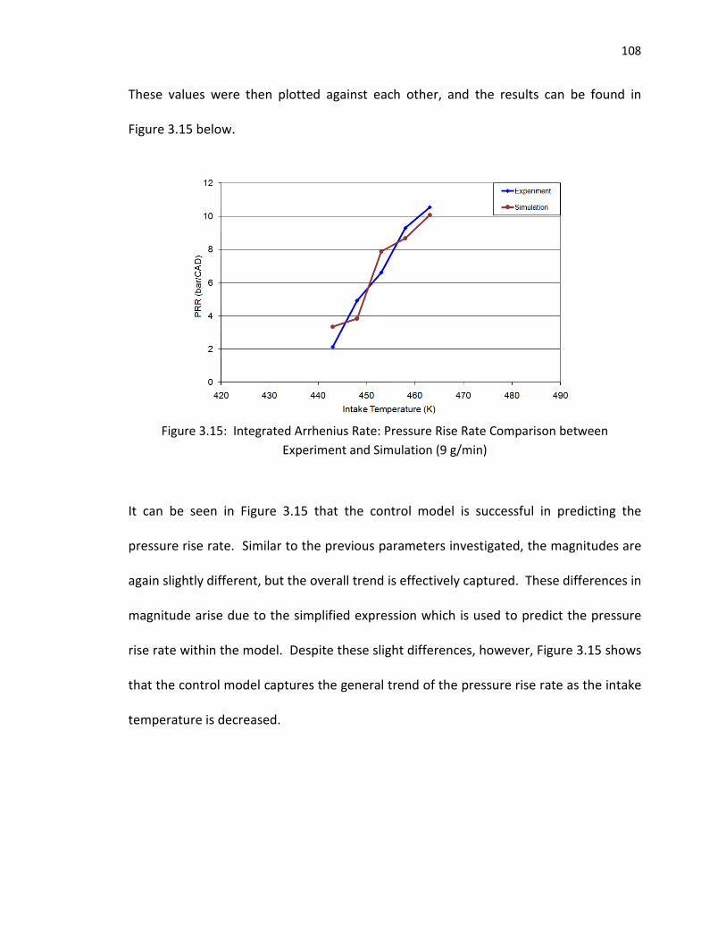
108

These values were then plotted against each other, and the results can be found in

Figure 3.15 below.

Figure 3.15: Integrated Arrhenius Rate: Pressure Rise Rate Comparison between


It can be seen in Figure 3.15 that the control model is successful in predicting the

pressure rise rate. Similar to the previous parameters investigated, the magnitudes are

again slightly different, but the overall trend is effectively captured. These differences in

magnitude arise due to the simplified expression which is used to predict the pressure

rise rate within the model. Despite these slight differences, however, Figure 3.15 shows

that the control model captures the general trend of the pressure rise rate as the intake

temperature is decreased.

109

3.3 C7H16: 6 G/MIN FUELING RATE

With the control model already benchmarked against experimental UTG96 data,

the next step was to further validate the model by benchmarking it against another set

of experimental data at a different operating point. This new set of data again used

UTG96 as the fuel, but had a significantly different fueling rate than that of the previous

data. This reduction in fueling rate caused the equivalence ratio to drop to 0.25, while

the external EGR was still held at zero. In order to benchmark the model for this fueling

rate, the intake temperature was again varied while all other inputs were held constant.

The Arrhenius Rate threshold value, as well as the value for θoffset, was also held

constant based on previous discussions. This again forced any changes in the model

outputs to be directly related to the changes in intake temperature. The results of this

benchmarking were tabulated, and can be seen below.

Table 3.5: Integrated Arrhenius Rate: Comparison of Experiment and Simulation I (6gpm)

Table 3.6: Integrated Arrhenius Rate: Comparison of Experiment and Simulation II (6gpm)

110

Table 3.7: Integrated Arrhenius Rate: Comparison of Experiment and Simulation III (6gpm)

Table 3.8: Integrated Arrhenius Rate: Comparison of Experiment and Simulation IV (6gpm)

As the intake temperature was varied, the model again seemed to track the

experimental values fairly well. Similar to the previous fueling rate, the model was again

run for intake temperatures outside of the range of experimental values. This allowed

for the behavior of the model outside of the experimental range to be investigated.

Once again, the outputs from the model were deemed to be the most important

parameters, and were therefore investigated first. Table 3.5 shows the results of the

peak pressure comparison, which were plotted on the same graph and can be seen

below in Figure 3.16. This Figure shows the behavior of the peak pressure for both the

experiment and simulation as the intake temperature is decreased. The most striking

difference between the two lines in this case is the fact that they appear to be slightly

offset from one another. This behavior was expected, however, again due to the

simplistic nature of the model being used. The model does seem to effectively capture

111

Figure 3.16: Integrated Arrhenius Rate: Peak Pressure Comparison between Experiment

and Simulation (6 g/min)

the overall trend of the pressure evolution, with a slight delay from those observed in

the experiment. This delay in the model can once again be explained by examining the

critical dynamics that take place when the combustion event crosses over the TDC

threshold. For the experimental case, Table 3.5 shows that the peak pressure begins to

decrease immediately, despite the fact that the start of combustion is occurring before

top dead center. This phenomenon is a result of the remainder of the compression

stroke having a smaller impact on the peak pressure as the combustion event

approaches TDC. In reality, when combustion occurs before TDC the pressure rise takes

place during the compression stroke, which acts to increase the peak pressure. Since

combustion is occurring closer and closer to TDC, the compression stroke therefore has

less of an impact on the pressure and it decreases accordingly. This phenomenon is

somewhat complex, and was therefore not included in the simplistic control model

developed. Due to this simplification, the control model predicts that the peak pressure

112

actually increases as combustion approaches TDC, which is evident in Table 3.5.

Therefore, the delay apparent in Figure 3.16 enters the model through this

simplification. Despite the delay, however, the overall trend of the experimental

pressure is indeed captured. Once the model pushes the combustion event past TDC,

the pressures begin to fall off similar to those in the experiment. As described

previously, the correct prediction of these trends is central to the operation of the

control model.

The next parameter that was investigated was the angle at which start of

combustion occurred. The intake temperature was varied, and the results for the

simulation, as well as the experiment, can be found in Table 3.5. These results were also

plotted against each other, and this diagram can be found in Figure 3.17 below.

Figure 3.17: Integrated Arrhenius Rate: Start of Combustion Comparison between


Figure 3.17 shows that the simulation again does a very good job of predicting the onset

of combustion. Both the magnitude and the trend of the start of combustion seem to

113

be captured by the control model. Figure 3.17 reveals that the model was calibrated

using experimental data from the previous fueling rate, which explains why the

simulation is no longer “pinned” to the experiment. Since the same fuel was being used,

the model could utilize the same threshold value in order to predict the onset of

combustion as the inlet conditions were varied. Figure 3.17 also shows that the control

model successfully captures both the magnitude and the trend of the onset of

combustion when compared against experimental data. This provides evidence that the

simplified control is doing a reasonable job of predicting engine outputs.

The next parameter that was investigated was the crank angle at which the peak

pressure was occurring, θ23. The most logical experimental value to compare against

was again the CA50 value, which is again the crank angle at which 50 percent of the total

heat release is realized. The simulation was run for the same inlet conditions as before

and the results, as well as the experimental CA50 values, can be found in Table 3.6.

These results were plotted against one another and can be seen in Figure 3.18 below.

This Figure shows that the model also does a reasonable job of predicting θ23. The

overall magnitudes are again slightly off, but the general trend seems to be captured by

the simulation. The reasoning behind the difference in magnitudes can again be

explained by looking at the combustion duration term, Δθ. As described previously, the

model utilizes a variable Δθ correlation which varies the combustion duration based

largely on where SOC is occurring. There is therefore no direct calibration of θ23, which

explains why the magnitudes seen in Figure 3.18 are slightly different. Despite these

114

Figure 3.18: Integrated Arrhenius Rate: Angle of Peak Pressure Comparison between


slight differences in magnitude, however, Figure 3.18 shows that the simulation does

successfully capture the overall trend of θ23. Similar to the case of the peak pressure,

capturing this overall trend is more important than precisely predicting the values.

The next parameter of interest was the temperature at the start of compression.

This point represented the temperature of the mixture after the induction and mixing of

both reactants and products. The simulation was run for the same inlet conditions and

compared with the experiment. These results were tabulated and can be seen in Table

3.6 along with the experimental values. These results were also plotted, and the results

can be found in Figure 3.19 below.

115

Figure 3.19: Integrated Arrhenius Rate: Temperature after Induction Comparison between


From Figure 3.19, it is evident that the simulation predicts the temperature at the start

of compression very well. Similar to the data for the previous fueling rate, the slopes of

the lines are almost identical and the magnitudes are only slightly off. One reason for

the difference in magnitudes comes about due to the simplicity of the model. While the

model includes a heat transfer term to account for the heat lost during the induction

phase, the actual process is far too complex to model. With that being said, the model

still predicts values for the temperature after induction that are within five degrees

Kelvin of the experimental values, which is again all that can be expected due to the

simplistic nature of the model. Once again, capturing the general trend is the most

important with respect to the control model, and Figure 3.19 displays that this trend is

indeed captured.

The next parameter of interest was the pressure just before the start of

combustion. While this parameter is usually not of particular interest with respect to

116

engine performance, it can still be used in order to verify whether or not the simulation

is predicting reasonable values. The simulation was run again, and compared against

the experimental pressure values from the Hatz engine. These results can be found in

Table 3.7. Once the values were known, they could be plotted on the same graph for

comparison. This plot can be seen in Figure 3.20 below.

Figure 3.20: Integrated Arrhenius Rate: Pressure after Compression Comparison between


The plot in Figure 3.20 shows that the simulation successfully tracks the pressure in the

cylinder after compression. Similar to the temperature after induction, the simulation

again seems to predict the overall trend of the pressure evolution, with the magnitudes

being only slightly off. As long as the simulation is able to predict the general behavior

of the pressure evolution, that is all that is required for a control scheme to operate. As

seen in Figure 3.20, the model does indeed capture this trend.

The pressure after expansion, at the instant the exhaust valve opens, is yet another

parameter that can be used to benchmark the model with the experiment. While this

117

pressure is usually not of much interest from the viewpoint of engine performance, it is

readily available from the experiment and therefore supplies an additional

benchmarking point for the control model. The simulation was run and compared

against the experiment, and the results of this comparison can also be found in Table

3.7. These results were also plotted against each other, and can be found in Figure 3.21

below.

Figure 3.21: Integrated Arrhenius Rate: Pressure after Expansion Comparison between


It can be seen in Figure 3.21 that the control model is also successful in predicting the

pressure after the expansion stroke, at the instant the exhaust valve opens. Similar to

the previous parameters investigated, the magnitudes are slightly different, but the

overall trend is the same. The differences in magnitude are again a result of the

simplifications made to the model. Figure 3.21 shows that the control model captures

the general behavior of the pressure evolution after the expansion stroke.

Another parameter that was readily available for comparison was the

temperature in the cylinder after combustion. Since this temperature occurred

118

immediately after combustion, it was therefore the peak temperature within the cycle.

The temperatures predicted by the model, along with those from the experiment, were

tabulated and can be found in Table 3.8 above. These values were plotted, and can be

seen in Figure 3.22 below.

Figure 3.22: Integrated Arrhenius Rate: Peak Temperature Comparison between


In Figure 3.22, the overall trend of the temperature evolution is captured, but the

magnitudes are again slightly different. This difference in magnitude can once again be

attributed to the simplifications that were made to the model. Due to the simplistic

nature of the model, heat transfer effects are not completely accounted for, which

results in values, especially for temperatures, that are higher than those seen in the

experiment. Even though the model seems to over predict the peak temperature in the

cycle, the general behavior of the parameter is captured for changes in inlet conditions.

Similar to previous arguments, this overall trend is all that is required for the control

model to operate effectively.

119

The next parameter that was used to benchmark the control model was the

exhaust temperature. Since exhaust gas recirculation was being utilized on the engine,

the temperature of the re-inducted exhaust from the previous cycle acted to heat up

the intake charge. This acted to provide a direct link from cycle to cycle within the

operation of the engine. These temperatures were obtained from the model and

experiment, and the results can be found in Table 3.8. These temperatures were then

plotted against each other, and this can be found in Figure 3.23 below.

Figure 3.23: Integrated Arrhenius Rate: Exhaust Temperature Comparison between


The results in Figure 3.23 show that when predicting the exhaust temperature, the

model once again displays a good correlation with the experiment. Again similar to the

case of peak pressure, the correct decreasing trend is captured by the model; it is

merely offset in magnitude. The fact that these magnitudes are different can once again

be explained by the simplifications to the model. Since heat transfer is not entirely

120

accounted for, the temperatures predicted by the model cannot be expected to match

exactly with the experiment. Figure 3.23 shows that the model accurately predicts the

correct trend in the exhaust temperature evolution, which is all that is necessary from a

controls perspective.

The final parameter that was used to benchmark the control model was again

the pressure rise rate. This parameter was of importance due to the fact that it had a

direct impact on the operating range of the engine. These pressure rise rates were


These values were then plotted against each other, and the results can be found in

Figure 3.24 below.

Figure 3.24: Integrated Arrhenius Rate: Pressure Rise Rate Comparison between Experiment

and Simulation (6 g/min)

It can be seen in Figure 3.24 that the control model is again successful in predicting the

pressure rise rate. Similar to the previous fueling rate investigated, the magnitudes are

121

again slightly different, but the overall trend is the same. These differences again arise

due to the simplified expression which is used to predict the pressure rise rate within

the model. Despite these slight differences in magnitude, Figure 3.24 shows that the

control model captures the general trend of the pressure rise rate as the intake

temperature is decreased.

This simplified Arrhenius Rate model showed good correlation to the experiment

for all of the parameters that were investigated for both fueling rates. Even if the model

did not precisely track the parameter, it was still able to capture the overall trends of

how that parameter was changing with inlet conditions. From the information supplied

in Figures 3.16-3.24, it can therefore be concluded that this Arrhenius Rate model is

capable of accurately predicting the trends of both the pressure and temperature

evolution within the cylinder. Accurate prediction of these trends provides valuable

evidence that this simplified Arrhenius Rate model can indeed be used in order to

develop a control scheme for effective control of an HCCI engine.

3.4 HCCI OPERATING RANGE

HCCI test data taken from the Hatz 1D50Z single-cylinder engine at Oak Ridge

National Labs seems to suggest a fairly narrow band of acceptable combustion timing

values which result in stable HCCI operation. As the timing is advanced from TDC,

combustion becomes increasingly violent resulting in higher and higher pressure rise

rates (PRR) and therefore unacceptable amounts of noise emission from the engine. If

the timing is retarded, combustion becomes sporadic and unpredictable resulting in

large amounts of cyclic variation. In order to get a better understanding of this

122

phenomenon, the combustion timing is varied within the model while the efficiency,

along with PRR, is used as a gauge to determine an acceptable range of operation. The

results of this analysis can be seen in Figure 3.25.

Figure 3.25: HCCI efficiency and PRR surface plots

Figure 3.25 shows both the efficiency (work out/fuel energy in) and the PRR predicted

by the model for a variety of different intake temperatures and equivalence ratios. The

efficiency (shown in blue) is predicted in the model using gross indicated work along

with fueling rate, and serves to roughly indicate when stable HCCI combustion is being

achieved. As shown in the Figure, the efficiency surface can be related to a waterfall,

where the water originates from the corner of high equivalence ratios/intake

temperatures and flows downstream to the corner of low equivalence ratios/intake

123

temperatures. For relatively high equivalence ratios and intake temperatures (i.e.

advanced combustion timing), the efficiency predicted by the model is fairly constant

for a variety of setpoints, and increases slightly as the “water” approaches the falloff.

For relatively low equivalence ratios and intake temperatures (i.e. retarded combustion

timing), the efficiency displays large spikes, which indicates that combustion is

becoming unstable thus resulting in large cyclic variations from cycle to cycle. Based on

these findings, an operating window for stable HCCI combustion has been defined using

the efficiency plot in Figure 3.25. The right edge of this window is defined using a PRR

limit of 10 bar/CAD [17], and is represented in Figure 3.25 by the solid black line. This

black line originates from the PRR predicted by the model (shown in red) and is simply

transposed down onto the efficiency surface. The left edge of this operating window is

already being predicted by the combustion model as the edge where the efficiency

begins to fall off. In other words, the model is predicting stable, acceptable HCCI

operation when the setpoint is kept to the right of the “waterfall” and to the left of the

PRR limit. For comparison, experimental data from the Hatz is also included in Figure

3.25, and is represented by the small orange and blue spheres. As is evident, these

experimental data points all fall within the window predicted by the model, which gives

confidence that the model is indeed predicting a reasonable operating window for HCCI

combustion.

124

4. PERTURBATION ANALYSIS

With the control model now developed and validated against experiment, a

logical next step is to investigate the effect of perturbations, or disturbances, on the

system. Within the control model there exist inputs which can be tweaked in order to

control the various output variables. In simulation, it is possible to exactly specify these

input variables without the inclusion of any type of extraneous noise. In practice,

however, this is not possible. The inputs, which are intake temperature, fueling rate

and external EGR fraction, are typically controlled on an actual engine using some sort

of actuator. These actuators are mechanical devices, which cannot realistically be

expected to provide noise free operation. There will always be some degree of

uncertainty associated with the actuator, along with various other disturbances, which

will cause the desired input to oscillate around some nominal value which has been

specified by the ECU. In light of this behavior, disturbances must therefore be

introduced into the control model in order to force the inputs to fluctuate around some

nominal value. The effects of these disturbances on the model outputs can then be

examined in order to determine the sensitivity of these outputs to small variations of

the input variables. From a controls standpoint, it is desired that the outputs remain

relatively unaffected by small variations in the inputs in order to maintain sufficient

control of the process. Within the control model developed, inputs include a pre-

heated intake temperature, fueling rate and the fraction of external EGR applied. In an

effort to duplicate the small variations typically seen in implementation, a random

125

number generator which used a Gaussian distribution about some nominal value was

utilized. This random number generator effectively produced input values on a cycle to

cycle basis that fluctuated around some desired input value. The magnitude of the

fluctuations was chosen so as to represent typical variations seen during experiment.

The intake temperature, which was controlled using a resistance heater, was allowed

fluctuations of one percent of the nominal value. The fraction of external EGR,

however, which was controlled using a solenoid, was allowed fluctuations of three

percent of the nominal value. These perturbations then allowed the corresponding

outputs to be monitored in order to determine their behavior.

4.1 TEMPERATURE PERTURBATIONS

The first perturbation analysis that was run corresponded to a fueling rate of 9

grams/minute, which resulted in an equivalence ratio of 0.38. The intake temperature

was assigned nominal values between 420 K and 560 K in an attempt to stay within the

typical HCCI operation range of the engine. For simplicity, the external EGR rate was set

to zero during this analysis. The internal EGR fraction, αi, was set at 0.05, which

corresponded to typical values seen in the experiment. The intake temperature was

varied under these conditions for 500 cycles, and return maps were created in order to

display the results. Both output variables, peak pressure and θ23, were investigated.

The results of this initial investigation can be seen in Figures 4.1 and 4.2.

126

0 5 10 15 20 25 30 35 40 45 50 55 60 650

5

10

15

20

25

30

35

40

45

50

55

60

65

Peak Pressure (i), (bar)

Pe

ak

Pre

ss

ure

(i+

1),

(b

ar)

Temp = 420

Temp = 430

Temp = 450

Temp = 480

Temp = 510

Temp = 540

Temp = 560

340 350 360 370 380 390 400 410 420 430 440 450 460 470 476340

350

360

370

380

390

400

410

420

430

440

450

460

470

476

Theta23 (i), (CAD)

Th

eta

23

(i+

1),

(C

AD

)

Temp = 420

Temp = 430

Temp = 450

Temp = 480

Temp = 510

Temp = 540

Temp = 560

Figure 4.1: θ23 Return Map for Varying Intake Temperatures: low iEGR (9 gpm fuel rate)

Figure 4.2: Peak Pressure Return Map for Varying Intake Temperatures: low iEGR

(9 gpm fuel rate)

As the intake temperature was increased, Figure 4.1 shows an overall trend of the angle

of peak pressure, θ23, decreasing. This result makes physical sense due to the fact that a

mixture which begins compression at a higher initial temperature should ignite sooner.

127

The model predicts that combustion timing will continue to advance with increasing

temperature, and will cross the TDC threshold for an intake temperature of

approximately 450 K. Figure 4.1 also reveals the sensitivity of θ23 to small variations of

intake temperature around the five nominal values which were used. It appears as

though θ23 gets less and less sensitive to perturbations as the intake temperature is

increased. This trend is evident in Figure 4.1 due to the noticeably smaller variations in

the output as intake temperature is disturbed. Figure 4.2 summarizes the second

output, which is the peak pressure. Since peak pressure values rely on combustion

timing for a particular engine cycle, these results follow closely to those seen in Figure

4.1. The variations again seem to diminish as the intake temperature is increased, as

can be seen by the smaller variations between data points. Peak pressure is unique,

however, in that it initially rises until it hits a maximum and then begins to fall. This

result makes sense, though, due to the dependence of peak pressure on combustion

timing. Since θ23 initially occurs after TDC (aTDC) and then advances to TDC, the

pressure will inherently rise between those points and reach a maximum at TDC. As θ23

advances beyond that even further, the pressure will then begin to drop off again due to

combustion initiating earlier in the compression stroke. Overall, the main trend

observed in these plots was the tendency of the output sensitivity to decrease as

nominal intake temperatures were increased. Figure 4.2 also seems to suggest an

operating envelope for the engine, in that combustion does not occur for intake

temperatures less than approximately 430K. Similar behavior has also been observed in

the experimental data.

128

340 350 360 370 380 390 400 410 420 430 440 450 460 470 476340

350

360

370

380

390

400

410

420

430

440

450

460

470

476

Theta23 (i), (CAD)

Th

eta

23

(i+

1),

(C

AD

)

Temp = 420

Temp = 430

Temp = 450

Temp = 480

Temp = 510

Temp = 540

Temp = 560

The next case investigated was similar in every way to the first case, with the

exception of the internal EGR fraction. In the previous simulation, this parameter was

set at 0.05 in order to reproduce experimental conditions. In this trial, however, the

internal EGR fraction was increased to 0.4 in order to determine the behavior of the

model when the intake temperature was perturbed about an elevated EGR rate. With

all other test parameters the same, the intake temperature was again assigned nominal

values between 420 K and 560 K with the external EGR set to zero for simplicity. Each

intake temperature was run for 500 cycles, and return maps were created in order to

display the results, which can be seen in Figures 4.3 and 4.4.

Figure 4.3: θ23 Return Map for Varying Intake Temperatures: high iEGR (9 gpm fuel rate)

129

0 5 10 15 20 25 30 35 40 45 50 55 60 650

5

10

15

20

25

30

35

40

45

50

55

60

65


Pe

ak

Pre

ss

ure

(i+

1),

(b

ar)

Temp = 420

Temp = 430

Temp = 450

Temp = 480

Temp = 510

Temp = 540

Temp = 560

Figure 4.4: Peak Pressure Return Map for Varying Intake Temperatures: high iEGR

(9 gpm fuel rate)

The effect of increasing the internal EGR in Figures 4.3 and 4.4 appears to have a drastic

impact on the sensitivity of the output variables. For a high internal EGR, neither the

angle of peak pressure, nor the peak pressure itself, appear to be significantly affected

by perturbations of intake temperature. This is in stark contrast to the results seen in

Figures 4.1 and 4.2 corresponding to a low EGR rate. This change in sensitivity can be

explained by looking at the temperature effect of the internal EGR. It was previously

concluded that sensitivity appeared to decrease as intake temperature increased with a

low EGR rate. In this case, the internal EGR rate is now significantly higher, which acts

to increase the in-cylinder temperature significantly from the previous case. Increasing

the intake temperature still has the same overall effect on the system, i.e. advancing

combustion timing along with decreasing pressure, the magnitude of this effect is

merely reduced due to the higher initial temperature of the mixture due to the hot

internal EGR present. Another interesting observation deals with the fact that for high

130

340 350 360 370 380 390 400 410 420 430 440 450 460 470 476340

350

360

370

380

390

400

410

420

430

440

450

460

470

476

Theta23 (i), (CAD)

Th

eta

23

(i+

1),

(C

AD

)

Temp = 420

Temp = 430

Temp = 450

Temp = 480

Temp = 510

Temp = 540

Temp = 560

internal EGR the range of combustion timings only varied 3-4 degrees whereas it varied

almost 20 degrees for low EGR. This hints at the idea that temperature difference may

play a role in determining the ability of the input to effectively vary the output.

With several cases already run for one fueling rate, the next step was to change

this fueling rate in order to determine the effects it would have on the system outputs.

This was accomplished by lowering the fueling rate to 6 grams/minute, which then

resulted in an equivalence ratio of φ=0.25. With this change, the first two cases could

now be repeated in order to determine the effects of altering the equivalence ratio. The

intake temperature was again assigned nominal values between 420 K and 560 K and

allowed to fluctuate +/- 1 percent of that value. The external EGR was again set at zero

for simplicity, and the internal EGR was set at 0.05 to replicate experimental conditions.

The simulation was run for 500 cycles at each intake temperature, and the results can

be seen in Figures 4.5 and 4.6.

Figure 4.5: θ23 Return Map for Varying Intake Temperatures: low iEGR (6 gpm fuel rate)

131

0 5 10 15 20 25 30 35 40 45 50 55 60 650

5

10

15

20

25

30

35

40

45

50

55

60

65


Pe

ak

Pre

ss

ure

(i+

1),

(b

ar)

Temp = 420

Temp = 430

Temp = 450

Temp = 480

Temp = 510

Temp = 540

Temp = 560

Figure 4.6: Peak Pressure Return Map for Varying Intake Temperatures: low iEGR

(6 gpm fuel rate)

With the only change being a lowered fueling rate, the results in Figures 4.5 and 4.6 can

therefore be directly compared with those in Figures 4.1 and 4.2 in order to determine

the effect of changing the equivalence ratio. Comparison of the results shows that the

overall behavior of the system is maintained for the lowered fueling rate, and that the

magnitudes are merely shifted. Due to a leaner mixture, combustion is occurring later

and with slightly more variability. The magnitude of the peak pressure is significantly

reduced, which can again be attributed to the leaner mixture being burned. Overall, it

still appears as though higher temperatures, and therefore more advanced combustion

timing, lead to smaller sensitivities with respect to the output variables.

The next case run with the new fueling rate was similar to the previous one, with

the only exception being the internal EGR rate. In order to duplicate the cases

previously run, this case again set the internal EGR to 0.4 in order to determine the

132

0 5 10 15 20 25 30 35 40 45 50 55 60 650

5

10

15

20

25

30

35

40

45

50

55

60

65


Pe

ak

Pre

ss

ure

(i+

1),

(b

ar)

Temp = 420

Temp = 430

Temp = 450

Temp = 480

Temp = 510

Temp = 540

Temp = 560

340 350 360 370 380 390 400 410 420 430 440 450 460 470 476340

350

360

370

380

390

400

410

420

430

440

450

460

470

476

Theta23 (i), (CAD)

Th

eta

23

(i+

1),

(C

AD

)

Temp = 420

Temp = 430

Temp = 450

Temp = 480

Temp = 510

Temp = 540

Temp = 560

effect it would have on the sensitivity of the output variables. The intake temperature

was still varied between 420 K and 560 K, and the external EGR remained at zero. The

simulation was again run for 500 cycles at each intake temperature, and the

corresponding results can be seen in Figures 4.7 and 4.8.

Figure 4.7: θ23 Return Map for Varying Intake Temperatures: high iEGR (6 gpm fuel rate)

Figure 4.8: Peak Pressure Return Map for Varying Intake Temperatures: high iEGR

(6 gpm fuel rate)

133

When compared to Figures 4.3 and 4.4, Figures 4.7 and 4.8 above display very similar

results to those for the previous fueling rate. The overall behavior is still present, while

the magnitudes are again slightly shifted. When compared to Figure 4.3, combustion

timing, while advancing with increasing temperature, occurs slightly later for lower

temperatures and again with slightly more variation. This variation is insignificant,

however, when compared with the temperature perturbations at low internal EGR rates

of shown in Figures 4.5 and 4.6. The peak pressure also shows more variation, and the

overall magnitudes drop due to the leaner mixture in the cylinder.

4.2 INTERNAL EGR PERTURBATIONS

Another perturbation case was run using the original fueling rate of 9

grams/minute, which attempted to look at the effect of adding a disturbance to the

internal EGR fraction. Despite the fact that the engine being modeled could not

independently vary the internal EGR using variable valve timings, this analysis was

performed to get a better understanding of what parameters the system outputs were

most sensitive to. In order to accomplish this, the internal EGR, αi, was assigned

nominal values between 0 and 0.6 (0-36% by mass), and was allowed to fluctuate +/- 3%

of that value. These values were chosen so as to represent reasonable values which

could be attained on an actual engine. The external EGR fraction was again set to zero

for simplicity. The intake temperature was set at 520K in order to attribute changes in

the outputs solely to the variations of internal EGR. This analysis was run for 500 cycles

at each nominal operating point, and the results can be seen in Figures 4.9 and 4.10.

134

340 350 360 370 380 390 400 410 420 430 440 450 460 470 476340

350

360

370

380

390

400

410

420

430

440

450

460

470

476

Theta23 (i), (CAD)

Th

eta

23

(i+

1),

(C

AD

)

alphae = 0 (0% mass)

alphae = .15 (12% mass)




0 5 10 15 20 25 30 35 40 45 50 55 60 650

5

10

15

20

25

30

35

40

45

50

55

60

65


Pe

ak

Pre

ss

ure

(i+

1),

(b

ar)

alphai = 0 (0% mass)

alphai = .15 (12% mass)




Figure 4.9: θ23 Return Map for Varying Internal EGR Rates: high Tin (9 gpm fuel rate)

Figure 4.10: Peak Pressure Return Map for Varying Internal EGR Rates: high Tin (9 gpm fuel rate)

This analysis showed both output variables to be noticeably less sensitive to

perturbations of internal EGR fraction than they were intake temperature. Both Figures

4.9 and 4.10 show that perturbing the internal EGR has only minor effects on θ23 and

135

the peak pressure. This somewhat correlates to the previous assumption that sensitivity

decreases with increasing temperature. For this case, the intake temperature was set at

520 K, which is already indicative of the upper end of the HCCI operating window. In

addition, internal EGR has naturally elevated temperatures due to the hot exhaust

gases, which acts to increase the temperature even more. This is one possible

explanation for the decrease in output sensitivity. These results also make physical

sense due to the elevated temperatures forcing combustion to always occur before TDC

(bTDC). Since combustion continues to advance with increasing EGR, the peak pressure

therefore decreases. One interesting observation from Figure 4.9 was that combustion

timing seems to remain constant once the internal EGR fraction reaches approximately

0.4. This phenomenon was most likely due to the ability of the internal EGR to both

heat up and dilute the fresh intake charge. This charge heating and dilution effectively

cancel each other out at high EGR rates so that the combustion timing remains fairly

constant.

The next case that was investigated was similar in every way to the previous case

where the internal EGR was varied, with the exception of the nominal intake

temperature. In the previous test, this parameter was held at 520 K in order to simulate

a high nominal temperature. In this simulation, however, the intake temperature was

lowered to 450 K in order to observe the behavior of the system when internal EGR was

varied about a low nominal temperature. With the fueling rate held at 9 grams/minute

and the internal EGR still assigned nominal values between 0 and 0.6, the simulation

136

0 5 10 15 20 25 30 35 40 45 50 55 60 650

5

10

15

20

25

30

35

40

45

50

55

60

65


Pe

ak

Pre

ss

ure

(i+

1),

(b

ar)






340 350 360 370 380 390 400 410 420 430 440 450 460 470 476340

350

360

370

380

390

400

410

420

430

440

450

460

470

476

Theta23 (i), (CAD)

Th

eta

23

(i+

1),

(C

AD

)






was again run for 500 cycles at each nominal EGR value. The results were summarized

in return maps, which can be seen in Figures 4.11 and 4.12.

Figure 4.11: θ23 Return Map for Varying Internal EGR Rates: low Tin (9 gpm fuel rate)

Figure 4.12: Peak Pressure Return Map for Varying Internal EGR Rates: low Tin (9 gpm fuel rate)

137

These results reveal that decreasing the intake temperature serves to increase the

sensitivity of the outputs to perturbations of the internal EGR rate. This again seems to

fortify the idea that sensitivity decreases with increasing temperature. Since the intake

temperature was decreased for this run, the temperature in the cylinder therefore

decreased as well. This could explain why there seems to be larger variations in the

output variables in Figures 4.11 and 4.12 for identical variations in the internal EGR rate.

The temperature in this case was high enough initially for combustion to occur bTDC,

which resulted in the peak pressure continuing to decrease as EGR was increased.

Similar to the previous case, the combustion timing once again seems to level off once

the internal EGR rate reaches approximately 0.4.

With several cases already run for the fueling rate of 9 gram/minute, the next

step was to change this fueling rate in order to determine the effects it would have on

the system outputs. This was accomplished by again lowering the fueling rate to 6

grams/minute, which then resulted in an equivalence ratio of φ=0.25. With this change,

the first two cases could now be repeated in order to determine the effects of altering

the equivalence ratio. The internal EGR fraction was again assigned nominal values

ranging between 0 and 0.6 in order to duplicate realistic values seen on a typical engine,

and allowed to fluctuate +/- 3 percent of that value. The external EGR was again set at

zero for simplicity, while the intake temperature was held at 520 K in order to simulate a

high temperature intake charge. This analysis was again run for 500 cycles at each

nominal operating point, and the results can be seen in Figures 4.13 and 4.14.

138

340 350 360 370 380 390 400 410 420 430 440 450 460 470 476340

350

360

370

380

390

400

410

420

430

440

450

460

470

476

Theta23 (i), (CAD)

Th

eta

23

(i+

1),

(C

AD

)






0 5 10 15 20 25 30 35 40 45 50 55 60 650

5

10

15

20

25

30

35

40

45

50

55

60

65


Pe

ak

Pre

ss

ure

(i+

1),

(b

ar)






Figure 4.13: θ23 Return Map for Varying Internal EGR Rates: high Tin (6 gpm fuel rate)

Figure 4.14: Peak Pressure Return Map for Varying Internal EGR Rates: high Tin (6 gpm fuel rate)

The results in Figures 4.13 and 4.14 show some striking similarities to those from the

previous fueling rate. When compared to Figures 4.9 and 4.10, the overall behavior of

the outputs are the same for each fueling rate. The elevated intake temperature forces

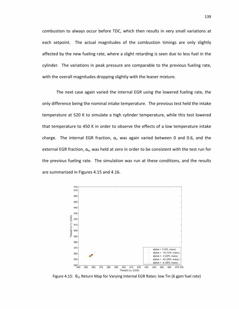
139

340 350 360 370 380 390 400 410 420 430 440 450 460 470 476340

350

360

370

380

390

400

410

420

430

440

450

460

470

476

Theta23 (i), (CAD)

Th

eta

23

(i+

1),

(C

AD

)






combustion to always occur before TDC, which then results in very small variations at

each setpoint. The actual magnitudes of the combustion timings are only slightly

affected by the new fueling rate, where a slight retarding is seen due to less fuel in the

cylinder. The variations in peak pressure are comparable to the previous fueling rate,

with the overall magnitudes dropping slightly with the leaner mixture.

The next case again varied the internal EGR using the lowered fueling rate, the

only difference being the nominal intake temperature. The previous test held the intake

temperature at 520 K to simulate a high cylinder temperature, while this test lowered

that temperature to 450 K in order to observe the effects of a low temperature intake

charge. The internal EGR fraction, αi, was again varied between 0 and 0.6, and the

external EGR fraction, αe, was held at zero in order to be consistent with the test run for

the previous fueling rate. The simulation was run at these conditions, and the results

are summarized in Figures 4.15 and 4.16.

Figure 4.15: θ23 Return Map for Varying Internal EGR Rates: low Tin (6 gpm fuel rate)

140

0 5 10 15 20 25 30 35 40 45 50 55 60 650

5

10

15

20

25

30

35

40

45

50

55

60

65


Pe

ak

Pre

ss

ure

(i+

1),

(b

ar)






Figure 4.16: Peak Pressure Return Map for Varying Internal EGR Rates: low Tin (6 gpm fuel rate)

The results in Figures 4.15 and 4.16 can be directly compared to those of Figures 4.11

and 4.12 in order to determine the effect of changing the fueling rate. Similar to the

previous cases, the results are again very similar to the previous fueling rate. The

lowered intake temperature allows combustion to initiate after TDC, and then

ultimately advance across the TDC threshold. The magnitudes of the combustion timing

are slightly later for this fueling rate, which is reasonable due to the leaner mixture

present in the cylinder. Also observed was the phenomenon of the combustion timing

seemingly leveling off when the internal EGR rate reaches approximately 0.4. Similar to

previous tests, the heating and dilution effects of the EGR are effectively cancelling each

other out. The variations in both timing and peak pressure are again comparable for

both fueling rates, with sensitivity seeming to increase slightly as the cylinder

temperature drops. The peak pressure values are again smaller, which can be explained

141

by the leaner mixture. Overall, the change in fueling rates seemed to affect only the

overall magnitudes of the outputs, and not necessarily their sensitivities. Similar trends

were seen for both fueling rates, which implies that the output sensitivities are not

dependent upon the fueling rate being used.

4.3 EXTERNAL EGR INVESTIGATION

With the issue of changing fueling rates now addressed, the next logical

parameter of interest is the external EGR rate, αe. Similar to the intake temperature,

this parameter is also an input to the control model which will be used to stabilize and

control the model outputs. On an actual engine, this external EGR will likely be

controlled with some sort of actuator. This implies that the EGR rate cannot be exactly

specified, and that it will rather oscillate about some nominal operating point specified

by the ECU. This is due to uncertainties, along with mechanical limitations, associated

with the actuator device. In order to simulate this oscillatory behavior, perturbations

were introduced to the input variable αe. The end goal in this study was to determine

the variations that these small perturbations would produce in the model outputs.

4.3.1 Low Temperature External EGR. The first case investigated in this series

dealt with varying the intake temperature while the external EGR was held constant in

an attempt to make a comparison to previous cases. In light of this, the intake

temperature was again varied between 420 K and 560 K to be consistent. Since the

fueling rate had previously been determined to be a nonfactor, it was arbitrarily chosen

to be 9 grams/minute. The internal EGR was held constant at 0.05, also similar to

previous tests. Since the external EGR was now being investigated, it was set at 0.4 to

142

340 350 360 370 380 390 400 410 420 430 440 450 460 470 480 490 500340

350

360

370

380

390

400

410

420

430

440

450

460

470

480

490

500

Theta23 (i), (CAD)

Th

eta

23

(i+

1),

(C

AD

)

Temp = 420

Temp = 450

Temp = 480

Temp = 510

Temp = 540

Temp = 560

represent a high EGR rate, where it had been set to zero in previous tests to simulate a

low EGR rate. In the end, this test consisted of varying the intake temperature for

conditions of low internal EGR and high external EGR. Since external EGR must be

rerouted into the intake stream via a lengthy process that allows for large amounts of

heat transfer, the corresponding EGR temperature was set at 300 K. This assumed that

the EGR being injected into the intake had been cooled down to ambient conditions.

Under these conditions, the simulation was again run for 500 cycles at each intake

temperature, and the results can be seen in Figures 4.17 and 4.18.

Figure 4.17: θ23 Return Map for Varying Intake Temperatures: cool eEGR (9 gpm fuel rate)

143

0 5 10 15 20 25 30 35 40 45 50 55 60 650

5

10

15

20

25

30

35

40

45

50

55

60

65

Peak Presssure (i), (bar)

Pea

k P

res

ss

ure

(i+

1),

(b

ar)

Temp = 420

Temp = 450

Temp = 480

Temp = 510

Temp = 540

Temp = 560

Figure 4.18: Peak Pressure Return Map for Varying Intake Temperatures: cool eEGR

(9 gpm fuel rate)

With the only difference being the addition of cool external EGR, these results can be

directly compared to those in Figures 4.1 and 4.2 in order to determine the effects on

output sensitivity. Comparison between the two cases reveals that the system behaves

significantly different when the intake temperature is varied about a high external EGR

fraction. For the high EGR rate, the timing was significantly retarded as compared to the

previous case due to the addition of large amounts of cooled EGR. This acted to cool

the intake charge enough to require intake temperatures of approximately 510K before

combustion would occur. This is in stark contrast to the intake temperatures of 430K

required to initiate combustion at a low external EGR rate in Figure 4.1. The variation

also appeared to increase for the case of high external EGR, especially for the operating

points corresponding to later timing. This observation fortifies the idea that cooler

temperatures, and therefore later combustion timing, increases the amount of variation

in the outputs.

144

340 360 380 400 420 440 460 480 500340

360

380

400

420

440

460

480

500

Theta23 (i), (CAD)

Th

eta

23

(i+

1),

(C

AD

)






For the next case, the intake temperature was held constant while the external

EGR fraction was varied. In order to simulate elevated temperatures, the intake

temperature was held constant at 520 K. The internal EGR fraction, similar to other

cases, was again held at 0.05 to simulate realistic conditions. Cooled EGR at ambient

temperature was applied using the same 9 gram/minute fueling rate as previously

mentioned. Five hundred cycles were run for varying external EGR rates ranging from 0

to 0.6 (0-36% mass) in order to easily compare the effects of both internal and external

EGR. This simulation was run, and the results can be seen in Figures 4.19 and 4.20.

Figure 4.19: θ23 Return Map for Varying External EGR Rates: high Tin (9 gpm fuel rate)

145

0 10 20 30 40 50 600

10

20

30

40

50

60


Pe

ak

Pre

ss

ure

(i+

1),

(b

ar)






Figure 4.20: Peak Pressure Return Map for Varying External EGR Rates: high Tin

(9 gpm fuel rate)

Figures 4.19 and 4.20 reveal some interesting behavior with respect to varying the cool

EGR fraction. One observation is the fact that the combustion timing actually retarded

with higher amounts of external EGR, whereas the hot internal EGR caused the timing to

advance. This behavior makes sense, however, due to the fact that the external EGR is

colder than the intake charge. Adding more and more EGR in this case therefore acts to

decrease the temperature in the cylinder, which in turn acts to retard the timing.

Another interesting observation is the fact that external EGR appears to have a far

greater impact on the peak pressure magnitude then the internal EGR. This behavior

can be explained by investigating the temperature of the EGR being injected. Since the

intake temperature was held at 520K, the cool external EGR therefore had a larger

temperature difference and was able to have a greater impact on the timing. The

effects of temperature are once again shown to dominate the process. One final

146

340 350 360 370 380 390 400 410 420 430 440 450 460 470 480 490 500340

350

360

370

380

390

400

410

420

430

440

450

460

470

480

490

500

Theta23 (i), (CAD)

Th

eta

23

(i+

1),

(C

AD

)






observation made here was the fact that the variations in the output variables appear to

increase as the external EGR is increased, shown by the larger circles in Figures 4.19 and

4.20. This behavior of increasing cyclic variability with increased EGR has also been

observed in the literature [18].

In this case, it was desired to determine the effect of varying the external EGR

fraction while the intake temperature was held low, as opposed to being held high in

the previous case. In staying consistent with previous tests, the intake temperature for

this test was held at 450 K, which was meant to represent a cool intake charge. The

internal residual remained at 0.05, and the same fueling rate of 9 grams/minute was

again used. The ambient temperature external EGR was again varied between nominal

values of 0 and 0.6. The results of this test can be found in Figures 4.21 and 4.22.

Figure 4.21: θ23 Return Map for Varying External EGR Rates: low Tin (9 gpm fuel rate)

147

0 5 10 15 20 25 30 35 40 45 50 55 60 650

5

10

15

20

25

30

35

40

45

50

55

60

65


Pe

ak

Pre

ss

ure

(i+

1),

(b

ar)






Figure 4.22: Peak Pressure Return Map for Varying External EGR Rates: low Tin (9 gpm fuel rate)

When compared to similar results for internal EGR, Figures 4.21 and 4.22 reveal

somewhat different behavior for the case when cool external EGR is applied. The

timing, for example, was initially late for the internal EGR and then began to advance

slightly as larger amounts of hot residual were added. Figure 4.21, however, reveals

that the timing is significantly retarded as cooler external EGR is added. This result

makes sense due to the low temperatures seen in the cylinder. The intake temperature

is held low, while the cool EGR acts to cool the mixture even further. This cooling effect

results in the mixture igniting later. The effect of temperature again seems to dominate

the process. Similar to the previous case, these results also seem to suggest that the

variability of the outputs increases with increased amounts of cool external EGR.

4.3.2 High Temperature External EGR. In order to fully understand the effect of

external EGR on the system, it was desired to increase the temperature of the EGR being

added and monitor the effects. The cases which were run at a low external EGR

148

350 360 370 380 390 400 410 420 430 440 450 460 470 480 490 500

350

360

370

380

390

400

410

420

430

440

450

460

470

480

490

500

Theta23 (i), (CAD)

Th

eta

23

(i+

1),

(C

AD

)

Temp = 400

Temp = 420

Temp = 450

Temp = 480

Temp = 510

Temp = 540

Temp = 560

temperature were repeated with the increased temperature in order to isolate the

effects of the temperature change. Any differences in the results between the two tests

could then be attributed solely to the increase in temperature of the external EGR. The

first test which was repeated was the case of varying the intake temperature about a

fixed high external EGR rate. The external EGR was held at 0.4, the internal EGR was

held at 0.05 and the same fueling rate of 9 grams/minute was used. The intake

temperature was varied in exactly the same manner as before, and the test was run for

500 cycles at each temperature. The results can be seen below in Figures 4.23 and 4.24.

Figure 4.23: θ23 Return Map for Varying Intake Temperatures: hot eEGR (9 gpm fuel rate)

149

0 5 10 15 20 25 30 35 40 45 50 55 60 650

5

10

15

20

25

30

35

40

45

50

55

60

65


Pe

ak

Pre

ss

ure

(i+

1),

(b

ar)

Temp = 400

Temp = 420

Temp = 450

Temp = 480

Temp = 510

Temp = 540

Temp = 560

Figure 4.24: Peak Pressure Return Map for Varying Intake Temperatures: hot eEGR

(9 gpm fuel rate)

The behavior in Figures 4.23 and 4.24 is strikingly dissimilar from that seen in Figures

4.17 and 4.18 for the case of cool external EGR. The overall behavior is the same for

each case, but the combustion timing is drastically advanced for the current case of hot

external EGR. This behavior is due to the elevated temperature of the EGR being

applied. The intake charge is initially hotter due to the hot EGR, which in turn causes

the engine to continue to operate for significantly lower intake temperatures. In fact,

the engine still operates for intake temperatures as low as 400K for the elevated

temperature EGR, whereas combustion stopped occurring around intake temperatures

of 510K for the case of cooled EGR. Another observation deals with the fact that

variability seems to decrease for the case of hot external EGR. This is even more

evidence that elevated temperatures lead to less variability.

The next case investigated looked at the effects of varying the now hot external

EGR about some fixed intake temperature. In order to reproduce the same conditions

150

340 350 360 370 380 390 400 410 420 430 440 450 460 470 476340

350

360

370

380

390

400

410

420

430

440

450

460

470

476

Theta23 (i), (CAD)

Th

eta

23

(i+

1),

(C

AD

)






0 5 10 15 20 25 30 35 40 45 50 55 60 650

5

10

15

20

25

30

35

40

45

50

55

60

65


Pe

ak

Pre

ss

ure

(i+

1),

(b

ar)






from the previously run test with cool EGR, this intake temperature was set at 520 K.

The internal residual was set at 0.05, again to duplicate the previous test case. The

external EGR was varied about the same nominal values, and the simulation was run for

500 cycles. The results of this analysis can be seen in Figures 4.25 and 4.26.

Figure 4.25: θ23 Return Map for Varying External EGR Rates: high Tin (9 gpm fuel rate)

Figure 4.26: Peak Pressure Return Map for Varying External EGR Rates: high Tin

(9 gpm fuel rate)

151

When compared to the case of cool EGR, Figures 4.25 and 4.26 reveal that varying hot

external EGR causes the system to behave somewhat differently. For the case of cool

EGR, the timing was retarded as the amount of exhaust gas was increased. When hot

EGR is applied, however, the timing actually advances as more is added. This behavior is

a result of the elevated temperature of the EGR, which acts to increase the overall

temperature of the charge and therefore cause combustion to occur earlier. This

reversing trend in the combustion timing hints at the idea of a temperature difference

effect. While the actual temperature of the EGR itself is important, the difference in

temperature between the EGR and the intake air may play a major role in determining

the overall behavior of the system. As in previous cases, the variability again increases

as more external EGR is applied.

The final test case to be investigated dealt with varying the elevated

temperature external EGR about a low intake temperature. This would again allow a

comparison of the effects of internal and external EGR. Holding true to a previous case,

the intake temperature was again set at 450 K to represent a cool intake charge. The

internal residual was set at 0.05 and the same fueling rate of 9 grams/minute was again

used. The hot external EGR was varied between the same nominal values as before, and

the simulation was run for 500 cycles at each of those values. The results can be seen in

Figures 4.27 and 4.28.

152

0 5 10 15 20 25 30 35 40 45 50 55 60 650

5

10

15

20

25

30

35

40

45

50

55

60

65


Pe

ak

Pre

ss

ure

(i+

1),

(b

ar)






350 360 370 380 390 400 410 420 430 440 450 460 470 480 490 500350

360

370

380

390

400

410

420

430

440

450

460

470

480

490

500

Theta23 (i), (CAD)

Th

eta

23

(i+

1),

(C

AD

)






Figure 4.27: θ23 Return Map for Varying External EGR Rates: low Tin (9 gpm fuel rate)

Figure 4.28: Peak Pressure Return Map for Varying External EGR Rates: low Tin (9 gpm fuel rate)

Similar to previous results, Figures 4.27 and 4.28 show that increasing the temperature

of the external EGR changes the overall behavior of the system. In fact, these results

show that timing and peak pressure behavior are the reverse of what they were in the

153

case of cool EGR. This can again be explained by the heating effect of the external EGR

on the intake charge. The hotter exhaust gas heats up the mixture, which then causes

combustion to occur sooner rather than later. While the output variability is minimal

for a given input, the sensitivity again seems to increase as more external EGR is added.

This effect is visible regardless of the temperature of the EGR being applied. In

summary, higher temperatures and more advanced combustion timing again seem to

reduce variability in the outputs. The temperature difference between the applied

external EGR and the intake charge also appears to be significant, in that it affects the

overall behavior of the system. Finally, the output variability also seems to increase as

the amount of external EGR is increased, regardless of its temperature.

Throughout the entire perturbation analysis, the cyclic coupling was determined

to be dominated by temperature effects rather than compositional effects. This was a

result of the exponential temperature relation within the Integrated Arrhenius Rate

which was used to predict the combustion timing within the model. While

compositional effects were also present in the Arrhenius Rate expression, they had a

minimal effect on the dynamics of the system, due largely to the assumption of

complete combustion at every engine operating condition. If the species present in the

intake charge were allowed to vary from cycle to cycle, the effects of composition would

most likely have a greater effect on the overall dynamics of the system. To this end,

considerations for future work will therefore relax the assumption of complete

combustion for very late ignition timings in an attempt to account for misfires and

partial burns.

154

4.4 COMPARISON TO EXPERIMENTAL DATA

One last comparison that needs to be made with respect to this variability

analysis is to the experimental data. Any given engine will always experience some level

of cyclic variability, which is comparable to the current study being done on the model.

In an effort to determine whether the model outputs are behaving similar to the

experiment, disturbances were applied to the inputs within the model following the

same procedure described above. Since available experimental data utilized variable

intake temperatures in order to vary combustion timing, perturbations were therefore

applied to the intake temperature within the model in order to make a good

comparison. The temperature perturbations were once again defined to be +/- 1

percent of the nominal value, which is representative of the uncertainty associated with

resistance heaters. The experiment was run with external EGR shut off, therefore the

external EGR was set to zero within the model. The same fueling rate of 9

grams/minute was used in both model and experiment. With all other variables

between model and experiment consistent, the intake temperature was varied within

the model, and the simulation was run for 500 cycles at each value. These results were

plotted against the cyclic experimental data on return maps, and can be seen in Figures

4.29 and 4.30.

These results show that the model effectively captures the overall behavior of

the experiment for the case when the intake temperature is varied. Since output

variability is in question, however, that is what is focused on. Figures 4.29 and 4.30

155

0 5 10 15 20 25 30 35 40 45 50 55 60 650

5

10

15

20

25

30

35

40

45

50

55

60

65


Pe

ak

Pre

ss

ure

(i+

1),

(b

ar)

Temp = 443 (Sim)

Temp = 448 (Sim)

Temp = 453 (Sim)

Temp = 458 (Sim)

Temp = 463 (Sim)

Temp = 443 (Exp)

Temp = 448 (Exp)

Temp = 453 (Exp)

Temp = 458 (Exp)

Temp = 463 (Exp)

340 350 360 370 380 390 400 410 420 430 440 450 460 470 476340

350

360

370

380

390

400

410

420

430

440

450

460

470

476

Theta23 (i), (CAD)

Th

eta

23

(i+

1),

(C

AD

)

Temp = 443 (Sim)

Temp = 448 (Sim)

Temp = 453 (Sim)

Temp = 458 (Sim)

Temp = 463 (Sim)

Temp = 443 (Exp)

Temp = 448 (Exp)

Temp = 453 (Exp)

Temp = 458 (Exp)

Temp = 463 (Exp)

Figure 4.29: θ23 Return Map for Varying Intake Temperatures (Exp vs Sim)(9 gpm fuel rate)

Figure 4.30: Peak Pressure Return Map for Varying Intake Temperatures (Exp vs Sim)

(9 gpm fuel rate)

reveal that the model exhibits a random Gaussian distribution, whereas the experiment

seems to exhibit more of a linear distribution. A Gaussian distribution was defined in

the model in order to represent random white noise, which is why the marks appear

circular in the Figures. The experimental marks, however, appear to be rectangular and

seem to follow a somewhat linear path on the return maps in Figures 4.29 and 4.30.

156

This is most likely due to the variations of experimental intake temperature not being

completely random, i.e. they were influenced by some other signal or vibration present

on the engine. Despite this influence on the experimental fluctuations, the model and

experiment still show reasonable agreement with respect to the output variability.

157

5. EXTENSION TO OTHER FUELS

For the case when the fuel will remain constant for a certain application, the

extension of the model to other fuels reduces to changing the fuel specific parameters

within the model, such as the stoichiometry, Arrhenius constants and fuel properties, to

match those of the particular fuel being used. If in a particular application, however, the

fuel is allowed to vary in real-time, then the extension of the model to multiple fuels

now becomes non-trivial. The model must be developed using a certain stoichiometry,

and then must detect and adapt to possible fuel changes during operation. If this type

of model is to be realized, we must first go back to the experimental data in order to

gather as much information as possible so as to get a better understanding of what is

physically happening when the fuel is switched in the experiment. Only with this

physical insight obtained from running experiments with various fuels can a logical

starting place be established for the development of a model with multiple fuel

capabilities. The key to arriving at the aforementioned starting point is by answering

the question, what physics does the model need to capture in order to be applicable to

a number of different fuels?

5.1 EXPERIMENTAL RELATION TO OI

In order to develop a model with multi-fuel capabilities, the experimental data

must first be examined for a number of different fuels in order to extract any and all

information that may explain the behavior as the fuel is switched. To this end,

successful HCCI experiments have been carried out by Jeff Massey at Oak Ridge National

158

Laboratories using the Hatz 1D50Z CI engine, which span a range of different types of

fuels. These fuels included an Unleaded Test Gasoline with a RON of 96, E85, E50, a

standard pump gas and a Toluene Reference Fuel (TRF). These fuels, along with their

properties, can be seen in Table 5.1.

Table 5.1: Fuel properties

Fuel Density (kg/m

3)

H/C Ratio MW

(g/mol) LHV

(KJ/g) (F/A)stoich RON MON

UTG96 0.7405 1.888 105.1 43.077 0.0688 96.4 87.8

E85 0.782 2.45 49.3 31.073 0.0973 113 94

E50 0.7645 2.35 63.74 36.385 0.0737 105 90

Pump Gas 0.74 2.25 114.232 44.4 0.0661 92 82

TRF 0.8123 1.53 75.489 38.633 0.0774 104.2 88.9

Each fuel was run at a fueling rate of 9 grams/minute (φ ~ .38), while UTG96 was also

run at a fueling rate of 6 grams/minute (φ ~ .25). In-cylinder pressure measurements

were taken for each fuel, and the results were used to calculate experimental heat

release for the various intake temperatures corresponding to each particular fuel.

These results can be seen in Figures 5.1-5.6.

Figure 5.1: Experimental heat release rate for UTG96 (9 g/min fueling rate)

159

Figure 5.2: Experimental heat release rate for UTG96 (6 g/min fueling rate)

Figure 5.3: Experimental heat release rate for E85 (9 g/min fueling rate)

Figure 5.4: Experimental heat release rate for E50 (9 g/min fueling rate)

160

Figure 5.5: Experimental heat release rate for Pump Gas (9 g/min fueling rate)

Figure 5.6: Experimental heat release rate for TRF (9 g/min fueling rate)

This heat release rate data was then used to calculate several parameters which were

determined to be pertinent to control, such as experimental start of combustion and

CA50. These results can be found in Figures 5.7 and 5.8.

161

348

352

356

360

364

368

372

376

420 430 440 450 460 470 480 490 500


CA

50 (

CA

D)

UTG96 9gpm

UTG96 6gpm

E85 9gpm

E50 9gpm

Pump Gas 9gpm

TRF 9gpm

348

352

356

360

364

368

372

376

420 430 440 450 460 470 480 490 500


SO

C (

CA

D)

UTG96 9gpm

UTG96 6gpm

E85 9gpm

E50 9gpm

Pump Gas 9gpm

TRF 9gpm

Figure 5.7: Experimental start of combustion values for various fuels and fueling rates

Figure 5.8: Experimental CA50 values for various fuels and fueling rates

The data in these figures represented the experimental temperature ranges between

which HCCI operation could be successfully achieved for each fuel. In Figures 5.7 and

5.8, it appeared as though a pattern was developing as the fuel was switched within the

experiment. Both the start of combustion and experimental CA50 values seemed to

display this pattern, which can be seen as a clear shift in the data as the fuel was varied.

In either figure, the general behavior, regardless of which fuel was used, seemed to be

to advance the timing as intake temperature was increased. As the fuel type was then

162

changed in the experiment, the same general behavior was again observed, with the

only difference being the range of intake temperatures between which that behavior

was occurring. In other words, each individual fuel reacted similarly to changes in intake

temperature, with the magnitude of that temperature being dependent upon which fuel

was being run. Pump gas could be operated at the lowest intake temperatures,

followed by E50, then by E85, UTG96 and TRF. The lowered fueling rate case run with

UTG96 required the highest intake temperatures in order to achieve HCCI. In each case,

both the SOC and CA50 values were similar in magnitude for all the fuels, they were

merely shifted farther to the right as the fuel was changed.

With the experimental data for a number of different fuels in hand, the next step

was to try and extract any information that would explain the apparent shift in

operating range for each fuel. Due to the fact that HCCI combustion is achieved via the

auto-ignition of a compressed mixture, it is therefore very similar to knock seen in SI

engines as described in previous sections. In SI engines, the knock propensity of a

particular fuel is given by its RON (Research Octane Number) and MON (Motor Octane

Number) values [34]. These numbers come from standardized tests, and are readily

available for a plethora of different fuels. Due to the similarities between HCCI and

knock in SI, it therefore makes sense that HCCI combustion may also be somewhat

dependent upon these RON and MON values, which are used to describe a fuels

“resistance” to auto-ignition. While there is indeed some correlation between the two,

previous work has shown that the auto-ignition behavior of different fuels cannot be

properly explained by RON or MON on their own in HCCI engines [34]. This arises due to

163

the fact that the RON and MON tests are standardized, which means that they are run

using primary reference fuels along with specific engine operating conditions. Since the

chemistry of real fuels is quite different from that of primary reference fuels, and the

engine operating conditions can vary from those seen in the RON and MON tests, the

auto-ignition quality of a fuel cannot be entirely described by RON and MON alone [37].

It turns out, however, that the auto-ignition behavior in HCCI, and therefore the shift

seen in Figures 5.7 and 5.8, can be explained more accurately by something called the

Octane Index, OI, where OI=RON-KS [34,35,36,37]. In this relationship, S is known as the

fuel sensitivity and is given by (RON-MON), while K is independent of the fuel and its

value depends only on the operating conditions of the engine. It is this K value that

allows the OI to properly describe the auto-ignition quality of fuels in HCCI due to the

inclusion of the engine operating conditions. By definition, the higher the OI is for a

particular fuel, the higher its “resistance” to auto-ignition.

In an attempt to test the hypothesis that HCCI auto-ignition can be described by

the Octane Index, values for the OI were calculated for each fuel using the experimental

data from the Hatz engine, along with Kalghatghi’s expression below.

( )1.567.3135.00497.where 15 −−=

−=

λcompTK

KSRONOI

In Equation 5.1, the value for K is dependent upon the normalized air/fuel ratio as well

as something termed Tcomp15. This Tcomp15 term is representative of the in-cylinder

temperature when the pressure reaches 15 bar during the compression stroke, and is

164

Gasoline Type

356

358

360

362

364

366

368

370

372

85 90 95 100 105 110

OI Index

CA

50 (

CA

D)

Tin=448

Tin=453

Tin=458

Tin=463

Oxygenates

356

358

360

362

364

366

368

370

372

85 90 95 100 105 110

OI Index

CA

50

(C

AD

)

Tin=448

Tin=453

Tin=458

Tin=463

arbitrarily chosen to represent the pressure/temperature history of the mixture

[34,36,37]. Since intake temperature was used to adjust the combustion timing on the

Hatz engine, this K value, and therefore the OI, will change with engine setpoint due to

Tcomp15 being directly affected by the temperature at the start of the compression stroke.

Using Equation 5.1, the OI was calculated at each setpoint for each of the different fuels

using the fuel properties in Table 5.1, along with the known intake temperatures from

the experiment. These results were tabulated and plotted, and can be seen in Table 5.2

and Figures 5.9 and 5.10, respectively.

Table 5.2: Calculated OI values for various fuels at different engine setpoints

UTG96 E85 E50 Pump Gas TRF

Intake Temp

(K) OI

Intake Temp

(K) OI

Intake Temp

(K) OI

Intake Temp

(K) OI

Intake Temp

(K) OI

463 93.1639 478 102.7524 468 98.4335 453 89.3336 473 96.7952

458 93.5548 473 103.6024 463 99.2611 448 89.7016 468 97.4702

453 93.885 468 104.4933 458 100.2169 443 90.3903 463 98.1622

448 94.5779 463 105.5768 453 100.9225 438 90.7176 458 99.1787

443 94.8303 458 106.5509 448 101.6617 433 91.1573 453 99.1879

453 107.6018 443 102.2087 428 91.5942 448 100.7974

438 103.0676

Figure 5.9: Relationship of CA50 to Octane Index at given intake temperatures for gasoline-type

and oxygenated fuels

TRF

UTG

PG UTG

TRF E50

E85

E50

E85

165

Gasoline Type

435

440

445

450

455

460

465

470

475

85 90 95 100 105 110

OI Index

Tin

(K

)theta23=357.5

theta23=358.5

theta23=360

theta23=365

Oxygenates

435

440

445

450

455

460

465

470

475

85 90 95 100 105 110

OI Index

Tin

(K

)

theta23=357.5

theta23=358.5

theta23=360

theta23=365

Figure 5.10: Relationship of intake temperature to Octane Index at given CA50 values for

gasoline-type and oxygenated fuels

These figures reveal that the auto-ignition quality of the fuels investigated, and

therefore at least some of the shift in the data seen in Figures 5.7 and 5.8, can indeed be

explained by the OI. Figures 5.9 and 5.10 have been divided into two fuel categories

represented by gasoline-type fuels and oxygenated fuels. This treatment was necessary

due to the much higher OI ethanol-based fuels resulting in earlier auto-ignition timing

than a gasoline-type for a similar intake temperature. This behavior is most likely due to

the oxygen content of the ethanol-based fuels, which requires that they be investigated

separately in order to eliminate any unknown effects caused by an increased oxygen

concentration in the cylinder. In Figure 5.8, it was evident that for a given intake

temperature, CA50 is retarded as the fuel is changed in the experiment from Pump Gas

to TRF. Figure 5.9 serves to validate this behavior by relating it back to the OI values for

the various fuels. In Figure 5.9, it is clear that for a given intake temperature, the CA50

values are increasing as the OI is increased. For each temperature band, the fuel with

the lowest OI ignites first, followed by the next lowest OI fuel and so on. Within the 448

K temperature band of Figure 5.9, for example, Pump Gas (OI=89.7) ignites first,

PG

TRF

TRF

PG

UTG

E50

E50

E85

E85

166

followed by UTG96 (OI=94.5) and finally by TRF (OI=100.7). Also evident in Figure 5.9 is

the fact that for approximately the same OI, CA50 values are retarded as intake

temperature is decreased. In other words, the higher the OI value the more reluctant

that particular fuel is to auto-ignite. This ordering predicted by the OI matches that

seen in the experiment, which indicates that the OI is indeed providing some correlation

between auto-ignition, and the temperatures required to achieve that auto-ignition.

Figure 5.10 validates this argument even further by revealing that for a given CA50 that

the intake temperature required to achieve that value increases with increasing OI. This

behavior again makes physical sense due to the fact that increasing OI results in the fuel

becoming more reluctant to auto-ignition, which then requires elevated temperatures in

order to maintain the given CA50. Figure 5.10 also reveals that for approximately the

same OI, advancing the timing requires increasingly higher intake temperatures in order

to achieve. Both of these trends agree well with the experimental data, which provides

even more evidence that the OI does indeed provide an explanation for the observed

shift in the experimental data when the fuel is changed. In summary, the OI was found

to explain the shifts observed in the experimental data, which suggests that the model

being developed must therefore capture some sort of information related to the OI in

order to successfully achieve multi-fuel capabilities.

5.2 CAPTURING OI INFORMATION IN THE MODEL USING RON AND MON

With the knowledge that the trends in the experimental data for different fuels

can be explained using the OI, the next step is to try and incorporate that information

into the control model. The model must be able to capture some type of information

167

about the OI so that it will be able to accurately predict engine output parameters if and

when the fuel is switched in the engine. With this in mind, a parameter within the

model must therefore be chosen which, when altered, will correlate with changes in OI,

and therefore the fuel. In addition, this parameter chosen to represent OI within the

model should ideally have some sort of physical relationship with the auto-ignition

quality of the fuel so as to make a correlation to the OI justifiable. After much

deliberation, the parameter chosen from the model to make this correlation was the

activation temperature, which is defined to be the activation energy divided by the

universal gas constant (Ea/Ru). This activation temperature is one of the Arrhenius

parameters, and provides information about the chemical kinetics used within the

model via the activation energy, Ea. The activation energy is defined to be the minimum

amount of energy necessary in order to start a chemical reaction, which means that a

fuel with a higher activation energy correlates to a higher resistance to that fuel

undergoing chemical reactions. It is this attribute of the activation energy which allows

it to correlate back to the OI for a given fuel. As the activation energy is increased, the

fuel will have a higher resistance to chemical reactions, and therefore auto-ignition in

the case of HCCI. This behavior mimics that of the OI, which predicts that a higher OI

will correspond to a fuel with a higher resistance to auto-ignition, and vice versa. Due to

the ability of the activation energy to mimic the behavior of the OI, along with the

apparent physical relationship between the two parameters, the activation temperature

therefore seems to be a logical parameter to vary within the model in order to account

for fuel variability.

168

In order to utilize the apparent relationship between activation temperature and

OI in the model, a mathematical correlation is first needed which is able to relate the

widely available RON and MON values used to calculate OI for a fuel to activation

temperatures which can then be used within the model. Using 15098 K as the baseline

activation temperature correlating to UTG96, along with the calculated OI values in

Table 5.2 for the various fuels, the model was calibrated using the experimental data in

Figures 5.7 and 5.8. This was done by observing the change in OI between fuels, and

then varying the activation temperature within the model accordingly in order to match

the predicted θ23 values to the corresponding CA50 values from the experiment. This

calibration was done for each fuel, and the resulting correlation between the activation

temperature and the OI was represented graphically in Figure 5.11.

Figure 5.11: Correlation between the activation temperature and OI based on model calibration

to match θ23 to experimental CA50

UTG96

E85 E50

Pump Gas

TRF

169

In order to be useful in the model, this correlation must first be written in functional

form. To accomplish this, a linear regression was done on the data seen in Figure 5.11

and the following power series function was established.

( ) ( ) ( ) ( ) ( )2.523.4120742596.162755493.2401746.150387.234 −+−+−= OIOIOIOI

R

E

u

a

This experimental correlation provides a link between the readily available RON and

MON for various fuels and the Arrhenius activation temperature by means of the OI.

While it is understood that the activation temperature is a complex mechanism and is

most likely dependent upon a number of variables, it seems to show a fairly strong

correlation to the OI. Therefore, since the control model requires that the correlation

remain as simple as possible while still capturing the key dynamics of the process, the

expression in Equation 5.2 relating activation temperature to OI was developed based

on experimental data. This correlation will allow the model to capture information

about the fuel using the RON and MON, and then convert that information into an

Arrhenius parameter which can be used within the chemical kinetics scheme of the

model to predict combustion timing for various fuels. In other words, this correlation

will allow the model to compensate for fuel changes by simply tweaking the activation

temperature based on the RON and MON of the fuel, while all other parameters remain

unchanged.

170

5.3 APPLYING OI CORRELATION TO PREDICT FUEL CHANGES

Using the correlation from Equation 5.2, the next step was to implement these

calculated activation temperatures based on OI into the model in order to determine

their ability to mimic the effect of fuel changes, which are evident in Figures 5.7 and 5.8.

In order to make a straightforward comparison with the experiment, the activation

temperature was modified for each fuel based on its OI and the model was then run

through the same set of intake temperatures as the experiment. This analysis would

allow for a direct comparison between the experimental results found in Figures 5.7 and

5.8, which display a clear shift in the data as the fuel is changed. This analysis was

completed and the model results for SOC are shown in Figure 5.12.

Figure 5.12: Predicted SOC values for various activation temperatures corresponding

to the various fuels

This figure contains SOC values predicted by the model as a result of changing only the

activation temperature. With the threshold value and fuel properties held constant, the

171

activation temperature was modified to simulate a fuel change and the resulting model

was run through a range of intake temperatures. In Figure 5.12, each line represents a

different “fuel” similar to the plot of experimental data in Figure 5.7. Since the

experimental OI correlation was calibrated using this experimental data, Figures 5.7 and

5.12 should therefore look very similar. If the correlation between OI and activation

temperature is indeed functioning properly, the two figures should display the same

ranking, or shift, in the lines as the fuel, or in this case the activation temperature, is

changed. When these two figures are compared, the model seems to do a very

reasonable job of predicting the shifts seen in the experiment, with the exception of the

alcohols. The model accurately predicts that pump gas will ignite at the lowest intake

temperatures, followed by UTG96 at slightly higher temperatures, then by TRF and

finally by the lowered fueling rate of UTG96. The alcohol based fuels, however, are out

of place when compared to the experiment. This result is not surprising, however, due

to the fact that oxygenated fuels were found to behave differently than gasoline-type

fuels with respect to combustion timing and OI in Figures 5.9 and 5.10. Due to the high

OI associated with alcohol fuels, the correlation in Equation 5.2 therefore assigns them

high activation temperatures. This suggests that higher intake temperatures are

required for reactions to occur in these fuels, and results in the uppermost (red) line in

Figure 5.12. This line therefore represents predicted SOC values for E85 when activation

temperature is used as the sole means of correcting for fuel changes. When compared

to the experimental data in Figure 5.7, these SOC values predicted by the model for E85

are significantly different. As a result, the current model is able to accurately predict the

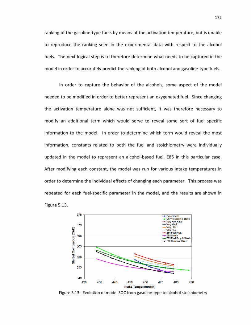
172

ranking of the gasoline-type fuels by means of the activation temperature, but is unable

to reproduce the ranking seen in the experimental data with respect to the alcohol

fuels. The next logical step is to therefore determine what needs to be captured in the

model in order to accurately predict the ranking of both alcohol and gasoline-type fuels.

In order to capture the behavior of the alcohols, some aspect of the model

needed to be modified in order to better represent an oxygenated fuel. Since changing

the activation temperature alone was not sufficient, it was therefore necessary to

modify an additional term which would serve to reveal some sort of fuel specific

information to the model. In order to determine which term would reveal the most

information, constants related to both the fuel and stoichiometry were individually

updated in the model to represent an alcohol-based fuel, E85 in this particular case.

After modifying each constant, the model was run for various intake temperatures in

order to determine the individual effects of changing each parameter. This process was

repeated for each fuel-specific parameter in the model, and the results are shown in

Figure 5.13.

Figure 5.13: Evolution of model SOC from gasoline-type to alcohol stoichiometry

173

This figure displays the individual effects of modifying fuel specific parameters within

the model to represent an alcohol fuel. It displays the entire evolution of the model

from a purely gasoline-type stoichiometry to one based on E85. From the previous

analysis, it was concluded that the activation temperature alone predicted combustion

timing that was significantly retarded from that observed in the experiment with respect

to E85. For this reason, the choice fuel parameter must therefore have the ability to

advance the timing to better match the experimental data. From Figure 5.13, it is clear

that the stoichiometry of the alcohol fuel must be captured in order to advance the

timing. In addition to the stoichiometry, a closer inspection reveals that the fuel

properties (molecular weight, lower heating value and stoichiometric F/A ratio) must

also be accounted for in order to accurately predict the in-cylinder pressure. As a result,

it was concluded that the effects of an oxygenated fuel were too complex to capture

with a simple parameter, and therefore a separate model was necessary in order to

predict the behavior of alcohol-based fuels undergoing HCCI combustion. This new

model for alcohol-type fuels was similar to that used for gasoline-type fuels in every

way, with the exception of the fuel properties and stoichiometry, which were updated

to represent an alcohol.

Due to the alcohol fuels displaying different combustion timing behavior as

compared to the gasoline fuels, it was therefore necessary to investigate whether or not

the previously developed Δθ correlation was still valid for these fuels. The correlation

from Equation 2.60 had been developed based on experimental data corresponding to

gasoline-type fuels, and therefore may not apply to alcohol fuels based on the above

174

0

5

10

15

20

25

348 350 352 354 356 358 360 362 364

SOC (CAD)

Combustion Duration (CAD)

UTG96 9gpm

E85 9gpm

E50 9gpm

Pump Gas 9gpm

TRF 9gpm

findings. In order to validate this theory, the experimental data used to develop the

correlation was investigated for both gasoline and alcohol fuels. This data can be seen

in Figure 5.14.

Figure 5.14: Experimental 10-90% burn data for various fuels in HCCI

This figure reveals that the 10-90% burn duration, which was used to develop the Δθ

correlation, was indeed behaving differently for oxygenated fuels. While all of the fuels

seemed to display a similar trend, the alcohols group was offset from that of the

gasoline-type fuels. This behavior again suggested that the oxygen content of the

alcohols had some effect on their combustion performance, and also served to verify

the hypothesis that a separate Δθ correlation was required to describe these alcohol-

type fuels. Using the experimental data in Figure 5.14 for E85, a new experimental Δθ

correlation was therefore developed for the oxygenated fuels similar to the one

previously developed for the gasoline-type fuels. The form of this correlation was

identical to the one for gasoline fuels, with the exception of the constants, which were

modified to represent E85.

175

( ) ( )( ) ( )[ ] ( )3.52483169.1002493.1240000000624.01010181.1 1,1,11

1,135

1++

−+−

+ ×=∆ kSOCkkSOCk TVV

k

θφ γ

θ

The correlation in Equation 5.3 could now be integrated directly into the newly

developed model for oxygenated fuels, and would allow for a more accurate prediction

of θ23. With the development of this correlation, the separate model for oxygenated

fuels, which accounted for fuel specific parameters and stoichiometry, as well as burn

duration, was now complete. For a given class of fuels, either gasolines or alcohols, the

combustion characteristics in HCCI could now be predicted using a universal model for

that particular class of fuels.

5.4 MULTI-FUEL VALIDATION WITH EXPERIMENTAL DATA

In order to verify the ability of the two models to predict HCCI behavior for

various fuels, it was necessary to compare them to the available experimental data from

the Hatz engine. For both the gasoline-type and alcohol fuels, the activation

temperature was modified in each code to simulate fuel changes according to the

experimental correlation developed in Equation 5.2. For each activation temperature,

or “fuel”, the model was run through a range of intake temperatures according to those

observed in the experimental data for the respective fuel. The Arrhenius threshold

value calculated for UTG96 was held constant for the gasoline-type fuels, while the

oxygenated fuels required a different threshold value, which was determined using

experimental SOC data corresponding to E85. This analysis was done for all five fuels,

and the results, which were grouped according to the fuel class, were plotted along with

the experimental data in Figures 5.15-5.17.

176

Gasoline-Type

348

353

358

363

368

373

378

420 430 440 450 460 470 480 490 500


The

ta2

3 (

CA

D)

Ea=15200 (TRF)

Exp TRF 9gpm

Ea=15098 (UTG96)

Exp UTG96 9gpm

Ea=14798 (Pump Gas)

Exp Pump Gas 9gpm

Ea=15098 (UTG96 6gpm)

Exp UTG96 6gpm

Oxygenates

348

353

358

363

368

373

378

420 430 440 450 460 470 480 490 500


Theta

23 (

CA

D)

Ea=15285 (E85)

Exp E85 9gpm

Ea=15210 (E50)

Exp E50 9gpm

Gasoline-Type

25

30

35

40

45

50

55

60

420 430 440 450 460 470 480 490 500


P3 (

bar)

Ea=15200 (TRF)

Exp TRF 9gpm

Ea=15098 (UTG96)

Exp UTG96 9gpm

Ea=14798 (Pump Gas)

Exp Pump Gas 9gpm

Ea=15098 (UTG96 6gpm)

Exp UTG96 6gpm

Oxygenates

25

30

35

40

45

50

55

60

420 430 440 450 460 470 480 490 500


P3 (

bar)

Ea=15285 (E85)

Exp E85 9gpm

Ea=15210 (E50)

Exp E50 9gpm

Gasoline-Type

348

353

358

363

368

373

378

420 430 440 450 460 470 480 490 500


SO

C (

CA

D)

.

Ea=15200 (TRF)

Exp TRF 9gpm

Ea=15098 (UTG96)

Exp UTG96 9gpm

Ea=14798 (Pump Gas)

Exp Pump Gas 9gpm

Ea=15098 (UTG96 6gpm)

Exp UTG96 6gpm

Oxygenates

348

353

358

363

368

373

378

420 430 440 450 460 470 480 490 500


SO

C (

CA

D)

Ea=15285 (E85)

Exp E85 9gpm

Ea=15210 (E50)

Exp E50 9gpm

Figure 5.15: Model vs. experimental SOC for gasoline-type and oxygenated fuels

Figure 5.16: Model θ23 vs. experimental CA50 for gasoline-type and oxygenated fuels

Figure 5.17: Model vs. experimental peak pressure for gasoline-type and oxygenated fuels

177

These figures reveal that modifying the activation temperature within the model allows

it to accurately predict the behavior of a number of different fuels to a level sufficient

for control. So long as the proper model is utilized according to the class of fuel being

used, a single universal model is able to accurately track the HCCI combustion

parameters which are most pertinent to control. This is significant from a controls

standpoint due to the fact that the model can be applied to a number of different fuels

without having to complete a time intensive calibration process for each one. With

knowledge of only the fuel class (gasoline-type or alcohol) and the RON and MON (OI),

the appropriate universal model, along with the activation temperature corresponding

to the OI of the fuel, can be used to predict the behavior of a plethora of different fuels

undergoing HCCI combustion. This ability to use only the OI of a particular fuel to

predict its behavior in HCCI, rather than an experimentally intensive engine mapping,

allows for a more simplistic model which is ideal for nonlinear control schemes.

178

6. CONCLUSIONS

Despite the high thermal efficiency and low emissions associated with HCCI, it is

inherently difficult to control due to the dependence of the combustion process on

chemical kinetics. A control-oriented nonlinear model of the HCCI process is therefore

presented, which is based on the underlying physics of the problem. This model is

developed in discrete-time by dividing the HCCI process into 5 distinct states, which

allows it to be directly applied to state space control methods. The model states are

meant to represent parameters with physical significance to the combustion process,

and are chosen to be the temperature at IVC, the residual gas fraction and the angle of

peak pressure. The outputs from this control model are also meant to represent

physical parameters, and are chosen to be the peak pressure, which gives an indication

of the work output, and the angle at which that peak pressure occurs. An integrated

Arrhenius rate is used to model the HCCI combustion process, which accounts for the

effects of both temperature and reactant concentrations on the auto-ignition process.

This combustion model predicts the onset of combustion based on an empirically

determined threshold value, which is representative of the concentration of fuel which

must be destroyed prior to ignition. A variable combustion duration is also utilized

within this combustion model, which allows the duration of combustion to vary with set

point. The model developed was validated against experimental data from an engine

running on a UTG96 RON fuel at two different fueling rates. It was shown to

successfully track the pressure evolution in the cylinder for both fueling conditions. The

179

simple model also captures the correct trend in both the start of combustion and the

location of peak pressure as the intake temperature is varied, which is crucial for its

application to control. Utilizing the relationship between the OI of a particular fuel and

its corresponding SOC values, the model was also shown to reasonably predict the

trends in both peak pressure and θ23 for a number of different gasoline-type fuels.

Despite the availability of various control approaches, the nonlinear model presented

here is developed primarily for application to nonlinear control. While linearized

models provide simplicity, they are only valid around some nominal operating point,

which is not characteristic of HCCI engines which regularly change set point. A nonlinear

model such as this one is able to retain system nonlinearities over a wider range of

operating conditions. The result of this modeling process is therefore a discrete-time

nonlinear control model which provides a platform for developing and validating various

nonlinear state-space control strategies.

180

APPENDIX A

HCCI CONTROL MODEL CODE

181

This appendix contains the HCCI control code which has been discussed in this thesis, and which was

developed using MATLAB R2008b. The m-file goes as follows:

% This code is a physics based control model for HCCI combustion of

% gasoline-type fuels.

%

% This code uses the integrated arrhenius rate combustion model and its

% parameters in order to predict combustion phasing.

%

% This code includes both heated internal EGR (alphai) and cooled external

% EGR (alphae)

%

% This code uses C7H16 as the operating fuel.

%

% The combustion parameters used are from Turns.

Control Model Code

cycles=25; % # times to loop program (engine cycles)

%----------Define Variable Matrices-------------

P1=zeros(1, cycles);

V1=zeros(1, cycles);

T1=zeros(1, cycles);




P3=zeros(1, cycles); % P3 in cycle, as opposed to output





P5=zeros(1,cycles);


P6=zeros(1,cycles);

alphae=zeros(1,cycles);

alphai=zeros(1,cycles);

Tin=zeros(1,cycles);

gpm=zeros(1,cycles);

N2=zeros(1, cycles);

N3=zeros(1, cycles);

z=zeros(1, cycles);

Psoc=zeros(1,cycles);

Tsoc=zeros(1,cycles);

Nt=zeros(1,cycles);

Xegr=zeros(1,cycles);

Negr=zeros(1,cycles);

Niegr=zeros(1,cycles);

Nfs=zeros(1,cycles);

PRR=zeros(1, cycles);


T1up=zeros(1, cycles); % Predicts T1 for the next cycle

alphaiup=zeros(1,cycles);

P3op=zeros(1, cycles); % output P3, as opposed to P3 in cycle

PRRop=zeros(1,cycles);

theta23=zeros(1, cycles);

theta23op=zeros(1,cycles);

W34op=zeros(1, cycles);

Wigef=zeros(1, cycles);

182

%-----------Inputs-----------

% alphae=0; % external EGR

% Tin=460; % pre-heated intake temperature (K)

% gpm=9; % fueling rate (gram/min)

%-----------Constants-----------

MWf=100.203; % molecular weight of fuel (g/mol)

MWa=29; % molecular weight of air (g/mol)

FAs=.06634; % stoichiometric fuel/air ratio

LHV=4501.72; % LHV of C8H18 (kJ/mol fuel)

LHV2=44.926; % LHV of C8H18 (KJ/g fuel)

N=188.49555921539; % engine speed (rad/sec)

s=7.0; % stroke (cm)

l=11.042; % connecting rod length (cm)

bore=9.6999; % bore diamater (cm)

crank=3.5; % crank radius (cm)

R=l/crank;

rc=14.5; % compression ratio

thetaEVO=476*pi/180; % radians

thetaTDC=360*pi/180; % radians

thetaLOW=320*pi/180; % radians

thetaIVO=704*pi/180; % radians

thetaIVC=228*pi/180; % radians

Tref=298; % reference temp corresponding to heat of formation (K)

Tegr=300; % temperature of cooled EGR (K)

Pin=.0101; % atmospheric pressure (kN/cm^2)

Vd=pi()*(bore^2)*0.25*s;% disp vol (cm^3)

Vc=Vd/(rc-1); % clearance vol=V(TDC)=V(360) (cm^3)

Vivc=492.9781; % (cm^3)

Vevo=444.1483; % (cm^3)

Vivo=51.4562; % (cm^3)

Vbdc=Vd+Vc; % (cm^3)

Cpc7h16R=.224076; % spec. heat of fuel in reactants (kJ/molfuel*K)

Cpo2R=.030481; % spec. heat of O2 in reactants (kJ/molO2*K)

Cpn2R=.029414; % spec. heat of N2 in reactant (kJ/molN2*K)

Cpco2P=.050523; % spec heat of CO2 in reinducted products (kJ/molCO2*K)

Cph20P=.0381; % spec heat of H2O in reinducted products (kJ/molH2O*K)

Cpn2P=.031091; % spec heat of N2 in reinducted products (kJ/molN2*K)

Cpo2P=.033376; % spec heat of O2 in reinducted products (kJ/molO2*K)

Cpn2E=.029075; % spec heat of N2 in cooled external EGR (kJ/molO2*K)

gamma=1.3; % spec. heat ratio of fuel

A=5.1e11; % Arrhenius rate pre-exponential factor (gmol/cm^3)^1-a-b/s

Ea=15098; % activation energy (K)

a=0.25; % Arrhenius rate parameter (unitless)

b=1.5; % Arrhenius rate parameter (unitless)

Kth=2.3072e-6; % Arrhenius threshold value (gmol/cm^3)

Ru1=.008314472; % universal gas constant (KJ/mol*K)

Ru2=.8314472; % universal gas constant (Kn-cm/mol*K)

X=0.86; % relationship between temperature of re-inducted

% products and exhaust temperature of

% last cycle where Treinduct=XTex

eps=0.1; % fraction of LHV representing heat loss due to combustion

183

%-----------Assumptions-----------

offset=120.249*(pi/180); % Offset value that corrects for the Arrhenius

% threshold value not being evaluated with

% constant temperatures

%-----------Initializations-----------

T6(1,2)=742; % temp of inducted products and reactants from "zeroth" cycle (K)

thetaSOC(1,3)=354*pi/180; % angle at which combustion initiates (radians)

Vsoc(1,3)=(Vc*(1+0.5*(rc-1)*(R+1-cos(thetaSOC(1,2))-...

(R^2-sin(thetaSOC(1,2))^2)^.5)));

dtheta(1,3)=11*pi/180; % combustion duration

theta23(1,3)=365*pi/180; % angle at which peak pressure is assumed to occur (radians)

V23(1,3)=(Vc*(1+0.5*(rc-1)*(R+1-cos(theta23(1,2))-...

(R^2-sin(theta23(1,2))^2)^.5))); % cylinder vol at peak pressure (cm^3)

PHI(1,1)=.384563; % initializes the equivalence ratio

PHI(1,2)=.384563;

Nf(1,2)=.000058; % initializes the moles of fuel inducted

Na(1,2)=.003; % initializes the moles of air inducted

alphai(1,3)=.0299; % initializes the internal EGR(valve overlap and

trapped residual)

alphae(1,1)=0;

alphae(1,2)=0; % initializes the external EGR

alphae(1,3)=0;

C1(1,2)=1.8614;

C2(1,2)=2.0053;

Cegr(1,2)=1.7411; % initializes the specific heat parameters

C3(1,2)=1770.1;

C4(1,2)=2.0053;

%-----------Begin Looping the Program---------------

for i=3:cycles;

% Input values for the intake temperature

Tin(1,i)=463;

% Gives gaussian distributed random values for Tin

% Tin(1,i) = normrnd(443,4.43);

% Input values for the external EGR

alphae(1,i)=0;

% Gives gaussian disributed random values for alphae

% alphae(1,i) = normrnd(0,.0001);

% Input values for the fueling rate

gpm(1,i)=9;

% Gives gaussian disributed random values for gpm

% gpm(1,i) = normrnd(9,.27);

184

%-----------1: Adiabatic Induction, Instant Mixing-----------

P1(1,i)=Pin;

V1(1,i)=(Vc*(1+0.5*(rc-1)*(R+1-cos(thetaIVC)-(R^2-sin(thetaIVC)^2)^.5)));

if i==3;

T1(1,i)=T6(1,2);

else

T1(1,i)=T6(1,i-1);

end

%-----------1-2: Isentropic Compression-----------

P2(1,i)=(P1(1,i)*((V1(1,i)/V23(1,i))^gamma));

T2(1,i)=(T1(1,i)*((V1(1,i)/V23(1,i))^(gamma-1)));

Psoc(1,i)=(P1(1,i)*((V1(1,i)/Vsoc(1,i))^gamma));

Tsoc(1,i)=(T1(1,i)*((V1(1,i)/Vsoc(1,i))^(gamma-1)));

%-----------Intermediate Calculations-----------------

N2(1,i)=(PHI(1,i-1)+52.36+(alphai(1,i)*((4*PHI(1,i-2))+52.36))+...

(alphae(1,i-1)*(PHI(1,i-1)+52.36))); % number of moles before combustion

N3(1,i)=((4*(PHI(1,i-1)+(PHI(1,i-2)*alphai(1,i))))+52.36*...

(1+alphai(1,i))+(alphae(1,i-1)*(PHI(1,i-1)+52.36))); % number of moles after % combustion

z(1,i)=N3(1,i)/N2(1,i); % product to reactant molar ratio for combustion reaction

%-----------2-3: Isochoric Combustion-----------

% Assume instantaneous, constant volume combustion

T3(1,i)=((C3(1,i-1)+((C1(1,i-1)+(C2(1,i-1)*alphai(1,i))+(Cegr(1,i-1)*...

alphae(1,i-1))-(Ru1*N2(1,i)))*T2(1,i))-((C1(1,i-1)-C4(1,i-1))*...

Tref))/((C2(1,i-1)*(alphai(1,i)))+(Cegr(1,i-1)*alphae(1,i-1))+...

C4(1,i-1)-(Ru1*N3(1,i))));

P3(1,i)=(z(1,i)*((V1(1,i)/V23(1,i))^gamma)*((C1(1,i-1)+(C2(1,i-1)*...

alphai(1,i))+(Cegr(1,i-1)*alphae(1,i-1))-(Ru1*N2(1,i)))/...

((((C2(1,i-1)*(alphai(1,i)))+(Cegr(1,i-1)*alphae(1,i-1))+...

C4(1,i-1)-(Ru1*N3(1,i)))*T3(1,i))-C3(1,i-1)+((C1(1,i-1)-...

C4(1,i-1))*Tref)))*Pin*T3(1,i));

%------------Pressure Rise Rate---------------

PRR(1,i)=((P3(1,i)-Psoc(1,i))*2*pi*100)/(dtheta(1,i)*360); % (bar/CAD)

%-----------3-4: Isentropic Expansion-----------

V4(1,i)=(Vc*(1+0.5*(rc-1)*(R+1-cos(thetaEVO)...

-sqrt(R^2-sin(thetaEVO)^2))));

T4(1,i)=(T3(1,i)*((V23(1,i)/V4(1,i))^(gamma-1)));

P4(1,i)=(P3(1,i)*((V23(1,i)/V4(1,i))^gamma));

%-----------4-5: Isentropic Exhaust-----------

T5(1,i)=(T4(1,i)*((Pin/P4(1,i))^((gamma-1)/gamma)));

P5(1,i)=Pin;

185

%%---------This section calculates the residual mass

% fraction trapped in the cylinder

w=30; % engine speed (rev/sec)

rc=14.5; % compression ratio

Pi=1.02235; % intake pressure

Pe=1.24596; % exhaust pressure

B=96.999; % bore diamater (mm)

Dv=31; % average valve seat diameter (mm)

Lv=5.334; % average valve lift (mm)

IVO=704; % intake valve opening (CAD)

EVC=20; % exhaust valve closing (CAD)

thetaoverlap=36; % valve overlap EVC-IVO (CAD)

%----------- Calculate the Overlap Factor OF-----------

OF = (1.45/B)*(107+7.8*thetaoverlap+(thetaoverlap^2))*((Lv*Dv)/B^2);

%------------ Calculate the residual mass fraction --------

alphai(1,i+1) = ((.401*(OF/w)*(1-exp((-4.78*(1-...

((Pi/Pe)^.7)))-(153.8*(1-((Pi/Pe)^4.5)))))*...

(Pe/Pi)*(Tin(1,i)/T5(1,i)))+((Pe*Tin(1,i))/...

(rc*Pi*T5(1,i))));

%-----------Calculate Air Inducted and Equivalence Ratio---------

Nf(1,i)=(gpm(1,i)*4*pi)/(MWf*N*60); % moles of fuel

Nt(1,i)=(Pin*(Vd+Vc))/(Ru2*Tin(1,i));

Xegr(1,i)=(alphae(1,i)*(PHI(1,i-1)+52.36))/...

(((PHI(1,i-1)+52.36)*(1+alphae(1,i)))+(alphai(1,i+1)*...

((15*PHI(1,i-1))+41.36+(11*(1-PHI(1,i-1))))));

Negr(1,i)=Xegr(1,i)*Nt(1,i); % moles of egr

Niegr(1,i)=alphai(1,i+1)*Nt(1,i);

if alphae(1,i)~=0

Na(1,i)=Nt(1,i)-Negr(1,i)-Niegr(1,i);

else

Na(1,i)=(Pin*Vd)/(Ru2*Tin(1,i));

end

Nfs(1,i)=(Na(1,i)*MWa*FAs)/(MWf); % stoich moles of fuel

PHI(1,i)=Nf(1,i)/Nfs(1,i); % equiv. ratio

C1(1,i)=PHI(1,i)*Cpc7h16R+11*Cpo2R+41.36*Cpn2R; % "specific heat" of reactants

C2(1,i)=7*PHI(1,i-1)*Cpco2P+8*PHI(1,i-1)*Cph20P+...

41.36*Cpn2P+11*(1-PHI(1,i-1))*Cpo2P; % "specific heat" of products

Cegr(1,i)=(PHI(1,i)+52.36)*Cpn2E; % "specific heat" of cooled EGR

C3(1,i)=PHI(1,i)*LHV*(1-eps);

C4(1,i)=7*PHI(1,i)*Cpco2P+8*PHI(1,i)*Cph20P+41.36*Cpn2P+11*(1-PHI(1,i))*Cpo2P;

186

%-----------State Update Equations-----------

T1up(1,i+1)=((C1(1,i)*Tin(1,i)+(C2(1,i)*alphai(1,i+1)*X*((((((C2(1,i-1)*...

(alphai(1,i)))+(Cegr(1,i-1)*alphae(1,i-1))+C4(1,i-1)-(Ru1*N3(1,i)))*...

T1(1,i))/(z(1,i)*(V1(1,i)/V23(1,i))*(C3(1,i-1)+((C1(1,i-1)+(C2(1,i-1)*...

alphai(1,i))+(Cegr(1,i-1)*alphae(1,i-1))-(Ru1*N2(1,i)))*(T1(1,i)*...

((V1(1,i)/V23(1,i))^(gamma-1))))-((C1(1,i-1)-C4(1,i-1))*Tref))))^...

((gamma-1)/gamma))*((C3(1,i-1)+((C1(1,i-1)+(C2(1,i-1)*alphai(1,i))+...

(Cegr(1,i-1)*alphae(1,i-1))-(Ru1*N2(1,i)))*(T1(1,i)*((V1(1,i)/...

V23(1,i))^(gamma-1))))-((C1(1,i-1)-C4(1,i-1))*Tref))/((C2(1,i-1)*...

(alphai(1,i)))+(Cegr(1,i-1)*alphae(1,i-1))+C4(1,i-1)-(Ru1*...

N3(1,i))))))+(Cegr(1,i)*alphae(1,i)*Tegr))/(C1(1,i)+(C2(1,i)*...

alphai(1,i+1))+(Cegr(1,i)*alphae(1,i)))); % state update equation

thetaSOC(1,i+1)=((((Kth*N)/(A*(PHI(1,i)^a)*((11*((alphai(1,i+1)*... (1-PHI(1,i-1)))+1))^b)))*((Vc*Ru2/Pin)^(a+b))*(((T1up(1,i+1)*...

(PHI(1,i)+52.36+(alphai(1,i+1)*((4*PHI(1,i-1))+52.36))+...

(alphae(1,i)*(PHI(1,i)+52.36))))/(V1(1,i)))^(a+b)))/...

(exp(-Ea/(T1up(1,i+1)*((V1(1,i)/Vc)^(gamma-1))))))+thetaIVC+offset;

Vsoc(1,i+1)=(Vc*(1+0.5*(rc-1)*(R+1-cos(thetaSOC(1,i+1))-(R^2-... sin(thetaSOC(1,i+1))^2)^.5))); % predicts volume at SOC for next cycle

% variable combustion duration for 10-90% MFB

% predicts the combustion duration using equivalence ratio,

% thetaSOC and temperature at SOC

dtheta(1,i+1)=((2.067699188524e-18)*(.0000351554746669643^...

PHI(1,i))*(.992961372838845^(((V1(1,i)/Vsoc(1,i+1))^...

(gamma-1))*T1up(1,i+1)))*(1.16093520650449^...

(thetaSOC(1,i+1)*(180/pi))))*(pi/180);

theta23(1,i+1)=((((Kth*N)/(A*(PHI(1,i)^a)*((11*((alphai(1,i+1)*... (1-PHI(1,i-1)))+1))^b)))*((Vc*Ru2/Pin)^(a+b))*(((T1up(1,i+1)*...

(PHI(1,i)+52.36+(alphai(1,i+1)*((4*PHI(1,i-1))+52.36))+...

(alphae(1,i)*(PHI(1,i)+52.36))))/(V1(1,i)))^(a+b)))/(exp(-Ea/...

(T1up(1,i+1)*((V1(1,i)/Vc)^(gamma-1))))))+dtheta(1,i+1)+...

thetaIVC+offset; % state update equation

V23(1,i+1)=(Vc*(1+0.5*(rc-1)*(R+1-cos(theta23(1,i+1))-(R^2-...

sin(theta23(1,i+1))^2)^.5))); % predicts volume at theta23 for next cycle

alphaiup(1,i+1) =(.091255843297*Tin(1,i))/((((((C2(1,i-1)*...

(alphai(1,i)))+(Cegr(1,i-1)*alphae(1,i-1))+C4(1,i-1)-(Ru1*...

N3(1,i)))*T1(1,i))/(z(1,i)*(V1(1,i)/V23(1,i))*(C3(1,i-1)+...

((C1(1,i-1)+(C2(1,i-1)*alphai(1,i))+(Cegr(1,i-1)*alphae(1,i-1))-...

(Ru1*N2(1,i)))*(T1(1,i)*((V1(1,i)/V23(1,i))^(gamma-1))))-...

((C1(1,i-1)-C4(1,i-1))*Tref))))^((gamma-1)/gamma))*((C3(1,i-1)+...

((C1(1,i-1)+(C2(1,i-1)*alphai(1,i))+(Cegr(1,i-1)*alphae(1,i-1))-...

(Ru1*N2(1,i)))*(T1(1,i)*((V1(1,i)/V23(1,i))^(gamma-1))))-...

((C1(1,i-1)-C4(1,i-1))*Tref))/((C2(1,i-1)*(alphai(1,i)))+...

(Cegr(1,i-1)*alphae(1,i-1))+C4(1,i-1)-...

(Ru1*N3(1,i))))); % state update equation

187

%-----------Output Equations-----------

P3op(1,i)=(z(1,i)*(V1(1,i)/V23(1,i))*Pin*((C3(1,i-1)+((C1(1,i-1)+...

(C2(1,i-1)*alphai(1,i))+(Cegr(1,i-1)*alphae(1,i-1))-(Ru1*N2(1,i)))*...

(T1(1,i)*((V1(1,i)/V23(1,i))^(gamma-1))))-((C1(1,i-1)-C4(1,i-1))*...

Tref))/(((C2(1,i-1)*(alphai(1,i)))+(Cegr(1,i-1)*alphae(1,i-1))+...

C4(1,i-1)-(Ru1*N3(1,i)))*T1(1,i)))); % output equation

theta23op(1,i)=((((Kth*N)/(A*(PHI(1,i-1)^a)*((11*((alphai(1,i)*...

(1-PHI(1,i-2)))+1))^b)))*((Vc*Ru2/Pin)^(a+b))*(((T1(1,i)*...

(PHI(1,i-1)+52.36+(alphai(1,i)*((4*PHI(1,i-2))+52.36))+...

(alphae(1,i-1)*(PHI(1,i-1)+52.36))))/(V1(1,i)))^(a+b)))/...

(exp(-Ea/(T1(1,i)*((V1(1,i)/Vc)^(gamma-1))))))+dtheta(1,i)+...

thetaIVC+offset; % output equation

PRRop(1,i)=((P3(1,i)-Psoc(1,i))*2*pi*100)/(dtheta(1,i)*360); % ouput equation

W34op(1,i)=((((V4(1,i)*((V23(1,i)/V4(1,i))^gamma))-V23(1,i))*(z(1,i)*...

(V1(1,i)/V23(1,i))*Pin*(C3(1,i-1)+((C1(1,i-1)+(C2(1,i-1)*...


((V1(1,i)/V23(1,i))^(gamma-1))))-((C1(1,i-1)-C4(1,i-1))*Tref)))+...

(Pin*((V23(1,i)*((V1(1,i)/V23(1,i))^gamma))-V1(1,i)+((1-gamma)*...

(V1(1,i)-V4(1,i))))*((((C2(1,i-1)*(alphai(1,i)))+(Cegr(1,i-1)*...

alphae(1,i-1))+C4(1,i-1)-(Ru1*N3(1,i)))*T1(1,i)))))/((((C2(1,i-1)*...


T1(1,i))*(1-gamma))); % output equation

Wigef(1,i)=((((V4(1,i)*((V23(1,i)/V4(1,i))^gamma))-V23(1,i))*(z(1,i)*...

(V1(1,i)/V23(1,i))*Pin*(C3(1,i-1)+((C1(1,i-1)+(C2(1,i-1)*...


((V1(1,i)/V23(1,i))^(gamma-1))))-((C1(1,i-1)-C4(1,i-1))*Tref)))+...

(Pin*((V23(1,i)*((V1(1,i)/V23(1,i))^gamma))-V1(1,i)+((1-gamma)*...

(V1(1,i)-V4(1,i))))*((((C2(1,i-1)*(alphai(1,i)))+(Cegr(1,i-1)*...

alphae(1,i-1))+C4(1,i-1)-(Ru1*N3(1,i)))*T1(1,i)))))/((((C2(1,i-1)*...


T1(1,i))*(1-gamma)))/(Nf(1,i)*100*LHV); % output equation

end;

188

Volume Pressure and Temperature Traces

%------------Plotting Volume trace-------------------

angle=(1:720);

V=(1:720);

theta=(1:720);

for i=1:720

angle(1,i)=i*(pi/180);

V(1,i)=Vc*(1+(0.5*(rc-1)*(R+1-(cos(angle(1,i)))-(((R^2)-...

(sin(angle(1,i)))^2)^.5))));

end

figure

plot(theta,V)

title('Cylinder Volume vs CAD')

xlabel('CAD'); ylabel('Cylinder Volume (cm^3)')

axis([0 720 20 600])

grid on

%------------Plotting Pressure trace-------------------

P(1:228)=Pin; % atmospheric pressure during induction

for i=229:round((theta23(1,cycles)-(pi/180))*(180/pi))

P(1,i)=(Pin*(V1(1,cycles)/V(1,i))^gamma); % pressure rise during compression

end

P(1,round(theta23(1,cycles)*(180/pi)))=(z(1,cycles)*((V1(1,cycles)/...

V23(1,cycles))^gamma)*((C1+(C2*alphai(1,cycles))+(Cegr*...

alphae(1,cycles-1))-(Ru1*N2(1,cycles)))/((((C2*(1+...

alphai(1,cycles)))+(Cegr*alphae(1,cycles-1))-(Ru1*...

N3(1,cycles)))*T3(1,cycles))-C3+((C1-C2)*Tref)))*...

Pin*T3(1,cycles)); % peak pressure after combustion (P3)

for i=round((theta23(1,cycles)+(pi/180))*(180/pi)):476

P(1,i)=(P3(1,cycles)*((V23(1,cycles)/V(1,i))^gamma)); % expansion pressure

end

for i=477:704

P(1,i)=Pin;

end

P(704:720)=Pin; % atmospheric pressure during exhaust

figure

plot(theta,P)

title('Pressure vs CAD')

xlabel('CAD'); ylabel('Pressure (bar)')

axis([0 720 0 62])

grid on

189

%------------Plotting Temperature trace-------------------

T=zeros(1,720);

for i=1:228

T(1,i)=((C1*Tin(1,cycles)+(C2*alphai(1,cycles)*X*T5(1,cycles))+...

(Cegr*alphae(1,cycles)*Tegr))/(C1+(C2*alphai(1,cycles))+(Cegr*...

alphae(1,cycles)))); % induction temperature dependent on previous cycle

end

for i=229:round((theta23(1,cycles))*(180/pi))

T(1,i)=T1(1,cycles)*(V1(1,cycles)/V(1,i))^(gamma-1); % compression temp.

end

T(1,round(theta23(1,cycles)*(180/pi)))=((C3+((C1+(C2*...

alphai(1,cycles-1))+(Cegr*alphae(1,cycles-1))-(Ru1*...

N2(1,cycles)))*T2(1,cycles))-((C1-C2)*Tref))/...

((C2*(1+alphai(1,cycles-1)))+(Cegr*alphae(1,cycles-1))-...

(Ru1*N3(1,cycles)))); % peak temperature after combustion (T3)

for i=round((theta23(1,cycles)+(pi/180))*(180/pi)):476

T(1,i)=T3(1,cycles)*((V23(1,cycles)/V(1,i))^(gamma-1)); % expansion temp.

end

for i=477:720

T(1,i)=T4(1,cycles)*(Pin/P4(1,cycles))^((gamma-1)/gamma); % exhaust temp.

end

figure

plot(theta,T)

title('Temperature vs CAD')

xlabel('CAD'); ylabel('Temperature (K)')

axis([0 720 400 2300])

grid on

190

APPENDIX B

HCCI TEST CASES

191

MODEL OPERATION

This tutorial provides guidance in effectively running the HCCI control model code found

in Appendix A. In order to get started, the number of engine cycles must be determined and

entered into the variable cycles. Once that is complete, the next section of the code which

requires attention is that labeled Constants. This section includes a variety of parameters

including fuel properties, engine geometry, EGR temperature, atmospheric pressure, specific

heat values, Arrhenius Rate parameters, and heat transfer terms (X and eps). In addition to

this section, there are also a few other parameters, mostly related to engine geometry, which

must be entered, and which are located in lines 255-264 of the code. The current values for all

of these parameters are set based on the engine geometry of the Hatz 1D50Z engine running on

C7H16. Once these parameters are defined, it is now possible to begin looping the program.

Since the model was developed for control using state space methods, all which is required to

run the program is to specify the various input variables within the model. These input variables

are intake temperature (Tin), external EGR fraction (alphae) and fueling rate (gpm). Random

perturbations can also be added to these input variables by un-commenting the commands

entitled normrnd under each input. Once these inputs have been defined, the m-file can now

be run in order to obtain the various outputs from the control model. These outputs include the

start of combustion (SOC), the angle of constant volume combustion (θ23), the pressure rise rate

(PRR), the peak pressure (P3), the gross indicated work (W34), and the efficiency (Wigef). The

following test cases provide examples which serve to inspire confidence that the control model

is indeed operating correctly. These test cases were run using the m-file entitled

C7H16_NewestEdition, and consist of the inputs, outputs, state variables and pressure traces for

three different engine operating conditions.

192

TEST CASE 1

Inputs:

� Tin = 463 K

� alphae = 0

� gpm = 9 g/min

Outputs:

� P3 = 0.5731 KN/cm2

� theta23 = 6.2297 rad

� PRR = 10.7766 bar/CAD

� W34 = 19.9583 KN-cm

� Wigef = 0.4442

State Variables:

� T1 = 475.7303 K

� thetaSOC = 6.1795 rad

� theta23 = 6.2297 rad

� alphai = 0.0515

Pressure Trace:

250 300 400 450228 4763600

10

20

30

40

50

60

CAD

Pre

ssure

(bar)

Figure A.1: Pressure trace for test case 1

193

TEST CASE 2

Inputs:

� Tin = 475 K

� alphae = 0.2

� gpm = 7 g/min

Outputs:

� P3 = 0.3983 KN/cm2

� theta23 = 6.5412 rad

� PRR = 0.9126 bar/CAD

� W34 = 15.7438 KN-cm

� Wigef = 0.4506

State Variables:

� T1 = 457.6105 K


� theta23 = 6.5412 rad

� alphai = 0.0567

Pressure Trace:

250 300 400360 450228 4760

10

20

30

40

50

60

CAD

Pre

ssure

(bar)


194

TEST CASE 3

Inputs:

� Tin = 48395 K

� alphae = 0.05

� gpm = 5.8 g/min

Outputs:

� P3 = 0.4735 KN/cm2

� theta23 = 6.3179 rad

� PRR = 2.5973 bar/CAD

� W34 = 13.0314 KN-cm

� Wigef = 0.4501

State Variables:

� T1 = 483.1816 K


� theta23 = 6.3179 rad

� alphai = 0.0613

Pressure Trace:

250 300 400360228 4764500

10

20

30

40

50

60

CAD

Pre

ssure

(bar)


195

BIBLIOGRAPHY

[1] Yao, Mingfa, Zhaolei Zheng, and Haifeng Liu. “Progress and recent trends in homogeneous

charge compression ignition (HCCI) engines”. Progress in Energy and Combustion Science 35

(2009): 398-437.

[2] Stanglmaier, Rudolf, and Charles Roberts. "Homogeneous Charge Compression Ignition

(HCCI): Benefits, Compromises, and Future Engine Applications." SAE paper 1999-01-3682.

[3] Juttu, S., S. Thipse, N. Marathe, and M. Gajendra Babu. "Homogeneous Charge Compression

Ignition (HCCI): A New Concept for Near Zero NOx and Particulate Matter (PM) from Diesel

Engine Combustion." SAE paper 2007-26-020.

[4] Shaver, Gregory, Matthew Roelle, and J. Gerdes. “Modeling cycle-to-cycle dynamics and

mode transition in HCCI engine with variable valve actuation”. Control Engineering Practice

14 (2006): 213-222.

[5] Ghazimirsaied, Ahmad, M. Shahbakhti and Charles R. Koch. “HCCI Engine Combustion

Phasing Prediction Using a Symbolic-Statistics Approach”. Journal of Engineering for Gas

Turbines and Power 132 (2010): 1-5.

[6] Kusaka, J, T. Yamamoto, and Y. Daisho. “Simulating the homogeneous charge compression

ignition process using a detailed kinetics model for n-heptane mixture”. Int. Journal Engine

Research (2000): 281-289

[7] Yao, Mingfa, and Zhaolei Zheng. “Numerical study on the chemical reaction kinetics of n-

heptane for HCCI combustion process”. Fuel 85 (2006): 2605-15

[8] Fiveland, SB, and DN Assanis. “Development of a two-zone HCCI combustion model

accounting for boundary layer effects”. SAE paper 2001-01-1028

[9] Fiveland, SB, and DN Assanis. “Development and validation of quasi-dimensional model for

HCCI engine performance and emissions studies under turbocharged conditions”. SAE paper

2001-01-1757

[10]Xu, HM, A Williams, HY Fu, S Wallace, S Richardson, and M Richardson. “Operating

characteristics of a homogeneous charge compression ignition engine with cam profile

switching-simulation study”. SAE paper 2003-01-1859

[11]Ogink, R. “Applications and results of a user-defined, detailed chemistry HCCI combustion

model in the AVL BOOST cycle simulation code”. International AVL User Meeting (2003): 14-

15

[12]Aceves SM, DL Flowers, CK Westbrook, JR Smith, WJ Pitz, RW Dibble et al. “A multi-zone

model for prediction of HCCI combustion and emissions”. SAE paper 2000-01-0327

196

[13]Shaver, G, M. Roelle, P. Caton, N. Kaahaaina, N. Ravi, J. Hathout et al. “A physics-based

approach to the control of homogeneous charge compression ignition engines with variable

valve actuation”. Int. Journal Engine Research (2005): 361-375

[14] Waero, Rolf R. "The Effect of Spark Timing on Residual Gas Fraction." Thesis. University of

Michigan, Ann Arbor, 1997.

[15] Massey, Jeffrey, James Drallmeier, Scott Eaton, and Robert Wagner. “Influence of the

Combustion Energy Release on Surface Accelerations of an HCCI Engine”. SAE Paper 2009-

01-2741

[16] Vance, J., P. He, B. Kaul, S. Jagannathan, and J. Drallmeier, “Neural network-based output

feedback controller for lean operation of spark ignition engines” Proc. of the Amer. Controls

Conf. (2006): 1898-1905.

[17] Iida, M, M. Hayashi, D.E. Foster, and J.K. Martin. “Characteristics of Homogeneous Charge

Compression Ignition (HCCI) Engine Operation for Variations in Compression Ratio, Speed,

and Intake Temperature While Using n-Butane as a Fuel”. Journal of Eng. For Gas Turbines

and Power (2003): 472-478

[18] Heywood, J.B. “Internal Combustion Engine Fundamentals”. McGraw-Hill, 1988.

[19] Fox, Jonathan W., Wai K. Cheng and John B. Heywood. “A Model for Predicting Residual Gas

Fraction in Spark-Ignition Engines.” SAE Paper 931025

[20] Shahbakhti, Mahdi, and Charles Robert Koch. “Physics Based Control Oriented Model for

HCCI Combustion Timing.” Journal of Dynamic Systems, Measurement and Control 132

(2010): 1-12

[21] Rausen, DJ, A.G. Stefanopoulou, JM Kang, JA Eng and TW Kuo. “A Mean-Value Model for

Control of Homogeneous Charge Compression Ignition (HCCI) Engines”. Proc. of the 2004

American Control Conference (2004): 125-131.

[22] Shahbakhti, Mahdi, and Charles Robert Koch. “Control Oriented Modeling of Combustion

Phasing for an HCCI Engine”. Proc. of the 2007 American Control Conference (2007): 3694-

3699.

[23] Ravi, Nikhil, Matthew Roelle, Adam Jungkunz and Christian Gerdes. “A Physically Based

Two-State Model for Controlling Exhaust Recompresion HCCI In Gasoline Engines”. Proc. of

International Mechanical Enginering Conference and Exposition (2006): 1-10.

[24] Chiang, Chia-Jiu, Anna Stefanopoulou and M. Jankovic. “Nonlinear Observer-Based Control

of Load Transitions in Homogeneous Charge Compression Ignition Engines”. IEEE

Transactions on Control Systems Technology 15.3 (2007): 438-448.

197

[25] Chiang, Chia-Jiu, and Anna Stefanopoulou. “Stability Analysis in Homogeneous Charge

Compression Ignition (HCCI) Engines With High Dilution”. IEEE Transactions on Control

Systems Technology 15.2 (2007): 209-218.

[26] Swan, Kevin, Mahdi Shahbakhti, and Charles Koch. “Predicting Start of Combustion Using a

Modified Knock Integral Method for an HCCI Engine”. SAE paper 2006-01-1086.

[27] Ogink, R. “Approximation of Detailed-Chemistry Modeling by a Simplified HCCI Combustion

Model”. SAE paper 2005-24-037.

[28] He, X., M. Donovan, B. Zigler, T. Palmer, S. Walton, M. Wooldridge, and A. Atreya. “An

experimental and modeling study of iso-octane ignition delay times under homogeneous

charge compresion ignition conditions.” Combustion and Flame 142 (2005): 266-275.

[29] Babajimopoulos, Aristotelis, George Lavoie and Dennis Assanis. “On the Role of Top Dead

Center Conditions in the Combustion Phasing of Homogeneous Charge Compression Ignition

Engines”. Combust. Science and Tech. 179 (2007): 2039-2063.

[30] Livengood, J., and P. Wu. “Correlation of Autoignition Phenomena in Internal Combustion

Engines and Rapid Compression Machines”. Fifth Int. Symposium on Combustion (1955):

347-356

[31] Turns, S.R.. “An Introduction to Combustion: Concepts and Applications.” McGraw-Hill, 2nd

edition, 2000.

[32] Chiang, C., and A. Stefanopoulou. “Sensitivity Analysis of Combustion Timing and Duration

time of homogeneous Charge Compression Ignition (HCCI) Engines.” Proc. of the Amer.

Controls Conf. (2006): 1857-62.

[33]Yang, Q., J. Vance, and S. Jagannathan, “Neural network control of non-affine nonlinear

discrete-time systems”, IEEE Transactions on Systems, Man and Cybernetics: Part B 38

(2008): 994-1001.

[34] Risberg, Per, Guatam Kalghatgi, and Hans-Erik Angstrom. “Auto-ignition Quality of Gasoline-

Like Fuels in HCCI Engines.” SAE paper 2003-01-3215.

[35] Kalghatgi, Guatam. “Auto-Ignition Quality of Practical Fuels and Implications for Fuel

Requirements of Future SI and HCCI Engines.” SAE paper 2005-01-0239.

[36] Kalghatgi, Guatam, Per Risberg, and Hans-Erik Angstrom. “A Method of Defining Ignition

Quality of Fuels in HCCI Engines.” SAE paper 2003-01-1816.

[37] Kalghatgi, Guatam, and R.A. Head. “The Available and Required Autoignition Quality of

Gasoline-Like Fuels in HCCI Engines at High Temperatures.” SAE paper 2004-01-1969.

198

VITA

Joshua Bradley Bettis was born in St. Louis, Missouri on May 13, 1985. He

graduated from Hillsboro High School in May of 2003. He did a summer internship with

the 3M Corporation during the summer of 2006 in Nevada, MO. In the spring of 2007,

he worked for Hunter Engineering Company in Bridgeton, MO as an engineering co-op.

In May 2008, he received his B.S. with Honors in Mechanical Engineering from the

University of Missouri-Rolla. During the summer of 2008, he worked for Caterpillar in

Aurora, IL as a summer intern. In December 2010, he received his M.S. degree in

Mechanical Engineering from the Missouri University of Science and Technology

(formerly known as University of Missouri-Rolla).

thermodynamic based modeling for - Scholars' Mine

Documents

Transcript of thermodynamic based modeling for - Scholars' Mine