Scholars' Mine Scholars' Mine

Masters Theses Student Theses and Dissertations

Spring 2010

Data aggregation in wireless sensor networks Data aggregation in wireless sensor networks

Priya Kasirajan

Follow this and additional works at: https://scholarsmine.mst.edu/masters_theses

Part of the Electrical and Computer Engineering Commons

Department: Department:

Recommended Citation Recommended Citation Kasirajan, Priya, "Data aggregation in wireless sensor networks" (2010). Masters Theses. 5002. https://scholarsmine.mst.edu/masters_theses/5002

This thesis is brought to you by Scholars' Mine, a service of the Missouri S&T Library and Learning Resources. This work is protected by U. S. Copyright Law. Unauthorized use including reproduction for redistribution requires the permission of the copyright holder. For more information, please contact scholarsmine@mst.edu.

DATA AGGREGATION

IN WIRELESS SENSOR NETWORKS

by

PRIYA KASIRAJAN

A THESIS

Presented to the Faculty of the Graduate School of the

MISSOURI UNIVERSITY OF SCIENCE AND TECHNOLOGY

In Partial Fulfillment of the Requirements for the Degree

MASTER OF SCIENCE IN ELECTRICAL ENGINEERING

2010

Approved by

Dr. J. Sarangapani, Advisor

Dr. M. Zawodniok

Dr. S. Madria

iii

PUBLICATION THESIS OPTION

This thesis consists of the following two articles that have been submitted for

publication:

Paper 1, pages 10 – 52, Priya Kasirajan, Carl Larsen and S. Jagannathan, ―A New

Data Aggregation Scheme via Adaptive Compression for Wireless Sensor Networks,‖

has been submitted to ACM Transactions on Sensor Networks.

Paper 2, pages 53 – 93, Priya Kasirajan, Maciej Zawodniok and S. Jagannathan,

―Hardware Verification of Data aggregation and Multi-interface Multi-channel Routing

Protocol,‖ intended for submission to International Journal of Distributed Sensor

Networks.

iv

ABSTRACT

Energy efficiency is an important metric in resource constrained wireless sensor

networks (WSN). Multiple approaches such as duty cycling, energy optimal scheduling,

energy aware routing and data aggregation can be availed to reduce energy consumption

throughout the network. This thesis addresses the data aggregation during routing since

the energy expended in transmitting a single data bit is several orders of magnitude

higher than it is required for a single 32 bit computation. Therefore, in the first paper, a

novel nonlinear adaptive pulse coded modulation-based compression (NADPCMC)

scheme is proposed for data aggregation. A rigorous analytical development of the

proposed scheme is presented by using Lyapunov theory. Satisfactory performance of the

proposed scheme is demonstrated when compared to the available compression schemes

in NS-2 environment through several data sets. Data aggregation is achieved by

iteratively applying the proposed compression scheme at the cluster heads.

The second paper on the other hand deals with the hardware verification of the

proposed data aggregation scheme in the presence of a Multi-interface Multi-Channel

Routing Protocol (MMCR). Since sensor nodes are equipped with radios that can operate

on multiple non-interfering channels, bandwidth availability on each channel is used to

determine the appropriate channel for data transmission, thus increasing the throughput.

MMCR uses a metric defined by throughput, end-to-end delay and energy utilization to

select Multi-Point Relay (MPR) nodes to forward data packets in each channel while

minimizing packet losses due to interference. Further, the proposed compression and

aggregation are performed to further improve the energy savings and network lifetime.

v

ACKNOWLEDGMENTS

I would like to add a few heartfelt words for the people who were part of my

thesis in numerous ways, people who gave unending support right from the beginning. I

would like to express my sincere gratitude to my advisor, Dr. Jagannathan Sarangapani,

for his continuous guidance and support. I would also like to thank Dr. Maciej

Zawodniok for his invaluable contributions and suggestions that helped me complete this

work. I would also like to thank Dr. Sanjay Madria for his kind support. Financial

assistance from the Air Force Research Laboratory and Army‘s Leonard Wood Institute

in the form of research assistantship is thankfully acknowledged. Lastly, I would like to

thank my parents and friends for their constant encouragement and support throughout

my education.

vi

TABLE OF CONTENTS

Page

PUBLICATION THESIS OPTION ................................................................................... iii

ABSTRACT ....................................................................................................................... iv

ACKNOWLEDGMENTS .................................................................................................. v

LIST OF ILLUSTRATIONS ........................................................................................... viii

LIST OF TABLES .............................................................................................................. x

SECTION

1. INTRODUCTION .................................................................................................. 1

1.1 MOTIVATION .................................................................................................... 2

1.2 ORGANIZATION OF THE THESIS .................................................................. 5

1.3 CONTRIBUTIONS OF THE THESIS ................................................................ 6

REFERENCES .......................................................................................................... 8

PAPER

1. A NEW DATA AGGREGATION SCHEME VIA ADAPTIVE

COMPRESSION FOR WIRELESS SENSOR NETWORKS…………………...10

ABSTRACT…………………………………………………………………………..10

I. INTRODUCTION ................................................................................................ 11

II. BACKGROUND .................................................................................................. 14

A. Quantization ....................................................................................................... 14

B. ADPCM .............................................................................................................. 15

III. PROPOSED METHODOLOGY .......................................................................... 16

A. Adaptive estimation ........................................................................................... 16

B. Analytical results ................................................................................................ 18

C. Algorithm ........................................................................................................... 26

IV. RESULTS AND DISCUSSION ........................................................................... 27

A. Synthetic data ..................................................................................................... 31

B. River discharge data ........................................................................................... 35

C. Audio data .......................................................................................................... 38

D. Geophysical data ................................................................................................ 40

vii

E. Performance as an aggregation scheme .............................................................. 43

F. Scalability ........................................................................................................... 46

V. CONCLUSIONS................................................................................................... 49

REFERENCES ............................................................................................................. 50

2. HARDWARE VERIFICATION OF DATA AGGREGATION AND MULTI-

INTERFACE MULTI-CHANNEL ROUTING PROTOCOL….……………….53

ABSTRACT…………………………………………………………………………..53

I. INTRODUCTION ................................................................................................ 54

II. BACKGROUND .................................................................................................. 57

A. Neighbor discovery ............................................................................................ 58

B. MPR selection .................................................................................................... 62

C. Topology discovery ............................................................................................ 64

D. Route selection and data transmission using the selected routes ....................... 65

III. IMPLEMENTATION OF THE ROUTING PROTOCOL ................................... 66

A. Hardware description and limitations ................................................................ 67

B. Implementation details ....................................................................................... 68

C. Node functions ................................................................................................... 70

D. Protocol verification ........................................................................................... 72

E. Real-time voice with MMCR ............................................................................. 76

IV. IMPLEMENTATION OF DATA AGGREGATION .......................................... 79

A. NADPCMC ........................................................................................................ 79

B. Zeolite sensors for explosive detection .............................................................. 81

C. Transmission of sensor data ............................................................................... 83

D. Energy consumption .......................................................................................... 89

V. CONCLUSIONS................................................................................................... 91

REFERENCES ............................................................................................................. 91

SECTION

2. CONCLUSIONS AND FUTURE WORK ............................................................. 94

APPENDIX - SOURCE CODE ON CD-ROM…………………………………………96

VITA……………………………………………………………………………………..97

viii

LIST OF ILLUSTRATIONS

Figure Page

INTRODUCTION

1.1. Architecture of a sensor node ...................................................................................... 1

1.2. CPU compute cycles versus transmission energy of one byte over three radios ......... 3

1.3. Thesis outline ............................................................................................................... 6

PAPER 1

1. Proposed architecture ................................................................................................. 16

2. Network topology ....................................................................................................... 29

3. Hardware architecture ................................................................................................ 31

4. Estimator output ......................................................................................................... 32

5. Reconstruction with 8 bit encoded error .................................................................... 33

6. Total reconstruction error with different error encodings .......................................... 33

7. Output of estimator .................................................................................................... 36

8. Reconstruction with 8 bit encoded error .................................................................... 36

9. Total reconstruction error with different error encodings .......................................... 37

10. Total reconstruction error with 8 bit encoded error ................................................... 39

11. Total reconstruction error with 6 bit encoded error ................................................... 39

12. Total reconstruction error with 8 bit encoded error ................................................... 41

13. Total reconstruction error with 6 bit encoded error ................................................... 42

14. Hardware architecture ................................................................................................ 43

15. Dependency on number of flows ............................................................................... 47

16. Average compression ratio at first cluster-head level ................................................ 48

17. Average compression ratio at second cluster-head level ............................................ 49

PAPER 2

1. Neighbor discovery .................................................................................................... 59

2. Handling BEAM packets ........................................................................................... 59

3. Sending ACK packets ................................................................................................ 60

4. Handling of ACK packets .......................................................................................... 61

5. Pseudo-code for MPR selection ................................................................................. 63

ix

6. MPRs selected by the algorithm ................................................................................ 63

7. Sending TC packets .................................................................................................... 64

8. Handling of TC packets ............................................................................................. 65

9. Handling of SWITCH packets ................................................................................... 66

10. G4 mote ...................................................................................................................... 68

11. Packet structure .......................................................................................................... 69

12. Application specific header ........................................................................................ 70

13. Activities of sender .................................................................................................... 71

14. Activities of an intermediate node ............................................................................. 71

15. Activities of a destination node .................................................................................. 72

16. Demonstration of MMCR .......................................................................................... 73

17. Performance metrics ................................................................................................... 74

18. Demonstration of channel switching .......................................................................... 75

19. Channel switching ...................................................................................................... 76

20. Real-time voice over MMCR ..................................................................................... 77

21. Performance metrics for real-time voice .................................................................... 78

22. NADPCMC flowchart ................................................................................................ 81

23. M2 mote ..................................................................................................................... 82

24. Prototyped sensor circuit response ............................................................................. 83

25. 8 bit NADPCMC in the presence of packet losses .................................................... 84

26. Modified 8 bit NADPCMC in the presence of packet losses ..................................... 85

27. Demonstration of data aggregation ............................................................................ 86

28. Performance metrics with 4 bit data aggregation ....................................................... 87

29. Reconstructed explosive sensor data .......................................................................... 88

30. Reconstructed river discharge data ............................................................................ 89

x

LIST OF TABLES

Table Page

PAPER 1

1. Performance metrics for synthetic data ...................................................................... 34

2. Performance metrics for river-discharge data ............................................................ 38

3. Performance metrics for audio data ........................................................................... 40

4. Performance metrics for geophysical data ................................................................. 42

PAPER 2

1. Specifications of G4 mote .......................................................................................... 68

2. Average performance metrics for raw data ................................................................ 74

3. Average performance metrics for real-time voice...................................................... 78

4. Effect of data aggregation .......................................................................................... 88

5. Energy expenditure .................................................................................................... 90

SECTION

1. INTRODUCTION

Wireless Sensor Networks (WSN) are one of the first practical real-world

examples of the pervasive computing paradigm - the concept of small, inexpensive,

robust, networked processing devices eventually permeating the environment. In 2003,

MIT‘s Technology Review magazine [1] described sensor networks as ―One of the ten

technologies that will change the world.‖ Though sensors have been available for

decades, the application of the technology was hampered until recently owing to the high

cost. The advances in semiconductor technology finally brought smaller and cheaper

sensors to life. The same semiconductor manufacturing techniques miniaturized radios

and processors. The system-on-a-chip (SoC) technology integrated microsensors,

onboard processing and wireless interfaces which is now referred to as a sensor node or a

mote. A sensor node with several features is shown in Figure 1.1.

Figure 1.1. Architecture of a sensor node

Transceiver

Microcontroller

ADC

Sensors

Energy

source

2

Once networked, deeply embeddable sensor nodes can reveal phenomena that

were previously unobservable. Existing and potential applications of WSNs include,

among others, radiation detection, habitat sensing, seismic monitoring, video

surveillance, traffic surveillance, environment monitoring, weather sensing, homeland

security, forest fire detection and chemical attack detection.

1.1 MOTIVATION

Energy constraints dominate algorithm and system design trade-offs for small

embedded sensor devices. The lifetime of a WSN depends on the energy that can be

stored or harvested by individual sensor nodes. WSNs are meant to be deployed in large

numbers in various environments, including remote and hostile regions, with ad-hoc

network communications as key way of connecting nodes. In most situations,

replacement of dead batteries is expensive. Hence lifetime maximization through energy

efficiency becomes an important issue. The following are a few ways to address the

power consumption issue.

1. Duty cycling – The energy consumption for idle listening, which is needed to keep the

receiving circuitry awake for possible packet reception, is a major source of current drain.

Duty cycling schemes [2] [3] define coordinated sleep/wakeup schedules consisting of

short active durations and long inactive ones.

2. Adaptive sampling – This method improves the network efficiency and the data

accuracy by dynamically changing the sampling rate of a node in response to its data

characteristics [4] or available resources [5]. Consider the example of a fire detection

3

sensor. If the temperature is nearly constant for a long time, the sampling rate of the

sensor node can be decreased to reduce the data transmission without affecting the data

quality. On the other hand, if the temperature increases rapidly above a threshold, the

base-station has to be informed impromptu and sampling rate of the sensor node should

be increased to improve the accuracy [6].

3. In-network processing –Data transmission is probably the most energy-intensive

operation performed by a sensor node. Figure 1.2 displays the number of

TIMSP430F1611 machine cycles equivalent in energy to the transmission of a single byte

over the CC2420, CC1000 and MaxStream XTend radios. This figure indicates that any

additional processing to reduce at least a single data bit might still be advantageous in

terms of energy efficiency.

Figure 1.2. CPU compute cycles versus transmission energy of one byte over three radios

(Reprint from [9])

4

In-network processing involves reducing the amount of data to be transmitted by

means of compression [7] and/or aggregation [8] techniques. As an example, consider a

Cluster-head receiving two packets from two different sources containing the locally

measured temperatures. Instead of forwarding the two packets, the sensor may compute

a statistical aggregate such as AVERAGE or MAX or MIN of the two readings and send

it in a single packet [6]. The tradeoff is that though this approach reduces the amount of

data to be sent over the network but it may also reduce the accuracy with which the

gathered information can be recovered at the sink. After aggregation, it is usually not

possible to perfectly reconstruct all of the original data.

4. Energy aware routing – While data aggregation is intended to reduce the number of

transmissions, routing is intended to ensure reliable packet delivery and minimize the

number of retransmissions. With the exponential growth in the energy-cost of radio

transmission with respect to the distance transmitted, it is very unlikely that every node

will reach the base station. Thus, multi-hop routing is mandatory. The basic idea for

multi-hop routing then is to route the packet through the minimum energy paths so as to

minimize the overall energy consumption for delivering the packet from the source to the

destination. Routing protocols use multiple paths rather than a single path in order to both

enable load balancing and increase fault tolerance capabilities. Moreover, some sensor

nodes have radios with multiple interfaces and can handle many non-overlapping

channels. This instigates the use of a multi-channel routing protocol that would balance

the load evenly on multiple channels and ensure reliable packet delivery with minimal

packet losses due to interference.

5

Thus, a variety of ways are available for reducing energy consumption in energy

and resource constrained WSNs. Moreover, as mentioned before, the key lies in the

minimization of the number of transmissions and retransmissions of sensor data. This

thesis explores the last two options for energy efficiency improvement in WSNs– Data

aggregation and multi-channel routing. Data aggregation reduces the number of

transmissions while efficient routing reduces the number of retransmissions.

Consequently, these two schemes can be applied together to achieve a significant amount

of energy efficiency improvement.

1.2 ORGANIZATION OF THE THESIS

This thesis is presented in two papers. Their relationship is shown in Figure 1.3.

Both the papers address energy efficiency improvement in WSNs through data

aggregation. In paper 1, a new compression scheme based on adaptive estimation and

quantization is proposed. Convergence is proved and analytical bounds on the distortion

are derived using Lyapunov theory. The proposed scheme is then tested on multiple

datasets and topologies with MATLAB and the Network Simulator NS-2. Then data

aggregation through iterative application of compression is analyzed. This is followed by

scalability tests to verify protocol performance in large WSNs.

Paper 2 deals with the hardware implementation of a proactive routing protocol

for WSNs - Multi-interface Multi-Channel Routing (MMCR) protocol. This protocol is

evaluated for different data flow cases. This is followed by hardware verification of the

aggregation scheme developed in paper 1 in conjunction with the routing protocol and

6

experimental results show that the proposed aggregation scheme indeed results in energy

efficiency beyond the energy efficient routing protocol can offer.

Figure 1.3. Thesis outline

1.3 CONTRIBUTIONS OF THE THESIS

Data aggregation reduces energy consumption by combining data from different

sensors and eliminates unnecessary packet transmission by filtering out redundant sensor

data. Most of the existing compression/aggregation methods [12] [13] operate well on

specific types of data while their performance on the others are unsatisfactory. This calls

for a compression scheme that would perform fairly well on various types of data. In the

first paper, a new compression scheme based on adaptive nonlinear estimation and

quantization is developed. Lyapunov theory is used to derive theoretical bounds on

performance in the presence of approximation errors. The scheme is then verified on

multiple data sets and on networks of varying sizes.

Data aggregation in Wireless

Sensor Networks

2. Hardware Verification of Data

Aggregation and Multi-interface

Multi-channel Routing Protocol

1. A New Data Aggregation Scheme

via Adaptive Compression for

Wireless Sensor Networks

7

The second paper deals with the hardware verification of the MMCR routing

protocol and data aggregation using NADPCMC on the Missouri S&T mote network.

Many existing routing methods [14] [15] do not exploit the possibility of using multiple

radio channels for routing. However, the MMCR protocol utilizes multiple channels for

transmission and improves quality of service by using a routing metric that involves

throughput, delay and energy utilization. The addition of in-network aggregation using

NADPCMC further improves the network utilization and energy efficiency.

8

REFERENCES

[1] MIT Technology Review – available online – http://www.techreview.com – accessed

on Nov 2009.

[2] W. Ye, J. Heidemann, and D. Estrin, ―An energy-efficient MAC protocol for wireless

sensor networks," Proc. of the IEEE INFOCOM, Vol. 3, pp. 1567 – 1576, Jun 2002.

[3] T.R. Park, K. Park, M.J. Lee, ―Design and analysis of asynchronous wakeup for

wireless sensor networks,‖ IEEE Transactions on Wireless Communications, Vol. 8, pp.

5530 – 5541, Nov 2009.

[4] R. Willett, A. Martin, R. Nowak, ―Backcasting - Adaptive sampling for sensor

networks,‖ IPSN, pp. 124 – 133, Apr 2004.

[5] A. Jain, E. Chang, ―Adaptive sampling for sensor networks,‖ Proc. of the 1st

international workshop on Data management for sensor networks, pp. 10 – 14, 2004.

[6] H. Wu, Q. Luo, ―Supporting adaptive sampling in wireless sensor networks,‖ IEEE

WCNC, pp. 3442 – 3447, Mar 2007.

[7] F. Marcelloni, M. Vecchio, ―A simple algorithm for data compression in wireless

sensor networks,‖ IEEE Communications Letters, Vol. 12, pp. 411 – 413, Jun 2008.

[8] E. Fasolo, M. Rossi, J. Widmerand M. Zorz, ―In-network aggregation techniques for

wireless sensor networks: A survey,‖ IEEE Transactions on Wireless Communications,

Vol. 14, pp. 70-87, Apr 2007.

[9] C.M. Sadler and M. Martonosi, ―Data compression algorithms for energy-constrained

devices in delay tolerant networks,‖ Proc. of the 4th Int’l conference on Embedded

networked sensor systems, pp. 265-278, 2006.

[10] S. Kee-Young, S. Junkeun, K. JinWon, Y. Misun, S.M. Pyeong, ―REAR: Reliable

energy aware routing protocol for wireless sensor networks‖, 9th

Int’l Conference on

Advanced Communication Technology, Vol. 1, pp. 525 – 530, Feb 2007.

[11] T. Stathopoulos, M. Lukac, D. Mclntire, J. Heidemann, D. Estrin, W.J. Kaiser, ―End-

to-end routing for dual-radio sensor networks‖, IEEE INFOCOMM, pp. 2252 – 2260,

May 2007.

[12] C. Alippi, R. Camplani, and C. Galperti, ―Lossless compression techniques in

wireless sensor networks: Monitoring Microacoustic Emissions,‖ Int’l Workshop on

Robotic and Sensors Environments, pp. 1-5, Oct 2007.

9

[13] P. Cummiskey, N.S. Jayant, and J.L. Flanagan, ―Adaptive quantization in

differential PCM coding of speech,‖ Bell Syst. Tech. J., vol. 52, pp. 1105-1118, Sept

1973.

[14] C.E. Perkins and P. Bhagwat, ―Highly dynamic destination-sequenced distance

vector routing (dsdv) for mobile computers,‖ Proc. of SIGCOMM, pp. 234 – 244, Sept

1994.

[15] C.E. Perkins and E. M. Royer, ―Ad-hoc on-demand distance vector routing,‖ Proc.

of WMCSA, pp. 90 – 100, Feb 1999.

10

PAPER

1. A NEW DATA AGGREGATION SCHEME VIA ADAPTIVE

COMPRESSION FOR WIRELESS SENSOR NETWORKS

Priya Kasirajan, Carl Larsen and S. Jagannathan

ABSTRACT — Data aggregation should be performed to extend network lifetime for

wireless sensor nodes with limited processing and power capabilities since energy

expended in transmitting a single data bit would be at least several orders of magnitude

higher when compared to that needed for a 32 bit computation. Therefore, in this paper,

a novel nonlinear adaptive pulse coded modulation-based compression (NADPCMC)

scheme is proposed for data aggregation. Satisfactory performance of the proposed

compression scheme in terms of distortion, compression ratio, energy efficiency and in

the presence of estimation and quantization errors is demonstrated using Lyapunov

approach. Then the performance of the proposed scheme is contrasted with the available

compression schemes in NS-2 environment through several data sets. Simulation and

hardware experimental results demonstrate that almost 50% energy savings with low

distortion levels less than 5% and low overhead are observed. Iteratively applying the

proposed compression scheme at the cluster head nodes over the network yields an

improvement of 20% in energy savings per aggregation with overall distortion below 8%.

Keywords: Compression, Data Aggregation, Energy Efficiency, Wireless Sensor

Networks

11

I. INTRODUCTION

Recent advancements in embedded processing and wireless networking have led

to the development of wireless sensor networks (WSN). A WSN is a multi-hop network

of nodes each with a short-range radio, limited sensing and on-board processing

capability. Sensor nodes are powered by small batteries, which determine their lifetime.

This necessitates network protocols with energy efficiency as a critical design goal. Some

popular tailored applications for fulfilling this goal include adaptive sampling [1],

energy-aware routing [2], energy-efficient data processing [3], and energy-optimal

topology construction [4].

In this paper, we focus on designing techniques to conserve energy by reducing

amount of data transmitted while still delivering all the information which is referred to

as data aggregation. This process usually involves data at select nodes, called Cluster-

heads, being combined by computing statistical aggregates such as COUNT, SUM,

AVERAGE, MAX or MIN and then sending this data to the observer at the base-station

node [3] [5]. In [6], a comprehensive survey of data aggregation schemes applicable for

different topologies such as flat, hierarchical, cluster-based and grid networks is

presented. In the literature [6], data aggregation methods focus only on reducing the

overall amount of data by combining data from geospatially located sensors. In many

applications such as monitoring of forest fire, humidity in a building, water level etc.,

sensors repeatedly report data values, and therefore the amount of data transmitted onto

the network can be further reduced if we combine multiple data values from a single

sensor over time. This task can be achieved through data compression, whereby a large

number of bits of data, in this case multiple sensor data values, are ―compressed‖ and

12

represented by a smaller number of bits in such a way that we can recreate the original

data at the base station from those bits. Since more data is represented using fewer bits,

energy required to transmit this compressed data is significantly less by every node that

forwards the data. Though these methods seem computationally intensive, the energy

required to transmit an extra bit is at least several orders of magnitude higher than the

energy required for a single 32 bit computation [7]. Thus, compression algorithms with a

reasonable level of complexity are certainly worth exploring for data aggregation.

While there are many compression algorithms [8], not many [9] [10] are currently

used in WSNs. Though audio and video data may tolerate some degradation in quality,

sensor data must be relayed faithfully without loss of vital information. Therefore, the

performance of popular entropy encoding schemes such as Huffman coding [11],

Adaptive Huffman coding and Delta coding are studied and compared in [12] for a

micro-acoustic emissions sensor network. In [7], the authors propose and evaluate a

variant of the famous LZW algorithm called S-LZW, specifically tailored for sensor

nodes. All these algorithms are lossless and provide light compression since they use a

heavy codebook.

When a certain amount of data loss can be tolerated, better compression can be

achieved using lossy compression algorithms. In [13], a combination of regression and

model based compression is suggested. A base signal is constructed from a set of values

that capture the most prominent features of the data. Then, the collected data is

partitioned into intervals that can be efficiently approximated as linear projections of

some part of the base signal. This method promises high accuracy and a satisfactory

reduction in bandwidth consumption for linearly varying data. There are a number of

13

methods [14] [15] based on regression to compress data with a certain percentage of

distortion. A new model based compression technique called adaptive learning vector

quantization (ALVQ) is proposed in [16] to compress historical data. A codebook is

created from training data at the sensor. This codebook is used to encode the samples in

real-time. When the buffer is full, the codebook is updated and a 2-level piece-wise linear

regression technique is applied to compress the codebook update.

The entropy encoding schemes [11] [12] work best on correlated data. By

contrast, the regression techniques [13] [14] [15] [16] perform well when the data is

linearly varying. Our objective is to develop a compression scheme that could be applied

on any form of data provided it is deterministic. Our motivation comes from the adaptive

differential pulse code modulation (ADPCM) [17] scheme wherein a linear estimate of

the sample is generated at every instant, compared with the original sample and only the

difference is quantized resulting in good compression. By contrast, we propose to

represent the data as a nonlinear relationship and use techniques from adaptive estimation

theory to obtain an accurate estimate. A novel nonlinear discrete-time estimator is

proposed and its performance is demonstrated using Lyapunov theory. It will be shown

that the nonlinear adaptive pulse coded modulation-based compression (NADPCMC)

indeed results in better compression ratio, reduced distortion, and higher energy

efficiency analytically when compared to its linear counterpart and other lossless

compression schemes. Subsequently, the performance of the NADPCMC is demonstrated

in NS-2 environment using various data sets and on hardware using multiple levels of

aggregation.

14

The rest of this paper is organized as follows. Section 2 outlines the necessary

background. Section 3 deals with the proposed methodology, discusses theoretical

bounds on the stability of the proposed scheme and presents the detailed algorithm. The

algorithm is tested with MATLAB and NS2, and results from the simulations and

hardware implementation are detailed in Section 4. Section 5 contains the concluding

remarks.

II. BACKGROUND

In this section, some background on quantization and linear ADPCM is briefly

revisited since quantization is still applied in the proposed approach as well.

A. Quantization

Quantization is a process by which a continuous signal is approximated and

mapped into a finite set of values. This mapping process invariably results in loss of some

information in the presence of quantization noise.

A uniform quantizer approximates the signal into equally spaced quantization

levels. In other words, the quantizer step size is typically held as a constant. For a b bit

quantization of a signal that has a dynamic range of , the required step size

is given by

(1)

The quantization noise depends on the reconstruction levels which in turn depend

on the step size. The maximum error in quantization is [8]. Thus, the

quantization noise depends on the dynamic range of the data and the resolution of the

15

encoder. In other words, for a given bit size, a signal with smaller dynamic range can be

approximated with less errors than one with a larger dynamic range. Thus, some

preprocessing has to be done on the data to reduce its dynamic range, so that the bit rate

can be reduced to achieve compression.

B. ADPCM

The ADPCM scheme is used widely in speech coding. It uses the correlation

between adjacent samples to reduce bit rate and achieve compression. Instead of

quantizing the speech signal directly, only the difference between the actual sample and

the predicted sample is quantized. If the prediction is accurate then the difference

between the real and predicted speech samples will have a lower variance than the real

speech samples, and will be accurately quantized with fewer bits than what would be

needed to quantize the original speech samples. At the decoder the quantized difference

signal is added to the predicted signal to give the reconstructed speech signal.

The amount of compression achieved depends on the performance of the

predictor. Real world sensor data does not always show good correlation as speech

signals. A linear predictor will not always be able to handle fast changing data. We

propose the use of an adaptive nonlinear estimator to get a better prediction of the sample

and reduce the bit rate. The idea of estimation is shown subsequently.

16

III. PROPOSED METHODOLOGY

Figure 1 depicts the proposed compression-based data aggregation approach. Two

stages are involved at the source node – estimation and quantization. In the first stage,

nonlinear adaptive estimation is performed to obtain a close estimate of the current

sample based on a few previous samples. In the second stage, the difference between the

actual value and the estimated value is quantized. This quantized value is sent to the next

node or to the destination. At the destination end, a similar estimator is used. A few initial

samples are fed directly to the estimator to help it get started. Subsequently, the

estimation errors from the first encoder are added to the estimate obtained from the

second to reconstruct the signal.

Figure 1. Proposed architecture

A. Adaptive estimation

Adaptive estimation of the data sequence is performed by representing the data as

a nonlinear autoregressive moving average sequence as

(2)

17

where is the basis function, is the unknown parameter vector, and

is the reconstruction error such that it is bounded above by . The

estimated signal is given by

(3)

where is the estimated parameter estimate vector and e(k) is the estimation error.

The estimation error is then given by

(4)

Substituting for and in (3) renders

(5)

where the parameter estimation error is defined by

(6)

Now consider the parameter update as

(7)

Here α is called the adaptation gain.

It will be shown by using the estimation error (5) and parameter update (7) that

the estimation error is bounded in the general case when there are reconstruction and

quantization errors and convergence of the estimation error to zero in the ideal case when

there are no reconstruction and quantization errors. Since the estimation error is related to

distortion, subsequently, it will be shown that the distortion is also bounded.

18

B. Analytical results

The following theorems examine the stability of the estimator and the

performance of the method. In the ideal case, when the estimation error , equation

(5) reduces to

(8)

where . Next the following theorem can be stated in the absence of

approximation errors.

Theorem 1 (Estimator-Ideal Performance): Let the proposed nonlinear estimator given

in (3) be utilized with the parameter vector be tuned by (7). In the ideal case with no

reconstruction errors and noise present, the estimation error approaches to zero

asymptotically while the parameter estimation error vector is bounded.

Proof: Select the Lyapunov candidate as

(9)

The first difference is given by

(10)

Let , where

(11)

19

(12)

Substituting (6) and (7) into (12) results in

(13)

Therefore (11) becomes

(14)

Thus,

(15)

(16)

where

(17)

and the maximum singular value of the gain matrix is given by

(18)

20

Since > 0 and , this shows stability in the sense of Lyapunov. Since is

negative semidefinite [18] and according to Lyapunov theory, summing both sides of

(16) and taking limits, it is easy to show that the estimation error approaches to zero

asymptotically i.e. as and the parameter estimation errors are

bounded. Thus, the estimation error tends asymptotically to zero in the absence of

reconstruction errors.

In the general non-ideal case, when the reconstruction error is nonzero, the

estimation error is as defined in (5) and the following theorem can be stated.

Theorem 2 (Estimator Performance—General Case): Let the hypothesis presented in

Theorem 1 hold and if the functional reconstruction error is bounded with ,

then estimation error is bounded while the parameter errors are also bounded.

Proof: Select the Lyapunov candidate as

(19)

Using (10), the first difference is given by

(20)

Let where

(21)

(22)

21

Substituting (6) and (7) into (22) results in

(23)

Now (11) can be written as,

(24)

Substituting for and simplifying,

(25)

From (17) and (18), and

Then,

22

(26)

Thus, as long as

(27)

This demonstrates that outside a compact set U. Thus, the estimation error

is bounded. By applying the persistency of excitation condition [18], it is easy to show

that the parameter estimates are bounded as long as the above equations (17), (18) and

(27) are satisfied.

The above theorems demonstrated the performance of the estimator. Let us now

analyze the overall approach. The proposed scheme (as shown in Fig. 1) involves 2

estimators – one at the transmitter and one at the receiver. The error in estimation from

the first is quantized and fed to the second.

The entire NADPCMC scheme can be expressed mathematically as follows: The

first estimator continuously produces an estimate . From (3), the estimated signal can

be represented as

(28)

The error in estimation is obtained from (4) as

(29)

The parameter is continuously updated such that the error e which is given by

is minimized. From (7), we have

(30)

23

Then, e(k) is quantized. This stage adds a quantization error

(31)

The first few samples of are sent to the receiver side estimator to initialize

. This is sufficient for it to start estimating . As in (3), the estimated signal is

given by,

(32)

Now, to obtain the original signal, we simply add the error offset to the estimate.

Thus, the recovered signal can be expressed as

(33)

The error in estimation is obtained from (4) as

(34)

The parameter is updated to account for the error that was incurred at the transmitter

side estimator. As in (7), we have

(35)

Loss of data can occur at both the estimation and quantization stages. The

quantization error is bounded by and thus, resolution of the quantizer has

to be chosen based on the permissible level of distortion. Let us now proceed to analyze

the maximum distortion introduced by our scheme.

24

In the proposed scheme, the amount of data lost is dependent on the total error in

reconstructing the data at the receiver. The total error after reconstruction is

. Now the following theorem can be stated.

Theorem 3 (NADPCMC Distortion): Consider the NADPCMC scheme presented in (3)

through (7). If the estimator reconstruction and quantization errors are considered

bounded, then the distortion at the destination is bounded. On the other hand in the

absence of estimator reconstruction and quantization errors, the distortion is zero.

Proof: Let us consider the case where there are no reconstruction and quantization errors.

The total reconstruction error after substituting from (33) is

(36)

Substituting from (29) and (31)

(37)

Simplifying (37), we get

(38)

Substituting (28) and (32) in (38) to get

(39)

Substituting from (34) and (31) to get

(40)

25

In the ideal case with zero quantization and reconstruction errors, is zero. Thus,

distortion is zero in an ideal case. In the non-ideal case, the quantization error is

nonzero but is bounded by . Then (40) can be written as,

(41)

Since the maximum singular gain matrix is normally selected less than one as

discussed in the previous theorem, the distortion (41) should be very small.

Remark: From (41), the following conclusions can be deduced:

The total distortion introduced by the proposed scheme is bounded and

made small by appropriately selecting the maximum singular value of the

gain matrix.

The distortion is dependent mainly on the quantization errors .

Theorem 4 (NADPCMC Performance): Consider the NADPCMC scheme presented in

(28) through (35). Let us consider be a sample vector of bits each and that the

receiver side estimator requires the first samples to initialize the regression vector.

Then the compression ratio, defined as the ratio of the amount of uncompressed data to

the amount of compressed data, is greater than one. Moreover, the proposed scheme will

render energy savings.

Proof: From (1), the resolution of the quantizer is given by

26

(42)

The estimation error has a smaller dynamic range compared to the original data. In other

words, Thus, . The compression ratio is then

given by

(43)

Since and , the numerator in (43) is greater than the denominator and

hence the compression ratio is greater than one.

This metric can be used to calculate the amount of energy savings that can be

achieved. Assuming that each bit requires the same amount of energy to be

transmitted, the amount of energy required to send the uncompressed data is and

that required to send the uncompressed data is . The total energy

savings is given by

(44)

Again, since and , a finite positive energy saving is achieved.

C. Algorithm

The proposed algorithm for the data compression using the nonlinear adaptive

estimator can be summarized as follows:

At the Transmitter:

Step 1: Initialize with first few data points

27

Step 2: Calculate estimate from (28)

Step 3: Calculate estimation error from (29)

Step 4: Calculate parameter update from (30)

Step 5: Quantize and send to receiver

Step 6: Update and repeat from step 2

At the Destination:

Step 1: Initialize with first few data points

Step 2: Calculate estimate from (32)

Step 3: Add and to reconstruct data as in (33)

Step 4: Calculate estimation error as difference between reconstructed and estimated

signals as in (34)

Step 5: Calculate parameter update from (35)

Step 6: Update and repeat from step 2

IV. RESULTS AND DISCUSSION

It is important to identify the proper metrics to use for evaluating the performance

of the proposed data compression scheme as data aggregator in a WSN environment. The

performance of compression algorithms in general can be measured by using the

following metrics:

• Quality / Percentage of distortion

28

• Compression ratio

• Latency - Speed of compression and decompression

• Hardware support

• Energy savings

Quality is an important factor for lossy compression algorithms. It is quantified by

percentage of distortion which is measured as the absolute difference between the

original data and the reconstructed data. We calculate it as

Compression ratio is defined as the ratio of the amount of uncompressed data to

the amount of compressed data and the additional overhead needed for reconstruction.

For the algorithm to be advantageous, compression ratio has to be greater than one. The

compression ratio is defined as

Latency of the compression/decompression process also plays a vital role. The

number of machine cycles utilized directly impacts the energy expended in computations.

Further, applications such as landslide monitoring and fire detection, cannot tolerate

delay in the reception of sensor data at the base station. Thus, the computation

complexity of the algorithm directly affects the applicability of the algorithm for the

sensor network case.

The memory requirement of the algorithm should also be considered while

designing or porting compression algorithms for the sensor node. The code footprint and

memory usage should be minimal.

29

However, the most important performance metric in the wireless sensor network

case is the energy saving provided by the algorithm. It is calculated as the ratio of

difference between the energy required to send the uncompressed data and that required

for the compressed data to the energy required to send the uncompressed data and is

expressed as a percentage.

Distortion and energy savings are not only important metrics for data compression

but are also two most commonly used metrics for the evaluation of data aggregation

schemes. As a result, these metrics are utilized to evaluate the proposed scheme both as a

data compression algorithm and as a method for data aggregation in WSN.

The algorithm was tested in three levels. It was first implemented in MATLAB

and was tested with different data sets. Then it was implemented in C to be tested with

the Network Simulator (NS2). The topology is shown in Figure 2. Three clusters of 9

nodes are considered. The empty circles represent sensor nodes. The shaded ones indicate

the cluster-heads and the striped one is the Base Station. Each cluster-head (CH)

aggregates the data and routes it to the base station (BS). TCP agents were used for

reliable packet delivery.

Figure 2. Network topology

30

The performance is compared with the popular lossless Huffman coding

algorithm [11] and its differential variant. Delta coding was performed at the nodes

followed by Huffman coding at the cluster-heads. Simulation results with plain

quantization of scaled data are also put forth to analyze the advantages of quantizing the

estimation error instead of the original data. The G.722 sub band linear ADPCM (8 bit)

was also evaluated to highlight the improvement provided by the nonlinear estimation

scheme.

The proposed NADPCMC algorithm (with 8 bit error encoding) was also

implemented on a low-cost, fan-less single board computer called Beagle Board [19]

running Ubuntu Linux and interfaced with Missouri S&T G4 motes. These motes provide

a common platform for sensing, networking and data processing. The platform consists of

an 8051 processor and an 802.15.4 (XBee) radio with micro Smart Digital (SD™) flash

storage, USB and RS-232 connectivity and an assortment of sensors. More information

can be found in [20]. The motes form a network and use a static routing protocol to

deliver data over multiple hops to a base station (as shown in Figure 3).

Initially, uncompressed data is packetized and sent over the network and the

energy expended is calculated. Then the data is compressed online using the proposed

algorithm, packetized and then routed to the base station. Once again the expended

energy is calculated. The same static multihop routing protocol utilized for no

compression case is also used. However, it is important to note that for data aggregation,

the type of routing protocol is not relevant since proposed aggregation scheme is

independent of routing. The data is recovered at the base station using the static routing

protocol and the performance metrics are calculated and averaged over 10 trials.

31

Simulations and hardware experimental results performed with different data sets

are now presented.

Figure 3. Hardware architecture

A. Synthetic data

This data was generated in MATLAB to resemble data from an explosive sensor.

Figure 4 shows the performance of the estimator. The estimate follows the highly non

linear sequence with a minimal delay.

32

0 10 20 30 40 50 60-0.5

0

0.5

1

1.5

2

2.5

3

Iteration

Am

plit

ud

e

Original

Linear estimated

Nonlinear estimated

Figure 4. Estimator output

Figure 5 depicts the performance of the proposed NADPCMC scheme with 8 bit

error encoding. The reconstructed data very closely resembles the original data. By

contrast, Figure 6 illustrates the reconstruction error for different resolutions of the

quantizer. The quality improves with the resolution. However, the overhead increases,

which in turn causes an increase in the energy expended. These results show that reduced

distortion implies higher compression ratio which translates into higher energy efficiency

but at the expense of more memory and computation.

33

0 10 20 30 40 50 600

0.5

1

1.5

2

2.5

3

Iteration

Am

plit

ud

e

NADPCMC with 8 bit encoded error

Original

Decoded

Figure 5. Reconstruction with 8 bit encoded error

0 10 20 30 40 50 60-0.7

-0.6

-0.5

-0.4

-0.3

-0.2

-0.1

0

Iteration

Re

co

nstr

uctio

n e

rro

r

Total error in NADPCMC reconstruction

8 bit error

6 bit error

4 bit error

Figure 6. Total reconstruction error with different error encodings

34

Table 1 shows a comparison of the proposed performance metrics for different

compression schemes on the synthetic data. Huffman coding is lossless and provides

good compression for correlated data. But this data set is synthetic and mostly nonlinear.

Hence Huffman coding does not offer much of an improvement. Further, there is an

overhead of 480 bytes per node to send the codebook to the base station. Differential

Huffman coding also suffers from the same problem.

Table 1. Performance metrics for synthetic data

Method Compress-

ion ratio

Energy

savings at

nodes

Energy

savings

at CH

Distortion Overhead

Huffman 1.188 NA 15.850% NA 480 bytes

Differential

Huffman

1.086 5.9% 11.375% NA 480 bytes

Scaling and 9 bit

quantization

1.778 43.76% 43.76% 0% 0

Scaling and 8 bit

quantization

2 50% 50% 2.111% 0

Scaling and 6 bit

quantization

2.667 62.5% 62.5% 13.627% 0

Linear ADPCM 2 50% 50% 18.9% 0

NADPCMC with

8 bit encoding

1.846 45.83% 45.83% 1.67% 20 bytes

NADPCMC with

6 bit encoding

2.342 57.29% 57.29% 3.64% 20 bytes

NADPCMC with

4 bit encoding

2.667 62.50% 62.50% 7.28% 20 bytes

Direct quantization of scaled data at the nodes provides good compression at the

expense of distortion. The linear ADPCM standard loses in terms of distortion. Since the

data is very coarse, 8 bit quantization of scaled data is slightly better than the encoding of

estimation error with 8 bits. However, the proposed scheme offers better performance for

35

lower resolutions of the quantizer. The overhead of 20 bytes (10 samples of 2 bytes each)

corresponds to the first few samples of the original data required by the receiver side

estimator. The parameter and regression vectors hold information about 10 previous

samples.

The hardware experiments with the proposed NADPCMC scheme using the

network illustrated in Fig. 3 with 8 bit error encoding provided an average energy savings

of 41.04% at the source nodes when compared with no compression. Packetization added

an overhead of 26 bytes per packet for routing purpose. This resulted in an average

compression ratio of 1.6961 when compared with no compression.

B. River discharge data

River discharge data from the Amazon basin [21] was used to evaluate the

algorithms. Figure 7 shows the performance of the proposed adaptive estimator which

indicates that the proposed non linear estimator is able to track the data very well

compared to its linear counterpart.

Figure 8 shows the performance of the proposed scheme with 8 bit error

encoding. The reconstructed data very closely resembles the original data. Figure 9 shows

the reconstruction error for different resolutions of the quantizer. As expected, the quality

improves with the resolution.

36

0 20 40 60 80 100 120 140 160 180-2

-1

0

1

2

3

4

5

Iteration

Am

plit

ud

e

Original

Linear estimated

Nonlinear estimated

Figure 7. Output of estimator

0 20 40 60 80 100 120 140 160 1800

0.5

1

1.5

2

2.5

3

3.5

4

4.5

5

Iteration

Am

plit

ud

e

NADPCMC with 8 bit encoded error

Original

Decoded

Figure 8. Reconstruction with 8 bit encoded error

37

0 20 40 60 80 100 120 140 160 180-1

-0.8

-0.6

-0.4

-0.2

0

0.2

0.4

0.6

0.8

Iteration

Re

co

nstr

uctio

n e

rro

r

Total error in NADPCMC reconstruction

8 bit error

6 bit error

Figure 9. Total reconstruction error with different error encodings

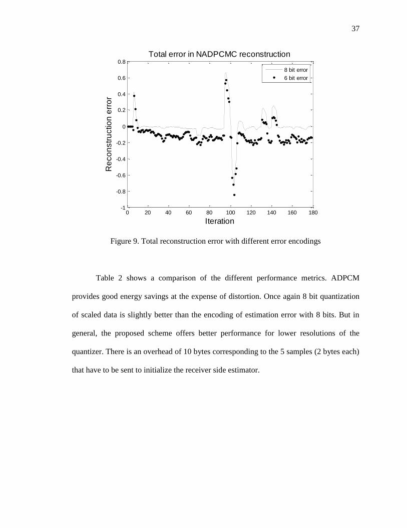
Table 2 shows a comparison of the different performance metrics. ADPCM

provides good energy savings at the expense of distortion. Once again 8 bit quantization

of scaled data is slightly better than the encoding of estimation error with 8 bits. But in

general, the proposed scheme offers better performance for lower resolutions of the

quantizer. There is an overhead of 10 bytes corresponding to the 5 samples (2 bytes each)

that have to be sent to initialize the receiver side estimator.

38

Table 2. Performance metrics for river-discharge data

Method Compression

ratio

Energy

savings

at nodes

Energy

savings

at CH

Distortion Overhead

Huffman 1.453 NA 31.177% NA 480 bytes

Differential

Huffman 1.642 21.56% 39.099% NA 480 bytes

Scaling and

approximation 1.137 13.65% 11.65% 0.0657% 0

Scaling and 9

bit

quantization

1.778 43.76% 43.76% 0.943% 0

Scaling and 8

bit

quantization

2.000 50% 50% 2.0685% 0

Scaling and5

bit

quantization

3.200 68.75% 68.75% 16.451% 0

Linear

ADPCM 2 50% 50% 13.72% 0

NADPCMC

with 8 bit

encoding

1.9459 48.61% 48.61% 2.65% 10 bytes

NADPCMC

with 6 bit

encoding

2.5487 60.76% 60.76% 6.08% 10 bytes

The hardware experiments with the proposed NADPCMC scheme with 8 bit error

encoding using the network shown in Figure 3 showed an average energy savings of

47.671% at the source nodes over no compression. The packet headers add an additional

26 bytes per packet for routing and hence a compression ratio of 1.911 was achieved

when compared with no compression.

C. Audio data

The proposed NADPCMC algorithm was also tested with a wav file. Since audio

data can tolerate a higher level of distortion, higher levels of compression can be

39

achieved at the expense of distortion. Figures 10 and 11 show the total reconstruction

error with 8 bit and 6 bit encoding of errors, respectively.

0 0.5 1 1.5 2 2.5 3 3.5 4

x 104

-0.025

-0.02

-0.015

-0.01

-0.005

0

0.005

0.01

0.015

0.02

0.025

Iteration

To

tal re

co

nstr

uctio

n e

rro

rNADPCMC with 8 bit encoded error

Figure 10. Total reconstruction error with 8 bit encoded error

0 0.5 1 1.5 2 2.5 3 3.5 4

x 104

-0.2

-0.15

-0.1

-0.05

0

0.05

0.1

0.15

Iteration

To

tal re

co

nstr

uctio

n e

rro

r

NADPCMC with 6 bit encoded error

Figure 11. Total reconstruction error with 6 bit encoded error

40

The performance metrics are tabulated in Table 3. The proposed scheme

outperforms the linear ADPCM implementation in terms of distortion. Additionally, the

nonlinear ADPCM is better than the scaling and quantization approach in terms of

distortion. The parameter and regression vectors were designed to hold 10 previous

samples. These 10 samples cause an overhead of 20 bytes.

Table 3. Performance metrics for audio data

Method Compress

-ion ratio

Energy

savings at

nodes

Distortion Overhead

Scaling and 8 bit

quantization

2 50% 10.59% NA

Scaling and 6 bit

quantization

2.67 62.5% 46.28% NA

5 bit linear ADPCM 3.199 68.74% 11.37% NA

4 bit linear ADPCM 4 75% 23.14% NA

3 bit linear ADPCM 5.332 81.25% 28.45% NA

2 bit linear ADPCM 8 87.5% 35.86% NA

NADPCMC with 8 bit

encoding

1.9992 49.98% 2.04% 20 bytes

NADPCMC with 6 bit

encoding

2.6653 62.48% 6.16% 20 bytes

NADPCMC with 4 bit

encoding

3.997 74.98% 14.44% 20 bytes

D. Geophysical data

The proposed algorithm was applied on geophysical data obtained from the

Calgary corpus data set [22]. This dataset is widely used in evaluating compression

41

algorithms. The authors mention that the geophysical data is particularly difficult to

compress because it contains a wide range of data values. Figures 12 and 13 show the

total reconstruction error obtained with 8 bit and 6 bit encoding of errors, respectively.

0 100 200 300 400 500 600 700 800 900 1000-0.03

-0.025

-0.02

-0.015

-0.01

-0.005

0

Iteration

To

tal re

co

nstr

uctio

n e

rro

r

NADPCMC with 8 bit encoded error

Figure 12. Total reconstruction error with 8 bit encoded error

Table 4 summarizes the performance metrics. The distortion was virtually

unnoticeable with 8 bit error encoding unlike in linear ADPCM. 10 samples of 2 bytes

each were used to initialize the estimator at the receiver. This adds an overhead of 20

bytes per sensor node.

42

0 100 200 300 400 500 600 700 800 900 1000-0.14

-0.12

-0.1

-0.08

-0.06

-0.04

-0.02

0

Iteration

To

tal re

co

nstr

uctio

n e

rro

r

NADPCMC with 6 bit encoded error

Figure 13. Total reconstruction error with 6 bit encoded error

Table 4. Performance metrics for geophysical data

Method Compress

-ion ratio

Energy

savings at

nodes

Distortion Overhead

Scaling and 8 bit

quantization

2 50% 4.36% 0

Scaling and 6 bit

quantization

2.667 62.5% 13.42% 0

Linear ADPCM 2 50% 35.87% 0

NADPCMC with 8

bit encoding

2 50% 1.02% 20 bytes

NADPCMC with 6

bit encoding

2.667 62.5% 4.22% 20 bytes

43

E. Performance as an aggregation scheme

The results discussed so far dealt with compression performed at the source node

only. This section examines the performance of the NADPCMC scheme when it is

applied at different cluster-heads showing multiple levels of aggregation.

Figure 14 shows the topology considered. A cluster-head aggregates synthetic

data received from three nodes and forwards it to the base station. NADPCMC with 8 bit

error encoding was performed at the source nodes and NADPCMC with 6 and 4 bit error

encodings were experimented at the Cluster-heads.

Figure 14. Hardware architecture

With compression only at the source level, all nodes reported an energy savings of

45.83% when compared with no compression. The average compression ratio at the

source nodes was still a constant at 1.846. By repeating compression implemented on the

44

MST Motes at the Cluster-head, the amount of data and the energy expended in

transmitting it are reduced further, however at the expense of distortion. When a second

level of data aggregation was performed on the already compressed data at the first

cluster-head, the compression ratio at the Cluster-head level was 2.526 amounting to an

energy savings of 60.42%. There is an overhead of 20 bytes added by the NADPCMC

scheme for every level of aggregation. The total distortion has increased from 1.67% to

4.60% with an additional level of aggregation which is considered to be acceptable.

These results clearly demonstrate that with repeated compression, the distortion increases

while energy savings and compression ratios improve.

In order to understand better the repeated compression along a route, more

simulations on aggregation were performed using synthetic data and the topology

described in Figure 2. Initially, 8 bit NADPCMC was performed at all source nodes and 6

bit NADPCMC was performed at cluster-heads 1, 2 and 3 respectively in order to

evaluate the effect of encoding on energy levels and distortion. The energy savings at the

aggregating and forwarding nodes (cluster-heads) increased from 45.83% (with no

aggregation at cluster head) to 61.34%. The overall distortion for all the nodes was only

1.90%. Then 4 bit NADPCMC was tried on cluster-heads 1, 2 and 3 with 8 bit at the

source nodes. The energy savings improved to 73.61% but the overall distortion summed

up to 6.10%.

Next a third level of aggregation was introduced at CH5. 8 bit NADPCMC was

performed at all source nodes, 6 bit NADPCMC was performed at cluster-heads 1, 2 and

3 and 4 bit NADPCMC was performed at cluster-head 5. Cluster-head 5 reported a total

45

energy saving of 74.54%. The overall distortion on the synthetic data was a tolerable at

7.01%.

In short, without aggregation and with compression at only the source nodes, all

nodes reported the same energy savings of 45.83%. With one level of aggregation, the

energy savings at the aggregating and the forwarding nodes improves to 61.34%. With a

second level of aggregation, the energy savings at the aggregating node improves to

74.54%. Based on this study, it can be concluded that compression and data aggregation

over multiple levels enhances the energy savings, increases distortion and overhead.

In order to evaluate the repeated compression along a route, a study was

conducted with data flows of varying sizes being aggregated at cluster-head 5. Two of

these were assumed to generate data from the river discharge data set. The third was

made to transmit data from the wav file tested earlier. The other sources remained the

same. All source nodes performed 8 bit NADPCMC. Cluster-heads 1, 2 and 3 performed

6 bit NADPCMC and cluster-head 5 performed 4 bit NADPCMC. Synthetic data was

observed to have a distortion of 7.01%. River discharge data reported 4.83% distortion

while voice degraded by 6.09%. From the aggregation point of view, the distortion levels

are dependent on the resolution of the quantizer and the number of aggregations

performed. Since each stage of aggregation is lossy, the quality declines with each added

level.

Synthetic data propagated through more hops and was compressed thrice while

the others were compressed only twice. This led to a higher degradation in synthetic data.

This demonstrates that the distortion increases with the number of aggregation levels.

46

F. Scalability

Scalability tests are important with any protocol. Real world sensor networks may

contain hundreds of nodes and the protocol should not fail during deployment in a dense

network. Simple tests were made with NS2 to check the behavior of the aggregation

scheme over networks of varying sizes (50 – 250 nodes). Different topologies with

varying cluster sizes were created. All source nodes use 8 bit NADPCMC. First level

cluster-heads use 6 bit NADPCMC and are one hop away from the sensor nodes. A

second level of aggregation with 4 bit NADPCMC is performed at a cluster-head that is

closest to the base station. Multiple data flows using synthetic, river discharge and audio

data were created for each of these topologies.

Figure 15 shows the compression ratio at the second cluster-head level with

increasing number of flows. In spite of increasing the number of flows, the overhead

remains constant at 20 bytes for every compression. But with higher flows, the amount of

data (N) flowing through the network is higher and the overhead (K) appears smaller.

This leads to a slight increase in compression ratio. From (43), the maximum

compression ratio that can be obtained with ‗b‘ bit NADPCMC is when and is

given by

(45)

Hence, 4 bit NADPCMC on 16 bit data (x = 16) would provide a maximum

compression ratio of 4. Thus, the curve tends asymptotically to 4.0 with an increase in

number of flows.

47

0 50 100 150 200 2503.8

3.82

3.84

3.86

3.88

3.9

3.92

3.94

3.96

3.98

4

No. of flows

Co

mp

ressio

n r

atio

Scalability test

Figure 15. Dependency on number of flows

Figure 16 shows the compression ratio at the first cluster-head level. Each

application of the NADPCMC scheme adds an overhead of 20 bytes. With increase in the

network size, more clusters were created. This led to an increase in the number of times

the compression scheme was applied. Since there is a small overhead associated with the

scheme, the compression ratio decreases slightly with increase in network size for the

same number of flows. Similarly, the average compression ratio decreases with an

increase in the number of flows for a given network size due to added overhead with the

number of flows although it is small.

48

50 100 150 200 2502.3

2.35

2.4

2.45

2.5

2.55

2.6

2.65

Network size

Ave

rag

e c

om

pre

ssio

n r

atio

at firs

t clu

ste

r le

ve

l

Scalability test

10 flows

25 flows

40 flows

Figure 16. Average compression ratio at first cluster-head level

Figure 17 shows the compression ratio at the second cluster-head level. There is

just a single node performing 4 bit NADPCMC in all the topologies considered. With

increase in the amount of data flowing, the percentage of overhead associated with

NADPCMC decreases. This leads to a slight increase in the compression ratio.

Another important inference can be made from the distortion values. Each data set

suffered a constant level of distortion in these different scenarios. Synthetic data was

distorted by 7.01%, river discharge data by 5.19% and audio data by 15.35%. This shows

that the performance of the NADPCMC scheme is only dependent on the number of

aggregation levels and not on the network size.

49

50 100 150 200 2503.8

3.82

3.84

3.86

3.88

3.9

3.92

3.94

3.96

3.98

4

Network size

Ave

rag

e c

om

pre

ssio

n r

atio

at se

co

nd

clu

ste

r le

ve

l

Scalability test

10 flows

25 flows

40 flows

Figure 17. Average compression ratio at second cluster-head level

V. CONCLUSIONS

In this paper, a novel compression scheme based on adaptive estimation and

quantization is introduced. Given a bounded sensor data, theoretical bounds on estimation

error are derived and shown to be bounded when reconstruction error and quantization

errors are bounded. Subsequently, distortion when using the proposed scheme has been

proven to be bounded and small. The scheme was tested using multiple data sets

including synthetic data, real world sensor data, and audio data. This proposed scheme is

shown to offer energy savings of approximately 50% at each source node at the cost of

around 2-3% distortion. Synthetic and river discharge data sets are coarser whereas the

audio and geophysical data sets are very fine. Though direct quantization works well on

50

coarse data, it fails with data with fine resolution. However the NADPCMC scheme

works fairly well on all these data sets. Hardware implementation of the proposed scheme

using Missouri S&T motes confirms highly satisfactory performance. Then data

aggregation through iterative compression was examined. Simulation results demonstrate

that aggregation can improve the over-all energy savings with a small level of distortion.

Moreover, the distortion depends mainly on the number of aggregation levels and not on

the network size. This indicates that the scheme is scalable and can be deployed for large

networks too.

REFERENCES

[1] C. Alippi, G. Anastasi, C. Galperti, F. Mancini, M. Roveri, ―Adaptive Sampling for

Energy Conservation in Wireless Sensor Networks for Snow Monitoring Applications,‖

Int’l Conference on Mobile Adhoc and Sensor Systems, pp. 1-6, Oct 2007.

[2] R. Anguswamy, M. Zawodniok and S. Jagannathan, ―A Multi-Interface Multi-

Channel Routing (MMCR) Protocol for Wireless Ad Hoc Networks,‖ Proc. of the IEEE

Wireless Communications and Networking Conference, pp. 1-6, Apr 2009.

[3] W. Heinzelman, A. Chandrakasan, and H. Balakrishnan, ―Energy-Efficient

Communication Protocol for Wireless Microsensor Networks,‖ Proc. Hawaii Intl. Conf.

System Sciences, pp. 3005-3014, Jan 2000.

[4] P.M. Wightman, M.A. Labrador, ―A3: A Topology Construction Algorithm for

Wireless Sensor Networks,‖ Global Telecommunications Conference , pp. 1-6, Nov-Dec

2008.

[5] W. Mangione-Smith and P.S. Ghang, ―A Low Power Medium Access Control

Protocol for Portable Multi-Media Systems,‖ Proc. of the 3rd Int’l Workshop on Mobile

Multimedia Communications, Sept 1996.

[6] R. Rajagopalan and P.K. Varshney, ―Data-Aggregation Techniques in Sensor

Networks – A Survey,‖ IEEE Communications Surveys & Tutorials, vol. 8, no. 4, pp. 48-

63, 2006.

51

[7] C.M. Sadler and M. Martonosi, ―Data Compression Algorithms for Energy-

Constrained Devices in Delay Tolerant Networks,‖ Proc. of the 4th Int’l conference on

Embedded networked sensor systems, pp. 265-278, 2006.

[8] K. Sayood, ―Introduction to Data compression,‖ Third edition, Morgan Kaufmann

Series in Multimedia Information and Systems, Dec 2005.

[9] N. Kimura, S. Latifi, ―A Survey on Data Compression in Wireless Sensor Networks‖,

Int’l Conference on Information Technology: Coding and Computing, vol. 2, pp. 8 -13,

2005.

[10] K. Barr and K. Asanovi´c, ―Energy Aware Lossless Data Compression,‖ ACM

Transactions on Computer Systems, vol. 24, pp. 250-291, 2006.

[11] D. A. Huffman, ―A Method for the Construction of Minimum-Redundancy Codes,‖

Proc. of the I. R. E., vol. 40, pp. 1098-1101, 1952.

[12] C. Alippi, R. Camplani, C. Galperti, ―Lossless Compression Techniques in Wireless

Sensor Networks: Monitoring Microacoustic Emissions,‖ Int’l Workshop on Robotic and

Sensors Environments, pp. 1-5, Oct 2007.

[13] A. Deligiannakis, Y. Kotidis and N. Roussopoulos, ―Compressing Historical

Information in Sensor Networks,‖ Proc. of the 2004 ACM SIGMOD Int’l conference on

Management of data, pp. 527-538, 2004.

[14] T. Banerjee, K. Chowdhury and D.P. Agrawal, ―Distributed Data Aggregation in

Sensor Networks by Regression Based Compression,‖ Int’l conference on mobile adhoc

and sensor systems, pp.-290, 2005.

[15] C. Guestrin, P. Bodix, R. Thibaux, M. Paskin and S. Madden, ―Distributed

Regression: an Efficient Framework for Modeling Sensor Network Data,‖ 3rd Int’l

Symposium on Information Processing in Sensor Networks, pp. 1-10, Apr 2004.

[16] S. Lin, D. Gunopulos, S. Lonardi, V. Kalogeraki, ―Applying LVQ Techniques to

Compress Historical Information in Sensor Networks,‖ Proc. of the 2005 Data

Compression Conference, pp. 468-474, 2005 .

[17] P. Cummiskey, N.S. Jayant, and J. L. Flanagan, ―Adaptive Quantization in

Differential PCM Coding of Speech,‖ Bell Syst. Tech. J., vol. 52, pp. 1105-1118, Sept

1973.

[18] S. Jagannathan, ―Wireless Ad hoc and Sensor Networks: Protocols, Performance

and Control,‖ CRC Press, 2007.

[19] Beagle Board Technical Specifications – available online -

http://beagleboard.org/static/BBSRM_latest.pdf - accessed on Feb 2009.

52

[20] J. Fonda, S. Watkins, S. Jagannathan, M. Zawodniok, ―Embeddable Sensor Mote

for Structural Monitoring,‖ SPIE 15th Annual Int’l Symposium on Smart Structures/NDE:

Sensors and Smart Structures Technologies for Civil, Mechanical, and Aerospace

Systems 2008, vol. 6932, pp. 69322V.1-69322V.11, 2008.

[21] Macrohydrological dataset for the Amazon basin – available online -

ftp://ftp.ufv.br/dea/macrohydr - accessed on Oct 2008.

[22] Geophysical data from Calgary corpus – available online -

http://corpus.canterbury.ac.nz/descriptions/#calgary – accessed on Oct 2008.

53

PAPER

2. HARDWARE VERIFICATION OF DATA AGGREGATION AND

MULTI-INTERFACE MULTI-CHANNEL ROUTING PROTOCOL

Priya Kasirajan, Maciej Zawodniok and S. Jagannathan

ABSTRACT — The goal of wireless sensor networks is to gather information with high

reliability and low energy. Considering the severe energy constraints of sensor nodes,

data aggregation and energy-efficient routing are essential for improving the energy

efficiency while maintaining packet delivery ratio. Typically, sensor nodes have radios

that can handle many non-overlapping channels. This necessitates the use of a multi-

channel routing protocol that would balance the load evenly on multiple channels using a

metric defined by throughput, end to end delay and energy utilization. We investigate a

proactive routing protocol called the Multi-interface Multi-channel Routing (MMCR)

protocol that uses Multi-Point Relay (MPR) nodes to forward data through the network,

thus reducing the amount of communication overhead. To further improve the energy

efficiency, data aggregation is performed along the routing path both at the source and

at the cluster head through iterative application of the adaptive pulse coded modulation-

based compression (NADPCMC) scheme. With the application of data aggregation,

hardware results show that at least a 50% energy saving with less than 5% distortion is

observed.

Keywords: Compression, Data Aggregation, Multi-channel Routing, Energy Efficiency,

Wireless Sensor Networks

54

I. INTRODUCTION

Routing in wireless mesh networks has been explored for a long time since direct

communication between all nodes in a network would be very expensive in terms of

transmission cost which grows exponentially with distance. This necessitates co-

operation between nodes so as to deliver packets over multiple hops from the source to

the destination [1]. A common practice is to represent the total cost of a path as the sum

of the link costs on the constituting links. Routing, then, aims at finding the path offering

the lowest overall cost. Most current ad hoc routing protocols select paths that minimize

hop count [2] [3] [4].

In static ad hoc wireless networks, minimal hop count paths can have degraded

performance because they tend to include wireless links between distant nodes. These

long wireless links can be slow or lossy leading to an unacceptable throughput. A routing

algorithm can select better paths by explicitly taking into account the quality of wireless

links. This is done in [5] by using a metric referred to as ―Expected Transmission Count‖

(ETX) which is a measure of the loss rate of broadcast packets between pairs of

neighboring nodes. In [6], ―Per-hop Round Trip Time‖ (RTT) is utilized to measure the

round trip delay seen by unicast probes between neighboring nodes. On the other hand,

the work of [7] uses ―Per-hop Packet Pair Delay‖ which is defined as the measured delay

between a pair of back-to-back probes to a neighboring node. Expected Transmission

Time (ETT) which is a function of the loss rate and the bandwidth of the link is used in

[8] as the routing metric. The individual link weights are combined into a path metric

called Weighted Cumulative ETT (WCETT) that explicitly accounts for the interference

among links that use the same channel.

55

Wireless technologies, such as IEEE 802.11a [9], provide multiple non-

overlapping channels. Multiple channels have been utilized in infrastructure-based

networks by assigning different channels to adjacent access points, thereby minimizing

interference between them. However, multi-hop wireless networks have typically used a

single channel to avoid the need for co-ordination between adjacent pair of nodes, which

is necessary in a multi-channel network. For meeting the ever-increasing throughput

demands of applications, it is becoming important to utilize the entire available spectrum,

thereby motivating the development of new protocols specifically designed for multi-

channel operation. Wireless hosts have typically been equipped with one wireless

interface. However, a recent trend of reducing hardware costs [10] has made it feasible to

equip nodes with multiple interfaces and increase the capacity of wireless mesh networks.

With multiple radios, more concurrent communications can be possible in spectrum,

space and time. To maximize the benefit of multiple radios, ideally we should use routes

that contain low interference among the constituting links [11].

A multi-interface multi-channel routing protocol (MMCR) is proposed in [12]. It

selects routes that enhance bandwidth utilization while maximizing energy efficiency and

minimizing end-to-end delay. This proactive routing protocol operates independently of a

particular scheme for receiver-based channel assignment. The protocol utilizes the

concept of Multi-Point Relays (MPRs) similar to [13]. The scheme forwards packets

using only the MPR nodes that are a fraction of the all one-hop neighbors. Hence, the

routing complexity reduces for the same network size when compared with other pro-

active routing protocols. This paper deals with the hardware verification of the MMCR

protocol on the Missouri S&T G4 motes [14].

56

The WSNs typically generate huge amount of heterogeneous data. The

propagation of redundant data is costly in terms of system performance and results in

energy depletion, network overloading, and congestion. While effective routing improves

the packet delivery ratio, other methods for in-network data processing must be employed

to reduce the number of messages relayed without much compromise on the fidelity.

With the focus shifting towards multimedia sensor networks for surveillance,

compression and aggregation techniques [15] [16] [17] are gaining importance every day.

A lot of research has been done on developing tailored compression/aggregation

techniques for WSNs. An ant colony approach is used for aggregation in [18]. In [19],

wavelets are used to achieve data reduction. In this paper, a Nonlinear Adaptive

Differential Pulse Coded Modulation-based Compression (NADPCMC) scheme [20] is

used for compression and aggregation in conjunction with the multi-channel routing

protocol.

This paper consists of the following sections. Section 2 describes the basic

activities of the MMCR scheme. Section 3 illustrates the hardware details, packet types

and the detailed algorithm of MMCR. A network of motes is used to relay dummy data

and real-time voice and the results are presented. Section 4 outlines the NADPCMC

algorithm and presents the results with compression and aggregation. Section 5 contains

the concluding remarks.

57

II. BACKGROUND

In general, MMCR routing scheme comprises of three periodic phases:

selection of MPRs for each node

selection of routes

data transfer through the selected MPRs

Simple local broadcast of HELLO messages is performed to discover one and

two-hop neighbors and their corresponding costs. Then the MPR nodes are selected. This

is followed by route selection globally for the whole network topology. Finally, the data

is forwarded through the selected paths. There are five types of control packets in

MMCR. They are listed below:

1) HELLO packet

Each node periodically broadcasts HELLO packets with information about its

energy level to its neighbors until timeout. Every node finds its one hop neighbors and

calculates the associated cost based on the received HELLO packets.

2) Acknowledgement (ACK) packet

Whenever a node receives a HELLO packet, it responds with an ACK packet with

a list of its own one hop neighbors and their link costs. Thus, each node finds its two hop

neighbors and calculates their associated cost based on the received ACK packets.

58

3) Topology Control (TC) packet

When the HELLO packet timeout elapses, each node selects MPRs among the

one hop neighbors such that all two hop neighbors are covered. The Topology Control

packet broadcasts this information to the one hop neighbors to indicate MPR selection

information.

4) SWITCH packet

This packet is broadcasted by the destination node to all other nodes in the

network to prompt them switch from a channel in the presence of interference.

5) BEAM packet

A BEAM packet is sent periodically by the destination node to all other nodes in

the network. This packet is used to synchronize the real-time clock of all other nodes to

facilitate accurate calculation of transmission delays.

The finer details of each phase in routing are presented next.

A. Neighbor discovery

Nodes broadcast HELLO message locally to learn about their one-hop neighbors

and their associated parameters such as energy, bandwidth and transmission delay. The

header of the HELLO packet includes the available bandwidth and the transmission time.

Figure 1 shows a flowchart of neighbor discovery stage.

59

Start Route Search or

HELLO Timeout

Broadcast HELLO packet

Start Timer

Return

Figure 1. Neighbor discovery

The node receiving the HELLO packet can calculate the delay using the

timestamp from the HELLO packet header. However, this requires time synchronization

between the nodes. This is established by BEAM packets broadcasted periodically by the

Base-station as shown in Figure 2.

Received BEAM

Synchronize real-time clock

Return

Figure 2. Handling BEAM packets

60

When a node receives a HELLO packet, it responds with an acknowledgement

(ACK) packet as shown in Figure 3. The ACK packets contain the list of its neighbors

and the energy utilization for each of these neighbors.

Received HELLO

Update one hop neighbor table with ID and cost

Send ACK with one hop neighbor IDs and costs

Return

Figure 3. Sending ACK packets

When ACK packets are received, each node updates this information on available

bandwidth, energy factor and the delay of the links from their neighbors in the ‗neighbor

table‘ as shown in Figure 4.

61

Received ACK

Investigate two hop neighbors

Calculate their link costs and store

Return

Figure 4. Handling of ACK packets

The utilization metric,U s,n2MPR

, of the path from node s to a two-hop neighbor node

n 2 through a relay node n1is calculated as follows:

U s,n2MPR

(B.F.* E.U.) /D (1)

B.F. BA /BS (2)

E.U. EAn1/ETXn1 n2

(3)

where B.F. is a bandwidth factor between nodes s and n1 (MPR), BA is an available (free)

incoming bandwidth at the n1, BS is an expected/requested outgoing bandwidth at the

source node s, E.U. is the energy utilization between nodes n1 to n2, EAn1 is an available

62

energy at the relay n1 in Joules, ETXn1 n2 is an energy used to transmit message from n1 to

n2, and D is an end to end delay from node s to node n1 in seconds.

The metric optimization will maximize available bandwidth using bandwidth

factor and minimize end-to-end delay using delay factor, D. Moreover, the metric will

maximize the energy utilization term, which is expressed as energy depletion due to

transmissions, thus increasing energy efficiency and lifetime of the nodes and network.

The utilization factor given by bits per second is a direct measure of the total throughput

of the link. Additionally, a route is selected if and only if the bandwidth factor for all the

links on the path is greater than one. Consequently, the route associated with a flow

guarantees sufficient bandwidth for the requested service.

B. MPR selection

Each node in the network uses its ‗neighbor table‘ to select multipoint relay

(MPR) nodes from the one-hop neighbors to reach all the two-hop neighbors with

minimum cost given by equation (1). The MPR selection metric proposed in [12] ensures

that the paths through the MPRs optimize the energy consumption, delay, and bandwidth

utilization. Additionally, the MPR selection algorithm ensures that there is sufficient

available bandwidth to support the existing and new traffic flows. The optimal set of

MPRs varies with traffic and network congestion. Hence, the nodes have to periodically

recalculate the set of MPRs using updated data from HELLO and ACK packets. Figure 5

illustrates the MPR selection algorithm.

63

# 1_hop_set is a set of one-hop neighbors of source

# 2_hop_set is a set of two-hop neighbors of source

mpr_set = {}; # empty set

foreach dest_node IN 2_hop_set DO

foreach mpr_candidate IN 1_hop_set

if mpr_candidate connects source and dest_node

then cost(mpr_candidate) = INFINITY;

else cost(mpr_condidate) =

COST (source TO mpr_candidate)

+ COST (mpr_candidate TO dest_node);

end foreach;

mpr_node = mpr_candidate with lowest cost;

add mpr_node TO mpr_set;

add to a routing table the mpr_node as a next hop

node toward dest_node;

end foreach;

# mpr_set holds the selected MPR nodes for the source

Figure 5. Pseudo-code for MPR selection

Reprint from [12]

Figure 6 shows the MPR nodes (shaded in the figure) selected by this algorithm.

These nodes would be sufficient relays to reach all nodes in the network.

Figure 6. MPRs selected by the algorithm

64

C. Topology discovery

The selected MPR nodes periodically transmit Topology Control (TC) messages

(as shown in Figure 7) with corresponding link utilization factor data. The updates are

propagated to all nodes in the network through the MPRs.

ACK Timeout elapsed

Select MPR nodes to maximize coverage

Update routing table

Return

Send TC message

Figure 7. Sending TC packets

Upon receiving the TC messages, each node in the network records the

information in the ‗topology table‘ as shown in Figure 8.

65

Received TC

Store MPR and link cost information

Return

Figure 8. Handling of TC packets

D. Route selection and data transmission using the selected routes

Each node in the network uses its ‗neighbor table‘ and ‗topology table‘ to

proactively compute the routes to all possible destinations. The protocol selects the path

that has the least route cost metric while ensuring that the bandwidth factor is always

greater than one for all the links on the path. This way, the algorithm eliminates routes

that do not provide sufficient bandwidth to carry the traffic, thus implementing admission

control mechanism. It ensures that the required flow data rate is supported throughout the

whole route. The cost factor for a route with k intermediate MPRs nodes in the path is

given by

C s,d C s,n2n1,Cn1,n3

n2,......,Cnk 2 ,nk

nk 1 ,Cnk 1,dnk

(4)

C s,n2MPR

1/U s,n2MPR

(5)

66

where C s,n2MPR is the cost metric between node s and its two-hop neighbor n2 N

2( s) through

the relay node n1 (MPR).

Once a route is found to the destination, the availability of multiple, independent

channels and interfaces are exploited to perform load balancing for a particular link. If a

particular link is suffering from interference, the receiver broadcasts a SWITCH packet to

indicate a channel switch as shown in Figure 9.

Received SWITCH

Change channel as requested

Return

Figure 9. Handling of SWITCH packets

III. IMPLEMENTATION OF THE ROUTING PROTOCOL

This section presents an overview of the hardware implementation of the MMCR

protocol.

67

A. Hardware description and limitations

Hardware verification of any algorithm is limited by hardware constraints such as

processing capabilities, on-board battery capacity and supported interfaces. Use of

specific hardware must be weighed against the precision, speed, and criticality of an

algorithm's implementation. Constraints addressed for the implementation of the MMCR

were use of low-power, small form-factor, and fast processing hardware. Hence the

hardware should be energy conservative; performance oriented and should be of small

form factor. Hence the processor architecture that can be deployed should be able to

satisfy all these demands. The Silicon Laboratories 8051 variant family was selected for

its ability to provide fast 8-bit processing, low-power consumption, and interface

compatibility to peripheral hardware components. This provides high-speed processing,

interconnectivity with the nodes, and a capable RF communications unit to facilitate a

development platform for the ad hoc networks. Limitations that are incurred through the

use of these 8051 variant family are a small memory space and limited floating point

processing. In the next section, a description of the specifications for the hardware

implemented nodes will be given.

The Generation-4 Smart Sensor Nodes (G4-SSN) [14], shown in Figure 10 were

used as sensor nodes for implementation of the MMCR routing protocol. These were

originally developed at Missouri S&T and subsequently updated at St Louis University

(SLU). These motes provide a common platform for sensing, networking and data

processing. The platform consists of an 8051 processor and an 802.15.4 (XBee) radio

with micro Smart Digital (SD™) flash storage, USB and RS-232 connectivity and an

assortment of sensors. These nodes have 8K RAM and 128K flash memory that make it a

68

suitable choice for the hardware implementation. Table 1 gives a summary of the

specifications of the G4-SSN. More information can be found in [14].

Figure 10. G4 mote

Table 1. Specifications of G4 mote

Ic at 3.3V 35 mA

Flash memory 128 kB

RAM 8448 bytes

Form-Factor 100-pin LQFP

MIPS 100

B. Implementation details

This section describes the implementation details of the MMCR routing protocol.

Six types of packets are created – five of them being control packets and one data packet.

The payload of each packet was prefixed with 2 headers – the XBee header and the

routing header. The general structure of a packet is shown in Figure 11. The XBee header

(shown in light gray) consists of information required by the XBee radios to process the

69

packets and the routing header (shown in dark gray) comprises of routing related

information:

API Start Byte (0x7E) 1 byte

API length 2 bytes

API ID 1 byte

API frame ID 1 byte

API Destination 2 bytes

API options 1 byte

Start Byte (0x42) 1 byte

Flag byte (0x75) 1 byte

MAC Destination 2 bytes

MAC Source 2 bytes

Packet length 1 byte

Destination ID 1 byte

Source ID 1 byte

Sequence number 1 byte

Time Stamp 4 bytes

Payload Many bytes

Payload CRC 1 byte

Packet checksum 1 byte

Figure 11. Packet structure

70

In addition, the DATA packet contains the application-specific headers and the

payload. The application specific headers are shown in Figure 12. The total number of

header bytes is 27 and the packet payload is fixed at 80 bytes. This leads to a 25.23%

control overhead per packet.

Module Type 1 byte

Module length 1 byte

Report type 1 byte

Payload Many bytes

Figure 12. Application specific header

C. Node functions

Figure 13 shows the activity of a node that wishes to transmit data. A route search

is started if no route is available to the required destination node. Otherwise the packet is

forwarded to the appropriate MPR.

Figure 14 shows the activities of intermediate nodes. If the destination is a one-

hop neighbor, the data packet is sent to it directly. Otherwise, it is relayed to the MPR

that is closest to the destination node.

71

Data Ready

Return

Send Data packet

Route Available to Destination

Start Route Search

Yes

No

Figure 13. Activities of sender

Is this Destination?

Return

Send Data packet

Destination is one hop

away

Send to MPR closest to Destination

Yes

No

Figure 14. Activities of an intermediate node

72

Figure 15 shows the activities of a destination node. It broadcasts BEAM packets

periodically to synchronize the real-time clock of all nodes in the network. Moreover, if

the throughput falls below a certain threshold indicating interference, the receiver

broadcasts a BEAM packet instructing the active nodes to switch to a different channel.

This is Destination

Return

Send packet to Application layer

Throughput > Threshold

Send SWITCH

Yes

No

Send BEAM

Figure 15. Activities of a destination node

D. Protocol verification

Figure 16 shows the placement of nodes for demonstrating MMCR. Packets from

source 1 were routed through intermediate nodes 1 and 2 to the destination. When

intermediate node 2 was turned off, intermediate node 3 was used to relay packets.

73

Figure 16. Demonstration of MMCR

The following were the performance metrics used to characterize the performance

of the protocol:

1. Throughput – Number of bits received per second

2. Drop rate – Number of bits missing per second

3. End-to-end delay – Total transmission delay in milliseconds

4. Jitter – Variation in delay in milliseconds

Figure 17 shows the metrics measured when raw uncompressed data was sent

over three hops through the network. Data was generated at 2.56 kbps. The total

74

transmission rate (including the packet headers) amounted to 3.424 kbps. All packets

were received in sequence. Thus, the drop rate is zero. The average end to end packet

delay over 3 hops was almost 20 ms. Table 2 lists the average values of the performance

metrics. All reported values are the average over 10 trials.

Figure 17. Performance metrics

Table 2. Average performance metrics for raw data

Data generation rate 2.56 kbps

Throughput (data transmission rate) 3.424 kbps

Drop rate 0

Average delay 20.2785 ms

Average jitter 0.7845 ms

75

Figure 18 shows the experimental setup used to verify the channel switching

functionality. Two-hop communication was established using Channel 14 through

MMCR as this channel is the default choice.

Figure 18. Demonstration of channel switching

When a different node which was broadcasting in the same channel was brought

within communication range, a drop in throughput was observed by the Destination node.

This triggered the sending of a SWITCH packet by the Destination node and the source

and intermediate nodes switched communication to Channel 15 which is one among the

list of available channels. Detailed selection of the channels is outside the scope of this

76

work. Figure 19 shows the switching of channels. The red throughput line indicates the

use of Channel 14 and the blue one indicates Channel 15.

Figure 19. Channel switching

E. Real-time voice with MMCR

The transmission of real-time voice through a bandwidth limited wireless channel

is a very challenging test case. A low-cost, fan-less single board computer called

Beagleboard [21] running Ubuntu Linux was interfaced with Missouri S&T motes. The

microphone connected to the Beagleboard generated data at 128kbps. A G.721 4 bit

ADPCM [22] was implemented to reduce the data rate to 32kbps. This data was

packetized and sent over the MMCR network to a destination node connected to a

77

speaker through another Beagleboard. All communication between the Beagleboard and

the motes were achieved through the UART interface. The Advanced Linux Sound

Architecture (ALSA) library [23] was used to create the audio interfaces. The experiment

setup is shown in Figure 20.

Figure 20. Real-time voice over MMCR

Figure 21 shows the results obtained. The voice data generation rate was 32kbps.

Including the packet headers, the generation rate is almost 40kbps. From the figure, it can

be observed that MMCR provides the required throughput with a few dropped packets.

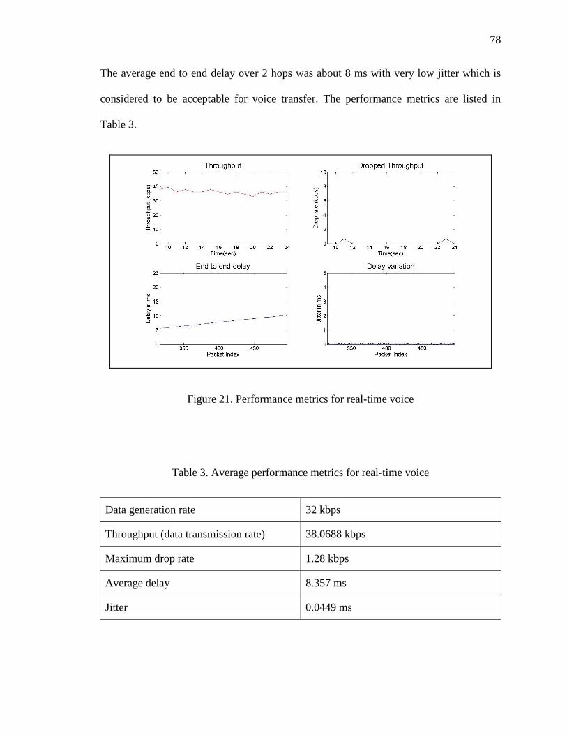
78

The average end to end delay over 2 hops was about 8 ms with very low jitter which is

considered to be acceptable for voice transfer. The performance metrics are listed in

Table 3.

Figure 21. Performance metrics for real-time voice

Table 3. Average performance metrics for real-time voice

Data generation rate 32 kbps

Throughput (data transmission rate) 38.0688 kbps

Maximum drop rate 1.28 kbps

Average delay 8.357 ms

Jitter 0.0449 ms

79

When the data generation rate is increased further, the number of dropped packets

starts increasing rapidly due to congestion in the network. These packet losses can be

minimized by compression/aggregation techniques as will be discussed next. The next

section describes the implementation of the NADPCMC scheme for this purpose.

IV. IMPLEMENTATION OF DATA AGGREGATION

This section provides a brief background of the NADPCMC scheme. This is

followed by the hardware implementation details and results.

A. NADPCMC

A nonlinear estimator [20] is used to generate the estimate of the data sample at

every instant. Adaptive estimation of the data sequence is performed by representing the

data as a nonlinear autoregressive moving average sequence as

(1)

where is the basis function, is the unknown parameter vector, and

is the reconstruction error which is bounded by . The estimated

signal is represented as

(2)

where is the estimated parameter estimate vector and e(k) is the estimation error.

The estimation error is then given by

(3)

80

Substituting for and in (3) renders

(4)

where the parameter estimation error is defined by

(5)

Now consider the parameter update as

(6)

Here α is called the adaptation gain.

The difference e(k) between the actual and the estimated sample is quantized and

sent to the destination. If the estimation error is small enough, the error can be

represented with smaller number of bits than the original sample. This leads to

compression.

At the receiver side, a similar estimator generates sample estimates. This

estimator requires synchronization of the basis function φ(k) with a few correct initial

samples from the transmitter. The error received from the transmitter is added to the

estimate to reconstruct the data. Figure 22 shows the flowchart with the source

functionality in blue and receiver functionality in red.

81

Yes

No

Initialize estimator

Calculate estimate

Add received error to estimate to

reconstruct data

Update parameter

More data

arriving

Return

Figure 22. NADPCMC flowchart

B. Zeolite sensors for explosive detection

Many multi-layer sensor mote architectures consist of a microcontroller (MCU)

layer and several slave layers for interfacing with other systems and the application

environment. Architectures such as the G4 SSN use direct pin assignment of the MCU to

the bus pins and this leads to a limitation of the number of supportable slave devices. The

G4 mote supports a single radio interface easily. It had the required UART interfaces for

Yes

No

Initialize estimator

Calculate estimate

Calculate error

Update parameter

More data

available

Tx Quantized error

82

a secondary radio but the architecture required some manual configuration tweaking and

the second radio added to the processor load. These issues call for a new architecture that

could support multiple slaves easily. The Missouri S&T M2 mote (shown in Figure 23)

addresses these issues through the use of a serial bus to connect the layers.

Figure 23. M2 mote

A network of wireless motes connected to chemical sensors is capable of

detecting, locating, and sending warning messages to appropriate decision makers about

the presence of explosive threats. In this implementation, we use Missouri S&T motes

connected to zeolite chemical sensor technology [24] as an input to the detection system.

The zeolite sensors utilize a coated fiber optic tip that measure the reflectivity of the fiber

as the chemical is introduced into the environment. An amplifier circuit translates this

reflectivity into a 0-3V level and is read by an ADC on the sensor mote which measures

the signal against several threshold levels. The sensor response to low concentration of

83

isopropanol molecule from a prototyped sensor circuit is shown in Figure 24. The first

threshold level at 1/3 of the dynamic range is considered to be the Early Warning Level

(EWL) and the second threshold at 2/3 the dynamic range is considered to be the Critical

Warning Level (CWL).

0 20 40 60 80 100 120 140 160 180 200-30

-20

-10

0

10

20

30

40

50

60

Time (s)

Am

plitu

de

(p

pm

)

Zeolite Sensor Response

CRITICAL WARNING LEVEL

EARLY WARNING LEVEL

Figure 24. Prototyped sensor circuit response

C. Transmission of sensor data

The M2 mote generates sensor data at 2.56 kbps. The 8-bit NADPCMC was

applied to reduce the transmission rate by almost half. This led to an energy saving of

46.67% with distortion limited to 0.78%. The transmitter and receiver side estimators

used the first 5 data samples for initialization. However, this approach has a major

84

drawback. When a data packet is dropped, the receiver does not have certain e(k) and

cannot reconstruct those samples. Since these samples are required to set the basis

function φ(k), it would be incorrectly set to zero. This leads to error in estimating the

forthcoming samples since depends φ(k) (from equation (2)). Thus, the

estimators on both sides would no longer be synchronized. This situation is shown in

Figure 25 where the second packet in the sequence is dropped. The receiver side

estimator does not have the appropriate regression vector to generate the next estimates,

thus forcing the reconstructed samples deviating from the original data.

0 100 200 300 400 500 600 700 8000

0.5

1

1.5

2

2.5

3

Iteration

Am

plit

ud

e

8 bit NADPCMC in presence of packet losses

Original

Decoded

Figure 25. 8 bit NADPCMC in the presence of packet losses

85

To mitigate this problem, each packet has to be made independent of the previous

packet. In other words, the basis function φ(k) of the receiver side estimator has to be re-

initialized for each data packet. This way, even if a packet is dropped, φ(k) would be

reset with 5 data samples through every other received packet. Thus, the estimated

for the other packets would be same at both transmitter and receiver side estimators. This

would add an additional overhead to each packet, reducing the compression ratio from

1.957 to 1.875. In addition, the energy savings reduces from 48.91% to 46.67%.

However, it improves the fault tolerance capability of the scheme in a significant manner.

Figure 26 shows the performance of the modified NADPCMC scheme when the second

packet in the sequence is dropped in the network.

0 100 200 300 400 500 600 700 8000

0.5

1

1.5

2

2.5

3

3.5

Iteration

Am

plit

ud

e

Modified NADPCMC in presence of packet losses

Original

Decoded

Figure 26. Modified 8 bit NADPCMC in the presence of packet losses

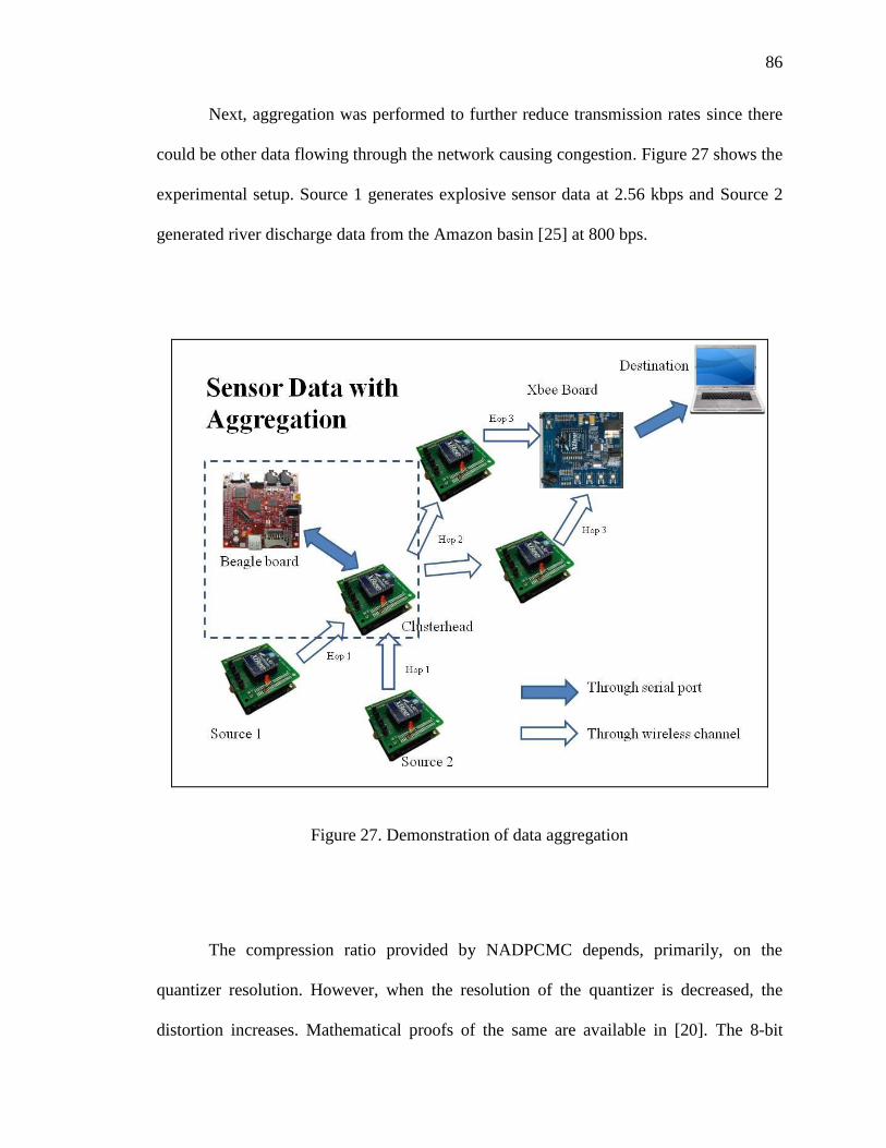
86

Next, aggregation was performed to further reduce transmission rates since there

could be other data flowing through the network causing congestion. Figure 27 shows the

experimental setup. Source 1 generates explosive sensor data at 2.56 kbps and Source 2

generated river discharge data from the Amazon basin [25] at 800 bps.

Figure 27. Demonstration of data aggregation

The compression ratio provided by NADPCMC depends, primarily, on the

quantizer resolution. However, when the resolution of the quantizer is decreased, the

distortion increases. Mathematical proofs of the same are available in [20]. The 8-bit

87

modified NADPCMC was used for compression at the source level while a 6 bit

NADPCMC at the Cluster-head level reduced the transmission rate to 1.284 kbps for the

aggregated flow. An energy savings of 56.99% was obtained and the distortion in both

data sets was limited to less than 4%. When 4 bit NADPCMC was used at the Cluster-

head level, the aggregated transmission rate was reduced to 856 bps. Including the packet

headers, the throughput was approximately 1 kbps as shown in Figure 28. Though the

energy savings improved to 71.43%, the distortion also increased to 8.21% for explosive

sensor data and 10.9% for river discharge data. Table 4 summarizes these results.

Figure 28. Performance metrics with 4 bit data aggregation

88

Table 4. Effect of data aggregation

Data

generation

rate

Transmissi

on rate

Compr

ession

ratio

Energy

savings

Distortion

Uncompressed

data

2.56 kbps 3.424 kbps NA NA NA

Compressed data 2.56 kbps 1.712 kbps 1.8751 46.67% 0.78% for sensor

data

0.81% for river

discharge data

Compressed and

aggregated data –

6 bit NADPCMC

2.56 kbps 1.284 kbps 2.3250 56.99% 3.58% for

sensor data

2.78% for river

discharge data

Compressed and

aggregated data –

4 bit NADPCMC

2.56 kbps 856 bps 3.5002 71.43% 8.21% for

sensor data

10.90% for river

discharge data

Figure 29 shows the reconstructed explosive sensor data samples with different

level of aggregation.

0 100 200 300 400 500 600 700 8000

0.5

1

1.5

2

2.5

3

3.5

Iteration

Am

plit

ud

e

Compression and Aggregation

Original

6 bit Aggregation

4 bit Aggregation

Figure 29. Reconstructed explosive sensor data

89

Figure 30 shows the reconstructed river discharge data samples with different

stages of aggregation.

0 20 40 60 80 100 120 140 160 1800

0.5

1

1.5

2

2.5

3

3.5

4

4.5

5

Iteration

Am

plit

ud

e

Compression and aggregation

Original

6 bit aggregation

4 bit aggregation

Figure 30. Reconstructed river discharge data

D. Energy consumption

To achieve true energy efficiency, the energy expended in the compression

algorithm must be less than that required to send the extra bits to the destination.

Generally a processor consumes less power for such computations than a radio that is

required to transmit a packet. In this case, Beagleboard uses the OMAP3530 processor

[26] which has a power rating of 250mW. The CPU clock frequency is 720 MHz and the

processor is capable of performing two 32-bit operations per cycle. In terms of Floating-

point Operations per Second (FLOPS), this amounts to 1.44 gigaFLOPS. Each FLOP

expends 0.17361nJ of energy. The NADPCMC encoding scheme consists of 7050 FLOPs

90

and the decoding scheme consists of 7425 FLOPs. Thus, the OMAP processor expends

1.224 micro Joules for every encoding and 1.289 micro Joules for every decoding.

The XBee radio uses a transmit power of 1mW for a 30m range [27]. This

translates to 5 nJ per bit. Sending 160 data samples without compression would require

20.32 µJ of energy. With compression, the number of bytes is reduced by half, thus

requiring 10.16 µJ is required for transmission. However, 2.45 µJ would be consumed in

computations. Thus, the total energy expenditure with compression is 12.61 µJ. When

aggregation is added, the number of bytes is cut down by another half and 5.08 µJ is

required for transmission. And 1.224 µJ would be expended in computations. Thus, the

total energy consumed is 6.304 µJ with data aggregation including computational

overhead when compared to transmission alone. Table 5 lists the total energy

consumption and the percentage savings. It indicates that even though some energy is

consumed on computations, data aggregation provides significant overall energy savings

to improve the network lifetime.

Table 5. Energy expenditure

Energy

consumption

Energy savings

Transmission of uncompressed data 20.32 µJ NA

Transmission of compressed data using

8 bit NADPCMC

12.61 µJ 37.94%

Transmission of compressed and

aggregated data – 4 bit NADPCMC

6.304 µJ 68.98%

91

V. CONCLUSIONS

This paper dealt with the hardware verification of routing using MMCR protocol

and data aggregation using NADPCMC scheme. Usage of multiple channels is shown to

help balance the load and reduce packet losses. However, when the data generation rate

increases which is normally observed in a WSN, there may be packets dropped due to

congestion, thus necessitating compression and aggregation techniques with routing. A 8

bit NADPCMC reduces amount of data at source level by almost half. To make the

scheme resilient to a lossy channel, a small overhead is added to each packet to re-

initialize the receiver-side estimator. This is shown to improve the performance in a

satisfactory manner. In-network aggregation further reduces the amount of data and

improves network lifetime. However a small amount of distortion is involved. The

aggregation scheme is proven to be truly energy efficient with the computations

consuming a very small amount of power compared to the power required for

transmission by the radio.

REFERENCES

[1] R. Ramanathan and R. Hain, ―Topology control of multihop wireless networks using

transmit power adjustment,‖ Proc. of INFOCOM, pp. 404 – 413, Mar 2000.

[2] V. D. Park and M. S. Corson, ―A highly adaptive distributed routing algorithm for

mobile wireless networks,‖ Proc. of INFOCOM, pp. 1405 - 1413, Apr 1997.

[3] C. E. Perkins and P. Bhagwat, ―Highly dynamic destination-sequenced distance

vector routing (dsdv) for mobile computers,‖ Proc. of SIGCOMM, pp. 234 – 244, Sept

1994.

92

[4] C. E. Perkins and E. M. Royer, ―Ad-hoc on-demand distance vector routing,‖ Proc. of

WMCSA, pp. 90 – 100, Feb 1999.

[5] D. De Couto, D. Aguayo, J. Bicket, and R. Morris, ―High-throughput path metric for

multi-hop wireless routing,‖ Proc. of MOBICOM, Vol. 11, pp. 419 – 434, Sept 2003.

[6] A. Adya, P. Bahl, J. Padhye, A. Wolman, and L. Zhou, ―A multiradio unification

protocol for IEEE 802.11 wireless networks,‖ Proc. of BroadNets, pp. 344 – 354, 2004.

[7] S. Keshav, ―A Control-theoretic approach to flow control,‖ Proc. of SIGCOMM, pp. 3

– 15, Sept 1991.

[8] R. Draves, J. Padhye, and B. Zill, ―Routing in multi-radio, multihop wireless mesh

networks,‖ Proc. of MobiCom, pp. 114 – 128, Sept 2004.

[9] IEEE Standard for Wireless LAN-Medium Access Control and Physical Layer

Specification, P802.11, 1999.

[10] P. Bahl, A. Adya, J. Padhye, and A. Wolman, ―Reconsidering wireless systems with

multiple radios,‖ ACM CCR, Vol. 34, pp. 39 – 46, Jul 2004.

[11] P. Kyasanur, and N.H. Vaidya, Routing and link-layer protocols for multi-channel

multi-interface ad hoc wireless networks, ACM SIGMOBILE Mobile Computing and

Communications Review, v.10 n.1, p.31-43, Jan 2006.

[12] R. Anguswamy, M. Zawodniok and S. Jagannathan, ―A multi-interface multi-

channel routing (MMCR) protocol for wireless ad hoc networks,‖ Proc. of the IEEE

Wireless Communications and Networking Conference, pp. 1-6, Apr 2009.

[13] A. Qayyum, L. Viennot and A. Laouiti, ―Multipoint relaying for flooding broadcast

messages in mobile wireless networks‖, Proc. of HICSS, pp. 3866 – 3875, Jan 2002.

[14] J. Fonda, S. Watkins, S. Jagannathan, and M. Zawodniok, ―Embeddable sensor mote

for structural monitoring,‖ SPIE 15th Annual Int’l Symposium on Smart Structures/NDE:

Sensors and Smart Structures Technologies for Civil, Mechanical, and Aerospace

Systems 2008, vol. 6932, pp. 69322V.1-69322V.11, 2008.

[15] K. Dasgupta, K. Kalpakis, and P. Namjoshi, ―An efficient clustering-based heuristic

for data gathering and aggregation in sensor networks,‖ Proc. Of WCNC, Vol. 3, 16-20

Mar 2003.

[16] Krishnamachari, D. Estrin, and S. Wicker, ―The impact of data aggregation in

wireless sensor networks,‖ Int’l Workshop on Distributed Event-Based Systems, pp. 414 –

415, Jul 2002.

[17] Boulis, S. Ganeriwal, and M.B. Srivastava. ―Aggregation in sensor networks: an

energy-accuracy trade-off,‖ Proc. of IEEE Sensor Network Protocols and Applications,

pp. 128 – 138, May 2003.

93

[18] R. Misra, C. Mandal, ―Ant-aggregation: ant colony algorithm for optimal data

aggregation in wireless sensor networks,‖ Proc. of IFIP Int’l Conference on Wireless and

Optical Communications Networks, pp. 1 – 5, 2006.

[19] W. Cai, M. Zhang, ―Data aggregation mechanism based on wavelet-entropy for

wireless sensor networks,‖ Proc. of WiCOM, pp. 1 – 4, Oct 2008.

[20] K. Priya, C. Larsen, S. Jagannathan, ―A new adaptive compression scheme for data

aggregation in wireless sensor networks,‖ to appear in IEEE WCNC 2010.

[21] Beagle Board Technical Specifications – available online -

http://beagleboard.org/static/BBSRM_latest.pdf - accessed on Feb 2009.

[22] G.721 32 kbps ADPCM Specifications – available online - http://www.itu.int/rec/T-

REC-G.721/en - accessed on Feb 2009.

[23] Advanced Linux Sound Architecture Library – available online - http://www.alsa-

project.org – accessed on Feb 2009.

[24] H. Xiao, Z. Jian, D. Junhang, L. Ming, L. Robert and Van Romero, ―Synthesis of

MFI zeolite films on optical fibers for detection of chemical vapors,‖ Optics Letters, vol.

30, no. 11, pp. 1270-1272, 2005.

[25] Macrohydrological dataset for the Amazon basin – available online -

ftp://ftp.ufv.br/dea/macrohydr - accessed on Oct 2008.

[26] OMAP35x Applications Processor Technical Reference Manual – available online -

http://focus.ti.com/lit/ug/spruf98d/spruf98d.pdf - accessed on Nov 2009.

[27] XBee®/XBee-PRO® SE (Smart Energy) RF Modules Specifications – available

online - http://www.digi.com/standards/smart-energy/assets/90033931_A.pdf - accessed

on Nov 2009.

94

SECTION

2. CONCLUSIONS AND FUTURE WORK

This thesis explores the possibility of energy efficiency improvement in wireless

sensor networks through data aggregation and efficient multi-channel routing. Since

existing compression schemes are tailored for specific types of data, a novel generic

compression scheme called NADPCMC based on adaptive nonlinear estimation and

quantization is developed in the first paper. Theoretical bounds on estimation error are

derived using Lyapunov theory and the total distortion is shown to be dependent on the

quantization error and the maximum singular value of the gain matrix. The scheme is

tested using multiple data sets with different resolutions and offers energy savings of

approximately 50% at each source node at the cost of around 2-3% distortion. Then data

aggregation through iterative compression is examined. Simulation results demonstrate

that aggregation can further improve the over-all energy savings with a small level of

distortion. Moreover, the distortion depends mainly on the number of aggregation levels

and not on the network size. This indicates that the scheme is scalable and is deployable

in larger networks.

While data aggregation helps in reducing energy consumption, efficient routing is

required to guarantee appropriate quality of service. The second paper deals with the

hardware verification of a proactive multi-channel routing protocol. MMCR is

implemented on Missouri S&T G4 motes by appropriately weighing the hardware

capabilities and limitations in memory size, processing power, energy consumption, form

factor and interface compatibility with other hardware components. The protocol uses

95

multiple channels, thereby providing high data rates and short end-to-end delays with

fewer dropped packets. Compression and aggregation through NADPCMC further

improve the throughput and energy savings. Moreover, NADPCMC is modified to be

made resilient to channel conditions through a minor overhead. It is also observed that

the energy consumed in the NADPCMC encoding and decoding algorithms are much

lesser than the energy required for transmitting the extra bytes making the

compression/aggregation worthwhile.

Future work could be directed towards achieving different quality of service

levels for different types of data. NADPCMC based compression/aggregation scheme

provides a constant a constant quality of service (i.e., constant distortion) for each flow.

In our experiments, the estimation parameters were designed to achieve less than 10%

distortion for each flow. In reality, voice and video signals can handle much higher

distortion than data. Thus, the estimator parameters can be data dependent. Though such

tunable compression/aggregation adds a small overhead in terms of communicating the

estimation parameters to the destination, it would be able to satisfy the quality of service

requirements of each flow better.

96

APPENDIX

SOURCE CODE ON CD-ROM

1. INTRODUCTION

Included with this Thesis is a CD-ROM, which contains the source code for the

NS2 simulations and hardware implementation. The file ―Info.txt‖ contains a short

description of the source code. All documents have been prepared as Microsoft Word

document files. An outline of the contents of the CD-ROM is as follows.

2. CONTENTS

Info.TXT

NS2 simulation:

datacompress.DOC

Hardware implementation:

routing_mmcr.DOC

97

VITA

Priya Kasirajan was born on July 18, 1985 in Tamilnadu, India. She received her

Bachelor of Technology degree in Electronics and Communication Engineering from

Pondicherry Engineering College in May 2006. She subsequently worked as a Software

Engineer with Robert Bosch Engineering and Business Solutions Ltd. until July 2008.

She began pursuing her graduate studies in Electrical Engineering at Missouri University

of Science and Technology in the Fall of 2008 and graduated in May 2010. She is a

member of Tau Beta Pi and can be reached at Priya.Kasirajan@gmail.com.

98

Source code of NS2 implementation:

datacompress.cc – new traffic type to send compressed data.

/* -*- Mode:C++; c-basic-offset:8; tab-width:8; indent-tabs-mode:t -*-

*/

/*

* Copyright (c) Priya Kasirajan 2009. All rights reserved.

*

*/

#ifndef lint

static const char rcsid[] =

“@(#) $Header: /nfs/jade/vint/CVSROOT/ns-2/tools/datacompress.cc,v 1.0

2008/20/12 18:45:32 Priya Exp $ (MST)”;

#endif

#include <stdio.h>

#include <math.h>

#include <stdlib.h>

#include <string.h>

#include “datacompress.h”

//#define HUFFMAN /* switch between Huffman coding and NADPCMC */

#define DC_DEBUG /* enable debug mode */

#ifdef HUFFMAN

//#include “ uffman.h”

#endif /* HUFFMAN */

float data[] =

{2231.6,2554.6,2416.7,3128.3,4031.5,3790.0,3842.4,2904.2,1379.9,597.0,573.7,1

334.8,1970.7,3125.9,3847.3,3813.4,3727.7,3946.9,4681.5,2899.7,1732.5,1784.2,1

048.7,1487.3,2420.9,3539.2,3984.5,3440.1,3460.4,3677.8,3433.6,1576.3,404.9,19

2.5,281.4,755.2,1967.2,2819.5,2827.5,3557.7,4116.4,3647.2,3931.9,2855.3,1626.

7,838.1,1244.8,1271.3,1464.0,3195.6,2624.9,1309.5,2766.3,3300.8,2755.9,1993.0

,1643.5,941.3,1002.3,2267.1,2593.3,2979.6,1704.4,2865.2,3290.2,4144.4,3971.2,

2848.7,1585.9,814.8,1219.7,2369.9,2613.5,2890.5,4027.0,4739.8,4570.3,4125.4,3

731.2,1569.6};

/* multiply two floating point vectors of length 5 */

float mult(float a[], float b[])

{

int i;

float ret = 0;

for (i = 0; i < 5; i++)

ret = ret + a[i]*b[i];

return ret;

}

/* compute tansig of a float value */

float tansig(float x)

{

return (2/(1+exp(-2*x))-1);

}

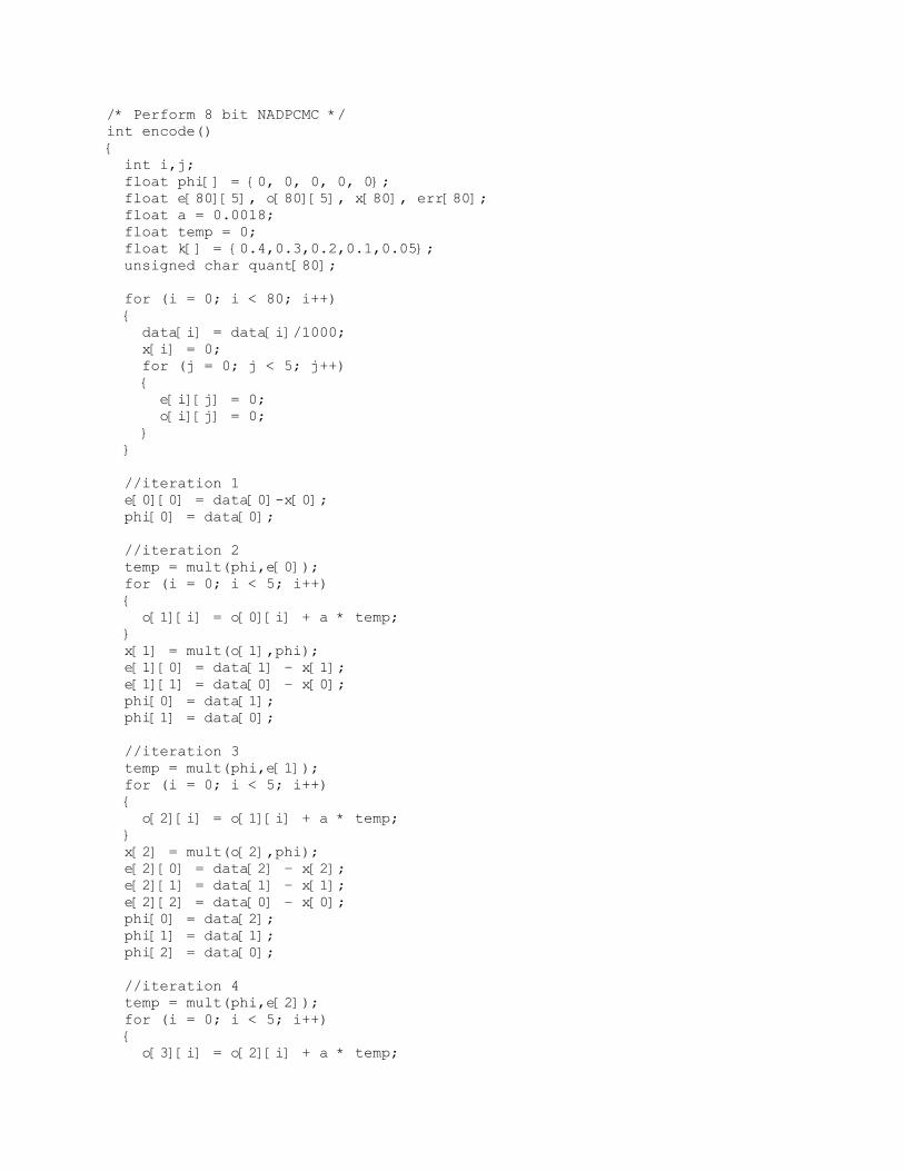
/* Perform 8 bit NADPCMC */

int encode()

{

int i,j;

float phi[] = {0, 0, 0, 0, 0};

float e[80][5], o[80][5], x[80], err[80];

float a = 0.0018;

float temp = 0;

float k[] = {0.4,0.3,0.2,0.1,0.05};

unsigned char quant[80];

for (i = 0; i < 80; i++)

{

data[i] = data[i]/1000;

x[i] = 0;

for (j = 0; j < 5; j++)

{

e[i][j] = 0;

o[i][j] = 0;

}

}

//iteration 1

e[0][0] = data[0]-x[0];

phi[0] = data[0];

//iteration 2

temp = mult(phi,e[0]);

for (i = 0; i < 5; i++)

{

o[1][i] = o[0][i] + a * temp;

}

x[1] = mult(o[1],phi);

e[1][0] = data[1] – x[1];

e[1][1] = data[0] – x[0];

phi[0] = data[1];

phi[1] = data[0];

//iteration 3

temp = mult(phi,e[1]);

for (i = 0; i < 5; i++)

{

o[2][i] = o[1][i] + a * temp;

}

x[2] = mult(o[2],phi);

e[2][0] = data[2] – x[2];

e[2][1] = data[1] – x[1];

e[2][2] = data[0] – x[0];

phi[0] = data[2];

phi[1] = data[1];

phi[2] = data[0];

//iteration 4

temp = mult(phi,e[2]);

for (i = 0; i < 5; i++)

{

o[3][i] = o[2][i] + a * temp;

}

x[3] = mult(o[3],phi);

e[3][0] = data[3] – x[3];

e[3][1] = data[2] – x[2];

e[3][2] = data[1] – x[1];

e[3][3] = data[0] – x[0];

phi[0] = data[3];

phi[1] = data[2];

phi[2] = data[1];

phi[3] = data[0];

//iteration 5

temp = mult(phi,e[3]);

for (i = 0; i < 5; i++)

{

o[4][i] = o[3][i] + a * temp;

}

x[4] = mult(o[4],phi);

e[4][0] = data[4] – x[4];

e[4][1] = data[3] – x[3];

e[4][2] = data[2] – x[2];

e[4][3] = data[1] – x[1];

e[4][4] = data[0] – x[0];

phi[0] = data[4];

phi[1] = data[3];

phi[2] = data[2];

phi[3] = data[1];

phi[4] = data[0];

for (i = 0; i < 5; i++)

x[i] = 0;

//other iterations

for (i = 5; i < 80; i++)

{

x[i] = mult(o[i-1],phi) + mult(k,e[i-1]);

for (j = 0; j < 5; j++)

e[i][j] = data[i-j] – x[i-j];

temp = mult(phi,e[i-1]);

for (j = 0; j < 5; j++)

o[i][j] = o[i-1][j] + a*temp;

phi[0] = tansig(data[i]);

phi[1] = e[i][0];

phi[2] = e[i-1][0];

phi[3] = e[i-2][0];

phi[4] = e[i-3][0];

}

// estimation over – calc error

//8 bit quantization

for (i = 0; i < 80; i++)

{

err[i] = data[i] – x[i];

if (err[i] > 1.9718)

quant[i] = 255;

else if (err[i] < -1)

quant[i] = 0;

else

quant[i] = ((err[i]+1)/0.0117);

#ifdef DC_DEBUG

printf(“%d “, quant[i]);

#endif /* DC_DEBUG */

}

#ifdef DC_DEBUG

printf(“\n”);

#endif /* DC_DEBUG */

return (5*sizeof(data[i]) + (i-5)*sizeof(quant[i]));

}

/* implement a source which takes packets, compresses them and generates

packets of

* the compressed size. It is parameterized by packet size and interval.

*/

static class DCTrafficClass : public TclClass {

public:

DCTrafficClass() : TclClass(“Application/Traffic/Datacompress”) {}

TclObject* create(int, const char*const*) {

return (new DC_Traffic());

}

} class_dc_traffic;

DC_Traffic::DC_Traffic() : seqno_(0), fp1(NULL), compress_(0), tsize(0),

isClusterHead_ (0)

{

bind_bw(“rate_”, &rate_);

bind(“maxpkts_”, &maxpkts_);

bind(“isClusterHead_”, &isClusterHead_);

bind(“compress_”, &compress_);

}

int DC_Traffic::command(int argc, const char*const* argv) {

if(argc==3){

if (strcmp(argv[1], “payload”) == 0) {

if ((fp1 = fopen(argv[2],”r”)) == NULL) {

fprintf(stderr,”File open error”);

return 1;

}

return 0;

}

}

return Application::command(argc,argv);

}

void DC_Traffic::init()

{

interval_ = (double)(40 << 3)/(double)rate_;

#ifdef DC_DEBUG

printf(“Interval is %ld \n”,interval_);

#endif /* DC_DEBUG */

if (agent_)

agent_->set_pkttype(PT_TCP);

}

void DC_Traffic::stop()

{

#ifdef DC_DEBUG

printf(“total size %d %d\n”,tsize, seqno_);

#endif /* DC_DEBUG */

fclose(fp1);

running_ = 0;

}

void DC_Traffic::start()

{

init();

running_ = 1;

// Clusterhead has to wait for aggregation

if (isClusterHead_ == 0) {

nextPkttime_ = next_interval(size_);

timer_.resched(nextPkttime_);

}

else

{

#ifdef DC_DEBUG

printf(“Clusterhead here…\n”);

#endif /* DC_DEBUG */

}

// Enable line below if you want to send immediately upon start

//timeout();

}

double DC_Traffic::next_interval(int& size) {

double t = interval_;

int len = 2000, temp = 0;

#ifdef HUFFMAN

FILE *fp2, *fp3;

if (compress_ == 1) {

fp2 = fopen(“./outputfile”,”r”);

fp3 = fopen(“./dummyfile”,”w”);

uffman_decode_file(fp2,fp3);

fclose(fp2);

fclose(fp3);

}

if (((fp2 = fopen(“./temp”,”w”)) != NULL) &&

((fp3 = fopen(“./outputfile”,”w”)) !=NULL)) {

char line[2000],newline[2000];

if (!feof(fp1)) {

fgets(line,len,fp1);

strncpy(newline,line,strlen(line)-2);

newline[strlen(line)-1] = „\0‟;

fputs(newline,fp2);

}

fclose(fp2);

if (compress_ == 1) {

fp2 = fopen(“./temp”,”r”);

uffman_encode_file(fp2,fp3);

fclose(fp3);

fp3 = fopen(“./outputfile”,”r”);

while (fgetc(fp3) != EOF)

temp++;

size_ = temp;

#ifdef DC_DEBUG

printf(“Compressing %d\n”,size_);

#endif /* DC_DEBUG */

fclose(fp2);

}

else

{

size_ = strlen(line);

#ifdef DC_DEBUG

printf(“Not compressing %d\n”,size_);

#endif /* DC_DEBUG */

}

tsize = tsize + size_;

fclose(fp3);

}*/

#else

if (!isClusterHead_)

{

if (compress_ == 1)

size_ = encode();

else

size_ = sizeof(data);

}

tsize = tsize + size_;

#endif /* HUFFMAN */

if (++seqno_ < maxpkts_)

{

#ifdef DC_DEBUG

printf(“Schedule packet…”);

#endif /* DC_DEBUG */

return(t);

}

else

{

#ifdef DC_DEBUG

printf(“Cant schedule packet..”);

#endif /* DC_DEBUG */

return(-1);

}

}

void DC_Traffic::generate_pkt(int size)

{

size_ = size;

nextPkttime_ = next_interval(size_);

#ifdef DC_DEBUG

printf(“Packet of size %d generated…%ld\n”,size_,nextPkttime_);

#endif /* DC_DEBUG */

timer_.resched(nextPkttime_);

}

void DC_Traffic::timeout()

{

if (! Running_)

return;

/* send a packet */

send(size_);

if (isClusterHead_ == 0) {

/* figure out when to send the next one */

nextPkttime_ = next_interval(size_);

/* schedule it */

if (nextPkttime_ > 0)

timer_.resched(nextPkttime_);

else

running_ = 0;

}

else

{

if (nextPkttime_ < 0)

running_ = 0;

}

}

datacompress.h – corresponding header file

/* -*- Mode:C++; c-basic-offset:8; tab-width:8; indent-tabs-mode:t -*-

*/

/*

* Copyright (c) Priya Kasirajan 2008. All rights reserved.

*

*/

#ifndef NS_DATACOMPRESS_H

#define NS_DATACOMPRESS_H

#include "trafgen.h"

/* implement a source which takes packets, compresses them and generates

packets of

* the compressed size. It is parameterized by packet size and interval.

*/

class DC_Traffic : public TrafficGenerator {

public:

DC_Traffic();

virtual double next_interval(int&);

int command(int argc, const char*const* argv);

void generate_pkt(int);

int isClusterHead_; /* is this node a clusterhead */

protected:

void init();

void start();

void stop();

void timeout();

double rate_; /* send rate during burst (bps) */

double interval_; /* inter-packet time at burst rate */

FILE *fp1; /* pointer to packet payload */

int seqno_; /* packet number */

int maxpkts_; /* max number of packets */

int compress_; /* is compression required */

int tsize; /* cumulative packet size */

};

#endif /* NS_DATACOMPRESS_H */

Source code of hardware implementation:

routing_mmcr.c – implementation of MMCR

/****************************************************************************

**

** Copyright (C) 2008-2009 Maciej Zawodniok, Priya Kasirajan. All rights

reserved.

**

** This file is part of the documentation of the UMR Mote Toolkit.

**

** This file may be used under the terms of the GNU General Public

** License version 2.0 as published by the Free Software Foundation

** and appearing in the file LICENSE.GPL included in the packaging of

** this file.

**

** This file is provided AS IS with NO WARRANTY OF ANY KIND, INCLUDING THE

** WARRANTY OF DESIGN, MERCHANTABILITY AND FITNESS FOR A PARTICULAR PURPOSE.

**

****************************************************************************/

#include "esnl_pub.h"

#ifdef FEAT_ENABLE_MMCR

#include "routing.h"

#include "routing_MMCR.h"

#include "network_hardware_ADFS.h"

#include "common.h"

#include "FEAT_Xbee_API/AT_scripts.h"

#include "FEAT_Queueing/Queuing.h"

#include "FEAT_Networking/tsp_common_pub.h"

#include "Application.h"

#include "FEAT_Networking/Phy_layer.h"

#include "packet.h"

#include "FEAT_Scheduler/sch_basic_pub.h"

#ifdef __KEIL__

#ifdef _ENABLE_F1_MOTE_TEST_01_

sbit YLED = P2 ^ 5;

#else // _ENABLE_F1_MOTE_TEST_01_

sbit YLED = P2 ^ 2;

#endif // else/not _ENABLE_F1_MOTE_TEST_01_

#endif

#ifdef __SDCC__

#ifdef _ENABLE_F1_MOTE_TEST_01_

#define YLED P2_5

#else // _ENABLE_F1_MOTE_TEST_01_

#define YLED P2_2

#endif // else/not _ENABLE_F1_MOTE_TEST_01_

#endif // __SDCC__

///////////////////////////////////////////////

///////////////////////////////////////////////

uint8_t mmcr_pkt_id = 0xFF;

unsigned char xdata mmcr_request_send_TC_ = 0 ; // request for sending

Topology control

// Variables to manage )periodic) timeout

uint8_t mmcr_hello_timeout_enabled_ = 0;

rtc_tick_t mmcr_hello_timeout_ = RTC_OVERFLOW_TIMER_VALUE;

#define RTR_MMCR_HELLO_PKT_SIZE 18

#define RTR_MMCR_TC_PKT_SIZE 14

#define MMCR_BANDWIDTH_FACTOR 1

#define MMCR_SWITCH_CHANNEL(c) (c>=MAX_RF_CHANNEL)?MIN_RF_CHANNEL:c+1

uint8_t mmcr_state_; // state of the routing agent (e.g. IDLE, routing in-

progress)

unsigned char xdata mmcr_Hello_countdown_; // ON - periodically send

HELLO

int xdata mmcr_route_search_BS_; // address of the target node (BS)

//Counters for the Routing Energy Analysis

unsigned char xdata mmcr_Hello_counter;

unsigned char xdata mmcr_ACK_MMCR_counter;

unsigned char xdata mmcr_DAT_MMCR_counter;

uint16_t mmcr_len_sample;

///////////////////////////////////////////////

struct ONEHOP

{

char ID;

bool MPR;

char Link[10]; // point to index (ID) of the second hop node

char Links;

uint32_t LinkCost;

};

struct TWOHOP

{

char ID;

char Covered;

};

struct

{

struct ONEHOP OneHop[10];

struct TWOHOP TwoHop[10];

int OneHopNodes;

int TwoHopNodes;

} Neighborhood;

struct RENTRY

{

char ID;

unsigned int NextHopID;

uint32_t NextHopCost;

unsigned int AltNextHopID;

uint32_t AltNextHopCost;

};

struct

{

char length;

struct RENTRY rentry[10];

} rtable;

///////////////////////////////////////////////

/**

* routing_init - performs initial setup of routing

*/

void routing_init_MMCR()

{

mmcr_route_search_BS_ = MY_DEST; // address of the target node (BS)

AODVcounter_update = 1;

mmcr_Hello_counter = 0;

mmcr_ACK_MMCR_counter = 0;

mmcr_DAT_MMCR_counter = 0;

mmcr_Hello_countdown_=0;

mmcr_state_=MMCR_STATE_IDLE;

mmcr_pkt_id = 0xFF;

enableDataTx_ = 0;

mmcr_request_send_HELLO_ = 1; // request for sending HELLO

// Variables to manage (periodic) timeout

mmcr_hello_timeout_ = RTC_OVERFLOW_TIMER_VALUE;

init_topology();

mpr_select();

mmcr_startRouteSearch(MY_DEST);

#ifdef MZ_TEMP_TEST_SCH_HIO

sch_add_loop(( sch_loop_func_t )mmcr_loop );

#endif // MZ_TEMP_TEST_SCH_HIO

}

///////////////////////////////////////////////

/**

* init_topology - performs initial setup of topology

*/

void init_topology()

{

int x,y;

for (x=0;x<10;x++)

{

Neighborhood.OneHop[x].ID=0;

Neighborhood.OneHop[x].MPR=false;

Neighborhood.OneHop[x].Links=0;

Neighborhood.OneHop[x].LinkCost=0xFFFFFFFF;

for (y=0;y<10;y++)

Neighborhood.OneHop[x].Link[y]=0;

Neighborhood.TwoHop[x].ID=0;

Neighborhood.TwoHop[x].Covered=0;

}

#ifdef NODE_1

Neighborhood.OneHopNodes = 2;

Neighborhood.TwoHopNodes = 1;

Neighborhood.OneHop[0].ID = 0x0C;

Neighborhood.OneHop[0].Links = 1;

Neighborhood.OneHop[0].Link[0] = 0x0B;

Neighborhood.OneHop[1].ID = 0x0D;

Neighborhood.OneHop[1].Links = 1;

Neighborhood.OneHop[1].Link[0] = 0x0B;

Neighborhood.TwoHop[0].ID = 0x0B;

#endif

#ifdef NODE_2

Neighborhood.OneHopNodes = 2;

Neighborhood.TwoHopNodes = 1;

Neighborhood.OneHop[0].ID = 0x0C;

Neighborhood.OneHop[0].Links = 1;

Neighborhood.OneHop[0].Link[0] = 0x0A;

Neighborhood.OneHop[1].ID = 0x0D;

Neighborhood.OneHop[1].Links = 1;

Neighborhood.OneHop[1].Link[0] = 0x0A;

Neighborhood.TwoHop[0].ID = 0x0A;

#endif

#ifdef NODE_3

Neighborhood.OneHopNodes = 2;

Neighborhood.TwoHopNodes = 0;

Neighborhood.OneHop[0].ID = 0x0A;

Neighborhood.OneHop[0].Links = 0;

Neighborhood.OneHop[1].ID = 0x0B;

Neighborhood.OneHop[1].Links = 0;

#endif

#ifdef NODE_4

Neighborhood.OneHopNodes = 2;

Neighborhood.TwoHopNodes = 0;

Neighborhood.OneHop[0].ID = 0x0A;

Neighborhood.OneHop[0].Links = 0;

Neighborhood.OneHop[1].ID = 0x0B;

Neighborhood.OneHop[1].Links = 0;

#endif

/* init routing table */

rtable.length = Neighborhood.TwoHopNodes;

for (x = 0; x < rtable.length; x++)

{

rtable.rentry[x].ID = Neighborhood.TwoHop[x].ID;

rtable.rentry[x].NextHopID = 0xFFFF;

rtable.rentry[x].NextHopCost = 0xFFFFFFFF;

rtable.rentry[x].AltNextHopID = 0xFFFF;

rtable.rentry[x].AltNextHopCost = 0xFFFFFFFF;

}

}

///////////////////////////////////////////////

/**

* mpr_select - performs MPR selection

*/

void mpr_select()

{

unsigned char mpr[10];

int x = 0;

int y = 0;

int z = 0;

unsigned char count[10];

bool uncovered;

int overcoverage;

for(x=0;x<10;x++)

{

count[x]=0;

mpr[x]=0;

}

/** MPR selection **/

// count coverage

for(x=0;x<Neighborhood.OneHopNodes;x++)

{

for(y=0;y<Neighborhood.OneHop[x].Links;y++)

{

for(z=0;z<Neighborhood.TwoHopNodes;z++)

{

if(Neighborhood.OneHop[x].Link[y] ==

Neighborhood.TwoHop[z].ID)

count[z]++;

}

}

}

// 1. select singular neighbors

for(x=0;x<Neighborhood.OneHopNodes;x++)

{

if(count[x] == 0)

{

Neighborhood.OneHop[x].MPR = true;

//TODO: search for single link

Neighborhood.TwoHop[find_two_hop_node(Neighborhood.OneHop[x].Link[0])].

Covered ++;

}

}

// 2. selects as MPR neighbors with the largest count of uncovered

twohop nodes

x=0;

uncovered = true;

while(x<Neighborhood.OneHopNodes /*&& uncovered*/)

{

//TODO: sort high-low

if(count[x]>0)

{

if(~Neighborhood.TwoHop[find_two_hop_node(Neighborhood.OneHop[x].Link[0

])].Covered)

{

Neighborhood.OneHop[x].MPR = true;

Neighborhood.TwoHop[find_two_hop_node(Neighborhood.OneHop[x].Link[0])].

Covered ++;

}

}

x++;

}

// 3. remove redundant nodes

for(x=0;x<Neighborhood.OneHopNodes;x++)

{

overcoverage = 0;

for(y=0;y<Neighborhood.OneHop[x].Links;y++)

{

//for(z=0;z<10;z++)

{

if(Neighborhood.TwoHop[find_two_hop_node(Neighborhood.OneHop[x].Link[y]

)].Covered > 1)

{

overcoverage ++;

}

}

}

if(overcoverage == Neighborhood.OneHop[x].Links)

{

Neighborhood.OneHop[x].MPR = false;

//TODO: reduce Covered

}

}

y = 0;

for(x=0;x<Neighborhood.OneHopNodes;x++)

{

if(Neighborhood.OneHop[x].MPR)

{

mpr[y++] = Neighborhood.OneHop[x].ID;

}

}

}

char find_one_hop_node(char ID)

{

int x;

for (x=0;x<10;x++)

{

if(Neighborhood.OneHop[x].ID == ID)

return x;

}

return -1;

}

char find_two_hop_node(char ID)

{

int x;

for (x=0;x<10;x++)

{

if(Neighborhood.TwoHop[x].ID == ID)

return x;

}

return -1;

}

///////////////////////////////////////////////

///////////////////////////////////////////////

/**

* senddummy_data - sends dummy data - test purpose

*

*

*/

unsigned int sendDATA_MMCR()

{

if(enableDataTx_)

{

mmcr_len_sample=80;

tsp_reserve_packet ( mmcr_len_sample, &mmcr_pkt_id, MY_DEST );

tsp_send_from_modules(mmcr_pkt_id);

mmcr_pkt_id = 0xFF;

}

return 1;

}

///////////////////////////////////////////////

///////////////////////////////////////////////

/**

* startRouteSearch - starts the route discovery procedure

*

*

*/

void mmcr_startRouteSearch ( unsigned int dst )

{

if ( ( 0 < mmcr_Hello_countdown_ ) || ( MMCR_STATE_IDLE != mmcr_state_

) )

{

return;

}

// ###############################

// start route Discovery toward BS

mmcr_route_search_BS_ = dst;

rtr_MMCR_Hello_Phase();

mmcr_Hello_countdown_ = MMCR_DEFAULT_ROUTE_SEARCH_ON_REPETITIONS;

mmcr_state_ = MMCR_STATE_ROUTE_DISCOVERY;

mmcr_set_tx_timeout ( 10 );

}

///////////////////////////////////////////////

///////////////////////////////////////////////

/**

* rtr_MMCR_Hello_Phase() - handles the routing phase of transmitting HELLO

pkts

*/

void rtr_MMCR_Hello_Phase()

{

int a;

if ( ROUTING_PROTOCOL_MMCR == my_protocol_ )

{

// Send HELLO routing packet

if ( 1 == mmcr_request_send_HELLO_ )

{

uint8_t packet[RTR_MMCR_HELLO_PKT_SIZE];

uint16_t len = mmcr_sendHELLO ( (hpkt_mmcr_t xdata*)packet

);

#ifdef _ENABLE_XBEE_API_

a = api_send_packet16( packet, len, 0xFFFF);

#endif // _ENABLE_XBEE_API_

if ( AODVcounter_update )

{

mmcr_Hello_counter++;

}

my_energy_ = my_energy_ - HELLO_LENGTH;

mmcr_request_send_HELLO_ = 0;

}

}

}

///////////////////////////////////////////////

///////////////////////////////////////////////

/**

* mmcr_set_tx_timeout(??) - set one-time timeout for MMCR hello/tc packets

*/

void mmcr_set_tx_timeout ( uint16_t ms )

{

mmcr_hello_timeout_ = rtc_get_ticks() + ms;

mmcr_hello_timeout_enabled_ = 1;

}

///////////////////////////////////////////////

///////////////////////////////////////////////

/**

* mmcr_sendHELLO - broadcasts a HELLO packet

*/

unsigned int mmcr_sendHELLO ( hpkt_mmcr_t xdata*hello_pkt )

{

int len = PKT_HEADER_LENGTH; // size of the packet header (start + flag

+ dst(2) + src(2) + len)

hpkt_mmcr_t xdata *hpkt = ( ( hpkt_mmcr_t xdata * ) hello_pkt);

hpkt->start = 0x55;

hpkt->flags = FLAG_HELLO_MMCR; // HELLO_MMCR packet

hpkt->mac_dst = MAC_BROADCAST; // Broadcast

hpkt->mac_src = MY_ADDR;

// FILL END-TO-END ADDRESSING

hpkt->dst_id = 0xFF;

hpkt->src_id = MY_ADDR;

hpkt->length=HELLO_LENGTH_MMCR - PKT_HEADER_LENGTH;;

// FILL THE MMCR field

hpkt->energy=my_energy_;

// FILL the CHECKSUM

// TODO: calculate checksum

hpkt->crc = 65;

return HELLO_LENGTH_MMCR;

}

///////////////////////////////////////////////

///////////////////////////////////////////////

/**

* mmcr_recvHELLO - handles a received HELLO packet

* should identify if this node is potential relay node

* if yes, then send response (ACK?)

*/

unsigned int mmcr_recvHELLO ( hpkt_mmcr_t xdata *hp )

{

unsigned long int link_factor, i=0;

uint32_t energy = hp->energy;

long int delay = TYPICAL_DELAY_FOR_LINK;

if (ENERGY_MAX_VALUE < energy)

energy = ENERGY_MAX_VALUE;

link_factor = ( energy * MMCR_BANDWIDTH_FACTOR * DELAY_SCALING ) /

(delay);

for (i = 0; i < Neighborhood.OneHopNodes; i++)

{

if (hp->mac_src == Neighborhood.OneHop[i].ID)

Neighborhood.OneHop[i].LinkCost= link_factor;

}

mmcr_sendACK( (hpkt_mmcr_t xdata *) hp);

return 1;

}

///////////////////////////////////////////////

///////////////////////////////////////////////

/**

* mmcr_sendACK - handles a sending of ACK packet

* collects all info for packet

* prepares timestamp

*/

unsigned int mmcr_sendACK ( hpkt_mmcr_t xdata*hp)

{

uint8_t i;

uint8_t xdata pkt[ACK_LENGTH_MMCR];

long int delay = TYPICAL_DELAY_FOR_LINK;

apkt_t_mmcr *ap = ( (apkt_t_mmcr *) pkt );

uint16_t *pkt_neighbor_addr = (uint16_t *)&(ap->neighbor_addr_first);

uint32_t *pkt_neighbor_cost = NULL;

uint8_t *pkt_crc;

ap->start = START_BYTE;

ap->flags = FLAG_ACK_MMCR;

ap->mac_dst = hp->mac_src; //MAC DST

ap->mac_src = MY_ADDR; // MAC SRC

ap->length = 15 + (Neighborhood.OneHopNodes*6);

ap->dst_id = hp->src_id;

ap->src_id = MY_ADDR;

ap->energy = my_energy_;

ap->neighbor_count=Neighborhood.OneHopNodes;

for(i=0;i<Neighborhood.OneHopNodes;i++)

{

*pkt_neighbor_addr = Neighborhood.OneHop[i].ID;

pkt_neighbor_addr++;

pkt_neighbor_cost = (uint32_t *)pkt_neighbor_addr;

*pkt_neighbor_cost = Neighborhood.OneHop[i].LinkCost;

pkt_neighbor_addr +=2;

}

pkt_crc = (uint8_t *)pkt_neighbor_addr;

*pkt_crc = STOP_BYTE;

if ( AODVcounter_update )

{

mmcr_ACK_MMCR_counter++;

}

my_energy_ = my_energy_ - ap->length;

#ifdef _ENABLE_XBEE_API_

api_send_packet16 ( (uint8_t xdata*) ap, ap->length, ap->mac_dst );

return ap;

#else // _ENABLE_XBEE_API_

return 0;

#endif // else _ENABLE_XBEE_API_

}

///////////////////////////////////////////////

///////////////////////////////////////////////

/**

* mmcr_revcACK - handles a received ACK packet

* should identify if this node is potential relay node

* if yes, then send response (ACK?)

*/

unsigned int mmcr_recvACK (apkt_t_mmcr *apkt )

{

apkt_t_mmcr xdata *ap = (( apkt_t_mmcr xdata * ) apkt);

long int delay = TYPICAL_DELAY_FOR_LINK;

unsigned long int link_factor;

uint32_t energy = ap->energy;

uint16_t *pkt_neighbor_addr = (uint16_t *)&(ap->neighbor_addr_first);

uint32_t *pkt_neighbor_cost = NULL;

int i,j,k;

if (ENERGY_MAX_VALUE < energy)

energy = ENERGY_MAX_VALUE;

link_factor = ( energy * MMCR_BANDWIDTH_FACTOR * DELAY_SCALING ) /

(delay);

for (i = 0; i < Neighborhood.OneHopNodes; i++)

{

if (ap->mac_src == Neighborhood.OneHop[i].ID)

{

Neighborhood.OneHop[i].LinkCost= link_factor;

for (k = 0; k < ap->neighbor_count; k++)

{

for (j = 0; j < Neighborhood.OneHop[i].Links; j++)

{

if (*pkt_neighbor_addr ==

Neighborhood.OneHop[i].Link[j])

{

pkt_neighbor_cost = (uint32_t

*)(pkt_neighbor_addr+1);

mmcr_set_route(*pkt_neighbor_addr, ap-

>mac_src, link_factor + *pkt_neighbor_cost);

}

}

pkt_neighbor_addr +=3;

}

}

}

return 1;

}

/////////////////////////////////

/**

* mmcr_sendTC - send channel switch message

*

*/

unsigned int mmcr_sendTC ( tpkt_t_mmcr xdata*tpkt )

{

int len = PKT_HEADER_LENGTH; // size of the packet header (start + flag

+ dst(2) + src(2) + len)

//tpkt_t_mmcr xdata *tpkt = ( ( tpkt_t_mmcr xdata * ) tc_pkt);

tpkt->start = 0xAA;

tpkt->flags = FLAG_TC_MMCR; // TC packet

tpkt->mac_dst = MAC_BROADCAST; // Broadcast

tpkt->mac_src = MY_ADDR;

tpkt->length = RTR_MMCR_TC_PKT_SIZE - PKT_HEADER_LENGTH; // of the

packet'd data

// FILL END-TO-END ADDRESSING

tpkt->dst_id = 0xFF;

tpkt->src_id = MY_ADDR;

tpkt->energy=my_energy_;

tpkt->channel=MMCR_SWITCH_CHANNEL(DEFAULT_RF_CHANNEL);

// FILL the CHECKSUM

// TODO: calculate checksum

tpkt->crc = 65;

return RTR_MMCR_TC_PKT_SIZE;

}

/////////////////////////////////

/**

* mmcr_recvTC - switch channel

*

*/

unsigned int mmcr_recvTC ( tpkt_t_mmcr *tp )

{

phy_set_RF_channel(tp->channel);

return 1;

}

///////////////////////////////////////////////

///////////////////////////////////////////////

/**

* mmcr_loop() - executes main loop block (BUT DOES NOT LOOP ITSELF!!!)

*/

void mmcr_loop( void )

{

if (1 == mmcr_hello_timeout_enabled_)

{

if ( mmcr_hello_timeout_ < rtc_get_ticks())

{

mmcr_hello_timeout_enabled_ = 0;

mmcr_hello_timeout_ = RTC_OVERFLOW_TIMER_VALUE;

mmcr_hello_timeout();

}

}

}

/////////////////////////////////

/**

* mmcr_hello_timeout(??) - runs the procedure of periodic sending of Hello

packets

*/

void mmcr_hello_timeout()

{

// Timeout reached -> is there a route found? or should I retransmit

HELLO?

unsigned int mac_addr = mmcr_neighbor_analyse(MY_DEST);

if ( 0 < mmcr_Hello_countdown_ )

{ mmcr_Hello_countdown_ --; // count down HELLO

retransmissions

// number of retransmission not reached -> resent HELLO

YLED = ~YLED;

mmcr_request_send_HELLO_ = 1;

mmcr_request_send_TC_= 1;

mmcr_set_tx_timeout(ROUTE_SEARCH_HELLO_INTERVAL);

rtr_MMCR_Hello_Phase();

YLED = ~YLED;

}

else

{

// all Hello messages has been without response -> STOP

mmcr_Hello_countdown_=0;

mmcr_request_send_HELLO_ = 0; //1;

mmcr_request_send_TC_ = 0;

mmcr_state_=MMCR_STATE_IDLE;

#ifdef NODE_1 //to handle any unprocessed acks

mmcr_set_route(0x0B,0x0C,0xCCCC);

mmcr_set_route(0x0B,0x0D,0xCCCD);

#endif

enableDataTx_ = 1;

}

}

///////////////////////////////////////////////

///////////////////////////////////////////////

/**

* mmcr_set_route - adds or updates a route to "dst_id"

*/

int mmcr_set_route ( unsigned int dst_id, unsigned int next_hop, uint32_t

metric )

{

int i;

mpr_select();

for (i = 0; i < rtable.length; i++)

{

if (rtable.rentry[i].ID == dst_id)

{

// rtable record spotted -> set next hop

if (rtable.rentry[i].NextHopID == 0xFFFF)

{

rtable.rentry[i].NextHopID = next_hop;

rtable.rentry[i].NextHopCost = metric;

return 1; //successfully added route

}

else if (rtable.rentry[i].NextHopID == next_hop)

{

rtable.rentry[i].NextHopCost = metric;

return 1; //successfully updated route

}

else if (rtable.rentry[i].AltNextHopID == 0xFFFF)

{

rtable.rentry[i].AltNextHopID = next_hop;

rtable.rentry[i].AltNextHopCost = metric;

return 1; //successfully added route

}

else if (rtable.rentry[i].AltNextHopID == next_hop)

{

rtable.rentry[i].AltNextHopCost = metric;

return 1; //successfully updated route

}

}

}

return 0; // two hop id not found!!!

}

///////////////////////////////////////////////

///////////////////////////////////////////////

/**

* neighbor_analyse - performs analysis of the neighbor table

and selects the best node

*/

unsigned int mmcr_neighbor_analyse(unsigned int dst_id)

{

unsigned int i, result = 0xFFFF; // by default FFFF indicating lack

of route

/* check if dst_id is a one hop neighbor */

for (i = 0; i < Neighborhood.OneHopNodes; i++)

{

if (Neighborhood.OneHop[i].ID == dst_id)

result = Neighborhood.OneHop[i].ID;

}

/* check if dst_id is a two hop neighbor */

for (i = 0; i < rtable.length; i++)

{

if (rtable.rentry[i].ID == dst_id)

{

if ((rtable.rentry[i].NextHopID == 0xFFFF) &&

(rtable.rentry[i].AltNextHopID == 0xFFFF))

result = 0xFFFF;

else if ((rtable.rentry[i].NextHopCost <=

rtable.rentry[i].AltNextHopCost) && (rtable.rentry[i].NextHopID != 0xFFFF))

result = rtable.rentry[i].NextHopID;

else if (rtable.rentry[i].AltNextHopID != 0xFFFF)

result = rtable.rentry[i].AltNextHopID;

}

}

return result;

}

///////////////////////////////////////////////

/**

* sendDATA - handles a sending of DATA packet

* 1) check if buffer ready then passes packet

* 2) else temporarly stores

*/

char MMCR_send_DATA_base ( unsigned int base )

{

unsigned int mac_d;

pkt_t * xdata pkt = ( pkt_t* ) ( & ( buffer0[ base] ) );

//&(QBUFF_ACCESS(base,0));

if (enableDataTx_)

//if (1)

{

mac_d = mmcr_neighbor_analyse ( pkt->dst_id );

if (0xFFFF==mac_d)

{

enableDataTx_ = 0;

return 0;

}

pkt->mac_dst = mac_d;

pkt->mac_src = MY_ADDR;

// send the packet

if ( AODVcounter_update )

{

mmcr_DAT_MMCR_counter++;

}

}

else

{

APPEND_LOG ( NODE_ID_STR, NODE_ID_STR_LEN );

APPEND_LOG ( "DROP DATA\r", 10 );

// drop the packet

return 0;

}

return 1;

}

///////////////////////////////////////////////

///////////////////////////////////////////////

/**

* recvAcceptData - handles a received ACCEPT DATA packet from BS

* 1) enables data transmission

* 2)

*/

unsigned int mmcr_recvAcceptData ( char *pkt )

{

pkt_t xdata *p = ( ( pkt_t_mmcr xdata * ) pkt);

// analyse ACK packet

if ( 0xFFFF == p->mac_dst )

{

// enable DATA transmission

enableDataTx_ = 1;

APPEND_LOG ( NODE_ID_STR, NODE_ID_STR_LEN );

APPEND_LOG ( "DATA - OK\r\r\r", 12 );

return 1;

}

// wrong trasmitter

return 0;

}

/////////////////////////////////

/**

* mmcr_dropped_link(??) - the link failed (after few retransmissions??) -

update routing

* and optionally restart route discovery

*/

void mmcr_dropped_link()

{

int i;

for (i = 0; i < rtable.length; i++)

{

if (rtable.rentry[i].ID == MY_DEST)

{

// rtable record spotted -> clear next hop

rtable.rentry[i].NextHopID = 0xFFFF;

}

}

if ((rtable.rentry[i].NextHopID == 0xFFFF) &&

(rtable.rentry[i].AltNextHopID == 0xFFFF))

mmcr_startRouteSearch(MY_DEST);

}

#endif /* FEAT_ENABLE_MMCR */