Thermal remote sensing in the framework of the SEN2FLEX project: field measurements, airborne data...

PLEASE SCROLL DOWN FOR ARTICLE

This article was downloaded by: [Universidad de Valencia]On: 25 September 2008Access details: Access Details: [subscription number 779262402]Publisher Taylor & FrancisInforma Ltd Registered in England and Wales Registered Number: 1072954 Registered office: Mortimer House,37-41 Mortimer Street, London W1T 3JH, UK

International Journal of Remote SensingPublication details, including instructions for authors and subscription information:http://www.informaworld.com/smpp/title~content=t713722504

Thermal remote sensing in the framework of the SEN2FLEX project: fieldmeasurements, airborne data and applicationsJ. A. Sobrino a; J. C. Jiménez-Muñoz a; G. Sòria a; M. Gómez a; A. Barella Ortiz a; M. Romaguera a; M.Zaragoza a; Y. Julien a; J. Cuenca a; M. Atitar a; V. Hidalgo a; B. Franch a; C. Mattar a; A. Ruescas a; L. Moralesb; A. Gillespie c; L. Balick d; Z. Su e; F. Nerry f; L. Peres g; R. Libonati g

a Global Change Unit, Department of Earth Physics and Thermodynamics, Faculty of Physics, University ofValencia, 46100 Burjassot, Spain b Departamento de Ciencias Ambientales y Recursos Naturales, Facultadde Ciencias Agronomicas, Universidad de Chile, Santiago de Chile, Chile c W. M. Keck Remote SensingLaboratory, Department of Earth and Space Sciences, University of Washington, Seattle, Washington 98195-1310, USA d Space and Remote Sensing Sciences Group, Los Alamos National Laboratory, Los Alamos, NM87545, USA e International Institute for Geoinformation Science and Herat Observation (ITC), Enschede, theNetherlands f LSIIT/TRIO, Louis Pasteur University, Parc d'innovation, Boulevard Sébastien Brant, BP 10413,F-67412, Illkirch cedex, France g Centro de Geofisica da Universidade de Lisboa (CGUL), Campo Grande,1749-016 Lisbon, Portugal

Online Publication Date: 01 January 2008

To cite this Article Sobrino, J. A., Jiménez-Muñoz, J. C., Sòria, G., Gómez, M., Ortiz, A. Barella, Romaguera, M., Zaragoza, M., Julien,Y., Cuenca, J., Atitar, M., Hidalgo, V., Franch, B., Mattar, C., Ruescas, A., Morales, L., Gillespie, A., Balick, L., Su, Z., Nerry, F.,Peres, L. and Libonati, R.(2008)'Thermal remote sensing in the framework of the SEN2FLEX project: field measurements, airbornedata and applications',International Journal of Remote Sensing,29:17,4961 — 4991

To link to this Article: DOI: 10.1080/01431160802036516

URL: http://dx.doi.org/10.1080/01431160802036516

Full terms and conditions of use: http://www.informaworld.com/terms-and-conditions-of-access.pdf

This article may be used for research, teaching and private study purposes. Any substantial orsystematic reproduction, re-distribution, re-selling, loan or sub-licensing, systematic supply ordistribution in any form to anyone is expressly forbidden.

The publisher does not give any warranty express or implied or make any representation that the contentswill be complete or accurate or up to date. The accuracy of any instructions, formulae and drug dosesshould be independently verified with primary sources. The publisher shall not be liable for any loss,actions, claims, proceedings, demand or costs or damages whatsoever or howsoever caused arising directlyor indirectly in connection with or arising out of the use of this material.

http://www.informaworld.com/smpp/title~content=t713722504

http://dx.doi.org/10.1080/01431160802036516

http://www.informaworld.com/terms-and-conditions-of-access.pdf

Thermal remote sensing in the framework of the SEN2FLEX project:field measurements, airborne data and applications

J. A. SOBRINO*{, J. C. JIMENEZ-MUNOZ{, G. SORIA{, M. GOMEZ{,

A. BARELLA ORTIZ{, M. ROMAGUERA{, M. ZARAGOZA{, Y. JULIEN{,

J. CUENCA{, M. ATITAR{, V. HIDALGO{, B. FRANCH{, C. MATTAR{,

A. RUESCAS{, L. MORALES{, A. GILLESPIE§, L. BALICK", Z. SU{{,

F. NERRY{{, L. PERES§§ and R. LIBONATI§§

{Global Change Unit, Department of Earth Physics and Thermodynamics, Faculty of

Physics, University of Valencia, Dr Moliner 50, 46100 Burjassot, Spain

{Departamento de Ciencias Ambientales y Recursos Naturales, Facultad de Ciencias

Agronomicas, Universidad de Chile, casilla 1004, Santiago de Chile, Chile

§W. M. Keck Remote Sensing Laboratory, Department of Earth and Space Sciences,

University of Washington, Seattle, Washington 98195-1310, USA

"Space and Remote Sensing Sciences Group, Los Alamos National Laboratory, Los

Alamos, NM 87545, USA

{{International Institute for Geoinformation Science and Herat Observation (ITC),

Enschede, the Netherlands

{{LSIIT/TRIO, Louis Pasteur University, Parc d’innovation, Boulevard Sebastien

Brant, BP 10413, F-67412, Illkirch cedex, France

§§Centro de Geofisica da Universidade de Lisboa (CGUL), Campo Grande, 1749-016

Lisbon, Portugal

(Received 12 December 2006; in final form 30 November 2007 )

A description of thermal radiometric field measurements carried out in the

framework of the European project SENtinel-2 and Fluorescence Experiment

(SEN2FLEX) is presented. The field campaign was developed in the region of

Barrax (Spain) during June and July 2005. The purpose of the thermal

measurements was to retrieve biogeophysical parameters such as land surface

emissivity (LSE) and temperature (LST) to validate airborne-based methodol-

ogies and to characterize different surfaces. Thermal measurements were carried

out using two multiband field radiometers and several broadband field

radiometers, pointing at different targets. High-resolution images acquired with

the Airborne Hyperspectral Scanner (AHS) sensor were used to retrieve LST and

LSE, applying the Temperature and Emissivity Separation (TES) algorithm as

well as single-channel (SC) and two-channel (TC) methods. To this purpose, 10

AHS thermal infrared (TIR) bands (8–13mm) were considered. LST and LSE

estimations derived from AHS data were used to obtain heat fluxes and

evapotranspiration (ET) as an application of thermal remote sensing in the

context of agriculture and water management. To this end, an energy balance

equation was solved using the evaporative fraction concept involved in the

Simplified Surface Energy Balance Index (S-SEBI) model. The test of the

different algorithms and methods against ground-based measurements showed

*Corresponding author. Email: [email protected]

International Journal of Remote Sensing

Vol. 29, Nos. 17–18, September 2008, 4961–4991

International Journal of Remote SensingISSN 0143-1161 print/ISSN 1366-5901 online # 2008 Taylor & Francis

http://www.tandf.co.uk/journalsDOI: 10.1080/01431160802036516

Downloaded By: [Universidad de Valencia] At: 15:15 25 September 2008

root mean square errors (RMSE) lower than 1.8 K for temperature and lower

than 1.1 mm/day for daily ET.

1. Introduction

In the framework of its Earth Observation Envelope Programme, the European

Space Agency (ESA) carries out a number of ground-based and airborne campaigns

to support geophysical algorithm development, calibration/validation and the

simulation of future spaceborne Earth observation (EO) missions.

The SENtinel-2 and FLuorescence EXperiment (SEN2FLEX) is a campaign that

combines different activities in support of initiatives related both to fluorescence

experiments (AIRFLEX) for observation of solar-induced fluorescence signals over

multiple surface targets and to the GMES Sentinel-2 initiative for prototyping

spectral bands, spectral widths and spatial/temporal resolutions to meet mission

requirements (www.uv.es/,leo/sen2flex/). Both initiatives require simultaneous

airborne hyperspectral and ground measurements for interpretation of fluorescence

signal levels (AIRFLEX), and simulation of an optical observing system capable of

assessing geo- and biophysical variables and classifying target surfaces by spectral,

spatial and temporal distinction (Sentinel-2).

Furthermore, the SEN2FLEX campaign includes activities in support of the

European Community Water Framework Directive (WFD) EO projects to improve

Europe’s water resources protection and management.

The main objectives of the SEN2FLEX campaign are: (i) to observe solar-

induced fluorescence signals over multiple agricultural and forest targets to verify

signal suitability for observations from space as proposed in the FLEX EO

mission, (ii) to provide feedback to the ESA on key issues related to ESA’s definition

of Sentinel-2’s multispectral mission requirements, (iii) to validate retrieval

algorithms based on hyperspectral and fluorescence signals, and (iv) to

provide feedback to the ESA on EO data requirements necessary to fulfil

the European Union Water Policy directive. These objectives require the

coordinated collection of satellite, airborne hyperspectral and coincident in situ

data together with analysis of the joint dataset. Two campaigns at different time

periods during the year 2005 were carried out to ensure different crop growth stages

and conditions: the first on 1, 2 and 3 June 2005 and the second on 12, 13 and 14

July 2005.

Our interest was focused on thermal measurements and Airborne Hyperspectral

Scanner (AHS) data analysis to demonstrate the use of thermal infrared

(TIR) remote sensing for different environmental applications. In particular, in

this paper we present the results obtained in Land Surface Temperature (LST)

and Land Surface Emissivity (LSE) retrieval from AHS data. These products (LST

and LSE) have been used to estimate the daily evapotranspiration (ET), which

provides useful information for water irrigation management. A previous study of

LST retrieval from AHS data acquired in 2004 was presented in Sobrino et al.

(2006). However, in that paper problems with some AHS TIR bands were found, so

the analysis was limited to the use of bands 75 to 79 (for technical details of the AHS

instrument see section 3.1). As described in section 5, calibration problems were not

found in 2005 so we were able to use 10 AHS thermal bands instead of the five bands

used in 2004. In addition, some comments and results related to LSE and ET

retrieval that were not treated in Sobrino et al. (2006) have been included in this

paper.

4962 J. A. Sobrino et al.


2. Field measurements

2.1 Study area

Field measurements and airborne imagery were collected in the agricultural area of

Barrax (39u39 N, 2u69 W, 700 m), which is located in Albacete, Spain. The area has

been selected in many other experiments because of its flat terrain, minimizing the

complications introduced by variable lighting geometry, and the presence of large,

uniform land-use units, suitable for validating moderate-resolution satellite image

products.

Barrax has a Mediterranean-type climate, with heavy rainfall in spring and

autumn and lighter rainfall in summer; it presents a high level of continentality, with

sudden changes from cold months to warm months and high thermal oscillations in

all seasons between the maximum and minimum daily temperatures.

The soils of the area are Inceptisols in terms of soil taxonomy. About 65% of

cultivated lands at Barrax are dryland (67% winter cereals, 33% fallow) and 35%

irrigated land (75% corn, 15% barley/sunflower, 5% alfalfa, 5% onions and

vegetables). The University of Castilla-La Mancha, through the ‘Escuela Tecnica

Superior de Ingenieros Agronomos’, operates three agro-meteorological stations in

the study area. More details about the test site are presented in Moreno et al. (2001).

Figure 1 shows an index map of the study area and the plots where measurements

were made.

2.2 Instrumentation

Various instruments were used to measure in the TIR domain, including multiband

and single-band radiometers with a fixed field-of-view (FOV). Calibration processes

Figure 1. Barrax study area and location of parcels where thermal infrared measurementswere performed. Crops are distributed in circles for irrigation purposes.

Recent Advances in Quantitative Remote Sensing II 4963


were carried out with the use of calibration sources (black bodies). The instruments

used are summarized in table 1.

The CIMEL detectors CE-312-1 and CE312-2 are two radiance-based TIR

radiometers comprising an optical head and a data storage unit. CE312-1 includes

one broadband filter (8–13 mm) and three narrower filters (8.2–9.2, 10.5–11.5 and

11.5–12.5 mm). CE312-2 includes six bands, a wide one (8–13 mm) and five narrower

filters (8.1–8.5, 8.5–8.9, 8.9–9.3, 10.3–11 and 11–11.7 mm). The temperature of an

external black body can be measured with a temperature probe. One CIMEL

CE312-1 and two CIMEL CE312-2 detectors were used during the field campaign.

The two portable RAYTEK ST6 radiometers, a standard model and a ProPlus

model, were also used. They have a single band at 8–14 mm, and a FOV of 7u and 2u,respectively. They cover a temperature range from 232uC to 400uC with a sensitivity

of 0.1 K and an accuracy of 1 K. A built-in laser beam helps users to aim at the

target. Three Raytek Thermalert MID radiometers with different FOVs (6u and 30u)were used. They have an IR sensor with a single band at 8–14 mm, a temperature

range from 240uC to 600uC, and a sensitivity of 0.5 K and an accuracy of 1 K. Four

different Licor LI-1000 dataloggers were used to store data from the radiometers set

up on masts.

Additional IR radiometers were also used in the field campaign: five portable

OPTRIS MiniSight Plus (with laser beam) IR radiometers, with a single band at 8–

14 mm, a FOV of 3u, a temperature range from 232uC to 530uC and with a

sensitivity of 0.7 K and an accuracy of 1 K; an Oakton Temp Testr I portable

radiometer, with a single band at 8–14 mm, a sensitivity of 0.5 K and an accuracy of

2 K, with fixed emissivity value set to 1; and two Everest radiometers model 4000,

with a FOV of 15u.Two thermal cameras were used during the field campaign. The Irisys-Iri1011

TIR camera has a single band at 8–14 mm, with an instantaneous FOV (IFOV) of

Table 1. Technical specifications for the instruments.

InstrumentSpectral

range (mm)Temperature

range (K)Accuracy

(K) Resolution FOV

Cimel CE312-1 8–13 193–323 0.1 8 mK 10u11.5–12.5 50 mK10.5–11.5 50 mK8.2–9.2 50 mK

Cimel CE312-2 8–13 193–333 0.1 8 mK 10u11–11.7 50 mK

10.3–11 50 mK8.9–9.3 50 mK8.5–8.9 50 mK8.1–8.5 50 mK

Raytek MID 8–14 233–873 1 0.5 K 30u (6u)Raytek ST 8–14 241–673 1 0.1 K 7–2uEverest 3000.4 8–14 243–373 0.5 0.1 K 4uOptris minisight 8–14 241–803 1 0.7 K 3uNEC TH9100 8–14 313–393 2 0.1 K 22u616uIrisys Iri-1011 8–14 263–573 2 0.5 K 20u620u

Calibration sourcesEVEREST 1000 Fixed to ambient 0.3 0.1 KGALAI 204-P Variable (273–373) 0.2 0.1 K



20u and adjustable emissivity operation mode. It covers a temperature range from210uC to 300uC with a sensitivity of 0.5 K. The NEC Thermo Tracer TH9100 Pro

thermal camera has a single band at 8–14 mm, with an IFOV of 22u616u and

adjustable emissivity operation mode. It ranges from 240uC up to 120uC with a

sensitivity of 0.1 K. A visible image can also be acquired simultaneously to the

thermal image.

Two calibration sources were used to calibrate the radiometers: a calibration

source EVEREST model 1000 with operating range 0–60uC, a sensitivity of 0.1 K

and an absolute accuracy of 0.3 K over the entire range; and the calibration source

GALAI model 204-P with operating range 0–100uC, a sensitivity of 0.1 K and anabsolute accuracy of 0.2 K over the entire range.

A diffuse reflectance standard plate, model Labsphere Infragold, was used to

estimate the sky irradiance.

2.3 Radiometric temperatures

A set of thermal radiometric measurements was carried out over different plots.Figure 1 shows the parcels where different measurements where carried out, where

BS is bare soil, W is wheat, L is the lysimeter field (green grass), WB is water body,

C is corn, RA is reforestation area (senescent vegetation), SC is small corn and V is

vineyard.

Prior to the radiometric measurements, a calibration was carried out to compare

each instrument with the reference black body sources. Raytek MID and EVEREST

radiometers were used for continuous recording of surface brightness temperature as

a function of time in different locations. CIMEL radiometers, Raytek ST and

OPTRIS portable radiometers were used mainly for transects over different samples.

Transects were carried out over selected surfaces, concurrently to the planeoverpass, starting half an hour before and ending half an hour after. Brightness

temperatures were measured with field radiometers, at regular steps (,3 m) along a

walk performed within a well-defined area. Measurements of sky downwelling

radiance were also performed.

Radiometric temperatures were recorded continuously with radiometers located

on fixed masts over determined areas and periods of time. Figure 2 shows the

temporal evolution of radiometric temperature of different samples (bare soil,

wheat, green grass) in the course of the first SEN2FLEX campaign (June). Air

temperature measured with a thermocouple is also represented.

2.4 Thermal pictures

The TH9100 thermal camera was used to characterize different crops in the region

of study (figure 3). Temporal series were acquired over selected samples and thermal

imaging of parcels was carried out during plane overpasses. Thermal imagery wasalso taken with the Irisys thermal camera to study spatial variation of radiometric

temperature for different samples (figure 4).

2.5 Emissivity spectra

Surface emissivities were obtained from ground-based measurements applying theTemperature and Emissivity Separation (TES) algorithm (Gillespie et al. 1998) to

data measured with the CIMEL CE312-2 instrument (Jimenez-Munoz and Sobrino

2006). Different emissivity spectra included in the Advanced Spaceborne Thermal



Emission and Reflection Radiometer (ASTER) spectral library (http://speclib.jpl.

nasa.gov/) were also used to retrieve band emissivities for the AHS thermal bands.

The emissivity spectrum for a sample of soil was also measured in the Jet Propulsion

Laboratory. Some results are presented in section 4.

3. The Airborne Hyperspectral Scanner (AHS)

3.1 Technical characteristics

The AHS (developed by SensyTech Inc., currently ArgonST, USA) is operated by

the Spanish Institute of Aeronautics (INTA), onboard its aircraft CASA 212-200

Paternina. The AHS incorporates advanced components to ensure high perfor-

mance while maintaining the ruggedness to provide operational reliability in a

survey aircraft. The main AHS technical specifications are:

N Optical design: scan mirror plus Cassegrain-type afocal telescope with a single

IFOV determining field stop (Pfund assembly)

N FOV/IFOV: 90u/2.5 mrad

N Ground sampling distance (GSD): 2.1 mrad (0.12u)N Scan rates: 12.5, 18.75, 25 and 35 Hz, with corresponding ground sampling

distances from 7 to 2 m

N Digitization precision: 12 bits to sample the analogue signal, with gain level

from 60.25 to 610

N Samples per scan line: 750 pixels/line

N Reference sources: two controllable thermal black bodies (‘cold’ and ‘hot’)

placed at the edges of the FOV acquired for each scanline

Figure 2. Continuous measurements of brightness temperature with Raytek ThermalertMID (R) radiometers on masts. Air temperature (T Air) measured with a thermocouple isalso represented.



N Spectrometer: four dichroic filters to split radiation in four optical ports

[visible/near-IR (VIS/NIR), shortwave IR (SWIR), mid-IR (MIR) and TIR],

and diffraction gratings within each port, plus lens assemblies for refocusing

light onto the detectors

N Detectors: Si array for VIS/NIR port; InSb and MCT arrays, cooled in N2

dewars, for SWIR, MIR and TIR ports

Figure 3. Visible and thermal imagery obtained with the NEC camera over parcels L13(green grass) and W1 (wheat) during the day and night-time.



N Spectral bands: continuous coverage in four spectral regions + single band at

1.5 mm, as shown in table 2

N Noise Equivalent Delta-Temperature (NEDT) for TIR bands ,0.25uC(depends on the band considered)

Figure 4. Thermal imaging with the Irisys camera over (a) bare soil, which shows a thermalamplitude of 12 K and a standard deviation of 2.4 K, and (b) grass, with a thermal amplitudeof 8 K and a standard deviation of 1.3 K.



Effective wavelengths for the AHS thermal bands from 71 to 80 (which are the main

bands used in this paper) are 8.18, 8.66, 9.15, 9.60, 10.07, 10.59, 11.18, 11.78, 12.35

and 12.93 mm.

3.2 Imagery dataset

During the SEN2FLEX campaign the AHS flights took place on 1, 2 and 3 June

2005 and 12, 13 and 14 July 2005, with a total of 24 AHS images (four flights each

day). Flights were made at three different altitudes (975, 2070 and 2760 m above sea

level) and at different times (ranging from 0800 to 1230 UTM, including two night-

time acquisitions at 2200 and 2230 UTM on 12 July 2005). The description of the

different flights is given in table 3.

Table 2. AHS spectral configuration.

PORT 1 PORT 2A PORT 2 PORT 3 PORT 4

Coverage (mm) 0.43–1.03 1.55–1.75 2.0–2.54 3.3–5.4 8.2–12.7FWHM (mm) 28 200 13 30 400–500l/Dl (minimum) 16 8 150 110 160Number of bands 20 1 42 7 10

Table 3. Description of the AHS flights carried out in the SEN2FLEX campaign. Altituderefers to the height of the flights above sea level.

Date (yymmdd) Time (UTM) Flight ID Altitude (m) w (g cm22) Pixel size (m)

050601 11:23 BDS 1675 (975) 0.37 2050601 11:48 MDS 2070 (1370) 0.51 3050601 12:11 I1 2760 (2060) 0.74 4050601 12:33 I2 2760 (2060) 0.74 4050602 11:19 BDS 1675 (975) 0.41 2050602 11:41 MDS 2070 (1370) 0.57 3050602 12:03 I1 2760 (2060) 0.83 4050602 12:25 I2 2760 (2060) 0.83 4050603 11:11 BDS 1675 (975) 0.61 2050603 11:34 MDS 2070 (1370) 0.79 3050603 11:57 I1 2760 (2060) 1.10 4050603 12:19 I2 2760 (2060) 1.10 4050712 11:56 BDS 1675 (975) 0.80 2050712 12:21 MDS 2070 (1370) 0.99 3050712 22:07 BNS 1675 (975) 0.48 2050712 22:32 MNS 2070 (1370) 0.63 3050713 7:52 B1S 1675 (975) 0.61 2050713 8:15 M1S 2070 (1370) 0.84 3050713 11:46 B2S 1675 (975) 0.58 2050713 12:01 M2S 2070 (1370) 0.74 3050714 8:03 B1S 1675 (975) 0.58 2050714 8:23 M1S 2070 (1370) 0.74 3050714 12:06 B2S 1675 (975) 0.48 2050714 12:25 M2S 2070 (1370) 0.63 3

Altitude above ground level is given in parentheses.w, atmospheric water vapour content calculated from atmospheric soundings launched nearthe AHS overpass and for the flight altitudes.



3.3 Processing and atmospheric correction

The INTA team provided the AHS imagery processed to at-sensor radiances, and also

the Image Geometry Model (IGM) files needed to perform the geometric correction.

The atmospheric correction of the AHS visible and near-infrared (VNIR) data

(bands from 1 to 20) was performed by an automatic method developed at the

University of Valencia (Guanter et al. 2005), from which the at-sensor radiance is

transformed to at-surface reflectivities. It is based on the retrieval of atmospheric

constituents (aerosol and water vapour content) from the data themselves. All

atmospheric calculations are based on MODTRAN4 (Berk et al. 1999) calculations

carried out during each image processing. The dependence of the atmospheric

optical parameters on the scan angle is accounted for by a polynomial fitting

technique that performs a quadratic interpolation between a set of tabulated

breakpoints giving the atmospheric parameters as a function of the scan angle.

Atmospheric correction of the AHS TIR bands (71 to 80) was performed

considering the radiative transfer equation:

Li Tið Þ~LLLRi tizL

:i ð1Þ

where Li(Ti) is the radiance measured by the sensor (Ti is the at-sensor brightness

temperature), ti the atmospheric transmissivity and Liq the upwelling path radiance.

The term LLLR is the land-leaving radiance (LLR) or radiance measured at ground

level, which is given by:

LLLRi ~eiBi Tsð Þz 1{eið ÞF

;i

pð2Þ

where ei is the surface emissivity, Bi(Ts) is the Planck radiance at surface temperature

Ts, and FiQ is the downwelling sky irradiance. In equation (2) the assumption of

lambertian behaviour for the surface has been considered in order to express the

reflection term as (12e)p21FQ. The magnitudes involved in equations (1) and (2) are

band-averaged values using the spectral response functions, and also depend on the

observation angle. Then, the atmospheric correction in the TIR region is reduced to:

LLLRi ~

Li Tið Þ{L:i

ti

ð3Þ

The atmospheric parameters ti, FiQ and Li

q involved in the above equations were

estimated using the MODTRAN-4 radiative transfer code and in situ radio-

soundings launched almost simultaneously with the AHS overpass. Band values

were finally obtained using AHS TIR band filter functions. These filter functions as

well as a comparison with atmospheric transmissivity are presented in Sobrino et al.

(2006). That work showed that AHS bands 71 and 80, located around 8 and 13 mm,

respectively, present the highest atmospheric absorption, whereas band 74 is located

in the region of ozone absorption (even though at the altitude of the AHS flights this

absorption is not observed). Therefore, the a priori optimal bands for TIR remote

sensing are 72, 73, 75, 76, 77, 78 and 79.

4. Vicarious calibration of the AHS thermal bands

Before the application of the different algorithms, it is convenient to compare data

provided by the sensor with data acquired in situ. In this way, technical or



calibration problems of the AHS sensor can be detected. According to Toonokaet al. (2005), the conditions required for calibration sites are: (i) targets should be

homogeneous in both surface temperature and emissivity, and (ii) atmospheric

conditions should be stable and cloud-free, with a small total amount of water

vapour. In this study, and to show the problems related to the heterogeneity of the

surface, we have also included heterogeneous targets. From all the measurements

collected in the field and presented in section 2, a total amount of 97 test points were

considered in the vicarious calibration and also in the algorithms testing (as shown

in section 5). These measurements were collected over water body (WB), corn (C1and C2), green grass (L13), bare soil (BS1, BS6, BS7, BS8, BS12 and BS16) and

vineyard (V) (see figure 1).

At-sensor radiances for each AHS TIR band have been reproduced from ground-

based measurements using equations (1) and (2). Surface temperatures (Ts in

equation (2)) were obtained from measurements carried out with broadband

radiometers after broadband emissivity correction (assumed to be 0.97 for bare

soil and 0.99 for water and green vegetation) and downwelling atmospheric radiance

(measured with the diffuse reflectance standard plate). As explained in section 3.3,atmospheric parameters were obtained with MODTRAN-4 and atmospheric

soundings. Emissivity spectra for water and green grass were extracted from the

ASTER spectral library (http://speclib.jpl.nasa.gov), and the bare soil emissivity

spectrum was measured in the Jet Propulsion Laboratory (www.jpl.nasa.gov) from a

sample collected in the field (the measurement procedure is described at http://

speclib.jpl.nasa.gov/documents/jpl_desc.htm). A constant value of 0.99 was assumed

for the corn plot, unlike the vineyard case, where an average value between bare soil

and 0.99 was considered. Figure 5 shows the AHS band emissivities for differentplots.

Figure 5. Emissivity values for the 10 AHS TIR bands (from 71 to 80) used in the vicariouscalibration. They were obtained from emissivity spectra included in the ASTER spectrallibrary (water body and green grass) or measured in the laboratory (bare soil, measured at theJet Propulsion Laboratory). A constant value of 0.99 was assumed for the corn plot (fullycovered) and average values of bare soil and vegetation (0.99) were considered for thevineyard.



A comparison between at-sensor values measured with the AHS and those

reproduced from ground-based measurements was made for the 97 test points.

Figures 6–10 show some illustrative examples of the results obtained over water

body, corn, green grass, bare soil and vineyard plots, respectively. The comparison is

presented in terms of at-sensor brightness temperatures. Some basic statistics such as

bias, standard deviation and root mean square errors (RMSE) are given. These

statistics refer to differences between AHS and measured (in situ) values for the 10

AHS TIR bands. In general, the shape of the spectra obtained from ground-based

measurements agrees with those extracted from the AHS images, which a priori

indicates that the AHS TIR bands do not have technical problems, as was found in

the SPARC 2004 campaign (Sobrino et al. 2006). As expected, the best results are

obtained for the water body (figure 6), with RMSE values below 1 K, as this plot is

the most homogeneous (in terms of temperature and emissivity). Despite the corn

plot being fully covered (figure 7), which could also be considered as homogeneous,

some heterogeneities were found, as shown by the high error bars of in situ values

(.3 K). This is probably due to soil influence in the field radiometers’ FOV, which is

minimized at sensor level. Some significant discrepancies were also found for the

green grass plot (figure 8). Despite this plot being labelled as ‘green’, some areas of

Figure 6. Comparison between the at-sensor brightness temperatures measured with the 10AHS TIR bands (from 71 to 80) and the temperatures reproduced from ground-basedmeasurements (Situ) for water body. Error bars for ‘Situ’ values refer to the standarddeviation of the different field measurements collected near the AHS overpass, and error barsfor ‘AHS’ values refer to the standard deviation of sampled 363 pixels. The top of the graphsshow date, flight ID (see table 2), plot and name of the field radiometer used to measuresurface temperature (in parentheses). On the right of each graph, values of bias (mean valuefor the difference between AHS values and the values measured in situ, for the 10 AHS TIRbands), standard deviation (St Dev) and root mean square errors (RMSE) are given.



Figure 7. Comparison between the at-sensor brightness temperatures measured with the 10AHS TIR bands (from 71 to 80) and the temperatures reproduced from ground-basedmeasurements (Situ) for the corn (fully-covered) plot. See figure 6 for further details.

Figure 8. Comparison between the at-sensor brightness temperatures measured with the 10AHS TIR bands (from 71 to 80) and the temperatures reproduced from ground-basedmeasurements (Situ) for the green grass (L13) plot. See figure 6 for further details.



dry grass are also visible. The results obtained over the bare soil plot (figure 9) are

typically good (RMSE<1 K). However, significant differences (.2 K) were obtained

in some cases. Following Balick et al. (2003), these differences could be attributed to

turbulence-induced temperature changes at the surface (also presented over the

canopy, although to a lesser degree). The worst results were obtained for the

vineyard (figure 10), which is expected because of the high degree of heterogeneity of

this plot (composed of soil, trunks and leaves, differences between sunlit and

shadowed leaves, etc.). The results were good (RMSE50.7 K) for the night-time

flight (050712_MNS), probably because of the thermal homogeneity achieved

during this time, with similar temperatures for soil and vegetation and without

shadows.

To assess the overall accuracy in the comparison between AHS and in situ data,

figure 11 shows the results obtained for all of the test points measured in each plot,

including values for the 10 AHS TIR bands. One of the graphs in figure 11 shows all

the test points, without distinction between plots. The RMSE values for water body,

corn, green grass, bare soil and vineyard plots are below 0.9, 1.8, 1.9, 1.9 and 2.2 K,

respectively. An overall RMSE,1.5 K has been finally obtained for the 97 test

points and for the 10 AHS TIR bands.

5. Applications

Land surface processes may be loosely defined as those attributes, exchanges and

relationships that contribute to the overall functioning of the concomitant physical,

biophysical and hydrological interactions that come together to form the landscape.

Figure 9. Comparison between the at-sensor brightness temperatures measured with the 10AHS TIR bands (from 71 to 80) and the temperatures reproduced from ground-basedmeasurements (Situ) for the bare soil plot. See figure 6 for further details.



These include the processes that occur across the land surface as well as between the

land surface and the atmosphere. Using this definition as a foundation or a baseline,

there are two fundamental reasons why TIR data contribute to an improved

understanding of land surface processes: (i) through measurement of surface

temperatures as related to specific landscape and biophysical components and (ii)

through relating surface temperatures to energy fluxes for specific landscape

phenomena or processes (Quattrochi and Luvall 1999). These statements highlight

the importance of TIR remote sensing for different environmental studies. In

particular, this section presents different algorithms for LST and LSE retrieval, and

also a simple methodology to estimate ET, which is an important parameter for

water irrigation management. It should be noted that although the algorithms

mainly use AHS TIR bands, the AHS VNIR bands is also used for retrieval of

complementary parameters. This also highlights the importance of the synergistic

use of optical and thermal remote sensing.

5.1 LST and emissivity retrieval

LST retrieval algorithms are based on the radiative transfer equation given by

equations (1) and (2), which can be combined to give:

Li Tið Þ~ eiBi Tsð Þz 1{eið ÞL;i

h itizL

:i ð4Þ

where LQ refers to the downwelling sky irradiance divided by p. As can be observed

in equation (4), there is a coupling between emissivity and temperature, so that

knowledge of surface emissivities is required to obtain accurate values of the LST.

Figure 10. Comparison between the at-sensor brightness temperatures measured with the 10AHS TIR bands (from 71 to 80) and the temperatures reproduced from ground-basedmeasurements (Situ) for the vineyard plot. See figure 6 for further details.



Surface emissivities per se are also useful for environmental studies, as for example

in mineralogical mapping. In the following subsections we show different

operational methods for retrieving both surface temperatures and emissivities.

5.1.1 Single-channel (SC) method assuming a constant value for emissivity. The first

method proposed for LST retrieval from AHS data is the SC method, which is based

on the inversion of the radiative transfer equation (4):

Ts~B{1 Li Tið Þ{L:i

tiei

{1{eið Þ

ei

L;i

!ð5Þ

Figure 11. Similar to Figure 6, but in this case all the measurements carried out over eachtest point and for the 10 AHS TIR bands are put together to show the overall accuracy foreach particular plot. The last graph includes all the test points. Values of correlation (r), bias,standard deviation (s) and root mean square errors (RMSE) are also given. The number ofpoints represented in the graphs (n) refers to the number of test points multiplied by thenumber of AHS TIR bands (10).



This is a priori the simplest method as it uses only one TIR band. We have also

assumed a constant value for emissivity of 0.98, which further simplifies the

application method. The atmospheric parameters in equation (5) were obtained

from MODTRAN-4 and atmospheric soundings. The relationships between these

parameters and the atmospheric water vapour content (which can be measured or

retrieved from remote sensing data) can also be considered, as described in Sobrino

et al. (2006). The optimal AHS TIR band for application of the SC algorithm was

selected according to the highest atmospheric transmissivity value. In all of the

atmospheric conditions during the SEN2FLEX campaign, the AHS band 75

(10.07 mm) provided the highest transmissivity, as shown in figure 12, so this band

was finally selected. The results obtained were validated against the 97 test points

mentioned in section 4 (see figure 13). The values retrieved with the SC method and

those measured in situ are well correlated (r50.98) and with low bias (20.4 K, where

the negative sign indicates an underestimation of the SC method). The RMSE value

is below 1.7 K, which agrees with typical errors in the LST retrieval (e.g. Gillespie et

al. 1998, Sobrino and Raissouni 2000, Kerr et al. 2004, Sobrino and Jimenez-Munoz

2005, Sobrino et al. 2006, 2007).

5.1.2 Two-channel (TC) technique and emissivity retrieval from the Normalized

Difference Vegetation Index (NDVI). The second method proposed for LST

retrieval is the TC technique, also called Split-Window (SW) when working in 10–

12 mm, which has been widely used by the scientific community (e.g. Kerr et al.

2004). In this case we have considered the TC algorithm proposed by Sobrino and

Raissouni (2000):

Ts~Tiza1 Ti{Tj

� �za2 Ti{Tj

� �2za0z a3za4wð Þ 1{eð Þz a5za6wð ÞDe ð6Þ

Figure 12. Atmospheric transmissivity values for each AHS thermal band and for flightsperformed during the SEN2FLEX campaign, obtained with MODTRAN4 and atmosphericsoundings.



where Ti and Tj are the at-sensor brightness temperatures (in K) for two different

AHS TIR bands, w is the atmospheric water vapour content (in g/cm2) and

e50.5(ei + ej) and De5(ei2ej) are, respectively, the mean emissivity and the emissivity

difference for the two AHS bands considered. As can seen, this method requires two

TIR bands. The coefficients ai (i50–6) are obtained from simulated data

(atmospheric soundings, MODTRAN-4 and emissivity spectra), as explained in

Sobrino et al. (2006). In this case, 61 atmospheric soundings and 108 emissivity

spectra extracted from the ASTER spectral library (soils, vegetation, water, ice and

whole rock chips) were used. AHS TIR bands 75 (10.07 mm) and 79 (12.35 mm) were

selected to apply to equation (6) because, according to the sensitivity analysis

presented in Sobrino et al. (2006), this combination of bands provides the best

results. Table 4 shows the numerical coefficients obtained for the different AHS

flight altitudes (see table 3), and table 5 shows the errors expected for the TC

algorithm according to the sensitivity analysis.

Taking into account the fact that the atmospheric water vapour (w) can be

extracted from atmospheric soundings (see values in table 3) or can be measured in

situ or obtained from remote sensing data, we need to estimate the land surface

emissivity to apply equation (6) in an operational way. In this case we considered the

following simplified approach:

ei~es,i 1{FVCð Þzev,iFVC ð7Þ

where es is the soil emissivity (obtained from the spectrum measured at the Jet

Figure 13. Validation of the Single-Channel method (LST SCh) against 97 in situmeasurements (LST In-Situ) over different crops and for different dates.

Table 4. Coefficients for the Two-Channel algorithm given by equation (6) and using AHSbands 75 and 79. The coefficients are given for three different altitudes, according to the AHS

flights performed during the SEN2FLEX campaign (see table 2).

Flight a0 a1 a2 a3 a4 a5 a6

B 20.0028 0.59776 0.04231 44.77 28.41 254.39 25M 20.033 0.68815 0.04266 44.73 26.2 259.09 21.45I 20.08463 0.723 0.04275 45.49 25.17 260.81 16.93



Propulsion Laboratory, see figure 5), ev is the vegetation emissivity (assumed to be a

constant value of 0.99) and FVC is the fractional vegetation cover estimated from

the NDVI according to Carlson and Ripley (1997):

FVC~NDVI{NDVIs

NDVIv{NDVIs

� �2

ð8Þ

where NDVIs is the soil NDVI and NDVIv the vegetation NDVI, estimated from

the NDVI histogram. This methodology has proved to be adequate over agricultural

areas, as presented, for example, in Jimenez-Munoz et al. (2006).

The TC algorithm (using surface emissivities estimated from the NDVI as input)

was also validated against 97 test points, and the results are shown in figure 14. A

similar bias to that in the previous case (SC method) was obtained, 0.4 K (in this

case with an overestimation of the TC algorithm), with a slightly higher standard

deviation, leading to a final RMSE of 1.8 K.

Figures 15 and 16 show, respectively, some illustrative land surface emissivity

(AHS band 75) and temperature maps for the four AHS flights made on 1 June 2005

(see table 3 for flights details). Figure 15 shows emissivity values for AHS band 75

ranging from 0.97 (soil) to 0.99 (vegetation), which justifies the selection of a

constant value of 0.98 in the SC method presented in section 5.1.1. This figure also

Table 5. Errors obtained in the sensitivity analysis of the Two-Channel algorithm using AHSbands 75 and 79.

Flight s (K) r e-NEDT (K) e-e (K) e-W (K) RMSE (K)

B 0.2 0.98 0.17 0.6 0.4 0.8M 0.2 0.98 0.19 0.6 0.4 0.8I 0.2 0.98 0.2 0.6 0.3 0.8

s, standard error of estimation; r, correlation coefficient; e-NEDT, error due to NoiseEquivalent Delta-Temperature; e-e, error due to uncertainty in the emissivity; e-W, error dueto uncertainty in the atmospheric water vapour; RMSE, root mean square error for the616108 cases in which the sensitivity analysis was performed.

Figure 14. Validation of the Split-Window algorithm using AHS bands 75 and 79 (LSTSW75–79) against 97 in situ measurements (LST In-Situ) over different crops and for differentdates.



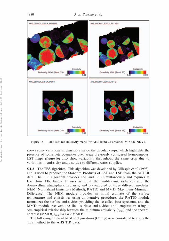
shows some variations in emissivity inside the circular crops, which highlights the

presence of some heterogeneities over areas previously considered homogeneous.

LST maps (figure 16) also show variability throughout the same crop due to

variations in emissivity and also due to different water supplies.

5.1.3 The TES algorithm. This algorithm was developed by Gillespie et al. (1998),

and is used to produce the Standard Products of LST and LSE from the ASTER

data. The TES algorithm provides LST and LSE simultaneously and requires at

least four TIR bands. It uses as input the land-leaving radiances and thedownwelling atmospheric radiance, and is composed of three different modules:

NEM (Normalized Emissivity Method), RATIO and MMD (Maximum–Minimum

Difference). The NEM module provides an initial estimate of the surface

temperature and emissivities using an iterative procedure, the RATIO module

normalizes the surface emissivities providing the so-called beta spectrum, and the

MMD module recovers the final surface emissivities and temperature using a

semiempirical relationship between the minimum emissivity (emin) and the spectral

contrast (MMD), emin5a + b6MMDc.

The following different band configurations (Config) were considered to apply the

TES method to the AHS TIR data:

Figure 15. Land surface emissivity maps for AHS band 75 obtained with the NDVI.



Config1 : AHS bands 75, 76, 77, 78, 79

Config2 : AHS bands 72, 73, 75, 76, 77, 78, 79

Config3 : AHS bands 71, 72, 73, 74, 75, 76, 77, 78, 79, 80

Config1 is not the optimal configuration as it uses five TIR bands, all of them

located in the region 10–12 mm. This is not the most appropriate region for

calculating realistic values of the spectral contrast MMD as variations in emissivity

for natural surfaces are typically low in the 10–12 mm region. However, this

configuration was considered because it was the one used by Sobrino et al. (2006).

Config2 is a priori the optimal configuration as it uses the seven optimal bands for

LST retrieval, as explained in section 3.3, including bands 72 and 73 located between

8 and 9 mm. Config3 makes use of the 10 AHS TIR bands, which is a priori better for

the calculation of the MMD, although bands 71, 74 and 80 are more affected by

atmospheric absorption.

The relationship between emin and MMD must be recalculated for each band

configuration. For this purpose, the 108 emissivity spectra used in the retrieval of

Figure 16. Land surface temperature maps obtained with the Split-Window algorithm usingAHS bands 75 and 79.



the TC coefficients (section 5.1.2) were used. The results of the statistical fitting are

the following:

Config1 : emin~1:001{0:655MMD0:715?r~0:958, s~0:006



where r is the correlation coefficient and s the standard error of estimation. As

expected, Config2 and Config3 provide the best results (highest r and lowest s).

The TES algorithm was applied to the AHS imagery using the three different

configurations, and the resulting LST values were tested against the 97 test points.

The results are presented in figure 17. Surprisingly, the three configurations provide

almost the same results, with correlations of 0.98 and bias near to 0, except for

Config3, with a bias of 0.25 K. An RMSE below 1.6 K was obtained in all three

cases. Differences between the three configurations were also computed for the

whole images. The results (not shown here) also showed small differences between

the configurations (RMSE values typically below 0.4 K), although some isolated

pixels showed significant differences (between 2 and 6 K). These similarities between

the results obtained with the three configurations can be explained by the low

spectral contrast and high emissivity values found over the agricultural areas. In

fact, all the plots considered in the test (water, corn, grass, bare soil and vineyard)

had MMD values lower than 0.03, except bare soil, with an MMD of 0.04, and

mean emissivity values ranging from 0.97 (bare soil) to 0.99 (corn). Therefore, the

emissivity effect is in some way minimized in the Barrax area.

Figure 17. Validation of the TES algorithm using different AHS bands configurationsagainst 97 in situ measurements (LST In-Situ) over different crops and for different dates.



Figures 18 and 19 show the LSE (band 75) and LST maps obtained with the TES

algorithm using Config2. A ‘noisy’ appearance of the emissivity maps in figure 18 is

apparent. It should be noted that TES algorithm is very sensitive to atmospheric

correction and noise of the sensor. There is also some controversy regarding the

threshold applied to the MMD to distinguish between low- and high-spectral

surfaces, set to 0.03 (see Gillespie et al. 1998). This condition seems to provoke

artefacts in the images (see, for example, the discussion presented in Jimenez-Munoz

et al. 2006, and Sobrino et al. 2007). A recent recommendation proposed removing

the threshold as well as the iterations in the TES algorithm (Gustafson et al. 2006).

According to the results presented in figure 19, the noise found in emissivity maps

does not appear in LST maps, at least by visual inspection. The LST maps are fairly

similar to those obtained with the TC algorithm (figure 16).

5.2 Daily evapotranspiration (ET)

ET refers to water lost from the soil surface (evaporation) and from crops (transpiration).

Knowledge of ET enables optimization of water use for irrigation, and estimation of ET

by solving the energy balance equation requires the availability of TIR data.

Figure 18. Land surface emissivity maps for AHS band 75 obtained with the TESalgorithm.



In this study, daily ET was retrieved according to the methodology presented in

Gomez et al. (2005) and Sobrino et al. (2005), which is based on the Simplified

Surface Energy Balance Index (S-SEBI) model (Roerink et al. 2000). The

Figure 19. Land surface temperature maps obtained with the TES algorithm.



instantaneous evapotranspiration (ETi) is given by:

LETi~Li Rni{Gið Þ ð9Þ

where L is the latent heat of vaporization (2.45 MJ kg21), L is the evaporative

fraction, Rn is the net radiation and G is the soil heat flux. The subscript ‘i’ refers to

‘instantaneous’ values and the subscript ‘d’ is used for ‘daily’ values. Then, daily ET

(ETd) can be obtained as:

ETd~LiCdiRni

Lð10Þ

where Cdi is the ratio between daily and instantaneous Rn, Cdi5Rnd/Rni (Seguin and

Itier 1983; Wassenaar et al. 2002), which is day and year dependent (Bastiaanssen et

al. 2000). This was estimated from measurements of net radiation registered in a

meteorological station located in the Barrax area. In the step from equation (9) to

equation (10), the assumption Li<Ld and Gd<0 was considered.

Instantaneous net radiation (Rni) is obtained from the balance between the

incoming and outgoing shortwave and longwave radiation:

Rni~ 1{asð ÞR;swzeR

;lw{esT4

S ð11Þ

where as is the surface albedo, RQsw and RQ

lw are, respectively, shortwave and

longwave incoming radiation (measured at meteorological stations), e and Ts are,

respectively, surface emissivity and temperature (estimated with any of the methods

presented in the previous section) and s is the Stefan–Boltzmann constant

(5.67061028 W m22 K24). The surface albedo was estimated from a weighted

mean of at-surface reflectivities (rsurface) estimated with AHS VNIR atmospherically

corrected bands:

as~X20

i~1

virsurfacei ð12Þ

where vi (i51–20) are the weight factors obtained from the solar irradiance

spectrum at the top of the atmosphere (see table 6). Finally, the evaporative fraction

is estimated as:

Li~TH{Ts

TH{TLETð13Þ

where TH and TLET are two characteristic temperatures obtained from the plot of

surface temperature versus surface albedo (Roerink et al. 2000).

The methodology was applied to the AHS imagery, and the daily ET values

extracted from the images were compared to those measured in situ in the lysimeter

station located in the green grass plot (festuca, L13). The results of the test are

shown in table 7, in which an RMSE of ,1 mm/day is obtained. The values

measured at the lysimeter station on 13 and 14 July were not available because of a

technical problem. Table 7 shows that ETd values for near consecutive flights are

almost the same, but ETd values along the same day are not constant, with

differences ranging between 1.3 and 1.9 mm/day. This indicates that some errors are

expected when a temporal integrated value of ET is obtained from instantaneous

values by means of the radio Cdi because daily ET refers to a unique value for a

certain day.



Figure 20 includes some illustrative daily ET maps for the images acquired on 1

June 2005. The ET values range between approximately 0 and 10 mm/day, with bare

soil and senescent vegetation providing the lowest values, and green vegetation

providing the highest ones, as expected. ET values for flights BDS and MDS (1123

and 1148 GMT, respectively) are higher than those for flights I1 and I2 (1211 and

1233 GMT, respectively), which also shows the unexpected variations in ETd along

the day, as noted earlier. The ET maps also show the irrigation patterns.

6. Summary and conclusions

Field campaigns, like the SEN2FLEX campaign, provide an excellent opportunity

for collecting different ground-based measurements and also for validating different

algorithms for the retrieval of biogeophysical parameters from remote sensing data

of interest in environmental studies.

In this paper we have focused on the analysis of thermal remote sensing data

acquired by the AHS sensor, with 10 thermal bands in the range 8–13 mm, which

allows the retrieval of LST, LSE and ET in combination with VNIR bands. A

vicarious calibration of the AHS TIR bands was previously considered, showing

errors below 1.5 K. Three methods for LST retrieval using different TIR bands

configurations were tested: SC (one band), TC (two bands) and TES (five, seven and

10 bands). In the SC method a constant emissivity was assumed (0.98), whereas in

the TC method surface emissivities were estimated from the NDVI approach. The

methods were validated against 97 test points, with RMSE values of 1.7, 1.8 and

1.6 K for the SC, TC and TES methods, respectively. Note that the accuracy on the

LST retrieval is limited by the error obtained in the vicarious calibration. The small

differences in the RMSE values do not allow us to conclude that one method is

Table 6. Weight factors (vi) used in the estimation of surface albedo according toequation (12).

AHS band lcentre (mm) SQ (W m22 mm21) vi

1 0.455 1923.1 0.0732 0.484 1886.8 0.0723 0.513 1829.1 0.0704 0.542 1774.3 0.0685 0.571 1740.5 0.0676 0.601 1689.2 0.0657 0.630 1602.5 0.0618 0.659 1510.0 0.0589 0.689 1403.9 0.05410 0.718 1324.1 0.05111 0.746 1240.6 0.04712 0.774 1152.4 0.04413 0.804 1089.5 0.04214 0.833 1014.9 0.03915 0.862 952.5 0.03616 0.891 894.5 0.03417 0.918 842.9 0.03218 0.948 806.4 0.03119 0.975 767.2 0.02920 1.004 726.0 0.028

SQ, solar irradiance at the top of the atmosphere.



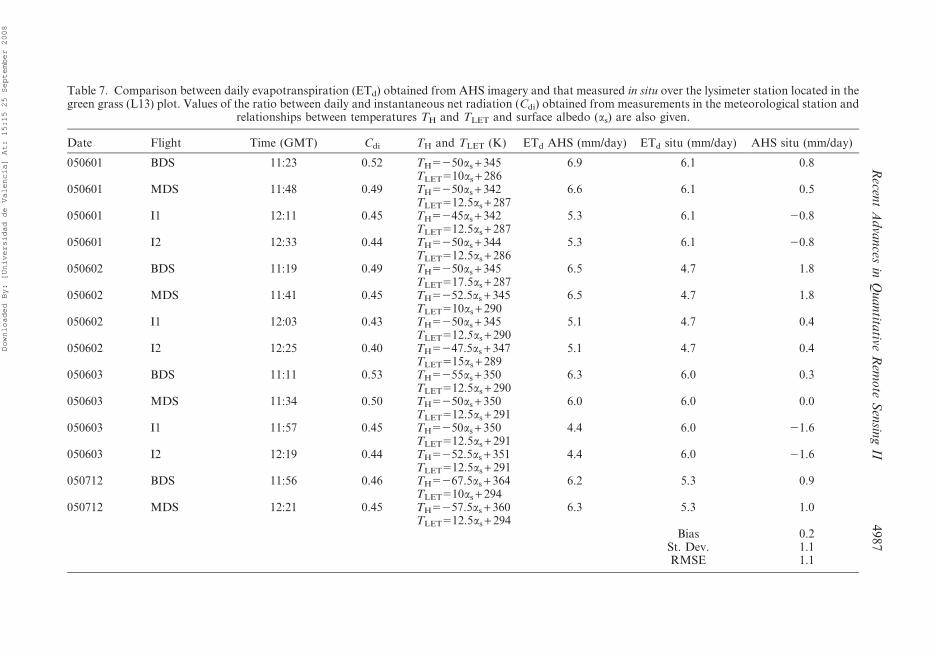
Table 7. Comparison between daily evapotranspiration (ETd) obtained from AHS imagery and that measured in situ over the lysimeter station located in thegreen grass (L13) plot. Values of the ratio between daily and instantaneous net radiation (Cdi) obtained from measurements in the meteorological station and

relationships between temperatures TH and TLET and surface albedo (as) are also given.

Date Flight Time (GMT) Cdi TH and TLET (K) ETd AHS (mm/day) ETd situ (mm/day) AHS situ (mm/day)

050601 BDS 11:23 0.52 TH5250as + 345 6.9 6.1 0.8TLET510as + 286

050601 MDS 11:48 0.49 TH5250as + 342 6.6 6.1 0.5TLET512.5as + 287

050601 I1 12:11 0.45 TH5245as + 342 5.3 6.1 20.8TLET512.5as + 287

050601 I2 12:33 0.44 TH5250as + 344 5.3 6.1 20.8TLET512.5as + 286

050602 BDS 11:19 0.49 TH5250as + 345 6.5 4.7 1.8TLET517.5as + 287

050602 MDS 11:41 0.45 TH5252.5as + 345 6.5 4.7 1.8TLET510as + 290

050602 I1 12:03 0.43 TH5250as + 345 5.1 4.7 0.4TLET512.5as + 290

050602 I2 12:25 0.40 TH5247.5as + 347 5.1 4.7 0.4TLET515as + 289

050603 BDS 11:11 0.53 TH5255as + 350 6.3 6.0 0.3TLET512.5as + 290

050603 MDS 11:34 0.50 TH5250as + 350 6.0 6.0 0.0TLET512.5as + 291

050603 I1 11:57 0.45 TH5250as + 350 4.4 6.0 21.6TLET512.5as + 291

050603 I2 12:19 0.44 TH5252.5as + 351 4.4 6.0 21.6TLET512.5as + 291

050712 BDS 11:56 0.46 TH5267.5as + 364 6.2 5.3 0.9TLET510as + 294

050712 MDS 12:21 0.45 TH5257.5as + 360 6.3 5.3 1.0TLET512.5as + 294

Bias 0.2St. Dev. 1.1RMSE 1.1

Recen

tA

dva

nces

inQ

ua

ntita

tiveR

emo

teS

ensin

gII

49

87


better than the other, which could lead to the conclusion that an improvement in

LST retrieval is not achieved when multispectral TIR data are used. However, some

observations should be emphasized to avoid inaccurate conclusions:

(1) SC methods provide good results only with a low atmospheric water vapour

content, as described by Sobrino and Jimenez-Munoz (2005). In this study,

and for the flight altitudes, water vapour values were less than 1 g/cm2, which

explains the good performance of the SC method. Furthermore, the

assumption of a constant value for emissivity is only acceptable over areaswith high emissivities and low value variations, as is the case in agricultural

areas such as the Barrax site (with emissivity values ranging between about

0.97 and 0.99).

(2) TC methods provide good results in global atmospheric conditions (except

for a very low atmospheric water vapour content, for which the SC method

can provide more accurate results, as indicated also by Sobrino and Jimenez-

Munoz, 2005). However, the main constraint is that prior knowledge of the

emissivity is required. If multispectral TIR data are not available, surfaceemissivities can be only estimated from VNIR bands, for example using a

simple approach with the NDVI. However, this method requires prior

Figure 20. Daily evapotranspiration maps.



knowledge of soil emissivity, and shows some problems over certain surfaces

such as water or senescent vegetation (which could be solved using ancillary

information).

(3) Although the TES algorithm is designed to work over all kinds of natural

surfaces, it is especially useful over areas with high spectral contrast. The

Barrax area has high emissivity values with low spectral contrast, so it is

more or less logical to expect similar results regardless of the number of TIR

bands used because the emissivity effect is not important over these kinds of

areas. The main constraint with the TES algorithm is that a precise

atmospheric correction is needed. However, if multispectral TIR data are

available, different atmospheric correction methods based on the image itself

could be applied, such as the Autonomous Atmospheric Compensation

(AAC; Gu et al. 2000) or In-Scene Atmospheric Compensation (ISAC)

(Young et al. 2002) algorithms.

The availability of TIR data also allows the estimation of heat fluxes and ET by

solving the energy balance equation. In this paper we have presented a simple

methodology for daily ET retrieval, in which instantaneous values are converted to

daily values using a time-dependent coefficient. The method was tested against

values measured in a lysimeter station located in the grass (festuca) plot. The results

are acceptable, with an RMSE of around 1 mm/day, but some variations in the daily

ET obtained with different images acquired during the same day were found.

With the results presented in this paper we hope to modestly contribute to the

scientific discussion regarding the usefulness of TIR data and their availability in

future sensors.

Acknowledgements

We thank to the European Union (EAGLE, project SST3-CT-2003-502057), the

Ministerio de Ciencia y Tecnologıa (DATASAT, project ESP2005-07724-C05-04),

the European Space Agency (SEN2FLEX, project RFQ 3-11291/05/I-EC) and the

Generalitat Valenciana (Conselleria d’Empresa, Universitat i Ciencia, project

ACOMP06/219) for financial support. We also thank the INTA team for pre-

processing the AHS imagery and for technical assistance.

ReferencesBALICK, L.K., JEFFERY, C.A. and HENDERSON, B.G., 2003, Turbulence-induced spatial

variation of surface temperature in high-resolution thermal IR satellite imagery.

Proceedings of SPIE, 4879, pp. 221–230.

BASTIAANSSEN, W.G.M., MOLDEN, D.J. and MAKIN, I.W., 2000, Remote sensing for irrigated

agriculture: examples from research and possible applications. Agricultural Water

Management, 46, pp. 137–155.

BERK, A., ANDERSON, G.P., ACHARYA, P.K., CHETWYND, J.H., BERNSTEIN, L.S.,

SHETTLE, E.P., MATTHEW, M.W. and ADLER-GOLDEN, S.M., 1999, MODTRAN4

User’s Manual (Hanscom AFB, MA: Air Force Research Laboratory).

CARLSON, T.N. and RIPLEY, D.A., 1997, On the relation between NDVI, fractional

vegetation cover, and leaf area index. Remote Sensing of Environment, 62, pp.

241–252.

GILLESPIE, A., ROKUGAWA, S., MATSUNAGA, T., COTHERN, J.S., HOOK, S. and KAHLE, A.B.,

1998, A temperature and emissivity separation algorithm for advanced spaceborne

thermal emission and reflection radiometer (ASTER) images. IEEE Transactions on

Geoscience and Remote Sensing, 36, pp. 1113–1126.



GOMEZ, M., SOBRINO, J.A., OLIOSO, A. and JACOB, F., 2005, Retrieval of evapotranspiration

over the Alpilles/ReSeDA experimental site using airborne POLDER sensor and

thermal camera. Remote Sensing of Environment, 96, pp. 399–408.

GU, D., GILLESPIE, A.R., KAHLE, A.B. and PALLUCONI, F.D., 2000, Autonomous

Atmospheric Compensation (AAC) of high resolution hyperspectral thermal infrared

remote-sensing imagery. IEEE Transactions on Geoscience and Remote Sensing, 38,

pp. 2557–2570.

GUANTER, L., RICHTER, R., ALONSO, L. and MORENO, J., 2005, Atmospheric correction

algorithm for remote sensing data over land. II. Application to ESA SPARC

campaigns: airborne sensors. In Proceedings of the SPARC, 4–5 July, Enschede, the

Netherlands (Noordwijk, The Netherlands: ESA Publications Division), WPP-250,

pp. 770–775.

GUSTAFSON, W.T., GILLESPIE, A.R. and YAMADA, G., 2006, Revisions to the ASTER

temperature/emissivity separation algorithm. In Recent Advances in Quantitative

Remote Sensing, J.A. Sobrino (Ed.), 25–29 September, Torrent (Valencia), Spain

(Spain: Publicacions de la Universitat de Valencia).

JIMENEZ-MUNOZ, J.C. and SOBRINO, J.A., 2006, Emissivity spectra obtained from field and

laboratory measurements using the temperature and emissivity separation algorithm.

Applied Optics, 45, pp. 7104–7109.

JIMENEZ-MUNOZ, J.C., SOBRINO, J.A., GILLESPIE, A., SABOL, D. and GUSTAFSON, W.T., 2006,

Improved land surface emissivities over agricultural areas using ASTER NDVI.

Remote Sensing of Environment, 103, pp. 474–487.

KERR, Y.H., LAGOUARDE, J.P., NERRY, F. and OTTLE, C., 2004, Land surface temperature

retrieval techniques and applications: case of the AVHRR. In Thermal Remote

Sensing in Land Surface Processes, D.A. Quattrochi and J.C. Luvall (Eds), pp. 33–109

(Boca Raton, FL: CRC Press).

MORENO, J., CASELLES, V., MARTINEZ-LOZANO, J.A., MELIA, J., SOBRINO, J.A., CALERA, A.,

MONTERO, F. and CISNEROS, J.M., 2001, The measurements programme at Barrax. In

DAISEX Final Results Workshop, 15–16 March (The Netherlands: ESTEC, ESA

Publications Division), SP-499, pp. 43–51.

QUATTROCHI, D.A. and LUVALL, J.C., 1999, Thermal infrared remote sensing data for

analysis of landscape ecological processes: methods and applications. Landscape

Ecology, 14, pp. 577–598.

ROERINK, G., SU, Z. and MENENTI, M., 2000, S-SEBI: a simple remote sensing algorithm to

estimate the surface energy balance. Physics and Chemistry of the Earth (B), 25, pp.

147–157.

SEGUIN, B. and ITIER, B., 1983, Using midday surface temperature to estimate daily

evaporation from satellite thermal IR data. International Journal of Remote Sensing,

4, pp. 371–383.

SOBRINO, J.A., GOMEZ, M., JIMENEZ-MUNOZ, J.C., OLIOSO, A. and CHEHBOUNI, G., 2005, A

simple algorithm to estimate evapotranspiration from DAIS data: application to the

DAISEX campaigns. Journal of Hydrology, 315, pp. 117–125.

SOBRINO, J.A. and JIMENEZ-MUNOZ, J.C., 2005, Land surface temperature retrieval

from thermal infrared data: an assessment in the context of the Surface

Processes and Ecosystem Changes Through Response Analysis (SPECTRA) mission.

Journal of Geophysical Research, 110, pp. D16103, doi: 10.1029/2004JD005588.

SOBRINO, J.A., JIMENEZ-MUNOZ, J.C., BALICK, L., GILLESPIE, A., SABOL, D. and

GUSTAFSON, W.T., 2007, Accuracy of ASTER level-2 thermal-infrared standard

products of an agricultural area in Spain. Remote Sensing of Environment, 106, pp.

146–153.

SOBRINO, J.A., JIMENEZ-MUNOZ, J.C., ZARCO-TEJADA, P.J., SEPULCRE-CANTO, G. and dE

MIGUEL, E., 2006, Land surface temperature derived from airborne

hyperspectral scanner thermal infrared data. Remote Sensing of Environment, 102,

pp. 99–115.



SOBRINO, J.A. and RAISSOUNI, N., 2000, Toward remote sensing methods for land cover

dynamic monitoring: application to Morocco. International Journal of Remote

Sensing, 21, pp. 353–366.

TOONOKA, H., PALLUCONI, F.D., HOOK, S.J. and MATSUNAGA, T., 2005, Vicarious calibration

of ASTER thermal infrared bands. IEEE Transactions on Geoscience and Remote

Sensing, 432, pp. 1113–1126.

WASSENAAR, T., OLIOSO, A., HASAGER, C., JACOB, F. and CHEHBOUNI, A., 2002, Estimation

of evapotranspiration on heterogeneous pixels. In Recent Advances in Quantitative

Remote Sensing, J.A. Sobrino (Ed.), Torrent (Valencia), Spain, 16–20 September

(Spain: Publicacions de la Universitat de Valencia), pp. 458–465.

YOUNG, S.J., JOHNSON, B.R. and HACKWELL, J.A., 2002, An in-scene method for atmospheric

compensation of thermal hyperspectral data. Journal of Geophysical Research, 107,

doi: 10.1029/2001JD001266.



Thermal remote sensing in the framework of the SEN2FLEX project: field measurements, airborne data...

Documents

Transcript of Thermal remote sensing in the framework of the SEN2FLEX project: field measurements, airborne data...