INTEGRATION OF MULTISOURCE REMOTE SENSING DATA FOR ...

Integration of multisource remote sensing data forimprovement of land cover classification

Author:Chu, Hai Tung

Publication Date:2013

DOI:https://doi.org/10.26190/unsworks/16056

License:https://creativecommons.org/licenses/by-nc-nd/3.0/au/Link to license to see what you are allowed to do with this resource.

Downloaded from http://hdl.handle.net/1959.4/52524 in https://unsworks.unsw.edu.au on 2022-06-01

http://dx.doi.org/https://doi.org/10.26190/unsworks/16056

https://creativecommons.org/licenses/by-nc-nd/3.0/au/

http://hdl.handle.net/1959.4/52524

https://unsworks.unsw.edu.au

https://unsworks.unsw.edu.au

INTEGRATION OF MULTISOURCE REMOTE

SENSING DATA FOR IMPROVEMENT OF

LAND COVER CLASSIFICATION

Hai Tung Chu

Supervised by A/Prof. Linlin Ge Co-supervised by Prof. Chris Rizos

A thesis submitted to the University of New South Wales for the degree of Doctor of Philosophy

School of Civil and Environmental Engineering (CVEN) Faculty of Engineering

The University of New South Wales Sydney, NSW 2052, Australia

March 2013

PLEASE TYPE

Surname or Family name: CHU

First name: HAl TUNG

THE UNIVERSITY OF NEW SOUTH WALES Thesis/Dissertation Sheet

Other name/s:

Abbreviat ion for degree as given in the Univers ity calendar: PhD

School: School of Surveying and Spatial Engineering Faculty: Engineering Faculty

Title: Integration of multisource remote sensing data for improvement of land cover classificat ion

Abstract 350 words maximum: (PLEASE TYPE)

The use of multisource remote sensing data for land cover classification has attracted the attention of researchers because the complementary

characteristics of different kinds of data can potential ly improve classificat ion results . However, using more input data does not necessarily

increase the classification performance. On the contrary, it increases data volumes, includ ing noise , redundant information and uncertainty with in

the dataset. Therefore it is essentia l to select relevant input features and combined datasets from the multisource data to achieve the best

classification accuracy. Other challeng ing tasks are the development of appropriate data process ing and classificat ion techniques to exploit the

advantages of multisource data. The goal of th is thesis is to improve the land cover classification process by using multisource remote sensing

data with recent advanced feature selection , data processing and classificat ion techniques.

The capabilit ies of non-parametric classifiers , such as Artificial Neural Network (ANN) and Support Vector Machine (SVM), were investigated using

various multisource datasets over different study areas in Vietnam and Austral ia. Resu lts showed that the non-parametric classifiers clea rly

outperformed the common ly used Maximum Likelihood algorithm.

The feature se lection techn ique based on Genetic Algorithm (GA) was proposed to search for appropriate combined datasets and classifier's

parameters . The integration of GA and SVM classifier was employed for classify ing multisource data in Western Australia . It was revealed that the

SVM-GA model gave significantly higher classification accuracy with less input data than the traditional method. The GA algorithm also performed

better than the conventional Sequential Forward Floating Search Algorithm.

To further increase the performance of multisource data classification the Multiple Classification System (MCS) was proposed and evaluated.

Moreover, the synergistic model us ing GA and the MCS was developed . An experiment was carried out with the MCS consisting of ANN , SVM and

Self-Organising Map (SOM) classifiers . Results confirmed that this newly hybrid model of GA and MCS outperformed other methods and

significantly improve the performance of both GA and MCS algorithm.

Resu lts and analysis presented in this thesis emphasise that using multisource remote sensing data is an appropriate approach for improvement

of land cover classification . The proposed methodologies are very efficient for handling combined multisource datasets.

Declaration relating to disposit ion of project thesis/dissertation

I hereby grant to the University of New South Wales or its agents the right to archive and to make available my thesis or dissertation in whole or in part in the University libraries in all forms of media , now or here after known, subject to the provisions of the Copyright Act 1968. I retain all property rights, such as patent rights . I also reta in the right to use in future works (such as articles or books) all or part of this thesis or dissertation .

I also authorise University Microfilms to use the 350 word abstract of my thes is in Dissertat ion Abstracts International (th is is applicable to doctoral theses only) .

Witness . .2~?3/~ ... .1.3>. .. ..

Date ... .. . ·~ ... .. ... .. .... . ..

The University recognises that there may be exceptional circumstances requ iring restrictions on copying or cond itions on use. Requests for restriction for a period of up to 2 years must be made in writing . Requests fo r a longer period of restriction may be considered in exceptiona l circumstances and re uire the a roval of the Dean of Graduate Research .

FOR OFFICE USE ONLY Date of completion of requ irements for Award:

THIS SHEET IS TO BE GLUED TO THE INSIDE FRONT COVER OF THE THESIS

ORIGINALITY STATEMENT

'I hereby declare that this submission is my own work and to the best of my knowledge it contains no materials previously published or written by another person, or substantial proportions of material which have been accepted for the award of any other degree or diploma at UNSW or any other educational institution, except where due acknowledgement is made in the thesis. Any contribution made to the research by others, with whom I have worked at UNSW or elsewhere, is explicitly acknowledged in the thesis. I also declare that the intellectual content of this thesis is the product of my own work, except to the extent that assistance from others in the project's design and conception or in style, presentation and linguistic expression is acknowledged.'

Signed

Date ........................ u;~ ... /.~ ..... ...t>...

COPYRIGHT STATEMENT

'I hereby grant the University of New South Wales or its agents the right to archive and to make available my thesis or dissertation in whole or part in the University libraries in all forms of media, now or here after known, subject to the provisions of the Copyright Act 1968. I retain all proprietary rights, such as patent rights. I also retain the right to use in future works (such as articles or books) all or part of this thesis or dissertation. I also authorise University Microfilms to use the 350 word abstract of my thesis in Dissertation Abstract International (this is applicable to doctoral theses only). I have either used no substantial portions of copyright material in my thesis or I have obtained permission to use copyright material; where permission has not been granted I have applied/will apply for a partial restriction of the digital copy of my thesis or dissertation.'

Signed

Date .. ... ........ ....... .. li/Q.)/ ..... MJ.J;) ....... .

AUTHENTICITY STATEMENT

'I certify that the Library deposit digital copy is a direct equivalent of the final officially approved version of my thesis. No emendation of content has occurred and if there are any minor variations in formatting, they are the result of the conversion to digital format.'

Signed

Date ....................... 2(/D>./. Q!j ...

i

ABSTRACT

The use of multisource remote sensing data for land cover classification has attracted the

attention of researchers because the complementary characteristics of different kinds of data

can potentially improve classification results. Such a multisource approach becomes

increasingly important with the ready availability of a variety of satellite imagery. However,

using more input data does not necessarily increase the classification performance. On the

contrary, using too many remotely sensed input datasets increases data volumes, including

noise, redundant information and uncertainty within the dataset. Therefore it is essential to

select relevant input features and combined datasets from the multisource data to achieve the

best classification accuracy. Other challenging tasks are the development of appropriate data

processing and classification techniques to efficiently exploit the advantages of multisource

data. The goal of this thesis is to improve the land cover classification process by using

multisource remote sensing data with recent advanced input feature selection, data processing

and classification techniques.

The capabilities of non-parametric classifiers, such as the Artificial Neural Network (ANN)

and Support Vector Machine (SVM), were investigated using various multisource datasets

over different study areas in Vietnam and Australia. Results showed that the multisource

datasets always gave higher classification accuracy than the single-type datasets. The non-

parametric classifiers clearly outperformed the commonly used Maximum Likelihood

algorithm.

The feature selection (FS) technique, specifically the wrapper approach, based on Genetic

Algorithm (GA) was proposed to search for the appropriate combined datasets and

classifier’s parameters. The integration of GA and SVM classifier was employed for

classifying multisource data in Western Australia, including multi-date, multi-polarised SAR

and optical images. It was revealed that the SVM-GA model gave significantly higher

classification accuracy with less input data than the traditional method. The GA algorithm

also performed better than the conventional Sequential Forward Floating Search algorithm.

The Multiple Classifier Systems (MCS) or classifier ensemble technique, which can

potentially improve classification performance by exploiting the strengths and alleviating the

ii

weaknesses of different classifiers, was also evaluated using different algorithms and

combination rules. An experiment was carried out with the MCS technique using the ANN,

SVM and Self-Organising Map (SOM) classifiers over a study area in New South Wales,

Australia. The investigation shows that the MCS technique, in general, provided higher

classification accuracy than individual classifiers.

Finally, a synergistic model using the FS based on GA and MCS techniques was developed to

further increase the performance of multisource data classification. Results confirmed that the

hybrid model of FS-GA and MCS outperformed other methods and significantly improved on

the performance of both the FS-GA and MCS algorithm.

Results and analyses presented in this thesis emphasise that using multisource remote sensing

data is an appropriate approach for improvement of land cover classification. The proposed

methodologies are very efficient for handling high dimensional, complex datasets such as

combined multisource data.

iii

ACKNOWLEDGEMENT

First of all I would like to thank Vietnamese Ministry of Education and Training (MOET) for

granting me a scholarship without which I would not be able to carry out this research. I

would like also to thank the National Centre for Remote Sensing, the Ministry of

Environment and Natural Resources (MONRE) of Vietnam for giving me an opportunity to

attend the PhD program and providing relevant image data for my study.

I would like to thank for my supervisor A. Prof. Linlin Ge for his valuable support and advice

during my research. I would also like to express my gratitude to my co-supervisor, Prof.

Chris Rizos for his guidance, and patiently correcting my writing.

I would like to show my thanks to the University of New South Wales and the School of

Surveying and Geospatial Engineering for allowing me to study there. I am also grateful to

our GEOS team members, including Dr. Jean Li, Dr. Mahmood Salah, Dr. Kui Zhang, Dr.

Alex Ng and Mr. Alex Hu for their enthusiasm and support.

I thank my friend Mr. Lawrence Greaves for his enthusiasm in helping me correct my

writing.

I wish to thank the European Space Agency (ESA) and Japan Aerospace Exploration Agency

(JAXA) for providing ENVISAT/ASAR and ALOS/PALSAR data that have been used in

this study. I would like also to thank for United State Geological Survey/Earth Resources

Observation and Science Center (USGS/EROS) for providing Landsat 5 TM data.

Last but not least, my special thanks go to my parents, my wife and daughters for their love,

constant support and understanding during the long journey of my study.

iv

LIST OF PUBLICATIONS

Journal papers

1. Chu, H. T., Ge, L., Ng, A. H-M., and Rizos, C., 2012. Application of Genetic

Algorithm and Support Vector Machine in Classification of Multisource Remote

Sensing Data. International Journal of Remote Sensing Application, Vol. 2, No. 3, pp.

1- 11.

2. Chu, H. T., and Ge, L., (in preparation). Integration of Feature Selection and Multiple

Classifier System for improvement of land cover classification using multisource

remote sensing data. International Journal of Applied Remote Sensing.

Conference papers

1. Chu, H. T., and Ge, L., 2010, Synergistic use of multi-temporal ALOS/PALSAR with

SPOT multispectral satellite imagery for Land cover Mapping in The Ho Chi Minh

City area, Vietnam. International Geoscience and Remote Sensing Symposium

(IGARSS), Honoluulu, HI, 25-30 July.

2. Chu, H.T., Li, X., Ge, L., & Zhang, K., 2010. Monitoring the 2009 Victorian

bushfires with multi-temporal and coherence ALOS PALSAR images. 15th

Australasian Remote Sensing & Photogrammetry Conf., Alice Springs, Australia, 13-

17 September, 313-325 (http://www.15.arspc.com/proceedings).

3. Chu, H.T., & Ge, L., 2010. Land cover classification using combinations of L- and C-

band SAR and optical satellite images. 31st Asian Conf. on Remote Sensing, Hanoi,

Vietnam, 1-5 November, paper TS39-2, CD-ROM procs.

4. Chu, H.T., Ge, L., & Wang, X., 2011. Using dual-polarized L-band SAR and optical

satellite imagery for land cover classification in Southern Vietnam: Comparison and

combination. Proc. published 2011 in Australian Space Science Conference Series,

ed. W. Short & I. Cairns, 10th Australian Space Science Conf., Brisbane, Australia,

27-30 September 2010, 161-173. (Refereed paper)

http://www.15.arspc.com/proceedings�

http://www.15.arspc.com/proceedings

v

5. Chu, H.T., & Ge, L., 2011. Improvement of land cover classification performance in

Western Australia using multisource remote sensing data. 7th Int. Symp. on Digital

Earth, Perth, Australia, 23-25 August.

6. Chu, H.T., & Ge, L., 2012. Combination of genetic algorithm & Dempster-Shafer

theory of evidence for land cover classification using integration of SAR & optical

satellite imagery. XXII Int. Society for Photogrammetry & Remote Sensing Congress,

Melbourne, Australia, 25 Aug - 1 September.

7. Chu, H.T., Ge, L., & Cholathat, R., 2012. Evaluation of multiple classifier

combination techniques for land cover classification using multisource remote sensing

data. 33rd Asian Conference on Remote Sensing (ACRS2012), Pattaya, Thailand, 26-

30 November, paper F5-1, CD-ROM procs.

vi

ACRONYMS AND ABBREVIATIONS

ALOS Advanced Land Observing Satellite

ANN Artificial Neural Network

ASAR Advanced Synthetic Aperture Radar

BP Back Propagation

CCRS/CCT Canada Centre for Remote Sensing/Centre Canadien de teledetection

DEM Digital Elevation Model

ENVISAT Environmental Satellite

ERS European Remote Sensing Satellite

ERS- ½ 1 /2 European Remote-Sensing Satellites

ESA European Space Agency

ETM+ Enhanced Thematic Mapper Plus

FS Feature Selection

GA Genetic Algorithm

GLCM Grey Level Co-occurrence Matrix

HH Horizontal transmit and horizontal receive

HV Horizontal transmit and vertical receive

JERS-1 Japanese Earth Resources Satellite-1

JAXA Japan Aerospace Exploration Agency

LiDAR Light Detection and Ranging

MLP Multilayer Perceptron

MODIS Moderate Resolution Imaging Spectroradiometer

NDVI Normalized Difference Vegetation Index

PALSAR Phased Array type L-band Synthetic Aperture Radar

P (Pan) Panchromatic

PCA Principle Component Analysis

RADAR Radio Detection And Ranging

SAR Synthetic Aperture Radar

SFS/SBS Sequential Forward Search/Sequential Backward Search

SFFS/SBFS Sequential Floating Forward/Backward Search

SIR-L/C/X Shuttle Imaging Radar-L/C/X

vii

SOM Self-organizing Map

SPOT Systeme Probatoire d’Observation de la Terre

SVM Support Vector Machine

TM Thematic Mapper

VH Vertical transmit and horizontal receive

VV Vertical transmit and vertical receive

XS Multispectral

viii

CONTENTS ABSTRACT i

ACKNOWLEDGEMENT iii

LIST OF PUBLICATIONS iv

ACRONYMS AND ABBREVIATIONS vi

CONTENTS viii

LIST OF TABLES xiii

LIST OF FIGURES ix

CHAPTER 1: INTRODUCTION 1

1.1. Problem statement 1

1.2. Objectives 3

1.3. Main contributions 4

1.4. Thesis outline 4

CHAPTER 2: BACKGROUND AND LITERATURE REVIEW 6

2.1. Image classification methods 6

2.1.1. Traditional supervised classification and Maximum likelihood

algorithm

7

2.1.2. Unsupervised classification 8

2.1.3. Non-parametric classification 9

2.2. Data pre-processing 20

2.2.1. Geometric correction 20

2.2.2. Radiometric calibration 22

2.2.3. Speckle noise filtering 24

2.3. Advantages of multisource remote sensing data, selection and integration

issues

26

2.3.1. Advantages of the combined approach 26

2.3.2. Selection and integration of remote sensing data and feature

parameters

37

2.4. Related work on land cover classification using multisource remote sensing

data

42

2.5. Summary 49

ix

CHAPTER 3: EVALUATION OF LAND COVER CLASSIFICATION USING NON-PARAMETRIC CLASSIFIERS AND MULTISOUCE REMOTE SENSING DATA 52

3.1. Application of multi-temporal/polarized SAR and optical imagery for land

cover classification 52

3.1.1. Study area and data used 53

3.1.2. Methodology 54

3.1.3. Results and discussion 58

3.1.4. Summary remarks 72

3.2. Combination of L- and C-band SAR and optical satellite images for land

cover classification in the rice production area 73





3.3. Use of multi-temporal SAR and interferometric coherence data for

monitoring the 2009 Victorian bushfires 86

3.3.1. Introduction 86





3.4. Concluding remarks 98

CHAPTER 4: APPLICATION OF FEATURE SELECTION TECHNIQUES FOR MULTISOURCE REMOTE SENSING DATA CLASSIFICATION 99

4.1. Significance of data reduction and feature selection for classification of

remote sensing data 99

4.2. Feature selection techniques used for classification of remote sensing data 101

4.3. Application of genetic algorithm and support vector machine in classification

of multisource remote sensing 108




x


4.3.5. Conclusions 123

CHAPTER 5: APPLICATION OF MULTIPLE CLASSIFIER SYSTEM FOR CLASSIFYING MULTISOURCE REMOTE SENSING DATA 125

5.1. MCS in remote sensing 125

5.1.1. Creation of MCS or classifier ensemble 126

5.1.2. Combination rules 127

5.2. Use of MCS and a combination of GA and MCS for classifying multisource

remote sensing data – a case study in Appin, NSW, Australia. 130


5.2.2. Study area and used data 133



5.2.5. Conclusions 151

CHAPTER 6: CONCLUSIONS 152

6.1. Summary and conclusions 152

6.2. Main findings 155

6.3. Future work 155

REFERENCES 157

xi

LIST OF FIGURES

Figure 2.1: Spectral classes represented by normal probability distribution ............................. 8

Figure 2.2: Artificial Neural Network classifier ...................................................................... 11

Figure 2.3: Example of linear support vector machine ............................................................ 14

Figure 2.4: SVMs projecting the training data to higher dimensional space. .......................... 16

Figure 2.5: Effect of platform/sensor position and orientation on geometry of image ........... 21

Figure 2.6: Relief displacement in optical and radar satellite image ....................................... 22

Figure 2.7: Spectral signatures of soil, vegetation and water in visible/infrared region of

spectrum ................................................................................................................................... 27

Figure 2.8: Microwave bands used in SAR systems ............................................................... 28

Figure 2.9: Penetration of SAR signals at different wavelengths or frequencies .................... 31

Figure 2.10: Radar transmission in vertical and horizontal polarisation ................................. 32

Figure 2.11: Surface scattering and volume scattering ............................................................ 33

Figure 3.1: Location of the study area ..................................................................................... 53

Figure 3.2: Land cover feature characteristics in SPOT 2 multi-spectral and ALOS/PALSAR

multi-temporal images ............................................................................................................. 56

Figure 3.3: Part of classification results using SVM and ANN classifiers on multi--date,

single-polarised (HH or HV), and multi-date, dual-polarised HH+HV images; ..................... 63

Figure 3.4: Part of the classification results using SVM and ANN classifiers on a SPOT 2 XS

image and the combination of SPOT 2 XS and multi-date ALOS/PALSAR HH polarised

images. ..................................................................................................................................... 65

Figure 3.5: Part of classification results using SVM and ANN classifiers on a SPOT 2 XS

image and combination of SPOT 2 XS and multi-date PALSAR HH, HV polarised datasets.

................................................................................................................................................. 68

Figure 3.6: Comparison of classification accuracy of SVM, ANN and ML classifiers .......... 71

Figure 3.7: Comparison of Kappa coefficients generated by SVM, ANN and ML classifiers 71

Figure 3.8: SPOT 4 multispectral false colour image (left) and ALOS/PALSAR HH

polarisation image (right), both images acquired on December 09, 2007 ............................... 75

Figure 3.9: Spectral properties of different land cover classes in the SPOT 4 XS image ....... 77

Figure 3.10: Backscatter properties of different land cover classes in the multi-date L- and C-

band SAR images .................................................................................................................... 77

xii

Figure 3.11: SVM Classification using four-date PALSAR images (left) and the combination

of four-date ASAR and four-date PALSAR images (right) .................................................... 80

Figure 3.12: ANN Classification using four-date PALSAR images (left) and the combination

of four-date ASAR and four-date PALSAR images (right) .................................................... 81

Figure 3.13: ANN classification using the SPOT 4 multi-spectral image (left) and

combination of SPOT 4 and four-date PALSAR images (right) ............................................. 82

Figure 3.14: SVM classification using the SPOT 4 multi-spectral image (left) and

combination of SPOT 4 and four-date PALSAR images (right) ............................................. 82

Figure 3.15: Comparison of classification accuracy of SVM, ANN and ML classifiers after

merging rice classes (only combined datasets with at least two input features are presented) 85

Figure 3.16: A) and C) showed fire affected areas are in purple to pink colour in multi-date

colour composites in 1st and 2nd study sites. B) and D) showed burnt area (dark colour) in

corresponding false colour Landsat TM images. ..................................................................... 91

Figure 3.17: A) and C) are RGB colour composites of Average SAR image (R), Temporal

Backscatter Change (G) and across-fire coherence data (B) in 1st and 2nd study sites. Burnt

areas appear Yellow to Reddish in colour in A) and C) RGB composites. ............................. 93

Figure 3.18: Backscatter values for burnt and unburnt classes over the first test site ............. 94

Figure 3.19: Coherence values for burnt and unburnt classes over the first test site .............. 94

Figure 3.20: Backscatter values for burnt and unburnt classes over the second test site ........ 95

Figure 3.21: Coherence values for burnt and unburnt classes over the second test site .......... 95

Figure 3.22: A) Burnt scars extraction from Landsat TM images, B) Burnt scars extraction

based on SVM classification (case 3), the Red areas represent burnt scars ............................ 97

Figure 4.1: An example of the Hughes phenomenon with increasing of input data

dimensionality........................................................................................................................ 100

Figure 4.2: Feature selection with filter (left) and wrapper (right) approach ........................ 104

Figure 4.3: Illustration of the crossover and mutation operators ........................................... 105

Figure 4.4: Landsat 5 TM (left) and ALOS/PALSAR HH (right) over the study area acquired

on 07/10 and 20/10/2010, respectively .................................................................................. 105

Figure 4.5: The binary coding of the chromosome ................................................................ 113

Figure 4.6: Major steps of feature selection using the Genetic Algorithm…………………114

Figure 4.7: Land cover feature characteristics in Landsat 5 TM (left) and multi-date PALSAR

(right) images ………………………………………………………………………………115

Figure 4.8: Improvement of accuracy by incorporating textural information with original

datasets using stack-vector and FS-GA approach. ………………………………………...119

xiii

Figure 4.9: Classification of the Landsat 5 TM image (left) and the integration of Landsat 5

TM and four-date PALSAR HH/HV images (right) using the GA technique……………..120

Figure 4.10: Classification accuracy using FS (SFFS and GA) compared to Non-FS (stack-

vector) approaches…………………………………………………………………………..122

Figure 4.11: Number of input features for the Non-FS (stack-vector) and FS (SFFS and GA)

approaches…………………………………………………………………………………..122

Figure 4.12: Impact of the proposed fitness function on overall classification accuracy

compared to the commonly used fitness function………………………………………….123

Figure 5.1: ENVISAT/ASAR VV polarised image acquired on 25/09/2010 ....................... 132

Figure 5.2: ALOS/PALSAR HH polarised image acquired on 07/10/2010 ......................... 132

Figure 5.3: Landsat 5 TM images (false colour) acquired on 10/09/2010 ............................ 133

Figure 5.4: Example of the SOM architecture with three input neurons and 25 (5x5) output

neurons……………………………………………………………………………………...136

Figure 5.5: The integration of feature selection based on GA and MCS techniques for

classifying multisource data………………………………………………………………...140

Figure 5.6: Results of classification of the 4th dataset using FS-GA with SVM classifier…143

Figure 5.7: Improvements of accuracy by applying the FA-GA approach for the SVM, ANN

and SOM classifiers…………………………………………………………………………143

Figure 5.8: Comparison of SVM classification with SVM-Bagging and SVM-Adaboost.M1

methods……………………………………………………………………………………..146

Figure 5.9: Comparison of ANN classification with ANN-Bagging and ANN-Adaboost.M1

methods……………………………………………………………………………………..146

Figure 5.10: Comparison of SOM classification with SOM-Bagging and ANN-Adaboost.M1

methods……………………………………………………………………………………..146

Figure 5.11: Comparison between the best classification results obtained by original

classifiers, MCS based and FS-GA approaches…………………………………………….148

Figure 5.12: Comparison between the BIC, FS-GA, the best results MCS, the best (FS-GA-

MCS1) and the poorest (FS-GA-MCS2) results of FS-GA-MCS methods for different

datasets……………………………………………………………………………………...149

Figure 5.13: Improvements of overall classification accuracy achieved by using FS-GA, MCS

and FS-GA-MCS approaches……………………………………………………………….150

xiv

LIST OF TABLES

Table 2.1: Specification of some optical satellite imagery…………………………………..40

Table 2.2: Specification of different SAR satellite imagery…………………………………41

Table 3.1: ALOS/PALSAR images for the study area………………………………………53

Table 3.2: Average values of Transformed Divergence (TD) and Jefferies-Matusita

separability indices of different combined datasets…………………………………………59

Table 3.3: Land cover classification accuracy of different SAR combination datasets….....61

Table 3.4. Producer and user accuracy (%) for the SVM classifier applied to five-date

PALSAR HH, HV, and five-date PALSAR dual-polarised (HH+HV) images…………......62

Table 3.5. Producer and user accuracy (%) for the ANN classifier applied to five-date

PALSAR HH, HV, and five-date PALSAR dual-polarised (HH+HV) images……………..62

Table 3.6: Land cover classification accuracy of different combinations of SPOT 2 XS and

PALSAR polarised images…………………………………………………………………..64

Table 3.7: Producer and user accuracy for ANN and SVM classifier applied to SPOT 2 XS

multispectral images…………………………………………………………………………66

Table 3.8: Producer and user accuracy for ANN and SVM classifier applied to combination

of SPOT 2 XS multi-spectral and five-date PALSAR HH polarised images……………….66

Table 3.9: Comparison of land cover classification with multi-date SAR images including

like-, cross- and dual-polarised data and combination of these images with their best textural

features………………………………………………………………………………………69

Table 3.10: ALOS/PALSAR and ENVISAT/ASAR images for the study area…………….74

Table 3.11: Overall classification accuracies (%) for different datasets…………………....78

Table 3.12: Confusion matrix for SVM classification using four-date ENVISAT/ASAR HH

polarised image………….…………………………………………………………………...79

Table 3.13: Confusion matrix for ANN classification using four-date ENVISAT/ASAR HH

polarised image………………………………………………………………………………79

Table 3.14: Confusion matrix for SVM classification using four-date ALOS/PALSAR HH

polarised images……………………………………………………………………………..79

Table 3.15: Confusion matrix for ANN classification using four-date ALOS/PALSAR HH

polarised images……………………………………………………………………………..80

xv

Table 3.16: Confusion matrix for SVM classification using four-date ALOS/PALSAR HH &

four-date ENVISAT/ASAR polarised images……………………………………………….81

Table 3.17: Confusion matrix for ANN classification using four-date ALOS/PALSAR HH &

four-date ENVISAT/ASAR polarised images……………………………………………….81

Table 3.18: Confusion matrix for ANN classification using SPOT 4 XS images…………...83

Table 3.19: Confusion matrix for SVM classification using SPOT 4 XS images…………...83

Table 3.20: Confusion matrix for ANN classification using SPOT 4 XS images and four-date

ALOS/PALSAR polarised images…………………………………………………………...83

Table 3.21: Confusion matrix for SVM classification using SPOT 4 XS images and four-date

ALOS/PALSAR polarised images…………………………………………………………...83

Table 3.22: ALOS/PALSAR images for the 1st study area…………………………………..88

Table 3.23: Interferometric pairs over 1st study area…………………………………………88

Table 3.24: ALOS/PALSAR images for the 2nd study area………………………………….88

Table 3.25: Interferometric pairs over 2nd study area……………………………………...…89

Table.3.26: Overall classification accuracy assessment for various combined datasets and

classifiers over the second test site…………………………………………………………...96

Table 4.1: ALOS/PALSAR images of the Western Australia study area…………………..109

Table 4.2: Contents of training and testing datasets………………………………………..116

Table 4.3: Classification accuracy of different datasets using SVM classifiers with the

traditional stack-vector approach…………………………………………………………...117

Table 4.4: Producer and user accuracy (%) of four-date PALSAR HH, HV and dual-polarised

images………………………………………………………………………………………117

Table 4.5: Comparison of land cover classification performance between SVM-GA, SVM-

SFFS and stack-vector approach; nf = number of selected features………………………..121

Table 5.1: ENVISAT/ASAR and ALOS/PALSAR images for the study area……………..131

Table 5.2: Combined datasets for land cover classification in the study area………………134

Table 5.3: Contents of training and testing datasets………………………………………...140

Table 5.4: The classification performance of SVM, ANN and SOM algorithms

on different combined multisource datasets………………………………………………...141

Table 5.5: Comparison of classification performance between FS-GA approach and

the Non-FS pproach………………………………………………………………………...142

Table 5.6: Results of classification using single SVM classifier, bagging and Adaboost.M1

techniques based on SVM classifier for different combined datasets………………………145

Table 5.7: Results of classification using single ANN classifier, bagging and

xvi

Adaboost.M1 techniques based on ANN classifier for different combined datasets……….145

Table 5.8: Results of classification using single SOM classifier, bagging and

Adaboost.M1 techniques based on SOM classifier for different combined datasets………145

Table 5.9: Comparison between the best classification results obtained by individual

classifiers and MCS based on the decision rules of Majority Voting, Sum and Dempster-

Shafer theory………………………………………………………………………………..147

Table 5.10: Comparison of best classification results using single classifier (Non-FS), FS-GA

and FS-GA-MCS classifier combination approaches………………………………………148

Table 5.11: Classification accuracies by applying MV, Sum and DS algorithm for

combination of FS-GA and MCS approaches……………………………………………...150

1

CHAPTER 1

INTRODUCTION

1.1. PROBLEM STATEMENT

Land cover information plays an important role in sustainable management, development and

exploitation of natural resources, environmental protection, planning, scientific analysis,

modelling and monitoring. These data become even more essential when there are rapid

changes on the Earth’s surface due to dynamic human activities as well as natural factors.

Remotely sensed data, in particular satellite images, with distinct advantages such as large

ground coverage, synoptic view, repetitive capabilities, multiple spectral bands or multiple

frequency/polarisation are one of the most effective tools for land cover mapping and have

been applied extensively for land cover monitoring and classification.

Satellite imagery can be acquired in various regions of the electromagnetic spectrum, from

the visible-near infrared (optical) to the microwave (radar) parts of the spectrum.

Consequently, different kinds of satellite imagery detect different characteristics of ground

surfaces. For instance, the optical images from missions such as Landsat, SPOT, MODIS,

IKONOS or Quick Bird provide information essentially on the reflectivity and absorption

capability of land cover features, since the imaging sensors are sensitive to the visible to near-

infrared regions of the spectrum. On the other hand, Synthetic Aperture Radar (SAR)

imagery, provided by missions such as RADARSAT, ENVISAT/ASAR, ALOS/PALSAR or

TerraSAR-X sensitive to the microwave region of the spectrum, contain information on

surface roughness, dielectric content and the structures of the illuminated ground or

vegetation. Thus integration of different types of satellite images could provide

complementary information and consequently improve the land cover classification results.

This approach has been fuelled by the large variety of remote sensing sensors which are now

2

more readily available than at any time in the past. Furthermore, derived information from

original remote sensing data, such as textural information, ratios, indices, coherence data,

Digital Elevation Model (DEM), or from other ancillary data sources can also contribute to

an increase in classification accuracies (Lu and Weng 2007, Tso and Mather 2009).

However, the increase in the amount of input data does not necessarily mean an increase in

classification performance. In addition, such an approach will create a large data volume with

more noisy and redundant data, which may reduce the classification accuracy (Lu and Weng

2007). Waske and Benediktsson (2007) suggested that data sources may not be at the same

level of reliability, where one source is more appropriate for one specific feature and another

source is more applicable to mapping another feature.

Therefore, the challenging tasks are to understand the contribution of each dataset, to select

the most useful input features and to determine the combined datasets which can maximise

the benefits of multisource remote sensing data and give the highest classification accuracy

(Peddle and Ferguson 2002). However, limited research has explored ways to determine

variables from multisource data in order to increase the classification accuracy (Lu and Weng

2007, Li et al. 2011). The Feature Selection (FS) techniques, which have been used

effectively in many applications including classification of remote sensing images (mainly

multispectral and hyperspectral data) but have not been well studied for classifying

multisource remote sensing data, could be useful for addressing this problem.

The classification algorithms are vital for classification. Appropriate selection of

classification algorithms can result in a substantial improvement in the quality of the

classification results. The traditional classification algorithms such as Minimum Distance,

Maximum Likelihood classifiers have been used widely to classify remote sensing images.

These classifiers can produce relatively good classification results in a comparatively short

time. However, the major limitation of these classifiers is their reliance on statistical

assumptions which may not sufficiently model remote sensing data. Furthermore, it is

difficult for statistical-based classifiers to incorporate different kinds of data for

classification. Recently, non-parametric classification techniques, based on machine learning

theory, have been developed. Unlike conventional classifiers, the new classification

algorithms, such as Artificial Neural Network (ANN), Support Vector Machine (SVM) or

Self Organising Map (SOM), do not rely on statistical principles and therefore can handle a

3

complex dataset more effectively (Pal and Mather 2005, Waske and Benedikson 2007).

Because of these properties, non-parametric classifiers are considered as important

alternatives to traditional methods, and the application of non-parametric classifiers to

classify remotely sensed data has become an attractive subject for research.

The classification performance could be enhanced further by applying a multiple classifier

systems (MCS) since it may take advantages of, and compensate weaknesses of, different

classifiers. Despite the robustness of such techniques, few studies have been conducted on the

application of these techniques for classifying combinations of different remote sensing

datasets.

Another strategy which has the potential to improve classification of multisource data is

integration of the MCS techniques with FS, particular the wrapper approach couple with the

Genetic Algorithm (GA). This strategy has not been considered by other researchers, and

therefore is in need of investigation.

1.2. OBJECTIVES

The objectives of this research were to improve the performance of land cover classification

using multisource remote sensing data with different advanced data processing, classification

techniques (including non-parametric classifiers), feature selection, multiple classifier

systems and their integration. The thesis objectives were:

To evaluate the capabilities of various non-parametric classification algorithms such

as ANN, SVM or SOM in classification of different combinations of multisource data,

including multi temporal/polarisation/frequency, coherence (for SAR), multispectral

data (for optical), transformed images, and textured measures; and to analyse the

impacts of these kinds of data and their contributions to final classification results.

To propose and evaluate the combination of FS techniques with the wrapper approach

and non-parametric classifiers for optimising datasets and classifier’s parameters in

land cover classification using multisource remote sensing data.

To evaluate the capabilities of the MCS using various algorithm and decision

approaches for classifying multisource data.

4

To propose and develop models for integration of FS wrapper techniques with MCS

for improvement in the classification performance of multisource remote sensing data.

1.3. MAIN CONTRIBUTIONS

The contributions of this research are:

1. Demonstration of the significance and usefulness of multisource remote sensing data

for land cover classification.

2. Demonstration of the strength and suitability of non-parametric classifiers for

classifying multisource data. These algorithms are capable of high classification

accuracy and often outperformed the traditional parametric classifiers.

3. Resolution of the problems of finding optimal combined datasets and classifier

parameters in the classification of high-dimensional multisource data by introducing

the feature selection technique based on the GA. This is a very effective method

which can increase classification accuracy while using fewer input features.

4. Analysis and comparisons of various MCS algorithms, including boosting and

bagging, majority voting, Bayesian sum and evidence reasoning, for improving the

classifications of complex multisource datasets.

5. Development of an effective method and model for combining the FS wrapper based

on GA and the MCS technique for further improvement of land cover classification

using multisource data. This new approach is capable to incorporate advantages of

both FS based on GA and MCS techniques for increasing classification accuracy.

1.4. THESIS OUTLINE

The problem statement, research objectives, contributions and thesis outline are given in

Chapter 1.

Chapter 2 reviews the principles of digital image classification techniques, potential

advantages of multisource remote sensing data, including multi-temporal/polarised/frequency

SAR data and optical images, their derivatives and ancillary data for land cover classification

and highlights the results of previous studies in this research area.

5

Chapter 3 reports studies on the use of non-parametric classifiers, particularly Artificial

Neural Network (ANN) and Support Vector Machine (SVM) in handling complex spatial

datasets such as combinations of SAR and multispectral satellite imagery. These studies

revealed the advantages of non-parametric classifiers compared to the traditional parametric

classifier for classifying multisource data. Impacts and contributions of each kind of spatial

data on the final classification of integrated datasets were also evaluated and highlighted.

Chapter 4 discusses different FS techniques used for remote sensing data analysis, such as

separability indices, sequential feature selection and GA, filter and wrapper approaches. The

FS based on the wrapper approach and GA technique has been proposed because of its ability

to handle global optimisation with large datasets. In this chapter the results of a case study of

the application of GA and SVM for classification of multisource satellite image data in

Western Australia are presented.

Chapter 5 discusses possibilities of using multiple classifiers systems to improve the

classification performance. The combination of the FS techniques with MCS was proposed

and implemented. This chapter also presents results of a case study in Appin, NSW,

Australia.

The conclusion, main findings and suggestions for future work are presented in Chapter 6.

6

CHAPTER 2

BACKGROUND AND LITERATURE REVIEW

The goal of this thesis is to improve land cover classification using multisource remote

sensing data. However, it does not intend to cover all of the algorithms, methodologies and

aspects of image classification. This thesis concentrates on the pixel-based classification

approach and a number of recently developed supervised classification algorithms.

In this chapter, firstly techniques of image classification using several kinds of classification

algorithms are presented, and advanced techniques such as feature selection and multiple

classifier systems (MCS) – considered as alternatives to traditional classification algorithms

in handling remote sensing data – are also briefly introduced. Major data pre-processing steps

are also described. The advantages of using multisource remote sensing data, particularly a

combination of SAR and optical images, will be discussed in detail. Finally, related studies

which have been undertaken in the utilisation of multisource remote sensing data for land

cover classification are examined in order to suggest directions for future research activities

in this field.

2.1. IMAGE CLASSIFICATION METHODS Image classification is a process of assigning a pixel to a pre-defined feature class.

Supervised and unsupervised classifiers are two classical methods of classification based on

spectral response characteristics of various land cover features present on images (Lillesand

and Kiefer 2004).

7

2.1.1. TRADITIONAL SUPERVISED CLASSIFICATION AND THE MAXIMUM

LIKELIHOOD ALGORITHM

The supervised classification process typically consists of several steps. Firstly, training areas

which represent the cover types or classes are selected. These training areas will be used to

generate the statistics, such as mean value, standard deviation and covariance matrix for each

class. These coefficients will then be subsequently used in particular classification

algorithms. Finally, decision rules, such as maximum likelihood classification, minimum

distance, will be used to assign pixels to classes.

Maximum likelihood algorithm

The maximum likelihood (ML) classifier is one of the most commonly used for remotely

sensed data classification (Jensen 2004, Lu and Weng 2007, Waske and Braun 2009, Lu et al.

2011). This algorithm is based on the assumption that all pixels of the training areas or

classes follow a normal distribution, as indicated in Figure 2.1 (Richards and Jia 2006).

Feature classes can then be statistically described by the mean vector and covariance matrix

of the spectral response pattern. According to these parameters the probabilities of pixels

belonging to a particular class are computed. Finally, the pixel is assigned to the class at

which the probability value is greatest. Among conventional classification algorithms the

maximum likelihood classifier usually provides the best accuracy of classification.

The Bayesian classifier is an important modification of the maximum likelihood classifier.

This classifier introduces a prior probability of occurrence for each class to be classified as

well as the cost for misclassification for each class. The classification will be implemented

with the condition that the loss due to classification is minimum over all classes. In other

words, the classification will be optimum. Nevertheless, in practice the prior probabilities are

usually unknown, hence it is often assumed that the prior probabilities are equal for all

classes (Richards and Jia 2006).

8

Figure 2.1: Spectral classes represented by normal probability distribution (source: Richard

and Jia 2006)

2.1.2. UNSUPERVISED CLASSIFICATION

Unlike supervised classification, in this method cover types to be classified and training areas

are not chosen. Instead, pixels are grouped into classes based on natural clusters present in

the image data. Classes generated by unsupervised classification are solely based on

properties of pixels (spectral or backscatter values), and properties of pixels within the same

class are similar. In the end, corresponding labels for each class will be assigned.

The simplest and most popular algorithm for computing differences between a pixel and

cluster centers is the Euclidean distance metric. The clustering algorithm mainly used in

unsupervised classification is the migrating mean or ISODATA algorithm. In this method, a

number of mean values are initially selected for clusters in multispectral data. Distance from

pixel to cluster mean values are then calculated and pixels will be assigned to the nearest

clusters. After all pixels have been classified, the clusters’ mean values will be recalculated.

The new set of clusters’ mean values then will be used to reclassify the image data. The

iteration process is terminated when the change in value of the cluster mean between two

successive iterations is smaller than some pre-defined threshold (Richard and Jia 2006). It

9

depends on actual contexts whether unsupervised or supervised classification, or a combined

approach (hybrid approach), can be applied.

2.1.3. NON-PARAMETRIC CLASSIFICATION

As mentioned earlier, the commonly used ML classifier is based on the assumption that all

pixels of the training areas or classes follow a normal distribution. Therefore, it is also

referred to as parametric classification. In fact, this assumption is not always true for

remotely sensed images, especially with a complex dataset (Dixon and Candade 2008, Waske

and Braun 2009). Another drawback of the parametric classifier as mentioned by Lu and

Weng (2007) is its difficulty in integrating spectral data with other kinds of data. Waske and

Braun (2009) pointed out that it is reasonable to weight different input data sources for the

classification process because of their different ability to discriminate land cover classes.

However, these weighting factors are not applicable to the conventional parametric

techniques. The non-parametric classifier does not require a normal distribution of the dataset

and, consequently, no statistical parameters are needed to differentiate land cover classes.

Thus, non-parametric classifiers are particularly suitable for incorporation of non-spectral

data into the classification process (Lu and Weng 2007, Tso and Mather 2009, Waske and

Braun 2009). This property has made non-parametric classification techniques very attractive

for land cover mapping. Previous studies revealed that non-parametric classification may give

better classification results than parametric classification, particularly in complex study areas

(Berberoglu et al. 2000, Foody 2002, Kavzoglu and Mather 2003, Waske and Braun 2009,

Kavzoglu and Colkesen 2009). Many non-parametric classification algorithms have been

applied successfully in remote sensing applications, such as Neural Network, Support Vector

Machine, Self-Organising Map, and Decision Trees (Lu and Weng 2007, Waske and

Benediktsson 2007, Salah et al. 2009).

2.1.3.1. Artificial neural network (ANN)

One kind of artificial intelligence technique that has been used for automatic classification is

the Artificial Neural Network (ANN), or Neural Network. This is considered an alternative to

the classical statistical classification methods (Lloyd et al. 2004, Paola and Schowengerdt

1995). The Multi Layer Perception (MLP) model using the Back Propagation (BP) algorithm

is the most well-known and commonly used ANN classifier (Dixon and Candade 2008,

10

Kavzoglu and Mather 2003, Tso and Mather 2009, Ban and Wu 2005). In this type of ANN

model, three layers or more are used with their processing elements as neurons or units. The

input layer supplies input values to all neurons in the next layer. The output layer is the last

processing layer in the network (Lloyd et al. 2004). For land cover classification, the input

variables are often spectral bands or other attributes such as textural information. Layers

between input and output layers are hidden layers. The classification includes three steps,

namely training, allocation and testing. The values of pixels and their known land cover

classes are introduced in the training process. The network weights are adjusted to minimise

error based on measuring the difference between the network generated and real output.

There are forward and backward processes in the back-propagation algorithm. In the forward

process, input training data are supplied to the network, while the weights connecting

network units are set randomly. The network output, which was generated using an activated

function, is then compared with a target and an error is calculated. In the backward process,

this error is fed backward through the network towards the input layer to modify the weights

of the connections in the previous layer in proportion to the error. This process is repeated

iteratively until the total error in the system decreases to a pre-defined level or when a pre-

defined number of iterations are reached (Lloyd et al. 2004, Kavzoglu and Mather 2003). The

most commonly used activation function are sigmoid and tanh functions:

xexsigmoidy −+==

11)( (2.1)

xx

xx

eeeexy −

−

+−

== )tanh( (2.2)

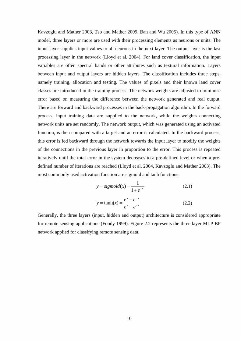
Generally, the three layers (input, hidden and output) architecture is considered appropriate

for remote sensing applications (Foody 1999). Figure 2.2 represents the three layer MLP-BP

network applied for classifying remote sensing data.

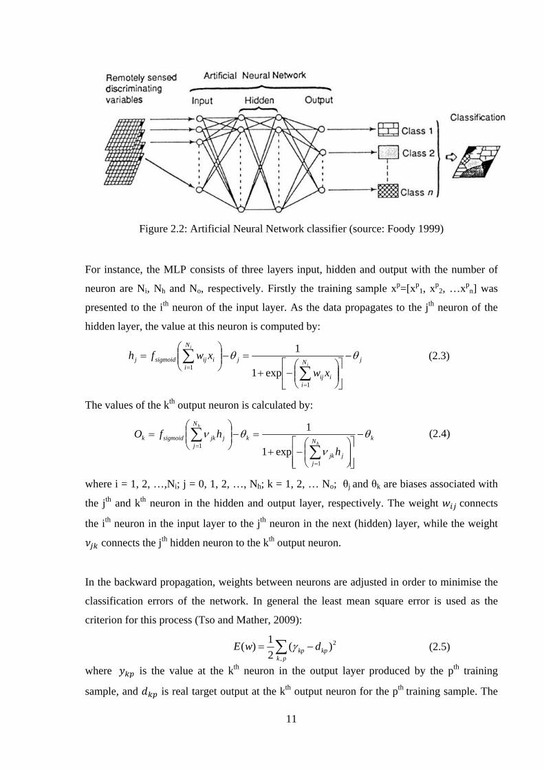
11

Figure 2.2: Artificial Neural Network classifier (source: Foody 1999)

For instance, the MLP consists of three layers input, hidden and output with the number of

neuron are Ni, Nh and No, respectively. Firstly the training sample xp=[xp1, xp

2, …xpn] was

presented to the ith neuron of the input layer. As the data propagates to the jth neuron of the

hidden layer, the value at this neuron is computed by:

jN

iiij

j

N

iiijsigmoidj

i

i

xwxwfh θθ −

⎥⎦

⎤⎢⎣

⎡⎟⎟⎠

⎞⎜⎜⎝

⎛−+

=−⎟⎟⎠

⎞⎜⎜⎝

⎛=

∑∑

=

=

1

1 exp1

1 (2.3)

The values of the kth output neuron is calculated by:

kN

jjjk

k

N

jjjksigmoidk

h

h

hhfO θ

ν

θν −

⎥⎥⎦

⎤

⎢⎢⎣

⎡⎟⎟⎠

⎞⎜⎜⎝

⎛−+

=−⎟⎟⎠

⎞⎜⎜⎝

⎛=

∑∑

=

=

1

1exp1

1 (2.4)

where i = 1, 2, …,Ni; j = 0, 1, 2, …, Nh; k = 1, 2, … No; θj and θk are biases associated with

the jth and kth neuron in the hidden and output layer, respectively. The weight connects

the ith neuron in the input layer to the jth neuron in the next (hidden) layer, while the weight

connects the jth hidden neuron to the kth output neuron.

In the backward propagation, weights between neurons are adjusted in order to minimise the

classification errors of the network. In general the least mean square error is used as the

criterion for this process (Tso and Mather, 2009):

2

,)(

21)( kp

pkkp dwE −= ∑ γ (2.5)

where is the value at the kth neuron in the output layer produced by the pth training

sample, and is real target output at the kth output neuron for the pth training sample. The

12

gradient descent method is often used to resolve the minimisation problem of E(w) and the

weights are then adjusted according to:

jkjkjk htt ηδνν +=+ )()1( (2.6)

pijijij xtwtw ηδ+=+ )()1( (2.7)

where w (t) and ν t are weight values at time t. The parameter η is in a range of 0 ≤ η ≤ 1,

and represents the learning rate. and are error value at the kth output neuron and jth

hidden neuron and calculated using:

))(1( kkkkk ydyy −−=δ (2.8)

jkk kjjj hh νδδ ∑−= )1( (2.9)

where is the value calculated by the network at the output neuron kth and is its desired

output. The momentum term α can be applied to make the learning process faster, for

example, the weight connecting the ith input neuron to the jth hidden neuron is modified as:

( ))1()()()1( −−++=+ twtwxtwtw ijijpijijij αηδ (2.10)

where 0 ≤ α ≤ 1.

The ANN has several advantages such as non-parametric base, easy adaptation to different

types of data and input structure. Consequently, it is a promising techniques for land cover

classification (Paola and Schowengerdt 1995, Huang et.al. 2002, Bruzzone et al. 2004, Lloyd

et al. 2004, Ban and Wu 2005, Berberoglu et al. 2007, Aitkenhead et al. 2008, Kavzoglu

2009, Tso and Mather 2009, Pacifici et al. 2009).

Selection of an appropriate network model and parameter values has a major influence on the

performance of the ANN classification process. The important factors are: number of input

neurons, hidden layers and neurons, and output neurons, initial weight range, activation

function, learning rate and momentum, and number of iterations (Zhou and Yang 2008).

Many heuristics have been proposed by researchers to find the optimum parameters for ANN

classifiers, however, none of them are officially accepted (Kavzoglu and Mather 2003). In the

study of Zhou and Yang (2008), 59 ANN models using different parameter values have been

examined for classifying Landsat TM images in the Atlanta metropolitan area, Georgia, USA.

It was found that activation function, learning rate, momentum and number of iterations

strongly influenced classification accuracy. They also reported that using a large number of

hidden layers did not provide a significant increase in classification accuracy.

13

Ban and Wu (2005) compared ANN and ML classifiers for classifying land use/cover

features in the rural-urban fringe of the Greater Toronto area, Canada using multi-temporal

Radarsat images. They found that the ANN classification of filtered SAR images improved

classification accuracies by 4-6% compared to ML. The authors claimed that ANN is more

robust than ML as ANN can minimise conflict of similar signatures between images while

extracting useful information from them. Bruzzone et al. (2004) developed a system for

automatic classification of multi-temporal SAR images based on the ANN classifier with

Radical Basis Function (RBF) as an activated function. The authors claimed the RBF neural

network is a very effective classifier for classifying SAR data. Pradhan et al. (2010)

compared the performance of an ANN classifier using a BP algorithm and an improved k-

Mean unsupervised classifier on land cover classification of the Eastern Himalayan State of

Sikkim. The authors concluded that the ANN-BP classifier produced the best result for

almost all the classes except for the thick forest region, where there was some confusion

between thin vegetation and dense forest. The overall classification accuracy obtained by

ANN-BP model was 90.70%. Heinl et al. (2009) investigated the performance of ANN and

ML classifiers and discriminant analysis (DA) for classifying Landsat 7 ETM+ multispectral

image in combination with ancillary data, including elevation, slope, aspect, sun elevation

angles and NDVI. The MLC and DA gave similar overall accuracy, in a range of 55-60% and

about 75% using only spectral data (Landsat 7 ETM+) and when ancillary data were

incorporated, respectively. The ANN classifier outperformed MLC and DA methods in all

cases with an overall accuracy of about 75% for using only Landsat7 ETM+ images, 85% for

ancillary data, and 86.3% for a combination of multispectral and ancillary data. However, the

authors claimed that while use of ancillary data allowed significant improvement in

classification accuracy, these increases of overall accuracy were observed independent of the

classifier. They went on to suggest that a greater consideration should be given to searching

for appropriate and optimised sets of input variables. The application of an ANN-MLP

network for paddy-field classification using moderate resolution imaging spectroradiometer

(MODIS) data was studied by Yamaguchi et al. (2010). The study showed the effectiveness

of the MODIS data and MLP classifier for mapping paddy-field. The overall accuracy

obtained was 90.8%, which is considered a good result.

Apart from the ANN-MLP network which has been used widely for image classifications,

there are also a few neural network algorithms that have been developed and introduced for

14

classifying remote sensing data, such as Furzy Artmap (Bruzzone et al. 2004, Gao 2009) and

Self-Organising Map (Hugo et al. 2006, Salah et al. 2009).

Results of the studies mentioned above illustrated that the ANN-based algorithm is more

robust and suitable for classifying remote sensing data than the traditional parametric ML

algorithm. However, the application of this technique for the classification of multisource

data has not been deeply studied in the literature.

2.1.3.2. Support vector machine (SVM)

SVM is a recent development of a non-parametric supervised classification technique, which

have proven to be very robust and reliable in the field of machine learning and pattern

recognition (Pal and Mather 2002, Waske and Benediktsson 2007, Anthony and Ruther 2007,

Safri and Ramle 2009, Kavzoglu and Colkesen 2009). SVM separates two classes by

determining an optimal hyper-plane that maximises the margin between these classes in a

multi-dimensional feature space (Kavzoglu and Colkesen 2009). Only the nearest training

samples – namely ‘support vectors’ in the training datasets (Figure 2.3) – are used to

determine the optimal hyper-plane. As the algorithm only considers samples close to the class

boundary it works well with small training sets, even when high-dimensional datasets are

being classified.

Figure 2.3: Example of linear support vector machine (adapted from Mountrakis et al. 2011)

15

As in a case of a binary classification, in n-dimensional feature space, xi is a training set of m

samples, i=1,2,…,m, and their class labels yi = -1 or +1. The optimum separation plane is

defined as:

,1. −≤+bxw i as x belong to class -1 (2.11)

,1. +≥+bxw i as x belong to class +1 (2.12)

or [ ] 1. ≥+bxwy ii i∀ (2.13)

In practice classes are not always fully separated by linear boundaries. Thus, the error

variable iξ is introduced:

[ ] ,1. iii bxwy ξ−≥+ 0≥iξ (2.14)

The optimum hyper-plane is identified based on solving the optimisation problem:

( ) ⎥

⎦

⎤⎢⎣

⎡+ ∑

=

m

iiCw

1

221min ξ (2.15)

where C is the penalty parameter according to the error ξi .

For nonlinear classification the SVM projects input data into a higher dimensional space

using a nonlinear vector mapping function φ so that classes become more separable (Anthony

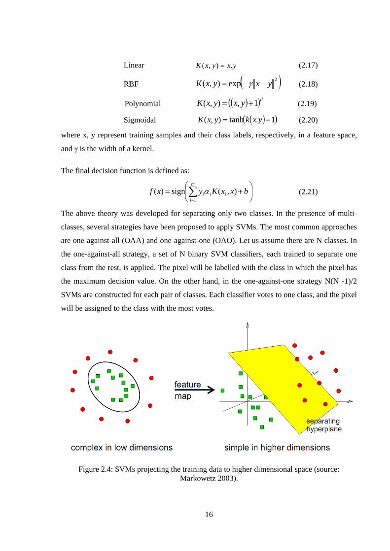
and Ruther 2007, Tso and Mather 2009). This strategy is appropriate for classification of

remote sensing data, which are usually not linearly separable. This concept is illustrated in

Figure 2.4.

In order to reduce the burden of computation, Vapnik (2000) proposed a kernel function

K(x,y), in which: K (xi, yj) = φ(xi)× φ(yj). Using the technique of Lagrange multipliers, the

optimisation problem becomes:

∑∑∑== =

−m

iijijij

m

i

m

ji xxKyy

11 121 ),(min ααα (2.16)

with ∑=

=m

iiiy

10α and Ci ≤≤α0 , i=1, 2, …,m

where αi is the Lagrange multipliers. The Lagrangian has to be minimised with respect to w, b

and maximised with respect to αi ≥ 0.

Major kernel functions are the Gaussian Radial Basis Function (RBF), linear, polynomial and

sigmoid functions:

16

Linear yxyxK .),( = (2.17)

RBF ( )2exp),( yxyxK −−= γ (2.18)

Polynomial ( )( )dyxyxK 1,),( += (2.19)

Sigmoidal ( )( )1.tanh),( += yxkyxK (2.20)

where x, y represent training samples and their class labels, respectively, in a feature space,

and γ is the width of a kernel.

The final decision function is defined as:

⎟⎠

⎞⎜⎝

⎛+= ∑

=

m

iiii bxxKyxf

1),(sign)( α (2.21)

The above theory was developed for separating only two classes. In the presence of multi-

classes, several strategies have been proposed to apply SVMs. The most common approaches

are one-against-all (OAA) and one-against-one (OAO). Let us assume there are N classes. In

the one-against-all strategy, a set of N binary SVM classifiers, each trained to separate one

class from the rest, is applied. The pixel will be labelled with the class in which the pixel has

the maximum decision value. On the other hand, in the one-against-one strategy N(N -1)/2

SVMs are constructed for each pair of classes. Each classifier votes to one class, and the pixel

will be assigned to the class with the most votes.

Figure 2.4: SVMs projecting the training data to higher dimensional space (source:

Markowetz 2003).

17

In SVMs, the problem of over-fitting in high-dimensional feature space is controlled by the

structure risk minimisation principle (Osuma 2005, Anthony and Ruther 2007, Mountrakis et

al. 2011). The SVMs have been applied successfully in many studies using remotely sensed

imagery. In these studies the SVMs often provided better (or at least no worse) level of

accuracy than other classifiers (Huang et al. 2002, Pal and Mather 2005, Waske and

Benediktsson 2007, Kavzoglu and Colkesen 2009, Pacini el al. 2009).

Pal and Mather (2005) compared SVMs, ML and the ANN approach for classifying Landsat

7 ETM+ and hyperspectral (DAIS) data. The results indicate that SVMs obtained higher

classification accuracy than either the ML or ANN classifier. Basili et al. (2008) investigated

the capabilities of SVM classification methods for land cover mapping in the city area of

Rome, Italy, for three periods in 1994, 1996 and 1999, using ERS 1/2 SAR data. The study

made use of different input parameters, including backscattered mean and standard deviation

images, coherence images, GLCM contrast and energy texture measures. The results

indicated that the SVM method is very applicable for land cover classification even in very

complex surfaces such as urban areas. Moreover, in this study the RBF kernel performed

significantly better than the 2nd order polynomial kernel.

Kavzoglu and Colkesen (2009) used Terra ASTER images and SVMs with radial basis and a

polynomial kernel function to classify land cover type in the Gebze District of Turkey. The

performance of SVMs was compared with the ML classifier. Results indicated that SVMs in

most cases outperform the ML algorithm in terms of overall accuracy (by 4%) and individual

classes. It was also found that the radial basis function (RBF) kernel gave higher accuracy

than the polynomial kernel by approximately 2% of overall accuracy.

In the study by Safri and Ramle (2009), SVM classifiers with different kernel functions,

including linear, radial, sigmoid and polynomial, were used to classify a SPOT 5 satellite

image. The performance of SVM classifiers were compared with the Decision Trees (DT).

Results showed that SVMs outperform DT in terms of classification accuracy. The lowest

overall classification accuracy given by SVM classifiers was 73.70% with the linear function

kernel, while the highest accuracy of 76.00 % was obtained by the RBF kernel. The overall

classification accuracy of the DT algorithm was only 68.78%.

18

Selecting the appropriate model is essential for the performance of the SVM classifier. In the

study carried out by Huang et al. (2002), performance of the SVM classifier has been

compared with ANN, DT and ML for land cover classification using Landsat TM images.

Two options for input variables were selected for testing, namely three input variables (Red,

NIR bands and NDVI images) and seven input variables (6 Landsat TM bands and NDVI

images). For the SVM classifier, different kernel functions (linear, RBF, polynomial) with

various relevant parameters were implemented. For the ANN classifier, the three layer model

(input, hidden, output) with a number of hidden neurons equal to one, two and three times

that of the input variables were tested. The classification results revealed that the SVM

classifier outperformed the ML and DT classifiers in most cases. The SVM classifier was

also more accurate than the ANN classifier for the case of using seven input variables.

However, the ANN provided higher classification accuracy when only three input variables

were employed. The possible reason was the limited success of the SVM algorithm in

transforming nonlinear class boundaries in a very low-dimensional space into linear ones in a

high-dimensional space. On the other hand, the complex network structure might allow ANN

to generate complex decision boundaries even with very few variables, and, as a result, have

better comparative performance than the SVM. Huang et al. (2002) also emphasised that

using more input variables resulted in more improvement in classification accuracy than

choosing better classification algorithms or increasing the training data size. Interestingly,

studies by Dixon and Candade (2008) showed that both SVM and ANN classification

produced better accuracy than ML classification, while SVM and ANN classification

produced comparable results.

Similar to the ANN classifier, although the SVM classifier often outperformed the commonly

used ML algorithm in classification of remote sensing data, and is theoretically more

appropriate than the ML algorithm for handling complex datasets, there are few studies using

this technique for classifying multisource data.

2.1.3.3. Feature selection techniques

The feature selection (FS) or feature subset selection (FSS) algorithm is very important for

data processing in general, as well as for classification of remote sensing data. This technique

allows the selection of only relevant, informative variables while removing the least effective,

highly correlated variables to generate the most separable input dataset for the classification

19

process. Therefore, the FS can help to reduce noise and uncertainty within datasets and lead

to improved classification performance. Because of these advantages the FS techniques have

been increasingly used for image classification and have given promising results, particularly

for highly dimensional datasets (Serpico and Bruzzone 2001, Kavzoglu and Mather 2002, Pal

2006, Anthony and Ruther 2007, Bruzzone and Persello 2009, Maghsoudi et al. 2011).

Among of the FS techniques, the Genetic Algorithm (GA) is one of the most efficient

methods, capable of working with a large search space and has more chance to avoid the

problem of local optimal solutions (Huang and Wang 2006, Zhuo et al. 2008). Consequently,

FS based on GA methods is suitable for large datasets such as in the case of multisource

remote sensing data. However, the use of GA techniques for classification of multisource

data has not been adequately researched. Detailed discussion of the concepts and the main FS

techniques, including GA and its application in land cover classification, will be presented in

chapter 4.

2.1.3.4. Multiple classifier systems (MCS)

Recently, the multiple classifier systems (MCS) or classifier ensemble algorithm has been

increasingly used in pattern recognition and remote sensing. This technique generates final

results by combining the output from different classification algorithms (Xie et al. 2006, Du

et al. 2009a). Consequently, the MCS algorithm has the potential to improve the classification

performance by incorporating advantages of various classifiers while reducing the uncertainty

of individual classifiers. The MCS algorithm is often more accurate than the least accurate

constituent classifier (Foody et al. 2007) and in the ideal case should outperform the best

individual classifier (Huang and Lees 2004). For these reasons, the MCS became attractive to

researchers. Many investigations have been carried out using MCS techniques to classify

remote sensing data (Briem et al. 2002, Bruzzone et al. 2004, Foody et al. 2007, Du et al.

2009b, Yan and Shaker 2011). However, there are not many studies using this technique to

classify multisource data. In this thesis, the MCS technique is proposed and evaluated for

classifying multisource remote sensing data. The concepts and applications of MCS for land

cover classification using remote sensing data will be reviewed in detail in Chapter 5.

20

2.2. DATA PRE-PROCESSING

The data pre-processing process, which removes (or at least reduces) the distortions of

satellite imagery, is essential for the success of remote sensing applications such as image

classification. The basic data pre-processing procedures are presented below.

2.2.1. GEOMETRIC CORRECTION

Remote sensing imagery suffers from the geometric distortion caused by different factors

during the image acquisition process. This kind of distortion leads to the displacements of

imaged pixels from their corrected positions. Thus it is necessary to carry out the geometric

correction (or geometric rectification) in order to eliminate or reduce the geometric

distortions to a satisfactory level (Gao 2009). This task is even more important for

multisource data applications since data from different sensors and databases needs to be

precisely transferred to the common reference systems for further integrated analysis. In

general, geometrical errors are considered as systematic or random depending on their nature.

The systematic errors can be predicted and completely eliminated. For example distortion

caused by Earth rotation and curvature, variation in the platform speed, inconsistency in

scanning mirror velocity (optical imagery) or antenna pattern and range spreading loss (radar

imagery) are systematic errors which can be removed prior to image distribution (Richards

and Jia 2005, Gao 2009). On the other hand, random errors are unpredictable and cannot be

removed completely. The image rectification process can only reduce these errors to an

acceptable level. For example, most of errors related to position and orientation (Figure 2.5)

of the sensor are random.

21

Figure 2.5: Effect of platform/sensor position and orientation on geometry of image (Source:

Gao 2009)

The image rectification process suppresses geometrical errors and transforms the imagery to

the reference system, which could be another image (base image) or preferably a cartographic

projection system such as Universal Tranverse Mecator (UTM). The transform model, which

represents relationship between image pixels and the corresponding coordinates in a

reference system, is determined using ground control points (GCPs). The GCPs must be

stable and clearly visible in both image and the reference system. Many geometrical models

have been applied for transformation of local image coordinate system to those of a reference

system. They can be categorised as either non-physical or physical. In the non-physical

22

approach, the transformation model is assumed to be a certain function, such as a polynomial

function. This method is simple and very flexible since it can be applied to any kind of

image. This method can give a very good result in areas of flat terrain. However, this model

is not rigorous and therefore the accuracy of geometric correction is not high in the case of

complex terrain such as mountainous areas. Moreover, this method cannot account for the

relief displacement (Figure 2.6) caused by the height of terrain. In contrast, the method using

a physical model, such as the co-linearity equation, precisely represents the geometry

between the two coordinate systems. The advantages of this method are robustness and high

accuracy. In particular, using a physical model allows ortho-rectification of image, in which

the relief displacement can be reduced by introducing data from a DEM. The limitations of

this method are complexity, time consuming, and not being available in many commercial

software. In addition, this method requires some sensor-specific parameters that can only

provided by the satellite vendors.

Figure 2.6: Relief displacement in optical and radar satellite image (D is a displacement, Δh

is height of points, η and 90o- η are viewing angles) (source: CCRS/CCT)

2.2.2. RADIOMETRIC CALIBRATION

Optical imagery

The radiances received at the sensors are often converted to digital number (DN) values.

However, in many cases the DN is not adequate for representing surface features, particularly

23

when multi-temporal and multi-sensor data are employed. Thus it is preferable to convert the

DN to radiance values. The sensor calibration is described by:

βαλ += DNL . (2.22)

where is spectral radiance, DN is a digital number, α is gain and β is an offset of the

sensor.

The spectral radiance is dependent on the illumination conditions, such as season, time of

day, geographical position, etc. Thus, it is more convenience to convert the radiance to a

reflectance value, which represents the ratio of radiance to irradiance. The reflectance is

unitless and allows direct comparison between images. For example the reflectance

(exoatmospheric reflectance) of Landsat TM images is presented by:

sESUN

dLθ

πρ

λ

λ

cos... 2

= (2.23)

where Lλ is the spectral radiance, d is the Earth-Sun distance in astronomical units, ESUNλ is

the mean solar exoatmospheric irradiance, and θs is the solar zenith angle in degrees. ESUNλ

is derived from tables provided in the Landsat Technical Notes (August 1986).

SAR imagery

The radar backscattering coefficient (Sigma Nought, σ0) and the radar brightness (Gamma

Nought γ), which represent the total return energy from the surface area within the projected

pixel, is given by (Absolute calibration of ASAR Level 1 products, 2004):

);sin( ,

2,0

, jiji

ji KDN

ασ = )cos( ,

0,

,ji

jiji α

σγ = (2.24)

for i = 1… L and j = 1….M.

where σi,j0 is Sigma Nought at image line and column “i,j”

DNi,j2 is the pixel intensity for pixel i, j

K is the absolute calibration constant

αi,j is incidence angle at image line and column “i,j”

γi,j is Gamma Nought at image line and column “i,j”

L,M are the number of image lines and columns

For rough terrain the local incident angle will be adjusted by the slope angle:

αi,j = β – θ

24

where β is look angle of the radar system

θ is local slope angle

2.2.3. SPECKLE NOISE FILTERING

The speckle noise is a natural and commonly seen phenomenon in radar imaging systems.

The radar system transmits in-phase waves to the target and receives backscattered signals.

After interacting with the target surface, these waves are no longer in-phase because of

differences in scattering properties or due to the distances to the targets. These out-of-phase

radar waves can interact in constructive or destructive ways to produce light and dark pixels,

which are the so-called speckle noise (Qiu et al. 2004). Radar speckle noise is often modelled

as a multiplicative process. This means that the noise increases with an increase in signal

strength. Speckle noise strongly affects the quality of SAR images and therefore must be

reduced before using the data for analysis.

Among of the noise suppression techniques the adaptive filters are considered the most

effective and appropriate for processing SAR data. The adaptive filter reduces the noise while

preserving image sharpness. The most commonly used adaptive filters are the Lee & Lee-

sigma, Gamma-Map and Frost filters.

Lee-Sigma and Lee Filters: In these filters Gaussian distribution for the noise in the image

data is assumed. The Lee-Sigma and Lee filters compute the value of the filtered pixel based

on the statistical distribution of the DN values within the moving window. The Lee filter

considers that the mean and variance of the target pixel is equal to the local mean and

variance of all surrounding pixels within the moving window (Lee, 1981):

DNout = [Mean] + K[DNin - Mean] (2.25)

where Mean = average of pixels in a moving window

)(][)(

22 xVarMeanxVarK+

=σ

(2.26)

and

[ ] [ ][ ]

[ ]22

2

1)( windowMeanwithin

SigmawindowMeanwithinthinwindowVariancewixVar −⎟⎟

⎠

⎞⎜⎜⎝

⎛

++

= (2.27)

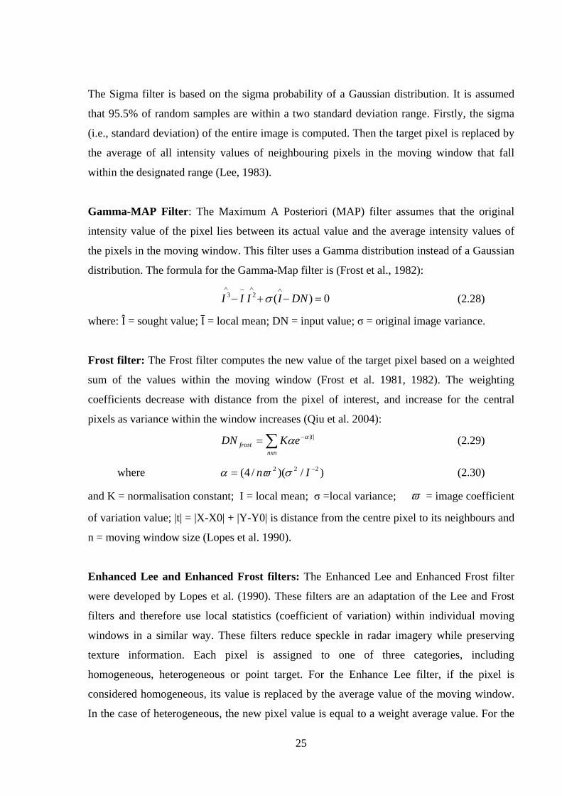
25

The Sigma filter is based on the sigma probability of a Gaussian distribution. It is assumed

that 95.5% of random samples are within a two standard deviation range. Firstly, the sigma

(i.e., standard deviation) of the entire image is computed. Then the target pixel is replaced by

the average of all intensity values of neighbouring pixels in the moving window that fall

within the designated range (Lee, 1983).

Gamma-MAP Filter: The Maximum A Posteriori (MAP) filter assumes that the original

intensity value of the pixel lies between its actual value and the average intensity values of

the pixels in the moving window. This filter uses a Gamma distribution instead of a Gaussian

distribution. The formula for the Gamma-Map filter is (Frost et al., 1982):

0)(23 =−+−∧∧−∧

DNIIII σ (2.28)

where: Î = sought value; I = local mean; DN = input value; σ = original image variance.

Frost filter: The Frost filter computes the new value of the target pixel based on a weighted

sum of the values within the moving window (Frost et al. 1981, 1982). The weighting

coefficients decrease with distance from the pixel of interest, and increase for the central

pixels as variance within the window increases (Qiu et al. 2004):

∑ −=nxn

tfrost eKDN ||αα (2.29)

where )/)(/4( 222 −= In σϖα (2.30)

and K = normalisation constant; I = local mean; σ =local variance; ϖ = image coefficient

of variation value; |t| = |X-X0| + |Y-Y0| is distance from the centre pixel to its neighbours and

n = moving window size (Lopes et al. 1990).

Enhanced Lee and Enhanced Frost filters: The Enhanced Lee and Enhanced Frost filter

were developed by Lopes et al. (1990). These filters are an adaptation of the Lee and Frost

filters and therefore use local statistics (coefficient of variation) within individual moving

windows in a similar way. These filters reduce speckle in radar imagery while preserving

texture information. Each pixel is assigned to one of three categories, including

homogeneous, heterogeneous or point target. For the Enhance Lee filter, if the pixel is

considered homogeneous, its value is replaced by the average value of the moving window.

In the case of heterogeneous, the new pixel value is equal to a weight average value. For the

26

point target category the pixel value is not changed. The Enhanced Frost filter treats the pixel

the same as the Enhanced Lee filter for the homogeneous and point target cases. For the

heterogeneous case, the pixel value is determined by an impulse response which is used as a

convolution kernel (Lopes et al. 1990). Recently, the multi-temporal speckle filter has been

developed by Quegan et al. (2000), and has been used effectively in applications such as

forest and rice mapping.

2.3. ADVANTAGES OF MULTISOURCE REMOTE SENSING DATA, SELECTION AND INTEGRATION ISSUES 2.3.1. ADVANTAGES OF THE COMBINED APPROACH

Multisource remote sensing data involve the satellite images themselves, derived products

such as textural information, indices, and ratios, and other additional data from, for example,

geographical information system (GIS) or field-based measurements. The obvious advantage

of a multiple data source is that various sources of complimentary information can contribute

to analysis process.

2.3.1.1. Combination of optical and SAR images

As in a case of integration of SAR and optical images, information in different parts of the

electromagnetic spectrum can be employed. Instead of using only the spectral response

characteristics of features in the visible/near-infrared or backscattered properties in the

microwave region, when they are collected separately, both of them are employed for the

classification process (Forster 1987). Haack (1984) claimed that the best classification could

be obtained by the combination of data from the major portions of the spectrum including

visible, near infrared, thermal and microwave. The visible/near-infrared imagery contains

information about surface response rather than structural details (Forster 1987). This surface

response represents the chemical properties of surface cover such as bare soil, urban areas,

water, and forests. For example, vegetation absorbs incident energy in the red channel for its

photosynthetic process and reflects strongly in the near-infrared region, while water

reflectance is higher for a shorter wavelength (blue) and reduces rapidly at longer

wavelengths (red and near-infrared) (Figure 2.7). The reflectance of dry soil rises uniformly

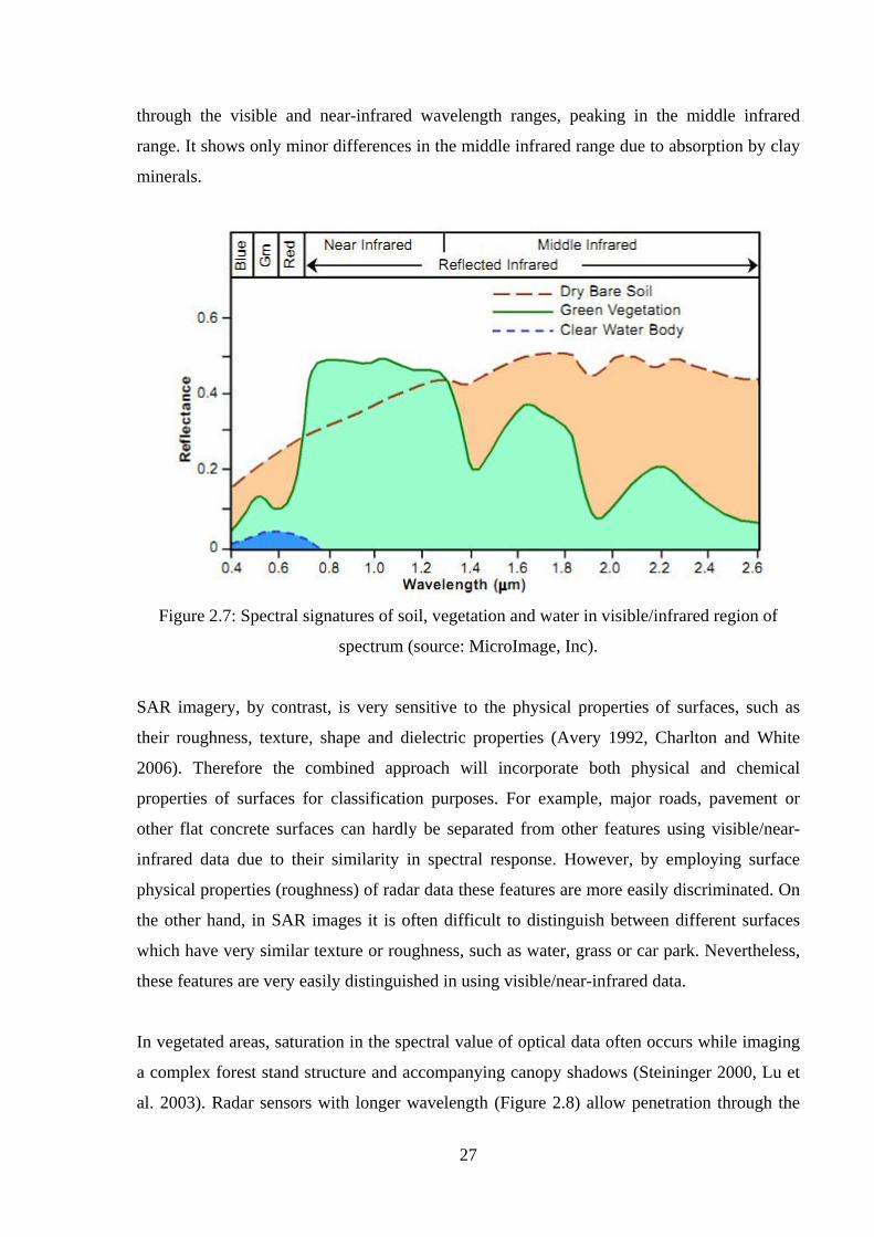
27

through the visible and near-infrared wavelength ranges, peaking in the middle infrared

range. It shows only minor differences in the middle infrared range due to absorption by clay

minerals.

Figure 2.7: Spectral signatures of soil, vegetation and water in visible/infrared region of

spectrum (source: MicroImage, Inc).

SAR imagery, by contrast, is very sensitive to the physical properties of surfaces, such as

their roughness, texture, shape and dielectric properties (Avery 1992, Charlton and White

2006). Therefore the combined approach will incorporate both physical and chemical

properties of surfaces for classification purposes. For example, major roads, pavement or

other flat concrete surfaces can hardly be separated from other features using visible/near-

infrared data due to their similarity in spectral response. However, by employing surface

physical properties (roughness) of radar data these features are more easily discriminated. On

the other hand, in SAR images it is often difficult to distinguish between different surfaces

which have very similar texture or roughness, such as water, grass or car park. Nevertheless,

these features are very easily distinguished in using visible/near-infrared data.

In vegetated areas, saturation in the spectral value of optical data often occurs while imaging

a complex forest stand structure and accompanying canopy shadows (Steininger 2000, Lu et

al. 2003). Radar sensors with longer wavelength (Figure 2.8) allow penetration through the

28

tree canopy, to a certain level, and give information on structures of vegetation stands (Santos

et al. 2003), and reduce the problem of spectral saturation (Lu and Weng 2007).

Figure 2.8: Microwave bands used in SAR systems (source: Henderson and Lewis 1998)

Forster (1986) compared the responses of Landsat MSS band 5 and band 7 data and SIR-B

SAR data over an urban area of Sydney. It was found that there was a high degree of overlap

between natural vegetation classes (forest) and residential areas with some amount of

vegetation such as grass or trees in the visible red and near-infrared bands. The spectral

response values of these two classes still overlapped in the combined data set, but the mean

spectral values were much more separated because the L-band SIR-B data can penetrate

through the tree canopy which covered the residential buildings. According to Forster (1986),

areas which were cleared for development were very similar to the intense urban areas

(commercial and industrial) in the optical image. However, this was not the case for the SAR

data, where the response from soil was low, because of its fairly smooth surface, compared to

the high backscatter from intense, rough urban areas.

Weydahl et al. (1995) also reported that satellite SAR images may add additional information

about hard targets within built-up areas, including building direction, complexity of objects,

materials, when they are used together with optical images. Many bright points in radar

images result from metal objects, roofs of buildings or corner reflectors formed between

29

buildings and the ground. This may, again, provide more information complimentary to

optical data.

2.3.1.2. Uses of multi-temporal data

The ability to collect multi-temporal data is one of the most useful properties of remote

sensing systems. Multi-temporal imagery is a valuable data source for land cover mapping

since it can provide signatures of ground features in the time domain. Many studies have

demonstrated that use of satellite imagery acquired in different seasons leads to improved

classification accuracy, particularly for crop and vegetation cover types (Brisco and Brown

1995, Pierce et al. 1998, Quegan el al. 2000, Agelis et al. 2002, Bruzzone et al. 2004, Chust

et al. 2004, Ban and Wu 2005, Park and Chi 2008, McNairna et al. 2009). McNaima et al.

(2009) evaluated the capabilities of multi-temporal optical and SAR imagery for annual crop

inventories in Canada. They concluded that although there are a variety of cropping systems,

crops can be successfully classified using multi-temporal satellite data. Guerschman et al.

(2003) explored the use of multi-date Landsat TM images for land cover classification in the

south-western part of the Argentine Pampas. It was shown that at least two Landsat TM

scenes from the same growing season are necessary for successfully identifying land cover

types. The acquisition dates of these images should be able to represent the shift between

winter and summer crops. The authors claimed that in order to discriminate winter crops and

rangelands, one spring (September to October) image and one summer (late December to

February) image were sufficient. Additional images acquired in late summer or fall can

improve separability of summer crops or pasture features at a marginal level.

However, it is often difficult to obtain optical multi-temporal data due to its heavy

dependence on weather conditions. Conversely, the capability of obtaining data at any time

under all weather conditions is one of the major advantages of SAR systems, hence they can

provide multi-temporal data on a regular basis. Multi-temporal SAR data permit the temporal

variation of the SAR signal to be taken into account as well as the extraction of additional

information on land cover class, provided that there has been no transition between land

cover classes during the period considered, but only a change in physical conditions (Agelis

et al. 2002). Quegan et al. (2000) investigated the responses of forests in ERS time series

images, and found that the temporal stability of a forest is greater compared with many other

types of land cover, and this kind of information can be used to effectively map forest areas.

30

McNairna et al. (2009), after comparing the performance of multi-temporal SAR with optical

image for crop classification in various sites in Canada, claimed that the multi-temporal SAR

(two ENVISAT/ASAR images) was comparable with the single optical (SPOT) image, while

the combined dataset (two ASAR images + one SPOT image) provided the greatest

classification accuracy. Shang et al. (2008) pointed out that when available, multi-temporal (2

to 3 scenes acquired at different growth stages) optical data are ideal for crop classification.

However, due to cloud and haze interference good optical data are not always obtainable and

a SAR-optical combination offers a good alternative. They also found that when only one

optical image is available, the addition of two ASAR images acquired in VV/HH polarisation

will provide acceptable accuracies. In Blaes et al. (2005) the performance of various multi-

temporal ERS datasets was evaluated. It was found that by increasing the number of images

the classification accuracies were significantly increased. The overall accuracies vary in a

range of 40% to 65%, depending on number of scenes and acquisition dates. Moreover,

single SAR images are often displayed in a grey scale format which causes considerable

difficulties for visual analysis. Uses of multi-temporal can provide data in the form of a

colour composite, and as a result may significantly ease interpretation tasks.

2.3.1.3. Use of multi-frequency data

SAR images can be acquired at different wavelengths (or frequencies) such as P-, L-, C- or

X-bands. These wavelengths allow different degrees of penetrations and sensitivities to

roughness, structures and scale of surface features. Figure 2.9 shows different penetration

capabilities through the tree canopy of L-, C- and X-band SAR signals. The shorter

wavelength (C-, X-bands) SAR with less capability of penetration often reflect information

from the top of surfaces, such as the upper levels of the tree canopy. The longer wavelength

(L-, P-bands) SAR with deeper penetration can provide more information on the layers

beneath (Forster, 1986).

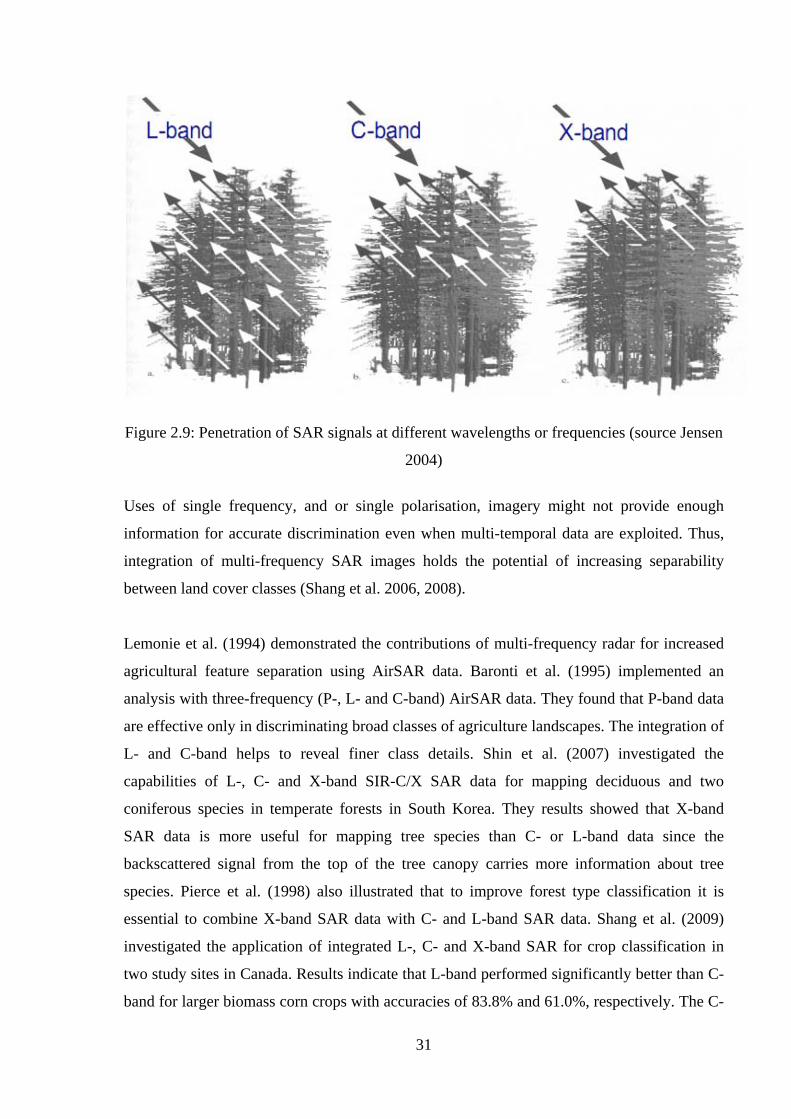
31

Figure 2.9: Penetration of SAR signals at different wavelengths or frequencies (source Jensen

2004)

Uses of single frequency, and or single polarisation, imagery might not provide enough

information for accurate discrimination even when multi-temporal data are exploited. Thus,

integration of multi-frequency SAR images holds the potential of increasing separability

between land cover classes (Shang et al. 2006, 2008).

Lemonie et al. (1994) demonstrated the contributions of multi-frequency radar for increased

agricultural feature separation using AirSAR data. Baronti et al. (1995) implemented an

analysis with three-frequency (P-, L- and C-band) AirSAR data. They found that P-band data

are effective only in discriminating broad classes of agriculture landscapes. The integration of

L- and C-band helps to reveal finer class details. Shin et al. (2007) investigated the

capabilities of L-, C- and X-band SIR-C/X SAR data for mapping deciduous and two

coniferous species in temperate forests in South Korea. They results showed that X-band

SAR data is more useful for mapping tree species than C- or L-band data since the

backscattered signal from the top of the tree canopy carries more information about tree

species. Pierce et al. (1998) also illustrated that to improve forest type classification it is

essential to combine X-band SAR data with C- and L-band SAR data. Shang et al. (2009)

investigated the application of integrated L-, C- and X-band SAR for crop classification in

two study sites in Canada. Results indicate that L-band performed significantly better than C-

band for larger biomass corn crops with accuracies of 83.8% and 61.0%, respectively. The C-

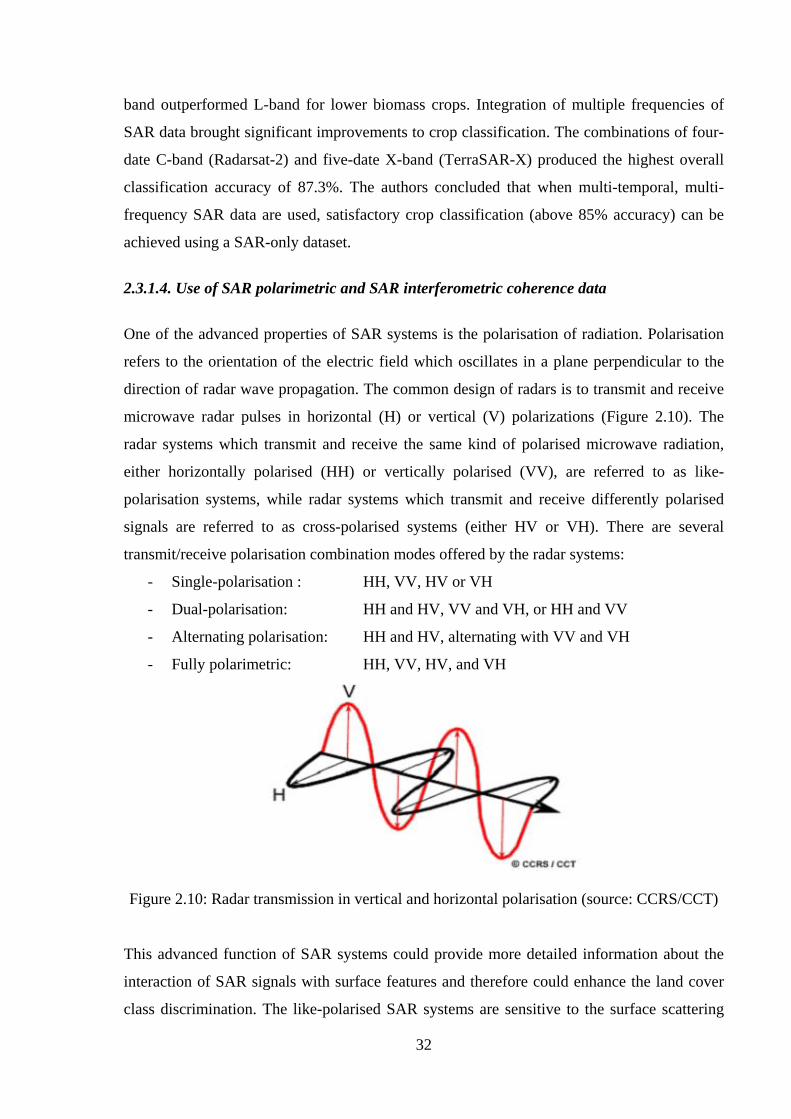
32

band outperformed L-band for lower biomass crops. Integration of multiple frequencies of

SAR data brought significant improvements to crop classification. The combinations of four-

date C-band (Radarsat-2) and five-date X-band (TerraSAR-X) produced the highest overall

classification accuracy of 87.3%. The authors concluded that when multi-temporal, multi-

frequency SAR data are used, satisfactory crop classification (above 85% accuracy) can be

achieved using a SAR-only dataset.

2.3.1.4. Use of SAR polarimetric and SAR interferometric coherence data

One of the advanced properties of SAR systems is the polarisation of radiation. Polarisation

refers to the orientation of the electric field which oscillates in a plane perpendicular to the

direction of radar wave propagation. The common design of radars is to transmit and receive

microwave radar pulses in horizontal (H) or vertical (V) polarizations (Figure 2.10). The

radar systems which transmit and receive the same kind of polarised microwave radiation,

either horizontally polarised (HH) or vertically polarised (VV), are referred to as like-

polarisation systems, while radar systems which transmit and receive differently polarised

signals are referred to as cross-polarised systems (either HV or VH). There are several

transmit/receive polarisation combination modes offered by the radar systems:

- Single-polarisation : HH, VV, HV or VH

- Dual-polarisation: HH and HV, VV and VH, or HH and VV

- Alternating polarisation: HH and HV, alternating with VV and VH

- Fully polarimetric: HH, VV, HV, and VH

Figure 2.10: Radar transmission in vertical and horizontal polarisation (source: CCRS/CCT)

This advanced function of SAR systems could provide more detailed information about the

interaction of SAR signals with surface features and therefore could enhance the land cover

class discrimination. The like-polarised SAR systems are sensitive to the surface scattering

33

mechanism, in which the radar pulse strikes and backscatters from rough surfaces such as

rocks, bare ground and built-up areas. In this scattering mode, the transmitted and

backscattered signals have the same polarisation. In other words, there are no, or little de-

polarisation effects in the backscattered energies. The cross-polarised SAR systems, on the

other hand, are more sensitive to the volume scattering mechanism, where radar signals are

de-polarised by surface materials and the polarisation of returned signals are changed.

Volume scattering often occurs when the radar signal strikes tree canopy, whereby the radar

pulses interact with various tree components such as leaves, branches, and so on, which cause

de-polarisation of the radar signal (Figure 2.11). Hence, synergistic use of both like- and

cross-polarised data can lead to an enhancement of the separability of land cover classes.

Figure 2.11: Surface scattering and volume scattering (source MicroImage, Inc).

Park and Chi (2008) have integrated multi-temporal/multi-polarisation C-band SAR data to

classify land cover in the Yedang plain, Korea (HH from Radarsat-1, and both VV and VH

from ENVISAT/ASAR). Results of this study indicated that the use of multi-polarisation

SAR data could improve classification accuracy significantly. The authors also made a

further suggestion on integration of multi-temporal/polarisation with optical data for land

cover mapping. Skriver (2008) found that single image with either single or dual-polarisation

did not give sufficient classification performance, while using multi-temporal acquisitions the

classification accuracy improves significantly for both kinds of polarisation data.

Dutra et al. (2009) studied capabilities of ALOS/PALSAR polarimetric data for land cover

classification in the Brazilian Amazon, and found that the best channel combination for

mapping tropical classes, consisting of the primary forest, secondary forest, bare soil,

34

agriculture and degraded forest, is dual-polarisation HH-HV images. However, the authors

pointed out that none of combined PALSAR dataset can discriminate one year regeneration

areas, and recommended the complementary use of optical images when possible, since in the

optical images, the ‘one year regeneration’ class can be differentiated from secondary forest.

Bargiel and Herrmann (2011) used 14 dual-polarised spotlight TerraSAR-X images acquired

during the vegetation season to classify two different agricultural study areas in North

Germany and Southeast Poland. Results showed that in all cases the highest classification

accuracy was achieved when both HH and VV polarisation were employed, and the accuracy

was notably reduced if only one polarisation was used in the classification process.

Interferometric coherence information is also useful to detect land cover features (Takeuchi et

al. 2001, Engdahl and Hyyppa 2003, Srivastava et al. 2006, Park and Chi 2008, Nizalapur et

al. 2011). Interferometric coherence images are generated from a pair of SAR single look

complex (SLC) images using both amplitude and phase information, in which one image is

considered as the ‘master’ and the other as the ‘slave’. Coherence between the two SAR SLC

images is calculated from:

2

22

1

*21

)(.)(.

)().(

∑∑∑

=xsxs

xsxsγ (2.31)

where s1 and s2 are two complex co-registered images.

In the coherence image, a feature which is rather stable, such as urban areas and native

forests, will have a high value of coherence and appear brighter, while a feature which is

changed over time, such as rice fields, will have low coherence and appear darker. This

information could be also incorporated with original SAR backscattered or optical images to

enhance land cover classification. Takeuchi et al. (2001) claimed that using coherence images

generated from pairs of ERS 1/2 Tandem mode and JERS repeated pass images can easily

identify plantation or deforestation areas based on their higher coherence values than that of

non-deforested forests. Engdahl and Hyyppa (2003) evaluated multi-temporal ERS 1/2

inteferometric data for land cover classification in southern Finland, and found that coherence

images provide more information on surface cover types than the standard backscatter

intensity images. They also claimed that the use of coherence data has greatly improved

classification accuracy and allowed them to detect two forest and two urban classes instead of

only one of each, as in the case of using backscattered data. Bruzzone et al. (2004) used 8

35

ERS complex SAR images, which were acquired within a period from June 1995 to May

1996, and the ANN classifiers for land cover mapping in the area of Bern, Switzerland. They

found that the combination of long-term coherence and backscatter temporal variability

which were generated from the above dataset gave the greatest classification accuracy.

Nizalapur et al. (2011) used a coherence image generated from two ENVISAT/ASAR C-band

images in conjuntion with backscatter difference and mean backscatter data to classify land

cover features in a forested area of Chattisgarh, Central India. The traditional ML classifier

was applied. Results of the study highlighted the potential of SAR data in land cover

classification over this area with an overall accuray of 82.5%, average producer’s accuracy of

83.69% and average user’s accuracy of 81%.

Interestingly, Thiel et al. (2009) monitored a large forested area in Siberia using

ALOS/PALSAR intensity and coherence data in summer and winter. They found that the

synergistic use of coherence with intensity data improved separation, particularly from forest.

For example, recent and old clear cuts are separated, and even fire scars can be potentially

discriminated from recent clear cuts. Temporal decorrelation in the forest-based classes are

mainly because of factors such as plant growth, wind, and changes of soil moisture. The use

of coherence data also enhanced the separability of urban areas from all other land cover

types, since the urban are least subjected to temporal decorrelation. The authors claimed that

by integrating coherence with original backscatter intensity images many classes can be

better discriminated.

2.3.1.5. Uses of spatial information

One of the main limitations of these classical classifiers is that they rely only on the spectral

response or backscattered values of cover types. In a complex ground surface, with many

cover types which have similar spectral properties, it is difficult to achieve high classification

accuracy by applying these classifiers. The improvement is possible if spatial information

(textures and pattern of image features) are taken into account since they can provide

additional information about image characteristics (Pacifici et al. 2009). Textures represent

spatial arrangement and variation of patterns on the Earth’s surface (Sheoral et al. 2009). A

large number of texture measures have been generated, analysed and applied for image

classification (Lu and Weng 2007). The most common texture measures are derived from the

Grey Level Co-occurrence Matrix (GLCM). However, Lloyd et al. (2004) claimed that geo-

36

statistical texture measures allow better classification performance than the GLCM texture

data. The texture measures are often incorporated with spectral data as inputs for the

classification process (Gong and Howarth 1990, Lloyd et al. 2004, Nyoungui et al. 2002,

Narasimha Rao et al. 2002, Puissant et al. 2005, Ban and Wu 2005, Berberoglu et al. 2007,

Tassetti et al. 2010). In general, this approach produces better classification accuracy

compared to the conventional method dealing with the original dataset alone. Gong and

Howarth (1990) pointed out that this classification procedure is particularly effective for

differentiation between rural and urban features at urban-rural fringes. For example, Herold et

al. (2005) applied various textured measures derived from Radarsat images to classify land

cover features in Africa. It was found that using a combination of Radarsat images and

texture data (variance) improved the classification accuracy by 16%, 21% and 4% in three

different areas compared to the case that only original data were used. In order to identify

appropriate textures it is crucial to select texture measure, spectral bands, size of moving

windows and other parameters (Chen et al. 2004, Lloyd et al. 2004). Recently, in the study of

Tassetti et al. (2010), textural information, including GLCM and edge-density measures

generated from IKONOS images, was incorporated with spectral data for classification. The

authors pointed out that the spectral/textural approach gave an overall accuracy of 80.01%

compared to 63.44% of accuracy given by using only spectral bands.

The multi-scale texture approach was studied by Coburn and Roberts (2004). In this study,

first-order (variance) and second-order (GLCM Entropy) texture measures generated from

different window sizes were employed as additional information for forest stand

classification. It was revealed that all of the different texture measures provided

improvements of from 4 to 13% in overall accuracy. The multi-scale image texture approach

gave significant increases of 4 to 8% compared with the use of single band texture measures.

Results of the study also indicated that there is no single window size that could sufficiently

represent the whole range of textural information in the image. Zhang et al. (2007)

emphasised the robustness of multi-scale texture analysis while using GLCM texture

measures derived from different window sizes and high spatial resolution IKONOS imagery

for urban land cover/use classification. According to Zhang et al. (2007), the overall accuracy

of the multi-scale approach was higher than cases of single scale texture and original spectral

data by ~6% and ~11%, respectively. This conclusion agrees with the result of Pacifici et al.

(2009), who applied multi-scale first- and second-order textural information extracted from

QuickBird and WorldView-1 panchromatic images for classifying land use of four different

37

urban areas: Las Vegas, Washington D.C., San Francisco (USA) and Rome (Italy). They

claimed that different asphalt surfaces such as roads, highway and parking lots can be

separated with the multi-scale approach based on differences of textural information content.

This approach also allows distinguishing residential houses, apartment blocks and towers

with high classification accuracy (Kappa coefficient is above 0.9).

However, adding textural information does not always increase the classification accuracy. It

has been claimed that radar texture did not give any improvement, but rather reduced the

overall accuracy for some classes (Sheoran et al., 2009). In Chu and Ge (2010a),

incorporation of textural information extracted from either optical or SAR images did not

give any significant improvement. In Salah et al. (2009) the GLCM entropy generated from

the intensity image did not make any contribution to the final result.

2.3.2. SELECTION AND INTEGRATION OF REMOTELY SENSED DATA AND

FEATURE PARAMETERS

As mentioned in the previous section, nowadays, there is a wide range of satellite imagery

with different spectral, spatial, and temporal properties, including both SAR and optical data,

available to users. On the one hand, this provides more opportunities for users to work with

various kinds of remotely sensed data, and various data compositions over the same area of

interest. On the other hand, it is a difficult task to select appropriate input datasets, processing

methods and parameters. As pointed out by Gamba et al. (2005) the amount of overlapping

datasets available for a given area may be very large and, accordingly, the exploitation of

such overlapping datasets may represent a serious challenge. For land cover classification, it

is crucial to understand strengths and weaknesses of different types of data so as to select the

most suitable dataset (Jensen 2004). In general, scale, image resolution and user requirements

are the most important factors for the selection of datasets. Gamba et al. (2005) also

suggested that the simplest way to select a suitable dataset would be one involving sensors

with similar resolution, while allowing capture of different characteristics of the same

environment, and the typical case could be for SAR and multi-spectral data. Different kinds

of optical and SAR satellite images are summarised in Tables 2.1 and 2.2.

2.3.2.1. The impacts and selection of the scale and spatial resolution of images on land

cover classification

38

The spatial resolution, which is defined as the dimension of the smallest recognizable and

non-divisible element of a digital image (Jensen 2004), plays an important role in land cover

mapping using satellite imagery. Because of a rapid increasing number of sources of remote

sensing data, the selection of the appropriate spatial resolution becomes a crucial task. The

spatial resolution and scale of images are often selected based on the ability to identify and

quantify the required land cover features and the mapping purposes.

At a local level, fine-scale classification process, the high spatial resolution data such as

SPOT 5, IKONOS, QuickBird, WorldView (optical) or TerraSAR-X, Radarsat fine mode, or

COSMO-Skymed (SAR) images should be applied. These kinds of data are suitable to map

small, detail features such as buildings, streets, car parks, trees and tree species. The lower

resolution data, but with larger spatial coverage, such as AVHRR, MODIS, MERIS, SPOT

Vegetation (optical) or SCANSAR should be employed for large regional or global scale

mapping projects. These datasets can identify broad land cover features such as urban-build

up areas, larger water bodies, forest and agricultural lands. On the other hand, medium

resolution data including Landsat TM, +ETM, SPOT 1-4, Aster (optical) and

ENVISAT/ASAR, Radarsat, PALSAR (SAR) should be used for medium or small region

scales (Lu and Weng 2007, Jensen 2004) to map various land cover features such as

residential, industrial areas different kind of water surfaces, forest, crops and pastures.

However, the definition of low or high spatial resolution is rather relative and depended on

the ground features to be mapped. According to Woodcock and Strahler (1987) if the pixel

size is smaller than size of objects the spatial resolution can be considered as high (H) while

it is considered as low (L) if pixels larger than objects to be mapped. At the optimal condition

for image classification the pixel size and the size of objects in the ground should be at the

same range (Woodcock and Harward, 1992; Marceau et al., 1994a; Marceau et al., 1994b).

The selection of appropriate scale or spatial resolution of image is also a function of the

environment, particularly the spatial structure (homogeneous or heterogeneous) of features on

the ground (Woodcock and Strahler 1987, Chen et al. 2004). Despite the fact that the higher

spatial resolution image can identify more detail land cover features, it does not necessarily

provide an increase in the classification accuracy. Markham and Townshend (1981) evaluated

the impact of spatial resolution on the image classification and founded that the accuracy of

classification was affected by two contradict factors. The first factor involved changes in a

proportion of boundary pixels which are often mixed of land features. As spatial resolution

39

becomes higher, the number of mixed pixels failing on the boundary of land cover classes

will decrease. Consequently, confusions between classes will be reduced and the better

classification accuracy will be achieved. On the other hand, the second factor involved the

increase of spectral variance within land-cover classes caused by the finer spatial resolution

of image data. This within-class variance reduces the spectral separability of classes and led

to lower classification accuracy. Therefore, it is necessary to use not only image spectral

characteristics but also other sources of information such as textures, contextual information,

combination of different sensors or object based data to classify land cover features in the

complex environment (Woodcock and Strahler 1987, Chen et al. 1999).

The benefits of using multisource remote sensing data are not confined to any particular scale

or spatial resolution of images. For examples, at a regional scale, Torbick et al. 2011

integrated MODIS and ALOS/PALSAR ScanSAR Wide-Beam (WB1) images to map paddy

rice attributes in the Poyang lake Watershed, Jiangxi province, China. The Landsat 7 ETM+

data was used to mask natural water and wetland areas from other features. It is found that

high overall accuracy of 89% was obtained for the rice paddy map. The authors claimed that

the combining SAR and optical approach coupled with continental-scale acquisition

strategies should be the solution for the large-area, operational agricultural rice mapping.

Thiel et al. 2007 employed multi-date ENVISAT/ASAR Wide Swath Mode (WSM) data and

ENVISAT/MERIS data for large scale monitoring water and vegetation in Africa. It showed

that, the synergistic use of SAR and optical data enhanced the classification performance by

compensating the limitation of the optical images. The uses of medium resolution

multisource data for land cover classification has been carried out successfully by many

researchers (e.g. Chust et al. 2004, Erasmi & Twelve 2009, Kim & Lee 2005, Huang et al.

2007, Sheoran et al. 2009, Chu & Ge 2010a, Ruiz et al. 2010). In a case of high resolution

data the combination approach also gave positive results (Burini et al. 2008, Amarsaikhan

2010, Salah et al. 2009, Pouteau et al. 2010, Makarau et al. 2011, Nordkvist et al. 2012). For

instance, Burini et al. 2007 combined SPOT 5 (optical) and TerraSAR-X data for land cover

classification in Tor Vergata/Frascati, Italy using the ANN algorithm. Amarshaikhan 2010,

evaluated the synergistic use of very high resolution Quickbird and TerraSAR-X images for

classifying urban land cover types in Ulaanbaatar, the capital city of Mongolia. It was

revealed that the ruled-based approach provided better classification accuracy than the

traditional ML algorithm and the information derived from the combination of very high

resolution optical and SAR images is very reliable.

40

The uses of multisource data comprising of multiple resolution data has been proposed and

evaluated by several authors (Chen and Stow 2003, Coburn and Roberts 2004, Zhang et al.

2008) to deal with diversity in sizes of land cover objects in the complex environment. Chen

and Stow 2003 introduced three different methods for selecting and integrating information

from multiple spatial resolutions datasets for classifying land cover features in rural-urban

fringe of Del Mar, San Diego County, California, USA. Five different simulated spatial

resolution of 4m, 8m, 12m, 16m and 20m were derived from the 1-m USGS color infrared

Digital Ortho Quarter Quads (DOQQ) image. The results showed significant improvement in

the classification accuracy when compared with those from single-resolution approaches. The

authors also suggested potential uses of these techniques to employ the combination of high

spatial resolution data (such as Ikonos) with the coarser spatial resolution data (such as

Landsat TM) for land-use and land-cover mapping. In the study of Coburn & Roberts (2003)

the multi-scale texture approach was applied. The multi-scale image texture approach gave

significant increases of 4 to 8% compared with using single-band texture measures.

Table 2.1: Specification of some optical satellite imagery.

Sensors Spectral bands Spatial resolution (m) Country Coverage (km)

SPOT 2 XS (multi-spectral) PAN (panchromatic)

20 10

France 60 x 60

SPOT 4 XS (multi-spectral)

PAN (panchromatic)

20

10 France 60 x 60

SPOT 5

XS (multi-spectral)

PAN (panchromatic)

PAN (panchromatic)

10

5

2,5

France 60 x 60

LANDSAT TM 1,2,3,4,5,6,7 30 USA 180 x 180

LANDSAT ETM+ 1,2,3,4,5,6,7

8 (panchromatic)

30

15 USA 180 x 180

ASTER

1,2,3N,3B

4,5,6,7,8,9

10,11,12,13,14

15

30

90

Japan 60 x 60

IKONOS

Panchromatic

Multi-spectral

Nadir off-nadir

0,82 1

3,2 4

USA 11 x 11

QUICKBIRD Multi-spectral Panchromatic 2,44

0,61 USA 16,5 x 16,5

41

RapidEye

2008

B 0.44-0.51; G 0.51-0.58

R 0.63-0.685

NIR:0.69-0.73; 0.76-0.90

6.5 77

GeoEye-1

2008

B 0.45-0.51; G 0.51-0.58 R 0.655-0.69

NIR: 0.78-0.92

1.65 15x15

WorldView-2

2009

0.40-0.45

B 0.45-0.51; G 0.51-0.58

Y 0.585-0.625; R 0.655-0.69

NIR: 0.705-0.745; 0.860-1.04

1.8 16.4

ResourceSAT-2

2011

G 0.52-0.59; R 0.62-0.68

0.77-0.86

5.8 (LISS-4)

23.5 (LISS-3) 70

Table 2.2: Specification of different SAR satellite imagery

Sensors Lauch Country Band Resolution (m)

ALMAZ-1 1991 Russia S 15 ERS-1 1991 ESA C 26 JERS-1 1992 Japan L 18 ERS-2 1995 ESA C 26

RADARSAT-1 1995 Canada C 10 SRTM 2000 USA Germany Italy C, X 30

ENVISAT-ASAR 2002 ESA C 30 ( Polarisation); 150 (Wide Swath);

1000 (Global Monitoring) ALOS-PALSAR 2006 Japan L 10 ( Polarisation); 100 (ScanSAR)

TERRASAR-X 2007 Germany X 1 TANDEM-X 2009 Germany X 1

RADARSAT-2 2007 Canada C 3

COSMO-SKYMED COSMO-1&2

COSMO-3 COSMO-4

2007

2008

2010

Italy X 1

RISAT 2008 India C 3

2.3.2.2. Selections of parameters for land cover classification

As well as the different kinds of satellite images mentioned above, many parameters are

involved in the land cover classification process, including spectral bands, vegetation indices,

texture measures, multi-temporal parameters, polarisation, frequencies, transformed images

42

and additional data (Lu and Weng 2007). Unfortunately, large data volumes does not always

produce high classification accuracy. Using too many parameters and too much image data

will also increase uncertainty between datasets and may actually reduce classification

accuracy. For example, in the case of ANN classifiers, Kavzoglu and Mather (2002) have

pointed out that a large amount of inputs decreases the generalisation capabilities of the

networks and produces more redundant and irrelevant data. Therefore it is necessary to select

only the parameters or sets of parameters that may significantly contribute to the separation

of land cover classes and which are less correlated to each other (Jensen 2004, Lillesand and

Kieffer 2004, Lu and Weng 2007, Tso and Mather 2009). It is important to apply techniques

such as feature selection, principal component analysis, discriminant analysis, transformed

divergence, Mahalanobis or Jeffrey Matusita distance, wavelet transform or mixture analysis

to minimise overlap or to extract the most useful parameters or type of data (Kavzoglu and

Mather 2002, Jensen 2004, Lillesand and Kieffer 2004, Richards and Jia 2006). It is even

more important in the case of multisource data since the data volume may be very large with

a significant degree of correlation.

Thus, an important research challenge is to select the best dataset, including original satellite

imaging data (optical and SAR, multi-temporal/frequencies/polarisation), derived data

(texture measures, indices, ratio, inteferometric coherence) and auxiliary parameters, for

classification with maximum uncorrelated content, minimum uncertainty and greatest

effectiveness.

2.4. RELATED WORK ON LAND COVER CLASSIFICATION USING MULTISOURCE REMOTE SENSING DATA

One of the first attempts to evaluate the capabilities of multiple remote sensing datasets was

made by Haack (1984). The work was to compare the performance of urban land cover

classification using combined radar and Landsat TM data, and each of them as a single

dataset. The classification process was carried out for eight major land cover types in the

urban region of Los Angeles, USA. The results indicated that the combined approach

produced better classification accuracy than any single dataset. The authors pointed out that

the best selection of a combined dataset is one which uses all major portions of the

electromagnetic spectrum, including visible, near-infrared, infrared and radar.

43

A comparison of the capabilities of optical (Landsat TM and SPOT) and SAR (JERS-1 and

ERS-1) satellite images for mapping tropical land cover was carried out by Hussin (1997)

over an area of 1750 km2 in Central Sumatra, Indonesia. Supervised classification was carried

out for each single dataset and all possible combinations including fused JERS-1+Landsat

TM, ERS-1 +Landsat TM, JERS-1+SPOT, ERS-1+SPOT, JERS-1+ERS-1+Landsat TM and

JERS-1+ERS-1+SPOT. Results of the classification indicate that although fusion of a SPOT

image with JERS-1 and ERS-1 provided a better accuracy than the single SPOT image, it

decreased the accuracy of results of single SAR data (JERS-1 and ERS-1). In contrast, the

combined dataset produced a slight increase in accuracy of Landsat TM data. This implied

that the increase in data volume does not necessarily increase accuracy of land cover

classification.

Kim and Lee (2005) classified land cover features in the Western coastal region of the

Korean peninsula using several combinations of Landsat ETM+ and Radarsat-1 images. The

standard ML classifier was employed for classification of eleven land cover classes. The

overall classification accuracy using combined datasets was improved to 74.6% as compared

to an accuracy of 69.35% using only Landsat ETM+ data.

Nizalapur (2008) analysed the potential of different fusions of SAR and optical data for land

cover classification in the Dandeli forested region, Karnataka, India. Two false colour

composite (FCC) images were generated, the first one from coherence and backscattering

images of ENVISAT/ASAR data (HH polarisation) on 25th September 2006 and 30th October

2006, the second one with ENVISAT/ASAR data (HH polarisation) on 25th September 2006

along with IRS-P6 LISS-III of 11th January 2005 using the intensity hue saturation (IHS)

fusion technique. The ML classification technique was applied separately to each FCC image.

Results suggested composition of coherence information along with backscatter images

enhanced the delineation capabilities of SAR data. The overall classification accuracy and

kappa coefficient of the FCC were observed to be 78% and 0.75, respectively. However, the

more interesting finding was observed by merging the optical LISS-III data with HH-

polarised ASAR data that allowed better delineation of the forest types from other land cover

classes and minimised the shadow effect. The overall classification accuracy and kappa

coefficient of the merged data was 82% and 0.80, respectively. This indicates the significance

of integrating SAR and optical data for better classification of the land cover classes.

44

Chu and Ge (2010b) investigated the classification of various land cover features in the south

of Vietnam using combinations of multi-temporal ALOS/ PALSAR (L-band),

ENVISAT/ASAR (C-band) SAR and SPOT multi-spectral optical satellite data. Results

demonstrated the advantages of the integration approach and clearly highlighted the

complementary characteristics of multisource datasets. The combination of optical and multi-

temporal SAR images gave increases in classification accuracy of 6.45% and 23.13% (SPOT

+ ENVISAT/ASAR) and 10.01% and 29.40% (SPOT + ALOS/PALSAR) in comparison to

the cases of using only single SPOT 4 multi-spectral, ASAR or PALSAR multi-date images.

Ruiz et al. (2010) also reported that the joint utilisation of optical (Landsat ETM+) and SAR

(Radarsat-1) provided useful information on land cover classes and improved classification

accuracy compared with using either type of images on their own.

As mentioned in the previous section, incorporation of texture information can enhance

classification accuracy. This has been demonstrated by Lu et al. (2007), who investigated

incorporation of Landsat ETM+ (multi-spectral + panchromatic) and Radarsat-1 SAR data

and their textures for classification over the Brazilian Amazon area. In this study, wavelet-

merging techniques were used to integrate Landsat ETM+ multi-spectral with Radarsat-1

SAR images. Texture information derived from GLCM based on Landsat ETM+

panchromatic band or Radarsat-1 data and different sizes of moving windows were

examined. Pearson’s correlation analysis was used to analyse the correlation between the

selected textures. The highly separable textures with low correlation coefficients were

selected. Although eight texture measures were derived with three window sizes (9x9, 15x15

and 21x21), the best three measure are mean (ME) with a 15x15 window, and variance (VA)

and second moment (SM) with a 21x21 window generated from panchromatic band, and ME,

VA and contrast (CO) with a 21x21 window based on the Radarsat C-HH band. These

textures were combined with original data for the ML classification process. Results of

classification on different combinations has shown that although classification accuracy from

other combinations did not improve significantly, or even slightly decreased (Landsat ETM+

multi-spectral +Panchromatic or Landsat ETM+ multi-spectral + SAR data) compared to

ETM-ALL (Landsat ETM+ multispectral), the combination of data fusion and textures from

both panchromatic and Radarsat data improved overall accuracies by 5.8% to 6.9% compared

to ETM-ALL. This study showed that texture measures are an important factor for improving

land cover classification performance. However, selection of suitable textures is a difficult

task since textures vary with the characteristics of the surface landscape and the kind of

45

images to be used. Identifying suitable textures involves the selection of appropriate texture

measures, moving window sizes, and image bands (Chen et al. 2004).

A similar study was performance by Haack and Bechdol (2000) in which multi-sensors

including Landsat TM and Shuttle Imaging Radar (SIR-C, C and L band) were evaluated for

east African landscapes. The main land cover features of interest were settlements, natural

vegetation, and agriculture. The common ML classifier was used for land cover

classification. Three texture algorithms were derived: mean euclidean distance (MED),

variance (VAR), and kurtosis (KRT) from two bands SIR-C data. The texture measures were

examined with eight different window sizes ranging from 3x3 to 17x17. After comparing the

classification accuracy using these texture measures it was concluded that the variance (2nd

order) measure of texture provided the best classification accuracies. The optimum window

size for texture measurement was 13x13. These results showed that the radar data by itself

provides excellent classification accuracies, particularly in combination with texture

measures. Haack and Bechdol (2000) pointed out that some combinations of radar with

optical data (Landsat TM band 4,5 and C-, L-band radar) also increased classification

performance compared to optical data alone, but were not as good as radar data, and L-band

was more useful than C-band for this area.

Huang et al. (2007) investigated the capability of incorporating Landsat ETM+ data with

multi-temporal SAR (Radarsat-1) images to enhance automatic land cover mapping over an

area of St. Louis, Missouri, USA. Two Landsat ETM+ and three Radarsat-1 images acquired

at different dates were used for this study. In addition, the texture measures generated from

SAR data and an ML classifier were applied. Eight texture images were derived (Gaussian

high pass filter (HPF), Gaussian low pass filter (LPF), Laplacian, mean, median, entropy and

data range (DR), and variance), and were applied to the Radarsat-1 data with sizes of moving

window ranging from 3x3 pixels up to 25x25. These data were then added to the Landsat

imagery as additional bands for classification. It was found that integration of multi-sensor

data improves the classification accuracy significantly over a single Landsat image. The

entropy measure consistently provides larger improvements in comparison with the other

seven measures. The integration of entropy derived from a 13x13 window with Landsat

images achieved an increase in classification accuracy of more than 7%. The greatest

accuracy of 84.36% was obtained with a combination of Landsat images and Radarsat-1

feature combinations from entropy, data range and mean generated from 13x13, 9x9 and

46

19x19 window sizes, respectively. The improvement was about 10% compared to the

classification using Landsat data alone.

The capability of integrated Interferometric SAR (InSAR) with ERS-1 and JERS-1 images

and optical SPOT XS data for land cover classification has been evaluated by Amarsaikhan

(2006) using a rule-based classification over an urban area of the city of Ulaanbaatar,

Mongolia. Firstly, seven combination datasets were used, including SPOT XS, coherence

images (generated from a pair of InSAR), JERS-1 and ERS-1 images, six first principal

component (PC-1) images and eight GLCM texture measures generated for standard ML

classification. The results indicated that the combination of SPOT XS multi-spectral and SAR

data (JERS-1, ERS-1) gave an improvement in classification performance. The selected

dataset was then used for initial segmentation with the Mahalanobis distance rule, which is a

modification of the ML classifier. A set of rules were introduced to assign pixels to land

cover classes. Although this is also a kind of parametric classification, the results were

significantly improved, up to 95.16 % of overall accuracy. Amarsaikhan (2006) concluded

that the integrated features of the optical and InSAR images can significantly improve the

classification of land cover types, and that the rule-based classification is a powerful tool for

the production of a reliable land cover map.

The synergy of dual-polarimetric SAR (Envisat/SAR) and optical medium resolution

(Landsat-ETM+) data for land cover classification at the regional level has been evaluated by

Erasmi and Twele (2009) in Central Sulawesi, Indonesia. The main objective of this work

was to identify intensively managed agricultural land (rice crops and cocoa plantations) and

discriminate cropland from forested land. It was expected that the multi-temporal SAR data

would improve the detection and separation of those cropping systems based on the

relationship between the temporal signature of the SAR backscatter signal and the

phenological status of the crops. Moreover, the contribution of dual-polarisation (cross- and

co-polarisation) on classification accuracy was also evaluated. Envisat/ASAR dual-

polarisation images were acquired at six different dates. Accompanying these data channels,

first order (mean, minimum, maximum, standard deviation) and second order (dissimilarity

and homogeneity) statistics were calculated. The SAR index, the Normalised Polarimetric

Difference Index (NPDI) defined as the ratio of the difference to the sum of co-polarised and

cross polarised backscatter values, was also tested. The Jeffries-Matusita Index (JMI)

(Richards and Jia 2006) was used to analyse separability between classes. In this study the

47

object-based classification was used with the nearest neighbour classifier. There were seven

land cover classes selected for classification, including natural forest, cocoa plantations, rice

cropping systems, fallow land/mixed, urban land, water and riverbed. Based on the results

obtained, the authors drew the following conclusions: 1) multi-temporal SAR datasets, in

general, allow differentiation of major land cover features (natural forest, cocoa plantations,

rice cropping systems); 2) multi-temporal SAR data enhance the accuracy of mapping crops

(e.g. rice crops); 3) integration of ASAR with Landsat images increased classification

accuracy significantly, and the combination of like-polarised ASAR time series and Landsat

multi-spectral data produced the best results ; 4) temporal statistical measures do not make a

noticeable contribution to a better separation of rice crops from other land cover classes; and

5) SAR-based texture measures have only minor effects on classification accuracy. The

authors also suggested future studies should investigate the improvement of land cover

classification from the application of satellite-based multi-frequency and full-polarimetric

SAR data that may be obtained in the near future and from the combination of different SAR

platforms (Envisat/ASAR, TerraSAR-X, ALOS-PALSAR).

Haack and Khatiwada (2010) used the Transformed Divergence (TD) separability index to

assess the integration of optical (Landsat TM) and Shuttle Imaging Radar –C (SIR-C) quad-

polarisation imagery for land cover mapping in a study site in Bangladesh. GLCM variance

texture measures with a 7x7 window size were also extracted for both kinds of data. It

revealed that the combination of two bands which gave the highest separability value was the

Landsat TM Mid-infrared (MIR) and the SIR-C L-HV texture. The authors suggested that

fusion of two datasets such as radar and Landsat TM can be valuable for improving the

classification accuracy for land cover/use.

Ruiz et al. (2010) reported that the combined utilisation of optical (Landsat ETM+) and SAR

(Radarsat-1) provided useful information on land cover classes and improved classification

accuracy compared with using either type of original image data on their own. However, in

contrast, Maillard et al. (2008) demonstrated that use of Radarsat-1 and ASTER data did not

improve the classification as compared to the case of using only ASTER data while

classifying wetland and vegetation features in the savanna region of Brazil.

Lehmann et al. (2011) combined Landsat TM and ALOS/PALSAR data for forest monitoring

over a test site in north-eastern Tasmania, Australia. The ML classifier was employed to

48

classify the forest and non-forest classes. The results indicated that the joint use of SAR and

optical data produced a better forest classification than that of either single dataset. The

combination approach gave the highest classification accuracy of 94.32%, with 5.7% and

2.3% improvement in overall accuracy over the PALSAR-only and Landsat-only

classifications, respectively. The authors also claim that HV-polarisation data are the most

useful for separating forest/non-forest in SAR data, and that the contributions of each band of

Landsat TM and PALSAR data to the final results are significantly different.

Recently, Nordkvist et al. (2012) investigated the combination of optical satellite data and

airborne laser scanner data for vegetation classification. In this study, the ML and DT

classifiers were used to classify SPOT 5 and Leica ALS 50-II data from 2009, over a test area

in mid-Sweden. Seven vegetation classes were identified for classification, including clear

cut, young, coniferous ( >15)m and coniferous (5-15m), deciduous, mixed forests and mire. It

was shown that the integration of SPOT and ALS data produced classification accuracy up to

72%, compared with 56% while using only SPOT data. The combined dataset significantly

reduced confusion between classes because of its complementary nature. While the SPOT 5

image was crucial for species separation, the ALS data was useful for distinguishing between

height classes which have similar spectral characteristics. The authors claimed that

integrating the large area laser scanning dataset could lead to significant improvement in

vegetation classification based on satellite imagery.

In Waske and Benediksson (2007), multi-temporal SAR data, including ENVISAT/ASAR

and ERS-2 images acquired from April to August 2005 and a Landsat 5 TM image on 28

May 2005, were employed for mapping land cover features in agricultural areas in Germany.

SAR and multi-spectral data were classified separately using the SVM classifiers. The final

results were obtained by fused outputs of these initial classification processes. The

combinations were carried out by another SVM classifier and several commonly used voting

methods, namely, majority voting and absolute maximum. Eight land cover classes were

determined for classification, including arable crops, cereals, forest, grassland, orchard,

canola, root crops and urban. Results illustrated that the approach based on combining

outputs of SVM classifications on single-source data performed better than all other single

classification algorithms. The fusion SVM approach gave an increase of 2% in overall

accuracy as compared to the SVM classifier which was the best single classifier and trained

by the whole combined multisource dataset. Use of multisource data has led to a significant

49

improvement in all classes and overall classification accuracy. The SVM classification on

multisource data resulted in an increase of total accuracy by up to 11.5% and 6% when

compared to accuracy obtained by classifying SAR and optical data, respectively. However,

the improvements of classification accuracy were observed also for other classifiers, such as

ML and DT.

A similar approach was used by Pouteau et al. (2010), who used three different information

sources: optical very high resolution IKONOS satellite image, SAR images from NASA

PACRIM II AirSAR mission and DEM data; for mapping plant species in a mountainous

tropical region in the Marquesas archipelago, French Polynesia. The three sources of

information were classified separately by the SVM algorithm and then combined by the SVM

fusion method. The fusion approach achieved an overall accuracy of 70%, which is

considered fairly good for such a complex study area, while the single data source provided

very poor results of 54%, 20% and 30% for IKONOS image, AirSAR and DEM data,

respectively.

Salah et al. (2009) used a fusion of lidar data, multi-spectral aerial images and 22 auxiliary

attributes, including texture strength, GLCM homogeneity and entropy, NDVI and standard

deviation of elevations and slope, for building detection in the area of the University of New

South Wales campus, New South Wales Australia. The SOM classifier was employed for this

study. The results show that the combination of lidar and aerial photography gave an

improvement of accuracy by 38% compared with using only an aerial image, and using

derived attributes further improved the result by 10%.

2.5. SUMMARY

Based on the discussion in Sections 2.1.3, 2.3.1, and 2.4, the following conclusions can be

drawn:

- The use of multisource remote sensing data, including various combinations of multi-

temporal/frequency/polarimetric or interferometric coherence SAR data and optical

satellite imagery, is an approach of high potential for land cover classification. This

approach can incorporate the advantages of different types of spatial information and

therefore improve the classification performance. Previous studies have shown that, in

50

general, use of multisource image data often produces better classification accuracy than

any single dataset. However, in some cases, the integrated datasets do not give an

increase in the classification accuracy, particularly when the ML classifier was applied.

This emphasises the need for selecting relevant input features and appropriate

classification techniques for classifying multisource data.

- In spite of its parametric nature and disadvantages in integrating different kinds of data,

the traditional ML is still the most commonly used classifier (Lu et al. 2011), including

for multisource data. Unlike the parametric classifier, the non-parametric classifiers such

as ANN and SVM are advanced techniques based on the principles of machine learning,

which do not require a normal distribution assumption of input data and therefore are

theoretically more suitable than the traditional statistical classifiers for handling complex

datasets. These classifiers have been applied successfully for the classification of single-

type datasets such as optical or SAR images. However, to date, there has not been much

work carried out on applying these classifiers for classifying multisource data.

Consequently, this approach will be evaluated in this thesis.

- In the studies mentioned above, the combined datasets were often generated by adding

different kinds of data together. This approach does not guarantee that one of the

combined datasets will give the best classification performance. The difficult tasks of

how to select relevant input data, optimal, or nearly-optimal combined datasets and

classifier parameters that could provide the highest classification accuracy have not yet

been considered. This becomes even more challenging for the cases of multisource

datasets where the volume and dimension of datasets could be extremely large, with a

high level of diversity (spectral, multi-temporal, polarisation, frequencies). Therefore, this

subject is one of the main targets of this research. In this thesis, the author proposes and

evaluates FS techniques, in particular the GA, to resolve these tasks. These techniques

have been applied successfully in a number of remote sensing applications, including

several studies on classification of multispectral and hyperspectral data. Although they

are considered to be effective tools to reduce data dimensions, their applications for

handling multisource data have previously been limited.

- The other powerful technique which has also been developed and increasingly used for

image classification, but not well addressed for classifying multisource remote sensing

51

data, is MCS or classifier ensemble. The MCS is capable of taking advantage of different

classifiers and compensating for their weaknesses, and therefore enhancing classification

accuracy. Thus, one of the objectives of this thesis is to utilise the MCS to improve the

classification of multisource remote sensing data, in which various classifiers and

combination techniques will be applied and evaluated.

- Finally, although both the MCS and GA based FS techniques are powerful and have been

used in classification of remote sensing data the integration of these techniques has not

been considered by researchers. Hence, one of the main contributions of this thesis is to

propose and evaluate the integration of these two techniques for classifying multisource

data. This newly developed method holds the potential to improve classification

performance by exploiting the strengths of both techniques.

52

CHAPTER 3

EVALUATION OF LAND COVER CLASSIFICATION

USING NON-PARAMETRIC CLASSIFIERS AND

MULTISOUCE REMOTE SENSING DATA

As has been mentioned earlier, although parametric classifiers such as Maximum Likelihood

(ML) are not suitable for handling complex datasets due to their assumption of a normal

distribution, they are still the most commonly used algorithm and there are many studies

using this kind of classifier for multisource remote sensing data (Nizalapur 2008, Erasmi and

Twele 2009, Ruiz et al. 2010, Lehmann et al. 2011, Lu et al. 2011, Nordkvist et al. 2012,

Wang et al. 2012). On the other hand, non-parametric classifiers, such as Artificial Neural

Network (ANN) or Support Vector Machine (SVM), have prominent advantages for

incorporating different type of data, but there are not many applications of these classifiers in

practice. This chapter will evaluate the performance of non-parametric classifiers for land

cover classification using different integrated datasets in study areas in Vietnam and

Australia.

3.1. APPLICATION OF MULTI-TEMPORAL/POLARISED SAR AND OPTICAL IMAGERY FOR LAND COVER CLASSIFICATION

The major objective of this study was to investigate the potential of using multisource remote

sensing data comprised of multi-temporal, dual-polarised SAR (ALOS/PALSAR) data in

combination with optical multi-spectral (SPOT 2 XS) satellite images for land cover

classification in southern Vietnam by using the non-parametric (ANN and SVM)

classification techniques. The classification process was carried out for different single-type

and combination datasets.

53

3.1.1. STUDYAREA AND DATA USED

The study area is located along the Saigon River in southern Vietnam, centred at the

coordinate 106o 46 E; 10o 48’ 30’’ N. The area covers a part of Ho Chi Minh City, and a

small part of the Dong Nai province (Figure 3.1). The terrain is very flat with the main land

cover features being water surface, vegetation, bare land and urban areas.

The SPOT 2 multi-spectral (SPOT 2 XS) imagery has a spatial resolution of 20m for two

visible (Green, Red) and one near-infrared spectral bands. The SPOT 2 XS image used for

this study was acquired on January 10, 2008. Five ALOS/PALSAR dual-polarised (HH/HV)

images acquired for the period from June 08, 2007 to June 10, 2008, were used for this study

(Table 3.1).

Table 3.1: ALOS/PALSAR images for the study area.

Satellite/Sensor Track -

Frame

Acquisition

dates

Polarisation Orbit Spatial

Resolution

ALOS/PALSAR 477_20

08 Jun 2007 HH/HV Ascending 12.5 m 08 Sep 2007 HH/HV Ascending 12.5 m 09 Dec 2007 HH/HV Ascending 12.5 m March 2008 HH/HV Ascending 12.5 m 10 Jun 2008 HH/HV Ascending 12.5 m

Figure 3.1: Location of the study area.

54

3.1.2. METHODOLOGY

ALOS/PALSAR images was geo-rectified to the map coordinates (WGS84, UTM projection,

zone 48) using the in-house developed software from the GEOS group at the University of

New South Wales. The software employed the physical modeling and used the SRTM-DEM

to create simulated SAR images and remove the distortion of images due to terrain

displacement. These geometrically corrected images from multiple dates were perfectly

matched with maximum errors less than 0.6 pixels.

The optical and SAR images were re-sampled to same spatial resolution (12.5m), so that they

can be easily registered and added together to generated combined datasets for classification

in a later step. In order to preserve the original pixel’s values the Nearest Neighbour

algorithm was employed for the re-sampling process. The SPOT 2 XS image was registered

to SAR images manually using the ENVI software version 4.6 with the image-to-image

procedure using Ground Control Points (GCPs). Since the difference of geometry of SAR and

optical images the GCPs had been selected carefully with the reference of Google Earth

images. Only features which can be clearly indentified in both kinds of images with relatively

flat surrounding area were selected as the GCPs. For examples, the cross of relatively small

roads or channels, or small isolate features such as houses. In order to avoid the image

distortion caused by the warping process only the first order polynomial function (linear

function) was used. The GCPs were distributed evenly over the entire study area. The testing

process was carried out after the image registration using test points which are different from

the GCPs to ensure that the maximum error of matching of the two images is less than 1

pixel.

The adaptive Enhanced Lee filter with window size of 3x3 was applied to remove speckle

noise from the SAR images. PALSAR backscatter values were converted to decibel (db):

Db = 10 * log10(DN2) + CF (3.1)

where Db, DN are magnitude values and CF is the Calibration Factor provided by the Japan

Aerospace Exploration Agency (JAXA).

Ten interferometric coherence images have been generated from five PALSAR HH polarised

images. There are four short-term coherence images derived from pairs of SAR single look

complex (SLC) images with 3 months difference in acquisition dates while the other

coherence images were generated from pairs of SLC images with larger differences in

acquisition dates.

55

In this study, the textured data generated from multi-date SAR images were employed. The

main objectives of using textural information were to evaluate the possibilities to improve

land cover mapping accuracy by combining multi-date PALSAR images with their textural

information. Grey Level Co-occurrence Matrix (GLCM) texture measures were extracted

from the First Principal Component (PC1) of each five-date PALSAR like- (HH) and cross-

(HV) polarisation dataset. Four GLCM texture measures were employed, namely, variance,

homogeneity, entropy and correlation. Since there is no preferred direction, average of

texture measures generated at eight different directions – 0o, 45o, 90o, 135o, 180o, 225o, 270o,

315o – were computed and integrated with SAR backscatter data for classification. Various

window sizes were tested for texture generation, including 3x3, 5x5, 7x7, 9x9, 11x11 and

13x13. For each window size the incorporation of GLCM texture measures with multi-date

PALSAR images was carried out using single, two, three and all four measures to generate

different combined datasets. These datasets would be used for classification with both SVM

and ANN classifiers. The two sets of textural features which provide the highest accuracy

when integrated with five-date HH and HV images were identified and combined with five-

date dual (HH+HV) images for classification. The GLCM measures are:

GLCM Variance 21

0,,

2 )( i

N

jijii iP μσ −= ∑

−

=

(3.2)

GLCM Homogeneity ∑−

= −+

1

0,2

,

)(1

N

ji

ji

jiP

(3.3)

GLCM Entropy )ln( ,

1

0,, ji

N

jiji PP −×∑

−

= (3.4)

GLCM Correlation ( )( ) ⎥

⎥

⎦

⎤

⎢⎢

⎣

⎡ −−∑−

=22

1

0,,

))((

ji

jiN

jiji

jiP

σσ

μμ (3.5)

where i, j are the pixel’s grey values; Pij is number of the co-occurrence of grey values i and j,

and N is the size of the moving window.

Two non-parametric classifiers, ANN and SVM, were tested in this study. In order to

compare the performance of non-parametric and parametric algorithm for classifying

multisource data, the commonly used ML classifier was also implemented. For the ANN, the

commonly used Multi Layer Perception (ANN-MLP) neural network with a Back

Propagation (BP) algorithm was applied. The networks consisted of three layers, including

56

input, hidden and output layers, since the use of more than three layers does not improve

accuracy significantly (Mills et al. 2006). Each input feature, such as SPOT XS image bands,

was introduced to the network by one input layer neuron. Land cover classes were presented

in the output layer neurons. The hidden layer neurons were automatically structured and

pruned by the ENVI software used for classification (Argany et al. 2006). The sigmoid

function (Equation 2.1), was used as an activated function. The parameters that were used for

the ANN classification processes were: number of iterations: 1000; learning rate: 0.1; training

momentum: 0.9; training RMS exit criteria: 0.1.

The SVM classifier using the Radial Basic Function kernel presented in Equation (2.18) was

selected for this study because of its robustness (Melgani and Bruzzone 2004, Foody and

Mather 2004, Kavzoglu and Colkesen, 2009). The optimal parameters, including γ (width of

a kernel) and C (penalties coefficient) for the SVM classifier, were determined using the grid

search algorithm and cross-validation technique.

Six land cover classes were identified for classification. These classes were: Water Surface

(WF), Bare Land (BL), Dense High Urban structures (DHU), Low Flat Urban structures

(LFU), High Dense Vegetation (HDV), and Low Sparse Vegetation (LSV). The spectral

properties and backscatter signatures of these features in the SPOT 2 multi-spectral and

multi-temporal PALSAR images are shown in Figure 3.2.

Figure 3.2: Land cover feature characteristics in SPOT 2 multi-spectral and ALOS/PALSAR

multi-temporal images.

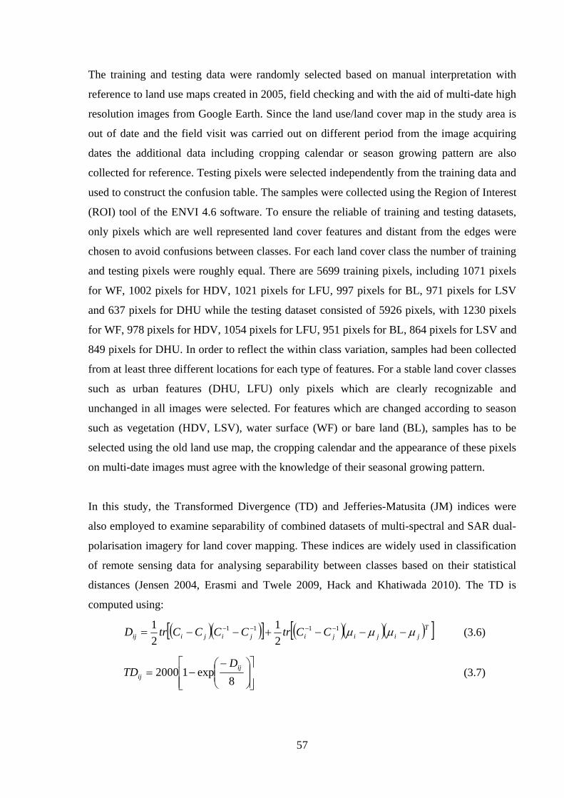
57

The training and testing data were randomly selected based on manual interpretation with

reference to land use maps created in 2005, field checking and with the aid of multi-date high

resolution images from Google Earth. Since the land use/land cover map in the study area is

out of date and the field visit was carried out on different period from the image acquiring

dates the additional data including cropping calendar or season growing pattern are also

collected for reference. Testing pixels were selected independently from the training data and

used to construct the confusion table. The samples were collected using the Region of Interest

(ROI) tool of the ENVI 4.6 software. To ensure the reliable of training and testing datasets,

only pixels which are well represented land cover features and distant from the edges were

chosen to avoid confusions between classes. For each land cover class the number of training

and testing pixels were roughly equal. There are 5699 training pixels, including 1071 pixels

for WF, 1002 pixels for HDV, 1021 pixels for LFU, 997 pixels for BL, 971 pixels for LSV

and 637 pixels for DHU while the testing dataset consisted of 5926 pixels, with 1230 pixels

for WF, 978 pixels for HDV, 1054 pixels for LFU, 951 pixels for BL, 864 pixels for LSV and

849 pixels for DHU. In order to reflect the within class variation, samples had been collected

from at least three different locations for each type of features. For a stable land cover classes

such as urban features (DHU, LFU) only pixels which are clearly recognizable and

unchanged in all images were selected. For features which are changed according to season

such as vegetation (HDV, LSV), water surface (WF) or bare land (BL), samples has to be

selected using the old land use map, the cropping calendar and the appearance of these pixels

on multi-date images must agree with the knowledge of their seasonal growing pattern.

In this study, the Transformed Divergence (TD) and Jefferies-Matusita (JM) indices were

also employed to examine separability of combined datasets of multi-spectral and SAR dual-

polarisation imagery for land cover mapping. These indices are widely used in classification

of remote sensing data for analysing separability between classes based on their statistical

distances (Jensen 2004, Erasmi and Twele 2009, Hack and Khatiwada 2010). The TD is

computed using:

( )( )[ ] ( )( )( )[ ]Tjijijijijiij CCtrCCCCtrD μμμμ −−−+−−= −−−− 1111

21

21 (3.6)

⎥⎥⎦

⎤

⎢⎢⎣

⎡⎟⎟⎠

⎞⎜⎜⎝

⎛ −−=

8exp12000 ij

ij

DTD (3.7)

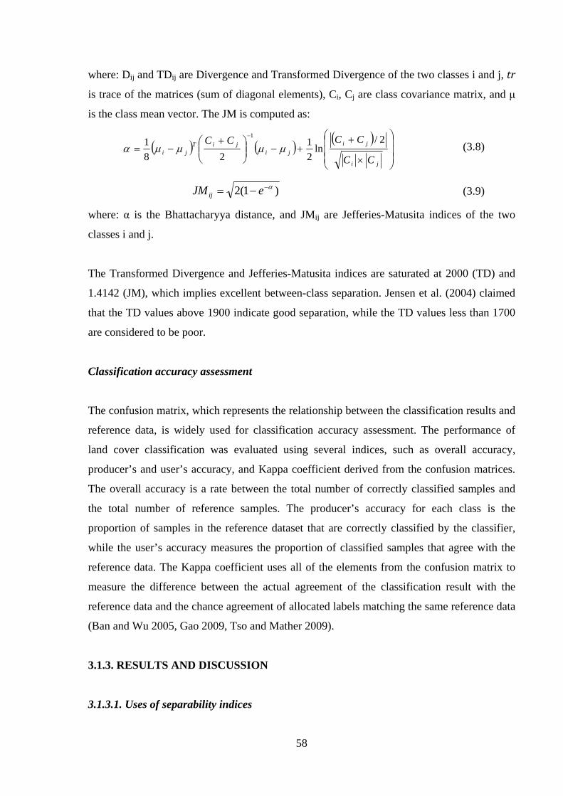
58

where: Dij and TDij are Divergence and Transformed Divergence of the two classes i and j, tr

is trace of the matrices (sum of diagonal elements), Ci, Cj are class covariance matrix, and μ

is the class mean vector. The JM is computed as:

( ) ( ) ( )⎟⎟⎟

⎠

⎞

⎜⎜⎜

⎝

⎛

×

++−⎟⎟

⎠

⎞⎜⎜⎝

⎛ +−=

−

ji

jiji

jiTji

CC

CCCC 2/ln

21

281

1

μμμμα (3.8)

)1(2 α−−= eJMij (3.9)

where: α is the Bhattacharyya distance, and JMij are Jefferies-Matusita indices of the two

classes i and j.

The Transformed Divergence and Jefferies-Matusita indices are saturated at 2000 (TD) and

1.4142 (JM), which implies excellent between-class separation. Jensen et al. (2004) claimed

that the TD values above 1900 indicate good separation, while the TD values less than 1700

are considered to be poor.

Classification accuracy assessment

The confusion matrix, which represents the relationship between the classification results and

reference data, is widely used for classification accuracy assessment. The performance of

land cover classification was evaluated using several indices, such as overall accuracy,

producer’s and user’s accuracy, and Kappa coefficient derived from the confusion matrices.

The overall accuracy is a rate between the total number of correctly classified samples and

the total number of reference samples. The producer’s accuracy for each class is the

proportion of samples in the reference dataset that are correctly classified by the classifier,

while the user’s accuracy measures the proportion of classified samples that agree with the

reference data. The Kappa coefficient uses all of the elements from the confusion matrix to

measure the difference between the actual agreement of the classification result with the

reference data and the chance agreement of allocated labels matching the same reference data

(Ban and Wu 2005, Gao 2009, Tso and Mather 2009).

3.1.3. RESULTS AND DISCUSSION

3.1.3.1. Uses of separability indices

59

Average values of TD and JM for all datasets with six land cover classes are given in Table

3.2. The averages of TD and JM indices of single-date images are ~1144 (TD) & ~0.9566

(JM), ~1085 (TD) & ~0.9457 (JM) and ~1470 (TD) & ~1.1252 (JM) for HH, HV and dual-

polarised (HH+HV), respectively.

Table 3.2: Average values of Transformed Divergence (TD) and Jefferies-Matusita

separability indices of different combined datasets.

ID Datasets TD JM

1 Five date PALSAR HH polarised images (5Date_HH) 1547 1.178

2 Five date PALSAR HV polarised images (5Date_HV) 1548 1.141

3 Five date PALSAR dual HH+HV polarised images (5Date_Dual) 1812 1.292

4 Five date PALSAR HH+ four coherence images (5date_HH +4 Coh) 1835 1.314

5 Five date PALSAR HV+ four coherence images (5date_HV +4 Coh) 1797 1.290

6 Five date PALSAR dual HH+HV polarised images + four coherence images

(5Date_Dual + 4Coh) 1923 1.351

7 Five date PALSAR HH+ ten coherence images (5date_HH +10 Coh) 1941 1.364

8 Five date PALSAR HV+ ten coherence images (5date_HV +10 Coh) 1930 1.354

9 Five date PALSAR HH + HV + ten coherence images (5date_HH+HV +10 Coh) 1974 1.383

10 SPOT2 multi-spectral images (SPOT 2 XS) 1881 1.331

11 SPOT 2 XS + single PALSAR dual-polarised HH+HV images (XS +1Date_Dual) 1992 1.396

12 SPOT 2 XS + five-date PALSAR HH polarised images (XS + 5Date_HH) 1999 1.407

13 SPOT 2 XS + five-date PALSAR HV polarised images (XS + 5Date_HV) 1914 1.366

14 SPOT 2 XS+ five-date PALSAR dual HH+HV polarised images (XS + 5Date_Dual) 2000 1.411

15 SPOT 2 XS + five-date PALSAR HH polarised images (XS + 5Date_HH+4Coh) 2000 1.412

16 SPOT 2 XS + five-date PALSAR HV polarised images (XS + 5Date_HV + 4Coh) 1951 1.388

17 SPOT 2 XS+ five-date PALSAR dual HH+HV polarised images

(XS + 5Date_Dual+ 4Coh) 2000 1.413

18 SPOT2 multi-spectral + five-date PALSAR HH polarised images + ten coherence

images (XS + 5Date_HH+10Coh) 2000 1.413

19 SPOT 2 XS + five-date PALSAR HV polarised images + ten coherence images

(XS + 5Date_HV + 10Coh) 1988 1.404

20 SPOT 2 XS + five-date PALSAR dual HH+HV polarised images

(XS + 5Date_Dual+ 10Coh) 2000 1.414

60

It appears that these indices in general are good indicator of separability between classes.

Single SAR images, no matter whether like-, cross- and dual-polarised images, gave very

poor separability. All of these images had TD values less than 1500 and JM values less than

1.2. The TD and JM values increased sharply for multi-date SAR images, which reach 1547

(TD) & 1.178 (JM) and 1548 (TD) and 1.141 (JM) for five-date HH and five-date HV data,

respectively. The five-date dual-polarised datasets further improved the separability to 1881

(TD) and 1.331 (JM). The interferometric coherence data also made a substantial

improvement of class separability when combined with multi-date SAR images. In particular,

their integration with multi-date dual-polarised SAR images provided TD and JM separability

values greater than 1900 and 1.350, respectively. These are considered to exhibit good

separation (Jensen, 2004). The SPOT 2 XS image had acceptable separability values of 1881

(TD) and 1.331 (JM), which are very close to the good separation level suggested by Jensen

(2004). It is clear that the integration of SPOT 2 XS image with multi-date SAR data gave

even higher values of separability – all of these combined datasets have TD values greater

than 1900 and six of them provided the saturated TD value of 2000, while their JM value

were also very high, and six of them had the JM values greater than 1.41 (which is very close

to the maximum value). However, it is worth noting that the average TD or JM value only

represents a general indication of separability between classes. For a detailed study the TD

and JM separability between particular pairs of classes should be investigated.

3.1.3.2. Combination of multi-date, multi-polarisation SAR images

The overall classification accuracy and Kappa coefficients for the ANN, SVM and ML

classifiers for different SAR combined datasets is summarised in Table 3.3 and Figure 3.3.

61

Table 3.3: Land cover classification accuracy of different SAR combination datasets.

Datasets

ID

SVM accuracy ANN accuracy ML accuracy

Overall (%) Kappa Overall (%) Kappa Overall (%) Kappa 1 58.12 0.50 56.87 0.48 52.57 0.43

2 54.00 0.45 50.89 0.41 53.00 0.44

3 65.51 0.59 68.16 0.62 63.35 0.56

4 71.04 0.65 65.86 0.59 70.55 0.65

5 68.87 0.63 63.25 0.56 62.98 0.56

6 75.43 0.71 74.03 0.69 62.97 0.56

7 65.51 0.59 62.94 0.55 61.59 0.54

8 58.39 0.50 59.62 0.52 57.39 0.49

9 72.31 0.67 67.99 0.62 67.06 0.61

Single-date and single-polarised SAR images provided very poor classification accuracy,

with averages of 49.35% and 45.53% using the SVM classifier for HH and HV polarised

images, respectively. The classification of a single SAR image was not possible for the ANN

and ML classifiers. The SVM classification of single-date, dual-polarised images provided an

increase of approximately 8.45% in overall accuracy. However, it is still considered to be

rather poor, with just 57.80% accuracy. Multi-date, single-polarised PALSAR images

produced some improvement in classification performance in comparison with single-date

SAR images – the classification accuracy using the SVM classifier increased by 8.77% and

8.47% for HH and HV polarised images, respectively. The SVM classifier provided a 7.71%

increase in accuracy for classifying multi-date, dual-polarised images. The improvement was

13.17% in the case of the ANN classifier. Use of multi-date, dual-polarised data resulted in a

remarkable improvement in classification accuracy as compared with using multi-date,

single-polarised datasets. The accuracy increased by 7.39% and 11.82% as compared with

multi-date HH images using SVM and ANN classifiers, respectively. The improvements

were even more significant for the multi-date HV image, with an increase of 11.51% (for

SVM classifier) and 17.27% (for ANN classifier) in classification accuracy.

Sensitivity of like- and cross-polarisation to surface and volume scattering mechanisms were

clearly demonstrated in the classification results. As can be seen in Figure 3.3 and Table 3.4,

for the SVM classifier, while the like-polarisation (HH) resulted in better accuracy for

62

classifying urban structures and bare land (which are subject to surface scattering), cross-

polarisation (HV) produced higher accuracy for both High Dense Vegetation (HDV) and Low

Sparse Vegetation (LSV) classes. The classification results of multi-date, dual-polarised

PALSAR images (Table 3.4) highlighted the complementary nature of like- and cross-

polarised SAR data. Accuracy for most land cover classes increased significantly, except for

the LSV class, compared to the case of classifying single-polarised data. These

complementary effects are also illustrated in Figure 3.3, which shows results of classification

using five-date, single-polarised (HH or HV), and five-date, dual-polarised (HH+HV) SAR

images. In the results of ANN classification, the use of SAR multi-date, dual-polarised

images also gave a remarkable improvement in classification performance as compared to the

multi-date, single-polarised images (Table 3. 5).

Table 3.4. Producer and user accuracy (%) for the SVM classifier applied to five-date

PALSAR HH, HV, and five-date PALSAR dual-polarised (HH+HV) images.

Land cover classes Five-date HH Five-date HV Five-date HH+HV

Producer User Producer User Producer User

Water Surface (WF) 40.89 76.44 47.48 76.84 47.80 85.89

Bare Land (BL) 57.73 47.91 51.21 55.59 58.15 59.72

Dense High Urban structures (DHU) 87.40 91.27 34.51 37.18 94.46 67.39

Low Flat Urban structures (LFU) 80.08 55.27 76.47 56.25 89.09 69.45

High Dense Vegetation (HDV) 48.88 48.43 54.19 52.95 57.16 65.84

Low Sparse Vegetation (LSV) 37.96 41.26 57.87 46.82 51.04 47.83

Table 3.5: Producer and user accuracy (%) for the ANN classifier applied to five-date

PALSAR HH, HV, and five-date PALSAR dual-polarised (HH+HV) images.

Land cover classes Five-date HH Five-date HV Five-date HH+HV


Water Surface (WF) 31.30 87.30 35.77 79.28 60.16 77.81

Bare Land (BL) 81.39 43.88 62.15 47.74 62.25 60.59

Dense High Urban structures (DHU) 82.21 97.90 0.00 0.00 83.98 96.61

Low Flat Urban structures (LFU) 79.32 55.88 98.29 43.02 95.54 63.53

High Dense Vegetation (HDV) 57.06 44.50 42.54 53.96 53.99 57.89

Low Sparse Vegetation (LSV) 13.77 46.12 61.69 55.87 53.82 60.94

63

Figure 3.3: Part of classification results using SVM and ANN classifiers on multi--date,

single-polarised (HH or HV), and multi-date, dual-polarised HH+HV images;

A) SPOT 2 XS false colour images, B) PALSAR HH polarised image, C) PALSAR HV

polarised image, D) SVM classification of multi-date, dual-polarised (HH+HV) images, E)

SVM classification of multi-date, single-polarised HH images, F) SVM classification of

multi-date, single-polarised HV images, G) ANN classification of multi-date, dual-polarised

(HH+HV) images, H) ANN classification of multi-date, single-polarised HH images, K)

ANN classification of multi-date, single-polarised HV images.

64

Integration of SAR interferometric coherence data with polarimetric images gave significant

increase in classification performance. For example, the combinations of five-date PALSAR

HH polarised images with four and ten coherence images resulted in a rise of 12.92% and

7.39% in the overall accuracy of the SVM classification, respectively, as compared to the

result of using only the multi-date PALSAR HH images. The increase of classification

accuracy was 9.52% and 6.6% for the ANN classifier, respectively. The integration of multi-

date PALSAR cross- and dual-polarisation images with coherence data also provided

remarkable improvements in accuracy in the range of 4.39% to 14.87%.

3.1.3.3. Combination of SAR multi-date polarisation, interferometric coherence and optical

images

Results of classification using different combinations of SAR and optical images is

summarised in Table 3.6.

Table 3.6: Land cover classification accuracy of different combinations of SPOT 2 XS and

PALSAR polarised images.

Datasets

ID

SVM accuracy ANN accuracy ML accuracy

Overall (%) Kappa Overall (%) Kappa Overall (%) Kappa 10 69.43 0.63 70.08 0.64 64.68 0.58

11 86.55 0.84 86.38 0.84 80.19 0.76

12 89.27 0.87 88.67 0.86 82.51 0.79

13 75.31 0.70 72.92 0.68 66.72 0.60

14 88.31 0.86 89.16 0.87 82.59 0.79

15 86.10 0.83 88.17 0.86 82.55 0.79

16 78.18 0.74 79.77 0.76 70.96 0.65

17 86.37 0.84 84.66 0.82 82.57 0.79

18 81.74 0.78 81.52 0.78 78.28 0.74

19 76.63 0.72 77.35 0.73 67.75 0.61

20 84.61 0.82 83.72 0.80 79.21 0.75

The SPOT multi-spectral image gave an acceptable classification accuracy using the ANN

and SVM classifier. However, as can be seen in Figure 3.4 and Table 3.7, for SPOT 2 XS

classification, the urban areas were confused with bare ground, and it was very hard to

distinguish between Dense High Urban (DHU), Low Flat Urban (LFU) and Bare Land (BL)

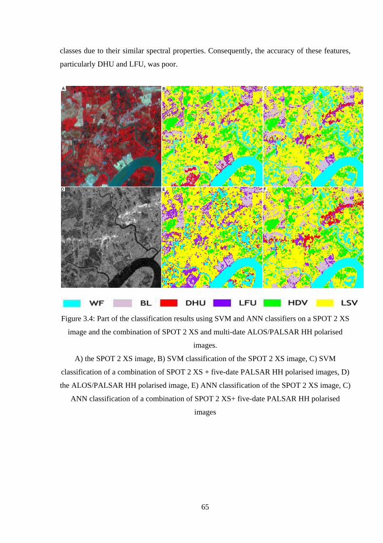
65

classes due to their similar spectral properties. Consequently, the accuracy of these features,

particularly DHU and LFU, was poor.

Figure 3.4: Part of the classification results using SVM and ANN classifiers on a SPOT 2 XS

image and the combination of SPOT 2 XS and multi-date ALOS/PALSAR HH polarised

images.

A) the SPOT 2 XS image, B) SVM classification of the SPOT 2 XS image, C) SVM

classification of a combination of SPOT 2 XS + five-date PALSAR HH polarised images, D)

the ALOS/PALSAR HH polarised image, E) ANN classification of the SPOT 2 XS image, C)

ANN classification of a combination of SPOT 2 XS+ five-date PALSAR HH polarised

images

66

Table 3.7: Producer and user accuracy for ANN and SVM classifier applied to SPOT 2 XS

multispectral images.

Land cover classes ANN SVM Producer

accuracy (%) User

accuracy (%) Producer

accuracy (%) User

accuracy (%) Water Surface (WF) 98.05 90.40 96.95 96.35

Bare Land (BL) 62.15 94.41 80.86 80.36

Dense High Urban structures (DHU) 2.47 56.76 44.17 38.11

Low Flat Urban structures (LFU) 86.05 46.47 26.94 35.68

High Dense Vegetation (HDV) 61.35 98.52 76.69 92.25

Low Sparse Vegetation (LSV) 95.83 60.70 86.89 65.47

The combination of SPOT 2 multi-spectral and multi-date SAR images gave the most

significant increase in classification accuracy, using either ANN or SVM classifiers. As can

be seen in Figures 3.4 and 3.5, and Table 3.8, confusion between BL, DHU and LFU was

significantly reduced by integrating SPOT 2 and PALSAR images because of differences in

the backscatter patterns of these features in SAR images. The highest overall accuracy was

89.27% for classifying the combined dataset of SPOT 2 + five-date PALSAR like- (HH)

polarised images using the SVM classifier. The improvements compared to the case of using

only SPOT 2 or five-date PALSAR HH images were 19.84% and 31.15%, respectively.

Table 3.8: Producer and user accuracy for ANN and SVM classifier applied to combination

of SPOT 2 XS multi-spectral and five-date PALSAR HH polarised images.

Land cover classes ANN SVM Producer

accuracy (%)

User

accuracy (%)

Producer

accuracy (%) User

accuracy (%)Water Surface (WF) 90.81 96.63 94.31 99.66

Bare Land (BL) 96.32 92.81 98.32 94.83

Dense High Urban structures (DHU) 84.45 96.89 78.45 98.09

Low Flat Urban structures (LFU) 94.50 87.91 95.45 82.12

High Dense Vegetation (HDV) 74.34 90.88 74.13 95.39

Low Sparse Vegetation (LSV) 90.51 70.45 92.36 71.76

Although the multi-date SAR, dual-polarised images (HH+HV) using SVM or ANN

classifiers provided significant improvements for classifying land cover features compared to

the single-polarised images, its combination with the optical data (SPOT 2 XS) did not yield

noticeably higher accuracy than the combination of multi-date PALSAR HH polarisation and

67

SPOT 2 XS images. Actually, this combination reduced the overall accuracy by 0.96% for

the SVM classification. However, it gave a slight increase in overall accuracy of 0.49% for

the ANN classification.

In a similar fashion, adding the interferometric coherence data to the combination of SPOT 2

XS + SAR multi-date polarised images did not further enhance the classification performance

as expected. Only the integration of interferometric coherence with the combination of SPOT

2 XS+ five-date, cross- (HV) polarised images gave a significant increase of overall

classification accuracy by 2.87% and 6.85% for SVM and ANN classifiers, respectively. In

the cases of SPOT 2 XS +like- (HH) or dual- (HH+HV) polarisation, the integration with

coherence data even noticeably decreased the classification accuracy for both SVM and ANN

classifiers.

It is also important to note that in all cases the integration of four short-term interferometric

coherence images produced better results than using all ten interferometric coherence images.

These results demonstrate that incorporation of more input data does not necessarily increase

the classification performance. It is crucial to apply appropriate techniques to select the

relevant features to be included in the classification datasets.

68

Figure 3.5: Part of classification results using SVM and ANN classifiers on a SPOT 2 XS

image and combination of SPOT 2 XS and multi-date PALSAR HH, HV polarised datasets.

A) SPOT 2 XS false colour image, B) PALSAR HH polarised image, C) PALSAR HV

polarised image, D) SVM classification of a SPOT 2 XS image, E) SVM classification of

SPOT 2 XS+ five-date PALSAR HH polarised image, F) SVM classification of SPOT 2 XS

+ five-date PALSAR HV polarised images, G) ANN classification of a SPOT 2 XS image, E)

ANN classification of SPOT 2 XS + five-date PALSAR HH polarised image, F) ANN

classification of SPOT 2 XS + five-date PALSAR HV polarised images

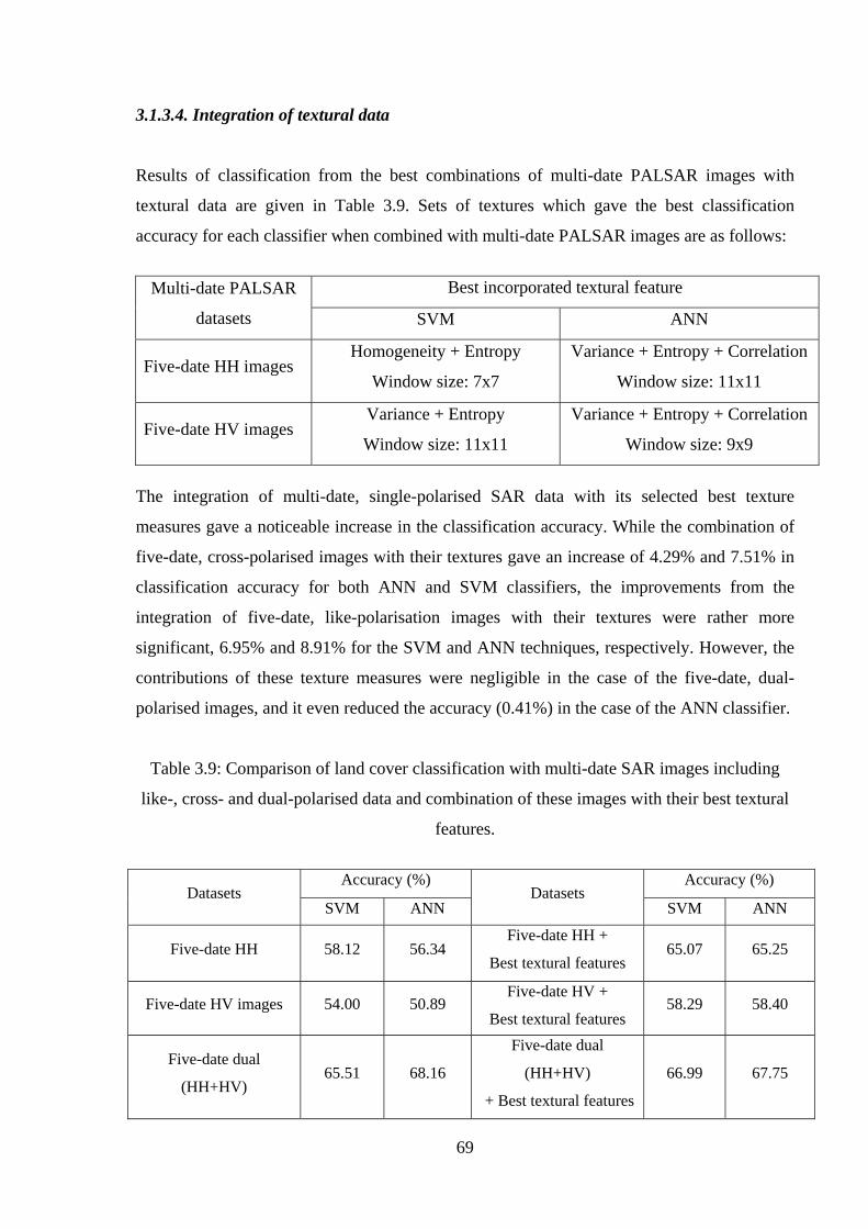
69

3.1.3.4. Integration of textural data

Results of classification from the best combinations of multi-date PALSAR images with

textural data are given in Table 3.9. Sets of textures which gave the best classification

accuracy for each classifier when combined with multi-date PALSAR images are as follows:

Multi-date PALSAR

datasets

Best incorporated textural feature

SVM ANN

Five-date HH images Homogeneity + Entropy

Window size: 7x7

Variance + Entropy + Correlation

Window size: 11x11

Five-date HV images Variance + Entropy

Window size: 11x11

Variance + Entropy + Correlation

Window size: 9x9

The integration of multi-date, single-polarised SAR data with its selected best texture

measures gave a noticeable increase in the classification accuracy. While the combination of

five-date, cross-polarised images with their textures gave an increase of 4.29% and 7.51% in

classification accuracy for both ANN and SVM classifiers, the improvements from the

integration of five-date, like-polarisation images with their textures were rather more

significant, 6.95% and 8.91% for the SVM and ANN techniques, respectively. However, the

contributions of these texture measures were negligible in the case of the five-date, dual-

polarised images, and it even reduced the accuracy (0.41%) in the case of the ANN classifier.

Table 3.9: Comparison of land cover classification with multi-date SAR images including

like-, cross- and dual-polarised data and combination of these images with their best textural

features.

Datasets Accuracy (%)

Datasets Accuracy (%)

SVM ANN SVM ANN

Five-date HH 58.12 56.34 Five-date HH +

Best textural features 65.07 65.25

Five-date HV images 54.00 50.89 Five-date HV +

Best textural features 58.29 58.40

Five-date dual

(HH+HV) 65.51 68.16

Five-date dual

(HH+HV) + Best textural features

66.99 67.75

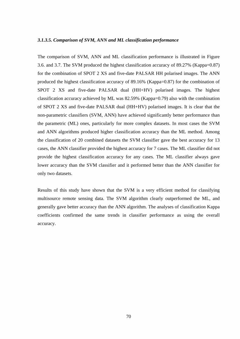
70

3.1.3.5. Comparison of SVM, ANN and ML classification performance

The comparison of SVM, ANN and ML classification performance is illustrated in Figure

3.6. and 3.7. The SVM produced the highest classification accuracy of 89.27% (Kappa=0.87)

for the combination of SPOT 2 XS and five-date PALSAR HH polarised images. The ANN

produced the highest classification accuracy of 89.16% (Kappa=0.87) for the combination of

SPOT 2 XS and five-date PALSAR dual (HH+HV) polarised images. The highest

classification accuracy achieved by ML was 82.59% (Kappa=0.79) also with the combination

of SPOT 2 XS and five-date PALSAR dual (HH+HV) polarised images. It is clear that the

non-parametric classifiers (SVM, ANN) have achieved significantly better performance than

the parametric (ML) ones, particularly for more complex datasets. In most cases the SVM

and ANN algorithms produced higher classification accuracy than the ML method. Among

the classification of 20 combined datasets the SVM classifier gave the best accuracy for 13

cases, the ANN classifier provided the highest accuracy for 7 cases. The ML classifier did not

provide the highest classification accuracy for any cases. The ML classifier always gave

lower accuracy than the SVM classifier and it performed better than the ANN classifier for

only two datasets.

Results of this study have shown that the SVM is a very efficient method for classifying

multisource remote sensing data. The SVM algorithm clearly outperformed the ML, and

generally gave better accuracy than the ANN algorithm. The analyses of classification Kappa

coefficients confirmed the same trends in classifier performance as using the overall

accuracy.

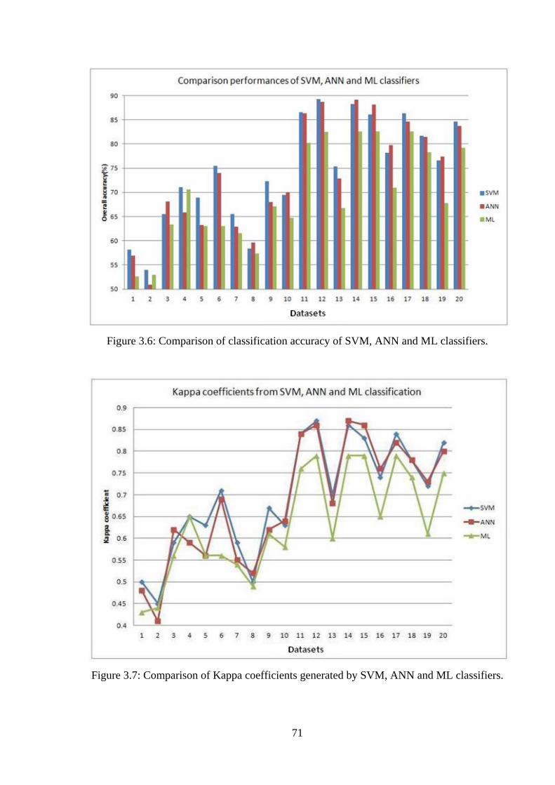
71

Figure 3.6: Comparison of classification accuracy of SVM, ANN and ML classifiers.

Figure 3.7: Comparison of Kappa coefficients generated by SVM, ANN and ML classifiers.

72

3.1.3.6. Relationship between separability indices and classification performance

The results of classification and an analysis of the separability indices have shown that, in

general, the TD and JM indices gave good indications of classification performance. Low

values of the TD or JM indices are synonymous with poor classification accuracy, while the

high values of TD or JM typically imply good classification performance. However, when the

separability values are high, these indices cannot measure the quality of classification

accurately. Many datasets, which have lower separability values, gave better classification

accuracy than those with higher TD or JM values. The other limitation of these separability

indices is that they tend to increase (even to the maximum level) as more features are

integrated into the datasets. The performance of the two indices was similar, however, the JM

was slightly better since TD index is more easily saturated than the JM index.

3.1.4. SUMMARY REMARKS

The evaluation in this study has revealed the advantages of the integrated approach,

combining multi-date, like- and cross-polarised and interferometric coherence SAR data with

optical images for mapping land cover features using non-parametric classification

algorithms. Joint application of like- and cross-polarised (or dual-polarised) SAR images

enhanced the performance of land cover mapping with respect to the case of using single-

polarised images. The dual-polarised dataset gave 65.51% and 68.16% of overall

classification accuracy for SVM and ANN classifiers, respectively, while the figure was less

than 59% for single-polarised datasets.

The combination of optical multi-spectral data and either single- or dual-polarised, as well as

multi-date, SAR images resulted in a significant improvement in classification accuracy, up

to 19.84% compared to the use of only a SPOT 2 XS image, and 31.15% compared to five-

date, single-polarised dataset. The contribution of interferometric coherence data is also

significant. Its integration with polarimetric SAR images increased the classification accuracy

dramatically. The highest classification accuracies were 75.43% (SVM) and 74.03% (ANN)

for the combination of multi-date, dual-polarised SAR images and the multi-date, short-term

coherence images. However, incorporation of these kinds of data with the combination of

SPOT 2 XS data and polarised SAR images did not produce a significant improvement

except for the case of SPOT 2 XS+ five-date, cross (HV) polarised images. Incorporation of

73

textural information with PALSAR images resulted in a considerable increase in

classification accuracy, particularly for the like-polarised images, with an improvement up to

8.91% (ANN).

The non-parametric classifiers (SVM and ANN) were successfully applied for classifying

multisource remote sensing data. The non-parametric classifiers clearly outperformed the

parametric classifiers (ML) in most cases, particularly for complex datasets. The

performances of the two non-parametric classifiers were rather comparable. However, the

SVM classifier was marginally better and in 13 out of 20 cases provided the highest accuracy.

It is also important to note that in many cases the integration of more input features did not

enhance the classification performance, occasionally reduced the classification accuracy. This

problem will be analysed and resolved in the next chapter of the thesis.

3.2. COMBINATIONS OF L- AND C-BAND SAR AND OPTICAL SATELLITE IMAGES FOR LAND COVER CLASSIFICATION IN THE RICE PRODUCTION AREA

The C-band SAR data mainly provides information on the upper layer of land cover, while

the properties of the lower surfaces can be captured using L-band SAR because of its greater

penetration capability. Hence, integration of L- and C-band SAR could enhance the capability

of land cover mapping. It is also expected that the classification performance could be further

improved by integrating multi-frequency SAR data with optical images, using an appropriate

classification algorithm such as non-parametric classifiers.

This study investigated the performance of non-parametric classifiers, including SVM and

ANN algorithms, to classify various land cover features in the south of Vietnam using a

multi-temporal/dual-frequency combination of ALOS/ PALSAR (L-band) radar,

ENVISAT/ASAR (C-band) radar and SPOT 4 multi-spectral optical satellite data. The

classification processes were carried out for selected single, and combined datasets. The

classification results of the SVM and ANN algorithms were compared with results of the

traditional parametric ML classifier.

74

3.2.1. STUDY AREA AND DATA USED

The study area is located within the borders between Tien Giang and Long An provinces and

Ho Chi Minh City in the South of Vietnam. The centred coordinate is 106o40’ E and 10o 25’

N. This area is typical for the rural area in the Mekong Delta region which is characterised by

very flat terrain and high fertility. It is the most important rice production region of the

country. The main land use/cover types are rice, mangrove, residential areas and water

surfaces.

Four ALOS/PALSAR (L-band) HH polarisation images acquired between June 2007 and

June 2008, and four ENVISAT/ASAR (C – band) HH polarisation images acquired for a

similar period (from May 2007 to July 2008) were used for this study (Table 3.10).

A SPOT 4 multispectral (SPOT 4 XS) image has similar properties as previous generations

(SPOT 1, 2 and 3) with a spatial resolution of 20m. However, instead of having only three

spectral bands – Green (G), Red (R) and Near-Infrared (NIR) – it has a fourth band obtained

in the shortwave infrared region (SWIR) of the spectrum. The SPOT 4 XS image for this

study was acquired on December 09, 2007 (Figure 3.8).

Table 3.10: ALOS/PALSAR and ENVISAT/ASAR images for the study area.

Sensors Date of Acquisition Orbit Wavelengths Polarisation

ALOS/PALSAR

08 Jun 2007 Ascending L HH 08 Sep 2007 Ascending L HH 09 Dec 2007 Ascending L HH 10 Jun 2008 Ascending L HH

ENVISAT/ASAR

30 May 2007 Ascending C HH 12 Sep 2007 Ascending C HH 26 Dec 2007 Ascending C HH 23 Jul 2008 Ascending C HH

75

Figure 3.8: SPOT 4 multispectral false colour image (left) and ALOS/PALSAR HH

polarisation image (right), both images acquired on December 09, 2007.

3.2.2. METHODOLOGY

The geo-rectification of ALOS/PALSAR and SPOT 4 XS images was carried out similarly to

the process described early in the section 3.1.2. The ENVISAT/ASAR images were firstly

geo-rectified using the Nest 4.0 software and then co-registered to the ALOS/PALSAR

images using the same procedure. All data were re-sampled to a pixel size of 25m.

ALOS/PALSAR and ENVISAT/ASAR backscatter data were converted to decibel (dB) and

filtered using the Enhanced Lee filter with 5x5 window size.

Although rice is largely predominant in the study area, the cultivated cycles vary depending

on each land holder. Thus, rice fields appear differently in any single-date image. As in the

case of the SPOT 4 multispectral image, the rice areas were currently growing rice, harvested

(temporally dry bare ground), or filled with water. Hence, the use of multi-date data is more

effective than single-date data for rice area mapping. For this reason this study employed

multi-temporal SAR images together with optical images to map land cover features. The

capability of single-date SAR image for classifying land cover classes was also evaluated,

based on a SAR image acquired on a similar date to the SPOT 4 images in December, 2007.

Grey Level Co-occurrence Matrix (GLCM) textures were generated for each data type with

different window sizes (3x3, 5x5, 7x7 and 9x9). Four texture measures, namely variance,

76

homogeneity, entropy and correlation, were selected because of their low correlation with

respect to each other.

Since the rice fields appear differently in images acquired at different dates, the

classifications were carried out in two steps. At the beginning, seven land cover classes were

defined for classification – Dense Residence (DR), Medium Sparse Residence (MR), Water

Body (WB), Mangrove (MG), Current Rice Field (CR), Rice Temporal Wet (RW) and Rice

Temporal Bare Ground (RG). After the classification process, Current Rice Field, Rice

Temporal Wet, Rice Temporal Bare Ground were merged together to form only one class:

Rice Field (RF). The spectral and backscatter properties of these classes are presented in

Figure 3.9 and 3.10.

The classification process was implemented on different datasets, including single- and multi-

date SAR images, SPOT 4 images, combination of multi-date ASAR+PALSAR data,

combination of SPOT 4 and multi-date SAR images. Similar to the previous section, SVM

using the Radical Basic Function (RBF) Kernel and ANN using the MLP-BP algorithm were

employed for classifying land cover features. The cross-validation technique was applied to

optimise parameters for the SVM classifier. Classifications using ML classifier were also

carried out for comparison. Training and testing datasets were collected based on manual

interpretation with reference to the available land use map created in 2005 over the study area

and from a study of multi-date Google Earth images as described earlier in the section 3.1.2.

77

3.2.3. RESULTS AND DISCUSIONS

Figure 3.9: Spectral properties of different land cover classes in the SPOT 4 XS image.

Figure 3.10: Backscatter properties of different land cover classes in the multi-date L- and C-

band SAR images (Lx_HH and Cx_HH represent L and C band HH polarised images,

respectively).

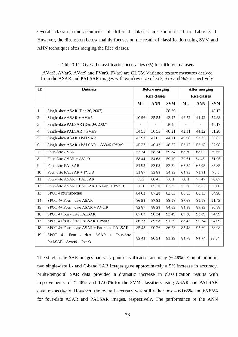
78

Overall classification accuracies of different datasets are summarised in Table 3.11.

However, the discussion below mainly focuses on the result of classification using SVM and

ANN techniques after merging the Rice classes.

Table 3.11: Overall classification accuracies (%) for different datasets.

AVar3, AVar5, AVar9 and PVar3, PVar9 are GLCM Variance texture measures derived from the ASAR and PALSAR images with window size of 3x3, 5x5 and 9x9 respectively.

ID Datasets Before merging

Rice classes

After merging

Rice classes

ML ANN SVM ML ANN SVM

1 Single-date ASAR (Dec 26, 2007) - - 38.26 - - 48.17

2 Single-date ASAR + AVar5 40.96 35.55 43.97 46.72 44.92 52.98

3 Single-date PALSAR (Dec 09, 2007) - - 36.8 - - 48.17

4 Single-date PALSAR + PVar9 34.55 36.55 40.21 42.31 44.22 51.28

5 Single-date ASAR +PALSAR 43.92 42.01 44.11 49.98 52.73 53.83

6 Single-date ASAR +PALSAR + AVar5+PVar9 45.27 46.42 48.87 53.17 52.13 57.98

7 Four-date ASAR 57.74 58.24 59.84 68.30 68.02 69.65

8 Four-date ASAR + AVar9 58.44 54.68 59.19 70.61 64.45 71.95

9 Four-date PALSAR 51.93 53.08 52.32 65.34 67.05 65.85

10 Four-date PALSAR + PVar3 51.87 53.88 54.83 64.95 71.91 70.0

11 Four-date ASAR + PALSAR 65.2 66.45 66.1 66.1 77.47 78.87

12 Four-date ASAR + PALSAR + AVar9 + PVar3 66.1 65.30 63.35 76.76 78.62 75.06

13 SPOT 4 multispectral 84.63 87.28 83.63 86.53 88.13 84.98

14 SPOT 4+ Four - date ASAR 86.58 87.83 88.98 87.68 89.18 91.43

15 SPOT 4+ Four - date ASAR + AVar9 82.87 88.28 84.63 84.88 89.83 86.88

16 SPOT 4+four - date PALSAR 87.03 90.34 93.49 89.28 93.89 94.99

17 SPOT 4+four - date PALSAR + Pvar3 86.33 89.58 91.59 88.43 90.74 94.09

18 SPOT 4+ Four - date ASAR + Four date PALSAR 85.48 90.26 86.23 87.48 93.69 88.98

19 SPOT 4+ Four - date ASAR + Four-date

PALSAR+ Avart9 + Pvar3 82.42 90.54 91.29 84.78 92.74 93.54

The single-date SAR images had very poor classification accuracy (~ 48%). Combination of

two single-date L- and C-band SAR images gave approximately a 5% increase in accuracy.

Multi-temporal SAR data provided a dramatic increase in classification results with

improvements of 21.48% and 17.68% for the SVM classifiers using ASAR and PALSAR

data, respectively. However, the overall accuracy was still rather low – 69.65% and 65.85%

for four-date ASAR and PALSAR images, respectively. The performance of the ANN

79

classifier was similar with the SVM classifier for multi-date SAR data with an overall

accuracy of 68.00% for ENVISAT/ASAR and 67.05% for ALOS/PALSAR images. The

confusion matrices, which showed classification accuracy of the SVM and ANN classifiers

on four-date ENVISAT/ASAR and four-date ALOS/PALSAR image, for each land cover

class, are listed in Tables 3.12 – 3.15.

Table 3.12: Confusion matrix for SVM classification using four-date ENVISAT/ASAR HH

polarised images. Land cover classes RF WB MG MR DR User’s accuracy (%)

RF 715 27 59 77 9 80.61

WB 33 299 0 0 0 90.06

MG 64 0 130 76 13 45.94

MR 103 0 59 143 78 37.34

DR 0 0 0 8 104 92.86

Producer’s accuracy (%) 78.14 91.72 52.42 47.04 50.98 Overall accuracy 69.65

Table 3.13: Confusion matrix for ANN classification using four-date ENVISAT/ASAR HH


RF 643 9 35 49 1 87.25

WB 34 317 0 0 0 90.31

MG 111 0 132 74 13 40.00

MR 127 0 81 175 99 36.31

DR 0 0 0 6 91 93.81


Table 3.14: Confusion matrix for SVM classification using four-date ALOS/PALSAR HH


RF 716 37 56 17 8 85.85

WB 83 275 0 0 0 76.82

MG 51 0 30 41 25 20.41

MR 17 0 162 243 78 44.83

DR 48 14 0 3 51 43.97


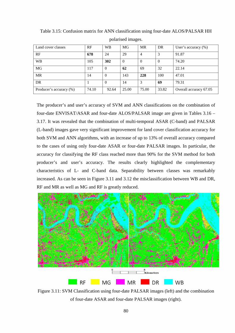
80

Table 3.15: Confusion matrix for ANN classification using four-date ALOS/PALSAR HH


RF 678 24 29 4 3 91.87

WB 105 302 0 0 0 74.20

MG 117 0 62 69 32 22.14

MR 14 0 143 228 100 47.01

DR 1 0 14 3 69 79.31


The producer’s and user’s accuracy of SVM and ANN classifications on the combination of

four-date ENVISAT/ASAR and four-date ALOS/PALSAR image are given in Tables 3.16 –

3.17. It was revealed that the combination of multi-temporal ASAR (C-band) and PALSAR

(L-band) images gave very significant improvement for land cover classification accuracy for

both SVM and ANN algorithms, with an increase of up to 13% of overall accuracy compared

to the cases of using only four-date ASAR or four-date PALSAR images. In particular, the

accuracy for classifying the RF class reached more than 90% for the SVM method for both

producer’s and user’s accuracy. The results clearly highlighted the complementary

characteristics of L- and C-band data. Separability between classes was remarkably

increased. As can be seen in Figure 3.11 and 3.12 the misclassification between WB and DR,

RF and MR as well as MG and RF is greatly reduced.

Figure 3.11: SVM Classification using four-date PALSAR images (left) and the combination

of four-date ASAR and four-date PALSAR images (right).

81

Figure 3.12: ANN Classification using four-date PALSAR images (left) and the combination

of four-date ASAR and four-date PALSAR images (right).

Table 3.16: Confusion matrix for SVM classification using four-date ALOS/PALSAR HH &

four-date ENVISAT/ASAR polarised images. Land cover classes RF WB MG MR DR User’s accuracy (%)

RF 847 17 36 27 11 90.30

WB 34 309 0 0 0 90.09

MG 9 0 95 35 14 62.09

MR 4 0 116 235 90 52.81

DR 21 0 1 7 89 75.42


Table 3.17: Confusion matrix for ANN classification using four-date ALOS/PALSAR HH &

four-date ENVISAT/ASAR polarised images. Land cover classes RF WB MG MR DR User’s accuracy (%)

RF 852 62 44 36 13 84.61

WB 20 264 0 0 0 92.96

MG 31 0 71 20 8 54.62

MR 12 0 133 239 62 53.59

DR 0 0 0 9 121 93.08


82

Results of classifications using SVM and ANN classifiers on the SPOT 4 XS image and its

combinations with four-date ALOS/PALSAR images, which produced highest classification

accuracy, are presented in Figures 3.13, 3.14 and Tables 3.18 - 3.21.

Figure 3.13: ANN classification using the SPOT 4 multi-spectral image (left) and

combination of SPOT 4 and four-date PALSAR images (right).

Figure 3.14: SVM classification using the SPOT 4 multi-spectral image (left) and

combination of SPOT 4 and four-date PALSAR images (right).

83

Table 3.18: Confusion matrix for ANN classification using SPOT 4 XS images.

Land cover classes RF WB MG MR DR User’s accuracy (%)

RF 840 44 16 65 15 85.71

WB 16 282 0 0 0 94.63

MG 0 0 232 0 0 100.00

MR 57 0 0 217 0 79.20

DR 2 0 0 22 189 88.73


Table 3.19: Confusion matrix for SVM classification using SPOT 4 XS images. Land cover classes RF WB MG MR DR User’s accuracy (%)

RF 757 48 1 27 12 89.59

WB 16 278 0 0 0 94.56

MG 0 0 231 0 0 100.00

MR 105 0 0 240 1 69.36

DR 37 0 16 37 191 67.97


Table 3.20: Confusion matrix for ANN classification using SPOT 4 XS images and four-date

ALOS/PALSAR polarised images. Land cover classes RF WB MG MR DR User’s accuracy (%)

RF 866 32 0 11 1 95.16

WB 15 294 0 0 0 95.15

MG 0 0 248 0 0 100.00

MR 26 0 0 270 6 89.40

DR 8 0 0 23 197 86.40


Table 3.21: Confusion matrix for SVM classification using SPOT 4 XS images and four-date

ALOS/PALSAR polarised images. Land cover classes RF WB MG MR DR User’s accuracy (%)

RF 894 30 10 9 4 94.40

WB 14 296 0 0 0 95.48

MG 0 0 237 0 0 100.00

MR 4 0 1 288 18 92.60

DR 3 0 0 7 182 94.79


84

Both ANN and SVM classifiers performed well with the SPOT 4 XS image, the overall

accuracy being 87.83% and 84.98% using ANN and SVM classifiers, respectively. However,

they produced a large amount of confusion between MR and RF due to the mixed of houses

and vegetation in the MR class.

The combination of optical and multi-temporal SAR images produced the most significant

improvement for classification accuracy. For example, the SVM classifier resulted in

increases in classification accuracy of 6.45% and 23.13% (SPOT 4 XS + ASAR) and 10.01%

and 29.4% (SPOT 4 XS + PALSAR) in comparison to the cases of using only SPOT 4 XS,

ASAR or PALSAR images. The integration of optical data with SAR images, no matter

whether C- or L-band, effectively reduced confusion between classes. The separability

between RF and MR increased noticeably for these combined dataset. It is interesting to note

that, while the classification accuracy of four-date PALSAR image was about 3% less than

the case of using four-date ASAR images, its integration with SPOT 4 images gave a little

higher accuracy for the combination of the four-date ASAR and the SPOT 4 images. The

possible reason is that the ASAR data with shorter wavelength appeared to be more highly

correlated with SPOT 4 XS data. The integration of SPOT 4 and both L- and C-band SAR

images also resulted in significantly increased classification accuracy compared to any single

kind of data. However, it provided less accuracy than from the integration of the SPOT 4 XS

image with either L- or C-band SAR data.

Integration of textural information

The integration of SAR backscattered data with their derived textural information was carried

out by gradually adding textural measures to the original datasets for classification. Results of

tests for different texture measures showed that the performance of variance was better than

other measures. However, the optimum window sizes were different for each combination.

The best window size to extract variance for the ASAR image on December 26, 2007 was

5x5, while it was 9x9 for the December 09, 2007 PALSAR image, and 3x3 for the four-date

PALSAR dataset. The tests on combinations of all of four texture measures did not give any

further improvement on the classification accuracy compared to a case of using only

variance. Texture information improved classification accuracy by 3 ~5% for the single SAR

images, four-date ASAR and four-date PALSAR images. However, no significant

85

improvement was found for the combination of multi-date ASAR + PALSAR or SPOT 4 XS

+ SAR datasets.

Performance of non-parametric and parametric algorithm

Results of classification using non-parametric (SVM, ANN) and parametric (ML) techniques

clearly showed that in most cases the SVM and ANN classifiers resulted in better

classification accuracy than the ML classifier (Figure 3.15). The SVM classifiers gave the

highest classification accuracy for 13 out of 19 cases, while the ANN classifier provided the

best accuracy for the six remaining cases. There are no cases for which the ML classifier

gave the highest accuracy. The highest classification accuracy was 94.99% for the SVM

classifier using the combination of SPOT 4 XS data + four-date PALSAR HH images. The

highest classification accuracy for ANN and ML classifier were 93.89% and 89.28%,

respectively. These results demonstrate that the SVM and ANN classifiers are very suitable

for classifying remote sensing data, particularly complex integration datasets.

Figure 3.15: Comparison of classification accuracy of SVM, ANN and ML classifiers after

merging rice classes (only combined datasets with at least two input features are presented).

42

52

62

72

82

92

4 5 6 7 8 9 10 11 12 13 14 15 16 17 18 19

Overall accuracy

Copmbined datasets

Comparison of performances of SVM, ANN and ML classifiers

SVM_Mg

ANN_Mg

ML_Mg

86

3.2.4. SUMMARY REMARK

The investigation has confirmed the advantages of combinations of multi-date, dual-

frequency SAR data as well as multi-date, dual-frequency SAR and optical data, for land

cover mapping in a complex rural area such as in the south of Vietnam. The integrated

approach always produced substantial increases in classification accuracy with respect to

cases of single datasets. The performance of non-parametric classifiers (SVM and ANN) is

better than the traditional ML classifier. The highest classification accuracy of 94.99% was

achieved using the SVM algorithm and the combination of SPOT 4 XS data and multi-date

PALSAR HH images. Therefore, theses non-parametric classifiers are considered more

appropriate for handling multisource remote sensing data.

However, as already mentioned in the previous section, in many cases the integration of more

features did not improve (and in some cases actually reduced) the classification accuracy.

This suggests the need for further studies to resolve this problem.

3.3. USES OF MULTI-TEMPORAL SAR AND INTERFEROMETRIC COHERENCE DATA FOR MONITORING THE 2009 VICTORIAN BUSHFIRES

In this section the application of multisource remote sensing data for a special case of land

cover mapping was investigated – the mapping of a burned area after bushfire. The

multisource data used for this study were multi-temporal SAR backscatter imagery and their

derived interferometric coherence data.

3.3.1. INTRODUCTION

In 2009 Australia experienced one of its historically worst natural disasters – The Victorian

Bushfires. The impact of this disaster was catastrophic. A total of 173 lives were lost, many

properties were damaged, and large areas of natural forests were severely destroyed. These

facts had emphasised needs for bushfire detection and monitoring. Optical satellite imagery

such as Landsat TM, SPOT, MODIS has been used extensively for forest fire mapping and

often give good results. However, the optical system can only operate during the day and

sensors may not “see” through clouds and smoke. Consequently it may not be possible to

observe the ground surface. In contrast, SAR systems operating in a microwave part of the

87

electromagnetic spectrum can image Earth’s surface at anytime with minimal impact from

clouds and smoke. Hence SAR imaging is appropriate for forest fire detection and the

mapping of burnt areas.

Use of SAR data for forest fire detection and burnt area mapping has been reported by a

number of investigators (Gimeno et al. 2004, Siegert and Hoffmann 2000, Siegert and

Ruecker 2000, Takeuchi and Yamada 2002, Almeida-Filho et al. 2007, Almeida-Filho et al.

2009). These studies mainly relied on differences in backscatter intensities between before

and after fire images to detect and map burnt areas. In Siegert and Rueker (2000), multi-

temporal ERS-2 SAR images were employed to identify burnt scars over a study site in east

Kalimantan, Indonesia. It was found that backscatter decreased by 2-5 dB in fire impacted

areas, while there was only a slight change in backscatter (less than 0.5 dB) for non-fire

impacted areas. Gimeno et al. (2004) reported that the changes of backscatter between

forested and fire-disturbed zones were up to +8 dB in ERS time series data for Mediterranean

forest regions. However, results of work carried out by Takeuchi and Yamada (2002) showed

a slight decrease in backscatter of JERS-1 SAR data after fire, but the difference was not

large enough to identify fire affected areas. Siegert and Hoffmann (2000) suggested that two

types of fire damage areas can be detected, severe damage with complete burning of

vegetation and medium damage with partly burnt vegetation. The first case related to a strong

decrease in backscatter while the latter related to areas with little change in backscatter.

Takeuhi and Yamada (2002) employed interferometric coherence SAR data for forest fire

damage monitoring. They reported a significant increase in coherence in damaged areas after

the fire allowing better interpretation and extraction of burnt areas compared to using

backscatter data. Antikidis et al. (1998) evaluated the capabilities of interferometric Tandem

ERS SAR data for mapping deforestation areas in Indonesia. It was found that there were

clear changes in coherences between images acquired before and after a fire event. The

objective of this study is to analyse the capabilities of multi-temporal SAR data, particularly

ALOS/PALSAR images, to identify burnt areas resulting from the Victorian Bushfires in

February 2009. The combination of SAR backscatter intensity and interferometric coherence

data is also a goal of the research.

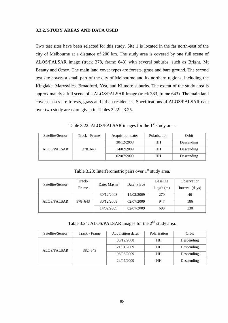
88

3.3.2. STUDY AREAS AND DATA USED

Two test sites have been selected for this study. Site 1 is located in the far north-east of the

city of Melbourne at a distance of 200 km. The study area is covered by one full scene of

ALOS/PALSAR image (track 378, frame 643) with several suburbs, such as Bright, Mt

Beauty and Omeo. The main land cover types are forests, grass and bare ground. The second

test site covers a small part of the city of Melbourne and its northern regions, including the

Kinglake, Marysviles, Broadford, Yea, and Kilmore suburbs. The extent of the study area is

approximately a full scene of a ALOS/PALSAR image (track 383, frame 643). The main land

cover classes are forests, grass and urban residences. Specifications of ALOS/PALSAR data

over two study areas are given in Tables 3.22 – 3.25.

Table 3.22: ALOS/PALSAR images for the 1st study area.

Satellite/Sensor Track - Frame Acquisition dates Polarisation Orbit

ALOS/PALSAR 378_643

30/12/2008 HH Descending



Table 3.23: Interferometric pairs over 1st study area.

Satellite/Sensor Track-

Frame Date: Master Date: Slave

Baseline

length (m)

Observation

interval (days)

ALOS/PALSAR 378_643

30/12/2008 14/02/2009 270 46

30/12/2008 02/07/2009 947 186

14/02/2009 02/07/2009 680 138

Table 3.24: ALOS/PALSAR images for the 2nd study area.

Satellite/Sensor Track - Frame Acquisition dates Polarisation Orbit

ALOS/PALSAR 382_643





89

Table 3.25: Interferometric pairs over 2nd study area.

Satellite/Sensor Track-

Frame Date: Master Date: Slave

Baseline

length (m)

Observation

interval(days)

ALOS/PALSAR 378_643

06/12/2008 21/01/2009 304 46

06/12/2008 08/03/2009 878 92

06/12/2008 24/07/2009 1510 230

21/01/2009 08/03/2009 579 46

21/01/2009 24/07/2009 1196 184

08/03/2009 24/07/2009 626 138

Site 1: Landsat 5 TM acquired on 24/01/2009 and 25/02/2009.

Site 2: Landsat 5 TM acquired on 31/01/2009 and 16/12/2009.

These images were acquired before and just after the bushfire.

3.3.3. METHODOLOGY

All ALOS/PALSAR satellite images, including intensities and coherence data, were

registered to the map coordinate system (UTM projection, WGS84 datum) with 30m spatial

resolution. Speckle noise in the PALSAR images was filtered out using the Enhanced Frost

Filter with a 5x5 window size. SAR backscatter values are converted to decibel (dB) using

Equation (3.1). The Temporal Backscatter Changed images were generated using the

following relation (Chu and Ge 2010a):

SARCH= Max(Db1, Db2,.., Dbn) – Min(Db1, Db2 …, Dbn) (3.13)

where SARCH is the Temporal Backscatter Change images, Db1, Db2 …Dbn are pixel

backscatter values in SAR images, Max and Min are the functions to obtain the largest and

smallest pixel’s values within all images.

The SARCH image is in fact a modification of the intensity differencing technique. It allows

selection of the largest changes of pixel values between multi-temporal images. This image is

therefore very useful for change detection. As mentioned earlier, interferometric coherence

between pairs of SAR images is valuable data for burnt forest mapping/monitoring. The

coherence images measure the correlation between two images. In the coherence images

stable objects appear bright with high coherence value, while changed objects appear darker

with low coherence value. Hence it is expected that the coherence of pixels in fire areas will

90

be low or reduced compared to areas that have not changed. Moreover, the coherence of

pixels in a burnt area in a pair of across fire SAR images would be lower than the coherence

in a pair of before fire or after fires images. In this study the coherence data over two test

sites were analysed in conjunction with backscatter intensity data. Utilisation of the Principal

Component Analysis (PCA) for forest fire monitoring has been reported by researchers

(Siegert and Hoffmann 2000, Gimeno et al. 2004). It is revealed that PCA products generated

from multi-temporal SAR images could be applied for change detection, particularly for

bushfire mapping. The First Component PC1, and sometime even the Second Component

PC2, often represent non-changed features. Other components contain variations due to

changes in the ground surface.

Visual interpretation is an important step for detecting and collecting relevant information

about fire affected areas and other land cover features. Earlier studies have shown that the use

of multi-temporal SAR data improved feature discrimination in comparison to using single-

scene/date data (Gimeno et al. 2004). It is also revealed that more features can be

distinguished in the RGB composites than in a single image. In this study, burnt areas and

other land cover classes were identified by visual interpretation of RGB composites, in which

Red, Green and Blue colour channels were assigned to different dated SAR images or their

derived products (SARCH, PC components or average of multi-date SAR images). Then,

properties of burnt areas as well as other features were extracted for analysis and

classification.

Classification

Three classification techniques, namely the Maximum Likelihood (ML), Artificial Neural

Network (ANN) and Support Vector Machine (SVM), were applied for burn scar

identification. The classification results were compared with the burnt areas derived from

Landsat TM data.

Validation

Due to a lack of ground truth data, the Landsat TM images acquired before and after the fire

event was used for validation at both study sites. It is fortunate that burnt areas appear very

clearly in these optical images. Firstly, the Normalised Difference Vegetation Index (NDVI)

91

was computed for each Landsat image. Then pre- and post-fire NDVIs were subtracted from

each other to create the NDVI difference images. Finally, the NDVI difference image was

segmented to extract burnt areas, which were then used for testing the results of burn area

mapping with ALOS/PALSAR backscatter images and its coherence data.


In both test sites uses of the RGB colour composite generated from original SAR backscatter

images (Figure 3.16) did not provide good separation between fire damaged areas and other

features. In these colour composite images burnt areas appeared in light purple or pink

colour, however the difference was relatively small and it was easy to confuse the similar

colours.

Figure 3.16: A) and C) showed fire affected areas are in purple to pink colour in multi-date

colour composites in 1st and 2nd study sites. B) and D) showed burnt area (dark colour) in

corresponding false colour Landsat TM images.

92

The temporal backscatter change images SARCH over the two study areas were generated

from multi-date SAR images. These images showed some burnt areas more clearly in very

bright tones, significantly different from surrounding features. However, other changed

features which were not subjected to fires also appear bright and it is difficult to differentiate

these changed features from the burnt areas.

An evaluation on all of interferometric coherence images revealed that, for both study sites

the coherence images generated from pairs of images acquired just before and after the

bushfire were useful. Burnt areas appear very dark due to low coherence between pre- and

post-fire events and are rather well separated from surrounding areas. Nevertheless, other

features such as unburnt forest may also exhibit low coherence due to natural de-correlation

factors (winds, changing of leaf position, etc.) and consequently appear similar in the

coherence data. Therefore the combination of backscatter intensity and interferometric

coherence data was applied and gave much better results compared to using any single

dataset. Based on this strategy the most useful RGB colour composite was found, where: Red

was assigned to Average SAR images (or the PC1 component), Green was assigned to

Temporal Backscatter Change images (SARCH) and Blue was assigned to interferometric

coherence data generated from an across-fire image pair. This RGB composite (Figure 3.17)

showed burnt areas in Yellow to Little Red colour due to strong backscatter (Red), large

changes (Green) and low coherence (Blue).

93

Figure 3.17: A) and C) are RGB colour composites of Average SAR image (R), Temporal

Backscatter Change (G) and across-fire coherence data (B) in 1st and 2nd study sites. Burnt

areas appear Yellow to Reddish in colour in A) and C) RGB composites.

PCA images were generated from multi-date SAR backscatter images. The PC1 components

were very similar with the average of all SAR images, and the PC3 and PC2 components

contained changed information useful for the first and second sites, respectively. However,

information on changed features can be readily obtained from the temporal backscatter

change image without concerns about noise as in the case of the PC2, PC3 components.

Based on visual interpretation several land cover classes were developed for each test site.

Site 1: Highly_burnt forest, Shadow_burnt, Un_burnt forest, Grass and Bare_ground.

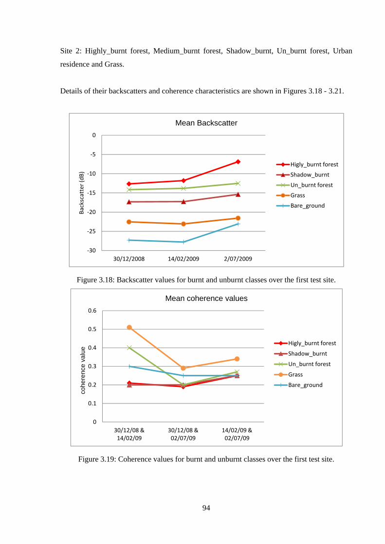
94

Site 2: Highly_burnt forest, Medium_burnt forest, Shadow_burnt, Un_burnt forest, Urban

residence and Grass.

Details of their backscatters and coherence characteristics are shown in Figures 3.18 - 3.21.

Figure 3.18: Backscatter values for burnt and unburnt classes over the first test site.

Figure 3.19: Coherence values for burnt and unburnt classes over the first test site.

‐30

‐25

‐20

‐15

‐10

‐5

0

30/12/2008 14/02/2009 2/07/2009

Backscatter (dB

)

Mean Backscatter

Higly_burnt forest

Shadow_burnt

Un_burnt forest

Grass

Bare_ground

0

0.1

0.2

0.3

0.4

0.5

0.6

30/12/08 & 14/02/09

30/12/08 & 02/07/09

14/02/09 & 02/07/09

cohe

renc

e va

lue

Mean coherence values

Higly_burnt forest

Shadow_burnt

Un_burnt forest

Grass

Bare_ground

95

Figure 3.20: Backscatter values for burnt and unburnt classes over the second test site.

Figure 3.21: Coherence values for burnt and unburnt classes over the second test site.

It is interesting to note that the backscatter increased after the bushfires over both study sites.

The reason is that in the case of the 2009 Victorian Bushfires for many regions only leaves or

parts of leaves burned while tree trunks remained. Consequently, there are strong corner

‐25

‐20

‐15

‐10

‐5

0

6/12/2008 12/01/2009 8/03/2009 24/07/2009

Back

scat

ter (

dB)

Mean Backscatter

Higly_burnt forest

Medium_burnt forest

Shadow_burnt

Un_burnt forest

Urban Residene

Grass

96

reflector effects in the SAR images resulting from an increase in backscatter. For the second

test site, as Highly-burnt forest and Medium-burnt forest were identified based on the level of

severity of burning and can be detected. The most challenging task was to identify the burnt

areas which were in shadow areas. To map this class it was necessary to analyse the terrain. It

is clear that coherence values of fire affected areas were very low across the fire image pairs

(30/12/2008 and 14/02/2009 in first test site, and 12/01/2009 and 08/03/2009 in the second

test site) making them distinguishable from other features.

The classification process was performed over the two test sites with classes mentioned

previously. At the last steps, classification results were merged into only two classes, namely

Burnt and Unburnt classes. This final result was then compared with the burnt areas extracted

from the Landsat TM images. Since it was cloudy in the lower part of the Landsat TM image

(acquired on 25/02/2009) over the first site, the Landsat TM data for this site was only used

for general comparison. Quantitative assessment was carried out only over the second test

site. The following datasets were selected for classification:

Case 1: All PALSAR backscatter data

Case 2: Combination of Average SAR image + Backscatter Change Image + across-fire

coherence images

Case 3: All PALSAR backscatter data + selected coherence images (before + across + after

fire data)

Results of burnt areas classification are given in Table 3.26 and Figure 3.22.

Table 3.26: Overall classification accuracy assessment for various combined datasets and

classifiers over the second test site. Classifiers/ Datasets ML ANN SVM

Case 1 81.11 % 80.49 % 81.26 %

Case 2 84.50 % 81.25 % 84.90 %

Case 3 85.42 % 80.47 % 84.35 %

It is clear that in general the results of Burnt/Unburnt mapping using multi-temporal SAR

images agreed well with the results derived from Landsat TM images (over 80% agreement).

The use of combined SAR backscatter and coherence data improved the classification

accuracy by more than 4% for the ML and SVM classifiers. Although it is expected that the

97

ANN and SVM classifiers would give higher accuracy than the traditional ML classifier, it is

not a case for this study. The classification accuracy for ML and SVM classifiers was very

similar, but it was noticeably decreased for the ANN classifier. The reason could be the

nature of the validation data generated from the Landsat TM images, which may not

represent burnt areas accurately. Availability of ground truth data would have allowed better

accuracy assessment.

Figure 3.22: A) Burnt scars extraction from Landsat TM images, B) Burnt scars extraction

based on SVM classification (case 3), the Red areas represent burnt scars.

3.3.5. SUMMARY REMARKS

The integration of multi-temporal ALOS/PALSAR backscatter intensity images and

interferometric coherence data has been proposed and applied successfully to identify and

map the 2009 Victorian Bushfires burnt areas. Results indicate that this multisource dataset is

very effective for bushfire monitoring.

Neither backscatter intensity nor interferometric coherence data gives satisfactory separation

between Burnt and Unburnt areas. However, the synergistic use of these data allows

significant improvement in the detections and mapping of fire damaged areas. It was found

that the RGB colour composite (of average multi-temporal SAR images), the temporal

backscatter images and the across-fire interferometric coherence data were the most efficient

datasets.

98

Three classification techniques were implemented. Burnt areas extracted from Landsat TM

images acquired before and after the bushfire were used as validation data. The ML and SVM

algorithms gave similar accuracy. The ANN classifier produced the lowest classification

accuracy. However, it is likely that with more reliable ground truth data the classification

accuracy assessment will be more reliable.

3.4. CONCLUDING REMARKS

In this chapter the performance of non-parametric classifiers, SVM and ANN, for classifying

different combined datasets has been investigated. The advantages of using multisource data

for land cover classification have been demonstrated. It is shown that integration of multiple

kinds of remote sensing data give significant improvement in classification performance. The

contributions of different kinds of data to the improvements of the final results are presented.

The integrated approach does not only enhance the separability, but also improves the

interpretability of different land cover features. Although the improvements in classification

results were not only based on the use of non-parametric classifiers, these classifiers have

proven to be more effective than the traditional parametric classifier. In most cases the non-

parametric classifiers resulted in significantly higher classification accuracy than the

parametric classifier, particularly for the highly complex datasets with more incorporated

input features. Although for the case study of mapping burnt area after a bushfire the ANN

classifier did not perform better than the ML classifier, the reason may be the unreliable

validation dataset. The investigation confirmed that the non-parametric classifiers are not

only suitable for classifying remote sensing data in general, but are even far more appropriate

for classifying multisource combination datasets.

The experiments also revealed that in many cases using more input features does not

necessarily improve the classification performance. On the contrary, there may even be a

noticeable decrease in classification accuracy. Hence it is critical to select only relevant

features to be included in the combined datasets in order to enhance the quality of

classification. The other challenging task is to further improve the classification performance

of multisource remote sensing data – which methods should be used and how much

improvement can be obtained. These problems will be addressed in the following chapters of

this thesis.

99

1. CHAPTER 4

APPLICATION OF FEATURE SELECTION

TECHNIQUES FOR MULTISOURCE REMOTE

SENSING DATA CLASSIFICATION 4.1. SIGNIFICANCE OF DATA REDUCTION AND FEATURE SELECTION FOR CLASSIFICATION OF REMOTE SENSING DATA

The availability of a large variety of remote sensing data permits investigators to combine

various sources of digital data for land cover classification. Such integrated approaches have

the potential to increase the classification performance since inclusion of more relevant

information may reduce the confusion between classes (Tso and Mather 2009). However,

adding too many input data features will also increase the data dimensionality, with more

redundancy due to correlation among features and increase in uncertainty within input

datasets. These factor, might lead to a decrease of classification accuracy as well as an

increase in processing costs (Kavzoglu and Mather 2001, Richard and Jia 2006). Pal (2006)

suggested that the classification process should include only features that add an independent

source of information to the total dataset. Features which do not make any, or very little,

contribution to the separability of land cover classes should be removed (Richard and Jia

2006).

The classification process requires a sufficient number of training pixels in order to reliably

determine the class signature. As the number of input features increase, the required number

of training pixels also increases (Richard and Jia 2006). This requirement becomes very

challenging in practice for high dimensionality data such as multisource remote sensing

datasets. Richard and Jia (2006) recommended that it is essential to use as small a number of

input features as possible in a classification procedure in order to achieve reliable results from

a given set of training pixels.

100

Another important issue regarding the use of high dimensionality data for classification is the

so-called Hughes phenomenon (Figure 4.1), or ‘curse of dimmensity’ (Hughes 1968).

According to Hughes (1968), with a limited training sample size, the mean accuracy will

increase until it reached a peaked value, beyond which no significant improvement will be

achieved with additional measurements. Hence, the difficult task is to identify the subset of

features which provide better, or at least similar, accuracies as compared to when all the

features are used in a classification task (Anthony and Ruther 2007).

Figure 4.1: An example of the Hughes phenomenon with increasing of input data

dimensionality (source: Richard and Jia 2006).

The experiments carried out in the previous chapter have also revealed that in many cases

adding more input features did not improve the classification performance, and in fact could

decrease the classification accuracy significantly. Hence, the application of feature reduction

techniques, which reduce the data dimensionality while preserve informative features, is very

important for classification of remote sensing data, particularly high dimensional and

complex datasets such as multisource remote sensing data.

101

Feature reduction is categorised as “feature selection” and “feature extraction” (or

transformation). Feature extraction (FE) transforms the original data to a new feature space in

which inter-class separability of the transformed feature subset is generally higher than in

original datasets. The most commonly used FE method is based on Principal Component

Analysis (PCA). Unlike FE, the goal of feature selection (FS) is to select a subset from the

original dataset that preserves relevant characteristics of the dataset while removing irrelevant

and redundant information from data for an application such as classification (Chova et. al.

2006, Anthony and Ruther 2007, Pal 2006). The major advantage of FS as compared to FE is

that while FS maintains the physical meaning of the selected features the transformation by

FE changes the physical nature of the original data and leads to difficulties in interpretation

and evaluation of the final results.

Kavzoglu and Mather (2001) pointed out three major advantages in using FS techniques.

Firstly, the performance of a classification might be improved by selecting a subset of a

smaller number of informative and less correlated features. This issue is important for

improving the generalisation capability of the training dataset. Secondly, the processing time

will be reduced with the use of a smaller number of input features. Thirdly, the smaller

datasets would be more appropriate in cases where the number of training pixels is limited

because of the direct relationship between the dimension of the data and the size of the

sample set. Thus, FS is crucial for classification of remote sensing data.

4.2. FEATURE SELECTION TECHNIQUES USED FOR CLASSIFCATION OF REMOTE SENSING DATA

In the classification context, the FS challenge can be defined as: given a set X of N features,

find the best subset of m features (m<N) to be input into the classification process. FS

requires a search strategy and an objective function (Osuma 2005, Pal 2006, Bruzzone and

Persello 2009). The search strategy is an algorithm designed to find candidate subsets of

features from the original dataset, while the objective function will evaluate the effectiveness

of these feature subsets. The output of the FS algorithm is the optimal (or nearly optimal)

subset obtained for the classification (Maghsoudi et al. 2011, Pal 2006). FS techniques can be

categorised according to the search strategies or the objective function.

102

Search Strategy

Exhaustive Search Method

The simplest and most straightforward procedure is an Exhaustive Search by which all

possible combined subsets of features are considered and evaluated. Although this is the only

method that can theoretically guarantee the optimal solution, it may require considerable

computational power, particularly for large datasets, and is often not applied in practical

situations (Pal 2006). For example, in a case of a dataset with d features, there are 2d – 1

possible combined subsets to be considered. Anthony and Ruther (2007) suggested that this

method is practicable if the number of features is less than 10, and use of 10 or more features

would be too expensive in terms of computational resources.

Sequential Feature Selection Methods

The most popular group of FS methods make use of a sequential algorithm. In these methods

features are added or removed sequentially based on a certain criteria (the objective function).

Typically there are sequential forward selection (SFS) and sequential backward selection

(SBS) methods. A SFS algorithm begins with an empty set of features and sequentially adds

new features that maximise an evaluation function when combined with the already selected

features (Osuma 2005). A SBS algorithm, on the other hand, commences with a complete set

of all features and sequentially removes a feature, at each step checking the evaluation

function. The main disadvantages of these two classes of algorithms are that the already

selected features cannot be removed after the addition of other features (SFS) and the already

discarded features cannot be reselected (SBS). Moreover, they might be influenced by the

initial condition. The more advanced alternative is the sequential forward floating search

algorithms (SFFS), as proposed by Pudil et al. (1994). In this approach, after each forward

step with an addition of one feature the backward step is implemented to remove one other

feature as long as the evaluated function was improved. The sequential backward floating

search (SBFS) is the backward version equivalent. The SFFS and SBFS algorithms flexibly

adjust the selected feature subset to approximate the optimal solution as closely as possible

(Kavzoglu and Mather 2002).

The steepest ascent (SA) search algorithm was proposed by Serpico and Bruzzone (2001) for

FS in the case of hyperspectral data. In the SA algorithm the solution is represented by a

discrete binary space, consisting of a binary string of ‘1’ and ‘0’ values. The constrained local

maxima in a subspace is searched based on a local maximum value of an evaluated function.

103

The authors also proposed the fast constrained search (FCS) algorithm, which is a

modification of the SA algorithm, with higher computational efficiency. In the study of

Serpico et. al. (2001), it is shown that the FCS always runs faster than or equal to the SA

algorithm. Moreover, the authors claim that the SA and FCS algorithms provided greater

improvements than the SFFS algorithm. Nevertheless, SFFS (or SBFS) algorithm(s) is(are)

still considered to be very efficient and are the most commonly used FS algorithms (Somol et

al. 2006).

Objective Functions

FS for classification can be categorised into either “filter” and “wrapper” methods (Figure

4.2) according to their objective function. The filter method is independent from the

classifiers to be employed and utilises statistical parameters derived from the training

datasets, such as separability indices, as objective functions to evaluate the feature subsets.

The separability indices measure how well the classes separate from each other. The most

widely used separability indices are the Bhattacharyya distance, Transformed Divergence,

and the Jeffries–Matusita distance. The wrapper method, on the other hand, uses the

classification accuracy as an objective function to evaluate the data subsets. In this approach,

in general, the subset of features yielding the best classification accuracy with a pre-defined

classifier will be selected.

The main advantages of the filter method are fast processing with low computational cost,

and high level of generality – as they do not have to be linked with any particular classifier.

However, the major limitations of this approach are that the filter tends to select the whole

dataset as an optimal solution (Osuma 2005), and in general it does not guarantee the highest

classification accuracy (Anthony and Ruther 2007).

The major advantages of the wrapper method include: providing better classification

accuracy than the filter method since they are tailored to the specific classifier, which

interacts directly with the candidate dataset and avoiding over-fitting by employing the cross-

validation techniques for accuracy anticipation. The main disadvantage of the wrapper

approach is slow processing with high computational cost since it has to train a classifier for

each feature subset. Nevertheless, to date, with the availability of powerful computer systems,

the wrapper approach has become more attractive to investigators. The other limitation of this

104

method is its lack of generality since it has to fit a specific classifier (Osuma 2005, Tso and

Mather 2009).

Figure 4.2: Feature selection with filter (left) and wrapper (right) approach (adapted from

Osuma 2005).

Genetic Algorithm

The genetic algorithm (GA) is a robust technique which has been increasingly used for

solving optimisation problems (Tso and Mather 2009). The central concept of the GA

depends upon the biological principle of natural selection and evolution (Anthony and Ruther

2007, Zhoe et al. 2008). In order to obtain the optimal solution the GA carries out a series of

search processes on a set of solutions which is referred as the population. These searching

processes are based on the notion of ”survival of the fittest” as expounded by Darwinian

theory. At the beginning an initial population consisting of various subsets of features is

chosen at random. Each individual in the population will be tested using either the filter or

wrapper approaches. Performance of individuals is evaluated based on the fitness functions

(i.e., objective functions) as specified by users. The individuals which have better fitness

values are then selected as parents to produce children for the next generation. Over

successive generations the GA modifies the population toward an optimal solution based on

105

fitness functions, taking into account operations such as crossover and mutation (Figure 4.3).

The evolution process will be implemented until the fitness threshold or a pre-defined

number of iterations is reached. The crossover operation produces children for the next

generation by combining pairs of parents in the current population. The mutation operation

creates children by employing random changes to an individual parent. Both operations play

important roles in the GA. While the crossover enables the algorithm to explore the new

searched regions, the mutation increases the diversity of a population and consequently

enhances the possibilities that the algorithm converges to the global optimal state (Matlab

Global Optimization Toolbox User’s Guide, 2010).

The feature subset (individual) in the population is often represented by a chromosome. The

common form of chromosome is a binary string of ‘0’ and ‘1’, in which ‘0’ means discarded

features and ‘1’ means selected features.

Figure 4.3: Illustration of the crossover and mutation operators (Huang & Wang, 2006).

The GA can work effectively with a large number of features and has more chance to avoid a

local minimum solution than other techniques. As noted by Goldberg (1989) and Tso and

Mather (2009), the GA can outperform other traditional search techniques since it has some

significant differences from other algorithms, including use of multiple start points for the

search process and ability to deal with special trial structures, its search process is driven by

an objective function(s) and is independent of auxiliary knowledge, and the evolution

between generations is not based on deterministic rules.

FS is effectively used in remote sensing application, including image classification (Kavzoglu

and Mather 2002, Gomez-Chova et al. 2003, Pal 2006, Anthony and Ruther 2007, Zhou

2010, Maghsoudi et al. 2011) to the reduced size and to optimise input datasets and classifier

106

parameters. In the study by Kavzoglu and Mather (2002), the GA and SFS techniques were

applied to select optimal input data features for Artificial Neural Network (ANN)

classification over two test sites in England using multi-date Landsat TM and SPOT HRV

images (site 1) and SIR-C SAR polarised and SPOT HRV images (site 2). The filter approach

was employed using various statistical separability measures and separability indices such as

Wilks’A, Transformed Divergence, and Jefferies-Matusita indices. Although only eight out

of 24 and 23 bands had been selected for the first and second datasets, respectively, the

overall classification accuracy was about 90%, which is close to the overall accuracy of 92%

when all bands were used. The authors claimed that the GA gave better solutions than the

SFS algorithm based on the value of separability indices. However, it is not guaranteed that

the classification based on these solutions would give better results. In other words, the

values of the separability measures from different datasets do not necessarily reflect the

accuracy of the ANN classifier.

Gomez-Chova et al. (2003) evaluated the utility of the SFFS algorithm for crop classification

using HyMap hyperspectral data in the study area of Barrax, Spain. The Bhattacharrya

distance was used as an objective function. The Maximum Likelihood (ML) algorithm was

selected for the classification. The results show that without FS the classification accuracy

did not improve when the number of input bands was greater than 20, and it decreased when

more than 100 bands were used. In a case in which the SFFS algorithm was applied only ten

bands had been selected and gave a similar accuracy as the best results from a non-feature

selection approach. The authors conclude that FS with the SFFS algorithm increased the

classification performance by reducing the Hughes phenomenon.

Pal (2006) investigated the capability of the Support Vector Machine (SVM) technique and

the GA feature selection using DAIS hyperspectral data. The SVM classification accuracy

achieved using a full set of 65 features was 91.76%. The SVM/GA approach obtained

classification accuracies ranging from 91.87% to 92.44%, with 15 features selected –

requiring long computing time. Luo et al. (2008) proposed a combination of GA and Back

Propagation (BP) algorithm for weight training of the ANN-Multi Layer Perception classifier

in classification of land cover features in China using MODIS data. Two other algorithms,

including the Fuzzy ARTMAP ANN and the ML, were also tested. The results show that the

GA/BP integrated method is not only more efficient, but also outperformed the other two

classifiers in terms of classification accuracy. Moreover, the authors claim that the proposed

107

method could help to avoid the risk of premature convergence while the BP network was in

training mode.

Anthony and Ruther (2007) evaluated two FS techniques, including exhaustive search (ES)

and population based incremental learning (PBIL), in conjunction with the SVM algorithm to

classify land cover features in two study areas in Northern Tanzania and Western Cape

Province of South Africa using Landsat TM multi-spectral images. The PBIL is considered a

modified version of the GA in which the probability vector is used instead of the population

for storing possible solutions. The Thornton’s separability index was employed to design the

objective function. The authors claim that both the ES and PBIL are appropriate FS

techniques for SVM classification, though the obtained classification accuracy was not better

than the Non-FS approach. The ES approach required more computing power than the PBIL

method.

Zhou et al. (2010) applied the GA and SVM to classify PHI hyperspectral data over the

Shanghai World Exposition Park, Shanghai, China. Results illustrate that the SVM-GA

method provided better classification accuracy than the ML and ANN-MLP classifiers and

that the integration of SVM and GA could improve the classification accuracy of

hyperspectral remote sensing data, particularly for the classification of vegetation classes.

However, according to the authors, the SVM-GA method was not superior to other methods

for classification of classes consisting of various textured information, such as cement floors

or car roofs.

The above literature review indicates that FS is a very effective technique for improving

classification performance. It has been applied mainly for hyperspectral data where the data

dimensionality is very high (Gomez-Chova et al. 2003, Pal 2006, Luo et al. 2008, Zhou et al.

2010). The usefulness of this approach has also been illustrated in some studies with smaller

datasets. However, in the case of multisource data, where the combined datasets could be as

large as hyperspectral data and with a much higher level of complexity, the application of FS

has not been adequately investigated.

108

4.3. APPLICATION OF GENETIC ALGORITHM AND SUPPORT VECTOR MACHINE IN CLASSIFICATION OF MULTISOURCE REMOTE SENSING 4.3.1. INTRODUCTION

As has been discussed in the previous section, the use of FS techniques for classification of

highly dimensional remote sensing data is an effective approach. On the other hand, the non-

parametric classifiers such as ANN or SVM are robust for classifying large, complex

datasets. Thus, integration of the FS techniques and non-parametric classifiers should be

investigated in order to improve the classification of multisource remote sensing data. In this

section the results of the integration of FS techniques based on GA and SVM are presented.

The SVM algorithm was selected because of its non-parametric nature, its robustness and its

recent development. The literature and investigations described in the previous chapter, have

shown that the SVM often provided better (or at least same level of) classification accuracy

than other algorithms (Waske and Braun 2007). It is also worth noting that although in

general, the SVM algorithm works well with high dimensional data, without reducing the

dimensionality of the feature space because its nature is based on maximising margin

between classes, it has been demonstrated by numerous studies that even this classifier

benefits from the dimensionality reduction of the feature space (Guyon et. al. 2002, Pal

2006). Among many FS techniques that have been used, the GA has proven to be very

effective for handling global optimisation problems with large datasets, and has less chances

of converging to a local optimal solution than other methods (Huang and Wang 2006, Zhuo et

al. 2008, Zhou et al. 2010). Moreover, the accuracy and efficiency of the SVM classifier

depends on both the input datasets and the kernel parameters. While other methods can only

deal with a single issue at a time, the GA techniques can find the optimal feature subset and

kernel parameters at the same time.

In this study the FS with wrapper approach was selected because of its capability in

producing high classification accuracy. The FS wrapper approach based on SVM-GA method

has been applied successfully in many applications, including biology, medical and financial

data analysis (for example, Huang and Wang 2006, Osowski et al. 2009, Zhuo et al. 2008, Pal

2006). In the field of remote sensing a few studies have been conducted for classification of

hyperspectral data (Pal 2006, Zhuo et al. 2008, Zhou et al. 2010). However, the application of

the SVM-GA method for classifying multisource remotely sensed data has not been

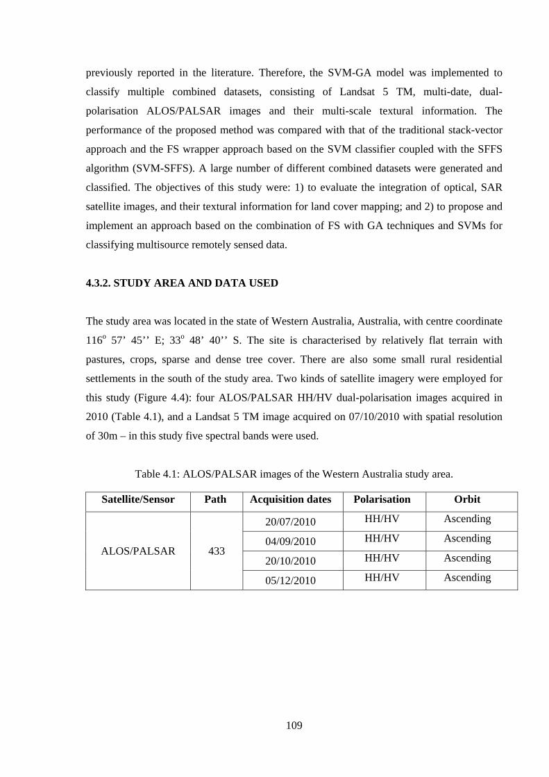
109

previously reported in the literature. Therefore, the SVM-GA model was implemented to

classify multiple combined datasets, consisting of Landsat 5 TM, multi-date, dual-

polarisation ALOS/PALSAR images and their multi-scale textural information. The

performance of the proposed method was compared with that of the traditional stack-vector

approach and the FS wrapper approach based on the SVM classifier coupled with the SFFS

algorithm (SVM-SFFS). A large number of different combined datasets were generated and

classified. The objectives of this study were: 1) to evaluate the integration of optical, SAR

satellite images, and their textural information for land cover mapping; and 2) to propose and

implement an approach based on the combination of FS with GA techniques and SVMs for

classifying multisource remotely sensed data.

4.3.2. STUDY AREA AND DATA USED

The study area was located in the state of Western Australia, Australia, with centre coordinate

116o 57’ 45’’ E; 33o 48’ 40’’ S. The site is characterised by relatively flat terrain with

pastures, crops, sparse and dense tree cover. There are also some small rural residential

settlements in the south of the study area. Two kinds of satellite imagery were employed for

this study (Figure 4.4): four ALOS/PALSAR HH/HV dual-polarisation images acquired in

2010 (Table 4.1), and a Landsat 5 TM image acquired on 07/10/2010 with spatial resolution

of 30m – in this study five spectral bands were used.

Table 4.1: ALOS/PALSAR images of the Western Australia study area.

Satellite/Sensor Path Acquisition dates Polarisation Orbit

ALOS/PALSAR 433

20/07/2010 HH/HV Ascending




110

Figure 4.4: Landsat 5 TM (left) and ALOS/PALSAR HH (right) over the study area acquired

on 07/10/2010 and 20/10/2010, respectively.

4.3.3. METHODOLOGY

4.3.3.1. Data processing

Landsat 5 TM images had been already processed to the Standard Terrain Correction (Level

1T) product by the United State Geological Survey (USGS). At this processing level, the

systematic radiometric and geometric corrections were undertaken using the platform

geometric model which employs both GCPs and DEM for removing the topographic

displacements. In this process, the Landsat 5 TM images were geo-rectified to the map

coordinate (UTM projection, WGS84 datum). The geo-rectification of ALOS/PALSAR

images and the co-registration of optical and SAR images were carried out as described in the

section 3.1.2. ALOS/PALSAR and Landsat 5 TM images were resampled to 10m pixel size.

Speckle noise in the PALSAR images was filtered using the Enhanced Lee Filter (Lopes et al.

1990) with a 5x5 window size. SAR backscatter values were converted to decibel using

Equation (3.1).

111

Besides the original ALOS/PALSAR images, several derivative images were also generated

and integrated for classification, including the Temporal Backscattered Change, average and

dual-polarised SAR index images. The Temporal Backscattered Change (SARCH) image was

generated using all four different SAR images (Equation (3.13)). This image highlights

differences between the stable or non-changing features (such as urban areas, permanent

vegetation, or still water) and temporally changing features (such as annual crops). The SAR

polarised index was computed:

(4.1)

where SARind is the SAR polarised index image derived from the corresponding SAR dual

HH/HV polarised image.

Two groups of texture measures were extracted and employed for classification, namely “first

order” and “second order” texture measures. The first order texture measures involve

statistics computed directly from the original image and do not model relationships with

neighbouring pixels. On the other hand, the second order texture measures consider the

mutual dependence of sets of surrounding pixels (Coburn and Roberts 2004, Hall-Beyer

2007). The most widely used second order textural data is the Grey Level Co-occurrence

matrix (GLCM), which measures relationships between pairs of pixels within a

neighborhood. The First Principal Components (PC1) images generated from each of the four

SAR and Landsat 5 TM images were used to derive textural information. In order to reduce

correlation within datasets it was necessary to select only components which are less

correlated to each other. Hence only three first order texture measures, namely mean,

variance and data range, and four GLCM texture measures, variance, homogeneity, entropy

and correlation, were employed. Since there is no preferred direction, the GLCM texture

measures were computed as an average of texture measures generated for the eight different

directions 0o, 45o, 90o, 135o, 180o, 225o, 270o, 315o. Texture measures were calculated using

the relations below. As the multi-scale texture approach was adopted, textural data were

generated from eight window sizes, including 3x3, 5x5, 7x7, 9x9, 11x11, 13x13, 15x15,

17x17, and used simultaneously.

First order texture measures (F_OR) were generated using the following relations:

HVHHHVHH

+−

=indSAR

112

∑=

×=n

kifi

WMean

0

1 (4.2)

( ) i

n

ifMean

WVariance ×−= ∑

=

2

011 (4.3)

( ) ( )iMiniMaxrangeData −=_ (4.4)

where fi is frequency of pixel’s value i appearing in a moving window and W is the total

number of pixels in a moving window, n is the quantisation level of the digital image (Jensen

2004). The second order GLCM texture measures were computed based on Equations (3.2 –

3.5).

4.3.3.2. Integration, feature selection, parameter optimisation and classification

SVM Classifier

In this study the SVM classifier with the Radial Basic Function (RBF) kernel was applied to

classify land cover features. Two parameters were optimally specified in order to ensure the

best accuracy: the penalty parameter C and the width of the kernel function γ. The common

means of determining the optimal C and γ is using a grid search algorithm (Kavzoglu and

Colkesen 2009).

Genetic Algorithm

The GA model for FS and parameter optimisation involves designing chromosomes,

definition of the fitness function, and specification of the system architecture.

Chromosome Design

The two parameters C and γ need to be defined. The GA-based model will try to optimise

both input features and the SVM’s parameters. Thus, the chromosome consists of three parts,

representing selected features, C and γ. A binary coding technique was used to define the

chromosome (Huang and Wang 2006). In Figure 4.5, Ib1 to IbNf represent input features,

Ibi=1 means a corresponding feature is selected, Ibi=0 means a feature is not selected. Cb1 ~

CbNc represents the value of C and γb1 ~ γbNγ represents the value of γ.

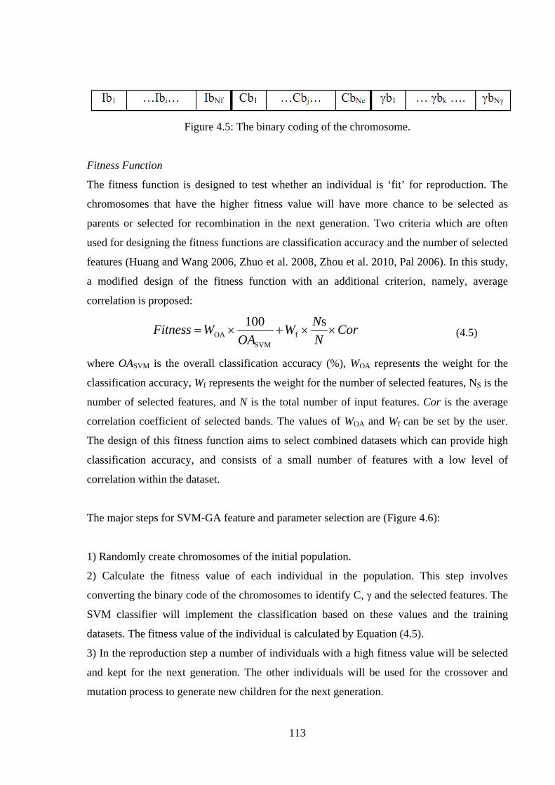
113

Figure 4.5: The binary coding of the chromosome.

Fitness Function

The fitness function is designed to test whether an individual is ‘fit’ for reproduction. The

chromosomes that have the higher fitness value will have more chance to be selected as

parents or selected for recombination in the next generation. Two criteria which are often

used for designing the fitness functions are classification accuracy and the number of selected

features (Huang and Wang 2006, Zhuo et al. 2008, Zhou et al. 2010, Pal 2006). In this study,

a modified design of the fitness function with an additional criterion, namely, average

correlation is proposed:

(4.5)

where OASVM is the overall classification accuracy (%), WOA represents the weight for the

classification accuracy, Wf represents the weight for the number of selected features, NS is the

number of selected features, and N is the total number of input features. Cor is the average

correlation coefficient of selected bands. The values of WOA and Wf can be set by the user.

The design of this fitness function aims to select combined datasets which can provide high

classification accuracy, and consists of a small number of features with a low level of

correlation within the dataset.

The major steps for SVM-GA feature and parameter selection are (Figure 4.6):

1) Randomly create chromosomes of the initial population.

2) Calculate the fitness value of each individual in the population. This step involves

converting the binary code of the chromosomes to identify C, γ and the selected features. The

SVM classifier will implement the classification based on these values and the training

datasets. The fitness value of the individual is calculated by Equation (4.5).

3) In the reproduction step a number of individuals with a high fitness value will be selected

and kept for the next generation. The other individuals will be used for the crossover and

mutation process to generate new children for the next generation.

CorNNW

OAWFitness ××+×=

s100f

SVMOA

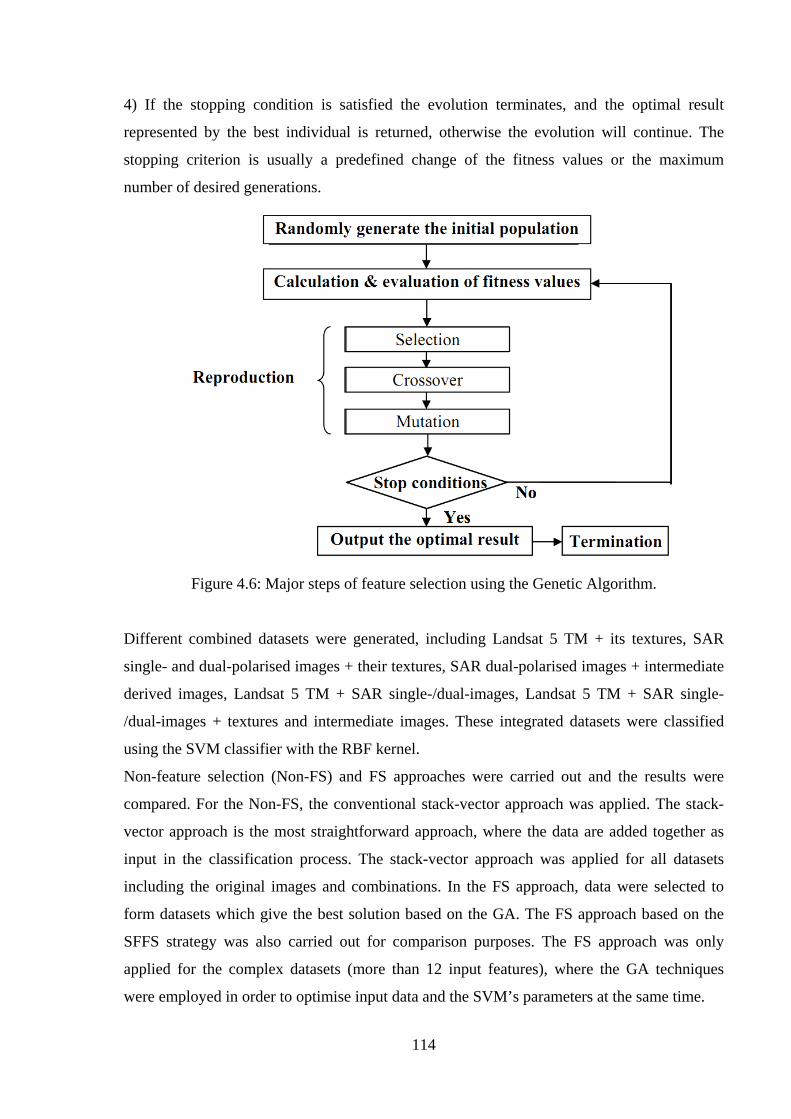
114

4) If the stopping condition is satisfied the evolution terminates, and the optimal result

represented by the best individual is returned, otherwise the evolution will continue. The

stopping criterion is usually a predefined change of the fitness values or the maximum

number of desired generations.

Figure 4.6: Major steps of feature selection using the Genetic Algorithm.

Different combined datasets were generated, including Landsat 5 TM + its textures, SAR

single- and dual-polarised images + their textures, SAR dual-polarised images + intermediate

derived images, Landsat 5 TM + SAR single-/dual-images, Landsat 5 TM + SAR single-

/dual-images + textures and intermediate images. These integrated datasets were classified

using the SVM classifier with the RBF kernel.

Non-feature selection (Non-FS) and FS approaches were carried out and the results were

compared. For the Non-FS, the conventional stack-vector approach was applied. The stack-

vector approach is the most straightforward approach, where the data are added together as

input in the classification process. The stack-vector approach was applied for all datasets

including the original images and combinations. In the FS approach, data were selected to

form datasets which give the best solution based on the GA. The FS approach based on the

SFFS strategy was also carried out for comparison purposes. The FS approach was only

applied for the complex datasets (more than 12 input features), where the GA techniques

were employed in order to optimise input data and the SVM’s parameters at the same time.

115

The chromosome and the fitness function for the GA were designed as shown in Figure 4.5,

and Equation (4.5). In this study the weight for classification accuracy (WOA) and the weight

for the number of selected features (Wf) were set in the range 0.65-0.8 and 0.2-0.35,

respectively. The other parameters for the GA were:

Population size = 20-40; Number of generations = 200; Crossover rate: 0.8; Elite count:

3-6; Mutation rate: 0.05.

The 5-fold cross validation techniques were used to estimate the accuracy of each classifier.

The grid search algorithm was applied in the stack-vector approach to search for the best

parameters (C, γ) for the SVM classifiers. The GA was implemented using the Global

Optimization toolbox in Matlab 7.11.1(2010b). The SFFS algorithm was also developed in

Matlab 7.11.1. For the implementation of the SVM classifiers the well-known LIBSVM 3.1

toolkit with Matlab interface was employed (Chang and Lin 2011).

Five land cover classes were identified for classification: Crop (CR), Permanent Pastures

(PA), Dense Forest (DF), Sparse Forest (SF) and Residential Area (RE). The spectral

properties and backscatter signatures of the five land cover features in the Landsat 5 TM

multi-spectral and multi-date PALSAR images are shown in Figure 4.7.

Figure 4.7: Land cover feature characteristics in Landsat 5 TM (left) and multi-date PALSAR

(right) images.

The land cover data used for training and validation were derived from visual interpretation

with the aid of aerial photography, Google Earth images and ground truth data collected from

two field surveys conducted on September 2, 2010 and August 23, 2010. The training and test

datasets were selected randomly and independently using the Region of Interest (ROI) tool of

the ENVI 4.6 software. The samples selection has been carried out based on the procedure

116

described earlier in the section 3.1.2. The sizes of the training and testing datasets are listed in

Table 4.2.

Table 4.2: Contents of training and testing datasets.

Classes Training data

(number of pixels)

Testing data

(number of pixels)

Crop 954 1076

Pasture 956 1107

Spare Forest 961 1080

Residential 313 198

Dense Forest 632 569


Overall classification accuracies of datasets (consisted of less than 12 features) using the

Non-FS (stack-vector approach) and SVM classifiers are summarised in Table 4.3. Results of

classification using the proposed SVM-GA FS technique, SVM-SFFS and the Non-FS

approach for the larger datasets are given in Table 4.4.

The classification results demonstrate the complimentary characteristics and efficiencies from

the integration of optical and SAR images. All combined datasets generated from both kinds

of data, no matter whether the Non-FS or FS approach was used, produced significant

improvements in classification accuracy compared to the original single datasets. In the case

of the stack-vector approach, although the Landsat 5 TM gave a high accuracy of 85.21%, it

exhibited extensive confusion between residential and vegetation classes (commission errors

were 56.39%). The combination of the original Landsat 5 TM and PALSAR images gave

remarkable increases of accuracy, in which the combined use of Landsat TM and four-date

PALSAR HH images resulted in a classification accuracy of 91.46%, with improvements of

6.25% and 25.60% for Landsat 5 TM and PALSAR HH data, respectively, while the

commission errors for the residential class were 29.29%. The integration of Landsat 5 TM

image with four-date PALSAR dual HH/HV images gave an overall accuracy of 88.93% with

an increase of 3.72% and 16.18% over Landsat 5 TM and PALSAR dual HH/HV data,

respectively, while the commission errors of the residential class were 39.94%. However, the

improvements are more obvious when using the GA-based FS approach. This integration

resulted in an overall accuracy of 92.26% with an increase of 7.05% and 19.51% compared to

the single-type datasets, while the residential commission errors were reduced to 19.83%.

117

Table 4.3: Classification accuracy of different datasets using SVM classifiers with the traditional stack-vector approach.

Datasets Overall accuracy (%)

Four-date HH images 65.86

Four-date HH images + HHAVE+HHCH 67.92

Four-date HV images 66.58

Four-date HV images + HVAVE+HVCH 68.44

Four-date HH/HV images 72.75

Four-date HH/HV images + HH/HVAVE + HH/HVCH 73.18

Four-date HH/HV images +SARind 72.73

Four-date HH images 65.86

Four-date HH/HV images + HH/HVAVE+HH/HVCH +SARind 73.20

L5 TM 85.21

(note: L5 TM = Landsat 5 TM; Four-date HH image = Four-date PALSAR HH polarised image; Four-date HV image = Four-date PALSAR HV polarised image; Four-date HH/HV

image = Four-date PALSAR dual HH/HV polarised image).

The complimentary properties of like- (PALSAR HH) and cross- (PALSAR HV) polarisation

images were also clearly highlighted. As can be seen in Table 4.4, except for the crop where

the classification accuracy of PALSAR HH and HV images are rather similar, the like-

polarisation gave better accuracy for the residential class (which is dependent on surface

scattering), while the cross-polarisation, due to its sensitivity to the volume scattering,

provided higher accuracy for vegetation classes Pasture, Sparse Forest and Dense Forest.

Utilisation of both SAR like- and cross-polarised data resulted in noticeable improvements in

overall classification accuracy, particularly for the Residential, Sparse Forest and Dense

Forest features.

Table 4.4: Producer and user accuracy (%) of four-date PALSAR HH, HV and dual-polarised

images.

Land cover classes Four-date HH Four-date HV Four-date HH/HV


Crop (CR) 80.11 65.80 78.07 69.19 77.79 69.35

Permanent Pasture (PA) 62.87 76.48 66.03 78.69 66.58 75.51

Sparse Forest (SF) 59.63 70.46 70.74 67.02 78.24 77.17

Residential (RE) 68.18 75.84 16.16 12.90 77.78 76.24

Dense Forest (DF) 55.71 44.15 55.54 63.33 63.09 65.27

118

Incorporation of the PALSAR original images with their additional derived data, such as

Average and Temporal Backscattered Change (SARCH), gave an increase in classification

accuracy. The improvements were 2.06% and 1.86% for the case of four-date PALSAR HH

and HV polarised images, respectively. However, in the case of PALSAR dual HH/HV

polarised images, there was only a very slight increase in accuracy of 0.43%. On the other

hand, the SAR polarised index images do not give any improvement compared to the

classification of the original PALSAR dual HH/HV polarised images.

Integration of optical and multi-date SAR data with their textural information gave a

noticeable increase in classification accuracy. As for the Non-FS approach, the combination

of four-date HH images with their textures gave very slight increases in accuracy of 0.81%,

0.92% and 1.34% using the first order, GLCM and both groups of texture measures,

respectively. On the other hand, the increase of 4.41%, 0.79%, and 6.79% in classification

accuracy was obtained for the four-date HV images. The improvements for the four-date

PALSAR dual HH/HV polarised images were 4.42%, 1.86% and 6.05%. The application of

textural information was also effective for optical images. The integration of Landsat 5 TM

images with their textures resulted in increases of 2.48%, 4.37% and 2.95% using the first

order, GLCM and both textural groups, respectively.

The efficiency of using textural information was even more impressive when the SVM-GA

methods were exploited. For example, the improvements for the four-date PALSAR dual

HH/HV polarisation increased by 6.98%, 2.95% and 6.93%. The combination of Landsat 5

TM images with their corresponding texture measures also gave significant improvements of

5.53%, 6.00% and 6.23%. In particular, the integration of four-date PALSAR HV polarised

images with both types of textures resulted in an increase of overall classification accuracy of

up to 12.95%.

It is worth mentioning that although the four-date PALSAR dual HH/HV images resulted in

much lower classification accuracy, 72.75% compared to 85.21% for the Landsat 5 TM

image, its combination with textural data and additional images using the SVM-GA method

gave an overall classification accuracy of 81.19%, which is closer to the accuracy obtained

using optical images. A comparison of classification improvement by incorporation of

textural information using stack-vector and FS-GA approach is shown in Figure 4.8.

119

Figure 4.8: Improvement of accuracy by incorporating textural information with original

datasets using stack-vector and FS-GA approach.

(F_OR(ST), GLCM(ST), F_OR+GLCM(ST) and F_OR(GA), GLCM(GA), F_OR+GLCM(GA) represent integration of textures using stack-vector and FS-GA approach,

respectively). The FS-GA approach clearly outperforms the commonly used Non-FS approach (Table 4.5

and Figure 4.10). In all cases the FS-GA approach gave better results than the Non-FS

approach. The increase of overall classification accuracy ranged from 0.87% (four-date

PALSAR HH/HV images + its first and second order textures) to 7.57% (four-date PALSAR

HV images + its first order textures). It is also important to emphasise that the FS-GA used

less input features than the stack-vector approach, see Figure 4.11.

While in many cases the Hughes phenomenon appeared in the stack-vector method, where

the classification accuracy decreased with an increase in the number of input measurements,

it is not the case for the SVM-GA method. For example, the integration of the Landsat 5 TM

image with PALSAR HH images gave an overall accuracy of 91.46%, while the integration

of the Landsat 5 TM image with PALSAR dual HH/HV images resulted in 88.93% accuracy,

a decrease of 2.53%. However, using the SVM-GA method the same integration gave an

overall accuracy of 92.26% with only six out of a total 13 features used (Figure 4.9).

Similarly, the combination of Landsat 5 TM image with its GLCM textures gave an accuracy

of 89.58%, but when the Landsat 5 TM image was combined with both first order and GLCM

texture measures the accuracy dropped to 88.16%. Nevertheless, when applying GA

techniques the classification accuracy still increased slightly to 91.44%.

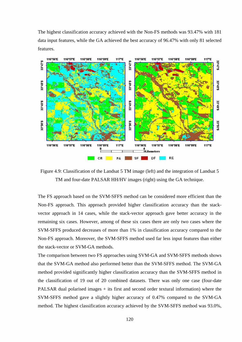
120

The highest classification accuracy achieved with the Non-FS methods was 93.47% with 181

data input features, while the GA achieved the best accuracy of 96.47% with only 81 selected

features.

Figure 4.9: Classification of the Landsat 5 TM image (left) and the integration of Landsat 5

TM and four-date PALSAR HH/HV images (right) using the GA technique.

The FS approach based on the SVM-SFFS method can be considered more efficient than the

Non-FS approach. This approach provided higher classification accuracy than the stack-

vector approach in 14 cases, while the stack-vector approach gave better accuracy in the

remaining six cases. However, among of these six cases there are only two cases where the

SVM-SFFS produced decreases of more than 1% in classification accuracy compared to the

Non-FS approach. Moreover, the SVM-SFFS method used far less input features than either

the stack-vector or SVM-GA methods.

The comparison between two FS approaches using SVM-GA and SVM-SFFS methods shows

that the SVM-GA method also performed better than the SVM-SFFS method. The SVM-GA

method provided significantly higher classification accuracy than the SVM-SFFS method in

the classification of 19 out of 20 combined datasets. There was only one case (four-date

PALSAR dual polarised images + its first and second order textural information) where the

SVM-SFFS method gave a slightly higher accuracy of 0.47% compared to the SVM-GA

method. The highest classification accuracy achieved by the SVM-SFFS method was 93.0%,

121

while it was 96.47% for the SVM-GA method. However, the SVM-SFFS method selected

only five input features, and the number of input feature was 81 in the case of the SVM-GA

method. It is also revealed that the problem of Hughes’s phenomenon was not fully resolved

by the SVM-SFFS method. In many cases that the higher dimensional datasets did not result

in increases in classification accuracy.

Table 4.5: Comparison of land cover classification performance between SVM-GA, SVM-SFFS and stack-vector approach; nf = number of selected features.

ID DATASETS SVM OVERALL ACCURACY (%)

Stack Vector SFFS GA

NF Accuracy NF Accuracy NF Accuracy

1 Four-date HH images + First- order textures 28 66.67 10 66.67 8 68.24

2 Four-date HH images +GLCM textures 36 66.77 10 68.06 19 69.08

3 Four-date HH +First – order & GLCM textures 60 67.20 12 64.99 21 70.59

4 Four-date HV + First-order textures 28 70.99 8 71.59 8 78.56

5 Four-date HV +GLCM textures 36 67.37 12 68.14 16 73.60

6 Four-date HV +First - order & GLCM textures 60 73.37 6 78.66 25 79.53

7 Four-date HH/HV images + First- order textures 56 77.17 5 78.01 23 79.73

8 Four-date HH/HV images +GLCM textures 72 74.61 12 73.13 34 75.70

9 Four-date HH/HV +First -order & GLCM textures 120 78.81 6 80.05 51 79.68

10 Four-date HH/HV images + HH/HVAVE + +HH/HVCH

+ SARind + First-order textures 64 77.15 11 78.21 24 80.23

11 Four-date HH/HV images + HH/HVAVE + +HH/HVCH +

SARind + GLCM textures 80 74.17 11 74.14 36 75.65

12 Four-date HH/HV images + HH/HVAVE + HH/HVCH +

SARind + First-order & GLCM textures 128 78.86 7 81.02 49 81.19

13 L5 TM + First-order textures 29 87.69 4 87.07 9 90.74

14 L5 TM + GLCM textures 37 89.58 5 90.02 13 91.21

15 L5 TM + First-order & GLCM textures 61 88.16 6 87.94 20 91.44

16 L5 TM + Four-date HH/HV 13 88.93 4 90.05 6 92.26

17 L5 TM + Four-date HH/HV + HH/HVAVE + +HH/HVCH

+ SARind 21 88.39 7 90.89 8 93.10

18 L5 TM + All of LS5_textures + Four-date HH/HV +

HH/HVAVE+HH/HVCH + SARind 77 92.21 5 92.48 32 95.24

19 L5 TM + All of L5 TM textures + Four-date HH/HV +

All of SAR textures 181 93.47 6 92.51 81 96.20

20 L5 TM + All L5 TM textures + Four-date HH/HV +

HH/HVAVE + HH/HVCH + SARind + All of SAR textures 189 92.98 5 93.00 81 96.47

122

Figure 4.10: Classification accuracy using FS (SFFS and GA) compared to Non-FS (stack-

vector) approaches.

Figure 4.11: Number of input features for the Non-FS (stack-vector) and FS (SFFS and GA)

approaches.

123

The proposed fitness function with an additional parameter of average correlation between

selected features has improved the overall classification accuracy for 18 out of 20 combined

datasets compared to using the commonly designed fitness function – for the remaining two

cases the classification accuracy decreased very slightly (about 0.1%). Impact of the proposed

fitness function compared to the commonly used fitness function is illustrated in Figure 4.12.

Figure 4.12: Impact of the proposed fitness function on overall classification accuracy

compared to the commonly used fitness function.

4.3.5. CONCLUSIONS

A feature selection approach based on the SVM-GA method has been proposed and

compared with non-feature selection approach and the SVM-SFFS method for classification

of multisource remotely sensed data, including optical, multi-date SAR and textural

information. Results of classification of different combined datasets (more than 30 for non-

feature selection and 20 for the feature selection approach) revealed advantages of

multisource remotely sensed data and SVM-based algorithms for land cover classification.

Incorporation of textural information with either optical or SAR data also resulted in an

improvement in accuracy. Feature selection using the SVM-GA method clearly outperformed

the classical stack-vector approach and the SVM-SFFS methods. The feature selection

124

approach based on SVM-GA method always resulted in better classification accuracy with

more significant improvement, and used less data input features, compared to the non-feature

selection approach. The SVM-GA method also provided better classification accuracy than

the SVM-SFFS method for 19 out of 20 combined multisource datasets. The highest overall

classification accuracy of 96.47% was obtained using the SVM-GA method for classifying

the combined dataset of original Landsat 5 TM, four-date PALSAR dual HH/HV polarised

images, all of their textures and additionally derived images with 81 out of 189 data input

features selected. Moreover, classification results also indicated that the proposed fitness

function in this study is more reliable than the commonly used version. Although the SVM-

SFFS method did not provide as high classification accuracy as the SVM-GA method it was

also considered a viable alternative which performed noticeably better than the traditional

stack-vector approach for 14 out of 20 experiment cases. However, the highest classification

accuracy achieved by the stack-vector approach (93.47%) was slightly better than the SVM-

SFFS method (93.0%). The most distinct advantage of the SVM-SFFS method is that it used

a far smaller number of input features than either the SVM-GA method and non-feature

selection approach.

125

CHAPTER 5

APPLICATION OF MULTIPLE CLASSIFIER SYSTEM

FOR CLASSIFYING MULTISOURCE REMOTE

SENSING DATA

The effectiveness of non-parametric classifiers such as Support Vector Machine (SVM) and

Artificial Neural Network (ANN) algorithms, and the advantages of using Feature Selection

(FS) techniques based on the Genetic Algorithm (GA) for classifying multisource remote

sensing data has been demonstrated in the previous chapters. Recently, a Multiple Classifier

System (MCS) has been increasingly used for remote sensing, particularly for handling large

volume and complex datasets (Yan and Shaker 2011). The goal of this chapter is to further

enhance the performance of land cover classification using multisource data by exploring the

capabilities of MCS, which also has the potential to improve the quality of image

classification. The main contribution of this chapter is to propose and to evaluate an

integration of MCS and FS based on GA techniques to resolve the challenge of classifying

highly dimensional combined datasets.

5.1. MCS IN REMOTE SENSING MCS or classifier ensemble has been proposed as a robust and effective method to increase

the classification accuracy (Briem et al. 2002, Bruzzone et al. 2004, Du et al. 2009b, Yan and

Shaker 2011). The MCS can be defined as a system that obtains the final classification results

by merging the outputs of multiple classifiers based on a certain combination rule (Xie et al,

2006, Du et al. 2009a). In general there is no perfect classifier which can give the best

performance in all cases. The classifier which is very effective for one dataset might not be

appropriate for other datasets, and therefore the MCS can provide the additional information

about classification patterns. Consequently, the MCS may outperform an individual classifier

by integrating the advantages of various classifiers. It is also worth mentioning that the

classifier ensemble certainly minimises the risk of poor selection (Polikar, 2006). It is also

126

claimed that the MCS can take advantage of complementary characteristics of multi-sensor

data for classification (Benediktsson et al. 2007).

5.1.1. CREATION OF MCS OR CLASSIFIER ENSEMBLE

In the MCS it is essential to maintain the diversity between the member (or base) classifiers

since if they are identical the combination will exhibit no improvement. It is suggested that

the member classifiers have different decision boundaries (Polikar, 2006). The diversity in

the ensembles is introduced to the system by using different classifiers, or by training

classifier with different parameters and different training datasets. The ensemble of classifiers

can be generated in different ways, including combination of different classifiers or

combination of the same classifiers with various versions of input training data. The

commonly used techniques of “boosting” and “bagging” are based on manipulating input

training sample data (Briem et al. 2002).

“Bagging” is an abbreviation of Bootstrap Aggregating which was introduced by Breiman

(1994). In this approach many training sample subsets (or “bags”) are generated by

employing the random and uniform selection with replacement of m samples from a training

sample set of size m (the same size). The classification process is then carried out based on

training data on each bag using a base classifier, resulting in various outputs. The final result

is constructed by combining all individual outputs. The bagging algorithm can noticeably

improve the classification accuracy with unstable base classifier. However, the classification

accuracy may be decreased in the case of stable classifiers since less training data are used for

each classifier (Tzeng et al. 2006, Briem et al. 2002, Briem et al. 2001).

The “boosting” algorithm was proposed by Schapire (1990) in order to increase the

classification accuracy of a weak classifier. At the beginning, the classifier is trained by

samples which have the same weight. Then, during the training stage, the boosting algorithm

successively reweights the training samples so that the misclassified samples are weighted

higher than the correctly classified samples. The next classifier in the ensemble is trained by

the newly modified samples. As the number of iterations increase, the weights of correctly

classified samples are decreased. Thus, the classifier is driven to concentrate on “difficult”

samples (Briem et al. 2002), and the bias and variance of the classification can be reduced

(Waske and Braun 2009). It is worth noting that, while the bagging can be operated in

127

parallel with all of the bags, boosting is implemented in an iterative procedure on the samples

with the newest weights. As a result the boosting algorithm requires more computational

power and longer processing time. The commonly used boosting algorithms in the field of

pattern recognition and remote sensing are AdaBoost.M1 and M2 methods (Freund and

Schapire, 1996).

5.1.2. COMBINATION RULES

The performance of the ensemble classification is also a function of the methods used to

combine the classification outputs. A range of methods are available depending on the type of

information derived from each classifier. There are three levels of outputs from the

classifiers: abstract level, rank level and measurement level (Foddy et al. 2007, Maghsoudi et

al. 2006). At the abstract level, the output from each classifier is a label, and the final labels

are decided by combining output labels of multiple classifiers. The most commonly used

technique for combining outputs of classifiers is by majority voting. At the rank level, the

output of a classifier is the possibility of a pixel belonging to each class given in a rank. The

rank level combination algorithm is used to determine the final class for each pixel. At the

measurement level, the output of the member classifier can be a quantitative value (e.g.,

separability, distance) or the probability of a pixel belonging to a certain class. In this case,

the quantitative index is employed to combine multiple classifiers, as a measurement level

combination.

The most widely used method to integrate the measurement level outputs is using Bayesian

decision rules, which linearly combine outputs of the individual classifiers. The main

Bayesian decision rules are Sum, Product, Maximum and Minimum:

Sum rule

)|(1

j

n

jii xwpSumP ∑

=

= i = 1, 2, 3,..., k. (5.1)

Product rule

)|(Pr1∏=

=n

jjii xwpoP i = 1, 2, 3,..., k. (5.2)

Max rule

)|(1 jinji xwpMaxMaxP == i = 1, 2, 3,..., k. (5.3)

128

Min rule

)|(1 jinji xwpMinMinP == i=1, 2, 3, …, k. (5.4)

where p(wi|xj) are the posteriori probabilities which represent the probability that the jth

classifier assigns the pixel x to the class wi. In each combination rule the winner is the class

with the largest value according to this rule.

Non-linear combination rules, such as evidence reasoning based on the Dempster-Shafer

theory of evidence and fuzzy integral, were also applied and provided very positive results

(Du et al. 2009a, Trinder et al. 2010, Salah et al. 2010). In the evidence reasoning algorithm,

the single data source is weighted in accordance with their importance or reliability. The

combination rules are generated upon the concepts of belief and plausibility in order to assign

labels to pixels (Mather 2010). Tso and Mather (2009), and Trinder et al. (2010) describe

uses of the evidence reasoning method for the classification of remote sensing data.

Some basics concepts, recent developments and application of MCS in remote sensing have

been reviewed by Benediksson et al. (2007). Briem et al. (2002) evaluated the performance of

bagging, boosting and Bayesian maximum rule on weighted linear and weighted products of

a posteriori probability combination for classifying several multisource remote sensing

datasets. Five classifiers, namely Minimum Eucledian Distance (MED), Maximum

Likelihood (ML), ANN-MLP with conjugated-gradient algorithm, Decision Table, Decision

Tree and simple 1R classifier (using only one feature when determining a class) were

employed. Results illustrated that all multiple classification strategies gave better

classification accuracy than a single classifier. The boosting approach with the AdaBoost.M1

method appeared to be the most accurate classifier for both training and testing datasets. The

authors claim that multiple classification methods can be considered as a valuable alternative

for the classification of multisource data. Tzeng et al. (2006) applied the MCS with the

bagging and boosting algorithms to classify land cover features in Taiwan using multispectral

data similar to SPOT satellite images. The ANN-MLP classifier was used as a base classifier.

In this study the original bagging and boosting methods had been modified by introducing the

concept of confidence index with a view to reduce the confusion among classes. The results

show that both the original and modified MCS significantly improved classification accuracy

compared to the single classifier. Foody et al. (2007) integrated five classifiers based on the

majority voting rule for mapping fernland in East Anglia, UK. The accuracy achieved by the

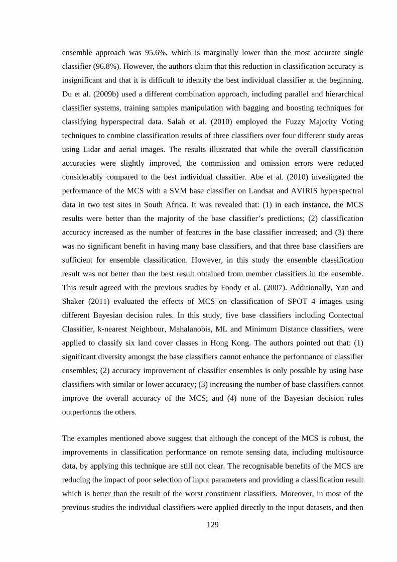
129

ensemble approach was 95.6%, which is marginally lower than the most accurate single

classifier (96.8%). However, the authors claim that this reduction in classification accuracy is

insignificant and that it is difficult to identify the best individual classifier at the beginning.

Du et al. (2009b) used a different combination approach, including parallel and hierarchical

classifier systems, training samples manipulation with bagging and boosting techniques for

classifying hyperspectral data. Salah et al. (2010) employed the Fuzzy Majority Voting

techniques to combine classification results of three classifiers over four different study areas

using Lidar and aerial images. The results illustrated that while the overall classification

accuracies were slightly improved, the commission and omission errors were reduced

considerably compared to the best individual classifier. Abe et al. (2010) investigated the

performance of the MCS with a SVM base classifier on Landsat and AVIRIS hyperspectral

data in two test sites in South Africa. It was revealed that: (1) in each instance, the MCS

results were better than the majority of the base classifier’s predictions; (2) classification

accuracy increased as the number of features in the base classifier increased; and (3) there

was no significant benefit in having many base classifiers, and that three base classifiers are

sufficient for ensemble classification. However, in this study the ensemble classification

result was not better than the best result obtained from member classifiers in the ensemble.

This result agreed with the previous studies by Foody et al. (2007). Additionally, Yan and

Shaker (2011) evaluated the effects of MCS on classification of SPOT 4 images using

different Bayesian decision rules. In this study, five base classifiers including Contectual

Classifier, k-nearest Neighbour, Mahalanobis, ML and Minimum Distance classifiers, were

applied to classify six land cover classes in Hong Kong. The authors pointed out that: (1)

significant diversity amongst the base classifiers cannot enhance the performance of classifier

ensembles; (2) accuracy improvement of classifier ensembles is only possible by using base

classifiers with similar or lower accuracy; (3) increasing the number of base classifiers cannot

improve the overall accuracy of the MCS; and (4) none of the Bayesian decision rules

outperforms the others.

The examples mentioned above suggest that although the concept of the MCS is robust, the

improvements in classification performance on remote sensing data, including multisource

data, by applying this technique are still not clear. The recognisable benefits of the MCS are

reducing the impact of poor selection of input parameters and providing a classification result

which is better than the result of the worst constituent classifiers. Moreover, in most of the

previous studies the individual classifiers were applied directly to the input datasets, and then

130

the MCS techniques were used to combine results of these classification processes. Only a

few authors (e.g. Abe et al. 2010) used feature selection (FS) techniques to search for relevant

input features before implementing the classification process. In the study of Abe et al.

(2010), different input datasets for the SVM classifier were selected after an exhaustive

search using a filter approach and the Bhattachryya distance separability index as an

objective function. However, as has been discussed in chapter 4, there are some limitations

that affect the performance of this approach: 1) the exhaustive search is not suitable for

handling high dimensionality datasets; 2) the filter approach does not guarantee a high

classification accuracy; and 3) the separability indices do not directly reflect the classification

accuracy. Therefore, in the next section, a more advanced method for integrating FS wrapper

approach based on the GA technique and MCS for classifying multisource remote sensing

data is proposed.

5.2. USE OF MCS AND A COMBINATION OF GA AND MCS FOR CLASSIFYING MULTISOURCE REMOTE SENSING DATA – A CASE STUDY IN APPIN, NSW, AUSTRALIA.

5.2.1. INTRODUCTION

The first aim of this study is to investigate the capabilities of MCS algorithms for classifying

multisource remote sensing data. Secondly, the combination of FS wrapper approach based

on the GA method and the MCS algorithm was proposed, developed and demonstrated.

Although these techniques have been used in classification of remote sensing data, this study

is one of the first attempts to integrate these techniques for classifying multisource satellite

imagery. It is expected that this new approach can improve the generality and diversity of the

final solution and therefore can increase the classification accuracy.

As mentioned earlier, various FS methods have been used in remote sensing, such as

Exhaustive Search, Forward and Backward Sequential Feature Selection, Simulated

Annealing and GA. Results of numerous studies and the work presented in Chapter 4 have

demonstrated that the GA technique is very efficient for dealing with large datasets and is

better able to avoid a local optimal solution than other methods (Goldberg 1989, Huang and

Wang 2006, Zhou et al. 2010). Another important advantage of the GA techniques is its

capability to search for input features and parameters of classifiers simultaneously. Therefore,

the FS technique based on the GA was employed to address the challenging task of selecting

131

the optimal combined subsets of features. In this study, the synergistic use of the FS wrapper

method with GA and multiple classifiers combination for classifying land cover features in

New South Wales, Australia will be evaluated. This approach is referred to here as the FS-

GA-MCS model.

The non-parametric classification algorithms, such as ANN with a Multilayer Perceptron-

Back Propagation algorithm (MLP-BP) or SVM, have proven to be more effective than the

commonly used ML algorithms for classifying multisource remote sensing data since they are

not constrained by the assumption of normal distribution. In this section, beside the SVM and

MLP-BP network, another non-parametric classifier, namely the Self-Organising Map (SOM)

is introduced and tested.

5.2.2. STUDY AREA AND USED DATA

The study area is located in Appin, in the state of New South Wales, Australia, centred

around coordinate 150o 44’ 30” E; 34o 12’ 30” S. The site is characterised by a diversity of

covered features such as native dense forest, grazing land, urban and rural residential areas,

facilities and water surfaces. Remote sensing data used for this study includes:

SAR: Six ENVISAT/ASAR VV polarisation and six ALOS/PALSAR HH polarisation

images acquired in 2010 (Figure 5.1, Figure 5.2 and Table 5.1).

Optical: Three Landsat 5 TM images acquired on 25/03/2010, 10/9/2010 (Figure 5.3) and

31/12/2010 with seven spectral bands and spatial resolution of 30m. In this study six spectral

bands (except the thermal band) were used.

Table 5.1: ENVISAT/ASAR and ALOS/PALSAR images for the study area.

Satellite/Sensors Date Polarisation Mode 04/01/2010 HH Ascending 22/05/2010 HH Ascending

ALOS/PALSAR 07/07/2010 HH Ascending 22/08/2010 HH Ascending 07/10/2010 HH Ascending 22/11/2010 HH Ascending 03/04/2010 VV Descending 24/06/2010 VV Ascending

ENVISAT/ASAR 25/06/2010 VV Descending 27/06/2010 VV Ascending 28/06/2010 VV Descending 25/09/2010 VV Descending

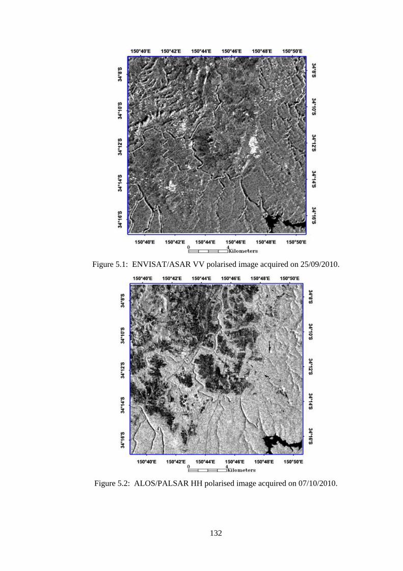
132

Figure 5.1: ENVISAT/ASAR VV polarised image acquired on 25/09/2010.

Figure 5.2: ALOS/PALSAR HH polarised image acquired on 07/10/2010.

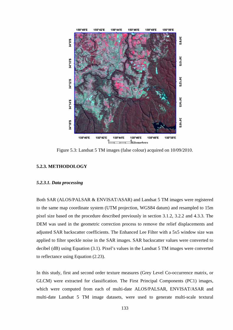
133

Figure 5.3: Landsat 5 TM images (false colour) acquired on 10/09/2010.

5.2.3. METHODOLOGY

5.2.3.1. Data processing

Both SAR (ALOS/PALSAR & ENVISAT/ASAR) and Landsat 5 TM images were registered

to the same map coordinate system (UTM projection, WGS84 datum) and resampled to 15m

pixel size based on the procedure described previously in section 3.1.2, 3.2.2 and 4.3.3. The

DEM was used in the geometric correction process to remove the relief displacements and

adjusted SAR backscatter coefficients. The Enhanced Lee Filter with a 5x5 window size was

applied to filter speckle noise in the SAR images. SAR backscatter values were converted to

decibel (dB) using Equation (3.1). Pixel’s values in the Landsat 5 TM images were converted

to reflectance using Equation (2.23).

In this study, first and second order texture measures (Grey Level Co-occurrence matrix, or

GLCM) were extracted for classification. The First Principal Components (PC1) images,

which were computed from each of multi-date ALOS/PALSAR, ENVISAT/ASAR and

multi-date Landsat 5 TM image datasets, were used to generate multi-scale textural

134

information. Finally, three first order texture measures, including Mean, Variance and Data

range, and four GLCM texture measures, namely Variance, Homogeneity, Entropy and

Correlation with four window sizes 5x5, 9x9, 13x13 and 17x17 were selected.

Normalised Difference Vegetation Indices (NDVI) images were computed from the Red and

Near-Infrared bands of Landsat 5 TM images:

REDNIRREDNIRNDVI

+−

= (5.5)

where NIR and RED are reflectance values of a pixel at the Near-Infrared and Red bands,

respectively.

Four different combined datasets have been generated and applied for the classification

processes (Table 5.2).

Table 5.2: Combined datasets for land cover classification in the study area.

ID Datasets Number of features

1 Six-date PALSAR + six-date ASAR images 12

2 Three-date Landsat 5 TM images 18

3 Three-date Landsat 5 TM + six-date PALSAR + six-date ASAR images 30

4 Three-date Landsat 5 TM + six-date PALSAR + six-date ASAR +

+ Landsat 5 TM & SAR’s textures + three-date NDVI images 173

5.2.3.2. Classification algorithms

Three non-parametric classifiers were employed for classification processes: MLP-BP, SOM

and the SVM.

Artificial Neural Network (ANN)

The MLP-BP model with three layers (input, hidden and output layer) was employed. The

number of neurons in the input layer is equal to the number of input features, the number of

neurons in the output layer is the number of land cover classes to be classified. The optimal

number of input neurons and the number of neurons in the hidden layer was searched by GA

techniques. The sigmoid function was used as the transfer function. The other important

135

parameters were set as follows: maximum number of iteration: 1000; learning rate: 0.01-0.1;

training momentum: 0.9.

Support Vector Machine (SVM)

The SVM classifier with a Gausian Radical Basis Function (RBF) kernel has been used

because of its highly effective and robust capabilities for handling of remote sensing data

(Kavzoglu and Colkesen 2009, Waske and Benediksson 2007). Two parameters need to be

optimally specified in order to ensure the best accuracy: the penalty parameter C and the

width of the kernel function γ. These values will be determined by the GA while searching

for optimal combined datasets. For other cases a grid search algorithm with multi-fold cross-

validation was used.

Self-Organising Map (SOM)

The SOM is another wellknow neural network classifier. The SOM network has the unique

property that it can automatically detect (“self-organising”) the relationships within the set of

input patterns without using any predefined data models (Salah et al. 2009, Tso and Mather

2009). Previous studies suggest that the SOM is an effective method for classifying remotely

sensed data (Ji 2000, Janwen and Bagan 2005, Hugo et al. 2006, Salah et al. 2009, Lee and

Lathrop 2007). As this algorithm has not been introduced in the previous chapter, the basic

concepts and applications of the SOM will be presented in this section.

The SOM network includes input and output layers. The input layer consists of neurons

which represent input feature vectors – the number of input neurons is equal to the number of

input features. The output layer is generally a two-dimensional array of neurons arranged in a

spatial rectangular or hexagonal lattice. A neuron j in the output layer is connected with

neuron i in the input layer by the synaptic weight Wji. These weights are set randomly at the

beginning and then are gradually modified in the training process to characterise input

patterns. In the final result, the neurons which have similar properties (in terms of weight

value) will be organised close together (Tso and Mather 2009). An example of a SOM

network architecture is shown in Figure 5.4.

136

Figure 5.4: Example of the SOM architecture with three input neurons and 25 (5x5) output

neurons.

Classification using the SOM network is carried out in two stages: coarse tuning and fine

tuning. The coarse tuning involves searching for the winning neuron which has synaptic

weights closest to the input data vector, updating weights of the winning neuron and its

neighbouring neurons, and finally assigning labels to neurons.

The Euclidean distance is often used to determine the wining neuron:

⎟⎠

⎞⎜⎝

⎛−= ∑

=

n

i

tji

tic wxM

1

2)(minarg (5.6)

where xit is the input to neuron i at a training step t, and wt

ji is the synaptic weight

connecting the input neuron i with output neuron j

Weights of the winning neuron and its neighbouring neurons are then adjusted so that the

wining neuron will be more similar to the input vector. The most commonly used functions

for determining the neighbourhood of the wining neuron is a decay function, which makes

the neighbourhood radius shrink over time:

⎟⎠⎞

⎜⎝⎛−=

λσσ 1exp)( 0t (5.7)

where σ(t) is the neighbourhood radius of the winning neuron at a training step t, σ0 is the

initial radius, and the λ is a time constant. A decay function reduces the neighbourhood radius

137

from an initial size that can include all of the neurons to a final one which includes only the

winner.

The weights of the winning neuron and its neighbours within a radius σ(t) are then updated

while those outside are left unchanged:

),(1 tji

ti

ttji

tji WxWW −+=+ α t

cAj∈∀ (5.8)

tc

tji

tji AjWW ∉∀=+ ,1 (5.9)

where Act is the set of neighbourhood neurons of the winning neuron j which fall inside the

radius σ(t), and αt is the learning rate at iteration t.

The learning rates also shrink based on a similar time decay function. During the training

process the winning neuron is gradually moved closer to the input training vector in the input

space. At the end of the training stage, a label for each neuron is determined based on a

majority voting rule. A neuron will be labelled by the class which was assigned to it most

frequently.

In the fine tuning stage the SOM network will be further trained and class labels initially

assigned by the coarse tuning phase will be refined according to Learning Vector

Quantisation (LVQ). The known input patterns are again input to the trained SOM and the

winning neuron is determined by selecting the closest Euclidean distance between the input

pattern and weights. Weights of the winning neuron are adjusted according to Equations

(5.10) and (5.11).

If the label of the winning neuron is the same as the input pattern, the corresponding weights

are adjusted so that they move toward the input pattern (Tso and Mather 2009):

)(11 tci

ttc

tc WxWW −+= ++ δ (5.10)

If the label of the winning neuron is not assigned correctly, then the corresponding weights

are adjusted so that they move away from the input pattern (Tso and Mather 2009):

)(11 tci

ttc

tc WxWW −−= ++ δ (5.11)

where Wc is the weight vector of the winning neuron, and δt is a gain term that will decrease

with time. The gain factor has to be set in the range of (0-1).

138

Ji (2000) evaluated the performance of the Kohonen SOM network for classifying seven land

use/cover classes using a Landsat 5 TM image over the northern sub-urban area of Beijing,

China. The classification by ML and Back Propagation network were also implemented for

comparison. It is revealed that the SOM network outperformed the ML method when four

spectral bands were used. The SOM achieved similar accuracy as the BP network. There are

a number of factors affecting the learning capability of SOM network such as size of

network, training samples and learning rate. The author went on to conclude that the SOM

network is a viable alternative for land use classification with remote sensing data. Jianwen

and Bagan (2005) used the SOM network to classify ASTER images over the Beijing area,

China. The SOM provided an increase in overall accuracy of 7% compared to the traditional

ML algorithm, and in particular a 50% increase for the features ‘residential area’ and ‘road’.

Hugo et al. (2006) carried out classification using the SOM classifier on MERIS full

resolution data acquired in 2004 for Portugual. Results of the classification using the SOM

for 19 land use/cover classes were then compared with the result of k-Nearest Neighbour

(kNN) classification. They found that the SOM was more efficient than the kNN for

classifying land cover features with MERIS data. Although the increase in classification

accuracy was only 3% the authors believe that there are some ways to further improve the

performance of the SOM. The authors suggested that the SOM algorithm is powerful, but that

it should be applied by experienced users since there are several parameters that need to be

tuned. The authors also recommended the use of multiple SOMs as an aspect for future

research. In the study of Salah et al. (2009) the SOM classifier has been applied successfully

for the detection of buildings from Lidar data and multi-spectral aerial images.

In this chapter, the input layer is dependent on different input datasets. The output layer of the

SOM was a two dimensional array of 15x15 of neurons (total 225 neurons). The neurons in

the input layer and output layer are connected by synaptic weights which are randomly

assigned within a range of 0 to 1.

GA techniques

FS based on the GA and wrapper approach was implemented. The application of the GA

requires the design of the chromosomes, the fitness function and the architecture of the

system. The fitness function is designed to take into account the classification accuracy, the

139

number of selected features and average correlation within selected features, and has been

described in Chapter 4 (Equation 4.5).

The weight for the classification accuracy (WOA) and the weight for the number of selected

features (Wfs) were set for the range 0.65-0.8 and 0.2-0.35, respectively. The other parameters

for the GA were:

Population size = 20-40; Number of generations = 200; Crossover rate: 0.8; Elite count:

3-6; Mutation rate: 0.05.

The experiments were carried out as follows. Firstly, the SVM, ANN and SOM classifiers

were used to classify the original combined datasets without searching for relevant features.

Then the FS with GA (FS-GA) was implemented for each combined datasets using the SVM,

ANN and SOM classifiers. These processes will give the classification results of each

classifier with corresponding optimal datasets and parameters. Results are compared with the

conventional non-feature selection approach. Secondly, the MCS techniques were applied to

the above results of the non-feature selection approach. Two MCS approaches were

investigated: including training samples manipulation with bagging and boosting

(Adaboost.M1) and a combination of different type of classifiers. Finally, the proposed model

which integrates the FS-GA and the MCS was implemented, in which results of classification

based on the FS-GA model with SVM, ANN and SOM classifiers were combined using MCS

techniques. For comparison purposes, three combination rules were employed to integrated

the classification results, namely the Majority Voting (MV), the Bayesian Sum (Sum) and the

evidence reasoning based on Dempster – Shafer theory (DS). This integration approach is

illustrated in Figure 5.5. In this study, all experiments were run on the Matlab 7.11.1(2010b)

platform. The ANN classification and the GA were implemented using the ANN toolbox and

the Global Optimization toolbox, respectively. The SVM classification was carried out using

the LIBSVM 3.1 toolkit. The SOM and MCS were also implemented in Matlab 7.11.1.

140

Figure 5.5: The integration of feature selection based on GA and MCS techniques for

classifying multisource data.

Six land cover classes, namely Native Forest (NF), Natural Pastures (NP), Sown Pastures

(SP), Urban Areas (UB), Rural Residential (RU) and Water Surfaces (WS) were identified

for classification. The UB class includes residential, commercial, industrial, educational or

research facilities, tourist developments, gaols, cemeteries or abandoned urban area.

The data used for training and validation were derived from visual interpretation of an old

land use map with the help of Google Earth images. The training and test data were selected

randomly and independently. The samples selection has been carried out based on the

procedure described earlier in the section 3.1.2. The sizes of training and testing datasets are

listed in Table 5.3.

Table 5.3: Contents of training and testing datasets.

Classes Training data

(number of pixels)

Testing data

(number of pixels)

Native Forest (NF) 719 718

Natural Pastures (NP) 616 682

Sow Pastures (SP) 458 466

Urban Areas (UB) 422 425

Rural Residential (RU) 419 458

Water Surfaces (WS) 343 376

141


5.2.4.1. Classification using Non-FS and FS-GA methods

The overall classification accuracy and Kappa coefficients for the SVM, ANN and SOM

classifiers over different datasets without feature selection is summarised in Table 5.4.

Table 5.4: The classification performance of SVM, ANN and SOM algorithms

on different combined multisource datasets.

Datasets

Overall classification accuracy (%) and Kappa coefficients

SVM ANN SOM

Accuracy Kappa Accuracy Kappa Accuracy Kappa

1 59.26 0.50 59.39 0.50 56.06 0.46

2 79.01 0.74 75.49 0.70 79.97 0.75

3 81.47 0.77 80.99 0.76 80.03 0.75

4 82.78 0.79 81.70 0.77 78.84 0.74

The classification results illustrate the efficiencies of the synergistic use of multi-date optical

and SAR images. All of the classifiers offered significant increases in classification accuracy

when the combined datasets (3rd and 4th) were used. The combined multi-date Landsat 5 TM

and SAR data increased overall accuracy by 2.46% and 22.1% for SVM, 5.5% and 21.6% for

ANN and 0.06% and 23.97% for SOM as compared to the cases that used only the multi-date

Landsat 5 TM or multi-date SAR images. The integration of textural information and NDVI

images slightly enhanced the classification results of the SVM and ANN classifiers by 1.31%

and 0.71%, respectively. However this integration reduced the accuracy by 1.19% in the case

of the SOM algorithm. The Hughe’s phenomenon could be the reason for this problem as the

number of input features is 173, which is very large.

A comparison of the performance of the SVM, ANN and SOM classifiers using feature

selection based on the GA (FS-GA) model and the non-feature selection approach is given in

Table 5.5.

142

Table 5.5: Comparison of classification performance between FS-GA approach and

the Non-FS approach.

Datasets

Overall classification accuracy (%)

Non-FS FS-GA

SVM ANN SOM SVM ANN SOM

1 59.26 59.39 56.06 59.94 61.15 57.41

2 79.01 75.49 79.97 81.06 80.19 80.37

3 81.47 80.99 80.03 82.37 81.28 80.74

4 82.78 81.70 78.84 85.22 82.77 81.54

The improvements obtained by using multisource data were more significant when the FS

approach was applied. For instance, with the FS-GA method, the classification of a

combination of original optical and SAR images with their textural and NDVI data (4th

dataset) gave increases of overall accuracy of 2.85%, 1.49% and 0.80% for the SVM, ANN

and SOM classifiers, respectively.

It is clear that the FS-GA approach performed better than the traditional Non-FS approach,

particularly with high dimensional datasets. For all of the datasets and classifiers that have

been evaluated, the FS-GA approach provided significant improvements in classification

accuracy. The increases of overall classification accuracy ranged from 0.29% (ANN classifier

with the 3rd dataset) to 2.70% (SOM classifier with the 4th dataset). The highest accuracy of

85.22% was achieved by the integration of FS approach with the SVM classifier for the 4th

dataset. The FS-GA approach used many less input features than the traditional approach. For

instance, in the case of the SVM classifier and the 4th dataset, only 68 out of 173 features

were selected. Moreover, the problem of Hughe’s phenomenon does not exist when the FS-

GA technique was applied. Unlike the conventional Non-FS approach, in the FS-GA

approach the classification using the SOM classifier on the 4th dataset led to a slight increase

of classification accuracy of 0.80%. Figure 5.6 shows the result of classification using the FS-

GA approach with the SVM classifier which gave the best accuracy for the 4th dataset.

143

Figure 5.6: Results of classification of the 4th dataset using FS-GA with SVM classifier.

The improvements of classification accuracy by using the FS-GA technique for different

classifiers and combined datasets was shown in Figure 5.7.

Figure 5.7: Improvements of accuracy by applying the FA-GA approach for the SVM, ANN

and SOM classifiers.

144

5.2.4.2. Classification using Multiple Classifier Systems (MCS)

Bagging and boosting

Results of the bagging and Adaboost.M1 methods with the SVM, ANN and SOM base

classifiers are presented in Tables 5.6 - 5.8 and Figures 5.8 - 5.10. It can be seen that the

bagging and boosting (Adaboost.M1) algorithm using the SVM base classifier did not

provide significant improvement in the classification of multisource data over the study area

as compared to the original single SVM classifier. In particular, in the case of bagging, the

overall classification accuracies decreased for all four datasets. The SVM-Adaboost.M1

algorithm gave some improvements in the 2nd and 3rd datasets, but had reduced classification

accuracy for the 1st and 4th datasets. This is not surprising since the SVM classifier is

considered to be a stable and accurate algorithm, and consequently the ensemble technique

does not help much to enhance the classification performance.

Unlike the case of SVM-based classifiers, the bagging and boosting algorithms using ANN

and SOM classifiers, in general, gave considerable improvements compared to the

performance of the original classifiers. The ANN-Bagging algorithm provided significant

increases in overall accuracy (up to 4.8%) for all four datasets. The ANN-Adaboost.M1 gave

noticeable improvement in classification accuracy for the 2nd and 3rd datasets, while

marginally reduced accuracy for the 1st and 4th datasets. Similarly, the SOM-Bagging

algorithm also outperformed the original SOM classifier in all of the datasets. The success of

these MCS techniques can be explained by the unstable nature of ANN and SOM algorithms.

However, the SOM-Adaboost.M1 produced noticeable decreases in classification

performance.

The highest classification accuracy obtained by the bagging and boosting techniques was

84.06% for the ANN-Bagging while classifying the 4th dataset. This result is slightly better

than the best result of an individual classifier, with 82.78% obtained by the SVM method

using the same dataset.

145

Table 5.6: Results of classification using single SVM classifier, bagging and Adaboost.M1

techniques based on SVM classifier for different combined datasets.

Datasets


SVM SVM-Bagging SVM-Adaboost.M1


1 59.26 0.50 59.20 0.50 58.98 0.50

2 79.01 0.74 74.27 0.68 80.93 0.77

3 81.47 0.77 74.72 0.69 82.37 0.78

4 82.78 0.79 80.38 0.76 80.42 0.76

Table 5.7: Results of classification using single ANN classifier, bagging and

Adaboost.M1 techniques based on ANN classifier for different combined datasets.

Datasets


ANN ANN-Bagging ANN-Adaboost.M1


1 59.39 0.50 64.19 0.55 59.04 0.49

2 75.49 0.70 77.09 0.7168 78.56 0.74

3 80.99 0.76 81.02 0.7662 80.35 0.76

4 81.70 0.77 84.06 0.80 82.91 0.79

Table 5.8: Results of classification using single SOM classifier, bagging and

Adaboost.M1 techniques based on SOM classifier for different combined datasets.

Datasets


SOM SOM-Bagging SOM-Adaboost.M1


1 56.06 0.46 58.46 0.49 52.90 0.419

2 79.97 0.75 80.86 0.76 78.02 0.7301

3 80.03 0.75 82.34 0.78 79.52 0.7485

4 78.84 0.74 79.30 0.75 77.76 0.7267

146

Figure 5.8: Comparison of SVM classification with SVM-Bagging and SVM-Adaboost.M1

methods.

Figure 5.9: Comparison of ANN classification with ANN-Bagging and ANN-Adaboost.M1

methods.

Figure 5.10: Comparison of SOM classification with SOM-Bagging and SOM-Adaboost.M1

methods.

147

MCS using Majority Voting, Sum and Dempster-Shafer theory combination rules

Results of combination of three classifiers for different datasets are presented in Table 5.9

and Figure 5.11 along with results of best individual classifier (BIC) for each dataset. It is

clear that the MCS approach outperformed the BICs in most cases. The MCS using Majority

Voting and Sum rules produced significantly higher classification accuracy then the best

individual classifiers in all cases, while the MCS based on the Dempster-Shafer rule gave

better performance in three out of four datasets. The highest accuracy of 84.77% (Kappa=

0.81) was achieved by using the MV rule classifying the largest datasets (which includes 173

features). The performance of the three decision rules was rather comparable, however the

MV and SM rules gave marginally better accuracy than the DS method. It is also worth

mentioning that the results of the MCS using a combination of three different classifiers

provided consistently higher classification accuracy than the bagging and boosting methods.

This superior classification performance can be explained by the higher level of diversity of

the different classifiers. The only exception is for the 1st dataset where the ANN-Bagging

approach gave the highest classification accuracy of 64.19%, while the MCS using the

Dempster-Shafer combination rule gave rather low accuracy of 57.76%.

Table 5.9: Comparison between the best classification results obtained by individual

classifiers and MCS based on the decision rules of Majority Voting, Sum and Dempster-

Shafer theory.

Datasets


BIC MV Sum DS

Accuracy Kappa Accuracy Kappa Accuracy Kappa Accuracy Kappa

1 59.39 0.50 60.32 0.51 59.49 0.50 57.76 0.48

2 79.97 0.75 81.41 0.77 81.06 0.77 80.51 0.76

3 81.47 0.77 83.17 0.79 83.52 0.80 82.98 0.79

4 82.78 0.79 84.77 0.81 84.48 0.81 84.54 0.81

148

Figure 5.11: Comparison between the best classification results obtained by original

classifiers, MCS based and FS-GA approaches.

5.2.4.3. Integration of feature selection techniques and multiple classifier system (FS-GA-

MCS)

The investigation on FS-GA and MCS techniques showed that these methods are very robust

and effective in classifying complex datasets. Thus, it could be an ideal approach to combine

these two methods in order to maximise the benefits of using multisource remote sensing

data.

A comparison of classification results between the BIC, FS-GA, best results of the MCS

approach and best results of integration approach (FS-GA-MCS) of FS-GA with the MCS

technique using MV, Sum and DS rules are given in Table 5.10 and Figure 5.12.

Table 5.10: Comparison of best classification results using single classifier (Non-FS), FS-

GA and FS-GA-MCS classifier combination approaches.

Datasets


BIC FS-GA Best MCS Best FS-GA-MCS


1 59.39 0.50 61.15 0.51 60.32 0.51 62.56 0.53

2 79.97 0.75 81.06 0.77 81.41 0.77 82.59 0.78

3 81.47 0.77 82.37 0.78 83.52 0.80 84.35 0.80

4 82.78 0.79 85.22 0.82 84.77 0.81 88.58 0.86

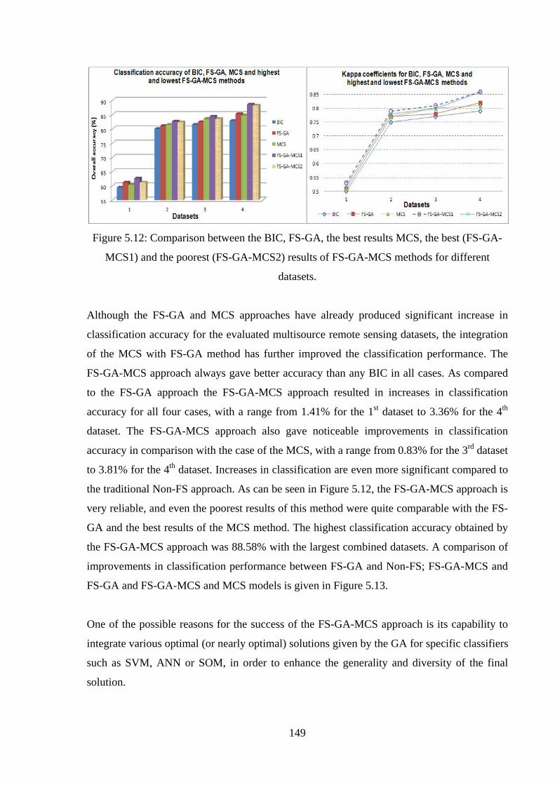
149

Figure 5.12: Comparison between the BIC, FS-GA, the best results MCS, the best (FS-GA-

MCS1) and the poorest (FS-GA-MCS2) results of FS-GA-MCS methods for different

datasets.

Although the FS-GA and MCS approaches have already produced significant increase in

classification accuracy for the evaluated multisource remote sensing datasets, the integration

of the MCS with FS-GA method has further improved the classification performance. The

FS-GA-MCS approach always gave better accuracy than any BIC in all cases. As compared

to the FS-GA approach the FS-GA-MCS approach resulted in increases in classification

accuracy for all four cases, with a range from 1.41% for the 1st dataset to 3.36% for the 4th

dataset. The FS-GA-MCS approach also gave noticeable improvements in classification

accuracy in comparison with the case of the MCS, with a range from 0.83% for the 3rd dataset

to 3.81% for the 4th dataset. Increases in classification are even more significant compared to

the traditional Non-FS approach. As can be seen in Figure 5.12, the FS-GA-MCS approach is

very reliable, and even the poorest results of this method were quite comparable with the FS-

GA and the best results of the MCS method. The highest classification accuracy obtained by

the FS-GA-MCS approach was 88.58% with the largest combined datasets. A comparison of

improvements in classification performance between FS-GA and Non-FS; FS-GA-MCS and

FS-GA and FS-GA-MCS and MCS models is given in Figure 5.13.

One of the possible reasons for the success of the FS-GA-MCS approach is its capability to

integrate various optimal (or nearly optimal) solutions given by the GA for specific classifiers

such as SVM, ANN or SOM, in order to enhance the generality and diversity of the final

solution.

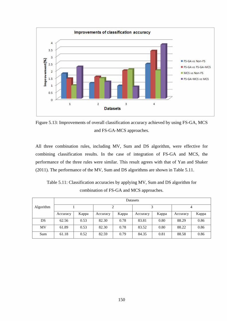
150

Figure 5.13: Improvements of overall classification accuracy achieved by using FS-GA, MCS

and FS-GA-MCS approaches.

All three combination rules, including MV, Sum and DS algorithm, were effective for

combining classification results. In the case of integration of FS-GA and MCS, the

performance of the three rules were similar. This result agrees with that of Yan and Shaker

(2011). The performance of the MV, Sum and DS algorithms are shown in Table 5.11.

Table 5.11: Classification accuracies by applying MV, Sum and DS algorithm for

combination of FS-GA and MCS approaches.

Algorithm

Datasets

1 2 3 4


DS 62.56 0.53 82.30 0.78 83.81 0.80 88.29 0.86

MV 61.89 0.53 82.30 0.78 83.52 0.80 88.22 0.86

Sum 61.18 0.52 82.59 0.79 84.35 0.81 88.58 0.86

151

5.2.5. CONCLUSIONS

Numerous MCS (classifier ensemble) techniques have been proposed and used to classify

different combined datasets of multi-date ENVISAT/ASAR, ALOS/PALSAR and Landsat 5

TM images. While the improvements in classification performance by employing the bagging

and boosting algorithms, except for the case of ANN-Bagging, are not very clear, the use of

MCS with SVM, ANN and SOM classifiers gave significant increases in classification

accuracy no matter which MV, Sum or DS combination rules were applied. The FS-GA

approach is very effective for handling multisource data, and its combination with any

classifier (ANN-MLP, SVM or SOM) gave considerable improvement in classification

accuracy.

The integration of FS-GA and the MCS techniques, which aims to further enhance the

performance of multisource data classification, has been implemented and evaluated. Results

of the investigation reveal that the proposal method is viable and useful. The FS-GA-MCS

approach outperformed the classical Non-FS, and both the FS-GA and MCS approaches in all

studied cases. The FS-GA-MCS approach always gave significantly higher accuracy than any

single best classifier. The FS-GA-MCS approach produced the highest overall classification

accuracy of 88.58% (Kappa=0.86) for the largest combined dataset consisted of original SAR

and optical images, their textural information and NDVI. The FS-GA and MCS based on

MV, Sum or DS combination rules are also very effective for classification of multisource

remote sensing data, although they are less accurate than the FS-GA-MCS approach. Finally,

the classification results confirm the advantages of multisource remote sensing data,

particularly the integration of SAR and optical data, for land cover mapping.

152

CHAPTER 6

CONCLUSIONS 6.1. SUMMARY AND CONCLUSIONS

The objectives of this thesis were to develop an appropriate methodology for improving land

cover classification using multisource remote sensing data.

To achieve this goal, firstly, an extensive literature review was conducted into the major

image classification techniques, the reported benefits of using multisource remote sensing

data and related work in this area. The review was conducted in chapter 2. It was revealed

that unlike the traditional parametric classifiers, the non-parametric classifiers are robust for

handling complex datasets because their principles are not constrained by the normal

distribution assumption. Hence, these algorithms should be, in principle, better suited for

classifying multisource remote sensing data. However, it was a surprise that in many studies,

which used combinations of different kinds of imagery and spatial data as an input for land

cover classification, the traditional Maximum Likelihood (ML) classifier was still very

popular. The application of non-parametric classifiers was reported in a number of studies but

they were not adequately investigated.

Chapter 3 was dedicated to evaluating the performance of multisource data and the non-

parametric algorithms for land cover classification in three different scenarios. A large

number of combined datasets generated from various types of data, including multi-temporal,

multi-polarisation and dual-frequency SAR images (ALOS/PALSAR and ENVISAT/ASAR),

multi-spectral images (SPOT 2 XS, Landsat TM) as well as derivative products such as

interferometric coherences, indices and textural information, were investigated. The Artificial

Neural Network (ANN) classifier based on the Multilayer Perceptron-Back Propagation

(MLP-BP) algorithm and the Support Vector Machine (SVM) non-parametric classifier were

applied, while the commonly used ML classifier was also implemented for comparison

purposes. The results obtained did confirm that the use of multisource data for land cover

153

classification is an appropriate approach. The classification based on combined datasets

always produced higher classification accuracy than that of single-type images/datasets. The

complimentary characteristics, and the impacts and contributions of each constituent data

type were taken into account and clearly emphasised. The use of multisource remote sensing

data not only provided an increase in the classification accuracy but also improved the

detectability/discernability/separability of land cover features. For instance, the combination

of ALOS/PALSAR backscatter and interferometric coherence data allowed visual detection

of burnt areas in the Victorian Bushfires, which was not possible using any single dataset.

Although these improvements in classification performance were obtained for all the

classifiers applied to multisource data, the MLP-BP and SVM algorithms did, in general,

outperform the ML algorithm, particularly when dealing with high dimensional, complex

datasets. Moreover, the SVM algorithm often provided the highest classification accuracy,

and marginally outperformed the MLP-BP classifier. This confirmed the advantages of non-

parametric classifiers over traditional parametric classifier for multisource remote sensing

data classification.

The integration of a feature selection technique based on the Genetic Algorithm (GA) with

the non-parametric classifiers was proposed as a means of resolving the challenging task of

selecting optimal combined datasets and defining parameters when classifying multisource

data. The GA algorithm has been used in remote sensing when dealing with high

dimensionality datasets such as hyperspectral data. However, the evaluation of this technique

for classification of multisource data has not been well addressed by previous investigators.

The basic concepts of feature selection, the GA algorithm and their application in an

experiment using a combination of SVM and GA algorithms (SVM-GA) for classifying

multisource remote sensing in Western Australia were discussed in chapter 4. In this

experiment the SVM-GA method has been used to classify 20 different combined datasets

generated from Landsat 5 TM multispectral, multi-temporal ALOS/PALSAR dual-

polarisation images and multi-level textural data. An approach based on “non-feature

selection” and the combination of SVM and Sequential Forward Floating Search (SVM-

SFFS) algorithms were also implemented for comparison purposes. Results of the

experiments illustrated the benefit of the proposed feature selection/SVM-GA approach. The

SVM-GA approach produced higher classification accuracy than the non-feature selection

/SVM-SFFS approach (in 19 out of 20 cases). The feature selection/SVM-GA approach also

achieved the highest overall classification accuracy of 96.47% for the largest combination

154

datasets, in which 81 out of 189 features were selected. It is interesting that in all cases that

the SVM-GA method was applied the Hughes phenomenon did not appear. Finally, the

modified objective function led to more reliable classification results than other functions

reported in the literature.

Other advanced techniques which have potential to increase classification accuracy of remote

sensing data, were also applied to multisource data classification. One is the Multiple

Classifier Systems (MCS) or classifier ensemble. The principles of MCS and its application

in remote sensing were reviewed in chapter 5. A new method was proposed and implemented

based on the integration of the GA with the MCS algorithm (FS-GA-MCS). Investigations

have been carried out using different MCS techniques with three non-parametric classifiers,

namely SVM, ANN-MLP and Self-Organising Map (SOM), feature selection based on the

GA (FS-GA) and the proposed approach over a study area in Appin, NSW, Australia. It was

revealed that both the FS-GA and MCS approaches (using classifier combination) produced

noticeable improvements in classification accuracy compared to the results of any individual

classifier. However, the FS-GA-MCS approach clearly outperformed other approaches in all

cases and gave the highest overall classification accuracy of 88.58% for the largest datasets.

This confirmed the value and effectiveness of the proposed approach for classifying

multisource data.

It must be emphasised that experiments in this thesis have been carried out successfully in

various study areas with highly diverse landscape and land cover patterns. These include two

test sites in Vietnam which represent an urban-suburban area in Ho Chi Minh City and the

typical rice production area in Mekong Delta; three test sites in Australia which represent

forest area prone to bushfire in Victoria, grassland (pasture) area in Western Australia and an

area with mixed use forest, pasture and residential in Appin, New South Wales. However,

because of time constraints the combination of the feature selection technique and the MCS

were only investigated for the Australian study areas. Nevertheless, the results of these

studies have illustrated the efficiency and usefulness of the proposed methods for different

types of land surfaces.

155

6.2. MAIN FINDINGS

The work carried out in the thesis has led to the following major findings:

- Multisource data can significantly improve the land cover classification performance,

because the complementary properties of different kinds of data are taken into

account.

- Non-parametric classifiers such as the ANN and SVM are appropriate for exploiting

the benefits of multisource remote sensing data. These algorithms generally produce

higher classification accuracy than a traditional parametric classifier such as the ML

algorithm.

- The integration of the GA with a non-parametric classifier is an efficient method for

handling multisource data. Such a hybrid approach ensures selection of the best

subsets and classifier parameters when applying them to high dimensionality datasets.

This method outperformed both the non-feature selection approach and the integration

of the conventional SFFS algorithm with the non-parametric classifier. In addition,

this method shows great capability to avoid the Hughes phenomenon, which limits the

classification accuracy while dealing with high dimensionality datasets.

- The MCS algorithm based on non-parametric classifiers is also capable of improving

the classification of multisource data, and this approach often resulted in higher

classification accuracy than any best individual classifier.

- The newly developed method of integration of the FS wrapper based on GA and the

MCS techniques is very robust and effective for classifying highly dimensional and

complex datasets. This method can exploit advantages of both FS-GA and MCS

techniques to improve the classification performance. It was found that this integrated

approach outperforms other approaches, including both FS-GA and MCS techniques.

6.3. FUTURE WORK

The proposed methodologies are not confined to the data that had been used for experiments

described in this thesis. To date, considering the large diversity of available satellite imagery

and other digital data sources, the use of these techniques with other kinds of imaging data,

such as high resolution optical and SAR images (Quick Bird, Worldview, TerraSAR-X or

Cosmo-SkyMed), hyperspectral (Chris/Proba, Hyperion) and Lidar data should be

investigated.

156

The textural information, particularly multi-level texture information, is a valuable data

source and has been incorporated into the classification process. However, the relationship

between textural data and particular feature classes has not been evaluated in detail.

Furthermore, some other kinds of texture measures, such as geostatistical and temporal

textures, have not been included in these studies. These issues could be investigated in future

work.

The feature selection technique based on the GA has been proposed and successfully applied

for handling highly complex datasets. However, the wrapper approach is very time

consuming, hence it is necessary to improve the efficiency of this approach. One possible

solution is to combine the filter and wrapper approaches into a single process.

Several MCS techniques have been applied for combining classification outputs and have

demonstrated positive results. In future, the use of other MCS techniques, such as multi-level

classification and fuzzy integral methods, should be studied.

The integration of several MCS and FS techniques based on GA algorithms studied in the

thesis has shown a great capability to improve the classification performance of multisource

remote sensing data. The further research should investigate on different combination of

these techniques to seek for the most efficient solution.

157

REFERENCES

Abe, B., Gidudu, A., and Marwal, T., 2010. Investigating the effects of ensemble

classification on remotely sensed data for land cover mapping, Proceeding of the

International Geoscience and Remote Sensing Symposium (IGARSS), Honolulu HI,

25-30 July, pp. 2382-2835.

Agelis, C.F., Freitas, C.C., Valeriano, D.M. and Dutra, L.V., 2002, Multitemporal analysis of

land use/land cover JERS-1 backscattering in the Brazilian tropical rainforest.

International Journal of Remote Sensing, 23 (7), pp. 1231–1240.

Aitkenhead, M.J., and Aalders, I.H., 2008. Classification of Landsat Thematic Mapper

imagery for land cover using neural networks, International Journal of Remote

Sensing 29 (7), pp. 2075–2084.

Almeida-Filho, R., Rosenqvist, A., Shimabukuro, Y.E., and Silva-Gomez, R., 2007.

Detecting deforestation with multitemporal L-band SAR imagery: a case study in

western Brazilian Amazonia. International Journal of Remote Sensing, 28 (6),

pp.1383-1390.

Almeida-Filho, R., Rosenqvist, A., Shimabukuro, Y.E., and Sanchez, G. A., 2009. Using

dual-polarized ALOS PALSAR data for detecting new fronts of deforestation in the

Brazilian Amazonia. International Journal of Remote Sensing 30 (14), pp. 3735-3743.

Amarsaikhan, D., 2006. Application of multisource data for urban land cover mapping.

Proceeding of ISPRS Commission VII Mid-term Symposium "Remote Sensing: From

Pixels to Processes", Enschede, the Netherlands, 8-11 May.

Anthony, G., and Ruther, H., 2007. Comparison of Feature Selection Techniques for SVM

classification. Proceeding of the ISPRS Working Group VII/1 Workshop

ISPMSRS’07: “ Physical Measurements and Signatures in Remote Sensing”, 12-14

March, Davos, Switzeland.

Antikidis, E., Arino, O., Laur, H., and Arnaud, A., 1998. ERS SAR coherence and ATSR hot

spots: a Synergy for Mapping Deforested Areas. The Special Case of the 1997 Fire

Event in Indonesia. Proceedings of the Retrieval of Bio and Geo-Physical Parameters

from SAR Data for Land Applications Workshop ESTEC, 21–23 October,

Netherlands, ESA SP 441.

Argany, M., Amini, J., and Saradjian, M.R., 2006. Artificial neural networks for

improvement of classification accuracy in Landsat +ETM images, Proceeding of Map

158

Middle East Conference, Dubai, 26-29 March. Available at:

http://www.gisdevelopment.net/proceeding/mapmiddleeast/2006/mm06pos_98.htm.

Avery, T. E., and Berlin, G. E., 1992. Fundamentals of Remote Sensing and Airphoto

Interpretation. Fifth Edition. Prentice Hall.

Ban, Y., and Wu, Q., 2005. RADARSAT SAR data for landuse/land-cover classification in

the rural-urban fringe of the greater Toronto area. Proceedings of 8th AGILE

Conference on Geographic Information Science, 26–28 May 2005, Estoril, Portugal.

Bargiel, D., and Herrmann, S., 2011. Multi-Temporal Land-Cover Classification of

Agricultural Areas in Two European Regions with High Resolution Spotlight

TerraSAR-X Data. Journal of Remote Sensing 3, pp. 859-877.

Baronti, S., Del Frate, F., Ferrazzoli, P., Paloscia, S., Pampaloni, P., and Schiavon, G. 1995.

SAR polarimetric features of agricultural areas. International Journal of Remote

Sensing 16 (14), pp. 2639–2356.

Basili, R., Del Frate, F., Luciani, M., Mesiano, F., Pacifici, F., and Rossi, R., 2008. A

comparative analysis of kernel-based methods for the classification of land cover

maps in satellite imagery. International Geoscience and Remote Sensing Symposium

(IGARSS), 4, 7-11 July, pp. IV - 735 - IV – 738.

Benediktsson, J.A., Chanussot, J., and Fauvel, M., 2007. Multiple classifier systems in

remote sensing: from basics to recent developments. In: M. Haindl, J. Kittler and F.

Roli, eds.Multiple Classifier Systems. Heidelberg, Germany: Springer, pp. 501–512.

Berberoglu, S., Lloyd, C. D., and Atkinson, P. M., Curran, P. J., 2000. The integration of

spectral and textural information using neural networks for land cover mapping in the

Mediterranean. Computer & Geosciences 26, pp.385-396.

Berberoglu, S., Curran, P. J., Lloyd, C. D., and Atkinson, P. M., 2007. Texture classification

of Mediterranean land cover. International Journal of Applied Earth Observation and

Geoinformation 9, pp. 322-334.

Blaes, X., Vanhalle, L., Defourny, P., 2005. Efficientcy of crop identification based on

optical and SAR image time series. Remote Sensing of Environment 96 (3-4), pp.

352-365.

Briem, G. J., Benediktsson, J. A., and Sveinsson, J. R., 2002. Multiple classifier applied to

multisource remote sensing data. IEEE Transactions on Geosciences & Remote

Sensing, 40 (10), pp. 2291-2299.

http://www.gisdevelopment.net/proceeding/mapmiddleeast/2006/mm06pos_98.htm

159

Briem, G. J., Benediktsson, J. A., and Sveinsson, J. R., 2001. Boosting, Bagging, and

Consensus Based Classification of Multisource Remote Sensing Data. Multiple

classifier systems – Lecture notes in Computer Science, 2096/2001, pp. 279-288,

DOI: 10.1007/3-540-48219-9_28.

Brisco, B. and Brown, R.J., 1995, Multidate SAR/TM synergism for crop classification in

western Canada. Photogrammetric Engineering and Remote Sensing 61, pp.1009-

1014.

Bruzzone, L., Marconcini, M., Wegmuller, U., Wiesmann, A., 2004. An advanced system for

the automatic classification of multitemporal SAR images. IEEE Transaction on

Geoscience & Remote Sensing 42 (6), pp. 1321-1334.

Bruzzone, L., and Persello, C., 2009. A Novel Approach to the Selection of Spatially

Invariant Features for the classification of Hyperspectral Images with Improved

Generalization Capability. IEEE Transactions on Geosciences & Remote Sensing 47

(9), pp. 3180-3191.

Charlton, M. B., and White, K., 2006. Sensitivity of radar backscatter to desert surface

roughness. International Journal of Remote Sensing 27 (8), pp. 1641-1659.

Chang, C. H., and Lin, C. J., 2011, LIBSVM : a library for support vector machines”, ACM

Transactions on Intelligent Systems and Technology, 2:27:1--27:27.

Chen, D. M., and Stow, D., 2003. Strategies for Integrating Information from Multiple

Spatial Resolutions into Land-Use/Land-Cover Classification Routines.

Photogrammetric Engineering & Remote Sensing Vol. 69 (11), pp. 1279 - 1287.

Chen, D., Stow, D.A. and Gong, P., 2004. Examining the effect of spatial resolution and

texture window size on classification accuracy: an urban environment case.

International Journal of Remote Sensing 25 (11), pp. 2177–2192.

Chova, L. G., Prieto, D. F., Calpe, J., Soria, E., Vila, J., Valls, G. C., 2006. Urban monitoring

using multi-temporal SAR and multi-spectral data. Journal of Pattern Recognition

Letter 27, pp. 234- 243.

Chu, H.T., and Ge, L., 2010a. Synergistic use of multi-temporal ALOS/PALSAR with SPOT

multispectral satellite imagery for land cover mapping in the Ho Chi Minh city area,

Vietnam. Proceeding of the International Geoscience and Remote Sensing

Symposium (IGARSS), Honolulu HI, 25-30 July, pp. 1465-1468.

Chu, H.T., and Ge, L., 2010b. Land cover classification using combination of L- and C-band

SAR and optical satellite images. Proceeding of 31st Asian conference of Remote

sensing (ACRS), Hanoi, 1-5 November, paper TS39-2, (on CD-ROM).

http://www.springerlink.com/content/t6dp5gn360gbngb6/�

http://www.springerlink.com/content/t6dp5gn360gbngb6/�

160

Chust, G., Ducrot, D., and Pretus, J. LL., 2004. Land cover discrimination potential of radar

multitemporal series and optical multispectral images in a Mediterranean cultural

landscape. International Journal of Remote Sensing 25 (17), pp. 3513–3528.

Coburn, C. A., and Roberts, A. C., 2004. A multiscale texture analysis procedure for

improved forest stand classification, International Journal of Remote Sensing 25 (20),

pp. 4287–4308.

Dixon, B., and Candade, N., 2008. Multispectral landuse classification using neural networks

and support vector machines: one or the other, or both. International Journal of

Remote Sensing 29 (4), pp. 1185–1206.

Du, P., Sun, H., and Zhang, W., 2009a. Multiple classifier combination for target

identification from high resolution remote sensing images. ISPRS Archive Volume

XXXVIII-1-4-7/W5, ISPRS Hannover Workshop 2009, High-Resolution Earth

Imaging for Geospatial Information, June 2-5, Hannover, Germany.

Du, P., Zhang, W., and Sun, H., 2009b. Multiple Classifier Combination for Hyperspetral

Remote Sensing Image Classification. MCS 2009, LNCS 5519, Springer-Verlag

Berlin Heidelberg. pp.52-61.

Dutra, L. V., Scofield, G. B., Neta, S. R. A., Negri, R. G., Freitas, C. C., Andrade, D., 2009.

Land Cover Classification in Amazon using Alos Palsar Full Polarimetric Data. Anais

XIV Simpósio Brasileiro de Sensoriamento Remoto, Natal, Brasil, 25-30 April 2009,

INPE, pp. 7259-7264

Engdahl, M. E., Hyyppa, J. M., 2003. Land cover classification Using Multi-temporal ERS -

1/2 InSAR Data. IEEE Transactions on Geosciences & Remote Sensing 41 (7), pp.

1620-1628.

Erasmi, S., and Twele, A., 2009. Regional land over mapping in the humid tropics using

combined optical and SAR satellite data – a case study from Central Sulawesi,

Indonesia. International Journal of Remote Sensing 30 (10), pp. 2465-2478.

Foody, G.M., 1999, Image classification with a neural network: from completely crisp to

fully-fuzzy situations, In P.M. Atkinson and N.J. Tate, Advances in Remote Sensing

and GIS analysis, Chichester: Wiley & Son.

Foody, G.M., 2002, Status of land cover classification accuracy assessment. Remote Sensing

of Environment, 80, pp. 185–201.

Foody, G. M., and A. Mathur. 2004. Toward intelligent training of supervised image

classifications: Directing training data acquisition for SVM classification. Remote

Sensing of Environment 93, pp.107-117

161

Foody, G. M., Boyd, D. S., and Sanchez-Hernandez, C., 2007. Mapping a specific class with

an ensemble of classifiers. International Journal of Remote Sensing 28 (8), pp. 1733-

1746.

Forster, B. C., 1986. Evaluation of Combined Multiple Incident Angle SIR-B Digital Data

and Landsat MSS Data over an Urban Complex. Proceeding of the 7th International

Symposium Remote Sensing for Resources Development and Environment

Management, Enschede, Netherlands, 25-29 August, pp. 813- 816.

Forster, B. C., 1987. Applications in Urban Monitoring and Engineering. Microwave Remote

Sensing, Course Notes, The University of New South Wales, School of Geomatic

Engineering, pp. 50 - 53.

Freund, Y., and Schapire, R. E., 1996. Experiments with a new boosting algorithm.

Proceedings of the Thirteenth International Conference of Machine Learning, pp. 148-

156.

Frost, V. S., Stiles, J. A., Shanmugan, K. S., and Holtzman, J. C., 1982. A Model for Radar

Images and Its Application to Adaptive Digital Filtering of Multiplicative Noise.

IEEE Transactions on Pattern Analysis and Machine Intelligence PAMI-4 (2), pp.

157-166.

Gamba, P., Fabio Dell’Acqua, F., Dasarathy, B. V., 2005. Urban remote sensing using

multiple data sets: Past, present, and future. Information Fusion 6, pp.319–326.

Gao, J., 2009, Digital Analysis of Remotely sensed imagery. McGraw-Hill Companies, Inc.

Gimeno, M., San-Miguel-Ayanz, J., and Schmuck, G., 2004, Identification of burnt areas in

Mediterranean forest environments from ERS-2 SAR time series. International

Journal of Remote Sensing 25 (22), pp. 4873-4888.

Gomez-Chova, L., Calpe, J., Camps-Valls, G., Martin, J.D., Soria, E., Vila, J., Alonso-

Chorda, L., Moreno, J., 2003. Feature Selection of Hyperspectral Data Through

Local Correlation and SFFS for Crop Classification. International Geoscience and

Remote Sensing Symposium (IGARSS), 1, pp. 555-557.

Gong, P., and P. J. Howarth, 1990. An Assesement of Some Factors Influencing

Multispectral Land-Cover Classification. Photogrammetric Engineering and Remote

Sensing 56 (1), pp. 597-603.

Goldberg, D., 1989, Genetic algorithm in Search, Optimization in Machine Learning

Reading, MA: Addison Wesley.

http://ieeexplore.ieee.org/search/searchresult.jsp?searchWithin=p_Authors:.QT.Calpe,%20J..QT.&newsearch=partialPref�

http://ieeexplore.ieee.org/search/searchresult.jsp?searchWithin=p_Authors:.QT.Moreno,%20J..QT.&newsearch=partialPref�

http://ieeexplore.ieee.org/xpl/mostRecentIssue.jsp?punumber=9010�

162

Guerschman, J.P., Paruelo, J. M., Di Bella, C., Giallorenzi, M. C., and Pacin, F., 2003. Land

cover classification in the Argentine Pampas using multi-temporal Landsat TM data,

International Journal of Remote Sensing 24 (17), pp. 3381-3402.

Guyon, I., Weston, J., Barnhill, S., and Vapnik, V., 2002. Gene selection for cancer

classification using support vector machines. Machine Learning 46, pp. 389–422.

Fundamentals of Remote Sensing, a Canada Centre for Remote Sensing Remote Sensing

Tutorial. Available at: http://www.nrcan.gc.ca/sites/www.nrcan.gc.ca.earth-

sciences/files/pdf/resource/tutor/fundam/pdf/fundamentals_e.pdf.

Haack, B. N., 1984. Multisensor Data Analysis of Urban Environments. Photogrammetric

Engineering and Remote Sensing 50 (10), pp. 1471 - 1477.

Haack, B., and Bechdol, M., 2000. Integrating multisensor data and RADAR texture

measures for land cover mapping. Computers & Geosciences 26, pp. 411- 421.

Haack, B., and Khatiwada, G., 2010. Comparison and integration of optical and

quadpolarization radar imagery for land cover/use delinieation. Journal of Applied

Remote Sensing 4 (1), pp. 1-16.

Hall-Beyer, M., 2007, GLCM Texture Tutorial; Version: 2.10, University of Calgary.

Available from: http://www.fp.ucalgary.ca/mhallbey/tutorial.htm.

Henderson, F.M., and A.J. Lewis (editors), 1998. Principles & Applications of Imaging

Radar, Manual of Remote Sensing, Third edition, Volume 2, American Society for

Photogrammetry and Remote Sensing, John Wiley & Sons, Inc., New York.

Herold, N. D., Haack, B. N., and Solomon, E., 2005. Radar spatial considerations for land

cover extraction. International Journal of Remote Sensing, 26 (7), pp.1383-140.

Hughes, G. F., 1968, On the mean accuracy of statistical pattern recognizers, IEEE

Transactions on Information Theory, 14(1), pp. 55–63.

Huang, C., Davis, L. S., Townshend, J. R. G., 2002. An assessment of support vector

machines for land cover classification. International Journal of Remote Sensing 23

(4), pp. 725–749.

Huang, Z. and Lees, B.G., 2004, Combining non-parametric models for multisource

predictive forest mapping. Photogrammetric Engineering and Remote Sensing, 70,

pp. 415–425.

Huang, C.L., Wang, C.J., 2006. A GA-based feature selection and parameters optimization

for support vector machines. Expert Systems with Applications 31, pp. 231-240.

http://www.fp.ucalgary.ca/mhallbey/tutorial.htm�

http://www.nrcan.gc.ca/sites/www.nrcan.gc.ca.earth-sciences/files/pdf/resource/tutor/fundam/pdf/fundamentals_e.pdf



163

Huang, H., Legarsky, J., and Othman, M., 2007. Land-cover Classification Using Radarsat

and Landsat Imagery for St. Louis, Missouri. Photogrammetric Engineering &

Remote Sensing 73 (1), pp. 037–043.

Hugo, C., Capao, L., Fernando, B. and Mario, C., 2006. Meris Based Land Cover

Classification with Self-Organizing Maps: preliminary results, Proceedings of the 2nd

EARSeL SIG Workshop on Land Use & Land Cover, 28 - 30 September, Bonn,

Germany.

Hussin, Y. A., 1997. Tropical Forest Cover Typees Differntiation using Satellite Optical and

Radar Data:A Case Study From Jambi, Indonesia. Proceeding of Asian Conference of

Remote Sensing (ACRS), Kuala Lumpur, Malaysia, 20-24 November.

Heinl, M., Walde, J., Tappeiner, G., and Tappeiner, U., 2009. Classifiers vs. input variables-

The drivers in image classification for land cover mapping. International journal of

Applied Earth Observation and Geoinformation 11, pp. 423-430.

Jensen, J.R., 2004. Introduction to Digital Image Processing: A remote sensing perspective,

4th edition, Prentice Hall.

Kavzoglu, T., and Mather, P. M., 2002. The role of feature selection in artificial neural

network applications. International journal of Remote sensing 23 (15), pp. 2919-2937.

Kavzoglu, T., and Mather, P. M., 2003. The use of backpropagating artificial neural network

in land cover classification. International journal of Remote sensing 24 (23), pp.

4907-4938.

Kavzoglu, T., 2009. Increasing the accuracy of neural network classification using refined

training data. Environmental Modelling & Software, 24 (7), pp 850-858.

Kavzoglu, T., and Colkesen, I., 2009. A kernel functions analysis for support vector machines

for land cover classification, International Journal of Applied Earth Observation &

Geoinformation 11 (5), pp. 352–359.

Kim, S.H., and Lee, K.S., 2005. Integration of Landsat ETM+ and Radarsat SAR for land

cover classification. Trans Tech Publications, Switzerland,

doi:10.4028/www.scientific.net/KEM.277-279.838.

Lee, J.-S., 1980. Digital Image Enhancement and Noise Filtering by Use of Local Statistics,

IEEE Transactions on Pattern Analysis and Machine Intelligence, .2 (2), pp. 165-168.

Lee, J.-S., 1981. Speckle Analysis and Smoothing of Synthetic Aperture Radar Images,

Computer Graphics and Image Processing 17 (1), pp. 24-32.

J. S. Lee, 1983. A simple speckle smoothing algorithm for synthetic aperture radar images

IEEE Transactions on Systems, Man, and Cybernetic SMC-13 (1), pp. 85–89.

http://www.sciencedirect.com/science?_ob=ArticleURL&_udi=B6VHC-4V7KBVG-1&_user=37161&_coverDate=07%2F31%2F2009&_alid=980995766&_rdoc=31&_fmt=high&_orig=search&_cdi=6063&_st=13&_docanchor=&_ct=1375&_acct=C000004218&_version=1&_urlVersion=0&_userid=37161&md5=d0958617edaef8b8dbfdf712a8a008f0�

http://www.sciencedirect.com/science?_ob=ArticleURL&_udi=B6VHC-4V7KBVG-1&_user=37161&_coverDate=07%2F31%2F2009&_alid=980995766&_rdoc=31&_fmt=high&_orig=search&_cdi=6063&_st=13&_docanchor=&_ct=1375&_acct=C000004218&_version=1&_urlVersion=0&_userid=37161&md5=d0958617edaef8b8dbfdf712a8a008f0�

http://www.scientific.net/KEM.277-279.838

164

Lehmann, E., Caccetta, P., Zhou, Z. –S., Mitchell, A., Tapley, I., Milne, A., Held, A., Lowell,

K., and McNeill, S., 2011. Forest Discrimination Analysis of Combined Landsat and

ALOS-PALSAR Data. Proceeding of the 34th International Symposium on Remote

Sensing of Environment, Sydney, Australia, 10-15 April.

Lemonie, G.G., de Grandi, G. F., and Sieber, A. j., 1994. Polarimetric contrast classification

of agricultureal fields using MASTRO1 AirSAR data, International journal of remote

sensing, Vol. 24 (1), pp. 28-35.

Li, G., Lu, D., Moran, E., and Hetrick, S., 2011, Land-cover classification in a moist tropical

region of Brazil with Landsat TM imagery, International Journal of Remote Sensing,

Vol. 32 (23), pp. 8207-8230.

Lillesand, T. M., and Kieffer, R. V., 2004. Remote sensing and Image Interpretation, Fourth

edition, John Wiley and Sons, New York, 2004.

Lloyd, C. D., Berberoglu, S., Curran, P. J., and Atkinson, P. M., 2004. A comparision of

texture measures for the per-field classification of Mediterranean land cover.


Lopes, A., Touzi, R., and Nezry, E., 1990, Adaptive Speckle Filters and Scene Heterogeneity,

IEEE Transactions on Geoscience & Remote Sensing, Vol. 28 (6), pp. 992-1000.

Luo, C., Liu, Z., and Meng, W., 2008. A integrated classifier for large regional-scale land

cover classifying. The International Archives of the Photogrammetry, Remote

Sensing and Spatial Information Sciences. Vol. XXXVII. Part B6b. pp.607-612.

Lu, D., Moran, E., and Batistella, M., 2003, Linear mixture model applied to Amazonian

vegetation classification. Remote Sensing of Environment, Vol. 87, pp. 456-469.

Lu, D., Batistella, M., and Moran, E., 2007. Land-cover classification in the Brazilian

Amazon with the integration of Landsat ETM+ and Radarsat data. International

Journal of Remote Sensing 28 (24), pp. 5447-5459.

Lu, D., Li, G., Moran, E., Dutra, L., and Batistella, M., 2011, A Comparison of Multisensor

Integration Methods for Land Cover Classification in the Brazilian Amazon. GIScience & Remote Sensing 48 (3), pp. 345–370.

Maghsoudi, Y., Alimohammadi, A., Valadan Zoej, M. J., and Mojaradi, B., 2006. Weighted

combination of multiple classifiers for the classification of hyperspectral images using

genetic algorithm. In : ISPRS Archives, Vol XXXVI(part 7)- Proceeding of the

ISPRS Commission VII Symposium ‘Remote Sensing: From Pixels to Processes’,

May 8-11, Enschede, The Netherlands.

165

Maghsoudi, Y., Valadan Zoej, M. J., and Michael Collins, M., 2011. Using class-based

feature selection for the classification of hyperspectral data, International Journal of

Remote Sensing, 32 (15), pp. 4311-4326

Maillard, P., Alencar-Silva, T. and Clausi, D., 2008. An evaluation of Radarsat-1 and ASTER

data for mapping veredas (palm swamps). Sensors, 8 (9), pp.6055-6076.

Marceau, D.J., Howarth, P.J., and D.J. Gratton, D. J., 1994a. Remote sensing and the

measurement of geographical entities in a forest environment 1: The scale and spatial

aggregation problem, Remote Sensing of Environment, Vol. 49, pp. 49:93–104.

Marceau, D.J., Howarth, P.J., and D.J. Gratton, D. J., 1994b. Remote sensing and the

measurement of geographical entities in a forest environment 2: The optimal spatial

resolution, Remote Sensing of Environment, Vol. 49, pp. 105–117.

Markham, B. L., and Townshend, J. R. G., 1981, Land cover classification accuracy as a

function of sensor spatial resolution. Proceedings of the 15th International Symposium

on Remote Sensing of Environment, Ann Arbor, MI, 11–15 May (Ann Arbor: ERIM),

pp. 1075–1090.

Markowetz, F., 2003, Classification by SVM, Practical DNA Microarray Analysis,

Available at: compdiag.molgen.mpg.de/ngfn/docs/2003/mar/SVM.pdf.

McNairna, H., Catherine Champagnea, C., Shanga, J., Holmstromb, D., Reichert, G.,2009.

Integration of optical and Synthetic Aperture Radar (SAR) imagery for delivering

operational annual crop inventories. ISPRS Journal of Photogrammetry & Remote

Sensing 64, pp. 434-449.

Melgani, F., and Bruzzone, L., 2004. Classification of hyperspectral remote sensing images

with support vector machine, IEEE Transactions on Geosciences and Remote Sensing

42 (8), pp. 1778-1790.

Mills, H., Cutller, M.E.J., and Fairbairn, D., 2006. Artificial neural network for mapping

regionalscale upland vegetation from high spatial resolution imagery, International

Journal of Remote Sensing 27 (11), pp 2177-2195.

Mountrakis, G., Im, J. and Ogole, C., 2011, Support vector machines in remote sensing: A

review. ISPRS Journal of Photogrammetry and Remote Sensing Vol. 66, pp. 247–

259.

Narasimha Rao, P.V., Sesha Sai, M.V.R., Sreenivas, K., Krishna Rao, M.V., Rao, B.R.M.,

Dwivedi, R.S. and Venkataratnam, L., 2002. Textural analysis of IRS-1D

panchromatic data for land cover classification. International Journal of Remote

Sensing, 23 (17), pp. 3327–3345.

166

Nizalapur, V., 2008, Land cover classification using multi-source data fusion of Envisat

ASAR and IRS P6 Liss-III Satellite data – a case study over tropical moist deciduos

forested region of Karnataka, India. The International Archives of the

Photogrammetry, Remote Sensing and Spatial Information Sciences. Vol. XXXVII.

Part B6b. pp. 329-334.

Nizalapur, V., Maduundu, R., and Jha, C. S., 2011. Coherence-based land cover classification

in forested area of Chttigarh, Central India, using environment satellite – advanced

synthetic aperture radar data. Journal of Applied Remote Sensing 5, pp. 059501-1-6.

Nordkvist, K., Granholm, A. H., Holmgren, J., Olsson, H., & Nilsson, M., 2012, Combining

optical satellite data and airborne laser scanner data for vegetation classification,

Remote Sensing Letters 3(5), pp. 393-401.

Nyoungui, A., Tonye, E. and Akono, A., 2002. Evaluation of speckle filtering and texture

analysis methods for land cover classification from SAR images. International Journal

of Remote Sensing 23 (9), pp. 1895–1925.

Osowski, S., Siroic, R., Markiewicz, T., and Siwek, K., 2009. Application of Support Vector

Machine and Genetic Algorithm for improved blood cell recognition, IEEE

Transactions on Instrumentation and Measurement 58 (7), pp.2159 – 2168.

Osuma, R., 2005. Pattern Analysis, Sequential Feature Selection, Lecture note. Texas A&M

University.

Pacifici, P., Chini, M., Emery, J. M, 2009. A neural network approach using multi-scale

textural metrics from very high-resolution panchromatic imagery for urban land-use

classification. Remote Sensing of Environment 113, pp. 1276–1292

Pal, M. and Mather, P.M., 2005. Support vector machines for classification in remote

sensing, International Journal of Remote Sensing 26 (5), pp. 1007–1011.

Pal, M., 2006. Support vector machine-based feature selection for land cover classification: a

case study with DAIS hyperspectral data', International Journal of Remote Sensing,

27 (14), pp. 2877-2894.

Pal, M., 2008, Ensemble of support vector machines for land cover classification,


Paola, J.D., and Schowengerdt, R.A., 1995. A review and analysis of back propagation

neural networks for classification of remotely sensed multispectral imagery.

International Journal of Remote Sensing 16 (16), pp. 3033–3058.

167

Park, N. –W., Chi, K. –H., 2008. Integration of multitemporal/polarization C– band SAR data

sets for Land cover Classification. International Journal of Remote Sensing 29 (16),

pp. 4667-4688.

Peddle, D. R., and Ferguson, D. T., 2002, Optimization of multisource data analysis: an

example using evidence reasoning for GIS data classification. Co mp u t e r s

& Geosciences 28, pp. 45-52.

Pierce L.E., Bergen K.M., Dobson M.C., and Ulaby F.T., 1998, Multitemporal land-cover

classification using SIR-C/X-SAR imagery, Remote Sensing of Environment 64 (1),

pp. 20-33.

Polikar, R., 2006. Ensemble Based Systems in Decision Making, IEE Circuits and Systems

Magazine 6 (3), pp. 21-45.

Pouteau, R., Stoll, B., and Chabrier, S., 2010. Multi-source SVM fusion for environmental

monitoring in Marquesas archipelago. Proceeding of the International Geoscience and

Remote Sensing Symposium (IGARSS), pp. 2719-2722. Honolulu, HI, 25-30 July.

Pradhan, R., Pradhan, M. P., Bhusan, A., Pradhan, R. K., and Ghose, M. K., 2010. Land-

cover classification and mapping for Eastern Himalayan State Sikkim. Journal of

Computing 2 (3), pp. 166-170.

Puissant, A., Hirsch, J., and C Weber, C., 2005. The utility of texture analysis to improve per-

pixel classification for high to very high spatial resolution imagery. International

Journal of Remote Sensing 26 (4), pp.733–745.

Quegan, S., Toan, T. L., Yu, J. J., Ribbes F., and Floury, N., 2000, Multitemporal ERS SAR

Analysis Applied to Forest Mapping, IEEE Transactions on Geoscience and Remote

Sensing 38 (2), pp. 741-753.

Qiu, F., Berglund, J., Jensen, J. R., Thakkar, P., and Ren, D., 2004, Speckle Noise Reduction

in SAR Imagery Using a Local Adaptive Median Filter, GIScience and Remote

Sensing 41 (3), pp. 244-266.

Richards,J. A., Jia, X., 2006. Remote Sensing Digital Image Analysis – An introduction.

Springer, Fourth Edition.

Shafri, H. Z. M., and Ramle, F. S. H., 2009. A comparison of Support Vector Machine and

Decision Tree Classifications Using Satellite Data of Langkawi Island, Information

Technology Journal 8 (1), pp. 64-70.

Salah, M., Trinder, J.C., Shaker, A., Hamed, M., and Elsagheer, A., 2010. Integrating

multiple classifiers with fuzzy majority voting for improved land cover classification.

168

ISPRS Int Arch Photogrammetric Engineering and Remote Sensing & SIS 39 (3), Part

A, pp.7-12.

Salah, M., Trinder, J. and Shaker, A., 2009. Evaluation of the self-organizing map classifier

for building detection from lidda data and multispectral aerial images. Journal of

Spatial Science, 54, pp. 15-34.

Santos, J.R., Freitas, C.C., Araujo, L.S., Dutra, L.V., Mura, J.C., Gama, F.F.,Soler, L.S. and

Sant’Anna, S.J.S., 2003, Airborne P-band SAR applied to the aboveground biomass

studies in the Brazilian tropical rainforest. Remote Sensing of Environment 87, pp.

482–493.

Schapire, R. E., 1990. The strength of weak learnability. Machine Learning 5 (2), pp. 197-

227.

Shang, J., McNairm, H., Champagne, C., and Jiao, X., 2009. Appliation of Multi-Frequency

Synthetic Aperture Radar(SAR) in Crop Classification, Chapter 27, Advances in

Geoscence and Remote Sensing, Published: October 01 by InTech.

Shang, J., McNairm, H., Champagne, C., and Jiao, X., 2008. Contribution of multi-

frequency, multi-sensor, and multi-temporal radar data to operational annual crop

mapping. Proceeding of the International Geoscience and Remote Sensing

Symposium, Boston (Massachusetts), 7-11 July, 4 pp. Invited paper.

Shang, J., McNairm, H., Champagne, C., and McNairm, H., 2006. Agriculture land use using

multi-sensor and multi-temporal Earth Observation data. Proceeding of the

MAPPS/ASPRS 2006 Fall Specialty conference, San Antonio, Texas, USA.

Shafri, H. Z. M., and Ramle, F. S. H., 2009. A comparison of Support Vector Machine and

Decision Tree Classifications Using Satellite Data of Langkawi Island, Information

Technology Journal 8 (1), pp. 64-70.

Sheoran, A., Haack, B., and Sawaya, S., 2009. Land cover/use classification using optial and

quad polarization radar imagery. Proceeding of the ASPRS 2009 Annual

Conferencce, Baltimore, Maryland, 9 -13 March.

Shin, J., Yoon, J., Kang, S., and Lee, K., 2007. Comparison of Signal Characteristics between

X-, C-, and L-band SAR Data in Forest Stand. Available at: http://www.a-a-r-

s.org/acrs/proceeding/ACRS2007/Papers/TS30.3.pdf.

Serpico, S. B., and Bruzzone, L., 2001. A new search algorithm for feature selection in

hyperspectral remote sensing images. IEEE Transactions on Geoscience and Remote

Sensing, 39 (7), pp. 1360-1367.

http://www.a-a-r-s.org/acrs/proceeding/ACRS2007/Papers/TS30.3.pdf�

http://www.a-a-r-s.org/acrs/proceeding/ACRS2007/Papers/TS30.3.pdf�

169

Siegert, F., and Hoffmann, A. A., 2000. The 1998 Forest Fires in East Kalimantan

(Indonesia): A Quantitative Evaluation Using High Resolution, Multitemporal ERS-2

SAR images and NOAA-AVHRR Hotspot Data. Remote Sensing of Environment, 72,

pp-64-67.

Siegert, F., and Ruecker, G., 2000. Use of multitemporal ERS-2 SAR images for identication

of burned scars in south-east Asian tropical rainforest. International Journal of

Remote Sensing 21 (4), pp. 831-837.

Skriver, H., 2008. Comparison between multi-temporal and polarimetric SAR data for land

cover classification. Proceeding of the International Geoscience and Remote Sensing

Symposium (IGARSS), Boston (Massachusetts), 7-11 July. pp.558-561.

Somol, P., Novovicova, J., and Pudil, P., 2006. Flexible-Hybrid Sequential Floating Search in

Statistical Feature Selection. Lecture Notes in Computer Science 4109/2006, pp. 632-

639, DOI: 10.1007/11815921_69.

Soria-Ruiz, J., Fernadez-Ordonez, Y., and Woodhouse, I. H., 2010. Land-cover lassification

using radar and optical images: a case study in Central Mexico. International Journal

of Remote Sensing 31 (12), pp. 3291–3305.

Srivastava, H. S., Patel, P., Navalgund, R. R., 2006. Application potentials of synthetic

aperture radar interferometry for land-cover mapping and crop-height estimation.

Current Science 91 (6), pp.783-788.

Steninger, M.K., 2000, Satellite estimation of tropical secondary forest aboveground biomass

data from Brazil and Bolivia. International Journal of Remote Sensing 21 (6),

pp.1139–1157.

Tassetti, A. N., Malinverni, E. N., and Hahn, M., 2010. Texture analysis to improve

supervised classification in IKONOS imagery, ISPRS TC VII Symposium – 100

Years ISPRS, Vienna, Austria, 5-7 July, IAPRS, Vol. XXXVIII, Part 7A, pp. 245-

250.

Takeuchi, S., Suga, Y., and Yoshimura, M., 2001. A comparative study of coherence

information by L band and C band SAR for detecting deforestation in tropical rain

forest. Proceeding of the International Geosciences and Remote Sensing Symposium

IGARSS’01, Sydney, Australia, 9-13 July, Vol. 5, pp. 2259-2261.

Takeuchi, S., and Yamada, S., 2002, Monitoring of Forest Fire Damage by Using JERS-1

InSAR. IEEE International Geosciences and Remote Sensing Symposium, IGARSS

’02, Torongto, Canada, 24-28 June, pp. 3290-3292.

170

Thiel, C. J., Thiel, C., and Schmullius, C. C., 2009. Operational Large-area forest Monitoring

in Siberia Using ALOS PALSAR Summer intensity and winter Coherence, IEEE

Transactions on Geoscience and Remote Sensing 47 (12), pp. 3993-4000.

Trinder, J.C., Salah, M., Shaker, A., Hamed, M., and Elsagheer, A., 2010. Combining

statistical and neural classifier using Dempster-Shafer theory of evidence for

improved building detection. Proceeding of 15th Australasian Remote Sensing &

Photogrammetry Conference (15th ARSPC), Alice Springs, Australia, 13-17

September.

Tzeng, Y. C., Chiu, S. H., and Chen, K. S., 2006. Improvement of Remote Sensing Image

Classification Accuracy by using a Multiple Classifiers System with Modified

Bagging and Boosting Algorithms. Proceeding of the International Geoscience and

Remote Sensing Symposium (IGARSS), Denver, Colorado, USA, 31 July- 04 August,

pp. 2758-2761.

Tso, B., and Mather, P., 2009. Classification Methods for remotely sensed data. Second

edition, CRC Press, Taylo & Francis Group.

Vapnik, V. N., 2000. The Nature of Statistical Learning Theory. Springer, New York,

(chapter 8)

Waske, B., and J. A. Benediktsson, J. A., 2007. Fusion of Support Vector Machines for

classification of multisensor data, IEEE Transactions on Geosciences & Remote

Sensing, 45 (12), pp. 3858-3866.

Waske, B. & Braun, M. (2009): Classifier ensembles for land cover mapping with multi-

spectral SAR imagery. International Journal of Photogrammetry and Remote Sensing

64 (5), pp. 450-457.

Wang, Y. C., Feng, C. C., and Vu, D. H., 2012. Integrating Multi-Sensor Remote Sensing

Data for Land Use/Cover Mapping in a Tropical Mountainous Area in Northern

Thailand. Geographical Research 50 (3), pp. 320-331.

Weydahl, D. J., Becquey, X., and Tollefsen, T., 1995. Combining ERS-1 SAR with Optical

Satellite Data over Urban Areas. Proceedings of International Geoscience and Remote

Sensing (IGARSS) 4, pp. 2161- 2163.

Woodcock, C.E., and Strahler, A.H., 1987. The factor of scale in remote sensing, Remote

Sensing of Environment, Vol. 21(3), pp. 311–332.

Woodcock, C.E., and Harward, V.J., 1992. Nested-hierarchical scene models and image

segmentation, International Journal of Remote Sensing, Vol. 13(16), pp. 3167–3187.

171

Yamaguchi, T., Kishida, K., Nunohiro, E., Park, J. G., Mackin, K. J., Hara, K., Matsushita,

K., and Harada, I., 2010. Artificial Neural networks paddy-field classifier using

spatiotemporal remote sensing data. Artif Life Robotics 15, pp. 221-224.

Yan, W. Y., and Shaker, A., 2011. The effects of combining classifiers with the same training

statistics using Bayesian decision rules, International Journal of Remote Sensing, 32

(13), pp. 3729-3745.

Zhang, Y., Chen, L., and Yu, B., 2007. Multi-scale texture analysis for urban land use/cover

classification using high spatial resolution satellite data, Geoinformatics 2007:

Remotely Sensed Data and Information, Proceeding of the SPIE 6752, pp. 67523G,

doi:10.1117/12.761232.

Zhou, M., Shu, J., Chen, Z., 2010. Classification of hyperspetral remote sensing image based

on Genetic Algorithm and SVM. Remote Sensing & Modeling of Ecosystems for

Sustainability VII, Proceeding of the SPIE 7809, pp.78090A.

Zhou, L., and Yang, X., 2008. Use of Neural networks for land cover classification from

remotely sensed imagery. The International Archives of the Photogrammetry, Remote

Sensing and Spatial Information Sciences. Vol. XXXVII. Part B7. Beijing 2008, 575-

578.

Zhuo, L., Zheng, J., Wang, F., Li, X., Ai, B., Qian, J., 2008. A Genetic Algorithm based

wrapper feature selection method for classification of hyperspectral images using

support vector machine. The International Archives of the Photogrammetry, Remote

Sensing & Spatial Information Sciences. Vol. XXXVII. Part B7. Beijing, pp.397-402.

INTEGRATION OF MULTISOURCE REMOTE SENSING DATA FOR ...

Documents

Transcript of INTEGRATION OF MULTISOURCE REMOTE SENSING DATA FOR ...