Theory of Production: Sessions 3 & 4

IsoquantsAn isoquant is a curve showing all possible efficient combinations of inputs that may be used to produce a given level of output.

Iso refers to same; quant refers to quantity.

In other words, the isoquant shows the range of alternative ways of producing the same level of output.

Labour

Capital

0

K2

ISO1

ISO2

ISO3

K1

L2 L1

    An isoquant map shows a set of iso-product curves. Each isoquant represents a different level of output. A higher isoquant shows a higher level of output and a lower isoquant represents a lower level of output. 

Isoquant Map 

Properties of Isoquants1.An isoquant slopes downward or

negatively sloped from left to right - this is because when capital (K) increase, the quantity of labour (L) must be reduced to keep the same level of output.

2.Higher isoquants represent a higher level of output.

3.Isoquants cannot cross over each other - i.e. two isoquants cannot intersect each other.

Properties of Isoquants Cont’d

4.Isoquants are convex to the origin – i.e. the marginal rate of technical substitution (MRTS) of one factor in terms of another factor diminishes along an isoquant.– In other words, they are convex to the origin due to diminishing marginal rate of technical substitution.

– Therefore as more and more capital are used to produce x units of a product, less and less labour is employed. Hence diminishing marginal rate of technical substitution is the reason for the convexity of an isoquant. 

Marginal Rate of Technical Substitution

• Marginal rate of technical substitution (MRTS) is the rate at which one input can be substituted for another while holding the level of output constant.

•  The slope of an isoquant represents this MRTS. For example, if 6 units of capital (K) can be replaced by 3 unit of labour (L), then MRTS is:

»MRTS = ΔK  = 6 = 2               ΔL      3

Isocost Curves• Different combinations of inputs can be used to produce a given level of output. A producer selects an efficient combination of the inputs, by choosing that which has the lowest cost of production.

• An isocost line, also called outlay line, price line or factor cost line, shows all the combinations of labour and capital that are available for a given total cost to the producer.

Isocost Curves Cont’d

Formula:

PLL + PKK = TC

where: – PL = price of input L – PK = price of input K – L = quantity of input

L – K = quantity of input

K – TC = isocost Labour

Capital

M/PK

M/PL

Slope = -PK/PL

0

Isocost LineAssume that there are two resources, Labour (L) and Capital (K).

Isocost CurvesK

L

Higher isocost lines represent greater total cost.

They all represent different combinations of factors that a firm may buy with the same level of expenditure.TC1

TC2TC3

Isocost Curves Cont’d• The isocost curves play an important role in the firm's decision-making, because depending on the level of output the firm wants to produce, it must look at the different cost structure that may yield that level of output.

• It may incur low cost by producing lesser output or it may incur higher costs by producing a larger quantity.

Calculating the Slope of an Isocost Line

PLL + PKK = TC

K=TC/PK − (PL/PK)L–If L=0, then K = TC/PK,–If K=0, then L = TC/PL,

Then slope of the line is –PL/PK.

Maximization of Output and Cost Minimization

• Maximization of output is producing the largest quantity of product given the firms budget, while cost minimization is producing that large quantity of product at the lowest.

• The optimum factors combination or the least cost combination refers to the combination of factors with which a firm can produce a specific quantity of output at the lowest possible cost.

• The least cost combination of factors for any level of output is that point where the isoquant curve is tangent to an isocost curve. The least cost combination of factors, also known as producer's equilibrium can be seen with the help of isoquant curves and isocost curves.

Maximization of Output and Cost Minimization

Labour

Capital

0

R

Cost is minimized when you choose the combination where the desired isoquant is tangent to the lowest isocost line.

ISO2

ISO1

ISO3

MPL/PL = MPK/PK

Producer Equilibrium - is the point where slope of the isoquant is equal to the slope of the isocost.

L*

K*

TC1TC2

TC3TC4

• The producer optimizes by choosing the point on his isocost curve that is tangent to his the highest isoquant.

• At this point, the slope of the isoquant (the marginal rate of technical substitution between the inputs) equals the slope of the isocost (the relative price of the inputs).

15

•When maximizing output, acquire resources such that the last dollar spent on capital adds the same amount to output as the last dollar spent on labour.

•The |slope| of the isocost line = PL/PK.

•The |slope| of the isoquant = MPL/MPK

COST ANALYSIS

Short Run Costs• Short-run refers to a period too short for the firm to alter the quantity of some of its inputs; such as plant and equipment which are considered fixed inputs in the short run.

• Fixed inputs determine the scale of the firm’s operation

• The three concepts of costs to be considered in the short-run are:– Total fixed costs = TFC– Total variable costs = TVC– Total costs = TFC + TVC

Total Fixed Cost (TFC)Total Fixed Cost (TFC) - occurs only in the short run. It is that part of total cost which does not vary with changes in output for a period of time. Fixed cost is incurred even if the output of the firm is zero. •Examples are building, machinery and equipment.

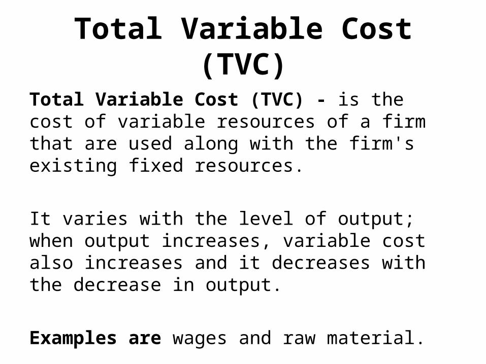
Total Variable Cost (TVC)

Total Variable Cost (TVC) - is the cost of variable resources of a firm that are used along with the firm's existing fixed resources.

It varies with the level of output; when output increases, variable cost also increases and it decreases with the decrease in output.

Examples are wages and raw material.  

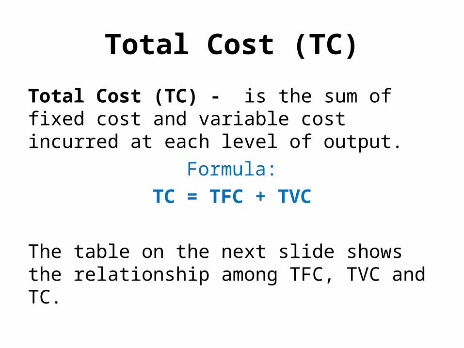
Total Cost (TC)Total Cost (TC) -  is the sum of fixed cost and variable cost incurred at each level of output.

Formula:TC = TFC + TVC

The table on the next slide shows the relationship among TFC, TVC and TC.

OUTPUT FC VC TC0 500 0 5001 500 90 5902 500 170 6703 500 270 7704 500 382 8825 500 450 9506 500 640 11407 500 790 12908 500 950 14509 500 1130 163010 500 1330 183011 500 1540 204012 500 2150 2650

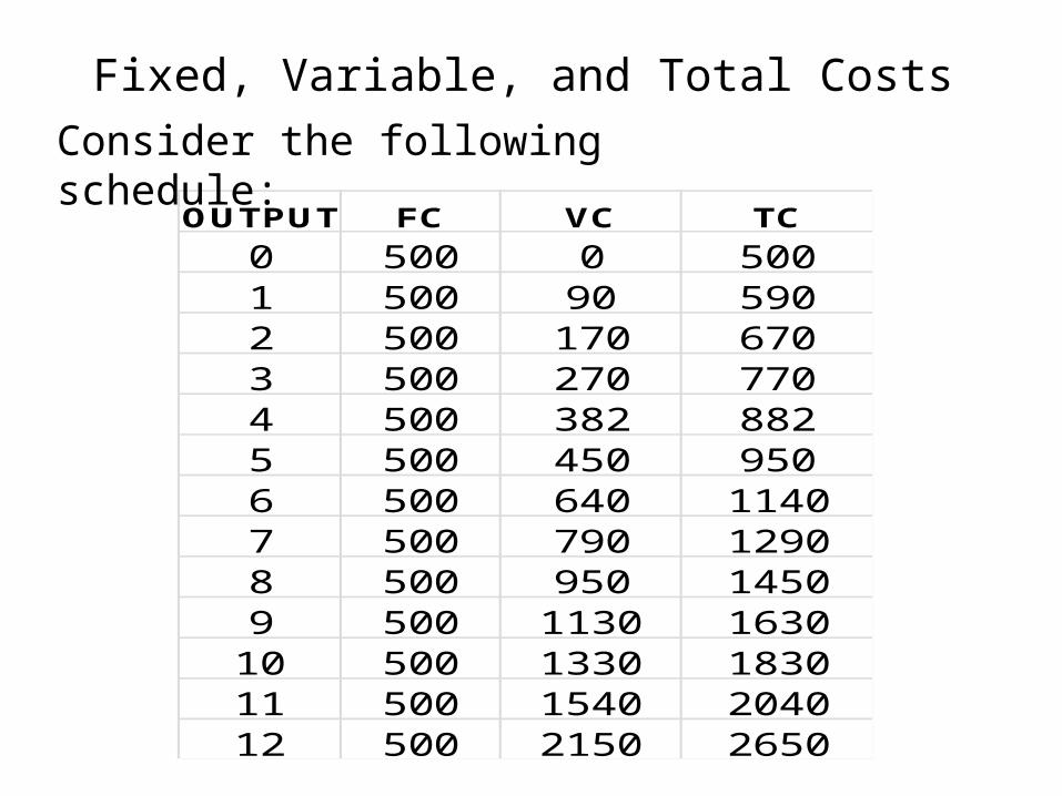
Fixed, Variable, and Total CostsConsider the following schedule:

• Note that total fixed cost remains at $500 regardless of the number of output. However, total variable costs increases with production levels.

• Total costs comprised of total fixed costs and total variable costs, and is seen in column 4.

• Total variable cost is always zero when output is zero, and total fixed costs is still at its constant level.

OUTPUT FC VC TC0 500 0 5001 500 90 5902 500 170 6703 500 270 7704 500 382 8825 500 450 9506 500 640 11407 500 790 12908 500 950 14509 500 1130 163010 500 1330 183011 500 1540 204012 500 2150 26500

500

1000

1500

2000

2500

3000

1 3 5 7 9 11 13

FCVCTC

Fixed, Variable, and Total CostsGraph plotted from schedule above

• As seen on the graph, fixed cost is a straight horizontal line, this is because it remains constant regardless of production levels.

• Total variable costs are represented by a curve that rises upward as output increases.

Average Cost• Average Total Cost (ATC) - refers to total cost per unit of output,

and is obtained by dividing the TC by the total number of units produced. Formula: ATC =  Total Cost (TC)

                               Output (Q)As output increases, ATC falls, and then rise after it reaches a minimum.

• Average Fixed Cost (AFC) - refers to fixed cost per unit of output. Formula:  AFC = TFC

   Output (Q)The average fixed cost begins to fall with the increase in the number of units produced, but it never becomes zero.

• Average Variable Cost (AVC) - refers to the variable costs per unit of output. Formula: AVC = TVC

    (Q)As firms increases output, the AVC cost decreases initially until it reaches a minimum, then increases again. In the beginning, a firm is not producing at its full capacity, but when the plant works to its full potential, the AVC is at its minimum. If the production is pushed to more than the plant capacity, AVC rise because production is no longer efficient.

Marginal Cost• Marginal Cost is an increase in total cost that results from a one unit change in output. MC is governed only by variable cost which changes with changes in output.

Formula: MC = Change in TC = ΔTC            Δ in Output        Δq

Average and Marginal CostsO UTPUT AFC AVC ATC M C

01 500.0 90.0 590.0 902 250.0 95.0 345.0 1003 166.7 90.0 256.7 804 125.0 95.5 220.5 1125 100.0 98.0 198.0 1086 83.3 106.7 190.0 1507 71.4 112.9 184.3 1508 62.5 118.8 181.3 1609 55.6 125.6 181.1 18010 50.0 133.0 183.0 20011 45.5 140.9 186.4 22012 41.7 179.2 220.8 600

Average and Marginal CostsAVC ATC M C FC VC

500 090.0 590.0 90 500 9095.0 345.0 100 500 19090.0 256.7 80 500 27095.5 220.5 112 500 38298.0 198.0 108 500 490106.7 190.0 150 500 640112.9 184.3 150 500 790118.8 181.3 160 500 950125.6 181.1 180 500 1130133.0 183.0 200 500 1330140.9 186.4 220 500 1550179.2 220.8 600 500 2150

0

100

200

300

400

500

600

700

1 2 3 4 5 6 7 8 9 10 11 12 13

AFCAVCATCM C

Opportunity CostsThe value of the other products that the resources used in production could have produced at their next best alternative.•Explicit costs include all such expenditure incurred by a firm for the hiring of factors of production and buying goods and services directly.•Implicit costs include opportunity costs of resources owned and used by the firm’s owner

Long Run Cost• It often considered to be the firm’s planning horizon.

• It describes alternative scales of operation when all inputs are variable.

Quantity of output

Average cost

In the short run, the shape of the average total cost curve (ATC) is U-shaped, and there is a different short run ATC structure at each stage of expansion. See below.

Deriving a Long Run Average Total Cost Curve

In the long run, all costs of a firm are variable. The firm have a longer time period to build larger plants to produce the anticipated output.

Quantity of Output

Average Cost

Short Run Average Cost Functions

Long Run Average Cost

The long run ATC curve is U-shaped but is flatter than the short run curve. It shows the minimum cost per unit of producing each output level at any scale of operation.

It is made up of all the points of tangency of short-run ATC curves and shows the least per unit cost at which any output can be produced in the long run.

SAC4

SAC2

SAC1

SAC3

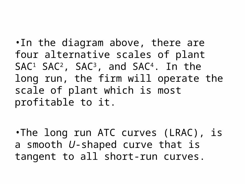
•In the diagram above, there are four alternative scales of plant SAC1 SAC2, SAC3, and SAC4. In the long run, the firm will operate the scale of plant which is most profitable to it.

•The long run ATC curves (LRAC), is a smooth U-shaped curve that is tangent to all short-run curves.

Economies of ScaleEconomies of scale refers to the cost advantages that a business obtains due to expansion, which result in significant decreasing costs per unit. There are factors that cause a producer’s average cost per unit to fall as the scale of output is increased.

Some sources of economies of scale are purchasing in bulk, producing at full capacity, favourable long-term contracts, specialization of managers, and obtaining lower interest charges on borrowing. These help to reduce the long run average costs (LRAC) of production by shifting the short-run average total cost (SRATC) curve down and to the right.

Diseconomies of scale are the opposite, where firms produce outputs at increasing costs, i.e. firms see an increase in marginal cost when output is increased. This may occur because of poor communication, increasing transportation costs, outdated technology, lack of control of production process, large scale pilferage and waste etc.

Economies of Scale

If the firm increases its production then it might experience:•Economies of scale means that as output increases, costs reduces by a larger proportion.•Diseconomies of scale means that as output increases, marginal costs increases also.•Constant scales means that output increases but costs remain the same (rare occurrence).