Intelligent Traffic Lights to Reduce Vehicle EmissionsVehicle Emissions

Ciprian Dobre, Adriana Szekeres, Florin Pop, Valentin Cristea, Fatos Xhafa

Emails: {ciprian.dobre, florin.pop, valentin.cristea}@cs.pub.ro, fatos@lsi.upc.edu

30.05.2012

Outline

• Scope and motivation

• Model for fuel consumption

• The proposed system

• Decision algorithmsDecision algorithms

• Experimental results

• Conclusions

30.05.2012

Scope and Motivation

• Road transportation is a major source for emissions of carbon monoxide, carbon dioxide, hydrocarbons, and other organic , , y , gcompounds into the environment

C i h l d i i l b i i llo Cars with petrol-driven internal combustion engines pollute

• Direct relation between the car’s emissions and its accelerationDirect relation between the car s emissions and its acceleration

o An accelerating car pollutes more than a non-speeding car

• Propose a system to guide driver’s decisions as he/she approaches the traffic lightapproaches the traffic light

o The goal = reduce vehicle emissions

Model for Fuel Consumption (1)

• Input: characteristics of cars• Output: recommended cruising speed

cosmgFFF

p g p• Parameters: distance between traffic light and car• Total normal force FN cosmgFFF NrNfN ota o a o ce N

30.05.2012

Model for Fuel Consumption (2)

• The engine generates torque, which when applied to the wheels causes them to rotate

• The force applied to the tires FT

rTF / Torque applied to the wheels

• When the car is in motion, the aerodynamic drag force is a

wwT rTF / Torque applied to the wheelswheel radius

When the car is in motion, the aerodynamic drag force is a function of density ρ, frontal area A, the square of the velocity magnitude, v, and a drag coefficient, CD

• The rolling friction force FR

FF * Total normal forcerNR FF * Total normal force

the coefficient of rolling friction for the vehicle

30.05.2012

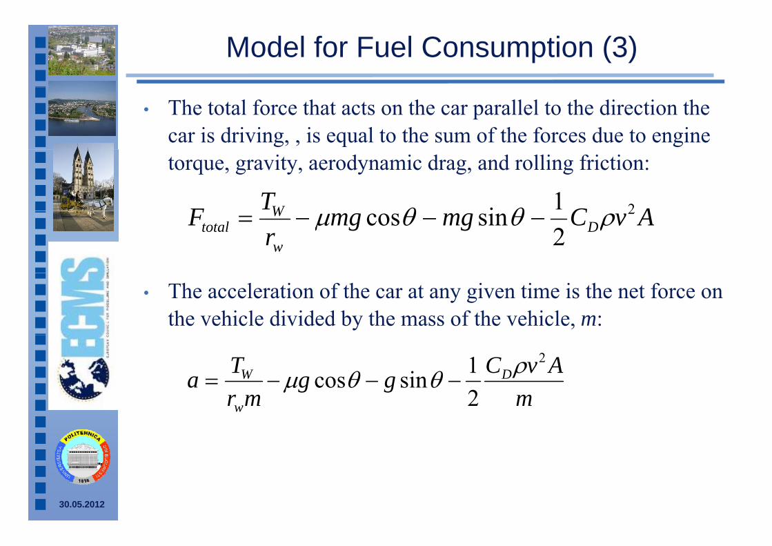
Model for Fuel Consumption (3)

• The total force that acts on the car parallel to the direction the car is driving, , is equal to the sum of the forces due to engine torque, gravity, aerodynamic drag, and rolling friction:

ACTF W 21i AvCmgmgr

F Dw

Wtotal

2

2sincos

• The acceleration of the car at any given time is the net force on the vehicle divided by the mass of the vehicle, m:

mAvCgg

mrTa DW

2

21sincos

mmrw 2

30.05.2012

Model for Fuel Consumption (4)

• The torque applied to the wheels of a car determines its acceleration.

o Before the engine torque is applied to the wheels, it passes g q pp , pthrough a transmission.

o The gears inside a transmission change the angular velocity and g g g ytorque transferred from the engine.

o There is also an additional set of gears between the transmission gand the wheels.

o The gear ratio of this final gearset is known as final drive ratio.

• Thus, the wheel torque, Tw, is equal to the engine torque, Te, multiplied by the gear ratio, gk, of whatever gear the car is in and the final drive ratio, G

AvCGgT Dk21i

30.05.2012m

AvCggmrGgTa D

w

ke

21sincos

Model for Fuel Consumption (5)

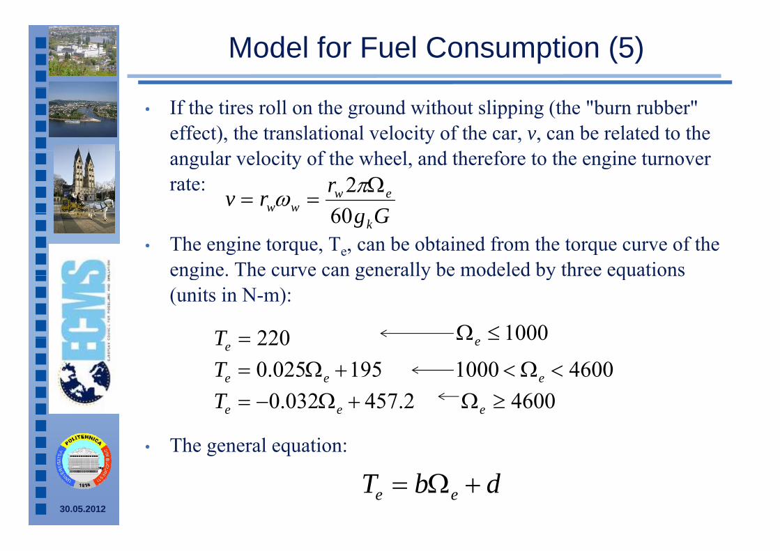
• If the tires roll on the ground without slipping (the "burn rubber" effect), the translational velocity of the car, v, can be related to the angular velocity of the wheel, and therefore to the engine turnover rate:

Grrv ew

ww 602

• The engine torque, Te, can be obtained from the torque curve of the engine. The curve can generally be modeled by three equations

Ggk60

engine. The curve can generally be modeled by three equations (units in N-m):

220T 1000220eT 1000e

195025.0 eeT 46001000 e

24570320 T 4600

• The general equation:

2.457032.0 eeT 4600e

30.05.2012

dbT ee

Model for Fuel Consumption (6)

• Acceleration of the car as a function of the current velocity is:

AvCGdgbvGg 222 160 m

AvCggmr

Gdgmr

bvGga D

w

k

w

k2 2

1sincos2

60

• We solved this differential equation using the fourth-order Runge-Kutta method

o Typical parameters for the rolling friction coefficient (0.015), the average frontal area of a car (1.94 m2), the wheel radius (0 3186)(0.3186)

• The relation between speed and fuel consumption and emission rate is given by the Haworth and Symmons model1

o Clearly shows that by accelerating or decelerating a car consumes relatively larger or smaller fuel quantities than it

ld llwould consume normally

30.05.20121Haworth, N.; M. Symmons. “Driving to reduce fuel consumption and improve road safety”, Proc. Road Safety Research, Policing and Education Conference, Melbourne

Model for Fuel Consumption (7)

• Typical emission rates for volatile organic compounds (Hydrocarbons -HC), carbon monoxide, nitrogen oxides and fuel consumption as a function of average speed for passenger cars conforming to ECE 15-04 regulationsof average speed for passenger cars conforming to ECE 15 04 regulations

30.05.2012

J. Rybicki, B. Scheuermann, W. Kiess, C. Lochert, P. Fallahi and M. Mauve, Challenge: Peers on wheels { A road to new traffic information systems, Proc. of the 13th Annual ACM International Conference on Mobile Computing and Networking (MOBICOM), Montral, Qubec, Canada, pp.215-221, 2007.

The proposed system

• Assumption: intersection equipped with traffic light (TL) with wireless communication capabilities

• TL sends information to approaching vehicles

o Periodically broadcasts data about the color and the time until it h f h f d i lchanges, for each segment of road it controls.

o The broadcasted package contains in addition the local time, which is used for synchronizationused for synchronization.

o The problem of short range communication is resolved by letting cars re-broadcast further all received messages for a limited time period.e b oadcast u t e a ece ved essages o a ted t e pe od.

• The vehicle uses the received information as input for an algorithm that outputs a recommendation speed that optimizes the quantity of car’s emissions.

o The algorithm is based on the computation of speed, movement, as ll f l tiwell as fuel consumption

30.05.2012

Computing fuel consumption (1)

• To model fuel consumption and emissions (CO2, CO, HC, NOx), we extended the work of Akcelik and Besley (2003)

h li i f h i d l b fl d b h i do The qualities of their model are better reflected by the extensive study conducted in (Dia et al. 2007).

• The method to estimate the value of fuel consumed (mL) or emissionsThe method to estimate the value of fuel consumed (mL) or emissions produced (g), in a time interval ( Δt), is given by:

[m/s] is the vehicle’s[kg] is the mass of the vehicle (1400 kg f li h hi l i i

M 2

[m/s] is the vehicle s instantaneous velocityon average for light vehicles in a city

environment

tvaMvRfFa

vTi

0

22

1 1000 0TR

0RtfF i 0TR[kN] represents total force acting on a car, including air drag and rolling resistance

30.05.2012

[mL or g] is the quantity consumed or gas emitted during a time interval

including air drag and rolling resistance

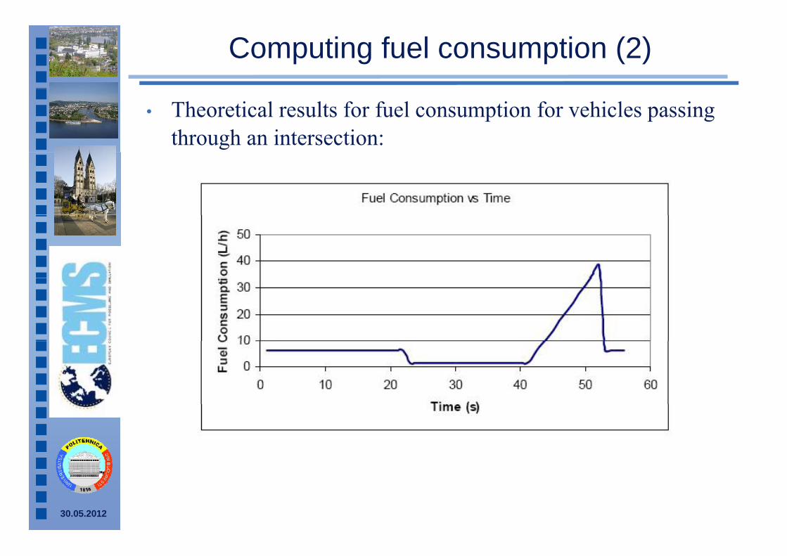
Computing fuel consumption (2)

• Theoretical results for fuel consumption for vehicles passing through an intersection:

30.05.2012

Decision algorithm

• Algorithm for prediction of the movement of the car on a given distance or in a given amount of time

E ti t th f t d d iti f tho Estimates the future speed and position of the car o Uses parameters such as the delay to reach a certain speed, the

acceleration style of the driver, the characteristics of the roadacceleration style of the driver, the characteristics of the road (curves, slopes)

• If the car receives Green Light, we consider two scenarios:1. the driver accelerates to catch the green light, 2. the driver slowly decelerated to stop at the red light

• The algorithm estimates the quantity of emissions for both two cases:

If the quantity of gases is smaller in the first case ito If the quantity of gases is smaller in the first case, it recommends the accelerating speed to the driver.

o Otherwise, it recommends a full stop at the red light.p g

30.05.2012

The algorithm for Green Light, case 1

1: car.distance ← 0 // the total distance traveled by the car2: car.time ←0 // the total time the car traveled3: timeIncrement ← 0:06 // the time increment to apply runge-kutta4: car.setMode("accelerate") // the driver accelerates5: while car.distance < distanceToTrafficLight doff g6: neededSpeed ← (distanceToTrafficLight – car.distance) ÷(greenTime – car.time)7: if neededSpeed > MaxSpeedAllowed then7: if neededSpeed MaxSpeedAllowed then8: return // the driver cannot catch the green light9: end if10: if neededSpeed <= car speed then10: if neededSpeed <= car.speed then11: car.setMode("cruise")12: end if13 d t S dA dL ti (ti I t)13: car.updateSpeedAndLocation(timeIncrement)

// this updates car.time, car.speed and car.distance14: car.estimateEmissions()

30.05.2012

15: end while

The algorithm for Green Light, case 21: car distance ← 0 // the total distance traveled by the car1: car.distance ← 0 // the total distance traveled by the car2: car.time ← 0 // the total time the car traveled3: timeIncrement ← 0:06 {the time increment to apply runge-kutta}4 tM d (" i ") // th d i i t i t t d4: car.setMode("cruise") // the driver maintains a constant speed5: while car.distance < distanceToTrafficLight - 100 do6: // assume the driver starts to break 100m before the intersection7: car.updateSpeedAndLocation(timeIncrement)8: car.estimateEmissions()9: end while10: car.setMode("break") // the driver breaks to stop at the red light11: while car.distance < distanceToTrafficLight do12: car.updateSpeedAndLocation(timeIncrement)12: car.updateSpeedAndLocation(timeIncrement)13: car.estimateEmissions()14: end while15: car setMode("accelerate") // the driver accelerates to the speed he had15: car.setMode( accelerate ) // the driver accelerates to the speed he had before stopping16: while car.speed < WantedSpeed do17 d t S dA dL ti (ti I t)

30.05.2012

17: car.updateSpeedAndLocation(timeIncrement)18: car.estimateEmissions()19: end while

The algorithm for Red Light, case 1

1: car.distance ← 0 // the total distance traveled by the car2: car.time ← 0 // the total time the car traveled3: timeIncrement ← 0:06 // the time increment to apply runge-3: timeIncrement ← 0:06 // the time increment to apply runge-kutta4: car.setMode("accelerate") // the driver accelerates5: while car distance < distanceToTrafficLight do5: while car.distance < distanceToTrafficLight do6: neededSpeed ← (distanceToTrafficLight - car.distance) ÷ (redTime – car.time)7 if d dS d M S dAll d h7: if neededSpeed < MinSpeedAllowed then8: return // the driver cannot avoid stopping at the red light9: end if10: if neededSpeed >= car.speed then11: car.setMode("cruise")( )12: end if13: car.updateSpeedAndLocation(timeIncrement)

// this updates car time car speed and car distance

30.05.2012

// this updates car.time, car.speed and car.distance14: car.estimateEmissions()15: end while

The algorithm for Red Light, case 21: car distance ← 0 // the total distance traveled by the car1: car.distance ← 0 // the total distance traveled by the car2: car.time ← 0 // the total time the car traveled3: timeIncrement ← 0:06 // the time increment to apply runge-kuttag4: car setMode("cruise") // the driver maintains a constant speed4: car.setMode( cruise ) // the driver maintains a constant speed5: while car.distance < distanceToTrafficLight - 100 do6: // assume the driver starts to break 100m before the intersection7 d S dA dL i ( i I )7: car.updateSpeedAndLocation(timeIncrement)8: car.estimateEmissions()9: end while10: car.setMode("break") // the driver breaks to stop at the red light11: while car.distance < distanceToTrafficLight do12: car.updateSpeedAndLocation(timeIncrement)p p ( )13: car.estimateEmissions()14: end while15: car.setMode("accelerate")15: car.setMode( accelerate )

// the driver accelerates to the speed he had before stoppingg16: while car.speed < NeededSpeed do17: car updateSpeedAndLocation(timeIncrement)

30.05.2012

17: car.updateSpeedAndLocation(timeIncrement)18: car.estimateEmissions()19: end while

Experimental results

• The evaluation was done using modeling and simulation. o Model vehicular traffic, communication from traffic lights , g

to vehicles, driver behavior (speed adaption) and fuel consumption and emissions.

• We were interested how acceleration relates to pollutant emissions

o These experiments verify that the simulation model corresponds in known-cases to the expected mathematical resultsresults

o We considered the case of an average car - the entry values for these experiments followed the analysis offor these experiments followed the analysis of Smith&Cloke (1999).

• We conducted two experiments that evaluate the fuel• We conducted two experiments that evaluate the fuel consumption for the typical driver behaviors.

30.05.2012

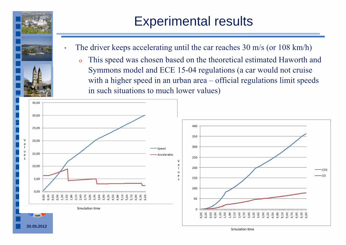
Experimental results

• The driver keeps accelerating until the car reaches 30 m/s (or 108 km/h)o This speed was chosen based on the theoretical estimated Haworth and

d l d l i ( ld iSymmons model and ECE 15-04 regulations (a car would not cruise with a higher speed in an urban area – official regulations limit speeds in such situations to much lower values))

30.05.2012

Experimental results

• Driver accelerates until the car reaches 15.22 m/s (or 54.8 km/h, a speed which is more acceptable for urban areas) and then maintains a constant speedspeed Comparing the results of the two

scenarios, it can be noticed that the quantity of gases emitted by the car in the second scenario (≈ 129g of CO2) isthe second scenario (≈ 129g of CO2), is smaller than the one obtained in the first scenario (≈ 360g of CO2)

30.05.2012

Case – Green light

• A car is traveling at 40 km/h (~11 m/s) and has 15 seconds to catch the green light. The distance between the traffic light and the car is 200 m.

hi d h h i i l i l hi ho This corresponds to the case when a car cruising at a relatively high speed in town approaches the intersection.

• The car predicts estimates the quantity of emissions:The car predicts estimates the quantity of emissions: o 1) driver catch the green light and accelerates until the needed speed is

reached and o 2) driver maintains a constant speed, stops and waits at the red light,

and then he/she accelerates until the previous speed is obtained. • The quantity of emissions in the first situation was ~54 grams of CO2 and• The quantity of emissions in the first situation was ~54 grams of CO2, and

in the second situation ~96 grams of CO2. • Based on these results, the system advises the driver to accelerate to catch

the green light. By doing this, the driver could reduce the quantity of CO2 by approximately 42 grams (going at high speed, but this higher limit depends on the maximum speed imposed by legislation in that particulardepends on the maximum speed imposed by legislation in that particular location).

30.05.2012

Experimental resultsresults

Quantity of emissions in situation 1

Quantity of emissions inQuantity of emissions in situation 2

30.05.2012

Conclusions

• Solution that uses traffic lights, mobile devices and wireless communication to reduce car emissions

• In order to decide whether the driver’s action of catching the green light leads to less fuel consumption, by recommending accelerate/decelerate we devised a method to predict the car’saccelerate/decelerate, we devised a method to predict the car s movement

o We use the motion equation of a car to predict its speed ando We use the motion equation of a car to predict its speed and position at any time

• To estimate a specific driver’s behavior and predict how the car is p pgoing to move in different situations is a difficult task, because of the number of parameters to be considered: all forces that act on the car coupled with the human factorcar, coupled with the human factor.

• The solution was evaluated using modeling and simulationo The results show that the proposed algorithm can recommendo The results show that the proposed algorithm can recommend

speeds that, in fact, lead to a decrease in the emissions of a car

Q&A

Thank y u!y

30.05.2012