Theory and applications of digital smear filters - University of ...
248
Theory and Applications of Digital Smear Filters A thesis presented for the degree of Doctor of Philosophy in Electrical & Electronic Engineering at the University of Canterbury, Christchurch, New Zealand. by Andrew John Rolls ? B. E. (Hons) March 1994
-
Upload
khangminh22 -
Category
Documents
-
view
1 -
download
0
Transcript of Theory and applications of digital smear filters - University of ...

Theory and Applications
of Digital Smear Filters
A thesis presented for the degree of Doctor of Philosophy
in Electrical & Electronic Engineering at the
University of Canterbury, Christchurch, New Zealand.
by Andrew John Rolls
?
B. E. (Hons) March 1994


"GINtERI~ LlIlRARV
Abstract
This thesis investigates the theory and applications of digital smear filters. A smear filter can be defined as a device that disperses the energy contained in a wide bandwidth pulse in time. A desmear filter performs the inverse operation to the smear filter by compressing the smeared pulse in time.
The first part of this thesis, consisting of chapters 2-4, presents a theoretical basis for digital smear filters and develops three methods for designing these filters. One of these methods is an extension of the window method used to design linear phase FIR filters; another is an extension to the frequency sampling method; the third design method has no linear phase FIR filter counterpart, and we have called it the iterative Wiener method.
The second part of this thesis, consisting of chapters 5-8, investigates novel applications for these smear / desmear filters. These applications include using smear / desmear filters to:
• Compress the dynamic range of speech. (A 3-4 dB reduction in the peak-to-rms ratio can be achieved.)
• Destroy the dependence between a signal and its quantization noise. (Smear filters can increase both the subjective quality and the intelligibility of hard limited I speech.)
• Encode data for transmission over a noisy channel in order to protect the data from bit errors. (A novel method for channel coding that uses smear filters is described, and the principles of this method are substantiated.)
• Scramble a signal for privacy. (Smeared speech signals can be made unintelligible for delays as short as 400 ms.)
Although smear / desmear filters are shown to be extremely versatile devices, they have one serious drawback: They introduce delay. Some of the applications described above require very long delays to approach their theoretical bounds of performance.
III


Acknowledgements
I would like to thank my supervisors' Mr J. A. Webb and Dr. H. R. Sirisena. I am grateful to Mr Webb for his guidance and encouragement during the first three and one half years of this research project. I am grateful to Dr Sirisena for his valuable assistance after Mr Webb's retirement.
The financial assistance of Telecom New Zealand Ltd has been a major contribution to this project. By granting myself leave on full pay, financing many of the expenses incurred during the project, and allowing me to use their computing resources after leaving the University of Canterbury their contribution has been a major one and greatly appreciated.
I am grateful for the cooperation of fellow students, academic staff, and librarians at the University of Canterbury, and also for the cooperation and support of my colleagues at Telecom New Zealand Ltd. I have enjoyed the stimulating discussions with these people and appreciated their efforts on my behalf.
Finally, I wish to thank my family and friends for their encouragement and support. I would especially like to thank my immediate family for the sacrifices they have made for me and the support they have given me; Mum, Ana, Ros, Dan, and Thaddeus, thank you very very much.
v


Contents
Abstract
Acknowledgements
1 Introduction 1.1 Smear /Desmear Radar
1.2 Thesis Outline. . . .
1.3 Definitions.....
1.4 Tacit Assumptions
2 Theory of Smear Digital Filters 2.1 Introduction ....
2.2 Filter Bank Model ...... .
2.3 Spectrogram....... ~ . . .
2.4 Temporal Position and Spread .
2.4.1 Measure for temporal position
2.4.2 Measure for temporal spread .
2.4.3 Alternate measure for temporal spread
2.5 Desmear Filter ....
2.5.1 Matched filter . . . . .
2.5.2 Wiener filter. . . . . .
2.5.3 Figure of merit (FOM)
2.6 Review of Smear Filter Design Methods
2.6.1 Time Domain Methods ...
2.6.2 Frequency Domain Methods
2.7 Conclusions ............ .
3 Designing Fm Digital Smear Filters 3.1 Introduction...................
3.2 Window Method .......... .
3.2.1 Design Example: 255-tap Chirp filter
Vll
... m
v
1
1
3
4
7
9
9
9
12
15
16
17 20 20
22
23
24 25
25 .25
28
29
29
30
30

Vlll
3.2.2 Choice of Window ...... .
3.2.3 Temporal Location of Window.
3.2.4 Avoiding Phase Discontinuities
3.2.5 Specifying 'Td(W) Using Interpolation
CONTENTS
34
36
39
40
3.3 Frequency Sampling Method . . . . . . . . . 49
3.3.1 ,Frequency Sampling Method vs Window Method 50
3.4 Iterative Wiener Method . . . . . . . 50
3.4.1 Refining a Smear Filter. . . . 53
3.4.2 Randomly Chosen Seed Filter 56
3.5 Conclusions . . . . . . . . . . . . . . 59
4 Mismatch Noise and Other Impairments 61
4.1 Introduction............. 61
4.2 Mismatch Noise . . . . . . . . . . . 61
4.3
4.4
4.2.1 Models for mismatch noise .
Transmission Impairments . . . . .
4.3.1 Magnitude and Phase Distortion
4.3.2 Frequency Translation
4.3.3 Additive White Noise .
Conclusions . . . .
5 Speech Compression
5.1 Introduction....
5.2 Smear filters as Speech Compressors
5.3 Speech data base
5.4 Smear Filters . . .
5.5 Definitions.....
5.5.1 Peak Level.
5.5.2 Rms level
5.5.3 Peak-to-rms ratio
5.5.4 Compressability Factor .
5.5.5 Cumulative function
5.6 Speech Compression Results ..
5.7 Simplified Speech Waves . . . .
5.8 Perceptual Quality of Expanded Speech. 5.9 Conclusions ...... .
65
68
68
69
69
71
73
73 74 75
76
78 78 80
80
80
81
84
90
94
95
6 Dithering and Smithering 97 6.1 Introduction............................. 97

CONTENTS
6.2 Motivation................
6.3 Hard-LimIter Excited by an Impulse
6.4 Hard Limited Speech . . . . . . . . . . .
6.4.1 Spectrogram of Hard Limited Speech
6.4.2 SNR of Hard Limited Speech
6.5 Subjective Tests . . . . . . . . . . . . . . . .
6.5.1 Preference Tests ........... .
6.5.1.1 Preference Test Procedure.
6.5.1.2 Results of Preference Test
6.5.2 Intelligibility Tests . . . . . . . . . .
6.5.2.1 Intelligibility Test Procedure
6.5.2.2
6.6 Conclusions
7 Smear Coding
7.1 Introduction.
7.2 Motivation ..
Results and Analysis.
7.3 The Binary PCM Smear Code .
7.3.1 Description . . . . .
7.3.2 Design Compromises . .
7.4 Discrete Channels . . . . . . . .
7.4.1 Binary Symmetric Channel (BSC) .
7.4.2 Gilbert Channel ..... .
7.4.3 Periodic Burst Channel .
7.5 Theoretical Analysis ... . . . .
7.5.1 Model . . . . . . . . . . .
7.5.2 Asymptotic Performance Bound .
7.5.3 Quantization Noise . . . . . . . .
7.5.4 Channel Noisefor BSC Channel.
7.5.5 Channel Noise for Gilbert Channel
7.5.6 Summary of Theoretical Analysis
IX
98
99
100
100
104
105
106
106
107
111 112
113
117
119
119
119
121
121
127
128
128
129
130
132
133
133
135
138
142
147
7.6 Simulation Results . . . . . . . . . . . . . 148
7.6.1 Simulation Results for BSC Channel 148
7.6.2 Simulation Results for Gilbert Channel . 150
7.6.3 Simulation Results for Periodic Burst Channel. 152
7.7 Statistics of Decoding Bit Errors ......... 152
7.8 Comparison with Block and Convolutional codes. 155
7.9 Conclusions . . . . . . . . . . . . . . . . . . . . . 157

x
8 Other Applications for Smear Filters
8.1 Introduction..............
8.2 Encryption using Smear Filters ...
8.3 Impulse Noise Suppression in Data Transmission.
804 Robust Quantization using Smear Filters
8.5 Conclusions . . . . . . . . . . .
9 Conclusions and future research
9.1 Conclusions to Part 1 ..
9.2 Conclusion to Part 2
9.3 Future research
A Filter Data Base
A.1 Naming Convention.
A.2 FIR3 ........ .
A.3 Command Files for All-Pass Filters
AA Command File for Non-Flat Smear Filters
A.5 Smear Filter Characteristics .....
B Steepest descent gradient algorithm
B.1 Introduction.
B.2 Algorithm . .
B.3 Convergence.
C Subjective Speech Tests
C.1 Introduction ....
C.2 Speakers . . . . . . . .
C.3 Listening Subjects ..
CA Preparation of Test Material .
C.5 Conditions of Test .....
D Noise Models for quantizers
D.1 Introduction ........ .
D.2 Comparison Between the two Models
References . . . . . . . . . . . . . . . . . . .
CONTENTS
159 159
159
162
165
167
169 169
170
171
173 173
174
175
188
193
217 217
217
220
223 223
223
223
224
224
229 229
231
233

Chapter 1
Introduction
This Ph.D. dissertation investigates the theory and applications of smear / desmear filters. A smear filter may be defined as a device that disperses the energy contained in a wide bandwidth pulse in time. A desmear filter performs the inverse operation to the smear filter by compressing the smeared pulse in time. This is illustrated in figure 1.1.
Smear / desmear filters were first used in pulse compression radar to overcome the conflicting design requirements of high range resolution and large maximum range of detection [Klauder et al., 1960; Cook and Bemfeld, 1967]. Since then, they have found use in a wide range of applications ranging from impulse noise suppression in data transmission systems [Beenker et al., 1985] through to devices for performing a Fourier transform.
To introduce the subject of smear/desmear filters, we briefly describe their founding application: Smear/desmear radar ..
1.1 Smear/Desmear Radar
Pulsed radar systems operate by periodically transmitting high intensity electromagnetic pulses. During the silent interval between transmitted pulses, the receiver is activated. As time elapses, echoes are received from reflecting objects at greater and greater distances, and by measuring the time taken for a particular echo to return, the range of the target may be estimated. Obviously, the thermal noise generated by the receiver will tend to mask weak echoes,
L Smear
-AI\I\Jl-Desmear ~
0
~I rv ~I ~ I 0 rv .. .. rv
.... ad.fia
Figure 1.1: Operation of smear and desmear filters.
1

2 CHAPTER 1. INTRODUCTION
and this limits the maximum range of detection. (Maximum range of detection measures the maximum range at which a target can be detected). One method for increasing the maximum range of detection is to increase the energy contained in each transmitted pulse, and this consideration usually results in the transmitter operating in its peak power limited region.
Range resolution measures the ability of the radar system to resolve closely spaced objects into separate dots on the radar screen. Conceptually, the simplest way to achieve high range resolution in a pulsed radar system is to use shorter pulses, so that reflections from closely spaced objects are received as distinct echoes. However, if shorter pulses are used, the amplitude of the transmitted pulse (and hence the peak power of the pulse) must be increased to maintain the maximum range of detection. Unfortunately, this may be impossible because of the peak power limitations of the transmitter.
Pulse compression is employed in radar to enable range resolution to be increased without sacrificing maximum range of detection nor encountering excessively high peak powers that cause electrical breakdown. In effect, pulse compression divorces the useful signal bandwidth (range resolution) from the transmitted pulse width. The basic concept behind pulse compression is to smear out the transmitted pulse before applying it to the power amplifier stage in the radar transmitter. This enables the average power of the pulse to be increased for given peak power limitations. A desmear filter in the receiver is used to compress the received echos to their minimum time-bandwidth product and hence realise good range resolution.
Since its discovery in the late 1950's, pulse compression radar has received intensive research attention and is now at a very advanced state. Therefore, rather than attempt to contribute to this highly specialised and well developed field of knowledge, this thesis will focus on other aspects of smear / desmear filters. Specifically, it will focus on developing simple and robust methods for designing Finite Impulse Response (FIR) smear / desmear filters, and it will also investigate some novel applications for these filters.
For further information on pulse compression radar, the reader is referred to two excellent texts on the subject: one by Cook and Bernfeld [Cook and Bernfeld, 1967] and the other by Rihaczek [Rihaczek, 1969]. A number of significant developments have occurred since publication of these two books. Some of these developments are contained in a book edited by Barton [Barton, 1975] which contains reprints of 18 important papers on pulse compression. This collection of reprints contains a wealth of valuable information on pulse compression, including the classic paper on pulse compression by Klauder et. al. [Klauder et al., 1960). More recently, Lewis et al. [Lewis et al., 1986] have published a book providing up-to-date information on important aspects of radar signal processing. This book includes a chapter on pulse compression and also contains reprints of important papers cited in each chapter.
1.2. THESIS OUTLINE 3
1.2 Thesis Outline
This thesis is structured into two parts. The first part, consisting of chapters 2-4, presents the basic theory and design methods for digital Finite Impulse Response (FIR) smear/desmear filters. The second part, consisting of chapters ?-8, investigates some novel applications for these filters.
Chapter 2 presents a cohesive theory for digital smear filters. It collects together in a single place information that is scattered throughout many research papers. Two sections within this chapter contain new material: Section 2.3 shows how the spectrogram of a smear filter impulse response provides a very useful description of the smear filter characteristics. And section 2.4 presents a novel discussion on the mechanisms for smearing out the smear filter impulse response and also derives an equation for estimating the number of taps required to implement an FIR all-pass smear filter.
Chapter 3 describes and compares three methods for designing FIR smear filters. The first two methods are extensions of the window method and the frequency sampling method used to design linear phase FIR filters. The third design method does not have a linear phase counterpart and can only be used to design smear filters. This chapter contains a significant amount of new research material.
Chapter 4 investigates the characteristics of the noise that is added to a signal when it is passed through a smear/desmear filter. This chapter highlights differences between the design methods described in chapter 3 and should be read before attempting to design a smear filter using one of these design methods. Once again, chapter 4 contains mainly new: research material.
Chapters 5-7 investigate novel applications of smear filters. Each chapter is devoted to a single application and is written as a stand-alone chapter.
Chapter 5 investigates the use of smear/desmear filters to compress the dynamic range of speech. It will be shown that a 3-4 dB reduction in the peakto-rms level of speech can be attained using smear/desmear filters; however, this reduction is achieved at the expense of introducing very long transmission delays.
Chapter 6 investigates the use of smear / desmear filters to enhance the subjective quality of hard limited speech. It will be shown that smear / desmear filters not only improve the perceptual quality of speech (as measured by a preference test), but can also increase the intelligibility of the speech. (This is in contrast to dithering which increases the perceptual quality of quantized speech, but reduces the intelligibility of speech for coarse quantizers.)
Chapter 7 investigates the use of smear filters in a digital communication system to provide reliable data transfer over a noisy channel. The problem investigated in this chapter is identical to the problem addressed by channel coding theory; however, the method of attaining reliable data transfer is different from normal coding theory.
Chapter 8 briefly describes three other applications for smear filters. One of

4 CHAPTER 1. INTRODUCTION
X(w) .1 LTI Y(w) •
Figure 1.2: Linear time invariant system
these is a novel technique for scrambling speech; the other two applications have been previously reported and deal with mitigating the effects of impulse noise on a data transmission system and improving the robustness of an instantaneous quantizer.
Finally chapter 9 concludes the dissertation and suggests areas for future research.
Four appendices are attached to the end of the thesis. Appendix A lists the smear filters used throughout this thesis and acts as a filter data base. The remaining appendices will be introduced by the specific chapters that cite them.
The remaining sections of this chapter will introduce some terminology that is used throughout the rest of this dissertation and will also state the assumptions that will be implicitly assumed throughout this thesis. It is particularly important that the reader take note of these assumptions because many of the equations used in this thesis are only true when these assumptions hold. Often, this will not be explicitly stated in the text.
1.3 Definitions
Consider the linear time invariant (LTI) system shown in figure 1.2. The frequency response (commonly called the transfer function) of this system is defined as [ANSI/IEEE Standards, 1988]
H( ) = Y(w) w X(w) (1.1)
where X(w) is the Fourier transform of the input signal and Y(w) is the Fourier transform of the output signal. The frequency response is a complex function of frequency and can be expressed in polar coordinates as
H(w) = IH(w)le j8(w) (1.2)
where IH(w)1 is called the magnitude characteristic and 9(w) is called the phase characteristic.
Another commonly used method for describing an LTI system is the propagation function defined as [Skilling, 1974J
')'(w) = In (X(W)) Y(w)
(1.3)

1.3. DEFINITIONS 5
where In(.) is the complex natural logarithm. The propagation function is also a complex function of frequency and can be expressed in rectangular coordinates as
I(w) = a(w) + j{3(w) (1.4)
where a(w) is called the attenuation function, and {3(w) is called the phase function.
From the above set of equations, it is evident that the following relationships exist between the two definitions:
"Y(w) -H(w) -a(w) -{3(w)
-In (H(w)) e-"Y(w)
-In (lH(w)l) -8(w)
(1.5) (1.6) (1.7) (1.8)
To emphasise the differences between these two methods for describing an LTl system, the response of a low-pass filter with a sinusoidal phase characteristic is plotted in figure 1.3. Figures 1.3 (a) and (b) show the magnitude characteristic and the phase characteristic of the frequency response respectively, and figures 1.3 (c) and (d) show the attenuation function and the phase function of the propagation function respectively. (Nb. the attenuation function is plotted in dB rather than nepers.)
The definition for the phase delay and group delay is independent of whether the frequency response or propagation function is used to describe the LTl system. The phase delay Tp(W) is defined as
(1.9)
where {3(w) is 'the phase function and D(w) is the phase characteristic respectively. The group delay Tg(W) is defined as
Tg(W) = d{3(w) = _ dD(w) dw dw
(1.10)
Both the phase characteristic and the phase function of an LTl system are computed using the inverse tangent. Now, for a single argument v, the inverse tangent has an infinite number of solutions: i.e.,
arctan ( v) = u + 21rl (1.11)
where u is the principal value of the inverse tangent and I is an integer. This leads to uncertainty as to which solution should be chosen. One commonly used technique for resolving this ambiguity is to always take the principal value when computing the inverse tangent. However, this has the disadvantage that the resulting phase characteristic may contain discontinuities as illustrated in figure 1.4 (a).

6
Magnitude Characteristic 10r----r~--~--~----~--~
S -10 ~ .. -g -30 :!: e If ::£ -50
-70L---~----~--~----~----0.0 0.1 0.2 0.3 0.4 0.5
Frequency (Hz)
(0)
Attenuation function 70r----r----~--~----~--_,
! 50
e :g 30 :J .s
;1( 10
-10L---~----~--~----~--~ 0.0 0.1 0.2 0.3 0.4 0.5
Frequency (Hz)
(C)
CHAPTER 1. INTRODUCTION
Phase Characteristic
0.0 0.1 0.2 0.3 0.4 0.5 Frequency (Hz)
(b)
Phase function
-11'
0.0 0.1 0.2 0.3 0.4 0.5 Frequency (Hz)
(d)
Figure 1.3: Comparison of frequency response and propagation function. a) Magnitude characteristic. b) Phase characteristic. c) Attenuation function. d) Phase function.
An alternative method for resolving this ambiguity is to compute the principal value of the phase characteristic and then add multiples of 21I' rads to appropriate frequency bands to make the phase characteristic continuous. This technique is called phase unwrapping, and the resulting phase characteristic is called the unwrapped phase characteristic [Oppenheim and Schafer, 1975; Tribolet, 1977]. Throughout this dissertation, we will use the term phase characteristic to refer to the unwrapped phase characteristic. Figure 1.4 (b) plots the unwrapped phase characteristic of figure 1.4 (a).
411' r----.---..-----.,..--...,--.....,
-~ ~--~----~--~----~----0.0 0.1 0.2 0.3 0.4 0.5
_~ L-__ ~ ____ ~ __ ~ ____ ~ __ ~
0.0 0.1 0.2 0.3 0.5 0.4 Frequency (Hz) Frequency (Hz)
(0) (b)
Figure 1.4: The unwrapped phase characteristic a) Principal value of the phase characteristic. b) Unwrapped phase characteristic.

1.4. TACIT ASSUMPTIONS 7
1.4 Tacit Assumptions
1. This dissertation focuses solely on smear / desmear filters. Therefore, all the smear/desmear filters described herein are either all-pass filters or approximately all-pass filters. No attempt has been made to combine the functions of a smear filter and a frequency shaping filter. Although this is would be quite straight forward to do, this has been deliberately avoided in order to isolate the smearing property of smear filters.
2. All smear / desmear filters are constrained to have real impulse responses. This means that the magnitude characteristic of a smear filter exhibits even symmetry about w = 0 rad/sec and the phase characteristic exhibits odd symmetry. Many of the equations derived within this dissertation make use these symmetry properties without explicitly stating the fact.
3. For most of the discussion on smear/desmear filters, the sampling frequency is normalised to 1.0 Hz.
4. The smear and desmear filter impulse responses are allowed to be noncausal. The advantage of using non-causal smear/desmear filters is that the linear phase term is removed from the phase characteristic of the smear filter. A non-causal FIR smear filter can be made causal by introducing a sufficiently long time delay.
5. The terms frequency (measured in Hz) and angular frequency (measured in rad/s) will be used interchangeably. For example, the phase characteristic, group delay response, and magnitude characteristic of a smear filter will usually be plotted in Hz. The text associated withthese figures, however, will usually talk in terms of angular frequency (rad/sec).


Chapter 2
Theory of Smear Digital Filters
2 .1 Introduction
This chapter presents a cohesive theory for digital smear filters. It collects together in a single place information that is scattered throughout many research papers. Often these papers focused on a topic other than digital smear filters and indirectly produced a result that was applicable to digital smear filter theory.
Two sections within this chapter contain new material: Section 2.3 shows how the spectrogram of a smear filter impulse response provides a very useful description of the smear filter characteristics. And section 2.4 presents a novel discussion on the mechanisms for smearing out the smear filter impulse response and also derives an equation for estimating the number of taps required to implement an FIR all-pass smear filter.
2.2 Filter Bank Model
(The ideas contained in this section were motivated by Hartley's classic work on dispersive channels [Hartley, 1941] and by Wait's work dealing with the distortion of pulses that suffer group delay distortion [Wait, 1970].)
Conceptually, the simplest way to construct a smear filter is to use the digital filter bank shown in figure 2.1. Each branch of this filter bank consists of an ideal bandpass filter Wi(e jW ) in cascade with a pure time delay e-jT;w.
The ideal bandpass filters partition the normalised frequency interval [0,11"] into N sub-bands, and each filter passes only a narrow band of frequencies about its center frequency Wi. By varying the time delay Ti introduced by each branch of the filter bank, it should be possible to disperse the energy of the input pulse in time.
Two advantages are enjoyed by the smear filter structure shown in figure 2.1. Firstly, the magnitude characteristic of the smear filter is flat, and hence, the power spectral density of the input signal will be preserved after it passes
9

10 CHAPTER 2. THEORY OF SMEAR DIGITAL FILTERS
-lw e-jT1W
W 2(e jW )
~ e-iT2W
I I I I E I I
1 I I I I I I WN(eiw ) I
I -Wh e-iTNW
Figure 2.1: Conceptually simple model for implementing a digital smear filter.
through the smear filter. This is important because it will result in optimal noise performan<::e, and it also simplifies system design. Secondly, the same filter bank structure could be used to construct the desmear filter used to compress the smeared pulse in time. In this latter case, the delay introduced by each branch of the desmear filter must equalise the delay introduced by the corresponding branch in the smear filter.
The main problem with the smear filter structure described above is, of course, that it requires ideal bandpass filters; therefore, it would be impossible to implement in practice. However, the model is useful because it suggests that an all-pass filter with non-constant group delay response will exhibit smearing properties. To prove this, we will model an all-pass filter by a filter bank similar to that shown in figure 2.1.
The frequency response of a digital all-pass filter may be expressed as
(2.1)
where 8( w) is the phase characteristic of the filter . Using the filter bank model, the frequency response can be written as
N H(eiw ) = L Wi (eiw)eiO(w) (2.2)
i=l
where Wi ( eiw ) and N are defined above. Figure 2.2 shows an example frequency response for Wi(eiw)eiO(w). Figure 2.2 (a) shows the magnitude characteristic

2.2. FILTER BANK MODEL
Magnitude Characteristic 1.5 ..-----,....---,..---,----r---.,
~ 1.0 ::J/
f "" o
::::e 0.5
0.0 '----'----'--'--'--'----'-----' 0.0 0.1 0.2. 0.3 0.4 0.5
frequency (Hz)
(0) .
11
Phase Characteristic 6n,--~--~--~----~-,
4n ..... -ll 2.n e '; 0 ., ~-2.n a.
-4n
-, ,-, ,/ ',,,""-', I "
I , I \ I , I \
I , : \
l\ ,/ i~, / ! I' ;
-61\ '-----'----'--,'---'-I--'-... -~--'-----' 0.0 0.1 0.2. 0.3 0.4 0.5
frequency (Hz)
(b)
Figure 2.2: Example frequency response for Wi(eiW )ei8(w). a) Magnitude characteristic IWi(eiw)l. b) Phase characteristic 8(w). The vertical dashed lines indicate the transWon frequencies ofWi(eiw).
IWi(eiw)I, and figure 2.2 (b) shows the phase characteristic O(w). That part of O(w) lying within the pass-band of Wi(eiW ) is drawn using a solid line in figure 2.2 (b); the remainder of the O(w) curve is drawn using a dashed line. The transition frequencies of Wi (eiw) are also indicated on this latter figure by vertical dashed lines. Obviously, only that portion of the phase characteristic lying within the passband of Wi ( eiw ) is important for this particular branch of the filter bank.
Provided the bandwidth of Wi(eiW ) is sufficiently narrow, the part of O(w) lying within the pass-band of Wi( &W) can be approximated by the first two terms of its Taylor series expansion about Wi: i.e.,
O(w) - O(Wi) + O'(Wi)(W - Wi) + Oll;~i) (w - Wi)2 + ... - 1/Ji - 'TiW
where
and 1/Ji = O(Wi) + 'TiWi
Substituting equation (2.3) into equation (2.2) yields
N H(eiw ) == I: Wi (eiw )e-iriweNi
i=l
(2.3)
(2.4)
(2.5)
(2.6)
Equation (2.6) shows that an all-pass filter can be approximated by the filter bank shown in figure 2.3. Each branch of this filter bank consists of an ideal bandpass filter Wi( eiw) in cascade with a pure time delay e-iriw and a constant phase shift eN;. This is almost identical to the branches of the filter bank shown in figure 2.1, except that an additional phase shifting block has been added to each branch of the filter bank.

12 CHAPTER 2. THEORY OF SMEAR DIGITAL FILTERS
I -Lw e-i'rlW eNl
W2(eiw )
~ e-i 'T2w eN2
I I I I I I E I I I
I I I I I I I I I WN(eiw) I
I -~ e-i'rNW eNN r---
Figure 2.3: Approximating an all-pass filter by a filter bank.
This constant phase shifting block does not affect the smearing action of the all-pass filter. This is easily proved by computing the impulse response for the term W.·(eiw)e-i'r;weNi If the bandwidth of w.·(eiw ) is B· Hz then the t· I . I,
impulse response of "Wi(eiw)e-i'r;weNi is given by .
(2.7)
From equation (2.7), it is evident that the impulse response consists of a carrier wave of frequency Wi with phase .,pi at n = Ti. The carrier wave is modulated by a sine function which is time delayed by Ti seconds. Thus, the energy contained in this narrow band of frequencies is concentrated about n= Ti. Figure 2.4 shows the impulse response of the single branch whose frequency response is plotted in figure 2.2. (The dashed curve plots the envelope sine function).
2.3 Spectrogram
The filter bank model described in the previous section is an extremely useful tool for analysing smear filters and can be formalised somewhat using the Short Term Fourier Transform (STFT). The STFT is a function of both frequency

2.3. SPECTROGRAM 13
-0.05 L:-:--:-::-::--",,-::,::,--J.::-:--':-:-7---=--~~-~-:-'-:---:-:! -250 -200 -150 -100 -50 0 50 100 150 200 250
lime (Sees)
Figure 2.4: Impulse response for the filter shown in figure 2.2
and time and is defined as [Allen et al., 1977]
00
H(e3W , k) = I:: w(k - n)h(n)e-iwn (2.8) n=-oo
where h( n) is the discrete time signal for which it is desired to compute the STFT, and w(k - n) is a time window function that isolates a section of h(n). Typical window functions include the Kaiser window and the Hamming window. The STFT can be interpreted in terms of a filter bank by holding the frequency constant and considering the STFT to be a function of time.
For our purposes, only the magnitude of H( eiw , k) is of interest, and therefore, a spectrogram can be used to display the results [Oppenheim, 1970]. A spectrogram plots IH(eiw , k)1 on a two dimensional graph. The abscissa of the spectrogram is time and the ordinate is frequency. The third dimension is introduced into the spectrogram by using a grey scale to representIH(eiw,k)l: the greater the magnitude of H( eiw , k) at a particular time-frequency coordinate, the darker this point is made on the spectrogram.
To illustrate the use of the spectrogram, figure 2.5 plots the filter characteristics of a chirp filter. Specifically, figure 2.5 (a) plots the impulse response of the chirp filter, figure 2.5 (b) plots the phase characteristic, figure 2.5 (c) plots the group delay response, and figure 2.5 (d) plots the spectrogram. The magnitude characteristic of this chirp filter is not plotted because it is unity at all frequencies. The spectrogram clearly shows that the first part of the chirp filter impulse response (n f',J -400 s) is primarily due to low frequency components, the center part of the impulse response (n f',J 0 s) is primarily due to frequency components about 0.25 Hz, while the tail of the impulse response (n '" 400 s) is due to high frequency components.
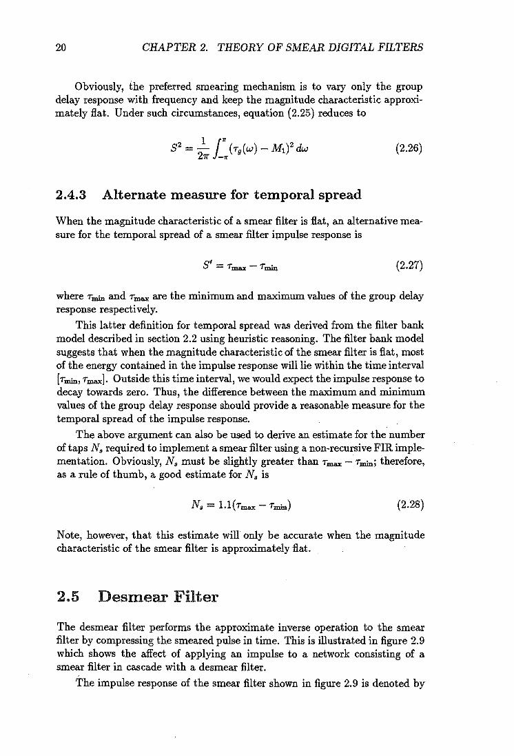
Comparing the spectrogram of the chirp filter with the group delay response, it is observed that these two graphs provide similar information. This is always the case provided the magnitude characteristic is fiat, the phase characteristic is continuous, and a suitable window is selected when performing the STFT. The reason for this similarity is due to the close relationship between the filter bank model and the STFT.
When the unwrapped phase characteristic contains phase discontinuities

14 CHAPTER 2. THEORY OF SMEAR DIGITAL FILTERS
0.06
0.04
~ 0.02 .a =a 0.00
~-0.02 -0.04
-0.06 -500 -250 0 250 500
Time (Seca)
(0)
Phose Characteristic 1207r
1001r 0.3
'0;' 'N' ::r:: -gS07r '-' .. it ';'601r c (I) ., ::> i!401r Q'
a.. ~ 207r 0.2
0.1 0.2 0.3 Frequency (Hz)
(b)
600 Group Delay Response
~ 200
I 0 Q.
Time (sec) e -200 (.l)
-600 0.0 0.1 0.2
(d) 0.3 0.4 0.5
Frequency (Hz)
(C)
Figure 2.5: Use of spectrogram for characterising a chirp filter. a) Impulse response. b) Phase characteristic. c) Group delay. d) Spectrogram using 128 point Hamming window.
or the magnitude characteristic is nonfiat, the concept of group delay becomes rather confused (or even undefined at phase discontinuities) and is of limited use. However, the spectrogram description remains valid and yields valuable insight into the performance of the filter.
For example, consider the filter shown in figure 2.6 with impulse response
1 1 h(n) = '2S(n + 15) + S(n) + '2S(n -15) (2.9)
The Fourier transform of equation (2.9), computed using the time shifting property of the Fourier transform, is given by
H(eiw) = 1 + .!.(ei1SW + e-i15W
) 2
(2.10)

2.4. TEMPORAL POSITION AND SPREAD 15
Impulse Response 1.5 .----.---T~--.---=---r--_._-....
I I O·~3Oi.---_"'2-0....l..-_"""1-0 -..1..0 --1 ...... 0-..1...--20'----'30
llme (Sees)
(0)
Magnitude Characteristic 2.5.------=---------..., 2.0
.GI
-g 1.5 'iE CI> :!il 1.0
0.5
!58
Frequency (Hz) lime (sec)
(b) (c)
Figure 2.6: Use of spectrogram for characterising a filter with a non-flat magnitude characteristic. a) Impulse response. b) Magnitude characteristic. c) Spectrogram of impulse response using 11 point Hamming window
::::} H(eiw) = 1 + cos(l5w) (2.11)
The magnitude characteristic ofthis filter is plotted in figure 2.6 (b). As H( eiw ) is purely real, its phase characteristic is zero for all frequencies, and, hence, its group delay response is also zero for all w. Thus, the group delay response provides very little useful information about the filter. The spectrogram on the other hand, provides a very useful description of the filter and is plotted in figure 2.6 (c).
2 .. 4 Temporal Position and Spread
Two of the smear filter design methods described in chapter 3 are frequency domain design methods. This means that the smear filter characteristics are specified in the frequency domain and then Fourier transformed to obtain the impulse response coefficients. When using these frequency domain design methods, it is necessary to predict certain properties of the smear filter impulse response from the frequency response of the smear filter: specifically, the location of the impulse response in the time domain (temporal position), and the time interval over which the impulse response is dispersed (temporal spread).
This section defines some scalar measures for the temporal position and the temporal spread of a smear filter impulse response and shows how these

16 CHAPTER 2. THEORY OF SMEAR DIGITAL FILTERS
measures are related to the frequency response of the filter.
2.4.1 Measure for temporal position
A suitable measure for the temporal position of the smear filter impulse response is the first moment of {h2(n)}, where {h2(n)} is the instantaneous energy of the smear filter impulse response {h(n)}. The first moment of {h2(n)} is defined as
(2.12)
The physical significance of Ml is most easily explained by resorting to classical dynamics. If the sequence {h2(n)} is interpreted as a sequence of uniformly spaced point masses along a straight line, then Ml locates the centre of mass for this system. Similarly, we may consider Ml to locate the "centre of energy" of the smear filter impulse response.
The relationship between Ml and the frequency response of the smear filter can be derived using Parseval's energy theorem:
(2.13)
Using Parseval's energy theorem, the denominator on the RHS of equation (2.12) is given by
(2.14)
The numerator on the RHS of equation (2.12) can also be evaluated using Parseval's energy theorem by letting x(n) = nh(n) and y"'(n) = h"'(n) in equation (2.13); thus
00
L nh(n) h"'(n) - 2~ L: jdHriW) H*(eiw ) dw (2.15) n=-oo
_ ~]11" (jdIH(eiW)I_IH(dW)ldO(W.)) IH(eiw)ldw 271" -11" dw dw
- 2~ L: rg{w)IH(eiw )12 dw
+ 1-]11" dIH(eiw)lIH(eiW)1 dw (2.16) 271" -11" dw
Now, the second term on the RHS of equation (2.16) is zero because the integrand is an odd function; therefore,
(2.17)

2.4. TEMPORAL POSITION AND SPREAD
Substituting equations (2.17) and (2.14) into equation (2.12) yields
f~7r Tg(w)IH(eiw )12 dw Ml = f~7r IH(eiw)12dw
17
(2.18)
This result is an intuitively appealing result and is consistent with the filter bank model described in section 2.2. Considering the numerator of this expression, the term IH(eiw)12 dw is the energy contained in an infintesimal frequency band dw, and Tg(W) is the point in time where this energy is centered about.
When the magnitude characteristic of the smear filter is flat (e.g., IH( eiw ) /2 = 1.0) equation (2.18) reduces to
1 j7r Ml = 21r -7r Tg(W) dw = 2 (0(0) - 0(7r)) (2.19)
Equation (2.19) shows that by simply inspecting the phase characteristic of an all-pass smear filter we can estimate the first moment for {h2(n)}. In particular, if 0(0) and 0(7r) both pass through 0 rads/sec, then Ml = O.
2.4.2 Measure for temporal spread
An obvious measure for the temporal spread of the smear filter impulse response is the standard deviation of {h2(n)}, defined as
(2.20)
where Ml is the first moment of {h2(n)}, and M2 is the second moment of {h 2(n)}, defined as
(2.21 )
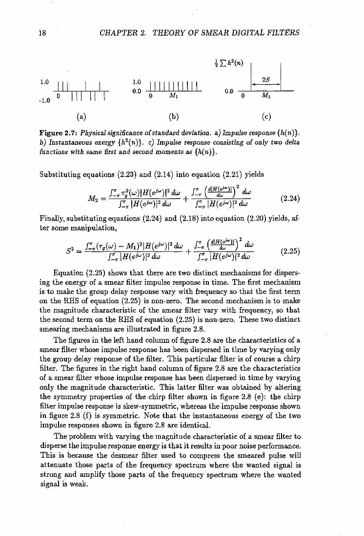
The physical significance of the standard deviation S is illustrated in figure 2.7. Figure 2.7 (a) shows a smear filter impulse response {hen)} whose coefficients assume the value +1 or -1, and figure 2.7 (b) shows the instantaneous energy of this impulse response. Figure 2.7 (c) shows the instantaneous energy of another impulse response that has the same first and second moments as {h 2 ( n ) }. This latter impulse response consists of only two delta functions - one located at Ml - S and the other located at Ml + S. Obviously, the standard deviation S provides a measure for the temporal spread of the impulse response.
Equation (2.21) can be transformed into the frequency domain using Parseval's energy theorem given in equation (2.13). Using this theorem, the numerator on the RHS of equation (2.21) can be written as
00
L nh(n)(nh(n))* n=-oo
18 CHAPTER 2. THEORY OF SMEAR DIGITAL FILTERS
! Eh2(n)
1.0 III I I 1.0 11111111111
28
0.0 0.0 0 III II I 0 Ml 0 Ml
-1.0
(a) (b) (c)
Figure 2.7: Physical significance of standard deviation. a) Impulse response {h(n)}. b) Instantaneous energy {h2(n)}. c) Impulse response consisting of only two delta functions with same first and second moments as {h( n)}.
Substituting equations (2.23) and (2.14) into equation (2.21) yields
J~1r r;(w)IH(eiw )12 dw J~1r (dIHJ;W)I)2 dw
M2 = .1-1r IH(eiw )12 dw + J~1r IH(eiw) 12 dw (2.24)
Finally, substituting equations (2.24) and (2.18) into equation (2.20) yields, after some manipulation,
(2.25)
Equation (2.25) shows that there are two distinct mechanisms for dispersing the energy of a smear filter impulse response in time. The first mechanism is to make the group delay response vary with frequency so that the first term on the RHS of equation (2.25) is non-zero. The second mechanism is to make the magnitude characteristic of the smear filter vary with frequency, so that the second term on the RHS of equation (2.25) is non-zero. These two distinct smearing mechanisms are illustrated in figure 2.8.
The figures in the left hand column of figure 2.8 are the characteristics of a smear filter whose impulse response has been dispersed in time by varying only the group delay response of the filter. This particular filter is of course a chirp filter. The figures in the right hand column of figure 2.8 are the characteristics of a smear filter whose impulse response has been dispersed in time by varying only the magnitude characteristic. This latter filter was obtained by altering the symmetry properties of the chirp filter shown in figure 2.8 (e): the chirp filter impulse response is skew-symmetric, whereas the impulse response shown in figure 2.8 (f) is symmetric. Note that the instantaneous energy of the two impulse responses shown in figure 2.8 are identical.
The problem with varying the magnitude characteristic of a smear filter to disperse the impulse response energy is that it results in poor noise performance. This is because the desmear filter used to compress the smeared pulse will attenuate those parts of the frequency spectrum where the wanted signal is strong and amplify those parts of the frequency spectrum where the wanted signal is weak.

2.4. TEMPORAL POSITION AND SPREAD 19
Group Delay Response 100.---~--~~----~----r---~
~ 50
~ ~ 0 Q. :l .. l5 -50
-100~--~----~----~----~--~ 0.0 0.1 0.2 0.3 0.4 0.5
Frequency (Hz)
(0)
Magnitude Characteristic 3.---~----~----~----r---~
2
i 1
~ 0 ... .. :::15.-1
-2
-3~--~~--~----~--~~--~ 0.0 0.1 0.2 0.3 0.4 0.5 Frequency (Hz)
(C)
Impulse Response 0.15 .-------....--=---..-,,.--.:....---........ -----, 0.10
i 0.05
i 0.00
~-0.05 -0.10
-0. 15 ':-:----~-----'----...I-----' -100 -50 0 50 100
TIme (Sees)
(e)
Group Delay Response 100.---~--~_r~--~----r_--~
~ 50
~ ~ O~----------------------~
a l5 -50
-100~--~----~----~----~----' 0.0 0.1 0.2 0.3 0.4 0.5
Frequency (Hz)
(b)
Magnitude Characteristic 3r---~-----r----~----'----~
2
II 1
~ 0 '" .. :::15-1
-2
-3~--~~-~--~--~~-~ 0.0 0.1 0.2 0.3 0.4 0.5 Frequency (Hz)
(d)
Impulse Response 0.15 .-------.---=-----.,.......:....---....------, 0.10
j 0.05
0.. 0.00
~-0.05 -0.10
-0.15 L:-:------':-:------''----...I---~ -100 -50 0 50 100
TIme (Sees)
(f)
Figure 2.8: mustration of two distinct smearing mechanisms. The figures in the left hand column are the filter characteristics of a smear filter whose impulse response is dispersed in time by varying only the group delay response. The figures in the right hand column are the filter characteristics of a smear filter whose impulse response is dispersed in time by varying only the magnitude characteristic. The instantaneous energy of the two impulse responses shown in this figure are identical.
20 CHAPTER 2. THEORY OF SMEAR DIGITAL FILTERS
Obviously, the preferred smearing mechanism is to vary only the group delay response with frequency and keep the magnitude characteristic approximately fiat. Under such circumstances, equation (2.25) reduces to
(2.26)
2.4.3 Alternate measure for temporal spread
When the magnitude characteristic of a smear filter is fiat, an alternative measure for the temporal spread of a smear filter impulse response is
S' = "'max - "'min (2.27)
where Tmin and Tmax are the minimum and maximum values of the group delay response respectively.
This latter definition for temporal spread was derived from the filter bank model described in section 2.2 using heuristic reasoning. The filter bank model suggests that when the magnitude characteristic of the smear filter is fiat, most of the energy contained in the impulse response will lie within the time interval [Tmin, "'max]. Outside this time interval, we would expect the impulse response to decay towards zero. Thus, the difference between the maximum and minimum values of the group delay response should provide a reasonable measure for the temporal spread of the impulse response.
The above argument can also be used to derive an estimate for the number of taps Ns required to implement a smear filter using a non-recursive FIR implementation. Obviously, Ns must be slightly greater than Tmax - "'min; therefore, as a rule of thumb, a good estimate for Ns is
(2.28)
Note, however, that this estimate will only be accurate when the magnitude characteristic of the smear filter is approximately fiat.
2.5 Desmear Filter
The desmear filter performs the approximate inverse operation to the smear filter by compressing the smeared pulse in time. This is illustrated in figure 2.9 which shows the affect of applying an impulse to a network consisting of a smear filter in cascade with a desmear filter.
The impulse response of the smear filter shown in figure 2.9 is denoted by

2.5. DESMEAR FILTER 21
L o
h,(n) 111111 110 III
Smear drrlnOIi IT Desmearl 0
c5( n) Filter h$(n) Filter I h8d(n)
Figure 2.9: Effect of connecting a smear and desmear filter back-to-back.
( ) _ { hs(n) ha n -o
o ::; n ::; Ns - 1
otherwise
and we assume without loss in generality that
hs(O) f. 0
hs(Na -1) f. 0
(2.29)
(2.30) (2.31)
The impulse response of the desmear filter is denoted by hd(n), where
otherwise
and, once again, we assume that
hd(O) f. 0
hd(Nd - 1) f. 0
(2.32)
(2.33) (2.34)
The desmear filter design problem may be stated as follows: For a given smear filter hs(n) and delay D, determine suitable values for the Nd variable coefficients of hd ( n) so that
(2.35)
where * denotes convolution, hSd(n) is the convolution of ha(n) and hd(n), and
S(n - D) = { ~ otherwise
(2.36)
Unfortunately, had(n) can only approximate a delta function at n = D. This is easily proved by considering what happens when hs(n) and hd(n) are
1 When discussing the desmear filter, it is convenient to consider only causal filter impulse responses. This is because our discussion will include mention of the delay D introduced by the smear/desmear filters

22 CHAPTER 2. THEORY OF SMEAR DIGITAL FILTERS
convolved together. From the defining equations for hs(n) and hd(n) it is evident that
hsd(O) -
hsd(D) -
hsd(Ns + Nd - 2) -
hs(O)hd(O) :f. 0 N#-l
2: hs(k)hd(D - k) ..:. 1 k=O
hs(Ns - l)hd(Nd -1) :f. 0
(2.37)
(2.38)
(2.39)
Thus, hSd(n) is non-zero for at least three delays: n = 0, n = D, and n = Ns + Nd - 2. Therefore, the cascade of hs(n) and hd(n) can only approximate an impulse at n = D.
The following subsections investigate the desmear filter in greater detail. Specifically, sections 2.5.1 and 2.5.2 describe two methods for computing suitable desmear filter coefficients for a given smear filter hs(n) and delay D. And Section 2.5.3 defines a figure-of-merit for a smear/desmear filter pair which measures how closely hsd( n) approaches a delta function at n = D.
2.5.1 Matched filter
The simplest way to obtain a desmear filter is to time reverse the smear filter impulse response: i.e.,
(2.40)
Such a filter is called a matched filter. When a matched filter is used as the desmear filter, the cascaded impulse response of hs(n) and hd(n) will be
00
hSd(n) - .2: hs(k)hd(n - k) (2.41) k=-oo
00
- 2: hs(k)hs(k - (n - Ns + 1)) (2.42) k=-oo
- Rs(n - (Ns - 1)) (2.43)
where Rs( n) is the autocorrelation function of hs( n), defined as
00
Rs(n) = 2: hs(k)hs(k + n) (2.44) k=-oo
If the magnitude characteristic of hs(n) is approximately fiat, then the autocorrelation function Rs(n) will approximate a delta function at n = O. Hence, from equation (2.43), hSd(n) will also a delta function at n = Ns - L
The great advantage of this method for computing the coefficients of the desmear filter is its simplicity. However, it can only be used when Ns = Nd and D = Ns - L Furthermore, if the magnitude characteristic is non-fiat, this method will produce a sub-optimal desmear filter.

2.5. DESMEAR FILTER 23
2.5.2 Wiener filter
An alternative method for deriving the desmear filter coefficients, which is optimal in the least squares sense, has been derived by Norbert Wiener [Levinson, 1947]. We have called the resulting desmear filter the Wiener filter.
For this method, the coefficients of hd ( n) are chosen to minimise the squared error function
(2.45)
where (2.46)
One method for solving this problem is to partially differentiate equation (2.45) with respect to each of the Nd variable coefficients of hd(k) and equate the resulting Nd simultaneous equations to zero. Thus,
BE 00
Bhd(k) = -2 n~oo e(n)hs(n - k) = ° k = 0, 1, ... Nd - 1 (2.47)
Substituting equations (2.46) and (2.44) into equation (2.47) and rearranging yields
Nd-1
l: Rs(j - k)hd(j) = hs(D - k) k = 0,1, ... Nd - 1 (2.48) j=O
where, as defined above, Rs(k) is the autocorrelation function of hs(n). The set of Nd simultaneous equations given by equation (2.48) are known as the normal equations.
Several standard methods exist for solving the normal equations. The most powerful methods, such as Gaussian elimination or Crout reduction, require N'j /3 + O(Nl) operations (multiplications and divisions) and Nl storage locations. However, when equation (2.48) is written in matrix notation it is observed that the autocorrelation matrix is a positive definite Toeplitz matrix2•
As a result of this, more efficient algorithms can be applied [Levinson, 1947; Robinson, 1967; Makhoul, 1975; Giordano and Hsu, 1985]. The most efficient direct method for solving this particular problem is the Durbin algorithm, which requires only Nl + O(Nd) operations and 2Nd storage locations [Durbin, 1960].
Besides these direct methods, there exist a number of iterative methods for solving the normal equations. For these latter methods, one begins with an initial estimate for hd( n) and then updates this estimate by adding a correction term. This process is repeated until a sufficiently accurate estimate for the optimal value of hd(n) is obtained. When the magnitude characteristic of the smear filter is approximately fiat, the steepest descent gradient algorithm converges very rapidly to the optimal solution for hd( n). Refer to appendix B for further details.
2 A Toeplitz matrix is a symmetric matrix whose elements along any diagonal are identical.

24 CHAPTER 2. THEORY OF SMEAR DIGITAL FILTERS
2.5.3 Figure of merit (FOM)
A figure-of-merit (FOM) is required to quantify the' match between the smear filter hs{n) and its desmear filter hd(n). Considering that the desired impulse response of hSd(n) is a delta function at n = D, an obvious definition for the FOM is [Golay, 1982]
[ ( ( ( h;iD) ) FOM hs n), hd n)] = 10loglo N.+Nd-2 2
En=O hm(n) (2.49)
where hsd(n) was defined in equation (2.35), and hm(n) is the mismatch filter defined as
h,.(n) = { ~'d(n) n::f.D
n=D (2.50)
This figure-of-merit can be interpreted in two ways. Firstly, it measures the ratio (in dB) of the peak-energy to sidelobe-energy of the impulse response hsd( n).
A second interpretation for this figure-of-merit is that it measures the signal-to-noise ratio (SNR) of a signal that has been passed through a smear and desmear filter when the only source of noise is mismatch noise (defined below). Referring to figure 2.10, if the input signal.applied to the smear filter is denoted by X{n), then the output signal Y(n) is given by
00
Y(n) = hsd(D)X(n - D) + I: X(k)hm(n - k) (2.51) k=-oo
The first term on the RHS of equation (2.51) is the wanted output signal, and the second term is the noise caused by the mismatch between the smear and desmear filters (the mismatch noise). The signal-to-noise ratio (SNR) of Y(n) is given by
(2.52)
X(n) h.d.(D)8(n - D) ~
Yen)
+
E~=_ooX(
- hm(n)
Figure 2.10: Computing the SNR of a signal that has been passed through a smear and desmear filter when the only source of noise is mismatch noise.

2.6. REVIEW OF SMEAR FILTER DESIGN METHODS 25
If X(n) is stationary, memoryless, and has zero mean, then equation (2.52) reduces to
SNR - 1010 ( h;iD) ) - glO E;;~tNa-2 h~(n)
The RHS of this equation is identical to equation (2.49); hence, under these conditions the SNR is numerically equal to the FOM.
2.6 Review of Smear Filter Design Methods
2.6.1 Time Domain Methods
Beenker et al. [Beenker et al., 1985] have described a time domain method for designing smear / desmear filters for use in data transmission systems. They suggested that the coefficients of the smear filter should be a number sequence whose aperiodic autocorrelation function has a very large peak-to-side-lobe ratio. For ease of implementation, Beenker et al. suggested that the sequence should be either a binary sequence or a ternary sequence. Techniques for finding good binary sequences have been described by Golay [Golay, 1977; Golay, 1982].
After locating a suitable number sequence for the smear filter coefficients, the desmear filter coefficients are derived using the Wiener algorithm described in section 2.5.2. The number of coefficients Nd in the desmear filter and the delay D suffered by the signal as it passes through the smear/desmear filters are determined using a trial and' error method. The values of Nd and D are increased until a suitable figure-of-merit is obtained.
Figure 2.11 shows the smear/desmear filter illustrated in Beenker's paper. The smear filter is a 59-tap Golay binary sequence (Ns = 59) [Golay, 1977]; the desmear filter is a 123-tap Wiener filter (Nd = 123); and the normalised time-delay suffered by the signal as it passes through the smear and desmear filter is 90 seconds (D = 90). The FOM for this smear/desmear filter pair is 20.5 dB.
An important point to note from figure 2.11 is that the magnitude characteristic of the smear and desmear filters are non-flat. Thus, these smear/desmear filters will degrade the performance of the data transmission system when the only source of noise is additive Gaussian noise.
2.6.2 Frequency Domain Methods
We have shown that an all-pass filter with non-constant group delay response exhibits smearing properties. This suggests that frequency domain design techniques that allow us to specify both the magnitude characteristic and the phase characteristic (or the group delay response) of the filter could be used to design smear filters.
One of the earliest attempts to design an FIR filter to satisfy a tolerance

26 CHAPTER 2. THEORY OF SMEAR DIGITAL FILTERS
Smear Filter Impulse Response 0.3 .-----...-----.,.---,:....---..--'---...---,
0.2
~ 0.1
~ 0.0 a. E <-0.1
-0.2
,\------
-0·~2L..5--0'---2'--5 ---'50----"'75--1 ..... 00--'125
TIme (Sees)
(0)
Magnitude Characteristic 10.---~~~-~--~-~
ai' 5 ~ ., ." 0
1 :::c -5
-10 '---"'""-----'---"'----'---' 0.0 0.1 0.2 0.3 0.4- 0.5
frequency (Hz)
(C)
Desmear Filter Impulse Response 0.3 .----._---r--,....:.---...........;..--r--~
~ 0.1 => ~ 0.0 E <-0.1
-0.2
-0·~25L....:----'0'----'25'-----"'50----"'75:---1 ..... oo:--~125 TIme (Sees)
(b)
Magnitude Characteristic 10.----~~~-----r---~--~
ai' 5 ~ ., ~ 0
8' :::c -5
-10'----~-~----~-~--' 0.0 0.1 0.2 0.3 0.4- 0.5
Frequency (Hz)
(d)
Figure 2.11: Smear/desmear filter designed by Beenker et al. for use in a baseband data transmission system. a) Impulse response rtf smear filter. b) Impulse response of desmear filter. c) Magnitude characteristic of smear filter. d) Magnitude characteristic of desmear filter.
scheme on both the magnitude and phase characteristic is due to Cuthbert [Cuthbert, 1974]. The basic concept of Cuthbert's method is to represent the unknown impulse response hs(n) by the sum of an even sequence and an odd sequence (a(k) and b(k) respectively). Thus the impulse response is written as (Ns even)
hs(k) - a(k) + b(k) k Ns
= 0,1, ... 2-1 (2.53)
The frequency response of hs(n) can be expressed in terms of a(k) and b(k) as
H,(eiW) _ 2e-;w"',-' (1;' a(k) cos (w (k _ N,; 1))
_j ~'b(k)Sin(W(k- N.;1))) (2.55)
The important point to note from equation (2.55) is that coefficients a(k) and b( k) reside in the real and imaginary parts of the equation enclosed within the

2.6. REVIEW OF SMEAR FILTER DESIGN METHODS 27
large bracktes respectively. Thus, the real and imaginary parts of the desired . N,-l .
frequency response eJW 2 HD( eJW) can be separately approximated by a real
cosine polynomial and a real sine polynomial respectively.
One problem with Cuthbert's method was that he used a least squares algorithm to solve for the filter coefficients which incorporated "dynamic weights" to ensure the tolerance scheme was met. As well as being rather awkward to use, the algorithm sometimes got stuck on local optima, and the error criterion had to be changed to climb out of the hole to enable the search for the global optima to continue [Cuthbert and Coward, 1972].
Holt et al. [Holt et al., 1976] followed a procedure similar to Cuthbert's, but used a minimax error criterion to optimize the filter coefficients. The advantage of this latter error criterion was that Holt was able to use the very efficient Remez exchange algorithm.
A problem with both Cuthbert's and Holt's method is that a separate tolerance scheme cannot be independently imposed on the magnitude and phase characteristic of the filter. If this is attempted, the weighting function used to weight the real part of the complex error function becomes dependent on the imaginary part of the complex error function and vice versa. Thus, the equations for the real part of the error function and the imaginary part of the error function are no longer independent.
Steiglitz [Steiglitz, 1981] addressed this ptoblem and showed that when the desired magnitude characteristic is 1.0 (i.e., the filter is an all-pass filter) linear programming can be applied to the problem and, to a first order approximation, a tolerance scheme can be independently applied to both the magnitude and phase characteristic. Steiglitz's design method can design smear filters with at least 61 taps.
Cortelazzo and Lightner [Cortelazzo and Lightner, 1984] considered the simultaneous design of both magnitude and group-delay of a digital filter on the basis of multiple criterion optimisation [Lightner and Director, 1981]. This technique differed from other design techniques in that the output from the optimization was an entire family of filters, called non-inferior filters. After performing the optimization, the designer still had to decide how to trade off between the two conflicting design objectives and select a single filter from the class of non-inferior filters. Although of academic interest, this method is not, at present a practical design technique. The authors observed that their implementation of the algorithm was only reliable for the design of FIR filters with 10 or less taps and that the method required a considerable amount of computing time.
Chen and Parks [Chen and Parks, 1987] described a design procedure which converted the complex, approximation problem into an almost equivalent real approximation problem. A standard linear programming algorithm for the Chebyshev solution of over determined equations was then used to solve the real approximation problem.
Preuss [Preuss, 1989] proposed an algorithm which dealt directly with the

28 CHAPTER 2. THEORY OF SMEAR DIGITAL FILTERS
complex error function. The magnitude of this error function was minimised in the Chebyshev sense using a generalisation of the Remez exchange algorithm. Unfortunately this method did not allow a tolerance scheme on both the magnitude and phase characteristic to be independently specified. However a partial solution was proposed which did allow some flexibility in the specifications for the tolerance scheme.
2.7 Conel usions
This chapter has provided the background theory for discussing smear / desmear filters.
The chapter began by describing a simple filter bank model for constructing a smear filter. It then showed that an all-pass filter, whose group delay response varied with frequency, was closely related to this model and could be used as a smear filter.
The filter bank model concept was then formalised by introducing the spectrogram. The spectrogram was shown to be a very useful tool for characterising smear and desmear filters. When the magnitude characteristic of the smear filter is flat, the spectrogram of the smear filter impulse response conveys similar information to the group delay response. When the magnitude characteristic of the smear filter is non-flat, the spectrogram of the smear filter impulse response provides more useful information than the group delay response.
Next, time domain measures for the temporal position (or epoch) and the temporal spread of the smear filter impulse response were defined. These time domain definitions were then transformed into the frequency domain and related to the frequency response of the smear filter. It was shown that the temporal position of a smear filter is determined solely by the group delay response of the filter, and that the temporal spread is determined by the variation in both the group delay response and the magnitude characteristic of the smear filter. An estimate was also derived for the number of taps required to implement an all-pass smear filter using an FIR nonrecursive filter structure.
Next the desmear filter was introduced, and two algorithms for computing the desmear filter coefficients were described. A Figure-Of-Merit (FOM) was then defined which measured the "goodness" of the smear/desmear filter pair.
Finally, a brief review of existing design techniques that could be used to design smear / desmear filters was presented.

Chapter 3
Designing FIR Digital Smear Filters
3.1 Introduction
The smear :filter design techniques described in section 2.6 are really only suitable for designing smear filters that can be implemented using an FIR filter with fewer than 1024 taps. This is because the frequency domain methods . require a minimax design problem to be solved, and this becomes increasingly difficult as Ns increases. The time domain method requires long binary or ternary sequences to be found whose aperiodic autocorrelation function has a very large peak-to-side--Iobe ratio, and the search for such sequences becomes far more difficult as Ns increases.
We wanted to be able to generate smear filters with very long impulse responses, and therefore, the design methods mentioned above were unsuitable. This chapter describes three design methods that are capable of designing high quality smear filters with very long impulse responses. (The longest smear filter impulse response we generated required an FIR filter with 16384 taps; even longer filters could have been designed had we desired.)
Two of these design methods are the window method and the frequency sampling method commonly used to design linear phase FIR filters. To the authors knowledge, the use of these two methods for designing a smear filter has not been previously reported in any of the research journals. This certainly indicates a lack of interest rather than lack of awareness, because it is well known that the window method and frequency sampling method can be used to design a filter with arbitrary magnitude and phase characteristic. It will be shown, however, that special precautions must be taken when applying these design methods to the smear filter design problem; these precautions are either not necessary, or can be glossed over when designing linear phase FIR filters.
The third design method is a completely new smear filter design method that has not been previously reported. We have called this method the iterative Wiener method.
29

30 CHAPTER 3. DESIGNING FIR DIGITAL SMEAR FILTERS
3.2 Window Method
The window method for designing an N-tap FIR filter with real coefficients consists of the following three steps:
1. Specify the desired frequency response of the FIR filter (HD( ejW )) in the frequency interval [0,11"].
2. Compute the impulse response of this filter using the inverse Fourier transform
1 1'1r . hD(n) = - IHD(e3W) I cos (wn + 8D(W)) dw
11" 0
3. Approximate hD(n) by the N,-tap FIR sequence
h,(n) = hD(n)w(n)
(3.1)
(3.2)
where wen) is a window function which has N,and only Ns non-zero weights: i.e.,
{wen)} = { ... 0 0 w(K) w(K + 1) ... w(K + N, -1) 0 0 ... } .
where the parameter K locates the window function in time.
Sometimes it is difficult or impossible to evaluate the inverse Fourier transform of HD(ejW) in closed form solution. Under these circumstances, the coefficients of hD(n) lying within the window wen) can be approximated by [Ra-biner and Gold, 1975] .
1 M-l hD(n) = - I: HD(ej2~")ej2~"
M k=O (3.3)
Clearly, equation (3.3) can be evaluated efficiently as the inverse Discrete Fourier ~ ~ i2wk
Transform of the sequence {HD(k) : HD(k) = HD(e M )j k::;;; 0,1, ... ,M -1}. For this approximation to be accurate, M > > Ns •
The window method is the simplest method for designing FIR filters and is well documented in many texts on digital signal processing [Rabiner and Gold, 1975; Oppenheim and Schafer, 1989]. The discussion below focuses on applying the window method to design smear filters with an all-pass magnitude' characteristic.
3.2.1 Design Example: 255-tap Chirp filter
As an example of using the window method to design a smear filter, we will design a 255-tap chirp filter whose desired group delay response varies linearly from -120 seconds at w = 0 rad/sec to 120 seconds at w = 11" rad/sec (refer to

3.2. WINDOW METHOD
A 2
rD(W) 0
-a ""2
o
31
1('/2
Frequency (rad/s)
Figure 3.1: Desired group delay response of chirp filter. For the example, ~ = 240
figure 3.1). We will use the rectangular window to truncate the infinite length impulse response hD(n) to 255 taps. (Justification for using this window will be deferred to the next section.)
The desired magnitude characteristic for this chirp filter is
(3.4)
(Le., it is an all pass filter). The desired group delay response is
.6. .6. rD(w) = -w--
1r 2 (3.5)
where .6. = 240 seconds. The desired phase characteristic, obtained by inte. grating -rD(x) over the interval [O,w], is
() .6. 2 .6.
OD w = --w +-w 21r 2
O<w:51!' (3.6)
The desired impulse response of the chirp filter is computed by substituting equations (3.6) and (3.4) into equation (3.1) and evaluating the resulting integral: i.e.,
hD(n) _ .!. [1r cos (wn + O(w)) dw 1r Jo
_ ~ r cos (~W2 _ (n + ·.6.)w) dw 1r Jo 21r 2
(3.7)
(3.8)
After some lengthy but reasonably straight forward manipulation, equation (3.8) can be expressed as
hD(n) = ~cos(i(n:t)') [0 (n~/2) -0 (n~/2)1 +
~ sin ( i (n ~/2)') [s ( n ~/2) _ S (n ~/2) 1 (3.9)

32 CHAPTER 3. DESIGNING FIR DIGITAL SMEAR FILTERS
0.8 .--------,,,-----,..------.-------...,
0.7
0.6
0.5
0.+ 0.3
0.2
0.1
2 Z
3
Figure 3.2: Fresnel integrals
where C(z) and S(z) are the Fresnel integrals defined as
C(z) - 10$ cos (;X2) dx
S(z) - 10$ sin (;x2) dx
+
(3.10)
(3.11)
To help interpret equation (3.9), figure 3.2 plots the functions C(z) and S(z) for z E [0,4]. The important points to note from this figure are that C(z) and S(z) are always positive for z > 0; both functions oscillate about the value 0.5; and as z increases, the amplitude of this oscillatio~ decays asymptotically to zero. Not shown in this figure, but very important to the subsequent discussion, is the fact that both C (z) and S (z) are odd functions of z. These symmetry relationships are easily proved from the defining equations for C(z) and S(z) respectively.
Referring now to equation (3.9), the first termon the right hand side of
this equation consists of the discrete cosine chirp function cos ( ~ (n+Ji2) 2) multiplied by the envelope function
For Inl ::; ll./2, the amplitude of this envelope function is large because the terms CCV~p) and _c(n*2) add constructively. Conversely for Inl >ll./2, the amplitude of the envelope function is small because the terms c(n+Ji2) and -c(n;fip) add destructively. As Inl"'-'+ 00, the amplitude of the envelope function must approach zero, because
lim C (n + ll./2) = lim C (n - ll./2) Inl-oo -.[is. Inl-oo -.[is.
Similar comments apply to the envelope function multiplying the sine chirp function in the second termon the right hand side of equation (3.9). Figure 3.3 (a) plots equation (3.9) when ll. = 240 sec.

3.2. WINDOW METHOD 33
Desired Impulse Response 0.10 ,----..-----'-...----'-...----..,
Truncated Impulse Response 0.10 .-----..,..-------,..----~,...----,
0.05 0.05
~ 0.00 I'>.
i i 0.00 1-----'
~ ~ -0.05 -0.05
-0.10 1-.---"'----"-----'-----' -0.10 1-.-_----'"--_----''--_----' __ ---' -200 -100 0 100 200 -200 -100 0 100 200
lime (Sees) lime (Sees)
(0) (b)
Group Delay Response 150 ...-----r--...;.....,-~...,....:..-__r-----,
100 '9i' '"'" 50
l 0 .... ~ -50
-100
-150 1-.-_-'-_---'-__ -'--_--'-__
0.0 0.1 0.2 0.3 0.4 0.5 Frequency (Hz)
(C)
Magnitude Characteristic 1.0....---.--__r--.,..---.-----,
S 0.5 ~
t 0.0
8' ::Ii -0.5
-1.0 1-.-_-'-_---' __ -'-_---'-_----' 0.0 0.1 0.2 0.3 0.4 0.5
Frequency (Hz)
(d)
Figure 3.3: Chirp filter with ~ = 240 seconds. a.) Desired impulse response, hD ( n). b) Windowed impulse response using 255 tap. rectangular window, hs(n). c) Group delay response ofhs(n). d) Magnitude characteristic of hs(n).
Having computed hD(n), the next step is to multiply hD(n) by the window function
{
1, wR(n) =
0,
K < n < K + Ns - 1; Ns = 255
otherwise (3.12)
Equation (3.12) is a slightly more general definition for the rectangular window than usual because it includes the parameter K. This parameter locates the window function in time. For example if K = 0, the window spans the interval [0, Ns - 1]; if Ns is odd and K = -(Ns - 1)/2, the window spans the interval [_N.-I N.-I]
2 , 2 •
Referring to figure 3.3 (a), it is seen that the impulse response hD(n) is centred about n = O. This suggests that the rectangular window should also be centred about zero and hence K should be approximately _Ns
2-I. To
show that K should be exactly -NrI, we note from equation (3.6) that the phase characteristic of the chirp filter is symmetrical about w = 11"/2 (Le., 8D(w) = 8D(1I" - w) 0 <w < 11"/2). Thus, hD(n) exhibits the symmetry property [Steiglitz, 1981]
(3.13)
Hence, the instantaneous energy of h D ( n ), defined as {h b ( n ) }, is symmetrically disposed about zero.

34 CHAPTER 3. DESIGNING FIR DIGITAL SMEAR FILTERS
Figure 3.3 (b) shows the truncated impulse response, hs(n), obtained by multiplying hD(n) and WRen), with K = -(Ns-1)j2 = -127. The group delay response and magnitude characteristic for hs(n) are plotted in figures 3.3 (c) and (d) respectively. Referring to these two figures, it is seen that truncating the impulse response to 255-taps has introduced ripple in both the group delay response and magnitude characteristic. However, the amplitude of this ripple is quite small, and the window method has resulted in a reasonable design.
A quantitative measure for the accuracy of this approximation can be obtained by computing the figure-of-merit for hs(n) when the matched filter is used as the desmear filter (Le., hd(n) = hs ( -n)). This figure-of-merit gives a measure for the error in approximating the all pass magnitude characteristic of hD(n). For the impulse response shown in figure 3.3 (b),
FOM[hs(n),hs(-n)] = 27.0 dB
A smearjdesmear filter pair with a 27.0 dB figure-of-merit is suitable for many applications. For example, Beenker et al. [Beenker et ai., 1985J have stated that smearjdesmear filters with a figure-of-merit as low as 20 dB can be used to suppress the effects of impulse noise in a baseband data transmission system.
3.2.2 Choice of Window
In the preceding section, the rectangular window was used to truncate hD(n) to an Ns-tap FIR sequence. This section justifies the use of this window.
A property of the rectangular window is that it minimises the mean squared error function defined as . .
(3.14)
where HD(eiw) is the desired frequency response and Hs(eiw ) is the frequency response of the truncated impulse response. To prove this property we transform equation (3.14) into the time domain using Parseval's relationship and then expand the time domain summation to explicitly show the effect of windowing: i.e.,
00
£2 = I: (hs(n) - hD(n))2 (3.15) 11.=-00
K-l K+Ns-l
I: h1(n) + I: (w(n)hD(n) - hD(n))2 + h1(n) (3.16) 11.=-00 n=K
Obviously the window function that minimises ~ will reduce the second term on the right hand side of equation (3.16) to zero. This will occur when
(3.17)

3.2. WINDOW METHOD 35
1.5 Hamming Window
0.10 Truncated Impulse Response
1.0 0.05 ., ., "" "" " " ~ 0.5 Ii 0.00 E ~ -<
0.0 -0.05
-0.5 -150 -100 -50 0 50 100
-0.10 150 -150 -100 100 150
Time (Secs)
(a)
150 Group Delay Response
5 Magnitude Characteristic
100 0 ~ to' >. 50 .:;. -5
" Q) 0; 0 ~-10 0 ...
5.-15 e -50 <.7 ~
-100 -20
-150 0.0 0.1 0.2 0.3 0.4- 0.5
-25 0.0 0.1 0.2 0.3 0.4- 0.5
Frequency (Hz) Frequency (Hz)
(C) (d)
Figure 3.4: Effect of truncating the chirp filter impulse response of figure 3.3 (a) with a 255 point Hamming window WHen). a) 255 point Hamming window WHen). b) Windowed impulse response hH(n) = wH(n)hD(n). c) Group delay response of hH(n). d) Magnitude characteristic ofhH(n).
Despite the rectangular window being optimal in the least squares sense, it is usually avoided when designing linear phase FIR filters. This is because the rectangular window causes excessive ringing about discontinuities in the magnitude characteristic that occur when the filter transitions from pass-band to stop-band and vice versa.
When designing smear filters with an all pass magnitude characteristic, neither the magnitude characteristic and nor the phase characteristic contain discontinuities. This suggests that the mean square error criterion defined in equation (3.14) should be a reasonable error criterion for selecting a window for designing smear filters.
To further justify the optimality of the rectangular window, figure 3.4 shows the affect of windowing the chirp filter impulse response of figure 3.3 (a) with a 255-tap Hamming window, defined as
() {
0.54-0.46cos(21rn/N), WH n =
0,
-127 < n ~ 127 (3.18)
otherwise
Figure 3.4 (a) plots the Hamming window used to truncate hD(n); figure 3.4 (b) plots the windowed impulse response wH(n)hD(n). Comparing figure 3.4 (b) with figure 3.3 (a), it is seen that the bell-shaped Hamming window has atten-

36 CHAPTER 3. DESIGNING FIR DIGITAL SMEAR FILTERS
uated the beginning and end of the impulse response. Figures 3.4 (c) and (d) plot the group delay response and magnitude characteristic of figure 3.4 (b) respectively. Although the group delay response approximates a linear ramp (as required for a chirp filter), the magnitude characteristic has been severely distorted. If the matched filter is used as the desmear filter for figure 3.4 (b), the figure-of-merit for the smear/desmear filter pair is only 1.5 dB.
The severe distortion in the magnitude characteristic can be easily explained using the filter bank model for smear filters. For the chirp filter, the energy contained in a narrow band of frequencies about 0 rad/sec, 1r /2 rad/sec, and 1r rad/ sec is concentrated at the beginning, centre, and end of the impulse response respectively. When the impulse response is multiplied by the bellshaped Hamming window, the different frequency bands are attenuated by different amounts. The frequency components that contribute most of the energy to the beginning and end of the impulse response (0 rad/sec and 1r rad/sec) are attenuated most; the frequency components that contribute most of the energy to the centre of the impulse response (7r/2 rad/sec) are attenuated least.
Obviously, the distortion in the magnitude characteristic of figure 3.4 (d) is caused by the bell-shaped window function and is not peculiar to the Hamming window. Therefore, all bell-shaped windows will exhibit this type of distortion.
Based on the above arguments, we conclude that the rectangular window is an optimal window for designing all-pass smear 4iltersl.
3.2.3 Temporal Location of Window
When designing the 255-tap chirp filter in section 3.2.1, considerable attention was given to locating the position of the rectangular window in time. Although this effort may have seemed unnecessary at the time, locating the temporal position of the rectangular window is a very important part of the window method for designing smear filters.
Equation (3.12) defined the rectangular window as
{
1, wR(n) =
0,
K < n :5 K + Ns - 1 (3.19)
otherwise
where the parameter K locates the start of the window in time. From equation (3.16), the mean square error in approximating hD(n) by wR(n)hD(n) is
K-l 00
:E hb(n) + :E hb(n) (3.20) 11.=-00 1I.=K +Nb
00 K+Nb-1
:E hb(n) - :E hb{n) (3.21) 11.=-00 1I.=K
may be possible to use a window whose amplitude is unity over the time interval [Tmin. Tmax] and then gradually attenuates (like the Hamming window) outside this intervaL Unfortunately, I simply ran out of time to investigate this particular window. Therefore, this work has been left for future research.

3.2. WINDOW METHOD 37
Obviously, the optimal value for K will minimize f2, and this will occur when ",K+N.-l h2 ( ) • .. d" • L..."n=K D n IS maXlIDlse ; I.e.,
(
K+N.-l )
Kopt = mr n~ hb(n) , -00 < K < 00 (3.22)
The optimal value for K can be located by sliding the rectangular window along hD ( n), computing the energy contained within the rectangular window for each delay, and selecting that delay that maximises E!;,;/!_-l hi,(n).
In practice the approximate value for Kopt is known before beginning the search for Kopt, and it is only necessary to perform a local search about this approximate value. For example, an estimate for Kopt can be obtained by simply inspecting the impulse response. Alternatively, a good estimate for Kopt can be obtained from the minimum (Tmin) and maximum (Tmax) values of the group delay response as
f< Ns - (Tmax - Tmin) opt = Tmin - 2 (3.23)
The validity of this latter estimate is readily seen from the filter bank model for the smear filter.
Figure 3.5 illustrates the importance of locating the optimal value for K. Figures 3.5 (a) and (b) plot the desired group delay response and the desired impulse response of an all pass smear filter respectively. The desired group delay response shown in figure 3.5 (a) was deliberately chosen to cause the instantaneous energy of the impulse response to be asymmetrically distributed about its first moment Ml = O. By inspection; it appears that the impulse response shown in figure 3.5 (b) can be reasonably approximated by a 511 tap FIR sequence; the dashed line on this figure shows the approximate location of this rectangular window estimated using equation (3.23).
Figure 3.5 (c) shows the truncated impulse response, hs(n) = wR(n)hD(n), when Ns = 511 and K = Kopt, and figure 3.5 (d) shows the group delay response of hs(n). Comparing figures 3.5 (a) and (d), it is seen that the group delay response of hs(n) is a good approximation to the desired group delay response. Figure 3.5 (e) plots the magnitude characteristic of hs(n). Referring to this latter figure, it is seen that the magnitude characteristic is approximately all-pass, as desired. Using the matched filter as the desmear filter, the FOM for the truncated impulse response shown in figure 3.5 (c) is 36.4 dB.
Figure 3.5 (f) shows what would happen if the rectangular window is simply centered on n = 0 (Le., Ns = 511 and K = -127) and no effort is made to locate the optimal value for K. Referring to this figure, it is seen that a significant amount of energy has been chopped off the right hand side of the impulse response, and the filter coefficients at the left hand side of the impulse response are inefficiently utilised. Figure 3.5 (g) plots the magnitude characteristic of figure 3.5 (f). As expected, there is a large null in the magnitude characteristic, corresponding to the frequency components that suffered the maximum delay.

38 CHAPTER 3. DESIGNING FIR DIGITAL SMEAR FILTERS
400 Desired Group Delay Response
'"'" 300 .5 ~ 200 0; Q
Q. :>
100 e
(J) 0
-100 0.0 0.1 0.2 0.3 0.4 0.5
Frequenc;y (Hl)
(d)
1.0 FIR Impulse Response (Optimal)
0.5 .. ... .a 'a 0.0 .A
~ -0.5
-1.0 -500 -2SO 0 2SO 500
lime (Sees)
(C)
Magnitude characteristic 'O.---~~~-r----~----r---~
~ O~------------------------~ 1:1
';"-10 ... ~-20 go 2_30
-4O~-~~-~---~----~--~ 0.0 0.1 0.2 0.3 0.4 0.5
Frequency (Hz)
(e)
Magnitude characteristic 10.---~~~~----~----r---~
~ o1------""1'1\ ... ---10
~-20 go 2-30
-40~--~----~----~----h---~ 0.0 0.1 0.2 0.3 0.4 0.5
Frequency (Hz)
(g)
Desired Impulse Response 1.0 r----.-----..:.....,r----...;...-.----~
0.5
-0.5 1-------------1 " K = Kept
-1.0'-----....... -----'----........ ---l -SOO -250 0 250 500
lime (Sees)
(b)
Group Delay Response 400.--~-----.-~-~----r---~
'"'" 300 .5 l' 200 ~ Q. 100 '" e
(J) 0
II) ...
-100~--~----~----~--~~--~ 0.0 0.1 0.2 0.3 0.4 0.5
Frequency (Hz)
(d)
FIR Impulse Resoponse (Sub-optimal) 1.0 .---~--r---....;...,r-----.---_,
0.5
,g 0.0 i------.jIM--------i t
-0.5
K = -255 -1~500~-----~2~50----~0------2~SO--...;...~5OO·
lime (Sees)
(f)
Figure 3.S: Smear filter design example illustrating the importance of locating Kopt. a) Desired group delay response of all-pass smear filter. b) Desired impulse response. c) Truncated impulse response h8(n) when K = Kopt. d) Group delay response ofh8(n). e) Magnitude characteristic ofhs(n). f) Truncated impulse response h~(n) when K == - (Nrl). g) Magnitude characteristic ofh:(n).

3.2. WINDOW METHOD 39
Using the matched filter as the desmear filter, the FOM for the truncated impulse response shown in figure 3.5 (f) is 9.1 dB. Thus using a sub-optimal value for K has severely degraded the performance of the smear filter.
3.2.4 Avoiding Phase Discontinuities
When designing aD. all-pass smear filter, it is far easier to work with the group delay response of the smear filter than the phase characteristic. This is because the filter bank model can be used to estimate coarse features of the impulse response from the group delay. Also, estimates for Ns and Kopt can be obtained from the desired group delay response of the smear filter using equations (2.28) and (3.23) respectively. After specifying the desired group delay response, the phase characteristic can be obtained as
()D(W) = - loU) TD( x) dx (3.24)
One problem with this method, however, is that a phase discontinuity can occur at W = 1f' rad/sec, as illustrated in figure 3.6. Figure 3.6 (a) shows the desired group delay response of a smear filter, and the solid curve in figure 3.6 (b) shows the resulting phase characteristic, obtained using equation (3.24). Referring to this latter figure, it is observed that the value of the phase characteristic at W = 1f' rad/ sec is 1.21f' radians. Hence a phase discontinuity occurs at this frequency. This phase discontinuity will cause a null in the magnitude characteristic at W = 1f' rad/sec and degrade the FOM for the smear filter.
To avoid discontinuities in the phase characteristic at W = 1f', the desired group delay response must satisfy the constraint
J E { ... - 1,0,1, ... } (3.25)
The simplest way to impose this constraint is to subtract a constant time delay (T) from TD(W) so that
(3.26)
In the time domain, subtracting the constant delay term T from TD(W) results in a pure time shift, and, hence, this operation is not considered to distort the smear filter. It is often convenient to choose J = 0 in equation (3.26) so that the first moment of {h~(n)} equals zero (Ml = 0).
Solving equation (3.26) for T with J set to zero gives
where
T = _-_e_D~( 1f'-=-) 1f'
(3.27)

40 CHAPTER 3. DESIGNING FIR DIGITAL SMEAR FILTERS
Group Delay Response Phase Characteristic 21T
'Ol' 1f ..... -................................................................... _ ............ .., J;
0
10 .... '-' 5 ~ ~ 0 Q.
~ -5
-10
0.1 0.2 0.3 0.'" 0.5 frequency (Hz)
(0)
Group Delay Response
-15 '-::--~---'---",---......I----' 0.0 0.1 0.2 0.3 0.'" 0.5
frequency (Hz)
(C)
.. OJ 0 .x::; 1:I.-1f
-21r 0.0 0.1 0.2 0.3 OA- 0.5
frequency (Hz)
(b)
Phase Characteristic 21f
'Ol' 1r .., J;
0 :! .,
.x::; 1:1....,.
-21r 0.0 0.1 0.2 0.3 0.'" 0.5
Frequency (Hz)
(d)
Figure 3.6: A voiding phase discontinuities when specifying the group delay response. a) Desired group delay response 6D{W). b) P4ase characteristic obtained by integrating 6D(W) shown in (a). c) Desired group delay response after subtracting constant delay term to avoid phase discontinuity. d) Phase characteristic obtained by integrating group delay response shown in (c).
This constant delay term can be subtracted directly from the group delay response (once E>D(7r) has been computed), or, alternatively, the linear phase term 9 D
7r(7r)w can be subtracted from the phase characteristic after integrating rD(w) ; i.e., .
(3.28)
(3.29)
The dotted line in figure 3.6 (b) shows this linear phase term, and figures 3.6 (c) and (d) plot the modified group delay response and phase characteristic respectively. Note that in this particular case, the modified phase characteristic passes through 0 radians at both w = 0 rad/ sec and w = 7r rad/ sec.
3.2.5 Specifying Td(W) Using Interpolation
When using the inverse DFT to estimate hD (n) for n E [K, K + Ns - 1], HD( eiw ) must be evaluated at M uniformly spaced sample points in the frequency interval [0,27r], where M » Ns • When HD(eiw) is explicitly defined

3.2. WINDOW METHOD 41
by an equation, this sampling process involves evaluating HD ( ejW ) at the M sample points Wk = 21rk/M. An alternative method for specifying HD(eiw/c) is to specify the value of HD(ejW ) at L nodal frequencies (L « M) and use an interpolation formula to compute HD ( ejW1<) at all other sample points in the interval [0,21r]. The advantage of this latter method is that smear filters with arbitrary shaped group delay responses can be easily constructed.
The steps involved in designing an all-pass smear filter using interpolation to specify the group delay response are listed below:
1. Specify the desired group delay for the smear filter at the nodal frequencies {WI: 1 = 0,1, ... L - I}. (Note: these nodal frequencies lie within the interval [0,1r]; Wo = Orad/sec, and WL-l = 1r rad/sec).
2. Specify the interpolation method to be used to compute 'TV ( w) for w E [0,7l'] and W =/: WI.
3. Estimate values for M, Ns , and Kopt '
4. Set IHv(eiw/c) I = 1.0 for all the sample points lying within the frequency interval [0,7l'].
5. Compute 'TV(Wk) for all the sample points lying within the frequency interval [0, 7l'].
6. Compute the desired phase characteristic lJD(Wk) for all the sample points lying within the frequency interval [0,7l'], using either Trapezoidal integration or Simpsons rule.
7. IT necessary, subtract a linear phase term to avoid a phase discontinuity at W = 7l'.
8. Use the symmetry properties of a real-valued FIR filter to specify the phase and magnitude characteristic for sample points lying in the interval [7l',27l'].
9. Use the M-point inverse DFT to estimate the coefficients hv(n).
10. Determine Kopt and truncate the desired impulse response to Ns-taps.
The smear filter charact.eristics shown in figures 3.7, 3.8, and 3.9 compare three interpolation methods for designing smear filters. Specifically, figure 3.7 shows the use of a linear interpolant, figure 3.8 shows the use of a raised-cosine interpolant, and figure 3.9 shows the use of a cubic spline interpolant. Other than the type of interpolant used during the design stage, all other design specifications for the three smear filters were identical: The nodal points are listed in table 3.1, M = 4096, K = Kopt, and Ns = 700.

42 CHAPTER 3. DESIGNING FIR DIGITAL SMEAR FILTERS
~: 0.0 0.05 0.10 0.15 0.20 0.25 0.30 0.35 0.40 0,45 0.50
'1"D(W,): -30 -190 o 190 250 -120 200 -200 -250 60 150
Table 3.1: Nodal points used to compare different interpolation methods for specifying the group delay response of an all-pass smear filter.
Group Delay Response ~r----r--~~~~~--~---,
:§; 200
6-~ 0 Q. :::J e-2oo
(.!)
0.1 0.2 0.3 0.4 0.5 Frequency (Hz)
(0)
Impulse Response 0.2 .---....--..,.;-..-...,.-~-.----r----.
0.1 (I)
" ~ 0.0 Q.
~ -0.1
-0.2 L..-. __ ~_-'--_,""-__ ,",,,,-__ --,-__ --I
-375 -250 -125 0 125 250 375 Time (Sees)
(C)
Magnitude Characteristic 0.10 r---..---"--,...----,...--..----,
i 0.05 '-'
-0.10 '-----'---"'---........ --"----1 0.0 0.1 0.2 0.3 0.4 0.5
Frequency (Hz)
Cd)
20rr
~lOrr e '-' 0 ~ .,g -1Orr
Q.. -2Orr
Phose Characteristic
_~ L..-. __ ~ ____ ~ __ ~ ____ -'--__ ~
0.0 0.1 0.2 0.3 0.4 0.5 Frequency (Hz)
(b)
0.5.-------.;..-r
0.4
0.1
0-24331.....----...-= 0
Time (sec)
Ce)
433
Figure 3.7: Filter characteristics for a smear filter designed using the interpolation method and linear interpolation. a) Phase characteristic. b) Group delay response. c) Impulse response. d) Magnitude characteristic. e) Spectrogram of impulse response using 128 length Hamming window.
3.2. WINDOW METHOD
Group Delay Response ~~--~--~-r~--~--~r----'
3 200
~ ~ 0 Q. ::l 2-200
" _~ 1--_---'" ____ ........ ____ ........ ___ '--__ ......1
0.0 0.1 0.2 0.3 0.4 0.5 Frequency (Hz)
(0)
Impulse Response 0.2 ~--~-----r------.----.,..._----.-----,
Q) '0 ::l
0.1
i 0.0 E <-0.1
-0.2 L..-__ ........ __ --'-__ ---'-____ "'--__ -'-__ ......I
-375 -250 -125 0 125 250 375 Time (Sees)
(C)
l.4agnitude Characteristic 0.1 0 .-----~........:'---r----~--~.-----___,
i 0.05 ~
<D
~ ~oor---------~------~WWW---~ ;!:: c g-O.05
:::::ii
-0.10 L--_--'-__ -'-__ -"--__ '--_--'
0.0 0.1 0.2 0.3 0.4 0.5 Frequency (Hz)
(d)
43
Phase Characteristic ~ ~--~-------r---~----'---------'
,.... ., 207r
'0 107r 2 ';' 0 ., ,g -107r n..
-207r
_~ L--__ --I. ____ --'-____ ~'---'------'
0.0 0.1 0.2 0.3 0.4 0.5 Frequency (Hz)
(b)
0.5 .---------....:......----.,...:;..,
0.4
¥ 0.3 ~
~ c: Q) ::l C"
~ 0.2
0.1
0·~433·~----";':; 0
Time (sec)
(e)
433
Figure 3.8: Filter characteristics for smear filter designed using the interpolation method and a raised cosine interpolant. a) Phase characteristic. b) Group delay response. c) Impulse response. d) Magnitude characteristic. e) Spectrogram of impulse response using 128 length Hamming window.

44 CHAPTER 3. DESIGNING FIR DIGITAL SMEAR FILTERS
Group Delay Response ~~--~--~~~--~---r--~
....... ~ 200
6-~ 0 a. :::I e-2oo (!)
-~~--~----~----~--~--~ 0.0 0.1 0.2 0.3 0.4 0.5
Frequency (Hz)
(0)
Impulse Response 0.2. ~--...----r---~--'---r----"'--~
0.1 Q)
"'0
~ 0.0 a. E <-0.1
-0.2 ~--",,----,---......... ----'---'------I -375 -250 -125 0 125 2.50 375
lime (Sees) (C)
Magnitude Characteristic 0.10 ~----r-::;--....----....---.---~
~ 0.05 '-'
.g "' __ ~'MJ'I' ~ Allh. :::I 0.00,.. 1/1, '2 "J, V
0-~-0.05
-0.10 ~_--'-__ ""'-__ ,--_--&..._----l
0.0 0.1 0.2 0.3 0.4 0.5 Frequency (Hz)
(d)
Phase Characteristic ~ ~--~----~--~""----r--~
2011"
1 1011" 2 '-' 0 m ,g -1011" Il-
-2011"
~ ~----'-----~--~-=--~--~ 0.0 0.1 0.2 0.3 0.4 0.5
0.5
0.4
0.1
0.0 ......... ---433
Frequency (Hz)
(b)
Spectrogram
o lime (sec)
(e)
Figure 3.9: Filter characteristics for smear filter designed using the interpolation method and cubic spline interpolation. a) Phase characteristic . . b) Group delay response. c) Impulse response. d) Magnitude characteristic. e) Spectrogram of impulse response using 128 length Hamming window.

3.2. WINDOW METHOD 45
When linear interpolation is used, the desired group delay response of the smear filter in the frequency interval [WI,WI+!] is given by
(3.30)
where WI and WI+! are adjacent nodal frequencies. A property of the linear interpolant is that the group delay response is piecewise linear as shown in figure 3.7 (a). The minimum and maximum values of this group delay response occur at nodal frequencies, and hence, values for 'Tmin and 'Tmax can be obtained directly from the nodal points: i.e.,
'Tmin -
'Tmax -
min {'TD(WI)} I=O.l .... L-l
max {'TD(WI)} I=O.l ... .L-l
(3.31)
(3.32)
This makes it easy to estimate values for M, Ns , and Kopt at step 3 of the design procedure.
Referring to figure 3.7 (c), it is seen that the impulse response for the linear interpolant smear filter is effectively smeared out over the time interval [-250,250] (corresponding to 'Tmin and 'Tmax respectively). Outside this time interval, the impulse response decays rapidly towards zero, although, as will be shown, not as rapidly as the other two interpolants. The magnitude characteristic shown in figure 3.7 (d) exhibits some ripple caused by truncating the impulse response to 700 taps. This ripple is most severe about the nodal frequencies corresponding to 'Tmin and 'Tmax.
When the raised cosine interpolant is used, the desired group delay response of the smear filter in the frequency interval [WI,Wl+1] is given by
'TD(W) = ('TD(WI) - 'TD (WI+1)) cos (11" W - Wl )
2 Wl+!-Wl
+ 'TD(W') + 'TD(Wl+!)
2 WI < W < WI+l (3.33)
where WI and WI+! are adjacent nodal frequencies. A property of the raised cosine interpolant is that the slope of the group delay response is zero at nodal frequencies, as shown in figure 3.8 (a). Also, the first derivative of the group delay response is continuous, and minimum and maximum values for 'TD(W)
occur at nodal frequencies. Therefore, like the linear interpolant case, values for 'Tmin and 'Tmax are given by equations (3.31) and (3.32) respectively. Thus, the raised cosine interpolant also enjoys the advantage that values for M, Ns ,
and Kopt are easy to estimate.
Referring to figure 3.8 (c), the impulse response of the raised cosine interpolant smear filter is effectively smeared out over the time interval [-250,250] (corresponding to 'Tmin and 'Tmax respectively). Outside this time interval, the impulse response decays rapidly towards zero. The ripple in the magnitude characteristic of figure 3.8 (d), caused by truncating the impulse response to

46 CHAPTER 3. DESIGNING FIR DIGITAL SMEAR FILTERS
700 taps, is small compared to the linear interpolant case - indicating that the impulse response generated using the raised cosine interpolant decays towards zero at a faster rate than the impulse response generated using the linear interpolant.
When the cubic spline is used, the desired group delay response of the smear filter in the frequency interval [WI, WI+l] is given by [Burden et al., 1981]
WI < W < WI+l (3.34)
where WI and WI+! are adjacent nodal frequencies. The coefficients for the cubic spline polynomials {at, hI, c" dl ; 1 = 0,1, ... L - 2} are determined by imposing the following constraints on the interpolated curve TD(W):
• TD(W) must pass through all the nodal points (WI, TD(WI» for 1 = 0, 1, ... L-1.
• TD(W) must be continuously differentiable over the interval [0,1r].
• The second derivative of TD(W) must be continuous and piece-wise linear over the interval [0, 1r].
• The boundary condition T;;(WO) = T;;(WL-l) = 0 must be satisfied2•
When using the cubic spline interpolant, values for Tmin and Tmax do not necessarily occur at nodal points. This is illustrated in figure 3.9 (a), which shows that Tmin . -304 seconds and occurs at W /21r ...:.. 0.38 Hz, whereas
min {TD(WI)} = -250 seconds I=O,l, .. .L-l
Similarly, Tmax"':'" 295 seconds and occurs at w/21r ...:... 0.19 Hz, whereas
max {TD(WI)} = 250 seconds I=O,l, .. .L-l
Thus the group delay response has undershot and overshot the minimum and maximum nodal points respectively.
One consequence of this phenomenon is that it is difficult to estimate values for Tmin and Tmax by inspecting the nodal points. This, in turn, makes it difficult to estimate values for M, Ns , and Kopt. When L is less than 10 and the nodal points are uniformly spaced in frequency, reasonable estimates for Tmin and Tmax may be obtained using equations (3.31) and (3.32) respectively. However, as the amount of overshoot and undershoot increases (which usually happens as L increases), more effort is required to accurately estimate Tmin and'Tmax. Also, the shape of the group delay response may differ substantially from what was expected. Therefore, as a rule of thumb, the cubic spline interpolant is only suitable when there are less than approximately 10 nodal points in the
20ther boundary conditions could be used.

3.2. WINDOW METHOD 47
interval [0, 1l'], and these nodal points are approximately uniformly distributed throughout the interval [0,11"].
A second consequence of the oscillatory nature of the cubic spline interpolant is that the impulse response of figure 3.9 (c) is smeared out over a greater time interval than either figure 3.7 (c) or figure 3.8 (c). This result is a direct consequence of the grater value of Tmax - T:min.
Even though Tmax-Tmin is larger for the cubic spline interpolant than for the linear interpolant, the ripple in the magnitude characteristic of figure 3.9 (d) (caused by truncating the impulse response to 700 taps) is less than the ripple in the magnitude characteristic of figure 3.7 (d). This suggests that the impulse response of figure 3.9 (c) decays more rapidly towards zero for n < Tmin and n> Tmax than is the case for figure 3.7(c).
Table 3.2 further compares the linear, raised cosine, and cubic spline interpolants by listing the FOM for these three smear filters as a function of Ns •
The bottom row of this table records the FOM for the three filters shown in figures 3.7,3.8, and 3.9. The remaining rows record the FOM for smaller values of Ns , all other design parameters being held constant. In all cases, the matched filter was used as the desmear filter when computing the FOM. Two sets of figures are presented for the cubic spline interpolant: the first set, written in normal type, record the FOM for specific values of Ns ; the second set, written in italics and enclosed in parentheses, record the FOM when Ns is a percentage of Tmax - T:min. Values have not been included within the parentheses for the linear and raised cosine interpolants because the two FOMs are identical: i.e., T max - T min = 500 for these two interpolants.
The results of table 3.2 show that when Ns 2:: 1.1(Tma.x - Tmin) the cubic spline interpolant produces the best smear filter, the raised cosine interpolant produces the second best filter, and the linear interpolant produces the worst filter of the three. However, even the linear interpolant performed well: When Ns = 1.1( Tmax-Tmin) the linear interpolant produced a smear filter with a FOM of 30.0 dB. (These results help substantiate equation (2.29) which provides an estimate for Ns from T ma.x and T min. )
Interestingly, when Ns = (Tma.x - Tmin), table 3.2 indicates that the linear interpolant performs best. Although this FOM may not be high enough for the desired application, the resulting filter could be used as a seed filter in the iterative Wiener algorithm described in section 3.4.1.
Obviously, all three interpolants described above produced good smear filters and can be used to design smear filters. The choice of which interpolant to use will depend on both the application and the amount of programming the filter designer is prepared to undertake. The cubic spline is far more difficult to work with than the other two interpolants because it has a tendency to oscillate about the nodal points, and because a set of simultaneous equations must be solved to determine the coefficients of the cubic polynomials. Because of the former problem, the cubic spline should only be used when L ~ 10 and the nodal points are approximately uniformly spaced in the frequency interval

48 CHAPTER 3. DESIGNING FIR DIGITAL SMEAR FILTERS
Interpolant
N. (-Tm5Tmin X 100) % Linear Raised Cosine Cubic Spline
500 (100%) 17.8 dB (.) 14.5 dB (.) 8.4 dB (14.8 dB)
525 (105%) 24.1 dB (.) 22.8 dB (.) 8.6 dB (24.7 dB)
550 (110%) 30.0 dB (.) 32.0 dB (.) 9.5 dB (97.4 dB)
575 (115%) 34.9 dB (.) 41.5 dB (.) 9.6 dB (51.9 dB)
600 (120%) 39.3 dB (.) 48.6 dB (.) 15.1 dB (69.4 dB)
650 (130%) 46.0 dB (.) 61.0 dB (.) 33.1 dB (87.2 dB)
700 (140%) 51.2 dB (.) 70.5 dB (.) 58.3 dB (91.3 dB)
Table 3.2: Comparison of linear, raised cosine, and cubic spline interpolants. Each row of this table records the FOM for three smear fileters designed using the three interpolation methods. Apart from this single difference, the filters design parameters for each row were held fixed: The nodal points are those listed in table 3.1; M = 4096; K = Kopt; Ns is specified in the first and second columns. In all cases, the matched filter was used as the desmear filter. (The notation "(.)" means that the value that should be enclosed within the parenthesis is identical to the value recorded immediately to the left of the parenthesis.)
[0,11"]. The great advantage of the linear and raised cosine interpolants is that they
are far easier to work with than the cubic spline interpolant: The interpolated values are easy to compute; and values for Tmin and .Tmax correspond to nodal frequencies, making it easy to estimate values for M, Ns , and Ko.pt. The linear interpolant is also the most effective interpolant at evenly dIspersing the energy contained in the frequency band [WI,WI+t] over the time interval [TD(WI), TD(WI+t)].
There may be other interpolants that perform as well as, or possibly even better than, the interpolants we have considered in this section. (For example a combination of linear interpolation and raised cosine interpolation could perform better then either interpolant alone). Therefore, to summarise this section, we list the properties that a good interpolant should exhibit:
• The group delay response should be continuous and preferably continuously differentiable.
• The energy contained in the frequency band [WI, WI+t] should be evenly smeared out over the time interval [TD(W,), TD(Wl+t)], where WI and WI+t are adjacent nodal frequencies.
• The interpolant should not have a tendency to oscillate about the nodal points.
3.3. FREQUENCY SAMPLING METHOD 49
II Estimates for M, N s , and Kopt should be available after inspecting the values of the L nodal points TD(Wl) .
• The impulse response should decay rapidly towards zero for n fj. [Tmin' TmaxJ,
where Tmin and Tmax are the minimum and maximum values for the group delay respectively.
• Preferably, the interpolation method should be computationally simple.
3.3 Frequency Sampling Method
An alternative method for designing an Ns-tap FIR filter is the frequency sampling method [Rabiner and Gold, 1975]. This design method is based on the interpolation equation
(3.35)
where HD (eiw(N.-l)/2) is the desired frequency response of the filter at the sampling frequency Wk = 21rkjNs • The interpretation of equation (3.35) is that to approximate any continuous frequency response, one can sample in frequency at Ns equi-spaced points around the unit circle (the frequency samples) and evaluate the continuous frequency response as an interpolation of the sampled frequency response. The approximation error would then be exactly zero at the sampling points and finite between them. The smoother the frequency response being approximated the smaller the error of interpolation between the sample points. .
When used to design linear phase FIR filters, the frequency sampling method is usually enhanced by making several frequency samples unconstrained variables (usually the frequency samples lying within the transition bands). The values of these unconstrained variables are chosen to minimize some simple function of the approximation error, such as the peak error of approximation.
Two difficulties are encountered when one attempts to apply this enhancement to the design of smear filters. Firstly, smear filters do not have a transition band and, hence, it is not immediately obvious which frequency samples should be selected as unconstrained variables. However, considering that the distortion will be most severe in the frequency bands where the group delay response is either minimum or maximum, we suspect that the unconstrained frequency samples should be selected from within these frequency bands.
A second, and more serious, problem with this enhancement is that the resulting optimization problem is a very difficult problem to solve. For example, if the error criterion to be minimized is the peak error of approximation, linear programming could be used to solve the problem as described in section 3.18 of [Rabiner and Gold, 1975]. Now, when Ns is small (as is the case for linear phase FIR filters), the resulting linear programming problem can be solved

50 CHAPTER 3. DESIGNING FIR DIGITAL SMEAR FILTERS
reasonably easily. However, when Ns is large (as is the case for smear filters), the linear programming. problem becomes a very large and difficult problem: E.g., a smear filter with Ns = 4096 generates 32,768 constraint equations in the linear programming problem!
Because of the two difficulties noted above, we did not allow any of the frequency samples to be unconstrained variables.
3.3.1 Frequency Sampling Method vs Window Method
Figure 3.10 compares the frequency sampling design method to the window design method. The left hand column of this figure shows the filter characteristics of a 256-tap chirp filter designed using the frequency sampling method. The right hand column shows the filter characteristics of a 256-tap chirp filter designed using the window method. The design specifications for the two filters shown in this figure were identical.
Comparing the magnitude characteristics shown in figures 3.10 (c) and (d), or the group delay responses shown in figures 3.10 (e) and (f) it is evident that the frequency sampling design method has generated an inferior filter to the window design method. This is not surprising considering that the window design method is an optimal design method in the least squares sense.
Figures 3.10 (g) and (h) plot the error in approximating the ideal impulse response for the frequency sampling design method and the window design method respectively. Comparing these two figures, it is seen that the approximation error for the frequency sampling method is caused by both truncation and aliasing, whereas the approximation error for the window design method is caused by truncation alone. .
Table 3.3 compares the FOM for the chirp filter designed using the two design methods for four values of A. (= Tmax - Tmin). The desmear filter used to compute the FOM for each entry in this table was the matched filter. As can be seen, the window design method has a 3 dB advantage over the frequency sampling method for designing smear filters. Thus we conclude that the frequency sampling method is inferior to the window method3 •
3 .. 4 Iterative Wiener Method
This section describes a third technique for designing smear filters which we have called the iterative Wiener method. This method can be used to design
3The frequency sampling method is sometimes useful for designing linear phase FIR filters with very narrow pass bands. In such cases, a large number of the frequency samples (those lying within the stop-band) are zero and equation (3.35) can be manipulated to reveal an efficient implementation for the FIR filter [Rabiner, 1971]. Unfortunately this advantage does not apply to smear filters, because these latter filters are approximately all-pass filters; therefore, none of the frequency samples taken about the unit circle are zero.

3.4. ITERATNE WIENER METHOD
.. ."
Frequency Sampling Method
0.10 r-----.----=.----.-:....--...,.....--......
0.05
i 0.00 1-----'
~ -0.05
-0.10 I....---~--...;.....'-----'-----I
~ ~
-200 -100 0 100 200 TIme (Secs)
(a)
Magnitude Characteristic 2r---~~:""--r--~--~-......
-21....--~--~--~--~----I 0.0 0.1 0.2 0.3 0.4 0.5
Frequency (Hz)
(C)
Group Delay Response 150.---~-~-r--...,.....--r---~
100
50
t! 0 0. & -50
-100
0.1 0.2 0.3 0.4 o.s Frequency (Hz)
(e)
Approximation Error 0.015 r-----.-::..:----.----.-----,
51
Window Method
0.05
-8 ::s t 0.00
~ -0.05
-0.10 1....-----'--------''-----'------200 -'00 0 200
TIme (Secs)
(b)
Magnitude Characteristic 2r--~~:""--r--...,.....----r----.
-~'-.0--0""'.'-:----:-0~.2--0::-'.3::----=0'-:.4----=0.5 Frequency (Hz)
(d)
Group Delay Response 150 .----.----=.-r~'--__,__:.--..---_,
100 ~
50 .f o 0
~ -so u -,00
-1500.~0--0~.1~---=0~2--0::-'.3::----=0'-:.4---0::-'.5 Frequency (Hz)
(f)
Approximation Error 0.015 r----....,....:...:.-.-......... ----.----,
~ 0.005 ~ ~ ...
0. ~l~-------------r .. -; ~-O.005
-0.01.:2'-00---_-"'-00----'0---' ...... 0-0----1200 -O.0'.:2L...OO---_-','-OO----'0---1~00------!2oo
TIme (Sees) TIme (Sees)
(g) (h)
Figure 3.10: Comparison of frequency sampling method and window metbod for designing a 256-tap chirp filter with Ll = Tmax - Tmin = 240. Tbe figures in the left hand column are the characteristics of the chirp filter designed using tbe frequency sampling method. The figures in the right hand column are the characteristics of the chirp filter designed using the window metbod.

52 CHAPTER 3. DESIGNING FIR DIGITAL SMEAR FILTERS
.6 = ('Tmax - 'Tmin) 220 230 240 250
Frequency sampling method 35.5 dB 30.2 dB 24.6 dB 19.0 dB
Window Method 38.5 dB 33.2 dB 27.5 dB 21.7 dB
Table 3.3: FOM for a 256-tap chirp filter designed using the frequency sampling method and the window method. (The desmear filter used to compute the FOM was the matched filter.)
a smear filter from scratch, or alternatively, it can be used to refine an existing smear filter, designed using either the window method or the frequency sampling method.
Before describing this design method, however, we need to introduce some additional terminology: Let the smear filter coefficients be denoted by the position vector h~i), where4
h~i) = [h~i)(O) h~i)(1) ... h~i)(N8 - 1) ]
and let the desmear filter coefficients be denoted by h~), where
h~i) = [h~)(O) h~)(l) ... h~i)(Nd -1) ]
(3.36)
(3.37)
The superscript is used to distinguish between the different coefficient values at each stage of the iteration process. Finally, let the mapping between a Wiener desmear filter h~i) and the smear filter h~i) be denoted by
h~i) = W [h~i), n] (3~38)
where n is the desired delay of the smear/desmear filtering operation.
The starting point for this design procedure is to specify a "seed" filter I which is denoted by h~O). Several methods can be used to initialise the coefficients of this seed filter. One method is to design a smear filter using either the window method or frequency sampling method described in sections 3.2 and 3.3 respectively. A second method is to use a sequence of numbers whose aperiodic autocorrelation function has a high peak-to-side-Iobe ratio (e.g., a Golay sequence). A third method is to simply generate a sequence of Ns random numbers and use these as the coefficients for the seed filter.
Having initialised the seed filter, the Wiener desmear filter is computed as
h~O) = w (h~O), n] (3.39)
The next step is the key to the iterative Wiener method. In this step, we treat h~O) as a smear filter and reapply the Wiener algorithm to compute
h~l) = W [h~O), n] (3.40)
4In this section, it is more convenient to assume the smear and desmear filters are causal, because our discussion will include the delay D introduced by these filters.
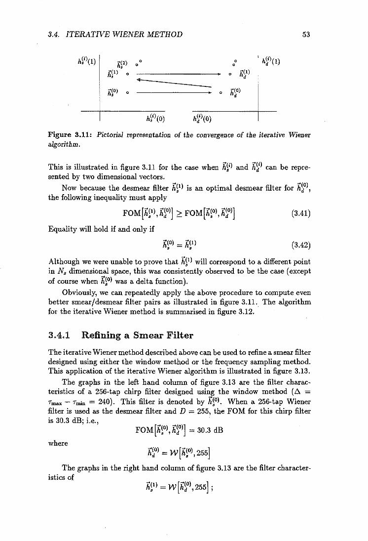
3.4. ITERATIVE WIENER METHOD
hii)(l) .... (2) 0 h, 0
.... (1) h, 0 ....
.... (0) h~ 0
o o
o h(l) d
53
Figure 3.11: Pictorial representation of the convergence of the iterative Wiener algorithm.
This is illustrated in figure 3.11 for the case when h~i) and h~i) can be represented by two dimensional vectors.
Now because the desmear filter h~l) is an optimal desmear filter for h~O), the following inequality :i:nust apply
(3.41)
Equality will hold if and only if
(3.42)
Although we were unable to prove that h~l) will correspond to a different point in Ns dimensional space, this was consistently observed to be the case (except of course when h~O) was a delta function).
Obviously, we can repeatedly apply the above procedure to compute even better smear/desmear filter pairs as illustrated in figure 3.11. The algorithm for the iterative Wiener method is summarised in figure 3.12.
3.4.1 Refining a Smear Filter
The iterative Wiener method described above can be used to refine a smear filter designed using either the window method or the frequency sampling method. This application of the iterative Wiener algorithm is illustrated in figure 3.13.
The graphs in the left hand column of figure 3.13 are the filter characteristics of a 256-tap chirp filter designed using the window method (.6. = Tmax - Tmin = 240). This filter. is denoted by h~O). When a 256-tap Wiener filter is used as the desmear filter and D = 255, the FOM for this chirp filter is 30.3 dB; i.e.,
where h~O) = w [h~O), 255]
The graphs in the right hand column of figure 3.13 are the filter characteristics of

54 CHAPTER 3. DESIGNING FIR DIGITAL SMEAR FILTERS
Step 0 Start
Step 1 Initialisation:
i=O
Specify the desired delay D
Specify the number of taps in the smear filter Ns
Specify the number of taps in the desmear filter Nd
Specify the minimum acceptable FOM FOMmin
Generate the seed filter h~O)
Compute h~O) = W[h~O),D]
Step 2 DO WHILE (FOM [h~i), h~i)] < FOMmin and i < 50)
i=i+l
h~i) = W [h~i-l), D] h~i) = W [h~i), D]
END DO
Step 4 Stop
Figure 3.12: Algorithm for designing smear/desmear filters using the iterative Wiener method.

3.4. ITERATNE WIENER METHOD
CD 'C ::I
Seed Filter
Impulse Response 0.1 0 .-----..----.----..---..---~-_._-...,
0.05
i[ 0.00
~ -0.05
-0.10 I....-_.L..-....:...."'--_ ....... _ ....... _ ......... ...;"... ......... _...J -50 0 50 100 150 200 250 300
lime (Secs)
(0)
Group Delay Response 300,--~--~---r--~---.
250 ,.,. ...... 200 ~ ~ 150 Q. e 100
(.') 50
O~-~---~--~--~---...J 0.0 0.1 0.2 0.3 0.4 0.5
Frequency (Hz)
(C)
Magnitude Characteristic 2.------~~-~--~--~--~
"iIi' ;:g. .. ] 0 ~ c
'" ~-1
-21....-__ ~~ __ ~ ____ -L ____ ~ ___ ...J 0.0 0.1 0.2 0.3 0.4 0.5
Frequency (Hz)
(e)
., 'C :::J
55
Refined Filter
Impulse Response 0.10 ,--,...----:-...----..---..---_._--.---,
0.05
i[ 0.00
~ -0.05
-0.10 I....-_.L..-_.L..-_ ....... _-'--_......,;~ ......... _...J -50 0 50 100 150 200 250 300
lime (Secs)
(b)
Group Delay Response 300,---~--~---r---r---,
250 ,.,. ...... 200 ~ ~ 150 Q. e 100
(.') 50
Ol....---~----~----~---~--...J
"iIi' ;:g. ..
0.0 0.1 0.2 0.3 0.4 0.5 Frequency (Hz)
(d)
Magnitude CharaCteristic 2.-----~--~----r---r----...,
] o~----.. ~~~~~~~~----~ ~ '" ~-1
-21....---~----~----~----~----...J 0.0 0.1 0.2 0.3 0.4 0.5
Frequency (Hz)
(f)
FiFoure 3.13: Comparison offilter characteristics for h~O) and h~l) when the seed filter (h80)) is a chirp filter designed using the window method. The filter characteristics in
the left hand column correspond to h~O); the filter characteristics on the right hand column correspond to h~l).

56 CHAPTER 3. DESIGNING FIR DIGITAL SMEAR FILTERS
Window Method Frequency Sampling Method
FOM [hiD), h~O)] 30.3 dB 27.5 dB
FOM [h~l), h~O)] 43.4 dB 41.8 dB
FOM [h~l), h~l)] 45.1 dB 44.5 dB
FOM [~2), h~l)] 45.7 dB 45.3 dB
FOM [h~2), h~2)] 46.1 dB 45.8 dB
FOM [~SO) I h~SO)] 64.0 dB 64.0 dB
Table 3.4: Use of the iterative Wiener method to refine two existing all-pass smear filters. One of the seed filters used in this design was generated using the window method; the other using the frequency sampling method. In both cases, the seed filter was a 256-tap chirp with .6. = Tmax - Tmin = 240, and D = 255.
i.e., the smear filter that is produced after one iteration of the DO LOOP in step 2 of figure 3.12.
Comparing the filter characteristics of hiO) and hil ), it is seen that hiO) approximates a linear ramp group delay response better than hil ), whereas hill approximates an all-pass magnitude characteristic better than h~O). In effect, the group delay response of hill has been modified slightly to concentrate more of the impulse response energy into the 256-tap time window.
Using filter h~l) = w[hil ),255] as the desmear filter,
This is a 14.8 dB improvement over FOM[hiO), h~O)]. Table 3.4 shows how the FOM improves for this example as the itera
tion process proceeds. This table also records the performance of the iterative Wiener method when the seed filter described aboved was ~enerated using the Frequency Sampling method. (Note the entry for FOM [h~30), h~30)] is not a mistake; it was included to show that the algorithm contmues improving the smear / desmear filter for some considerable time.)
3.4.2 Randomly Chosen Seed Filter
An alternative method for generating the seed filter hiO) is to generate a sequence of random numbers and use these for the coefficients of hiO).
Figure 3.14 illustrates this for a 256-tap smear filter. The filter characteristics in the left hand column of this figure are the characteristics of a seed filter whose coefficients were randomly chosen from a uniform distribution. This seed filter is denoted by hiO). The filter characteristics on the right hand column are the filter characteristics of the resulting smear filter after fifty iterations of the iterative Wiener algorithm (i = 50). Using the terminology defined above, this

3.4. ITERATIVE WIENER METHOD
Seed filter: Impulse response o.2.....---------T-----.:...--____,
0.1
] '5. 0.0
~ -0.1
-0~1~2~7-------~0-------~127
lime (Sees)
(0)
Magnitude Characteristic 10.....---~~--~--~~-~--____,
'iii' 0 3
~-10
~-20 -.30 1...-__ ---'-____ -'-_--''--_-'-__ ----'
0.0 0.1 0.2 0.3 0.4 0.5 Frequency (Hz)
(C)
Time (sec)
(e)
57
Smear filter: Impulse response 0.2 ,..-----------,.:-----:.--___,
0.1
] '5. 0.0
~ -0.1
-0.2 '-:-::---------':---------------:-" -127 0 127
lime (Sees)
(b)
Magnitude Characteristic 10,..---~~--,--~~---r-___,
! 0
!-10 c ~-20
-.30 I...------'------'-----":---:"-~____:' 0.0 0.1 0.2 0.3 0.4 0.5
Frequency (Hz)
(d)
Spectrogram
o Time (sec)
(f)
Figure 3.14: Comparison of niter characteristics for h~O) and h~50). The filter characteristics in the left hand column are for h~O), and the filter characteristics in the right hand column are for h~50). (The spectrograms were obtained using a 31-tap Hamming window.)

58 CHAPTER 3. DESIGNING FIR DIGITAL SMEAR FILTERS
smear filter is denoted by h~50), and
Comparing the impulse responses of h~O) and h~50) (figures 3.14 (a) and (b) respectively), it is seen that application of the iterative Wiener method has concentrated the instantaneous energy of h~50) towards the centre of the impulse response. Also, some quite large peaks occur in h~50) compared to hiO).
Comparing the magnitude characteristics of hiD) and h150), it is seen that application of the iterative Wiener method has smoothed out the magnitude characteristic of h~50) compared to h~O), and h~50) is beginning to approach an all-pass filter. However, even h~50) has sufficient ripple in its magnitude characteristic to be described by a different adjective than all-pass. We will call such smear filters "non-flat" smear filters and arbitrarily define a nonflat smear filter as a smear filter exhibiting greater than 1 dB of ripple in its magnitude characteristic5•
Figures 3.14 (e) and (f) plot the spectrogram for hiO) and hi50) respectively. Referring to these two figures, it is seen that the nonflat magnitude characteristic has introduced echoes into the signal; ie. the energy in a narrow band of frequencies is not concentrated about a single point in time as is the case for all-pass smear filters. Obviously, the spectrogram for a non-flat smear filter is far more complex than the spectrogram for the all-pass smear filter.
Figure 3.15 investigates the convergence properties of the iterative Wiener method when seed filter's coefficients are randomly generated. Specifically, figure 3.15 (a) recods the convergence of the iterative Wiener algorithm for ten randomly chosen seed filters when Ns = Nd = N = 256, and D = N -1 = 255. Figures 3.15 (b)-(d) record similar convergence data for N varying from 1024 through to 16384.
Comparing the four graphs in this figure, it is seen that the basic shape of the convergence curves are independent of N. The only effect of increasing N is to reduce the variation between curves and cluster them more tightly about the mean convergence curve. Thus, the ten curves plotted on figure 3.15 (d) overlap each other and appear as a single line. This characteristic is obviously due to statistical averaging.
The results show that approximately 20 interations are required to generate a smearjdesmear filter whose FOM exceeds 30 dB. Further, the number of iterations required for convergence is independent of N. Also independent of N is the average FOM for h~O) and h~O) which has a value of approximately 5 dB. Initially, we found this result rather surprising because intuition suggested.that as N increased, the FOM should improve. However, upon reflection it became obvious that this result is similar to the phenomenon encountered in power spectral analysis: i.e., the variance of the periodogram estimate for the power spectral density does not asymptotically approach zero as the length of the
5This name was suggested by one the examiners.

3.5. CONCLUSIONS
N=256 40 ....--...,---..-----.--..,..--...., 35 30
'iD"25 "0 ...... 20 ;:l;
~ 15 10 5
°0~-~10~~2~0--7~~-4O~-~50 Iteration (i)
(0)
N=4096 40 ,..---.....---,.-----,--..----...., 35 30
'iD"25 't:I ...... 20 ;:l;
~ 15 10
5
0~--~-~-_7~-~-~ o 10 20 ~ 40 50 Iteration (I)
(C)
59
N=1024 40.-----.----....--.----.-----. 35 30
'iD"25 "0
;20 ~ 15
10 5
°0~-~10--~2~0--730~-4O~-~50 Iteration (I)
(b)
N=16384 40,---.-----.---.....---.-----, 35 30
'iD"25 "0
';'20 ~ 15
10 5
O~-~-~--~~-~--~ o 10 20 30 50 Iteration (1)
(d)
Figure 3.15: Convergence of the iterative Wiener method for different length smear/desmear filters. In all cases, N8 = Nd = Nand D = N - 1.
window increases; rather, it remains approximately constant with increasing window length [Oppenheim and Schafer, 1989; Jenkins and Watts, 1968].
One problem with using the iterative Wiener method to design a smear / desmear filter from scratch, however, is that the method is computationally expensive. For example, the average CPU time required to generate a 2048 length non~flat smear filter on a VAX/VMS 750 is 80 minutes.
3 .. 5 Conclusions
This chapter has described three techniques for designing smear filters. Two of these design techniques - the window method and the frequency sampling method - are extensions of linear phase FIR filter design techniques. The third design method - the iterative Wiener method - is a previously unreported design technique and i.s only applicable to designing smear filters.
Both the window method and the frequency sampling method can be used to design an all-pass smear filter. (An all~pass smear filter was defined as having less than 1 dB of ripple in its magnitude characteristic.) The iterative Wiener method can be used to refine an existing all-pass smear filter, or it can be used to design a non-flat smear filter. (A non-flat smear filter was defined as having greater than 1 dB of ripple in its magnitude characteristic and typically has 8 dB of ripple.)

60 CHAPTER 3. DESIGNING FIR DIGITAL SMEAR FILTERS
When designing an all-pass smear filter using the window method, the rectangular window should be used for truncating the impulse response. Other bell-shaped windows, such as the hamming window, severely distort the magnitude characteristic. Also, care must be exercised when locating the temporal position of the rectangular window to ensure that the maximum amount of energy lies within the rectangular window. A major advantage of the window method is that it is an optimal design technique in the least squares sense.
The frequency sampling method generates inferior all-pass smear filters to the window design method. This is because the approximation error introduced by the frequency sampling method is caused by both truncation and aliasing, whereas the approximation error introduced by the window method is caused by truncation alone.
When using either the window method or the frequency sampling method, care must be exercised when specifying the desired group delay response of the smear filter. In some cases, it may be necessary to subtract a constant time delay from the desired group delay response to avoid introducing a phase discontinuity at the normalised frequency w = 7r rad/sec.
The use of interpolation for specifying the desired group delay response of an all-pass smear filter was also investigated, and the requirements of a good interpolant were established. Three good interpolants were identified: the linear interpolant, the raised cosine interpolant, and the cubic spline interpolant; although, cubic spline interpolation should only be used when there are less than approximately ten nodal points in the frequency interval [0,7r].
The iterative Wiener method was also described. This design method can be used to design a filter from scratch or refine an existing smear filter.
The following chapter provides some addition information which will help the smear filter designer choose between the various design methods described here.

Chapter 4
Mismatch Noise and Other Impairments
4.1 Introduction
Ideally, the overall impulse response of a smear :filter that is connected backto-back to a desmear :filter should be
.5(n - D) = { ~ n=D (4.1)
nf.D
where D is the delay introduced by the smear/desmear :filters. However, as was discussed in section 2.5, this ideal can never be achieved; the smear/desmear :filters always introduce some mismatch noise due to the non-zero coefficients of the mismatch filter.
This chapter will show that the characteristics of this mismatch noise are dependent on the method used to design the smear :filter. The chapter will also briefly investigate the effect of other transmission impairments on the performance of the smear/desmear :filters.
4.2 Mismatch Noise
Figure 2.9 (a) in section 2.5 shows what happens when a delta function is applied to the input of a smear filter that is cascaded with a desmear :filter. The desired output from the desmear :filter is a delta function delayed by D seconds; however, because of the unavoidable mismatch between the smear and desmear :filters, there is a superimposed noise component which causes ripples either side of this delta function. This noise is called mismatch noise.
The mismatch noise is dependent on the input signal and, as discussed in
61

62 CHAPTER 4. MISMATCH NOISE AND OTHER IMPAIRMENTS
section 2.5.3, is given by
00
M(n) = I: X(n)hm(n - k) (4.2) k=-oo
where X(n) is the signal applied to the input of the smear filter, and hm(n) is the impulse response of the mismatch filter. hm (n) has already been defined in section 2.5.3; however, for convenience we repeat its definition here:
n=fD
n=D (4.3)
where hs(n) is the impulse response of the smear filter, helen) is the impulse response of the desmear filter,and * denotes convolution.
The characteristics of the mismatch filter provide a very informative description for the behaviour of a smearjdesmear filter pair and also reveals significant differences between the smear filter design methods described in the previous chapter.
Figures 4.1--4.4 plot the mismatch filter characteristics for a smear and desmear filter pair designed using four different smear filter design methods: Figure 4.1 used the window method to generate the smear filter; figure 4.2 used the frequency sampling method; figure 4.3 used the iterative Wiener method to refine an existing all-pass smear filter; and figure 4.4 used the iterative Wiener method with a randomly generated seed filter. In all cases a 256-tap Wiener filter was used as the desmear filter, and the delay introduced by the causal smearjdesmear filters was 255 seconds. (The impulse responses shown in figures 4.1-4.4 are noncausal, and D = 0 for these figures.) Beforeplotting figures 4.1--4.4, all the mismatch filter impulse responses were normalised to have unit energy.
Figure 4.1 plots the mismatch filter characteristics for a smear filter designed using the window method. The smear filter used to generate this plot was the chirp filter described in section 3.3.1. (Refer to the right hand column plots of figure 3.10 for the filter characteristics of this smear filter.) Figure 4.1 (a) shows that the energy of the mismatch filter is dispersed in time, and thus it will act like a smear filter for the input signal. However, more of the energy is located at the centre of the impulse response than at the extremities. Figure 4.1 (b) shows that the magnitude characteristic of the mismatch filter exhibits some frequency selectivity. That is, the frequency components in the band 0.2-0.3 Hz will be attenuated by approximately 15 dB compared to those components at either 0 Hz or 0.5 HZ1. One consequence of this is that the power spectral density of the mismatch noise will be given by
(4.4)
lThis figure is not a very good example of the frequency-selective properties of this type of mismatch filter. Better examples can be found in appendix A. For example, look at the filter characteristics for ap2048asl

4.2. MISMATCH NOISE 63
0.3 Impulse Response
0..5
0.2
~ 0.1 :2
i 0.0 0.4
~-o.1 -0.2
-0.3 300
,.... -300 -200 -100 0 100 200 ~ 0.3
lime (5ec8) ""-'
(0) is' c (J) ::l 0-
20 Magnitude Characteristic ~ 0.2
,... 10 III ~
0.1
0.0 Io.i.-____ ""-'
-216 0 216 Time (sec)
(c)
Figure 4.1: Mismatch 11lter characteristics for a smear/desmear filter designed using the window method. The characteristics of the original smear 11lter are plotted in the right hand column of11gure 3.10; the desmear filter used to derive the mismatch 11lter was the Wiener 111ter. a) Normalised mismatch filter impulse response. b) Magnitude characteristic. c) Spectrogram of mismatch 11lter impulse response using a 64-tap Hamming window.
where Pxx (eiw) and PMM ( eiw ) are the power spectral densities of the input signal and the mismatch noise respectively, and Hm(eiw ) is the frequency response of hm(n). Thus the power spectral density of the mismatch noise will differ from the power spectral density of the desired output signal.
Figure 4.2 plots the mismatch filter characteristics for a smear filter designed using the frequency sampling method. The smear filter used in this example was the chirp filter described in section 3.3.1. (Refer to the left hand column plots of figure 3.10 for the filter characteristics of this smear filter.) Figure 4.2 (a) shows that significantly more energy is located at the extremities of this mismatch filter impulse response than was the case for figure 4.1 (a). This is obviously caused by the aliasing which occurred during the design stage of the smear filter. Figure 4.2 (b) clearly demonstrates that this mismatch filter also exhibits some frequency selectivity, as was the case for figure 4.1 (b).
Figure 4.3 plots the mismatch filter characteristics for an all-pass smear filter that was refined using a single iteration of the iterative Wiener method. The seed filter used in this refining process was the same smear filter used to generate the results for figure 4.1, and the refined smear filter is described in section 3.4.1. {Refer to the right hand column of figure 3.13 for the filter

64 CHAPTER 4. MISMATCH NOISE AND OTHER IMPAIRMENTS
0.3 Impulse
0.5
0.2
'" 0.1 "tJ .i:'l a, 0.0 0.4
~-0.1 -0.2.
-0.3 -300 -2.00 -100 0 100 200 300 'N' 0.3
llme (Sees) :::t: '-'
(0) ~ <: !II :I cr
20 Magnitude Characteristic ~ 0.2
'Di' 10 "tJ '-'
.g 0 0.1
'" :t:: c co §-10
-20 0.0 0.1 0.2 0.3 0.4 0.5 0 216
F'requeney (Hz) lime (sec) (b) (c)
Figure 4.2: Mismatch filter characteristics for a smear/desmear filter designed using the frequency sampling method. The characteristics of the original smear filter are plotted in the left hand column of figure 3.10; the desmear filter used to derive the mismatch filter was the Wiener filter. a) Normalised mismatch filter impulse response. b) Magnitude characteristic. c) Spectrogram of mismatch filter impulse response using a 64-tap Hamming window.
characteristics of this smear filter.) Figure 4.3 (a) shows that the energy at the centre of the mismatch filter impulse response has been suppressed, and most of the energy is now located at the extremities. This appears to be a property of the iterative Wiener algorithm, and this characteristic was observed for all the filters that were generated using this algorithm.
The magnitude characteristic of this mismatch filter (figure 4.3 [b]) is approximatelyflat; it does not exhibit the frequency selective properties of figure 4.1 (b). Once again, this appears to be a property of the iterative Wiener algorithm. The fact that the magnitude characteristic has been altered compared to figure 4.1 (b) is not surprising, because the iterative Wiener method operates by slightly modifying those characteristics of the smear filter that contribute to the mismatch noise.
Figure 4.4 plots the mismatch filter characteristics for a non-flat smear/desmear filter. The smear filter used to generate this plot was designed using fifty iterations of the iterative Wiener algorithm and is described in section 3.4.2. (Refer to the right hand column of figure 3.14 for the filter characteristics of this smear filter.) Most of the energy of the mismatch filter impulse response (figure 4.4 [aD is located at the extremities of the impulse response; the energy
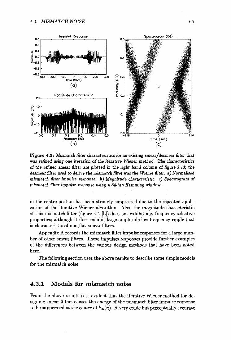
4.2. MISMATCH NOISE
Impulse Response 0.3 ...--.---.,.:--.,--.:........,.---......-----.
0.2
j 0.1
a 0.0
'!!-0.1
-0.2
-O~~-~-~-~-~--~~ -300 -200 -100 0 100 200 300
lime (Sees)
(0)
Magnitude Characteristic w...---~~~--~-~-~
! 0
i :0 -10
0.1
o lime (sec)
(C)
65
216
Figure 4.3: Mismatch filter characteristics for an existing smear/desmear filter that was refined using one iteration of the iterative Wiener method. The characteristics of the refined smear filter are plotted in the right hand column of figure 3.13; the desmear filter used to derive the mismatch filter was the Wiener filter. a) Normalised mismatch filter impulse response. b) Magnitude characteristic. c) Spectrogram of mismatch filter impulse response using a 64-tap Hamming window.
in the centre portion has been strongly suppressed due to the repeated application of the iterative Wiener algorithm. Also, the magnitude characteristic of this mismatch filter (figure 4.4 [b]) does not exhibit any frequency selective properties; although it does exhibit large-amplitude low-frequency ripple that is characteristic of non-:flat smear filters.
Appendix A records the mismatch filter impulse responses for a large number of other smear filters. These impulses responses provide further examples of the differences between the various design methods that have. been noted here.
The following section uses the above results to describe some simple models for the mismatch noise.
4.2.1 Models for mismatch noise
From the above results it is evident that the iterative Wiener method for designing smear filters causes the energy of the mismatch filter impulse response to be suppressed at the centre of hm(n). A very crude but perceptually accurate

66 CHAPTER 4. MISMATCH NOISE AND OTHER IMPAIRMENTS
0.3 0.5
0.2
~ 0.1 ::J
i 0.0
L O•1
-0.2
~~~~~~--~--~--~--~ -300 -200 -100 0 100 200 300
lime (Sees)
(0)
Magnitude Characteristic w~--~~~--~----~--~
~ 0
i :::t-10
0.4
0.1
0.0 -216 o
lime (sec) (c)
216
Figure 4.4: Mismatch filter characteristics for a non-Bat smearJdesmear filter. The characteristics of the original smear filter are plotted in the right hand column of figure 3.10; the desmear filter used to derive the mismatch filter was the Wiener filter. a) Normalised mismatch filter impulse response. b) Magnitude characteristic. c) Spectrogram of mismatch filter impulse response using a 64-tap Hamming window.
model for such a mismatch filter is
(4.5)
where (4.6)
This model assumes that both the smear and desmear filter are causal and the correlation peak of hs(n) * hd(n) is unity.
Using this model, if speech that has been sampled at 10 kHz is passed through a 16384-tap non-fiat smear/desmear filter, a low volume "pre-echo" will be heard 1.6 seconds before the main signal arrives, and a low volume post-echo will be heard for 1.6 seconds after the main signal has stopped. If the FOM for this smear/desmear filter pair is 30 dB, then these two echos would each be 33 dB below the main signal. A good approximation to this predicted effect was indeed observed when listening to speech that had been passed through such filters.
For a smear filter that has been designed using either the window method or the frequency sampling method, the model described by equation (4.5) does not apply. A better model is shown in figure 4.5. This figure models the mismatch

4.2. MISMATCH NOISE 67
X(n) __ +-+(
+
N(n)
Figure 4.5: Additive noise model for modelling the mismatch noise.
noise by an additive coloured noise source; the power spectral density of the noise source is computed using equation (4.4). After determining the spectral density of this noise, the mismatch noise is then assumed to be independent of the input signal. Obviously, this model can only be used when the input signal is stationary and ergodic; it could not be used if either one of these conditions were not satisfied.
Also, because the mismatch noise is actually obtained by passing the input signal through the mismatch filter, the mismatch filter is correlated with X (n ). However, because the impulse response of hm ( n) is similar to . that of a smear filter, X(n) and M(n + m) are only weakly correlated. To prove, this we will derive an equation for the normalised cross-correlation of X(n) and M(n) when the power spectral density of X(n) is white.
The normalised cross-correlation of X ( n) and M ( n) is defined as
() RXM(m)
PXM m = UXUM
(4.7)
where RXM(m) is the cross-correlation of X(n) and M(n + m), and
ui - E[(X - E[X])2] (4.8) 00
(4.9) k=-oo
The advantage of using the normalised cross-correlation is that it is bounded within the interval [-1,1]. If X(n) and M(n + m) are uncorrelated, then pXM(m) = 0; if X(n) = ±M(n + m), then pXM(m) = ±1.
RXM(m) can be computed as
RXM(m) - E[X(n)M(n + m)] (4.10) 00
- E[X(n) I: hm(k)X(n + m - k)] (4.11) k=-oo
00
I: hm(k)Rxx(m - k) (4.12) k=-oo
where Rxx(m) is the autocorrelation function of X(n). If the power spectral density of X(n) is white, equation (4.12) reduces to
00
RXM(m) - ui I: hm(k)8(m k) k=-oo
(4.13)
(4.14)

68 CHAPTER 4. MISMATCH NOISE AND OTHER IMPAIRMENTS
X(n) 6(n - D) -V
Y(n)
+
M(n)
hm{n)
Figure 4.6: Modelling the mismatch noise using the mismatch filter.
Thus for a white noise input signal, the cross-correlation between the input signal and resulting mismatch noise is proportional to the impulse response of the mismatch filter2.
Substituting equations (4.14) and (4.9) into equation (4.7) yields
(4.15)
This last equation shows that the normalised cross-correlation of X (n) and M(n) is identical to the normalised impulse response of the mismatch filter. Referring to the normalised impulse responses shown in figures 4.1 and 4.2 it is seen that the noise is only weakly correlated with the input signal because of the smearing action of the mismatch filter impulse responses. Therefore, as a first order approximation this correlation could be ignored in the analysis.
If neither of the above models are sufficiently accurate, then the model shown in figure 4.6 could be used.
4.3 Transmission Impairments
This section considers other impairments besides the mismatch noise that could inhibit the use of smear / desmear filters. For this investigation, we will ignore the mismatch noise and assume that the smear and desmear filters are ideal. Therefore, the smear and desmear filters act like a pure time delay when· connected back-to-back.
4.3.1 Magnitude and Phase Distortion
Assume the smear and desmear filters are separated from each other by a channel that introduces both magnitude and phase distortion. If the frequency response of the channel is denoted by Hc( eiw ), and the input signal applied to
2This result is well known and often serves as the basis for estimating the impulse response or frequency response of an LTI system.
4.3. TRANSMISSION IMPAIRMENTS 69
the smear filter is denoted by X(eiw ), then the output of the desmear filter is given by
Ji(eiw) __ X(eiW)lls (eiw)llc(eiw)lld (eiw )
__ e-iwD X(eiw)llc(eiw ) (4.16)
(4.17)
Clearly, the operation of the smear and desmear filters has been unaffected by the magnitude and phase distortion, because multiplication is a commutative operation. Of course, the output signal has still been distorted because the term llc(eiw) still appears on the right hand side of equation (4.17); however, this distortion exists whether the smear/desmear filters are present or absent.
Obviously any operation that is commutative with respect to convolution in the time domain, or equivalently commutative with respect to multiplication in the frequency domain, can be performed on the smeared signal without affecting the performance of the desmear filter.
4.3.2 :Frequency Translation
If the smeared signal undergoes a transformation which is not commutative with respect to convolution, the performance of the desmear filter may deteriorate significantly.
An important transformation belonging to this latter class of transformations is frequency translation. We did not investigate this latter problem; however, it is noted that the theoretical framework for investigating this problem has already been well developed in connection with the ambiguity function used in pulse compression radar [Cook and Bernfeld, 1967; Rabiner and Gold, 1975].
4.3.3 Additive White Noise
Figure 4.7 shows a smear and desmear filter that are separated by an additive white noise channel. Using the terminology defined in this figure, the output of the desmear filter is given by
(4.18)
where we have assumed that
Vw (4.19)
Not surprisingly, equation (4.18) shows that the desmear filter recovers W( eiw) correctly but cannot remove the noise component N(eiw ).
If the smear filter used to smear out W( eiw ) has a non-flat magnitude characteristic, then the desmear filter will also have a non-flat magnitude characteristic. However, the desmear filter will attenuate those frequency components that were amplified by the smear filter and vice versa. This suggests that the

70 OHAPTER 4. MISMATOH NOISE AND OTHER IMPAIRMENTS
N(elW)
Figure 4.7: Using smear/desmear filters when white noise is superimposed on the smeared signal.
non-fiat desmear filter will degrade the signal-to-noise ratio of the output signal. To prove this, consider what happens when the power spectral density of N(eiw ) is white with power spectral density No, and the power gain of the smear filter is fixed at unity: i.e.,
(4.20)
The SNR is then given by
(4.21)
where
(4.22)
Using constraint equation (4.19), the integral in the denominator of eq"Qation (4.21) can be written as .
[7r7r 11/Hs(eiw )1 2 dw
Now the Schwarz inequality states that
Therefore, substituting Hs(eiw) for 91(W) in equation (4.23) and l/Hs(eiw) for 92(W) yeilds
Ij7r Hs(eiw) H t 'w) dwl2 < j7r IHs(eiw) 12 dw j" H t .w) 2 dw (4.24) -7r S eJ -7r -7r 8 eJ
The left hand side of this last equation is equal to 4'1l"2, and from equation (4.20), the first factor on the right hand side is equal to 2'1l". Therefore, substituting these values into equation (4.24) and dividing both sides by 4'1l"2 yields
1 j7r 1 2
-2 H ('w) dw ~ 1.0 '1l" -'/r S eJ (4.25)
4.4. CONCLUSIONS 71
Equality will hold if and only if
Vw (4.26)
I.e. only if the smear filter has an all-pass magnitude characteristic.
Using the knowledge of this inequality in equation (4.21), it is obvious that non-flat smear filters will degrade the received signal-to-noise ratio. This degradation is, however, rather modest. For example, if the channel signal-tonoise ratio in figure 4.7 is 15 dB and non-flat filters nf2048a_vl and nf2048a_vli are used as the smear and desmear filters respectively (refer to appendix A), then the output signal-to-noise ratio is approximately 14 dB. Thus under these conditions, nf2048a_vli degrades the received signal-to-ratio by only 1 dB.
4.4 Conclusions
This chapter investigated the characteristics of the mismatch noise. The main tool used to investigate this noise was the filter characteristics of the mismatch filter.
It was shown that the smear filter design techniques described in chapter 3 produce very different types of mismatch noise. The mismatch noise introduced by an all-pass filter designed using either the window method or the frequency sampling method can be modelled by an additive noise source. The power spectral density of this noise source depends on the input signal: If the power spectral density of the input signal is white, the power spectral density of the mismatch noise will equal the square of the magnitude characteristic of the mismatch filter.
The mismatch noise introduced by a non-flat smear filter designed using the iterative Wiener method can be crudely modeled by two echoes: one preceding the main signal and one following the main signal. This result clearly suggests that the iterative Wiener method should be avoided when designing smear filters where distinct echoes would be objectionable (such as high quality speech and high quality image signals).
The effects of three types of transmission impairments were also briefly mentioned: It was also shown that amplitude and phase distortion has no effect on the operation of smear / desmear filters, but that frequency translation could seriously degrade performance. It was also shown that non-flat smear/desmear filters degrade the received signal-to-noise ratio slightly when channel noise is added to the smeared signal. All-pass smear filters do not degrade the signalto-noise ratio.
This concludes the first part of the dissertation; the remaining chapters will investigate novel applications for smear filters.

Chapter 5
Speech Compression
5.1 Introduction
Speech signals encountered in the Public Switched Telephone Network (PSTN) vary over a range of approximately 60 dB [Purton, 1962; Richards, 1964]. This variation in the instantaneous amplitude of speech is due to two factors:
.. There is a spread in the long-time mean level of different conversations measured at the same point in a network, because of differences in speaking level and differences in circuit losses between the talker and point of measurement. This accounts for approximately 30 dB of variation.
.. For a given conversation at constant mean volume, the instantaneous speech level is spread out about the mean because of variations in speech sounds. This accounts for the other 30 dB variation in the range of levels encountered.
The long-time variation in volume, caused by different speakers and varying transmission losses, can be reduced using automatic gain adjusting devices that selectively amplify the weaker signals [Norwine, 1938; Smith, 1957].
The short-time variation in level, caused by different speech sounds, can be reduced using either syllabic companding, instantaneous companding, or clipping. Syllabic compandors reduce the dynamic range of the speech wave by adjusting the gain of an amplifier at the syllabic rate, so that weaker sounds are selectively amplified relative to the stronger sounds [Norwine, 1938; Wright, 1938; Carter et al., 1946]. Instantaneous compandors pass the speech wave through a compressor that has a non-linear transfer characteristic which amplifies weaker signals more than stronger signals [Smith, 1957]. A problem with instantaneous companding, however, is that the bandwidth of the compressed signal is expanded because of the nonlinear transfer characteristic of the compressor. Thus, instantaneous companding is only used when the compressed signal is sampled, quantized, and transmitted in digital form. Clipping is also effective at reducing the dynamic range of the speech. For example, clipping
73

74 CHAPTER 5. SPEECH COMPRESSION
the speech at a level only exceeded during 1% of the time speech is present, reduces the power-handling capacity by at least 3 dB and is quite unnoticeable [Richards, 1964].
This chapter investigates the possibility of using smear / desmear filters to compress the short-time variation in speech. The following section provides the motivation for this investigation.
5.2 Smear filters as Speech Compressors
Figure 5.1 (a) shows two seconds of a typical speech waveform. From this figure, it is evident that the energy of the speech signal is unevenly distributed in time. The large amplitude (high energy) parts of the speech wave are due to voiced sounds, the low amplitude parts of the speech wave are due to unvoiced sounds, and the very low amplitude parts of the speech wave are due to background noise during inter-word silences.
Because the short-time statistics of the speech wave vary with time, it should be possible to reduce the peak-to-rms ratio of the speech wave by redistributing the energy of the speech waveform more evenly in time. This can be achieved by passing the speech wave through a smear filter.
Obviously, the very best that can be achieved using this technique would be to transform the pdf of the speech waveform into a Gaussian distribution. This would occur as the length of the smear filter approaches infinity. To indicate the order of compression available by this technique, figure 5.1 (b) shows some stationary Gaussian noise with the same rms voltage and power spectral density as the continuous speech wave in figure 5.1 (a). Comparing these two figures, it does appear that that a reasonable compression gain could be realised.
. After compressing the speech wave using a smear filter, the original speech can be recovered using a desmear filter. The penalty paid for using this compression technique, is of course, the time delay introduced into the signal due to the smear / desmear filtering. It will be shown that this time delay is rather excessive, and hence, this compression technique would not be suitable for general use on the PSTN. However, there may be other specialised communication systems where the transmission delay is not so critical, such as a simplex communication system.
When speech has been compressed using either syllabic companding or clipping, the resulting speech wave still consists of talk spurts followed by silent intervals. Smear/desmear filters offer the possibility of compressing the speech wave even further by dispersing the energy due to talk spurts into the silent intervals of the speech wave. This could be applied in addition to syllabic companding and clipping; however, for the purposes of this investigation, smear filters will used by themselves to compress speech.

5.3. SPEECH DATA BASE
8~----------'------------r----------~~--------~ G
4
~ 2. :::J ~ Ol---.... ~_ c.. ~ -2.
-4
-5
lime (sec)
(0)
8r-----------,------------r----------~~--------~
6
lime (sec)
(b)
75
Figure 5.1: Time domain waveforms of a typical speech waveform and some station~ ary Gaussian noise. a) Typical speech waveform (first 2 seconds of the wide~band maebrit phrase). b) Waveform of Gaussian noise with the same rms voltage and power spectral density as the speech waveform in (a).
5.3 Speech data base
The speech used for this investigation consisted of the seven utterances listed in table 5.1. Four of these utterances were spoken by male speakers and three were spoken by female speakers. The individual utterances listed in this table are labelled according to the code gender-initials-phrase.
All the utterances were recorded in an anechoic chamber using a good quality microphone and good quality recording equipment. The utterances were subsequently passed through an anti-aliasing filter, sampled at 10 kHz, and uniformly quantized to 12 bits. . To verify the quality of the digitized speech, the utterances were converted back to analog form using a D / A converter, amplified, and applied to a pair of good quality headphones. In all cases, the reproduced speech was of good quality with a very high SNR. The only noticeable degradation in speech quality was the loss of fidelity caused by passing the speech through the anti-aliasing filter. This filter had a bandwidth of 0-4.5 kHz.
As the bandwidth of the digitized speech is wider than a typical telephone

76 CHAPTER 5. SPEECH COMPRESSION
Label Gender Initials Phrase Duration
maebrit M AE Stitching London together, from one 11.7 (sec) bank of the Thames to the other, are 32 bridges: 20 for road traffic, 10 for rail, and 2 for pedestrians only. With-out these bridges, Britain
maewal M AE The time has come the walrus said, 8.3 (sec) to speak of many things. Of ships and shoes and ceiling wax, and cabbages and kings.
mbmwal M BM " 7.1 (sec)
mwtwal M WT " 7.8 (sec)
fkgwal F KG " 6.4 (sec)
ftcwal F TC " 7.0 (sec)
fcwwal F CW " 7.6 (sec)
Table 5.1: Speech utterances used to investigate effectiveness of smear/desmear filters to compress speech.
channel, these speech samples will be referred to as wide-band speech. It was also of interest to band limit these utterances to 300-3400 Hz to see what effect this had on the compression of the speech wave. This was achieved by passing the speech samples through a linear phase FIR digital filter with magnitude characteristic shown in figure 5.2. The resulting band pass filtered speech waves will be referred to as narrow-band speech.
5 .. 4 Smear Filters
The fourteen smear filters listed in table 5.2 will be used will be used to compress the speech for this investigation. Six of these filters are 4096-tap all-pass filters; one of them is a 4096-tap non-fiat smear filter; another six are 16384-tap all-pass smear filters; and the remaining filter is a 16384-tap non-fiat smear filter. This range of smear filters will enable us to identify the important factors that affect the ability of a smear filter to compress speech.
The naming convention used to label the smear filters is self explanatory (refer to table 5.2); however, an understanding of the rationale used to select th~ two-letter codes in the column labeled "Group Delay" may help the reader. The first letter "s" means that the smear filter has a sawtooth-shaped group delay response. The second letter (a, b, d, h, or p) indicates the number of teeth in the nyquist interval (e.g. a=1, b=2, d=4, and so on). Some parts of this chapter will use an abbreviated form of the naming convention defined in table 5.2 by simply listing the letters that identify the type of filter (ap or nf), and the letters that identify the shape of the group delay response. For example, ap-sh will collectively refer to filters ap4096sh_v1 and ap16384sh_v1

5.4. SMEAR FILTERS
10r-----~------~----~~----_r----~
o 'iIi' ~ -10
cu -g -20 -·c 01 -30 c ~
-40
-50~----~------~----~----~~UU~WW a 1 000 2000 3 000
Frequency (Hz) 4 000 5000
77
Figure 5.2: Band pass filter used to band limit speech. The resulting band pass filtered speech will be referred to as narrow-band speech
Filter Type Taps Group Delay Version Label
ap 4096 sa 1 ap4096s3-vl
ap 4096 sb 1 ap4096sb~vl
ap 4096 sd 1 ap4096sd~vl
ap 4096 sh 1 ap4096shsl
ap 4096 sp 1 ap4096sp_vl
ap 4096 h 1 ap4096h_vl
nf 4096 a 1 ap4096s3-vl
ap 16384 sa 1 apl6384s3-vl
ap 16384 sb 1 apl6384s3-vl
ap 16384 sd 1 ap16384sc:Lvl
ap 16384 sh 1 apl6384shsl
ap 16384 sp 1 apl6384sp_vl
ap 16384 h 1 ap16384hsl
nf 16384 a 1 nf163843-vl
Table 5.2: Smear filters that will be used to compress speech.

78 CHAPTER 5. SPEECH COMPRESSION
unless the context clearly restricts the use of this abbreviation to either one of the filters alone.
The shape of the group delay response for the twelve all-pass smear filters is shown in figure 5.3. This figure plots the group delay response for the six 4096-tap all-pass smear filters; the group delay response of the 16384-tap smear filters have the same shape as those of figure 5.3, but the scaling along the yaxis is different (refer to appendix A). Note that group delay response of the five filters shown in figures 5.3 (a)-(e) vary in a controlled manner; the group delay response for the sixth filter (figure 5.3 (f)) is very different. Also note that for clarity, the x-axis for figure 5.3 (f) is only plotted over the frequency interval 0-600 Hz. This group delay response continues to oscillate very rapidly over the remaining frequency interval 600-5000 Hz. (Refer to appendix A to see this group delay response over the entire nyquist interval.)
5.5 Definitions
. This section defines the metrics used to investigate the effectiveness of smear filters at compressing speech. In the equations below, the random variable V will represent the amplitude of the speech sample at some arbitrary point in time.
5.5.1 Peak Level
The simplest way of defining the peak level of sampled speech is to locate that sample which has the maximum absolute value and define this as the peak of the signal. However, because this peak level could be due to an uncharacteristic noise spike, we decided not to use this definition. Instead, we used the 1-percentile peak level.
The I-percentile peak level (Pv) is defined as the value of Pv that satisfies the equation
lpV
-PV /v( v) dv :::: 0.99 (5.1)
where /v(v) is the pdf of V. This percentile was chosen (rather than say the 0.5-percentile) because speech can be clipped at the I-percentile peak level with little degradation in perceptual quality [Purton, 1962; Richards, 1964].
Other researchers have defined different measures for the peak level of speech. In particular, Brady suggested that a more reliable method for measuring the peak level of speech was to measure the rms value of those samples exceeding a certain threshold and then estimate the peak level from the rms value by assuming that the samples lying above the threshold are exactly log uniformly distributed [Brady, 1965; Brady, 1968]. Unfortunately, after filtering speech through a smear filter, the pdf of the output signal differs markedly from that of the input, and the assumption that the samples above a certain thresh-

5.5. DEFINITIONS
500
"Oi' 400 .s ~ 300 V ~ 200 ::J e 100 (l)
500
..,. 400
.s ~ JOO v Q
200 a. ::J
l5 100
..,. 400
.s ~300 ~ 200
& 100
1 000
1000
ap4096sa..v1
2000 3000 Frequency (Hz)
(0)
ap4096scLv1
2000 3 000 Frequency (Hz)
(e)
4000 5000
4000
5000
79
500 ap4096sb_v1
"Oi'4OO .s ~ 300 Ii Q
200 a. ::J e 100 (l)
1 000 2000 3000 4000 F req uenC)' (Hz)
(b)
500 ap4096sh..v1
"Oi' 400 .s ~300
;! 200 0. ::. e
(l)
5000
ap4096h..v1 OOOr-------~--------~------_;
"Oi' 400 .s ~ 300 ijj
~ 200 ::J e
(l) 100
200 400 sao Frequency (Hz)
(f)
Figure 5.3: Group delay response of the six 4096-tap all-pass smear filters used to compress speech. The six 16384-tap all-pass smear filters have similar shaped group delay responses but a different scaling along the y-axis. a) ap4096sa..vl. b) ap4096sb-vl. c) ap4096sd_vl. d) ap4096sh_vl. e) ap4096sp-vl. f) ap4096h_vl

80 CHAPTER 5. SPEECH COMPRESSION
old are log uniformly distributed is no longer valid. Consequently, Brady's peak level could not be used.
5.5.2 Rms level
The rms level of the speech signal is defined as
(Tv = 1 N - LV? N i=l ~
(5.2)
where N is the number of samples in the speech sample, and Vi is the value of the i'th sample. Obviously, the rms voltage is affected by the number of zerovalued samples appended to either end of each utterance. For all the phrases listed in table 5.1, the zero valued samples were trimmed off either end of the digitised speech sample.
5.5.3 Peak-to-rms ratio
The peak-to-rms ratio (Rv) is defined as
Rv = (::) (5.3)
where Pv is the peak level defined in sub-section 5.5.1, and (Tvrms is the rms voltage defined in sub-section 5.5.2.
When (Tv = 1.0, Rv is numerically equal to Pv.
5.5.4 Compressability Factor
Smear filters compress a signal by making its pdf approach a Gaussian distribution. They can be applied successfully to speech because the pdf of the speech signal approximates a Gamma distribution, and this has a higher peak level than the Gaussian distribution (refer to figure 5.4). Obviously, if the signal to be compressed already had a Gaussian pdf, smear filtering will be of no use at all. Even worse, if the signal has a uniform pdf (such as an image waveform), the smear filter will actually increase the peak level of the smeared waveform.
Considering the significance of the Gaussian distribution, a good metric for measuring· the "compress ability" of a waveform can be defined as
Cv = 20 log (~:) dB (5.4)
where Pv is the peak level of the waveform to be compressed, and PG is the peak level of a Gaussian pdf with the same variance as V.
We called this useful metric the "compressability factor". A positive value for the compressability factor indicates that the waveform can be compressed

5.5. DEFINITIONS 81
using smear filters. A negative value indicates that smear filters will increase the peak level of the waveform and obviously should not be used to compress the signal. A value of zero for the compress ability factor indicates that the smear filters will have no effect on the peak-level of the waveform.
It is very easy to construct a signal which violates the above interpretation of the compressability factor. For example, if the signal to be compressed has a Gamma distribution, and it is passed through the desmear filter before being applied to the smear filter, then the smear filter will obviously increase the peak-level of the waveform. Another signal that violates this interpretation is the sine wave. In this case the smear filter will have no effect on the amplitude of the sine wave irrespective of the value of the compressability factor. However, for a random signal such as speech that has not been passed through a desmear filter, it seems quite reasonable to expect the above interpretation for the compressability factor will be valid.
5 __ 5.5 Cumulative function
When applied to speech, the cumulative function Fx(x) is usually defined as
Fx(x) = P(X > x) (5.5)
where X is a random variable and x denotes a particular value of X. Note that this definition is the complement to that normally used in mathematics; however, it is commonly used in speech literature [Brady, 1965; Davenport, 1952; Dunn and White, 1940; Sivian, 1929].
Some researchers have defined X to represent the instantaneous power of the speech signal, and the cumulative function is plotted on a graph whose abscissa is in dB [Purton, 1962; Brady, 1965]. For our purposes, however, it is more convenient to follow Holbrook and Dixon [Holbrook and Dixon, 1939] who defined X as
crv (5.6)
The advantage of this latter definition, is that the relatiollship between the peak level and peak-to-rms ratio can be easily determined from the cumulative function.
Figure 5.4 plots the cumulative function for the seven test utterances listed in table 5.1. Figure 5.4 (a) records the cumulative function for the wide-band speech, and figure 5.4 (b) for the narrow-band speech. Also plotted on these two graphs are the theoretical cumulative functions for the Gamma distribution, the Laplacian distribution, and the Gaussian distribution.
Cumulative functions for the Gamma and Laplacian distributions are included because they are often used to approximate the pdf of speech [Paez and Glisson, 1972; Rabiner and Schafer, 1978]. (Obviously, the Gamma distribution is a better approximation than the Laplacian distribution; this observation has been noted by other researchers [Niederjohn and Haworth, 1983].) The Gaussian distribution is included because the pdf of the smeared speech approaches

82 CHAPTER 5. SPEECH COMPRESSION
Density Pdf Fx(x)
Gaussian 1 ( exp ",fiKO'v
v~ ) -20'f erfc(x/0.)
Laplacian 1 exp ( _ v21 v I ) -../2:r; e
V2O'v O'v
Gamma .Jk e-k1vl J3
2V'i ~ where k = 2uv eric (V.V; x )
Table 5.3: Denning equations for the Gaussian, Laplacian, and Gamma pdfs; and their respective normalised cumulative functions.
this distribution when the length of the smear filter is made very long (This is a consequence of the central limit theorem). Table 5.3 lists the equations for the pdfs and the cumulative functions for these distributions.
The peak-level can be determined from figure 5<.4 by locating the intersection of the horizontal line P(X > x) = 10-2 with the cumulative function Fx(x). The x-coordinate of this point is the (normalised) peak-level of the waveform. For example, the horizontal line P(X > x) = 10-2 intersects the cumulative function for the Gaussian pdf at x = 2.53V and with the wide-band maebrit phrase at x = 4.2 V. The compress ability factor for the maebrit phrase is therefore
I 4.2
20 og 2.53 = 4.4 dB
It is also obvious from figure 5.4 that there is considerable variation .between the cumulative functions for the different speakers. Three factors that contribute to this variation appeared to be
1. the speed at which the speaker quoted the phrase;
2. the gender of the speaker; and
3. long-time variations in the volume of the speech (due to, for example, slight variations in the coupling between the microphone and speaker when recording the phrase).
The exact cause of the observed variation is not of particular concern for this current investigation, provided of course that the variation is typical of speech. Considering how the cumulative functions for the seven utterances are distributed about the Gamma distribution (which is known to be a reasonable approximation for speech), we feel confident that this variation is indeed typical of speech.

5.5. DEFINITIONS 83
10°=------------r------------~----------_.----------~
,--... x 1\ x '-' 0...
10"'"
10°
10-1
,...... x 1\ X '-' 0...
10-2
0 2
2
--------_ .. ................... _~_6_._._._._
-.. - .. - .. -~.-. -- - - --- - -- .
-- - --
(x)
(0)
--- ----_ .. .. ~ ................ -.-.-.-.-.-.~
_ .. _ .. - .. _ .. -. - - ---_. _. _ ...
4 Threshold (x)
(b)
maebrit (11.7 5)
maewal (6.3 s)
mbmwal (7.1 s)
mwlwal (7.6 s)
fcwwal (7.6 s)
fkgwal (6.4 s)
ftewal (7.0 s)
-'-
6 8
maebrit (11.7s)
maewal (6.3 s)
mbmwal (7.1 s)
mwtwal (7.8 s)
fewwal (7.6 s)
fkgwal (6.4 s)
ftewal (7.0 s)
....
6 8
Figure 5.4: Cumulative functions for the seven utterances listed in table 5.1. a) Wide-band speech. b) Narrow-band speech.

84 CHAPTER 5. SPEECH COMPRESSION
5.6 Speech Compression Results
Having introduced the test utterances and smear filters that were used in this investigation, and having defined all the terms, we are now in a position to present the speech compression results themselves.
Figure 5.5 plots the time domain waveforms for the wide-band maebrit waveform. Figure 5.5 (a) plots the first four seconds of the uncompressed waveform (i.e., the signal applied to the input of the smear filter). Figures 5.5 (b) and (c) plot the smeared signal after it has been passed through filters ap4096sh_ vI and apl6384sh_vl respectively. Clearly, the smear filters are dispersing the energy of the speech wave into the silent intervals as described in section 5.2; however, very long filters are obviously required to approach the theoretical limit for this compression scheme.
Figure 5.6 plots the cumulative function for the maebrit phrase when it is compressed using the seven 4096-tap smear filters listed in section 5.4. Figure 5.6 (a) records the results for the wide-band speech and figure 5.6 (b) records the results for the narrow band speech. This figure shows that there is considerable variation between the smear filters themselves: Filters ap4096sp_ vI, ap4096h_vl, and nf4096a-vl appear to do a better job at compressing the speech than the other four smear filters. This figure also shows that the pdf of the smeared speech is starting to approach a Gaussian distribution; however, the compress ability factor of the smeared speech is still greater than 0 dB, indicating that further improvement could be obtained by using longer smear filters.
Figure 5.7 plots the cumulative function for speech that has been compressed using the I6384-tap smear filters. Obviously, increasing the length of the smear filters has improved the compression of the speech wave; however, even these very long smear filters have not reduced the compress ability factor to o dB. Once again, there is considerable variation between the different smear filters, and filters nf16384a_vl, ap16384h_vl, and apl6384sp_vl appear to perform better than the other smear filters.
The above two plots were obtained from the maebrit phrase, and therefore, they do not contain any information about the variability of smear filter performance for different speakers. This information is presented in figure 5.8, which plots the compressability factor of the smeared speech as a function of the different smear filters. The compress ability factors recorded in these plots were obtained by taking the arithmetic mean of the individual compressability factors for each combination of smear filter and utterance. (For example, each data point lying on the dashed curves in figures (a )-( d) is the arithmetic mean of seven compress ability factors.) For reference, the compress ability factor for the uncompressed speech is also included on the figures; this data point is labelled "none".
Figures 5.8 (a) and (b) reveal that there is a significant difference between the compressability factors for the male speech and female speech. Specifically,

5.6. SPEECH COMPRESSION RESULTS
Original speech B~----------~--------~~~------------~------------,
-8
~0~----------~------------~2~----------~3~----------~ lime (sec)
(0)
Smeared speech using 4096 length filter. 8~-----------.------------~------------.-------------,
4
-8 z ::l
:E; 0 Q.
~ -z -4
~~----------~------------~2------------~3~----------~4 lime (sec)
(b)
Smeared speech using 16384 length filter. B~-----------.------------~------------.-------------,
4
-8 2
~ 01--........ _ Q.
~ -2
-6
~~----------~-------------72------------~----------~4 lime (sec)
(c)
85
Figure 5.5: Time domain waveforms for speech that has been compressed using smear filters. (These waveforms were obtained from the maebrit phrase.) a) Uncompressed speech. b) Speech that has been compressed using filter ap4096sh_vl. c) Speech that has been compressed using filter ap16384sh_vl.

86 CHAPTER 5. SPEECH COMPRESSION
maebrit (Wide-band Speech) 10o~----------~-------------.------------~----------~
,....... x 1\ x "--' a..
10-3
10°
10-1
,....... x 1\ x "--' a..
1 0-2
0
- - - - - - - - - - ap4096sCLVl
_._. - ._. _.-.- ap4096sb_vl
- .. _ .. - .. _ .. _. ap4096scLvl
------. ap4096sILv1
_.-.-.-.- ap4096sp_vl
ap4096ILvl
......... "." .... , nf4096CLVl
2 4 6 x
(a)
maebrit (Narrow-band Speech)
Gaussian
2 4 x
(b)
--------_ .. -.-.-. _.- '_._'"'
- .. -.. -~.- .. -. -----_ .. _._._._--
.................. ~
ap4096sCLV1
ap4096sb_vl
ap4096scLvl
ap4096sILvl
a p4096sp_v 1
ap4096h..vl
nf4096CLV1
6
8
8
Figure 5.6: Cumulative function for speech that has been compressed using the seven 4096-tap smear filters listed in table 5.2. The cumulative functions were estimated from the maebrit utterance. a) Wide-band speech. b) Narrow-band speech.

5.6. SPEECH COMPRESSION RESULTS 87
,.-... x A x
"'-" a..
,.-... x A x "'-" a..
maebrit (Wide-band Speech) 100~-----------r------------~-----------.----------~
---------- ap16384sQ..vl
-,_._,-.-._.- ap16384sb_vl
_ .. _ .. _ .. - .. -. ap16384scLvl
------- ap16384stLvl
_._._._.- ap16384sp_vl
- - - - ap16384tLVl
.. , .. , .. ,.......... nf16384<Lvl
10--3 0 2 4 6 8
x (a)
100 maebrit (Narrow-band Speech)
--------- .. ap16384sQ..vl
_._.""'._.-.-_ .. ap16384sb_vl _ .. _ .. _ .. _ .. _. ap16384scLvl
10-1 -----_ ... ap16384stLvl
-.-.-._.- ap16384sp-vl
- - - - ap 16384tLvl
... , ... ~ ... ~ . ~ ... ~ . nf16384<Lvl
1 0-2
Gaussian
10--3~----------~------~----~~~--~--~---------=~ o 2 4
X
(b)
6 B
Figure 5.7: Cumulative function for speech that has been compressed using the seven 16384-tap smear filters listed in table 5.2. The cumulative functions were estimated from the maebrit utterance. a) Wide-band speech. b) Narrow-band speech.

88 CHAPTER 5. SPEECH COMPRESSION
Wide band Speech; 16384-tap filters
I 6~ .2 4 l; , :! i 3 , r ; -~----"!I--------..... ''''"tJ== ... ! 8 ~ Ii ~ 'S1 iii g.i.~
c & & & & & c c
--Female
FIlter
(a)
Narrow-band Speech; 16384-tap filters
--Male
--Female
- - .. - Av.
(b)
Wide-band Speech; 4096-taps
__��__ Female
- - .. - Av.
(c)
Narrow-band Speech; 4096-taps
--Male
--Female
- - .. - Av.
(d)
Figure 5.8: Averaged compressabiJity factors for different smear filter treatments. a) CompressabiJity factors for the wide-band speech and 16384-tap smear filters. b) Narrow-band speech and 16384-tap smear filters. c) Wide band speech and 4096-tap smear filters. d) Narrow-band speech and 4096-tap filters.

5.6. SPEECH COMPRESSION RESULTS 89
0.8 ''9 • WB; 16384 !
" 0.6 , --m- NB; 16384 US •• ill • ,
OA .. ~. ' '51 ' •• - - • - - WB: 4096
0.2 (I) 0 .a "0 J::. 0. J::. 0 - - fl- - NB;4096 c
'" '" '" 6. If 6. .,!. 0 0. 0. 0. 0. C C 0 0 0 0 0
0
Filter
Figure 5.9: Standard deviation of compressabiHty factors for the seven speakers.
as the all-pass filter is varied from ap16384sa..vl (labelled ap-sa in the figure) to ap16384sp_ vI the male speech shows an improvement in the compressability factor (i.e., it gets closer to 0 dB), whereas the female speech shows no improvement. A similar trend is observed in figures 5.8 (c) and (d) for the 4096-tap filters when the smear filter changes from ap4096sb_vl to ap4096sp_vl. This difference is probably due to the shorter pitch period of the female speech and will be explored further in section 5.7.
Figure 5.8 also shows that both the non-flat smear filters (nf-a) and allpass filters ap-h perform very well for both the male and female speech. For the I6384-tap filters at least, these two filters perform significantly better than any of the other smear filters examined. This result clearly suggests that when very long all-pass smear filters are used to compress speech (> 4096 taps), the group delay response of the smear filter should vary rapidly with frequency (as is the case for ap16384h-YI and nf16384a). Although we have only recorded the results of a single non-flat smear filter in this chapter, we investigated a total of ten different non-flat filters (five 4096-tap filters and five I6384-tap filters). In all cases the non-flat smear filters performed very well, and nf16384a..vl and nf4096a_vl can be considered to be typical non-flat smear filters.
The final point to note from figure 5.8 is that filters nf16384a_vl and ap16384h_vl have reduced the peak-to-rms ratio of the speech by approximately 3 dB; and the compressability factor for this compressed speech is approximately I dB.
Figure 5.9 provides additional information on this compression technique that has not been recorded in any of the previous figures. It records the standard deviation of the compressability factor as a function of the smear .filter. The four curves on this figure correspond to the four combinations of bandwidthxfilter-Iength used in the previous figures. Referring to this figure, it is observed that as the smear filter is changed from "none" to ap-sa to apsb, the standard deviation of the compressability factor reduces. This is quite logical, because the compressability factors for the individual utterances are all approaching a common bound; therefore, it would be expected that the standard deviation should reduce as this bound is approached. Surprisingly,
90 CHAPTER 5. SPEECH COMPRESSION
however, the standard deviation does not continue to reduce as the smear filter changes from ap-sd to ap-sh through to nf-a. This is particularly surprising considering that the average compressability factors for filters ap-h and nf-a showed little variation between the male and female speech (figure 5.8).
To explain this phenomenon, we need to analyse some simple waveforms that approximate the voiced sounds of speech. This is the subject of the next section.
5.7 Simplified Speech Waves
Speech waveforms are composed of voiced sounds, unvoiced sounds, and silent intervals. Voiced sounds correspond to the high-energy parts of the speech waveform and consist of a sequence of low-frequency quasi-periodic pulses. Unvoiced sounds correspond to the low-energy parts of the speech wave and are generated by turbulence somewhere within the vocal tract. The frequency response of the unvoiced sounds are noise-like and approximately flat [Flanagan, 1972; Jayant and Noll, 1984; Rabiner and Schafer, 1978]. As a result of this, voiced sounds are far more difficult to smear out in time than unvoiced sounds, and they (the voiced sounds) dominate the peak-to-rms ratio of the speech. Therefore, this section examines two simple models for a voiced sound in an attempt to explain the results observed in section 5.6.
Figure 5.10 (a) models a voiced sound by a 200 Hz sine wave pulse of 50 ms duration. We will call this model waveform the one-tone pulse. The frequency response of the one-tone pulse is shown in figure 5.10 (b). As expected, the spectrum is dominated by a single spectral lobe. Figure 5.10 (c) and (d) plot a second' model for a voiced sound. This latter model also consists of a 50 ms pulse, but there are now two spectral components in the wave: one at 200 Hz and the other at 400 Hz. This model waveform will be called the two-tone pulse.
Figures 5.11 (a), (b), and (c) show what happens when the one-tone pulse is passed through smear filters ap4096sh_v1, ap4096h_v1, and nf4096a_v1 respectively. (The horizontal dashed lines on these three figures are equal to the extrema of the input waveform.) Clearly, filter ap4096sh_ vI has not dispersed the energy of the one-tone pulse very well, and in fact the extrema of the smeared signal is slightly greater than the extrema of the input signal. This filter has not performed very well because its group delay response varies by only 25 ms over the frequency interval 180-220 Hz (corresponding to the width of the main spectral lobe in figure 5.10 (b)).
Figure 5.11 (b) shows that ap4096h_v1 has done a reasonable job at dispersing the energy of the input waveform in time. Significant amounts of energy have been dispersed over the time interval 100-400 ms. The extrema of the smeared waveform still approaches the peak dashed curves drawn on this figure; however, now only one or two cycles of the wave approach this line (rather than ten in figure 5.10 (a)). Careful inspection of the group delay response for filter

5.7. SIMPLIFIED SPEECH WAVES
.. .., :r i[ a ~
-1
-2~~--~~--~--~~--~ -10 0 10 20 30 40 50 60
lime (ms)
(0)
-2~~--~~--~--~~--~ -10 0 10 20 3D 40 50 60
lime (ma)
(c)
i 1.0
i :z 0.5
-8 1.0 :r '2 8' :z 0.5
91
100 200 300 400 500 600 frequency (Hz)
(b)
Figure 5.10: Two simple models for voiced sounds. a) Time domain waveform of the "one-tone pulse". b) Spectrum of the one-tone pulse. c) Time domain waveform of the "two-tone pulse". d) Spectrum of the two-tone pulse.
ap4096h_v1 in figure 5.3 (a) reveals that the group delay response of this filter varies very rapidly over the interval 18Q-220 Hz, and this is why this particular filter has performed reasonably well. Obviously, if the frequency of this tone was reduced slightly to correspond to a maxima or minima of the group delay response, the filter would not perform so well.
Figure 5.11 (c) records the result for filter nf4096a_vl. Once again, this smear filter performed very well. The very rapid changes in the group delay response (refer to appendix A) of this filter combined with the echoes introduced by the non-flat magnitude characteristic have effectively dispersed the energy of the one-tone pulse over quite a wide time interval. Possibly nf4096a_v1 has performed just slightly better than ap4096h_v1 at dispersing the energy of the one-tone pulse; however, there is certainly not much between the performance of these two filters.
From the above results, we conclude that if the short-time spectrum of voiced sounds are dominated by a single spectral lobe, the group delay response of the smear filters should change very rapidly with frequency to ensure that the speech energy is effectively dispersed in time. The short-time spectrum of female speech is far more likely to be dominated by a single spectral lobe than male speech because of the shorter pitch period of the female speaker. This is why the female speech was far harder to compress (as shown in figure 5.8) and why filters ap-sa, ap-sb, ap-sd, ap-sh, and ap-sp were not very effective at

92 CHAPTER 5. SPEECH COMPRESSION
2r-----~----~------~----~------~----~----~----~
{)
~ 0 I-------.....,r''''''
!
{) :::I
-1
-2~----~----~------~----~------~----~----~----~ o 50 100 150 200 250 300 350 400 lime (ms)
(0)
2r-----~----~------~----~------~----~----~----~
-1
-20~----~OO~----1~00~--~1~OO~--~2~00~--~25~0----~3OO~--~3~570----~400 lime (ms)
(b)
2r-----~----~------~----~------~----~----~----__,
~ 0 1-VV~WV1ll\M~"""''''"nnIUlnllul
~ -1
-20~----~50~----1~00------'~50------2~00------25~0----~3OO~----3~5~0----~400 lime (ms)
(C)
Figure 5.11: Effect of using three different smear filters to compress the waveform shown in figure 5.10 (a). a) Filter ap4096sh_v1. b) Filter ap4096h_v1. c) Filter nf4096a... v 1.
compressing this speech.
Figure 5.12 (b), and (c) show what happens when the two-tone pulse is passed through smear filter~ ap4096sh_ vI and nf4096a_ vI respectively. When passed through filer ap4096sh_vl (figure 5.12 [b]), the fundamental component of the two-tone pulse is delayed by 120· ms and the second harmonic is delayed by 260 ms. Thus, the fundamental frequency and the second harmonic no longer overlap in time, and hence the waveform has been compressed by the smear filter. The differing delays introduced into these two frequency components is obviously caused by the variation of group delay response of ap4096sh_ vI as shown in figure 5.12 (a).
Also plotted on figure 5.12 (a) are the group delay responses for filters ap4096sa... vI and ap4096sp_ vI. Firstly looking at the group delay response of

5.7. SIMPLIFIED SPEECH WAVES 93
400
1300 ap4096sp_v1
......
i'200 Q
co. " e 100 t!)
~
ap4096~vl
°0 100 200 400 500 flOO 700 900 1000 frequency (Hz)
(0)
2~----~------~------r-----~------~------~----~------,
-20~-----~~-----1~00~----~1~~-----200~-----~~-----='3OO=-----~~~----~400
llme (me)
(b)
2r-----~------~------~----~------~------r_--~~----__. ----_ ......... _--
i 0 """''''''V''II'''''''''flA/lJW~A~M'M~I\RA~InIll~ ~
-1
-20~-----~~-----1~00-------1~~-----2~00------2~®------~3OO~----~3=®~--~400
llme (ms)
(C)
Figure 5.12: Effect of using different smear filters to compress the waveform shown in figure 5.10 (b). a) Group delay response ofap4096s&-vl, ap4096sh_vl, and ap4096sp_vl. b) Smeared waveform using filter ap4096shsl. c) Smeared waveform using filter nf4096asl.

94 CHAPTER 5. SPEECH COMPRESSION
filter ap4096s&-vl, it is seen that for this filter the group delay varies by only 80 ms over the frequency interval 0-1000 Hz. Obviously this filter will not be very good at compressing the waveform shown in figure 5.10 (d), and we would not expect it to be very good at compressing real speech either. Of all the 4096-tap filters examined in section 5.6 ap4096sa_ vI was the worst filter at compressing the the male speech; similar comments can be made about apl6384s&-vl. Obviously the compression can be improved by making the group-delay response vary more rapidly with frequency.
However, making the group delay response vary more rapidly with frequency is not guaranteed to improve the effectiveness of the smear filter at compressing a waveform. For example, if the two-tone pulse is passed through smear filter ap4096sp_ vI, then both the fundamental frequency and the second harmonic would be delayed by approximately the same amount (figure 5.12 [aD . Obviously ap4096sp_vl will not compress the two-tone pulse very well. If, however, the fundamental frequency of the two tone pulse is reduced to 100 Hz, then ap4096sp_vl would become an effective smear filter for compressing this wave.
It is this phenomenon that probably caused the standard deviation of the compress ability factors to remain large when filters ap-h and nf-a were used as the smear filters. Changes in the pitch period that occur when we go from one speaker to another could cause significant changes in the differential delay introduced into harmonically related frequencies.
Figure 5.12 (c) plots the smeared waveform when filter nf4096a_vl is used to compress the two-tone test waveform. This signal has been effectively dispersed over quite a wide time interval indicating that the non-fiat smear filter has performed reasonably well. The separate frequency components of the input waveform have not been separated by this filter because this filter is so effective at dispersing the energy contained within a single spectral lobe (refer to figure 5.11 [cD.
5 .. 8 Perceptual Quality of Expanded Speech
When a speech waveform is compressed using a 4096-tap or 16384-tap smear filter, the compressed speech wave becomes completely unintelligible. This is because the sounds of temporaly-distinct phonemes in the original signal overlap each other when dispersed in time by the smear filter, and this confuses the speech signal. In fact for a 16384-tap smear filter, an uninitiated listener would not even recognize the compressed wave as a speech signal. (Section 8.2 discusses the use of smear filters to scramble a speech signal for privacy.) Because of this, the signal must be expanded using a desmear filter to recover the original signal at the receiver.
The most noticeable effect of passing the speech wave through a smear J desmear filter is the time delay introduced into the signal. For example, the 16384-tap smearJdesmear filters (sampled at 10 kHz) introduced a time delay of 1.6 sec-

5.9. GONGL USIONS 95
onds! Obviously, smear filters are not suitable for use on the PSTN; however, they could be used on a simplex communication channel.
Another effect that was noticed for both the non-flat smear filters and the all-pass filters that had been refined using the iterative Wiener algorithm was. the presence of low-volume pre- and post-echoes of the original speech waveform. These echoes could only be heard the at the very beginning of the expanded speech (before the main signal arrived), during long pauses in the speech wave itself, and at the very end of the utterance (after the main signal had terminated). These echoes were caused by the mismatch filter as described in chapter 4.2. Echoes were not noticeable for all-pass smear filters that were designed using the window method.
Apart from these echoes and the delay, the expanded wave was of very good quality and sounded exactly like the original.
5.9 Conclusions
This investigation has shown that smear filters can be used to compress the short-time level variations encountered in speech.
When the peak level is defined as the I-percentile peak level, a reduction of approximately 4 dB in the peak-to-rms ratio of speech can be theoretically achieved using smear/desmear filters. However very long smear filters must be used to realise this level of compression. Even when using 16384-tap smear filters we could only achieve 3 dB of compression.
The main problem with this compression technique is that it introduces a large time delay into the signal (1.6 seconds for a 16384 tap FIR filter sampled at 10 kHz). Thus, this technique would not be suitable for general use on the PSTN. However, there may be other specialised communication systems where this delay may not be of great concern (such as a simplex communication system).
One advantage of this compression technique is that in addition to providing speech compression, smear filters can also provide speech scrambling as discussed in chapter 8.
One area for future research is to investigate the possibility of combining other compression techniques such as clipping and syllabic companding with smear / desmear filters.


Chapter 6
Dithering and Smithering
6.1 Introduction
When a sampled waveform is quantized using an instantaneous quantizer, the output signal of the quantizer is a deterministic function of the input signal. Mathematically, this can be expressed as
Yen) = Q[X(n)] (6.1)
where X(n) is the input signal applied to the quantizer, yen) is the output signal, and Q[.] is a staircase ramp function that maps X(n) onto Yen). The difference between Yen) and X(n) is called the quantization noise and is denoted by Nq(n):
Nq(n) = Yen) - X(n) = Q[X{n)] - X(n) (6.2)
Obviously, Nq(n) is also a deterministic function of X(n). When the input signal X(n) is a random variable, Yen) and Nq(n) are also random variables and are dependent on X(n).
Perceptual studies of speech and image waveforms have shown that when the dependence between X(n) and Nq(n) is destroyed, the perceived quality of the quantized signal Yen) improves, even if the signal-to-quantization noise ratio remains unaltered [Roberts, 1962; Rabiner and Johnson, 1972]. One technique for destroying this dependence is to add a dither signal to the input of the quantizer and then subtract this same dither signal from the output of the quantizer [Jayant and Rabiner, 1972]. The addition of the dither signal to X(n) and subsequent subtraction from Yen) does not alter the signal-toquantization noise ratio of the output signal; however, it does cause Nq(n) and X(n) to become independent random variables.
This chapter investigates a new technique for destroying the dependence between X(n) and Nq(n). This technique uses smear/desmear filters, and because it performs a similar function to dithering, we have called it "smithering" . To the authors knowledge, this technique has not been previously reported in any of the research journals.
97

98 CHAPTER 6. DITHERING AND SMITHERING
6.2 Motivation
Figure 6.1 illustrates how smearJdesmear filters can be used to destroy the dependence between the quantization noise and the wanted signal. In this figure, the signal to be quantized is denoted by Wen). Before being applied to the quantizer, however, Wen) is smeared out in time by smear filter hs(n) to produce X(n). It is this smeared signal that is applied to the input of the quantizer to produce Yen). (If the reason for quantizing Wen) is to transmit it across a digital channel, it is the digital representation of Y( n) that would be transmitted across the channel.)
Now Yen) consists of two components: the wanted signal X(n) and the quantization noise Nq(n) = Q[X(n)] - X(n). When yen) is passed through the desmear filter, signal component X (n) will be desmeared to produce W (n) due to the correlation that exists between Wen) and X(n). However, the noise component will be smeared out in time because the nonlinear transfer characteristic of the quantizer will destroy the correlation between W( n) and Nq(n). The desmeared noise will thus be given by
00
Ndq(n) - l: hd(n - k)Nq(k) k=-oo
This last equation shows that Ndq(n) is a very complicated function of a large number of consecutive input samples Wen). Obviously, if Wen) exhibits some sort of randomness between these samples and does not contain any periodices, Ndq(n) will no longer be a deterministic function of Wen). Whether or not Ndq(n) and Wen) can be made truly independent, however, is unknown.
The following two sections provide evidence that the desmear filter does indeed act like a smear filter for the quantization noise.
h,(n) Quantizer hd(n) W(n)
"... X(n) + Y(n)
"'" Z(n)
"'" "...
"'" ,.",
Signal dependent noise source Nq(n)
Figure 6.1: Utilising smear/desmear filters to destroy the dependence between a signal and its quantization noise

6.3. HARD-LIMITER EXCITED BY AN IMPULSE 99
6.3 Hard-Limiter Excited by an Impulse
Let the quantizer shown in figure 6.1 be a one bit quantizer with transfer characteristic
{ +a
Y(n) = Q[X(n)] = -a X(n) 2: 0
X(n) < 0 (6.3)
(Such a quantizer is called a hard limiter.) And let the desmear filter be a matched filter; i.e.,
(6.4)
Now consider what happens when
W(n) = 6(n) = { : n=O
(6.5)
The signal applied to the input of the quantizer is given by
X(n) = hs(n) (6.6)
and the signal at the output of the quantizer is
Y(n) = aX(n) + Nq(n) (6.7)
where a is a scale factor that depends on the value of a in equation (6.3). A least squares estimate for the value of a can be obtained by making X(n) orthogonal to Nq(n) [Giordano and Hsu, 1985]:
00
L: X(n)Nq(n) n=-oo
:::} a =
00
L: X(n)(Y(n) - aX(n)) n=-oo L~=-oo X(n)Y(n) L~=-oo X2 (n )
o (6.8)
(6.9)
The output signal Z(n) is obtained from Y(n) using the desmear filter
00
Z(n) = L: Y(k)hd(n - k) (6.10) k=-oo
Substituting equations 6.7, 6.6, and 6.4 into equation (6.10) yields
00
Z(n) = L: (ahs(k)hs(k - n) + Nq(k)hs(k - n)) (6.11) k=-oo
00
aRs(n) + L: Nq(k)hs(k - n) (6.12) k=-oo
where Rs(n) is the autocorrelation function of hs(n) (and Rs(n) ~ h'(n)). The first term on the RHS of equation (6.12) contains the wanted signal W(n) and
TH [~ L!8~'I'dTY
UNfVEF;,31TY 0[= CJ}\NT~=ntHJRY
CHfiIGTCHURCH, N.Z.
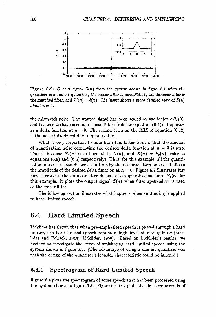
100 CHAPTER 6. DITHERING AND SMITHERING
1.2 .----r---..,.--.....----.---.,.----,----,.----,
1.0
0.8
,.... 0.6 c:
NO.4
0.2
1.StI\f O.S~.y
-0.5 '--------' -4 -2 0 2 4
0.0 !----........ ".. .......... III/IM-----j -0.2 '--_.L-_-'-_-"-_-'-_~ _ __L _ __'__---'
-4000 -3000 -2000 -1000 0 1000 2000 3000 4000 n
Figure 6.2: Output signal Z( n) from the system shown in figure 6.1 when the quantizer is a one--bit quantizer, the smear filter is ap4096d_v1, the desmear Dlter is the matched filter, and Wen) = D(n). The insert shows a more detailed view of Zen) about n = O.
the mismatch noise. The wanted signal has been scaled by the factor aRs (0), and because we have used non-causal filters (refer to equation (6.4)), it appears as a delta function at n = O. The second term on the RHS of equation (6.12) is the noise introduced due to quantization.
What is very important to note from this latter term is that the amount of quantization noise corrupting the desired delta function at n = 0 is zero. This is because Nq(n) is orthogonal to X(n), and X(n) = hs(n) (refer to equations (6.8) and (6.6) respectively). Thus, for this example, all the quantization noise has been dispersed in time by the desmear filter; none of it affects the amplitude of the desired delta function at n = O. Figure 6.2 illustrates just how effectively the desmear filter disperses the quantization noise Nq(n) for this example. It plots the output signal Z(n) when filter ap4096d_v1 is used as the smear filter.
The following section illustrates what happens when smithering is applied to hard limited speech.
6.4 Hard Limited Speech
Licklider has shown that when pre-emphasised speech is passed through ahard limiter, the hard limited speech retains a high level of intelligibility [Licklider and Pollack, 1948; Licklider, 1950]. Based on Licklider's results, we decided to investigate the effect of smithering hard limited speech using the system . shown in figure 6.3. (The advantage of using a one bit quantizer was that the design of the quantizer's transfer characteristic could be ignored.)
6.4.1 Spectrogram of Hard Limited Speech
Figure 6.4 plots the spectrogram of some speech that has been processed using the system shown in figure 6.3. Figure 6.4 ( a) plots the first two seconds of

6.4. HARD LIMITED SPEEOH 101
Pre-emphasis Hard hs (n) filter limiter hd(n)
W(n) 1----001 ~ X(n) Z(n)
Figure 6.3: System used to investigate the effects of smithering on hard limited speech
the input waveform W(n)j figure 6.4 (b) plots the output signal Z(n) when the smear and desmear filters are absent; and figures 6.4 (c) and (d) plot the spectrograms of Z(n) when an all-pass smear/desmear filter and a non-flat smear / desmear filter are used respectively. Each of these spectrograms will now be considered in more detail.
Figure 6.4 (a) plots the first two seconds of the input speech signal W(n). This input signal was a high quality digital recording of the sentence
Men sunlight strikes raindrops in the air, they act like a prism and form a rainbow.
It was spoken at normal speed by a male speaker, who was located in an anechoic chamber during the recording. There were two long pauses in the speech wave caused by natural breaks in the speech. The longer paused lasted for 500 ms and separated the dependent clause at the beginning of the sentence from the main clause. The other long pause lasted for 240 ms seconds and separated the main clause from the conjunction that connected the verbal phrase to the end of the sentence.
Figure 6.4 (b) shows the spectrogram of Z(n) without smithering applied; i.e., hs(n) = hd(n) = 8(n). It is evident from this figure that there are no pauses or gaps in the hard limited speech waveform sound is continuously present for the entire utterance. This is because all the input samples were hard limited, even those samples due to noise in the silent periods of the input speech wave. By comparing figure 6.4 (b) with figure 6.4 (a), traces of the wanted speech wave can be discerned; however, it is quite obvious that the signal-to-quantization noise ratio is very poor.
When listening to the signal in figure 6.4 (b), the speech sounded both very distorted and very noisy. In spite of this, however, the speech was still highly intelligible. Possibly the most objectionable aspect of the hard limited speech was the noise that occurred during the two long silent intervals of the input waveform. During these two silent intervals, the volume of the noise increased abruptly, because the input of the hard limiter was controlled by noise alone. In fact these bursts of noise were perceived to be significantly louder than the speech signal itself, presumably because of the differing spectral content of the noise and speech!. Even when the speech signal was present at the output of
1 Note that the sentences used for the subjective tests in section 6.5 did not contain any long pauses; therefore, this factor did not affect the results of these tests.

102
3000
"....,4000 N :::r: ....., 6' 3 000
c !g 2000 C"
2! IJ.. t 000
3000
,.....,.4000 N :::r: ....., >. 3 000 0 c ~ 2000 C"
2! IJ.. t 000
CHAPTER 6. DITHERING AND SMITHERING
1.0 Time (sec)
(0)
1.0 Time (sec)
(b)
Time (sec)
(C)
1.0 Time (sec)
(d)
Figure 6.4: Spectrogram of hard limited speech wave. a) First 2 seconds of input signal W( n ). b) First 2 seconds of output signal Z( n) when no smeal' filters is used. c) First 2 seconds of Z(n) when all-pass smear filter ap4096dsl is used as the smeal' filter (note the 400 ms time delay). d) First 2 seconds of Z(n) when non-Bat smear filter nf4096a...vl is used as the smear filter (note the 400 ms time delay).
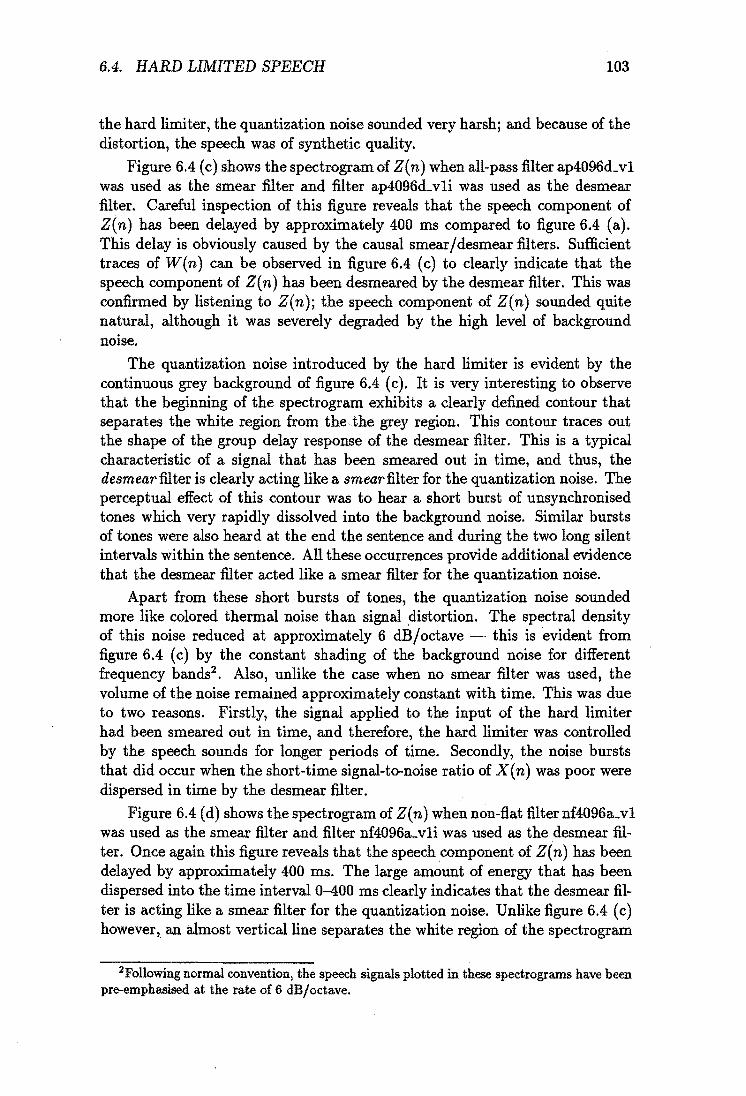
6.4. HARD LIMITED SPEECH 103
the hard limiter, the quantization noise sounded very harsh; and because of the distortion, the speech was of synthetic quality.
Figure 6.4 (c) shows the spectrogram of Z (n) when all-pass filter ap4096d_ vI was used as the smear filter and filter ap4096d_vli was used as the desmear filter. Careful inspection of this figure reveals that the speech component of Zen) has been delayed by approximately 400 ms compared to figure 6.4 (a). This delay is obviously caused by the causal smear / desmear filters. Sufficient traces of Wen) can be observed in figure 6.4 (c) to clearly indicate that the speech component of Zen) has been desmeared by the desmear filter. This was confirmed by listening to Zen); the speech component of Zen) sounded quite natural, although it was severely degraded by the high level of background noise.
The quantization noise introduced by the hard limiter is evident by the continuous grey background of figure 6.4 (c). It is very interesting to observe that the beginning of the spectrogram exhibits a clearly defined contour that separates the white region from the,the grey region. This contour traces out the shape of the group delay response of the desmear filter. This is a typical characteristic of a signal that has been smeared out in time, and thus, the desmearfilter is clearly acting like a smear filter for the quantization noise. The perceptual effect of this contour was to hear a short burst of unsynchronised tones which very rapidly dissolved into the background noise. Similar bursts of tones were also heard at the end the sentence and during the two long silent intervals within the sentence. All these occurrences provide additional evidence that the desmear filter acted like a smear filter for the quantization noise.
Apart from these short· bursts of tones, the quantization noise sounded more like colored thermal noise than signal distortion. The spectral density of this noise reduced at approximately 6 dB/octave - this is evident from figure 6.4 (c) by the constant shading of the background noise for different frequency bands2
• Also, unlike the case when no smear filter was used, the volume of the noise remained approximately constant with time. This was due to two reasons. Firstly, the signal applied to the input of the hard limiter had been smeared out in time, and therefore, the hard limiter was controlled by the speech sounds for longer periods of time. Secondly, the noise bursts that did occur when the short-time signal-to-noise ratio of X(n) was poor were dispersed in time by the desmear filter.
Figure 6.4 (d) shows the spectrogram of Zen) when non-flat filternf4096a_vl was used as the smear filter and filter nf4096a_ vli was used as the desmear filter. Once again this figure reveals that the speech component of Z (n) has been delayed by approximately 400 ms. The large amount of energy that has been dispersed into the time interval 0-400 ms clearly indicates that the desmear filter is acting like a smear filter for the quantization noise. Unlike figure 6.4 (c) however, an almost vertical line separates the white region of the spectrogram
2Following normal convention, the speech signals plotted in these spectrograms have been pre-emphasised at the rate of 6 dB/octave.

104 CHAPTER 6. DITHERING AND SMITHERING
from the shaded region at the very beginning of the utterance. (This is a typical characteristic of non-flat smear filters.) Thus, the short burst of tones heard when listening to figure 6.4 (c) were not present when listening to figure 6.4 (d). Apart from this exception, the other comments made about figure 6.4 (c) also apply to figure 6.4 (d).
The most important conclusion to draw from the above discussion is that the desmear has a very different effect on two signal components at the output of the hard limiter: The desmear filter desmears the speech component (as desired) but smears out the noise component.
6.4.2 SNR of Hard Limited Speech
Section 8.4 describes how smear / desmear filters can sometimes improve the signal-to-quantization-noise ratio (SNR) of a signal. In particular, table 8.1 shows that if the input signal applied to a hard limiter has a Gamma pdf, smear filtering can improve the SNR by approximately 5.5 dB.
To verify this theoretical result, we computed signal to uncorrelated noise ratio ([Jayant and Noll, 1984]) of the hard-limited speech waveforms shown in figure 6.4 (and for two additional smear filters that will be used in the next section). The following results were obtained:
Smear filter SNR Improvement None -0.9 dB o dB ap256d_v1 1.0 dB 1.9 dB ap1024d_v1 1.7 dB 2.6 dB ap4096d_v1 1.8 dB 2.7 dB nf4096a_vl 1.8 dB 2.7 dB
Thus smearing out the speech prior to hard limiting has improved the long-time SNR by as much as 2.7 dB.
Even though the long-time SNR of the speech has been improved, this improvement could be due to the reduced noise power during the silent intervals, and the short-time SNR of the hard limited speech wave may not be improved at all. To check this we computed the short-time SNR of the hard limited speech for three smear filter treatments: No smear filter, ap4096d_v1, and nf4096&-vI. Once again the signal-to-uncorrelated-noise ratio was used as the definition for the short-time SNR. The results of this investigation are recorded in figure 6.5. Clearly, the short-time SNR has been improved by the smear / desmear filters.
Although these results indicate an improvement in the SNR when smear filters are used, they must be interpreted with caution. Simple SNR measures, like the ones used above, do not always align with subjective measures of speech quality. Therefore, the following section presents the results of some subjective speech tests which validate the use of smithering.

6.5. SUBJECTIVE TESTS 105
15~----------~~------------~------------r-----------~ none
---------. ap4096cLv1
................... nf4096~vl
" E 1=
l o
Figure 6.5: Short-time SNR of hard-limited speech. (The curve labelled "none" records the short-time SNR when no smear filters are applied.)
6.5 Subjective Tests
Two speech tests were carried out to determine the effect of smithering on hard-limited speech: a preference test and an intelligibility test. The objective of the preference test was to prove that listeners prefer to listen to smithered hard limited speech than to straight hard limited speech. The objective of the intelligibility test was to determine whether the addition of smithering affects the intelligibility of the hard limited speech wave. Both these tests followed the procedures used by Rabiner and Johnson when investigating the perceptual effects of dither on the speech waveform [Rabiner and Johnson, 1972].
One of the first things that had to be decided when designing this experiment was which smear filters to use for smithering. The following five smear filter treatments were selected. (These smear filter treatments will be indexed by the number assigned to each filter in the list below):
Index Smear Filter Desmear Filter 1 No smear filter No desmear filter 2 ap256d_v1 ap256d .. vli 3 aplO24d .. v1 ap1024d .. vli 4 ap4096d .. v1 ap4096d..vli 5 nf4096a..v1 nf4096a .. vii
It was hoped that this selection of smear filters would enable us to draw conclusions about the following issues:
• The effectiveness of smithering at improving the subjective quality of hard-limited speech.
• The effect of varying the length of the smear/desmear filters on the subjective quality of the speech.
• The relative merits of all-pass versus non-fiat smear filters.

106 CHAPTER 6. DITHERING AND SMITHERING
Day Date Type of Test Performed
Day 0 11/9/91 Training session for intelligibility tests
Day 1 19/9/91 Preference test (Male speaker) Intelligibility test (100 words)
Day 2 20/9/91 Preference test (Female Speaker) Intelligibility test (100 words)
Table 6.1: Summary of tests carried out on days 0, 1, and 2 of the experiment.
The speech tests themselves were spread over three separate days, and each day's test took approximately one hour to perform. A summary of the experiments conducted on each day is given in table 6.1. Additional information about these tests is given below and also in appendix C.
6.5.1 Preference Tests
Two preference tests were carried out during the course of the experiments: The first preference test was carried out on day 1 of the experiment and involved a male speaker; the second preference test was carried out on day 2 of the experiment and involved a female speaker.
Below we describe the procedure for the preference test, but omit those details that are contained in appendix C.
6.5.1.1 Preference Test Procedure
The stimuli for the preference tests were the set of five sentences listed in table 6.2. Good quality digital recordings of these five sentences were obtained for the male speaker and the female speaker using the recording technique described in appendix C.
Having obtained the digital recordings, a computer simulation of the system shown in figure 6.3 was then used to process the speech. This processed speech was subsequently recorded onto an audio tape in preparation for the actual test.
As there were five smear filter treatments to compare, a complete preference test involved comparing 25 pairs of sentences. The stimuli used for each sentence pair was selected using the following criteria:
.. The same stimuli was used for the first and second sentence of each sentence pair .
.. Only male speech was used on day 1, and only female speech was used on day 2.

6.5. SUBJECTIVE TESTS 107
1. Walking's my favourite exercise.
2. Here's a nice quiet place to rest.
3. Our Janitor sweeps the floor every night.
4. Open your windows before you go to bed.
5. Do you think she should stay out so late?
Table 6.2: Sentences used in the preference tests.
• Each sentence was used exactly five times during a single preference tests.
Apart from these cOnstraints, the remainder of the experimental design was completely random.
After processing the speech on computer, the test material for each days test was recorded onto an audio tape; this tape was subsequently used to play back the test material to the listening subjects.
Twelve listening subjects participated in the experiment. Each subject was given both written and verbal instructions on how to respond to the test material. The written instructions were:
In this test you will be listening to pairs of sentences. Each of the two sentences (first called 1, second called 2) was processed by some type of speech transmission system. After you hear both sentences, there is a five second interval during which time you are to decide which sentence you prefer and record the result on your answer sheet. H you:
• prefer the first sentence circle 1
• prefer the second sentence circle 2
You must choose either 1 or 2 - even if you have no preference.
6.5.1.2 Results of Preference Test
For each listening subject, a matrix of preferences was determined from their score sheet in which a 1 in a particular cell of the matrix indicated that the first sentence was preferred to the second sentence, and a zero indicated the reverse condition. Each element of these matrices was a binary-valued random variable and was denoted by Blish where subscript i indicates the smear filter treatment applied to the first sentence (i = 1, 2, ... 5), j indicates the smear filter treatment applied to the second sentence (j = 1,2 ... 5), s indicates the speaker (1 =male, 2 =female), and I indicates the listener (l = 1,2 ... 12).
Table 6.3 (a) shows the matrix obtained by summing the individual matrices for all the listening subjects with s = 1 (i.e., for the male speaker). The

108 CHAPTER 6. DITHERING AND SMITHERING
1
1 2
i 3
4
5
1 2 3 4 5
7 3 1 1 0
8 7 3 3 0
12 12 5 7 4
12 5 6 7 4
11 8 8 4 6
(a)
1
1 2
i 3
4
5
1 2 3 4 5
7 8 1 1 1
10 8 3 4 1
11 11 9 4 9
12 8 10 7 4
10 12 10 7 6
(b)
Table 6.3: Results of preference test. a) Male speaker results Bij1. (Test carried out on day 1 of the experiment ). b) Female speaker results Bij2. (Test carried out on day 2 of the experiment).
elements of this matrix are denoted by Bij1., where the dot notation implies summation over the subscript it replaces; i.e.,
12
B i j1. = L Bijll (6.13) 1=1
Similarly, table 6.3 (b) shows the matrix for Bij2 ..
As there were twelve listening subjects, the highest score that could be assigned to a single cell in table 6.3 is 12 - indicating a very strong preference for the first sentence over the second. The lowest score that could be assigned to a single cell is 0 - indicating a very strong preference for the second sentence over the first sentence. The very high scores of some cells below the main diagonal of these matrices, and the very low scores above the main diagonal suggest that strong preferences are indicated by the data.
A careful inspection of this matrix reveals that the dominant factor influencing the outcome of these two tests is the smear filter treatment. For example, the very high scores for B 31s. B411M and B 51s• (s = 1, 2) indicate that speech treated with filters 3, 4, or 5 is strongly preferred to speech that is treated with filter 1. Evidence to support this conclusion found in the very low scores for B 13s., B 14s. and B 15s., which show that when the order of presentation is reversed, the listening subjects still showed the same strong preference for filters 3, 4, and 5. Finally, because the values for these six random variables indicate almost unanimous agreement between the listeners, we conclude that the listener factor only had a minor influence on the outcome of these results.
Although the raw data summarised in table 6.3 clearly indicates strong preferences, it was rather difficult to analyse in this form. Therefore, to facilitate the statistical analysis, a new random variable was defined as
0=1
0=2 (6.14)

6.5. SUBJECTNE TESTS 109
In this equation, subscript mn (mn E [51,52,53,54,41,42,43,31,32,21]) specifies the two filters that were compared in a single pair-wise comparison test but does not provide any information on the order in which the filter treatments were presented; these ten treatments will be collectively referred to as the comparison factor. 0 specifies the order in which the two filter treatments were presented to the listening subjects (1 = m heard first; 2 = n heard first) and will be referred to as the order factor. As before, subscript 8 specifies the treatment applied to the speaker factor (l=male, 2-female). Thus, C(mn)os records the number of listeners who voted for filter m in a single pair-wise comparison and has a value in the range [0,1, ... 12]. A value greater than six indicates that filter m was preferred to filter n.
Because the order factor did not make any sense when the same filter treatment was applied to both sentences, the data along the diagonals of the matrices in table 6.3 was discarded. This is why [11,22,33,44,55] ¢ mn. This will result in some loss of information regarding the order factor. However, it should not cause any loss in information regarding the relative merits of different filter treatments, because, as will be shown, there was no significant interaction between the order factor and the comparison factor.
Note that the above random variable also sums over the listeners and therefore, the listener factor was ignored during the analysis. The reason for summing over the listeners was to make the pdf of C(mn)os approximately Gaussian (as required for an analysis of variance). Also, the raw data itself suggested that the listener factor was not a particularly important factor. For example, seven of the fifty cells in table 6.3 have scores of either zero or twelve indicating unanimous agreement between the listeners. Another nine of these cells have scores of either one or eleven, indicating that exactly one listener disagreed with the remaining eleven listeners. These Dine dissenting opinions were due to six different listeners.
Table 6.4 summarises the results of 'an analysis of variance on these 10 x 2 x 2 = 40 data points obtained for C(mn)os' This analysis clearly indicates that the comparison factor is significant at the 0.98 significance level, but fails to reject the null hypothesis for the other factors.
Table 6.5 ranks the ten treatments of the comparison factor according to their mean preference score, defined as
_ 1 2 2
C(mn) .. = "4 L: L: C(mn)so 8=20=1
A score of greater than six in table 6.5 indicates filter m is preferred to filter n. Listed in the right hand column of table 6.5 is the probability
P (C(mn) .. 2:: Mean)
computed under the null hypothesis that no preference existed and the listening subjects simply tossed an unbiased coin when filling in their score sheet. These probabilities were very easy to compute, because under this hypothesis the

110 CHAPTER 6. DITHERING AND SMITHERING
Factor Deg. Freedom Sum of Squares Mean Square F Value Pr> F
Comparison 9 139.125 15.458 4.09 0.0192
Order 1 2.025 2.025 0.54 0.4807
Speaker 1 0.625 0.625 0.17 0.6927
Comparison x Speaker 9 23.125 2.569 0.68 0.7128
Comparison x Order 9 39.725 4.414 1.17 0.4028
Error 10 37.75 3.775
Table 6.4: Results of analysis of variance test on the forty data points C(mn)os'
These results were obtained using the Anova procedure of SAS [SAS, 1989}.
Comparison Mean P(G(mn) .. ~ Mean)
G(41) .. 11.50 > 0.0001
G(Sl) .. 11.25 > 0.0001
G(51) .. 11.00 > 0.0001
G(52) .. 10.75 > 0.0001
G(S2) .. 10.25 > 0.0001
C(21) .. 7.75 0.052
G(42) .. 7.50 0.085
C(43) .. 7.25 0.130
C(53) .. 7.25 0.130
C(54) .. 6.75 0.266
Table 6.5: Ranking of averaged preference scores for the ten treatments of the comparison factor.
pdf of C(mn) .. can be accurately approximated by a Gaussian distribution with mean equal to six and variance equal to one3 •
One thing to note from table 6.5 is that the results are logically consistent. For example, C(43) .. = 7.25, indicating that filter 4 was preferred slightly tofilter 3 when these two filters were compared. Similarly, C(32) .. = 10.25, indicating that filter 3 was preferred to filter 2 when these two filters were compared. Logically, therefore, we would expect filter 4 to be preferred to filter 2 when these two filters were compared; this is indeed the case - C(mn) .. = 7.5. Although this value is not as high as one might expect, it still indicates that filter 4 is preferred to filter 2. All other logical tests of this nature also tum out to be true.
SWhen computing the values for these probabilities, corrections were made for the continuity of the Gaussian Distribution. For example, p(C(mn) .. > 6.75) was computed as
1 roo -:c3 /2d -::;:;; JO.625 e :t:.
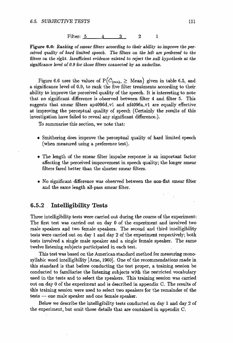
6.5. SUBJECTNE TESTS 111
Filter: ....::5'--_--=4 __ ....;3=__ 2 1
Figure 6.6: Ranking of smear filters according to their ability to improve the perceived quality of hard limited speech. The filters on the left are preferred to the filters on the right. Insufficient evidence existed to reject the null hypothesis at the significance level of 0.9 for those filters connected by an underline.
Figure 6.6 uses the values of P (G(mn) .. ;::: Mean) given in table 6.5, and a significance level of 0.9, to rank the five filter treatments according to their ability to improve the perceived quality of the speech. It is interesting to note that no significant difference is observed between filter 4 and filter 5. This suggests that smear filters ap4096d_vl and nf4096a-vl are equally effective at improving the perceptual quality of speech (Certainly the results of this investigation have failed to reveal any significant difference.).
To summarise this section, we note that:
• Smithering does improve the perceptual quality of hard limited speech (when measured using a preference test).
• The length of the smear filter impulse response is an important factor affecting the perceived improvement in speech quality; the longer smear filters fared better than the shorter smear filters.
• No significant difference was observed between the non-flat smear filter and the same length all-pass smear filter.
6.5.2 Intelligibility Tests
Three intelligibility tests were carried out during the course of the experiment: The first test was carried out on day 0 of the experiment and involved two male speakers and two female speakers. The second and third intelligibility tests were carried out on day 1 and day 2 of the experiment respectively; both tests involved a single male speaker and a single female speaker. The same twelve listening subjects participated in each test.
This test was based on the American standard method for measuring monosyllabic word intelligibility [Ame, 1960]. One of the recommendations made in this standard is that before conducting the test proper, a training session be conducted to familiarise the listening subjects with the restricted vocabulary used in the tests and to select the speakers. This training session was carried out on day 0 of the experiment and is described in appendix C. The results of this training session were used to select two speakers for the remainder of the tests - one male speaker and one female speaker.
Below we describe the intelligibility tests conducted on day 1 and day 2 of the experiment, but omit those details that are contained in appendix C.

112 CHAPTER 6. DITHERING AND SMITHERING
6.5.2.1 Intelligibility Test Procedure
The stimuli used for the intelligibility tests conducted on days 1 and 2 of the experiment were the set of 200 key-words listed in PB lists 5, 7, 8, and 12 of [Ame, 1960]. Each key-word was spoken in the carrier sentence
Would you write (key-word) now
Digital recordings of these sentences were obtained for both the male speaker and the female speaker using the recording technique described in appendix C. All the recordings were screened to ensure correct pronunciation of all the keywords; any word that was mis-pronounced was re-recorded.
These sentences were then processed on computer using a similar procedure to that described for the preference tests. The stimuli used for each days test was selected using the following criteria:
• Words were drawn from PB lists 7 and 8 for day 1 of the experiment and from PB lists 5 and 12 for day 2.
• A complete PB list was processed before using the words from a second list.
• The sequence of key words-presented to the listening subjects was split in blocks of size ten. Within each block, each combination of speaker x filter was heard exactly once.
Apart from these constraints, the remainder of the design was completely random.
Twelve listening subjects participated in the experiment, and each subject was given both verbal and written instructions on how to respond to the test material. The written instructions were:
In this test you will be listening to sentences of the form:
"Would you write (key word) now"
where (key word) has been replaced by a substitute word. For each sentence print the keyword, and only the key word, on your answer sheet. Remain synchronised with the tape, even if you have to skip entries on the score sheet. You will be required to identify approximately 15 key words per minute.
While running the experiment on day 1, an interruption caused one of the key-words to be repeated. The result recorded on the score sheets for this key-word was the response to the repeated sentence, not the initial sentence. Therefore, these twelve data points had to be discarded during the analysis. (These data points should have contributed to the intelligibility scores computed for the female speaker and filter 5 on day 1 of the experiment.)

6.5. SUBJECTNE TESTS 113
After completing the tests, the test subjects marked their own intelligibility score sheet. An answer was marked correct if and only if the answer recorded on the score sheet sounded identical to the correct answer (thus homophones and mis-spelt words were marked correct). All other words were marked as incorrect. Several of the score sheets were subsequently selected at random and checked for correct scoring. In all cases, the test sheets had been correctly marked.
The results of the intelligibility test were then entered into a computer by scoring a correct answer as 1 and an incorrect answer as O. Intelligibility scores were then computed for each combination of listener, filter, speaker, and repetition, giving a total of 12 x 5 x 2 x 2 = 240 data points. Each intelligibility score was obtained by averaging over ten outcomes of the experiment, with the exception that the data points for the female speaker and filter 5 on day 1 of the experiment which was averaged over only nine outcomes. (The effect of averaging over nine outcomes instead of ten will increase the variance of these latter twelve data points by the factor 10/9 compared to the other data points. This relatively minor affect was ignored during the analysis.)
6.5.2.2 Results and Analysis
The results of the intelligibility test are summarised in figure 6.7. Figure 6.7 (a) plots the intelligibility scores for the male and female speakers obtained by averaging over the twelve listeners. The dashed curves show the results obtained on day 1 of the experiment and the solid curves show the results for day 2. Figure 6.7 (b) plots the same data averaged over more factors: the solid curves have been averaged over listeners and repetitions; the dashed curve has been averaged over listeners, repetitions, and speakers.
An analysis of variance was performed on the data summarised in figure 6.7 using the SAS statistical analysis package [SAS, 1989]. The four factors used in the analysis (and the number oflevels of each factor) were:
1. Filter (5 levels)
2. Speaker (2 levels)
3. Listener (12 levels)
4. Repetition (2 levels)
The results of this analysis are recorded in table 6.6. This table shows that all the factors listed above had a significance level exceeding 0.995 and also indicates some very strong interaction between the factors. The most significant factor was the speaker, indicating that the hard limited speech from one of the speakers was more intelligible than the other. This result is clearly evident from figure 6.7 (b) which shows that the male speaker scored consistently higher than the female speaker.

114
0.9
0.8
! 0.7 o . M 0.6
0.5
CHAPTER 6. DITHERING AND SMITHERING
Intelli ibilit Scores Avera ad Over Listeners
- - II -
~Dayl.M
II Day 1. F
- - ~ - - Day 2. M
0.4 .k::=-_I---~~:::::::::==:!:==~ - - II - - Day2. F
0.9
0.8
! 0.7 o M 0.6
0.5
1 2 3
Filter
(a)
4 5
Scores Avera ad Over Listeners and Re etitions
)t------. -fl-II-F
- - 111- - Av'
OA~------~------~------~------~ 1 2 3
FIlter
4 5
(b)
Figure 6.1: Summary of intelligibility test results obtained on day 1 and day 2 of the experiment. a) Intelligibility scores averaged over listeners. The solid curves are the results for the male and female speaker on day 1 of the experiment; the dashed curves are the results for the male and female speaker for day 2 of the experiment. b) Solid curves are the intelligibility scores obtained by averaging over listeners and repetitions; the dashed curve is the intelligibility score obtained by averaging over listeners, repetitions, and speakers.

6.5. SUBJECTNE TESTS 115
Factor Deg. Freedom Sum of Squares Mean Square F Value Pr > F
Speaker 1 1.407 1.40726 95.81 0.0001
Repetition 1 0.885 0.88547 60.29 0.0001
Filter 4 0.999 0.24974 17.00 0.0001
Listener 11 0.445 0.04045 2.75 0.0029
Repetition X Speaker 1 0.415 0.41482 28.24 0.0001
SpeakerxFilter 4 0.446 0.11159 7.60 0.0001
Repetition x Filter 4 0.093 0.02320 1.58 0.1830
Listener x Filter 44 0.796 0.01810 1.23 0.1807
Repetition x Listener 11 0.128 0.01166 0.79 0.6459
Listener X Speaker 11 0.046 0.00420 0.29 0.9876
Rep x Speakx Filt 4 0.249 0.06218 4.23 0.0029
Error 143 2.100 0.01468742
Table 6.6: Results of analysis of variance test for the intelligibility data. These results were obtained using the Anova procedure of SAS.
The next most significant factors were repetition and repetition x speaker, indicating a fairly large amount of learning between repetitions and some interaction effect between repetition and speaker. Comparing the solid and dashed curves in figure 6.7 (a), it is evident that some learning did occur between day 1 and day 2 of the experiment. The strong interaction between repetition and speaker is obviously caused by the comparatively poor intelligibility scores obtained on day 1 of the experiment for the female speaker when filters 4 and 5 were used to smither the speech. These two data points are a bit of an anomaly, because all the other data points for these two filters (including those for the female speaker on day 2) showed a large improvement in the intelligibility scores when compared to filter 1.
The next most significant factors, both with a significance level exceeding 0.999, were the filter and the filterxspea.ker interaction. This indicates that the smear filter treatment was an important factor affecting the intelligibility of the speech; although once again, the anomalous data points obtained for the female speaker on day 1 of the experiment using filters 4 and 5 have caused significant filter-speaker interaction.
Figure 6.8 ranks the smear filters according to their mean intelligibility scores obtained by averaging over listener, speaker, and repetition. To determine which of these means were significantly different, Duncan's multiple range test [SAS, 1989; Duncan, 1955; Hines and Montgomery, 1980] and the
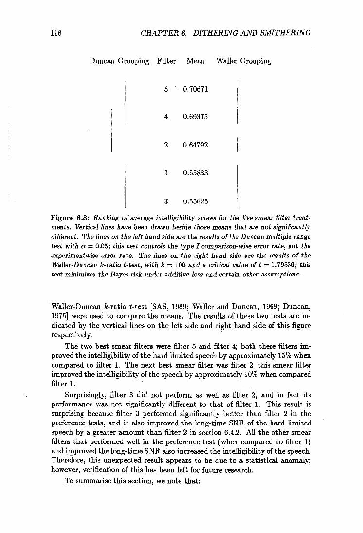
116 CHAPTER 6. DITHERING AND SMITHERING
Duncan Grouping Filter Mean Waller Grouping
5 ' 0.70671
4 0.69375
2 0.64792
1 0.55833
3 0.55625
Figure 6.8: Ranking of average intelligibility scores for the five smear filter treatments. Vertical lines have been drawn beside those means that are not significantly different. The lines on the left hand side are the results of the Duncan multiple range test with a = 0.05; this test controls the type I comparison-wise error rate, not the experimentwise error rate. The lines on the right hand side are the results of the Waller-Duncan k-ratio t-test, with k = 100 and a critical value oft = 1.79536; this test minimizes the Bayes risk under additive loss and certain other assumptions.
Waller-Duncan k-ratio t-test [SAS, 1989; Waller and Duncan, 1969; Duncan, 1975] were used to compare the means. The results of these two tests are indicated by the vertical lines on the left side and right hand side of this figure respectively.
The two best smear filters were filter 5 and filter 4; both these filters improved the intelligibility of the hard limited speech by approximately 15% when compared to filter 1. The next best smear filter was filter 2; this smear filter improved the intelligibility of the speech by approximately 10% when compared filter 1.
Surprisingly, filter 3 did not perform as well as filter 2, and in fact its performance was not significantly different to that of filter 1. This result is surprising because filter 3 performed significantly better than filter 2 in the preference tests, and it also improved the long-time SNR of the hard limited speech by a greater amount than filter 2 in section 6.4.2. All the other smear filters that performed well in the preference test (when compared to filter 1) and improved the long-time SNR also increased the intelligibility of the speech. Therefore, this unexpected result appears to be due to a statistical anomaly; however, verification of this has been left for future research.
To summarise this section, we note that:
6.6. CONCLUSIONS 117
II Smithering can improve the intelligibility of hard-limited speech. This improvement is obviously due to the improved signal-to-noise ratio of the smithered speech (refer to section 6.4).
II The length of the smear filter does appear to be an important factor affecting the increased intelligibility of the smithered However, the results failed to show a linear relationship between smear filter length and improved intelligibility. (This is probably because of a statistical anomaly.)
II No significant difference was observed between the non-flat smear filter and the same length all-pass smear filter.
6.6 Conclusions
This chapter described a new technique for destroying the dependence between a signal and its quantization noise. By smearing out a signal before applying it to a quantizer and subsequently desmearing the signal after it has been quantized, it is possible to destroy the dependence between the wanted signal and the desmeared quantization noise.
Objective and subjective results were obtained to validate this technique. The objective results demonstrated that the desmear filter does indeed act like a smear filter for the quantization noise. These results also showed that smithering improves the SNR of hard limited speech by 2.7 dB when 409B-tap smear / desmear filters are used.
The subjective tests demonstrated that smithering improves both the perceptual quality and the intelligibility of hard limited speech. The improvement in perceptual quality occurred because the dependence between the speech signal and its quantization noise was destroyed by the desmear filter and also because the SNR of the hard limited speech was improved. The improvement in intelligibility occurred because of the improved SNR. When using 4096-tap smear filters, the intelligibility of the hard limited speech was improved by 15% (when compared to unsmithered speech).
To conclude this chapter, we list the significant differences between smithering and dithering:
II Smithering uses smear / desmear filters to destroy the dependence of the quantization noise and the wanted signal; dithering uses a dither signal.
4;\ Smithering introduces a time delay; dithering is instantaneous.
• Smithering does not require any signal to be subtracted from the quantized signal when it is being reconstructed; dithering requires that the dither signal be subtracted from the dithered signal before it is reconstructed (although this can be neglected if a slight reduction in signal-tonoise ratio can betolerated).

118 CHAPTER 6. DITHERING AND SMITHERING
• Smithering can improve the intelligibility of speech for coarse quantizersj dithering degrades the intelligibility of speech· for coarse quantizers.
Chapter 7
Smear Coding
7.1 Introduction
This chapter describes and validates a new technique for reliably transmitting data over a noisy power-limited channel. The technique combines smear / desmear filtering with a non-linear modulation system (also called a twisted modulation system [Wozencraft and Jacobs, 1965]) to protect data from bit errors during transmission. Because this technique pedorms a similar function to channel coding, it is called "smear coding": the prefix "smear" distinguishes smear codes from block codes, convolutional codes, and trellis codes; and also indicates that smear / desmear filters are an integral part of the coding scheme.
7.2 Motivation
Figure 7.1 shows how smear/desmear filters can be combined with a non-linear modulation system to provide reliable data communication over a noisy channel. The input signal applied to the smear filter is assumed to be a sequence of antipodal voltage samples whose polarity is determined by the information being transmitted. This input signal is passed through the smear filter and then applied to the input of the non-linear modulator. The non-linear modulator maps the modulation signal onto the transmitted signal using a non-linear mapping function. The transmitted signal is then transmitted over the noisy channel and received by the non-linear demodulator. This demodulator performs the inverse operation to the modulator and maps the received signal onto the demodulated signal. The demodulated signal is then passed through the de smear filter and applied to the threshold detector. This detector estimates the polarity of the original antipodal input signal and produces the received data signal.
By using a non-linear modulation system (rather than a linear modulation system), it is possible to improve the signal-to-noise ratio of the demodulated signal without increasing the transmitter power [Shannon, 1949;
119

120 X2 CHAPTER 7. SMEAR CODING
Smear
,.; Non-Lin . .....
..... Mod .
?+ Desmear
n(t)
Thresh. ..... Non-Lin. - foot-- ..... foot--Det. ..., Demod .
Figure 7.1: Block diagram of a data transmission system illustrating the principle of smear coding.
Wozencraft and Jacobs, 1965]. Examples of such non-linear modulation systems include pulse position modulation, pulse code modulation, and frequency modulation. (Obviously, if frequency modulation was used in the figure 7.1 additional components besides the FM modulator would have to be included in the non-linear modulator block. These additional components would map the discrete-time samples at the output of the smear filter onto an analog waveform that could be applied to the FM modulator. Similar comments apply to the demodulator block.)
The fundamental idea of smear coding is to use the non-linear modulation system to improve the demodulated signal-to-noise ratio so as to reduce the number of errors made by the threshold detector.
A problem however, is that all non-linear modulation systems exhibit a threshold effect. As the received SNR approaches the threshold level, impulse noise spikes will appear at the demodulator output. Thus even though the signal-to-noise ratio might be quite high at the demodulator output, the demodulated noise will contain noise spikes (especially when the threshold effect comes in to play). Without the desmear filter, these noise spikes would cause bit errors. With the desmear filter connected however, the noise spikes will be smeared out in time. This will enable the demodulator to operate somewhere slightly below its threshold level without causing bit errors at the output of the threshold detector.
The objective of this current chapter is to validate the above argument. We want to show that smear filters can be combined with a non-linear modulation system (as described above) to provide reliable data communication over a noisy power limited channel. The objective of this chapter is not to design a near-optimal smear code. All we want to do is validate this coding scheme.
. To do this we will use a pulse code modulator for the modulator shown in figure 7.1. The advantage of pulse code modulation is that it is simple to understand, it remains tractable during analysis, and it is easy to simulate on

7.3. THE BINARY POM SMEAR OODE 121
computer. However, it will be shown that these benefits are obtained at the expense of performance - PCM is sub-optimal in many respects.
7.3 The Binary PCM Smear Code
This section describes the data transmission system that will be analysed in the remainder of this chapter. We have called this system a binary PCM smear code. The term binary is used because the input bits are represented as antipodal voltage samples at the input of the smear filter. The term PCM is used because a PCM modulation system is used for the non-linear modulator shown in figure 7.1.
7.3.1 Description
Figure 7.2 shows the block diagram of the binary PCM smear code. Specifically, figure 7.2 (a) shows the entire digital transmission system from the source to the sink, and figure 7.2 (b) shows an exploded view of the PCM modulator (or waveform encoder as it is labelled in this figure).
We will assume that the source shown in figure 7.2 (a) is a discrete memoryless source that randomly generates binary digits at the rate of 1 bit/sec. The binary digit generated by the source at time t = k is denoted by Xl (k). Xl (k) assumes the value 0 when binary digit 0 is generated, and 1 when binary digit 1 is generated.
Encoder E1 maps XI(k) onto a two-level (binary) voltage sample X2(k):
If X}(k) = 0
If XI(k) = 1 (7.1)
As the source is memoryless and generates its binary symbols with equal probability, the power spectral density of X2(k) is white, and
P(X2(k) = A) - P(X2(k) = -A) E[X2(k)] - 0
O't - A2
0.5 (7.2)
(7.3)
(7.4)
where E[.] is the expectation operator, and O'.kz is the variance of X2(k). A sample function of X2(k) is plotted in figure 7.3 (a).
The output of encoder E1 (X2(k)) is then passed through the smear filter to produce X3(k). The smearing action of the filter causes the pdf of X3(k) to approach a Gaussian distribution, and because the smear filter is all pass with unity gain
Var [X3(k)] = Var [X2(k)] = O'iz A sample function of X3(k) is plotted in figure 7.3 (b).
(7.5)

122
Xa
CHAPTER 7. SMEAR CODING
Channel Encoder r-----------------, Smear
I X2 Xa lWaveforlI
I Xli Encoder ,..,
Source ,.., I I El ,.., Encoder I n bils/.
1 bii/s I I
~-----------------~
piscrete Channe
Channel Decoder r--------------------, I Desmear I I
Y2 trhreshold Ya Y4 lWaveforn I
Yl 1 Decoder ,.., Sink ~ f+- f+- ,.., f+- ~
D1 Detector - Decoder I I I L ____________________ ~
( a)
Waveform Encoder r---------------------,
Code Word enerato I
I I L _____________________ ~
(b)
Discrete
Channel
Figure 7.2: Block diagram of a digital transmission system using a binary PCM smear code. a) Generic block diagram of digital smear code. b) Exploded view of the binary PCM smear code waveform encoder.

7.3. THE BINARY PCM SMEAR CODE 123
X2 2 4r----,----~----~----~--~
3
.. ." :s ;!;l 0 ... ~
-1
2 . .
':r ~~~¥.~f~i~~~!¥~~~~~\ -3
-2 0 200 400 600 800 1000
-4 0 200 400 600 800 1000
11me TIme
(0) (b)
Xs Y4 <I- 4 3 3
2
-2 -2 -3 -3 -<I-
a 200 400 600 800 1000 -4
0 200 400 600 800 1000 TIme TIme
(C) (d)
Y4 - Xe Y,3 <I- 2 3 2
'" ." .g 1 ~i~~~:;~1\*·;~::.;.lf·i~~·~~1i:~~.¥tf:,·~t?~?~1~:<~;~~lf:~~:.¢.
:s ;t< 0 Q.
::s ~ 0
~-1 -2 -3
~ -1 :::~:~;~t:~::~~:i.~f,:;.:~Y~~i·~://':;~;:,?,);(I;[.·~i!.;.~;,'.t:;~f· -<I-
0 200 400 600 800 1000 -2
1000 0 200 400 600 BOO lime TIme
(e) (f)
Y2 Y2 - X2 2 2
'" ... :::1
;!;l 0 ... .. ... :::1
;!;l a ... ~ ~
-1 -1
-2 -2 0 200 400 600 BOO 1000 0 200 400 600 BOO 1000
TIme lime
(g) (h)
Figure 7.3: The signal at various points along the transmission system shown in figure 7.2. Each sample is represented by a dot.

124 CHAPTER 7. SMEAR CODING
X3(k) is then passed through the pre-amplifier to produce X4(k) (refer to figure 7.2 (b)). The gain of this pre-amplifier is adjusted to make the variance of X4(k) equal to unity.
The output of the pre-amplifier X4(k) is then passed through the instantaneous Q-level quantizer to produce Xs(k). The transfer characteristic of this quantizer minimises the quantization noise power when the input signal (X4(k)) has unit variance and Gaussian pdf . Such a quantizer is called a Max quantizer [Max, 1960; Jayant and Noll, 1984]. The quantizer's threshold levels are denoted by {Uj : Ui-l < Ui, i = 0,1, ... Q}, and these levels form a partition on X4(k). The quantizer's reconstruction levels are denoted by {Vi, i = 1,2, ... Q}; reconstruction level Vi occurs when X4(k) lies within the interval (Ui-l,Ui).
The process of quantization introduces noise into the digital transmission system. H this quantization is too coarse (i.e. Q is too small), the quantization noise produces decoding errors, and hence, this imposes a lower bound on the value for Q. H, on the other hand, the quantization is too fine (i.e. Q is too large), the channel noise increases causing an increase in the rate of decoding errors. (When Q increases, the channel signalling rate must also increase and hence this reduces the energy per channel bit). To reduce the probability of a decoding error to an acceptably low value, Q was chosen to equal 16. For this value of Q, the probability of a decoding error over a noiseless channel is 9 x 10-25 • H Q was chosen equal to 8, the probability of a decoding error due to quantization noise alone increases to 6 x 10⁻⁸ , and this was considered to be an unacceptably high BER. (These BER figures were computed by assuming that the desmeared quantization noise had a Gaussian pdf and ignored the effect of mismatch noise.) Table 7.11ists the values for Uj and Vi when Q = 16.
The quantized signal X5(k) is then passed through the post amplifier to produce X6(k). The post-amplifier adjusts the overall gain of the digital transmission system to unity. The gain factor 1/0. is included in the post-amplifier because a gain plus additive noise model is used to model the quantizer (refer to appendix D). The Q discrete voltage levels that X6(k) can assume are denoted by {WI, W2, ••• wQ} and are related to the reconstruction levels of the normalised quantizer by
(7.6)
A sample function of X6(k) is plotted in figure 7.3 (c).
X6(k) is then passed through the code word generator, which maps the Qary signal onto n-bit codes words using a Folded Binary Code (FBC) assignment l
[Jayant and Noll, 1984], where
n = log2Q = 4 (7.7)
The n-bit code word used to represent level Wi is denoted by C(Wi), and values for C ( Wi) are also listed in table 7.1.
IThis code assignment was selected because it is the best code assignment that I am aware of. It is better than both the normal binary code and the Gray code.

7.3. THE BINARY PCM SMEAR CODE 125
i 'Uj Vi C(Wi)
0 -00
1 -2.401 -2.733 0111
2 -1.844 -2.069 0110
3 -1.437 -1.618 0101
4 -1.099 -1.256 0100
5 -0.780 -0.942 0011
6 -0.522 -0.657 0010
7 -0.258 -0.388 0001
8 0.000 -0.128 0000
9 0.258 0.128 1000
10 0.522 0.388 1001
11 0.780 0.657 1010
12 1.099 0.942 1011
13 1.437 1.256 1100
14 1.844 1.618 1101
15 2.401 2.069 1110
16 00 2.733 1111
Table 7.1: Specifications for the waveform encoder: Ui are the threshold levels, and Vi are the reconstruction levels used in the Max quantizer; C( Wi) is the codeword assigned to level Wi = ()' ~2 Vi
The data at the output of the code word generator is then serially transmitted across the discrete channel at rate n bits/so Three discrete channel models will be used during the analysis of this smear code: The BSC channel, the Gilbert channel, and the periodic burst channel. These three discrete channel models will be described in section 7.4.
The waveform decoder performs the inverse operation to the code word generator. It maps the received code words onto the Q-ary voltage samples {WI, W2, •• • wQ}. Because of channel bit errors, the received code word sometimes differs from the transmitted code word; however, as there is no way to distinguish between correct and errored code words, all received code words are decoded and applied to the desmear filter. Thus, channel bit errors introduce impulse-type noise into the transmission system. The signal at the output of the waveform decoder is denoted by Y.t(k), and a sample function for Y.t(k) is plotted in figure 7.3 (d). The difference between Y.t(k) and Xa(k) is plotted in figure 7.3 (e). This latter figure clearly illustrates that the effect of channel bit errors is to introduce impulse-type noise into the digital transmission system.
l4(k) is then passed through the desmear filter to produce Ya(k). The desmeared signal Ya(k) provides a noisy estimate for X2(k) and consists of four

126 CHAPTER 7. SMEAR CODING
components:
• The wanted signal X2 (k).
• A noise component due to quantization noise.
• A noise component due to channel bit errors.
• A noise component due to mismatch noise.
The mismatch noise can be made negligible compared to the other noise sources by chosing smear filters with a high figure-of-merit. Therefore, this noise source will be ignored from now on. A sample function for Ya( k) is plotted in figure 7.3 (f).
In an attempt to produce a better estimate for X2(k), Ya(k) is passed through the threshold detector to produce l'2(k):
{
-A l'2(k) = A
H Ya(k) < 0
HYa(k) >0 (7.8)
The threshold detector corresponds to a maximum likelihood detector when the noise component of Ya(k) is zero mean Gaussian noise, and
A sample function for l'2(k) is plotted in figure 7.3 (g), and the difference between l'2(kj and X2(k) is plotted in figure 7.3 (h). Referring to this latter figure, it is observed that for this particular sample function all the samples were received correctly, even though some of the channel code words were received In error.
The output signal from the threshold detector l'2( k) is finally passed through decoder D1 to produce l'J.(k). Decoder D1 performs the inverse operation to encoder El. It maps the 2-level voltage samples at the output of the threshold detector onto binary digits using the rule:
Yi(k) = { : If l'2(k) = -A
If l'2(k) = +A (7.9)
(Obviously decoder Dl is redundant as the threshold detector could have generated l'J.(k) directly. The reason for including this block, however, is to enable X2(k) to be compared with its estimated value, Y2(k).)
Having described the data transmission system, we will now briefly list some of the design compromises that we have accepted.

7.3. THE BINARY PCM SMEAR CODE 127
7.3.2 Design Compromises
The first and most obvious design compromise is the choice of waveform en~ coder. PCM is very sensitive to transmission bit errors and other waveform encoders exist which are more tolerant of channel bit errors (e.g. delta modu~ lation). Due to the sensitivity of PCM to bit errors, the variance of the channel noise will be high for a fixed channel Bit Error Rate (BER). Considering that the binary PCM smear code normally operates in the channel limited region of operation (Le., the reconstruction noise is dominated by channel noise), the choice of a PCM~type waveform encoder is a major design compromise.
Even when we restrict ourselves to the class of PCM waveform encoders, the binary PCM smear code is still sub~optimal. For example, the PCM waveform encoder used in the binary PCM smear code normally operates in the channel limited region. This suggests that a r&optimised quantizer should be used in the PCM waveform encoder rather than a Max quantizer [Kurten~ bach and Wintz, 1967]. The transfer characteristic of are-optimised quantizer minimizes the variance of the reconstruction noise at a specific (non-zero) channel BER. In contrast to this, a Max quantizer minimizes the variance of the reconstruction noise when the channel BER is 0 (i.e., the Max quantizer minimizes only the variance of the quantization noise). The use of a re~optimized quantizer was investigated, and a modest improvement in the demodulated signal~t~noise ratio was observed. For example, when the quantizer was reoptimised for the BSC channel and q = 0.005 a signal-to-noise ratio improve~ ment of 0.14 dB was observed at the re~optimised channel BER. Unfortunately however, three problems were encountered with the re~optimised quantizer:
1. It caused the quantization noise to become correlated with the channel noise; thus complicating the theoretical analysis.
2. It caused the transfer characteristic of the quantizer to become dependent on the discrete channel model thus complicating the design.
3. It increased the quantization noise and, hence, degraded the performance of the binary PCM smear code when the channel was noiseless.
Because of these problems, the r&optimized quantizer was not used.
Entropy coding could also have been used to improve the performance of the binary PCM smear code. The entropy of each sample at the output of the waveform encoder is 3.77 bits. The codeword generator, on the other hand, maps each quantized sample onto a 4-bit code word thus introducing an entropy mismatch. For a power~limited channel, this entropy mismatch reduces the energy-per-channel bit by 10 log ( 4/3.77) = 0.26 dB and hence increases the channel BER. Entropy coding was not employed in the binary PCM smear code, however, because it significantly complicated the design and analysis of the smear code.
Finally, the codeword generator uses an FBC code assignment to map the quantized samples onto codewords for transmission over the discrete channel.
128 CHAPTER 7. SMEAR CODING
Although this is a good code assignment, it may not be the optimal code assignment. Unfortunately, because of the large number of code assignments to choose from (16!), an exhaustive search for the optimal code assignment was infeasible.
7.4 Discrete Channels
The previous section described the binary PCM smear code. Howe~er before we can analyse this code, we have to decide how to model the discrete channel (refer to figure 7.2). Thus, this section will describe the three discrete channel models that will be used to investigate the performance of the binary PCM smear code.
The transmission of a single channel bit over the discrete channel can be described by the formula
(7.10)
where E9 denotes modulo 2 addition, Tk is the transmitted bit (Tk E [0,1]), Rk is the received bit (Rk E [0,1]), and
E. = { ~ If bit error occurs (7.11)
If no bit error occurs
The operation of a discrete channel is completely described by the error sequence {Ek}. Therefore, a commonly used method for simulating a discrete channel is to use an underlying mechanism to generate a binary discrete-time stochastic process and map the output of this process onto the error sequence {Ek }.
Three channel models will be used to generate the error sequence {Ek}:
1. The Binary Symmetric Channel (BSC).
2. The Gilbert channel (2-state Markov model).
3. And the periodic burst channel.
These models are discussed in the following three sub-sections.
7.4.1 Binary Symmetric Channel (BSC)
For the BSC channel, error sequence {Ek } is generated by repeatedly tossing a biased coin. If the coin turns up heads on the kth toss, Ek = 1; otherwise, Ek = O. The probability of the coin turning up heads remains constant with time and is equal to the channel BER q.
From the above description it is evident that the BSC channel has the following properties:

7.4. DISCRETE CHANNELS 129
POI
Pro pu
PIO
Figure 7.4: 2-State Markov Chain used for Gilbert model.
• It is memoryless.
• The probability of a channel bit error is q, irrespective of whether the input bit applied to the channel is 0 or 1 (i.e. the channel is symmetrical).
• The model is completely described by the single parameter q, which equals the Bit Error Rate (BER) of the channel.
7.4.2 Gilbert Channel
The Gilbert channel, named after its inventor, models a discrete channel that clusters bit errors into bursts [Gilbert, 1960]. The channel is controlled by the 2-state Markov chain shown in figure 7.4. The two states of the Markov chain are labelled G (for good) and B (for Bad or Burst) respectively. In state G, no transmission errors occur. In state B, transmission errors occur with probability 0.5.
The state of the Markov process at t = k is denoted by Sk, where
• Sk = 0 if the Markov process is in stateG at t = k, and
• Sk = 1 if the Markov process is in state B at t = k.
The state sequence, {Sk}, is mapped onto the error sequence {Ek} using the rule:
• If Sk = 0, then Ek = O.
• If Sk = 1, then peEk = 0) = peEk = 1) = 0.5
Aftergenerating Ek in state Sk, the Markov chain makes a transition to state Sk+1 and generates Ek+1' To simulate burst errors, the states G and B must tend to persist: i.e., the transition probabilities
POI = P(Sk = 1/Sk-1 = 0)
and P10 = P(Sk = 0/Sk-1 = 1)
will be small, and the probabilities
Poo = P(Sk = O/Sk-l = 0) = 1 - POI
(7.12)
(7.13)
(7.14)

130 CHAPTER 7. SMEAR CODING
and PH = P(Sk = I/Sk-1 = 1) = 1-PIo (7.15)
of remaining in state G and B respectively, will be large. Thus, runs of state G will alternate with runs of state B. The run lengths
have geometric distributions with mean I/Pol for the G-runs, and mean I/PlO for the B-runs. The geometric distribution for G-runs is a realistic model if the various clicks, pops, .and crashes which might cause errors on a real channel are independent. (see [Feller, 1968], section XIII.9).
Only mathematical simplicity justifies the geometric distribution for Bruns. For most real channels, after a noise burst has persisted for some time, the probability of the noise burst continuing decreases. Using Gilbert's channel model, however, the probability of the noise burst continuing remains constant with time. The result of this is that Gilbert's channel model will occasionally generate very long noise bursts that are uncharacteristic of real channels. Hence, Gilbert's channel model will severely stress the binary PCM smear code2 •
The 2-state Markov chain shown in figure 7.4 is completely described by its initial state probabilities and its transition probabilities. To simplify analysis, the initial state probabilities 'of the Markov chain are set equal to the steady state probabilities of being in state G and B respectively at an arbitrary point in time: i.e.,
P(SO = 0) - PIO
POI + PIO
P(SO = 1) - 1 - P(So = 0)
(7.16)
(7.17)
Rather than use the transition probabilities as parameters for the Gilbert model, the channel BER q, and average duration of a noise burst I-' (defined as the average length of a B-run) will be used. These latter parameters have greater physical significance. The transition probabilities are related to q and I-' by the following equations [Gilbert, 1960]:
1 PIO -
I-'
Pol q
- 1-'(0.5 - q)
PH - 1-PIo
Paa - 1- Pol
7.4.3 Periodic Burst Channel
(7.18)
(7.19)
(7.20)
(7.21)
As stated in the previous section, the Gilbert channel occasionally generates very long noise bursts that are uncharacteristic of real channels. To determine
2Improvements to Gilbert's model have been suggested by various researchers; however, for the purposes of this investigation, the Gilbert model was considered satisfactory. See [Kana! and Sastry, 1978] for a review of developments to Gilbert's model.

7.4. DISCRETE CHANNELS 131
Channe1Bits
r----- --------, I I I I I I I I I I I I Discrete I I I I Channel : G :
I J I I .* I I ,.. • I " I
------~-----=--..I---------! Received bits
(a)
Sta1eB - -
Sta1eG -
Time-
(b)
Figure 7.5: Model for the periodic burst channel. a) The periodic burst channel is modelled by a switch that periodically switches between states Gana B. No bit errors occur in state G; bit errors occur with probability 0.5 in state B. b) State of switch as a function of time.
the effect of these occasional long-duration noise bursts on the binary PCM smear code, the periodic burst channel was developed. Like the Gilbert channel, the periodic burst channel clusters channel bit errors into bursts. However, the duration of each noise burst remains constant for' the periodic burst channel, and hence long duration noise bursts do not occur.
The periodic burst channel is modelled by a switch which periodically switches between an ideal channel (state G), where no bit errors occur, and a noisy channel (state B), where bit errors occur with probability 0.5 (see figure 7.5). Thus, the deterministic state sequence for the switch is mapped onto the error sequence {Ek } using the rule:
., If S k = G then P (Ek = 0) = 1.
• If Sk = B then P(Ek = 0) = P(Ek = 1) = 0.5
The parameters used to describe this channel model are the same ones used

132 CHAPTER 7. SMEAR CODING
to describe the Gilbert channel model: i.e., the duration of each noise burst Jt, and the channel BER q. In this case, Jt is defined as the number of bits transmitted over the noisy channel during a single noise burst, and q is defined by the formula
(7.22)
where Np is the number of bits transmitted over the periodic burst channel during each switching period (refer to figure 7.5 [bJ). When Jt is held constant, q can be varied by varying the period of the switching cycle (i.e., by varying Np ).
The physical significance of the parameters q and Jt for the periodic burst channel and Gilbert's channel are identical. In both cases, q is the long-term channel BER, and Jt is the average duration of individual noise bursts. Because of this,· the simulation results obtained for the periodic burst channel will be compared against the asymptotic bound for the Gilbert channel.
7.5 Theoretical Analysis
Having described the binary PCM smear code and the discrete channel models, we are now in a position to analyse the smear code. Therefore, this section presents a theoretical analysis of the binary PCM smear code. The analysis is based on the observation that the pdf of the desmeared reconstruction noise approaches a Gaussian distribution as the length of the desmear filter increases. For the analysis, therefore, the desmeared reconstruction noise is assumed to be Gaussian noise and uncorrelated to the wanted signal. These assumptions, although not always valid, do allow a'useful asymptotic performance bound to be derived for the binary PCM smear code. The conditions under which these assumptions are valid will be discussed.
Section 7.5.1 describes the model used to analyse the binary PCM smear code. Section 7.5.2 uses this model to derive an asymptotic bound for the performance of the binary PCM smear code. This bound is approached as the length of the desmear filter is increased. Sections 7.5.3, 7.5.4, and 7.5.5 justify the assumptions made in sections 7.5.1 and 7.5.2 when deriving the asymptotic bound and derive equations for the variance of the quantization noise and channel noise. Specifically, section 7.5.3 discusses quantization noise, section 7.5.4 discusses channel noise when the discrete channel is modelled by the BSC channel, and section 7.5.5 discusses channel noise when the discrete channel is modelled by the Gilbert channel. Finally section 7.5.6 provides a summary of the results obtained in this section.
Before proceeding, it is helpful to describe the convention that will be used for naming variables. Variables representing noise components injected into the digital transmission system prior to desmearing are named using a single subscript that identifies the noise source. Variables representing noise components at the output of the desmear filter are named using two subscripts.

7.5. THEORETICAL ANALYSIS 133
The first subscript is always d indicating that the noise has been desmeared. The second subscript identifies the noise source. For example, the quantization noise injected into the transmission system by the Q-Ievel quantizer is denoted by Nq(k); the desmeared quantization noise is denoted by Ndq(k).
Also, in the equations that follow, it will sometimes be convenient to shorten the random variable name by omitting the time index k: e.g. Xi(k) will sometimes be written as Xi.
7.5.1 Model
Two sources of noise are encountered in the digital transmission system illustrated in figure 7.2 (remember, we are ignoring the mismatch noise): the quantization noise and the channel noise. These two noise sources can be modelled by additive uncorrelated noise sources, as shown in figure 7.6 (a). Comparing figure 7.6 (a) with figure 7.2, the quantizeris modelled by a gain plus additive noise model, and the combination of the codeword generator, the discrete channel, and the waveform decoder are collectively modelled by a simple additive noise model.
Using block diagram manipulation, the block diagram of figure 7.6 (a) can be reduced to figure 7.6 (b). The signal applied to the input of the threshold detector (Y3 ( k)) is given by
Y3(k) = X2(k) + Ndc(k) + Ndq(k) (7.23)
where X2( k) is the wanted signal, Ndc( k) is the desmeared channel noise, and Ndq( k) is the desmeared quantization noise. Sometimes it will be convenient to model both desmeared noise sources by a single noise source as shown in figure 7.6 (c). This single desmeared noise source is called the reconstruction noise and is denoted by Ndr(k). Ndr(k) is related to Ndc(k) and Ndq(k) by
Ndr(k) = Ndc(k) + Ndq(k) (7.24)
7.5.2 Asymptotic Performance Bound
The probability of a decoding error (Pe ) is equal to the probability of the threshold detector making an error when estimating the value of X2 (k) from Ya(k) at arbitrary time k. To compute this probability, it is necessary to partition Pe over the possible symbols that X2( k) can assume. If we denote the symbols that X2(k) can assume by {Xi: Xo = -A,Xl = +A} then
1
Pe = 2: P(Y2(k) "I X 2(k),X2(k) = Xi) i=O
1
(7.25)
- 2: P(Y2(k) "I X2(k)jX2(k) = Xi) P(X2(k) = Xi) (7.26) i=O
(7.27)

134 CHAPTER 7. SMEAR CODING
Quantizer Smear r---- ,
X2 """ Xa X6 """ """ Discrete Channel
1 + 1
1 +1 Ne 1 1 L_ - _I
Desmear
Y2 Ya """ 1'4 Det. """ """
(a)
Desmear
Ne """ """ """
X 2 Nde
Ya Det. Y2
Desmear Ndq Nq """ ~
.-v
(b)
X2 E Ya
Y2 Det.
Ndc Ndr
(c)
Figure 7.6: Model used to analyse the binary PCM smear code. a) Basic model. b) Model after block diagram manipulation. c) Model that explicitly shows the reconstruction noise, and its relationship to the desmeared quantization noise and the desmeared channel noise.

7.5. THEORETICAL ANALYSIS 135
Now, because the threshold detector's decision threshold is OV, an error occurs whenever INdr(k)1 > IX2(k)1 and Ndr(k) and X 2(k) have opposite signs. Therefore, P(Y2(k) ::f. X2(k)jX2(k) := Xi) depends on the magnitude of X2(k), and also depends on the pdf of Ndr(k). Because X2(k) is an antipodal signal and the gain of the transmission system is unity, the magnitude of X2(k) is fixed and equal to A. The pdf of Ndr(k) depends on the length of the desmear filter, but it approaches a Gaussian distribution as the length of the desmear filter increases. Therefore, an asymptotic performance bound can be derived for Pe by assuming that the pdf of Ndr( k) is Gaussian, with mean zero and
• 2 varIance U dr' By making this assumption, and also assuming that Ndr(k) and X2(k) are
uncorrelated, equation (7.27) can be evaluated as
Pe = ~ erfc (0Audr) (7.28)
Note that in deriving equation (7.28), no mention was made about the modulation system used to map the message space onto the signal space. The only assumptions made were that X 2( k) and Ndr( k) were uncorrelated and that the pdf of Ndr(k) approached a Gaussian distribution as the length of the desmear filter increased. Provided these assumptions are satisfied eqiIation (7.28) will provide an asymptotic bound for all binary smear codes, not just the binary PCM smear code. The choice of modulation system, however, will affect the value of Udr and hence, will determine the performance of the code.
For the binary PCM smear code, u~r is given by
u3r - Var[Ndc(k) + Ndq(k)]
- u~c + U~q +E[NdcNdq]
(7.29) (7.30)
where uJc ;:: Var[Ndc(k)] , U~q = Var[Ndq(k)] , and E[NdcNdq] is the crosscorrelation between Ndc(k) and Ndq(k). Totty and. Clarke have shown that this cross-correlation term is zero for a PCM transmission system using Max quantization [Totty and Clarke, 1967]. Therefore, for the binary PCM smear code, equation (7.30) reduces to
(7.31)
The following sub-sections analyse the two noise components which compose the reconstruction noise. For each noise component, an equation describing the variance of the noise will be derived, and the statistical properties of the noise will be investigated to verify the modelling assumptions made above.
7.5.3 Quantization Noise
The quantizer used in the waveform encoder is a Max quantizer optimised for the Gaussian pdf. This quantizer and its model are discussed in detail

136 CHAPTER 7. SMEAR CODING
I I I I
X4(k) : : Xs(k)
I
~----------- -----
Figure 7.7: Gain plus additive noise model used to model the Max quantizer.
in appendix D. The following discussion presents a resume of this appendix, derives an equation for the variance of the desmeared quantization noise, and investigates the statistical properties of the desmeared quantization noise.
A property of Max quantizers is that the variance of the output signal is less than the variance of the input signal (Le. Var[Xs(k)] < Var[X4(k)]). Thus, if the Max quantizer is modelled using a simple additive noise model, the quantization noise becomes negatively correlated with the input signal. By using the gain plus additive noise model shown in figure 7.7, it is possible to adjust the gain a to make the correlation between X4(k) a~d Nq(k) zero. The value of a for which this occurs is (refer to appendix D)
For Q = 16, a = 0.9905.
E[X~(k)] a = E[Xl(k)]
(7.32)
Using the gain plus additive noise model, the quantization noise is defined as (refer to figure 7.7)
Nq(k) = Xs(k) - aX4(k)
and the quantization noise power is given by
(7.33)
E[N;(k)] - E[(Xs(k) - aX4(k))2] (7.34)
- E[X;(k)] - 2aE[X5(k)X4(k)] + a2E[X~(k)] (7.35)
Using equation (7.32) the first term on the RHS of equation (7.35) can be expressed as
(7.36)
Substituting equation (7.33) into the second termon the RHS of equation (7.35) and noting that a was chosen to make E[Nq(k)X4(k)] = 0, the second term reduces to
(7.37)
Substituting equations (7.36) and (7.37) into equation (7.35) and using the fact that E[Xl(k)] = 1.0 yields
(7.38)

7.5. THEORETICAL ANALYSIS 137
6 10"
4-.. .., 10'" :e 2 Q.
~ 0 ~10"* 11 -2 0 z
-4-10"
10" -6 -4 -2 0 2 4- 6
lime (a) Noise Amplitude
(0) (b)
-20 0.1 ....... .t.
-25 a:: c:
In ~ .., .. 0-30 ! 0.0 Ie 8
I :I e (.)
-40 0.0 0.1 0.2 0.3 0.4 0.5
-0.1 -100 -50 0 50 100
Frequency (Hz) .,. (C) (d)
Figure 7.8: Statistics of the desmeared quantization noise, Ndq(k), for the binary PCM smear code using desmear nIter apl024asli. a) Normalised sample function for Ndq(k). b) Estimate of normalised pdf for Ndq(k), and comparison with Gaussian distribution. c) Estimate of power spectral density for Ndq(k). d) Estimate of normalised cross-correlation between Ndq(k) and X2(k).
Referring to figure 7.6 (b), the quantization noise Nq(k) is amplified by gain O"X2/a and then desmeared to produce the desmeared quantization noise, Ndq(k). As the desmear filter is all pass with unity gain, the variance of the desmeared quantization noise is
(7.39)
Figure 7.8 investigates the desmeared quantization noise for the binary PCM smear code when desmear filter ap1024a.-v1i is used. Figure 7.8 (a) shows a normalised sample function for Ndq(k). Referring to this figure, the quantization noise power is evenly distributed in time. The normalised pdf of Ndq( k) was estimated from this sample function and is plotted in figure 7.8 (b) with crosses. For comparison, a Gaussian distribution with zero mean and unit variance is also drawn on this figure (solid curve). To highlight the tail regions of these pdfs, a logarithmic y-axis is used in this graph. (Note: all pdfs plotted in this chapter will use a logarithmic y-axis to highlight the tail regions). Figure 7.8 (b) shows that the Gaussian distribution is a reasonable model for the first order pdf of Ndq(k).
Figure 7.8 (c) plots an estimate of the Power Spectral Density (PSD) of Ndq(k). Based on this result, and the results of Bennett [Bennett, 1948], the

138 CHAPTER 7. SMEAR CODING
quantization noise is assumed white. Figure 7.8 (d) plots an estimate for the normalised cross-correlation between X2(k) and Ndq(k) for delays in the range (-100,100). As can be seen there is no correlation between the wanted signal, X2(k), and the desmeared quantization noise, Ndq(k).
These results substantiate the modelling assumptions made for the desmeared quantization noise when deriving the model in section 7.5.1.
7.5.4 Channel Noise for BSC Channel
The channel noise is defined as (refer to figure 7.6 (a))
Nc(k) = 14(k) - Xa(k) (7.40)
Whenever a channel codeword is received in error, a noise impulse is introduced into the transmission system. For example, if codeword C( Wj) is received in response to codeword C( Wi) being transmitted, a noise impulse of amplitude
(7.41)
is introduced into the transmission system. The probability of nij occurring is
(7.42)
where P(14 = Wj/Xa = Wi) is the transition probability of the BSC channel and is given by
(7.43)
In this last equation, Hij is the Hamming distance between codewords C(Wj) and C(Wi), n is the number of bits in each channel code word (n=4), andq is the BER of the BSC channel. .
P(X6 = Wi) is equal to the probability of X4(k) lying within the interval [Ui-1, Ui) and is given by
1 lUi 2/ P(Xa = Wi) = -- e-a: 2 dx V2ir U'-1
The variance of the channel noise, O'~, is given by
Q Q
O'~ = E[N;] = I:I)Wj - Wi)2p(14 = Wj/Xa = Wi) P(X6 = Wi) i=l j=l
(7.44)
(7.45)
Now Wi (i = 1,2, ... Q) is proportional to the variance of the input signal X2 (k) as shown in equation (7.6). Therefore, it is convenient to normalise equation (7.45) by expressing it in terms of the reconstruction levels of the normalised quantizer (Vi). Substituting equations 7.6 and 7.43 into equation (7.45) yields
(7.46)

7.5. THEORETICAL ANALYSIS 139
Equation (7.46) can be expressed exactly as a polynomial in q of order n = 4: I.e.,
(7.47)
where (i are the channel coefficients [Jayant and Noll, 1984]. For the FBC code assignment, the values for (i are:
(0 o
(1 6.35
(3 -0.77
Referring now to figure 7.6 (b), Ne(k) is filtered by the desmear filter to produce the desmeared channel noise, Nde(k). As the desmear filter is all pass with unity gain, the variance of the desmeared channel noise (O"~e) is equal to O"~. Therefore,
(7.48)
Figures 7.9, 7.10, and 7.11 investigate the statistical properties of the desmeared channel noise for the binary PCM smear code and the BSC channel. Figures 7.9 and 7.10 show the effect of the desmear filter length on Ndc(k) when q = 0~001. Figure 7.9 plots sample functions for Ndc( k) for six different length desmear filters. As can be seen, as the length of the desmear filter increases the energy of the desmeared channel noise becomes more evenly distributed in time.
Figure 7.10 compares estimates for the normalised pdf of Ndc(k) (crosses) with the Gaussian distribution (solid line), for the same six filters of figure 7.9. As can be seen, the pdf of the desmeared channel noise approaches a Gaussian distribution as the length of the desmear filter increases. When the desmear filter has 16384 taps, the Gaussian distribution is a good approximation for the pdf of Ndc(k).
Figure 7.11 illustrates the cross-correlation between the desmeared channel noise, Ndc(k), and the wanted signal X2(k). Figure 7.11 (a) plots the correlation coefficient as a function of the channel BER q, where the correlation coefficient is defined as
p = jE[N3c]E[Xil (7.49)
(Values for the correlation coefficient were estimated from sample functions of Ndc(k) and X2(k).)
Referring to this figure, it is seen that Ndc( k) is negatively correlated with X2(k), and the magnitude of the correlation increases with q. This correlation between X2(k) and Ndc(k) is caused by the simple additive noise model used for the channel noise. For example, when q is 0.5 the simple additive noise model predicts that X2(k) should still be present at the output of the desmear filter. However, the channel cannot convey any information when q = 0.5 and,

140
1.0...-----,----.:..,...-----r---,
Q) 0.5 "0 a Ii E 0.0 ..: i '0 :z -0.5
-1.001----5 ....... 000---10 ..... 0'-00--1-5 ""'000---'
nme (9)
(0)
Filter op20480 v1 1.0...-----,-----.-----,.----,
~ 0.5 " := is. E 0.0 -< j ~ -0.5
~ a Ii E -< ~
-1.0 0'----5 ...... 000---10 ..... ooo'----1-5 .... ooo--2.....,j0 000
Time (s)
(C)
Filter op81920 v1 1.0...----...-------'-.----...----,
0.5
0.0
~ -0.5
-1.001----5 ..... 000---10 ..... 000'----1-5"-000--20-1000
Time (8)
(e)
CHAPTER 7. SMEAR CODING
Filter op10240 v1 1.0 r---..,.----,.-----.----.,
~ 0.5 '::!I
i[ E 0.0 ..: i ~ -0.5
~ .e is. E -< j
5000 10000 15000 20000 nme (9)
(b)
Filter op40960 v1 1.0,-----,----,..----.....---,
0.5
0.0
~ -0.5
-8 i E
-<
5000 10000 15000 20000 Time (s)
(d)
Filter op163840 v1 1.0...----..,.----.-----.----,
0.5 "
0.0
j ~ -0.5
-1.0 0=---=-5 ~000:::--:-::10:-'000=---.1 =-5 "=000:::----::-:-'
Time (s)
(f)
Figure 7.9: Effect of fi.lter length on Ndc(k) when the channel is modelled by a BSC channel and q = 0.001. a) 512 tap filter. b) 1024 tap fi.lter. c) 2048 tap fi.lter. d) 4096 tap filter. e) 8192 tap fi.lter. f) 16384 tap fi.lter.

7.5. THEORETICAL ANALYSIS
Filter ap512a..v1 10°r---~---r--~----T---~---'
10 .... x XX
X
xX 10 .... L-x __ ~ __ ~ __ ~ ____ ~ __ ~~~ -6 -4 -2 o 2 4 6
Noille Amplitude
(0)
10' Filter ap204BCLv1
10-'
lHj"
10 ....
10'"" x
-6 -4 -2 0 2 4 6 Noise AmpUtude
(c)
10· Filter ap8192a..v1
10·'
l10·a
10·'
10 .... x
-6 6 Noise Amplitude
(e)
141
10· Filter ap1024a..v1
10·'
l10..z
10"""
'" 10 .... -6 -4 -2 o 2 4 6
Noise Amplitude
(b)
10" Filter ap4096CLv1
10-'
l1Cj"
10 ....
10'"" -6 -4 -2 o 2 4 6
Noise Amplitude
(d)
10· filter ap16384a..v1
10'"
lHr 10"""
10'"" -6 -4 6
Noise Amplitude
(f)
Figure 7.10: Effect of desmear Dlter length on the normalised pdf for Ndc(k) when the channel is modelled by the BSC channel and q = 0.001. a) 512 tap Dlter. b) 1024 tap filter. c) 2048 tap filter. d) 4096 tap Dlter. e) 8192 tap Dlter. f) 16384 tap Dlter.

142 CHAPTER 7. SMEAR CODING
0.2
0.0 j---------'lC._-:- - - - 0.1
Q. -0.2 :£ 0.0 II: 1
-0.4 -0.1
-0.2 -100 -50 0 50 100 -0.610.... 10'" 10.... 10'" 10'"
q 'I'
(0) (b)
Figure 7.11: Estimated cross-correlation of Ndc(k) and X2(k) for the BSC channel. a) Correlation coefficient (p) vs q . b) Normalised cross-correlation when q = 0.01.
hence, X2(k) cannot be extracted from Ya(k): the signal at the output of the desmear filter must be due to channel noise alone.
When q < 10-2 , Ndc(k) is only weakly correlated with X2(k); therefore, to a first order approximation, these two signals can be assumed uncorrelated. Furthermore, the accuracy of this assumption improves as q reduces. For q > 10-2, Ndc(k) and X2(k) can no longer be assumed uncorrelated. However, for this region of operation Pe is high, and consequently it is an uninteresting region of operation.
Figure 7.11 (b) shows an estimate for the normalised cross-correlation of X2(k) and Ndc(k) when the channel BER was 0.01 as a function of time shift 7. Referring to this figure, the only point at which these two signals become correlated is when 7 = 0; hence, the correlation coefficient does give a good indication of the amount of correlation between these two signals.
7.5.5 Channel Noise for Gilbert Channel
Following a similar argument to that used for the BSC channel, the channel noise for the Gilbert channel is given by
(7.50)
and the pdf of Nc( k) is
P(Nc = nij) = P(Y4 = Wj/Xs = Wi) P(Xs = Wi) (7.51)
As before, P(Xs = Wi) is equal to the probability of X4(k) lying within the interval [Ui-I, ud and is given by equation (7.44).
To compute the transition probability P(Y4 = Wj/ Xs = Wi) for the Gilbert channel, it is necessary to partition this probability over the ensemble of state sequences which the Markov chain can assume during the transmission of a single channel code word. To do this, we need to define some additional terminology. As each codeword is n bits long, the Markov chain makes n transitions during the transmission of a single codeword. Assume that during the transmission of codeword C( Wi) at t = k the state sequence of the Markov chain

7.5. THEORETICAL ANALYSIS 143
IS
[ Sk = So Sk+l. = 81 Sk+2. = 82 Sk+.E. = 83 ] n n n
where 8i E {O, 1}, i = 0,1,2,3. Then the state sequence of the Markov chain can be expressed in vector notation as
.... .... S=sm
where
S [Sk Sk+~ Sk+~ Sk+~] 8m - [so SI 82 8 3 ]
n-l
m = LSj2j
j=O
(7.52)
(7.53)
(7.54)
(7.55)
U sing this terminology, the first order probability of Nc( k) can be written as
Q-l
P(No = nij) = L P(14 = Wj/Xs = Wi,S = 8m ) P(Xs = Wi)P(S = 8m ) m=O
(7.56)
As discussed in section 7.5.4, the variance of Ndo(k) is equal to the variance of Nc(k). Therefore,
Q-l Q-l
O"Jo = Var[Ncl = L L n;jP(Nc = nij) (7.57) i=O j=o
Substituting equations (7.6) and (7~56) into equation (7.57) and rearranging yields
2 Q-l QQ.
O"Jc = 0"~2 L LL(Vj-Vi)2p(X6 = Wi)P(14 = Wj/Xs ':'" Wi,S = 8m) p(S = 8m) a m=Oj=l i=1
(7.58) Equation (7.58) can be evaluated for different values of q and ",.
One problem with equation (7.58), however, is that it does not explicitly show the effects of q and '" on O"Jc. This effect is hidden in the term P (S = 8m). An approximate expression for O"Jc can be derived by noting that, for the Gilbert channel, states B and G of the Markov chain tend to persist, and state transitions are rare events. This becomes more so as '" increases. Therefore, most of the channel noise will be introduced into the system when the Markov chain remains in state B for the entire transmission of a code word. Ignoring channel noise introduced when the Markov chain transitions between states, equation (7.58) can be approximated by
2 QQ.
O"~c":' 0"~2p(S= 8Q-l) LL(Vj-vi?P(14 = Wj/X6 = Wi,S = 8Q-l) P(X6 = Wi) a j=li=l
(7.59)

144 CHAPTER 7. SMEAR CODING
Now when the Markov chain remains in state B for the entire transmission of a code word
(7.60)
which is independent of the code word assignment. Furthermore, the probability of state sequence SQ-1 is given by
P (8 = SQ-1) POI 71.-1 (7.61) -
POI + PIo Pu
- 2q(1-1/It)n-1 (7.62)
- ( n -1) 2q 1- -It- (7.63)
This last result is intuitively satisfying. It shows that when It is large the probability of state sequence SQ-1 occurring approaches twice the channel BER. This is exactly what would be expected if most of the channel bit errors occur when the Markov chain remains in state B for the entire transmission of a code word.
Substituting equations (7.60) and (7.63) into equation (7.59) and simplifying yields
O'~c ~ j2(lq (1- n: 1) (7.64)
where Q Q
(I = 0.571.-1 2: 2:( Vj - Vi)2P(XS = Wi) = 6.34 (7.65) j=li=l
Two interesting observations can be made from equations (7.64) and (7.65) :
1. IT a code assignment other than the FBC code is used, equation (7.64) will not change. Therefore, for the Gilbert channel case, O'Jc is only a very weak function of the code assignment.
2. When It is large, (71.;1) is small, and 0'2c is determined primarily by the BER of the channel, q.
The statistical properties of the desmeared channel noise for the Gilbert channel are investigated in figures 7.12, 7.13, and 7.14.
Figure 7.12 shows the effect of increasing the desmear filter length while holding q and It fixed: q = 0.002, It = 10. Four different length filters are used, ranging from a 1024 tap filter to a 16384 tap filter. For each desmear filter, an estimate for the normalised pdf of Ndc(k) is plotted on the graph using crosses. For comparison, a Gaussian distribution with zero mean and unit variance is also plotted (solid line). Referring to this figure, it is observed that as the desmear filter length increases the first order pdf of Ndc(k) approaches a Gaussian distribution.
Figure 7.13 shows the effect of varying It, while holding q and the desmear filter length fixed: q = 0.002, desmear filter = ap16384a...vli. Four different
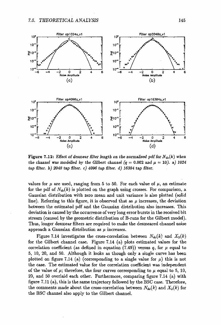
7.5. THEORETICAL ANALYSIS
Filter ap1024o..vl 10' r---...---...--.....;...,......-----...----....----..
-4 -2 0 2 4 6 Noise Ampflhlde
(a)
Filter op4096o..v1 1~r---...----...--.....;...,..._____...----.--_,
10-'
10""
l< 10~~~~~--~--~--~--~--~ -6 -4 -2 0 2 4 6
Noi," Ampntude
(c)
10·
10-'
:l!10-z
10""
10-' -6
10·
10-'
:l!10-z
10-11
10'" -6
145
Filter ap2048o..vl
,«< lC
-4 -2 0 2 4 6 Noise Amplitude
(b)
Filter ap 16384o..vl
-4 -2 0 2 4 6 Noise Amplitude
(d)
Figure 7.12: Effect of desmear filter length on the normalised pdf for Ndc(k) when the channel was modelled by the Gilbert channel (q = 0.002 and J1. = 10). a) 1024 tap filter. b) 2048 tap filter. c) 4096 tap filter. d) 16384 tap filter.
values for p are used, ranging from 5 to 50. For each value of p, an estimate for the pdf of Ndc( k) is plotted on the graph using crosses. For comparison, a Gaussian distribution with zero mean and unit variance is also plotted (solid line). Referring to this figure, it is observed that as J1. increases, the deviation between the estimated pdf and the Gaussian distribution also increases. This deviation is caused by the occurrence of very long error bursts in the received bit stream (caused by the geometric distribution of B-runs for the Gilbert model). Thus, longer desmear filters are required to make the desmeared channel noise approach a Gaussian distribution as p increases.
Figure 7.14 investigates the cross-correlation between Ndc(k) and X2(k) for the Gilbert channel case. Figure 7.14 (a) plots estimated values for the correlation coefficient (as defined in equation (7.49)) versus q, for p equal to 5, 10, 20, and 50. Although it looks as though only a single curve has been plotted on figure 7.14 (a) (corresponding to a single value for p) this is not the case. The estimated value for the correlation coefficient was independent of the value of p; therefore, the four curves corresponding to p equal to 5, 10, 20, and 50 overlaid each other. Furthermore, comparing figure 7.14 (a) with figure 7.11 (a), this is the same trajectory followed by the BSe case. Therefore, the comments made about the cross-correlation between Ndc(k) and X2(k) for the BSe channel also apply to the Gilbert channel.

146 CHAPTER 7. SMEAR CODING
10· 1-'=5
10° 1-'=10
10·' 10'"
~10·· ~10'"
10'" 10'"
X 10'" 10'"
-6 -4 -2 0 2 4 6 -6 -4 -2 0 2 4 6 Noise Amplitude Noise Amplitude
(a) (b)
10° 1-'=50
10.'
~10'"
10'" Xx
)( 10'" -2 0 2 4 6 -6 -2 0 2 6
Noise Amplitude Noiae Amplitude
(C) (d)
Figure 7.13: Effect ofvaryingJ.t on the normalised pdf for Ndc(k), while holding q and the desmear nlter fixed (q = 0.002; desmear nlter = ap16384a...vli). a) J.t = 5. b) J.t = 10. c) J.t = 20. d) J.t = 50.
0.2 0.2
0.0 0.1
Q. -0.2 ~ 0.0 , -0.4 -0.1
-0.610
.... -0.2 10'" 10"'" 10'" 10'" -100 -50 0 50 100 q .,.
(0) (b)
Figure 7.14: Estimate for the cross-correlation between Ndc(k) and X 2(k) for Gilbert channel a) Correlation coefficient VB q for J.t = 5,10,20, and 50 (Note, the four curves overlay each other and appear as a single curve). b) Normalised cross· correlation when q = 0.01 and J.t = 50.

7.5. THEORETICAL ANALYSIS 147
Figure 7.11 (b) shows the normalised cross-correlation of X2(k) and Nde(k) for q = 0.01 and p, = 50. Referring to this figure, the only point at which these two signals become correlated is when r = 0; hence, the correlation coefficient does give a good indication of the amount of correlation between these two signals.
7.5.6 Summary of Theoretical Analysis
This sub-section summarises the main theoretical results that have been derived.
An asymptotic bound has been derived for the probability of a decoding bit error for binary smear codes. This bound is given by:
Pe = ~ erfc ( v'2A
O" dr) (7.66)
where erfc(.) is the complimentary error function, A is the magnitude of X 2 (k) at the threshold detector's input, and O"Jr is the variance of Ndr(k). This bound is approached as the length of the desmear filter increases.
For the binary PCM smear code,
(7.67)
where O"~q is the variance of the desmeared quantization noise, and O"~e is the variance of the desmeared channel noise.
O"Jq is given by
(7.68)
where a is the gain of the gain plus additive noise model used to model the Max quantizer and assumes the value 0.9905 for Q = 16.
For the BSC channel, O"Je is given by
0"2 n 0"2 = X2 '\:"""' I' .qi de 2 L...J ':.'
a i=O
where (i are the channel coefficients and are given by:
(0 o
(3 -0.77
(7.69)
For the Gilbert channel, O"Jc is given by
0"2 Q-l Q Q
O"~e = ~2 L LI:(Vj-Vi)2p(X6 = Wi)P(Y4 = Wj/X6 = Wi,S = 8m ) p(S = Sm) a m=Oj=l i=l
(7.70)

148 CHAPTER 7. SMEAR CODING
7.6 Simulation Results
The binary PCM smear code was simulated on computer to obtain the simulated performance of the code. This section presents these simulation results and compares them with the performance bounds derived in section 7.5 for the BSC channel and Gilbert Channel. Simulation results are also presented for the binary PCM smear code when the channel was modelled by the periodic burst channel. These latter simulation results are compared against the performance bound for the Gilbert channel.
7.6.1 Simulation Results for BSC Channel
Figure 7.15 plots the probability of a decoded bit error (Pe ) against the probability of a channel bit error (q) for the BSC channel case. The solid line shown in this figure is the asymptotic bound for the binary PCM smear code for the BSC channel, computed using using equations 7.66, 7.67, 7.68, and 7.69. The shape of this theoretical curve follows the classic waterfall curve exhibited by all channel coders; hence, the binary PCM smear code does exhibit coding properties.
Also plotted on this figure are the simulation results obtained when the following six smear/ desmear filters are used in the binary PCM smear code:
1. ap512a_v1/ap512a_vli
2. ap1024~v1/ap1024~vli
3. ap2048a_v1/ap2048a_vli
4. ap4096a..v1/ap4096a..vli
5. ap8192a..v1/ap8192a..vli
6. ap16384a_vl/ap16384a_v1i.
For smear filter ap16384~v1 there is good agreement between the theoretical results and the experimental results; although, a slight discrepancy is observed when q approaches 0.5. This discrepancy is caused by the increasing correlation between X 2 (k) and Ndr(k) as q approaches 0.5 (refer to figure 7.11). This correlation was ignored in the theoretical analysis. (Note that for q > 1 X 10⁻² the simulation points for the six smear filters overlaid each other forming a large solid dot.)
As the smear/desmearfilter length is reduced (ap8192a..v1, ap4096a_vl. .. ), then for low channel bit error rates the discrepancy between the theoretical results and experimental results increases. This discrepancy arises because these shorter desmear filters are not as effective at desmearing the channel noise, and the pdf of Ndc( k) is no longer Gaussian. (This effect was illustrated in figure 7.10 for q = 0.001.) These results are consistent with the assumption

7.6. SIMULATION RESULTS
0...0> 10-5
A ap512a...vl
• apl024a...vl
o ap204Ba...vl
+ ap4096a...vl
)( opB192o_v1
'" ap163B4o..vl
Asymptotic Bound
149
Figure 1.15: Performance of the binary PCM smear code over the BSC channel.

150 CHAPTER 7. SMEAR CODING
that the pdf of Ndr(k) approaches a Gaussian distribution as the desmear filter length increases.
In summary, the results shown in figure 7.15 demonstrate that the asymptotic bound for the binary PCM smear code can be approached by increasing the length of the desmear filter. However, very long desmear filters are required to approach this bound when q is small- at least 16384 taps are required when the channel is modelled by the BSC channel.
7.6.2 Simulation Results for Gilbert Channel
Figure 7.16 shows the asymptotic bound (solid curve) and simulation results (asterisks) for the binary PCM smear code when the discrete channel is modelled by the Gilbert channel. All the simulation results shown in this figure were obtained using smear filter ap16384a...v1 and desmear filter apI6384a...vli. As the Gilbert channel is controlled by two parameters (J.L and q), four sets of results are presented. Each sub-figure in figure 7.16 shows the performance of the binary PCM smear code when J.L is held constant and q is varied. Results are presented for I/. equal to 5, 10, 20, and 50.
Comparing the four theoretical curves shown in figures 7.16 (a), (b), (c), and (d), it is seen that the asymptotic bound for the binary PCM smear code remains virtually the same for each value of 1/.; hence, this bound is a very weak function of 1/.. In fact the trajectory of these four theoretical curves follow the same curve as for the BSC channel case (refer to figure 7.15). This verifies that the asymptotic bound for the binary PCM smear code is determined primarily by the BER of the channel (q) and is quite insensitive to the other statistical properties of the channel noise (e.g. whether the bit errors occur randomly or cluster into bursts).
For I/. = 5, the experimental results approach the asymptotic bound for the binary PCM smear code - although a slight discrepancy is observed when q approaches 0.5. This discrepancy is caused by the increasing correlation between Ndc(k) and X2(k) as q approaches 0.5 (refer to figure 7.14). This correlation was ignored in the theoretical analysis. As I/. increases (J.L = 10, 20, 50), the discrepancy between the simulation results and asymptotic bound also increases for low channel bit error rates. This occurs because the Gilbert channel occasionally produces very long noise bursts (due to the geometric distribution B-runs), causing the first order pdf of Ndc(k) to depart from Gaussian (refer to figure 7.13). This suggests that longer desmear filters are required to make the binary PCM smear code approach its asymptotic bound.
To prove that this discrepancy is indeed caused by the occurrence of very long noise bursts, and not the noise bursts themselves, the performance of the binary PCM smear code was investigated using the periodic burst channel. These results are presented in the next section.
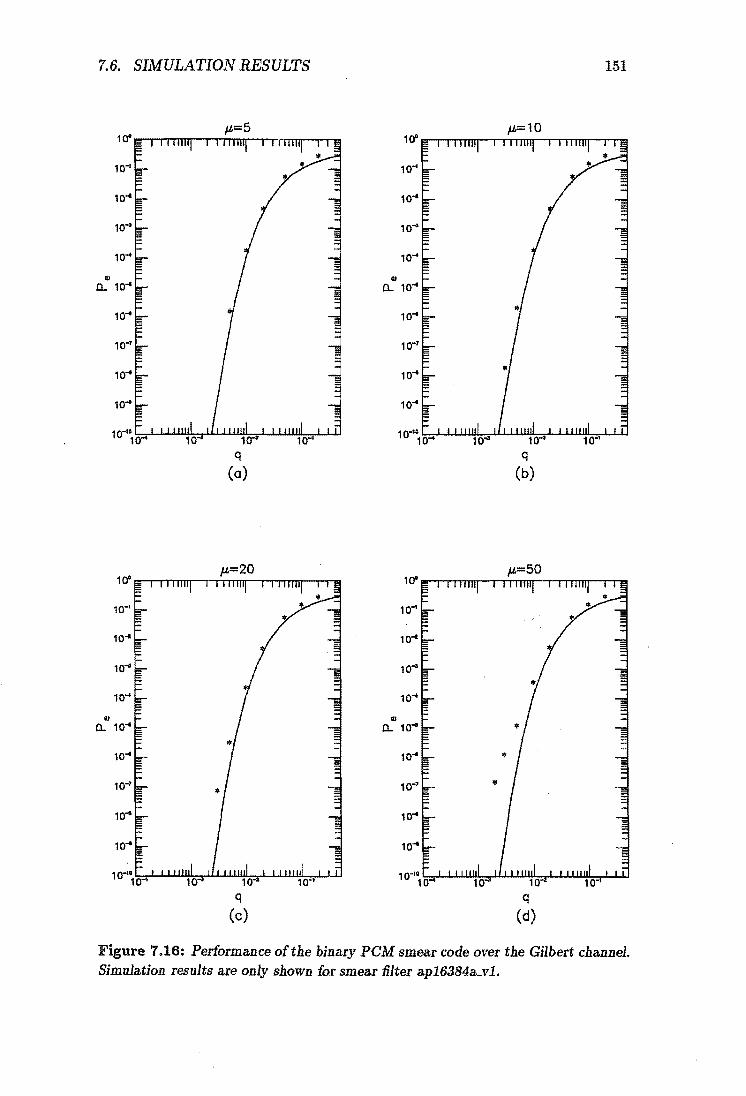
7.6. SIMULATION RESULTS
jt=5
10·'
jt=20
10"
10·'
10'"
10 ....
10'"
01
0. 10'"
10"
jt=10
q
(b)
jt=50
151
Figure 7.16: Performance of the binary PCM smear code over the Gilbert channel. Simulation results are only shown for smear 1i1ter ap16384a...vl.

152 CHAPTER 7. SMEAR CODING
",,=100
10'"
10->
10'"
10'"
q
Figure 7.17: Performance of binary PCM smear code over the periodic burst channel. Simulation results only shown for smear filter ap16384a..vl.
7.6.3 Simulation Results for Periodic Burst Channel
The important characteristic of the periodic burst channel is that the duration of noise bursts are fixed; hence, the long duration noise. bursts that were occasionally encountered in the Gilbert channel model do not occur in theperiodic burst channel.
The performance of the binary PCM smear code over the periodic burst channel is shown in figure 7.17. The solid curve is the asymptotic bound for the binary PCM smear code when 11 = 100 (computed using the equations derived for the Gilbert Channel and setting 11 = 100). The asterisks are the simulation results obtained for the periodic burst channel using desmear filter ap16384a...vli and setting 11 = 100. As can be seen, the simulation results closely follow the asymptotic bound. This proves that the binary PCM smear code is capable of correcting errors which cluster into bursts, and that the discrepancy between the simulation results and asymptotic bound for the Gilbert channel was indeed caused by the occasional very long duration noise burst.
7.7 Statistics of Decoding Bit Errors
A unique property of the binary PCM smear code is that under certain circumstances the decoded bit errors are independently distributed. This is in contrast to block codes and convolutional codes where decoded bit errors al-

7.7. STATISTICS OF DECODING BIT ERRORS 153
ways cluster into bursts. This section demonstrates this property of the binary PCM smear code and discusses the conditions that must be satisfied for this property to apply.
We first define the random process {Dk}, which is the error sequence for the decoded bit stream, and then describe a sufficient condition that must be satisfied if Dk and Dk+T are independent random variables. Using this condition for independence, we then show that the autocorrelation function of Dk contains sufficient information to determine whether Dk and Dk+T are independent. Having set this ground work, we then plot an estimate for the autocorrelation function of Dk and argue that this demonstrates that Dk and Dk+T are independent. Finally we discuss the conditions under which these results can be generalised to other smear codes using different modulation systems.
The decoded error sequence {Dk } is defined by the equation
(7.71)
where Ee denotes modulo 2 addition, Xl(k) and Yi(k) were defined in section 7.3, and Dk E {do = 0, d1 = I}. Thus Dk is 0 if no decoding bit error occurs at t = k, and 1 if a decoding bit error does occur.
If Dk and Dk+T are independent, then
P(Dk+T = dj/ Dk = di ) = P(Dk+T = dj)
U sing the relationships
'Vj=O,lji=O,1
P(Dk+T = 0/ Dk = di) = 1 - P(Dk+T = 1/ Dk = di) i = 0,1
and 1
(7.72)
(7.73)
P(Dk+T = 1) = I: P(Dk+T = 1, Dk = dj ) (7.74) j=O
it is a simple matter to prove that a sufficient condition for independence of Dk and Dk+T is
'VT=JO (7.75)
Now, the autocorrelation function for Dk is given by
RD(T) E[DkDk+Tl (7.76) 1 1
- I: I: didjP(Dk+T = dj/ Dk = di ) P(Dk = dd (7.77) i=Oj=O
- P(Dk = 1) P(Dk+T = 1/ Dk = 1) (7.78) - PeP(Dk+T = I/Dk = 1) (7.79)
Thus, RD ( T) is proportional to the conditional probability P (Dk+T = 1/ D k = 1). If Dk+T and Dk are independent, then P(Dk+T = I/Dk = 1) = P(Dk+T = 1) = Pe , and the autocorrelation function is given by
{ Pe
RD(T) = p2
e
T=O
T=JO (7.80)

154 CHAPTER 7. SMEAR CODING
10-1~------T-------~------~------~
10-4
1cr'b2Sd 10"" 10"" 10"" 10'"
-2 -1 0 1 2
10-~~------~------~------~------~ -20 000 -10 000 o 10 000 20 000
T
Figure 7.18: Estimate for the autocorrelation function of Dk (Pe = 0.01, and the desmear filter is ap16384a_vli).
Equation (7.80) shows that by inspecting the autocorrelation function RD( r) we will be able to determine whether or not Dk and Dk+r are independent. Figure 7.18 shows an estimate for the autocorrelation function of Dk for the binary PCM smear code operating over the BSC channel. This estimate was computed from a sample function of Dk when Pe = 0.01 and filter ap16384a_vli was used as the desmear filter. Referring to this figure, it is seen that the estimated autocorrelation function is approximately Pe at r = 0 and P; for r f::. 0 - exactly what would be expected if Dk and Dk+r (r f::. 0) were independent. H the decoded bit errors clustered into bursts, as is the case for block codes and convolutional codes, the autocorrelation function would decay gradually from RD(O) = Pe to RD(r) = P; for Irl » 1. Thus, we conclude that, under the conditions stated above, decoded bit errors occur independently of each other for the binary PCM smear code.
Tt is interesting to ask what conditions must be satisfied for these results to apply to smear codes in general. As a partial answer to this question, we have identified two necessary conditions that must be satisfied for decoding bit errors to be independently distributed. (1 do not know whether these conditions are sufficient however.)
The first necessary condition is that the power spectral density of Ndr(k) must be white. To prove this we note that if Dk and Dk+r are independent, then the noise samples Ndr(k) and Ndr(k + r), which influence the threshold detector's decision at t = k and t = k+r respectively, must also be independent. Hence, the power spectral density of Ndr(k) must be white.
The second condition that must be satisfied is that the smear code must be operating close to its asymptotic bound. This ensures that the short-time power of Ndr(k) remains constant with time. Fluctuations in this short-time power can occur if the desmear filter is too short, causing the pdf of Ndr(k) to depart from a Gaussian distribution and causing decoding bit errors to cluster into bursts (refer to figures 7.9 and 7.10). This condition can be satisfied by using suitably long desmear filters.

7.8. COMPARISON WITH BLOCK AND CONVOLUTIONAL CODES 155
To summarise this section, we have shown that under certain circumstances the decoded bit errors that occur at the output of the smear coder are independently distributed.
7.8 Comparison with Block and Convolutional codes
This section compares the binary PCM smear code with block codes and convolutional codes.
Figure 7.19 shows how the binary PCM smear code improves the performance of a power-limited coherent Binary Phase Shift Key (BPSK) channel, when the channel is corrupted by Gaussian noise, and the information rate is held constant. This graph plots the probability of a decoded bit error (Pe )
against the energy-per-bit to noise-density ratio at the receiver input (Eb/No). The solid curve shows the theoretical performance of a coherent BPSK channel without channel coding. The dashed curve shows the theoretical performance of the coherent BPSK channel when a binary PCM smear code is applied. When binary PCM smear coding is applied, four channel bits must be transmitted for every information bit (under steady state conditions). As the information rate is held constant and the channel is power-limited, the energy per channel bit is reduced by 6 dB, and this increases the probability of a channel bit error. However, this increased channel bit error rate is offset by the error correcting properties of the binary PCM smear code, so that for sufficiently high values of Eb/No an overall coding improvement is observed.
Comparing the uncoded BPSK curve with the coded BPSK curve, a coding threshold is observed at Eb/No ...:.. 11.5 dB. Below this coding threshold, the coded system actually degrades the performance of the data transmission system; above this coding threshold a coding gain is observed. A coding threshold is found in all coded systems; however, this threshold is usually much lower: At decoded bit error rates of 10-5 , block codes and convolutional codes can typically yield coding gains between 1.5-7.5 dB, depending on the complexity of the code [Bhargava, 1983]. For example, a (23,12) Golay code has a coding threshold of about 3.5 dB. In comparison to this, the binary PCM smear code is operating below its coding threshold and causing a coding loss of approximately 1.3 dB.
Also, compared to block codes and convolutional codes, the binary PCM smear code introduces very long transmission delays. For example, a (23,12) Golay block code will delay the information bit stream by 24n seconds (ignoring processing delay), where l/Tb is the information bit rate. A binary PCM smear code using smear filter ap16384a_v1, on the other hand, will delay the information bits by 16384Tb seconds. This very long delay is caused by the causal smear / desmear filters used in the smear code.
A second consequence of using smear / desmear filters with very long impulse

156
10-1
10-4
CHAPTER 7. SMEAR CODING
... ... ... , , , , \
\ \ \
Uncoded Coherent BPSK
Coded Coherent BSPK (Binary pet.! Smear Coding)
\ \ \ \ \ \ I I I \ \ \ I \ \ I I I
10-10 '--_-'-_-'-_--'-_---'-__ '----'-..1....L..----J
-2.5 0.0 2.5 5.0 7.5 10.0 12.5 15.0 Eb/NO (dB)
Figure 7.19: Comparison of Coherent BPSK performance, with and without binary PCM smear coding. The channel is assumed to be an AWGN power-limited channel.
responses is that smear codes are unsuitable for transmitting short-:duration bursts of information. For example, consider what happens when the binary PCM smear code is used to transmit a single information bit across a noisy channel. The channel encoder maps this information bit onto nNT channel bits, where NT is the number of taps in the smear filter. As NT is very large, this would make very inefficient use of the channel.
Obviously the binary PCM smear code performs very poorly compared to block codes and convolutional codes and would never be used in practice. However as was stated at the beginning of this chapter, the primary objective of this investigation was to demonstrate the coding properties of smear codes - not to design a near-optimal smear code. Therefore, a simple-to-analyse but sub-optimal smear code implementation was examined. Smear code performance may be improved by using a superior modulation system to PCM for improving the demodulated signal-to-noise ratio. In this respect a pulse position modulation system or a frequency modulation transmission system using a. phase"locked loop detector may yield superior performance.
Despite the serious drawbacks listed above, the binary PCM smear code did exhibit some very useful properties. Firstly, under suitable conditions, decoded bit errors which occur at the output of the binary PCM smear decoder are independently distributed. In contrast to this, block codes and convolutional

7.9. CONCLUSIONS 157
codes always cluster decoded bit errors into bursts.
Secondly, the asymptotic performance of the binary PCM smear code is determined primarily by the bit error rate of the channel and is insensitive to the burstiness of the channel noise. Block codes and convolutional codes are usually very sensitive to the type of channel noise; although, this can be overcome by using interleaving. (However, interleaving increases the coding delay).
Finally, the probability of a decoded bit error can be estimated from the received bit stream: i.e., the variance of the reconstruction noise can be estimated from the signal at the output of the de smear filter; knowing this variance, one can compute the probability of a decoded bit error. This estimate can be computed even though the channel is modelled by a discrete channel. This property can be exploited to give a reliability measure for the decoded data.
7.9 Conclusions
This chapter has investigated a new technique for reliably transmitting data over a noisy channel called smear coding. The technique combines smear I desmear filtering with a wide bandwidth non-linear modulation system to provide a forward error checking channel code.
To validate this channel coding technique, a simple but sub-optimal smear code implementation was investigated in detail, called a binary PCM smear code. This implementation combined smear I desmear filtering with a PCMtype modulation system. The performance of the binary PCM smear code was investigated using three discrete channel models: 1) the BSCchannel, 2) the Gilbert channel, and 3) the periodic burst channel. Both theoretical results and computer simulation results were obtained for the performance of the code.
The following results were obtained:
• The binary PCM smear code did exhibit channel coding properties -thus validating the principle upon which smear codes were based. (Demonstrating this was the primary objective of this investigation.)
• The asymptotic performance of the binary PCM smear code was determined primarily by the bit error rate of the discrete channel; other statistical properties of the channel noise, such as the burstiness of the noise, had little affect on the asymptotic performance of the code.
• Very long desmear filters had to be used to approach the asymptotic performance bound for the binary PCM smear code (typically 16384 taps).
• Under suitable conditions, decoded bit errors that occurred at the output of the binary PCM smear decoder were independently distributed. In contrast to this, block codes and convolutional codes always cluster decoded bit errors into bursts.

158 CHAPTER 7. SMEAR CODING
.. The probability of a decoded bit error could be estimated from the received bit stream, even when the channel was modelled by a discrete channel. This property could be exploited to give a reliability measure for the decoded data.
Although the binary PCM smear code did exhibit coding properties, it performed very poorly compared to block codes and convolutional codes. For example:
.. The binary PCM smear code introduced very long coding delays into the digital transmission system. This problem is an inherent limitation of all smear codes and will restrict the range of applications that smear codes are suited to .
• The coding gain of the binary PCM smear code compared very unfavourably with typical coding gains achieved by block codes and convolutional codes.
The very poor coding gain observed for the binary PCM smear code was caused by the numerous compromises made during the design stage. We conjecture that smear code performance could be significantly improved by using a better modulation system than PCM. However, this possibility is left for further research.

Chapter 8
Other Applications for Smear Filters
8.1 Introduction
This chapter describes three additional applications for smear / desmear filters that were briefly investigated during the course of my Ph. D. research program. However, insufficient time was devoted to these topics to thoroughly research them. Nevertheless, some interesting and novel results were obtained.
Section 8.2 describes how smear/ desmear filters can be used to encrypt (or more correctly scramble) an analog signal. The section focuses specifically on scrambling speech. To the authors knowledge, this application has not been previously reported in any of the research journals.
Section 8.3 describes the use of smear / desmear filters to suppress the effects of impulse noise in a data transmission system. The results presented in this section formed the basis of a paper presented at the mobile satellite conference held at the JPL Laboratories in May of 1988 [Webb et al., 1988].
Finally, section 8.4 describes how smear / desmear filters can be used to enhance the performance of an instantaneous quantizer for some signals. This section appeared in the first version of my thesis published in October 1990. Since then, Popat and Zeger [Popat and Zeger, 1992] have published a paper in the IEEE Transactions of Communications describing the same application.
8.2 Encryption using Smear Filters
This section describes how smear / desmear filters can be used as encryption devices. The original idea for using smear filters as an encryption devices was my supervisor's Mr J. A. Webb; he had taken out a patent on the concept [Webb, 1992]. As a result of this research, an equipment vendor - Cardinal Encryption Systems - developed a new signal encryption product that made use of smear / desmear filters. (This product was initially targeted at the Group
159

160 CHAPTER 8. OTHER APPLICATIONS FOR SMEAR FILTERS
Input Smear Scrambled Desmear Descrambled
Signa~ __ s~nal ___ -ooI{lJ ..... __ Si_gnal
Insecure channel
Figure 8.1: Utilising smear filters to scramble or encrypt a signal
3 facsimile market). As I was not directly involved in the development of this product, nor was I privy to the additional research that supplemented its development, I cannot report on this specific application. However, I did investigate the possibility of using smear J desmear filters for scrambling speech, and these results are briefly presented below.
Figure 8.1 illustrates how smearJdesmear filters can be used to encrypt an analog signal prior to transmission over an insecure channel. The idea is to encrypt the signal at the transmitting end by smearing out the signal in time; the signal is decrypted at the receiving end by desmearing the received signal. Only those people who know the characteristics of the de smear filter will be able to decrypt the received signal; therefore, by keeping this information secret, some level of privacy is ensured. An advantage of this scrambling scheme is that it can be applied to any analog signal: speech, the output from a modem, or even a television signal.
Figure 8.2 shows what happens when this scrambling technique is applied to speech. Figure 8.2 (a) shows the spectrogram of a typical speech waveform, and figure 8.2 (b) shows the spectrogram of this same waveform after being passed through smear filter ap4096a_v1. Comparing these two figures, it is evident that the all-pass smear filter has delayed different frequency bands by different amounts; the delay at any frequency is equal to the group delay of the smear filter at that frequency (refer to appendix A to see a plot for the group delay response of ap4096a_v1). When listening to the scrambled speech waveform of figure 8.2 (b), the energy exciting the ear at a given instant in time will be due to several phonemes, each spoken at different instant of time. This tends to confuse the speech, and if the group delay distortion introduced by the smear filter is sufficiently severe, the smeared speech wave is rendered completely unintelligible.
A number of informal listening tests were carried out on the scrambled speech wave and the following observations were made:
1. All-pass smear filters were more effective at scrambling the speech wave than non-flat smear filters.
2. A reasonable scrambling effect could be achieved using 4096-tap all-pass smear filters (The speech was sampled at 10 kHz, and therefore, the maximum delay that could be introduced by these smear filter was 409.6 ms.) After being scrambled by a 4096-tap all-pass smear filter, the coarse

8.2. ENCRYPTION USING SMEAR FILTERS 161
lime (1.1)
(0)
lime (8)
(b)
Figure 8.2: Scrambling speech using smear filters. a) Typical spectrogram of speech wave. b) Spectrogram of scrambled speech using filter ap4096a_vl.
rhythm of the speech could be discerned; however, no words could be identified, even after repeatedly listening to the scrambled speech wave.
3. Very good scrambling effects were achieved with 8192-tap and 16384-tap smear filters. Both the all-pass smear filters and the non-Hat smear filters performed well. Except for very long pauses in the speech wave, these long smear filters also destroyed the rhythm of the speech.
4. When all-pass smear filters were used, high quality speech could be recovered from the scrambled wave using the desmear filter. The only noticeable effect was to introduce a time delay into the signal.
5. When non-Hat smear filters were used, the descrambled speech was also of high quality, except for the presence of a low volume pre-echo and a low volume post echo as discussed in chapter 4.
A disadvantage of this speech encryption system is the delay introduced into the signal because of the causal smear / desmear filtering. A second disadvantage is that the group delay response of an all-pass smear filter can be extracted from the encrypted signal using a spectrogram. A third disadvantage of the encryption technique is that it is susceptible to a known plain text attack: If an attacker obtains a copy of both the input signal and the encrypted signal,

162 CHAPTER 8. OTHER APPLICATIONS FOR SMEAR FILTERS
he can determine the smear filter impulse response using correlation. Obviously this encryption technique is only suitable for protecting against casual eavesdroppers.
Advantages of this speech encryption system are that unintelligible speech can be produced for a delay of approximately 400 ms, and the degree of scrambling can be increased by increasing the delay. The decrypted speech is of very good quality (however, see comments in section 4.3). No synchronization is required between the transmitter and the receiver; and no equalisation of the channel is required: If the magnitude distortion and the group delay distortion of the channel is good enough to support communication without encryption, it will also be good enough to support communication when smearjdesmear filters are used.
8.3 Impulse Noise Suppression in Data Trans-• • mISSIon
Smear filters have been applied to data transmission systems to reduce the effects impulse type noise. This technique was first proposed by Wainwright in 1961 [Wainwright, 1961] and has received sporadic attention by various researchers since then [Engel, 1965; Richter and Smits, 1971; Vanelli and Shehadeh, 1980; Beenker et al., 1985].
Figure 8.3 illustrates how smear j desmear filters are used in this application. The output signal of the sending-end modem is passed through a smear filter before being applied to the channel, and at the receiver, the signal is passed through the desmear filter before being applied to the receive..:end modem. The desmear filter compresses the wanted signal in time, thus allowing the receive-end modem to correctly decode the transmitted data. However, the desmear filter acts like a smear filter for the impulse noise· that has been introduced by the channel. Thus, the impulse noise is smeared out in time; its peak amplitude is reduced; and hopefully it will not cause any data errors.
Very little time was devoted to researching this application in my Ph. D. program, mainly because of pressures to focus on other areas. However, some
---+I Modem
____________ ..1
r------------I Desmear Rx I X4 I'V X5 X6
,..., Modem 1---_ ,....
1.. ___________ _
Imp.ulse nOIse
son tee
Figure 8.3: Block diagram of data transmission system utilising smear/desmear filters to overcome impulse noise.

8.3. IMPULSE NOISE SUPPRESSION IN DATA TRANSMISSION 163
simple computer simulation results were obtained that illustrate the potential advantage of smear filters for this application. Below, we briefly describe this computer simulation and present the results [Webb et al., 1988].
The system that was simulated on computer is similar to that shown in figure 8.3. The impulse noise channel was modelled by a switch: It was assumed that the bursts of impulse noise could be reliably detected at the front end of the receiver, and when this occurrence was detected, the switch was opened and X4(n) was set to zero. When no noise bursts were present, the switch was closed and X4(n) = X3(n).
The sending end modem of figure 8.3 was modelled as an ideal low pass filter with cutoff frequency of 0.5 Hz. This filter was excited by a train of periodic impulses, with period of one second, whose amplitude was modulated by the binary data sequence to be transmitted; this binary data sequence is denoted by Xl(n); Xl(n) E [1, -1]. The receive modem was modelled by a sampler that was perfectly synchronised with the input signal and a threshold detector with decoding rule
X6(n) = { +1.0
-1.0
If Xs(n) > 0
If Xs(n) < 0 (8.1)
Typical signals at various points along the transmission system of figure 8.3 are plotted in figures 8,4 (a)-(e). This particular example shows the effect of a single noise burst which caused X4(n) to be set to zero for 50 seconds. The reader should particularly note figure 8,4 (e), which shows that the desmear filter has smeared out the effect of the signal fade in time. Careful inspection of this latter plot suggests that the threshold detector will correctly decode all the transmitted data for this particular example. Figure 8,4 (f) confirms this by plotting the product of Xl(n) and Xa(n). If any errors did occur, the curve would exhibit a negative spike that touched the -1 amplitude.
Figure 8.5 shows how the average number of bit errors varies. as duration of a single noise burst varies. (The duration of a noise burst is measured in terms of the number of consecutive bits that would have been interrupted had the smear / desmear filters not been used.) The data points for these plots were obtained from computer simulation. Figure 8.5 (a) shows the results for a 128-tap smear/desmear filter, and figure 8.5 (b) shows the results for a 1024-tap smear I desmear filter. The dashed lines in these figures indicate the expected number of errors if the smear and desmear filters were absent. In this case it is assumed that guesses are made for the missing bits.
These results clearly illustrate the advantage of using smear I desmear filters when the channel suffers from impulse type noise.

164 CHAPTER 8. OTHER APPLICATIONS FOR SMEAR FILTERS
X,3 4.-------~----~--~------_;
-.~------------------------~
TIme (s) TIme (s)
(0) (b)
DO -g is 0
-3
t -,I----e.~~~~~j~~i;r~:~ "'0 IlOO .000 -20!-----...,IS(JO~----:.*OOO::-----~.I100·
TIme (8) TIme (s)
(c) (d)
X6
.. " ,g 0 ... ~ -. -.
-20 IlOO .-TIme (8) TIme (8)
(e) (f)
Figure 8.4: Typical signals at various points along the transmission system of figure B.3. The smear and desmear filters used in this example were apl024a..vl and apl024a..vli respectively; the noise burst lasted for 50 seconds and would have interrupted the transmission of 50 consecutive bits had the smear/desmear filters not been used. a) Input signal X1(n). b) Signal at output of smear filter X3(n). c) Signal applied to input of desmear filter X4(n). d) Signal at output of desmear filter Xs(n). e) Output signal X6(n). f) X1(n) X X6(n). (This latter curve was plotted by connecting sample points with a solid line; therefore, if any bit errors had occurred, the plot would exhibit large negative spikes.)

8.4. ROBUST QUANTIZATION USING SMEAR FILTERS 165
e20.-~~--~~--~~~~~
g IJJ 15 '5 ; J 10
8, 5 I!: ,. .
"
,. ,. " .' .'
"
~ °O~~--~~~--~~~~~ 5 10 15 20 25 30 35 40
Bits Interrupted by Noise Burst
(0)
~30r-~~~,~--~~--~~~
~ 25 :'
'520 ; / ~ 15 .-
z 10 " II ,
~ 5 :'
, ,
~ 0 " 0~-2~5--M~-75~~10-0~12-5~1M--1~7-5~200 Bits Interrupted by Noise Burst
(b)
Figure 8.5: A verage number of bit errors caused by a single noise burst vs number of bits interrupted by the noise burst. The dashed curves plot the expected number of errors if the smear/desmear filters were absent. a) Results for smear filter ap128a..vl and desmear filter ap128a..vli. b) Results for smear filter apl024asl and desmear filter ap1024a..vli.
8.4 Robust Quantization using Smear Filters
An instantaneous quantizer maps a continuous amplitude input sample onto a discrete amplitude output sample. It does this by passing the input signal through a device whose transfer characteristic looks like a staircase: the rises of the staircase occur at the threshold levels of the quantizer; the treads of the staircase occur at the reconstruction levels. The threshold levels and reconstruction levels can be chosen to minimise the quantization noise introduced by the quantizer. However, to carry out such an optimization, the pdf of the input signal must be specified. [Max, 1960; Paez and Glisson, 1972; Gersho, 1978; Jayant and Noll, 1984; Rabiner and Schafer, 1978].
If the pdf of the input signal actually applied to the input of the quantizer is different to that for which the quantizer was optimized, then the quantizer will no longer be an optimal quantizer for this input signal. There are two situations where this is of particular concern:
1. When the input signal is nonstationary, in which case the short-time pdf may change drastically with time. (A good example of this is speech).
2. When different types of signals may be applied to the input of a quantizer. (For example, both speech and data signals may be applied to the input of an instantaneous quantizer used in the public switched telephone network).
One technique for overcoming this problem is to use logarithmic companding followed by uniform quantization [Gersho, 1978]. Another technique is to use an adaptive quantizer which adapts its transfer characteristic based on measurements made on the short-time statistics of the signal [Jayant and Noll, 1984].
Popat and Zeger [Popat and Zeger, 1992] have suggested an alternative technique that uses smear /desmear filters. Figure 8.6 shows how this technique

166 OHAPTER 8. OTHER APPLIOATIONS FOR SMEAR FILTERS
Smear
x ---1L..._Z_:---~'1 Quantizer I----
y
Figure 8.6: Use of smear 1ilter for smearing out signal prior to quantization.
Number Probability density of input signal
of Levels
Uniform Gaussian Laplacian Gamma
2 4.77 dB 2.44 dB 0.0 dB -3.01 dB
4 11.76 dB 8.76 dB 6.70 dB 5.20 dB
8 17.99 dB 14.46 dB 12.40 dB 11.20 dB
16 24.07 dB 20.18 dB 18.07 dB 16.99 dB
32 30.10 dB 26.01 dB 23.85 dB 22.82 dB
64 36.12 dB 31.91 dB 29.74 dB 28.71 dB
Table 8.1: Theoretical signal-to-quantization noise ratios for the optimal uniform, optimal Gaussian, optimal Laplacian, and optimal Gamma instantaneous quantizers. The SNR was computed using the gain plus additive noise model (refer to appendix D).
works. The input signal is first smeared out in time by a smear filter and then quantized using an instantaneous quantizer. Because the smear filter causes the pdf of the smeared signal to approach a Gaussian pdf the quantizer is optimized for the Gaussian pdf. The desmear filter is then used to recover the original signal from the quantized samples. (If the reason for quantizing the signal is to transmit it over a digital channel, the smear filter and quantizer would be located in the transmitter, and the desmear filter would be located in the receiver.)
The assumption that the smear filter will cause the smeared signal to approach a Gaussian pdf is not always true. For example, it is very easy to construct a signal for which smear filtering makes the distribution appear less Gaussian - simply filter a signal with Gamma pdf using the desmear filter and use the result for the input signal to the smear filter. (In this example, the smear filter is acting like the desmear filter). However, for randomly generated signals that have not been passed through the desmear filter, experience suggests that this assumption will hold.
To illustrate the effectiveness of this method, table 8.1 compares the signalto-quantization noise ratio! (SNR) of four different signals. This table lists the
lThe SNR was computed using the gain plus additive noise model for the quantizer (refer

8.5. CONCLUSIONS 167
theoretical SNR when each signal is quantized with an instantaneous quantizer optimised for its own specific pdf. The four pdfs considered are the Uniform, Gaussian, Laplacian and Gamma densities. If, as proposed here, the signal was smeared out in time prior to quantization, the output SNR for all four signals would be given by the Gaussian column.
Comparing the rows of this table, it is observed that smearing out the signal prior to quantization would improve the SNR of those signals with a Gamma or Laplacian density, but would degraded the SNR of those signals with a uniform pdf. An interesting observation from these results is that if an instantaneous quantizer optimised for a specific pdf does not perform as well as an instantaneous quantizer optimised for the Gaussian pdf, the performance of the quantizer can be improved by smearing out the signal prior to quantization. A further advantage of this quantizing scheme is that the dependence between the wanted signal and the quantization noise is destroyed by the smearing action of the desmear filter. This is discussed in Chapter 6.
Finally, it should be noted that it is debatable whether a quantizer which utilises a smear filter to smear out the signal prior to quantization should be called an "instantaneous quantizer". This is because the smear / desmear filtering introduces a time delay into the output signal.
8.5 Conclusions
This chapter has briefly described three additional applications for smear filters that have not been mentioned elsewhere in this thesis:
1. The use of smear / desmear filters for scrambling speech signals.
2. The use of smear / desmear filters to suppress impulse noise in a data transmission system.
3. The use of smear / desmear filters for improving the performance of an instantaneous quantizer.
to a.ppendix D)


Chapter 9
Conclusions and future research
This thesis was structured into two parts. The first part, consisting of chapters 2-4, presented the basic theory and design methods for digital Finite Impulse Response (FIR) smearjdesmear filters. The second part, consisting of chapters 5-8, investigated some novel applications for these filters.
9.1 Conclusions to Part 1
The first part of this thesis began by presenting a cohesive theory for digital smear filters (chapter 2). Using this theoretical base, three design methods were then developed for designing smear filters: the window method, the frequency sampling method, and the iterative Wiener method (chapter 3). These three design methods were then compared against each other by investigating the characteristics of the mismatch filter (chapter 4).
Based on these results, the window method appears to be the best design method for designing all-pass smear filters. It is an optimal design method in the least squares sense; it is simple to use; it is computationally efficient; and the noise introduced by mismatch between the smear and desmear filter is more like noise-like than echo-like.
The frequency sampling method has a 3 dB disadvantage when compared to the window method because the approximation error includes an aliasing error term in addition to a truncation error term.
Non-flat smear filters should be avoided because they are computationally expensive to generate; they degrade the performance of a system when white noise is added to the smeared signal; and they produce noise that can be crudely approximated by echoes. (When used as encryption devices, the additional complexity introduced by the non-flat magnitude characteristic may outweigh these disadvantages.) Furthermore, on the few occasions we compared non-flat smear filters and all-pass smear filters in the applications part of the thesis, we failed to observe any significant advantage of the non-flat smear filter.
When using the window method to design an all-pass smear filter, the
169

170 CHAPTER 9. CONCLUSIONS AND FUTURE RESEARCH
rectangular window should be used to truncate the impulse response. Bell shaped windows like the Hamming window should be avoided because they introduce very large approximation errors into the magnitude characteristic of the smear filter. Care must also be exercised when locating the position of the rectangular window in time. Often it will be necessary to carry out a localised search to determine the optimal location for the window.
The use of interpolation for specifying the desired group delay response of an all-pass smear filter was investigated, and the requirements of a good interpolant were established. Three good interpolants were identified: the linear interpolant, the raised cosine interpolant, and the cubic spline interpolant; although, the cubic spline interpolation should only be used when there are less than approximately ten nodal points in the frequency interval [0,11"].
It was shown that the iterative Wiener algorithm can be used to improve the figure-of-merit for an existing all-pass smear filter. This refinement technique is particularly useful when the desired group delay response of the smear filter is specified using linear interpolation between a set of nodal points in the frequency interval [0,11"]. Many of the filters listed in appendix A were generated using this method. However, I would recommend that no more than two iterations of the iterative Wiener method be used to refine an existing allpass smear filter. This is because repeated application of the iterative Wiener method causes the mismatch noise to become echo-like~ (If the figure-of-merit is too low after two iterations. of the iterative Wiener algorithm, it is probably better to increase the number of taps in the smear and desmear filters rather than to continue refining the smear filter using the iterative Wiener algorithm.)
9 .. 2 Conclusion to Part 2
The second part of this thesis investigated a number of novel applications for smear / desmear filters.
The first application involved the use of smear/desmear filters to compress the short-time power variations encountered in speech. By using a 16384-tap smear filter, we managed to compress the peak-to-rms ratio of speech by 3 dB. Theoretically, the speech could be compressed by as much as 4 dB; however, very long filters are obviously required to achieve this. To effectively compress the high amplitude voiced sounds of.speech, it was shown that the group delay response of the smear filter must change very rapidly with frequency.
The second application we investigated was a new technique for destroying the dependence between a signal and its quantization noise. This application performed a similar function to dithering, and because it used smear filters we called it smithering. Objective and subjective results were obtained for hard limited speech which proved that smithering does indeed enhance the quality of speech that has been passed through a very coarse quantizer.
The third application we investigated used smear/desmearfilters to reliably

9.3. FUTURE RESEARCH 171
transmit data over a noisy channel. This technique combined smearJdesmear filters with a non-linear modulation system to provide a forward error checking channel code. We managed to validate the principle of this coding scheme by investigating the performance of the binary PCM smear code. However, because of the many compromises made during the design stage, the binary PCM smear code did not perform very well when compared to block codes and convolutional codes.
Finally three additional applications of smear filters were briefly described. One of these applications was a novel technique for scrambling speech; another investigated the use of smear J desmear filters to mitigate the effects of impulse noise in a data transmission system; and the third application used smearJdesmear filters to improve the robustness of an instantaneous quantizer.
The above applications have shown smear J de smear filters are extremely versatile building blocks and can be applied to a wide range of applications. Despite this however, many of the potential applications for smear filters have not been investigated by the research community. This lack of interest can be attributed to two limitations of smear J desmear filters: The first limitation is that smearJdesmear filters introduce delay, and for many real-time applications this delay just cannot be tolerated. This is an inherent limitation of smear filters and will always restrict the range of applications to which they are suited.
The second limitation is that long smear filters are very difficult to implement using existing technology. Today, 2M-tap FIR filters can be easily implemented using off-the-shelf components; however, to implement a realtime 16384 tap filter is still quite a challenge. This problem is a technology problem and should become less serious as technology evolves. In the meantime, this problem can be partially solved by designing smear filters whose group delay response exhibits certain symmetry properties that reduce the number of multiplications required to implement the smear filter [Steiglitz, 1981; Crochiere and Rabiner, 1976].
9.3 Future research
The techniques developed within this thesis for designing smear filters are fairly complete. The only additional research I can think of is to investigate a possible refinement to the window method. Instead of using a rectangular window, it may be better to use a window that is unity over the time interval [Tmiu, Tmaxl and then gently rolls off to zero outside this interval. This window may have a small advantage over the rectangular window when the linear interpolant is used to specify the group delay response. (It may make it unnecessary to refine the smear filter using the iterative Wiener algorithm). The reason I didn't investigate this window is because the idea occurred to me very late in the research program, and I did not have time to investigate it.
Below, I briefly list several other avenues for future research:

172 CHAPTER 9. CONCLUSIONS AND FUTURE RESEARCH
• Investigate the possibility of combining smear filters with other speech compression techniques, such as clipping and syllabic companding.
• Carry out speech tests to determine whether there is any subjective difference between smithering and dithering.
• Investigate the possibility of combining smear filters with a low bit rate speech encoder in order to destroy the synthetic quality of such low bit rate speech. (The low bit rate speech encoder should be based on the auditory model of the human ear, not the vocal tract model for speech production as used by many speech encoders.)
• Investigate the use of different non-linear modulation techniques for smear coding.

Appendix A
Filter Data Base
This appendix lists the smear filters that have been referred to throughout this thesis. These filters were all designed using a computer program called FIR3. This program was written in by the author and incorporated all the smear filter design concepts described in chapter 3.
This appendix begins by describing the naming convention used to label smear and desmear filters (section A.l). It then describes the Fffi3 computer program (section A.2) and lists the FIR3 command files used to generate the all-pass smear filters (section A.3) and the non-flat smear filters (section AA). The appendix concludes by plotting out the filter characteristics of all the smear filters. .
A.I Naming Convention
The smear filters were labeled using the convention
{filter-type} { Filter-length} { Group-delay} _ { Version}
where
.. Filter-type is a two-letter code that specifies the type of smear filter (ap=all-pass, nf=non-flat).
l1li Filter-length specifies the number of taps in the smear filter.
• Group-delay is a one or two letter code that identifies the shape of the group delay response .
• Version specifies the version number of the smear filter (e.g. vI)
Desmear filters were labelled using exactly the same convention except that the letter "i" was appended to the filter name.
As an example of this labelling scheme, filter ap512a_vl is 512-tap all-pass FIR filter. The shape of the group delay response for this filter is specified by
173

174 APPENDIX A. FILTER DATA BASE
the letter code "a", and it is a version 1 filter. Filter ap512a_vli is the Wiener desmear filter for ap512a_vl.
A.2 FIR3
FIR3 is an interactive program for designing both linear phase FIR filters and smear FIR filters. It was called FIR3 because it evolved from another computer program called FIR2. This latter program was developed by Dr R. C. Stephen as part of his Ph. D. research program and I am very grateful to Dr Stephen for making this program available to me. FIR2 was capable of designing both linear phase and nonlinear phase FIR digital filters.
FIR3 is written in VAX fortran version 5.0 and possesses the following features:
• On line help (type HELP to the FIR3> prompt).
• Utilises DEC eli routines for parsing and executing commands. The general format of a FIR3 command is
VERB/QUALIFIER[S] PARAMETER[S]
• Remembers the last 20 FIR3 commands.
• Extensive error handling capabilities. A fatal error encountered during an interactive session will abort execution of the current verb, invoke the error handler, and return the user to the FIR3> prompt.
• Control C interrupt.
• Extensive plot commands. Can plot the impulse response, the wrapped or unwrapped phase characteristic, the group delay response, and the magnitude characteristic of a filter.
• Executes command files either interactively or in batch mode. May also use IF-ELSE-END, FOR/NEXT and GOTO constructs in command files.
• Performs command line symbol substitution. This enables parameters to be passed to command files.
• Keeps a journal file during an interactive session (called FIR3.JRN). To save a journal file, terminate an interactive session with the command QUIT/SAVE. The journal file also enables you to recover from a crashed FIR3 interactive session.
FIR3 has 4 buffers which are available to the user labelled bO, bl, b2 and b3. Each buffer consists of a header, an x-array, and a v-array. The header contains such information as the buffer sampling frequency, the length of the x and y arrays, the domain used to represent the data (time or frequency),

A.3. COMMAND FILES FOR ALL-PASS FILTERS 175
the coordinates used to represent the data (rectangular or polar), etc. The x and y arrays contain a representation of the smear filter impulse response. If the buffer domain is equal to "time" and the buffer coordinates are equal to "rectangular", the x-array will contain the real impulse response of the smear filter and the y-array will be zero. If the buffer domain is equal to "frequency" and the buffer coordinates are equal to "polar", the x-array will contain the magnitude characteristic of the smear filter and the y array will contain the phase characteristic.
A.3 Command Files for All .. Pass Filters
!******************************************************************** ap.cnd
Command file for generating all-pass smear filters
Gap filter version [write] [plot] [fom]
goto 'pi' _'p2'
!***************************************************************** ap128a_v1:
define length 1112811
mag/filt=ap/samp=1/npfft=8192 bO phase/group_delay/nodes=4/coord=(O,O,O.125.-45,O.875,45,O.5,O)/int=linear bO truncate/length=128/equal bO bO
invert b1 bO
goto outputdata
!***************************************************************** ap256d_v1 :
define length 11256" mag/filt=ap/samp=1/npfft=8192 bO random/seed=5671129/range=3 phase/nodes=25/int=cubic bO truncate/length=256/equal bO bO
invert b1 bO
goto outputdata
!***************************************************************** ap512a_v1:
define length 11512" mag/filt=ap/samp=1/npfft=8192 bO phase/group_delay/nodes=4/coord=(O,O,O.125,-210.0.875.210.0.5.0)/int=linear bO truncate/length=512/equal bO bO

176 APPENDIX A. FILTER DATA BASE
invert b1 bO
goto output data
!***************************************************************** ap512sh_v1:
define length 1151211 mag/filt=ap/samp=1/npfft=8192 bO phase/group_delay/nodes=9/coord=(O,-190,O.0625,190,O.125,-190,0.1875,-190,0.25,-190,0.3125,190,0.375,-190,0.4375,190,0.5,-19O)/int=linear bO truncate/length=512/eqUal bO bO
invert b1 bO invert bO b1 invert b1 bO
goto outputdata
!***************************************************************** ap1024~v1:
de:fine length "102411
mag/filt=ap/samp=1/npfft=8192 bO phase/group_delay/nodes=4/coord=(O, 0,0. 125,-420,0.375, 420 ,0.5 ,O)/int=linear bO truncate/length=1024/equal bO bO
invert b1 bO
goto outputdata
!***************************************************************** ap1024d_v1:
define length "1024" mag/filt=ap/samp=1/npfft=8192 bO random/seed=5671129/range=16 phase/nodes=25/int=cubic bO truncate/length=1024/equal bO bO
invert b1 bO
goto outputdata
!***************************************************************** ap1024sh_v1:
define length "1024" mag/filt=ap/samp=1/npfft=8192 bO phase/group_delay/nodes=9/coord=(0.-440,O.0625,440,O.125.-440,0.1875,-440.0.25,-440,0.3125,440,0.375,-440,0.4375,440,0.5,-440)/int=linear bO truncate/length=1024/equal bO bO

A.3. COMMAND FILES FOR ALL-PASS FILTERS
invert bl bO invert bO bl invert bl bO
goto outputdata
!***************************************************************** ap2048a_vl:
define length "2048"
177
mag/filt=ap/samp=1/npfft=8192 bO phase/group_delay/nodes=4/coord=(O,O,O.126,-930,O.375,930,O.6,O)/int=linear bO truncate/length=2048/equal bO bO
invert bl bO
goto output data
!***************************************************************** ap2048b_vl:
define length 11204811
mag/filt=ap/samp=1/npfft=8192 bO random/seed=89921/range=203 phase/nodes=7/int=cubic bO truncate/length=2048/equal bO bO
invert bl bO
goto outputdata
!***************************************************************** ap2048c_vl:
define length "2048" mag/filt=ap/samp=1/npfft=8192 bO random!seed=909123/range=52 phase/nodes=15/int=cubic bO truncate/length=2048/equal bO bO
invert bl bO
goto output data
!***************************************************************** ap2048d_vl :
define length 112048" mag/filt=ap/samp=1/npfft=8192 bO random/seed=5671129/range=33.5 phase/nodes=2S/int=cubic bO truncate/length=2048/equal bO bO

178 APPENDIX A. FILTER DATA BASE
invert b1 bO
goto outputdata
!*** •• *** •• *** •• **********.****.*.**.**.** •••• ***** ••• *.**.** •••• * ap2048e_ v1 :
define length "2048" mag!filt=ap!samp=1!npfft=8192 bO random!seed=6439201!range=22.5 phase!nodes=35!int=cubic bO truncate!length=2048!equal bO bO
invert b1 bO
goto outputdata
!* •• * •• ******.**.****.***.** •• *****.****** •• *.*****.**.*****.***** ap2048f_v1 :
define length "2048" mag!filt=ap!samp=1!npfft=8192 bO random!group_delay!seed=635201!range=1000 phase!group_delay!nodes=50!int=linear bO truncate!length=2048!equal bO bO
invert b1 bO invert bO b1 invert b1 bO
goto outputdata
!*****.*********.****.*******.*.*****.*.****.********.***.******** ap2048g_v1 :
define length "2048 11
mag!filt=ap!samp=1!npfft=8192 bO random!group_delay!seed=13654141!range=900 phase!group_delay!nodes=101!int=linear bO truncate!length=2048!equal bO bO
invert b1 bO invert bO b1 invert b1 bO
goto outputdata
!.*********.**.* •• **.*.****.****.************.***.****.*****.***.* ap2048h_ v1 :
define length "2048" mag!filt=ap!samp=1!npfft=8192 bO random!group_delay!seed=122333!range=750 phase!group_delay!nodes=377!int=linear bO truncate!length=2048!equal bO bO

A.3. COMMAND FILES FOR ALL-PASS FILTERS
invert b1 bO invert bO b1 invert b1 bO
goto outputdata
!***************************************************************** ap2048sa_v1:
define length "2048" mag!filt=ap!samp=1!npfft=8192 bO phase!group_delay!nodes=2!coord={0.-980.0.S.980)!int=1inear bO truncate!length=2048!equal bO bO
invert b1 bO invert bO b1 invert b1 bO
goto outputdata
!***************************************************************** ap2048sb_v1:
define length "2048" mag!filt=ap!samp=1!npfft=819ZbO phase!group_delay!nodes=3!coord=(0.-9S0.0.2S.960.0.S.-960)!int=linear bO truncate!length=2048!equal bO bO
invert b1 bO invert bO b1 invert b1 bO
goto outputdata
!***************************************************************** ap2048sd_v1:
define length "2048" mag!filt=ap!samp=1!npfft=8192 bO phase!group_delay!nodes=6!int=linear!coord=(0.-930,O.126,930.0.2S,-930,O.37S,930,O.S,-930) bO truncate!length=2048!equal bO bO
invert b1 bO invert bO b1 invert b1 bO
goto outputdata
!***************************************************************** ap2048sh_v1:
define length "2048" mag!filt=ap!samp=1!npfft=8192 bO
179

180 APPENDIX A. FILTER DATA BASE
phase/group_delay/nodes=9/coord=(O,-890,O.0625,890,O.125,-890,0.1876,-890,0.25,-890,0.3125,890,0.375,-890,0.4375,890,0.5,-89O)/int=linear bO truncate/length=2048/equal bO bO
invert b1 bO invert bO b1 invert b1 bO
goto output data
!***************************************************************** ap2048sp_v1:
define length "2048" mag/filt=ap/samp=1/npfft=8192 bO phase/group_delay/nodes=17/int=linear/coord=(O,-800,.0313,800,.063,-800,.0938,800,.125,-800,.1563,800,.188,-800,.219,800,.25,-800,.281,800,.313,-800,0.344,800,.375,-800,.406,800,.438,-800,.469,800,.5,-800) bO truncate/length=2048/equal bO bO
invert b1 bO invert bO b1 invert b1 bO
goto outputdata
!***************************************************************** ap4096~v1:
define length "4096" mag/filt=ap/samp=1/npfft=16384 bO phase/group_delay/nodes=4/coord=(0,O,O.12S,-1900,O.376,1900,O.5,O)/int=linear bO truncate/length=4096/equal bO bO
invert b1 bO
goto outputdata
!***************************************************************** ap4096b_v1:
define length "4096" mag/filt=ap/samp=1/npfft=16384 bO random/seed=89921/range=416 phase/nodes=7/int=cubic bO truncate/length=4096/equal bO bO
invert b1 bO
goto outputdata
!***************************************************************** ap4096c_vl:
define length "4096"

A. 3. COMMAND FILES FOR ALL-PASS FILTERS
mag/filt=ap/samp=1/npfft=16384 bO random/seed=909123/range=108 phase/nodes=16/int=cubic bO truncate/length=4096/equal bO bO
invert bl bO
goto outputdata
!***************************************************************** ap4096d_vl:
define length "4096" mag/filt=ap/samp=1/npfft=16384 bO random/seed=6671129/range=70 phase/nodes=25/int=cubic bO truncate/length=4096/equal bO bO
invert bl bO
goto outputdata
!***************************************************************** ap4096e_vl:
define length 114096" mag/filt=ap/samp=1/npfft=16384 bO random/seed=6439201/range=47 phase/nodes=36/int=cubic bO truncate/length=4096/equal bO bO
invert bl bO
goto outputdata
1***************************************************************** ap4096f_vl :
define length "4096" mag/filt=ap/samp=1/npfft=16384 bO randomlgroup_delay/seed=636201/range=2016 phase/group_delay/nodes=60/int=linear bO truncate/length=4096/equal bO bO
invert bl bO invert bO bl invert bl bO
goto outputdata
!***************************************************************** ap4096g_vl:
define length "4096" mag/filt=ap/samp=1/npfft=16384 bO
181

182 APPENDIX A. FILTER DATA BASE
random/group_delay/seed=13654141/range=1800 phase/group_delay/nodes=101/int=linear bO truncate/length=4096/equal bO bO
invert b1 bO invert bO b1 invert b1 bO
goto outputdata
!***************************************************************** ap4096h_ v1 :
define length "409611
mag/filt=ap/samp=1/npfft=16384 bO random/group_delay/seed=122333/range=1500 phase/group_delay/nodes=377/int=linear bO truncate/length=4096/equal bO bO
invert b1 bO invert bO b1 invert b1 bO
goto outputdata
!***************************************************************** ap4096sa_v1:
define length "409611
mag/filt=ap/samp=1/npfft=16384 bO phase/group_delay/nodes=2/coord=(O,-2030.0.5.2030)/int=1inear bO truncate/length=4096/equal bO bO .
invert b1 bO invert bO b1 invert b1 bO
goto outputdata
!***************************************************************** ap4096sb_v1:
define length 114096" mag/filt=ap/samp=1/npfft=16384 bO phase/group_delay/nodes=3/coord=(O,-2000,O.25,2000.0.5.-2000)/int=linear bO truncate/length=4096/equal bO bO
invert b1 bO invert bO b1 invert b1 bO
goto outputdata
!***************************************************************** ap4096sd_v1:
A.S. COMMAND FILES FOR ALL-PASS FILTERS
define length "4096" mag/filt=ap/samp=1/npfft=16384 bO phase/group_delay/nodes=6/int=linear/coord=(0.-1980.0.126.1980,O.26,-1980,O.376,1980,O.6,-1980) bO truncate/length=4096/equal bO bO
invert bl bO invert bO bl invert bl bO
goto outputdata
'***************************************************************** ap4096sh_vl:
define length "4096"
183
mag/filt=ap/samp=1/npfft=16384 bO phase/group_delay/nodes=9/coord=(O,-1960,O.0626,1960,O.126,-1960,0.1876,-1960,0.26,-1960,0.3126,1950,0.376,-1960,0.4375,1960,0.6,-1960)/int=linear bO truncate/length=4096/equal bO bO
invert bl bO invert bO bl invert bl bO
goto outputdata
!***************************************************************** ap4096sp_vl:
define length "4096" mag/filt=ap/samp=1/npfft=16384 bO phase/group_delay/nodes=17/int=linear/coord=(O,-1930,.0313,1930,.063.-1930,.0938,1930,.126,-1930,.1663.1930,.188.-1930,.219.1930 •. 26.-1930,.281,1930,.313.-1930.0.344,1930,.375.-1930,.406,1930,.438,-1930,.469,1930,.5,-1930) bO truncate/length=4096/equal bO bO
invert bl bO invert bO bl invert bl bO
goto outputdata
!***************************************************************** ap8192a_vl:
define length "8192" mag/filt=ap/samp=1/npfft=32768 bO phase/group_delay/nodes=4/coord=(0.O,O.125.-3960,O.376.3960,O.6,O)/int=linear bO truncate/length=8192/equal bO bO
invert bl bO
goto outputdata

184 APPENDIX A. FILTER DATA BASE
!***************************************************************** ap8192d_v1:
define length "8192" mag/filt=ap/samp=1/npfft=32768 bO random!seed=5671129/range=143 phase/nodes=25/iDt=cubic bO truncate/length=8192/equal bO bO
invert b1 bO
goto outputdata
!***************************************************************** ap8192sh_v1:
define length "8192" mag/filt=ap/samp=1/npfft=32768 bO phase/group_delay/nodes=9/coord=(0,-4000,0.0626,4000,0.126,-4000,0.1875,-4000,0.25,-4000,0.3125,4000,0.375,-4000,0.4376,4000,0.5,-4000)/iDt=linear bO truncate/length=8192/equal bO bO
invert b1 bO invert bO b1 invert b1 bO
goto outputdata
1***************************************************************** ap16384a_v1:
define length "16384" mag/filt=ap/samp=1/npfft=32768 bO phas e/group_delay/nodes=4/coord= (0 , 0,0. 125,-7960,0.375 ,7950,0.5,0)/int=linear bO truncate/length=16384/equal bO bO
invert b1 bO
goto outputdata
!***************************************************************** ap16384b_v1:
define length "16384" mag/filt=ap/samp=1/npfft=32768 bO random/seed=89921/range=1700 phase/nodes=7/int=cubic bO truncate/length=16384/equal bO bO
invert b1 bO
goto outputdata

A.3. COMMAND FILES FOR ALL-PASS FILTERS
!***************************************************************** ap16384c_v1:
define length "16384" mag/filt=ap/samp=1/npfft=32768 bO random/seed=909123/range=450 phase/nodes=15/int=cubic bO truncate/length=16384/equal bO bO
invert b1 bO
goto outputdata
!***************************************************************** ap16384d_ v1 :
define length "16384" mag/filt=ap/samp=1/npfft=32768 bO random/seed=5671129/range=290 phase/nodes=25/int=cubic bO truncate/length=16384/equal bO bO
invert b1 bO
goto outputdata
!***************************************************************** ap16384e_v1:
define length 1116384" mag/filt=ap/samp=1/npfft=32768 bO random/seed=6439201/range=200 phase/nodes=35/int=cubic bO truncate/length=16384/equal bO bO
invert b1 bO
goto output data
!***************************************************************** ap16384f_v1 :
define length 1116384" mag/filt=ap/samp=1/npfft=32768 bO random/group_delay/seed=635201/range=9050 phase/group_delay/nodes=50/int=linear bO truncate/length=16384/equal bO bO
invert b1 bO invert bO b1 invert b1 bO
goto outputdata
185
186 APPENDIX A. FILTER DATA BASE
1***************************************************************** ap16384g_vl:
define length "16384" mag/filt=ap/samp=1/npfft=32768 bO random/group_delay/seed=13654141/range=8000 phase/group_delay/nodes=101/int=linear bO truncate/length=16384/equal bO bO
invert bl bO invert bO bl invert bi bO
goto outputdata
!***************************************************************** ap16384h_vl:
define length "16384" mag/filt=ap/samp=1/npftt=32768 bO random!group_delay/seed=122333/range=7600 phase/group_delay/nodes=377/int=linear bO truncate/length=16384/equal bO bO
invert bl bO invert bO bl invert bl bO
goto outputdata
!***************************************************************** ap16384sa_vl:
define length "16384" mag/filt=ap/samp=1/npfft=32768 bO phase/group_delay/nodes=2/coord=(O.-8200.0.6.8200)/int=linear bo truncate/length=16384/equal bO bO
invert bl bO invert bO bl invert bl bO
goto outputdata
1***************************************************************** ap16384sb_vl:
detine length "16384" mag/filt=ap/samp=1/npfft=32768 bO phase/group_delay/nodes=3/coord=(O.-8200.0.26.8200.0.6.-8200)/int=linear bO truncate/length=16384/equal bO bO
invert bl bO invert bO bl invert bl bO

A.3. COMMAND FILES FOR ALL-PASS FILTERS
goto outputdata
!***************************************************************** ap16384sd_v1 :
de'fine length "16384" mag/filt=ap/samp=1/npfft=32768 bO phase/group_delay/nodes=5/int=linear/coord=(O,-8150,O.125,8150,O.25,-8150,O.375,8150,O.5,-8150) bO truncate/length=16384/equal bO bO
invert b1 bO invert bO b1 invert b1 bO
goto output data
!***************************************************************** ap16384sh_v1:
define length "16384"
187
mag/filt=ap/samp=1/npfft=32768 bO phase/group_delay/nodes=9/coord=(O,-8090,O.0625,8090,O.125,-8090,0.1875.-8090.0.25,-8090,0.3125,8090,0.375,-8090,0.4375,8090,0.5.-8090)/int=linear bO truncate/length=16384/equal bO bO
invert b1 bO invert bO b1 invert b1 bO
goto outputdata
!***************************************************************** ap16384sp_ v1:
define length "16384" mag/filt=ap/samp=1/npfft=32768 bO phase/group_delay/nodes=17/int=linear/coord=(O,-8030 •. 0313,8030,.063,-8030,.0938,8030,.126,-8030,.1663,8030 •. 188,-8030,.219,8030,.26,-8030,.281.8030..313,-8030,0.344,8030,.375,-8030,.406,8030 •. 438.-8030 •• 469,8030,.5,-8030) bO truncate/length=16384/equal bO bO
invert b1 bO invert bO b1 invert b1 bO
goto outputdata
!***************************************************************** outputdata:
! Write

188
IF/string 'p3' 11=" write
EID
vrite filters:'p1'_'p2'.sig bO vrite filters:'p1'_'p2'i.sig b1
! FOil IF/string 'pS' "=" fom
EID
define lengthx2 "2*'length H1
pack/length= , lengthx2' b2 bO pack/length=' lengthx2' b3 b1 fft/domain=f b2 fft/domain=f b3 arith/mult=b3 b2 b2 merit/fom_symbol=tom b2
! Plot IF 'p4' 11=" plot
APPENDIX A. FILTER DATA BASE
set plot/font/code=ucsa1/number=3/svitch=IF 'p6' "=" fom
define/string graphtitle "Filter 'p1'-_CO'p2' (FOil = 'fom' dB)" ELSE
de:fine/string graphtitle "Filter 'p1'- _CO tp2 '" EID set plot/edit=on plot impulse/vievport=(6.21,8.4)'yvindi' bO p79
set clipping off set vindov 0,0 8.4 set text direction/vector 1,0 set text size 0.3 1 set text justify centre bottom text '''graphtitle H1 4.6.5 set clipping on
quit set plot/:font/simplex plot magnitude/vievport=(6,14.6,8,4)/xvind=(O,O.5)/xtsp=0.1'yvindm' bO plot phase/vievport=(6,8,8,4)/xvind=(O,0.S)/xtsp=0.1'yvindp' bO-
/resolution=32768 set plot/edit=of:f
EHD
quit
A.4 Command File for Non-Flat Smear Filters
!*******************************************************************
! nf.cnd

A.4. COMMAND FILE FOR NON-FLAT SMEAR FILTERS
*******
Command procedure for designing non-flat smear filters
FORHAT Gnf filter version [write] [plot] [fom]
P1 specifies the name of the filter to be generated. P2 specifies the version number (eg vi) P3 optional parameter -- If present, writes out the
impulse response in .sig format. P4 Optional parameter -- If present, plots out the
filter response on the default plotting device. P5 Optional parameter -- If present, requests that the
fom for the filter pair be computed.
Note, if the optional parameters are absent, their place must still be specified using 1111. so that the parameter is defined as null.
define/string ywindi 1111
define/string ywindp 1111
define/string ywindm 1111
define/string ywindg "" define numberofiterations "30" goto 'pi' _ 'p2 J
!******************************************************************** nf256a_vi: define length "256" generate noise/samp=1/awun/npfft=256/seed=1287691 bO normalise/power bO bO define numberofiterations "50" goto iterate
!******************************************************************** nf1024a_v1 :
define length "1024" generate noise/samp=1/AWUN/npfft=1024/seed=3427651 bO normalise/power bO bO goto iterate !******************************************************************** nf1024b_v1:
define length 111024" generate noise/samp=1/AWUN/npfft=1024/seed=89673i3 bO normalise/power bO bO goto iterate
!******************************************************************** nfi024c_v1:
define length "1024" generate noise/samp=1/AWUN/npfft=1024/seed=978377 bO normalise/power bO bO goto iterate
!********************************************************************
189

190 APPENDIX A. FILTER DATA BASE
define length "1024" generate noise/samp=1/AWUN/npfft=1024/seed=122333 bO normalise/power bO bO goto iterate 1******************************************************************** nf1024e_v1:
define length "1024" generate noise/samp=1/AWUN/npfft=1024/seed=9120765 bO normalise/power bO bO goto iterate !******************************************************************** nf2048a_v1:
define length "2048" generate noise/samp=1/AWUN/npfft=2048/seed=3427651 bO normalise/power bO bO goto iterate 1******************************************************************** nf2048b_v1:
define length "2048" generate noise/samp=1/AWUN/npfft=2048/seed=8967313 bO normalise/power bO bO goto iterate !******************************************************************** nf2048c_v1:
define length "204811
generate noise/samp=1/AWUI/npfft=2048/seed=978377 bO normalise/power bO bO goto iterate 1******************************************************************** nf2048d_v1:
define length 112048" generate noise/samp=1/AWUI/npfft=2048/seed=122333 bO normalise/power bO bO goto iterate 1******************************************************************** nf2048e_ v1 :
define length "204811
generate noise/samp=1/AWUI/npfft=2048/seed=9120765 bO normalise/power bO bO goto iterate
!******************************************************************** nf4096a_ v1 :
define length "4096" generate noise/samp=1/AWUH/npfft=4096/seed=8967313 bO normalise/power bO bO goto iterate

AA. COMMAND FILE FOR NON-FLAT SMEAR FILTERS
!******************************************************************** n£4096b_ vi :
define length "4096/1 generate noise/samp=1/AWUN/npfft=4096/seed=78929 bO normalise/power bO bO goto iterate !******************************************************************** nf4096c_v1:
define length "409611
generate noise/samp=1/AWUN/npfft=4096/seed=978377 bO normalise/power bO bO goto iterate !******************************************************************** nf4096d_v1:
define length "409611
generate noise/samp=1/AWUN/npfft=4096/seed=122333 bO normalise/power bO bO goto iterate
!******************************************************************** nf4096e_v1:
define length "4096/1 generate noise/samp=1/AWUN/npfft=4096/seed=9120766 bO normalise/power bO bO goto iterate 1******************************************************************** nf8192a_ vi:
define length "8192" generate noise/samp=1/AWUU/npfft=8192/seed=8967313 bO normalise/power bO bO goto iterate !******************************************************************** nf8192b_v1:
define length "8192" generate noise/samp=1/AWUN/npfft=8192/seed=9301446 bO normalise/power bO bO goto iterate !******************************************************************** n£16384a_v1:
define length "16384" generate noise/samp=1/AWUN/npfft=16384/seed=8967313 bO normalise/power bO bO goto iterate
!******************************************************************** nf16384b_v1 :
define length "1638411
generate noise/samp=1/AWUN/npfft=16384/seed=334253 bO
191

192 APPENDIX A. FILTER DATA BASE
normalise/power bO bO goto iterate 1******************************************************************** nf16384c_v1:
define length "1638411
generate noise/samp=1/AWUN/npfft=16384/seed=7438901 bO normalise/power bO bO goto iterate !******************************************************************** nf16384d_v1:
define length "16384" generate noise/samp=1/AWUN/npfft=16384/seed=3312303 bO normalise/power bO bO goto iterate !******************************************************************** nf16384e_v1:
define length "16384" generate noise/samp=1/AWUH/npfft=16384/seed=S672073 bO normalise/power bO bO goto iterate !******************************************************************** iterate:
for/first=1/last='numberofiterations' invert b1 bO invert bO b1
next
! Now output the data .•. ! Write IF/string 'p3' "=" write
EID
write filters:'p1'_'p2'.sig b1 write filters:'p1'_'p2'i.sig bO
! FON IF/string 'pS' "=" fom
EID
define lengthx2 "2*'length'lI pack/length= 'lengthx2' b2 bO pack/length:'lengthx2' b3 b1 fft/domain=f b2 fft/domain=f b3 arith/mult=b3 b2 b2 merit/fom_symbol=fom b2
! Plot IF 'p4' 11=" plot
set plot/font/code=ucsa1/number=3/switch=IF 'pS' 11=11 fom
define/string graphtitle "Filter 'p1'·_CI2'p2· (FO)! = 'fom' dB)" ELSE

A.5. SMEAR FILTER CHARACTERISTICS
define/string graphtitle "Filter 'pl'-_«I'p2'u BID set plot/edit=on plot impulse/viewport=(6.21.8,4)'ywindi' bO p79
set clipping off set window 0.0 8,4 set text direction/vector 1,0 set text size 0.3 1 set text justify centre bottom text '"graphtitle''' 4.5.5 set clipping on
quit set plot/font/simplex
193
plot magnitude/viewport=(6.14.6,8,4)/xwind=(O,O.5)/xtsp=0.l'ywindm' bO plot phase/viewport=(6.8.8.4)/xwind=(0.0.5)/xtsp=0.1'ywindp' bO-
/resolution=32768 set plot/edit=off
Em>
quit
A.5 Smear Filter Characteristics
This section plots the filter characteristics for all the smear filters referred to in the main text of this thesis and some additional filters besides. The plots have been arranged according the length of the smear filter (shortest smear filter first) and then according to alphabetical order. .
For all the filters, we plot the impulse response, the group delay response, and the magnitude characteristic of the smear filter, and we also plot the normalised impulse response of the mismatch filter. For the 2048-length smear filters, we also plot the characteristics of the desmear filter and the magnitude characteristic of the mismatch filter.
When plotting the impulse response of the mismatch filter or measuring the FOM for the smear/desmear filter, the Wiener filter was always used for the desmear filter, and Ns ::::: N d, and D ::::: Ns - 1.

194
Impulse Response 0.2.------....,...:.-..,....,,.....,..-=------......,
-0.2 I...-_____ --''--_....!....-...:.. __ --I
-63 0 63 Time (Sees)
Magnitude Characteristic 0.03 r-----.----..----,---,..-----,
$ 0.02
~ 0.01 Q)
-g 0.00 ~1I1\.I\M,MruIllRAjI\llJlJ1~1J :!: a.-O•Ol c :::lE-0.02
-0.03 L:---::'-:----:-"::--::-'::--~"----::I 0.0 0.1 0.2 0.3 0.... O.S
Frequency (Hz)
APPENDIX A. FILTER DATA BASE
...... (/j '-'
~ "iii C Q. :::I e
(.!)
60
+0
20
0
-20
-40
-60 0.0
0.3
0.2
.g 0.1
Group Delay Response
0.1 0.2 0.3 0 .... Frequency (Hz)
Impulse Response of Mismatch Filter
g 0.0 I-'IMIN'fi'M Q.
~-0.1 -0.2
0.5
-0.3 ~-----~~-:..-----:-l. -127 0 127
Time (Sees)
Figure A.I: Smear filter ap128a...v1 and ap128a...v1i FOM = 41.0 dB.

A.5. SMEAR FILTER CHARACTERISTICS 195
Impulse ReslDDlrlse 0.3 r----.--.:.---,.--.....::...-------,
0.2
~ 0.1 :::I
~ 0.0 t-I'"''II'I.l'''IIHII
~-D.l -0.2
-0.3 '-:-------"'----------' -127 0 127
Time (Sees)
Magnitude Characteristic 0.2 r----.-----r--...,..---.-----,
'i 0.1 "-'
4)
-g 0.0 ..... 'c C\ ~-D.l
-0.2 1...-_--' __ __'_ __ ....... __ _'_:...-____'
0.0 0.1 0.2 0.3 0.+ 0.5 Frequency (Hz)
Group Delay Response lDOr--~--.--.:.~~~~----r_-_;
:E 50
~ ~ 0 0. :::I e -50 (!)
-100L--~----'---~---'------' 0.0 0.1 0.2 0.3 0.+ 0.5
II) "C
0.2
0.1
~ 0.0 0.
~-0.1
Frequency (Hz)
Impulse Response of Mismatch Filter
-0.2 1...-------"'-----------' -255 0 255
Time (Secs)
Figure A.2: Smear filter ap256dsl and ap256d_vli. FOM = 40.9 dB.
Impulse Response 0.3 r-------';.......-..--""--------.
0.2
.g 0.1
~ 0.0
~-D.l -0.2
-0.31...-------"----------1 -127 o 127
Time (Sees)
6 Magnitude Characteristic
- 4-CD .:Eo 4) 2
"t'l :::I :t! 0 c: C\ c
-2 ::E
-4-0.0 0.1 0.2 0.3 0.4- 0.5
Frequency (Hz)
100
..... en SO "-'
~ iii 0 Q
0. :::I e -so (!)
-100 0.0
0.3
0.2
~ 0.1
~ 0.0 0.
~-0.1 -0.2
Group Delay Response
~ /'.
~
V v
0.1 0.2 0.3 0.4- 0.5 Frequency (Hz)
Impulse Response of Mismatch Filter
-0.3 L--______ "--_____ ____'
-255 o 255 Time (Secs)
Figure A.S: Smear filter nf256a..vl and nf256a.vli, FOM = 35.3 dB.
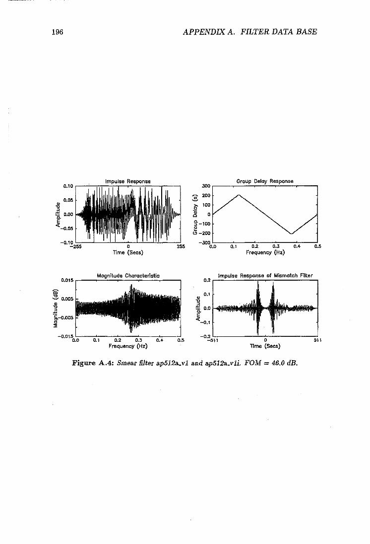
196 APPENDIX A. FILTER DATA BASE
0.10 r----'~:-:-r-':___,-..,....._'_:_:_-__r--...,
0.05 ~ :::l
i[ 0.00 E «-0.05
-0.10 1...-_....L._--!'-'-_-'---'-"':"';'.....I..!..l-__ ...1 -255 0 255
TIme (Sees)
Magnitude Characteristic 0.015 ,...----.-"---..--........ ---,...--..,
Iii' ~ 0.005
~ ;2 6,-O.OOS c :::;;
-0.015 L-_---' __ --'-__ ---'-__ -'-__ ...1
0.0 0.1 0.2 0.3 0.4- 0.5 Frequency (Hz)
Group Delay Response 300r----~---~--~~~--~----...,
"(jj" 200 ..... ~ 100
t!!5 0
g.-loo e (!) -200
-300~--~---~--~----~---...I
Q) "C
0.0 0.1 0.2 0.3 0.4- 0.5 Frequency (Hz)
0.2 Impulse Response of Mismatch Filter
0.1
~o.o~~.M. E «-0.1
-0.2 L-____ ---::...-..:~---_-~ -511 0 511
TIme (Sees)
Figure A.4: Smear filter ap512a..vl and ap512a_vli. FOM = 46.0 dB.

A.5. SMEAR FILTER CHARACTERISTICS 197
Impulse Response 0.08,-----:...---...,.-...:...-----,
<II "C ::J
0.04
~ 0.00
E <-0.04
-0.08 L:-:------....... ------~ -511 a 511
lime (Secs)
Magnitude Characteristic 0.01l ..----,-"----..--.....,----.----,
'CD' "C 0.02 ....... <II 'g-0.02 ::!:! c: g'-o.OIl ::i
-0.10 ":----:''--~:__--:-''::__---'---~ 0.0 0.1 0.2 0.3 0.4 0.5
Frequency (Hz)
s Group Delay Response
600,-----.~-~-~~--_._--,
~ 200
~ g- -200 E!
<.?
-600~-~--~--~--~-~ 0.0 0.1 0.2 0.3 0.4 0.5
Frequency (Hz)
0.2 Impulse Response of Mismatch Filter
0.1
-0=10~~------~0------~1~023
lime (Secs)
Figure A.S: Smear filter apl024a_vl and ap1024asli FOM = 54.8 dB.
Impulse Response 0.15,------'---.,.--'--------,
0.10
{l 0.05 ::J
~ 0.00
~-0.05 -0.10
-0.1.:5-~1":"1------.... 0-------5-'11
lime (Secs)
Magnitude Characteristic 0.3 ,-----r--==----.---......---..----,
'CD' 0.2
.:s 0.1 <II 'g 0.0 ::!:! 5,-0.1 o ::i-0.2
-0.3 ~_--''--_--L __ -'-__ ...... __ ...J
0.0 0.1 0.2 0.3 0.4 0.5 Frequency (Hz)
Group Delay Response 600,-----.--~-~-r"---~-___,
s ~ 200 Qi o
g- -200 E!
<.?
-600~--~--~--~---~-~ 0.0 0.1 0.2 0.3 0.4 0.5
0.15
0.10
{l 0.05 ::J
;!:; 0.00 Q..
~-O.OS -0.10
Frequency (Hz)
Impulse Response of Mismatch Filter
-0·~0':-:2:-::3~-----..... 0-------l...1023
lime (Secs)
Figure A.6: Smear filter ap1024d_v1 and ap1024ds1i, FOM = 41.3 dB.

198 APPENDIX A. FILTER DATA BASE
Impulse Response 0.06 ,..-----..:....--.,..---:-----___.
0.04
.:g 0.02 :::J i 0.00
~-0.02 -0.04
-0.061...-------....... ---------1
Q. :::l
-1023 o 1023 Time (Secs)
Group Deloy Response 1000r--~----~--~~~--~----~
~ -500 (!)
-10001...----~---~---~----~----I 0.0 0.1 0.2 0.3 0.4 0.5
Frequency (Hz)
Magnitude Characteristic 0.2 ,--........ -----..,.-----.-----.----.,
CD "C 0.1 '-'
Q)
-g 0.0,..._.
~ g-O.l
:::;;
-0.2 '----''-----'---......... ---'---.... 0.0 0.1 0.2 0.3 0.4 0.5
0.15
0.10
.:g 0.05
Frequency (Hz)
Impulse Response of Mismatch Noise
~ 0.00 r--IIIiIIII ••• ~-0.05
-0.10
-0. ~20':-4-=7-------0>--------2....J0 ... 7
Time (Secs)
Impulse Response 0.06 ...-------:.....--.,.---=---------., 0.04
.:g 0.02 :::J i 0.00
~-0.02 -0.04
-0.061...-------....... --------1 -1023 o 1023
Time (Sees)
Group Delay Response 1000r----~-~~~-~----r_--___.
..-.
..!!!" 500 f;' 4i c Q. :::I
o
~ -500 (!)
-1000L..--~~----~----~-~~----I 0.0 0.1 0.2 0.3 0.... 0.5
Frequency (Hz)
Magnitude Characteristic 0.01 ,--.....,--;......",--,.-----.-----..----,
..-. m ~ Q)
-g 0.00 :l::! c 01 t:I :::;;
-0.01 1...-__ '--___ "--_"--'--__ '--_ ___1
0.0 0.1 0.2 0.3 0 .... Frequency (Hz)
Magnitude Char. of Mismatch Noise 20r---~----------------------~
o Q)
"C -20 ;2 c g -40
:::!!
-60L..-------------------------~ 0.0 0.5
Frequency (Hz)
Figure A.7: Smear filter ap20483-vl and ap20483-vli. FOM = 48.8 dB.

A.5. SMEAR FILTER CHARACTERISTICS 199
Impulse Response 0.10 r------...:.---,,....-.:....------,
CD -0 ::l
0.05
~ 0.00 E <-0.05
-0.101...-------....... --------' -1023 0 1023
Time (Secs)
Group Delay Response 1000 r------.,-----r------r-----.-~-...,
C. ::J e -500
(.')
-10001...---~--~----~-~~---' 0.0 0.1 0.2 0.3 0.4- 0.5
Frequency (Hz)
Magnitude Characteristic 0.2 r----..---.;:......-,---..,.....--..----,
....... !g 0.1 -CD -g 0.0 ~ c: g'-0.1 ::i
-0.2 L:---::"":----::-'-::--~--"------l 0.0 0.1 0.2 0.3 0.4 0.5
CD -0
0.10
0.05
~ 0.00 c.
.i-o.os
Frequency (Hz)
Impulse Response of Mismatch Noise
-0·~20':-4:-::7-------0'--------2-.1047
Time (Secs)
Impulse Response 0.10 r----------.------------,
CD -0 ::J
0.05
~ 0.00 E <-0.05
-0.10 1.--______ ....... _____ ---1
-1023 0 1023
C. ::J & -500
Time (Secs)
-1 000 ":---::"":----=-'="---:::-'=----::'~--:-l 0.0 0.1 0.2 0.3 0.4 0.5
Frequency (Hz)
Magnitude Characteristic 0.06 r---.....,.---.;:......-,---..,.-----,..----,
....... 0.04 CD
~ 0.02 CD
-g 0.00"' •• ~
6r0•02 o ::i-O.04
-0.06 L-___ '--'-_~ __ ":_-__::_'":----'
0.0 0.1 0.2 0.3 0.5 Frequency (Hz)
20 Magnitude Char. of Mismatch Noise
..-.. CD 0 -0 -CD -0 -20 ::l ti c: CI I:]
::::E -40
-60 0.0 0.5
Frequency (Hz)
Figure A.8: Smear filter ap2048d_vl and ap2048dsli. FOM = 46.0 dB.

200 APPENDIX A. FILTER DATA BASE
Impulse Response 0.10 .------.;...-.-...--'---------.,
II) "0 ~
0.05
i 0.00 E <-0.05
-0.101.--------'---------' -1023 0 1023
lime (Sees)
Group Delay Response 800.-----r----'-r-~--~---~-_,
,..... ~ 400
Magnitude Characteristic 0.6 ....---,..---.-----r---__ ..---_,
CD 0 .. 4 ~ Q) 0.2 "0 ~
=2 0.0 Cl
~ -0.2
Q) "0
0.2
0.1
g 0.0 Q.
~ -0.1
Impulse Response of Mismatch Noise
-0320~4~7----------~0~-----------2~047
lime (Sees)
0.10,.-------.,----------,
Q) "0 ~
0.05
i 0.00 E <-0.05
-0.10 L-..--------'--------::' -1023 0 1023
Q. ::l e -400
(,!)
lime (Sees)
0.1 0.2 0.3 0.5 Frequency (Hz)
Magnitude Characteristic 0.4 r------.-~---r--.....,..--..,......---.
~ 0.2 ...... Q)
"g 0.0 :!: t:
g'-0.2 ::E
-0.4 '-_ ....... __ -:--__ -:-'::--_--L._---' 0.0 0.1 0.2 0.3 0.4 0.5
m "0 .....
10
~ -10
:E c: g' -30
::E
Frequency (Hz)
Magnitude Char. of Mismatch Noise
-50'-------------------------' 0.0 0.5
Frequency (Hz)
Figure A.9: Smear filter ap2048h_vl and ap2048h_vli. FOM = 35.7 dB.

A.5. SMEAR FILTER CHARACTERISTICS 201
Impulse Response 0.04 .------~-...--....:-------,
CD "1;1 :::I i 0.00 E «-0.02
-0'':~0'-:2~3------''''0-------I1023
Time (Secs)
Group Delay Response 1000 r-----r---;....,.-,;....--...-~-...,....---",
0.1 0.2 0.3 0.4 0.5 Frequency (Hz)
Magnitude Characteristic 0.02 .------.-=---,-----.---.....,....---,
-~ 0.01 ...., CD -g 0.00
;!: c: 0'1 ~-o.01
-0.02 '::----I.-:---~:__--':::__---'-----' 0.0 0.1 0.2 0.3 0.4 0.5
Frequency (Hz)
O.OB Impulse Response of Mismatch Noise
0.04 CD
"1;1 :::I i 0.00
~-0.04 -O.OB
-2047 0 2047 Time (Secs)
Impulse Response 0.04 .------~-...---------...,
0.02
-0.04 I...-______ -'--______ ..J
-1023 0 1023 Time (Secs)
Group Delay Response 1000~--~--~--.-----~----r---_,
0-:::I
o
e -500 C)
-1000 I...-_-J. __ --'-__ -':::__---'--~
~O ~1 ~2 ~3 OA Frequency (Hz)
Mcu,nlIuoe Characteristic 0.02 .......... --....-=---...,.--.....,..--...,...--...,
-~ 0.01 ...., CD -g 0.00 ;!: c: go-O.Ol :::i!
-0.02 I...-_--"_~__L __ -':::__-...... --....
0.0 0.1 0.2 0.3 0.4 0.5 Frequency (Hz)
Magnitude Char. of Mismatch Noise
- 10 III "1;1 -CD -10 "1;1 :::I
;!: c: Cl -30 0
:::i!
-50 0.0 0.5
Frequency (Hz)
Figure A.I0: Smear Iilter ap2048sa-vl and ap2048sa-vli. FOM = 62.5 dB.

202 APPENDIX A. FILTER DATA BASE
Impulse Response 0.06 r-------...,.--------, 0.04
~ 0.02 :I
~ 0.00
.!f-O.02
-0.04
-0.06 1..---------'---------' -1023 o 1023
lime (Sees)
Group Delay Response 1000 r-----.--;.....,--:::-.....,.~-_._--.....
Ui' ....... 500
~ Qj Q
Co :::I
o
2 -500 C!)
-1000 t.-__ '--__ '--__ '--__ '--_~
0.0 0.1 0.2 0.3 0.4 0.5 Frequency (Hz)
Magnitude Characteristic 0.02 r----.-~--r--.....,..--...... --.....
Q)
-g 0.00 :t:! !::: en ~-0.01
-0.02 I...-_--' __ --I. __ -'-__ -'-__ ...J
0.0 0.1 0.2 0.3 0.4 0.5 Frequency (Hz)
0.10 Impulse Response of Mismatch Noise
0.05 Q)
-g ~ 0.00
.!f -0.05
-0. !.020':-4~7-------0'-------2""047
lime (Sees)
Impulse Response 0.06 r-----"---..,......-'------.., 0.04
~ 0.02 :I
~ 0.00
.!f-O.02
-0.04
-0.06 ~------~------~ -1023 0 1023
lime (Sees)
Group Delay Response 1000 r---.---..;..-,..---~--.------,
Co :::I
o
e -500 C!)
-1000 1..---'----"----=--"----"-----' 0.0 0.1 0.2 0.3 0.4 0.5
Frequency (Hz)
Magnitude Characteristic 0.02 r----,_~--r--....,.---.---.....
i 0.01 ....... QI
-g 0.00 :t:! !:::
g-O.Ol :il
-0.02 1...-_---"'--___ '---_-'--1..-__ '--_--'
0.0 0.1 0.2 0.3 0.4 0.5 Frequency (Hz)
10 Magnitude Char. of Mismatch Noise
-40I...----------~--------...J 0.0 0.5
Frequency (Hz)
Figure A.11: Smear filter ap204Bsh_v1 and ap204Bsh_v1i. FOM = 64.1 dB.

A.5. SMEAR FILTER CHARACTERISTICS 203
Impulse Response 0.08 .---------..,.....~-----.,
CI)
" ::I
0.04
~ 0.00 E <-0.04
-O.OB I:-::-::------"'-------.J -1023 0 1023
TIme (Sees)
Group Delay Response 1000 ,-----.--;.....,.-..:...--..,....:...---.----,
Co ::J E! -SOO
(!)
0.1 0.4 0.5
Magnitude Characteristic O.~,---~-~~----..,..---.----~
CD 0.02
~ 0.01 Q)
-g 0.00 :t:: 6,-0.Q1 o
:::1':-0.02
-0.03 '-:----::"":---:-'-:----::-'::----:-'----:l 0.0 0.1 0.2. 0.3 0.4 O.S
0.15
0.10
~ 0.05 ::l ~ 0.00
if-o.os
Frequency (Hz)
Impulse Response of Mismatch Noise
-O·'!..5204':-7------..... 0-------2....1047
Time (Secs)
Impulse Response O.OB .------..:...-:...--..--~----___.
CI)
" ::I
0.04
~ 0.00 E <-0.04
-0.08 '-------"'----------' -1023 0 1023
Time (Secs)
Group Delay Response 1000,-----.--;.....,.-..:...--..,....:...---.------,
3 500
-1000 '----'----'----'----::-'------' 0.0 0.2 0.3 0.5
_ 0.01 tIl
" ....... ~ 0.00
:e I::
8'-0.01 :::I':
Frequency (Hz)
Magnitude Characteristic
-0.02 '-_-J.-:--~~:--_-:"'::--_~_--:-' 0.0 0.1 0.2 0.3 0.4 O.S
Frequency (Hz)
Magnitude Char. of Mismatch Noise 10.--~~----~----~~----_r--.,
-CD o
~ -10 Q)
-g -20 -'§, -30 o
:::I': -40
-50'--------------------------....1 0.0 0.5
Frequency (Hz)
Figure A.12: Smear filter ap2048sds1 and ap2048sd_v1i. FOM = 57.1 dB.

204 APPENDIX A. FILTER DATA BASE
Impulse Response 0.1 0 r-----:---:--"'--:-""!'"'"--::--::--:-~_:__-_,
Q) "0 :::I
0.05
~ 0.00
~ -0.05
-0.10 L-_..:......;.....:........:.........:...-1-..l-.:....;... ___ ...:...._ ... -1023 0
...... II) ...... >, 0 1) c 0.. :J
1000
500
0
2 -500 (!)
TIme (Secs)
Group Delay Response
-1000L---~_:__-_7_:_-~-:--~--~ 0.0 0.1 0.2 0.3 0.4 0.5
...... 0.01 CD ~ ~ 0.00
:E c 8'-0.00 :::s
0.15
0.10
~ 0.05
.g 0.00 0..
~-0.05 -0.10
Frequency (Hz)
Magnitude Characteristic
Impulse Response of Mismatch Noise
-0.15 L-______ -'-______ ...I
-2047 0 2047 TIme (Secs)
0.10 ...... --:--...,.,..-:-=---.--..:---"....,..--..,
Q) "0 :::I
0.05
~ 0.00 0.. E «-0.05
o 1023 TIme (Secs)
Group Delay Response 1000.--~--~---r"'--~----~
~ 500
~ ~ 0 0.. :J 2 -500 (!)
-1000~-_7-:--~-:--~-:--~--~ 0.0 0.1 0.2 0.3 0.4 0.5
Frequency (Hz)
Magnitude Characteristic 0.015 .----,-"--.....,.---.----,...---,
CD .:5!. 0.005
Q) "0 :J
:0= g.-0.005 o :::s
Magnitude Char. of Mismatch Noise 10r---~-------------------___,
CD 0 "0 ...... Q) -10
"0 :J '2 -20 0>
~-30
-40L-------------------------...I 0.0 0.5
Frequency (Hz)
Figure A.13: Smear filter ap2048shsl and ap2048sh_vli. FOM = 57.7 dB.

A.5. SMEAR FILTER CHARACTERISTICS 205
Impulse Response 0.15 r----.....::....--.,--...:..------,
0.10
~ 0.05 ::J
~ 0.00
~-0.05 -0.10
-0. ~O '-23-=-------'-0-------,-'023
lime (Sees)
800
..... ~ 400
Group Delay Response
A A A A
(j' 1) 0 0 Q. :::J
'-400 e (!)
-800 V V V V ~ V V 0.0 0.1 0.2 0.3 0.4 0.5
Frequency (Hz)
Magnitude Characteristic 0.03 .-----,r--"----r---.,..--~--..,
'iii' 0.02
.:e 0.01 Q)
-g 0.00 ;!:
6,-0.01 o
:::E-0.02
-0.03 '------'----'-----'----'----' 0.0
0.15
0.10
~ 0.05 ::J
~ 0.00
~-0.05 -0.10
0.1 0.2 0.3 0.4 0.5 Frequency (Hz)
Impulse Response of Mismatch Noise
-0.:.104':-:-::7------.... 0--------'2047
lime (Sees)
Impulse Response 0.15.---------.---------,
0.10
~ 0.05 ::J
~ 0.00
~-0.05 -0.10
-0.15 '---------'--------'
..... ~ (j' 1) 0 Q. :::J 0 ...
(!)
-1023 0
800
400
0
-400 r
-800 0.0
A
V
lime (Secs)
Group Delay Response
A A A A
V V V V .V 0.1 0.2 0.3 0.4
Frequency (Hz)
1023
A
V 0.5
Magnitude Characteristic 0.02 r------.-"----r---...--~--..,
...... !g 0.01 ...., QI
-g 0.00 ;!: C 0> ~-o.ol
-0.02 '-----''---'----'------'----'----' 0.0 0.1 0.2 0.3 0.4 0.5
Frequency (Hz)
Magnitude Char. of Mismatch Noise 10~~~--~r-~--------~--..,
'iii' 0 .:e
CD -10 "0 ::J
~-20 0>
~-30
-4O'------------~-----------' 0.0 0.5 Frequency (Hz)
Figure A.14: Smear filter ap2048sp_vl and ap2048sp_vli. FOM = 57.0 dB.

206 APPENDIX. A. FILTER DATA BASE
0.10 ;----------...----------,
q) -0 ::l
0.05
'[ 0.00 E <-0.05
-0.101--------"'---------' -1023 a 1023
Time (Sees)
Group Delay Response looor--~~-~--~--~--~
a. :J E -500
(.!)
-1000 I--_--''---_ ....... __ ......... __ ....... __ ..J 0.0 0.1 0.2 0.3 0.4 O.S
Frequency (Hz)
Magnitude Characteristic Br---~-~~---~---~----~
'iii' 6
~ 4 Q)
-g 2 ~ a. 0
~ -2
-41-----'--~---~--~~---..J 0.0
0.15
0.10
~ 0.05
~ 0.00 a. ~-0.05
-0.10
0.1 0.2 0.3 0.4 0.5 Frequency (Hz)
Impulse Response of Mismatch Noise
-0'~20:-4:-::7-------::-0------~
Time (Secs)
Impulse Response 0.10 r-----'---..,--'-------,
q) -0 :J
O.OS
'[ 0.00
E <-0.05
-0·!.?,0'-:2:::3------~0-------:-'1023
Time (Sees)
Group Delay Response 1000r---,--~--_r--~--,
"iii' ....... 500 i;' qj c a. ::l
o
2 -500 (.!)
-1000 '":---::-'--~:__-_:"'::__-_:_'_:'--:_' 0.0 0.1 0.2 0.3 0.4 0.5
Frequency (Hz)
Magnitude Characteristic 4r---~-~~--~-~-r----,
'iii' 2 ~ 0
II)
~ -2
a. -4 o
::E -6
-BI----....... ---~---~--~----...I 0.0 0.1 0.2 0.3 0.4 0.5
Frequency (Hz)
Magnitude Char. of Mismatch Noise
-SOI--~---------------------' 0.0 0.5
Frequency (Hz)
Figure A.1S: Smear filter nf2048&-vl and nf2048a_vli. FOM = 33.2 dB.

A.5. SMEAR FILTER CHARACTERISTICS 207
Impulse Response 0.04 ...------:...--...-.....:....------.
<Il "0 :::J
0.02
~ 0.00
E <-0.02
Group Delay Response 2000...---~~-~-~~~~~-~
3 1000
~ ~ 0 0.. :::J E -1000 c:>
-0.04 L..-______ -'--_____ ____l -2000 L..... ____ .....::._--' __ --'-__ --'-__ ...J
0.1 0.2 0.3 0.4 0.5 -2047 0 2047 0.0 lime (Secs)
Magnitude Characteristic 0.10 r--~r--=----r----.-----.---.,
Ul 0.05 ~
Ql o.oot-__ "0 :::J ~-0.05 CI
~-0.10
-0.15 L..-_--'-'-_~ __ _'__---I.-'-_ ____l
0.0 0.1 0.2 0.3 0.4 0.5 frequency (Hz)
0.15
0.10
.g 0.05
frequency (Hz)
Impulse Response of Mismatch Filter
~ 0.00 1-.......... """" .. iIIIIIII 0..
~-0.05 -0.10 -0.15 L.. ______ -'-_____ ---l
-4095 0 4095 lime (Secs)
Figure A.16: Smear filter ap4096a...vl and ap4096a...vli. FOM = 52.3 dB.
Impulse Response O.OB .--------.,;~-.,....~--------.
0.04
Group Delay Response 2000r--~r---~-~~~-~r_-~
3 1000
~ ~ a c.. :::J E -1000
c:> -0.08 L..... ______ '"'--______ ...J -2000 L.._...-!!J'--_--'-__ --'-__ !!.!... _ ____l
-2047 a 2047 0.0 0.1 0.2 0.3 0.4 lime (Sees) frequency (HZ)
Magn1tude Characteristic 0.2 r-----,,.......~--.---,..---.---..., 0.10
Impulse Response of Mismatch Filter
Ul 0.1 "0 ...."
Q) 0.0 "0 :::J
~-o.1 CI
~-0.2
Ql "0
0.05
~ 0.00 c.. E <-0.05
0.5
-0.3 'c-_--''-_~ __ --'-__ ........ _ ____l -0.101..--------'-----------l 0.0 0.1 0.2 0.3 0.4 0.5
frequency (Hz) -4095 o
lime (Secs)
Figure A.17: Smear filter ap4096d_vl and ap4096ci.vli. FOM = 45.0 dB.
4095

208
Impulse Response O.OB .------'---.---'-------..,
(I) -c :::J
0.04
~ 0.00 E <-0.0 ...
APPENDIX A. FILTER DATA BASE
~ 1000
~ "ii a Cl c.. 5 -1000 ...
(.!)
-0.08 L..-____ ~_""--______ ..... -2000 L...-_--'-__ ........ __ --'-__ -'-_--'
-2047 a 2047 0.0 0.1 0.2 0.3 0.... 0.6 TIme (Sees) Frequency (Hz)
Magnitude Characteristic 0.3 .-----.-.;;;..-...... ----,---....,..--..,
CD 0.2
~ 0.1 (I)
-g 0.0 ;!;:! a.-0•1 a ::i-0.2
-0.3 L..-_--' __ --'-__ ......... __ -'-__ -' 0.0 0.1 0.2 0.3 0.... 0.5
Frequency (Hz)
(I) -c :::J
O.OS
0.0'"
~ 0.00 E <-0.04
Impulse Response of Mismatch Filter
-o·~~L..-5------0"'----------'4095
TIme (Sees)
Figure A.1S: Smear filter ap4096h_v1 and ap4096h_v1i. FOM = 43.1 dB.
Impulse Response 0.03 .------'---.---'------..,
0.02
{l 0.01 ::J
~ 0.00 c.. ~-0.01
-0.02 -0.03 L..-______ ......... _______ -'
-2047 a TIme (Sees)
2047
Magnitude Characteristic 0.0'" .------,r--.;;;..--,--.....,.---,---..,
~ 0.02 '-" (I)
-g 0.00 ;!;:! c: C1 ~-0.02
-0.04 '::----:"-:----::""-:---~_--'----' 0.0 0.1 0.2 0.3 0.... 0.5
Frequency (Hz)
Group Delay Response 3000.------.----T----r'---~-~
:§: ~ 1000 "ii Cl
g.-lOaD e
(.!)
-3000 L----:-'-_-'='='-_~-_:''----:l 0.0 0.1 0.2 0.3 0.4 0.6
0.06
0.04
~ 0.02 :::J
~ 0.00
~-0.02 -0.04
Frequency (Hz)
Impulse Response of Mismatch Filter
-0.06 L..-_______ "'_ _________ ____'
-4095 a 4095 TIme (Sees)
Figure A.19: Smear filter ap4096sa_v1 and ap4096sa_vli. FOM = 52.6 dB.

A.S. SMEAR FILTER CHARACTERISTICS 209
QJ "'C :::I
0.04 ,.-----'---.,--....;.-------,
0.02
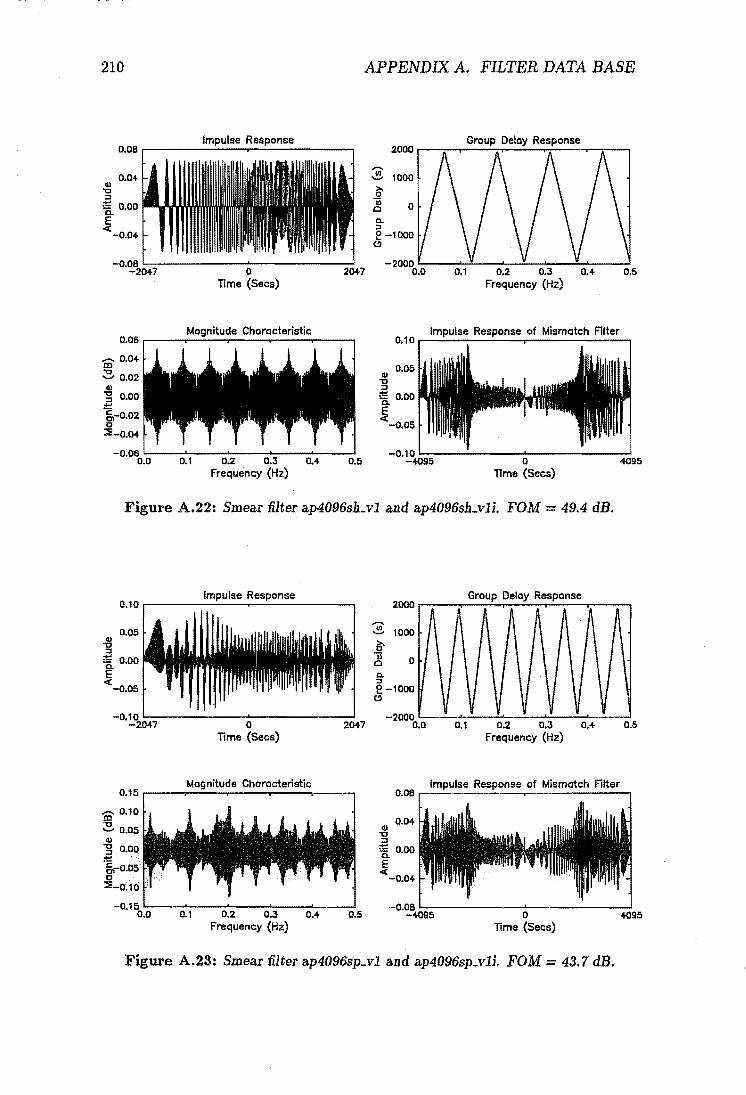
210 APPENDIX A. FILTER DATA BASE
Q) "t:I :J
Impulse Response o.o6,..-----:...--..,.-...:------..,
0.04
'[ 0.00
E <-0.04
::§: 1000
~ ~ 0 Q. ::> e -1000 (!)
-0·~204'-::-7------..... 0-------:-'2047 -20000 ..... 0--0 .... -1.:.--0 .... ,2--'---0 ..... 3-.....:. .... 0 ..... 4--0-'.5
Time (Sees) Frequency (Hz)
Mognitude Characteristic 0.06 r-----.-::..--,.---..--....... --..,
'@' 0.04
~ 0.02 Q)
'g 0.00 ~
6,-0.02 c ::i-0.04
-0.06 '-----'"---'----t.----'----' 0.0 0.5
Q) "t:I :J
0.10
0.05
'[ 0.00
E <-0.05
Impulse Response of Mismatch Filter
-0.10 L--__ ....:-___ -'--______ -'
-4095 0 4095 Time (Sees)
Figure A.22: Smear filter ap4096sbsl and ap4096sbsli. FOM = 49.4 dB.
Impulse Response 0.10 r-----'---...---------,
0.05 ~ :J
'[ 0.00 E <-0.05
-0. !.0204~7------":-0-------2 ... 047
Time (Sees)
Magnitude Characteristic 0.15 r----,----,.---r--__ ---,
'@' 0.10
~ 0.05 Q)
'g 0.00 ~ 6,'-0.05 c ::i-o.10
-0.15 '----:'~-__:_'"---:-'----'---..... 0.0 0.1 0.2 0.3 0.4 0.5
Frequency (Hz)
2000
:E 1000 i;' ~ 0 Q. :l e -1000
(!)
-2000 0.0
Q) "t:I
0.06
0.04
.g 0.00 a.
~ -0.04
Group Delay Response
A A A A A A A A
V V V V V V V 0.1 0.2 0.3 0.4 0.5
Frequency (Hz)
Impulse Response of Mismatch Filter
-0.06 '--______ -'--______ ..J
-4095 o 4095 Time (Secs)
Figure A.23: Smear filter ap4096spsl and ap4096sp_vli. FOM = 43.7 dB.

A.5. SMEAR FILTER CHARACTERISTICS 211
_______ ~rm~pu~r~se:!~~~------~ O.OB r-
~ 1000 1;-~ 0 0-:::l e -1000
<.!)
-0·~204L....:-7-----------'-""'0------------l2047 -20000.1...0----...... ---0 ..... 2-----0..,..3-----'------'
lime (Secs) Frequency (Hz)
Magnitude Characteristic B,----~--~-T-----r----~--~
m 6
.:s 4 Q)
"g 2 ~ en 0 o
:::i< -2
-4~--~---~~--~~---'---~ 0.0 0.1 0.2 0.3 0.4- 0.5
Frequency (Hz)
41 "C :::l
0.10
0.05
~ 0.00 E <-0.05
Impulse Response of Mismatch Filter
-0.10 1..--------------'-------------..1 -4095 0 4095
lime (Sees)
Figure A.24: Smear filter nf4096a_vl and nf4096a..vli. FOM = 32.7 dB.
Impulse Response 0.03 ;----------'----...---'----------'"1 0.02
~ 0.01 :::l
~ 0.00
Jij-0.01
-0.02
-O·~4091...-5--------0"-----------I4095
lime (Sees)
lAagnitude Characteristic 0.2 ,-----,..."..::...---..--....... ----,..-r-----,
m 0.1
.:s 0.01-_. Q)
"g-o.1 :!:! 5,-0.2 o
:::i<-o.3
-0.4 ':-----'------'---....... -----'----1 0.0 0.1 0.2 0.3 0.4 0.5
Frequency (Hz)
Group Delay Response ~r----r--~~~~~~T----,
~ 2000
6-~ 0 0-:::l e -2000
<.!)
~I..---~~--~----~----~--~ 0.0 0.1 0.2 0.3 0.4 0.5
0.15
0.10
~ 0.05 :::l
Frequency (Hz)
Impulse Response of Mismatch Filter
~ 0.00 1-..... ___ ....
Jij-0.05
-0.10
-o.~~ 1...19:-1:---------"":'0--------~a..J191
lime (Sees)
Figure A.25: Smear filter ap8192a_vl and ap8192a..vli. FOM = 45.6 dB.

212 APPENDIX A. FILTER DATA BASE
0.02 ...-------'----,....-'------.....,
0.Q1 Q) "0 ::l
~ 0.00 E <-0.01
~ fj'
Q.l Q
a. ::l
E CI
-0.021...--------'------........ -8 191 0 8 191
lime (Sees)
Magnitude Characteristic 0.15.-----.---.----,---.....-----,
~0.05 ' ... ~ ~--~II .... ----.... ~II .... ~ -g-o.o5 :!: c: 0> jl-0.15
-0.250.01...--0='".":-1 ---:0 .. .2--0='".3------::0"'":.4---:-1 0.5 Frequency (Hz)
10000 Group Delay Response
0
-10000 0.0 0.1 0.2 0.3 0.4 0.5
Frequency (Hz)
0.3 Impulse Response of Mismatch Filter
0.2
~ 0.1 I J ~ 0.0 J a. I I r E <-0.1
-0.2
-0.3 -16383 0 16383
lime (Secs)
Figure A.26: Smear filter ap16384a..vl and ap16384a..vli. FOM = 49.8 dB.
Impulse Response 0.04 .....----......;.----,,...-'--------,
0.02 ~ ::l
~o.oo E <-0.02
-o.~ 191 o lime (Sees)
a 191
Magnitude Characteristic 0.15 ..---......... ---'=---.----.---.-----.
'iii' 0.10
~ 0.05 Q)
-g 0.00 :!: g.-0.05 o ::;;-0.10
-0.15 I...-_ ........ __ -'-__ ..L-__ "--_---l
0.0 0.1 0.2 0.3 0.4 0.5 Frequency (Hz)
0.2 Impulse Response of Mismatch Filter
0.1
I. Il> "0
~ 0.0 ~". a. co.,.. I .. E <-0.1 - 1
I"",
-0.2 L::-::-::------~-----""':'_' -16 383 0 16 383
lime (Secs)
Figure A.27: Smear filter ap16384hsl and ap16384h_vli. FOM = 46.4 dB.
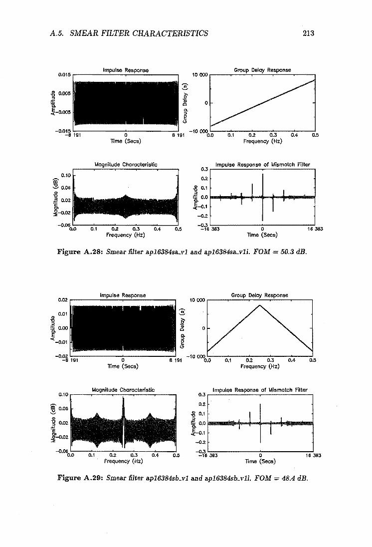
A.5. SMEAR FILTER CHARACTERISTICS 213
0.015
{J 0.005 ::::t ~ Ci. ~-o.o05
0.10 Iii' .:2. 0.06
(]) "0 ~ 0.02 'c 01 :§l-o.02
Impulse
~ f;'
1i) Q
Q. ::::t e (!I
0 8191 lime (Secs)
Magnitude Characteristic
0.1 0..2 0.3 0.4 Frequency (Hz)
10000 Group Delay Response
0
-10000 0.0 0.1 0.2 0.3 0.4 0.5
Frequency (Hz)
0.3 Impulse Response of Mismatch Filter
0.2
-8 0•1 I J ~ 0.0 ~ .... I~J~f-I·+--+-+ .. 1lllllllta1lllllllrj Q. T 1 l' ~-0.1
-0.2
-0.3 ~~----~-----~. -163S3 0 16383
lime (Sees)
Figure A.28: Smear filter ap16384sa...vl and ap16384sa_vli. FOM = 50.3 dB.
(])
"0
0.02 ....----......:.----......--=--------,.
0.D1
Group Delay Response 10 000 ,-----.---=-..,.--.....::....--,...:---r----,
~ 0.00 Q.
o E «-0.D1
-O.OZ 1..-_____ ___' ________ --1 -10 000 1....-_-'" __ -'-__ -'--__ '--_........1
-8 191 0 8 191 0.0 0.1 0.2 0.3 0.4 0.5 lime (Sees) Frequency (Hz)
Magnitude Characteristic 0.10 ....----r-...::'---.---.....---.-----. 0.3
0.2
Impulse Response of Mismatch Filter
-8 0.1 l i 0.0 _-.iII+-d-+~ ...... f-... J~IjIIIIIlII_BI ~-0.1 I I
-0..2
-0.3 '-:-:-:------~------........I -16383 0 16383
lime (Sees)
Figure A.29: Smear filter ap16384sbsl and ap16384sb_vli. FOM = 48.4 dB.

214 APPENDIX A. FILTER DATA BASE
Impulse Response 0.03....------=-----.-:------,
0.02
.g 0.01 :::l
~ 0.00
~-o.01 -0.02
Group Delay Response 10 000 ...---....---':'-,...---='--..,....:.--,...--....,
....... ~
~ 1i.'i 0 C
0-j
e (!)
-O'£i 191 o -10 000 I..-_---'-__ -'-__ -'--__ '--_......J
8 191 0.0 0.1 0.2 0.3 0.4 0.5 Time (Sees)
Magnitude Characteristic 0.06 ,....----,.---''---,...--..,------,r---.
'iii' 0.04
~ 0.02 Q)
-g 0.00 :!: 6,-0.02 o :::E-0.04
-0.06 1..-_-'-__ -'-__ "'-__ '--_ .......
0.0 0.1 0.2 0.3 0.4 Frequency (Hz)
0.3
0.2
Frequency (Hz)
Impulse Response of Mismatch Filter
.g 0.1 l.1 ~ O.O .... r-+-+.....;-I .... ·-B1 ~-0.1
-0.2 -0.3 L-_____ --' ______ -i
-16383 0 16383 Time (Secs)
Figure A.SO: Smear filter ap16384sd_v1 and ap16384sd_v1i. FOM = 48.6 dB.
0.04 ...------:.----.--.:'-------.,
0.02 .g :::I
~O.oo E <-0.02
....... ~
~ 1i.'i C 0-:::l e (!)
-0.04 '----------'------...... 8191 -8 191 0
'iii' 0.02 ~ Q) 0.00 -0 :::l
=E-o.02
8' :::E-O.04
Time (Sees)
Magnitude Characteristic
0.1 0.2 0.3 0.4 0.5 -0.06 L.:---::'--:---~-___:::".:_-__:''----='
0.0 Frequency (Hz)
10000 Group Delay Response
0
-10000 0.0 0.1 0.2 0.3 0.4 0.5
Frequency (Hz)
0.3 Impulse Response of Mismatch Filter
0.2
.g 0.1 I I :::I
~ 0.0 I I E <-0.1
-0.2
-0.3 -16383 0 16383
Time (Sees)
Figure A.Sl: Smear filter ap16384sh_v1 and ap16384shs1i. FOM = 49.1 dB.

A.5. SMEAR FILTER CHARACTERISTICS 215
Impulse Response 0.0& ,....----.....;.---,-~------,
0.04
~. 0.02 ::J
~O.oo Co
~-0.02 -0.04
-0.0& '-------........ --------1
,...... -!!,
fi' '1ii Q
Co :::I e (!)
-8191 o 8 191 Time (Sees)
Magnitude Characteristic 0.10 ,---.......,.---::.......-,----.----,----.
~ 0.05 ~
Q)
-g 0.00 ~ c: 8'-0.05 :::l:
-0.10 '---....... ---'----'----'-----1 0.0 0.1 0.2 0.3 0.4 0.5
Frequency (Hz)
2.000
-8000 0.0
0.2
0.1 III
" ~ 0.0 Co E <-0.1
Group Delay Response
A A A A A
V V V V V 0.1 0.2 0.3 0.4 0.5
Frequency (Hz)
Impulse Response of Mismatch Filter
~·f61...38-3--------'-0------1--16 383
Time (Secs)
Figure A.S2: Smear filter ap16384sp_vl and ap16384sp_vli. FOM = 46.7 dB.
0.02 Q)
" ::J
~ 0.00
~ -0.02
-0.04 '--------''--........ --------' -8191 0 819t
Time (Sees)
Magnitude Characteristic 6,----.......,.'--~-,----~---r_--_.
-8 000 '--_---'" __ -'-__ -'-__ "'-_--1 0.0 0.1 0.2 0.3
0.04
0.02 Q)
" :::I
~ 0.00 E <-0.02
Frequency (Hz)
Impulse Response of Mismatch Filter
o Time (Sees)
Figure A.SS: Smear filter nf16384a..vl and nf16384a..vli. FOM = 32.9 dB.


Appendix B
Steepest descent gradient algorithm
B.l Introduction
This appendix describes how the steepest descent gradient algorithm can be used to determine the coefficients of the Wiener desmear filter (refer to section 2.5). It also examines the convergence properties of this algorithm and shows that when the magnitude characteristic of the smear filter is fiat, the steepest descent gradient algorithm converges rapidly to the optimal solution.
We denote the impulse response of the smear filter by h8(n), and the impulse response of the desmear filter by hd( n). We assume that the desmear filter is to be implemented as an Nd-tap FIR filter and represent the coefficients of this filter by the position vector
(B.I)
where the superscript T denotes transpose, and hd( i) is the gain of the i'th tap of the Wiener filter.
The optimization problem involves locating that value of hd that minimises the squared error function
(B.2)
where 6(n - D) is the desired impulse response of h8(n) in cascade with hd(n). The value of hd that minimises equation (B.2) is denoted by h~*), and the estimate for h~*) after i iterations of the gradient algorithm is denoted by h~).
B.2 Algorithm
The steepest descent gradient algorithm is listed in figure B.1.
217

218 APPENDIX B. STEEPEST DESCENT GRADIENT ALGORITHM
Step 1 of this algorithm normalises the impulse response of the smear filter to unit energy, provides an initial estimate for h~*), denoted by h~O), and initialises the control variables used in the algorithm. Fortunately, the accuracy of the initial estimate h~O) will not affect the minimum to which the algorithm
... ... "'(0) converges, because E(hd) is a concave function of hd. Therefore, hd has been simply set to O. (The accuracy of h~O) will, however, affect the number of iterations required for convergence.)
Step 2 of the algorithm updates the current estimate for h~*) (h~i») by locating the minimum of E(hd) along the path
(B.3)
In this equation, p is a scalar variable that controls the distance moved along path i1(i), and VE(h~i») is the gradient of E(hd) at h~i) and points in the direc-tion of the maximum rate of change of E(hd). V E(h~i») is defined as
VE(h~i») = [a(i)(O) a(i)(l) ... a(i)(Nd -1) ]T (BA)
where
(B.5)
The value of p that minimises E(r(f») is denoted by Pmm and can be found by substituting equation (B.3) into equation (B.2) and differentiating with respect to Pi i.e,
E(h~;) + pVE(h~»)) = .f;~ (8(n - D) _ :~' h.(n _ k)(h~)(k) + pa(i) (k))) 2
(B.7) Differentiating equation (B.7) with respect to p, equating to zero, and solving for Pmm yields (after some manipulation)
1 2:f,:;l (a(i) ( k)) 2
Pmm = ---------...:.--...:.-.---..",. 22:~=_oo (2:f,:;l hs(n - k)a(i)(k))
2 (B.8)
Thus, the updated estimate for h~*) is given by
h~i+l) = h~i) + Pmm V E(h~») (B.9)
Step 2 of the algorithm is repeated until a sufficiently accurate estimate for h~*) is obtained or the loop counter i exceeds 200. An accurate estimate for h~*)

B.2. ALGORITHM
Step 0 Start
Step 1 Initialisation
Scale hs ( n) to have unit energy.
h~O) = 0 IIV E(h~O»)112 = 2.0
f = 5 X 10⁻³
i=O
Step 2 DO WHILE (IIV E(h~i»)112 > f and i < 200)
Compute [V E(h~i»)]
Step 3
Pmm = mjn {E (h~i) + P [V E(h~i»)])} h~i+l) = h~i) + Pmin V E(h~i))
~-------------= IIV E(h~i»)112 = [V E(h~i»)] [V E(h~i») t i=i+1
END DO
219
Figure B.1: Steepest descent gradient algorithm for computing the Wiener desmear filter.
is detected by comparing the euclidean length of the gradient vector against an acceptably small error bound f. The euclidean length of the gradient vector is defined as
IIV E(h~i»)112 = [V E(h~i»)] [V E(h~i»)t = Nfl (a(i)(k))2 . k=O
(B.1O)
and approaches the value zero as h~i) approaches h~*). (The value for € is set to 5 X 10⁻³ in figure B.1. Its value assumes that the impulse response hs ( n) has unit energy.) An upper limit on the loop counter value is required because some problems are very poorly conditioned for the gradient algorithm, causing the algorithm to converge very slowly.
Finally step 3 of the algorithm outputs the computed desmear filter coefficients h~), the number of iterations taken by the algorithm to converge, and the value of IIV E(h~i»)112'

220 APPENDIX B. STEEPEST DESCENT GRADIENT ALGORITHM
B.3 Convergence
To examine the convergence properties of the gradient algorithm, it is useful to rewrite equation (B.2) using matrix notation. Thus,
where
00 ( Nd-1 )'2 E = n~oo 8(n - D) - t; h~i)(k)hs(n - k)
00 Nd-1 00
- L 82(n - D) - 2 L h~i)(k) L hs(n - k)8(n - D) n=-oo ],:=0 n=-oo
+ J;~ (11
h\i) (k)h.(n - k)) 2
_ 82(n _ D) - 2 [h~i)]Tb+ [h~i)]T Ah~i)
(B.ll)
(B.12)
(B.13)
h~i) _ [h~i)(O) h~i)(I) h~i)(2) ... ' h~)(Nd _ 1) ]T (B.14)
b - [hs(D) hs(D - 1) hs(D - 2) ... hs(D - Nd + 1) ]T (B.15)
Rs(O) Rs(l) Rs(2) Rs(Nd - 1)
A -R~(O)
The Nd X Nd matrix defined in equation (B.16) is called the autocorrelation matrix and the elements Rs(k) are the autocorrelation function of hs(n). This matrix is a positive definite symmetric Toeplitz matrix. The positive definite property of the autocorrelation matrix can be easily be proved by equating equivalent terms in equation (B.13) and equation (B.12): i.e.,
A property of positive definite matrices is that they are nonsingular, and therefore, they have a unique inverse [Burden et al., 1981].
~ ~
The optimal Wiener filter h* can be found by setting the gradient of E(hd) to zero and solving for h~*). Thus
['\7 E(hd)] - -2b + 2Ahd ::} h~*) _ A-1b
(B.17)
(B.IS)

B.3. CONVERGENCE 221
Although equation (B.18) could be used directly to solve for h~*), the difficulty of inverting the large Nd x Nd autocorrelation matrix made us prefer the gradient algorithm. Our current interest with equation (B.18) is that it provides insight into the convergence of the gradient algorithm.
lithe estimate for h~*) is h~), then the direction we should move in to locate h~*) in a single iteration is
(B.19)
(B.20)
However, using the gradient algorithm the direction we actually move in is
(B.21)
Solving equation (B.21) for h~i) and substituting this into equation (B.20) yields
(B.22)
From equation (B.22), it is evident that the gradient vector points directly at the optimum if and only if A is a diagonal matrix of the form
A=aI (B.23)
where I is the identity matrix and a is a scalar constant. When the smear filter hs ( n) approximates an all-pass filter (as is the case for
an all-pass smear filter designed using the window method), the autocorrelation function of hs(n) is approximately
(B.24)
Hence, for this case, the autocorrelation matrix is approximately
(B.25)
and the gradient algorithm converges very rapidly to the optimal solution. Typically only three iterations are required for convergence in step 2 of the gradient algorithm. (It was observed that the number of iterations.required for convergence is independent of the length of the smear and desmear filters).
When hs(n) has a non flat magnitude characteristic, the off diagonal elements of the autocorrelation matrix A are no longer zero, and therefore, the gradient vector no longer points directly at h~*). However, even in these cases the gradient algorithm still converged reasonably quickly: When the smear filter was a non-flat smear filter like those listed in appendix A, the gradient algorithm typically required 15 iterations for convergence. When the smear filter coefficients were a sequence of randomly generated numbers like those used as seed filters in the iterative Wiener algorithm, the gradient algorithm typically required 130 iterations for convergence.


Appendix C
Subjective Speech Tests
C.l Introduction
This appendix provides additional information on the subjective speech tests described in chapter 6.
C.2 Speakers
The two speakers who generated the stimuli for the speech tests were native New Zealanders of European descent. Neither speaker had an accent nor did they have any obvious speech defect. One of the speakers was a male; the other was a female.
These two speakers were selected on day 0 of the experiment from a group of two male speakers and two female speakers. During this day, an intelligibility test was conducted using PB lists 5, 7, 8, 12, and 16 of [Arne, 1960]. The stimuli used for this intelligibility test was extracted from the original recordings for each speaker. It had not been processed on computer, and therefore, had a very high signal-to-noise ratio. Each of the five PB lists was heard exactly once during this intelligibility test, and a different speaker was used for each PB list, except that the same speaker was used for the first and last PB list. All listening subjects participated in this intelligibility test.
The resulting intelligibility scores obtained for each list were then averaged over the listeners and used to select the best male speaker and the best female speaker. The male speaker that was selected attained an intelligibility score of 0.94, and the female speaker attained an intelligibility score of 0.96.
C.3 Listening Subjects
The listening subjects were student volunteers from the University of Canterbury (Most of them were post graduate students within the Electrical Engi-
223

224 APPENDIX C. SUBJECTIVE SPEECH TESTS
neering Department of the University of Canterbury). All of them were aged between 20 to 30 years; all of them had English as their native tongue; and all of them had lived in New Zealand for the last five years. Each listening subject was given a hearing test by a qualified health nurse to ensure they had no hearing defect. Only those students whose hearing loss averaged no more than 10 dB when measured at 500 Hz, 1000 Hz, 2000 Hz, and 4000 Hz, and whose hearing loss at anyone of these frequencies did not exceed 15 dB, were allowed to participate in the experiment.
C.4 Preparation of Test Material
All the test material was pre-recorded onto a magnetic tape for the experiment. This was necessary because the speech signals had to be processed off-line on a computer.
The original audio recording of the speech material was carried out in an anachoic chamber using good quality recording equipment. This recording was then digitized by playing it back through an anti-aliasing filter, sampling the signal at 10 kHz, and linearly quantizing it to 12 bits. The system shown in figure 6.3 was then simulated on the computer and used to process the digitized speech. The following five treatments of the the smear filter factor were used to process the speech:
Index Smear Filter Desmear Filter 1 No Smear Filter 2 ap256d_vl ap256d_vli 3 ap1024d_vl ap1024d_ vIi 4 ap4096d_v1 ap4096d_ vli 5 nf4096a..vl nf4096a..vli
After processing the speech on computer, the processed samples were linearly quantized to 12 bitsl, played back through a digital to analog converter, and recorded onto an audio tape. This latt~r tape contained the test material that was presented to the listening subjects.
C .. 5 Conditions of Test
The speech tests themselves were conducted in one of the language laboratories at the University of Canterbury. The language laboratory was equipped with a number of open booths; each booth was equipped with a pair of high quality head phones. During the test, each test subject occupied a separate booth and listened to the pre-recorded test material through their head phones. A master
1 After passing the hard-limited speech through the desmear filter, the output samples possessed an almost continuous pdf.
C.5. CONDITIONS OF TEST 225
tape deck, located at the front of the laboratory, was used to simultaneously play back the pre-recorded test material to all the test subjects. This enabled each test to be administered in parallel to all test subjects under supervised conditions. Each listening subject could independently adjust their listening volume to a comfortable leveL
The score sheets used by the listening subjects to record their response to the preference test and intelligibility tests are presented in figures C.l and C.2.

226 APPENDIX C. SUBJECTNE SPEECH TESTS
Speech Preference Test Sheet
Name: Date: ----------~------------------ ------
Seat: Test No.:
1) 1 2 18) 1 2 35) 1 2
2) 1 2 19) 1 2 36) 1 2
3) 1 2 20) 1 2 37) 1 2
4) 1 2 21) 1 2 38) 1 2
5) 1 2 22) 1 2 39) 1 2
6) 1 2 23) 1 2 40) 1 2
7) 1 2 24) 1 2 41) 1 2
8) 1 2 25) 1 2 42) 1 2
9) 1 2 26) 1 2 43) 1 2
10) 1 2 27) 1 2 44) 1 2
11) 1 2 28) 1 2 45) 1 2
12) 1 2 29) 1 2 46) 1 2
13) 1 2 30) 1 2 47) 1 2
14) 1 2 31) 1 2 48) 1 2
15) 1 2 32) 1 2 49) 1 2
16) 1 2 33) 1 2
17) 1 2 34) 1 2
Figure C.l: Score sheet used for preference tests.

C.5. CONDITIONS OF TEST 227
Speech Intelligibility Test Sheet
Name: Date: ----~
Seat Test No.:
1) 18) 35)
2) 19) 36)
3) 20) 37)
4) 21) 38)
5) 22) 39)
6) 23) 40)
7) 24) 41)
8) 25) 42)
9) 26) 43)
10) 27) 44)
11) 28) 45)
12) 29) 46)
13) 30) 47)
14) 31) 48)
15) 32) 49)
16) 33) 50)
17) 34)
Figure C.2: Score sheet used for the speech intelligibility tests.


Appendix D
Noise Models for quantizers
D.l Introduction
The problem of designing an optimal (in the least squares sense) instantaneous quantizer was investigated by Max in 1960 [Max, 1960]. Max obtained the following set of 2M - 1 simultaneous equations which can be solved to yield the optimal quantizer.
Xi Yi + Yi+l i = 1,2, ... , M - 1 (D.1) -
2
Yi f~'-l xfx(x) dx
i = 1,2, ... ,M (D.2) -f~i_l fx(x) dx
In these equations, M is the number of quantization levels, fx(x) is the pdf of the input signal and {xo, Xl, X2 .... XM} defineS a partition of the input signal, such that any sample lying in the interval (Xi-I, Xi) is represented by the single output level Yi (Ref. to figure D.1). Solutions to this set of simultaneous equations have been tabulated by Max for the Gaussian distribution [Max, 1960] and by Paez and Glisson for the Laplacian and Gamma distributions [Paez and Glisson, 1972].
y
_X_--toI.! Quantizer ~ x
(a) (b)
Figure D.I: a) Block diagram of quantizer. b) Transfer Characteristic of quantizer.
229

230 APPENDIX D. NOISE MODELS FOR QUANTIZERS
r---------'" ~----------------~ I
x Y x Y
, """-----------
(a) (b)
Figure D.2: Noise Models for the Quantizer. a) Additive noise model (AN model) b) Gain plus additive noise model (GPAN model).
The additive noise (AN) model shown in figure D.2 (a) is commonly used to model the effect of quantization [Gersho, 1978]. Using this model the quantization noise, denoted by N1 , is defined as
(D.3)
The noise power may be computed as
E[N;] - E[(Y - X)2]
- t l i1Ji
(x - Yi)2 fx(x) dx i=l iIJ'_l
_ E[X2] _ E[y2] (DA)
The final expression on the RHS of equation (DA) states that the variance of the output signal will always be less than the variance of the input signal for an optimal quantizer. Hence the quantization noise must be negatively correlated with the signal [Bucklew and Gallagher, 1979]. In fact it is a simple matter to show that
(D.5)
If the quantizer is one part of a larger system, then the negative correlation between the quantization noise and signal may complicate the analysis. To overcome this problem, the gain plus additive noise (GPAN) model has been proposed and is shown in figure D.2 (b) [Jayant and Noll, 1984]. The only difference between the two models is that the GPAN model allows the quan~izer to have gain of a, whereas the AN model assumes that the gain is exactly 1.0. The quantization noise (NOt) in the GPAN model is defined as,
NOt = Y - aX (D.6)
The gain of the quantizer ( a) is adjusted so that the noise becomes uncorrelated with the signal ie.
E[XNOt] -
-
E[X(Y - aX)] E[XY] E[X2]
o (D.7)

D.2. COMPARISON BETWEEN THE TWO MODELS
But for the optimal quantizer, equation (DA) yields
E[(Y - X?] _ E[y2] - 2E[XY] + E[X2] _ E[X2] _ E[y2]
=? E[XY] E[y2]
Substituting equation (D.S) into equation (D.7) we finally obtain
231
(D.S)
(D.9)
Thus the gain of the quantizer equals the output power of the quantizer divided by the input power. The advantage of the GPAN model is that it allows us to treat the quantization noise as additive, uncorrelated noise.
D.2 Comparison Between the two Models
When the pdf of the input signal applied to the quantizer has a uniform distribution, the set of simultaneous equations given in equations (D.l) and (D.2) can be solved explicitly. The resulting quantizer has a uniform step size, Xi-l - Xi = constant and output level Yi lies midway between Xi-l and Xi.
Fortunately for this case, we can also obtain explicit solutions for the gain and SNR of the uniform quantizer. The gain of the optimum uniform quantizer, computed using equation (D.9), is given by
(D.lO)
The SNR will obviously depend on exactly how we define this quantity. For the AN model shown in figure D.2 (a), it seems most natural to define the SNR as
(dB) (D.ll)
It should be noted that this definition completely ignores the fact that the signal and noise are negatively correlated. Evaluating this expression for the optimal uniform quantizer yields
SNR1 = 20 log M (dB) (D.l2)
For the GPAN model shown in figure D.2 (b), the SNR would be defined as
E[(aX)2] SNRa = lOlog E[N~] (dB)
Evaluating this expression for the optimal uniform quantizer yields
SNRa = 101og(M2 -1) (dB)
(D.l3)
(D.l4)

232 APPENDIX D. NOISE MODELS FOR QUANTIZERS
Number of quantization levels (M)
2 4 8 16 32 64
Gain 0.6366 0.8825 0.9654 0.9905 0.9975 0.9994
Gaussian SNR", 2.44 dB 8.76 dB 14.46 dB 20.18 dB 26.01 dB 31.91 dB
SNR1 4.40 dB 9.30 dB 14.61 dB 20.22 dB 26.02 dB 31.91 dB
Gain 0.5000 0.8238 0.9455 0.9846 0.9959 0.9989
Laplacian SNR", 0.00 dB 6.70 dB 12.40 dB 18.07 dB 23.85 dB 29.74 dB
SNRl 3.01 dB 7.54 dB 12.64 dB 18.13 dB 23.86 dB 29.75 dB
Gain 0.3333 0.7682 0.9295 0.9804 0.9948 0.9987
Gamma SNR", -3.01 dB 5.20 dB 11.20 dB 16.99 dB 22.82 dB 28.71 dB
SNRl 1.76 dB 6.35 dB 11.52 dB 17.07 dB 22.85 dB 28.71 dB
Table D.l: Quantizer gain and SNR for instantaneous quantizers optimized for the
Gaussian, Laplacian and Gamma probability density functions.
Comparing equations (D.12) and (D.14) it is observed that the SNR computed using the GPAN model gives a slightly worse value than that for the AN model.
Table D.1 compares the two noise models for instantaneous quantizers optimized for the Gaussian, Laplacian and Gamma densities respectively~ For each instantaneous quantizer, the gain and SNR was tabulated for the GPAN model for M = 2,4,8,16,32,64. For comparison, the SNR computed using the AN model was also tabulated. Referring to this table, it is observed that the SNR computed using the GPAN model gives a slightly worse value than that for the AN model. From the above results, it is apparent that the difference between the two models is only significant for small M (coarse quantization).

REFERENOES 233
References
J. B. Allen, D. A. Berkley, and J. Blauert. Multimicrophone signal-processing technique to remove room reverberation from speech signals. Jour. Acoust. Soc. Amer., Vol. 62, No.4, pp. 912-915, October 1977.
American Standards Association. American standard method for measurement of monosyllabic word intelligibility, 1960.
ANSI/IEEE Standards. IEEE Standard dictionary of Electrical and Electronics Terms. IEEE Inc., fourth edition, 1988.
D. K. Barton. Radars: Pulse compression, Vol. 3. Artech House, 610 Wash. ington street, Dedham, Massachusetts 02026, 1975.
G. F. M. Beenker, T. A. Claasen, and P. J. VAN GERWen. Design of smearing filters for data transmission systems. IEEE Trans. Commun., Vol. COM-33, pp. 955-963, September 1985.
W. R. Bennett. Spectra of quantized signals. Bell System Technical Journal, Vol. 27, pp. 446-472, July 1948.
V. K. Bhargava. Forward error correction schemes for digital communications. IEEE Communications Magazine, Vol. 21, No.1, pp. 11-19, January 1983.
P. T. Brady. A statistical basis for objective measurements of speech levels. Bell System Technical Journal, pp. 1453-1486, Sept. 1965.
P. T. Brady. Equivalent peak level: A threshold-independent speech-level measure. Jour. Acoust. Soc. Amer., Vol. 44, No.3, pp. 695-699, March 1968.
James A. Bucklew and Neal C. Gallagher. A note on optimal quantization. IEEE Trans. Inform. Theory, Vol. IT -25, pp. 365-366, May 1979.
R. L. Burden, J. D. Faires, and A.C Reynolds. Numerical Analysis, (second edition). PWS Publishers, 1981.
C. W. Carter, A. C. Dickieson, and D Mitchell. Application of compandors to telephone circuits. AlEE, Vol. 65, pp. 1079-1086, Dec. 1946.
X. Chen and T. W. Parks. Design of FIR filters in the complex domain. IEEE Trans. Acoustics, Speech and Signal Processing, Vol. ASSP-35, No.2, pp. 144-153, February 1987.
C. E. Cook and M. Bernfeld. Radar signals. Academic Press, New York, 1967.
G. Cortelazzo and M. R. Lightner. Simultaneous design in both magnitude and group-delay of IIR and FIR filters based on multiple criterion optimization. IEEE Trans. Acoustics, Speech and Signal Processing, Vol. ASSP-32, No.5, pp. 949-967, October 1984.

234 NOISE MODELS FOR QUANTIZERS
R Crochiere and 1. R. Rabiner. Further considerations in the design of decimators and interpolators.· IEEE Trans. Acoustics, Speech and Signal Processing, Vol. ASSP-24, No.4, , August 1976.
L. G. Cuthbert. Optimizing non-recursive digital filters to nonlinear phase characteristics. Radio and Electron. Eng., Vol. 44, pp. 645-651, December 1974.
L. G. Cuthbert and P. R. Coward. The design of finite duration impulse response digital filters using optimisation techniques. In IERE Conference on Digital Processing of signals in Communications, pp. 53-66, April 1972.
W. B. Davenport. An experimental study of speech-wave probability distributions. Jour. Acoust. Soc. Amer., Vol. 24, No.4, pp. 390-399, July 1952.
D. B. Duncan. Multiple range and multiple f tests. Biometrics, Vol. 11, pp. 1-42, 1955.
D. B. Duncan. t-tests and intervals for comparisons suggested by data. Biometrics, VoL 31, pp. 339-359, 1975.
H. K. Dunn and S. D. White. Statistical measurements on conversational speech. Jour. Acoust. Soc. Amer., Vol. 11, pp. 278-288, Jan. 1940.
J. Durbin. The fitting of time-series models. Rev. Inst. Int. Statist., Vol. 28, No.3, pp. 233-243, 1960.
J. S. Engel. Digital transmission in the presence of impulsive noise. Bell System Technical Journal, pp. 1699-1743, October 1965.
W. Feller. An introduction to probability theory and its applications, Vol. 1. John Wiley & Sons, third edition, 1968.
J. L. Flanagan. Speech analysis synthesis and perception. Springer-Verlag, New York, 1972.
A. Gersho. Principles of quantization. IEEE Trans. Circuits and Systems, Vol. CAS-25, pp. 427-436, July 1978.
E. N. Gilbert. Capacity of a burst-noise channel. Bell System Technical Journal, pp. 1253-1265, September 1960.
A. A. Giordano and F. M. Hsu. Least square estimation with applications to digital signal processing. John Wiley & Sons, 1985.
M. J. E. Golay. Sieves for low autocorrelation binary sequences. IEEE Trans. Inform. Theory, Vol. IT-23, No.1, pp. 43-51, January 1977.

REFERENCES 235
M. J. Golay. The merit factor of long low autocorrelation binary sequences. IEEE Trans. Inform. Theory, Vol. IT-28, No.3, pp. 543-549, May 1982.
R. V. 1. Hartley. Steady state delay as related to aperiodic signals. Bell System Technical Journal, Vol. 20, pp. 222-234, April 1941.
W. W. Hines and D. C. Montgomery. Probability and statistics in engineering and management science. John Wiley & Sons, second edition, 1980.
B. D. Holbrook and J. T. Dixon. Load rating theory for multichannel amplifiers. Bell System Technical Journal, Vol. 18, pp. 624-644, Oct. 1939.
A. G. Holt, J. Attikiouzel, and R. Bennett. Iterative technique for designing non-recursive digital filters with non-linear phase characteristics. Radio and Electron. Eng., Vol. 46, pp. 589-592, December 1976.
N. S. Jayant and P. Noll. Digital coding of waveforms. Principles and applications to speech and video. Prentice-Hall Inc., Englewood Cliffs, New Jersey, 1984.
N. S. Jayant and L. R. Rabiner. The application of dither to the quantization of speech signals. Bell System Technical Journal, Vol. 51, No.6, pp. 1293-1304, July-August 1972.
G.M. Jenkins and D.G. Watts. Spectral Analysis and Its Applications. HoldenDay, San Francisco, 1968.
L. N. Kanal and A. R. K. Sastry. Models for channels with memory and treir applications to error control. Proceedings of the IEEE, Vol. 66, No.7, pp. 724-744, July 1978 ..
J. R. Klauder, A. C. Price, S. Darlington, and W. J. Albersheim. The theory and design of chirp radars. Bell System. Technical Journal, Vol. 39, No.4, pp. 745-808, July 1960.
A. J. Kurtenbach and P. A. Wintz. Optimum quantization. IEEE Trans. Aerospace and Electronic Systems (Suppl.) , Vol. AES-3, pp. 563-580, November 1967.
N. Levinson. The Wiener RMS (root mean square) error criterion'in filter design and prediction. J. Math. Phys., Vol. 25, No.4, pp. 261-278, 1947. ( Reprinted in appendix B of Extrapolation, Interpolation and smoothing of stationary time series, by N. Weiner; Cambridge, Mass.: MIT Press, 1949).
B. Lewis, F. Kretschmer, and W. Shelton. Aspects of radar signal processing. Artech House, Inc., 685 Canton Street, Norwood, MA 02062, 1986.
J. C. Licklider. The intelligibility of amplitude-dichotomized, time-quantized speech waves. Jour. Acoust. Soc. Amer., Vol. 22, pp. 820-823, Nov. 1950.

236 NOISE MODELS FOR QUANTIZERS
J. C. Licklider and 1. Pollack. Effects of differentiation, integration and infinite peak clipping upon the intelligibility of speech. Jour. Acoust. Soc. Amer., VoL 20, pp. 42-51, January 1948.
M. R. Lightner and S. W. Director. Multiple criterion optimization for the design of electronic circuits. IEEE Trans. Circuits and Systems, Vol. CAS-28, No.3, pp. 169-179, March 1981.
J. Makhoul. Linear prediction: A tutorial review. Proceedings of the IEEE, Vol. 63, pp. 561-580, April 1975. (Reprinted in Speech Analysis, IEEE Press, Edited by Schafer and Markel).
J. Max. Quantizing for minimum distortion. IRE Trans. on Inform. Theory, Vol. IT-6, pp. 7-12, March 1960. .
R. J. Niederjohn and D. G. Haworth. The relationship between the }ms level and the average absolute magnitude of long-time continuous speech. Jour. Acoust. Soc. Amer., Vol. 72, No.2, pp. 444-446, August 1983.
A. C. Norwine. Devices for controlling amplitude characteristics of telephonic signals. Bell System Technical Journal, Vol. 17, pp. 539-554, Oct. 1938.
A. V. Oppenheim. Speech spectrograms using the fast Fourier transform. IEEE Spectrum, pp. 57-62, August 1970.
A. V. Oppenheim and R. W. Schafer. Digital Signal Processing. Prentice-Hall Inc., 1975. ISBN 0132146355.
A. V. Oppenheim and R. W. Schafer. Discrete-time signal processing. Prentice-Hall International, Inc., 1989. .
M. D. Paez and T. H. Glisson. Minimum mean-squared-error quantization in speech PCM and DPCM systems. IEEE Trans. Commun:, pp. 225-230, April 1972.
K. Popat and K. Zeger. Robust quantization of memoryless sources using dispersive FIR filters. IEEE Trans. Commun., Vol. 40, No. 11, pp. 1670-1674, November 1992.
K. Preuss. On the design of FIR filters by complex Chebyshev ap-proximation. IEEE Trans. Acoustics, Speech and Signal Processing, Vol. 37, No.5, pp. 702-712, May 1989.
R. F. Purton. A survey of telephone speech signal statistics and their significance in the choice of a PCM companding law. Proc. lEE, VoL 109 Part B, pp. 60-66, Jan. 1962.
L. R. Rabiner. Techniques for designing finite-duration impulse-response digital filters. IEEE Trans. Commun., Vol. COM-19, No.2, pp. 188-195, April 1971.

REFERENCES 237
L. R. Rabiner and B. Gold. Theory and Application of Digital Signal Processing. Prentice-Hall, New Jersey, 1975.
1. R. Rabiner and J. A. Johnson. Perceptual evaluations of the effects of dither on low bit rate PCM systems. Bell System Technical Journal, Vol. 51, No.7, pp. 1487-1494, Sept. 1972.
L. R. Rabiner and R. W. Schafer. Digital processing of speech signals. PrenticeHall, Englewood Cliffs, New Jersey, 1978.
D. L. Richards. Statistical properties of speech signals. Proc. lEE, Vol. 111, No.5, pp. 941-949, May 1964.
W. J. Richter and T. 1. Smits. Signal design and error rate of an impulsive noise channel. IEEE Trans. Gommun., Vol. COM-19, pp. 446-458, August 1971.
A.W. Rihaczek. Principles of high-resolution radar. McGraw-Hill, New York, 1969.
L. G. Roberts. Picture coding using psuedo-random noise. IRE Trans. inform. Theory, Vol. IT-8, pp. 145-154, Feb. 1962.
E. A. Robinson. Statistical communication and detection. Hafner, New York, 1967.
SAS Institute Inc. SAS/STAT user guide, Version 6, Fourth Edition, Volume 1, Gary, NG:SAS Institute Inc., 1989.
C. E. Shannon. Communication in the presence of noise. Proceedings of the IRE, pp. 10-21, January 1949.
L. J. Sivian. Speech power and its measurement. Bell System Technical Journal, Vol. 8, pp. 646-661, Oct. 1929.
H. H. Skilling. Electric networks. John Wiley and Sons, 1974.
Bernard Smith. Instantaneous companding of quantized signals. Bell System Technical Journal, Vol. 36, pp. 653-709, May 1957.
K. Steiglitz. Design of FIR digital phase networks. IEEE Trans. Acoustics, Speech and Signal Processing, VoL ASSP-29, No.2, pp. 171-176, April 1981.
R. E. Totty and G. C. Clarke. Reconstruction error in waveform transmission. IEEE Trans. Inform. Theory, pp. 336-338, April 1967.
J. M. Tribolet. A new phase unwrapping algorithm. IEEE Trans. Acoustics, Speech and Signal Processing, Vol. ASSP-25, No.2, pp. 170-177, April 1977.

238 NOISE MODELS FOR QUANTIZERS
J. C. Vanelli and N. M. Shehadeh. Signal parameter optimization for the impulse noise channel. IEEE Trans. Commun., Vol. COM-28, pp. 379-385, March 1980.
R.A. Wainwright. On the potential advantage of a smearing-desmearing filter technique in overcomming impulse-noise problems in data systems. IRE Trans. Commun. Sys., pp. 362-366, December 1961.
J. R. Wait. Distortion of pulsed signals when the group delay is a nonlinear function of frequency. Proceedi,ings of the IEEE, pp. 1292-1294, August 1970.
R. A. Waller and D. B. Duncan. A bayes rule for the symmetric multiple comparison problem. Journal of the American Statistical Association, Vol. 64, pp. 1484-1499, 1969. And (1972) Corrigenda, 67, 253-255.
J. A. Webb. US Patent 5,000,000,101,432 Signal Encryption, 31 March 1992.
Joseph A. Webb, Andrew J. Rolls, and H. R. Sirisena. Extending the impulse response in order to reduce errors due to impulse noise and signal fading. In Proceedings of the Mobile Satellite Conference, pp. 345-350, May 3-5 1988. JPL Publication 88-9.
J. Wozencraft and 1. Jacobs. Principles of Communication Engineering. John Wiley & Sons, 1965.
S. B. Wright. Amplitude range control. Bell System Technical Journal, Vol. 17, pp. 520-538, Oct 1938.