Low Order Anti-aliasing Filters for Sparse Signals

in Embedded Applications

J V Satyanarayana A G Ramakrishnan

Indian Institute of Science, Bangalore, India

Abstract

Major emphasis, in compressed sensing (CS) research, has been on

the acquisition of sub-Nyquist number of samples of a signal which has a

sparse representation on some tight frame or an orthogonal basis, and sub-

sequent reconstruction of the original signal using a plethora of recovery

algorithms. In this paper, we present compressed sensing data acquisition

from a different perspective, wherein we a set of signals are reconstructed

at a sampling rate which is a multiple of the sampling rate of the ADCs

that sample the signals. We illustrate how this can facilitate usage of anti-

aliasing filters with relaxed frequency specifications and consequently of

lower order.

Keywords: Compressed sensing, Analogue-to-digital converter, Stream-

ing data, Anti-aliasing filter

1 Introduction

Traditionally, the restriction imposed by the Nyquist sampling theorem has been

handled by the use of analog, low pass, anti-aliasing (AA) filters at the front-

end of data acquisition. These analog filters, built out of passive and active

analog components in most embedded designs, lead to significant utilization of

space, power dissipation and increased cost. The number of components used, is

1

directly related to the filter order which in turn depends on the sharpness of the

transition from passband to stop band. Historically, several formulas [Kai74,

OS89] have been proposed and are being used to calculate the order of the filter

as a function of the sampling and the cutoff frequencies. It is very clear that

higher the sampling rate the more relaxed are the restrictions on the filter. While

substantial research has already been done in designing optimal filters for signals

with general frequency characteristics, what remains to be explored is if one

could further optimise filter design with some additional a priori knowledge of

the signal, like for example, the signal having a sparse spectral support. Sparse

signals have been handled, in the past decade, by a relatively new paradigm

called compressed sensing (CS)[Don06, CW08, CT06, Me09a], which emphasizes

on combining data acquisition and subsequent compression into a single step,

thereby achieving sub-Nyquist rate sampling of the signals. While most of

CS research has gone into design of undersampling architectures and efficient

reconstruction algorithms, considerable focus has also been given to acquire high

sampling rate reconstructions of Nyquist sampled signals, again leveraging upon

the sparsity assumption. In this work, we explore the possibility of acquiring

signals at higher effective sampling rate, allowing the use of low order AA filters.

2 The filtering problem

Consider an ensemble of signals si:, 0 ≤ i ≤ N − 1 with constituent frequencies

in the band [0, fm]. The sampling rate, F of the analog to digital converter

(ADC) for acquiring each signal must satisfy F ≥ fNYQ = 2fm, fNYQ denoting

the Nyquist rate. If the anti-aliasing (AA) filters used have a sharp transition

from passband to stop band, then the analog signal is captured reasonably well.

In other words, (fstop − fpass) /fNYQ, where fpass and fstop are the pass band

and stop band cut-off frequencies, must be a small positive value. However, this

necessitates the use of a high order filter, a requirement which is detrimental

to desirable features like compactness, minimal power consumption and lower

2

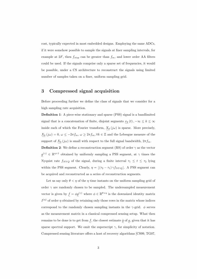
cost, typically expected in most embedded designs. Employing the same ADCs,

if it were somehow possible to sample the signals at finer sampling intervals, for

example at 2F , then fstop can be greater than fm, and lower order AA filters

could be used. If the signals comprise only a sparse set of frequencies, it would

be possible, under a CS architecture to reconstruct the signals using limited

number of samples taken on a finer, uniform sampling grid.

3 Compressed signal acquisition

Before proceeding further we define the class of signals that we consider for a

high sampling rate acquisition.

Definition 1: A piece-wise stationary and sparse (PSS) signal is a bandlimited

signal that is a concatenation of finite, disjoint segments xk::

(t) ,−∞ ≤ k ≤ ∞

inside each of which the Fourier transform, Xk::

(jω) is sparse. More precisely,

Xk::

(jω) = 0, ω ≤ −2πfm, ω ≥ 2πfm,∀k ∈ Z and the Lebesgue measure of the

support of Xk::

(jω) is small with respect to the full signal bandwidth, 2πfm.

Definition 2: We define a reconstruction segment (RS) of order γ as the vector

g:

(γ) ∈ Rη×1 obtained by uniformly sampling a PSS segment, at γ times the

Nyquist rate fNYQ of the signal, during a finite interval τ1 ≤ t ≤ τ2 lying

within the PSS segment. Clearly, η = b(τ2 − τ1) γfNYQc. A PSS segment can

be acquired and reconstructed as a series of reconstruction segments.

Let us say only θ < η of the η time instants on the uniform sampling grid of

order γ are randomly chosen to be sampled. The undersampled measurement

vector is given by f:

= φg:

(γ) where φ ∈ Rθ×η is the downsized identity matrix

I(η) of order η obtained by retaining only those rows in the matrix whose indices

correspond to the randomly chosen sampling instants in the γ-grid. φ serves

as the measurement matrix in a classical compressed sensing setup. What then

remains to be done is to get from f:, the closest estimate g

:of g

:, given that it has

sparse spectral support. We omit the superscript γ, for simplicity of notation.

Compressed sensing literature offers a host of recovery algorithms [CS99, TG07,

3

De07, CM05] for solving this problem, the most popular being those based on

Basis Pursuit [CS99] and Orthogonal Matching Pursuit [TG07]. In our previous

work [SR11], we have highlighted the inadequacy of some of the existing recovery

methods for reconstructing general signals with frequencies that are non-integral

multiples of the fundamental DFT frequency. In [SR11] we have discussed the

merits and demerits of these solutions and provided empirical evidence of better

performance by a method based on eigen decomposition proposed in [DB12].

This method employs the root-MUSIC algorithm for finding out the component

frequencies in the signal. MUSIC obtains the eigen values and the eigen vectors

of the signal autocorrelation matrix and evaluates a score function that returns

the specified number of largest score function peaks as the frequencies present

in the signal. The expected number K of component frequencies in the signalis

fed as input to the algorithm. Root-MUSIC is an extension of MUSIC which

calculates the peaks from the zeros of a polynomial that depends upon the noise

subspace eigen vectors.

Like in greedy CS methods, the K frequencies are obtained iteratively. The

initial residue r0:

is equal to the measurement vector f:. In the subsequent

iterations, the residue is given as

rj:

= f:− φgj−1

:::(1)

where rj:

is the residue in iteration j, φ is the measurement matrix, f:

the

measurement vector and gj−1:::

the estimate of the reconstruction segment in the

previous iteration. An itermediate estimate is calculated from the residue.

h:

= gj−1:::

+ φT rj:

(2)

The intermediate estimate is fed to the Root-MUSIC algorithm as input along

with the expected number K of component frequencies. The prominent fre-

quencies ωk and the corresponding coefficients ak, 1 ≤ k ≤ K are returned by

the algorithm from which the final estimate for the jth iteration is calculated as

4

the linear combination of the K chosen sinusoids.

gj:

=

K∑k=1

ake (ωk) (3)

4 High sampling rate reconstruction scheme

4.1 Streaming data acquisition

Most CS recovery algorithms focus on finite length signals which are recon-

structed offline with sub-Nyquist number of samples. In our approach, contin-

uous streaming data is acquired, in real time, as finite length blocks defined

previously as reconstruction segments. The RSs are compressively sampled

and reconstructed using the MUSIC based algorithm described in the last sub-

section. Interesting methods have been proposed by Boufounos and Asif in

[BA10] and Mishali and Eldar in [ME09b] for dealing with infinite-dimensional

signals to avoid blocking artifacts introduced due to finite length blocks. The

method we propose can incorporate these reconstruction algorithms. However,

we choose to restrict to the finite dimensional reconstruction algorithm, since

our interest is mainly in achieving higher sampling rate to facilitate use of low

order AA filters. Our approach is based on the multiplexed signal acquisition

architecture, operating on streaming data, proposed by us in our previous work

[SR10]. Each of the signals is acquired as a series of overlapping reconstruction

segments. Thus each new RS that is sampled has a significant overlap with the

previous RS. In the region of overlap, all the previously reconstructed samples

of the grid, of chosen order γ (from the previous RS), are taken as it is. The

non-overlapping portion is compressively sampled, that is, sub-Nyquist num-

ber of samples are taken at random instants of time as explained in section 3.

After each RS is reconstructed, the deviation between the reconstructed sig-

nal values and the actual measured values at the few random instants, in the

non-overlapping portion, where samples have been taken, is calculated. If the

deviation exceeds a small threshold, then the RS would have crossed the bound-

5

ary of a new PSS segment. The first RS after the detection of a PSS boundary is

reconstructed without overlap. Subsequently, the reconstruction segments shall

again overlap. The process continues until the next boundary is detected. Small

reconstruction error at PSS boundaries, is unavoidable. This is usually small

due to significant overlap between consecutive RSs. By virtue of the overlap

between RSs, it is not necessary to have exact a priori knowledge of

the PSS segment boundaries since the reconstruction error is restricted to

the small non-overlapping portion of the RS falling on the PSS boundary. This

is because each PSS segment is reconstructed as several overlapping RSs and

most of the samples in an RS are obtained from the overlapping portion (say 80

percent) which would have been already reconstructed as part of the preceding

RS. The new samples are obtained by direct measurement on the signal in the

non-overlapping portion (the remaining 20 percent). The absence of beforehand

information of the PSS boundaries does not cause significant error since any PSS

segment boundary will always fall in the non-overlapping portion of the last RS

within a PSS segment. Since the non-overlapping portion is small, the contri-

bution of the samples from this portion in the reconstruction of the this last

RS is small and therefore, the reconstruction error due to the non-stationarity

is small and mostly confined to the non-overlapping portion of the RS. The re-

construction error though small, would have crossed the threshold for real-time

detection of PSS boundary. Once the boundary is detected, the very first RS

in the new PSS would have no overlap with the previous RS. Overlap will re-

sume from the second RS onwards. However, a rough estimate of the minimum

length of any PSS segment during the data acquisition is required. In other

words, there needs to exist an assurance that the length of any PSS segment

will certainly not be less than this value. This is to ensure that the calculated

length of the RS [SR10] is not more than the length of any PSS segment as this

will cause the very first RS (in a new PSS) itself to fall on a PSS boundary,

thereby causing significant reconstruction error.

6

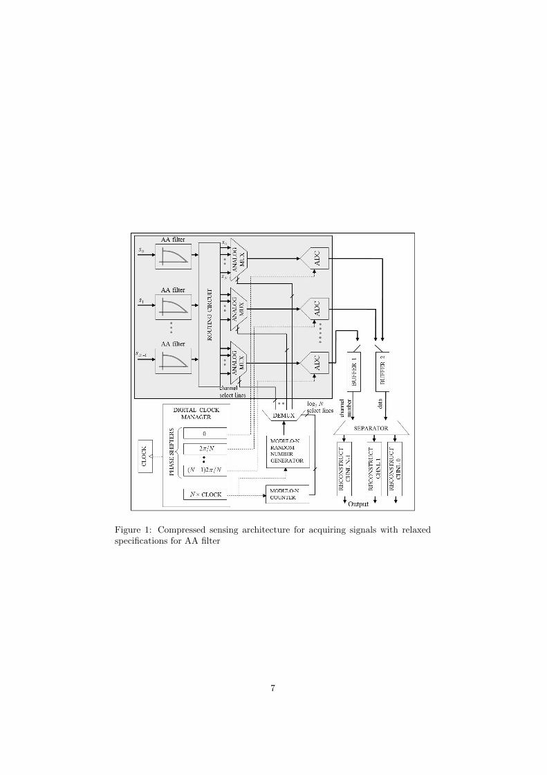
Figure 1: Compressed sensing architecture for acquiring signals with relaxedspecifications for AA filter

7

4.2 The architecture

Given the optimal sampling rate of each of the N ADCs as F Hz, let each ADC

operate on clocks which have the same period T = 1/F , but are phase shifted

from each other by τ . In other words, if the acquisition starts at time t, the ith

ADC, 0 ≤ i ≤ N−1, operates at the time instants: t+iτ, t+iτ+T, t+iτ+2T...

and so on. If we choose τ = T/N , we have a data acquisition system, employing

N ADCs, operating on a uniform sampling grid with a sampling interval of T/N

or equivalently an effective sampling frequency of

Feff = NF (4)

The finer uniform sampling grid, of order γ = N , is available to all the N

signals. During acquisition, time instants are randomly chosen from the finer

grid provided by all the N ADCs together to collectively sample the N analog

signals. This requires each ADC to be able to multiplex between the different

analog signals in real time, which is practically realizable due to the presence of

built-in multiplexers in commercially available ADCs. Figure 1 shows the data

acquisition scheme that we propose in this work. The shaded section in the

figure, which is the analog section, consists of N ADCs together with the corre-

sponding N multiplexers. N analog signals are input to the system. Each of the

signals, after passing through AA filter, is routed to every analog multiplexer.

The rest of the design (the unshaded region) is digital and can be implemented

in a small size low cost FPGA. The Digital Clock Manager (DCM) is a very

standard block commonly implemented in commercially available FPGAs. The

DCM generates N phase shifted versions of the input clock of F Hz, in the range

0 to (N − 1) 2π/N , which are input to the ADCs. The DCM also generates an-

other clock whose frequency is NF , which is input to a modulo-N counter and a

modulo-N random number generator. The modulo-N random number generator

outputs a random number between 0 and N − 1 at every tick of its clock input

for choosing the analog channel to be sampled. By using a proper seed, care is

8

taken that over sufficiently long interval of acquisition, each analog channel gets

an equal share of the time instants when it is sampled. The modulo-N counter

releases counts from 0 to N−1 in succession, such that the demultiplexer routes

the number of the analog channel to be sampled to the analog multiplexers of

successive ADCs, in synchronization with their respective clocks. The analog

multiplexer of the ADC, which gets a clock tick, routes the chosen analog signal

to the ADC. Thus while each of the individual ADCs operate at their optimal

sampling rate of F Hz, the collective acquisition takes place at NF Hz. The

process of acquisition and reconstruction of the signals takes place in a series

of acquisition cycles. There are two digital buffers which store the samples col-

lected by all the ADCs together. During any acquisition cycle, one of the buffers

is active into which the ADCs deposit the samples collected by them in succes-

sion. The other buffer, which contains the samples collected in the previous

acquistion cycle, is read by the separator. The separator separates the samples

into the individual channels with the help of the random sequence generated by

the modulo-N random generator, that is fed to it at the end of an acquisition

cycle. For any channel, as soon as time corresponding to an RS has elapsed, the

collected samples are fed to the CS reconstruction block, the output of which

is the reconstructed signal. The length of the acquisition cycle, which decides

the size of the buffers, must cater for the estimated worst case execution time

of reconstruction in the cycle where all the signals have a complete RS available

for reconstruction.

4.3 A note on the complexity of the method

Since the setup operates on streaming data, the execution of the algorithm is

independent of the number of PSS segments. The main chunk of computation

lies in the compressed sensing reconstruction based on the Root-MUSIC algo-

rithm. This computation time reduces if the size of each RS is small, or in other

words there are more number of RSs within each PSS segment. However, too

small an RS would cause the sparsity assumption, required for CS reconstruc-

9

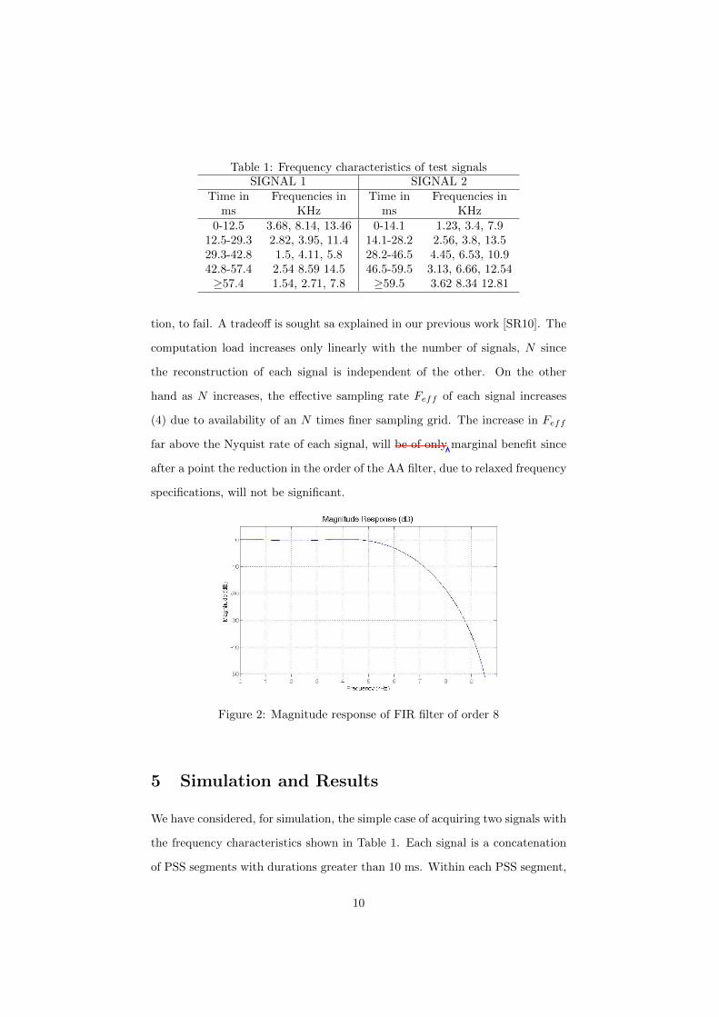
Table 1: Frequency characteristics of test signalsSIGNAL 1 SIGNAL 2

Time in Frequencies in Time in Frequencies inms KHz ms KHz

0-12.5 3.68, 8.14, 13.46 0-14.1 1.23, 3.4, 7.912.5-29.3 2.82, 3.95, 11.4 14.1-28.2 2.56, 3.8, 13.529.3-42.8 1.5, 4.11, 5.8 28.2-46.5 4.45, 6.53, 10.942.8-57.4 2.54 8.59 14.5 46.5-59.5 3.13, 6.66, 12.54≥57.4 1.54, 2.71, 7.8 ≥59.5 3.62 8.34 12.81

tion, to fail. A tradeoff is sought sa explained in our previous work [SR10]. The

computation load increases only linearly with the number of signals, N since

the reconstruction of each signal is independent of the other. On the other

hand as N increases, the effective sampling rate Feff of each signal increases

(4) due to availability of an N times finer sampling grid. The increase in Feff

far above the Nyquist rate of each signal, will be of only marginal benefit since

after a point the reduction in the order of the AA filter, due to relaxed frequency

specifications, will not be significant.

Figure 2: Magnitude response of FIR filter of order 8

5 Simulation and Results

We have considered, for simulation, the simple case of acquiring two signals with

the frequency characteristics shown in Table 1. Each signal is a concatenation

of PSS segments with durations greater than 10 ms. Within each PSS segment,

10

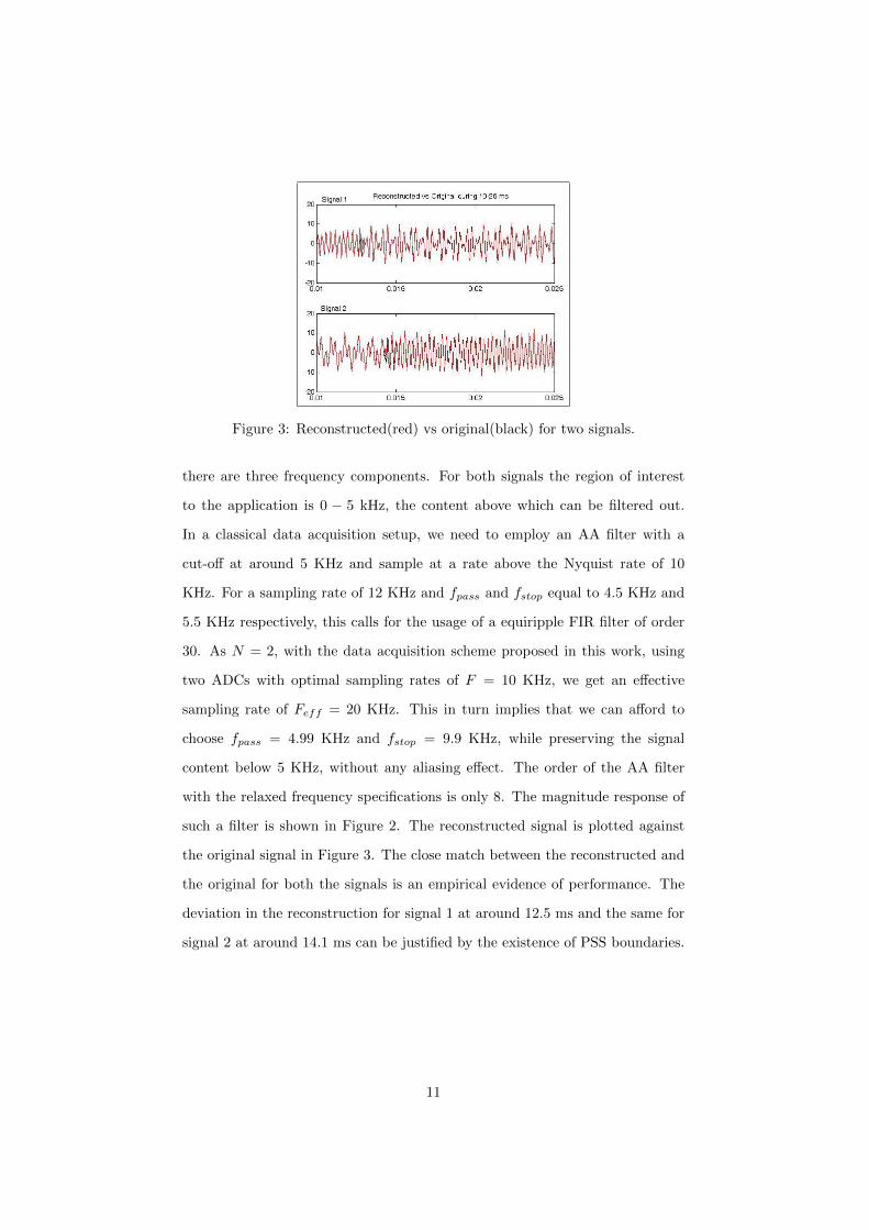
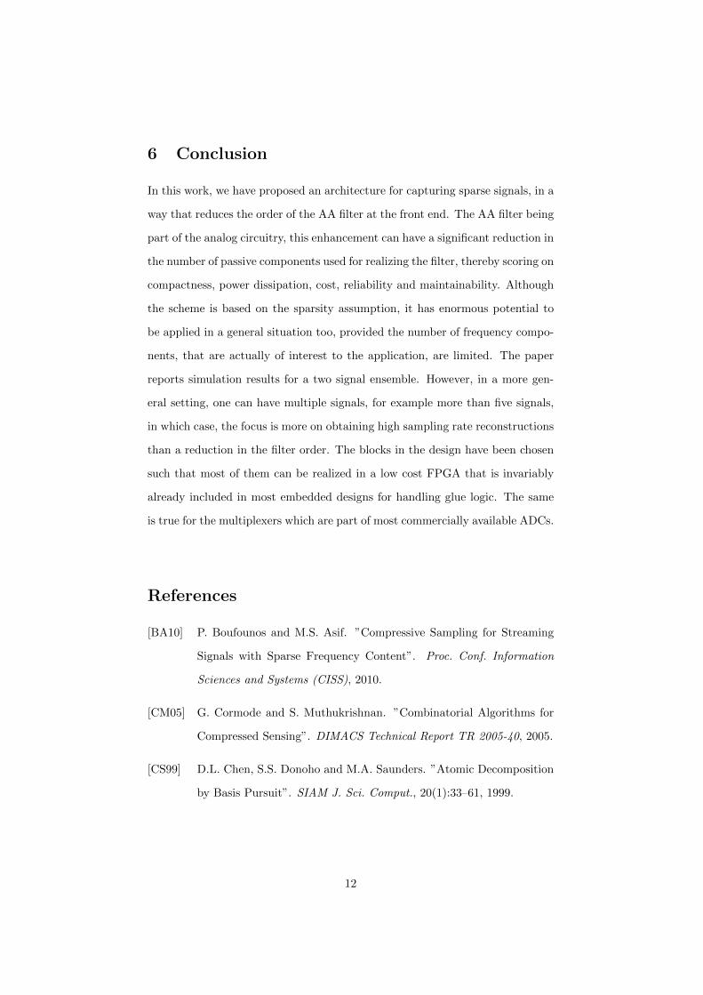
Figure 3: Reconstructed(red) vs original(black) for two signals.

there are three frequency components. For both signals the region of interest

to the application is 0 − 5 kHz, the content above which can be filtered out.

In a classical data acquisition setup, we need to employ an AA filter with a

cut-off at around 5 KHz and sample at a rate above the Nyquist rate of 10

KHz. For a sampling rate of 12 KHz and fpass and fstop equal to 4.5 KHz and

5.5 KHz respectively, this calls for the usage of a equiripple FIR filter of order

30. As N = 2, with the data acquisition scheme proposed in this work, using

two ADCs with optimal sampling rates of F = 10 KHz, we get an effective

sampling rate of Feff = 20 KHz. This in turn implies that we can afford to

choose fpass = 4.99 KHz and fstop = 9.9 KHz, while preserving the signal

content below 5 KHz, without any aliasing effect. The order of the AA filter

with the relaxed frequency specifications is only 8. The magnitude response of

such a filter is shown in Figure 2. The reconstructed signal is plotted against

the original signal in Figure 3. The close match between the reconstructed and

the original for both the signals is an empirical evidence of performance. The

deviation in the reconstruction for signal 1 at around 12.5 ms and the same for

signal 2 at around 14.1 ms can be justified by the existence of PSS boundaries.

11

6 Conclusion

In this work, we have proposed an architecture for capturing sparse signals, in a

way that reduces the order of the AA filter at the front end. The AA filter being

part of the analog circuitry, this enhancement can have a significant reduction in

the number of passive components used for realizing the filter, thereby scoring on

compactness, power dissipation, cost, reliability and maintainability. Although

the scheme is based on the sparsity assumption, it has enormous potential to

be applied in a general situation too, provided the number of frequency compo-

nents, that are actually of interest to the application, are limited. The paper

reports simulation results for a two signal ensemble. However, in a more gen-

eral setting, one can have multiple signals, for example more than five signals,

in which case, the focus is more on obtaining high sampling rate reconstructions

than a reduction in the filter order. The blocks in the design have been chosen

such that most of them can be realized in a low cost FPGA that is invariably

already included in most embedded designs for handling glue logic. The same

is true for the multiplexers which are part of most commercially available ADCs.

References

[BA10] P. Boufounos and M.S. Asif. ”Compressive Sampling for Streaming

Signals with Sparse Frequency Content”. Proc. Conf. Information

Sciences and Systems (CISS), 2010.

[CM05] G. Cormode and S. Muthukrishnan. ”Combinatorial Algorithms for

Compressed Sensing”. DIMACS Technical Report TR 2005-40, 2005.

[CS99] D.L. Chen, S.S. Donoho and M.A. Saunders. ”Atomic Decomposition

by Basis Pursuit”. SIAM J. Sci. Comput., 20(1):33–61, 1999.

12

[CT06] J. Candes, E. Romberg and T. Tao. ”Robust Uncertainty Principles:

Exact Signal Reconstruction from Highly Incomplete Frequency Infor-

mation”. IEEE Trans. Inform. Theory, 52(2):489–509, Feb. 2006.

[CW08] E. Candes and M. Wakin. ”An Introduction to Compressive Sam-

pling”. IEEE Signal Proc. Magazine, 25(2):21–30, March 2008.

[DB12] M.F. Duarte and Richard G. Baraniuk. ”Spectral Compressive Sens-

ing”. Applied and Computational Harmonic Analysis, Aug. 2012.

[De07] D.L. Donoho et.al. ”Sparse Solution of Undetermined Linear Equa-

tions by Stagewise Orthogonal Matching Pursuit”. Preprint, 2007.

[Don06] D.L. Donoho. ”Compressed Sensing”. IEEE Trans. Inform. Theory,

52(4):1289–1306, April 2006.

[Kai74] J.F. Kaiser. ”Nonrecursive Digital Filter Design using the - Sinh Win-

dow Function”. Proc. IEEE Symp. Circuits and Systems, pages 20–23,

April 1974.

[Me09a] F. Marvasti et.al. ”A Unified Approach to Sparse Signal Processing”.

CoRR, 2009.

[ME09b] M. Mishali and Y. Eldar. ”blind multiband signal reconstruction:

Compressed sensing for analog signals”. IEEE Trans. Sig. Proc.,

57:993–1009, March 2009.

[OS89] A.V. Oppenheim and R.W. Schafer. ”Discrete-Time Signal Process-

ing”. Prentice-Hall, pages 458–562, 1989.

[SR10] J.V. Satyanarayana and A.G. Ramakrishnan. ”mosaics: Multiplexed

optimal signal acquisition involving compressed sensing”. Proc. Inter-

national Conference on Signal Processing and Communications (SP-

COM), July 2010.

13

[SR11] J.V. Satyanarayana and A.G. Ramakrishnan. ”Multiplexed Com-

pressed Sensing of General Frequency Sparse Signals”. Proc. of

ICCSP, pages 423–427, 2011.

[TG07] J. Tropp and A. Gilbert. ”Signal Recovery from Random Measure-

ments via Orthogonal Matching Pursuit”. IEEE Trans. on Informa-

tion Theory, 53(12):4655–4666, Dec. 2007.

14