Computers and Mathematics with Applications 64 (2012) 350–360

Contents lists available at SciVerse ScienceDirect

Computers and Mathematics with Applications

journal homepage: www.elsevier.com/locate/camwa

Theoretical and computational studies of some bioreactor modelsRene Alt a,∗, Svetoslav Markov b

a Laboratoire d’Informatique de Paris 6, University Pierre et Marie Curie, 4 place Jussieu, 75252 Paris cedex 05, Franceb Institute of Mathematics and Informatics, Bulgarian Academy of Sciences, ‘‘Acad. G. Bonchev’’ st., bl. 8, 1113 Sofia, Bulgaria

a r t i c l e i n f o

Keywords:BioreactorChemostatMicrobial growthMonod modelHaldane/Andrews functionBatch mode

a b s t r a c t

Westudy certain classical basicmodels for bioreactor simulation in case of batchmodewithdecay. It is shown that in many cases the two-dimensional differential system describingthe dynamics of the substrate and biomass concentrations can be reduced to an algebraicequation for the biomass together with a single differential equation for the substrate.Then from an analogy with the Henri–Michaelis–Menten enzyme kinetic mechanism asimple model is proposed for a bioreactor in batch mode with decay. Two more modelsare also proposed taking into account the phases of microbial growth. Some propertiesof these two models are studied and compared to classical Monod type models usingcomputer simulations.

© 2012 Elsevier Ltd. All rights reserved.

1. Introduction

It has been often mentioned in the literature that Monod type microbial growth models describe adequately bio-processes appearing in bioreactors, under certain favorable conditions when micro-organisms actively produce specificenzymes for the degradation and consumption of nutrient substrates and growat themaximumpossible rate [1,2]. However,conditions in bio-reactors sometimes become unfavorable, microbial growth may be inhibited and bio-technologicalprocessesmay go out of control. In this workwe study theoretically and computationally severalMonod typemodels, takinginto account phases in microbial growth under unfavorable conditions. To this end several familiar bioreactor models aretheoretically analyzed with respect to properties of their solutions. In particular we investigate (in the spirit of [3]) somemodels of batch mode bioreactors with decay of the form:

s′t = −αµ(s)x,x′

t = µ(s)x − kdx,(1)

with positive initial conditions and positive α and kd. The function µ(s) ≥ 0 in (1) is defined for s ≥ 0 and may takevarious forms, see e.g. [1]. The emphasis is on the case when µ(s) is the Monod function [4], the Webb function [5] and itsparticular cases: the Haldane function [6] and the Andrews function [7]. In this paper it is shown that if

ds/µ(s) exists

thenmodel (1) can be simplified to a single differential equation plus an algebraic relation of the form x = x(s). As examplesthe corresponding algebraic functions are derived for each of the four above functions.

In the last part of this work we consider a class of models for bacterial growth proposed in [8] as an alternative to (1).Three particular models from this class, inspired from the Henri–Michaelis–Menten enzyme kinetic mechanism, are studiedcomputationally. It is shown that these type of models are an alternative to Monod type models for bioreactors with decayand that they lead to similar solutions. The figures illustrating the theoretical results of this paper have been obtained usingthe ordinary differential equations solver LSODE from ODEPACK [9].

∗ Corresponding author. Tel.: +33 144278790.E-mail addresses: Rene.Alt@lip6.fr (R. Alt), smarkov@bio.bas.bg (S. Markov).

0898-1221/$ – see front matter© 2012 Elsevier Ltd. All rights reserved.doi:10.1016/j.camwa.2012.02.046

R. Alt, S. Markov / Computers and Mathematics with Applications 64 (2012) 350–360 351

2. The classical simple bioreactor model

A simple continuous bioreactor involving a single nutrient substrate s and one bacteria strain x is often described by theMonod type differential system:

s′t = −αµ(s)x − q(s − sin),x′

t = µ(s)x − qx, (2)

with initial conditions s0, x0 in t = 0; t is the time, s(t) and x(t) are the concentrations at time t of the substrate and of thebiomass of bacteria; α, q, sin are nonnegative constants. More precisely 1/α is the growth yield, sin is the concentration (g/l)of fresh nutrient and q = F/V , F being the inflow (liters/hour) and V being the volume (in liters) of the chemostat. In caseof batch mode there is no inflow and q = 0.

The function µ(s) represents the specific growth rate of the biomass. More than 30 functions µ(s) have been discussedin [1]. They can be classified as follows:

1. Models representing only the bacterial growth (e.g. Monod), most are rational functions in s;2. Models representing bacterial growth including the effect of substrate inhibition (e.g. Haldane, Andrews), most are

rational functions in s;3. Models for bacterial growth including the effect of product inhibition, most are also rational functions in s and x;4. Models describing the influence of the pH value or other experimental conditions on bacterial growth.

The following functions are often used in the literature:

(i) Monod function [4]:

µm(s) = µ∗s

K + s; (3)

(ii) Webb function [5]

µw(s) = µ∗s(1 + βs/Ki)

K + s + s2/Ki. (4)

(iii) Haldane function [6]:

µh(s) = µ∗s

(K + s)(1 + s/Ki); (5)

(iv) Andrews function [7]:

µa(s) = µ∗s

K + s + s2/Ki. (6)

We note that all parameters µ∗, K and Ki in formulae (3)–(6) are positive and represent different physical/biologicalquantities, so strictly speaking we should have used a different notation for all the parameters. Haldane and Andrewsfunctions are equivalent in the sense that using a transformation of the parameters, function (5) can be written in theform (6):

µh(s) = µ∗Ki/(K + Ki)s

KKi/(K + Ki) + s + s2/(K + Ki);

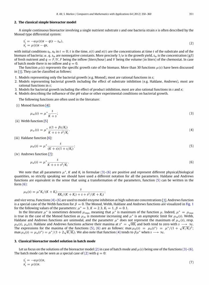
and vice versa. Functions (4)–(6) are used tomodel enzyme inhibition at high substrate concentrations [1]. Andrews functionis a special case of the Webb function for β = 0. The Monod, Webb, Haldane and Andrews functions are visualized in Fig. 1for the following values of the parameters: µ∗

= 3, K = 2.3, Ki = 1, β = 0.1.In the literature µ∗ is sometimes denoted µmax, meaning that µ∗ is maximum of the function µ. Indeed, µ∗

= µmaxis true in the case of the Monod function as µm is monotone increasing and µ∗ is an asymptotic limit for µm(s). Webb,Haldane and Andrews functions are unimodal, and the parameter µ∗ does not represent the maximum of µw(s), resp.µh(s), µa(s). Haldane and Andrews functions achieve their maxima at s∗ =

√KKi and both tend to zero with s −→ ∞.

The expressions for the maxima of the functions (5), (6) are as follows: maxµh(s) = µh(s∗) = µ∗/(1 +√K/Ki)

2;maxµa(s) = µa(s∗) = µ∗/(1 + 2

√K/Ki). We also note that function (4) tends to βµ∗ when s −→ ∞.

3. Classical bioreactor model solution in batch mode

Let us focus on the solutions of the bioreactormodel (2) in case of batchmode andµ(s) being one of the functions (3)–(6).The batch mode can be seen as a special case of (2) with q = 0:

s′t = −αµ(s)x,x′

t = µ(s)x. (7)

352 R. Alt, S. Markov / Computers and Mathematics with Applications 64 (2012) 350–360

Fig. 1. Monod, Webb, Haldane and Andrews functions with values of the parameters: µ∗= 3, K = 2.3, Ki = 1, β = 0.1.

It is known that inmodel (7) x can be solved in termsof s and thus the two-dimensional differential systemcanbe replacedby a single differential equation.Moreover it can be seen that for any nonnegativeµ(s), function s(t) ismonotone decreasingand function x(t) is monotone increasing. This is an evident consequence of (7) together with the fact that by their nature,α and x(t) are positive. In the literature it has been often pointed out that the form of function µ(s) may play a decisive rolefor the inhibition of bacterial growth. Two extremal cases should be considered: prolonged depletion and prolonged excessof s. Concerning the first case, we note that no nonnegative function µ(s) can cause decay of the biomass even long afterthe substrate has been totally exhausted. If we need to model the death of bacteria due to prolonged depletion of nutrientsubstrate then we need to include a decay term in the second equation of system (7). This fact is also well-known, see [1].Concerning inhibition due to (toxic) excess of substrate, functions (4)–(6) prove to be useful. Note that the Monod function(3) cannot contribute to the inhibition of substrate uptake due to excess of s, whereas functions (4)–(6) do cause inhibition.

One of the main purposes of this work is to show that: (i) in many cases the two-dimensional differential system (1) canbe replaced by a single differential equation plus an algebraic relation; (ii) the inhibition effects that are usually aimed bymeans of function µ(s), can be achieved by other means.

3.1. Batch bioreactor with decay

Because of the above reasons, in what follows the studied model will be the classical model (1) for a bioreactor withdecay term −kdx.

Proposition 1. In the two-dimensional system (1), if 1/µ(s) admits an antiderivative function, then x can be solved in terms ofs and the system can be reduced to a single differential equation in s.

Proof. Following an idea of Volterra, see for example [10], the ratio of the second equation to the first equation of system (1)leads to:

dxds

=1α

kd

µ(s)− 1

. (8)

Let φ be an antiderivative of 1/µ: φ(s) =ds/µ(s), then, taking into account the initial conditions s(0) = s0, x(0) = x0:

x(s) =1α

[kd(φ(s) − φ(s0)) − (s − s0)] + x0, (9)

which proves the proposition. �

Let us now apply Proposition 1 to the above mentioned functions µ(s).

Proposition 2. In the case of Monod function, the second equation in system (1) can be expressed as:

x(s) = x0 +1

αµ∗[kdK ln(s/s0) − (µ∗

− kd)(s − s0)]. (10)

R. Alt, S. Markov / Computers and Mathematics with Applications 64 (2012) 350–360 353

The proof follows from a simple calculation of φ(s) =ds/µ(s), µ(s) being the Monod function and replacing it

in (9). �Similar calculations can be also done with the Webb function and its particular cases of Andrews and Haldane functions

leading to:

Proposition 3. In the case of the Webb function we have

φ(s) =1µ∗

(ln(as + 1))/a + K ln(s/(as + 1)) +

1Ki

(s/a − (ln(as + 1))/a2)

with a = β/Ki so that the second equation of system (1) can be expressed as:

x(s) = x0 +1

αµ∗

kda

−kdKia2

ln

as + 1as0 + 1

+ kdK ln

s(as0 + 1)s0(as + 1)

+

kdKia

− µ∗

(s − s0)

. (11)

Proposition 4. In the case of Haldane and Andrews functions, the second equation of system (1) respectively reduces to:

x(s) = x0 +1

αµ∗

kdK ln

ss0

+

kd +

kdKKi

− µ∗

(s − s0) +

kd2Ki

(s2 − s20)

.

x(s) = x0 +1

αµ∗

kdK ln

ss0

+ (kd − µ∗)(s − s0) +kd2Ki

(s2 − s20)

.

(12)

Formulae (12) can be obtained directly from (9) by calculating φ(s) with the Haldane and Andrews formulations, ordirectly from (11) with β tending to zero for Andrews function.

Similar calculations can be done each timeds/µ(s) exists. This has been illustrated by the above examples. Thus it

has been demonstrated that, even in the case of a model with decay, the two-dimensional differential system can be oftenreduced to a single differential equation for the substrate together with an algebraic equation for the biomass. Let us seenext that in the case of no decay (kd = 0) the differential equation can sometimes be solved in terms of t as a function of s.

3.2. Special case of a model without decay

In the special case when kd = 0 it is known that the model with the Monod function can be solved in terms of twofunctions s = s(t) and x = x(t), more precisely, when the system is close to the steady state the differential equation hasan approximate explicit solution using the LambertW -function:

s(t) = KWs0K

exps0 − Cµ∗t

K

with C = αx0 + s0. W (x) is the Lambert function which is the inverse to the function y = xex, i.e. such that x =

W (x) exp(W (x)) [11,12]. This solution can be obtained in the special case of the steady state with the Monod function.Let us see next that the above expression (10) and (12) for x(s) lead to differential equations that can be solved in terms

of time as a function of s, that is t = t(s).When kd = 0 for any model, Eq. (8) reduces to dx/ds = −1/α and leads to

x(s) = x0 −1α

(s − s0).

The latter expression, when respectively replaced in the expression of s′(t) in (7) leads to a differential equation withseparable variables which can be easily solved for theMonod, Andrews and Haldane functions. Recall that

ds/(s(C − s)) =

1C ln(s/(s − C)) for any constant C such that C − s > 0. The solutions are:• For the Monod function:

t =

KC

lns0(C − s)s(C − s0)

+ ln

C − sC − s0

µ∗.

• For the Andrews function:

t =

KC

lns0(C − s)s(C − s0)

+

1 +

CKi

ln

C − sC − s0

+

s − s0Ki

µ∗.

• For the Haldane function:

t =

KC

lns0(C − s)s(C − s0)

+

1 +

C + KKi

ln

C − sC − s0

+

s − s0Ki

µ∗.

with C = αx0 + s0.

354 R. Alt, S. Markov / Computers and Mathematics with Applications 64 (2012) 350–360

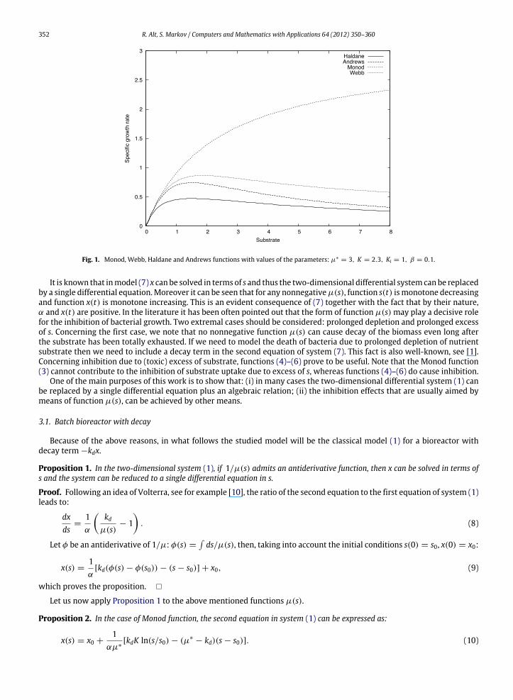
Fig. 2. Time as a function of substrate for the Monod, Haldane and Andrews functions.

Remark. Analogous calculations can be done for any function µ(s) leading to s′(t) in (7) being a differential equation withseparable variables once x is replaced by its expression x(s).

Fig. 2 presents the above functions t = t(s) obtained for the following values of the parameters: K = 0.1, Ki = 0.1, α =

1./23, µ∗= 1.35, s0 = 2.0K , x0 = 0.25K/α, c = s0 + αx0. The computed solutions are dimensionless. Note that the

curves of Fig. 2 should be read from right to left.It can be checked that the three curves t(s) are symmetric to the corresponding s(t) with respect to the first diagonal,

that is the line t = s. Thus when t tends to ∞, s(t) tends to 0 and symmetrically when s tends to 0, then t tends to +∞.Hence the three solutions s(t) are asymptotic to the vertical axis when s tends to 0.

These equations express the time t as a function of the substrate swhich is not very convenient. But, for any t , they can besolved using a classical solver such as Raphson–Newton and hence they can be written as functions s = s(t). This is usefulwhen one needs to compute the value of the substrate at a given time t without computing all the preceding values withsome step.

Let us see next that a model for a batch bioreactor with decay can be obtained using a different approach.

4. A model of batch bioreactor with decay suggested by enzyme kinetics

4.1. Motivation

The following considerations come from the analogy between the reactions in a bioreactor and enzyme kinetics. Let usconsider the well-known Henri–Michaelis–Menten (HMM) model in enzyme kinetics:

ds/dt = −k1es + k−1c,de/dt = −k1es + (k−1 + k2)c,dc/dt = k1es − (k−1 + k2)c,

(13)

with initial conditions s(0) = s0, e(0) = e0, c(0) = 0. In system (13) s, e and c are respectively the concentrations of thesubstrate, the enzyme and the complex (bounded enzyme).

Remark. We have omitted the differential equation for the product as being decoupled. Besides the form of the equationfor the product depends on the mechanism of the biochemical process, see e.g. [13].

Using that de/dt + dc/dt = 0 implies e(t) + c(t) = e0 = const and thus c = e0 − e (or e = e0 − c), system (13) reducesto two equations either for the variables s, e:

ds/dt = −k1es + k−1(e0 − e),de/dt = −k1es + (k−1 + k2)(e0 − e),s(0) = s0, e(0) = e0;

(14)

R. Alt, S. Markov / Computers and Mathematics with Applications 64 (2012) 350–360 355

or for the variables s, c:

ds/dt = −k1(e0 − c)s + k−1c,dc/dt = k1(e0 − c)s − (k−1 + k2)c,s(0) = s0, c(0) = 0.

(15)

We shall next look for comparisons and analogies with the substrate microbial dynamics in a simple bioreactor with onelimiting substrate and one microbial strain.

Recall that the Michaelis–Menten dynamics of substrate uptake:

ds/dt = −Vs/(Km + s), V = k2e0 = const, (16)

is obtained from Eq. (15) by an approximation based on the two (related) assumptions (i) s0 ≫ e0 and (ii) c ′= const.

We see from (16) that the Michaelis–Menten rate of substrate uptake is a rational function of s involving a denominatorKm + s. It is this denominator which slows down the rate of substrate uptake from exponential one (if the denominator isabsent) up to a hyperbolic one (or even almost uniform for large values of s). Three important points should be recalled:(i) the MM-uptake (16) is an approximation of the correct substrate uptake given by any one of the systems (13)–(15);(ii) any one of the systems (13)–(15) models the substrate uptake correctly (as based on mass action law); (iii) none ofsystems (13)–(15) makes use of any rational expressions involving variables in denominators. In addition let us recall that,the assumption s0 ≫ e0 may be far from reality, when modeling substrate microbial dynamics of a simple bioreactor, seee.g. [14,15].

We shall next propose two alternative approaches inspired from the correct enzyme kinetic descriptions (13)–(15). Thefirst approach consists in hybridizing systems (14), (15) into a new (but similar) system of two ODE’s taking into accountcertain analogies between biomass and enzymes. In this case themodel shall involve a singlemicrobial variable, say x, whosedynamics possesses certain features of the dynamics of the enzyme variables (free or bounded).

The second approach is to start from the original correct dynamical system (13). In this case we shall look for analogiesbetween the enzyme kinetic variables e, c and two variables, say x, y, corresponding to different microbial phases.

We note that both approaches ensure that the dynamics of the substrate uptake is similar toMonod dynamics (at least fors0 ≫ e0). Thereby this is achieved without introducing a rational function of the substrate variable s in the right-hand-side.In addition, the second approach offers a better description of microbial dynamics due to the employment of two microbialphases. The advantages of using microbial phases have been advocated by several authors, see e.g. [16–18,2].

We start with the first approach which is more simple. Our aim is to construct a model in analogy to models (14), (15)extracting from the latter appropriate information formodelingmicrobial growth. Passing fromenzymekinetics tomicrobialdynamics it seems reasonable to assume that the rate constant k−1 corresponding to the reverse enzyme reaction is zero.(Assuming k−1 = 0 in a bacterial growth model may mean that under certain conditions bacteria throw up (vomit) some ofthe already swallowed nutrient substrate.) This simplifies systems (14), (15) to:

ds/dt = −k1es,de/dt = −k1es + k2(e0 − e),

and, resp. (for s and c):

ds/dt = −k1es = −k1(e0 − c)s,dc/dt = k1es − k2c = k1(e0 − c)s − k2c.

Remark. Note that systems (14), (15) (and the two above systems) are direct consequences of the assumption e+c =const.The latter is a realistic restriction reflecting a structural property of the model. This restriction remains in large extent validwhile modeling bacterial growth (although, if necessary, can be slightly modified). On the contrary the assumption c ′

= 0used in the derivation of (16) is quite unrealistic in modeling microbial growth.

4.2. A simple model

The similarity of the curves obtained with models (14), (15) and those obtained with models (1) with any of the threeµ-functions (3)–(6) suggests that microbial growth can be modeled with some modification/hybridization of systems(14), (15). Thereby there will be no rational functions of the substrate variable in the formulation of the model, whichsimplifies the latter. The idea arises from the similar roles played by enzymes and microorganisms in relation to substrateuptake/consumption.

The following Model 1 illustrates this idea. The model is a hybrid of the two systems (14) and (15). We assume thatbacteria behave similar to free enzymes w.r.t. substrate uptake/consumption. Denoting bacteria biomass by x we mayexpect that equation ds/dt = −k1xs models quite adequately the consumption of nutrient substrate by bacteria. (A moresophisticated model accounting for the inhibition on the uptake for excessive values of s may involve an additional termsuch as +kis.) On the other side bacteria behave similarly to bounded enzymes when it comes to bacterial dynamics(growth/decay). The above reflections lead us to the following simple model.

356 R. Alt, S. Markov / Computers and Mathematics with Applications 64 (2012) 350–360

Model 1. A simple substrate microbial dynamics is described by means of the following system of two ODE’s:

ds/dt = −k1xs,

dx/dt = k1xs − k3x,(17)

with initial conditions s(0) = s0, x(0) = x0.

Remark. A modeler of microbial-nutrient system should not feel restricted to assign precisely one specified form of theenzyme (free or bounded) to a specific microbial state. At this point the modeler should feel free to use any one of these twosystems as a base for his microbial growsmodel and to use elements of the other system. Indeed, it seems to us possible thatwhen being in a specific state, bacteria may behave sometimes as a free, and sometimes as a bounded enzyme. For examplewhile in active state, bacteria consume nutrients like free enzymes uptake substrate, but these bacteria decay like boundedenzymes pass to free ones. Thus, in the right-hand side of the second equation of Model 1 : dx/dt = k1xs − k3x, the firstterm corresponds to the term k1es from (15), whereas the second term −k3x corresponds to the term −k2c from (15).

Wewish to also remark that Model 1 is intentionally simplified in order to demonstrate our ideas. Namely, to replace therational function µ by means of polynomial function in the right-hand sides, and to show that this simplified model does(almost) the same work as model (1) with Monod function. Note that if we substitute µ(s) = s in (1) then we obtain themodel:

ds/dt = −αxs,dx/dt = αxs − k3x,

which is a special case of (17). Model (17) does not model realistically bacterial growth well for large values of s, but manysources report that the Monod kinetics model (1) does not work well for large s too.

As in the case of the batch bioreactor model of the preceding section, we have the next proposition.

Proposition 5. System (17) reduces to a single differential equation.

Proof. As has been done in the preceding section using a Volterra idea the ratio of the second equation to the first equationof system (17) leads to:

dx/ds = −k1/k1 + k3/(sk1)

which can be integrated as:

x = −k1k1

s +k3k1

ln(s) + M.

The constantM is obtained from the initial conditions x0 and s0.Hence the single differential equation with algebraic relation:

s′ = −k1xs,

x = x0 +k3k1

lnss0

−k1k1

(s − s0)(18)

is equivalent to (17). �

It can be remarked that the expression for x in (18) is very close to the one for x in (10).Let us now see that if the coefficients for the Monod system (10) are known it is possible to obtain some conditions on

the coefficients k1, k1, k3 of (17) or equivalently of (18) so that the two models give close solutions. A simple condition isthat the maximum in the solution for x in (10) is identical to the one for x in (18). Let us call sm (resp. sm1) the values of s forwhich x(s) has its maximum, then: x′(s) = 0 in (10) leads to sm = kdK/(µ∗

− kd) and x′(s) = 0 in (18) leads to sm1 = k3/k1.The identification of sm and sm1 leads to a ratio k3/k1 which depends only on the coefficients of the Monod model (10).

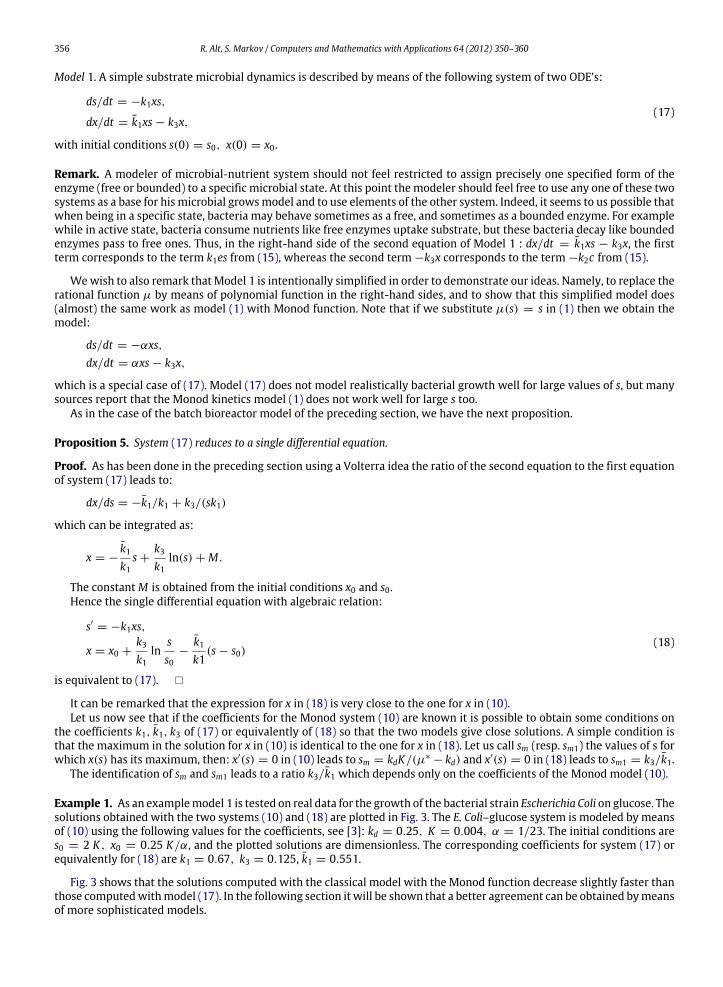
Example 1. As an examplemodel 1 is tested on real data for the growth of the bacterial strain Escherichia Coli on glucose. Thesolutions obtained with the two systems (10) and (18) are plotted in Fig. 3. The E. Coli–glucose system is modeled by meansof (10) using the following values for the coefficients, see [3]: kd = 0.25, K = 0.004, α = 1/23. The initial conditions ares0 = 2 K , x0 = 0.25 K/α, and the plotted solutions are dimensionless. The corresponding coefficients for system (17) orequivalently for (18) are k1 = 0.67, k3 = 0.125, k1 = 0.551.

Fig. 3 shows that the solutions computed with the classical model with the Monod function decrease slightly faster thanthose computedwithmodel (17). In the following section it will be shown that a better agreement can be obtained bymeansof more sophisticated models.

R. Alt, S. Markov / Computers and Mathematics with Applications 64 (2012) 350–360 357

Fig. 3. E. Coli–glucose system modeled by systems (10) and (18).

5. Models using microbial growth phases

Bacterial growth in batch culture involves several phases such as: lag, log, stationary and death phases, cf. e.g. [1]. Thefirst three phases are modeled by the logistic curve which solves the Verhulst–Pearl ODE: dx/dt = ax(1 − x). However,Verhulst–Pearlmodel does not involve variables corresponding to bacteria biomass in specific phases, neither does it involvethe dynamics of the nutrient substrate.

In the literature onbioreactors/chemostats one can rarely findmodels involvingmicrobial growthphases. Someexamplesof such ‘‘structured’’ models can be found in [16–18,2]. The models proposed and studied in these papers are not inspiredby models from enzyme kinetic; a characteristic feature of these models is that they employ Monod type specific growthfunctions that are rational functions of the substrate variable. It is important to note that models using phases are reportedto be biologically adequate in many realistic situations and therefore deserve special attention.

5.1. Introducing phases in microbial growth models

Aiming at possibly simpler models we subdivide the microbial population into two subgroups:(i)microorganisms in the lag and stationary phases are classified into one subclasswith biomass denoted x. It is assumed thatmicroorganisms in that class experience unfavorable growth conditions and are not able to immediately produce enzymes;(ii) active (viable) microorganisms in log phase, denoted y, possessing a complete set of active enzymes.

Bacteria in the dying state shall be modeled by decay terms and need not be assigned to a special subgroup.Under these assumptions there is a clear analogy between amicrobial–nutrient system and an enzyme–substrate system.

A possible start is to relate the sub-population x to free enzymes e and the sub-population y to bounded enzymes c and thenmake suitable realistic modifications. As in the preceding section, plausible dynamic models of a batch mode bioreactor canbe constructed in analogy to the HMM-law of enzyme kinetic (13). Assuming k−1 = 0, system (13) looks as follows:

ds/dt = −k1xs,dx/dt = −k1xs + k2y,dy/dt = k1xs − k2y,

(19)

with initial conditions s(0) = s0, x(0) = x0, y(0) = y0.A structural property of this system is x + y = x0 = const but when modeling a bacterial–substrate system we can

slightly deviate from this property.

5.2. Two microbial growth models using phases

Adding appropriate additional terms in (19) a variety ofmodels can be obtained. Belowwe study numerically twomodelsof a microbial–nutrient batch mode bioreactor proposed in [8], the second model has been slightly modified. Both modelsinvolve two microbial growth phases.

358 R. Alt, S. Markov / Computers and Mathematics with Applications 64 (2012) 350–360

Fig. 4. Microbial growth, model (20).

Model 2. Consider the following system of ODE’s:

ds/dt = −k1xs − βys,dx/dt = −k1xs + k2y − kdx2,dy/dt = k1xs − k2y + βys,

(20)

with the initial conditions s(0) = s0, x(0) = x0, y(0) = y0. One may see that system (20) is obtained from system (19) byadding some additional terms. The terms participating in system (20) have the following meaning:k1xs —models the consuming of s by bacteria x and the transition of (fasting) bacteria x into (viable, active) bacteria y;βys —models the consuming of s by bacteria y and the increase of bacteria biomass y due to nutrition and reproduction;k2y —models the random transitions of bacteria from class y into class x;kdx2 —models competition and decay of (starving) bacteria x.

The meaning of the coefficients k1 and k2 are similar to that in the enzymatic HMM system (13).The presented numerical experiments concern as before the tandem microbial-substrate system described in [3]. The

solutions are visualized on Fig. 4. The parameters in system (20) are chosen as follows: k1 = 0.23; k2 = 0.85; kd = 0.3; β =

1.0; and the initial conditions are: s0 = 2.0; x0 = 0.25; y0 = 0. A fast growth of the population of active bacteria is observedduring a sufficient supply of substrate nutrient s. The decay in the total amount of biomass x + y due to substrate depletionis also clearly seen in Fig. 4.

As can be seen on Fig. 5 model (20) provides solutions for s and the total biomass x + y which are very close to the oneobtained with the model (1) with Monod µ-function (3).Model 3. Consider next the following system of ODE’s:

ds/dt = −k1xs − (α + β)ys,dx/dt = −k1xs + k2y + αys − kxx,dy/dt = k1xs − k2y + βys − kyy,

(21)

with the initial conditions s(0) = s0, x(0) = x0, y(0) = y0 = 0.The new terms in system (21) have the following meaning:

kxx —models the decay of bacteria x;kyy —models the decay of bacteria y.

The meaning of the remaining coefficients/terms is similar to that in system (20) with one difference: in (21) the termαyswith α ≤ β models a part of (overfed, poisoned) bacteria y which pass from compartment y to compartment x.

In Fig. 6 the solutions of model (21) are visualized and the comparison of the solutions obtained with model (1) withMonod µ-function (3) and model 3 is reported in Fig. 7. The values of the coefficients are k1 = 0.05, k2 = 0.85,kx = ky = 0.23, β = 1.5 and α = 1.35.

The numerical simulations show that all three models (17), (20) and (21) adequately reflect the microbial growthlimitation by nutrient depletion. The presence ofmore parameters and terms allows us the freedom to tune themodel betterto particular realistic situations. The behavior of the computed solutions is close to the experimentally observed behaviorof microbial growth under both favorable and unfavorable environments.

R. Alt, S. Markov / Computers and Mathematics with Applications 64 (2012) 350–360 359

Fig. 5. Microbial growth, comparing models (1) and (20).

Fig. 6. Microbial growth model (21).

It has been experimentally shown that in the case of a batch bioreactor with decay the coefficients of the proposedmodels can be adapted in a way that the computed solutions with these models are close to the one obtained with theMonodmodel. In fact themain condition is that themaxima of the solutions for the total biomass are the same and obtainedat identical values of time t with each model. Once this condition has been stated the coefficients of the HMM like modelsuch as models 1–3 can be obtained with an optimization program allowing the computation of the minimum distancebetween the maximum of the Monod solution and the one of new model solution.

6. Conclusion

In this paper some theoretical properties of the Monod type models for a bioreactor with decay have been investigated.It has been shown that in most cases the two-dimensional differential system of the model can be reduced to a one-dimensional one together with an algebraic equation. The particular cases of the Monod, Haldane and Andrews functionshave been detailed and the resp. one-dimensional systems have been discussed. It has been proved that when there isno decay an explicit solution can be obtained in terms of the time as a function of the nutrient. The reciprocal functioncan then be numerically obtained using some function solver. Some models inspired by adaptations from enzyme kinetics

360 R. Alt, S. Markov / Computers and Mathematics with Applications 64 (2012) 350–360

Fig. 7. Microbial growth models (1) and (21).

mechanisms have been proposed and their solutions have been compared to the ones provided by Monod type models. Ithas been shown that with appropriately chosen coefficients, these models are good alternatives to classical Monod typemodels, especially when introducingmicrobial phases. Some hints to compute the parameters of the proposedmodels havebeen given. The presented computational experiments concern the growthof themicrobial strain E. Coli on glucose substrate.Computational studies related to experimental data onmicrobial growth reported in [19,20] are in progress. Futureworkwillconcern a more complete theory of the relations between Monod type models and Henri–Michaelis–Menten type modelsadapted to bioreactors.

Acknowledgments

The authors wish to thank the anonymous reviewers for their extremely useful comments and critical remarks. Thesecond author was partially supported by the Bulgarian NSF Project DO 02-359/2008.

References

[1] M. Gerber, R. Span, An analysis of availablemathematical models for anaerobic digestion of organic substances for production of biogas, in: Proc. IGRC,Paris, 2008.

[2] C.J. Sissons, M. Cross, S. Robertson, A new approach to the mathematical modelling of biodegradation processes, AMM 10 (1986) 33–40.[3] H. Smith, P. Waltman, The Theory of Chemostat, Cambridge University press, 1995, see also: http://math.la.asu.edu/halsmith/bacteriagrow.pdf.[4] J. Monod, The growth of bacterial cultures, Annual Reviews of Microbiology 3 (1949) 371–394.[5] J.L. Webb, Enzyme and Metabolic Inhibitors, Academic Press, 1963.[6] J.B.S. Haldane, Enzymes, Longmans, London, 1930.[7] J.F. Andrews, A mathematical model for the continuous culture of microorganisms utilizing inhibitory substrates, Biotechnology and Bioengineering

10 (1968) 707–723.[8] S. Markov, On the mathematical modelling of microbial growth: some computational aspects, Serdica Journal of Computing 5 (2) (2011) 153–168.[9] A.C. Hindmarsh, et al., Odepack, a systematized collection of ode solvers, in: R.S. Stepleman (Ed.), Scientific Computing, North-Holland, 1983, pp. 55–64.

[10] H.T. Davis, Introduction to Non Linear Differential and Integral Equations, Dover, 1962.[11] S. Schnell, C. Mendoza, A closed-form solution for time-dependent enzyme kinetic, Journal of theoretical Biology 187 (1997) 207–212.[12] S. Schnell, C. Mendoza, Time-dependent closed form solution for fully competitive enzyme kinetics, Bulletin of Mathematical Biology 62 (2000)

321–336.[13] S. Schnell, M.J. Chappell, N.D. Evans, M.R. Roussel, The mechanism distinguishability problem in biochemical kinetics: the single-enzyme single-

substrate reaction as a case study, C. R. Biologies 329 (2006) 51–61.[14] S. Schnell, P.K. Maini, Enzyme kinetics at high enzyme concentration, Bulletin of Mathematical Biology 62 (2000) 483–499.[15] S. Schnell, P.K. Maini, A century of enzyme kinetics: reliability of the KM and vmax estimates, Comments on Theoretical Biology 8 (2003) 169–187.[16] J.-L. Gouzé, V. Lemesle, Two simple growth models in the chemostat, ARIMA 9 (2008) 145–155.[17] V. Lemesle, J.-L. Gouzé, A simple unforced oscillatory growth model in the chemostat, Bulletin of Mathematical Biology 70 (2008) 344–357.[18] V. Lemesle, J.-L. Gouzé, A biochemically based structured model for phytoplankton growth in the chemostat, Ecological Complexity 2 (2005) 21–33.[19] N. Burhan, Ts. Sapundzhiev, V. Beschkov, Mathematical modelling of cyclodestrin-glucano-transferase production by batch cultivation, Biochemical

Engineering Journal 24 (2005) 73–77.[20] N. Burhan, Ts. Sapundzhiev, V. Beschkov, Mathematical modelling of cyclodestrin-glucano-transferase production by immobilised cells of Bacillus

circulans ATCC21783 at batch cultivation, Biochemical Engineering Journal 35 (2007) 114–119.