arX

iv:0

710.

1064

v1 [

astr

o-ph

] 4

Oct

200

7

THE VARIATION OF MAGNESIUM DEPLETION WITH LINE

OF SIGHT CONDITIONS

Adam G. Jensen and Theodore P. Snow

Center for Astrophysics and Space Astronomy

University of Colorado at Boulder, Campus Box 389

Boulder, CO 80309-0389

Adam.Jensen@colorado.edu, tsnow@casa.colorado.edu

ABSTRACT

In this paper we report on the gas-phase abundance of singly-ionized mag-

nesium (Mg II) in 44 lines of sight, using data from the Hubble Space Telescope

(HST). We measure Mg II column densities by analyzing medium- and high-

resolution archival STIS spectra of the 1240 A doublet of Mg II. We find that Mg

II depletion is correlated with many line of sight parameters (e.g. f(H2), EB−V ,

EB−V /r, AV , and AV /r) in addition to the well-known correlation with <nH>.

These parameters should be more directly related to dust content and thus have

more physical significance with regard to the depletion of elements such as magne-

sium. We examine the significance of these additional correlations as compared

to the known correlation between Mg II depletion and <nH>. While none of

the correlations are better predictors of Mg II depletion than <nH>, some are

statistically significant even assuming fixed <nH>. We discuss the ranges over

which these correlations are valid, their strength at fixed <nH>, and physical

interpretations.

Subject headings: ISM: abundances — ultraviolet: ISM

1. INTRODUCTION AND BACKGROUND

Magnesium is both a relatively abundant element in the Galaxy and an important

component in most interstellar dust models. Mg I has an ionization potential of only 7.65

eV, while Mg II has an ionization potential of 15.04 eV. In H I regions, the dominant form

of gas-phase interstellar magnesium should be Mg II. In H II regions, magnesium should

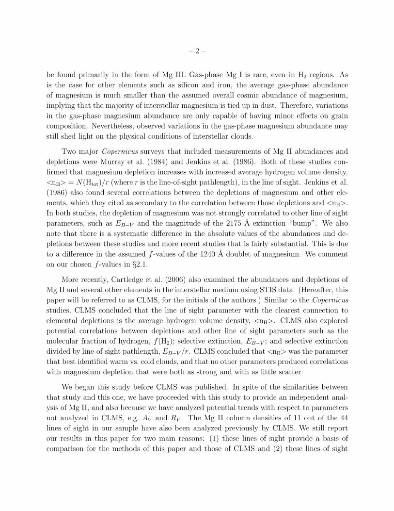
– 2 –

be found primarily in the form of Mg III. Gas-phase Mg I is rare, even in H2 regions. As

is the case for other elements such as silicon and iron, the average gas-phase abundance

of magnesium is much smaller than the assumed overall cosmic abundance of magnesium,

implying that the majority of interstellar magnesium is tied up in dust. Therefore, variations

in the gas-phase magnesium abundance are only capable of having minor effects on grain

composition. Nevertheless, observed variations in the gas-phase magnesium abundance may

still shed light on the physical conditions of interstellar clouds.

Two major Copernicus surveys that included measurements of Mg II abundances and

depletions were Murray et al. (1984) and Jenkins et al. (1986). Both of these studies con-

firmed that magnesium depletion increases with increased average hydrogen volume density,

<nH> = N(Htot)/r (where r is the line-of-sight pathlength), in the line of sight. Jenkins et al.

(1986) also found several correlations between the depletions of magnesium and other ele-

ments, which they cited as secondary to the correlation between those depletions and <nH>.

In both studies, the depletion of magnesium was not strongly correlated to other line of sight

parameters, such as EB−V and the magnitude of the 2175 A extinction “bump”. We also

note that there is a systematic difference in the absolute values of the abundances and de-

pletions between these studies and more recent studies that is fairly substantial. This is due

to a difference in the assumed f -values of the 1240 A doublet of magnesium. We comment

on our chosen f -values in §2.1.

More recently, Cartledge et al. (2006) also examined the abundances and depletions of

Mg II and several other elements in the interstellar medium using STIS data. (Hereafter, this

paper will be referred to as CLMS, for the initials of the authors.) Similar to the Copernicus

studies, CLMS concluded that the line of sight parameter with the clearest connection to

elemental depletions is the average hydrogen volume density, <nH>. CLMS also explored

potential correlations between depletions and other line of sight parameters such as the

molecular fraction of hydrogen, f(H2); selective extinction, EB−V ; and selective extinction

divided by line-of-sight pathlength, EB−V /r. CLMS concluded that <nH> was the parameter

that best identified warm vs. cold clouds, and that no other parameters produced correlations

with magnesium depletion that were both as strong and with as little scatter.

We began this study before CLMS was published. In spite of the similarities between

that study and this one, we have proceeded with this study to provide an independent anal-

ysis of Mg II, and also because we have analyzed potential trends with respect to parameters

not analyzed in CLMS, e.g. AV and RV . The Mg II column densities of 11 out of the 44

lines of sight in our sample have also been analyzed previously by CLMS. We still report

our results in this paper for two main reasons: (1) these lines of sight provide a basis of

comparison for the methods of this paper and those of CLMS and (2) these lines of sight

– 3 –

can be analyzed with respect to the aforementioned line of sight parameters not analyzed in

CLMS. A comparison of the column density measurements for these common lines of sight

is found in §2.3.

In §2 we discuss our observations and data reduction, including comments on the 1240 A

doublet and our derivation of column densities and abundances. In §3 we discuss our results,

including observed correlations and a review of the Galactic abundance of magnesium. In

§4 we summarize our findings.

2. OBSERVATIONS AND DATA REDUCTION

2.1. The Mg II Doublet at λλ1239,1240

Morton (2003), summarizing several sources, cites only four major, ground-state dou-

blets of Mg II—a strong doublet with transitions at 2795.5 A and 2802.7 A, a much weaker

doublet at 1239.9 A and 1240.4 A, a doublet at 1026.0 A and 1026.1 A similar in strength

to the 1240 A doublet, and an even weaker doublet at 946.7 A and 946.8 A. STIS data sets

that cover the wavelength of strong doublet near 2800 A exist for only one of our lines of

sight (HD 93205); if more data did exist, the lines would be saturated in most cases, though

each line might show damping wings for a more certain derivation of column density in a few

cases. The doublets at 946 A and 1026 A, in addition to being self-blended in FUSE data,

are both wiped out by strong hydrogen absorption in the high-column density lines of sight

in this sample (H2 wipes out the 946 A doublet and H I Lyman-β absorption wipes out the

1026 A doublet).

Thus, the two lines of the 1240 A doublet are the only absorption lines of use. Morton

(2003) notes that there are converging theoretical values for the combined magnitude of

the f -values of this doublet, though there is some variation between different authors in

the calculated ratio of the f -values. The studies under discussion in Morton (2003) in-

clude Fleming et al. (1998), Godefroid & Froese Fischer (1999), Theodosiou & Federman

(1999), and Majumder et al. (2002). Morton (2003) ultimately opts for the values by

Theodosiou & Federman (1999). These sources calculate a combined f -value of the dou-

blet that is consistent to within 0.13 dex. In keeping with Morton (2003), we elect to use the

Theodosiou & Federman (1999) f -values of f1239.9 = 6.32 × 10−4 and f1240.4 = 3.56 × 10−4.

CLMS also opted to use these f -values; thus, f -values are not a source of systematic error

between this study and CLMS. Morton (2003) notes that despite consistency in the com-

bined f -value of the doublet, there is some discrepancy in the f -value ratio between the

two lines. However, the Theodosiou & Federman (1999) f -values represent a ratio (1.78)

– 4 –

that is consistent with empirical values by Fitzpatrick (1997) and Sofia et al. (2000) and

the theoretical calculations of Majumder et al. (2002); these sources quote ratios between

1.74 and 1.82. Note, however, that Godefroid & Froese Fischer (1999) found a ratio of 2.54,

while Fleming et al. (1998) only calculated the combined f -value of the doublet and not of

the individual lines.

The damping constants of these lines are not reported in Morton (2003), but in all

cases the lines are much too weak for damping constants to have a significant effect. We use

this doublet exclusively for the determination of column densities. We describe our fitting

methods below (§2.3), but first describe the STIS data and relevant procedures used to

observe the lines.

2.2. HST Data

Archival STIS data are available for all 44 of the lines of sight in this study. Lines of sight

were initially chosen from several literature sources in attempts to examine abundances of

silicon and iron. Basic line of sight parameters (e.g. spectral types and Galactic coordinates

of the background stars) are given in Table 1. A summary of the STIS data sets used is

given in Table 2. Hydrogen column densities and related parameters (e.g. f(H2)) are given

in Table 3, while extinction and reddening parameters EB−V , AV , and RV are given in Table

4.

We used “on-the-fly” calibrated (Micol et al. 1999) data. For observations with the

E140H grating, the 1240 A line is found in two echelle orders. We coadded these echelle

orders and multiple observations where available. We performed the same fitting routines

described below (§2.3) in test cases on the individual echelle orders and observations and

found consistency between those results and our results for the coadded spectra.

We assumed empirically measured point-spread functions (S. V. Penton, private commu-

nication) in analyzing data that utilize the E140H and E140M gratings and various apertures.

We have noted the use of this PSF in our previous work (Jensen et al. 2007; Jensen & Snow

2007). This empirical PSF is not Gaussian.

2.3. Column Density Measurements and Errors

Measurements of Mg II column densities are derived solely through measurements of

the 1240 A doublet. Assuming the f -values given in §2.1 and the PSF described in §2.2,

we fit Voigt profiles simultaneously to the two lines of the doublet. The Voigt profile is

– 5 –

the most general absorption profile; it is inherently Gaussian for unsaturated weak lines,

and inherently damped for very strong lines. The observed profile is the convolution of the

inherent profile and the PSF. When the lines of the doublet are asymmetric or multiple

velocity components are clearly resolved, we fit each individual component with a Voigt

profile.

We fit these multiple components without any a priori assumptions on the overall veloc-

ity structure of the line of sight. This involves “χ-by-eye” to first order, then comparing the

reduced χ2 of fits with a different number of components. Though high-resolution optical

data on the velocity structure exist for some of these lines of sight (e.g. Pan et al. 2004;

Welty & Hobbs 2001; Welty et al. 2003), the ionization potential of the species studied (K

I and Ca I) is smaller than the ionization potential of Mg I (7.6 eV) and much smaller than

the ionization potential of Mg II (15.1 eV), indicating that those elements and Mg II are

unlikely to have high spatial coincidence. Therefore, fitting observed resolved components

and asymmetries is no less—and mostly likely better—justified than assuming the velocity

structure of one of these other elements.

Our profile-fitting1code simultaneously fits the profiles of both doublet lines with a single

total line-of-sight column density, and three parameters for each observed velocity compo-

nent: b-value, velocity offset, and fraction of total column density. The code outputs errors

for each of these parameters, though the errors on total column density are often somewhat

small. To properly account for continuum placement, which should be the dominant source

of error, we calculate the equivalent widths (Wλ) and errors in Wλ due to a 1-σ shift in the

continuum (determined by the S/N). We then assume that the fractional error in column

density is the same as the average fractional error in the Wλ of the two lines of the doublet.

This is a slightly more conservative estimate of the column density error than our code oth-

erwise produces. Two samples of the fit profiles are shown in Figure 1. Our column density

results, along with derived abundances (see §2.4) and equivalent widths, are shown in Table

5.

Potential systematic errors in our methods could come from the aforementioned uncer-

tainties in the f -values, incorrect normalization of the continuum, and concerns of unresolved

or misidentified saturation. Our choice of f -values was discussed above (§2.1). As noted

there, while there is some range in the theoretical values summarized by Morton (2003), two

recent empirical studies determine ratios consistent with our chosen ratio of 1.78, and only

one of the three theoretical values that Morton cites is inconsistent with this value. Because

1Note that our use of the phrase “profile fitting” is different than that of CLMS, in that, as described

above, we do not place any a prior constraints on the components that we identify.

– 6 –

we cannot guarantee that both components are unsaturated in most cases, we cannot inde-

pendently analyze the ratio of f -values. However, we feel confident that the aforementioned

data are converging toward an f -value ratio of ≈ 1.78.

Normalizing the continuum is fairly trivial in this spectral region, as this doublet is far

from any other major spectral features in most lines of sight. In a few lines of sight, broad

stellar features do appear, but fitting the background spectra is still easily accomplished

with the use of multiple order polynomials.

Saturation can pose a problem in two different ways. First, if there are unresolved

saturated components, our fits might determine a column density that is too small. Second,

if we observe a resolved saturated component, and the inherent width of the line is not

much broader than the width of the PSF, the fit will be very uncertain, which could result

in significant deviations from the true column density. Both of these concerns should be

somewhat alleviated by the fact that our method of simultaneously fitting the profiles of

both lines of the doublet constrains saturation as much as is possible given the data. This

is especially true of the latter concern of misidentifying the b-value of a resolved, saturated

component.

We also note that in the 11 lines of sight where we have overlapping data with CLMS,

our methods produce column densities that are generally consistent with their profile fitting

and apparent optical depth methods (hereafter PF and AOD, respectively). A comparison

of the common lines of sight is shown in Table 6. Of the 22 comparison pairs (our results

versus each method for all 11 lines of sight), 19 possess 1-σ agreement. Another two pairs

(our measurements versus the AOD measurements for HD 37021 and HD37903) miss 1-σ

agreement but are consistent within 2-σ and agree within 1-σ on the PF measurements.

Conversely, our measurement of HD 147888 agrees with the AOD measurement of CLMS,

but not with the PF measurement. CLMS note this line of sight as by far the most discrepant

between the two methods in their study (0.19 dex). However, CLMS also discuss strategies

for correction to the AOD method by Savage & Sembach (1991) and Jenkins (1996), the

former of which brings the two methods to within 0.08 dex. CLMS elect to adopt their PF

results in all cases.

These comparisons allow us to conclude that our methods are consistent with the (un-

corrected) AOD method, which itself is typically consistent with the PF method of CLMS.

The discrepancy for HD 147888 is well outside the norm in this regard. We also note that

our equivalent widths (reported in Table 5) are consistent with equivalent widths of CLMS

to within errors (though note that CLMS only report the equivalent width of the 1239.9 A

line).

– 7 –

2.4. Hydrogen Column Densities

In order to analyze abundances and depletions, we need to have hydrogen column den-

sities. We define N(Htot) = [N(H I) + 2N(H2)], neglecting contributions from H II regions.

Given the ionization potentials of H I and Mg II (13.6 eV and 15.1 eV), it is reasonable to

assume that the vast majority of magnesium is found in the form of Mg I and Mg II in H I

and H2 regions, with only a minimal amount of Mg II from H II regions contributing to the

Mg II column density that we see.

The atomic hydrogen column densities are determined through profile fitting of the

Lyman-α line of atomic hydrogen. The fits come from several sources, summarized in Table

3. Three stars are cooler than type B2.5: HD 27778, HD 91597, and HD 147888. Therefore,

the Lyman-α fits of these lines might be subject to stellar contamination. However, in all

cases, estimations of stellar Lyman-α and/or consistency checks with other methods of H I

determination have been employed. For a full discussion of these, see the references in which

the measurements originally appear (Cartledge et al. 2004 for HD 27778 and HD 147888;

Diplas & Savage 1994 for HD 91597) or consult our previous discussions of these lines of

sight (Jensen et al. 2007; Jensen & Snow 2007).

Molecular hydrogen column densities are taken from recent FUSE surveys and other

FUSE data (primarily J. M. Shull et al., in preparation, but see Table 3 for all references).

In these papers N(H2) is determined for each line of sight by fitting several low-J lines.

Reliable FUV data do not exist for HD 37021 and HD 37061; therefore, in these two lines

of sight we cannot report H2 column densities or f(H2), and our N(Htot) and <nH> are

only measures of atomic hydrogen column density and volume density, respectively. This is

unfortunate, because as discussed in §3, these two lines of sight have two of the five largest

depletions of any of the lines of sight in this sample. If N(H2) is large in either of these lines

of sight, then they likely have the greatest depletions of all the lines of sight in this sample,

perhaps by a significant amount. However, Cartledge et al. (2001) have argued that f(H2)

is likely small in both of these lines of sight. This is based on observations of little or no

Cl I in these lines of sight; the Cl I ionization potential of 12.97 eV implies that N(H2) is

similarly small, in turn implying a small value of f(H2).

– 8 –

3. RESULTS AND DISCUSSION

3.1. Correlations

Our results for the column densities of Mg II are given in Table 5. The major correlation

found by both Jenkins et al. (1986) and CLMS is that the depletion of magnesium and many

other elements increases with overall line of sight density, <nH>. Both interpreted their

models in light of the model by Spitzer (1985). The Spitzer model contends that the ISM

contains two distinct varieties of cloud (warm and cold), each with a distinct depletion level.

In this model, lines of sight with average densities of a few-tenths of a particle per cm−3 are

largely sampling the warm ISM, while lines of sight with average densities of a few particles

per cm−3 are largely sampling the cold ISM. This explains the observed plateaus of depletion

at both low and high densities, with a transition near average densities of ∼ 1 cm−3, where

lines of sight are sampling both types of clouds. This model, however, does not take into

account the transition to a much different regime of cloud chemistry expected for translucent

clouds (for a recent review, see Snow & McCall 2006).

Jenkins et al. (1986) also found evidence of lesser correlations between the depletion of

various elements and other parameters of reddening and extinction, but concluded that these

correlations were secondary to the correlation with <nH>. CLMS examined the depletion

of Mg II compared to f(H2), EB−V , and EB−V /r. CLMS concluded that only EB−V /r

provided a correlation with magnesium depletion that was as at least roughly as significant

as the correlation with <nH>, but with increased scatter.

However, in our recent work (Jensen & Snow 2007), we explored the possibility of cor-

relations between iron depletion and various other line of sight parameters. We found very

similar correlations between iron depletion and measures of dust density (EB−V /r and AV /r)

and the molecular fraction of hydrogen (f(H2)). We also examined iron depletion as a func-

tion of RV , the ratio of total visual extinction to selective extinction, though a conclusive

trend did not present itself. Using many of the same lines of sight in this paper as in

Jensen & Snow (2007), we find the same correlations generally hold with respect to mag-

nesium depletion. In what follows, we discuss the nature of these correlations and possible

interpretations.

3.1.1. Correlations with Hydrogen

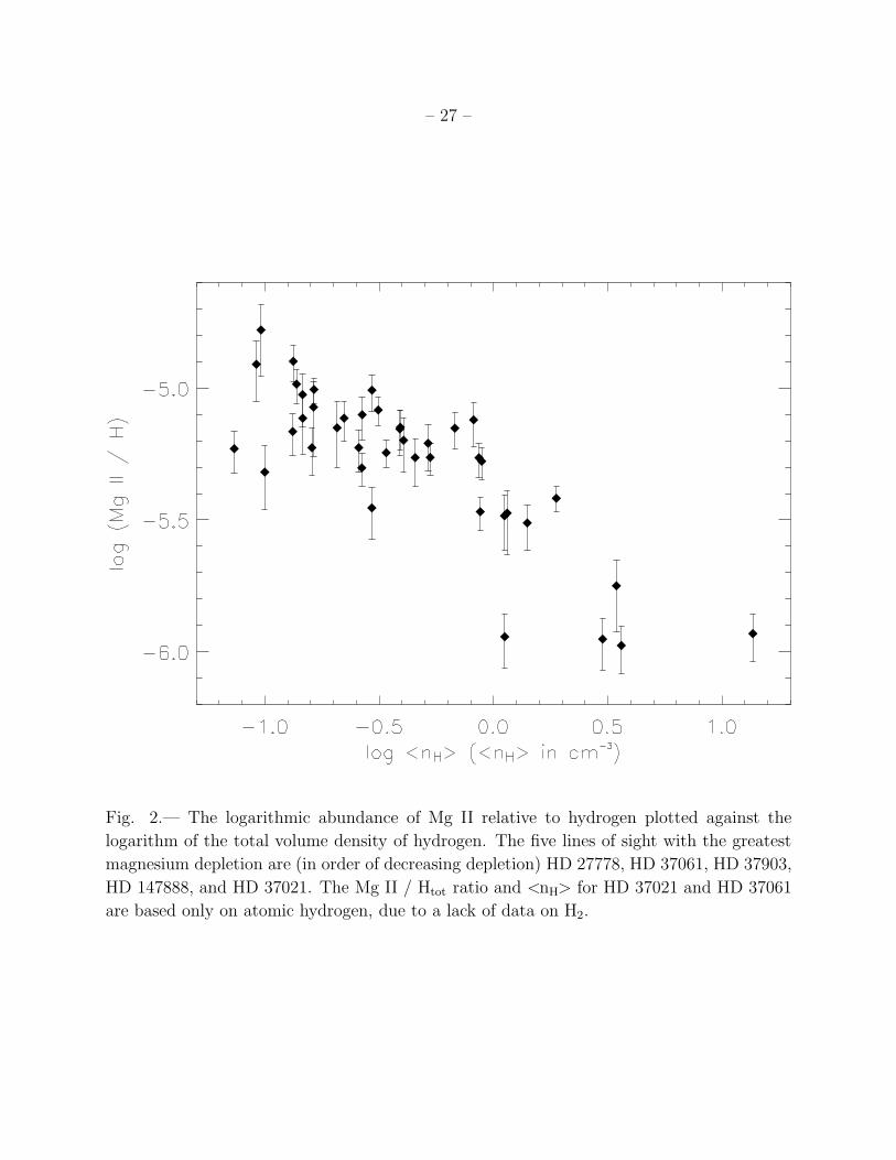
First, we note that magnesium depletion is clearly correlated with total hydrogen volume

density <nH>. Five lines of sight (HD 27778, HD 37021, HD 37061, HD 37903, and HD

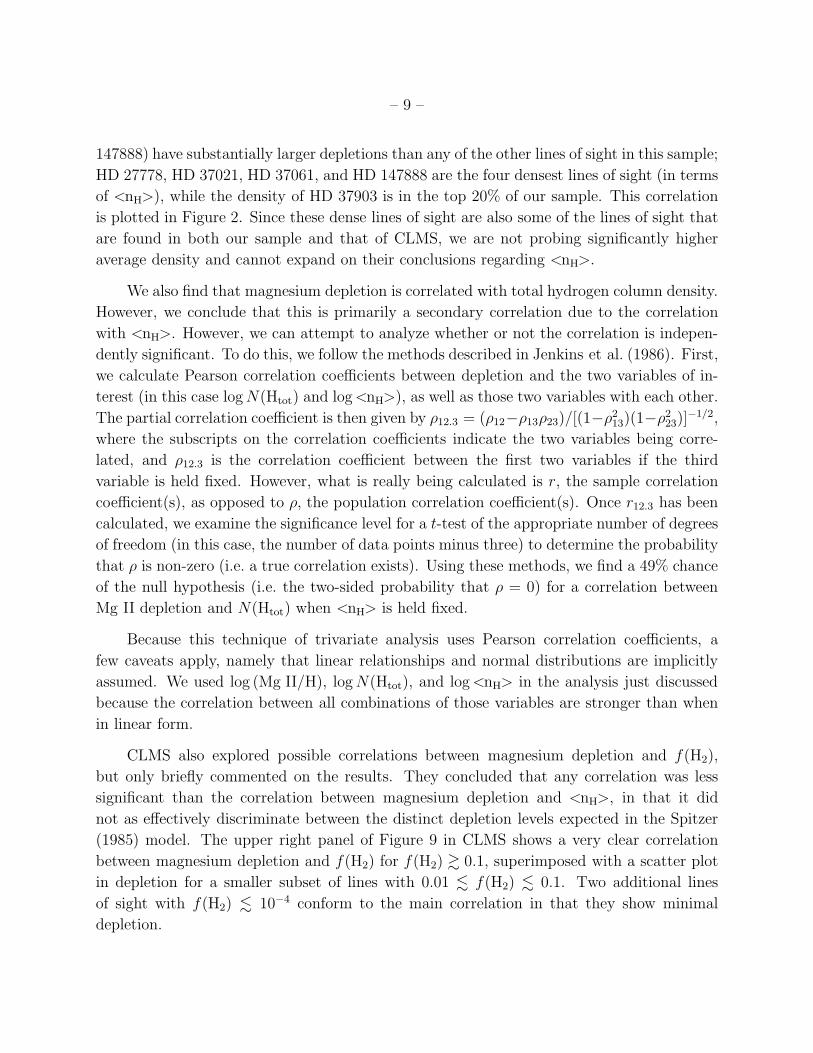
– 9 –

147888) have substantially larger depletions than any of the other lines of sight in this sample;

HD 27778, HD 37021, HD 37061, and HD 147888 are the four densest lines of sight (in terms

of <nH>), while the density of HD 37903 is in the top 20% of our sample. This correlation

is plotted in Figure 2. Since these dense lines of sight are also some of the lines of sight that

are found in both our sample and that of CLMS, we are not probing significantly higher

average density and cannot expand on their conclusions regarding <nH>.

We also find that magnesium depletion is correlated with total hydrogen column density.

However, we conclude that this is primarily a secondary correlation due to the correlation

with <nH>. However, we can attempt to analyze whether or not the correlation is indepen-

dently significant. To do this, we follow the methods described in Jenkins et al. (1986). First,

we calculate Pearson correlation coefficients between depletion and the two variables of in-

terest (in this case log N(Htot) and log <nH>), as well as those two variables with each other.

The partial correlation coefficient is then given by ρ12.3 = (ρ12−ρ13ρ23)/[(1−ρ213)(1−ρ2

23)]−1/2,

where the subscripts on the correlation coefficients indicate the two variables being corre-

lated, and ρ12.3 is the correlation coefficient between the first two variables if the third

variable is held fixed. However, what is really being calculated is r, the sample correlation

coefficient(s), as opposed to ρ, the population correlation coefficient(s). Once r12.3 has been

calculated, we examine the significance level for a t-test of the appropriate number of degrees

of freedom (in this case, the number of data points minus three) to determine the probability

that ρ is non-zero (i.e. a true correlation exists). Using these methods, we find a 49% chance

of the null hypothesis (i.e. the two-sided probability that ρ = 0) for a correlation between

Mg II depletion and N(Htot) when <nH> is held fixed.

Because this technique of trivariate analysis uses Pearson correlation coefficients, a

few caveats apply, namely that linear relationships and normal distributions are implicitly

assumed. We used log (Mg II/H), log N(Htot), and log <nH> in the analysis just discussed

because the correlation between all combinations of those variables are stronger than when

in linear form.

CLMS also explored possible correlations between magnesium depletion and f(H2),

but only briefly commented on the results. They concluded that any correlation was less

significant than the correlation between magnesium depletion and <nH>, in that it did

not as effectively discriminate between the distinct depletion levels expected in the Spitzer

(1985) model. The upper right panel of Figure 9 in CLMS shows a very clear correlation

between magnesium depletion and f(H2) for f(H2) & 0.1, superimposed with a scatter plot

in depletion for a smaller subset of lines with 0.01 . f(H2) . 0.1. Two additional lines

of sight with f(H2) . 10−4 conform to the main correlation in that they show minimal

depletion.

– 10 –

We also see a clear correlation between magnesium depletion and the molecular fraction

of hydrogen, f(H2), plotted in Figure 3, with depletion increasing with increasing f(H2).

There is the exception of one discrepant point, HD 147888, that exhibits substantial depletion

at f(H2) ∼ 0.1. We note that CLMS found a larger column density for this line of sight

than we do (0.2 dex); however, even if we adopt the CLMS Mg II column density for this

line of sight, its abundance is still 0.26 dex smaller than any line of sight in our sample with

f(H2) < 0.4.

We concur with CLMS that the correlation between magnesium depletion and f(H2) is

not as rigorous as the correlation with <nH>. We examine the data using various combina-

tions of the variables in their logarithmic (where correlations are the strongest) and linear

forms. In all cases, we find that the probability of the null hypothesis (i.e. ρ = 0, as discussed

above) between Mg II depletion and f(H2) with <nH> held constant is less than 5%; in most

cases, it is . 1%. Conversely, the probability that there is no correlation between Mg II

depletion and <nH> with f(H2) held constant is less than 0.1%. Therefore, we conclude

that while <nH> is clearly the dominant correlation, the correlation with f(H2) has some

independent significance.

A question of interest is where scatter seems to be introduced and why. Between Figure

9 of CLMS and Figure 3 of this paper, scatter is only observed at f(H2) . 0.1. In our recent

related work on Fe II (Jensen & Snow 2007), we note that Fe II depletion is also correlated

with f(H2), but there are a few exceptions to the trend at both high and low values of f(H2).

The most severe exceptions noted in that paper were HD 147888 and HD 164740 (with large

depletions but f(H2) . 0.1) and HD 210121 (with less depletion despite f(H2) ∼ 0.7). For

Mg II, however, we do not see any outlying points at values of f(H2) larger than ∼ 0.1 within

either this sample or CLMS. Points such as HD 147888, however, still require explanation.

Snow (1983) put forth the possibility that in some dense environments an increased

average grain size, which decreases the grain surface area per unit volume, may suppress

H2 formation (as H2 is thought to form on grain surfaces). This scenario was specifically

discussed in the context of the ρ Oph cloud, for which there is indepedent evidence (in part, a

value of RV greater than the interstellar average of 3.1) that grain coagulation has occurred.

Our main outlying line of sight, HD 147888 (with RV of 4.06), passes through the ρ Oph

cloud, so observing the combination of a dense, depleted environment with small f(H2) is

not surprising in this case.

Two of the other lines of sight with large depletions are HD 37021 and HD 37061.

Reliable far-ultraviolet data sets do not exist for these lines of sight; therefore, they do

not have measurements of the molecular hydrogen column densities or subsequently derived

molecular fractions of hydrogen. However, as stated above in §2.4, Cartledge et al. (2001)

– 11 –

has argued that these lines of sight have small values of f(H2) based on a lack of Cl I. These

two lines of sight also have large values of RV (5.54 and 4.23, respectively), implying a larger

average grain size. The possible effect of grain size on depletions and H2 formation, and

other interpretations, will be discussed further in §3.1.2.

Barring such outlying points, the trend of increased Mg II depletion with increased f(H2)

has a relatively clear interpretation. H2 is formed in the same dense, dusty environments that

foster large depletions. Within the context of this sample and CLMS, this seems to hold for

lines of sight with f(H2) & 0.1. While the ubiquity of H2 even in diffuse regions complicates

the issue (see conclusions of Rachford et al. 2002), there is still a physical argument that

f(H2) should be a good diagnostic of the local conditions of interstellar clouds, and therefore

depletions. It is worth noting that the similar trend between iron depletion and f(H2)

exhibits scatter up to f(H2) ∼ 0.3 in the work of Savage & Bohlin (1979), in addition to the

outlying points mentioned above from Jensen & Snow (2007). Whether the range in f(H2)

over which there is scatter in the abundances is truly different for magnesium and iron or is

simply a selection effect is unclear.

3.1.2. Correlations with Extinction and Reddening Parameters

We find that the depletion of Mg II is correlated to both selective extinction, EB−V ,

and total visual extinction, AV . However, there is significant scatter in these correlations.

Because these are integrated line of sight parameters, it makes sense to divide by line-of-sight

pathlength. Both EB−V and AV are strongly correlated with N(Htot), and both are thought

to be rough measures of the total dust column density. Therefore, EB−V /r and AV /r should

be strongly correlated with <nH> and be approximations of the total dust volume density.

When we look for correlations between magnesium depletion and EB−V /r and AV /r we find

that the correlations are substantially increased when compared to the integrated line of sight

parameters. Therefore, we can say, with reasonable confidence, that magnesium depletion is

increased in increasingly dusty environments. The correlations with EB−V /r and AV /r are

plotted in Figures 4 and 5.

As with the correlation between depletion and f(H2), we examine partial correlation

coefficients to determine the independent significance of these correlations. The partial cor-

relation coefficient between Mg II depletion and log EB−V /r with log <nH> held fixed implies

that the probability of the null hypothesis is less than 6%. The same partial correlation co-

efficient with log AV /r implies that there is less than a 1% chance of the null hypothesis.

(Note that both probabilities are two-sided to a t-distribution.) We consider these variables

in their logarithmic forms because these are the versions of the variables that exhibit the

– 12 –

strong correlations (for all combinations of the variables in question). However, if the vari-

ables are considered in non-logarithmic forms, the probability of the null hypothesis generally

increases. Again we note that this type of trivariate statistical measure implicitly assumes

that the correlation is linear with normally distributed scatter. As with the correlation be-

tween depletion and f(H2), we conclude that while these correlations do not improve on

<nH> as a predictor of depletions, this is limited evidence that they are significant in their

own right.

We have briefly explored the possibility that the additional (or “missing”) magnesium

that is depleted from these lines of sight is found in the form of gas-phase Mg I in regions

that are presumably shielded from radiation by dust. While the STIS data do not cover Mg I

absorption lines in many cases, our results indicate that gas-phase Mg I column densities are

far too small to account for the order-of-magnitude increase in depletion seen in gas-phase

Mg II. Therefore, it likely that the missing gas-phase magnesium is tied up in the additional

grains found in these environments, supporting the conclusion above that the correlations

between Mg II depletion and the parameters log EB−V /r and log AV /r are physically signif-

icant. It is also worth noting that in no case do we see Mg/H less than ∼ 1 ppm, even in

the densest environments, with values of EB−V /r and AV /r several times larger than the

average of the sample. This suggests that these lines of sight are not probing what might

be considered “translucent clouds” (though some may be “translucent lines of sight”; see

Snow & McCall 2006).

The Mg II abundance is plotted against the ratio of total visual to selective extinction,

RV ≡ AV /EB−V , in Figure 6. The plot shows significant scatter; however, some statistical

measures show the possibility of a slight correlation. A Pearson correlation coefficient be-

tween log (Mg II/H) and RV implies that the probability of the null hypothesis is about 31%.

A Spearman’s ρ rank correlation coefficient, which does not depend on the functional form

assumed (including whether variables are considered linearly or logarithmically) beyond as-

suming that the correlation is either monotonically increasing or monotonically decreasing,

shows a negative correlation (decreasing abundance/increasing depletion as RV increases)

and is significant to approximately 1.3-σ. Therefore, there is evidence of a possible slight

correlation between depletion and RV . However, this is far from a certain conclusion. Sig-

nificant selection effects are also a possibility, as the correlations are dominated by some of

the points that have greater depletion and large values of RV . In fact, if these lines of sight

are excluded, the trend begins to reverse toward a positive correlation between increasing

Mg II abundance and increasing RV . In general, we conclude that RV is a poor predictor of

depletions; as one anecdotal counterexample, HD 91597 has a very large value of RV = 4.9

but does not exhibit particularly large Mg II depletion.

– 13 –

However, there are a few lines of sight that present interesting interpretive challenges

where the value of RV may provide insight. As discussed above, the possibility of large

magnesium depletion but small f(H2) exists for three lines of sight: HD 37021, HD 37061,

and HD 147888. In the latter case the effect is clear, while in the former two cases the small

value of f(H2) is merely inferred. What is interesting, as noted above, is that these three lines

of sight all have values of RV > 4 which is a fairly significant deviation from the interstellar

average of 3.1. Because large grains contribute to AV (i.e. grey extinction) but less so to

EB−V , RV is thought to be correlated to average grain size. Explaining why depletion should

increase in a line of sight with large grains is difficult. As mentioned above in our discussion

of H2 and iron depletion, increased grain size decreases dust surface area per unit volume,

and therefore reduces H2 formation rates. However, decreased surface area per unit volume

also implies a reduction in rates of sticking between dust grains and gas-phase atoms.

It seems we can reasonably conclude that the large values of RV , i.e. the larger average

grain populations, are not responsible for the large depletions by way of atoms and ions

sticking to the grains. One possibility is that the large depletions are instead “locked in”

prior to grain coagulation. Another possibility is the effect of a high-radiation field: this is

known for the line of sight toward HD 147888 (ρ Oph D) as well as HD 37021 and HD 37061

which are in Orion (radiation is presumed to be responsible for the relative lack of Cl I, and

thus also H2, as mentioned in §2.4). However, Snow (1983) argues that the increased radiation

is unlikely to be entirely responsible for the low f(H2) in the ρ Oph cloud. Whether or not

this is the case for HD 37021 and HD 37061 is unclear. More details about the radiation field

and the exact nature of the grain population (we have only considered the crude measure of

RV ) are probably necessary to fully understand these lines of sight.

3.1.3. Anticorrelation with Distance

We find that magnesium depletion is generally anticorrelated with distance to the back-

ground star, that is, line of sight pathlength; this relationship is shown in Figure 7. Depletion

decreases by nearly an order of magnitude between very short lines of sight and those up

to about 2 kpc or so, and then is relatively constant (to within about 0.3-0.4 dex) out to

about 6 kpc. As we concluded for a similar anticorrelation seen between iron depletion and

distance (Jensen & Snow 2007), the long pathlengths are likely sampling a variety of cloud

conditions, resulting in the constant depletion for long-pathlength lines of sight. On the

other hand, given the comparable hydrogen column densities of all the lines of sight in this

study (log N(Htot) ≈ 21 − 22), the shorter lines of sight are generally the denser lines of

sight.

– 14 –

3.1.4. Spatial Variations

We find one very interesting correlation with Galactic location: the five stars with the

largest depletions reside at higher Galactic latitudes of |b| > 15◦. However, with pathlengths

of less than 1 kpc, these lines of sight are still primarily in the Galactic disk. When we analyze

magnesium depletions against the height from the center of the Galactic disk, z = r sin b, we

do not see a strong correlation. The variation with respect to Galactic latitude is most likely

a coincidence, given that these are some of the densest and most reddened lines of sight. We

do not see any other evidence of significant spatial variations.

3.2. Mg/H of Galactic Stars

In the last several years, three major papers have attempted to analyze the cosmic

abundance “standards” in the ISM through studies of stellar abundances and meteoritic

abundances—Snow & Witt (1996), Sofia & Meyer (2001), and Lodders (2003). The impor-

tance of these standards is to compare them with the observed gas-phase abundances and

infer an absolute value for depletions—and therefore absolute values for the amount of these

elements in phases other than atomic gas, i.e. dust grains and molecules.

Of the major elements relevant to dust, the element with the best determined cosmic

abundance is iron. The four major measurements of the cosmic Fe/H ratio—solar, B stars,

F and G stars, and CI chondrites—all agree very closely, largely within the errors. The

situation is somewhat more complex for other elements. Carbon and oxygen show apparent

overabundances in the Sun compared to F and G stars (whether or not the solar and F/G star

abundances potentially agree within the errors depends on the choice of solar abundances,

regarding which there is still some uncertainty), while B stars show relative deficits in these

abundances compared to the Sun and other F and G stars. The chondritic abundances of

C and O are even smaller. Nitrogen seems to be somewhat less abundant in B stars than in

the Sun, though the two are reconciliable within the errors; F and G nitrogen abundances

are generally unknown, and the chondritic abundances are substantially lower. Silicon seems

to be most abundant in F and G stars, slightly less abundant in the Sun, and about half

as abundant in B stars. The errors, however, do not rule out agreement between all three

measurements. However, the chondritic abundance tightly matches the solar abundance.

Both Sofia & Meyer (2001) and Lodders (2003), cite Holweger (2001) for the solar abun-

dance of magnesium, log (Mg/H) = −4.46; Snow & Witt (1996) report a slightly older value

from Anders & Grevesse (1989) of log (Mg/H) = −4.42, though these values are consistent

within the errors. The chondritic abundances in Lodders (2003) of log (Mg/H) = −4.44 are

– 15 –

also very consistent with these solar values. The discrepancy arises when various stellar abun-

dances are considered. Both Snow & Witt (1996) and Sofia & Meyer (2001) found signifi-

cantly smaller abundances of Mg for B stars. Snow & Witt (1996) found log (Mg/H) = −4.63

for field B stars and log (Mg/H) = −4.68 for cluster B stars; Sofia & Meyer (2001), mak-

ing no distinction between cluster and field stars, found log (Mg/H) = −4.64 for all B

stars. Though there is marginal agreement within the very large errors in these num-

bers, the B star abundances are ≈ 60% smaller than the solar abundances. Snow & Witt

(1996) and Sofia & Meyer (2001) also disagree on the Mg abundance in F and G stars

(log (Mg/H) = −4.52 and −4.37, respectively) due most likely to Sofia & Meyer (2001) re-

stricting their sample to stars with ages of ≤ 2 Gyr. Again, however, these values have

relatively large errors and are reconciliable with the B star abundances, though just barely.

What effect does the choice of a cosmic magnesium abundance have for the implied

dust-phase abundances to be used in dust models? The differences between the cosmic

abundances just discussed leads to nontrivial differences in the dust-phase abundances. Our

weighted interstellar average of Mg II/H is 2.7 ± 0.1 ppm (parts per million), though the

median value in our 44 lines of sight is somewhat larger at 6.2 ppm. Taking the extremes of

the above numbers, anywhere between ∼ 20 and ∼ 40 ppm of Mg is available for creating

dust. Examining the various models compared in Table 3 of Snow & Witt (1996), we find

that most models require much more Mg than the lower value of ∼ 20 implied by a B

star abundance standard. That a B star abundance is less likely to represent the cosmic

abundance was also found by Zubko et al. (2004), who had more difficulty fitting dust models

to observations using the dust-phase abundances implied by assuming B star abundances

as the cosmic standard. In fact, this is true even though Zubko et al. assumed ≈ 0 ppm

of magnesium to be in the gas-phase. If the few ppm of magnesium in the gas-phase as

measured by this paper and CLMS were included, the Zubko et al. (2004) fits would become

even more strained (the best fits for B star abundances were at the limit of the error in

those abundances and inferior to the fits obtained using other abundances). Therefore, the

major conclusion that we can make regarding cosmic abundances and the incorporation of

magnesium into dust is to add to the evidence that B star abundances, despite B stars

being younger and therefore potentially good tracers of the current ISM, are a poor cosmic

standard. Whether or not the solar or an F and G star abundance standard for Mg is a

better fit is a test that is too sensitive for us to comment on, given the uncertainties in those

abundances.

– 16 –

4. SUMMARY

We have analyzed the abundance of Mg II in 44 lines of sight. Our study does not probe

substantially larger average hydrogen volume densities than previously observed by CLMS;

therefore, we observe the same correlations between Mg II and the <nH> and EB−V /r. We

also note a correlations between magnesium depletion and AV /r, a different measure of dust

density. Correlations between N(Htot) and the reddening and extinction parameters EB−V

and AV mean that correlations between Mg II depletion and dust density measures are ex-

pected. However, these latter correlations, while not strong than the correlation between

depletion and <nH>, show some evidence of being significant even at fixed <nH> and should

be more directly related to the line-of-sight dust content. We also note a correlation be-

tween magnesium depletion and f(H2) in our data; combined with the results of CLMS, this

correlation seems to be valid for f(H2) & 0.1 but not at smaller f(H2). A question that is

related to the trend with f(H2) is why so little H2 forms in certain high-density lines of sight.

Our results are consistent with the Snow (1983) suggestion that the reduced grain surface

area per unit volume of large grains plays a role in reducing H2 formation rates. For similar

reasons, we can conclude that the grain coagulation probably occurs after depletions are

already “locked into” the dust, rather than depletion of gas-phase atoms onto grain surfaces.

The authors would like to thank the anonymous referee for many helpful comments that

greatly improved the manuscript. The authors also wish to thank S. V. Penton for the use of

his measurements of the STIS point-spread functions; B. A. Keeney for the original version of

the profile-fitting code that we adapted to our purposes; and J. M. Shull and B. L. Rachford

for the use of their unpublished measurements of molecular hydrogen column densities. This

work was supported by NASA grant NAG5-12279.

REFERENCES

Aiello, S., Barsella, B., Chlewicki, G., Greenberg, J. M., Patriarchi, P., & Perinotto, M.

1988, A&AS, 73, 195

Anders, E., & Grevesse, N. 1989, Geochim. Cosmochim. Acta, 53, 197

Andre, M. K., Oliveira, C. M., Howk, J. C., Ferlet, R., Desert, J.-M., Hebrard, G., Lacour,

S., Lecavelier des Etangs, A., Vidal-Madjar, A., & Moos, H. W. 2003, ApJ, 591, 1000

Cartledge, S. I. B., Lauroesch, J. T., Meyer, D. M., & Sofia, U. J. 2004, ApJ, 613, 1037

—. 2006, ApJ, 641, 327

– 17 –

Cartledge, S. I. B., Meyer, D. M., Lauroesch, J. T., & Sofia, U. J. 2001, ApJ, 562, 394

Diplas, A., & Savage, B. D. 1994, ApJS, 93, 211

Fitzpatrick, E. L. 1997, ApJ, 482, L199

Fleming, J., Hibbert, A., Bell, K. L., & Vaeck, N. 1998, MNRAS, 300, 767

Garmany, C. D., & Stencel, R. E. 1992, A&AS, 94, 211

Godefroid, M., & Froese Fischer, C. 1999, Journal of Physics B Atomic Molecular Physics,

32, 4467

Holweger, H. 2001, in AIP Conf. Proc. 598: Joint SOHO/ACE workshop ”Solar and Galactic

Composition”, ed. R. F. Wimmer-Schweingruber, 23

Hoopes, C. G., Sembach, K. R., Hebrard, G., Moos, H. W., & Knauth, D. C. 2003, ApJ,

586, 1094

Jenkins, E. B. 1996, ApJ, 471, 292

Jenkins, E. B., Savage, B. D., & Spitzer, Jr., L. 1986, ApJ, 301, 355

Jensen, A. G., Rachford, B. L., & Snow, T. P. 2007, ApJ, 654, 955

Jensen, A. G., & Snow, T. P. 2007, ApJ, submitted

Lodders, K. 2003, ApJ, 591, 1220

Majumder, S., Merlitz, H., Gopakumar, G., Das, B. P., Mahapatra, U. S., & Mukherjee, D.

2002, ApJ, 574, 513

Micol, A., Durand, D., Pirenne, B., Gaudet, S., & Hodge, P. 1999, in ASP Conf. Ser. 172:

Astronomical Data Analysis Software and Systems VIII, ed. D. M. Mehringer, R. L.

Plante, & D. A. Roberts, 191

Morton, D. C. 2003, ApJS, 149, 205

Murray, M. J., Dufton, P. L., Hibbert, A., & York, D. G. 1984, ApJ, 282, 481

Neckel, T., Klare, G., & Sarcander, M. 1980, Bulletin d’Information du Centre de Donnees

Stellaires, 19, 61

Pan, K., Federman, S. R., Cunha, K., Smith, V. V., & Welty, D. E. 2004, ApJS, 151, 313

– 18 –

Rachford, B. L., Snow, T. P., Tumlinson, J., Shull, J. M., Blair, W. P., Ferlet, R., Friedman,

S. D., Gry, C., Jenkins, E. B., Morton, D. C., Savage, B. D., Sonnentrucker, P.,

Vidal-Madjar, A., Welty, D. E., & York, D. G. 2002, ApJ, 577, 221

Savage, B. D., & Bohlin, R. C. 1979, ApJ, 229, 136

Savage, B. D., Massa, D., Meade, M., & Wesselius, P. R. 1985, ApJS, 59, 397

Savage, B. D., & Sembach, K. R. 1991, ApJ, 379, 245

Snow, T. P. 1983, ApJ, 269, L57

Snow, T. P., Destree, J. D., & Jensen, A. G. 2007, ApJ, 655, 285

Snow, T. P., & McCall, B. J. 2006, ARA&A, 44, 367

Snow, T. P., & Witt, A. N. 1996, ApJ, 468, L65

Sofia, U. J., Fabian, D., & Howk, J. C. 2000, ApJ, 531, 384

Sofia, U. J., & Meyer, D. M. 2001, ApJ, 554, L221

Spitzer, L. 1985, ApJ, 290, L21

Theodosiou, C. E., & Federman, S. R. 1999, ApJ, 527, 470

Welty, D. E., & Hobbs, L. M. 2001, ApJS, 133, 345

Welty, D. E., Hobbs, L. M., & Morton, D. C. 2003, ApJS, 147, 61

Zubko, V., Dwek, E., & Arendt, R. G. 2004, ApJS, 152, 211

This preprint was prepared with the AAS LATEX macros v5.2.

– 19 –

Table 1. Lines of Sight: Stellar Data

Star Name Spectral Class l b Distance (pc) Ref.

BD +35◦4258 B0.5Vn 77.19 -4.74 3100 1

CPD -59◦2603 O7V... 287.59 -0.69 2630 2

HD 12323 O9V 132.91 -5.87 3900 1

HD 13745 O9.7II((N)) 134.58 -4.96 1900 1

HD 15137 O9.5V 137.46 +7.58 3300 2

HD 27778 B3V 172.76 -17.39 223 3

HD 37021 B0V 209.01 -19.38 450 4

HD 37061 B1V 208.92 -19.27 580 5

HD 37903 B1.5V 206.85 -16.54 910 5

HD 40893 B0IV 180.09 +4.34 2800 5

HD 66788 O8/O9Ib 245.43 +2.05 · · · · · ·

HD 69106 B1/B2II 254.52 -1.33 1600 5

HD 91597 B7/B8IV/V 286.86 -2.37 6400 5

HD 91651 O9VP: 286.55 -1.72 3500 1

HD 92554 O9.5III 287.60 -2.02 6795 2

HD 93205 O3V 287.57 -0.71 2600 1

HD 93222 O7III((f)) 287.74 -1.02 2900 1

HD 93843 O6III(f) 228.24 -0.90 2700 1

HD 94493 B0.5Ib 289.01 -1.18 2900 5

HD 99857 B1Ib 294.78 -4.94 3058 2

HD 99890 B0.5V: 291.75 +4.43 3070 2

HD 103779 B0.5II 296.85 -1.02 3500 5

HD 104705 B0.5III 297.45 -0.34 3500 5

HD 109399 B1Ib 301.71 -9.88 1900 5

HD 116781 O9/B1(I)E 307.05 -0.07 · · · · · ·

HD 122879 B0Ia 312.26 +1.79 4800 5

HD 124314 O7 312.67 -0.42 1100 1

HD 147888 B3/B4V 353.65 +17.71 136 3

HD 152590 O7.5V 344.84 +1.83 1800 4

HD 168941 B0III/IV 5.82 -6.31 5000 5

HD 177989 B2II 17.81 -11.88 5100 5

HD 185418 B0.5V 53.60 -2.17 950 5

HD 192639 O7.5IIIF 74.90 +1.48 1100 5

HD 195965 B0V 85.71 +5.00 1300 5

HD 202347 B1V 88.22 -2.08 1300 1

HD 203374 B0IVpe 100.51 +8.62 820 2

HD 206267 O6(F) 99.29 +3.74 1000 4

HD 207198 O9II 103.14 +6.99 1000 5

HD 207308 B0.5V 103.11 +6.82 · · · · · ·

HD 207538 O9.5V 101.60 +4.67 880 5

HD 209339 BOIV 104.58 +5.87 1100 1

HD 210839 O6e 103.83 +2.61 505 3

HD 224151 B0.5IISBV 115.44 -4.64 1355 2

HD 303308 O3V 287.59 -0.61 2630 2

References. — Spectral classes and Galactic coordinates compiled from SIMBAD

database at http://simbad.u-strasbg.fr/simbad/sim-fid. References for distances:

(1) Savage et al. (1985). (2) Diplas & Savage (1994). (3) Hipparcos 4-σ—Hipparcos

parallax of 4-σ precision or better. (4) Member of an OB association, cluster, or

multiple-star system, DIB database at http://dib.uiuc.edu; values compiled from

the literature or derived by L. M. Hobbs. (5) Spectroscopic distance modulus from

the DIB database.

– 20 –

Table 2. Lines of Sight: STIS Data Sets Used

Star Name Data Set(s) Grating Aperturea

BD +35◦4258 O6LZ89010 E140M 0.2X0.2

CPD -59◦2603 O4QX03010 E140H 0.2X0.09

HD 12323 O63505010 E140M 0.2X0.2

HD 13745 O6LZ05010 E140M 0.2X0.2

HD 15137 O5LH02010 E140H 0.1X0.03

O5LH02020

O5LH02030

O5LH02040

HD 27778 O59S01010 E140H 0.2X0.09

O59S01020

HD 37021 O59S02010 E140H 0.2X0.09

HD 37061 O59S03010 E140H 0.1X0.03

HD 37903 O59S04010 E140H 0.2X0.09

HD 40893 O8NA02010 E140H 0.2X0.2

O8NA02020

HD 66788 O6LZ26010 E140M 0.2X0.2

HD 69106 O5LH03010 E140H 0.1X0.03

O5LH03020

HD 91597 O6LZ32010 E140M 0.2X0.2

HD 91651 O6LZ34010 E140M 0.2X0.2

HD 92554 O6LZ36010 E140M 0.2X0.2

HD 93205 O4QX01010 E140H 0.2X0.09

HD 93222 O4QX02010 E140H 0.2X0.09

HD 93843 O5LH04010 E140H 0.1X0.03

O5LH04020

HD 94493 O54306010 E140H 0.1X0.03

HD 99857 O54301010 E140H 0.1X0.03

O54301020

O54301030

HD 99890 O6LZ45010 E140M 0.2X0.2

HD 103779 O54302010 E140H 0.1X0.03

HD 104705 O57R01010 E140H 0.2X0.09

HD 109399 O54303010 E140H 0.1X0.03

HD 116781 O5LH05010 E140H 0.1X0.3

O5LH05020

HD 122879 O5LH07010 E140H 0.1X0.03

O5LH07020

HD 124314 O54307010 E140H 0.1X0.03

HD 147888 O59S05010 E140H 0.2X0.09

HD 152590 O8NA04010 E140H 0.2X0.2

O8NA04020

O5C08P010

HD 168941 O6LZ81010 E140M 0.2X0.2

HD 177989 O57R03010 E140H 0.2X0.09

O57R03020

HD 185418 O5C01Q010 E140H 0.2X0.2

– 21 –

Table 2—Continued

Star Name Data Set(s) Grating Aperturea

HD 192639 O5C08T010 E140H 0.2X0.2

HD 195965 O6BG01010 E140H 0.1X0.03

HD 202347 O5G301010 E140H 0.1X0.03

HD 203374 O5LH08010 E140H 0.1X0.03

O5LH08020

O5LH08030

HD 206267 O5LH09010 E140H 0.1X0.03

O5LH09020

HD 207198 O59S06010 E140H 0.2X0.09

O59S06020

HD 207308 O63Y02010 E140M 0.2X0.06

O63Y02020

HD 207538 O63Y01010 E140M 0.2X0.06

O63Y01020

HD 209339 O5LH0B010 E140H 0.1X0.03

O5LH0B020

HD 210839 O54304010 E140H 0.1X0.03

HD 224151 O54308010 E140H 0.1X0.03

HD 303308 O4QX04010 E140H 0.2X0.09

aAperture is length X width of the slit, with both

values in arcseconds.

– 22 –

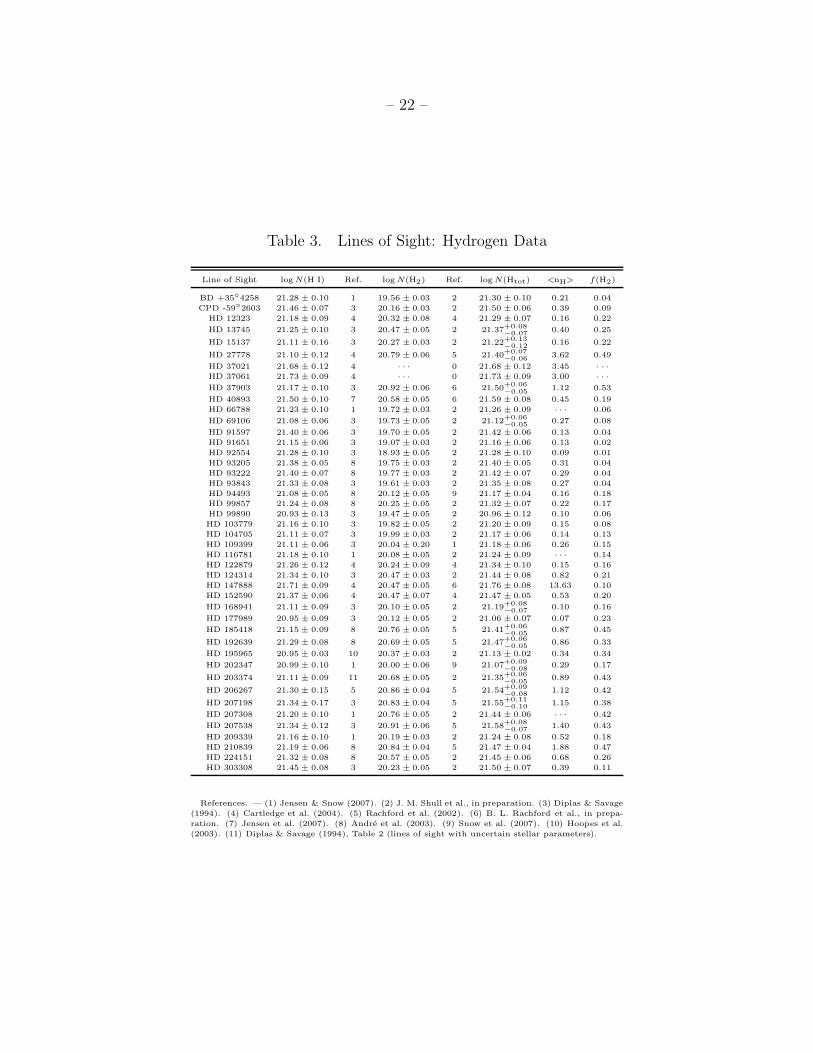
Table 3. Lines of Sight: Hydrogen Data

Line of Sight log N(H I) Ref. log N(H2) Ref. log N(Htot) <nH> f(H2)

BD +35◦4258 21.28 ± 0.10 1 19.56 ± 0.03 2 21.30 ± 0.10 0.21 0.04

CPD -59◦2603 21.46 ± 0.07 3 20.16 ± 0.03 2 21.50 ± 0.06 0.39 0.09

HD 12323 21.18 ± 0.09 4 20.32 ± 0.08 4 21.29 ± 0.07 0.16 0.22

HD 13745 21.25 ± 0.10 3 20.47 ± 0.05 2 21.37+0.08−0.07

0.40 0.25

HD 15137 21.11 ± 0.16 3 20.27 ± 0.03 2 21.22+0.13−0.12

0.16 0.22

HD 27778 21.10 ± 0.12 4 20.79 ± 0.06 5 21.40+0.07−0.06

3.62 0.49

HD 37021 21.68 ± 0.12 4 · · · 0 21.68 ± 0.12 3.45 · · ·

HD 37061 21.73 ± 0.09 4 · · · 0 21.73 ± 0.09 3.00 · · ·

HD 37903 21.17 ± 0.10 3 20.92 ± 0.06 6 21.50+0.06

−0.051.12 0.53

HD 40893 21.50 ± 0.10 7 20.58 ± 0.05 6 21.59 ± 0.08 0.45 0.19

HD 66788 21.23 ± 0.10 1 19.72 ± 0.03 2 21.26 ± 0.09 · · · 0.06

HD 69106 21.08 ± 0.06 3 19.73 ± 0.05 2 21.12+0.06−0.05

0.27 0.08

HD 91597 21.40 ± 0.06 3 19.70 ± 0.05 2 21.42 ± 0.06 0.13 0.04

HD 91651 21.15 ± 0.06 3 19.07 ± 0.03 2 21.16 ± 0.06 0.13 0.02

HD 92554 21.28 ± 0.10 3 18.93 ± 0.05 2 21.28 ± 0.10 0.09 0.01

HD 93205 21.38 ± 0.05 8 19.75 ± 0.03 2 21.40 ± 0.05 0.31 0.04

HD 93222 21.40 ± 0.07 8 19.77 ± 0.03 2 21.42 ± 0.07 0.29 0.04

HD 93843 21.33 ± 0.08 3 19.61 ± 0.03 2 21.35 ± 0.08 0.27 0.04

HD 94493 21.08 ± 0.05 8 20.12 ± 0.05 9 21.17 ± 0.04 0.16 0.18

HD 99857 21.24 ± 0.08 8 20.25 ± 0.05 2 21.32 ± 0.07 0.22 0.17

HD 99890 20.93 ± 0.13 3 19.47 ± 0.05 2 20.96 ± 0.12 0.10 0.06

HD 103779 21.16 ± 0.10 3 19.82 ± 0.05 2 21.20 ± 0.09 0.15 0.08

HD 104705 21.11 ± 0.07 3 19.99 ± 0.03 2 21.17 ± 0.06 0.14 0.13

HD 109399 21.11 ± 0.06 3 20.04 ± 0.20 1 21.18 ± 0.06 0.26 0.15

HD 116781 21.18 ± 0.10 1 20.08 ± 0.05 2 21.24 ± 0.09 · · · 0.14

HD 122879 21.26 ± 0.12 4 20.24 ± 0.09 4 21.34 ± 0.10 0.15 0.16

HD 124314 21.34 ± 0.10 3 20.47 ± 0.03 2 21.44 ± 0.08 0.82 0.21

HD 147888 21.71 ± 0.09 4 20.47 ± 0.05 6 21.76 ± 0.08 13.63 0.10

HD 152590 21.37 ± 0.06 4 20.47 ± 0.07 4 21.47 ± 0.05 0.53 0.20

HD 168941 21.11 ± 0.09 3 20.10 ± 0.05 2 21.19+0.08−0.07

0.10 0.16

HD 177989 20.95 ± 0.09 3 20.12 ± 0.05 2 21.06 ± 0.07 0.07 0.23

HD 185418 21.15 ± 0.09 8 20.76 ± 0.05 5 21.41+0.06

−0.050.87 0.45

HD 192639 21.29 ± 0.08 8 20.69 ± 0.05 5 21.47+0.06

−0.050.86 0.33

HD 195965 20.95 ± 0.03 10 20.37 ± 0.03 2 21.13 ± 0.02 0.34 0.34

HD 202347 20.99 ± 0.10 1 20.00 ± 0.06 9 21.07+0.09−0.08

0.29 0.17

HD 203374 21.11 ± 0.09 11 20.68 ± 0.05 2 21.35+0.06−0.05

0.89 0.43

HD 206267 21.30 ± 0.15 5 20.86 ± 0.04 5 21.54+0.09−0.08

1.12 0.42

HD 207198 21.34 ± 0.17 3 20.83 ± 0.04 5 21.55+0.11−0.10

1.15 0.38

HD 207308 21.20 ± 0.10 1 20.76 ± 0.05 2 21.44 ± 0.06 · · · 0.42

HD 207538 21.34 ± 0.12 3 20.91 ± 0.06 5 21.58+0.08

−0.071.40 0.43

HD 209339 21.16 ± 0.10 1 20.19 ± 0.03 2 21.24 ± 0.08 0.52 0.18

HD 210839 21.19 ± 0.06 8 20.84 ± 0.04 5 21.47 ± 0.04 1.88 0.47

HD 224151 21.32 ± 0.08 8 20.57 ± 0.05 2 21.45 ± 0.06 0.68 0.26

HD 303308 21.45 ± 0.08 3 20.23 ± 0.05 2 21.50 ± 0.07 0.39 0.11

References. — (1) Jensen & Snow (2007). (2) J. M. Shull et al., in preparation. (3) Diplas & Savage

(1994). (4) Cartledge et al. (2004). (5) Rachford et al. (2002). (6) B. L. Rachford et al., in prepa-

ration. (7) Jensen et al. (2007). (8) Andre et al. (2003). (9) Snow et al. (2007). (10) Hoopes et al.

(2003). (11) Diplas & Savage (1994), Table 2 (lines of sight with uncertain stellar parameters).

– 23 –

Table 4. Lines of Sight: Reddening Data

Line of Sight EB−V Ref. AV Ref. RV Ref.

(mag) (mag)

BD +35◦4258 0.29 1 0.93 2 3.21 3

CPD -59◦2603 0.46 4 1.45 3 3.15 5

HD 12323 0.24 1 0.74 2 3.08 3

HD 13745 0.46 4 1.42 2 3.09 3

HD 15137 0.31 4 1.10 2 3.55 3

HD 27778 0.37 6 1.01 3 2.73 6

HD 37021 0.54 6 2.99 3 5.54 6

HD 37061 0.52 6 2.20 3 4.23 6

HD 37903 0.35 4 1.28 3 3.66 6

HD 40893 0.46 6 1.13 3 2.46 6

HD 66788 0.20 5 0.69 2 3.45 3

HD 69106 0.18 6 0.58 2 3.22 3

HD 91597 0.27 6 1.33 2 4.93 3

HD 91651 0.30 4 0.95 2 3.17 3

HD 92554 0.39 4 1.15 2 2.95 3

HD 93205 0.37 4 1.21 2 3.27 3

HD 93222 0.37 7 1.18 2 3.19 3

HD 93843 0.34 4 1.03 2 3.03 3

HD 94493 0.20 4 0.71 2 3.55 3

HD 99857 0.33 4 1.10 2 3.33 3

HD 99890 0.24 4 0.72 2 3.00 3

HD 103779 0.21 4 0.68 2 3.24 3

HD 104705 0.26 4 0.80 2 3.08 3

HD 109399 0.26 4 0.81 2 3.12 3

HD 116781 0.34 5 1.40 2 4.12 3

HD 122879 0.36 7 1.12 2 3.11 3

HD 124314 0.53 4 1.64 2 3.09 3

HD 147888 0.47 6 1.91 3 4.06 6

HD 152590 0.46 6 1.51 3 3.28 6

HD 168941 0.37 4 1.03 2 2.78 3

HD 177989 0.25 4 0.25 2 1.00 3

HD 185418 0.50 6 1.16 3 2.32 6

HD 192639 0.66 4 1.87 3 2.83 6

HD 195965 0.25 4 0.77 2 3.08 3

HD 202347 0.19 8 0.53 2 2.79 3

HD 203374 0.60 9 1.88 2 3.13 3

HD 206267 0.53 6 1.41 3 2.66 6

HD 207198 0.62 6 1.50 3 2.42 6

HD 207308 0.52 8 1.61 2 3.10 3

HD 207538 0.64 6 1.44 3 2.25 6

HD 209339 0.38 8 1.09 2 2.87 3

HD 210839 0.57 4 1.58 3 2.77 6

HD 224151 0.44 4 1.52 2 3.45 3

HD 303308 0.45 7 1.09 2 2.42 3

References. — (1) Savage et al. (1985). (2) Neckel et al. (1980).

(3) Derived from the other two quantities via the relationship

RV ≡ AV /EB−V . (4) Diplas & Savage (1994). (5) Jensen & Snow

(2007). (6) DIB Database, http://dib.uiuc.edu; EB−V compiled by

L. M. Hobbs, RV derived by B. L. Rachford through polarization or

infrared photometry Rachford et al. (for method and examples, see

2002). (7) Aiello et al. (1988). (8) Garmany & Stencel (1992). (9)

Diplas & Savage (1994), Table 2 (lines of sight with uncertain stellar

parameters).

– 24 –

Table 5. Mg II Column Density Results

Line of Sight log N(Mg II) log (Mg II/H) Mg/H (ppm) W1239.9 W1240.4

BD +35◦4258 16.15+0.06−0.08

−5.15+0.10−0.15

7.1+1.8−2.1

81.4 ± 10.4 54.8 ± 10.4

CPD -59◦2603 16.35 ± 0.03 −5.15+0.06−0.08

7.1+1.1−1.3

112.4 ± 6.6 78.8 ± 7.4

HD 12323 16.06+0.04−0.05

−5.23+0.07−0.10

5.9+1.1−1.3

64.3 ± 5.1 43.9 ± 6.0

HD 13745 16.18+0.06−0.07

−5.20+0.08−0.12

6.3+1.3−1.5

93.3 ± 10.1 61.3 ± 10.9

HD 15137 16.15 ± 0.02 −5.07+0.09−0.19

8.5+2.1−3.0

72.1 ± 2.4 50.9 ± 2.9

HD 27778 15.42+0.05−0.06

−5.98+0.07−0.11

1.1 ± 0.2 16.0 ± 1.7 10.6 ± 1.5

HD 37021 15.93+0.03

−0.04−5.75+0.10

−0.171.8+0.5

−0.633.7 ± 2.2 23.7 ± 2.2

HD 37061 15.78 ± 0.03 −5.95+0.08

−0.121.1+0.2

−0.327.0 ± 1.5 19.8 ± 1.4

HD 37903 15.55+0.07−0.09

−5.94+0.09−0.12

1.1 ± 0.3 21.1 ± 3.1 14.2 ± 3.2

HD 40893 16.33 ± 0.03 −5.26+0.07−0.11

5.5+1.0−1.2

95.5 ± 5.0 69.8 ± 5.3

HD 66788 16.11+0.08−0.10

−5.15+0.11−0.17

7.1+2.0−2.3

81.2 ± 10.6 39.5 ± 11.1

HD 69106 15.81+0.02−0.03

−5.30+0.05−0.07

5.0 ± 0.7 37.3 ± 1.7 25.3 ± 1.8

HD 91597 16.25 ± 0.05 −5.16+0.07−0.09

6.8+1.2−1.3

94.4 ± 8.7 66.1 ± 9.6

HD 91651 16.26+0.03

−0.04−4.90+0.06

−0.0812.7+1.9

−2.1108.0 ± 6.6 72.3 ± 6.9

HD 92554 16.37+0.04

−0.05−4.91+0.09

−0.1412.3+2.8

−3.4109.4 ± 9.1 80.0 ± 9.3

HD 93205 16.32+0.02−0.03

−5.08+0.05−0.06

8.3+1.0−1.1

113.7 ± 4.9 77.9 ± 5.9

HD 93222 16.41+0.01−0.02

−5.01+0.06−0.08

9.8+1.4−1.7

114.4 ± 3.0 84.3 ± 3.6

HD 93843 16.25 ± 0.02 −5.10+0.07−0.10

7.9+1.3−1.6

104.0 ± 3.4 69.8 ± 4.1

HD 94493 16.16 ± 0.02 −5.00+0.04−0.05

9.9 ± 1.1 77.2 ± 3.2 53.5 ± 3.6

HD 99857 16.21 ± 0.03 −5.11+0.06−0.09

7.7+1.2−1.4

80.6 ± 4.1 55.8 ± 4.4

HD 99890 16.18 ± 0.03 −4.78+0.10

−0.1816.6

+4.2

−5.683.4 ± 4.5 57.3 ± 5.3

HD 103779 16.17 ± 0.02 −5.02+0.08

−0.129.5+1.9

−2.381.6 ± 3.4 56.0 ± 3.9

HD 104705 16.19 ± 0.02 −4.98+0.06−0.08

10.4+1.4−1.7

83.8 ± 3.2 57.2 ± 3.4

HD 109399 15.95 ± 0.05 −5.23+0.07−0.09

5.9+1.0−1.1

56.8 ± 5.0 36.9 ± 5.4

HD 116781 16.14 ± 0.03 −5.11+0.08−0.12

7.8+1.5−1.8

75.5 ± 4.4 51.8 ± 4.8

HD 122879 16.22 ± 0.02 −5.11+0.08−0.14

7.7+1.6−2.1

86.5 ± 2.8 60.4 ± 3.2

HD 124314 16.32 ± 0.02 −5.12+0.07−0.10

7.6+1.3−1.6

97.6 ± 3.0 70.9 ± 3.7

HD 147888 15.83 ± 0.03 −5.93+0.07−0.11

1.2+0.2−0.3

24.1 ± 1.5 18.9 ± 1.5

HD 152590 16.20 ± 0.03 −5.26+0.05

−0.075.5+0.7

−0.871.3 ± 4.3 52.1 ± 4.2

HD 168941 15.87+0.08

−0.10−5.32+0.10

−0.144.8+1.2

−1.342.8 ± 7.0 28.9 ± 7.0

HD 177989 15.83 ± 0.03 −5.23+0.06−0.09

5.9+0.9−1.1

40.7 ± 2.0 27.1 ± 2.2

HD 185418 15.94 ± 0.03 −5.47+0.05−0.07

3.4+0.4−0.5

41.7 ± 2.1 30.0 ± 2.1

HD 192639 16.20 ± 0.03 −5.26+0.05−0.07

5.4+0.7−0.8

60.3 ± 3.2 46.9 ± 3.7

HD 195965 15.89+0.04−0.05

−5.24 ± 0.05 5.7 ± 0.7 45.0 ± 3.4 30.3 ± 4.1

HD 202347 15.62+0.04−0.05

−5.45+0.08−0.12

3.5+0.7−0.8

27.5 ± 2.2 17.6 ± 2.2

HD 203374 16.07 ± 0.02 −5.28+0.05

−0.075.3+0.7

−0.863.3 ± 2.7 44.3 ± 2.8

HD 206267 16.05 ± 0.04 −5.48+0.08

−0.133.3+0.6

−0.958.1 ± 4.2 40.7 ± 4.7

HD 207198 16.08 ± 0.02 −5.47+0.08−0.16

3.4+0.7−1.0

56.6 ± 2.2 40.8 ± 2.7

HD 207308 15.93 ± 0.05 −5.51+0.07−0.10

3.1+0.5−0.6

45.9 ± 4.1 31.7 ± 4.6

HD 207538 16.07+0.03−0.04

−5.51+0.07−0.10

3.1+0.5−0.6

58.2 ± 3.5 41.4 ± 4.1

HD 209339 16.04 ± 0.02 −5.21+0.07−0.11

6.2+1.1−1.3

53.9 ± 1.8 38.4 ± 2.0

HD 210839 16.05 ± 0.03 −5.42+0.04−0.05

3.8 ± 0.4 63.1 ± 3.3 42.9 ± 3.7

HD 224151 16.30 ± 0.03 −5.15+0.06

−0.087.1

+1.0

−1.2104.6 ± 5.8 72.4 ± 6.5

HD 303308 16.34+0.04

−0.05−5.15+0.07

−0.107.0+1.3

−1.4108.1 ± 8.6 75.8 ± 9.0

– 25 –

Table 6. Comparison with CLMS

Line of Sight log N(Mg II)

This paper CLMS AODa CLMS PFb CLMS AEc

HD 12323 16.06+0.04−0.05 16.03 ± 0.02 16.04 ± 0.05 0.05

HD 27778 15.42+0.05−0.06 15.49 ± 0.02 15.48 ± 0.01 0.02

HD 37021 15.93+0.03−0.04 15.85 ± 0.02 15.90 ± 0.02 0.03

HD 37061 15.78 ± 0.03 15.78 ± 0.01 15.80 ± 0.05 0.05

HD 37903 15.55+0.07−0.09 15.65 ± 0.02 15.62 ± 0.06 0.06

HD 122879 16.22 ± 0.02 16.22 ± 0.02 16.23 ± 0.01 0.02

HD 147888 15.83 ± 0.03 15.84 ± 0.03 16.03 ± 0.03 0.04

HD 152590 16.20 ± 0.03 16.19 ± 0.02 16.20 ± 0.09 0.09

HD 185418 15.94 ± 0.03 15.97 ± 0.02 15.96 ± 0.01 0.02

HD 192639 16.20 ± 0.03 16.19 ± 0.02 16.21 ± 0.02 0.03

HD 207198 16.08 ± 0.02 16.08 ± 0.01 16.08 ± 0.02 0.02

aCLMS results, apparent optical depth method (uncorrected).

bCLMS results, profile fitting method.

cAdopted error of CLMS. Note that CLMS adopt profile fitting results for

the best column density, but adopt errors that are the errors of the apparent

optical depth and profile fitting methods added in quadrature.

– 26 –

Fig. 1.— Two samples of the fits made by our techniques. Spectra are shown normalized

but without velocity correction. Error bars for the STIS data are shown, with profile fits

plotted in red and the continuum level plotted in blue. Top:—HD 15137. Bottom:—HD

93205.

– 27 –

Fig. 2.— The logarithmic abundance of Mg II relative to hydrogen plotted against the

logarithm of the total volume density of hydrogen. The five lines of sight with the greatest

magnesium depletion are (in order of decreasing depletion) HD 27778, HD 37061, HD 37903,

HD 147888, and HD 37021. The Mg II / Htot ratio and <nH> for HD 37021 and HD 37061

are based only on atomic hydrogen, due to a lack of data on H2.

– 28 –

Fig. 3.— The logarithmic abundance of Mg II relative to hydrogen plotted against the

molecular fraction of hydrogen. Two lines of sight with large depletions are not plotted due

to a lack of information on H2, HD 37021 and HD 37061. The anomalous point, with a large

depletion but small f(H2), is the HD 147888 line of sight. Compare this figure to the upper

right panel of Figure 9 of CLMS. See §3.1.1 in this paper for further discussion.

– 29 –

Fig. 4.— The logarithmic abundance of Mg II relative to hydrogen plotted against the

logarithm of selective extinction divided by pathlength. See §3.1.2 for further discussion.

– 30 –

Fig. 5.— The logarithmic abundance of Mg II relative to hydrogen plotted against the

logarithm of total visual extinction divided by pathlength. See §3.1.2 for further discussion.

– 31 –

Fig. 6.— The logarithmic abundance of Mg II relative to hydrogen plotted against the

ratio of total visual extinction to selective extinction. Trends are visually less apparent than

for other parameters, but a reasonably strong linear correlation exists between magnesium

depletion and RV , which implies that magnesium depletion is correlated with increasing

grain size. See §3.1.2 for further discussion.

– 32 –

Fig. 7.— The logarithmic abundance of Mg II relative to hydrogen plotted against path-

length. Note the trend of decreasing depletion up to about 1.5–2 kpc, and relatively constant

depletion beyond 2 kpc.