arX

iv:1

307.

5864

v1 [

astr

o-ph

.CO

] 22

Jul

201

3

Mon. Not. R. Astron. Soc.000, 1–?? (2012) Printed 10 January 2014 (MN LATEX style file v2.2)

The UVES Large Program for Testing Fundamental Physics II:Constraints on a Change in µ Towards Quasar HE 0027−1836⋆

H. Rahmani1, M. Wendt2,3, R. Srianand1, P. Noterdaeme4, P. Petitjean4, P. Molaro5,6,J. B. Whitmore7, M. T. Murphy7, M. Centurion5, H. Fathivavsari8, S. D’Odorico9,T. M. Evans7, S. A. Levshakov10,11, S. Lopez12, C. J. A. P. Martins6, D. Reimers2,

and G. Vladilo51 Inter-University Centre for Astronomy and Astrophysics, Post Bag 4, Ganeshkhind, Pune 411 007, India2 Hamburger Sternwarte, Universitat Hamburg, Gojenbergsweg 112, 21029 Hamburg, Germany3 Institut fur Physik und Astronomie, Universitat Potsdam, 14476 Golm, Germany4 Institut d’Astrophysique de Paris, CNRS-UMPC, UMR7095, 98bis Bd Arago, 75014 Paris, France5 INAF-Osservatorio Astronomico di Trieste, Via G. B. Tiepolo 11, 34131 Trieste, Italy6 Centro de Astrofısica, Universidade do Porto, Rua das Estrelas, 4150-762 Porto, Portugal7 Centre for Astrophysics and Supercomputing, Swinburne University of Technology, Hawthorn, VIC 3122, Australia8 Department of Theoretical Physics and Astrophysics, University of Tabriz P.O. Box 51664, Tabriz, Iran9 ESO, Karl Schwarzschild-Str. 1 85748 Garching, Germany10 Ioffe Physical-Technical Institute, Polytekhnicheskaya, Str. 26, 194021 Saint Petersburg, Russia11 St. Petersburg Electrotechnical University ’LETI’, Prof.Popov Str. 5, 197376 St. Petersburg, Russia12 Departamento de Astronomia, Universidad de Chile, Casilla36-D, Santiago, Chile

10 January 2014

ABSTRACTWe present an accurate analysis of the H2 absorption lines from thezabs ∼ 2.4018 dampedLyαsystem towards HE 0027−1836 observed with the Very Large Telescope Ultraviolet andVisual Echelle Spectrograph (VLT/UVES) as a part of the European Southern ObservatoryLarge Programme ”The UVES large programme for testing fundamental physics” to constrainthe variation of proton-to-electron mass ratio,µ ≡ mp/me. We perform cross-correlation anal-ysis between 19 individual exposures taken over three yearsand the combined spectrum tocheck the wavelength calibration stability. We notice the presence of a possible wavelengthdependent velocity drift especially in the data taken in 2012. We use available asteroids spec-tra taken with UVES close to our observations to confirm and quantify this effect. We considersingle and two component Voigt profiles to model the observedH2 absorption profiles. We useboth linear regression analysis and Voigt profile fitting where∆µ/µ is explicitly considered asan additional fitting parameter. The two component model is marginally favored by the statis-tical indicators and we get∆µ/µ = −2.5± 8.1stat± 6.2sys ppm. When we apply the correctionto the wavelength dependent velocity drift we find∆µ/µ = −7.6± 8.1stat± 6.3sys ppm. It willbe important to check the extent to which the velocity drift we notice in this study is presentin UVES data used for previous∆µ/µmeasurements.

Key words: galaxies: quasar: absorption line – galaxies: intergalactic medium – quasar:individual: HE 0027−1836

1 INTRODUCTION

Fundamental theories in physics rely on a set of free parameterswhose values have to be determined experimentally and cannotbe calculated on the basis of our present knowledge of physics.

⋆ Based on data obtained with UVES at the Very Large Telescope of theEuropean Southern Observatory (Prgm. ID 185.A-0745)

These free parameters are called fundamental constants as theyare assumed to be time and space independent in the simpler ofthe successful physical theories (see Uzan 2011, and referencestherein). The fine structure constant,α ≡ e2 / ~c, and the proton-to-electron mass ratio,µ, are two such dimensionless constants thatare more straightforward to be measured experimentally. Currentlaboratory measurements exclude any significant variationof thesedimensionless constants over solar system scales and on geolog-

c© 2012 RAS

2 Rahmani et. al.

ical time scales (see Olive & Skillman 2004; Petrov et al. 2006;Rosenband et al. 2008; Shelkovnikov et al. 2008). However, it isneither observationally nor experimentally excluded thatthese fun-damental constants could vary over cosmological distancesandtime scales. Therefore, constraining the temporal and spatial varia-tions of these constants can have a direct impact on cosmology andfundamental physics (Amendola et al. 2012; Ferreira et al. 2012).

It is known that the wavelengths of the rovibronic moleculartransitions are sensitive toµ. In a diatomic molecule the energyof the rotational transitions is proportional to the reduced massof the molecule,M, and that of vibrational transitions is propor-tional to

√M, in the first order approximation. The frequency of

the rovibronic transitions in Born-Oppenheimer approximation canbe written as,

ν = celec+ cvib/√µ + crot/µ (1)

wherecelec, cvib, andcrot are some numerical coefficients related,respectively, to electronic, vibrational and rotational transitions.Therefore, by comparing the wavelength of the molecular transi-tions detected in quasar spectra with their laboratory values onecan measure the variation inµ (i.e. ∆µ/µ ≡ (µz − µ0)/µ0 whereµz andµ0 are the values of proton-to-electron mass ratio at red-shift z and today) over cosmological time scales. Using interven-ing molecular absorption lines seen in the high-z quasar spectrafor measuring∆µ/µ in the distant universe was first proposed byThompson (1975). As H2 is the most abundant molecule its Lymanand Werner absorption lines seen in the quasar absorption spectrahave been frequently used to constrain the variation ofµ. How-ever, H2 molecules are detected in only a few percent of the highredshift damped Lyman-α (DLA) systems (Petitjean et al. 2000;Ledoux et al. 2003; Noterdaeme et al. 2008; Srianand et al. 2012;Jorgenson et al. 2013) with only a handful of them being suitablefor probing the variation ofµ (see Petitjean et al. 2009).

If µ varies, the observed wavelengths of different H2 lines willshift differently with respect to their expected wavelengths basedon laboratory measurements and the absorption redshift. The sen-sitivity of the wavelength of the i’th H2 transition to the variationof µ is generally parametrised as

λi = λ0i (1+ zabs)

(

1+ Ki∆µ

µ

)

, (2)

whereλ0i is the rest frame wavelength of the transition,λi is the ob-

served wavelength,Ki is the sensitivity coefficient of i’th transition,andzabs is the redshift of the H2 absorber. Alternatively Eq. 2 canbe written as

zi = zabs+CKi , C = (1+ zabs)∆µ

µ(3)

which clearly shows thatzabs is only the mean redshift of transitionswith Ki = 0. Eq. 3 is sometimes presented as

zred ≡(zi − zabs)(1+ zabs)

= Ki∆µ

µ(4)

that shows the value of∆µ/µ can be determined using a lin-ear regression analysis of reduced redshift (zred) vs Ki. Thismethod has been frequently used in the literature for constrain-ing the variation of µ (see Varshalovich & Levshakov 1993;Cowie & Songaila 1995; Levshakov et al. 2002; Ivanchik et al.2005; Reinhold et al. 2006; Ubachs et al. 2007; Thompson et al.2009b; Wendt & Molaro 2011, 2012). However, at present mea-surements of∆µ/µ using H2 is limited to 6 H2-bearing DLAsat z ≥ 2. All of these analyses suggest that|∆µ/µ| ≤ 10−5 at2 ≤ z ≤ 3. The best reported constraints based on a single system

being∆µ/µ = +(0.3 ± 3.7) × 10−6 reported by King et al. (2011)towards Q 0528−250.

At z ≤ 1.0 a stringent constraint on∆µ/µ is obtained usinginversion transitions of NH3 and rotational molecular transitions(Murphy et al. 2008; Henkel et al. 2009; Kanekar 2011). The bestreported limit using this technique is∆µ/µ = −(3.5 ± 1.2) × 10−7

(Kanekar 2011). Bagdonaite et al. (2013) obtained the strongestconstraint to date of∆µ/µ = (0.0 ± 1.0) × 10−7 at z = 0.89 us-ing methanol transitions. However,∆µ/µmeasurements using NH3

and CH3OH are restricted to only two specific systems atz ≤ 1.Alternatively one can place good constraints using 21-cm absorp-tion in conjunction with metal lines and assuming all other con-stants have not changed (see for example Tzanavaris et al. 2007).Rahmani et al. (2012) have obtained∆µ/µ= (0.0 ± 1.50) × 10−6

using a well selected sample of four 21-cm absorbers atzabs∼1.3.Srianand et al. (2010) have obtained∆µ/µ= (−1.7 ± 1.7) × 10−6

at z ∼3.17 using the 21-cm absorber towards J1337+3152. How-ever, one of the main systematic uncertainties in this method comesfrom how one associates 21-cm and optical absorption compo-nents. More robust estimates can be obtained from observationsof microwave and submillimeter molecular transitions of the samemolecule which have different sensitivities toµ-variations (for a re-view, see Kozlov & Levshakov 2013).

Here we report a detailed analysis of H2 absorption inz=2.4018 DLA towards HE 0027−1836 (Noterdaeme et al. 2007)using the Ultraviolet and Visual Echelle Spectrograph mounted onthe Very Large Telescope (VLT/UVES) spectra taken as part ofthe UVES large programme for testing the fundamental physics(Molaro et al. 2013).

2 OBSERVATION AND DATA REDUCTION

HE 0027−1836 (UM 664) with a redshiftzem = 2.55 and an r-bandmagnitude of 18.05 was discovered by MacAlpine & Feldman(1982) as part of their search for high redshift quasars. Theop-tical spectroscopic observations of HE 0027−1836 were carriedout using VLT/UVES (Dekker et al. 2000) Unit Telescope (UT2)8.2-m telescope at Paranal (Chile) [as part of ESO Large Pro-gramme 185.A-0745 “The UVES Large Program for testing Funda-mental Physics” (Molaro et al. 2013)]. All observations were per-formed using the standard beam splitter with the dichroic #2(set-ting 390+580) that covers roughly from 330 nm to 450 nm on theBLUE CCD and from 465 nm to 578 nm and from 583 nm to 680nm on the two RED CCDs. A slit width of 0.8′′ and CCD read-out with no binning were used for all the observations, resultingin a pixel size of≈ 1.3 - 1.5 km s−1 on the BLUE CCD and spec-tral resolution of≈ 60,000. All the exposures were taken with theslit aligned with the parallactic angle to minimize the atmosphericdispersion effects. The observations are comprised of 19 exposurestotalling 33.3 hours of exposure time in three different observingcycles started in 2010 and finished in 2012. The amount of observ-ing time in different cycles are, respectively, 10.4 , 12.5 , and 10.4hours for the first, second, and third cycles. Table 1 summarizes theobserving date and exposure time along with the seeing and air-mass for all the 19 exposures divided into three groups basedonobserving cycles.

D’Odorico et al. (2000) have shown that the resetting of thegrating between an object exposure and the ThAr calibrationlampexposure can result in an error of the order of a few hundred metersper second in the wavelength calibration. To minimize this effecteach science exposure was followed immediately by an attached

c© 2012 RAS, MNRAS000, 1–??

Constraining∆µ/µ towards HE 0027−1836 3

ThAr lamp exposure. For wavelength calibration of each scienceexposure we use the attached mode ThAr frame just taken afterit. The data were reduced using UVES Common Pipeline Library(CPL) data reduction pipeline release 5.3.11 using the optimal ex-traction method. We used 4th order polynomials to find the disper-sion solutions. The number of suitable ThAr lines used for wave-length calibration was usually more than 700 and the rms error wasfound to be in the range 40 – 50 m s−1 with zero average. Howeverthis error reflects only the calibration error at the observed wave-lengths of the ThAr lines that are used for wavelength calibration.The systematic errors affecting the wavelength calibration shouldbe measured by other techniques that will be discussed laterin thepaper.

To avoid rebinning of the pixels we use the final un-rebinnedextracted spectrum of each order produced by CPL. We apply theCPL wavelength solutions to each order and merge the orders byimplementing a weighted mean in the overlapping regions. All thespectra are corrected for the motion of the observatory around thebarycenter of the Sun-Earth system. The velocity componentof theobservatory’s barycentric motion towards the line of sightto thequasar was calculated at the exposure mid point. Conversionof airto vacuum wavelengths was performed using the formula giveninEdlen (1966). For the co-addition of the different exposures, weinterpolated the individual spectra and their errors to a commonwavelength array (while conserving the pixel size) and thencom-puted the weighted mean using weights estimated from the errors ineach pixel. The typical SNR measured in a line free region of 3786-3795 Å is given in the seventh column of Table 1. We notice thatour final combined spectrum has a SNR of∼ 29 at this wavelengthinterval.

3 SYSTEMATIC UNCERTAINTIES IN THE UVESWAVELENGTH SCALE

The shortcomings of the ThAr wavelength calibration of quasarspectra taken with VLT/UVES have already been discussed bya number of authors (Chand et al. 2006; Levshakov et al. 2006;Molaro et al. 2008; Thompson et al. 2009a; Whitmore et al. 2010;Agafonova et al. 2011; Wendt & Molaro 2011; Rahmani et al.2012; Agafonova et al. 2013). The availability of 19 independentspectra taken over a 3 year period allows us to investigate the pres-ence of any velocity drift as a function of wavelength in our spectraand study its evolution with time before we embark on∆µ/µ mea-surements. In the last column of Table 1 we give∆v, the velocityoffset based on the meanzabs of H2 lines detected below and above3650Å. Ideally, if∆µ/µ= 0 we expect this to distribute randomlyaround zero. But we notice that apart from one case the valuesarealways positive. Below we use cross-correlation analysis to addressthis in great detail.

3.1 Cross-correlation analysis

Any systematic velocity offset that may be present between differ-ent spectra can be estimated using a cross-correlation technique.Here we cross-correlate the individual spectra as well as the com-bined spectrum of each cycle with respect to the combined spec-trum of all 19 exposures in the wavelength windows each typicallyspread over one echelle order. As we are interested in H2 lines,

1 http://www.eso.org/sci/facilities/paranal/instruments/uves/doc/

-400 -200 0 200 400Applied shift (m s-1)

-400

-200

0

200

400

Mea

sure

d sh

ift (

m s

-1)

1/10th Pixel

Figure 1. Result of the Monte Carlo simulations to check the validity of ourcross-correlation analysis. The abscissa is the applied shift and the ordinateis the mean of the measured shifts for 90 realizations. On thesolid linethe measured and applied shifts are identical. The asterisks are the residuals(measured - applied) and the long dashed lines are the mean and 3–σ scatterof the residuals. The two vertical dashed lines indicate 1/10th of a pixel size(∆v ∼ 0.14 km s−1).

5 10 15

-400

-200

0

200

400

Exposure ID

Vel

ocity

offs

et (

m s

-1)

Figure 2. Cross-correlation between the spectrum of different orders in in-dividual exposures and the combined spectrum (See Table A1–A3 in theappendix). The results of cross-correlation for different orders of each ex-posure are shown as asterisks.The mean value and 1σ range of the shiftsfound for each exposure are also shown.

we limit this analysis to 3320< λ(Å) < 3780 while excluding thewavelength range covered by the very strong Lyβ absorption (i.e.echelle order number 134) of the DLA with logN(H i) ∼ 21.7. Thewavelength coverage of each window, that varies between 25–31 Å,are large enough to have a couple of saturated or nearly saturatedabsorption lines. This renders the cross-correlation results less sen-sitive to the photon noise in the low SNR regions of the spectra,

c© 2012 RAS, MNRAS000, 1–??

4 Rahmani et. al.

Table 1. Log of the optical spectroscopic observation of HE 0027−1836 with VLT/UVES⋆.

Exposure Observing Starting Exposure Seeing Airmass SNR ∆videntification date time (UT) (s) (arcsec) (km s−1)

(1) (2) (3) (4) (5) (6) (7) (8)

cycle 1 : 2010EXP01 2010-07-13 07:59:03.56 6250 0.68 1.11 9.04 +0.16EXP02 2010-07-15 07:46:52.45 6250 0.81 1.12 8.22 +0.47EXP03 2010-08-09 06:33:45.04 6250 0.55 1.07 11.23+0.62EXP04 2010-08-10 07:06:48.37 6250 0.65 1.02 9.13 +0.36EXP05 2010-08-19 07:45:02.18 6250 0.82 1.01 10.49+0.23EXP06 2010-10-05 01:22:39.57 6250 1.04 1.32 7.56 +0.40

cycle 2 : 2011EXP07 2011-10-31 02:30:27.36 6400 1.01 1.01 8.35 +0.30EXP08 2011-10-31 04:20:34.65 6400 1.28 1.10 8.38 +0.30EXP09 2011-11-01 02:10:20.43 6400 0.72 1.01 9.04 +0.42EXP10 2011-11-02 01:57:51.97 6400 1.05 1.01 8.64 −0.20EXP11 2011-11-03 02:03:07.21 6400 1.02 1.01 8.66 +0.36EXP12 2011-11-04 00:36:35.75 6400 1.63 1.10 8.02 +0.63EXP13 2011-11-04 02:33:35.34 6700 1.27 1.01 9.35 +0.58

cycle 3 : 2012EXP14 2012-07-16 08:19:06.35 6250 0.73 1.06 8.21 +0.56EXP15 2012-07-25 07:34:12.34 6250 0.66 1.07 10.25+0.49EXP16 2012-08-14 06:22:02.87 6250 0.66 1.06 10.19+0.68EXP17 2012-08-16 05:57:14.67 6250 0.79 1.09 7.73 +0.80EXP18 2012-08-16 07:54:15.53 6250 1.00 1.01 6.58 +0.57EXP19 2012-08-22 07:37:54.22 6250 0.55 1.01 9.93 +0.35

Column 5: Seeing at the beginning of the exposure as recordedby Differential Image Motion Monitor (DIMM) at Paranal. Column 6: Airmass at thebeginning of the exposure. Column 7: SNR calculated from a line free region in the observed wavelength range 3786-3795 Å.Column 8: The mean velocitydifference between the clean H2 lines with observed wavelengths larger and smaller than 3650 Å.⋆All the exposure are taken using 390+580 setting with no binning for CCD readout and slit aligned to the parallactic angle.

125 130 135 140Absolute echelle orders

-500

0

500

1000

1500

Vel

ocity

offs

et (

m s

-1)

Figure 3. Cross-correlation of individual exposures with the combinedspectrum after excluding EXP19. The results of cross-correlation for dif-ferent orders of each exposure are shown as asterisks. Filled squares showthe corresponding velocity offsets measurements for different regions ofEXP19. The long dashed lines are marking the mean (3 m s−1) and 1σ (120m s−1) velocity scatter of the asterisks.

thereby increasing the accuracy of such an analysis. We appliedthe cross-correlation by rebinning each pixel of size∼ 1.4 km s−1

into 20 sub-pixels of size∼ 70 m s−1 and measure the offset as the

-0.1

0.0

0.1

-0.1

0.0

0.1

3400 3500 3600 3700

-0.1

0.0

0.1Vel

ocity

shi

ft (k

m s

-1)

Wavelength ( )

cyc1

cyc2

cyc3

Figure 4. Velocity offsets between the combined spectrum of all exposuresand the combined spectrum for each observing cycle. The long-dashed linesshow the line fitted to these shifts. The asterisks are the results after exclud-ing EXP19 where the short-dashed lines show the line fitted tothem.

minimum of theχ2 curve of the flux differences in each window(see Agafonova et al. 2011; Rahmani et al. 2012; Wendt & Molaro2012; Levshakov et al. 2012, for more detail).

As our cross-correlation analysis implements a rebinning ofthe spectra on scales of 1/20 of a pixel size and involves very fine

c© 2012 RAS, MNRAS000, 1–??

Constraining∆µ/µ towards HE 0027−1836 5

interpolations it should be tested against the possible systematicsintroduced. To check the accuracy of our cross-correlationanaly-sis we carried out a Monte Carlo simulation as follows: (1) gener-ate 90 realizations of the combined spectrum in the range of 3750< λ(Å) < 3780, with a SNR roughly one fifth of the combinedspectrum to mimic the individual exposures, (2) randomly exclud-ing 25–35 pixels from the realized spectrum to mimic the cosmicray rejected pixels, (3) applying the same velocity shift toall the 90realizations and (4) cross-correlating the combined spectrum witheach of the 90 spectra to measure the shifts. The filled circles inFig. 1 show the mean measured shifts from 90 realizations vs theapplied shifts for a sample of 100 given shifts uniformly chosen be-tween -400 to 400 m s−1. The residuals, shown as asterisks, have astandard deviation of 6 m s−1 and are randomly distributed aroundthe mean of 0 m s−1. The dashed vertical lines in Fig. 1 show thescale of one-tenth of our pixel size. The exercise demonstrates thatour method works very well in detecting the sub-pixel shiftsbe-tween the combined spectra and the individual spectrum.

In Fig. 2 we present the measured velocity offset betweenthe combined spectrum and the individual exposures in m s−1 oversmall wavelength ranges (of size typical of one echelle order). Theweighted mean and standard deviation of velocities for eachexpo-sure are shown as filled circle and error bar. Apart from exposure 19(EXP19) all the spectra seem to have average shifts of less than 100m s−1. In the case of EXP19 the average shift is 195 m s−1. In addi-tion, only one wavelength window has a negative shift and theresthave positive shifts. Therefore, this exposure seems to be severelyaffected by some systematics. Having a reasonably high SNR, thisexposure has already transformed this systematic error to the com-bined spectrum leading to a erroneous shift estimation. To have acorrect estimate of the velocity offsets we make a combined spec-trum after excluding EXP19 and repeat the cross-correlation anal-ysis. Fig. 3 presents the amplitude of the velocity offset in m s−1 indifferent windows for all of the exposures measured with respecttothe combined spectrum excluding EXP19. The velocity offsets cor-responding to the EXP19 are shown as filled squares. These pointshave a mean value of 740 m s−1. There also exists a mild trend forthe measured shifts of EXP19 to be larger in the red (smaller echelleorders) compared to the blue part (larger echelle orders). We con-firm the large velocity shifts in EXP19 using two independentdatareductions.

The three cycles of quasar observations are separated by gapsof approximately one year. We next cross-correlate the combinedspectrum with that of each cycle to check the stability of theUVESduring our observations. The filled circles in different panels of Fig.4 present the results of this analysis for each cycle. While velocityoffsets of the first two cycles show a weak decreasing trend (toptwo panels of Fig. 4) with increasing wavelength the last cycle datashows a more pronounced trend of velocity offset increasing withincreasing wavelength. The filled asterisks in Fig. 4 show the re-sult of similar analysis but after excluding EXP19 both in the totalcombined spectrum and the combined spectrum of the third cycle.A careful comparison of the asterisks and circles in the firsttwo cy-cles shows that forλ ≥ 3500 Å all asterisks have larger values whilefor λ ≤ 3500 Å they do match. The wavelength dependent trend inthe last cycle has been weakened a bit but still persists evenafter re-moving the contribution of EXP19 to the combined spectrum. Theexercise shows that in addition to a constant shift there could be awavelength dependent drift in EXP19. Further we also see thein-dication that even other exposures taken in cycle-3 may havesomesystematic shift with respect to those observed in previous2 cy-cles. Such trends if real should then be seen in the UVES spectra of

the other objects observed in 2012. Probing this will require brightobjects where high SNR spectrum can be obtained with short ex-posure times. Asteroids have been frequently observed withUVESduring different cycles and they provide a unique tool for this pur-pose. We test our prediction about UVES using asteroids in section3.2.

3.2 Analysis of the asteroids spectra observed with UVES

The cross-correlation analysis presented above allowed usto detectthe regions and/or exposures that have large velocity offsets in com-parison to the combined spectrum. However, this exercise ismainlysensitive to detect relative shifts. One needs an absolute wavelengthreference with very high accuracy for investigating any absolutewavelength drift in the UVES spectrum. Moreover, the low SNRofthe individual spectra in the wavelength range ofλ . 3600 Å doesnot allow for the direct one-to-one comparison between differentindividual exposures. As a result an accurate understanding of thepossible UVES systematics requires some other absolute referencesand/or spectra of bright objects. Asteroids are ideally suited for thiskind of analysis (see Molaro et al. 2008) as they are very bright,their radial velocities are known to an accuracy of 1 m s−1, andtheir spectra are filled with the solar absorption features throughoutany spectral range of interest. Several asteroids have beenobservedwith UVES during different observing cycles for the purpose oftracking the possible wavelength calibration issues in UVES. Inthis section we make use of the spectra of these objects observedwith UVES to investigate the possible wavelength dependentveloc-ity shifts during different cycles. To do so we select asteroids thatwere observed with UVES setting of 390 nm in the BLUE similarto our observations (see Table 1). Table 2 shows the observing logof the asteroids used in our analysis. We reduced these data follow-ing the same procedure described in section 2 while using attachedmode ThAr lamp for all the exposures. Table 2 shows that the timegap between different observations can vary from hours to years.This allows us to probe the UVES stability in both short and longterms. We further use the solar spectrum as an absolute referenceand compare it with the UVES calibrated spectra of the asteroids.

3.2.1 Asteroid-asteroid comparison

We apply a cross-correlation analysis as described in Section 3.1 tocompare asteroid spectra observed at different epochs. Fig. 5 showsthe mean subtracted velocity shifts between the asteroids spectraobserved with one or two nights of time gap during three differentcycles. The abscissa is the absolute echelle order of the UVES andwe have only shown the results for the orders that cover the wave-length range of 3330-3800 Å. The velocity offsets hardly reach apeak-to-peak difference of 50 m s−1 in the case of 2011 and 2012observation. The scatter we notice here is very much similarto theone found by Molaro et al. (2008). The larger velocity errorsandscatter seen in the case of 2010 observation is related to thelowerSNR of the spectra of these asteroids as they are observed in ahighairmass (see Table 2). However, this exercise shows that UVES isstable over short time scales (i.e. a gap of up to 2 days). Fig.6shows the velocity offsets between the spectra of IRIS observedin 2006 and 2012 (bottom panel) and spectra of CERES observedin 2010 and 2011 (top panel). Asterisks are used to show the in-dividual velocity offsets seen in each order and the filled squaresshow the mean of them. While in the case of CERES we find a(random) pattern (within a∆v = 20 ms−1 ) similar to what we see

c© 2012 RAS, MNRAS000, 1–??

6 Rahmani et. al.

Table 2. Observing log of the UVES asteroids observations.

Name Observation Exposure Seeing Airmass Spectral Slit widthdate (s) (arcsec) resolution (arcsec)

IRIS 19-12-2006 300 1.21 1.50 81592 0.623-12-2006 300 1.48 1.47 82215 0.624-12-2006 300 1.25 1.46 81523 0.625-12-2006 300 1.35 1.44 81381 0.626-12-2006 450 1.79 1.44 81479 0.629-03-2012 600 1.07 1.14 59107 0.830-03-2012 600 1.20 1.17 59151 0.831-03-2012 600 1.19 1.18 58439 0.801-04-2012 600 0.99 1.21 58538 0.8

CERES 31-10-2011 180 0.99 1.07 57897 0.831-10-2011 180 0.83 1.09 57810 0.801-11-2011 180 1.09 1.08 62204 0.830-10-2010 180 1.54 1.37 60828 0.801-11-2010 180 1.20 1.36 60621 0.703-11-2010 180 0.97 1.41 60415 0.8

EROS 27-03-2012 600 1.14 1.12 58852 0.828-03-2012 600 1.23 1.18 58535 0.829-03-2012 600 1.72 1.22 58841 0.831-03-2012 600 0.97 1.19 57681 0.8

-0.1

0.0

0.1

-0.1

0.0

0.1

125 130 135 140

-0.1

0.0

0.1

Absolute echelle orders

Vel

ocity

shi

ft (k

m s

-1)

CERES-2010: 30 OCT/01 NOV

CERES-2011: 31 OCT/01 NOV

IRIS-2012: 31 MAR/01 APR

Figure 5. The velocity shifts between different asteroid exposures, aftersubtracting a mean velocity difference, with time gaps of one or two nights.The name of the asteroid and observing dates of the two exposures areshown in each panel. The standard deviation of the velocities are shownas dotted lines.

in Fig. 5, in the case of IRIS there exists a clear steep increase ofthe mean velocity offsets as one goes towards lower echelle orders(or longer wavelengths). The wavelength dependent velocity shiftsseen in the case of IRIS is a signature of a severe systematic effectaffecting the UVES spectrum taken in the year 2012 as suggestedby our cross-correlation analysis of the quasar spectra (see Fig. 4).As the experiment carried out here is relative we cannot clearlyconclude whether the problem comes from either of the cyclesorboth. However, Molaro et al. (2008) did not find any wavelengthdependent systematics while comparing its absorption wavelengthsin IRIS spectrum taken in the year 2006 with those of solar spectrafor λ ≥ 4000 Å. Unraveling this problem requires a very accurateabsolute wavelength reference. We will consider the solar spectrum

-0.1

0.0

0.1

125 130 135 140

-0.1

0.0

0.1

Absolute echelle orders

Vel

ocity

shi

ft (k

m s

-1)

CERES : 2010-2011

IRIS : 2006-2012

Figure 6. The velocity shifts measured in different echelle orders betweenasteroid exposures observed in different cycles. The dotted line shows thestandard deviation of the velocity offsets.

as an absolute reference for this purpose in the next sectionfor fur-ther exploring this systematic.

3.2.2 Solar-asteroid comparison

Molaro et al. (2008) have used the very accurate wavelengthsof thesolar absorption lines in the literature as the absolute reference andcompared them with the measured wavelengths of the same linesin the asteroid spectrum observed with UVES. Unfortunately, suchan exercise is only possible forλ ≥ 4000 Å as the solar absorptionlines are severely blended for shorter wavelengths. However usingan accurately calibrated solar spectrum we can cross-correlate itwith the asteroid spectra of different years. We use the solar spectra

c© 2012 RAS, MNRAS000, 1–??

Constraining∆µ/µ towards HE 0027−1836 7

0.0

0.2

-0.2

IRIS-2006

IRIS-2012

0.0

0.2

-0.2

CERES-2010

3400 3500 3600 3700 3800

CERES-2011

3400 3500 3600 3700 3800

0.0

0.2

-0.2

EROS-2012

Vel

ocity

shi

ft (k

m s

-1)

Wavelength ( )

Figure 7. The velocity shift measurements using cross-correlation analysisbetween solar and asteroids spectra. The solid line in each panel shows thefitted line to the velocities. The∆µ/µ corresponding to the slope of the fittedstraight line is also given in each panel.

discussed in Kurucz (2005, 2006) as the solar spectrum template2.This spectrum is corrected for telluric lines and the wavelengthscale of the spectrum is corrected for the gravitational redshift (∼0.63 km s−1) and given in air. Therefore we used UVES spectra be-fore applying air-to-vacuum conversion for the correlation analysis.The uncertainties associated with the absolute wavelengthscale ofKurucz (2005) is∼ 100 ms−1. We then measure the velocity offsetbetween the solar and asteroid spectra in windows of the sizes ofthe UVES orders between 3330 Å to 3800 Å.

The results of the correlation analysis are presented in Fig. 7 asthe solar-asteroid offset velocity vs the wavelength. Different sym-bols in each panel correspond to different asteroid exposures ob-tained within a period of couple of days. We have subtracted themean velocity offset (coming from the radial velocity differences)in each case to bring the mean level to zero. A qualitative inspec-tion shows that the velocity offsets in all cases increase as wave-lengths increase though with different slopes for different years.Obviously the two asteroids spectra acquired in 2012 show thelargest slopes. As wavelength dependent velocity shifts can mimica non-zero∆µ/µ, it is important to translate the observed trend to anapparent∆µ/µ. To estimate what is the effect of such a wavelengthdependent systematics in our∆µ/µ measurements we carried outthe following exercise: (1) First we fit a straight line to thevelocityoffset vs wavelength to get∆v(λ), (2) finding the offset∆v andσ∆v

at the observed wavelengths of our interested H2 lines and assign aK i to each∆v, (3) generating 2000 Gaussian realizations of each∆v(or reduced redshift) with the scatter ofσ∆v, (4) a∆µ/µ measure-ments from reduced redshift vs K analysis for each of the 500 real-izations, and (5) finding the mean and the scatter of the distributionas the systematic∆µ/µ and its error. In Fig. 7 we have shown theestimated∆µ/µ for each of the asteroid data. Typical error in∆µ/µis found to be 2.5×10−6. The minimum∆µ/µ = (2.5±2.5)×10−6 isobtained for the case of CERES-2010 observation. Spectra ofIRIS-2012 and EROS-2012 show trends that are significant at more that4.5σ level. These trends translates to a∆µ/µ of (13.3±2.3)×10−6

2 The spectrum is taken from http://kurucz.harvard.edu/sun/fluxatlas2005/

-0.4 -0.2 0.0 0.2 0.40

5

10

15

20

25

30

Num

ber

Figure 8. The distribution of the relative redshift error differences betweenvpfit output and simulation. Here∆σ = σsimulation− σvpfit. In 73% ofthe simulated cases thevpfit error is larger than that of the simulation. Thissuggests that the statistical redshift errors fromvpfit are not underestimated.

and (13.7±2.8)×10−6 respectively for IRIS-2012 and EROS-2012.This clearly confirms our finding that the UVES data acquired in2012 has large wavelength drifts. As the amplitude of∆µ/µ fromthe wavelength drift noted above is close to∆µ/µ we wish to detectwith our H2 lines it is important to remove these systematics fromthe data. Therefore, in what follows in addition to standard∆µ/µmeasurements we also present∆µ/µmeasurements after correctingthe redshifts of H2 lines using the relationship found between thevelocity offset and wavelength for the asteroid spectrum obtainedclosest to the quasar observations.

In summary the analysis presented in this section suggests thatone of the exposures (EXP19) shows a systematically large shiftcompared to the rest of the data. Therefore, we exclude this expo-sure when we discuss our final combined data to measure∆µ/µ.Our analysis also suggests the existence of wavelength dependentvelocity shift in particular in the spectra acquired in year2012.Therefore, we present our results for combined data of only firsttwo cycles of data to gauge the influence of wavelength dependencedrift in the data acquired in 2012.

4 CONSTRAINTS ON ∆µ/µ

Thez = 2.4018 DLA towards HE 0027−1836 produces more than100 H2 absorption lines in the observed wavelength range of 3330Å to 3800 Å (see Figs. 19 – 25 in Noterdaeme et al. 2007). Theseare from different rotational states spanning fromJ = 0 to J = 6.While we detect a couple of transitions ofJ = 6 in absorption, theyare too weak to lead to any reasonable estimation of the absorptionline parameters (in particular the accurate value ofz) of this level.Therefore, we do not make use of them for constraining∆µ/µ. Foreach rotational level we detect several absorption lines arising fromtransitions having wide range of oscillator strengths. This makes itpossible to have very reliable estimation of fitting parameters andassociated errors in our Voigt profile analysis of H2 lines. From allthe detected H2 absorption we select 71 useful lines for constrain-ing ∆µ/µ, out of which 24 may have a mild contamination in the

c© 2012 RAS, MNRAS000, 1–??

8 Rahmani et. al.

0

1

L10R3

L10P3C

L8R3

0

1

W0Q3C

W0P3C

L5R3C

0

1

L4R3

L4P3C

L3P3

-50 0 50

0

1

L2P3C

-50 0 50

L2R3

-50 0 50

L1P3C

Figure 9. Absorption profile of H2 transitions ofJ = 3 level and the best fitted Voigt profile to the combined spectrum of all exposures after excluding EXP19.The normalized residual (i.e.([data]−[model])/[error]) for each fit is also shown in the top of each panel along with the 1σ line. We identify the clean absorptionlines by using the letter ”C” in the right bottom of these transitions. The vertical ticks mark the positions of fitted contamination.

Velocity (km s−1)

No

rmal

ized

Flu

x

wings from other unrelated absorption features. These mildly con-taminated H2 lines are also included in the analysis as their linecentroids are well defined and the additional contaminations canbe modeled accurately through multiple-component Voigt-profilefitting. H2 lines used in the current study and results of the singlecomponent fit are presented in Tables B1 and B2.

Noterdaeme et al. (2007), have found that the width of highJ lines are systematically broader than that of lowJ lines when asingle Voigt profile component was used. As our combined spec-trum has a better SNR and pixel sampling compared to that usedin Noterdaeme et al. (2007), we revisit the Voigt profile fitting, us-ing vpfit3, before measuring∆µ/µ. First we fit all the identifiedH2 transitions considering singleb andz for all the levels and withthe column density being different for differentJ-levels. Our bestfitted model has a reducedχ2 of 1.421. The best fitted value ofthe b-parameter is 2.10±0.04 km s−1. In addition, the derived col-umn densities suggest an ortho-to-para ratio (OPR; see Eq. 1ofSrianand et al. 2005, for the definition) of 11.55±1.42, while≤ 3is expected in a normal local thermal equilibrium (LTE) condi-

3 http://www.ast.cam.ac.uk/ rfc/vpfit.html

tions. Next we tried the fit very similar to that of Noterdaemeet al.(2007), where we have allowed theb parameter to be different fordifferentJ-levels. In this case the best fit is obtained with a reducedχ2 of 1.190 and we notice that the OPR is 2.26±0.15 as expected inthe cold interstellar medium. Most of the total H2 column densityin this system is contributed byJ = 0 andJ = 1 levels. The bestfittedb-parameters are 0.89±0.05 km s−1 and 1.40±0.04 km s−1 re-spectively forJ = 0 andJ = 1 levels. The abnormal values of OPRobtained when we fixb to be same for allJ-levels can be attributedto the line saturation and the averageb being much higher than thebest fittedb values ofJ = 0 andJ = 1. This exercise, confirms thefinding of Noterdaeme et al. (2007) that the absorption profile ofhigh-J-levels are broader than that of the low-J ones. This is oneof the models we use in our analysis to find the best fitted valueof∆µ/µ. As pointed out by Noterdaeme et al. (2007), observed differ-ences in the excitation temperatures and velocity width of high andlow J-levels may point towards multiphase nature of the absorbinggas. In order to take this into account we allow for the mean redshiftof absorption from differentJ levels to be different in our analysis.

Alternatively, one could model the two phase nature of the ab-sorbing gas by using two component Voigt profile fits. In this case

c© 2012 RAS, MNRAS000, 1–??

Constraining∆µ/µ towards HE 0027−1836 9

we constrainz andb of the two components to be the same for dif-ferentJ-levels and perform Voigt profile fits. Our best fit model hasa reducedχ2 of 1.192 with two components havingb = 0.94±0.04km s−1 andb = 1.89±0.3 km s−1and velocity separation of 4.4±0.2km s−1. This reducedχ2 is very similar to what we found for thesingle component fit with differentb values for differentJ-levelsdiscussed above. The first component atz = 2.401842 contains∼99% of the total H2 column density and has an OPR of 2.27±0.13.The second weaker component has an OPR of 3.07±0.42. We fur-ther model the H2 lines with two components while allowing differ-entJ-levels to have differentb values. In this modelz is constrainedto be same for allJ-levels. The best fitted model in such a case hasa reducedχ2 of 1.177 with two components having a velocity sep-aration of 4.0±0.4 km s−1. The reducedχ2 is slightly improved incomparison with the case whereb was tied. The first component atz= 2.401844 contains more than 99% of the total H2 column den-sity and has an OPR of 2.11±0.16. The second weaker componenthas an OPR of 2.92±0.57. Unlike the previous 2-component model,here both components have OPR consistent with what is expectedunder the LTE conditions. We consider this two component modelas the second case while measuring the∆µ/µ value from our data.

There are two approaches used in literature to measure∆µ/µ

using H2 absorption lines: (i) linear regression analysis ofzred vs Ki

with ∆µ/µ as the slope (see for example Varshalovich & Levshakov1993; Ivanchik et al. 2005; Reinhold et al. 2006; Wendt & Molaro2011) or (ii) use∆µ/µ as an additional parameter in thevpfitprogramme (see for example King et al. 2008; Malec et al. 2010;King et al. 2011). We employ both the methods to derive∆µ/µfrom our data considering two cases: (i) single component Voigtprofile fit (called case-A) and (ii) two component fit (called case-B).

4.1 Statistical errors from vpfit

The vpfit program estimates errors in each parameter only usingthe diagonal terms of the covariance matrix. These are reliable incases where the lines are not strongly contaminated and are re-solved out of the instrumental resolution. Measuredb parametersof the H2 lines detected towards HE 0027−1836, especially thosefrom J = 0 andJ = 1 levels, are several times smaller than the in-strumental resolution which is∼ 5.0 km s−1 (see Table 3). In suchcases the reliability of thevpfit errors should be investigated (seeCarswell et al. 2011). To do so we generate 100 simulated spec-tra with a same SNR as the final combined spectrum. For this weconsider our best fitted single component Voigt profile modelob-tained byvpfit and add Gaussian noise to achieve the same SNRas the original spectrum. We then fit the H2 lines of each mockspectrum using the same fitting regions and initial guess parame-ters as those used in case of our best fit model. Finally for eachof the H2 transitions we compare the 1σ distribution from the 100mock redshifts with the estimated error fromvpfit. Fig. 8 showsthe distribution of the relative error differences of redshifts, (i.e.(σsimulation− σvpfit)/σvpfit) of all the H2 lines used in this analy-sis. Clearly when we use majority of the transitionsvpfit does notunderestimate the redshift errors. As it can be seen from this his-togram the two errors are always consistent and in∼ 73% of casesvpfit predicts a higher value for the error. We confirm that the sameresult holds for errors associated with N andb parameters obtainedfrom thevpfit. We repeated the analysis for the two component fitas well and found that the error obtained from thevpfit adequatelyrepresents the statistical error of the parameters. Therefore we willonly use thevpfit errors as statistical errors in redshifts.

4.2 ∆µ/µmeasurements using z-vs-K analysis

Following previous studies (Ivanchik et al. 2005; Reinholdet al.2006; Ubachs et al. 2007; Wendt & Molaro 2011, 2012) we carryout∆µ/µmeasurements based on thez-vs-K linear regression anal-ysis in this section. We use the redshifts of individual transitionsobtained from thevpfit for case-A discussed above. Fig. C1 showsour best fitted Voigt profile forJ = 3 transitions for the combinedspectrum made of all exposures excluding EXP19. H2 transitionsL1P3, L2P3, L4P3, L5R3, W0Q3, and L10P3 are the examples ofwhat we classify as CLEAN lines. The rest of the H2 absorptionlines shown in Fig. C1 are classified as blended. Voigt profilefitsto these lines are performed by suitably taking care of the blend-ing. Fits to H2 lines from otherJ-levels are shown in Appendix C.The fitting results for H2 lines used in∆µ/µmeasurements are pre-sented in Appendix B. Table 3 summarizes the H2 column density,b parameter, and the mean redshift for eachJ-level. AsJ-level in-creases the velocity offset with respect toJ = 0 and theb parameterof the corresponding level also increases. The only exception is J= 4 that its velocity offset andb parameter are less than those ofJ= 3 but still larger thanJ = 2.

In our linear regression analysis we do not use the redshift er-rors fromvpfit as our analysis in section 3.2 shows that the wave-lengths of different regions may be affected by some systematicerror. As this error is independent of the statistical redshift errorit makes the distribution of the H2 redshift to have a larger scatterthan that allowed by the statistical error we get from the Voigt pro-file fitting. Therefore, we use a bootstrap technique for estimatingthe realistic error of our regression analysis. To do so we generate2000 random realizations of the measured redshifts and estimate∆µ/µ for each of these realization. We finally quote the 1σ scatterof the 2000∆µ/µ as the estimated error in∆µ/µ. From Table 3 wecan see that the mean redshifts of differentJ-levels may be differentin this case. Therefore in our analysis we allow for the redshifts ofdifferentJ to be different by allowing the intercept inz-vs-K plotto be different for differentJ-levels.

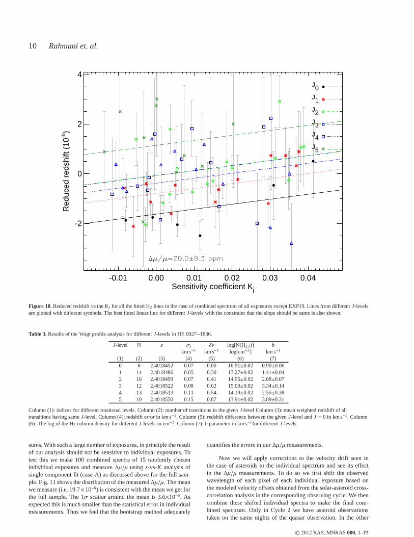
In Fig. 10 we plot the reduced redshift vsK for different tran-sitions. The points from differentJ-levels are marked with differentsymbols. The best fitted line for points from differentJ-levels arealso shown in the figure with different line styles. As discussed be-fore, we constrained the slope (i.e.∆µ/µ) of these lines to be samewhile allowing for the intercept (i.e. mean redshift) to be differentfor differentJ-levels. The best fitted value for∆µ/µ is 20.0 ± 9.3ppm (See column 2 of the last row in Table 4). The quoted error isobtained using bootstrapping as discussed above.

As the wavelength dependent velocity shift is found to be min-imum in the case of first two cycles we measured the∆µ/µ us-ing only the data obtained in the first two cycles (i.e. 13 exposuresand total integration time of∼ 23 hrs). We call this sub-sample as“1+2”. The results of the∆µ/µ measurement for this case is alsogiven in Table. 4. We find∆µ/µ = +10.7±11.4 ppm. As expectedthe mean∆µ/µ obtained from this sub-sample is less than the oneobtained for the whole sample. The amount of observing time indifferent cycles are respectively 10.4 hours, 12.5 hours, and 10.4hours for the first, second, and third cycle. Therefore, we also mea-sured∆µ/µ using data obtained in individual cycles. The total ob-serving time in each cycle is sufficiently good for estimating∆µ/µbased on each cycle. We get∆µ/µ = −1.7±16.3 ppm,+30.2±12.2ppm and+41.6 ± 19.5 ppm respectively for the first, second andthird cycles. The progressive increase in the mean∆µ/µ is consis-tent with what we notice in Fig. 7 for the asteroids.

The final combined spectrum used here is based on 18 expo-

c© 2012 RAS, MNRAS000, 1–??

10 Rahmani et. al.

-0.01 0.00 0.01 0.02 0.03 0.04Sensitivity coefficient Ki

-2

0

2

4R

educ

ed r

edsh

ift (

10-6)

J0J1J2J3J4J5

Figure 10. Reduced redshift vs the Ki for all the fitted H2 lines in the case of combined spectrum of all exposures except EXP19. Lines from differentJ-levelsare plotted with different symbols. The best fitted linear line for differentJ-levels with the constraint that the slope should be same is also shown.

Table 3. Results of the Voigt profile analysis for differentJ-levels in HE 0027−1836.

J-level N z σz δv log[N(H2J)] bkm s−1 km s−1 log[cm−2] km s−1

(1) (2) (3) (4) (5) (6) (7)0 6 2.4018452 0.07 0.00 16.91±0.02 0.90±0.061 14 2.4018486 0.05 0.30 17.27±0.02 1.41±0.042 16 2.4018499 0.07 0.41 14.95±0.02 2.68±0.073 12 2.4018522 0.08 0.62 15.00±0.02 3.34±0.144 13 2.4018513 0.11 0.54 14.19±0.02 2.55±0.385 10 2.4018550 0.15 0.87 13.91±0.02 3.89±0.31

Column (1): indices for different rotational levels. Column (2): number of transitionsin the givenJ-level Column (3): mean weighted redshift of alltransitions having sameJ-level. Column (4): redshift error in km s−1. Column (5): redshift difference between the givenJ-level andJ = 0 in km s−1. Column(6): The log of the H2 column density for differentJ-levels in cm−2. Column (7):b parameter in km s−1for differentJ-levels

sures. With such a large number of exposures, in principle the resultof our analysis should not be sensitive to individual exposures. Totest this we make 100 combined spectra of 15 randomly chosenindividual exposures and measure∆µ/µ usingz-vs-K analysis ofsingle component fit (case-A) as discussed above for the fullsam-ple. Fig. 11 shows the distribution of the measured∆µ/µ. The meanwe measure (i.e. 19.7×10−6) is consistent with the mean we get forthe full sample. The 1σ scatter around the mean is 3.6×10−6. Asexpected this is much smaller than the statistical error in individualmeasurements. Thus we feel that the bootstrap method adequately

quantifies the errors in our∆µ/µ measurements.

Now we will apply corrections to the velocity drift seen inthe case of asteroids to the individual spectrum and see its effectin the ∆µ/µ measurements. To do so we first shift the observedwavelength of each pixel of each individual exposure based onthe modeled velocity offsets obtained from the solar-asteroid cross-correlation analysis in the corresponding observing cycle. We thencombine these shifted individual spectra to make the final com-bined spectrum. Only in Cycle 2 we have asteroid observationstaken on the same nights of the quasar observation. In the other

c© 2012 RAS, MNRAS000, 1–??

Constraining∆µ/µ towards HE 0027−1836 11

Table 4. ∆µ/µmeasurement for each cycle in 10−6 unit.

z-vs-K vpfit

1-component 1-component 2-components(1) (2) (3) (4) (5) (6) (7) (8) (9) (10) (11) (12) (13)

cycle original corrected† original χ2ν AICC corrected† χ2

ν original χ2ν AICC corrected† χ2

ν

1 −1.7±16.3 −4.6±16.8 +21.1±10.0 1.037 6302 +19.8± 9.9 1.029 −11.7±12.2 1.032 6295 −12.1±11.8 1.0222 +30.2±12.2 +26.7±12.7 +15.5±10.5 0.974 5948 +10.0±10.5 0.972 +10.7±11.9 0.969 5936 +5.2±11.9 0.967

3⋆ +41.6±19.5 +30.1±19.0 +30.2±14.3 0.932 5705 +14.5±12.5 0.927 +12.9±13.5 0.912 5614 −0.8±13.4 0.9071+2 +10.7±11.4 +13.8±10.2 +18.8± 7.7 1.128 6825 +15.8± 7.7 1.123 +0.8± 8.6 1.120 6794 −1.5± 8.7 1.115

1+2+3⋆ +20.0± 9.3 +15.0±9.3 +21.8± 6.9 1.188 7167 +15.6± 6.9 1.179 −2.5± 8.1 1.178 7115 −7.6± 8.1 1.171

⋆ result of the cases that EXP19 is excluded.† results after correcting the systematics based on the solar-asteroid cross-correlation.

10 15 20 25 30 350

5

10

15

Num

ber

Figure 11. The distribution of 100∆µ/µ measured from combined spectramade out of 15 randomly chosen exposures. The long-dashed and short-dashed lines show the mean and 1σ scatter of the distribution which respec-tively are 19.7×10−6 and 3.6×10−6.

two cycles the nearest asteroid observations are obtained within 3.5months to the quasar observations. While this is not the ideal situa-tion this is the best we can do. Results of∆µ/µmeasurements afterapplying the drift correction for different cases are summarized incolumn 3 of Table 4. The results of∆µ/µ after applying drift cor-rections are summarized in column 4 of Table 4. We find∆µ/µ =+15.0± 9.3 ppm for the combined data after applying corrections.Clearly an offset at the level of 5 ppm comes from this effect alonein the combined data. We wish to note that the estimated∆µ/µ afterapplying corrections should be considered as an indicativevalue aswe do not have asteroid observations on the same nights of quasarobservations. In addition the quasar and asteroid observations arevery different in terms of the exposure times and the source angularsize.

We notice that because of severe blending,z-vs-K method can-not be easily applied to the two component fit (case-B). In thefol-lowing section we obtain∆µ/µ directly fromvpfit for both singleand two component fits.

4.3 ∆µ/µmeasurements using vpfit

We performed the Voigt profile fitting of all the chosen H2 lineskeeping∆µ/µ as an additional fitting parameter. The results are alsosummarized in columns 4 – 13 in Table 4. When we consider thesingle component fit (case-A) we find∆µ/µ = +21.8± 6.9 ppm forthe full sample with a reducedχ2 of 1.188 (see columns 4 and 5in Table 4). This is very much consistent with what we have foundabove usingz-vs-K analysis. We find the final∆µ/µ value to berobust using different input parameter sets. When we fit the dataobtained from first two cycles we find∆µ/µ = +18.8 ± 7.7 ppmwith a reducedχ2 of 1.128. This also confirms our finding that theaddition of third year data increases the measured mean of∆µ/µ.Table 4 also summarizes the results of∆µ/µmeasurements for datataken on individual cycles. When we use the corrected spectrum forthe full sample we get∆µ/µ = +15.6±6.9 ppm. The∆µ/µmeasure-ments for different cases after applying the correction and the cor-responding reducedχ2 are given in columns 7 and 8 respectively.As noted earlier the statistical errors from thevpfit are about 25 to30% underestimated compared to the bootstrap errors obtained inthe z-vs-K analysis. It is also clear from the table that correctingthe velocity offset leads to the reduction of the∆µ/µ up to 6.2 ppmfor the combined dataset. Column 6 in Table 4 gives the Akaikein-formation criteria (AIC; Akaike 1974) corrected for the finite sam-ple size (AICC; Sugiura 1978) as given in the Eq. 4 of King et al.(2011). We can use AICC in addition to the reducedχ2 to discrim-inate between the models.

Next we consider the two component Voigt profile fits (i.e.case-B) where we keep∆µ/µ as an additional fitting parameter.The results are also summarized in columns 9 – 13 of Table 4. The∆µ/µ measurements, associated reducedχ2 and AICC parametersfor uncorrected data are given in columns 9, 10 and 11 respectively.Results for the corrected data are provided in columns 12 and13.For the whole sample we find∆µ/µ = −2.5 ± 8.1 ppm with a re-ducedχ2 of 1.177. The reducedχ2 in this case is slightly lower thanthe corresponding single component fit. In addition we find the dif-ference in AICC is 52 in favour of two component fit (i.e. case B).Table 4 also presents results for individual cycle data for the twocomponents fit.

The comparison of AICC given in columns 6 and 11 of the Ta-ble 4 also clearly favours the two component fit (i.e. case-B). There-fore, we will only consider measurements based on two componentfit in the following discussions. However, bootstrapping errors inthe case ofz-vs-K linear regression analysis (of single componentfit) are larger and robust when comparing with the errors fromvp-fit. In the case of combined spectrum of all exposures (last row ofTable 4) we need to quadratically add 6.2 ppm to thevpfit error

c© 2012 RAS, MNRAS000, 1–??

12 Rahmani et. al.

1.0 1.5 2.0 2.5 3.0Redshift

-10

0

10

Figure 12. Comparing∆µ/µ measurement in this work and those in theliterature. All measurements at 2.0< z < 3.1 are based on the analysis ofH2 absorption. The filled asterisk shows our result. The downwards emptyand filled triangles are the∆µ/µmeasurements from van Weerdenburg et al.(2011) and Malec et al. (2010). The filled upward triangle andthe emptyand filled squares are respectively from King et al. (2011), King et al.(2008), and Wendt & Molaro (2012). The solid box and the open circlepresent the constraint obtained respectively by Rahmani etal. (2012) andSrianand et al. (2010) based on the comparison between 21-cmand metallines in Mgii absorbers under the assumption thatα andgp have not varied.The∆µ/µ at z < 1 are based on ammonia and methanol inversion transi-tions that their 5σ errors are shown. The two measurements atz ∼ 0.89with larger and smaller errors are respectively from Henkelet al. (2009)and Bagdonaite et al. (2013) based on the same system. The two∆µ/µ atz∼ 0.684 with larger and smaller errors are respectively from Murphy et al.(2008) and Kanekar (2011) based on the same system.

to get thez-vs-K error. This can be considered as typical contribu-tion of the systematic errors. So we consider the two component fitresults with the enhanced error in further discussions.

5 DISCUSSION

We have analyzed the H2 absorption lines from a DLA atzabs =

2.4018 towards HE 0027−1836 observed with VLT/UVES as partof the ESO Large Programme ”The UVES large programme fortesting fundamental physics”. We carried out∆µ/µ measurementsbased onz-vs-K analysis. Our cross-correlation analysis shows thatone of the exposures has a large velocity shift with respect to theremaining exposures. Excluding this exposure from the combinedspectrum we find a∆µ/µ = (−2.5± 8.1stat± 6.2sys) × 10−6.

To understand the possible systematics affecting our observa-tions we studied the asteroids observed with VLT/UVES in dif-ferent cycles. Comparing the asteroids spectra and very accuratesolar spectrum we show the existence of a wavelength dependentvelocity shift with varying magnitude in different cycles. Correct-ing our observations for these systematics we measure∆µ/µ =

(−7.6± 8.1stat± 6.2sys)× 10−6. Our measurement is consistent withno variation inµ over the last 10.8 Gyr at a level of one part in 105.Our null result is consistent with∆µ/µ measurements in literaturefrom analysis of different H2-bearing sightlines (Thompson et al.2009a, Table 1).

Fig. 12 summarizes the∆µ/µ measurements based on dif-ferent approaches at different redshifts. As can be seen our newmeasurement is also consistent with the more recent accurate mea-surements using H2 at z ≥ 2. Wendt & Molaro (2012) found a∆µ/µ = (4.3 ± 7.2) × 10−6 using the H2 absorber atz = 3.025 to-wards Q0347−383. King et al. (2011) and van Weerdenburg et al.(2011) used H2 and HD absorbers at respectivelyz = 2.811 and2.059 towards Q0528−250 and J2123−005 to find∆µ/µ = (0.3 ±3.2stat ± 1.9sys) × 10−6 and∆µ/µ = (8.5 ± 4.2) × 10−6. The mea-surement towards Q0528−250 is the most stringent∆µ/µ mea-surements reported till date. However, large discrepancies (a fac-tor of ∼ 50) in the reported N(H2) values by King et al. (2011)and Noterdaeme et al. (2008) is a concern and its effect on∆µ/µneeds to be investigated. King et al. (2008) have found∆µ/µ =(10.9 ± 7.1)× 10−6 at z= 2.595 towards Q0405−443. Using thesemeasurements and ours we find the weighted mean of∆µ/µ =

(4.1 ± 3.3) × 10−6. If we use the measurement of Thompson et al.(2009a) of∆µ/µ = (3.7 ± 14) × 10−6 for the system towardsQ0405−443 we get the mean value of∆µ/µ = (3.2 ± 2.7) × 10−6.However we wish to point out that three out of four UVES basedmeasurements show positive values of∆µ/µ. As any wavelengthdependent drift in these cases could bias these measurements to-wards positive∆µ/µ (See Section 3.2.2) we should exercise cautionin quoting combined∆µ/µ measurements.

Best constraints on∆µ/µ in quasar spectra are obtained us-ing either NH3 or CH3OH (Murphy et al. 2008; Henkel et al. 2009;Kanekar 2011; Bagdonaite et al. 2013). These measurements reacha sensitivity of 10−7 in ∆µ/µ. However, only two systems at highredshift are used for these measurements and both atz < 1. Basedon 21-cm absorption we have∆µ/µ= (0.0± 1.5)× 10−6 (at z∼ 1.3by Rahmani et al. 2012) and∆µ/µ= (−1.7± 1.7)× 10−6 (atz∼ 3.2by Srianand et al. 2010). While these measurements are more strin-gent than H2 based measurements one has to assume no variationin α andgp to get a constraint on∆µ/µ. Also care needs to be takento minimize the systematics related to the line of sight to radio andoptical emission being different.

ACKNOWLEDGEMENT

R. S. and P. P. J. gratefully acknowledge support from the Indo-French Centre for the Promotion of Advanced Research (CentreFranco-Indian pour la Promotion de la Recherche Avancee) un-der contract No. 4304-2. P.M. and C.J.M. acknowledge the fi-nancial support of grant PTDC/FIS/111725/2009 from FCT (Por-tugal). C.J.M. is also supported by an FCT Research Professor-ship, contract reference IF/00064/2012. The work of S.A.L. issupported by DFG Sonderforschungsbereich SFB 676 TeilprojektC4. M.T.M. thanks the Australian Research Council forDiscoveryProjectgrant DP110100866 which supported this work.

REFERENCES

Agafonova, I. I., Levshakov, S. A., Reimers, D., Hagen, H.-J., &Tytler, D., 2013, A&A, 552, A83

Agafonova, I. I., Molaro, P., Levshakov, S. A., & Hou, J. L., 2011,A&A, 529, A28+

Akaike, A., 1974, IEEE Trans. Autom. Control, 19, 716Amendola, L., Leite, A. C. O., Martins, C. J. A. P., Nunes, N. J.,Pedrosa, P. O. J., & Seganti, A., 2012, Phys. Rev. D, 86, 063515

c© 2012 RAS, MNRAS000, 1–??

Bagdonaite, J., Jansen, P., Henkel, C., Bethlem, H. L., Menten,K. M., & Ubachs, W., 2013, Science, 339, 46

Bailly, D., Salumbides, E. J., Vervloet, M., & Ubachs, W., 2010,Molecular Physics, 108, 827

Carswell, R. F., Jorgenson, R. A., Wolfe, A. M., & Murphy, M. T.,2011, MNRAS, 411, 2319

Chand, H., Srianand, R., Petitjean, P., Aracil, B., Quast, R., &Reimers, D., 2006, A&A, 451, 45

Cowie, L. L. & Songaila, A., 1995, ApJ, 453, 596Dekker, H., D’Odorico, S., Kaufer, A., Delabre, B., & Kot-zlowski, H., 2000, in Proc. SPIE Vol. 4008, p. 534-545, Opticaland IR Telescope Instrumentation and Detectors, Masanori Iye;Alan F. Moorwood; Eds., pp. 534–545

D’Odorico, S., Cristiani, S., Dekker, H., Hill, V., Kaufer,A., Kim,T., & Primas, F., 2000, in Society of Photo-Optical Instrumenta-tion Engineers (SPIE) Conference Series, Vol. 4005, Society ofPhoto-Optical Instrumentation Engineers (SPIE) Conference Se-ries, J. Bergeron, ed., pp. 121–130

Edlen, B., 1966, Metrologia, 2, 71Ferreira, M. C., Juliao, M. D., Martins, C. J. A. P., & Monteiro,A. M. R. V. L., 2012, Phys. Rev. D, 86, 125025

Henkel, C., Menten, K. M., Murphy, M. T., et al., 2009, A&A,500, 725

Ivanchik, A., Petitjean, P., Varshalovich, D., Aracil, B.,Srianand,R., Chand, H., Ledoux, C., & Boisse, P., 2005, A&A, 440, 45

Jorgenson, R. A., Murphy, M. T., Thompson, R., & Carswell,R. F., 2013, submitted to MNRAS

Kanekar, N., 2011, ApJ, 728, L12King, J. A., Murphy, M. T., Ubachs, W., & Webb, J. K., 2011,MNRAS, 417, 3010

King, J. A., Webb, J. K., Murphy, M. T., & Carswell, R. F., 2008,Physical Review Letters, 101, 251304

Kozlov, M. G. & Levshakov, S. A., 2013, Annalen der Physik, inpress (arXiv: physics.atom-ph/1304.4510)

Kurucz, R. L., 2005, Memorie della Societa Astronomica ItalianaSupplementi, 8, 189

—, 2006, ArXiv:astro-ph/0605029Ledoux, C., Petitjean, P., & Srianand, R., 2003, MNRAS, 346,209

Levshakov, S. A., Centurion, M., Molaro, P., D’Odorico, S.,Reimers, D., Quast, R., & Pollmann, M., 2006, A&A, 449, 879

Levshakov, S. A., Combes, F., Boone, F., Agafonova, I. I.,Reimers, D., & Kozlov, M. G., 2012, A&A, 540, L9

Levshakov, S. A., Dessauges-Zavadsky, M., D’Odorico, S., &Molaro, P., 2002, MNRAS, 333, 373

MacAlpine, G. M. & Feldman, F. R., 1982, ApJ, 261, 412Malec, A. L., Buning, R., Murphy, M. T., et al., 2010, MNRAS,403, 1541

Molaro, P., Centurion, M., Whitmore, J. B., et al., 2013, A&A,555, A68

Molaro, P., Levshakov, S. A., Monai, S., Centurion, M., Bonifa-cio, P., D’Odorico, S., & Monaco, L., 2008, A&A, 481, 559

Murphy, M. T., Flambaum, V. V., Muller, S., & Henkel, C., 2008,Science, 320, 1611

Noterdaeme, P., Ledoux, C., Petitjean, P., Le Petit, F., Srianand,R., & Smette, A., 2007, A&A, 474, 393

Noterdaeme, P., Ledoux, C., Petitjean, P., & Srianand, R., 2008,A&A, 481, 327

Olive, K. & Skillman, E., 2004, Astrophys. J., 617, 29Petitjean, P., Srianand, R., Chand, H., Ivanchik, A., Noterdaeme,P., & Gupta, N., 2009, Space Science Reviews, 35

Petitjean, P., Srianand, R., & Ledoux, C., 2000, A&A, 364, L26

Petrov, Y., Nazarov, A., Onegin, M., Petrov, V., & Sakhnovsky, E.,2006, Phys. Rev. C, 74

Rahmani, H., Srianand, R., Gupta, N., Petitjean, P., Noterdaeme,P., & Vasquez, D. A., 2012, MNRAS, 425, 556

Reinhold, E., Buning, R., Hollenstein, U., Ivanchik, A., Petitjean,P., & Ubachs, W., 2006, Phys. Rev. Lett., 96, 151101

Rosenband, T., Hume, D., Schmidt, P., et al., 2008, Science,319,1808

Shelkovnikov, A., Butcher, R. J., Chardonnet, C., & Amy-Klein,A., 2008, Phys. Rev. Lett., 100, 150801

Srianand, R., Gupta, N., Petitjean, P., Noterdaeme, P., & Ledoux,C., 2010, MNRAS, 405, 1888

Srianand, R., Gupta, N., Petitjean, P., Noterdaeme, P., Ledoux, C.,Salter, C. J., & Saikia, D. J., 2012, MNRAS, 421, 651

Srianand, R., Petitjean, P., Ledoux, C., Ferland, G., & Shaw, G.,2005, MNRAS, 362, 549

Sugiura, N., 1978, Commun. Stat. A-Theor., 7, 13Thompson, R. I., 1975, Astrophys. Lett., 16, 3Thompson, R. I., Bechtold, J., Black, J. H., et al., 2009a, ApJ, 703,1648

Thompson, R. I., Bechtold, J., Black, J. H., & Martins, C. J. A. P.,2009b, New A, 14, 379

Tzanavaris, P., Murphy, M. T., Webb, J. K., Flambaum, V. V., &Curran, S. J., 2007, MNRAS, 374, 634

Ubachs, W., Buning, R., Eikema, K. S. E., & Reinhold, E., 2007,Journal of Molecular Spectroscopy, 241, 155

Uzan, J.-P., 2011, Living Reviews in Relativity, 14, 2van Weerdenburg, F., Murphy, M. T., Malec, A. L., Kaper, L., &Ubachs, W., 2011, Physical Review Letters, 106, 180802

Varshalovich, D. A. & Levshakov, S. A., 1993, Soviet JournalofExperimental and Theoretical Physics Letters, 58, 237

Wendt, M. & Molaro, P., 2011, A&A, 526, A96+—, 2012, A&A, 541, A69Whitmore, J. B., Murphy, M. T., & Griest, K., 2010, ApJ, 723, 89

APPENDIX A: RESULTS OF CORRELATION ANALYSIS

APPENDIX B: LABORATORY WAVELENGTH OF THECHOSEN H2 LINE ALONG WITH THE BEST FITTEDREDSHIFTS FROM THE VOGIT PROFILE ANALYSIS.

APPENDIX C: RESULTS OF VOIGT PROFILE FITTINGANALYSIS FOR DIFFERENT H2 J-LEVELS

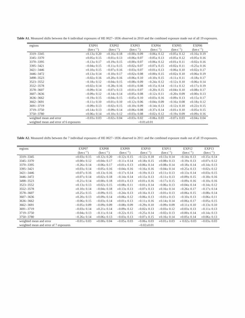
Table A1. Measured shifts between the 6 individual exposures of HE 0027−1836 observed in 2010 and the combined exposure made out of all 19 exposures.

regions EXP01 EXP02 EXP03 EXP04 EXP05 EXP06(km s−1) (km s−1) (km s−1) (km s−1) (km s−1) (km s−1)

3319−3345 +0.13± 0.20 +0.16± 0.18 +0.00± 0.09 −0.06± 0.12 +0.05± 0.12 +0.16± 0.193345−3370 +0.05± 0.15 −0.01± 0.13 +0.06± 0.07 −0.05± 0.13 +0.05± 0.12 +0.05± 0.163370−3395 −0.13± 0.17 +0.19± 0.15 +0.00± 0.07 +0.06± 0.12 +0.01± 0.11 −0.02± 0.163395−3421 −0.04± 0.15 −0.11± 0.15 +0.02± 0.07 +0.07± 0.15 +0.02± 0.11 −0.25± 0.163421−3446 +0.10± 0.15 −0.07± 0.16 −0.03± 0.07 +0.01± 0.13 −0.06± 0.10 +0.02± 0.173446−3472 +0.13± 0.14 −0.10± 0.17 +0.02± 0.08 +0.00± 0.15 +0.02± 0.10 +0.06± 0.193498−3523 −0.02± 0.16 +0.20± 0.16 +0.06± 0.10 +0.10± 0.15 −0.11± 0.11 −0.18± 0.173523−3552 −0.18± 0.12 −0.04± 0.15 +0.08± 0.09 −0.24± 0.12 −0.12± 0.10 −0.06± 0.143552−3578 +0.02± 0.14 −0.28± 0.16 +0.01± 0.08 +0.15± 0.14 −0.11± 0.12 +0.17± 0.193578−3607 −0.09± 0.14 −0.07± 0.13 +0.01± 0.07 −0.20± 0.15 +0.04± 0.10 +0.08± 0.173607−3636 −0.09± 0.12 −0.14± 0.14 +0.05± 0.08 −0.12± 0.11 −0.20± 0.09 +0.00± 0.133636−3662 −0.19± 0.15 −0.04± 0.15 −0.05± 0.10 +0.03± 0.16 −0.09± 0.13 +0.15± 0.173662−3691 −0.11± 0.10 +0.01± 0.10 +0.12± 0.06 −0.04± 0.09 −0.16± 0.08 +0.18± 0.123691−3719 −0.09± 0.13 −0.02± 0.15 +0.10± 0.09 −0.14± 0.13 −0.12± 0.10 +0.22± 0.153719−3750 +0.14± 0.13 −0.09± 0.14 +0.06± 0.08 −0.37± 0.14 −0.01± 0.10 −0.05± 0.153750−3780 +0.06± 0.14 +0.10± 0.12 +0.03± 0.08 −0.02± 0.12 −0.19± 0.09 +0.09± 0.16weighted mean and error −0.03± 0.03 −0.02± 0.04 +0.03± 0.02 −0.06± 0.03 −0.07± 0.03 +0.04± 0.04weighted mean and error of 6 exposures −0.01±0.01

Table A2. Measured shifts between the 7 individual exposures of HE 0027−1836 observed in 2011 and the combined exposure made out of all 19 exposures.

regions EXP07 EXP08 EXP09 EXP10 EXP11 EXP12 EXP13(km s−1) (km s−1) (km s−1) (km s−1) (km s−1) (km s−1) (km s−1)

3319−3345 +0.03± 0.15 +0.12± 0.20 −0.12± 0.15 −0.12± 0.18 +0.13± 0.14 −0.14± 0.13 +0.15± 0.143345−3370 +0.00± 0.12 +0.04± 0.17 −0.11± 0.14 +0.18± 0.15 +0.08± 0.13 −0.19± 0.13 +0.07± 0.123370−3395 −0.26± 0.14 −0.06± 0.17 +0.01± 0.13 +0.06± 0.14 +0.08± 0.14 +0.18± 0.14 +0.14± 0.133395−3421 +0.03± 0.14 −0.05± 0.16 −0.04± 0.16 −0.16± 0.16 −0.04± 0.14 +0.25± 0.13 −0.02± 0.123421−3446 +0.07± 0.16 +0.13± 0.16 −0.17± 0.14 −0.19± 0.13 +0.11± 0.13 +0.13± 0.14 +0.03± 0.153446−3472 +0.07± 0.14 +0.02± 0.18 −0.14± 0.14 +0.15± 0.13 −0.11± 0.13 +0.09± 0.15 −0.18± 0.163498−3523 −0.21± 0.14 +0.00± 0.18 +0.01± 0.13 +0.01± 0.16 −0.17± 0.15 −0.09± 0.16 −0.10± 0.163523−3552 +0.13± 0.13 +0.02± 0.15 +0.08± 0.11 −0.01± 0.14 −0.06± 0.13 +0.04± 0.14 −0.14± 0.123552−3578 +0.10± 0.14 −0.04± 0.18 +0.13± 0.13 −0.07± 0.13 +0.16± 0.14 −0.26± 0.17 −0.17± 0.143578−3607 +0.25± 0.15 −0.09± 0.15 −0.24± 0.13 +0.16± 0.13 −0.01± 0.13 +0.06± 0.15 −0.08± 0.143607−3636 +0.20± 0.13 +0.09± 0.14 +0.06± 0.12 −0.06± 0.13 −0.01± 0.13 −0.10± 0.13 −0.06± 0.113636−3662 −0.06± 0.15 −0.03± 0.14 +0.01± 0.13 −0.11± 0.16 +0.14± 0.14 +0.06± 0.17 −0.05± 0.153662−3691 −0.05± 0.09 −0.09± 0.09 −0.08± 0.09 −0.29± 0.10 −0.09± 0.09 +0.11± 0.10 −0.13± 0.103691−3719 −0.03± 0.14 +0.21± 0.14 −0.09± 0.12 −0.02± 0.13 −0.03± 0.12 +0.03± 0.13 −0.11± 0.133719−3750 −0.04± 0.13 −0.11± 0.14 −0.22± 0.15 −0.25± 0.14 −0.02± 0.13 +0.00± 0.14 +0.14± 0.133750−3780 −0.26± 0.14 +0.06± 0.13 −0.03± 0.13 −0.07± 0.15 +0.16± 0.14 +0.05± 0.14 +0.06± 0.13weighted mean and error −0.01± 0.03 +0.00± 0.04 −0.05± 0.03 −0.06± 0.03 +0.01± 0.03 + 0.02± 0.03 −0.03± 0.03weighted mean and error of 7 exposures −0.02±0.01

Table A3. Measured shifts between the 6 individual exposures of HE 0027−1836 observed in 2012 and the combined exposure made out of all 19 exposures.

regions EXP14 EXP15 EXP16 EXP17 EXP18 EXP19(km s−1) (km s−1) (km s−1) (km s−1) (km s−1) (km s−1)

3319−3345 −0.32± 0.19 +0.03± 0.14 +0.02± 0.11 +0.03± 0.21 −0.14± 0.21 +0.03± 0.133345−3370 −0.05± 0.15 −0.01± 0.12 −0.11± 0.10 −0.07± 0.17 −0.21± 0.25 +0.08± 0.113370−3395 −0.11± 0.16 −0.09± 0.11 −0.12± 0.11 +0.08± 0.17 +0.01± 0.22 +0.18± 0.133395−3421 +0.06± 0.16 +0.02± 0.12 +0.04± 0.10 −0.07± 0.20 −0.38± 0.20 −0.05± 0.143421−3446 +0.09± 0.15 −0.18± 0.11 −0.01± 0.13 −0.04± 0.14 +0.19± 0.20 +0.08± 0.133446−3472 −0.18± 0.16 −0.07± 0.11 +0.13± 0.11 −0.08± 0.15 +0.06± 0.19 +0.19± 0.143498−3523 −0.18± 0.19 +0.20± 0.12 −0.10± 0.11 −0.02± 0.16 +0.08± 0.23 +0.11± 0.153523−3552 +0.17± 0.15 −0.01± 0.11 −0.11± 0.12 −0.08± 0.15 +0.11± 0.20 +0.32± 0.123552−3578 +0.04± 0.17 +0.00± 0.11 −0.11± 0.12 −0.05± 0.16 +0.05± 0.20 +0.40± 0.153578−3607 +0.16± 0.16 +0.00± 0.11 −0.02± 0.11 −0.22± 0.17 +0.37± 0.23 +0.18± 0.123607−3636 +0.21± 0.15 −0.12± 0.11 +0.00± 0.12 +0.08± 0.14 +0.19± 0.23 +0.40± 0.123636−3662 +0.06± 0.16 +0.03± 0.11 +0.14± 0.14 +0.09± 0.14 −0.15± 0.26 +0.17± 0.153662−3691 +0.24± 0.11 −0.10± 0.08 +0.07± 0.09 −0.05± 0.11 +0.32± 0.17 +0.35± 0.083691−3719 −0.11± 0.17 +0.06± 0.11 −0.08± 0.13 +0.04± 0.14 −0.07± 0.23 +0.14± 0.133719−3750 +0.27± 0.15 +0.04± 0.10 +0.25± 0.13 −0.05± 0.14 +0.21± 0.21 +0.19± 0.123750−3780 +0.00± 0.16 +0.07± 0.11 +0.01± 0.13 +0.09± 0.16 −0.12± 0.22 +0.30± 0.13weighted mean and error +0.05± 0.04 −0.02± 0.03 +0.00± 0.03 −0.02± 0.04 +0.05± 0.05 +0.20± 0.03weighted mean and error of 6 exposures 0.04±0.01

Table B1. Laboratory wavelength of the set of H2 transitions that are fitted along with the best redshift and errors from Vogit profile analysis. The uncontami-nated (CLEAN) H2 lines are highlighted in bold letters.

Line ID Lab wavelengtha (Å) Redshift Velocity (km s−1) K coefficientb

L10R0 981.4387 2.401853(049) +0.35±0.44 +0.041L7R0 1012.8129 2.401850(047) +0.07±0.42 +0.031L3R0 1062.8821 2.401843(019) −0.55±0.17 +0.012L2R0 1077.1387 2.401845(016) −0.41±0.14 +0.006L1R0 1092.1952 2.401846(017) −0.32±0.16 −0.001L0R0 1108.1273 2.401845(013) −0.36±0.12 −0.008L9R1 992.0163 2.401855(055) +0.47±0.49 +0.038L9P1 992.8096 2.401853(038) +0.30±0.34 +0.037L8R1 1002.4520 2.401854(037) +0.43±0.33 +0.034W0Q1 1009.7709 2.401845(041) −0.43±0.36 −0.006L7R1 1013.4369 2.401854(047) +0.43±0.42 +0.030L7P1 1014.3272 2.401848(033) −0.16±0.29 +0.030L5R1 1037.1498 2.401851(033) +0.14±0.29 +0.021L4R1 1049.9597 2.401849(029) +0.01±0.26 +0.016L4P1 1051.0325 2.401848(034) −0.14±0.30 +0.016L2R1 1077.6989 2.401850(018) +0.07±0.17 +0.005L2P1 1078.9254 2.401846(010) −0.28±0.09 +0.004L1R1 1092.7324 2.401848(018) −0.14±0.16 −0.001L1P1 1094.0519 2.401850(016) +0.08±0.15 −0.003L0R1 1108.6332 2.401850(013) +0.03±0.12 −0.008L10R2 983.5911 2.401855(054) +0.53±0.48 +0.039L10P2 984.8640 2.401855(046) +0.53±0.41 +0.038W1R2 986.2440 2.401852(035) +0.26±0.32 +0.006W1Q2 987.9745 2.401858(032) +0.75±0.29 +0.004L9P2 994.8740 2.401851(039) +0.13±0.35 +0.035L8R2 1003.9854 2.401862(035) +1.08±0.32 +0.033L8P2 1005.3931 2.401854(041) +0.39±0.37 +0.031W0R2 1009.0249 2.401856(035) +0.62±0.32 −0.005L5R2 1038.6902 2.401852(016) +0.27±0.15 +0.020L5P2 1040.3672 2.401853(070) +0.34±0.62 +0.019L4R2 1051.4985 2.401851(031) +0.12±0.28 +0.015L4P2 1053.2842 2.401850(029) +0.08±0.26 +0.013L3R2 1064.9948 2.401849(016) −0.01±0.15 +0.010L2R2 1079.2254 2.401849(010) −0.04±0.09 +0.004L2P2 1081.2660 2.401848(010) −0.15±0.09 +0.002L1R2 1094.2446 2.401845(022) −0.41±0.20 −0.003L10R3 985.9628 2.401842(053) −0.63±0.47 +0.036L10P3 987.7688 2.401852(035) +0.21±0.31 +0.035L8R3 1006.4141 2.401844(070) −0.44±0.62 +0.030W0Q3 1012.6796 2.401850(040) +0.04±0.35 −0.009W0P3 1014.5042 2.401853(029) +0.32±0.26 −0.011L5R3 1041.1588 2.401850(020) +0.08±0.18 +0.018L4R3 1053.9761 2.401856(042) +0.56±0.37 +0.013L4P3 1056.4714 2.401852(016) +0.26±0.15 +0.011L3P3 1070.1408 2.401855(028) +0.48±0.25 +0.005L2R3 1081.7112 2.401853(052) +0.31±0.46 +0.001L2P3 1084.5603 2.401857(019) +0.63±0.17 −0.001L1P3 1099.7872 2.401849(023) −0.01±0.20 −0.008W1Q4 992.0508 2.401857(076) +0.68±0.67 −0.000W1P4 994.2299 2.401849(052) +0.00±0.46 −0.002L9R4 999.2715 2.401859(068) +0.88±0.61 +0.030L9P4 1001.6557 2.401858(067) +0.77±0.60 +0.028L8R4 1009.7196 2.401845(068) −0.39±0.60 +0.027L6P4 1035.1825 2.401847(052) −0.19±0.46 +0.017L5R4 1044.5433 2.401853(042) +0.33±0.38 +0.014L4R4 1057.3807 2.401858(038) +0.75±0.34 +0.009L4P4 1060.5810 2.401854(046) +0.38±0.41 +0.007L3P4 1074.3129 2.401845(033) −0.35±0.29 +0.001L2R4 1085.1455 2.401851(037) +0.16±0.33 −0.002L2P4 1088.7954 2.401850(033) +0.06±0.29 −0.005L1P4 1104.0839 2.401849(077) −0.04±0.68 −0.012

Column (1): Name of the H2 fitted transitions. Column (2): The laboratory wavelengths. Columns (2) and (3): The best fitted redshifts for H2 lines and theirerrors. Column (5): Velocity offset between the redshift of a given H2 transition and the weighted mean redshift of the all the H2 lines. Column (6) Sensitivitycoefficient of H2 lines.a Wavelengths are from Bailly et al. (2010).b K coefficient are from Ubachs et al. (2007).

Table B2. Table B1 continued.

Line ID Lab wavelength (Å) Redshift Velocity (km s−1) K factorW1Q5 994.9244 2.401857(063) +0.64±0.56 −0.003W0R5 1014.2425 2.401862(065) +1.11±0.58 +0.000L8P5 1017.0043 2.401858(086) +0.80±0.77 +0.020W0Q5 1017.8315 2.401855(054) +0.47±0.48 −0.014L6P5 1040.0587 2.401853(073) +0.29±0.64 +0.012L5P5 1052.4970 2.401854(095) +0.42±0.84 +0.007L4R5 1061.6972 2.401852(062) +0.22±0.55 +0.005L3R5 1075.2441 2.401861(069) +1.02±0.61 +0.000L3P5 1079.4004 2.401845(062) −0.38±0.55 −0.003L2P5 1093.9550 2.401860(119) +0.96±1.06 −0.010

0

1

L9R1

L9P1 C

L8R1 C

0

1

W0Q1

L7R1 C

L7P1 C

0

1

L5R1 C

L4R1 C

L4P1 C

0

1

L2R1

L2P1 C

L1R1 C

-50 0 50

0

1

L1P1 C

-50 0 50

L0R1

Figure C1. The absorption profiles of H2 transitions withJ = 1 in HE 0027−1836 and the best fitted Voigt profile to the combined spectrumof all exposuresafter excluding EXP19. The normalized residual (i.e. ([data]-[model])/[error]) for each fit is shown in top of each panel along with the 1σ horizontal line. Thevertical ticks mark the positions of fitted contamination.

Velocity (km s−1)

No

rmal

ized

Flu

x

0

1

L10R2 C

L10P2 C

W1R2 C

0

1

W1Q2 C

L9P2

L8R2 C

0

1

L8P2 C

W0R2

L5R2 C

0

1

L5P2

L4P2 C

L4R2

0

1

L3R2

L2R2 C

L2P2 C

-50 0 50

0

1

L1R2 C

Figure C2. The absorption profiles of H2 transitions withJ = 2 in HE 0027−1836 and the best fitted Voigt profile to the combined spectrumof all exposuresafter excluding EXP19. The normalized residual (i.e. ([data]-[model])/[error]) for each fit is shown in top of each panel along with the 1σ horizontal line. Thevertical ticks mark the positions of fitted contamination.

Velocity (km s−1)

No

rmal

ized

Flu

x

0

1

W1Q4

W1P4

L9R4

0

1

L9P4 C

L8R4

L6P4 C

0

1

L5R4 C

L4R4

L4P4 C

0

1

L3P4 C

L2R4 C

L2P4 C

-50 0 50

0

1

L1P4 C

Figure C3. The absorption profiles of H2 transitions withJ = 4 in HE 0027−1836 and the best fitted Voigt profile to the combined spectrumof all exposuresafter excluding EXP19. The normalized residual (i.e. ([data]-[model])/[error]) for each fit is shown in top of each panel along with the 1σ horizontal line. Thevertical ticks mark the positions of fitted contamination.

Velocity (km s−1)

No

rmal

ized

Flu

x

0

1

L10R0

C

L7R0

C

L3R0

C

-50 0 50

0

1

L2R0

-50 0 50

L1R0

C

-50 0 50

L0R0

C

0

1

W1Q5

W0R5C

L8P5C

0

1

W0Q5C

L6P5

L5P5C

0

1

L4R5C

L3R5C

L3P5

-50 0 50

0

1

L2P5C

Figure C4. The absorption profiles of H2 transitions withJ = 0 (top) andJ = 5 (bottom) in HE 0027−1836 and the best fitted Voigt profile to the combinedspectrum of all exposures after excluding EXP19. The normalized residual (i.e. ([data]-[model])/[error]) for each fit is shown in top of each panel along withthe 1σ horizontal line. The vertical ticks mark the positions of fitted contamination.

Velocity (km s−1)

No

rmal

ized

Flu

x

Velocity (km s−1)

No

rmal

ized

Flu

x