The Sigma Profile: A Formal Tool to StudyOrganization and its Evolution at Multiple Scales

Carlos Gershenson1,2

1 New England Complex Systems Institute24 Mt. Auburn St. Cambridge MA 02138, USA

carlos@necsi.org http://necsi.org2Centrum Leo Apostel, Vrije Universiteit Brussel

Krijgskundestraat 33 B-1160 Brussel, Belgiumcgershen@vub.ac.be http://homepages.vub.ac.be/∼cgershen

September 2, 2008

Abstract

The σ profile is presented as a tool to analyze the organization of systems at differentscales, and how this organization changes in time. Describing structures at differentscales as goal-oriented agents, one can define σ ∈ [0, 1] (”satisfaction”) as the degree towhich the goals of each agent at each scale have been met. σ reflects the organizationdegree at that scale. The σ profile of a system shows the satisfaction at different scales,with the possibility to study their dependencies and evolution. It can also be used toextend game theoretic models. A general tendency on the evolution of complexity andcooperation naturally follows from the σ profile. Experiments on a virtual ecosystemare used as illustration.

1 Introduction

We use metaphors, models, and languages to describe our world. Different descriptions maybe more suitable than others. We tend to select from a pool of different descriptions thosethat fit with a particular purpose. Thus, it is natural that there will be several useful,overlapping descriptions of the same phenomena, useful for different purposes.

In this paper, the σ profile is introduced to describe the organization of systems atmultiple scales. Some concepts were originally developed for engineering [1]. Here they areextended with the purpose of scientific description, in particular to study evolution.

This article is organized as follows. In the following sections, concepts from multi-agentsystems, game theory, and multiscale analysis are introduced. These are then used to describenatural systems and evolution. In the following sections, a simple simulation and experimentsare presented to illustrate the σ profile. Conclusions close the paper.

1

arX

iv:0

809.

0504

v1 [

q-bi

o.PE

] 2

Sep

200

8

2 Agents

Any phenomenon can be described as an agent. An agent is a description of an entitythat acts on its environment [1, p. 39]. Thus, the terminology of multi-agent systems[2, 3, 4, 5] can be used to describe complex systems and their elements. An electron actson its surroundings with its electromagnetic field, a herd acts on an ecosystem, a car actson city traffic, a company acts on a market. Moreover, an observer can ascribe goals to anagent. An electron tries to reach a state of minimum energy, a herd tries to survive, a cartries to get to its destination as fast as possible, a company tries to make money. We candefine a variable σ to represent satisfaction, i.e. the degree to which the goals of an agenthave been reached. This will also reflect the organization of the agent [6, 7, 1].

Since agents act on their environment, they can affect positively, negatively, or neutrallythe satisfaction of other agents. We can define the friction φi between agents A and B as

φA,B =−∆σA −∆σB

2. (1)

This implies that when the decrease in ∆σ (satisfaction reduced) for one agent is greaterthan the increase in ∆σ (satisfaction increased) for the other agent, φA,B will be positive.In other words, the satisfaction gain for one agent is lesser than the loss of satisfaction inthe other agent. The opposite situation, i.e. a negative φA,B implies an overall increase insatisfaction, i.e. synergy.

Generalizing, the friction within a group of n agents will be

φn =−

∑ni ∆σi

n. (2)

Satisfactions at different scales can also be compared. This can be used to study howsatisfaction changes of elements affect satisfaction changes of the system they compose.

φn,sys =φn −∆σsys

2. (3)

3 Games

Game theory [8, 9] and in particular the prisoner’s dilemma [10, 11] have been used to studymathematically the evolution of cooperation [12]. It will be used here to exemplify theconcepts of the σ profile. A well studied abstraction is given when players (agents) choosebetween cooperation or defection. A cooperator pays a cost c for another to receive a benefitb, while a defector does not pay a cost nor deals benefits [13] 1. The possible interactionscan be arranged in the two by two matrix (4), where the payoff refers to the ‘row player’A. When both cooperate, A pays a cost (−c), but receives a benefit b from B. When Bdefects, A receives no benefit, so it loses −c. This might tempt A to defect, since it will gainb > b− c if B cooperates and will not lose if B also defects as 0 > −c.

1b > c is assumed.

2

A\B C DC b− c −cD b 0

(4)

We can use the payoff of an agent to measure its satisfaction σ. Moreover, we cancalculate the friction between agents A and B with φA,B (1) as shown in (5):

φA,B C DC −(b− c) − b−c

2

D − b−c2

0(5)

If we assume that A and B form of a system, we can define naively its satisfaction asthe sum of the satisfactions of the elements. Therefore, the satisfaction of the system σA,B

would be also the negative of (5) times two:

σA,B C DC 2(b− c) b− cD b− c 0

(6)

Thus, we can study satisfactions at two different scales. At the lower scale, agents arebetter off defecting, given the conditions of (4). However, at the higher scale, the system willhave a higher satisfaction if agents cooperate, since b − c > b−c

2> 0. Here we can see that

reducing the friction φ at the lower scale increases the satisfaction σsys at the higher scale.This has been shown to be valid also for the more general case, when σsys 6=

∑ni σi and has

been used as a design principle to engineer self-organizing systems [1].

4 Multiscale Analysis

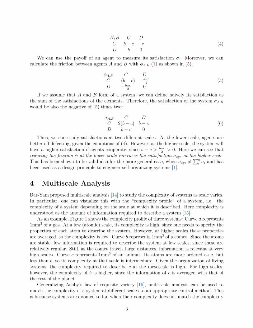
Bar-Yam proposed multiscale analysis [14] to study the complexity of systems as scale varies.In particular, one can visualize this with the “complexity profile” of a system, i.e. thecomplexity of a system depending on the scale at which it is described. Here complexity isunderstood as the amount of information required to describe a system [15].

As an example, Figure 1 shows the complexity profile of three systems: Curve a represents1mm3 of a gas. At a low (atomic) scale, its complexity is high, since one needs to specify theproperties of each atom to describe the system. However, at higher scales these propertiesare averaged, so the complexity is low. Curve b represents 1mm3 of a comet. Since the atomsare stable, few information is required to describe the system at low scales, since these arerelatively regular. Still, as the comet travels large distances, information is relevant at veryhigh scales. Curve c represents 1mm3 of an animal. Its atoms are more ordered as a, butless than b, so its complexity at that scale is intermediate. Given the organization of livingsystems, the complexity required to describe c at the mesoscale is high. For high scales,however, the complexity of b is higher, since the information of c is averaged with that ofthe rest of the planet.

Generalizing Ashby’s law of requisite variety [16], multiscale analysis can be used tomatch the complexity of a system at different scales to an appropriate control method. Thisis because systems are doomed to fail when their complexity does not match the complexity

3

Scale

Complexity

a

b

c

Figure 1: Complexity profile for three systems. See text for details.

of their environment. In other words, solutions need to match the complexity of the problemthey are trying to solve at a particular scale.

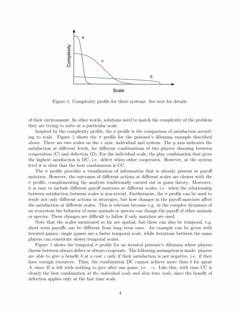
Inspired by the complexity profile, the σ profile is the comparison of satisfaction accord-ing to scale. Figure 2 shows the σ profile for the prisoner’s dilemma example describedabove. There are two scales on the x axis: individual and system. The y axis indicates thesatisfaction at different levels, for different combinations of two players choosing betweencooperation (C) and defection (D). For the individual scale, the play combination that givesthe highest satisfaction is DC, i.e. defect when other cooperates. However, at the systemlevel it is clear that the best combination is CC.

The σ profile provides a visualization of information that is already present in payoffmatrixes. However, the outcomes of different actions at different scales are clearer with theσ profile, complementing the analysis traditionally carried out in game theory. Moreover,it is easy to include different payoff matrixes at different scales, i.e. when the relationshipbetween satisfaction between scales is non-trivial. Furthermore, the σ profile can be used tostudy not only different actions or strategies, but how changes in the payoff matrixes affectthe satisfaction at different scales. This is relevant because e.g. in the complex dynamics ofan ecosystem the behavior of some animals or species can change the payoff of other animalsor species. These changes are difficult to follow if only matrixes are used.

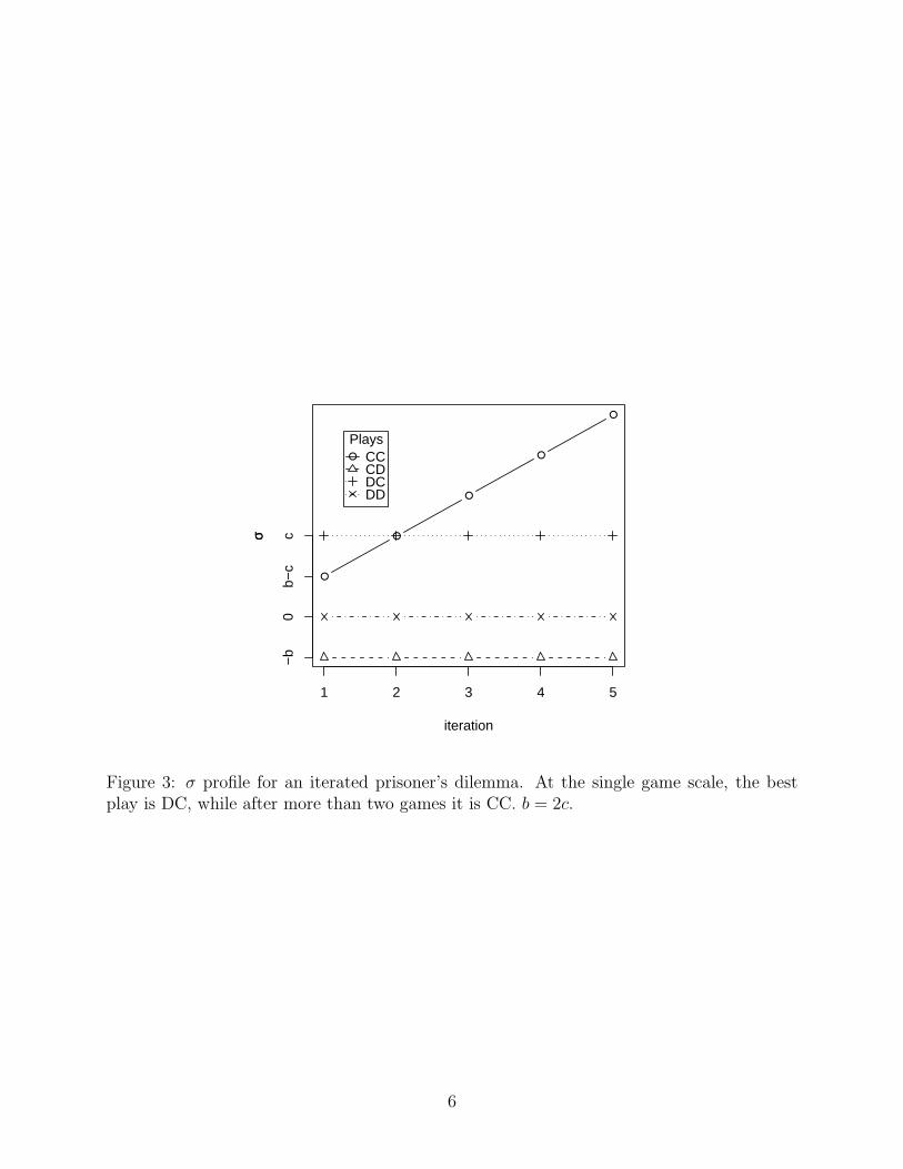
Note that the scales mentioned so far are spatial, but these can also be temporal, e.g.short term payoffs can be different from long term ones. An example can be given withiterated games: single games are a faster temporal scale, while iterations between the sameplayers can constitute slower temporal scales.

Figure 3 shows the temporal σ profile for an iterated prisoner’s dilemma where playerschoose between always defect or always cooperate. The following assumption is made: playersare able to give a benefit b at a cost c only if their satisfaction is not negative, i.e. if theyhave enough resources. Thus, the combination DC cannot achieve more than b for agentA, since B is left with nothing to give after one game, i.e. −c. Like this, with time CC isclearly the best combination at the individual scale and slow time scale, since the benefit ofdefection applies only at the fast time scale.

4

●

●

scale

σσ

individual system

−b

0b−

cc

●

●

●

PlaysCCCDDCDD

Figure 2: σ profile for the prisoner’s dilemma. At the individual scale, the best play is DC,while at the system level it is CC. For graphical purposes, b = 2c.

5

●

●

●

●

●

1 2 3 4 5

iteration

σσ

−b

0b−

cc

●

PlaysCCCDDCDD

Figure 3: σ profile for an iterated prisoner’s dilemma. At the single game scale, the bestplay is DC, while after more than two games it is CC. b = 2c.

6

5 Nature

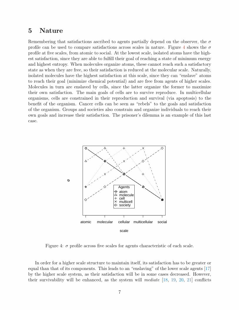
Remembering that satisfactions ascribed to agents partially depend on the observer, the σprofile can be used to compare satisfactions across scales in nature. Figure 4 shows the σprofile at five scales, from atomic to social. At the lowest scale, isolated atoms have the high-est satisfaction, since they are able to fulfill their goal of reaching a state of minimum energyand highest entropy. When molecules organize atoms, these cannot reach such a satisfactorystate as when they are free, so their satisfaction is reduced at the molecular scale. Naturally,isolated molecules have the highest satisfaction at this scale, since they can “enslave” atomsto reach their goal (minimize chemical potential) and are free from agents of higher scales.Molecules in turn are enslaved by cells, since the latter organize the former to maximizetheir own satisfaction. The main goals of cells are to survive reproduce. In multicellularorganisms, cells are constrained in their reproduction and survival (via apoptosis) to thebenefit of the organism. Cancer cells can be seen as “rebels” to the goals and satisfactionof the organism. Groups and societies also constrain and organize individuals to reach theirown goals and increase their satisfaction. The prisoner’s dilemma is an example of this lastcase.

●

●

●

●

●

scale

σσ

atomic molecular cellular multicellular social

●

●

●

●

●

●

Agentsatommoleculecellmulticellsociety

Figure 4: σ profile across five scales for agents characteristic of each scale.

In order for a higher scale structure to maintain itself, its satisfaction has to be greater orequal than that of its components. This leads to an “enslaving” of the lower scale agents [17]by the higher scale system, as their satisfaction will be in some cases decreased. However,their survivability will be enhanced, as the system will mediate [18, 19, 20, 21] conflicts

7

between agents to reduce their friction for its own “selfish” satisfaction. Like this, evenwhen the satisfaction of animals is lower when they are social, they have better chancesof survival, since they benefit from the social organization and are able to cope with moreenvironmental complexity as a group. The same applies to cells: they are less “free” in amulticelular organism, as they obey intracellular signals that can imply their own destruction.Nevertheless, cells within a multicellular organism have more chances to survive than similarones competing against each other for resources. In a similar way, many molecules wouldnot be able to maintain themselves if it weren’t for the organization provided by a cell [22].Finally, free atoms are more prone to change their minimal energy state by interacting withother atoms than those that are already binded in molecules.

Agents at each scale will try to maximize their own satisfaction, so the only way forhigher scale agents to emerge is to mediate or enslave the lower scale agents. The scaledominating the σ profile, i.e. with a higher satisfaction, reflects the degree of organizationand complexity of the system. In Figure 4, agents characteristic of a scale have the highestsatisfaction at that scale.

6 Evolution

There has been much work discussing the evolution of complexity [23, 24, 25]. Our uni-verse has seen an increase of complexity throughout its history, from the Big Bang to theinformation age. People have described this as an “arrow” in evolution [26, 27]. However,some others have seen this increase as a natural drift [28, 29]. This means that starting withonly simple elements, with random variations you can only get more complex. However, thisexplanation does not account for the increasing speed at which complexity has evolved.

The σ profile can be used to gradually measure metasystem transitions [30, 31]2, whichclearly indicate an increase of complexity. Thus, the σ profile can be used to understandbetter the evolution of complexity. Each agent at its own scale tries to maximize its satis-faction. But a high satisfaction does not always imply a higher evolutionary fitness. Somesystems will have high σ values at higher or lower scales. But those with high values at highscales will have a higher fitness in comparison, since an agent at a high scale needs to ensurethe sustainability and cooperation of all agents at its lower scales to maintain itself. On theother hand, independent agents at lower scales will not be able to do much beyond their ownscale to ensure their survivability.

The above scenario does not imply that complexity will always increase. Like with anyevolutionary process, a source of variation is needed. Once there is a competition betweentwo different systems, one with a higher organizational scale will tend to win the evolutionaryrace. Since it is beneficial to have high σ at high scales, systems which can evolve higherscales of organization will tend to evolve. And those who can evolve faster will prevail.There are many ways in which cooperation can evolve [13], but this seems to be a generalevolutionary tendency, not only in biological systems, but also in economical, technological,and informational systems, where an increasing increase of complexity is also observed [22].Whether there is an upper bound for complexity increase is still an open question.

2A metasystem transition occurs when the σ at a higher scale dominates the profile.

8

7 Simulation

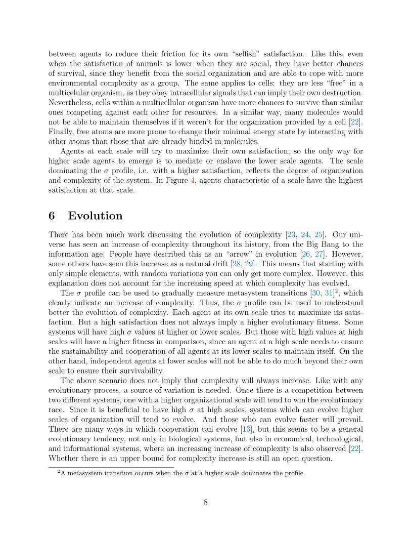
A simple multi-agent simulation was developed in NetLogo [32]. Agents move randomly ina toroidal virtual world with a certain step size at a certain energy cost. Resources growrandomly at a certain growth rate. Agents feed on resources, increasing their energy by acertain resource energy. If the agent’s internal energy ∈ [0, 100] reaches zero, it dies. Ifthe energy reaches one hundred, it reproduces by splitting. This reduces the energy of theparent to half, and creates an offspring with the other half of the energy.

In this simple simulated ecological system, typical behaviors can be observed dependingon the parameters. If the resource growth rate or resource energy is low, or the agent’senergy cost is high or step size is small, the agents will become extinct. As these variableschange, larger agent populations can be maintained. Depending on the precise variablevalues, the population sizes of agents and resources can be roughly constant or oscillatearound a mean.

To study the benefit of aggregating, a variable group advantage is introduced. If anagent is not in an aggregate, every time step its energy is reduced by a certain energy cost,as mentioned above. However, if the agent is part of a group, its energy will be reduced byenergy cost/group advantage. Thus, the larger the value of group advantage, the less energythat an agent in an aggregate will lose. It should be noted, however, that if many agents areaggregated, there will be less resources left for them.

When an agent is born, it is decided with a probability pjoin whether it will join otheragents when it is next to them. Likewise, it is decided with a probability psplit whether itwill cut links made with or by another agent. These probabilities vary ±0.05 from the par-ent’s probabilities. Depending on the parameter values, agents with different pjoin and psplit

probabilities will have greater advantages, and these will be selected after several generations.We can measure satisfaction at three levels: the resource level, the agent level, and

the system level. The resource σ is defined as the percentage of resources available in theenvironment. It is one if the environment is covered by resources, and zero if there are noresources at all. The agent σ is measured with their energy/100. It is one if the agents areabout to reproduce, and zero if they are dead. The system σ is defined as the proportion ofagents that are joined in the largest group. It is one if all the agents are joined in one group,and zero if no agent is joined.

A screenshot of the simulation can be seen in Fig. 5. The reader is invited to try thesimulation at the URL http://homepages.vub.ac.be/∼cgershen/MO/MO.html.

8 Experiments

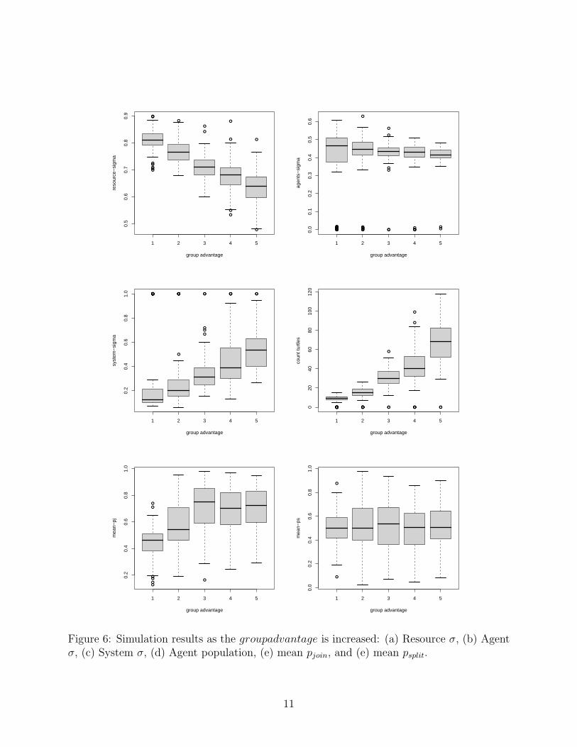
Figure 6 shows results of one hundred simulation runs of ten thousand time steps for differentvalues of group advantage. All simulations start with an initial population of one hundredagents with pjoin = psplit = 0.5 and a random energy. Table 8 lists the values of parametersused.

We can see that as group advantage is increased, the system σ also increases (Fig. 6(c)).On the other hand, the resource σ and agent σ are reduced (Figs. 6(a) and 6(b) ). However,the survivability of the individual agents is increased, as indicated by the population size

9

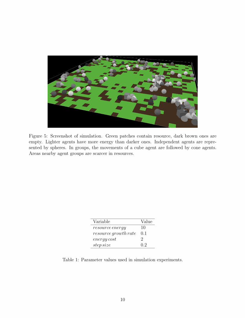
Figure 5: Screenshot of simulation. Green patches contain resource, dark brown ones areempty. Lighter agents have more energy than darker ones. Independent agents are repre-sented by spheres. In groups, the movements of a cube agent are followed by cone agents.Areas nearby agent groups are scarcer in resources.

Variable Valueresource energy 10resource growth rate 0.1energy cost 2step size 0.2

Table 1: Parameter values used in simulation experiments.

10

●

●●

●

●●●

●

●

●

●

●

●

●

●

●

1 2 3 4 5

0.5

0.6

0.7

0.8

0.9

group advantage

reso

urce

−si

gma

●●●●●●●●●●●●●●●●●

●●●●●●

●

●● ●

●

●

●

●

●

●●●●

●●

1 2 3 4 5

0.0

0.1

0.2

0.3

0.4

0.5

0.6

group advantage

agen

ts−

sigm

a●●●●●●●●●●●●●●●●● ●●●

●

●●●●● ●

●

●●

● ●●●● ●●

1 2 3 4 5

0.2

0.4

0.6

0.8

1.0

group advantage

syst

em−

sigm

a

●●●●●●●●●●●●●●●●● ●●●●●●●● ●

●

●

●

●●

●

●● ●●

1 2 3 4 5

020

4060

8010

012

0

group advantage

coun

t tur

tles

●●

●●

●

●

●

1 2 3 4 5

0.2

0.4

0.6

0.8

1.0

group advantage

mea

n−pj

●

●

1 2 3 4 5

0.0

0.2

0.4

0.6

0.8

1.0

group advantage

mea

n−ps

Figure 6: Simulation results as the groupadvantage is increased: (a) Resource σ, (b) Agentσ, (c) System σ, (d) Agent population, (e) mean pjoin, and (e) mean psplit.

11

(Fig. 6(d)).For higher values of group advantage, there is a selective pressure towards joining in

groups, so the mean pjoin is increased (Fig. 6(e)). This is not favored for low values ofgroup advantage, since close agents need to share local resources, leading to friction betweenneighbors. For this case, it is more advantageous for the agents to spread as much as possiblein their environment, to avoid the friction. On the other hand, high values of group advantagereduce this friction and promote the agent aggregation. Since a high pjoin will make agentsto join groups even if they split constantly from them, there is no pressure on the value ofpsplit (Fig. 6(e)). Note that the reproduction and mutation takes place at the agent level,so there is no direct selection of systems. However, the properties of a high system σ givebetter chances of survival to agents, even if their σ is lower compared to the case when thesystem σ is low.

These experiments are intended to illustrate the concepts presented in the paper. Theyare not attempted as a proof. Concepts can only prove their usefulness and suitability withtime.

9 Conclusions

The σ profile has several potential uses to describe and compare systems at multiple scales.One explored here is the difference between satisfaction (payoff) and survivability. A highsatisfaction does not imply survivability. This can seem as a problem for some game theo-retical formalizations. However, as we observe the satisfactions of agents at different scales(spatial and temporal), it is clear that the survivability of a system is related to the satis-faction of the highest scale.

Systems can achieve high satisfaction with mediators [18, 19, 20, 21] to reduce frictionbetween agents. Friction reduction can be seen as a generalization of cooperation, which isessential in the emergence of new levels of organization [20, 13, p. 1563].

References

[1] Carlos Gershenson. Design and Control of Self-organizing Systems. CopIt Arxives,Mexico, 2007. http://copit-arxives.org/TS0002EN/TS0002EN.html.

[2] Pattie Maes. Modeling adaptive autonomous agents. Artificial Life, 1(1&2):135–162,1994.

[3] M. Wooldridge and N. R . Jennings. Intelligent agents: Theory and practice. TheKnowledge Engineering Review, 10(2):115–152, 1995.

[4] Michael Wooldridge. An Introduction to MultiAgent Systems. John Wiley and Sons,Chichester, England, 2002.

[5] Frank Schweitzer. Brownian Agents and Active Particles. Collective Dynamics in theNatural and Social Sciences. Springer Series in Synergetics. Springer, Berlin, 2003.

12

[6] W. Ross Ashby. Principles of the self-organizing system. In H. Von Foerster andG. W. Zopf, Jr., editors, Principles of Self-Organization, pages 255–278, Oxford, 1962.Pergamon.

[7] Carlos Gershenson and Francis Heylighen. When can we call a system self-organizing?In W Banzhaf, T. Christaller, P. Dittrich, J. T. Kim, and J. Ziegler, editors, Advancesin Artificial Life, 7th European Conference, ECAL 2003 LNAI 2801, pages 606–614,Berlin, 2003. Springer.

[8] John von Neumann and Oskar Morgenstern. Theory of Games and Economic Behavior.Princeton University Press, 1944.

[9] John Maynard Smith. Evolution and the Theory of Games. Cambridge University Press,1982.

[10] Albert Tucker. A two-person dilemma. Reprinted in UMAP Journal 1 (1980), 101.,1950.

[11] W Poundstone. Prisoner’s Dilemma: John Von Neumann, Game Theory and the Puzzleof the Bomb. Doubleday, New York, NY, USA, 1992.

[12] R. M. Axelrod. The Evolution of Cooperation. Basic Books, New York, 1984.

[13] Martin A. Nowak. Five rules for the evolution of cooperation. Science, 314:1560–1563,December 2006.

[14] Y. Bar-Yam. Multiscale variety in complex systems. Complexity, 9(4):37–45, 2004.

[15] Mikhail Prokopenko, Fabo Boschetti, and Alex Ryan. An information-theoretic primeron complexity, self-organisation and emergence. Complexity, In Press.

[16] W. Ross Ashby. An Introduction to Cybernetics. Chapman & Hall, London, 1956.

[17] Hermann Haken. Information and Self-organization: A Macroscopic Approach to Com-plex Systems. Springer-Verlag, Berlin, 1988.

[18] Richard E. Michod. Cooperation and conflict in the evolution of individuality. i. multi-level selection of the organism. American Naturalist, 149:607–645, 1997.

[19] Richard E. Michod. Darwinian Dynamics: Evolutionary Transitions in Fitness andIndividuality. Princeton University Press, Princeton, NJ, 2000.

[20] Richard E. Michod. Cooperation and conflict mediation during the origin of multicel-lularity. In P. Hammerstein, editor, Genetic and Cultural Evolution of Cooperation,chapter 16, pages 261–307. MIT Press, Cambridge, MA, 2003.

[21] Francis Heylighen. Mediator evolution: a general scenario for the origin of dynamicalhierarchies. In Diederik Aerts, Bart D’Hooghe, and Nicole Note, editors, Worldviews,Science and Us. World Scientific, 2006.

13

[22] Stuart A. Kauffman. Reinventing the Sacred: A New View of Science, Reason, andReligion. Basic Books, 2008.

[23] John Tyler Bonner. The Evolution of Complexity, by Means of Natural Selection. Prince-ton University Press, 1988.

[24] M. Bedau, J. McCaskill, P. Packard, S. Rasmussen, D. Green, T. Ikegami, K. Kaneko,and T. Ray. Open Problems in Artificial Life. Artificial Life, 6(4):363–376, 2000.

[25] Carlos Gershenson and Tom Lenaerts. Evolution of complexity. Artificial Life, 14(3):1–3, Summer 2008. Special Issue on the Evolution of Complexity.

[26] Mark A. Bedau. Four puzzles about life. Artificial Life, 4:125–140, 1998.

[27] John Stewart. Evolution’s Arrow: The Direction of Evolution and the Future of Hu-manity. Chapman Press, 2000.

[28] D. McShea. Mechanisms of large-scale evolutionary trends. Evolution, 48:1747—1763,1994.

[29] T Miconi. Evolution and complexity: the double-edged sword. Artificial Life, 14(3),Summer 2008. Special Issue on the Evolution of Complexity.

[30] Valentin Turchin. The Phenomenon of Science. A Cybernetic Approach to HumanEvolution. Columbia University Press, New York, 1977.

[31] J. Maynard Smith and E. Szathmary. The major transitions in evolution. OxfordUniversity Press, 1995.

[32] Uri Wilensky. NetLogo, 1999.

14