THE ROLE OF THE SERVICE SECTOR IN THE

PROCESS OF INDUSTRIALIZATION

by

Mukesh Eswaran and Ashok Kotwal

University of British Columbia

1st June, 2000

INTRODUCTION

² Is high agricultural output (per capita) a help ora hindrance to industrialization?

{ The historical evidence is mixed: the Industrial

Revolution in Britain; Canadian development andthe Staple Theory of Growth.

{ Matsuyama (1992) gives examples of agricul-turally deprived countries that became leading in-

dustrial nations

² Trade-o®: high per capita agricultural output im-plies high wages but it also means high domestic

demand for industrial goods.

{ high wages work against the emergence of an in-

dustrial sector that could withstand internationalcompetition.

{ high domestic demand is conducive to the emer-gence of an industrial sector in a closed economy

² The land-surplus countries of North America de-veloped through growth ¯nanced by primary ex-

ports

{ Staple Theory of Growth argues that primary

exports spearhead growth of industrialization

² Matsuyama (1992) provides model capturing thetrade-o® stemming from high agricultural produc-

tivity.

{ in a closed economy, high agricultural output

aids industrialization through the creation of in-

dustrial demand and, once an industrial sector

is created, industrial productivity grows through

learning-by-doing.

{ in an open economy, on the other hand, a coun-

try with comparative advantage in agricultural

goods may never industrialize unless government

protects its nascent industry

² Matsuyama's model does not explain how indus-trialization occured in some countries despite fee-

ble attempts at protecting its nascent industry

(e.g., Canada); his model embodies the linkages

from the demand side but not those on the supply

side

² We build a model that explicitly takes into ac-count the supply side linkages that the Staple

Theory deems important

{ speci¯cally, we focus on the role of the service

sector in the process of industrialization.

{ we focus on non-traded services (e.g., construc-

tion, transportation, distribution, credit and in-

surance)

{ many of these are both consumer and producer

services; `construction' includes the construction

of both homes and factories, `transportation' moves

both passengers and cargo

² Expansion of the service sector bene¯ts the in-dustrial sector by (i) enabling greater specializa-tion and division of labour [Jones and Kierzowski(1988 ), Francois(1990)], and (ii) by lowering thee®ective costs of service inputs to industrial pro-duction; we focus on the latter.

{ the greater the variety of competing services,the lower are the e®ective costs. This is becausegreater variety a®ords greater °exibility to pro-ducers in minimizing the cost of producing a givenlevel of output.

{ income growth, whether as a result of primaryexport growth or some other exogenous reason,will lead to a larger service sector and hence to anindustrial sector that is better able to withstandinternational competition.

² Thus a primary exporting economy can industri-alize without having to resort to protection.

{ this part of our paper can be viewed as a modelof the Staple Theory.

² We show that the three-sector model yields inter-esting results:

(a) growth in the primary sector productivity of

a small open economy (SOE) may lead to the

emergence of a domestic industrial sector

(b) a decline in its terms of trade may lead to the

emergence of a domestic industrial sector even

when comparative advantage remains with agri-

culture

(c) industrialization will be accompanied by a sharp

increase in the welfare of the representative con-

sumer (RC)

(d) between two SOEs, the one with the smaller

land-to-labour ratio could achieve a higher welfare

for its RC.

THE MODEL

² It is assumed that services are non-tradeable, whilethe outputs of agriculture and manufacturing are

tradeable.

² Factor endowments of the LDC: land and labour.Let L0 denote the labour force ( population) and

H0 its stock of land.

{ land distribution is egalitarian: agent owns an

amount (H0=L0).

Consumption Side

² Preferences are non-homothetic

{ consumers spend all of their income on food

(grain) until they have had a su±cient amount,

G, and at higher levels of income they spend all of

their additional income on manufactures (M)and

an aggregate of services (S).

² The preferences over M and S of a consumer

who has had G units of grain to consume is rep-

resented by the utility function:

U(M;S) =M1¡®S®; 0 < ® < 1: (1)

The aggregate S comprises a bundle of n ser-

vices, Si; i = 1;2; :::; n, (such as transportation,

refrigeration, etc.).

² We assume that the aggregator S is given by theconstant elasticity form:

S =

24nX

i=1

(Si)®

351=®

: (2)

{ hereafter, this aggregate input is referred to as

`Service'.

² Grain is the numeraire. Denote the income of

a RC by y. If y � G, the consumer's demand

for the goods, denoted, respectively, by Gd,Md,and SCdi = 0; i = 1;2; :::; n; are

Gd = y; Md = 0; SCdi = 0; i = 1;2; :::; n: (3)

If y > G, the consumer's demand function forgrain is given by Gd = G; those for manufacturesand the various services are given by the solutionto:

maxM;fSig

U(M;S) s:t: y¡G ¸ PmM+nX

j=1

pjSj ;

(4)where Pm is the price of manufactures and pj ; j =1; 2; :::n; is the price of the jth service. Sincemanufactures are tradeable but services are not,Pm is given by the world market while the pj areendogenously determined.

² The consumer's demand functions, SCdi andMd,respectively, can be shown to be:

SCdi =(pi)

¡µPnj=1(pj)

1¡µ®(y ¡G); i = 1; 2; :::; n;

Md = (1¡ ®)(y ¡G)=Pm; (5)

where µ ´ (1¡ ®)¡1.

{ the consumer spends a fraction ® of her incomein excess of G on services and the rest on manu-factures.

Production Side

² Grain production requires land (Hg) and labour(Lg), and the production function is Cobb-Douglas:

Gs = A(Lg)°(Hg)

1¡°; 0 < ° < 1; (6)

where A denotes the total factor productivity inagriculture.

² Manufacturing uses labour (Lm) and Service (Sm)in ¯xed proportions:

Ms = BminfLm; Sm=¹g; (7)

where B is the total factor productivity in man-ufacturing and ¹ (> 0) is the Service-to-labourratio.

² The agricultural and manufacturing sectors areperfectly competitive.

² If w denotes the wage rate of labour, v the land

rental rate, and pS the price of the aggregate

service, the cost function for grain is:

CG(w;v;G) = KGw°v1¡°G; (8)

where KG ´ °¡°(1¡ °)¡(1¡°)=A, and that formanufactures is

CM(w;pS ;M) = (1=B)(w+ ¹pS)M: (9)

² The price, pS, of Service in terms of those of theindividual services is:

pS =

0@nX

i=1

(pi)¡®µ

1A¡1=(®µ)

: (10)

{ we can interpret pS as the price index of all

services.

² If the manufacturing sector produces an outputMs, the conditional demand for Service is ¹Ms=B,

and the conditional demand, SMdi , for service i;

i = 1; 2; :::; n; can be derived as:

SMdi = ¹

Ms

B

(pi)¡µ

³Pnj=1(pj)

¡®µ´1=®: (11)

² Each service is produced by a single producer, andthe service sectors are monopolistically competi-

tive.

{ services are produced using only labour and pro-

duction requires the incurrence of a ¯xed cost, F

(in units of labour), and ¾ units of labour to pro-

duce one unit of any service.

{ the price of each service will not equal MC

because the service industry is monopolistically

competitive.

² If the aggregate income of the economy is Y ,the aggregate demand, SAdi , for service i; i =

1; 2; :::; n; from consumers and manufacturing is

given by

SAdi =

2664®(Y ¡GL0)Pnj=1(pj)

1¡µ +(¹=B)Ms

³Pnj=1(pj)

¡®µ´1=®

3775 (pi)

¡µ:

(12)

² Themonopolistic producer of service i; i = 1;2; :::; n;solves

maxpi

(pi ¡ ¾w)SAdi ¡wF: (13)

{ as is standard in models of monopolistic com-

petition [Dixit and Stiglitz (1977)], each producer

is assumed to take the expression in the square

bracket of (12) as parametric.

{ the optimal price for service i; i = 1; 2; :::; n; is

pi = ¾w=®; (14)

a standard result which says that each producer

marks up the price over MC by the factor (1=®¡1).

{ if LDC does not produce manufactures, the sec-

ond term in (12) will be absent, but the optimal

price of service stays the same.

² The price of the aggregate service, pS, given by(10) reduces to

pS =¾w

®n1=(®µ): (15)

{ the larger the number of services available, the

lower is the price of Service

THE GENERAL EQUILIBRIUM

Specialization in Agriculture

² Suppose LDC specializes in agriculture

- consumption of manufactures are ¯nanced by

grain exports, and services are produced only for

consumption.

² Must determine the allocation of labour betweenthe agricultural and service sectors, the factor

prices, the number of services produced, and the

consumption levels of grain, services, and manu-

factures.

² Since only agriculture uses land, we will haveHg =H0 in equilibrium.

{ the remunerations of labour and land, respec-

tively, are given by their marginal products in the

grain sector, which depend on Lg:

w(Lg) = A°(H0=Lg)1¡°; v(Lg) = A(1¡°)(Lg=H0)°

(16)

For a given Lg, the aggregate income in the econ-

omy given by

Y (Lg) = L0w(Lg) +H0v(Lg): (17)

At this income level, the aggregate demand for

labour from the service sector, LdS(Lg; n), is given

by

LdS(Lg; n) = nF +®2

w(Lg)[Y (Lg)¡GL0]: (18)

² The labour market clearing condition may thenbe written as:

Lg +LdS(Lg; n) = L0: (19)

{ the solution to (19) determines the labour em-

ployed in agriculture, Lg(n), as a function of the

number of services being produced.

² To determine the number of services produced,invoke zero pro¯t condition in each service sector.

{ setting pi = ¾w=® for all i in the objective func-

tion of (13), the zero pro¯t condition becomes:

®¾[Y (Lg(n)) ¡GL0]n¾µw(Lg(n))

¡ F = 0: (20)

{ this condition determines the number of ser-

vices, n¤, that will be provided in equilibrium.

{ the per capita income in this equilibrium is given

by y = Y (Lg(w(n¤))=L0. Each agent's con-

sumption of (imported) manufactures and domes-

tic services can now be obtained.

² The supposition that the LDC specializes in agri-culture may be incorrect.

{ if so, at the equilibrium computed above, man-

ufactures can be can pro¯tably produced, that is,

Pm will exceed the LDC's MC of producing man-

ufactures.

{ if this is so, the economy is necessarily diversi-

¯ed and the GE has to be computed anew.

Diversi¯ed Economy

² Let G(Lg) denote the amount of grain producedby LDC when Lg workers are employed in agricul-ture.

{ the di®erence between the production and con-sumption of grain, [G(Lg) ¡ L0G], is exportedand these exports will ¯nance the import of anamount, [G(Lg) ¡ L0G]=Pm, of manufactures.Consumers spend on manufactures a fraction (1¡®) of their income in excess of G, that is, theyconsume an amount (1¡ ®)[Y (Lg) ¡GL0]=Pmof manufactures.

{ the di®erence between domestic consumptionand imports of manufactures yields the amount ofmanufactures, Ms(Lg), that is domestically pro-duced:

Ms(Lg) =n(1¡ ®)[Y (Lg)¡GL0]¡ [G(Lg)¡L0G]

o

(21)where, for brevity, only Lg has been retained asan argument on the left hand side.

² For a diversi¯ed economy, the demand for serviceswill come from consumers and from the manufac-turing sector.

{ if Ms(Lg) is the output of manufactures, theservice sector demand for labour now becomes:

LdS(Lg; n) = nF+®2

w(Lg)[Y (Lg)¡GL0]+¾

Ms(Lg)

Bn1=(®µ):

(22)

² Manufacturing demands labour directly for pro-duction and also indirectly, through its use of ser-vices.

{ if Lm(Lg) is the amount of direct labour de-manded by this sector when its output isMs(Lg),from ¯xed coe±cient production function it fol-lows that Lm(Lg) =Ms(Lg)=B.

² The labour market clearing condition which re-places (19) now is given by

Lg + LdS(Lg; n) +Lm(Lg) = L0: (23)

As before, the solution to the above equation

yields the amount of labour employed in agricul-

ture in terms of the number of services, Lg(n).

² The equilibrium value of n is obtained from the

zero pro¯t condition for service producers:

1=(®µ)¾

"®2(Y (Lg(n))¡GL0)n¾w(Lg(n))

+ ¹Ms(Lg(n))

Bn1=®

#¡F =

(24)

As before, all the endogenous variables of interest

can now be obtained.

RESULTS

² We present some simulation results of the modelset out above. Intuition is robust.

² First consider the e®ects of (exogenous) agricul-tural productivity growth on the GE.

{ Figure 1 (a) depicts the e®ect on the utility

of a RC. Parameters are such that even at low

values of the agricultural TFP, A, the LDC has

comparative advantage in agriculture.

{ as A increases, the RC spends her higher in-

come on imported manufactures and nontraded

services.

{ at a su±ciently high value of A, the economy

acquires comparative advantage in manufactur-

ing.

{ the higher consumer income increases the va-

riety of services produced, as seen from Figure 1

(b).

{ this reduces manufacturing costs, as the greater

variety of services reduces the price of Service

(Fig.1 (c)).

{ cost reduction enables the manufacturing sec-

tor to come into existence, despite international

competition.

{ this contrasts with the result of Matsuyama's

(1992) learning-by-doing model, where agricul-

tural productivity growth in a SOE can only re-

duce the growth rate of industry

{ Figure 1 (d) shows extreme scenario where the

SOE reverses its comparative advantage and be-

comes an industrial exporter.

² Transition is accompanied by a discrete increasein the RC's utility.

{ when the manufacturing sector becomes viable,

its demand for services augments that from con-

sumers, leading to a discrete increase in the va-

riety of the services produced and an increase in

the RC's utility.

{ further e®ect: the larger volume and variety of

services draw away labour from agriculture, in-

creasing its marginal product and the utility of a

consumer.

² Even while exporting manufactures, the SOE con-tinues to produce some agricultural output

{ further increases in agricultural productivity raise

the RC's utility as expected.

{ however, the higher wages shrink the size of

the manufacturing sector (consistent with Mat-

suyama's claim) and thereby reduce the industrial

demand for services. So variety of services pro-

duced declines.

² After the transition, increases in agricultural pro-ductivity increase the domestic consumption of

manufactures while domestic production declines.

So, exports of manufactures decline (Fig. 1 (d)).

{ when agricultural productivity is su±ciently high,

the economy's comparative advantage reverts back

to agriculture.

² The discrete increase in the RC's utility, as shownin Fig. 1 (a), is caused by the emergence ofthe industrial sector rather than by the reversalin comparative advantage.

{ it is very likely that the emergence of a domesticindustrial sector is not accompanied by a reversalof comparative advantage but only by a reductionin the imports of manufactures (Fig. 2(b)).

² When agricultural productivity is su±ciently high,Figure 2(a) shows, paradoxically, that there is adiscrete fall in the consumers' utility.

{ this extreme scenario occurs because the man-ufacturing sector shuts down due to very highwages and there is a discrete decline in the num-ber of (non-traded) services produced, which hurtsconsumers.

{ such an outcome is not possible in standardtrade models of SOEs, where an increase in theproductivity of a domestic sector cannot lower theRC's utility.

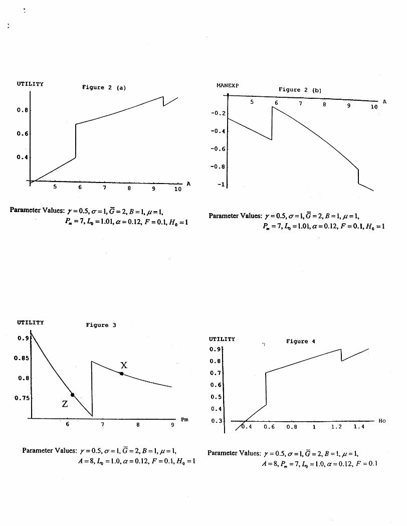
² The e®ect of an increase in the relative price ofmanufactures (Pm) on the well being of the RC

is shown in Fig. 3. (Economy with a comparative

advantage in agriculture.)

{ as Pm increases (i.e., the country's terms of

trade decline), the RC's utility ¯rst declines, then

discontinuously increases before continuing to de-

crease again. The discontinuous increase is caused

by the domestic industrialization. Over the entire

range of Pm depicted in the Figure, the economy

is importing manufactures.

{ in the Figure the RC's utility is lower at a point

like Z than at a point like X even though the terms

of trade at Z are less adverse than at X.

{ we cannot infer that a decline in a country's

terms of trade is necessarily to its detriment.

² In a standard trade model, an increase in Pmcould result in an increase in the well-being of

the RC only when it leads to a switch in the coun-

try's comparative advantage. At a point like Z the

country is exporting the agricultural good while at

a point like X it would be exporting manufactures.

{ in our model, by contrast, an increase in Pmcould make the RC better o® despite the fact that

the country continues to export the agricultural

good.

² Figure 4 displays the GE e®ects of increasing land-to-labour ratio.

{ these e®ects are similar to of an agricultural

productivity increase.

{ this peculiar behaviour of the utility of the RC

arises because there exists a range of intermedi-

ate values of the land-to-labour ratio for which

industrialization is viable.

{ industrialization is not possible below this range

because the per capita income is too low, and

above this range because the wage rate is too

high.

{ Sachs-Warner (1995): countries rich in natural

resources tend to grow more slowly than others.

CONCLUSIONS

² In this paper, we have examined how the servicesector impinges on the process of development of

a SOE.

{ the service sector's output is nontraded and pro-

duction exhibits scale economies

{ service sector is a link between consumption and

industrialization.

{ any increase in income leads to an increase in

the consumption demand for, and the variety of,

services; and this leads to a reduction in the cost

of manufacturing goods.

² We have demonstrated that at a high enough levelof agricultural productivity (and hence per capita

income), an industrial sector could become viable

even when the economy remains open.

{ agricultural productivity growth, therefore, can

lead to industrialization.

{ this is our formalization of the Staple Theory of

economic development [Watkins (1963)].

² Wellbeing of a RC can increase through two av-enues: through the increase in the variety (and,

hence, e®ective price) of the services available for

consumption, and the increase in income associ-

ated with a movement of labour out of agricul-

ture.

{ the emergence of an industrial sector adds a

quantum increase in the size of the service sector,

which in turn contributes to a discrete increase in

welfare.

{ the rapid increase in welfare in the East Asian

success stories may be due to causes such as

these.

² The service sector plays the same role in our ¯nd-ing that an adverse change in the terms of trade

for a primary exporting country could result in a

discrete increase in the welfare of a RC.

² We also ¯nd that, between two SOEs, the onewhich is relatively better endowed with land (that

is, with the larger land-to-labour ratio) can be

poorer in per capita terms, ceteris paribus.

² Paper makes stark assumption that industry usesservices as an input but agriculture does not.

{ but it is only essential that industry uses services

more intensively than agriculture.