University of WollongongResearch Online

Faculty of Commerce - Economics WorkingPapers Faculty of Commerce

2008

What Would the Average Public Sector Employeebe Paid in the Private Sector?P. SiminskiUniversity of Wollongong, peter_siminski@uow.edu.au

Research Online is the open access institutional repository for theUniversity of Wollongong. For further information contact ManagerRepository Services: morgan@uow.edu.au.

Recommended CitationSiminski, P., What Would the Average Public Sector Employee be Paid in the Private Sector?, Department of Economics, Universityof Wollongong, 2008.http://ro.uow.edu.au/commwkpapers/188

University of Wollongong Economics Working Paper Series 2008 http://www.uow.edu.au/commerce/econ/wpapers.html

What Would the Average Public Sector Employee be Paid in the Private Sector?

Peter Siminski University Of Wollongong

WP 08-05

March 2008

What Would the Average Public Sector Employee be Paid in the 

Private Sector? 

 

Peter Siminski1 

March 2008 

Abstract 

This paper estimates  the average Australian public sector wage premium.  It 

includes  a  detailed  critical  review  of  the methods  available  to  address  this 

issue.  The  chosen  approach  is  a  quasi‐differenced  panel  data  model, 

estimated  by  the  Generalised  Method  of  Moments,  which  has  many 

advantages over other methods and has not been used before for this topic. I 

find a positive average public sector wage premium for both sexes. The best 

estimates are 6.7% for men and 10.5% for women. The estimate is statistically 

significant  for men  (p  =  0.024)  and  for women  (p  <  0.001). No  evidence  is 

found to suggest that the public sector has an equalising effect on the wages 

of its workers. 

 

 

JEL classification codes: J45, J31, J38 

Keywords: public sector, wages, premium, panel data, GMM, Australia 

                                                            1  I  thank Garry  Barrett  and  Peter  Saunders  for many  useful  discussions  and  suggestions. Discussions with 

Robert  Clark were  also  very  constructive.  I  gratefully  acknowledge  the  financial  support  provided  by  the 

University  of  New  South  Wales  and  the  Centre  for  Health  Service  Development  at  the  University  of 

Wollongong. Any errors of  fact or omission are  the responsibility of  the author. This paper uses unit record 

data  from  the Household,  Income and Labour Dynamics  in Australia  (HILDA) Survey. The HILDA Project was 

initiated and  is  funded by the Australian Government Department of Families, Housing, Community Services 

and Indigenous Affairs (FaHCSIA) and  is managed by the Melbourne Institute of Applied Economic and Social 

Research  (MIAESR). The  findings  and  views  reported, however,  are  those of  the  author  and  should not be 

attributed to either FaHCSIA or the MIAESR. 

1

I Introduction 

The public sector accounts for 16% of total employment in Australia (Australian Bureau of Statistics, 

2007a).  This  is  similar  to many  other  OECD  countries  (OECD,  2001).  Government  thus  has  the 

potential  for  major  distributional  effects  through  wage  setting  policy.  Much  research  has 

investigated  the public sector wage  ‘premium’, motivated primarily by concerns over efficiency as 

well as equity.2 As discussed by Gregory & Borland (1999), wage setting in the public sector may not 

necessarily follow private sector principles. The public sector process may be insulated from market 

competition. To varying extents, all governments will seek to control employment costs  in order to 

achieve  efficiency  goals.  But  wage  policy may  also  be motivated  by  equity  goals.  Public  sector 

practice may  also  be motivated  by  political  incentives,  and  bureaucratic  budget‐maximising  (or 

minimising) incentives, which may be at odds with social welfare goals.  

The aim of this paper  is to estimate the public sector wage premium. Specifically,  it addresses the 

question: ‘What would an average public sector employee be paid under private sector wage setting 

principles?’  The  evaluation  problem  is  to  overcome  the  missing  counterfactual,  which  is  the 

unobserved private sector wage for public sector employees at a point in time. 

The  econometric  difficulties  involved  in  addressing  this  question  are  substantial.  The  observed 

sectoral wage gap may include a constant effect across all employees. It may also stem from sectoral 

differences  in returns to the characteristics of employees, which  include education and experience 

as well as unobserved (by the econometrician) skills such as interpersonal skills, intelligence or work 

ethic.  These  effects  need  to  be  distinguished  from  the  sectoral  differences  in  the  stock  of  such 

characteristics. Selection bias  is hence an  important  issue. A given employee may select one sector 

over  the  other  according  to  the  potential  returns  to  their  given  (observed  and  unobserved) 

characteristics.  The  employer may  also  select  from  the potential pool of  employees  according  to 

such characteristics. These issues are described in Section II, whilst reviewing the most common and 

the most recent approaches that have been applied, or could be applied, to this topic. 

The chosen model is discussed in Section III. It is a panel data model, similar to that used by Lemieux 

(1993;  1998)  to  analyse  the  effect  of  unionisation  on  wages.  The  parameters  of  interest  are 

estimated  using  the  Generalised Method  of Moments  (GMM)  after  quasi‐differencing  the wage 

equation. This approach has many advantages over  the other methods  reviewed. To  the author’s 

knowledge, it has not previously been applied to this topic. 

                                                            2  This literature is surveyed by Bender (1998) and Gregory & Borland (1999). 

2

The data source  is  the Household  Income and Labour Dynamics  in Australia  (HILDA) panel survey, 

which  is described  in  Section  IV.  Section V presents  results,  including  regression  estimates  and  a 

decomposition of the average wage premium. Section VI offers conclusions. The results of alternate 

specifications are shown in an Appendix. 

 

II Review of Previous Approaches and Their Limitations There  is a  large  literature on sectoral wage differences, surveyed by Bender  (1998) and Gregory & 

Borland (1999). In the last 10‐15 years the focus of such research has shifted from estimates of the 

average public sector effect on wages  to  the effect on  the entire wage distribution. However,  the 

econometric difficulties  in such analyses make  it difficult  to confidently measure even the average 

effect, as will be argued below.  In order to motivate the methods used  in this paper,  I first discuss 

the methods previously used and  their  limitations.  I  then note  that  these  limitations also apply  to 

the analogous quantile regression methods. 

Models of the average wage premium 

First consider the following model: 

iiii XbSaw μβ +++=)ln(     i = (1,...,N)            (1) 

Here, wi is the observed hourly earnings of employee i and N is the number of observed employees. 

The left hand side is the natural log of wi. The right hand side is linear in sector of employment (S = 1 

if sector = public; S = 0 if sector = private) and other observable characteristics (X). In this model, b is 

the average public sector premium. The parameters (a, b, β) can be estimated by OLS. In estimating 

b,  this method holds X constant and  thus  takes account of differences  in observed characteristics 

between sectors. In this model,  it  is assumed that S  is exogenous and hence uncorrelated with the 

residual. This  implies that any sectoral differences  in unobserved characteristics of workers do not 

affect wages. This model also assumes that returns to observed (and unobserved) characteristics are 

equal  in the two sectors. It can be argued all of these assumptions may not hold, but these can be 

relaxed in other specifications, as will be shown. 

The fixed effects (FE) model utilises repeated observations on individuals: 

itittititit DXbSaw μθγβ +++++=)ln( 

i = (1,...,N)  t = (1,...,T)      (2) 

3

The subscript t denotes the time point of the observation and T is the number of time points, θi is a 

time‐invariant individual effect, Dt is a vector of time dummy variables, γt is a vector of coefficients of 

Dt, with γ0 = 0.  In  such a model, b  is  identified  through  the variation  in wages within people who 

move between sectors: ‘movers’. FE thus improves on OLS in two ways. It accounts for differences in 

unobserved characteristics of workers between sectors, assuming these do not vary over time. FE is 

also more robust to endogeneity of sector choice than OLS. FE allows sector choice to be made on 

observables  (X)  and  time‐invariant  unobservables  (θ).  In  other words,  the  expected  value  of  the 

error term is zero conditional on X, θ and S at all time points: E(μit|Xit,Sit,θ  i) = 0,  t. In comparison, 

OLS is only consistent if sector choice occurs only on observables. A remaining limitation of FE is that 

it assumes that observable and unobservable characteristics are valued equally in the two sectors. In 

practice,  a  given  individual may  earn  a  higher wage  in  one  sector  over  the  other  because  of  a 

constant  sector  effect  (b)  but  also  because  of  differences  in  returns  to  characteristics.  As  an 

estimator of the average wage premium,   will be biased if there are differences between sectors in 

the returns to observed or unobserved characteristics. 

∀

b̂

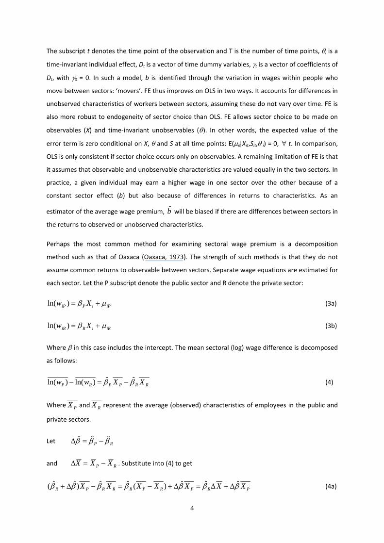
Perhaps  the  most  common  method  for  examining  sectoral  wage  premium  is  a  decomposition 

method such as  that of Oaxaca  (Oaxaca, 1973). The strength of such methods  is  that  they do not 

assume common returns to observable between sectors. Separate wage equations are estimated for 

each sector. Let the P subscript denote the public sector and R denote the private sector: 

iPiPiP Xw μβ +=)ln(                     (3a) 

iRiRiR Xw μβ +=)ln(                     (3b) 

Where β in this case includes the intercept. The mean sectoral (log) wage difference is decomposed 

as follows: 

RRPPRP XXww ββ ˆˆ)ln()ln( −=−                 (4) 

Where PX and RX represent the average (observed) characteristics of employees  in the public and 

private sectors.  

Let 

 RP βββ ˆˆˆ −=Δ

and  RP XXX −=Δ . Substitute into (4) to get 

PRPRPRRRPR XXXXXXX βββββββ ˆˆˆ)(ˆˆ)ˆˆ( Δ+Δ=Δ+−=−Δ+         (4a) 

4

The first term represents the effect of differences in characteristics between sectors. Specifically it is 

the  return  in  the  private  sector multiplied  by  the  average  difference  in  characteristics  between 

sectors.  The  second  term  is  the  effect  of  differences  in  the  returns  to  observable  characteristics 

between sectors. In this version of the Oaxaca decomposition, returns to observable characteristics 

in the private sector are the  ‘benchmark’ against which returns  in the public sector are compared. 

The  returns  provided  in  the  public  sector  are  thus  contrasted  directly with  those  of  the  private 

market.  This  is  the  appropriate  comparison  for  the  research question under  consideration  in  this 

paper.  Other  related  decomposition  approaches  are  proposed  by  Reimers  (1983)  and  Neumark 

(1988), which are suited to analysing discrimination, but are less relevant here. 

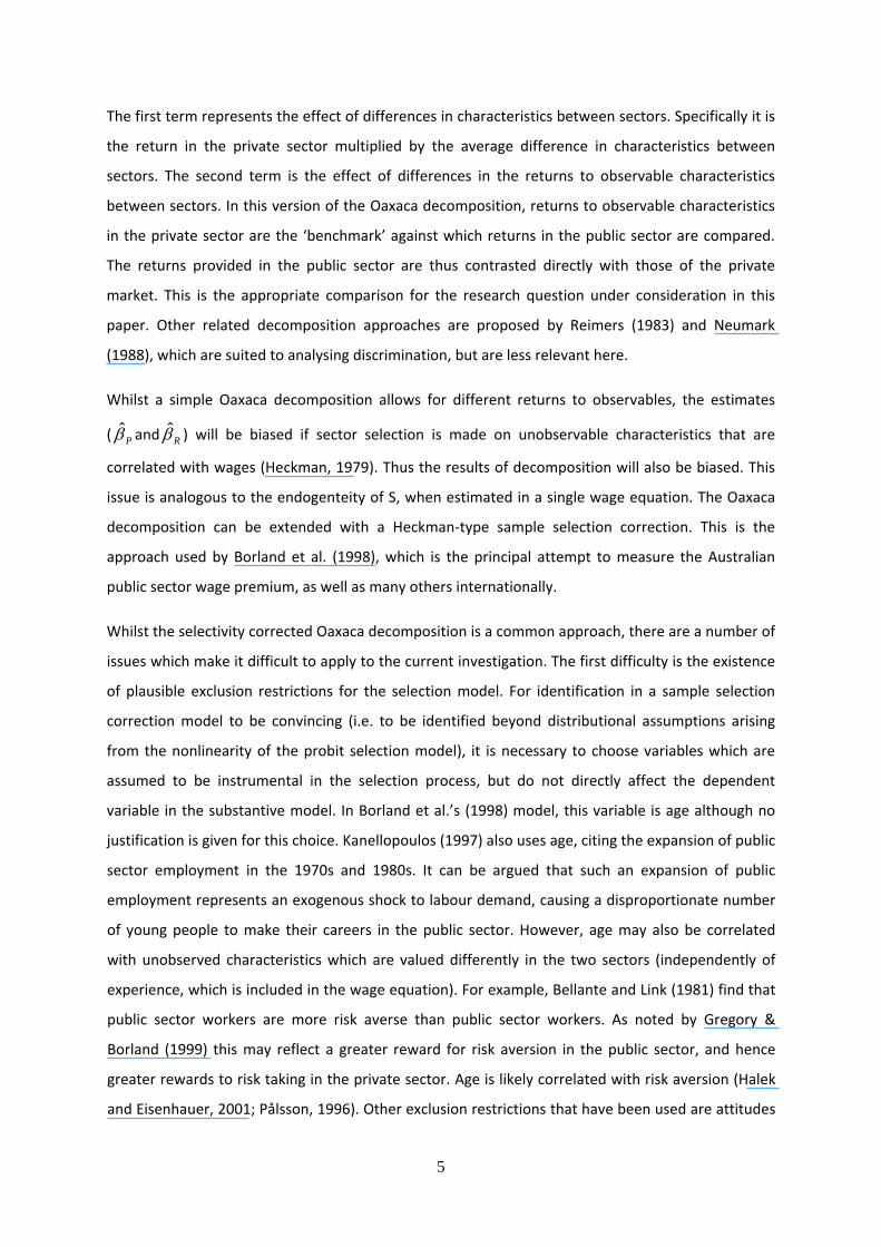
Whilst  a  simple Oaxaca  decomposition  allows  for  different  returns  to  observables,  the  estimates 

( and )  will  be  biased  if  sector  selection  is made  on  unobservable  characteristics  that  are 

correlated with wages (Heckman, 1979). Thus the results of decomposition will also be biased. This 

issue is analogous to the endogenteity of S, when estimated in a single wage equation. The Oaxaca 

decomposition  can  be  extended  with  a  Heckman‐type  sample  selection  correction.  This  is  the 

approach used by Borland et al.  (1998), which  is  the principal attempt  to measure  the Australian 

public sector wage premium, as well as many others internationally. 

Pβ̂ Rβ̂

Whilst the selectivity corrected Oaxaca decomposition is a common approach, there are a number of 

issues which make it difficult to apply to the current investigation. The first difficulty is the existence 

of plausible exclusion  restrictions  for  the  selection model. For  identification  in a  sample  selection 

correction model  to be  convincing  (i.e.  to be  identified beyond distributional  assumptions  arising 

from  the nonlinearity of  the probit selection model),  it  is necessary  to choose variables which are 

assumed  to  be  instrumental  in  the  selection  process,  but  do  not  directly  affect  the  dependent 

variable  in the substantive model.  In Borland et al.’s (1998) model, this variable  is age although no 

justification is given for this choice. Kanellopoulos (1997) also uses age, citing the expansion of public 

sector  employment  in  the  1970s  and  1980s.  It  can  be  argued  that  such  an  expansion  of  public 

employment represents an exogenous shock to labour demand, causing a disproportionate number 

of young people  to make  their careers  in  the public  sector. However, age may also be correlated 

with unobserved characteristics which are valued differently  in  the  two  sectors  (independently of 

experience, which is included in the wage equation). For example, Bellante and Link (1981) find that 

public  sector workers  are more  risk  averse  than  public  sector workers.  As  noted  by  Gregory  & 

Borland  (1999)  this may  reflect a greater  reward  for  risk aversion  in  the public  sector, and hence 

greater rewards to risk taking in the private sector. Age is likely correlated with risk aversion (Halek 

and Eisenhauer, 2001; Pålsson, 1996). Other exclusion restrictions that have been used are attitudes 

5

towards unions (since union membership  is correlated with public sector status (eg. Bender, 2003; 

Heitmeuller, 2006; Melly, 2006). This  is a  contentious  choice  since  such attitudes are  likely  to be 

endogenous to working in a unionised environment (as acknowledged by Melly). Father’s occupation 

has  been  frequently  used  (eg.  Bender,  2003;  Dustmann  and  van  Soest,  1998;  Hartog  and 

Oosterbeek,  1993;  Hou,  1993;  Melly,  2006;  Terrell,  1993).  This  assumes  that  one’s  father’s 

employment  in  the  public  sector  affects  the  selection  decision  but  not  wages.  This  may  be 

contentious if one’s father has contacts in their sector of employment which translate to higher pay 

(although Melly’s results suggest this is not an important issue for Germany). The assumption is also 

violated  if  intergenerationally  transmitted  attitudes  to  the  public  sector  employment  are 

accompanied by  intergenerationally  transmitted  (unobserved)  skills. To put  this  in another way,  if 

one  lives with a public sector worker during childhood, they may acquire some skills or knowledge 

which are valued in public sector labour markets (and similarly for the private sector). Some studies 

(Hartog  and  Oosterbeek,  1993;  Hou,  1993)  use  parent’s  education,  which  is  also  likely  to  be 

correlated with unobserved skills.  If multiple  instruments are available, overidentification tests can 

be  used  to  support  or  reject  the  assumptions  underlying  exclusion  restrictions.  However,  their 

results are contingent on statistical power. 

Another limitation of the selectivity‐corrected decomposition approach is that it cannot decompose 

the effect of differences in the stock of unobserved characteristics from the effect of differences in 

their  returns.  In  the  selectivity  corrected decomposition,  the equality  shown  in equations  (4) and 

(4a)  does  not  hold.  The  decomposition  has  additional  terms,  which  are  the  effects  of  sample 

selection in the wage equations: 

)ˆˆ(ˆˆ)ln()ln( RRPPPRRP XXww λθλθββ −+Δ+Δ=−             (5) 

where  λ   is  the estimated mean  Inverse Mills Ratio  in  the models  for each  sector, and    is  the 

estimated coefficient of λ  in the selectivity corrected wage equation  in each sector. The selectivity 

correction  terms capture both  the effects of differences  in unobserved  skills and  returns  to  those 

unobserved  skills.  In general,  it  is  impossible  to decompose  these  two effects. This  is discussed  in 

detail by Gyourku and Tracy (1988) and more recently by Neuman and Oaxaca (2004) in a different 

context. One approach  is  to  take  the  selectivity  correction  terms  to  the  left hand  side of  (5) and 

thereby  decompose  the  selectivity  corrected wage  difference: 

θ̂

)ˆRλθˆ()ln()ln( RPPRP ww λθ −−− . 

The  resulting  decomposition  recovers  the  ‘unconditional’  wage  differential  between  sectors 

)ˆ( PXβΔ . This approach corresponds to the following thought experiment. Take a person from the 

population of all employees who has the same observed characteristics as the average public sector 

6

worker. What  is the expected difference between sectors  in the wages that person could earn?  In 

contrast, analysis of the ‘conditional’ wage differential addresses the following thought experiment. 

Take a person at  random  from  the public  sector and put  them  in  the private  sector. What  is  the 

expected  change  in  their wage?  This  is  the  relevant  thought  experiment  for  the  question  in  this 

paper. The selectivity corrected decomposition does not recover this estimate, unless one assumes 

that there are no differences in returns to unobservable characteristics between sectors. 

A third complication for the selectivity corrected approach is that sector selection derives from both 

the supply and demand sides of the labour market. Workers who have the most to gain from public 

sector employment are most likely to prefer the public sector. However, public sector employers will 

choose  the  most  appropriate  workers  from  the  pool  of  applicants.  A  single  sample  selection 

correction may not adequately account for the complexity. A more appropriate model is a two‐stage 

nested selection model, where the employees choice of applying for public sector work is modelled 

first, and the employer’s choice of choosing from applicants is modelled next (see Farber, 1983; and 

Lemieux, 1993  in  relation  to  selection  and unionisation).  This  could be  implemented  as part of  a 

selection  correction model.  But  it would  require  a  further  exclusion  restriction which  influences 

employers’ selection of workers, but not the worker’s productivity in that sector. 

Models of the distribution of the public sector wage premium 

All  the methods discussed so  far estimate  the average sectoral wage premium. However, much of 

the recent literature is focussed on the effect at all points of the wage distribution, mainly through 

quantile regression approaches. All of the methods discussed above now have analogous methods in 

the  quantile  regression  framework.  Quantile  regressions  are  able  to  estimate  the  effect  of  a 

covariate  at  any  quantile  of  the  conditional  distribution  of  the  dependent  variable  (Koenker  and 

Bassett  Jr,  1978).  Briefly,  the  quantile  regression  method  is  to  minimise  the  weighted  sum  of 

absolute differences  (rather than the sum of squares) between the data points and the regression 

line. The choice of weight determines  the quantile being considered. Thus one could estimate  the 

effect of working in the public sector (P) on the entire distribution of wages using a series of quantile 

regressions.  This  section  serves  to briefly highlight  that  the  limitations of  the methods discussed 

above also apply to the quantile regression models. These methods are discussed in turn below. 

The model  in equation  (1), which allows  sector  to enter as a  constant  term,  can be estimated by 

quantile regression at any point of the conditional wage distribution. 

Fixed Effects models are not possible  in quantile regression.  In a paper that  is yet to be published, 

Abrevaya and Dahl (2006) propose a panel data quantile regression model, which is analogous to the 

7

correlated random effects model for  least squares proposed by Chamberlain  (1982).  In this model, 

the fixed effect  is modelled as a  linear projection of observable characteristics  in each period. This 

model  can be  interpreted  in a  similar way  to  FE models,  in  that  the effect of  sector on wages  is 

identified  by movers  between  sectors.  It  has  the  same major  limitation  as  the  FE model,  as  it 

assumes equal returns to observed and unobserved characteristics in the two sectors. 

Decomposition approaches also have quantile regression equivalents, as proposed by Machado and 

Mata  (2005).  This was  adapted  by Melly  (2005)  and  applied  to  estimate  the  public  sector wage 

premium in Germany. This approach was also used by Cai and Liu (2007) to examine the Australian 

union  wage  premium. Melly  (2006)  has  also made  an  attempt  to  incorporate  sample  selection 

correction into a quantile regression decomposition. However, the method is complex and is yet to 

be published. 

 

III The Model The approach adopted in this paper is based on that used by Lemieux (1993; 1998) to estimate the 

effect  of  unions  on wages.  This  is  a  quasi‐differenced  panel  data model,  originally  proposed  by 

Chamberlain  (1982)3.  It  combines  the  strengths  of  FE  (allowing  for  differences  in  unobserved 

characteristics  and  allowing  sector  selection  to  be  correlated with  time‐invariant  unobservables) 

with that of Oaxaca decomposition (allowing for differences  in returns between sectors). Unlike all 

the other approaches considered, it also identifies the effect of differences in returns to unobserved 

characteristics,  distinguishing  this  from  the  effect  of  differences  in  their  stock.  The  method  is 

described below, drawing heavily on Lemieux (1998). 

Assume that employees derive utility from consumption and leisure. Assume further that employees 

can choose  their quantity of working hours  in a given  job.  It  follows  from  these assumptions  that 

employees will  choose  a  job with  the  highest hourly  earnings of  all  available options.  The  set of 

available options depends on their skills. Their skills consist of the quantity and quality of experience 

and education as well as other factors such as intelligence, interpersonal skills and so on. A particular 

skill set may be more valuable in some jobs than in others. 

Begin with expressions for the expected  log wage for person  i  in each sector, denoted   and   

in  (6a) and  (6b). Each equation  includes observed skills  (X) and sector specific returns  (β)  to  those 

characteristics.  Each  equation  contains  two  time  invariant unobserved  components:  θ and  ξ.  The 

Rity P

ity

                                                            3 See also Gibbons et al. (2005) for an application of this approach in the context of industry wage models. 

8

first  of  these  (θ)  represents  comparative  advantage,  those  unobserved  skills  which  are  valued 

differently between sectors, while ψ represents the extent to which those returns differ. The second 

(ξ)  represents  absolute  advantage,  or  those  unobserved  skills which  are  equally  valued  in  both 

sectors.4 Observations are taken at more than one period (t): 

iiitRR

tRit Xy ξθβδ +++=                   (6a) 

iiitPP

tPit Xy ξψθβδ +++=                   (6b) 

These  two  expressions  can  be  combined  into  a  single  wage  equation  by  substituting  into  the 

following: 

itRitit

Pititit yPyPw ε ′+−+= )1(ln  

where P = 1  if  the employee  is  in  the public sector and zero otherwise. ε’  is an  idiosyncratic error 

term. The resulting expression can be written as: 

itiitRP

itR

ititRtit PPXPw εθψβββδδ +−++−+++= )]1(1[)]([ln

       (7) 

where  Rt

Pt δδδ −=

  and  itiit εξε ′+=  

Under  the assumptions outlined above,  there  is no explicit  role  for  job characteristics  (other  than 

sector) in the model. Since utility is not derived from the job itself, the characteristics of the job do 

not have an  independent effect on wages. Recall that an employee chooses a  job with the highest 

hourly earnings. For that  individual, the set of jobs available  is a function of their skill set. Thus job 

characteristics  (including  industry and occupation) are a consequence of a person’s skills,  rather a 

separate effect  in the wage equation. This does not  imply that returns to say, a university degree, 

are equal across occupations and industries. It merely states that a given person will choose the job 

which maximises the returns to their own particular skill set. 

I also do not  control  for  size of employer or union  status. The public  sector  is a highly unionised 

workforce characterised by large employers. Both of these factors are associated with higher hourly 

earnings (Miller and Mulvey, 1996; Wooden, 2001).  I treat these as  inherent features of the public 

sector which I do not wish to abstract from. Wooden (2001) has shown that in the Australian labour 

market, characterised by enterprise bargaining, the effect of unions on wages operates at the  level 

                                                            4 ξ is orthogonal to θ by construction and is inconsequential for much of what follows. See Lemieux (1998) for 

more detail on this specification of time invariant effects.  

9

of  the workplace  rather  than  the  individual. Thus workers  in highly unionised workplaces enjoy a 

wage premium, regardless of their personal union membership. Since HILDA does not  include such 

data on the workplace, any attempt to explicitly account for the effect of unionisation is likely to be 

misleading. 

Decomposition of the Average Sectoral Wage Gap 

If estimable, the parameters in (7) can be used in a decomposition which distinguishes between the 

effects of differences in observed and unobserved characteristics as well as the effects of differences 

in  returns  to  both  observed  and  unobserved  characteristics.  Consider  the mean wage  difference 

between sectors: 

)()()ln()ln( RRRRR

tPPPPP

tRP XXww ξθβδξθψβδ +++−+++=−        

RPRR

PP XX θθψββδ −+−+=  

)]()[(])1()([ RPR

RPRRP

P XXX θθβθψββδ −+−+−+−+=  

The contents of the first square brackets represent the effects of differences in wage setting policies, 

which  includes a constant difference  (δ ) and differences  in returns to characteristics. The second 

term represents the effects of differences in characteristics. 

Estimation5 

The  first  step  to  estimating  (7)  is  to  ‘quasi‐difference’.  That  is,  to  substitute θ for  the  expression 

obtained when θ is made the subject of the argument in a first lag as follows: 

)]1(1/[])]([([ln 1111111 −++−+++−= −−−−−−− ψεβββδδθ ititRP

itR

ititRtiti PPXPw

   (8) 

Substituting into (7): 

ititittitit

ititittit ePXFw

PPPXFw +−×

−+−+

+= −−−−−

)],([ln)]1(1[

)]1(1[),(ln 11111 ψψ

      (9) 

where: 

11 )]1(1[

)]1(1[−

− −+−+

−= itit

ititit P

Pe εψ

ψε  

                                                            5 Analysis was conducted using SAS V9 and Stata V9.2 

10

and 

)]([),( RPit

Ritit

Rtititt PXPPXF βββδδ −+++=  

Equation  (9)  is nonlinear and  includes an endogenous  regressor:  , which  is correlated with 1ln −itw

1−itε and  hence  with  .  The  endogenous    can  be  instrumented  by  ,  which  is 

available for this study. I also use the interactions of   with  ,  ,  ,  and   as 

well as the interactions of the sector history variables:  ,   and   with   and   as 

further  instruments.  Equation  (9)  can  be  estimated  consistently  using  the method  of  Nonlinear 

Instrumental  Variables  (NLIV)  (Amemiya,  1974).

ite 1ln −itw 2ln −itw

2ln −itw 1−itX itX 2−itP 1−itP itP

itP 1−itP 1−itit PP 1−itX itX

6  NLIV  can  be motivated  by  first‐order moment 

conditions.  Let  Zi  denote  the  set  of  instrumental  variables  (including  X  and  P).  The  first  order 

population moment condition is E(eitZi) = 0. Consistent estimates of the structural parameters (α) are 

obtained by choosing those α which minimise the following objective function: 

)()()( 1 αα eZZZZe ′′′ −  

Where e(α) = (eit,...,eMt), M is the number of people in the sample, and Z = (Z1’:...: ZM’)’.  

Whilst NLIV is a consistent estimator, an efficient GMM estimator minimises the following objective 

function: 

)()( αα eZZWe ′′  

                                                            6 Note that whilst e is a function of P, the two are uncorrelated. To demonstrate this, consider: 

⎟⎟⎠

⎞⎜⎜⎝

⎛−+−+

=⎟⎟⎠

⎞⎜⎜⎝

⎛−+−+

−= −−

−−

11

11 )]1(1[

)]1(1[)]1(1[)]1(1[)()( it

it

ititit

it

itititititit P

PPEP

PPEPEePE εψψε

ψψε  

 The expression )]1(1[)]1(1[

1 −+−+

− ψψ

it

itit

PPP

   = 0, when  0=itP  

          = 1, when 1=itP  and  11 =−itP  

          = ψ, when 1=itP  and  01 =−itP  

In all cases,  0)]1(1[)]1(1[

11

=⎟⎟⎠

⎞⎜⎜⎝

⎛−+−+

−−

itit

itit

PPPE ε

ψψ

 and hence  0)( =ititePE . Similarly for . )( 1 itit ePE −

11

where  the  weighting matrix W  is  the  inverse  of  the  estimated  variance matrix  of  the moment 

functions, estimated by NLIV (see Davidson and MacKinnon, 1993; Greene, 2003; Hansen, 1982). 

In order to separately identify  ,  and Rtδ R

t 1−δ δ , it is necessary to impose a further restriction on the 

parameters. The expected value of θ across all people and both years is constrained to be zero: 

∑ =+⎟⎠⎞

⎜⎝⎛= −

iititN

0)ˆˆ(21

1θθθ  

where N is the number of people and 

)]1(1/[)]}([({lnˆ −+−+++−= ψβββδδθ isRP

isR

isisRsisis PPXPw

 for  )1,( −∈ tts    (8b) 

Note that whilst θ is a consistent estimate of the mean value of θ,  the distribution of  may be 

dissimilar to the distribution 

isθ̂

isθ  (see Lemieux, 1993). This is because   in (8b) is partly a function 

of 

isθ̂

isε  as can be seen in (8) for s = t‐1. 

Identification 

The estimates of δ  and ψ are identified only by movers between sectors. This can be seen by noting 

that both disappear  from  (9) when 1−= itit PP . Thus  reasonable estimates of  δ  and ψ can only be 

obtained with a data set that has a sufficiently large number of movers. 

Similarly, the coefficients of X in each sector (βP and βR) are only independently identified by people 

whose X changes between t‐1 and t  (‘changers’). The main observed characteristics of  interest are 

the  standard  human  capital  variables:  experience  and  education.  To  separately  identify  sectoral 

differences in returns to education, it is necessary for the data to contain individuals (in each sector) 

whose educational attainment changed between observations.  In the case of experience, the main 

issue for identification is the ability to distinguish it’s effect from that of pure wage inflation or other 

changes between observations  that affect all workers  (as measured by  ). The  returns  to 

experience can thus identified by the set of people whose experience increased by less than the time 

elapsed between observations. 

Rt

Rt 1−− δδ

If the number of ‘changers’ is insufficient, an alternate identification strategy is available. Education 

can be treated as time  invariant  if changers are excluded from the analysis. Education can thus be 

incorporated as a component of θ, and differences in returns to education can be incorporated in ψ. 

This  highlights  the  key  difference  between  this model  and  standard  panel  data models.  In  a  FE 

12

model,  leaving  education  in  θ  implies  an  assumption  of  no  sectoral  differences  in  returns  to 

education. This is not the case here. The disadvantage of this strategy is that sectoral differences in 

returns to education are not separately identified from differences in returns to other time invariant 

skills. This is not a major limitation, as all of the components of the decomposition are consistently 

identified.  Thus  differences  in  time  invariant  skills  (including  education)  are  identified  by movers 

between sectors. 

A  similar  strategy  is  available  to  incorporate  the  effects  of  experience.  One  can  assume  that 

experience  increased by  a  constant  amount between  time  t‐1  and  t.  Since  the model  relies on  a 

three period balanced panel of employees, this constant  is equal to the  time elapsed between  t‐1 

and t. Experience at time t can be incorporated into θ , similarly to the treatment of education. The 

effect of a one period increase in experience is incorporated into  . Rt

Rt 1−− δδ

This alternate identification strategy is implicit in Lemieux (1998). Lemieux did not observe changes 

in  experience  or  education.  This  is  also  the  approach  applied  in  this  paper. As will  be  discussed 

below,  HILDA  does  observe  employees  whose  educational  attainment  changes  between 

observations, but their numbers are insufficient.  

An assumption shared by this approach and Lemieux’s  is that sector choice  is uncorrelated with e, 

conditional on X and θ. This does not  allow  for  the possibility  that people  change  sectors due  to 

shocks  in  person  and  sector  specific  productivity  shocks  (i.e.  temporary  comparative  advantage). 

Lemieux argues that this possibility  is reduced by considering only  involuntary  job changers. These 

were  people  who  changed  jobs  due  to  ‘plant  closing,  family  responsibilities,  illness,  geographic 

moves, dismissal, or other forms of  layoffs’. This does not seem to be a convincing argument for a 

number  of  reasons.  Firstly,  people may  be  dismissed  or  laid  off  precisely  due  to  a  fall  in  sector‐

specific productivity (especially if institutional constraints prevent a wage reduction). Secondly, even 

if an involuntary job loss is assumed to be exogenous, there is no reason to believe that subsequent 

sector  choice  in  the next  job  is  similarly  exogenous. Rather  than  following  Lemieux’s  approach,  I 

accept as a limitation the assumption that sector choice is uncorrelated with e, conditional on X and 

θ. Furthermore, the number of sector changers who changed jobs involuntarily is too small in HILDA 

to adopt this approach. For example, such an approach would restrict the number of sector movers 

to 6 males and 13 females in the main model (estimated on Waves 4, 5 and 6).

Factors Not Accounted For in the Model 

Some factors that may affect sectoral wage differences have not been incorporated in the model. In 

particular,  earnings  are  an  incomplete measure of  the  total  return  to  labour.  Employees may be 

13

willing to accept lower earnings in exchange for other benefits. Superannuation and paid maternity 

leave entitlements may be particularly important considerations. 

Employer contributions to superannuation are a major component of total remuneration. Under the 

Superannuation  Guarantee,  employers  have  been  required  to  contribute  to  each  employee’s 

superannuation at a rate equal to at least 9% of earnings since 2002. Historically, superannuation in 

the public sector has been generous. The Commonwealth Superannuation Scheme commenced  in 

1922,  providing  retirees with  a  defined  benefit  pension  equal  to  up  to  70%  of  their  final  salary, 

indexed  to  inflation  (Department of Finance and Administration, 2001). Subsequent  reforms have 

resulted  in  less generous pensions. If superannuation schemes remain more generous  in the public 

sector,  this may have a downward effect on public sector earnings  through a compensating wage 

differential. However, sectoral comparisons of employer contributions are hampered by differences 

in  the  benefit  structures  of  superannuation  schemes.  Schemes  fall  into  three  main  structures: 

accumulation,  defined  benefits  and  a  hybrid  of  the  two.  In  accumulation  funds,  employers 

contribute  superannuation  continuously,  in  proportion  to  earnings.  In  defined  benefit  funds,  the 

value of employer contributions  is  sometimes unknown until  retirement because  the benefits are 

often  defined  in  relation  to  employees’  final  salary.  For  this  reason,  the major  recent  survey  of 

superannuation  in Australia, the Survey of Employment Arrangements and Superannuation  (SEAS), 

only provides a measure of employer contributions  for  those who have active accumulation  funds 

(and no defined benefit or hybrid accounts) (Australian Bureau of Statistics, 2001). This excludes 63% 

of public  sector employee  respondents and 15% of  those  in  the private  sector. For  the  remaining 

sample, average employer contributions are similar in the two sectors (6.6% in the public sector and 

6.8%  in  the  private  sector).7  This  is  unlikely  to  be  a  good  indication  of  the  overall  generosity  of 

employer  contributions  in  the  public  sector.  It  does  suggest,  however,  that  few  private  sector 

employees receive more than the minimum legislated contribution from their employer. 

In Australia, paid maternity leave is not mandatory. Public sector employers are much more likely to 

provide  paid maternity  leave  than  private  sector  employers.  In  2005,  the  Australian  Bureau  of 

                                                            7 Author’s calculations from the SEAS Expanded Confidentialised Unit Record File. The percentage contribution 

was  calculated  by  the  author  for  each  employee  as  total  employer  contributions  divided  by  usual weekly 

income from main  job. The sample was restricted to employees. Employees of own business were excluded. 

People with more  than one  job were excluded as  the employer contribution variable does not differentiate 

between  jobs. At the time of the survey, the minimum  legislated employer contribution was 8%. Employees 

with monthly income below $450 per month are exempt, as are those under 18 years of age working less than 

30 hours per week. Thus it is reasonable for the average contribution to be less than 8%. 

14

Statistics surveyed women who had a child under two years of age. Of those who were public sector 

employees whilst  pregnant,  76%  accessed  paid maternity  leave,  compared  to  27%  in  the  private 

sector  (Australian  Bureau  of  Statistics,  2007b:  135).  Paid maternity  leave may  have  a  downward 

effect  on  public  sector wages  for  females  to  the  extent  that  they  are willing  to  sacrifice  some 

earnings in order to access this benefit. 

Other sectoral differences that have not been accounted may include job security and flexibility and 

possible differences in the utility derived from the work itself. 

 

IV Data The  data  used  for  this  study  are  from  the  Household  Income  and  Labour  Dynamics  in  Australia 

(HILDA)  Survey.  HILDA  is  a  nationally  representative  household‐based  panel  survey, with  annual 

observations  taken since 2001. At  the  time of writing,  the  first six waves are available  for analysis 

(2001‐2006) and government funding has been committed for at least a further six waves.  

The model described in the previous section requires a balanced panel with three observations per 

person and is identified by changes in X and P between the last two observations. One approach is to 

use Waves 4, 5 and 6  (W456), the most recent waves. Recall the notation  in the previous sections 

referring to time periods t, t‐1 and t‐2. Time period t thus refers to Wave 6 of HIDLA, t‐1 refers to 

Wave 5 and t‐2 refers to Wave 4. The main parameters of this model are identified by sector movers 

between Waves 5 and 6. 

In order to  improve the precision of the estimates,  I supplement this approach with three pairs of 

corresponding models for Waves 3, 4 and 5 (W345), for Waves 2, 3 and 4 (W234), and for Waves 1, 2 

and 3 (W123), respectively, which are  identified by a different set of movements between sectors. 

The  results  of  the W456 model  are  shown  in  detail  in  this  section.  The  key  results  of  the  other 

models are also discussed  in this section and are shown  in detail  in the Appendix. The four sets of 

estimates are treated as equally valid, and are combined to form one overall estimate for each sex, 

discussed at the end of the results section. 

The dependent variable is the log of hourly earnings. Hourly earnings are derived as ‘current weekly 

gross wage and salary in main job’ divided by ‘hours per week usually worked in main job’. Sector of 

main  job was self‐reported and  includes  ‘Government business enterprise or commercial statutory 

authority’ and ‘Other governmental organisation’. 

15

The  only  other  observed  characteristic  included  in  the model  (X)  is  a  dummy  variable  for  casual 

employment contracts. This  is  included because  the wages of  ‘casual’ employees usually  include a 

loading that compensates for a lack of entitlements received under other contracts. The size of such 

loadings,  however,  varies  considerably,  depending  on  the  Award  or  enterprise  agreement  under 

which an employee is covered. Watson (2005) notes a variation of 15% to 33.3% amongst enterprise 

bargaining  agreement  in  the  ACIRRT  ADAM  database  between  1994‐2002.  The  loading  is  also 

between 15% and 33%  in most Awards, but  is sometimes  less than this and can be as high as 50% 

(Owens, 2001). Furthermore, many self‐identified casuals do not receive any loading at all (Wooden 

and Warren, 2003). A manual adjustment  to  the wages of casual workers  is considered  infeasible, 

since  it  is unclear how  large such an adjustment would need to be. Thus the size of the  loading  is 

estimated by the model. Secondly,  it  is possible that average casual  loadings are different between 

the two sectors. In the main set of estimates, however, the loading is constrained to be equal in the 

two sectors, because of a small number of observations which would identify this parameter for the 

public  sector.  The main  results  are  not  sensitive  to  the  relaxation  of  this  assumption,  as will  be 

shown. 

Observations  are  weighted  by  the  cross  sectional  probability  weight  provided  on  the  Wave  6 

responding persons file. 

The  sample  is  defined  as  the  set  of  responding  persons who were  employees  (excluding  those 

employed by their own business) at all three observations, who changed employers between the last 

two observations and who had non‐missing values for the variables included in the model.8 Separate 

models are estimated for men and for women. The final sample for the W456 model consists of 346 

men and 282 women. Table 1 details  the exclusions  from  the  final sample. The  requirement  for a 

balanced panel of job changers accounts for the majority of exclusions. The sample size is similar for 

the W345, W234 and W123 models. 

                                                            8  Sector of employment  is  self  reported  in HILDA.  It  is possible  that  some apparent  sector movers actually 

result from reporting errors in this variable. To address this issue, the sample is limited to those who reported 

a  change  in  employer  between  the  last  two  observations,  which  follows  Lemiuex’s  (1998)  approach  in 

principle. In preliminary analysis, it was found that more than half of apparent sector movers did not report a 

change  in  employer  in  this  same  period.  This  suggests  that  a  large  proportion  of  sector movers may  be 

misclassified. There are, however, a number of other possible explanations. It may result from reporting errors 

in the change in employer variable, since this relies on retrospective recall. It is also possible for employees to 

change sector without changing employer. This is the case when a public corporation is privatised. In any case, 

the  conservative  approach  is  taken  here,  by  limiting  the  sample  to  employees who  reported  a  change  in 

employer. 

16

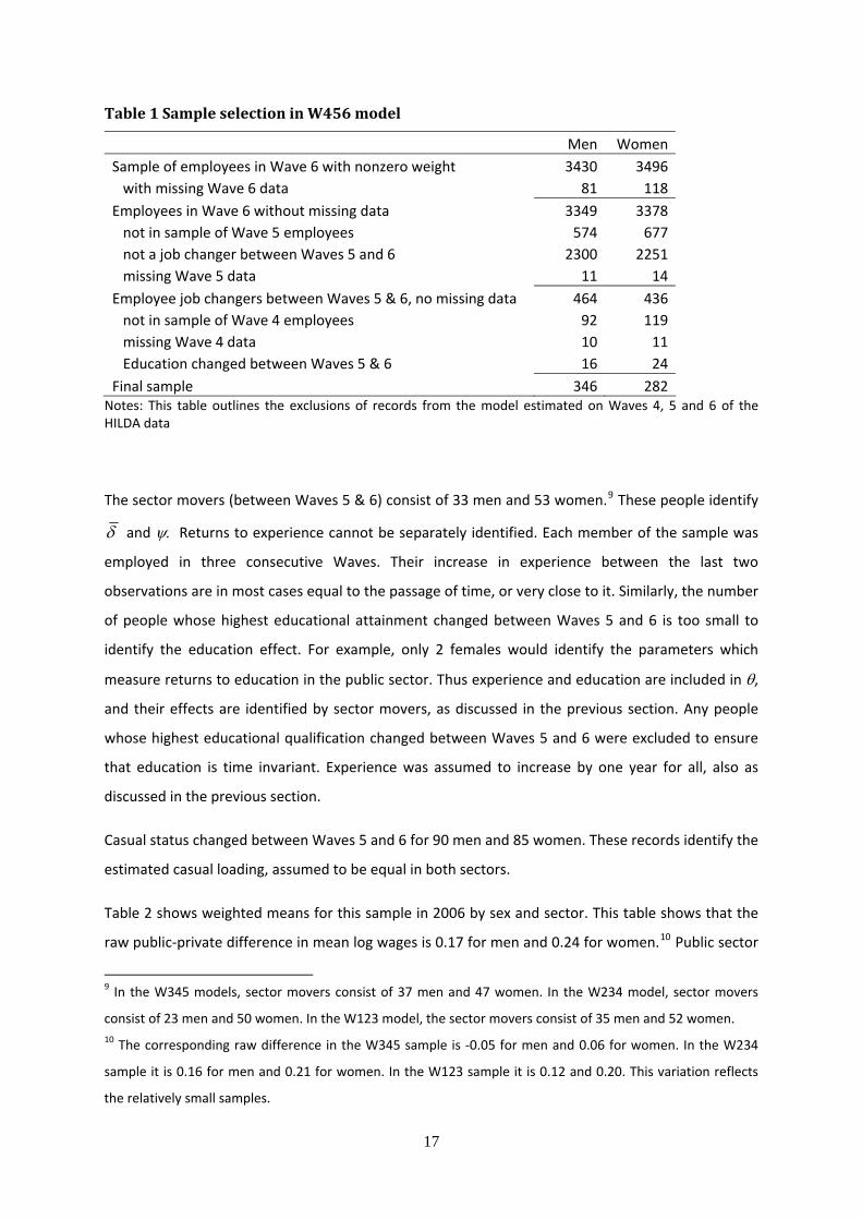
Table 1 Sample selection in W456 model 

   Men Women Sample of employees in Wave 6 with nonzero weight  3430 3496    with missing Wave 6 data  81 118 Employees in Wave 6 without missing data  3349 3378    not in sample of Wave 5 employees  574 677    not a job changer between Waves 5 and 6  2300 2251    missing Wave 5 data  11 14 Employee job changers between Waves 5 & 6, no missing data  464 436    not in sample of Wave 4 employees  92 119    missing Wave 4 data  10 11    Education changed between Waves 5 & 6  16 24 Final sample  346 282 

Notes: This  table outlines  the exclusions of  records  from  the model estimated on Waves 4, 5 and 6 of  the HILDA data 

 

The sector movers (between Waves 5 & 6) consist of 33 men and 53 women.9 These people identify 

δ and ψ.  Returns to experience cannot be separately  identified. Each member of the sample was 

employed  in  three  consecutive  Waves.  Their  increase  in  experience  between  the  last  two 

observations are in most cases equal to the passage of time, or very close to it. Similarly, the number 

of people whose highest educational attainment changed between Waves 5 and 6  is  too  small  to 

identify  the  education  effect.  For  example,  only  2  females would  identify  the  parameters which 

measure returns to education in the public sector. Thus experience and education are included in θ, 

and  their effects are  identified by sector movers, as discussed  in  the previous section. Any people 

whose highest educational qualification changed between Waves 5 and 6 were excluded to ensure 

that education  is  time  invariant. Experience was assumed  to  increase by one  year  for all, also as 

discussed in the previous section. 

Casual status changed between Waves 5 and 6 for 90 men and 85 women. These records identify the 

estimated casual loading, assumed to be equal in both sectors. 

Table 2 shows weighted means for this sample in 2006 by sex and sector. This table shows that the 

raw public‐private difference in mean log wages is 0.17 for men and 0.24 for women.10 Public sector 

                                                            9  In  the W345 models, sector movers consist of 37 men and 47 women.  In the W234 model, sector movers 

consist of 23 men and 50 women. In the W123 model, the sector movers consist of 35 men and 52 women. 10 The corresponding raw difference  in the W345 sample  is  ‐0.05 for men and 0.06 for women.  In the W234 

sample it is 0.16 for men and 0.21 for women. In the W123 sample it is 0.12 and 0.20. This variation reflects 

the relatively small samples. 

17

employees  are much more  likely  to hold  a degree or higher qualification.  They  also have  slightly 

more  experience on  average. Private  sector  employees  are more  likely  to be  employed  in  casual 

jobs. 

 

Table 2 Sample means (2006)* 

   Men  Women 

Variable  Public  Private  Public  Private 

ln wage  3.26  3.09 3.13 2.89Experience (years)  15.88  14.48 15.82 14.98Education            University degree  0.54  0.21 0.58 0.22   Trade  0.27  0.36 0.09 0.27   Year 12  0.12  0.26 0.15 0.26   less than Year 12  0.06  0.17 0.18 0.25

Casual  0.07  0.27 0.21 0.31* The sample is limited to that of the main analysis as reported in the text. 

 

Table 3 shows the results of OLS regressions using the sample described above at Wave 6. It suggests 

that for both sexes, the public sector wage premium is positive, but not significantly different from 

zero. The return to experience  is about 1.7% per year for men and 0.5% for women. The return to 

university  education  is  estimated  to  be  large  for  both  sexes.  The  estimated  effect  of  a  casual 

contract is negative for both sexes, despite the loading that compensates a lack of entitlements. This 

suggests  that  casual  status  is  correlated with unobserved  characteristics  that  are  associated with 

lower wages. 

Table 4 shows the results of  fixed effects regressions using observations at 2006 and 2005  for the 

sample described above. For the same reasons discussed above for the main model, education and 

experience are excluded as regressors. The estimated public sector premium is similar for both sexes 

to  the  OLS  estimates  for  both  sexes.  This  suggests  that  for  this  sample  at  least,  time  invariant 

unobserved  characteristics  of  employees  do  not  lead  to  a major  bias  in  the OLS  estimates.  The 

estimated public  sector premium  is not  statistically  significant  for either  sex. The effect of  casual 

status  is positive, as expected, as opposed to the OLS estimates and  is statistically significant. This 

confirms  that  casual  status  is  correlated with unobserved  characteristics  that  are  associated with 

lower wages. 

18

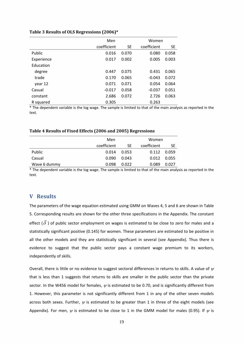
Table 3 Results of OLS Regressions (2006)* 

   Men  Women    coefficient SE coefficient SE Public  0.016 0.070 0.080  0.058 Experience  0.017 0.002 0.005  0.003 Education            degree  0.447 0.075 0.431  0.065    trade  0.170 0.065 ‐0.043  0.072    year 12  0.071 0.071 0.054  0.064 Casual  ‐0.017 0.058 ‐0.037  0.051 constant  2.686 0.072 2.726  0.063 R squared  0.305    0.263    

* The dependent variable is the log wage. The sample is limited to that of the main analysis as reported in the text. 

 

Table 4 Results of Fixed Effects (2006 and 2005) Regressions 

   Men  Women    coefficient SE coefficient SE Public  0.014 0.053 0.112  0.059 Casual  0.090 0.043 0.012  0.055 Wave 6 dummy  0.098 0.022 0.089  0.027 

* The dependent variable is the log wage. The sample is limited to that of the main analysis as reported in the text. 

 

V Results The parameters of the wage equation estimated using GMM on Waves 4, 5 and 6 are shown in Table 

5. Corresponding results are shown for the other three specifications in the Appendix. The constant 

effect (δ ) of public sector employment on wages  is estimated to be close to zero for males and a 

statistically significant positive (0.145) for women. These parameters are estimated to be positive in 

all  the other models  and  they  are  statistically  significant  in  several  (see Appendix).  Thus  there  is 

evidence  to  suggest  that  the  public  sector  pays  a  constant  wage  premium  to  its  workers, 

independently of skills. 

Overall, there is little or no evidence to suggest sectoral differences in returns to skills. A value of ψ 

that  is  less  than 1  suggests  that  returns  to  skills are  smaller  in  the public  sector  than  the private 

sector. In the W456 model for females, ψ is estimated to be 0.70, and is significantly different from 

1. However,  this parameter  is not  significantly different  from 1  in any of  the other  seven models 

across both  sexes. Further, ψ  is estimated  to be greater  than 1  in  three of  the eight models  (see 

Appendix).  For men, ψ  is estimated  to be  close  to 1  in  the GMM model  for males  (0.95).  If ψ  is 

19

restricted  to  equal  1,  the model  simplifies  to  the  fixed  effects model,  the  results  of which  are 

reported above in Table 4. Thus it is not surprising that the GMM estimate of δ  is small, similarly to 

the  ‘Public’  coefficient  in  the  fixed effects model. The  standard errors are also  similar  in  the  two 

models.  This  demonstrates  that  there  is  little  efficiency  loss  due  to  the  instrumental  variable 

approach. 

The W456 models suggest a positive loading for casual work for both genders, and it is significantly 

different from zero for men. The estimates in the other specifications are also positive, ranging from 

0.03 to 0.17. As discussed above, the estimated casual  loadings are constrained to be equal across 

sectors, but there is little change in the main results if this is relaxed, as will be shown subsequently. 

 

Table 5 GMM regression estimates of wage equations (Waves 4, 5 & 6) 

   Men  Women 

   coefficient  SE  coefficient  SE 

constant effect (δ )  0.005  0.052  0.145  0.038 

Returns to time invariant skills in public sector (ψ)  0.952  0.185  0.700  0.102 

Casual  0.125  0.037  0.038  0.037 Rtδ   3.078  0.018  2.901  0.018 

Rt 1−δ   2.973  0.027  2.806  0.017 

* The dependent variable is the log wage. The sample is limited to that of the main analysis as reported in the text. 

 

Decomposition of the Average Sectoral Wage Gap 

The  decomposition  based  on  the W456  results  is  shown  in  Table  6.  The main  result  is  that  the 

average public sector wage premium  is estimated to be close to zero (‐0.003) for men and positive 

for  women  (0.113).  Statistically,  this  estimate  is  significantly  different  from  zero  for  women 

(p=0.018) and not for men.11 

In  the  three  alternate  specifications,  the  estimates  of  the  average  public  sector  premium  are  all 

positive for both sexes. For men, the other point estimates are 0.018, 0.117 and 0.120. For women 

                                                            11 The results of the decomposition are a  function of the estimated coefficients and the sample means. The 

standard  errors  of  the  decomposition  take  account  of  the  variance‐covariance  matrix  of  the  estimated 

parameter vector. They also take account of the standard errors on the sample means. They also account for 

the  fact  that  the estimated mean  time  invariant  characteristics of workers  in each  sector  ( Pθ and  Rθ ) are 

functions of the estimated parameters and the sample means. 

20

they are 0.113, 0.062 and 0.075 (Table 7). For both sexes, the confidence intervals of these estimates 

all overlap. The four models are assumed to be equally valid and so the overall estimate is calculated 

as the weighted average of the four. The weighting is inversely proportional to the variance of each 

estimate.  This maximises  the  precision  of  the  overall  estimate.  The  four  pairs  of  estimates  are 

treated as  independent, since they are each  identified by different movements between sectors.12 

The overall estimate is thus 0.065 for men and 0.100 for women. These imply a public sector wage 

premium of e0.065 – 1 = 6.7% for men and e0.100 – 1 = 10.5% for women. The estimates are statistically 

significant (p=0.024 for and p<0.001 for women). The 95% confidence intervals are (0.009, 0.121) for 

men and  (0.058, 0.141)  for women. These estimates do not  change greatly  if  casual  loadings are 

allowed to vary between sectors (0.064 for men; 0.088 for women). 

 

Table 6 Decomposition of Sectoral Wage Gap from GMM results (Waves 4, 5 & 6) 

   Men  Women    Estimate SE Estimate  SE Public Sector Wage Premium:            constant effect (δ )  0.005  0.052  0.145  0.038 

   differences in returns to fixed characteristics  ‐0.008  0.036  ‐0.033  0.017 

   Total average wage premium  ‐0.003  0.086  0.113  0.048 

         

Effect of differences in characteristics:         

   casual status  ‐0.025  0.010  ‐0.004  0.004 

   fixed characteristics  0.202  0.085  0.134  0.048 

   Total effect of different characteristics  0.177  0.087  0.131  0.048 

         

Unadjusted Wage Gap  0.174     0.243     

Returning to Table 6, the largest components of the decomposition are due to sectoral differences in 

the  stock  of  time  invariant  skills  (which  include  education,  experience  and  unobserved 

characteristics). For both  sexes,  this  is a positive effect,  suggesting  that  the average public  sector 

employee is more skilled than his or her private sector counterpart. This is consistent with Table 2, 

which shows that they are more educated and more experienced. 

                                                            12 Strictly speaking, the estimates are not independent. Across the four specifications and both sexes, the key 

parameters  of  the models  are  identified  by  330  employees who  changed  sector. Of  these,  38  employees 

changed sectors  twice and hence contribute  to  the  identification of  two of  the estimates. Nevertheless,  the 

assumption of independence should produce reasonable estimates for the standard errors. 

21

Table  7  Summary  of  estimated  average  public  sector wage  premiums  across  all  GMM models 

   Men  Women  Model  Estimate  SE estimate SEWaves 4, 5 & 6  ‐0.003  0.086 0.113 0.048Waves 3, 4 & 5  0.018  0.046 0.062 0.050Waves 2, 3 & 4  0.117  0.049 0.075 0.051Waves 1, 2 & 3  0.120  0.073 0.118 0.031Overall estimate  0.065  0.029 0.100 0.021

* The overall estimates are weighted arithmetic means of the estimates from the three models. The weights are inversely proportional to the variance of the estimates, as described in the text. 

 

VI Conclusion This analysis suggests that the average Australian public sector employee is paid more than he or she 

would be paid in the private sector. The best estimates of this public sector wage premium are 6.7% 

for men and 10.5% for women. This does not  include the value of benefits such as superannuation 

and paid maternity  leave which are also more generous  in the public sector. This positive average 

premium is consistent with most of the international literature on this topic. It may result from the 

higher rates of unionisation in the public sector. It is also possible that this ‘premium’ compensates 

public sector workers for unfavourable working environments. However, the evidence for Australia 

suggests little or no sectoral difference in levels of work‐related stress or job satisfaction (Lewig and 

Dollard, 2001; Macklin et al., 2006). The estimate  is  thus slightly higher  for women  than  for men, 

though  their  difference  is  not  statistically  significant.  This  is  also  consistent with most  previous 

research internationally.  

The  results  also  suggest  that  this  premium  results  primarily  from  a  constant  effect  across  all 

employees  that  is  independent of  skills. No evidence was  found  to  suggest  that  the public  sector 

provides  lower  returns  to skills, which would  imply  that  it compresses  the wage distribution of  its 

workers.  This  contrasts  with  studies  that  have  addressed  this  issue  for  other  countries,  which 

typically  find  that  the  public  sector  does  compress  the wage  distribution  (Gregory  and  Borland, 

1999; Melly, 2006).  

 

 

22

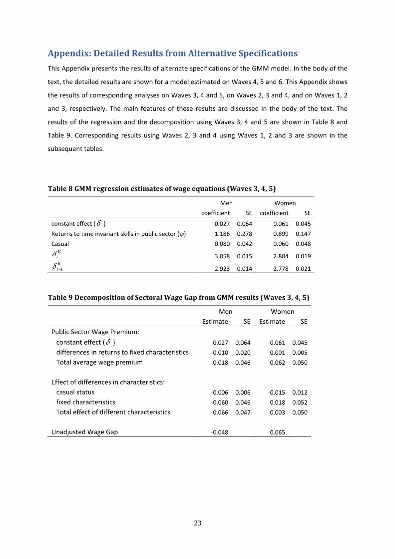
Appendix: Detailed Results from Alternative Specifications 

This Appendix presents the results of alternate specifications of the GMM model. In the body of the 

text, the detailed results are shown for a model estimated on Waves 4, 5 and 6. This Appendix shows 

the results of corresponding analyses on Waves 3, 4 and 5, on Waves 2, 3 and 4, and on Waves 1, 2 

and 3,  respectively. The main  features of  these  results are discussed  in  the body of  the  text. The 

results of the regression and the decomposition using Waves 3, 4 and 5 are shown  in Table 8 and 

Table 9. Corresponding  results using Waves 2, 3 and 4 using Waves 1, 2 and 3 are  shown  in  the 

subsequent tables.  

 

Table 8 GMM regression estimates of wage equations (Waves 3, 4, 5) 

   Men  Women 

   coefficient  SE  coefficient  SE 

constant effect (δ )  0.027  0.064  0.061  0.045 

Returns to time invariant skills in public sector (ψ)  1.186  0.278  0.899  0.147 

Casual  0.080  0.042  0.060  0.048 Rtδ   3.058  0.015  2.884  0.019 Rt 1−δ   2.923  0.014  2.778  0.021 

 

Table 9 Decomposition of Sectoral Wage Gap from GMM results (Waves 3, 4, 5) 

   Men  Women    Estimate SE Estimate  SE Public Sector Wage Premium:            constant effect (δ )  0.027  0.064  0.061  0.045 

   differences in returns to fixed characteristics  ‐0.010  0.020  0.001  0.005 

   Total average wage premium  0.018  0.046  0.062  0.050 

         

Effect of differences in characteristics:         

   casual status  ‐0.006  0.006  ‐0.015  0.012 

   fixed characteristics  ‐0.060  0.046  0.018  0.052 

   Total effect of different characteristics  ‐0.066  0.047  0.003  0.050 

         

Unadjusted Wage Gap  ‐0.048     0.065    

 

23

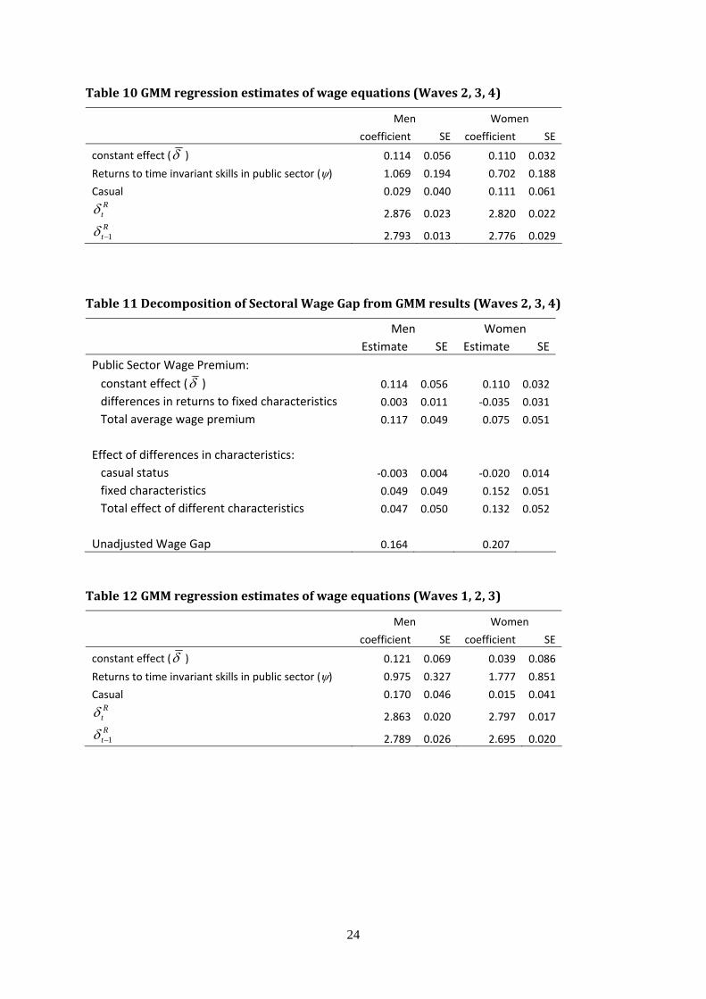
Table 10 GMM regression estimates of wage equations (Waves 2, 3, 4) 

   Men  Women 

   coefficient  SE  coefficient  SE 

constant effect (δ )  0.114  0.056  0.110  0.032 

Returns to time invariant skills in public sector (ψ)  1.069  0.194  0.702  0.188 

Casual  0.029  0.040  0.111  0.061 Rtδ   2.876  0.023  2.820  0.022 Rt 1−δ   2.793  0.013  2.776  0.029 

 

  

Table 11 Decomposition of Sectoral Wage Gap from GMM results (Waves 2, 3, 4) 

   Men  Women    Estimate SE Estimate  SE Public Sector Wage Premium:            constant effect (δ )  0.114  0.056  0.110  0.032 

   differences in returns to fixed characteristics  0.003  0.011  ‐0.035  0.031 

   Total average wage premium  0.117  0.049  0.075  0.051 

         

Effect of differences in characteristics:         

   casual status  ‐0.003  0.004  ‐0.020  0.014 

   fixed characteristics  0.049  0.049  0.152  0.051 

   Total effect of different characteristics  0.047  0.050  0.132  0.052 

         

Unadjusted Wage Gap  0.164     0.207     

Table 12 GMM regression estimates of wage equations (Waves 1, 2, 3) 

   Men  Women 

   coefficient  SE  coefficient  SE 

constant effect (δ )  0.121  0.069  0.039  0.086 

Returns to time invariant skills in public sector (ψ)  0.975  0.327  1.777  0.851 

Casual  0.170  0.046  0.015  0.041 Rtδ   2.863  0.020  2.797  0.017 Rt 1−δ   2.789  0.026  2.695  0.020 

 

24

Table 13 Decomposition of Sectoral Wage Gap from GMM results (Waves 1, 2, 3) 

   Men  Women    Estimate SE Estimate  SE Public Sector Wage Premium:            constant effect (δ )  0.121  0.069  0.039  0.086 

   differences in returns to fixed characteristics  ‐0.002  0.021  0.079  0.082 

   Total average wage premium  0.120  0.073  0.118  0.031 

         

Effect of differences in characteristics:         

   casual status  0.045  0.074  0.119  0.031 

   fixed characteristics  ‐0.027  0.011  ‐0.003  0.009 

   Total effect of different characteristics  ‐0.002  0.025  0.079  0.082 

         

Unadjusted Wage Gap  0.118     0.197     

 

 

References 

 

Abrevaya,  J. and Dahl, C. M.  (2006),  'The effects of birth  inputs on birthweight: evidence 

from  quantile  estimation  on  panel  data',  (Department  of  Economics,  Purdue 

University). 

Amemiya,  T.  (1974),  'The  Nonlinear  Two‐Stage  Least‐Squares  Estimator',  Journal  of 

Econometrics, 2, 105‐10. 

Australian  Bureau  of  Statistics  (2001),  'Superannuation  Coverage  and  Financial 

Characteristics, Australia, April to June 2000', ABS Cat. No. 6360.0 (Canberra: ABS). 

‐‐‐  (2007a),  Wage  and  Salary  Earners,  Public  Sector,  Australia  Jun  2007  (ABS  Cat.  No. 

6248.0.55.001 Canberra: ABS). 

‐‐‐ (2007b),  'Maternity  leave arrangements', Australian Social Trends 2007 (Canberra: ABS), 

132‐6. 

Bellante, D. and Link, A. N. (1981), 'Are Public Sector Workers More Risk Averse Than Private 

Sector Workers', Industrial and Labor Relations Review, 24, 408‐12. 

Bender, K. A. (1998), 'The Central Government‐Private Sector Wage Differential', Journal of 

Economic Surveys, 12 (2), 177‐220. 

25

‐‐‐  (2003),  'Examining  equality  between  public‐and  private‐sector  wage  distributions', 

Economic Inquiry, 41 (1), 62‐79. 

Borland,  J., Hirschberg,  J., and Lye,  J.  (1998),  'Earnings of Public Sector and Private Sector 

Employees in Australia: Is There a Difference?' Economic Record, 74 (224), 36‐53. 

Cai,  L.  and  Liu,  A.  L.  C.  (2007), Union Wage  Effects  in  Australia:  Are  There  Variations  in 

Distribution? (Melbourne Institute Working Paper No. 17/07; Melbourne: University 

of Melbourne). 

Chamberlain,  G.  (1982),  'Multivariate  Regression  Models  for  Panel  Data',  Journal  of 

Econometrics, 18, 5‐46. 

Davidson, R. and MacKinnon,  J. G.  (1993), Estimation and  Inference  in Econometrics  (New 

York: Oxford University Press). 

Department of Finance and Administration (2001), 'Submission to Senate Select Committee 

on  Superannuation  and  Financial  Services  Inquiry  into  Benefit  Design  of 

Commonwealth Public  Sector and Defence  Force Unfunded  Superannuation  Funds 

and Schemes'. 

Dustmann, C. and van Soest, A. (1998), 'Public and private sector wages of male workers in 

Germany', European Economic Review, 42, 1417‐41. 

Farber, H. S. (1983),  'The Determination of the Union Status of Workers', Econometrica, 51 

(5), 1417‐37. 

Gibbons,  R.,  Katz,  L.  F.,  Lemieux,  T.,  and  Parent,  D.  (2005),  'Comparative  Advantage, 

Learning, and Sectoral Wage Determination', Journal of Labor Economics, 23 (4), 681‐

723. 

Greene, W. H. (2003), Econometric Analysis (5 edn.: Prentice Hall). 

Gregory, R. G. and Borland, J. (1999), 'Recent Developments in Public Sector Labor Markets', 

in  O  Ashenfelter  and  D  Card  (eds.),  Handbook  of  Labor  Economics  (Volume  3: 

Elsevier), 3573‐630. 

Gyourko, J. and Tracy, J.  (1988),  'An Analysis of Public‐ and Private‐Sector Wages Allowing 

for  Endogenous  Choices  of  Both Government  and Union  Status',  Journal  of  Labor 

Economics, 6 (2), 229‐53. 

Halek, M. and Eisenhauer, J. (2001), 'Demography of Risk Aversion', The Journal of Risk and 

Insurance, 68 (1), 1‐24. 

26

Hansen,  L.  P.  (1982),  'Large  Sample  Properties  of  Generalized  Method  of  Moments 

Estimators', Econometrica, 50 (4), 1029‐54. 

Hartog, J. and Oosterbeek, H. (1993),  'Public and private sector wages  in the Netherlands', 

European Economic Review, 37, 97‐114. 

Heckman, J. J. (1979), 'Sample Selection Bias as a Specification Error', Econometrica, 47 (1), 

153‐61. 

Heitmeuller  (2006),  'Public‐Private  Sector  Pay  Differentials  In  A  Develolved  Scotland', 

Journal of Applied Economics, 9 (2), 295‐323. 

Hou, J. W. (1993), 'Public‐private wage comparison: A case study of Taiwan', Journal of Asian 

Economics, 4 (2), 347‐62. 

Kanellopoulos, C. N. (1997), 'Public‐private wage differentials in Greece', Applied Economics, 

29 (8), 1023‐32. 

Koenker, R. and Bassett Jr, G. (1978), 'Regression Quantiles', Econometrica, 46 (1), 33‐50. 

Lemieux, T.  (1993),  'Estimating  the Effects of Unions on Wage  Inequality  in a Two Sector 

Model with Comparative Advantage and Nonrandom Selection', Working Paper no. 

0493  (Montreal: Centre de Recherche et Developpement en Economique, Working 

Paper No 0493). 

‐‐‐ (1998), 'Estimating the Effects of Unions on Wage Inequality in a Panel Data Model with 

Comparative Advantage and Nonrandom Selection', Journal of Labor Economics, 16 

(2), 261‐91. 

Lewig,  K.  A.  and  Dollard,  M.  F.  (2001),  'Social  construction  of  work  stress:  Australian 

newsprint media portrayal of stress at work, 1997‐98', Work & Stress, 15 (2), 179‐90. 

Machado,  J. A. F. and Mata,  J.  (2005),  'Counterfcatual Decomposition of Changes  in Wage 

Distributions Using Quantile Regression',  Journal of Applied Econometrics, 20, 445–

65. 

Macklin, D. S., Smith, L. A., and Dollard, M. F. (2006), 'Public and private sector work stress: 

Workers  compensation,  levels  of  distress  and  job  satisfaction,  and  the  demand‐

control‐support model', Australian Journal of Psychology, 58 (3), 130‐43. 

Melly,  B.  (2005),  'Public‐private  sector  wage  differentials  in  Germany:  Evidence  from 

quantile regression', Empirical Economics, 30, 505‐20. 

‐‐‐  (2006),  'Public and private  sector wage distributions controlling  for endogenous  sector 

choice', (Universität St. Gallen). 

27

Miller, P. and Mulvey, C. (1996),  'Unions, firm size and wages', Economic Record, 72 (217), 

138‐53. 

Neuman, S. and Oaxaca, R.  (2004),  'Wage decompositions with  selectivity‐corrected wage 

equations: A methodological note', Journal of Economic Inequality, 2, 3‐10. 

Neumark,  D.  (1988),  'Employers  Discriminatory  Behavior  And  The  Estimation  Of  Wage 

Discrimination', The Journal of Human Resources, 23 (3), 279‐95. 

Oaxaca, R. (1973),  'Male‐Female Wage Differentials  in Urban Labor Markets',  International 

Economic Review, 14 (3), 693‐709. 

OECD (2001), Highlights of Public Sector Pay and Employment Trends (PUMA/HRM(2001)11; 

Paris: OECD). 

Owens, R. J. (2001), 'The 'Long‐Term or Permanent Casual' ‐ An Oxymoron or 'A Well Enough 

Understood Australianism' in the Law?' Australian Bulletin of Labour, 27 (2), 118‐36. 

Pålsson,  A.‐M.  (1996),  'Does  the  degree  of  relative  risk  aversion  vary  with  household 

characteristics?' Journal of Economic Psychology, 17 (6), 771‐87. 

Reimers, C. W.  (1983),  'Labor Market Discrimination Against Hispanic and Black Men', The 

Review of Economics and Statistics, 65 (4), 570‐79. 

Terrell, K. (1993), 'Public‐private wage differentials in Haiti: Do public servants earn a rent?' 

Journal of Development Economics, 42 (2), 293‐314. 

Watson, I. (2005),  'Contented Workers  in Inferior Jobs? A Re‐assessing Casual Employment 

in Australia ', The Journal of Industrial Relations, 47 (4), 371‐92. 

Wooden, M. (2001), 'Union wage effects in the presence of enterprise bargaining', Economic 

Record, 77 (236), 1‐18. 

Wooden,  M.  and  Warren,  D.  (2003),  The  Characteristics  of  Casual  and  Fixed‐Term 

Employment: Evidence  from  the HILDA Survey  (Melbourne  Institute Working Paper 

No. 15/03; Melbourne: Melbourne Institute). 

 

 

28