I

THE ROLE OF IRRIGATION ON IMPROVEMENT OF FOOD

AVAILABILITY AND NUTRITION STATUS OF CHILDREN

AGED 6 – 59 MONTHS: A case study of Kieni East Division of Nyeri

District, Kenya.

By

Veronica Wanjiru Kirogo (BSc Agriculture and Home Economics)

A thesis submitted in partial fulfilment of the requirements for the degree of

Master of Science in Applied Human Nutrition in the Applied Nutrition

Programme, Department of Food Technology & Nutrition, College of Agriculture

and Veterinary Sciences, University of Nairobi.

2003

II

Declaration

I, Veronica Wanjiru Kirogo, hereby declare that this thesis is my original work and

has not been presented for a degree in any other university.

Veronica Wanjiru Kirogo

Date

This thesis has been submitted with our approval as university supervisors

Dr. Wambui Kogi-Makau Professor Nelson Muroki

Senior Lecturer, DFT&N Senior Lecturer, DFT&N

Date Date

III

Dedication

This work is dedicated to my husband Kirogo Mwangi, children Gichui and Cici,

for their encouragement and support and to my mother Shelmith Wanjiku for her

parental guidance that moulded me to whom I am today.

IV

Acknowledgement

I wish to express my gratitude to the Embassy of Belgium for sponsoring me for

the MSc. Course as well as this study. Special thanks to my employer, Ministry of

agriculture, for granting me study leave to undertake this course.

I am greatly indebted to Mr. & Mrs. Munga Kimondo who made my relocation

from Nyeri to Nairobi easier by offering me accommodation in their lovely home

during the first month of my study period.

I am sincerely indebted to my supervisors Dr. Wambui Kogi-Makau and Professor

Nelson Muroki for their guidance, suggestions and valuable comments from the

early stages of the proposal writing and throughout the data analysis and writing

period.

During the fieldwork I received a lot of assistance from different people. Sincere

thanks to Kieni East divisional extension co-ordinator, Mr. Macharia, for

allocating me a vehicle and a driver throughout the period of my fieldwork. I

would also like to thank the Medical Officer of Health of Nyeri District, Dr. Isaac

Kimani for not only assisting me with the necessary tools for fieldwork but also

allowing me to hold a training session for the field assistants at the local health

centre. Thanks to the District Statistics Officer, Mr. Mugane for assisting me with

anthropometry measurement tools. I would like to express my gratitude to all the

V

field assistants who worked tirelessly, and whose commitment to work made it

possible for me to complete my field work on time. I am greatly indebted to the

families in Kieni East who gave freely their time and made this study possible.

Many thanks to Phyllis Wanjiku for assisting in data entry and giving me moral

and physical support when I felt frustrated by having to re-enter the data. A

special note of thanks to Dr. Grace Irimu for her encouragement and also for

assisting me with several reference books.

Finally, I wish to express my sincere love to my husband, not only for his full

support of my work, but also for his technical assistance in computer operations,

comments and suggestions on an earlier draft of this thesis. My love to my

children, Gichui and Cici for their perseverance and understanding throughout the

study period. May God bless you all!

VI

Abstract

Over dependence on rain-fed agriculture is one of the major problems in Kenya’s

agricultural sector. Irrigation, use of fertiliser and improved crop varieties have

been identified as the key inputs for increasing crop yields. Given that about 80

percent of the country’s land surface falls under arid and semi-arid areas and

majority of the population living in rural areas depend on agriculture for their

livelihood, irrigation is inevitable. However, what is not clear is the role of

irrigation water on household food security and nutritional status per se. This

study investigated the role of irrigation on improvement of household food

security and nutritional status. The study was conducted in Kieni East division of

Nyeri district; an area of high agricultural potential but aridity hinders its

exploitation. The Nyeri Dry Area Smallholder Community Services Development

Project has been involved in provision of irrigation water in the study area with the

aim of raising food production and improving the nutritional status of the target

population.

Two random sub-samples that consisted of 59 households each were selected.

They comprised of project households (those with irrigation water) and non-

project households (those without irrigation water). Agricultural production data

was based on production figures of the year 2000, while the 24-hour dietary recall

determined dietary energy and nutrient intake. Food security was assessed in

terms of household dietary energy adequacy ratio and proportion of income spent

VII

on food. Households whose energy adequacy ratio was below 0.8 or who spent

more than 60 percent of income on food were considered food insecure.

Anthropometric measurements were used to assess the nutritional status of

children aged 6 – 59 months.

Provision of irrigation water increased crop yields such that the average maize

yield in the project households (141.1kg/acre) was 3.2 times more than that of

non-project, which was 44.2kg/acre; the difference was significant. It can be

concluded that irrigation has led to a shift from subsistence to commercial farming

since significantly more project households than non-project households engage in

commercial farming. Commercial farming was found to have a positive effect on

income levels. The number of non-commercial farming households below the

rural poverty line (KSh. 1240) was three times significantly more that of

commercial farming households. However, improvement of income in

commercial farming does not appear to have a significant influence on household

food security.

Although the prevalence of underweight and stunting in the project households

(3% and 10% respectively) was lower than in non-project households, which was

10% and 17%, there was no significant difference. This implies that provision of

water in Kieni East division has not lead to a significant improvement of

nutritional status of young children. However, this may not be the case because

VIII

the impact of irrigation could have been misrepresented, since the reference period

was characterised by drought, which subsequently affected availability of water.

This calls for further research to establish the true situation.

IX

Table of Content

Declaration II

Dedication III

Acknowledgement IV

Abstract VI

Table of Content IX

List of Tables .....................................................................................................XII Abbreviation and acronyms ............................................................................. XIV Operational Definitions .................................................................................... XVI

CHAPTER 1 ........................................................................................................ 1

1.0 Introduction 1

1.1 General Background 1

1.2 Statement of the Problem 3

1.3 Main objective of the study 4

1.4 Immediate Objectives 4

1.5 Hypotheses 5

1.6 Justification of the Study 5

CHAPTER 2 ........................................................................................................ 7 2.0 Literature Review 7

2.1 Malnutrition 7

2.2 Food Security 12

2.3 Alleviation of Malnutrition 18

CHAPTER 3 ...................................................................................................... 21 3.0 Methodology 21

3.1 Study Setting 21

3.2 Research Design 22

3.3 Study Population 22

3.4 Sampling Procedure 22

3.5 Training of Research Assistants 24

3.6 Pre-testing of Questionnaires 25

X

3.7 Data Collection 25

3.7.1 Food Production 26

3.7.2 Household Income and Expenditure Patterns 26

3.7.3 Dietary Intake 27

3.7.4 Anthropometric Measurements 28

3.7.4.1 Weight 28

3.7.4.2 Length/Height 28

3.7.4.3 Mid-upper Arm Circumference (MUAC) 29

3.8 Data Management 29

3.9 Data Quality Control 30

3.10 Data Entry and Analysis 30

CHAPTER 4 ...................................................................................................... 32 4.0 Benefits of Irrigation on Agricultural Production, Income and

Food Security 32

4.1 Introduction 32

4.2 Results 33

4.2.1 Social-demographic Characteristics of Survey Households 33

4.2.2 Land Ownership 36

4.2.3 Crop Production 38

4.2.4 Livestock Production 42

4.2.5 Income 45

4.2.5.1 Sources of Income 45

4.2.5.2 Income Levels 45

4.2.5.3 Income Expenditure 46

4.2.6 Food Security 49

4.2.6.1 Food Security Coping Strategies 51

4.2.7 Summary of Findings 51

4.3 Discussion of Results 52

CHAPTER 5 ...................................................................................................... 59

XI

5.0 Role of Irrigation on Improvement of Nutritional Status of

Young Children 59

5.1 Introduction 59

5.2 Results 60

5.2.1 Dietary Intake 60

5.2.2 Nutritional Status of Children 6 – 59 months 63

5.2.3 Summary of Findings 69

5.3 Discussion of Results 69

CHAPTER 6 ...................................................................................................... 74 6.0 Conclusion and recommendations 74

6.1 Conclusion 74

6.2 Recommendations 75

BIBLIOGRAPHY ................................................................................................ 77 APPENDICES .................................................................................................... 85

Appendix 1 Equivalent Weights of Commonly Used Containers 85

Appendix 2 Equivalents Weights and Volumes of Foods 85

Appendix 3 Daily Requirements of Energy, Protein, Iron and

Vitamin A for Different Age Groups 86

Appendix 4 Mean Z-scores by Selected Variables 87

Appendix 5 Percentage of Children Between 6-59 Months Below

Common Cut-offs for Nutritional Status by Area, Type of

Farming, Sex of Index Child and Land Size 88

Appendix 6 Questionnaire 89

XII

List of Tables

TABLE 4.1 SOCIO-DEMOGRAPHIC CHARACTERISTICS OF STUDY HOUSEHOLDS 34

TABLE 4.2 PERCENT DISTRIBUTION OF MOTHERS AND FATHERS BY THE HIGHEST LEVEL OF EDUCATION ATTAINED AND OCCUPATION 35

TABLE 4.3 PERCENT DISTRIBUTION OF HOUSEHOLDS BY LAND SIZE, FERTILISER USE

AND TYPE OF FARMING 37

TABLE 4. 4 DISTRIBUTION OF HOUSEHOLDS BY CROPS GROWN 38

TABLE 4.5 MEAN ACREAGE DEVOTED TO CROPS BY AREA 39

TABLE 4.6 DISTRIBUTION OF HOUSEHOLDS BY CROP, NUMBER THAT PLANTED AND

REALISED YIELDS 41

TABLE 4. 7 MEAN YIELD PER ACRE, AMOUNT SOLD AND PERCENT KEPT FOR OWN

CONSUMPTION AND PERCENT OF HOUSEHOLDS WHO ARE FOOD SELF-

SUFFICIENT 43

TABLE 4.8 ANNUAL LIVESTOCK PRODUCTION BY AREA, 2000 44

TABLE 4.9 DISTRIBUTION OF HOUSEHOLDS BY SOURCE OF INCOME AND AREA 45

TABLE 4.10 PERCENT DISTRIBUTION OF HOUSEHOLDS BY INCOME GROUP, AREA

AND TYPE OF FARMING 46

TABLE 4.11 MEAN ANNUAL EXPENDITURE BY AREA 47

TABLE 4.12 MEAN ANNUAL FOOD EXPENDITURE BY AREA AND SELECTED FOOD

GROUPS 48

TABLE 4. 13 MEAN ANNUAL NON-FOOD EXPENDITURE BY AREA 49

TABLE 4. 14 DISTRIBUTION OF HOUSEHOLDS BY MEASURE OF FOOD SECURITY, AREA

AND TYPE OF FARMING 50

TABLE 4. 15 FOOD SECURITY COPING STRATEGIES BY AREA 51

TABLE 5. 1 MEAN ENERGY AND PROTEIN INTAKE BY AGE GROUP 61

TABLE 5. 2 MEAN INTAKES OF IRON AND VITAMIN A BY AGE AND AREA 62

TABLE 5. 3 MEAN Z-SCORES BY AREA, TYPE OF FARMING, SEX OF INDEX CHILD,

INCOME LEVEL AND LAND SIZE 65

TABLE 5. 4 PREVALENCE OT STUNTING BY AREA AND SELECTED VARIABLES 67

XIII

TABLE 5. 5 PREVALENCE OF UNDERWEIGHT BY AREA AND SELECTED VARIABLES 68

LIST OF FIGURES FIGURE 2. 1 THE COMPLEX CAUSAL PATTERN OF MALNUTRITION 11

FIGURE 2. 2 CAUSES OF HOUSEHOLD FOOD INSECURITY 13

FIGURE 3. 1 SCHEMATIC PRESENTATION OF SAMPLING PROCEDURE 24

FIGURE 4. 1 AVERAGE YIELDS PER ACRE BY AREA 40

FIGURE 5. 1 PERCENT DISTRIBUTION OF CHILDREN AGED 6 – 59 MONTHS WITH

ENERGY AND NUTRIENT INTAKE BELOW RDA 63

FIGURE 5. 2 PREVALENCE OF STUNTING, WASTING AND UNDER-WEIGHT 66

XIV

Abbreviation and acronyms ACC/SCN Administrative Committee on Coordination and Subcommittee on

Nutrition

BSF Belgium Survival Fund

CU Consumer Unit

FAO Food and Agriculture Organisation

GoK Government of Kenya

HAZ Z-score for height-for-age

HDEAR Household Dietary Energy Adequacy Ratio

HH Household

IFAD International Fund for Agriculture Development

Kcal Kilocalories

KDHS Kenya Demographic and Health Survey

KSh Kenya shilling (one US dollar is equivalent to Ksh. 79)

KWMS Kenya Welfare Monitoring Survey

MOALD Ministry of Agriculture and Livestock Development

MUAC Mid-Upper Arm Circumference

NCHS National Centre for Health Statistics

NDAP Nyeri Dry Area Smallholder Community Services Development

Project

RDA Recommended Daily Allowance

XV

RDI Recommended Dietary Intake

RE Retinol equivalent

SD Standard Deviation

UN United Nations

UNICEF United Nations Children’s Fund

WAZ Z-score for weight-for-age

WHO World Health Organisation

WHZ Z-score for weight-for-height

XVI

Operational Definitions

Consumer unit is the nutrient requirement (mainly used for energy) of an

individual expressed as a ratio of the recommended daily intake for sex and age.

Family dish refers to meal prepared for the whole family.

Food insecure households are those that do not satisfy 80 percent of their total

dietary requirements or those that allocate more than 60 percent of the total

income on food.

Food security refers to access to food by households, assessed by the degree of

adequacy of dietary energy intake or the proportion of household income spent on

food.

Household dietary energy adequacy ratio is the total dietary energy intake of a

household divided by the total energy required by the household based on sex and

age.

Household refers to a person or group of related and unrelated persons who live

together in the same dwelling unit(s), who acknowledge one adult male or female

as the head of household, who share the same housekeeping arrangement and are

considered as one unit.

XVII

Index child is the youngest child in the household whose age is between 6 – 59

months.

Jua Kali refers to informal small-scale business.

Nutritional status refers to the nutritional state of the body as expressed

according to anthropometric indices namely height-for-age, weight-for-age and

weight-for-height.

Rural poverty line refers to monthly household income of KSh.1240, which is the

minimum amount necessary to afford an adult equivalent their basic minimum

food and non-food requirements in the rural area in Kenya.

Stunting measures linear growth and indicates chronic malnutrition that is usually

associated with long-term factors such as poverty, frequent infections and poor

feeding practices.

Underweight is a composite measure of both stunting and wasting.

XVIII

Wasting describes a recent and severe process that has produced a substantial

weight loss, usually as a consequence of acute shortage of food and/or severe

disease.

1

Chapter 1

1.0 Introduction

1.1 General Background

In Africa, malnutrition continues to kill millions of children, predisposes children

to various diseases, and impedes overall social-economic progress (Ntiru, Diene

and Ndure, 1999). Many studies have consistently shown that the highest

incidence of malnutrition is usually found among those with the lowest purchasing

power (Caliendo, 1979; Alderman and Garcia, 1993; Howarth and Bouis, 1990;

Martorell, 1985). Over the last decade, the rate of malnutrition in many countries

in sub-Saharan Africa has remained high.

During the period 1980-1995 no progress was made in reducing stunting in Sub-

Saharan Africa. The number of children who were stunted increased by an

alarming 62% (ACC/SCN, 1997). In Kenya, the estimate of stunting as reported

in 1998 Kenya Demographic and Health Survey (KDHS) is parallel to that of 1993

KDHS, suggesting no improvement in the nutritional status of young children over

the past five years (NCPD, CBS and MI, 1994 and NCPD, CBS and MI, 1999).

The prevalence of stunting reported in the 1998 survey was 33 percent as

compared to 32.7 percent in 1993. Factors that have been identified as causes of

malnutrition include: food insecurity, which is as a result of inadequate food

2

supply leading to poor/low nutrient intake, limited purchasing power, poor

environmental conditions, and inadequate knowledge on nutrition (Harper, 1984).

Much effort has been made to improve the nutrition situation in Africa, yet

malnutrition continues to affect large proportions of the population in the

continent. Multisectoral intervention strategies that take into consideration the

linkages between agriculture, education, economic status, environmental health,

sanitation, and nutrition have been introduced. Nyeri Dry Area Smallholder and

Community Services Development Project (NDAP) funded by Belgium Survival

Fund (BSF) through the International Fund for Agriculture Development (IFAD)

in Kieni East and Kieni West divisions of Nyeri district (1991-1998) is one such

intervention. The primary objective of the project was to improve the welfare and

standard of living of the community in the two divisions (MOALD, 1998). The

project aims were: to raise food production, the income and well being of the

target population through increase in agricultural production; to improve the health

of the population through cost-effective primary health care, the provision of safe

drinking water and the promotion of an improved diet; and to promote agricultural

techniques that would protect the environment.

The Home Economics sector in the Ministry of Agriculture was charged with the

responsibility of implementing the nutrition component of the NDAP through the

following strategies that targeted formal women groups:

3

Ø Diversification of food production and consumption through promotion of

kitchen gardens and rearing of small livestock such as rabbit and poultry.

Ø Promotion of increased production of indigenous, drought tolerant and under-

utilised foods such as sorghum, millet, sweet potatoes, soybeans, and cassava.

Ø Food preservation, in particular vegetables and grains.

Ø Nutrition education and cookery demonstrations utilising the locally available

foodstuffs.

Ø Promotion of women friendly, time saving, and energy efficient technologies

and practices.

Ø Population education – planning families in relation to resources available to

households.

Ø Promotion of rural income generating activities.

1.2 Statement of the Problem

The unreliability of rain experienced in Kieni East division has made the area

vulnerable to food insecurity and under nutrition. The Nyeri District Development

Plan 1997-2001 noted that despite the low level of malnutrition in the district,

Kieni East and West divisions continue to report comparatively high levels of

malnutrition, mainly because of drought and low income levels (GoK, 1997). This

area mostly relies on drought relief food aid.

4

At the end of the project (1998), the NDAP reported that it achieved most of its

objectives particularly in improving the nutritional situation of the beneficiaries

and provision of water (MOALD, 1998). However, impact on nutritional status

could not be quantified due to non-availability of baseline data. The report also

noted that provision of water led to the shift from subsistence to commercial

agriculture whose effect on households’ nutrition and food security situation has

not been determined. It could be assumed that this may lead to deterioration of the

nutrition situation but since this may not be the case, a survey is needed to

establish the true situation.

1.3 Main objective of the study

The main objective of this study was to determine the effects of provision of

irrigation water on nutrition and food availability in NDAP area.

1.4 Immediate Objectives

1.4.1 To compare agricultural production between project and non-project

households.

1.4.2 To investigate whether there exist differences in income expenditure patterns

in the project and non-project households.

1.4.3 To compare energy adequacy of diets consumed by the two sets of study

households.

5

1.4.4 To compare dietary intake of children aged 6-59 months in the project and

non-project households.

1.4.5 To compare nutritional status of children aged 6 – 59 months in the project

and non-project households.

1.5 Hypotheses

1.5.1 There is no significant difference in nutritional status between project and

non-project households.

1.5.2 There is no significant difference in food security between project and non-

project households

1.6 Justification of the Study

Provision of irrigation water is more often accompanied by increased level of crop

production, which may lead to improved household food and nutrition security.

This study aimed at establishing the role of irrigation on improvement of

household food security and nutritional status of children in the study area. More

often, provision of irrigation water encourages shift from subsistence to

commercial farming. Therefore, it was of interest to confirm and also establish the

effect of commercial farming on nutritional status, since several studies have

conflicting findings, with some suggesting deterioration while others indicate that

it has no effect. The study will also provide baseline data on nutrition and food

6

security situation of the study population, which in future may be, used as a

benchmark in designing intervention strategies.

7

Chapter 2 2.0 Literature Review

2.1 Malnutrition

Malnutrition is defined as the human pathological condition brought about by the

inadequacy of one or more of the essential nutrients that the body cannot make but

that are necessary for growth and reproduction, capacity to work, learn and

function in the society (Berg, 1988). Malnutrition can present itself as primary or

secondary malnutrition. Primary malnutrition refers to inadequacies and

imbalances in the diet, in either the quantity or quality of foods consumed and it is

the major concern in developing countries. Secondary malnutrition on the other

hand refers to increased risk of malnutrition from disease and disability e.g. cardio

vascular disease, diabetes mellitus etc. (Simko and Cowell, 1984).

The ACC/SCN (2000) report estimated that 32.5 percent of children under five

years of age in the developing countries are stunted. There has been no progress in

reducing stunting in Sub-Saharan during the period 1980 – 1995. This trend is

further amplified by the high population growth rates in this region; subsequently

the number of stunted children continues to increase each year. The highest levels

of stunting were estimated for Eastern Africa at 48 percent in the year 2000

indicating a rise in stunting rate from 47 percent ten years ago. Similar trend was

observed in Kenya where the level of stunting slightly increased from 32.7 percent

8

in 1993 to 33 percent in 1998 (NCPD, CBS and MI, 1999). The level of stunting,

wasting and underweight in 1998 was reported as 28 percent, 6 percent and 14

percent respectively for Central province in which the study area is located.

Nutritional status reflects health of an individual as it results from consumption

and utilisation of food in the body. The type and amount of nutrient that is taken

into the body and how complete they are used to meet the body needs determine

the nutritional status. Nutritional status is influenced by several factors among

which, dietary intake, social and economic variable are the most significant

predictors of nutritional status. Harper (1984) identified food availability, income

levels, education, and food utilisation as the major determinants of nutritional

status.

Malnutrition leads to increased susceptibility to infection, higher morbidity and

mortality rates, greater demand for health services, and increased medical

expenditures. Other effects of obvious economic importance include low work

productivity and diminished intellectual and social competence. Growth failure is

mainly due to malnutrition, which may be caused by inadequate food/nutrient

intake or by disease state. Thus, results of anthropometry are appropriately used to

indicate nutritional status (Alderman and Garcia, 1993). The prevalence of

malnutrition in children in the 6-59 months age group is usually used as an

9

indicator for nutritional status of the entire population because this sub-group is

more sensitive to nutritional stress.

Three anthropometric indices are used in assessment of nutritional status namely

height-for-age, weight-for-age and weight-for-height. These use the WHO

recommended reference standards, which are based on National Centre for Health

Statistics (NCHS) reference children.

Ø Stunting refers to shortness that is a deficit in height for a given age. It

indicates chronic malnutrition, which is usually associated with long-term

factors such as poverty, frequent infections and poor feeding practices. It is

defined as low height-for-age at < -2 standard deviations (SD) of the median

value of the NCHS/WHO international growth reference.

Ø Wasting describes a recent and severe process that has produced a substantial

weight loss, usually as a consequence of acute shortage of food and/or severe

disease. It refers to low weight-for-height at < -2SD of the median value of the

NCHS/WHO international weight-for-height reference.

Ø Underweight is a composite measure of both stunting and wasting, and applies

to all children below minus two standard deviation of the NCHS/WHO

international reference median weight for age.

The UNICEF conceptual framework identifies the immediate causes of

malnutrition as poor diet and disease, which result from the underlying causes

10

such as food insecurity, inadequate maternal and childcare, and poor health

services and environment (GoK/UNICEF, 1998). The basic causes are social

structures and institutions, political systems and ideology, economic distribution,

and political resources (Figure 2.1). The problem of malnutrition is thus a

multifaceted one and not just a problem of food shortage. Poverty is a primary

cause of malnutrition in many countries, hence increasing individual income and

purchasing power is regarded as an important prerequisite for improved nutritional

status of a community.

11

Figure 2. 1 The complex causal pattern of malnutrition

Manifestation

Immediate

causes

Underlying

Causes

Basic Causes

Source: GoK/UNICEF (1998)

Inadequate Dietary intake Disease

Insufficient Household Food Security

Inadequate Maternal and Child Care

Insufficient Health Services and Unhealthy Environment

Formal and Non-Formal Institutions

Political and Ideological Superstructure

Economic Structure

Potential Resources

Malnutrition and Death

12

2.2 Food Security

Food security has been defined as access to food that is adequate in quality,

quantity, and safety to ensure healthy and active lives for all household members

(FAO and WHO, 1992). However, global or national food security does not

necessarily ensure household or individual food security. Thus it is the access to

food or the household’s ability to obtain food that is critical to ensuring household

food security.

Food security can be assessed by the degree of adequacy of dietary energy intake

(in comparison with appropriate norms) for the health, growth, and activity of all

individual members (Gillespie and Mason, 1991). Households that do not satisfy

80 percent of their total dietary energy requirements are considered food insecure,

while households whose household dietary energy adequacy ratio (HDEAR) is 0.8

or above are food secure. The other method is based on the proportion of

household income spent on food. According to Engel’s law, the proportion of a

household’s budget devoted to food declines as household’s income rises.

Therefore, households which allocate more than 60 percent of the total income on

food are considered food insecure while households whose budget allocation on

food is less than 60 percent are food secure (GoK, 2000).

Basically there are two types of household food insecurity: Transitory food

insecurity results from a temporary decline in household’s access to food, due to

13

instability in production, food prices, or income. Chronic food insecurity on the

other hand results from inadequate dietary intake arising from continual inability

of households to acquire needed food either through production or purchases.

Figure 2.2 presents a problem analysis framework of household food insecurity.

Figure 2. 2 Causes of Household Food Insecurity

Existing problem situation

Effect

Core problem

Causes

Insufficient household food security

Food shortage

Household inability to acquire needed food

Low purchasing power

Poor crop production

Low income Limited access to farm inputs

Unavailability of irrigation water

Poor farming techniques

Unreliable rainfall

Inadequate water storage facilities

14

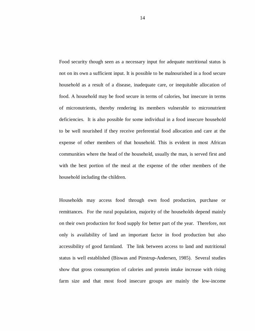
Food security though seen as a necessary input for adequate nutritional status is

not on its own a sufficient input. It is possible to be malnourished in a food secure

household as a result of a disease, inadequate care, or inequitable allocation of

food. A household may be food secure in terms of calories, but insecure in terms

of micronutrients, thereby rendering its members vulnerable to micronutrient

deficiencies. It is also possible for some individual in a food insecure household

to be well nourished if they receive preferential food allocation and care at the

expense of other members of that household. This is evident in most African

communities where the head of the household, usually the man, is served first and

with the best portion of the meal at the expense of the other members of the

household including the children.

Households may access food through own food production, purchase or

remittances. For the rural population, majority of the households depend mainly

on their own production for food supply for better part of the year. Therefore, not

only is availability of land an important factor in food production but also

accessibility of good farmland. The link between access to land and nutritional

status is well established (Biswas and Pinstrup-Andersen, 1985). Several studies

show that gross consumption of calories and protein intake increase with rising

farm size and that most food insecure groups are mainly the low-income

15

smallholder farmers who have limited access to land, finances and farm inputs

(Martorell, 1985; Alderman and Garcia, 1993).

A study on child malnutrition and land ownership in Southern Brazil established

that the prevalence of stunting and underweight was higher among children of

landless families than children of landed families (Victoria et al, 1986). Similar

studies carried out in Sri Lanka and rural Kenya concurred with the above findings

(Wandel, 1989; Haaga et al, 1986). A positive correlation between land ownership

and nutritional status has been demonstrated in India (UNICEF, 1985).

Evidence from Kenya and a number of developing countries indicates that

malnutrition tends to be higher in areas with poor soils. In areas where land is of

high quality and can be irrigated or receives adequate rainfall, a farm of less than

one hectare can provide (directly or indirectly) an adequate diet for a farm family.

On the other hand, where soil quality is low and rainfall erratic even 10 – 50

hectares may be insufficient to guarantee an adequate diet throughout the year.

The key inputs of raising land productivity are fertiliser, irrigation and improved

crop varieties. Problems in agriculture and food production have a direct bearing

on the household’s ability to have sufficient income and consume an adequate

balanced diet. The problems emanate from ecological and constitutional

constraints; rapid population increase, inefficient methods of farming, imbalances

between cash and food crops, uneconomical systems of land ownership, poor

16

transport systems, undeveloped marketing systems, unequal distribution of farm

produce and inadequate male contribution to household labour (UNICEF, 1989).

As aforementioned most food insecure groups are mainly the low-income

smallholder farmers and consequently have the highest incidence of malnutrition

due to their low purchasing power. This is mainly because low income levels limit

the kinds and amounts of food available for consumption and increase the

likelihood of infection through mechanisms such as inadequate shelter and

housing, limited facilities and supplies for personal hygiene, and poor sanitation

(Martorell, 1985). For the poorest members of the society the immediate impact

of rise in income is increased consumption of food, which helps in overcoming

malnutrition particularly where protein and calories are limiting.

In a study carried out in rural Pakistan, Alderman and Garcia (1993) found out that

malnutrition in children tends to be more severe in households with lower average

income per capita, and that it would take a thirty- percent increase in income to

achieve a ten- percent rise in calories intakes. Bouis and Haddad (1990) in a

survey on corn and sugar producing households in Philippines concluded that

raising income appears to be a necessary but not sufficient condition for

substantially improving nutritional status of pre-school children. This is mainly

because increased cash income is not translated into increased food production or

consumption or other health benefits.

17

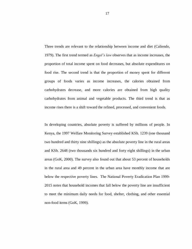
Three trends are relevant to the relationship between income and diet (Caliendo,

1979). The first trend termed as Engel’s law observes that as income increases, the

proportion of total income spent on food decreases, but absolute expenditures on

food rise. The second trend is that the proportion of money spent for different

groups of foods varies as income increases, the calories obtained from

carbohydrates decrease, and more calories are obtained from high quality

carbohydrates from animal and vegetable products. The third trend is that as

income rises there is a shift toward the refined, processed, and convenient foods.

In developing countries, absolute poverty is suffered by millions of people. In

Kenya, the 1997 Welfare Monitoring Survey established KSh. 1239 (one thousand

two hundred and thirty nine shillings) as the absolute poverty line in the rural areas

and KSh. 2648 (two thousands six hundred and forty eight shillings) in the urban

areas (GoK, 2000). The survey also found out that about 53 percent of households

in the rural area and 49 percent in the urban area have monthly income that are

below the respective poverty lines. The National Poverty Eradication Plan 1999-

2015 notes that household incomes that fall below the poverty line are insufficient

to meet the minimum daily needs for food, shelter, clothing, and other essential

non-food items (GoK, 1999).

18

2.3 Alleviation of Malnutrition

The government of Kenya in collaboration with donor agencies and non-

governmental organisation have come up with multisectoral intervention strategies

aimed at alleviating malnutrition. These include: improving household food

security, preventing and controlling specific micronutrient deficiencies, promoting

appropriate diets and promoting breastfeeding.

NDAP is one of the projects in the country making efforts to alleviate malnutrition

and improve the standard of living in general, among the rural community. As

mentioned in Chapter One, the aim of the project was to increase food production

and improve nutritional status of the target population. This was achieved through

provision of irrigation water to the project area. Irrigation has been known to

significantly increase both the yield of the crops as well as the number of crops

that can be grown in a year in areas with good quality soils. Consequently this

encourages commercial farming as a way of generating income in households that

rely exclusively on farming.

Although commercialisation of agriculture is seen as the cornerstone of economic

development in many developing countries it has had a negative effect on the

staple food production as well as food consumption (UNICEF, 1989).

Commercialisation of agriculture and in particular export cropping has often been

19

implicated as a cause of poor nutrition (Boius and Haddad, 1990). Critics contend

that if the resources used to produce agricultural exports were used instead to

produce food for local economy, the problem of malnutrition in many countries

could significantly be reduced, or even eliminated. The conventional hypothesis

states that an increased emphasis on commercial agricultural production leads to a

deterioration of household food consumption and poorer nutritional status of

children.

In Kenya, people concerned with improving nutrition and health have expressed

concern that in areas with increased cash cropping deterioration in household level

food security has occurred. Evaluation studies in Kenya have supported this

concern and indicated that cultivation of cash crops detracts from food cultivation

and this is one of the main causes underlying malnutrition (Hoorweg and

Niemeijer, 1989). More often cash cropping is at the expense of food production

for family use, moreover the amount of money generated from this shift does not

always produce the purchasing and marketing patterns needed to offset the lack of

food produced for family consumption (Harper, 1984). On the contrary, Kennedy

and Cogill (1987) established that commercial agriculture has no effect on

nutritional status.

Concern about possible negative effects of cash cropping on family welfare in

Kenya, was reflected in the national food policy paper of 1981, which

20

recommended that particular attention be given to safeguarding the family diet of

small farmer who switch from food crop to cash crop production (GoK, 1981). A

study carried out in South Nyanza, Kenya found that household energy intake in

the sugar farms was not significantly different from that in non-sugar farm

household and there were no differences in the nutritional status or health of young

children (Kennedy and Cogill, 1987).

However, a study carried out in Taita Taveta district in Kenya concluded that

commercial production of coffee and vegetables is associated with better

nutritional status of children. Therefore it is evident from the above findings that

information on the effects of commercialisation of agriculture is conflicting, with

some researchers suggesting deterioration of nutritional status while others

indicate that cropping pattern is not related to nutritional status. Thus conditions

prevailing in any area must be studied in order to determine what actions need to

be taken to improve nutritional status.

21

Chapter 3

3.0 Methodology

3.1 Study Setting

Nyeri district is one of the six districts in Central province and is situated between

longitudes 360 and 380 east and between the equator, and latitude 00 38’ south. The

district experiences equatorial type of climate with two rainfall seasons. The long

rains occur from March to May and short rains from October to December. Annual

rainfall ranges from 500-2300mm (GoK, 1997).

The study area, Kieni East is one of the seven divisions in the district covering an

area of 727 km2 (22% of the total district area) and is situated in the drier western

leeward side of Mt. Kenya. The area lies between 2130-2400m above sea level

with hill soils that are of moderate to high fertility, but aridity hinders full

exploitation of its existing agriculture potential. Rainfall varies with altitude and

generally ranges between 500-1200mm rising to over 2000mm in the upper areas.

However, the rainfall pattern is erratic and is characterised by heavy showers and

storms that sometimes cause severe erosion and considerable crop damage. The

area has an average daily temperature range of between 160 - 270C.

The study area is a recent settlement with a population of 83,635 according to the

1999 Kenya Population and Housing census (GoK, 2001). There are 21738

households with 30% growing high value cash crops such as pyrethrum and

22

horticultural crops and 40% households with high value food crops such as maize,

beans, and Irish potatoes. The area relies heavily on irrigation water for

horticultural production. Through the assistance of the NDAP 16 irrigation

schemes have been established out of which 5 namely, Kambura-ini, Gitwe,

Kirinyaga-Nyange, Narumoro-aguthi and Waraza/Lusoi have been operational for

at least five years.

3.2 Research Design

A comparative, retrospective cross-sectional design that was also descriptive and

analytical in nature was employed on two sub-samples to compare household food

security and nutritional status of children in households with and without access to

irrigation water.

3.3 Study Population

The study population consisted of two group of households. Households with

irrigation water comprised the study group referred as project area in this study,

while households without irrigation water made up the comparison group referred

to as non-project area.

3.4 Sampling Procedure

A multistage sampling model was employed. NDAP funded the implementation of

most of the water projects in the study area and hence the purposive selection of

23

Kieni East division. Out of the total sixteen water projects that are funded by the

NDAP, only five qualified to be included in the study after satisfying the selection

criteria of being in operation for at least five years. From these five, three projects,

namely Kambura-ini, Waraza-lusoi and Narumoro-aguthi were randomly chosen

through lottery. A list of all households, which also indicated whether or not

households were connected to irrigation water supply, constituted the sampling

frame comprising of 385 project households and 136 non-project households.

From this list a total of 59 non-project households satisfied the selection criteria of

having at least one child aged between 6 – 59 months and being practising

farmers. Subsequently, an equal number of project households (59) was randomly

sampled using predetermined sampling interval, after meeting the selection

criteria. The sampling interval was obtained by dividing the total number of

households in each area by the number of households to be sampled per village.

24

Figure 3. 1 Schematic presentation of sampling procedure

Nyeri District (purposive sampling)

Kieni East Division (purposive sampling)

(3 out of 5 operational water projects randomly sampled)

385 project households 136 non-project households

(Random sampling)

Selection criteria:

At least one child

aged 6 – 59 months

Practising farming

59 project households 59 non-project households

3.5 Training of Research Assistants

Several training sessions were organised for the research assistants involved in the

study. The training that lasted three days addressed the following areas:

Ø Interviewing techniques and how to complete the questionnaires.

Ø Methods used to estimate land size and crop yields.

Ø How to undertake 24 – hour dietary recall.

Ø How to take anthropometric measurement. This consisted of a practical

session at Narumoro Health Centre where the research assistants were able

to take measurements of children who had attended clinic during that day.

25

3.6 Pre-testing of Questionnaires

The questionnaires, which were written in English and translated to Kikuyu

language, were pre tested to ensure understanding and clarity. The investigator and

four research assistants carried out the exercise, the latter had undergone a three

days training on how to complete the questionnaires and how to take

anthropometric measurements. Pre- testing involved 20 purposively selected

households from Kirinyaga-Nyange water project, an area with similar

geographical characteristics to those of the study area. Based on observations in

the field, revisions were made accordingly.

3.7 Data Collection

A structured close-ended questionnaire was designed to collect the following

information:

• Households’ socio-demographic/economic characteristic

• Food production

• Income and expenditure patterns

• 24-hour dietary intake

• Anthropometric measurements

26

3.7.1 Food Production

Data collected was based on production figures of the period between January to

December 2000. Respondents were asked to recall the crops that they had grown

during the reference year, area under crop, yields, and amount of yield sold and

that consumed at home. To confirm the yields of cereals and pulses, research

assistant requested the respondents to measure (using provided containers) crop

produce equivalent to amount that was harvested. The measurements were then

converted into kilograms using respective conversions (Appendix 1).

To confirm the area under each crop during the reference year, respondents were

requested show in the farm the portion that had been planted with each of the

crops. Research assistants then confirmed the acreage by actual walking along and

across each portion of land while counting the number of footsteps made. Each

footstep was estimated at one foot (30cm). The actual area in acres was then

calculated using the standard conversion ratio of 1 acre is approximately 43,560

square feet.

3.7.2 Household Income and Expenditure Patterns

This encompassed spending and acquisition history of common foods and non-

food items by households. Respondents were asked to recall food and non-food

27

expenditure in terms of quantity and monetary value per week or month. This was

then used to estimate annual expenditure of each item for each household.

3.7.3 Dietary Intake

Energy and nutrient intake was determined using the 24-hour recall method. In

this method, the mother of the index child or the person who prepared the food

was asked to describe all the dishes that were prepared for the child during the

previous day or the past 24 hours, as well as the ingredients that were used for

each dish. The person was then asked to use the same utensils as in the previous

day and measure water equivalent to the amount of ingredients used. The water

was then measured using a calibrated jug and readings recorded in millilitres

(mls). Similarly, the amounts served to the index child as well as any leftovers

were recorded. The amount of leftovers was deducted from the original serving

and the child’s portion recorded in mls. The measurements were then converted

into grams using respective conversion factors in Appendix 2 (King and Burgess,

1993). The nutritive value of all the ingredients used in the preparation of the

different dishes and for all the foods consumed by the index child was determined

using the national food composition tables developed for Kenya (Sehmi, 1993).

The nutrients of interest were energy, protein, iron and vitamin A. The index

children’s intakes were then compared to the recommended dietary intake (RDI)

for children of the same age group in order to determine the level of intake in

relation to the RDI (Appendix 3).

28

To determine the total energy available to the household per day, the calories in all

the food prepared for the family were standardised by converting into equivalent

consumer unit (CU) where one CU is equivalent to an energy standard reference

by WHO of 2960 kilocalories per adult equivalent. The energy requirements of

individuals in each household were expressed as a ratio of the reference and the

total requirements for each household calculated in terms of CUs. The total CUs

available to the household were then expressed as a ratio of the total required CUs

to obtain the household dietary energy adequacy ratio (HDEAR).

3.7.4 Anthropometric Measurements

3.7.4.1 Weight

Weight was measured according to WHO recommendation to the nearest 0.1kg

using SALTER scales with plastic pant, adjusted to zero before every reading

(WHO, 1983). The index children wore light clothing. A correction for clothing

was made during data analysis by subtracting 150 grams from all children’s

weight. This weight was arrived at after averaging the weights of light clothes

worn by children of different age groups during the survey.

3.7.4.2 Length/Height

Recumbent height of children below two years of age or standing height of those

aged two years and above was taken using a standardised length board, which had

29

a fixed head rest and a movable foot piece and placed on a flat surface according

to WHO recommendations (WHO, 1983; UN, 1986). The index child wore no

shoes. Care was taken to maintain the child’s head in an upright position, with

legs stretched to a full extent and feet at right angles with legs. The height

measurement was recorded to the nearest 0.1cm.

3.7.4.3 Mid-upper Arm Circumference (MUAC)

MUAC was taken using a non-stretchable measuring tape and measurement

recorded to the nearest 0.1cm. The circumference of the upper-arm was measured

midway between the point of the shoulder and the point of the elbow of the left

arm (UN, 1986). The tape was put around the arm so that it fit closely but not so

tight that it made folds in the skin.

3.8 Data Management

Weight-for-age, weight-for-height and height-for-age and their corresponding

standard deviations (SD) scores, generally referred to as Z score, were calculated

using Epi-info computer programme, and compared with those of the NCHS

population. A Z score of 2 or –2 meant that the child is 2SD above or 2SD below

the median of the respective Z score. WHZ refers to the Z score for weight-for-

height, HAZ refers to Z score for height-for-age and WAZ refers to Z score for

weight-for-age. Index children were thereafter classified based on Z-scores as

30

normal (WHZ > = - 2.0 and HAZ >= -2.0), wasted (WHZ < -2.0 ), stunted (WHZ

> = - 2.0), or wasted and stunted (WHZ < - 2.0 and HAZ < - 2.0) (WHO, 1995).

MUAC was analysed based on the following cut-offs: children with measurement

below 12.5cm were classified as severely undernourished; 12.5 – 13.5cm as

moderately nourished and those above 13.5cm as well nourished (King and

Burgess, 1993).

3.9 Data Quality Control

At the end of every day, questionnaires were screened to check for recording

errors and completeness. The weighing scales were checked for accuracy,

reliability and precision at the beginning of the survey, midway through the survey

and before the last week of data collection. This was done by weighing standard

weights to ensure that the scales reading coincided with the respective weights.

3.10 Data Entry and Analysis

Data entry was done through use of ISSA-X computer package and then exported

to STATA for Windows version 6.0 where cleaning for any possible

inconsistencies was done. On STATA, standard tabulations were formulated and

the data was analysed. Calculation of anthropometric indices was done using EPI

6 computer package. Exclusion criteria for impossible values as provided by the

package were used. No measurements were considered invalid among the three

31

nutritional indices. The statistical paired t-tests and chi-square were used to test the

differences between project and non-project households at 0.05 level of

significance.

32

Chapter 4 4.0 Benefits of Irrigation on Agricultural Production, Income and Food

Security

4.1 Introduction

Agriculture is the backbone of Kenya’s economy. About 80 percent of the

population rely on it for their livelihood. This proportion of the population

depends mainly on their own production for household food supply and therefore

any problem affecting food production has a direct bearing on the households

accessibility to an adequate balanced diet. Consequently, the nutritional status of

the rural population can sometimes be linked to the availability and accessibility to

good farmland (UNICEF, 1989).

In Kenya, over dependence on rainfed agriculture is a major problem in food

production, but it can be overcome through provision of irrigation water. The

study area, Kieni East Division of Nyeri District, is situated in the drier western

leeward side of Mt.Kenya and is characterised by erratic rainfall pattern. Although

the soils are of moderate to high fertility, the full exploitation of the existing

agriculture potential in the division is hindered by aridity. NDAP has since 1991

been assisting the community in this division in development of smallholder

irrigation schemes and supporting agricultural extension.

33

Access to food which is not only adequate in quantity but also in quality, may

result to good nutritional status. Households may acquire food through their own

production, purchases or remittances from friends or relatives. For an agrarian

population, problems that affect agriculture and food production have a direct

bearing on the household’s ability to have sufficient income and access to an

adequate diet. A household is said to be food insecure when one or more of its

potential sources of food are strained or threatened. The purpose of this study was

to investigate the effects of provision of irrigation water on household food

production and food security in Kieni East Division.

4.2 Results

4.2.1 Social-demographic Characteristics of Survey Households

Findings on socio-demographic characteristics of the survey households showed

that the two sets of households were similar in terms of household size, marital

status of respondent, maternal and paternal education and occupation (Tables 4.1

and 4.2). Majority of the heads of households (95% in the project area and 88% in

non-project area) were male (Table 4.1). There was no significant difference in

the average household size, although households in the project area had slightly

smaller households (5.0) compared to 5.2 in non-project households. Most of the

respondents in the whole sample (90% in the project area and 86% in non-project

area) were married.

34

Table 4.1 Socio-demographic Characteristics of Study Households Characteristic

Project HH n %

Non-project HH

n %

Statistical analysis p-value Test

Respondent’s sex Male

Female

3 5

56 95

4 7

55 93

0.7 x2

Sex of Household Head Male

Female

56 95

3 5

52 88

7 12

0.2 x2

Mean household size 5.0 (1.7) 5.2 (2.1) 0.6 t-test

Marital Status of Respondent Married

Single

Divorced/separated

Widowed

53 90

3 5

1 2

2 3

51 86

2 3

3 5

3 5

0.7 x2

Notes:

The number in parentheses are standard deviations.

X2 is chi square test

HH refers to household

NS indicates that p-value is not significant

Data on education showed that in non-project households, the number of mothers

of index child who had only completed 1 – 4 years of primary education (16%),

was twice that of mothers in the project households, which was 8%, but the

difference was not significant (Table 4.2). Close to a half (49%) of mothers from

project households had completed between 5 – 8 years of primary education

compared to slightly over half (55%) in non-project households.

35

Table 4.2 Percent Distribution of Mothers and Fathers by the Highest Level of Education Attained and Occupation Characteristic

Project HH n percent

Non-project HH n percent

Statistical analysis p-value Test

Mother’s Education Percent ever attended school

Completed 1-4 of primary

Completed 5 – 8 of primary

Completed secondary school

Not completed secondary school

Post secondary

59 100

5 8

29 49

14 24

9 15

2 3

58 98

9 16

32 55

11 19

6 10

0 0

0.3 x2

0.4

Mother’s Occupation Farming

Salaried employment

Casual labour

Jua-kali/business

Other

55 93

2 3

0 0

2 3

0 0

51 86

3 5

3 5

2 3

0 0

0.3 x2

Father’s Education Ever attended school

Completed 1 – 4 of primary

Completed 5 – 8 of primary

Completed secondary

Not completed secondary

Post secondary

51 96

1 2

15 29

22 43

10 20

3 6

49 96

4 8

22 45

20 41

3 6

0 0

1.0 x2

0.04

Father’s Occupation Farming

Salaried employment

Casual labour

Jua-kali/business

Other

17 32

13 25

3 6

19 36

1 2

16 31

14 27

8 16

11 22

2 4

0.3 x2

Notes:

X2 refers to chi square test

HH refers to household

NS indicates that the p-value is not significant

In the project households, the proportion of fathers of index child (69%) who had

attained post-primary education was significantly higher than in non-project

36

households where the number was 31 percent (p = 0.04). Further analysis

showed that husbands from the project households were 2.5 times more likely to

have attained post-primary education than husbands from non-project households.

4.2.2 Land Ownership

On land availability, majority of the project households (85%) compared to

slightly over three-quarter (78%) of non-project households owned less than 3

acres, but the difference was not significant (Table 4.3). There was no significant

difference in land size between the two sets of households, although the average

acreage for non-project households was slightly higher than that of project

households. The average land size of the project households was 2.1 acres

(median = 1.75 acres) versus 2.3 acres (median = 1.5 acres) in non-project

households.

Information on fertiliser use show that a significantly higher percentage of project

households used both fertiliser and manure than did non-project households (p =

0.0002). Project households were 4.4 times significantly more likely to use both

fertiliser and manure than non-project households. On the other hand, slightly

over two fifths (42%) of non-project households compared to about a quarter

(24%) of the project households used manure alone. In the two groups of

households fertiliser was mainly used on horticultural crops whereas manure and

occasionally fertilisers were used on maize, beans and Irish potatoes.

37

There was highly significant difference in the number of households practising

commercial farming (p = 0.0002). About two thirds (66%) of project households

compared to close to a third (31%) of non-project households engaged in

commercial farming. Project households were 4.4 times more likely to engage in

commercial farming than non-commercial farming (odds ratio lies between 2.1

and 9.6 and p-value = 0.0001).

Table 4.3 Percent Distribution of Households by Land Size, Fertiliser Use and Type of Farming

Variable

Households Project Non-project N=59 N=59

Statistical analysis p-value Test

Land Size Less than 3 acres

More than 3 acres

Mean Acreage Median

85 78

15 22

2.1 (1.8) 2.3 (2.1)

1.75 1.5

0.3 chi-square

0.7 t-test

Fertiliser Use Fertiliser only

Manure

Fertiliser and manure

None

7 17

24 42

68 32

1 8

0.0002 chi-square

Type of farming Commercial

Non-commercial

66 31

34 69

0.0002 chi-square

Notes:

The numbers in parentheses are the standard deviations

38

4.2.3 Crop Production

Crop production in the study area had greatly been affected by drought that the

area had experienced since 1998. There had been shortage of irrigation water as a

result of declining water levels in the rivers, which resulted in water rationing. It

was reported that the last time the area had a substantial harvest was in 1997.

Therefore, crop production figures of the reference year, 2000, were lower than

expected.

Table 4.4 Distribution of Households by Crops Grown Household growing crop (% of total HH)

Project Households N = 59

Non-project Households N = 59

Maize

Beans

Potatoes

Cabbage

Carrot

Onions

Tomatoes

Snowpea

Other

97

93

81

29

7

7

5

34

0

95

88

86

5

0

2

2

2

8

Majority of project and non-project households mainly grew maize, beans and

potatoes (Table 4.4). Cabbages were grown by slightly over a quarter (29%) of

project households while slightly over a third (34%) grew snowpea1. A few

1 Snowpea is a type of vegetable whose pods are eaten green before seeds are formed. It is mainly grown for export.

39

project households grew other horticultural crops such as carrots, onions and

tomatoes.

Table 4.5 presents the area devoted to various crops. The mean acreage of any of

the crops was small, ranging from 0.2 to 1.1 acres. Greater emphasis on

subsistence crops was apparent in both study households. There were no

significant differences in areas devoted either to maize or beans or potatoes

although non-project households allocated slightly larger area per crop.

Table 4.5 Mean Acreage Devoted to Crops by Households.

Notes: The numbers in parentheses are standard deviations *Only one observation NA means not applicable CI = confidence interval

Crops

Area devoted to crops (acres) Statistical analysis p-value CI

Project Households

Non-project Households

Maize

Beans

Potatoes

Cabbages

Carrots

Onions

Tomatoes

Snowpea

1.0 (0.7)

0.6 (0.6)

0.4 (0.5)

0.6 (1.4)

0.2

0.2

0.2

0.3

1.1 (0.9

0.8 (0.9)

0.5 (0.4)

0.5 (0.5)

0

0.1*

0.1*

0.1*

0.3 0.9 – 1.2

0.2 0.5 – 0.8

0.8 0.4 – 0.5

0.9 -0.03 – 1.2

NA

NA

NA

NA

40

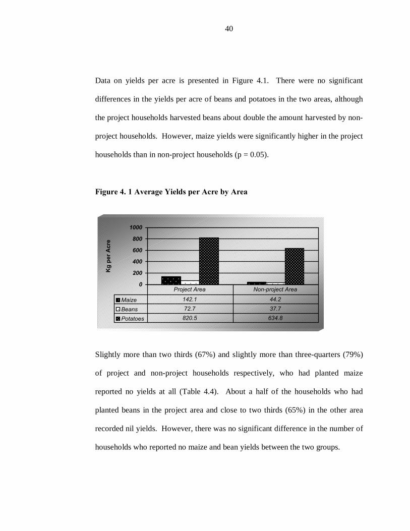
Data on yields per acre is presented in Figure 4.1. There were no significant

differences in the yields per acre of beans and potatoes in the two areas, although

the project households harvested beans about double the amount harvested by non-

project households. However, maize yields were significantly higher in the project

households than in non-project households (p = 0.05).

Figure 4. 1 Average Yields per Acre by Area

Slightly more than two thirds (67%) and slightly more than three-quarters (79%)

of project and non-project households respectively, who had planted maize

reported no yields at all (Table 4.4). About a half of the households who had

planted beans in the project area and close to two thirds (65%) in the other area

recorded nil yields. However, there was no significant difference in the number of

households who reported no maize and bean yields between the two groups.

0

200

400

600

800

1000

Kg

per A

cre

Maize 142.1 44.2

Beans 72.7 37.7

Potatoes 820.5 634.8

Project Area Non-project Area

41

As expected, significantly more project than non-project households reported that

they harvested potatoes during the year of reference (p = 0.03). It was also noted

that the project households were 2.4 times more likely to realise potato yields than

non-project households were (odds ratio lies between 1.08 – 5.99 and p-

value=0.03).

Table 4.6 Distribution of Households by Crop, Number That Planted and Realised Yields

Crops No of HH that Planted

P NP

n n

Yields No Yields

P NP P NP p-value

n n n n

Maize 57 (97) 56 (95) 19 (33) 12 (21) 38 (67) 44 (79) 0.2

Beans 55 (93) 52 (88) 22 (40) 18 (35) 33 (60) 34 (65) 0.6

Potatoes 48 (81) 51 (86) 32 (67) 23 (45) 16 (33) 28 (55) 0.03*

Notes:

The numbers in parentheses are percentages

Chi-square test is used to test that odds ratio = 1

*Odds ratio =2.43 and 95% confidence interval (1.08, 5.99)

NP refers to non-project

P refers to project

n = number of households

HH refers to household

Non-project households sold slightly more than a quarter (27%) of the maize

produced as compared to only 8 percent sold by the project households. In both

sets of households only a small percentage of beans was sold, about 14 percent and

42

5 percent per acre in project and non-project households respectively. About a

quarter of potatoes harvested were sold by the project households area versus close

to a half (45%) in non-project area. However, there were no significant

differences in amount of the three crops sold between the two types of households

(Table 4.7).

The study established that most of the produce of maize, beans and potatoes was

left for home consumption by the two types of households. There was no

significant difference in produce left for own consumption, although non-project

households left slightly more than project households. There was no significant

difference in the number of households in which maize, beans and potatoes lasted

until the next harvest season. About two fifths of the project households compared

to slightly over a quarter of non-project households reported that their maize lasted

to the next harvest season.

4.2.4 Livestock Production

Data on livestock production is presented in Table 4.8. There were no significant

differences in the number of households keeping any of the three types of

livestock between the two areas. The average milk and egg production per annum

in the non-project households was higher than in the project households but there

was no significant difference.

43

Table 4.7 Mean Yield per Acre, Amount Sold and Percent Kept for Own

Consumption and Percent of Food Self-Sufficient Households

Description

Project HH

Non-project HH

Statistical Analysis p-value CI

Yields (kilogram per acre) Maize

Bean

Potatoes

142.1 (348.1)

72.7 (163.3)

820.5 (1320.7)

44.2 (136.1)

37.7 (82.1)

634.8 (1482.9)

0.05 43.5 – 143.6

0.2 30.6 – 80.8

0.5 445.1 – 1004.6

Amount sold (kilogram per acre) Maize

Bean

Potatoes

11.8 (45.0)

10.5 (36.3)

207.9 (607.5)

12.1 (90.2)

1.8 (8.0)

286.6 (1261.0)

1.0 - 1.3 – 25.1

0.09 1.1 – 11.4

0.7 50.0 – 446.9

HH whose produce last to next harvest (% of total HHs growing the crop) Maize

Beans

Potatoes

40 (49.4)

38 (48.9)

36 (48.6)

29 (45.8)

35 (48.0)

34 (47.9)

0.2 25.5 – 43.6

0.7 26.8 – 45.5

0.8 25.4 – 44.7

Produce kept for home consumption (% of total production) Maize

Beans

Potatoes

88.7 (20.2)

89.0 (20.9)

81.8 (33.3)

93.8 (21.7)

94.4 (14.1)

81.8 (31.7)

0.5 83.1 – 98.2

0.4 85.6 – 97.2

1.0 73.1 – 90.5

Notes:

The numbers in parentheses are standard deviations

Statistical t-tests are used to compare differences between the means in the two areas

CI refers to confidence interval.

HH refers to household.

44

Table 4.8 Annual Livestock Production by Area, 2000 Description Project area Non-project

area Statistical analysis p-value CI

Cattle HH keeping cattle (% of total HHs

keeping livestock)

Mean number of animals

Mean milk production (kilogram

per animal)

Milk sold (% of total production)

Milk kept for consumption (% of

total production)

66

2.8 (1.9)

1235.3 (842.3)

30 (33.1)

69 (33.7)

63

2.5 (1.7)

1671 (971.2)

38 (30.8)

61 (30.9)

0.7 56.0 – 73.0

0.4 2.2 – 3.1

0.07 1193.6 – 1669.4

0.3 25.0 – 41.6

0.3 56.8 – 73.6

Chicken HHs keeping chicken

Mean number of birds

Mean egg production (egg per

bird)

Eggs sold

Eggs kept for consumption

71

10.0 (10.4)

125.8 (86.9)

22.2 (30.4)

77.8 (30.4)

59

8.0 (7.1)

131.7 105.3)

23.4 (32.7)

74.9 (32.7)

0.2 57.0 – 74.0

0.3 7.0 – 11.1

0.8 104.8 – 152.5

0.8 14.9 – 30.7

0.7 68.5 – 84.3

Sheep HHs keeping sheep

Mean number of animals

41 (49.5)

3.9 (3.0)

32 (47.1)

6.3 (6.8)

0.3 27.6 – 45.3

0.1 3.4 – 6.6

Notes: The number in parentheses are standard deviations.

Statistical t-tests are used to compare the differences in livestock production between the two areas.

CI = confidence interval

HH refers to household

45

4.2.5 Income

4.2.5.1 Sources of Income

Apart from farming, the other sources of income in the study area are salaried

employment, casual work and business. Close to a quarter (24%) of the two types

of households reported salaried employment as a source of income (Table 4.9).

Significantly more non-project households engaged in casual work (p = 0.02).

There was no significant difference in the number of households that reported

business as a source of income, although more project households (37%) than non-

project households (31%) operated small business/juakali.

Table 4.9 Distribution of Households by Source of Income Source of Income

Households Statistical Analysis

Project n %

Non-project n %

p-value CI

Salaried Employment 14 24 14 24 1.0 15.9 – 31.5

Casual Labour 13 22 25 42 0.02 23.6 – 40.8

Business/ Jua-kali 22 37 18 31 0.4 25.2 – 42.6

Notes

Chi Square was used to test the difference

CI – Confidence Interval

4.2.5.2 Income Levels

Table 4.10 shows percent distribution of households by income group and type of

farming. Slightly less than a fifth (19%) of project households and close to a

quarter (24%) of non-project households were below the rural poverty line (below

46

Ksh.1240), although the difference was not significant. However, when the

households were classified according to the type of farming, the percentage of

households below poverty line was significantly higher in non-commercial

farming households (31%) than in commercial farming households, where this was

11 percent (p = 0.01).

Table 4.10 Percent Distribution of Households by Income Group and Type of Farming

Households/Type of Farming

Income Level

Below Poverty Line Above Poverty Line

Households Project

Non-project

p-value = 0.5

19 81

24 75

Type of Farming Commercial

Non-commercial

P = 0.01

11 89

30 67

Notes:

Chi square test was used to compare the differences between groups.

4.2.5.3 Income Expenditure

Table 4.11 presents the mean annual food and non-food expenditure by type of

households. There was no significant difference either in the mean expenditure or

the percent expenditure. The two types of households spent slightly over half of

47

the total budget on food (52% by non-project households and 51% by project

households).

Table 4.11 Mean Annual Expenditure by Households

Area/statistical

analysis

Food Non-food

Expenditure Percent Expenditure Percent

Households

Project

Non-project

40632.6 51

40214.7 52

54281.6 49

44157.5 48

p-value 0.9 0.9 0.6 0.9

Confidence interval 34399.7 – 46424.1 47.8 – 55.4 30960.1 – 67117.5 44.6 – 52.2

Notes:

Statistical t-tests were used to compare the differences between the two areas.

Data on Table 4.12 shows that non-project households spent a larger percentage

(11.6%) of the total budget on cereals and grains than the project households,

which spent 7.8%. This was also the case with pulses and tubers where non-

project households allocated more money than project households. On the other

hand, project households spent significantly more money on milk (13.0%) than

non-project households, which spent 8.1% (p-value = 0.02).

48

The mean annual non-food expenditure is shown in Table 4.13. Project

households allocated a relatively higher proportion of the total budget (17.5% and

about KSh. 16652)) to farming than non-project households, where the proportion

was 11% and about KSh. 9239, although there was no significant difference

between the two areas.

Table 4.12 Mean Annual Food Expenditure by Selected Food Groups

Food Group

Project HH Expenditure

Ksh percent

Non-project HH Expenditure

Ksh percent

Statistical analysis p-value CI

Cereals and Grains 7441.9 7.8 9826.5 11.6 0.5 5464.4 – 11889.1

Roots and Tubers 5195.8 5.5 5219.2 6.4 1.0 3461.0 – 6954.5

Pulses 4755.6 5.0 5541.7 6.5 0.6 3573.7 – 6819.4

Vegetables 3033.5 3.2 2969.4 3.7 0.9 2288.7 – 3721.6

Fruits 2202.2 2.3 3410.4 3.9 0.4 1406.7 – 4302.8

Meat 3814.1 4.0 3194 3.6 0.5 2465.9 – 45.2.6

Milk 12181.3 12.8 6826 8.1 0.02 7042.5 – 11672.7

Fats and oils 2420.2 2.6 2515.7 3.0 0.8 2006.8 – 2932.5

Sugar 4285.1 4.5 3893.4 4.4 0.7 3004.1 – 5140.3

Notes:

Statistical t-tests are used to compare the differences in food expenditure between the two areas.

CI refers to confidence interval

Expenditure is inclusive of food items produced by households.

There were no significant differences in amount of money spent on anyone non-

food category between the two sets of households. As expected, project

households spent more money (1.8 times) on farming than non-project households.

49

Table 4.13 Mean Annual Non-food Expenditure by Area

Non-food item

Project area Expenditure

(KSh) percent

Non-project area Expenditure

(KSh) percent

Statistical analysis p-value CI

Education 11747.0 12.4 7182.3 8.5 0.3 5495.8 – 13519.6

Farming 16651.9 17.5 9238.9 11.0 0.3 5352.7 – 20403.3

Fuel 4461.3 4.7 6849.4 8.1 0.1 4095.9 – 7300

Clothes 5937.5 6.3 6604.2 7.6 0.7 4150.0 – 8391.5

Household goods 4134.6 4.4 4648.8 5.5 0.7 2784.9 – 6026.6

Health 3826.7 4.0 2346.3 2.7 0.4 1171.9 – 5001.0

Transport 4728.7 5.0 8122.3 9.3 0.3 3263.7 – 9795.1

Family events 5815.0 6.1 2860.9 3.3 0.4 994.1 – 7415.6

Notes:

Statistical t-tests are used to compare differences in non-food expenditure between the two areas.

Households goods include items such as soap, petroleum jelly, lotion and toothpaste

Family events include all get together parties or welfare groups where household make contributions in cash

4.2.6 Food Security

In order to determine energy adequacy of diets consumed by study households,

energy intake and requirements were calculated in terms of calories per adult

equivalent. This method is most appropriate because it takes into consideration

specific caloric requirements for each age and sex. In the two groups of

households, the mean energy adequacy was well above 100 percent. However

about a quarter of project households compared to close to a third (33%) of non-

project households were below 80 percent of caloric requirement, although the

difference was not significant (Table 4.14).

50

A slightly higher percentage of non-project households (28%) spent more than 60

percent of income on food compared to close to a quarter (22%) of project

households.

When households were categorised by type of farming, the study found out that

non-commercial farming households were 2.6 times more likely to spend a larger

proportion of income on food than commercial farming households, but the

difference was not significant. This indicates that commercial farming households

are more likely to be food secure than non-commercial farming households.

Table 4.14 Distribution of Households by Measure of Food Security and Type of Farming

Household/Type of farming

Measure of Food Security

Income spent on food Energy adequacy

> 60% < 60% < 80% > 80%

Household Project

Non-project

p-value

confidence interval

22 77 25 75

28 72 31 69

0.6 0.6

13.3 – 36.7 63.3 – 86.7 18.5 – 36.5 63.4 – 81.5

Type of farming Commercial

Non-commercial

p-value

confidence interval

17 83 25 75

34 66 30 70

0.1 0.6

13.3 – 36.7 63.3 – 86.7 18.5 – 36.5 63.4 – 81.5

Notes:

Statistical t-tests are used to compare the difference in food security between the two areas and also between types of

farming

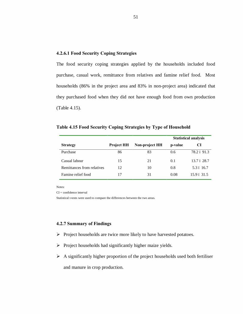
51

4.2.6.1 Food Security Coping Strategies

The food security coping strategies applied by the households included food

purchase, casual work, remittance from relatives and famine relief food. Most

households (86% in the project area and 83% in non-project area) indicated that

they purchased food when they did not have enough food from own production

(Table 4.15).

Table 4.15 Food Security Coping Strategies by Type of Household

Strategy

Project HH

Non-project HH

Statistical analysis p-value CI

Purchase 86 83 0.6 78.2 – 91.3

Casual labour 15 21 0.1 13.7 – 28.7

Remittances from relatives 12 10 0.8 5.3 – 16.7

Famine relief food 17 31 0.08 15.9 – 31.5

Notes:

CI = confidence interval

Statistical t-tests were used to compare the differences between the two areas.

4.2.7 Summary of Findings

Ø Project households are twice more likely to have harvested potatoes.

Ø Project households had significantly higher maize yields.

Ø A significantly higher proportion of the project households used both fertiliser

and manure in crop production.

52

Ø On the other hand a significantly higher percentage of non-project households

used only manure.

Ø Non-project households are more likely to engage in casual work as a means of

earning a livelihood.

Ø A significantly higher proportion of non-commercial households had income

below KSh. 1240, which is the poverty line for rural areas in the country.

Ø In either project or non-project households, about half of the total budget was

spent on food.

Ø Project households spent significantly more money on milk.

Ø A higher percentage of the project households and commercial farming

households were food secure than were non-project households and non-

commercial farming households respectively.

Ø Irrigation and commercial farming had significant influence on household food

security.

4.3 Discussion of Results

The average household size of both the project households (5.0) and non-project

households (5.2) is higher than the national average of 4.5 and that of Central

Province (3.9) reported in the 1999 Kenya population and housing survey.

Considering that the study area is arid or marginal area, the average land size of

2.1 acres in the project area and 2.3 in non-project area may be insufficient in

providing adequate food and income for an average household size of five

53

members. This is evident from the fact that only 40 percent of the project

households and 29 percent of non-project households are self sufficient in maize,

which is the staple food in the area. This seems to support the findings by Lynman

(1979), that farmers in marginal areas and with land size less than five acres have

difficulties in providing adequate food for home consumption. In a study in

Nakuru district, Kigutha (1994) established that land size less than three acres was

inadequate to meet the food needs of an average household. In 1973 the World

Bank had estimated that in Central Province (Kenya), an average family size of 6

members that relies exclusively on farm production requires about 7.9 acres of

high quality land to provide adequate food and income (World Bank, 1973).

Irrigation is a major input in increasing crop yields alongside use of fertiliser,

pesticide and improved seed varieties (Biswas and Per Pinstrup-Andersen, 1985;

Smith, 1986). This could be the reason why project households compared with

non-project households are four times more likely to use both fertiliser and

manure. Also, a household is more likely to recover money used to purchase

fertiliser, when relying on irrigated agriculture than on rainfed agriculture since

one is more certain of a harvest. On the other hand, non-project households would

rather use manure, which is cheaply available to them, than spend more in order to

purchase fertiliser for yields that may never be realised, given that in this area

rainfall is unreliable.

54

Irrigation encourages households to shift from subsistence to commercial farming.

Households are able to grow high value crops, mainly horticultural crops which

have high gross margins thereby generating income. As mentioned in Chapter

three, the study area has soils of moderate to high fertility, which if irrigated can

allow double or triple cropping hence utilising the available land optimally. The

most commonly grown horticultural crops are cabbages and snowpea. This is due

to the fact that the two crops have ready market and good returns, especially if

planting is timed such that harvesting coincides with a period when demand is

high. However, project households are unable to take full advantage of the ready

market because of the limiting land sizes and unreliability of irrigation water. The

average acreage devoted to anyone horticultural crop was small ranging between

0.2 to 0.6 acres. It was noted that due to unpredictability of rainfall, non-project

households do not grow crops that are very sensitive to water stress, such as

horticultural crops and hence have relatively few crops that compete for the small

land size unlike the project households.

The impact of irrigation on food production in the study area may be understated,

given that the reference year was a drought period. This affected irrigation water

availability, resulting in water rationing and consequently unreliability of water,

particularly to project households located far from the water catchment area.

However, inspite of unreliable irrigation water, project households were twice as

likely to realise potato yields than non-project households were, emphasising the

55

importance of irrigation water. Also, the fact that yields per acre of maize in the

project area were significantly higher than in non-project area indicates the

importance of irrigation and fertiliser in crop production.

In livestock production, the study established that irrigation has no significant

influence on the mean milk and egg production. This could be attributed to the

great emphasis on horticulture by project households and thereby allocating more

land to crop production and leaving little land that cannot sustain livestock. Since

horticulture is both time and labour intensive, it is likely that livestock get less

attention due to the fact that horticultural crops have better returns. Moreover it

appears that the study households keep livestock mainly for subsistence purpose,

given that most of the eggs and milk produced is consumed at home. The lower

milk production in the project households could have resulted to a deficit in supply

of milk for family consumption forcing the households to spend more money than

non-project households to offset the shortage.

The main sources of income in the study area include farming, casual labour,

salaried employment and business or jua-kali. This study established that

significantly more non-project households than the project households reported

casual work as a source of income. Non-project households unlike the project

household do not grow any short period maturing crop and consequently have low

labour demand, hence offer casual labour mostly to project households, in order to

56

generate the badly needed fast cash. Snowpea, which is grown by about a third of

the project households requires intensive labour throughout the growing and

harvesting period, ensuring availability of regular casual work.

Commercial farming does not only increase household income but is also seen as

the cornerstone of economic development in many developing countries (Kennedy

and Cogill, 1987; UNICEF, 1989). This is supported by the findings of this study,

which show that a significant number of commercial farming households had

average monthly income above Ksh 1240, which is the rural poverty line

according to the 1997 KWMS (GoK, 2000). Households that have income below

the poverty line are unable to access the minimum requirement of food and

essential non-food commodities. A study carried out in South-western Kenya

found that commercial households had significantly higher incomes than non-

commercial farming (Kennedy and Cogill, 1987).

The mean annual non-food expenditure by the project households is higher than

that of non-project households. Similar findings were observed by Mwadime

(1992) and Kennedy and Cogill (1987). Provision of irrigation water encourages

growing of horticultural crops, which require more capital than growing of

subsistence crops, and it is also labour intensive. Consequently, project

households allocate more money on farming than non-project households.

57

Furthermore, with reliable irrigation water, households are certain of high yields

and they can risk investing substantially in farming.

A household is said to be food secure if it meets 80% or more of its total dietary

energy requirement. For an agrarian population, problems that affect agriculture

have a direct bearing on the household’s ability to have sufficient income and

consume adequate diet (UNICEF, 1989). The study area is a marginal area and

had experienced drought prior to survey period, which resulted to irrigation water

rationing and in most households consequent crop failure. This affected not only

crop production, but also household income; hence the findings of this study could

have underestimated the impact of irrigation. Rationing of irrigation water not

withstanding, three quarters of project households were food secure emphasizing

contribution of irrigation in sustaining household food availability. There was

marginal difference in the number of households spending more than 60 percent of

income on food between commercial and non-commercial farming households.

This could be explained by the fact that significant number of commercial farming

households had higher income than non-commercial farming households, thereby

allocating smaller proportion of income on food. This follows Engel’s law, which

states that “as income increases, the proportion of total income on food decreases”

(Caliendo, 1979). However, since there was no significant difference in household

food security between commercial farming households and non-commercial

farming households the second hypothesis of this study is accepted. That is there

58

is no significant difference in food security between project and non- project

households.

59

Chapter 5 5.0 Role of Irrigation on Improvement of Nutritional Status of Young

Children

5.1 Introduction

Irrigation is a major input in increasing crop yields especially in areas with good

quality soils, which subsequently leads to either, increased household income

and/or improved household food availability. In households where the resultant

increase in yields or income is used to meet the dietary needs, improved nutritional

status results. The previous chapter established that irrigation in the study area has

resulted to improved crop production and higher income. Chapter 5 investigates

the role of irrigation on improvement of nutritional status of young children.

Prevalence of malnutrition in 6 – 59 months age group is usually used as an

indicator for nutritional status of the entire population, because this sub-group is

more sensitive to nutritional stress. Nutritional status is determined using height-

for-age, weight-for-age and weight-for-height indices. In developing countries,

stunting affects about a third of the children below five years of age. In Africa, the

prevalence of underweight and wasting has been reported to be 29.1% and 9.6%

respectively. The highest levels of stunting are observed in Eastern Africa; where

on average 48.1 percent of pre-school children are affected (ACC/SCN, 2000). In

Kenya, the prevalence of stunting has been reported to be 33%, wasting 6% and

underweight 22% (NCPD, CBS and MI, 1999). Central Province where the study

60

area is located has lower prevalence (28% stunted; 6% wasted and 14%

underweight) than the national figure. The Nyeri district development plan

reported that the prevalence of malnutrition in the study area could be worse due to

the fact that it is arid and characterised by erratic rainfall pattern (GoK, 1997).

However no data was available on the prevalence of malnutrition in the semi-arid

and arid areas in the district.

5.2 Results

5.2.1 Dietary Intake

The mean daily energy and protein intake of the index children is presented in

Table 5.1. There were no significant differences in energy and protein intake

either between the two areas or between commercial and non-commercial

households. On average, all children had higher energy and protein intakes except

for children (12 – 23 months) from non-project households whose energy intake

was below the recommended daily intake. The mean energy and protein intake of

children (24 – 35 and 35 – 59 months age group) from non-project households was

higher than that of children from project households.

61

Table 5. 1 Mean Energy and Protein Intake by Age Group

Notes:

* n was 3 in either of the study area.

The numbers in parentheses are standard deviations

CI refers to confidence intervals

Statistical t-tests are used to compare the means of each nutrient in the two areas.

Table 5.2 presents the mean iron and vitamin A intake and shows that on average

all the children in the two areas consumed more vitamin A and iron than the RDA.

Children below two years of age and from non-project households had higher

Vitamin A intake than children of the same age from the project households. The

mean intake of iron of children from project households was higher than that of

Age in Months

Energy (kcal) Statistical analysis Proteins (grams) Statistical analysis

Project NP p-value CI Project NP p-value CI

* 6 – 11 - - - - - - - -

12 – 23

n

1317.1 1121.4

(552.7) (622.8)

16 16

0.4 1007.4 – 1431.1 46.4 41.5

(18.8) (25.3)

0.5 36.0 – 51.9

24 – 35

n

1488.4 1818.0

(565.8) (750.2)

17 11

0.2 1365.1 – 1870.7 51.5 59.1

(19.8) (22.3)

0.4 46.4 – 62.5

36 – 59

n

1858.3 1861.3

(954.8) (704.9)

22 25

1.0 1618.6 – 2101.2 64.5 64.9

(37.4 (26.1)

1.0 55.4 – 73.9

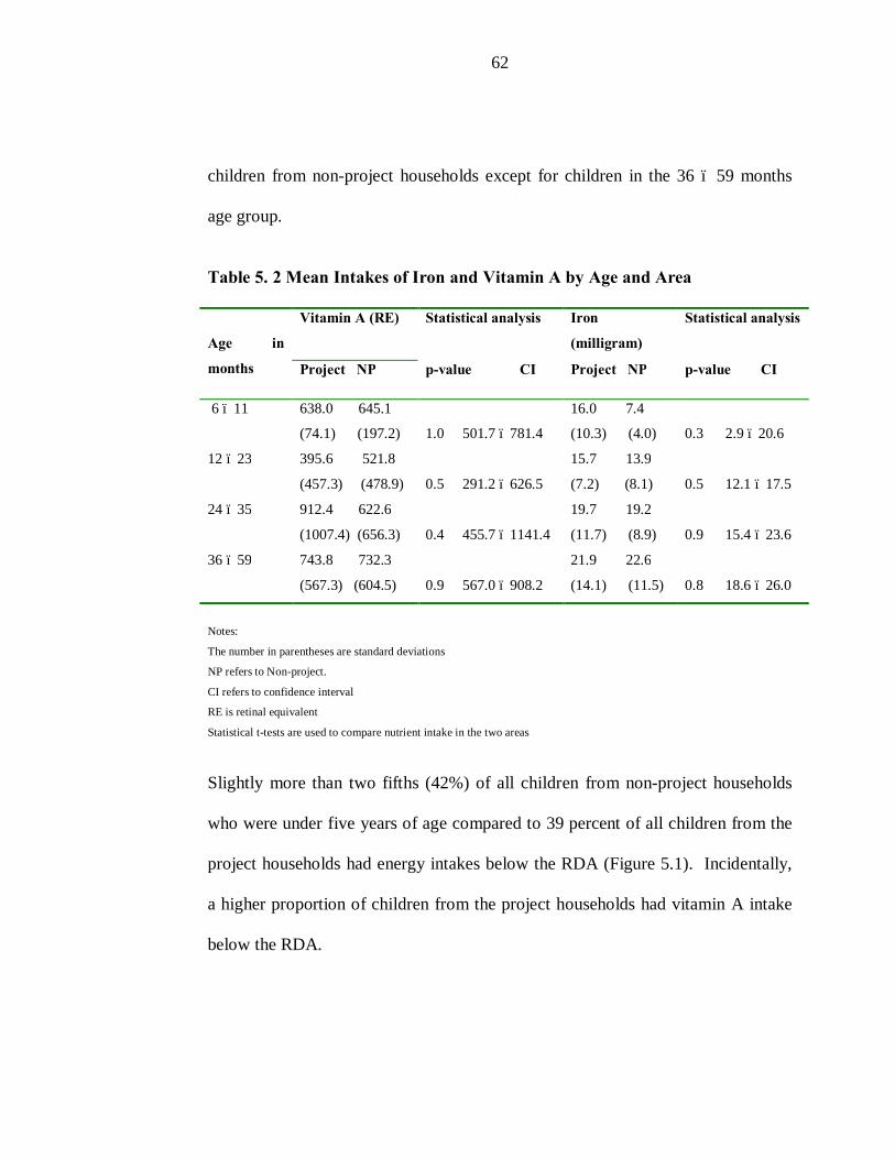
62

children from non-project households except for children in the 36 – 59 months

age group.

Table 5. 2 Mean Intakes of Iron and Vitamin A by Age and Area Age in months

Vitamin A (RE) Statistical analysis Iron (milligram)

Statistical analysis

Project NP p-value CI Project NP p-value CI

6 – 11 638.0 645.1

(74.1) (197.2)

1.0 501.7 – 781.4

16.0 7.4

(10.3) (4.0)

0.3 2.9 – 20.6

12 – 23 395.6 521.8

(457.3) (478.9)

0.5 291.2 – 626.5

15.7 13.9

(7.2) (8.1)

0.5 12.1 – 17.5

24 – 35 912.4 622.6

(1007.4) (656.3)

0.4 455.7 – 1141.4

19.7 19.2

(11.7) (8.9)

0.9 15.4 – 23.6

36 – 59 743.8 732.3

(567.3) (604.5)

0.9 567.0 – 908.2

21.9 22.6

(14.1) (11.5)

0.8 18.6 – 26.0

Notes:

The number in parentheses are standard deviations

NP refers to Non-project.

CI refers to confidence interval

RE is retinal equivalent

Statistical t-tests are used to compare nutrient intake in the two areas

Slightly more than two fifths (42%) of all children from non-project households

who were under five years of age compared to 39 percent of all children from the

project households had energy intakes below the RDA (Figure 5.1). Incidentally,

a higher proportion of children from the project households had vitamin A intake

below the RDA.

63

Figure 5. 1 Percent Distribution of Children Aged 6 – 59 months With Energy and Nutrient Intake Below RDA

5.2.2 Nutritional Status of Children 6 – 59 months

Data on Table 5.3 show that on average, children from the project households had

higher HAZ, WHZ and WAZ, although there were no significant differences.

When the study households were categorised by type of farming, children from

commercial farming households in the project area had significantly higher WAZ

(p = 0.05). Also, children from project households with income above the rural

poverty line had significantly higher HAZ than those from non-project households

(p = 0.04).

0

5

10

15

20

25

30

35

40

45

Energy 39 42.4

Protein 1.7 1.7

Iron 5 3

Vitamin A 37.3 33.9

Project Area Non-project Area

64

There were no significant differences in any nutritional indicators between female

and male children although female children had higher HAZ and WHZ while male

children had higher WAZ (Appendix 4). Male children from the project

households had higher HAZ, WAZ and WHZ than their counterparts in non-

project households.

It was interesting to note that children from male-headed households had higher Z-

scores than children from female-headed households. Although there was no

significant difference, children from households with bigger land holdings had

better Z-scores than children from households with smaller land sizes. Irrespective

of land sizes, children from project households had better mean z scores

suggesting that irrigation has some influence on the nutritional status though not

significant.

65

Table 5. 3 Mean Z-scores by Area, Type of Farming, Income Level, Sex of

Index Child and Land Size

Variable HAZ WAZ WHZ

Project NP Project NP Project NP Houeehold -0.65 -0.99

(1.3) (1.4)

-0.43 -0.7

(1.0) (1.2)

0.05 -0.01

(1.1) (1.2)

Type of Farming Commercial

Non-commercial

-0.73 -1.0

(1.4) (1.2)

-0.5 -0.99

(1.3) (1.5)

-0.42a -1.03

(1.2) (0.9)

-0.45 -0.55

(0.8) (1.3)

0.11 -0.45

(1.1) (0.9)

-0.07 0.19

(0.7) (1.3)

Income Level Below KSh.1240

Above or Equal to KSh.1240

-0.93 -0.13

(1.5) (1.8)

-0.59b -1.2

(1.3) (1.2)

-0.68 -0.67

(1.0) (1.5)

-0.37 -0.72

(1.1) (1.1)

-0.06 -0.63

(1.0) (1.1)

0.08 0.12

(1.0) (1.1)

Sex of Index Child Male

Female

-0.7 -1.0

(1.2) (1.0)

-0.6 -0.97

(1.5) (1.8)

-0.3 -0.83

(1.0) (0.9)

-0.59 -0.57

(1.1) (1.4)

0.19 -0.24

(1.1) (0.8)

-0.11 0.24

(0.9) (1.6)

Land Size Less or Equal to 3 acres

More than 3 acres

-0.69 -1.1

(1.4) (1.4)

-0.4 -0.5

(0.8) (1.4)

-0.5 -0.8

(1.1) (1.2)

-0.1 -0.4

(0.9) (1.3)

0.02 -0.001

(1.0) (1.3)

0.22 -0.02

(0.8) (0.9)

Notes: Statistical t-tests are used to compare the difference in mean z scores between the two areas.

The numbers in parentheses are standard deviation. a p-value = 0.05. b p-value = 0.04.

NP refers to Non-project area

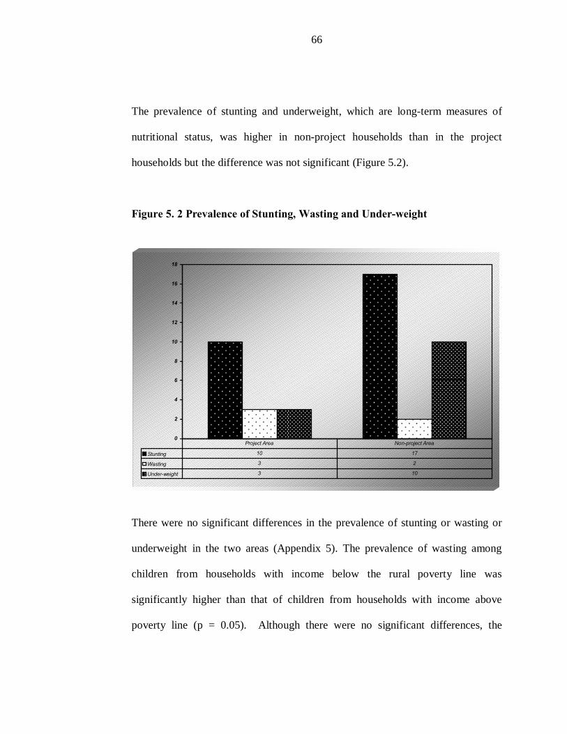
66

The prevalence of stunting and underweight, which are long-term measures of

nutritional status, was higher in non-project households than in the project

households but the difference was not significant (Figure 5.2).

Figure 5. 2 Prevalence of Stunting, Wasting and Under-weight

There were no significant differences in the prevalence of stunting or wasting or

underweight in the two areas (Appendix 5). The prevalence of wasting among

children from households with income below the rural poverty line was

significantly higher than that of children from households with income above

poverty line (p = 0.05). Although there were no significant differences, the

0

2

4

6

8

10

12

14

16

18

Stunting 10 17

Wasting 3 2

Under-weight 3 10

Project Area Non-project Area

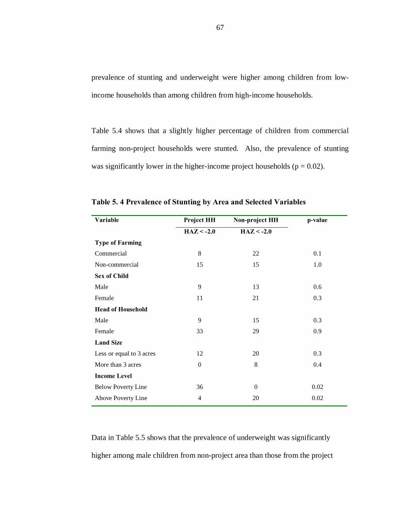
67

prevalence of stunting and underweight were higher among children from low-

income households than among children from high-income households.

Table 5.4 shows that a slightly higher percentage of children from commercial

farming non-project households were stunted. Also, the prevalence of stunting

was significantly lower in the higher-income project households (p = 0.02).

Table 5. 4 Prevalence of Stunting by Area and Selected Variables

Variable Project HH Non-project HH p-value

HAZ < -2.0 HAZ < -2.0 Type of Farming Commercial

Non-commercial

8

15

22

15

0.1

1.0

Sex of Child Male

Female

9

11

13

21

0.6

0.3

Head of Household Male

Female

9

33

15

29

0.3

0.9

Land Size Less or equal to 3 acres

More than 3 acres

12

0

20

8

0.3

0.4

Income Level Below Poverty Line

Above Poverty Line

36

4

0

20

0.02

0.02

Data in Table 5.5 shows that the prevalence of underweight was significantly

higher among male children from non-project area than those from the project

68

households (p = 0.03). Although there were no significant differences, the

proportion of children who are underweight is slightly lower in the project

households among the selected variables.

Table 5. 5 Prevalence of Underweight by Area and Selected Variables

Variable Project Households

Non-project Households

p-value

WAZ < - 2.0 WAZ < - 2.0

Type of Farming Commercial

Non-commercial

3

5

11

10

0.2

0.5

Sex of Child Male

Female

0

7

13

7

0.03

0.9

Head of Household Male

Female

4

0

8

29

0.4

0.3

Land Size Less or equal to 3 acres

More than 3 acres

4

0

11

8

0.2

0.4

Income Level Below Poverty Line

Above Poverty Line

9

2

14

9

0.7

0.1

69

5.2.3 Summary of Findings

Ø Slightly over two fifths (42%) of children from non-project households

compared to 39% from the project households consumed calories below the

RDA.

Ø Children from commercial farming households in the project area had

significantly higher WAZ

Ø Children from high-income project households had significantly higher HAZ.

Ø The prevalence of stunting was significantly lower in project households with

higher income.

Ø The prevalence of wasting was significantly higher in low-income households

than in high-income households.

Ø Irrigation has influence on the nutritional status of young children.

5.3 Discussion of Results

The findings of this study clearly show that the average calorie and nutrient intake

of children under five years of age were above the RDA. However, the mean

energy intake of children (12 – 35 months) from non-project households was lower

than the RDA. This could probably be due to the fact that, in most households,

children of this age are commonly fed from the family dish, which may not

provide them with adequate calories. Moreover, family dish comprised of a

mixture of maize, beans and occasionally potatoes and this is typically a diet high

in bulk, which is not only of poor digestibility but also highly unpalatable to these

70

children. Furthermore young children with limited stomach capacity are unable to

consume sufficient quantities of such food to cover their energy and nutrient

requirements.

This study established that irrigation has no significant influence on dietary energy

intake of pre-school children. However, this may not be the case since the drought

experienced in the study area during the reference year adversely affected

household food availability and this could have resulted to low calorie intake. It

can also be argued that project households could not realise good yields of

horticultural crops due to unreliability of irrigation water and therefore had limited

economic returns. Subsequently less income was available to purchase food in

order to offset the lack of food produced for family consumption. Another

explanation could be that income earned from sale of cash crops was not

necessarily used to meet the households' dietary needs. Therefore, there is need

for further research in order to establish the true situation.

A higher proportion of children from the project households had lower vitamin A

intke than the RDA compared to children from the non-project households. The

most plausible explanation is that project households normally grew vegetables

(which are good sources of vitamin A) mainly for sale thereby leaving little or

none for home consumption. A good number of project households grew

snowpea, which even though it is a source of vitamin A, it was not consumed at

71

home. This is an export crop and rural households do not have knowledge on its

preparation method. In fact most homemakers reported that snowpea that is

rejected by the buyer is usually used as livestock feed.

Although the prevalence of underweight and stunting among children in the

project households was lower, the fact that there were no significant differences

indicates that provision of irrigation water per se does not have a significant

influence on nutritional status. Therefore, the first hypothesis of this study that

states that “there is no significant difference in the nutritional status between

project and non-project households” is valid. However there is need for further

investigation on the role of irrigation on nutritional status, because the findings of

this study could have underscored the importance of irrigation given that drought

that was prevalent in this area adversely affected availability of the water. This

consequently had negative impact on crop yields as well as household income and

hence affected household food availability. The prevalence of stunting was higher

in non-project households while the proportion of children who were wasted was

higher in the project households, concurring with findings by Matsvimbo (1997).

The prevalence of stunting and underweight (which are long-term measures of

nutritional status) were lower among children from commercial farming

households than non-commercial farming households. There were no significant

differences between type of farming and nutritional status. Kennedy and Cogill

72

(1987) observed similar findings in a study on nutritional effects of the

commercialisation of agriculture in southwestern Kenya. These findings

contradict the conventional hypothesis that increased emphasis of commercial

farming lead to poorer nutritional status of children.

Interestingly, children from male-headed households had better Z-scores than

children from female-headed households. This is contrary to findings by Kennedy

and Cogill (1987) that children from female-headed households do significantly

better on both HAZ and WAZ. This could be attributed to the small number of

female-headed household in study sample; only five percent in the project

households and twelve percent in non-project households.

The link of access to land and nutritional status is well established, with

prevalence of stunting and underweight being higher among children of landless

households than children of landed households (Biswas and Pinstrup-Andersen,

1985; Victoria et al., 1986; Haaga et al., 1986). In this study, the prevalence of

wasting, stunting and underweight was higher among children from households

with less land. Also, the average Z-scores of all the three nutritional indicators

were lower in households with less land. The importance of irrigation on

improvement of nutritional status is once again noted in that irrespective of land

size, children from project households had better Z-scores.

73

The study found that the prevalence of wasting was significantly higher in low-

income households. This supports the findings by Martorell (1985) that low-

income smallholder households have the highest incidence of malnutrition because

low-income levels limit the kinds and amount of food available for consumption

by households. Alderman and Garcia (1983) also found out that malnutrition in

children was more severe in households with lower average per capita. This is in

line with the findings of this study that the prevalence of wasting, stunting and

underweight was higher in households with income below poverty line.

According to the 2000 Kenya Economic Survey, households with income below

the poverty line are unable to access the minimum requirement of food and

essential non-food commodities.

The influence of irrigation on nutritional status is evident from the fact that

children from higher-income project households had significantly higher HAZ and

also the prevalence of stunting was significantly lower

74

Chapter 6 6.0 Conclusion and recommendations

6.1 Conclusion

The findings of this study show that irrigation is a key input in increasing crop

yields in arid and semi-arid areas. In the study area where households mainly

relied on farm production, increase in yields subsequently led to improved

household food availability and/or higher incomes.

Research results do not allow a definite conclusion to be drawn regarding the role

of irrigation on the nutritional status of young children. However, it is clear that

irrigation has safeguarded the nutritional status of young children because children

from the project households were better off.

1. Provision of irrigation water positively influence crop yields particularly when

combined with good crop husbandry practices. Project households were twice

as likely to realise potato yields than non-project households. The yields in the

project households could have been much higher, were it not for unreliability

of irrigation water.

2. Irrigation has positive influence on dietary energy intake of young children but

it has negative influence on vitamin A and iron intake.

75

3. Irrigation has encouraged commercial farming and this has led to higher

household incomes and a higher likelihood of sustaining households above the

Kenyan rural poverty line (Ksh 1240).

4. The improvement of income in commercial farming households has influence

on household food security.

5. Irrigation has contributed to improvement of household food security.

6. Irrigation has led to sustained food production for home consumption and

subsequently households spend less money on food purchases.

7. Irrigation has influence on the nutritional status of young children.

6.2 Recommendations

1. Water project management committee should mobilise the households to

ensure that irrigation water is available throughout the year, in order to

maximize the potential benefit of irrigation on crop production and nutritional

status of young children.

76

2. Non-project households should apply appropriate technologies to harness the

available water to irrigate home gardens and small, but intensive vegetable

plots.

3. All households should be trained on utilisation of snowpea and other under-

utilised micronutrient-rich local foods in order to encourage their consumption

at household level.

4. Kitchen gardening should be promoted, particularly in the project households

where more children consumed diets with less vitamin A and iron than RDA.

Since in project households most vegetables are grown for sale, this would

ensure that households have some vegetables for home consumption.

5. Micro-irrigation techniques such as drip irrigation alongside soil and water

conservation measures should be promoted in the study area. This will ensure

efficient utilisation of the available water.

6. Food preservation should be encouraged during peak seasons to ensure year

round food availability.

77

Bibliography

ACC / SCN. (2000) The Fourth Report on the World Situation. United Nations

Administrative Committee on Co-ordination and Sub-committee on Nutrition,

Geneva Pp 1 – 20.

ACC/SCN. (1997). The Third Report on World Nutrition Situation. United

Nations Administrative Committee on Co-ordination and Sub-committee on

Nutrition, Geneva Pp 1, 83-88.

Alderman, H and Garcia, M. (1993). Poverty, Household Food Security and

Nutrition in Rural Pakistan. Research report, International Food Policy Research

Institute, Washington D.C, Pp 50-64.

Allen, L.H. (1994). Nutritional influences of linear growth: A general review.

European Journal of Clinical Nutrition, Vol. 48, supplement 1, Pp 575-589.

Armar-Klemesu, M., Rikimar, T., Kennedy, D.O., Harrison, E., Kido, Y. and

Takyi, E.E. (1995) Household food security and children’s diet in rural Ghana.

Food and Nutrition Bulletin Vol.16 No.1 United Nation University Press Pp 27 –

33.

78

Balderston, J.B., Wilson, A.B., Freire, M.E., Simonen, M.S. (1981).

Malnourished Children of the Rural Poor: The web of food, health, education,

fertility, and agricultural production. Auburn House Publishing Co., Boston, Pp 1-

15.

Berg, A. (1988). Malnutrition, What Can Be Done? John Hopkins University

Press, Maryland, Pp1-8

Biswas, M.R and Pinstrup-Andersen, P. (1985). Nutrition and Development.

Oxford University Press, New York. Pp 21-42.

Bouis, H.E. and Haddad, L.J. (1990). Effects of Agricultural Commercialisation

on Land Tenure, Household Resource Allocation, and Nutrition in the

Philippines. Research report, International Food Policy Research Institute,

Washington, D.C.

Caliendo, M.A. (1979). Nutrition and the World Food Crisis. Macmillan

Publishing Co. Inc. New York, Pp 261-267.

FAO and WHO (1992). International Conference on Nutrition. Final Report of

the Conference. FAO, Rome, Italy. Pp 24 – 49

79

Gillespie, S.R and Mason, J.B (1991). Nutrition-relevant actions: Some

experiences from the eighties and lessons for the nineties. ACC/SCN State of the

Art Series. Nutrition Policy Discussion Paper No,10 ACC/SCN Geneva Pp 30-

53.

Government of Kenya (1981). Sessional Paper No.4 of 1981 on National Food

Policy, Government printers, Nairobi. Pp 16 – 24.

Government of Kenya (1997). Nyeri District Development Plan, 1997-2001.

Government printer, Nairobi, Pp 1 – 15; 41-66.

Government of Kenya (1999). National Poverty Eradication Plan (1999-2015).

Government Printers, Nairobi. Pp 1 – 19.

Government of Kenya (2000) Economic Survey 2000. Government Printers,

Nairobi. Pp 188 – 218.

Government of Kenya (2001) The 1999 Population and Housing Census

Volume 1, Government Printers, Nairobi. Pp 1-17.

Government of Kenya / UNICEF (1998) Situation Analysis of Children and

Women in Kenya, Nairobi Pp 122 – 124

80

Government of Kenya/ UNICEF (1992). Children and Women in Kenya: A

Situation Analysis. Regal Press Ltd., Nairobi, Pp 57 - 84.

Harper, L.J. (1984). Food, Nutrition, and Agriculture: Teachers’ Manual.

FAO, Rome, Pp 19 - 37.

Hoorweg and Niemeijer. (1989). Intervention in Child Nutrition; Evaluation

Studies in Kenya. Kegan Paul International Ltd., Pp 120-124.

Kennedy, E. and Oniang’o, R. (1990). Health and Nutritional Effects of

Sugarcane Production in South Western Kenya. Food and Nutrition Bulletin

Vol. 12, No. 4. United Nation University Press, Tokyo, Pp 261-267.

Kennedy, E.T. and Cogill, B. (1987). Income and Nutritional Effects of the

Commercialisation of Agriculture in Southwestern Kenya. Research report,

International Food Policy Research Institute, Washington, D.C. Pp 9-59.

Kigutha H.N. (1995). Effects of Season on Household Food Security and

Nutritional Status of Smallholder Rural Households in Nakuru District,

Kenya. Food and Nutrition Studies Programme Report, Africa studies, Laiden and

Ministry of Planning and National Development, Nairobi Pp 4 -20.

81

Kigutha, H.N. (1994) Household Food Security and Nutritional Status of

Vulnerable Groups in Kenya: A seasonal study among low-income smallholder

rural households. Published Phd thesis, Wageningen Agricultural University.

African Studies Centre, Laiden Pp 47 – 67.

King, F.S. and Burgess, A. (1993) Nutrition for Developing Countries, Oxford

University Press. Pp 165 – 188; 433 – 443.

Martorell, R. (1985). Nutrition and Health indicators: Suggestion for surveys of

the standard of living in developing countries. LSMS Working Paper No. 13. Pp

4-12.

Matsvimbo, N (1997) Nutritional Status of School Children and Associated

Factors in Rupangwana Irrigation Scheme, Zibambwe. Unpublished MSc

Thesis, University of Nairobi, Kenya.

Melville, B.F. (1988). Land Availability and Nutritional Status. Food and

Nutrition Bulletin, Vol.10 No. 2. United Nation University Press, Pp 44-47.

82

Mwandime, R.K. (1992) Expenditure, Food Consumption Patterns and

Nutritional Status of Tenants in Mwea-Tebere Irrigation Scheme, Kenya.

Unpublished Master of Science Thesis, University of Nairobi, Kenya.

National Council for Population Development (NCPD), Central Bureau of

Statistics (CBS) (Office of the Vice president and Ministry of planning and

National Development) [Kenya], and Macro International Inc. (MI) (1999). Kenya

Demographic and Health Survey 1998. Claverton, Maryland. Pp 115 – 124.

Ntiru, M., Sy N..M., Diene, S.M. and Ndure, K.S. (1999). Best Practices and

Lessons Learned for Sustainable Community Nutrition Programming.

USAID, African Bureau, p 1 - 6.

Sehmi, J.K. (1993) National Food Composition Tables and the Planning of

Satisfactory Diets in Kenya, Government Printers, Nairobi.

Simko, M.D. and Cowell, C. (1984). Nutritional Assessment; A comprehensive

Guide for Planning Intervention. Aspen System Co-operation, Maryland, Pp 1-

10.

83

Smith, M.F. (1986) The Impact of Changing Agricultural Systems on the

Nutritional Status of Farm Households in Developing Countries. Food and

Nutrition Bulletin Vol.8 No.3 United Nation University Press. Pp 25 – 29.

UN (1986) How to Weigh and Measure Children: Assessing the Nutritional

Status of Young Children in Household Surveys. UN Department of Technical Co-

operation for Development and Statistical Office, New York.

UNICEF (1989). Situation Analysis of Children and Women in Kenya. Royal

Press Ltd. Nairobi, Pp 71-76.

UNICEF. (1991). National Capacity Building for Child Survival and

Development; Proceeding of the 2nd African Regional Workshop held in

Ibadan, Nigeria 8-12/10/1990. International Child Development Centre, Florence,

Italy. Pp 81-82.

Victoria, V.R., Vaughan, J.P., Kirkwood, B., Martines, J.C., Barcelos, L.B. (1986)

Child Malnutrition and Land Ownership in Southern Brazil. Ecology of Food and

Nutrition. Pp 265 – 275.

Wandel, M (1989). Household Food Consumption and Seasonal Variations in

Food Availability in Sri Lanka. Ecology of Food and Nutrition 22. Pp 169 – 182.

84

WHO (1983) Measuring Change in Nutritional Status; Guidelines for

Assessing the Nutritional Impact of Supplementary Feeding Programmes for

Vulnerable Groups. WHO, Switzerland. Pp 12-13.

World Bank (1973). Agricultural Sector Survey- Kenya Volume 1. World Bank.

Annexe 1 Pp1 – 24.

85

Appendices

Appendix 1 Equivalent Weights of Commonly Used Containers

Container Weight in Kilograms 2 kg Kimbo tin of cereals or grains or pulses 2

1 debe of cereals/grains/pulses 16

1 bag of cereals/grains/pulses 90

1 bag of potatoes 130

1 bag of cabbage 126

1 bag of carrots 138

1 box of tomatoes 64

1 carton snowpea 2.5

Appendix 2 Equivalents Weights and Volumes of Foods

Food Weight of food (grams) in 100ml Cereals flours 59

Stiff porridge 100

Soft porridge 100

Raw rice 85

Potato raw diced 63

Beans/peas raw 80

Cabbage raw shredded 30

Green leaves raw chopped 31

Onions raw chopped 68

Tomato sliced 77

Banana mashed 95

Pawpaw mashed 100

Sugar 83

86

Meat mince/ground 95

Milk fresh 100

Margarine 95

Oil 88

Appendix 3 Daily Requirements of Energy, Protein, Iron and Vitamin A for

Different Age Groups

Age (months) Energy (kcal) Protein (g) Iron (mgs) Vitamin A (RE)

0 – 11 820 13.5 5 –10 300

12 – 23 1150 13.5 5 –10 250

24 – 35 1350 15.5 5 – 10 550

36 – 59 1550 17.5 5 - 10 300

Source: Sehmi, J.K. (1993) National Food Composition Tables and the Planning of

Satisfactory Diets in Kenya, Government printers, Nairobi.

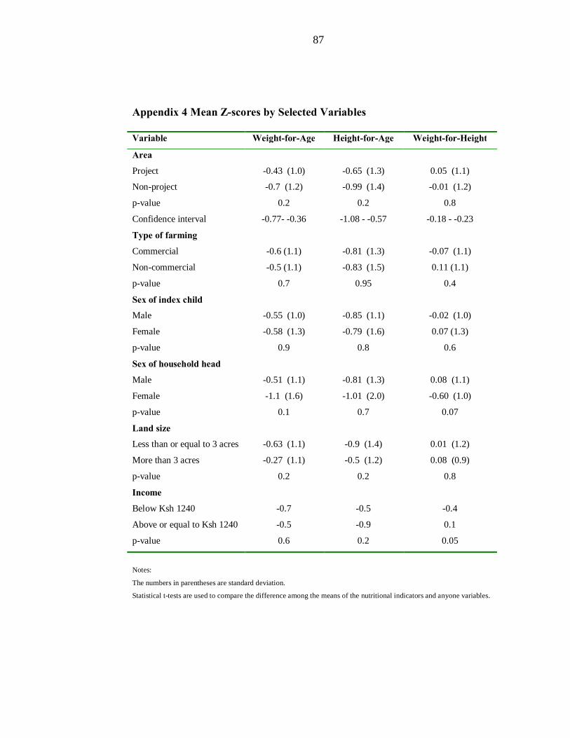
87

Appendix 4 Mean Z-scores by Selected Variables

Variable Weight-for-Age Height-for-Age Weight-for-Height

Area Project

Non-project

p-value

Confidence interval

-0.43 (1.0)

-0.7 (1.2)

0.2

-0.77- -0.36

-0.65 (1.3)

-0.99 (1.4)

0.2

-1.08 - -0.57

0.05 (1.1)

-0.01 (1.2)

0.8

-0.18 - -0.23

Type of farming Commercial

Non-commercial

p-value

-0.6 (1.1)

-0.5 (1.1)

0.7

-0.81 (1.3)

-0.83 (1.5)

0.95

-0.07 (1.1)

0.11 (1.1)

0.4

Sex of index child Male

Female

p-value

-0.55 (1.0)

-0.58 (1.3)

0.9

-0.85 (1.1)

-0.79 (1.6)

0.8

-0.02 (1.0)

0.07 (1.3)

0.6

Sex of household head Male

Female

p-value

-0.51 (1.1)

-1.1 (1.6)

0.1

-0.81 (1.3)

-1.01 (2.0)

0.7

0.08 (1.1)

-0.60 (1.0)

0.07

Land size Less than or equal to 3 acres

More than 3 acres

p-value

-0.63 (1.1)

-0.27 (1.1)

0.2

-0.9 (1.4)

-0.5 (1.2)

0.2

0.01 (1.2)

0.08 (0.9)

0.8

Income Below Ksh 1240

Above or equal to Ksh 1240

p-value

-0.7

-0.5

0.6

-0.5

-0.9

0.2

-0.4

0.1

0.05

Notes:

The numbers in parentheses are standard deviation.

Statistical t-tests are used to compare the difference among the means of the nutritional indicators and anyone variables.

88

Appendix 5 Percentage of Children Between 6-59 Months Below Common

Cut-offs for Nutritional Status by Area, Type of Farming, Sex of Index Child

and Land Size

Variable n Underweight Stunted Wasted

Area Project

Non-project

p-value

59

59

3

10

0.1

10

17

0.3

3

2

0.6

Type of farming Commercial

Non-commercial

p-value

57

61

5

8

0.5

12

15

0.7

4

2

0.5

Sex of index child Male

Female

p-value

62

56

6

7

0.9

11

16

0.5

2

4

0.5

Land size Less than or equal to 3 acres

More than 3 acres

p-value

96

22

7

5

0.6

16

5

0.2

3

0

0.4

Income Less than Ksh 1240

More than or equal to Ksh

1240

p-value

12

5

0.3

16

12

0.6

8

1

0.05

Notes:

Statistical t-tests are used to compare the difference in the two areas.

89

Appendix 6 Questionnaire

HOUSEHOLD FOOD SECURITY AND NUTRITION SURVEY

KIENI EAST DIVISION

NYERI DISTRICT

Household’s background information

Location …………………… Sub-location

……………………………

Water scheme …………….. Household number

Respondent’s Name ------------ Sex: Male = 1, Female = 2

Marital status

1= Married, 2 = Single, 3 = Separated/Divorced, 4 = Widowed

Name of Household head ---------- Sex: Male = 1, Female = 2

Name of Interviewer ----------- Date / /

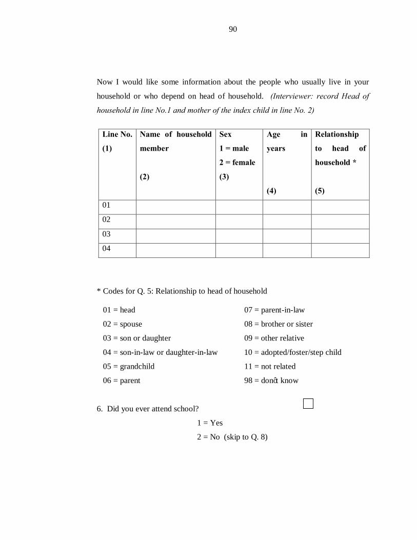
90

Now I would like some information about the people who usually live in your

household or who depend on head of household. (Interviewer: record Head of

household in line No.1 and mother of the index child in line No. 2)

* Codes for Q. 5: Relationship to head of household

01 = head 07 = parent-in-law

02 = spouse 08 = brother or sister

03 = son or daughter 09 = other relative

04 = son-in-law or daughter-in-law 10 = adopted/foster/step child

05 = grandchild 11 = not related

06 = parent 98 = don’t know

6. Did you ever attend school?

1 = Yes

2 = No (skip to Q. 8)

Line No. (1)

Name of household member

(2)

Sex 1 = male 2 = female

(3)

Age in years

(4)

Relationship to head of household *

(5)

01

02

03

04

91

7. What is the highest level you attended?

1 = Completed 1-4 of primary 6 = Adult education

2 = Completed 5-8 of primary 98= don’t know

3 = Completed secondary

4 = Not completed secondary

5 = Post secondary

8. What is your main activity?

1 = Farming/ housewife

2 = Salaried employed

3 = Casual labourer

4 = Jua-kali/ business

96 = Other (specify)

(Check the marital status of respondent, if not married skip to Q 12, if married then ask)

9. Did your husband ever attend school?

1 = Yes

2 = No (skip to Q.11)

10. What is the highest level he attended?

1 = Completed 1-4 of primary

2 = Completed 5-8 of primary

3 = Completed secondary

4 = Not completed secondary

5 = Post secondary

6 = Adult education

98 = don’t know

92

11. What is your husband’s occupation?

1 = Farmer

2 = Salaried employed

3 = Casual labourer

4 = Jua-kali/ business

96=other (specify)

Water availability

12. What is the main source of water for this household?

1 = Piped water

2 = River/Spring

3 = Well

4 = Rain water

13. How long does it take you to get there, get water, and come back?

------

Minutes

------ Km

0 = on premises

14. Do you use the water to irrigate your crops?

1 = Yes

2 = No

93

15. How reliable is the water supply?

1 = reliable (skip to Q.17)

2 = slightly reliable

3 = unreliable

16. If 2 or 3, for how many months in a year is the water not reliable?

----------

Months

Food production

17. What is the size of your land?

Land size in acres Owned …………

Rented …………

Others ………….

Total ……………

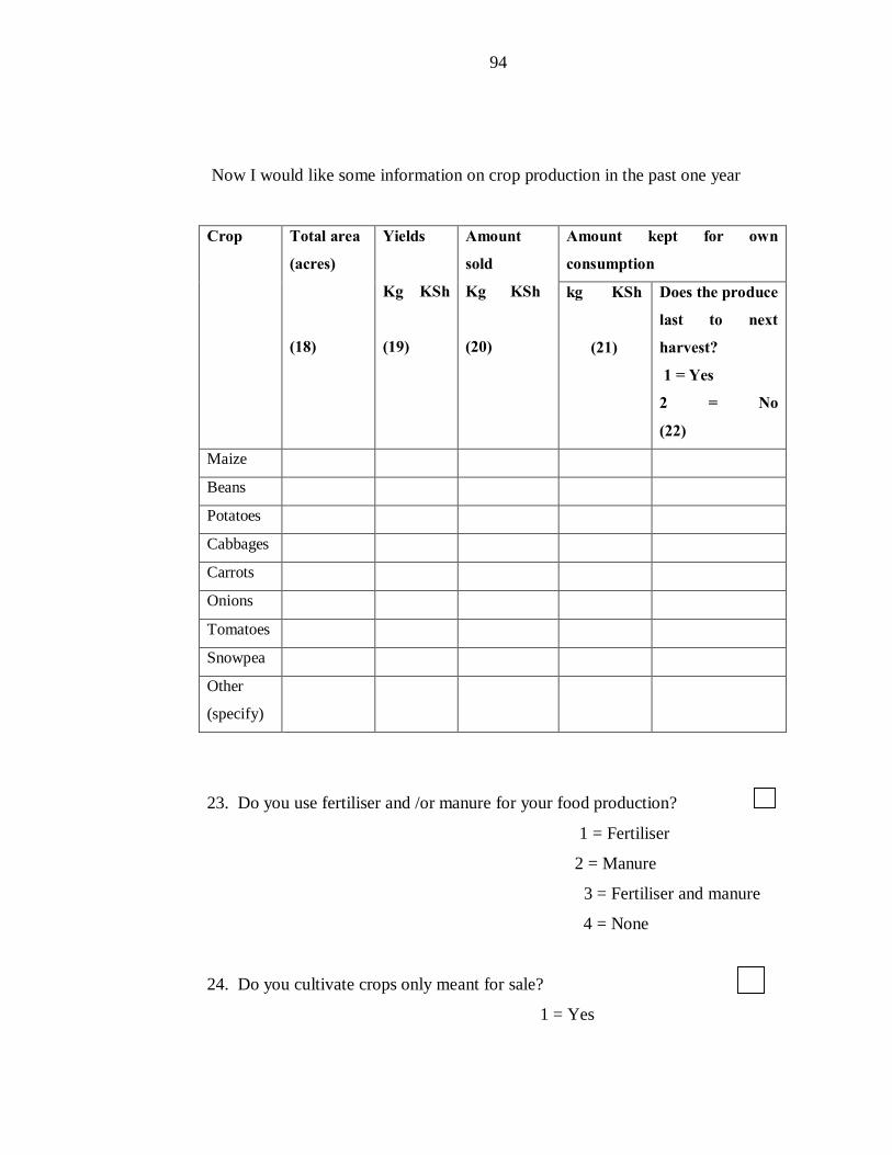
94

Now I would like some information on crop production in the past one year

Crop Total area (acres) (18)

Yields Kg KSh (19)

Amount sold Kg KSh (20)

Amount kept for own consumption

kg KSh (21)

Does the produce last to next harvest? 1 = Yes 2 = No

(22)

Maize

Beans

Potatoes

Cabbages

Carrots

Onions

Tomatoes

Snowpea

Other

(specify)

23. Do you use fertiliser and /or manure for your food production?

1 = Fertiliser

2 = Manure

3 = Fertiliser and manure

4 = None

24. Do you cultivate crops only meant for sale?

1 = Yes

95

2 = No (skip to Q.27)

If Yes, Which crops and how much land is usually allocated to each?

Crop (25)

Acreage (26)

27. Apart from own production how else do you obtain food for your household?

(Interviewer: code accordingly)

Food source

1 = Yes 2 = No

Purchase from the market

Casual work

Remittances from relatives

Famine relief food

28. Do you keep livestock?

1 = Yes

2 = No (skip to Q.33)

96

Now I would like some information about the livestock you have kept in the past

one year?

Livestock (29)

Number (30)

Production

(31)

Amount

(32)

No. of animals

Average production

Consumed Sold

Income and expenditure 33. Apart from farming what are the other sources of your household income?

(Check by ticking applicable source to the household)

Sources Check

1 = Salaried employment

2 = Casual labour

3 = Business/Jua-kali

96 = Other (specify)

34. How much is the monthly income for your household?

1 = Less than 1,240

shillings

2 = Over 1,240 shillings

98= Don’t know

97

35. What amount of household income per month is allocated to:

(Expenditure on food items includes all food purchased and home produced)

24 -Hour Dietary Recall (Record the following information for the index child - the youngest child in the

household

aged between 6-59 months)

36. Name of the index child …………………….

Sex : Male Female Age months

Food items Expenditure per year (KSh)

Non-food items Expenditure per year (ksh)

Own Prodn.

Purchased Total

Cereals and

grains

Education

Root and

tubers

Farming

Pulses Fuel

Vegetables Clothes

Fruits Supplies and

household goods

Meat Health expenses

Milk Transport

Fats and oils Family events

Sugar

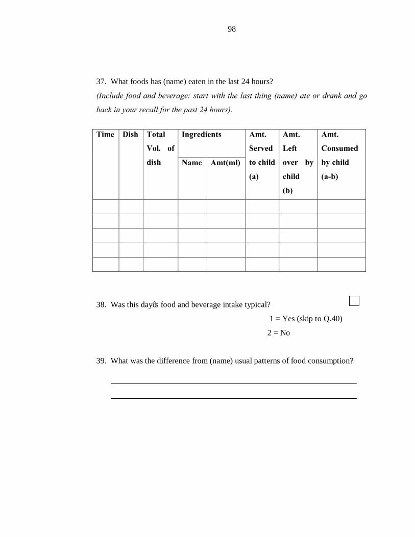
98

37. What foods has (name) eaten in the last 24 hours?

(Include food and beverage: start with the last thing (name) ate or drank and go

back in your recall for the past 24 hours).

38. Was this day’s food and beverage intake typical?

1 = Yes (skip to Q.40)

2 = No

39. What was the difference from (name) usual patterns of food consumption?

Time Dish Total Vol. of dish

Ingredients

Amt. Served to child

(a)

Amt. Left over by

child (b)

Amt. Consumed by child

(a-b) Name Amt(ml)

99

Anthropometric measurements

Now I would like to take the height, weight and arm circumference measurements

of (name of the index child).

40. Anthropometric measurement for the index child

Line No. Child’s name

……………………………………

Sex : Male Female Date of Birth / / /

Age------ Months Date of weighing / / /

1st Weight (0.1 kg) ----------- 1st Height (0.1 cm) ----------

2nd Weight (0.1 kg) -------- 2nd Height (0.1 cm) -----------

MUAC (0.1mm) -----------