This content has been downloaded from IOPscience. Please scroll down to see the full text.

Download details:

IP Address: 128.183.181.119

This content was downloaded on 06/06/2014 at 14:16

Please note that terms and conditions apply.

The role of axisymmetric flow configuration in the estimation of the analogue surface gravity

and related Hawking like temperature

View the table of contents for this issue, or go to the journal homepage for more

2014 Class. Quantum Grav. 31 035002

(http://iopscience.iop.org/0264-9381/31/3/035002)

Home Search Collections Journals About Contact us My IOPscience

Classical and Quantum Gravity

Class. Quantum Grav. 31 (2014) 035002 (29pp) doi:10.1088/0264-9381/31/3/035002

The role of axisymmetric flow configurationin the estimation of the analogue surfacegravity and related Hawking liketemperature

Neven Bilic1, Arpita Choudhary2,5, Tapas K Das3

and Sankhasubhra Nag4

1 Rudjer Boskovic Institute, 10002 Zagreb, Croatia2 University of Lucknow, Lucknow 226007, India3 Harish Chandra Research Institute, Chhatnag Rd, Jhunsi, Allahabad 211 019, India4 Sarojini Naidu College for Women, Kolkata 700028, India

E-mail: bilic@thphys.irb.hr, arpita@tls-tautenburg.de, tapas@hri.res.in andsankhasubhra_nag@yahoo.co.in

Received 5 June 2013, revised 4 November 2013Accepted for publication 22 November 2013Published 23 December 2013

AbstractWe investigate the salient features of the acoustic geometry corresponding to theaxially symmetric accretion of dissipationless inhomogeneous fluid onto a non-rotating astrophysical black hole under the influence of a generalized pseudo-Schwarzschild gravitational potential. For a few chosen flow configurations,we determine the location of the acoustic horizon and calculate analyticallythe corresponding analogue surface gravity κ and the associated analogueHawking temperature TAH. We study the dependence of κ on various boundaryconditions and geometry governing the dynamic and thermodynamic propertiesof the background flow.

Keywords: accretion, accretion discs, analogue gravity, general relativity, fluidmechanicsPACS numbers: 04.70.Dy, 95.30.Sf, 97.10.Gz, 97.60.Lf

(Some figures may appear in colour only in the online journal)

1. Introduction

Contemporary works in the field of analogue gravity phenomena have attracted significantattention in the community in theoretical front [1–4] as well as in the laboratory set up

5 Present Address: Thuringer Landessternwarte Tautenburg, Sternwarte 5, D-07778, Tautenburg, Germany.

0264-9381/14/035002+29$33.00 © 2014 IOP Publishing Ltd Printed in the UK 1

Class. Quantum Grav. 31 (2014) 035002 N Bilic et al

[5–9]. Proper equivalence has been established between the physics of the propagating acoustic(and acoustic type) perturbations embedded in an inhomogeneous dynamical fluid system andcertain kinematic features of the general theory of relativity. Such formalism has opened upthe possibility of simulating various important features of black hole space time within thelaboratory set up.

Conventional works in this field, however, concentrate on the physical systems forwhich gravity like effects are realized as emergent phenomena. Such systems do not usuallycontain any source that produces active gravitational field in any form. In recent years,though, attempts have been made to study the analogue effects in strong gravity environment[10–18]. The uniqueness of such systems lies in the fact that those are the only analoguemodels studied so far that simultaneously contain both kind of horizons, the gravitational aswell as the acoustic–allowing one to go for a close comparison between the general relativisticand the analogue Hawking effect.

Till date, analogue gravity effects in the axisymmetrically accreting black hole systemshave been studied for the flow structure assumed to be in hydrostatic equilibrium in the verticaldirection. Two other configurations for the axially symmetric black hole accretion are alsopossible. The accretion flow in conical equilibrium [19] and ‘flat disc’ kind of flow withconstant flow thickness have also been studied in the literature (for a detailed review, see, e.g.,[20]). As a compromise between the easy handling of the Newtonian framework of gravity andmore rigorous and non-tractable complete general relativistic description of the strong gravityspace time, four different ‘modified’ Newtonian ‘black hole potentials’ have been introducedin the literature which are commonly known as pseudo-Schwarzschild potentials (for furtherdetails about such potentials, see, e.g., [21] and [22]). The three aforementioned different flowstructures in the pseudo-Schwarzschild gravitational potentials have recently been studied ingreat detail [23].

In our present work, we study the analogue gravity effects in accreting black hole systemsunder the influence of pseudo-Schwarzschild potentials for three different flow configurations–the flow in conical and in vertical equilibrium and the flow with constant thickness (height).The main motivation behind this work is to study the dependence of the salient features of theacoustic geometry on the background matter geometry realized through the aforementionedthree different flow configurations. To accomplish such a task, we calculate the acoustic surfacegravity for the same set of accretion parameters but for all possible flow configurations in apseudo-Schwarzschild potentials.

2. Acoustic surface gravity for classical analogue systems

Classical analogue gravity systems (alternatively, the classical ‘black hole analogues‘) are fluiddynamical analogue of black holes in general relativity. Such an analogue may occur whena small linear perturbation propagates through a dissipationless inhomogeneous barotropictransonic fluid at finite temperature. The corresponding acoustic metric, which specifiesthe geometry in which the perturbation propagates, may be constructed in terms of theflow variables defining the unperturbed background continuum. The transonic surface actsas acoustic horizon—a null hypersurface with acoustic null geodesics, the phonons, as itsgenerators. The acoustic black hole horizon, which resembles the black hole event horizonsin many ways and forms at the regular transonic point of the fluid, whereas an acoustic whitehole horizon may be formed at the hypersurface where the fluid makes a discontinuous sonictransition, e.g., through a stationary shock [13, 24].

2

Class. Quantum Grav. 31 (2014) 035002 N Bilic et al

In his pioneering work, Unruh [25] introduced the concept of acoustic geometry inside asupersonic fluid and demonstrated that an analogue surface gravity κ may be associated with anacoustic black hole type event horizon, and one of the most interesting aspects of the acoustichorizon is to emit the Hawking type radiation of thermal phonons. Such acoustic Hawkingradiation may be characterized by an analogue Hawking6 temperature TAH = �κ

2π. In Unruh’s

original approach, the acoustic surface gravity could be associated with the component of thebulk velocity of the flow normal to the acoustic horizon u⊥ and the speed of propagation ofthe acoustic perturbation cs as

κ ∝(

1

cs

∂u⊥∂η

)rh

, (1)

where ∂∂η

= ημ∂μ represents the space derivative taken along the normal to the acoustichorizon, and the quantities in brackets in equation (1) have been evaluated at the location ofthe acoustic horizon rh.

In equation (1), however, the sound speed was assumed to be a position independentconstant. Unruh’s work was followed by several other important contributions ([26–29], toname a few). The concept of the acoustic geometry in a transonic fluid was first realized byMoncrief [30] while studying the stability properties of the relativistic spherical accretiononto astrophysical black holes. Visser [28] implemented a contribution due to the positiondependent sound speed and obtained a modified expression for the surface gravity

κ ∝[

cs∂

∂η(cs − u⊥)

]rh

. (2)

The acoustic horizon is a surface defined by the equation [28]

u2⊥ − c2

s = 0, (3)

for a stationary background flow configuration. Equation (3) basically states that the acoustichorizons are a transonic surface. The supersonic region of a transonic flow defines the acousticergo region.

The concept of acoustic geometry has been extended to a relativistic fluid flow in a generalbackground space time [31]. For an ideal barotropic fluid, the relativistic Euler equation andthe equation of continuity obtained from the energy momentum conservation can be linearizedin order to obtain the wave equation for the propagating perturbation in analogue curvedspace time along with the corresponding acoustic metric. The generalized form of the acousticsurface gravity turns out to be

κ =∣∣∣∣∣

√χμχμ(

1 − cs2) ∂

∂η(u⊥ − cs)

∣∣∣∣∣rh

, (4)

where χμ is the Killing field which is null on the corresponding acoustic horizon. The algebraicexpression corresponding to the

√χμχμ may thus be evaluated once the background stationary

metric governing the fluid flow as well as the propagation of the perturbation in a specifiedgeometry with well posed boundary conditions are realized. It is worth mentioning that thegeneralized form for κ as defined in equation (4) can further be reduced to its Newtonian/semi-Newtonian counterpart depending on the nature of the gravitational potential describing thebackground fluid motion.

6 Hereafter, the phrases ‘acoustic’ and ‘analogue’ will be used synonymously for the sake of brevity.

3

Class. Quantum Grav. 31 (2014) 035002 N Bilic et al

3. Acoustic surface gravity for axisymmetric black hole accretion

From (2) and (4), it is clear that, in order to find the acoustic surface gravity κ for the Newtonianas well as for the relativistic acoustic geometry, it is sufficient to calculate the location rh ofthe acoustic horizon, the sound speed cs of the small linear perturbation and its normal spacegradient dcs/dη, as well as the normal (to the acoustic horizon) component of the flow velocityu⊥ and its normal space gradient du⊥/dη, evaluated on the acoustic horizon.

For a transonic accretion onto an astrophysical black hole, one thus needs to consider theEuler equation and the equation of continuity for a specific symmetry of the problem. TheEuler and the continuity equation may then be linearized (for a general linearization schemeand its application to the study of axisymmetric black hole accretion for three different flowgeometries, see [23]) in order to construct the corresponding acoustic metric and thus tospecify the relevant acoustic geometry. The structure of the stationary background fluid flowmay be provided by the stationary solution of the Euler and the continuity equations. For acertain set of values of the initial conditions describing the transonic accretion flow governedby certain barotropic equation of state, it may be possible to find the location of the saddletype transonic point, which is identical to the acoustic black hole horizon [12, 13, 15, 31].The quantities [u⊥, cs, du⊥/dr, dcs/dr] subject to the gravitational field which governs theaccretion may then be evaluated at the acoustic horizon radius rh to estimate the acousticsurface gravity using equation (4). The quantity

√χμχμ evaluated at the acoustic horizon is

a function of rh = rtransonic (as will be demonstrated in subsequent paragraphs) depending oninitial conditions.

In general, we consider the equatorial slice of the axisymmetric gravitating accretion ofhydrodynamic fluid onto non-rotating black holes. Accretion is assumed to possess finite radialvelocity u commonly known as the ‘advective velocity’ in the accretion literature. Consideringv to be the magnitude of the three velocity, u is the component of three velocity perpendicularto the set of timelike hypersurfaces {�v} defined by v2 = constant. The advective velocity uis thus perpendicular to the acoustic horizon and hence u is identical with u⊥. Hereafter, wedrop the subscript ⊥ in u⊥ and simply use u instead. The gravitational field of the black holeis assumed to be described by certain pseudo-Schwarzschild potentials.

As mentioned in section 1, several pseudo-Schwarzschild potentials exists in the literatureto mimic the space time around a non-rotating black hole. In this work, we formulate the generalequations in terms of a generalized pseudo-Schwarzschild potential � and subsequentlypresent the specific results for the following four pseudo-Schwarzschild black hole potentials

�1 = − 1

2(r − 1), �2 = − 1

2r

[1 − 3

2r+ 12

(1

2r

)2]

,

�3 = − 1 +(

1 − 1

r

) 12

, �4 = 1

2ln

(1 − 1

r

).

The potential �1 was introduced in [45]. �1 correctly represents the location of the marginallystable and the marginally bound orbit, rs and rb, respectively. For further detail about themarginally stable and the bound orbit, see, e.g., [47]. The angular momentum distribution ofthe accreting matter in the Schwarzschild metric is best represented using the potential �1.

The potential �2 had been proposed in [46], to analyse the normal mode of the acousticoscillations within a thin accretion disc and can reproduce the correct general relativistic valueof the angular velocity at the marginally stable orbit and the best approximate value of theradial epicycle frequency for radial distance greater than the marginally stable orbit.

�3 and �4 have been formulated in [21]. While �3 produces the accurate value of thefree fall acceleration of a test particle at any given radial distance, �4 gives the value of a free

4

Class. Quantum Grav. 31 (2014) 035002 N Bilic et al

fall acceleration that is equal to the value of the co-variant component of the three dimensionalfree fall acceleration vector of a test particle that is at rest in the Schwarzschild referenceframe. A detailed comparative discussion of the effective (gravitational plus centrifugal) blackhole potential for all the aforementioned pseudo potentials for the axisymmetric flow ofnon self-gravitating matter around non-rotating compact astrophysical objects with respect tothe effective potentials corresponding to the actual Schwarzschild metric is available in thesection 2 of [22].

The low angular momentum sub-Keplerian advective inviscid flow will be consideredwhere the specific flow angular momentum λ will be assumed to be a position independentconstant. Viscous transport of angular momentum will not be taken into account sinceclose to the black hole, the infall time scale for the highly supersonic flow is rather smallcompared to the corresponding viscous time scale (for further details, see, e.g., [22, 32, 33]and references therein). Also for advective accretion, large radial velocity at larger distancesare the consequence of the small rotational energy of the flow [34–36].

The energy-momentum tensor of a relativistic ideal fluid can be expressed as

T μν = (ε + p)vμvν + pgμν.

ε being the energy density including the rest mass density and the internal energy, and p isfluid pressure. Vanishing of the four divergence of the energy momentum tensor provides thegeneral relativistic version of the Euler equation

T μν

;ν = 0. (5)

The continuity equation is obtained from

(ρvμ);μ = 0. (6)

We define two killing vectors ξμ = δμt and φμ = δ

μφ corresponding to stationarity and

axisymmetry of the flow, respectively.We contract equation (5) with φμ to obtain,

φμ[(ε + p)vμvν];ν + φμ p,νgμν = 0.

But φν p,ν = 0 due to axisymmetry, hence

φμ[(ε + p)vμvν];ν = 0,

which further provides,

gμφ[(ε + p)vμvν];ν = 0, (7)

since φμ = δμφ . Since gμλ;ν = 0, equation (7) can be written as

[gμφ(ε + p)vμvν];ν = 0;from where we obtain

[φμhvν];ν = 0. (8)

From equation (8), one thus infers φμhvμ = hvφ and hence hvφ , the angular momentum perbaryon for the axisymmetric flow, is conserved. We write L = −hvφ .

We now contract equation (5) with ξμ

ξμT μν

;ν = 0,

to obtain that hvt is conserved. hvt may be interpreted as the conserved specific energy of theflow and is denoted by E . For adiabatic accretion, E is a first integral of motion along a the

5

Class. Quantum Grav. 31 (2014) 035002 N Bilic et al

flow streamline, and is identified with the relativistic Bernoulli’s constant. Hence, the quantity

LE = −vφ

vt= Constant = λ (say),

where λ is the specific constant angular momentum of the flow for an inviscid axisymmetricstationary accretion.

The angular velocity � is defined as

� = vφ

vt.

With the help of the following transformation properties of the metric elements

gtt = − gφφ

g2tφ − gttgφφ

gtφ = gtφ

g2tφ − gttgφφ

gφφ = − gφφ

g2tφ − gttgφφ

gθθ = 1

gθθ

and

grr = 1

grr,

we obtain

� = vφ

vt

= gtφvt + gφφvφ

gtφvφ + gttvt

= gtφ − gφφλ

gtt − gtφλ

=gtφ

g2tφ−gtt gφφ

+ gtt

g2tφ−gtt gφφ

λ

− gφφ

g2tφ−gtt gφφ

− gtφ

g2tφ−gtt gφφ

λ

= − gtφ + gttλ

gφφ + gtφλ.

Thus, the corresponding angular velocity � may be expressed as,

� = − gtφ + λgtt

gφφ + λgtφ, (9)

where gi j are the metric components.The corresponding surface gravity κ can now be expressed as

κ =∣∣∣∣∣√

χμχμ

−grr

1

1 − c2s

[d

dr(u − cs)

]∣∣∣∣∣rh

, (10)

6

Class. Quantum Grav. 31 (2014) 035002 N Bilic et al

where χμ = ξμ + �ςμ and the Killing vectors ξμ and ςμ are the generators of the temporaland the axial symmetry group. The norm of the Killing vector χμ may be computed as√

χμχμ = (gtt + 2�gtφ + �2gφφ

) 12 = ��

gφφ + λgtφ, (11)

where

�2 = g2tφ − gttgφφ,

�2 = (gtt + 2λgtφ + λ2gφφ

). (12)

In the Newtonian limit

gtt = 1 + 2�, gφφ = −r2, grr = −1, gtφ = 0, (13)

� being the corresponding pseudo potential. Hence, the acoustic surface gravity foraxisymmetric black hole accretion under the influence of the pseudo-Schwarzscild potentialbecomes

κ =∣∣∣∣∣√

(1 + �)

(1 − λ2

r2− 2�

λ2

r2

) (1

1 − c2s

[du

dr− dcs

dr

])∣∣∣∣∣rh

. (14)

with the corresponding analogue Hawking temperature

TAH = κ

2π. (15)

Since the quantities rh and cs, du/dr and dcs/dr (evaluated at rh) are expressed in terms ofthe specific energy of the accretion flow E , the specific angular momentum of the accretingmatter λ and the polytropic index γ for an axisymmetric accretion onto a non-rotating blackhole, the temperature TAH is a function of E , λ and γ . In the subsequent sections, we presentfurther details about the parametrization scheme of the flow.

The general relativistic Hawking temperature TH is given by

TH = �c3

8πGMBHkB≈ 6.17 × 10−8 M�

MBHK, (16)

where M� and MBH stand for the solar and black-hole masses, respectively. From Eq. (16), itis obvious that the observation of the Hawking radiation is possible only for a black hole ofrelatively small mass (e.g.. a primordial black hole) and the maximal Hawking temperature isobtained when the black-hole mass approaches zero.

For an analogue Hawking temperature, such a straightforward dependence on a massparameter of the system is not available. Instead, the temperature TAH nonlinearly depends onthe set of parameters [E, λ, γ ]. One thus needs to explore the three dimensional parameterspace spanned by [E, λ, γ ] to find out what initial set of boundary conditions are needed toobtain a significant TAH and hence the observable signature of the analogue Hawking radiation.For axisymmetric accretion, one also needs to understand which flow configuration out of thethree discussed in subsequent sections, yields large analogue Hawking temperature.

The Hawking like effects in a dispersive medium can manifest non-conventional classicalfeatures which may, in principle, be observed within the laboratory set up [37–42]. The originof such non-trivial features may be attributed to a modified dispersion relation close to theacoustic horizon. In the limit of the strong dispersion relation where the background flow hasnon-constant velocity gradient, the measure of the analogue temperature, unlike the generalrelativistic Hawking temperature, depends on the frequency of the propagating perturbationembedded in the background flow. The distinction between the analogue Hawking like effectsin a dispersive medium and the standard general relativistic Hawking effect is in that theformer is sensitive to the spatial velocity gradient of the stationary background flow solutions.

7

Class. Quantum Grav. 31 (2014) 035002 N Bilic et al

The dispersion relation near the acoustic horizon strongly influences the Hawking likespectra for a nonlinear velocity profile of the background fluid. Such phenomenon, is howevernot expected to take place for the gravitational horizon. Close to the gravitational horizon,the modification of the dispersion relation is known to appear at extremely short lengthscale—below the Planck’s scale to be more specific and no significant deviation from theaforementioned universality can be perceived thereof. Nevertheless, for non-gravitationalcases, the phase integral method of determination of the associated analogue temperatureceases to be valid if the velocity gradient tends to diverge [41, 42]. The acoustic surfacegravity as expressed in (14) is an analytical function of the space gradient of the steady statebulk velocity of the background fluid. Such velocity gradient influences the universality (aswell as the departure from it) of the Hawking radiation, and various other properties of theanomalous scattering of the acoustic mode due to the modified dispersion relation at theacoustic horizon.

The acoustic surface gravity estimated in our present work can further be used to study themodified dispersion relation as well as the non universal features of the classical Hawking likeprocess for a flat background flow subject to the gravitational force. In addition to the spacevelocity gradient, the surface gravity for the accreting black hole system is a function of thespace gradient of the propagation speed of acoustic perturbations. Hence, for a non isothermalequation of state, the position dependent sound speed will contribute to the modified dispersionrelation.

From the aforementioned discussions, one understands that the main task hereafter boilsdown to the identification of the location of the acoustic horizon and to the evaluation ofcs, dcs/dr, du/dr as defined on the horizon, in terms of the initial boundary conditionsgoverning the flow. This will enable us to conceive a ’calibration space’ spanned by variousastrophysically relevant parameters governing the flow, for which the extremization of κ as wellas TAH can be performed for the axisymmetric accretion of a particular geometric configurationand described by a specific equation of state under the influence of a generalized pseudo-Schwarzschild black hole potential. We then perform a similar operation for various otherflow geometries described by different equations of state. This will give us a comprehensiveidea about the influence of initial boundary conditions governing the flow and about the natureof the geometric configuration of the black hole accretion flow. Besides, this analysis willhelp us perform the extremization process of the analogue surface gravity and understand thereason for the departure of the associated Hawking like effects from the universal behaviourdue to the modified dispersion relation in the background flow in a strong gravity environment.In a related work [43], we plan to show how such parameter spaces and the flow geometrydependence of κ can be studied using the full general relativistic framework.

4. On flow geometries and equation of state

The governing equations describing the dynamics of axially symmetric pseudo-Schwarzschildinviscid hydrodynamics accretion are the equation for the conservation of linear momentum(the Euler equation):

∂

∂tu(r, t) + u(r, t)

∂

∂ru(r, t) + 1

ρ(r, t)

∂ p(r, t)

∂r− λ2

r3+ �′ = 0, (17)

where u, ρ and p, being the flow velocity, the fluid density and the pressure, respectively, arefunctions of both r and t. �′ represents the space derivative ∂�

∂r , where � may be taken as anyone of the pseudo-Schwarzschild potentials described in equation as mentioned in section 3.

8

Class. Quantum Grav. 31 (2014) 035002 N Bilic et al

The mass conservation equation (the continuity equation) can be written as:

∂

∂tρ(r, t) + ∂

∂r[ρ(r, t)u(r, t)rH] = 0. (18)

The quantity H is the flow thickness which is different in three different flow configurationsdescribed in detail below.

4.1. Three different geometrical configurations of background stationary axisymmetric fluid

In the standard literature of accretion astrophysics (see, e.g., [47]), the local flow thickness foran inviscid axisymmetric flow described by a adiabatic as well as an isothermal equation ofstate, can have three different geometric configurations as described below:

4.1.1. Flow with constant thickness. The thickness of the flow (the disc height) is takento be constant—such height does not change with the radial distance (measured from theevent horizon along the equatorial plane) for a stationary flow configuration. The geometricconfiguration resembles a right circular cylinder of constant height with a symmetry about thez axis. In absence of convention currents along any non-equatorial direction (the assumptionadopted in the present work), any circular plane orthogonal to the axis of symmetry may thusbe considered as the equatorial plane on which the flow dynamics is studied. This is consideredto be the simples possible flow geometry. Since in all our calculations the differential form ofthe accretion rate will be involved (see the subsequent sections), the disc height for a constantthickness flow may be normalized to unity as long as the calculation of the value of the acousticsurface gravity κ is concerned.

4.1.2. Wedge shaped flow with conical geometry. In its next variant, we consider the quasi-spherical flow. The absolute spherical symmetry (Bondi [44] like flow) is destroyed due tothe introduction of the angular momentum of the flow. However, the flow thickness remainsproportional to the radial distance and the ratio of the local flow thickness to the local radialdistance remains constant. The numerical value of the constant is determined by the solidangle (<4π ) subtended by the flow at the centre. Once again, as long as the computation of thevalue of κ is concerned, the absolute value of the geometric constant measuring the ratio H/r,H being the local flow thickness and r being the local radius respectively, may be normalizedto unity for the convenience of the calculation.

It is to be mentioned that the conical flow is the ideal-most candidate to model theinviscid flow since the absence of viscosity implies the existence of a weakly rotating flowwhich can be best modelled by a rotating quasi-spherical mass possessing a constant specificangular momentum. Incidentally, the first ever modelling of the multi-transonic flow under theinfluence of the pseudo-Schwarzschild black hole potential was performed for quasi-sphericalflow in conical geometry [19].

4.1.3. Flow in hydrostatic equilibrium along the vertical direction. The background stationaryflow is assumed to have a rather complex dependence of local flow thickness on the local radialdistance (as well as on the speed of propagation of the acoustic perturbation embedded in thebackground fluid flow). The central plane is assumed to coincide with the equatorial plane ofthe black hole and the gravity is balanced by the component of the fluid pressure acting alongthe vertical direction. While the variation of the dynamical flow variables (bulk flow velocity,for example) are studied over the equatorial plane only, the corresponding thermodynamicvariables are usually averaged over the flow thickness (local disc height), see, e.g.,

9

Class. Quantum Grav. 31 (2014) 035002 N Bilic et al

Das, T. K., 2002, ApJ, 577, 880 and references therein for further detail of the aforementionedflow geometry.

4.2. Equation of state

All the aforementioned geometric configurations will be studied for both an adiabatic as wellas an isothermal equation of state, i.e., two different variants of a barotropic equation of statein general where the speed of the propagation of the acoustic perturbation cs can be expressedas

cs =(

∂ρ

∂ p

) 12

.

An adiabatic equation of state of the form p = Kργ will be adopted where γ = cp/v is theratio of the specific heats of the fluid at the constant pressure and at the constant volume,respectively. The entropy per particle σ is related to K and γ as (Landau L. D., & LifshitzE. M., 1994, Statistical Mechanics, Oxford: Pergamon, p. 125)

σ = 1

γ − 1log K + γ

γ − 1+ constant,

where the constant depends on the chemical composition of the accreting material. The aboveequation implies that K is a measure of the specific entropy of the background matter flow.The polytropic (adiabatic) sound speed cs

adia = γ pρ

depends on the radial distance r since thebulk flow temperature varies with r to keep the total specific energy of the flow to be invariant.

The isothermal flow will be described by the equation p = ρκBTμmH

. The quantitiesK, γ , κB, T, μ and mH are the entropy per particle, the Boltzmann constant, the isothermalflow temperature, the reduced mass and the mass of the Hydrogen atom, respectively. The flowtemperature for a stationary configuration remains invariant with respect to the radial distance

for isothermal fluid, hence the isothermal sound speed cisos =

(pρ

) 12

is position independentand is entirely described by the bulk flow temperature T (which is used as parameter in ourwork, see subsequent sections).

With the help of the equation of state, and the specified radial dependence of the flowthickness, we can find stationary solutions of the Euler and the continuity equations and drawthe Mach number versus the radial distance phase portrait for the integral flow solutions. Withthis, we obtain the detailed information about the location of the acoustic horizon as well asthe horizon related quantities.

5. Adiabatic accretion

For an adiabatic equation of state of the form p = Kργ , we integrate the time independentpart of the Euler equation7. The integral solution of the stationary part of the Euler equationprovides the energy first integral of motion of the following form:

E = u2

2+ c2

s

γ − 1+ λ2

2r2+ �. (19)

The conserved specific energy E does not depend on the flow configuration for obviousreason. Since r dependence of H varies for different flow geometries, the integral solution of

7 The equation of state has been used to integrate the 1ρ

dpdr term since an equation of state connecting p and ρ, i.e.,

a barotropic equation of state, is necessary to integrate the aforementioned term contains p and ρ, both of which areposition dependent quantity.

10

Class. Quantum Grav. 31 (2014) 035002 N Bilic et al

the continuity equation, which is another first integral of motion and is referred to as the massaccretion rate, will be different for three different accretion configurations. Expressions forthe mass accretion rate can be obtained as

MCH = ρurHc, (20a)

MCM = �ρur2, (20b)

MVE =√

1

γucsρr

32 (�′)−

12 , (20c)

where the subscript CH, CM and VE stands for the flow with constant height (CH), in conicalmodel (CM), and in vertical equilibrium (VE), and implies that the respective algebraicequations are to be solved to obtain the critical point for the corresponding flow geometries.The quantity Hc is the constant disc height and � is the solid angle sustained by the flow.The mass accretion rate for the flow in vertical equilibrium not only depends on the mattergeometry (through the radial dependence of H), but also the information about the spacetime geometry is encrypted in MVE through the explicit appearance of the derivative of thepseudo-Schwarzschild potential. One defines the entropy accretion rate as ([19, 48]):

M = Mγ1

γ−1 K1

γ−1 . (21)

Substitution of M from equations (20a)–(20c) in the above equation provides the expressionfor M in terms of the adiabatic sound speed, radial distance and the flow velocity. The spacegradient of the sound speed and the flow velocity for various flow geometries can be obtainedby differentiating equation (19) and equation (21):(

dcs

dr

)CH

= (1 − γ )cs

u

(1

2

du

dr+ u

2r

), (22a)

(dcs

dr

)CM

= (1 − γ )cs

u

(1

2

du

dr+ u

r

), (22b)

(dcs

dr

)VE

=(

1 − γ

1 + γ

)cs

u

[du

dr+ u

2

(3

r− �′′(r)

�′(r)

)], (22c)

(du

dr

)CH

=u(

c2sr + λ2

r3 − �′(r))

(u2 − c2

s

) , (23a)

(du

dr

)CM

=u(

2c2s

r + λ2

r3 − �′(r))

(u2 − c2

s

) , (23b)

(du

dr

)VE

=u[

c2s

(1+γ )

(3r − �′′(r)

�′(r)

)+ λ2

r3 − �′(r)]

(u2 − 2

1+γc2

s

) . (23c)

The critical point conditions may be obtained by simultaneously making the numeratorand the denominator of equations (23a)–(23c) vanish, and the aforementioned critical pointconditions may thus be expressed as:

11

Class. Quantum Grav. 31 (2014) 035002 N Bilic et al

(u)rc = (cs)rc , (24a)

(cs)rc =√

rc�′(rc) − λ2

r2c

, (24b)

(u)rc = (cs)rc , (25a)

(cs)rc =√

rc�′(rc)

2− λ2

2r2c

, (25b)

(u)rc =√

2

γ + 1(cs)rc , (26a)

(cs)rc =

√√√√√(γ + 1)

[�′(rc) − λ2

r3c

][

3rc

− �′′(rc )

�′(rc )

] , (26b)

where rc is the location of the critical point.The critical point conditions for the constant height flow, the conical model flow and the

flow in vertical equilibrium are stated in equations (24a), (24b), (25a), (25b) and (26a), (26b)respectively. Linearizing the Euler and the continuity equation for accretion in hydrostaticequilibrium in the vertical direction, one can show that the linear perturbation propagates with

the speed√

21+γ

cs instead of cs. We thus define√

21+γ

cs to be the ‘effective’ sound speed forsuch a flow. This happens because, for the flow in vertical equilibrium, the expression forthe flow thickness contains the adiabatic sound speed cs = γ p/ρ. Hence, the critical point rc

actually is identical with the radial location of the event horizon.For a set of fixed values of [E, λ, γ ], the location of the critical point for a particular flow

model can be obtained by substituting the corresponding critical point condition (as expressedin equations (24a)–(26b) in the energy first integral (19) for a particular pseudo-Schwarzschildblack hole potential. Once these expressions are substituted, the energy first integral becomesan algebraic expression of rc. Exact value of rc for the constant height flow, the flow in conicalmodel and in hydrostatic equilibrium can thus be obtained by solving the following equations

ECH − 1

2

(γ + 1

γ − 1

) [rc(�

′)rc − λ2

r2c

]− �(rc) − λ2

2r2c

= 0, (27a)

ECM − 1

4

(γ + 1

γ − 1

) [rc(�

′)rc − λ2

r2c

]− �(rc) − λ2

2r2c

= 0, (27b)

EVE − 2γ

γ − 1

[rc�

′(rc) − λ2

r2c

] [3 − rc

(d2�dr2

�′

)rc

]−1

− �(rc) − λ2

2r2c

= 0. (27c)

The exact location of rc can be evaluated once the astrophysically relevant range of[E, λ, γ ] can be realized. One can argue [18] that the relevant values in the parameter space{E, λ, γ } can be set as

[1 � E � 2, 0 < λ � 2, 4/3 � γ � 5/3

].

A solution to equations (27a)–(27c) may exhibit either one (saddle type), or three (onecentre type flanked by two saddle type) critical points depending on the chosen set of parameters[E, λ, γ ]. Certain [E, λ, γ ] mc ⊂ [E, λ, γ ] thus provides the multi criticality in accretionsolutions, where the subscript ‘mc’ stands for ‘multi critical’. The acoustic horizon is thus

12

Class. Quantum Grav. 31 (2014) 035002 N Bilic et al

a collection of the ‘sonic’ points for which the radial Mach number becomes unity. Such ahorizon is located on the combined integral solution of equations (22a)–(22c) and (23a)–(23c).For an inviscid flow, a physically acceptable transonic solution which passes through a saddletype sonic point can be realized. Such a solution would be an example which confirms thehypothesis that every saddle type critical point is accompanied by its sonic point but no centretype critical point has its sonic counterpart. For an axisymmetric configuration, in all threegeometries discussed in this work, a multi-critical flow is thus a theoretical abstraction wherethree critical points (out of which one is always a centre type, through which the integralsolution can never pass) are obtained as a mathematical solution of the energy conservationequation (through the critical point condition), whereas a multi-transonic flow is a realisticconfiguration where accretion solution passes through two different saddle type sonic points.One should, however, note that a smooth accretion solution can never encounter more thanone regular sonic point, hence no continuous transonic solution exists which passes throughtwo different acoustic horizons. The only way the multi-transonicity could be realized is acombination of two different otherwise smooth solutions passing through two different saddletype critical (and hence sonic) points and are connected to each other through a discontinuousshock transition. Such a shock has to be stationary and will be located in between twosonic points. For a specific [E, λ, γ ]No Shock ⊂ [E, λ, γ ]mc, three critical points (two saddlesembracing a centre one) are routinely obtained but no stationary shock forms. Hence, nomulti-transonicity is observed even if the flow is multi-critical, and real physical accretionsolution can have access only to the outer type saddle point out of the two. Thus, multi-criticalaccretion and multi-transonic accretion are not topologically isomorphic in general. A truemulti-transonic flow can only be realized for [E, λ, γ ]Shock ⊂ [E, λ, γ ]mc, if the criteria forforming a standing shock are met (for details about such shock formation and related multi-transonic shocked flow topologies, see [22, 32, 49]). For a mono-transonic flow, one can haveonly one acoustic horizon on which the related surface gravity may be evaluated. For multi-transonic shocked accretion, however, one can have two black hole type acoustic horizons (atthe inner and the outer saddle type critical point) and can calculate the corresponding twodifferent values of the acoustic surface gravity. We show this in subsequent sections.

Once the critical point is located, the critical derivatives of the sound speed( dcs

dr

)rc

and ofthe flow velocity

(dudr

)rc

, evaluated at the critical point rc (which coincides with the location ofthe acoustic horizon rh), can be obtained for various flow models by applying L’ Hospital’srule to the numerator and the denominator of (23a), (23b) and (23c)∣∣∣∣(

du

dr

)CH

∣∣∣∣rc

= 1

rc

(1 − γ

1 + γ

) √rc�′(rc) − λ2

r2c

±

√√√√√ 1

r2c

(1 − γ

1 + γ

)2 (rc�′(rc) − λ2

r2c

)−

(γ

r2c

(rc�′(rc) − λ2

r2c

)+ 3λ2

r4c

+ �′′(rc))

√rc�′(rc) − λ2

r2c

,

(28a)

∣∣∣∣(

du

dr

)CM

∣∣∣∣rc

= 2

rc

(1 − γ

1 + γ

) √rc�′(rc)

2− λ2

2r2c

±

√√√√√ 4

r2c

(1 − γ

1 + γ

)2( rc�′(rc)

2− λ2

2r2c

)−

(2(2γ−1)

r2c

(rc�′(rc )

2 − λ2

2r2c

)+ 3λ2

r4c

+ �′′(rc))

(1 + γ )√

rc�′(rc )

2 − λ2

2r2c

,

(28b)

13

Class. Quantum Grav. 31 (2014) 035002 N Bilic et al

∣∣∣∣(

du

dr

)VE

∣∣∣∣rc

= 2uc

(γ − 1

8γ

) [3

rc+ �′′′(rc)

�′(rc)

]

±√

γ + 1

4γ

[u2

c

γ − 1

γ + 1

γ − 1

4γ

(3

rc+ �′′(rc)

�′(rc)

)2

−u2c

1 + γ

2

(�′′′(rc)

�′(rc)− 2γ

(1 + γ )2

(�′′′(rc)

�′(rc)

)2

+ 6(γ − 1)

γ (γ + 1)2

�′′(rc)

�′(rc)− 6(2γ − 1)

γ 2(γ + 1)2

)− �′′(rc) + 3λ2

r4c

]1/2

. (28c)

The quantity uc in (28c) may be substituted from equations (26a) and (26b).The acoustic surface gravity κ as defined in equation (14) may now be evaluated for various

space time geometries for adiabatic accretion. The location of the acoustic horizon (the criticalpoint rc) and [u, cs, dcs/dr, du/dr]rc

can be evaluated as a function of the initial boundaryconditions as defined by the parameters [E, λ, γ ] for the adiabatic flow and [u, cs, du/dr]rc

can be calculated as a function of [T, λ] for the isothermal flow for a fixed flow geometry inall four pseudo potentials as well as under the influence of a particular pseudo potentials in allthree different flow geometries.

6. Isothermal accretion

For an isothermal equation of state of the form p ∝ ρ, we integrate the time independent partof the Euler equation. The integral solution of the time independent Euler equation providesthe following first integral of motion

u2

2+ c2

s ln ρ + λ2

2r2+ �(r) = Constant. (29)

Obviously, this constant of motion cannot be identified with the specific energy of the flow. Theisothermal sound speed is proportional to T

12 . The mass accretion rate, another first integral

of motion of the accreting system of aforementioned kind, may be obtained for three differentflow geometries as

MisoCH = ρurHc, (30a)

MisoCM = �ρur2, (30b)

MisoVE = csρur

32 (�′)−

12 . (30c)

The space gradients of the velocities for these three models become(du

dr

)iso

CH

=u(

c2sr − �′(r) + λ2

r3

)(u2 − c2

s

) , (31a)

(du

dr

)iso

CM

=u(

2c2s

r − �′(r) + λ2

r3

)(u2 − c2

s

) , (31b)

(du

dr

)iso

VE

=u[

c2s

2

(3r − �′′(r)

�′(r)

)− �′(r) + λ2

r3

](u2 − c2

s

) , (31c)

14

Class. Quantum Grav. 31 (2014) 035002 N Bilic et al

which provides the following critical point conditions

(u)rc = (cs)rc =√

κB

μmHT

12 =

√rc[�′]rc − λ2

r2c

, (32)

(u)rc = (cs)rc =√

κB

μmHT

12 =

√1

2

(rc[�′]rc − λ2

r2c

)(33)

and

(u)rc = (cs)rc =√

κB

μmHT

12 =

√2

(rc[�′]rc − λ2

r2c

) 12(

3 − rc

[�′′

�′

]rc

)− 12

, (34)

for the flows with constant thickness (32), in conical equilibrium (33) and in hydrostaticequilibrium in the vertical direction (34), respectively. A two parameter input [T, λ] (T beingthe isothermal flow temperature), can solve equations (32)–(34) to obtain the location of theacoustic horizon for three different flow configurations as mentioned above. The critical spacegradients of the flow velocities as evaluated on the acoustic horizon are given by∣∣∣∣∣

(du

dr

)iso

CH

∣∣∣∣∣rc

= ± 1√2

√−�′′(rc) −

(c2

s

r2c

+ 3λ2

r4c

), (35a)

∣∣∣∣∣(

du

dr

)iso

CM

∣∣∣∣∣rc

= ± 1√2

√−�′′(rc) −

(2c2

s

r2c

+ 3λ2

r4c

)(35b)

and∣∣∣∣∣(

du

dr

)iso

VE

∣∣∣∣∣rc

= ± 1√2

√√√√c2s

2

[(�′′(rc)

�′(rc)

)2

−(

�′′′(rc)

�′(rc)

)]−

(�′′(rc) + 3c2

s

2r2c

+ 3λ2

r4c

). (35c)

Hence, the acoustic surface gravity for isothermal accretion can be evaluated for three differentflow models as a function of only two parameters, namely, the flow angular momentum λ andthe isothermal flow temperature T .

7. Analytical calculation of the acoustic surface gravity and the correspondinganalogue Hawking temperature

In this section, we calculate the surface gravity κ for a fluid gravitating in the Paczynski andWiita [45] pseudo-Schwarzschild potential �1 = − 1

2(r−1)for the flows with constant height,

in conical shape and in hydrostatic equilibrium in the vertical direction, for both the adiabaticas well as the isothermal accretion, and will study the variation of κ for three different flowgeometries used. In addition, we calculate κ for the same set of initial boundary conditionsfor both the adiabatic and the isothermal accretion under the influence of all four pseudo-Schwarzschild potentials under consideration in the present work, for a flow in any of thethree geometries mentioned before. Studying the acoustic surface gravity κ as a function of �

provides information about the dependence of κ on the background space time geometry.

7.1. Adiabatic accretion

In subsequent sections, we will calculate κ for three different models using Paczynski andWiita potential [45] for adiabatic accretion.

15

Class. Quantum Grav. 31 (2014) 035002 N Bilic et al

7.1.1. Accretion flow with constant thickness. We start with the simplest flowconfiguration—axisymmetric flow with constant thickness. The space gradient of the speed ofsound and the flow velocity can be computed as:

dcs

dr= cs(1 − γ )

2

[1

r+ 1

u

du

dr

], (36a)

du

dr=

u[

c2sr + λ2

r3 − 12(r−1)2

](u2 − c2

s ). (36b)

The corresponding critical point conditions can thus be obtained as:

(cs)rc = (u)rc =√[

rc

2(rc − 1)2− λ2

r2c

]rc

(37)

By substituting the above condition into the equation for the energy first integral (19), a fourthdegree polynomial in rc can be obtained in the form

r4c + �1r3

c + �2r2c + �3rc + �4 = 0, (38)

where

�1 = (γ − 3) − 8E (γ − 1)

4E (γ − 1); �2 = (2E − 1)(γ − 1) + 2λ2

2E (γ − 1),

�3 = −2λ2

E (γ − 1); �4 = λ2

E (γ − 1).

The location of the acoustic horizon in terms of [E, λ, γ ] can be obtained analytically bysolving the algebraic equation (38) for rc using the Ferrari’s method (for the details of theFerrari’s method and its use in classical algebra, see, e.g., [50]). Then, from equation (37), onefinds the flow velocity and the sound speed for each solution rc. The critical space gradient ofthe flow velocity and the sound speed evaluated on the acoustic horizon can then be obtainedby applying l’Hospital’s rule on the numerator and the denominator of du/dr in (36a), andthen by substituting the value of (du/dr)rc

in the expression of dcs/dr in (36b) on the acoustichorizon:(

dcs

dr

)rc

= uc

rc

(1 − γ

1 + γ

)−

√(1 − γ )2

(1 + γ )

[u2

c (1 − 3γ )

4(1 + γ )r2c

+ 1

4(rc − 1)3− 3λ2

4r4c

],

(du

dr

)rc

= uc

rc

(1 − γ

1 + γ

)−

√u2(1 − 3γ )

r2c (1 + γ )2

+ 1

(1 + γ )(rc − 1)3− 3λ2

r4c (1 + γ )

. (39)

Note that the quantities rc, cs, dcs/dr and du/dr evaluated at the acoustic horizon are expressedin terms of elementary functions of E , λ, and γ . Hence, the surface gravity κ can be calculatedanalytically as a function of [E, λ, γ ] since

κCH = ζCH

(r, cs,

dcs

dr,

du

dr

)rc

, (40)

as is obvious from equation (14).

7.1.2. Conical model. For a conical flow, the space gradient of cs and u can be obtained asdcs

dr= cs(1 − γ )

2

[1

u

du

dr+ 2

r

],

du

dr=

u[

2c2s

r + λ2

r3 − 12(r−1)2

](u2 − c2

s ). (41)

16

Class. Quantum Grav. 31 (2014) 035002 N Bilic et al

Hence, the critical point condition becomes

(cs)rc = (u)rc =√[

rc

4(rc − 1)2− λ2

2r2c

]rc

. (42)

The corresponding fourth degree polynomial in rc can be expressed as

r4c + �1r3

c + �2r2c + �3rc + �4 = 0, (43)

where

�1 = (3γ − 5) − 16E (γ − 1)

8E (γ − 1), �2 = 2(γ − 1)(2E − 1) − λ2(γ − 3)

4E (γ − 1),

�3 = λ2(γ − 3)

2E (γ − 1), �4 = λ2(3 − γ )

4E (γ − 1).

The critical gradient of the sound speed and the flow velocity can be obtained as,(dcs

dr

)rc

= 2uc

rc

(1 − γ

1 + γ

)−

[uc(1 − γ )4

r2c (1 + γ )2

− λ2(2 − rc)(1 − γ )2

2r4c (1 + γ )

+ (1 − γ )2[rc(3 − 2γ ) + (2γ − 1)]

8rc(1 + γ )(rc − 1)3

] 12

, (44a)

(du

dr

)rc

= 2uc

rc

(1 − γ

1 + γ

)−

[4u2

c

r2c

(1 − γ

1 + γ

)2

− 2λ2(2 − rc)

(1 + γ )r4c

+ rc(3 − 2γ ) + (2γ − 1)

2rc(1 + γ )(rc − 1)3

] 12

.

(44b)

Using equation (42)–(44b), the acoustic surface gravity for the conical flow

κCM = ζCM

(r, cs,

dcs

dr,

du

dr

)rc

. (45)

can thus be calculated analytically as a function of [E, λ, γ ].

7.1.3. Flow in hydrostatic equilibrium in vertical direction. For a flow in hydrostaticequilibrium in the vertical direction, the velocity gradients and the corresponding criticalpoint conditions become

dcs

dr= cs

(γ − 1

γ + 1

) [−1

u

du

dr− 5r − 3

2r(r − 1)

],

du

dr= u(γ + 1)

[λ2

r3 − 12(r−1)2 + c2

s (5r−3)

r(r−1)(γ+1)

]u2(γ + 1) − 2c2

s

, (46)

√2

1 + γ(cs)rc = (u)rc =

√√√√√2[�′(rc) − λ2

r3c

][

3rc

− �′′(rc )

�′(rc )

] . (47)

The corresponding fourth degree polynomial in rc can be expressed as

r4c + �1r3

c + �2r2c + �3rc + �4 = 0, (48)

17

Class. Quantum Grav. 31 (2014) 035002 N Bilic et al

where

�1 =5 − 16E − 2γ

γ−1

10E , �2 =6E − 3 + γ−5

γ−1λ2

10E ,

�3 = 8λ2

10(γ − 1)E , �4 = (γ + 3)λ2

10(γ − 1)E .

The critical gradient of the flow velocity can be found as(du

dr

)rc

= −β −√

β2 − 4αδ

2α, (49)

where,

α = 4γ ,

β = 2(γ − 1)(5rc − 3)uc

rc(rc − 1),

δ = λ2(γ + 1)(rc − 2)

r4c (rc − 1)

− γ + 1

2rc(rc − 1)3+ (5rc − 3)(γ − 1)

2rc(rc − 1)3− λ2(5rc − 3)(γ − 1)

r4c (rc − 1)

− 5(γ + 1)

2(rc − 1)2(5rc − 3)+ 5λ2(γ + 1)

r3c (5rc − 3)

.

Hence, the critical gradient of the speed of sound can be found as(dcs

dr

)rc

=(√

(γ + 1)(r3c − 2(rc − 1)2λ2)

2r2c (rc − 1)(5rc − 3)

) (γ − 1

γ + 1

) [−1

uc

(du

dr

)rc

− 5rc − 3

2rc(rc − 1)

],

(50)

where(

dudr

)rc

is to be substituted from equation (49).

7.2. Isothermal accretion

For an isothermal flow under the influence of the Paczynski and Wiita (1980) [45] potential,specific energy does not remain one of the first integrals of motion any more. The massaccretion rate, however, still remains a constant of motion. Since the temperature is constant,the value of the isothermal sound speed cs = √

κB/(μmH )T12 is position independent and

hence dcs/dr = 0 identically. Mach number profile for the isothermal accretion is thus foundto be a scaled down version of the dynamical velocity profile. The stationary solution iscompletely characterized by two parameters [T, λ], T being the isothermal flow temperature.

7.2.1. Accretion flow with constant thickness. For a constant thickness flow, the velocitygradient

du

dr=

u[

c2sr + λ2

r3 − 12(r−1)2

](u2 − c2

s

) (51)

provides the critical point condition as

(u)rc = (cs)rc =√

κB/(μmH )T12 =

√[rc

2(rc − 1)2− λ2

r2c

]. (52)

The corresponding fourth degree polynomial is

r4c + �1r3

c + �2r2c + �3rc + �4 = 0, (53)

18

Class. Quantum Grav. 31 (2014) 035002 N Bilic et al

where

�1 = −2 − 1

2c2s

, �2 = 1 + λ2

c2s

, �3 = −2λ2

c2s

, �4 = λ2

c2s

. (54)

The critical flow velocity gradient becomes(du

dr

)rc

=√

rc + 1

4rc(rc − 1)3− λ2

r4c

. (55)

Although both cs and du/dr evaluated at the acoustic horizon depend only on the angularmomentum of the flow and not on the flow temperature, the location of the acoustic horizonitself (the critical point rc) is a function of both T and λ, hence

κ isoCH = ζ iso

CH

(r, cs,

du

dr

)rc

(56)

can be calculated analytically (for all three different flow models considered here, as we willsee in subsequent sections) as a function of only two accretion parameters [T, λ].

7.2.2. Conical model. For a conical flow, the velocity gradient

du

dr=

u[

2c2s

r + λ2

r3 − 12(r−1)2

](u2 − c2

s )(57)

provides the critical point condition as

(u)rc = (cs)rc =√

κB/(μmH )T12 =

√[rc

4(rc − 1)2− λ2

r2c

]. (58)

The corresponding polynomial in rc becomes

r4c + �1r3

c + �2r2c + �3rc + �4 = 0, (59)

where

�1 = −2 − 1

4c2s

, �2 = 1 + λ2

2c2s

, �3 = −λ2

c2s

, �4 = λ2

2c2s

(60)

and the critical gradient of the flow velocity is thus(du

dr

)rc

=√

rc + 1

4rc(rc − 1)3− λ2

r4c

, (61)

which is identical to that obtained for a flow with constant thickness, (eq. (55)). Thecorresponding acoustic surface gravity

κ isoCM = ζ iso

CM

(r, cs,

du

dr

)rc

(62)

can thus be calculated analytically as a function of [T, λ].

7.2.3. Accretion in hydrostatic equilibrium in vertical direction. For a flow in hydrostaticequilibrium in the vertical direction, the corresponding quantities are

du

dr= u

[c2

s (5r−3)

2r(r−1)+ λ2

r3 − 12(r−1)2

](u2 − c2

s

) , (63)

19

Class. Quantum Grav. 31 (2014) 035002 N Bilic et al

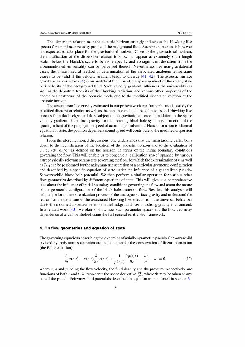
Figure 1. Acoustic surface gravity versus specific angular momentum of the flow for amono-transonic adiabatic accretion characterized by E = 0.06 and γ = 1.333 for threedifferent flow geometries: a flow in hydrostatic equilibrium in the vertical direction(solid green line), a constant thickness flow (long dashed black line) and the conicalmodel (dotted red line).

(u)rc = (cs)rc =√

κB/(μmH )T12 =

√2rc(rc − 1)

(5rc − 3)

[1

2(rc − 1)2− λ2

r3c

], (64)

r4c + �1r3

c + �2r2c + �3rc + �4 = 0, (65)

where

�1 = −1 + 8c2s

5c2s

, �2 = 3c2s + 2λ2

5c2s

, �3 = −4λ2

5c2s

, �4 = 2λ2

5c2s

, (66)

(du

dr

)rc

=√

1

2rc(rc − 1)(5rc − 3)

[5r2

c − 3

2(rc − 1)2− 2λ2(5r2

c − 9rc + 3)

r3c

] 12

, (67)

and the corresponding acoustic surface gravity

κ isoVE = ζ iso

VE

(r, cs,

du

dr

)rc

(68)

can be evaluated accordingly.

8. Dependence of the acoustic surface gravity on the flow geometry and initialboundary conditions

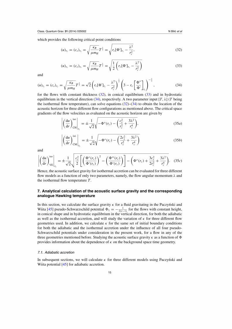
8.1. Adiabatic flow

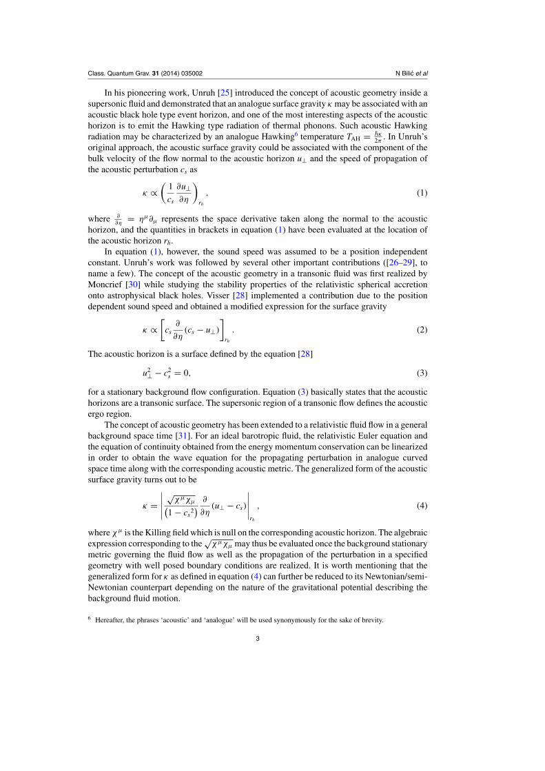
8.1.1. Mono-transonic accretion. Figure 1 shows the acoustic surface gravity κ as a functionof the specific angular momentum λ for a mono-transonic adiabatic accretion. The specificenergy and the polytropic index have been kept constant at the fixed values E = 0.06 andγ = 1.333, respectively. The range of λ for which κ has been calculated for a particular flowmodel constructs a subset in the [E, λ, γ ] parameter space for which the representative flow

20

Class. Quantum Grav. 31 (2014) 035002 N Bilic et al

models produces mono-transonic accretion for a fixed set of values of [E]. Alternative rangesfor λ for other similar subsets of [E, λ, γ ] parameter space may also be considered to studythe κ − λ profile for other fixed values of [E, γ ].

The solid green line represents the κ - λ profile for mono-transonic accretion in verticalequilibrium (VE), whereas the dotted red and the long dashed black lines represent suchdependence for a flow with constant height (CH) and for a conical flow (CM), respectively.

It is usually observed that κ varies with λ nonlinearly and non monotonically. For relativelylower values of the specific angular momentum, the acoustic surface gravity correlates withthe specific angular momentum and attains a peak characterized by an unique value of thespecific angular momentum denoted by λmax, and subsequently falls of with λ for λ > λmax.λmax is different for different flow models and one notes that

λCMmax > λVE

max > λCHmax. (69)

For a set of fixed values of [E, λ], for a particular flow model, λmax can be calculated completelyanalytically. We illustrate such procedure for a constant thickness flow. A similar proceduremay be applied to calculate λmax for the other two flow geometries.

For a constant thickness flow, equation (40) provides the dependence of κ on the criticalpoints, on the sound speed and its space gradient, and on the space gradient of the flowvelocity itself, everything evaluated at the acoustic horizon (the critical point). The quantities(cs)rc

, (dcs/dr)rcand (du/dr)rc

can be expressed as a function of rc and [E, λ, γ ] usingequations (37) and (40), respectively. The critical point rc itself can be computed in terms of[E, λ, γ ] by solving the polynomial in rc as represented through equation (38). Hence, theacoustic surface gravity κ for a constant thickness flow can be specified in terms of [E, λ, γ ].Analytical expression for κCH≡κCH [E, λ, γ ] can be maximized with respect to the specificangular momentum and the corresponding λmax can thus be obtained.

From figure 1, one should note that for the common range of the specific angularmomentum for which all three flow models will produce a mono-transonic flow for a fixedset of value of [E, λ], does not allow to explore the complete non monotonic κ - λ profile forall three flow models simultaneously. For example, for the common range of λ for which allthree flow geometries produce a mono-transonic accretion, for both the constant height flowand the conical model, the acoustic surface gravity κ will anti correlate with λ, whereas forthe full range of allowed λ for which a mono-transonic accretion forms at individual level, theκ - λ profile for both the aforementioned flows exhibits a maximum.

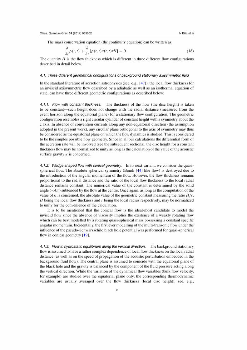
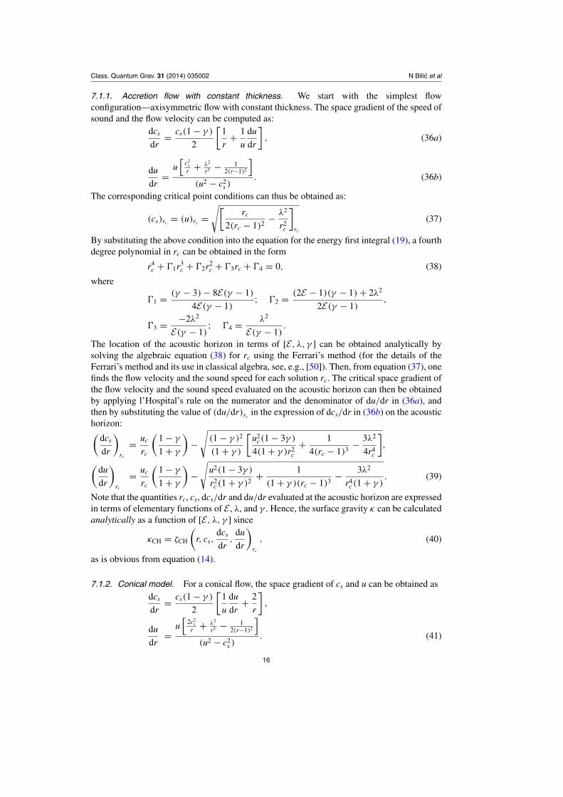
The κ - E profile depicted in figure 2 shows a similar behaviour. For a fixed set of [λ, γ ] fora constant height flow, κCH apparently correlates with E , whereas κCM and κVE anti-correlatewith E . Such a trend, however, does not provide the complete information about the κ - Eprofile in general since the range of E for which the figure is drawn is taken from the commonregion of [E, λ, γ ] space for which all the three flow geometries produce a mono-transonicaccretion for a fixed value of [λ, γ ]. If one allows κ to vary with E for the entire range of thespecific energy for which a particular flow model provides the mono-transonic accretion for afixed value of [λ, γ ], κ - E profile would have a non monotonic behaviour with a correspondingEmax separately for every flow configuration. The corresponding Emax for every flow modelcould then be estimated by maximizing the expression for the acoustic surface gravity withrespect to E by keeping [λ, γ ] constant. One thus understands that the ‘anti correlating’ κ - Eprofiles for a conical flow (represented by the dotted red curve) and for a flow in hydrostaticequilibrium along the vertical direction (solid green curve) are the post-peak (E > Emax)descending parts of the complete non monotonic κ - E profiles for the corresponding flowconfigurations. Similarly, the ‘correlating’ κ - E profile for a constant height flow (representedby the long dashed black curve) is the pre-peak (E < Emax) ascending part of the complete

21

Class. Quantum Grav. 31 (2014) 035002 N Bilic et al

Figure 2. Acoustic surface gravity versus specific energy of the flow for a mono-transonic adiabatic accretion characterized by λ = 1.835 and γ = 1.333 for threedifferent flow geometries: a flow in hydrostatic equilibrium in the vertical direction(solid green line), a constant thickness flow (long dashed black line) and the conicalmodel (dotted red line). Only the common range of specific energy for which all theflow configurations produce an adiabatic mono-transonic flow is presented. See text fordetails.

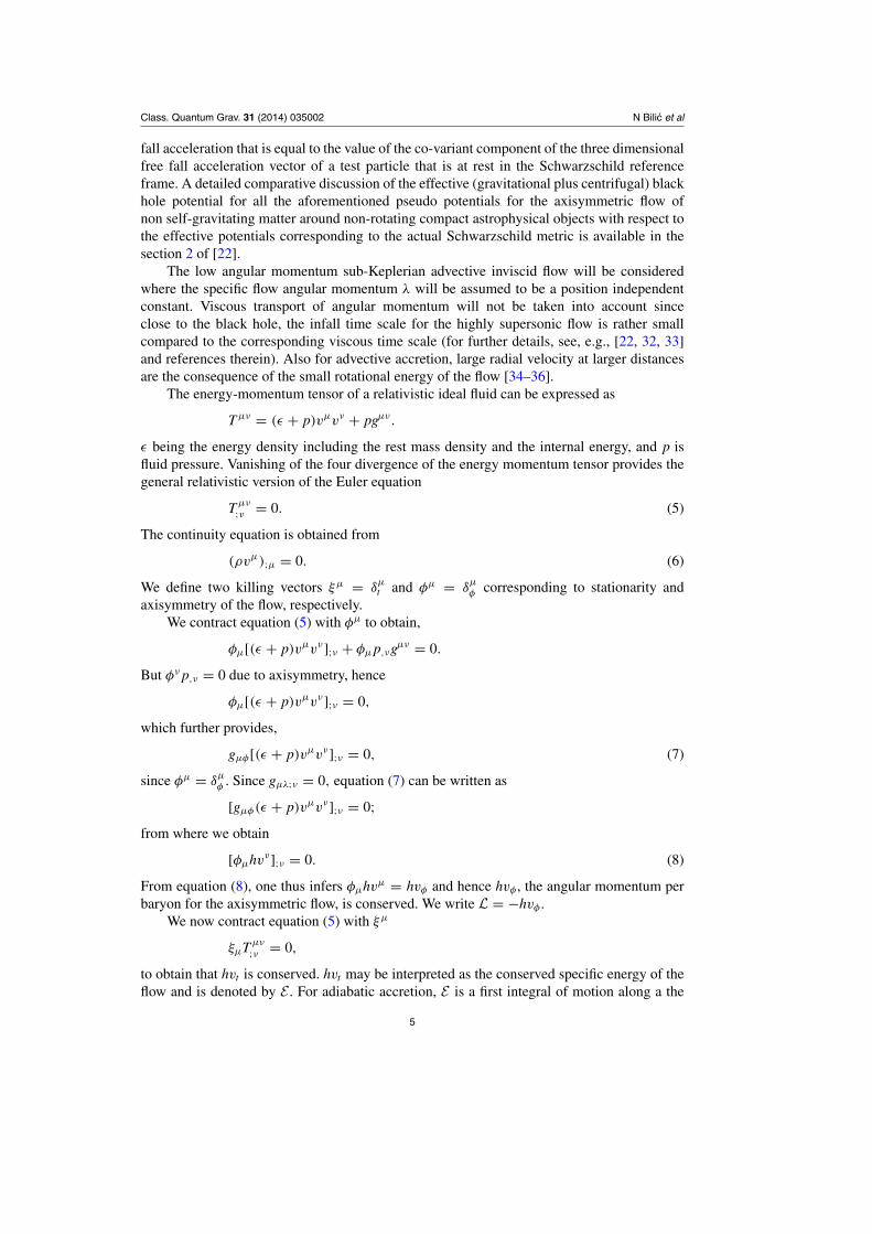
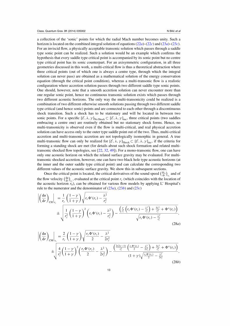
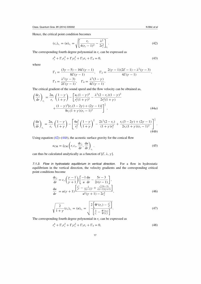
Figure 3. Aacoustic surface gravity versus specific energy of the flow for a mono-transonic adiabatic accretion characterized by λ = 1.85 and E = 0.06 for three differentflow geometries: the flow in hydrostatic equilibrium in the vertical direction (solid greenline), the constant thickness flow (long dashed black line) and the conical model (dottedred line).

non monotonic κ - E profile for the corresponding flow geometry. Hence, ECHmax is the largest

among all the values of Emax corresponding to all three different flow configurations.Figure 3 shows the κ - γ profile (for a fixed set of [E, λ]). It is obvious from the figure that

γ CHmax has the largest value among all three values of γmax corresponding to three different flow

22

Class. Quantum Grav. 31 (2014) 035002 N Bilic et al

configurations. Emax and γmax for any particular model can also be estimated by maximizing κ

with respect to the respective parameters.One thus understands that for a mono-transonic adiabatic accretion characterized by a fixed

set of values of [E, λ, γ ], the analogue surface gravity for three different flow configurationsexhibit the following trend

κadCM > κad

VE > κadCH. (70)

Hence for the adiabatic mono-transonic accretion, the flow in conical shape produces the largestwhereas the flow with constant thickness the lowest value TAH of the analogue Hawking liketemperature for the same set of initial boundary conditions.

As has been mentioned in section 5, a multi-transonic accretion with stationary shock maybe realized for all three different flow configurations for adiabatic as well as for isothermalaccretion, studied here in this work. For such flow topologies, two black hole type acoustichorizons form at the inner and the outer saddle type sonic points. The corresponding acousticsurface gravity κin and κout can be evaluated at the inner and the outer sonic points, respectively.It has been observed that the overall κin − [E, λ, γ ] as well as the κout − [E, λ, γ ] profilesare qualitatively similar to the κ − [E, λ, γ ] profile for all three flow configurations, where κ

is the acoustic surface gravity evaluated for the mono-transonic accretion. For all three flowgeometries considered in this work, the value of κout is, however, several orders of magnitudeless than the corresponding value of κin for the same set of initial boundary conditions. Thisis because the outer acoustic horizons form at a much larger distance away from the blackhole event horizon than the distance of the inner acoustic horizon. For a typical set of initialboundary conditions, the inner acoustic horizon may form at a distance 1.5–5 Schwarzschildradii away from the black hole event horizon whereas the outer acoustic horizon may belocated at 103–106 Schwarzschild radii away, or even more. The weakness of gravity at such alarge distance where the outer sonic horizons form restrict the acoustic surface gravity to takea small numerical value. The analogue Hawking temperatures evaluated at the inner and theouter acoustic horizons take on the correspondingly large and small values, respectively.

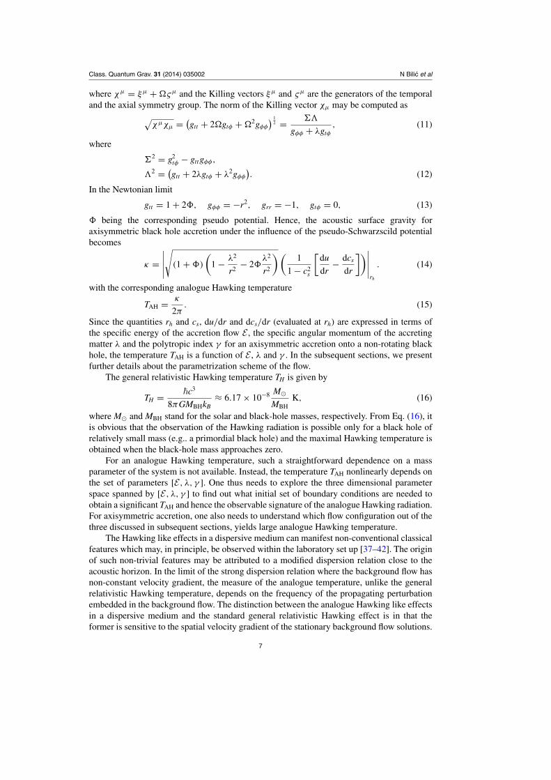
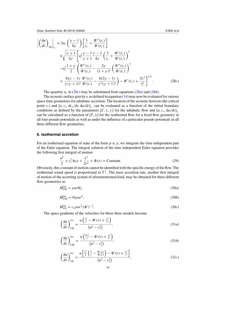
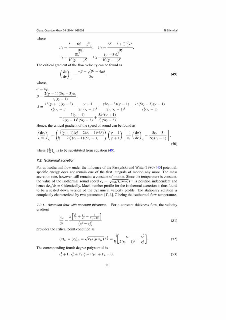
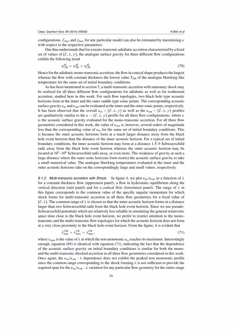
8.1.2. Multi-transonic accretion with Shock. In figure 4, we plot κin/κout as a function of λ

for a constant thickness flow (uppermost panel), a flow in hydrostatic equilibrium along thevertical direction (mid panel) and for a conical flow (lowermost panel). The range of λ inthis figure corresponds to the common value of the specific angular momentum for whichshock forms for multi-transonic accretion in all three flow geometries for a fixed value of[E, λ]. The common range of λ is chosen so that the inner acoustic horizon forms at a distancelarger than two Schwarzschild radii from the black hole event horizon. Since we use pseudo-Schwarzschild potentials which are relatively less reliable in simulating the general relativisticspace time close to the black hole event horizon, we prefer to restrict attention to the mono-transonic and the multi-transonic flow topologies for which the acoustic horizon does not format a very close proximity to the black hole event horizon. From the figure, it is evident that

λCMmax > λVE

max > λCHmax, (71)

where λmax is the value of λ at which the non monotonic κio reaches its maximum. Interestinglyenough, equation (69) is identical with equation (71), indicating the fact that the dependenceof the acoustic surface gravity on initial boundary conditions is similar for both the mono-and the multi-transonic shocked accretion in all three flow geometries considered in this work.Once again, the κin/κout - λ dependence does not exhibit the peaked non monotonic profilesince the common range corresponding to the shock forming λ is not sufficient to provide therequired span for the κin/κout - λ variation for any particular flow geometry for the entire range

23

Class. Quantum Grav. 31 (2014) 035002 N Bilic et al

Figure 4. The ratio of the acoustic surface gravities evaluated at the inner and outeracoustic horizons versus specific angular momentum for fixed E = 0.0002 and γ = 4/3of a multi-transonic flow for which a stationary shock may form.

of λ for which the corresponding flow model produces a shocked multi-transonic accretion fora fixed value of [E, λ].

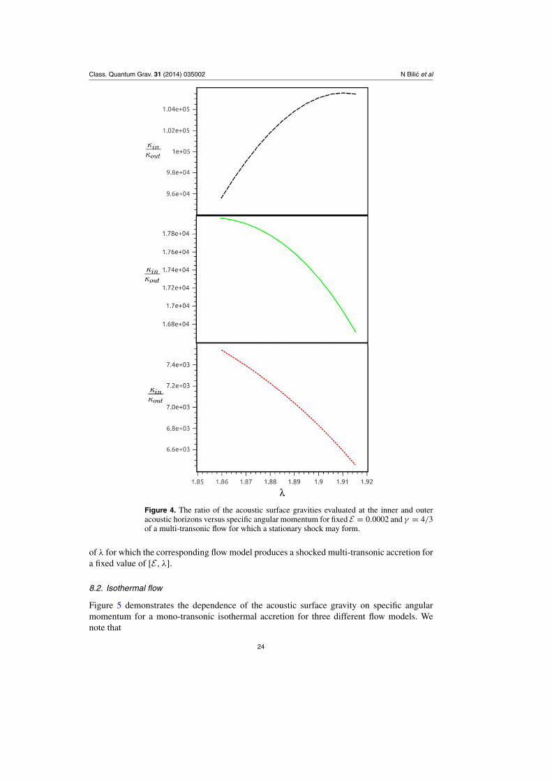
8.2. Isothermal flow

Figure 5 demonstrates the dependence of the acoustic surface gravity on specific angularmomentum for a mono-transonic isothermal accretion for three different flow models. Wenote that

24

Class. Quantum Grav. 31 (2014) 035002 N Bilic et al

Figure 5. Acoustic surface gravity versus specific angular momentum of the flow for amono-transonic isothermal accretion characterized by the isothermal flow temperatureT10 = 22 for three different flow geometries: the flow in hydrostatic equilibrium in thevertical direction (solid green line), the constant thickness flow (long dashed black line)and the conical model (dotted red line).

Figure 6. Acoustic surface gravity versus isothermal flow temperature for a mono-transonic isothermal accretion characterized by λ = 1.8 for three different flowgeometries: the flow in hydrostatic equilibrium in the vertical direction (solid greenline), the constant thickness flow (long dashed black line), and the conical model (dottedred line).

λCMmax > λVE

max > λCHmax. (72)

In figure 6, we plot the dependence of κ on the isothermal flow temperature T (scaled by afactor of 1010 degree Kelvin - T10≡T×10−10). We obtain

T CMmax > T VE

max > T CHmax. (73)

25

Class. Quantum Grav. 31 (2014) 035002 N Bilic et al

The value of λmax and Tmax for the mono-transonic isothermal flow may be estimated for allthree flow geometries in a way similar to what has been accomplished for an adiabatic flow.

9. Discussion

Axisymmetric accretion onto a non-rotating astrophysical black hole under the influence ofpseudo-Schwarzschild potentials is a natural example of classical analogue systems foundin the universe. The corresponding acoustic geometry may be studied for three differentflow configurations, viz, the accretion with constant flow thickness, the conical flow and theaccretion disc in hydrostatic equilibrium in the vertical direction. For each background flowgeometry, eight different configurations of acoustic geometry may be studied: adiabatic andisothermal accretion in four different pseudo potentials. For any specific pseudo potential, sixdifferent configurations of acoustic flow geometry may be studied: adiabatic and isothermalaccretion in three different flow geometries. For any geometric configuration of the adiabaticflow under the influence of a particular potential, three initial parameters, viz., the specificenergy E , the specific angular momentum λ and the adiabatic index of the flow γ completelyspecify the corresponding acoustic geometry. Similarly, for an isothermal flow in any potentialand with any flow geometry, two initial parameters, viz., the constant flow temperature T andthe specific angular momentum λ, completely specify the corresponding acoustic geometry.

Among six possible flow configurations for any particular pseudo potential used, only theadiabatic flow in vertical equilibrium exhibits an ‘effective’ sound speed which is a scaledversion of the adiabatic sound speed with a γ dependent scaling constant. The scaling constantbecomes unity for the isothermal flow. The reason is that for the accretion in vertical equilibriumthe flow thickness is a function of the adiabatic sound speed, as well as a function of the spacederivative of the pseudo potential used, since the expression for the flow thickness is obtainedby balancing the pressure gradient with the relevant component of the gravitational force. Oneshould, however, bear in mind that the corresponding expressions for the flow thickness in allthree flow geometries used are derived using a set of idealized assumptions. In principle, amore realistic derivation of the flow thickness may be worked out by employing the non-LTEradiative transfer [51, 52] or by taking recourse to the Grad–Shafranov equations for the MHDflow [53–55].

For a multi-transonic flow, two acoustic black holes are formed at two regular saddle typesonic points, whereas the acoustic white hole forms at the shock location, in agreement withthe results obtained by [24] and [13]. The acoustic surface gravity is formally infinite for theacoustic white hole since the flow velocity as well as the sound speed changes discontinuouslyat the shock location, in agreement with [56] .

The surface gravity κ (or TAH) profile obtained for a multi-transonic flow at the inneracoustic horizon is similar to the κ profile for a mono-transonic flow. This indicates thatirrespective of the phase topology, the surface gravity is basically determined by the physicalproximity of the acoustic horizon to the black hole event horizon. This is further supported bythe fact that irrespective of the flow geometry, pseudo potentials or the equation of state usedto describe the accretion flow, the value of κ at the outer acoustic horizon (for a multi-transonicflow) is much less than that evaluated at the inner acoustic horizon.

For a fixed set of [E, λ, γ ] describing an adiabatic accretion as well as for a fixed set of[T, λ] describing an isothermal accretion, the conical flow produces the largest whereas the flowwith constant thickness the smallest surface gravity and the analogue Hawking temperature.The accretion flow in hydrostatic equilibrium in the vertical direction provides the value ofκ and TAH in between the respective values of κ and TAH for the conical and the constant

26

Class. Quantum Grav. 31 (2014) 035002 N Bilic et al

thickness flow. The influence of the flow geometry in determining the acoustic surface gravityhas thus been successfully investigated in this work.

One of our major achievements is the analytical computation of the acoustic surfacegravity and the investigation of its dependence on various flow geometries and on variousaccretion parameters. However, one should note that this has been possible owing to a specificfeature of the chosen pseudo potential. With the Paczynski & Wiita (1980) [45] potential�1 = − 1

2(r−1), the energy first integral for the adiabatic accretion (19) as well as the critical

point condition for the isothermal flow (equations (40)–(42)) can be recast into a fourth degreepolynomial in rc (equivalently in rh) in an exactly solvable form. This has not been possiblewith other pseudo potentials, for which such an exactly solvable polynomial in rh cannot beconstructed. With other potentials, however, the surface gravity κ can still be studied as afunction of various flow parameters and flow geometries, with the help of numerical methods.Remarkably, it has been demonstrated in the literature ([21, 22] and references therein) thatout of the four pseudo-Schwarzschild potentials as shown in equation (43), the potential �1

mimics the Schwarzschild space time most efficiently in constructing the integral flow solutionfor transonic accretion.

However, even if one cannot employ a complete analytical calculation and even if �1 isthe most suitable potential to mimic a Schwarzschild space time, our generalized formalismfor the evaluation of [u, cs, dcs/dr, du/dr]rh

and the corresponding values of κ and TAH in termsof a general � is still important in the following sense. There exists a possibility that a newform of � more effective than �1 will be suggested in the future in order to approximate theSchwarzschild space time in constructing the integral accretion solutions for a transonic flow.In such a case, if a general model is capable of computing the acoustic surface gravity (andhence the analogue Hawking temperature) in a way presented in this work, then this modelwill be able to readily accommodate that novel form of the pseudo-Schwarzschild potentialwith no need to significantly change the fundamental structure of the formulation and thesolution scheme. In this case, one need not worry about providing any new unique schemevalid exclusively for a particular form of pseudo potential.

The methodology developed in this paper can also be used to construct the relevantacoustic geometry for the equatorial slice of the accretion flow under the influence of variouspseudo-Kerr potentials and to study the dependence of the surface gravity on black hole spin.Such work is in progress and will be reported elsewhere.

However, one should be cautious when using the pseudo potentials because none of thepotentials discussed here can be directly derived from the Einstein equations. These potentialsare used to obtain more accurate correction terms over and above the pure Newtonian results.Hence, any ‘radically new’ result obtained using these potentials should be cross checkedvery carefully against general relativity. Besides, one should bear in mind that these potentialsare not too reliable for modeling the space time in the very close neighborhood of the eventhorizon since strong gravity effects dominate in this region. Hence, our formalism may notbe quite realistic if the acoustic horizon forms very close to the black hole event horizon. Wethus consider only those initial boundary conditions for which rh > 2 ensuring our findings tobe trustworthy.

Acknowledgments

AC would like to acknowledge the kind hospitality provided by HRI, Allahabad, India, undera visiting student research programme. The visits of SN at HRI was partially supported byastrophysics project under the XIth plan at HRI. The work of TKD has been partially supported

27

Class. Quantum Grav. 31 (2014) 035002 N Bilic et al

by a research grant provided by S. N. Bose National Centre for Basic Sciences, Kolkata, India,under a guest scientist (long term sabbatical visiting professor) research programme. Theresearch of TKD is partially funded by the astrophysics project under the XIth plan at HRI.The work of NB has been supported by the Ministry of Science, Education and Sport of theRepublic of Croatia under contract no 098-0982930-2864. We would like to acknowledge thevery useful comments from the referees and the board members.

References

[1] Novello M, Visser M and Volovik G E (ed) 2002 Artificial Black Holes (Singapore: World Scientific)[2] Cardoso V 2005 Acoustic black holes arXiv:physics/0503042[3] Bercelo C, Liberati S and Visser M 2005 Living Rev. Relativ. 8 12 http://relativity.livingreviews.

org/Articles/lrr-2005-12/[4] Schutzhold R and Unruh W H (ed) 2007 Quantum Analogues: From Phase Transitions to Black

Holes and Cosmology (Berlin: Springer)[5] Philbin T G, Kuklewicz C, Robertson S, Hill S, Konig F and Leonhardt U 2008 Science

319 1367–70[6] Rousseaux G, Mathis C, Massa P, Philbin T G and Leonhardt U 2008 New J. Phys. 10 053015[7] Ousseaux G, Massa P, Mathis C, Coullet P, Philbin T G and Leonhardt U 2010 New J.

Phys. 12 095018[8] Weinfurtner S, Tedford E W, Penrice M C J, Unruh W G and Lawrence G A 2011 Phys. Rev.

Lett. 106 021302[9] Weinfurtner S, Tedford E W, Penrice M C J, Unruh W G and Lawrenc G A 2013 arXiv:1302.0375

[gr-qc][10] Das T K 2004 Class. Quantum Grav. 21 5253[11] Kinoshita S, Sendouda Y and Takahashi K 2004 Phys. Rev. D 70 123006[12] Dasgupta S, Bilic N and Das T K 2005 Gen. Rel. Gravit. 37 1877[13] Abraham H, Bilic N and Das T K 2006 Class. Quantum Grav. 23 2371[14] Naskar T, Chakravarty N, Bhattacharjee J K and Ray A K 2007 Phys. Rev. D 76 123002[15] Das T K, Bilic N and Dasgupta S 2007 J. Cosmol. Astropart. Phys. JCAP06(2007)009[16] Mach P and Malec E 2008 Phys. Rev. D 78 124016[17] Mach P 2009 Rep. Math. Phys. 64 257[18] Pu H-Y, Maity I, Das T K and Chang H-K 2012 Class. Quantum Grav. 29 245020[19] Abramowicz M A and Zurek W H 1981 Astrophys. J. 246 314–20[20] Kato S, Fukue J and Mineshige S 1998 Black Hole Accretion Disks (Kyoto University Press)[21] Artemova I V, Bjornsson G and Novikov I D 1996 Astrophys. J. 461 565[22] Das T K 2002 Astrophys. J. 577 880[23] Nag S, Acharya S, Ray A K and Das T K 2012 New Astron. 17 285[24] Bercelo C, Liberati S, Sonego S and Visser M 2004 New J. Phys. 6 186[25] Unruh W G 1981 Phys. Rev. Lett. 46 1351[26] Jacobson T A 1991 Phys. Rev. D 44 1731[27] Unruh W G 1995 Phys. Rev. D 51 2827[28] Visser M 1998 Class. Quantum Grav. 15 1767[29] Jacobson T A 1999 Prog. Theor. Phys. Suppl. 136 1[30] Moncrief V 1980 Astrophys. J.. 235 1038[31] Bilic N 1999 Class. Quantum Grav. 16 3953[32] Das T K, Pendharkar J K and Mitra S 2003 Astrophys. J. 592 1078[33] Das T K and Czerny B 2012 New Astron. 17 254[34] Beloborodov A M and Illarionov A F 1991 Mon. Not. R. Astron. Soc. 323 167[35] Igumenshchev I V and Beloborodov A M 1997 Mon. Not. R. Astron. Soc. 284 767[36] Proga D and Begelman M C 2003 Astrophys. J. 582 69[37] Rousseaux G, Mathis C, Massa P, Philbin T G and Leonhardt U 2008 New J. Phys. 10 053015[38] Rousseaux G, Massa P, Mathis C, Coullet P, Philbin T G and Leonhardt U 2010 New J.

Phys. 12 095018[39] Jannes G, Piquet R, Maissa P, Mathis C and Rousseaux G 2011 Phys. Rev. E 83 056312

28

Class. Quantum Grav. 31 (2014) 035002 N Bilic et al

[40] Weinfurtner S, Tedford E W, Penrice M C J, Unruh W G and Lawrence G A 2011 Phys. Rev.Lett. 106 021302

[41] Leonhardt U and Robertson S 2012 New J. Phys. 14 053003[42] Robertson S J 2012 J. Phys. B: At. Mol. Opt. Phys. 45 163001[43] Tarafdar P and Das T K 2013 Dependence of acoustic surface gravity on geometric configuration

of matter for axisymmetric background flow in Schwarzschild metric arXiv:1305.7134 [gr-qc][44] Bondi H 1952 Mon. Not. R. Astron. Soc. 112 195[45] Paczynski B and Wiita P J 1980 Astron. Astrophys. 88 23[46] Nowak M A and Wagoner R V 1991 Astrophys. J. 378 656[47] Frank J, King A and Raine D 2002 Accretion Power in Astrophysics (Cambridge: Cambridge

University Press)[48] Blaes O 1987 Mon. Not. R. Astron. Soc. 227 975[49] Chakrabarti S and Das S 2001 Mon. Not. R. Astron. Soc. 327 808[50] Kurosh A G 1972 Higher Algebra (Moscow: Mir)[51] Hubeny I and Hubeny V 1998 Astrophys. J. 505 558[52] Davis S W and Hubeny I 2006 Astrophys. J. Suppl. 164 530[53] Beskin V S 1997 Phys.–Usp. 40 659[54] Beskin V S and Tchekhovskoy A 2005 Astron. Astrophys. 433 619[55] Beskin V S 2009 MHD Flows in Compact Astrophysical Objects: Accretion, Winds and Jets (Berlin:

Springer)[56] Liberati S, Sonego S and Visser M 2000 Class. Quantum Grav. 17 2903

29