The Outperformance Probability of Mutual Funds - MDPI

Journal of

Risk and FinancialManagement

Article

The Outperformance Probability of Mutual Funds

Gabriel Frahm * and Ferdinand Huber

Chair of Applied Stochastics and Risk Management, Department of Mathematics and Statistics,Helmut Schmidt University, 22043 Hamburg, Germany* Correspondence: [email protected]

Received: 5 May 2019; Accepted: 19 June 2019; Published: 26 June 2019��

Abstract: We propose the outperformance probability as a new performance measure, which can beused in order to compare a strategy with a specified benchmark, and develop the basic statisticalproperties of its maximum-likelihood estimator in a Brownian-motion framework. The given resultsare used to investigate the question of whether mutual funds are able to beat the S&P 500 or theRussell 1000. Most mutual funds that are taken into consideration are, in fact, able to beat the market.We argue that one should refer to differential returns when comparing a strategy with a givenbenchmark and not compare both the strategy and the benchmark with the money-market account.This explains why mutual funds often appear to underperform the market, but this conclusionis fallacious.

Keywords: exchange traded funds; inverse coefficient of variation; mutual funds; outperformanceprobability; performance measurement; Sharpe ratio

JEL Classification: G11; G19

1. Motivation

The total value of assets under management in open-end funds was 46.7 trillion US dollarsat the end of 2018 (ICI 2019). Nowadays, investors and investment advisors have access to anabundant number of performance measures in order to compare investment vehicles with eachother. Most performance measures are based on the seminal work of Jensen (1968); Lintner (1965);Mossin (1966); Sharpe (1964 1966); Treynor (1961). The best-known performance measure is the Sharperatio, which divides the expected excess return on investment by the standard deviation of the excessreturn. Most other performance measures that can be found in the literature are based on the sameprinciple, i.e., they divide the return on investment by its risk, where the precise meaning of “return”and “risk” differs from one performance measure to another. A typical example is the expected excessreturn to value at risk, which goes back to Alexander and Baptista (2003) as well as Dowd (2000).Other examples are the conditional Sharpe ratio, in which case one chooses the expected shortfall,the tail conditional expectation, or similar downside risk measures as a denominator (Baweja et al.2015; Chow and Lai 2015). The number of possible combinations of numerators and denominatorsis practically unbounded. Depending on whether one chooses either the expected excess return orthe first higher partial moment as a numerator and some lower partial moment, drawdown measure,or some value-at-risk measure as a denominator, the resulting performance measure is called Omega(Keating and Shadwick 2002), Sortino ratio (Sortino et al. 1999), Calmar ratio (Young 1991), Sterlingratio (Kestner 1996), or Burke ratio (Burke 1994), etc. A nice overview of those performance measurescan be found in Table 1 of Eling and Schuhmacher (2006). However, it is evident that any list ofreturn-to-risk measures must be far from exhaustive.

In this work, we propose a new performance measure called outperformance probability (OP).It differs in many aspects from return-to-risk measures:

J. Risk Financial Manag. 2019, 12, 108; doi:10.3390/jrfm12030108 www.mdpi.com/journal/jrfm

http://www.mdpi.com/journal/jrfm

http://www.mdpi.com

http://dx.doi.org/10.3390/jrfm12030108

http://www.mdpi.com/journal/jrfm

https://www.mdpi.com/1911-8074/12/3/108?type=check_update&version=2

J. Risk Financial Manag. 2019, 12, 108 2 of 29

1. The OP compares some strategy with a specified benchmark, which need not necessarily be themoney-market account.

2. It is a probability. Thus, it is easy to understand also for a nonacademic audience, more precisely,for people who are not educated in statistics or probability theory.

3. The holding period of the investor is considered random. This enables us to compute theperformance of an investment opportunity for arbitrary liquidity preferences.

Ad 1: Most financial studies that make use of performance measures compare, e.g., the Sharperatio of some strategy, according to Sharpe (1966), with the Sharpe ratio of a benchmark. The Sharperatios measure the outperformance both of the strategy and of the benchmark with respect to themoney-market account, i.e., the riskless asset. Hence, one needs to calculate two performance measuresto evaluate the given strategy. By contrast, our approach is based on the idea of analyzing differentialreturns, not necessarily excess returns.1 This idea goes back to Sharpe (1994). To be more precise, sincewe do not use the money market as an anchor point, we need only one measure in order to comparetwo different investment opportunities. We will see that this sheds a completely different light on thequestion of whether or not one should prefer actively managed funds to passively managed funds.This fundamental question is still discussed in the finance literature and it is a commonplace that mostfund managers are not able to beat their benchmarks after accounting for all management fees andagency costs. We will come back to this point in Section 3.1. However, our empirical study reveals thatmost actively managed funds, in fact, are able to outperform their benchmarks. The reason for thisobservation might be explained as follows: The difference between the performance of two investmentopportunities is not the same as the performance of one investment opportunity compared to another.Simply put, in general, performance measures are not linear. Let RS be the return on some strategy,RB be the return on a benchmark, and r be the risk-free interest rate after some holding period.Further, let π be any performance measure. Hence, the performance of the strategy with respect tothe money-market account is π(RS − r), whereas π(RB − r) is the corresponding performance of thebenchmark. Now, the problem is that, in general,

π(RS − r)− π(RB − r) 6= π((RS − r)− (RB − r)

)= π(RS − RB) .

We suggest to calculate π(RS − RB) in order to understand whether or not the strategy is betterthan its benchmark and not to compare π(RS − r) with π(RB − r). By comparing π(RS − r) withπ(RB − r), one investigates the question of which of the two investment opportunities is better ableto outperform the money-market account. However, the fact that one investment opportunity is betterable to outperform the riskless asset than another investment opportunity does not imply that the firstinvestment opportunity outperforms the second one. This observation is crucial and we will providean analytical example in Section 2.4.

Ad 2: We do not claim that the OP is more practicable than other performance measures. Indeed,given the computational capacities that are nowadays available, it is quite easy to compute any otherperformance measure as well. Instead, we refer to a social problem that is frequently discussed instatistical literacy, namely that a major part of our population has no clear understanding of basicstatistics. Hence, most people cannot comprehend the precise meaning of “expected value,” “standarddeviation,” or “variance,” etc. Presumably, everybody of us knows that it is hard to explain thedifference between the sample mean and the expected value to the layman. The same holds trueregarding the empirical variance, sample variance, and population variance, etc. Further, our ownexperience shows that, at the beginning of their studies, many finance students have problems tounderstand the distinction between an ex-ante and an ex-post performance measure, which can be

1 Each excess return is a differential return but not vice versa.


attributed to the fact that they are struggling with statistics and probability theory.2 Thus, we areespecially concerned about the problem of financial literacy, not only regarding an academic audience.According to the OECD (2016), the “overall levels of financial literacy, indicated by combining scoreson knowledge, attitudes and behaviour are relatively low” in all 30 countries that participated in theOECD study. More precisely, it is reported that “only 42% of adults across all participating countriesand economies are aware of the additional benefits of interest compounding on savings” and that“only 58% could compute a percentage to calculate a simple interest on savings.” Moreover, “only abouttwo in three adults [. . . ] were aware that it is possible to reduce investment risk by buying a range ofdifferent stocks” and, in some countries, “no more than half of respondents understood the financialconcept of diversification.” The OECD study reveals a very low level of numeracy: Many peopleeven are not able to calculate the balance of an account after an interest payment of 2%. Similarresults can be found in the comprehensive review article by Lusardi and Mitchell (2013). For example,many people cannot say whether single stocks or mutual funds are more risky.3 In the light of thesefindings, we conclude that it is clearly impossible for most people in our population to comprehendthe core message of a return-to-risk measure. The OP is a probability and thus it can be much betterunderstood by a nonacademic audience—at least in an intuitive way. Hence, it might help bridgingtheory and practice.

Ad 3: Performance measures usually presume a fixed holding period. It is well-known that a givenperformance ratio cannot be extended to other holding periods without making any simplifying—andsometimes quite problematic—assumptions, which are frequently discussed in the literature see,e.g., Lin and Chou (2003); Lo (2002); Sharpe (1994). For example, suppose that the value process{St}t≥0 of some asset follows a geometric Brownian motion with drift coefficient µ ∈ R and diffusioncoefficient σ > 0.4 We may assume without loss of generality that the instantaneous risk-free interestrate per year is zero. Hence, the (excess) return on the asset at time T > 0 is given by

R = exp((

µ− σ2

2

)T + σWT

)− 1,

which means that the expected return is E(R) = eµT − 1. Further, the variance of the return amountsto Var(R) =

(eσ2T − 1

)e2µT . We conclude that the Sharpe ratio of the strategy is

Sh =1− e−µT√

eσ2T − 1.

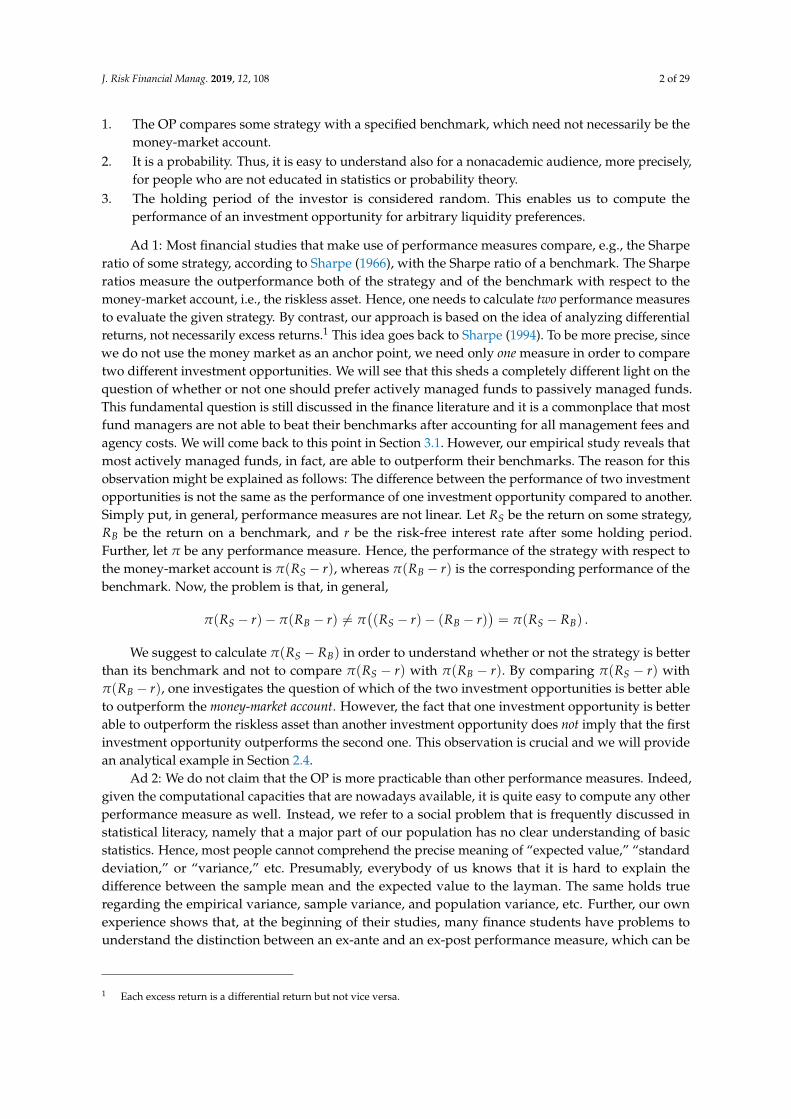
Figure 1 depicts the Sharpe ratio of two different assets depending on the holding period T.Asset 1 possesses the parameters µ1 = 0.1 and σ1 = 0.2, whereas Asset 2 has the parameters µ2 = 0.2and σ2 = 0.3. We can see that the Sharpe ratio is essentially determined by the time of liquidation.Interestingly, the Sharpe ratio is not linear and even not monotonic in time. If we use the Sharpe ratioas a performance measure, it can happen that we prefer Asset 1 for shorter holding periods but Asset 2for longer holding periods.5 Hence, the optimal choice between Asset 1 and Asset 2 heavily dependson the investment horizon. That is, in order to give a clear recommendation, we must know theholding period of the investor. However, most investors do not liquidate their strategies after a fixedperiod of time. More precisely, the time of liquidation is not known to them in advance, which meansthat it represents a random variable. We take the individual liquidity preference of the investor into

2 It is a matter of fact that some students do not understand even the distinction between parameter and estimator afterattending a statistics course.

3 According to Lusardi and Mitchell (2013, pp. 15–16), we can expect that a large number of people cannot understand thequestion at all because they are unfamiliar with stocks, bonds, and mutual funds.

4 From now on, we will omit the subscript “t ≥ 0” for notational convenience.5 In the given example, the critical time point is, approximately, T = 5 years.


account by specifying a holding-time distribution. Our approach is time-continuous, whereas mostother performance measures are based on a one-period model. This clearly distinguishes the OP fromother performance measures and we think that this is one of our main contributions to the literature.

Frahm and Huber, 2019 • The Outperformance Probability of Mutual Funds

0 2 4 6 8 100.1

0.2

0.3

0.4

0.5

0.6

0.7

0.8

0.9

1

Figure 1: Sharpe ratios as a function of time.

funds that try to beat the S&P 500 or the Russell 1000 stock-market index. We decided to choose

these funds because they focus on growth stocks in the US, have a large amount of assets under

management, and their issuers enjoy a good reputation. The question of whether or not it is

worth investing in actively managed funds at all is essential because if they do not outperform

their benchmarks, market participants might be better advised to refrain from investing their

money in those funds in favor of exchange traded funds (ETFs). More precisely, they should

prefer so-called index ETFs, which aim at tracking a stock-market index. Analogously, if it turns

out that the mutual funds are not able to outperform the bond market, it could be better to

buy some US treasury-bond ETFs.6 Further, it could happen that the money-market account is

preferable and, in the worst case, it is even better to keep the money under the mattress.

What are the merits of the OP compared to other performance measures?

1. The first one is conceptual:

(a) A simple thought experiment reveals that comparing two performance measures with

one another, where each one compares an investment opportunity with the money-

market account, can lead to completely different conclusions than evaluating only

one performance measure that compares the given investment opportunities without

taking the money-market account into consideration at all. The former comparison

refers to the question of which of the two investment opportunities is better able to

outperform the money-market account, whereas the latter comparison refers to the

6The reason why we focus on ETFs is discussed in Section 3.1.

6

Figure 1. Sharpe ratios as a function of time.

In order to test the OP of different trading strategies, we selected 10 actively managed mutualfunds that try to beat the S&P 500 or the Russell 1000 stock-market index. We decided to choose thesefunds because they focus on growth stocks in the US, have a large amount of assets under management,and their issuers enjoy a good reputation. The question of whether or not it is worth investing inactively managed funds at all is essential because if they do not outperform their benchmarks, marketparticipants might be better advised to buy exchange traded funds (ETFs). More precisely, they shouldprefer so-called index ETFs, which aim at tracking a stock-market index. Analogously, if it turns outthat the mutual funds are not able to outperform the bond market, it could be better to buy some UStreasury-bond ETFs.6 Further, it could happen that the money-market account is preferable and, in theworst case, it is even better to refrain from financial markets at all.

What are the merits of the OP compared to other performance measures?

1. The first one is conceptual:

(a) A simple thought experiment reveals that comparing two performance measureswith one another, where each one compares an investment opportunity with themoney-market account, can lead to completely different conclusions than evaluating onlyone performance measure that compares the given investment opportunities withouttaking the money-market account into consideration at all. The former comparisonrefers to the question of which of the two investment opportunities is better able tooutperform the money-market account, whereas the latter comparison refers to the questionof whether the first investment opportunity is able to outperform the second. In general,performance measures are not linear and so the former comparison does not imply the latter,i.e., an investment opportunity that is better able to produce excess returns than anotherinvestment opportunity need not be better than the other.

(b) Most performance measures presume that the holding period of the investor is fixed.This assumption is clearly violated in real-life because investors usually do not know,in advance, when they will liquidate all their assets. We solve this problem by incorporatingany holding-time distribution, which specifies the individual liquidity preference of the

6 The reason why we focus on ETFs is discussed in Section 3.1.


investor. It can be either discrete or continuous and it can have a finite or infinite rightendpoint. Any fixed holding period can be considered a special case, which means that wecan treat one-period models, too.

2. The second one is empirical:

(a) The natural logarithm of the assets under management of the mutual funds that are takeninto consideration are highly correlated with their inverse coefficient of variation (ICV).The ICV is a return-to-risk measure, which is based on differential log-returns but not(necessarily) on excess log-returns, and in the Brownian-motion framework it is the mainingredient of the OP. This means that capital allocation and relative performance arestrongly connected to one another, which suggests that market participants take differential(log-)returns implicitly into account when making their investment decisions.

(b) We emphasize our results by comparing the p-values of the differences between the Sharperatios of all mutual funds and the Sharpe ratios of the given benchmarks. The p-valuesindicate that it is hard to distinguish between the former and the latter Sharpe ratios.For this reason, we cannot say that any fund is better than the benchmark by comparing twoSharpe ratios with one another. A completely different picture evolves when consideringthe p-values of the ICVs of all funds with respect to their benchmarks. Those p-values aremuch lower and economically significant, i.e., it turns out that most funds are able to beattheir benchmarks.

The rest of this work is organized as follows: In Section 2 we present and discuss the OP. To be moreprecise, Section 2.1 contains our basic assumptions and our general definition of the OP. In Section 2.2we investigate its theoretical properties, whereas in Section 2.3 we derive the statistical propertiesof our maximum-likelihood (ML) estimator for the OP. Section 2.4 contains a general discussion ofthe OP compared to other performance measures. Further, Section 3 contains the empirical part ofthis work, in which we investigate the question of whether or not mutual funds are able to beattheir benchmarks. More precisely, in Section 3.1 we discuss some general observations related to theperformance of mutual funds and index ETFs, whereas Section 3.2 contains our empirical results fordifferent holding-time distributions. Our conclusion is given in Section 4.

2. The Outperformance Probability

2.1. Basic Assumptions and Definition

Let {St} be the value process of some trading strategy and {Bt} be the value process of abenchmark. We implicitly assume that {St} and {Bt} are, almost surely, positive. The strategy starts attime t = 0 and stops at some random time T > 0. Hence, T can be considered the time of liquidationand is referred to as the holding period. Throughout this work, time is measured in years. Moreover,we suppose that S0 = B0 = 1 without loss of generality.

Definition 1 (Outperformance probability). The OP is defined as Π = P(ST > BT

).

Hence, Π is the probability that the value of the strategy will be greater than the value of thebenchmark when the investor liquidates his strategy. The time of liquidation, T, is considered a randomvariable and so the law of total probability leads us to

Π = ET

[P(St > Bt | T = t

)].

The performance measure Π ranges between 0 and 1. In the case that Π = 1, the strategy isalways better than the benchmark, where “always” means “with probability 1,” i.e., almost surely.This can be considered a limiting case, which usually does not appear in real life because otherwise


the investor would have a weak arbitrage opportunity (Frahm 2016).7 By contrast, if we have thatΠ = 0, the benchmark turns out to be always at least as good as the strategy, which does not meanthat the benchmark is always better.8 More generally, if the strategy outperforms its benchmark withprobability Π, the benchmark outperforms the strategy with probability less than or equal to 1−Π.Therefore, the OP is not symmetric. Finally, if Π is near 0.5, there is no clear recommendation in favoror against the strategy. However, if a fund manager claims to be better than the benchmark, we shouldexpect Π to be greater than 0.5.

We make the basic assumption that the time of liquidation does not depend on whether or not thestrategy outperforms the benchmark, viz.

P(St > Bt | T = t

)= P

(St > Bt

), ∀ t ≥ 0 .

Put another way, the decision of the investor whether or not to terminate the strategy at time tdoes not depend on its performance relative to the benchmark. It follows that

Π = ET

[P(ST > BT

)]=∫ ∞

0P(St > Bt

)dF(t),

where F represents the cumulative distribution function of the holding period T.

2.2. Theoretical Properties

In this work, we rely on the standard model of financial mathematics, i.e., we suppose that {St}and {Bt} follow a 2-dimensional geometric Brownian motion. This means that the stochastic processesobey the stochastic differential equations

dSt

St= µS dt + σS dWSt and

dBt

Bt= µB dt + σB dWBt ,

where E(dWStdWBt

)= ρdt with −1 ≤ ρ ≤ 1. It follows that

[log(St)

log(Bt)

]∼ N

(γt, Σt

), ∀ t ≥ 0,

with

γ =

[γSγB

]=

[µS − σ2

S/2µB − σ2

B/2

]and Σ =

[σ2

S σSσBρ

σBσSρ σ2B

].

The numbers γS and γB are called the growth rates of {St} and {Bt}, respectively (Frahm 2016).Thus, we have that

X := log(

S1

B1

)∼ N

(µS − µB −

σ2S − σ2

B2

, σ2S + σ2

B − 2σSσBρ

).

Hence, the random variable X represents the relative log-return on the strategy with respect to itsbenchmark after the first period of time. We implicitly assume that

σ2S + σ2

B − 2σSσBρ > 0

7 More precisely, the strategy would dominate the benchmark in the sense of Merton (1973).8 P(X > Y) = 0 does not imply that P(X < Y) = 1 but P(X ≤ Y) = 1.


in order to avoid the case in which X is degenerate, i.e., constant with probability 1. In ourBrownian-motion framework, this happens if and only if Π ∈

{0, 1}

.It follows that

P(St > Bt

)= P(X > 0) = Φ

√t · µS − µB − (σ2

S − σ2B)/2√

σ2S + σ2

B − 2σSσBρ

,

where Φ is the cumulative distribution function of the standard normal distribution. This leads us to

Π =∫ ∞

0Φ

√t · µS − µB − (σ2

S − σ2B)/2√

σ2S + σ2

B − 2σSσBρ

dF(t) ,

which demonstrates that the OP essentially depends on the diffusion coefficient σS and not only on thedrift coefficient µS of the considered strategy.

For example, if we choose the money-market account as a benchmark, we obtain µB = r andσB = 0, where r is the instantaneous risk-free interest rate per year. In this standard case, the OPamounts to

Π =∫ ∞

0Φ

(√

t · µS − r− σ2S/2

σS

)dF(t).

In general, the benchmark is risky and we can see that the inverse coefficient of variation of thestrategy with respect to its benchmark, i.e.,

ICV :=E(X)

Std(X)=

µS − µB − (σ2S − σ2

B)/2√σ2

S + σ2B − 2σSσBρ

,

plays a crucial role when calculating the OP. Note that the ICV refers to the differential log-returnX = log(S1)− log(B1), not to the excess log-return log(S1)− r.

Now, we are ready for our first theorem. Its proof has already been given throughout the previousexplanations and so it can be skipped.

Theorem 1 (Outperformance probability). Under the aforementioned assumptions, the OP is given by

Π =∫ ∞

0Φ(√

t ICV)

dF(t). (1)

Hence, Π is strictly increasing in ICV. This means that the higher the ICV the higher the OP.9

However, under the given assumptions, the OP can never be 0 or 1.For example, suppose that the holding period is fixed and equal to T > 0. In this case, the OP

simply amounts to Π = Φ(√

T ICV). By contrast, if the holding period is uniformly distributed

between 0 and M > 0, we obtain

Π =1M

∫ M

0Φ(√

t ICV)

dt .

Further, if the holding period is exponentially distributed with parameter λ > 0, we have that

Π = λ∫ ∞

0Φ(√

t ICV)

e−λtdt ,

9 Thus, if a strategy has a higher OP than another strategy, given some holding-time distribution, the same holds true for anyother holding-time distribution.


and if we assume that T has a Weibull distribution with parameters κ > 0 and γ > 0, we obtain

Π =κ

γ

∫ ∞

0Φ(√

t ICV)( t

γ

)κ−1e−(t/γ)κ

dt .

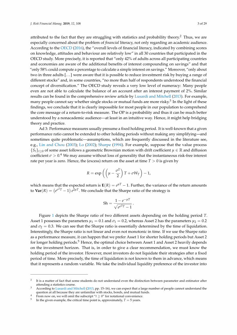
Note that for κ = 1 and γ = λ−1, the Weibull distribution turns into an exponential distributionwith parameter λ. It is evident that the spectrum of possibilities to capture the distribution of T isalmost infinite. In this work, we restrict to the aforementioned holding-time distributions. Obviously,F need not be continuous or even differentiable. The first holding-time distribution, which asserts thatT is a constant, is deterministic, which poses no problem at all, too.

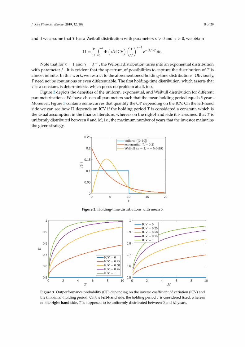
Figure 2 depicts the densities of the uniform, exponential, and Weibull distribution for differentparameterizations. We have chosen all parameters such that the mean holding period equals 5 years.Moreover, Figure 3 contains some curves that quantify the OP depending on the ICV. On the left-handside we can see how Π depends on ICV if the holding period T is considered a constant, which isthe usual assumption in the finance literature, whereas on the right-hand side it is assumed that T isuniformly distributed between 0 and M, i.e., the maximum number of years that the investor maintainsthe given strategy.


years that the investor maintains the given strategy.

0 5 10 15 200

0.05

0.1

0.15

0.2

0.25

Figure 2: Holding-time distributions with mean 5.

0 2 4 6 8 100.5

0.6

0.7

0.8

0.9

1

0 2 4 6 8 100.5

0.6

0.7

0.8

0.9

1

Figure 3: OP depending on the ICV and the (maximal) holding period. On the left-hand side, theholding period T is considered fixed, whereas on the right-hand side, T is supposed tobe uniformly distributed between 0 and M years.

2.3. Statistical Inference

Here, we propose a parametric estimator for Π, based on the assumption that the value processes

{St} and {Bt} follow a 2-dimensional geometric Brownian motion. Let

Xt = log(

St

St−∆

)− log

(Bt

Bt−∆

), t = ∆, 2∆, . . . , n∆,

12

Figure 2. Holding-time distributions with mean 5.


years that the investor maintains the given strategy.

0 5 10 15 200

0.05

0.1

0.15

0.2

0.25

Figure 2: Holding-time distributions with mean 5.

0 2 4 6 8 100.5

0.6

0.7

0.8

0.9

1

0 2 4 6 8 100.5

0.6

0.7

0.8

0.9

1

Figure 3: OP depending on the ICV and the (maximal) holding period. On the left-hand side, theholding period T is considered fixed, whereas on the right-hand side, T is supposed tobe uniformly distributed between 0 and M years.


Here, we propose a parametric estimator for Π, based on the assumption that the value processes

{St} and {Bt} follow a 2-dimensional geometric Brownian motion. Let

Xt = log(

St

St−∆

)− log

(Bt

Bt−∆

), t = ∆, 2∆, . . . , n∆,

12

Figure 3. Outperformance probability (OP) depending on the inverse coefficient of variation (ICV) andthe (maximal) holding period. On the left-hand side, the holding period T is considered fixed, whereason the right-hand side, T is supposed to be uniformly distributed between 0 and M years.



Here, we propose a parametric estimator for Π, based on the assumption that the value processes{St} and {Bt} follow a 2-dimensional geometric Brownian motion. Let

Xt = log(

St

St−∆

)− log

(Bt

Bt−∆

), t = ∆, 2∆, . . . , n∆,

be the difference between the log-return on the strategy and the log-return on the benchmark at time t.The period between t− ∆ and t, i.e., ∆ > 0, is fixed. Throughout this work, we assume that one yearconsists of 252 trading days and so we have that ∆ = 1/252.

The ML-estimator for the ICV is

ICVn =1√∆

1n ∑n∆

t=∆ Xt√1n ∑n∆

t=∆(Xt − 1

n ∑n∆t=∆ Xt

)2.

Our first proposition asserts that the ML-estimator for the ICV is strongly consistent.

Proposition 1. We have thatICVn

a.s.−→ ICV, n −→ ∞.

Proof. The strong law of large numbers implies that

1n

n∆

∑t=∆

Xta.s.−→ γS − γB and

1n

n∆

∑t=∆

(Xt −

1n

n∆

∑t=∆

Xt

)2a.s.−→ σ2

S + σ2B − 2σSσBρ

as n→ ∞. Hence, the continuous mapping theorem immediately reveals that ICVn converges almostsurely to ICV as the number of observations, n, grows to infinity.

The next proposition refers to the asymptotic distribution of√

n(ICVn − ICV

).

Proposition 2. We have that

√n(ICVn − ICV

) d−→ N(

0,1∆+

ICV2

2

), n −→ ∞ .

Proof. The ICV can be treated like a Sharpe ratio and thus 1 + ICV2/2 is the asymptotic variance of√n(ICVn − ICV

)in the case that ∆ = 1 (Frahm 2018, p. 6).

Hence, provided that the sample size n is large, the standard error of ICVn is

Std(ICVn

)≈√

1n∆

+ICV2

2n.

Our empirical study in Section 3 reveals that the ICV does not exceed 1 and, since the sample sizen is large, we can ignore the term ICV2/(2n).10 Note also that m := n∆ corresponds to the samplelength measured in years. Thus, we obtain the following nice rule of thumb:

Std(ICVn

)≈ 1√

m. (2)

10 This term can be attributed to the estimation error regarding the standard deviation of X (Frahm 2018).


The ML-estimator for Π is obtained, in the usual way, by substituting ICV with ICVn.

Definition 2 (ML-estimator). The ML-estimator for Π is given by

Πn =∫ ∞

0Φ(√

t ICVn

)dF(t).

The following theorem asserts that Πn is strongly consistent.

Theorem 2. We have thatΠn

a.s.−→ Π, n −→ ∞.

Proof. From Proposition 1 we already know that ICVn converges almost surely to ICV as n → ∞.According to Equation (1), we have that

Π : ICV 7−→∫ ∞

0Φ(√

t ICV)

dF(t)

and it is clear that Π is continuous in ICV. Hence, the continuous mapping theorem reveals that Πn

converges almost surely to Π as the number of observations, n, grows to infinity.

The next theorem provides the asymptotic distribution of√

n(Πn −Π

), which can be used in

order to calculate confidence intervals or conduct hypotheses tests. For this purpose, we need onlyassume that the expected value of

√T is finite.11 In fact, in most practical applications we even have

that E(T) < ∞, which holds true also for all holding-time distributions that are considered in thiswork. Hence, the moment condition is always satisfied.

Theorem 3. Assume that E(√

T)< ∞. We have that

√n(Πn −Π

) d−→ N(0, σ2), n −→ ∞,

with

σ2 =

(∫ ∞

0

√t φ(√

t ICV)

dF(t))2(

1∆+

ICV2

2

),

where φ is the probability density function of the standard normal distribution.

Proof. Note that

0 ≤ Φ(√

t x1)−Φ

(√t x0)

x1 − x0≤ dΦ

(√t x)

dx

∣∣∣∣∣x=0

=√

t φ(0)

for all x0 < x1 and t ≥ 0. Further, we have that∫ ∞

0

√t φ(0) dF(t) = φ(0)E

(√T)< ∞.

Thus, we can apply the dominated convergence theorem, i.e.,

dΠ(ICV)

dICV=

ddICV

∫ ∞

0Φ(√

t ICV)

dF(t) =∫ ∞

0

√t φ(√

t ICV)

dF(t).

11 This is true whenever E(Tk) < ∞ for any k ≥ 12 .


Now, by applying the delta method and using Proposition 2, we obtain

√n(Πn −Π

) d−→(∫ ∞

0

√t φ(√

t ICV)

dF(t))N(

0,1∆+

ICV2

2

), n −→ ∞ ,

which leads us to the desired result.

Hence, provided that n is sufficiently large, we can apply Theorem 3 in order to approximate thestandard error of Πn by

Std(Πn)≈ 1√

m

∫ ∞

0

√t φ(√

t ICVn

)dF(t).

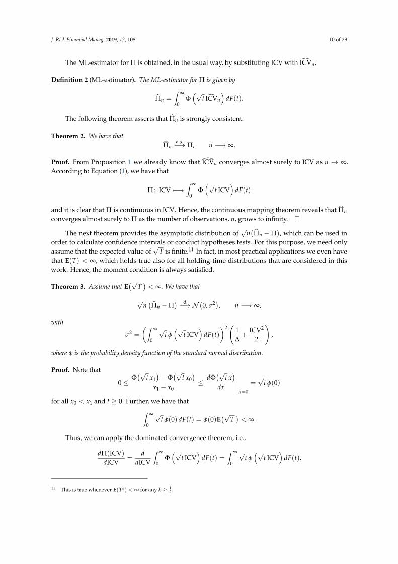
Figure 4 quantifies the standard error of Πn as a function of m, i.e., the years of observation,for different ICVs. Note that Std

(Πn)

is an even function of ICV and so we may focus on ICV ≥ 0.On the left-hand side it is assumed that T equals 5 years, whereas on the right-hand side T is supposedto be uniformly distributed between 0 and 10 years. Obviously, the specific choice of the holding-timedistribution is not essential for the standard errors. They are high even if the sample length, m, is big.This is a typical problem of performance measurement (Frahm 2018). Further, we can see that thestandard error of the ML-estimator essentially depends on the ICV. To be more precise, the higher theICV the lower the standard error.


0 5 10 15 200

0.2

0.4

0.6

0.8

1

0 5 10 15 200

0.2

0.4

0.6

0.8

1

Figure 4: Standard error of Πn depending on the ICV. On the left-hand side, the holding periodT is considered fixed and is equal to 5 years, whereas on the right-hand side, T issupposed to be uniformly distributed between 0 and 10 years.

A typical null hypothesis is H0 : Π ≤ Π0 ∈ (0, 1), which can be tested by means of the p-value

pn = Φ

(− Πn −Π0

Std(Πn))

.

More precisely, given some significance level α, H0 can be rejected if and only if pn < α, in which

case Π turns out to be significantly larger than Π0.

2.4. Discussion

Classical performance measures are based on the Capital Asset Pricing Model (CAPM). The

most prominent performance measures are the Sharpe ratio (Sharpe, 1966), the Treynor ratio

(Treynor, 1961), and Jensen’s Alpha (Jensen, 1968). Let R be the discrete return on some strategy

after a predefined period of time. Further, let r be the discrete risk-free interest rate after the

given holding period and RM be the return on the market portfolio.

Consider the linear regression equation

R− r = α + β(

RM − r)+ ε,

where α is the Alpha, β is the Beta, and ε represents the unsystematic risk of the strategy. Further,

let σ2ε be the variance of ε.

An actively managed fund aims at beating its benchmark. Let us suppose that the benchmark

16

Figure 4. Standard error of Πn depending on the ICV. On the left-hand side, the holding period T isconsidered fixed and is equal to 5 years, whereas on the right-hand side, T is supposed to be uniformlydistributed between 0 and 10 years.

A typical null hypothesis is H0 : Π ≤ Π0 ∈ (0, 1), which can be tested by means of the p-value

pn = Φ

(− Πn −Π0

Std(Πn))

.

More precisely, given some significance level α, H0 can be rejected if and only if pn < α, in whichcase Π turns out to be significantly larger than Π0.

2.4. Discussion

Classical performance measures are based on the Capital Asset Pricing Model (CAPM). The mostprominent performance measures are the Sharpe ratio (Sharpe 1966), the Treynor ratio (Treynor 1961),and Jensen’s Alpha (Jensen 1968). Let R be the discrete return on some strategy after a predefinedperiod of time. Further, let r be the discrete risk-free interest rate after the given holding period andRM be the return on the market portfolio.


Consider the linear regression equation

R− r = α + β(

RM − r)+ ε,

where α is the Alpha, β is the Beta, and ε represents the unsystematic risk of the strategy. Further, let σ2ε

be the variance of ε.An actively managed fund aims at beating its benchmark. Let us suppose that the benchmark is

the market portfolio. If the fund manager performs a strategy with β = 1, we have that

R− r = α +(

RM − r)+ ε

and so we obtain the differential return R− RM = α + ε. Hence, if we want to know whether or notthe fund is able to beat the market portfolio, we should analyze the differential return R− RM and notthe excess return R− r. More precisely, we should calculate the generalized Sharpe ratio according toSharpe (1994), i.e.,

Sh1994 =E(R− RM)

Std(R− RM)=

α

σε,

and not the ordinary Sharpe ratio (Sharpe 1966), i.e.,

Sh1966 =E(R)− rStd(R)

,

which is based on the CAPM (Lintner 1965; Mossin 1966; Sharpe 1964).What happens if the fund’s Beta does not equal 1? In this case we should compare the fund with

a benchmark strategy that possesses the Beta of the fund. Let β be the proportion of equity that isinvested in the market portfolio and 1− β be the proportion of equity that is deposited in the moneymarket. The corresponding (benchmark) return is thus

RB = βRM + (1− β)r = r + β(

RM − r).

Hence, we obtain the differential return R− RB = α + ε, which leads us to the same result asbefore, i.e., Sh1994 = α/σε.

Why is it so important to consider differential returns instead of excess returns if we want tounderstand whether or not a given strategy is able to outperform its benchmark? The most simpleillustration goes like this: Consider two random variables X and Y. The probability that X is positiveis P(X > 0) and the probability that Y is positive is P(Y > 0). Suppose that we want to knowthe probability that X exceeds Y. Then we would calculate P(X > Y) = P(X − Y > 0) but notP(X > 0)− P(Y > 0) and the same holds true for performance measurement.

This means that in order to judge whether or not a strategy is able to outperform its benchmarkwe should not compare one ordinary Sharpe ratio with another. Ordinary Sharpe ratios are calculatedon the basis of excess returns and so they answer the question of how good a given investmentopportunity is able to beat the money-market account. Analogously, by comparing P(X > 0) withP(Y > 0) we answer the question of whether it is more probable that X or that Y exceeds 0. However,in performance measurement we want to know whether or not a strategy is able to outperform itsbenchmark, which is a completely different question and it has nothing to do with the money-marketaccount. Analogously, we have to calculate the probability that X exceeds Y and not compare P(X > 0)with P(Y > 0).

This shall be illustrated, in financial terms, by a simple thought experiment. Suppose, for thesake of simplicity but without loss of generality, that the risk-free interest rate is zero. Further, let usassume that the return on some mutual fund is R = RM + ε, where ε is a positive random variable that


is uncorrelated with RM.12 Hence, the fund always yields a better return than the market portfolio andso it is clearly preferable. The ordinary Sharpe ratio of the market portfolio is

Sh1966M =

µMσM

,

where µM > 0 is the expected return on the market portfolio and σM > 0 represents the standarddeviation of the return on the market portfolio. Thus, we have that Sh1966

M > 0. By contrast, the ordinarySharpe ratio of the strategy is

Sh1966S =

µM + µε√σ2

M + σ2ε

,

where µε > 0 is the expected value and σ2ε > 0 is the variance of ε. We conclude that also Sh1966

Sis positive.

Now, depending on µε and σ2ε , we can construct situations in which the fund appears to be

better than the market portfolio and other situations in which it appears to be worse. To be moreprecise, we can find a positive random variable ε with a fixed expectation and an arbitrarily highvariance. For example, suppose that ε = γ + δξ, where γ, δ > 0 and ξ is a random variablesuch that P(ξ = 0) = 1− p and P(ξ = 1/p) = p > 0. Hence, we have that E(ε) = γ + δ andVar(ε) = δ2(1− p)/p, which means that Sh1966

S ↘ 0 as p ↘ 0. Put another way, it holds thatSh1966

S < Sh1966M if we make p sufficiently low. Nonetheless, the OP of the fund is

Π = P(R > RM) = P(ε > 0) = 1,

which means that the fund outperforms the market portfolio almost surely! It is evident that in sucha case every rational investor should prefer the fund.

Why do we come to such a misleading conclusion by comparing the two ordinary Sharpe ratioswith one another? The reason is that we analyze the marginal distributions of R and RM instead ofanalyzing their joint distribution. In fact, since ε is positive, it is better for the investor to have a largevariance σ2

ε , not a small one. Thus, it makes no sense to penalize the expected return on the fund by σ2ε ,

but this is precisely what we do when we calculate Sh1966S . However, it is worth noting that, in this

particular case, it makes no sense either to calculate the generalized Sharpe ratio

Sh1994S =

E(R− RM)

Std(R− RM)=

µε

σε.

The problem is that ε is positive, which means that σε is the wrong risk measure in that context.13

However, irrespective of the parameters µε and σε, we always have that Π = 1, which clearly indicatesthat the fund is better than its benchmark. We could imagine plenty of other examples that are lessstriking, but the overall conclusion remains the same: One should use differential (log-)returns insteadof excess (log-)returns when comparing some strategy with a benchmark.

The main goal of this work is to provide a performance measure that is better understandablefor a nonacademic audience. The OP is based on the ICV, which compares the log-return on thestrategy with the log-return on the benchmark. Thus, it is compatible with Sharpe’s (Sharpe 1994)principal argument and so we hope that it can serve its purpose in the finance industry. Most investorswant to know whether they can beat a risky benchmark, not the money-market account. It is worthemphasizing that the OP is based on a continuous-time model and we do not make any use of capitalmarket theory. For this reason, the OP cannot be compared with performance measures that are based

12 This is not a linear regression equation because E(ε) > 0.13 This kind of situation cannot happen in our Brownian-motion framework.


on a one-period model without making any simplifying assumption and thus sacrificing the meritsof continuous-time finance. This holds true, in particular, for the classical performance measuresmentioned above. The reason why we use log-returns instead of discrete returns is because our modelis time-continuous. More precisely, it is build on the standard assumption that the value processesfollow a geometric Brownian motion. It is worth noting that return-to-risk measures can changeessentially when substituting log-returns with discrete returns or vice versa—even if we work withdaily asset (log-)returns.

The classical performance measures are based on the CAPM and so they are vulnerable to a modelmisspecification. On the contrary, the OP is not based on any capital-market model—it is a probabilisticmeasure. Thus, it is model-independent although we assume that the value processes of the strategyand of the benchmark follow a 2-dimensional geometric Brownian motion. This assumption is madeonly for statistical reasons and it has nothing to do with the OP itself (see Definition 1). Hence,it is possible to find nonparametric estimators for the OP, which are not based on any parametric modelregarding the value processes of the strategy and of the benchmark. We plan to investigate such kindof estimators in the future.

Nonetheless, in this work we deal with the ML-estimator for Π and this estimator isnot unimpeachable:

• It is based on a parametric model, namely the geometric Brownian motion. While this modelis standard in financial mathematics, we may doubt that value processes follow a geometricBrownian motion in real life. The assumption that log-returns are independent and identicallynormally distributed contradicts the stylized facts of empirical finance.

• We assume that the time of liquidation does not depend on whether or not the strategyoutperforms the benchmark. This assumption might be violated, for example, if investors sufferfrom the disposition effect, i.e., if they tend to sell winners too early and ride losers too long(Shefrin and Statman 1985).

• Also the holding-time distribution follows a parametric model, which can either be true or false,too. Indeed, we have to choose some model for T but need not necessarily know its parameters.However, in order to estimate the parameters of F, we would need appropriate data and then thestatistical properties of the ML-estimator might change essentially.

The reader might ask whether we want to suggest a better alternative to return-to-risk measuresfrom a pure theoretical perspective or to provide a more illustrative performance measure for theasset-management industry. The answer is that we aim at both. However, it is worth emphasizing thatwe do not try to convince the audience that return-to-risk measures are useless or fallacious per se.In fact, the OP itself is based on a return-to-risk measure, namely the ICV, and we will see that this isthe most important ingredient of the OP. The question is whether one should use two return-to-riskmeasures or just one in order to compare a strategy with some benchmark. We decidedly propagate thelatter approach and refer to the arguments raised by Sharpe (1994). Simply put, performance measuresare not linear and so the difference between the performance of two investment opportunities is notthe same as the performance of the first investment opportunity compared to the second. Our ownreturn-to-risk measure is the ICV and we transform the ICV into a probability by treating the time ofliquidation stochastic. This is done in order to account for the individual liquidity preference of theinvestor and, especially, for a better practical understanding.

3. Empirical Investigation

3.1. General Observations

Actively managed funds usually aim at beating some benchmark, typically a stock-market index.Our financial markets and computer technology provide many possibilities in order to pursue thattarget. For example, we could think about stock picking, market timing, portfolio optimization,


technical analysis, fundamental analysis, time-series analysis, high-frequency trading, algorithmictrading, etc. The list of opportunities is virtually endless, but the problem is that most sophisticatedtrading strategies produce high transaction costs and other expenses like management fees andagency costs. The principal question is whether or not actively managed funds are able to beat theirbenchmarks after taking all expenses into account.

Jensen (1968) reports that the 115 (open-end) mutual funds that he considered in his study, whichcovers the period from 1945 to 1964, “were on average not able to predict security prices well enoughto outperform a buy-the-market-and-hold policy.” He states also that “there is very little evidencethat any individual fund was able to do significantly better than that which we expected from mererandom chance.” By contrast, Ippolito (1989) investigated 143 mutual funds over the period from 1965to 1984 and finds that “mutual funds, net of all fees and expenses, except load charges, outperformedindex funds on a risk-adjusted basis.” This is in contrast to many other studies, but he emphasizesthat “the industry alpha, though significantly positive, is not sufficiently large to overcome the loadcharges that characterize the majority of funds in the sample.” Hence, after taking sales charges orcommissions into account, the Alpha of mutual funds disappears. Further, Grinblatt and Titman (1989)considered the sample period from 1974 to 1984. They write that “superior performance may in factexist, particularly among aggressive-growth and growth funds and those funds with the smallestnet asset values.” However, “these funds also have the highest expenses so that their actual returns,net of all expenses, do not exhibit abnormal performance.” Hence, they come to the conclusion that“investors cannot take advantage of the superior abilities of these portfolio managers by purchasingshares in their mutual funds.” Finally, Fama and French (2010) considered the period from 1984 to 2006and they conclude that “fund investors in aggregate realize net returns that underperform three-factor,and four-factor benchmarks by about the costs in expense ratios,” which means that “if there are fundmanagers with enough skill to produce benchmark-adjusted expected returns that cover costs, theirtracks are hidden in the aggregate results by the performance of managers with insufficient skill.” Tosum up, it seems to be better for the market participants to track a stock-market index or to choose themarket portfolio.

There exists a large number of passively managed ETFs on the market, which aim at replicatinga specific stock-market index like the S&P 500 or the Russell 1000. Elton et al. (1996) vividly explainwhy it makes sense to compare actively managed funds with index ETFs, and not with stock-marketindices, in order to analyze whether or not fund managers are able to beat the market:

“The recent increase in the number and types of index funds that are available to individual investorsmakes this a matter of practical as well as theoretical significance. Numerous index funds, which trackthe Standard and Poor’s (S&P) 500 Index or various small-stock, bond, value, growth, or internationalindexes, are now widely available to individual investors. [. . . ] Given that there are sufficient indexfunds to span most investors’ risk choices, that the index funds are available at low cost, and that thelow cost of index funds means that a combination of index funds is likely to outperform an active fundof similar risk, the question is, why select an actively managed fund?”

Before the first index ETF, i.e., the SPDR S&P 500 ETF (SPY), came up in 1993, authors had tothink about how a private investor would replicate a stock index by himself. That is, they had to takeall transaction costs, exchange fees, taxes, time and effort, etc., into account. Index ETFs solved thatproblem all at once. There are no loading charges and, except for minor broker fees and very lowtransaction costs, private investors do not have to care about anything in order to track a stock index.Many index funds are very liquid and their tracking error seems to be very small. Thus, it is clear whyinvestors usually are not able or willing to replicate a stock-market index by themselves, which is thereason why we treat index ETFs as benchmarks in this work.

Compared to actively managed funds, index ETFs have much lower expense ratios, but theirperformance might be worse. In order to clarify whether or not the additional costs of an activelymanaged fund are overcompensated by a better performance, we compare 10 mutual funds with


index ETFs. Most of the funds contain US large-cap stocks and have 1 to 60 billion US dollars ofassets under management. In any case, they try to outperform the S&P 500 or the Russell 1000. Hence,our first benchmark is the SPDR S&P 500 ETF. This is almost equivalent to the S&P 500 total returnstock index, which serves as a proxy for the overall US stock market. The second benchmark is theiShares Russell 1000 Growth ETF (IWF). That ETF seeks to track the Russell 1000, which is composedof large- and mid-cap US equities exhibiting growth characteristics. In order to reflect the US mid-termtreasury-bond market, we chose the iShares 7–10 Year Treasury Bond ETF (IEF). This ETF is composedof US treasury bonds with remaining maturities between 7 and 10 years, including only AAA-ratedsecurities. Our next benchmark is the US money-market account, based on the London Inter-bankOffered Rate (LIBOR) for overnight US-dollar deposits. Our last benchmark is cash, without anyinterest or risk, i.e., “keeping the money under the mattress.” In this special case, the OP quantifiesthe probability that the final value of the strategy exceeds its initial value, i.e., Π = P(ST > 1).Hence, to outperform cash just means to generate a positive return, which is the least one shouldexpect when investing money.

Our empirical analysis is based on daily price observations from 2 January 2003, to 31 December2018. Hence, we take also the financial crisis 2008 into account. The length of that history amounts ton = 4027 trading days. All ETFs and mutual funds, together with their symbols, their estimated driftcoefficients (µ), diffusion coefficients (σ), growth rates (γ), expense ratios (ER), and their assets undermanagement (AUM) are presented in Table 1. It is separated into two parts: The first part shows thebenchmarks, whereas the second part contains the mutual funds. We can see that the expense ratios ofthe mutual funds are up to 90 basis points higher compared to the S&P 500 ETF (SPY). On average,investors pay 67 basis points more for a mutual fund compared to the S&P 500 ETF and 56 basispoints more compared to the Russell 1000 ETF (IWF). MSEGX possesses the highest drift coefficientand growth rate,14 whereas FKGRX has the lowest volatility, i.e., diffusion coefficient, among allmutual funds. PINDX has the lowest drift coefficient and growth rate but the second highest volatility.While the stock-index ETFs are hard to distinguish according to µ and σ, it should be noted that theRussell 1000 ETF has a slightly higher estimated growth rate, γ, compared to the S&P 500 ETF.

Table 1. Basic characteristics of the benchmarks and funds that are taken into consideration, i.e., theestimated drift coefficients (µ), diffusion coefficients (σ), growth rates (γ) as well as their expense ratios(ER) and assets under management (AUM).

Benchmark/Fund Symbol µ σ γ ER (%) AUM (bn $)

SPDR S&P 500 ETF SPY 0.0995 0.1815 0.0830 0.09 264.06iShares Russell 1000 Growth ETF IWF 0.1064 0.1774 0.0906 0.20 44.44iShares 7–10 Year Treasury Bond ETF IEF 0.0465 0.0656 0.0444 0.15 13.31Money market – 0.0100 0.0007 0.0100 – –Cash – 0 0 0 – –

Fidelity Blue Chip Growth FBGRX 0.1135 0.1919 0.0951 0.72 26.89T. Rowe Price Blue Chip Growth TRBCX 0.1200 0.1974 0.1005 0.70 60.37Franklin Growth A FKGRX 0.1064 0.1708 0.0918 0.84 14.96JPMorgan Large Cap Growth A OLGAX 0.1105 0.1900 0.0924 0.94 15.15Vanguard Morgan Growth VMRGX 0.1094 0.1889 0.0915 0.37 14.79Morgan Stanley Institutional Growth A MSEGX 0.1299 0.2164 0.1064 0.89 6.93BlackRock Capital Appreciation MAFGX 0.1060 0.1931 0.0873 0.76 3.13AllianzGI Focused Growth Fund Admin PGFAX 0.1129 0.1942 0.0940 0.99 1.02Goldman Sachs Large Cap Growth Insights GCGIX 0.1015 0.1829 0.0848 0.53 2.16Pioneer Disciplined Growth A PINDX 0.0993 0.2077 0.0777 0.87 1.22

� 0.1110 0.1933 0.0922 0.76 14.66

14 It holds that E(ST) = eµS T and so the drift coefficient µS can be considered the internal rate of return on the fund.


However, the quantities µ, σ, and γ are subject to estimation errors and it is well-known that theestimation errors regarding µ and γ are much higher than those regarding σ. Even if we work withdaily observations, they cannot be neglected. Hence, Table 1 gives no clear recommendation in favoror against the mutual funds if we compare the quantities of the index ETFs and the mutual funds witheach other. On average, the annualized drifts, volatilities, and growth rates of the mutual funds areclose to those of the S&P 500 ETF and the Russell 1000 ETF. Does the overall picture change if weevaluate the ordinary Sharpe ratios of the mutual funds?

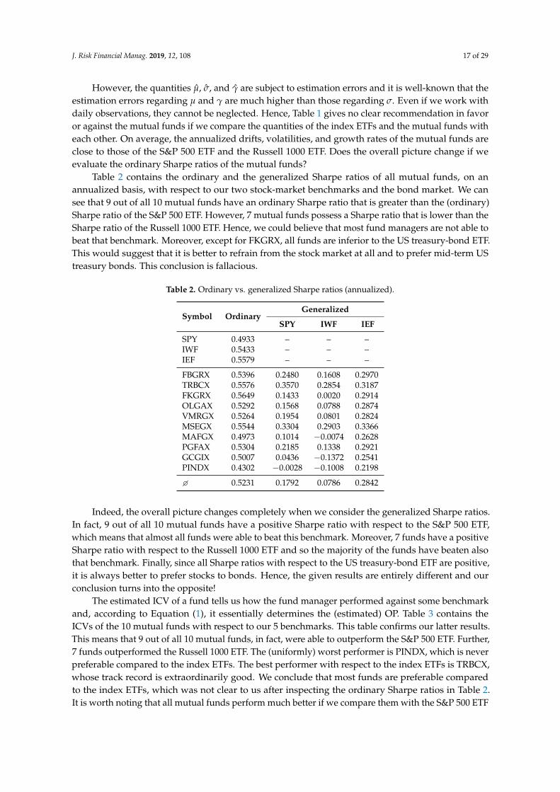
Table 2 contains the ordinary and the generalized Sharpe ratios of all mutual funds, on anannualized basis, with respect to our two stock-market benchmarks and the bond market. We cansee that 9 out of all 10 mutual funds have an ordinary Sharpe ratio that is greater than the (ordinary)Sharpe ratio of the S&P 500 ETF. However, 7 mutual funds possess a Sharpe ratio that is lower than theSharpe ratio of the Russell 1000 ETF. Hence, we could believe that most fund managers are not able tobeat that benchmark. Moreover, except for FKGRX, all funds are inferior to the US treasury-bond ETF.This would suggest that it is better to refrain from the stock market at all and to prefer mid-term UStreasury bonds. This conclusion is fallacious.

Table 2. Ordinary vs. generalized Sharpe ratios (annualized).

Symbol OrdinaryGeneralized

SPY IWF IEF

SPY 0.4933 – – –IWF 0.5433 – – –IEF 0.5579 – – –

FBGRX 0.5396 0.2480 0.1608 0.2970TRBCX 0.5576 0.3570 0.2854 0.3187FKGRX 0.5649 0.1433 0.0020 0.2914OLGAX 0.5292 0.1568 0.0788 0.2874VMRGX 0.5264 0.1954 0.0801 0.2824MSEGX 0.5544 0.3304 0.2903 0.3366MAFGX 0.4973 0.1014 −0.0074 0.2628PGFAX 0.5304 0.2185 0.1338 0.2921GCGIX 0.5007 0.0436 −0.1372 0.2541PINDX 0.4302 −0.0028 −0.1008 0.2198

� 0.5231 0.1792 0.0786 0.2842

Indeed, the overall picture changes completely when we consider the generalized Sharpe ratios.In fact, 9 out of all 10 mutual funds have a positive Sharpe ratio with respect to the S&P 500 ETF,which means that almost all funds were able to beat this benchmark. Moreover, 7 funds have a positiveSharpe ratio with respect to the Russell 1000 ETF and so the majority of the funds have beaten alsothat benchmark. Finally, since all Sharpe ratios with respect to the US treasury-bond ETF are positive,it is always better to prefer stocks to bonds. Hence, the given results are entirely different and ourconclusion turns into the opposite!

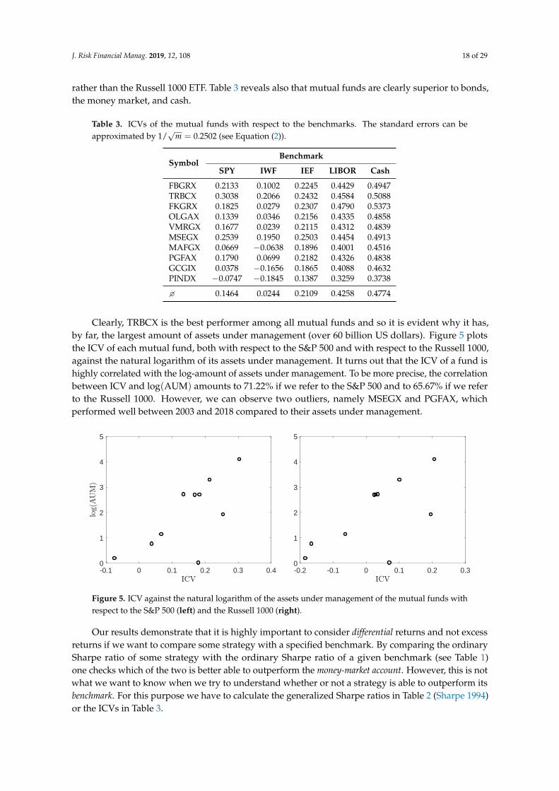
The estimated ICV of a fund tells us how the fund manager performed against some benchmarkand, according to Equation (1), it essentially determines the (estimated) OP. Table 3 contains theICVs of the 10 mutual funds with respect to our 5 benchmarks. This table confirms our latter results.This means that 9 out of all 10 mutual funds, in fact, were able to outperform the S&P 500 ETF. Further,7 funds outperformed the Russell 1000 ETF. The (uniformly) worst performer is PINDX, which is neverpreferable compared to the index ETFs. The best performer with respect to the index ETFs is TRBCX,whose track record is extraordinarily good. We conclude that most funds are preferable comparedto the index ETFs, which was not clear to us after inspecting the ordinary Sharpe ratios in Table 2.It is worth noting that all mutual funds perform much better if we compare them with the S&P 500 ETF


rather than the Russell 1000 ETF. Table 3 reveals also that mutual funds are clearly superior to bonds,the money market, and cash.

Table 3. ICVs of the mutual funds with respect to the benchmarks. The standard errors can beapproximated by 1/

√m = 0.2502 (see Equation (2)).

SymbolBenchmark

SPY IWF IEF LIBOR Cash

FBGRX 0.2133 0.1002 0.2245 0.4429 0.4947TRBCX 0.3038 0.2066 0.2432 0.4584 0.5088FKGRX 0.1825 0.0279 0.2307 0.4790 0.5373OLGAX 0.1339 0.0346 0.2156 0.4335 0.4858VMRGX 0.1677 0.0239 0.2115 0.4312 0.4839MSEGX 0.2539 0.1950 0.2503 0.4454 0.4913MAFGX 0.0669 −0.0638 0.1896 0.4001 0.4516PGFAX 0.1790 0.0699 0.2182 0.4326 0.4838GCGIX 0.0378 −0.1656 0.1865 0.4088 0.4632PINDX −0.0747 −0.1845 0.1387 0.3259 0.3738

� 0.1464 0.0244 0.2109 0.4258 0.4774

Clearly, TRBCX is the best performer among all mutual funds and so it is evident why it has,by far, the largest amount of assets under management (over 60 billion US dollars). Figure 5 plotsthe ICV of each mutual fund, both with respect to the S&P 500 and with respect to the Russell 1000,against the natural logarithm of its assets under management. It turns out that the ICV of a fund ishighly correlated with the log-amount of assets under management. To be more precise, the correlationbetween ICV and log(AUM) amounts to 71.22% if we refer to the S&P 500 and to 65.67% if we referto the Russell 1000. However, we can observe two outliers, namely MSEGX and PGFAX, whichperformed well between 2003 and 2018 compared to their assets under management.


Benchmark

Symbol SPY IWF IEF LIBOR Cash

FBGRX 0.2133 0.1002 0.2245 0.4429 0.4947TRBCX 0.3038 0.2066 0.2432 0.4584 0.5088FKGRX 0.1825 0.0279 0.2307 0.4790 0.5373OLGAX 0.1339 0.0346 0.2156 0.4335 0.4858VMRGX 0.1677 0.0239 0.2115 0.4312 0.4839MSEGX 0.2539 0.1950 0.2503 0.4454 0.4913MAFGX 0.0669 -0.0638 0.1896 0.4001 0.4516PGFAX 0.1790 0.0699 0.2182 0.4326 0.4838GCGIX 0.0378 -0.1656 0.1865 0.4088 0.4632PINDX -0.0747 -0.1845 0.1387 0.3259 0.3738

� 0.1464 0.0244 0.2109 0.4258 0.4774

Table 3: ICVs of the mutual funds with respect to the benchmarks. The standard errors can beapproximated by 1/

√m = 0.2502 (see Equation 2).

Russell 1000, against the natural logarithm of its assets under management. It turns out that the

ICV of a fund is highly correlated with the log-amount of assets under management. To be more

precise, the correlation between ICV and log(AUM) amounts to 71.22% if we refer to the S&P

500 and to 65.67% if we refer to the Russell 1000. However, we can observe two outliers, namely

MSEGX and PGFAX, which performed well compared to their assets under management.

-0.1 0 0.1 0.2 0.3 0.40

1

2

3

4

5

-0.2 -0.1 0 0.1 0.2 0.30

1

2

3

4

5

Figure 5: ICV against the natural logarithm of the assets under management of the mutual fundswith respect to the S&P 500 (left) and the Russell 1000 (right).

Our results demonstrate that it is highly important to consider differential returns and not

excess returns if we want to compare some strategy with a specified benchmark. By comparing

the ordinary Sharpe ratio of some strategy with the ordinary Sharpe ratio of a given benchmark

26

Figure 5. ICV against the natural logarithm of the assets under management of the mutual funds withrespect to the S&P 500 (left) and the Russell 1000 (right).

Our results demonstrate that it is highly important to consider differential returns and not excessreturns if we want to compare some strategy with a specified benchmark. By comparing the ordinarySharpe ratio of some strategy with the ordinary Sharpe ratio of a given benchmark (see Table 1)one checks which of the two is better able to outperform the money-market account. However, this is notwhat we want to know when we try to understand whether or not a strategy is able to outperform itsbenchmark. For this purpose we have to calculate the generalized Sharpe ratios in Table 2 (Sharpe 1994)or the ICVs in Table 3.


Our arguments shall be clarified also from a statistical point of view: Let ShSn be the empiricalestimator for the annualized Sharpe ratio of the strategy and ShBn be the empirical estimator for theannualized Sharpe ratio of the benchmark. Further, let ∆Sh := ShS − ShB be the difference betweenthe annualized Sharpe ratio of the strategy, ShS, and the annualized Sharpe ratio of the benchmark,i.e., ShB. Then one uses the test statistic ∆Shn := ShSn − ShBn in order to test the null hypothesisH0 : ∆Sh ≤ 0. Our results are presented on the right-hand side of Table 4, which contains also thecorresponding p-values for H0 in parentheses. By contrast, the left-hand side of Table 4 contains theestimated ICVs and their corresponding p-values for the null hypothesis H0 : ICV ≤ 0.15 We can seethat most p-values on the left-hand side are smaller than those on the right-hand side. This holds truein particular when we compare the funds with the Russell 1000 ETF and the US treasury-bond ETF.Hence, using the ICV instead of comparing two Sharpe ratios with one another in order to test whethera strategy outperforms its benchmark leads to results that are more significant in an economic sense.To be more precise, in the majority of cases, the estimated ICVs are positive and their p-values are lowenough in order to conclude that most fund managers are able to beat their benchmarks. However,the given results are still insignificant in a statistical sense.

Table 4. Test statistics ICVn and ∆Shn together with their corresponding p-values (in parentheses) forthe null hypotheses H0 : ICV ≤ 0 and H0 : ∆Sh ≤ 0, respectively.

SymbolICVn ∆Shn

SPY IWF IEF SPY IWF IEF

FBGRX 0.2133 0.1002 0.2245 0.0463 −0.0183 −0.0038(0.1970) (0.3444) (0.1848) (0.2908) (0.5168) (0.5233)

TRBCX 0.3038 0.2066 0.2432 0.0643 −0.0003 0.0142(0.1123) (0.2044) (0.1654) (0.2193) (0.5003) (0.4149)

FKGRX 0.1825 0.0279 0.2307 0.0717 0.0071 0.0216(0.2329) (0.4556) (0.1782) (0.1756) (0.4935) (0.3822)

OLGAX 0.1339 0.0346 0.2156 0.0360 −0.0286 −0.0141(0.2963) (0.4450) (0.1944) (0.3664) (0.5264) (0.5706)

VMRGX 0.1677 0.0239 0.2115 0.0331 −0.0315 −0.0170(0.2513) (0.4619) (0.1989) (0.3315) (0.5289) (0.6200)

MSEGX 0.2539 0.1950 0.2503 0.0611 −0.0035 0.0110(0.1550) (0.2178) (0.1585) (0.3071) (0.5032) (0.4575)

MAFGX 0.0669 −0.0638 0.1896 0.0040 −0.0606 −0.0460(0.3946) (0.6006) (0.2243) (0.4829) (0.5556) (0.7294)

PGFAX 0.1790 0.0699 0.2182 0.0371 −0.0275 −0.0130(0.2371) (0.3899) (0.1915) (0.3403) (0.5252) (0.5728)

GCGIX 0.0378 −0.1656 0.1865 0.0074 −0.0571 −0.0426(0.4400) (0.7460) (0.2280) (0.4587) (0.5524) (0.7818)

PINDX −0.0747 −0.1845 0.1387 −0.0631 −0.1277 −0.1131(0.6173) (0.7696) (0.2897) (0.7481) (0.6165) (0.8875)

3.2. Empirical Results

In this section, we present our estimates of the OPs for different holding-time distributions.More precisely, we consider a fixed, a uniformly distributed, an exponentially distributed, and aWeibull distributed holding period. In order to make the results comparable, we chose the parameterssuch that the mean holding period equals 5 years for each holding-time distribution.

Our principal question is whether or not actively managed funds are able to beat their benchmarks,which can be answered in a very simple way by estimating their OPs. In the case that Π ≤ 0.5, we can

15 All p-values have been computed by using the asymptotic results reported by Frahm (2018).


say that the fund manager is not able to beat the specified benchmark.16 Then it makes not much sensefor an investor to buy the fund share because, with probability greater or equal to 50%, the benchmarkperforms at least as good as the mutual fund. Hence, our null hypothesis is H0 : Π ≤ 0.5. Of course,we have to take estimation errors into account and so we report the estimated OPs along with theirstandard errors and p-values.

3.2.1. Fixed Holding Period

Let us begin by considering the holding period T > 0 fixed. In this case, the ML-estimator for theOP is simply Πn = Φ

(√T ICVn

). Further, its standard error is, approximately,

Std(Πn)≈√

Tm

φ(√

T ICVn).

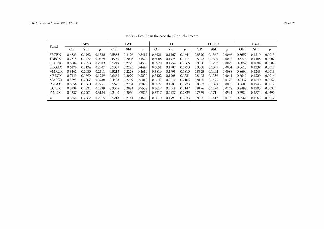
Table 5 contains the results if we assume that the holding period equals 5 years. We can see that9 out of the 10 mutual funds that are taken into consideration are able to outperform the S&P 500and 7 funds can outperform the Russell 1000. In fact, this follows also from Table 3 because the OP isgreater than 0.5 if and only if ICV > 0. Nonetheless, Table 5 provides some additional information.It reveals that the OPs typically range between 0.5 and 0.7 with regard to the index ETFs. An apparentexception is the T. Rowe Price Blue Chip Growth Fund (TRBCX), which has a tremendous OP of0.7515 with respect to the S&P 500. The worst fund is the Pioneer Disciplined Growth Fund (PINDX),which underperforms both the S&P 500 and the Russell 1000 with a quite small OP of 0.4337 and0.3400, respectively.

Despite the fact that most funds outperform their stock-market benchmarks, the results are notstatistically significant. All p-values that are related to the index ETFs exceed α = 0.05. Only TRBCXcomes very close to α with a p-value of 0.0779, given that we use the S&P 500 ETF as a benchmark.Of course, this does not mean that we have that Π ≤ 0.5 for any fund. Performance measurement isvery susceptible to estimation risk (Frahm 2018) and thus, in that context, we cannot expect to obtainstatistically significant results. Nevertheless, we may say that the results are, at least, economicallysignificant. This was surprising to us, since in the finance community it is usually asserted that fundmanagers, in general, do not better than their benchmarks. This was already discussed in Section 3.1.

All mutual funds outperform the bond market, but these results are not significant either.However, most funds at least outperform the money-market account and cash on a significancelevel of α = 0.01, which can be seen by the p-values at the end of Table 5. The corresponding OPsusually exceed 0.8, which means that the probability of generating some excess return or of making anyprofit at the time of liquidation is greater than 80%. Once again, an exception is PINDX, whose OPswith respect to the money-market account and cash are lower than 80%.

16 Note that this is precisely the case in which we have that ICV ≤ 0.


Table 5. Results in the case that T equals 5 years.

FundSPY IWF IEF LIBOR Cash

OP Std p OP Std p OP Std p OP Std p OP Std p

FBGRX 0.6833 0.1992 0.1788 0.5886 0.2176 0.3419 0.6921 0.1967 0.1644 0.8390 0.1367 0.0066 0.8657 0.1210 0.0013TRBCX 0.7515 0.1772 0.0779 0.6780 0.2006 0.1874 0.7068 0.1925 0.1414 0.8473 0.1320 0.0042 0.8724 0.1168 0.0007FKGRX 0.6584 0.2053 0.2203 0.5249 0.2227 0.4555 0.6970 0.1954 0.1566 0.8580 0.1257 0.0022 0.8852 0.1084 0.0002OLGAX 0.6176 0.2134 0.2907 0.5308 0.2225 0.4449 0.6851 0.1987 0.1758 0.8338 0.1395 0.0084 0.8613 0.1237 0.0017VMRGX 0.6462 0.2080 0.2411 0.5213 0.2228 0.4619 0.6819 0.1995 0.1810 0.8325 0.1402 0.0088 0.8604 0.1243 0.0019MSEGX 0.7149 0.1899 0.1289 0.6686 0.2029 0.2030 0.7122 0.1908 0.1331 0.8403 0.1359 0.0061 0.8640 0.1220 0.0014MAFGX 0.5595 0.2207 0.3938 0.4433 0.2209 0.6013 0.6642 0.2040 0.2105 0.8145 0.1496 0.0177 0.8437 0.1340 0.0052PGFAX 0.6556 0.2060 0.2251 0.5621 0.2204 0.3890 0.6872 0.1981 0.1723 0.8333 0.1398 0.0085 0.8603 0.1243 0.0019GCGIX 0.5336 0.2224 0.4399 0.3556 0.2084 0.7558 0.6617 0.2046 0.2147 0.8196 0.1470 0.0148 0.8498 0.1305 0.0037PINDX 0.4337 0.2201 0.6184 0.3400 0.2050 0.7825 0.6217 0.2127 0.2835 0.7669 0.1711 0.0594 0.7984 0.1574 0.0290

� 0.6254 0.2062 0.2815 0.5213 0.2144 0.4623 0.6810 0.1993 0.1833 0.8285 0.1417 0.0137 0.8561 0.1263 0.0047


3.2.2. Uniformly Distributed Holding Period

Now, we assume that the investor has a holding period that is uniformly distributed between 0and M years. The ML-estimator for Π is

Πn =1M

∫ M

0Φ(√

t ICVn

)dt

and its standard error can be approximated by

Std(Πn)≈ 1√

m1M

∫ M

0

√t φ(√

t ICVn

)dt.

Table 6 contains the results if we assume that the holding period is uniformly distributed between0 and 10 years. As we can see, the given results are not essentially different compared to those inTable 5. However, it is conspicuous that the OPs are slightly lower. The same effect can be observedalso in Figure 3 if we compare the OPs on the left-hand side for T = 5 with the OPs on the right-handside for M = 10. The reason is that liquidating a strategy with a positive ICV prematurely lowersthe OP. The problem is that later liquidations cannot compensate for earlier ones if the strategy isprofitable compared to its benchmark, i.e., ICV > 0.

While the OPs in Table 6 are slightly lower compared to those in Table 5, we can verify that allfunds are still better than the bond market. The majority of funds are even significantly better than themoney-market account and cash on a level of 1%. To sum up, in general, it is preferable to invest inmutual funds also if the holding period of the investor is uniformly distributed. However, there arenoticeable differences regarding the performance of the mutual funds, which means that investorsshould be aware that some funds perform much better than others. The question of whether or notthe estimated OP of a fund is a persistent performance measure is not answered in this study. If it ispersistent, i.e., if it can be used as an ex-ante and not only as an ex-post performance measure, investorsshould clearly prefer funds with a high estimated OP.


Table 6. Results in the case that T is uniformly distributed between 0 and 10 years.




� 0.6174 0.1917 0.2794 0.5200 0.2006 0.4621 0.6694 0.1841 0.1800 0.8030 0.1258 0.0114 0.8274 0.1113 0.0037


3.2.3. Exponentially Distributed Holding Period

In this section, we discuss the results that are obtained by assuming that the holding period isexponentially distributed. This distributional assumption might be considered more realistic than afixed or a uniformly distributed holding period. It assigns a high probability to early liquidationsand a low probability to late ones. The exponential distribution has no finite right endpoint, whichmeans that T is unbounded above. Hence, this distribution allows for large holding periods. However,the survival probability P(T > t) decreases exponentially with t.

The ML-estimator for the OP is

Πn = λ∫ ∞

0Φ(√

t ICVn

)e−λtdt ,

where λ > 0 is the parameter of the exponential distribution. The standard error of the ML-estimatorcan be approximated by

Std(Πn)≈ λ√

m

∫ ∞

0

√t e−λtφ

(√t ICVn

)dt.

We set the parameter λ to 0.2, which means that the mean holding period equals 5 years.The results are given by Table 7. As we can see, the OPs are, once again, slightly lower than thosein Table 6 and thus also lower than those in Table 5. The reason is that the exponential distributionassigns earlier liquidations a substantially higher probability than later ones (see Figure 2). The overallconclusion does not differ compared to our previous findings, but it is worth noting that the standarderrors and thus also the p-values are somewhat lower than in Tables 5 and 6. Now, we have a p-valueof 0.0675 for TRBCX against the S&P 500 ETF, which comes very close to the significance level of 5%.In any case, the mutual funds still outperform the bond market and the riskless investments, i.e., themoney market and cash.


Table 7. Results in the case that T is exponentially distributed with λ = 0.2.




� 0.6093 0.1771 0.2769 0.5187 0.1867 0.4618 0.6577 0.1685 0.1760 0.7784 0.1131 0.0101 0.8004 0.1009 0.0033


3.2.4. Weibull Distributed Holding Period

Finally, we report the results that are obtained by assuming that the holding period is Weibulldistributed. The Weibull distribution generalizes the exponential distribution and allows us to considerunimodal holding-time distributions with mode greater than 0 (see Figure 2). The correspondingML-estimator for the OP is

Πn =κ

γ

∫ ∞

0Φ(√

t ICVn

)( tγ

)κ−1e−(t/γ)κ

dt

and its standard error can be approximated by

Std(Πn)≈ κγ−κ

√m

∫ ∞

0tκ− 1

2 e−(t/γ)κφ(√

t ICVn

)dt.

In our empirical study, the parameters of the Weibull distribution are κ = 2 and γ = 5.6419.Once again, this leads us to a mean holding period of 5 years. The results are contained in Table 8.Now, we can observe that the OPs are close to those that are obtained with respect to the index ETFsby assuming that T = 5 is fixed (see Table 5). However, the OPs with respect to the US treasury-bondETF, the money-market account, and to cash are slightly lower than in Table 5 but still higher thanin Tables 6 and 7. Nonetheless, we can see that the given results are not very much driven by ourspecific assumption about the distribution of the holding period. It turns out that the OP is essentiallydetermined by the ICV, not by the holding-time distribution, provided that the considered holding-timedistributions have the same mean.


Table 8. Results in the case that T is Weibull distributed with κ = 2 and γ = 5.6419.




� 0.6201 0.1966 0.2801 0.5205 0.2053 0.4622 0.6734 0.1892 0.1811 0.8118 0.1316 0.0123 0.8374 0.1171 0.0041


4. Conclusions

We propose the OP as a new performance measure, especially for a nonacademic audience.It differs in many aspects from return-to-risk measures: (i) The OP compares some strategy with aspecified benchmark, not necessarily with the money-market account. (ii) It is easy to understand forpeople who are not educated in statistics or probability theory. (iii) The holding period of the investoris considered random. In our Brownian-motion framework, the OP is essentially determined by theICV, i.e., the expected annual relative log-return on the strategy with respect to its benchmark dividedby the standard deviation of that log-return. By contrast, the choice of the holding-time distributionseems to be secondary, provided that the mean holding period is the same for all distributions.

The ML-estimator for the OP is strongly consistent and, if the square root of the holding periodhas a finite expectation, it is also asymptotically normally distributed under the usual standardization.The moment condition is very mild and allows us to take almost any holding-time distributioninto consideration. Our asymptotic results enable us to calculate confidence intervals or to conducthypotheses tests. The basic null hypothesis is that the OP does not exceed 50%, which means thatthe strategy does not outperform its benchmark. Our empirical results reveal that most mutualfunds, in fact, are able to beat their benchmarks, although the results are not statistically significant.Nonetheless, they are economically significant. This might be surprising because it is a commonplacein the finance literature that most fund managers cannot beat the market. However, the crucial point isthat one should refer to differential returns when comparing some strategy with a given benchmark,not to excess returns.

The best performer is the T. Rowe Price Blue Chip Growth Fund, whereas the worst one is thePioneer Disciplined Growth Fund. It is evident that market participants prefer to invest their moneyin those funds that have a high ICV with respect to the S&P 500 or the Russell 1000. More precisely,the ICV with respect to any index ETF is highly correlated with the log-amount of assets undermanagement of the mutual fund. This means that relative performance and capital allocation arestrongly connected to one another, which suggests that market participants take differential returnsimplicitly into account when making their investment decisions.

Author Contributions: G.F. developed the theoretical part, whereas both authors are responsible for the empiricalpart of this work.

Funding: This research received no external funding.

Acknowledgments: We would like to thank Philipp Adämmer and Alexander Jonen for our helpful discussionson the manuscript.

Conflicts of Interest: The authors declare no conflict of interest.

References

Alexander, Gordon J., and Alexandre M. Baptista. 2003. Portfolio performance evaluation using value at risk.Journal of Portfolio Management 29: 93–102. [CrossRef]

Baweja, Meena, Ratnesh R. Saxena, and Deepak Sehgal. 2015. Portfolio optimization using conditional Sharperatio. International Letters of Chemistry, Physics and Astronomy 53: 130–36. [CrossRef]

Burke, Gibbons. 1994. A sharper Sharpe ratio. Futures 23: 56.Chow, Victor, and Christine W. Lai. 2015. Conditional Sharpe ratios. Finance Research Letters 12: 117–33. [CrossRef]Dowd, Kevin. Adjusting for risk: An improved Sharpe ratio. International Review of Economics and Finance 9: 209–22.

[CrossRef]Eling, Martin, and Frank Schuhmacher. 2006. Hat die Wahl des Performancemaßes einen Einfluss auf die

Beurteilung von Hedgefonds-Indizes? Kredit und Kapital 39: 419–54.Elton, Edwin J., Martin J. Gruber, and Christopher R. Blake. 1996. The persistence of risk-adjusted mutual fund

performance. Journal of Business 69: 133–57.Fama, Eugene F., and Kenneth R. French. 2010. Luck versus skill in the cross-section of mutual fund returns.

Journal of Finance 65: 1915–47.

http://dx.doi.org/10.1111/j.1540-6261.2010.01598.x

http://dx.doi.org/10.3390/risks6020040

http://dx.doi.org/10.1086/296468

http://dx.doi.org/10.1142/S0219024916500060


Frahm, Gabriel. 2016. Pricing and valuation under the real-world measure. International Journal of Theoretical andApplied Finance 19. [CrossRef]

Frahm, Gabriel. 2018. An intersection-union test for the Sharpe ratio. Risks 6. [CrossRef]Grinblatt, Mark, and Sheridan Titman. 1989. Mutual fund performance: An analysis of quarterly portfolio holdings.

Journal of Business 62: 393–416. [CrossRef]ICI. 2019. Worldwide Regulated Open-End Fund Assets and Flows, Fourth Quarter 2018. Available online:

https://www.iciglobal.org/iciglobal/research/stats/ww/ci.ww_q4_18.global (accessed on 6 April 2019).[CrossRef]

Ippolito, Richard A. 1989. Efficiency with costly information: A study of mutual fund performance, 1965–1984.Quarterly Journal of Economics 104: 1–23. [CrossRef]

Jensen, Michael C. 1968. The performance of mutual funds in the period 1945–1964. Journal of Finance 23: 389–416.[CrossRef]

Keating, Con, and William F. Shadwick. 2002. A universal performance measure. Journal of Performance Measurement6: 59–84.

Kestner, Lars N. 1996. Getting a handle on true performance. Futures 25: 44–46.Lin, Mei-Chen, and Pin-Huang Chou. 2003. The pitfall of using Sharpe ratio. Finance Letters 1: 84–89. [CrossRef]Lintner, John. 1965. The valuation of risky assets and the selection of risky investments in stock portfolios and

capital budgets. Review of Economics and Statistics 47: 13–37.Lo, Andrew W. 2002. The statistics of Sharpe ratios. Financial Analysts Journal 58: 36–52. [CrossRef]Lusardi, Annamaria, and Olivia S. Mitchell. 2013. The Economic Importance of Financial Literacy: Theory and Evidence.

Technical Report. Cambridge: National Bureau of Economic Research.Merton, Robert C. 1973. Theory of rational option pricing. Bell Journal of Economics and Management Science

4: 141–83.Mossin, Jan. 1966. Equilibrium in a capital asset market. Econometrica 34: 768–83. [CrossRef]OECD. 2016. OECD/INFE International Survey of Adult Financial Literacy Competencies. Technical Report.

Paris: OECD. [CrossRef]Sharpe, William F. 1964 Capital asset prices: A theory of market equilibrium under conditions of risk. Journal of

Finance 19: 425–42. [CrossRef]Sharpe, William F. 1966. Mutual fund performance. Journal of Business 39: 119–38.Sharpe, William F. 1994. The Sharpe ratio. Journal of Portfolio Management 21: 49–58. [CrossRef]Shefrin, Hersh, and Meir Statman. 1985. The disposition to sell winners too early and ride losers too long: Theory

and evidence. Journal of Finance 40: 777–90. [CrossRef]Sortino, Frank, Robert Van Der Meer, and Auke Plantinga. 1999. The Dutch triangle. Journal of Portfolio Management

26: 50–58. [CrossRef]Treynor, Jack L. 1961. Market value, time, and risk. Available online: https://dx.doi.org/10.2139/ssrn.2600356

(accessed on 25 June 2019).Young, Terry W. 1991. Calmar ratio: A smoother tool. Futures 20: 1. [CrossRef]

c© 2019 by the authors. Licensee MDPI, Basel, Switzerland. This article is an open accessarticle distributed under the terms and conditions of the Creative Commons Attribution(CC BY) license (http://creativecommons.org/licenses/by/4.0/).

http://dx.doi.org/10.1142/S0219024916500060

http://dx.doi.org/10.1086/294846

http://dx.doi.org/10.3905/jpm.1999.319775

https://www.iciglobal.org/iciglobal/research/stats/ww/ci.ww_q4_18.global


http://dx.doi.org/10.1111/j.1540-6261.1985.tb05002.x

http://dx.doi.org/10.18052/www.scipress.com/ILCPA.53.130

http://dx.doi.org/10.2307/3003143

http://dx.doi.org/10.2307/1910098

http://dx.doi.org/10.1016/j.frl.2014.11.001

http://dx.doi.org/10.2469/faj.v58.n4.2453

http://dx.doi.org/10.1016/S1059-0560(00)00063-0

http://dx.doi.org/10.2307/1924119


http://dx.doi.org/10.2307/2937832

https://dx.doi.org/10.2139/ssrn.2600356

http://dx.doi.org/10.1111/j.1540-6261.1968.tb00815.x

http://creativecommons.org/

http://creativecommons.org/licenses/by/4.0/.

The Outperformance Probability of Mutual Funds - MDPI

Documents

Transcript of The Outperformance Probability of Mutual Funds - MDPI