The OPTX Project. I. The Flux and Redshift Catalogs for the CLANS, CLASXS, and CDF-N Fields

arX

iv:0

811.

0824

v1 [

astr

o-ph

] 5

Nov

200

8Draft version February 25, 2013Preprint typeset using LATEX style emulateapj v. 08/22/09

THE OPTX PROJECT I: THE FLUX AND REDSHIFT CATALOGS FOR THECLANS, CLASXS, AND CDF-N FIELDS1

L. Trouille2, A. J. Barger2,3,4, L. L. Cowie4, Y. Yang5, and R. F. Mushotzky6

Draft version February 25, 2013

ABSTRACT

We present the redshift catalogs for the X-ray sources detected in the Chandra Deep Field North(CDF-N), the Chandra Large Area Synoptic X-ray Survey (CLASXS), and the Chandra LockmanArea North Survey (CLANS). The catalogs for the CDF-N and CLASXS fields include redshiftsfrom previous work, while the redshifts for the CLANS field are all new. For fluxes above 10−14

ergs cm−2 s−1 (2−8 keV) we have redshifts for 76% of the sources. We extend the redshift informationfor the full sample using photometric redshifts. The goal of the OPTX Project is to use these threesurveys, which are among the most spectroscopically complete surveys to date, to analyze the effectof spectral type on the shape and evolution of the X-ray luminosity functions and to compare theoptical spectral types with the X-ray spectral properties.

We also present the CLANS X-ray catalog. The nine ACIS-I fields cover a solid angle of ∼0.6 deg2

and reach fluxes of 7×10−16 ergs cm−2 s−1 (0.5−2 keV) and 3.5×10−15 ergs cm−2 s−1 (2−8 keV). Wefind a total of 761 X-ray point sources. Additionally, we present the optical and infrared photometriccatalog for the CLANS X-ray sources, as well as updated optical and infrared photometric catalogsfor the X-ray sources in the CLASXS and CDF-N fields.

The CLANS and CLASXS surveys bridge the gap between the ultradeep pencil-beam surveys, suchas the CDFs, and the shallower, very large-area surveys. As a result, they probe the X-ray sourcesthat contribute the bulk of the 2− 8 keV X-ray background and cover the flux range of the observedbreak in the logN−logS distribution. We construct differential number counts for each individualfield and for the full sample.Subject headings: cosmology: observations — galaxies: active

1. INTRODUCTION

We combine data from the Chandra Deep Field North(CDF-N), the Chandra Large Area Synoptic X-ray Sur-vey (CLASXS), and the Chandra Lockman Area NorthSurvey (CLANS) to provide one of the most spectroscop-ically complete large samples of Chandra X-ray sourcesfor use in the OPTX Project. In this article, the firstin the OPTX Project series, we present the databasethat we use in Yencho et al. (2008) to examine the X-rayluminosity functions and their dependence on spectralclassification and in L. Trouille et al. (2008, in prepara-tion) to compare the optical spectral classifications withthe X-ray spectral properties.

As a community, we have obtained a myriad of X-raysurveys, from deep pencil-beam to shallow wide-field sur-veys (see Figure 1 in Brandt & Hasinger 2005). The ul-tradeep surveys (CDF-N, Brandt et al. 2001 and Alexan-

1 Some of the data presented herein were obtained at the W.M. Keck Observatory, which is operated as a scientific partner-ship among the California Institute of Technology, the Universityof California, and the National Aeronautics and Space Administra-tion. The observatory was made possible by the generous financialsupport of the W. M. Keck Foundation.

2 Department of Astronomy, University of Wisconsin-Madison,475 N. Charter Street, Madison, WI 53706

3 Department of Physics and Astronomy, University of Hawaii,2505 Correa Road, Honolulu, HI 96822

4 Institute for Astronomy, University of Hawaii, 2680 WoodlawnDrive, Honolulu, HI 96822

5 Department of Astronomy, University of Illinois, 1002 W.Green St., Urbana, IL 61801

6 NASA Goddard Space Flight Center, Code 662, Greenbelt, MD20771

der et al. 2003; Chandra Deep Field South or CDF-S,Giacconi et al. 2002) have resolved nearly 100% of the2 − 8 keV X-ray background (hereafter XRB; see Chu-razov et al. 2007 for a recent measurement of the XRBusing INTEGRAL and Gilli et al. 2007 and Frontera etal. 2007 for in-depth comparisons of the various XRBmeasurements to date). The shallow (ASCA, Ueda etal. 1999; XBootes, Murray et al. 2005) and intermediate-depth (SEXSI, Harrison et al. 2003; CLASXS, Yang etal. 2004; AEGIS, Nandra et al. 2005, Davis et al. 2007;extended-CDF-S, Lehmer et al. 2005, Virani et al. 2006a;XMM-COSMOS, Cappelluti et al. 2007; ChaMP, Kim etal. 2007a; and CLANS, this article) wide-area surveysimprove statistics on active galactic nuclei (AGN) evo-lution and luminosity functions, detect the rarer sources(obscured QSOs and high-redshift AGNs), and uncoverthe extent of large-scale structure.

However, it is essential that these surveys be followedup spectroscopically as completely as possible. Whiledeep multi-band photometry for surveys has made de-termining photometric redshifts possible (e.g., Rowan-Robinson et al. 2008 and references therein) and the re-liability can be improved by incorporating near-infrared(NIR) and mid-infrared (MIR) data (Wang et al. 2006),with optical spectra of the X-ray sources we can bothmake redshift identifications and spectrally classify thesources. Throughout this paper, “identification” of red-shifts is defined as the robust determination of a redshiftfrom the observed optical spectrum. We can also usethe optical spectra to compare optical emission line lu-minosities with X-ray luminosities (Mulchaey et al. 1994;

http://arxiv.org/abs/0811.0824v1

2 Trouille et al.

Alonso-Herrero et al. 1997).While other X-ray surveys have numerous redshifts,

they are relatively incomplete in heterogeneous ways (seeTable 1). In contrast, the present article is one in a seriesfocusing on three of the most uniformly observed andspectroscopically complete surveys to date. The deeppencil-beam CDF-N survey is the most spectroscopicallycomplete of all of the X-ray survey fields. Our group(Barger et al. 2002, 2003, 2005; present work) has spec-troscopically observed 459 of the 503 X-ray sources inthis field and has obtained reliable redshift identifica-tions for 312. In comparison, of the 349 X-ray sourcesin the 1 Ms CDF-S, 251 have been spectroscopically ob-served and 168 have redshift identifications (Szokoly etal. 2004).

Our two intermediate-depth wide-area surveys providean essential step between the ultradeep narrow Chandrasurveys and the shallow wide-area surveys. They coverlarge cosmological volumes, detect rare, high-luminosityAGNs, and robustly probe AGN evolution between z ∼ 0and 1.

Yang et al. (2004) undertook an ∼0.4 deg2 contigu-ous Chandra survey of the Lockman Hole-Northwestfield. The Chandra Large Area Synoptic X-ray Survey(CLASXS) was designed to sample a large, contiguoussolid angle, while remaining sensitive enough to measure2−3 times fainter than the observed break in the 2−8 keVlogN−logS distribution. Our group (Steffen et al. 2004;present work) has spectroscopically observed 468 of the525 X-ray sources in the CLASXS field and obtained re-liable redshift identifications for 280.

In 2004 the Chandra/SWIRE team (PI, B. Wilkes) ob-served a solid angle of ∼0.6 deg2 in a second field in theLockman Area to a 2−8 keV limiting flux of 3.5×10−15

ergs cm−2 s−1. This field is also part of the Spitzer Wide-Area Infrared Extragalactic Survey (SWIRE; Lonsdaleet al. 2003, 2004), which surveyed approximately 65 deg2

distributed over 7 fields in the northern and southern sky.Polletta et al. (2006) used Chandra/SWIRE to study theSpitzer selected sources in the field. Here we describe theChandra survey in detail for the first time. For clarity, wehave renamed it the Chandra Lockman Area North Sur-vey (CLANS). We have spectroscopically observed 533of the 761 X-ray sources in the CLANS field and haveobtained reliable redshift identifications for 336.

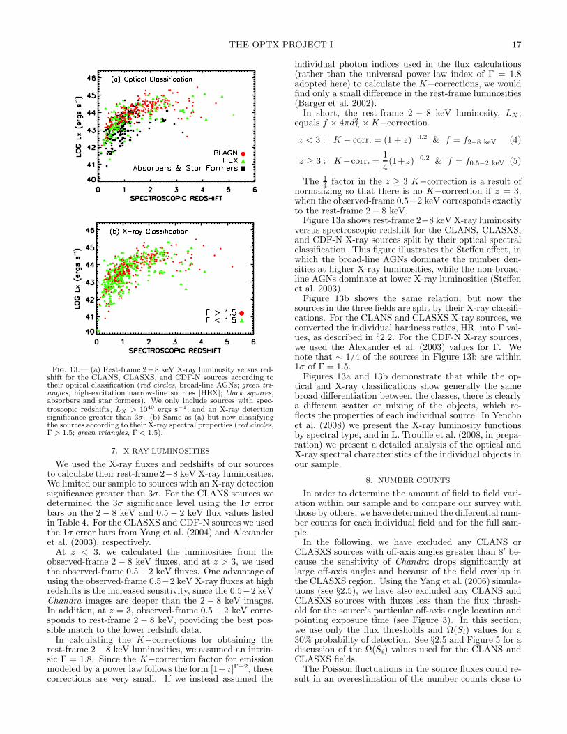
In this paper we present the X-ray data for the CLANSfield and the most up-to-date photometric and spectro-scopic data of the optical and infrared counterparts tothe X-ray sources for the CLANS, CLASXS, and CDF-Nfields. In §2 we describe the CLANS X-ray observationsand provide the X-ray catalog. We discuss our opticaland infrared imaging data in §3, our redshift informa-tion in §4, and our optical spectral classifications in §5.In §6 we present the CLANS, CLASXS, and CDF-N opti-cal and infrared photometric and spectroscopic catalogs.We calculate the rest-frame 2 − 8 keV X-ray luminosi-ties in §7, and in §8 we construct differential logN−logSrelations and compare our results with those of othersurveys.

We use J2000 coordinates and assume ΩM = 0.3, ΩΛ =0.7, and H0 = 70 km s−1 Mpc−1. All magnitudes are inthe AB magnitude system and, unless otherwise speci-fied, fluxes are in ergs cm−2 s−1.

2. X-RAY PROPERTIES

2.1. CLANS X-ray Observations

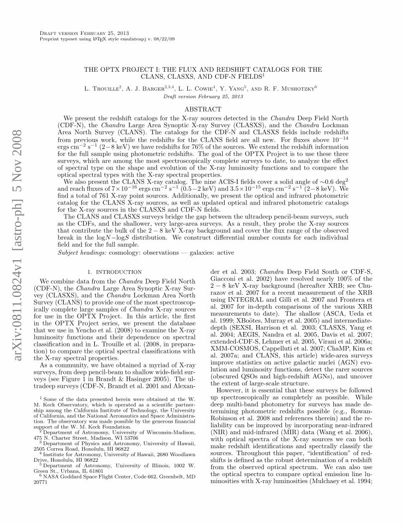
Fig. 1.— (a) Location of the CLANS and CLASXS pointingsin the Lockman Hole. The circles delimit 5′ from the pointingcenters (the area within which the sensitivity of source detectionin the ACIS-I images is approximately uniform). Location of the(b) CLANS and (c) CLASXS X-ray sources. The circles delimit8′ from the pointing centers, which is the limiting off-axis angleused in §8 when calculating the logN−logS distributions for thesefields. The numbers 1-9 in (b) correspond to the Chandra/SWIRELockman pointings listed in Table 2.

To minimize the effects of Galactic attenuation, both

THE OPTX PROJECT I 3

the CLANS and CLASXS fields reside in the LockmanHole high latitude region of extremely low Galactic HIcolumn density (5.7 × 1019 cm−2; Lockman et al. 1986).The Galactic HI column density along the line of sightto the CDF-N is 1.6 × 1020 cm−2 (Stark et al. 1992).

CLANS consists of nine separate ∼70 ks Chan-dra ACIS-I exposures centered at (α, δ)J2000 =(10h46m, +5901′) (see Table 2) combined to create an∼0.6 deg2 image containing 761 sources. The X-ray fluxlimits are f2−8 keV ∼ 3.5 × 10−15 ergs cm−2 s−1 andf0.5−2 keV ∼ 7 × 10−16 ergs cm−2 s−1.

While the ACIS-I field of view is 17′ × 17′, the sensi-tivity of the source detection is approximately uniformonly within off-axis angles less than ∼ 5′. As the off-axisangle increases, the sensitivity drops due to vignettingeffects, quantum efficiency changes across the field, andthe broadening of the point-spread functions (see Fig-ure 3 and §2.5). Therefore, while the CLANS ACIS-Ipointings exposed an almost contiguous area, the actualcoverage, as evidenced by the gaps between the 5′ circlesin Figure 1a, is non-uniform. The survey was optimizedto obtain the largest solid angle possible. The CLASXSsurvey, on the other hand, was designed to achieve uni-form field coverage (at off-axis angles ≈ 5′, the CLASXSpointings overlap slightly as shown in Figure 1a).

In Figures 1b and 1c we show 8′ circles around theCLANS and CLASXS pointings. This is the limiting off-axis angle used in §8 when calculating the logN−logSdistributions for these fields. While there is substantialoverlap between the CLASXS pointings at these off-axisangles, the CLANS pointings overlap very little. This isimportant in the determination of the effective areas foreach field (see §2.5).

In Table 3 we list the characteristics of the CLANS fieldin terms of the Chandra exposure times, areas covered,X-ray flux limits, and total number of X-ray sources.We include the CLASXS and CDF-N characteristics forcomparison.

2.2. CLANS X-ray Source Detection and Fluxes

Brandt et al. (2001) and Alexander et al. (2003) usedthe wavdetect tool included in the CIAO package (Free-man et al. 2002) to detect the X-ray sources in the CDF-N. Yang et al. (2004) also used wavdetect on the CLASXSfield, in particular because the program uses a set ofscales to optimize the source detection, making it ex-cellent at separating nearby sources in crowded fields. Ingeneral, wavdetect provides better sensitivity than theclassical sliding-box methods.

We ran wavdetect on the full-resolution CLANS imageswith wavelet scales of 1,

√2, 2, 2

√2, 4, 4

√2, and 8. We

used a significance threshold of 10−7, which translatesto a probability of a false detection of 0.4 per ACIS-Ifield based on Monte Carlo simulation results (Freemanet al. 2002).

We used the aperture photometry tool for source fluxextraction described in detail in Yang et al. (2004). Themethod uses circular extraction cells. We linearly inter-polated the CIAO Library PSFs to the off-axis anglesand ∼ 95% of the enclosed energies for each source. Inthe 0.5−2 keV (2−8 keV) band, the 95% encircled radiusis equal to 2.5′′ at an off-axis angle of 3′ (2′) and is equalto 9.5′′ (10′′) at an off-axis angle of 8′. For a plot of the

variation of the 95% encircled radius with off-axis angle,see Figure 3 in Yang et al. (2004). If the determined PSFvalue were greater than 2.′′5, then we used it as the radiusof the circular extraction cell for that source and appliedan aperture correction to the final flux determination. Ifit were less than 2.′′5, then we used a fixed 2.′′5 radius. Asdescribed in Yang et al. (2004), we estimated the back-ground using an eight-piece segmented annulus regionfour times as large as the source cell area, with an innerradius 5′′ larger than the source cell radius. We excludedany segments containing more counts than the 3σ Pois-son upper limit in order to avoid nearby sources. Wethen determined the background surface brightness bydividing the counts by the area enclosed in the remain-ing segments. By multiplying this background surfacebrightness by the area within the circular extraction cell,we determined the background counts. We obtained thenet counts by subtracting the background counts fromthe counts within the circular extraction cell.

We then made full-resolution spectrally weighted expo-sure maps. We used these exposure maps only to correctfor vignetting. We computed the flux conversion at theaim point using spectral modeling (using monochromaticmaps does not change the results significantly). For eachsource we convolved the exposure map with the PSF gen-erated using mkpsf and normalized it to the exposuretime at the aim point. This gives the effective expo-sure time if the source is at the aim point. In XSPECwe obtained the count rate to flux conversion factor atthe aim point by assuming each source has a single powerlaw spectrum with Galactic absorption (using the CIAO-scripts mkacisrmf and mkarf to generate the necessaryRMF and ARF files). We calculated the power law pho-ton index, Γ, for each source using the hardness ratio, de-fined as HR≡C2−8 keV/C0.5−2 keV, where C2−8 keV andC0.5−2 keV are the count rates. For a more detailed de-scription and analysis of this flux conversion method, seeYang et al. (2004).

4 Trouille et al.

TABLE 1Spectroscopic Completeness of Selected Surveys from the Literature

eCDF-S AEGIS SEXSI ChaMPArea (deg2) 0.3 0.5 2 9.6X-ray Flux Limit (10−16 ergs cm2 s−1) 6.7a 8.2b 300c 9.0d

Optical Limit for Spectroscopic Follow-up RAB < 25 RAB < 24.1 RAB < 24 r′AB < 24Spectroscopic Completenesse 35%f

· · ·g 40-70%h 54%i

Note. — a 2 − 8 keV: average on-axis flux limit (Lehmer et al. 2005).b 2 − 7 keV: defined as the flux to which at least 1% of the survey area is sensitive (Nandra et al. 2005).c 2 − 10 keV: corresponds to the deepest flux reached by all 27 non-contiguous fields in SEXSI. 1 deg2 of the survey probes to a deeperflux limit of f2−10 keV = 10−14 ergs cm2 s−1 (Harrison et al. 2003).d 0.5 − 8 keV: corresponds to the flux limit for the deepest ChaMP exposure. ChaMP is a non-contiguous survey with exposure timesranging from 0.9 to 124 ks (Kim et al. 2007a).e Fraction of X-ray sources with optical magnitudes brighter than the optical limit for spectroscopic follow-up for which spectroscopicredshifts have been determined.f Virani et al. (2006b).g Spectroscopic redshifts for 84 AEGIS X-ray sources have been obtained to date from the DEEP2 Galaxy Redshift Survey. We havenot found in the literature the number of AEGIS X-ray sources with RAB < 24.1 so are unable to provide a percentage for spectroscopiccompleteness (Davis et al. 2003, 2007; Bundy et al. 2008; Georgakakis et al. 2007).h Eckart et al. (2006).i Silverman et al. (2008).

TABLE 2CLANS Observation Summary

Exposurea

Target Name Observation ID α2000 δ2000 Observation Start Date (ks)SWIRE LOCKMAN 5 (center) 5023 10 46 00.00 +59 01 00.00 2004 Sept 12 21:30:56 67SWIRE LOCKMAN 1 5024 10 44 46.15 +58 41 55.45 2004 Sept 16 06:53:47 65SWIRE LOCKMAN 2 5025 10 46 39.44 +58 46 51.24 2004 Sept 17 20:30:04 70SWIRE LOCKMAN 3 5026 10 48 32.77 +58 51 47.33 2004 Sept 18 16:17:12 69SWIRE LOCKMAN 4 5027 10 44 06.67 +58 56 05.28 2004 Sept 20 14:40:35 67SWIRE LOCKMAN 6 5028 10 47 53.44 +59 05 57.00 2004 Sept 23 03:36:12 71SWIRE LOCKMAN 7 5029 10 43 27.23 +59 10 15.07 2004 Sept 24 03:43:15 71SWIRE LOCKMAN 8 5030 10 45 20.56 +59 15 11.16 2004 Sept 25 19:47:08 66SWIRE LOCKMAN 9 5031 10 47 13.85 +59 20 06.95 2004 Sept 26 14:47:00 65

aTotal good time with dead-time correction

TABLE 3X-ray Data Specifications

Category CLANS CLASXS CDF-NExposure Time ∼ 70 ks ∼ 40 ks (73 ksa) 2 Ms

Area (deg2) 0.6 0.45 0.1240.5 − 2 keV Flux Limitb 7 12 (7)c 0.25

2 − 8 keV Flux Limitb 35 60 (35)c 1.5Total # of X-ray Sources 761 525 503aExposure time for the central pointing. All other pointings have

exposure times of ∼ 40 ks.bFlux limit (for a S/N = 3) at the pointing center in 10−16 ergs

cm−2 s−1.cFlux limit (for a S/N = 3) at the pointing center of the ∼ 40 ks

(73 ks) exposure.


TABLE 4CLANS X-ray Catalog: Basic Source Properties

∆α ∆δ

Num. α2000 δ2000 (arcsec) (arcsec) f0.5−2 keVa f2−8 keV

a f0.5−8 keV HRb Γc

(1) (2) (3) (4) (5) (6) (7) (8) (9) (10)1 160.58846 59.25157 0.831 0.457 3.37+0.70

−0.51 11.82+2.80−2.31 14.36+2.17

−1.80 0.79+0.25−0.20 1.05+0.25

−0.26

2 160.64172 59.17641 0.301 0.239 7.79+0.97−0.83 10.01+2.28

−1.75 17.98+1.94−1.62 0.37+0.10

−0.08 1.71+0.20−0.19

3 160.64175 59.16873 0.710 0.376 0.63+0.38−0.22 0.75+0.79

−0.52 1.45+0.60−0.50 0.34+0.42

−0.27 1.76+0.78−0.69

4 160.65615 59.11504 1.231 0.581 1.52+1.01−0.57 0.51+1.74

−0.42 2.20+1.30−0.67 0.13+0.46

−0.12 2.37+0.36−1.08

5 160.66704 59.07057 0.983 0.559 1.19+0.46−0.31 6.34+2.12

−1.83 7.88+1.83−1.51 1.09+0.56

−0.42 0.74+0.44−0.13

6 160.66924 59.25401 1.004 0.460 0.93+0.37−0.28 4.63+1.86

−1.38 5.86+1.49−1.21 1.03+0.59

−0.44 0.80+0.49−0.18

.. .. .. .. .. .. .. .. .. ..

Note. — Table 4 is presented in its entirety in the electronic edition of the Astrophysical Journal Supplement. A portion is shown herefor guidance regarding its form and content.a In units of 10−15 ergs s−1. For any source detected in one band but with a very weak signal in the other, the background-subtractedflux could be negative. In this case, only the upper Poisson error is quoted and we flag it with a < symbol.b For sources with a very weak signal in the 0.5− 2 keV (2 − 8 keV) band, we list the lower (upper) limit and flag it with a > (<) symbol.c For sources detected in one band but not in the other, Γ = −99.

TABLE 5CLANS X-ray Catalog: Additional Source Properties

t0.5−2 keV t2−8 keV t0.5−8 keV RNum. n0.5−2 keV

a n2−8 keVa n0.5−8 keV

a (104 s) (104 s) (104 s) (arcminutes)(1) (2) (3) (4) (5) (6) (7) (8)1 36.50+7.63

−5.56 26.00+6.16−5.07 59.75+9.04

−7.48 5.90 5.34 5.80 9.72 83.75+10.45

−8.90 29.75+6.78−5.20 112.50+12.16

−10.12 6.47 6.26 6.40 6.83 6.75+4.01

−2.35 2.25+2.38−1.57 9.25+3.85

−3.21 6.48 6.28 6.41 6.84 5.75+3.83

−2.15 0.75+2.54−0.62 7.50+4.44

−2.28 2.71 2.62 2.65 7.25 12.75+4.94

−3.32 13.25+4.44−3.82 27.00+6.26

−5.17 5.65 5.40 5.54 8.56 11.00+4.41

−3.28 11.00+4.41−3.28 23.00+5.86

−4.77 6.27 6.07 6.20 7.8.. .. .. .. .. .. .. ..

Note. — Table 5 is available in its entirety in the electronic edition of the Astrophysical Journal Supplement. A portion is shown herefor guidance regarding its form and content.a The eight-piece segmented annulus region we use to estimate the background for each source is 4 times as large as the source cell area.Therefore, the net counts for the majority of the sources are multiples of 0.25. For a few sources we exclude background segments containingmore counts than the 3σ Poisson upper limit in order to avoid nearby sources. Therefore the net counts for these sources are not multiplesof 0.25.

6 Trouille et al.

2.3. CLANS X-ray Catalog

The CLANS observations consist of a 3×3 raster withan ∼ 2′ overlap between continguous pointings (Pollettaet al. 2006; see our Figure 1). Following the prescriptionin Yang et al. (2004) for the CLASXS field, we mergedthe nine individual pointing catalogs to create the finalCLANS X-ray catalog. For sources with more than onedetection in the nine fields, we used the detection fromthe observation in which the effective area of the sourcewas the largest.

We present the CLANS X-ray catalog in Tables 4 and5. In both tables, column (1) is the source number. Thenumbers correspond to ascending order in right ascen-sion. In Table 4, columns (2) and (3) give the right as-cension and declination coordinates of the X-ray sources.Columns (4) and (5) list the 95% confidence errors fromwavdetect on these right ascension and declination co-ordinates. Columns (6), (7), and (8) provide the X-rayfluxes in the 0.5 − 2 keV, 2 − 8 keV, and 0.5 − 8 keVbands, respectively, in units of 10−15 ergs cm−2 s−1. Theerrors quoted are the 1σ Poisson errors, using the ap-proximations from Gehrels (1986). They do not includethe uncertainty in the flux conversion factor; however,the errors are generally dominated by the Poisson errors.Column (9) gives the hardness ratio, as defined in §2.2.Column (10) lists the value of Γ for each source. Theerrors in Columns 9 and 10 are the 1σ errors propagatedfrom the 1σ errors on the counts listed in Table 5.

In Table 5, columns (2), (3), and (4) list the net countsin the 0.5− 2 keV, 2− 8 keV, and 0.5− 8 keV bands, re-spectively. The errors quoted are the 1σ Poisson errors,using the approximations from Gehrels (1986). Columns(5), (6), and (7) give the effective exposure times fromthe exposure maps in each of the three energy bands.Column (8) provides the distance from the pointing cen-ter for each source.

2.4. Flux Limits

Following the prescription in Alexander et al. (2003),we determined the flux limits for a signal-to-noise ratio(S/N) of 3 for the CLANS and CLASXS fields. To de-termine the sensitivity across the field it is necessary totake into account the broadening of the PSF with off-axisangle, as well as changes in the effective exposure andbackground rates across the field. Under the simplifyingassumption of

√N uncertainties, we can determine the

sensitivity across the field following Muno et al. (2003)as

S =n2

σ

2(1 + [1 +

8b

n2σ

]1/2), (1)

where S is the number of source counts and b is thenumber of background counts in a source cell. The nσ isthe required signal-to-noise ratio.

After setting nσ = 3, the only component within Equa-tion 1 that we need to measure is the background counts.We determined the median number of background countsat each off-axis angle (using the method described in§2.2) and inputted this into Equation 1 to determine Sat each off-axis angle. Using the flux conversion methoddiscussed in §2.2, we converted S from counts to fluxvalues.

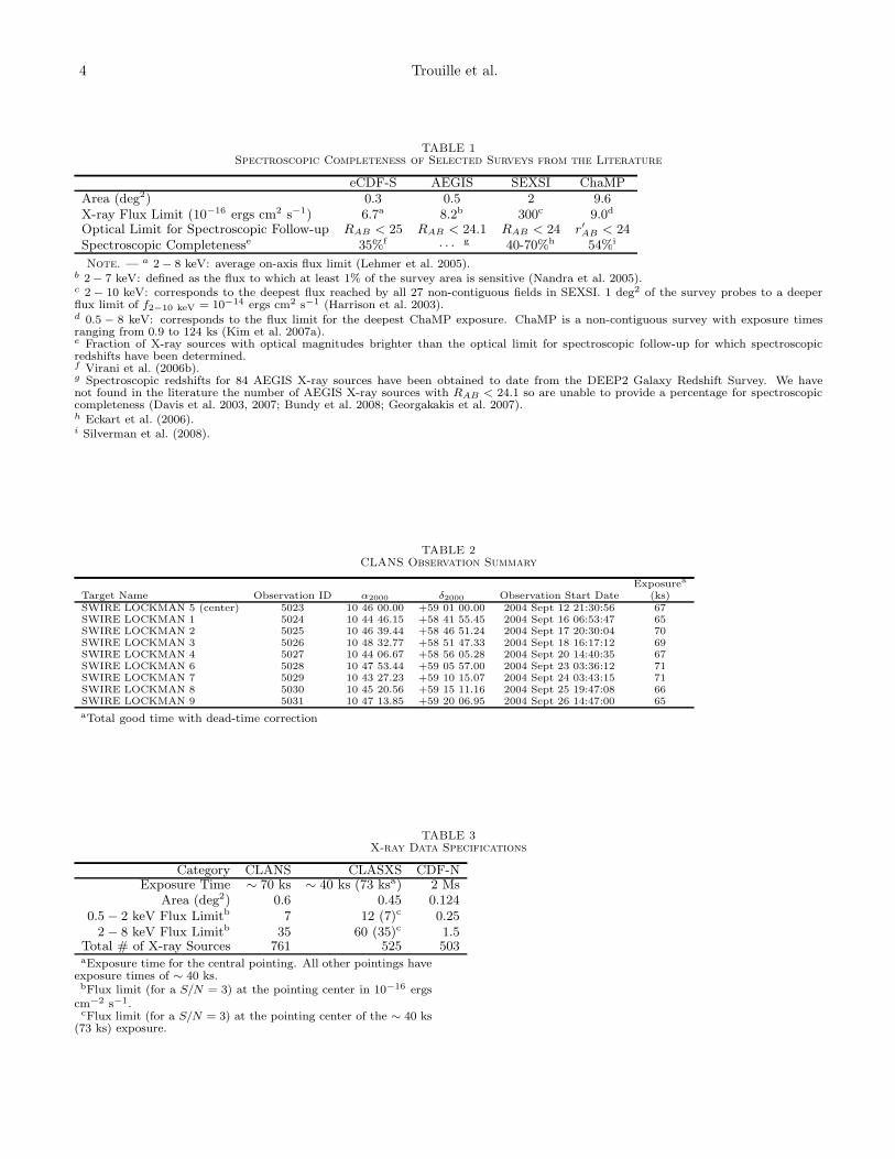
The red lines in Figure 2 show the flux limits (for

Fig. 2.— 2 − 8 keV and 0.5 − 2 keV flux versus off-axis anglefor the X-ray sources in the CLANS, CLASXS, and CDF-N fields(red lines, S/N = 3 flux limits at the off-axis angle of each sourcedetected by wavdetect ; dashed red lines, S/N = 3 flux limits for thedeeper 73 ks pointing in the CLASXS field; green circles, sourceswith fluxes greater than the corresponding flux limit; black squares,sources with fluxes below the corresponding flux limit).

a S/N = 3) versus the off-axis angle. The green cir-cles (black squares) identify the sources whose fluxes aregreater (less) than the corresponding flux limit. Be-cause all of the CLANS pointings have exposure timesof ∼70 ks, there is only a single red line that increasesslightly in flux as the off-axis angle increases. In theCLASXS field, however, the LHNW-1 pointing has anexposure time of 73 ks, while the other pointings are all∼40 ks. Thus, the dashed red line located at slightlylower fluxes than the solid red line shows the flux limitscorresponding to the deeper 73 ks ACIS-I pointing. Thebottom plots in Figure 2 show the Alexander et al. (2003)flux limits (for a S/N = 3) for the CDF-N field.

2.5. Effective Areas

Yang et al. (2004, 2006) used Monte Carlo simulationsof the CLASXS 40 ks and 70 ks 2−8 keV and 0.5−2 keVband ACIS-I images to examine the incompleteness intheir number counts. The sensitivity of the source de-tection drops with off-axis angle due to vignetting ef-fects, quantum efficiency changes across the field, and thebroadening of the point-spread functions. Using wavde-tect on their simulated images, Yang et al. obtained anestimate of the detection probability function, or proba-bility that a source would be detected by wavdetect, atdifferent fluxes and off-axis angles.


The differences at small and large off-axis angles be-tween their 2004 and 2006 simulations are attributableto two methodological changes. First, in their 2004 sim-ulations they used many fewer simulated sources, caus-ing an undersampling at small off-axis angles. Second, intheir 2004 simulations they did not use large wave scales,causing a quick drop in source detection at off-axis anglesgreater than 6′.

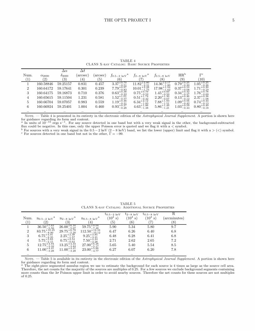
We interpolated from their 40 ks and 70 ks 2006 sim-ulations to the exposure times for the nine pointings inboth the CLANS and CLASXS fields, respectively (seeTable 2 for the CLANS field exposure times and Yang etal. 2004 Table 1 for the CLASXS field exposure times)to determine the probability of detection for a source ata given off-axis angle and flux in each pointing. Figure 3shows the probability of source detection as a function ofoff-axis angle and 2 − 8 keV flux for the central CLANSpointing (Chandra/SWIRE Lockman 5 in Table 2) withan exposure time of 67 ks. As expected, the probabilityof detecting a source at a given off-axis angle decreasesas the flux of the source decreases.

We then determined the effective sky area for eachpointing using the formula

A(fx) =

∫ a

0

2πa da D(a, fx) g(a), (2)

where a is the off-axis angle from the pointing center,g(a) is the geometric fraction, and D(a, fx) is the detec-tion probability, equivalent to an incompleteness factor.

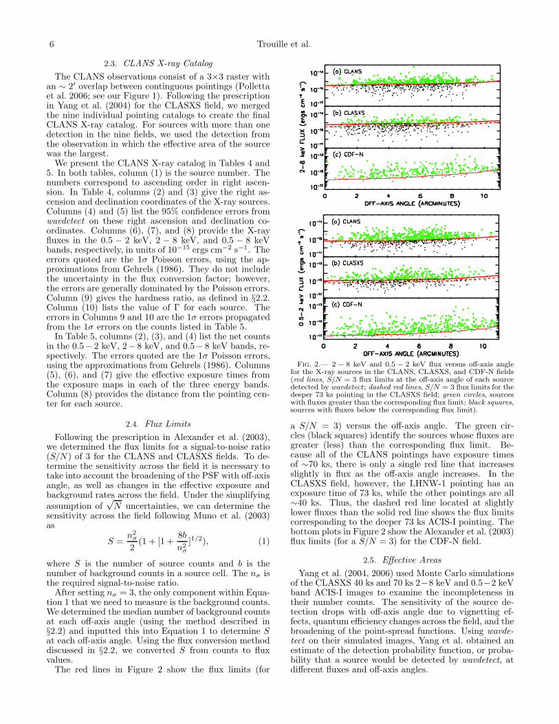
Figure 4 shows the geometric fraction, or fraction of thetotal area covered by an annulus of width 0.′5 and outerradius a that is contained within the ACIS-I chip. Figure4a shows our ULBCam H-band image (see §3.3) of theCLANS field overlaid with the ACIS-I chip outline (thesquare) and two annuli with off-axis angles 7′ − 7.′5 and9.′5 − 10′. Figure 4(b) shows that the geometric fractionis 1 for all annuli with outer radii less than ∼ 8′. Ata > 8′, g(a) decreases rapidly.

We determined A(fx) for 5 different limiting detectionprobabilities, 20%, 30%, 50%, 70%, and 90%. In thedetermination of A(fx), if the simulated D(a, fx) at theoff-axis angle of a source of flux fx were found to be be-low this limiting detection probability, then we assignedD(a, fx) = 0 for that source.

Because the sensitivity of Chandra degrades at largeoff-axis angles, we exclude sources with off-axis anglesgreater than 8′ in our number counts determination (see§8). In the CLANS field at these off-axis angles there islittle overlap between pointings, so Ω(fx) ≈

∑

Ai(fx).However, in the CLASXS field the pointings overlap sig-nificantly (as shown in Figure 1). We used the ds9 fun-tools function that determines area within region files tosubtract the overlapping area from the total Ω(fx) value.We also made sure that any area that had already beensubtracted as part of the geometric fraction determina-tion was not subtracted a second time at this stage.

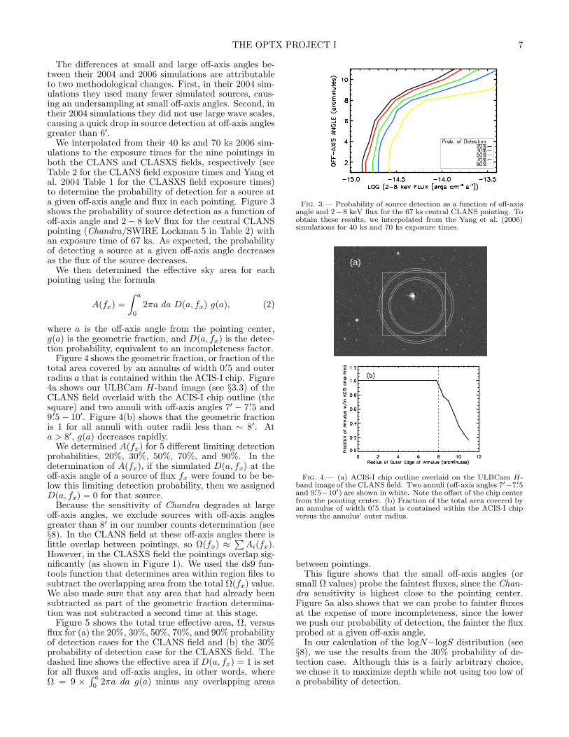
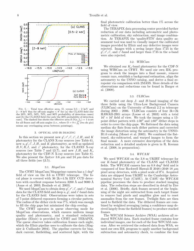
Figure 5 shows the total true effective area, Ω, versusflux for (a) the 20%, 30%, 50%, 70%, and 90% probabilityof detection cases for the CLANS field and (b) the 30%probability of detection case for the CLASXS field. Thedashed line shows the effective area if D(a, fx) = 1 is setfor all fluxes and off-axis angles, in other words, whereΩ = 9 ×

∫ a

0 2πa da g(a) minus any overlapping areas

Fig. 3.— Probability of source detection as a function of off-axisangle and 2−8 keV flux for the 67 ks central CLANS pointing. Toobtain these results, we interpolated from the Yang et al. (2006)simulations for 40 ks and 70 ks exposure times.

(a)

Fig. 4.— (a) ACIS-I chip outline overlaid on the ULBCam H-band image of the CLANS field. Two annuli (off-axis angles 7′−7.′5and 9.′5−10′) are shown in white. Note the offset of the chip centerfrom the pointing center. (b) Fraction of the total area covered byan annulus of width 0.′5 that is contained within the ACIS-I chipversus the annulus’ outer radius.

between pointings.This figure shows that the small off-axis angles (or

small Ω values) probe the faintest fluxes, since the Chan-dra sensitivity is highest close to the pointing center.Figure 5a also shows that we can probe to fainter fluxesat the expense of more incompleteness, since the lowerwe push our probability of detection, the fainter the fluxprobed at a given off-axis angle.

In our calculation of the logN−logS distribution (see§8), we use the results from the 30% probability of de-tection case. Although this is a fairly arbitrary choice,we chose it to maximize depth while not using too low ofa probability of detection.

8 Trouille et al.

Fig. 5.— Total true effective area, Ω, versus 0.5 − 2 keV and2− 8 keV flux for off-axis angles < 8′ for (a) the CLANS field (forthe 20%, 30%, 50%, 70%, and 90% probability of detection cases)and (b) the CLASXS field (for only the 30% probability of detectioncase). The dashed line shows the effective area if D(a, fx) = 1 is setfor all fluxes and off-axis angles (i.e., where Ω = 9×

R a

02πa da g(a)

minus any overlapping areas between pointings).

3. OPTICAL AND IR IMAGING

In this section we present new g′, r′, i′, z′, J, H , and Kphotometry for the CLANS X-ray sources (see Table 6),new u, g′, i′, J, H , and K photometry, as well as updatedB, V, R, I, and z′ photometry, for the CLASXS X-raysources (see Table 7 and §3.7), and new J, H, and Ks

photometry for the CDF-N X-ray sources (see Table 8).We also present the Spitzer 3.6 µm and 24 µm data forall three fields (see §3.5).

3.1. MegaCam

The CFHT MegaCam/Megaprime camera has a 1 deg2

field of view on the 3.6 m CFHT telescope. The fo-cal plane is covered with 36 2k×4.5k EEV CCD detec-tors with excellent response between 3200 A and 9000 A(Aune et al. 2003; Boulade et al. 2003).

We used MegaCam to obtain deep g′, r′, i′, and z′-banddata for the CLANS field and deep u, g′, and i′-band datafor the CLASXS field. Observations were taken in setsof 7-point dithered exposures forming a circular pattern.The radius of the dither circle was 7.′′5, which was enoughto fill the chip gaps but minimized the chip overlap.

The CFHT operates in queue observing mode forMegaCam observations, which ensures uniform imagequality and photometry, and a standard reductionpipeline (Elixir) is provided by CFHT and TERAPIX.The queue observer takes calibration frames each night,which the Elixir pipeline uses to calibrate the data (Mag-nier & Cuillandre 2004). The pipeline corrects for bias,dark current, flatfielding, and scattered light, with the

final photometric calibration better than 1% across thefield of view.

The TERAPIX data processing center provided furtherreduction of our data including astrometric and photo-metric calibration, sky subtraction, and image combina-tion. At TERAPIX the ‘qualityFITS’ data quality as-sessment tool was used to visually inspect the calibratedimages provided by Elixir and any defective images wererejected. Images with a seeing larger than 1.′′25 in theg′, r′, i′, and z′-band and larger than 1.′′35 in the u-bandwere also rejected.

3.2. WIRCam

We obtained our Ks-band photometry for the CDF-Nusing WIRCam on CFHT. We used our own IDL pro-gram to stack the images into a final mosaic, removecosmic rays, establish a background estimation, align theastrometry to the USNO catalog, and derive a final ze-ropoint via comparison with 2MASS. More details of theobservations and reductions can be found in Barger etal. (2008).

3.3. ULBCam

We carried out deep J- and H-band imaging of thethree fields using the Ultra-Low Background Camera(ULBCam) on the University of Hawaii 2.2 m telescopeduring 2003 − 2006. ULBCam consists of four 2k×2kHAWAII-2RG arrays (Loose et al. 2003) with a total16′ × 16′ field of view. We took the images using a 13-point dither pattern with ±30′′ and ±60′′ dither steps inorder to cover the chip gaps. We flattened the data usingmedian sky flats from each dither pattern and correctedthe image distortion using the astrometry in the USNO-B1.0 catalog (Monet et al. 2003). We combined the flat-tened, sky-subtracted, and warped images to form thefinal mosaic. A more extensive description of the datareduction and a detailed analysis is given in R. Keenanet al. (2008, in preparation).

3.4. WFCAM

We used WFCAM on the 3.8 m UKIRT telescope forour K-band photometry of the CLANS and CLASXSfields. The WFCAM camera has an 0.8 deg2 field and iscomposed of four Rockwell Hawaii-II 2048×2048 18 µmpixel array detectors, with a pixel scale of 0.′′4. Acquireddata are shipped from UKIRT to the Cambridge Astro-nomical Survey Unit (CASU). At CASU the WFCAMpipeline processes the data to produce stacked imagingdata. The reduction steps are described in detail by Dyeet al. (2006). Briefly, dark frames secured at the begin-ning of the night are subtracted from each target frameto remove bad pixels and amplifier glow and to resetanomalies from the raw frames. Twilight flats are thenused to flatfield the data. The dithered frames are com-bined by weighted averaging (using a confidence map de-rived largely from the flatfield frames) to produce stackedframes.

The WFCAM Science Archive (WSA) archives all re-duced WFCAM data. Each stacked frame contains fourindividual images, one for each of the four WFCAM cam-eras. After we retrieved the reduced data from WSA, weused our own IDL program to apply another backgroundsubtraction and astrometry check, to combine the four


tiles into one frame, and to align the astrometry to theUSNO catalog. A more extensive description of the datareduction is given in R. Keenan et al. (2008, in prepara-tion).

3.5. Spitzer

To improve our photometric redshift determinationsin the CLANS and CLASXS fields, we obtained 3.6 µmdata from the Spitzer Wide-Area Infrared ExtragalacticSurvey (SWIRE; Lonsdale et al. 2003) Legacy ScienceProgram. We used the online NASA/IPAC Infrared Sci-ence Archive via GATOR to retrieve the 3.6 µm and24 µm photometric catalogs, using a search radius of2′′ around our NIR counterpart source locations. The3.6 µm (24 µm) catalog has a 5σ limit of 5 µJy (230 µJy)(Polletta et al. 2006).

Polletta et al. (2006) carried out an extensive anal-ysis of the probability of false matches to the SpitzerIRAC catalogs for the CLANS field. Of the 774 X-raysources in their catalog, they expect ≈ 19 false assoca-tions. We find a similar result of 23 false matches to theIRAC catalog using a simple randomization of our 761CLANS X-ray sources. We find only 2 false matches tothe MIPS catalog, which has many fewer sources thanthe IRAC catalog. The IRAC and MIPS data providecomplete coverage for the CLANS field area. However,while the MIPS data provide complete coverage for theCLASXS field area, the IRAC data only cover 305 of the525 CLASXS X-ray sources.

For the CDF-N X-ray sources, we obtained the rele-vant 3.6 µm and 24 µm data from the Great Observa-tories Origins Deep Survey-North (GOODS-N) SpitzerLegacy Science Project. We followed the method de-scribed in detail in Wang et al. (2006) to determine the3.6 µm Spitzer magnitudes from the GOODS-N first, in-terim, and second data release products (DR1, DR1+,DR2; M. Dickinson et al. 2008, in preparation). For the24 µm data, we used the DR1 + MIPS source list and theversion 0.36 MIPS map provided by the Spitzer LegacyProgram. The MIPS catalog is flux-limited and completeat 80 µJy and the median 1σ sensitivity of the MIPS mapis 6.4 µJy. The 5σ sensitivity limit for the 3.6 µm data is0.327 µJy (Wang et al. 2006). Of the 503 CDF-N X-raysources, 379 are in the area covered by the GOODS-N3.6 µm and 24 µm micron observations.

Of the 761 CLANS, 305 CLASXS, and 379 CDF-NX-ray sources observed in the IRAC 3.6 µm band, 633CLANS, 249 CLASXS, and 351 CDF-N sources are de-tected to the limits of the SWIRE and GOODS-N sur-veys.

Of the 761 CLANS, 525 CLASXS, and 379 CDF-NX-ray sources observed in the MIPS 24 µm band, 222CLANS, 119 CLASXS, and 200 CDF-N sources are de-tected to the limits of the SWIRE and GOODS-N sur-veys.

3.6. Optical and NIR Source Detection and Photometry

We performed source detection and determined op-tical and NIR magnitudes using SExtractor (Bertin &Arnouts 1996). We set the detection threshold at eightcontiguous pixels with counts at least 2σ above the lo-cal sky background. Using the ASSOC PARAMS func-tion, we searched a 2.′′5 radius around the X-ray point

TABLE 6CLANS Optical & Near-IR Specifications

Filter Telescope Average Seeing 3σ Limit Total Areaa

(arcsec) (AB mag) (deg2)g′ CFHT 0.8 26.9 0.96r′ CFHT 1.1 26.5 1.16i′ CFHT 0.9 26.0 1.21z′ CFHT 0.9 25.3 1.33J UH 2.2 m 0.9 24.0 0.86H UH 2.2 m 0.9 23.2 0.83K UKIRT 1.2 22.1 0.74aFor comparison, the CLANS X-ray survey covers 0.6 deg2.

TABLE 7CLASXS Optical & Near-IR Specifications


(arcsec) (AB mag) (deg2)u CFHT 1.3 25.9 1.16g′ CFHT 0.9 27.1 0.96i′ CFHT 1.0 25.3 1.12J UH 2.2 m 0.9 24.3 0.76H UH 2.2 m 1.1 23.1 0.68K UKIRT 1.0 22.1 0.74aFor comparison, the CLASXS X-ray survey covers 0.45 deg2.

TABLE 8CDF-N Near-IR Specifications


(arcsec) (AB mag) (deg2)J UH 2.2 m 1.2 24.7 0.25H UH 2.2 m 1.2 24.8 0.29Ks CFHT 0.8 24.2 0.29aFor comparison, the CDF-N X-ray survey covers 0.124 deg2.

source location in the z′-band image to determine thenearest optical counterpart location. We then used thisz′-band optical counterpart location to determine themagnitudes in the other bands. If there was no z′-bandoptical counterpart but there was a g′-band counterpartwithin the 2.′′5 radius, we used this location instead. Wethen checked all sources by eye to ensure that the samesource was being used to determine the optical and NIRmagnitudes. In the CDF-N, for which we only presentnew NIR photometry, we used the Barger et al. (2003)X-ray source optical counterpart locations.

For sources with z′ < 21, we used the MAG AUTOmagnitudes. For z′ > 21, we used the 3′′ aperture-corrected magnitudes. We determined these by tak-ing the 3′′ MAG APER magnitude for each source andthen applying an offset. We calculated the offset as themedian difference between the 3′′ MAG APER and 6′′

MAG APER magnitudes for sources with 18 < z′ < 20.The typical offset is 0.2 magnitudes with a 1σ error of0.06. As expected, there is a slight trend towards smalleroffsets with increasing magnitude (δoffset < 0.05 magni-tudes). Between 18 < z′ < 20, the MAG AUTO and 6′′

MAG APER magnitudes generally agree well, with theMAG AUTO magnitudes 0.01-0.03 magnitudes fainterthan the 6′′ MAG APER magnitudes. See R. Keenanet al. (2008, in preparation) for a more detailed discus-sion.

As stated above, in the catalogs we include magnitudesfor sources with counts at least 2σ above the local skybackground (as determined by SExtractor). We providethe aperture-corrected 3σ limits of the images in Tables6, 7, and 8, which show the depth of our optical and

10 Trouille et al.

NIR data. We determined these limits by laying downrandom 3′′ apertures away from objects on the images.We masked out the areas around bright stars to preventerroneous detections and measurements from scatteredlight. We derived the aperture-corrected 3σ limit foreach image from

3σ =−2.5 log(3 RMS√

π × (1.′′5/platescale)2)

+ZP + OFFSET, (3)

where RMS is the average standard deviation of theblank apertures, ZP is the zeropoint for the image inquestion, and OFFSET is the aperture-correction asdiscussed in the previous paragraph. A more detaileddescription of this method is given in R. Keenan etal. (2008, in preparation).

Typical 1σ errors on the CLANSg′, r′, i′, z′, J, H, K, 3.6 µm and 24 µm fluxes are0.2, 0.3, 0.4, 0.9, 3.3, 7.2, 4.8, 10.2, and 629.9 × 10−30

ergs cm−2 s−1 Hz−1, respectively. For the CLASXSfield, typical 1σ errors for the u, g′, i′, J, H, K, 3.6 µmand 24 µm fluxes are 0.2, 0.2, 0.9, 2.4, 5.4, 3.6, 10.2,and 629.9 × 10−30 ergs cm−2 s−1 Hz−1, respectively.And typical 1σ errors for the CDF-N J, H, K, 3.6 µmand 24 µm fluxes are 1.5, 1.3, 0.8, 0.5, and 64.0 × 10−30

ergs cm−2 s−1 Hz−1, respectively.

3.7. CLASXS: Updated Optical Photometry

The original CLASXS catalog of Steffen et al. (2004)presented B, V, R, I, and z′ photometry from CFHTand Subaru observations for 521 of the 525 X-ray pointsources. When comparing the spectral energy distribu-tions (SEDs) using these data with our more recent u, g′,and i′-band CFHT observations, we found that the origi-nal zeropoints for all but the B-band data were incorrect.The zeropointing errors reflect the difficulty of calibrat-ing the Subaru Suprime-Cam images. Due to Subaru’slarge collecting area, calibration stars saturate even withthe shortest possible exposure times. Also, the Steffen etal. (2004) CFHT data were taken using CFH12K, whichdoes not operate in queue mode, so no automatic calibra-tions were done (in contrast with the standard MegaCamqueue mode procedure).

To determine the zeropoint offsets, we compared SEDscreated from the Steffen et al. (2004) CFH12K data withSEDs made from the more recently obtained u, g′, andi′-band MegaCam data. We restricted our sample tosources with 21 < g′ < 23. The zeropoint offsets listedin Table 9 are the mean of the values needed to shift theSEDs made from the original CFHT data onto the SEDsmade from the new u, g′, and i′-band data.

We did this separately for the SEDs with a more obvi-ous bluer slope (ascending SED as frequency increases)and those with a more obvious redder slope (descendingSED as frequency increases), and found no major differ-ences in the offsets between these two types of sources.We found that the CFHT B-band data had a negligi-ble offset while the R- and z′-band data were best re-zeropointed using an offset of -0.6.

We followed the same method to re-zeropoint the orig-inal Subaru V, R, I, and z′-band data (see Table 9).

4. REDSHIFT INFORMATION

4.1. Spectroscopic Observations

TABLE 9CLASXS Zeropoint Offsets

B V R I z′

Subaru · · · -0.5 -0.5 -0.4 -0.3CFHT 0. · · · -0.6 · · · -0.6

We have carried out extensive spectroscopic observa-tions of the X-ray sources in the CLANS, CLASXS, andCDF-N fields. All of the CLANS spectroscopic observa-tions are presented for the first time in this article. Inaddition, we have obtained some new spectroscopic ob-servations for the CLASXS and CDF-N fields.

For the CLANS field we obtained all the optical spec-tra using the Deep Extragalactic Imaging Multi-ObjectSpectrograph (DEIMOS; Faber et al. 2003) on the 10 mKeck II telescope. We used the 600 line mm−1 grating,which yielded a resolution of 3.5 A and a wavelength cov-erage of 5300 A. The exact central wavelength dependson the slit position, but the average was 7200 A. Each∼1 hr exposure was broken into three subsets, with theobjects stepped along the slits by 1.′′5 in each direction.

The DEIMOS spectroscopic reductions follow the sameprocedures used by Cowie et al. (1996) for the Low-Resolution Imaging Spectrograph (LRIS; Oke et al.1995) reductions. In brief, we removed the sky contri-bution by subtracting the median of the dithered im-ages. We then removed cosmic rays by registering theimages and using a cosmic ray rejection filter as we com-bined the images. We also removed geometric distor-tions and applied a profile-weighted extraction to obtainthe spectrum. We did the wavelength calibration usinga polynomial fit to known sky lines rather than usingcalibration lamps. We inspected each spectrum individ-ually and measured a redshift only for sources where arobust identification was possible. The high-resolutionDEIMOS spectra can resolve the doublet structure of the[O II] λλ3727 and 3729 lines, allowing spectra to be iden-tified by this doublet alone. For sources not identified bythis doublet, only redshift identifications based on multi-ple emission and/or absorption lines were included in thesample. We find that the spectroscopic redshifts for thenon-broad-line AGNs (broad-line AGNs) are accurate to∼ 0.001 (∼ 0.005).

Steffen et al. (2004) presented a spectroscopic red-shift catalog for the CLASXS X-ray sources. Most ofthe spectroscopically observed sources were observed us-ing DEIMOS, following the same procedures as for theCLANS field, but some of the brighter sources (I < 19)were observed using HYDRA (Barden et al. 1994) onthe WIYN 3.5 m telescope. However, for any source ob-served with HYDRA for which Steffen et al. (2004) wereunable to determine a redshift and classification, they re-observed the source with DEIMOS. Thus, only a smallnumber of the CLASXS sources have redshifts and classi-fications based on their HYDRA spectra. Subsequent toSteffen et al. (2004), we obtained 11 additional spectrain the CLASXS field using DEIMOS. We have redshiftidentifications and classifications for all 11. In Table 12,s indicates the spectroscopic redshifts from Steffen etal. (2004).

Barger et al. (2003) presented a spectroscopic redshiftcatalog for the 2 Ms CDF-N X-ray sources. The spectrawere obtained with either DEIMOS or LRIS. Fainter ob-


jects were observed a number of times with DEIMOSsuch that the total exposure times for these sourcesare greater than the ∼ 1 hr used for the CLANS andCLASXS sources. For this reason, the redshift identifica-tion rate for the CDF-N, as compared with the CLANSand CLASXS fields, is slightly higher. We supplementthese CDF-N spectroscopic observations with eight red-shifts obtained by Chapman et al. (2005) and Swinbanket al. (2004), adopting the Swinbank et al. (2004) NIRredshifts over the Chapman et al. (2005) optical red-shifts, where available, because redshift measurementsare generally more reliable when they are made fromemission-line features. Where there are redshifts fromboth sources, the redshifts are within < 0.008 of eachother. We acquired one more spectroscopic redshift fromReddy et al. (2006). The source classifications, how-ever, are not available for the Chapman et al. (2005),Swinbank et al. (2004), and Reddy et al. (2006) red-shifts. Subsequent to Barger et al. (2003), we obtained49 additional spectra in the CDF-N field using DEIMOS.We have redshift identifications and classifications for39 of these. In Table 13, a, b, c, and d indicate thespectroscopic redshifts from Barger et al. (2003), Swin-bank et al. (2004), Chapman et al. (2005), and Reddy etal. (2006), respectively.

4.2. Spectroscopic Completeness

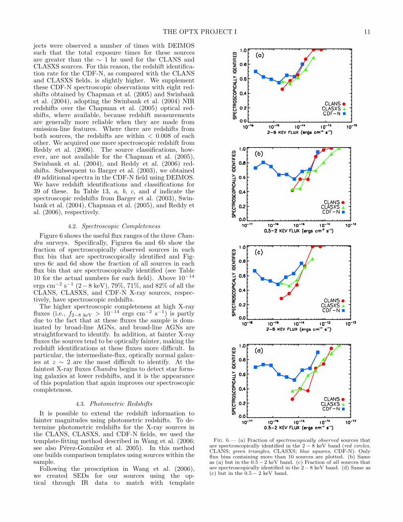
Figure 6 shows the useful flux ranges of the three Chan-dra surveys. Specifically, Figures 6a and 6b show thefraction of spectroscopically observed sources in eachflux bin that are spectroscopically identified and Fig-ures 6c and 6d show the fraction of all sources in eachflux bin that are spectroscopically identified (see Table10 for the actual numbers for each field). Above 10−14

ergs cm−2 s−1 (2−8 keV), 79%, 71%, and 82% of all theCLANS, CLASXS, and CDF-N X-ray sources, respec-tively, have spectroscopic redshifts.

The higher spectroscopic completeness at high X-rayfluxes (i.e., f2−8 keV > 10−14 ergs cm−2 s−1) is partlydue to the fact that at these fluxes the sample is dom-inated by broad-line AGNs, and broad-line AGNs arestraightforward to identify. In addition, at fainter X-rayfluxes the sources tend to be optically fainter, making theredshift identifications at these fluxes more difficult. Inparticular, the intermediate-flux, optically normal galax-ies at z ∼ 2 are the most difficult to identify. At thefaintest X-ray fluxes Chandra begins to detect star form-ing galaxies at lower redshifts, and it is the appearanceof this population that again improves our spectroscopiccompleteness.

4.3. Photometric Redshifts

It is possible to extend the redshift information tofainter magnitudes using photometric redshifts. To de-termine photometric redshifts for the X-ray sources inthe CLANS, CLASXS, and CDF-N fields, we used thetemplate-fitting method described in Wang et al. (2006;see also Perez-Gonzalez et al. 2005). In this methodone builds comparison templates using sources within thesample.

Following the prescription in Wang et al. (2006),we created SEDs for our sources using the op-tical through IR data to match with template

Fig. 6.— (a) Fraction of spectroscopically observed sources thatare spectroscopically identified in the 2 − 8 keV band (red circles,CLANS; green triangles, CLASXS; blue squares, CDF-N). Onlyflux bins containing more than 10 sources are plotted. (b) Sameas (a) but in the 0.5− 2 keV band. (c) Fraction of all sources thatare spectroscopically identified in the 2− 8 keV band. (d) Same as(c) but in the 0.5 − 2 keV band.

12 Trouille et al.

SEDs. The CLANS field has 8 bands of coverage(g′, r′, i′, z′, J, H, K, 3.6 µm), the CLASXS field has 11bands of coverage (u, B, g′, V, R, i′, z′, J, H, K, 3.6 µm),and the CDF-N field has 10 bands of coverage(U, B, V, R, I, z′, J, H, Ks, 3.6 µm). We used the J-bandfluxes to normalize the bolometric fluxes for each source.

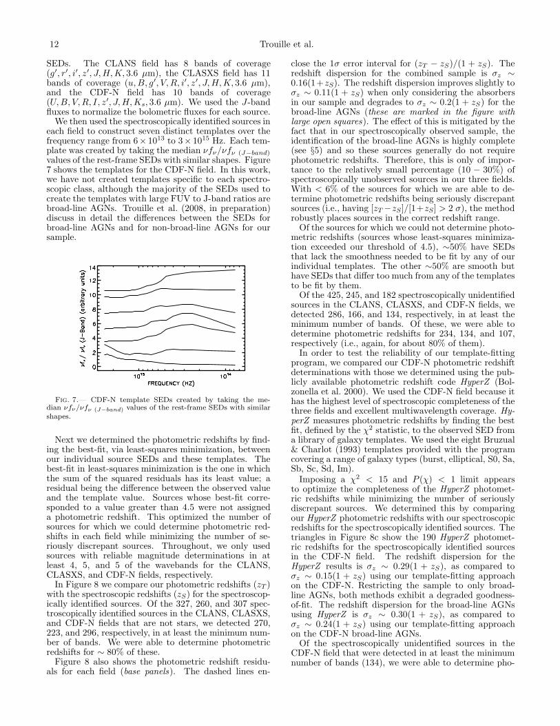
We then used the spectroscopically identified sources ineach field to construct seven distinct templates over thefrequency range from 6× 1013 to 3× 1015 Hz. Each tem-plate was created by taking the median νfν/νfν (J−band)

values of the rest-frame SEDs with similar shapes. Figure7 shows the templates for the CDF-N field. In this work,we have not created templates specific to each spectro-scopic class, although the majority of the SEDs used tocreate the templates with large FUV to J-band ratios arebroad-line AGNs. Trouille et al. (2008, in preparation)discuss in detail the differences between the SEDs forbroad-line AGNs and for non-broad-line AGNs for oursample.

Fig. 7.— CDF-N template SEDs created by taking the me-dian νfν/νfν (J−band) values of the rest-frame SEDs with similarshapes.

Next we determined the photometric redshifts by find-ing the best-fit, via least-squares minimization, betweenour individual source SEDs and these templates. Thebest-fit in least-squares minimization is the one in whichthe sum of the squared residuals has its least value; aresidual being the difference between the observed valueand the template value. Sources whose best-fit corre-sponded to a value greater than 4.5 were not assigneda photometric redshift. This optimized the number ofsources for which we could determine photometric red-shifts in each field while minimizing the number of se-riously discrepant sources. Throughout, we only usedsources with reliable magnitude determinations in atleast 4, 5, and 5 of the wavebands for the CLANS,CLASXS, and CDF-N fields, respectively.

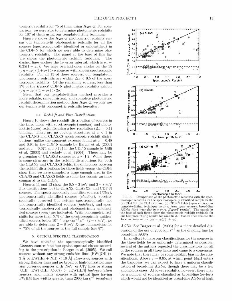
In Figure 8 we compare our photometric redshifts (zT )with the spectroscopic redshifts (zS) for the spectroscop-ically identified sources. Of the 327, 260, and 307 spec-troscopically identified sources in the CLANS, CLASXS,and CDF-N fields that are not stars, we detected 270,223, and 296, respectively, in at least the minimum num-ber of bands. We were able to determine photometricredshifts for ∼ 80% of these.

Figure 8 also shows the photometric redshift residu-als for each field (base panels). The dashed lines en-

close the 1σ error interval for (zT − zS)/(1 + zS). Theredshift dispersion for the combined sample is σz ∼0.16(1+zS). The redshift dispersion improves slightly toσz ∼ 0.11(1 + zS) when only considering the absorbersin our sample and degrades to σz ∼ 0.2(1 + zS) for thebroad-line AGNs (these are marked in the figure withlarge open squares). The effect of this is mitigated by thefact that in our spectroscopically observed sample, theidentification of the broad-line AGNs is highly complete(see §5) and so these sources generally do not requirephotometric redshifts. Therefore, this is only of impor-tance to the relatively small percentage (10 − 30%) ofspectroscopically unobserved sources in our three fields.With < 6% of the sources for which we are able to de-termine photometric redshifts being seriously discrepantsources (i.e., having [zT −zS]/[1+zS] > 2 σ), the methodrobustly places sources in the correct redshift range.

Of the sources for which we could not determine photo-metric redshifts (sources whose least-squares minimiza-tion exceeded our threshold of 4.5), ∼50% have SEDsthat lack the smoothness needed to be fit by any of ourindividual templates. The other ∼50% are smooth buthave SEDs that differ too much from any of the templatesto be fit by them.

Of the 425, 245, and 182 spectroscopically unidentifiedsources in the CLANS, CLASXS, and CDF-N fields, wedetected 286, 166, and 134, respectively, in at least theminimum number of bands. Of these, we were able todetermine photometric redshifts for 234, 134, and 107,respectively (i.e., again, for about 80% of them).

In order to test the reliability of our template-fittingprogram, we compared our CDF-N photometric redshiftdeterminations with those we determined using the pub-licly available photometric redshift code HyperZ (Bol-zonella et al. 2000). We used the CDF-N field because ithas the highest level of spectroscopic completeness of thethree fields and excellent multiwavelength coverage. Hy-perZ measures photometric redshifts by finding the bestfit, defined by the χ2 statistic, to the observed SED froma library of galaxy templates. We used the eight Bruzual& Charlot (1993) templates provided with the programcovering a range of galaxy types (burst, elliptical, S0, Sa,Sb, Sc, Sd, Im).

Imposing a χ2 < 15 and P (χ) < 1 limit appearsto optimize the completeness of the HyperZ photomet-ric redshifts while minimizing the number of seriouslydiscrepant sources. We determined this by comparingour HyperZ photometric redshifts with our spectroscopicredshifts for the spectroscopically identified sources. Thetriangles in Figure 8c show the 190 HyperZ photomet-ric redshifts for the spectroscopically identified sourcesin the CDF-N field. The redshift dispersion for theHyperZ results is σz ∼ 0.29(1 + zS), as compared toσz ∼ 0.15(1 + zS) using our template-fitting approachon the CDF-N. Restricting the sample to only broad-line AGNs, both methods exhibit a degraded goodness-of-fit. The redshift dispersion for the broad-line AGNsusing HyperZ is σz ∼ 0.30(1 + zS), as compared toσz ∼ 0.24(1 + zS) using our template-fitting approachon the CDF-N broad-line AGNs.

Of the spectroscopically unidentified sources in theCDF-N field that were detected in at least the minimumnumber of bands (134), we were able to determine pho-


tometric redshifts for 75 of them using HyperZ. For com-parison, we were able to determine photometric redshiftsfor 107 of them using our template-fitting technique.

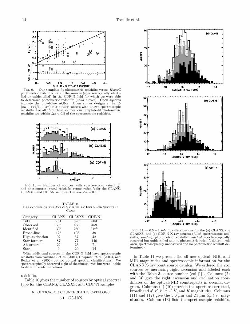
Figure 9 shows the HyperZ photometric redshifts ver-sus our template-fit photometric redshifts for all thesources (spectroscopically identified or unidentified) inthe CDF-N for which we were able to determine pho-tometric redshifts. The panel at the base of this fig-ure shows the photometric redshift residuals. Thedashed lines enclose the 1σ error interval, which is σz ∼0.25(1 + zS). We have overlaid open circles on the 15(zH −zT )/(1+zT ) > σ sources with known spectroscopicredshifts. For all 15 of these sources, our template-fitphotometric redshifts are within ∆z < 0.5 of the spec-troscopic redshifts. Of the remaining sources, less than5% of the HyperZ CDF-N photometric redshifts exhibit(zH − zT )/(1 + zT ) > 2σ.

Given that our template-fitting method provides amore reliable, self-consistent, and complete photometricredshift determination method than HyperZ, we only useour template-fit photometric redshifts hereafter.

4.4. Redshift and Flux Distributions

Figure 10 shows the redshift distribution of sources inthe three fields with spectroscopic (shading) and photo-metric (open) redshifts using a low-resolution (∆z = 0.1)binning. There are no obvious structures at z < 1 inthe CLANS and CLASXS spectroscopic redshift distri-butions, unlike the apparent excesses found at z = 0.48and 0.94 in the CDF-N sample by Barger et al. (2003)and at z = 0.674 and 0.734 in the CDF-S sample by Gilliet al. (2003) and Szokoly et al. (2004). There may bea grouping of CLASXS sources at z ∼ 1.2. While thereis some structure in the redshift distributions for boththe CLANS and CLASXS fields, the differences betweenthe redshift distributions for those fields versus the CDFsshow that we have sampled a large enough area in theCLANS and CLASXS fields to suffer less cosmic variancecompared to the CDFs.

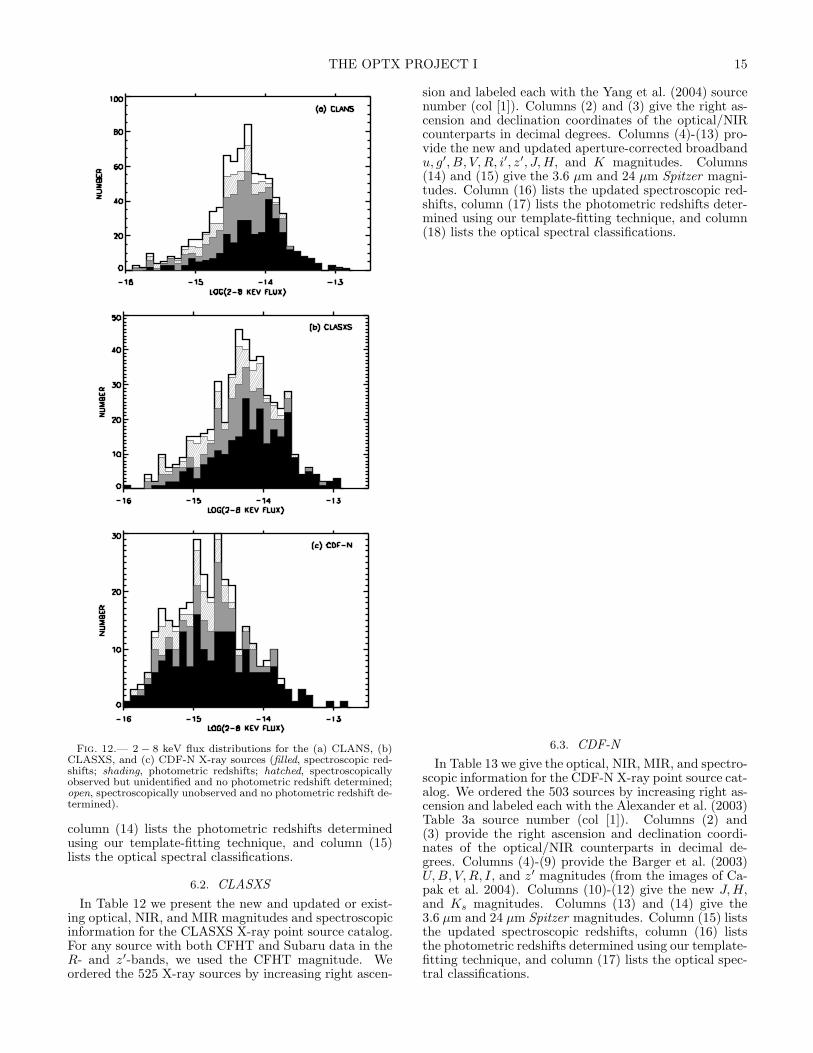
Figures 11 and 12 show the 0.5− 2 keV and 2− 8 keVflux distributions for the CLANS, CLASXS, and CDF-Nsources. The spectroscopically identified sources (filled),photometrically identified sources (shading), spectro-scopically observed but neither spectroscopically norphotometrically identified sources (hatched), and spec-troscopically unobserved and photometrically unidenti-fied sources (open) are indicated. With photometric red-shifts for more than 50% of the spectroscopically uniden-tified sources below 10−14 ergs cm−2 s−1 (2−8 keV), weare able to determine 2 − 8 keV X-ray luminosities for∼ 75% of all the sources in the full sample (see §7).

5. OPTICAL SPECTRAL CLASSIFICATION

We have classified the spectroscopically identifiedChandra sources into four optical spectral classes accord-ing to the prescription in Barger et al. (2005). We callsources without any strong emission lines [EW([OII])<3 A or EW(Hα + NII) < 10 A] absorbers ; sources withstrong Balmer lines and no broad or high-ionization linesstar formers ; sources with [NeV] or CIV lines or strong[OIII] [EW([OIII] λ5007) > 3EW(Hβ)] high-excitationsources ; and, finally, sources with optical lines havingFWHM line widths greater than 2000 km s−1 broad-line

Fig. 8.— Comparison of the photometric redshifts with the spec-troscopic redshifts for the spectroscopically identified sample in the(a) CLANS, (b) CLASXS, and (c) CDF-N fields (open circles, ourtemplate-fitting technique results; large open squares, broad-lineAGNs; filled triangles in c only, HyperZ results). The panels atthe base of each figure show the photometric redshift residuals forour template-fitting results for each field. Dashed lines enclose the1σ error interval for (zT − zS)/(1 + zS).

AGNs. See Barger et al. (2005) for a more detailed dis-cussion of the use of 2000 km s−1 as the dividing line forbroad-line AGNs.

In an effort to have our classifications for the sources inthe three fields be as uniformly determined as possible,several of the authors repeated the classifications for allof the sources in all three fields and came to a consensus.We note that there may be some redshift bias in the clas-sifications. Above z ∼ 0.65, at which point MgII entersthe bandpass, we can expect to have a uniform classifi-cation of broad-line AGNs, though there may be a fewanomolous cases. At lower redshifts, however, there maybe a number of sources classified as broad-line Seyfertswhich would not be identified as broad-line AGNs at high

14 Trouille et al.

Fig. 9.— Our template-fit photometric redshifts versus HyperZphotometric redshifts for all the sources (spectroscopically identi-fied or unidentified) in the CDF-N field for which we were ableto determine photometric redshifts (solid circles). Open squaresindicate the broad-line AGNs. Open circles designate the 15(zH − zT )/(1 + zT ) > σ outlier sources with known spectroscopicredshifts. For all 15 of these sources, our template-fit photometricredshifts are within ∆z < 0.5 of the spectroscopic redshifts.

Fig. 10.— Number of sources with spectroscopic (shading)and photometric (open) redshifts versus redshift for the CLANS,CLASXS, and CDF-N samples. Bin size ∆z = 0.1.

TABLE 10Breakdown of the X-ray Samples by Field and Spectral

Class

Category CLANS CLASXS CDF-NTotal 761 525 503Observed 533 468 459Identified 336 280 312a

Broad-line 126 103 39High-excitation 92 57 42Star formers 87 77 146Absorbers 22 23 71Stars 9 20 14aNine additional sources in the CDF-N field have spectroscopic

redshifts from Swinbank et al. (2004), Chapman et al. (2005), andReddy et al. (2006) but no optical spectral classifications. Wespectroscopically observed eight of the nine sources but were unableto determine identifications.

redshifts.Table 10 gives the number of sources by optical spectral

type for the CLANS, CLASXS, and CDF-N samples.

6. OPTICAL/IR COUNTERPARTS CATALOGS

6.1. CLANS

Fig. 11.— 0.5− 2 keV flux distributions for the (a) CLANS, (b)CLASXS, and (c) CDF-N X-ray sources (filled, spectroscopic red-shifts; shading, photometric redshifts; hatched, spectroscopicallyobserved but unidentified and no photometric redshift determined;open, spectroscopically unobserved and no photometric redshift de-termined).

In Table 11 we present the all new optical, NIR, andMIR magnitudes and spectroscopic information for theCLANS X-ray point source catalog. We ordered the 761sources by increasing right ascension and labeled eachwith the Table 3 source number (col [1]). Columns (2)and (3) give the right ascension and declination coor-dinates of the optical/NIR counterparts in decimal de-grees. Columns (4)-(10) provide the aperture-corrected,broadband g′, r′, i′, z′, J, H, and K magnitudes. Columns(11) and (12) give the 3.6 µm and 24 µm Spitzer mag-nitudes. Column (13) lists the spectroscopic redshifts,


Fig. 12.— 2 − 8 keV flux distributions for the (a) CLANS, (b)CLASXS, and (c) CDF-N X-ray sources (filled, spectroscopic red-shifts; shading, photometric redshifts; hatched, spectroscopicallyobserved but unidentified and no photometric redshift determined;open, spectroscopically unobserved and no photometric redshift de-termined).

column (14) lists the photometric redshifts determinedusing our template-fitting technique, and column (15)lists the optical spectral classifications.

6.2. CLASXS

In Table 12 we present the new and updated or exist-ing optical, NIR, and MIR magnitudes and spectroscopicinformation for the CLASXS X-ray point source catalog.For any source with both CFHT and Subaru data in theR- and z′-bands, we used the CFHT magnitude. Weordered the 525 X-ray sources by increasing right ascen-

sion and labeled each with the Yang et al. (2004) sourcenumber (col [1]). Columns (2) and (3) give the right as-cension and declination coordinates of the optical/NIRcounterparts in decimal degrees. Columns (4)-(13) pro-vide the new and updated aperture-corrected broadbandu, g′, B, V, R, i′, z′, J, H, and K magnitudes. Columns(14) and (15) give the 3.6 µm and 24 µm Spitzer magni-tudes. Column (16) lists the updated spectroscopic red-shifts, column (17) lists the photometric redshifts deter-mined using our template-fitting technique, and column(18) lists the optical spectral classifications.

6.3. CDF-N

In Table 13 we give the optical, NIR, MIR, and spectro-scopic information for the CDF-N X-ray point source cat-alog. We ordered the 503 sources by increasing right as-cension and labeled each with the Alexander et al. (2003)Table 3a source number (col [1]). Columns (2) and(3) provide the right ascension and declination coordi-nates of the optical/NIR counterparts in decimal de-grees. Columns (4)-(9) provide the Barger et al. (2003)U, B, V, R, I, and z′ magnitudes (from the images of Ca-pak et al. 2004). Columns (10)-(12) give the new J, H,and Ks magnitudes. Columns (13) and (14) give the3.6 µm and 24 µm Spitzer magnitudes. Column (15) liststhe updated spectroscopic redshifts, column (16) liststhe photometric redshifts determined using our template-fitting technique, and column (17) lists the optical spec-tral classifications.

16 Trouille et al.

TABLE 11CLANS Optical/IR Counterparts Catalog

# RA DEC g′ r′ i′ z′ J H K 3.6 µm 24 µm zspec zphot class(1) (2) (3) (4) (5) (6) (7) (8) (9) (10) (11) (12) (13) (14) (15)1 -99.000 -99.000 -99.00 -99.00 -99.00 -99.00 -99.00 -99.00 -99.00 -99.00 -99.00 -1.00 -99.00 -12 160.642 59.176 23.04 22.40 21.91 21.78 21.02 19.80 -99.00 19.50 -99.00 1.43 -3.00 43 160.642 59.169 25.43 25.04 24.40 23.71 22.53 21.93 -99.00 -99.00 -99.00 -1.00 1.35 -14 -99.000 -99.000 -99.00 -99.00 -99.00 -99.00 -99.00 -99.00 -99.00 -99.00 -99.00 -1.00 -99.00 -15 -99.000 -99.000 -99.00 -99.00 -99.00 -99.00 -99.00 -99.00 -99.00 20.87 -99.00 -1.00 -99.00 -1.. .. .. .. .. .. .. .. .. .. .. .. .. .. ..

Note. — Table 11 is available in its entirety in the electronic edition of the Astrophysical Journal Supplement. A portion is shown herefor guidance regarding its form and content. All magnitudes are in AB magnitudes.Typical photometric uncertainties are given in §3.6.Magnitude = −99, source not detected (2σ significance).zspec = 0 and corresponding class = −99, source spectroscopically observed but neither the redshift nor the class could be identified.zspec = −1 and corresponding class = −1, source not yet spectroscopically observed.zspec = −2 and corresponding class = −2, source is a star.zphot = −3, source has a spectroscopic redshift.zphot = −99, source has neither a spectroscopic nor a photometric redshift.class = 0, absorbers; class = 1, star formers; class = 3, high-excitation sources; class = 4, broad-line AGNs.

TABLE 12CLASXS Optical/IR Counterparts Catalog

# RA DEC u B g′ V R i′ z′ J H K 3.6 µm 24 µm zspec zphot class

(1) (2) (3) (4) (5) (6) (7) (8) (9) (10) (11) (12) (13) (14) (15) (16) (17) (18)

1 157.731 57.556 24.33 -99.00 23.69 -99.00 22.44 21.91 -99.00 20.17 20.30 -99.00 -1.00 -99.00 -1.00s 0.55 -12 157.748 57.646 -99.00 -99.00 23.74 -99.00 21.97 21.44 -99.00 20.44 20.17 -99.00 -1.00 17.84 -1.00s 0.45 -13 157.764 57.614 23.96 -99.00 -99.00 -99.00 22.80 22.65 -99.00 22.06 21.88 -99.00 -1.00 -99.00 0.00s 0.25 -994 157.774 57.630 23.80 -99.00 23.78 -99.00 23.04 22.96 23.05 22.56 -99.00 -99.00 -1.00 -99.00 0.00s -99.00 -995 157.800 57.590 25.29 24.51 24.27 -99.00 23.24 22.71 22.39 21.94 21.76 -99.00 -1.00 -99.00 0.00s 0.35 -99.. .. .. .. .. .. .. .. .. .. .. .. .. .. .. .. .. ..

Note. — Table 12 is available in its entirety in the electronic edition of the Astrophysical Journal Supplement. A portion is shown herefor guidance regarding its form and content. All magnitudes are in AB magnitudes.Typical photometric uncertainties are given in §3.6.Magnitude = −99, source not detected (2σ significance).zspec = 0 and corresponding class = −99, source spectroscopically observed but neither the redshift nor the class could be identified.zspec = −1 and corresponding class = −1, source not yet spectroscopically observed.zspec = −2 and corresponding class = −2, source is a star.zphot = −3, source has a spectroscopic redshift.zphot = −99, source has neither a spectroscopic nor a photometric redshift.class = 0, absorbers; class = 1, star formers; class = 3, high-excitation sources; class = 4, broad-line AGNs.Reference for zspec: s=Steffen et al. (2004). All other spectroscopic redshifts presented here for the first time.

TABLE 13CDF-N Optical/IR Counterparts Catalog

# RA DEC U B V R I z′ J H Ks 3.6 µm 24 µm zspec zphot class(1) (2) (3) (4) (5) (6) (7) (8) (9) (10) (11) (12) (13) (14) (15) (16) (17)1 188.813 62.235 26.4 25.7 25.3 25.1 25.2 24.8 -99.0 -99.0 23.12 -99.00 -99.00 -1.00 -99.00 -12 188.820 62.261 25.4 24.9 24.9 24.5 24.7 24.5 -99.0 22.1 21.41 -99.00 -99.00 0.00a -99.00 -993 188.828 62.264 21.3 20.2 19.1 18.6 18.2 18.0 17.0 16.7 16.62 -99.00 -99.00 0.14a -3.00 04 188.831 62.228 27.2 26.7 25.6 24.4 23.6 23.2 -99.0 22.3 21.70 -99.00 -99.00 -1.00 0.65 -15 188.839 62.274 23.2 22.8 22.4 21.8 21.4 21.2 20.6 20.2 20.06 -99.00 -99.00 0.56a -3.00 1.. .. .. .. .. .. .. .. .. .. .. .. .. .. .. .. ..

Note. — Table 13 is available in its entirety in the electronic edition of the Astrophysical Journal Supplement. A portion is shown herefor guidance regarding its form and content. All magnitudes are in AB magnitudes.Typical photometric uncertainties are given in §3.6.Magnitude = −99, source not detected (2σ significance).zspec = 0 and corresponding class = −99, source spectroscopically observed but neither the redshift nor the class could be identified.zspec = −1 and corresponding class = −1, source not yet spectroscopically observed.zspec > 0 and class = 10, spectroscopic redshift from the literature without a corresponding spectrum.zspec = −2 and corresponding class = −2, source is a star.zphot = −3, source has a spectroscopic redshift.zphot = −99, source has neither a spectroscopic nor a photometric redshift.class = 0, absorbers; class = 1, star formers; class = 3, high-excitation sources; class = 4, broad-line AGNs.Reference for zspec: a=Barger et al. (2003), b=Swinbank et al. (2004), c=Chapman et al. (2005), d=Reddy et al. (2006). All otherspectroscopic redshifts presented here for the first time.


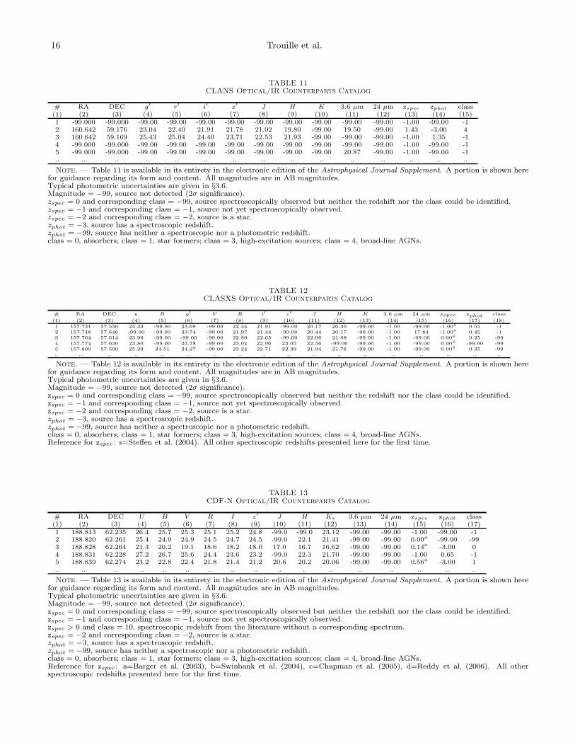
Fig. 13.— (a) Rest-frame 2−8 keV X-ray luminosity versus red-shift for the CLANS, CLASXS, and CDF-N sources according totheir optical classification (red circles, broad-line AGNs; green tri-angles, high-excitation narrow-line sources [HEX]; black squares,absorbers and star formers). We only include sources with spec-troscopic redshifts, LX > 1040 ergs s−1, and an X-ray detectionsignificance greater than 3σ. (b) Same as (a) but now classifyingthe sources according to their X-ray spectral properties (red circles,Γ > 1.5; green triangles, Γ < 1.5).

7. X-RAY LUMINOSITIES

We used the X-ray fluxes and redshifts of our sourcesto calculate their rest-frame 2−8 keV X-ray luminosities.We limited our sample to sources with an X-ray detectionsignificance greater than 3σ. For the CLANS sources wedetermined the 3σ significance level using the 1σ errorbars on the 2 − 8 keV and 0.5 − 2 keV flux values listedin Table 4. For the CLASXS and CDF-N sources we usedthe 1σ error bars from Yang et al. (2004) and Alexanderet al. (2003), respectively.

At z < 3, we calculated the luminosities from theobserved-frame 2 − 8 keV fluxes, and at z > 3, we usedthe observed-frame 0.5− 2 keV fluxes. One advantage ofusing the observed-frame 0.5−2 keV X-ray fluxes at highredshifts is the increased sensitivity, since the 0.5−2 keVChandra images are deeper than the 2 − 8 keV images.In addition, at z = 3, observed-frame 0.5 − 2 keV corre-sponds to rest-frame 2 − 8 keV, providing the best pos-sible match to the lower redshift data.

In calculating the K−corrections for obtaining therest-frame 2− 8 keV luminosities, we assumed an intrin-sic Γ = 1.8. Since the K−correction factor for emissionmodeled by a power law follows the form [1+z]Γ−2, thesecorrections are very small. If we instead assumed the

individual photon indices used in the flux calculations(rather than the universal power-law index of Γ = 1.8adopted here) to calculate the K−corrections, we wouldfind only a small difference in the rest-frame luminosities(Barger et al. 2002).

In short, the rest-frame 2 − 8 keV luminosity, LX ,equals f × 4πd2

L × K−correction.

z < 3 : K − corr. = (1 + z)−0.2 & f = f2−8 keV (4)

z ≥ 3 : K−corr. =1

4(1+z)−0.2 & f = f0.5−2 keV (5)

The 14 factor in the z ≥ 3 K−correction is a result of

normalizing so that there is no K−correction if z = 3,when the observed-frame 0.5−2 keV corresponds exactlyto the rest-frame 2 − 8 keV.

Figure 13a shows rest-frame 2−8 keV X-ray luminosityversus spectroscopic redshift for the CLANS, CLASXS,and CDF-N X-ray sources split by their optical spectralclassification. This figure illustrates the Steffen effect, inwhich the broad-line AGNs dominate the number den-sities at higher X-ray luminosities, while the non-broad-line AGNs dominate at lower X-ray luminosities (Steffenet al. 2003).

Figure 13b shows the same relation, but now thesources in the three fields are split by their X-ray classifi-cations. For the CLANS and CLASXS X-ray sources, weconverted the individual hardness ratios, HR, into Γ val-ues, as described in §2.2. For the CDF-N X-ray sources,we used the Alexander et al. (2003) values for Γ. Wenote that ∼ 1/4 of the sources in Figure 13b are within1σ of Γ = 1.5.

Figures 13a and 13b demonstrate that while the op-tical and X-ray classifications show generally the samebroad differentiation between the classes, there is clearlya different scatter or mixing of the objects, which re-flects the properties of each individual source. In Yenchoet al. (2008) we present the X-ray luminosity functionsby spectral type, and in L. Trouille et al. (2008, in prepa-ration) we present a detailed analysis of the optical andX-ray spectral characteristics of the individual objects inour sample.

8. NUMBER COUNTS

In order to determine the amount of field to field vari-ation within our sample and to compare our survey withthose by others, we have determined the differential num-ber counts for each individual field and for the full sam-ple.

In the following, we have excluded any CLANS orCLASXS sources with off-axis angles greater than 8′ be-cause the sensitivity of Chandra drops significantly atlarge off-axis angles and because of the field overlap inthe CLASXS region. Using the Yang et al. (2006) simula-tions (see §2.5), we have also excluded any CLANS andCLASXS sources with fluxes less than the flux thresh-old for the source’s particular off-axis angle location andpointing exposure time (see Figure 3). In this section,we use only the flux thresholds and Ω(Si) values for a30% probability of detection. See §2.5 and Figure 5 for adiscussion of the Ω(Si) values used for the CLANS andCLASXS fields.

The Poisson fluctuations in the source fluxes could re-sult in an overestimation of the number counts close to

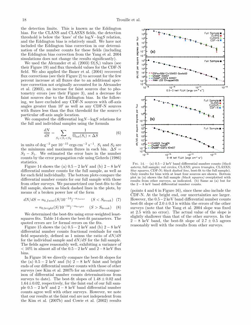
18 Trouille et al.

the detection limits. This is known as the Eddingtonbias. For the CLANS and CLASXS fields, the detectionthreshold is below the ‘knee’ of the logN−logS relation,and the Eddington bias is relatively small. We have notincluded the Eddington bias correction in our determi-nation of the number counts for these fields (includingthe Eddington bias correction from the Yang et al. 2004simulations does not change the results significantly).

We used the Alexander et al. (2003) Ω(Si) values (seetheir Figure 19) and flux threshold values for the CDF-Nfield. We also applied the Bauer et al. (2004) recoveredflux corrections (see their Figure 2) to account for the fewpercent increase at all fluxes due to an additional aper-ture correction not originally accounted for in Alexanderet al. (2003), an increase for faint sources due to pho-tometry errors (see their Figure 3), and a decrease forfaint sources due to the Eddington bias. In the follow-ing, we have excluded any CDF-N sources with off-axisangles greater than 10′ as well as any CDF-N sourceswith fluxes less than the flux threshold for the source’sparticular off-axis angle location.

We computed the differential logN−logS relations forthe full and individual samples using the formula

dN

dS=

∑

S1<Si<S2

1

Ωtot(Si) × ∆S(6)

in units of deg−2 per 10−15 ergs cm−2 s−1. S1 and S2 arethe minimum and maximum fluxes in each bin. ∆S =S2 − S1. We estimated the error bars in the numbercounts by the error propagation rule using Gehrels (1986)statistics.

Figure 14 shows the (a) 0.5− 2 keV and (b) 2− 8 keVdifferential number counts for the full sample, as well asfor each field individually. The bottom plots compare thedifferential number counts for our full sample with thosefrom other surveys. We parametrized our best-fits to thefull sample, shown as black dashed lines in the plots, bymeans of a broken power law of the form

dN/dS = n0,faint(S/10−14)−αfaint (S < Sbreak) (7)

= n0,bright(S/10−14)−αbright (S > Sbreak) (8)

We determined the best-fits using error-weighted least-squares fits. Table 14 shows the best-fit parameters. Thequoted errors are 1σ formal errors on the fits.

Figure 15 shows the (a) 0.5− 2 keV and (b) 2− 8 keVdifferential number counts fractional residuals for eachfield separately, defined as 1 minus the ratio of dN/dSfor the individual sample and dN/dS for the full sample.The fields agree reasonably well, exhibiting a variance of< 10% in almost all of the 0.5−2 keV and 2−8 keV fluxbins.

In Figure 16 we directly compare the best-fit slopes forthe (a) 0.5 − 2 keV and (b) 2 − 8 keV faint and brightends of our differential number counts with those of othersurveys (see Kim et al. 2007b for an exhaustive compar-ison of differential number counts determinations fromsurveys to date). The best-fit slopes of 1.48 ± 0.02 and1.64±0.02, respectively, for the faint end of our full sam-ple 0.5 − 2 keV and 2 − 8 keV band differential numbercounts agree well with other surveys. However, we notethat our results at the faint end are not independent fromthe Kim et al. (2007b) and Cowie et al. (2002) results

Fig. 14.— (a) 0.5−2 keV band differential number counts (blackasterix, full sample; red circles, CLANS; green triangles, CLASXS;blue squares, CDF-N; black dashed line, best-fit to the full sample).Only results for bins with at least four sources are shown. Bottomplot in (a) shows the full sample (black squares) overplotted withresults from other surveys, as indicated. (b) Same as (a) but forthe 2 − 8 keV band differential number counts.

(points 4 and 6 in Figure 16), since these also include theCDF-N. At the bright end, our uncertainties are larger.However, the 0.5−2 keV band differential number countsbest-fit slope of 2.0±0.3 is within the errors of the othersurveys (note that the Yang et al. 2004 slope was fixedat 2.5 with no error). The actual value of the slope isslightly shallower than that of the other surveys. In the2 − 8 keV band, the best-fit slope of 2.7 ± 0.5 agreesreasonably well with the results from other surveys.


TABLE 14Broken Power Law Best-fit Parameters for the Full Sample

Diff. Num. Counts Faint End Break Flux Bright Endn0 α n0 α

0.5 − 2 keV 16.5 ± 1.2 1.48 ± 0.02 6.5 × 10−15 11.3 ± 0.4 2.0 ± 0.32 − 8 keV 29.7 ± 1.2 1.64 ± 0.02 1.44 × 10−14 59.0 ± 27.0 2.7 ± 0.5

Fig. 15.— 0.5 − 2 keV and 2 − 8 keV band differential number count residuals, defined as 1 minus the ratio of dN/dS for the individualsample and dN/dS for the full sample, for the CLANS, CLASXS, and CDF-N fields. Only results for bins with at least four sources areshown.

Fig. 16.— (Top) Faint and (bottom) bright power indices of the differential number counts for this and previous studies in (a) the 0.5−2 keVband and (b) the 2−8 keV band. The references are as follows: (1) this study; (2) Yang et al. (2004) CLASXS; (3) Chiappetti et al. (2005)XMM LSS; (4) Kim et al. (2007b) ChaMP+CDFs; (5) Kim et al. (2007b) ChaMP; (6) Cowie et al. (2002) CDFs+SSA13+SSA22. Notethat Yang et al. (2004) fixed the bright slope as 2.5 in the 0.5 − 2 keV band, so there is no error.

20 Trouille et al.

9. SUMMARY

In this paper, we compiled the database for theOPTX project, which combines data from the CLANS,CLASXS, and CDF-N fields to create one of the mostspectroscopically complete samples of Chandra X-raysources to date. With this database, we can analyzethe effect of spectral type on the shape and evolution ofthe X-ray luminosity functions and compare the opticaland X-ray spectral properties of the X-ray sources in oursample.

In detail, we presented the first X-ray, infrared, andoptical photometric and spectroscopic catalogs for theCLANS field. The CLANS X-ray survey covers 0.6 deg2

and reaches fluxes of 7 × 10−16 ergs cm−2 s−1 in the0.5 − 2 keV band and 3.5 × 10−15 ergs cm−2 s−1 in the2−8 keV band. We presented g′, r′, i′, z′, J, H, K, 3.6 µm,and 24 µm photometry for the 761 X-ray sources inthe sample. We spectroscopically observed 533 of theCLANS sources, obtaining redshift identifications for336. We extended the redshift information to faintermagnitudes using photometric redshifts, which resultedin an additional 234 redshifts.

We also presented new and updated CLASXS pho-tometry and some new spectroscopy, along with existingdata. Using new u, g′, and i′ magnitudes, we correctedthe zeropoints for the original Steffen et al. (2004) V, R, I,and z′ photometry (the B-band zeropoint was fine). Wealso obtained J, H, K, 3.6 µm, and 24 µm photometryfor the 525 X-ray sources in the sample. Since the pub-lication of the Steffen et al. (2004) redshift catalog forthis field, we have obtained an additional 11 spectra andidentified redshifts for all 11. As a result, of the now468 spectroscopically observed CLASXS sources, we havepresented redshift identifications for 280. We extendedthe redshift information for the CLASXS field to include

an additional 134 photometric redshifts.Furthermore, we presented new CDF-N J, H, and Ks

photometry and some new optical spectroscopy, alongwith existing data. We also included the GOODS-NSpitzer 3.6 µm and 24 µm detections. Since the pub-lication of the Barger et al. (2003) redshift catalog forthis field, we have obtained an additional 49 spectra andidentified redshifts for 39. As a result, of the 503 X-raysources in the CDF-N field, we have spectroscopically ob-served 459, obtaining redshift identifications for 312. Weextended the redshift information for the CDF-N field toinclude an additional 107 photometric redshifts.

Finally, we determined the differential X-ray numbercounts for each survey individually and for the full sam-ple. Our differential number counts for the combinedsample agree well with the results from other X-ray sur-veys.

We thank John Silverman for alerting us to the zero-point problems with the optical data for the CLASXSX-ray sources. We thank the TERAPIX team for thework they do to produce the CFHT data. L. T. wassupported by a National Science Foundation GraduateResearch Fellowship and a Wisconsin Space Grant Con-sortium Graduate Fellowship Award during portions ofthis work. We also gratefully acknowledge support fromNSF grants AST 0239425 and AST 0708793 (A. J. B. )and AST 0407374 and AST 0709356 (L. L. C. ), theUniversity of Wisconsin Research Committee with fundsgranted by the Wisconsin Alumni Research Foundation(A. J. B. ), and the David and Lucile Packard Founda-tion (A. J. B. ). This article is part of L. T.’s Ph.D. thesiswork at the University of Wisconsin-Madison.

REFERENCES

Alexander, D. M., et al. 2003, AJ, 126, 539Alonso-Herrero, A., Ward, M. J., & Kotilainen, J. K. 1997,

MNRAS, 288, 977Aune S., et al. 2003, Proc. SPIE, 4841, 513Barden, S. C., Armandroff, T., Muller, G., Rudeen, A. C., Lewis,

J., & Groves, L. 1994, Proc. SPIE, 2198, 87Barger, A. J., Cowie, L. L., Brandt, W. N., Capak, P., Garmire,

G. P., Hornschemeier, A. E., Steffen, A. T., & Wehner, E. H.2002, AJ, 124, 1839

Barger, A. J., et al. 2003, AJ, 126, 632Barger, A. J., Cowie, L. L., Mushotzky, R. F., Yang, Y., Wang,

W., Steffen, A. T., & Capak, P. 2005, AJ, 129, 578Barger, A. J., Cowie, L. L., & Wang, W.-H. 2008, ApJ, in pressBauer, F. E., Alexander, D. M., Brandt, W. M., Schneider, D. P.,

Triester, E., Hornschemeier, A. E., & Garmire, G. P. 2004, AJ,128, 2048

Bertin, E., & Arnouts, S. 1996, A&AS, 117, 393Bolzonella, M., Miralles, J.-M., & Pello, R. 2000, A&A, 363, 476Boulade, O., et al. 2003, Proc. SPIE, 4841, 72Brandt, W. N., et al. 2001, AJ, 122, 2810Brandt, W.N., & Hasinger, G. 2005, ARA&A, 43, 829Bruzual, G. & Charlot, S. 1993, ApJ, 405, 538Bundy, K., et al. 2008, ApJ, in pressCapak, P., et al. 2004, AJ, 127, 180Cappelluti, N., et al. 2007, ApJS, 172, 341Chapman S. C., Blan, A. W., Smail, I., & Ivison, R. J. 2005, ApJ,

622, 772Chiappetti, L., et al. 2005, A&A, 439, 413Churazov, E., et al. 2007, A&A, 467, 529Cowie, L. L., Songaila, A., Hu, E. M., & Cohen, J. G. 1996, AJ,

112, 839

Cowie, L. L., Garmire, G. P., Bautz, M. W., Barger, A. J.,Brandt, W. N., & Hornschemeier, A. E. 2002, ApJ, 566, L5

Davis, M., et al. 2003, Proc. SPIE, 4834, 161Davis, M., et al. 2007, ApJ, 660, 1Dye., S., et al. 2006, MNRAS, 372, 1227Eckart, M. E., Stern, D., Helfand, D. J., Harrison, F. A., Mao, P.

H., & Yost, S. A. 2006, A&A, 450, 535Faber, S. M., et al. 2003, Proc. SPIE, 4841, 1657Freeman, P. E., Kashyap, V., Rosner, R., & Lamb, D. Q. 2002,

ApJS, 138, 185Frontera, F., et al. 2007, ApJ, 666, 86Gehrels, N. 1986, ApJ, 303, 336Georgakakis, A., et al. 2007, ApJ, 660, L15Giacconi, R., et al. 2002, ApJS, 139, 369Gilli, R., et al. 2003, ApJ, 592, 721Gilli, R., Comastri, A., & Hasinger, G. 2007, A&A, 463, 79Harrison, F., Eckart, M. E., Mao, P. H., Helfand, D. J., & Stern,

D. 2003, ApJ, 596, 944Kim, M., et al. 2007a, ApJS, 169, 401Kim, M., Wilkes, B. J., Kim, D-W., Green, P. J., Barkhouse, W.

A., Lee, M. G., Silverman, J. D., & Tananbaum, H. D. 2007b,ApJ, 659, 29

Lehmer, B. D., et al. 2005, ApJS, 161, L21Lockman, F. J., Jahoda, K., & McCammon, D., 1986, ApJ, 302,

432Lonsdale, C. J., et al. 2003, PASP, 115, 897Lonsdale, C. J., et al. 2004, ApJS, 154, 54Loose, M., Farris, M. C., Garnett, J. D., Hall, D. N. B., &

Kozlowski, L. J. 2003, Proc. SPIE, 4850, 867Magnier, E. A., & Cuillandre, J.-C. 2004, PASP, 116, 449Monet, D., et al. 2003, AJ, 125, 984


Mulchaey, J. S., Koratkar, A., Ward, M. J., Wilson, A. S.,Whittle, M., Antonucci, R., Kinney, A. L., & Hurt, T. 1994,ApJ, 436, 586

Muno, M. P., et al. 2003, ApJ, 589, 225Murray S. S., et al. 2005, ApJS, 161, 1Nandra, K., Adelberger, K., Gardner, J. P., Mushotzky, R. F.,

Rhodes, J., Steidel, C. C., Teplitz, H. I., Arnaud, K. A. 2005,MNRAS, 356, 568

Oke, J. B., et al. 1995, PASP, 107, 375Polletta, M., et al. 2006, ApJ, 642, 673Perez-Gonzalez, P. G., et al. 2005, ApJ, 630, 82Reddy, N. A., Steidel, C., Erb, D. K., Shapley, A. E., & Pettini,

M. 2006, ApJ, 653, 1004Rowan-Robinson, M., et al. 2008, MNRAS, 386, 697Silverman, J. D., et al. 2008, ApJ, 675, 1025Stark, A. A., Gammie, C. F., Wilson, R. W., Bally, J., Linke, R.

A., Heiles, C., & Hurwitz, M. 1992, ApJS, 79, 77Steffen, A. T., Barger, A. J., Cowie, L. L., Mushotzky, R. F., &

Yang, Y. 2003, ApJ, 596, L23Steffen, A. T., Barger, A. J., Capak, P., Cowie, L. L., Mushotzky,

R. F., & Yang, Y. 2004, AJ, 128, 1483

Swinbank, A. M., Smail, I., Chapman, S. C., Blain, A. W., Ivison,R. J., & Keel, W. C. 2004, ApJ, 617, 64

Szokoly, G. P., et al. 2004, ApJS, 155, 271Ueda, Y., Takahashi, T., Ohashi, T., & Makishima, K. 1999, ApJ,

524, L11Virani, S. N., Treister, E., Urry, M., & Gawiser, E. 2006a, AJ,

131, 2373Virani, S. N., et al. 2006b, in Proceedings of the X-ray Universe,

Ed. A. Wilson (Madrid: El Escorial), 849Wang, W., Cowie, L. L., & Barger, A. J. 2006, ApJ, 647, 74Yang, Y., Mushotzky, R. F., Steffen, A. T., Barger, A. J., &

Cowie, L. L. 2004, AJ, 128, 1501Yang, Y., Mushotzky, R. F., Barger, A. J., & Cowie, L. L. 2006,

ApJ, 645, 68Yencho, B., Barger, A. J., Trouille, L., & Winter, L. M. 2008,

ApJ, submitted

The OPTX Project. I. The Flux and Redshift Catalogs for the CLANS, CLASXS, and CDF-N Fields

Documents

Transcript of The OPTX Project. I. The Flux and Redshift Catalogs for the CLANS, CLASXS, and CDF-N Fields