arX

iv:1

004.

1181

v4 [

hep-

ex]

11

Dec

201

0

Observation of Single Top Quark Production and Measurement of |Vtb| with CDF

T. Aaltonen,24 J. Adelman,14 B. Alvarez Gonzalezw,12 S. Amerioee,44 D. Amidei,35 A. Anastassov,39 A. Annovi,20

J. Antos,15 G. Apollinari,18 J. Appel,18 A. Apresyan,49 T. Arisawa,58 A. Artikov,16 J. Asaadi,54 W. Ashmanskas,18

A. Attal,4 A. Aurisano,54 F. Azfar,43 W. Badgett,18 A. Barbaro-Galtieri,29 V.E. Barnes,49 B.A. Barnett,26

P. Barriagg,47 P. Bartos,15 G. Bauer,33 P.-H. Beauchemin,34 F. Bedeschi,47 D. Beecher,31 S. Behari,26

G. Bellettiniff ,47 J. Bellinger,60 D. Benjamin,17 A. Beretvas,18 A. Bhatti,51 M. Binkley∗,18 D. Biselloee,44

I. Bizjakkk,31 R.E. Blair,2 C. Blocker,7 B. Blumenfeld,26 A. Bocci,17 A. Bodek,50 V. Boisvert,50 D. Bortoletto,49

J. Boudreau,48 A. Boveia,11 B. Braua,11 A. Bridgeman,25 L. Brigliadoridd,6 C. Bromberg,36 E. Brubaker,14

J. Budagov,16 H.S. Budd,50 S. Budd,25 K. Burkett,18 G. Busettoee,44 P. Bussey,22 A. Buzatu,34 K. L. Byrum,2

S. Cabreray,17 C. Calancha,32 S. Camarda,4 M. Campanelli,31 M. Campbell,35 F. Canelli14,18 A. Canepa,46

B. Carls,25 D. Carlsmith,60 R. Carosi,47 S. Carrillon,19 S. Carron,18 B. Casal,12 M. Casarsa,18 A. Castrodd,6

P. Catastinigg,47 D. Cauz,55 V. Cavalieregg,47 M. Cavalli-Sforza,4 A. Cerri,29 L. Cerritoq,31 S.H. Chang,28

Y.C. Chen,1 M. Chertok,8 G. Chiarelli,47 G. Chlachidze,18 F. Chlebana,18 K. Cho,28 D. Chokheli,16 J.P. Chou,23

K. Chungo,18 W.H. Chung,60 Y.S. Chung,50 T. Chwalek,27 C.I. Ciobanu,45 M.A. Cioccigg,47 A. Clark,21 D. Clark,7

G. Compostella,44 M.E. Convery,18 J. Conway,8 M.Corbo,45 M. Cordelli,20 C.A. Cox,8 D.J. Cox,8 F. Crescioliff ,47

C. Cuenca Almenar,61 J. Cuevasw,12 R. Culbertson,18 J.C. Cully,35 D. Dagenhart,18 N. d’Ascenzov,45 M. Datta,18

T. Davies,22 P. de Barbaro,50 S. De Cecco,52 A. Deisher,29 G. De Lorenzo,4 M. Dell’Orsoff ,47 C. Deluca,4

L. Demortier,51 J. Dengf ,17 M. Deninno,6 M. d’Erricoee,44 A. Di Cantoff ,47 B. Di Ruzza,47 J.R. Dittmann,5

M. D’Onofrio,4 S. Donatiff ,47 P. Dong,18 T. Dorigo,44 S. Dube,53 K. Ebina,58 A. Elagin,54 R. Erbacher,8

D. Errede,25 S. Errede,25 N. Ershaidatcc,45 R. Eusebi,54 H.C. Fang,29 S. Farrington,43 W.T. Fedorko,14 R.G. Feild,61

M. Feindt,27 J.P. Fernandez,32 C. Ferrazzahh,47 R. Field,19 G. Flanagans,49 R. Forrest,8 M.J. Frank,5 M. Franklin,23

J.C. Freeman,18 I. Furic,19 M. Gallinaro,51 J. Galyardt,13 F. Garberson,11 J.E. Garcia,21 A.F. Garfinkel,49

P. Garosigg,47 H. Gerberich,25 D. Gerdes,35 A. Gessler,27 S. Giaguii,52 V. Giakoumopoulou,3 P. Giannetti,47

K. Gibson,48 J.L. Gimmell,50 C.M. Ginsburg,18 N. Giokaris,3 M. Giordanijj ,55 P. Giromini,20 M. Giunta,47

G. Giurgiu,26 V. Glagolev,16 D. Glenzinski,18 M. Gold,38 N. Goldschmidt,19 A. Golossanov,18 G. Gomez,12

G. Gomez-Ceballos,33 M. Goncharov,33 O. Gonzalez,32 I. Gorelov,38 A.T. Goshaw,17 K. Goulianos,51 A. Greseleee,44

S. Grinstein,4 C. Grosso-Pilcher,14 R.C. Group,18 U. Grundler,25 J. Guimaraes da Costa,23 Z. Gunay-Unalan,36

C. Haber,29 S.R. Hahn,18 E. Halkiadakis,53 B.-Y. Han,50 J.Y. Han,50 F. Happacher,20 K. Hara,56 D. Hare,53

M. Hare,57 R.F. Harr,59 M. Hartz,48 K. Hatakeyama,5 C. Hays,43 M. Heck,27 J. Heinrich,46 M. Herndon,60

J. Heuser,27 S. Hewamanage,5 D. Hidas,53 C.S. Hillc,11 D. Hirschbuehl,27 A. Hocker,18 S. Hou,1 M. Houlden,30

S.-C. Hsu,29 R.E. Hughes,40 M. Hurwitz,14 U. Husemann,61 M. Hussein,36 J. Huston,36 J. Incandela,11 G. Introzzi,47

M. Ioriii,52 A. Ivanovp,8 E. James,18 D. Jang,13 B. Jayatilaka,17 E.J. Jeon,28 M.K. Jha,6 S. Jindariani,18

W. Johnson,8 M. Jones,49 K.K. Joo,28 S.Y. Jun,13 J.E. Jung,28 T.R. Junk,18 T. Kamon,54 D. Kar,19 P.E. Karchin,59

Y. Katom,42 R. Kephart,18 W. Ketchum,14 J. Keung,46 V. Khotilovich,54 B. Kilminster,18 D.H. Kim,28 H.S. Kim,28

H.W. Kim,28 J.E. Kim,28 M.J. Kim,20 S.B. Kim,28 S.H. Kim,56 Y.K. Kim,14 N. Kimura,58 L. Kirsch,7

S. Klimenko,19 K. Kondo,58 D.J. Kong,28 J. Konigsberg,19 A. Korytov,19 A.V. Kotwal,17 M. Kreps,27 J. Kroll,46

D. Krop,14 N. Krumnack,5 M. Kruse,17 V. Krutelyov,11 T. Kuhr,27 N.P. Kulkarni,59 M. Kurata,56 S. Kwang,14

A.T. Laasanen,49 S. Lami,47 S. Lammel,18 M. Lancaster,31 R.L. Lander,8 K. Lannonu,40 A. Lath,53 G. Latinogg,47

I. Lazzizzeraee,44 T. LeCompte,2 E. Lee,54 H.S. Lee,14 J.S. Lee,28 S.W. Leex,54 S. Leone,47 J.D. Lewis,18

C.-J. Lin,29 J. Linacre,43 M. Lindgren,18 E. Lipeles,46 A. Lister,21 D.O. Litvintsev,18 C. Liu,48 T. Liu,18

N.S. Lockyer,46 A. Loginov,61 L. Lovas,15 D. Lucchesiee,44 J. Lueck,27 P. Lujan,29 P. Lukens,18 G. Lungu,51

J. Lys,29 R. Lysak,15 D. MacQueen,34 R. Madrak,18 K. Maeshima,18 K. Makhoul,33 P. Maksimovic,26 S. Malde,43

S. Malik,31 G. Mancae,30 A. Manousakis-Katsikakis,3 F. Margaroli,49 C. Marino,27 C.P. Marino,25 A. Martin,61

V. Martink,22 M. Martınez,4 R. Martınez-Balların,32 P. Mastrandrea,52 M. Mathis,26 M.E. Mattson,59 P. Mazzanti,6

K.S. McFarland,50 P. McIntyre,54 R. McNultyj ,30 A. Mehta,30 P. Mehtala,24 A. Menzione,47 C. Mesropian,51

T. Miao,18 D. Mietlicki,35 N. Miladinovic,7 R. Miller,36 C. Mills,23 M. Milnik,27 A. Mitra,1 G. Mitselmakher,19

H. Miyake,56 S. Moed,23 N. Moggi,6 M.N. Mondragonn,18 C.S. Moon,28 R. Moore,18 M.J. Morello,47 J. Morlock,27

P. Movilla Fernandez,18 J. Mulmenstadt,29 A. Mukherjee,18 Th. Muller,27 P. Murat,18 M. Mussinidd,6

J. Nachtmano,18 Y. Nagai,56 J. Naganoma,56 K. Nakamura,56 I. Nakano,41 A. Napier,57 J. Nett,60 C. Neuaa,46

M.S. Neubauer,25 S. Neubauer,27 J. Nielseng,29 L. Nodulman,2 M. Norman,10 O. Norniella,25 E. Nurse,31

L. Oakes,43 S.H. Oh,17 Y.D. Oh,28 I. Oksuzian,19 T. Okusawa,42 R. Orava,24 K. Osterberg,24 S. Pagan Grisoee,44

C. Pagliarone,55 E. Palencia,18 V. Papadimitriou,18 A. Papaikonomou,27 A.A. Paramanov,2 B. Parks,40

S. Pashapour,34 J. Patrick,18 G. Paulettajj,55 M. Paulini,13 C. Paus,33 T. Peiffer,27 D.E. Pellett,8 A. Penzo,55

2

T.J. Phillips,17 G. Piacentino,47 E. Pianori,46 L. Pinera,19 K. Pitts,25 C. Plager,9 L. Pondrom,60 K. Potamianos,49

O. Poukhov∗,16 F. Prokoshinz,16 A. Pronko,18 F. Ptohosi,18 E. Pueschel,13 G. Punziff ,47 J. Pursley,60

J. Rademackerc,43 A. Rahaman,48 V. Ramakrishnan,60 N. Ranjan,49 I. Redondo,32 P. Renton,43 M. Renz,27

M. Rescigno,52 S. Richter,27 F. Rimondidd,6 L. Ristori,47 A. Robson,22 T. Rodrigo,12 T. Rodriguez,46 E. Rogers,25

S. Rolli,57 R. Roser,18 M. Rossi,55 R. Rossin,11 P. Roy,34 A. Ruiz,12 J. Russ,13 V. Rusu,18 B. Rutherford,18

H. Saarikko,24 A. Safonov,54 W.K. Sakumoto,50 L. Santijj ,55 L. Sartori,47 K. Sato,56 V. Savelievv,45

A. Savoy-Navarro,45 P. Schlabach,18 A. Schmidt,27 E.E. Schmidt,18 M.A. Schmidt,14 M.P. Schmidt∗,61

M. Schmitt,39 T. Schwarz,8 L. Scodellaro,12 A. Scribanogg,47 F. Scuri,47 A. Sedov,49 S. Seidel,38 Y. Seiya,42

A. Semenov,16 L. Sexton-Kennedy,18 F. Sforzaff ,47 A. Sfyrla,25 S.Z. Shalhout,59 T. Shears,30 P.F. Shepard,48

M. Shimojimat,56 S. Shiraishi,14 M. Shochet,14 Y. Shon,60 I. Shreyber,37 A. Simonenko,16 P. Sinervo,34

A. Sisakyan,16 A.J. Slaughter,18 J. Slaunwhite,40 K. Sliwa,57 J.R. Smith,8 F.D. Snider,18 R. Snihur,34 A. Soha,18

S. Somalwar,53 V. Sorin,4 P. Squillaciotigg,47 M. Stanitzki,61 R. St. Denis,22 B. Stelzer,34 O. Stelzer-Chilton,34

D. Stentz,39 J. Strologas,38 G.L. Strycker,35 J.S. Suh,28 A. Sukhanov,19 I. Suslov,16 A. Taffardf ,25 R. Takashima,41

Y. Takeuchi,56 R. Tanaka,41 J. Tang,14 M. Tecchio,35 P.K. Teng,1 J. Thomh,18 J. Thome,13 G.A. Thompson,25

E. Thomson,46 P. Tipton,61 P. Ttito-Guzman,32 S. Tkaczyk,18 D. Toback,54 S. Tokar,15 K. Tollefson,36 T. Tomura,56

D. Tonelli,18 S. Torre,20 D. Torretta,18 P. Totarojj ,55 M. Trovatohh,47 S.-Y. Tsai,1 Y. Tu,46 N. Turinigg,47

F. Ukegawa,56 S. Uozumi,28 N. van Remortelb,24 A. Varganov,35 E. Vatagahh,47 F. Vazquezn,19 G. Velev,18

C. Vellidis,3 M. Vidal,32 I. Vila,12 R. Vilar,12 M. Vogel,38 I. Volobouevx,29 G. Volpiff ,47 P. Wagner,46 R.G. Wagner,2

R.L. Wagner,18 W. Wagnerbb,27 J. Wagner-Kuhr,27 T. Wakisaka,42 R. Wallny,9 S.M. Wang,1 A. Warburton,34

D. Waters,31 M. Weinberger,54 J. Weinelt,27 W.C. Wester III,18 B. Whitehouse,57 D. Whitesonf ,46 A.B. Wicklund,2

E. Wicklund,18 S. Wilbur,14 G. Williams,34 H.H. Williams,46 P. Wilson,18 B.L. Winer,40 P. Wittichh,18

S. Wolbers,18 C. Wolfe,14 H. Wolfe,40 T. Wright,35 X. Wu,21 F. Wurthwein,10 A. Yagil,10 K. Yamamoto,42

J. Yamaoka,17 U.K. Yangr,14 Y.C. Yang,28 W.M. Yao,29 G.P. Yeh,18 K. Yio,18 J. Yoh,18 K. Yorita,58 T. Yoshidal,42

G.B. Yu,17 I. Yu,28 S.S. Yu,18 J.C. Yun,18 A. Zanetti,55 Y. Zeng,17 X. Zhang,25 Y. Zhengd,9 and S. Zucchellidd6

(CDF Collaboration†)1Institute of Physics, Academia Sinica, Taipei, Taiwan 11529, Republic of China

2Argonne National Laboratory, Argonne, Illinois 604393University of Athens, 157 71 Athens, Greece

4Institut de Fisica d’Altes Energies, Universitat Autonoma de Barcelona, E-08193, Bellaterra (Barcelona), Spain5Baylor University, Waco, Texas 76798

6Istituto Nazionale di Fisica Nucleare Bologna, ddUniversity of Bologna, I-40127 Bologna, Italy7Brandeis University, Waltham, Massachusetts 02254

8University of California, Davis, Davis, California 956169University of California, Los Angeles, Los Angeles, California 90024

10University of California, San Diego, La Jolla, California 9209311University of California, Santa Barbara, Santa Barbara, California 93106

12Instituto de Fisica de Cantabria, CSIC-University of Cantabria, 39005 Santander, Spain13Carnegie Mellon University, Pittsburgh, PA 15213

14Enrico Fermi Institute, University of Chicago, Chicago, Illinois 6063715Comenius University, 842 48 Bratislava, Slovakia; Institute of Experimental Physics, 040 01 Kosice, Slovakia

16Joint Institute for Nuclear Research, RU-141980 Dubna, Russia17Duke University, Durham, North Carolina 27708

18Fermi National Accelerator Laboratory, Batavia, Illinois 6051019University of Florida, Gainesville, Florida 32611

20Laboratori Nazionali di Frascati, Istituto Nazionale di Fisica Nucleare, I-00044 Frascati, Italy21University of Geneva, CH-1211 Geneva 4, Switzerland

22Glasgow University, Glasgow G12 8QQ, United Kingdom23Harvard University, Cambridge, Massachusetts 02138

24Division of High Energy Physics, Department of Physics,University of Helsinki and Helsinki Institute of Physics, FIN-00014, Helsinki, Finland

25University of Illinois, Urbana, Illinois 6180126The Johns Hopkins University, Baltimore, Maryland 21218

27Institut fur Experimentelle Kernphysik, Karlsruhe Institute of Technology, D-76131 Karlsruhe, Germany28Center for High Energy Physics: Kyungpook National University,Daegu 702-701, Korea; Seoul National University, Seoul 151-742,

Korea; Sungkyunkwan University, Suwon 440-746,Korea; Korea Institute of Science and Technology Information,

Daejeon 305-806, Korea; Chonnam National University, Gwangju 500-757,Korea; Chonbuk National University, Jeonju 561-756, Korea

3

29Ernest Orlando Lawrence Berkeley National Laboratory, Berkeley, California 9472030University of Liverpool, Liverpool L69 7ZE, United Kingdom

31University College London, London WC1E 6BT, United Kingdom32Centro de Investigaciones Energeticas Medioambientales y Tecnologicas, E-28040 Madrid, Spain

33Massachusetts Institute of Technology, Cambridge, Massachusetts 0213934Institute of Particle Physics: McGill University, Montreal, Quebec,

Canada H3A 2T8; Simon Fraser University, Burnaby, British Columbia,Canada V5A 1S6; University of Toronto, Toronto, Ontario,

Canada M5S 1A7; and TRIUMF, Vancouver, British Columbia, Canada V6T 2A335University of Michigan, Ann Arbor, Michigan 48109

36Michigan State University, East Lansing, Michigan 4882437Institution for Theoretical and Experimental Physics, ITEP, Moscow 117259, Russia

38University of New Mexico, Albuquerque, New Mexico 8713139Northwestern University, Evanston, Illinois 6020840The Ohio State University, Columbus, Ohio 4321041Okayama University, Okayama 700-8530, Japan

42Osaka City University, Osaka 588, Japan43University of Oxford, Oxford OX1 3RH, United Kingdom

44Istituto Nazionale di Fisica Nucleare, Sezione di Padova-Trento, eeUniversity of Padova, I-35131 Padova, Italy45LPNHE, Universite Pierre et Marie Curie/IN2P3-CNRS, UMR7585, Paris, F-75252 France

46University of Pennsylvania, Philadelphia, Pennsylvania 1910447Istituto Nazionale di Fisica Nucleare Pisa, ffUniversity of Pisa,

ggUniversity of Siena and hhScuola Normale Superiore, I-56127 Pisa, Italy48University of Pittsburgh, Pittsburgh, Pennsylvania 15260

49Purdue University, West Lafayette, Indiana 4790750University of Rochester, Rochester, New York 14627

51The Rockefeller University, New York, New York 1002152Istituto Nazionale di Fisica Nucleare, Sezione di Roma 1,

iiSapienza Universita di Roma, I-00185 Roma, Italy53Rutgers University, Piscataway, New Jersey 08855

54Texas A&M University, College Station, Texas 7784355Istituto Nazionale di Fisica Nucleare Trieste/Udine,

I-34100 Trieste, jjUniversity of Trieste/Udine, I-33100 Udine, Italy56University of Tsukuba, Tsukuba, Ibaraki 305, Japan

57Tufts University, Medford, Massachusetts 0215558Waseda University, Tokyo 169, Japan

59Wayne State University, Detroit, Michigan 4820160University of Wisconsin, Madison, Wisconsin 53706

61Yale University, New Haven, Connecticut 06520(Dated: April 5, 2010)

We report the observation of electroweak single top quark production in 3.2 fb−1 of pp colli-sion data collected by the Collider Detector at Fermilab at

√s = 1.96 TeV. Candidate events in

the W+jets topology with a leptonically decaying W boson are classified as signal-like by fourparallel analyses based on likelihood functions, matrix elements, neural networks, and boosted de-cision trees. These results are combined using a super discriminant analysis based on geneticallyevolved neural networks in order to improve the sensitivity. This combined result is further com-bined with that of a search for a single top quark signal in an orthogonal sample of events withmissing transverse energy plus jets and no charged lepton. We observe a signal consistent withthe standard model prediction but inconsistent with the background-only model by 5.0 standarddeviations, with a median expected sensitivity in excess of 5.9 standard deviations. We mea-sure a production cross section of 2.3+0.6

−0.5(stat + sys) pb, extract the CKM matrix element value

|Vtb| = 0.91+0.11−0.11(stat + sys)± 0.07(theory), and set a lower limit |Vtb| > 0.71 at the 95% confidence

level, assuming mt = 175 GeV/c2.

PACS numbers: 14.65.Ha, 13.85.Qk, 12.15.Hh, 12.15.Ji

∗Deceased†With visitors from aUniversity of Massachusetts Amherst,Amherst, Massachusetts 01003, bUniversiteit Antwerpen, B-2610

Antwerp, Belgium, cUniversity of Bristol, Bristol BS8 1TL,United Kingdom, dChinese Academy of Sciences, Beijing 100864,

4

Contents

I. Introduction 5

II. The CDF II Detector 7

III. Selection of Candidate Events 8

IV. Signal Model 11A. s-channel Single Top Quark Model 11B. t-channel Single Top Quark Model 12C. Validation 13D. Expected Signal Yields 13

V. Background Model 15A. Monte Carlo Based Background Processes 15B. Non-W Multijet Events 16C. W+Heavy Flavor Contributions 17D. Rates of Events with Mistagged Jets 19E. Validation of Monte Carlo Simulation 21

VI. Jet Flavor Separator 22

VII. Multivariate Analysis 25A. Multivariate Likelihood Function 27

1. Kinematic Constraints 282. 2-Jet t-channel Likelihood Function 303. 2-Jet s-channel Likelihood Function 304. 3-Jet Likelihood Function 305. Distributions 316. Validation 317. Background Likelihood Functions 31

B. Matrix Element Method 341. Event Probability 342. Transfer Functions 353. Integration 35

China, eIstituto Nazionale di Fisica Nucleare, Sezione di Cagliari,09042 Monserrato (Cagliari), Italy, fUniversity of CaliforniaIrvine, Irvine, CA 92697, gUniversity of California Santa Cruz,Santa Cruz, CA 95064, hCornell University, Ithaca, NY 14853,iUniversity of Cyprus, Nicosia CY-1678, Cyprus, jUniversity Col-lege Dublin, Dublin 4, Ireland, kUniversity of Edinburgh, Edin-burgh EH9 3JZ, United Kingdom, lUniversity of Fukui, Fukui City,Fukui Prefecture, Japan 910-0017, mKinki University, Higashi-Osaka City, Japan 577-8502, nUniversidad Iberoamericana, Mex-ico D.F., Mexico, oUniversity of Iowa, Iowa City, IA 52242,pKansas State University, Manhattan, KS 66506, qQueen Mary,University of London, London, E1 4NS, England, rUniversityof Manchester, Manchester M13 9PL, England, sMuons, Inc.,Batavia, IL 60510, tNagasaki Institute of Applied Science, Na-gasaki, Japan, uUniversity of Notre Dame, Notre Dame, IN46556, vObninsk State University, Obninsk, Russia, wUniversityde Oviedo, E-33007 Oviedo, Spain, xTexas Tech University, Lub-bock, TX 79609, yIFIC(CSIC-Universitat de Valencia), 56071 Va-lencia, Spain, zUniversidad Tecnica Federico Santa Maria, 110vValparaiso, Chile, aaUniversity of Virginia, Charlottesville, VA22906, bbBergische Universitat Wuppertal, 42097 Wuppertal, Ger-many, ccYarmouk University, Irbid 211-63, Jordan, kkOn leavefrom J. Stefan Institute, Ljubljana, Slovenia

4. Event Probability Discriminant 365. Validation 36

C. Artificial Neural Network 371. Input Variables 372. Distributions 403. Validation 404. High NN Discriminant Output 40

D. Boosted Decision Tree 401. Distributions 432. Validation 43

VIII. Systematic Uncertainties 43A. Rate Uncertainties 45B. Shape-Only Uncertainties 47

IX. Interpretation 48A. Likelihood Function 48B. Cross Section Measurement 51

1. Measurement of σs+t 512. Extraction of Bounds on |Vtb| 51

C. Check for Bias 51D. Significance Calculation 52

X. Combination 53

XI. One-Dimensional Fit Results 55

XII. Two-Dimensional Fit Results 57

XIII. Summary 59

References 61

5

I. INTRODUCTION

The top quark is the most massive known elementaryparticle. Its mass, mt, is 173.3± 1.1 GeV/c2 [1], aboutforty times larger than that of the bottom quark, thesecond-most massive standard model (SM) fermion. Thetop quark’s large mass, at the scale of electroweak sym-metry breaking, hints that it may play a role in the mech-anism of mass generation. The presence of the top quarkwas established in 1995 by the CDF and D0 collabora-tions with approximately 60 pb−1 of pp data collectedper collaboration at

√s = 1.8 TeV [2, 3] in Run I at the

Fermilab Tevatron. The production mechanism used inthe observation of the top quark was tt pair productionvia the strong interaction.Since then, larger data samples have enabled detailed

study of the top quark. The tt production cross sec-tion [4], the top quark’s mass [1], the top quark decaybranching fraction to Wb [5], and the polarization of Wbosons in top quark decay [6] have been measured pre-cisely. Nonetheless, many properties of the top quarkhave not yet been tested as precisely. In particular, theCabibbo-Kobayashi-Maskawa (CKM) matrix element Vtb

remains poorly constrained by direct measurements [7].The strength of the coupling, |Vtb|, governs the decayrate of the top quark and its decay width into Wb; otherdecays are expected to have much smaller branching frac-tions. Using measurements of the other CKM matrix el-ements, and assuming a three-generation SM with a 3×3unitary CKM matrix, |Vtb| is expected to be very closeto unity.Top quarks are also expected to be produced singly

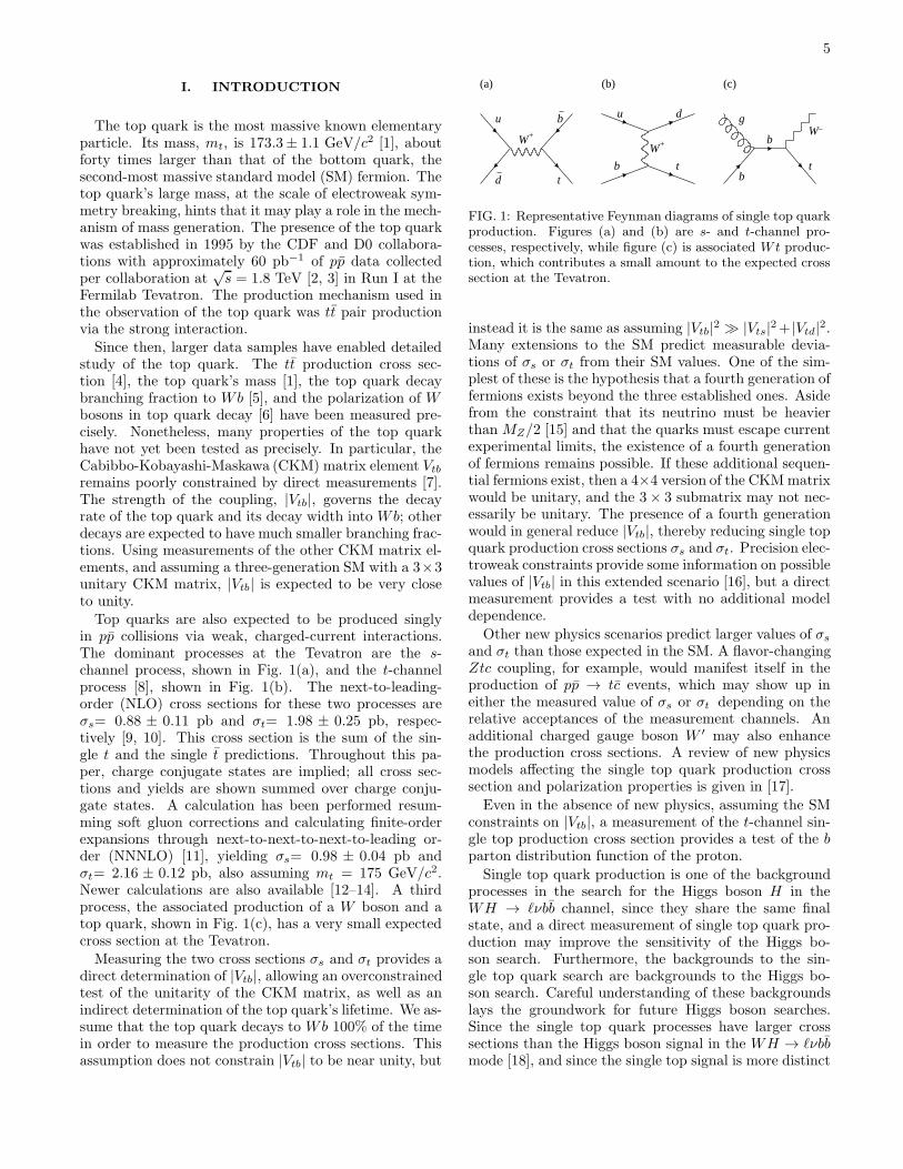
in pp collisions via weak, charged-current interactions.The dominant processes at the Tevatron are the s-channel process, shown in Fig. 1(a), and the t-channelprocess [8], shown in Fig. 1(b). The next-to-leading-order (NLO) cross sections for these two processes areσs= 0.88 ± 0.11 pb and σt= 1.98 ± 0.25 pb, respec-tively [9, 10]. This cross section is the sum of the sin-gle t and the single t predictions. Throughout this pa-per, charge conjugate states are implied; all cross sec-tions and yields are shown summed over charge conju-gate states. A calculation has been performed resum-ming soft gluon corrections and calculating finite-orderexpansions through next-to-next-to-next-to-leading or-der (NNNLO) [11], yielding σs= 0.98 ± 0.04 pb andσt= 2.16 ± 0.12 pb, also assuming mt = 175 GeV/c2.Newer calculations are also available [12–14]. A thirdprocess, the associated production of a W boson and atop quark, shown in Fig. 1(c), has a very small expectedcross section at the Tevatron.Measuring the two cross sections σs and σt provides a

direct determination of |Vtb|, allowing an overconstrainedtest of the unitarity of the CKM matrix, as well as anindirect determination of the top quark’s lifetime. We as-sume that the top quark decays to Wb 100% of the timein order to measure the production cross sections. Thisassumption does not constrain |Vtb| to be near unity, but

u

d

W+

b

t

(a)

b

u d

t

W+

(b)

g

b

bW_

t

(c)

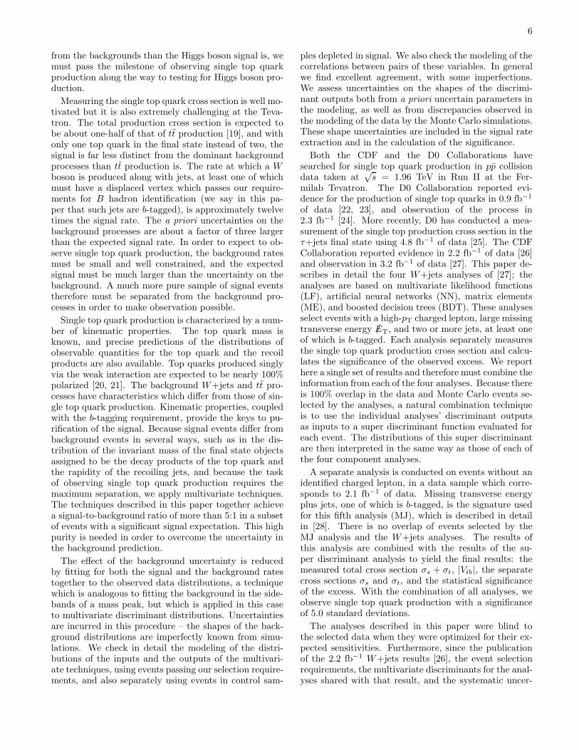
FIG. 1: Representative Feynman diagrams of single top quarkproduction. Figures (a) and (b) are s- and t-channel pro-cesses, respectively, while figure (c) is associated Wt produc-tion, which contributes a small amount to the expected crosssection at the Tevatron.

instead it is the same as assuming |Vtb|2 ≫ |Vts|2+ |Vtd|2.Many extensions to the SM predict measurable devia-tions of σs or σt from their SM values. One of the sim-plest of these is the hypothesis that a fourth generation offermions exists beyond the three established ones. Asidefrom the constraint that its neutrino must be heavierthan MZ/2 [15] and that the quarks must escape currentexperimental limits, the existence of a fourth generationof fermions remains possible. If these additional sequen-tial fermions exist, then a 4×4 version of the CKMmatrixwould be unitary, and the 3× 3 submatrix may not nec-essarily be unitary. The presence of a fourth generationwould in general reduce |Vtb|, thereby reducing single topquark production cross sections σs and σt. Precision elec-troweak constraints provide some information on possiblevalues of |Vtb| in this extended scenario [16], but a directmeasurement provides a test with no additional modeldependence.

Other new physics scenarios predict larger values of σs

and σt than those expected in the SM. A flavor-changingZtc coupling, for example, would manifest itself in theproduction of pp → tc events, which may show up ineither the measured value of σs or σt depending on therelative acceptances of the measurement channels. Anadditional charged gauge boson W ′ may also enhancethe production cross sections. A review of new physicsmodels affecting the single top quark production crosssection and polarization properties is given in [17].

Even in the absence of new physics, assuming the SMconstraints on |Vtb|, a measurement of the t-channel sin-gle top production cross section provides a test of the bparton distribution function of the proton.

Single top quark production is one of the backgroundprocesses in the search for the Higgs boson H in theWH → ℓνbb channel, since they share the same finalstate, and a direct measurement of single top quark pro-duction may improve the sensitivity of the Higgs bo-son search. Furthermore, the backgrounds to the sin-gle top quark search are backgrounds to the Higgs bo-son search. Careful understanding of these backgroundslays the groundwork for future Higgs boson searches.Since the single top quark processes have larger crosssections than the Higgs boson signal in the WH → ℓνbbmode [18], and since the single top signal is more distinct

6

from the backgrounds than the Higgs boson signal is, wemust pass the milestone of observing single top quarkproduction along the way to testing for Higgs boson pro-duction.

Measuring the single top quark cross section is well mo-tivated but it is also extremely challenging at the Teva-tron. The total production cross section is expected tobe about one-half of that of tt production [19], and withonly one top quark in the final state instead of two, thesignal is far less distinct from the dominant backgroundprocesses than tt production is. The rate at which a Wboson is produced along with jets, at least one of whichmust have a displaced vertex which passes our require-ments for B hadron identification (we say in this pa-per that such jets are b-tagged), is approximately twelvetimes the signal rate. The a priori uncertainties on thebackground processes are about a factor of three largerthan the expected signal rate. In order to expect to ob-serve single top quark production, the background ratesmust be small and well constrained, and the expectedsignal must be much larger than the uncertainty on thebackground. A much more pure sample of signal eventstherefore must be separated from the background pro-cesses in order to make observation possible.

Single top quark production is characterized by a num-ber of kinematic properties. The top quark mass isknown, and precise predictions of the distributions ofobservable quantities for the top quark and the recoilproducts are also available. Top quarks produced singlyvia the weak interaction are expected to be nearly 100%polarized [20, 21]. The background W+jets and tt pro-cesses have characteristics which differ from those of sin-gle top quark production. Kinematic properties, coupledwith the b-tagging requirement, provide the keys to pu-rification of the signal. Because signal events differ frombackground events in several ways, such as in the dis-tribution of the invariant mass of the final state objectsassigned to be the decay products of the top quark andthe rapidity of the recoiling jets, and because the taskof observing single top quark production requires themaximum separation, we apply multivariate techniques.The techniques described in this paper together achievea signal-to-background ratio of more than 5:1 in a subsetof events with a significant signal expectation. This highpurity is needed in order to overcome the uncertainty inthe background prediction.

The effect of the background uncertainty is reducedby fitting for both the signal and the background ratestogether to the observed data distributions, a techniquewhich is analogous to fitting the background in the side-bands of a mass peak, but which is applied in this caseto multivariate discriminant distributions. Uncertaintiesare incurred in this procedure – the shapes of the back-ground distributions are imperfectly known from simu-lations. We check in detail the modeling of the distri-butions of the inputs and the outputs of the multivari-ate techniques, using events passing our selection require-ments, and also separately using events in control sam-

ples depleted in signal. We also check the modeling of thecorrelations between pairs of these variables. In generalwe find excellent agreement, with some imperfections.We assess uncertainties on the shapes of the discrimi-nant outputs both from a priori uncertain parameters inthe modeling, as well as from discrepancies observed inthe modeling of the data by the Monte Carlo simulations.These shape uncertainties are included in the signal rateextraction and in the calculation of the significance.

Both the CDF and the D0 Collaborations havesearched for single top quark production in pp collisiondata taken at

√s = 1.96 TeV in Run II at the Fer-

milab Tevatron. The D0 Collaboration reported evi-dence for the production of single top quarks in 0.9 fb−1

of data [22, 23], and observation of the process in2.3 fb−1 [24]. More recently, D0 has conducted a mea-surement of the single top production cross section in theτ+jets final state using 4.8 fb−1 of data [25]. The CDFCollaboration reported evidence in 2.2 fb−1 of data [26]and observation in 3.2 fb−1 of data [27]. This paper de-scribes in detail the four W+jets analyses of [27]; theanalyses are based on multivariate likelihood functions(LF), artificial neural networks (NN), matrix elements(ME), and boosted decision trees (BDT). These analysesselect events with a high-pT charged lepton, large missingtransverse energy /ET, and two or more jets, at least oneof which is b-tagged. Each analysis separately measuresthe single top quark production cross section and calcu-lates the significance of the observed excess. We reporthere a single set of results and therefore must combine theinformation from each of the four analyses. Because thereis 100% overlap in the data and Monte Carlo events se-lected by the analyses, a natural combination techniqueis to use the individual analyses’ discriminant outputsas inputs to a super discriminant function evaluated foreach event. The distributions of this super discriminantare then interpreted in the same way as those of each ofthe four component analyses.

A separate analysis is conducted on events without anidentified charged lepton, in a data sample which corre-sponds to 2.1 fb−1 of data. Missing transverse energyplus jets, one of which is b-tagged, is the signature usedfor this fifth analysis (MJ), which is described in detailin [28]. There is no overlap of events selected by theMJ analysis and the W+jets analyses. The results ofthis analysis are combined with the results of the su-per discriminant analysis to yield the final results: themeasured total cross section σs + σt, |Vtb|, the separatecross sections σs and σt, and the statistical significanceof the excess. With the combination of all analyses, weobserve single top quark production with a significanceof 5.0 standard deviations.

The analyses described in this paper were blind tothe selected data when they were optimized for their ex-pected sensitivities. Furthermore, since the publicationof the 2.2 fb−1 W+jets results [26], the event selectionrequirements, the multivariate discriminants for the anal-yses shared with that result, and the systematic uncer-

7

tainties remain unchanged; new data were added withoutfurther optimization or retraining. When the 2.2 fb−1

results were validated, they were done so in a blind fash-ion. The distributions of all relevant variables were firstchecked for accurate modeling by our simulations anddata-based background estimations in control samples ofdata that do not overlap with the selected signal sample.Then the distributions of the discriminant input vari-ables, and also other variables, were checked in the sam-ple of events passing the selection requirements. Afterthat, the modeling of the low signal-to-background por-tions of the final output histograms was checked. Onlyafter all of these validation steps were completed werethe data in the most sensitive regions revealed. Two newanalyses, BDT and MJ, have been added for this paper,and they were validated in a similar way.This paper is organized as follows: Section II describes

the CDF II detector, Section III describes the event selec-tion, Section IV describes the simulation of signal eventsand the acceptance of the signal, Section V describesthe background rate and kinematic shape modeling, Sec-tion VI describes a neural-network flavor separator whichhelps separate b jets from others, Section VII describesthe four W+jets multivariate analysis techniques, Sec-tion VIII describes the systematic uncertainties we as-sess, Section IX describes the statistical techniques forextraction of the signal cross section and the significance,Section X describes the super discriminant, Section XIpresents our results for the cross section, |Vtb|, and thesignificance, Section XII describes an extraction of σs andσt in a joint fit, and Section XIII summarizes our results.

II. THE CDF II DETECTOR

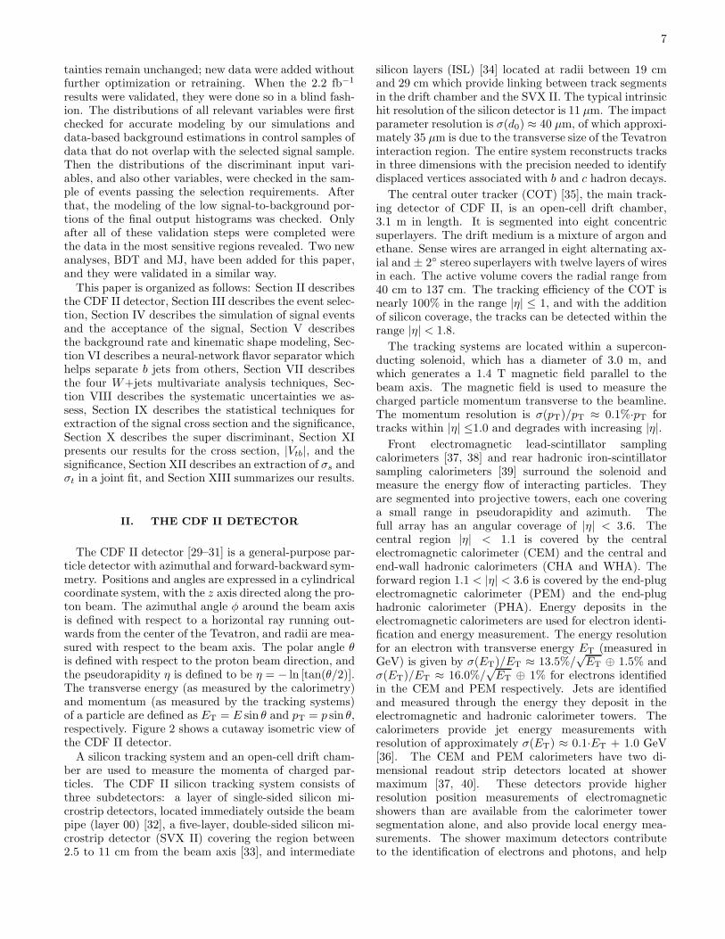
The CDF II detector [29–31] is a general-purpose par-ticle detector with azimuthal and forward-backward sym-metry. Positions and angles are expressed in a cylindricalcoordinate system, with the z axis directed along the pro-ton beam. The azimuthal angle φ around the beam axisis defined with respect to a horizontal ray running out-wards from the center of the Tevatron, and radii are mea-sured with respect to the beam axis. The polar angle θis defined with respect to the proton beam direction, andthe pseudorapidity η is defined to be η = − ln [tan(θ/2)].The transverse energy (as measured by the calorimetry)and momentum (as measured by the tracking systems)of a particle are defined as ET = E sin θ and pT = p sin θ,respectively. Figure 2 shows a cutaway isometric view ofthe CDF II detector.A silicon tracking system and an open-cell drift cham-

ber are used to measure the momenta of charged par-ticles. The CDF II silicon tracking system consists ofthree subdetectors: a layer of single-sided silicon mi-crostrip detectors, located immediately outside the beampipe (layer 00) [32], a five-layer, double-sided silicon mi-crostrip detector (SVX II) covering the region between2.5 to 11 cm from the beam axis [33], and intermediate

silicon layers (ISL) [34] located at radii between 19 cmand 29 cm which provide linking between track segmentsin the drift chamber and the SVX II. The typical intrinsichit resolution of the silicon detector is 11 µm. The impactparameter resolution is σ(d0) ≈ 40 µm, of which approxi-mately 35 µm is due to the transverse size of the Tevatroninteraction region. The entire system reconstructs tracksin three dimensions with the precision needed to identifydisplaced vertices associated with b and c hadron decays.

The central outer tracker (COT) [35], the main track-ing detector of CDF II, is an open-cell drift chamber,3.1 m in length. It is segmented into eight concentricsuperlayers. The drift medium is a mixture of argon andethane. Sense wires are arranged in eight alternating ax-ial and ± 2◦ stereo superlayers with twelve layers of wiresin each. The active volume covers the radial range from40 cm to 137 cm. The tracking efficiency of the COT isnearly 100% in the range |η| ≤ 1, and with the additionof silicon coverage, the tracks can be detected within therange |η| < 1.8.

The tracking systems are located within a supercon-ducting solenoid, which has a diameter of 3.0 m, andwhich generates a 1.4 T magnetic field parallel to thebeam axis. The magnetic field is used to measure thecharged particle momentum transverse to the beamline.The momentum resolution is σ(pT)/pT ≈ 0.1%·pT fortracks within |η| ≤1.0 and degrades with increasing |η|.Front electromagnetic lead-scintillator sampling

calorimeters [37, 38] and rear hadronic iron-scintillatorsampling calorimeters [39] surround the solenoid andmeasure the energy flow of interacting particles. Theyare segmented into projective towers, each one coveringa small range in pseudorapidity and azimuth. Thefull array has an angular coverage of |η| < 3.6. Thecentral region |η| < 1.1 is covered by the centralelectromagnetic calorimeter (CEM) and the central andend-wall hadronic calorimeters (CHA and WHA). Theforward region 1.1 < |η| < 3.6 is covered by the end-plugelectromagnetic calorimeter (PEM) and the end-plughadronic calorimeter (PHA). Energy deposits in theelectromagnetic calorimeters are used for electron identi-fication and energy measurement. The energy resolutionfor an electron with transverse energy ET (measured inGeV) is given by σ(ET)/ET ≈ 13.5%/

√ET ⊕ 1.5% and

σ(ET)/ET ≈ 16.0%/√ET ⊕ 1% for electrons identified

in the CEM and PEM respectively. Jets are identifiedand measured through the energy they deposit in theelectromagnetic and hadronic calorimeter towers. Thecalorimeters provide jet energy measurements withresolution of approximately σ(ET) ≈ 0.1·ET + 1.0 GeV[36]. The CEM and PEM calorimeters have two di-mensional readout strip detectors located at showermaximum [37, 40]. These detectors provide higherresolution position measurements of electromagneticshowers than are available from the calorimeter towersegmentation alone, and also provide local energy mea-surements. The shower maximum detectors contributeto the identification of electrons and photons, and help

8

End-Plug ElectromagneticCalorimeter (PEM)

End-Wall HadronicCalorimeter (WHA)

End-Plug HadronicCalorimeter (PHA)

Cherenkov LuminosityCounters (CLC)

Central MuonChambers (CMU)

Central Muon Upgrade (CMP)

Central Muon Extension (CMX)

Protons

Barrel MuonChambers (BMU)

TevatronBeampipe

Anti-protons

Central Outer Tracker (COT)

Solenoid

Central ElectromagneticCalorimeter (CEM)

Central HadronicCalorimeter (CHA)

Interaction Region

Layer 00

Silicon Vertex Detector (SVX II)

Intermediate Silicon Layers (ISL)

z x

y

φθ

FIG. 2: Cutaway isometric view of the CDF II detector.

separate them from π0 decays.

Beyond the calorimeters resides the muon system,which provides muon detection in the range |η| < 1.5.For the analyses presented in this article, muons aredetected in four separate subdetectors. Muons withpT > 1.4 GeV/c penetrating the five absorption lengthsof the calorimeter are detected in the four layers of pla-nar multi-wire drift chambers of the central muon detec-tor (CMU) [41]. Behind an additional 60 cm of steel,a second set of four layers of drift chambers, the cen-tral muon upgrade (CMP) [29, 42], detects muons withpT > 2.2 GeV/c. The CMU and CMP cover the samepart of the central region |η| < 0.6. The central muonextension (CMX) [29, 42] extends the pseudorapidity cov-erage of the muon system from 0.6 to 1.0 and thus com-pletes the coverage over the full fiducial region of theCOT. Muons with 1.0 < |η| < 1.5 are detected by thebarrel muon chambers (BMU) [43].

The Tevatron collider luminosity is determined withmulti-cell gas Cherenkov detectors [44] located in the re-gion 3.7 < |η| < 4.7 which measure the average numberof inelastic pp collisions per bunch crossing. The totaluncertainty on the luminosity is ±6.0%, of which 4.4%comes from the acceptance and the operation of the lu-minosity monitor and 4.0% comes from the uncertaintyof the inelastic pp cross section [45].

u

d

W+

b

t

b

l+

νl

W+

(a)

b

u d

t

W+

b

l+

νl

W+

(b)

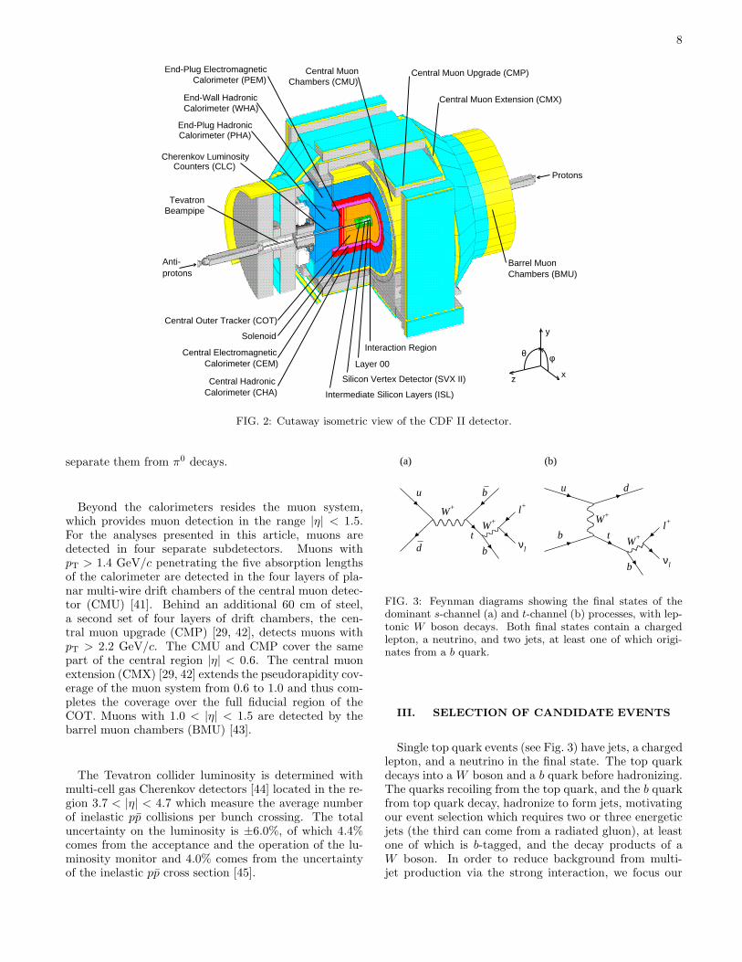
FIG. 3: Feynman diagrams showing the final states of thedominant s-channel (a) and t-channel (b) processes, with lep-tonic W boson decays. Both final states contain a chargedlepton, a neutrino, and two jets, at least one of which origi-nates from a b quark.

III. SELECTION OF CANDIDATE EVENTS

Single top quark events (see Fig. 3) have jets, a chargedlepton, and a neutrino in the final state. The top quarkdecays into a W boson and a b quark before hadronizing.The quarks recoiling from the top quark, and the b quarkfrom top quark decay, hadronize to form jets, motivatingour event selection which requires two or three energeticjets (the third can come from a radiated gluon), at leastone of which is b-tagged, and the decay products of aW boson. In order to reduce background from multi-jet production via the strong interaction, we focus our

9

event selection on the decays of the W boson to eνe orµνµ in these analyses. Such events have one chargedlepton (an electron or a muon), missing transverse energyresulting from the undetected neutrino, and at least twojets. These events constitute the W+jets sample. Wealso include the acceptance for signal and backgroundevents in which W → τντ , and the MJ analysis also issensitive to W boson decays to τ leptons.

Since the pp collision rate at the Tevatron exceeds therate at which events can be written to tape by five ordersof magnitude, CDF has an elaborate trigger system withthree levels. The first level uses special-purpose hard-ware [46] to reduce the event rate from the effective beam-crossing frequency of 1.7 MHz to approximately 15 kHz,the maximum rate at which the detector can be read out.The second level consists of a mixture of dedicated hard-ware and fast software algorithms and takes advantageof the full information read out of the detector [47]. Atthis level the trigger rate is reduced further to less than800 Hz. At the third level, a computer farm running fastversions of the offline event reconstruction algorithms re-fines the trigger selections based on quantities that arenearly the same as those used in offline analyses [48]. Inparticular, detector calibrations are applied before thetrigger requirements are imposed. The third level triggerselects events for permanent storage at a rate of up to200 Hz.

Many different trigger criteria are evaluated at eachlevel, and events passing specific criteria at one level areconsidered by a subset of trigger algorithms at the nextlevel. A cascading set of trigger requirements is knownas a trigger path. This analysis uses the trigger pathswhich select events with high-pT electron or muon can-didates. The acceptance of these triggers for tau lep-tons is included in our rate estimates but the triggers arenot optimized for identifying tau leptons. An additionaltrigger path, which requires significant /ET plus at leasttwo high-pT jets, is also used to add W+jets candidateevents with non-triggered leptons, which include chargedleptons outside the fiducial volumes of the electron andmuon detectors, as well as tau leptons.

The third-level central electron trigger requires a COTtrack with pT> 9 GeV/c matched to an energy cluster inthe CEM with ET> 18 GeV. The shower profile of thiscluster as measured by the shower-maximum detector isrequired to be consistent with those measured using test-beam electrons. Electron candidates with |η| > 1.1 arerequired to deposit more than 20 GeV in a cluster in thePEM, and the ratio of hadronic energy to electromagneticenergy EPHA/EPEM for this cluster is required to be lessthan 0.075. The third-level muon trigger requires a COTtrack with pT>18 GeV/c matched to a track segment inthe muon chambers. The /ET+jets trigger path requires/ET > 35 GeV and two jets with ET> 10 GeV.

After offline reconstruction, we impose further require-ments on the electron candidates in order to improvethe purity of the sample. A reconstructed track withpT> 9 GeV/c must match to a cluster in the CEM with

ET> 20 GeV. Furthermore, we require EHAD/EEM <0.055 + 0.00045× E/GeV and the ratio of the energy ofthe cluster to the momentum of the track E/p has to besmaller than 2.0 c for track momenta ≤ 50 GeV/c. Forelectron candidates with tracks with p > 50 GeV/c, norequirement on E/p is made as the misidentification rateis small. Candidate objects which fail these requirementsare more likely to be hadrons or jets than those that pass.

Electron candidates in the forward direction (PHX) aredefined by a cluster in the PEM with ET > 20 GeV andEHAD/EEM < 0.05. The cluster position and the primaryvertex position are combined to form a search trajectoryin the silicon tracker and seed the pattern recognition ofthe tracking algorithm.

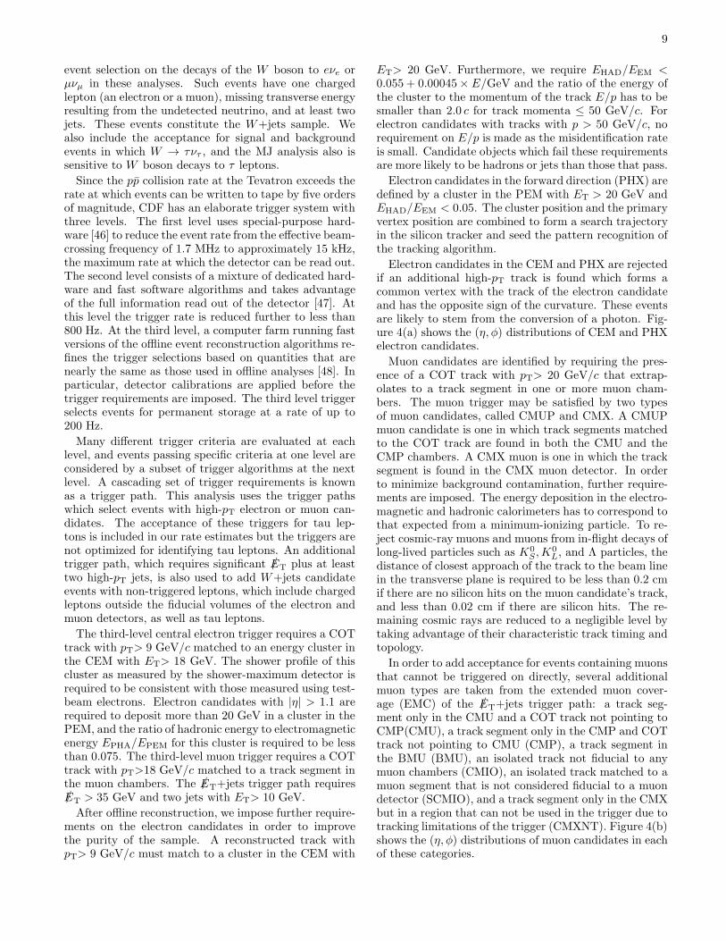
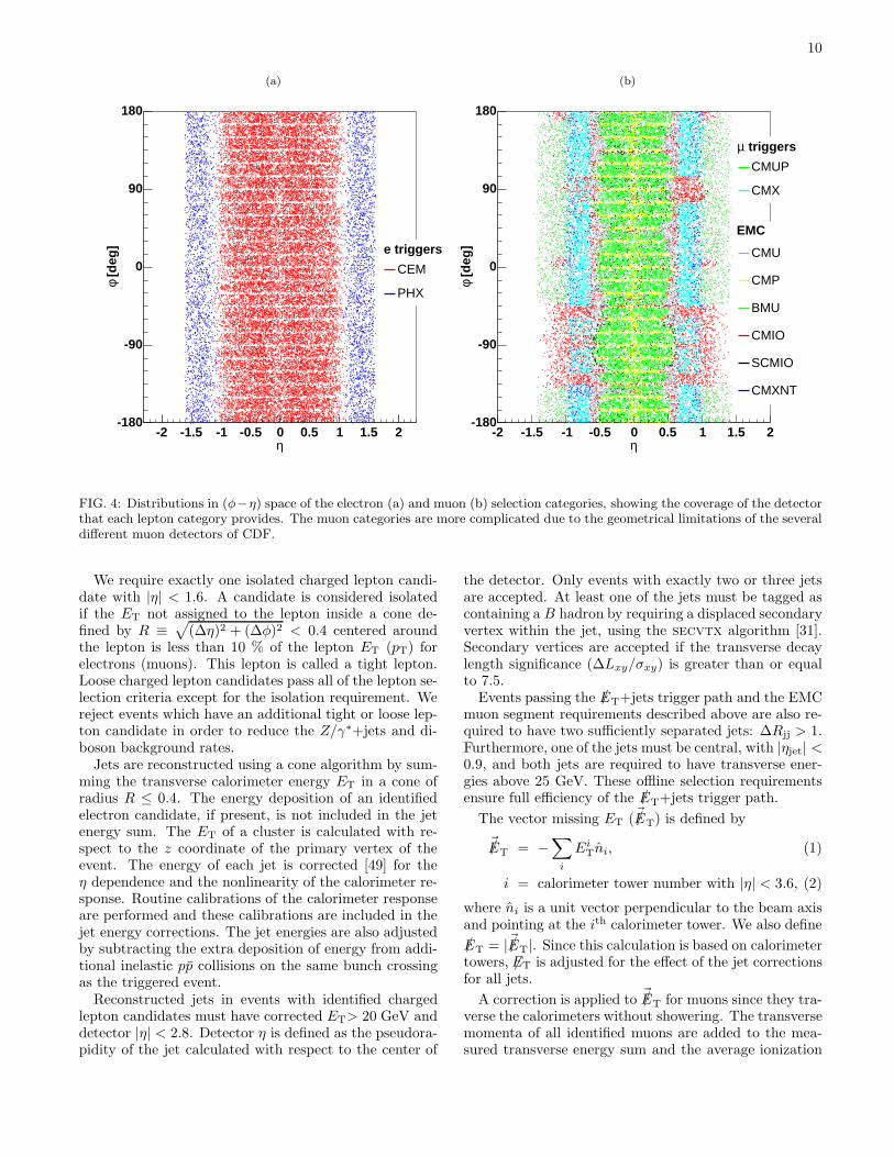
Electron candidates in the CEM and PHX are rejectedif an additional high-pT track is found which forms acommon vertex with the track of the electron candidateand has the opposite sign of the curvature. These eventsare likely to stem from the conversion of a photon. Fig-ure 4(a) shows the (η, φ) distributions of CEM and PHXelectron candidates.

Muon candidates are identified by requiring the pres-ence of a COT track with pT> 20 GeV/c that extrap-olates to a track segment in one or more muon cham-bers. The muon trigger may be satisfied by two typesof muon candidates, called CMUP and CMX. A CMUPmuon candidate is one in which track segments matchedto the COT track are found in both the CMU and theCMP chambers. A CMX muon is one in which the tracksegment is found in the CMX muon detector. In orderto minimize background contamination, further require-ments are imposed. The energy deposition in the electro-magnetic and hadronic calorimeters has to correspond tothat expected from a minimum-ionizing particle. To re-ject cosmic-ray muons and muons from in-flight decays oflong-lived particles such as K0

S,K0L, and Λ particles, the

distance of closest approach of the track to the beam linein the transverse plane is required to be less than 0.2 cmif there are no silicon hits on the muon candidate’s track,and less than 0.02 cm if there are silicon hits. The re-maining cosmic rays are reduced to a negligible level bytaking advantage of their characteristic track timing andtopology.

In order to add acceptance for events containing muonsthat cannot be triggered on directly, several additionalmuon types are taken from the extended muon cover-age (EMC) of the /ET+jets trigger path: a track seg-ment only in the CMU and a COT track not pointing toCMP(CMU), a track segment only in the CMP and COTtrack not pointing to CMU (CMP), a track segment inthe BMU (BMU), an isolated track not fiducial to anymuon chambers (CMIO), an isolated track matched to amuon segment that is not considered fiducial to a muondetector (SCMIO), and a track segment only in the CMXbut in a region that can not be used in the trigger due totracking limitations of the trigger (CMXNT). Figure 4(b)shows the (η, φ) distributions of muon candidates in eachof these categories.

10

(a)

η-2 -1.5 -1 -0.5 0 0.5 1 1.5 2

[d

eg]

φ

-180

-90

0

90

180

e triggers

CEM

PHX

(b)

η-2 -1.5 -1 -0.5 0 0.5 1 1.5 2

[d

eg]

φ

-180

-90

0

90

180

triggersµ

EMC

CMUP

CMX

CMU

CMP

BMU

CMIO

SCMIO

CMXNT

FIG. 4: Distributions in (φ−η) space of the electron (a) and muon (b) selection categories, showing the coverage of the detectorthat each lepton category provides. The muon categories are more complicated due to the geometrical limitations of the severaldifferent muon detectors of CDF.

We require exactly one isolated charged lepton candi-date with |η| < 1.6. A candidate is considered isolatedif the ET not assigned to the lepton inside a cone de-fined by R ≡

√

(∆η)2 + (∆φ)2 < 0.4 centered aroundthe lepton is less than 10 % of the lepton ET (pT) forelectrons (muons). This lepton is called a tight lepton.Loose charged lepton candidates pass all of the lepton se-lection criteria except for the isolation requirement. Wereject events which have an additional tight or loose lep-ton candidate in order to reduce the Z/γ∗+jets and di-boson background rates.Jets are reconstructed using a cone algorithm by sum-

ming the transverse calorimeter energy ET in a cone ofradius R ≤ 0.4. The energy deposition of an identifiedelectron candidate, if present, is not included in the jetenergy sum. The ET of a cluster is calculated with re-spect to the z coordinate of the primary vertex of theevent. The energy of each jet is corrected [49] for theη dependence and the nonlinearity of the calorimeter re-sponse. Routine calibrations of the calorimeter responseare performed and these calibrations are included in thejet energy corrections. The jet energies are also adjustedby subtracting the extra deposition of energy from addi-tional inelastic pp collisions on the same bunch crossingas the triggered event.Reconstructed jets in events with identified charged

lepton candidates must have corrected ET> 20 GeV anddetector |η| < 2.8. Detector η is defined as the pseudora-pidity of the jet calculated with respect to the center of

the detector. Only events with exactly two or three jetsare accepted. At least one of the jets must be tagged ascontaining a B hadron by requiring a displaced secondaryvertex within the jet, using the secvtx algorithm [31].Secondary vertices are accepted if the transverse decaylength significance (∆Lxy/σxy) is greater than or equalto 7.5.Events passing the /ET+jets trigger path and the EMC

muon segment requirements described above are also re-quired to have two sufficiently separated jets: ∆Rjj > 1.Furthermore, one of the jets must be central, with |ηjet| <0.9, and both jets are required to have transverse ener-gies above 25 GeV. These offline selection requirementsensure full efficiency of the /ET+jets trigger path.

The vector missing ET (~/ET) is defined by

~/ET = −∑

i

EiTni, (1)

i = calorimeter tower number with |η| < 3.6, (2)

where ni is a unit vector perpendicular to the beam axisand pointing at the ith calorimeter tower. We also define

/ET = |~/ET|. Since this calculation is based on calorimetertowers, 6ET is adjusted for the effect of the jet correctionsfor all jets.

A correction is applied to ~/ET for muons since they tra-verse the calorimeters without showering. The transversemomenta of all identified muons are added to the mea-sured transverse energy sum and the average ionization

11

energy is removed from the measured calorimeter energydeposits. We require the corrected /ET to be greater than25 GeV in order to purify a sample containing leptonicW boson decays.A portion of the background consists of multijet events

which do not contain W bosons. We call these “non-W”events below. We select against the non-W backgroundby applying additional selection requirements which arebased on the assumption that these events do not have alarge /ET from an escaping neutrino, but rather the /ET

that is observed comes from lost or mismeasured jets. Inevents lacking a W boson, one would expect small valuesof the transverse mass, defined as

MWT =

√

2(

pℓT /ET − pℓx /ET

x − pℓy /ET

y). (3)

Because the /ET in events that do not contain W bosonsoften comes from jets which are erroneously identified as

charged leptons, ~/ET often points close to the lepton can-didate’s direction, giving the event a low transverse mass.Thus, the transverse mass is required to be above 10 GeVfor muons and 20 GeV for electrons, which have more ofthese events.

Further removal of non-W events is performed with avariable called /ET significance (/ET,sig), defined as

/ET,sig =/ET

√

∑

jetsC2JES cos

2

(

∆φjet,~/ET

)

ErawT,jet + cos2

(

∆φ~ET,uncl,~/ET

)

∑

ET,uncl

, (4)

where CJES is the jet energy correction factor [49], ErawT,jet

is a jet’s energy before corrections are applied, ~ET,uncl

refers to the vector sum of the transverse components ofcalorimeter energy deposits not included in any recon-structed jets, and

∑

ET,uncl is the sum of the magni-tudes of these unclustered energies. The angle between

the projections in the rφ plane of a jet and ~/ET is de-noted ∆φ

jet, ~ET,uncl, and the angle between the projec-

tions in the rφ plane of∑

ET,uncl and ~/ET is denoted∆φ~ET,uncl,

~/ET

. When the energies in Equation 4 are mea-

sured in GeV, /ET,sig is an approximate significance, as

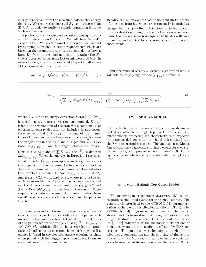
the dispersion in the measured /ET in events with no true/ET is approximated by the denominator. Central elec-tron events are required to have /ET,sig > 3.5 − 0.05MT

and /ET,sig > 2.5− 3.125∆φjet2,/ET, where jet 2 is the jet

with the second-largestET, and all energies are measuredin GeV. Plug electron events must have /ET,sig > 2 and/ET > 45 − 30∆φjet,~/ET

for all jets in the event. Theserequirements reduce the amount of contamination fromnon-W events substantially, as shown in the plots inFig. 5.

To remove events containing Z bosons, we reject eventsin which the trigger lepton candidate can be paired withan oppositely-signed track such that the invariant massof the pair is within the range 76 GeV/c2 ≤ mℓ,track ≤106 GeV/c2. Additionally, if the trigger lepton candi-date is identified as an electron, the event is rejected if acluster is found in the electromagnetic calorimeter that,when paired with the trigger lepton candidate, forms aninvariant mass in the same range.

IV. SIGNAL MODEL

In order to perform a search for a previously unde-tected signal such as single top quark production, ac-curate models predicting the characteristics of expecteddata are needed for both the signal being tested andthe SM background processes. This analysis uses MonteCarlo programs to generate simulated events for each sig-nal and background process, except for non-W QCDmul-tijet events for which events in data control samples areused.

A. s-channel Single Top Quark Model

The matrix element generator madevent [50] is usedto produce simulated events for the signal samples. Thegenerator is interfaced to the CTEQ5L [51] parameteri-zation of the parton distribution functions (PDFs). Thepythia [53, 54] program is used to perform the partonshower and hadronization. Although madevent usesonly a leading-order matrix element calculation, stud-ies [10, 52] indicate that the kinematic distributions ofs-channel events are only negligibly affected by NLO cor-rections. The parton shower simulates the higher-ordereffects of gluon radiation and the splitting of gluons intoquarks, and the Monte Carlo samples include contribu-tions from initial-state sea quarks via the proton PDFs.

12

FIG. 5: Plots of /ET,sig vs. MWT for W+jets Monte Carlo, the selected data in the ℓ + /ET+2 jets sample, and the two

distributions subtracted for all CEM candidates. The black lines indicate the requirements which are applied. Events withlower /ET,sig or MW

T are not selected.

b

u d

t

W+

(a)

g

u d

t

b

b

W+

(b)

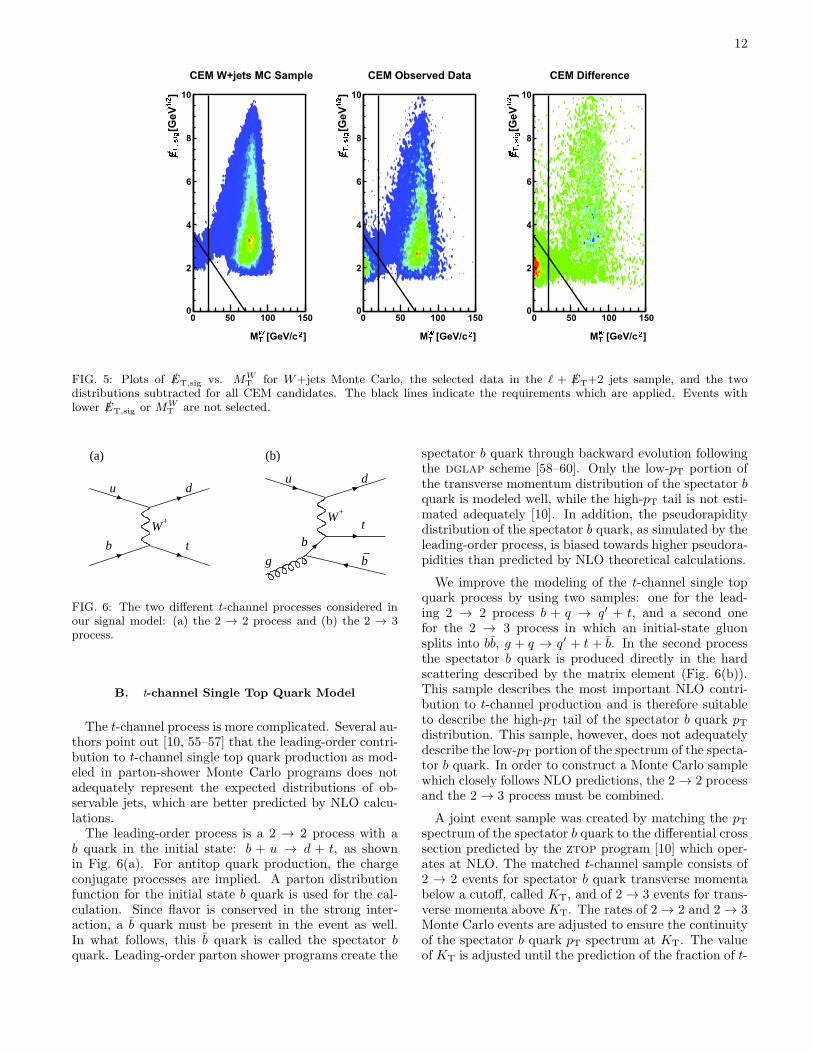
FIG. 6: The two different t-channel processes considered inour signal model: (a) the 2 → 2 process and (b) the 2 → 3process.

B. t-channel Single Top Quark Model

The t-channel process is more complicated. Several au-thors point out [10, 55–57] that the leading-order contri-bution to t-channel single top quark production as mod-eled in parton-shower Monte Carlo programs does notadequately represent the expected distributions of ob-servable jets, which are better predicted by NLO calcu-lations.The leading-order process is a 2 → 2 process with a

b quark in the initial state: b + u → d + t, as shownin Fig. 6(a). For antitop quark production, the chargeconjugate processes are implied. A parton distributionfunction for the initial state b quark is used for the cal-culation. Since flavor is conserved in the strong inter-action, a b quark must be present in the event as well.In what follows, this b quark is called the spectator bquark. Leading-order parton shower programs create the

spectator b quark through backward evolution followingthe dglap scheme [58–60]. Only the low-pT portion ofthe transverse momentum distribution of the spectator bquark is modeled well, while the high-pT tail is not esti-mated adequately [10]. In addition, the pseudorapiditydistribution of the spectator b quark, as simulated by theleading-order process, is biased towards higher pseudora-pidities than predicted by NLO theoretical calculations.

We improve the modeling of the t-channel single topquark process by using two samples: one for the lead-ing 2 → 2 process b + q → q′ + t, and a second onefor the 2 → 3 process in which an initial-state gluonsplits into bb, g + q → q′ + t + b. In the second processthe spectator b quark is produced directly in the hardscattering described by the matrix element (Fig. 6(b)).This sample describes the most important NLO contri-bution to t-channel production and is therefore suitableto describe the high-pT tail of the spectator b quark pTdistribution. This sample, however, does not adequatelydescribe the low-pT portion of the spectrum of the specta-tor b quark. In order to construct a Monte Carlo samplewhich closely follows NLO predictions, the 2 → 2 processand the 2 → 3 process must be combined.

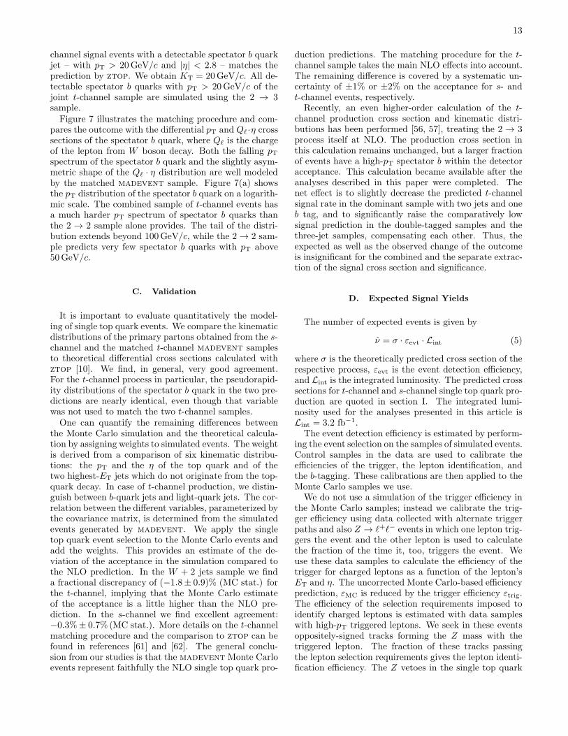
A joint event sample was created by matching the pTspectrum of the spectator b quark to the differential crosssection predicted by the ztop program [10] which oper-ates at NLO. The matched t-channel sample consists of2 → 2 events for spectator b quark transverse momentabelow a cutoff, called KT, and of 2 → 3 events for trans-verse momenta above KT. The rates of 2 → 2 and 2 → 3Monte Carlo events are adjusted to ensure the continuityof the spectator b quark pT spectrum at KT. The valueof KT is adjusted until the prediction of the fraction of t-

13

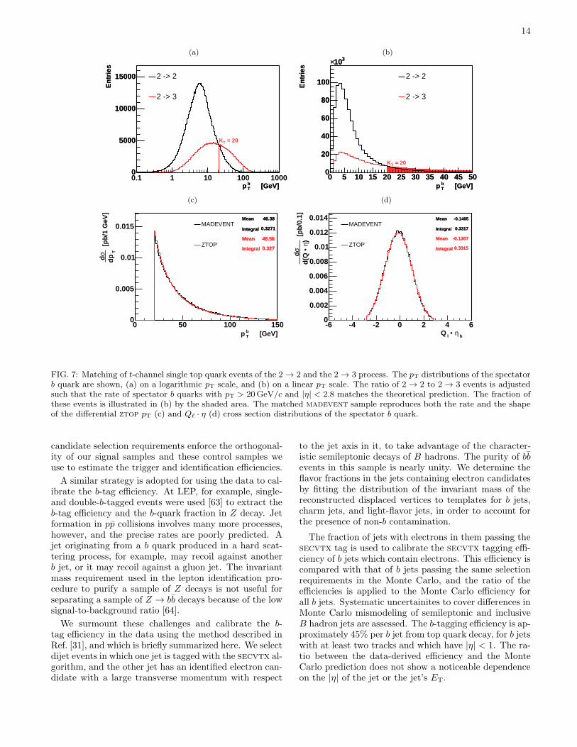
channel signal events with a detectable spectator b quarkjet – with pT > 20GeV/c and |η| < 2.8 – matches theprediction by ztop. We obtain KT = 20GeV/c. All de-tectable spectator b quarks with pT > 20GeV/c of thejoint t-channel sample are simulated using the 2 → 3sample.Figure 7 illustrates the matching procedure and com-

pares the outcome with the differential pT and Qℓ ·η crosssections of the spectator b quark, where Qℓ is the chargeof the lepton from W boson decay. Both the falling pTspectrum of the spectator b quark and the slightly asym-metric shape of the Qℓ · η distribution are well modeledby the matched madevent sample. Figure 7(a) showsthe pT distribution of the spectator b quark on a logarith-mic scale. The combined sample of t-channel events hasa much harder pT spectrum of spectator b quarks thanthe 2 → 2 sample alone provides. The tail of the distri-bution extends beyond 100GeV/c, while the 2 → 2 sam-ple predicts very few spectator b quarks with pT above50GeV/c.

C. Validation

It is important to evaluate quantitatively the model-ing of single top quark events. We compare the kinematicdistributions of the primary partons obtained from the s-channel and the matched t-channel madevent samplesto theoretical differential cross sections calculated withztop [10]. We find, in general, very good agreement.For the t-channel process in particular, the pseudorapid-ity distributions of the spectator b quark in the two pre-dictions are nearly identical, even though that variablewas not used to match the two t-channel samples.One can quantify the remaining differences between

the Monte Carlo simulation and the theoretical calcula-tion by assigning weights to simulated events. The weightis derived from a comparison of six kinematic distribu-tions: the pT and the η of the top quark and of thetwo highest-ET jets which do not originate from the top-quark decay. In case of t-channel production, we distin-guish between b-quark jets and light-quark jets. The cor-relation between the different variables, parameterized bythe covariance matrix, is determined from the simulatedevents generated by madevent. We apply the singletop quark event selection to the Monte Carlo events andadd the weights. This provides an estimate of the de-viation of the acceptance in the simulation compared tothe NLO prediction. In the W + 2 jets sample we finda fractional discrepancy of (−1.8± 0.9)% (MC stat.) forthe t-channel, implying that the Monte Carlo estimateof the acceptance is a little higher than the NLO pre-diction. In the s-channel we find excellent agreement:−0.3%± 0.7% (MC stat.). More details on the t-channelmatching procedure and the comparison to ztop can befound in references [61] and [62]. The general conclu-sion from our studies is that the madevent Monte Carloevents represent faithfully the NLO single top quark pro-

duction predictions. The matching procedure for the t-channel sample takes the main NLO effects into account.The remaining difference is covered by a systematic un-certainty of ±1% or ±2% on the acceptance for s- andt-channel events, respectively.Recently, an even higher-order calculation of the t-

channel production cross section and kinematic distri-butions has been performed [56, 57], treating the 2 → 3process itself at NLO. The production cross section inthis calculation remains unchanged, but a larger fractionof events have a high-pT spectator b within the detectoracceptance. This calculation became available after theanalyses described in this paper were completed. Thenet effect is to slightly decrease the predicted t-channelsignal rate in the dominant sample with two jets and oneb tag, and to significantly raise the comparatively lowsignal prediction in the double-tagged samples and thethree-jet samples, compensating each other. Thus, theexpected as well as the observed change of the outcomeis insignificant for the combined and the separate extrac-tion of the signal cross section and significance.

D. Expected Signal Yields

The number of expected events is given by

ν = σ · εevt · Lint (5)

where σ is the theoretically predicted cross section of therespective process, εevt is the event detection efficiency,and Lint is the integrated luminosity. The predicted crosssections for t-channel and s-channel single top quark pro-duction are quoted in section I. The integrated lumi-nosity used for the analyses presented in this article isLint = 3.2 fb−1.The event detection efficiency is estimated by perform-

ing the event selection on the samples of simulated events.Control samples in the data are used to calibrate theefficiencies of the trigger, the lepton identification, andthe b-tagging. These calibrations are then applied to theMonte Carlo samples we use.We do not use a simulation of the trigger efficiency in

the Monte Carlo samples; instead we calibrate the trig-ger efficiency using data collected with alternate triggerpaths and also Z → ℓ+ℓ− events in which one lepton trig-gers the event and the other lepton is used to calculatethe fraction of the time it, too, triggers the event. Weuse these data samples to calculate the efficiency of thetrigger for charged leptons as a function of the lepton’sET and η. The uncorrected Monte Carlo-based efficiencyprediction, εMC is reduced by the trigger efficiency εtrig.The efficiency of the selection requirements imposed toidentify charged leptons is estimated with data sampleswith high-pT triggered leptons. We seek in these eventsoppositely-signed tracks forming the Z mass with thetriggered lepton. The fraction of these tracks passingthe lepton selection requirements gives the lepton identi-fication efficiency. The Z vetoes in the single top quark

14

(a)

[GeV] b Tp

-1 0 1 2 3

En

trie

s

0

5000

10000

15000

[GeV] b Tp

-1 0 1 2 3

En

trie

s

0

5000

10000

15000 2 -> 2

2 -> 3

0.1 1 10 100 1000

= 20TK

(b)

[GeV] b Tp

0 5 10 15 20 25 30 35 40 45 50

En

trie

s

0

20

40

60

80

100

310×

[GeV] b Tp

0 5 10 15 20 25 30 35 40 45 50

En

trie

s

0

20

40

60

80

100

310×

2 -> 2

2 -> 3

= 20TK

(c)

Mean 46.38

Integral 0.3271

[GeV] b Tp

0 50 100 150

[p

b/1

GeV

] T

dpσd

0

0.005

0.01

0.015Mean 46.38

Integral 0.3271

Mean 45.56

Integral 0.327

Mean 45.56

Integral 0.327

MADEVENT

ZTOP

(d)

Mean -0.1405

Integral 0.3317

bη • lQ-6 -4 -2 0 2 4 6

[p

b/0

.1]

)η •d

(Q σ

d

0

0.002

0.004

0.006

0.008

0.01

0.012

0.014 Mean -0.1405

Integral 0.3317

Mean -0.1367

Integral 0.3315

Mean -0.1367

Integral 0.3315

MADEVENT

ZTOP

FIG. 7: Matching of t-channel single top quark events of the 2 → 2 and the 2 → 3 process. The pT distributions of the spectatorb quark are shown, (a) on a logarithmic pT scale, and (b) on a linear pT scale. The ratio of 2 → 2 to 2 → 3 events is adjustedsuch that the rate of spectator b quarks with pT > 20GeV/c and |η| < 2.8 matches the theoretical prediction. The fraction ofthese events is illustrated in (b) by the shaded area. The matched madevent sample reproduces both the rate and the shapeof the differential ztop pT (c) and Qℓ · η (d) cross section distributions of the spectator b quark.

candidate selection requirements enforce the orthogonal-ity of our signal samples and these control samples weuse to estimate the trigger and identification efficiencies.

A similar strategy is adopted for using the data to cal-ibrate the b-tag efficiency. At LEP, for example, single-and double-b-tagged events were used [63] to extract theb-tag efficiency and the b-quark fraction in Z decay. Jetformation in pp collisions involves many more processes,however, and the precise rates are poorly predicted. Ajet originating from a b quark produced in a hard scat-tering process, for example, may recoil against anotherb jet, or it may recoil against a gluon jet. The invariantmass requirement used in the lepton identification pro-cedure to purify a sample of Z decays is not useful forseparating a sample of Z → bb decays because of the lowsignal-to-background ratio [64].

We surmount these challenges and calibrate the b-tag efficiency in the data using the method described inRef. [31], and which is briefly summarized here. We selectdijet events in which one jet is tagged with the secvtx al-gorithm, and the other jet has an identified electron can-didate with a large transverse momentum with respect

to the jet axis in it, to take advantage of the character-istic semileptonic decays of B hadrons. The purity of bbevents in this sample is nearly unity. We determine theflavor fractions in the jets containing electron candidatesby fitting the distribution of the invariant mass of thereconstructed displaced vertices to templates for b jets,charm jets, and light-flavor jets, in order to account forthe presence of non-b contamination.

The fraction of jets with electrons in them passing thesecvtx tag is used to calibrate the secvtx tagging effi-ciency of b jets which contain electrons. This efficiency iscompared with that of b jets passing the same selectionrequirements in the Monte Carlo, and the ratio of theefficiencies is applied to the Monte Carlo efficiency forall b jets. Systematic uncertainites to cover differences inMonte Carlo mismodeling of semileptonic and inclusiveB hadron jets are assessed. The b-tagging efficiency is ap-proximately 45% per b jet from top quark decay, for b jetswith at least two tracks and which have |η| < 1. The ra-tio between the data-derived efficiency and the MonteCarlo prediction does not show a noticeable dependenceon the |η| of the jet or the jet’s ET.

15

The differences in the lepton identification efficiencyand the b-tagging between the data and the simulationare accounted for by a correction factor εcorr on the singletop quark event detection efficiency. Separate correctionfactors are applied to the single b-tagged events and thedouble b-tagged events. Systematic uncertainties are as-sessed on the signal acceptance due to the uncertaintieson these correction factors.The samples of simulated events are produced such

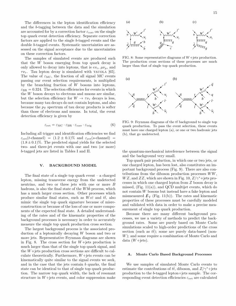
that the W boson emerging from top quark decay isonly allowed to decay into leptons, that is eνe, µνµ, andτντ . Tau lepton decay is simulated with tauola [65].The value of εMC, the fraction of all signal MC eventspassing our event selection requirements, is multipliedby the branching fraction of W bosons into leptons,εBR = 0.324. The selection efficiencies for events in whichthe W boson decays to electrons and muons are similar,but the selection efficiency for W → τντ decays is less,because many tau decays do not contain leptons, and alsobecause the pT spectrum of tau decay products is softerthan those of electrons and muons. In total, the eventdetection efficiency is given by

εevt = εMC · εBR · εcorr · εtrig (6)

Including all trigger and identification efficiencies we findεevt(t-channel) = (1.2 ± 0.1)% and εevt(s-channel) =(1.8± 0.1)%. The predicted signal yields for the selectedtwo- and three-jet events with one and two (or more)b-tagged jets are listed in Tables I and II.

V. BACKGROUND MODEL

The final state of a single top quark event – a chargedlepton, missing transverse energy from the undetectedneutrino, and two or three jets with one or more Bhadrons, is also the final state of the Wbb process, whichhas a much larger cross section. Other processes whichproduce similar final states, such as Wcc and tt, alsomimic the single top quark signature because of misre-construction or because of the loss of one or more compo-nents of the expected final state. A detailed understand-ing of the rates and of the kinematic properties of thebackground processes is necessary in order to accuratelymeasure the single top quark production cross section.The largest background process is the associated pro-

duction of a leptonically decaying W boson and two ormore jets. Representative Feynman diagrams are shownin Fig. 8. The cross section for W+jets production ismuch larger than that of the single top quark signal, andthe W+jets production cross sections are difficult to cal-culate theoretically. Furthermore, W+jets events can bekinematically quite similar to the signal events we seek,and in the case that the jets contain b quarks, the finalstate can be identical to that of single top quark produc-tion. The narrow top quark width, the lack of resonantstructure in W+jets events, and color suppression make

u

d

W+

g

l+

νl

b

b

(a)

s

g

W+

g

c

l+

νl

(b)

u

d

W+

g

g

l+

νl

(c)

FIG. 8: Some representative diagrams of W+jets production.The production cross sections of these processes are muchlarger than that of single top quark production.

q

q

t

t

b

l+

νl

W+

b

l_

νl

W_

(a)

q

q

t

t

b

q

q

W+

b

l_

νl

W_

(b)

FIG. 9: Feynman diagrams of the tt background to single topquark production. To pass the event selection, these eventsmust have one charged lepton (a), or one or two hadronic jets(b), that go undetected.

the quantum-mechanical interference between the signaland the background very small.Top quark pair production, in which one or two jets, or

one charged lepton, has been lost, also constitutes an im-portant background process (Fig. 9). There are also con-tributions from the diboson production processes WW ,WZ, and ZZ, which are shown in Fig. 10, Z/γ∗+jets pro-cesses in which one charged lepton from Z boson decay ismissed, (Fig. 11(a)), and QCD multijet events, which donot contain W bosons but instead have a fake lepton andmismeasured /ET (Fig. 11(b)). The rates and kinematicproperties of these processes must be carefully modeledand validated with data in order to make a precise mea-surement of single top quark production.Because there are many different background pro-

cesses, we use a variety of methods to predict the back-ground rates. Some are purely based on Monte Carlosimulations scaled to high-order predictions of the crosssection (such as tt); some are purely data-based (non-W ); and some require a combination of Monte Carlo anddata (W+jets).

A. Monte Carlo Based Background Processes

We use samples of simulated Monte Carlo events toestimate the contributions of tt, diboson, and Z/γ∗+jetsproduction to the b-tagged lepton+jets sample. The cor-responding event detection efficiencies εevt are calculated

16

q

q

W+

W_

l+

νl

d

u

(a)

u

d

W+

Z

l+

νlq

q

(b)

q

q

Z

Z

l+

l_

q

q

(c)

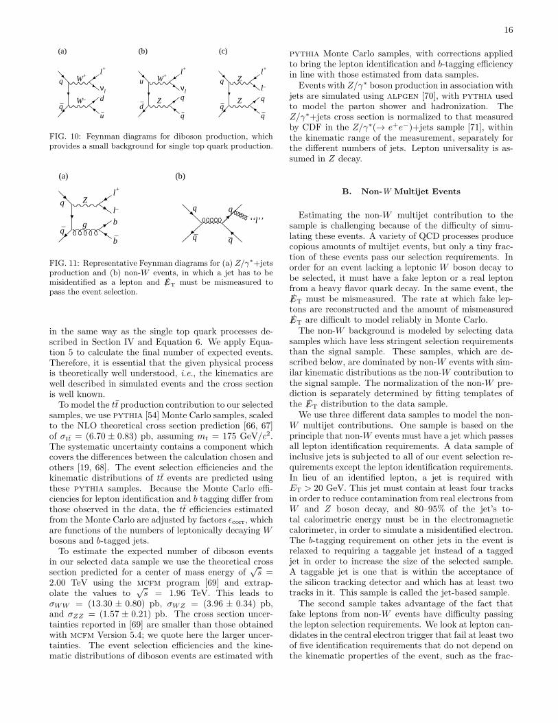
FIG. 10: Feynman diagrams for diboson production, whichprovides a small background for single top quark production.

q

q

Z

g

l+

l_

b

b

(a)

q

q

q

q

‘‘l’’

(b)

FIG. 11: Representative Feynman diagrams for (a) Z/γ∗+jetsproduction and (b) non-W events, in which a jet has to bemisidentified as a lepton and /ET must be mismeasured topass the event selection.

in the same way as the single top quark processes de-scribed in Section IV and Equation 6. We apply Equa-tion 5 to calculate the final number of expected events.Therefore, it is essential that the given physical processis theoretically well understood, i.e., the kinematics arewell described in simulated events and the cross sectionis well known.To model the tt production contribution to our selected

samples, we use pythia [54] Monte Carlo samples, scaledto the NLO theoretical cross section prediction [66, 67]of σtt = (6.70 ± 0.83) pb, assuming mt = 175 GeV/c2.The systematic uncertainty contains a component whichcovers the differences between the calculation chosen andothers [19, 68]. The event selection efficiencies and thekinematic distributions of tt events are predicted usingthese pythia samples. Because the Monte Carlo effi-ciencies for lepton identification and b tagging differ fromthose observed in the data, the tt efficiencies estimatedfrom the Monte Carlo are adjusted by factors ǫcorr, whichare functions of the numbers of leptonically decaying Wbosons and b-tagged jets.To estimate the expected number of diboson events

in our selected data sample we use the theoretical crosssection predicted for a center of mass energy of

√s =

2.00 TeV using the mcfm program [69] and extrap-olate the values to

√s = 1.96 TeV. This leads to

σWW = (13.30 ± 0.80) pb, σWZ = (3.96 ± 0.34) pb,and σZZ = (1.57 ± 0.21) pb. The cross section uncer-tainties reported in [69] are smaller than those obtainedwith mcfm Version 5.4; we quote here the larger uncer-tainties. The event selection efficiencies and the kine-matic distributions of diboson events are estimated with

pythia Monte Carlo samples, with corrections appliedto bring the lepton identification and b-tagging efficiencyin line with those estimated from data samples.Events with Z/γ∗ boson production in association with

jets are simulated using alpgen [70], with pythia usedto model the parton shower and hadronization. TheZ/γ∗+jets cross section is normalized to that measuredby CDF in the Z/γ∗(→ e+e−)+jets sample [71], withinthe kinematic range of the measurement, separately forthe different numbers of jets. Lepton universality is as-sumed in Z decay.

B. Non-W Multijet Events

Estimating the non-W multijet contribution to thesample is challenging because of the difficulty of simu-lating these events. A variety of QCD processes producecopious amounts of multijet events, but only a tiny frac-tion of these events pass our selection requirements. Inorder for an event lacking a leptonic W boson decay tobe selected, it must have a fake lepton or a real leptonfrom a heavy flavor quark decay. In the same event, the/ET must be mismeasured. The rate at which fake lep-tons are reconstructed and the amount of mismeasured/ET are difficult to model reliably in Monte Carlo.The non-W background is modeled by selecting data

samples which have less stringent selection requirementsthan the signal sample. These samples, which are de-scribed below, are dominated by non-W events with sim-ilar kinematic distributions as the non-W contribution tothe signal sample. The normalization of the non-W pre-diction is separately determined by fitting templates ofthe /ET distribution to the data sample.We use three different data samples to model the non-

W multijet contributions. One sample is based on theprinciple that non-W events must have a jet which passesall lepton identification requirements. A data sample ofinclusive jets is subjected to all of our event selection re-quirements except the lepton identification requirements.In lieu of an identified lepton, a jet is required withET > 20 GeV. This jet must contain at least four tracksin order to reduce contamination from real electrons fromW and Z boson decay, and 80–95% of the jet’s to-tal calorimetric energy must be in the electromagneticcalorimeter, in order to simulate a misidentified electron.The b-tagging requirement on other jets in the event isrelaxed to requiring a taggable jet instead of a taggedjet in order to increase the size of the selected sample.A taggable jet is one that is within the acceptance ofthe silicon tracking detector and which has at least twotracks in it. This sample is called the jet-based sample.The second sample takes advantage of the fact that

fake leptons from non-W events have difficulty passingthe lepton selection requirements. We look at lepton can-didates in the central electron trigger that fail at least twoof five identification requirements that do not depend onthe kinematic properties of the event, such as the frac-

17

tion of energy in the hadronic calorimeter. These objectsare treated as leptons and all other selection requirementsare applied. This sample has the advantage of having thesame kinematic properties as the central electron sample.This sample is called the ID-based sample.

The two samples described above are designed tomodel events with misidentified electron candidates. Be-cause of the similarities in the kinematic properties of theID-based and the jet-based events, we use the union ofthe jet-based and ID-based samples as our non-W modelfor triggered central electrons (the CEM sample). Re-markably, the same samples also simulate the kinematicsof events with misidentified triggered muon candidates;we use the samples again to model those events (theCMUP and CMX samples). The jet-based sample aloneis used to model the non-W background in the PHX sam-ple because the angular coverage is greater.

The kinematic distributions of the reconstructed ob-jects in the EMC sample are different from those in theCEM, PHX, CMUP, and CMX samples due to the triggerrequirements, and thus a separate sample must be usedto model the non-W background in the EMC data. Thisthird sample consists of events that are collected with the/ET+jets trigger path and which have a muon candidatepassing all selection requirements except for the isolationrequirement. It is called the non-isolated sample.

The non-W background must be determined not onlyfor the data sample passing the event selection require-ments, but also for the control samples which are usedto determine the W+jets backgrounds, as described inSections VC and VD. The expected numbers of non-Wevents are estimated in pretag events – events in whichall selection criteria are applied except the secondary ver-tex tag requirement. We require that at least one jet ina pretagged event is taggable. In order to estimate thenon-W rates in this sample, we also remove the /ET eventselection requirement, but we retain all other non-W re-jection requirements. We fit templates of the /ET distri-butions of the W+jets and the non-W samples to the /ET

spectra of the pretag data, holding constant the normal-izations of the additional templates needed to model thesmall diboson, tt, Z+jets, and single top backgrounds.The fractions of non-W events are then calculated in thesample with /ET > 25 GeV. The inclusion or omissionof the single top contribution to these fits has a negligi-ble impact on the non-W fractions that are fit. These fitsare performed separately for each lepton category (CEM,PHX, CMUP, CMX, and EMC) because the instrumen-tal fake lepton fractions are different for electrons andmuons, and for the different detector components. In alllepton categories except PHX, the full /ET spectrum isused in the fit. For the PHX electron sample, we require/ET > 15 GeV in order to minimize sensitivity to thetrigger. The fits in the pretag region are also used to es-timate the W+jets contribution in the pretag region, asdescribed in Section VC. As Fig. 12 shows, the resultingfits describe the data quite well.

Estimates of the non-W yields in the tagged sam-

ples used to search for the single top signal are alsoneeded. These samples are more difficult because thenon-W modeling samples are too small to apply taggingdirectly – only a few events pass the secondary vertex re-quirement. However, since the data show no dependenceof the b-tagging rate on /ET, we use the untagged non-W templates in the fits to the /ET distributions in thetagged samples. These fits are used to extract the non-W fractions in the signal samples. As before, the MonteCarlo predictions of diboson, tt, Z+jets, and single topproduction are held constant and only the normalizationsof the W+jets and the non-W templates are allowed tofloat. The resulting shapes are shown in Fig. 13 for thesingle-tagged sample, and these are used to derive thenon-W fractions in the signal samples. As before, theinclusion or omission of the single top contributions inthe fits has a negligible effect on the fitted non-W frac-tions. Because of the uncertainties in the tagging rates,the template shapes, and the estimation methods, the es-timated non-W rates are given systematic uncertaintiesof ±40% in single-tagged events and ±80% in double-tagged events. These uncertainties cover the differencesin the results obtained by fitting variables other than/ET, as well as by changing the histogram binning, vary-ing the fit range, and using alternative samples to modelthe non-W background. The uncertainty in the double-tagged non-W prediction is larger because of the largerstatistical uncertainty arising from the smaller size of thedouble-tagged sample.

C. W+Heavy Flavor Contributions

Events with a W boson accompanied by heavy fla-vor production constitute the majority of the b-taggedlepton+jets sample. These processes are Wbb, shownin Fig. 8(a), Wcc, which is the same process as Wbb,but with charm quarks replacing the b quarks, and Wcj,which is shown in Fig. 8(b). Each process may be ac-companied by more jets and pass the event selection re-quirements for the W+3 jets signal sample. Jets mayfail to be detected, or they may fail to pass our selectionrequirements, and such events may fall into the W+1 jetcontrol sample. While these events can be simulated us-ing the alpgen generator, the theory uncertainties onthe cross sections of these processes remain large com-pared with the size of the single top quark signal [72–79]. It is because of these large a priori uncertaintieson the background predictions and the small signal-to-background ratios in the selected data samples that wemust use advanced analysis techniques to purify furtherthe signal. We also use the data itself, both in controlsamples and in situ in the samples passing all selectionrequirements, to constrain the background rates, reduc-ing their systematic uncertainties. The in situ fits aredescribed in Section IX, and the control sample fits aredescribed below.The control samples used to estimate the W+ heavy

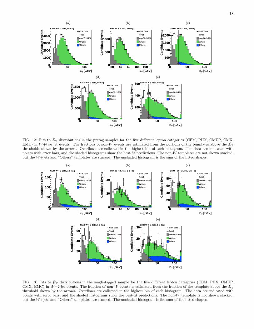
18

(a)

0 50 1000

1000

2000

3000

4000

[GeV]TE0 50 100

Can

did

ate

Eve

nts

0

1000

2000

3000

4000

CDF Data

Total

non-W: 5.2%

W+jets

Others

CEM W + 2 Jets, Pretag

(b)

20 40 60 80 1000

500

1000

[GeV]TE20 40 60 80 100

Can

did

ate

Eve

nts

0

500

1000

CDF Data

Total

non-W: 5.6%

W+jets

Others

PHX W + 2 Jets, Pretag

(c)

0 50 1000

500

1000

1500

2000

[GeV]TE0 50 100

Can

did

ate

Eve

nts

0

500

1000

1500

2000CDF Data

Total

non-W: 1.4%

W+jets

Others

CMUP W + 2 Jets, Pretag

(d)

0 50 1000

500

1000

1500

[GeV]TE0 50 100

Can

did

ate

Eve

nts

0

500

1000

1500 CDF Data

Total

non-W: 1.5%

W+jets

Others

CMX W + 2 Jets, Pretag

(e)

0 50 1000

200

400

600

[GeV]TE0 50 100

Can

did

ate

Eve

nts

0

200

400

600CDF Data

Total

non-W: 6.1%

W+jets

Others

EMC W + 2 Jets, Pretag

FIG. 12: Fits to /ET distributions in the pretag samples for the five different lepton categories (CEM, PHX, CMUP, CMX,EMC) in W+two jet events. The fractions of non-W events are estimated from the portions of the templates above the /ET

thresholds shown by the arrows. Overflows are collected in the highest bin of each histogram. The data are indicated withpoints with error bars, and the shaded histograms show the best-fit predictions. The non-W templates are not shown stacked,but the W+jets and “Others” templates are stacked. The unshaded histogram is the sum of the fitted shapes.

(a)

0 50 1000

50

100

150

[GeV]TE0 50 100

Can

did

ate

Eve

nts

0

50

100

150CDF Data

Total

non-W: 6.1%

W+jets

Others

CEM W + 2 Jets, 1 b Tag

(b)

20 40 60 80 1000

20

40

[GeV]TE20 40 60 80 100

Can

did

ate

Eve

nts

0

20

40

CDF Data

Total

non-W: 6.4%

W+jets

Others

PHX W + 2 Jets, 1 b Tag

(c)

0 50 1000

20

40

60

80

[GeV]TE0 50 100

Can

did

ate

Eve

nts

0

20

40

60

80

CDF Data

Total

non-W: 1.5%

W+jets

Others

CMUP W + 2 Jets, 1 b Tag

(d)

0 50 1000

20

40

60

[GeV]TE0 50 100

Can

did

ate

Eve

nts

0

20

40

60CDF Data

Total

non-W: 1.5%

W+jets

Others

CMX W + 2 Jets, 1 b Tag

(e)

0 50 1000

10

20

30

[GeV]TE0 50 100

Can

did

ate

Eve

nts

0

10

20

30 CDF Data

Total

non-W: 4.1%

W+jets

Others

EMC W + 2 Jets, 1 b Tag

FIG. 13: Fits to /ET distributions in the single-tagged sample for the five different lepton categories (CEM, PHX, CMUP,CMX, EMC) in W+2 jet events. The fraction of non-W events is estimated from the fraction of the template above the /ET

threshold shown by the arrows. Overflows are collected in the highest bin of each histogram. The data are indicated withpoints with error bars, and the shaded histograms show the best-fit predictions. The non-W template is not shown stacked,but the W+jets and “Others” templates are stacked. The unshaded histogram is the sum of the fitted shapes.

19

flavor predictions and uncertainties are the pretaggedW +n jets samples and the tagged W +1 jet sample. Weuse the alpgen+pythia Monte Carlo model to extrap-olate the measurements in the control samples to makepredictions of the W+heavy flavor background contri-butions in the data samples passing our signal selectionrequirements. The pretaggedW+n jets samples are usedto scale the alpgen predictions, and the tagged W + 1jet sample is used to check and adjust alpgen’s predic-tions of the fractions of W+jets events which are Wbb,Wcc, and Wcj events. A full description of the methodfollows.The number of pretag W+jets events is estimated by

assuming that events not included in the predictionsbased on Monte Carlo (these are the tt and diboson pre-dictions – the single top quark signal is a negligible com-ponent of the pretag sample) or non-W multijet events,are W+jets events. That is:

NpretagW+jets = Npretag

data × (1− fpretagnon-W )−Npretag

MC (7)

where Npretagdata is the number of observed events in the

pretag sample, fpretagnon-W is the fraction of non-W events

in the pretag sample, as determined from the fits de-scribed in Section VB, and Npretag

MC is the expected num-ber of pretag tt and diboson events. Alpgen typicallyunderestimates the inclusive W+jets rates by a factor ofroughly 1.4 [80]. To estimate the yields of Wbb, Wcc,and Wcj events, we multiply this data-driven estimateof the W+jets yield by heavy flavor fractions.The heavy flavor fractions in W+jets events are also

not well predicted by our alpgen+pythia model. Inorder to improve the modeling of these fractions, we per-form fits to templates of flavor-separating variables in theb-tagged W+1 jet data sample, which contains a vanish-ingly small component of single top quark signal eventsand is not otherwise used in the final signal extractionprocedure. This sample is quite large and is almost en-tirely composed of W+jets events. We include MonteCarlo models of the small contributions from tt and di-boson events as separate templates, normalized to theirSM expected rates, in the fits to the data. Care must beexercised in the estimation of the W+heavy flavor frac-tions, because fitting in the W+1 jet sample and usingthe fit values for the W+2 jet and W+3 jet samples isan extrapolation. We seek to estimate the b and charmfractions in these events with as many independent meth-ods as possible and we assign generous uncertainties thatcover the differences between the several estimations ofthe rates.We fit the distribution of the jet-flavor separator bNN

described in Section VI. Template distributions are cre-ated based on alpgen+pythia Monte Carlo samples forthe W+LF, Wcc, Wcj, Wbb, and Z/γ∗+jets processes,where W+LF events are those in which none of the jetsaccompanying the leptonically decaying W boson con-tains a b or c quark. The template distributions for thesefive processes are shown in Fig. 14(a). The tt and diboson

templates are created using pythia Monte Carlo sam-ples. The non-W model described in Section VB is alsoused. The W+LF template’s rate is constrained by thedata-derived mistag estimate, described in Section VD,within its uncertainty; the other W+jets templates’ ratesare not constrained. The tt, diboson, Z/γ∗+jets, andnon-W contributions are constrained within their uncer-tainties. The Wbb and Wcc components float in the fitbut are scaled with the same scaling factor, as the samediagrams, with b and c quarks interchanged, contributein the alpgen model, and we expect a similar corre-spondence for the leading processes in the data. We alsolet the Wcj fraction float in the fit. The best fit in theW+1 jet sample is shown in Fig. 14(b).The fit indicates that the alpgen-predicted Wbb +

Wcc fraction must be multiplied by 1.4± 0.4 in order forthe templates to match the data, and the best-fit valueof the Wcj fraction is also 1.4 ± 0.4 larger than thatpredicted by alpgen. In addition to the fit to the bNN

distribution, we also fit the W+heavy flavor fractions inthe b-tagged W+1-jet sample with another variable, thereconstructed invariant mass of the secondary vertex. Weperform this alternate fit in our standard b-tagged sampleas well as in one with loosened b-tag requirements.We obtain additional information from [81], in which

a direct measurement of the Wc fraction is made usinglepton charge correlations. The central value of this mea-surement agrees well with the Monte Carlo predictions.We thus set the multiplicative factor of the Wc compo-nent to 1.0± 0.3 for use in the two- and three-jet bins.The 30% uncertainties assessed on the Wbb+Wcc and

Wcj yields cover the differences in the measured fit valuesand also approximates our uncertainty in extrapolatingthis fraction to W+2 and 3 jet events. We check theseextrapolations in the W+2 and 3 jet events as shownin Figs. 14(c) and 14(d); no additional fit is performedfor this comparison. The rates and flavor compositionsmatch very well with the observed data in these sam-ples. The uncertainties in the fit fractions arising fromthe uncertainties on the shapes of the bNN templates dis-cussed in Section VI are a negligible component of thetotal uncertainty.Since the yields of W+heavy flavor events are esti-

mated from b-tagged data using the same secvtx algo-rithm as is used for the candidate event selection, the un-certainty in the b-tagging efficiency does not factor intothe prediction of these rates.

D. Rates of Events with Mistagged Jets

Some W+LF events pass our event selection require-ments due to the presence of mistagged jets. A mistaggedjet is one which does not contain a weakly-decaying Bor charm hadron but nonetheless passes all of the sec-ondary vertex tagging requirements of the secvtx algo-rithm [31]. Jets are mistagged for several reasons: track-ing errors such as hit misassignment or resolution effects

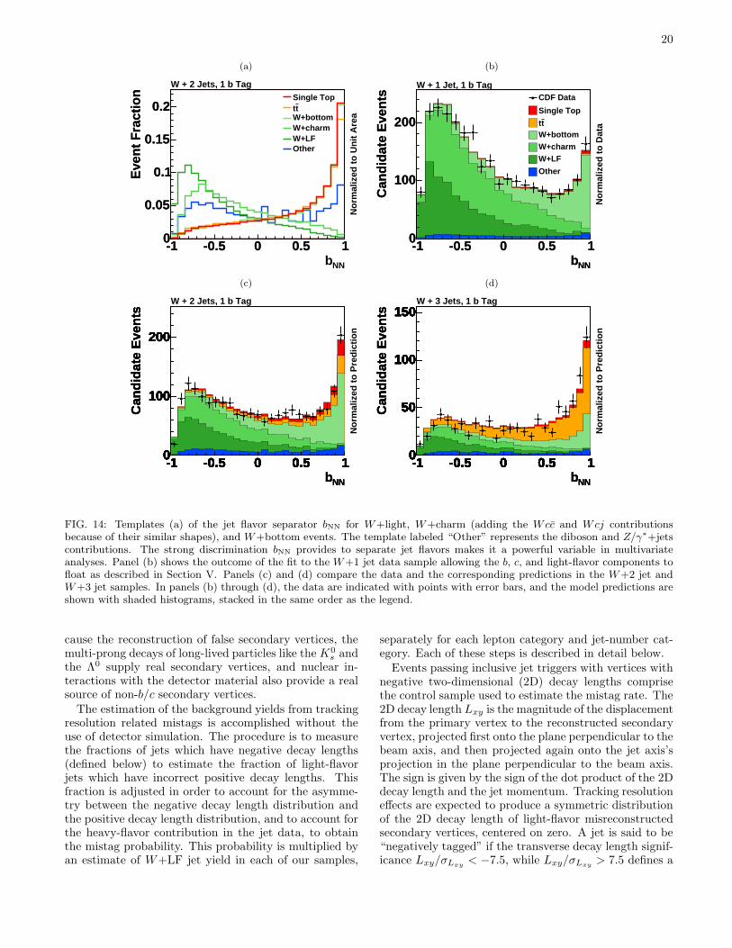
20

(a)

NNb-1 -0.5 0 0.5 1

Eve

nt

Fra

ctio

n

0

0.05

0.1

0.15

0.2

-1 -0.5 0 0.5 1

Eve

nt

Fra

ctio

n

0

0.05

0.1

0.15

0.2Single Toptt

W+bottomW+charmW+LFOther

W + 2 Jets, 1 b Tag

No

rmal

ized

to

Un

it A

rea

(b)

NNb-1 -0.5 0 0.5 1

Can

did

ate

Eve

nts

0

100

200

NNb-1 -0.5 0 0.5 1

Can

did

ate

Eve

nts

0

100

200

CDF Data

Single Top

ttW+bottomW+charmW+LF

Other

W + 1 Jet, 1 b Tag

No

rmal

ized

to

Dat

a

(c)

NNb-1 -0.5 0 0.5 1

Can

did

ate

Eve

nts

0

100

200

-1 -0.5 0 0.5 10

100

200

-1 -0.5 0 0.5 10

100

200

-1 -0.5 0 0.5 10

100

200

-1 -0.5 0 0.5 10

100

200

-1 -0.5 0 0.5 10

100

200

-1 -0.5 0 0.5 10

100

200

NNb-1 -0.5 0 0.5 1

Can

did

ate

Eve

nts

0

100

200

NNb-1 -0.5 0 0.5 1

Can

did

ate

Eve

nts

0

100

200

-1 -0.5 0 0.5 10

100

200

W + 2 Jets, 1 b Tag

No

rmal

ized

to

Pre

dic

tio

n

(d)

NNb-1 -0.5 0 0.5 1

Can

did

ate

Eve

nts

0

50

100

150

-1 -0.5 0 0.5 10

50

100

150

-1 -0.5 0 0.5 10

50

100

150

-1 -0.5 0 0.5 10

50

100

150

-1 -0.5 0 0.5 10

50

100

150

-1 -0.5 0 0.5 10

50

100

150

-1 -0.5 0 0.5 10

50

100

150

NNb-1 -0.5 0 0.5 1

Can

did

ate

Eve

nts

0

50

100

150

NNb-1 -0.5 0 0.5 1

Can

did

ate

Eve

nts

0

50

100

150

-1 -0.5 0 0.5 10

50

100

150W + 3 Jets, 1 b Tag

No

rmal

ized

to

Pre

dic

tio

n

FIG. 14: Templates (a) of the jet flavor separator bNN for W+light, W+charm (adding the Wcc and Wcj contributionsbecause of their similar shapes), and W+bottom events. The template labeled “Other” represents the diboson and Z/γ∗+jetscontributions. The strong discrimination bNN provides to separate jet flavors makes it a powerful variable in multivariateanalyses. Panel (b) shows the outcome of the fit to the W+1 jet data sample allowing the b, c, and light-flavor components tofloat as described in Section V. Panels (c) and (d) compare the data and the corresponding predictions in the W+2 jet andW+3 jet samples. In panels (b) through (d), the data are indicated with points with error bars, and the model predictions areshown with shaded histograms, stacked in the same order as the legend.

cause the reconstruction of false secondary vertices, themulti-prong decays of long-lived particles like the K0

s andthe Λ0 supply real secondary vertices, and nuclear in-teractions with the detector material also provide a realsource of non-b/c secondary vertices.The estimation of the background yields from tracking

resolution related mistags is accomplished without theuse of detector simulation. The procedure is to measurethe fractions of jets which have negative decay lengths(defined below) to estimate the fraction of light-flavorjets which have incorrect positive decay lengths. Thisfraction is adjusted in order to account for the asymme-try between the negative decay length distribution andthe positive decay length distribution, and to account forthe heavy-flavor contribution in the jet data, to obtainthe mistag probability. This probability is multiplied byan estimate of W+LF jet yield in each of our samples,

separately for each lepton category and jet-number cat-egory. Each of these steps is described in detail below.Events passing inclusive jet triggers with vertices with

negative two-dimensional (2D) decay lengths comprisethe control sample used to estimate the mistag rate. The2D decay length Lxy is the magnitude of the displacementfrom the primary vertex to the reconstructed secondaryvertex, projected first onto the plane perpendicular to thebeam axis, and then projected again onto the jet axis’sprojection in the plane perpendicular to the beam axis.The sign is given by the sign of the dot product of the 2Ddecay length and the jet momentum. Tracking resolutioneffects are expected to produce a symmetric distributionof the 2D decay length of light-flavor misreconstructedsecondary vertices, centered on zero. A jet is said to be“negatively tagged” if the transverse decay length signif-icance Lxy/σLxy < −7.5, while Lxy/σLxy > 7.5 defines a

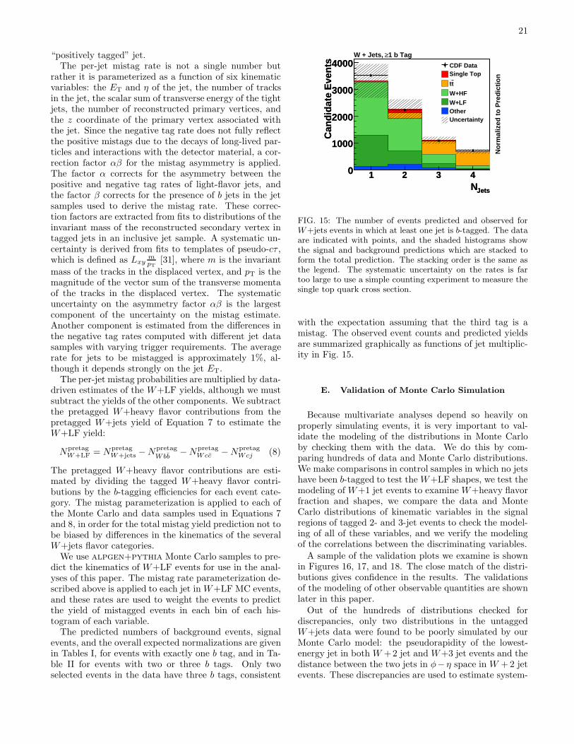
21

“positively tagged” jet.The per-jet mistag rate is not a single number but

rather it is parameterized as a function of six kinematicvariables: the ET and η of the jet, the number of tracksin the jet, the scalar sum of transverse energy of the tightjets, the number of reconstructed primary vertices, andthe z coordinate of the primary vertex associated withthe jet. Since the negative tag rate does not fully reflectthe positive mistags due to the decays of long-lived par-ticles and interactions with the detector material, a cor-rection factor αβ for the mistag asymmetry is applied.The factor α corrects for the asymmetry between thepositive and negative tag rates of light-flavor jets, andthe factor β corrects for the presence of b jets in the jetsamples used to derive the mistag rate. These correc-tion factors are extracted from fits to distributions of theinvariant mass of the reconstructed secondary vertex intagged jets in an inclusive jet sample. A systematic un-certainty is derived from fits to templates of pseudo-cτ ,which is defined as Lxy

mpT

[31], where m is the invariant

mass of the tracks in the displaced vertex, and pT is themagnitude of the vector sum of the transverse momentaof the tracks in the displaced vertex. The systematicuncertainty on the asymmetry factor αβ is the largestcomponent of the uncertainty on the mistag estimate.Another component is estimated from the differences inthe negative tag rates computed with different jet datasamples with varying trigger requirements. The averagerate for jets to be mistagged is approximately 1%, al-though it depends strongly on the jet ET.The per-jet mistag probabilities are multiplied by data-

driven estimates of the W+LF yields, although we mustsubtract the yields of the other components. We subtractthe pretagged W+heavy flavor contributions from thepretagged W+jets yield of Equation 7 to estimate theW+LF yield:

NpretagW+LF = Npretag

W+jets −Npretag

Wbb−Npretag

Wcc −NpretagWcj (8)

The pretagged W+heavy flavor contributions are esti-mated by dividing the tagged W+heavy flavor contri-butions by the b-tagging efficiencies for each event cate-gory. The mistag parameterization is applied to each ofthe Monte Carlo and data samples used in Equations 7and 8, in order for the total mistag yield prediction not tobe biased by differences in the kinematics of the severalW+jets flavor categories.We use alpgen+pythia Monte Carlo samples to pre-

dict the kinematics of W+LF events for use in the anal-yses of this paper. The mistag rate parameterization de-scribed above is applied to each jet in W+LF MC events,and these rates are used to weight the events to predictthe yield of mistagged events in each bin of each his-togram of each variable.The predicted numbers of background events, signal

events, and the overall expected normalizations are givenin Tables I, for events with exactly one b tag, and in Ta-ble II for events with two or three b tags. Only twoselected events in the data have three b tags, consistent

JetsN1 2 3 4

Can

did

ate

Eve

nts

0

1000

2000

3000

4000

JetsN1 2 3 4

Can

did

ate

Eve

nts

0

1000

2000

3000

40001 b Tag≥W + Jets,

No

rmal

ized

to

Pre

dic

tio

n

CDF DataSingle Top

tt

W+HF

W+LFOtherUncertainty

FIG. 15: The number of events predicted and observed forW+jets events in which at least one jet is b-tagged. The dataare indicated with points, and the shaded histograms showthe signal and background predictions which are stacked toform the total prediction. The stacking order is the same asthe legend. The systematic uncertainty on the rates is fartoo large to use a simple counting experiment to measure thesingle top quark cross section.

with the expectation assuming that the third tag is amistag. The observed event counts and predicted yieldsare summarized graphically as functions of jet multiplic-ity in Fig. 15.

E. Validation of Monte Carlo Simulation

Because multivariate analyses depend so heavily onproperly simulating events, it is very important to val-idate the modeling of the distributions in Monte Carloby checking them with the data. We do this by com-paring hundreds of data and Monte Carlo distributions.We make comparisons in control samples in which no jetshave been b-tagged to test the W+LF shapes, we test themodeling of W+1 jet events to examine W+heavy flavorfraction and shapes, we compare the data and MonteCarlo distributions of kinematic variables in the signalregions of tagged 2- and 3-jet events to check the model-ing of all of these variables, and we verify the modelingof the correlations between the discriminating variables.A sample of the validation plots we examine is shown

in Figures 16, 17, and 18. The close match of the distri-butions gives confidence in the results. The validationsof the modeling of other observable quantities are shownlater in this paper.Out of the hundreds of distributions checked for

discrepancies, only two distributions in the untaggedW+jets data were found to be poorly simulated by ourMonte Carlo model: the pseudorapidity of the lowest-energy jet in both W +2 jet and W+3 jet events and thedistance between the two jets in φ− η space in W +2 jetevents. These discrepancies are used to estimate system-

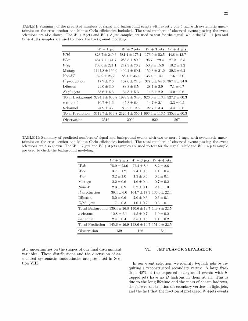
22

TABLE I: Summary of the predicted numbers of signal and background events with exactly one b tag, with systematic uncer-tainties on the cross section and Monte Carlo efficiencies included. The total numbers of observed events passing the eventselections are also shown. The W + 2 jets and W + 3 jets samples are used to test for the signal, while the W + 1 jets andW + 4 jets samples are used to check the background modeling.

W + 1 jet W + 2 jets W + 3 jets W + 4 jets

Wbb 823.7 ± 249.6 581.1 ± 175.1 173.9 ± 52.5 44.8 ± 13.7

Wcc 454.7 ± 141.7 288.5 ± 89.0 95.7± 29.4 27.2± 8.5

Wcj 709.6 ± 221.1 247.3 ± 76.2 50.8± 15.6 10.2± 3.2

Mistags 1147.8 ± 166.0 499.1 ± 69.1 150.3 ± 21.0 39.3± 6.2

Non-W 62.9 ± 25.2 88.4± 35.4 35.4± 14.1 7.6± 3.0

tt production 17.9 ± 2.6 167.6 ± 24.0 377.3 ± 54.8 387.4 ± 54.8

Diboson 29.0 ± 3.0 83.3± 8.5 28.1± 2.9 7.1± 0.7

Z/γ∗+jets 38.6 ± 6.3 34.8± 5.3 14.6± 2.2 4.0± 0.6

Total Background 3284.1 ± 633.8 1989.9 ± 349.6 926.0 ± 113.4 527.7 ± 60.3

s-channel 10.7 ± 1.6 45.3± 6.4 14.7± 2.1 3.3± 0.5

t-channel 24.9 ± 3.7 85.3± 12.6 22.7± 3.3 4.4± 0.6

Total Prediction 3319.7 ± 633.8 2120.4 ± 350.1 963.4 ± 113.5 535.4 ± 60.3

Observation 3516 2090 920 567

TABLE II: Summary of predicted numbers of signal and background events with two or more b tags, with systematic uncer-tainties on the cross section and Monte Carlo efficiencies included. The total numbers of observed events passing the eventselections are also shown. The W + 2 jets and W + 3 jets samples are used to test for the signal, while the W + 4 jets sampleare used to check the background modeling.

W + 2 jets W + 3 jets W + 4 jets

Wbb 75.9 ± 23.6 27.4± 8.5 8.2± 2.6

Wcc 3.7 ± 1.2 2.4± 0.8 1.1± 0.4

Wcj 3.2 ± 1.0 1.3± 0.4 0.4± 0.1

Mistags 2.2 ± 0.6 1.6± 0.4 0.7± 0.2

Non-W 2.3 ± 0.9 0.2± 0.1 2.4± 1.0

tt production 36.4 ± 6.0 104.7 ± 17.3 136.0 ± 22.4

Diboson 5.0 ± 0.6 2.0± 0.3 0.6± 0.1

Z/γ∗+jets 1.7 ± 0.3 1.0± 0.2 0.3± 0.1

Total Background 130.4 ± 26.8 140.6 ± 19.7 149.8 ± 22.5

s-channel 12.8 ± 2.1 4.5± 0.7 1.0± 0.2

t-channel 2.4 ± 0.4 3.5± 0.6 1.1± 0.2

Total Prediction 145.6 ± 26.9 148.6 ± 19.7 151.9 ± 22.5

Observation 139 166 154

atic uncertainties on the shapes of our final discriminantvariables. These distributions and the discussion of as-sociated systematic uncertainties are presented in Sec-tion VIII.

VI. JET FLAVOR SEPARATOR

In our event selection, we identify b-quark jets by re-quiring a reconstructed secondary vertex. A large frac-tion, 48% of the expected background events with b-tagged jets have no B hadrons in them at all. This isdue to the long lifetime and the mass of charm hadrons,the false reconstruction of secondary vertices in light jets,and the fact that the fraction of pretaggedW+jets events

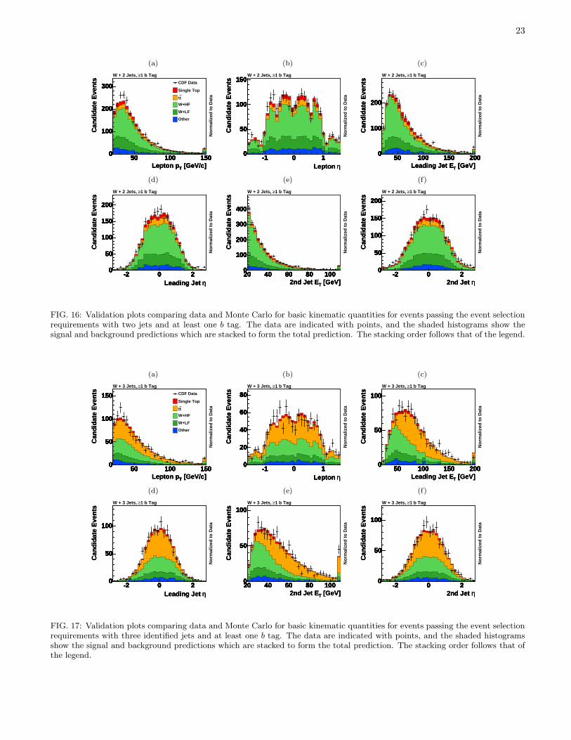
23

(a)

[GeV/c]TLepton p50 100 150

Can

did

ate

Eve

nts

0

100

200

300

50 100 1500

100

200

300

50 100 1500

100

200

300

50 100 1500

100

200

300

50 100 1500

100

200

300

50 100 1500

100

200

300

[GeV/c]TLepton p50 100 150

Can

did

ate

Eve

nts

0

100

200

300

[GeV/c]TLepton p50 100 150

Can

did

ate

Eve

nts

0

100

200

300

50 100 1500

100

200

300CDF Data

Single Top

tt

W+HF

W+LF

Other

1 b Tag≥W + 2 Jets,

No

rmal

ized

to

Dat

a

(b)

ηLepton -1 0 1

Can

did

ate

Eve

nts

0

50

100

150

-1 0 10

50

100

150

-1 0 10

50

100

150

-1 0 10

50

100

150

-1 0 10

50

100

150

-1 0 10

50

100

150

ηLepton -1 0 1

Can

did

ate

Eve

nts

0

50

100

150

ηLepton -1 0 1

Can

did

ate

Eve

nts

0

50

100

150

-1 0 10

50

100

1501 b Tag≥W + 2 Jets,

No

rmal

ized

to

Dat

a

(c)

[GeV]TLeading Jet E50 100 150 200

Can

did

ate

Eve

nts

0

100

200

50 100 150 2000

100

200

50 100 150 2000

100

200

50 100 150 2000

100

200

50 100 150 2000

100

200

50 100 150 2000

100

200

[GeV]TLeading Jet E50 100 150 200

Can

did

ate

Eve

nts

0

100

200

[GeV]TLeading Jet E50 100 150 200

Can

did

ate

Eve

nts

0

100

200

50 100 150 2000

100

200

1 b Tag≥W + 2 Jets,

No

rmal

ized

to

Dat

a

(d)

ηLeading Jet -2 0 2

Can

did

ate

Eve

nts

0

50

100

150

200

-2 0 20

50

100

150

200

-2 0 20

50

100

150

200

-2 0 20

50

100

150

200

-2 0 20

50

100

150

200

-2 0 20

50

100

150

200

ηLeading Jet -2 0 2

Can

did

ate

Eve

nts

0

50

100

150

200

ηLeading Jet -2 0 2

Can

did

ate

Eve

nts

0

50

100

150

200

-2 0 20

50

100

150

200

1 b Tag≥W + 2 Jets,

No

rmal

ized

to

Dat

a

(e)

[GeV]T2nd Jet E20 40 60 80 100

Can

did

ate

Eve

nts

0

100

200

300

400

20 40 60 80 1000

100

200

300

400

20 40 60 80 1000

100

200

300

400

20 40 60 80 1000

100

200

300

400

20 40 60 80 1000

100

200

300

400

20 40 60 80 1000

100

200

300

400

[GeV]T2nd Jet E20 40 60 80 100

Can

did

ate

Eve

nts

0

100

200

300

400

[GeV]T2nd Jet E20 40 60 80 100

Can

did

ate

Eve

nts

0

100

200

300

400

20 40 60 80 1000

100

200

300

400

1 b Tag≥W + 2 Jets,

No

rmal

ized

to

Dat

a

(f)

η2nd Jet -2 0 2

Can

did

ate

Eve

nts

0

50

100

150

200

-2 0 20

50

100

150

200

-2 0 20

50

100

150

200

-2 0 20

50

100

150

200

-2 0 20

50

100

150

200

-2 0 20

50

100

150

200

η2nd Jet -2 0 2

Can

did

ate

Eve

nts

0

50

100

150

200

η2nd Jet -2 0 2

Can

did

ate

Eve

nts

0

50

100

150

200

-2 0 20

50

100

150

2001 b Tag≥W + 2 Jets,

No

rmal

ized

to

Dat

a

FIG. 16: Validation plots comparing data and Monte Carlo for basic kinematic quantities for events passing the event selectionrequirements with two jets and at least one b tag. The data are indicated with points, and the shaded histograms show thesignal and background predictions which are stacked to form the total prediction. The stacking order follows that of the legend.

(a)

[GeV/c]TLepton p50 100 150

Can

did

ate

Eve

nts

0

50

100

150

50 100 1500

50

100

150

50 100 1500

50

100

150

50 100 1500

50

100

150

50 100 1500

50

100

150

50 100 1500

50

100

150

[GeV/c]TLepton p50 100 150

Can

did

ate

Eve

nts

0

50

100

150

[GeV/c]TLepton p50 100 150

Can

did

ate

Eve

nts

0

50

100

150

50 100 1500

50

100

150 CDF Data

Single Top

tt

W+HF

W+LF

Other

1 b Tag≥W + 3 Jets,

No

rmal

ized

to

Dat

a

(b)

ηLepton -1 0 1

Can

did

ate

Eve

nts

0

20

40

60

80

-1 0 10

20

40

60

80

-1 0 10

20

40

60

80

-1 0 10

20

40

60

80

-1 0 10

20

40

60

80

-1 0 10

20

40

60

80

ηLepton -1 0 1

Can

did

ate

Eve

nts

0

20

40

60

80

ηLepton -1 0 1

Can

did

ate

Eve

nts

0

20

40

60

80

-1 0 10

20

40

60

801 b Tag≥W + 3 Jets,

No

rmal

ized

to

Dat

a

(c)

[GeV]TLeading Jet E50 100 150 200

Can

did

ate

Eve

nts

0

50

100

50 100 150 2000

50

100

50 100 150 2000

50

100

50 100 150 2000

50

100

50 100 150 2000

50

100

50 100 150 2000

50

100

[GeV]TLeading Jet E50 100 150 200

Can

did

ate

Eve

nts

0

50

100

[GeV]TLeading Jet E50 100 150 200

Can

did

ate

Eve

nts

0

50

100

50 100 150 2000

50

100

1 b Tag≥W + 3 Jets,

No

rmal

ized

to

Dat

a

(d)

ηLeading Jet -2 0 2

Can

did

ate

Eve

nts

0

50

100

-2 0 20

50

100

-2 0 20

50

100

-2 0 20

50

100

-2 0 20

50

100

-2 0 20

50

100

ηLeading Jet -2 0 2

Can

did

ate

Eve

nts

0

50

100

ηLeading Jet -2 0 2

Can

did

ate

Eve

nts

0

50

100

-2 0 20

50

100

1 b Tag≥W + 3 Jets,

No

rmal

ized

to

Dat

a

(e)

[GeV]T2nd Jet E20 40 60 80 100

Can

did

ate

Eve

nts

0

50

100

20 40 60 80 1000

50

100

20 40 60 80 1000

50

100

20 40 60 80 1000

50

100

20 40 60 80 1000

50

100

20 40 60 80 1000

50

100

[GeV]T2nd Jet E20 40 60 80 100

Can

did

ate

Eve

nts

0

50

100

[GeV]T2nd Jet E20 40 60 80 100

Can

did

ate

Eve

nts

0

50

100

20 40 60 80 1000

50

1001 b Tag≥W + 3 Jets,

No

rmal

ized

to

Dat

a

(f)

η2nd Jet -2 0 2

Can

did

ate

Eve

nts

0

50

100

-2 0 20

50

100

-2 0 20

50

100

-2 0 20

50

100

-2 0 20

50

100

-2 0 20

50

100

η2nd Jet -2 0 2

Can

did

ate

Eve

nts

0

50

100

η2nd Jet -2 0 2

Can

did

ate

Eve

nts

0

50

100

-2 0 20

50

100

1 b Tag≥W + 3 Jets,

No

rmal

ized

to

Dat

a

FIG. 17: Validation plots comparing data and Monte Carlo for basic kinematic quantities for events passing the event selectionrequirements with three identified jets and at least one b tag. The data are indicated with points, and the shaded histogramsshow the signal and background predictions which are stacked to form the total prediction. The stacking order follows that ofthe legend.

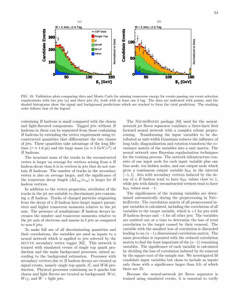
24

(a)

[GeV]TE50 100 150

Can

did

ate

Eve

nts

0

100

200

300

50 100 1500

100

200

300

50 100 1500

100

200

300

50 100 1500

100

200

300

50 100 1500

100

200

300

50 100 1500

100

200

300

[GeV]TE50 100 150

Can

did

ate

Eve

nts

0

100

200

300

[GeV]TE50 100 150

Can

did

ate

Eve

nts

0

100

200

300

50 100 1500

100

200

300

CDF Data

Single Top

tt

W+HF

W+LF

Other

1 b Tag≥W + 2 Jets,

No

rmal

ized

to

Dat

a

(b)

[GeV]TE50 100 150

Can

did

ate

Eve

nts

0

50

100

50 100 1500

50

100

50 100 1500

50

100

50 100 1500

50

100

50 100 1500

50

100

50 100 1500

50

100

[GeV]TE50 100 150

Can

did

ate

Eve

nts

0

50

100

[GeV]TE50 100 150

Can

did

ate

Eve

nts

0

50

100

50 100 1500

50

100

1 b Tag≥W + 3 Jets,

No

rmal

ized

to

Dat

a

FIG. 18: Validation plots comparing data and Monte Carlo for missing transverse energy for events passing our event selectionrequirements with two jets (a) and three jets (b), both with at least one b tag. The data are indicated with points, and theshaded histograms show the signal and background predictions which are stacked to form the total prediction. The stackingorder follows that of the legend.

containing B hadrons is small compared with the charmand light-flavored components. Tagged jets without Bhadrons in them can be separated from those containingB hadrons by extending the vertex requirement using re-constructed quantities that differentiate the two classesof jets. These quantities take advantage of the long life-time (τ ≈ 1.6 ps) and the large mass (m ≈ 5 GeV/c2) ofB hadrons.

The invariant mass of the tracks in the reconstructedvertex is larger on average for vertices arising from a Bhadron decay than it is in vertices in jets that do not con-tain B hadrons. The number of tracks in the secondaryvertex is also on average larger, and the significance ofthe transverse decay length (∆Lxy/σxy) is larger for Bhadron vertices.

In addition to the vertex properties, attributes of thetracks in the jet are suitable to discriminate jets contain-ing a B hadron. Tracks of charged particles originatingfrom the decay of a B hadron have larger impact param-eters and higher transverse momenta relative to the jetaxis. The presence of semileptonic B hadron decays in-creases the number and transverse momenta relative tothe jet axis of electrons and muons in b jets as comparedto non-b jets.

To make full use of all discriminating quantities andtheir correlations, the variables are used as inputs to aneural network which is applied to jets selected by thesecvtx secondary vertex tagger [82]. This network istrained with simulated events of single top quark pro-duction and the main background processes, mixed ac-cording to the background estimation. Processes withsecondary vertices due to B hadron decays are treated assignal events, namely single top quark, tt, and Wbb pro-duction. Physical processes containing no b quarks butcharm and light flavors are treated as background: Wcc,Wcj, and W + light jets.

The NeuroBayes package [83] used for the neural-network jet flavor separator combines a three-layer feedforward neural network with a complex robust prepro-cessing. Transforming the input variables to be dis-tributed as unit-width Gaussians reduces the influence oflong tails; diagonalization and rotation transform the co-variance matrix of the variables into a unit matrix. Theneural network uses Bayesian regularization techniquesfor the training process. The network infrastructure con-sists of one input node for each input variable plus onebias node, ten hidden nodes, and one output node whichgives a continuous output variable bNN in the interval[−1, 1]. Jets with secondary vertices induced by the de-cay of a B hadron tend to have bNN values close to 1,while jets with falsely reconstructed vertices tend to havebNN values near −1.

The significances of the training variables are deter-mined automatically during the preprocessing in Neu-

roBayes. The correlation matrix of all preprocessed in-put variables is calculated, including the correlation of allvariables to the target variable, which is +1 for jets withB hadron decays and −1 for all other jets. The variablesare omitted one at a time to determine the loss of totalcorrelation to the target caused by their removal. Thevariable with the smallest loss of correlation is discardedleading to an (n−1)-dimensional correlation matrix. Thesame procedure is repeated with the reduced correlationmatrix to find the least important of the (n−1) remainingvariables. The significance of each variable is calculatedby dividing the loss of correlation induced by its removalby the square root of the sample size. We investigated 50candidate input variables but chose to include as inputsonly those with a significance larger than 3.0, of whichthere are 25.

Because the neural-network jet flavor separator istrained using simulated events, it is essential to verify

25

that the input and output distributions are modeled well,and to assess systematic uncertainties where discrepan-cies are seen. The shapes of the input variable distri-butions in the data are found to be reasonably well re-produced by the simulation. We also examine the dis-tribution of bNN for both b signal and non-b background.The b signal distribution is checked with double-secvtx-tagged dijet events and compared against Monte Carlojets with B hadron decays. One jet in addition is re-quired to have an electron with a large transverse mo-mentum with respect to the jet axis, in order to purifyfurther the b content of the sample. The jet opposite tothe electron-tagged jet is probed for its distribution ofthe neural network output. The distribution of bNN inthese jets is well simulated by that of b jets in the MonteCarlo [82].

To test the response of the network to light-flavoredjets, negative-tagged jets were tested in data and MonteCarlo. A correction function was derived [82] to adjustfor the small discrepancy observed in the output shape.This correction function is parameterized in the sum oftransverse energies in the event, the number of tracks perjet, and the transverse energy of the jet. The correctionfunction is applied to light-flavored and charm MonteCarlo jets in the analyses presented in this paper, butnot to b jets. The uncorrected neural network outputs areused to evaluate systematic uncertainties on the shapesof the final discriminant distributions.

The resulting network output bNN distinguishes the bsignal from the charm and light-flavored background pro-cesses with a purity that increases with increasing bNN,as can be seen in Fig. 14(a). Furthermore, the networkgives very similar shapes for different b-quark-producingprocesses, indicating that it is sensitive to the propertiesof b-quark jets and does not depend on the underlyingprocesses that produce them.

Not only is bNN a valuable tool for separating the sin-gle top quark signal from background processes that donot contain b jets, it is also valuable for separating thedifferent flavors of W+jets events, which is crucial inestimating the background composition. As describedin Section V, the distribution of bNN is fit in b-taggedW+1 jet events, and the heavy-flavor fractions for b andcharm jets are extracted. Using also a direct measure-ment of the Wc rate [81], predictions are made of the band charm jet fractions in the two- and three-jet bins.These predictions are used to scale the alpgen MonteCarlo samples, which are then compared with the datain the two- and three-jet b-tagged samples, without refit-ting the heavy-flavor composition, as shown in Fig. 14(c)and (d). The three-jet sample has a larger sample of ttevents which are enriched in b jets. The successful mod-eling of the changing flavor composition as a function ofthe number of identified jets provides confidence in thecorrectness of the background simulation.

All multivariate methods described here use bNN asan input variable, and thus we need bNN values for allMonte Carlo and data events used to model the final dis-

tributions. For the mistagged W+LF shape prediction,we use the W+LF Monte Carlo sample, where the eventsare weighted by the data-based mistag prediction for eachtaggable jet. This procedure improves the modeling overwhat would be obtained if Monte Carlo mistags wereused, as the mistag probabilities are based on the data,and it increases the sample size we use for the mistagmodeling. An issue that arises is that parameterizedmistagged events do not have bNN values and randomvalues must be chosen for them from the distribution inlight-flavor events. If a W+LF event has more than onetaggable jet, then random values are assigned to bothjets. These events are used for both the single-mistagprediction and the double-mistag prediction with appro-priate weights. The randomly chosen flavor-separatorvalues must be the same event-by-event and jet-by-jet foreach of the four analyses in this paper in order for thesuper discriminant combination method to be consistent.The distributions of bNN for non-W multijet events are

more difficult to predict because the flavor compositionof the jets in these events is poorly known. Specifically,since a non-W event must have a fake lepton (or a leptonfrom heavy-flavor decay), and also mismeasured /ET, theflavor composition of events passing the selection require-ments depends on the details of the detector response,particularly in the tails of distributions which are diffi-cult to model. It is necessary therefore to constrain theseflavor fractions with CDF data, and the flavor fractionsthus estimated are specific to this analysis. The non-Wevent yields are constrained by the data as explained inSection VB.The fraction of each flavor: b, charm, and light-flavored

jets (originating from light quarks or gluons), is estimatedby applying the jet flavor separator to b-tagged jets in the15 < /ET < 25 GeV sideband of the data. In this sample,we find a flavor composition of 45% b quark jets, 40% cquark jets, and 15% light-flavored jets. Each event in thenon-W modeling samples (see Section VB) is randomlyassigned a flavor according to the fraction given aboveand then assigned a jet flavor separator value chosen atrandom from the appropriate flavor distribution. Thefractions of the non-W events in the signal sample areuncertain both due to the uncertainties in the sidebandfit and the extrapolation to the signal sample. We take asan alternative flavor composition estimate 60% b quarkjets, 30% c quark jets, and 10% light-flavored jets, whichis the most b-like possibility of the errors on the flavormeasurement. This alternative flavor composition affectsthe shapes of the final discriminant distribution throughthe different flavor-separator neural network values.

VII. MULTIVARIATE ANALYSIS

The search for single top quark production and themeasurement of its cross section present substantial ex-perimental challenges. Compared with the search for ttproduction, the search for single top quarks suffers from a

26

lower SM production rate and a larger background. Sin-gle top quark events are also kinematically more similarto W+jets events than tt events are, since there is onlyone heavy top quark and thus only one W boson in thesingle top quark events, while there are two top quarks,each decaying to Wb, in tt events. The most serious chal-lenge arises from the systematic uncertainty on the back-ground prediction, which is approximately three timesthe size of the expected signal. Simply counting eventswhich pass our selection requirements will not yield aprecise measurement of the single top quark cross sec-tion no matter how much data are accumulated becausethe systematic uncertainty on the background is so large.In fact, in order to have sufficient sensitivity to expectto observe a signal at the 5 σ level, the systematic uncer-tainty on the background must be less than one-fifth ofthe expected signal rate.

Further separation of the signal from the background isrequired. Events that are classified as being more signal-like are used to test for the presence of single top quarkproduction and measure the cross section, and eventsthat are classified as being more background-like improveour knowledge of the rates of background processes. Inorder to optimize our sensitivity, we construct discrimi-nant functions based on kinematic and b-tag propertiesof the events, and we classify the events on a continuousspectrum that runs from very signal-like for high valuesof the discriminants to very background-like for low val-ues of the discriminants. We fit the distributions of thesediscriminants to the background and signal+backgroundpredictions, allowing uncertain parameters, listed in Sec-tion VIII, to float, in a manner described in Section IX.

To separate signal events from background events, welook for properties of the events that differ between signaland background. Events from single top quark produc-tion have distinctive energy and angular properties. Thebackgrounds, too, have distinctive features which can beexploited to help separate them. Many of the variableswe compute for each selected candidate event are moti-vated by a specific interpretation of the event as a signalevent or a background event. It is not necessary thatall variables used in a discriminant are motivated by thesame interpretation of an event, nor do we rely on the cor-rectness of the motivation for the interpretation of anygiven event. Indeed, each analysis is made more optimalwhen it includes a mixture of variables that are based ondifferent ways to interpret the measured particles in theevents. We optimize our analyses by using variables forwhich the distributions are maximally different betweensignal events and background events, and for which wehave reliable modeling as verified by the data.

We list below some of the most sensitive variables,and explain why they are sensitive in terms of the differ-ences between the signal and background processes thatthey exploit. The three multivariate discriminants, like-lihood functions, neural networks, and boosted decisiontrees, use these variables, or variations of them, as in-puts; the analyses also use other variables. The matrix

element analysis uses all of these features implicitly, andit uses bNN explicitly. Normalized Monte Carlo predic-tions (“templates”) and modeling comparisons of thesevariables are shown in Figs. 19 and 20.

• Mℓνb: the invariant mass of the charged lepton,the neutrino, and the b jet from the top quarkdecay. The pz of the neutrino, which cannot bemeasured, is inferred by constraining Mℓν to theW boson mass, using the measured charged leptoncandidate’s momentum and setting pνT = 6ET. Theneutrino’s pz is the solution of a quadratic equa-tion, which may have two real solutions, one realsolution, or two complex solutions. For the casewith two real solutions, the one with the lower |pz|is chosen. For the complex case, the real part of thepz solution is chosen. Some analyses use variationsof this variable with different treatment of the un-measured |pz| of the neutrino. The distribution ofMℓνb peaks near mt for signal events, with broaderspectra for background events from different pro-cesses.

• HT: the scalar sum of the transverse energies ofthe jets, the charged lepton, and /ET in the event.This quantity is much larger for tt events than forW+jets events; single top quark events populatethe region in between W+jets events and tt eventsin this variable.

• Mjj : the invariant dijet mass, which is substan-tially higher on average for events containing topquarks than it is for events with W+jets.

• Q × η: the sign of the charge of the lepton timesthe pseudorapidity of the light quark jet [84]. LargeQ×η is characteristic of t-channel single top quarkevents, because the light quark recoiling from thesingle top quark often retains much of the momen-tum component along the z axis it had before ra-diating the W boson. It therefore often produces ajet which is found at high |η|. Multiplying η by thesign of the lepton’s charge Q improves the separa-tion power of this variable since 2/3 of single topquark production in the t-channel is initiated by au quark in the proton or a (u) quark in the antipro-ton, and the sign of the lepton’s charge determinesthe sign of the top quark’s charge and is correlatedwith the sign of the η of the recoiling light-flavoredjet. The other 1/3 of single top quark productionis initiated by down-type quarks and has the op-posite charge-η correlation. W+jets and tt eventslack this correlation, and also have fewer jets pass-ing our ET requirement at large |η| than the singletop quark signal.

• cos θℓj : the cosine of the angle between the chargedlepton and the light quark jet [20]. For t-channelevents, this tends to be positive because of the V −A angular dependence of the W boson vertex. This

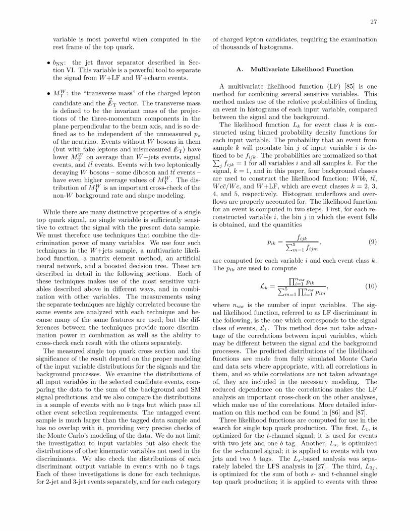
27

variable is most powerful when computed in therest frame of the top quark.

• bNN: the jet flavor separator described in Sec-tion VI. This variable is a powerful tool to separatethe signal from W+LF and W+charm events.

• MWT : the “transverse mass” of the charged lepton

candidate and the ~/ET vector. The transverse massis defined to be the invariant mass of the projec-tions of the three-momentum components in theplane perpendicular to the beam axis, and is so de-fined as to be independent of the unmeasured pzof the neutrino. Events without W bosons in them(but with fake leptons and mismeasured /ET) havelower MW

T on average than W+jets events, signalevents, and tt events. Events with two leptonicallydecaying W bosons – some diboson and tt events –have even higher average values of MW

T . The dis-tribution of MW

T is an important cross-check of thenon-W background rate and shape modeling.

While there are many distinctive properties of a singletop quark signal, no single variable is sufficiently sensi-tive to extract the signal with the present data sample.We must therefore use techniques that combine the dis-crimination power of many variables. We use four suchtechniques in the W+jets sample, a multivariate likeli-hood function, a matrix element method, an artificialneural network, and a boosted decision tree. These aredescribed in detail in the following sections. Each ofthese techniques makes use of the most sensitive vari-ables described above in different ways, and in combi-nation with other variables. The measurements usingthe separate techniques are highly correlated because thesame events are analyzed with each technique and be-cause many of the same features are used, but the dif-ferences between the techniques provide more discrim-ination power in combination as well as the ability tocross-check each result with the others separately.The measured single top quark cross section and the

significance of the result depend on the proper modelingof the input variable distributions for the signals and thebackground processes. We examine the distributions ofall input variables in the selected candidate events, com-paring the data to the sum of the background and SMsignal predictions, and we also compare the distributionsin a sample of events with no b tags but which pass allother event selection requirements. The untagged eventsample is much larger than the tagged data sample andhas no overlap with it, providing very precise checks ofthe Monte Carlo’s modeling of the data. We do not limitthe investigation to input variables but also check thedistributions of other kinematic variables not used in thediscriminants. We also check the distributions of eachdiscriminant output variable in events with no b tags.Each of these investigations is done for each technique,for 2-jet and 3-jet events separately, and for each category

of charged lepton candidates, requiring the examinationof thousands of histograms.

A. Multivariate Likelihood Function

A multivariate likelihood function (LF) [85] is onemethod for combining several sensitive variables. Thismethod makes use of the relative probabilities of findingan event in histograms of each input variable, comparedbetween the signal and the background.The likelihood function Lk for event class k is con-

structed using binned probability density functions foreach input variable. The probability that an event fromsample k will populate bin j of input variable i is de-fined to be fijk. The probabilities are normalized so that∑

j fijk = 1 for all variables i and all samples k. For thesignal, k = 1, and in this paper, four background classesare used to construct the likelihood function: Wbb, tt,Wcc/Wc, and W+LF, which are event classes k = 2, 3,4, and 5, respectively. Histogram underflows and over-flows are properly accounted for. The likelihood functionfor an event is computed in two steps. First, for each re-constructed variable i, the bin j in which the event fallsis obtained, and the quantities

pik =fijk

∑5

m=1 fijm, (9)

are computed for each variable i and each event class k.The pik are used to compute

Lk =

∏nvar

i=1 pik∑5

m=1

∏nvar

i=1 pim, (10)

where nvar is the number of input variables. The sig-nal likelihood function, referred to as LF discriminant inthe following, is the one which corresponds to the signalclass of events, L1. This method does not take advan-tage of the correlations between input variables, whichmay be different between the signal and the backgroundprocesses. The predicted distributions of the likelihoodfunctions are made from fully simulated Monte Carloand data sets where appropriate, with all correlations inthem, and so while correlations are not taken advantageof, they are included in the necessary modeling. Thereduced dependence on the correlations makes the LFanalysis an important cross-check on the other analyses,which make use of the correlations. More detailed infor-mation on this method can be found in [86] and [87].Three likelihood functions are computed for use in the

search for single top quark production. The first, Lt, isoptimized for the t-channel signal; it is used for eventswith two jets and one b tag. Another, Ls, is optimizedfor the s-channel signal; it is applied to events with twojets and two b tags. The Ls-based analysis was sepa-rately labeled the LFS analysis in [27]. The third, L3j ,is optimized for the sum of both s- and t-channel singletop quark production; it is applied to events with three

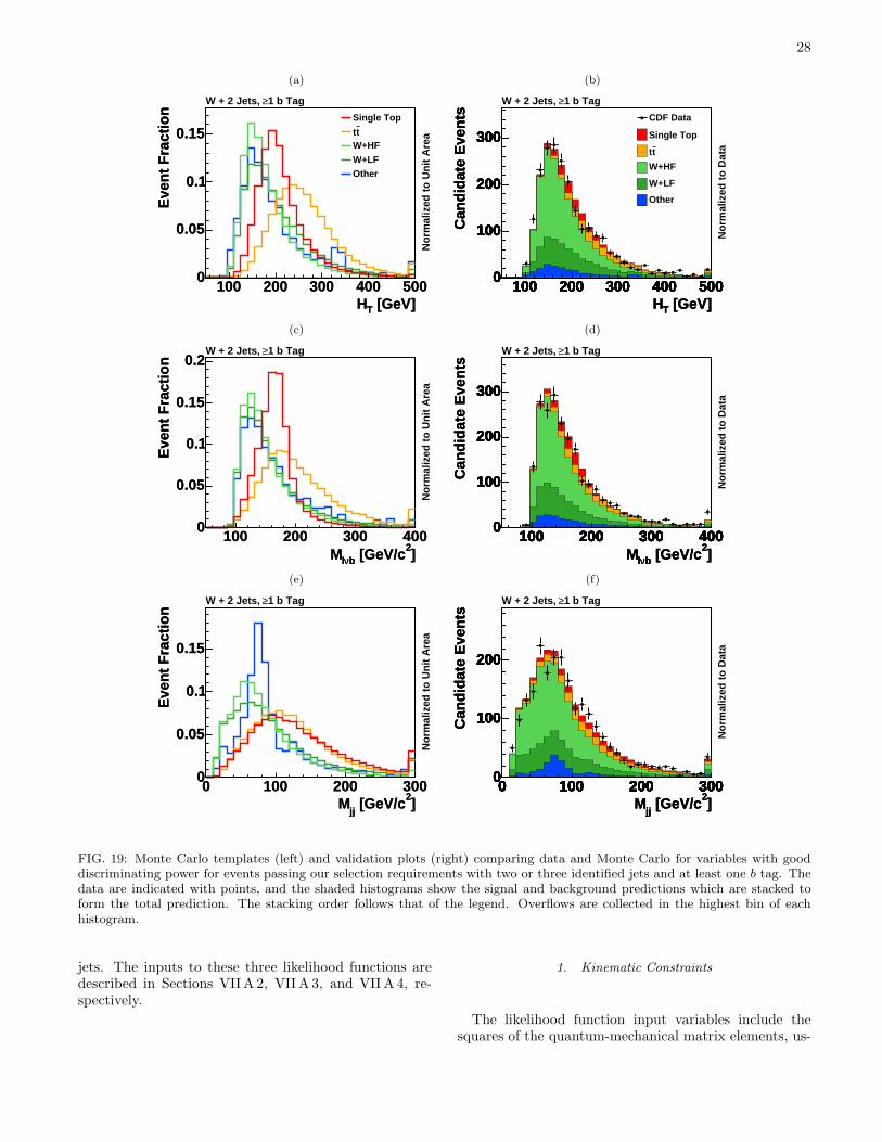
28

(a)

[GeV]TH100 200 300 400 500

Eve

nt

Fra

ctio

n

0

0.05

0.1

0.15

[GeV]TH100 200 300 400 500

Eve

nt

Fra

ctio

n

0

0.05

0.1

0.15Single Top

ttW+HF

W+LF

Other

1 b Tag≥W + 2 Jets,

No

rmal

ized

to

Un

it A

rea

(b)

[GeV]TH100 200 300 400 500

Can

did

ate

Eve

nts

0

100

200

300

100 200 300 400 5000

100

200

300

100 200 300 400 5000

100

200

300

100 200 300 400 5000

100

200

300

100 200 300 400 5000

100

200

300

100 200 300 400 5000

100

200

300

[GeV]TH100 200 300 400 500

Can

did

ate

Eve

nts

0

100

200

300

[GeV]TH100 200 300 400 500

Can

did

ate

Eve

nts

0

100

200

300

100 200 300 400 5000

100

200

300CDF Data

Single Top

tt

W+HF

W+LF

Other

1 b Tag≥W + 2 Jets,

No

rmal

ized

to

Dat

a

(c)

]2 [GeV/cbνlM100 200 300 400

Eve

nt

Fra

ctio

n

0

0.05

0.1

0.15

0.2

]2 [GeV/cbνlM100 200 300 400

Eve

nt

Fra

ctio

n

0

0.05

0.1

0.15

0.21 b Tag≥W + 2 Jets,

No

rmal

ized

to

Un

it A

rea

(d)

]2 [GeV/cbνlM100 200 300 400

Can

did

ate

Eve

nts

0

100

200

300

100 200 300 4000

100

200

300

100 200 300 4000

100

200

300

100 200 300 4000

100

200

300

100 200 300 4000

100

200

300

100 200 300 4000

100

200

300

]2 [GeV/cbνlM100 200 300 400

Can

did

ate

Eve

nts

0

100

200

300

]2 [GeV/cbνlM100 200 300 400

Can

did

ate

Eve

nts

0

100

200

300

100 200 300 4000

100

200

300

1 b Tag≥W + 2 Jets,

No

rmal

ized

to

Dat

a

(e)

]2 [GeV/cjj

M0 100 200 300

Eve

nt

Fra

ctio

n

0

0.05

0.1

0.15

]2 [GeV/cjj

M0 100 200 300

Eve

nt

Fra

ctio

n

0

0.05

0.1

0.15

1 b Tag≥W + 2 Jets,

No

rmal

ized

to

Un

it A

rea

(f)

]2 [GeV/cjj

M0 100 200 300

Can

did

ate

Eve

nts

0

100

200

0 100 200 3000

100

200

0 100 200 3000

100

200

0 100 200 3000

100

200

0 100 200 3000

100

200

0 100 200 3000

100

200

]2 [GeV/cjj

M0 100 200 300

Can

did

ate

Eve

nts

0

100

200

]2 [GeV/cjj

M0 100 200 300

Can

did

ate

Eve

nts

0

100

200

0 100 200 3000

100

200

1 b Tag≥W + 2 Jets,

No

rmal

ized

to

Dat

a

FIG. 19: Monte Carlo templates (left) and validation plots (right) comparing data and Monte Carlo for variables with gooddiscriminating power for events passing our selection requirements with two or three identified jets and at least one b tag. Thedata are indicated with points, and the shaded histograms show the signal and background predictions which are stacked toform the total prediction. The stacking order follows that of the legend. Overflows are collected in the highest bin of eachhistogram.

jets. The inputs to these three likelihood functions aredescribed in Sections VIIA 2, VIIA 3, and VII A 4, re-spectively.

1. Kinematic Constraints

The likelihood function input variables include thesquares of the quantum-mechanical matrix elements, us-

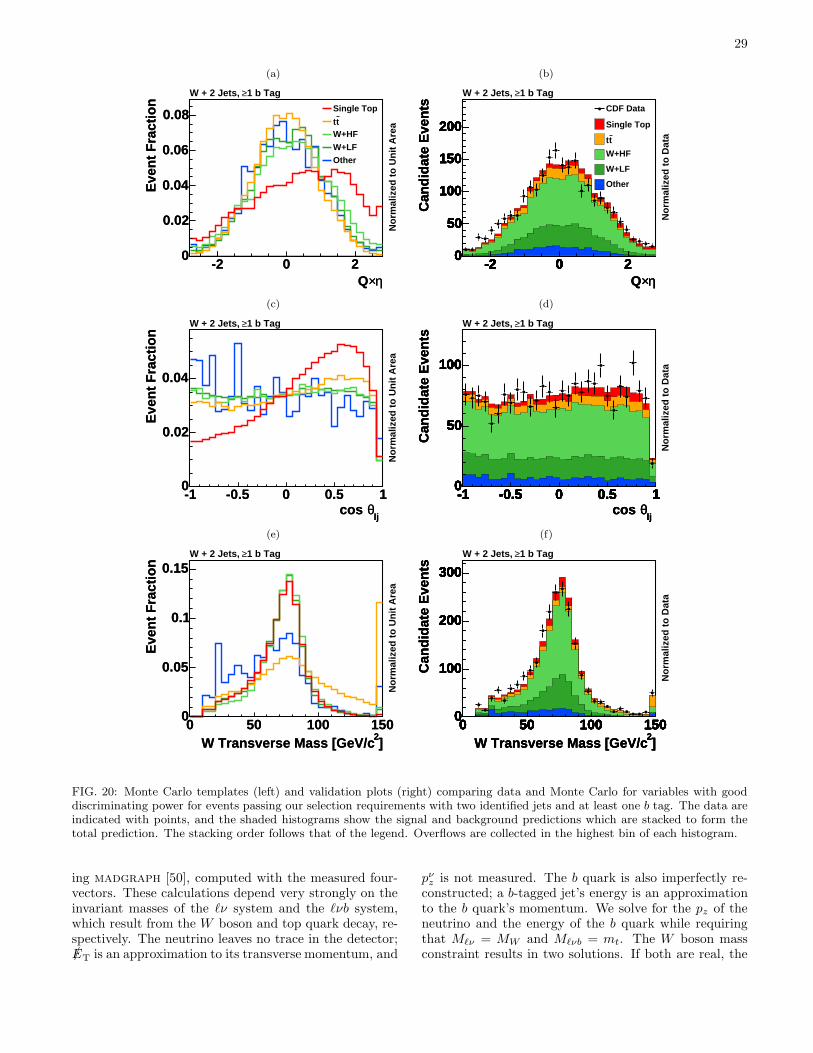
29

(a)

η×Q-2 0 2

Eve

nt

Fra

ctio

n

0

0.02

0.04

0.06

0.08

η×Q-2 0 2

Eve

nt

Fra

ctio

n

0

0.02

0.04

0.06

0.08 Single Top

ttW+HF

W+LF

Other

1 b Tag≥W + 2 Jets,

No

rmal

ized

to

Un

it A

rea

(b)

η×Q-2 0 2

Can

did

ate

Eve

nts

0

50

100

150

200

-2 0 20

50

100

150

200

-2 0 20

50

100

150

200

-2 0 20

50

100

150

200

-2 0 20

50

100

150

200

-2 0 20

50

100

150

200

η×Q-2 0 2

Can

did

ate

Eve

nts

0

50

100

150

200

η×Q-2 0 2

Can

did

ate

Eve

nts

0

50

100

150

200

-2 0 20

50

100

150

200CDF Data

Single Top

tt

W+HF

W+LF

Other

1 b Tag≥W + 2 Jets,

No

rmal

ized

to

Dat

a

(c)

ljθcos

-1 -0.5 0 0.5 1

Eve

nt

Fra

ctio

n

0

0.02

0.04

ljθcos

-1 -0.5 0 0.5 1

Eve

nt

Fra

ctio

n

0

0.02

0.04

1 b Tag≥W + 2 Jets,

No

rmal

ized

to

Un

it A

rea

(d)

ljθcos

-1 -0.5 0 0.5 1

Can

did

ate

Eve

nts

0

50

100

-1 -0.5 0 0.5 10

50

100

-1 -0.5 0 0.5 10

50

100

-1 -0.5 0 0.5 10

50

100

-1 -0.5 0 0.5 10

50

100

-1 -0.5 0 0.5 10

50

100

ljθcos

-1 -0.5 0 0.5 1

Can

did

ate

Eve

nts

0

50

100

ljθcos

-1 -0.5 0 0.5 1

Can

did

ate

Eve

nts

0

50

100

-1 -0.5 0 0.5 10

50

100

1 b Tag≥W + 2 Jets,

No

rmal

ized

to

Dat

a

(e)

]2W Transverse Mass [GeV/c0 50 100 150

Eve

nt

Fra

ctio

n

0

0.05

0.1

0.15

]2W Transverse Mass [GeV/c0 50 100 150

Eve

nt

Fra

ctio

n

0

0.05

0.1

0.151 b Tag≥W + 2 Jets,

No

rmal

ized

to

Un

it A

rea

(f)

]2W Transverse Mass [GeV/c0 50 100 150

Can

did

ate

Eve

nts

0

100

200

300

0 50 100 1500

100

200

300

0 50 100 1500

100

200

300

0 50 100 1500

100

200

300

0 50 100 1500

100

200

300

0 50 100 1500

100

200

300

]2W Transverse Mass [GeV/c0 50 100 150

Can

did

ate

Eve

nts

0

100

200

300

]2W Transverse Mass [GeV/c0 50 100 150

Can

did

ate

Eve

nts

0

100

200

300

0 50 100 1500

100

200

3001 b Tag≥W + 2 Jets,

No

rmal

ized

to

Dat

a

FIG. 20: Monte Carlo templates (left) and validation plots (right) comparing data and Monte Carlo for variables with gooddiscriminating power for events passing our selection requirements with two identified jets and at least one b tag. The data areindicated with points, and the shaded histograms show the signal and background predictions which are stacked to form thetotal prediction. The stacking order follows that of the legend. Overflows are collected in the highest bin of each histogram.

ing madgraph [50], computed with the measured four-vectors. These calculations depend very strongly on theinvariant masses of the ℓν system and the ℓνb system,which result from the W boson and top quark decay, re-spectively. The neutrino leaves no trace in the detector;/ET is an approximation to its transverse momentum, and

pνz is not measured. The b quark is also imperfectly re-constructed; a b-tagged jet’s energy is an approximationto the b quark’s momentum. We solve for the pz of theneutrino and the energy of the b quark while requiringthat Mℓν = MW and Mℓνb = mt. The W boson massconstraint results in two solutions. If both are real, the

30

one with the smaller |pz| is used. If both are complex,a minimal amount of additional /ET is added parallel tothe jet axis assigned to be the b from the top quark’sdecay until a real solution for |pνz | can be obtained. Inrare cases in which this procedure still fails to produce areal |pνz |, additional /ET is added along the b-jet axis tominimize the imaginary part of |pνz |, and then a minimalamount of /ET is added perpendicular to the b-jet axisuntil a real |pνz | is obtained.The top quark mass constraint can be satisfied by scal-

ing the b-jet’s energy, holding the direction fixed, untilMℓνb = mt. As the b-jet’s energy is scaled, the /ET is ad-justed to be consistent with the change. We then recal-culate pνz using the MW constraint described above, andthe process is iterated until Mℓνb = mt. The resultingfour-vectors of the b quark and the neutrino are then usedwith the measured four-vector of the charged lepton inthe matrix element expressions to construct discriminantvariables that separate the signal from the background.

2. 2-Jet t-channel Likelihood Function

The t-channel likelihood function Lt uses seven vari-ables, and assumes the b-tagged jet comes from top quarkdecay. The variables used are:

• HT, the scalar sum of the ET ’s of the two jets, thelepton ET, and /ET.

• Q × η, the charge of the lepton times the pseudo-rapidity of the jet which is not b-tagged.

• χ2kin, the χ2 of the comparison of the measured b

jet energy and the one the kinematic constraints re-quire in order to make Mℓνb = mt and Mℓν = MW ,using the nominal uncertainty in the b jet’s energy.Any additional /ET which is added to satisfy themℓν = MW constraint is added to χ2

kin using thenominal uncertainty in the /ET measurement.

• cos θℓj, the cosine of the angle between the chargedlepton and the untagged jet in the top quark decayframe.

• Mjj , the invariant mass of the two jets.

• MEt−chan, the differential cross section for the t-channel process, as computed by madgraph usingthe constrained four-vectors of the b, ℓ, and ν.

• The jet flavor separator output bNN described inSection VI.

3. 2-Jet s-channel Likelihood Function

The s-channel likelihood function Ls uses nine vari-ables. Because these events have exactly two jets, bothof which are required to be b-tagged, we decide which jet

comes from the top quark decay with a separate likeli-hood function that includes the transverse momentum ofthe b quark, the invariant mass of the b quark and thecharged lepton, and the product of the scattering angleof the b jet in the initial quarks’ rest frame and the lep-ton charge. To compute this last variable, the pz of theneutrino has been solved for using the mW constraint.The variables input to Ls are:

• Mjj , the invariant mass of the two jets.

• pjjT , the transverse momentum of the two-jet sys-tem.

• ∆Rjj , the separation between the two jets in φ–ηspace.

• Mℓνb, the invariant mass of the charged lepton, theneutrino, and the jet assigned to be the b jet fromthe top quark decay.

• Ej1T , the transverse energy of the leading jet, that

is, the jet with the largest ET.

• ηj2 , the pseudorapidity of the non-leading jet.

• pℓT, the transverse momentum of the charged lep-ton.

• Q× η, the charge of the lepton times the pseudora-pidity of the jet which is not assigned to have comefrom the top quark decay.

• The logarithm of the likelihood ratio constructedby matrix elements computed by madgraph, us-ing the pνz solution which maximizes the likelihooddescribed in the next point. This likelihood ratiois defined as MEs+MEt

MEs+MEt+MEWbb.

• The output of a kinematic fitter which chooses asolution of pνz that maximizes the likelihood of thesolution by allowing the values of pνx and pνy to varywithin their uncertainties. This likelihood is mul-tiplied by the likelihood used to choose the b jetthat comes from the top quark, and their productis used as a discriminating variable.

4. 3-Jet Likelihood Function

Three-jet events have more ambiguity in the assign-ment of jets to quarks than two-jet events. A jet must beassigned to be the one originating from the b quark fromtop quark decay, and another jet must be assigned to bethe recoiling jet, which is a light-flavored quark in thet-channel case and a b quark in the s-channel case. In allthere are six possible assignments of jets to quarks not al-lowing for grouping of jets together. The same proceduredescribed in Section VII A 1 is used on all six possible jetassignments. If only one jet is b-tagged, it is assumedto be the b quark from top quark decay. If two jets are

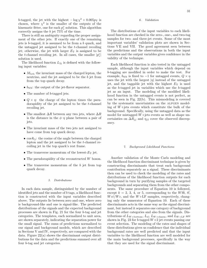
31

b-tagged, the jet with the highest − logχ2 + 0.005pT ischosen, where χ2 is the smaller of the outputs of thekinematic fitter, one for each pνz solution. This algorithmcorrectly assigns the b jet 75% of the time.There is still an ambiguity regarding the proper assign-

ment of the other jets. If exactly one of the remainingjets is b-tagged, it is assumed to be from a b quark, andthe untagged jet assigned to be the t-channel recoilingjet; otherwise, the jet with larger ET is assigned to bethe t-channel recoiling jet. In all cases, the smaller |pνz |solution is used.The likelihood function L3j is defined with the follow-

ing input variables:

• Mℓνb, the invariant mass of the charged lepton, theneutrino, and the jet assigned to be the b jet fromfrom the top quark decay.

• bNN: the output of the jet-flavor separator.

• The number of b-tagged jets.

• Q × η: the charge of the lepton times the pseu-dorapidity of the jet assigned to be the t-channelrecoiling jet.

• The smallest ∆R between any two jets, where ∆Ris the distance in the φ–η plane between a pair ofjets.

• The invariant mass of the two jets not assigned tohave come from top quark decay.

• cos θℓj: the cosine of the angle between the chargedlepton and the jet assigned to be the t-channel re-coiling jet in the top quark’s rest frame.

• The transverse momentum of the lowest-ET jet.

• The pseudorapidity of the reconstructed W boson.

• The transverse momentum of the b jet from topquark decay.

5. Distributions

In each data sample, distinguished by the number ofidentified jets and the number of b tags, a likelihood func-tion is constructed with the input variables describedabove. The outputs lie between zero and one, where zerois background-like and one is signal-like. The predicteddistributions of the signals and the expected backgroundprocesses are shown in Fig. 21 for the four b-tag and jetcategories. The templates, each normalized to unit area,are shown separately, indicating the separation power forthe small signal. The sums of predictions normalized toour signal and background models, which are describedin Sections V and IV, respectively, are compared with thedata. Figure 22(a) shows the discriminant output distri-butions for the data and the predictions summed over allfour b-tag and jet categories.

6. Validation

The distributions of the input variables to each likeli-hood function are checked in the zero-, one-, and two-tagsamples for two- and three-jet events. Some of the mostimportant variables’ validation plots are shown in Sec-tions VE and VII. The good agreement seen betweenthe predictions and the observations in both the inputvariables and the output variables gives confidence in thevalidity of the technique.

Each likelihood function is also tested in the untaggedsample, although the input variables which depend onb-tagging are modified in order to make the test. Forexample, bNN is fixed to −1 for untagged events, Q × ηuses the jet with the largest |η| instead of the untaggedjet, and the taggable jet with the highest ET is usedas the b-tagged jet in variables which use the b-taggedjet as an input. The modeling of the modified likeli-hood function in the untagged events is not perfect, ascan be seen in Fig. 22(b). This mismodeling is coveredby the systematic uncertainties on the alpgen model-ing of W+jets events which constitute the bulk of thebackground. Specifically, using the untagged data as themodel for mistagged W+jets events as well as shape un-certainties on ∆Rjj and ηj2 cover the observed discrep-ancy.

7. Background Likelihood Functions

Another validation of the Monte Carlo modeling andthe likelihood function discriminant technique is given byconstructing discriminants that treat each backgroundcontribution separately as a signal. These discriminantsthen can be used to check the modeling of the rates anddistributions of the likelihood function outputs for eachbackground in turn by purifying samples of the targetedbackgrounds and separating them from the other compo-nents. The same procedure of Equation 10 is followed,except k = 2, 3, 4, or 5, corresponding to the Wbb, tt,Wcc/Wc, and the W+LF samples, respectively, chang-ing only the numerator of Equation 10. Each of thesediscriminants acts in the same way as the signal discrimi-nant, but instead it separates one category of backgroundfrom the other categories and also from the signals. Dis-tributions of LW+bottom, Ltt, LW+charm, and LW+LF areshown in Fig. 23 for b-taggedW+2 jet events passing ourevent selection. The modeling of the rates and shapes ofthese distributions gives us confidence that the individualbackground rates are well predicted and that the inputvariables to the likelihood function are well modeled forthe main background processes, specifically in the waythat they are used for the signal discriminant.

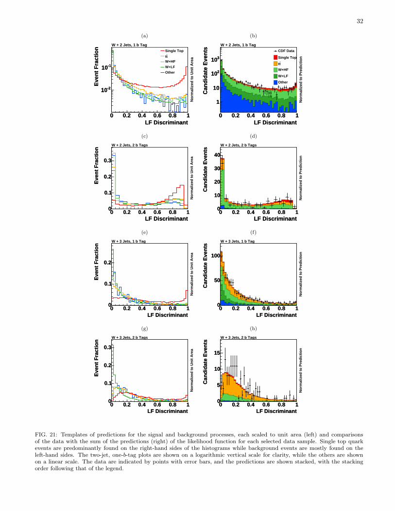
32

(a)

LF Discriminant0 0.2 0.4 0.6 0.8 1

Eve

nt

Fra

ctio

n

-210

-110

LF Discriminant0 0.2 0.4 0.6 0.8 1

Eve

nt

Fra

ctio

n

-210

-110

W + 2 Jets, 1 b Tag

No

rmal

ized

to

Un

it A

rea

Single Top

ttW+HF

W+LF

Other

(b)

LF Discriminant0 0.2 0.4 0.6 0.8 1

Can

did

ate

Eve

nts

1

10

210

310

LF Discriminant0 0.2 0.4 0.6 0.8 1

Can

did

ate

Eve

nts

1

10

210

310

W + 2 Jets, 1 b Tag

No

rmal

ized

to

Pre

dic

tio

n

CDF Data

Single Top

tt

W+HF

W+LF

Other

(c)

LF Discriminant0 0.2 0.4 0.6 0.8 1

Eve

nt

Fra

ctio

n

0

0.1

0.2

0.3

LF Discriminant0 0.2 0.4 0.6 0.8 1

Eve

nt

Fra

ctio

n

0

0.1

0.2

0.3

W + 2 Jets, 2 b Tags

No

rmal

ized

to

Un

it A

rea

(d)

LF Discriminant0 0.2 0.4 0.6 0.8 1

Can

did

ate

Eve

nts

0

10

20

30

40

LF Discriminant0 0.2 0.4 0.6 0.8 1

Can

did

ate

Eve

nts

0

10

20

30

40

W + 2 Jets, 2 b Tags

No

rmal

ized

to

Pre

dic

tio

n

(e)

LF Discriminant0 0.2 0.4 0.6 0.8 1

Eve

nt

Fra

ctio

n

0

0.1

0.2

LF Discriminant0 0.2 0.4 0.6 0.8 1

Eve

nt

Fra

ctio

n

0

0.1

0.2

W + 3 Jets, 1 b Tag

No

rmal

ized

to

Un

it A

rea

(f)

LF Discriminant0 0.2 0.4 0.6 0.8 1

Can

did

ate

Eve

nts

0

50

100

LF Discriminant0 0.2 0.4 0.6 0.8 1

Can

did

ate

Eve

nts

0

50

100

W + 3 Jets, 1 b Tag

No

rmal

ized

to

Pre

dic

tio

n

(g)

LF Discriminant0 0.2 0.4 0.6 0.8 1

Eve

nt

Fra

ctio

n

0

0.1

0.2

0.3

LF Discriminant0 0.2 0.4 0.6 0.8 1

Eve

nt

Fra

ctio

n

0

0.1

0.2

0.3

W + 3 Jets, 2 b Tags

No

rmal

ized

to

Un

it A

rea

(h)

LF Discriminant0 0.2 0.4 0.6 0.8 1

Can

did

ate

Eve

nts

0

5

10

15

LF Discriminant0 0.2 0.4 0.6 0.8 1

Can

did

ate

Eve

nts

0

5

10

15

W + 3 Jets, 2 b Tags

No

rmal

ized

to

Pre

dic

tio

n

FIG. 21: Templates of predictions for the signal and background processes, each scaled to unit area (left) and comparisonsof the data with the sum of the predictions (right) of the likelihood function for each selected data sample. Single top quarkevents are predominantly found on the right-hand sides of the histograms while background events are mostly found on theleft-hand sides. The two-jet, one-b-tag plots are shown on a logarithmic vertical scale for clarity, while the others are shownon a linear scale. The data are indicated by points with error bars, and the predictions are shown stacked, with the stackingorder following that of the legend.

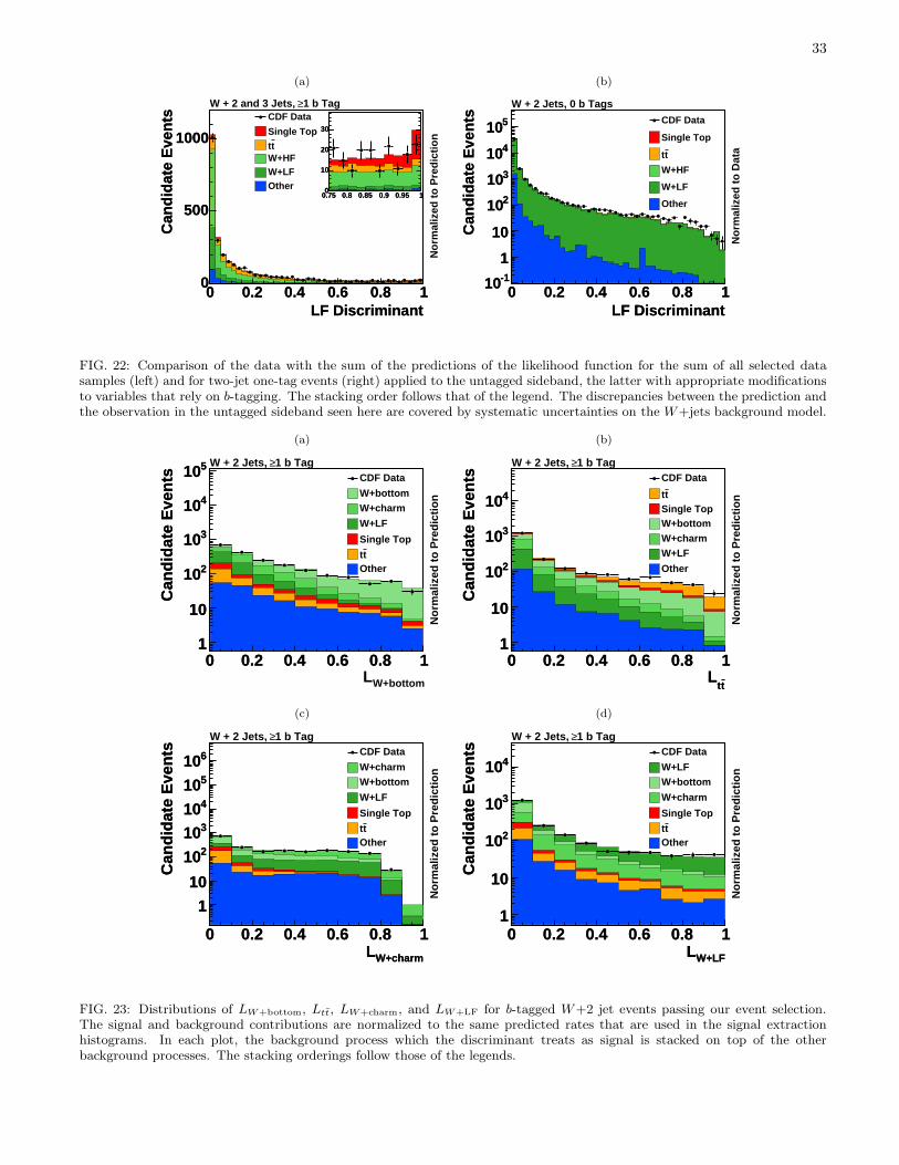
33

(a)

LF Discriminant0 0.2 0.4 0.6 0.8 1

Can

did

ate

Eve

nts

0

500

1000

LF Discriminant0 0.2 0.4 0.6 0.8 1

Can

did

ate

Eve

nts

0

500

1000

1 b Tag≥W + 2 and 3 Jets,

No

rmal

ized

to

Pre

dic

tio

n

CDF Data

Single Top

ttW+HFW+LFOther

0.75 0.8 0.85 0.9 0.95 10

10

20

30

0.75 0.8 0.85 0.9 0.95 10

10

20

30

(b)

LF Discriminant0 0.2 0.4 0.6 0.8 1

Can

did

ate

Eve

nts

-110

1

10

210

310

410

510

LF Discriminant0 0.2 0.4 0.6 0.8 1

Can

did

ate

Eve

nts

-110

1

10

210

310

410

510

W + 2 Jets, 0 b Tags

No

rmal

ized

to

Dat

a

CDF Data

Single Top

tt

W+HF

W+LF

Other

FIG. 22: Comparison of the data with the sum of the predictions of the likelihood function for the sum of all selected datasamples (left) and for two-jet one-tag events (right) applied to the untagged sideband, the latter with appropriate modificationsto variables that rely on b-tagging. The stacking order follows that of the legend. The discrepancies between the prediction andthe observation in the untagged sideband seen here are covered by systematic uncertainties on the W+jets background model.

(a)

W+bottomL0 0.2 0.4 0.6 0.8 1

Can

did

ate

Eve

nts

1

10

210

310

410

510

0 0.2 0.4 0.6 0.8 1

Can

did

ate

Eve

nts

1

10

210

310

410

5101 b Tag≥W + 2 Jets,

No

rmal

ized

to

Pre

dic

tio

n

CDF Data

W+bottomW+charm

W+LF

Single Top

ttOther

(b)

ttL

0 0.2 0.4 0.6 0.8 1

Can

did

ate

Eve

nts

1

10

210

310

410

ttL

0 0.2 0.4 0.6 0.8 1

Can

did

ate

Eve

nts

1

10

210

310

410

1 b Tag≥W + 2 Jets,

No

rmal

ized

to

Pre

dic

tio

n

CDF Data

ttSingle TopW+bottomW+charmW+LF

Other

(c)

W+charmL0 0.2 0.4 0.6 0.8 1

Can

did

ate

Eve

nts

1

10

210

310

410

510

610

W+charmL0 0.2 0.4 0.6 0.8 1

Can

did

ate

Eve

nts

1

10

210

310

410

510

610

1 b Tag≥W + 2 Jets,

No

rmal

ized

to

Pre

dic

tio

n

CDF Data

W+charmW+bottom

W+LF

Single Top

ttOther

(d)

W+LFL0 0.2 0.4 0.6 0.8 1

Can

did

ate

Eve

nts

1

10

210

310

410

W+LFL0 0.2 0.4 0.6 0.8 1

Can

did

ate

Eve

nts

1

10

210

310

410

1 b Tag≥W + 2 Jets, N

orm

aliz

ed t

o P

red

icti

on

CDF Data

W+LFW+bottom

W+charm

Single Top

ttOther

FIG. 23: Distributions of LW+bottom, Ltt, LW+charm, and LW+LF for b-tagged W+2 jet events passing our event selection.The signal and background contributions are normalized to the same predicted rates that are used in the signal extractionhistograms. In each plot, the background process which the discriminant treats as signal is stacked on top of the otherbackground processes. The stacking orderings follow those of the legends.

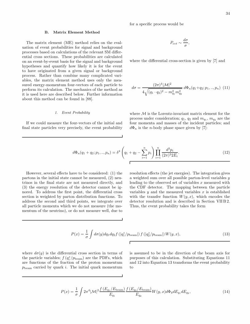
34

B. Matrix Element Method

The matrix element (ME) method relies on the eval-uation of event probabilities for signal and backgroundprocesses based on calculations of the relevant SM differ-ential cross sections. These probabilities are calculatedon an event-by-event basis for the signal and backgroundhypotheses and quantify how likely it is for the eventto have originated from a given signal or backgroundprocess. Rather than combine many complicated vari-ables, the matrix element method uses only the mea-sured energy-momentum four-vectors of each particle toperform its calculation. The mechanics of the method asit is used here are described below. Further informationabout this method can be found in [88].

1. Event Probability

If we could measure the four-vectors of the initial andfinal state particles very precisely, the event probability

for a specific process would be

Pevt ∼dσ

σ,

where the differential cross-section is given by [7] and

dσ =(2π)4|M|2

4√

(q1 · q2)2 −m2q1m

2q2

dΦn(q1+q2; p1, .., pn) (11)

where M is the Lorentz-invariant matrix element for theprocess under consideration; q1, q2 and mq1 , mq2 are thefour momenta and masses of the incident particles; anddΦn is the n-body phase space given by [7]:

dΦn(q1 + q2; p1, .., pn) = δ4

(

q1 + q2 −n∑

i=1

pi

)

n∏

i=1

d3pi(2π)32Ei

. (12)

However, several effects have to be considered: (1) thepartons in the initial state cannot be measured, (2) neu-trinos in the final state are not measured directly, and(3) the energy resolution of the detector cannot be ig-nored. To address the first point, the differential crosssection is weighted by parton distribution functions. Toaddress the second and third points, we integrate overall particle momenta which we do not measure (the mo-mentum of the neutrino), or do not measure well, due to

resolution effects (the jet energies). The integration givesa weighted sum over all possible parton-level variables yleading to the observed set of variables x measured withthe CDF detector. The mapping between the particlevariables y and the measured variables x is establishedwith the transfer function W (y, x), which encodes thedetector resolution and is described in Section VIIB 2.Thus, the event probability takes the form

P (x) =1

σ

∫

dσ(y)dq1dq2f (|qz1/pbeam|) f (|qz2/pbeam|)W (y, x), (13)

where dσ(y) is the differential cross section in terms ofthe particle variables; f (qzi /pbeam) are the PDFs, whichare functions of the fraction of the proton momentumpbeam carried by quark i. The initial quark momentum

is assumed to be in the direction of the beam axis forpurposes of this calculation. Substituting Equations 11and 12 into Equation 13 transforms the event probabilityto

P (x) =1

σ

∫

2π4|M|2 f (Eq1/Ebeam)

Eq1

f (Eq2/Ebeam)

Eq2

W (y, x)dΦ4dEq1dEq2 , (14)

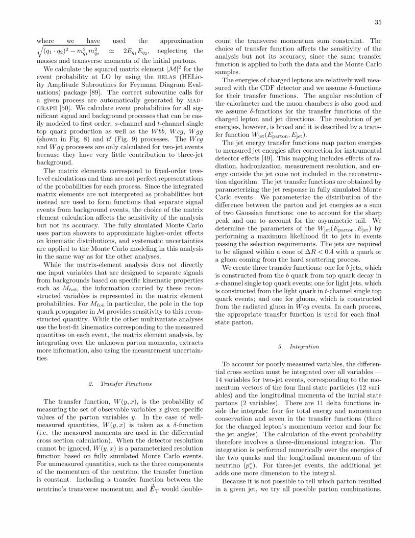
35

where we have used the approximation√

(q1 · q2)2 −m2q1m

2q2 ≃ 2Eq1Eq2 , neglecting the

masses and transverse momenta of the initial partons.We calculate the squared matrix element |M|2 for the

event probability at LO by using the helas (HELic-ity Amplitude Subroutines for Feynman Diagram Eval-uations) package [89]. The correct subroutine calls fora given process are automatically generated by mad-

graph [50]. We calculate event probabilities for all sig-nificant signal and background processes that can be eas-ily modeled to first order: s-channel and t-channel singletop quark production as well as the Wbb, Wcg, Wgg(shown in Fig. 8) and tt (Fig. 9) processes. The Wcgand Wgg processes are only calculated for two-jet eventsbecause they have very little contribution to three-jetbackground.The matrix elements correspond to fixed-order tree-

level calculations and thus are not perfect representationsof the probabilities for each process. Since the integratedmatrix elements are not interpreted as probabilities butinstead are used to form functions that separate signalevents from background events, the choice of the matrixelement calculation affects the sensitivity of the analysisbut not its accuracy. The fully simulated Monte Carlouses parton showers to approximate higher-order effectson kinematic distributions, and systematic uncertaintiesare applied to the Monte Carlo modeling in this analysisin the same way as for the other analyses.While the matrix-element analysis does not directly

use input variables that are designed to separate signalsfrom backgrounds based on specific kinematic propertiessuch as Mℓνb, the information carried by these recon-structed variables is represented in the matrix elementprobabilities. For Mℓνb in particular, the pole in the topquark propagator in M provides sensitivity to this recon-structed quantity. While the other multivariate analysesuse the best-fit kinematics corresponding to the measuredquantities on each event, the matrix element analysis, byintegrating over the unknown parton momenta, extractsmore information, also using the measurement uncertain-ties.

2. Transfer Functions

The transfer function, W (y, x), is the probability ofmeasuring the set of observable variables x given specificvalues of the parton variables y. In the case of well-measured quantities, W (y, x) is taken as a δ-function(i.e. the measured momenta are used in the differentialcross section calculation). When the detector resolutioncannot be ignored, W (y, x) is a parameterized resolutionfunction based on fully simulated Monte Carlo events.For unmeasured quantities, such as the three componentsof the momentum of the neutrino, the transfer functionis constant. Including a transfer function between the

neutrino’s transverse momentum and ~/ET would double-

count the transverse momentum sum constraint. Thechoice of transfer function affects the sensitivity of theanalysis but not its accuracy, since the same transferfunction is applied to both the data and the Monte Carlosamples.The energies of charged leptons are relatively well mea-

sured with the CDF detector and we assume δ-functionsfor their transfer functions. The angular resolution ofthe calorimeter and the muon chambers is also good andwe assume δ-functions for the transfer functions of thecharged lepton and jet directions. The resolution of jetenergies, however, is broad and it is described by a trans-fer function Wjet(Eparton, Ejet).The jet energy transfer functions map parton energies

to measured jet energies after correction for instrumentaldetector effects [49]. This mapping includes effects of ra-diation, hadronization, measurement resolution, and en-ergy outside the jet cone not included in the reconstruc-tion algorithm. The jet transfer functions are obtained byparameterizing the jet response in fully simulated MonteCarlo events. We parameterize the distribution of thedifference between the parton and jet energies as a sumof two Gaussian functions: one to account for the sharppeak and one to account for the asymmetric tail. Wedetermine the parameters of the Wjet(Eparton, Ejet) byperforming a maximum likelihood fit to jets in eventspassing the selection requirements. The jets are requiredto be aligned within a cone of ∆R < 0.4 with a quark ora gluon coming from the hard scattering process.We create three transfer functions: one for b jets, which

is constructed from the b quark from top quark decay ins-channel single top quark events; one for light jets, whichis constructed from the light quark in t-channel single topquark events; and one for gluons, which is constructedfrom the radiated gluon in Wcg events. In each process,the appropriate transfer function is used for each final-state parton.

3. Integration

To account for poorly measured variables, the differen-tial cross section must be integrated over all variables —14 variables for two-jet events, corresponding to the mo-mentum vectors of the four final-state particles (12 vari-ables) and the longitudinal momenta of the initial statepartons (2 variables). There are 11 delta functions in-side the integrals: four for total energy and momentumconservation and seven in the transfer functions (threefor the charged lepton’s momentum vector and four forthe jet angles). The calculation of the event probabilitytherefore involves a three-dimensional integration. Theintegration is performed numerically over the energies ofthe two quarks and the longitudinal momentum of theneutrino (pνz ). For three-jet events, the additional jetadds one more dimension to the integral.Because it is not possible to tell which parton resulted

in a given jet, we try all possible parton combinations,

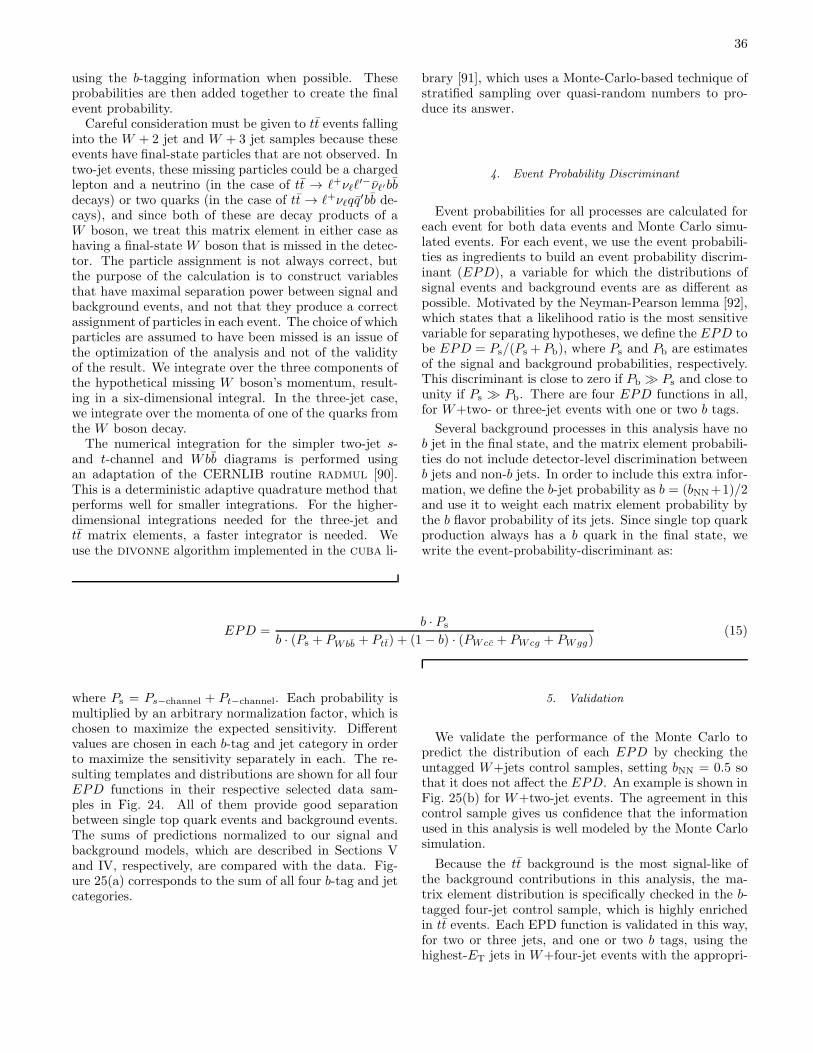
36

using the b-tagging information when possible. Theseprobabilities are then added together to create the finalevent probability.Careful consideration must be given to tt events falling

into the W + 2 jet and W + 3 jet samples because theseevents have final-state particles that are not observed. Intwo-jet events, these missing particles could be a chargedlepton and a neutrino (in the case of tt → ℓ+νℓℓ

′−νℓ′bbdecays) or two quarks (in the case of tt → ℓ+νℓqq

′bb de-cays), and since both of these are decay products of aW boson, we treat this matrix element in either case ashaving a final-state W boson that is missed in the detec-tor. The particle assignment is not always correct, butthe purpose of the calculation is to construct variablesthat have maximal separation power between signal andbackground events, and not that they produce a correctassignment of particles in each event. The choice of whichparticles are assumed to have been missed is an issue ofthe optimization of the analysis and not of the validityof the result. We integrate over the three components ofthe hypothetical missing W boson’s momentum, result-ing in a six-dimensional integral. In the three-jet case,we integrate over the momenta of one of the quarks fromthe W boson decay.The numerical integration for the simpler two-jet s-

and t-channel and Wbb diagrams is performed usingan adaptation of the CERNLIB routine radmul [90].This is a deterministic adaptive quadrature method thatperforms well for smaller integrations. For the higher-dimensional integrations needed for the three-jet andtt matrix elements, a faster integrator is needed. Weuse the divonne algorithm implemented in the cuba li-

brary [91], which uses a Monte-Carlo-based technique ofstratified sampling over quasi-random numbers to pro-duce its answer.

4. Event Probability Discriminant

Event probabilities for all processes are calculated foreach event for both data events and Monte Carlo simu-lated events. For each event, we use the event probabili-ties as ingredients to build an event probability discrim-inant (EPD), a variable for which the distributions ofsignal events and background events are as different aspossible. Motivated by the Neyman-Pearson lemma [92],which states that a likelihood ratio is the most sensitivevariable for separating hypotheses, we define the EPD tobe EPD = Ps/(Ps + Pb), where Ps and Pb are estimatesof the signal and background probabilities, respectively.This discriminant is close to zero if Pb ≫ Ps and close tounity if Ps ≫ Pb. There are four EPD functions in all,for W+two- or three-jet events with one or two b tags.

Several background processes in this analysis have nob jet in the final state, and the matrix element probabili-ties do not include detector-level discrimination betweenb jets and non-b jets. In order to include this extra infor-mation, we define the b-jet probability as b = (bNN+1)/2and use it to weight each matrix element probability bythe b flavor probability of its jets. Since single top quarkproduction always has a b quark in the final state, wewrite the event-probability-discriminant as:

EPD =b · Ps

b · (Ps + PWbb + Ptt) + (1− b) · (PWcc + PWcg + PWgg)(15)

where Ps = Ps−channel + Pt−channel. Each probability ismultiplied by an arbitrary normalization factor, which ischosen to maximize the expected sensitivity. Differentvalues are chosen in each b-tag and jet category in orderto maximize the sensitivity separately in each. The re-sulting templates and distributions are shown for all fourEPD functions in their respective selected data sam-ples in Fig. 24. All of them provide good separationbetween single top quark events and background events.The sums of predictions normalized to our signal andbackground models, which are described in Sections Vand IV, respectively, are compared with the data. Fig-ure 25(a) corresponds to the sum of all four b-tag and jetcategories.

5. Validation

We validate the performance of the Monte Carlo topredict the distribution of each EPD by checking theuntagged W+jets control samples, setting bNN = 0.5 sothat it does not affect the EPD. An example is shown inFig. 25(b) for W+two-jet events. The agreement in thiscontrol sample gives us confidence that the informationused in this analysis is well modeled by the Monte Carlosimulation.

Because the tt background is the most signal-like ofthe background contributions in this analysis, the ma-trix element distribution is specifically checked in the b-tagged four-jet control sample, which is highly enrichedin tt events. Each EPD function is validated in this way,for two or three jets, and one or two b tags, using thehighest-ET jets in W+four-jet events with the appropri-

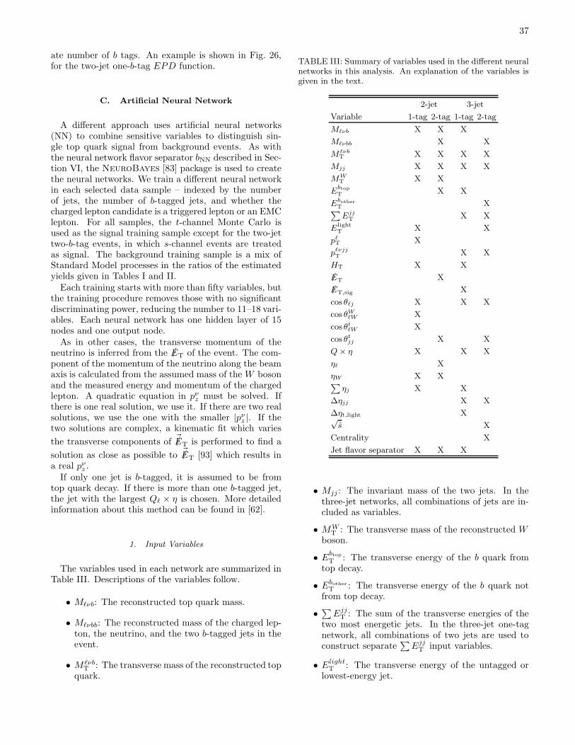
37

ate number of b tags. An example is shown in Fig. 26,for the two-jet one-b-tag EPD function.

C. Artificial Neural Network

A different approach uses artificial neural networks(NN) to combine sensitive variables to distinguish sin-gle top quark signal from background events. As withthe neural network flavor separator bNN described in Sec-tion VI, the NeuroBayes [83] package is used to createthe neural networks. We train a different neural networkin each selected data sample – indexed by the numberof jets, the number of b-tagged jets, and whether thecharged lepton candidate is a triggered lepton or an EMClepton. For all samples, the t-channel Monte Carlo isused as the signal training sample except for the two-jettwo-b-tag events, in which s-channel events are treatedas signal. The background training sample is a mix ofStandard Model processes in the ratios of the estimatedyields given in Tables I and II.Each training starts with more than fifty variables, but

the training procedure removes those with no significantdiscriminating power, reducing the number to 11–18 vari-ables. Each neural network has one hidden layer of 15nodes and one output node.As in other cases, the transverse momentum of the

neutrino is inferred from the /ET of the event. The com-ponent of the momentum of the neutrino along the beamaxis is calculated from the assumed mass of the W bosonand the measured energy and momentum of the chargedlepton. A quadratic equation in pνz must be solved. Ifthere is one real solution, we use it. If there are two realsolutions, we use the one with the smaller |pνz |. If thetwo solutions are complex, a kinematic fit which varies

the transverse components of ~/ET is performed to find a

solution as close as possible to ~/ET [93] which results ina real pνz .If only one jet is b-tagged, it is assumed to be from

top quark decay. If there is more than one b-tagged jet,the jet with the largest Qℓ × η is chosen. More detailedinformation about this method can be found in [62].

1. Input Variables

The variables used in each network are summarized inTable III. Descriptions of the variables follow.

• Mℓνb: The reconstructed top quark mass.

• Mℓνbb: The reconstructed mass of the charged lep-ton, the neutrino, and the two b-tagged jets in theevent.

• M ℓνbT : The transverse mass of the reconstructed top

quark.

TABLE III: Summary of variables used in the different neuralnetworks in this analysis. An explanation of the variables isgiven in the text.

2-jet 3-jet

Variable 1-tag 2-tag 1-tag 2-tag

Mℓνb X X X

Mℓνbb X X

M ℓνbT X X X X

Mjj X X X X

MWT X X

EbtopT X X

EbotherT X∑

Ejj

T X X

Elight

T X X

pℓT X

pℓνjjT X X

HT X X

/ET X

/ET,sig X

cos θℓj X X X

cos θWℓW X

cos θtℓW X

cos θtjj X X

Q× η X X X

ηℓ X

ηW X X∑

ηj X X

∆ηjj X X

∆ηt,light X√s X

Centrality X

Jet flavor separator X X X

• Mjj : The invariant mass of the two jets. In thethree-jet networks, all combinations of jets are in-cluded as variables.

• MWT : The transverse mass of the reconstructed W

boson.

• EbtopT : The transverse energy of the b quark from

top decay.

• EbotherT : The transverse energy of the b quark not

from top decay.

• ∑EjjT : The sum of the transverse energies of the

two most energetic jets. In the three-jet one-tagnetwork, all combinations of two jets are used toconstruct separate

∑

EjjT input variables.

• ElightT : The transverse energy of the untagged or

lowest-energy jet.

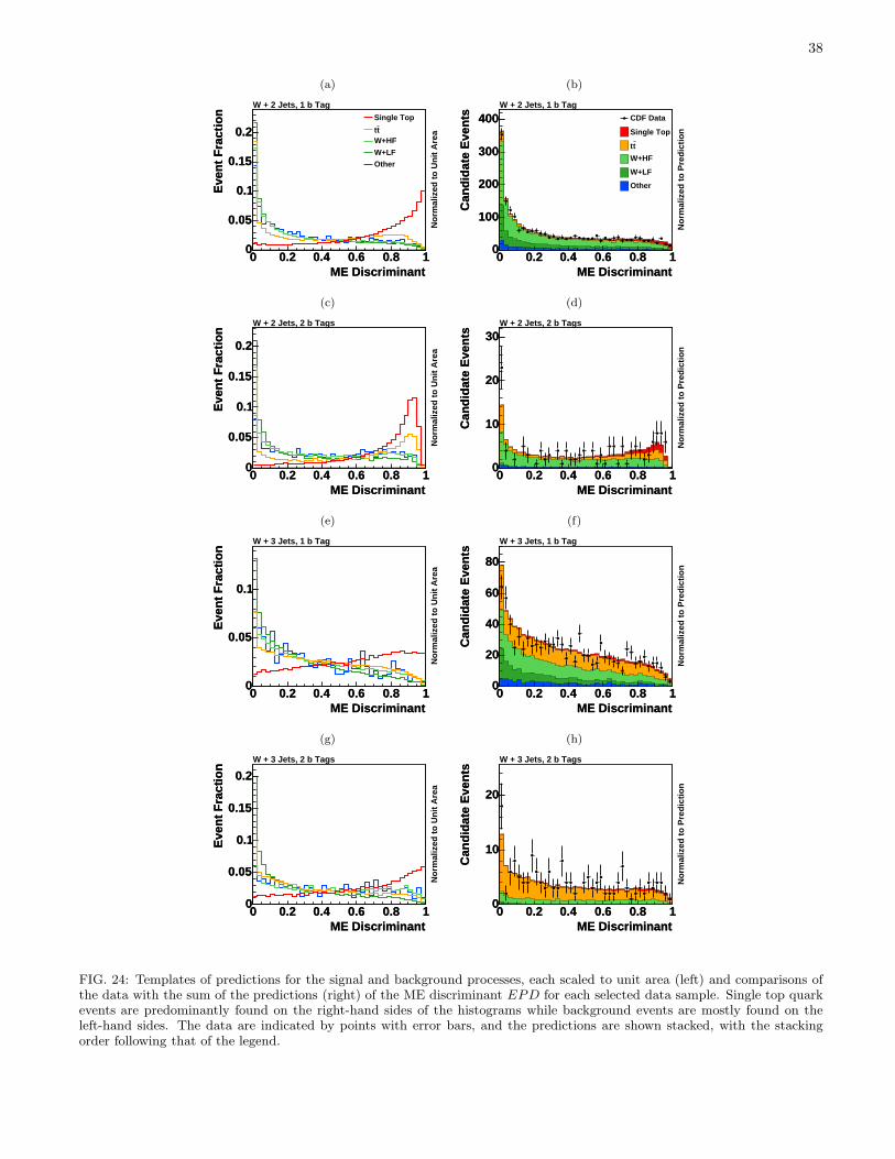
38

(a)

ME Discriminant0 0.2 0.4 0.6 0.8 1

Eve

nt

Fra

ctio

n

0

0.05

0.1

0.15

0.2

ME Discriminant0 0.2 0.4 0.6 0.8 1

Eve

nt

Fra

ctio

n

0

0.05

0.1

0.15

0.2

W + 2 Jets, 1 b Tag

No

rmal

ized

to

Un

it A

rea

Single Top

ttW+HF

W+LF

Other

(b)

ME Discriminant0 0.2 0.4 0.6 0.8 1

Can

did

ate

Eve

nts

0

100

200

300

400

ME Discriminant0 0.2 0.4 0.6 0.8 1

Can

did

ate

Eve

nts

0

100

200

300

400W + 2 Jets, 1 b Tag

No

rmal

ized

to

Pre

dic

tio

n

CDF Data

Single Top

tt

W+HF

W+LF

Other

(c)

ME Discriminant0 0.2 0.4 0.6 0.8 1

Eve

nt

Fra

ctio

n

0

0.05

0.1

0.15

0.2

ME Discriminant0 0.2 0.4 0.6 0.8 1

Eve

nt

Fra

ctio

n

0

0.05

0.1

0.15

0.2

W + 2 Jets, 2 b Tags

No

rmal

ized

to

Un

it A

rea

(d)

ME Discriminant0 0.2 0.4 0.6 0.8 1

Can

did

ate

Eve

nts

0

10

20

30

ME Discriminant0 0.2 0.4 0.6 0.8 1

Can

did

ate

Eve

nts

0

10

20

30W + 2 Jets, 2 b Tags

No

rmal

ized

to

Pre

dic

tio

n

(e)

ME Discriminant0 0.2 0.4 0.6 0.8 1

Eve

nt

Fra

ctio

n

0

0.05

0.1

ME Discriminant0 0.2 0.4 0.6 0.8 1

Eve

nt

Fra

ctio

n

0

0.05

0.1

W + 3 Jets, 1 b Tag

No

rmal

ized

to

Un

it A

rea

(f)

ME Discriminant0 0.2 0.4 0.6 0.8 1

Can

did

ate

Eve

nts

0

20

40

60

80

ME Discriminant0 0.2 0.4 0.6 0.8 1

Can

did

ate

Eve

nts

0

20

40

60

80

W + 3 Jets, 1 b Tag

No

rmal

ized

to

Pre

dic

tio

n

(g)

ME Discriminant0 0.2 0.4 0.6 0.8 1

Eve

nt

Fra

ctio

n

0

0.05

0.1

0.15

0.2

ME Discriminant0 0.2 0.4 0.6 0.8 1

Eve

nt

Fra

ctio

n

0

0.05

0.1

0.15

0.2W + 3 Jets, 2 b Tags

No

rmal

ized

to

Un

it A

rea

(h)

ME Discriminant0 0.2 0.4 0.6 0.8 1

Can

did

ate

Eve

nts

0

10

20

ME Discriminant0 0.2 0.4 0.6 0.8 1

Can

did

ate

Eve

nts

0

10

20

W + 3 Jets, 2 b Tags

No

rmal

ized

to

Pre

dic

tio

n

FIG. 24: Templates of predictions for the signal and background processes, each scaled to unit area (left) and comparisons ofthe data with the sum of the predictions (right) of the ME discriminant EPD for each selected data sample. Single top quarkevents are predominantly found on the right-hand sides of the histograms while background events are mostly found on theleft-hand sides. The data are indicated by points with error bars, and the predictions are shown stacked, with the stackingorder following that of the legend.

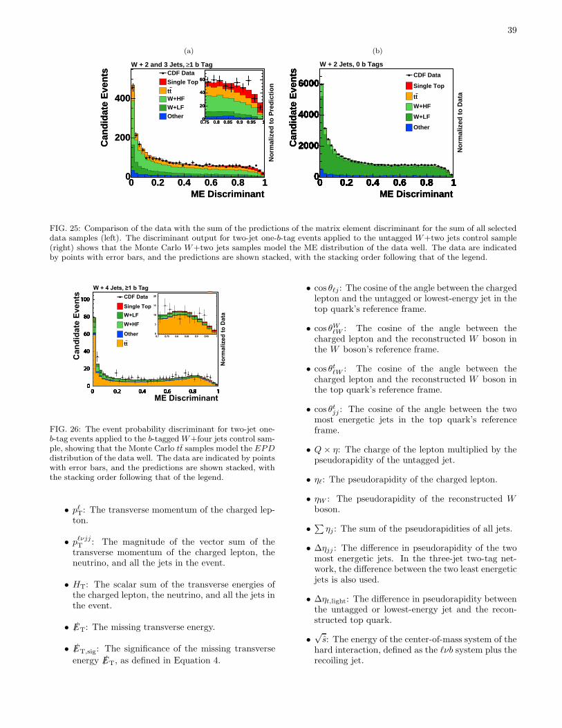
39

(a)

ME Discriminant0 0.2 0.4 0.6 0.8 1

Can

did

ate

Eve

nts

0

200

400

ME Discriminant0 0.2 0.4 0.6 0.8 1

Can

did

ate

Eve

nts

0

200

400

1 b Tag≥W + 2 and 3 Jets,

No

rmal

ized

to

Pre

dic

tio

n

CDF Data

Single Top

ttW+HFW+LFOther

0.75 0.8 0.85 0.9 0.95 10

20

40

60

0.75 0.8 0.85 0.9 0.95 10

20

40

60

(b)

ME Discriminant0 0.2 0.4 0.6 0.8 1

Can

did

ate

Eve

nts

0

2000

4000

6000

0 0.2 0.4 0.6 0.8 10

2000

4000

6000

0 0.2 0.4 0.6 0.8 10

2000

4000

6000

0 0.2 0.4 0.6 0.8 10

2000

4000

6000

0 0.2 0.4 0.6 0.8 10

2000

4000

6000

0 0.2 0.4 0.6 0.8 10

2000

4000

6000

ME Discriminant0 0.2 0.4 0.6 0.8 1

Can

did

ate

Eve

nts

0

2000

4000

6000

ME Discriminant0 0.2 0.4 0.6 0.8 1

Can

did

ate

Eve

nts

0

2000

4000

6000

0 0.2 0.4 0.6 0.8 10

2000

4000

6000CDF Data

Single Top

tt

W+HF

W+LF

Other

W + 2 Jets, 0 b Tags

No

rmal

ized

to

Dat

a

FIG. 25: Comparison of the data with the sum of the predictions of the matrix element discriminant for the sum of all selecteddata samples (left). The discriminant output for two-jet one-b-tag events applied to the untagged W+two jets control sample(right) shows that the Monte Carlo W+two jets samples model the ME distribution of the data well. The data are indicatedby points with error bars, and the predictions are shown stacked, with the stacking order following that of the legend.

tt

ME Discriminant0 0.2 0.4 0.6 0.8 1

Can

did

ate

Even

ts

0

20

40

60

80

100

0 0.2 0.4 0.6 0.8 1

0

20

40

60

80

100

0 0.2 0.4 0.6 0.8 1

0

20

40

60

80

100

0 0.2 0.4 0.6 0.8 1

0

20

40

60

80

100

0 0.2 0.4 0.6 0.8 1

0

20

40

60

80

100

0 0.2 0.4 0.6 0.8 1

0

20

40

60

80

100

0 0.2 0.4 0.6 0.8 1

0

20

40

60

80

100

0 0.2 0.4 0.6 0.8 1

0

20

40

60

80

100

0 0.2 0.4 0.6 0.8 1

0

20

40

60

80

100

0 0.2 0.4 0.6 0.8 1

0

20

40

60

80

100

0 0.2 0.4 0.6 0.8 1

40

60

80

100

0 0.2 0.4 0.6 0.8 1

0.7 0.75 0.8 0.85 0.9 0.95 1

0

5

10

15

20

0.7 0.75 0.8 0.85 0.9 0.95 1

0

5

10

15

20

≥1 b TagW + 4 Jets,

No

rma

lize

d t

o D

ata

CDF Data

Single Top

W+HF

W+LF

Other

FIG. 26: The event probability discriminant for two-jet one-b-tag events applied to the b-tagged W+four jets control sam-ple, showing that the Monte Carlo tt samples model the EPDdistribution of the data well. The data are indicated by pointswith error bars, and the predictions are shown stacked, withthe stacking order following that of the legend.

• pℓT: The transverse momentum of the charged lep-ton.

• pℓνjjT : The magnitude of the vector sum of thetransverse momentum of the charged lepton, theneutrino, and all the jets in the event.

• HT: The scalar sum of the transverse energies ofthe charged lepton, the neutrino, and all the jets inthe event.

• /ET: The missing transverse energy.

• /ET,sig: The significance of the missing transverse

energy /ET, as defined in Equation 4.

• cos θℓj : The cosine of the angle between the chargedlepton and the untagged or lowest-energy jet in thetop quark’s reference frame.

• cos θWℓW : The cosine of the angle between thecharged lepton and the reconstructed W boson inthe W boson’s reference frame.

• cos θtℓW : The cosine of the angle between thecharged lepton and the reconstructed W boson inthe top quark’s reference frame.

• cos θtjj : The cosine of the angle between the twomost energetic jets in the top quark’s referenceframe.

• Q × η: The charge of the lepton multiplied by thepseudorapidity of the untagged jet.

• ηℓ: The pseudorapidity of the charged lepton.

• ηW : The pseudorapidity of the reconstructed Wboson.

• ∑ ηj : The sum of the pseudorapidities of all jets.

• ∆ηjj : The difference in pseudorapidity of the twomost energetic jets. In the three-jet two-tag net-work, the difference between the two least energeticjets is also used.

• ∆ηt,light: The difference in pseudorapidity betweenthe untagged or lowest-energy jet and the recon-structed top quark.

•√s: The energy of the center-of-mass system of the

hard interaction, defined as the ℓνb system plus therecoiling jet.

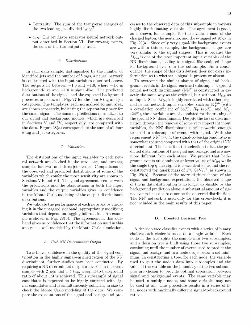
40

• Centrality: The sum of the transverse energies ofthe two leading jets divided by

√s.

• bNN: The jet flavor separator neural network out-put described in Section VI. For two-tag events,the sum of the two outputs is used.

2. Distributions

In each data sample, distinguished by the number ofidentified jets and the number of b tags, a neural networkis constructed with the input variables described above.The outputs lie between −1.0 and +1.0, where −1.0 isbackground-like and +1.0 is signal-like. The predicteddistributions of the signals and the expected backgroundprocesses are shown in Fig. 27 for the four b-tag and jetcategories. The templates, each normalized to unit area,are shown separately, indicating the separation power forthe small signal. The sums of predictions normalized toour signal and background models, which are describedin Sections V and IV, respectively, are compared withthe data. Figure 28(a) corresponds to the sum of all fourb-tag and jet categories.

3. Validation

The distributions of the input variables to each neu-ral network are checked in the zero, one, and two-tagsamples for two- and three-jet events. Comparisons ofthe observed and predicted distributions of some of thevariables which confer the most sensitivity are shown inSections VE and VII. The good agreement seen betweenthe predictions and the observations in both the inputvariables and the output variables gives us confidencein the Monte Carlo modeling of the output discriminantdistributions.We validate the performance of each network by check-

ing it in the untagged sideband, appropriately modifyingvariables that depend on tagging information. An exam-ple is shown in Fig. 28(b). The agreement in this side-band gives us confidence that the information used in thisanalysis is well modeled by the Monte Carlo simulation.

4. High NN Discriminant Output

To achieve confidence in the quality of the signal con-tribution in the highly signal-enriched region of the NNdiscriminant, further studies have been conducted. Byrequiring a NN discriminant output above 0.4 in the eventsample with 2 jets and 1 b tag, a signal-to-backgroundratio of about 1:3 is achieved. This subsample of signalcandidates is expected to be highly enriched with sig-nal candidates and is simultaneously sufficient in size tocheck the Monte Carlo modeling of the data. We com-pare the expectations of the signal and background pro-

cesses to the observed data of this subsample in varioushighly discriminating variables. The agreement is good,as is shown, for example, for the invariant mass of thecharged lepton, the neutrino, and the b-tagged jetMℓνb inFig. 29(a). Since only very signal-like background eventsare within this subsample, the background shapes arevery similar to the signal shapes. This is because theMℓνb is one of the most important input variables of theNN discriminant, leading to a signal-like sculpted shapefor background events in this subsample. As a conse-quence, the shape of this distribution does not carry in-formation as to whether a signal is present or absent.To overcome the similar shapes of signal and back-

ground events in the signal-enriched subsample, a specialneural network discriminant (NN′) is constructed in ex-actly the same way as the original, but without Mℓνb asan input. Since Mℓνb is highly correlated with other orig-inal neural network input variables, such as M ℓνb

T (witha correlation coefficient of 65%), HT (45%), and Mjj

(24%), these variables are also omitted for the training ofthe special NN′ discriminant. Despite the loss of discrimi-nation through the removal of some very important inputvariables, the NN′ discriminant is still powerful enoughto enrich a subsample of events with signal. With therequirement NN′ > 0.4, the signal-to-background ratio issomewhat reduced compared with that of the original NNdiscriminant. The benefit of this selection is that the pre-dicted distributions of the signal and background are nowmore different from each other. We predict that back-ground events are dominant at lower values ofMℓνb whilethe single top quark signal is concentrated around the re-constructed top quark mass of 175 GeV/c2, as shown inFig. 29(b). Because of the more distinct shapes of thesignal and background expectations, the observed shapeof the in data distribution is no longer explicable by thebackground prediction alone; a substantial amount of sig-nal events is needed to describe the observed distribution.The NN′ network is used only for this cross-check; it isnot included in the main results of this paper.

D. Boosted Decision Tree

A decision tree classifies events with a series of binarychoices; each choice is based on a single variable. Eachnode in the tree splits the sample into two subsamples,and a decision tree is built using those two subsamples,continuing until the number of events used to predict thesignal and background in a node drops below a set mini-mum. In constructing a tree, for each node, the variableused to split the node’s data into subsamples and thevalue of the variable on the boundary of the two subsam-ples are chosen to provide optimal separation betweensignal and background events. The same variable maybe used in multiple nodes, and some variables may notbe used at all. This procedure results in a series of fi-nal nodes with maximally different signal-to-backgroundratios.

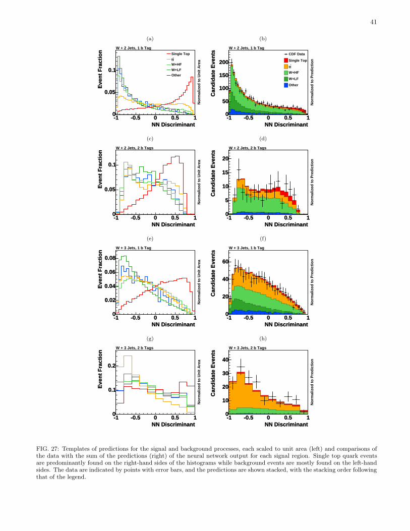
41

(a)

NN Discriminant-1 -0.5 0 0.5 1

Eve

nt

Fra

ctio

n

0

0.05

0.1

NN Discriminant-1 -0.5 0 0.5 1

Eve

nt

Fra

ctio

n

0

0.05

0.1

W + 2 Jets, 1 b Tag

No

rmal

ized

to

Un

it A

rea

Single Top

ttW+HF

W+LF

Other

(b)

NN Discriminant-1 -0.5 0 0.5 1

Can

did

ate

Eve

nts

0

50

100

150

200

NN Discriminant-1 -0.5 0 0.5 1

Can

did

ate

Eve

nts

0

50

100

150

200

W + 2 Jets, 1 b Tag

No

rmal

ized

to

Pre

dic

tio

n

CDF Data

Single Top

tt

W+HF

W+LF

Other

(c)

NN Discriminant-1 -0.5 0 0.5 1

Eve

nt

Fra

ctio

n

0

0.05

0.1

NN Discriminant-1 -0.5 0 0.5 1

Eve

nt

Fra

ctio

n

0

0.05

0.1

W + 2 Jets, 2 b Tags

No

rmal

ized

to

Un

it A

rea

(d)

NN Discriminant-1 -0.5 0 0.5 1

Can

did

ate

Eve

nts

0

5

10

15

20

NN Discriminant-1 -0.5 0 0.5 1

Can

did

ate

Eve

nts

0

5

10

15

20

W + 2 Jets, 2 b Tags

No

rmal

ized

to

Pre

dic

tio

n

(e)

NN Discriminant-1 -0.5 0 0.5 1

Eve

nt

Fra

ctio

n

0

0.02

0.04

0.06

0.08

NN Discriminant-1 -0.5 0 0.5 1

Eve

nt

Fra

ctio

n

0

0.02

0.04

0.06

0.08

W + 3 Jets, 1 b Tag

No

rmal

ized

to

Un

it A

rea

(f)

NN Discriminant-1 -0.5 0 0.5 1

Can

did

ate

Eve

nts

0

20

40

60

NN Discriminant-1 -0.5 0 0.5 1

Can

did

ate

Eve

nts

0

20

40

60

W + 3 Jets, 1 b Tag

No

rmal

ized

to

Pre

dic

tio

n

(g)

NN Discriminant-1 -0.5 0 0.5 1

Eve

nt

Fra

ctio

n

0

0.1

0.2

NN Discriminant-1 -0.5 0 0.5 1

Eve

nt

Fra

ctio

n

0

0.1

0.2

W + 3 Jets, 2 b Tags

No

rmal

ized

to

Un

it A

rea

(h)

NN Discriminant-1 -0.5 0 0.5 1

Can

did

ate

Eve

nts

0

10

20

30

40

NN Discriminant-1 -0.5 0 0.5 1

Can

did

ate

Eve

nts

0

10

20

30

40

W + 3 Jets, 2 b Tags

No

rmal

ized

to

Pre

dic

tio

n

FIG. 27: Templates of predictions for the signal and background processes, each scaled to unit area (left) and comparisons ofthe data with the sum of the predictions (right) of the neural network output for each signal region. Single top quark eventsare predominantly found on the right-hand sides of the histograms while background events are mostly found on the left-handsides. The data are indicated by points with error bars, and the predictions are shown stacked, with the stacking order followingthat of the legend.

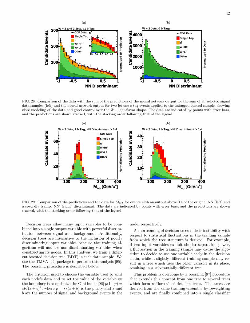
42

(a)

NN Discriminant-1 -0.5 0 0.5 1

Can

did

ate

Eve

nts

0

100

200

300

NN Discriminant-1 -0.5 0 0.5 1

Can

did

ate

Eve

nts

0

100

200

300 1 b Tag≥W + 2 and 3 Jets,

No

rmal

ized

to

Pre

dic

tio

n

CDF Data

Single Top

ttW+HFW+LFOther

0.5 0.6 0.7 0.8 0.9 10

20

40

60

0.5 0.6 0.7 0.8 0.9 10

20

40

60

(b)

NN Discriminant-1 -0.5 0 0.5 1

Can

did

ate

Eve

nts

0

1000

2000

3000

4000

NN Discriminant-1 -0.5 0 0.5 1

Can

did

ate

Eve

nts

0

1000

2000

3000

4000

W + 2 Jets, 0 b Tags

No

rmal

ized

to

Dat

a

CDF Data

Single Top

tt

W+HF

W+LF

Other

FIG. 28: Comparison of the data with the sum of the predictions of the neural network output for the sum of all selected signaldata samples (left) and the neural network output for two-jet one-b-tag events applied to the untagged control sample, showingclose modeling of the data and good control over the W+light-flavor shape. The data are indicated by points with error bars,and the predictions are shown stacked, with the stacking order following that of the legend.

(a)

]2 [GeV/cbνlM100 200 300 400

Can

did

ate

Eve

nts

0

20

40

60

]2 [GeV/cbνlM100 200 300 400

Can

did

ate

Eve

nts

0

20

40

60

W + 2 Jets, 1 b Tag, NN Discriminant > 0.4

No

rmal

ized

to

Pre

dic

tio

n

CDF Data

Single Top

tt

W+HF

W+LF

Other

(b)

]2 [GeV/cbνlM100 200 300 400

Can

did

ate

Eve

nts

0

10

20

30

40

100 200 300 400

Can

did

ate

Eve

nts

0

10

20

30

40

W + 2 Jets, 1 b Tag, NN’ Discriminant > 0.4

No

rmal

ized

to

Pre

dic

tio

nFIG. 29: Comparison of the predictions and the data for Mℓνb for events with an output above 0.4 of the original NN (left) anda specially trained NN′ (right) discriminant. The data are indicated by points with error bars, and the predictions are shownstacked, with the stacking order following that of the legend.

Decision trees allow many input variables to be com-bined into a single output variable with powerful discrim-ination between signal and background. Additionally,decision trees are insensitive to the inclusion of poorlydiscriminating input variables because the training al-gorithm will not use non-discriminating variables whenconstructing its nodes. In this analysis, we train a differ-ent boosted decision tree (BDT) in each data sample. Weuse the TMVA [94] package to perform this analysis [95].The boosting procedure is described below.

The criterion used to choose the variable used to spliteach node’s data and to set the value of the variable onthe boundary is to optimize the Gini index [96] p(1−p) =sb/(s+ b)2, where p = s/(s+ b) is the purity and s andb are the number of signal and background events in the

node, respectively.

A shortcoming of decision trees is their instability withrespect to statistical fluctuations in the training samplefrom which the tree structure is derived. For example,if two input variables exhibit similar separation power,a fluctuation in the training sample may cause the algo-rithm to decide to use one variable early in the decisionchain, while a slightly different training sample may re-sult in a tree which uses the other variable in its place,resulting in a substantially different tree.

This problem is overcome by a boosting [97] procedurethat extends this concept from one tree to several treeswhich form a “forest” of decision trees. The trees arederived from the same training ensemble by reweightingevents, and are finally combined into a single classifier

43

which is given by a weighted average of the individualdecision trees. Boosting stabilizes the response of the de-cision trees with respect to fluctuations in the trainingsample and is able to considerably enhance the perfor-mance with respect to a single tree.This analysis uses the adaboost [97] (adaptive boost)

algorithm, in which the events that were misclassified inone tree are multiplied by a common boost weight α inthe training of the next tree. The boost weight is derivedfrom the fraction of misclassified events, r, of the previoustree,

α =1− r

r. (16)

The resulting event classification yBDT(x) for theboosted tree is given by

yBDT(x) =∑

i∈forest

ln(αi) · hi(x), (17)

where the sum is over all trees in the forest. Large (small)values of yBDT(x) indicate a signal-like (background-like)event. The result hi(x) of an individual tree can either bedefined to be +1 (−1) for events ending up in a signal-like(background-like) leaf node according to the majority oftraining events in that leaf, or hi(x) can be defined as thepurity of the leaf node in which the event is found. Wefound that the latter option performs better for single-tag samples, while the double tag samples–which havefewer events–perform better when trained with the for-mer option.While non-overlapping samples of Monte Carlo events

are used to train the trees and to produce predictions ofthe distributions of their outputs, there is the possibilityof “over-training” the trees. If insufficient Monte Carloevents are classified in a node of a tree, then the train-ing procedure can falsely optimize to separate the fewevents it has in the training sample and perform worseon a statistically independent testing sample. In orderto remove statistically insignificant nodes from each treewe employ the cost complexity [98] pruning algorithm.Pruning is the process of cutting back a tree from thebottom up after it has been built to its maximum size.Its purpose is to remove statistically insignificant nodesand thus reduce the over-training of the tree.The background processes included in the training are

tt andWbb for double-b-tag channels, and those as well asWc and W+LF for the single-b-tag channels. Includingthe non-dominant background processes is not found tosignificantly increase the performance of the analysis.

1. Distributions

In each data sample, distinguished by the number ofidentified jets and the number of b tags, a BDT is con-structed with the input variables described above. Theoutput for each event lies between −1.0 and 1.0, where

−1.0 indicates the event has properties that make it ap-pear much more to be a background event than a signalevent, and 1.0 indicates the event appears much morelikely to have come from a single top signal. The pre-dicted distributions of the signals and the expected back-ground processes are shown in Fig. 30 for the four b-tagand jet categories. The templates, each normalized tounit area, are shown separately, indicating the separa-tion power for the small signal. The sums of predictionsnormalized to our signal and background models, whichare described in Sections V and IV, respectively, are com-pared with the data. Figure 31(a) corresponds to the sumof all four b-tag and jet categories.

2. Validation

The distributions of the input variables to each BDTare checked in the zero, one, and two b-tag samples fortwo- and three-jet events, and also in the four-jet samplecontaining events with at least one b tag. Some of themost important variables’ validation plots are shown inSections VE and VII. The good agreement seen betweenthe predictions and the observations in both the inputvariables and the output variables gives us confidencein the Monte Carlo modeling of the distributions of thediscriminant outputs.We validate the modeling of the backgrounds in each

boosted tree by checking it in the sample of events withno b tags, separately for events with two and three jets.For variables depending on b-tagging information likeMℓνb and Q × η, the leading jet is chosen as the “b-tagged” jet, and for the bNN variable the output valueis randomly taken from a W+LF template. An exampleis shown in Fig. 31(b), which shows the two-jet, one b-tag BDT tested with the two-jet, zero b-tag sample. Thedominant source of background tested in Fig. 31(b) isW+LF, and the alpgen Monte Carlo predicts the BDToutput very well. We further test the four-jet sample withone or more b-tags, shown in Fig. 32, taking the leadingtwo jets to test the two-jet, one b-tag BDT. The domi-nant background in this test is tt, and the good modelingof the distribution of the output of the BDT by pythia

raises our confidence that this background, too, is mod-eled well in the data samples.

VIII. SYSTEMATIC UNCERTAINTIES

The search for single top quark production and themeasurement of the cross section require substantial in-put from theoretical models, Monte Carlo simulations,and extrapolations from control samples in data. We as-sign systematic uncertainties to our predictions and in-clude the effects of these uncertainties on the measuredcross sections as well as the significance of the signal.We consider three categories of systematic uncertainty:

uncertainty in the predicted rates of the signal and back-

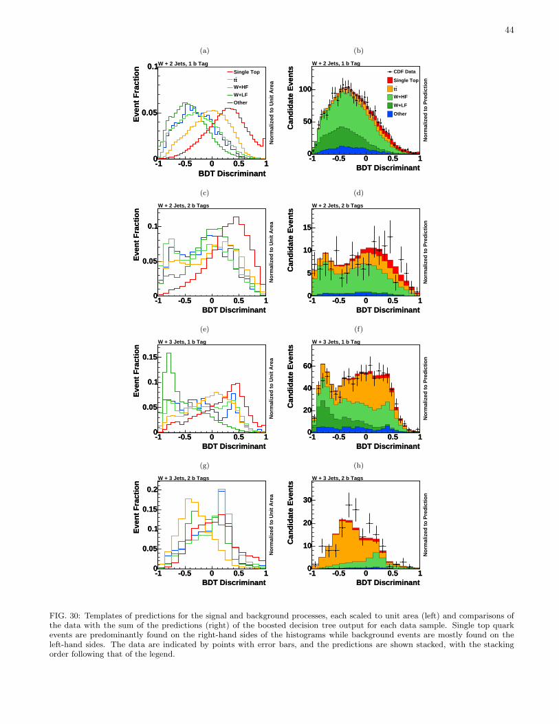
44

(a)

BDT Discriminant-1 -0.5 0 0.5 1

Eve

nt

Fra

ctio

n

0

0.05

0.1

BDT Discriminant-1 -0.5 0 0.5 1

Eve

nt

Fra

ctio

n

0

0.05

0.1W + 2 Jets, 1 b Tag

No

rmal

ized

to

Un

it A

rea

Single Top

ttW+HF

W+LF

Other

(b)

BDT Discriminant-1 -0.5 0 0.5 1

Can

did

ate

Eve

nts

0

50

100

BDT Discriminant-1 -0.5 0 0.5 1

Can

did

ate

Eve

nts

0

50

100

W + 2 Jets, 1 b Tag

No

rmal

ized

to

Pre

dic

tio

n

CDF Data

Single Top

tt

W+HF

W+LF

Other

(c)

BDT Discriminant-1 -0.5 0 0.5 1

Eve

nt

Fra

ctio

n

0

0.05

0.1

BDT Discriminant-1 -0.5 0 0.5 1

Eve

nt

Fra

ctio

n

0

0.05

0.1

W + 2 Jets, 2 b Tags

No

rmal

ized

to

Un

it A

rea

(d)

BDT Discriminant-1 -0.5 0 0.5 1

Can

did

ate

Eve

nts

0

5

10

15

BDT Discriminant-1 -0.5 0 0.5 1

Can

did

ate

Eve

nts

0

5

10

15

W + 2 Jets, 2 b Tags

No

rmal

ized

to

Pre

dic

tio

n

(e)

BDT Discriminant-1 -0.5 0 0.5 1

Eve

nt

Fra

ctio

n

0

0.05

0.1

0.15

BDT Discriminant-1 -0.5 0 0.5 1

Eve

nt

Fra

ctio

n

0

0.05

0.1

0.15

W + 3 Jets, 1 b Tag

No

rmal

ized

to

Un

it A

rea

(f)

BDT Discriminant-1 -0.5 0 0.5 1

Can

did

ate

Eve

nts

0

20

40

60

BDT Discriminant-1 -0.5 0 0.5 1

Can

did

ate

Eve

nts

0

20

40

60

W + 3 Jets, 1 b Tag

No

rmal

ized

to

Pre

dic

tio

n

(g)

BDT Discriminant-1 -0.5 0 0.5 1

Eve

nt

Fra

ctio

n

0

0.05

0.1

0.15

0.2

BDT Discriminant-1 -0.5 0 0.5 1

Eve

nt

Fra

ctio

n

0

0.05

0.1

0.15

0.2

W + 3 Jets, 2 b Tags

No

rmal

ized

to

Un

it A

rea

(h)

BDT Discriminant-1 -0.5 0 0.5 1

Can

did

ate

Eve

nts

0

10

20

30

BDT Discriminant-1 -0.5 0 0.5 1

Can

did

ate

Eve

nts

0

10

20

30

W + 3 Jets, 2 b Tags

No

rmal

ized

to

Pre

dic

tio

n

FIG. 30: Templates of predictions for the signal and background processes, each scaled to unit area (left) and comparisons ofthe data with the sum of the predictions (right) of the boosted decision tree output for each data sample. Single top quarkevents are predominantly found on the right-hand sides of the histograms while background events are mostly found on theleft-hand sides. The data are indicated by points with error bars, and the predictions are shown stacked, with the stackingorder following that of the legend.

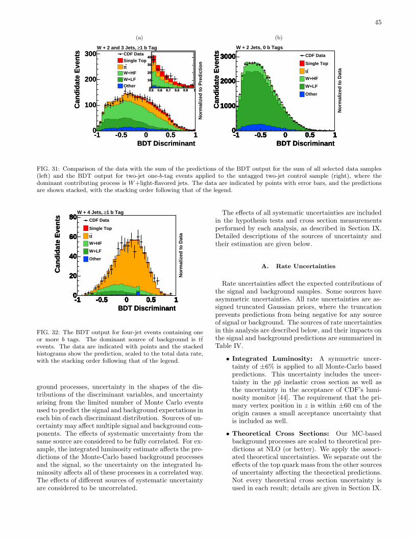
45

(a)

BDT Discriminant-1 -0.5 0 0.5 1

Can

did

ate

Eve

nts

0

100

200

300

BDT Discriminant-1 -0.5 0 0.5 1

Can

did

ate

Eve

nts

0

100

200

3001 b Tag≥W + 2 and 3 Jets,

No

rmal

ized

to

Pre

dic

tio

n

CDF Data

Single Top

ttW+HFW+LFOther

0.5 0.6 0.7 0.8 0.9 10

10

20

30

40

0.5 0.6 0.7 0.8 0.9 10

10

20

30

40

(b)

BDT Discriminant-1 -0.5 0 0.5 1

Can

did

ate

Eve

nts

0

1000

2000

3000

-1 -0.5 0 0.5 10

1000

2000

3000

-1 -0.5 0 0.5 10

1000

2000

3000

-1 -0.5 0 0.5 10

1000

2000

3000

-1 -0.5 0 0.5 10

1000

2000

3000

-1 -0.5 0 0.5 10

1000

2000

3000

BDT Discriminant-1 -0.5 0 0.5 1

Can

did

ate

Eve

nts

0

1000

2000

3000

BDT Discriminant-1 -0.5 0 0.5 1

Can

did

ate

Eve

nts

0

1000

2000

3000

-1 -0.5 0 0.5 10

1000

2000

3000 CDF Data

Single Top

tt

W+HF

W+LF

Other

W + 2 Jets, 0 b Tags

No

rmal

ized

to

Dat

a

FIG. 31: Comparison of the data with the sum of the predictions of the BDT output for the sum of all selected data samples(left) and the BDT output for two-jet one-b-tag events applied to the untagged two-jet control sample (right), where thedominant contributing process is W+light-flavored jets. The data are indicated by points with error bars, and the predictionsare shown stacked, with the stacking order following that of the legend.

BDT Discriminant-1 -0.5 0 0.5 1

Can

did

ate

Eve

nts

0

20

40

60

80

-1 -0.5 0 0.5 10

20

40

60

80

-1 -0.5 0 0.5 10

20

40

60

80

-1 -0.5 0 0.5 10

20

40

60

80

-1 -0.5 0 0.5 10

20

40

60

80

-1 -0.5 0 0.5 10

20

40

60

80

BDT Discriminant-1 -0.5 0 0.5 1

Can

did

ate

Eve

nts

0

20

40

60

80

BDT Discriminant-1 -0.5 0 0.5 1

Can

did

ate

Eve

nts

0

20

40

60

80

-1 -0.5 0 0.5 10

20

40

60

80 CDF Data

Single Top

tt

W+HF

W+LF

Other

1 b Tag≥W + 4 Jets,

No

rmal

ized

to

Dat

a

FIG. 32: The BDT output for four-jet events containing oneor more b tags. The dominant source of background is ttevents. The data are indicated with points and the stackedhistograms show the prediction, scaled to the total data rate,with the stacking order following that of the legend.

ground processes, uncertainty in the shapes of the dis-tributions of the discriminant variables, and uncertaintyarising from the limited number of Monte Carlo eventsused to predict the signal and background expectations ineach bin of each discriminant distribution. Sources of un-certainty may affect multiple signal and background com-ponents. The effects of systematic uncertainty from thesame source are considered to be fully correlated. For ex-ample, the integrated luminosity estimate affects the pre-dictions of the Monte-Carlo based background processesand the signal, so the uncertainty on the integrated lu-minosity affects all of these processes in a correlated way.The effects of different sources of systematic uncertaintyare considered to be uncorrelated.

The effects of all systematic uncertainties are includedin the hypothesis tests and cross section measurementsperformed by each analysis, as described in Section IX.Detailed descriptions of the sources of uncertainty andtheir estimation are given below.

A. Rate Uncertainties

Rate uncertainties affect the expected contributions ofthe signal and background samples. Some sources haveasymmetric uncertainties. All rate uncertainties are as-signed truncated Gaussian priors, where the truncationprevents predictions from being negative for any sourceof signal or background. The sources of rate uncertaintiesin this analysis are described below, and their impacts onthe signal and background predictions are summarized inTable IV.

• Integrated Luminosity: A symmetric uncer-tainty of ±6% is applied to all Monte-Carlo basedpredictions. This uncertainty includes the uncer-tainty in the pp inelastic cross section as well asthe uncertainty in the acceptance of CDF’s lumi-nosity monitor [44]. The requirement that the pri-mary vertex position in z is within ±60 cm of theorigin causes a small acceptance uncertainty thatis included as well.

• Theoretical Cross Sections: Our MC-basedbackground processes are scaled to theoretical pre-dictions at NLO (or better). We apply the associ-ated theoretical uncertainties. We separate out theeffects of the top quark mass from the other sourcesof uncertainty affecting the theoretical predictions.Not every theoretical cross section uncertainty isused in each result; details are given in Section IX.

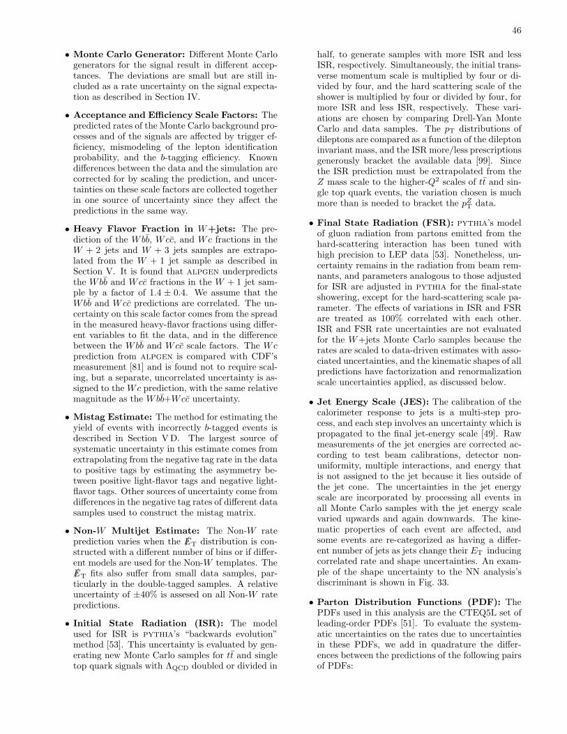
46

• Monte Carlo Generator: Different Monte Carlogenerators for the signal result in different accep-tances. The deviations are small but are still in-cluded as a rate uncertainty on the signal expecta-tion as described in Section IV.

• Acceptance and Efficiency Scale Factors: Thepredicted rates of the Monte Carlo background pro-cesses and of the signals are affected by trigger ef-ficiency, mismodeling of the lepton identificationprobability, and the b-tagging efficiency. Knowndifferences between the data and the simulation arecorrected for by scaling the prediction, and uncer-tainties on these scale factors are collected togetherin one source of uncertainty since they affect thepredictions in the same way.

• Heavy Flavor Fraction in W+jets: The pre-diction of the Wbb, Wcc, and Wc fractions in theW + 2 jets and W + 3 jets samples are extrapo-lated from the W + 1 jet sample as described inSection V. It is found that alpgen underpredictsthe Wbb and Wcc fractions in the W + 1 jet sam-ple by a factor of 1.4 ± 0.4. We assume that theWbb and Wcc predictions are correlated. The un-certainty on this scale factor comes from the spreadin the measured heavy-flavor fractions using differ-ent variables to fit the data, and in the differencebetween the Wbb and Wcc scale factors. The Wcprediction from alpgen is compared with CDF’smeasurement [81] and is found not to require scal-ing, but a separate, uncorrelated uncertainty is as-signed to the Wc prediction, with the same relativemagnitude as the Wbb+Wcc uncertainty.

• Mistag Estimate: The method for estimating theyield of events with incorrectly b-tagged events isdescribed in Section VD. The largest source ofsystematic uncertainty in this estimate comes fromextrapolating from the negative tag rate in the datato positive tags by estimating the asymmetry be-tween positive light-flavor tags and negative light-flavor tags. Other sources of uncertainty come fromdifferences in the negative tag rates of different datasamples used to construct the mistag matrix.

• Non-W Multijet Estimate: The Non-W rateprediction varies when the /ET distribution is con-structed with a different number of bins or if differ-ent models are used for the Non-W templates. The/ET fits also suffer from small data samples, par-ticularly in the double-tagged samples. A relativeuncertainty of ±40% is assesed on all Non-W ratepredictions.

• Initial State Radiation (ISR): The modelused for ISR is pythia’s “backwards evolution”method [53]. This uncertainty is evaluated by gen-erating new Monte Carlo samples for tt and singletop quark signals with ΛQCD doubled or divided in

half, to generate samples with more ISR and lessISR, respectively. Simultaneously, the initial trans-verse momentum scale is multiplied by four or di-vided by four, and the hard scattering scale of theshower is multiplied by four or divided by four, formore ISR and less ISR, respectively. These vari-ations are chosen by comparing Drell-Yan MonteCarlo and data samples. The pT distributions ofdileptons are compared as a function of the dileptoninvariant mass, and the ISR more/less prescriptionsgenerously bracket the available data [99]. Sincethe ISR prediction must be extrapolated from theZ mass scale to the higher-Q2 scales of tt and sin-gle top quark events, the variation chosen is muchmore than is needed to bracket the pZT data.

• Final State Radiation (FSR): pythia’s modelof gluon radiation from partons emitted from thehard-scattering interaction has been tuned withhigh precision to LEP data [53]. Nonetheless, un-certainty remains in the radiation from beam rem-nants, and parameters analogous to those adjustedfor ISR are adjusted in pythia for the final-stateshowering, except for the hard-scattering scale pa-rameter. The effects of variations in ISR and FSRare treated as 100% correlated with each other.ISR and FSR rate uncertainties are not evaluatedfor the W+jets Monte Carlo samples because therates are scaled to data-driven estimates with asso-ciated uncertainties, and the kinematic shapes of allpredictions have factorization and renormalizationscale uncertainties applied, as discussed below.

• Jet Energy Scale (JES): The calibration of thecalorimeter response to jets is a multi-step pro-cess, and each step involves an uncertainty which ispropagated to the final jet-energy scale [49]. Rawmeasurements of the jet energies are corrected ac-cording to test beam calibrations, detector non-uniformity, multiple interactions, and energy thatis not assigned to the jet because it lies outside ofthe jet cone. The uncertainties in the jet energyscale are incorporated by processing all events inall Monte Carlo samples with the jet energy scalevaried upwards and again downwards. The kine-matic properties of each event are affected, andsome events are re-categorized as having a differ-ent number of jets as jets change their ET inducingcorrelated rate and shape uncertainties. An exam-ple of the shape uncertainty to the NN analysis’sdiscriminant is shown in Fig. 33.

• Parton Distribution Functions (PDF): ThePDFs used in this analysis are the CTEQ5L set ofleading-order PDFs [51]. To evaluate the system-atic uncertainties on the rates due to uncertaintiesin these PDFs, we add in quadrature the differ-ences between the predictions of the following pairsof PDFs:

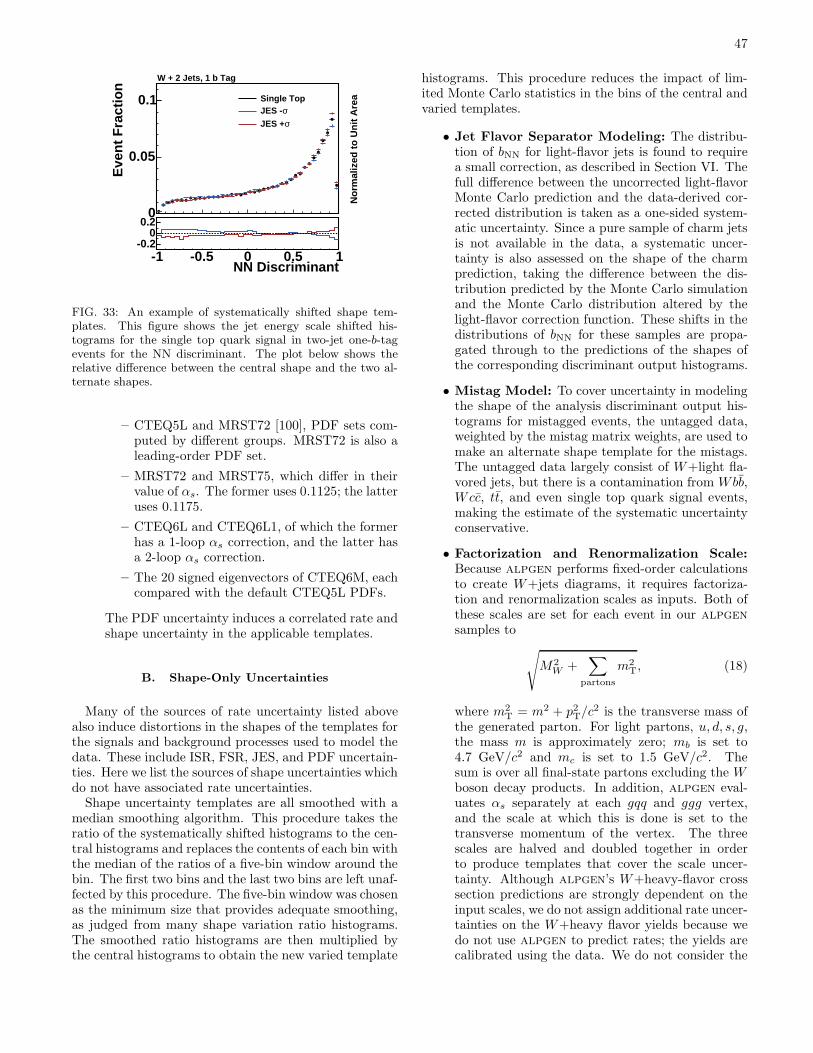
47

NN Discriminant-1 -0.5 0 0.5 1

Eve

nt

Fra

ctio

n

0

0.05

0.1

No

rmal

ized

to

Un

it A

reaSingle Top

σJES -

σJES +

NN Discriminant-1 -0.5 0 0.5 1

-0.20

0.2

W + 2 Jets, 1 b Tag

FIG. 33: An example of systematically shifted shape tem-plates. This figure shows the jet energy scale shifted his-tograms for the single top quark signal in two-jet one-b-tagevents for the NN discriminant. The plot below shows therelative difference between the central shape and the two al-ternate shapes.

– CTEQ5L and MRST72 [100], PDF sets com-puted by different groups. MRST72 is also aleading-order PDF set.

– MRST72 and MRST75, which differ in theirvalue of αs. The former uses 0.1125; the latteruses 0.1175.

– CTEQ6L and CTEQ6L1, of which the formerhas a 1-loop αs correction, and the latter hasa 2-loop αs correction.

– The 20 signed eigenvectors of CTEQ6M, eachcompared with the default CTEQ5L PDFs.

The PDF uncertainty induces a correlated rate andshape uncertainty in the applicable templates.

B. Shape-Only Uncertainties

Many of the sources of rate uncertainty listed abovealso induce distortions in the shapes of the templates forthe signals and background processes used to model thedata. These include ISR, FSR, JES, and PDF uncertain-ties. Here we list the sources of shape uncertainties whichdo not have associated rate uncertainties.Shape uncertainty templates are all smoothed with a

median smoothing algorithm. This procedure takes theratio of the systematically shifted histograms to the cen-tral histograms and replaces the contents of each bin withthe median of the ratios of a five-bin window around thebin. The first two bins and the last two bins are left unaf-fected by this procedure. The five-bin window was chosenas the minimum size that provides adequate smoothing,as judged from many shape variation ratio histograms.The smoothed ratio histograms are then multiplied bythe central histograms to obtain the new varied template

histograms. This procedure reduces the impact of lim-ited Monte Carlo statistics in the bins of the central andvaried templates.

• Jet Flavor Separator Modeling: The distribu-tion of bNN for light-flavor jets is found to requirea small correction, as described in Section VI. Thefull difference between the uncorrected light-flavorMonte Carlo prediction and the data-derived cor-rected distribution is taken as a one-sided system-atic uncertainty. Since a pure sample of charm jetsis not available in the data, a systematic uncer-tainty is also assessed on the shape of the charmprediction, taking the difference between the dis-tribution predicted by the Monte Carlo simulationand the Monte Carlo distribution altered by thelight-flavor correction function. These shifts in thedistributions of bNN for these samples are propa-gated through to the predictions of the shapes ofthe corresponding discriminant output histograms.

• Mistag Model: To cover uncertainty in modelingthe shape of the analysis discriminant output his-tograms for mistagged events, the untagged data,weighted by the mistag matrix weights, are used tomake an alternate shape template for the mistags.The untagged data largely consist of W+light fla-vored jets, but there is a contamination from Wbb,Wcc, tt, and even single top quark signal events,making the estimate of the systematic uncertaintyconservative.

• Factorization and Renormalization Scale:Because alpgen performs fixed-order calculationsto create W+jets diagrams, it requires factoriza-tion and renormalization scales as inputs. Both ofthese scales are set for each event in our alpgen

samples to

√

M2W +

∑

partons

m2T, (18)

where m2T = m2 + p2T/c

2 is the transverse mass ofthe generated parton. For light partons, u, d, s, g,the mass m is approximately zero; mb is set to4.7 GeV/c2 and mc is set to 1.5 GeV/c2. Thesum is over all final-state partons excluding the Wboson decay products. In addition, alpgen eval-uates αs separately at each gqq and ggg vertex,and the scale at which this is done is set to thetransverse momentum of the vertex. The threescales are halved and doubled together in orderto produce templates that cover the scale uncer-tainty. Although alpgen’s W+heavy-flavor crosssection predictions are strongly dependent on theinput scales, we do not assign additional rate uncer-tainties on the W+heavy flavor yields because wedo not use alpgen to predict rates; the yields arecalibrated using the data. We do not consider the

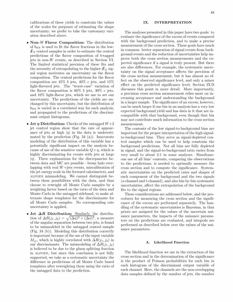
48

calibrations of these yields to constrain the valuesof the scales for purposes of estimating the shapeuncertainty; we prefer to take the customary vari-ation described above.

• Non-W Flavor Composition: The distributionof bNN is used to fit the flavor fractions in the low-/ET control samples in order to estimate the centralpredictions of the flavor composition of b-taggedjets in non-W events, as described in Section VI.The limited statistical precision of these fits andthe necessity of extrapolating to the higher-/ET sig-nal region motivates an uncertainty on the flavorcomposition. The central predictions for the flavorcomposition are 45% b jets, 40% c jets, and 15%light-flavored jets. The “worst-case” variation ofthe flavor composition is 60% b jets, 30% c jets,and 10% light-flavor jets, which we use to set ouruncertainty. The predictions of the yields are un-changed by this uncertainty, but the distribution ofbNN is varied in a correlated way for each analysis,and propagated to the predictions of the discrimi-nant output histograms.

• Jet η Distribution: Checks of the untaggedW+2jet control region show that the rate of appear-ance of jets at high |η| in the data is underesti-mated by the prediction (Fig. 34 (a)). Inaccuratemodeling of the distribution of this variable has apotentially significant impact on the analysis be-cause of use of the sensitive variable Q×η, which ishighly discriminating for events with jets at large|η|. Three explanations for the discrepancies be-tween data and MC are possible—beam halo over-lapping with real W+jets events, miscalibration ofthe jet energy scale in the forward calorimeters, andalpgen mismodeling. We cannot distinguish be-tween these possibilities with the data, and thuschoose to reweight all Monte Carlo samples by aweighting factor based on the ratio of the data andMonte Carlo in the untagged sideband, to make al-ternate shape templates for the discriminants forall Monte Carlo samples. No corresponding rateuncertainty is applied.

• Jet ∆R Distribution: Similarly, the distribu-tion of ∆R(j1, j2) =

√

(∆η)2 + (∆φ)2, a measureof the angular separation between two jets, is foundto be mismodeled in the untagged control sample(Fig. 34 (b)). Modeling this distribution correctlyis important because of the use of the input variableMjj , which is highly correlated with ∆R(j1, j2) inour discriminants. The mismodeling of ∆R(j1, j2)is believed to be due to the gluon splitting fractionin alpgen, but since this conclusion is not fullysupported, we take as a systematic uncertainty thedifference in predictions of all Monte Carlo basedtemplates after reweighting them using the ratio ofthe untagged data to the prediction.

IX. INTERPRETATION

The analyses presented in this paper have two goals: toevaluate the significance of the excess of events comparedwith the background prediction, and to make a precisemeasurement of the cross section. These goals have muchin common: better separation of signal events from back-ground events and the reduction of uncertainties help im-prove both the cross section measurements and the ex-pected significance if a signal is truly present. But thereare also differences. For example, the systematic uncer-tainty on the signal acceptance affects the precision ofthe cross section measurement, but it has almost no ef-fect on the observed significance level, and only a minoreffect on the predicted significance level; Section IXDdiscusses this point in more detail. More importantly,a precision cross section measurement relies most on in-creasing acceptance and understanding the backgroundin a larger sample. The significance of an excess, however,can be much larger if one bin in an analysis has a very lowexpected background yield and has data in it that are in-compatible with that background, even though that binmay not contribute much information to the cross sectionmeasurement.The contents of the low signal-to-background bins are

important for the proper interpretation of the high signal-to-background bins. They serve as signal-depleted con-trol samples which can be used to help constrain thebackground predictions. Not all bins are fully depletedin signal, and the signal-to-background ratio varies fromvery small to about 2:1 in some analyses. Simultane-ous use of all bins’ contents, comparing the observationsto the predictions, is needed to optimally measure thecross section and to compute the significance. System-atic uncertainties on the predicted rates and shapes ofeach component of the background and the two signals(s-channel and t-channel), and also bin-by-bin systematicuncertainties, affect the extrapolation of the backgroundfits to the signal regions.These considerations are addressed below, and the pro-

cedures for measuring the cross section and the signifi-cance of the excess are performed separately. The han-dling of the systematic uncertainties is Bayesian, in thatpriors are assigned for the values of the uncertain nui-sance parameters, the impacts of the nuisance parame-ters on the predictions are evaluated, and integrals areperformed as described below over the values of the nui-sance parameters.

A. Likelihood Function

The likelihood function we use in the extraction of thecross section and in the determination of the significanceis the product of Poisson probabilities for each bin ineach histogram of the discriminant output variable ofeach channel. Here, the channels are the non-overlappingdata samples defined by the number of jets, the number

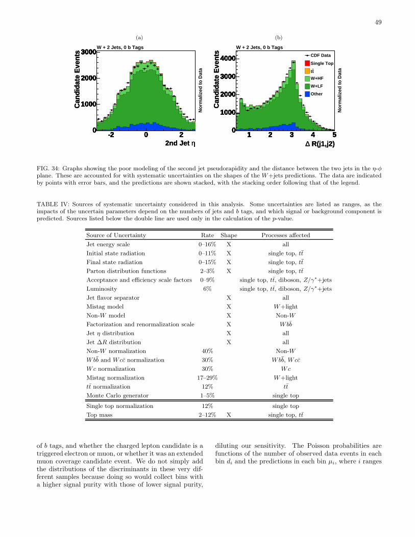
49

(a)

η2nd Jet -2 0 2

Can

did

ate

Eve

nts

0

1000

2000

3000

-2 0 20

1000

2000

3000

-2 0 20

1000

2000

3000

-2 0 20

1000

2000

3000

-2 0 20

1000

2000

3000

-2 0 20

1000

2000

3000

η2nd Jet -2 0 2

Can

did

ate

Eve

nts

0

1000

2000

3000

η2nd Jet -2 0 2

Can

did

ate

Eve

nts

0

1000

2000

3000

-2 0 20

1000

2000

3000W + 2 Jets, 0 b Tags

No

rmal

ized

to

Dat

a

(b)

R(j1,j2)∆1 2 3 4 5

Can

did

ate

Eve

nts

0

1000

2000

3000

4000

1 2 3 4 50

1000

2000

3000

4000

1 2 3 4 50

1000

2000

3000

4000

1 2 3 4 50

1000

2000

3000

4000

1 2 3 4 50

1000

2000

3000

4000

1 2 3 4 50

1000

2000

3000

4000

R(j1,j2)∆1 2 3 4 5

Can

did

ate

Eve

nts

0

1000

2000

3000

4000

R(j1,j2)∆1 2 3 4 5

Can

did

ate

Eve

nts

0

1000

2000

3000

4000

1 2 3 4 50

1000

2000

3000

4000 CDF Data

Single Top

tt

W+HF

W+LF

Other

W + 2 Jets, 0 b Tags

No

rmal

ized

to

Dat

a

FIG. 34: Graphs showing the poor modeling of the second jet pseudorapidity and the distance between the two jets in the η-φplane. These are accounted for with systematic uncertainties on the shapes of the W+jets predictions. The data are indicatedby points with error bars, and the predictions are shown stacked, with the stacking order following that of the legend.

TABLE IV: Sources of systematic uncertainty considered in this analysis. Some uncertainties are listed as ranges, as theimpacts of the uncertain parameters depend on the numbers of jets and b tags, and which signal or background component ispredicted. Sources listed below the double line are used only in the calculation of the p-value.

Source of Uncertainty Rate Shape Processes affected

Jet energy scale 0–16% X all

Initial state radiation 0–11% X single top, tt

Final state radiation 0–15% X single top, tt

Parton distribution functions 2–3% X single top, tt

Acceptance and efficiency scale factors 0–9% single top, tt, diboson, Z/γ∗+jets

Luminosity 6% single top, tt, diboson, Z/γ∗+jets

Jet flavor separator X all

Mistag model X W+light

Non-W model X Non-W

Factorization and renormalization scale X Wbb

Jet η distribution X all

Jet ∆R distribution X all

Non-W normalization 40% Non-W

Wbb and Wcc normalization 30% Wbb, Wcc

Wc normalization 30% Wc

Mistag normalization 17–29% W+light

tt normalization 12% tt

Monte Carlo generator 1–5% single top

Single top normalization 12% single top

Top mass 2–12% X single top, tt

of b tags, and whether the charged lepton candidate is atriggered electron or muon, or whether it was an extendedmuon coverage candidate event. We do not simply addthe distributions of the discriminants in these very dif-ferent samples because doing so would collect bins witha higher signal purity with those of lower signal purity,

diluting our sensitivity. The Poisson probabilities arefunctions of the number of observed data events in eachbin di and the predictions in each bin µi, where i ranges

50

from 1 to nbins. The likelihood function is given by

L =

nbins∏

i=1

µdi

i e−µi

di!. (19)

The prediction in each bin is a sum over signal and back-ground contributions:

µi =

nbkg∑

k=1

bik +

nsig∑

k=1

sik (20)

where bik is the background prediction in bin i for back-ground source k; nbkg is the total number of backgroundcontributions. The signal is the sum of the s-channel andt-channel contributions; nsig = 2 is the number of signalsources, and the sik are their predicted yields in eachbin. The predictions bik and sik depend on nnuis uncer-tain nuisance parameters θm, where m = 1...nnuis, onefor each independent source of systematic uncertainty.These nuisance parameters are given Gaussian priors cen-tered on zero with unit width, and their impacts on thesignal and background predictions are described in thesteps below.In the discussion below, the procedure for applying sys-

tematic shifts to the signal and background predictionsis given step by step, for each kind of systematic uncer-tainty. Shape uncertainties are applied first, then bin-by-bin uncertainties, and finally rate uncertainties. Thebin-by-bin uncertainties arise from limited Monte Carlo(or data from a control sample) statistics and are takento be independent of each other and all other sources ofsystematic uncertainty. The steps are labeled b0 for thecentral, unvaried background prediction in each bin, andb4 for the prediction with all systematic uncertainties ap-plied.The contribution to a bin’s prediction from a given

source of shape uncertainty is modified by linearly in-terpolating and extrapolating the difference between thecentral prediction b0ik and the prediction in a histogramcorresponding to a +1σ variation κm+

b,ik if θm > 0, andperforming a similar operation using a −1σ varied his-togram if θm < 0:

b1ik = b0ik +

nnuis∑

m=1

{

(κm+b,ik − b0ik)θm : θm ≥ 0

(b0ik − κm−b,ik)θm : θm < 0

. (21)

The parameter list is shared between the signal and back-ground predictions because some sources of systematicuncertainty affect both in a correlated way. The appli-cation of shape uncertainties is not allowed to producea negative prediction in any bin for any source of back-ground or signal:

b2ik = max(0, b1ik). (22)

Each template histogram, including the systematicallyvaried histograms, has a statistical uncertainty in eachbin. These bin-by-bin uncertainties are linearly interpo-lated in each bin in the same way as the predicted values.This procedure works well when the shape-variation tem-plates share all or most of the same events, but it overes-timates the bin-by-bin uncertainties when the alternateshape templates are filled with independent samples. Ifthe bin-by-bin uncertainty on b0ik is δ0b,ik, and the bin-by-

bin uncertainty on bm±ik is δm±

b,ik , then

δ1b,ik = δ0b,ik +

nnuis∑

m=1

{

(δm+b,ik − δ0b,ik)θm : θm ≥ 0

(δ0b,ik − δm−b,ik )θm : θm < 0

.

(23)Each bin of each background has a nuisance parameterηb,ik associated with it.

b3ik = b2ik + δ1b,ikηb,ik, (24)

where ηb,ik is drawn from a Gaussian centered on zerowith unit width when integrating over it. If b3ik < 0, thenηb,ik is re-drawn from that Gaussian.

Finally, rate uncertainties are applied multiplicatively.If the fractional uncertainty on b0ik due to nuisance pa-rameter m is ρm+

b,ik for a +1σ variation and it is ρm−b,ik

for a negative variation, then a quadratic function is de-termined to make a smooth application of the nuisanceparameter to the predicted value:

bik = b4ik = b3ik

nnuis∏

m=1

(

1 +ρm+b,ik + ρm−

b,ik

2θ2m +

ρm+b,ik − ρm−

b,ik

2θm

)

. (25)

The rate uncertainties are applied multiplicatively be-cause most of them affect the rates by scale factors, suchas the luminosity and acceptance uncertainties, and theyare applied last because they affect the distorted shapes

in the same way as the undistorted shapes. Multipleshape uncertainties are treated additively because mostof them correspond to events migrating from one bin toanother.

51

The signal predictions are based on their StandardModel rates. These are scaled to test other values ofthe single top quark production cross sections:

sik = s4ikβk, (26)

where βs scales the s-channel signal and βt scales thet-channel signal, and the “4” superscript indicates thatthe same chain of application of nuisance parameters isapplied to the signal prediction as is applied to the back-ground.The likelihood is a function of the observed data

D = {di}, the signal scale factors β = {βs, βt}, the nui-sance parameters θ = {θm} and η = {ηs,ik, ηb,ik}, thecentral values of the signal and background predictionss = {s0ik} and b = {b0ik}, and the rate, shape, and bin-by-bin uncertainties ρ = {ρm±

b,ik , ρm±s,ik}, κ = {κm±

b,ik , κm±s,ik},

δ = {δ0b,ik, δm±b,ik , δ

0s,ik, δ

m±s,ik}:

L = L(D|β, θ, η, s, b, ρ, κ, δ). (27)

B. Cross Section Measurement

Because the signal template shapes and the tt back-ground template rates and shapes are functions of mt,we quote the single top quark cross section assuming atop quark mass of mt = 175 GeV/c2 and also evaluate∂σs+t/∂mt. We therefore do not include the uncertaintyon the top quark mass when measuring the cross section.

1. Measurement of σs+t

We measure the total cross section of single top quarkproduction σs+t, assuming the SM ratio between s-channel and t-channel production: βs = βt ≡ β. Weuse a Bayesian marginalization technique [101] to incor-porate the effects of systematic uncertainty:

L′(β) =

∫

L(D|β, θ, η, s, b, ρ, κ, δ)π(θ)π(η)dθdη, (28)

where the π functions are the Bayesian priors assigned toeach nuisance parameter. The priors are unit Gaussianfunctions centered on zero which are truncated when-ever the value of a nuisance parameter would result in anon-physical prediction. The measured cross section cor-responds to the maximum of L′, which occurs at βmax:

σmeass+t = σSM

s+tβmax. (29)

The uncertainty corresponds to the shortest interval[βlow, βhigh] containing 68% of the integral of the pos-terior, assuming a uniform positive prior in β π(β) = 1:

0.68 =

∫ βhigh

βlowL′(β)π(β)dβ

∫∞

0L′(β)π(β)dβ

. (30)

This prescription has the property that the numericalvalue of the posterior on the low end of the interval isequal to that on the high end of the interval.

Following the example of other top quark propertiesanalyses, the single top quark cross section is measuredassuming a top quark mass of 175 GeV/c2. This mea-surement is repeated with separate Monte Carlo sam-ples and background estimates generated with masses of170 GeV/c2 and 180 GeV/c2, and the result is used tofind dσs+t/dmt.

2. Extraction of Bounds on |Vtb|

The parameter

β =σmeass+t

σSMs+t

(31)

is identified in the Standard Model as |Vtb|2, under theassumption that |Vtd|2 + |Vts|2 ≪ |Vtb|2, and that newphysics contributions affect only |Vtb|. The theoreticaluncertainty on σSM

s+t must be introduced for this calcula-tion. The 95% confidence lower limit on |Vtb| is calculatedby requiring 0 ≤ |Vtb| ≤ 1 and finding the point at which95% of the likelihood curve lies to the right of the point.This calculation uses a prior which is flat in |Vtb|2.

C. Check for Bias

As a cross-check of the cross-section measurementmethod, simulated pseudoexperiments were generated,randomly fluctuating the systematically uncertain nui-sance parameters, propagating their impacts on the pre-dictions of each signal and background source in each binof each histogram, and drawing random Poisson pseudo-data in those bins from the fluctuated means. Samplesof pseudoexperiments were generated assuming differentsignal cross sections, and the cross section posterior wasformed for each one in the same way as it is for the data.We take the value of the cross section that maximizes

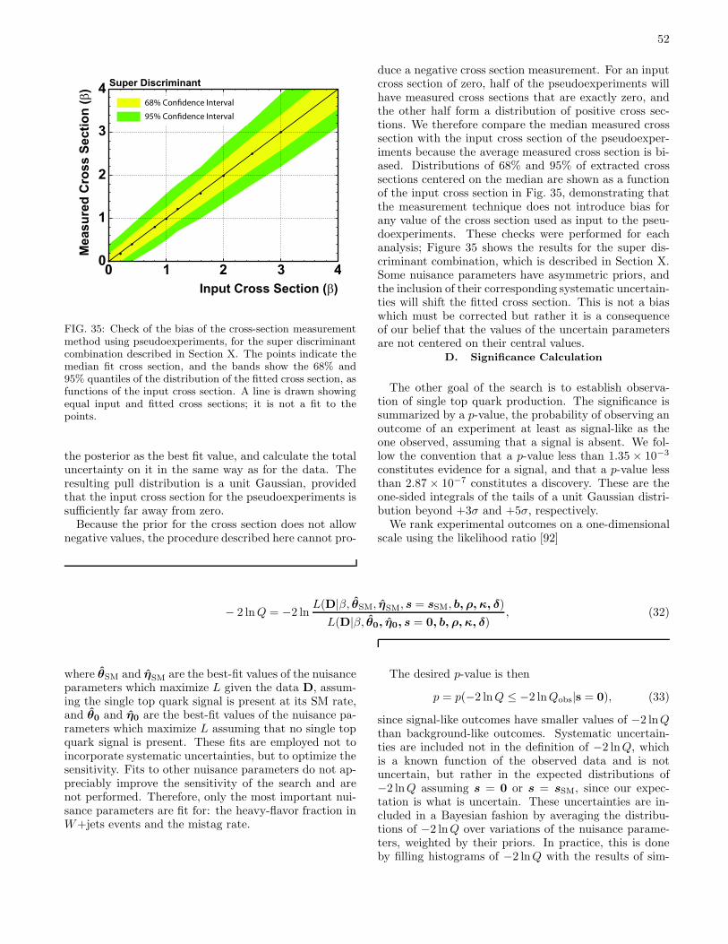
52

FIG. 35: Check of the bias of the cross-section measurementmethod using pseudoexperiments, for the super discriminantcombination described in Section X. The points indicate themedian fit cross section, and the bands show the 68% and95% quantiles of the distribution of the fitted cross section, asfunctions of the input cross section. A line is drawn showingequal input and fitted cross sections; it is not a fit to thepoints.

the posterior as the best fit value, and calculate the totaluncertainty on it in the same way as for the data. Theresulting pull distribution is a unit Gaussian, providedthat the input cross section for the pseudoexperiments issufficiently far away from zero.Because the prior for the cross section does not allow

negative values, the procedure described here cannot pro-

duce a negative cross section measurement. For an inputcross section of zero, half of the pseudoexperiments willhave measured cross sections that are exactly zero, andthe other half form a distribution of positive cross sec-tions. We therefore compare the median measured crosssection with the input cross section of the pseudoexper-iments because the average measured cross section is bi-ased. Distributions of 68% and 95% of extracted crosssections centered on the median are shown as a functionof the input cross section in Fig. 35, demonstrating thatthe measurement technique does not introduce bias forany value of the cross section used as input to the pseu-doexperiments. These checks were performed for eachanalysis; Figure 35 shows the results for the super dis-criminant combination, which is described in Section X.Some nuisance parameters have asymmetric priors, andthe inclusion of their corresponding systematic uncertain-ties will shift the fitted cross section. This is not a biaswhich must be corrected but rather it is a consequenceof our belief that the values of the uncertain parametersare not centered on their central values.

D. Significance Calculation

The other goal of the search is to establish observa-tion of single top quark production. The significance issummarized by a p-value, the probability of observing anoutcome of an experiment at least as signal-like as theone observed, assuming that a signal is absent. We fol-low the convention that a p-value less than 1.35 × 10−3

constitutes evidence for a signal, and that a p-value lessthan 2.87 × 10−7 constitutes a discovery. These are theone-sided integrals of the tails of a unit Gaussian distri-bution beyond +3σ and +5σ, respectively.We rank experimental outcomes on a one-dimensional

scale using the likelihood ratio [92]

− 2 lnQ = −2 lnL(D|β, θSM, ηSM, s = sSM, b, ρ, κ, δ)

L(D|β, θ0, η0, s = 0, b, ρ, κ, δ), (32)

where θSM and ηSM are the best-fit values of the nuisanceparameters which maximize L given the data D, assum-ing the single top quark signal is present at its SM rate,and θ0 and η0 are the best-fit values of the nuisance pa-rameters which maximize L assuming that no single topquark signal is present. These fits are employed not toincorporate systematic uncertainties, but to optimize thesensitivity. Fits to other nuisance parameters do not ap-preciably improve the sensitivity of the search and arenot performed. Therefore, only the most important nui-sance parameters are fit for: the heavy-flavor fraction inW+jets events and the mistag rate.

The desired p-value is then

p = p(−2 lnQ ≤ −2 lnQobs|s = 0), (33)

since signal-like outcomes have smaller values of −2 lnQthan background-like outcomes. Systematic uncertain-ties are included not in the definition of −2 lnQ, whichis a known function of the observed data and is notuncertain, but rather in the expected distributions of−2 lnQ assuming s = 0 or s = sSM, since our expec-tation is what is uncertain. These uncertainties are in-cluded in a Bayesian fashion by averaging the distribu-tions of −2 lnQ over variations of the nuisance parame-ters, weighted by their priors. In practice, this is doneby filling histograms of −2 lnQ with the results of sim-

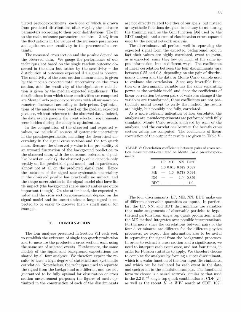
53

ulated pseudoexperiments, each one of which is drawnfrom predicted distributions after varying the nuisanceparameters according to their prior distributions. The fitto the main nuisance parameters insulates −2 lnQ fromthe fluctuations in the values of the nuisance parametersand optimizes our sensitivity in the presence of uncer-tainty.The measured cross section and the p-value depend on

the observed data. We gauge the performance of ourtechniques not based on the single random outcome ob-served in the data but rather by the sensitivity – thedistribution of outcomes expected if a signal is present.The sensitivity of the cross section measurement is givenby the median expected total uncertainty on the crosssection, and the sensitivity of the significance calcula-tion is given by the median expected significance. Thedistributions from which these sensitivities are computedare Monte Carlo pseudoexperiments with all nuisance pa-rameters fluctuated according to their priors. Optimiza-tions of the analyses were based on the median expectedp-values, without reference to the observed data. Indeed,the data events passing the event selection requirementswere hidden during the analysis optimization.In the computation of the observed and expected p-

values, we include all sources of systematic uncertaintyin the pseudoexperiments, including the theoretical un-certainty in the signal cross sections and the top quarkmass. Because the observed p-value is the probability ofan upward fluctuation of the background prediction tothe observed data, with the outcomes ordered as signal-like based on −2 lnQ, the observed p-value depends onlyweakly on the predicted signal model, and in particular,almost not at all on the predicted signal rate. Hencethe inclusion of the signal rate systematic uncertaintyin the observed p-value has practically no impact, andthe shape uncertainties in the signal model also have lit-tle impact (the background shape uncertainties are quiteimportant though). On the other hand, the expected p-value and the cross section measurement depend on thesignal model and its uncertainties; a large signal is ex-pected to be easier to discover than a small signal, forexample.

X. COMBINATION

The four analyses presented in Section VII each seekto establish the existence of single top quark productionand to measure the production cross section, each usingthe same set of selected events. Furthermore, the samemodels of the signal and background expectations areshared by all four analyses. We therefore expect the re-sults to have a high degree of statistical and systematiccorrelation. Nonetheless, the techniques used to separatethe signal from the background are different and are notguaranteed to be fully optimal for observation or crosssection measurement purposes; the figures of merit op-timized in the construction of each of the discriminants

are not directly related to either of our goals, but insteadare synthetic functions designed to be easy to use duringthe training, such as the Gini function [96] used by theBDT analysis, and a sum of classification errors squaredused by the neural network analysis.The discriminants all perform well in separating the

expected signal from the expected background, and infact their values are highly correlated, event to event,as is expected, since they key on much of the same in-put information, but in different ways. The coefficientsof linear correlation between the four discriminants varybetween 0.55 and 0.8, depending on the pair of discrim-inants chosen and the data or Monte Carlo sample usedto evaluate the correlation. Since any invertible func-tion of a discriminant variable has the same separatingpower as the variable itself, and since the coefficients oflinear correlation between pairs of variables change if thevariables are transformed, these coefficients are not par-ticularly useful except to verify that indeed the resultsare highly, but possibly not fully, correlated.As a more relevant indication of how correlated the

analyses are, pseudoexperiments are performed with fullysimulated Monte Carlo events analyzed by each of theanalyses, and the correlations between the best-fit crosssection values are computed. The coefficients of linearcorrelation of the output fit results are given in Table V.

TABLE V: Correlation coefficients between pairs of cross sec-tion measurements evaluated on Monte Carlo pseudoexperi-ments.

LF ME NN BDT

LF 1.0 0.646 0.672 0.635

ME — 1.0 0.718 0.694

NN — — 1.0 0.850

BDT — — — 1.0

The four discriminants, LF, ME, NN, BDT make useof different observable quantities as inputs. In particu-lar, the LF, NN, and BDT discriminants use variablesthat make assignments of observable particles to hypo-thetical partons from single top quark production, whilethe ME method integrates over possible interpretations.Furthermore, since the correlations between pairs of thefour discriminants are different for the different physicsprocesses, we expect this information also to be usefulin separating the signal from the background processes.In order to extract a cross section and a significance, weneed to interpret each event once, and not four times, inorder for Poisson statistics to apply. We therefore chooseto combine the analyses by forming a super discriminant,which is a scalar function of the four input discriminants,and which can be evaluated for each event in the dataand each event in the simulation samples. The functionalform we choose is a neural network, similar to that usedin the 2.2 fb−1 single top quark combination at CDF [26]as well as the recent H → WW search at CDF [102].

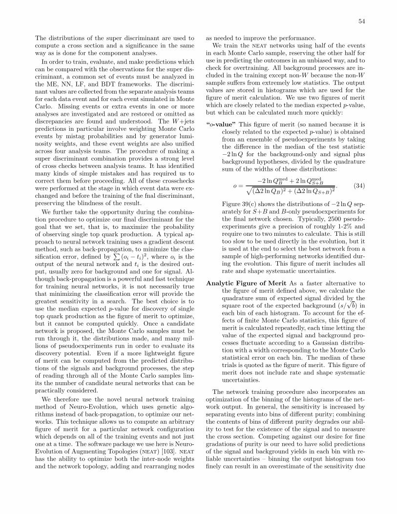
54

The distributions of the super discriminant are used tocompute a cross section and a significance in the sameway as is done for the component analyses.

In order to train, evaluate, and make predictions whichcan be compared with the observations for the super dis-criminant, a common set of events must be analyzed inthe ME, NN, LF, and BDT frameworks. The discrimi-nant values are collected from the separate analysis teamsfor each data event and for each event simulated in MonteCarlo. Missing events or extra events in one or moreanalyses are investigated and are restored or omitted asdiscrepancies are found and understood. The W+jetspredictions in particular involve weighting Monte Carloevents by mistag probabilities and by generator lumi-nosity weights, and these event weights are also unifiedacross four analysis teams. The procedure of making asuper discriminant combination provides a strong levelof cross checks between analysis teams. It has identifiedmany kinds of simple mistakes and has required us tocorrect them before proceeding. All of these crosscheckswere performed at the stage in which event data were ex-changed and before the training of the fnal discriminant,preserving the blindness of the result.

We further take the opportunity during the combina-tion procedure to optimize our final discriminant for thegoal that we set, that is, to maximize the probabilityof observing single top quark production. A typical ap-proach to neural network training uses a gradient descentmethod, such as back-propagation, to minimize the clas-sification error, defined by

∑

(oi − ti)2, where oi is the

output of the neural network and ti is the desired out-put, usually zero for background and one for signal. Al-though back-propagation is a powerful and fast techniquefor training neural networks, it is not necessarily truethat minimizing the classification error will provide thegreatest sensitivity in a search. The best choice is touse the median expected p-value for discovery of singletop quark production as the figure of merit to optimize,but it cannot be computed quickly. Once a candidatenetwork is proposed, the Monte Carlo samples must berun through it, the distributions made, and many mil-lions of pseudoexperiments run in order to evaluate itsdiscovery potential. Even if a more lightweight figureof merit can be computed from the predicted distribu-tions of the signals and background processes, the stepof reading through all of the Monte Carlo samples lim-its the number of candidate neural networks that can bepractically considered.

We therefore use the novel neural network trainingmethod of Neuro-Evolution, which uses genetic algo-rithms instead of back-propagation, to optimize our net-works. This technique allows us to compute an arbitraryfigure of merit for a particular network configurationwhich depends on all of the training events and not justone at a time. The software package we use here is Neuro-Evolution of Augmenting Topologies (neat) [103]. neathas the ability to optimize both the inter-node weightsand the network topology, adding and rearranging nodes

as needed to improve the performance.We train the neat networks using half of the events

in each Monte Carlo sample, reserving the other half foruse in predicting the outcomes in an unbiased way, and tocheck for overtraining. All background processes are in-cluded in the training except non-W because the non-Wsample suffers from extremely low statistics. The outputvalues are stored in histograms which are used for thefigure of merit calculation. We use two figures of meritwhich are closely related to the median expected p-value,but which can be calculated much more quickly:

“o-value” This figure of merit (so named because it isclosely related to the expected p-value) is obtainedfrom an ensemble of pseudoexperiments by takingthe difference in the median of the test statistic−2 lnQ for the background-only and signal plusbackground hypotheses, divided by the quadraturesum of the widths of those distributions:

o =−2 lnQmed

B + 2 lnQmedS+B

√

(∆2 lnQB)2 + (∆2 lnQS+B)2. (34)

Figure 39(c) shows the distributions of −2 lnQ sep-arately for S+B and B-only pseudoexperiments forthe final network chosen. Typically, 2500 pseudo-experiments give a precision of roughly 1-2% andrequire one to two minutes to calculate. This is stilltoo slow to be used directly in the evolution, but itis used at the end to select the best network from asample of high-performing networks identified dur-ing the evolution. This figure of merit includes allrate and shape systematic uncertainties.

Analytic Figure of Merit As a faster alternative tothe figure of merit defined above, we calculate thequadrature sum of expected signal divided by thesquare root of the expected background (s/

√b) in

each bin of each histogram. To account for the ef-fects of finite Monte Carlo statistics, this figure ofmerit is calculated repeatedly, each time letting thevalue of the expected signal and background pro-cesses fluctuate according to a Gaussian distribu-tion with a width corresponding to the Monte Carlostatistical error on each bin. The median of thesetrials is quoted as the figure of merit. This figure ofmerit does not include rate and shape systematicuncertainties.

The network training procedure also incorporates anoptimization of the binning of the histograms of the net-work output. In general, the sensitivity is increased byseparating events into bins of different purity; combiningthe contents of bins of different purity degrades our abil-ity to test for the existence of the signal and to measurethe cross section. Competing against our desire for finegradations of purity is our need to have solid predictionsof the signal and background yields in each bin with re-liable uncertainties – binning the output histogram toofinely can result in an overestimate of the sensitivity due

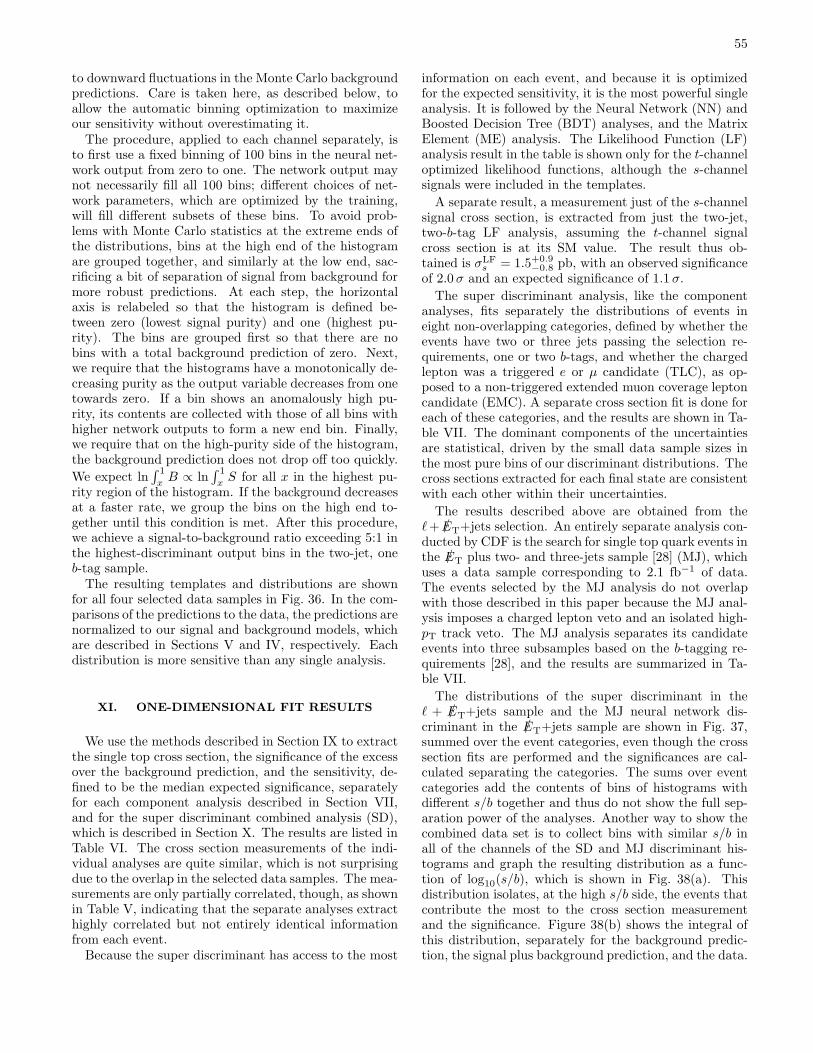
55

to downward fluctuations in the Monte Carlo backgroundpredictions. Care is taken here, as described below, toallow the automatic binning optimization to maximizeour sensitivity without overestimating it.The procedure, applied to each channel separately, is

to first use a fixed binning of 100 bins in the neural net-work output from zero to one. The network output maynot necessarily fill all 100 bins; different choices of net-work parameters, which are optimized by the training,will fill different subsets of these bins. To avoid prob-lems with Monte Carlo statistics at the extreme ends ofthe distributions, bins at the high end of the histogramare grouped together, and similarly at the low end, sac-rificing a bit of separation of signal from background formore robust predictions. At each step, the horizontalaxis is relabeled so that the histogram is defined be-tween zero (lowest signal purity) and one (highest pu-rity). The bins are grouped first so that there are nobins with a total background prediction of zero. Next,we require that the histograms have a monotonically de-creasing purity as the output variable decreases from onetowards zero. If a bin shows an anomalously high pu-rity, its contents are collected with those of all bins withhigher network outputs to form a new end bin. Finally,we require that on the high-purity side of the histogram,the background prediction does not drop off too quickly.

We expect ln∫ 1

xB ∝ ln

∫ 1

xS for all x in the highest pu-

rity region of the histogram. If the background decreasesat a faster rate, we group the bins on the high end to-gether until this condition is met. After this procedure,we achieve a signal-to-background ratio exceeding 5:1 inthe highest-discriminant output bins in the two-jet, oneb-tag sample.The resulting templates and distributions are shown

for all four selected data samples in Fig. 36. In the com-parisons of the predictions to the data, the predictions arenormalized to our signal and background models, whichare described in Sections V and IV, respectively. Eachdistribution is more sensitive than any single analysis.

XI. ONE-DIMENSIONAL FIT RESULTS

We use the methods described in Section IX to extractthe single top cross section, the significance of the excessover the background prediction, and the sensitivity, de-fined to be the median expected significance, separatelyfor each component analysis described in Section VII,and for the super discriminant combined analysis (SD),which is described in Section X. The results are listed inTable VI. The cross section measurements of the indi-vidual analyses are quite similar, which is not surprisingdue to the overlap in the selected data samples. The mea-surements are only partially correlated, though, as shownin Table V, indicating that the separate analyses extracthighly correlated but not entirely identical informationfrom each event.Because the super discriminant has access to the most

information on each event, and because it is optimizedfor the expected sensitivity, it is the most powerful singleanalysis. It is followed by the Neural Network (NN) andBoosted Decision Tree (BDT) analyses, and the MatrixElement (ME) analysis. The Likelihood Function (LF)analysis result in the table is shown only for the t-channeloptimized likelihood functions, although the s-channelsignals were included in the templates.

A separate result, a measurement just of the s-channelsignal cross section, is extracted from just the two-jet,two-b-tag LF analysis, assuming the t-channel signalcross section is at its SM value. The result thus ob-tained is σLF

s = 1.5+0.9−0.8 pb, with an observed significance

of 2.0 σ and an expected significance of 1.1 σ.

The super discriminant analysis, like the componentanalyses, fits separately the distributions of events ineight non-overlapping categories, defined by whether theevents have two or three jets passing the selection re-quirements, one or two b-tags, and whether the chargedlepton was a triggered e or µ candidate (TLC), as op-posed to a non-triggered extended muon coverage leptoncandidate (EMC). A separate cross section fit is done foreach of these categories, and the results are shown in Ta-ble VII. The dominant components of the uncertaintiesare statistical, driven by the small data sample sizes inthe most pure bins of our discriminant distributions. Thecross sections extracted for each final state are consistentwith each other within their uncertainties.

The results described above are obtained from theℓ+ /ET+jets selection. An entirely separate analysis con-ducted by CDF is the search for single top quark events inthe /ET plus two- and three-jets sample [28] (MJ), whichuses a data sample corresponding to 2.1 fb−1 of data.The events selected by the MJ analysis do not overlapwith those described in this paper because the MJ anal-ysis imposes a charged lepton veto and an isolated high-pT track veto. The MJ analysis separates its candidateevents into three subsamples based on the b-tagging re-quirements [28], and the results are summarized in Ta-ble VII.

The distributions of the super discriminant in theℓ + /ET+jets sample and the MJ neural network dis-criminant in the /ET+jets sample are shown in Fig. 37,summed over the event categories, even though the crosssection fits are performed and the significances are cal-culated separating the categories. The sums over eventcategories add the contents of bins of histograms withdifferent s/b together and thus do not show the full sep-aration power of the analyses. Another way to show thecombined data set is to collect bins with similar s/b inall of the channels of the SD and MJ discriminant his-tograms and graph the resulting distribution as a func-tion of log10(s/b), which is shown in Fig. 38(a). Thisdistribution isolates, at the high s/b side, the events thatcontribute the most to the cross section measurementand the significance. Figure 38(b) shows the integral ofthis distribution, separately for the background predic-tion, the signal plus background prediction, and the data.

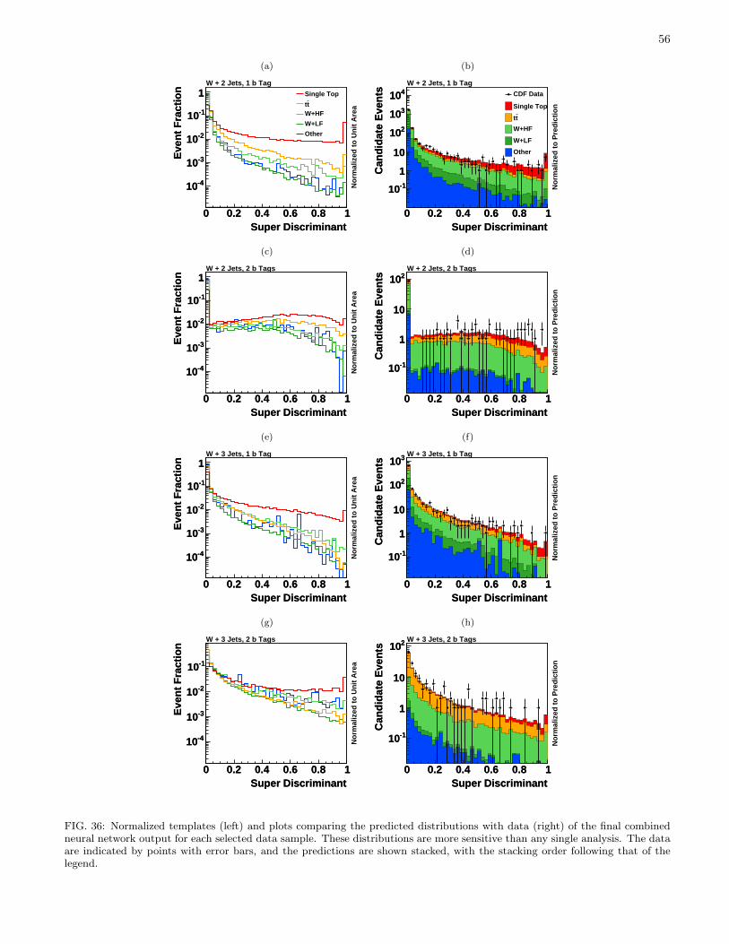
56

(a)

Super Discriminant0 0.2 0.4 0.6 0.8 1

Eve

nt

Fra

ctio

n-410

-310

-210

-110

1

Super Discriminant0 0.2 0.4 0.6 0.8 1

Eve

nt

Fra

ctio

n-410

-310

-210

-110

1W + 2 Jets, 1 b Tag

No

rmal

ized

to

Un

it A

rea

Single Top

ttW+HF

W+LF

Other

(b)

Super Discriminant0 0.2 0.4 0.6 0.8 1

Can

did

ate

Eve

nts

-110

1

10

210

310

410

Super Discriminant0 0.2 0.4 0.6 0.8 1

Can

did

ate

Eve

nts

-110

1

10

210

310

410W + 2 Jets, 1 b Tag

No

rmal

ized

to

Pre

dic

tio

n

CDF Data

Single Top

tt

W+HF

W+LF

Other

(c)

Super Discriminant0 0.2 0.4 0.6 0.8 1

Eve

nt

Fra

ctio

n

-410

-310

-210

-110

1

Super Discriminant0 0.2 0.4 0.6 0.8 1

Eve

nt

Fra

ctio

n

-410

-310

-210

-110

1W + 2 Jets, 2 b Tags

No

rmal

ized

to

Un

it A

rea

(d)

Super Discriminant0 0.2 0.4 0.6 0.8 1

Can

did

ate

Eve

nts

-110

1

10

210

Super Discriminant0 0.2 0.4 0.6 0.8 1

Can

did

ate

Eve

nts

-110

1

10

210W + 2 Jets, 2 b Tags

No

rmal

ized

to

Pre

dic

tio

n

(e)

Super Discriminant0 0.2 0.4 0.6 0.8 1

Eve

nt

Fra

ctio

n

-410

-310

-210

-110

1

Super Discriminant0 0.2 0.4 0.6 0.8 1

Eve

nt

Fra

ctio

n

-410

-310

-210

-110

1W + 3 Jets, 1 b Tag

No

rmal

ized

to

Un

it A

rea

(f)

Super Discriminant0 0.2 0.4 0.6 0.8 1

Can

did

ate

Eve

nts

-110

1

10

210

310

Super Discriminant0 0.2 0.4 0.6 0.8 1

Can

did

ate

Eve

nts

-110

1

10

210

310W + 3 Jets, 1 b Tag

No

rmal

ized

to

Pre

dic

tio

n

(g)

Super Discriminant0 0.2 0.4 0.6 0.8 1

Eve

nt

Fra

ctio

n

-410

-310

-210

-110

Super Discriminant0 0.2 0.4 0.6 0.8 1

Eve

nt

Fra

ctio

n

-410

-310

-210

-110

W + 3 Jets, 2 b Tags

No

rmal

ized

to

Un

it A

rea

(h)

Super Discriminant0 0.2 0.4 0.6 0.8 1

Can

did

ate

Eve

nts

-110

1

10

210

Super Discriminant0 0.2 0.4 0.6 0.8 1

Can

did

ate

Eve

nts

-110

1

10

210W + 3 Jets, 2 b Tags

No

rmal

ized

to

Pre

dic

tio

n

FIG. 36: Normalized templates (left) and plots comparing the predicted distributions with data (right) of the final combinedneural network output for each selected data sample. These distributions are more sensitive than any single analysis. The dataare indicated by points with error bars, and the predictions are shown stacked, with the stacking order following that of thelegend.

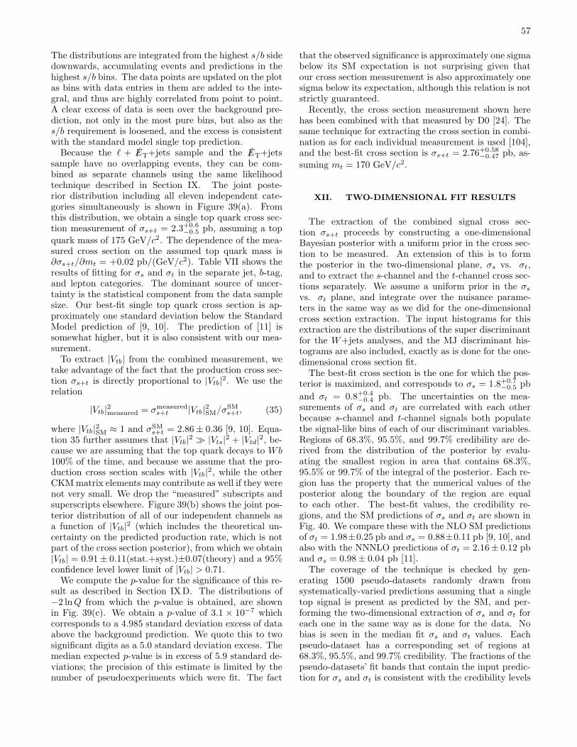
57

The distributions are integrated from the highest s/b sidedownwards, accumulating events and predictions in thehighest s/b bins. The data points are updated on the plotas bins with data entries in them are added to the inte-gral, and thus are highly correlated from point to point.A clear excess of data is seen over the background pre-diction, not only in the most pure bins, but also as thes/b requirement is loosened, and the excess is consistentwith the standard model single top prediction.Because the ℓ + /ET+jets sample and the /ET+jets

sample have no overlapping events, they can be com-bined as separate channels using the same likelihoodtechnique described in Section IX. The joint poste-rior distribution including all eleven independent cate-gories simultaneously is shown in Figure 39(a). Fromthis distribution, we obtain a single top quark cross sec-tion measurement of σs+t = 2.3+0.6

−0.5 pb, assuming a top

quark mass of 175 GeV/c2. The dependence of the mea-sured cross section on the assumed top quark mass is∂σs+t/∂mt = +0.02 pb/(GeV/c2). Table VII shows theresults of fitting for σs and σt in the separate jet, b-tag,and lepton categories. The dominant source of uncer-tainty is the statistical component from the data samplesize. Our best-fit single top quark cross section is ap-proximately one standard deviation below the StandardModel prediction of [9, 10]. The prediction of [11] issomewhat higher, but it is also consistent with our mea-surement.To extract |Vtb| from the combined measurement, we

take advantage of the fact that the production cross sec-tion σs+t is directly proportional to |Vtb|2. We use therelation

|Vtb|2measured = σmeasureds+t |Vtb|2SM/σSM

s+t, (35)

where |Vtb|2SM ≈ 1 and σSMs+t = 2.86± 0.36 [9, 10]. Equa-

tion 35 further assumes that |Vtb|2 ≫ |Vts|2 + |Vtd|2, be-cause we are assuming that the top quark decays to Wb100% of the time, and because we assume that the pro-duction cross section scales with |Vtb|2, while the otherCKMmatrix elements may contribute as well if they werenot very small. We drop the “measured” subscripts andsuperscripts elsewhere. Figure 39(b) shows the joint pos-terior distribution of all of our independent channels asa function of |Vtb|2 (which includes the theoretical un-certainty on the predicted production rate, which is notpart of the cross section posterior), from which we obtain|Vtb| = 0.91± 0.11(stat.+syst.)±0.07(theory) and a 95%confidence level lower limit of |Vtb| > 0.71.We compute the p-value for the significance of this re-

sult as described in Section IXD. The distributions of−2 lnQ from which the p-value is obtained, are shownin Fig. 39(c). We obtain a p-value of 3.1 × 10−7 whichcorresponds to a 4.985 standard deviation excess of dataabove the background prediction. We quote this to twosignificant digits as a 5.0 standard deviation excess. Themedian expected p-value is in excess of 5.9 standard de-viations; the precision of this estimate is limited by thenumber of pseudoexperiments which were fit. The fact

that the observed significance is approximately one sigmabelow its SM expectation is not surprising given thatour cross section measurement is also approximately onesigma below its expectation, although this relation is notstrictly guaranteed.Recently, the cross section measurement shown here

has been combined with that measured by D0 [24]. Thesame technique for extracting the cross section in combi-nation as for each individual measurement is used [104],and the best-fit cross section is σs+t = 2.76+0.58

−0.47 pb, as-

suming mt = 170 GeV/c2.

XII. TWO-DIMENSIONAL FIT RESULTS

The extraction of the combined signal cross sec-tion σs+t proceeds by constructing a one-dimensionalBayesian posterior with a uniform prior in the cross sec-tion to be measured. An extension of this is to formthe posterior in the two-dimensional plane, σs vs. σt,and to extract the s-channel and the t-channel cross sec-tions separately. We assume a uniform prior in the σs

vs. σt plane, and integrate over the nuisance parame-ters in the same way as we did for the one-dimensionalcross section extraction. The input histograms for thisextraction are the distributions of the super discriminantfor the W+jets analyses, and the MJ discriminant his-tograms are also included, exactly as is done for the one-dimensional cross section fit.The best-fit cross section is the one for which the pos-

terior is maximized, and corresponds to σs = 1.8+0.7−0.5 pb

and σt = 0.8+0.4−0.4 pb. The uncertainties on the mea-

surements of σs and σt are correlated with each otherbecause s-channel and t-channel signals both populatethe signal-like bins of each of our discriminant variables.Regions of 68.3%, 95.5%, and 99.7% credibility are de-rived from the distribution of the posterior by evalu-ating the smallest region in area that contains 68.3%,95.5% or 99.7% of the integral of the posterior. Each re-gion has the property that the numerical values of theposterior along the boundary of the region are equalto each other. The best-fit values, the credibility re-gions, and the SM predictions of σs and σt are shown inFig. 40. We compare these with the NLO SM predictionsof σt = 1.98±0.25 pb and σs = 0.88±0.11 pb [9, 10], andalso with the NNNLO predictions of σt = 2.16± 0.12 pband σs = 0.98± 0.04 pb [11].The coverage of the technique is checked by gen-

erating 1500 pseudo-datasets randomly drawn fromsystematically-varied predictions assuming that a singletop signal is present as predicted by the SM, and per-forming the two-dimensional extraction of σs and σt foreach one in the same way as is done for the data. Nobias is seen in the median fit σs and σt values. Eachpseudo-dataset has a corresponding set of regions at68.3%, 95.5%, and 99.7% credibility. The fractions of thepseudo-datasets’ fit bands that contain the input predic-tion for σs and σt is consistent with the credibility levels

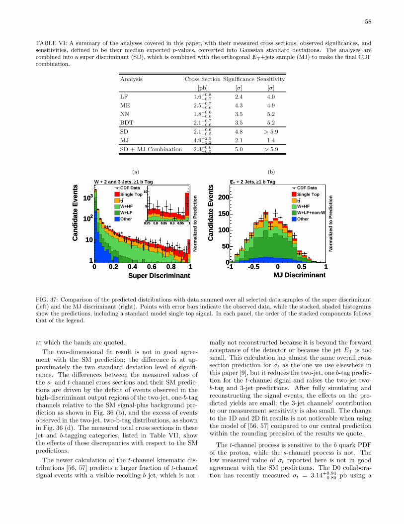
58

TABLE VI: A summary of the analyses covered in this paper, with their measured cross sections, observed significances, andsensitivities, defined to be their median expected p-values, converted into Gaussian standard deviations. The analyses arecombined into a super discriminant (SD), which is combined with the orthogonal /ET+jets sample (MJ) to make the final CDFcombination.

Analysis Cross Section Significance Sensitivity

[pb] [σ] [σ]

LF 1.6+0.8−0.7 2.4 4.0

ME 2.5+0.7−0.6 4.3 4.9

NN 1.8+0.6−0.6 3.5 5.2

BDT 2.1+0.7−0.6 3.5 5.2

SD 2.1+0.6−0.5 4.8 > 5.9

MJ 4.9+2.5−2.2 2.1 1.4

SD + MJ Combination 2.3+0.6−0.5 5.0 > 5.9

(a)

Super Discriminant0 0.2 0.4 0.6 0.8 1

Can

did

ate

Eve

nts

1

10

210

310

Super Discriminant0 0.2 0.4 0.6 0.8 1

Can

did

ate

Eve

nts

1

10

210

310

1 b Tag≥W + 2 and 3 Jets,

No

rmal

ized

to

Pre

dic

tio

n

CDF Data

Single Top

ttW+HFW+LFOther

0.75 0.8 0.85 0.9 0.95 10

5

10

0.75 0.8 0.85 0.9 0.95 10

5

10

(b)

MJ Discriminant-1 -0.5 0 0.5 1

Can

did

ate

Eve

nts

0

50

100

150

200

MJ Discriminant-1 -0.5 0 0.5 1

Can

did

ate

Eve

nts

0

50

100

150

200

TE 1 b Tag≥ + 2 Jets, CDF Data

Single Top

ttW+HFW+LF+non-WOther

No

rmal

ized

to

Pre

dic

tio

n

FIG. 37: Comparison of the predicted distributions with data summed over all selected data samples of the super discriminant(left) and the MJ discriminant (right). Points with error bars indicate the observed data, while the stacked, shaded histogramsshow the predictions, including a standard model single top signal. In each panel, the order of the stacked components followsthat of the legend.

at which the bands are quoted.

The two-dimensional fit result is not in good agree-ment with the SM prediction; the difference is at ap-proximately the two standard deviation level of signifi-cance. The differences between the measured values ofthe s- and t-channel cross sections and their SM predic-tions are driven by the deficit of events observed in thehigh-discriminant output regions of the two-jet, one-b-tagchannels relative to the SM signal-plus background pre-diction as shown in Fig. 36 (b), and the excess of eventsobserved in the two-jet, two-b-tag distributions, as shownin Fig. 36 (d). The measured total cross sections in thesejet and b-tagging categories, listed in Table VII, showthe effects of these discrepancies with respect to the SMpredictions.

The newer calculation of the t-channel kinematic dis-tributions [56, 57] predicts a larger fraction of t-channelsignal events with a visible recoiling b jet, which is nor-

mally not reconstructed because it is beyond the forwardacceptance of the detector or because the jet ET is toosmall. This calculation has almost the same overall crosssection prediction for σt as the one we use elsewhere inthis paper [9], but it reduces the two-jet, one b-tag predic-tion for the t-channel signal and raises the two-jet two-b-tag and 3-jet predictions. After fully simulating andreconstructing the signal events, the effects on the pre-dicted yields are small; the 3-jet channels’ contributionto our measurement sensitivity is also small. The changeto the 1D and 2D fit results is not noticeable when usingthe model of [56, 57] compared to our central predictionwithin the rounding precision of the results we quote.

The t-channel process is sensitive to the b quark PDFof the proton, while the s-channel process is not. Thelow measured value of σt reported here is not in goodagreement with the SM predictions. The D0 collabora-tion has recently measured σt = 3.14+0.94

−0.80 pb using a

59

(a) (b)

FIG. 38: Distributions of data and predictions for the SD and MJ analyses, where bins of similar s/b have been collected together(left). The points with error bars indicate the observed data, while the stacked, shaded histograms show the predictions,including a standard model single top signal. These distributions are integrated starting on the high-s/b side, and the resultingcumulative event counts are shown on the right, separately for the observed data, for the background-only prediction, and thesignal-plus-background prediction.

TABLE VII: A summary of the measured values of the singletop production cross section σs +σt using the super discrimi-nant analysis, separately for each of the non-overlapping finalstate categories, based on the number of jets, the number ofb tags, and the lepton category. Also listed are the MJ crosssection fit results by b-tagging category.

Category Cross Section [pb]

SD 2-Jet, 1-Tag, TLC 1.7+0.7−0.6

SD 2-Jet, 2-Tag, TLC 4.1+2.3−1.9

SD 3-Jet, 1-Tag, TLC 2.4+2.1−1.7

SD 3-Jet, 2-Tag, TLC 6.3+4.9−4.2

SD 2-Jet, 1-Tag, EMC 2.3+1.4−1.1

SD 2-Jet, 2-Tag, EMC 9.8+5.7−4.4

SD 3-Jet, 1-Tag, EMC 7.2+5.5−4.6

SD 3-Jet, 2-Tag, EMC 0.0+8.8−0.0

SD 2.1+0.6−0.5

MJ 2-Tag 5.9+4.2−3.7

MJ 1-Tag +jetprob 2.7+4.6−2.7

MJ 1-Tag 4.3+2.6−2.3

MJ 4.9+2.5−2.2

SD + MJ Combination 2.3+0.6−0.5

data sample corresponding to 2.3 fb−1 of integrated lu-minosity [105], which is larger than the standard modelprediction. Taken together, there is insufficient evidenceto exclude a standard model explanation of the results.

XIII. SUMMARY

The observation of single top quark production posesmany difficult experimental challenges. CDF performsthis analysis in proton-antiproton collisions at 1.96 TeVin events with a leptonically decaying W boson and jets.The low signal-to-background ratio in the data samplespassing our selection requirements necessitates precisemodeling of the signal and background kinematic dis-tributions with matrix-element-based Monte Carlo gen-erators using full parton showering and detailed detec-tor simulation, and also requires the normalization ofthe dominant background rates to measured rates insideband data samples. The small signals and large,uncertain background processes also require us to takemaximum advantage of the expected kinematic and fla-vor differences between the signals and the backgroundprocesses. We develop novel, powerful techniques forcombining information from several observable quanti-ties computed for each event. We purify a subsample ofsingle top quark events with a predicted signal to back-ground ratio exceeding 5:1 from a sample starting witha signal to background ratio of 1:16 after b-tagging.

Our final discriminant variables are functions of manykinematic and b-tagging variables. Incorrect modeling ofone or more variables, or even of the correlations betweenvariables, can bias the results. We therefore evaluate anexhaustive list of systematic uncertainties which affectthe predicted signal and background components’ ratesand kinematic distributions, including both theoreticaluncertainties and uncertainties which arise from discrep-ancies observed between the data and the simulations incontrol regions. The correlations between the systematic

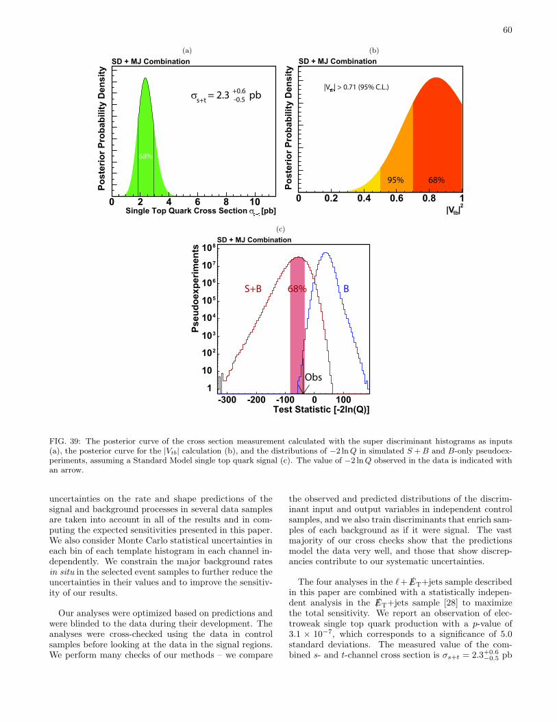
60

(a) (b)

(c)

FIG. 39: The posterior curve of the cross section measurement calculated with the super discriminant histograms as inputs(a), the posterior curve for the |Vtb| calculation (b), and the distributions of −2 lnQ in simulated S +B and B-only pseudoex-periments, assuming a Standard Model single top quark signal (c). The value of −2 lnQ observed in the data is indicated withan arrow.

uncertainties on the rate and shape predictions of thesignal and background processes in several data samplesare taken into account in all of the results and in com-puting the expected sensitivities presented in this paper.We also consider Monte Carlo statistical uncertainties ineach bin of each template histogram in each channel in-dependently. We constrain the major background ratesin situ in the selected event samples to further reduce theuncertainties in their values and to improve the sensitiv-ity of our results.

Our analyses were optimized based on predictions andwere blinded to the data during their development. Theanalyses were cross-checked using the data in controlsamples before looking at the data in the signal regions.We perform many checks of our methods – we compare

the observed and predicted distributions of the discrim-inant input and output variables in independent controlsamples, and we also train discriminants that enrich sam-ples of each background as if it were signal. The vastmajority of our cross checks show that the predictionsmodel the data very well, and those that show discrep-ancies contribute to our systematic uncertainties.

The four analyses in the ℓ+ /ET+jets sample describedin this paper are combined with a statistically indepen-dent analysis in the /ET+jets sample [28] to maximizethe total sensitivity. We report an observation of elec-troweak single top quark production with a p-value of3.1 × 10−7, which corresponds to a significance of 5.0standard deviations. The measured value of the com-bined s- and t-channel cross section is σs+t = 2.3+0.6

−0.5 pb

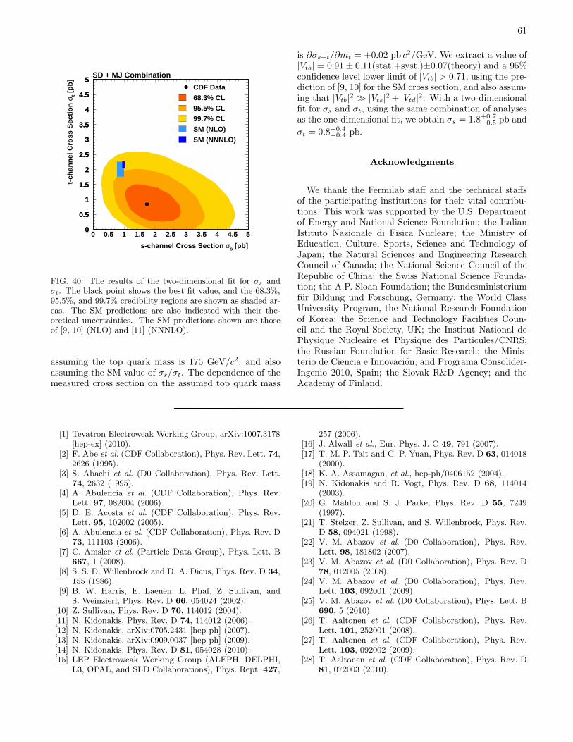
61

0

0.5

1

1.5

2

2.5

3

3.5

4

4.5

5SD + MJ Combination

0 0.5 1 1.5 2 2.5 3 3.5 4 4.5 50

0.5

1

1.5

2

2.5

3

3.5

4

4.5

5

s-channel Cross Section σs [pb]

t-ch

ann

el C

ross

Sec

tio

n σ

t [p

b]

CDF Data68.3% CL95.5% CL99.7% CLSM (NLO)SM (NNNLO)

FIG. 40: The results of the two-dimensional fit for σs andσt. The black point shows the best fit value, and the 68.3%,95.5%, and 99.7% credibility regions are shown as shaded ar-eas. The SM predictions are also indicated with their the-oretical uncertainties. The SM predictions shown are thoseof [9, 10] (NLO) and [11] (NNNLO).

assuming the top quark mass is 175 GeV/c2, and alsoassuming the SM value of σs/σt. The dependence of themeasured cross section on the assumed top quark mass

is ∂σs+t/∂mt = +0.02 pb c2/GeV. We extract a value of|Vtb| = 0.91± 0.11(stat.+syst.)±0.07(theory) and a 95%confidence level lower limit of |Vtb| > 0.71, using the pre-diction of [9, 10] for the SM cross section, and also assum-ing that |Vtb|2 ≫ |Vts|2 + |Vtd|2. With a two-dimensionalfit for σs and σt, using the same combination of analysesas the one-dimensional fit, we obtain σs = 1.8+0.7

−0.5 pb and

σt = 0.8+0.4−0.4 pb.

Acknowledgments

We thank the Fermilab staff and the technical staffsof the participating institutions for their vital contribu-tions. This work was supported by the U.S. Departmentof Energy and National Science Foundation; the ItalianIstituto Nazionale di Fisica Nucleare; the Ministry ofEducation, Culture, Sports, Science and Technology ofJapan; the Natural Sciences and Engineering ResearchCouncil of Canada; the National Science Council of theRepublic of China; the Swiss National Science Founda-tion; the A.P. Sloan Foundation; the Bundesministeriumfur Bildung und Forschung, Germany; the World ClassUniversity Program, the National Research Foundationof Korea; the Science and Technology Facilities Coun-cil and the Royal Society, UK; the Institut National dePhysique Nucleaire et Physique des Particules/CNRS;the Russian Foundation for Basic Research; the Minis-terio de Ciencia e Innovacion, and Programa Consolider-Ingenio 2010, Spain; the Slovak R&D Agency; and theAcademy of Finland.

[1] Tevatron Electroweak Working Group, arXiv:1007.3178[hep-ex] (2010).

[2] F. Abe et al. (CDF Collaboration), Phys. Rev. Lett. 74,2626 (1995).

[3] S. Abachi et al. (D0 Collaboration), Phys. Rev. Lett.74, 2632 (1995).

[4] A. Abulencia et al. (CDF Collaboration), Phys. Rev.Lett. 97, 082004 (2006).

[5] D. E. Acosta et al. (CDF Collaboration), Phys. Rev.Lett. 95, 102002 (2005).

[6] A. Abulencia et al. (CDF Collaboration), Phys. Rev. D73, 111103 (2006).

[7] C. Amsler et al. (Particle Data Group), Phys. Lett. B667, 1 (2008).

[8] S. S. D. Willenbrock and D. A. Dicus, Phys. Rev. D 34,155 (1986).

[9] B. W. Harris, E. Laenen, L. Phaf, Z. Sullivan, andS. Weinzierl, Phys. Rev. D 66, 054024 (2002).

[10] Z. Sullivan, Phys. Rev. D 70, 114012 (2004).[11] N. Kidonakis, Phys. Rev. D 74, 114012 (2006).[12] N. Kidonakis, arXiv:0705.2431 [hep-ph] (2007).[13] N. Kidonakis, arXiv:0909.0037 [hep-ph] (2009).[14] N. Kidonakis, Phys. Rev. D 81, 054028 (2010).[15] LEP Electroweak Working Group (ALEPH, DELPHI,

L3, OPAL, and SLD Collaborations), Phys. Rept. 427,

257 (2006).[16] J. Alwall et al., Eur. Phys. J. C 49, 791 (2007).[17] T. M. P. Tait and C. P. Yuan, Phys. Rev. D 63, 014018

(2000).[18] K. A. Assamagan, et al., hep-ph/0406152 (2004).[19] N. Kidonakis and R. Vogt, Phys. Rev. D 68, 114014

(2003).[20] G. Mahlon and S. J. Parke, Phys. Rev. D 55, 7249

(1997).[21] T. Stelzer, Z. Sullivan, and S. Willenbrock, Phys. Rev.

D 58, 094021 (1998).[22] V. M. Abazov et al. (D0 Collaboration), Phys. Rev.

Lett. 98, 181802 (2007).[23] V. M. Abazov et al. (D0 Collaboration), Phys. Rev. D

78, 012005 (2008).[24] V. M. Abazov et al. (D0 Collaboration), Phys. Rev.

Lett. 103, 092001 (2009).[25] V. M. Abazov et al. (D0 Collaboration), Phys. Lett. B

690, 5 (2010).[26] T. Aaltonen et al. (CDF Collaboration), Phys. Rev.

Lett. 101, 252001 (2008).[27] T. Aaltonen et al. (CDF Collaboration), Phys. Rev.

Lett. 103, 092002 (2009).[28] T. Aaltonen et al. (CDF Collaboration), Phys. Rev. D

81, 072003 (2010).

62

[29] A. Abulencia et al. (CDF Collaboration), J. Phys. G 34,2457 (2007).

[30] D. E. Acosta et al. (CDF Collaboration), Phys. Rev. D71, 032001 (2005).

[31] D. E. Acosta et al. (CDF Collaboration), Phys. Rev. D71, 052003 (2005).

[32] C. S. Hill (CDF Collaboration), Nucl. Instrum. MethodsA 530, 1 (2004).

[33] A. Sill (CDF Collaboration), Nucl. Instrum. Methods A447, 1 (2000).

[34] A. A. Affolder et al. (CDF Collaboration), Nucl. In-strum. Methods A 453, 84 (2000).

[35] A. A. Affolder et al. (CDF Collaboration), Nucl. In-strum. Methods A 526, 249 (2004).

[36] F. Abe et al. (CDF Collaboration), Phys. Rev. Lett. 68,1104 (1992).

[37] L. Balka et al. (CDF Collaboration), Nucl. Instrum.Methods A 267, 272 (1988).

[38] M. G. Albrow et al. (CDF Collaboration), Nucl. In-strum. Methods A 480, 524 (2002).

[39] S. Bertolucci et al. (CDF Collaboration), Nucl. Instrum.Methods A 267, 301 (1988).

[40] G. Apollinari, K. Goulianos, P. Melese, and M. Lind-gren, Nucl. Instrum. Methods A 412, 515 (1998).

[41] G. Ascoli et al., Nucl. Instrum. Methods A 268, 33(1988).

[42] R. Blair et al. (CDF Collaboration), FERMILAB-PUB-96-390-E (1996).

[43] A. Artikov et al., Nucl. Instrum. Methods A 538, 358(2005).

[44] D. Acosta et al., Nucl. Instrum. Methods A 494, 57(2002).

[45] S. Klimenko, J. Konigsberg, and T. M. Liss,FERMILAB-FN-0741 (2003).

[46] E. J. Thomson et al., IEEE Trans. Nucl. Sci. 49, 1063(2002).

[47] R. Downing et al., Nucl. Instrum. Methods A 570, 36(2007).

[48] G. Gomez-Ceballos et al., Nucl. Instrum. Methods A518, 522 (2004).

[49] A. Bhatti et al., Nucl. Instrum. Methods A 566, 375(2006).

[50] F. Maltoni and T. Stelzer, J. High Energy Phys. 02, 027(2003).

[51] H. L. Lai et al. (CTEQ Collaboration), Eur. Phys. J. C12, 375 (2000).

[52] Z. Sullivan, Phys. Rev. D 72, 094034 (2005).[53] T. Sjostrand et al., Comput. Phys. Commun. 135, 238

(2001).[54] T. Sjostrand, S. Mrenna, and P. Skands, J. High Energy

Phys. 05, 026 (2006).[55] E. E. Boos, V. E. Bunichev, L. V. Dudko, V. I. Savrin,

and A. V. Sherstnev, Phys. Atom. Nucl. 69, 1317(2006).

[56] J. M. Campbell, R. Frederix, F. Maltoni, and F. Tra-montano, Phys. Rev. Lett. 102, 182003 (2009).

[57] J. M. Campbell, R. Frederix, F. Maltoni, and F. Tra-montano, J. High Energy Phys. 10, 042 (2009).

[58] Y. L. Dokshitzer, Sov. Phys. JETP 46, 641 (1977).[59] V. N. Gribov and L. N. Lipatov, Sov. J. Nucl. Phys. 15,

438 (1972).[60] G. Altarelli and G. Parisi, Nucl. Phys. B 126, 298

(1977).[61] J. Lueck, diplom Thesis, University of Karlsruhe, 2006,

FERMILAB-MASTERS-2006-01.[62] J. Lueck, Ph.D. Thesis, University of Karlsruhe, 2009,

FERMILAB-THESIS-2009-33.[63] G. Abbiendi et al. (OPAL Collaboration), Eur. Phys. J.

C 8, 217 (1999).[64] J. Donini et al., Nucl. Instrum. Methods A 596, 354

(2008).[65] S. Jadach, Z. Was, R. Decker, and J. H. Kuhn, Comput.

Phys. Commun. 76, 361 (1993).[66] R. Bonciani, S. Catani, M. L. Mangano, and P. Nason,

Nucl. Phys. B 529, 424 (1998).[67] M. Cacciari, S. Frixione, M. L. Mangano, P. Nason, and

G. Ridolfi, J. High Energy Phys. 04, 068 (2004).[68] E. L. Berger and H. Contopanagos (1997), arXiv:hep-

ph/9706356.[69] J. M. Campbell and R. K. Ellis, Phys. Rev. D 60,

113006 (1999).[70] M. L. Mangano, M. Moretti, F. Piccinini, R. Pittau,

and A. D. Polosa, J. High Energy Phys. 07, 001 (2003).[71] T. Aaltonen et al. (CDF Collaboration), Phys. Rev.

Lett. 100, 102001 (2008).[72] Z. Bern, L. J. Dixon, D. A. Kosower, and S. Weinzierl,

Nucl. Phys. B 489, 3 (1997).[73] Z. Bern, L. J. Dixon, and D. A. Kosower, Nucl. Phys.

B 513, 3 (1998).[74] W. T. Giele, S. Keller, and E. Laenen, Nucl. Phys. Proc.

Suppl. 51C, 255 (1996).[75] R. K. Ellis and S. Veseli, Phys. Rev. D 60, 011501

(1999).[76] F. Febres Cordero, L. Reina, and D. Wackeroth, Phys.

Rev. D 74, 034007 (2006).[77] J. M. Campbell, R. K. Ellis, F. Maltoni, and S. Willen-

brock, Phys. Rev. D 75, 054015 (2007).[78] J. M. Campbell et al., Phys. Rev. D 79, 034023 (2009).[79] F. F. Cordero, L. Reina, and D. Wackeroth, Phys. Rev.

D 80, 034015 (2009).[80] T. Aaltonen et al. (CDF Collaboration), Phys. Rev. D

77, 011108 (2008).[81] T. Aaltonen et al. (CDF Collaboration), Phys. Rev.

Lett. 100, 091803 (2008).[82] S. Richter, Ph.D. Thesis, University of Karlsruhe, 2007,

FERMILAB-THESIS-2007-35.[83] M. Feindt and U. Kerzel, Nucl. Instrum. Methods A

559, 190 (2006).[84] C. P. Yuan, Phys. Rev. D 41, 42 (1990).[85] K. Ackerstaff et al. (OPAL Collaboration), Eur. Phys.

J. C 1, 425 (1998).[86] S. R. Budd, Ph.D. Thesis, University of Illinois, 2008,

FERMILAB-THESIS-2008-41.[87] K. Nakamura, Ph.D. Thesis, University of Tsukuba,

2009, FERMILAB-THESIS-2009-13.[88] P. J. Dong, Ph.D. Thesis, University of California at

Los Angeles, 2008, FERMILAB-THESIS-2008-12.[89] I. Murayama, H. Watanabe and K. Hagiwara, Tech.

Rep. 91-11, KEK (1992).[90] A. Genz and A. Malik, J. Comput. Appl. Math. 6,

295 (1980), implemented as CERNLIB algorithm D120,documented in http://wwwasdoc.web.cern.ch/wwwasdoc/shortwrupsdir/d151/top.html.

[91] T. Hahn, Comput. Phys. Commun. 168, 78 (2005).[92] J. Neyman and E. Pearson, Phil. Trans. of the Royal

Soc. of London A 31, 289 (1933).[93] A. Papaikonomou, Ph.D. Thesis, University of Karl-

sruhe, 2009, FERMILAB-THESIS-2009-21.

63

[94] A. Hocker et al., PoS ACAT, 040 (2007).[95] B. Casal Larana, Ph.D. Thesis, University of Cantabria,

2010, FERMILAB-THESIS-2010-04.[96] C. Gini, Variabilita e Mutabilita, (1912), reprinted in

Memorie di Metodologica Statistica, edited by E. Pizettiand T. Savemini, Rome: Libreria Eredi Virgilio Veschi,1955.

[97] Y. Freund and R. Schapire, Computer and System Sci-ence 55, 119 (1997).

[98] L. Breiman, J. Friedman, R. Olshen, and C. Stone, Clas-sification and Regression Trees (Wadsworth, 1984).

[99] A. Abulencia et al. (CDF Collaboration), Phys. Rev. D73, 032003 (2006).

[100] A. D. Martin, R. G. Roberts, W. J. Stirling, and R. S.Thorne, Eur. Phys. J. C 4, 463 (1998).

[101] C. Amsler et al. (Particle Data Group), Phys. Lett. B667, 324 (2008).

[102] T. Aaltonen et al. (CDF Collaboration), Phys. Rev.Lett. 102, 021802 (2009).

[103] K. Stanley and R. Miikkulainen, Evolutionary Compu-ation 10, 99 (2002).

[104] Tevatron Electroweak Working Group, arXiv:0908.2171(2009).

[105] V. M. Abazov et al. (D0 Collaboration), Phys. Lett. B682, 363 (2010).