The Modeling Process of the Materials Management System in a Manufacturing Company Based on the...
18
79 The Modeling Process of the Materials Management System in a Manufacturing Company Based on the System Dynamics Method Małgorzata Baran * Abstract The arcle presents the steps of modeling of the material management system in a manufacturing company. First, the modeling procedures indicang by Forrester, Łukaszewicz, Souček, Tarajkowski and Sterman were described and the essence of materials management in a manufacturing company was presented. Next, modeling of the materials management system was shown - step by step. Inially, the variables of the mental model connected with materials were defined, then variables in casual loop diagrams were linked. Diagrams were transformed into a simulaon model that has been verified. The validaon of the simulaon model was conducted by using the following methods: assessing the correctness of the boundary of modeling, adequacy of the model structure and adopted values (constants) compared with available knowledge about the modelled system; test of the accuracy and consistency of the units of variables adopted in the model and test of the model behavior in extreme condions. The study endpoints included the simulaon of the model on empirical data, which were collected in the company Alpha and test of the “what ... if ...”. The test showed that the small changes in control norms (constants), which control the system, could have influenced to more raonal management of that system. Keywords: simulaon modeling, system dynamics, materials in a manufacturing company. Introducon Modeling should be understood as an experimental or mathemacal method for invesgang complex systems, phenomena and processes (technical, physical, chemical, economic, social) on the basis of construcng models. One of the methods of the modeling is a method of System Dynamics (Łukaszewicz, 1975; Coyle, 1977; Wąsik, 1983; Richardson, 1996a, 1996b; Radosiński, 2001; Śliwa, 1994; 2001, 2012; Kasperska, 2005; Senge, 2006; Łatuszyńska, 2008; Krupa, 2008; Baran, 2009, 2010a, 2010b, 2010c). The method was developed in the late 50-ies of XX century by J. Forrester (1961; 1969; 1971; 1972). It * Małgorzata Baran, Ph.D., University of Rzeszów, [email protected].
Transcript of The Modeling Process of the Materials Management System in a Manufacturing Company Based on the...

79
The Modeling Process of the Materials Management System in a Manufacturing Company Based on the System Dynamics
Method
Małgorzata Baran*
AbstractThe article presents the steps of modeling of the material management system in a manufacturing company. First, the modeling procedures indicating by Forrester, Łukaszewicz, Souček, Tarajkowski and Sterman were described and the essence of materials management in a manufacturing company was presented. Next, modeling of the materials management system was shown - step by step. Initially, the variables of the mental model connected with materials were defined, then variables in casual loop diagrams were linked. Diagrams were transformed into a simulation model that has been verified. The validation of the simulation model was conducted by using the following methods: assessing the correctness of the boundary of modeling, adequacy of the model structure and adopted values (constants) compared with available knowledge about the modelled system; test of the accuracy and consistency of the units of variables adopted in the model and test of the model behavior in extreme conditions. The study endpoints included the simulation of the model on empirical data, which were collected in the company Alpha and test of the “what ... if ...”. The test showed that the small changes in control norms (constants), which control the system, could have influenced to more rational management of that system.Keywords: simulation modeling, system dynamics, materials in a manufacturing company.
IntroductionModeling should be understood as an experimental or mathematical method for investigating complex systems, phenomena and processes (technical, physical, chemical, economic, social) on the basis of constructing models. One of the methods of the modeling is a method of System Dynamics (Łukaszewicz, 1975; Coyle, 1977; Wąsik, 1983; Richardson, 1996a, 1996b; Radosiński, 2001; Śliwa, 1994; 2001, 2012; Kasperska, 2005; Senge, 2006; Łatuszyńska, 2008; Krupa, 2008; Baran, 2009, 2010a, 2010b, 2010c). The method was developed in the late 50-ies of XX century by J. Forrester (1961; 1969; 1971; 1972). It
* Małgorzata Baran, Ph.D., University of Rzeszów, [email protected].

System Theories and Practice, M. Baran, K. Śliwa (Eds.)
80 / The Modeling Process of the Materials Management System in a Manufacturing Company Based on the System Dynamics Method
is used to build simulation models of complex systems, including economic systems, and to explore and investigate their dynamic behaviour. The main objective of modeling using the System Dynamics is not only a graphical representation of the structure of the system, its complexity and relations, but also look for possible solutions to the problems, which are included in it. Experiments carried out in the virtual world help design the real world (perceived), and real world experiences provide information to the virtual world. A clear and unambiguous indication of the problem (or problems) for which the system will be modelled is one of the most important aspects of modeling.
The purpose of this article is to present the steps of modeling of the material management system in a manufacturing company. The basis for the construction of the model was the model built by Sterman (2000, p.727). The model was slightly modified by the author (and management of the Alpha**) and adopted to the realities of business activity of Alpha enterprise. The simulation model uses empirical data collected in that company.
Literature reviewGeneral principles of modeling systems have been presented by Forrester in Principles of Systems (1971). In thirty one points he included, among others, guidelines for determining the boundaries of the system, linking variables in feedback loops, determining accumulations, flows, information variables in systems and the principles of simulation.
A pioneer in the convention modeling methods in Polish literature was Łukaszewicz (1975). He pointed out 10 steps for modeling and analysis of specific, investigated system from identification and formulation of the problem by identification the information feedback loop connecting decision rules, then construction of the structural and mathematical model, verification model and ending with implementation of the system changes, which are connected with experimental results conducted on the model.
Souček (1979) draws attention to the four basic principles of construction of models, emphasizing, that each system is made of tanks, which are combination of channels, through which items flow streams from one tank to another. The size of streams of individual elements in the system is created on the basis of decisions, that must be understood as a process of converting information about system into control signals of flowing streams in the system. For any decision included in the model, the rule that specifies how and on what information decisions will be made, should be established. During modeling, each modeller should also take into account exogenous
** Executives asked to change the name of your company.

Journal of Entrepreneurship Management and Innovation (JEMI), Volume 9, Issue 2, 2013: 79-96
81 Małgorzata Baran /
variables of the system, which should be regarded as a relatively independent of the explored system.
Tarajkowski (2008) points to the existence of the eight essential steps of modeling systems, assigning each stage the specific tasks, which must be performed. In the first stage it is necessary to identify an object (or system issues) to be modelled. One can come here for various difficulties both methodological and cognitive. Therefore it is important to present the issues, that makes it possible to distinguish it from all others and to collect such information of the system, which will remain in alignment with the real world. The second step is to determine how modelled system behaves from the point of view of logic, and what tasks meet. The third and fourth stage focus on a graphical presentation of memory system architecture. The structure of the system initially is shown with simple graphs, identifying common feedback and their types, and next, as a cause - effect diagram including accumulation, flow, and auxiliary variables. The fifth step is a quantification of the model and determination of the characteristic behaviour, that characterizes the individual variables in the model, as well as the identification of delay. It allows for building relevant equations and making a selection of simulation program in the sixth stage. In the seventh stage of the research the correctness of the model by comparing the historical values of variables with simulation values and modification the simulation model in case of detecting different types of discrepancies are carried out. And at the end, in the eighth stage, one ought to determine the final version of the model, conduct a number of predictive tests, test various hypotheses and strategies and acceptance of the final results.
Research methodsIn this article, the authoress is used the modeling procedure of systems specified by Sterman (2000, p. 86). The management of Alpha made that choice. The Systems Dynamics method isn`t widely practised in Poland and the management trusted the foreign expert. Sterman suggests the following steps, when we working with a model of the selected system:
Selection of the problem or issue that will be subject of process of 1) modeling and indication for him:
modeling boundaries; •key variables, that fully present the system; •the time horizon, which is such a time period, which takes into account •both the past behavior of the variables of the problem (based on the historical data), as well as their behavior in the future, possible to identify thanks to the subsequent simulation; the time horizon should

System Theories and Practice, M. Baran, K. Śliwa (Eds.)
82 / The Modeling Process of the Materials Management System in a Manufacturing Company Based on the System Dynamics Method
be long enough to be able to capture all interactions that may occur between these variables.
Formulation of dynamic hypotheses by considering how the given 2) problems and phenomena in the modelled system are formed, what kind of behaviour they are characterized and building structure of model using tools, such as:
a list of endogenous variables (characterizing for investigated system), •exogenous variables (external factors constantly affecting the system) and the variables excluded from the model;general sketches of the subsystems, that build the whole system, •taking into account endogenous and exogenous variables;depending diagrams, that make it possible to capture the cause - effect •relationships between variables and determine kinds of feedback;accumulation and flow maps, which clearly indicate the accumulation •variables, that are the heart of the model, variables having an effect on the accumulation (flows) and other necessary auxiliary variables (information);diagrams, that focus on strategies and direction of action for the •management of individual flows, taking into account the information flowing and delays, which arising from the waiting time between the decision, their implementation and consequences.
Construction of the simulation model (using appropriate software), in 3) which:
variable will be assigned by the appropriate numerical data (value); •variables will be linked to the corresponding equations; •will set the initial values for each accumulation. •
Testing the model, which usually consists of the following processes:4) assessing the adequacy of the choice of the boundary model structure •compared with the available knowledge of the modelled system;evaluating the accuracy and consistency of assumed units of the •variables in the model;assessing consistency adopted parameter values with the actual •values;testing the model under extreme conditions; •estimating the ability of the model (e.g. using statistical methods) to •reproduce the real behaviour of the system.
Design and evaluation of different strategies resulting from observing 5) the behaviour of the variables in the model, testing possible solutions.
In realization of the subsequent steps of the modeling process, management of Alpha tried to give answers to supporting questions, which summarized in Table 1.

Journal of Entrepreneurship Management and Innovation (JEMI), Volume 9, Issue 2, 2013: 79-96
83 Małgorzata Baran /
Table 1. Supporting questions in modeling process
Step of the modeling process
Supporting questions
1. Selection of the problem or issue that will be subject of process of modeling
What is the problem? •What key variables directly related to the problem should be •considered?What is the time interval needed to capture the essential behavior •of the variables in the model?What behavior was characterized by the key variables in the past •and how they might behave in the future?
2. Dynamic hypotheses
What are the current theories explaining the activity of the •system?Which key variables will be accepted as endogenous and •exogenous?Assuming the boundary of modeling, which previously adopted •variables should be excluded from the model?Can one identify any specific subsystems of the whole system? •What kinds of feedback loops exist between the variables? What •is the cause and what is effect?Which of accepted variables are accumulations and flows? •Are there any auxiliary variables? •In which areas in the model, will there be a delay? What will be •the delays type and nature?Are there specific strategies for targeting the flows? •
3. Construction of the simulation model
What value will the variables in the model take? •What type of equations will be connected with chosen •variables?What are the initial values for accumulations? •How long are the delays? •
4. Testing the model Is the behavior of the variables in the model consistent with •reality and historical data?What is the behavior of the variables under changed conditions? •How does model behave under extreme conditions? •
5. The project’s strategy and its assessment
What changes in policies related to the management of the •system can be improved? How to present them in the model?Will the changes solve the problems considered in the system? •What are the consequences of the modifications? • Other questions like: „what ... if ....? •
Source: Own elaboration on basis of Sterman (2000).
The modeling process is an iterative process. The initial plan dictates the frame and the scope of work in the model, but a more detailed analysis and understanding of the essence of the issues often results in the return of thinking of modeling - the results of the relevant step force to return and improve the previous steps.

System Theories and Practice, M. Baran, K. Śliwa (Eds.)
84 / The Modeling Process of the Materials Management System in a Manufacturing Company Based on the System Dynamics Method
Analysis and study
Materials management in a manufacturing companyMaterials management in a manufacturing company is closely related to its basic activity and results of conceptual preparation of production (Sołtysiński, 1963; Bik, 1974; Liwowski, 1977; Skowronek, 1989). To ensure timely delivery of materials to the production process, it is necessary to determine the type of manufactured goods and their quantity. The next step is to establish standards of material usage per unit of product. This allows for the calculation of demand resulting from the assumed production plans. If you plan to purchase due to the size of demand, stocks held as collateral against the occurrence of discontinuities in the flow of materials targeted for production should be also included. Stocks may be current and minimum. Current stocks are associated with the progressive wear of the materials in the production process and often end before the next supply of materials. Their size is therefore dependent on supply frequency and size of a single delivery. Minimal stocks are protection against delays in deliveries and are used only when a company wears fully supply current. In determining the size of the store, the minimum time should be specified, in which it will be possible to maintain the undisturbed course of production, thanks to the supply from the minimum stocks, while the current stocks are exhausted.
The main warehouse processes related to material management may include the following (Niemczyk, 2010, p. 119):
receiving the materials from external suppliers, both in the physical •sense as the unloading of materials, as well as in terms of register in the form of reports of acceptance;storage of materials associated with the location of stocks in the •warehouse;completing, including taking materials in accordance with the •assortment and quantity specification to create a collection of materials required for specific stages of production;handing over materials connected to the physical delivery of a set •of completed materials to the production line confirmed by delivery reports.
Modeling of material management system in the company AlphaAlpha is a medium-size clothing company based in Podkarpacie, in Poland. The scope of business includes sewing smart men’s trousers to the Polish market and to overseas markets. Customers are primarily other clothing companies, clothing stores and warehouses, as well as individuals. For the production of trousers, company need the following materials: a top cloth, buttress (stiffening strip bar), plywood, zip, buttons and thread.

Journal of Entrepreneurship Management and Innovation (JEMI), Volume 9, Issue 2, 2013: 79-96
85 Małgorzata Baran /
Initially, the key mental model variables of the system of materials management at Alpha have been defined. The variables are presented in Table 2.
Table 2. Variables of mental model
Variable Description
Receipt of materialsStream of materials flowing to the warehouse of materials, resulting directly from “ Desired size of the supply of materials “
Desired quantity of the supply of materials
Desired quantity of materials to be delivered to the company, resulting from the sum of the variables “Desired weekly usage of materials“ and “Adjustment for materials inventory“
Desired weekly usage of materials
Desired amount of raw materials needed to produce finished products, resulting from “Materials usage per unit“ and “Desired production“
Materials usage per unit Number of sets of materials needed to produce one unit of the finished product
Desired production The level of desired production, which results from orders – exogenous variable
Adjustment for materials inventory
Adjustment the quantity of materials to the desired level
Desired level of materials inventory
Number of sets of materials needed for the manufacturing process, resulting from “Desired weekly usage of materials“ and “Time of maintaining stocks“
Time to correct the level of materials inventory
The time between placing an order for the materials, and the actual receipt from the supplier
Minimum level of materials inventory
The lowest number of stocks of materials, which the company maintains in warehouse of materials
Time maintaining materials inventory
Planned length of time, in which the company keeps inventory of materials in the warehouse of materials
Materials inventory The quantities of materials inventory in warehouse of materials, increased by “Receipt of materials“ and decreased by “Usage of materials“
Usage of materials A stream of materials issued to production
Limit for usage of materials per week
Possible amount of materials that can be given to the production, due to their availability in the current stock of materials and depended on time to prepare them for usage
Time to prepare materials for usage
The duration of all activities necessary for the preparation of materials for giving them on the production line
Possible production of the availability of materials
Possible production volume of finished products, due to the availability of materials taken from stocks of materials
In the next step a diagram showing direct and indirect cause - effect relationships between variables was constructed (Figure 1).

System Theories and Practice, M. Baran, K. Śliwa (Eds.)
86 / The Modeling Process of the Materials Management System in a Manufacturing Company Based on the System Dynamics Method
Figure 1. Cause – effect diagram of the materials management systemSource: Author’s elaboration in Vensim DSS Version 5.9e.
Next the authoress converted the above diagram into a simulation model of the system of materials management at Alpha. Mental model variables were presented as mathematical variables and constants. Needed coefficients were added. The accumulation, flow variables and auxiliary variables (information) and the mathematical relationships existing between them were indicated. Model was built in the simulation systems Vensim DSS Version 5.9e, so the mathematical apparatus was presented with the available functions and mathematical expressions.
The Figure 2 shows the resulting model, consisting of two parts. The first part of the model is related to the stocks of materials A and the second - the stocks of materials B. The stocks of materials A include: buttress (stiffening strip bar), plywood, zip, buttons and thread. The stocks of materials B include: the top cloth. Separation of materials A and B resulted in the similarity to each other by “Time to correct the level of materials inventory”. In case of materials A, that time was 0.2 week and in case of materials B – 2 weeks. These differences have an impact on the behaviour of the individual parts of the model.
While the “Materials A inventory” is used in each case, “Materials B inventory” can be activated or not, by changing the “Turn on materials B inventory”. The variables and constants in the model “Materials B inventory”
JOURNAL OF ENTREPRENEURSHIP, MANAGEMENT AND INNOVATION
JOURNAL OF ENTREPRENEURSHIP MANAGEMENT AND INNOVATION,a scientific journal published by Nowy Sacz School of Business – National-Louis University
www.jemi.edu.plul. Zielona 27, 33-
6
Time maintaining materials inventoryPlanned length of time, in which the company keeps inventory of materials in the warehouse of materials
Materials inventoryThe quantities of materials inventory in warehouse of materials, increased by "Receipt of materials" and decreased by "Usage of materials"
Usage of materials A stream of materials issued to production
Limit for usage of materials per weekPossible amount of materials that can be given to the production, due to their availability in the current stock of materials and depended on time to prepare them for usage
Time to prepare materials for usageThe duration of all activities necessary for the preparation of materials for giving them onthe production line
Possible production of the availability of materials
Possible production volume of finished products, due to the availability of materials taken from stocks of materials
In the next step a diagram showing direct and indirect cause - effect relationships between variables was constructed (Figure 1).
Possible production ofthe availability of
materials
Materials inventory
Receipt of materialsUsage of materials
+
Materials usage perunit
-
Desired weekly usageof materials
+
+
Limit for usage ofmaterials per week
+
Time to preparematerials for usage
-
Desired level ofmaterials inventory
Time maintainingmaterials inventory
+
Desired quantity ofthe supply of
materials
+
Adjustment formaterials inventory
-
Time to correct thelevel of materials
inventory
-
+
+
+
B1
B2
<Desiredproduction>
+
+
+
Minimum level ofmaterials inventory
+
+
-
B3
+
FIGURE 1. Cause – effect diagram of the materials management system
Source: Author’s elaboration in Vensim DSS Version 5.9e.Next the authoress converted the above diagram into a simulation model of the system of
materials management at Alpha. Mental model variables were presented as mathematical variables and constants. Needed coefficients were added. The accumulation, flow variablesand auxiliary variables (information) and the mathematical relationships existing between them were indicated. Model was built in the simulation systems Vensim DSS Version 5.9e, so the mathematical apparatus was presented with the available functions and mathematical expressions.
The Figure 2 shows the resulting model, consisting of two parts. The first part of the model is related to the stocks of materials A and the second - the stocks of materials B. The stocks of materials A include: buttress (stiffening strip bar), plywood, zip, buttons and thread.The stocks of materials B include: the top cloth. Separation of materials A and B resulted inthe similarity to each other by “Time to correct the level of materials inventory”. In case of

Journal of Entrepreneurship Management and Innovation (JEMI), Volume 9, Issue 2, 2013: 79-96
87 Małgorzata Baran /
are the same as in the “Materials A inventory” but to distinguish their name, the authoress placed symbol B.
Figure 2. Simulation model of the materials management systemSource: Author’s elaboration in Vensim DSS Version 5.9e.
Accumulation variables in above models are:a) “Materials A inventory” increased by a flow variable “Receipt of
materials A” and reduced by a flow variable “Usage of materials A”;b) “Materials B inventory” increased by a flow variable “Receipt of
materials B” and reduced by a flow variable “Usage of materials B”.Definitions of variables and mathematical constants contained in parts
of the simulation model are presented in Table 3.

System Theories and Practice, M. Baran, K. Śliwa (Eds.)
88 / The Modeling Process of the Materials Management System in a Manufacturing Company Based on the System Dynamics Method
Table 3. Definitions of model vabiables/constans
Variable/constant The definition of a variable / constant Unit
Desired production
[(0,0)-(51,250)],(0,61),(1,135),(2,0),(3,8),(4,29),(5,10),(6,47),(7,37),(8,87), (9,76),(10,61),(11,185),(12,169),(13,216),(14,72),(15,118),(16,79),(17,143),(18,69),(19,128),(20,58),(21,35),(22,73),(23,29),(24,59),(25,0),(26,0),(27,0),(28,35),(29,25),(30,52),(31,83),(32,114),(33,15),(34,72),(35,92),(36,81),(37,85),(38,99),(39,80),(40,103),(41,120),(42,93),(43,129),(44,122),(45,92),(46,74),(47,105),(48,228),(49,166),(50,151),(51,0) (empirical data)
[Widgets/Week]
Materials A usage per unit
1 [Materials/Widget]
Desired weekly usage of materials A
MAX(0, Materials A usage per unit * Desired production (Time))
[Materials/Week]
Desired level of materials A inventory
MAX (Minimum level of materials A inventory, Desired weekly usage of materials A* Time maintaining materials A inventory)
[Materials]
Time maintaining materials A inventory
1 (empirical data)
[Week]
Minimum level of materials A inventory
100 (empirical data)
[Materials]
Adjustment for materials A inventory
(Desired level of materials A inventory – Materials A inventory)/ Time to correct the level of materials A inventory
[Materials/Week]
Materials A inventory INTEG(Receipt of materials A - Usage of materials A) Initially value: Desired level of materials A inventory
[Materials]
Time to correct the level of materials A inventory
0.2 (empirical data)
[Week]
Desired quantity of the supply of materials A
MAX(0, Desired weekly usage of materials A+ Adjustment for materials A inventory)
[Materials/Week]
Receipt of materials A Desired quantity of the supply of materials A [Materials/Week]
Usage of materials A MIN(Limit for usage of materials A per week, Desired weekly usage of materials A)
[Materials/Week]
Limit for usage of materials A per week
Materials A inventory / Time to prepare materials A for usage
[Materials/Week]

Journal of Entrepreneurship Management and Innovation (JEMI), Volume 9, Issue 2, 2013: 79-96
89 Małgorzata Baran /
Time to prepare materials A for usage
0.037 (empirical data)
[Week]
Possible production of the availability of materials A
Usage of materials A/ Material A usage per unit [Widgets/Week]
Turn on materials B inventory
1 [-]
Desired weekly usage of materials B
MAX(0, Materials B usage per unit * Desired production(Time)* Turn on materials B inventory)
[Materials/Week]
Possible production of the availability of materials B
IF THEN ELSE(Turn on materials B inventory =1, Usage of materials B/ Materials B usage per unit, 0)
[Widgets/Week]
Time maintaining materials B inventory
2 (empirical data)
[Week]
Time to correct the level of materials B inventory
2 (empirical data)
[Week]
Time to prepare materials B for usage
0.25 (empirical data)
[Week]
Minimum level of materials B inventory
300 (empirical data)
[Materials]
Other variables associated with the part, in which there are materials B, are similarly defined as in the case of materials A.
The model differs in some details from model of Sterman. The variable “Desired Material Inventory Coverage” was replaced by one constant “Time maintaining materials inventory”, new constant “Minimum level of materials inventory” was introduced (and measured in materials) and the variable “Material Usage Ratio” was omitted.
In the next investigations, the validation of the simulation model was conducted by using the following methods:
a) assessing the correctness of the boundary of modeling, adequacy of the model structure and adopted values (constants) compared with available knowledge about the modelled system;
b) test of the accuracy and consistency of the units of variables adopted in the model;
c) test of the model behavior in extreme conditions.The main objective of building the model was a general representation
of materials management system in a manufacturing company with key decision rules of controlling this system. Accordingly, those variables were

System Theories and Practice, M. Baran, K. Śliwa (Eds.)
90 / The Modeling Process of the Materials Management System in a Manufacturing Company Based on the System Dynamics Method
chosen, which could present quantitatively the system. Executives surveyed enterprise and the experts were attended during the selection of variables to the model, as well as during creation of the model structure. The scientific literature was used, too. The persons authorized by management provided the parameter values that have been adopted in the model. All parameter values (constants) were averaged by them. All those activity can prove the correctness of the boundary of modeling and structure of the system and the accuracy of the adopted model parameters.
One of the key measures of determining the correctness of relationship variables in the model, which is also responsible for the overall validity of the model, is to test the cohesion of units of variables adopted in the model. The test was made directly in the program, in which the model was built, by using the command Check Units. The test confirmed the correctness of units.
Testing of the model in extreme conditions was to check its behavior when the values of the constants have taken an amount equal to 0 or very large size. During the testing the program reported exceeding the range of size numbers by some variables for several times, what interrupted the simulation. Those were mainly variables that appeared in the equations describing the model, especially in the denominators of equation and took the value of 0. The MAX function was used in the definition of those variables to prevent such errors.
The simulation of the model of the materials management system in Alpha After completing the model data obtained in Alpha, the simulation of the model was conducted. The 0.015625 simulation step was set. Runs of accumulation variables are shown in Figure 3.

Journal of Entrepreneurship Management and Innovation (JEMI), Volume 9, Issue 2, 2013: 79-96
91 Małgorzata Baran /
Figure3. The level of the materials inventory A and B in the AlphaSource: Author’s elaboration in Vensim DSS Version 5.9e.
In the analyzed period of time we have seen fluctuations both in the volume of “Materials A inventory” (the blue graph and the upper scale) and “Materials B inventory” (the red graph and the lower scale) resulting in incoming orders, which determined the size of “Desired production” and “Time maintaining materials inventory”. The runs of “Materials B inventory” in comparison with run of “Materials A inventory” was more stable. This resulted mainly from the longer time required to correct the level of those stocks to the desired level.
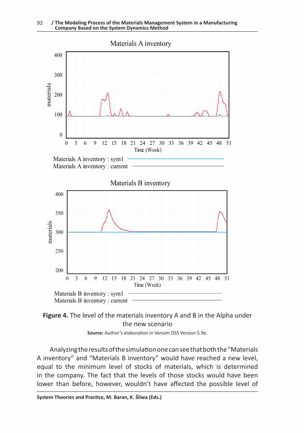
In the last step of investigations, the analysis of a scenario “what ... if ...?” was conducted. The “Time maintaining A inventory” was changed from 1 week (current) to 0.5 week (sym 1), and the “Time maintaining B inventory” from 2 weeks to 1 week. Step simulation remained unchanged. Figure 4 shows the simulation results.
JOURNAL OF ENTREPRENEURSHIP, MANAGEMENT AND INNOVATION
JOURNAL OF ENTREPRENEURSHIP MANAGEMENT AND INNOVATION,a scientific journal published by Nowy Sacz School of Business – National-Louis University
www.jemi.edu.plul. Zielona 27, 33-
10
Materials inventory A and B400 materials400 materials
200 materials300 materials
0 materials200 materials
0 6 12 18 24 30 36 42 48Time (Week)
Materials A inventory : current materialsMaterials B inventory : current materials
FIGURE3. The level of the materials inventory A and B in the Alpha
Source: Author’s elaboration in Vensim DSS Version 5.9e.
In the analyzed period of time we have seen fluctuations both in the volume of "Materials A inventory" (the blue graph and the upper scale) and "Materials B inventory" (the red graph and the lower scale) resulting in incoming orders, which determined the size of "Desired production" and "Time maintaining materials inventory". The runs of "Materials B inventory" in comparison with run of "Materials A inventory" was more stable. This resulted mainly from the longer time required to correct the level of those stocks to the desired level.
In the last step of investigations, the analysis of a scenario "what ... if ...?" was conducted.The "Time maintaining A inventory" was changed from 1 week (current) to 0.5 week (sym 1), and the " Time maintaining B inventory" from 2 weeks to 1 week. Step simulation remained unchanged. Figure 4 shows the simulation results.
Materials A inventory400
300
200
100
00 3 6 9 12 15 18 21 24 27 30 33 36 39 42 45 48 51
Time (Week)
mat
eria
ls
Materials A inventory : sym1Materials A inventory : current
System Theories and Practice, M. Baran, K. Śliwa (Eds.)
92 / The Modeling Process of the Materials Management System in a Manufacturing Company Based on the System Dynamics Method
Figure 4. The level of the materials inventory A and B in the Alpha under the new scenario
Source: Author’s elaboration in Vensim DSS Version 5.9e.
Analyzing the results of the simulation one can see that both the “Materials A inventory” and “Materials B inventory” would have reached a new level, equal to the minimum level of stocks of materials, which is determined in the company. The fact that the levels of those stocks would have been lower than before, however, wouldn’t have affected the possible level of
JOURNAL OF ENTREPRENEURSHIP, MANAGEMENT AND INNOVATION
JOURNAL OF ENTREPRENEURSHIP MANAGEMENT AND INNOVATION,a scientific journal published by Nowy Sacz School of Business – National-Louis University
www.jemi.edu.plul. Zielona 27, 33-
10
Materials inventory A and B400 materials400 materials
200 materials300 materials
0 materials200 materials
0 6 12 18 24 30 36 42 48Time (Week)
Materials A inventory : current materialsMaterials B inventory : current materials
FIGURE3. The level of the materials inventory A and B in the Alpha
Source: Author’s elaboration in Vensim DSS Version 5.9e.
In the analyzed period of time we have seen fluctuations both in the volume of "Materials A inventory" (the blue graph and the upper scale) and "Materials B inventory" (the red graph and the lower scale) resulting in incoming orders, which determined the size of "Desired production" and "Time maintaining materials inventory". The runs of "Materials B inventory" in comparison with run of "Materials A inventory" was more stable. This resulted mainly from the longer time required to correct the level of those stocks to the desired level.
In the last step of investigations, the analysis of a scenario "what ... if ...?" was conducted.The "Time maintaining A inventory" was changed from 1 week (current) to 0.5 week (sym 1), and the " Time maintaining B inventory" from 2 weeks to 1 week. Step simulation remained unchanged. Figure 4 shows the simulation results.
Materials A inventory400
300
200
100
00 3 6 9 12 15 18 21 24 27 30 33 36 39 42 45 48 51
Time (Week)
mat
eria
ls
Materials A inventory : sym1Materials A inventory : current
JOURNAL OF ENTREPRENEURSHIP, MANAGEMENT AND INNOVATION
JOURNAL OF ENTREPRENEURSHIP MANAGEMENT AND INNOVATION,a scientific journal published by Nowy Sacz School of Business – National-Louis University
www.jemi.edu.plul. Zielona 27, 33-
11
Materials B inventory400
350
300
250
2000 3 6 9 12 15 18 21 24 27 30 33 36 39 42 45 48 51
Time (Week)
mat
eria
ls
Materials B inventory : sym1Materials B inventory : current
FIGURE 4. The level of the materials inventory A and B in the Alpha under the new scenario
Source: Author’s elaboration in Vensim DSS Version 5.9e.
Analyzing the results of the simulation one can see that both the "Materials A inventory" and "Materials B inventory" would have reached a new level, equal to the minimum level of stocks of materials, which is determined in the company. The fact that the levels of thosestocks would have been lower than before, however, wouldn’t have affected the possible level of production resulted from the availability of those materials. This means that the company could significantly reduce the costs associated with the storage of excess materials without affecting the final results of production.
ConclusionSimulation of the modelled material management system in the company Alpha, allowed for discovery of the behavior of that system in the real world and discovery correlations between variables building blocks of the system. Simulation "what ... if ..." showed that the small changes in control norms (constants), which control the system, could have influenced to more rational management of that system.However, a question can arise, whether a reduction of the time maintaining inventory will not affect the increase in costs associated with more frequent delivery of materials, higher ordering, monitoring, and transportation costs. The question may be an incentive for further modeling and investigations conducting in the company Alpha.
It should be noted that the model described in this paper is a homomorphic. This means that it is a simplification of the real system, which is the material management in a manufacturing company and contains only the most important elements of the system. However, it can be used by other companies after the appropriate converting or expanding and adapting to the conditions prevailing in them.
In fact, the process of modeling is only a small part (subsystem) of a much larger system, which consists of: real world feedback information, mental models, strategies, structures and decision rules and choices. Simulation models of systems are developed by mental models of

Journal of Entrepreneurship Management and Innovation (JEMI), Volume 9, Issue 2, 2013: 79-96
93 Małgorzata Baran /
production resulted from the availability of those materials. This means that the company could significantly reduce the costs associated with the storage of excess materials without affecting the final results of production.
ConclusionSimulation of the modelled material management system in the company Alpha, allowed for discovery of the behavior of that system in the real world and discovery correlations between variables building blocks of the system. Simulation “what ... if ...” showed that the small changes in control norms (constants), which control the system, could have influenced to more rational management of that system.
However, a question can arise, whether a reduction of the time maintaining inventory will not affect the increase in costs associated with more frequent delivery of materials, higher ordering, monitoring, and transportation costs. The question may be an incentive for further modeling and investigations conducting in the company Alpha.
It should be noted that the model described in this paper is a homomorphic. This means that it is a simplification of the real system, which is the material management in a manufacturing company and contains only the most important elements of the system. However, it can be used by other companies after the appropriate converting or expanding and adapting to the conditions prevailing in them.
In fact, the process of modeling is only a small part (subsystem) of a much larger system, which consists of: real world feedback information, mental models, strategies, structures and decision rules and choices. Simulation models of systems are developed by mental models of the participants and thanks to the information collected from the real world. Policies, structures and decision-making principles applied in the real world can be presented and tested in a virtual world. The results of those tests change mental models of participants and lead to the design of new strategies, structures and decision rules. New action directions, which are introduced in real world thanks to virtual decisions and feedback information leads to new changes in mental models. Modeling is therefore not a one-off activity, but it is still repeated cycle of activities between the virtual world and the real world.
System Theories and Practice, M. Baran, K. Śliwa (Eds.)
94 / The Modeling Process of the Materials Management System in a Manufacturing Company Based on the System Dynamics Method
ReferencesBaran, M. (2009). Zastosowanie metody Dynamiki Systemów
w przedsiębiorstwie odzieżowym. In: W. Gonciarski, P. Zaskórski (Ed.) Wybrane koncepcje i metody zarządzania XXI wieku (pp. 239-250). Warszawa: Wydawnictwo Wojskowej Akademii Technicznej.
Baran, M. (2010a). Rozwinięcie symulacyjnego modelu dostosowania zatrudnienia do potrzeb produkcyjnych przedsiębiorstwa Alfa w konwencji Dynamiki Systemów. Zeszyty Naukowe Politechniki Rzeszowskiej Marketing i Zarządzanie, 17 (4/2010), 9-16.
Baran, M. (2010b). Diffusion of Innovation in the Systems Thinking Approach. Management Business Innovation, 6, 16-24. Retrieved from: http://www.mbi.wsb-nlu.edu.pl/2_2010.pdf.
Baran, M. (2010c). Dynamika związków pomiędzy podsystemami produkcji i zatrudnieniem. Przypadek przedsiębiorstwa ALFA. In: A. Nalepka, A. Ujwary-Gil (Eds.), Organizacje komercyjne i niekomercyjne wobec wzmożonej konkurencji oraz wzrastających wymagań konsumentów, Vol. 9 (pp. 117-131). Nowy Sącz: Wyższa Szkoła Biznesu – National-Louis University.
Bik, J. (1974). Gospodarka materiałowa w procesach produkcyjnych. Katowice: Polskie Towarzystwo Ekonomiczne.
Coyle, R. G. (1977). Management System Dynamics. Chichester: John Wiley & Sons.
Forrester, J. (1961). Industrial Dynamics. Cambridge: MIT Press.Forrester, J. (1969). Urban Dynamics. Cambridge: MIT Press.Forrester, J. (1971). World Dynamics. Waltham, MA: Pegasus
Communications.Forrester, J. (1971). Principles of Systems. Cambridge: MIT Press.Kasperska, E. (2005). Dynamika Systemowa. Symulacja i Optymalizacja.
Gliwice: Wydawnictwo Politechniki Śląskiej.Krupa, K. (2008). Modelowanie, symulacja i prognozowanie. Systemy ciągłe.
Warszawa: Wydawnictwa Naukowo – Techniczne.Liwowski, B. (1997). Działalność podstawowa przedsiębiorstwa i jej
wyspecjalizowane zakresy. In: J. Kortan (Ed.), Podstawy ekonomiki i zarządzania przedsiębiorstwem, (pp. 255-267). Warszawa: Wydawnictwo C. H. Beck.
Łatuszyńska, M. (2008). Symulacja komputerowa dynamiki systemów. Gorzów Wielkopolski: Wydawnictwo Państwowej Wyższej Szkoły Zawodowej.
Łukaszewicz, R. (1975). Dynamika systemów zarządzania. Warszawa: PWN.Niemczyk, A. (2010). Zarządzanie magazynem. Poznań: Wyższa Szkoła
Logistyki.Radosiński, E. (2001). Systemy informatyczne w dynamicznej analizie decyzji.
Warszawa:PWN.

Journal of Entrepreneurship Management and Innovation (JEMI), Volume 9, Issue 2, 2013: 79-96
95 Małgorzata Baran /
Richardson, G. P. (Ed.). (1996a). Modeling for Management. Volume I. Simulation In Support of Systems Thinking. Dartmouth: Publishing Company Limited.
Richardson, G. P. (Ed.). (1996b). Modelling for Management. Volume II. Simulation In Support of Systems Thinking. Dartmouth: Publishing Company Limited.
Senge, P. M. (2006). Piąta dyscyplina. Teoria i praktyka organizacji uczących się. Kraków: Oficyna Ekonomiczna Wolters Kluwer Polska.
Skowronek, C. (1989). Gospodarka materiałowa w samodzielnym przedsiębiorstwie. Warszawa: PWE.
Sołtysiński, B. (1963). Zaopatrzenie i gospodarka materiałowa w przedsiębiorstwie przemysłowym. Warszawa: PWE.
Souček, Z. (1979). Modelowanie i Projektowanie Systemów Gospodarczych. Warszawa: PWE.
Sterman, J. (2000). Business Dynamics: Systems Thinking and Modeling for a Complex World. Boston: Irwin McGraw-Hill.
Śliwa, K. R. (1994). System Dynamics Model of Water Management in Puebla. Paper presented at International Conference on Modeling and Simulation, Lugano, Switzerland.
Śliwa, K. R., (2001). O Organizacjach Inteligentnych i rozwiązywaniu złożonych problemów zarządzania nimi. Warszawa: Oficyna Wydawnicza WSM SIG.
Śliwa, K. R., (2012). Languages in problem solving and modeling. In: A. Ujwary-Gil (Ed.), Contemporary Innovation and Entrepreneurship Concepts, Journal of Entrepreneurship, Management and Innovation, 8(4), 69-82.
Tarajkowski, J. (Ed.). (2008). Elementy Dynamiki Systemów. Poznań: Wydawnictwo Akademii Ekonomicznej.
Wąsik, B. (1983). Elementy dynamiki systemowej dla ekonomistów. Kraków: Wydawnictwo Akademia Ekonomicznej.

System Theories and Practice, M. Baran, K. Śliwa (Eds.)
96 / The Modeling Process of the Materials Management System in a Manufacturing Company Based on the System Dynamics Method
Abstrakt (in Polish)W artykule przedstawiono kolejne etapy modelowania systemu gospodarki materia-łowej w przedsiębiorstwie produkcyjnym. Na początku podano procedury modelowa-nia, wskazane przez takich autorów, jak: Forrester, Łukaszewicz, Souček, Tarajkowski oraz Sterman oraz wytłumaczono istotę zarządzania materiałami w przedsiębiorstwie produkcyjnym. Następnie przedstawiono – krok po kroku – kolejne etapy modelowania systemu zarządzania materiałami. Zdefiniowano zmienne modelu myślowego systemu i powiązano je w pętle przyczynowo – skutkowe zwane diagramami zależności. Diagra-my przekształcono w model symulacyjny, który poddano weryfikacji. Proces weryfika-cji modelu obejmował: ocenę poprawności wyboru granic modelowania, poprawno-ści struktury modelu oraz spójności przyjętych wartości parametrów (stałych modelu) w porównaniu z dostępną wiedzą na temat modelowanego systemu; testowa-nie poprawności i spójności jednostek zmiennych przyjętych w modelu oraz te-stowanie działania modelu przy narzuconych warunkach skrajnych. Badania końcowe obejmowały symulację modelu na danych empirycznych zebranych w przedsiębiorstwie Alfa oraz badanie scenariusza „a co…jeśli…”. Badania modelu pokazały, że nawet niewielkie zmiany norm sterujących systemem zarządzania mate-riałami w Alfa mogą mieć istotny wpływ na poprawę racjonalnego zarządzania tym systemem. Słowa kluczowe: modelowanie symulacyjne, Dynamika Systemów, gospodarka ma-teriałowa w przedsiębiorstwie produkcyjnym.