Ensaios Econômicos

Escola de

Pós-Graduação

em Economia

da Fundação

Getulio Vargas

N 429 ISSN 0104-8910

The Missing Link: Using the NBER Reces-

sion Indicator to Construct Coincident and

Leading Indices of Economic Activity

João Victor Issler, Farshid Vahid

Julho de 2001

URL: http://hdl.handle.net/10438/1025

Os artigos publicados são de inteira responsabilidade de seus autores. Asopiniões neles emitidas não exprimem, necessariamente, o ponto de vista daFundação Getulio Vargas.

ESCOLA DE PÓS-GRADUAÇÃO EM ECONOMIA

Diretor Geral: Renato Fragelli CardosoDiretor de Ensino: Luis Henrique Bertolino BraidoDiretor de Pesquisa: João Victor IsslerDiretor de Publicações Cientícas: Ricardo de Oliveira Cavalcanti

Victor Issler, João

The Missing Link: Using the NBER Recession Indicator to

Construct Coincident and Leading Indices of Economic Activity/

João Victor Issler, Farshid Vahid Rio de Janeiro : FGV,EPGE,

2010

(Ensaios Econômicos; 429)

Inclui bibliografia.

CDD-330

The Missing Link: Using the NBER Recession Indicator to

Construct Coincident and Leading Indices of Economic

Activity∗

João Victor Issler†

Graduate School of Economics — EPGEGetulio Vargas FoundationPraia de Botafogo 190 s. 1100Rio de Janeiro, RJ 22253-900

Braziljissler@fgv.br

Farshid VahidDepartment of Econometrics and Business Statistics

Monash UniversityP.O. Box 11EVictoria 3800Australia

Farshid.Vahid@BusEco.monash.edu.au

March 2001J.E.L. Codes: C32, E32.

∗Acknowledgments: João Victor Issler acknowledges the hospitality of Monash University and FarshidVahid acknowledges the hospitality of the Getulio Vargas Foundation. We have benefited from comments and

suggestions of Heather Anderson, Antonio Fiorencio, Carlos Martins-Filho, Helio Migon, and Ajax Moreira,

who are not responsible for any remaining errors in this paper. João Victor Issler acknowledges the support of

CNPq-Brazil and PRONEX. Farshid Vahid is grateful to the Australian Research Council Small Grant scheme

and CNPq Brazil for financial assistance.†Corresponding author.

1. Introduction

Since Burns and Mitchell (1946) there has been a great deal of interest in making inference

about the “state of the economy” from sets of monthly variables that are believed to be

either concurrent or to lead the economy’s business cycles (the so called “coincident” and

“leading” indicators respectively). Although the business-cycle status of the economy is not

directly observable, our most educated estimate of it is the binary variable announced by the

NBER Business Cycle Dating Committee. These announcements are based on the consensus

of a panel of experts, and they are made some time (usually six months to one year) after

a turning point in the business cycle has occurred. NBER summarizes its deliberations as

follows:

“The NBER does not define a recession in terms of two consecutive quarters of

decline in real GNP. Rather, a recession is a recurring period of decline in total

output, income, employment, and trade, usually lasting from six months to a year,

and marked by widespread contractions in many sectors of the economy.”

(Quoted from http://www.nber.org/cycles.html)

The time it takes for the NBER committee to deliberate and decide that a turning point

has occurred is often too long to make these announcements practically useful. This gives

importance to two constructed indices, namely the coincident index and the leading indicator

index. The traditional coincident index constructed by the Department of Commerce is a

combination of four representative monthly variables on total output, income, employment

and trade. These variables are believed to have cycles that are concurrent with the latent

“business cycle” (see Burns and Mitchell 1946). The traditional leading index is then a combi-

nation of other variables that are believed to lead the coincident index. Recently, alternative

“experimental” coincident and leading indices have been proposed that are based on sophis-

ticated statistical methods of extracting a common latent dynamic factor from the coincident

variables that comprise the traditional index; see, e.g., Stock and Watson (1988a, 1988b, 1989,

1991, 1993a), and Chauvet (1998).

The basic idea behind this paper is simple: use the information content in the NBER

Business Cycle Dating Committee decisions, which are generally accepted as the chronology

of the U.S. business-cycles1, to construct a coincident and a leading index of economic activity.

The NBER’s Dating Committee decisions have been used extensively to validate various

models of economic activity. For example, to support his econometric model, Hamilton (1989)

compares the smoothed probabilities of the “recessionary regime” implied by his Markov

switching model with the NBER recession indicator. Since then, this has become a routine1See Stock and Watson (1993a, p. 98).

2

exercise for evaluating variants of Markov-switching models, see Chauvet (1998) for a recent

example. Stock and Watson (1993a) use the NBER recession indicator to develop a procedure

to validate the predictive performance of their experimental recession index. Estrella and

Mishkin (1998) use the NBER recession indicator to compare the predictive performance of

potential leading indicators of economic activity. However, as far as we know, no one has

actually used the NBER recession indicator to construct coincident and leading indicators.

We therefore ask “Why not?”. In our opinion, this is much more appealing than imposing

stringent statistical restrictions to construct a common latent dynamic factor, hoping that it

represents the economy’s business cycle.

The method that we employ here is based on the following ingredients. First, we use a

probit regression which has the NBER recession indicator as its dependent variable. Because

we are interested in constructing indices of business-cycle activity, we only use the cyclical

parts of the coincident series as the regressors to explain the NBER recession indicator. This

ensures that noise in the coincident series does not affect the final index2. Second, we allow for

the possibility of measurement error and simultaneity by using instrumental-variable methods

when running the probit regression. Natural candidates for the instruments are the variables

that are traditionally used to construct the leading index.

The coincident index proposed here is a simple fixed-weight linear combination of the

coincident series. Likewise, our leading index is also a simple fixed-weight linear combination

of the leading series. This means that coincident and leading indices will be readily available

to all users, who will not have to wait for them to be calculated and announced by a third

party. The indices constructed by The Conference Board — TCB, formerly constructed by the

Department of Commerce, are used much more widely than other proposed indices, because

of their ready availability.

We like to think that our method uncovers the “Missing Link” between the pioneering

research of Burns and Mitchell (1946), who proposed the coincident and leading variables to be

tracked over time, and the deliberations of the NBER Business Cycle Dating Committee who

define a recession as: “... a recurring period of decline in total output, income, employment,

and trade, usually lasting from six months to a year, and marked by widespread contractions

in many sectors of the economy”.

Another feature of the present research effort is that it integrates two different strands

of the modern macroeconometrics literature. The first seeks to construct indices of and to

forecast business-cycle activity, and is perhaps best exemplified by the work of Stock and

Watson (1988a, 1988b, 1989, 1991, 1993a), the collection of papers in Lahiri and Moore

(1993) and in Stock and Watson (1993b), as well as by the recent work of Chauvet (1998).2The extraction of the cyclical part of the coincident series is performed using canonical-correlation analysis

due to Hotelling (1935, 1936). This method is explained in Section 2.

3

The second seeks to characterize and test for common-cyclical features in macroeconomic

data, where a business-cycle feature is regarded as a similar pattern of serial-correlation for

different macroeconomic series, showing that they display short-run co-movement; see Engle

and Kozicki (1993), Vahid and Engle (1993, 1997), and Hecq, Palm and Urbain (2000) for the

basic theory and Engle and Issler (1995) and Issler and Vahid (2001) for applications.

The performance of our constructed coincident index is promising. In formal econometric

tests it encompasses two of the most popular indices currently in use — the TCB and Stock

and Watson’s coincident indices. Conversely our index is not encompassed by these others.

Regarding our leading index, its behavior seems to anticipate the current state of the economy

quite well.

The structure of the rest of the paper is as follows. In Section 2 we present the basic

ingredients of our methodology in a non-technical way, leaving the technical details for the

Appendix. Section 3 presents the coincident and leading indices, and Section 4 concludes.

2. Theoretical underpinning of the indexes

In this Section we explain the method that we use for constructing the coincident and leading

indices of economic activity. Technical details are included in the Appendix.

2.1. Determining a basis for the cyclical components of coincident variables

We require that the coincident index be a linear combination of the cyclical components of

coincident variables. This means that in our view, the “business cycle” is a linear combination

of the cycles of the four coincident series (output, income, employment and trade), and there

is no unimportant cyclical fluctuation in these variables that is excluded. This contrasts with

the single latent dynamic index view of a coincident index (e.g., Stock and Watson 1989 and

Chauvet 1998), which restricts the “business cycle” to be a single common cyclical factor

shared by the coincident variables. In order to identify the common cycle, the single latent

dynamic factor approach has to allow the coincident variables to have other idiosyncratic

cyclical factors, and this provides no control over how strong these idiosyncratic cycles are

relative to the common cycle; see the discussion in Appendix A.1.

We define as “cyclical” any variable which can be linearly predicted from the past in-

formation set. The past information set includes lags of both sets of coincident and leading

variables. The inclusion of lags of leading variables in addition to lags of coincident variables

in the information set, in effect, serves two purposes. First, it combines the estimation of

coincident and leading indicator indices. Second, it allows for the possibility of asymmetric

cycles in coincident series by including lags of variables such as interest rates and the spread

between interest rates which are known to be nonlinear processes (Anderson 1997, Balke and

4

Fomby 1997) as exogenous predictors. There are infinitely many linear combinations of the

coincident variables that are predictable from the past, that is, that are cyclical. We use

canonical-correlation analysis to find a basis for the space of these cycles.

Canonical-correlation analysis, introduced by Hotelling (1935, 1936), has been used in

multivariate statistics for a long time. It was first used in multivariate time series analysis by

Akaike (1976). Akaike aptly referred to the canonical variates as “the channels of information

interface between the past and the present” and he referred to canonical correlations as the

“strength” of these channels. We explain the concept briefly in our context, leaving more

technical details for the Appendix.

Denote the set of coincident variables (income, output, employment and trade) by the

vector xt = (x1t, x2t, x3t, x4t)0 and the set of m (m ≥ 4) “predictors” by the vector zt (this

includes lags of xt as well as lags of the leading variables). Canonical correlations analysis

transforms xt into four independent linear combinations A(xt) = (α01xt,α02xt,α03xt,α04xt) withthe property that α01xt is the linear combination of xt that is most (linearly) predictable fromzt, α

02xt is the second most predictable linear combination of xt from zt after controlling for

α01xt, and so on3. These linear combinations will be uncorrelated with each other and theyare restricted to have unit variances so as to identify them uniquely up-to a sign change. By-

products of this analysis are four linear combination of zt, Γ(zt) = (γ01zt, γ02zt, γ03zt, γ04zt) , withthe property that γ0izt is the linear combination of zt that has the highest squared correlationwith α0ixt, for i = 1, 2, 3, 4. Again, the elements of Γ(zt) are uncorrelated with each other,

and they are uniquely identified up-to a sign switch with the additional restriction that all

four have unit variances. The regression R2 between α0ixt and γ0izt for i = 1, 2, 3, 4, which we

denote by λ21,λ

22,λ

23,λ

24 , are the squared canonical correlations between xt and zt.

In the present application, we call (α01xt,α02xt,α03xt,α04xt) the “basis cycles” in xt. Ourview that cycles are predictable from the past information, justifies using this term. It is

important to note that moving from xt to A (xt) is just a change of coordinates. In particular,

no structure is placed on these variables from outside, and no information is thrown away in

this transformation. Hence, the information content in A (xt) is neither more nor less than

the information content in xt.

The advantage of this basis change is that it allows us to determine if the cyclical behavior

of the coincident series can be explained by less than four basis cycles. Note that in the first

basis cycle, i.e. the linear combination of xt with maximal correlation with the past, reveals the

combination of coincident series with the most pronounced cyclical feature. Analogously, the

linear combination associated with the minimal canonical correlation reveals the combination3The fact that canonical correlations analysis studies channels of linear dependence between x and z does

not necessarily imply that it will be only useful for linear multivariate analysis. By including nonlinear basis

functions (e.g. Fourier series, Tchebyschev polynomials) in z, one can use canonical correlation analysis for

nonlinear multivariate modelling. See Anderson and Vahid (1998) for an example and further references.

5

of the xt with the weakest cyclical feature. We can use a simple statistical-test procedure to

examine whether the smallest canonical correlation (or a group of canonical correlations) is

statistically equal to zero; see Appendix A.2. If this hypothesis is not rejected, then the linear

combination corresponding to the statistically insignificant canonical correlation cannot be

predicted from the past, i.e. it is white-noise, and therefore can be dropped from the set of

basis cycles. In that case, we can conclude that all cyclical behavior in the four coincident

series can be written in terms of less than four basis cycles.

Hence, the use of linear combination of xt’s that are not associated with a zero canonical

correlation is equivalent to using only the cyclical components of the coincident series. Any

linear combination of the significant basis cycles is a linear combination of the cyclical com-

ponents of coincident variables, which is convenient for our purposes, because it implies that

our coincident index will be a linear combination of the coincident variables themselves.

If the canonical-correlation tests suggest that only one cycle is needed to explain the

dependence of the four coincident variables with the past, then that unique common cycle will

be the candidate for the coincident index. In such a case, our coincident index will be close to

the coincident index constructed through a single hidden dynamic factor approach. However,

our analysis, which is reported in Section 3, shows that this was not the case. Jumping to our

results, our proposed coincident index is a linear combination of three statistically significant

basis cycles that explain the NBER recession indicator.

2.2. Using probit analysis to compute coincident and leading indices

One way to estimate the weights associated with each basis cycle is to estimate a simple

probit model with the NBER indicator as the binary dependent variable and the basis cycles

associated with the non-zero canonical correlations as explanatory variables. Since the basis

cycles are linear combinations of the four coincident series, we will ultimately end up explaining

the state of the economy by a linear combination of the coincident series. This was exactly

our goal from the outset — use the information content in the NBER Business Cycle Dating

Committee decisions to construct a coincident index of economic activity that is a simple

linear combination of the coincident series.

The above procedure may be a good first approximation for the problem at hand. However,

the basis cycles series are measured with error for two reasons. First, the coincident series

are subject to constant revisions; see Stock and Watson (1988a). The data that we use in our

analysis is a revised version of the data that the NBER Business Cycle Dating Committee had

available to them when they decided on the state of the economy (recession vs. not recession).

Second, our basis cycles are estimates of the population linear combinations associated with

the non-zero canonical correlations. Therefore, we have a typical error-in-variables problem in

estimation, which calls for instrumental-variable techniques. We use the zt variables (i.e. lags

6

of coincident and leading variables) as instruments for the basis cycles. Notice that canonical-

correlation analysis produces estimates of γ01zt, γ02zt, γ03zt, and γ04zt, which are the best linearpredictors for each of the basis cycles respectively.

Several alternative estimators have been proposed for the consistent estimation of parame-

ters of a single equation with a limited dependent variable in a simultaneous equations model.

These estimators differ in their ease of calculation versus their degree of efficiency. We use

the two stage conditional maximum likelihood (2SCML) estimator proposed by Rivers and

Vuong (1988). In our context, and using already the empirical results stated below, we assume

that the four coincident series can be explained by three significant basis cycles c1t, c2t, c3t.Denoting the NBER indicator by NBERt, the first stage of the 2SCML estimation involves

regressing c1t, c2t, c3t on the instruments zt and saving the residuals, which we denote byv1t, v2t, v3t . In the second stage, both the basis cycles c1t, c2t, c3t and the residuals of thefirst stage v1t, v2t, v3t are included in the probit model:

Pr (NBERt = 1) = Φ (β0 + β1c1t + β2c2t + β3c3t + β4v1t + β5v2t + β6v3t) ,

where Φ is the standard normal cumulative distribution function. The estimates of β1, β2,

and β3 from the second stage probit will be the 2SCML estimates. Our coincident index is

then given by4:

Coincident indext = − β1c1t + β2c2t + β3c3t

= − β1α01xt + β2α

02xt + β3α

03xt

= − β1α01 + β2α

02 + β3α

03 xt,

which shows that it can be expressed as a linear combination of the coincident series xt.

Similarly, our leading index can be expressed as a linear combination of the leading series zt.

The simple probit standard errors cannot be used for inference and have to be modified as

shown by Rivers and Vuong (1988). There is an added complication here because the value of

the dependent variable is set by the Business Cycle Dating Committee several periods after

time t and therefore, it embodies information that cannot be predicted at time t. This fact

cannot be exploited in constructing a better index because future information is not available

at the time when the index is computed. However, it implies that the model has a moving

average error, and therefore its standard-errors have to be modified to make inference robust

to dynamic misspecification. These technicalities are explained further in Appendix A.3.

In summary, our complete statistical model is the following:

4The minus sign in front of β1c1t + β2c2t + β3c3t is to ensure that the index dips down during recessions.

7

NBERt =1 if y∗t > 00 if y∗t ≤ 0

y∗t = ψ0 + ψ0 xt4×1

+ ut (2.1)

xt = Π4×m zt

m×1+ εt,

where ut may be correlated with εt, ut and εt are jointly normal, and Π has rank 3.

2.3. Encompassing tests for alternative coincident indices

After obtaining our coincident index, it is desirable to evaluate its performance in explain-

ing the state of the economy relative to alternative coincident indices. Natural candidates

of alternative indices are TCB’s (Dept. of Commerce) and Stock and Watson’s coincident

indices. The first is chosen because it is a simple linear combination of the coincident series

that is widely used by practitioners. The second is chosen because it is constructed using a

sophisticated dynamic factor model, which is put forward as a basis for rationalizing NBER’s

decisions on the state of the economy; see Appendix A.1 for more details on both indices.

In principle all three coincident indices attempt to summarize the current state of the

economy. Hence, it seems natural to evaluate them with respect to their ability to predict

the current state of the economy represented by the binary variable announced by the NBER

Business Cycle Dating Committee. The exercise would be straightforward if the underlying

models were all nested within each other. However, this is not the case, and we use non-nested

tests. These can be viewed as misspecification tests for our econometric model in (2.1).

Suppose we want to compare two competing coincident indices, index1t and index2t. The

easiest test would be to include both indices in a linear probability model, which has the

NBER recession indicator as its dependent variable, i.e.,

NBERt = θ0 + θ1index1t + θ2index2t + et (2.2)

If given index 1t, index2t is insignificant in explaining NBERt, then index 1t encompasses

index2t. If given index 2t, index1t is insignificant in explaining NBERt, then index2t encom-

passes index1t. Otherwise, neither encompasses the other. If linearity is of concern, one can

add higher powers of index 1t and index 2t to the right-hand side of equation (2.2), for example,

NBERt = θ0+θ1index1t+θ01index2

1t+θ001index3

1t+θ2index2t+θ02index2

2t+θ002index3

2t+et. (2.3)

Then, index 1t encompasses index2t if we cannot reject that θ2 = θ02 = θ

002 = 0, index2t encom-

passes index1t if we cannot reject that θ1 = θ01 = θ

001 = 0, and neither encompasses the other

in all other cases.

8

Of course, linear probability models are heteroskedastic and, in our context, the above

equations are likely to have serially correlated errors because of the timing issue discussed

above. Therefore, heteroskedasticity and serial-correlation robust covariance matrices should

be used when testing the encompassing hypotheses. The issue of measurement errors in the

coincident variables that constitute the indices can be taken care of by using zt as instruments

for the indices, and basing the encompassing tests on the generalized instrumental variable

(or GMM) estimates and standard errors of the parameters.

Although a linear specification is not strictly appropriate for modelling a binary dependent

variable because it can lead to predictions for Pr (NBERt = 1) that are outside the [0, 1] inter-

val for some t, it is convenient for testing hypotheses without making a restrictive assumption

about the functional form. The encompassing test explained above, with all its complications

arising out of heteroskedasticity and serial dependence of errors and measurement error in the

independent variables, can be readily computed by standard econometrics software. Alterna-

tively, one can take the probit specification as the correct specification under the null, and

design the encompassing test along the lines of the so-called “artificial regression” approach5

described in Davidson and McKinnon (1993, pp. 523-528); we provide some technical details

of the latter in Appendix A.4.

3. Calculating coincident- and leading-indicator indices

3.1. Identification of the basis cycles

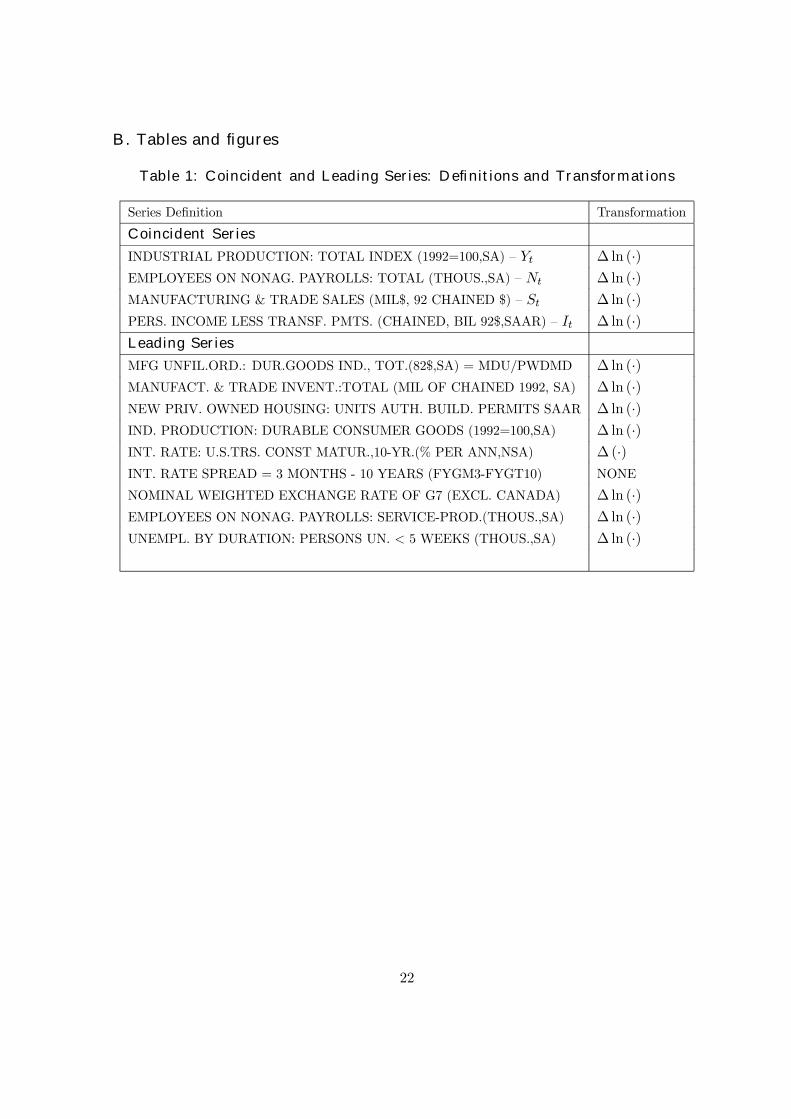
We begin our analysis by considering the coincident series, which are defined in Table 1, and are

plotted in Figure 1, where shaded areas represent the NBER dating of recession periods. All

four series show signs of dropping during recessions, although this behavior is more pronounced

for Industrial Production (∆ lnYt) and Employment (∆ lnNt). These two series also show a

more visible cyclical pattern, whereas, for example, it is hard to notice the cyclical pattern in

Sales (∆ lnSt) or Income (∆ ln It). Before modelling the joint cyclical pattern of the coincident

series in (∆ ln It, ∆ lnYt, ∆ lnNt, ∆ lnSt), we performed cointegration tests to verify if the

series in (ln It, lnYt, lnNt, lnSt) share a common long-run component. As in Stock and Watson

(1989), we find no cointegration among these variables.

Conditional on the evidence of no cointegration for the elements of (ln It, lnYt, lnNt, lnSt),

we model them as a Vector Autoregression (VAR) in first differences. Besides

(∆ ln It, ∆ lnYt, ∆ lnNt, ∆ lnSt) and their lags, the VAR also contains the lags of trans-

formed (mostly by log first differences) leading series as a conditioning set. The latter is a

sensible choice because we should expect, a priori, that these leading series are helpful in5 Indeed our test regressions in equations (2.2) and (2.3) are “artificial regressions” based on, respectively,

linear and flexible nonlinear specifications.

9

forecasting the coincident series. A list of these leading series is also presented in Table 1.

They were used by Stock and Watson(1988a) and comprise a subset of the variables initially

chosen by Burns and Mitchell (1946) to be leading indicators6.

The Akaike Information Criterion chose a VAR of order 2. Conditional on a V AR (2) we

calculated the canonical correlations between the coincident series (∆ ln It, ∆ lnYt, ∆ lnNt,

∆ lnSt) and the respective conditioning set, comprising of two lags of (∆ ln It, ∆ lnYt, ∆ lnNt,

∆ lnSt) and of two lags of the leading series. The canonical-correlation test results in Table 2

allow the conclusion that there is only one linear combination of the coincident series which

is white noise. Hence, the cyclical behavior of (∆ ln It, ∆ lnYt, ∆ lnNt, ∆ lnSt) can be repre-

sented by three orthogonal canonical factors. These factors, (c1t, c2t, c3t), were labelled as the

coincident basis cycles and are a linear combination of the coincident series. A plot of them is

presented in Figure 2. Figure 3, on the other hand, presents the estimates of the linear com-

binations of the leading series in the canonical-correlation analysis, (γ01zt, γ02zt, γ03zt), labelledleading factors.

Below, we show the linear combinations of the four coincident indicators that yield the

three basis cycles:

c1t

c2t

c3t

=

1.03 0.31 19.44 −0.68−1.68 1.12 1.12 4.64

−0.27 7.78 −13.46 −2.33×

∆ ln It

∆ lnYt

∆ lnNt

∆ lnSt

(3.1)

A correlation matrix for all six (coincident and leading) factors is presented in Table 3. To

investigate their ability in explaining NBER recessions we include in this correlation matrix

the NBER recession indicator dummy (which is equal to one during periods identified by

NBER as recessions and zero otherwise). As could be expected a priori, the first factor

(either coincident or leading) is the one with the highest correlation with the NBER dummy

variable, followed by the second, and finally by the third.

3.2. “The Missing Link”: computing simple indices with a probit regression

As a basic procedure to calculate a coincident index, which is a linear combination of (∆ ln It,

∆ lnYt, ∆ lnNt, ∆ lnSt), we estimate a probit regression of the NBER recession indicator on

the three coincident basis cycles. The result of this probit estimation are presented in Table

4. The overall fit of this simple probit regression is 0.55. Using a cutoff probability of 0.5,

this model has a 70% success rate in predicting recessions (94% success rate in estimating

the correct state overall). Because the NBER recession indicator is a highly dependent series,

there is some evidence of significant serial correlation in the pseudo-residuals of this regression.6Stock and Watson smooth some of these leading indicators. Here, we make no use of such transformations.

10

However, this serial correlation cannot be used to improve the quality of the leading indicator

index in real time, because NBER recession indicator is often announced with a considerable

lag. For correct inference though, all reported standard errors are calculated to be robust to

serial correlation and heteroskedasticity.

Since the three coincident factors are a linear combination of the four coincident series,

from the estimated coefficients of this simple probit regression we can construct a “simple”

coincident index which is a linear combination of the four coincident series. Using the weights

in (3.1) and the estimated coefficients in the probit regression (Table 4), we arrive at the

following coincident-indicator linear combination (∆CIt):

∆CIt = 15.52×∆ ln It + 50.67×∆ lnYt + 522.83×∆ lnNt + 17.78×∆ lnSt. (3.2)

Normalizing the weights in (3.2) to add up to unity, we arrive at the following standardized

coincident-indicator linear combination (∆CI 0t):

∆CI 0t = 0.03×∆ ln It + 0.08×∆ lnYt + 0.86×∆ lnNt + 0.03×∆ lnSt. (3.3)

The formula in (3.3) shows that most of the weight is given to employment. This is not

surprising given our previous analysis of Figure 1, since this series has a more pronounced

coherence with the NBER recession indicator.

It is interesting to compare our measure of the “simple” coincident indicator with other

measures currently in the literature. The corresponding weights that are used by the Con-

ference Board to calculate the coincident index7 are (0.28, 0.13, 0.48, 0.11) . Although both

indices place the largest weight on employment, the weights are quite different.

The results of the encompassing test explained in equation (2.2) are reported in Table 6.

They show that our simple index encompasses the TCB index (p-value of 0.46) but it is not

encompassed by it (p-value <0.01)8. We also compare our simple index with the coincident

index9 (XCI) proposed by Stock and Watson (1989). The encompassing tests suggest that,

at usual significance levels, our index encompasses XCI but is not encompassed by it (with

respective p-values of 0.40 and <0.01)10.

3.3. “The Missing Link”: computing a more sophisticated index

For a good reason, one may suspect that the simple probit regression is not an appropriate

framework for revealing the implicit weights on the four coincident series used by the NBER

Dating Committee. Coincident series are subject to constant revisions, i.e., they are mea-

sured with error. Moreover, our basis cycles used in probit regressions are estimates, not the7The Conference Board Index is also known as the Department of Commerce Index (or the DOC Index).8Corresponding p-values for the Davidson-McKinnon encompassing tests are 0.07 and <0.01 respectively.9We have downloaded this series from http://ksghome.harvard.edu/~.JStock.Academic.Ksg/xri/0012/xindex.asc.10Corresponding p-values for the Davidson-McKinnon encompassing tests are 0.34 and 0.06 respectively.

11

actual underlying cycles. Therefore, we have to use instrumental variables to consistently

estimate weights in probit regressions. As discussed above, natural candidates for instru-

ments are the leading series. Notice that canonical-correlation analysis has already produced

γ01zt, γ02zt, γ

03zt which are the best linear predictors for each of the three basis cycles. We

use the two stage conditional maximum likelihood (2SCML) estimator proposed by Rivers

and Vuong (1988) to obtain instrumental variable estimates for the coefficients of each basis

cycle.

The 2SCML estimates are presented in Table 5. The “implicit weights” for the instrumental-

variable coincident series (∆IV CIt) are:

∆IV CIt = 0.02×∆ ln It + 0.13×∆ lnYt + 0.80×∆ lnNt + 0.05×∆ lnSt. (3.4)

Equation (3.4) shows that, again, most of the weight is given to employment, and that

employment and industrial production get 93% of the weight altogether. A plot of this index

is presented in Figure 4. Once again, the striking difference between our weights and the

TCB’s is that Income is weighed much more heavily in the TCB index than in ours, and

employment is weighed more heavily in our index than in theirs.

The encompassing test that compares our coincident index with the TCB index (reported

in Table 7) suggests that our index encompasses the TCB index (p-value of 0.83) but it is not

encompassed by it (p-value of 0.04)11. Regarding the XCI series of Stock and Watson, the

encompassing tests suggest that, at usual significance levels, our index encompasses XCI, but

is not encompassed by it (with respective p-values of 0.51 and <0.01)12.

Finally, as a by-product of this analysis, we can construct a leading index, which uses the

same weights estimated by instrumental-variable probit and the leading factors (γ01zt, γ02zt, γ03zt)weighed by their respective canonical correlations. This index is labelled ∆IV LIt and is pre-

sented in Figure 5. Its behavior is very similar to that of our coincident index and it tracks

reasonably well NBER recessions.

4. Conclusion

The basic idea behind this paper is simple: use the information content in the NBER Busi-

ness Cycle Dating Committee decisions to construct a coincident index of economic activity.

Although several authors have devised sophisticated coincident indices with the ultimate goal

of matching NBER recessions, no one has used the information in the NBER decisions to

construct a coincident index. A second ingredient of our method is that we use canonical

correlation analysis to filter out the noisy information contained in the coincident series. As

a result, our final index is only influenced by the cyclical components of the coincident series.11Corresponding p-values for the Davidson-McKinnon encompassing tests are 0.43 and 0.01 respectively.12Corresponding p-values for the Davidson-McKinnon encompassing tests are 0.34 and 0.03 respectively.

12

Finally, in our preferred coincident index of the U.S. business cycle, we take account of mea-

surement error in the coincident series by using instrumental-variable methods. The resulting

index is a simple linear combination of the four coincident series originally proposed by Burns

and Mitchell (1946).

As explained in the Introduction, we like to think that our method uncovers the “Missing

Link” between the pioneering research of Burns and Mitchell (1946) and the deliberations

of the NBER Business-Cycle Dating Committee. This is a consequence of the way we have

constructed our coincident and leading indices: the coincident index is a linear combination

of the four coincident series proposed by Burns and Mitchell chosen to match, using an

appropriate probit regression technique, the deliberations of the NBER Business Cycle Dating

Committee.

Our methodology also conveniently produces a leading index of economic activity which is

a linear combination of lags of coincident and leading variables. Moreover, the probit model

that produces our coincident index is in fact a model of probability of recessions. Therefore,

this model can easily produce estimates of the probability of a recession.

The performance of our constructed coincident index is promising. In encompassing tests,

it encompassed two currently popular constructed indices — the TCB and Stock and Watson’s

coincident indices. However, it was not encompassed by any of them in formal testing. Some

may object to our encompassing tests as being unfair on the grounds that our indices use the

NBER recession indicator in their construction, while TCB and XCI indices don’t. Our reply

to such objections would be, “Exactly. Why do TCB and XCI indices ignore this vital piece

of information in their construction?”

References

Akaike, H. (1976), “Canonical Correlation Analysis of Time Series and the Use of an In-

formation Criterion”, in R.K. Mehra and D.G. Lainiotis (Eds) System Identification:

Advances and Case Studies, New York: Academic Press, pp. 27-96.

Anderson, T. W. (1984), An Introduction to Multivariate Statistical Analysis (2nd ed.).

NewYork: John Wiley and Sons.

Anderson, H. M. and F. Vahid (1998), “Testing Multiple Equation Systems for Common

Nonlinear Factors”, Journal of Econometrics, 84, 1 - 37.

Balke, N.S. and T.B. Fomby (1997), “Threshold Cointegration”, International Economic

Review, 38, 627-647.

Burns, A. F. and Mitchell, W. C.(1946), “Measuring Business Cycles,” New York: National

Bureau of Economic Research.

13

Chauvet, M. (1998), “An Econometric Characterization of Business Cycle Dynamics with

Factor Structure and Regime Switching”, International Economic Review, 39, 969 - 996.

Davidson, R. and MacKinnon, J.G.(1993), “Estimation and Inference in Econometrics,”

Oxford: Oxford University Press.

Engle, R. F. and Kozicki, S. (1993), “Testing for Common Features”, Journal of Business

and Economic Statistics, 11, 369-395, with discussions.

Engle, R. F. and Issler, J. V. (1995), “Estimating Sectoral Cycles Using Cointegration and

Common Features”, Journal of Monetary Economics, 35, 83-113.

Estrella A. and F. S. Mishkin (1998), “Predicting U.S. Recessions: Financial Variables as

Leading Indicators”, Review of Economics and Statistics, 80, 45 - 61.

Geweke, J. (1977), “The Dynamic Factor Analysis of Economic Time Series,” Chapter 19

in D.J. Aigner and A.S. Goldberger (eds) Latent Variables in Socio-Economic Models,

Amsterdam: North Holland.

Hamilton, J.D. (1994), Time Series Analysis, Princeton: Princeton University Press.

Hamilton, J.D. (1989), “A New Approach to the Economic Analysis of Nonstationary Time

Series and the Business Cycle”, Econometrica, 57, 357-384.

Hecq, A., F. Palm and J.P. Urbain (2000), “Permanent-Transitory Decomposition in VAR

Models with Cointegration and Common Cycles”, Oxford Bulletin of Economics and

Statistics, 62, 511-532.

Hotelling, H. (1935), “The Most Predictable Criterion”, Journal of Educational Psychology,

26, 139-142.

Hotelling, H. (1936), “Relations Between Two Sets of Variates”, Biometrika, 28, 321-377.

Issler, J.V. and Vahid, F. (2001), “Common Cycles and the Importance of Transitory Shocks

to Macroeconomic Aggregates,” Journal of Monetary Economics, 47, 449-475.

Lahiri, K. and G. Moore (1993), Editors, “Leading Economic Indicators: New Approaches

and Forecasting Records.” New York: Cambridge University Press.

Newey, W. and K. West (1987), “A Simple Positive Semi-Definite, Heteroskedasticity and

Autocorrelation Consistent Covariance Matrix,” Econometrica, 55, 703-708.

Rivers, D. and Q.H. Vuong (1988), “Limited Information Estimators and Exogeneity Tests

for Simultaneous Probit Models”, Journal of Econometrics, 39, 347-366.

14

Stock, J. and Watson, M.(1988a), “A New Approach to Leading Economic Indicators,”

mimeo, Harvard University, Kennedy School of Government.

Stock, J. and Watson, M.(1988b), “A Probability Model of the Coincident Economic Indi-

cator”, NBER Working Paper # 2772.

Stock, J. and Watson, M.(1989) “New Indexes of Leading and Coincident Economic Indi-

cators”, NBER Macroeconomics Annual, pp. 351-95.

Stock, J. and Watson, M.(1991), “A Probability Model of the Coincident Economic Indica-

tors”, in “Leading Economic Indicators: New Approaches and Forecasting Records,” K.

Lahiri and G. Moore, Eds. New York: Cambridge University Press.

Stock, J. and Watson, M.(1993a), “A Procedure for Predicting Recessions with Leading

Indicators: Econometric Issues and Recent Experiences,” in “New Research on Busi-

ness Cycles, Indicators and Forecasting,” J.H. Stock and M.W. Watson, Eds., Chicago:

University of Chicago Press, for NBER.

Stock, J. and Watson, M.(1993b), Editors, “New Research on Business Cycles, Indicators

and Forecasting” Chicago: University of Chicago Press, for NBER.

The Conference Board (1997), “Business Cycle Indicators,” Mimeo, The Conference Board,

downloadable from http://www.tcb-indicators.org/bcioverview/bci4.pdf.

Vahid, F. and Engle, R. F. (1993), “Common Trends and Common Cycles”, Journal of

Applied Econometrics, 8, 341-360.

Vahid, F. and Engle, R.F.(1997), “Codependent Cycles,” Journal Econometrics, vol. 80,

pp. 199-121.

Wooldridge, J.M.(1994), “Estimation and Inference for Dependent Processes,” in “Handbook

of Econometrics IV,” R.F. Engle and D. McFadden, Editors. Amsterdam: Elsevier

Press.

15

A. Econometric and statistical techniques

A.1. Statistical foundation of TCB and XCI indices

A coincident index, which is widely used by practitioners, is the index constructed by The Con-

ference Board — TCB. This coincident index is a weighted average of the coincident variables

— employment, output, sales and income, where weights are the reciprocal of the standard

deviation of each component’s growth rate and add up to unity; see The Conference Board

(1997).

Stock and Watson’s experimental coincident index (XCI) is based on an “unobserved sin-

gle index” or “dynamic factor” model; see Geweke(1977), for example. There, the growth rate

of the four coincident series (output, sales, income and employment) share a common cycle,

∆XCIt, which is a latent dynamic factor that represents (the change of) “the state of the econ-

omy.” Denoting the growth rates of the coincident series in a vector xt = (x1t, x2t, x3t, x4t)0 ,

their proposed statistical model is as follows:

xt = β + γ(L)∆XCIt + ut,

φ(L)∆XCIt = δ + ηt,

D(L)ut = ²t, (A.1)

where φ(L) and γ(L) are scalar polynomials on the lag operator L, and D(L) is a matrix

polynomial on L. The error structure is restricted so as to have Eηt²t

ηt²t

0=

diag(σ2η,σ

2²1 , ...,σ

2²4), and D(L) = diag[dii(L)], which makes innovations mutually uncorre-

lated.

The model (A.1) assumes that there is a single source of comovement among the growth

rates of the coincident series — ∆XCIt. Still, these series are allowed to have their own

idiosyncratic cycle, since the vector of error terms ut is composed of serially correlated com-

ponents that are mutually orthogonal. Hence, each of the four coincident series in xt has two

cyclical components: a common and an idiosyncratic one. In this view, the “business cycle”

is the intersection of the cycles in output, income, employment, and trade. Moreover, there

is no guarantee that idiosyncratic cycles do not dominate the common cycle in explaining the

variation of the four series in xt.

In contrast, in our view, the “business cycle” is the union of the cycles in output, income,

employment, and trade. There are no idiosyncratic cycles that can be put aside, the only

part of xt that we leave out is the non-cyclical combination resulting from the canonical-

correlation analysis. Comparing our method with Stock and Watson’s clearly shows that

neither model is a special case of the other. Hence, neither model is nested within the other

one, and comparisons between them have to be made using non-nested tests. Chauvet (1998)

16

has generalized the framework in Stock and Watson by allowing a two-state mean for the

latent factor ∆XCIt in (A.1), representing recession and non-recession regimes.

A.2. Canonical correlations

Consider two (stationary) random vectors x0t = (x1t, x2t, ..., xnt) and z0t = (z1t, z2t, ..., zmt),

m ≥ n such that:xtzt

∼ 0

0,ΣXX ΣXZΣZX ΣZZ

.

The zero mean assumption is to simplify notation and does not involve any loss of generality.

Canonical-correlation analysis seeks to rotate xt and zt so as to maximize the correlation

between their transformed images. Formally, it seeks to find matrices

A0(n×n)

=

α01α02......

α0n

and Γ0(n×m)

=

γ01γ02......

γ0nsuch that:

1. The elements of A0xt have unit variance and are uncorrelated with each other:

E(A0xtx0tA) = A0ΣXXA= In

2. The elements of Γ0zt have unit variance and are uncorrelated with each other:

E(Γ0ztz0tΓ) = Γ0ΣZZΓ= In, and,

3. The i-th element of A0xt is uncorrelated with the j-th element of Γ0zt, i 6= j. For i = j,this correlation is a called canonical correlation, denoted by λi, such that:

E(A0xtz0tΓ) = A0ΣXZΓ=Λ,

where,

Λ=

λ1 0 · · · · · · 0

0 λ2 0 · · · 0...

. . ....

.... . . 0

0 · · · · · · 0 λn

, and,

1 ≥ |λ1| ≥ |λ2| ≥ ... ≥ |λn| ≥ 0.

17

The following basic results in Anderson (1984) and Hamilton (1994) are worth reporting here.

Proposition A.1. The k-th canonical correlation between xt and zt is given by k-th high-

est root of−λΣXX ΣXZ

ΣZX −λΣZZ= 0, denoted by λk. The linear combinations αk and γk

associated with λk can be found by making λ = λk in−λΣXX ΣXZ

ΣZX −λΣZZαk

γk= 0, considering also the unit-variance restrictions in 1

and 2 above.

Proposition A.2. Let X = (x1,x2, ..., xT )0 and Z= (z1, z2, ..., zT ) be samples of T obser-

vations of xt and zt. The n first eigenvalues of the matrix H= (X 0X)−1X 0Z(Z 0Z)−1Z 0Xare consistent estimates of the squared populational canonical correlations (λ2

1,λ22, ...,λ

2n).

The corresponding eigenvectors are consistent estimates of the parameters in A. More-

over, the first n eigenvalues of H are identical to the first n eigenvalues of the matrix

G = (Z 0Z)−1Z 0X(X 0X)−1X 0Z, whose corresponding eigenvectors are consistent estimates

of the elements of Γ.

Proposition A.3. The likelihood ratio test statistic for the null hypothesis that the smallest

n−k canonical correlations are jointly zero, Hk : λk+1 = λk+2 = ... = λn = 0, can be computed

using the squared sample canonical correlations λ2

i , i = k+ 1, · · · , n, in the following fashion:

LR = −Tn

i=k+1

ln(1− λ2

i ).

Moreover, the asymptotic distribution of this likelihood-ratio test statistic is chi-squared, as

follows:

LRd−→ χ2

(n−k)(m−k).

Canonical-correlation analysis can be applied in the present context for analyzing a large

multivariate data set, summarizing the correlations between a group of stationary series x

and a group of stationary series z. For example, we suppose that the coincident series in xtcan be modelled using a Vector Autoregression (VAR), using its own the lags, xt−1, · · · , xt−p,and also the lags of some other (leading) series, wt−1, · · · , wt−p, as follows:

xt = A1xt−1 + · · ·+Apxt−p +B1wt−1 + · · ·+Bpwt−p + εt, (A.2)

where εt is a white-noise process.

Here, we are interested in summarizing the correlations between the variables in xt and

the variables in zt = x0t−1, · · · , x0t−p, w0t−1, · · · , w0t−p 0. In this framework, the cyclical feature

in xt has to arise from the elements in zt, since εt is a white-noise process, devoid of any

cyclical features; see Engle and Kozicki(1993).

18

A.3. Instrumental-variable probit regressions

Denoting by c1t, · · · , ckt, (cit = α0ixt, i = 1, · · · , k) , the k basis cycles associated with the firstk non-zero canonical correlations, the NBER business-cycle indicator is linked to them through

the latent variable y∗t :

y∗t = β0 + β1c1t + · · ·+ βkckt + ut (A.3)

NBERt =1 if y∗t > 00 if y∗t ≤ 0

.

As argued above, because the series c1t, · · · , ckt, are measured with error, we cannot use asimple probit-regression procedure to estimate βi, i = 0, 1, · · · , k. The possible correlationbetween c1t, · · · , ckt and the errors ut is modelled as follows,

cit = λi γ0izt + vit, i = 1, · · · , k (A.4)

ut

vt∼ N 0,

σ2u σ0vuσvu Σvv

where the vit, i = 1, · · · , k, are collected into a k-vector vt, λi and γ0izt for i = 1, · · · , k comefrom the canonical-correlation analysis, Σvv is a k× k diagonal variance-covariance matrix ofvt, σvu is a k× 1 vector of covariances between ut and vt. Because of measurement error, thebasis cycles c1t, · · · , ckt are correlated with ut. Joint normality of ut and vt implies:

ut = v0tδ + ηt

where δ = Σ−1vv σvu, ηt ∼ N 0,σ2

u − σ0vuΣ−1vv σvu and ηt is independent of vt. Substituting for

ut in equation (A.3), we obtain,

y∗t = β0 + β1c1t + · · ·+ βkckt + v0tδ + ηt (A.5)

NBERt =1 if ηt < β0 + β1c1t + · · ·+ βkckt + v0tδ0 if ηt ≥ β0 + β1c1t + · · ·+ βkckt + v0tδ

.

Notice that, by construction, all the regressors in (A.5) are uncorrelated with the error

term ηt. As usual for probit models the mean parameters θ = β0,β1,β2,β3, δ0 0 and the

variance parameter σ2η = σ

2u − σ0vuΣ−1

vv σvu are not separately identifiable. The convenient

normalization σ2η = 1 will identify the mean parameters. Obtaining the two stage conditional

maximum likelihood (2SCML) estimator proposed by Rivers and Vuong (1988) entails the

following steps:

1. Regress cit, i = 1, · · · , k, on zt to get vit and Σvv, a consistent estimate of Σvv.

2. From vit, i = 1, · · · , k, form vt and then run a probit regression (A.5) to get consistent

estimates of θ = β0,β1,β2,β3, δ0 0, denoted by θ.

19

For inference on θ, if ηt is i.i.d., the following central-limit theorem holds:√T θ − θ d−→ N 0, V θ ,

where the appropriate formula for the asymptotic covariance matrix V θ is given in Rivers

and Vuong(1988, p. 354).

The error term ηt in (A.5) is likely to be a moving average process since the NBER dating

committee uses future information in deciding on the state of the economy. Since this future

information is unpredictable at time t, it is still valid to use zt as instruments for estimation.

However, autocorrelation robust standard errors have to be used for correct inference. See

Newey and West (1987) or Wooldridge (1994).

A.4. Encompassing tests for probit regressions

Davidson and McKinnon(1993) discuss testing non-nested models in a limited-dependent vari-

able framework. They start with two competing models to explain y∗t :

H1 : E (y∗t |Ωt−1 ) = F1 (X1t−1γ1)

H2 : E (y∗t |Ωt−1 ) = F2 (X2t−1γ2) , (A.6)

where F1 (·) and F2 (·) are cumulative density functions, X1t−1, X2t−1, γ1 and γ2 are respec-

tively the explanatory variables and associated coefficients present in models one and two.

These models may differ either because F1 (·) and F2 (·) are different, because X1t−1 and

X2t−1 are different, or because of both. To nest these two models in a compound model that

can serve as a basis for estimation they propose:

HC : E (y∗t |Ωt−1 ) = (1− α)F1 (X1t−1γ1) + αF2 (X2t−1γ2) , (A.7)

where γ2, the maximum likelihood estimate of γ2 under H2, is necessarily used in (A.7) for

its parameters to be identified.

Testing H1 against HC is simply a test of the null that α = 0. i.e., a test of irrelevance

of model two. Because H1 and H2 are non-linear models, a convenient transformation of HC ,

by means of a first-order Taylor expansion is usually preferable to work with for hypothesis

testing. In the present context, we consider expanding the following function:

g (α,β1) = (1− α)F1 (X1t−1γ1) + αF2 (X2t−1γ2) ,

around α = 0, and β1 = β1, where β1 is the probit estimate of β1 under H1. Then, it can be

shown that testing α = 0 in (A.7) using a t-test is asymptotically equivalent to testing a = 0

using a t-test in the following normalized artificial regression:

V−1/2t y∗t − F1t = V

−1/2t f1tX1t−1b+ aV

−1/2t F2t − F1t + residual, (A.8)

20

where F1t and f1t are respectively consistent estimates of the cumulative density and density

functions of model one, where the maximum likelihood estimate of γ2 is used in constructing

F2t, and V−1/2t is an estimate of the conditional variance of y∗t used to normalize the variables

in HC taking into account the fact that the regression model is heteroskedastic. An analogous

test can be constructed for testing H2 against HC .

21

B. Tables and figures

Table 1: Coincident and Leading Series: Definitions and Transformations

Series Definition Transformation

Coincident Series

INDUSTRIAL PRODUCTION: TOTAL INDEX (1992=100,SA) — Yt ∆ ln (·)EMPLOYEES ON NONAG. PAYROLLS: TOTAL (THOUS.,SA) — Nt ∆ ln (·)MANUFACTURING & TRADE SALES (MIL$, 92 CHAINED $) — St ∆ ln (·)PERS. INCOME LESS TRANSF. PMTS. (CHAINED, BIL 92$,SAAR) — It ∆ ln (·)Leading Series

MFG UNFIL.ORD.: DUR.GOODS IND., TOT.(82$,SA) = MDU/PWDMD ∆ ln (·)MANUFACT. & TRADE INVENT.:TOTAL (MIL OF CHAINED 1992, SA) ∆ ln (·)NEW PRIV. OWNED HOUSING: UNITS AUTH. BUILD. PERMITS SAAR ∆ ln (·)IND. PRODUCTION: DURABLE CONSUMER GOODS (1992=100,SA) ∆ ln (·)INT. RATE: U.S.TRS. CONST MATUR.,10-YR.(% PER ANN,NSA) ∆ (·)INT. RATE SPREAD = 3 MONTHS - 10 YEARS (FYGM3-FYGT10) NONE

NOMINAL WEIGHTED EXCHANGE RATE OF G7 (EXCL. CANADA) ∆ ln (·)EMPLOYEES ON NONAG. PAYROLLS: SERVICE-PROD.(THOUS.,SA) ∆ ln (·)UNEMPL. BY DURATION: PERSONS UN. < 5 WEEKS (THOUS.,SA) ∆ ln (·)

22

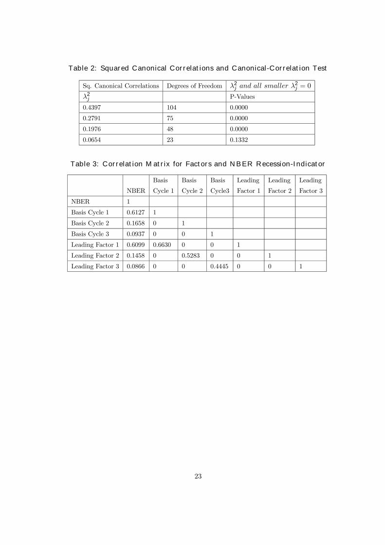
Table 2: Squared Canonical Correlations and Canonical-Correlation Test

Sq. Canonical Correlations Degrees of Freedom λ2j and all smaller λ

2j = 0

λ2j P-Values

0.4397 104 0.0000

0.2791 75 0.0000

0.1976 48 0.0000

0.0654 23 0.1332

Table 3: Correlation Matrix for Factors and NBER Recession-Indicator

Basis Basis Basis Leading Leading Leading

NBER Cycle 1 Cycle 2 Cycle3 Factor 1 Factor 2 Factor 3

NBER 1

Basis Cycle 1 0.6127 1

Basis Cycle 2 0.1658 0 1

Basis Cycle 3 0.0937 0 0 1

Leading Factor 1 0.6099 0.6630 0 0 1

Leading Factor 2 0.1458 0 0.5283 0 0 1

Leading Factor 3 0.0866 0 0 0.4445 0 0 1

23

Table 4: Simple Probit Regression Results

Regressor Est. Coeff. Robust S.E.

c1t 33.24 3.80

c2t 10.53 2.24

c3t 3.65 2.06

Constant -0.67 0.22

Table 5: Instrumental-Variable Probit Regression Results

Regressor Est. Coeff. Robust S.E.

c1t 75.13 10.71

c2t 32.56 7.45

c3t 14.01 8.27

Constant -0.15 0.23

Table 6: Encompassing Test Results - Simple Probit Index

Null hypothesis index1 encompasses index2 encompasses

Competing Coincident Indicator Models index2 (p-value) index1 (p-value)

Issler-Vahid (index1) vs. TCB (index2) 0.46 <0.01

Issler-Vahid (index1) vs. Stock-Watson (index2) 0.40 <0.01

Table 7: Encompassing Test Results - Instrumental-Variable Probit Index

Null hypothesis index1 encompasses index2 encompasses

Competing Coincident Indicator Models index2 (p-value) index1 (p-value)

Issler-Vahid (index1) vs. TCB (index2) 0.83 <0.01

Issler-Vahid (index1) vs. Stock-Watson (index2) 0.51 0.04

24

-0.03

-0.02

-0.01

0.00

0.01

0.02

0.03

65 70 75 80 85 90 95 00

Income - Transfers

-0.06

-0.04

-0.02

0.00

0.02

0.04

65 70 75 80 85 90 95 00

Industrial Production

-0.04

-0.02

0.00

0.02

0.04

65 70 75 80 85 90 95 00

Manuf. & Trade Sales

-0.010

-0.005

0.000

0.005

0.010

0.015

65 70 75 80 85 90 95 00

Employment

Figure 1: The Coincident Series

25

-0.3

-0.2

-0.1

0.0

0.1

0.2

65 70 75 80 85 90 95

Coincident Factor 1

-0.2

-0.1

0.0

0.1

0.2

65 70 75 80 85 90 95

Coincident Factor 2

-0.2

-0.1

0.0

0.1

0.2

65 70 75 80 85 90 95

Coincident Factor 3

Figure 2: Basis Cycles

26

-0.2

-0.1

0.0

0.1

0.2

65 70 75 80 85 90 95 00

Leading Factor 1

-0.2

-0.1

0.0

0.1

0.2

65 70 75 80 85 90 95 00

Leading Factor 2

-0.2

-0.1

0.0

0.1

0.2

0.3

65 70 75 80 85 90 95 00

Leading Factor 3

Figure 3: Leading Factors

27

-0.02

-0.01

0.00

0.01

0.02

65 70 75 80 85 90 95

Growth rate of IVCI

-0.02

-0.01

0.00

0.01

0.02

65 70 75 80 85 90 95

Growth rate of the TCB index

-0.03

-0.02

-0.01

0.00

0.01

0.02

0.03

65 70 75 80 85 90 95

Growth rate of XCI

Figure 4: Coincident Indices

28

-0.03

-0.02

-0.01

0.00

0.01

0.02

65 70 75 80 85 90 95

Growth rate of IVLI

Figure 5: The Leading Index

29