Forecasting the New York State Economy with "Terraced" VARs and Coincident Indices

FALL 2010

14

Forecasting the New York State Economy with “Terraced” VARs and Coincident Indices

Eric Doviak* and Sean MacDonald**

ABSTRACT

This paper introduces “Terraced” Vector Autoregressive (VAR) models, an innovative twist on traditional VAR

modeling, which allows the econometrician to simultaneously forecast both exogenous and endogenous variables

and the confidence intervals around those forecasts.

In an application of our Terraced VAR framework, we have estimated coincident indices of economic activity

for the United States, New York State and the six largest metropolitan areas of New York State and incorporated

them into Terraced VARs, which forecast the unemployment rate, total non-farm employment, real wages and

average hours worked in manufacturing in those regions.

I. Introduction Forecasting regional economic variables poses a difficult task because the data series often exhibit

negative first-order serial correlation (i.e. the series looks “jagged” or “saw-toothed”). Perhaps more

importantly, the frequent fluctuations in the series make it difficult to discern whether a one-month

increase in the unemployment rate or a one-month decrease in non-farm employment represent a

deterioration of local economic conditions or simply represent the natural fluctuations of the series.

Figures 1 and 2, which plot Rochester’s unemployment rate and non-farm employment level, illustrate

the point.

To overcome this difficulty, we used Kalman’s (1960) filtering algorithm to estimate a coincident

index of labor market activity from the unemployment rate, non-farm employment, average hours

worked in manufacturing and real wages. Such an index of Rochester’s economy is shown in Figure 3.

Because the index does not exhibit negative first-order serial correlation, it follows a simple

autoregressive process, which is relatively easy to forecast. And because the coincident index was

estimated from the economic variables of interest to us, it is highly correlated with those variables and

allows us to forecast them with more accuracy than we could achieve if we had not incorporated the

coincident index into our forecasting models.

On a monthly basis, we use our forecasting model to produce reports on the state of New York’s

labor market for the New York State Banking Department, which sponsored our research. Readers of

___________________________ * Asst. Director, Banking Research and Statistics, New York State Banking Department, New York, NY, 10004, Tel.: 212-709-1538, [email protected], [email protected] ** Asst. Professor of Economics, New York City College of Technology, City University of New York, Brooklyn, NY 11201, Tel.: 718-260-5084, [email protected]

NEW YORK ECONOMIC REVIEW

15

Figure 1: Rochester Unemployment Rate (seasonally adjusted)

Note: The series depicted above ends in May 2010.

Figure 2: Rochester Nonfarm Employment (seasonally adjusted)


FALL 2010

16

Figure 3: Coincident Index of the Rochester Economy

Note: The data used to generate the coincident index depicted above ends in May 2010.

the reports appreciate the visual smoothness of the coincident index because it allows them to quickly

discern the trend in regional labor market activity.

Section II of this paper introduces and defines a methodology for constructing a coincident index

of labor market indicators for the United States, New York State and the six largest metropolitan

statistical areas (MSAs) of New York State1. In explaining what a coincident index is, the paper also

describes the coincident indices of national, state and regional economic activity that other economists

have developed.

We did not develop coincident indices for their own sake. We developed them for the purpose of

forecasting variables that depend on the state of the labor market, such as banks’ non-current loans (a

topic of particular interest to the Banking Department). To that end, we incorporated the coincident

indices into “terraced” vector autoregressive (VAR) models, which can be used to forecast variables of

interest, such as the unemployment rate and rates of foreclosure on residential mortgages.

In other words, we hypothesized that homeowners’ difficulties in the labor market have been a

major contributor to the recent increase in mortgage delinquency. We did find a strong correlation

between our coincident indices and non-current loans, but we are reluctant to publish those findings

because the FDIC’s Statistics on Depository Institutions (our source of bank financial data) is only

available on a quarterly basis since 2003 and on an annual basis since 1992.

The “terraced” VAR methodology, which we describe in section III, is our primary contribution to

the economic literature. Unlike traditional VAR forecasting, “terraced” VARs do not require exogenous

and endogenous variables to be forecast in two separate steps. Instead, the exogenous and


17

endogenous variables are forecast simultaneously, which allows the econometrician to obtain

confidence intervals that depend only on the respective “predictor” variables.

For example, suppose that the New York City coincident index depends on past values of the

national coincident index, but the reverse is not true. In such a simple, two-variable “terraced” VAR,

the confidence interval around the forecast of the New York City index would depend on the residual

variance of its regression equation, the residual variance of the national index’s regression equation

and the covariance between them. By contrast, the confidence interval around the forecast of the

national index would only depend on the residual variance of its own regression equation.

Consequently, the “terraced” VAR methodology allows us to simultaneously compute the appropriate

confidence intervals around both the New York City and national coincident indices.

Thus, the paper seeks to extend and build upon the existing literature on state-level coincident

indices, while introducing new applications, such as incorporating the coincident indices into “terraced”

VARs to forecast “key economic variables.” The indices can therefore help policymakers anticipate the

future course of key economic trends. For example, the coincident indices can be used to forecast

unemployment rates, total employment as well as indicators of banks’ financial health (e.g. rates of

foreclosure filings and non-current loans). By including the forecast confidence intervals, we also

provide policymakers with an indication of how accurate they can expect our forecasts to be. These

uses of our methodology are briefly discussed in the conclusion of our paper, section IV.

II. Coincident Indices 1. Survey of Literature

In common speech, people often refer to the “state of the economy” with statements such as:

“The economy is strong,” or “The economy is in bad shape right now.” As a question of measurement

however, one must wonder what they are referring to. Are they referring to growth of real Gross

Domestic Product (GDP)? Are they referring to growth of real household income? Are they referring to

job growth? Are they referring to the unemployment rate?

Assuming that they are referring to some combination of those measures, how then do we

evaluate a period in which real GDP grows, but the unemployment rate rises? Is the state of the

economy “strong” or “weak?”

Obviously, one can easily define a weighted average of such measures, but what are the

appropriate weights to apply to each measure? Should those weights be constant over time?

Kacapyr’s (2010) Tompkins County index, for example, weights each element in inverse proportion to

its volatility and adjusts the weights periodically. One can also imagine other reasons why the weights

should not be constant over time. For example, if the economy is experiencing a structural shift, in

which the manufacturing sector shrinks as the service sector grows, then it hardly makes sense to

apply the same weight to manufacturing sector employment over time.

FALL 2010

18

In addressing such questions, Stock and Watson (1989) made an original and valuable

contribution to the econometric literature by observing that each of the measures described above

depends on the underlying “state of the economy” and the particular characteristics that define each

measure. They then used Kalman’s (1960) filtering algorithm to identify the unobservable “state of the

economy” in a single index, called the “coincident index.”

Visually significant decreases in Stock and Watson’s original coincident index matched the

beginnings and endings of recessions, as defined by the National Bureau of Economic Research

(NBER). Visually significant increases, of course, corresponded to economic expansions. Stock and

Watson also used a Vector Auto-Regression (VAR) model to forecast changes in the coincident index.

The forecast of the coincident index is called the “leading index.”

More recently, two economists at the New York State Division of the Budget, Megna and Xu

(2003), used Stock and Watson’s methodology to develop coincident and leading indices for the New

York State economy, which they then used to forecast changes in state tax revenue.

There is major difference between Stock and Watson’s index and Megna and Xu’s index however.

Specifically, Stock and Watson were interested in developing an index based on co-movements in

several macroeconomic time series, whereas Megna and Xu were interested in forecasting state tax

revenue. Consequently, they used different data series to develop their indices.2

Economists at the Federal Reserve Bank of New York have also developed a coincident index of

the New York State economy. Orr et al. (1999) developed such an index to predict changes in the

regional economy that do not necessarily coincide with national trends.3

A recent update of their index conducted by Bram et al. (2009) suggests that the New York regional

economy remained far more resilient than the national economy (in the sense that the New York

region entered the current recession several months later than the nation as a whole). They also found

that New York State’s economic activity peaked in February 2008, while New York City’s continued to

expand through June 2008. They also note that New York City’s economy has already experienced a

“steeper downturn than a number of metropolitan areas in upstate New York.”

Such trends also appear in our own indices. Our indices suggest that the United States entered

the current economic recession almost one year before the economies of New York State and New

York City. Specifically, our indices date the national recession as beginning in March 2007, while New

York State and New York City entered recession in May 2008 and March 2008 respectively.

More broadly, Crone and Clayton-Matthews (2005) applied Stock and Watson’s methodology to

estimate a consistent set of coincident indicators for all 50 states. They developed their indices

because the considerable lag with which the Bureau of Economic Analysis releases Gross State

Product (GSP) series inhibits timely monitoring of state economic trends. In developing their index,

they also found that the indices are a useful for comparing “the length, depth, and timing of recessions

at the state level.”


19

The Federal Reserve Bank of Philadelphia (2009) argues that Crone and Clayton-Matthews’ state

coincident indices are comparable across states because they are generated from a consistent set of

models and variables, but we remain skeptical. Specifically, we suspect that some of the indices may

appear more volatile than others because the parameter values in their filters differ across states.

Even if they are correct however, the fact that there is less data available to us at the sub-state

level than at the national and state level would prevent us from constructing an index of regional

economic activity that is comparable to a state or national index unless we were willing to discard

valuable data.

Consequently, the index that we develop for one region is not directly comparable to another’s

because the coincident indices do not have a common unit of measurement. New York City’s index is

measured in “New York City coincident units,” while Rochester’s index is measured in “Rochester

coincident units.”

2. Data Used to Estimate the Coincident Index

With two exceptions, the data that we used to estimate the coincident index were the same four

data series that Crone and Clayton-Matthews (2005) used to develop coincident indices for all 50

states. Three of the four series that Crone and Clayton-Matthews used – nonagricultural payroll

employment, the unemployment rate and average hours worked in manufacturing – are monthly data

series from the US Bureau of Labor Statistics.

Although the unemployment rate is generally identified as a lagging indicator of economic activity, it

is an appropriate variable to use when estimating the current state of the labor market. Moreover, its

use as a coincident indicator of economic activity is consistent with the models established in the

earlier works of Stock and Watson (1989), Orr et al. (1999), Megna and Xu (2003), and Crone and

Clayton-Matthews (2005).

Because the fourth series that Crone and Clayton-Matthews used, the U.S. Bureau of Economic

Analysis’ quarterly real wages and salary disbursements series, is not available at the sub-state level,

we calculated real wages by adjusting the U.S. Bureau of Labor Statistics’ total wage series for

inflation with the U.S. consumer price index. For consistency, we also used the total wage series in our

estimates of the U.S. and New York State coincident indices.

The fact that the total wage series is quarterly, while the other series are monthly, does not pose a

problem. In their paper, Crone and Clayton-Matthews show that interpolation is not necessary to

handle mixed monthly and quarterly series. Instead, they show that the Kalman Filter can be adapted

to handle any missing data simply by altering the dimensions of the relevant matrices. In fact, Petris’

(2009) “dlm” package for R (R Development Core Team, 2008), which we used to implement the

Kalman Filter, is designed to handle missing data.

In a second departure from Crone and Clayton-Matthews’ framework, we did not use average

hours worked in manufacturing in our sub-state coincident indices because the series is not available

FALL 2010

20

at the sub-state level. We also did not use the real wage series in our estimates of the Rochester and

Buffalo-Niagara Falls coincident indices because the extreme volatility of those series inhibited our

ability to estimate the parameters of the Kalman Filter when we tried to include them.

Additionally, we used the US Census Bureau’s X-12-ARIMA seasonal adjustment software (2007)

to seasonally adjust the New York State “average hours” series, all of the quarterly wage series and

the sub-state unemployment rates.

Finally, to account for serial correlation in the data series, we took differences of the

unemployment rate series and log differences of the other series. Differencing also enabled us to

overcome the problems associated with the change in industrial classification from SIC to NAICS,

which was implemented by the U.S. Bureau of Labor Statistics in 1990. Since both classifications

attempted to measure the same economic variable, we assumed that the log-differences of the two

classifications are highly correlated with each other and switched from SIC to NAICS at the earliest

possible point (i.e. from 1990 onward).

3. Estimation of the Coincident Index

To implement the Kalman Filter, we used a structure based loosely on the one used by Megna

and Xu (2003)4. Specifically, we used the following structure for the measurement equation:

⎥⎥⎥⎥⎥

⎦

⎤

⎢⎢⎢⎢⎢

⎣

⎡

+

⎥⎥⎥⎥

⎦

⎤

⎢⎢⎢⎢

⎣

⎡

ΔΔΔΔ

⎥⎥⎥⎥

⎦

⎤

⎢⎢⎢⎢

⎣

⎡

=

⎥⎥⎥⎥

⎦

⎤

⎢⎢⎢⎢

⎣

⎡

ΔΔΔΔ

−

−

−

thours

twages

temp

tunemp

t

t

t

t

t

t

t

t

uuu

u

cccc

hourswagesemp

unemp

,

,

,

,

3

2

1

10

210

10

3210

00000

)ln()ln(

)ln(

δδγγγ

ββαααα

(1)

and the following structure for the transition equation:

⎥⎥⎥⎥

⎦

⎤

⎢⎢⎢⎢

⎣

⎡

+

⎥⎥⎥⎥

⎦

⎤

⎢⎢⎢⎢

⎣

⎡

ΔΔΔΔ

⎥⎥⎥⎥

⎦

⎤

⎢⎢⎢⎢

⎣

⎡

=

⎥⎥⎥⎥

⎦

⎤

⎢⎢⎢⎢

⎣

⎡

ΔΔΔΔ

−

−

−

−

−

−

−

000

10000100001000

4

3

2

110

3

2

1

t

t

t

t

t

t

t

t

t v

cccc

cccc φφ

, (2)

where Δct is the change in the coincident index at time t and the residuals ui,t and vt are assumed to

have zero mean and constant variance.

As mentioned in section II.2, average hours worked in manufacturing is not available at the sub-

state level, so the last row of equation 1 does not appear in the local economies' measurement

equations.

We also used a slightly different structure for the measurement and transition equations of the

Rochester and Buffalo-Niagara Falls Metropolitan Statistical Areas (MSAs). As mentioned in section

II.2, we did not use the real wage series in our estimates of their coincident indices. We also found that

a different structure worked better for their economies. Specifically, with the data for the Rochester


21

and Buffalo-Niagara Falls MSAs we used the following structure for the measurement equation:

⎥⎦

⎤⎢⎣

⎡+

⎥⎥⎥⎥

⎦

⎤

⎢⎢⎢⎢

⎣

⎡

ΔΔΔΔ

⎥⎦

⎤⎢⎣

⎡=⎥

⎦

⎤⎢⎣

⎡ΔΔ

−

−

−

temp

tunemp

t

t

t

t

t

tu

u

cccc

empunemp

,

,

3

2

1

210

32100)ln( βββαααα

(3)

and the following structure for the transition equation:

⎥⎥⎥⎥

⎦

⎤

⎢⎢⎢⎢

⎣

⎡

+

⎥⎥⎥⎥

⎦

⎤

⎢⎢⎢⎢

⎣

⎡

ΔΔΔΔ

⎥⎥⎥⎥

⎦

⎤

⎢⎢⎢⎢

⎣

⎡

=

⎥⎥⎥⎥

⎦

⎤

⎢⎢⎢⎢

⎣

⎡

ΔΔΔΔ

−

−

−

−

−

−

−

000

100001000010

4

3

2

13210

3

2

1

t

t

t

t

t

t

t

t

t v

cccc

cccc φφφφ

. (4)

Although the transition equations are designed to yield a single index, Petris’ (2009) “dlm”

package, which we used to implement the Kalman Filter, does not output a single index. Instead, it

outputs four (one for each row of the transition equation). In practice however, each successive index

contains the lagged values of the previous one and (after accounting for the lags) the differences

between the four indices can safely be ignored.

4. What the Coincident Index Tells Us

To evaluate the quality of our coincident indices, it is helpful to compare our national and New York

State index with the national and New York State indices published by the Federal Reserve Bank of

Philadelphia and with Megna and Xu’s (2003) New York State index. Figures 4 and 5 provide a visual

comparison of our indices with those published by the Philadelphia Fed and the text of this section

provides a qualitative comparison.5

As mentioned in Section II.1, visually significant decreases in the coincident index indicate that the

economy is in recession. Consequently, the peaks and troughs in the index can be used to mark the

beginnings and endings of economic recessions. Therefore, the periods during which our coincident

index indicates that the economy was in recession should roughly correspond to the recessionary

periods in their indices.

As Figures 4 and 5 show, our indices exhibit much more dramatic swings in labor market activity

than the Philadelphia Fed’s indices do. This difference does not bother us. On the contrary, we feel

that the dramatic swings in our indices more accurately reflect the state of the labor market.

For example, the value of the Philadelphia Fed’s index for the US economy was 158.55 in May

2010, which was roughly the same as the 158.66 reading in February 2006. The state of the labor

market was very different at those two points in time however. After all, the unemployment rate was

4.9 percentage points higher and non-farm employment was 3.5 percent lower in May 2010 than it

FALL 2010

22

was in February 2006. By contrast, our United States index value was 107.0 in February 2006 and

52.5 in May 2010.

Similarly, the value of the Philadelphia Fed’s index for the New York State economy was 155.32 in

May 2010, which was roughly the same as the 155.32 reading in December 2007. Once again, the

state of the labor market was very different in those two periods. New York’s unemployment rate was

3.6 percentage points higher and its non-farm employment was 2.5 percent lower in May 2010 than it

was in December 2007. Once again, our New York index more accurately reflects the change in the

state of the labor market, as its index values were 142.5 in December 2007 and 119.9 in May 2010.

Figure 4: Coincident Indices of the New York State Economy


Figure 5: Coincident Indices of the United States Economy



23

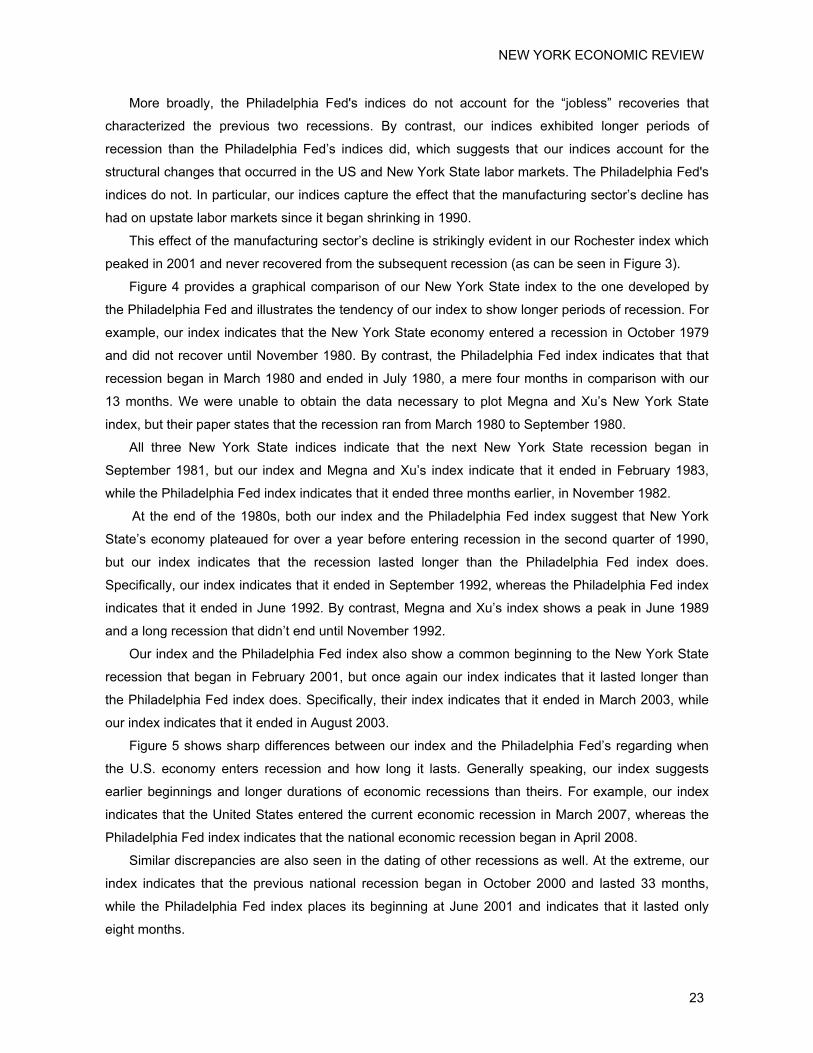
More broadly, the Philadelphia Fed's indices do not account for the “jobless” recoveries that

characterized the previous two recessions. By contrast, our indices exhibited longer periods of

recession than the Philadelphia Fed’s indices did, which suggests that our indices account for the

structural changes that occurred in the US and New York State labor markets. The Philadelphia Fed's

indices do not. In particular, our indices capture the effect that the manufacturing sector’s decline has

had on upstate labor markets since it began shrinking in 1990.

This effect of the manufacturing sector’s decline is strikingly evident in our Rochester index which

peaked in 2001 and never recovered from the subsequent recession (as can be seen in Figure 3).

Figure 4 provides a graphical comparison of our New York State index to the one developed by

the Philadelphia Fed and illustrates the tendency of our index to show longer periods of recession. For

example, our index indicates that the New York State economy entered a recession in October 1979

and did not recover until November 1980. By contrast, the Philadelphia Fed index indicates that that

recession began in March 1980 and ended in July 1980, a mere four months in comparison with our

13 months. We were unable to obtain the data necessary to plot Megna and Xu’s New York State

index, but their paper states that the recession ran from March 1980 to September 1980.

All three New York State indices indicate that the next New York State recession began in

September 1981, but our index and Megna and Xu’s index indicate that it ended in February 1983,

while the Philadelphia Fed index indicates that it ended three months earlier, in November 1982.

At the end of the 1980s, both our index and the Philadelphia Fed index suggest that New York

State’s economy plateaued for over a year before entering recession in the second quarter of 1990,

but our index indicates that the recession lasted longer than the Philadelphia Fed index does.

Specifically, our index indicates that it ended in September 1992, whereas the Philadelphia Fed index

indicates that it ended in June 1992. By contrast, Megna and Xu’s index shows a peak in June 1989

and a long recession that didn’t end until November 1992.

Our index and the Philadelphia Fed index also show a common beginning to the New York State

recession that began in February 2001, but once again our index indicates that it lasted longer than

the Philadelphia Fed index does. Specifically, their index indicates that it ended in March 2003, while

our index indicates that it ended in August 2003.

Figure 5 shows sharp differences between our index and the Philadelphia Fed’s regarding when

the U.S. economy enters recession and how long it lasts. Generally speaking, our index suggests

earlier beginnings and longer durations of economic recessions than theirs. For example, our index

indicates that the United States entered the current economic recession in March 2007, whereas the

Philadelphia Fed index indicates that the national economic recession began in April 2008.

Similar discrepancies are also seen in the dating of other recessions as well. At the extreme, our

index indicates that the previous national recession began in October 2000 and lasted 33 months,

while the Philadelphia Fed index places its beginning at June 2001 and indicates that it lasted only

eight months.

FALL 2010

24

A similarly large difference exists in the dating of the national recession of the early 1990s. Our

index indicates that it lasted from April 1990 to June 1992, whereas the Philadelphia Fed indicates that

it lasted from October 1990 to May 1991.

The differences in the dating are smaller however when we compare the dating of the two

recessions in the early 1980s. Our index indicates that the first one began in July 1979 and lasted 14

months, while the Philadelphia Fed index indicates that the first one began in April 1980 and lasted

four months. There is slightly more agreement on the dating of the second recession in the early

1980s. Our index indicates that it lasted from May 1981 until January 1983, whereas the Philadelphia

Fed index indicates that it lasted from September 1981 until November 1982.

These few similarities aside, our indices and the Philadelphia Fed’s disagree sharply on the dates

when recessions began and ended (because our indices suggest that recessions last longer). On a

very general level however, their indices and ours both identify the same recessions. If the

Philadelphia Fed’s indices are considered a benchmark, then this rough similarity in dating would still

allow us to conclude that our indices adequately capture movement in overall economic activity in both

the United States and New York State.

III. Forecasting Because the coincident index measures the underlying state of the labor market, forecasts of the

coincident index (called a “leading index”) predict the future course of labor market activity and provide

policymakers with an outlook for the future course of variables that depend on the state of the labor

market, such as banks’ non-current loans and rates of mortgage delinquency.

Because it is constructed from the unemployment rate, non-farm employment and average hours

worked in manufacturing, the coincident index is also an excellent predictor of those variables, so we

include forecasts of these “key economic variables” in our monthly reports. These forecasts have the

added benefit of providing the reader of our reports with a concrete understanding of what the

coincident index forecast means.

1. “Terraced” VARs Our forecasting model consists of a set of “terraces.” The top terrace forecasts exogenous

variables that are useful in predicting changes in the national coincident index. The forecasts of those

exogenous variables are passed down to the next terrace, which forecasts the change in the national

coincident index. The national index forecast is then passed down to the next terrace, which forecasts

the change in a sub-national index. Finally, at the lowest level, the sub-national index forecast is used

to forecast changes in the “key economic variables.”

Forecasts on a given terrace are based on autoregressive models, which assume that the change

in a given variable depends on past changes in that variable and on past changes in variables at

higher level terraces. To be more concrete, this section will explain our forecasting model in terms of a


25

simple three variable “terraced” vector autoregressive (VAR) model. In practice, there are many more

variables in our model, but – to keep the example simple here – these will be discussed in further

detail in Section III.4.

The specific example of a terraced VAR that we will use is as follows:

⎥⎥⎥

⎦

⎤

⎢⎢⎢

⎣

⎡

+⎥⎥⎥

⎦

⎤

⎢⎢⎢

⎣

⎡

ΔΔΔ

⎥⎥⎥

⎦

⎤

⎢⎢⎢

⎣

⎡

=⎥⎥⎥

⎦

⎤

⎢⎢⎢

⎣

⎡

ΔΔΔ

−

−

−

tunemp

tNYC

tUS

t

t

t

unempNYC

NYCUS

US

t

t

t

uuu

unempNYCUS

unempNYCUS

,

,

,

1

1

1

0000

γγββ

α . (5)

The top row of equation 5 (or “top terrace”) models the change in the U.S. coincident index at time

t (denoted: ΔUSt ). In this case, it is assumed that ΔUSt depends only on the previous value of the

change in the US index (i.e. ΔUSt-1 ) and the residual: uUS,t . In such a model, forecasts of the change

in the U.S. coincident index will therefore depend exclusively on past values of the change in the US

index.

The second row models the change in the New York City coincident index at time t (denoted:

ΔNYCt). According to equation 5, ΔNYCt depends on ΔUSt-1, its own past value (i.e. ΔNYCt-1) and the

residual: uNYC,t . Forecasts of the change in the New York City coincident index will therefore depend

on past values of the change in the New York City index as well as past values of the change in the

U.S. index.

Finally, the third row models the change in the New York City unemployment rate at time t

(denoted: Δunempt). In this case, it is assumed that Δunempt depends on ΔNYCt-1, its own past value

(i.e. Δunempt-1) and the residual: uunemp,t. Forecasts of the change in the New York City unemployment

rate will depend on past values of the change in the New York City unemployment rate and past

values of the change in the New York City coincident index. It is important to note that forecasts of the

change in the New York City unemployment rate will also depend on past values of the change in the

U.S. index (because the change in the New York City index depends on past values of the change in

the U.S. index).

To set up the terraced VAR, we first created an ordinary VAR using Pfaff’s (2008) “vars” package

for R (R Development Core Team, 2008). We then used ordinary least squares (OLS) regression to

estimate the coefficients of the terraced VAR and replaced the ordinary VAR coefficients with the

coefficients of the terraced VAR.

We also replaced the residuals in the VAR object with the rescaled residuals6 from the OLS

equations, so that the VAR object’s residual covariance matrix could be used to compute the

confidence intervals around our forecasts.

2. Long-Run Assumptions

As mentioned previously, a terraced VAR models changes in the variables of interest. We had to

express each model in terms of changes to remove the spurious correlation that arises between two

unrelated variables that trend upward (or downward) over time.

FALL 2010

26

We also had to make sure that our terraced VARs do not contain a “unit root,” so that the effect of

any given shock will fade over time. (In other words, the model assumes that the events of 20 or 30

years ago do not affect the month-to-month fluctuations in the variables we are examining.)

Because all shocks fade over time and because our terraced VARs do not contain an intercept

term, our models implicitly assume that the changes in the coincident index and changes in the key

economic variables converge to zero in the long run. Since the changes are zero in the long run, the

model assumes that the coincident index and key economic variables remain constant in the long run.

In theory, this implies a prediction that the economy will never recover from the current economic

crisis. In practice however, forecasts of exogenous leading economic indicators, such as unfilled

orders for durable goods (discussed in Section III.4) act as an implicit intercept, which allow our model

to predict both recovery from recession and decline from expansion.

3. Confidence Intervals

When forecasting, we must assume that the errors in equation 5 will equal zero. In other words,

when forecasting the New York City coincident index we implicitly assume that we know the future

course of the US index with certainty. Similarly, when we forecast the New York City unemployment

rate we implicitly assume that we know the future course of the New York City index with certainty.

Of course, we do not know those values with certainty. All of our forecasts are prone to error,

which we must account for. To that end, we estimate a range of forecast values, within which we can

be 90 percent certain that the true values will fall. As mentioned in Section 3.1, these estimates are

based on the residuals that we obtained when we estimated the coefficients of the terraced VAR.

To compute the confidence intervals, Pfaff’s “vars” package uses forecast error variance

decomposition, which is based on the Wold (1954) moving average decomposition for stable VAR-

processes, which is defined as:

L+++= −− 22110 tttt uΦuΦuΦy , (6)

where yt is the vector of dependent variables at time t, u t-I is the residual vector at time t – i and the Φi

are matrices of parameters that depend on the coefficients of the VAR (or terraced VAR in our case). If

the residuals are interpreted as unforeseen economic shocks, then equation 6 shows that current

changes in our model’s variables depend entirely on past shocks.

To compute the values of Φi , Pfaff’s “vars” package sets Φ0 equal to an identity matrix (with the

same number of dimensions as the VAR has variables) and recursively computes Φs as:

∑=

−=sΦΦ

1jjjss A for s = 1,2,…, (7)

where Aj is matrix j of the p matrices of VAR coefficients 6 and where Aj = 0 for j > p. The values of Φi


27

are then used to compute the forecast error covariance matrix:

( )

⎥⎥⎥⎥⎥

⎦

⎤

⎢⎢⎢⎢⎢

⎣

⎡

⊗

⎥⎥⎥⎥

⎦

⎤

⎢⎢⎢⎢

⎣

⎡

=⎟⎟⎟⎟

⎠

⎞

⎜⎜⎜⎜

⎝

⎛

⎥⎥⎥

⎦

⎤

⎢⎢⎢

⎣

⎡

−

−

−

−

−−++

++

I

I

TI

I

I

I0I

CovTh

Th

h

hhThThT

TTT

000

0000

2

11

21

1

|

|11

MOM

L

L

OM

L

M Φ

ΦΦ

Σ

ΦΦ

Φ

yy

yy

u , (8)

where T is last period for which data is available, h is the number of forecast periods, Ih is an identity

matrix with h dimensions, Σu is the residual covariance matrix, the operator ⊗ is the Kronecker product

and yT+h - yT+h ІT is the difference between the true value of the dependent variable vector at time T+h

and our forecast of it, given the information available to us at time T.

The square roots of the diagonal elements of the forecast error covariance matrix are the standard

errors of the forecasted variables, which we then use to compute the confidence intervals.

Had we estimated the terraced VAR that was used as an example in Section III.1 and then

computed the confidence interval around its forecasts, we would find that the confidence interval

around the U.S. coincident index is computed as if the New York City variables were not in the

terraced VAR at all.

The confidence interval around the New York City index would depend on the variances of the

U.S. and New York City index residuals and the covariance between them (i.e. just as if it had come

from a standard two-variable VAR), but would be blind to the presence of the New York City

unemployment rate in the terraced VAR.

In the third forecast period (and thereafter), the confidence interval around New York City’s

unemployment rate would depend on all six variances and covariances (just as one would expect from

the model).

There are two sources of error, however, that the forecast error variance decomposition cannot

account for. One is revisions of the data used to generate the index and forecasts. The other is

sampling error. Forecast error variance decomposition does not account for sampling error because it

implicitly assumes that the VAR’s coefficients are exactly equal to their true values. Had we estimated

the coefficients from a different time interval, we would have obtained different coefficient estimates

and thus gotten a different forecast.

As Feldstein (1971) has shown, sampling error implies that the forecast error of the New York City

variables (in Section III.1) would not be distributed normally. To overcome the problems associated

with non-normality, McCullough (1996) proposed bootstrapping.

We have chosen not to use bootstrapped confidence intervals however for two reasons. First,

given the complexity of our models, the bootstrapping code is very difficult to write and could introduce

an unknown degree of human error into the bootstrapped confidence intervals. Second, the purpose of

this exercise is to provide the reader of our reports with a general sense of the direction in which the

national, state and local economies are headed and with a basic sense of accuracy. We do not need

precise estimates of the distribution of the forecast error.

FALL 2010

28

4. Forecast Accuracy

It is simple to create a terraced VAR and compute the confidence intervals around its forecasts,

but there are many possible terraced VAR structures to choose from. Therefore, we need to select the

structure that has the most predicative power. In this section, we also wish to show that using

coincident indices in our forecasting models increases the model’s predicative power.

To that end, we estimated the coefficients of many possible terraced VAR structures using the

available data between from 1990 to 2004. We then used the estimated coefficients and the rest of the

available data (which ended in December 2008) to create 37 sets of 12-month forecasts and 11 sets of

shorter forecasts. Finally, we compared the forecasts to the actual values and computed the Mean

Squared Error (MSE) of the model’s forecasts:

( )∑−

=+++++ −=

1

0

2|

1 n

iiTkiTkiTk yy

nMSE ,

where k is the number of periods ahead for which the variable yt is forecasted, yT+i+k|T+i is the

forecasted value of yT+i+k given the information available at time T+i and n is the number of k-period

ahead forecasts.

As Greene (2000) notes, the MSE does not have a scale which allows us to compare the MSE of

one forecasted variable to the MSE of another. To get around this problem, we compared the MSE to

the variance of the forecasted variable by creating a “relative MSE” statistic, which is similar in spirit to

the coefficient of determination:

)var(1.

kt

kk y

MSEMSElRe+

−=

where var(yt+k) is the variance of the variable yt+k in the forecast period.

A relative MSE of one implies perfect prediction, while lower values imply weaker forecasting

performance. It is important to note that this statistic may be negative, but – because we cannot know

what the variable’s mean will be in the forecast period – negativity does not necessarily mean that the

forecast is poor. Sometimes, a slightly negative relative MSE is the highest value one can obtain when

forecasting a very volatile variable.

Table 1 uses relative MSE to compare our forecast models to both a random walk and an

“alternative model,” in which the region’s coincident index is not used to forecast “key economic

variables” (i.e. the unemployment rate, non-farm employment and average hours worked in

manufacturing). To keep the table concise, the reported relative MSE statistic is the average of the 12

Rel.MSEk:

∑=

=12

kkMSElReMSElRe

1.

121.


29

Table 1 shows that our forecast models always outperform the “random walk” forecasts (i.e.

TT|kT y y =+ for all k). In other words, our forecast models always provide better prediction than simply

observing present economic conditions and assuming that the same condition will continue to hold for

the foreseeable future.

With three exceptions, Table 1 shows that our forecast models always outperform the forecasts of

the “alternative model,” which is the best model that we could develop that does not include the

region’s coincident index as an explanatory variable. This shows that the region’s coincident index is a

good predictor of the variables that were used to create it.

The three exceptions were the unemployment rates of New York State and the Nassau-Suffolk

MSA and non-farm employment of the Putnam-Rockland-Westchester MSA, but in each of these

cases, the difference between the forecast model and the alternative model was small. Given the

proximity of Nassau-Suffolk and Putnam-Rockland-Westchester to New York City, it may be the case

that the labor markets in these two MSAs are more dependent on the state of the New York City

economy than they are on their own. Moreover, the fact that New York City accounts for approximately

43 percent of the New York State population, the New York State unemployment rate may also be

heavily dependent on the state of the New York City economy.

Interestingly, the coincident indices turned out to be good predictors of themselves. This may be

attributable to the auto-regressive processes that the coincident indices follow (i.e. to the

“smoothness” of the coincident index series).

The U.S. coincident index also appears to be a good predictor of state and regional coincident

indices. This may be attributable to the fact that regional economies are strongly influenced by national

economic conditions.

While developing our forecasting models, we also experimented with other variables, such as the

Federal Reserve’s measures of industrial production and capacity, the Census Bureau’s series on

housing starts, durable goods and retail sales. The model that provided the most predicative power

however only included the Census Bureau’s durable goods unfilled orders series as an exogenous

variable.

Housing starts, which are often mentioned as a leading indicator, did not prove to be a good

predictor of our indices. The lack of correlation may be attributable to the fact that the time period over

which we tested our forecast models includes the period during which the housing bubbles in the U.S.

and New York State burst. Housing starts were very weak from January 2007 through mid-2009.

In any case, forecast models that included unfilled orders for durable goods proved to be a

significantly stronger predictor of our indices than forecast models that included housing starts.

Taken as a whole, one can conclude from the reasonably high values of our forecast models’

relative MSE statistics that our forecasting models capture a good share of the out-of-sample variation

in the variables that the models predict.

FALL 2010

30

Table 1: Forecast Accuracy Forecast Model Alternative Model R. Walk

Rel. MSE specification Rel. MSE specification Rel. MSE

United States Dur. Goods Unfill. Orders -0.220 DGU(1,2,3,4,5,6) -0.770Coincident Index 0.609 DGU(4), US(1,2) 0.494Unemployment Rate 0.348 US(1,2), UR(1,2) -0.020 DGU(4), UR(1,2) -0.320Nonfarm Employment 0.615 US(1,2), EMP(1,2) 0.390 DGU(4), EMP(1,2) 0.273Avg. Hours Worked Manuf. 0.080 US(1,2), HR(1,2) 0.001 DGU(4), HR(1,2) -0.752

New York State Coincident Index 0.475 US(1,2), NYS(1,2), NYC(1,2) 0.069Unemployment Rate 0.368 US(1,2), NYS(1,2), UR(1,2) 0.371 US(1,2), NYC(1,2), UR(1,2) -0.449Nonfarm Employment 0.185 NYS(1,2), EMP(1,2) -0.045 US(1,2), NYC(1,2), EMP(1,2) -0.640Avg. Hours Worked Manuf. 0.047 US(1,2), NYS(1,2), NYC(1,2), HR(1,2) 0.028 US(1,2), NYC(1,2), HR(1,2) -0.895

New York City Coincident Index 0.783 US(1,2), NYC(1,2) 0.408Unemployment Rate 0.259 US(1,2), NYC(1,2), UR(1,2) 0.241 US(1,2), UR(1,2) -0.703Nonfarm Employment 0.147 NYC(1,2), EMP(1,2) -0.234 US(1,2), EMP(1,2) -0.468

Nassau-Suffolk Coincident Index 0.773 US(1,2), NYC(1,2), NS(1,2) 0.419Unemployment Rate 0.263 US(1,2), NYC(1,2), NS(1,2), UR(1,2) 0.269 US(1,2), NYC(1,2), UR(1,2) -0.509Nonfarm Employment 0.166 NYC(1,2), NS(1,2), EMP(1,2) 0.134 US(1,2), NYC(1,2), EMP(1,2) -0.740

Putnam-R'land-West'r Coincident Index 0.661 US(1,2), NYC(1,2), PRW(1,2) 0.479Unemployment Rate 0.229 PRW(1,2), UR(1,2) 0.216 US(1,2), NYC(1,2), UR(1,2) -0.537Nonfarm Employment 0.058 US(1,2), NYC(1,2), PRW(1,2), EMP(1,2) 0.095 US(1,2), NYC(1,2), EMP(1,2) -1.030 Table continues on the next page


31

Table 1 (continued): Forecast Accuracy

Forecast Model Alternative Model R. Walk Rel. MSE specification Rel. MSE specification Rel. MSE

Buffalo-Niagara Falls Coincident Index 0.641 US(1,2), BN(1,2) 0.456Unemployment Rate 0.254 US(1,2), BN(1,2), UR(1,2) 0.207 US(1,2), UR(1,2) -0.721Nonfarm Employment 0.031 BN(1,2), EMP(1,2) -0.012 US(1,2), NYS(1,2), EMP(1,2) -1.055

Rochester Coincident Index 0.660 US(1,2), Rch(1,2) 0.505Unemployment Rate 0.292 US(1,2), NYS(1,2), Rch(1,2), UR(1,2) 0.240 US(1,2), NYS(1,2), UR(1,2) -0.603Nonfarm Employment -0.039 NYS(1,2), Rch(1,2), EMP(1,2) -0.210 US(1,2), EMP(1,2) -1.168

Albany-Sch.-Troy Coincident Index 0.721 US(1,2), NYS(1,2), AST(1,2) 0.496Unemployment Rate 0.193 US(1,2), NYS(1,2), AST(1,2), UR(1,2) 0.169 US(1,2), NYS(1,2), UR(1,2) -0.774Nonfarm Employment 0.124 AST(1,2), EMP(1,2) 0.122 US(1,2), NYS(1,2), EMP(1,2) -1.030

The numbers in parenthesis are the lag numbers of the variables that appear in the model's equation. DGU – Durable Goods Unfilled Orders BN – Buffalo-Niagara Falls Coincident Index US – United States Coincident Index Rch – Rochester Coincident Index NYS – New York State Coincident Index AST – Albany-Schenectady-Troy Coincident Index NYC – New York City Coincident Index UR – Unemployment Rate NS – Nassau-Suffolk Coincident Index HR – Average Hours Worked in Manufacturing PRW – Putnam-Rockland-Westchester Coincident Index EMP – Nonfarm Employment


32

IV. Conclusion and Direction for Future Research This paper has explained what a coincident index is and has detailed the methodology employed to

estimate the values of the coincident index for the United States, New York State and the six largest

MSAs in New York State. It has also explained how we use the coincident index to forecast the future

course of “key economic variables” in those regions.

No forecast will ever be perfect; however, we account for the inevitable error in our forecasts by using

Terraced VARs to simultaneously forecast all of the variables in the model and compute confidence

intervals that depend solely on the variables that affect the value of the forecasted variables. The

confidence intervals are imperfect because they do not account for sampling error, but these

imperfections occur in all VAR model forecast confidence intervals (not just terraced VARs).

As Section III.4 has shown, our forecasts are more accurate than those we could obtain from

assuming a random walk and those that we would obtain had we not included the coincident index in our

forecasting models.

In future work, we will explore the correlation between our index and other variables of interest. For

example, to the extent that borrowers’ ability to meet their monthly mortgage and consumer credit

payments depends on the state of their local economy, then we can examine whether there is a

correlation between loans past due and the coincident index. We have already found such a correlation in

our preliminary work, so we hope to use the forecast of the coincident index to forecast loans past due

and predict future delinquency trends.

ENDNOTES 1. The coincident index estimates exclude Utica-Rome, Syracuse, Elmira, and Binghamton due to

insufficient data.

2. Stock and Watson used data on industrial production, personal income net of transfer payments,

hours worked by employees of nonagricultural establishments and total manufacturing and trade

sales to develop their index, while Megna and Xu used data on total employment, sales tax revenue

(as a proxy for retail sales), hours worked in manufacturing and the unemployment rate.

3. Orr et al. developed their index from data on total employment, real wages and salaries, the

unemployment rate and average hours worked in manufacturing.

4. It should be noted, however, that Megna and Xu’s framework used monthly sales tax collection data

as a proxy for retail sales instead of a real wage series.

5. We requested, but were unable to obtain, Megna and Xu’s New York State index. Our comparisons

with their results are based on their published paper.

6. Rescaling the residuals was necessary to account for the difference in degrees of freedom between

the ordinary VAR and the OLS regression.

7. The number of VAR coefficient matrices, p, is equal to the lag order of the VAR.


33

ACKNOWLEDGEMENTS We would like to thank the New York State Banking Department for supporting our research and for

providing many useful comments and suggestions. The views expressed in this article are our own

opinions and do not necessarily reflect the opinions of the New York State Banking Department.

REFERENCES

Bram, Jason, James Orr, Rae Rosen, Robert Rich and J. Song (Sept. 2009). “Is the Worst Over?

Economic Indexes and the Course of the Recession in New York and New Jersey.” Current Issues in

Economics and Finance, 15(5).

Crone, Theodore M. and Alan Clayton-Matthews (Nov. 2005). “Consistent Economic Indexes for the 50

States.” Review of Economics and Statistics, 87(4):593–603.

Federal Reserve Bank of Philadelphia. State Coincident Indexes (2008, 2009).

http://www.philadelphiafed.org/research-and-data/regional-economy/indexes/coincident/.

Feldstein, Martin (1971). “The Error of Forecast in Econometric Models when the Forecast-Period

Exogenous Variables are Stochastic”. Econometrica, 39(1):55–60.

Greene, William H. (2000), Econometric Analysis, Upper Saddle River, NJ, Prentice Hall, 4 edition.

Kacapyr, Elia (2010). “The Index of Economic Activity in Tompkins County.”

http://www.ithaca.edu/hs/economics/tcdex.htm.

Kalman, Rudolf E. (1960). “A New Approach to Linear Filtering and Prediction Problems.” Transactions of

the ASME – Journal of Basic Engineering, 82(1):35–45.

McCullough, B.D. (1996). “Consistent Forecast Intervals when the Forecast-period Exogenous Variables

are stochastic.” Journal of Forecasting, 15(4):293–304.

Megna, Robert and Qiang. Xu (2003). “Forecasting the New York State Economy: The Coincident and

Leading Indicators Approach.” International Journal of Forecasting, 19(4):701–713.

Orr, Jason, Robert Rich and Rae Rosen (Oct. 1999). “Two New Indexes Offer a Broad View of Economic

Activity in the New York-New Jersey Region.” Current Issues in Economics and Finance, 5(14).

Petris, Giovanni (2009). dlm: Bayesian and Likelihood Analysis of Dynamic Linear Models, R package

version 0.99-0.

Pfaff, Bernhard (Jul. 2008). “VAR, SVAR and SVEC Models: Implementation Within R Package ‘vars.”’

Journal of Statistical Software, 27(4):1–32. http://www.jstatsoft.org/v27/i04/.

R Development Core Team (2008). R: A Language and Environment for Statistical Computing. R

Foundation for Statistical Computing. Vienna, Austria, 2008. http://www.R-project.org.

Stock, James H. and Mark W. Watson (1989). “New Indexes of Coincident and Leading Economic

Indicators.” NBER Macroeconomics Annual, 4:351–394.

US Census Bureau, Time Series Staff. X-12-ARIMA. Washington, DC, 15 June 2007. Version 0.3.

FALL 2010

34

Wold, Hermann. (1954). A Study in the Analysis of Stationary Time Series. Almqvist and Wiksell Book

Co., Uppsala.

Forecasting the New York State Economy with "Terraced" VARs and Coincident Indices

Documents

Transcript of Forecasting the New York State Economy with "Terraced" VARs and Coincident Indices