THE �-MEU MODEL: A COMMENT1

Jürgen Eichberger2

Alfred Weber Institut,

Universität Heidelberg, Germany.

Simon Grant3

Department of Economics,

Rice University, Texas, USA

and University of Queensland, Australia.

David Kelsey4

Department of Economics,

University of Exeter, England.

Gleb A. Koshevoy5

Central Institute of Mathematics and Economics RAS,

Moscow, Russia.

26th August 2010

1Research in part supported by ESRC grant no. RES-000-22-0650 and a Leverhulme Research Fellowship.For comments and discussion we would like to thank Dieter Balkenborg, Paolo Ghirardato, Klaus Nehring, JanWenzelburger, Yiannis Vailakis, participants in seminars in Exeter and Heidelberg the referee and associate editorof this journal.

2e-mail, juergen.eichberger@awi.uni-heidelberg.de3Corresponding Author Simon Grant, Department of Economics, Rice University, PO Box 1892, Hous-

ton, Texas 77251-1892, USA (e-mail: sgrant@rice.edu) fax. 71-3-348-5278.4e-mail, D.Kelsey@exeter.ac.uk5e-mail, gleb_koshevoy@mail.ru

Abstract

In [7], Ghirardato, Macheroni and Marinacci propose a method for distinguishing between perceived

ambiguity and the decision-maker's reaction to it. They study a general class of preferences which they

refer to as invariant biseparable. This class includes CEU and MEU. They axiomatize a subclass of

�-MEU preferences. If attention is restricted to �nite state spaces, we show that any �-MEU preference

relation, satis�es GMM's axioms if and only if � D 0 or 1, that is, the preferences must be either maxmin

or maxmax. We show by example that these axioms may be satis�ed when the state space is [0,1].

Keywords, Ambiguity, multiple priors, invariant biseparable, Clarke derivative, ambiguity-preference.

JEL Classi�cation: D81.

1 Introduction

Ghirardato, Macheroni and Marinacci [7] (henceforth GMM), axiomatize a class of preferences which

they refer to as invariant biseparable. This class encompasses both the Choquet expected utility (hence-

forth CEU) model of Schmeidler [11] and the maxmin expected utility model (also known as the multiple

prior model) of Gilboa and Schmeidler [8].1 Let < be an invariant biseparable preference order on the

set of acts which map states from a set S to consequences in a set X . GMM de�ne the (generally) partial

ordering <� that is the maximal sub-relation of < satisfying all the axioms of subjective expected utility

(SEU) except completeness.2 They refer to <� as the unambiguous preference relation and show that it

admits a representation in the style of Bewley [2]: in particular, there is a utility function u .�/ de�ned

on the set of outcomes X and a non-empty, compact and convex set of probability measures P de�ned

on the state space S such that for any pair of acts f and g,

f <� g ()

ZSu . f .s// dP .s/ >

ZSu .g .s// dP .s/ , 8 P 2 P .

The relation <� is complete if and only if P is a singleton in which case < equals <� and has the SEU

form.

Furthermore, they establish the existence of a function � .�/ that maps each act f to a weight � . f /

in [0; 1], such that < can be represented by the functional:

M . f / D � . f /minP2P

ZSu . f .s// dP .s/C .1� � . f //max

P2P

ZSu . f .s// dP .s/ : (1)

They show that the set P also admits a straightforward differential characterization. Typically M will

have kinks at constant acts, (that is, acts which assign the same utility to every state). Thus it is not

possible to apply conventional notions of differentiation. Instead GMM use the Clarke derivative.3 For

our purposes it is enough to note that for the functional I : RS ! R, which satis�es I .u � f / D M . f /,

for each act f , the set P is precisely @ I .0/, the Clarke differential of I at 0.

GMM are careful to note the following feature of their representation. To generate preferences in

their class it is not enough to �x an arbitrary (non-empty, weak* compact and convex) set of probability1See GMM [7], Axioms 1-5. The formal statements of these axioms appear in the appendix below.2Note this is equivalent but not identical to the original de�nition, for details see [7]. Related research can be found in

Nehring [10].3The Clarke derivative is one way to extend the concept of a derivative on Rn to functions which have some kinks. It is

also a generalization of the super-gradient to a function which is not necessarily concave. For further details see Clarke [4].

1

measures P and an arbitrary index � .�/ and substitute them into Eq. (1): Rather in order for expression

(1) to generate an invariant biseparable preference relation for a given set P and index � .:/, we need to

check that the associated Clarke differential of I at 0 is indeed equal to P .

At �rst glance expression (1) appears closely related to the classic �-MEU model:

V . f / D �minP2D

ZSu . f .s// dP .s/C .1� �/max

P2D

ZSu . f .s// dP .s/ . (2)

However there are two differences. First in the classic �-MEU model the weight � on the minimum

expected utility is constant, whereas in expression (1) the weight � . f / depends on the act f . Second in

the classic �-MEU model the set D can be any non-empty weak* compact set of probability measures,

whereas in expression (1), P must be equal to the Clarke differential at 0.

GMM provide an axiomatic characterization that combines the key features of the two models: the

ambiguity-aversion index � .�/ is constant and equal to some �xed weight � in [0; 1], and the set of

probabilities is given by the Clarke differential at 0.4 That is, the preferences admit a representation

of the form given in expression (2) with the restriction that D D @ I .0/, where I .u � f / D V . f /.

Imposing the additional restriction that � . f / be constant implies GMM's representation must satisfy a

type of �xed point property. If one starts with a given set D and constructs a set of �-MEU preferences

with this set of priors; then it is necessary that the Clarke differential at 0 be equal toD. For a �nite state

space, however, we show that for any relation that satis�es GMM's axiomatization (that is, their Axioms

1-5 and 7) the constant ambiguity-aversion index, �; is equal either to 0 or to 1. Or equivalently, the

preference relation is either maxmax expected utility or maxmin expected utility.

Our strategy of proof is to �x a closed convex set, D, of probability distributions on a �nite set S

and an � in [0; 1], and consider the preferences de�ned by expression (2) and de�ne I : Rn ! R by

I .u � f / D V . f /. If the preferences satisfy the GMM axioms, then @ I .0/ should yield the original

set D. The analysis in section 3 shows that when we take the Clarke derivative, we do not get back the

original set D unless the ambiguity-aversion index, �; is equal either to 1 or to 0.

The intuition is most clear in the case where D is a circle as shown in �gure 1. The �gure considers

a given act f . The expected value of f is maximised at q 2 D and minimised at q 0. The probability used

to calculate the expectation of f (and hence value V . f /) is accordingly �q 0 C .1� �/ q. As f varies,4The axiomatization consists of their Axioms 1-5 and an additional axiom Axiom 7. The formal statement of this axiom

appears in the appendix below.

2

Figure 1: Circular set of priors

the corresponding probability associated with each act traces out the boundary of the inner circle. The

Clarke differential, @ I .0/, is the convex hull of these points, which is represented by the shaded area in

the diagram. As can be seen, it is a proper subset of the set of priors D.

A similar result does not hold for in�nite state spaces. We show that there exist examples of �-MEU

preferences satisfying GMM's axioms in this case.

Organization of the paper The next section provides a review of some of the mathematical tech-

niques we shall be using. In section 3 we show that when the state space is �nite there is no �-MEU

preference, which satis�es the GMM axioms. However there are examples of such preferences over

in�nite state spaces as we shall demonstrate in section 4. Formal statements of GMM's axioms appear

in the appendix.

2 Mathematical Preliminaries

This section reviews some mathematical concepts which we need, in particular the Clarke derivative.

3

2.1 Lipschitz functions

The Clarke derivative is de�ned for functions which are locally Lipschitz. These are de�ned as follows.

De�nition 1 Let X be a subset of a Banach space. A function f : X ! R is said to be Lipschitz if there

exists L > 0 such that for all x; y 2 X; j f .x/� f .y/j < L kx � yk : A function g : X ! R; is said to

be locally Lipschitz if for all x 2 X; there is a neighbourhood of x on which g is Lipschitz.

Lemma 1 Let f and g be two real valued functions de�ned on an open subset U of Rn . Then if both f

and g are Lipschitz so is f � g.

Proof. Since f and g are Lipschitz, there exist L 0; L 00 > 0 such that j f .x/ � f .y/j < L 0 kx � yk

and jg .x/� g .y/j < L 00 kx � yk : Now let L D maxfL 0; L 00g and note that . f � g/.x/ D f .x/ �

g.x/; then we have j. f � g/.x/ � . f � g/.y/j D j f .x/� g.x/� f .y/C g.y/j 6 j f .x/� f .y/j C

jg .x/� g .y/j < L kx � yk C L kx � yk D 2L kx � yk :

Clarke [4] shows that any bounded convex function is Lipschitz.

Proposition 1 (Clarke [4], Proposition 2.2.6, p.34) Let U be an open subset of a Banach space X;

and let f : U ! R be convex and bounded above on a neighbourhood of some point of U. Then for any

x in U, f is Lipschitz near x.

2.2 Derivatives

The usual derivative on Rn is de�ned as follows.

De�nition 2 A function V : Rn ! R; is said to be differentiable at x if there exists a linear function

dVx : Rn ! R such that:

limh!0

V .x C h/� V .x/� dVx .h/khk

D 0:

The limit is required to be independent of the direction from which h approaches 0. The linear

function dVx may be represented by the gradient, rV , of V in the sense that dVx .h/ D rV � h, for all

h 2 Rn .

Typically when there is ambiguity, preferences are represented by functions which are not differ-

entiable everywhere. To overcome this problem GMM use the Clarke derivative. Below we de�ne the

Clarke (directional) derivative which measures the slope of a function in a particular direction.

4

De�nition 3 Let V : Rn ! R be a locally Lipschitz function. The Clarke (lower) directional derivative

of V at x in direction d is de�ned by:

DV .x; d/ D lim infy!x;t#0

V .y C td/� V .y/t

.

At a point where V is continuously differentiable DV .x; d/ is equal to the derivative dVx .d/. If V

is not differentiable at x , there is locally more than one normal vector to the indifference curves of V .

Next we de�ne the Clarke differential, which is essentially the closure of the convex hull of these local

normal vectors. It can be seen as playing the role of the normal vector at points where the function is

not differentiable.

De�nition 4 Let V : Rn ! R be a locally Lipschitz function. The Clarke differential of V at x is

de�ned by:

@V .x/ D�z 2 Rn : z:d > DV .x; d/ ;8d 2 Rn

.

The Clarke differential is a generalization of the derivative onRn . Recall that at a point where a func-

tion is differentiable, the derivative may be represented by the gradient vector. The Clarke differential is

equal to the gradient at points where the function is continuously differentiable. A Lipschitz function on

Rn is differentiable almost everywhere. Let Oy be a point where V is not differentiable. Then there exists

a sequence of points, at which V is differentiable, which tends to Oy. One can then consider the limit of

the gradient of V at these points. In general, the limit will depend on the sequence chosen. Thus we get

a set of gradients at Oy, which is the union of the limits of the gradients taken over all sequences which

converge to Oy. The Clarke differential is the convex hull of this set of gradients. The following result

characterizes the Clarke differential in �nite dimensional spaces. Its proof can be found in Clarke [4].

Theorem 1 (Clarke [4], Theorem 2.5.1) Let V : Rn ! R be Lipschitz near x and suppose N is

any null set (i.e. a set of Lebesgue measure 0) in Rn: Then

@V .x/ D co flimrV .xi / : xi ! x; xi 2 0V ; xi =2 N g ;

where 0V denotes the set of points at which V is differentiable and co .A/ denotes the convex hull of A:

5

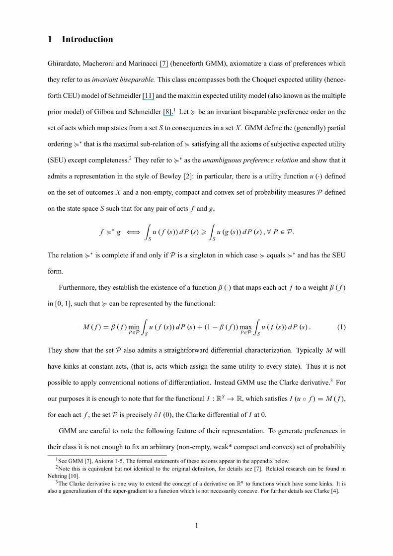
3 Finite State Spaces

The main result of this section is to show that when the state space is �nite, GMM's axioms 1-5 plus 7

imply that the weight � in expression (2) is equal either to 1 or to 0. First we shall present the proof,

then we shall discuss some examples which illustrate key points.

3.1 The Main Result

Throughout this section we assume that there is a �nite set, S, of n states of nature. Let 1.S/ denote

the set of probability distributions over S. For simplicity we shall also assume that acts pay-off in utility

terms, hence an act is a function from S to R. This is without any essential loss of generality, since our

analysis could also be conducted using a conventional utility function over outcomes, if desired. As a

result we may identify the functional I with the functional V in expression (2). This allows us to write

the Clarke differential at 0 as @V .0/. The set of all acts is denoted by A .S/, which can be identi�ed

with Rn .

The strategy of proof is as follows. As already noted, if we take invariant biseparable preferences

represented by expression (1) and impose the extra restriction that � . f / be a constant function then a

�xed point property must be satis�ed. We show that a �xed point only exists if � . f / � 1 or � . f / � 0.

In particular, if � . f / � � for some � in .0; 1/, then the extreme points of the set of priors, D, are not

included in the Clarke differential.

Let D be a given closed convex set of probabilities on S and de�ne the functions �; : A .S/! R

by � . f / D minp2D p � f and . f / D maxp2D p � f . That is, � and represent maxmin and maxmax

expected utility preferences respectively. The functions � and are clearly not differentiable at constant

acts. If D does not have full dimension (that is, n� 1) or there are kinks in the boundary of D, they may

have other points of non-differentiability as well.5 However, since � is concave and is convex, these

functions are differentiable almost everywhere.

In order to apply the analysis from [4] we need to establish that V is Lipschitz, which is shown in

the next result.

Lemma 2 For all f 2 A .S/ ; V is locally Lipschitz at f:5By the dimension of D we mean the dimension of the af�ne space spanned by D.

6

Proof. Let B denote the closed ball with radius � around f and let Nx D maxs2S f .s/ : Then for all

g 2 B; � .g/ 6 Nx C � and .g/ 6 Nx C �: Hence both . f / and � . f / are bounded on a neighbourhood

of f . Both .1� a/ . f / and ��� . f / are convex functions and are therefore locally Lipschitz by

Proposition 1. Since V is the difference of these two functions, which are locally Lipschitz, V itself is

locally Lipschitz by Lemma 1.

The next result shows that at a point where � is differentiable, the minimizing probability distribution

is unique and is equal to the derivative. It also �nds an expression for the derivative of V at points where

both � and are differentiable. If f 2 A .S/ is a given act, we shall use the notation p f (resp. Np f ) to

denote an element of argminp2D p � f; (resp. argmax p2D p � f ).

Lemma 3

1. If � (resp. ) is differentiable at f then argminp2D p: f (resp. argmaxp2D p: f ) is unique.

2. Suppose that � (resp. ) is differentiable at f; then d� f .y/ D p f � y; (resp. d f .y/ D Np f � y) for

all y 2 Rn . This may be expressed in terms of gradients as p f D r� . f /, (resp. Np f D r . f /).

3. Let V be an �-MEU preference functional. If � and are differentiable at f , then V is differen-

tiable at f 2 A .S/ and rV . f / D � p f C .1� �/ Np f .

Proof. We shall prove parts 1 and 2 for �: A similar argument applies to : Suppose that � is differ-

entiable at f . Then since d� f is a linear function on Rn; there exists z 2 Rn such that d� f .y/ D z:y;

for all y 2 Rn: Let p f be an element of argminp2D p: f: Suppose, if possible, z 6D p f : Consider

h 2 Rn such that p f :h D 0 and z:h > 0: Let Qq be an element of argminp2D p: . f C �h/ : Then

Qq: . f C �h/ 6 p f : . f C �h/ : Thus �. fC�h/��. f /�d� f .�h/k�hk DQq:. fC�h/�p f : f��z:h

�khk 6 p f :. fC�h/�p f : f��z:h�khk

Dp f : fC� p f :h�p f : f��z:h

�khk D � �z:h�khk D � z:h

khk < 0: Hence lim�!0�. fC�h/��. f /�d� f .�h/

k�hk 6 � z:hkhk < 0: How-

ever this contradicts the assumption that � is differentiable at f: Thus we may conclude that z D p f :

Parts 1 and 2 of the lemma now follow. Part 3 follows from part 2 and linearity of the derivative on Rn .

Let L denote the linear span of fp � q : p; q 2 Dg and denote by L? the orthogonal complement of

the vector space L .6 If D has full rank then L? will consist just of the constant vectors in A.S/ D Rn .7

6We need to consider differences, since 1.S/ is an af�ne subspace not a linear subspace of Rn .7We say that D has full rank if the dimension of L is n � 1:

7

If the dimension ofD is less than n�1, then L? will contain, in addition, non-constant acts with respect

to which argminp2D p � f D argmax p2D p � f D D holds. Recall that any f 2 A .S/ can be uniquely

written in the form f D g C h; where g 2 L and h 2 L?. The next result relates the Clarke differential

@V .0/ to L :

Lemma 4 Let D � 1.S/ be a closed convex set of probabilities with cardinality greater than 1; let

V : Rn ! R be an �-MEU preference functional with set of priors D then,

@V .0/ � co�� argminp2D p � f C .1� �/ argmaxp2D p � f : f 2 Ln f0g

:

Proof. Since � is a concave function and is a convex function, the set of points at which they are both

differentiable, 0� \ 0 ; is of full Lebesgue measure. Hence by Theorem 1 and Lemma 3,

@V .0/ D co�limrV . fn/ : fn ! 0; fn 2 0V \ 0� \ 0

D co

nlim

�� p fn C .1� �/ Np fn

�: fn ! 0; fn 2 0V \ 0� \ 0

o:

Note that L? \�0� \ 0

�D ?; because at h 2 L?, � and are not differentiable. This follows,

provided D is not a singleton, since h 2 L? implies p � h D p0 � h for all p; p0 2 D and hence,

argminp2D p � h and argmaxp2D p � h are not singletons.

Consider a particular sequence fn ! 0; fn 2 0V \ 0� \ 0 such that lim�� p fn C .1� �/ Np fn

�exists. Fix an n. Write fn D gn C hn , where gn 2 L and hn 2 L?. Since fn 2 0� \ 0 we know

that fn =2 L? and hence gn 6D 0. De�ne Ogn D gnkgnk : Since p � hn D p0 � hn for all p; p0 2 D, we have

p fn D p Ogn and Np fn D Np Ogn : Therefore � p fn C .1� �/ Np fn D � p Ogn C .1� �/ Np Ogn .

Returning to the sequence fn ! 0; fn 2 0V \ 0� \ 0 , consider the corresponding sequences of

Ogn's, p Ogn 's and Np Ogn 's. By construction the Ogn's lie in a compact set (the unit ball). The p Ogn 's and Np Ogn 's

also lie in a compact set (the simplex). Hence, by taking a subsequence if necessary, we may assume

that the three sequences Ogn , p Ogn and Np Ogn all converge. Let Og; p and Np be the respective limit points. By

construction Og 6D 0. Furthermore Og 2 L because L is a �nite dimensional subspace and therefore closed.

By the upper hemi-continuity of argmax and argmin we know that Np 2 argmaxp2D p � Og and p 2

argminp2D p � Og. Putting the steps together we have lim�� p fn C .1� �/ Np fn

�D � p C .1� �/ Np 2

� argminp2D p � Og C .1� �/ argmaxp2D p � Og; where Og 2 Ln0:8

8We would like to thank the referee and associate editor for their helpful comments and suggestions in constructing theproof of this result.

8

Preferences of the �-MEU form are not differentiable at constant acts. If these are the only points at

which V .�/ is not differentiable (as is the case for Hurwicz preferences, de�ned below) then the Clarke

differential is actually equal to

co�� argminp2D p � f C .1� �/ argmaxp2D p � f : f 2 Ln f0g

.

If there are other points where V .�/ is not differentiable, it is possible that @V .0/ is a proper subset

of co�� argminp2D p � f C .1� �/ argmaxp2D p � f : f 2 Ln f0g

. Whether the set inclusion is strict

or not, the next result shows that extreme points of D are not contained in this set and hence, as an

immediate corollary to Lemma 4, are not included in @V .0/.

Lemma 5 Let D be a closed convex subset of1.S/ with cardinality greater than 1; let V : Rn ! R be

an �-MEU preference function with set of priors D and 0 < � < 1. If Op is an extreme point of D, then

Op =2 co�� argminp2D p � f C .1� �/ argmaxp2D p � f : f 2 Ln f0g

:

Proof. By construction, the af�ne span of D is a translation of the subspace L . Thus if we view vectors

in Ln f0g as functionals onD none of them is constant onD, that is, for all f 2 Ln f0g, argminp2D p � f \

argmax p2D p � f D ?. By de�nition, an extreme point of D cannot be written as a convex combination

of two other distinct elements of D. Therefore Op =2 con� p f C .1� �/ Np f : f 2 Ln f0g

o.

In �nite dimensions, a closed convex set always contains an extreme point Op.9 Thus in conjunction with

Lemmas 3, 4 and 5, we have established there exists a point Op in D such that Op =2 @V .0/. However this

constitutes a failure of the preferences to admit a representation of the form given in expression (2) with

the restriction that D D @V .0/. Hence we have established the following result.

Theorem 2 Let D � 1.S/ be a closed convex subset with cardinality greater than 1; let V : Rn ! R

be an �-MEU preference function with set of priors D and 0 < � < 1 and let < be a preference order

on Rn , which is represented by V : Then < cannot satisfy GMM axioms 1-5 and 7.

3.2 Examples

We illustrate our analysis by considering two examples, Hurwicz preferences and the case where the set

of priors consists of the convex combinations of two probability distributions.9Indeed by the Krein-Milman theorem ([5], p. 440) a closed convex set is the closure of the convex hull of its extreme

points.

9

Figure 2: D has full rank

10

3.2.1 Hurwicz Preferences

Hurwicz preferences are de�ned as follows.

De�nition 5 The Hurwicz preference functional,10 H : A .S/! R is de�ned by

H . f / D � minP21.S/

ZSf .s/ dP .s/C .1� �/ max

P21.S/

ZSf .s/ dP .s/

or equivalently H . f / D � f.n/ C .1� �/ f.1/. Here for a given vector f 2 Rn; f.k/ denotes the kth

highest component of f . Hence f.1/ > f.2/ > ::: > f.n/:

Figure 2 illustrates how our analysis applies to Hurwicz preferences when there are 3 states. In this

case the set of priors is1.S/, which has full dimension. The space L? consists just of the constant acts.

Let f be a given non-constant act. The dashed lines connect points at which the expected value of f is

constant (in probability space). For any non-constant act, the maximum and minimum expected utility

occur at two distinct vertices of the simplex. For the given act f; the maximum and minimum expected

utility occurs at p1 D 1 and p3 D 1 respectively. The probability used in evaluating the expectation of

f is therefore h1� �; 0; �i : In general, the probability, � pg C .1� �/ Npg, used to evaluate the expec-

tation of any non-constant act, g, must be one of the following six vectors: h�; 1� �; 0i, h�; 0; 1� �i,

h1� �; �; 0i, h1� �; 0; �i, h0; �; 1� �i and h0; 1� �; �i. The Clarke differential @H .0/ is accord-

ingly the convex hull of these six vectors, which forms a hexagon inside the simplex. This set is clearly

closed. The extreme points of 1.S/ are the three vertices, p1 D 1; p2 D 1 and p3 D 1. As can be seen

from �gure 2, for any �; 0 < � < 1; these points are not contained in @H .0/. Moreover it is only the

three vertices which are not contained in @H .0/ for all � : 0 < � < 1; i.e. for any other point in 1.S/

there is a range of values of � for which the given point is contained in @H .0/.11

3.2.2 One-dimensional set of priors

In �gure 3, the set of priors consists of all convex combinations of two probability distributions Oq D

ha; 0; 1� ai and Qq D hb; 1� b; 0i. The set of priors is a one-dimensional subset of the simplex and

hence does not have full dimension. In this case L? D�f 2 A .S/ : Oq � f D Qq � f

. This is a two

dimensional subspace of R3, which contains the constant acts. Graphically it consists of acts whose10See Hurwicz [9]. A more detailed discussion of these preferences can be found in L. Hurwicz. Optimality criteria for

decision making under ignorance. Discussion paper 370, Cowles Commission, 1951.11For further details of how the GMM representation applies to Hurwicz preferences see [6].

11

Figure 3: D has less than full rank

indifference surfaces are parallel to the line connecting Oq and Qq . The given act f , attains its maximum

at Oq and its minimum at Qq: Accordingly its expectation is taken with respect to the probability � Qq C

.1� �/ Oq . The Clarke differential, @V .0/, is equal to the shorter line shown in bold. In this case the

extreme points are just Oq and Qq. As in the previous case, the extreme points are not contained in the

Clarke differential for any value of � : 0 < � < 1. All other members of the set of priors are contained

in the Clarke differential for some range of �'s.

4 In�nite State Spaces

In this section we show by example that when the state space is in�nite, Axioms 1 - 5 and 7 can be

satis�ed.12 That is, we �nd a set of preferences with a representation of the form given in expression

(2) with an � in .0; 1/ that also satis�es the constraint D D @V .0/. Indeed, our example shows it is

possible to construct a set D which is independent of �.13

Let the set of states of nature be S D [0; 1] and let 6 denote the � -algebra of Borel sets of [0; 1].

Assume that acts lie in C .S/ ; the space of continuous functions on S with the sup norm. The topological

dual of C .S/ may be identi�ed with ca [0; 1] the set of all countably additive, bounded and Borel-12In private correspondence, Klaus Nehring has informed us of an example satisfying the GMM axioms in which the set

of priors is the set of all �nitely additive measures on [0; 1] ; which assign zero probability to all events of Lebesgue measurezero.13It is not immediately clear from the representation in equation (3) (see page 14) that such a D would exist.

12

measurable set-functions, where the topology on ca [0; 1] is given by the total variation norm. If s 2 S;

let �s denote the Dirac measure on S; i.e. �s .A/ D 1; if s 2 AI D 0; otherwise. Let H denote the

set of all countably additive probability distributions on [0; 1] and consider the following preference

functional.

De�nition 6 De�ne a preference functional W : C .S/! R by

W . f / D �minp2H

Zf dp C .1� �/max

p2H

Zf dp:

Let <0 denote the preference relation on C .S/ de�ned by f <0 g , W . f / > W .g/ :

These preferences may be seen as the in�nite dimensional analogue of the Hurwicz preferences

discussed in section 3.14 We shall show that W .�/ satis�es the �xed point property,H D @W .0/, hence

the preferences generated by W .:/ satisfy GMM's axiomatization.

Proposition 2 The preference relation <0 satis�es GMM's axioms 1-5 plus 7.

In order to prove this result we use Lemma 6 and the following two results which describe properties

of the Clarke differential of a real-valued function on an arbitrary Banach space, (not necessarily Rn).

Proposition 3 (Clarke [4], Corollary 2, p.39) Let X be a Banach space and let V and V 0 be real-

valued functions on X. For any �; � 2 R, @��V C �V 0

�.x/ � �@V .x/C �@V 0 .x/ :

Proposition 4 (Clarke [4], Proposition 2.2.7) Let U be an open convex subset of a Banach space

X: If V is convex (resp. concave) on U and Lipschitz near x, then @V .x/ coincides with the sub-gradient

(resp. super-gradient) at x in the sense of convex analysis:

De�ne functionals � (resp. � ): A .S/! R by � . f / D minp2HRf dp; (resp. � . f / D maxp2H

Rf dp).

Lemma 6 shows that if Os minimizes f 2 C [0; 1], then the Dirac measure � Os is a super-gradient of � at

f and therefore is in the Clarke differential @� . f / :

Lemma 6 Let f 2 C [0; 1] be such that Os 2 argmin s2[0;1] f .s/ ; (resp. Qs 2 argmaxs2[0;1] f .s/) then

� Os 2 @� . f / (resp. � Qs 2 @� . f /).14We would like to thank the associate editor for suggesting this argument.

13

Proof. By Proposition 4, it is suf�cient to show that the linear functional � : C [0; 1] ! R; de�ned

by � .h/ DRh� Os is a super-gradient of � at f: Let g 2 C [0; 1] : Then � . f / D f

�Os�DRf d� Os and

� .g/ 6 g�Os�D f

�Os�C�g�Os�� f

�Os��D � . f / C

R.g � f / � Os : This establishes that � is a super-

gradient of � at f: The other case is similar.

Proof of Proposition 2 As explained earlier, GMM's axioms 1-5 plus 7 are equivalent to the fol-

lowing representation:

M . f / D � minP2P

ZSf .s/ dP .s/C .1� �/max

P2P

ZSf .s/ dP .s/ and @M .0/ D P; (3)

for some constant � in [0; 1] : We shall demonstrate that for W . f / from De�nition 6 one obtains

@W .0/ D H: The rest of the representation is clearly satis�ed.

Let Os be a given point in .0; 1/ : Fix an integer n > 0: Then there is a piecewise-linear func-

tion fn 2 C .S/ such that fn .0/ D 0; fn�Os � 1

n �1n2�D 0; fn

�Os � 1

n

�D � 1

n ; fn�Os � 1

n C1n2�D

0; fn�Os C 1

n �1n2�D 0; fn

�Os C 1

n

�D 1

n ; fn�Os C 1

n C1n2�D 0; fn .1/ D 0: (Thus fn is a function which

has a unique maximum at OsC 1n and a unique minimum at Os�

1n .) The function fn is illustrated in �gure

4. The sequence of functions fn converges to 0, (in the sup norm).

It is clear that � OsC 1nD argmaxq2H

Rfndq and � Os� 1

nD argmin q2H

Rfndq . Thus by Lemma 6 and

Proposition 3, wn D �� Os� 1nC .1� �/ � OsC 1

n2 @W . fn/ : Since W is positively homogenous by [7]

Proposition A.3, @W . fn/ � @W .0/ : Hence wn 2 @W .0/ : De�ne

J D co��� Os� 1

nC .1� �/ � OsC 1

n: Os 2 .0; 1/ ; 1 6 n 61; Os � 1

n2 .0; 1/ ; Os C

1n2 .0; 1/

�;

where the bar denotes closure in the weak* topology. Clearly J � H:

Since for any g 2 C .S/ ;Rgdwn ! g

�Os�DRgd� Os; the sequence wn weak* converges to � Os : This

establishes that the Dirac measures are in J : The convex hull of the Dirac measures is the set of discrete

measures on [0; 1] : By Bauer [1] (Corollary 7.7.4, p. 230) the weak* closure of the discrete measures is

the set of all countably additive measures on [0; 1] : In other words the �xed point property,H D @W .0/

holds.

As noted above, these preferences may be seen as the in�nite dimensional analogue of the Hurwicz

preferences. In both cases the set of beliefs is the closed convex hull of the Dirac measures on the

relevant state space. It is clear that the Dirac measures are extreme points of the set H. For a �nite

state space, the set of priors is the set of all convex combinations of those probability distributions which

14

Figure 4: The function fn

assign probability one to a given state, that is, the Dirac measures. If there are a �nite number, n say, of

states, then there are n Dirac measures. In this case, the topology on the state space is discrete. Hence

each state is topologically isolated. No state is a limit of a sequence of other states and hence the Dirac

measures are not the limit of a sequence of other Dirac measures.

For the preferences studied in this section, the state space is [0; 1] with the usual topology. In this

case any state may be approximated by a sequence of other states and consequently any of the Dirac

measures may be approximated by a sequence of other Dirac measures. If the set of priors had one or

more isolated extreme points then a similar problem would arise as in �nite dimensions and the GMM

axioms would not be satis�ed.

In in�nite dimensions it is possible to construct a sequence fn such that argmin q2HRfndq and

argmaxq2HRfndq are unique and the maximizer of

Rfndq and the minimizer of

Rfndq converge to

a common limit as n tends to in�nity. This is not possible in �nite dimensions, even if the set D has

an in�nite number of extreme points, since the maximizer and minimizer ofRfndq will lie on opposite

sides of the set D as illustrated in �gure 1.

There are a number of ways in which we could extend this example. For instance assume that the

state space, S; is any given closed convex subset of Rn; and the space of acts is the set of continuous

15

real valued functions on S: Then ifD consists of all countably additive measures over any closed convex

subset of S; one can show using a similar argument that the GMM axioms will be satis�ed. Another

interesting case is where the set of beliefs consists of convex combinations of a given prior, q; and an

arbitrary countably additive measure, p; on [0; 1] ; i.e. D D f.1� / q C p : p 2 Hg : This can be

recognized as a version of the neo-additive preferences axiomatized in Chateauneuf et al. [3]. Both of

these cases can be shown to satisfy the GMM axioms by similar reasoning to that used in the proof of

Proposition 2.

However even with an in�nite state space, the need to satisfy a �xed-point property limits the mem-

bership of the family of preference relations which can admit a representation V .�/ of the form in

expression (2) with � in .0; 1/ and satisfying D D @V .0/. By similar reasoning to that used in section

3, the set of priors D cannot be �nitely generated.15 That is, D cannot be the set of all convex com-

binations of a given �nite set of probability distributions. More generally these constraints cannot be

satis�ed when the set D lies in a �nite dimensional (af�ne) subspace of ca .S/. Another case where the

GMM axioms cannot be satis�ed for an � in .0; 1/ is whereD contains an isolated extreme point. (Since

the isolated extreme point will not be in the Clarke differential @V .0/.)

An open problem is to �nd a characterization of those sets of priors over in�nite states spaces which

satisfy the GMM axioms. As explained above, expression (3) imposes constraints, which imply that not

any set of priors can satisfy these axioms. The precise implications of these constraints are not clear.

Appendix: GMM Axioms 1-5 and 7.

As a reference for the reader, we list here GMM's axioms 1-5 and 7.

Axiom 1 (Weak order) For all f , g, h 2 A .S/ :

1. either f % g or g % f ,

2. if f % g and g % h, then f % h.

Axiom 2 (Certainty Independence) For all f , g 2 A .S/, all x 2 X, and all � 2 .0; 1] :

f % g , � f C .1� �/ x % �g C .1� �/ x.15In private correspondence Marciano Siniscalchi has informed us that he has an independent proof of this result.

16

Axiom 3 (Archimedean Axiom) For all f , g, h 2 A .S/, if f � g and g � h, then there exist �, � 2

.0; 1/ such that

� f C .1� �/ h � g and g � � f C .1� �/ h.

Axiom 4 (Monotonicity) For all f , g 2 A .S/, if f .s/ % g .s/ for all s 2 S, then f % g.

Axiom 5 (Nondegeneracy) There are f , g 2 A .S/ such that f � g.

In order to state the last axiom, recall that %� is the maximal sub-relation of % that satis�es all the

axioms of subjective expected utility except completeness.

Axiom 7 For all f , g 2 A .S/, if f %� x , g %� x and x %� f , x %� g for all x 2 X ; then

f � g.

References

[1] H. Bauer, Probability Theory and Elements of Measure Theory, Holt Rinehart and Winston, New

York, 1972.

[2] T. Bewley, Knightian decision theory part I, Decisions in Econ. and Finance, 2 (2002), 79�110.

[3] A. Chateauneuf, J. Eichberger, S. Grant, Choice under uncertainty with the best and worst in mind:

NEO-additive capacities, J. of Econ. Theory, 137 (2007), 538�567.

[4] F. H. Clarke, Optimization and Nonsmooth Analysis, Society for Industrial and Applied Mathe-

matics, Philadelphia, 1983.

[5] N. Dunford, J. T. Schwartz, Linear Operators, Wiley, New York, 1958.

[6] J. Eichberger, S. Grant, D. Kelsey, Differentiating ambiguity: An expository note, Econ. Theory,

38 327�336, 2008.

[7] P. Ghirardato, F. Maccheroni, M. Marinacci, Differentiating ambiguity and ambiguity attitude, J.

of Econ. Theory, 118 133�173, 2004.

[8] I. Gilboa, D. Schmeidler, Maxmin expected utility with a non-unique prior, J. of Math. Econ. 18

(1989), 141�153.

17

[9] L. Hurwicz, Some speci�cation problems and application to econometric models, Econometrica,

19 (1951), 343�344 .

[10] K. Nehring, Imprecise probabilitistic beliefs as a context of decision-making under ambiguity, J.

of Econ. Theory, 144 (2009), 1054�1091.

[11] D. Schmeidler, Subjective probability and expected utility without additivity, Econometrica, 57

(1989), 571�587.

18