arX

iv:1

109.

5023

v1 [

gr-q

c] 2

3 Se

p 20

11

The kernel and the injectivity of the EPRL map

Wojciech Kamiński1, Marcin Kisielowski2, Jerzy Lewandowski2

1Max-Planck-Institut für Gravitationsphysik (Albert-Einstein-Institut),Am Mühlenberg 1 D-14476 Golm, Germany

2Instytut Fizyki Teoretycznej, Uniwersytet Warszawski,ul. Hoża 69, 00-681 Warszawa (Warsaw), Polska (Poland)

Abstract In this paper we prove injectivity of the EPRL map for |γ| < 1, filling the gap of ourprevious paper.

I. INTRODUCTION

The Engle-Pereira-Rovelli-Livine (EPRL) map [1] (see also [2–4]) is used to define the spinfoam amplitudes between the states of Loop Quantum Gravity [7–9]. The states are labelledby the SU(2) invariants, whereas the gauge group of the EPRL model is Spin(4) or Spin(3,1)depending on the considered spacetime signature. The EPRL map carries the invariants of thetensor products of SU(2) representations into the invariants of the tensor products of Spin(4), orSpin(3,1) representations. Those LQG states which are not in the domain of or happen to beannihilated by the EPRL map are not given a chance to play a role in the physical Hilbert space.Therefore, it is important to understand which states of LQG are not annihilated. In the Spin(4)case this issue is particularly subtle, because both the SU(2) representations as well as the Spin(4)representations are labelled by elements of 1

2N , the EPRL map involves rescaling by constants

depending on the Barbero-Immirzi parameter γ, and the labels (taking values in 12N) before and

after the map have to sum to an integer. The ‘injectivity’ we prove in the current paper means,that given a necessarily rational value γ ∈ Q, for every k1, ..., kn – n-tuple of elements of 1

2N –the EPRL map defined in the space of invariants InvHk1

⊗ ...⊗Hknis injective unless the target

Hilbert space of the corresponding Spin(4) invariants is trivial. The issue of the injectivity of theEPRL map has been raised in [3] and [4]. However, the assumption that “the target Hilbert spaceof the corresponding Spin(4) invariants is not trivial” was overlooked there. After adding thisassumption, the proof presented in [3] for γ ≥ 1 works without any additional corrections. Hence,in the current paper we consider only the case of |γ| < 1. In this case, the theorem formulated in[4] is true if we additionally assume that the values of γ = p

qare such that non of the relatively

primary numbers p or q is even. In the current paper we formulate and prove an injectivity theoremvalid for every γ ∈ Q, and provide a proof for |γ| < 1.

II. THE EPRL MAP, THE MISSED STATES, THE ANNIHILATED STATES AND

STATEMENT OF THE RESULT

1. Definition of the EPRL map

Let (j, k, l) ∈ 12N × 1

2N × 12N satisfy triangle inequalities and j + k + l ∈ N. We denote by Ckl

j

the natural isometric embedding Hj → Hk ⊗ Hl and by Cjkl the adjoint operator. In the index

notation we omit j, k, l, e.g. CA1

A2A3:= (Cj

kl)A1

A2A3.

Let ki ∈12N, i ∈ {1, . . . , n}. We denote by Inv (Hk1

⊗ · · · ⊗ Hkn) the subspace of Hk1

⊗· · ·⊗Hkn

consisting of tensors invariant under the action of SU(2) group.

Definition 1. Given γ ∈ Q and ki ∈12N, i ∈ {1, . . . , n} such that ∀i j±i := |1±γ|

2 ki ∈12N, the

Engle-Pereira-Rovelli-Livine map

ιk1...kn: Inv (Hk1

⊗ · · · ⊗ Hkn) → Inv

(

Hj+

1

⊗ · · · ⊗ Hj+n

)

⊗ Inv(

Hj−

1

⊗ · · · ⊗ Hj−

n

)

(2.1)

is defined as follows [1, 3]:

ιk1...kn(I)A

+

1...A+

nA−

1...A−

n = IA1...AnCB

+

1B

−

1

A1· · ·C

B+n B−

n

AnP+A

+

1...A+

n

B+

1...B

+nP−A

−

1...A−

n

B−

1...B

−

n,

2

where P+ : Hj+

1

⊗· · ·⊗Hj+n→ Inv

(

Hj+

1

⊗ · · · ⊗ Hj+n

)

, P− : Hj−

1

⊗· · ·⊗Hj−

n→ Inv

(

Hj−

1

⊗ · · · ⊗ Hj−

n

)

are standing for the orthogonal projections.

2. The missed states

Given a value of the Barbero-Immirzi parameter γ, the EPRL map is defined on an in-variant space Inv(Hk1

⊗ ... ⊗ Hkn), only if the spins k1, ..., kn ∈ 12N are such that also each

|1±γ|2 k1, ...,

|1±γ|2 kn ∈ 1

2N. That is why we are assuming that γ is rational,

γ =p

q,

where p, q ∈ Z and they relatively irrational (the fraction can not be farther reduced.) If we need

an explicit formula for k ∈ 12N such that |1±γ|

2 k ∈ 12N, we find two possible cases of γ and the

corresponding formulas for k:

(i) both p and q odd ⇒ k = qs where s ∈ 12N,

(ii) (p even and q odd) or (p odd and q even) ⇒ k = 2qs where s ∈ 12N.

Invariants involving even one value of spin ki which is not that of (i), or, respectively, (ii) dependingon γ, are not in the domain of the EPRL, hence they are missed by the map.

3. The annihilated states

Suppose there is given a space of invariants Inv(Hk1⊗ ...⊗Hkn

) such that each k1, ..., kn satisfies(i) or, respectively, (ii) above. Suppose also the space is non-trivial, that is

ki ≤∑

i′ 6=i

ki′ , i = 1, .., n (2.2)

∑

i

ki ∈ N. (2.3)

The target space of the EPRL map Inv (Hk1⊗ · · · ⊗ Hkn

) → Inv(

Hj+

1

⊗ · · · ⊗ Hj+n

)

⊗Inv(

Hj−

1

⊗ · · · ⊗ Hj−

n

)

is nontrivial, if and only if

j±i ≤∑

i′ 6=i

j±i , i = 1, .., n (2.4)

∑

i

j±i ∈ N. (2.5)

Whereas (2.2) does imply (2.4), the second condition

∑

i

j±i =1± γ

2

∑

i

ki ∈ N (2.6)

is not automatically satisfied for arbitrary γ.For example, let

γ =1

4, k1, k2, k3 = 4.

Certainly the space Inv(H4 ⊗H4 ⊗H4) is non-empty. However,

j−1 , j−2 , j−3 =3

2, j+1 , j+2 , j+3 =

5

2

3

and

Inv(H 32⊗H 3

2⊗H 3

2)⊗ Inv(H 5

2⊗H 5

2⊗H 5

2) = {0} ⊗ {0}.

In other words, if γ is 0.25 (close to the “Warsaw value” γ = .27... [5, 6] usually assumed inthe literature), then the EPRL map annihilates the SU(2) invariant corresponding to the spinsk1 = k2 = k3 = 4.

Generally, for γ and k1, ..., kn of the case (i) in the previous subsection, actually (2.3) doesimply (2.5). In the case (ii), on the other hand, there is a set of non-trivial subspaces Inv(Hk1

⊗

... ⊗ Hkn) which are annihilated by the EPRL map for the target Inv

(

Hj+

1

⊗ · · · ⊗ Hj+n

)

⊗

Inv(

Hj−

1

⊗ · · · ⊗ Hj−

n

)

is just the trivial space.

The theorem formulated below exactly states, that the EPRL map does not annihilate morestates, then those characterised above.

4. The injectivity theorem

Theorem 2. Assume γ ∈ Q. For ki ∈12N, i ∈ {1, . . . , n} such that:

• ∀i j±i := 1±γ2 ki ∈

12N,

•∑n

i=1 j+i ∈ N

the EPRL map defined above (def. 1) is injective.

Note that when Inv (Hk1⊗ · · · ⊗ Hkn

) is trivial, injectivity trivially holds.In this article we use the following definition:

Definition 3. A sequence (k1, k2, . . . , kn), ki ∈12N is admissible iff the space Inv (Hk1

⊗ · · · ⊗ Hkn)

is nontrivial. This is equivalent to the conditions

∀i ki ≤∑

j 6=i

kj , and∑

i

ki ∈ N . (2.7)

For γ ≥ 1 the proof of the theorem 2 is presented in [3]. Here we present the proof for |γ| < 1.In order to make the presentation clear, we divide it into sections. The main result is an inductivehypothesis stated and proved in section IV. The injectivity of EPRL map follows from that result.In the preceding section III we present proof of theorem restricted to certain intertwiners whichwe call tree-irreducible. We use it in the proof of the main result.

III. PROOF OF THE THEOREM IN SIMPLIFIED CASE

A. Tree-irreducible case of inductive hypothesis

In the tree-irreducible case we restrict to intertwiners which we call tree-irreducible. We saythat I ∈ Inv (Hk1

⊗ · · · ⊗ Hkn) is tree-irreducible, if for all l ∈ {1, . . . , n − 1} the orthogonal

projection P l : Inv (Hk1⊗ · · · ⊗ Hkn

) → Inv (Hk1⊗ · · · ⊗ Hkl

) ⊗(

Hkl+1⊗ . . .⊗Hkn

)

annihilatesI.

The inductive proof we present needs an extended notion of the EPRL map. This will be themap ι analogous to EPRL map but defined under a bit different conditions:

Con n: Sequences (k1, . . . , kn) and (j±1 , . . . , j±n ), where ki, j±i ∈ 1

2N, are such that

• (k1, . . . , kn) is admissible,

• ki 6= 0 for all i > 1,

• j+1 + j−1 = k1,

4

• j±i = 1±γ2 ki for i 6= 1 and

1 + γ

2k1 −

1

2≤ j+1 ≤

1 + γ

2k1 +

1

2(3.1)

• j±1 + . . .+ j±n ∈ N

• (ordering) ∃i ≥ 1:j+l ∈ N l ≤ i

j+l ∈ N+ 12 l > i

.

Few remarks are worth to mention:

• We would like to emphasize that although EPRL map usually do not satisfy those conditions,it can be easily replaced by an equivalent map that satisfies Con n.

First of all we can assume that in the EPRL map ki 6= 0 for i ≥ 1. Secondly, we can permuteki in such a way that

∃i : j+l ∈ N, for l ≤ i, j+l ∈ N+1

2, for l ≤ i. (3.2)

These are exactly conditions of Con n.

• From the definition above follows that j+i + j−i = ki for all i = 1, . . . , n.

• It follows also that

1− γ

2k1 −

1

2≤ j−1 ≤

1− γ

2k1 +

1

2.

• From conditions Con n follows that (j±1 , . . . , j±n ) satisfy admissibility conditions – this willbe proved in lemma 4.

Lemma 4. Let (k1, . . . , kn) and (j±1 , . . . , j±n ) be elements of 12N, such that: (k1, . . . , kn) is admis-

sible, j±i = 1±γ2 ki for i 6= 1, 1+γ

2 k1 +12 ≥ j+1 ≥ 1+γ

2 k1 −12 , j

+1 + j−1 = k1, j

±1 + . . .+ j±n ∈ N, then

(j±1 , . . . , j±n ) satisfy admissibility conditions.

Proof. From the definition of j±i and from the fact that (k1, . . . , kn) are admissible, we know that

j±1 ≤1± γ

2k1 +

1

2≤

1± γ

2(k2 + . . .+ kn) +

1

2= j±2 + . . .+ j±n +

1

2.

We have j±1 + . . . + j±n ∈ N, so j±1 < j±2 + . . . + j±n + 12 . As a result j±1 ≤ j±2 + . . .+ j±n . This is

one of the desired inequalities.Similarly for i 6= 1 we have:

j±i =1± γ

2ki ≤

1± γ

2k1 +

∑

l>1,l 6=i

1± γ

2kl ≤

∑

l 6=i

j±l +1

2

As in previous case j±1 + . . . + j±n ∈ N implies j±i <∑

l 6=i j±l + 1

2 and finally j±i ≤∑

l 6=i j±l . This

finishes proof of this lemma.

We will base the proof of theorem 2, in the case I is tree-irreducible, on the following inductivehypothesis (n ∈ N+, n ≥ 3):

Hyp n: Suppose that (k1, . . . , kn), (j±1 , . . . , j±n ) satisfy condition Con n and thatI ∈ Inv (Hk1

⊗ · · · ⊗ Hkn) is tree-irreducible. Then, there exists

φ ∈ Inv(

Hj+

1

⊗ · · · ⊗ Hj+n

)

⊗ Inv(

Hj−

1

⊗ · · · ⊗ Hj−

n

)

such that 〈φ, ιk1...kn(I)〉 6= 0.

5

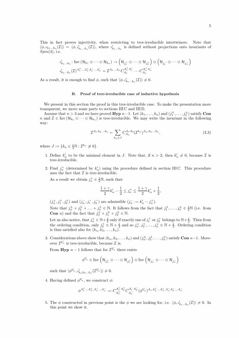
This in fact proves injectivity, when restricting to tree-irreducible intertwiners. Note that〈φ, ιk1...kn

(I)〉 = 〈φ, ι′k1...kn(I)〉, where ι′k1...kn

is defined without projections onto invariants ofSpin(4), i.e.

ι′k1...kn: Inv (Hk1

⊗ · · · ⊗ Hkn) →

(

Hj+

1

⊗ · · · ⊗ Hj+n

)

⊗(

Hj−

1

⊗ · · · ⊗ Hj−

n

)

ι′k1...kn(I)A

+

1...A+

nA−

1...A−

n = IA1...AnCA

+

1A

−

1

A1· · ·C

A+nA−

n

An

As a result, it is enough to find φ, such that 〈φ, ι′k1...kn(I)〉 6= 0.

B. Proof of tree-irreducible case of inductive hypothesis

We present in this section the proof in this tree-irreducible case. To make the presentation moretransparent, we move some parts to sections III C and III D.

Assume that n > 3 and we have proved Hyp n−1. Let (k1, . . . , kn) and (j±1 , . . . , j±n ) satisfy Conn and I ∈ Inv (Hk1

⊗ · · · ⊗ Hkn) is tree-irreducible. We may write the invariant in the following

way:

IA1A2...An =∑

kα∈J

CA1A2

Aα(Ikα)AαA3...An , (3.3)

where J := {kα ∈ 12N : Ikα 6≡ 0}.

1. Define k′α to be the minimal element in J . Note that, if n > 2, then k′α 6= 0, because I istree-irreducible.

2. Find j+α (determined by k′α) using the procedure defined in section III C. This procedureuses the fact that I is tree-irreducible.

As a result we obtain j+α ∈ 12N, such that:

1 + γ

2k′α −

1

2≤ j+α ≤

1 + γ

2k′α +

1

2,

(j+α , j+1 , j+2 ) and (j−α , j−1 , j−2 ) are admissible (j−α := k′α − j+α ).

Note that j±α + j±3 + . . . + j±n ∈ N. It follows from the fact that j±1 , . . . , j±n ∈ 12N (i.e. from

Con n) and the fact that j±α + j±1 + j±2 ∈ N.

Let us also notice, that j+α ∈ N+ 12 only if exactly one of j+1 or j+2 belongs to N+ 1

2 . Then from

the ordering condition, only j+2 ∈ N + 12 and so j+α , j+3 , . . . , j+n ∈ N+ 1

2 . Ordering conditionis thus satisfied also for (kα, k3, . . . , kn).

3. Considerations above show that (kα, k3, . . . , kn) and (j±α , j±3 , . . . , j±n ) satisfy Con n−1. More-

over Ik′

α is tree-irreducible, because I is.

From Hyp n− 1 follows that for Ik′

α there exists

φk′

α ∈ Inv(

Hj+α⊗ · · · ⊗ Hj

+n

)

⊗ Inv(

Hj−

α⊗ · · · ⊗ Hj

−

n

)

such that 〈φk′

α , ι′kαk3...kn(Ik′

α)〉 6= 0.

4. Having defined φk′

α , we construct φ:

φA+

1...A+

n ,A−

1...A−

n := CA

+

1A

+

2

A+α

CA

−

1A

−

2

A−

α

(φk′

α )AαA+

3...A+

n ,A−

αA−

3...A−

n

5. The φ constructed in previous point is the φ we are looking for, i.e. 〈φ, ι′k1...kn(I)〉 6= 0. In

this point we show it.

6

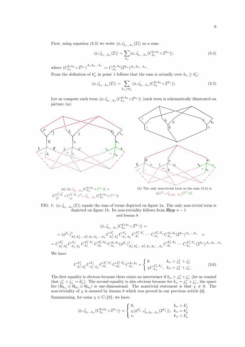
First, using equation (3.3) we write 〈φ, ι′k1...kn(I)〉 as a sum:

〈φ, ι′k1...kn(I)〉 =

∑

kα

〈φ, ι′k1...kn(Ck1k2

kα◦ Ikα)〉, (3.4)

where (Ck1k2

kα◦ Ikα)

A1A2...An

:= CA1A2

Aα(Ikα )AαA3...An .

From the definition of k′α in point 1 follows that the sum is actually over kα ≥ k′α:

〈φ, ι′k1...kn(I)〉 =

∑

kα≥k′

α

〈φ, ι′k1...kn(Ck1k2

kα◦ Ikα)〉. (3.5)

Let us compute each term 〈φ, ι′k1...kn(Ck1k2

kα◦ Ikα)〉 (such term is schematically illustrated on

picture 1a):

(a) 〈φ, ι′k1...kn

(Ck1k2

kα◦ Ikα)〉 =

〈Cj+

1j+

2

j+α

◦ Cj−

1j−

2

j−

α

φk′

α , ι′k1...kn

(Ck1k2

kα◦ Ikα)〉

(b) The only non-trivial term in the sum (3.4) is

χ〈φk′

α , ι′kαk3...kn

(Ik′

α)〉.

FIG. 1: 〈φ, ι′k1...kn(I)〉 equals the sum of terms depicted on figure 1a. The only non-trivial term is

depicted on figure 1b. Its non-triviality follows from Hyp n− 1

and lemma 8.

〈φ, ι′k1...kn(Ck1k2

kα◦ Ikα)〉 =

= (φk′

α)†A

+αA

+

3...A

+nA

−

αA−

3...A

−

n

CA+

α

A+

1A

+

2

CA−

α

A−

1A

−

2

CA+

1A−

1

A1· · ·C

A+nA−

n

AnCA1A2

Aα(Ikα)Aα...An =

= CA+

α

A+

1A

+

2

CA−

α

A−

1A

−

2

CA

+

1A

−

1

A1C

A+

2A

−

2

A2CA1A2

Aα(φk′

α)†A

+αA

+

3...A

+nA

−

αA−

3...A

−

n

CA

+

3A

−

3

A3· · ·C

A+nA−

n

An(Ikα )AαA3...An

We have

CA+

α

A+

1A+

2

CA−

α

A−

1A−

2

CA

+

1A

−

1

A1C

A+

2A

−

2

A2CA1A2

Aα=

{

0 kα > j+α + j−α

χCA+

αA−

α

Aα, kβ = j+α + j−α .

(3.6)

The first equality is obvious because there exists no intertwiner if kα > j+α +j−α (let us remindthat j+α + j−α = k′α). The second equality is also obvious because for kα = j+α + j−α , the spaceInv (Hkα

⊗Hk2⊗Hk3

) is one-dimensional. The nontrivial statement is that χ 6= 0. Thenon-triviality of χ is assured by lemma 8 which was proved in our previous article [4].

Summarizing, for some χ ∈ C\{0}, we have:

〈φ, ι′k1...kn(Ck1k2

kα◦ Ikα)〉 =

0, kα > k′αχ〈φk′

α , ι′kαk3...kn(Ik′

α)〉, kα = k′α∗, kα < k′α

7

As a result all but one term in the sum (3.5) are equal zero and:

〈φ, ι′k1...kn(I)〉 = χ〈φk′

α , ι′kαk3...kn(Ik′

α)〉 6= 0

We obtained that for n > 3, Hyp n follows from Hyp n − 1. In order to finish the inductiveproof, it remains to check that Hyp 3 is true. In this case sequences (k1, k2, k3) and (j±1 , j±2 , j±3 )are admissible and invariant spaces are one dimensional. Hyp 3 follows now from lemma 8.

This proof of first inductive step is valid in general case, because for n = 3 all invariants aretree-irreducible.

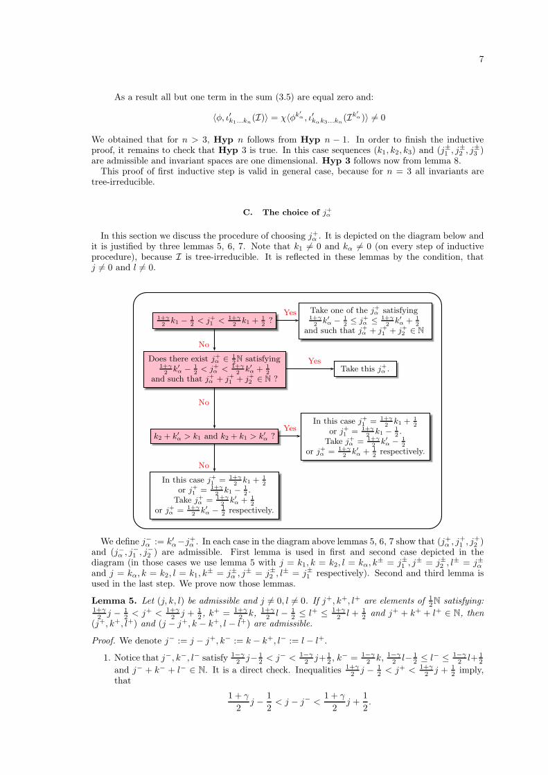
C. The choice of j+α

In this section we discuss the procedure of choosing j+α . It is depicted on the diagram below andit is justified by three lemmas 5, 6, 7. Note that k1 6= 0 and kα 6= 0 (on every step of inductiveprocedure), because I is tree-irreducible. It is reflected in these lemmas by the condition, thatj 6= 0 and l 6= 0.

1+γ

2k1 − 1

2< j+1 < 1+γ

2k1 +

1

2?

Take one of the j+α satisfying1+γ

2k′α − 1

2≤ j+α ≤ 1+γ

2k′α +

1

2

and such that j+α + j+1 + j+2 ∈ N

Does there exist j+α ∈ 1

2N satisfying

1+γ

2k′α − 1

2< j+α < 1+γ

2k′α +

1

2

and such that j+α + j+1 + j+2 ∈ N ?Take this j+α .

k2 + k′α > k1 and k2 + k1 > k′

α ?

In this case j+1 =1+γ

2k1 +

1

2

or j+1 =1+γ

2k1 −

1

2.

Take j+α =1+γ

2k′α − 1

2

or j+α =1+γ

2k′α +

1

2respectively.

In this case j+1 =1+γ

2k1 +

1

2

or j+1 =1+γ

2k1 −

1

2.

Take j+α =1+γ

2k′α +

1

2

or j+α =1+γ

2k′α − 1

2respectively.

No

No

Yes

Yes

No

Yes

We define j−α := k′α−j+α . In each case in the diagram above lemmas 5, 6, 7 show that (j+α , j+1 , j+2 )and (j−α , j−1 , j−2 ) are admissible. First lemma is used in first and second case depicted in thediagram (in those cases we use lemma 5 with j = k1, k = k2, l = kα, k

± = j±1 , j± = j±2 , l± = j±αand j = kα, k = k2, l = k1, k

± = j±α , j± = j±2 , l± = j±1 respectively). Second and third lemma isused in the last step. We prove now those lemmas.

Lemma 5. Let (j, k, l) be admissible and j 6= 0, l 6= 0. If j+, k+, l+ are elements of 12N satisfying:

1+γ2 j − 1

2 < j+ < 1+γ2 j + 1

2 , k+ = 1+γ

2 k, 1+γ2 l − 1

2 ≤ l+ ≤ 1+γ2 l + 1

2 and j+ + k+ + l+ ∈ N, then(j+, k+, l+) and (j − j+, k − k+, l − l+) are admissible.

Proof. We denote j− := j − j+, k− := k − k+, l− := l − l+.

1. Notice that j−, k−, l− satisfy 1−γ2 j− 1

2 < j− < 1−γ2 j+ 1

2 , k− = 1−γ2 k, 1−γ

2 l− 12 ≤ l− ≤ 1−γ

2 l+ 12

and j− + k− + l− ∈ N. It is a direct check. Inequalities 1+γ2 j − 1

2 < j+ < 1+γ2 j + 1

2 imply,that

1 + γ

2j −

1

2< j − j− <

1 + γ

2j +

1

2.

8

As a result

−1 + γ

2j −

1

2< −j− <

−1 + γ

2j +

1

2

and

1− γ

2j −

1

2< j− <

1− γ

2j +

1

2

The same with 1−γ2 l− 1

2 ≤ l− ≤ 1−γ2 l+ 1

2 and k− = 1−γ2 k is obvious. Finally j−+k−+ l− ∈ N

follows from the fact that j+ + k+ + l+ ∈ N and j + k + l ∈ N.

2. Note also that j− ≥ 0, k− ≥ 0, l− ≥ 0: 1−γ2 j − 1

2 < j−, so − 12 < j−; similarly 1−γ

2 l− 12 ≤ l−

implies − 12 < l−, because l 6= 0 and |γ| < 1; k± ≥ 0 is straightforward.

3. We check now triangle inequalities.

j+ + k+ >1 + γ

2j −

1

2+

1 + γ

2k =

1 + γ

2(j + k)−

1

2≥

1 + γ

2l −

1

2≥ l+ − 1.

It follows that

j+ + k+ − l+ > −1.

However j+ + k+ + l+ ∈ N, so j+ + k+ − l+ ∈ Z. As a result

j+ + k+ − l+ ≥ 0.

Similarly,

k+ + l+ ≥1 + γ

2k +

1 + γ

2l−

1

2=

1 + γ

2(k + l)−

1

2≥

1 + γ

2j −

1

2> j+ − 1.

We obtain k+ + l+ − j+ ≥ 0.

We have also

l+ + j+ >1 + γ

2l +

1 + γ

2j − 1 =

1 + γ

2(j + l)− 1 ≥

1 + γ

2k − 1 = k+ − 1.

Finally l++j+−k+ ≥ 0. This proves that (j+, k+, l+) is admissible. The proof for (j−, k−, l−)is the same.

Lemma 6. Let (j, k, l) be admissible and j 6= 0, l 6= 0. If j+, k+, l+ are elements of 12N satisfying:

j+ = 1+γ2 j ± 1

2 , k+ = 1+γ2 k, l+ = 1+γ

2 l ∓ 12 , j+ + k+ + l+ ∈ N, k + l > j and j + k > l, then

(j+, k+, l+) and (j − j+, k − k+, l − l+) are admissible.

Proof. As previously, we denote j− := j − j+, k− := k − k+, l− := l − l+ (it is easy to check, thatthey are nonnegative).

Let us check triangle inequalities:

j+ + k+ =1 + γ

2j ±

1

2+

1 + γ

2k =

1 + γ

2(j + k)±

1

2>

1 + γ

2l±

1

2= l+ ∓ 1

By arguments used in previous lemma, we obtain j+ + k+ − l+ ≥ 0.Let us check another inequality:

k+ + l+ =1 + γ

2k +

1 + γ

2l ∓

1

2=

1 + γ

2(k + l)∓

1

2>

1 + γ

2j ∓

1

2= j+ ± 1.

As a result k+ + l+ − j+ ≥ 0.Finally

j+ + l+ =1 + γ

2j ±

1

2+

1 + γ

2l ∓

1

2=

1 + γ

2(j + l) ≥

1 + γ

2k = k+

This finishes the prove of triangle inequalities. Proof for j−, k−, l− is the same.

9

Lemma 7. Let (j, k, l) be admissible and j 6= 0, l 6= 0. If j+, k+, l+ are elements of 12N satisfying:

j+ = 1+γ2 j ± 1

2 , k+ = 1+γ2 k, l+ = 1+γ

2 l ± 12 , j+ + k+ + l+ ∈ N, k + l = j or j + k = l, then

(j+, k+, l+) and (j − j+, k − k+, l − l+) are admissible.

Proof. Let k+ l = j. Then k+ + l+ = j+ which proves triangle inequalities. The proof is the samefor j + k = l. One checks in the same way that (j − j+, k − k+, l− l+) is admissible.

D. The fact that χ 6= 0

The fact that χ 6= 0 was proved in our previous paper [4]. Here we recall only the result.

Lemma 8. Let (j+, k+, l+),(j−, k−, l−) be admissible. Define j = j+ + j−, k = k+ + k−, l =

l+ + l−. Take any non-zero η ∈ Inv (Hj ⊗Hk ⊗H∗l ), η+ ∈ Inv

(

H∗j+

⊗H∗k+ ⊗Hl+

)

and η− ∈

Inv(

H∗j−

⊗H∗k− ⊗Hl−

)

. We have:

η+C+

A+B+η−C−

A−B−CA+A−

A CB+B−

B ηABC = χ CC+C−

C

for χ 6= 0.

Interestingly, this lemma may be proved also using argument different from the one used in [4].Now we present it.

First notice, it is enough to show, that, under assumptions above,

η+C+

A+B+η−C−

A−B−CA+A−

A CB+B−

B ηABC CC

C+C− 6= 0

for some non-zero Cll+l−

.

However the expression η+C+

A+B+η−C−

A−B−CA+A−

A CB+B−

B ηABC CC

C+C− is proportional with non-zeroproportionality factor to 9j-symbol, i.e.:

η+C+

A+B+η−C−

A−B−CA+A−

A CB+B−

B ηABC CC

C+C− = λ

j− l− k−

j+ l+ k+

j l k

,

where λ 6= 0. The appearance of this 9j-symbol here is strictly connected with the expansion offusion coefficient into product of 9j-symbols done in four-valent case in the article [10]. From theproperties of 9j-symbol and admissibility of (j+, k+, l+), (j−, k−, l−) follows that this 9j-symbol isproportional to a 3j-symbol (see e.g. equation (37) in [10]) with non-zero proportionality constant,i.e.:

j− l− k−

j+ l+ k+

j l k

= µ

(

l− l+ l

j− − k− j+ − k+ −(j − k)

)

,

where µ 6= 0.Recall that l = l+ + l−, so

(

l− l+ lj− − k− j+ − k+ −(j − k)

)

=

= (−1)l−−l++j−k

[

(2l−)!(2l+)!)

(2l+ 1)!

(l + j − k)!(l − j + k)!

(l− + j− − k−)!(l− − j− + k−)!(l+ + j+ − k+)!(l+ − j+ + k+)!

]12

.

From admissibility of (j+, k+, l+), (j−, k−, l−) follows that

(

l− l+ lj− − k− j+ − k+ −(j − k)

)

6= 0.

Finally:

η+C+

A+B+η−C−

A−B−CA+A−

A CB+B−

B ηABC CC

C+C− = λµ

(

l− l+ l

j− − k− j+ − k+ −(j − k)

)

6= 0.

10

IV. PROOF OF THE THEOREM

A. The inductive hypothesis

We base our prove on the following inductive hypothesis for n ≥ 3, n ∈ N:

Hyp n: Suppose that (k1, . . . , kn), (j±1 , . . . , j±n ) satisfy condition Con n and thatI ∈ Inv (Hk1

⊗ · · · ⊗ Hkn). Then, there exists

φ ∈ Inv(

Hj+

1

⊗ · · · ⊗ Hj+n

)

⊗ Inv(

Hj−

1

⊗ · · · ⊗ Hj−

n

)

such that 〈φ, ιk1...kn(I)〉 6= 0.

Notice that we do not restrict to tree-irreducible intertwiners anymore. As mentioned before, thisproves injectivity of the EPRL map (theorem 2) for n ≥ 3. One needs to check cases n = 1 andn = 2 separately but this is straightforward.

B. Proof

Previously we restricted ourselves to tree-irreducible intertwiners, because then the lowest spinkα in the decomposition (3.3) (we denote it by k′α) as well as k1 are different than 0, if n > 3. Ingeneral k′α or k1 may be equal 0 for n > 3 and then our procedure determining j+α and j−α maynot be applied (lemmas 5, 6, 7 require kα 6= 0, k1 6= 0). Actually the case k′α = 0 (so k1 = k2) andj+1 = j+2 is not problematic – we simply take j+α = 0 and follow steps 3-5 in section III B. The casek1 = 0 is also simple, because j+1 + j−1 = k1 = 0 implies j±1 = 0 and the inductive step is trivial.Problems appear, when k′α = 0 and j+1 = j+2 ± 1

2 , j−1 = j−2 ∓ 12 . We treat this case separately.

The inductive step we start (as in simplified case in section III) by expanding I as in equation(3.3) and finding minimal kα which we call k′α. We may perform standard procedure unless we arein the problematic case. Note that in this case

j+i ∈ N+1

2, i > 1, (4.1)

as j+1 = j+2 ± 12 and sequences are ordered. If this is the case, we expand the intertwiner I one

level further, i.e. instead of formula (3.3) we use the following one:

IA1A2...An =∑

(kα,kβ)∈K

CA1A2

AαCAαA3

Aβ(Ikαkβ )AβA4...An , (4.2)

where K := {(kα, kβ) ∈12N× 1

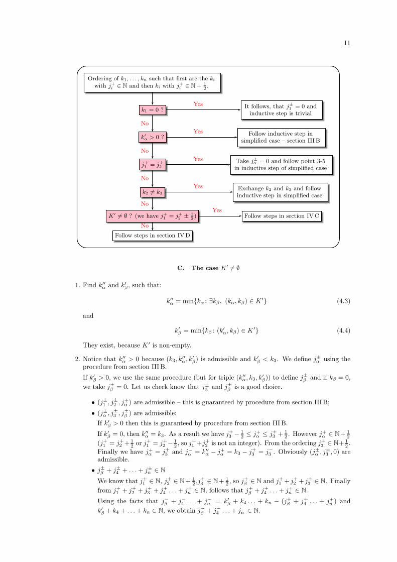
2N : Ikαkβ 6≡ 0}. We define K ′ = K∩{(kα, kβ) : kβ < k3}. There aretwo cases K ′ = ∅ and K ′ 6= ∅ which we describe in next two sections. The procedure is summarisedby the diagram below.

Importantly notice that in case n = 4, we either obtain k′α > 0 or kα′ = 0, j+1 = j+2 . In thiscase notice that either j+1 ∈ N, j+2 ∈ N or j+1 ∈ N+ 1

2 , j+2 ∈ N+ 12 (this follows from the fact that

j+1 + j+2 + j+3 + j+4 ∈ N and from ordering of ki) – as a result if k′α = 0 then j+1 = j+2 . This meansthat when n = 4, the inductive step from simplified case may be used. As a result the check ofinitial conditions done in the proof of tree-irreducible case is sufficient in general case presentedhere.

11

Ordering of k1, . . . , kn such that first are the kiwith j+i ∈ N and then ki with j+i ∈ N+

1

2.

k1 = 0 ?It follows, that j±1 = 0 and

inductive step is trivial

k′α > 0 ?

Follow inductive step insimplified case – section III B

j+1 = j+2Take j±α = 0 and follow point 3-5in inductive step of simplified case

k2 6= k3Exchange k2 and k3 and followinductive step in simplified case

K′ 6= ∅ ? (we have j+1 = j+2 ± 1

2) Follow steps in section IVC

Follow steps in section IVD

No

No

Yes

Yes

Yes

Yes

No

No

No

Yes

C. The case K′ 6= ∅

1. Find k′′α and k′β , such that:

k′′α = min{kα : ∃kβ , (kα, kβ) ∈ K ′} (4.3)

and

k′β = min{kβ : (k′α, kβ) ∈ K ′} (4.4)

They exist, because K ′ is non-empty.

2. Notice that k′′α > 0 because (k3, k′′α, k

′β) is admissible and k′β < k3. We define j±α using the

procedure from section III B.

If k′β > 0, we use the same procedure (but for triple (k′′α, k3, k′β)) to define j±β and if kβ = 0,

we take j±β = 0. Let us check know that j±α and j±β is a good choice.

• (j±1 , j±2 , j±α ) are admissible – this is guaranteed by procedure from section III B;

• (j±α , j±3 , j±β ) are admissible:

If k′β > 0 then this is guaranteed by procedure from section III B.

If k′β = 0, then k′′α = k3. As a result we have j+3 − 12 ≤ j+α ≤ j+3 + 1

2 . However j+α ∈ N+ 12

(j+1 = j+2 + 12 or j+1 = j+2 − 1

2 , so j+1 +j+2 is not an integer). From the ordering j+3 ∈ N+ 12 .

Finally we have j+α = j+3 and j−α = k′′α − j+α = k3 − j+3 = j−3 . Obviously (j±α , j±3 , 0) areadmissible.

• j±β + j±4 + . . .+ j±n ∈ N

We know that j+1 ∈ N, j+2 ∈ N+ 12 ,j+3 ∈ N+ 1

2 , so j+β ∈ N and j+1 + j+2 + j+3 ∈ N. Finally

from j+1 + j+2 + j+3 + j+4 . . .+ j+n ∈ N, follows that j+β + j+4 . . .+ j+n ∈ N.

Using the facts that j−β + j−4 . . . + j−n = k′β + k4 . . . + kn − (j+β + j+4 . . . + j+n ) and

k′β + k4 + . . .+ kn ∈ N, we obtain j−β + j−4 . . .+ j−n ∈ N.

12

• We see that 1+γ2 k′β −

12 ≤ j+β ≤ 1+γ

2 k′β+12 . We have also j+4 ∈ N+ 1

2 and so the orderingproperty is satisfied.

Eventually, Con n− 2 is fulfilled for (k′β , k4, . . . , kn) and (j±β , j±4 , . . . , j±n ).

3. From Hyp n− 2 follows that for Ik′′

αk′

β from (4.2) there exists

φk′′

αk′

β ∈ Inv(

Hj+α⊗Hj

+

β⊗ · · · ⊗ Hj

+n

)

⊗ Inv(

Hj−

α⊗Hj

+

β⊗ · · · ⊗ Hj

−

n

)

,

such that

〈φk′′

αk′

β , ι′k′

β...kn

(Ik′′

αk′

β )〉 6= 0.

4. Having defined φk′′

αk′

β , we construct φ:

φA+

1...A+

n ,A−

1...A−

n := CA

+

1A

+

2

A+α

CA+

αA+

3

A+

β

CA

−

1A

−

2

A−

α

CA−

αA−

3

A−

β

(φk′′

αk′

β )A+

βA

+

4...A+

n ,A−

βA

−

4...A−

n

5. The φ constructed in previous point is the φ we are looking for, i.e. 〈φ, ι′k1...kn(I)〉 6= 0. We

now prove this statement.

(a) First, using equation (4.2) write 〈φ, ι′k1...kn(I)〉 as a sum:

〈φ, ι′k1...kn(I)〉 =

∑

(kα,kβ)∈K

〈φ, ι′k1...kn(Ck1k2

kα◦ Ckαk3

kβ◦ Ikαkβ )〉, (4.5)

where (Ck1k2

kα◦ Ckαk3

kβ◦ Ikαkβ )

A1A2...An

:= CA1A2

AαCAαA3

Aβ(Ikαkβ )AβA4...An .

(b) Let us compute 〈φ, ι′k1...kn(Ck1k2

kα◦ Ckαk3

kβ◦ Ikαkβ )〉 (see fig. IVC):

〈φ, ι′k1...kn(Ck1k2

kα◦ Ckαk3

kβ◦ Ikαkβ )〉 = (φk′′

αk′

β )†A

+

βA

+

4...A

+n ,A

−

βA

−

4...A

−

n

CA+

α

A+

1A

+

2

CA+

β

A+αA

+

3

CA−

α

A−

1A

−

2

CA−

β

A−

αA−

3

CA

+

1A

−

1

A1. . . C

A+nA−

n

AnCA1A2

AαCAαA3

Aβ(Ikαkβ )AβA4...An = C

A+α

A+

1A+

2

CA−

α

A−

1A−

2

CA

+

1A

−

1

A1C

A+

2A

−

2

A2CA1A2

Aα

CA

+

β

A+αA

+

3

CA

−

β

A−

αA−

3

CA

+

3A

−

3

A3CAαA3

Aβ(φk′′

αk′

β )†A

+

βA

+

4...A

+n ,A

−

βA

−

4...A

−

n

CA

+

4A

−

4

A4. . . C

A+nA−

n

An(Ikαkβ )AβA4...An

Using lemma 8 we obtain, that for some ξ1 6= 0

CA+

α

A+

1A

+

2

CA−

α

A−

1A

−

2

CA

+

1A

−

1

A1C

A+

2A

−

2

A2CA1A2

Aα=

{

0, kα > j+α + j−α

ξ1CA+

αA−

α

Aα, kα = j+α + j−α

Applying this lemma second time we get, that for some ξ2 6= 0

CA

+

β

A+αA

+

3

CA

−

β

A−

αA−

3

CA+

αA−

α

AαC

A+

3A

−

3

A3CAαA3

Aβ=

{

0, kβ > j+β + j−β

ξ2CA

+

βA

−

β

Aβ, kβ = j+β + j−β

Finally, for ξ := ξ1ξ2 6= 0 :

〈φ, ι′k1...kn(Ck1k2

kα◦ Ckαk3

kβIkαkβ )〉 =

0, kα > k′′α or kβ > k′βξ〈φk′′

αk′

β , ι′k′

β...kn

(Ik′′

αk′

β )〉, kα = k′α and kβ = k′β

∗, otherwise

(4.6)

13

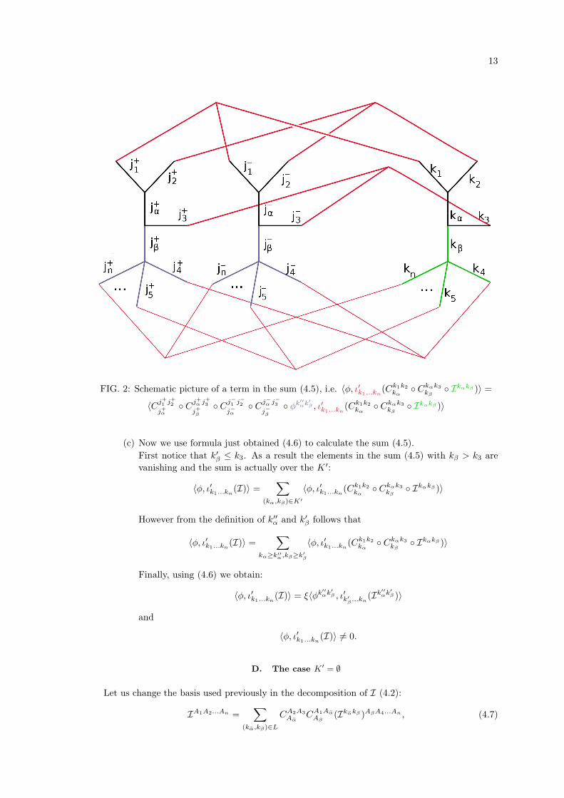
FIG. 2: Schematic picture of a term in the sum (4.5), i.e. 〈φ, ι′k1...kn(Ck1k2

kα◦ Ckαk3

kβ◦ Ikαkβ )〉 =

〈Cj+

1j+

2

j+α◦ C

j+α j+

3

j+β

◦ Cj−

1j−

2

j−α◦ C

j−α j−

3

j−β

◦ φk′′

αk′

β , ι′k1...kn(Ck1k2

kα◦ Ckαk3

kβ◦ Ikαkβ )〉

(c) Now we use formula just obtained (4.6) to calculate the sum (4.5).

First notice that k′β ≤ k3. As a result the elements in the sum (4.5) with kβ > k3 are

vanishing and the sum is actually over the K ′:

〈φ, ι′k1...kn(I)〉 =

∑

(kα,kβ)∈K′

〈φ, ι′k1...kn(Ck1k2

kα◦ Ckαk3

kβ◦ Ikαkβ )〉

However from the definition of k′′α and k′β follows that

〈φ, ι′k1...kn(I)〉 =

∑

kα≥k′′

α,kβ≥k′

β

〈φ, ι′k1...kn(Ck1k2

kα◦ Ckαk3

kβ◦ Ikαkβ )〉

Finally, using (4.6) we obtain:

〈φ, ι′k1...kn(I)〉 = ξ〈φk′′

αk′

β , ι′k′

β...kn

(Ik′′

αk′

β )〉

and

〈φ, ι′k1...kn(I)〉 6= 0.

D. The case K′= ∅

Let us change the basis used previously in the decomposition of I (4.2):

IA1A2...An =∑

(kα̃,kβ)∈L

CA2A3

Aα̃C

A1Aα̃

Aβ(Ikα̃kβ )AβA4...An , (4.7)

14

where L := {(kα̃, kβ) ∈12N× 1

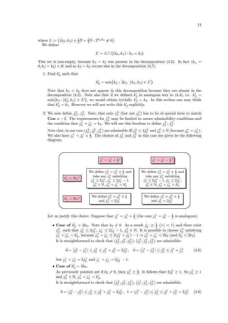
2N : Ikα̃kβ 6≡ 0}.We define:

L′ = L ∩ {(kα̃, kβ) : kβ = k3}

This set is non-empty, because kβ = k3 was present in the decomposition (4.2). In fact (kα =0, kβ = k3) ∈ K and so kβ = k3 occurs also in the decomposition (4.7).

1. Find k′α̃ such that:

k′α̃ = min{kα̃ : ∃kβ , (kα̃, kβ) ∈ L′}

Note that kβ < k3 does not appear in this decomposition because they are absent in thedecomposition (4.2). Note also that if we defined k′β in analogous way to (4.4), i.e. k′β =

min{kβ : (k′α̃, kβ) ∈ L′}, we would obtain trivially k′β = k3. In this section one may think

that k′β = k3. However we will not write this k′β explicitly.

2. We now define j±α̃ , j±β . Note, that only j±β (but not j+α̃ ) has to be of special form to match

Con n− 2. The requirements for j±α̃

may be limited to assure admissibility conditions and

the condition that j+α̃+ j−

α̃= kα̃. We will use this freedom to define j±

α̃, j±β .

Note that, in our case (j±2 , j±3 , j±α̃) are admissible iff j±

α̃≤ 2j±2 and j±

α̃∈ N (because j+2 = j+3 ).

We also have j+1 = j+2 ± 12 . The choices of j±α̃ and j±β in this case are given be the following

diagram.

j+1 = j+2 +1

2? j+1 = j+2 − 1

2?

k′α < 2k2?

We define j±β = j±2 ± 1

2and

take any j±α̃

satisfyingj+α̃

≤ 2j+2 , j−α̃

≤ 2j−2 − 1,j±α̃

∈ N, j+α̃+ j−

α̃= k′

α̃

We define j±β = j±2 ∓ 1

2and

take any j±α̃

satisfyingj+α̃

≤ 2j+2 − 1, j−α̃

≤ 2j−2 ,j±α̃

∈ N, j+α̃+ j−

α̃= k′

α̃

k′α < 2k2?

We define j±β = j±2 ∓ 1

2

and j±α̃

= 2j±2

We define j±β = j±2 ± 1

2

and j±α̃

= 2j±2

Let us justify this choice. Suppose that j+1 = j+2 + 12 (the case j+1 = j+2 − 1

2 is analogous).

• Case of k′α̃ < 2k2. Note that k2 6= 0. As a result j−2 ≥ 12 (|γ| < 1) and there exist

j±α̃ , such that j+α̃ ≤ 2j+2 , j−α̃ ≤ 2j−2 − 1, j±α̃ ∈ N. It is possible to choose j±α̃ satisfying

j+α̃+ j−

α̃= k′α̃, because j+

α̃+ j−

α̃≤ 2(j+2 + j−2 )− 1 ⇒ j+

α̃+ j−

α̃< 2k2 (and k′α̃ < 2k2).

It is straightforward to check that (j±2 , j±3 , j±α̃), (j±1 , j±

α̃, j±β ) are admissible:

0 = |j±2 − j±3 | ≤ j±α̃

≤ j±2 + j±3 = 2j±2 , 0 = |j±1 − j±β | ≤ j±α̃

≤ j±1 + j±β (4.8)

but j+1 + j+β = 2j+2 and j−1 + j−β = 2j−2 − 1.

• Case of k′α̃ = 2k2.

As previously pointed out if k2 6= 0, then j±2 ≥ 12 . It follows that 2j±2 ≥ 1. So j±α̃ ≥ 1

and j±α̃

∈ N, j+α̃+ j−

α̃= k′α̃.

It is straightforward to check that (j±2 , j±3 , j±α̃), (j±1 , j±

α̃, j±β ) are admissible:

0 = |j±2 − j±3 | ≤ j±α̃

≤ j±2 + j±3 = 2j±2 , 1 = |j±1 − j±β | ≤ j±α̃

≤ j±1 + j±β = 2j±2 (4.9)

15

3. Note that because j+1 and j+α̃

are natural then also j+β ∈ N. Recall also that j+1 ∈ N,j+2 , j+3 ∈

N + 12 and j+1 + . . . j+n ∈ N. As a result j+β + j+4 + . . . j+n ∈ N and j−β + j−4 + . . . j−n =

k3 + k4 + . . .+ kn − (j+β + j+4 + . . . j+n ) ∈ N.

We have also that 1+γ2 k3 −

12 ≤ j+β ≤ 1+γ

2 k3 +12 and j+4 ∈ N + 1

2 , so Con n − 2 is fulfilled

for (k3, k4, . . . , kn) and (j±β , j±4 , . . . , j±n ).

4. From Hyp n− 2 follows that for Ik′

α̃k3 from (4.7) there exists

φk′

α̃k3 ∈ Inv(

Hj+α⊗Hj

+

β

⊗ · · · ⊗ Hj+n

)

⊗ Inv(

Hj−

α⊗Hj

+

β

⊗ · · · ⊗ Hj−

n

)

,

such that

〈φk′

α̃k3 , ι′k3...kn(Ik′

α̃k3)〉 6= 0.

5. Having defined φk′

α̃k3 , we construct φ:

φA+

1...A+

n ,A−

1...A−

n := CA

+

2A

+

3

A+

α̃

CA

+

α̃A

+

1

A+

β

CA

−

2A

−

3

A−

α̃

CA

−

α̃A

−

1

A−

β

(φk′

α̃k3)A+

βA

+

4...A+

n ,A−

βA

−

4...A−

n

6. The φ constructed in previous point is the φ we are looking for, i.e. 〈φ, ι′k1...kn(I)〉 6= 0. We

now prove this statement.

(a) First, using equation (4.7) write 〈φ, ι′k1...kn(I)〉 as a sum:

〈φ, ι′k1...kn(I)〉 =

∑

(kα̃,kβ)∈L

〈φ, ι′k1...kn(Ck2k3

kα̃◦ Ck1kα̃

kβ◦ Ikα̃kβ )〉, (4.10)

where (Ck2k3

kα̃◦ Ck1kα̃

kβ◦ Ikα̃kβ )

A1A2...An

:= CA2A3

Aα̃C

A1Aα̃

Aβ(Ikα̃kβ )AβA4...An .

(b) Let us compute 〈φ, ι′k1...kn(Ck2k3

kα̃◦ Ck1kα̃

kβ◦ Ikα̃kβ )〉 (see fig. IVD):

〈φ, ι′k1...kn(Ck1k2

kα◦ Ckαk3

kβ◦ Ikαkβ )〉 = (φk′

α̃k′

β )†A

+

βA

+

4...A

+n ,A

−

βA

−

4...A

−

n

CA

+

β

A+

α̃A

+

1

CA

+

α̃

A+

2A

+

3

CA

−

β

A−

α̃A

−

1

CA

−

α̃

A−

2A

−

3

CA

+

1A

−

1

A1. . . C

A+nA−

n

AnCA2A3

Aα̃C

Aα̃A1

Aβ(Ikα̃kβ )AβA4...An = C

A+

α̃

A+

2A

+

3

CA

−

α̃

A−

2A

−

3

CA

+

2A

−

2

A2C

A+

3A

−

3

A3CA2A3

Aα̃

CA

+

β

A+

α̃A

+

1

CA

−

β

A−

α̃A

−

1

CA

+

1A

−

1

A1C

Aα̃A1

Aβ(φk′

α̃k′

β )†A

+

βA

+

4...A

+n ,A

−

βA

−

4...A

−

n

CA

+

4A

−

4

A4. . . C

A+nA−

n

An(Ikα̃kβ )AβA4...An

Using lemma 8 we obtain, that for some ρ1 6= 0

CA

+

α̃

A+

2A

+

3

CA

−

α̃

A−

2A

−

3

CA

+

2A

−

2

A2C

A+

3A

−

3

A3CA2A3

Aα̃=

{

0, kα̃ > j+α̃ + j−α̃

ρ1CA

+

α̃A

−

α̃

Aα̃, kα̃ = j+α̃ + j−α̃

Applying this lemma second time we get, that for some ρ2 6= 0

CA

+

β

A+

α̃A

+

1

CA

−

β

A−

α̃A

−

1

CA

+

α̃A

−

α̃

Aα̃C

A+

1A

−

1

A1C

Aα̃A1

Aβ=

{

0, kβ > j+β + j−β

ρ2CA+

βA−

β

Aβ, kβ = j+β + j−β

Finally, for ρ := ρ1ρ2 6= 0 :

〈φ, ι′k1...kn(Ck2k3

kα̃◦ Ckα̃k1

kβIkα̃kβ )〉 =

0, kα̃ > k′α̃ or kβ > k′βρ〈φk′

α̃k′

β , ι′k′

β...kn

(Ik′

α̃k′

β )〉, kα̃ = k′α̃ and kβ = k′β

∗, otherwise

(4.11)

16

FIG. 3: Schematic picture of a term in the sum (4.10), i.e. 〈φ, ι′k1...kn(Ck2k3

kα̃◦ Ckα̃k1

kβ◦ Ikα̃kβ )〉 =

〈Cj+2j+3

j+

α̃

◦ Cj+

α̃j+

1

j+

β

◦ Cj−2j−3

j−

α̃

◦ Cj−

α̃j−

1

j−

β

◦ φk′

α̃k3 , ι′k1...kn(Ck2k3

kα̃◦Ckα̃k1

kβ◦ Ikα̃kβ )〉

(c) Now we use formula just obtained (4.11) to calculate the sum (4.10).

First notice that in this case kβ ≥ k3. Moreover, the elements in the sum (4.10) withkβ > k3 are vanishing (4.11) and the sum is actually over L′:

〈φ, ι′k1...kn(I)〉 =

∑

(kα̃,kβ)∈L′

〈φ, ι′k1...kn(Ck2k3

kα̃◦ Ck1kα̃

kβ◦ Ikαkβ )〉

However from the definition of k′α̃ follows that

〈φ, ι′k1...kn(I)〉 =

∑

kα̃≥k′

α̃

〈φ, ι′k1...kn(Ck2k3

kα̃◦ Ck1kα̃

k3◦ Ikα̃k3)〉

Finally, using (4.11) we obtain:

〈φ, ι′k1...kn(I)〉 = ρ〈φk′

α̃k3 , ι′k3...kn(Ik′

α̃k3)〉

and

〈φ, ι′k1...kn(I)〉 6= 0.

Acknowledgement: The work was partially supported by the grants N N202 104838, N N202287538, and 182/N-QGG/2008/0 (PMN) of Polish Ministerstwo Nauki i Szkolnictwa Wyższego.Wojciech Kamiński is partially supported by grant N N202 287538. Marcin Kisielowski acknowl-edges financial support from the project ”International PhD Studies in Fundamental Problems of

17

Quantum Gravity and Quantum Field Theory” of Foundation for Polish Science, co-financed fromthe programme IE OP 2007-2013 within European Regional Development Fund.

[1] Engle J, Livine E, Pereira R, Rovelli C (2008), LQG vertex with finite Immirzi parameter, Nucl.Phys.B799:136-149 (Preprint gr-qc/0711.0146v2)

[2] Freidel L, Krasnov K (2008), A New Spin Foam Model for 4d Gravity, Class.Quant.Grav. 25:125018(Preprint gr-qc/0708.1595v2)

[3] Kamiński W,Kisielowski M, Lewandowski J (2010), Spin-Foams for All Loop Quantum Gravity, Class.Quantum Grav. 27 095006 (Preprint arXiv:0909.0939v2)

[4] Kamiński W,Kisielowski M, Lewandowski J (2010), The EPRL intertwiners and corrected partitionfunction, Class. Quantum Grav. 27 165020 (Preprint arXiv:0912.0540v1)

[5] Domagała M, and Lewandowski J (2004), Black hole entropy from Quantum Geometry, Class. Quant.Grav. 21 , 5233-5244 (Preprint gr-qc/0407051)

[6] Meissner K (2004), Black hole entropy in Loop Quantum Gravity, Class. Quant. Grav. 21, 5245-5252(Preprint gr-qc/0407052)

[7] Thiemann T (2007), Introduction to Modern Canonical Quantum General Relativity (CambridgeUniversity Press, Cambridge)Rovelli C (2004), Loop Quantum Gravity, (Cambridge University Press, Cambridge)Ashtekar A and Lewandowski J (2004), Background independent quantum gravity: A status report,Class. Quant. Grav. 21 R53, (Preprint gr-qc/0404018)Han M, Huang W, Ma Y (2007) Fundamental Structure of Loop Quantum Gravity, Int. J. Mod. Phys.D16, pp. 1397-1474

[8] Baez J (2000), An introduction to Spinfoam Models of BF Theory and Quantum Gravity, Lect.NotesPhys. 543 25-94 (Preprint gr-qc/9905087v1)

[9] Perez A (2003), Spinfoam models for Quantum Gravity, Class.Quant.Grav. 20 R43 (Preprintgr-qc/0301113v2)

[10] Alesci E, Bianchi E, Magliaro E, Perini C (2008), Asymptotics of LQG fusion coefficients, PreprintarXiv:0809.3718v2 [gr-qc]