arX

iv:0

710.

3238

v1 [

mat

h.D

S] 1

7 O

ct 2

007 The inverse integrating factor

and the Poincare map. ∗

Dedicated to Javier Chavarriga.

Isaac A. Garcıa (1), Hector Giacomini (2) and Maite Grau (1)

Abstract

This work is concerned with planar real analytic differential systems with

an analytic inverse integrating factor defined in a neighborhood of a regular

orbit. We show that the inverse integrating factor defines an ordinary dif-

ferential equation for the transition map along the orbit. When the regular

orbit is a limit cycle, we can determine its associated Poincare return map

in terms of the inverse integrating factor. In particular, we show that the

multiplicity of a limit cycle coincides with the vanishing multiplicity of an

inverse integrating factor over it. We also apply this result to study the ho-

moclinic loop bifurcation. We only consider homoclinic loops whose critical

point is a hyperbolic saddle and whose Poincare return map is not the iden-

tity. A local analysis of the inverse integrating factor in a neighborhood of

the saddle allows us to determine the cyclicity of this polycycle in terms of

the vanishing multiplicity of an inverse integrating factor over it. Our result

also applies in the particular case in which the saddle of the homoclinic loop

is linearizable, that is, the case in which a bound for the cyclicity of this

graphic cannot be determined through an algebraic method.

2000 AMS Subject Classification: 37G15, 37G20, 34C05

Key words and phrases: inverse integrating factor, Poincare map, limit cycle, homoclinic

loop.

1 Introduction and statement of the main results

We consider two–dimensional autonomous systems of real differential equations ofthe form

x = P (x, y), y = Q(x, y), (1)

∗The authors are partially supported by a DGICYT grant number MTM2005-06098-C02-02.

1

where P (x, y) and Q(x, y) are analytic functions defined on an open set U ⊆ R2.Here, the dot denotes, as usual, derivative with respect to the independent variablet. The vector field associated to system (1) will be denoted X = P (x, y)∂x +Q(x, y)∂y and its divergence is divX := ∂P/∂x + ∂Q/∂y.

Definition 1 An inverse integrating factor for system (1) in U is a non–locallynull C1 solution V : U ⊂ R2 → R of the linear partial differential equation

XV = V divX . (2)

If V is an inverse integrating factor of system (1) then the zero–set of V , V −1(0) :={(x, y) | V (x, y) = 0}, is composed of trajectories of (1). In fact it is easy to seethat for any point p ∈ U , if Φ(t; p) is the orbit of (1) that satisfies Φ(0; p) = p, then

V (Φ(t; p)) = V (p) exp

(∫ t

0

divX ◦ Φ(s; p) ds

)

. (3)

Thus if V (p) = 0 then V (Φ(t; p)) = 0 for all t provided that V is defined on Φ(t; p).

We consider a certain regular orbit of system (1) and we assume the existenceof an analytic inverse integrating factor in a neighborhood of this regular orbit.We show that some qualitative properties of the orbits in a neighborhood of theconsidered regular orbit can be deduced from the known inverse integrating factor.

We consider a regular orbit φ(t) of system (1) and two transversal sectionsΣ1 and Σ2 based on it. We are going to study the transition map of the flow ofsystem (1) in a neighborhood of this regular orbit. This transition map is studiedby means of the Poincare map Π : Σ1 → Σ2 which is defined as follows. Givena point in Σ1, we consider the orbit of system (1) with it as initial point and wefollow this orbit until it first intersects Σ2. The map Π makes correspond to thepoint in Σ1 the encountered point in Σ2.

Let (ϕ(s), ψ(s)) ∈ U , with s ∈ I ⊆ R be a parameterization of the regularorbit φ(t) between the base points of Σ1 and Σ2. In particular s can be the time tassociated to system (1). Given a point (x, y) in a sufficiently small neighborhoodof the orbit (ϕ(s), ψ(s)), we can always encounter values of the curvilinear coordi-nates (s, n) that realize the following change of variables: x(s, n) = ϕ(s)− nψ′(s),y(s, n) = ψ(s)+nϕ′(s). We remark that the variable n measures the distance per-pendicular to φ(t) from the point (x, y) and, therefore, n = 0 corresponds to theconsidered regular orbit φ(t). We can assume, without loss of generality, that thetransversal section Σ1 corresponds to Σ1 := {s = 0} and Σ2 to Σ2 := {s = L},for a certain real number L > 0.

We perform the change to curvilinear coordinates (x, y) 7→ (s, n) in a neigh-borhood of the regular orbit n = 0 with s ∈ I = [0, L]. Then, system (1) readsfor

n = N(s, n), s = S(s, n), (4)

2

where N(s, 0) ≡ 0 since n = 0 is an orbit and S(s, 0) 6= 0 for s ∈ I becauseit is a regular orbit. Therefore, and in order to study the behavior of the orbitsin a neighborhood of n = 0, we can consider the following ordinary differentialequation:

dn

ds= F (s, n) . (5)

We denote by Ψ(s;n0) the flow associated to the equation (5) with initial conditionΨ(0;n0) = n0. In these coordinates, the Poincare map Π : Σ1 → Σ2 between thesetwo transversal sections is given by Π(n0) = Ψ(L;n0).

We assume the existence of an analytic inverse integrating factor V (x, y) in aneighborhood of the considered regular orbit φ(t) of system (1). In fact, whenΣ1 6= Σ2 and no return is involved, there always exists such an inverse integratingfactor. It is clear that in a neighborhood of a regular point there is always aninverse integrating factor. Applying the characteristics’ method, we can extendthis function following the flow of the system until we find a singular point or areturn is involved.

The change to curvilinear coordinates gives us an inverse integrating factor forequation (5), denoted by V (s, n) and which satisfies

∂V

∂s+∂V

∂nF (s, n) =

∂F

∂nV (s, n). (6)

The following theorem gives the relation between the inverse integrating factorand the Poincare map defined over the considered regular orbit.

Theorem 2 We consider a regular orbit φ(t) of system (1) which has an inverseintegrating factor V (x, y) of class C1 defined in a neighborhood of it and we considerthe Poincare map associated to the regular orbit between two transversal sectionsΠ : Σ1 → Σ2. We perform the change to curvilinear coordinates and we considerthe ordinary differential equation (5) with the inverse integrating factor V (s, n)which is obtained from V (x, y). In these coordinates, the transversal sections canbe taken such that Σ1 := {s = 0} and Σ2 := {s = L}, for a certain real valueL > 0. We parameterize Σ1 by a real parameter denoted σ. The following identityholds.

V (L,Π(σ)) = V (0, σ)Π′(σ). (7)

The proof of this result is given in Section 2.We remark that if we know an inverse integrating factor for system (1), we

can construct the function V (s, n) and equation (7) gives an ordinary differentialequation for Π(σ), which is always of separated variables. Thus, we can determinethe expression of Π(σ) in an implicit way and up to quadratures. The first examplein Section 3 illustrates this remark.

3

We notice that the definition of the Poincare map Π is geometric and Theorem2 gives an ordinary differential equation to compute an explicit expression of Π,provided that an inverse integrating factor is known. As far as the authors know,no such a way of describing the Poincare map has been given in any previous work.

It is well–known, due to the flow box theorem, that a regular orbit of system(1) which is not a separatrix of singular points nor a limit cycle has an associatedPoincare map conjugated with the identity. There are several results which estab-lish that the vanishing set of an inverse integrating factor gives the orbits whoseassociated Poincare map is not conjugated with the identity. In this sense, Giaco-mini, Llibre and Viano [13], showed that any limit cycle γ ⊂ U ⊆ R2 of system (1)satisfies γ ⊂ V −1(0) provided that the inverse integrating factor V is defined in U .

Lately it was shown that the zero–set of V often contains the separatrices ofcritical points in U . More precisely, in [3] Berrone and Giacomini proved that, ifp0 is a hyperbolic saddle–point of system (1), then any inverse integrating factorV defined in a neighborhood of p0 vanishes on all four separatrices of p0, providedV (p0) = 0. We emphasize here that this result does not hold, in general, for non–hyperbolic singularities (see [11] for example).

We are going to consider regular orbits whose Poincare map is a return map. Wetake profit from the result stated in Theorem 2 in order to study the Poincare mapassociated to a limit cycle or to a homoclinic loop, in terms of the inverse integratingfactor. Although we have used curvilinear coordinates to state Theorem 2, we donot need to use them to establish the results described in the following Theorems3 and 5. The only hypothesis that we need is the existence and the expression ofan analytic inverse integrating factor in a neighborhood of the limit cycle or thehomoclinic loop. In particular, we are able to give the cyclicity of a limit cycleor of a homoclinic loop from the vanishing multiplicity of the inverse integratingfactor over the limit cycle or the homoclinic loop. The vanishing multiplicity of ananalytic inverse integrating factor V (x, y) of system (1) over a regular orbit φ(t) isdefined as follows. We recall the local change of coordinates x(s, n) = ϕ(s)−nψ′(s),y(s, n) = ψ(s) + nϕ′(s) defined in a neighborhood of the considered regular orbitn = 0. If we have the following Taylor development around n = 0:

V (x(s, n), y(s, n)) = nm v(s) + O(nm+1), (8)

where m is an integer with m ≥ 1 and the function v(s) is not identically null, wesay that V has multiplicity m on φ(t). In fact, as we will see in Lemma 6, v(s) 6= 0for any s ∈ I, and thus, the vanishing multiplicity of V on φ(t) is well–defined overall its points.

4

Let us consider as regular orbit a limit cycle γ and we use the parameterizationof γ in curvilinear coordinates (s, n) with s ∈ [0, L). The Poincare return map Πassociated to γ coincides with the previously defined map in which Σ := Σ1 = Σ2.Since the qualitative properties of Π do not depend on the chosen transversalsection Σ, we take the one given by the curvilinear coordinates and, thus, Π(n0) =Ψ(L;n0). It is well known that Π is analytic in a neighborhood of n0 = 0. We recallthat the periodic orbit γ is a limit cycle if, and only if, the Poincare return map Πis not the identity. If Π is the identity, we have that γ belongs to a period annulus.We recall the definition of multiplicity of a limit cycle: γ is said to be a limit cycleof multiplicity 1 if Π′(0) 6= 1 and γ is said to be a limit cycle of multiplicity mwith m ≥ 2 if Π(n0) = n0 + βm n

m0 + O(nm+1

0 ) with βm 6= 0. The following resultstates that given a limit cycle γ of (1) with multiplicity m, then the vanishingmultiplicity of an analytic inverse integrating factor defined in a neighborhood ofit, must also be m.

Theorem 3 Let γ be a periodic orbit of system (1) and let V be an analytic inverseintegrating factor defined in a neighborhood of γ.

(a) If γ is a limit cycle of multiplicity m, then V has vanishing multiplicity mon γ.

(b) If V has vanishing multiplicity m on γ, then γ is a limit cycle of multiplicitym or it belongs to a continuum of periodic orbits.

The proof of this theorem is given in Section 2.The idea to study the multiplicity of a limit cycle by means of the vanishing

multiplicity of the inverse integrating factor already appears in the work [14]. Inthat work the considered limit cycles are semistable and the vanishing multiplicityis defined in terms of polar coordinates, which only apply for convex limit cycles.

Since the Poincare map of a periodic orbit is an analytic function and themultiplicity of a limit cycle is a natural number, we obtain the following corollaryfrom the previous result.

Corollary 4 Let γ be a periodic orbit of system (1) and let V be an inverse inte-grating factor of class C1 defined in a neighborhood of γ. We take the change tocurvilinear coordinates x(s, n) = ϕ(s) − nψ′(s), y(s, n) = ψ(s) + nϕ′(s) defined ina neighborhood of γ. If we have that the leading term in the following developmentaround n = 0:

V (x(s, n), y(s, n)) = nρ v(s) + o(nρ),

where v(s) 6≡ 0 is such that either ρ = 0 or ρ > 1 and ρ is not a natural number,then γ belongs to a continuum of periodic orbits.

5

We remark that this corollary applies, for instance, in the following case: let usconsider an invariant curve f = 0 of system (1) with an oval γ such that ∇f |γ 6= 0and let us assume that γ corresponds to a periodic orbit of the system and thatthere exists an inverse integrating factor of the form V = f ρg, where g is an nonzerofunction of class C1 in a neighborhood of γ and ρ ∈ R, with either ρ = 0 or ρ ≥ 1in order to have a C1 inverse integrating factor in a neighborhood of γ. If we havethat either ρ = 0 or ρ is not a natural number, then we deduce that γ belongs toa period annulus, by Corollary 4. On the other hand, applying Theorem 3, in thecase that ρ = m ∈ N, we deduce that either γ belongs to a period annulus or it isa limit cycle with multiplicity m.

A regular orbit φ(t) = (x(t), y(t)) of (1) is called a homoclinic orbit if φ(t) → p0

as t→ ±∞ for some singular point p0. We emphasize that such kind of orbits arisein the study of bifurcation phenomena as well as in many applications in severalsciences. A homoclinic loop is the union Γ = φ(t) ∪ {p0}. We assume that p0 is ahyperbolic saddle, that is, a critical point of system (1) such that the eigenvaluesof the Jacobian matrix DX (p0) are both real, different from zero and of contrarysign. We remark that this type of graphics always has associated (maybe only itsinner or outer neighborhood) a Poincare return map Π : Σ → Σ with Σ any localtransversal section through a regular point of Γ. Moreover, in this work we onlystudy compact homoclinic loops that are the α– or ω–limit set of the points in itsneighborhood, i.e., homoclinic loops with finite singular point and a return mapdifferent from the identity. This fact implies that Γ is a compact set, that is, itdoes not have intersection with the equator in the Poincare compactification. Infact the same results can be used for some homoclinic loops whose saddle is inthe equator of the Poincare compactification, but we always assume that the affinechart we are working with completely contains the homoclinic loop, that is, thehomoclinic loops we take into account are compact in the considered affine chart.

Our goal in this work is to study the cyclicity of the described homoclinic loopΓ in terms of the vanishing multiplicity of an inverse integrating factor. Roughlyspeaking, the cyclicity of Γ is the maximum number of limit cycles which bifurcatefrom it under a smooth perturbation of (1), see [19] for a precise definition. Thestudy of the cyclicity of Γ has been tackled by the comparison between the Poincarereturn map of the unperturbed system (1) and that one of the perturbed systemin terms of the perturbation parameters. The main result in this study is due toRoussarie and appears in [19]. Roussarie presents the asymptotic expression ofthe Poincare map associated to the homoclinic loop Γ which allows to characterizethe cyclicity of Γ. We recall this result in the following Section 2. A good bookon the subject where these and other results are stated with proofs is [20]. Theway we contribute to the study of the cyclicity of Γ is based on the use of inverseintegrating factors. We take profit from the result of Roussarie to characterize the

6

cyclicity of Γ as we are able to relate the Poincare return map with the inverseintegrating factor.

The Poincare map Π : Σ → Σ associated to a homoclinic loop Γ = φ(t)∪{p0} isgiven as the composition of the transition map along the regular homoclinic orbitφ(t), which we denote by R, with the transition map in a neighborhood of thesaddle point p0, which we denote by ∆. We recall that Σ is a transversal sectionbased on a regular point of Γ. We have that R is an analytic diffeomorphismdefined in a neighborhood of the regular part φ(t) of Γ and, in this context, itcoincides with the Poincare map associated along the whole φ(t) which satisfiesthe identity described in Theorem 2. The map ∆ is the transition map definedin a neighborhood of the critical point p0. This map ∆ is characterized by thefirst non–vanishing saddle quantity associated to p0. We recall that the first saddlequantity is α1 = divX (p0) and it classifies the point p0 between being strong(when α1 6= 0) or weak (when α1 = 0). If p0 is a weak saddle point, the saddlequantities are the obstructions for it to be analytically orbitally linearizable. Wegive the definition of a saddle point to be analytically orbitally linearizable in thefollowing Section 2.

In order to define the saddle quantities associated to p0, we translate the saddle–point p0 to the origin of coordinates and we make a linear change of variables so thatits unstable (resp. stable) separatrix has the horizontal (resp. vertical) directionat the origin. Let p0 be a weak hyperbolic saddle point situated at the origin ofcoordinates and whose associated eigenvalues are taken to be ±1 by a rescaling oftime, if necessary. Then, it is well known, see for instance [17], the existence of ananalytic near–identity change of coordinates that brings the system into:

x = x +

k−1∑

i=1

ai xi+1yi + ak x

k+1yk + · · · ,

y = −y −k−1∑

i=1

ai xiyi+1 − bk x

kyk+1 + · · · ,(9)

with ak − bk 6= 0 and where the dots denote terms of higher order. The first non–vanishing saddle quantity is defined by αk+1 := ak − bk. We remark that the firstnon–vanishing saddle quantity can be obtained through an algebraic algorithm.

We consider a homoclinic loop Γ = φ(t)∪{p0} where φ(t) is a homoclinic orbitthrough the hyperbolic saddle point p0. We assume that there exists an analyticinverse integrating factor V defined in a neighborhood of the homoclinic loop Γ.The following theorem establishes the relation between the vanishing multiplicityof the inverse integrating factor V over the homoclinic orbit φ(t) and the cyclicityof Γ. We remark that the vanishing multiplicity of the inverse integrating factor

7

also allows to determine the first non–vanishing saddle quantity associated to thehyperbolic saddle point p0, in case it exists.

Theorem 5 Let Γ be a compact homoclinic loop through the hyperbolic saddle p0

of system (1) whose Poincare return map is not the identity. Let V be an analyticinverse integrating factor defined in a neighborhood of Γ with vanishing multiplicitym over Γ. Then, m ≥ 1 and the first possible non–vanishing saddle quantity isαm. Moreover,

(i) the cyclicity of Γ is 2m− 1, if αm 6= 0,

(ii) the cyclicity of Γ is 2m, otherwise.

This theorem is proved in Section 2. Theorems 2 and 5 are the main resultspresented in this work. We consider the following situation: we have an analyticsystem (1) with a compact homoclinic loop Γ through the hyperbolic saddle pointp0 and whose Poincare return map is not the identity and we aim at determining thecyclicity of Γ. Theorem 5 gives us an algorithmic procedure to solve this problem,provided we know an analytic inverse integrating factor V of (1) in a neighborhoodof Γ with vanishing multiplicity m over it. We compute the mth saddle quantityαm at p0 recalling that all the previous saddle quantities vanish. If αm 6= 0 thenthe cyclicity of Γ is 2m− 1. Otherwise, when αm = 0, the cyclicity of Γ is 2m.

We notice that the determination of the mth saddle quantity can be overcomethrough an algebraic procedure. Thus, our result also applies in the particularcase in which the saddle of the homoclinic loop is linearizable, that is, the case inwhich a bound for the cyclicity of this graphic cannot be determined through analgebraic method.

We remark that the same result can be applied to a double homoclinic graphic,that is, two homoclinic orbits which share the same hyperbolic saddle point p0.This kind of graphics has also been treated in [16].

This paper is organized as follows. Next section contains the proof of themain results, which are stated in this first section. Moreover, in Section 2 severaladditional results related with the problems of studying the cyclicity of a limit cycleor a homoclinic loop appear. These results allow the proof of the main results andare interesting by themselves as they give the state-of-the-art of the aforementionedproblems. Much of the results that we present are generalizations of previous onesand can be better understood within the context of this work. Last section containsseveral examples which illustrate and complement our results.

8

2 Additional results and proofs

We consider a regular orbit of system (1) and we are going to prove the resultwe have about it, Theorem 2. We consider the aforementioned transition mapΠ : Σ1 → Σ2 along the regular orbit. The key tool to study this Poincare map isto change the coordinates of system (1) to local coordinates in a neighborhood ofthe regular orbit, that is, to change to the defined curvilinear coordinates (s, n).We recall that n = 0 denotes the considered regular orbit and s ∈ I ⊂ R givesthe transition along the orbits since the two transversal sections can be taken asΣ1 = {s := 0} and Σ2 = {s := L}, with L a strictly positive real value. Thesecoordinates also allow to give a definition for the Poincare map in terms of the flowΨ(s;n0) associated to the ordinary differential equation (5) as Π(n0) = Ψ(L;n0).We remark that the expression of the flow Ψ(s;n0) in a neighborhood of the consid-ered orbit n0 = 0 can be encountered by means of recursive formulae at each orderof n0. This recursive determination of the flow Ψ(s;n0) allows the study of thePoincare map Π(n0). However, these recursive formulae involve iterated integralswhich can be, and usually are, very difficult to be computed. The explanation ofthis process and an application to the study of the multiplicity of a limit cycle canbe encountered in the work [12].

We assume the existence of an inverse integrating factor V (x, y) of class C1

defined in a neighborhood of the regular orbit of system (1). Then, we can con-struct an inverse integrating factor for the equation (5) which we denote by V (s, n)and which satisfies the partial differential equation (6). Moreover, the change tocurvilinear coordinates gives the definition of vanishing multiplicity of V (x, y) overthe considered regular orbit, as described through the expression (8).

The following auxiliary lemma gives us that the vanishing multiplicity of Vover the regular orbit is well–defined on all its points.

Lemma 6 The function v(s) appearing in (8) is different from zero for any s ∈ I.

Proof. First, we recall that the relationship between V (x, y) and V (s, n) is V (s, n) =V (x(s, n), y(s, n))/(J(s, n)S(s, n)) where J(s, n) is the Jacobian of the change(x, y) 7→ (s, n) to curvilinear coordinates and S(s, n) comes from the time rescal-ing t 7→ s and is the function defined by system (4). We note that J(s, n) =ϕ′(s)2 + ψ′(s)2 + O(n) and thus J(s, 0) 6= 0 for any s ∈ I. Moreover, it is clearthat S(s, 0) 6= 0 for all s ∈ I.

The Taylor development of V around n = 0 is of the form

V (s, n) = v(s)nm +O(nm+1) .

Here, v(s) = j(s)v(s) where j(s) = 1/(J(s, 0)S(s, 0)) 6= 0 for any s ∈ I.

9

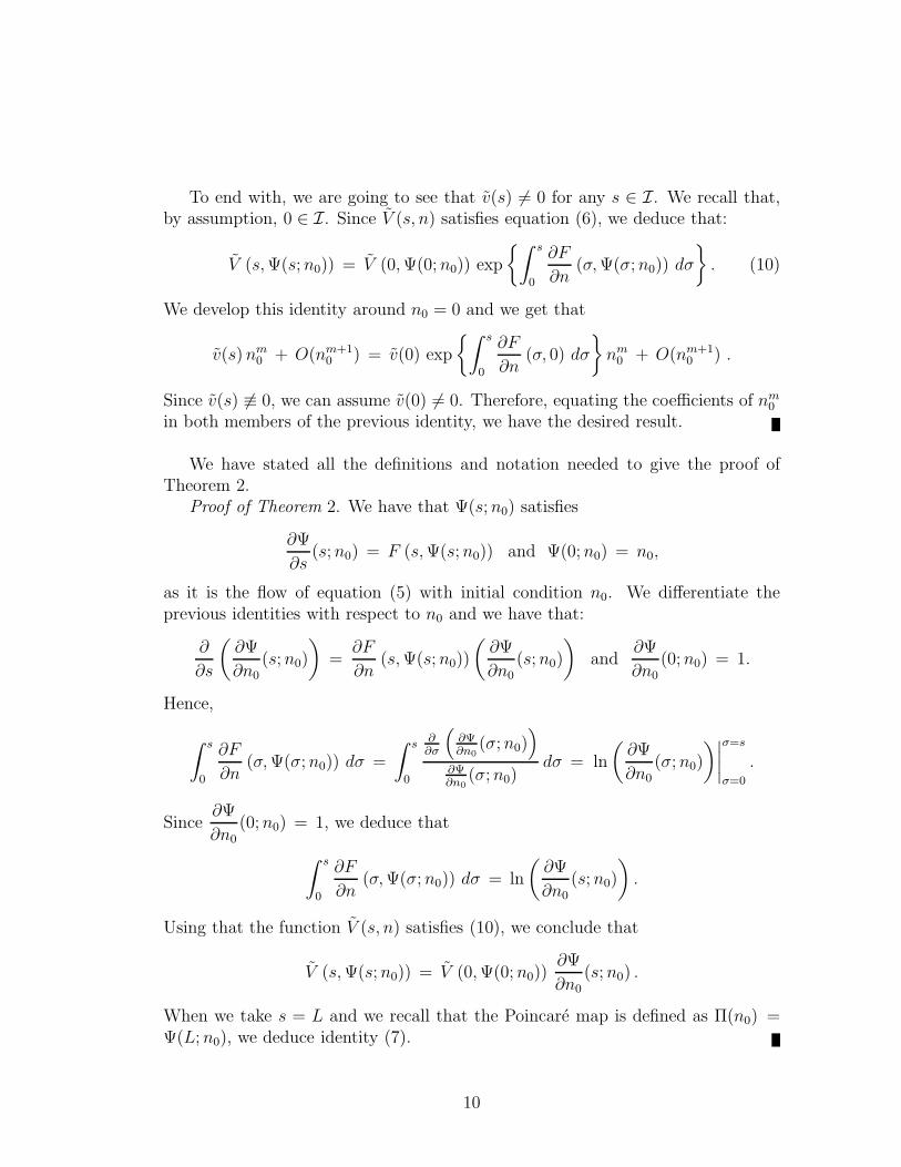
To end with, we are going to see that v(s) 6= 0 for any s ∈ I. We recall that,by assumption, 0 ∈ I. Since V (s, n) satisfies equation (6), we deduce that:

V (s,Ψ(s;n0)) = V (0,Ψ(0;n0)) exp

{∫ s

0

∂F

∂n(σ,Ψ(σ;n0)) dσ

}

. (10)

We develop this identity around n0 = 0 and we get that

v(s)nm0 + O(nm+1

0 ) = v(0) exp

{∫ s

0

∂F

∂n(σ, 0) dσ

}

nm0 + O(nm+1

0 ) .

Since v(s) 6≡ 0, we can assume v(0) 6= 0. Therefore, equating the coefficients of nm0

in both members of the previous identity, we have the desired result.

We have stated all the definitions and notation needed to give the proof ofTheorem 2.

Proof of Theorem 2. We have that Ψ(s;n0) satisfies

∂Ψ

∂s(s;n0) = F (s,Ψ(s;n0)) and Ψ(0;n0) = n0,

as it is the flow of equation (5) with initial condition n0. We differentiate theprevious identities with respect to n0 and we have that:

∂

∂s

(

∂Ψ

∂n0(s;n0)

)

=∂F

∂n(s,Ψ(s;n0))

(

∂Ψ

∂n0(s;n0)

)

and∂Ψ

∂n0(0;n0) = 1.

Hence,

∫ s

0

∂F

∂n(σ,Ψ(σ;n0)) dσ =

∫ s

0

∂∂σ

(

∂Ψ∂n0

(σ;n0))

∂Ψ∂n0

(σ;n0)dσ = ln

(

∂Ψ

∂n0(σ;n0)

)∣

∣

∣

∣

σ=s

σ=0

.

Since∂Ψ

∂n0

(0;n0) = 1, we deduce that

∫ s

0

∂F

∂n(σ,Ψ(σ;n0)) dσ = ln

(

∂Ψ

∂n0

(s;n0)

)

.

Using that the function V (s, n) satisfies (10), we conclude that

V (s,Ψ(s;n0)) = V (0,Ψ(0;n0))∂Ψ

∂n0

(s;n0) .

When we take s = L and we recall that the Poincare map is defined as Π(n0) =Ψ(L;n0), we deduce identity (7).

10

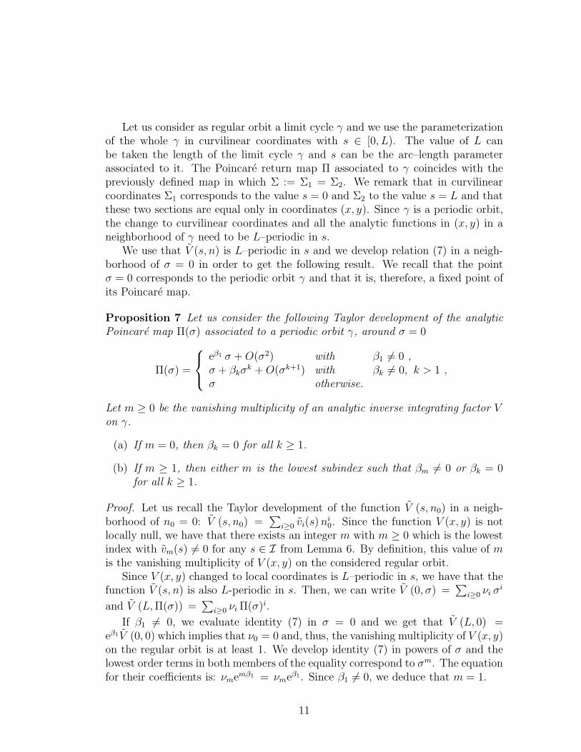
Let us consider as regular orbit a limit cycle γ and we use the parameterizationof the whole γ in curvilinear coordinates with s ∈ [0, L). The value of L canbe taken the length of the limit cycle γ and s can be the arc–length parameterassociated to it. The Poincare return map Π associated to γ coincides with thepreviously defined map in which Σ := Σ1 = Σ2. We remark that in curvilinearcoordinates Σ1 corresponds to the value s = 0 and Σ2 to the value s = L and thatthese two sections are equal only in coordinates (x, y). Since γ is a periodic orbit,the change to curvilinear coordinates and all the analytic functions in (x, y) in aneighborhood of γ need to be L–periodic in s.

We use that V (s, n) is L–periodic in s and we develop relation (7) in a neigh-borhood of σ = 0 in order to get the following result. We recall that the pointσ = 0 corresponds to the periodic orbit γ and that it is, therefore, a fixed point ofits Poincare map.

Proposition 7 Let us consider the following Taylor development of the analyticPoincare map Π(σ) associated to a periodic orbit γ, around σ = 0

Π(σ) =

eβ1 σ +O(σ2) with β1 6= 0 ,σ + βkσ

k +O(σk+1) with βk 6= 0, k > 1 ,σ otherwise.

Let m ≥ 0 be the vanishing multiplicity of an analytic inverse integrating factor Von γ.

(a) If m = 0, then βk = 0 for all k ≥ 1.

(b) If m ≥ 1, then either m is the lowest subindex such that βm 6= 0 or βk = 0for all k ≥ 1.

Proof. Let us recall the Taylor development of the function V (s, n0) in a neigh-borhood of n0 = 0: V (s, n0) =

∑

i≥0 vi(s)ni0. Since the function V (x, y) is not

locally null, we have that there exists an integer m with m ≥ 0 which is the lowestindex with vm(s) 6= 0 for any s ∈ I from Lemma 6. By definition, this value of mis the vanishing multiplicity of V (x, y) on the considered regular orbit.

Since V (x, y) changed to local coordinates is L–periodic in s, we have that thefunction V (s, n) is also L-periodic in s. Then, we can write V (0, σ) =

∑

i≥0 νi σi

and V (L,Π(σ)) =∑

i≥0 νi Π(σ)i.

If β1 6= 0, we evaluate identity (7) in σ = 0 and we get that V (L, 0) =eβ1V (0, 0) which implies that ν0 = 0 and, thus, the vanishing multiplicity of V (x, y)on the regular orbit is at least 1. We develop identity (7) in powers of σ and thelowest order terms in both members of the equality correspond to σm. The equationfor their coefficients is: νmemβ1 = νmeβ1. Since β1 6= 0, we deduce that m = 1.

11

Let k > 1 be the lowest subindex such that βk 6= 0. We have that Π(σ) =σ + βkσ

k + O(σk+1). We subtract V (0, σ) from both members of (7) and we getthe following relation:

∑

i≥1

νi

(

Π(σ)i − σi)

=

(

ν0 +∑

i≥1

νiσi

)

(

kβkσk−1 + O(σk)

)

. (11)

The left hand side of (11) has order at least σk which implies that ν0 = 0, in orderto have the same order in both members. Therefore, m > 0. We have that thelowest order terms in both sides of (11) correspond to σm+k−1 and the equation oftheir coefficients is: mβk νm = k βk νm, which implies that k = m.

Proof of Theorem 3. It is a straightforward consequence of the previous Propo-sition 7. We have preferred to state this proposition as we are going to use thesame reasoning for the transition map associated to a homoclinic orbit.

Let us now consider a homoclinic loop Γ = φ(t) ∪ {p0} whose critical point p0

is a hyperbolic saddle–point. We will denote by λ and µ the eigenvalues associatedto the Jacobian matrix DX (p0) with the convention µ < 0 < λ. We associate top0 its hyperbolicity ratio r = −µ/λ. We say that the singular point p0 is strong ifdivX (p0) 6= 0 (equivalently r 6= 1) and it is weak otherwise. The hyperbolic saddlep0 is called p : q resonant if r = q/p ∈ Q+ with p and q natural and coprimenumbers.

A homoclinic loop Γ is called stable (unstable) if all the trajectories in someinner or outer neighborhood of Γ approach Γ as t → +∞ (t → −∞). In theinvestigation of the stability of a homoclinic loop Γ of system (1) through a saddlep0 the quantity

α1 = divX (p0) (12)

plays an important role. In short, it is well known, see for instance p. 304 of[1], that Γ is stable (unstable) if α1 < 0 (α1 > 0). For this reason such kind ofhomoclinic loops Γ are said to be simple if α1 6= 0 and multiple otherwise.

The cyclicity of Γ is linked with its stability. It is notable to observe that,in the simple case α1 6= 0, the stability of Γ is only determined by the nature ofthe saddle point itself. Andronov et al. [1] proved that if α1 6= 0, the possiblelimit cycle that bifurcates from Γ after perturbing the system by a multiparameterfamily has the same type of stability than Γ, hence this limit cycle is unique forsmall values of the parameters. After that, Cherkas [8] showed that, if α1 = 0and the associated Poincare map of the loop Γ is hyperbolic, then the maximumnumber of limit cycles that can appear near Γ perturbing the system in the C1 classis 2. We recall that a real map is said to be hyperbolic at a point if its derivative atthe point has modulus different from 1. In [19] Roussarie presents a generalization

12

of these results which determine the asymptotic expression of the Poincare mapassociated to the loop Γ.

The Poincare map Π associated to Γ is defined over a transversal section Σwhose base point is a regular point of Γ. We parameterize the transversal sectionΣ by the real local coordinate σ. The value σ = 0 corresponds to the intersectionof Σ with Γ and σ > 0 is the side of Γ where Π(σ) is defined. Roussarie’s result istwofold: on one hand the asymptotic expansion of Π(σ) is determined and, on theother hand, the cyclicity of Γ is deduced from it.

Theorem 8 [19] Let us consider any smooth perturbation of system (1). Then wehave:

(i) If r 6= 1 (equivalently, α1 6= 0), then Π(σ) = c σr(1 + o(1)) with c > 0 and atmost 1 limit cycle can bifurcate from Γ.

(ii) If α1 = 0 and β1 6= 0, then Π(σ) = eβ1σ + o(σ) and at most 2 limit cyclescan bifurcate from Γ.

(iii) If αi = βi = 0 for i = 1, 2, . . . , k with k ≥ 1 and αk+1 6= 0, then Π(σ) =σ+αk+1σ

k+1 log σ+o(σk+1 log σ) and at most 2k+1 limit cycles can bifurcatefrom Γ.

(iv) If αi = βi = αk = 0 for i = 1, 2, . . . , k − 1 with k > 1 and βk 6= 0, thenΠ(σ) = σ + βkσ

k + o(σk) and at most 2k limit cycles can bifurcate from Γ.

(v) If αi = βi = 0 for all i ≥ 1, then Π(σ) = σ and the number of limit cyclesthat can bifurcate from Γ has no upper bound.

The values αi, with i ≥ 1, are the saddle quantities associated to p0 and areevaluated by a local computation. The values βi, with i ≥ 1, are called separatrixquantities of Γ and correspond to a global computation. The determination of theαi can be explicitly done through the algebraic method of normal form theory nearp0. Additionally, β1 =

∫

ΓdivX dt, and a more complicated expression for β2 can

be encountered in [16] and it involves several iterated integrals. On the contrary,as far as we know, there is no closed form expression to get βi for i ≥ 3. We remarkthat our result provides a way to determine the cyclicity of the homoclinic loop Γwithout computing any βi.

A graphic Γ = ∪ki=1φi(t)∪{p1, . . . , pk} is formed by k singular points p1, . . . , pk,

pk+1 = p1 and k oriented regular orbits φ1(t), . . . , φk(t), connecting them such thatφi(t) is an unstable characteristic orbit of pi and a stable characteristic orbit ofpi+1. A graphic may or may not have associated a Poincare return map. In case ithas one, it is called a polycycle. Of course, the homoclinic loops that we consider

13

are polycycles with just one singular point. In [3], the case of a system (1) with acompact polycycle Γ whose associated Poincare map is not the identity and whosecritical points p1, p2, . . . , pk are all non–degenerate is studied and it is shown thatif there exists an inverse integrating factor V defined in a neighborhood of Γ, thenΓ ⊆ V −1(0). A strong generalization of this result is given in [11], where it is showedthat any compact polycycle contained in U with non–identity Poincare return mapis contained into the zero–set of V under mild conditions. More concretely, Garcıaand Shafer give the following result.

Theorem 9 [11] Assume the existence of an analytic inverse integrating factorV defined in a neighborhood N of any compact polycycle Γ of system (1) withassociated Poincare return map different from the identity. Then, Γ ⊂ V −1(0).

In [11], this result is also given for an inverse integrating factor V with lowerregularity than analytic and assuming several conditions. In fact, a consequenceof their results is that if we consider a compact homoclinic loop Γ whose Poincaremap is not the identity and such that there exists an inverse integrating factor Vof class C1 defined in a neighborhood of Γ, then Γ ⊂ V −1(0).

Along this paper, we will work with inverse integrating factors V (x, y) analyticin a neighborhood of a compact homoclinic loop Γ = φ(t) ∪ {p0} with associatedPoincare map different from the identity. Hence, Γ ⊂ V −1(0).

Regarding the existence problem, it is well known that the partial differentialequation (2) has a solution in a neighborhood of any regular point, but not neces-sarily elsewhere. In [6] it is shown that if system (1) is analytic in a neighborhoodN ⊂ U of a critical point that is either a strong focus, a nonresonant hyperbolicnode, or a Siegel hyperbolic saddle, then there exists a unique analytic inverseintegrating factor on N up to a multiplicative constant. Hence, we only have atthe moment the local existence of inverse integrating factors in a neighborhoodof convenient singular points. But, we shall need to know a priori whether thereexists an inverse integrating factor V defined on a neighborhood of the whole ho-moclinic loop Γ of system (1). This is a hard nonlocal problem of existence ofglobal solutions of the partial differential equation (2) for which we do not knowits answer. We describe one obstruction to the existence of an analytic inverseintegrating factor defined in a neighborhood of certain homoclinic loops.

Proposition 10 Suppose that system (1) has a homoclinic loop Γ through thehyperbolic saddle point p0 which is not orbitally linearizable, p : q resonant andstrong (p 6= q). Then, there is no analytic inverse integrating factor V (x, y) definedin a neighborhood of Γ.

Proof. Let us assume that there exists an analytic inverse integrating factor V (x, y)defined in a neighborhood of Γ. Let us consider fλ(x, y) = 0 and fµ(x, y) = 0 the

14

local analytic expressions of each of the separatrices associated to p0, where thesubindex denotes the corresponding eigenvalue. As we will see in Proposition 12(iii), we have that V (x, y) factorizes, as analytic function in a neighborhood of p0,in the form V = f 1+kq

λ f 1+kpµ u with u(p0) 6= 0 and an integer k ≥ 0. Since V (x, y)

is defined on the whole loop Γ, it needs to have the same vanishing multiplicityon each separatrix at p0, which implies that k = 0. Thus, we have that the localfactorization of V in a neighborhood of p0 is V = fλ fµ u.

Let us take local coordinates in a neighborhood of p0, which we assume to beat the origin. We recall, see [2] and the references therein, that given an analyticsystem x = λx + · · ·, y = µy + · · · near the origin with µ/λ = −q/p ∈ Q− withp and q natural and coprime numbers (p : q resonant saddle) then the system hastwo analytic invariant curves passing through the origin. Moreover, it is formallyorbitally equivalent to

X = pX[

1 + δ(U ℓ + aU2ℓ)]

, Y = −qY , (13)

with U = XqY p, a ∈ R, ℓ an integer such that ℓ ≥ 1 and δ ∈ {0,±1}. The normalform theory ensures that p0 is orbitally linearizable if, and only if, δ = 0. We areassuming that p0 is not orbitally linearizable and, thus, δ 6= 0.

Let us consider V (X, Y ) the formal inverse integrating factor of system (13)constructed with the transformation of V (x, y) with the near–identity normalizingchange of variables divided by the jacobian of the change. We have that V (X, Y ) =X Y u(X, Y ) where u is a formal series such that u(0, 0) 6= 0. We can assume,without loss of generality, that u(0, 0) = 1. Easy computations show that if u isconstant, we have that V (X, Y ) cannot be an inverse integrating factor of system(13) with δ 6= 0. If we have that u is not a constant, we develop u as a formal seriesin X and Y and we can write u = 1 +Vs(X, Y ) + · · · where the dots correspond toterms of order strictly greater than s in X and Y and Vs(X, Y ) is a homogenouspolynomial in X and Y of degree s. We consider the partial differential equationsatisfied by V :

pX[

1 + δ(U ℓ + aU2ℓ)] ∂V

∂X− qY

∂V

∂Y=

=(

p− q + pδ(1 + ℓq)U ℓ + aδp(1 + 2ℓq)U2ℓ)

V .

We equate terms of the same lowest degree, we deduce that s = ℓ(p+ q) and that:

pX∂Vs

∂X− qY

∂Vs

∂Y= δℓpqXℓqY ℓp.

Easy computations show that the general solution of this partial differential equa-tion is Vs(X, Y ) = δℓ2pq2U ℓ lnX + G(U) where G is an arbitrary function. We

15

deduce that this partial differential equation has no polynomial solution Vs(X, Y )unless δ = 0.

We conclude that the existence of such an inverse integrating factor V (X, Y )implies that δ = 0 in contradiction with our hypothesis.

We observe that homoclinic loops considered in Proposition 10 are simple, sincethe hyperbolic saddle point is strong. As we have already mentioned in the intro-duction, it is well–known that its cyclicity is 1. Therefore, the obstruction to theexistence of an analytic inverse integrating factor in a neighborhood of these ho-moclinic loops is not relevant in the context of the bifurcation theory.

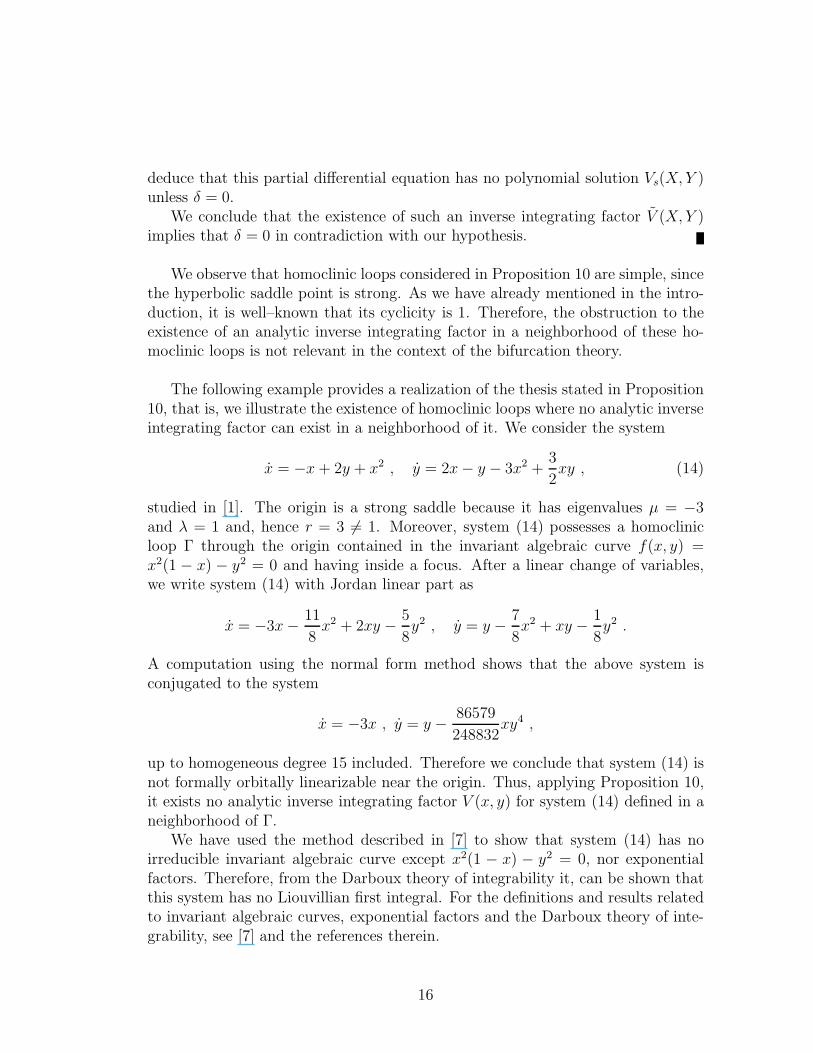
The following example provides a realization of the thesis stated in Proposition10, that is, we illustrate the existence of homoclinic loops where no analytic inverseintegrating factor can exist in a neighborhood of it. We consider the system

x = −x+ 2y + x2 , y = 2x− y − 3x2 +3

2xy , (14)

studied in [1]. The origin is a strong saddle because it has eigenvalues µ = −3and λ = 1 and, hence r = 3 6= 1. Moreover, system (14) possesses a homoclinicloop Γ through the origin contained in the invariant algebraic curve f(x, y) =x2(1 − x) − y2 = 0 and having inside a focus. After a linear change of variables,we write system (14) with Jordan linear part as

x = −3x− 11

8x2 + 2xy − 5

8y2 , y = y − 7

8x2 + xy − 1

8y2 .

A computation using the normal form method shows that the above system isconjugated to the system

x = −3x , y = y − 86579

248832xy4 ,

up to homogeneous degree 15 included. Therefore we conclude that system (14) isnot formally orbitally linearizable near the origin. Thus, applying Proposition 10,it exists no analytic inverse integrating factor V (x, y) for system (14) defined in aneighborhood of Γ.

We have used the method described in [7] to show that system (14) has noirreducible invariant algebraic curve except x2(1 − x) − y2 = 0, nor exponentialfactors. Therefore, from the Darboux theory of integrability it, can be shown thatthis system has no Liouvillian first integral. For the definitions and results relatedto invariant algebraic curves, exponential factors and the Darboux theory of inte-grability, see [7] and the references therein.

16

In this paper we will always assume as a hypothesis the existence of an analyticinverse integrating factor V defined on a neighborhood of Γ. Under this condition,we now refer to the uniqueness problem. In the last section of this work, we presentseveral examples of differential systems with a homoclinic loop which satisfy all ourhypothesis and in which an explicit expression of an analytic inverse integratingfactor is given.

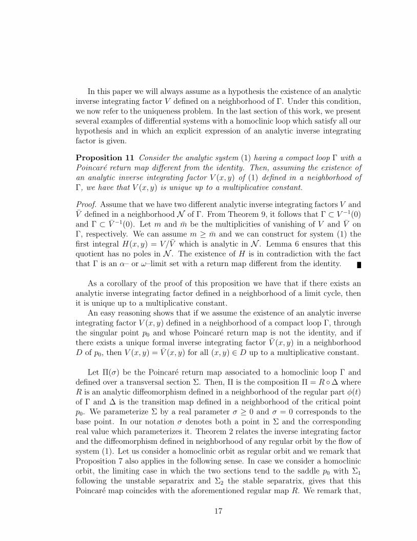
Proposition 11 Consider the analytic system (1) having a compact loop Γ with aPoincare return map different from the identity. Then, assuming the existence ofan analytic inverse integrating factor V (x, y) of (1) defined in a neighborhood ofΓ, we have that V (x, y) is unique up to a multiplicative constant.

Proof. Assume that we have two different analytic inverse integrating factors V andV defined in a neighborhood N of Γ. From Theorem 9, it follows that Γ ⊂ V −1(0)and Γ ⊂ V −1(0). Let m and m be the multiplicities of vanishing of V and V onΓ, respectively. We can assume m ≥ m and we can construct for system (1) thefirst integral H(x, y) = V/V which is analytic in N . Lemma 6 ensures that thisquotient has no poles in N . The existence of H is in contradiction with the factthat Γ is an α– or ω–limit set with a return map different from the identity.

As a corollary of the proof of this proposition we have that if there exists ananalytic inverse integrating factor defined in a neighborhood of a limit cycle, thenit is unique up to a multiplicative constant.

An easy reasoning shows that if we assume the existence of an analytic inverseintegrating factor V (x, y) defined in a neighborhood of a compact loop Γ, throughthe singular point p0 and whose Poincare return map is not the identity, and ifthere exists a unique formal inverse integrating factor V (x, y) in a neighborhoodD of p0, then V (x, y) = V (x, y) for all (x, y) ∈ D up to a multiplicative constant.

Let Π(σ) be the Poincare return map associated to a homoclinic loop Γ anddefined over a transversal section Σ. Then, Π is the composition Π = R ◦∆ whereR is an analytic diffeomorphism defined in a neighborhood of the regular part φ(t)of Γ and ∆ is the transition map defined in a neighborhood of the critical pointp0. We parameterize Σ by a real parameter σ ≥ 0 and σ = 0 corresponds to thebase point. In our notation σ denotes both a point in Σ and the correspondingreal value which parameterizes it. Theorem 2 relates the inverse integrating factorand the diffeomorphism defined in neighborhood of any regular orbit by the flow ofsystem (1). Let us consider a homoclinic orbit as regular orbit and we remark thatProposition 7 also applies in the following sense. In case we consider a homoclinicorbit, the limiting case in which the two sections tend to the saddle p0 with Σ1

following the unstable separatrix and Σ2 the stable separatrix, gives that thisPoincare map coincides with the aforementioned regular map R. We remark that,

17

if I = (a, b) covers the whole homoclinic orbit in the sense of the flow, this limitingcase corresponds to go from Σ1, based on a value of s such that s → a+, to Σ2

based on a value of s such that s→ b−.We note that, since V (x, y) is a well–defined function in a neighborhood of

the whole Γ, the function V (s, n) takes the same value in the limiting case, i.e.,when s tends to the boundaries of I. We define V (a, n) = lims→a+ V (s, n) andV (b, n) = lims→b− V (s, n) and these limits exist from the same reasoning. More-over, V (a, n) = V (b, n). Thus, the result stated in Proposition 7 is also valid tostudy the regular map R associated to a homoclinic orbit defined with sections inthe limiting case.

In order to relate inverse integrating factors and the Poincare return map as-sociated to a homoclinic loop, we need to study the local behavior of the solutionsin a neighborhood of the critical saddle point p0.

The following proposition establishes some relationships between the vanishingmultiplicity of V on the separatrices of a hyperbolic saddle p0 and the nature ofp0, provided that V (p0) = 0.

Proposition 12 Let V (x, y) be an analytic inverse integrating factor defined in aneighborhood of a hyperbolic saddle p0 with eigenvalues µ < 0 < λ of an analyticsystem (1). Let us consider fλ(x, y) = 0 and fµ(x, y) = 0 the local analytic expres-sion of each of the separatrices associated to p0, where the subindex denotes thecorresponding eigenvalue. Then the next statements hold:

(i) If p0 is strong, then V (p0) = 0.

(ii) If p0 is nonresonant, then V = fλ fµ u with u(p0) 6= 0.

(iii) If p0 is p : q resonant and strong, then V = f 1+kqλ f 1+kp

µ u with u(p0) 6= 0 andan integer k ≥ 0.

(iv) If p0 is weak and V (p0) = 0, then V = fmλ fm

µ u with u(p0) 6= 0 and m anatural number with m ≥ 1.

Proof. Statement (i) is clear from the definition (2) of inverse integrating factor.The other three statements are based on a result due to Seidenberg [21], see

also [7]. Since V is analytic, we can locally factorize near p0 as V = fm1

λ fm2

µ u withu(p0) 6= 0 and mi nonnegative integers. Then, we have divX (p0) = m1λ + m2µ.Hence, (m1 − 1)λ+ (m2 − 1)µ = 0 and statements (ii)–(iv) easily follow.

Let us consider an analytic system (1) where p0 is a weak hyperbolic saddle.By an affine change of coordinates and rescaling the time, if necessary, the systemcan be written as

x = x+ f(x, y) , y = −y + g(x, y) , (15)

18

where f and g are analytic in a neighborhood of the origin with lowest terms atleast of second order. It is well known the existence of a formal near–identitychange of coordinates (x, y) 7→ (X, Y ) = (x+ · · · , y + · · ·) that brings system (15)into the Poincare normal form

X = X

[

1 +∑

i≥1

ai(XY )i

]

, Y = −Y[

1 +∑

i≥1

bi(XY )i

]

. (16)

From this expression, we see that system (15) has an analytic first integral in aneighborhood of the saddle if and only if the saddle quantities αi+1 := ai − bi arezero for all i ≥ 1, see [17] and references therein for a review. In particular weobserve that system (15) has a 1:1 resonant saddle at the origin. In [15], it is provedthat a planar dynamical system is analytically orbitally linearizable at a resonanthyperbolic saddle, that is whose hyperbolicity ratio r is a rational number, if andonly if it has an analytic first integral in a neighborhood of the saddle. We recallthat a saddle is analytically orbitally linearizable if there exists an analytic near–identity change of coordinates transforming the system to a local normal form suchthat Y /X = −rY/X in a neighborhood of the saddle.

We say that system (15) is analytically orbitally linearizable (integrable) at theorigin if there exists an analytic near–identity change of coordinates transformingthe system to

X = Xh(X, Y ) , Y = −Y h(X, Y ) ,

with h(0, 0) = 1. In this case, V (X, Y ) = XkY kh(X, Y ) is a 1–parameter familyof analytic inverse integrating factors for any integer k ≥ 1.

In [4], Brjuno shows that any resonant hyperbolic saddle point of an analyticsystem is analytically orbitally linearizable if and only if it is formally orbitallylinearizable. In particular, this fact means that either there exists at least onesaddle quantity αi different from zero or the system becomes analytically orbitallylinearizable. Moreover, we can prove the following result.

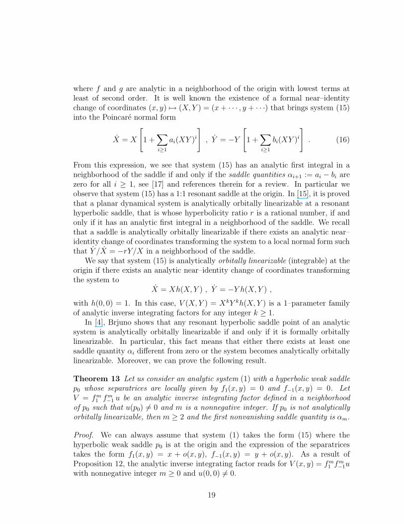
Theorem 13 Let us consider an analytic system (1) with a hyperbolic weak saddlep0 whose separatrices are locally given by f1(x, y) = 0 and f−1(x, y) = 0. LetV = fm

1 fm−1 u be an analytic inverse integrating factor defined in a neighborhood

of p0 such that u(p0) 6= 0 and m is a nonnegative integer. If p0 is not analyticallyorbitally linearizable, then m ≥ 2 and the first nonvanishing saddle quantity is αm.

Proof. We can always assume that system (1) takes the form (15) where thehyperbolic weak saddle p0 is at the origin and the expression of the separatricestakes the form f1(x, y) = x + o(x, y), f−1(x, y) = y + o(x, y). As a result ofProposition 12, the analytic inverse integrating factor reads for V (x, y) = fm

1 fm−1u

with nonnegative integer m ≥ 0 and u(0, 0) 6= 0.

19

If m = 0, then V (p0) 6= 0 and there exists an analytic first integral defined ona neighborhood of p0 for system (1). Hence, p0 is analytically orbitally linearizableand the saddle quantities of p0 satisfy αi = 0 for any i ≥ 1.

If m = 1, then V = f1f−1u with u(p0) 6= 0. Then, by statement (iii) of Theorem5.10 of [9], we conclude that p0 is also analytically orbitally linearizable and thesaddle quantities of p0 satisfy αi = 0 for any i ≥ 1.

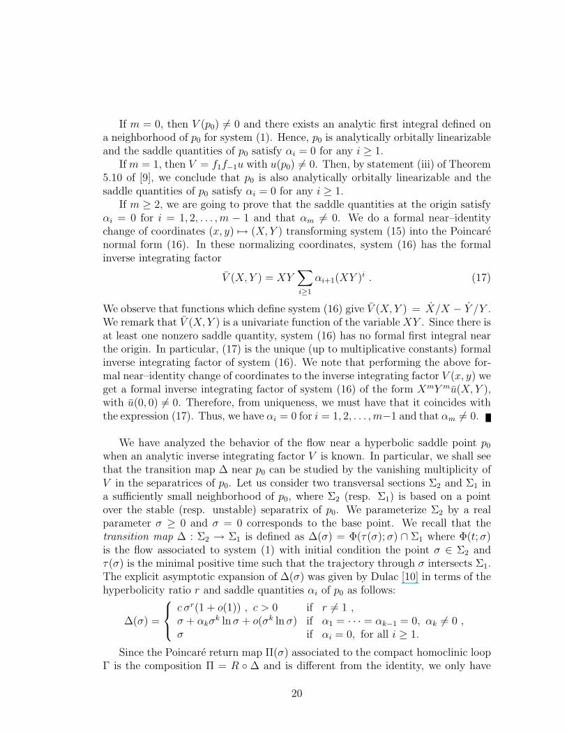
If m ≥ 2, we are going to prove that the saddle quantities at the origin satisfyαi = 0 for i = 1, 2, . . . , m − 1 and that αm 6= 0. We do a formal near–identitychange of coordinates (x, y) 7→ (X, Y ) transforming system (15) into the Poincarenormal form (16). In these normalizing coordinates, system (16) has the formalinverse integrating factor

V (X, Y ) = XY∑

i≥1

αi+1(XY )i . (17)

We observe that functions which define system (16) give V (X, Y ) = X/X − Y /Y .We remark that V (X, Y ) is a univariate function of the variable XY . Since there isat least one nonzero saddle quantity, system (16) has no formal first integral nearthe origin. In particular, (17) is the unique (up to multiplicative constants) formalinverse integrating factor of system (16). We note that performing the above for-mal near–identity change of coordinates to the inverse integrating factor V (x, y) weget a formal inverse integrating factor of system (16) of the form XmY mu(X, Y ),with u(0, 0) 6= 0. Therefore, from uniqueness, we must have that it coincides withthe expression (17). Thus, we have αi = 0 for i = 1, 2, . . . , m−1 and that αm 6= 0.

We have analyzed the behavior of the flow near a hyperbolic saddle point p0

when an analytic inverse integrating factor V is known. In particular, we shall seethat the transition map ∆ near p0 can be studied by the vanishing multiplicity ofV in the separatrices of p0. Let us consider two transversal sections Σ2 and Σ1 ina sufficiently small neighborhood of p0, where Σ2 (resp. Σ1) is based on a pointover the stable (resp. unstable) separatrix of p0. We parameterize Σ2 by a realparameter σ ≥ 0 and σ = 0 corresponds to the base point. We recall that thetransition map ∆ : Σ2 → Σ1 is defined as ∆(σ) = Φ(τ(σ); σ) ∩ Σ1 where Φ(t; σ)is the flow associated to system (1) with initial condition the point σ ∈ Σ2 andτ(σ) is the minimal positive time such that the trajectory through σ intersects Σ1.The explicit asymptotic expansion of ∆(σ) was given by Dulac [10] in terms of thehyperbolicity ratio r and saddle quantities αi of p0 as follows:

∆(σ) =

c σr(1 + o(1)) , c > 0 if r 6= 1 ,σ + αkσ

k lnσ + o(σk ln σ) if α1 = · · · = αk−1 = 0, αk 6= 0 ,σ if αi = 0, for all i ≥ 1.

Since the Poincare return map Π(σ) associated to the compact homoclinic loopΓ is the composition Π = R ◦ ∆ and is different from the identity, we only have

20

the four possibilities (i)–(iv) described in Theorem 8.

In the following theorem, the cyclicity of Γ denotes the maximum number oflimit cycles that bifurcate from Γ under smooth perturbations of (1).

Theorem 14 Let Γ be a compact homoclinic loop through the hyperbolic saddle p0

of system (1) whose Poincare return map is not the identity. Let V be an analyticinverse integrating factor defined in a neighborhood of Γ with vanishing multiplicitym over Γ. Then the following statements hold:

(a) m ≥ 1.

(b) If p0 is strong, then m = 1 and the cyclicity of Γ is 1.

(c) If p0 is weak, then:

(c.1) If p0 is not analytically orbitally linearizable, then m ≥ 2, αi = βi = 0for i = 1, 2, . . . , m − 1 and αm 6= 0. Moreover, the cyclicity of Γ is2m− 1.

(c.2) If p0 is analytically orbitally linearizable, then β1 = β2 = · · · = βm−1 = 0and βm 6= 0. Moreover, the cyclicity of Γ is 2m.

Proof. Statement (a) is a straight consequence of the fact that Γ ⊂ V −1(0), seeTheorem 9.

Statement (b) follows taking into account statements (ii) and (iii) of Proposition12 where we recall that the vanishing multiplicity of V in each of the separatricesof p0 needs to be the same since Γ is a loop. In particular, we observe that thevalue of k in statement (iii) of Proposition 12 must be zero by the same argument.

We assume that p0 is weak. We may have that all its associated saddle quan-tities are zero or that there is at least one saddle quantity different from zero. Ifthis last case applies, the first non–vanishing saddle quantity is αm as a result ofTheorem 13. Therefore, we compute the mth saddle quantity associated to p0,knowing than the previous saddle quantities need to be zero and we can determineif p0 is analytically orbitally linearizable (if αm = 0) or not (if αm 6= 0). The case(c.1) in the theorem corresponds to αm 6= 0 and the case (c.2) to αm = 0.

The case (c.1) is a consequence of Theorem 13 and part (b) of Proposition7. More concretely, since p0 is not analytically orbitally linearizable, then usingTheorem 13 we have m ≥ 2, αi = 0 for i = 1, 2, . . . , m−1 and αm 6= 0. In addition,by part (b) of Proposition 7, we get βi = 0 for i = 1, 2, . . . , m−1. We remark that,in this case, either βm 6= 0 or βk = 0 for all k ≥ 1. In any case, from statement(iii) of Theorem 8, the cyclicity of Γ is 2m− 1.

Finally, the proof of (c.2) works as follows. Since p0 is analytically orbitallylinearizable, then αk = 0 for all k ≥ 1. By hypothesis, the Poincare map is not the

21

identity, so βk = 0 for all k ≥ 1 is not possible. Hence, by part (b) of Proposition7, we get that βi = 0 for i = 1, 2, . . . , m − 1 and βm 6= 0. Thus, using statement(iv) of Theorem 8, the cyclicity of Γ is 2m.

Proof of Theorem 5. The thesis of Theorem 5 is a corollary of Theorem 14.

3 Examples

This section contains several examples which illustrate and complete our results.The first example shows how to give an implicit expression of the Poincare mapassociated to a regular orbit via identity (7). The second example is given to showthe existence of analytic planar differential systems with a compact homoclinicloop Γ whose cyclicity can be determined by the vanishing multiplicity of an in-verse integrating factor defined in a neighborhood of it. The third example targetsto show that there is no upper bound for the number of limit cycles which bifurcatefrom a compact homoclinic loop whose Poincare return map is the identity. Thesystem considered in this example has a numerable family of inverse integratingfactors such that for any natural number n there exists an analytic inverse inte-grating factor whose vanishing multiplicity on the compact homoclinic loop is n.

Example 1. The following system is studied in [5] where a complete descriptionof its phase portrait in terms of the parameters is given using the inverse integratingfactor as a key tool. The system

x = λx− y + λm1x3 + (m2 −m1 +m1m2)x

2y + λm1m2xy2 +m2y

3,

y = x+ λy − x3 + λm1x2y + (m1m2 −m1 − 1)xy2 + λm1m2y

3,(18)

where λ, m1 and m2 are arbitrary real parameters, has the following inverse inte-grating factor

V (x, y) = (x2 + y2) (1 +m1x2 +m1m2y

2). (19)

In [5] it is shown that if λ 6= 0, m1 < 0, m1 6= −1 and m2 > 0, then the ellipsedefined by 1+m1x

2 +m1m2y2 = 0, and which we denote by γ, is a hyperbolic limit

cycle of system (18). Moreover, with the described values of the parameters, wehave that the origin of coordinates is a strong focus whose boundary of the focalregion is γ. Moreover, since the vanishing set of V is only the focus at the originand the limit cycle γ, we deduce by Theorem 9, that the region, in the outside ofγ in which the orbits spiral towards or backwards to it, is unbounded.

We remark that we reencounter that this limit cycle is hyperbolic using that thevanishing multiplicity of the inverse integrating factor over it is 1. In this examplewe are not concerned with the multiplicity of the limit cycle but with the Poincare

22

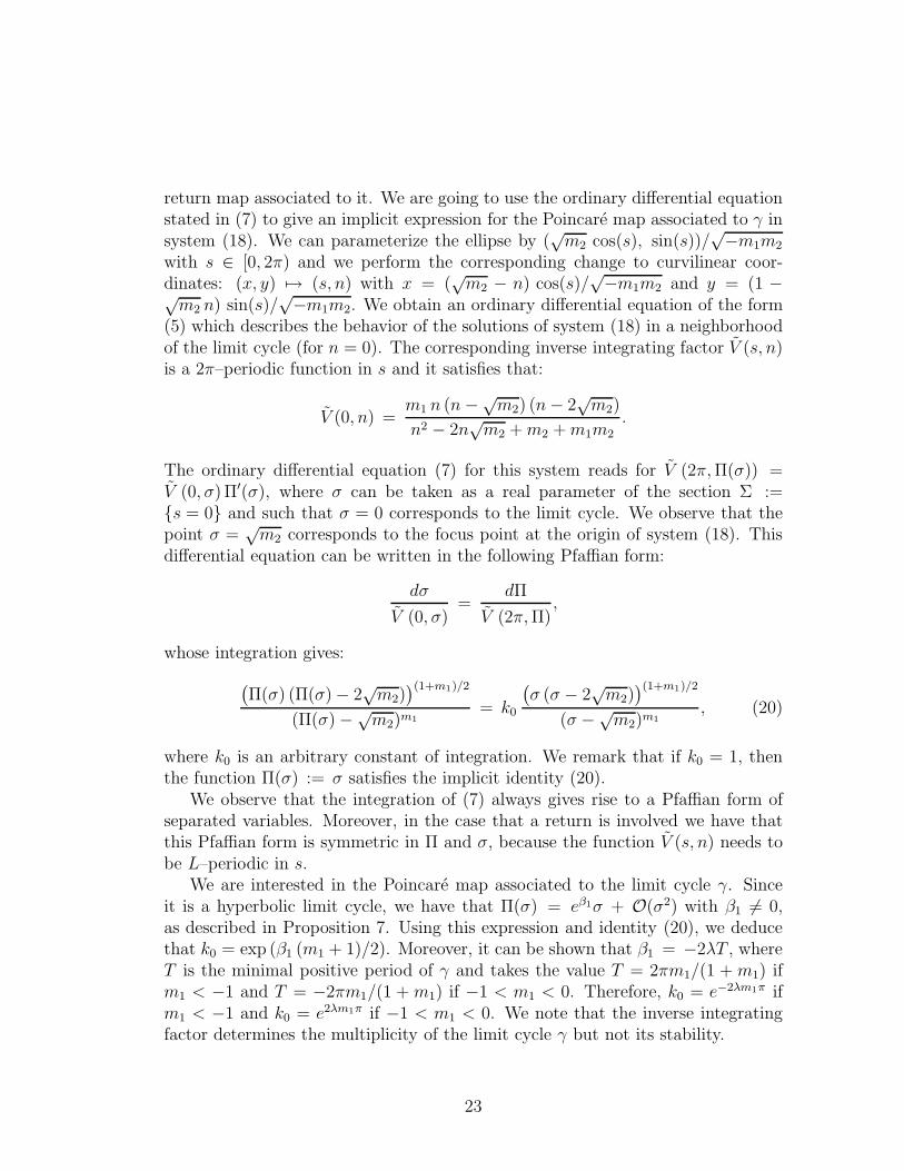
return map associated to it. We are going to use the ordinary differential equationstated in (7) to give an implicit expression for the Poincare map associated to γ insystem (18). We can parameterize the ellipse by (

√m2 cos(s), sin(s))/

√−m1m2

with s ∈ [0, 2π) and we perform the corresponding change to curvilinear coor-dinates: (x, y) 7→ (s, n) with x = (

√m2 − n) cos(s)/

√−m1m2 and y = (1 −√m2 n) sin(s)/

√−m1m2. We obtain an ordinary differential equation of the form(5) which describes the behavior of the solutions of system (18) in a neighborhoodof the limit cycle (for n = 0). The corresponding inverse integrating factor V (s, n)is a 2π–periodic function in s and it satisfies that:

V (0, n) =m1 n (n−√

m2) (n− 2√m2)

n2 − 2n√m2 +m2 +m1m2

.

The ordinary differential equation (7) for this system reads for V (2π,Π(σ)) =V (0, σ)Π′(σ), where σ can be taken as a real parameter of the section Σ :={s = 0} and such that σ = 0 corresponds to the limit cycle. We observe that thepoint σ =

√m2 corresponds to the focus point at the origin of system (18). This

differential equation can be written in the following Pfaffian form:

dσ

V (0, σ)=

dΠ

V (2π,Π),

whose integration gives:

(

Π(σ) (Π(σ) − 2√m2)

)(1+m1)/2

(Π(σ) −√m2)m1

= k0

(

σ (σ − 2√m2)

)(1+m1)/2

(σ −√m2)m1

, (20)

where k0 is an arbitrary constant of integration. We remark that if k0 = 1, thenthe function Π(σ) := σ satisfies the implicit identity (20).

We observe that the integration of (7) always gives rise to a Pfaffian form ofseparated variables. Moreover, in the case that a return is involved we have thatthis Pfaffian form is symmetric in Π and σ, because the function V (s, n) needs tobe L–periodic in s.

We are interested in the Poincare map associated to the limit cycle γ. Sinceit is a hyperbolic limit cycle, we have that Π(σ) = eβ1σ + O(σ2) with β1 6= 0,as described in Proposition 7. Using this expression and identity (20), we deducethat k0 = exp (β1 (m1 + 1)/2). Moreover, it can be shown that β1 = −2λT , whereT is the minimal positive period of γ and takes the value T = 2πm1/(1 + m1) ifm1 < −1 and T = −2πm1/(1 + m1) if −1 < m1 < 0. Therefore, k0 = e−2λm1π ifm1 < −1 and k0 = e2λm1π if −1 < m1 < 0. We note that the inverse integratingfactor determines the multiplicity of the limit cycle γ but not its stability.

23

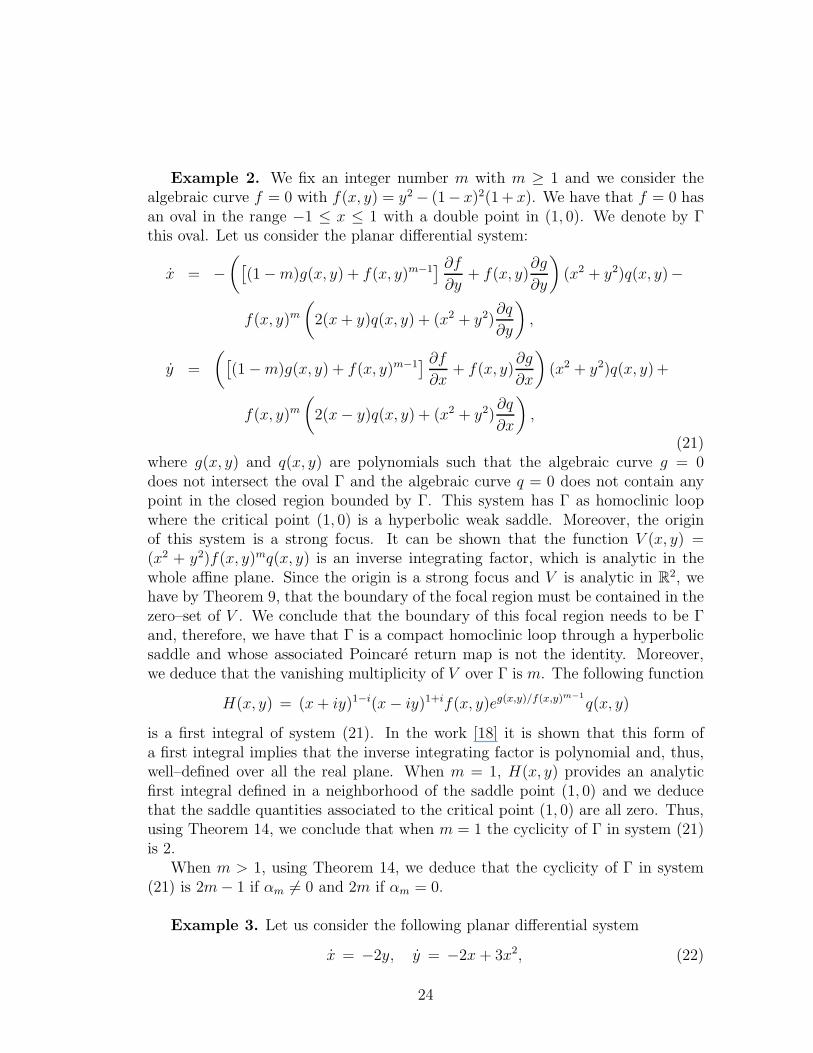
Example 2. We fix an integer number m with m ≥ 1 and we consider thealgebraic curve f = 0 with f(x, y) = y2 − (1− x)2(1 + x). We have that f = 0 hasan oval in the range −1 ≤ x ≤ 1 with a double point in (1, 0). We denote by Γthis oval. Let us consider the planar differential system:

x = −(

[

(1 −m)g(x, y) + f(x, y)m−1] ∂f

∂y+ f(x, y)

∂g

∂y

)

(x2 + y2)q(x, y)−

f(x, y)m

(

2(x+ y)q(x, y) + (x2 + y2)∂q

∂y

)

,

y =

(

[

(1 −m)g(x, y) + f(x, y)m−1] ∂f

∂x+ f(x, y)

∂g

∂x

)

(x2 + y2)q(x, y) +

f(x, y)m

(

2(x− y)q(x, y) + (x2 + y2)∂q

∂x

)

,

(21)where g(x, y) and q(x, y) are polynomials such that the algebraic curve g = 0does not intersect the oval Γ and the algebraic curve q = 0 does not contain anypoint in the closed region bounded by Γ. This system has Γ as homoclinic loopwhere the critical point (1, 0) is a hyperbolic weak saddle. Moreover, the originof this system is a strong focus. It can be shown that the function V (x, y) =(x2 + y2)f(x, y)mq(x, y) is an inverse integrating factor, which is analytic in thewhole affine plane. Since the origin is a strong focus and V is analytic in R2, wehave by Theorem 9, that the boundary of the focal region must be contained in thezero–set of V . We conclude that the boundary of this focal region needs to be Γand, therefore, we have that Γ is a compact homoclinic loop through a hyperbolicsaddle and whose associated Poincare return map is not the identity. Moreover,we deduce that the vanishing multiplicity of V over Γ is m. The following function

H(x, y) = (x+ iy)1−i(x− iy)1+if(x, y)eg(x,y)/f(x,y)m−1

q(x, y)

is a first integral of system (21). In the work [18] it is shown that this form ofa first integral implies that the inverse integrating factor is polynomial and, thus,well–defined over all the real plane. When m = 1, H(x, y) provides an analyticfirst integral defined in a neighborhood of the saddle point (1, 0) and we deducethat the saddle quantities associated to the critical point (1, 0) are all zero. Thus,using Theorem 14, we conclude that when m = 1 the cyclicity of Γ in system (21)is 2.

When m > 1, using Theorem 14, we deduce that the cyclicity of Γ in system(21) is 2m− 1 if αm 6= 0 and 2m if αm = 0.

Example 3. Let us consider the following planar differential system

x = −2y, y = −2x+ 3x2, (22)

24

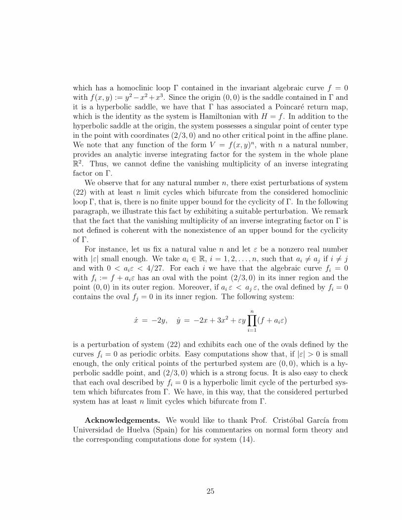
which has a homoclinic loop Γ contained in the invariant algebraic curve f = 0with f(x, y) := y2−x2 +x3. Since the origin (0, 0) is the saddle contained in Γ andit is a hyperbolic saddle, we have that Γ has associated a Poincare return map,which is the identity as the system is Hamiltonian with H = f . In addition to thehyperbolic saddle at the origin, the system possesses a singular point of center typein the point with coordinates (2/3, 0) and no other critical point in the affine plane.We note that any function of the form V = f(x, y)n, with n a natural number,provides an analytic inverse integrating factor for the system in the whole planeR2. Thus, we cannot define the vanishing multiplicity of an inverse integratingfactor on Γ.

We observe that for any natural number n, there exist perturbations of system(22) with at least n limit cycles which bifurcate from the considered homoclinicloop Γ, that is, there is no finite upper bound for the cyclicity of Γ. In the followingparagraph, we illustrate this fact by exhibiting a suitable perturbation. We remarkthat the fact that the vanishing multiplicity of an inverse integrating factor on Γ isnot defined is coherent with the nonexistence of an upper bound for the cyclicityof Γ.

For instance, let us fix a natural value n and let ε be a nonzero real numberwith |ε| small enough. We take ai ∈ R, i = 1, 2, . . . , n, such that ai 6= aj if i 6= jand with 0 < aiε < 4/27. For each i we have that the algebraic curve fi = 0with fi := f + aiε has an oval with the point (2/3, 0) in its inner region and thepoint (0, 0) in its outer region. Moreover, if ai ε < aj ε, the oval defined by fi = 0contains the oval fj = 0 in its inner region. The following system:

x = −2y, y = −2x+ 3x2 + εyn∏

i=1

(f + aiε)

is a perturbation of system (22) and exhibits each one of the ovals defined by thecurves fi = 0 as periodic orbits. Easy computations show that, if |ε| > 0 is smallenough, the only critical points of the perturbed system are (0, 0), which is a hy-perbolic saddle point, and (2/3, 0) which is a strong focus. It is also easy to checkthat each oval described by fi = 0 is a hyperbolic limit cycle of the perturbed sys-tem which bifurcates from Γ. We have, in this way, that the considered perturbedsystem has at least n limit cycles which bifurcate from Γ.

Acknowledgements. We would like to thank Prof. Cristobal Garcıa fromUniversidad de Huelva (Spain) for his commentaries on normal form theory andthe corresponding computations done for system (14).

25

References

[1] A.A. Andronov, et al. Theory of bifurcations of dynamic systems on aplane, John Wiley and Sons, New York, 1973.

[2] V.I. Arnold and Y.S. Il’yashenko, Encyclopedia of Math. Sci. Vol 1[Dynamical Systems, 1], Springer–Verlag, Berlin, 1988.

[3] L.R. Berrone and H. Giacomini, On the vanishing set of inverse inte-grating factors, Qual. Th. Dyn. Systems 1 (2000), 211–230.

[4] A.D. Brjuno, Analytic form of differential equations, Trans. Moscow Math.Soc. 25 (1971), 131–288.

[5] J. Chavarriga, H. Giacomini and J. Gine, On a new type of bifurcationof limit cycles for a planar cubic system. Nonlinear Anal. 36 (1999), Ser. A:Theory Methods, 139–149.

[6] J. Chavarriga, H. Giacomini, J. Gine and J. Llibre, On the integra-bility of two-dimensional flows, J. Diff. Equations 157 (1999), 163–182.

[7] J. Chavarriga, H. Giacomini and M. Grau, Necessary conditions for theexistence of invariant algebraic curves for planar polynomial systems, Bull. Sci.Math. 129 (2005), 99–126.

[8] L.A. Cherkas, Structure of a succesor function in the neighborhood of aseparatrix of a perturbed analytic autonomous system in the plane, Translatedfrom Differentsial’nye Uravneniya 17 (1981), 469–478.

[9] C. Christopher, P. Mardesic and C. Rousseau, Normalizable, inte-grable and linearizable saddle points in complex quadratic systems in C2, J.Dynam. Control Systems 9 (2003), 311–363.

[10] H. Dulac, Recherche sur les points singuliers des equations differentielles ,J. Ecole Polytechnique 2 (1904), 1–25.

[11] I.A. Garcıa and D.S. Shafer, Integral invariants and limit sets of planarvector fields, J. Differential Equations 217 (2005), 363–376.

[12] A. Gasull, J. Gine and M. Grau, Multiplicity of limit cycles and ana-lytic m-solutions for planar differential systems, J. Differential Equations 240

(2007), 375–398.

[13] H. Giacomini, J. Llibre and M. Viano, On the nonexistence, existence,and uniqueness of limit cycles, Nonlinearity 9 (1996), 501–516.

26

[14] H. Giacomini, J. Llibre and M. Viano, Semistable limit cycles thatbifurcate from centers, Internat. J. Bifur. Chaos Appl. Sci. Engrg. 13 (2003),3489–3498.

[15] M. Han and K. Jiang, Normal forms of integrable systems at a resonantsaddle, Ann. Differential Equations 14 (1998), 150–155.

[16] M. Han and Z. Huaiping, The loop quantities and bifurcations of homo-clinic loops, J. Differential Equations 234 (2007), 339–359.

[17] J. Li, Hilbert’s 16th problem and bifurcations of planar polynomial vectorfields, International Journal of Bifurcation and Chaos 13 (2001), 47–106.

[18] J. Llibre and C. Pantazi, Polynomial differential systems having a givenDarbouxian first integral, Bull. Sci. Math. 128 (2004), 775–788.

[19] R. Roussarie, On the number of limit cycles which appear by perturbation ofseparatrix loop of planar vector fields, Bol. Soc. Bras. Mat. 17 (1986), 67–101.

[20] R. Roussarie, Bifurcations of planar vector fields and Hilbert’s sixteenthproblem, Progress in Mathematics Vol 164, Birkhauser Verlag, 1998.

[21] A. Seidenberg, Reduction of singularities of the differential equation Ady =B dx, Amer. J. Math. 90 (1968) 248–269.

Addresses and e-mails:(1) Departament de Matematica. Universitat de Lleida.Avda. Jaume II, 69. 25001 Lleida, SPAIN.E–mails: garcia@matematica.udl.cat, mtgrau@matematica.udl.cat

(2) Laboratoire de Mathematiques et Physique Theorique. C.N.R.S. UMR 6083.Faculte des Sciences et Techniques. Universite de Tours.Parc de Grandmont 37200 Tours, FRANCE.E-mail: giacomini@phys.univ-tours.fr

27