The International Journal on Advances in Intelligent Systems ...

The International Journal on Advances in Intelligent Systems is Published by IARIA.

ISSN: 1942-2679

journals site: http://www.iariajournals.org

contact: [email protected]

Responsibility for the contents rests upon the authors and not upon IARIA, nor on IARIA volunteers,

staff, or contractors.

IARIA is the owner of the publication and of editorial aspects. IARIA reserves the right to update the

content for quality improvements.

Abstracting is permitted with credit to the source. Libraries are permitted to photocopy or print,

providing the reference is mentioned and that the resulting material is made available at no cost.

Reference should mention:

International Journal on Advances in Intelligent Systems, issn 1942-2679

vol. 4, no. 3 & 4, year 2011, http://www.iariajournals.org/intelligent_systems/

The copyright for each included paper belongs to the authors. Republishing of same material, by authors

or persons or organizations, is not allowed. Reprint rights can be granted by IARIA or by the authors, and

must include proper reference.

Reference to an article in the journal is as follows:

<Author list>, “<Article title>”

International Journal on Advances in Intelligent Systems, issn 1942-2679

vol. 4, no. 3 & 4, year 2011, <start page>:<end page> , http://www.iariajournals.org/intelligent_systems/

IARIA journals are made available for free, proving the appropriate references are made when their

content is used.

Sponsored by IARIA

www.iaria.org

Copyright © 2011 IARIA

International Journal on Advances in Intelligent Systems

Volume 4, Number 3 & 4, 2011

Editor-in-Chief

Freimut Bodendorf, University of Erlangen-Nuernberg, Germany

Editorial Advisory Board

Dominic Greenwood, Whitestein Technologies AG, SwitzerlandJosef Noll, UiO/UNIK, NorwaySaid Tazi, LAAS-CNRS, Universite Toulouse 1, FranceRadu Calinescu, Oxford University, UKWeilian Su, Naval Postgraduate School - Monterey, USA

Editorial Board

Autonomus and Autonomic Systems

Michael Bauer, The University of Western Ontario, Canada Radu Calinescu, Oxford University, UK Larbi Esmahi, Athabasca University, Canada Florin Gheorghe Filip, Romanian Academy, Romania Adam M. Gadomski, ENEA, Italy Alex Galis, University College London, UK Michael Grottke, University of Erlangen-Nuremberg, Germany Nhien-An Le-Khac, University College Dublin, Ireland Fidel Liberal Malaina, University of the Basque Country, Spain Jeff Riley, Hewlett-Packard Australia, Australia Rainer Unland, University of Duisburg-Essen, Germany

Advanced Computer Human Interactions

Freimut Bodendorf, University of Erlangen-Nuernberg Germany Daniel L. Farkas, Cedars-Sinai Medical Center - Los Angeles, USA Janusz Kacprzyk, Polish Academy of Sciences, Poland Lorenzo Masia, Italian Institute of Technology (IIT) - Genova, Italy Antony Satyadas, IBM, USA

Advanced Information Processing Technologies

Mirela Danubianu, "Stefan cel Mare" University of Suceava, Romania Kemal A. Delic, HP Co., USA Sorin Georgescu, Ericsson Research, Canada Josef Noll, UiO/UNIK, Sweden Liviu Panait, Google Inc., USA

Kenji Saito, Keio University, Japan Thomas C. Schmidt, University of Applied Sciences – Hamburg, Germany Karolj Skala, Rudjer Bokovic Institute - Zagreb, Croatia Chieh-yih Wan, Intel Corporation, USA Hoo Chong Wei, Motorola Inc, Malaysia

Ubiquitous Systems and Technologies

Matthias Bohmer, Munster University of Applied Sciences, Germany Dominic Greenwood, Whitestein Technologies AG, Switzerland Arthur Herzog, Technische Universitat Darmstadt, Germany Reinhard Klemm, Avaya Labs Research-Basking Ridge, USA Vladimir Stantchev, Berlin Institute of Technology, Germany Said Tazi, LAAS-CNRS, Universite Toulouse 1, France

Advanced Computing

Dumitru Dan Burdescu, University of Craiova, Romania Simon G. Fabri, University of Malta – Msida, Malta Matthieu Geist, Supelec / ArcelorMittal, France Jameleddine Hassine, Cisco Systems, Inc., Canada Sascha Opletal, Universitat Stuttgart, Germany Flavio Oquendo, European University of Brittany - UBS/VALORIA, France Meikel Poess, Oracle, USA Said Tazi, LAAS-CNRS, Universite de Toulouse / Universite Toulouse1, France Antonios Tsourdos, Cranfield University/Defence Academy of the United Kingdom, UK

Centric Systems and Technologies

Razvan Andonie, Central Washington University - Ellensburg, USA / Transylvania University ofBrasov, Romania

Kong Cheng, Telcordia Research, USA Vitaly Klyuev, University of Aizu, Japan Josef Noll, ConnectedLife@UNIK / UiO- Kjeller, Norway Willy Picard, The Poznan University of Economics, Poland Roman Y. Shtykh, Waseda University, Japan Weilian Su, Naval Postgraduate School - Monterey, USA

GeoInformation and Web Services

Christophe Claramunt, Naval Academy Research Institute, France Wu Chou, Avaya Labs Fellow, AVAYA, USA Suzana Dragicevic, Simon Fraser University, Canada Dumitru Roman, Semantic Technology Institute Innsbruck, Austria Emmanuel Stefanakis, Harokopio University, Greece

Semantic Processing

Marsal Gavalda, Nexidia Inc.-Atlanta, USA & CUIMPB-Barcelona, Spain Christian F. Hempelmann, RiverGlass Inc. - Champaign & Purdue University - West Lafayette,

USA Josef Noll, ConnectedLife@UNIK / UiO- Kjeller, Norway Massimo Paolucci, DOCOMO Communications Laboratories Europe GmbH – Munich, Germany Tassilo Pellegrini, Semantic Web Company, Austria Antonio Maria Rinaldi, Universita di Napoli Federico II - Napoli Italy Dumitru Roman, University of Innsbruck, Austria Umberto Straccia, ISTI – CNR, Italy Rene Witte, Concordia University, Canada Peter Yeh, Accenture Technology Labs, USA Filip Zavoral, Charles University in Prague, Czech Republic

International Journal on Advances in Intelligent Systems

Volume 4, Numbers 3 & 4, 2011

CONTENTS

Optimal State Estimation under Observation Budget Constraints

Praveen Bommannavar, Stanford University, United States

Nicholas Bambos, Stanford University, United States

57 - 67

Multilingual Ontology Library Generator for Smart-M3 Information Sharing Platform

Dmitry G. Korzun, Petrozavodsk State University, Russia

Alexandr A. Lomov, Petrozavodsk State University, Russia

Pavel I. Vanag, Petrozavodsk State University, Russia

Sergey I. Balandin, FRUCT Oy, Finland

Jukka Honkola, Innorange Oy, Finland

68 - 81

A Distributed Workflow Platform for High-Performance Simulation

Toan Nguyen, INRIA, France

Jean-Antoine Desideri, INRIA, France

82 - 101

Opportunistic Object Binding and Proximity Detection for Multi-modal Localization

Maarten Weyn, Artesis University College of Antwerp, Belgium

Isabelle De Cock, Artesis University College of Antwerp, Belgium

Yannick Sillis, Artesis University College of Antwerp, Belgium

Koen Schouwaerts, Artesis University College of Antwerp, Belgium

Bruno Pauwels, Artesis University College of Antwerp, Belgium

Willy Loockx, Artesis University College of Antwerp, Belgium

Charles Vercauteren, Artesis University College of Antwerp, Belgium

102 - 112

Semantic Matchmaking for Location-Aware Ubiquitous Resource Discovery

Michele Ruta, Politecnico di Bari, Italy

Floriano Scioscia, Politecnico di Bari, Italy

Eugenio Di Sciascio, Politecnico di Bari, Italy

GIacomo Piscitelli, Politecnico di Bari, Italy

113 - 127

Personalized Access to Contextual Information by using an Assistant for Query

Reformulation

Ounas Asfari, ERIC Laboratory , University of Lyon 2, France

Bich-Liên Doan, SUPELEC/Department of Computer Science, France

Yolaine Bourda, SUPELEC/Department of Computer Science, France

Jean-Paul Sansonnet, LIMSI-CNRS, University of Paris 11, France

128 - 146

Modeling, Analysis and Simulation of Ubiquitous Systems Using a MDE Approach

Amara Touil, Université de Brest, France

147 - 157

Makhlouf Benkerrou, Université de Brest, France

Jean Vareille, Université de Brest, France

Fred Lherminier, Terra Nova Energy, France

Philippe Le Parc, Université de Brest, France

Contextual Generation of Declarative Workflows and their Application to Software

Engineering Processes

Gregor Grambow, Aalen University, Germany

Roy Oberhauser, Aalen University, Germany

Manfred Reichert, Ulm University, Germany

158 - 179

Adding Self-scaling Capability to the Cloud to meet Service Level Agreements

Antonin Chazalet, France Telecom - Orange Labs, France

Frederic Dang Tran, France Telecom - Orange Labs, France

Marina Deslaugiers, France Telecom - Orange Labs, France

Alexandre Lefebvre, France Telecom - Orange Labs, France

Francois Exertier, Bull, France

Julien Legrand, Bull, France

180 - 187

SERSCIS-Ont : Evaluation of a Formal Metric Model using Airport Collaborative Decision

Making

Mike Surridge, The University of Southampton IT Innovation Centre, United Kingdom

Ajay Chakravarthy, The University of Southampton IT Innovation Centre, United Kingdom

Maxim Bashevoy, The University of Southampton IT Innovation Centre, United Kingdom

Joel Wright, The University of Southampton IT Innovation Centre, United Kingdom

Martin Hall-May, The University of Southampton IT Innovation Centre, United Kingdom

Roman Nossal, Austro Control, Austria

188 - 202

Financial Business Cloud for High-Frequency Trading A Research on Financial Trading

Operations with Cloud Computing

Arden Agopyan, Software Group, IBM Central & Eastern Europe, Turkey

Emrah Şener, Center for Computational Finance, Özyeğin University, Turkey

Ali Beklen, Software Group, IBM Turkey, Turkey

203 - 217

Design and Evaluation of Description Logics based Recognition and Understanding of

Situations and Activities for Safe Human-Robot Cooperation

Stephan Puls, Institute of Process Control and Robotics (IPR), Karlsruhe Institute of Technology

(KIT), Germany

Jürgen Graf, Institute of Process Control and Robotics (IPR), Karlsruhe Institute of Technology (KIT),

Germany

Heinz Wörn, Institute of Process Control and Robotics (IPR), Karlsruhe Institute of Technology (KIT),

Germany

218 - 227

Adaptable Interfaces 228 - 233

Ken Krechmer, University of Colorado, USA

Interactive Rule Learning for Access Control: Concepts and Design

Matthias Beckerle, Technische Universität Darmstadt, Germany

234 - 244

A Universal Model for Hidden State Observation in Adaptive Process Controls

Melanie Senn, Institute of Computational Engineering at IAF, Karlsruhe University of Applied

Sciences, Germany

Norbert Link, Institute of Computational Engineering at IAF, Karlsruhe University of Applied

Sciences, Germany

245 - 255

Behaviour-inspired Data Management in the Cloud

Dariusz Krol, AGH University of Science and Technology, Faculty of Electrical Engineering,

Automatics, Computer Science and Electronics, Department of Computer Science, Poland

Renata Slota, AGH University of Science and Technology, Faculty of Electrical Engineering,


Wlodzimierz Funika, AGH University of Science and Technology, Faculty of Electrical Engineering,


256 - 267

Business-Policy driven Service Provisioning in HPC

Eugen Volk, High Performance Computing Center Stuttgart (HLRS), Germany

268 - 287

Online Evolution in Dynamic Environments using Neural Networks in Autonomous

Robots

Christopher Schwarzer, Institute for Evolution and Ecology, University of Tuebingen, Germany

Florian Schlachter, Institute for Parallel and Distributed Systems, University of Stuttgart, Germany

Nico K. Michiels, Institute for Evolution and Ecology, University of Tuebingen, Germany

288 - 298

Animated Virtual Agents to Cue User Attention

Santiago Martinez, University of Abertay Dundee, United Kingdom

Robin Sloan, University of Abertay Dundee, United Kingdom

Andrea Szymkowiak, University of Abertay Dundee, United Kingdom

Ken Scott-Brown, University of Abertay Dundee, United Kingdom

299 - 308

A System-On-Chip Platform for HRTF-Based Realtime Spatial Audio Rendering With an

Improved Realtime Filter Interpolation

Wolfgang Fohl, HAW Hamburg, Germany

Jürgen Reichardt, HAW Hamburg, Germany

Jan Kuhr, HAW Hamburg, Germany

309 - 317

An Integrated Approach for Data- and Compute-intensive Mining of Large Data Sets in

the GRID

Matthias Röhm, Ulm University, Germany

Matthias Grabert, Ulm University, Germany

318 - 331

Franz Schweiggert, Ulm University, Germany

Towards an Approach of Formal Verification of Web Service Composition

Mohamed Graiet, MIRACL , ISIMS, Tunisia

Lazhar Hamel, MIRACL, ISIMS, Tunisia

Raoudha Maraoui, MIRACL, ISIMS, Tunisia

Mourad Kmimech, MIRACL, ISIMS, Tunisia

Mohamed Tahar Bhiri, MIRACL, ISIMS, Tunisia

Walid Gaaloul, Computer Science Department Telecom SudParis, France

332 - 342

Virtual Reality Technologies: A Way to Verify and Design Dismantling

Caroline Chabal, CEA, France

Jean-François Mante, CEA, France

Jean-Marc Idasiak, CEA, France

343 - 356

An Event-based Communication Concept for Human Supervision of Autonomous Robot

Teams

Karen Petersen, Technische Universität Darmstadt, Germany

Oskar von Stryk, Technische Universität Darmstadt, Germany

357 - 369

A Virtual Navigation in a Reconstruction of the Town of Otranto in the Middle Ages for

Playing and Education

Lucio Tommaso De Paolis De Paolis, Department of Innovation Engineering - University of Salento,

Italy

Giovanni Aloisio Aloisio, Department of Innovation Engineering - University of Salento, Italy

Maria Grazia Celentano, Scuola Superiore ISUFI - University of Salento, Italy

Luigi Oliva Oliva, Scuola Superiore ISUFI - University of Salento, Italy

Pietro Vecchio Vecchio, Scuola Superiore ISUFI - University of Salento, Italy

370 - 379

A Novel Graphical Interface for User Authentication on Mobile Phones and Handheld

Devices

Sarosh Umar, Aligarh Muslim University, Aligarh, India

Qasim Rafiq, Aligarh Muslim University, Aligarh, India

380 - 387

Specification and Application of a Taxonomy for Task Models in Model-Based User

Interface Development Environments

Gerrit Meixner, German Research Center for Artificial Intelligence (DFKI), Germany

Marc Seissler, German Research Center for Artificial Intelligence (DFKI), Germany

Marius Orfgen, German Research Center for Artificial Intelligence (DFKI), Germany

388 - 398

Personality and Mental Health Assessment: A sensor-based approach to estimate

personality and mental health

Javier Eguez Guevara, Tokyo Institute of Technology, Japan

Ryohei Onishi, Tokyo Institute of Technology, Japan

399 - 409

Hiroyuki Umemuro, Tokyo Institute of Technology, Japan

Kazuo Yano, Hitachi, Ltd., Japan

Koji Ara, Hitachi, Ltd., Japan

A Semi-Automatic Method for Matching Schema Elements in the Integration of

Structural Pre-Design Schemata

Peter Bellström, Department of Information Systems, Sweden

Jürgen Vöhringer, econob GmbH, Austria

410 - 422

57

International Journal on Advances in Intelligent Systems, vol 4 no 3 & 4, year 2011, http://www.iariajournals.org/intelligent_systems/

2011, © Copyright by authors, Published under agreement with IARIA - www.iaria.org

Optimal State Estimation under Observation Budget Constraints

Praveen BommannavarManagement Science and Engineering

Stanford [email protected]

Nicholas BambosElectrical Engineering and

Management Science and EngineeringStanford [email protected]

Abstract—In this paper, we consider the problem of monitor-ing an intruder in a setting where the number of opportunitiesto conduct surveillance is budgeted. Specifically, we studya problem in which we model the state of an intruder inour system with a Markov chain of finite state space. Theseproblems are considered in a setting in which we have a hardlimit on the number of times we may view the state. Weconsider the Markov chain together with an associated metricthat measures the distance between any two states. We developa policy to optimally (with respect to the specified metric) keeptrack of the state of the chain at each time step over a finitehorizon when we may only observe the chain a limited numberof times. The tradeoff captured is the budget for surveillanceversus having a more accurate estimate of the state; the decisionat each time step is whether or not to use an opportunityto observe the process. We also examine a scenario in whichthere is a budget constraint as described as well as a coston observation. Finally, theoretical properties of the solutionare presented. Hence, we present the problem of monitoringthe state of an intruder using a Markov chain approach andpresent an optimal policy for estimating the intruder’s state.

Keywords-monitoring; surveillance; budget; resource alloca-tion; dynamic programming; convexity; optimal estimation.

I. INTRODUCTIONThe importance of monitoring technologies in today’s

world can hardly be overstated. Indeed, there are volumesdedicated to this field [2] [3]. In recent years, the need foreffective security measures has become especially evident.Indeed, at present, Microsoft announces almost one hundrednew vulnerabilities each week [4]. Perhaps more alarmingis the fact that government agencies routinely must managedefenses for network security and are hardly equipped to doso. This is evidenced by the fact that 10 agencies accountingfor 98% of the Federal budget have been attacked with ashigh of a success rate as 64% [5].This paper is concerned with a mathematical treatment

of these important problems, as initially proposed in [1].Specifically, we consider a scenario in which we modelthe activities of an intruder as a state in a Markov chain.We develop the problem of monitoring the state in a finite-horizon discrete-time setting where we are only able to makeobservations a limited number of times. Such a budget arisesnaturally in wireless settings, for example, where power isat a premium. We present an algorithm for deciding when touse opportunities to view the process in order to minimize

the surveillance error. This error is accrued at each timestep according to a metric indicating how far from the truestate the estimate was. We also consider problems in whichadditional cost is accrued for each observation that is made.In this way a hard constraint as well as a soft constraint areconsidered together.Section II describes some state-of-the-art research in this

field as well as our contribution to it. In Section III, we beginby introducing the monitoring problem mathematically. Wecontinue with a derivation of the optimal policy usingdynamic programming and then present the implementationof the optimal policy. Section IV gives an adjusted policyin an extended scenario where observations accrue costin addition to being budgeted. Section V contains a briefnote about dealing with large state spaces and in SectionVI, we demonstrate performance using numerical resultsand examine theoretical properties of the solution structure.Finally, in Section VII, we conclude the paper and offerdirections for future work in this vein.

II. STATE-OF-THE-ARTA growing literature addresses security from a mathe-

matical perspective, with a range of theoretical tools beingemployed for managing threats. In [6], a network dynam-ically allocates defenses to make the system secure in theappropriate areas as time progresses. Parallels between thesecurity problem and queuing theory are drawn upon, wherevulnerabilities are treated as jobs in a backlog. The modelof [7] uses ideas from game theory for intrusion detectionwhere an attacker and the network administrator are playinga non-cooperative game. A related problem is addressed in[8] as well.More generally, theoretical work in signal estimation

has also been greatly developed [9]. Related works haveconsidered aspects of decision making with limitations onthe available information. In [10], an estimation problemis considered in which the received signal may or maynot contain information. Similar issues are studied in [11]and [12] but in a control theoretic context in which theactuator has a non-zero probability of dropping estimationand control packets.Approaches in the sensor network literature also attempt

to mitigate power usage while tracking an object, as in [13]

58



where ‘smart sleeping policies’ are considered. Algorithmsfor GPS as studied by the mobile device community alsodraw on techniques to minimize estimation error in thepresence of noise and power limitations [14]. The approachpresented here focuses on a hard constraint on energy usage,while [15] approaches a related problem with a constrainton the expected energy usage.The unique aspect of our formulation is the nature of

the power limitation. This non-standard constraint was in-troduced in [16] and developed in other works such as [17].All of these problems consider finite horizon frameworks inwhich decisions are usage limited and hence the ability tomake actions is a resource to be appropriately allocated.In this paper, we aim to describe a model for intrusion

detection with a notion of a power budget for observations,and continue by seeking an optimal policy for this problemformulation and proving some properties about the solution.

III. MONITORING

Let us now examine the monitoring/surveillance problemin greater detail. In what follows, we shall consider thestates of a Markov chain as an abstraction for the positionof an intruder in our system. Such a model is able tocapture several scenarios. In one, we may wish to spatiallymonitor the location of an adversary using equipment thathas usage constraints. Another situation is that we canconsider the state of the intruder to be a location in adata network. Although many interpretations are possible,our goal is to be able to track this state with as littleerror as possible. We begin by presenting the model in amathematical state estimation framework, and then presentthe solution structure.

A. Model

Consider a Markov chain M with finite state space S,transition matrix P and associated measure d : S ! S " R

as in Figure 1. The metric gives a sense of how close statesare so that we can measure the effectiveness of an estimateof the true state. We assume that the process is known to startat initial state x0 and we are interested in having an accurateestimate of the process over a finite horizon k = 1, ..., N#1.The decision space is simply u $ {0, 1} where 0 correspondsto no observation being made and 1 corresponds to anobservation being made. When an observation is made, thestate xk of M is perfectly known. Without an observation,on the other hand, we must form an estimate xk for thestate given all observed information thus far. The number oftimes observations may be made is limited to M < N .The cost of making estimate xk at time k when the true

state is actually xk is d(xk, xk). If d is a metric, we have

the important properties

1. d(x, y) % 0 &x, y $ S

2. d(x, x) = 0 &x $ S

3. d(x, y) = d(y, x) &x, y $ S

4. d(x, z) ' d(x, y) + d(x, z) &x, y, z $ S

Figure 1. Markov chain with transitions P (·, ·) and measure d(·, ·). Selfloops are captured by outgoing edge probabilities summing to less thanone.

At each time k, the state of our system can be representedby {(r, s, t); xN!t!r; xN!t} where r is the number of timeslots that have passed since the last observation, s is thenumber of opportunities remaining to make an observation,t is the number of time slots remaining in the problem,xN!t!r is the last observed state of M and xN!t is thecurrent state. We seek a policy ! = {µk}N!1

k=1 such that theactions uk = µk((r, s, t), xN!t!r) $ {0, 1} are chosen tominimize the cumulative estimation error. The policy ! isadmissible if it abides by the additional constraint that thenumber of times observations are made is no greater thanM . Denote the class of admissible policies by !.We want to find a policy !" $ ! to minimize

E

!

N!1"

k=1

d(xk, xk)

#

It should be noted that the estimate xk depends on theaction uk because if uk = 1 then xk = xk and there isno estimation error, while if uk = 0 then we must makethe best guess of the state that is possible with the knowninformation.Deciding on the distance metric is an issue of modeling

and may be specific to the application at hand. We considera few alternatives here:

59



1) Probability of Error: To recover a cost structure thatresults in the same penalty regardless of which state ischosen in error (probability of error criterion), we simplyset the distance metric as

d(x, y) =

$

0 if x = y1 otherwise

Such a choice maximizes the likelihood of estimating thecorrect state.2) Euclidean distance: We may suppose that states corre-

spond to physical locations - in this case, we may choose tolet the distance d(·, ·) correspond to the Euclidean distancebetween states so that best estimates minimize the error asmeasured spatially.Several other choices could also be made for a distance

metric, such as the well known Metropolis distance orChebyshev distance. In this paper, we are most interestedin keeping track of an intruder, so we shall concern our-selves primarily with the probability of error and Euclideandistances.

B. Dynamic ProgrammingWe use a dynamic programming approach to obtain an

optimal policy [18]. Before presenting our algorithm fordetermining !", however, we first develop some importantnotation. In order to proceed, we must begin by determiningseveral quantities offline. Let d(w) be the vector of distancesof each state from w. Then we proceed by cataloging thequantities

w"

r (x) = arg minw#S

%

&

'

"

y#S

P[xr = y|x0 = x]d(y, w)

(

)

*

= arg minw#S

{(P rd(w))(x)}

e"r(x) = (P rd(w"

r (x)))(x)

for r = 1, ..., N . The values w"r (x) and e"r(x) correspond

to the optimal estimate and estimation error, respectively,when we must determine the current state given that r timesteps ago we observed that the state was x. There may, insome cases, be an efficient way to determine these quantities,but in general we must do this by simply cataloging thesequantities offline through brute force. This may be done withrelative ease if the state space is of tractable size or if thespecific application displays certain sparsity (if our intruderis moving at a bounded rate then we may narrow down hislocation to a sparse set of states).Now we proceed to construct the solution using back-

wards induction. We begin with t = 1, which corresponds toone unit of time remaining in the problem, and then continuefor t = 2, 3, ... until we are able to determine a recursion.As we build backwards in time (and forward in t), we let svary and keep track of the cost Jr,s,t(x) where x is a stateof the Markov chain. This is depicted graphically in Figure

2, where the index r has been omitted. A given state (s, t)can transition to (s # 1, t # 1) or (s, t # 1). The transitionrepresents whether an observation was made or not - if so,then s is decremented, otherwise it remains the same. Inthe special case of s = t, the only sensible policy is toalways use an observation, and in the case of s = 0, theonly admissible policy is not to make an observation. Thisis also shown in Figure 2.

Figure 2. Admissible transitions for backwards induction. The pair(s,t) represents the number of observations and remaining time steps,respectively.

For t = 1, we can either have s = 0 or s = 1. Thesecosts, respectively, are (in vector form)

J(r,0,1) = e"r

J(r,1,1) = 0

since not having an observation means we need to make abest estimate, and having an observation leads to zero cost.Moving on to t = 2, the values of s can range from s = 0,

s = 1 or s = 2. For s = 0 we have

J(r,0,2) = e"r + e"r+1

since we would need to make an optimal estimate with nofurther information for the next two time slots. If s = 1,there are two choices: use an opportunity to make anobservation so that u = 1, or do not observe, in whichcase u = 0. These choices can be denoted with superscriptsabove the cost function for each stage:

J(0)(r,1,2)(x) = e"r(x) + J(r+1,1,1)(x) = e"r(x)

J(1)(r,1,2)(x) = 0 +

"

y#S

P [xN!2 = y|xN!2!r = x]e"1(y)

For u = 0, we accrue error for the current time slot and noerror afterwards. When an observation is made, no error is

60



accrued for the current time slot N # 2, but there is error inthe next time slot, which depends on the current observation.In vector form, we may write

J(0)(r,1,2) = e"r + J(r+1,1,1) = e"r

J(1)(r,1,2) = P re"1

We now introduce some new notation:

"(r,1,2) = J(0)(r,1,2) # J

(1)(r,1,2)

= e"r # P re"1

so that if "(r,1,2)(x) ' 0, then we should not make anobservation, whereas we should make an observation if"(r,1,2)(x) > 0. We proceed now by defining sets "(r,1,2)

and "c(r,1,2) such that

x $ "c(r,1,2) ( "(r,1,2)(x) ' 0

x $ "(r,1,2) ( "(r,1,2)(x) > 0

and we also define an associated vector 1(r,1,2) $ {0, 1}S

1(r,1,2)(x) =

$

1 if x $ "c(r,1,2)

0 otherwiseMoving on to s = 2, we have J(r,2,2) = 0, since there are

as many opportunities to observe the process as there areremaining time slots. We continue with t = 3:

J(r,0,3) = e"r + e"r+1 + e"r+2

since there are three time slots to make estimates for withno new information arriving. For s = 1, we again have achoice of u = 0 and u = 1. For u = 0, we accrue a cost forthe current stage, and then count the future cost dependingon the current state:

J(0)(r,1,3)(x) = e"r(x) + 1(r+1,1,2)(x)J (0)

(r+1,1,2)(x)

+ (1 # 1(r+1,1,2)(x))J (1)(r+1,1,2)(x)

and combining terms gives us

J(0)(r,1,3)(x) = e"r(x) + J

(1)(r+1,1,2)(x)

+ 1(r+1,1,2)(x)"(r+1,1,2)(x)

which after substituting the value of J(1)(r+1,1,2)(x) and

putting things in vector form gives us:

J(0)(r,1,3) = e"r + P r+1e"1 + diag(1(r+1,1,2))"(r+1,1,2)

Now we consider the u = 1 case:

J(1)(r,1,3)(x) = 0 +

"

y#S

P [xN!3 = y|xN!3!r = x]J(1,0,2)(y)

="

y#S

P [xN!3 = y|xN!3!r = x](e"1(y) + e"2(y))

which can be put in vector form:

J(1)(r,1,3) = P r(e"1 + e"2)

We now write the expression for"(r,1,3) = J(0)(r,1,3)#J

(1)(r,1,3):

"(r,1,3) = e"r + P r+1e"1 + diag(1(r+1,1,2))"(r+1,1,2)

# P r(e"1 + e"2)

Continuing with s = 2,

J(0)(r,2,3)(x) = e"r(x) + 0

whereas for u = 1,

J (1)(r,2,3)(x) = 0 +

"

y#S

P [xN!3 = y|xN!3!r = x]

+

1(1,1,2)(y)J (0)(1,1,2)(y) + (1 # 1(1,1,2)(y))J (1)

(1,1,2)(y),

where we have accounted for the cost stage by stage: inthe current stage, no error is accrued since an observationis made but future costs depend on the observation that ismade. That is, future costs depend on whether the currentstate xN!3 is observed to be in the set "(1,1,2). Averagingover these, we obtain the expression above. Combining liketerms as above, we arrive at:

J(1)(r,2,3)(x) = 0 +

"

y#S

P [xN!3 = y|xN!3!r = x]

+

J(1)(1,1,2)(y) + 1(1,1,2)(y)"(1,1,2)(y)

,

Substituting the expression for J(1)(1,1,2)(y), we get

J(1)(r,2,3)(x) =

"

y#S

P [xN!3 = y|xN!3!r = x]

-

"

z#S

P [xN!2 = z|xN!3 = y]e"1(z)

+1(1,1,2)(y)"(1,1,2)(y)

.

We simplify the expression by bringing the first summa-tion in the parentheses. Then we apply the Kolmogorov-Chapman equation to get

J (1)(r,2,3)(x) =

"

z#S

P [xN!2 = z|xN!3!r = x]e"1(z)

+"

y#!c

(1,1,2)

P [xN!3 = y|xN!3!r = x]"(1,1,2)(y)

Putting this into vector form, we have the expression:

J (1)(r,2,3) = P r+1e"1 + P rdiag(1(1,1,2))"(1,1,2)

We use these expressions to get "(r,2,3).

"(r,2,3) = e"r # P r+1e"1 # P rdiag(1(1,1,2))"(1,1,2)

Finally, letting s = 3, we get

J(r,3,3)(x) = 0

This process can be continued for t = 4, 5, .... For eachstage (r, s, t), we may determine J

(0)(r,s,t) and J

(1)(r,s,t). These

61



costs then allow us to determine when we should make anobservation in the process and when we should not. Theimplementation of this policy is detailed in the followingsubsection.

C. SolutionWe now present a method for constructing an optimal

policy. We do this by storing for each (r, s, t) a subset of S,denoted by "c

(r,s,t), which is the set of last observed statesfor which we do not use an opportunity to view the processwhen we are at stage (r, s, t). That is, if the last observedstate x was seen r time slots ago, it is in the set "c

(r,s,t),there are s opportunities remaining to make observationsand there are t time slots remaining in the horizon then weshould not make an observation at this time and simply makean estimate w"

r (x). On the other hand, if x $ "(r,s,t) thenwe should make an observation at stage (r, s, t) and accruezero cost for that stage.More precisely, an optimal policy !" is given by

u(r,s,t)(x) =

$

0 if x $ "c(r,s,t)

1 otherwiseLet us introduce three vector valued functions:

F(r,s,t), "(r,s,t) $ RS and 1(r,s,t) $ {0, 1}S. We fillin values for these functions by using the followingrecursions:

F(r,s,t) = F(r+1,s!1,t!1)

+ P rdiag(1(1,s!1,t!1))"(1,s!1,t!1)

"(r,s,t) = e"r + F(r+1,s,t!1) # F(r,s,t)

+ diag(1(r+1,s,t!1))"(r+1,s,t!1)

1(r,s,t)(x) =

$

0 if "(r,s,t)(x) > 01 otherwise

for 1 < s < t < N and 1 ' r ' N # t + 1. We also havethe boundary conditions

F(r,t,t) = 0, F(r,1,t) = P rt!1"

j=1

e"j , "(r,t,t) = e"r

These recursions allow us to determine the sets "c(r,s,t)

for s, t, r in the bounds specified, which in turn defines ouroptimal policy. Specifically, we assign

x $ "c(r,s,t) ( "(r,s,t)(x) ' 0

We conclude by giving expressions for the cost-to-go fromany particular state when a particular action u $ {0, 1} istaken. The superscripts denote whether or not an observationwill be made in the current stage.

J(0)(r,s,t) =e"r + F(r+1,s,t!1) + diag(1(r+1,s,t!1))"(r+1,s,t!1)

J(1)(r,s,t) =F(r,s,t)

Observe that "(r,s,t) is the difference between thesetwo quantities. Hence, "(r,s,t) functions as a method of

determining whether or not to make an observation in thecurrent time step.We note that although the curse of dimensionality can

make the operations required for the solution to be in-tractable for large scale problems, the structure of specificproblems may allow us to generate good approximationsto the solution. For medium sized problems, we see thatwith the given algorithms we do not need to conductany sort of value iteration to converge at the optimum,but rather the dynamic programming has been reduced tomatrix multiplications. Hence, the algorithm provided hereoutperforms conventional Dynamic Programming tools suchas Dynamic Programming via Linear Programming or valueiteration because this algorithm has been tailored to ourspecific problem. In the following section we apply ourresults to small example problems.

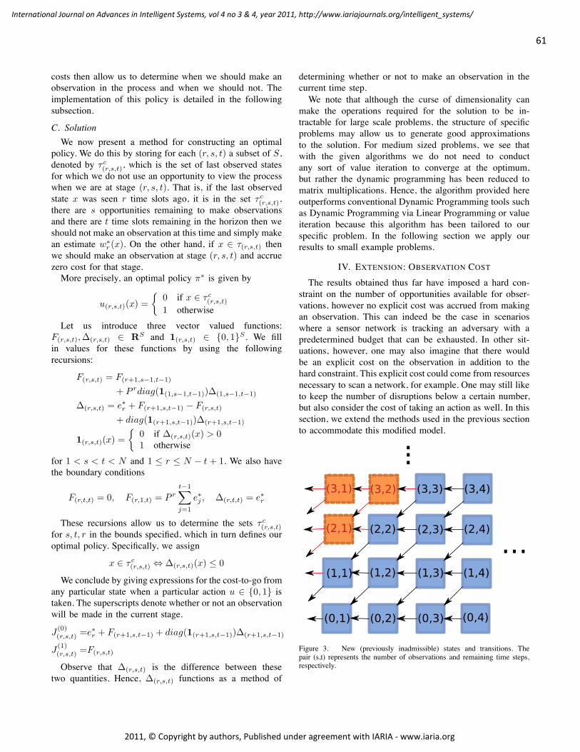
IV. EXTENSION: OBSERVATION COSTThe results obtained thus far have imposed a hard con-

straint on the number of opportunities available for obser-vations, however no explicit cost was accrued from makingan observation. This can indeed be the case in scenarioswhere a sensor network is tracking an adversary with apredetermined budget that can be exhausted. In other sit-uations, however, one may also imagine that there wouldbe an explicit cost on the observation in addition to thehard constraint. This explicit cost could come from resourcesnecessary to scan a network, for example. One may still liketo keep the number of disruptions below a certain number,but also consider the cost of taking an action as well. In thissection, we extend the methods used in the previous sectionto accommodate this modified model.

Figure 3. New (previously inadmissible) states and transitions. Thepair (s,t) represents the number of observations and remaining time steps,respectively.

62



A. New ModelWe proceed with the same formulation proposed in Sec-

tion III with an added feature to the model: the cost ofmaking an observation (taking an action u = 1) is c. Wemay now ask what the interpretation of this is as relatedto our original distance measure d(·, ·). We suppose that alinear cost is attached with the estimation error at each timestep. This cost is measured in the same units as the cost c ofmaking an observation. Note that our problem statement inthis form now allows for a new degree of freedom that wasnot seen in the previous section: in the backwards inductionprocess, it is now necessary to consider states for whichs > t (Figure 3), since it is possible to come to such a stateby not using an observation even when s = t. This wouldhappen if the cost of using an observation is prohibitivelyhigh, a scenario left unconsidered earlier.

B. Dynamic ProgrammingBeginning with stage t = 1, we can reuse our previous

calculation of

J(r,0,1) = e"r

since an added observation cost does not change this quan-tity. In the s = 1 case, however, we now must decide whetherit is worthwhile to use this observation opportunity. We canwrite:

J(0)(r,1,1) = e"r J

(1)(r,1,1) = c

where we have abbreviated c to be the vector where allelements are c. This results in a function

"(r,1,1) = e"r # c

with associated set "(r,1,1). Larger values of s behave thesame way as s = 1. For t = 2, we again recycle the result

J(r,0,2) = e"r + e"r+1

and must consider s = 1 as follows:

J(0)(r,1,2)(x) = e"r + c + 1(r+1,1,1)(x)"(r+1,1,1)(x)

J(1)(r,1,2)(x) = c + P re"1

Once again, "(r,1,2) and "(r,1,2) can be found by con-struction.For the s = 2 case we must again look at both u = 0 and

u = 1 cases.

J(0)(r,2,2)(x) = e"r + c + 1(r+1,2,1)(x)"(r+1,2,1)(x)

J(1)(r,2,2)(x) = 2c + 1(r+1,1,1)(x)"(r+1,1,1)(x)

Larger values of s behave exactly the same as s = 2, and" as well as " can be constructed in the usual way.We can continue in the same manner as the previous

section, incrementing t and s accordingly. We omit thesedetails and present the solution, whose structure closelymirrors the no-cost case.

C. SolutionAn optimal policy is given by

u(r,s,t)(x) =

$

0 if x $ "c(r,s,t)

1 otherwiseWe again have three vector valued functions:

F(r,s,t), "(r,s,t) $ RS and 1(r,s,t) $ {0, 1}S. We fillin values for these functions by using the followingrecursions:

F(r,s,t) = F(r+1,s!1,t!1) + c

+ P rdiag(1(1,s!1,t!1))"(1,s!1,t!1)

"(r,s,t) = e"r + F(r+1,s,t!1) # F(r,s,t)

+ diag(1(r+1,s,t!1))"(r+1,s,t!1)

1(r,s,t)(x) =

$

0 if "(r,s,t)(x) > 01 otherwise

for 1 < s, t < N and 1 ' r ' N # t + 1. We also have theboundary conditions

F(r,1,t) = c + P rt!1"

j=1

e"j , "(r,s,1) = e"r # c

These recursions allow us to determine the sets "c(r,s,t)

for s, t, r in the bounds specified, which in turn defines ouroptimal policy. Specifically, we assign

x $ "c(r,s,t) ( "(r,s,t)(x) ' 0

We conclude by giving expressions for the cost-to-go fromany particular state when a particular action u $ {0, 1} istaken. The superscripts denote whether or not an observationwill be made in the current stage.

J(0)(r,s,t) =e"r + F(r+1,s,t!1) + diag(1(r+1,s,t!1))"(r+1,s,t!1)

J(1)(r,s,t) =F(r,s,t)

The modification to our algorithm is surprisingly minimal- we only need to add cost c in the appropriate places toconsider this larger class of problems. Indeed, in this casewe are able to profit from the work that was required inSection III.

D. Implementation OptimizationNote that in this modified solution structure, the number

of possible dynamic programming states has approximatelydoubled. This is due to the fact that dynamic programmingstates for which s > t are now possible. However, once canalso see that for quantities indexed as (r, s, t) where s > t,the values are exactly the same as for s = t. In fact, the onlything changing is the indexing, since there is no utility toobservations that cannot be used. For reducing complexityduring deployment then, one could simply collapse s > tstates into the s = t state, but for the purposes of clarityand accounting for observation usage, we have chosen torepresent them as different states.

63



V. EXTENSION: LARGE STATE SPACESWe now include a short note about dealing with very large

state spaces. For the most part, when state spaces becomeprohibitively large in this type of problem setting, one mustconsider the specific structure of the problem at hand tofind a technique to either approximate or simply the trueproblem. There are, however, a couple general methods tocut down on the problem size.

A. Breadth First SearchIn some cases, the size of state space is much larger than

the subset of states that are reachable for the process inthe time horizon under consideration. This is unlikely tohappen since the size of a set covered by breadth first searchexponentially increases, but for problems with a small timehorizon, it is a good first step and suffers no performanceloss. The downside is that this approach is applicable onlyfor shorter time horizon problems.

B. Agglomeration of StatesAnother way to reduce the complexity of the problem

at hand is to examine the distance measure and combinestates that are close to each other compared to the averagedistance between states. A threshold can be set for how closetwo states must be in order to warrant agglomeration. Thisthreshold can be used to bound the additional error accrueddue to this simplification. This method can be effective ifthere is a high probability that the process will take manyof the longer transitions over the course of the problem, butcan be a poor approximation technique if the intruder spendsmany time steps traversing the smaller arcs of the graph.

C. Truncation of StatesStill another way to reduce the number of states under

consideration in the solution for this problem is to findthose states that are probabilistically unlikely to be reached.These states on the Markov chain can be omitted. Indeed, inthe case of hypercubes and euclidean distance as the statespace and measure respectively, there are results boundingthe probability with which the process will drift outside agiven radius. Depending on the resources at hand, one canperform the prescribed state space reduction in several ways.One method can be to simulate many paths and eliminatethose that have not been reached often. Another techniquecan be to simply find the transitions in the Markov chainwith lowest probability and remove them until many statesare no longer reachable. The downside of eliminating seldomreached paths could also introduce the danger of missingnew intrusion patterns.

D. CombinationIn reality, a combination of these approaches should be

attempted when attempting to simplify a problem. One cancombine the agglomeration and truncation approaches by

(1, 1) (2, 1)

(2, 2)(1, 2)

pab

paa

pad pbc

pbb

pba

pcc

pcb

pcd

pdd

pda

pdc

Figure 4. Markov chain M2!2

combining only those states that satisfy a proximity metricin addition to being unlikely to be reached.

VI. NUMERICAL RESULTS

Let us now examine the performance of our algorithm.Everything that follows pertains to the no-cost observationcase, unless explicitly stated. We fix a horizon length andplot the cost that the prescribed algorithm accrues versusthe number of opportunities to make observations. Let usconsider Markov chains of the type Mn$n in Figure 4,which is an n-by-n grid of states where the transitionprobabilities are given in the figure. Such a constructionis simple enough for quick simulation but can capture theinherent variations that our algorithm is able to leverage.

A. Surveillance

Suppose we would like to track the position of an intruderin an environment modeled by the Markov chainM3$3 overa discrete-time horizon of 30 time slots. However, updatingthe location of the intruder requires battery power of amobile device due to communications with a satellite andhence we are not able to request the position of the intruderat every time. Fixing the initial position of the device to be(2, 1), let us vary the number of opportunities to retrieve thetrue location from 0 to 30. The distance metric we take isthe standard Euclidian norm, which may be represented in

64



matrix form as:

D =

/

0

0

0

0

0

0

0

0

0

0

0

0

0

1

0 1 2 1)

2)

5 2)

5)

81 0 1

)2 1

)2

)5 2

)5

2 1 0)

5)

2 1)

8)

5 21

)2

)5 0 1 2 1

)2

)5)

2 1)

2 1 0 1)

2 1)

2)5

)2 1 2 1 0

)5

)2 1

2)

5)

8 1)

2)

5 0 1 2)5 2

)5

)2 1

)2 1 0 1)

8)

5 2)

5)

2 1 2 1 0

2

3

3

3

3

3

3

3

3

3

3

3

3

3

4

and we choose the transition matrix to be

P =

/

0

0

0

0

0

0

0

0

0

0

0

0

1

0 0.1 0 0.9 0 0 0 0 00.1 0 0.9 0 0 0 0 0 00 0.1 0.8 0 0 0.1 0 0 00 0 0 0 0.2 0 0.8 0 00 0.7 0 0.15 0 0.15 0 0 00 0 0.5 0 0 0 0 0 0.50 0 0 0.9 0 0 0 0.1 00 0 0 0 0.8 0 0 0 0.20 0 0 0 0 0.5 0 0.4 0.1

2

3

3

3

3

3

3

3

3

3

3

3

3

4

where we have ordered the states by the firstindex and then the second (that is in order(1, 1), (1, 2), (1, 3), (2, 1), (2, 2), (2, 3), (3, 1), (3, 2), (3, 3)).We note that the topology of the state space with thechosen distance metric is rather uniform, but the transitionprobabilities widely vary from state to state.We expect the estimation error to monotonically decrease

with the number of opportunities to learn the true state.In Figure 5, we see that this indeed the case, and alsocompare it to a benchmark strategy of randomly distributingobservations.

0 5 10 15 20 25 300

5

10

15

20

25

Number of Observations

Opt

imal

Erro

r

Optimal Error vs. Number of Observations

OptimalRandom

Figure 5.

Another expected property is that for fixed r, t, as sincreases, the number of states for which "(r,s,t) % 0decreases. That is, we expect that having more opportunitiesto make observations results in a more liberal optimal policy,and vice versa. We see this in Figure 6.

0 5 10 15 20 25 300

1

2

3

4

5

6

7

8

9

Number of ObservationsN

umbe

r of O

bser

vatio

n St

ates

Number of Observation States vs. Number of Observations

Figure 6.

Finally, let us consider one more plot with the sameMarkov chain states and distance metric, but a differenttransition matrix. Specifically, let us choose transitions thathave uniform probabilities to each neighbor. The resultingmatrix is given by

P =

/

0

0

0

0

0

0

0

0

0

0

0

0

1

0 12 0 1

2 0 0 0 0 013 0 1

3 0 13 0 0 0 0

0 12 0 0 0 1

2 0 0 013 0 0 0 1

3 0 13 0 0

0 14 0 1

4 0 14 0 1

4 00 0 1

2 0 0 0 0 0 12

0 0 0 12 0 0 0 1

2 00 0 0 0 1

3 0 13 0 1

30 0 0 0 0 1

2 0 12 0

2

3

3

3

3

3

3

3

3

3

3

3

3

4

This removes most of the variability from the problem -in fact, the only non-uniformity is due to the fact that thestate space is not large compared to the horizon of theproblem, and hence, the edges introduce some small amountof variation. In Figure 7, it is apparent that the optimal policyis practically a straight line. There is not much variability toexploit, so we aren’t able to exploit situations with sparseobservations as we could in Figure 5.

B. Analysis of PerformanceWe now note several properties of our curve in Figures

5,6 and 7. In some cases, the justification for the property isclear and we briefly explain it, where as in others we delveinto a more complete proof.

65



0 5 10 15 20 25 300

5

10

15

20

25

30

Number of Observations

Opt

imal

Erro

rOptimal Error vs. Number of Observations

Figure 7.

1) Endpoints: First, the endpoints in an estimation errorvs. number of observations plot are fixed no matter whatpolicy is used. This is because when there are zero oppor-tunities to make observations or there are 30 chances toview the process, there is no way to come up with policiesthat result in different decisions. There is only one way toallocate opportunities to observe the process. Moving now toFigure 6, we note that the end points in this type of curve arealso fixed. Specifically, in any plot of number of states with"(r,s,t) % 0 vs. number of observations, we have the points(0, 0) and (t, |S|). The point (0, 0) is guaranteed becausewithout any observations, there is no chance that one canbe made at any state. The point (t, |S|) is certain becausewhen the number of observations is equal to the number oftime steps remaining in the problem, the cost J (0) of notobserving can never be less than the cost J (1) of making anobservation.2) Diminishing Returns: Next, in Figure 5 we note that

our algorithm outperforms a benchmark strategy of ran-domly placing observations over the 30 time slots. We seethat the greatest “savings” occurs when we have a sparsity ofopportunities to make observations. This can be quantifiedby how strong the convexity of this curve is. We will shortlyprove that these curves are always convex, but the salientpoint here is that as opportunities to observe the processare more readily available, there is a law of diminishingreturns and these opportunities become less valuable. Thedegree of convexity depends greatly on the transition matrixP of the Markov chain. For example, if the grid Mn$n

has transitions that are all equal, the optimal policy comesout to be almost a straight line, as we verified in Figure 7.This is because there is little variation in the Markov chain toexploit. A highly variable Markov chain would allow a singleobservation to reduce much variability in future predictions,

hence reducing error drastically with a small budget.3) Monotonicity: In the two types of plots we have given,

monotonicity is another property that is present in general.First, let us consider plots of the type in Figure 5 and 7.In error vs number of observations plots, we can provemonotonicity by contradiction. Suppose that these curve arenot guaranteed to be monotonically decreasing and that thereexists some model and s such that J(r,s,t) < J(r,s+1,t).The the policy for s + 1 could not possibly be optimal,because we can simply apply the policy for s to the sameproblem and achieve better performance. The plot in Figure6 is monotonically increasing, a property that also matchesour expectation: as the number of opportunities to makeobservations increases, the probability of making one (undera uniform prior) increases, and therefore the number of statesthat result in an observation being made should increase.4) Convexity: Finally, we observe the convexity of the

optimal cost vs. number of observations curve. Indeed, it isconsistent with our intuition that having an extra opportunityto make observations should be of greater utility when ob-servations are sparse and less utility when they are abundant.We can sketch a proof for this. First note that the inequalitywe would like to prove is

J(r,s,t) '1

2

5

J(r,s!1,t) + J(r,s+,t)

6

in the range 0 < s < t. We can rewrite this as

2J(r,s,t) ' J(r,s!1,t) + J(r,s+,t).

Let us change perspective at this point and consider thisa problem not in allocating observations, but rather inallocating ‘holes’, or instances without observations. Wewant to dynamically schedule holes in a way that theestimation error accrued due to the presence of these holes isminimal. Estimation error is only accrued for holes, not forobservations. Let us now consider two processes happeningin parallel of horizon t and the same value r. One processhas s holes to be allocated, and the other has s # 1 holesto be allocated. Suppose we must now choose a process towhich another hole is to be added. That is, an additionalestimate must be formed on one of the two processes insuch a way to minimize the total estimation error of the twoprocesses. It is clear that we should choose the process withfewer holes since this process has more information aboutthe state of the process and hence is likely to induce a lowerestimation error increase due to the additional hole. We cansee this more graphically in Figure 8.Returning to our original problem, we can translate this to

conclude that it is preferable, in the event of two processeswith J(r,s!1,t) and J(r,s,t), to add an observation to the onewith fewer observations. That is, 2J(r,s,t) is preferable toJ(r,s!1,t) + J(r,s+1,t), which is what we wanted to show.

66



Figure 8. Allocation of holes to two processes.

VII. CONCLUSION AND FUTURE WORK

In this paper, we have described a problem in monitoringover a finite horizon when there are a limited number ofopportunities to conduct surveillance. We mathematicallymodel this as a problem of state estimation. In the estimationproblem we hope to minimize the distortion from estimatingthe state of a Markov chain when the number of time theprocess may be viewed is limited to a few times over thetotal horizon. The distortion is measured using a specifiedmetric d(x, y), which tells us how “far apart” states x andy are.In our optimal policy, a set of recursive equations with

boundary conditions give a practical method for determiningan optimal policy. Although the policy could have beendetermined using standard methods in dynamic program-ming, such as value iteration, the algorithm given here reliesonly on the ability to store data and conduct matrix multi-plications. Hence, larger problems can be handled beforeintractability results due to state space complexity.Extensions to this basic formulation are then covered,

such as a treatment of the same problem with a cost onmaking observations. Techniques for handling problems withvery large state spaces are also discussed. Finally, severalstructural properties of the solution are presented.There are many further problems to consider in future

work. Rather than fixing the problem of interest to aparticular horizon length, we may consider problems witha variable horizon. That is, we might consider problemsin which the Markov chain dictates a random stoppingtime for the process during which we may only makeobservations a limited number of times. Additionally, thereare practical scenarios in which one does not have completeinformation about the transition matrix. In this case, wemay be interested in coupling parameter estimation withefficient budget allocation. Finally, distributed problems inwhich many sensors are available for measurement but eachhas a battery limitation are of great interest, and certainlycan be explored in the context of the budgeted estimationscheme suggested here.Overall, the area of budgeted estimation holds much

promise, and there are many avenues left to investigate inthis power limited framework.

ACKNOWLEDGMENT

The first author is supported by the Department ofDefense (DoD) through the National Defense Science &Engineering Graduate Fellowship (NDSEG) Program.

REFERENCES

[1] P. Bommannavar and N. Bambos, “Optimal State Surveillanceunder Budget Constraints,” in Proceedings of the SecondInternational Conference on Emerging Network Intelligence,Florence, Italy: IARIA, October 2010, pp. 68-73.

[2] E. Wilson, Network Monitoring and Analysis: A ProtocolApproach to Troubleshooting. Prentice Hall, 2000.

[3] D. Josephsen, Building a Monitoring Infrastructure with Na-gios. 1st ed., Prentice Hall, 2007.

[4] Microsoft Security Center, Retrieved fromhttp://technet.microsoft.com/en-us/security, May, 2010,accessed: Jan 2012.

[5] General Accounting Office, Information Security: ComputerAttacks at Department of Defense Pose Increasing Risks.GAO/AIMD-96-84, May, 1996.

[6] R. A. Miura-Ko and N. Bambos, “Dynamic risk mitigation incomputing infrastructures,” in Third International Symposiumon Information Assurance and Security. IEEE, 2007, pp. 325- 328.

[7] K. C. Nguyen, T. Alpcan, and T. Basar, “Fictitious playwith imperfect observations for network intrusion detection,”13th Intl. Symp. Dynamic Games and Applications (ISDGA),Wroclaw, Poland, June 2008.

[8] T. Alpcan and X. Liu, “A game theoretic recommendationsystem for security alert dissemination,” in Proc. of IEEE/IFIPIntl. Conf. on Network and Service Security (N2S 2009), Paris,France, June 2009.

[9] H.V. Poor, An Introduction to Signal Detection and Estimation.2nd ed., Springer-Verlag, 1994.

[10] N. E. Nahi, “Optimal recursive estimation with uncertainobservation,” in IEEE Transactions on Information Theory, vol.15, no. 4, pp. 457 - 462, July 1969.

[11] B. Sinopoli, L. Schenato, M. Franceschetti, K. Poolla, M. I.Jordan, and S. S. Sastry, “Kalman filtering with intermittentobservations,” IEEE Transactions on Automatic Control, vol.49, no. 9 , pp. 1453 - 1464, September 2004.

[12] S. Yuksel, O. C. Imer and T. Basar, “Constrained stateestimation and control over communication networks,” in Proc.of 38th Annual Conference on Information Science and Systems(CISS), Princeton, NJ, March 2004.

[13] J. Fuemmeler and V.V. Veeravalli, “Smart Sleeping Policiesfor Energy Efficient Tracking in Sensor Networks,” IEEETransactions on Signal Processing, vol. 56 no. 5: pp. 2091-2102, May 2008.

67



[14] N. Agarwal, J. Basch, P. Beckmann, P. Bharti, S. Bloebaum,S. Casadei, A. Chou, P. Enge, W. Fong, N. Hathi, W. Mann,A. Sahai, J. Stone, J. Tsitsiklis, and B. Van Roy, “Algorithmsfor GPS Operation Indoors and Downtown,” GPS Solutions,Vol. 6, No. 3, pp. 149-160, December 2002.

[15] S. Appadwedula, V.V. Veeravalli, and D.L. Jones, “EnergyEfficient Detection in Sensor Networks,” in IEEE Journal onSelected Areas in Communications, vol. 23 no. 4, pp. 693-702,April 2005.

[16] O.C. Imer. Optimal Estimation and Control under Communi-cation Network Constraints. Ph.D. Dissertation, UIUC, 2005.

[17] P. Bommannavar and N. Bambos, Patch Scheduling for RiskExposure Mitigation Under Service Disruption Constraints.Technical Report, Stanford University, 2010.

[18] D. P. Bertsekas, Dynamic Programming and Optimal Control.Belmont, MA: Athena Scientic, 1995.

68



Multilingual Ontology Library Generator

for Smart-M3 Information Sharing Platform

Dmitry G. Korzun∗†, Alexandr A. Lomov∗, Pavel I. Vanag∗, Sergey I. Balandin‡, and Jukka Honkola§

∗Department of Computer Science

Petrozavodsk State University – PetrSU

Petrozavodsk, Russia†Helsinki Institute for Information Technology – HIIT

Aalto University

Helsinki, Finland‡FRUCT Oy

Helsinki, Finland§Innorange Oy

Helsinki, Finland

Email: {dkorzun, lomov, vanag}@cs.karelia.ru, [email protected], [email protected]

Abstract—Web Ontology Language (OWL) allows struc-turing smart space content in high-level terms of classes,relations between them, and their properties. Smart-M3 is anopen-source platform that provides a multi-agent distributedapplication with a shared view of dynamic knowledge andservices in ubiquitous computing environments. A Smart-M3Semantic Information Broker (SIB) maintains its smart spacein low-level terms of triples, based on Resource DescriptionFramework (RDF). This paper describes SmartSlog, a softwaredevelopment tool for programming Smart-M3 agents (Knowl-edge Processors, KPs) that consume/produce smart spacecontent according with its high-level ontological representation.SmartSlog applies the code generation approach. Given anOWL ontology description, SmartSlog produces the ontologylibrary. The latter provides 1) API to access the smart spacevia its SIB and 2) data structures and functions to representand maintain locally in KP code all ontology classes, relations,properties, and individuals. The developer easier constructsthe KP code, thinking in high-level ontology terms insteadof low-level RDF triples. SmartSlog supports generation ofmultilingual ontology libraries (ANSI C and C# in the currentimplementation). Such libraries are modest to the devicecapacity, portable and suitable even for small devices. TheSmartSlog ontology library generation scheme, architecture,design solutions, and directions for use are the main output ofthis paper.

Keywords-Smart spaces; Smart-M3; OWL/RDF ontology; codegenerator; knowledge processor; low-performance devices

I. INTRODUCTION

Smart-M3 is an open-source platform for information

sharing [1]–[3]. It provides applications with a smart space

infrastructure to use a shared view of dynamic knowledge

and services in ubiquitous computing environments [4]. Ap-

plications are implemented as distributed agents (knowledge

processors, KPs) running on the various computers, includ-

ing mobile and embedded devices. Shared knowledge is

represented using Resource Description Framework (RDF)

and kept in RDF triple-stores, each is accessible via a

Semantic Information Broker (SIB). The RDF representation

allows semantic reasoning; simple methods are available

on the SIB side, more complex ones are implemented in

dedicated KPs.

A Smart-M3 application consists of several KPs that share

the smart space using the space-based [5] and pub/sub [6]

communication models. The KPs produce (insert, update,

remove) or consume (query, subscribe/unsubscribe) informa-

tion. The Smart Space Access Protocol (SSAP) implements

the SIB ↔ KP communication, using operations with RDF

content as parameters. Each KP understands its subset of

information, usually defined by the KP ontology.

Real-life scenarios often involve a lot of information,

which leads both to largish ontologies and possibly complex

instances that the KPs need to handle. Thus, programming

KPs on the level of SSAP operations and RDF triples bring

unnecessary complexity for the developers, who have to

divert effort for managing triples instead of concentrating on

the application logic. The OWL representation of knowledge

as classes, relations between classes, and properties maps

quite well to object-oriented paradigm in practice (but not so

well in theory). Therefore, it is feasible to map OWL classes

into object-oriented classes and instances of OWL classes

into objects in programming languages. (These objects only

have attributes, but no methods and thus no behavior.) This

approach effectively binds the RDF subgraph describing an

instance of an OWL class (individual) to an object in a

programming language.

SmartSlog is a Smart Space ontology library generator [1],

[7] for Smart-M3. It maps an OWL ontology description to

code (ontology library), abstracting the ontology and smart

space access in KP application logic. As a result, SmartSlog

simplifies constructing KP code compared with the low-level

69



RDF-based KP development. The code manipulates with

ontology classes, relations, and individuals using predefined

data structures and library Application Programming Inter-

face (API). The number of domain elements in KP code

is reduced. The API is generic, hence does not depend on

concrete ontology; all ontology entities appear as arguments

in API functions. Search requests to SIB are written com-

pactly by defining only what you know about the object to

find (even if the object has many other properties).

The vision of ubiquitous involves a lot of small devices to

participate in surrounding computing environments. Smart-

Slog targets low-performance devices by producing ontology

libraries in pure ANSI C with minimal dependencies to

system libraries, the property is essential in many embed-

ded systems [8]. SmartSlog takes into account the limited

resources available on small computers such as mobile and

embedded devices. For example, the KP code does not need

to maintain the whole ontology as unused entities can be

removed. Also, RDF triples are not kept indefinitely, and

the local memory is freed immediately after the use. Even

if a high-level ontology entity consists of many triples, its

synchronization with SIB transfers only a selected subset,

saving on communication.

ANSI C programming is too low-level for some classes of

devices. For example, although writing KP in ANSI C for

the Blue&Me platform (Windows mobile for Automotive)

is possible, it is complicated, and some developers prefer

the .NET/C# language for this case. SmartSlog allows mul-

tilingual ontology library generation. The current SmartSlog

implementation supports ontology libraries in ANSI C and

C#, validating our multilingual approach.

The rest of the paper is organized as follows. Section II

provides an introduction to the Smart-M3 platform. Sec-

tion III overviews Smart-M3 KP development tools with

focus on SmartSlog; we describe the ontology library ap-

proach for KP development. In Section IV, we introduce the

ontology library generation scheme designed for SmartSlog.

Example application construction with SmartSlog is shown

in Section VI. Then, Section VII analyzes the problems that

are common for ontology library generators independently

on target programming languages. It includes the issues of

ontology manipulations and code optimization on the KP

side. Section VIII summarizes the paper.

II. SMART-M3 PLATFORM AND ITS NOTION OF

APPLICATION

Smart-M3 is an open-source interoperability platform for

information sharing [2], [3], [9]. “M3” stands for Multide-

vice, Multidomain, and Multivendor. It has been developed

by a consortium of companies and within research projects:

EU Artemis funded Sofia project (Smart Objects for In-

telligent Applications) [10] and Finnish nationally funded

program DIEM (Device Interoperability Ecosystem) [11].

Smart-M3 implements smart space infrastructures for multi-

agent distributed applications following the smart space

concept [12]–[14]; the latter is becoming popular in semantic

computing. In this section we provide an overview of Smart-

M3 platform and its core concepts.

A. Space-based computing

Space-based (or tuplespace) computing has its roots in

parallel and distributed programming. Gelernter [15] de-

fined the generative communication model where common

information is shared in a tuplespace; parallel processes of

a distributed application cooperate by publishing/retrieving

tuples into/from the space. A tuple is an ordered list of typed

fields. Data tuples contain static data. Process tuples repre-

sent processes under execution. This asynchronous (publish-

based) inter-process communication model allows building

programs by gluing together active pieces [5].

Aiming at automated processing in such a giant distributed

system as the World Wide Web, Berners-Lee [16] introduced

the Semantic Web. Its content is described in a structured

manner, where ontologies become the basic building block.

Fensel [17] brought the idea of triple space computing as

communication and coordination paradigm based on the

convergence of space-based computing and the Semantic

Web. Triple space computing inherits the publication-based

communication model from the tuplespace communication

model and extends it with semantics: tuples are RDF triples

(subject, predicate, object). They in turn are composed

to RDF graphs with subjects and objects as nodes and

predicates as edges. Hence, semantic-aware queries to the

space are possible, utilizing matching algorithms [18] and

semantic query languages like SPARQL [19].

In fact, the triple space computing paradigm states a

scalable semantic infrastructure for web applications; it

enables integration, communication, and coordination of

many autonomous, distributed, and heterogeneous web ser-

vice providers and consumers. Information stored in the

same space can be further processed, providing deduced

knowledge that otherwise cannot be available from a single

source [5]. Semantic web spaces [20] apply this possibility

for a new coordination model: a participant can infer new

facts as a reaction to knowledge that has been published by

others. Semantic web spaces extends tuplespaces: tuples are

RDF triples and matching uses RDF Schema reasoning.

Conceptual Spaces (CSpaces) [21] extends triple space

computing to be applicable in different scenarios apart from

web services. An important set of scenarios is due to the

ubiquitous computing vision, i.e. when computers seam-

lessly integrate into human lives and applications provide

right services anywhere and anytime [22]. One of the key

features of CSpaces is a composition of the tuplespace

publish-based model with the publish/subscribe model from

the pub/sub communication paradigm (e.g., see [6]). Trans-

action support is included to guarantee the successful exe-

70



cution of a group of operations. This advanced coordination

model provides flow decoupling from the client side [6], in

addition to time and space decoupling already available in

the tuplespace coordination model.

B. Smart spaces and Smart-M3 infrastructure

Smart spaces constitute a smart environment, which is

“able to acquire and apply knowledge about its environment

and to adapt to its inhabitants in order to improve their

experience in that environment” [12]. In accordance with

the ubiquitous computing vision, smart spaces encompass

the following information spaces: (i) physical spaces with

sensing devices such as homes or cars, (ii) service spaces

with information retrieval and processing such as Inter-

net services or surrounding services in tourist place, and

(iii) user spaces with personal information such as user

profiles or address books. The information is dynamically

shared by multiple heterogeneous participants (humans and

machines), allowing each user to interact continuously with

the surrounding environment, and the services continuously

adapt to the current needs of the user [14].

Smart spaces require a software infrastructure that turns

the constituting spaces into programmable distributed en-

tities. Smart-M3 provides such an infrastructure to use a

shared view of dynamic knowledge and services within

a distributed application. Although several studies have

showed the convenience of the space-based approach for

ubiquitous and pervasive computing environments and even

for Internet of Things [23]–[25], to the best of our knowl-

edge the Smart-M3 platform is the only general-purpose

open-source platform available recently.

In addition to the normal range of personal computers

and embedded devices, mobile devices with various means

of connectivity become the primary gateway to the service

space and the major storage point in the user space [13],

[14]. Smart-M3 follows the space-agent approach. Each

device, service, or storage point is programmable as an

agent. In this multidevice system, agents place, share, and

manipulate with local and global information using their own

locally agreed semantics [13].

Information sharing in Smart-M3 is based on the space-

based models using the same mechanisms as in the Semantic

Web, thus allowing multidomain applications, where the

RDF representation allows easy exchange and linking of

data between different ontologies, making cross-domain

interoperability straightforward [26]. Smart-M3 currently

supports only limited reasoning, e.g., queries with subclass

relations; see [27] for more details and possible extensions.

The security issues of information sharing in Smart-M3 can

be found in [28]–[30].

The basic architecture of Smart-M3 space infrastructure

is illustrated in Figure 1. Its core component is semantic

information broker (SIB)—an access point to the smart

space. Each SIB maintains a part of information represented

Figure 1. Smart spaces form a publish/subscribe system in a ubiquitousenvironment: KPs run on various types of computers and devices, the dis-tributed knowledge store supports reasoning over cross-domain information

as an RDF triplestore. It provides simple reasoning, e.g.,

understanding the owl:sameAs concept. The current Smart-

M3 implementation supports WilburQL as a basic query

language; migration to SPARQL is in progress. Note that

WilburQL was originally conceived as Nokia Research

Center’s toolkit (Helsinki, Finland) for applications that use

RDF, written in Common Lisp; the new Python-based toolkit

(Piglet) is partially open-sourced as a part of Smart-M3.

A device participates in the space using a software

agent—knowledge processor (KP). A KP connects a SIB

over some network and can modify and query the infor-

mation by insert, remove, update, query, and (un)subscribe

operations using the smart space access protocol (SSAP).

Each SIB provides many network connectivity mechanisms

(e.g., HTTP, plain TCP/IP, NoTA, Bluetooth), yielding

multivendor device interoperability. Accessing the space is

session-based with join and leave operations, thus providing

the base for mechanisms of access control and secure

information sharing.

From the KP point of view the information in the space

constitutes an RDF graph, usually according to some OWL

ontology. The use of any specific ontology is not mandated,

and a group of KPs can locally agreed which ontology to use

for interpreting a certain part of the space. The consistency

of stored information is not guaranteed. KPs are free to

interpret the information in whatever way they want.

When several SIBs make up a smart space the SIB

network follows a protocol with distributed deductive clo-

sure [31]. Hence any KP sees the same information content

regardless the SIB it connects to. The current implementa-

tion supports the simplest case with one SIB only.

71



C. Smart-M3 applications

A Smart-M3 application can be considered a composition

of possible scenarios enabled by a certain group of KPs.

Execution of the composition targets the current needs of

the user. For instance, an email application consists of the

following scenarios [26]: sending, receiving, composing,

and reading email. Each scenario can be implemented by

a dedicated KP. The same KP can be used in different

applications. For instance, a KP for composing email can

be a part of application for browsing social networks.

From this point of view, the basic principle is that the user

has a collection of KPs. They are capable to execute certain

scenarios. If the given collection does not support a needed

scenario, additional KPs should be found. Each KP should

understand its own, non-exclusive set of information. The set

is typically described with the ontology of the KP, at least

implicitly. Overlap of the sets of different KPs is needed for

interoperability; the KPs can see each other actions.

An application is constructed as ad-hoc assembly of KPs.

Each scenario emerges from the observable actions taken

by KPs based on smart space content or from the use

of available services. Some scenarios can be transient: the

execution is changed as the participating KPs join and leave

the smart space as well as some services become available

or unavailable.

The aim of this Smart-M3 approach is at the ease of

combining multiple scenarios into various applications. The

key point is the loose coupling between the participating

KPs. They use the space-based and pub/sub communication

models modifying and querying the information in the com-

mon smart space. Thus, the effect of any KP participation to

others is limited by to the information the KP provides into

the space. Note that Smart-M3 does not prevent direct con-

tacts between KPs, thus some actions can be activated based

on traditional inter-process communication models. Adding

elements of this traditional approach, however, impedes the

easy use of affected KPs in other applications, reducing the

benefit from Smart-M3.

Concrete examples of Smart-M3 applications include con-

text gathering in meetings [32], organization of conferences

and meetings [33], [34], smart home [35], gaming, wellness

and music mashup [26], social networks [36], and semantic

multi-blogging [37].

III. SMART-M3 ONTOLOGY LIBRARIES AND RELATED

WORK

Existing Smart-M3 KP development tools are language-

specific and platform-dependent. Many of them are oriented

to the RDF representation of information, thus complicating

the KP code compared with the OWL representation. In

this section we overview available tools and motivate the

ontology library approach for Smart-M3 applications. The

approach is implemented in SmartSlog with possibility to

write KPs in different languages and for different platforms.

The developers of KP application logic use a KP In-

terface (KPI) to access information in the smart space.

The content conform the ontological description. Low-level

access requires the user code to operate with RDF triples

(directly following the SSAP operations with triples as basic

exchange elements). In contrast, high-level KP development

is based on an ontology library. It allows the user code to be

written using high-level ontology entities (classes, relations,

individuals); they implemented in the code with predefined

data structures and methods. Table I shows available low-

level KPIs and ontology library generators for several pop-

ular programming languages.

An ontology library simplifies constructing KP application

logic providing the developer a programming language view

to the concepts of the given ontology. The number of domain

elements is reduced since an ontology entity consists of

many triples. The library API is generic: its syntax does

not depend on a particular ontology, ontology-related names

do not appear in names of API methods, and ontology

entities are used only as arguments. For example, creating

an individual of lady Aino Peterson can be written in C as

individual_t *aino

= new_individual(CLASS_WOMAN);

set_property(aino, PROPERTY_LNAME, "Peterson");

Figure 2 shows the SmartSlog ontology library structure.

It consists of two parts: ontology-independent and ontology-

dependent. The former is the same for any KP and im-

plements generic API to access knowledge in the smart

space. The latter is produced by SmartSlog CodeGen by a

given OWL description (provided by the KP developer) and

implements data structures for particular ontology entities.

The library internally performs OWL-RDF transformations

and calls a low-level KPI for data exchange with SIB.

In particular, the current SmartSlog implementation uses

KPI Low, both for ANSI C and C# ontology libraries. If

the low-level KPI is in a different language then a kind of

wrappers can be used for corresponding calls. For instance,

SmartSlog utilizes wrappers to implement a C# ontology

library since it uses KPI Low written in C.

Templates

OntologyOWL

Developer

Application logic

Dependent part

Independent part

Ontology library

Knowledge processor

KPI_Low

Wrapper

SmartSlog

CodeGen

Figure 2. The SmartSlog ontology library architecture: ontology-dependentand ontology-independent parts

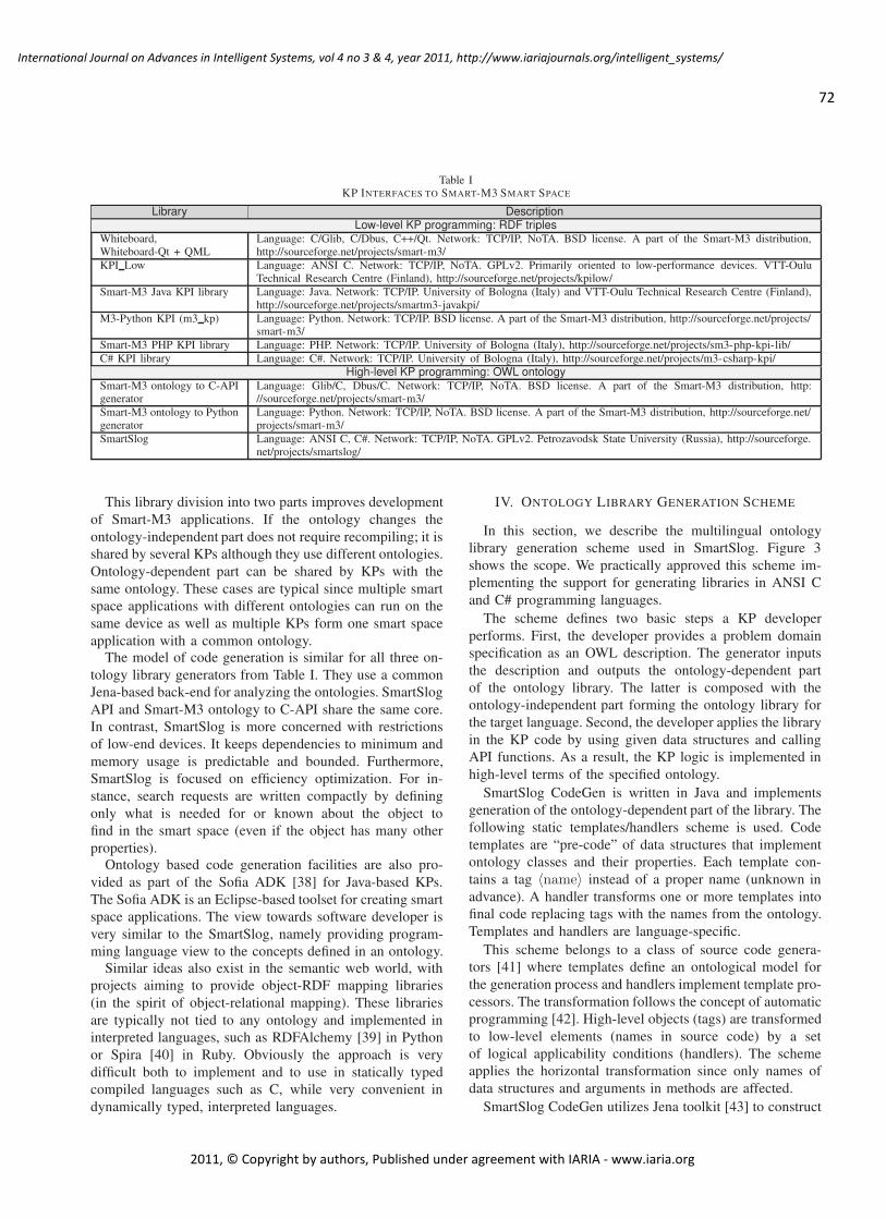
72



Table IKP INTERFACES TO SMART-M3 SMART SPACE

Library DescriptionLow-level KP programming: RDF triples

Whiteboard,Whiteboard-Qt + QML

Language: C/Glib, C/Dbus, C++/Qt. Network: TCP/IP, NoTA. BSD license. A part of the Smart-M3 distribution,http://sourceforge.net/projects/smart-m3/

KPI Low Language: ANSI C. Network: TCP/IP, NoTA. GPLv2. Primarily oriented to low-performance devices. VTT-OuluTechnical Research Centre (Finland), http://sourceforge.net/projects/kpilow/

Smart-M3 Java KPI library Language: Java. Network: TCP/IP. University of Bologna (Italy) and VTT-Oulu Technical Research Centre (Finland),http://sourceforge.net/projects/smartm3-javakpi/

M3-Python KPI (m3 kp) Language: Python. Network: TCP/IP. BSD license. A part of the Smart-M3 distribution, http://sourceforge.net/projects/smart-m3/

Smart-M3 PHP KPI library Language: PHP. Network: TCP/IP. University of Bologna (Italy), http://sourceforge.net/projects/sm3-php-kpi-lib/

C# KPI library Language: C#. Network: TCP/IP. University of Bologna (Italy), http://sourceforge.net/projects/m3-csharp-kpi/

High-level KP programming: OWL ontologySmart-M3 ontology to C-APIgenerator

Language: Glib/C, Dbus/C. Network: TCP/IP, NoTA. BSD license. A part of the Smart-M3 distribution, http://sourceforge.net/projects/smart-m3/

Smart-M3 ontology to Pythongenerator

Language: Python. Network: TCP/IP, NoTA. BSD license. A part of the Smart-M3 distribution, http://sourceforge.net/projects/smart-m3/

SmartSlog Language: ANSI C, C#. Network: TCP/IP, NoTA. GPLv2. Petrozavodsk State University (Russia), http://sourceforge.net/projects/smartslog/

This library division into two parts improves development

of Smart-M3 applications. If the ontology changes the

ontology-independent part does not require recompiling; it is

shared by several KPs although they use different ontologies.

Ontology-dependent part can be shared by KPs with the

same ontology. These cases are typical since multiple smart

space applications with different ontologies can run on the

same device as well as multiple KPs form one smart space

application with a common ontology.

The model of code generation is similar for all three on-

tology library generators from Table I. They use a common

Jena-based back-end for analyzing the ontologies. SmartSlog

API and Smart-M3 ontology to C-API share the same core.

In contrast, SmartSlog is more concerned with restrictions

of low-end devices. It keeps dependencies to minimum and

memory usage is predictable and bounded. Furthermore,

SmartSlog is focused on efficiency optimization. For in-

stance, search requests are written compactly by defining

only what is needed for or known about the object to

find in the smart space (even if the object has many other

properties).

Ontology based code generation facilities are also pro-

vided as part of the Sofia ADK [38] for Java-based KPs.

The Sofia ADK is an Eclipse-based toolset for creating smart

space applications. The view towards software developer is

very similar to the SmartSlog, namely providing program-

ming language view to the concepts defined in an ontology.

Similar ideas also exist in the semantic web world, with

projects aiming to provide object-RDF mapping libraries

(in the spirit of object-relational mapping). These libraries

are typically not tied to any ontology and implemented in

interpreted languages, such as RDFAlchemy [39] in Python

or Spira [40] in Ruby. Obviously the approach is very

difficult both to implement and to use in statically typed

compiled languages such as C, while very convenient in

dynamically typed, interpreted languages.

IV. ONTOLOGY LIBRARY GENERATION SCHEME

In this section, we describe the multilingual ontology

library generation scheme used in SmartSlog. Figure 3

shows the scope. We practically approved this scheme im-

plementing the support for generating libraries in ANSI C

and C# programming languages.

The scheme defines two basic steps a KP developer

performs. First, the developer provides a problem domain

specification as an OWL description. The generator inputs

the description and outputs the ontology-dependent part

of the ontology library. The latter is composed with the

ontology-independent part forming the ontology library for

the target language. Second, the developer applies the library

in the KP code by using given data structures and calling

API functions. As a result, the KP logic is implemented in

high-level terms of the specified ontology.

SmartSlog CodeGen is written in Java and implements

generation of the ontology-dependent part of the library. The

following static templates/handlers scheme is used. Code

templates are “pre-code” of data structures that implement

ontology classes and their properties. Each template con-

tains a tag 〈name〉 instead of a proper name (unknown in

advance). A handler transforms one or more templates into

final code replacing tags with the names from the ontology.

Templates and handlers are language-specific.

This scheme belongs to a class of source code genera-

tors [41] where templates define an ontological model for

the generation process and handlers implement template pro-

cessors. The transformation follows the concept of automatic

programming [42]. High-level objects (tags) are transformed

to low-level elements (names in source code) by a set

of logical applicability conditions (handlers). The scheme

applies the horizontal transformation since only names of

data structures and arguments in methods are affected.

SmartSlog CodeGen utilizes Jena toolkit [43] to construct

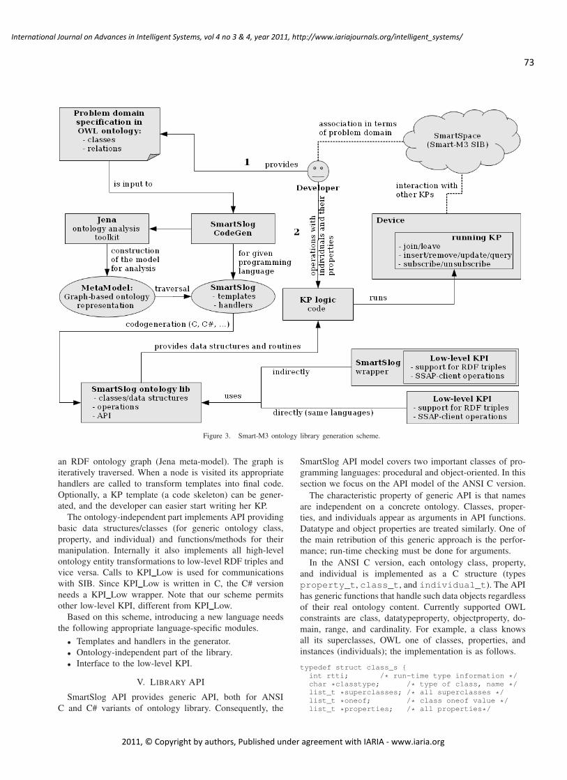
73



Figure 3. Smart-M3 ontology library generation scheme.

an RDF ontology graph (Jena meta-model). The graph is

iteratively traversed. When a node is visited its appropriate

handlers are called to transform templates into final code.

Optionally, a KP template (a code skeleton) can be gener-

ated, and the developer can easier start writing her KP.

The ontology-independent part implements API providing

basic data structures/classes (for generic ontology class,

property, and individual) and functions/methods for their

manipulation. Internally it also implements all high-level

ontology entity transformations to low-level RDF triples and

vice versa. Calls to KPI Low is used for communications

with SIB. Since KPI Low is written in C, the C# version

needs a KPI Low wrapper. Note that our scheme permits

other low-level KPI, different from KPI Low.

Based on this scheme, introducing a new language needs

the following appropriate language-specific modules.

• Templates and handlers in the generator.

• Ontology-independent part of the library.

• Interface to the low-level KPI.

V. LIBRARY API

SmartSlog API provides generic API, both for ANSI

C and C# variants of ontology library. Consequently, the

SmartSlog API model covers two important classes of pro-

gramming languages: procedural and object-oriented. In this

section we focus on the API model of the ANSI C version.

The characteristic property of generic API is that names

are independent on a concrete ontology. Classes, proper-

ties, and individuals appear as arguments in API functions.

Datatype and object properties are treated similarly. One of

the main retribution of this generic approach is the perfor-

mance; run-time checking must be done for arguments.

In the ANSI C version, each ontology class, property,

and individual is implemented as a C structure (types

property_t, class_t, and individual_t). The API

has generic functions that handle such data objects regardless

of their real ontology content. Currently supported OWL

constraints are class, datatypeproperty, objectproperty, do-

main, range, and cardinality. For example, a class knows

all its superclasses, OWL one of classes, properties, and

instances (individuals); the implementation is as follows.

typedef struct class_s {

int rtti; /* run-time type information */

char *classtype; /* type of class, name */

list_t *superclasses; /* all superclasses */

list_t *oneof; /* class oneof value */

list_t *properties; /* all properties*/

74



list_t *instances; /* all individuals */

} class_t;

API functions are divided into two groups: for manipu-

lating with local objects and for communicating with SIB.

The first group (local) includes functions for

• Classes and individuals: creating data structures and

manipulating with them locally.

• Properties: operations set/get, update, etc. in local store

(also run-time checks for correctness, e.g., cardinality

and property values).

For example, creating individual and setting its properties:

individual_t *aino = new_individual(CLASS_WOMAN);

set_property(aino, PROPERTY_LNAME, "Peterson");

In this example, the definitions of CLASS_WOMAN and

PROPERTY_LNAME are in the library ontology-dependent

part for the ontology shown in Figure 4. (We used GrOwl

tool [44]: classes are in blue rectangles, datatype properties

are in brown ovals, object properties are in blue ovals.)

The second group (to/from smart space) has prefix “ss_”

in function names and allows accessing smart space for

• Individuals: insertion, removal, and update.

• Properties: similarly to the local functions but the data

are to/from smart space (it requires transformation

to/from triples and calling the mediator library).

• Querying for individuals in smart space (existence,

yes/no answer).

• Populating individuals from smart space by query or

by subscription.

For example, inserting an individual and then updating some

of its properties:

ss_insert_individual(aino);

. . .

ss_update_property(aino,

PROPERTY_LNAME, "Ericsson");

Subscription needs more discussion. In advance, a sub-

scription container is created to add those individuals which

to subscribe for. Optionally, the container contains the prop-

erties whose values are interested only. Then KP explicitly

subscribes for selected properties of selected individuals.

Subscription is synchronous or asynchronous. The former

case is simplest; KP is blocked waiting for updates. Even de-

vices without thread support allow synchronous subscription.

The latter case is implemented with a thread that controls

Figure 4. Ontology for humans and their drinks

updates from smart space and assigns them to the containers.

KP is not blocked, and updates come in parallel.

Internally, communication with SIB leads to the compo-

sition/decomposition of high-level ontology entities from/to

RDF triples and calling the low-level KPI for triple-based

data exchange. To the best of our knowledge, SmartSlog is

the only ontology library generator that uses KPI Low as

the low-level mediator KPI (see Table I). Since KPI Low is

oriented to low-performance devices, this design selection

strengthens SmartSlog applicability in application develop-

ment for this class of devices.

Compared with the Smart-M3 ontology to C-API gen-

erator, which provides similar communication primitives,

SmartSlog has the following advantages. The Smart-M3

ontology to C-API generator depends on glib library, e.g.,

using list data structures. Low-performance devices do not

support glib. In contrast, SmartSlog has no such require-

ments for underlying libraries. The Smart-M3 ontology to

C-API generator does not allow asynchronous subscription

important for smart space applications.

SmartSlog generic API is extended with ‘knowledge pat-

terns’ for ontology-based filtering and search. A general

model of a knowledge pattern will be considered later in

Section VII-B; here we illustrate its representation for ANSI

C. Each knowledge pattern is an individual_t structure

and can be thought as an abstract individual where only a

subset of properties is set. A knowledge pattern is either

pattern-mask or pattern-request.

A pattern-mask is for selecting properties of a given a

class or individual. It needs when a subset of properties is

used, and the pattern includes only those properties. Then

this pattern is applied to the given class or individual, e.g. for

modest updating the properties. For example, let us update

only the last name of “Aino” (see the ontology in Figure 4).

pattern_t *aino_p = new_pattern(CLASS_WOMAN, NULL);

add_check_property_pattern(aino_p, PROPERTY_LNAME,

NULL, PATTERN_COND_NO);

ss_update_by_pattern(aino, aino_p);

As a result, only the last name value is transferred to

smart space. Compared with ss_update_property()

the benefit becomes obvious when KP needs to update

several properties at once or it can form the property subset

only in run-time. The same scheme works for population to

transfer data modestly from smart space.

A pattern-request is for compact definition of search

queries to smart space. A pattern is filled with those prop-

erties and values that characterize the individual to find. For

example, let us find all men whose first name is “Timo” and

wife’s first name is “Aino”.

pattern_t *timo_p = new_pattern(CLASS_MAN, NULL);

pattern_t *aino_p = new_pattern(CLASS_WOMAN, NULL);

add_check_property_pattern(timo_p, PROPERTY_FNAME,

"Timo", PATTERN_COND_NO);

add_check_property_pattern(aino_p, PROPERTY_FNAME,

75



"Aino", PATTERN_COND_NO);

add_check_property_pattern(timo_p, PROPERTY_HAS_WIFE,

aino_p, PATTERN_COND_NO);

timo_list = ss_get_individuals_by_pattern(timo_p);

In this example, two patterns (“Timo” and “Aino”) and

two properties (datatype “fname” and object “has wife”)

form a subgraph. The SmartSlog library matches the sub-

graph to the smart space content. As a result, a list of

available individuals is returned. Currently, searching leads

to iterative triple exchange and matching on the local side.

In future, it can be implemented on the top of SPARQL on

the SIB side.

VI. USE CASE EXAMPLE

In this section, we show how SmartSlog can be used for

constructing a simple Smart-M3 application in C. In spite of

the simplicity, the example illustrates such SmartSlog fea-

tures as knowledge patterns and subscriptions (synchronous

and asynchronous). Both datatype and object properties are

used.

Let Ericsson’s family consist of Timo (husband) and Aino

(wife). Timo likes drinking beer outside home. Aino has to

control Timo’s drinking via monitoring the amount of beer

he has drunk already. If the amount is exceeding a certain

bound (e.g., MAX_LITRES_VALUE=3) she notifies Timo

by SMS that it’s good time to come back to home.

The ontology for such personal human data was shown

in Figure 4 above. When Timo starts drinking he associates

his object property “drinks” with class “Beer”. Then Timo

keeps his drink counter “number of drinks” in smart space

and regularly updates it. Aino can subscribe to this counter.

For messaging, the family uses the ontology shown in

Figure 5. Aino sends SMS to notify Timo via smart space.

Timo subscribes for SMS and checks each SMS he received

for who sent it (by phone number). Hence Timo recognizes

a notification SMS from his wife.

Given these two ontology files, SmartSlog generator pro-

duces files drinkers.{c, h}. Since the ontology includes

more details than needed for this application, excessive

classes and properties can be disabled in the final code by

compiler preprocessor directives.

The KP code for Timo can be constructed with SmartSlog

using the following scheme.

Figure 5. Ontology for messaging

1. Create Timo, set his properties, and insert the individual

to the smart space.

individual_t *timo = new_individual(CLASS_MAN);

set_property(timo,PROPERTY_FNAME, "Timo");

. . .

ss_insert_individual(timo);

2. Timo keeps his counter in the smart space.

individual_t *beer = new_individual(CLASS_BEER);

ss_set_property(timo, PROPERTY_DRINKS, beer);

3. Timo subscribes to SMS from Aino: creating an in-

dividual for SMS and filling the subscribe container. Then

asynchronous (parameter “true”) subscription starts.

individual_t *sms = new_individual(CLASS_SMS);

add_data_to_list(subscribed_prop_list,

PROPERTY_FROM);

add_data_to_list(subscribed_prop_list,

PROPERTY_TO);

subscription_container_t *container=

new_subscription_container();

add_individual_to_subscribe(container,

sms, subscribed_prop_list);

ss_subscribe_container(container, true);

4. Timo drinks, updates the counter, and checks SMS.

while(sms_notify(sms)) {

amount += drink(timo);

ss_update_property(timo,

PROPERTY_NUMBER_OF_DRINKS, amount);

}

Similarly, the KP code for Aino is constructed as follows.

1. Aino searches Timo in the smart space by pattern.

individual_t *wife = new_individual(CLASS_WOMAN);

set_property(wife, PROPERTY_LNAME, "Ericsson");

set_property(wife, PROPERTY_FNAME, "Aino");

pattern_t *timo_p = new_pattern(CLASS_MAN, NULL);

add_check_property_pattern(timo_p, PROPERTY_FNAME,

"Timo", PATTERN_COND_NO);

add_check_property_pattern(timo_p, PROPERTY_HAS_WIFE,

aino_p, PATTERN_COND_NO);

. . .

list = ss_get_individuals_by_pattern(timo_p);

individual_t *timo = ...;

2. Synchronous (parameter “false”) subscription waits for

Timo is starting to drink.

subscription_container_t *container=

new_subscription_container();

add_individual_to_subscribe(container, timo,

properties);

ss_subscribe_container(container, false)

property_t *drinks = get_property(timo,

PROPERTY_DRINKS);

if (drinks==NULL) wait_subscribe(container);

3. Monitoring Timo’s counter and checking the limit.

Synchronous subscription is similar to the above.

/* Subscribing for Timo’s counter */

76



. . .

while(1) {

amount = get_property(timo,

PROPERTY_NUMBER_OF_DRINKS);

if (amount >= MAX_LITRES_VALUE) {

/* Send SMS to Timo */

break;

}

wait_subscribe(container_counter);

}

4. Create an individual for SMS and insert it to the smart

space. Properties “to” and “from” are required.

individual_t *sms=new_individual(CLASS_SMS);

set_property(sms, PROPERTY_TO,

TIMO_PHONE_NUMBER);

set_property(sms, PROPERTY_FROM,

WIFE_PHONE_NUMBER);

ss_insert_individual(sms);

VII. DESIGN FEATURES

The same ontological and optimization methods, which

improves the KP development and code efficiency, can be

applied in the multilingual case. In this section, we discuss

currently implemented features as well as recent design

solutions.

A. Ontology composition

Smart space content can be structured with a set of

different ontologies instead of a single big ontology. Figure 6

shows that in this case the generator produces a common

library for several ontologies.

Figure 6. Ontology composition: a common ontology library.

1) Ontology integration: Integration is either complete or

partial [45]. Complete integration means that the multiple

ontologies are treated as all combined into a single one.

Partial integration means that only some entities (classes,

properties) are taken from each ontology. After integration

the KP can work with knowledge structured in the smart

space with different ontologies.

The KP can cooperate with other KPs even if they access

the smart space differently, e.g., each of them operates with

a disjoint part of the space. Given a set of ontologies, the

generator produces the library that allows KP to manipulates

with entities from the ontologies. All namespaces, entity

names are available in KP application logic and it can

manipulate with several knowledge sets in the smart space

via a single KP. Similarly to the previous SmartSlog design,

the developer can select (or deselect) the ontology entities

she needs (does not need).2) The same property in different ontologies: Figure 7

shows another scheme for composition of multiple ontolo-

gies. Assume that there is a mapping that defines what prop-

erties are the same in several ontologies of the given set. This

mapping uses additional properties—bridge properties [46].

Values of such a multi-ontology property are stored in all

corresponding parts of the smart space.

Figure 7. Ontology composition: different ontologies refer to the sameproperty

The same knowledge can be of different types due to

different ontologies. In some cases the type is not important.

For example, titles of books are available in different parts

of the space. In one part the title corresponds to a printed

book. In another part it corresponds to an electronic version

of the same book.

The KP code can use the only active property for ma-

nipulating with all of the same properties. Active property

links all other properties via the bridge property. The latter

duplicates the request to corresponding parts of the smart

space, and KP accesses values of all properties. Furthermore,

bridge property can transform data to common format. For

example, if the property refers to a date then the bridge

property converts the value to the format the KP requires.

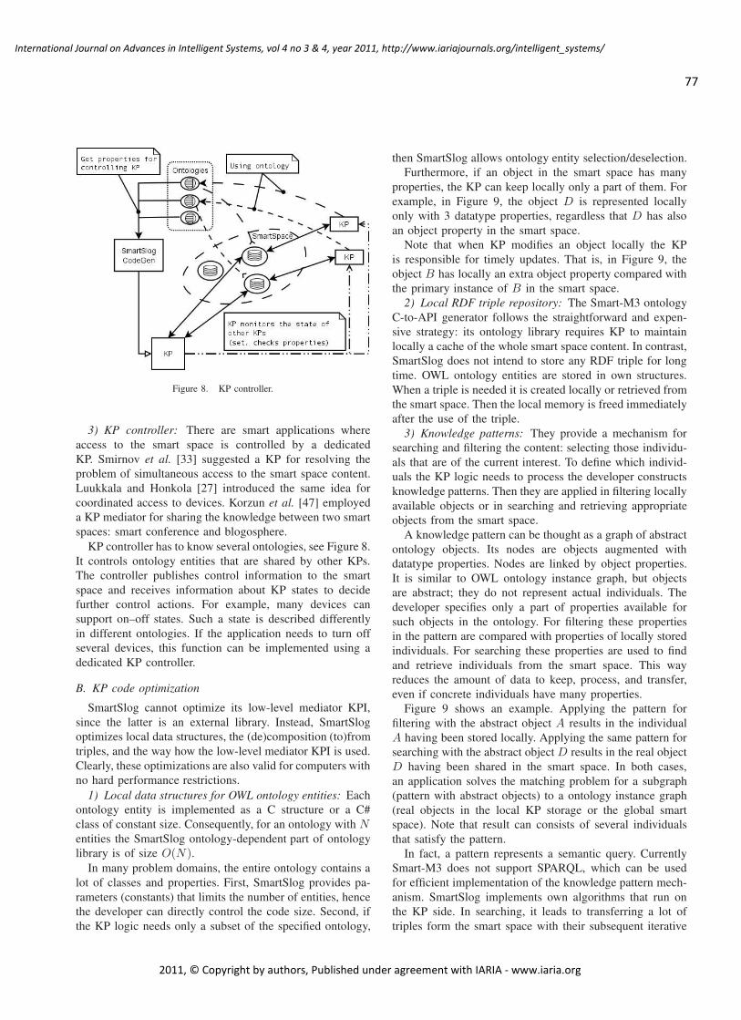
77



Figure 8. KP controller.

3) KP controller: There are smart applications where

access to the smart space is controlled by a dedicated

KP. Smirnov et al. [33] suggested a KP for resolving the

problem of simultaneous access to the smart space content.

Luukkala and Honkola [27] introduced the same idea for

coordinated access to devices. Korzun et al. [47] employed

a KP mediator for sharing the knowledge between two smart

spaces: smart conference and blogosphere.

KP controller has to know several ontologies, see Figure 8.

It controls ontology entities that are shared by other KPs.

The controller publishes control information to the smart

space and receives information about KP states to decide

further control actions. For example, many devices can

support on–off states. Such a state is described differently

in different ontologies. If the application needs to turn off

several devices, this function can be implemented using a

dedicated KP controller.

B. KP code optimization

SmartSlog cannot optimize its low-level mediator KPI,

since the latter is an external library. Instead, SmartSlog

optimizes local data structures, the (de)composition (to)from

triples, and the way how the low-level mediator KPI is used.

Clearly, these optimizations are also valid for computers with

no hard performance restrictions.

1) Local data structures for OWL ontology entities: Each

ontology entity is implemented as a C structure or a C#

class of constant size. Consequently, for an ontology with N

entities the SmartSlog ontology-dependent part of ontology

library is of size O(N).In many problem domains, the entire ontology contains a

lot of classes and properties. First, SmartSlog provides pa-

rameters (constants) that limits the number of entities, hence

the developer can directly control the code size. Second, if

the KP logic needs only a subset of the specified ontology,

then SmartSlog allows ontology entity selection/deselection.

Furthermore, if an object in the smart space has many

properties, the KP can keep locally only a part of them. For

example, in Figure 9, the object D is represented locally

only with 3 datatype properties, regardless that D has also

an object property in the smart space.

Note that when KP modifies an object locally the KP

is responsible for timely updates. That is, in Figure 9, the

object B has locally an extra object property compared with

the primary instance of B in the smart space.

2) Local RDF triple repository: The Smart-M3 ontology

C-to-API generator follows the straightforward and expen-

sive strategy: its ontology library requires KP to maintain

locally a cache of the whole smart space content. In contrast,

SmartSlog does not intend to store any RDF triple for long

time. OWL ontology entities are stored in own structures.

When a triple is needed it is created locally or retrieved from

the smart space. Then the local memory is freed immediately

after the use of the triple.

3) Knowledge patterns: They provide a mechanism for

searching and filtering the content: selecting those individu-

als that are of the current interest. To define which individ-

uals the KP logic needs to process the developer constructs

knowledge patterns. Then they are applied in filtering locally

available objects or in searching and retrieving appropriate

objects from the smart space.

A knowledge pattern can be thought as a graph of abstract

ontology objects. Its nodes are objects augmented with

datatype properties. Nodes are linked by object properties.

It is similar to OWL ontology instance graph, but objects

are abstract; they do not represent actual individuals. The

developer specifies only a part of properties available for

such objects in the ontology. For filtering these properties

in the pattern are compared with properties of locally stored

individuals. For searching these properties are used to find

and retrieve individuals from the smart space. This way

reduces the amount of data to keep, process, and transfer,

even if concrete individuals have many properties.

Figure 9 shows an example. Applying the pattern for

filtering with the abstract object A results in the individual

A having been stored locally. Applying the same pattern for

searching with the abstract object D results in the real object

D having been shared in the smart space. In both cases,

an application solves the matching problem for a subgraph

(pattern with abstract objects) to a ontology instance graph

(real objects in the local KP storage or the global smart

space). Note that result can consists of several individuals

that satisfy the pattern.

In fact, a pattern represents a semantic query. Currently

Smart-M3 does not support SPARQL, which can be used

for efficient implementation of the knowledge pattern mech-

anism. SmartSlog implements own algorithms that run on

the KP side. In searching, it leads to transferring a lot of

triples form the smart space with their subsequent iterative

78



Smart Space(sib store)

KP(local objects)

Pattern(abstract object)

Filtering Searching

DataType

Object

DataType

Object

DataType

ObjectDataType

Object

Object

Object

Object

Object

Object

Object

Object

DataType

DataType

DataType

DataType

DataType

DataType

DataType

DataType DataType

DataType

DataType

DataType

DataType

DataType

DataType

DataType

DataType

DataType

DataType

DataType DataType

DataType

DataType

DataType

DataType

DataType

Object A

Object B

Object C

Object D

Object A

Object B

Object C

Object D

Object A

Object B

Object C

Object D

Figure 9. SmartSlog content representation and knowledge patterns for filtering and searching. Objects are stored globally in the smart space (SIB); KPcaches them partially; knowledge patters allow efficient manipulations with both object stores.

processing.

Knowledge patterns allow defining an object by ontolog-

ical class, UUID, and checked properties (properties that

object should have). For more intelligent characterization,

patterns can be extended to support unchecked properties

(properties that object should not have) and conditional

properties (with relations like ≤,≥,≤,≥).

The possible points of further optimization are the follow-

ing. Optimization of patterns as semantic queries since the

performance of matching algorithms depends on the query

representation [18]. For filtering, the access to properties can

be optimized using hash tables.

4) Synchronization: SmartSlog supports both types of

subscriptions: synchronous and asynchronous. The latter

case requires threading. SmartSlog uses POSIX threads,

available on many embedded systems [8]. Nevertheless,

SmartSlog allows switching the asynchronous subscription

off if the target device has no thread support.

SmartSlog provides direct access both to the smart space

and local content. If many KPs asynchronously change

information in the smart space, the KP is responsible to

keep in the actual state the knowledge that KP is interested

in. Another way for data synchronization is subscription.

Consider the example in Figure 10. Let A be data to

synchronize. After local manipulations A is transformed

to A′ on the local side. In the smart space it is still A.

After the synchronization both sides keep the same A′. Then

A′ is transformed to A′′ on the SIB side (by some other

participants) while A′ remains locally. After synchronization

the same A′′ is on both sides. ∆1 is the period with stale

data in SIB and ∆2 is the period with locally stale data. The

synchronization problem is to minimize these periods.

SmartSlog supports blocking and non-blocking synchro-

nization (synchronous and asynchronous subscription). Both

require setting explicitly the objects to synchronize. In some

cases it can be difficult from the point of view of a KP

programmer. Therefore, KP should track for changing of

objects itself and keep them up to date.

When an object is changed locally then it is marked for

future synchronization. When an object is changed in the

smart space then the KP synchronizes the object in the non-

blocking mode. As a result, the developer uses local objects

assuming that they are always up to date. Since frequent

synchronization leads to the high resource consumption

(network throughput, SIB processing time) there should

be options to control synchronization. For instance, the

developer sets the data importance for better tradeoffs.

Finally, there should be a mechanism for determination

of synchronization time moments. The following parameters

affects this mechanism.

• Memory use: marking changed objects uses additional

memory, synchronize when the memory threshold has

been reached.

• Latest synchronization: synchronize when a time

threshold has been reached after the latest synchroniza-

tion. For instance, if a data item is changed rarely it is

synchronized immediately after its change.

• Network load: if the network is overloaded then the

79



Figure 10. Synchronization problem. δs are periods of desynchronization.

synchronization rate is reduced;

• Device load: if the device is overloaded then the syn-

chronization rate is reduced.

VIII. CONCLUSION

The addressed area of ontology library generation for

multitude of devices is very important. The realization of

the ubiquitous computing vision will by definition include a

lot of heterogeneous and transiently available devices around

us. Allowing these devices to easily share information with

other devices and architectures, large or small, will be very

important. SmartSlog is a tool that supports easy program-

ming of such devices for participating them in Smart-M3

applications.

This paper contributed the design of SmartSlog with

the advanced scheme of ontology library generation. A

KP developer can choose among several programming lan-

guages for the ontology library. The current implementation

supports ANSI C and C#. The operability was tested on

Linux- and Windows- based platforms, including console

(ANSI C), Qt (C/C++), and .NET (C#) environments.

The KP code is compact due to high-level ontology style.

SmartSlog ontology libraries are portable due to the reduc-

tion of system dependencies. For low-performance devices

the ontology library code follows ANSI C and POSIX stan-

dards. There are mechanisms for making ontology library

code modest and optimizable to device capacity.

The SmartSlog design allows adopting advanced ontolog-

ical and optimization methods. We showed that the ontology

library generation scheme supports multiple ontologies if

KP needs to access different parts of the smart space.

We identified several points in the SmartSlog generation

process where certain performance optimization methods

can be applied for the problems of device CPU/memory

consumption, network load, and data synchronization. Im-

plementation of these ontological and optimization features

as well as its experimental confirmation are topics of our

ongoing research.

ACKNOWLEDGMENT

Authors would like to thank Open Innovations Association

FRUCT for the provided support and R&D infrastructure.

We would also like to thank Iurii Bogoiavlenskii, Vesa

Luukkala, and Ronald Brown for providing feedback and

guidance during the construction of the SmartSlog tool.

REFERENCES

[1] D. Korzun, A. Lomov, P. Vanag, J. Honkola, and S. Balandin,“Generating modest high-level ontology libraries for Smart-M3,” in Proc. 4th Int’l Conf. Mobile Ubiquitous Computing,Systems, Services and Technologies (UBICOMM 2010), Oct.2010, pp. 103–109.

[2] J. Honkola, H. Laine, R. Brown, and O. Tyrkko, “Smart-M3 information sharing platform,” in Proc. IEEE Symp.Computers and Communications, ser. ISCC ’10. IEEEComputer Society, Jun. 2010, pp. 1041–1046.

[3] “Smart-M3: Free development software downloads atSourceForge.net,” Release 0.9.5beta, Dec. 2011. [Online].Available: http://sourceforge.net/projects/smart-m3/

[4] I. Oliver, “Information spaces as a basis for personalisingthe semantic web,” in Proc. 11th Int’l Conf. EnterpriseInformation Systems (ICEIS 2009), May 2009, pp. 179–184.

[5] L. J. B. Nixon, E. Simperl, R. Krummenacher, and F. Martin-recuerda, “Tuplespace-based computing for the semantic web:A survey of the state-of-the-art,” Knowl. Eng. Rev., vol. 23,pp. 181–212, Jun. 2008.

[6] P. T. Eugster, P. A. Felber, R. Guerraoui, and A.-M. Kermar-rec, “The many faces of publish/subscribe,” ACM Comput.Surv., vol. 35, pp. 114–131, June 2003.

[7] “SmartSlog: free development software downloadsat SourceForge.net,” Dec. 2011. [Online]. Available:http://sourceforge.net/projects/smartslog/

[8] M. Barr and A. Massa, Programming Embedded Systems:With C and GNU Development Tools. O’Reilly Media, Inc.,2006.

80



[9] P. Liuha, A. Lappetelainen, and J.-P. Soininen, “Smart ob-jects for intelligent applications - first results made open,”ARTEMIS Magazine, no. 5, pp. 27–29, Oct. 2009.

[10] “SOFIA project – smart objects for intelligent applications,”Dec. 2011. [Online]. Available: http://www.sofia-project.eu/

[11] “Devices and interoperability ecosystem,” Dec. 2011.[Online]. Available: http://www.diem.fi/

[12] D. J. Cook and S. K. Das, “How smart are our environments?an updated look at the state of the art,” Pervasive and MobileComputing, vol. 3, no. 2, pp. 53–73, 2007.

[13] I. Oliver and S. Boldyrev, “Operations on spaces of informa-tion,” in Proc. IEEE Int’l Conf. Semantic Computing (ICSC’09). IEEE Computer Society, Sep. 2009, pp. 267–274.

[14] S. Balandin and H. Waris, “Key properties in the developmentof smart spaces,” in Proc. 5th Int’l Conf. Universal Access inHuman-Computer Interaction. Part II: Intelligent and Ubiq-uitous Interaction Environments (UAHCI ’09). Springer-Verlag, 2009, pp. 3–12.

[15] D. Gelernter, “Generative communication in linda,” ACMTrans. Program. Lang. Syst., vol. 7, pp. 80–112, Jan. 1985.

[16] T. Berners-Lee, J. Hendler, and O. Lassila, “The semanticweb,” Scientific American, pp. 34–43, May 2001.

[17] D. Fensel, “Triple-space computing: Semantic web servicesbased on persistent publication of information,” in Proc. IFIPInt’l Conf. Intelligence in Communication Systems (INTELL-COMM 2004), ser. LNCS 3283. Springer, Nov. 2004, pp.43–53.

[18] J. Euzenat and P. Shvaiko, Ontology matching. Heidelberg(DE): Springer-Verlag, 2007.

[19] E. Prud’hommeaux and A. Seaborne, “SPARQL querylanguage for RDF,” W3C Recommendation, Jan. 2008.[Online]. Available: http://www.w3.org/TR/rdf-sparql-query/

[20] L. Nixon, E. P. B. Simperl, O. Antonechko, and R. Tolksdorf,“Towards semantic tuplespace computing: the semantic webspaces system,” in Proc. 2007 ACM symp. Applied computing,ser. SAC ’07. ACM, 2007, pp. 360–365.

[21] F. Martın-Recuerda, “Towards Cspaces: A new perspectivefor the Semantic Web,” in Proc. 1st IFIP WG12.5 WorkingConf. Industrial Applications of Semantic Web, M. Bramerand V. Terziyan, Eds., vol. 188. Springer, Aug. 2005, pp.113–139.

[22] M. Weiser, “The computer for the twenty-first century,”Scientific American, vol. 265, no. 3, pp. 94–104, 1991.

[23] D. Khushraj, O. Lassila, and T. W. Finin, “sTuples: Semantictuple spaces,” in Proc. 1st Annual Int’l Conf. Mobile andUbiquitous Systems (MobiQuitous 2004). IEEE ComputerSociety, 2004, pp. 268–277.

[24] R. Krummenacher, J. Kopecky, and T. Strang, “Sharingcontext information in semantic spaces,” in Proc. OTM 2005Workshops on the Move to Meaningful Internet Systems 2005,ser. LNCS 3762. Springer, 2005, pp. 229–232.

[25] A. Gomez-Goiri and D. Lopez-De-Ipina, “A triple space-based semantic distributed middleware for internet of things,”in Proc. 10th Int’l Conf. Current trends in web engineering(ICWE’10). Springer-Verlag, 2010, pp. 447–458.

[26] J. Honkola, H. Laine, R. Brown, and I. Oliver, “Cross-domaininteroperability: A case study,” in Proc. 9th Int’l Conf. NextGeneration Wired/Wireless Networking (NEW2AN’09) and2nd Conf. Smart Spaces (ruSMART’09), ser. LNCS 5764.Springer-Verlag, 2009, pp. 22–31.

[27] V. Luukkala and J. Honkola, “Integration of an an-swer set engine to smart-m3,” in Proc. 3rd Conf. SmartSpaces (ruSMART’10) and 10th Int’l Conf. Next GenerationWired/Wireless Networking (NEW2AN’10). Springer-Verlag,2010, pp. 92–101.

[28] J. Suomalainen, P. Hyttinen, and P. Tarvainen, “Secure infor-mation sharing between heterogeneous embedded devices,” inProc. 4th European Conf. Software Architecture (ECSA ’10):Companion Volume. ACM, 2010, pp. 205–212.

[29] A. Koren and A. Buntakov, “Access control in personallocalized semantic information spaces,” in Proc. 3rd Conf.Smart Spaces (ruSMART’10) and 10th Int’l Conf. NextGeneration Wired/Wireless Networking (NEW2AN’10), ser.ruSMART/NEW2AN’10. Springer-Verlag, 2010, pp. 84–91.

[30] A. D’Elia, D. Manzaroli, J. Honkola, and T. S. Cinotti,“Access control at triple level: Specification and enforcementof a simple RDF model to support concurrent applications insmart environments,” in Proc. 11th Int’l Conf. Next Genera-tion Wired/Wireless Networking (NEW2AN’11) and 4th Conf.Smart Spaces (ruSMART’11). Springer-Verlag, 2011.

[31] S. Boldyrev, I. Oliver, and J. Honkola, “A mechanism formanaging and distributing information and queries in a smartspace environment,” UBICC Journal, Jul 2009.

[32] I. Oliver, E. Nuutila, and S. Torma, “Context gatheringin meetings: Business processes meet the agents and thesemantic web,” in The 4th Int’l Workshop on Technologies forContext-Aware Business Process Management (TCoB 2009)within Proc. Joint Workshop on Advanced Technologies andTechniques for Enterprise Information Systems. INSTICCPress, May 2009.

[33] A. Smirnov, A. Kashnevik, N. Shilov, I. Oliver, S. Balandin,and S. Boldyrev, “Anonymous agent coordination in smartspaces: State-of-the-art,” in Proc. 9th Int’l Conf. Next Genera-tion Wired/Wireless Networking (NEW2AN’09) and 2nd Conf.Smart Spaces (ruSMART’09), ser. LNCS 5764. Springer-Verlag, 2009, pp. 42–51.

[34] D. Korzun, I. Galov, A. Kashevnik, K. Krinkin, andY. Korolev, “Integration of Smart-M3 applications: Blog-ging in smart conference,” in Proc. 4th Conf. SmartSpaces (ruSMART’11) and 11th Int’l Conf. Next GenerationWired/Wireless Networking (NEW2AN’11).

[35] K. Framling, A. Kaustell, I. Oliver, J. Honkola, and J. Nyman,“Sharing building information with smart-m3,” InternationalJournal on Advances in Intelligent Systems, vol. 3, no. 3&4,pp. 347–357, 2010.

81



[36] S. Balandin, I. Oliver, and S. Boldyrev, “Distributed architec-ture of a professional social network on top of M3 smart spacesolution made in PCs and mobile devices friendly manner,”in Proc. 3rd Int’l Conf. Mobile Ubiquitous Computing, Sys-tems, Services and Technologies (UBICOMM 2009). IEEEComputer Society, 2009, pp. 318–323.

[37] D. Zaiceva, I. Galov, and D. Korzun, “A blogging applicationfor smart spaces,” in Proc. 9th Conf. of Open InnovationsFramework Program FRUCT and 1st Regional MeeGo Sum-mit Russia–Finland, Apr. 2011, pp. 154–163.

[38] J. F. Gomez-Pimpollo and R. Otaolea, “Smart objects forintelligent applications – ADK,” in Proc. 2010 IEEE Symp.Visual Languages and Human-Centric Computing (VL/HCC),Sep 2010, pp. 267–268.

[39] “RDFAlchemy: an ORM (Object RDF Mapper) for semanticweb users,” Dec. 2011. [Online]. Available: http://www.openvest.com/trac/wiki/RDFAlchemy

[40] B. Lavender, “Spira: A linked data ORM for Ruby,” Dec.2011. [Online]. Available: http://blog.datagraph.org/2010/05/spira

[41] K. Czarnecki and U. W. Eisenecker, Generative Program-ming: Methods, Tools, and Applications. Addison-Wesley,2000.

[42] C. Rich and R. C. Waters, “Approaches to automatic pro-gramming,” Advances in Computers, vol. 37, pp. 1–57, 1993.

[43] “Jena: Java toolkit for developing semantic web applicationsbased on W3C recommendations for RDF and OWL,” Dec.2011. [Online]. Available: http://jena.sourceforge.net/,http://incubator.apache.org/jena/

[44] S. Krivov, R. Williams, and F. Villa, “GrOWL: A tool for vi-sualization and editing of OWL ontologies,” Web Semantics:Science, Services and Agents on the World Wide Web, vol. 5,no. 2, pp. 54–57, 2007.

[45] N. Choi, I.-Y. Song, and H. Han, “A survey on ontologymapping,” SIGMOD Record, vol. 35, pp. 34–41, Sep. 2006.

[46] A. Maedche, B. Motik, L. Stojanovic, R. Studer, and R. Volz,“Ontologies for enterprise knowledge management,” IEEEIntelligent Systems, vol. 18, pp. 26–33, Mar. 2003.

[47] D. Korzun, I. Galov, A. Kashevnik, K. Krinkin, and Y. Ko-rolev, “Blogging in the smart conference system,” in Proc.9th Conf. of Open Innovations Framework Program FRUCTand 1st Regional MeeGo Summit Russia–Finland, Apr. 2011,pp. 63–73.

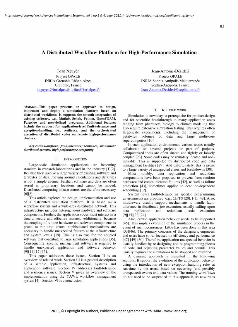
82



A Distributed Workflow Platform for High-Performance Simulation

Toàn Nguyên

Project OPALE

INRIA Grenoble Rhône-Alpes

Grenoble, France

[email protected], [email protected]

Jean-Antoine-Désidéri

Project OPALE

INRIA Sophia-Antipolis Méditerranée

Sophia-Antipolis, France

[email protected]

Abstract—This paper presents an approach to design,

implement and deploy a simulation platform based on

distributed workflows. It supports the smooth integration of

existing software, e.g., Matlab, Scilab, Python, OpenFOAM,

Paraview and user-defined programs. Additional features

include the support for application-level fault-tolerance and

exception-handling, i.e., resilience, and the orchestrated

execution of distributed codes on remote high-performance

clusters.

Keywords-workflows; fault-tolerance; resilience; simulation;

distributed systems; high-performance computing

I. INTRODUCTION

Large-scale simulation applications are becoming standard in research laboratories and in the industry [1][2]. Because they involve a large variety of existing software and terabytes of data, moving around calculations and data files is not a simple avenue. Further, software and data are often stored in proprietary locations and cannot be moved. Distributed computing infrastructures are therefore necessary [6][8].

This article explores the design, implementation and use of a distributed simulation platform. It is based on a workflow system and a wide-area distributed network. This infrastructure includes heterogeneous hardware and software components. Further, the application codes must interact in a timely, secure and effective manner. Additionally, because the coupling of remote hardware and software components is prone to run-time errors, sophisticated mechanisms are necessary to handle unexpected failures at the infrastructure and system levels [19]. This is also true for the coupled software that contribute to large simulation applications [35]. Consequently, specific management software is required to handle unexpected application and software behavior [9][11][12][15].

This paper addresses these issues. Section II is an overview of related work. Section III is a general description of a sample application, infrastructure, systems and application software. Section IV addresses fault-tolerance and resiliency issues. Section V gives an overview of the implementation using the YAWL workflow management system [4]. Section VI is a conclusion.

II. RELATED WORK

Simulation is nowadays a prerequisite for product design and for scientific breakthrough in many application areas ranging from pharmacy, biology to climate modeling that also require extensive simulation testing. This requires often large-scale experiments, including the management of petabytes volumes of data and large multi-core supercomputers [10].

In such application environments, various teams usually collaborate on several projects or part of projects. Computerized tools are often shared and tightly or loosely coupled [23]. Some codes may be remotely located and non-movable. This is supported by distributed code and data management facilities [29]. And unfortunately, this is prone to a large variety of unexpected errors and breakdowns [30].

Most notably, data replication and redundant computations have been proposed to prevent from random hardware and communication failures [42], as well as failure prediction [43], sometimes applied to deadline-dependent scheduling [12].

System level fault-tolerance in specific programming environments are proposed, e.g., CIFTS [20], FTI [48]. Also, middleware usually support mechanisms to handle fault-tolerance in distributed job execution, usually calling upon data replication and redundant code execution [9][15][22][24].

Also, erratic application behavior needs to be supported [45]. This implies evolution of the simulation process in the event of such occurrences. Little has been done in this area [33][46]. The primary concerns of the designers, engineers and users have so far focused on efficiency and performance [47] [49] [50]. Therefore, application unexpected behavior is usually handled by re-designing and re-programming pieces of code and adjusting parameter values and bounds. This usually requires the simulations to be stopped and restarted.

A dynamic approach is presented in the following sections. It support the evolution of the application behavior using the introduction of new exception handling rules at run-time by the users, based on occurring (and possibly unexpected) events and data values. The running workflows do not need to be suspended in this approach, as new rules

83



can be added at run-time without stopping the executing workflows.

This allows on-the-fly management of unexpected events. This approach also allows a permanent evolution of the applications that supports their continuous adaptation to the occurrence of unforeseen situations [46]. As new situations arise and data values appear, new rules can be added to the workflows that will permanently take them into account in the future. These evolutions are dynamically hooked onto the workflows without the need to stop the running applications. The overall application logics is therefore maintained unchanged. This guarantees a constant adaptation to new situations without the need to redesign the existing workflows. Further, because exception-handling codes are themselves defined by new ad-hoc workflows, the user interface remains unchanged [14].

III. TESTCASE APPLICATION

A. Example

This work is performed for the OMD2 project (Optimisation Multi-Discipline Distribuée, i.e., Distributed Multi-Discipline Optimization) supported by the French National Research Agency ANR.

An overview of two running testcases is presented here. It deals with the optimization of an auto air-conditioning system [36]. The goal of this particular testcase is to optimize the geometry of an air conditioner pipe in order to avoid air flow deviations in both pressure and speed concerning the pipe output (Figure 1). Several optimization methods are used, based on current research by public and industry laboratories.

Figure 1. Flow pressure (left) and speed (right) in an air-conditioner pipe (ParaView screenshots).

This example is provided by a car manufacturer and involves several industry partners, e.g., software vendors, and academic labs, e.g., optimization research teams (Figure 1).

The testcases are a dual faceted 2D and 3D example. Each facet involves different software for CAD modeling, e.g. CATIA and STAR-CCM+, numeric computations, e.g., Matlab and Scilab, and flow computation, e.g., OpenFOAM and visualization, e.g., ParaView (Figure 12, at the end of this paper).

The testcases are deployed on the YAWL workflow management system [4]. The goal is to distribute the testcases on various partners locations where the software are running (Figure 2). In order to support this distributed computing approach, an open source middleware is used [17].

A first step is implemented using extensively the virtualization technologies (Figure 3), i.e., Oracle VM VirtualBox, formerly SUN’s VirtualBox [7]. This allows hands-on experiments connecting several virtual guest computers running heterogeneous software (Figure 10, at the end of this paper). These include Linux Fedora Core 12,

Windows 7 and Windows XP running on a range of local workstations and laptops (Figure 11, at the end of this paper).

B. Application Workflow

In order to provide a simple and easy-to-use interface to the computing software, a workflow management system is used (Figure 2). It supports high-level graphic specification for application design, deployment, execution and monitoring. It also supports interactions among heterogeneous software components. Indeed, the 2D example testcase described in Section III.A involves several codes written in Matlab, OpenFOAM and displayed using ParaView (Figure 7). The 3D testcase involves CAD files generated using CATIA and STAR-CCM+, flow calculations using OpenFOAM, Python scripts and visualization with ParaView. Extensions allow also the use of the Scilab toolbox.

Because proprietary software are used, as well as open-source and in-house research codes, a secured network of connected computers is made available to the users, based on existing middleware (Figure 8).

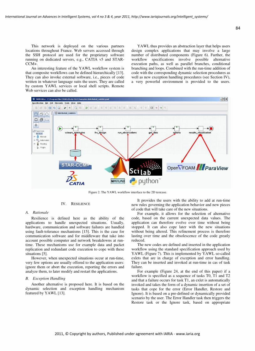
84



This network is deployed on the various partners locations throughout France. Web servers accessed through the SSH protocol are used for the proprietary software running on dedicated servers, e.g., CATIA v5 and STAR-CCM+.

An interesting feature of the YAWL workflow system is that composite workflows can be defined hierarchically [13]. They can also invoke external software, i.e., pieces of code written in whatever language suits the users. They are called by custom YAWL services or local shell scripts. Remote Web services can also be called.

YAWL thus provides an abstraction layer that helps users design complex applications that may involve a large number of distributed components (Figure 6). Further, the workflow specifications involve possible alternative execution paths, as well as parallel branches, conditional branching and loops. Combined with the run-time addition of code with the corresponding dynamic selection procedures as well as new exception handling procedures (see Section IV), a very powerful environment is provided to the users.

Figure 2. The YAWL workflow interface to the 2D testcase.

IV. RESILIENCE

A. Rationale

Resilience is defined here as the ability of the applications to handle unexpected situations. Usually, hardware, communication and software failures are handled using fault-tolerance mechanisms [15]. This is the case for communication software and for middleware that take into account possible computer and network breakdowns at run-time. These mechanisms use for example data and packet replication and redundant code execution to cope with these situations [5].

However, when unexpected situations occur at run-time, very few options are usually offered to the application users: ignore them or abort the execution, reporting the errors and analyze them, to later modify and restart the applications.

B. Exception Handling

Another alternative is proposed here. It is based on the dynamic selection and exception handling mechanism featured by YAWL [13].

It provides the users with the ability to add at run-time new rules governing the application behavior and new pieces of code that will take care of the new situations.

For example, it allows for the selection of alternative code, based on the current unexpected data values. The application can therefore evolve over time without being stopped. It can also cope later with the new situations without being altered. This refinement process is therefore lasting over time and the obsolescence of the code greatly reduced.

The new codes are defined and inserted in the application workflow using the standard specification approach used by YAWL (Figure 7). This is implemented by YAWL so-called exlets that are in charge of exception and error handling. They can be inserted and invoked at run-time in cas of task failure.

For example (Figure 24, at the end of this paper) if a workflow is specified as a sequence of tasks T0, T1 and T2 and that a failure occurs for task T1, an exlet is automatically invoked and takes the form of a dynamic insertion of a set of tasks that cope for the error (Error Handler, Restore and Ignore). It is based on a pre-defined or dynamically provided scenario by the user. The Error Handler task then triggers the Restore task or the Ignore task, based on appropriate

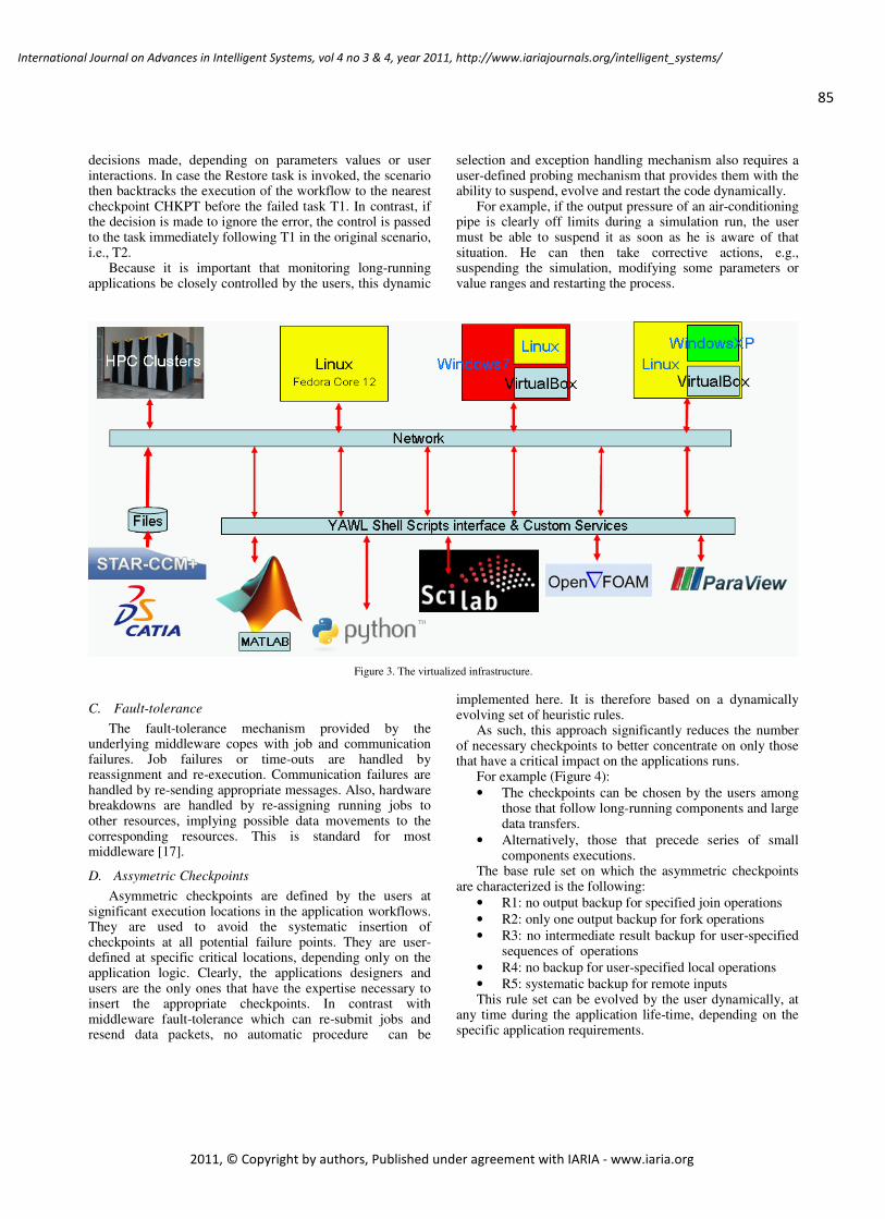
85



decisions made, depending on parameters values or user interactions. In case the Restore task is invoked, the scenario then backtracks the execution of the workflow to the nearest checkpoint CHKPT before the failed task T1. In contrast, if the decision is made to ignore the error, the control is passed to the task immediately following T1 in the original scenario, i.e., T2.

Because it is important that monitoring long-running applications be closely controlled by the users, this dynamic

selection and exception handling mechanism also requires a user-defined probing mechanism that provides them with the ability to suspend, evolve and restart the code dynamically.

For example, if the output pressure of an air-conditioning pipe is clearly off limits during a simulation run, the user must be able to suspend it as soon as he is aware of that situation. He can then take corrective actions, e.g., suspending the simulation, modifying some parameters or value ranges and restarting the process.

Figure 3. The virtualized infrastructure.

C. Fault-tolerance

The fault-tolerance mechanism provided by the underlying middleware copes with job and communication failures. Job failures or time-outs are handled by reassignment and re-execution. Communication failures are handled by re-sending appropriate messages. Also, hardware breakdowns are handled by re-assigning running jobs to other resources, implying possible data movements to the corresponding resources. This is standard for most middleware [17].

D. Assymetric Checkpoints

Asymmetric checkpoints are defined by the users at significant execution locations in the application workflows. They are used to avoid the systematic insertion of checkpoints at all potential failure points. They are user-defined at specific critical locations, depending only on the application logic. Clearly, the applications designers and users are the only ones that have the expertise necessary to insert the appropriate checkpoints. In contrast with middleware fault-tolerance which can re-submit jobs and resend data packets, no automatic procedure can be

implemented here. It is therefore based on a dynamically evolving set of heuristic rules.

As such, this approach significantly reduces the number of necessary checkpoints to better concentrate on only those that have a critical impact on the applications runs.

For example (Figure 4):

• The checkpoints can be chosen by the users among those that follow long-running components and large data transfers.

• Alternatively, those that precede series of small components executions.

The base rule set on which the asymmetric checkpoints are characterized is the following:

• R1: no output backup for specified join operations

• R2: only one output backup for fork operations

• R3: no intermediate result backup for user-specified sequences of operations

• R4: no backup for user-specified local operations

• R5: systematic backup for remote inputs This rule set can be evolved by the user dynamically, at

any time during the application life-time, depending on the specific application requirements.

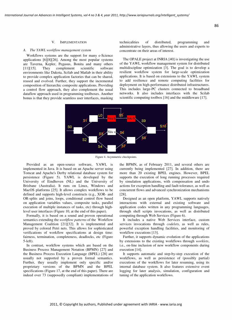
86



V. IMPLEMENTATION

A. The YAWL workflow management system

Workflows systems are the support for many e-Science

applications [6][8][26]. Among the most popular systems

are Taverna, Kepler, Pegasus, Bonita and many others

[11][15]. They complement scientific software

environments like Dakota, Scilab and Matlab in their ability

to provide complex application factories that can be shared,

reused and evolved. Further, they support the incremental

composition of hierarchic composite applications. Providing

a control flow approach, they also complement the usual

dataflow approach used in programming toolboxes. Another

bonus is that they provide seamless user interfaces, masking

technicalities of distributed, programming and

administrative layers, thus allowing the users and experts to

concentrate on their areas of interest.

The OPALE project at INRIA [40] is investigating the use

of the YAWL workflow management system for distributed

multidiscipline optimization [3]. The goal is to develop a

resilient workflow system for large-scale optimization

applications. It is based on extensions to the YAWL system

to add resilience and remote computing facilities for

deployment on high-performance distributed infrastructures.

This includes large-PC clusters connected to broadband

networks. It also includes interfaces with the Scilab

scientific computing toolbox [16] and the middleware [17].

Figure 4. Asymmetric checkpoints.

Provided as an open-source software, YAWL is

implemented in Java. It is based on an Apache server using

Tomcat and Apache's Derby relational database system for

persistence (Figure 5). YAWL is developed by the

University of Eindhoven (NL) and the University of

Brisbane (Australia). It runs on Linux, Windows and

MacOS platforms [25]. It allows complex workflows to be

defined and supports high-level constructs (e.g., XOR- and

OR-splits and joins, loops, conditional control flow based

on application variables values, composite tasks, parallel

execution of multiple instances of tasks, etc) through high-

level user interfaces (Figure 10, at the end of this paper).

Formally, it is based on a sound and proven operational

semantics extending the workflow patterns of the Workflow

Management Coalition [21][32]. It is implemented and

proved by colored Petri nets. This allows for sophisticated

verifications of workflow specifications at design time:

fairness, termination, completeness, deadlocks, etc (Figure

5-left).

In contrast, workflow systems which are based on the

Business Process Management Notation (BPMN) [27] and

the Business Process Execution Language (BPEL) [28] are

usually not supported by a proven formal semantics.

Further, they usually implement only specific and/or

proprietary versions of the BPMN and the BPEL

specifications (Figure 17, at the end of this paper). There are

indeed over 73 (supposedly compliant) implementations of

the BPMN, as of February 2011, and several others are

currently being implemented [27]. In addition, there are

more than 20 existing BPEL engines. However, BPEL

supports the execution of long running processes required

by simulation applications, with compensation and undo

actions for exception handling and fault-tolerance, as well as

concurrent flows and advanced synchronization mechanisms

[28].

Designed as an open platform, YAWL supports natively

interactions with external and existing software and

application codes written in any programming languages,

through shell scripts invocations, as well as distributed

computing through Web Services (Figure 6).

It includes a native Web Services interface, custom

services invocations through codelets, as well as rules,

powerful exception handling facilities, and monitoring of

workflow executions [13].

Further, it supports dynamic evolution of the applications

by extensions to the existing workflows through worklets,

i.e., on-line inclusion of new workflow components during

execution [14].

It supports automatic and step-by-step execution of the

workflows, as well as persistence of (possibly partial)

executions of the workflows for later resuming, using its

internal database system. It also features extensive event

logging for later analysis, simulation, configuration and

tuning of the application workflows.

87



Additionally, YAWL supports extensive organizations

modeling, allowing complex collaborative projects and

teams to be defined with sophisticated privilege

management: access rights and granting capabilities to the

various projects members (organized as networked teams of

roles and capabilities owners) on the project workflows,

down to individual components, e.g., edit, launch, pause,

restart and abort workitems, as well as processing tools and

facilities (Figure 5-right) [25].

Current experiments include industrial testcases,

involving the connection of the Matlab, Scilab, Python,

ParaView and OpenFOAM software to the YAWL platform

[3]. The YAWL workflow system is used to define the

optimization processes, include the testcases and control

their execution: this includes reading the input data

(StarCCM+ files), the automatic invocation of the external

software and automatic control passing between the various

application components, e.g., Matlab scripts, OpenFOAM,

ParaView (Figure 11, at the end of this paper).

Figure 5. The user interfaces: YAWL Editor (left) and YAWL Control Center (right).

B. Exception handling

The exception handlers are automatically tested by the

YAWL workflow engine when the corresponding tasks are

invoked. This is standard in YAWL and constraint checking

can be activated and deactivated by the users [4].

For example, if a particular workflow task WT invokes

an external EXEC code through a shell script SH (Figure 7)

using a standard YAWL codelet, an exception handler EX

can be implemented to prevent from undesirable situations,

e.g., infinite loops, unresponsive programs, long network

delays, etc. Application variables can be tested, allowing for

very close monitoring of the applications behavior, e.g.,

unexpected values, convergence rates for optimization

programs, threshold transgressions, etc.

A set of rules (RDR) is defined in a standard YAWL

exlet attached to the task WT and defines the exception

handler EX. It is composed here of a constraint checker CK,

which is automatically tested when executing the task WT. A

compensation action CP triggered when a constraint is

violated and a notifier RE warning the user of the exception.

This is used to implement resilience (Section V. C.).

The constraint violations are defined by the users and

are part of the standard exception handling mechanism

provided by YAWL. They can attach sophisticated exception

handlers in the form of specific exlets that are automatically

triggered at runtime when particular user-defined constraints

are violated. These constraints are part of the RDR attached

to the workflow tasks.

Resilience is the ability for applications to handle

unexpected behavior, e.g., erratic computations, abnormal

result values, etc. It is inherent to the applications logic and

programming. It is therefore different from systems or

hardware errors and failures. The usual fault-tolerance

mechanisms are therefore inappropriate here. They only cope

with late symptoms, at best.

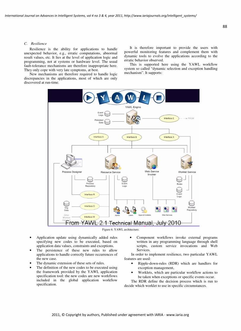
88



C. Resilience

Resilience is the ability for applications to handle unexpected behavior, e.g., erratic computations, abnormal result values, etc. It lies at the level of application logic and programming, not at systems or hardware level. The usual fault-tolerance mechanisms are therefore inappropriate here. They only cope with very late symptoms, at best.

New mechanisms are therefore required to handle logic discrepancies in the applications, most of which are only discovered at run-time.

It is therefore important to provide the users with

powerful monitoring features and complement them with dynamic tools to evolve the applications according to the erratic behavior observed.

This is supported here using the YAWL workflow system so called “dynamic selection and exception handling mechanism”. It supports:

Figure 6. YAWL architecture.

• Application update using dynamically added rules specifying new codes to be executed, based on application data values, constraints and exceptions.

• The persistence of these new rules to allow applications to handle correctly future occurrences of the new case.

• The dynamic extension of these sets of rules.

• The definition of the new codes to be executed using the framework provided by the YAWL application specification tool: the new codes are new workflows included in the global application workflow specification.

• Component workflows invoke external programs written in any programming language through shell scripts, custom service invocations and Web Services.

In order to implement resilience, two particular YAWL

features are used:

• Ripple-down-rules (RDR) which are handlers for

exception management,

• Worklets, which are particular workflow actions to

be taken when exceptions or specific events occur.

The RDR define the decision process which is run to

decide which worklet to use in specific circumstances.

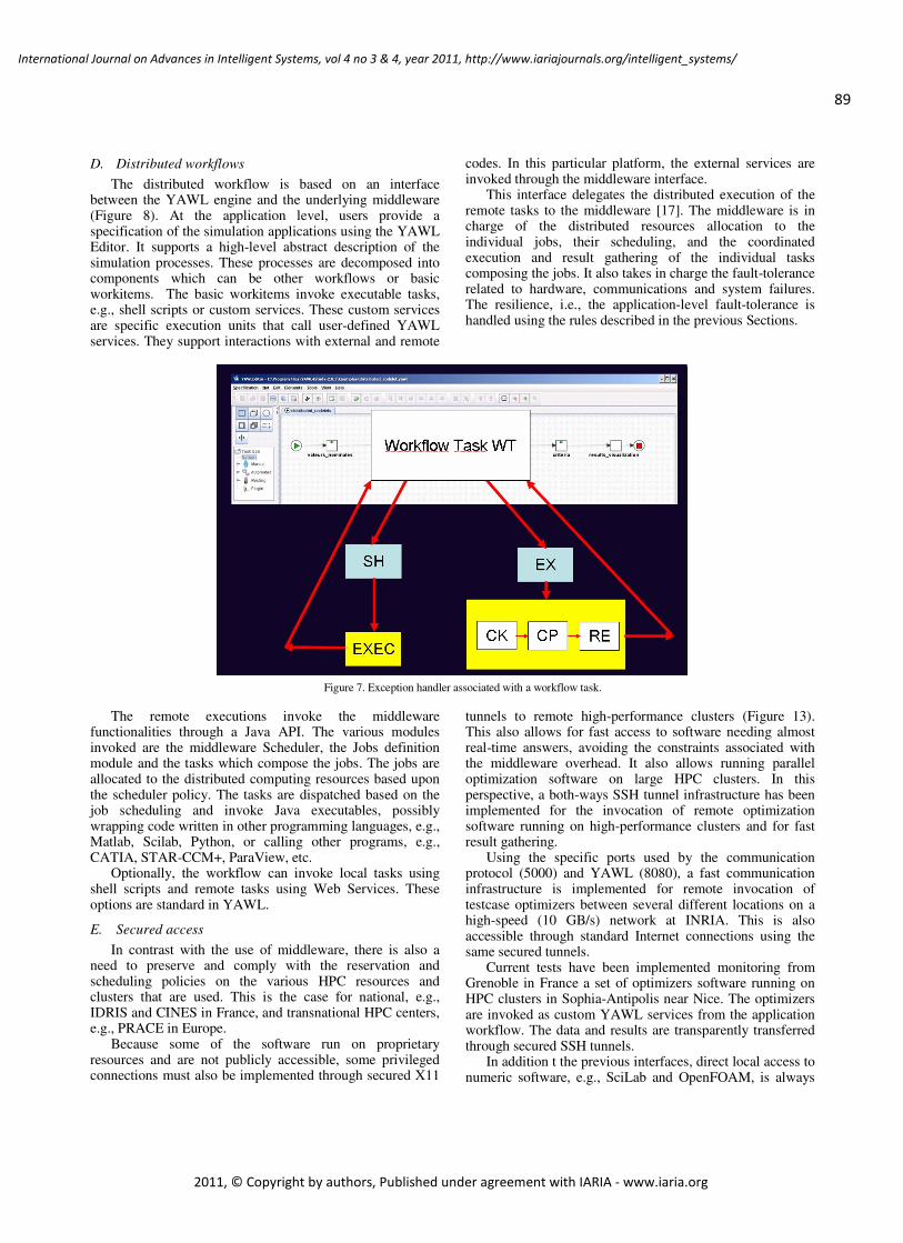
89



D. Distributed workflows

The distributed workflow is based on an interface between the YAWL engine and the underlying middleware (Figure 8). At the application level, users provide a specification of the simulation applications using the YAWL Editor. It supports a high-level abstract description of the simulation processes. These processes are decomposed into components which can be other workflows or basic workitems. The basic workitems invoke executable tasks, e.g., shell scripts or custom services. These custom services are specific execution units that call user-defined YAWL services. They support interactions with external and remote

codes. In this particular platform, the external services are invoked through the middleware interface.

This interface delegates the distributed execution of the remote tasks to the middleware [17]. The middleware is in charge of the distributed resources allocation to the individual jobs, their scheduling, and the coordinated execution and result gathering of the individual tasks composing the jobs. It also takes in charge the fault-tolerance related to hardware, communications and system failures. The resilience, i.e., the application-level fault-tolerance is handled using the rules described in the previous Sections.

Figure 7. Exception handler associated with a workflow task.

The remote executions invoke the middleware functionalities through a Java API. The various modules invoked are the middleware Scheduler, the Jobs definition module and the tasks which compose the jobs. The jobs are allocated to the distributed computing resources based upon the scheduler policy. The tasks are dispatched based on the job scheduling and invoke Java executables, possibly wrapping code written in other programming languages, e.g., Matlab, Scilab, Python, or calling other programs, e.g., CATIA, STAR-CCM+, ParaView, etc.

Optionally, the workflow can invoke local tasks using shell scripts and remote tasks using Web Services. These options are standard in YAWL.

E. Secured access

In contrast with the use of middleware, there is also a need to preserve and comply with the reservation and scheduling policies on the various HPC resources and clusters that are used. This is the case for national, e.g., IDRIS and CINES in France, and transnational HPC centers, e.g., PRACE in Europe.

Because some of the software run on proprietary resources and are not publicly accessible, some privileged connections must also be implemented through secured X11

tunnels to remote high-performance clusters (Figure 13). This also allows for fast access to software needing almost real-time answers, avoiding the constraints associated with the middleware overhead. It also allows running parallel optimization software on large HPC clusters. In this perspective, a both-ways SSH tunnel infrastructure has been implemented for the invocation of remote optimization software running on high-performance clusters and for fast result gathering.

Using the specific ports used by the communication protocol (5000) and YAWL (8080), a fast communication infrastructure is implemented for remote invocation of testcase optimizers between several different locations on a high-speed (10 GB/s) network at INRIA. This is also accessible through standard Internet connections using the same secured tunnels.

Current tests have been implemented monitoring from Grenoble in France a set of optimizers software running on HPC clusters in Sophia-Antipolis near Nice. The optimizers are invoked as custom YAWL services from the application workflow. The data and results are transparently transferred through secured SSH tunnels.

In addition t the previous interfaces, direct local access to numeric software, e.g., SciLab and OpenFOAM, is always

90



available through the standard YAWL custom services using the 8080 communication port and shell script invocations. Therefore, truly heterogeneous and distributed environments can be built here in a unified workflow framework.

F. Interfaces

To summarize, the simulation platform which is based on

the YAWL workflow management system for the application specification, execution and monitoring, provides three complementary interfaces that suit all potential performance, security, portability and interoperability requirements of the current sophisticated simulation environments.

These interfaces run concurrently and are used transparently for the parallel execution of the different parts of the workflows (Figure 14). These interfaces are:

• The direct access to numeric software through YAWL custom services that invoke Java executables and shell scripts that trigger numeric software, e.g., OpenFOAM, and visualization tools, e.g., ParaView (Figure 2)

• The remote access to high-performance clusters running parallel software, e.g., optimizers, through secured SSH tunnels, using remote invocations of custom services (Figure 13)

• The access to wide-area networks through a grid middleware, e.g., Grid5000, for distributed resource reservation and job scheduling (Figure 9)

Figure 8. The distributed simulation platform.

G. Service orchestration

The YAWL system provides a native Web service

interface. This is a very powerful standard interface to distributed service execution, although it might impact HPC concerns. This is the reason why a comprehensive set of interfaces are provided by the platform (Section F, above).

Combined altogether and offered to the users, this rich set of functionalities is intended to support most application requirements, in terms of performance, heterogeneity and standardization.

Basically, an application workflow specifies general services orchestration. General services include here not only Web services, but also shell scripts, YAWL custom services implemented by Java class executables and high-level operators, as defined in the workflow control flow patterns of the Workflow Management Coalition [5][21], e.g., AND-joins, XOR-joins, conditional branchings, etc.

The approach implemented here therefore not only fulfills sound and semantically proved operators for task specification, deployment, invocation, execution and. synchronization. It also fulfills the stringent requirements for heterogeneous distributed and HPC codes to be deployed and executed in a unified framework. This

91



provides the users with high-level GUIs and hides the technicalities of distributed, and HPC software combination, synchronization and orchestration.

Further, because resilience mechanisms are implemented at the application level (Section C), on top of the middleware, network and OS fault-tolerance features, a secured and fault resilient HPC environment is provided,

based on high-level constructs for complex and large-scale simulations [41].

The interface between the workflow tasks and the actual simulation codes can therefore be implemented as Web Services, YAWL custom services, and shell scripts through secured communication channels. This is a unique set of possibilities offered by our approach (Figure 14).

Figure 9. The YAWL workflow and middleware interface.

H. Dataflow and control flow

The dual requirements for the dataflow and control flow

properties are preserved. Both aspects are important and address different requirements [6]. The control flow aspect addresses the need for user control over the workflow tasks execution. The dataflow aspect addresses the need for high-performance and parallel algorithms to be implemented effectively.

The control flow aspect is required in order to provide the users with control over the synchronization and execution of the various heterogeneous and remote software that run in parallel and contribute to the application results. This aspect is exemplified in the previous sections (Secttion III) where multiple software contribute to the application results and visualization. This is natively supported by YAWL.

The dataflow aspect is also preserved here in two complementary ways:

• the workflow data is transparently managed by the YAWL engine to ensure the proper synchronization, triggering and stopping of the tasks and complex operators among the different parallel branches of the workflows, e.g., AND joins, OR and XOR forks, conditional branchings. This includes a unique YAWL feature called “cancellation set” that refers to a subset of a workflow that is frozen when another designated task is triggered [3]

• the data synchronization and dataflow scheme implemented by the specific numeric software

invoked remain unchanged using a separation of concerns policy, as explained below

The various software with dataflow dependencies are wrapped in adequate YAWL workflow tasks, so that the workflow engine does not interfere with the dataflow policies they implement.

This allows high-performance concerns to be taken into consideration along with the users concerns and expectations concerning the sophisticated algorithms associated with these programs.

Also, this preserves the global control flow approach over the applications which is necessary for heterogeneous software to cooperate in the workflow.

As a bonus, it allows user interactions during the workflow execution in order to cope with unexpected situations (Section IV). This would otherwise be very difficult to implement because when unexpected situations occur while using a pure dataflow approach, it requires stopping the running processes or threads in the midst of possibly parallel and remote running calculations, while (possibly remote) running processes are also waiting for incoming data produced by (possibly parallel and remote) erratic predecessors in the workflow. This might cause intractable situations even if the errors are due to rather simple events, e.g., network data transfers or execution time-outs.

Note that so far, because basic tasks cannot be divided into remote components in the workflow, the dataflow control is not supported between remotely located software. This also avoids large uncontrolled data transfers on the

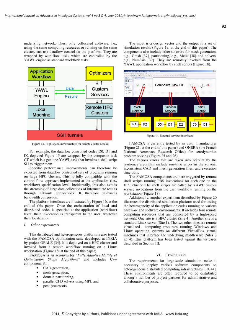
92



underlying network. Thus, only collocated software, i.e., using the same computing resources or running on the same cluster, can use dataflow control on the platform. They are wrapped by workflow tasks which are controlled by the YAWL engine as standard workflow tasks.

Figure 13. High-speed infrastructure for remote cluster access.

For example, the dataflow controlled codes D0, D1 and D2 depicted Figure 15 are wrapped by the composite task CT which is a genuine YAWL task that invokes a shell script SH to trigger them.

Specific performance improvements can therefore be expected from dataflow controlled sets of programs running on large HPC clusters. This is fully compatible with the control flow approach implemented at the application (i.e., workflow) specification level. Incidentally, this also avoids the streaming of large data collections of intermediate results through network connections. It therefore alleviates bandwidth congestion.

The platform interfaces are illustrated by Figure 16, at the end of this paper. Once the orchestration of local and distributed codes is specified at the application (workflow) level, their invocation is transparent to the user, whatever their localization.

I. Other experiments

This distributed and heterogeneous platform is also tested

with the FAMOSA optimization suite developed at INRIA by project OPALE [34]. It is deployed on a HPC cluster and invoked from a remote workflow running on a Linux workstation (Figure 18, at the end of this paper).

FAMOSA is an acronym for “Fully Adaptive Multilevel Optimization Shape Algorithms” and includes C++ components for:

• CAD generation,

• mesh generation,

• domain partitioning,

• parallel CFD solvers using MPI, and

• post-processors

The input is a design vector and the output is a set of simulation results (Figure 19, at the end of this paper). The components also include other software for mesh generation, e.g., Gmsh [37], partitioning, e.g., Metis [38] and solvers, e.g., Num3sis [39]. They are remotely invoked from the YAWL application workflow by shell scripts (Figure 18).

Figure 14. External services interfaces.

FAMOSA is currently tested by an auto manufacturer (Figure 21, at the end of this paper) and ONERA (the French National Aerospace Research Office) for aerodynamics problem solving (Figure 25 and 26).

The various errors that are taken into account by the resilience algorithm include run-time errors in the solvers, inconsistent CAD and mesh generation files, and execution time-outs.

The FAMOSA components are here triggered by remote shell scripts running PBS invocations for each one on the HPC cluster. The shell scripts are called by YAWL custom service invocations from the user workflow running on the workstation (Figure 18).

Additionally, another experiment described by Figure 20 illustrates the distributed simulation platform used for testing the heterogeneity of the application codes running on various hardware and software environments. It includes four remote computing resources that are connected by a high-speed network. One site is a HPC cluster (Site 4). Another site is a standard Linux server (Site 1). The two other sites are remote virtualized computing resources running Windows and Linux operating systems on different VirtualBox virtual machines that interface the underlying middleware (Sites 3 an 4). This platform has been tested against the testcases described in Section III.

VI. CONCLUSION

The requirements for large-scale simulation make it necessary to deploy various software components on heterogeneous distributed computing infrastructures [10, 44]. These environments are often required to be distributed among a number of project partners for administrative and collaborative purposes.

93



This paper presents an experiment for deploying a distributed simulation platform. It uses a network of high-performance computers connected by a middleware layer. Users interact dynamically with the applications using a workflow management system. It allows them to define, deploy and control the application executions interactively.

In contrast with choreography of services, where autonomous software interact in a controlled manner, but where resilience and fault-tolerance are difficult to implement, the approach used here is an orchestration of heterogeneous and distributed software components that interact in a dynamic way under the user control, in order to contribute to the application results [29]. This allows the dynamic interaction with the users in case of errors and erratic application behavior. This approach is also fully compatible with both the dataflow and control flow approaches which are often described as poorly compatible [30][31][32] and are extensively used in numeric software platforms.

Figure 15. Dataflow tasks wrapped by a composite YAWL task.

The underlying interface to the distributed components is a middleware providing resource allocation and job scheduling [17]. Because of the heterogeneity of the software and resources used, the platform also combines secured access to remote HPC clusters and local software in a unified workflow framework (Figure 20, at the end of this paper).

This approach is also proved to combine in an elegant way the dataflow control used by many HPC software and the control flow approach required by complex and distributed application execution and monitoring.

A significant bonus of this approach is that besides fault-tolerance provided by the middleware, which handles communication, hardware and job failures, the users can define and handle application logic failures at the workflow specification level. This means that a new abstraction layer is introduced to cope with application-level errors at run-time. Indeed, these errors do not necessarily result from programming and design errors. They may also result from unforeseen situations, data values and limit conditions that could not be envisaged. This is often the case for simulations due to their experimental nature, e.g., discovering the behavior of the system being simulated.

This provides support to resiliency using an asymmetric checkpoint mechanism. This feature allows for efficient handling mechanisms to restart only those parts of an application that are characterized by the users as necessary for overcoming erratic behavior.

Further, this approach can be evolved dynamically, i.e., when applications are running. This uses the dynamic selection and exception handling mechanism in the YAWL workflow system. It allows for new rules and new exception handling to be added on-line if unexpected situations occur at run-time.

ACKNOWLEDGMENT

This work is supported by the European Commission FP7 Cooperation Program “Transport (incl. aeronautics)”, for the GRAIN Coordination and Support Action (“Greener Aeronautics International Networking”), grant ACS0-GA-2010-266184. It is also supported by the French National Research Agency ANR (Agence Nationale de la Recherche), OMD2 project (Optimisation Multi-Discipline Distribuée), grant ANR-08-COSI-007, program COSINUS (Conception et Simulation).

REFERENCES

[1] T. Nguyên and J-A Désidéri, “A Distributed Workflow Platform for Simulation”, Proc. 4th Intl. Conf on Advanced Engineering Computing and Applications in Sciences (ADVCOMP2010), Florence (I), October 2010, pp. 375-382.

[2] A. Abbas, “High Computing Power: A radical Change in Aircraft Design Process”, Proc. 2nd China-EU Workshop on Multi-Physics and RTD Collaboration in Aeronautics, Harbin (China) April 2009, pp. 115-122.

[3] T. Nguyên and J-A Désidéri, “Dynamic Resilient Workflows for Collaborative Design”, Proc. 6th Intl. Conf. on Cooperative Design, Visualization and Engineering, Luxemburg, September 2009, Springer-Verlag, LNCS 5738, pp. 341–350 (2009)

[4] W. Van der Aalst et al., “Modern Business Process Automation: YAWL and its support environment”, Springer (2010).

[5] N. Russel, A.H.M ter Hofstede, and W. Van der Aalst, “Workflow Control Flow Patterns, A Revised View”, Technical Report, University of Eindhoven (NL), 2006.

[6] E. Deelman and Y. Gil., “Managing Large-Scale Scientific Workflows in Distributed Environments: Experiences and Challenges”, Proc. 2nd IEEE Intl. Conf. on e-Science and the Grid, Amsterdam (NL), December 2006, pp. 211-222.

[7] Oracle VM VirtualBox, User Manual, 2011. http://www.virtualbox.org Retreived: January, 2012.

[8] M. Ghanem, N. Azam, M. Boniface, and J. Ferris, “Grid-enabled workflows for industrial product design”, Proc. 2nd Intl. Conf. on e-Science and Grid Computing, Amsterdam (NL), December 2006, pp. 325-336.

[9] G. Kandaswamy, A. Mandal, and D.A. Reed., “Fault-tolerant and recovery of scientific workflows on computational grids”, Proc. 8th Intl. Symp. On Cluster Computing and the Grid, Lyon (F), May 2008, pp. 167-176.

[10] H. Simon, “Future directions in High-Performance Computing 2009- 2018”, Lecture given at the ParCFD 2009 Conference, Moffett Field (Ca), May 2009.

[11] J. Wang, I. Altintas, C. Berkley, L. Gilbert, and M.B. Jones, “A high-level distributed execution framework for scientific workflows”, Proc. 4th IEEE Intl. Conf. on eScience. Indianapolis (In), December 2008, pp. 233-246.

94



[12] D. Crawl and I. Altintas, “A Provenance-Based Fault Tolerance Mechanism for Scientific Workflows”, Proc. 2nd Intl. Provenance and Annotation Workshop, IPAW 2008, Salt Lake City (UT), June 2008, Springer, LNCS 5272, pp 152-159.

[13] M. Adams, A.H.M ter Hofstede, W. Van der Aalst, and N. Russell, “Facilitating Flexibility and Dynamic Exception Handling in Workflows through Worklets”, Technical report, Faculty of Information Technology, Queensland University of Technology, Brisbane (Aus.), October 2006.

[14] M. Adams and L. Aldred, “The worklet custom service for YAWL, Installation and User Manual”, Beta-8 Release, Technical Report, Faculty of Information Technology, Queensland University of Technology, Brisbane (Aus.), October 2006.

[15] L. Ramakrishna, et al., “VGrADS: Enabling e-Science workflows on grids and clouds with fault tolerance”, Proc. ACM/IEEE Intl. Conf. High Performance Computing, Networking, Storage and Analysis (SC09), Portland (Or.), November 2009, pp. 475-483.

[16] M. Baudin, “Introduction to Scilab”, Consortium Scilab, January 2010, Also: http://wiki.scilab.org/ Retreived: January, 2012.

[17] F. Baude et al., “Programming, composing, deploying for the grid”, in "GRID COMPUTING: Software Environments and Tools", Jose C. Cunha and Omer F. Rana (Eds), Springer Verlag, January 2006.

[18] http://edition.cnn.com/2009/TRAVEL/01/20/mumbai.overview Retreived: January, 2012.

[19] J. Dongarra, P. Beckman, et al., “The International Exascale Software Roadmap”, vol. 25, n.1, 2011, International Journal of High Performance Computer Applications, ISSN 1094-3420, pp, 89-96, Available at: http://www.exascale.org/ Retreived: January, 2012.

[20] R. Gupta, P. Beckman, et al., “CIFTS: a Coordinated Infrastructure for Fault-Tolerant Systems”, Proc. 38th Intl. Conf. Parallel Processing Systems, Vienna (Au), September 2009, pp. 289-296.

[21] The Workflow Management Coalition. http://www.wfmc.org Retreived: January, 2012.

[22] D. Abramson, B. Bethwaite, et al., “Embedding Optimization in Computational Science Workflows”, Journal of Computational Science 1 (2010), Pp 41-47, Elsevier, pp. 89-95.

[23] A.Bachmann, M. Kunde, D. Seider, and A. Schreiber, “Advances in Generalization and Decoupling of Software Parts in a Scientific Simulation Workflow System”, Proc. 4th Intl. Conf. Advanced Engineering Computing and Applications in Sciences, Florence (I), October 2010, pp. 179-186.

[24] R. Duan, R. Prodan, and T. Fahringer, “DEE: a Distributed Fault Tolerant Workflow Enactment Engine for Grid Computing”, Proc. 1st. Intl. Conf. on High-Performance Computing and Communications, Sorrento (I), LNCS 3726, September 2005, pp. 231-240.

[25] http://www.yawlfoundation.org/software/documentation. The YAWL foundation, 2010, Retreived: January, 2012.

[26] Y.Simmha, R. Barga, C. van Ingen, E. Lazowska, and A. Szalay, “Building the Trident Scientific Workflow Workbench for Data Management in the Cloud”, Proc. 3rd Intl. Conf. on Advanced Engineering Computing and Applications in Science (ADVCOMP2009), Sliema (Malta), October 2009, pp. 179-186.

[27] Object Management Group / Business Process Management Initiative, BPMN Specifications, http://www.bpmn.org, Retreived: January, 2012.

[28] Emmerich W., B. Butchart, and L. Chen, “Grid Service Orchestration using the Business Process Execution Language (BPEL)”, Journal of Grid Computing, vol. 3, pp 283-304, Springer.2006, pp. 257-262.

[29] Sherp G., Hoing A., Gudenkauf S., Hasselbring W., and Kao O., “Using UNICORE and WS-BPEL for Scientific Workfow execution in Grid Environments”, Proc. EuroPAR 2009, LNCS 6043, Springer, 2010, pp. 135-140.

[30] B. Ludäscher, M. Weske, T. McPhillips, and S. Bowers, “Scientific Workflows: Business as usual ?” Proc. BPM 2009, LNCS 5701, Springer, 2009, pp. 345-352.

[31] Montagnat J., Isnard B., Gatard T., Maheshwari K., and Fornarino M., “A Data-driven Workflow Language for Grids based on Array Programming Principles”, Proc. 4th Workshop on Workflows in Support of Large-Scale Science, WORKS 2009, Portland (Or), ACM 2009, pp. 123-128.

[32] Yildiz U., Guabtni A. and Ngu A.H., “Towards Scientific Workflow Patterns”, Proc. 4th Workshop on Workflows in Support of Large-Scale Science, WORKS 2009, Portland (Or), ACM 2009, pp. 247-254.

[33] Plankensteiner K., Prodan R., and Fahringer T., “Fault-tolerant Behavior in State-of-the-Art Grid Workflow Management Systems”, CoreGRID Technical Report TR-0091, October 2007.

[34] Duvigneau R., Kloczko T., and Praveen C.., “A three-level parallelization strategy for robust design in aerodynamics”, Proc. 20th Intl. Conf. on Parallel Computational Fluid Dynamics, May 2008, Lyon (F), pp. 379-384.

[35] E.C. Joseph, et al., “A Strategic Agenda for European Leadership in Supercomputing: HPC 2020”, IDC Final Report of the HPC Study for the DG Information Society of the EC, July 2010, Available at: http://www.hpcuserforum.com/EU/ Retreived: January, 2012.

[36] P.E. Gill, Murray W. and Wright M.H., Practical Optimization, Elsevier Academic Press, 2004.

[37] Gmsh. https://geuz.org/gmsh/ Retreived: January, 2012.

[38] Metis. http://glaros.dtc.umn.edu/gkhome/metis/metis/overview

Retreived: January, 2012.

[39] Num3sis. http://num3sis.inria.fr/blog/ Retreived: January, 2012.

[40] OPALE project at INRIA. http://www-opale.inrialpes.fr and http://wiki.inria.fr/opale Retreived: January, 2012.

[41] L. Trifan and T. Nguyên, “A Dynamic Workflow Simulation Platform”, Proc. 2011 Intl. Conf. on High-Performance Computing & Simulation, Istanbul (TK), July 2011, pp. 115-122.

[42] Plankensteiner K., Prodan R., and Fahringer T., “A New Fault-Tolerant Heuristic for Scientific Workflows in Highly Distributed Environments based on Resubmission impact”, Proc. 5th IEEE Intl. Conf. on e-Science, Oxford (UK), December 2009, pp 313-320.

[43] Z. Lan and Y. Li, “Adaptive Fault Management of Parallel Applications for High-Performance Computing”, IEEE Trans. On Computers, vol. 57, no. 12, December 2008, pp. 337-344.

[44] S. Ostermann, et al., “Extending Grids with Cloud Resource Management for Scientific Computing”, Proc. 10th IEEE/ACM Intl. Conf. on Grid Computing, 2009, pp. 457-462.

[45] E. Sindrilaru, A. Costan, and V. Cristea,. “Fault-Tolerance and Recovery in Grid Workflow Mangement Systems”, Proc. 4th Intl. Conf. on Complex, Intelligent and Software Intensive Systems, Krakow (PL), February 2010, pp. 85-92.

[46] S. Hwang and C. Kesselman, “Grid Workflow: A Flexible Failure Handling Framework for the Grid”, Proc. 12th IEEE Intl. Symp. on High Performance Distributed Computing, Seattle (USA), 2003, pp. 235-242.

[47] The Grid Workflow Forum: http://www.gridworkflow.org/snips/gridworkflow/space/start Retreived: January, 2012.

[48] Bautista-Gomez L., et al., “FTI: high-performance Fault Tolerance Interface for hybrid systems”, Proc. ACM/IEEE Intl. Conf. for High Performance Computing, Networking, Storage and Analysis (SC11), pp. 239-248, Seattle (Wa.)., November 2011.

[49] Bogdan N. and Cappello F., “BlobCR: Efficient Checkpoint-Retart for HPC Applications on IaaS Clouds using Virtual Disk Image Snapshots”, Proc. ACM/IEEE Intl. Conf. High Performance Computing, Networking, Storage and Analysis (SC11), pp. 145-156, Seattle (Wa.)., November 2011.

[50] Moody A., G.Bronevetsky, K. Mohror, B. de Supinski. “Design, Modeling and Evaluation of a Scalable Multi-level checkpointing System”, Proc. ACM/IEEE Intl. Conf. for High Performance Computing, Networking, Storage and Analysis (SC10), pp. 73-86. New Orleans (La.), November 2010.

95



Figure 10. The YAWL testcase and workflow editor deployed on a virtual machine: Linux Fedora Core 12 host running VirtualBox and Windows XP guest.

Figure 11. Parameter sweeping and YAWL interface to remote simulation codes.

96



Figure 12. The 3D testcase visualization (ParaView screenshot).

Figure 16. The platform interfaces to local and distributed codes.

97



Figure 17. BPMN metamodel - © 2007 OMG.

Figure 18. A distributed optimization experiment.

98



Figure 19. The FAMOSA optimization suite - © 2010 Régis Duvigneau – Project OPALE.

Figure 20. The distributed simulation platform.

99



Figure 21. Mesh for vehicle aerodynamics simulation (Gmsh screenshot).

Figure 22. Examples of resilience and fault-tolerance software.

100



Figure 23. Asymmetric checkpoints software for application resilience.

Figure 24. Error handler for task T1 error: YAWL exlet.

101



Figure 25. Pressure on a NACA airfoil (OpenFOAM testcase).

Figure 26. Pressure over a 2D airfoil (OpenFOAM testcase).

102



Opportunistic Object Binding and ProximityDetection for Multi-modal LocalizationMaarten Weyn, Isabelle De Cock, Yannick Sillis, Koen Schouwaert, Bruno Pauwels,

Willy Loockx and Charles VercauterenDept. of Applied Engineering

Artesis University College of AntwerpAntwerp, Belgium

[email protected]{Isabelle.decock, yannick.sillis, koen.schouwaert, bruno.pauwels}@student.artesis.be

{willy.loockx, charles vercauteren}@artesis.be

Abstract—In this paper, opportunistic object binding is pro-posed to improve multi-modal localization. Object binding andproximity detection will be realized using Bluetooth and WirelessSensor Networks. Multi-modal localization is created using anopportunistic seamless localization system, fusing Wi-Fi, Blue-tooth, Wireless Sensor Networks, GSM, GPS, RFID and inertialsensors. In this paper object binding is used to locate deviceswhich can not be located without the help of bound objects.

Index Terms—object binding, localization, opportunistic lo-calization, multi-modal localization, Bluetooth, WSN, Wi-Fi,proximity detection.

I. INTRODUCTION

Today, location based services are widely spread andalready integrated in many applications such as GPSnavigation systems, Google Earth, track and trace systems,Foursquare, etc. Outdoor localization is mostly accomplishedby means of GPS, but usually GPS does not work indoorbecause there has to be a minimum of four satellites in lineof sight, which is usually not the case indoor. Indoors, we canuse Bluetooth [1], [2], Wi-Fi [3] or GSM [4], or even othertechniques such as Wireless Sensor Network (WSN) [5], [6]and Ultra Wide Band (UWB) [7].

One big challenge is fusing these techniques into a singlesystem. Acquiring the sensor data of multiple sensors can berealized because most mobile devices such as Personal DigitalAssistants (PDAs) and smart phones are very often equippedwith GSM, GPS, WiFi or a combination of these. A systemwhich combines this technologies is called OpportunisticSeamless Localization System (OLS) [3].

The future of localization systems most likely will evolvetowards systems that can adapt and cope with any availableinformation provided by mobile clients without the needto install any additional dedicated infrastructure. This typeof localization is called opportunistic localization. It isdefined as [8]: “An opportunistic localization system is asystem, which seizes the opportunity and takes advantageof any readily available location related information in anenvironment, network and mobile device for the estimation of

the mobile device absolute or relative position without relyingon the installation of any dedicated localization hardwareinfrastructure.”

The OSL system combines the earlier mentionedtechnologies together with the information of accelerometers,compass and camera.

Currently, in OSL, the clients or ’trackable objects’ canbe any laptop running Windows or Linux, any smartphonerunning Windows Mobile, Android or OpenMoko or dedicatedOSL Wi-Fi or Zigbee tags. The complete system overview isshown in Figure 1.

OSL Server

Communication Interface

OSLController

Service API

Localization Engine

Database

3rd PartyEnd-Applications

Sensor data

Location update

Location update

Sensor data

Location update

MobileClients

LaptopClients

Sensor dataWiFi

TagsOSLTools

Fig. 1. The OSL system architecture

The clients send raw sensors data of the above mentionedtechnologies to the server, where the communication interfacewill parse these messages and send the appropriate data to thelocalization engine which will calculate a position estimation.This estimation is sent to the Service API which facilitatesthe communication with 3rd party application to, for example,visualize the positions on a map or trigger any events.

The localization engine seamlessly fuses the heterogeneoussensor data using an adaptive observation model for theparticle filter, taking the availability of every technology andsensor data into account. A particle filter [9] is a sequentialMonte Carlo based technique used for position estimation.Since we are working with a real-time system, it is even

103



harder to estimate the correct position therefore heavy andnumerous calculations are not recommended.

Limiting the number of particles is recommended in orderto avoid extensive time-consuming calculations. For example,when the system is implemented in a large scale environment,such as an airport where many devices are present, the systemmight be delayed due to these calculations for all thosedevices. Obviously, some objects will travel together such aspeople traveling by bus. In such cases, it is not necessaryto calculate all their positions with different particle clouds.Instead, we could combine all these objects and bind themin one group, in which case we only have to calculate oneposition for this group.

Besides from this optimization related reason for objectbinding, object binding also enables the system to locateobjects which can not be located by its own.

Bluetooth, for example, is a useful technology to detectother adjacent Bluetooth devices. Which would enable the pos-sibility to detect whether people are moving together. Anotherinteresting reason to use Bluetooth may be the possibility tolocate unknown people. This can, for example, be useful toestimate the amount of people in a given area.

Another technology, which can be used to detect theproximity of one device towards another, is WSN.

A third way of using object binding is to combine multipletags or devices which are related to one object, for example,a person having a laptop and a smartphone. In this casethe location data of the two devices has to be analyzed.Two possibilities can happen, first the object can be merged,for example, when the laptop and the smartphone are bothin the neigbhourhood of each other and most probablyalso in the neighbourhood of the person. Alternatively,heuristics can determine that the two devices are not atthe same place, for example, when the laptop is still inthe office but the person is walking with his smartphonethrough the building. In this case the position of the laptopcan not be connected with the position of the person anymore.

This paper is structured as follows: at first, Bluetooth objectbinding is discussed, where the scanning method for Bluetoothis analyzed followed by some real experiments to determinethe operational range of Bluetooth devices. Thereafter,Bluetooth signal strength values are discussed. This is thenfollowed by a short introduction about opportunistic seamlesslocalization and the explanation of the Bluetooth measurementmodel. Afterwards, WSN proximity detection is discussedwith some corresponding experiments. Finally, before theconclusion, multiple device binding is explained.

II. BLUETOOTH OBJECT BINDING

In this section, the use of Bluetooth for object binding andthe localization algorithm will be explained.

A. Bluetooth

Bluetooth [10] is a technology developed by Ericsson.This universal radio interface in the 2.45 GHz band makes itpossible to connect portable wireless devices with each other.Bluetooth uses frequency hopping to avoid interference withother devices, which also use the license-free 2.45 GHz band.

1) Discovering: There are two ways of discovering [11]devices when using Bluetooth. The first, and mostly usedmethod, is inquiry-based tracking. In case of inquiry-basedtracking, the base station needs to scan for devices and topage all present devices in order to find them. All devicesneed to be detectable but they need not to be identified inadvance.

Scanning for devices absorbs a relatively large amount oftime because primarily every base station sends a search-packet on all 32 radio channels. Every detectable device thatreceives this packet will answer. To avoid collision, everydevice will send his packet with a random delay. This isthe reason why an inquiry has to run for at least 10.24 sto be reliable. Many devices are undiscoverable in order toincrease the security and privacy of the owner. This is anothertechnical problem that could occur and consequently it is notpossible to find these devices by scanning the area.

A second method of tracking is the connection-basedtracking. With connection-based tracking, devices areconsidered to be in a close range when one device hasthe possibility to connect with another device. All deviceshave to be paired with each other and this is a majorproblem when using the Radio Frequency Communications(RFCOMM) layer [12] connections with connection-basedtracking. Practically, this requires human input which istime-consuming. Although, some communication services donot require this, it is still necessary that one of both devicesknows the other one exists.

In practice, the creation of an Asynchronous ConnectionlessLink (ACL) [12] and a basic Logical Link Control andAdaptation Protocol (L2CAP) layer [12] connection isuniversal and authorization-free. These connections arelimited but they are in compliance with the requirementsfor tracking usage. It is only necessary to know whether aconnection is possible and if this is the case, these 2 devicesare in the same range. This connection also supports somelow-level tasks such as RSSI measurements and L2CAP echorequests.

Both tracking techniques have their own advantages anddisadvantages and they are both not ideal. Choosing thecorrect technique will depend on the situation. When using

104



inquiry-based tracking, it is possible to find every detectabledevice without the need of knowing the devices in advance.The major disadvantage will be the relatively long scan time.When we choose the other option, connection-based tracking,the time to find the devices will be shorter and there is alsothe possibility to find undiscoverable devices. The majordisadvantage here is the requirement that at least one partyknows about the existence of the other one.

Another option could be a combination of both techniques.Combining these two techniques will not decrease therelatively long scan time because we always need totake the longest scan time in account. The advantage ofcombining both techniques is the possibility to find known’undiscoverable’ devices as well as unknown discoverabledevices.

In this paper, the first option is chosen because inquiry-based tracking has the possibility to track unknown devices,which will be useful for object binding.

2) Range: Bluetooth devices can be divided in threedifferent classes. Generally, class 1 and class 2 are usedinstead of class 3, which is due to the very short operatingrange of class 3.

Class Maximum Power Operating Range1 100 mW (20 dBm) Up to 100 m2 2.5 mW (4 dBm) Up to 10 m3 1 mW (0 dBm) Up to 1 m

These operating ranges are frequently used to estimate aposition since signal strength is not always a good parameterdue to effects like reflection and multi-path propagation [13] .

The operating range of a Bluetooth device can be definedby the maximum allowable path loss which can be calculatedwith Equation 1:

Ltotal = 20 ∗ log10(f) +N ∗ log10(d) + Lf (n)− 28(1)Ltotal = 40 + 20 ∗ log10(d) (2)

where N is the Distance Power Loss Coefficient, f is theFrequency (Mhz), d is the distance (meters) between thenodes , Lf is the Floor Penetration Loss Factor (dB) and n isthe number of floors penetrated.

When working in an open-air environment, Equation 2which is the simplified version of Equation 1, can beused [14].

As operating ranges will be used to estimate a position,some tests were done in order to decide which maximumrange will be used. A Dell XPS M1530 laptop has been setup as a base station. The two test devices were a SamsungE250 mobile phone (test device 1) and a Samsung F450

mobile phone (test device 2). All devices, including thebase station are devices of class 2. The measurements werestarted at a distance of one meter away from the basestation and afterwards extended by steps of one meter. Everymeasurement was repeated five times in order to have reliableresults.

Fig. 2. Experiment 1

The first experiment, as shown in Figure 2, was done inopen space in which the two test devices are in line-of-sightof the base station.

Both test devices could easily bridge a distance of 9 m.Once the distance was increased, test device 1 was not longerdetectable. Test device 2 was detectable until we reached adistance of 12 m.

Fig. 3. Experiment 2

In the next experiment, the influence of obstacles betweenthe base station and the test devices was tested. Thisexperiment was firstly done with a window between the basestation and the test devices. Secondly the experiment wasrepeated with a 14 cm thick brick wall instead of a window,see Figure 3.

Theoretically, obstacles comparable to a wall shouldsignificantly decrease the Bluetooth signal or even make itimpossible to connect with devices behind such obstacles.According to [?] the attenuation of a 2.4 Ghz signal througha brick wall of 8.9 cm is 6 dBi, of a concrete wall of 45 cm is17 dBi and the attenuation of an exterior single pane windowis 7 dBi. It is very hard to predict the attenuation becausethe exact material of the obstacle is generally not know. Ourtest with a window started showing problems with detectingtest device 1 at a distance of 4 m. Test device 2 remaineddetectable up to 7 m and at larger distances it started to showsome discontinuities.

The following test with a wall instead of a windowpaneshowed these results: at a distance of 4 m, test device 1 startedto disappear and at larger distances, test device 1 was rarelydetected. Test device 2 on the other hand, was much longervisible. In a range up to 7 m, test device 2 was still detectable.

These results, as can be seen in Figure 4, show a generalrange of 10 m when the base station and test device residein the same area hence we are working in an open space.

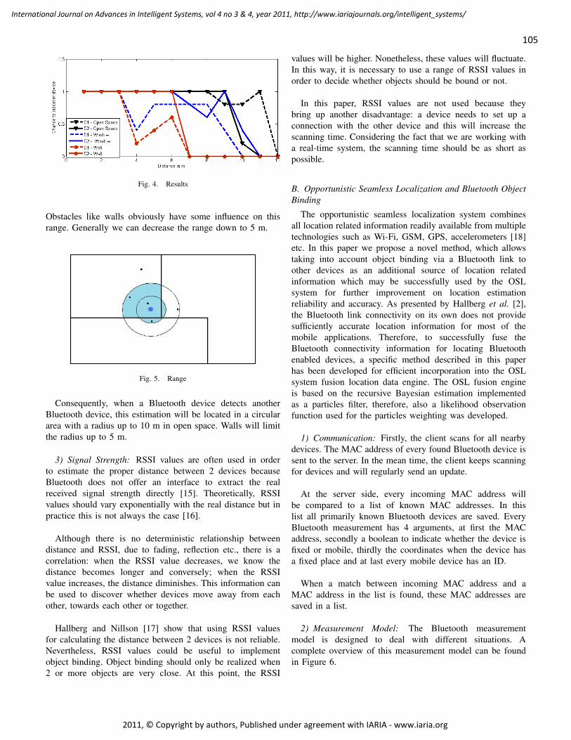
105



Fig. 4. Results

Obstacles like walls obviously have some influence on thisrange. Generally we can decrease the range down to 5 m.

Fig. 5. Range

Consequently, when a Bluetooth device detects anotherBluetooth device, this estimation will be located in a circulararea with a radius up to 10 m in open space. Walls will limitthe radius up to 5 m.

3) Signal Strength: RSSI values are often used in orderto estimate the proper distance between 2 devices becauseBluetooth does not offer an interface to extract the realreceived signal strength directly [15]. Theoretically, RSSIvalues should vary exponentially with the real distance but inpractice this is not always the case [16].

Although there is no deterministic relationship betweendistance and RSSI, due to fading, reflection etc., there is acorrelation: when the RSSI value decreases, we know thedistance becomes longer and conversely; when the RSSIvalue increases, the distance diminishes. This information canbe used to discover whether devices move away from eachother, towards each other or together.

Hallberg and Nillson [17] show that using RSSI valuesfor calculating the distance between 2 devices is not reliable.Nevertheless, RSSI values could be useful to implementobject binding. Object binding should only be realized when2 or more objects are very close. At this point, the RSSI

values will be higher. Nonetheless, these values will fluctuate.In this way, it is necessary to use a range of RSSI values inorder to decide whether objects should be bound or not.

In this paper, RSSI values are not used because theybring up another disadvantage: a device needs to set up aconnection with the other device and this will increase thescanning time. Considering the fact that we are working witha real-time system, the scanning time should be as short aspossible.

B. Opportunistic Seamless Localization and Bluetooth ObjectBinding

The opportunistic seamless localization system combinesall location related information readily available from multipletechnologies such as Wi-Fi, GSM, GPS, accelerometers [18]etc. In this paper we propose a novel method, which allowstaking into account object binding via a Bluetooth link toother devices as an additional source of location relatedinformation which may be successfully used by the OSLsystem for further improvement on location estimationreliability and accuracy. As presented by Hallberg et al. [2],the Bluetooth link connectivity on its own does not providesufficiently accurate location information for most of themobile applications. Therefore, to successfully fuse theBluetooth connectivity information for locating Bluetoothenabled devices, a specific method described in this paperhas been developed for efficient incorporation into the OSLsystem fusion location data engine. The OSL fusion engineis based on the recursive Bayesian estimation implementedas a particles filter, therefore, also a likelihood observationfunction used for the particles weighting was developed.

1) Communication: Firstly, the client scans for all nearbydevices. The MAC address of every found Bluetooth device issent to the server. In the mean time, the client keeps scanningfor devices and will regularly send an update.

At the server side, every incoming MAC address willbe compared to a list of known MAC addresses. In thislist all primarily known Bluetooth devices are saved. EveryBluetooth measurement has 4 arguments, at first the MACaddress, secondly a boolean to indicate whether the device isfixed or mobile, thirdly the coordinates when the device hasa fixed place and at last every mobile device has an ID.

When a match between incoming MAC address and aMAC address in the list is found, these MAC addresses aresaved in a list.

2) Measurement Model: The Bluetooth measurementmodel is designed to deal with different situations. Acomplete overview of this measurement model can be foundin Figure 6.

106



Fig. 6. Flowchart

There are 3 possible options when one or more Bluetoothdevices are found. The first option happens when the founddevices are unknown. These devices can not be used tolocalize the client device. Though, these devices can givesome interesting information, such as how many devices werepresent at a certain time in a certain place. This is alreadyimplemented at some places such as Brussels Airport [19].Every Bluetooth device that is discoverable will be detectedby fixed antennas. In this way it is possible to measurethe time necessary to move from one point to another andconsequently it will be possible to calculate the waiting timeto pass for example through the safety zone. When the founddevice is known, there are 2 options left: this device can bea fixed device, this is the second option, or a mobile devicewhich is the third option.

Dealing with the second option, returns a fixed positionwith the exact coordinates of the fixed device. With theknowledge that a Bluetooth device is only visible within acertain area around that device, the weight of all particlesfrom the client can be adapted.

Calculating the euclidean distance between every particleand the fixed device is the first step. After having calculatedthe distance between one particle and the fixed device, therewill be a wall check. A wall has a big influence on the signalstrength and for that reason it is important to know whetherthere is a wall between the fixed device and the particle. Thechoice to work with a larger or smaller range depends on theabsence or presence of a wall. Based on this range, the newparticle weight will be calculated.

If the third option occurs, a known mobile device isfound. This device does not show exact coordinates since thelocation of every mobile device is predicted with a particlecloud. Depending on the situation, a particle cloud can consistout of 100 particles up to 1000 particles. Comparing everyparticle of the found device with every particle of the clientdevice would be too heavy for a real-time system. For thisreason, 10 percent of random particles from the found deviceare compared to all particles of the client device. Choosing10 percent still gives us a reliable amount of particles. Thecoordinates of these particles are loaded and the distancebetween these particles and the client device particles iscalculated. Again, we need to check if there is no wallbetween the particles. Based on this information, the particleweight can be calculated.

Obviously, it is possible that more than one device isfound. For all those devices, previously mentioned optionswill be looked at and for every device, the correct optionwill be chosen. Working with multiple found devices, allcalculated particle weights are multiplied for every clientparticle. In this way all found devices are brought into thecalculation and the result becomes more accurate.

3) Particle Weight: According to the test results in thesection ’Range’, a range of 10 m will be used in open spaceand there will be a range of 5 m when there is an intersectionof a wall. It would be inaccurate to assume that discovereddevices are always in a range of 10 m with equal chancesto be everywhere in that circle. For this reason, using thesigmoid function gives a more realistic image. In this case,the following functions are used:

y =1

1 + ex−10(3)

y =1

1 + ex−5(4)

Equation (3) is used for open space. This functiongradually decreases and the particle weight will be based onthis function, see Figure 7. Equation (4) is used when a wallbetween the 2 devices is detected. This function will decreaseearlier because the obstacle has a big influence on the signalstrength which consequently will decrease quickly.

The measurement model for using Bluetooth measurementswith fixed devices is shown in Algorithm 1. An examplemeasurement probability is shown in Figure 8. In Figure 8(a)the likelihood function when a device at position (0,0)is discovered, is shown. A Class 2 Bluetooth device canbe discovered up to 10 m distance in line-of-sight. ASigmoid function is used to create a soft threshold betweenthe discoverable and the non-discoverable distance. In theexample, there is a wall from (-20,-3) to (-20,3). Since a wallattenuates the Bluetooth signal, the maximum discoverable

107



Fig. 7. Sigmoid function

(a) Bluetooth device at (0,0).

(b) Bluetooth device at (0,0) and (10,0).

Fig. 8. Example of Bluetooth measurement probability with a wall at y =-3.

distance will be lowered to 5 m if passing a wall. InFigure 8(b) two devices are discovered, one at (0,0) and oneat (10,0). In the case of multiple devices, the LikelihoodObservation Function (LOF) for each device is multiplied toget a LOF, which incorporates all discoverable devices.

The measurement model for using Bluetooth devices withmobile devices using object binding is shown in Algorithm 2and an example of such a likelihood based on a bound objectlocated with Wi-Fi is shown in Figure 9.

III. BLUETOOTH BASED OBJECT BINDING EXPERIMENTS

For these experiments, indoor localization is accomplishedby using Wi-Fi and Bluetooth. In these tests, the client isonly located by using Bluetooth. Multiple tests with fixed

Algorithm 1: Bluetooth Measurement Model ( zt, xt )1: w = 12: for all Bluetooth devices b ∈ zt do3: if b is known and fixed position xb then4: if no wall between xt and xb then5: w = w.

1

1 + ed(xt,xb)−10

6: else7: w = w.

1

1 + ed(xt,xb)−5

8: end if9: end if

10: end for11: return w

Algorithm 2: Object Binding Bluetooth Measurement Model( zt, xt )

1: w = 12: for all Bluetooth devices b ∈ zt do3: if b is known and particle distribution Xb known then4: take sample set Xb from Xb

5: for all xib in Xt do6: if no wall between xt and xib then7: w = w.

1

1 + ed(xt,xib)−10

8: else9: w = w.

1

1 + ed(xt,xib)−5

10: end if11: end for12: end if13: end for14: return w

Fig. 9. Example of Bluetooth measurement probability using object binding.

108



and mobile Bluetooth devices were done. The first test wasdone with one fixed and known device, see Figure 10(a).

The estimated position is located at the center of the circle,the real position is represented by a square and the positionof the found and known Bluetooth devices is represented bydots. It shows good room level accuracy, although still someparticles -representing different hypothesises- are in adjacentroom.

(a) Test with 1 fixed de-vice

(b) Test with 4 fixed de-vices

Fig. 10. Comparison between test with 1 or 4 fixed devices

Repeating this test, but now with 4 known and fixeddevices gives us a better result, see Figure 10(b). You see thatall hypothesises, represented by the particles, are now insidethe correct room. Using more found and known devicesresults logically in a more accurate estimation. This is dueto trilateration. The location of every fixed device will alsohave an influence on the accuracy, as shown in Figure 11(c)and 11(d). 11(c) shows a good location of fixed devices,the area where the client can be located is very small andconsequently more accurate. In 11(d), all fixed devices areclose to each other and therefore, the area where the clientcan be located is still large.

Fig. 11. Trilateration

Obviously the area where the client can be located is a lotsmaller when more devices are found. This illustrates whythe error rate decreases when the amount of found and knowndevices increases. Because we are using fixed devices only,it is possible to compare the clients particles with one exactposition. Every fixed device has a known position which doesnormally not change. Therefore the estimated position can beeasily calculated with a 100 percent certainty of the locationof the fixed Bluetooth device.

Of course this is a kind of localization which is previouslyalready developed in other research such as [2]. But Bluetoothcan be used stronger as a sensor when combined with othertechnologies to perform object binding.

In dynamic object binding, instead of static devices, othermobile devices will be used as references. Mobile devices donot have one exact and correct position. The likelihood of theirposition is estimated with a particle cloud. In order to calculatethe position of the client, all particles will be compared with10 percent of the particles from a found and known Bluetoothdevice. It is possible to increase the threshold of 10 percent,but using more particles will result in heavy calculations, usingless particles will make the final result inaccurate.

Fig. 12. Test with 1 mobile device

In this test, the client location, shown in 12(a), is calculatedbased on the particles of another mobile device, shown in12(b). Due to the fact that we do not have an exact positionof the mobile device, we have to estimate the client positionbased on another estimation. Consequently, the error rate isincreased, compared to the test with fixed devices. The errordepends largely on the correctness and distribution of thelikelihood of the dynamic reference device.

Dynamic object binding makes it possible to locate anyfound Bluetooth device without the necessity to have any othertechnology embedded in the device itself. Localization infor-mation from all found devices will be used to correctly locatethe client device. Merging different technologies improves thefinal result but within this structure, the position estimation ofeach device has always been created independent from otherdevices.

Of course we can combine dynamic reference devices andfixed devices when they are both discovered by the device.This increases the reliability of the estimation.

IV. WIRELESS SENSOR NETWORK PROXIMITYDETECTION

Wireless sensor networks are characterized by low-costwireless sensors to perform some action. The ideal wirelesssensor should meet certain conditions. Properties likescalability, low power consumption, integration in a network,programmability, capability of fast data transmission andlittle cost to purchase and install are very important duringthe fabrication of the sensors. It is not possible to meet allthese requirements. Therefore it is very important to know

109



all prerequisites of the application where the sensors will beused. There are two considerations to make, namely the useof low data rate sensors or high data rate sensors. Examplesof low data rate sensor include temperature and humidity.Examples of high rate sensors include strain, acceleration andvibration.

Today it is possible to assemble the sensors, radiocommunications and digital electronics into a single package.Therefore it is possible to make a wireless sensor network ofvery low cost sensors communicating with each other usingsmart routing protocols. Basically a WSN network consistsof a base station (gateway) and some sensor nodes. Thesesensor nodes send information directly to the gateway or ifnecessary use some other wireless sensor nodes to forwardthe data to the gateway. Eventually the data received in thegateway is presented to the system for processing.

Minimizing power consumption of any wireless sensingnode is a key feature to deal with. Mostly the radio subsystemrequires the largest amount of power. To minimize powerconsumption it is recommended to send data over the networkonly when required. There is also a possibility to minimizethe power consumption of the sensor itself. A lot of energycan be saved by only performing sensor measurement whenneeded instead of continuously. For example to locate people,it is not necessary to send data every second so energy couldbe saved by only send data every 5 seconds.

A. WSN Network Topology

Different topologies can be used to organize a WSN net-work:

In a star topology, all nodes are connected to a singlehub node. This node handles the routing and must be ableto perform more intensive messaging since it handles all thetraffic in the network. The hub node is very essential, when itgoes inactive, the network will be destroyed.

By using the ring topology, there is no coordinator. Allmessages travel in one direction, so when one node leavesthe ring, the communication is broken.

A bus topology has the property of broadcasting messagesto all the nodes connected to the bus. Each node checks thedestination address of the message’s header and checks if theaddress is equal to its address. When there is a match, thenode accepts the message, otherwise the node does nothing.

More complex, fully connected networks are characterizedby a connection from every node to every node. There are a lotof backups, so when one node leaves the network, messagescan still be routed via the other nodes. By adding nodes to thenetwork, the number of links increase exponentially, so therouting becomes too complex.

Finally, mesh networks are generally described as dis-tributed networks. Such networks allow communication be-tween a node and all other nodes including those outsideits radio transmission range. A big advantage of using this

topology is the use of multi-hop communication. Multi-hopcommunication allows transmission between 2 nodes thataren’t in each other range.

By using self-healing algorithms a mesh network has theproperty to enable a network to operate even when one nodebreaks down.

B. Existing WSN Localization Systems

Localization using WSN can be applied by using differentalgorithms. Getting the best results for the localization processdepends on two major parts: the influence of noise and thedifferent system parameter settings. Each algorithm performbetter in on other environments or with other WSN motes, sofor good localization, the used motes and the environmentshave to be taken into account. The localization techniques forWSN can be divided into two categories: range-based andconnectivity-based.

Range-based methods estimate the distance between nodeswith ranging methods such as Time-of-Flight, Angle ofArrival and Received Signal Strength. These techniquestypically provide better accuracy compared to connectivity-based algorithms, but are more complex. Connectivity-basedalgorithms do not estimate the distance between nodes butdetermine the position of a blind node by their proximity toanchor nodes [20].

Langendoen et al. [5] present in a survey 3 categories ofalgorithms for WSN localization: ad-hoc positioning [21],n-hop multi-lateration [22] and robust positioning [23]. Thesurvey concludes that no single algorithm performs perfectlyin every situation.

Another comparison is done by Zanca et al. [24]. Thispaper compares four algorithms: Min-Max, multi-lateration[5], Maximum Likelihood [25] and ROCRSSI [26]. Theabsolute ranging errors of the algorithms are presented withthe number of anchor nodes as a parameter. The authorsconclude that multi-lateration provides superior accuracycompared to the other algorithms when the number of anchornodes is high enough. Interestingly, despite its simplicity,Min-Max achieves reasonable performance.

MoteTrack [27] is a decentralized location tracking system.The location of each blind node is computed using a RSS sig-nature from the anchor nodes. This database of RSS signaturesis stored at the anchor nodes themselves.

Blumenthal et al. [28] present weighted centroidlocalization, the position of a blind node is calculatedas the centroid of the anchor nodes.

C. OSL and WSN Proximity Detection

The goal of this research is to use the nodes of a WSNnetwork to perform localization. Proximity localization willbe used to determine the mobile terminals position relative

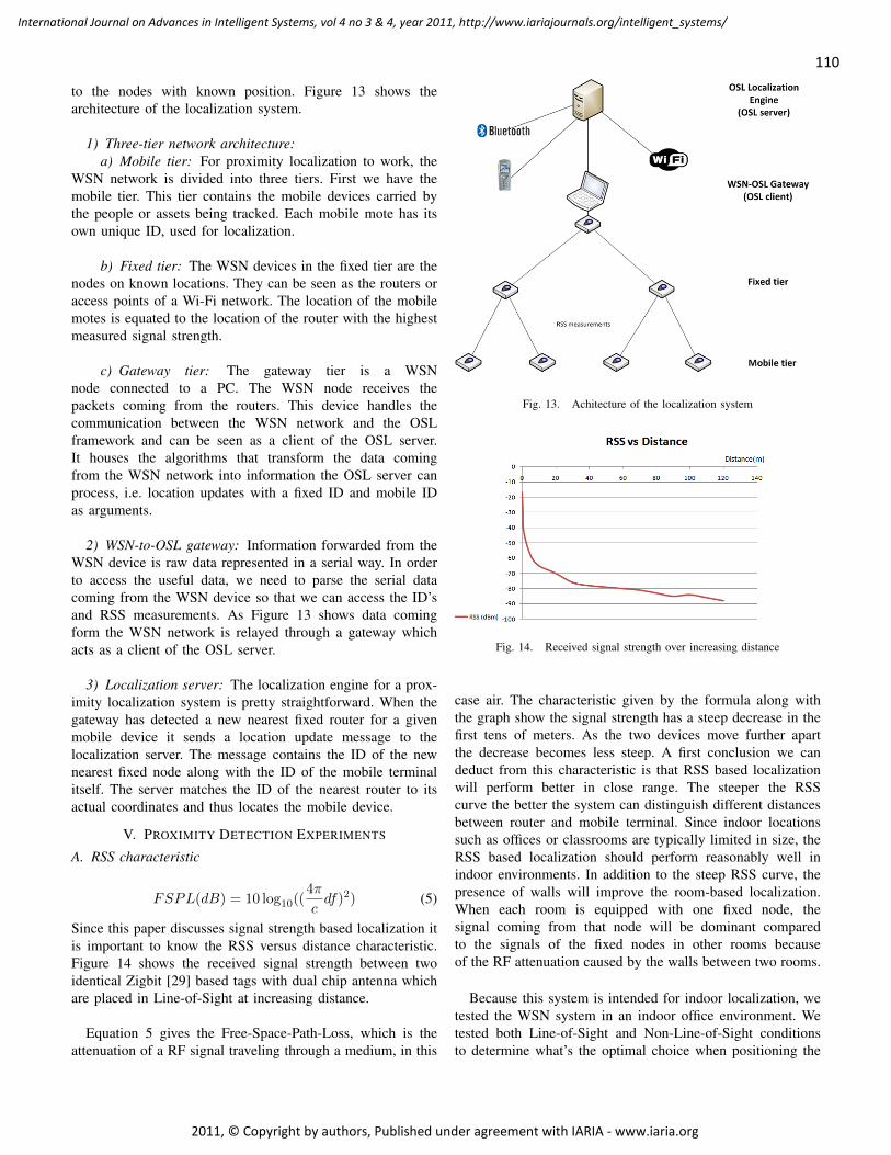
110



to the nodes with known position. Figure 13 shows thearchitecture of the localization system.

1) Three-tier network architecture:a) Mobile tier: For proximity localization to work, the

WSN network is divided into three tiers. First we have themobile tier. This tier contains the mobile devices carried bythe people or assets being tracked. Each mobile mote has itsown unique ID, used for localization.

b) Fixed tier: The WSN devices in the fixed tier are thenodes on known locations. They can be seen as the routers oraccess points of a Wi-Fi network. The location of the mobilemotes is equated to the location of the router with the highestmeasured signal strength.

c) Gateway tier: The gateway tier is a WSNnode connected to a PC. The WSN node receives thepackets coming from the routers. This device handles thecommunication between the WSN network and the OSLframework and can be seen as a client of the OSL server.It houses the algorithms that transform the data comingfrom the WSN network into information the OSL server canprocess, i.e. location updates with a fixed ID and mobile IDas arguments.

2) WSN-to-OSL gateway: Information forwarded from theWSN device is raw data represented in a serial way. In orderto access the useful data, we need to parse the serial datacoming from the WSN device so that we can access the ID’sand RSS measurements. As Figure 13 shows data comingform the WSN network is relayed through a gateway whichacts as a client of the OSL server.

3) Localization server: The localization engine for a prox-imity localization system is pretty straightforward. When thegateway has detected a new nearest fixed router for a givenmobile device it sends a location update message to thelocalization server. The message contains the ID of the newnearest fixed node along with the ID of the mobile terminalitself. The server matches the ID of the nearest router to itsactual coordinates and thus locates the mobile device.

V. PROXIMITY DETECTION EXPERIMENTS

A. RSS characteristic

FSPL(dB) = 10 log10((4π

cdf)2) (5)

Since this paper discusses signal strength based localization itis important to know the RSS versus distance characteristic.Figure 14 shows the received signal strength between twoidentical Zigbit [29] based tags with dual chip antenna whichare placed in Line-of-Sight at increasing distance.

Equation 5 gives the Free-Space-Path-Loss, which is theattenuation of a RF signal traveling through a medium, in this

Fig. 13. Achitecture of the localization system

Fig. 14. Received signal strength over increasing distance

case air. The characteristic given by the formula along withthe graph show the signal strength has a steep decrease in thefirst tens of meters. As the two devices move further apartthe decrease becomes less steep. A first conclusion we candeduct from this characteristic is that RSS based localizationwill perform better in close range. The steeper the RSScurve the better the system can distinguish different distancesbetween router and mobile terminal. Since indoor locationssuch as offices or classrooms are typically limited in size, theRSS based localization should perform reasonably well inindoor environments. In addition to the steep RSS curve, thepresence of walls will improve the room-based localization.When each room is equipped with one fixed node, thesignal coming from that node will be dominant comparedto the signals of the fixed nodes in other rooms becauseof the RF attenuation caused by the walls between two rooms.

Because this system is intended for indoor localization, wetested the WSN system in an indoor office environment. Wetested both Line-of-Sight and Non-Line-of-Sight conditionsto determine what’s the optimal choice when positioning the

111



fixed nodes. The fixed nodes are placed 15m apart in eachother’s line of sight in the first test and out of each other’sline of sight in the second test. A test person carrying themobile devices moves from one fixed node to another in stepsof one meter. After every step the person turns 360 degreesto check the localization’s dependency of the orientation ofthe tag.

(a) Line-Of-Sight (b) Non-Line-Of-Sight

Fig. 15. Indoor Localization Results

In figure 15 the position of the fixed nodes are indicatedby the dots and the area where the localization depends onthe orientation of the tag by a highlighted area. As figure15 shows there is a small area round the door where thelocalization performs poorly. Figure 15(b) shows this area isclearly smaller in the NLOS case than in the LOS case offigure 15(a). The reason for this is that when a fixed nodein one room has a line of sight into another room, it’s RFsignals will propagate through that door, or other openingfor that matter, without the attenuation caused by the walls.When the fixed nodes have no line of sight into the adjacentrooms, as in figure 15(b), the signals of the fixed nodes willattenuate when propagating through the walls or through thedoor after reflecting on the other walls.

VI. MULTIPLE DEVICE BINDING

The concept of object binding can also be considered intwo extra ways. The first one is tackling the issue of peoplewearing more than one tracked device. The second focusingon storage areas where dozens of tracked assets are stocked.In both cases the goal is to reduce objects visible on theclient user interface [30].

The multiple device issue shouldn’t so much be seen asa problem but as an improvement. If a person is carrying3 devices, this means the server will calculate his position3 times. This results in 3 coordinates, each with their ownquality of location circle suggesting the area where thepersons actual position is. Figure 16 below shows how the

most likely area can be narrowed in 2 ways.

Fig. 16. Multiple device binding. On the left side by trilateration. On theright side using the average of only the outermost X and Y values.

On the left trilateration is used to merge the 3 coordinates.The quality of location (QoL) is used as the radius. QoLis a measure of how confident the OSL server is aboutit’s calculated position. This technique should be the mostaccurate. On the right side another technique uses theminimum and maximum coordinate value of all pointsin each dimension to calculate the middle. Although thiscalculation needs less processing power, it is also the leastaccurate. Both show the concepts in only 2 dimensions,OSL calculates the position in 3. Another way is to takethe average of each dimension. This technique should scorebetween previous two techniques in terms of accuracy anduses about the same processing power as the second technique.

The second issue concerning the assets could be handledby adding a static location. When the assets are within rangeof the storage area, they can be snapped to the static location.This way coupling stored assets into 1 location will increaseend-user data comprehensibility. The implementation forthis can be done in roughly the same way as stated for themultiple device issue only there is no need to calculate anaverage position.

VII. CONCLUSION AND FUTURE WORK

In this paper, a method to realise dynamic object binding ispresented. We choose Bluetooth to accomplish object bindingbecause of its appearance in many mobile devices. For thisproject, the Bluetooth technology is fused with multiple othertechnologies in order to get an accurate localization system.Some real experiments were done to test the Bluetoothmeasurement model. These results showed room accuracywhen only Bluetooth was used. Obstacles like walls havea big influence on the signal strength which will make iteasier to achieve room-level accuracy. This information isincorporated in the Bluetooth measurement model.

Dynamic object biding is used to locate devices whichcannot be located by any other technology but can discoverother devices which are located by other means. Dynamic

112



object binding can increase the likelihood of the position ofthese devices.

This paper shows that Wireless Sensor Networks can beused for localization purposes and how it is incorporatedint the Opportunistic Seamless Localization framework. Inindoor environments however the room-level localization isreasonably accurate depending on the location of the fixednodes and the configured transmission power depending onthe layout of the indoor environment.

Tests indicate that this Wireless Sensor Networks ProximityLocalization system performs poorly in large outdoorenvironments, for outdoor use a GPS is recommended. Forindoor environments however, exactly where this system isdesigned for, the localization seems to be pretty accurate.Also the position of the fixed nodes plays a role in thereliability of the locations yielded by the system. The idealconditions are an indoor environment with rooms up to 20m long, with fixed nodes placed in such a way so they havea limited line of sight into the adjacent rooms. The thickerthe walls separating the rooms, the better the room-levellocalization will perform.

REFERENCES

[1] I. De Cock, W. Loockx, M. Klepal, and M. Weyn, “Dynamic ObjectBinding for Opportunistic Localisation,” in UBICOMM 2010: TheFourth International Conference on Mobile Ubiquitous Computing,Systems, Services and Technologies. Florence, Italy: IARIA, October2010, pp. 405–411.

[2] J. Hallberg, M. Nilsson, and K. Synnes, “Positioning with bluetooth,” in10th International Conference on Telecommunications. ICT 2003, 2003,pp. 954–958.

[3] M. Weyn, “Opportunistic Seamless Localization,” Ph.D. dissertation,University of Antwerp, 2011.

[4] A. Varshavsky, E. de Lara, J. Hightower, A. LaMarca, and V. Otsason,“GSM indoor localization,” Pervasive and Mobile Computing, vol. 3,no. 6, pp. 698–720, 2007.

[5] K. Langendoen and N. Reijers, “Distributed localization in wireless sen-sor networks: a quantitative comparison,” Computer Networks, vol. 43,no. 4, pp. 499–518, 2003.

[6] A. Nasipuri and K. Li, “A Directionality based Location DiscoveryScheme for Wireless Sensor Networks,” in Proceedings of the First ACMInternational Workshop on Wireless Sensor Networks and Applications,2002.

[7] S. Gezici, Z. Tian, G. V. Giannakis, H. Kobaysahi, A. F. Molisch, H. V.Poor, and Z. Sahinoglu, “Localization via Ultra-Wideband Radios: ALook at Positioning Aspects for Future Sensor Networks,” IEEE SignalProcessing Magazine, vol. 22, pp. 70–84, 2005.

[8] M. Weyn and M. Klepal, “OLS - Opportunistic Localization System forSmart Phones Devices,” in Mobile Phones: Technology, Networks andUser Issues. Nova, 2011.

[9] F. Gustafsson, F. Gunnarsson, N. Bergman, U. Forssell, J. Jansson,R. Karlsson, and P. Nordlund, “Particle filters for positioning, navigation,and tracking,” IEEE Transactions on signal processing, vol. 50, no. 2,pp. 425–437, 2002.

[10] J. Haartsen, “Bluetooth-The universal radio interface for ad hoc, wirelessconnectivity,” Ericsson review, vol. 3, no. 1, pp. 110–117, 1998.

[11] S. Hay and R. Harle, “Bluetooth Tracking without Discoverability,” inLocation and Context Awareness: 4th International Symposium, LoCA2009 Tokyo, Japan, May 7-8, 2009 Proceedings. Springer-Verlag NewYork Inc, 2009, pp. 120–137.

[12] J. Bray and C. Sturman, Connect without cables. Prentice Hall PTRUpper Saddle River, NJ, USA, 2000.

[13] A. Huang, “The use of Bluetooth in Linux and location aware comput-ing,” Ph.D. dissertation, Citeseer, 2005.

[14] Weidler, “Rugged Bluetooth Scanners,” Motorola, Tech. Rep., 2010.[15] S. Feldmann, K. Kyamakya, A. Zapater, and Z. Lue, “An indoor

Bluetooth-based positioning system: concept, implementation and exper-imental evaluation,” in International Conference on Wireless Networks,2003, pp. 109–113.

[16] U. Bandara, M. Hasegawa, M. Inoue, H. Morikawa, and T. Aoyama,“Design and implementation of a bluetooth signal strength based lo-cation sensing system,” in 2004 IEEE Radio and Wireless Conference,2004, pp. 319–322.

[17] J. Hallberg and M. Nilsson, “Positioning with bluetooth, irda andrfid,” Computer Science and Engineering, Lulea University of technol-ogy/2002, vol. 125, 2002.

[18] I. Bylemans, M. Weyn, and M. Klepal, “Mobile Phone-Based Displace-ment Estimation for Opportunistic Localisation Systems,” in The ThirdInternational Conference on Mobile Ubiquitous Computing, Systems,Services and Technologies (UBICOMM 2009). IEEE, 2009, pp. 113–118.

[19] B. A. Company, “Accurate real-time informa-tion on waiting times,” 2010. [Online]. Available:http://www.brusselsairport.be/en/news/newsItems/361700

[20] J. Hightower and G. Borriello, “A survey and taxonomy of locationsystems for ubiquitous computing,” IEEE Computer, vol. 34, no. 8, pp.57–66, 2001.

[21] D. Niculescu and B. Nath, “DV based positioning in ad hoc networks,”Telecommunication Systems, vol. 22, no. 1, pp. 267–280, 2003.

[22] A. Savvides, H. Park, and M. B. Strivastava, “The bits and flops ofthe n-hop multilateration primitive for node localization problems,” inProceedings of the 1st ACM international workshop on Wireless sensornetworks and applications. ACM, 2002, p. 121.

[23] C. Savarese, J. Rabaey, and K. Langendoen, “Robust positioning al-gorithms for distributed ad-hoc wireless sensor networks,” in USENIXtechnical annual conference, vol. 2. Monterey, CA, 2002.

[24] G. Zanca, F. Zorzi, A. Zanella, and M. Zorzi, “Experimental comparisonof RSSI-based localization algorithms for indoor wireless sensor net-works,” in Proceedings of the workshop on Real-world wireless sensornetworks, April, 2008, pp. 01–01.

[25] N. Patwari, R. O’Dea, and Y. Wang, “Relative location in wirelessnetworks,” in Vehicular Technology Conference, 2001. VTC 2001 Spring.IEEE VTS 53rd, vol. 2. IEEE, 2002, pp. 1149–1153.

[26] C. Liu, K. Wu, and T. He, “Sensor localization with ring overlappingbased on comparison of received signal strength indicator,” in MobileAd-hoc and Sensor Systems, 2004 IEEE International Conference on.IEEE, 2005, pp. 516–518.

[27] K. Lorincz and M. Welsh, “MoteTrack: a robust, decentralized approachto RF-based location tracking,” Personal and Ubiquitous Computing,vol. 11, no. 6, pp. 489–503, 2007.

[28] J. Blumenthal, R. Grossmann, F. Golatowski, and D. Timmermann,“Weighted centroid localization in Zigbee-based sensor networks,” inIntelligent Signal Processing, 2007. WISP 2007. IEEE InternationalSymposium on. IEEE, 2008, pp. 1–6.

[29] “ZigBit Development Kit 2.3 User Guide,” ZigBit, Tech. Rep., October2008.

[30] R. T. Ng and J. Han, “Efficient and effective clustering methods forspatial data mining,” p. 12, 1994.

113



Semantic Matchmaking for Location-Aware Ubiquitous Resource Discovery

Michele Ruta, Floriano Scioscia, Eugenio Di Sciascio, Giacomo Piscitelli Politecnico di Bari Via Re David 200 I-70125, Bari, Italy

{m.ruta, f.scioscia, disciascio, piscitel}@poliba.it

Abstract— Semantic technologies can increase effectiveness of resource discovery in mobile environments. Nevertheless, a full exploitation is currently braked by limitations in stability of data links and in availability of computation/memory capabilities of involved devices. This paper presents a platform-independent mobile semantic discovery framework as well as a working prototypical implementation, enabling advanced knowledge-based services taking into account user’s location. The approach allows to rank discovered resources based on a combination of their semantic similarity with respect to the user request and their geographical distance from the user itself, also providing a logic-based explanation of outcomes. A distinguishing feature is that the presented mobile decision support tool can be proficiently exploited by a nontechnical user thanks to careful selection of features, GUI design and optimized implementation. The proposed approach is clarified and motivated in a ubiquitous tourism case study. Performance evaluations are presented to prove its feasibility and usefulness.

Keywords-Ubiquitous Computing; Semantic Web; Resource Discovery; Matchmaking; Location-based Services; Human-Computer Interaction

I. INTRODUCTION Mobile solutions for semantic-based geographical

resource discovery [1] are a growing research and business opportunity, as a growing number of people make use of informative resources exploiting mobile systems [2]. The ICT (Information and Communication Technology) paradigm “anytime and anywhere for anyone” is nowadays deeply actual, but some practical aspects hinder a widespread diffusion of concrete and useful advanced applications. In ubiquitous computing scenarios, information technology can assist users in discovering resources, thus aiding people to retrieve information satisfying their needs and/or giving more elements to make rational decisions. Nevertheless, when stable network infrastructures are lacking and exploited devices are resource-constrained, the process of supporting the user searching goods or services is a challenging subject [3].

Techniques and ideas of the Semantic Web initiative are potential means to give flexibility to discovery [4]. In fact, Semantic Web technologies applied to resource retrieval open new possibilities, including: (i) formalization of annotated descriptions that become machine understandable so enabling interoperability; (ii) reasoning on descriptions to

infer new knowledge; (iii) validity of the Open World Assumption (OWA) (what is not specified has not to be interpreted as a constraint of absence) [5], overcoming limits of structured data models. Though interesting results have been obtained in the evolution of canonical service discovery in the Web, several issues are still present in ad-hoc and ubiquitous environments, because of both host mobility and limited capabilities of mobile devices. Hence, many people equipped with handheld devices usually prefer traditional fixed discovery channels so renouncing to an instant fruition of resources or services. Nevertheless, the rising potentialities of wireless-enabled handheld devices today open new possibilities for implementing flexible discovery approaches.

This paper proposes a general framework which enables a semantic-based location-aware discovery in ubiquitous environments. It has been implemented in a mobile Decision Support System (DSS) whose main goal is to allow users equipped with handheld devices to take advantage of semantic resource annotation and matchmaking as well as of logic-based ranking and explanation services, while hiding all technicalities from them and letting to interact with the system without requiring dependable wired infrastructures.

In order to better clarify the proposed settings and the rationale behind them, a u-tourism [6] case study is presented. The proposed approach allows to perform a selective resource discovery based on proximity criteria. Since users equipped with PDAs or smartphones are dipped in a pervasive environment, they could be specifically interested in resources or services near them. Hence, during discovery, resources/services close to the user should be ranked better than the ones far off (supposing an equivalent semantic distance from the request). In other words, the semantic distance between request and an offered resource should be properly rectified taking into account the physical distance occurring between user and resource itself (supposing it has an environmental collocation). In the proposed touristic virtual guide application, this feature has been implemented by means of the integration of a positioning module within the discovery tool. The application recognizes the user location and grades matchmaking outcomes according to vicinity criteria.

The retrieval process is accomplished across multiple steps. Request formulation is the most important one. It is particularly critical in case of ontology-based systems: the query language has to be simple but, in the same way, its

114



expressiveness must allow to correctly express user requirements. A selective retrieval of what the user is really looking for has to be so enabled. The paper faces the above issues and presents a general framework which allows semantic-based matchmaking and retrieval, exploiting an intuitive Graphical User Interface (GUI).

Main features of the proposed approach are: • Full exploitation of non-standard inferences

introduced in [7] to enable explanation services and bonuses calculation;

• Semantic-based ranking of retrieved resources; • Fully graphical and usable interface with no prior

knowledge of any logic principles; • No physical space-temporal bonds in system

exploitation. The proposed tool can be considered as a subsidiary

system to be exploited whenever more comfortable means to perform a resource discovery are not available. It is a general-purpose mobile DSS where the knowledge domain is encapsulated within a specific ontology the user must select at the beginning of her interaction with the system. The knowledge about a domain can be exploited, in order to derive new information from the one stated within metadata associated to each resource.

Since the interest domain is modeled with an OWL (Web Ontology Language) [8] ontology, the user is able to browse the related knowledge starting from “her vague idea” about the resource she wants to discover. By means of a preliminary selection of the reference ontology, the user focuses on a specified scenario, so determining the context for the following interactions with the system. Different sessions in the application exploitation could refer to different ontologies and then could entail interactions with the system aimed at different purposes. For example a generic user could exploit the application as a pocket virtual guide for tourist purposes selecting a cultural heritage ontology and in a further phase, after concluding her visit, she can adopt it as a mobile shopping assistant to buy goods in a B2C m-marketplace: in that case, she will select an e-commerce ontology. Once the request has been composed, its formal relations are exploited, in order to find resources able to satisfy user requirements. Based on the formal semantics of both the request and the returned resource/service descriptions, an explanation of the matchmaking outcome is then provided to foster further interaction.

The remaining of the paper is structured as follows: in the next section, motivation of the paper is outlined and in the third section basics of matchmaking and exploited Description Logics inference services are briefly recalled. Sections IV and V describe the framework and the implemented prototypical system, respectively. The subsequent section helps to understand and justify the approach through a case study referred to a u-tourism scenario. Some performance evaluation is reported in Section VII, while Section VIII discusses related work. Finally, conclusion and future research directions close the paper.

II. MOTIVATION Service/resource discovery is a challenging task. Finding

resources and/or services encountering user needs often requires too much effort and time, especially when a user has just a vague idea of what she wants.

Several issues concerning traditional service discovery are exasperated in “evanescent” scenarios such as ubiquitous environments, due to both host mobility and limited capabilities of mobile devices. Small displays, uncomfortable input methods, reduced memory availability and low computational power restrain the exploitation of such applications. Hence usually, many people equipped with handheld devices still tend to prefer traditional fixed discovery channels (e.g., via a PC), so renouncing to an instant fruition of resources or services.

Nevertheless the rising potentialities of wireless-enabled handheld devices provide the needed basic requirements for implementing flexible discovery frameworks. They involve advanced techniques permitting to find and share information more easily and more effectively. The final aim is to reduce the human effort in resource retrieval procedure, also granting an acceptable level of accuracy and coping with user mobility and heterogeneous scenarios. In most cases users are unable to exploit logic formulas needed to use a formal ontology; they want a simple visual representation to manipulate the domain of interest. A suitable discovery framework should be able to rapidly retrieve resources according to beneficiary’s interests and to present them in an appealing fashion that facilitates examination and checking of their features.

Techniques and ideas of the Semantic Web initiative [9] are potential means to give flexibility to discovery [4]. In fact, Semantic Web technologies applied to resource retrieval open new possibilities, including:

• Formalization of annotated descriptions that become machine understandable so enabling interoperability;

• Reasoning on descriptions and inference of new knowledge;

• Validity of the Open World Assumption (OWA) (what is not specified has not to be interpreted as a constraint of absence) [5], overcoming limits of structured data models.

From this standpoint, the possibility of going beyond physical boundaries of structured and fixed network infrastructures is a significant added value. That is, a concrete exploitation of semantics in mobile contexts could enable further applications improving the trust of users in service fruition “from everywhere” [3].

III. BACKGROUND

A. Matchmaking Basics Given R (for Request) and O (for Offer) both consistent

with respect to an ontology , logic-based approaches to matchmaking proposed in the literature [10,11] use classification and consistency to grade match results in five categories:

115



• Exact. All the features requested in R are exactly the same provided by O and vice versa – in formulae R O.

• Full-Subsumption. All the features requested in R are contained in O – in formulae O R.

• Plug-In. All the features offered in O are contained in R – in formulae R O.

• Potential-Intersection. There is an intersection between features offered in O and the ones requested in R – in formulae Ø (R O).

• Partial-Disjoint. Some features requested in R are conflicting with some other ones offered in O – in formulae Ø (R O).

A toy example will clarify differences among previous match types; let us suppose a tourist is making a visit and she is interested in seeing “medieval palaces with courtyards” (this is what we the previously named R). If there is a resource Oexact annotated as “medieval palace with a courtyard”, R and O coincide. From a matchmaking perspective, Exact matches are obviously the best, because both R and O express the same preferences and, since all the resource characteristics requested in R are semantically implied by O (and vice versa), the user finds exactly what she is looking for. On the contrary, if there is Ofull annotated as “medieval palace with a courtyard and frescoed roofs”, all requirements in R are satisfied by O, but other non-conflicting characteristics are also specified in the returned resource. In a Full match, all the interpretations for O are surely also interpretations for R and then O completely satisfies R. This means that all the resource characteristics requested in R are semantically implied by O but not, in general, vice versa. Then, in a full match, O may expose some unrequested characteristics. From a requester’s standpoint, this is not a bad circumstance, since anyway characteristics she was looking for are satisfied. If the provided resource is Oplug−in simply labeled as “medieval palace”, all characteristics in O were required by R, but the requirement of a courtyard is not explicitly satisfied. Plug-In match expresses the circumstance when O is more generic than R, and then it is possible that the latter can be satisfied by the former. Some characteristics in R are not specified, implicitly or explicitly, in O. This is surely more appealing for the provider than for the requester (as said, here we adopt the OWA). In case the returned resource is Opotential annotated as a “medieval palace with a frescoed roof”, neither all elements in R are in O nor vice versa. R and O are still compatible, since an explicit conflict does not occur. With Potential match it can only be said that there is some similarity between O and R, hence O might potentially satisfy R; probably some features of O are underspecified in its description, so the requester should contact the provider to know something more about them. Finally, supposing Opartial is a “medieval church with a courtyard”, a requirement in R is explicitly violated by O, making the provided resource incompatible with the request. Partial match states that R and O are conflicting (as evident a

church cannot be represented as a palace), yet notice that the disjointness between them might be due only to some – maybe negligible from the requester’s standpoint – incompatible characteristics. Hence, after a revision of opposed features, an agreement can be reached.

Standard logic-based matchmaking approaches usually allow only a categorization within match types. But while exact and full matches can be rare, a user may get several potential and partial matches. Then, a useful logic-based matchmaker should provide an ordering of available resources with respect to the request, but what one would get using classification and consistency is a Boolean answer. Also partial matches might be just “near miss”, e.g., maybe just one requirement is in conflict, but a pure consistency check returns a hopeless false result, while it could be interesting to order “not so bad” ads according to their similarity to the request.

B. Description Logics Inference Services The proposed approach is grounded on Description

Logics (DLs), a family of logic formalisms for Knowledge Representation, also known as Terminological languages, in a decidable fragment of First Order Logic [5].

Basic syntax elements are: concept names, role names, and individuals. They can be combined using constructors to build concept and role expressions. Each DL exposes a different set of constructors. A constructor used in every DL is the conjunction of concepts, usually denoted as ; some

DLs include also disjunction and complement Ø (to close concept expressions under Boolean operations). Roles can be combined with concepts using existential role quantification and universal role quantification. Other constructs may involve counting, such as number restrictions. Many other constructs can be defined, so increasing the expressiveness of the language. Nevertheless, this usually leads to a growth in computational complexity of inference services [12]. Hence a trade-off is worthwhile.

OWL DL [8] is a W3C (World Wide Web Consortium) standard language for the Semantic Web, based on DLs theoretical studies. It allows a satisfactory expressiveness keeping computational completeness (all entailments are guaranteed to be computed) and decidability (all computations will finish in finite time) in reasoning procedures. OWL DL includes all OWL language constructs with restrictions such as type separation (a class cannot also be an individual or property, a property cannot also be an individual or a class) maintaining interesting computational properties for a concrete application of reasoning systems in various common scenarios.

In this paper, we refer to the (Attributive Language with Unqualified Number Restrictions) subset of OWL DL, which has polynomial computational complexity for standard and nonstandard inferences. Constructs of DL are reported hereafter (see Table I for further details):

• , universal concept. All the objects in the domain.

116



• ^, bottom concept. The empty set. • A, atomic concepts. All the objects belonging to the

set A. • Ø, atomic negation. All the objects not belonging to

the set A. • C D, intersection. The objects belonging both to

C and D. • "R.C, universal restriction. All the objects

participating in the R relation whose range are all the objects belonging to C.

• $R, unqualified existential restriction. There exists at least one object participating in the relation R.

• ³n R, £n R , =n R, unqualified number restrictions. Respectively the minimum, the maximum and the exact number of objects participating in the relation R. Notice that $R is semantically equivalent to (³1R) and that (=nR) is a syntactic shortcut for (³n

R) (£ nR).

• TABLE I. SYNTAX AND SEMANTICS OF DL CONSTRUCTS

Name Syntax Semantics top D

bottom ^ Æ intersection C D C D

atomic negation Ø A D – A universal

quantification " R.C {d1 Î D | d2 D: (d1, d2)

Î R I ® d2 Î C }

concept inclusion A C A Í C

concept definition A º C A = C

number restrictions

(³ n R)

{d1 Î D | # {d2 Î D: (d1,

d2) Î R } ≥ n}

(³ n R)

{d1 Î D | # {d2 Î D: (d1,

d2) Î R } n}

Hereafter, for the sake of brevity, we will formalize examples by adopting DL syntax instead of OWL DL. In the prototypical system we realized, DIG (Description logics Implementation Group) [13] is exploited. It is a syntactic variant of OWL DL but it is less verbose, and this is a good feature in mobile ad hoc contexts.

In a DL framework, an ontology is a set of axioms in

the form: A D or A º D where A is an atomic concept and

D is a generic concept. Such ontologies are also called Terminological Boxes (TBox).

Given an ontology and two generic concepts C and D, DL reasoners provide at least two basic standard reasoning services: concept subsumption and concept satisfiability. In a nutshell they can be defined as reported hereafter.

• Concept subsumption: C D. Check if C is more specific than (implies) D with respect to the information modeled in .

• Concept satisfiability: C ^. Check if the information in C is not consistent with respect to the information modeled in .

In a generic matchmaking process, subsumption and satisfiability may be powerful tools in case a Boolean answer is needed. Suppose you have an ontology modeling information related to resources available in a given mobile environment and resources capabilities are described with respect to such ontology. In case you have a resource description C and a request D, whenever C D holds, resource features entail the ones requested by the user. On the other hand, C D ^ means that resource capabilities are not compatible with the request.

However, in more advanced scenarios, yes/no answers do not provide satisfactory results. Often a result explanation is required. In [7] Concept Abduction Problem (CAP) and Concept Contraction Problem (CCP) were introduced and defined as non-standard inferences for DLs. CAP allows to provide an explanation when subsumption does not hold. Given an ontology and

two concepts C and D, if C D is false then we

compute a concept H (for hypothesis) such that C H

D is true. That is, H is a possible explanation about why resource characteristics do not imply requested ones or, in other words, H represents missing capabilities in the resource C, able to completely satisfy a request D with respect to the information modeled in . Actually, given a CAP, there are more than one valid solution, hence some minimality criteria have to be defined. We refer the interested reader to [14] for further details.

If the conjunction C D is unsatisfiable in the TBox representing the ontology, i.e., C, D are not compatible with each other, the requester can retract some requirements G (for Give up) in D, to obtain a concept K (for Keep) such that K C is satisfiable in (Concept Contraction

Problem). CCP is formally defined as follows. Let be a DL, C, D be two concepts in and be a set of axioms in , where both C and D are satisfiable in . A Concept Contraction Problem (CCP), identified by á, C, D, ñ is

finding a pair of concepts áG, Kñ ´ such that D

117



º G K, and K C is satisfiable in . Then K is a

contraction of D according to C and . If nothing can be kept in D during the contraction

process, we get the worst solution – from a matchmaking standpoint – áG, Kñ = áD, ñ, that is give up everything of

D. If D C is satisfiable in , that is a potential match

occurs, nothing has to be given up and the solution is á, Dñ, i.e., give up nothing. Hence, a Concept Contraction problem amounts to an extension of satisfiability. Like for the abduction problem, some minimality criteria in the contraction must be defined [7], since usually one wants to give up as few things as possible.

In most cases, a pure logic-based approach could not be sufficient to decide between what to give up and what to keep. There is the need to define and use some extra-logical information. For instance, one could be interested in contracting only some specific part of a request, while considering the other ones as strictly needed [15].

A further interesting feature is the exploitation of previously described inference services with respect to an open world semantics scenario. Consider that, actually, if the provider specifies information about a resource which is not in the user request, this information is not used in the matchmaking process. That is, the so called bonuses put at disposal by a provider have no weight while retrieving appealing resources. On the other hand, if in the resource description there is no bonus, we conclude the information modeling the request implies the provided one [16]. If such bonuses are canceled from D, the implication relation is reached. Equivalently, the same relation holds if we add the bonuses to C. In the first case, removing bonuses from D, we basically produce a resource underspecification; in the latter one we have a query enrichment based on information which are elicited from D. Hence, a bonus can be seen as what has to be hypothesized in C, in order to make D implied by C, which may lead to an actual exact match. In DL words, when an inconsistency between a request and a resource description ensues, the only way to conclude the matchmaking process is by contracting C and subsequently continuing using only KC, that is the part of C which is compatible with D. So, a slight extension of the approach outlined before allows us to consider bonuses to try reaching the equivalence relation between the request and the offered resource. Solving the CAP á, P, KC, ñ, where is the reference domain ontology, we produce H intended as what has to be hypothesized and added to KC to obtain KC H D. In this case H, from now on B (for Bonus), is the set of bonuses offered by D. By definition it results both KC B ¹

^ and C B º ^. Trivially, also, in this case, minimality in the hypotheses

allows to avoid redundancy. In [7], among others, the conjunctive minimal solution to a CAP is proposed for DLs

admitting a normal form with conjunctions of concepts. It is in the form B = i=1,…,k bi, where bi are DLs concepts and the

“” is irreducible, i.e., B is such that for each h Î 1, ..., k,

i=1,…,h-1,h+1,…,k bi is not a solution for the CAP. By applying the algorithm for bonuses computation, the

returned set contains all the bonuses available in the resources (which can be used to refine the query) and what is still missing for each available resource to obtain an exact bidirectional match.

IV. PROPOSED FRAMEWORK

A. Architecture Fig. 1 shows the system architecture. A classical

client/server paradigm is adopted: in our current prototype the resource provider is a fixed host over the Internet, exposing an enhanced DIG interface; the mobile client is connected through wireless technologies, such as IEEE 802.11 or UMTS/CDMA.

Available resources (supplies) were collected from several sources. The DBpedia [17] RDF Knowledge Base, which is an extract of structured information from Wikipedia, was used to automatically obtain relevant information for many entries. DBpedia is a prominent example of the Linked Data effort [18], aimed at publishing structured data on the Web and to connect data between different data sources. URIs (Uniform Resource Identifiers) and RDF (Resource Description Framework) provide the framework that allows both data to be machine understandable and related concepts from different datasets to be related to each other. Tens of datasets are already available, collectively containing several billion RDF statements and covering multiple application domains such as: encyclopedic, artistic and literary topics; healthcare, environmental and governmental data and statistics; commerce and finance. Resource providers can build innovative solutions, like the one presented here, upon these public Knowledge Bases (KBs).

RDF documents concerning resources of interest were directly retrieved from the KB using SPARQL query language. Obtained profiles were then sanitized (e.g., by removing textual abstracts, redundant and unnecessary information) and aligned through a semi-automatic procedure to custom ontology (in the proposed case study it is referred to the cultural heritage domain). Then each semantic annotation was geographically tagged exploiting the Google Maps API. In the current prototype, each resource is supplied with a picture and a textual description. Finally, all resources were stored into a semantic registry whose records contain:

• A semantic annotation (in DIG language); • A numeric ontology identifier, marking the domain

ontology the annotation refers to;

118



• A set of data-oriented attributes manageable by proper utility functions (see later on for further details);

• A set of user-oriented attributes. On the client side, the user focuses on a given scenario

early selecting the reference terminology. So she determines a specific context for the following interactions with the system. Different sessions in the application exploitation could refer to different ontologies and then could entail interactions aimed at different purposes. For example, a generic user could exploit the application as a pocket virtual guide for tourist purposes selecting a cultural heritage ontology and in a further phase, after concluding her visit, she can adopt it as a mobile shopping assistant to buy goods in a B2C (Business to Consumer) mobile marketplace: in that case she will select an e-commerce ontology.

Matchmaking can be carried out only among requests and supplied resources sharing the semantics of descriptions, i.e., referred to the same ontology. Hence a preliminary agreement between client and server is required. Ontology identifiers are used for this purpose [19]. Then the client can submit her request, which consists in: (i) a DIG expression of the required resource features; (ii) geographical coordinates of the current device location; (iii) maximum acceptable distance for service/resource fruition.

When a request is received, the server performs the following processing steps.

1. Resources referring to the same ontology are extracted from the registry.

2. A location-based pre-filter excludes resources outside the maximum range w.r.t. the request, as explained in the following subsection.

3. The reasoning engine computes the semantic distance between request and each resource in range.

4. Results of semantic matchmaking are transferred to the utility function calculation module, which computes the final ranking according to the scoring functions reported hereafter.

5. Finally, the ranked list of best resource records is sent back to the client in a DIG reply.

B. Location-based Resource Filtering Semantic-based matchmaking should be extended to take

location into account, so as to provide an overall match degree that best suits the user needs in her current situation. Research in logic-based matchmaking has achieved some degree of success in extending useful inference services to DLs with concrete domains (datatype properties in Semantic Web words) [5], nevertheless these results are hardly transferred to mobile scenarios due to architectural and performance limitations. A different approach to the multi-attribute resource ranking problem is based on utility functions, a.k.a. Score Combination Functions (SCF). It consists in combining semantic-based match metrics with other partial scores computed from quantitative –in our case location-dependent– resource attributes.

In general, if a request and available resources are characterized by m attributes, the problem is to find a ranking of the set R of supplied resources according to the request )md,,2d,1(dd = . For each resource

Ri1R,)mi,r,,i,2r,i,1(rir ≤≤∈= , a set of local scores

Figure 1 Architecture of the system prototype.

119



mj1,ji,s ≤≤ is computed as )ji,r,j(djfji,s = . Then the

overall score si for ri is obtained by applying an SCF f, that is )mi,s,,i,2s,i,1f(sis = . Resources are so sorted and

ranking is induced by the SCF. The framework devised in this paper integrates a

semantic score fss and a geographic score fgs, combined by the SCF fsc. The operating principle is illustrated in Fig. 2: a circular area is identified, centered in the user's position; the service provider will only return resources located in it. The user request contains a (latitude, longitude) pair of geographical coordinates for current device location along with a maximum range R. In the same way, each available resource collected by the provider is endowed with its coordinates. Distance d is computed between the user and the resource. If d > R, the resource is excluded, otherwise it is admitted to next processing stage.

The semantic score is computed as:

)_max(),(_),(

matchssrmatchssrfss =

where s)s_match(r, is the semantic match distance from request r to resource s (computed by means of the inference services explained before), while max(s_match) s_match(r,) is the maximum semantic distance, which depends on axioms in the reference domain ontology. Hence,

[0,1]ssf ∈ and lower values are better. The second score involves the physical distance:

Rddfgs =)(

Also, [0,1]gsf ∈ and lower values are preferable. It

should be noticed that, in both local scoring functions, denominators are maximum values directly depending on the specific user request. They may change across different resource retrieval sessions, but correctly rank resources w.r.t. the request within the same session.

Finally, the SCF is defined as:

])()(1[100),( 1 αβα

γε −+⋅+−⋅= ss

R

gssc ffSdf

It is a monotonic function providing a consistent resource ranking, and it converts results to a more user-friendly scale where higher outcomes represent better results. A tuning phase can be performed to determine parameter values following requirements of a specific discovery application. In detail, [0,1]α ∈ weighs the relevance of semantic and geographic factors, respectively. With 0α → the semantic score is privileged, whereas with 1α → the geographic one is made more significant. The exponent of the geographic

factor is multiplied byβR

. This is because, when the

maximum search range R grows, distance should reasonably become a more selective attribute, giving more relevance to resources in the user’s neighborhood. The coefficient β regulates the curve decay, as shown in Fig. 3 for different values of β and 0.5α = , 0ε = , 30d = km.

Parameters [0,1]ε ∈ and [0,1]γ∈ control the outcome in case of either semantic or geographic full match. As explained in Section III, semantic full match occurs when all features in the request are satisfied by the resource. Geographic full match occurs when the user is located exactly in the same place of resource she is looking for. Both cases are desirable but very unlikely in practical scenarios. Hence, in the model adopted for system evaluation we could pose 0γε == :

])()(1[100),( 1 αβα

−⋅−⋅= ss

R

gssc ffSdf

This means that full matches will always be shown at the top of the result list, since either 0gsf = or 0ssf = implies

100scf = regardless of the other factors.

V. SYSTEM PROTOTYPE

A. Design and Development Guidelines The above framework has been exploited within a

prototypical mobile client for semantic-based service/resource discovery. It is aimed at employing the semantic matchmaking approach outlined above. Design and

Figure 3 Geographic score contribution w.r.t. range R

Figure 2 Location-based resource pre-filtering.

120



development of the proposed application were driven by the following guidelines, taking the objective of maximizing efficiency, effectiveness and usability.

• Limited computing resources of the target platform must be carefully taken into account. From a performance standpoint, it is impractical to reuse existing Semantic Web tools and libraries on current mobile devices. A compact and optimized implementation of the required features and technologies is thus needed.

• Mobile computing platforms are much more heterogeneous than personal computers, with devices highly differentiating in form factor, computational and communication capabilities and operating systems. Cross-platform runtime environments can allow to overcome this fragmentation. This constraint can be partially in conflict with the former one, since a high-level platform increases portability (abstracting from hardware and operating system) usually at detriment of performance.

• Human-Computer Interaction (HCI) design should endorse the peculiarities of mobile and pervasive computing. Unlike their desktop counterparts, mobile applications are characterized by a bursting usage pattern, i.e., with frequent and short sessions. Hence, a mobile Graphical User Interface (GUI) must be designed so that users can satisfy their needs in a quick and straightforward way. A task-oriented and consistent look and feel is required, leveraging familiar metaphors which most users are accustomed to.

• Finally, software design must be conscious of the inherent constraints of mobile ad-hoc networks. From the application perspective, the most important issues are unpredictable disconnections and low data rates. The former is mainly due to host mobility, higher transmission error rates of wireless links and limited battery duration. The latter is a typical concern of wireless networks with respect to wired ones and it is also due to energy saving requirements for small devices. Applications must be designed with built-in resilience against failures and QoS (Quality of Service) degradation at the network level, so as to prevent unexpected behaviors.

B. Technologies For a greater compatibility with various mobile

platforms, our client tool was developed using Java Micro Edition (ME) technology. Java ME is the most widespread cross-platform mobile environment and it offers a rich feature set. In general, the compliance with one of the Java ME profiles ensures the compatibility with a broad class of mobile computing devices. The Java Mobile Information Device Profile (MIDP) was selected, which is currently available for the majority of mobile phones and PDAs. Our tool is fully compliant with Java MIDP 2.0 specification and API. All UI elements are accessible through the keyboard/keypad of the mobile device; additionally, MIDP

transparently adapts to pointer-based interaction (e.g., via touchscreen) on platforms where it is available.

The MVC (Model-View-Controller) pattern was adopted in user interface design and two different GUI flavors were developed and evaluated. The UI has been carefully studied due to management and presentation of semantic-based data (ontology browsing and display of semantically annotated resource results), which have an intrinsically complex data model. The first GUI version was entirely based on MIDP API for the graphical interface, in order to maximize device compatibility and minimize application resource requirements. Custom items were built to extend the basic built-in GUI elements. The second version was entirely based on SVG (Scalable Vector Graphics) instead, using the Scalable 2D Vector Graphics API JSR-226. Vector-based graphics allows to produce better-looking graphics across screens with different resolutions. Furthermore, sophisticated animations and transition effects were introduced to make user interaction more pleasant and natural, as well as supporting intuitive user gestures for scrolling and dragging.

In order to allow location-based service/resource provisioning, the application exploits the Java Location API JSR-179 to determine the device's location. JSR-179 provides a unified API to interact with all location providers – i.e., real-time positioning technologies – available on the device. These may include an internal GPS (Global Positioning System) receiver, an external GPS device connected e.g., via Bluetooth and the mobile phone network itself (cell-based positioning). Accuracy depends on the positioning method, being typically higher for GPS than for cell-based techniques. Our tool requests a high-accuracy location determination firstly; if the accuracy requirement cannot be satisfied by available location providers on the device, the constraint is relaxed.

The proposed tool supports a subset of the DIG 1.1 interface extended for MaMaS-tng reasoner [20]. This HTTP-based interface allows interaction with the state-of-the-art of Knowledge Representation Systems (KRS) through a classical request/reply interaction.

A lightweight implementation of the client-side DIG interface has been developed in Java. A specialized library was designed for efficient manipulation of knowledge bases. In order to minimize runtime memory consumption, kXML Java streaming XML parser was adopted, which implements the open standard XML Pull API [21].

Streaming parsers allow an application to closely control the parsing process and do not build an in-memory syntax tree model for the XML document (as DOM parsers do). This increases speed and reduces memory requirements, which is highly desirable in resource-constrained environments. Moreover, streaming parsers are the best choice for processing XML data incoming from network connections, since parsing can be pipelined with the incoming input.

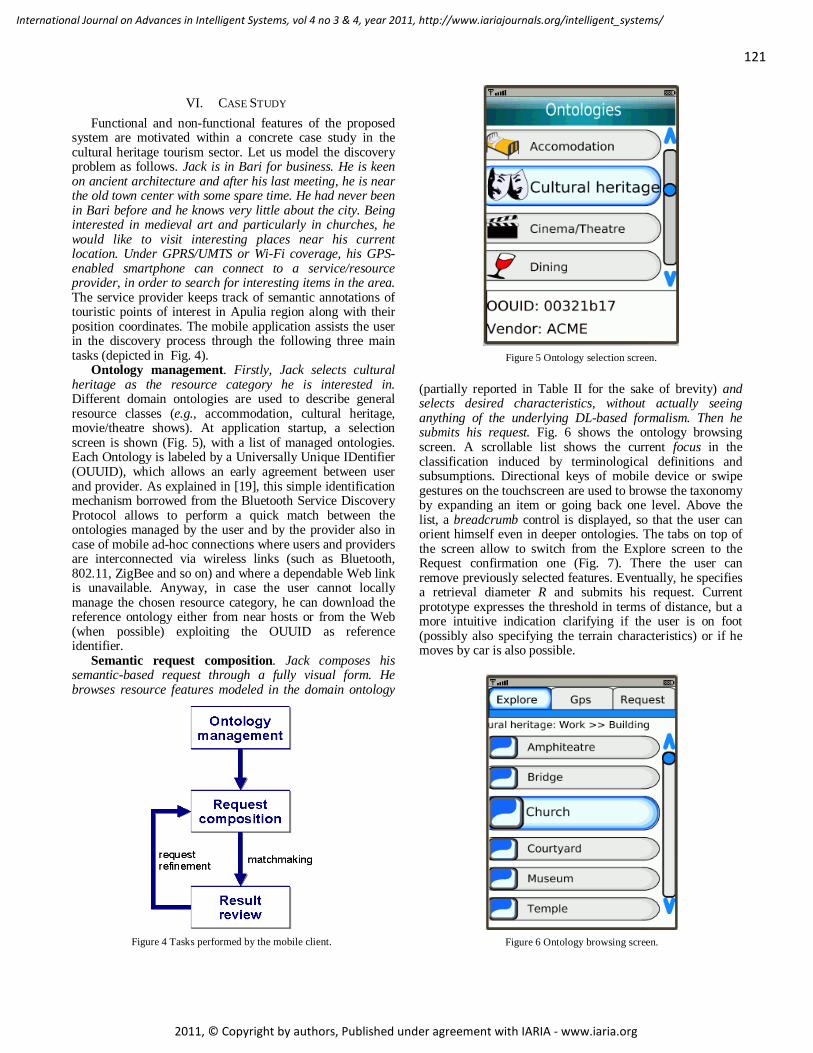
121



VI. CASE STUDY Functional and non-functional features of the proposed

system are motivated within a concrete case study in the cultural heritage tourism sector. Let us model the discovery problem as follows. Jack is in Bari for business. He is keen on ancient architecture and after his last meeting, he is near the old town center with some spare time. He had never been in Bari before and he knows very little about the city. Being interested in medieval art and particularly in churches, he would like to visit interesting places near his current location. Under GPRS/UMTS or Wi-Fi coverage, his GPS-enabled smartphone can connect to a service/resource provider, in order to search for interesting items in the area. The service provider keeps track of semantic annotations of touristic points of interest in Apulia region along with their position coordinates. The mobile application assists the user in the discovery process through the following three main tasks (depicted in Fig. 4).

Ontology management. Firstly, Jack selects cultural heritage as the resource category he is interested in. Different domain ontologies are used to describe general resource classes (e.g., accommodation, cultural heritage, movie/theatre shows). At application startup, a selection screen is shown (Fig. 5), with a list of managed ontologies. Each Ontology is labeled by a Universally Unique IDentifier (OUUID), which allows an early agreement between user and provider. As explained in [19], this simple identification mechanism borrowed from the Bluetooth Service Discovery Protocol allows to perform a quick match between the ontologies managed by the user and by the provider also in case of mobile ad-hoc connections where users and providers are interconnected via wireless links (such as Bluetooth, 802.11, ZigBee and so on) and where a dependable Web link is unavailable. Anyway, in case the user cannot locally manage the chosen resource category, he can download the reference ontology either from near hosts or from the Web (when possible) exploiting the OUUID as reference identifier.

Semantic request composition. Jack composes his semantic-based request through a fully visual form. He browses resource features modeled in the domain ontology

(partially reported in Table II for the sake of brevity) and selects desired characteristics, without actually seeing anything of the underlying DL-based formalism. Then he submits his request. Fig. 6 shows the ontology browsing screen. A scrollable list shows the current focus in the classification induced by terminological definitions and subsumptions. Directional keys of mobile device or swipe gestures on the touchscreen are used to browse the taxonomy by expanding an item or going back one level. Above the list, a breadcrumb control is displayed, so that the user can orient himself even in deeper ontologies. The tabs on top of the screen allow to switch from the Explore screen to the Request confirmation one (Fig. 7). There the user can remove previously selected features. Eventually, he specifies a retrieval diameter R and submits his request. Current prototype expresses the threshold in terms of distance, but a more intuitive indication clarifying if the user is on foot (possibly also specifying the terrain characteristics) or if he moves by car is also possible.

Figure 5 Ontology selection screen.

Figure 6 Ontology browsing screen.

Figure 4 Tasks performed by the mobile client.

122



TABLE II. EXCERPT OF AXIOMS IN THE CASE STUDY ONTOLOGY

AD Age BC Age Middle_Age AD Centralized Floor_Plan Longitudinal Floor_Plan Quadrangular Floor_Plan Square Quadrangular Byzantine Style Romanesque Style Gothic Style Baroque Style Portal Architectural_Element Cathedra Architectural_Element Aisle Architectural_Element Altar Architectural_Element Pulpit Architectural_Element Crypt Architectural_Element Apse Architectural_Element Window ArchitecturalElement Single_Light Window Double_Light Window Triple _Light Window Religious Destination Private Destination Public Destination Private ØPublic Private ØReligious Building $ has_age ⊓ $ has_floor_plan ⊓ $ has_style Residence Building ⊓ $ Destination ⊓ " Destination.Private Church ⊑ Building ⊓ $ Destination ⊓ " Destination.Religious ⊓ $ has_altar ⊓ " has_altar.Altar Castle Residence

Jack would like to visit a Romanesque Middle Age

church with longitudinal floor plan and two aisles. W.r.t. the cultural heritage ontology, the request can be formally expressed as: R: Church " has_age.Middle_Age " has_floor_plan.Longitudinal ³2 has_aisle " has_style.Romanesque

It can be noticed that requests are formulated as DL conjunctive queries. Each conjunct is a requested resource feature; it can be an atomic concept selected from the ontology, a universal quantifier or an unqualified number restriction on roles. The GUI masks this level of complexity from the user, allowing him to simply browse lists of features and select the desired ones: translation into DL expression is automated, taking into account the concept

structure and relationships in the reference ontology. The communication module was designed as a finite state

machine to precisely retain knowledge about the progress of

client-server interaction. By doing so, only failed operations are actually repeated, thus improving efficiency from both time and energy standpoints.

Results review and query refinement. The server processes the request as explained in Section 4. Let us consider the following resources in the provider KB: S1: Basilica of St. Nicholas, Bari (distance from user: d = 0.9 km). A Romanesque Middle Age church, with longitudinal floor plant, an apse, two aisles, three portals and two towers. Other notable elements are its crypt, altar, cathedra and Baroque ceiling. W.r.t. domain ontology, it is expressed as:

Church =2 has_aisle " has_age.Middle_Age " has_style.Romanesque =1 has_apse =3 has_portal =1 has_crypt =1 has_altar =2 has_tower =1 has_cathedra $ ceiling_style " ceiling_style.Baroque " has_floor_plan.Longitudinal

S2: Norman-Hohenstaufen Castle, Bari (d = 0.57 km). It is described as a Middle Age castle, with Byzantine architectural style and a quadrangular plan with four towers. In DL notation:

Castle " has_floor_plan.Quadrangular =4 has_tower " has_style.Byzantine " has_age.Middle_Age

S3: Church of St. Scholastica (d = 1.3 km). It is described as a Romanesque Middle Age church, with longitudinal floor plan, three aisles, an apse and a tower. That is:

Church " has_style.Romanesque " has_age.Middle_Age " has_floor_plan.Longitudinal =3 has_aisle =1 has_tower =1 has_apse

S4: Church of St. Mark of the Venetians, Bari (d = 0.65 km). It is described as a Romanesque Middle Age church with two single-light windows and a tower, whose DL translation is:

Church " has_style.Romanesque " has_window.Single_Light =2 has_window " has_age.Middle_Age =1 has_tower

Figure 7 Request confirmation screen.

123



Table III reports on matchmaking results for the above example. S3 is discarded in the location-based pre-filtering, as its distance from the user exceeds the limit, even though it would result in a full match. S1 is a full match with the request, because it explicitly satisfies all user requirements. On the other hand, S4 is described just as Romanesque Middle Age church, therefore due to OWA it is not specified whether it has a longitudinal floor plan with aisles or not: these characteristics become part of the Hypothesis computed through CAP. Finally, S2 produces a partial match since it refers to a castle: this concept is incompatible with user request, so it forms the Give Up feature computed through CCP. Overall scores of advertised resources are finally computed. An example of result screen is reported in Fig. 8: retrieved resources are listed, best matching first. When the user selects a resource, its picture is shown as in Fig. 9 in addition to its address, distance from the user and semantically relevant properties contributing to the outcome.

If Jack is not satisfied with results, he can refine his request and submit it again. The user can go back to the ontology browsing screen to modify the request. Furthermore, he can select some elements of the Bonus (respectively Give Up) list in the result screen and they will be added to (resp. removed from) the request.

VII. SYSTEM EVALUATION

A. System Performance Performance analysis was executed on a Sony-Ericsson

P990i smartphone, endowed with ARM processor at 208 MHz clock frequency, 64 MB of RAM, 80 MB of storage memory, a TFT 2,8” touchscreen with 240x320 pixel resolution, GSM/UMTS, IEEE 802.11b Wi-Fi connectivity and GPS, Symbian 9.1 operating system, manufacturer-

supplied Java ME runtime compatible with MIDP 2.0 and all optional packages described in Section V-B. P990i smartphone was connected via UMTS to the matchmaking engine. Fig. 10 displays some screenshots of the u-tourism decision support system running on that mobile device. As performance metrics, RAM usage and latency time were considered for each tasks in Figure 4.

For memory analysis, the Memory Monitor profiling tool in Sun Java Wireless Toolkit was used. Results are reported in Fig. 11 for a typical usage session. RAM occupancy is always below 2 MB, which is the recommended threshold for MIDP applications. Memory peaks correspond to more graphical-intensive tasks, such as ontology browsing and preparation of the results screen.

TABLE III. MATCHMAKING RESULTS

Supply Match type s_match [max=54]

Outcome Score [α=0.5,β=1,

γ=0.014, ε=0] S1: Basilica of St.

Nicholas Full 0 Hypothesis H:

Bonus B: =1 has_apse =3 has_portal =1 has_crypt =1 has_altar =2 has_tower =1 has_cathedra $ ceiling_style ⊓ " ceiling style.Baroque

88.8

S4: Church of St. Mark

Potential 3 Hypothesis H: ³2 has_aisle " has_floor_plan. Longitudinal Bonus B: =1 has_tower =2 has_window "has_window.Single_Light

78.3

S2: Norman-Hohenstaufen

Castle

Partial 11 Give up G: Church Keep K: Building "has_age.Middle_age Hypothesis H: "has_floor_plan.Longitudinal ³2 has_aisle "has_style.Romanesque Bonus B: =4 has_tower "has_style.Byzantine

64.8

S3: Church of St. Scholastica

N.A. N.A. Discarded due to distance N.A.

Figure 8 Displayed results.

124



The diagram in Fig. 11 is not significant for assessment of user-perceived latency, since idle times due to user reading the screen are also counted. Latency was measured through timers in the application code. The usage session described in the case study was repeated three times, exactly in the same way. Table IV contains average times obtained in loading each screen. The result list screen loading time includes interaction with the matchmaker (submitting the request, waiting for matchmaking computation, receiving the reply and building the result list GUI), and it is by far the highest value, posing a potential issue for practical usability. Latency in other tasks can be deemed as acceptable. In order to provide further insight into matchmaking computation performance – a key aspect for the feasibility of the proposed approach – a simulated testbed was used to assess semantic matchmaking processing times. Three ontologies with an increasing complexity were created and examined, and five different requests for each one were submitted to the system. Average response times were recorded. In Fig. 12 the matchmaking time (absolute and relative) is reported. The relative value is obtained by weighting the absolute matchmaking time according to the ontology size (expressed in terms of number of contained concepts). The relative time computation is needed because reasoning procedures are strongly conditioned by the complexity of the exploited ontology. So, the relative matchmaking evaluation produces an average time per concept which is a more precise indication of the matchmaking computational load with respect to the absolute one.

By examining the provided Fig. 12, it can be concluded that, for the most complex ontologies, semantic matchmaking time assumes a considerable value. Nevertheless, considering that applications as the one proposed here are required to be interactive and with fast response times, this is a relevant issue to solve. It was also pointed out by Ben Mokhtar et al. [21], who devised optimizations to reduce online reasoning time in a semantic-based mobile service discovery protocol. The main

proposed optimizations were offline pre-classification of ontology concepts and concept encoding: both solutions, however, are viable in matchmaking schemes based on pure subsumption (and therefore able to provide only binary yes/no answers), but they are not directly applicable to our matchmaking approach.

B. Semantic Web Technologies in Ubiquitous Computing Common issues rising from the integration of Semantic

Web approaches with ubiquitous computing scenarios were evidenced in [23]. Let us take them as a check-list and evaluate our proposal against it.

TABLE IV. GUI LATENCY.

Loading Screen Loading latency (s) Ontology selection 0.678 Ontology browsing 3.136 Request confirmation 0.939 Result list 11.107

Figure 10 Screenshots of prototype tool.

Figure 9 Result details screen.

125



A. Simple architectures lack intelligence of Semantic Web technologies. The current proposal allows mobile devices equipped with commonly available technologies to fully exploit semantic-based resource discovery. Ideas and technologies devised for resource retrieval in the Semantic Web were adapted with a satisfactory success, through careful selection of features and optimization of implementation.

B. Semantic Web architectures use devices with a secondary, passive role. In our prototype the client has a key role and it does not only act as a GUI for request composition via ontology browsing. It also enables: location determination; interaction with a state-of-the-art, DIG-based reasoning engine; interactive visualization of discovery results for query refinement.

C. Semantic Web architectures rely on a central component that must be deployed and configured beforehand for each specific scenario. The proposed system prototype still relies on a centralized server for resource matchmaking. Future work aims at building a fully mobile peer-to-peer architecture. A major step is to design and implement embedded DL reasoners with acceptable performance: early results have been achieved in this concern [24].

D. Most architectures do not use the Web communication model, essentially HTTP. For communication we only use DIG, a standard based on the HTTP POST method and on an XML-based concept language. Such a choice allows – among other things – to cope with scalability issues: particularly, the interaction model is borrowed from the Web experience in order to grant an acceptable behaviour also in presence of large amounts of exchanged data.

E. Devices are not first-class actors in the environment with autonomy, context-awareness and reactiveness. Though the typical usage scenario for our current prototype is user-driven, it shows how a non-technical user can fully leverage Semantic Web technologies via her personal

mobile device to discover interesting resources in her surroundings.

VIII. RELATED WORK Significant research and industry efforts are focusing on

service/resource discovery in mobile and ubiquitous computing. The main challenge is to provide paradigms and techniques that are effective and flexible, yet intuitive enough to be of practical interest for a potentially wide user base.

In [25], a prototypical mobile client is presented for semantic-based mobile service discovery. An adaptive graph-based representation allows OWL ontology browsing. However, a large screen seems to be required to explore ontologies of moderate complexity with reasonable comfort. Also preference specification requires a rather long interaction process, which could be impractical in mobile scenarios. Authors acknowledged these issues and introduced heuristic mechanisms to simplify interaction, e.g., the adoption of default values.

In [26], a location- and context-aware mobile Semantic Web client is proposed for tourism scenarios. The goal of integrating multiple information domains has led to a division of the user interface into many small sections,

0

500

1000

1500

2000

0 10 20 30 40 50 60

Mem

ory

usag

e(k

B)

Time (s)

Task Ontologyselection

Ontologybrowsing

Requestconfirmation

Result calculationand review

Resultdetails

Memory Peak (kB) 888 1846 690 1651 1459 Figure 11 Main memory usage profile and peaks.

Ontology size

0

100

200

300

400

500

# of c

once

pts

# concepts 418 156 48

Electronics Clothing Toys

Absolute matchmaking time

02468

101214

Avg.

tim

e (s)

Avg time (s) 12,184 1,571 0,382


Relative matchmaking time

0,0000,0050,0100,0150,0200,0250,0300,035

Avg.

tim

e / co

ncep

t (s)

Avg time (s) 0,029 0,010 0,008


Figure 12 Performace evaluation of semantic matchmaking.

126



whose clarity and practical usability seem questionable. Moreover, knowledge is extracted from several independent sources to build a centralized RDF triple store accessible through the Internet. The proposed architecture is therefore hardly adaptable to mobile ad-hoc environments.

A more open framework is presented in [27], allowing the translation and publication of OpenStreetMap data into an Open Linked Data repository in RDF. A public endpoint on the Web allows users to submit queries in SPARQL RDF query language, in order to retrieve geo-data of a specific region, optionally filtered by property values. Nevertheless, developed facilities currently cannot support advanced LBSs such as semantic matchmaking for resource discovery.

Van Aart et al. [28] presented a mobile application for location-aware semantic search, bearing some similarities with the proposal presented here. An augmented reality client for iPhone sends GPS position and heading to a server and receives an RDF dataset relevant to locations and objects in the route of the user. Applicability of the approach is limited by the availability of pre-existing RDF datasets, since the problem of creating and maintaining them was not considered.

DBpedia Mobile [29] allows user to search for resources located nearby, by means of information extracted from DBpedia and other datasets. The system also enables users to publish pictures and reviews that further enrich POIs. The user may filter the map for resources matching specific constraints or a SPARQL query. However, in the first case approximated matches are not allowed; a resource is found if and only if the overall query is satisfied. In the second case, the SPARQL query builder requires the user to know language fundamentals. Our approach aims at overcoming both restrictions.

Peer-to-peer interaction paradigms are actually needed for fully decentralized semantic-based discovery infrastructures. Hence, mobile hosts themselves should be endowed with reasoning capabilities. Pocket KRHyper [30] was the first available reasoning engine for mobile devices. It provides satisfiability and subsumption inference services, which have been exploited by authors in a DL-based matchmaking between user profiles and descriptions of resources/services [31]. A limitation of that prototype is that it does not allow explicit explanation of outcomes. More recently, in [24] an embedded DL reasoning engine was presented in a mobile dating application, though applicable to other discovery scenarios. It acts as a mobile semantic matchmaker, exploiting non-standard inference services also used in the present framework. Semantically annotated personal profiles are exchanged via Bluetooth and matched with preferences of mobile phone users, to discover suitable partners in the neighbourhood.

Due to the resource constraints of mobile devices, as well as to the choice of a cross-platform runtime environment, both the above solutions privilege simplicity of managed resource/service descriptions over expressiveness and flexibility. We conjecture that a native language optimized implementation can provide acceptable

performance for larger ontologies and more resource-intensive inferences.

IX. CONCLUSION AND FUTURE WORK The paper presented a framework for semantic-enabled

resource discovery in ubiquitous computing. It has been implemented in a visual mobile DSS able to retrieve resources/services through a fully dynamic wireless infrastructure, without relying on support facilities provided by wired information systems. The system recognizes via GPS the user location and grades matchmaking outcomes according to proximity criteria. Future work aims at simplifying the complexity of matchmaker module claiming for optimization and rationalization of the reasoner structure, in order to improve performance and scalability and to allow its integration into mobile computing devices and systems. Furthermore, a navigation engine will be integrated in the mobile application and the user interface will be enhanced to be even more friendly for non-expert users. Finally, we are investigating a new approach based on the semantic-based annotation of OpenStreetMap cartographic data, in order to exploit crowd-sourcing to face the issue of resource annotation.

ACKNOWLEDGMENT The authors acknowledge partial support of Apulia

region strategic projects PS_025 and PS_121.

REFERENCES [1] M. Ruta, F. Scioscia, E. Di Sciascio, G. Piscitelli, “Semantic-based

Geographical Matchmaking in Ubiquitous Computing”, The Fourth International Conference on Advances in Semantic Processing (SEMAPRO 2010), pp. 166-172, 2010.

[2] A. Smith, “35% of American adults own a smartphone”, Pew Internet & American Life Project, July 2011, http://pewinternet.org/~/media//Files/Reports/2011/PIP_Smartphones.pdf, accessed on July 12, 2011.

[3] T. Di Noia, E. Di Sciascio, F.M. Donini, M. Ruta, F. Scioscia, E. Tinelli, “Semantic-based Bluetooth-RFID interaction for advanced resource discovery in pervasive contexts”. International Journal on Semantic Web and Information Systems, vol. 4(1), pp. 50-74, 2008.

[4] A. Langegger, W. Wöß, “Product finding on the semantic web: A search agent supporting products with limited availability”. International Journal of Web Information Systems, Vol. 3, No. 1/2, Emerald Group Publishing Limited, 2007, pp. 61-88.

[5] F. Baader, D. Calvanese, D. Mc Guinness, D. Nardi, P. Patel-Schneider, “The Description Logic Handbook”, Cambridge University Press, New York, 2002.

[6] R. Watson, S. Akselsen, E. Monod, L. Pitt, “The Open Tourism Consortium: Laying The Foundations for the Future of Tourism”. European Management Journal, vol. 22(3), pp. 315–326, 2004.

[7] T. Di Noia, E. Di Sciascio, F.M. Donini, “Semantic matchmaking as non-monotonic reasoning: A description logic approach”. Journal of Artificial Intelligence Research, vol. 29(1), pp. 269-307, AAI, 2007.

127



[8] D.L. McGuinness, F. van Harmelen, “OWL Web Ontology Language”, W3C Recommendation. http://www.w3.org/TR/owl-features/, accessed on July 12, 2011.

[9] T. Berners-Lee, J. Hendler, O. Lassila, “The Semantic Web”, Scientific American, vol. 248(4), pp.34–43, 201.

[10] M. Paolucci, T. Kawamura, T.R. Payne, K. Sycara. “Semantic Matching of Web Services Capabilities”. The Semantic Web - ISWC 2002, Lecture Notes in Computer Science, vol. 2342, pp. 333-347, 2002.

[11] L. Li, I. Horrocks, “A Software Framework for Matchmaking Based on Semantic Web Technology”. International Journal of Electronic Commerce, vol. 8(4), pp. 39–60, 2004.

[12] R. Brachman, H. Levesque, “The Tractability of Subsumption in Frame-based Description Languages". In proc. of Fourth National Conference on Artificial Intelligence (AAAI-84), pp. 34-37, Morgan Kaufmann, 1984.

[13] S. Bechhofer, R. Möller, P. Crowther, “The DIG Description Logic Interface”. In proc. of the 16th International Workshop on Description Logics (DL’03), CEUR Workshop Proceedings, vol. 81, 2003.

[14] S. Colucci, T. Di Noia, A. Pinto, A. Ragone, M. Ruta, E. Tinelli, “A Non-Monotonic Approach to Semantic Matchmaking and Request Refinement in E-Marketplaces”. International Journal of Electronic Commerce, vol. 12(2), pp. 127-154, 2007.

[15] S. Colucci, T. Di Noia, E. Di Sciascio, F.M. Donini, M. Mongiello, “Concept Abduction and Contraction for Semantic-based Discovery of Matches and Negotiation Spaces in an E-Marketplace”. Electronic Commerce Research and Applications, vol. 4(4), pp. 345-361, 2005.

[16] S. Colucci, T. Di Noia, E. Di Sciascio, F.M. Donini, A. Ragone, “Knowledge Elicitation for Query Refinement in a Semantic-Enabled E-Marketplace”. In proc. of 7th International Conference on Electronic Commerce (ICEC05), pp. 685-691, ACM Press, 2005.

[17] S. Auer, C. Bizer, G. Kobilarov, J. Lehmann, R. Cyganiak, Z. Ives, “Dbpedia: A nucleus for a web of open data”, The Semantic Web, pp. 722-735, Springer, 2007.

[18] C. Bizer, T. Heath, K. Idehen, T. Berners-Lee, “Linked data on the web”. In proc. of the 17th international conference on World Wide Web, pp. 1265-1266, ACM, 2008.

[19] M. Ruta, T. Di Noia, E. Di Sciascio, F.M. Donini, “Semantic based collaborative p2p in ubiquitous computing”. Web Intelligence and Agent Systems, vol. 5, n. 4, pp. 375–391, 2007.

[20] T. Di Noia, E. Di Sciascio, F.M. Donini, M. Mongiello, “A System for Principled Matchmaking in an Electronic

Marketplace”. International Journal of Electronic Commerce, vol. 8(4), pp. 9-37, 2004.

[21] A. Slominski, S. Haustein, "XML Pull Parsing API”, 2005, available at http://xmlpull.org/, accessed on July 12, 2011.

[22] S. Ben Mokhtar, A. Kaul, N. Georgantas, V. Issarny, “Efficient Semantic Service Discovery in Pervasive Computing Environments”. In proc. of the ACM/IFIP/USENIX 7th International Middleware Conference, Middleware ’06, 2006.

[23] J.I. Vazquez, D. López de Ipiña, I. Sedano, “SoaM: A Web-powered Architecture for Designing and Deploying Pervasive Semantic Devices”. International Journal of Web Information Systems, vol. 2(3/4) , pp. 212-224, Emerald Group Publishing Limited, 2006.

[24] M. Ruta, T. Di Noia, E. Di Sciascio, F. Scioscia, “Abduction and Contraction for Semantic-based Mobile Dating in P2P Environments”. In proc. of 6th IEEE/WIC/ACM International Conference on Web Intelligence (WI08), pp. 626–632, IEEE, 2008.

[25] O. Noppens, M. Luther, T. Liebig, M. Wagner, M. Paolucci, “Ontology supported Preference Handling for Mobile Music Selection”. In proc. of the Multidisciplinary Workshop on Advances in Preference Handling, Riva del Garda, Italy, 2006.

[26] M. Wilson, A. Russell, D. Smith, A. Owens, M. Schraefel, “mSpace Mobile: A Mobile Application for the Semantic Web.” In proc. of the End User Semantic Web Workshop at ISWC 2005, 2005.

[27] S. Auer, J. Lehmann, S. Hellmann. LinkedGeoData - Adding a Spatial Dimension to the Web of Data. In proc. of 8th International Semantic Web Conference (ISWC). Springer-Verlag, 2009.

[28] C. J. van Aart, B. J. Wielinga, and W. R. van Hage. Mobile Cultural Heritage Guide: Location-Aware Semantic Search. In proc. of 17th International Conference on Knowledge Engineering and Knowledge Management (EKAW 2010), volume 6385 of Lecture Notes in Computer Science, pages 257–271, Berlin Heidelberg, 2010. Springer-Verlag.

[29] C. Becker, C. Bizer, “Exploring the Geospatial Semantic Web with DBpedia Mobile”. Web Semantics: Science, Services and Agents on the World Wide Web, vol. 7(4), pp. 278-286, Elsevier, 2009.

[30] A. Sinner, T. Kleemann, “KRHyper - In Your Pocket”. In proc. of 20th International Conference on Automated Deduction (CADE-20), pp. 452–457, 2005.

[31] T. Kleemann, A. Sinner, “User Profiles and Matchmaking on Mobile Phones”. In proc. of 16th International Conference on Applications of Declarative Programming and Knowledge Management (INAP2005), pp. 135-147, Springer, 2005.

128



Personalized Access to Contextual Information by using an Assistant for Query Reformulation

Ounas ASFARI ERIC Laboratory

University of Lyon 2 Bron, France

[email protected]

Bich-Liên Doan, Yolaine Bourda SUPELEC/Department of Computer Science

Gif-Sur-Yvette, France [email protected], [email protected]

Jean-Paul Sansonnet LIMSI-CNRS

University of Paris 11 Orsay, France [email protected]

Abstract— Access to relevant information adapted to the needs and the context of the user is a real challenge in Web Search, owing to the increases of heterogeneous resources and the varied data on the web. There are always certain needs behind the user query, these queries are often ambiguous and shortened, and thus we need to handle these queries intelligently to satisfy the user’s needs. For improving user query processing, we present a context-based hybrid method for query expansion that automatically generates new reformulated queries in order to guide the information retrieval system to provide context-based personalized results depending on the user profile and his/her context. Here, we consider the user context as the actual state of the task that the user is undertaking when the information retrieval process takes place. Thus State Reformulated Queries (SRQ) are generated according to the task states and the user profile which is constructed by considering related concepts from existing concepts in domain ontology. Using a task model, we will show that it is possible to determine the user’s current task automatically. We present an experimental study in order to quantify the improvement provided by our system compared to the direct querying of a search engine without reformulation, or compared to the personalized reformulation based on a user profile only. The preliminary results have proved the relevance of our approach in certain contexts.

Keywords-Information Retrieval; Query Reformulation; Context; Task modeling; Personalization; user profile.

I. INTRODUCTION

The Internet offers almost unlimited access to all kinds of information (text, audiovisual, etc.), there is a vast, growing expanse of data to search, heterogeneous data, and an expanding base of users with many diverse information needs; thus, the Information Retrieval (IR) field has been more critical than ever. Information Retrieval Systems (IRS) aims to retrieve relevant documents in response to a user need, which is usually expressed as a query. The retrieved documents are returned to the user in decreasing order of relevance, which is typically determined by weighting models. As the volume of the heterogeneous resources on the web increases and the data becomes more varied, massive response results are issued to user queries. Thus, large amounts of information are returned in which it is often difficult to distinguish relevant information from secondary information or even noise; this is due to information retrieval

systems IRS that generally handle user queries without considering the contexts in which users submit these queries [1]. Therefore it is difficult to obtain desired results from the returned results by IRS. In recent research, IR researchers have begun to expand their efforts to satisfy the information needs that users express in their queries by considering the personalized information retrieval area and by using the context notion in information retrieval.

Recent studies, like [2], have tried to enhance a user query with user’s preferences, by creating a dynamic user profile, in order to provide personalized results. However, a user profile may not be sufficient for a variety of user queries. Take as an example a user who enters the query “Java” into a personalized Web search engine. Let us now suppose that the user has an interest for computer programming. With this information at hand, it should be possible for a personalized search engine to disambiguate the original query “Java”. The user should receive results about Java programming language in the top results. But in particular situations, the supposed user may need information about the Java Island, to prepare a trip for example, or information about the Java Coffee that is not specified in his profile. Thus the user will hardly find these results subjectively interesting in a particular situation. One disadvantage of automatic personalization techniques is that they are generally applied out of context. Thus, not all of the user interests are relevant all of the time, usually only a subset is active for a given situation, and the rest cannot be considered as relevant preferences.

To overcome the previous problem and to address some of the limitations of classic personalization systems, studies taking into account the user context are currently undertaken [3]. The user context can be assimilated to all factors that can describe his intentions and perceptions of his surroundings [3]. These factors may cover various aspects: environment (light, services, people, etc.), spatial-temporal (location, time, direction, etc.), personal (physiological, mental, professional, etc.), social (friends, colleagues, etc.), task (goals, information task), technical, etc. Fig. 1 shows these factors and examples for each one [4].

The user context has been applied in many fields, and of course in information retrieval area. Context in IR has been subject to a wide scope of interpretation and application [5]. The problem to be addressed here includes how to represent the context, how to determine it at runtime, and how to use it

129



to influence the activation of user preferences. It is very difficult to take into consideration all the contextual factors in one information retrieval system, so the researchers often define the context as certain factorsinformation [6], physical user location Web pages [8], session interaction data [9

Figure 1. A context model.

In this paper, our definition of the context is that the context describes the user’s current task, its changes over time and its states, i.e., we take into consideration user is undertaking when the information retrieval process occurs. Consequently, in this paper, when we talk about the context, we talk about the user’s current task and its states over times.

In the present, it has become common to seek dailinformation on the Web, including such tasks as using information retrieval system for shopping, travel booking, academic research, and so on. Thus, it is important to attempt to determine not only what the user is looking for, but also the task that he is trying to accomplish. Indeed the user task is critical to improve the processing of user needs. On the other hand, the increase of mobile devices (such as PDA, cellular phone, laptop…) including diverse platforms, various work environments, have created new considerations and stakes to be satisfied.use the mobile devices anywhere to seek information needed to perform the task at hand. This is the case of the mobile user. As we consider the user’s current task, thus weinto account the case of mobile user when he seeks information, needed to perform his current task, by using the mobile devices. Knowing that, the information needs of mobile users to perform tasks are related to contextual factors such as user interests, user current task, location, direction, etc. Here, the problem is that the classic information retrieval systems do not consider the case of mobile users and provide same results to them needs, contexts, intentions and personalities, soirrelevant results are provided, it is often difficult to distinguish context-relevant information fromresults.

references. It is very difficult to take into consideration all the contextual factors in one information retrieval system, so the researchers often

factors, such as desktop [7], recently visited 9], etc.

A context model.

our definition of the context is that the context current task, its changes over time and

consideration the task which the user is undertaking when the information retrieval process

when we talk about the we talk about the user’s current task and its states

the present, it has become common to seek daily eb, including such tasks as using

information retrieval system for shopping, travel booking, t is important to attempt

to determine not only what the user is looking for, but also Indeed understanding

the user task is critical to improve the processing of user the increase of mobile devices

(such as PDA, cellular phone, laptop…) including diverse , have created new

considerations and stakes to be satisfied. So, it is expected to anywhere to seek information needed

This is the case of the mobile user. As we consider the user’s current task, thus we take into account the case of mobile user when he seeks information, needed to perform his current task, by using the

the information needs of are related to contextual

ests, user current task, location, problem is that the classic

t consider the case of to them for different

needs, contexts, intentions and personalities, so too many irrelevant results are provided, it is often difficult to

relevant information from the irrelevant

User query is an element that specifies an information need, but the majorities of these queries are short (85% of users search with no more than 3 keywordsambiguous, and often fail to represent the information need,especially the queries of the provide a complete specification of the information need. Many relevant terms can be abseincluded may be ambiguous, thus queries must be processed intelligently to address more of the user’s intended requirements. Typical solution includesrepresentation that refers to methods of query reformulation, i.e., any kind of transformation applied to a query to facilitate a more effective retrieval. reformulation process the initial user query is reformulatedby adding relevant terms. Manytechniques to select these rbetween them depend on the source of may extract from results of previous research (relevance feedback) or from an external resource (semantic user profile,…etc), or depend onselect relevant terms to be added to the initial query.

The research, presented in thisadvantages of the two areas order to provide context-based personalized results as appropriate answer to the user query submitted in a particular context. In fact, the user query Web search engine, or information retrieval system, is not sufficient to retrieve the desired results, thus an aid to the user to formulate his/her query beinformation retrieval system will be effective, especially in the case of the mobile user because his/her query is often short and related to a task at hand. In this study we do not consider the information retrieval models that on the match between the resource (indexed files) and the user query to provide the relevant resultsto understand the user query, but the main idea of this study is to propose an intelligent assistant that can generate new reformulated query before submitting it to the information retrieval system in order to personalize and contextualize the access to information. Thus query processing based on the uarea) and the user context (context area). algorithm to generate contextfrom the initial user query. Thus, method to reformulate user queries depending on profile, which contains the usertogether with the user‘s contextactual state of his/her current task. The generated query is denoted: State Reformulated Query SRQ. these SRQ queries will guide the based personalized results which those provided by using the initial user query and those provided by using the user query with simple personalization, depending only on the user profile, in the same context.

We propose that the user queriesduring the performance of one task at hand, are related to thistask, indeed that are part of it. may include one or more activities, in other words

User query is an element that specifies an information he majorities of these queries are short (85% of

ers search with no more than 3 keywords [10]) and , and often fail to represent the information need,

of the mobile user, which do not provide a complete specification of the information need. Many relevant terms can be absent from queries and terms included may be ambiguous, thus queries must be processed intelligently to address more of the user’s intended

Typical solution includes expanding query hat refers to methods of query reformulation,

.e., any kind of transformation applied to a query to facilitate a more effective retrieval. Thus in the query

process the initial user query is reformulated Many approaches use different

these relevant terms, the difference the source of these terms, which

from results of previous research (relevance feedback) or from an external resource (semantic resource, user profile,…etc), or depend on the method which is used to

terms to be added to the initial query. presented in this paper, combines the

advantages of the two areas context and personalization in based personalized results as

ser query submitted in a particular In fact, the user query that is submitted to a typical

, or information retrieval system, is not sufficient to retrieve the desired results, thus an aid to the user to formulate his/her query before submitting it to the information retrieval system will be effective, especially in the case of the mobile user because his/her query is often short and related to a task at hand. In this study we do not consider the information retrieval models that mainly focus

the match between the resource (indexed files) and the user query to provide the relevant results, and do not attempt

, but the main idea of this study is to propose an intelligent assistant that can generate new reformulated query before submitting it to the information retrieval system in order to personalize and contextualize the access to information. Thus we tries to improve the user

the user profile (personalization (context area). We will present an

generate context-related personalized queries Thus, this paper presents a hybrid

method to reformulate user queries depending on his/her the user’s interests and preferences, context, which is considered as the

actual state of his/her current task. The generated query is denoted: State Reformulated Query SRQ. We will prove that

queries will guide the IRS to provide context-which are more relevant than

provided by using the initial user query and those using the user query with simple

personalization, depending only on the user profile, in the

user queries, which are submitted during the performance of one task at hand, are related to this task, indeed that are part of it. A task is a work package that may include one or more activities, in other words the

130



activities are required to achieve the task. Thus the user task can be represented by using UML activity diagram in order to detect the transitions between the task states at time changes. The activities, in UML activity diagram, are states of doing something. For instance, if a user has to organize a workshop, there are many states for this task, such as the choice of the workshop topics and the choice of the program committee members, etc. Submitting two equivalent queries in tow different states, the relevant results at each task state will be different, so the proposed system has to provide the different relevant results at each state.

The rest of the paper is organized as follows: Section 2 shows the related work; Section 3 introduces models and algorithms to reformulate a user queries and it presents the architecture of our system; Section 4 shows the experimental study and the evaluation of our system; Finally, Section 5 gives the conclusion and future work to be done.

II. RELATED WORK

Many studies have been employed to expand the user query in information retrieval area, as far as we know these studies do not depend on the user task, in this paper, we depend on a task model for expansion the user query, thus in section A, we describe related work where the query expansion had been investigated. In section B, we review studies where task model had been used.

A. Query Expansion

Query expansion is the process of augmenting the user’s query with additional terms in order to improve results by including terms that would lead to retrieving more relevant documents. Many works have been done for providing personalized results by query reformulation. Approaches based on the user profile for query enrichment have been proposed, this process consists in integrating elements of the user profile into the user’s query [11]. The limitation of these approaches is that they do not take into consideration the user context to activate elements from the user profile.

Studies on query reformulation by relevance feedback are proposed, the aim is to use the initial query in order to begin the search and then use information about whether or not the initial results are relevant to perform a new query [12]. Because relevance feedback requires the user to select which documents are relevant, it is quite common to use negative feedback. Furthermore the techniques of disambiguation aim to identify precisely the meaning referred by the terms of the query and focus on the documents containing the words quoted in the context defined by the corresponding meaning [13]. But this disambiguation may cause the query to move in a direction away from the user’s intention and augment the query with terms related to the wrong interpretation.

Many approaches, like [14], try to reformulate the web queries based on a semantic knowledge by using ontology in order to extract the semantic domain of a word and add the related terms to the initial query, but sometimes these terms are related to the query only under a particular context. Others use sense information (WordNet) to expand the query [15].

In fact, most of the existing query expansion frameworks have an inherent problem of poor coherence between expansion terms and user’s search goal. User’s search goal, even for the same query, may be different at different states. This often leads to poor retrieval performance. In the logic cases, the user’s current search is influenced by his/her current context and in many instances it is influenced by his/her recent searches. In this paper, we propose a hybrid query expansion method that automatically generates query expansion terms from the user profile and the user task. In our approach we exploit both a semantic knowledge (Ontology) and a linguistic knowledge (WordNet) to learn the user’s task.

B. Task Model

One aspect of characterizing user’s contexts is to consider the tasks which have led them to engage in information retrieval behavior. Users use documents to understand a task and solve a specific problem. Thus, when a user begins a task, he searches the information that will help solve the problem at hand. It must be distinguished between the task of information retrieval and the task that requires the information retrieval in one of its phases. In the second type, it is important to understand the task and its subtasks to detect the related context that will aid the task execution.

Various researchers have demonstrated that the desired search results differ according to types of tasks. According to [16], two types of tasks: Informational task which involves the intent to acquire some information assumed to be present on one or more web pages; transactional task which is based on the intent to perform some web-mediated activity. The approach [17] proves that the nature of the task has an impact on decisions of relevance and usefulness.

The task modeling consists of describing of an optimal procedure to achieve the goal, a sequence of actions or operations in a given environment. Watson’s “Just-in-time” information retrieval system [18] monitors user’s tasks, anticipates task-based information needs, and proactively provides users with task-relevant information. The effectiveness of such systems depends both on their capability to track user tasks and on their ability to retrieve information that satisfies task-based needs. Here, the user’s tasks are monitored by capturing content from Internet Explorer and Microsoft Word applications.

In the approach [19], a language model of a user task is defined as a weighted mixture of task components: queries, result sets, click stream documents, and browsed documents. Approach [5] describes a study on the effect on retrieval performance of using additional information about the user and their search tasks when developing IRF (Implicit Relevance Feedback) algorithms.

In fact, while known to be useful in the development of interactive systems, task models are also known to be difficult to build and to maintain. This difficulty is due to the fact that in order to support a variety of task applications and analyses, task models should include representations of various levels of information, from the highest level user goals down to the lowest level events, and they should be represented in a single, coherent representation scheme.

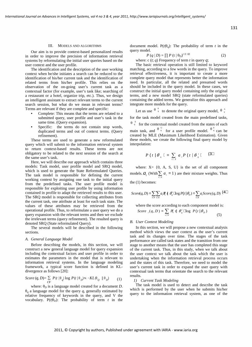
131



III. MODELS AND ALGORITHMS

Our aim is to provide context-based personalized results in order to improve the precision of information retrieval systems by reformulating the initial user queries based on the user context and the user profile.

The identification and the description of the user working context when he/she initiates a search can be reduced to the identification of his/her current task and the identification of related terms from his/her profile. This relies on the observation of the on-going user’s current task as a contextual factor (for example, user’s task like; searching of a restaurant or a hotel, organize trip, etc.). Thus, we design an intelligent assistant to extract relevant terms to the current search session, but what do we mean in relevant terms? Terms are relevant if they are complete and specific:

• Complete: This means that the terms are related to a submitted query, user profile and user’s task in the same time. (Query expansion).

• Specific: the terms do not contain stop words, duplicated terms and out of context terms. (Query refinement).

These terms are used to generate a new reformulated query which will submit to the information retrieval system to return context-based results. These terms are not obligatory to be related to the next session of the search at the same user’s task.

Here, we will describe our approach which contains three models: Task model, user profile model and SRQ model, which is used to generate the State Reformulated Queries. The task model is responsible for defining the current working context by assigning one task to the initial query from the predefined tasks. The user profile model is responsible for exploiting user profile by using information contained in profile to adapt the retrieved results to this user. The SRQ model is responsible for collecting attributes from the current task, one attribute at least for each task state. The values of these attributes may be retrieved from the operational profile. Thus, to reformulate a user query we do a query expansion with the relevant terms and then we exclude the irrelevant terms (query refinement). The resulted query is denoted SRQ (State reformulated Query).

The several models will be described in the following sections.

A. General Language Model

Before describing the models, in this section, we will construct a new general language model for query expansion including the contextual factors and user profile in order to estimates the parameters in the model that is relevant to information retrieval systems. In the language modeling framework, a typical score function is defined in KL-divergence as follows [20]:

Score (q, D) = ∑∈Vt

P ( t | θ q) log P (t | θ D

)∝ − KL ( θ Q || θ D) (1)

where: θD is a language model created for a document D. θq a language model for the query q, generally estimated by relative frequency of keywords in the query, and V the vocabulary. P(t|θD): The probability of term t in the

document model. P(t|θq): The probability of term t in the query model. P (q | D) = ∏ P (t | θD)c (t ;q) (2)

where: c (t; q) Frequency of term t in query q; The basic retrieval operation is still limited to keyword

matching, according to a few words in the query. To improve retrieval effectiveness, it is important to create a more complete query model that represents better the information need. In particular, all the related and presumed words should be included in the query model. In these cases, we construct the initial query model containing only the original terms, and a new model SRQ (state reformulated queries) containing the added terms. We generalize this approach and integrate more models for the query.

Let us use 0θ q to denote the original query model,

Aθ q

for the task model created from the main predefined tasks, S θ q for the contextual model created from the states of each

main task, and Uθ q for a user profile model.

0θ q can be created by MLE (Maximum Likelihood Estimation). Given these models, we create the following final query model by interpolation:

∑∈

) | (=) | (Xi

i

qiq tPatP θθ (3)

where: X= {0, A, S, U} is the set of all component

models. ia (With 1=∑∈ Xi

ia ) are their mixture weights. Thus

the (1) becomes:

∑∑ ∑∈ ∈ ∈

= | ( ) | (=Vt Xi Xi

iiDiqi DqScoreatPtPaDqScore ),()log),( θθ (4)

where the score according to each component model is:

∑∈

| ( ) | (=Vt

Diqi tPtPDqScore )log),( θθ

(5)

B. User Context Modeling

In this section, we will propose a new contextual analysis method which views the user context as the user’s current task and its changes over time. The stages of the task performance are called task states and the transition from one stage to another means that the user has completed this stage of the current task. Thus, in this study, when we talk about the user context we talk about the task which the user is undertaking when the information retrieval process occurs and the states of this task. Therefore, we need to model the user’s current task in order to expand the user query with contextual task terms that orientate the search to the relevant results.

1) Current Task Modeling The task model is used to detect and describe the task

which is performed by the user when he submits his/her query to the information retrieval system, as one of the

132



contextual factors which surround the user during the information retrieval process.

Firstly, we have to distinguish between the activity and the task. In fact, an activity can be something you are just doing, and it may or may not have any purpose, it is the action actually performed, while a task is the purpose which is prescribed. Thus the activities are required to achieve the task. In other words, a task is a work package that may include one or more activities. Accordingly we can represent the user’s task by a UML activity diagram which contains all the activities needed to perform this task. Each stage which is needed to accomplish the current task is called task state. Thus, the actual activity in the UML activity diagram expresses the actual state of the current task.

In our task model, we depend on study questionnaires [5] which were used to elicit tasks that were expected to be of interest to subjects during the study. In that study [5], subjects were asked to think about their online information seeking activities in terms of tasks, and to create personal labels for each task. They were provided with some example tasks such as “writing a research paper,” “travel,” and “shopping” but in no other way were they directed, influenced or biased in their choice of tasks. A generic classification was devised for all tasks identified by all subjects, producing the following nine task groupings: 1. Academic Research; 2. News and Weather; 3. Shopping and Selling; 4. Hobbies and Personal Interests; 5. Jobs/Career/Funding; 6. Entertainment; 7. Personal Communication; 8. Teaching; 9. Travel.

For example, the task labels “viewing news”, “read the news”, and “check the weather” would be classified in Group 2: “News and Weather”.

We construct a UML activity diagram for each main task in order to detect the changes over time in the activities needed to accomplish this task and for describing all the sequences of the performed task. Each activity in the generated UML activity diagram expresses the task’s actual state. This state can be explained by terms that are called state terms. Thus there is at least one term for each task state.

The task related to a specific query is selected (either manually or automatically) for each query.

• Manually: by the user who assigns one task from the proposed predefined tasks to his/her query. This method is effective when the user can determine exactly his/her current task.

• Automatically: in assigning one task to the user query automatically. For that, we will conceive an algorithm based on the vector space model and using advantages of existing linguistic resources (WordNet) and semantic resources (Ontology). this way can facilitate the process to users, we will explain this algorithm in the following:

At first, we construct an index of terms called Task Terms Index. This Task Index consists of:

• Terms of the predefined main tasks. <t1, t2, ….,ti>. For example: {News, Weather, Shopping, Selling, Teaching…..}.

• State terms <t1, t2, ….,tj> for each predefined task: the terms that describe the actual task state. There is

at least one term for each task state, for instance, if a user is currently in one activity “Find a Restaurant” to do one task at hand for example travel task, then the state term that explains the activity will be “Restaurant”.

• Terms which represent the related-task concepts from ontology such as ODP (Open Directory Project) taxonomy <t1, t2, ….,tk>.

This index consists of r terms. Table 1 shows an example of this task terms index. We will use this index when using the vector space model.

TABLE I. INDEX OF TASK TERMS

Term_Id Term tf Occurrence (postings) 1 News 2 A2:1 A9:1 2 weather 2 A2:1 A9:1 3 Shopping 1 A3:1 4 Restaurant 2 A4:1 A9:1

…. …. …. …. r

We suppose that each main predefined task can be considered as one document which includes the terms related to this task from the task index. This document can be represented by a terms vectorA

r

. We treat weights as coordinates in the vector space. Term’s weight is computed using the term frequency and the inverse document frequency “tf * idf” as follows:

) ||

( log is

is

aais n

AtfWa ∗=

where: A is a set of documents which represent the predefined tasks. Thus |A| is the total number of this set A. According to our proposition |A|=9. asi: state term that represent the state si of the current task A*.

isan: A number of documents that represent the predefined

tasks in which term asi occurs. isatf : is the frequency of term

asi in the task A*є A or number of times a term asi occurs in a document that represents a task A* .

Table 2 shows the weights of few terms in the task terms index. We present the terms related to the task A2 “news and weather”, as an example.

TABLE II. EXAMPLE OF CALCULATING TERM’ S WEIGHTS isWa .

Counts TFasi Weights, Wasi = TFasi* IDFasi

Terms A1 A2 .. A9 nasi IDFasi A1 A2 .. A9 News 0 1 1 2 0.653 0 0.653 0.653 Weather 0 1 1 2 0.653 0 0.653 0.653 Tidings 0 1 0 1 0.954 0 0.954 0 Program 0 1 1 2 0.653 0 0.653 0.653 information 1 1 1 3 0.477 0.477 0.477 0.477 temperature 0 1 0 1 0.954 0 0.954 0 atmospheric 0 1 0 1 0.954 0 0.954 0 Meteorological

0 1 0 1 0.954 0 0.954 0

… r

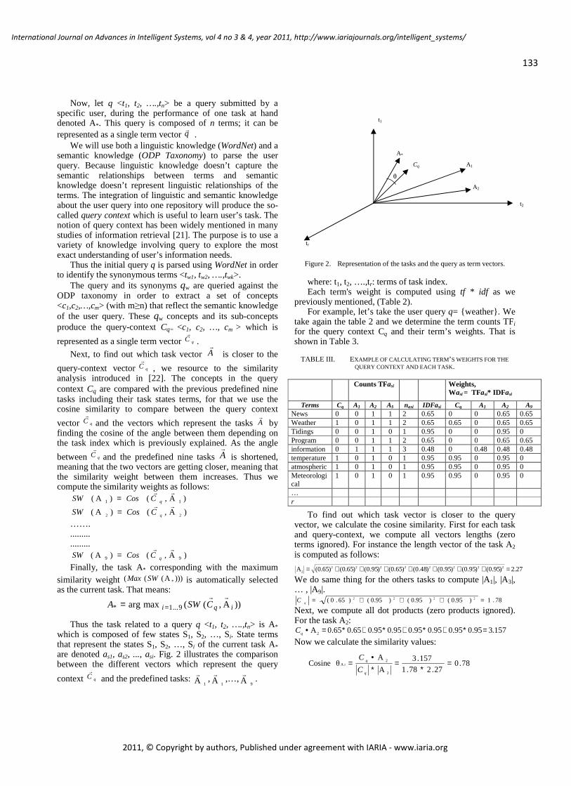
133



Now, let q <t1, t2, ….,tn> be a query submitted by a specific user, during the performance of one task at hand denoted A*. This query is composed of n terms; it can be represented as a single term vectorq

r.

We will use both a linguistic knowledge (WordNet) and a semantic knowledge (ODP Taxonomy) to parse the user query. Because linguistic knowledge doesn’t capture the semantic relationships between terms and semantic knowledge doesn’t represent linguistic relationships of the terms. The integration of linguistic and semantic knowledge about the user query into one repository will produce the so-called query context which is useful to learn user’s task. The notion of query context has been widely mentioned in many studies of information retrieval [21]. The purpose is to use a variety of knowledge involving query to explore the most exact understanding of user’s information needs.

Thus the initial query q is parsed using WordNet in order to identify the synonymous terms <tw1, tw2, ….,twk>.

The query and its synonyms qw are queried against the ODP taxonomy in order to extract a set of concepts <c1,c2,…,cm> (with m≥n) that reflect the semantic knowledge of the user query. These qw concepts and its sub-concepts produce the query-context Cq= <c1, c2, …, cm > which is

represented as a single term vector qCr

.

Next, to find out which task vector Ar

is closer to the

query-context vector qCr

, we resource to the similarity analysis introduced in [22]. The concepts in the query context Cq are compared with the previous predefined nine tasks including their task states terms, for that we use the cosine similarity to compare between the query context

vector qCr

and the vectors which represent the tasks Ar

by finding the cosine of the angle between them depending on the task index which is previously explained. As the angle

between qCr

and the predefined nine tasks Ar

is shortened, meaning that the two vectors are getting closer, meaning that the similarity weight between them increases. Thus we compute the similarity weights as follows:

)A,()A( 11

rr

qCCosSW =

)A,()A( 22

rr

qCCosSW =

……. ......... .........

)A,()A( 99

rr

qCCosSW = Finally, the task A* corresponding with the maximum

similarity weight )))A((( *SWMax is automatically selected as the current task. That means:

))A,((maxarg 9...1* iqi CSWArr

==

Thus the task related to a query q <t1, t2, ….,tn> is A* which is composed of few states S1, S2, …, Si. State terms that represent the states S1, S2, …, Si of the current task A* are denoted as1, as2, ..., asi. Fig. 2 illustrates the comparison between the different vectors which represent the query

context qCr

and the predefined tasks: 1A

r,

1Ar

,…,9A

r.

Figure 2. Representation of the tasks and the query as term vectors.

where: t1, t2, ….,tr: terms of task index. Each term's weight is computed using tf * idf as we

previously mentioned, (Table 2). For example, let’s take the user query q= {weather}. We

take again the table 2 and we determine the term counts TFi

for the query context Cq and their term’s weights. That is shown in Table 3.

TABLE III. EXAMPLE OF CALCULATING TERM’ S WEIGHTS FOR THE QUERY CONTEXT AND EACH TASK.

To find out which task vector is closer to the query vector, we calculate the cosine similarity. First for each task and query-context, we compute all vectors lengths (zero terms ignored). For instance the length vector of the task A2 is computed as follows:

27.2)0.95()0.95()0.95()0.48()65.0()0.95()65.0()65.0(A 222222222 =+++++++=

We do same thing for the others tasks to compute |A1|, |A3|, … , |A9|.

78.1)0.95()0.95()0.95()65.0( 2222 =+++=qC

Next, we compute all dot products (zero products ignored). For the task A2:

157.30.950.950.950.950.950.950.650.65A 2 =∗+∗+∗+∗=•qC

Now we calculate the similarity values:

78.027.278.1

157.3

A

ACosine θ

2

2A 2 =

∗=

∗•

=q

q

C

C

Counts TFasi Weights, Wasi = TFasi* IDF asi

Terms Cq A1 A2 A9 nasi IDFasi Cq A1 A2 A9 News 0 0 1 1 2 0.65 0 0 0.65 0.65 Weather 1 0 1 1 2 0.65 0.65 0 0.65 0.65 Tidings 0 0 1 0 1 0.95 0 0 0.95 0 Program 0 0 1 1 2 0.65 0 0 0.65 0.65 information 0 1 1 1 3 0.48 0 0.48 0.48 0.48 temperature 1 0 1 0 1 0.95 0.95 0 0.95 0 atmospheric 1 0 1 0 1 0.95 0.95 0 0.95 0 Meteorological

1 0 1 0 1 0.95 0.95 0 0.95 0

… r

Cq

t1

A2

t2

tr

θ

A*

A1

134



Finally, the task corresponding with the maximum similarity value is automatically selected as the current task. In this example the task A2 has the maximum similarity with the query context Cq.

Let’s take an example to extract the query context Cq from the initial user query q= {Tourism in Toulouse}. The steps of our algorithm are shown in Table 4:

TABLE IV. APPLYING TASK MODEL TO THE QUERY Q= {T OURISM IN TOULOUSE}.

Description Knowledge used

Result

Parsing the initial query q using WordNet

WordNet A set of query terms (t1,.., tn) (tourism, Toulouse) and its synonym terms (that will be used as the baseline query: (services to tourists, touring, travel, city in France)

The concepts in ontology that represent the baseline query terms are identified, in order to identify the query-context Cq.

Ontological information from ontology (such as, ODP taxonomy).

Set of concepts: query-context (Cq= <C1, C2, …,.Cm> with m≥n) relevant to the baseline query: (Travel Guides, Travel and Tourism, Vacations and Touring, Touring Cars, Weather, Food, Maps and Views, hotel, University of Toulouse, Commerce and economy, ….)

Thus, the assigned task to the user query q is: A9= “Travel” as it has the maximum similarity weight with the query context Cq.

2) Contextual Task State A task is a work package that may include one or more

activities needed to perform this task. A task state is a stage of the task processing, or an efficient way of specifying a particular behavior. Thus the actual state of the current task expresses the actual activity needed to accomplish this task. Each main task consists of several states that can be sequential or parallel, the transition between the task states is related to the events that could occur in the state.

For instance, if we have a task “shopping”, we can consider the task states for the user uj as following:

• S1: Tell you what parts you need. • S2: where to find them relative to your location in the

store? • S3: What is on sale? • S4: Do comparative pricing. • S5: Use your previous profile information to

customize shopping and delivery. Once the user’s task is detected (either manually or

automatically), as mentioned in the previous section, it is important to determine the actual state of the current task in order to use the related contextual information in the task modeling. We can consider for each task state at least one term which describes this state and expresses the actual activity, this state term is denoted state attribute asi for the state Si. For example, if the actual state is “Find a Restaurant”, then the state attribute will be “Restaurant”. We will see later that related terms from the user profile (such as vegetarian, Italian, etc.) may be assigned to this state attribute.

Accordingly, we can represent the user task including their different states by a UML activity diagram which contains all the activities needed to perform this task. This diagram illustrates the changes in the task-needs over time and describes all the sequences of the performed task. For instance, for the task “Travel” (discussed in the previous section) we can design a UML activity diagram for the user uj that contains all activities as shown in Fig. 3.

Book a flight

Book a hotelSearch for tourist

informationFind a

restaurant

News aboutPari s ci ty

Tourist photos

Figure 3. Example of a “travel task” that is modeled by UML activity

diagram.

In fact, because a mobile device moves with the user, it is possible to take into account the actual task state in which the user is in when submitting certain queries to the information retrieval system IRS. Such contextual information may come automatically from various sources such as the user’s schedule, sensors, entities that interact with the user; it may also be created by the user.

In our approach, according to our assumption that we have 9 main predefined tasks, thus for each user uj we have one UML activity diagram for each main pre-defined task. After the user's query is submitted to our platform, the related task is assigned automatically to the user query. In this time the system can generate the suitable UML diagram that contains all task states. Set of State Reformulated Queries SRQ related to each state are presented to the user. The user is then asked to choose the appropriate query SRQ according to his state. Finally, from the selected task state, the system will follow the UML activity diagram to present the next query SRQ which is appropriate to the next task state. Thus we need a feedback from the user in order to determine exactly his actual state or his actual activity to perform the main task. This feedback is given by selecting the appropriate query related to the actual state of the user task.

Each query session is defined by the: qs=<q, uj, Si, Si-1>, where Si: is the actual state of the current task for the user uj. Si-1: the previous task state. The change from one state to another is done over time when the user uj complete the actual activity and start the next one. Fig. 4 shows the query session over times.

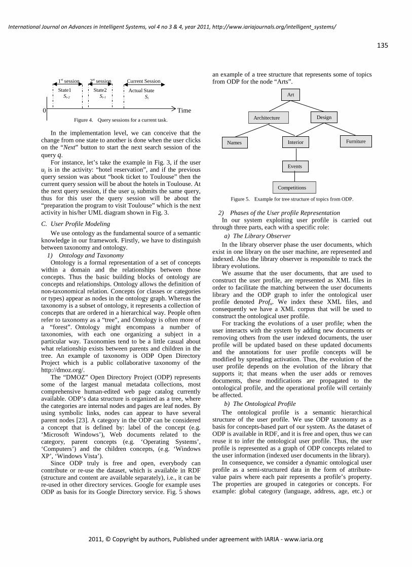
135



1st session 2st session Current Session 0 Time

Figure 4. Query sessions for a current task.

In the implementation level, we can conceive that the change from one state to another is done when the user clicks on the “Next” button to start the next search session of the query q.

For instance, let’s take the example in Fig. 3, if the user uj is in the activity: “hotel reservation”, and if the previous query session was about “book ticket to Toulouse” then the current query session will be about the hotels in Toulouse. At the next query session, if the user uj submits the same query, thus for this user the query session will be about the “preparation the program to visit Toulouse” which is the next activity in his/her UML diagram shown in Fig. 3.

C. User Profile Modeling

We use ontology as the fundamental source of a semantic knowledge in our framework. Firstly, we have to distinguish between taxonomy and ontology.

1) Ontology and Taxonomy Ontology is a formal representation of a set of concepts

within a domain and the relationships between those concepts. Thus the basic building blocks of ontology are concepts and relationships. Ontology allows the definition of non-taxonomical relation. Concepts (or classes or categories or types) appear as nodes in the ontology graph. Whereas the taxonomy is a subset of ontology, it represents a collection of concepts that are ordered in a hierarchical way. People often refer to taxonomy as a “tree”, and Ontology is often more of a “forest”. Ontology might encompass a number of taxonomies, with each one organizing a subject in a particular way. Taxonomies tend to be a little casual about what relationship exists between parents and children in the tree. An example of taxonomy is ODP Open Directory Project which is a public collaborative taxonomy of the http://dmoz.org/.

The “DMOZ” Open Directory Project (ODP) represents some of the largest manual metadata collections, most comprehensive human-edited web page catalog currently available. ODP’s data structure is organized as a tree, where the categories are internal nodes and pages are leaf nodes. By using symbolic links, nodes can appear to have several parent nodes [23]. A category in the ODP can be considered a concept that is defined by: label of the concept (e.g. ‘Microsoft Windows’), Web documents related to the category, parent concepts (e.g. ‘Operating Systems’, ‘Computers’) and the children concepts, (e.g. ‘Windows XP’, ‘Windows Vista’).

Since ODP truly is free and open, everybody can contribute or re-use the dataset, which is available in RDF (structure and content are available separately), i.e., it can be re-used in other directory services. Google for example uses ODP as basis for its Google Directory service. Fig. 5 shows

an example of a tree structure that represents some of topics from ODP for the node “Arts”.

Figure 5. Example for tree structure of topics from ODP.

2) Phases of the User profile Representation In our system exploiting user profile is carried out

through three parts, each with a specific role: a) The Library Observer

In the library observer phase the user documents, which exist in one library on the user machine, are represented and indexed. Also the library observer is responsible to track the library evolutions.

We assume that the user documents, that are used to construct the user profile, are represented as XML files in order to facilitate the matching between the user documents library and the ODP graph to infer the ontological user profile denoted Profu. We index these XML files, and consequently we have a XML corpus that will be used to construct the ontological user profile.

For tracking the evolutions of a user profile; when the user interacts with the system by adding new documents or removing others from the user indexed documents, the user profile will be updated based on these updated documents and the annotations for user profile concepts will be modified by spreading activation. Thus, the evolution of the user profile depends on the evolution of the library that supports it; that means when the user adds or removes documents, these modifications are propagated to the ontological profile, and the operational profile will certainly be affected.

b) The Ontological Profile The ontological profile is a semantic hierarchical

structure of the user profile. We use ODP taxonomy as a basis for concepts-based part of our system. As the dataset of ODP is available in RDF, and it is free and open, thus we can reuse it to infer the ontological user profile. Thus, the user profile is represented as a graph of ODP concepts related to the user information (indexed user documents in the library).

In consequence, we consider a dynamic ontological user profile as a semi-structured data in the form of attribute-value pairs where each pair represents a profile’s property. The properties are grouped in categories or concepts. For example: global category (language, address, age, etc.) or

Art

Architecture Design

Names Interior Furniture

Events

Competitions

State1 Si-2

State2 Si-1

Actual State Si

136



preference categories (preferences of restaurants, hotel, travel, music, videos, etc.). This allows us to help users to understand relationships between concepts, moreover, to avoid the use of wrong concepts inside queries. e.g., for a query “looking for a job as a Professor”, ODP concepts suggests relevant related terms such as teaching, research, etc.

From the ODP concepts, we annotate those related to the user documents. This is done by giving values to these ODP related concepts and weight to each value based on an accumulated similarity with the index of user documents [24], consequently an ontological user profile is created consisting of all concepts with non null value.

Thus, a graph of related concepts of the ODP (Open Directory Project) is inferred using the indexed XML documents, this is shown in Fig.6. Each leaf node in the ontological user profile is a pair, (concept, value), where the annotated value for that concept infer by the comparison with the user documents, this value will be also annotated by a score (VS) that reflects the degree of user interest. In Fig. 6, for instance, we consider the node “Music” and its children nodes from the ODP taxonomy nodes, we can infer the ontological user profile from these nodes based on the matching with the indexed user documents in the library. Next the concept “Jazz” is annotated with the value “Dixieland” from the user information because the user has shown interest in Dixieland Jazz, this value is annotated with a score (VS) which is “0.08”. We can add another value for this concept “Jazz” and then score to this value if the user is also interested in another jazz type.

Now we will overview how we can compute the value score VS. The score of the concept value (VS) is computed using the term frequency and the inverse document frequency (tf * idf) as follows:

∑∈

∗=Dd v

v n

DtfVS )]

||( log [

where: D is the set of user documents used to construct the user profile, |D|: is the total number of this set D.

nv: is a number of documents in which value v occurs. tfv: is the frequency of value v in document d є D, this is

computed as follows:

d

dvdv N

n tf ,

, =

where nv,d is the number of occurrences of the considered term (value v) in document d, and the denominator is the sum of number of occurrences of all terms in document d, that is, the size of the document | d |.

Example: Let’s consider a set of user documents contains 40

documents, and the value “Dixieland” appear in 3 documents: d7, d24, d33, (2 times in d7, only once time in d24, d33), the size of documents d7, d24, d33 is 80, 50, and 35, sequentially.

Thus: tfv,7 = 2/80 , tfv,24 = 1/50, tfv,33 = 1/35 . We can calculate VS by the previous formula:

))]3/40log(*0286.0())3/40log(*02.0())3/40log(*025.0[( ++=VS 0,0828 =VS

Thus the value V of the leaf node concept in the ontological user profile will be annotated with a score (VS) or weight that reflects the degree of user interest for this concept value, in our example the score of the value “Dixieland” is VS=0.0828 as shown in Fig. 6.

Figure 6. Inferring the ontological profile from user documents and ODP.

Thus, the ontological profile for each user consists of a list of concepts and their current weighted values. For example, a user profile could look like this:

Profile = (<user>, <Concept>, <weighted value>) E.g.: (Someone, sport, surf 0.8 - ski 0.2 -football 0.9) (Someone, restaurant, Italian 0.7- French 0.2) (Someone, cinema, action 0.6- horror 0.4) In fact using ontology as the basis of the profile allows

the user behavior to be matched with existing concepts in the domain ontology and relationship between these concepts. Based on the user’s behavior over many interactions, the interest score of the concept values can be incremented or decremented based on contextual evidence. As a result, a graph of related ODP concepts is inferred by using the matching with the user library in order to represent the user profile.

c) The Operational Profile The operational profile is derived from the ontological

profile, as a list of related relevant terms that can be easily used by the other models.

Once the ontological profile is created, the query context-related concepts, from this ontological profile, must be activated in order to extract the operational profile. This is done by mapping the query-context Cq[ i] on this ontological user profile (note that, the query context Cq is computed during the construction of the task model). This allows activating for each query-context concept its semantically related concepts from the ontological user profile, following our algorithm, depending on the relevance propagation [25],

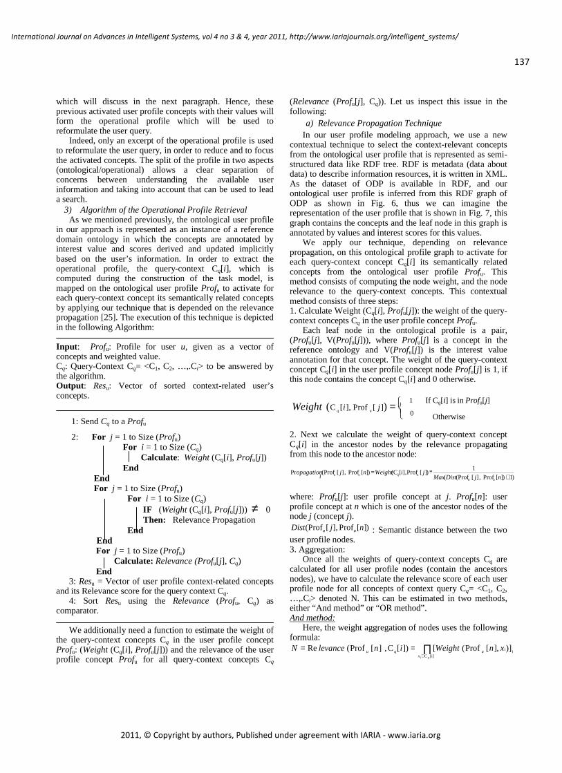
137



which will discuss in the next paragraph. Hence, these previous activated user profile concepts with their values will form the operational profile which will be used to reformulate the user query.

Indeed, only an excerpt of the operational profile is used to reformulate the user query, in order to reduce and to focus the activated concepts. The split of the profile in two aspects (ontological/operational) allows a clear separation of concerns between understanding the available user information and taking into account that can be used to lead a search.

3) Algorithm of the Operational Profile Retrieval As we mentioned previously, the ontological user profile

in our approach is represented as an instance of a reference domain ontology in which the concepts are annotated by interest value and scores derived and updated implicitly based on the user’s information. In order to extract the operational profile, the query-context Cq[i], which is computed during the construction of the task model, is mapped on the ontological user profile Profu to activate for each query-context concept its semantically related concepts by applying our technique that is depended on the relevance propagation [25]. The execution of this technique is depicted in the following Algorithm:

Input : Profu: Profile for user u, given as a vector of concepts and weighted value. Cq: Query-Context Cq= <C1, C2, …,.Ci> to be answered by the algorithm. Output : Resu: Vector of sorted context-related user’s concepts.

1: Send Cq to a Profu

2: For j = 1 to Size (Profu) For i = 1 to Size (Cq) Calculate: Weight (Cq[ i], Profu[j]) End End For j = 1 to Size (Profu) For i = 1 to Size (Cq) IF (Weight (Cq[i], Profu[j])) ≠ 0 Then: Relevance Propagation End

End For j = 1 to Size (Profu) Calculate: Relevance (Profu[ j], Cq) End 3: Resu = Vector of user profile context-related concepts

and its Relevance score for the query context Cq. 4: Sort Resu using the Relevance (Profu, Cq) as

comparator. We additionally need a function to estimate the weight of

the query-context concepts Cq in the user profile concept Profu: (Weight (Cq[i], Profu[j])) and the relevance of the user profile concept Profu for all query-context concepts Cq

(Relevance (Profu[j], Cq)). Let us inspect this issue in the following:

a) Relevance Propagation Technique In our user profile modeling approach, we use a new

contextual technique to select the context-relevant concepts from the ontological user profile that is represented as semi-structured data like RDF tree. RDF is metadata (data about data) to describe information resources, it is written in XML. As the dataset of ODP is available in RDF, and our ontological user profile is inferred from this RDF graph of ODP as shown in Fig. 6, thus we can imagine the representation of the user profile that is shown in Fig. 7, this graph contains the concepts and the leaf node in this graph is annotated by values and interest scores for this values.

We apply our technique, depending on relevance propagation, on this ontological profile graph to activate for each query-context concept Cq[i] its semantically related concepts from the ontological user profile Profu. This method consists of computing the node weight, and the node relevance to the query-context concepts. This contextual method consists of three steps: 1. Calculate Weight (Cq[i], Profu[j]): the weight of the query-context concepts Cq in the user profile concept Profu.

Each leaf node in the ontological profile is a pair, (Profu[j], V(Profu[j])), where Profu[j] is a concept in the reference ontology and V(Profu[j]) is the interest value annotation for that concept. The weight of the query-context concept Cq[ i] in the user profile concept node Profu[ j] is 1, if this node contains the concept Cq[i] and 0 otherwise.

=

1

0)( ][Prof ],[C ji uqWeight

2. Next we calculate the weight of query-context concept Cq[i] in the ancestor nodes by the relevance propagating from this node to the ancestor node:

)1)][ Prof , ][ Prof((

1*)][ Prof],[C()][ Prof , ][ Prof(Pr u +

=njDistMax

jiWeightnji

opagationuU

quu

where: Profu[j]: user profile concept at j. Profu[n]: user profile concept at n which is one of the ancestor nodes of the node j (concept j).

)][Prof ],[Prof( njDist uu : Semantic distance between the two user profile nodes. 3. Aggregation:

Once all the weights of query-context concepts Cq are calculated for all user profile nodes (contain the ancestors nodes), we have to calculate the relevance score of each user profile node for all concepts of context query Cq= <C1, C2, …,.Ci> denoted N. This can be estimated in two methods, either “And method” or “OR method”. And method:

Here, the weight aggregation of nodes uses the following formula:

∏∈

== [i]C

)],][ Prof([)][C,][ Prof(Reqix

iiuqu xnWeightinlevanceN

If Cq[i] is in Profu[ j]

Otherwise

138



Thus, depending on the previous formula, the relevance score N is not null for only the nodes which contain all the query-context concepts directly or in their ancestor nodes. Thus this will give the smallest relevant sub tree contains the previous concepts Cq=<C1, C2,…, Ci>.

We use the formula And, only when we need user profile fragments that contain all the query concepts, and neglect those contain some of query concepts. This case is not appropriate to our system, so we will use the OR method for computing the relevance score of user profile nodes for the query-context concepts. OR method:

The weight aggregation of nodes uses the following formula:

∑∈

==][C

* )],][ Prof([)][C,][ Prof(Reix

iiuquqi

xnWeightinlevanceN

The relevance score N is not null if the node contains one of the query-context concepts directly or in their ancestor nodes. So this will give fragments of user profile that are sorted by decreasing order of N. Example:

Let’s consider the initial query q, and the query-context Cq which is composed of three concepts: Cq= {C1, C2, C3}.

We consider also the user profile u, which is composed of many concepts represented as RDF graph (metadata); Fig. 7 shows the user profile graph u.

The leaf nodes: n3, n6, n9, n10, n12 annotate by values, and interest score to these values. Now we calculate the relevance of the user profile nodes for the query-context Cq using the formulas of weight and propagation. For example we calculate the relevance score fore the node n4:

1)(8

,1

=ncWeight

1)(5

,2

=ncWeight

1)(7

,3

=ncWeight

Figure 7. Example of a user profile graph Profu.

Then we follow the algorithm to compute the relevance score of the node n4 for the concepts C1, C2, C3. We have to propagate the weight not null to n4:

21

)1),((),(

),(Pr47

37473

=+

=nnDistMax

CnWeightnn

Copagation

21

)1),((),(

),(Pr45

2545

2=

+=

nnDistMax

CnWeightnn

Copagation

31

)1),((

),(),(Pr

48

1848

1

=+

=nnDistMax

CnWeightnn

Copagation

And:

12

1

2

1*

2

1*

3

1),()C ,(Re

3,2,144 === ∏

=i

iqq CnWeightnlevance

OR:

3

4

2

1

2

1

3

1),()C ,(Re

3

144 =++== ∑

=i

iqq CnWeightnlevance

We do the same steps to compute the relevance score of

the other user profile nodes, the results are shown in Table 5 for the “And method” and the “Or method”.

If we consider the “And” method then the smallest relevant sub tree that contains all query concepts is the sub-tree that is presented by the node n4 and its descending nodes to leafs, because the node n4 has the most relevance score as shown in Table 5.

But if we consider the “OR” method then the node n7 has the most relevance score, as shown in Table 5 below. In this case the most relevant result is the sub-tree which is presented by the node n7 and its descending nodes until the leaf nodes.

As we mentioned previously, the leaf nodes may be annotated by many values, and each one annotates with score VS, so we select the value that has the greater score VS. As a result the concepts of the user profile related to the query-context concepts are: n7, n8, n9, n10 and the values of n9, n10 which have greater score VS.

These concepts and their values constitute the operational profile; we will depend on this operational profile to generate the reformulated queries SRQ, based on the user profile and his/her context, those queries can be easily used in the search process to get relevant results which are needed to accomplish the task at hand.

TABLE V. RELEVANCE SCORE OF USER PROFILE CONCEPTS PROFU

USING BOTH “A ND METHOD” NN , “OR METHOD” N* N RESPECTIVELY.

Nn C3 C2 C1 Node

0.0125 0.25 0.25 0.2 n1

0.0277 0.333 0.333 0.25 n2

0 0 0 0 n3

0.0833 0.5 0.5 0.333 n4

0 0 1 0 n5

0 0 0 0 n6

0 1 0 0.5 n7

0 0 0 1 n8

0 0 0 0 n9

0 0 0 0 n10

0 0 0 1 n11

0 0 0 0 n12

N* n C3 C2 C1 Node

0.7 0.25 0.25 0.2 n1

0.916 0.333 0.333 0.25 n2

0 0 0 0 n3

1. 333 0.5 0.5 0.333 n4

1 0 1 0 n5

0 0 0 0 n6

1.5 1 0 0.5 n7

1 0 0 1 n8

0 0 0 0 n9

0 0 0 0 n10

1 0 0 1 n11

0 0 0 0 n12

C3

C2

n1

n9 n10

n6

n5

n3

n7

n4 n12

n11 n2 C1

C1

C3

n8

139



D. SRQ Model (State Reformulated Queries)

Short queries usually lack sufficient words to capture relevant documents and thus negatively affect the retrieval performance, and thus fail to represent the information need. Query expansion is a technique where original query is supplemented with additional related terms. Existing query expansion frameworks have the problem of poor coherence between expansion terms and user’s search goal, For instance, if the query jaguar be expanded as the terms {auto, car, model, cat, jungle,...} and user is looking for documents related to car, then the expansion terms such as cat and jungle are not relevant to user’s search goal.

1) SRQ Definition In the following, we will introduce a new notion State

Reformulated Queries (SRQ) which are provided by the reformulation of the initial user queries q, related to the current task, depending on the actual state of this task and the user profile. The states of the current task are expressed by activities which are required to accomplish this task and grouped in UML activity diagram including the relations between them, each state represents one search session. The change from one state to another is done over time when the user uj complete the actual activity and start the next one. Thus for two different task states, submitting the same query the relevant results will not be the same.

Let q= {t1, t2..., tn} be an initial query which is related to the task at hand. The state reformulated query at the task state Si and for a specific user profile Pj is: SiRQ<Q,Pj,Si>, this query contains the initial query q and the expansion terms E(q)={t q,1 , tq,2 , tq,3 , ...}. Thus we have to get the expansion terms E(q) = {tq,1 , tq,2 , tq,3,...} which are relevant to user’s search goal by exploiting user’s implicit feedback at the time of search. The relevant results Di at the states Si are produced by applying SiRQ<Q,Pj,Si> on an information retrieval system. We expect that the results Di at the task state Si are more relevant than those produced by using the initial query q at the same state Si.

A search is handled as follows: the user expresses his/her query, our assistant identifies the context of this search, and it creates the context description and proposes relevant terms to be added to the initial query. The initial user query will be reformulated depending on these relevant terms in order to generate SRQ (State Reformulated Query) to improve the retrieval performance. The assistant then submits the new reformulated query SRQ to a search engine on the Web and gets the results. The documents are then presented to the user in the order of decreasing estimated relevance.

2) Query Reformulation Phases The two phases to generate the State Reformulated

Queries (SRQ) are: query expansion and query refinement. a) Query expansion

The initial query is expanded with two types of generated terms which are denoted expansion terms E(q) = {tq,1, tq,2, tq,3,..}:

• Terms which represent the actual state of the current task A* (as1, as2, …,asi). There is at least one term for each task state which describes this state, this state term is denoted state attribute asi. These attributes are

computed using the Task model which was previously explained.

• Terms which represent the query-relevant concepts from the ontological user profile with its values (operational profile). The algorithm of extracting these terms from the ontological user profile was previously explained. These terms are denoted user profile attributes (au1, au2, …, auj).

b) Query Refinement After the user query is expanded by new terms, the tool

of query refinement must be applied in order to consider only the terms that are related to the actual task context, and disregard those are out of focus for the given context. Thus Query refinement is the incremental process of transforming an initial query into a new reformulated query SRQ that reflects the user’s information need in more accurate way.

Sometimes irrelevant attributes may be presented in the retrieved user profile concepts, and thus irrelevant terms are recommended by the operational profile, in order to keep only the relevant user profile attributes for the current task state Si, we compare between these generated attributes and the actual state attributes, next we consider the attribute of the previous task state, and then we exclude from the generated user profile attributes those non similar with the state attributes. Also we have to exclude the duplicated terms if they exist in the resulting SRQ.

Another method for filtering the previous terms is by asking the user to choose the relevant terms before adding them to the final reformulated query.

Finally, state reformulated queries SRQ are built according to the syntax required by the used search engine in order to submit the queries SRQ and to retrieve relevant results to the user at the actual state of the current task. Boolean operators can be used to construct the final query and adequate care is taken to ensure that the final query meets the syntax requirements, after each step, the user is asked if the query reflects his intension. If so, the final query is constructed using the appropriate syntax and submitted to the search engine.

For the Boolean operator, we use “And” with the terms that are extracted from the actual state of the current task, and “Or” with the terms that are extracted from the operational profile, because the task state terms are always required while the operational profile terms can be sometimes abandoned. For example, we can imagine the state reformulated query as follows:

SRQ: q AND hotel OR 2 stars OR single where: • q is the initial user query. • “hotel”: the state term that represents the task actual

state (state attribute). • “2 stars” and “single” are the relevant terms from

the operational profile.

E. System Architecture

Fig. 8 illustrates the system architecture. It combines the three models which are described in the previous sections: The task model, the user profile model and the SRQ model.

140



Figure 8. System Architecture.

IV. EVALUATION

The evaluation of the personalized information retrieval in context systems is known to be a difficult and expensive [26] due to the dynamic aspect of the system environment and its strongly adaptive properties. A formal evaluation of the contextualization techniques requires a significant amount of extra feedback from users in order to measure how much better a retrieval system can perform with the proposed techniques than without them. Our proposed approach which was described in this paper have been implemented in an experimental prototype, and tested by real users. Evaluation in the context of an evolving real-world system is always a challenge. In order to evaluate and to quantify the improvement provided by our system compared to the direct querying of a search engine without

reformulation, or more generally to the use of other assistants, we should verify that using a user context improves the search results, by focusing the system on the most relevant part of the profile. The standard evaluation measures from the Information Retrieval field require the comparison between the performances of retrieval:

• Using the initial user query without any personalization and contextualization.

• Using the user query with simple personalization, depending only on the user profile, (i.e., regardless of the user context, more precisely regardless of his/her task at hand).

• Using the state reformulated queries SRQ which are generated depending on the user context and his/her

User Query q = {t1, t2, …, tn}

User Profile

Cq= <C1, C2, …,Cm>

siss aaa ,....,, 21

Activity 1

Activity 2

Activity I

UML Activity diagramfor the current task A*

Tasks :={ A1, A2,..., Ai}

Contextual Application

Sensor

Actual Task State Si

Profile Retrieval Model

ujuu aaa ,....,, 21

SRQ Model State Reformulated Query

Query Expansion

Query Refinement

Information Retrieval System IR

Results

WordNet

Ontology (ex: ODP)

Domain Knowledge

141



profile, (i.e., constrained to the context of his/her current task).

Currently, to compare different configurations (corresponding to different profile, context, query); several agents are used simultaneously by the assistant when handling user query. Thus our experiments have been done with three agents: the « default » agent simply linked to Google, and a « personalized » agent which uses the user profile to rank the results without taking the context into account. A third agent « personalization with context» is also used.

A. Experimental Study

In order to evaluate the use of the task context together with the user profile to contextualize returned results, a prototype around the search engine, Google for example, is built using the Google API. This program builds a log of the initial user queries, the returned results by Google, the result on which the user clicked, and the summaries, titles and ranks of the returned results from Google. This log information is used to compute the evaluation metrics at the experimental queries and to evaluate the performance of our system. To conduct the experiments and calculate the evaluation metrics, 10 users are asked to use our system to perform similar tasks by submitting initial queries. The 10 users are classified in three groups, novice, medium and expert, depending on their experience levels in computer science and search engine. Each one is asked to submit queries on 3 different scenarios, where we put the users in specific scenarios to make them thinking about writing appropriate queries for these scenarios. We depend on scenarios such as travel, shopping, restaurant searching, etc. we will illustrate an example of these scenarios in the next section. Consequently a total of 30 queries are selected as experimental queries. The prototype records results on which the users clicked, which we use as a form of implicit user relevance in our analysis.

After the data is collected, we remove from the experimental queries that were no contextual information available for that particular query, and thus we had a log of 30 queries averaging 3 queries per user. We will calculate, at each experimental query, the evaluation metrics in the three cases: using classic search engine Google, using only personalized search without user context, and using our system based on user context and his/her profile.

1) Example of the experimental scenarios Here we will take an example of the scenarios that are

used in the experimental study. We consider the task “Travel” which was discussed in the section task modeling (section 3). We have illustrated in Fig. 3, a UML activity diagram for the user uj that contains all activities needed to perform this task. Now when the user submits his initial query q, which is related to the current task, in our platform, let it be q: “Trip to Paris”, the task model will assign the task “Travel” to this query as the first step. Next, the UML activity diagram for this task which is shown in Fig. 3 is retrieved. The system then uses the attributes associated with each task state and the user profile attributes for producing the relevant terms (query expansion phase), next the

irrelevant terms are excluded (query refinement phase), finally, the system generate the appropriate state reformulated query SRQ for each task state: S1: Book a flight ⇒S1RQ :{ trip Paris + “Flight” OR Ticket + OR Inexpensive}. S2: Book a hotel ⇒S2RQ :{ trip Paris + “hotel” +2 star OR single}. S3: Search for tourist information ⇒S3RQ :{ trip Paris + “Monuments” OR Weather OR plan OR Metro}. S4: Find a restaurant ⇒S4RQ :{ trip Paris + “restaurant” + Italian OR Vegetarian}. S5: Tourist photos ⇒S5RQ :{ trip Paris + “Photos”}. S6: News about Paris city ⇒S6RQ: {trip Paris+ “News” OR Weather}. where: “Flight”, “hotel”, “Monuments”, “ restaurant”, “ Photos” and “News” are the terms that represent task state attributes. “Ticket”, “Inexpensive”, “2 star”, “single”, “Weather”, “plan” , “Metro”, “Vegetarian” and “Italian” are the relevant terms from the user operational profile.

To evaluate our proposed framework we have to compute the evaluation metrics based on the experimental scenarios.

B. Evaluation Metrics

There are many evaluation metrics in the literature for the classic information retrieval evaluation, these metrics often depend on relevance judgments for the returned results, one of the most known of them is the “Precision and Recall” (PR), this metric takes into account the rate of relevant retrieved documents (precision) and the quantity of relevant retrieved documents (recall). Another metric is the Precision at n (P@N) [27], P@N is the ration between the number of relevant documents in the first n retrieved documents and n. The P@N value is more focused on the quality of the top results, with a lower consideration on the quality of the recall of the system. These evaluation metrics for classic IR can be also applied by IIR (Interactive Information Retrieval) authors [9], but IIR system authors must incorporate human subjective judgments, either implicitly (analyzing interaction logs) or explicitly (asking the users to rate the results to provide a best order).

The classic IR evaluation metrics are not sufficient to evaluate our system due to the contextual aspect of the system and the need to provision a real user judgement. Thus to evaluate our proposed framework, the used metrics must cover on one hand the evaluation of the proposed expansion terms which are used to reformulate the initial user query, and on the other hand they must cover the evaluation of returned results. Thus we will use three metrics:

• Quality: measures the quality of expansion terms. • Precision@k: measures the retrieval effectiveness. • Dynamics: measures the capability of adapting to the

changing needs of users and the changing states of his/her task at hand.

Now we will compute these three evaluation metrics: quality, precision@k, and dynamics, based on the experimental scenarios.

142



1) Quality

Let q be an initial user query, given an IR system, )(q

cD is the set of documents actually visited by the user for q. Thus

)(qcD represents the relevant results which are evaluated by the

user at his/her actual context and taking into account his/her profile using q. Therefore, the ideal information retrieval

system should retrieve these documents )(q

cD in the foreground and present them to the user at the specific context.

Given a query expansion system, let )(qE be the set of

expansion terms for the query q, i.e.: { },.....,, 3,2,1,

)(qqq

qE τττ=

Then the quality of the expansion terms is defined as follows:

)(

)()( ),( ρ q

qc

q

E

DEQuality=

where: ),( ρ )()( q

cq DE : The matching terms between

)(qE and)(q

cD , that’s mean:

{ }dDdEDE qc

qqc

q ∈∈∃∈= τττ s.t. ,),( ρ )()()()(

For example, if we take the scenario presented in the

previous section and the user query q=‘‘ trip Paris’’, during this scenario, we take the second state S2 which is searching a hotel in Paris, at this actual task state we execute the query q by using Google and we present the returned results to the user, then the user visits the relevant documents at S2. If the

user visits 5 documents then 5 )( =qcD . At this actual state S2,

our system proposes set of expansion terms)(qE , this set

contains 5 terms which are: trip, Paris, hotel, 2 star, single. Thus: 5)( =qE . From these 5 terms, if there are 3 terms

existing in the 5 visited documents )(q

cD at S2, then: 3),( ρ )()( =q

c

q DE

Thus the quality of the expansion terms over this query q is:

6.0),( ρ

)(

)()(

==q

q

c

q

E

DEQuality

We do the same steps for the other queries at the different states of this task and then we can compute the average quality of the expansion terms over 10 queries submitted by 10 different users. In consequence, the average quality of the expansion terms by our system is 0.73 for this scenario. Finally we can compute the average quality of the expansion terms over all experimental queries (30 queries) at the different scenarios.

If we depend only on the user profile to generate the

expansion terms )(qE for the same user’s queries at the same

context and the same conditions, thus the )(qE will be

different from the first case. In the same steps we calculate

the average quality of expansion terms)(qE which are

extracted from the user profile and do not taking into account the user context at the same user’s queries for the previous scenario (trip Paris). In consequence the average quality is 0.34 in this case.

We notice that the average quality of the generated expansion terms, depending on user profile and user context (first case), is higher than that generated depending only on the user profile. Thus our system has an improvement of about 39% in the average quality of the generated expansion terms compared with that of standard personalized systems.

2) Precision@k

The second metric is the Precision@k, Let )(q

nD be the set of top n documents retrieved by the IR system using the query q. To define retrieval effectiveness, we determine the

number of documents in )(q

nD which are closely related to the

documents in)(q

cD . We use cosine similarity (previously explained) to define the closeness between two documents.

Let )(q

rD be a set of documents from

)(qnD for which the cosine

similarity with at least one of the document in )(q

cD is above a

threshold simΘ , that’s mean: { }simji

qcj

qnii

q ddSimDdDddr

D Θ≥∈∃∈= ),( s.t. , )()()(

Thus, to measure the retrieval effectiveness, we define the Precision@k as follows:

kr

Dkprecision@

q)(

=

To facilitate the experiments, let’s n=20, then)(

20SRQD

represents the first 20 documents from the retrieved results by the IR system (Google for example) by using the state reformulated query SRQ which contains the expansion terms

)(qE . In the previous section, we mentioned that )(q

cD

represents the relevant results for the initial user query q,

these )(q

cD are evaluated by the user at his/her actual context and taking into account his/her profile. In order to define the

closeness between )(

20SRQD and

)(qcD we compute the cosine

similarity between the documents of the two sets. We

determine the number of documents from )(

20SRQD which are

closely related to the documents in)(q

cD . Let )( SRQ

rD be a set of

documents from )(

20SRQD for which the cosine similarity with

at least one of the document in )(q

cD is above a thresholdsimΘ .

In this study we define )( SRQ

rD with the threshold value [simΘ

= 0.5], because as we know the value of cosine similarity is in the range of [0, 1], we consider the middle point as the threshold value, thus:

{ }5.0),( s.t. , )()(

20

)( ≥∈∃∈= ji

q

cj

SRQ

ii

SRQ ddSimDdDddr

D

143



Thus: Kr

DKprecision@

SRQ)(

=

Note that, the set of relevant documents )(q

cD is obtained from the query log or from the user exploring at the snippets

of the returned results whereas the set )(

20SRQD is obtained from

our experimental retrieval system after simulating the query sequence and submitting the reformulated queries.

Now we compute the retrieval performance (precision@k) of our proposed query reformulation system based on user profile and his/her context for all experimental queries of the experimental scenarios. We give the values 5, 10, 20 to k, in order to compute the Precision@5, Precision@10 and Precision@20.

We consider again the scenario “travel” in the previous section and the query q=‘‘ trip Paris”. We take, as an example, the second state S2 which is searching a hotel in

Paris, at this task state the 5 )( =qcD

and the S2RQ is: {trip Paris + “hotel” + 2 star OR single}. We execute this S2RQ by using Google and then we compute )( 2 RQS

rD in the three

cases (k=5, k=10, k=20) by calculating the cosine similarity

between )(q

cD and)(

52RQSD for k=5,

)(

102RQSD for k=10 and

)(

202RQSD

for k=20. Thus:

6.05

3

5 5

)( 2

===RQS

rD

precision@

where: { }5.0),( s.t. , )()(

5

)( 22 ≥∈∃∈= ji

q

cj

RQS

ii

RQS ddSimDdDddr

D )(

52RQSD is the set of top 5 documents retrieved by IR system

using S2RQ.

For K=10: 5.010

5

10 10

)( 2

===RQS

rD

precision@

where: { }5.0),( s.t. , )()(

10

)( 22 ≥∈∃∈= ji

q

cj

RQS

ii

RQS ddSimDdDddr

D

For K=20: 4.020

8

20 20

)( 2

===RQS

rD

precision@

where: { }5.0),( s.t. , )()(

20

)( 22 ≥∈∃∈= ji

q

cj

RQS

ii

RQS ddSimDdDddr

D

Otherwise we can compute based on the user judgment of relevant results from the top k returned results by using SRQ. That means the user evaluates the relevant results himself without using the cosine similarity, but this will require more feedbacks from the user.

In the same method, we can calculate the precision of our system for the other task states in the actual taken scenario and for the others task states in the three experimental scenarios.

In order to quantify the improvement provided by our system compared to the direct querying of a search engine without reformulation or with simple personalization, depending only on the user profile, we calculate the retrieval performance of the standard Google search system and the retrieval performance of the query reformulation system based only on the user profile, by using the same

experimental queries in the same experimental scenarios and the same users. Fig. 9 shows a comparison between the Precision@5, Precision@10, Precision@20 averages of our proposed system and those of the standard search without any reformulation and personalized search based only on the user profile. We notice that the precision average of our proposed framework is more precise than the precision average of the standard Google search in the specific task state, and more precise than that of the query reformulation system based on the user profile in the same task state. Thus our retrieval system is more effective at a specific context than that of the classic information retrieval systems and the personalized retrieval systems at the same context.

Figure 9. Comparison between the Precision@k averages of the different

systems.

3) Dynamics The third evaluation metric is the dynamics in query

expansion. For a query q, our system of query reformulation returns different expansion terms at different search sessions

of the task at hand. Let )(q

iE and )(q

jE be the set of expansion terms for a query q at two different task states i and j, we define the dynamics between the two states i, j as follows:

),(1),( )()()( qj

qi

q EESimji −=δ

For example, to calculate the dynamics in query expansion terms for the two states S1, S2 of the previous experimental scenario (travel) and the query q= trip Paris, we have to calculate the similarity between the expansions terms proposed in the two states. The all expansion terms in this two states S1, S2 are 9 terms, there are 2 common terms, and thus the similarity between these two states is 2/9, and the dynamics will be:

78.0)92

(1),(1),( )()(21

)(

21=−=−= srq

ssrq

ssrq EESimssδ

In the same method we can calculate the dynamics in query expansion terms of the other states and for the three experimental scenarios. Fig. 10 shows the average of the dynamics in query expansion over the experimental queries which are submitted during the three proposed scenarios.

0

0,2

0,4

0,6

0,8

1

precision@5 precision@10 precision@20

Reformulationusing User Context+ User Profile(SRQ)

Reformulationusing only UserProfile (rq)

WithoutReformulation (q)

)( 2RQS

rD

144



In fact the personalization-based query expansion systems have a dynamics of zero in all cases, because these systems always return the same expansion terms in all task states irrespective of user’s search goal or task states, because the expansion terms, in this case, are based on the user’s profile only.

We notice from Fig. 10 that our proposed system has a small dynamics in the expansion terms among the states of the simple tasks, such as scenario 2 (shopping), and it has a high dynamics in expansion terms among the states of the complex tasks, such as task in scenario 1 (travel). Thus our proposed framework is able to adapt to the changing needs of the users and generate expansion terms dynamically.

Figure 10. The average dynamics in query expansion terms for our system in the three experimental scenarios.

C. Discussion

From the various experiments, we observed that our proposed framework provides more relevant expansion terms compared with the query expansion mechanisms based on user profile only. Most importantly, our system can dynamically adapt to the changing needs of the user by generating state reformulated queries for the initial user query q in each search session. These generated queries SRQ will be different from one task state to another for the same user and the same initial query q. Consequently these queries SRQ provide more relevant results, in a specific context, compared with the results returned by the standard information retrieval system IRS using the initial user query q or the results returned by the personalized information retrieval systems.

In fact we notice from the experiments that our system is more effective when the user is not expert in computer science because he/she needs an aide to formulate the query that reflects his/her needs. Also our system is effective when the user needs are vague, especially when he is in the context of performing one task. Our system is also effective when the user query is short, so the query expansion will lead to disambiguate the query and to provide relevant results. Because the queries of mobile users are often short, and their information needs are often related to contextual factors to perform one task, thus our system is more effective in

providing relevant results for mobile users. In addition, we notice that our proposed system is more effective when the task has many clear and different states (such as the travel task). In this case our system has high dynamics in expansion terms among the states of this task. Whereas the proposed system is less effective with the simple tasks (such as shopping task), in this case our system has small dynamics in the expansion terms among the states of this task types.

One of the system disadvantages, which has emerged during the experiments, that when the expansion terms increase greatly the precision of our system will decrease, but we cannot determine a specific ideal number of expansion terms. Indeed the limitation of our experiments is the manual relevance judgments by several users; this is due to the dynamic aspect of our system and the absence of a standard test collection for the context-based personalized information retrieval systems.

However the experiments show that our approach of context-based information retrieval can greatly improve the relevance of search results.

V. CONCLUSION AND FUTURE WORKS

We have proposed a hybrid method to reformulate user queries depending on an ontological user profile and user context, with the objective of generating a new reformulated query more appropriate than that originally expressed by the user. The objective of the new reformulated query denoted State Reformulated Queries SRQ is to provide the user with context-based personalized results, we proved in an experimental study that these results are more relevant than the results provided by using the initial user query q and those provided by using the user query with simple personalization, depending only on the user profile, in the same context, because the user profile is not relevant all the time, thus we consider only the preferences that are in the semantic scope of the ongoing user activity for personalization, and disregard those are out of focus for a given context.

In this paper, the user context describes the user’s current task, its changes over time and its states, i.e., to define the user context; we define the task which the user is undertaking when the information retrieval process occurs and the states of this task. The stages of the task performance are called task states and the transition from one stage to another means that the user has completed this stage of the current task.

Consequently the user queries which are submitted during the task at hand are related to this task, indeed that are part of it. Because the queries of mobile users are often short, and their information needs are often related to contextual factors to perform task at hand, thus an intelligent assistant that can propose new reformulated query before submitting it to the information retrieval system is more effective in the case of a mobile user. Therefore our system is more useful in providing relevant results for mobile users.

On the other hand, we initialize a user profile by using mass of information existing on his/her workstation (personal files), and next we retrieve relevant elements from this profile to use them in query reformulation. In our system

0

0,2

0,4

0,6

0,8

1

Average Dynamics

(scenario_1)

Average Dynamics

(scenario_2)

Average Dynamics

(scenario_3)

Reformulation using user context + user profile

Reformulation using user profile

Without reformulation

145



the user profile is ontological because it is constructed by considering related concepts from existing concepts in domain ontology (such as ODP taxonomy). Our proposed approach involves new methodology to retrieve query-related elements from the ontological user profile. This methodology has been applied successfully to retrieve information from the semi-structured data.

We have constructed a general architecture that combines several models: task model, user profile model and SRQ model. And we have constructed a new general language model for query expansion including the contextual factors and user profile in order to estimates the parameters in the model that is relevant to information retrieval systems.

We use both a semantic knowledge (ODP Open Directory Project taxonomy) and a linguistic knowledge (WordNet) to improve web querying processing because the linguistic knowledge doesn’t capture the semantic relationships between concepts and the semantic knowledge doesn’t represent linguistic relationships of the concepts. Parsing the user query by the two previous types of knowledge generate the so-called query context. We proved that the integration of linguistic and semantic information into one repository was useful to learn user’s task.

UML activity diagram is used to represent the user’s current task in order to detect the changes over time in the activities needed to accomplish this task and for describing all the sequences of the performed task. Each activity in the generated UML activity diagram expresses the task’s actual state.

Our “State Reformulated Query” system has been implemented in a prototype and applied to web queries. We had achieved an experimental study using few scenarios by several users; the preliminary results from the prototype are encouraging. Also we proposed an evaluation protocol which uses three evaluation metrics to cover the evaluation of the expansion terms and the evaluation of returned results. The aim is to quantify the improvement provided by our system compared to the personalized reformulation query systems and the standard search without reformulation. From the various experiments, we have proved that the proposed framework provide more relevant results compared to the standard information retrieval system and the baseline query expansion mechanisms based only on the user profile. Thus, the experiments showed that our proposed context-based approach for information retrieval can greatly improve the relevance of search results.

A. Future Works

This research can be extended in several directions. Firstly to optimize the quality of generated terms and then the precision of results, secondly to optimize the detection of the user’s task and its states by improving the task model.

To facilitate the use of the contextual model, we can use the contextual graph [28], instead of UML activity diagram to represent the user's current task. In our future work we plan to use this contextual graph.

In future work for this research, we propose to use a Markov models to select the actual task state implicitly by predicting from a number of observed events, the next event

from the probability distribution of the events which have followed these observed events in the past. For example, when the task at hand consists of predicting WWW pages to be requested by a user, the last observed event could be simply the last visited WWW page or it could contain additional information, such as the link which was followed to visit this page or the size of the document.

In perspective we can also improve the assistant of generating reformulated queries (SRQ) to be more intelligent by using the ChatBot technique; that means the assistant can chat with a user in order to focus on the actual task state.

Further validation by using different types of queries and domains is required to provide more conclusive evidence. Further work is also needed to determine the circumstances under which the approach may not yield good results.

We plan also to evaluate this method by using another evaluation protocol by constructing a test collection and determining relevant results for several queries in a particular context, and next comparing between these relevant results and the results that are returned by our system for the same queries in the same context.

REFERENCES [1] O. Asfari, B-L. Doan, Y. Bourda and J-P. Sansonnet,

“Context-based Hybrid Method for User Query Expansion”, Proceedings of the fourth international conference on Advances in Semantic Processing, SEMAPRO 2010, pp. 69-74, Italy, Florence, 2010.

[2] A. Micarelli, F. Gasparetti, F. Sciarrone and S. Gauch, “Personalized Search on the World Wide Web”, The Adaptive Web 2007, P. Brusilovsky, A. Kobsa, and W. Nejdl (Eds.), LNCS 4321, pp. 195-230, Springer-Verlag Berlin Heidelberg 2007.

[3] Ph. Mylonas, D. Vallet, P. Castells, M. Fernández, and Y. Avrithis, “Personalized information retrieval based on context and ontological knowledge”, Knowledge Engineering Review 23(1), special issue on Contexts and Ontologies, pp. 73-100, March 2008.

[4] A. Kofod-Petersen and J. Cassens, “Using Activity Theory to Model Context Awarenessa”, American Association for Artificial Intelligence, Berlin, 2006.

[5] R. W. White and D. Kelly, “A Study on the Effects of Personalization and Task Information on Implicit Feedback Performance”, CIKM’06, USA, 2006.

[6] S. Dumais, E. Cutrell, J. Cadiz, G. Jancke, R. Sarin, and D. C. Robbins, (Stuff I’ve Seen) “A system for personal information retrieval and re-use”, Proceedings of 26th ACM SIGIR 2003, pp. 72-79, Toronto, July 2003.

[7] M. Melucci, “Context modeling and discovery using vector space bases”, CIKM '05: Proceedings of the 14th ACM international conference on Information and knowledge management. ACM, Bremen, Germany, pp. 808-815, 2005.

[8] K. Sugiyama, K. Hatano and M. Yoshikawa, “Adaptive Web Search Based on User Profile Constructed without Any Effort from Users”, WWW 2004, pp.17-22, New York, USA, May, 2004.

[9] X. Shen, B. Tan and C. Zhai, “Implicit User Modeling for Personalized Search”, CIKM’05, Bremen, Germany, 31 November, 2005.

[10] B.J. Jansen, A. Spink, J. Bateman and T. Saracevic, “Real life information retrieval: a study of user queries on the Web”, SIGIR Forum 32(1): pp. 5-17, 1998.

146



[11] G. Koutrika and Y. E. Ioannidis, “Personalization of Queries in Database Systems”, Proceedings of the 20th International Conference on Data Engineering, USA, 2004.

[12] Y. Lv and C. Zhai, “Adaptive Relevance Feedback in Information Retrieval”, CIKM, 2009, Hong Kong.

[13] H. Wakaki, T. Masada, A. Takasu, and J. Adachi, “A New Measure for Query Disambiguation Using Term Co-occurrences”, Lecture Notes Computer Science, NUMB 4224, pp. 904-911, 2006.

[14] J. Bhogal, A. Macfarlane and P. Smith, “A review of ontology based query expansion, Information Processing and Management”, International Journal, v.43 n.4, pp. 866-886, July, 2007.

[15] R. Navigli and P. Velardi, “An Analysis of Ontology-based Query Expansion Strategies”, Workshop on Adaptive Text Extraction and Mining at the 14th European Conference on Machine Learning, Cavtat-Dubrovnik, Croatia, 2003.

[16] H. Terai, H. Saito, M. Takaku, Y. Egusa, M. Miwa and N. Kando, “Differences between informational and transactional tasks in information seeking on the web”, Proceedings of the Second Symposium IIiX, 2008.

[17] L. Freund, E.G. Toms and C. Clarke, “Modeling task-genre relationships for IR in the workplace”, SIGIR 2005, Salvador, Brazil, 2005.

[18] D. Leake, R. Scherle, J. Budzik and K. Hammond, “Selecting Task-Relevant Sources for Just-in-Time Retrieval”, Proceedings of the AAAI-99 Workshop on Intelligent Information Systems, Menlo Park, CA, 1999.

[19] J. Luxenburger, S. Elbassuon and G. Weikum, “Task-aware search personalization”, Proceedings of the 31st annual international ACM SIGIR, Singapore, 2008.

[20] H. Bouchard and J. Nie, “Modèles de langue appliqués à la recherche d'information contextuelle”, Proceedings of CORIA 2006 Conf en Recherche d’Information et Applications. pp. 213-224, Lyon, 2006.

[21] J. Allan, “Challenges in information retrieval and language modeling”, report of a workshop held at the center for intelligent information retrieval, University of Massachusetts Amherst, SIGIR Forum, 37, 1, pages 31-47, 2003.

[22] E. Garcia, “Cosine Similarity and Term Weight Tutorial”, http://www.miislita.com/information-retrieval-tutorial/cosinesimilarity-tutorial.html, pp.187-219, 2006.

[23] P. A Chirita, W. Nejdl, R. Paiu and Ch. Kohlschutter, “Using ODP Metadata to Personalize Search”, Proc. of the 28th Annual Int’l ACM SIGIR Conf., pp. 178-185, Salvador, Brazil, 2005.

[24] A. Sieg, B. Mobasher and R. Burke, “Ontological User Profiles for Representing Context in Web Search”, Proceedings of the Workshop on Web Personalization and Recommender Systems in conjunction with the ACM International Conference on Web Intelligence, Silicon Valley, CA, November 2007.

[25] O. Asfari, Modèle de recherche contextuelle orientée contenu pour un corpus de documents XML, The fifth Francophone Conference on Information Retrieval and Applications, CORIA ET RJCRI 2008, pp. 377-384, Trégastel, France, 2008.

[26] Y. Yang and B. Padmanabhan, “Evaluation of Online Personalization Systems: A Survey of Evaluation Schemes and a Knowledge-Based Approach”, Journal of Electronic Commerce Research, pp. 112-122, 2005.

[27] R. Kraft, C. Chang, F. Maghoul and R. Kumar,“Searching with Context”, WWW'06: Proceedings of the 15th international conference on World Wide Web. ACM, Edinburgh, Scotland, pp. 367-376, 2006.

[28] P. Brézillon, “Task-realization models in Contextual Graphs”, 5th International and Interdisciplinary Conference on Modeling and Using Context, Lectures Notes in Artificial Intelligence, Vol 3554, pp. 55-68, Springer-Verlag, 2005.

147



Modeling, Analysis and Simulation of UbiquitousSystems Using a MDE Approach

Amara Touil∗, Makhlouf Benkerrou∗, Jean Vareille∗, Fred Lherminier†, and Philippe Le Parc∗∗Universite de Brest, France

Universite Europeenne de BretagneLabSTICC - UMR CNRS 6285

20 av. Victor Le Gorgeu, BP 809, F-29285 [email protected], [email protected],

[email protected], [email protected] (contact author)†Terra Nova Energy

28 rue Victor Grignard, F-29490 [email protected]

Abstract—The growth of industrial activities during the lastdecades and the diversity of industrial products require stan-dards and common methodologies for building and integratingsystems. It is also required that working groups use the sameterminologies and concepts needed for each domain. The ModelDriven Engineering approach aims to give an answer, while usinga high level method based on models and transformations. In thispaper, we use this approach to model ubiquitous systems. Thosesystems are composed of devices interconnected through variouskinds of network, in order to get and provide information. Wepresent a model for this class of systems and, its use, in termsof analysis and simulation, in the field of energy while studyingreal cases from our industrial partner, Terra Nova Energy.

Keywords-Domain Specific Language; Model Driven Engi-neering; Ubiquitous Systems; Analysis; Simulation.

I. INTRODUCTION

Ubiquity is often defined as the property of being ableto be in several places at the same time. In the field ofInformation Technologies, this definition can be improved intwo different ways, that may look opposite. Here is the firstapproach: as in [2] users are surrounded with ”intelligent”systems, that may deliver them needed information: in thiscase, computing technologies are used in order to locate users,to understand their environment, to anticipate their needsand to make it possible that any information they requireis available anywhere at anytime. The second approach isto offer people to be able to get information on a systemlocated somewhere and to be able to act safely on it: here,computing technologies are used to make it possible to be”virtually” present in several places at the same time. Weplace our work in the second approach, in order to modeland analyze telecontrol applications as a kind of ubiquitoussystems.

Terra Nova Energy (TNE) is an innovative company [3] thatprovides solutions for data mining in the fields of electricity,hydraulics and pulse-energy. It integrates sensing, acting andcommunicating devices in telecontrol systems, for collectingdata from different sites using various technologies. TNE’s

systems allow real-time operating and provide processes forhandling different data.

In order to improve its development, this company is facingtwo problems: how to design remote monitoring systems asautomatically as possible and how to speed up their on-sitedeployment ?

To answer these questions, we intend to use a basedmodel approach, relying on specific components for telecontroldomain and libraries integrating industrial parts coming fromvarious providers. Our project is to build a framework [4]following the Model Driven Engineering (MDE) methodology[5][6] to setup a telecontrol ontology and proper transforma-tions for building, generating, analyzing and deploying suchubiquitous telecontrol systems.

Our aim is to define a generic meta-model and to use it forvarious systems, as case study examples, one of them beingof the TNE system.

This paper is organized as follows: first of all, the MDEapproach, Domain Specific Languages (DSL) and transfor-mations that may be conducted are briefly introduced. Then,we explain the originality of our work while describing ourmethod. In the Section IV, we introduce the proposed genericmeta-model, and in Section V this general meta-model isapplied to our case study, while defining an instance forTNE. Then, we explain how to carry a static analysis on agiven instance and show the first results. We then describeautomatic transformation that makes it possible to simulate,using PtolemyII [7], an instance. Finally we discuss ourmethod and we finish by further work.

II. RELATED WORKSIn this section, we introduce some basic notions about the

MDE approach and DSL, and how to carry out transformationson models in order to analyse them. A focus is also made onsimulation concepts and tools.

A. The MDE approachA model is an abstracted view of a system that expresses

related knowledge and information. It is defined by a set of

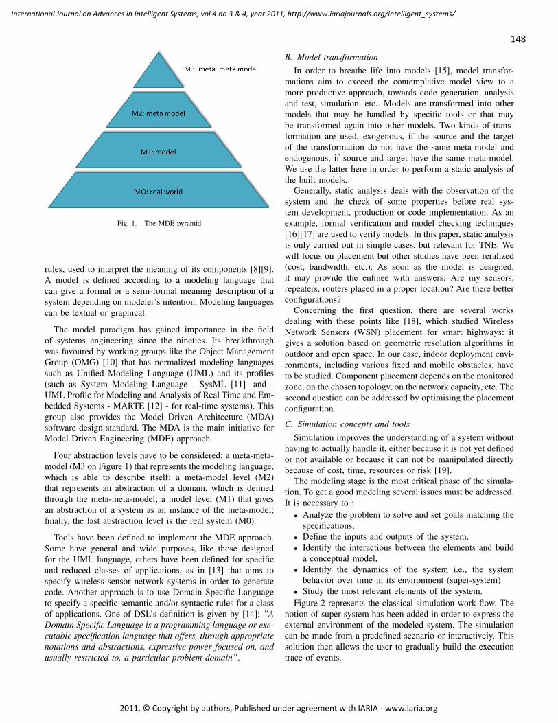
148



Fig. 1. The MDE pyramid

rules, used to interpret the meaning of its components [8][9].A model is defined according to a modeling language thatcan give a formal or a semi-formal meaning description of asystem depending on modeler’s intention. Modeling languagescan be textual or graphical.

The model paradigm has gained importance in the fieldof systems engineering since the nineties. Its breakthroughwas favoured by working groups like the Object ManagementGroup (OMG) [10] that has normalized modeling languagessuch as Unified Modeling Language (UML) and its profiles(such as System Modeling Language - SysML [11]- and -UML Profile for Modeling and Analysis of Real Time and Em-bedded Systems - MARTE [12] - for real-time systems). Thisgroup also provides the Model Driven Architecture (MDA)software design standard. The MDA is the main initiative forModel Driven Engineering (MDE) approach.

Four abstraction levels have to be considered: a meta-meta-model (M3 on Figure 1) that represents the modeling language,which is able to describe itself; a meta-model level (M2)that represents an abstraction of a domain, which is definedthrough the meta-meta-model; a model level (M1) that givesan abstraction of a system as an instance of the meta-model;finally, the last abstraction level is the real system (M0).

Tools have been defined to implement the MDE approach.Some have general and wide purposes, like those designedfor the UML language, others have been defined for specificand reduced classes of applications, as in [13] that aims tospecify wireless sensor network systems in order to generatecode. Another approach is to use Domain Specific Languageto specify a specific semantic and/or syntactic rules for a classof applications. One of DSL’s definition is given by [14]: ”ADomain Specific Language is a programming language or exe-cutable specification language that offers, through appropriatenotations and abstractions, expressive power focused on, andusually restricted to, a particular problem domain”.

B. Model transformationIn order to breathe life into models [15], model transfor-

mations aim to exceed the contemplative model view to amore productive approach, towards code generation, analysisand test, simulation, etc.. Models are transformed into othermodels that may be handled by specific tools or that maybe transformed again into other models. Two kinds of trans-formation are used, exogenous, if the source and the targetof the transformation do not have the same meta-model andendogenous, if source and target have the same meta-model.We use the latter here in order to perform a static analysis ofthe built models.

Generally, static analysis deals with the observation of thesystem and the check of some properties before real sys-tem development, production or code implementation. As anexample, formal verification and model checking techniques[16][17] are used to verify models. In this paper, static analysisis only carried out in simple cases, but relevant for TNE. Wewill focus on placement but other studies have been reralized(cost, bandwidth, etc.). As soon as the model is designed,it may provide the enfinee with answers: Are my sensors,repeaters, routers placed in a proper location? Are there betterconfigurations?

Concerning the first question, there are several worksdealing with these points like [18], which studied WirelessNetwork Sensors (WSN) placement for smart highways: itgives a solution based on geometric resolution algorithms inoutdoor and open space. In our case, indoor deployment envi-ronments, including various fixed and mobile obstacles, haveto be studied. Component placement depends on the monitoredzone, on the chosen topology, on the network capacity, etc. Thesecond question can be addressed by optimising the placementconfiguration.

C. Simulation concepts and toolsSimulation improves the understanding of a system without

having to actually handle it, either because it is not yet definedor not available or because it can not be manipulated directlybecause of cost, time, resources or risk [19].

The modeling stage is the most critical phase of the simula-tion. To get a good modeling several issues must be addressed.It is necessary to :

• Analyze the problem to solve and set goals matching thespecifications,

• Define the inputs and outputs of the system,• Identify the interactions between the elements and build

a conceptual model,• Identify the dynamics of the system i.e., the system

behavior over time in its environment (super-system)• Study the most relevant elements of the system.Figure 2 represents the classical simulation work flow. The

notion of super-system has been added in order to express theexternal environment of the modeled system. The simulationcan be made from a predefined scenario or interactively. Thissolution then allows the user to gradually build the executiontrace of events.

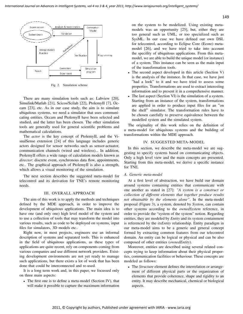
149



Fig. 2. Simulation scheme

There are many simulation tools such as: Labview [20],Simulink/Matlab [21], Scicos/Scilab [22], PtolemyII [7], Oc-cam [23], etc. As in our case study, the aim is to simulateubiquitous systems, we need a simulator that uses communi-cating entities. Occam and PtolemyII have been selected andstudied, and the latter has been chosen. The other simulationtools are generally used for general scientific problems andmathematical calculations.

The actor is the key concept of PtolemyII, and the Vi-sualSense extension [24] of this language includes genericactors designed for sensor networks such as sensor-actuator,communication channels (wired and wireless)... In addition,PtolemyII offers a wide range of calculation models known asdirector: discrete event, synchronous data flow, appointments,etc.. The graphical approach of PtolemyII is also a strength,which allows a visual monitoring of the simulation.

The next section describes the suggested meta-model fortelecontrol and its derivation for TNE’s remote monitoringneeds.

III. OVERALL APPROACH

The aim of this work is to apply the methods and techniquesdefined by the MDE approach, in order to improve thedevelopment of ubiquitous applications. The main idea is tohave one (and only one) high level model of the system andto use a collection of tools that may transform the model intovarious results, such as code to be deployed on systems, inputfiles for simulators, 3D models etc..

Right now, in most projects, engineers use an informaldescription of systems and separated tools. This is enhancedin the field of ubiquitous applications, as these types ofapplications are quite recent, rely on components coming fromvarious companies and use different network providers. Exist-ing development environments are not yet ready to managesuch applications, but there exists a lot of work that has beendone that could be interconnected and re-used.

It is a long term work and, in this paper, we focussed onlyon three main aspects:

• The first one is to define a meta-model (Section IV), thatwill make it possible to capture the maximum information

on the system to be modelized. Using existing meta-models was an opportunity [25], but, either they aretoo general such as UML, or too specialized such asSysML. In our case we have defined our own DSLfor telecontrol, according to Eclipse Core (Ecore) meta-model [26], and we have tried to take into accountthe specifity of ubiquitous applications. From this meta-model, we are able to build the unique model (or instance)of a system. This instance can be seen as the main inputof the transformation tools.

• The second aspect developed in this article (Section V)is the analysis of the instance. In that case, we have just”had a look” to it and we have tried to assess someproperties. Transformations are used to extract interestinginformation and to present it in a comprehensive manner.

• The last aspect (Section VI) is the simulation of a system.Starting from an instance of the system, transformationsare applied in order to produce input files for an ”onthe shelf” simulator. The transformation rules have tobe chosen carefully to preserve equivalence between themodelled system and the simulated system.

The originality of this work relies on the definition ofa meta-model for ubiquitous systems and the building oftransformations within the MDE approach.

IV. SUGGESTED META-MODEL

In this section, we describe the meta-model we are sug-gesting to specify systems based on communicating objects.Only a high level view and the main concepts are presented.Starting from this meta-model, we derive a specific instancefor TNE.

A. Generic meta-model

At a first level of abstraction, we have build our domainaround systems containing entities that communicate withone another as stated in [27]: ”A system is a construct orcollection of different elements that together produce resultsnot obtainable by the elements alone”. In the meta-modelproposal (Figure 3), a system, denoted by System, can containother systems according to the ownedSystem reference, inorder to provide the “system of the system” notion. Regardingentities, they are modeled by Entity and its system containmentis referenced by the itsEntity relationship. Entity paradigm inour meta-model aims to be a generic and general conceptformed by extracting common features from our telecontroldomain. An entity can be logical or physical and can be alsocomposed of other entities (ownedEntity).

Moreover, entities are described using several related con-cepts trying to keep information about their physical proper-ties, communication facilities or behaviour. These concepts aremodeled as follows:

• The Structure element defines the interrelation or arrange-ment of different physical parts or the organization ofelements that provide coherence, shape and rigidity to anentity. It may describe mechanical, chemical or biologicalaspects.

150



Fig. 3. A view of generic meta-model components (Basic package)

• Actions performed by entities are described by the Taskconcept. They can be internal, such as making computa-tion, external such as sending out information and alsoconnected to the real world such as sensing or acting ona real device.

• The ContactInterface element allows connection betweenentities. It can be a physical contact, or a logical interfacedepending on the specification level, on the refinementdegree or on its own structure.

• An entity may contain Data related to itself or to itsenvironment.

• The Message element provides data exchange betweenentities. To send (or to receive a message) from entityA to entity B, A and B must be connected throughContactInterfaces, directly or, it may exist a path ofentities that may forward messages.

• To each entity, a Behavior concept is added, in orderto describe the different tasks an entity may perform.From this concept, code generation or simulation maybe improved.

• Energy is a major concern in ubiquitous applications.Entities consume energy in different manners and alsomay get energy in different ways.

As the Entity concept is very general, in order to improveour generic meta-model, different sub-entities have been de-fined using the concept of heritage:

• Device represents a physical component such as a sensor,a router, a computing unit, etc.

• Medium represents an entity, deployed and used betweenother entities to enable communication. In classical ap-proaches, medium is often omitted and considered as aperfect link. In our work, medium has its own structure,

behavior, contact interfaces, data, messages and tasks.Different types of medium may be described and classi-fied following their own specifications, wired or wirelessfor example.

• User is used to model a person interacting with otherentities, it is a kind of human avatar. Like other entitiesUser can have different presentations depending on modelview.

• The different entities composing the system are subjectedto some physical conditions and constraints that influencethe global behaviour. In our meta-model we introducethe Environment concept to describe such conditions.Because we are dealing with a complex system, theEnvironment is an entity of this system and not just anexternal element. In our modeling approach, Environmentacts on internal elements in order to build a generalframework of circumstances for the evolving system andgives context for ubiquitous entities and systems that arecontext-aware.

• The concept of time is crucial for telecontrol systems thatis why a TimeClock entity is added to our generic meta-model to measure, record or indicate time.

The presented generic meta-model intends to specify anykind of system containing communicating objects. At thisabstraction level, we present only a first aspect (also namedBasic package), without getting into all the details of the meta-model. Note that environment and medium entities allow tomodel the super-systems previously introduced.

B. Terra Nova Energy meta-model

In the previous section, a generic meta-model at a first levelof abstraction with some inherited elements from entity such

151



Fig. 4. A view of Terra Nova Energy meta-model

as Device has been presented.According to the concept of inheritance, the TNE meta-

model (Figure 4) is built as an extention and a generalizationof the generic meta-model. The first element is the TNESystemthat inherits from the generic element System. Other elementshave been spread over two sets: generic devices and off theshelf devices that could be grouped in a specialized library.

1) Terra Nova Energy generic devices: This first set ofelements represents generic devices that allow to add a newindustrial component to a library or to build a specific system.All these devices inherit from the generic Device, importedfrom Basic package as shown in Figure 4. We present themsuccessively as follows:

• the BoxaNova is the main device of TNE systems. Itcollects information, sends orders and manages the entireflow of data between different devices and users.

• the Router element modelizes a device that handles mes-sage transfers between different TNE elements. It handlesalso some other functions like controlling repeaters, sen-sors, actuators and some other server facilities.

• Concentrator is used to model a collecting place of datacoming from repeaters, sensors, actuators before sendingthem to routers according to requests or preprogrammedsending tasks.

• Sensor ActuatorDevice is used to capture measurementdata and to send them or to act pursuant to an order.

• Repeater is used to ensure the link between a Concentra-tor and Sensor ActuatorDevice elements if they are notwithin reach.

• RadioModule models the device that ensures exchangingdata messages between all other devices when wirelesscommunication links are used.

Since TNE devices are specialized from the generic elementDevices, they inherit all its properties and references.

2) Terra Nova Energy off-the-shelf devices: This secondset of elements represents the real devices, ready to be usedin the framework. They are another level of specialization ofthe first set. They may be grouped in a kind of library (lowerbox in Figure 4), composed with industrial devices comingfrom different manufacturers and in order to be integrated intoTNE systems. In this paper, we neither describe this libraryof devices nor the way they were designed because we focuson some other properties and aspects of model analysis.

In the next section, we propose a methodology of analysisshowing the usefulness of these presented meta-models, andtheir examination and validation on real industrial cases.

V. MODEL ANALYSIS

In this section, we present how to exploit the MDE approachto analyse placement for a given instance, and automaticplacement of repeaters and concentrators for a system, whereonly sensor positions are known.

The first part describes our methodological approach, basedon processing properties and applied constraints for model’selements.

A. Presentation

From the TNE domain specific meta-model, presented inthe previous section, an instance that describes a real systemof telecontrol may be defined. According to the user’s needs,this instance captures a particular concern for a system andgives the necessary elements and their relevant properties.Such a model requires some processing stages to meet the finalrequirements in terms of analysis. These processing stages are

152



done in response to expected system constraints, applied toits various elements. Figure 5 shows a model overview of thevarious elements used to carry out those processes.

The first analysis component (ModelIn) loads the instancethat describes a telecontrol system according to its meta-model. This instance is composed of elements called El-ementIn. The Engine scans the input model, element byelement, in order to find different properties and constraints.For each property the Analyzer checks if it fits well theassociated constraint. When properties are verified, the ele-ment will be transformed by Transformation and treated byElementOut. The ModelOut automatically generates the outputmodel formed by those transformed elements. Output modelshould be consistent with its meta-model, that may be the inputone or another depending on the performed transformation(endogeneous or exogeneous).

Generally, input models have a tree shape structure and theircomponents can be composed of other components. Propertiesand applied constraints can also have this composition crite-rion. In order to deal with this kind of structure and having ageneric analyzer, possible compositions have been taken intoaccount for analyzing and transforming tasks. In Figure 5,these composition aspects are represented by the Composedreference.

Fig. 5. A view of analyzer’s engine model

The next part of this section deals with an application of thismethodology to a system. First of all, analyses for a completelydescribed given instance are conducted to verify that elementsare well placed and may communicate together properly. Sec-ondly, we show that the Model Driven Engineering approachused, may also be helpful to build instances, in the case ofan uncomplete system, where only sensors and actuators areknown, by adding the necessary repeaters and concentrators.

B. First case study with a complete TNE instance

In this first case study, an instance of a TNE meta-modelhas been created with a tree editor as shown in Figure6. It is an abstraction of a TNESystem named Telecontrol-System 1 composed of two BoxaNova that manage twentySensor ActuatorDevices. Each BoxaNova consists in two Con-centrator elements and a Router. Communication betweenthese components uses two Mediums; a coaxial cable that

Fig. 6. A screen shot of manual instance creation

connects the first concentrator and the router and a RS232cable that provides serial communication between the secondconcentrator and the router.

Sensors and actuator devices use a ZigBee protocol(IEEE 802.15.4 standard) [28] to communicate with the Box-aNova and the concentrators. To complete this task, theyuse radioModules. Concentrators also have their own radiomodules. In general, wireless propagation environments inTNE systems may have different attenuations. Thus, eachcommunication link between a sensor/actuator and its repeateror concentrator is defined by a medium with relevant propertiesand necessary (contact) interfaces. In our model, this informa-tion is captured by properties such as the attenuation value,speed of transmission, signal length, etc.. The connection withthe medium and other elements is ensured by the definition oftwo entities as ContactInterface; one for the medium and theother for the associated element.

The model also captures other information like the physicallocation (x, y coordinates) of the different parts of the system.In this way, a Communication vs. placement analysis has beenconducted. In fact, component’s placement in TNE sytems iscrucial, to ensure good communication and proper informationtransfer. As the model is fully known, an analyzer can becreated to verify that every Sensor ActuatorDevice element

153



according to its coordinates may communicate to its corre-sponding concentrator. This verification takes into account theattenuation between communicating elements , specified as aproperty of the medium that links them. Another analyzer canbe defined and used to inspect the number of sensor/actuatordevices for each concentrator and its compliance to the spec-ified maxElement property.

From the information analysis of the obtained text file (seetransformation model to text in [15]), manual corrections maybe performed. This task is manageable for small systemsbut gets difficult and very expensive for large ones withmany components. The next part gives an illustration of amethodology that can solve this difficulty.

C. Second case study with a partial TNE instance

In this second case study, only the number and the positionof the sensor/actuator are given. The instance is partial, and theobjective is to automatically find a solution for the repeater’sand concentrator’s placements. Finding the better placementis a complex problem and several solutions may be found inliterature [18][28][29]. We used a very simple algorithm forthis study.

In our case the input model is generated automaticallywith the required properties: as a first step, an instance ofthe TNE meta-model is created with a predefined numberof sensor ActuatorDevice and an environment that representsa factory hall. We suppose here that radio measurementswere made in the environment and have identified attenuationvalues.

In a second step, a placement analysis engine, composed ofthree analysers, is used:

1) The primary analyzer performs an initial refinementof the input model. First, it divides the environment,specified in the input model, in zones where medium hasthe same attenuation so that the range of sensor-actuatorradio modules, which are currently inside, will reach themiddle. This range is calculated by applying the attenua-tion value imposed in the input model. Then, dependingon the number of sensor/actuator devices, it creates thenecessary repeaters with their radio modules, and addsthem to the input model, with their coordinates aroundthe centre of the sub-environment. Finally, it createsconnections (ContactInterface) between repeaters andsensor/actuator elements and adds them to the model.

2) A second improvement stage of refinement with thesame processing approach is made by the second an-alyzer. Its objective is to connect repeaters with con-centrators. The input model environment is split up intoseveral zones with new radio module repeater ranges.The number of added concentrators will depend on theircapacity and also on the number of repeaters withinreach.

3) The third analyzer performs an optimization of theobtained model, in order to detect the sensor/actuator de-vices that can communicate directly with concentratorswithout the use of a repeater. This analyzer checks for

each sensor/actuator device if it reaches any concentratorand changes its connection from a repeater to a con-centrator. Repeaters without connected sensor/actuatordevices are removed.

At the end of these three analyzes, a new output model isobtained. It is composed of the initial sensor/actuator devicesand added components (repeaters, concentrators and connec-tions). Figure 7 shows a simple placement layout of TNEsystem components obtained with the following initial inputs:200 sensor/actuator devices (the location of these elementshas been randomly chosen for the test), an environment thatrepresents a factory with a 800-meter length and a 600-meterwidth and an attenuation value of 5 decibels by meter. Rectan-gles represent repeaters, triangles represent concentrators andcircles represent sensor/actuator devices.

Fig. 7. Placement layout

The generated model allows us to have a first proposalfor the positions of the repeaters and of the concentrators inthe environment. This obtained placement is of course notoptimal, as simple hypotheses have been used. Indeed, thepresence of mobile obstacles in the environment and theirinfluence on signal propagation should be considered. Tooptimize the placement and to ensure the highest data rate,optimal algorithms should also be used. The orientation ofelements should also be taken into account.

Nevertheless, our objective is to show that using modelanalysis for ubiquitous systems within MDE approach, mayhelp engineers in the design of their systems and verifyingsome properties at early stages without real implementation.

VI. SIMULATION

In this section, we present how an instance may be trans-formed into a model to be simulated, that can be used bya simulation tool like PtolemyII. The first stage is to definewhich actors of the PtolemyII framework correspond to theentities defined in our own model for ubiquitous systems.The second stage consists in the realisation (programming) ofthe different transformations needed. We conclude with someexperiments made to validate the process.

154



A. From ”entities” to ”actors”

Four different entities have been defined in our model (seeFigure 3): User, Medium, Device, Environment. In this work,the first one has not been yet described.

1) Medium: The VisualSense extension of PtolemyII pro-vides an actor named PowerLossChanel, which may be used torepresent the parametric model of a wireless channel. Range,power, propagation speed and power propagation factor maybe set up, in order to define the medium used. Values mayalso be chosen in order to define a perfect medium withoutpropagation delay and attenuation.

More, PtolemyII makes it possible to specify special com-ponents that may play an attenuation role. For example, theseelements may be used to simulate walls, in order to representreal environments. The signal propagation is then completelymanaged by the tool.

In fact, PtolemyII includes elements external to the systemand permits the simulation of super-systems.

2) Device: To modelize devices, the choice has been made,to use the Wireless Composite actor of PtolemyII, whichcontain wireless input and output ports, and the behavior ofwhich is defined internally by a discrete event model.

In order to represent TNE systems, a specific wirelesscomposite has to be defined for each TNE specific devices.Among these, only the sensor will be presented in the rest ofthis section.

At a first level, a sensor may be represented as in Figure 8.The left part corresponds to the control of the input signal interms of power; if the power is to low, the input signal is notprocessed and not forwarded to the sensing part (right-handside of the figure).

Fig. 8. Internal view of a wireless composite representing a sensor

The sensor element includes a Finite State Machine (FSM),which defines its behavior (see Figure 9). It is composed ofthree main parts: initialization (top of the FSM), reaction toinputs (right part of the FSM), which means forwarding valuesto a concentrator or a BoxaNova in this case, and reaction tocontrol orders such as in defect or repaired (left part of theFSM).

As stated before, for each real element’s behavior has to becoded with a FSM. This coding has to be made carefully, tofit as much as possible with the behavior of the real element.One may imagine that in the future, device’s manufacturerswill deliver their products with such a description, in order tobe directly integrated into simulation tools.

3) Environment: The environment of the system can notbe fully specified. In our experiments, we considered thatsensors received a random value, as we are interested in value’spropagation and not in value exploitation.

A WirelessComposite actor has also been used to representthe environment. This component is able to send informationto the different sensors using a specific medium named en-vMedium. It is considered a perfect medium to deliver thevalues without delay.

As studying the system in case of failures is also addressedin our research, a second perfect medium (controlMedium) hasbeen added in order to send orders to the different devicessuch as start, stop, defect or repaired. A third medium,checkMedium is also used to get data from the BoxaNova.

The environment entity makes it possible to express asimulation scenario where, step by step, values are sent tosensors and orders are provided to the different devices. Itallows several scenarios, to be tested on the same system.

B. Transformation

As soon as the equivalent actors of PtolemyII have beenchosen to express the entities of our model of ubiquitoussystem, the second stage may be started. It consists in trans-forming automatically a model of a system into a PtolemyIIXML input file (eXtensible Markup Language).

It has been considered here that scenarios are seen asexternal artifacts of our modelization. The first step is then toadd to our model the different medium defined in the previoussection and the corresponding ContactInterfaces (see Figure3). It corresponds to an endogenous transformation, which canbe easily described by rules and implemented. Figure 10 showsthe result of such a transformation, where the left-hand partdescribed a model before the transformation, and the right-hand part after the transformation.

Fig. 10. First transformation

155



Fig. 9. Finite State Machine for a sensor

The second step consists in an exogenous transformation,to generate an XML input file for PtolemyII. The latter willcontain all the needed information in order to express everyentity of the system to model (Medium, Devices, Environment)with its coordinates, its specific parameters and its behavior.The transformation is performed automatically and can be usedfor every TNE system.

PtolemyII can then be launched to simulate the system.

C. Results

The transformation chain has been tested on a case studycoming from our partner Terra Nova Energy. The modeledsystem is composed of 7 sensors, 1 sensor-actuator, 3 repeatersand 1 BoxaNova. In this example, only one type of mediumhas been used, but the distance between the different elementshas been chosen in order to restrict the atteignability: eachsensor may reach a repeater or the Boxa Nova, some mayreach two repeaters but not more.

Figure 11 shows the different elements and their local-ization. This type of document corresponds to those that anengineer may use to describe where and which devices willbe used for a specific application. This document is thenexpressed into an model under our Kermeta environment.

Fig. 11. Case study specification

Transformations are applied automatically and the XML filefor PtolemyII is produced. Simulation can be start and theresulting interface appears on Figure 12.

The top of the figure corresponds to the different devicesmodeled by PtolemyII’s actors. The links indicate communi-cation between the elements. The large circles indicate the

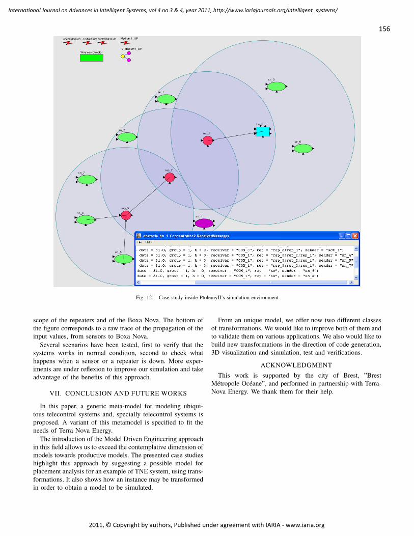
156



Fig. 12. Case study inside PtolemyII’s simulation environment

scope of the repeaters and of the Boxa Nova. The bottom ofthe figure corresponds to a raw trace of the propagation of theinput values, from sensors to Boxa Nova.

Several scenarios have been tested, first to verify that thesystems works in normal condition, second to check whathappens when a sensor or a repeater is down. More exper-iments are under reflexion to improve our simulation and takeadvantage of the benefits of this approach.

VII. CONCLUSION AND FUTURE WORKS

In this paper, a generic meta-model for modeling ubiqui-tous telecontrol systems and, specially telecontrol systems isproposed. A variant of this metamodel is specified to fit theneeds of Terra Nova Energy.

The introduction of the Model Driven Engineering approachin this field allows us to exceed the contemplative dimension ofmodels towards productive models. The presented case studieshighlight this approach by suggesting a possible model forplacement analysis for an example of TNE system, using trans-formations. It also shows how an instance may be transformedin order to obtain a model to be simulated.

From an unique model, we offer now two different classesof transformations. We would like to improve both of them andto validate them on various applications. We also would like tobuild new transformations in the direction of code generation,3D visualization and simulation, test and verifications.

ACKNOWLEDGMENT

This work is supported by the city of Brest, ”BrestMetropole Oceane”, and performed in partnership with Terra-Nova Energy. We thank them for their help.

157



REFERENCES

[1] A. Touil, J. Vareille, F. Lherminier, and P. Le Parc, “Modeling andanalysing ubiquitous systems using mde approach,” in The FourthInternational Conference on Mobile Ubiquitous Computing, Systems,Services and Technologies. UBICOMM 2010. Florence, Italy, Oct. 2010.

[2] M. Weiser, “The computer for the 21st century,” Scientific AmericanSpecial Issue on Communications, Computers, and Networks, 1991.

[3] Terra Nova Energy, “Online Energy Intelligence,” http://www.terra-nova-energy.com, 2012, [Online; accessed 09-jan-2012].

[4] P. Le Parc, A. Touil, and J. Vareille, “A model-driven approach forbuilding ubiquitous applications,” in The Third International Conferenceon Mobile Ubiquitous Computing, Systems, Services and Technologies- UBICOMM 2009, Oct. 2009.

[5] S. Kent, “Model driven engineering,” Lecture notes in computer science,pp. 286–298, 2002.

[6] F. Fleurey, J. Steel, and B. Baudry, “Validation in model-driven engi-neering: testing model transformations,” in Workshop WS5 at the 7thInternational Conference on the UML, Lisbon, Portugal, 2004.

[7] UC Berkeley, “Ptolemy Project Home Page,”http://ptolemy.eecs.berkeley.edu/, 2012, [Online; accessed 09-jan-2012].

[8] S. Gerard, F. Terrier, and Y. Tanguy, “Using the model paradigm forreal-time systems development: Accord/uml,” Lecture notes in computerscience, vol. 2426, pp. 260 – 269, 2002.

[9] D. Moody, “Graphical Entity Relationship Models: Towards a More UserUnderstandable Representation of Data,” Lecture Notes in ComputerScience, vol. 1157, pp. 227–244, 1996.

[10] S. Cranefield and M. Purvis, “UML as an ontology modelling language,”in Proceedings of the Workshop on Intelligent Information Integration,16th International Joint Conference on Artificial Intelligence (IJCAI-99),vol. 212, 1999.

[11] SysML.org, “SysML Open Source Specification Project,”http://www.wotug.org/occam/documentation/oc21refman.pdf, 2012,[Online; accessed 09-jan-2012].

[12] H. Espinoza, J. Medina, H. Dubois, S. Grard, and F. Terrier, “Towardsa uml-based modelling standard for scheduability analysis of real-time systems,” in In proceedings of MARTES workshop at MODELSconference, Genova Italy, 2006.

[13] F. Losilla, C. Vecente-Chicote, B. Alvarez, A. Iborra, and P. Sanchez,“Wireless sensor network application development: An architecture-centric mde approach,” Lecture Notes in Computer Science, vol. 4758,p. 179, 2007.

[14] A. van Deursen, P. Klint, and J. Visser, “Domain-specific languages: anannotated bibliography,” SIGPLAN Notices, vol. 35, no. 6, pp. 26–36,June 2000.

[15] K. Czarnecki and S. Helsen, “Classification of model transformation ap-proaches,” in Proceedings of the 2nd OOPSLA Workshop on GenerativeTechniques in the Context of the Model Driven Architecture, 2003.

[16] T. Alenljung and B. Lennartson, “Formal Verification of PLC ControlledSystems Using Sensor Graphs,” in Proceedings of the fifth annual IEEEinternational conference on Automation science and engineering. TheInstitute of Electrical and Electronics Engineers Inc., 2009, pp. 164–170.

[17] A. Voronov and K. AAkesson, “Verification of process operations usingmodel checking,” in CASE’09: Proceedings of the fifth annual IEEEinternational conference on Automation science and engineering. TheInstitute of Electrical and Electronics Engineers Inc., 2009, pp. 415–420.

[18] S. Ghosh and S. Rao, “Sensor network design for smart highways,” inCASE’09: Proceedings of the fifth annual IEEE international conferenceon Automation science and engineering. The Institute of Electrical andElectronics Engineers Inc., 2009, pp. 353–360.

[19] B. Combemale, X. Crgut, J.-P. Giacometti, P. Michel, and M. Pantel,“Introducing Simulation and Model Animation in the MDE TopcasedToolkit,” in 4th European Congress EMBEDDED REAL TIME SOFT-WARE (ERTS). Toulouse, France: SIA & SEE, Jan. 2008.

[20] National Instruments, “NI Labview - Improving the Productivity ofEngineers and Scientists,” http://www.ni.com/labview, 2012, [Online;accessed 09-jan-2012].

[21] MathWorks, “Simulink - imulation and Model-Based Design,”http://www.mathworks.com/products/simulink/, 2012, [Online; accessed09-jan-2012].

[22] Inria, “Scicos Homepage,” http://www-rocq.inria.fr/scicos/, 2012, [On-line; accessed 09-jan-2012].

[23] SGS-THOMSON Microelectronics ltd, “Occam 2.1 reference Manual,”http://www.sysml.org/, 2012, [Online; accessed 09-jan-2012].

[24] P. Baldwin, S. Kohli, E. A. Lee, X. Liu, and Y. Zhao, “Visualsense:Visual modeling for wireless and sensor network systems,”http://ptolemy.eecs.berkeley.edu/papers/05/visualsense/visualsense.pdf,Technical Memorandum UCB/ERL M05/25, University of California,Berkeley, USA, Tech. Rep., July 2005, [Online; accessed 09-jan-2012].

[25] M. Mernik, J. Hering, and A. Sloane, “Acm computing surveys,” Whenand how to develop Domain Specific Languages, vol. 37, no. 4, pp.316–344, 2005.

[26] R. Gronback, “Eclipse Modeling Project: A Domain-Specific Language(DSL) Toolkit,” Addison-Wesley Professional, 2009.

[27] I. C. Committee, “A consensus of the incose fellows,”http://www.incose.org/practice/fellowsconsensus.aspx, InternationalCouncil On Systems Engineering, Tech. Rep., 2012, [Online; accessed09-jan-2012].

[28] P. Baronti, P. Pillai, V. Chook, S. Chessa, A. Gotta, and Y. Hu, “Wirelesssensor networks: A survey on the state of the art and the 802.15. 4 andZigBee standards,” Computer Communications, vol. 30, no. 7, pp. 1655–1695, 2007.

[29] X. Cheng, D. Du, L. Wang, and B. Xu, “Relay sensor placement inwireless sensor networks,” Wireless Networks, vol. 14, no. 3, pp. 347–355, 2008.

158



Contextual Generation of Declarative Workflows and their Application to Software Engineering Processes

Gregor Grambow and Roy Oberhauser Computer Science Department

Aalen University, Germany {gregor.grambow, roy.oberhauser}@htw-aalen.de

Manfred Reichert Institute for Databases and Information Systems

Ulm University, Germany [email protected]

Abstract—Process management can increase the efficiency and effectiveness of process activities by structuring and coordinating their execution. However, its application can become problematic in dynamic environments such as software engineering, since rigidly pre-specified process models are not capable of adequately handling dynamic aspects of the processes. Therefore, this work presents a declarative, problem-oriented process modeling technique that enables the modeling of dynamic sets of candidate activities from which a subset is automatically selected for execution. The system selects the subset based on the contextual properties of situations and subsequently utilizes it to build executable workflows. Thus, the same process model is used to generate various workflows matching the properties of different situations. Preliminary results suggest this technique can be beneficial in addressing both high workflow diversity and workflow modeling effort reduction while providing useable process guidance.

Keywords-application of semantic processing; domain-oriented semantic applications; automated workflow adaptation; situational method engineering; process-aware information systems; software engineering environments

I. INTRODUCTION This article extends previous work in [1] that describes a

solution for dynamically generating workflows according to situational properties extraneous to the SE process. Business process management (BPM) and automated human process guidance have been shown to be beneficial in various industries [2][3]. However, existing BPM technology is often based on rigid models making its application difficult in highly dynamic and possibly evolving domains with diverse workflows such as software engineering (SE) [4]. SE is characterized by multiform and divergent process models, unique projects, multifarious issues, a creative and intellectual process, and collaborative team interactions, all of which affect workflow models [5][6]. These challenges have hitherto hindered automated concrete process guidance and often relegated processes to generalized and rather abstract process models (e.g., Open Unified Process [7] and VM-XT [8]) with inanimate documentation for process guidance. Manual project-specific process model tailoring is typically done via documentation without investing in automated workflow guidance. While automated workflows could assist overburdened software engineers by providing

direct orientation and activity guidance, the latter must coincide with the reality of the situation or the guidance will be ignored, and may cause the entire system to be mistrusted or ignored. To further adopt automated workflow guidance in SE environments (SEEs), adaptation and pertinence to the dynamic and diverse SE situations is requisite.

A. Problem Statement While SE process models support development

efficiency [9], it remains difficult to provide comprehensive operational level guidance for activities. The reason is that process models often remain rather abstract, do not cover all executed activities, and do not reach the involved actors [10]. Another issue in this dynamic discipline stems from the fact that reality often diverges from rigidly pre-defined processes [11][5].

In this paper, we distinguish between two types of workflows to be processed in any SE project: Intrinsic Workflows denote workflows covered by the SE process model. Extrinsic Workflows, in turn, are not part of the process model, but cover issues that frequently recur in SE projects and are thus neither explicitly governed nor supported nor traceable. Examples of such intrinsic and extrinsic workflows are illustrated in Figure 1. As a fundamental part of a software development project, expected activities for source code development and testing are mostly covered by the SE process model. Other activities often related to maintenance like bug fixing, test failure analysis, or refactoring due to quality threshold violations often exemplify extrinsic workflows since they are unplanned and occur unpredictably.

Figure 1. Intrinsic vs. extrinsic workflows.

Intrinsic workflows may lend themselves to foreseeable

common workflows with conformant sequences because they are mostly planned. However, the diversity and ad-hoc

159



nature of extrinsic workflows presents a challenge in respect to their modeling and otherwise. Considering SE, guidance is desirable for issues such as specialized refactoring, fixing bugs, technology switches, customer support, etc., yet it is generally not feasible to pre-specify workflows for SE issue processing, since SE issue types can vary greatly (e.g., due to tool problems, API issues, test failure reproduction, component versioning, merge problems, documentation inconsistencies, etc.). Either one complex workflow model with many execution paths becomes necessary, taking all different use cases into account, or many workflow variants need to be modeled, adapted, and maintained for such dynamic environments [12]. The associated exorbitant expenditures thus limit workflow usage to well-known common sequences as typically seen with industrial BPM usage.

In this paper, we use a simplified example of an extrinsic workflow to demonstrate the problem as well as the developed solution.

Example 1 (Bug Fixing Issue): As mentioned before, SE issues that are not modeled in the standard process flow of defined SE processes (such as OpenUP [7] and VM-XT [8]) include bug fixing, refactoring, technology swapping, or infrastructural issues. Since there are so many different kinds of issues with ambiguous and subjective delineation, it is difficult and burdensome to universally and correctly model them in advance for acceptability and practicality. Many activities may appear in multiple issues but are not necessarily required, bloating different SE issue workflows with many conditional activities if pre-modeled. Figure 12 shows such a workflow for bug fixing that contains nearly 30 activities (i.e., steps), many of these being conditionally executed for accomplishing different tasks like testing or documentation. One example is static analysis activities that are eventually omitted for very urgent use cases. Furthermore, there are various reviewing activities with different parameters (such as effectiveness or efficiency) where the choice can be based on certain project parameters (e.g., risk or urgency). The same applies to different testing activities. Moreover, it has to be determined if a bug fix should be merged into various other version control branches.

The resulting workflow problems for environments such as SE are first that the exorbitant cost of modeling diverse workflows results in the absence of extrinsic workflow models and subsequently automated guidance for these types of workflows, yet these special use cases are often the ones where guidance is especially helpful and desirable. Second, rigid, pre-specified workflow models are limited in their adaptability, thus the workflows become situationally irrelevant and are ignored [13]. Third, entwining the complex modeling of situational property influences (e.g., risk or urgency) on workflows within the workflows themselves incorporates an implicit modeling that unduly increases their complexity and aggravates maintenance. The cognitive effort required to create and maintain large process models syntactically [14] can lower the attention towards the incorporated semantic problem-oriented content.

B. Contribution This paper contributes a more comprehensive support of

automation for SE. Since the terms of workflow and process will be used extensively throughout this paper, they are informally defined here and delimited against each other in alignment with other definitions, as the ones from Gartner Research [15] or the Workflow Management Coalition [16].

Business Process Management deals with the explicit identification, implementation, and governance of processes as well as their improvement and documentation. This incorporates different aspects such as organizational and business aspects or strategic alignment of the activities. Workflow Management, in turn, deals with the automation of business processes; i.e., a workflow is the technical implementation of a process.

Our previous work has described CoSEEEK (Context-aware Software Engineering Environment Event-driven frameworK), a holistic approach to support the SE process that includes semantic technologies for enabling SE lifecycles [17] and context-awareness [18]. On this basis, different approaches have been developed. For example, [19] presents a workflow modeling language for SE that supports the connection of abstract SE process models with concretely executed activities. Further, a combination of SE processes with SQA (software quality assurance) is described in [20][21][22], enabling the automated integration of software quality measures into executing SE workflows.

This article, focuses on engendering context-awareness by utilizing semantic processing and situational method engineering (SME) [23] for automatically adapting workflows executed by a process-aware information system [24]. Support is provided for both intrinsic and extrinsic workflows. The modeling of contextual property influences is transferred from the workflows themselves to an ontology, simplifying that modeling and making property effects explicit. Dynamic on-the-fly workflow generation and adaptation using contextual knowledge for a large set of diverse workflow variants is thus supported, enabling pertinent workflow guidance for workers in such environments. As SE workflows, and especially the extrinsic ones, are very dynamic, the traditional imperative way of modeling these might not always be appropriate for capturing their dynamic properties. Declarative approaches offer a way of modeling that integrates a certain amount of flexibility into the models [25]. This can be beneficial in situations, when the exact set of needed activities is not known prior to execution. Therefore, our work on declarative workflow modeling and automated generation [26] is also integrated and extended to form a holistic solution capable of the following features:

- Incorporating extrinsic workflows including automated

execution support, - Problem-oriented modeling of extrinsic workflows,

facilitating their systematic creation, - Support for the easy modeling and reuse of process

fragments, and

160



- Automated workflow generation and adaptation matching various situations using SME in alignment with the workflows.

The remainder of this paper is organized as follows:

Section II elicits the requirements for the approach we developed, whereas Section III describes the solution. In Section IV, the realization is portrayed followed by an evaluation in Section V. Related work is discussed in Section VI, followed by our conclusion in Section VII.

II. REQUIREMENTS This section presents detailed requirements that have to

be satisfied to enable comprehensive automated process support for SE as described in the preceding section. These requirements have been elicited based on experiences collected at industrial partner companies of this project supported by a literature study. The requirements have been split up into three areas: Process coverage, process modeling, and the modeling of contextual factors in alignment with the process.

Process coverage: To enable comprehensive process

support, a tool for process governance should cover the actual activities as closely as possible. This particularly includes extrinsic activities mostly unaddressed by standard process models.

Requirement R:CovInEx (Intrinsic / extrinsic support): There should be a facility to support both intrinsic and extrinsic activities by an automated system or framework.

Requirement R:CovU (Uniform workflow realization): Both intrinsic and extrinsic activities should be executed in a uniform way to support uniform assistance for the user and to enable easy tracking and analysis of executed workflows.

Modeling: To support the users not only at executing the

workflows but also at creating them, an easy way of modeling shall be provided that also accommodates the special properties of the extrinsic workflows.

Requirement R:ModDy (dynamic modeling): Compared to intrinsic workflows, extrinsic workflows are more dynamic and less foreseeable. Their modeling should enable coverage of various possible situations without bloating process models or making them too complex.

Requirement R:ModRe (modeling for reuse): The workflow modeling itself should remain easy and foster the reuse of modeled solutions or the parts thereof.

Requirement R:ModHi (hide complexity): The workflow modeling should hide the inherent complexity of the workflow models to assist the user with problem-oriented creation of the models.

Contextual modeling: To be able to generate workflows

matching various situations, a method of modeling contextual influences and connecting them to the workflow models is required. Facilities to gather contextual information is also necessary.

Requirement R:CtxGet (Gather contextual information): There should be facilities to automatically gather information

on the current situation from users or the development environment.

Requirement R:CtxInf (Model contextual influences): The modeling environment should be capable of modeling contextual influences to be able to use situational information directly.

Requirement R:CtxCon (Connect workflow and context): A facility to model the connections of contextual properties to workflow activities is required to enable their automated situational selection.

III. SOLUTION APPROACH This section describes the concepts we developed to

address the aforementioned requirements.

A. Solution Procedure The solution developed in this paper utilizes CoSEEEK.

It incorporates a set of sensors that enable the automatic gathering of contextual information as, e.g., state transitions of certain SE tools or SE artifacts (cf. R:CtxGet). In this paper, facilities are developed to model contextual properties that can be used to describe a situation as, e.g., ‘Risk’ or ‘Complexity’ (cf. R:CtxInf). These properties, in turn, have calculated values that can be derived from various sources as the skill level of a user executing an activity or the measured code complexity of a processed source code artifact. To be able to contextually integrate process execution into the projects and thus enable the process to be influenced by the properties of various situations, explicit connections of process management concepts to context properties are introduced (cf. R:CtxCon).

As concrete workflow execution is often relatively dynamic in SE, a rigid pre-planning of activity sequences is not always advantageous. Therefore, we provide a means of declaratively modeling candidate activities for a workflow at build-time that enables a system to automatically select appropriate activities for various situations at run-time (cf. R:ModDy). The modeling is designed to be hierarchical, separating workflow models into several nestable blocks. These blocks can be modularized and be logically treated as simple activities, fostering their reuse in multiple workflow models and simplifying these (cf. R:ModRe). To support process engineers in modeling declarative context-dependent workflows, an easy way of specifying context properties, workflows, contained blocks, and activities is provided (cf. R:ModHi).

Utilizing this modeling method, extrinsic workflows can be addressed (cf. R:CovInEx). To unite this with traditional imperative process modeling that is still useful for more predictable processes [24], our approach unites both ways of modeling under a common process management concept (cf. R:CovU). The succeeding sections will provide details on CoSEEEK and will introduce the different parts of the concept: contextual extensions to process models, modeling of contextual influences, gathering of contextual information, and declaratively modeling processes.

161



B. Software Engineering Environment To be able to provide the aforementioned features, a

system or framework must incorporate certain facilities:

A. A technical facility to automatically gather and process information from the development environment.

B. A facility to manage all contextual information and to relate it to process management.

C. A facility to govern workflows to support process execution.

D. Flexible and reliable data storage and communication to connect all modules of the framework and thus all parts of the solution.

This section gives a brief overview of CoSEEEK and

how it realizes these facilities. CoSEEEK is founded on a hybrid semantic computing approach towards improved context-aware SEEs [18]. Its conceptual architecture is shown in Figure 2.

The environment (cf. Facility A) in a SE project consists of artifacts and SE tool usage. The collection and processing of information concerning these items is realized by two CoSEEEK modules: Event Extraction provides sensors acquiring events of state changes from various SE tools like IDEs (Integrated Development Environments) or source control systems. Event Processing, in turn, is used to process the detected events. It enables the combination of multiple low-level events (e.g., switching to the debug perspective in an IDE) to derive higher-level events (e.g., the user is doing bug fixing).

The management of high-level contextual information is realized by Context Management (cf. B) that utilizes semantic web technologies such as an ontology and a reasoner.

Figure 2. CoSEEEK conceptual architecture.

Workflow governance and support (cf. Facility C) is done by Process Management. To respond to the dynamicity of SE workflow execution, this module enables dynamic workflow execution, meaning that it is capable of correctly and dynamically adapting running workflows.

Shared data (cf. Facility D) is provided by the Data Storage module, which is realized as a tuple space [27]. A loosely-coupled communication infrastructure is provided with each module able to store and receive events.

CoSEEEK provides comprehensive automated process support to address the aforementioned challenges. While the

automated support provided for intrinsic workflows is imperatively modeled and described in [28], both the support for extrinsic workflows as well as the method for their semantic, problem-oriented modeling (utilizing situational method engineering) are an emphasis of this paper.

C. Context-aware Business Process Management CoSEEEK aims to provide holistic infrastructural support

for SE projects concerning software development process execution. This is achieved by assisting project participants during their various activities. The process is tightly integrated with contextual information and the project environment. This section introduces the basic contextual extensions to process management on which most framework features rely. In our prior work [22][21] we developed these extensions for standard intrinsic workflow execution. Together with [1] and [26], this article now extends this approach with support for a greater degree of workflow dynamicity as well as for extrinsic workflows. To elucidate the overall concept, we first summarize how the contextual extension of process management concepts is realized.

To enable the contextual integration of process execution into SE projects, the Context Management module and the Process Management module are tightly integrated. The main responsibility of the Process Management module is to govern the activities in both intrinsic and extrinsic workflows. This includes dynamic adaptations to running workflows as well as correctness guarantees (e.g., absence of deadlocks and correct data flow) for both workflow execution and adaptation [29][30]. The Context Management module has three main responsibilities:

- It collects and aggregates contextual information

retrieved from users or SE tools. - It adds annotations to the process management concepts

and extends these. - It has high-level workflow governance authority,

connecting context information using the logical capabilities provided by semantic web technology and the functionalities of the Process Management module. This connection is illustrated in Figure 3.

The Process Management module shows three sample

workflows ‘A’, ‘B’, and ‘C’ which have been modeled based on standard workflow patterns such as AND- or XOR-gates (see [31][32][33] for readings on different kinds of workflow patterns). These three workflows as well as each of the contained activities have mappings in the Context Management module that are directly connected to them. A workflow is mapped by a so-called Work Unit Container, and an activity is mapped by a so-called Work Unit. Note that the horizontal governance (governance of the activities in a workflow) is handled by the Process Management module, while the vertical governance (governance of the connection between the different workflow levels) is managed by the Context Management module. This enhances connection flexibility as illustrated in Figure 3.

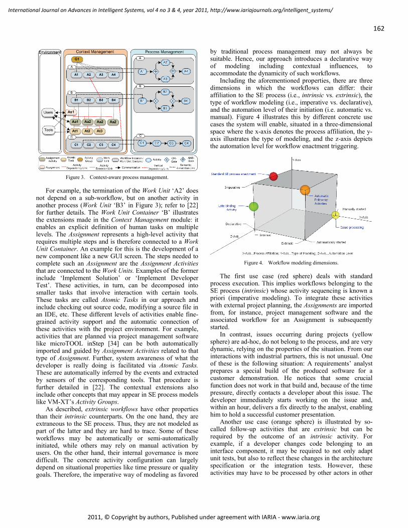
162



Figure 3. Context-aware process management.

For example, the termination of the Work Unit ‘A2’ does not depend on a sub-workflow, but on another activity in another process (Work Unit ‘B3’ in Figure 3); refer to [22] for further details. The Work Unit Container ‘B’ illustrates the extensions made in the Context Management module: it enables an explicit definition of human tasks on multiple levels. The Assignment represents a high-level activity that requires multiple steps and is therefore connected to a Work Unit Container. An example for this is the development of a new component like a new GUI screen. The steps needed to complete such an Assignment are the Assignment Activities that are connected to the Work Units. Examples of the former include ‘Implement Solution’ or ‘Implement Developer Test’. These activities, in turn, can be decomposed into smaller tasks that involve interaction with certain tools. These tasks are called Atomic Tasks in our approach and include checking out source code, modifying a source file in an IDE, etc. These different levels of activities enable fine-grained activity support and the automatic connection of these activities with the project environment. For example, activities that are planned via project management software like microTOOL inStep [34] can be both automatically imported and guided by Assignment Activities related to that type of Assignment. Further, system awareness of what the developer is really doing is facilitated via Atomic Tasks. These are automatically inferred by the events and extracted by sensors of the corresponding tools. That procedure is further detailed in [22]. The contextual extensions also include other concepts that may appear in SE process models like VM-XT’s Activity Groups.

As described, extrinsic workflows have other properties than their intrinsic counterparts. On the one hand, they are extraneous to the SE process. Thus, they are not modeled as part of the latter and they are hard to trace. Some of these workflows may be automatically or semi-automatically initiated, while others may rely on manual activation by users. On the other hand, their internal governance is more difficult. The concrete activity configuration can largely depend on situational properties like time pressure or quality goals. Therefore, the imperative way of modeling as favored

by traditional process management may not always be suitable. Hence, our approach introduces a declarative way of modeling including contextual influences, to accommodate the dynamicity of such workflows.

Including the aforementioned properties, there are three dimensions in which the workflows can differ: their affiliation to the SE process (i.e., intrinsic vs. extrinsic), the type of workflow modeling (i.e., imperative vs. declarative), and the automation level of their initiation (i.e. automatic vs. manual). Figure 4 illustrates this by different concrete use cases the system will enable, situated in a three-dimensional space where the x-axis denotes the process affiliation, the y-axis illustrates the type of modeling, and the z-axis depicts the automation level for workflow enactment triggering.

Figure 4. Workflow modeling dimensions.

The first use case (red sphere) deals with standard process execution. This implies workflows belonging to the SE process (intrinsic) whose activity sequencing is known a priori (imperative modeling). To integrate these activities with external project planning, the Assignments are imported from, for instance, project management software and the associated workflow for an Assignment is subsequently started.

In contrast, issues occurring during projects (yellow sphere) are ad-hoc, do not belong to the process, and are very dynamic, relying on the properties of the situation. From our interactions with industrial partners, this is not unusual. One of these is the following situation: A requirements’ analyst prepares a special build of the produced software for a customer demonstration. He notices that some crucial function does not work in that build and, because of the time pressure, directly contacts a developer about this issue. The developer immediately starts working on the issue and, within an hour, delivers a fix directly to the analyst, enabling him to hold a successful customer presentation.

Another use case (orange sphere) is illustrated by so-called follow-up activities that are extrinsic but can be required by the outcome of an intrinsic activity. For example, if a developer changes code belonging to an interface component, it may be required to not only adapt unit tests, but also to reflect these changes in the architecture specification or the integration tests. However, these activities may have to be processed by other actors in other

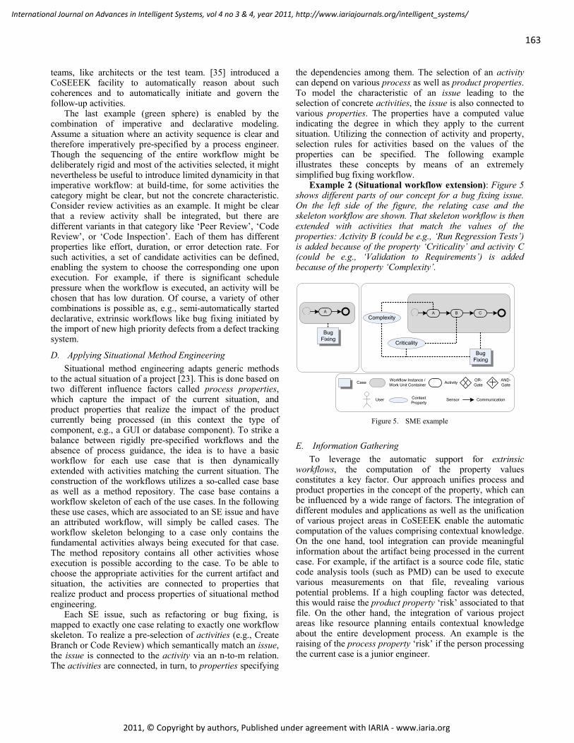
163



teams, like architects or the test team. [35] introduced a CoSEEEK facility to automatically reason about such coherences and to automatically initiate and govern the follow-up activities.

The last example (green sphere) is enabled by the combination of imperative and declarative modeling. Assume a situation where an activity sequence is clear and therefore imperatively pre-specified by a process engineer. Though the sequencing of the entire workflow might be deliberately rigid and most of the activities selected, it might nevertheless be useful to introduce limited dynamicity in that imperative workflow: at build-time, for some activities the category might be clear, but not the concrete characteristic. Consider review activities as an example. It might be clear that a review activity shall be integrated, but there are different variants in that category like ‘Peer Review’, ‘Code Review’, or ‘Code Inspection’. Each of them has different properties like effort, duration, or error detection rate. For such activities, a set of candidate activities can be defined, enabling the system to choose the corresponding one upon execution. For example, if there is significant schedule pressure when the workflow is executed, an activity will be chosen that has low duration. Of course, a variety of other combinations is possible as, e.g., semi-automatically started declarative, extrinsic workflows like bug fixing initiated by the import of new high priority defects from a defect tracking system.

D. Applying Situational Method Engineering Situational method engineering adapts generic methods

to the actual situation of a project [23]. This is done based on two different influence factors called process properties, which capture the impact of the current situation, and product properties that realize the impact of the product currently being processed (in this context the type of component, e.g., a GUI or database component). To strike a balance between rigidly pre-specified workflows and the absence of process guidance, the idea is to have a basic workflow for each use case that is then dynamically extended with activities matching the current situation. The construction of the workflows utilizes a so-called case base as well as a method repository. The case base contains a workflow skeleton of each of the use cases. In the following these use cases, which are associated to an SE issue and have an attributed workflow, will simply be called cases. The workflow skeleton belonging to a case only contains the fundamental activities always being executed for that case. The method repository contains all other activities whose execution is possible according to the case. To be able to choose the appropriate activities for the current artifact and situation, the activities are connected to properties that realize product and process properties of situational method engineering.

Each SE issue, such as refactoring or bug fixing, is mapped to exactly one case relating to exactly one workflow skeleton. To realize a pre-selection of activities (e.g., Create Branch or Code Review) which semantically match an issue, the issue is connected to the activity via an n-to-m relation. The activities are connected, in turn, to properties specifying

the dependencies among them. The selection of an activity can depend on various process as well as product properties. To model the characteristic of an issue leading to the selection of concrete activities, the issue is also connected to various properties. The properties have a computed value indicating the degree in which they apply to the current situation. Utilizing the connection of activity and property, selection rules for activities based on the values of the properties can be specified. The following example illustrates these concepts by means of an extremely simplified bug fixing workflow.

Example 2 (Situational workflow extension): Figure 5 shows different parts of our concept for a bug fixing issue. On the left side of the figure, the relating case and the skeleton workflow are shown. That skeleton workflow is then extended with activities that match the values of the properties: Activity B (could be e.g., ‘Run Regression Tests’) is added because of the property ‘Criticality’ and activity C (could be e.g., ‘Validation to Requirements’) is added because of the property ‘Complexity’.

ActivityWorkflow Instance / Work Unit Container

AND-Gate

OR-Gate

Communication

A B C

Case

Complexity

Criticality

Bug Fixing

User SensorContext Property

A

Bug Fixing

Figure 5. SME example

E. Information Gathering To leverage the automatic support for extrinsic

workflows, the computation of the property values constitutes a key factor. Our approach unifies process and product properties in the concept of the property, which can be influenced by a wide range of factors. The integration of different modules and applications as well as the unification of various project areas in CoSEEEK enable the automatic computation of the values comprising contextual knowledge. On the one hand, tool integration can provide meaningful information about the artifact being processed in the current case. For example, if the artifact is a source code file, static code analysis tools (such as PMD) can be used to execute various measurements on that file, revealing various potential problems. If a high coupling factor was detected, this would raise the product property ‘risk’ associated to that file. On the other hand, the integration of various project areas like resource planning entails contextual knowledge about the entire development process. An example is the raising of the process property ‘risk’ if the person processing the current case is a junior engineer.

164



Both of these aspects deal with implicit information gathering. Since not all aspects of a case are necessarily covered by implicit information, and not all options for gaining knowledge about the case are always present, the system utilizes explicit information gathering from the user processing the case. To enable and encourage the user to provide meaningful information, a simple response mechanism is integrated into the CoSEEEK GUI (shown in the next section). Via this mechanism, the user can directly influence process as well as product properties. To keep the number of adjustable parameters small, the concept of product category was introduced. The product category unites the product properties in a pre-specified way. An example of this would be a database component or a GUI component: the database component is likely to have more dependencies, whereas the GUI component presumably has more direct user impact. The influence of the product categories on the different properties is specified in advance and can be adapted to fit various projects. Selected process properties can be set directly. The computation of all other influences on the properties is explained in the following section.

F. Declarative Workflow Modeling After completing the computation of the property values,

activities must be selected and correctly sequenced to enable dynamic construction of the workflow for an SE issue. This is done utilizing the connection between properties and activities. An activity can depend on one or more properties. Examples include selection rules such as:

• ‘Choose activity code inspection if risk is very high,

criticality is high, and urgency is low’ or • ‘Choose activity code review if risk and criticality are

both high’. The sequencing of the chosen activities in our initial

approach [1] was very simple and did not allow for choices or the parallel execution of activities. Therefore, this section integrates our work from [26] and extends it. Declarative workflow modeling approaches incorporate a certain amount of flexibility in the workflow models [25] and thus enable the latter to be applicable for different situations. However, the declarative way of modeling can be difficult to understand [36] and can produce models that are hard to maintain [37]. Therefore, our declarative workflow modeling approach is based on very simple constraints and so called Building Blocks that enable further structuring of the workflow and structural nesting.

This modeling type is illustrated and compared to classical workflow modeling in Figure 13. The figure shows the modeling of the Work Unit Containers above and the derived workflows for execution below. ‘Work Unit Container 1’ shows a simple, imperatively modeled workflow that is also executed in that form (as ‘Workflow 1’). ‘Work Unit Container 2’ illustrates declarative modeling of the same workflow: the exact structure of the workflow is not rigidly pre-specified. There are only simple constraints connecting activities in the workflow. Examples in Figure 13

are ‘Requires’, expressing that one activity requires the presence of another, and ‘Parallel’, expressing that both activities should be executed in parallel. The generated workflow for these constraints looks exactly like the imperatively modeled ‘Work Unit Container 1’. Activities in the declarative approach also have relations to contextual properties in order to enable the system to select a subset of the pre-specified activities for the execution workflow. Finally, ‘Work Unit Container 3’ demonstrates the use of Building Blocks. These are used for further structuring the workflow. Three Building Blocks are shown for sequential, parallel, and repeated execution of the contained elements in Figure 13. ‘Workflow 3’ shows how a workflow is built based on constraints and the Building Blocks. Furthermore, it demonstrates contextual relations, in this case assuming that the contextual properties of the situation led the system to the selection of activities ‘1’, ‘2’, ‘3’, and ‘5’ while omitting activities ‘4’ and ‘6’.

In the following, all available constraints and Building Blocks are shown, as well as conditions to be fulfilled for declarative modeling and that are later checked by the framework.

The constraints were designed in a way such that they remain simple and facilitate basic workflow modeling. Structures that are more complex can be expressed using Building Blocks. The constraints are categorized into sequencing constraints and existence constraints. Existence constraints govern which activities should be present in a workflow, while sequencing constraints govern how they should be arranged in the workflow. The available constraints are shown in Table I.

TABLE I. DECLARATIVE CONSTRAINTS

Constraint Meaning Type

X hasSuccessor Y if X and Y are present, X should appear before Y sequencing

X hasParallel Y

if X and Y are present, they should appear parallel (like two branches that are connected by AND gates in classical process modeling)

sequencing

X requires Y if X is present, Y must also be present existence

X mutualExclusion Y if X is present, the presence of Y is prohibited existence

Utilizing these constraints, very basic workflows are

possible, specifying “should” / “should not” appear together and a sequence or parallel arrangement.

The Building Blocks that enable complex structures have been developed to mirror standard workflow patterns for block-structured workflows [38]. This way of structuring enables easy separation of the workflow into nested blocks. These blocks can be activities, patterns, or the workflow itself. Each block must have a unique start and end point [39][40][41]. The blocks can be regularly nested, meaning that they may not overlap [42][41][40]. For workflows that are not structured like this, in most cases a transformation to a block structured model can be applied [40][43][41]. For control flow modeling in workflows, the basic patterns are:

165



Sequence, AND-split, AND-join, XOR-split, XOR-join, and Loop [31]. With these patterns, most models that are used in practice can be covered since they are the basis of any process specification language [44][45][46]. They can also be easily transformed to formal languages like Petri Nets [29] and to other widespread process languages like WS-BPEL [47][48]. There also exist other control flow patterns like the Multi-Choice / OR-split [31]. This work presumes the sole usage of the basic control flow patterns, because the use of other patterns can complicate the process model and promote error-proneness [43][49][50]. Furthermore, it is possible to construct other control flow patterns using the basic ones like, e.g., composing an OR-split with XOR- and AND-splits [38][51]. The available Building Blocks and their relation to control flow patterns is shown in Table II.

TABLE II. BUILDING BLOCKS

Building Block Control Flow Pattern(s) Sequence Sequence Parallel AND-split, AND-join Loop Loop

Conditional XOR-split, XOR-join ‘Work Unit Container 3 / Execution Workflow 3’ in

Figure 13 demonstrates how nested Building Blocks are transformed into the control-flow structure of a workflow.

Compared to [26], the Building Block ‘Conditional’ has been added to cover all basic workflow patterns. This Building Block implies a deferred decision about the executed activities: At run-time, based on a certain variable, the XOR pattern chooses exactly one activity from a set of contained activities or, in case one empty branch exists in the XOR pattern, no activity might be chosen. Furthermore, for the decision made in the XOR pattern, the value range of the variable used for the decision should be completely covered to avoid deadlocks in execution [52][53]. This, combined with the fact that Building Blocks contain candidate activities from which a subset is to be chosen, makes it error-prone. The value range can become only partially covered, and it is possible that two or more activities (from which a selection was intended by the modeler) are omitted due to context properties, leaving no valid choice at run-time. In light of these problems, two options are supported in modeling a ‘Conditional’ Building Block: the first one contains no empty branch. For this variant, the system checks the coverage of the value range during construction and no activities can be omitted for that block. That way, run-time choices not dependent on context properties can be modeled. The second variant contains an empty branch. In that case omitting activities due to contextual factors is permitted. The system assigns all uncovered sections of the value range to the empty branch. That way it is possible to model a deferred decision that incorporates contextual factors including the case that none of the activities comes to execution.

However, the usage of Building Blocks not only enables the modeling of workflow structures containing all basic structural patterns, but also simplifies modeling since it fosters the reuse of different fragments of a workflow: in

traditional process management, reuse is limited to workflows or activities. In contrast, our declarative modeling approach supports the reuse of fragments of the workflows. These fragments, captured as Building Blocks, are encapsulated as simple activities, and thus simplify the workflow structure and hide its inherent complexity. Another factor supporting reuse is the relation to context properties: each simple activity and Building Block can have these context connections. That way a Building Block can be used in various different workflows for various situations. The following example illustrates this.

Example 3 (Building Block): A Building Block for different code review activities can be defined, containing review activities with different properties. These are for example ‘Peer Review’, ‘Code Review’, ‘Walkthrough’, or ‘Code Inspection’. Utilizing connections to context properties like ‘Urgency’ or ‘Risk’, these activities “know” the situations to which they apply, and the surrounding Building Block can thus be easily used for all of these situations without additional effort.

With this method of declarative modeling, one can model ‘candidate activities’ and relate them to context properties during build-time, while the system decides at run-time which of the activities will be used to construct the execution workflow matching the current situation. This implies that several activities may be omitted for a certain execution workflow. To ensure that proper workflows are still constructible out of a declarative workflow specification, the system conducts a so-called ‘auto-completion’ on the specified workflows as illustrated in Figure 6.

A

DC

B

A DC

B D

A: Auto completion B: Workflow Examples

Activity Successor Constraint Parallel Constraint

Figure 6. Workflow auto-completion example.

In Figure 6(A), the red-dashed constraints are added by the system. This enables the construction of workflows from subsets of the specified activities as exemplified in Figure 6(B). A set of conditions is verified by the system to ensure that correct basic modeling and all specified workflows are properly completed. These conditions concern the workflows as a whole as well as the different Building Blocks. An example of such a condition is shown in the following:

Condition C1: Each workflow shall have a unique start

and end point. This promotes simple and understandable models as suggested in [43].

The conditions and the auto completion feature are

further explained in [26]. Structural integrity of the workflows is guaranteed upon creation based on the built-in

166



mechanisms of the process management system, which imply correctness checks for each change operation applied to the workflow [52].

G. Workflow treatment dimensions There are different combinations of intrinsic and

extrinsic workflows that are modeled imperatively or declaratively, as illustrated in Figure 4. This section briefly explains how different combinations are enabled. As both declarative and imperative workflows are realized by sub-types of the Work Unit Container, it is possible to use both types for intrinsic as well as for extrinsic workflows.

There are different levels of automation concerning workflow starts: intrinsic workflows are automatically started as they belong to the running SE process. In contrast to this, extrinsic workflows can be started out of different situations: first, they can be started manually by the user utilizing the CoSEEEK GUI. Second, they can be started semi-automatically, e.g., when an activity is assigned to a user in a bug tracking system monitored by a sensor. The sensor generates an event that causes the instantiation and start of a new workflow for the respective user. The third case is the follow-up activities required by other activities. These are automatically initiated by the system. That case is illustrated in the following example.

Example 4 (Follow-up activities): Consider a source code modification conducted as part of an intrinsic activity. That modification was applied to an artifact that belongs to the interface of a component. The change thus only impacts the component itself and its implementation, but also other areas. The areas ‘testing’ and ‘architecture’ might also be impacted since eventually the integration tests or the architecture specification has to be adapted. The determination of such impacts from one project area to another and the governance of the follow-up activities are described further in [35].

The system shall enable activity support matching various situations and provide a simple way of modeling. Therefore, it is not only possible to model dynamic Work Unit Containers but also dynamic activities. These so-called Late Binding Activities can be used if it is known that, e.g., some type of activity has to be done but it is not known prior to process execution which exact characteristic the activity should have [54]. Therefore, the activity is connected to a Building Block. The latter implies the possibility to model a set of candidate activities, connect these with context properties, and govern their sequencing. When the respective workflow is started, the system determines the matching activities using the current context properties and integrates them into the workflow.

H. Concrete Procedure The concrete procedure for the handling of an SE issue in

is as follows. At first, the workflow for the issue is modeled declaratively as illustrated in Figure 14. This procedure comprises composing the workflow out of various Building Blocks, connecting these to context properties, and connecting both to a case. After the workflow construction is completed, the system verifies it. As an entry point for the

execution of a workflow, there is an event indicating that an SE issue is assigned to a user. This event can come from various sources. Examples include the assignment of an SE issue to a person in a bug tracker system or the manual triggering by a user via the GUI. The next step is to determine a case for that issue like ‘Bug fixing’ or ‘Refactoring’. Depending on the origin of the event, this can be done implicitly or explicitly by the user.

When the case is specified, the workflow starts for the user, applying the workflow skeleton assigned to that case. The first execution step is to gather contextual information as illustrated in Figure 14. This information can come from various sensors that provide information on the state transitions of SE tools or directly from the user via the GUI.

After having determined the properties of the case, the additional activities matching the current situation and product are selected. The set of activities is then checked for integrity and correctly sequenced utilizing semantic constraints. Subsequently, the activities are integrated into the running workflow that provides activity guidance for the user.

If one or more of the properties change during the execution of the workflow, the prospective activities are deleted (if still possible) and a new sequence of activities is computed.

I. Modeling Effort The presented approach consists of many components

and introduces a fair amount of complexity. However, this does not impose complicated modeling or workflow enactment for the user. The required components are discussed in the following: - Context Properties: The system needs explicitly

modeled context properties for the selection of appropriate activities. These properties have to be connected to other facts to be automatically computed. An example for this is ‘If the skill level of the applying person is low, the risk is increased’. These properties can be reused for all cases and have thus only to be modeled once.

- Activities: The workflows consist of activities that have to be modeled and to be connected to context properties to enable the system to know when they apply. Like the properties, the activities only have to be modeled once and can be reused.

- Building Blocks: Building Blocks are used to group activities together and to govern their sequencing. They are further connected to context properties and can be reused. Building Blocks offer great potential for reuse and for simplifying modeling: They are encapsulated as simple activities and thus simplify the structure of the containing Work Unit Container. Consider the four code review activities of example 3: These four activities can be grouped together, e.g., in a Parallel Building Block called ‘Review Activities’. For future workflows, the latter can be used instead of incorporating multiple activities and choices, leaving

167



the system responsible for selecting the matching activities for the current situation during run-time.

- Cases: For each concrete issue like ‘Bug Fixing’, one case is defined. The definition of a case is very simple since all defined activities, context properties, and Building Blocks can be reused. The structure of the cases is also very simple as there are only four constraints needed for connecting the activities or Building Blocks. More complex control flow modeling is handled and encapsulated by the Building Blocks.

IV. REALIZATION This section describes the concrete implementation of the

SE issue process introduced in the preceding section.

A. Technical component realization Before describing the procedural realization, the

technical realization of the participating components is briefly introduced as illustrated in Figure 7.

Figure 7. CoSEEEK realization architecture.

While various other Java (Mantis, inStep, PMD, xRadar, etc.) and .NET (Visual Studio 2010, Team Foundation Server) SE Tools are integrated, to exemplify the realization just a few will be described. Source code and test code Artifacts are processed via the version control management system Subversion and the IDE Eclipse. All communication between the modules is performed using a custom XML implementation of the Tuple Space paradigm [27] that uses the eXist XML database [55] for collaborative event storage and Apache CXF for web service communication. The Hackystat framework [56], which provides a rich set of sensors for various applications, is used for Event Extraction via its tool sensor components and for storage of high volume basic events in a relational database. Event Processing is performed via the complex event processing (CEP) [57] tool esper [58], that detects and triggers higher-order complex events from the multiple basic events.

The Process Management module requires an adaptable process-aware information system (PAIS) to cope with the dynamic nature of SE processes the current approach seeks to address. Therefore, the AristaFlow BPM suite (formerly ADEPT2) [52][39] was chosen for its realization. It allows authorized agents [59] to dynamically adapt and evolve the structure of process models during run-time. Such dynamic

process changes do not lead to unstable system behavior, i.e., none of the guarantees achieved by formal checks at build-time are violated due to the dynamic change at run-time [42]. Correctness is ensured in two stages. First, structural and behavioral soundness of the modified process model is guaranteed, independent from whether or not the change is applied at the process instance level. Second, when performing structural schema changes at the process instance level, this must not lead to inconsistent or erroneous process states afterwards. AristaFlow applies well-elaborated correctness principles in this context [60]. Despite its comprehensive support for dynamic process changes, ADEPT2 has not considered automated workflow adaptations so far.

The Context Management module has three main responsibilities: it realizes the case base, the method repository, and contains context information about the entire project. This information is stored in an OWL-DL [61] ontology to unify project knowledge and to enable reasoning over it. The use of an ontology reduces portability, flexibility, and information sharing problems that are often coupled to relational databases. Additionally, ontologies facilitate extensibility since they are, in contrast to relational databases, based on an open world assumption and thus allow the modeling of incomplete knowledge. To programmatically access the ontology, the Jena API [62] is used within the Context Module. Reasoning and classification of information is provided by the reasoner Pellet [63].

B. Concrete Procedure This section illustrates the communication of the modules

by means of a concrete example that is depicted in Figure 15. Basic event extraction and event processing is presumed. In that concrete case, the bug tracker Mantis is used in conjunction with a sensor that generates an ad hoc workflow event when an SE issue is assigned to a person (1) and is stored in the XML tuple space. That event contains information about the kind of issue for case selection and about the person. In case of a real ad hoc issue not recorded in a bug tracker, the event for instantiating a workflow can be triggered from the GUI as well, requiring the user to select a case manually (1). The GUI is a lightweight web interface developed in PHP that can be executed in a web browser as well as preferably directly in the users IDE. Figure 8(A) shows the GUI: in the upper area, contextual information is displayed while the lower area is reserved for workflow governance. The upper area also provides the option to start a case manually. The event is then automatically received by the Process Management module (cf. Figure 15(2)), which instantiates a workflow skeleton based on the template of the selected case (3). The activity components of AristaFlow (called environments) for these workflows are customized to communicate over the Tuple Space (4) and thus, enable user interaction during the execution of each activity. The first activity of each SE issue is ‘Analyze Issue’ to let the user gain knowledge about the issue and provide information about process and product properties to the system via the GUI (5). Figure 8(B) shows

168



the GUI that enables the user to directly adjust process properties and to choose a product category that affects product properties.

(A) – Start Case (B) – Property Acquisition Figure 8. CoSEEEK GUI.

The adaptation of running workflows works as follows: the workflow skeleton is instantiated, offering the user the aforementioned ‘Analyze Issue’ task to provide information as shown in Figure 15(6). The information from the user is encapsulated in an event received by the process module (7). The Process Management module sends an event via the tuple space (8) that is received by the Context Management module (9). The latter provides the set of activities to be inserted in the running workflow (10, 11). The Process Management module utilizes that information to perform the adaptation of the workflow, inserting all required activities (12). Thus, the process is already aligned to the current situation and product when the user continues.

C. Context Module This subsection describes how the Context Management

module utilizes the ontology to derive property values and to select appropriate activities. To leverage real contextual awareness, the ontology features various concepts for different areas of a project. These are semantic enhancements to process management utilized for intrinsic workflows, quality management, project staffing, and traceability. For process management, the concepts of Work Unit, Work Unit Container, Assignment, Assignment Activity, and Atomic Task are used to enrich processes and activities, and with semantic information as illustrated in Figure 3. Quality management features the concepts of the Metric, Measure, Problem, Risk, Severity, and KPI (key performance indicator) to incorporate and manage quality aspects in the project context. The concepts of Person, Team, Role, Effort, Skill Level, and Tool are integrated to connect project staffing with other parts of the project. To further integrate all project areas and to facilitate a comprehensive end-to-end traceability, the concepts of Tag and Event can be connected and used in conjunction with all other ones. The relevant concepts are shown in a simplified excerpt from the ontology in Figure 16.

To predefine the different SE issues, a set of template classes has been defined with their workflow skeletons and activities as well as the properties applying to them. Each Issue Template is connected to a Work Unit Container Template storing the information about the concrete process template in AristaFlow. The Work Unit Container Template has two disjoint subclasses for representing imperative and declarative workflows: the Imperative Container Template containing Work Unit Templates, and the Declarative Container Template containing Building Block Templates. The latter are used to model candidate activities for declarative workflows and have various subclasses. These incorporate the different Building Block types as the Sequence or the Loop for modeling. However, there are also concepts used for validation purpose by the reasoner, e.g., to validate the different Building Blocks. For example, a Sequence may not contain parallel activities (in that case it would be classified as an Inconsistent Sequence). Other concepts are used for structural validation (e.g., Building Block with Successor, Building Block Start). That way it can be checked, e.g., if a container has a unique starting point (otherwise it would be classified as an Inconsistent Declarative Container). The validation procedure is explained in [26]. Since Activity is a subclass of the Building Block, simple Activities and complex Building Blocks are treated equivalently. The Issue Template is also connected to one or more Property Templates, yielding the capability to specify not only a unique set of activities for each Issue, but also a unique set of Properties with a unique relation to the activities.

When completing the modeling, the workflow is checked for correctness utilizing various conditions for the workflow itself and the contained Building Blocks. One example of these conditions is ‘Condition 1’ introduced in Section III.F. The realization of this condition in the ontology is discussed in the following:

Condition C1: To check whether a unique start and end point are specified, the BuildingBlock has two sub-classes BuildingBlock_Start and BuildingBlock_End. A BuildingBlock is classified as a BuildingBlock_Start if it has no predecessor. If multiple parallel BuildingBlocks are executed at the beginning of the workflow, none of them should have any predecessor. The same applies to BuildingBlock_End and successors:

redecessorBlockWithPl.BuildinghasParallessorhasPredeceockBuildingBlock_StartBuildingBl

¬∃∧¬∃∧≡

Two concepts define a BuildingBlock with a successor or predecessor:

orhasSuccessockBuildingBlcessorockWithSucBuildingBlssorhasPredeceockBuildingBldecessorockWithPreBuildingBl

∃∧≡∃∧≡

To validate a modeled workflow, the concepts

Consistent_SME_Workflow_Container and Inconsis-tent_SME_Workflow_Container are used. The condition is that if a container has two BuildingBlock_Start individuals not connected in parallel, it constitutes an inconsistent

169



container. Currently, the check is implemented programmatically via the Jena framework. After validating the workflow, the completion procedure also mentioned in Section III.F is conducted, enabling the system to construct consistent workflows out of subsets of the specified activities. We refer interested readers to [26] for further details.

When a new SE Issue is instantiated, it derives the Work Unit Container and the Properties from its associated Issue Template. Each Property holds a value indicating how much this Property applies to the current situation. These values can be influenced by various factors also defined by the Property Template. Figure 16 exemplifies three different kinds of influences currently used. Future work will include the integration of further concepts of the ontology that influence the Properties, as well as extending the ontology to fully leverage the context knowledge available to CoSEEEK.

The ProductCategory specified in the GUI has a direct influence on the product Properties. Furthermore, there can be Problems relating to the processed Artifact, e.g., indicated by violations of source code metrics. The Skill Level of the Person dealing with the SE Issue serves as example for an influence on the process properties here. There are four possible relations between entities affecting the Properties, and the Properties capture strong to weak negative as well as positive impacts. These are all used to compute the values of the Properties. The values are initialized with ‘0 (neutral)’ and are incremented / decremented by one or two based on the relations to the different influences. The values are limited to a range from ‘-2 (very low)’ to ‘2 (very high)’, thus representing five possible states of the degree to which the property applies to the current situation.

To select appropriate Building Blocks according to the current properties, six possible connections are utilized. These are ‘weaklyDependsOn’, ‘stronglyDependsOn’, and ‘dependsOn’, meaning the Activity is suitable if the value of the Property is ‘1 (high)’ or ‘2 (very high)’, or just positive and the other three connections for negative values. Each Building Block can be connected to multiple Properties. Based on an Issue, for each attributed ActivityTemplate a SPARQL query is dynamically generated which returns the corresponding Activity if the Properties of the current situation match. Listing 1 shows such a query for an Activity ‘act’ that is based on an ActivityTemplate ‘at’ and depends on two different Properties ‘prop1’ and ‘prop2’ which are, in turn, based on Property Templates ‘pt1’ and ‘pt2’.

Listing 1 Activity selection SPARQL query

PREFIX project: <http://www.htw-aalen.de/coseeek/context.owl#> SELECT ?act WHERE {

?act project:basedOnActivityTemplate ?at. ?at project:title "AT_CodeReview". ?issue project:title "CodeFixRequired". ?issue project:hasProperty ?prop. ?prop project:basedOnPropertyTemplate ?pt. ?at project:weaklyDependsOn ?pt. ?prop project:weight "1". ?issue project:hasProperty ?prop2.

?prop2 project:basedOnPropertyTemplate ?pt2. ?at project:stronglyDependsOn ?pt2. ?prop2 project:weight "2".}

Based on this activity selection, the Work Unit Container

comprises all applicable Building Blocks and Activities. Based upon this, the workflow skeleton is adapted and Work Units are generated for the Activities that are to be executed. This is described in detail in [18].

The significance of this contribution is, on the one hand, that workflows for SE issues, which are extrinsic to archetype SE processes, are not only explicitly modeled, but also dynamically adapted to the current issue and situation based on various properties derived from the current product, process, the context, and the user. Thus, it is possible to provide situational and tailored support as well as guidance for software engineers processing SE issues. On the other hand, the proposed approach shows promise for improving and simplifying process definition for extrinsic workflows. The initial effort to define all the activities, issues, properties, and workflow skeletons may not be less than predefining huge workflows for the issues, but the reuse of the different concepts is fostered. Thereafter, the creation of new issues is simplified since they only need to be connected to activities they should contain. The latter are later automatically inserted to match the current situation. Yet the main advantage is of semantic nature: the process of issue creation is much more problem-oriented using the concepts in the ontology versus creating immense process models. The process engineer can concentrate on activities matching the properties of different situations rather than investing cognitive efforts in the creation of huge rigid process models matching every possible situation. Likewise, the analysis of issues allows simple queries to the ontology returning problem-oriented knowledge such as ‘Which activities apply to which issues’ or ‘Which activities are applied to high-risk time critical situations’.

D. Modeling Effort This section provides further details about the real

modeling effort required for specifying declarative workflows including contextual properties. A web-based GUI was developed to support this kind of process modeling, multiple screenshots of which are shown in Figure 17. The screens on the left side depict the full GUI, while the ones on the right side show only selected relevant parts.

The GUI enables the easy creation of context properties, activities, Building Blocks, and cases. For each of these, one screen in the GUI enables the creating, editing, and deleting of these items. Figure 17(C) shows the screen containing the list of Building Blocks. From that list, the screen for editing / creating Building Blocks can be accessed, as shown in Figure 17. (B). It enables defining a name, a description, and a category for the Building Block. The type of Building Block can also be selected and, according to the type, the special properties of the block. Figure 17(B) shows this for a ‘Sequence’: on the left, the contained activities / Building Blocks can be specified, and on the right, the context properties to which the specified Building Block should

170



apply. Activities can be defined similarly as shown in Figure 17(D): A name, a description, and a category can be defined, as well as context properties to which the activity shall apply.

The definition of context properties is depicted in Figure 17(D). For them, a name, a description, and influences can be defined. The example shows the ‘Skill Level’ of the person processing the activity as influence, which is defined to enhance the context property ‘Risk’ when it is low. The definition of cases can be easily accomplished as well (cf. Figure 17(A)). Besides a name and a description, the user can define how Building Blocks or activities shall be included utilizing the four basic constraints.

E. Case learning Taking the variety of possible SE issues into account, it is

not likely that all of them will be modeled a priori. To support the integration of cases for new issues into the system, our approach features the so-called ‘Case learning’ functionality. It enables the user to start a new issue even if the latter is not known by the system. The user can then choose which activities to process for that issue and the system records it. The relevant part of the CoSEEEK GUI is shown in Figure 9. Via the lower part of that GUI, the user can name the issue he is processing and choose an activity category and activity to process. When he clicks ‘Process Activity’, the activity chosen is recorded for that new issue. When the issue is finished, the user clicks ‘Complete Issue’ to stop the issue recording.

Figure 9. GUI with case learning feature.

A process engineer can then utilize that information to model workflows for new cases. That way, if an unknown issue was recorded multiple times, the applicable Building Blocks to cover that various possibilities can be derived by a process engineer. Future work can even consider deriving new workflow templates automatically, similar to the approach shown in [46][64]. It considered the automatic generation of new process models from different instance variants derived from the same model to provide models that better match real execution.

V. EVALUATION This section illustrates the advantages of the proposed

approach via a synthetic, but concrete practical scenario generated in a lab environment. Future work will include analysis of currently ongoing industrial case studies utilizing CoSEEEK with partners of the research project.

A. Scenario Solved For the bug fix issue presented in Section I.A, the

concrete scenario considered two possible generated workflows. More precisely, for this scenario, a set of properties has been defined as well as activities and their dependencies on these properties. The first case deals with an urgent fix of a GUI component. That component is assumed to be part of a simple screen not often used by customers. The second case deals with a database component. The fix is assumed to have an impact on multiple tables in the database. Table III depicts the product and process properties that were selected for cases in this scenario as well as the values that were chosen for them by the developer via the CoSEEEK web GUI.

TABLE III. EXAMPLE SME PROPERTIES OF CASES

Component GUI (Case 1) DB (Case 2) Product criticality o +

Properties user impact ++ o dependencies - + complexity o + risk o +

Process risk - o Properties urgency + -

complexity - + dependencies o o

It is assumed that no other influences exist for the

properties. The activities being part of this scenario are shown in Figure 18. The figure illustrates different levels of encapsulated Building Blocks that foster easy modeling, while hiding the inherent complexity of the approach: on the top level, where the ‘Case’ is modeled, there is only a simple sequence consisting of activities and Building Blocks that realize the workflow structure. The scenario also shows the advanced flexibility of the approach. Activities can be flexibly integrated: the ‘Validation to Requirements’ activity will not always be required. Therefore it is simply integrated and connected to a very high value (++) of the complexity property. (This connection is not shown in Figure 18 to preserve better readability.) The testing activities were integrated, mutually excluding each other in the initial workflow. In the declarative specification, they are grouped in a Parallel Building Block and connected to different situational properties. Thus, the situation determines the execution of more than one or none of them. The two types of Conditional Building Blocks are also included. The review activities are mutually exclusive and it is possible that none of them comes to execution. Opposed to this, the ‘Integration’ Building Block requires one of the two mutually exclusive activities to be executed. To support better readability, Figure 18 shows only a selection of the mutual

171



connections between Building Blocks and the connections of Building Blocks to situational properties.

The chosen values lead to the selection of different activities for the different workflows as illustrated in Figure 10. Because of the low complexity of the GUI case, the bug fix needs no special preparation or design. Due to the direct user impact of the GUI component, a GUI test and the documentation in the change log has been chosen. The unit test activities have been modeled to be applicable only for cases that are not urgent and thus they were omitted. Due to the risk and complexity of the database component and the task relating to it, the creation of a separate branch as well as an explicit check for dependencies have been prescribed. In the given case, the ‘Design Solution’ activity was nevertheless omitted since it was modeled to be only applicable if ‘Complexity’ is very high (++). Unit as well as regression test activities were included because of low urgency and high criticality, whereas the creation of a regression test was conditionally integrated depending on the presence of regression tests. A code review has also been prescribed due to the complexity and criticality of the case. The higher dependencies of the database component also caused the inclusion of an activity to inform other team about the changes. The integration activities are also more complex here for working with multiple branches. A requirement constraint ensures the presence of the ‘Branch Integration’ activities if a separate branch was created.

Analyze Issue

ActivityEnd PointStart Point XOR-Gate

GUI Case Workflow

Database Case Workflow

Implement Solution GUI Test

Document in Change Log

Integrate and Build Close Issue

Analyze Issue

Close Issue

Create CR Branch

Check Dependencies

Implement Solution

Adapt Unit Test

Run Unit Test

Code Review

Check for other Branches

Integrate and Build

Create Patches

Run Regression Test

Run Unit Test

Create Regression Test

Inform other Team

Adapt Unit Test

Figure 10. Examples of generated workflows.

These workflows are much simpler than the pre-modeled example mentioned in the Problem Scenario section. Assuming the presence of an activity and Building Block library, the modeling is also simpler and more problem-oriented. The automated adaption supports workflow diversity, reducing complexity and maintenance compared to all-encompassing models. The scenario illustrates the usefulness of the guidance via the chosen activities by these two considerably different workflows containing tasks matching the situation as well as the processed artifact. Future case studies will be used to further evaluate the

practicality of the workflows and to refine the properties and their relation to the activities.

B. Further examples of use cases This section illustrates other use cases that typically

occur in SE projects to show the broader applicability of the approach and its reuse and simplicity capabilities. These use cases deal with technology swapping, migration, customer support, and infrastructural issues and are illustrated in Figure 11.

Development Cycle

Analyze Issue

Prepare Transfer Documentation Testing Integration Close Issue

Additional Cases

Technology Swap / Migration:

Infrastructural Issue:

Customer / 3rd Level Support:

Support Treatment

Analyze Issue

Contact Actuator Close Issue

Infrastructure Treatment

Analyze Issue

Contact Actuator Close Issue

Figure 11. Additionally modeled use cases.

‘Migration’ deals with the migration to a new software version of a supporting technology as, for instance, a web services framework. ‘Technology Swap’, in turn, deals with the replacement of a technology. Both of them are similar with the main difference being that ‘Technology Swapping’ is more complex and riskier. Therefore, they can be consolidated into one case. That use case includes a ‘Prepare Transfer’ Building Block containing activities to, e.g., analyze the new technology or technology version. Subsequently, the activities ‘Development Cycle’ and ‘Documentation’ are attached. The latter is extended to also include internal documentation, since in case of migrations or technology swaps internal documents of the developers may have to be adjusted. After that, the activities for testing and integration are included.

The case of ‘Customer / 3rd level Support’ deals with situations where developers provide direct support to customers and start with the receipt of a support request. At the top level it has a very simple workflow: the actuator of the support request is to be contacted and the support activity is to be executed. The ‘Contact Actuator’ Building Block therefore contains multiple conditional activities for contacting the customer by mail, telephone, or directly. The Building Block for the treatment, in turn, contains conditional activities for direct and deferred treatment. Direct treatment means the immediate fixing of a problem and contains the aforementioned activities for development, testing, etc. Deferred treatment, in turn, includes activities for creating a new entry in the bug tracking system. Both of the top level Building Blocks described here also contain the option not to execute any activity. That way various situations can be handled. For example, if the developer realizes that the problem was only caused by misunderstanding or customer misconduct, he can just contact the customer to sort out the problem and close the case.

The ‘Infrastructural Issue’ use case deals with problems relating to the infrastructure that are reported to the responsible person. For this case, the ‘Customer / 3rd level

172



Support’ case can almost be completely recycled since there may also be the necessity to contact the actuator of the request to gain additional info or to provide support on it. The second activity, the resolution of the issue, if required, contains slightly modified activities compared to the other cases. There is also the option for deferred treatment involving the creation of a new bug report. Immediate treatment is split into two activities: for simple cases such as a version change or simple compatibility issue, the issue can be directly resolved, but in more complex cases such as instability or licensing changes, further clarification, e.g., with the project manager might be required.

VI. RELATED WORK This section discusses work in different areas related to

the presented concept.

A. Contextual Integration of Process Management The combination of semantic technology and process

management technology has been used in various approaches. The concept described in [65] utilizes the combination of Petri Nets and an ontology to achieve machine-readable process models for better integration and automation. This is achieved creating direct mappings of Petri Net concepts in the ontology. The focus of the approach presented in [66] is the facilitation of process models across various model representations and languages. It features multiple levels of semantic annotations such as the meta-model annotation, the model content annotation, and the model profile annotation as well as a process template modeling language. The approach described in [67] presents a semantic business process repository to automate the business process lifecycle. Its features include checking in and out as well as locking capabilities and options for simple querying and reasoning that is more complex. Business process analysis is the focus of COBRA presented in [68]. It develops a core ontology for business process analysis with the aim to improve analysis of processes to comply with standards or laws like the Sarbanes-Oxley act. The approach described in [69] proposes the combination of semantic and agent technology to monitor business processes, yielding an effective method for managing and evaluating business processes. A similar approach is followed by SeaFlows [70]. While these approaches feature a process-management-centric use of semantic technology, CoSEEEK not only aims to further integrate process management with semantic technology, it also integrates contextual information on a semantic level to produce novel synergies alongside new opportunities for problem-oriented process management.

B. Automated Process Support With regard to automatic workflow support and

coordination, several approaches exist. CASDE [71] utilizes activity theory to provide a role-based awareness module managing mutual awareness of different roles in the project. CAISE [72], a collaborative SE framework, enables the integration of SE tools and the development of new SE tools based on collaboration patterns. Caramba [73] features support for ad-hoc workflows utilizing connections between

different artifacts, resources, and processes to provide coordination of virtual teams. UML activity diagram notation is used for pre-modeled workflows. For ad-hoc workflows not matching a template, an empty process is instantiated. In that case, work between different project members is coordinated via so-called Organizational Objects. Finally, EPOS [74] applies planning techniques to automatically adapt a process instance if certain goals are violated. These approaches primarily focus on the coordination of dependencies between different project members and do not provide unified, context-aware process guidance incorporating intrinsic as well as extrinsic workflows.

C. Flexible Process Models The problem of rigid processes unaligned to the actual

situation is addressed in different ways by approaches like Provop [12], WASA2 [75], ADEPT2 [52], Worklets [76], DECLARE [77], Agentwork [78], Alaska [79],Pockets of Flexibility (PoF) [80], ProCycle [81][82], and CAKE2 [83].

Provop provides an approach for the modeling and configuration of process variants; i.e., starting with a given process reference model, a particular process model variant can be configured taking contextual properties into account as well [84]. As opposed to our approach, however, the Provop context model is relatively simple and does not consider ontologies or semantic processing. A similar approach, which requires form-based user interaction when configuring a process model variant, is provided in [85].

WASA2 and ADEPT2 constitute examples of adaptive process management systems. Both enable dynamic process changes at the process type as well as the process instance level; e.g., to cope with organizational changes or to deal with exceptional situations when executing a certain workflow instance. In particular, ADEPT2 enables the common application of both kinds of changes [86]. A detailed overview of these and other adaptive process management systems can be found in [87].

Worklets feature the capability of binding sub-process fragments or services to activities at run-time, thus not enforcing concrete binding at design time. DECLARE, in turn, provides a constraint-based model that enables any sequencing of activities at run-time as long as no constraint is violated. Similarly, Alaska allows users to execute and complete declarative workflows. A combination of predefined process models and constraint-based declarative modeling has been proposed in [80], wherein at certain points in the defined process model (called Pockets of Flexibility) it is not exactly defined at design time which activities should be executed in which sequence. For such a PoF, a set of possible activities and a set of constraints are defined, enabling some run-time flexibility. However, the focus of DECLARE, Alaska and PoF is on the constraint-based composition and execution of workflows by end users, and less on automatic workflow adaptations.

Agentwork [78] features automatic process adaptations utilizing predefined but flexible process models, building upon ADEPT1 technology [88]. The adaptations are realized

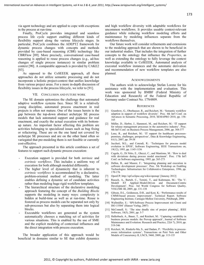
173



via agent technology and are applied to cope with exceptions in the process at run-time.

Finally, ProCycle provides integrated and seamless process life cycle support enabling different kinds of flexibility support along the various lifecycle stages. In particular, ProCycle combines the ADEPT2 framework for dynamic process changes with concepts and methods provided by case-based reasoning (CBR) technology like CBRFlow [89]. More precisely, conversational case-based reasoning is applied to reuse process changes (e.g., ad-hoc changes of single process instances) in similar problem context [90]. A comparable approach is provided by CAKE2 [83].

As opposed to the CoSEEEK approach, all these approaches do not utilize semantic processing and do not incorporate a holistic project-context that unifies knowledge from various project areas. For a more in-depth discussion of flexibility issues in the process lifecycle, we refer to [91].

VII. CONCLUSION AND FUTURE WORK The SE domain epitomizes the challenge that automated

adaptive workflow systems face. Since SE is a relatively young discipline, automated process enactment in real projects is often not mature. One of the issues herein is the gap between the top-down abstract archetype SE process models that lack automated support and guidance for real enactment, and exactly the actual execution with its bottom-up nature. An important factor affecting this problem are activities belonging to specialized issues such as bug fixing or refactoring. These are on the one hand not covered by archetype SE processes and are on the other hand often so variegated that pre-modeling them is not feasible or currently cost-effective.

The approach presented in this article combines a set of features to support such dynamic process execution:

- Execution support is provided for both intrinsic and

extrinsic workflows. This includes a uniform way of execution for both although modeled differently.

- The higher level of dynamicity that is inherent to extrinsic workflows is accommodated by a declarative, problem-oriented method of modeling. The latter enables defining a dynamic set of candidate activities rather than modeling huge rigid workflow templates.

- The hierarchical structure of the declarative modeling approach featuring the concept of the Building Blocks supports the modeling in many ways: complexity is hidden at build-time as well as at run-time. Reuse is fostered as process models can be separated not only by sub-processes but also by separating them into logical blocks.

- Executable workflows are generated as the system automatically chooses a matching set of activities for various situations. This is enabled by the use of SME and the explicit modeling of contextual influences and the direct integration with process execution.

The broader application of this approach would be

beneficial in domains similar to SE that exhibit dynamics

and high workflow diversity with adaptable workflows for uncommon workflows. It provides useable context-relevant guidance while reducing workflow modeling efforts and maintenance by modeling influences separate from the workflows themselves.

Our future work will consider refinements and extensions to the modeling approach that are shown to be beneficial in our industrial studies. That includes the integration of further concepts to the ontology that influence the Properties, as well as extending the ontology to fully leverage the context knowledge available to CoSEEEK. Automated analysis of executed workflow instances and the automatic derivation and recommendation of new workflow templates are also planned.

ACKNOWLEDGMENTS The authors wish to acknowledge Stefan Lorenz for his

assistance with the implementation and evaluation. This work was sponsored by BMBF (Federal Ministry of Education and Research) of the Federal Republic of Germany under Contract No. 17N4809.

REFERENCES [1] Grambow, G., Oberhauser, R., and Reichert, M.: ‘Semantic workflow

adaption in support of workflow diversity’. Proc. 4th Int'l Conf. on Advances in Semantic Processing, 2010, SEMAPRO 2010, pp. 158-165

[2] Müller, D., Herbst, J., Hammori, M., and Reichert, M.: ‘IT support for release management processes in the automotive industry’. Proc. 4th Int'l Conf. on Business Process Management, 2006, pp. 368-377

[3] Lenz, R., and Reichert, M.: ‘IT support for healthcare processes-premises, challenges, perspectives’, Data & Knowledge Engineering, 61(1), 2007, pp. 39-58

[4] Jaccheri, M.L., and Conradi, R.: ‘Techniques for process model evolution in EPOS’, Software Engineering, IEEE Transactions on, 19(12), 1993, pp. 1145-1156

[5] Cugola, G., Di Nitto, E., Ghezzi, C., and Mantione, M.: ‘How to deal with deviations during process model enactment’. Proc. 17th Int'l Conf. on Software engineering, 1995, pp. 265-273

[6] Dellen, B., and Maurer, F.: ‘Integrating planning and execution in software development processes’. Proc. 5th Workshop on Enabling Technologies: Infrastructure for Collaborative Enterprises, 1996, pp. 170-176

[7] OpenUP, http://epf.eclipse.org/wikis/openup/ [Januray 2012] [8] Rausch, A., Bartelt, C., Ternité, T., and Kuhrmann, M.: ‘The V-

Modell XT Applied–Model-Driven and Document-Centric Development’. Proc. 3rd World Congress for Software Quality, VOLUME III, 2005, pp. 131-138

[9] Gibson, D.L., Goldenson, D.R., and Kost, K.: ‘Performance results of CMMI-based process improvement’. Technical Report. Software Engineering Institute, Carnegie-Mellon University, Pittsburgh, 2006

[10] Wallmüller, E.: ‘SPI-Software Process Improvement mit Cmmi und ISO 15504’ (Hanser Verlag, 2007)

[11] McConnell, S.: ‘The nine deadly sins of project planning’, IEEE Software, 18(5), 2001, pp. 5-7

[12] Hallerbach, A., Bauer, T., and Reichert, M.: ‘Capturing variability in business process models: the Provop approach’, Journal of Software Maintenance and Evolution: Research and Practice, 22(6 7), 2010, pp. 519-546

[13] Reichert, M., Rinderle-Ma, S., and Dadam, P.: ‘Flexibility in process-aware information systems’, Transactions on Petri Nets and Other Models of Concurrency II, LNCS, 5460, 2009, pp. 115-135

174



[14] Weber, B., Reichert, M., Mendling, J., and Reijers, H.A.: ‘Refactoring large process model repositories’, Computers in Industry, 62(5), 2011, pp. 467-486

[15] Hill, J., Pezzini, M., and Natis, Y.: ‘Findings: confusion remains regarding BPM terminologies’, Gartner Research, 501(G00155817), 2008

[16] WfMC. 1993. Workflow management coalition. http:// www. wfmc.org/

[17] Oberhauser, R., and Schmidt, R.: ‘Towards a Holistic Integration of Software Lifecycle Processes using the Semantic Web’. Proc. 2nd Int. Conf. on Software and Data Technologies, 2007, pp. 137-144

[18] Oberhauser, R.: ‘Leveraging Semantic Web Computing for Context-Aware Software Engineering Environments’, in Wu, G. (Ed.): ‘Semantic Web’ (In-Tech, Vienna, Austria, 2010)

[19] Grambow, G., Oberhauser, R., and Reichert, M.: ‘Towards a Workflow Language for Software Engineering’. Proc. 10th IASTED Conference on Software Engineering, 2011, pp.130-137

[20] Grambow, G., and Oberhauser, R.: ‘Towards Automated Context-Aware Selection of Software Quality Measures’. Proc. 5th Intl. Conf. on Software Engineering Advances, 2010, pp. 347-352

[21] Grambow, G., Oberhauser, R., and Reichert, M.: ‘Employing Semantically Driven Adaptation for Amalgamating Software Quality Assurance with Process Management’. Proc. 2nd Int’l. Conf. on Adaptive and Self-adaptive Systems and Applications, 2010, pp. 58-67

[22] Grambow, G., Oberhauser, R., and Reichert, M., ‘Contextual Quality Measure Integration into Software Engineering Processes,’ International Journal on Advances in Software, 4(1&2), 2011, pp. 76-99

[23] Ralyté, J., Brinkkemper, S., and Henderson-Sellers, B.: ‘Situational method engineering: Fundamentals and experiences’ (Springer, 2007)

[24] Reichert, M., Weber, B.: Enabling Flexibility in Process-aware Information Systems – Challenges, Methods, Technologies, Springer (to appear)

[25] Pichler, P., Weber, B., Zugal, S., Pinggera, J., Mendling, J., and Reijers, H.A.: ‘Imperative versus Declarative Process Modeling Languages: An Empirical Investigation’. Accepted for publication in Proc. 2nd Int'l Workshop on Empirical Research in Business Process Management, 2011

[26] Grambow, G., Oberhauser, R., and Reichert, M.: ‘Semantically-Driven Workflow Generation using Declarative Modeling for Processes in Software Engineering’. Accepted for publication in Proc. 4th Int'l Workshop on Evolutionary Business Processes, 2011

[27] Gelernter, D.: ‘Generative communication in Linda’, ACM Transactions on Programming Languages and Systems (TOPLAS), 7(1), 1985, pp. 80-112

[28] Oberhauser, R.: ‘Towards Automated Test Practice Detection and Governance’. Proc. Int'l Conf. on Advances in System Testing and Validation Lifecycle, 2009, pp. 19-24

[29] Van der Aalst, W.M.P.: ‘The application of Petri nets to workflow management’, Journal of Circuits Systems and Computers, 8(1), 1998, pp. 21-66

[30] Rinderle, S., Reichert, M., and Dadam, P.: ‘Evaluation of correctness criteria for dynamic workflow changes’. Proc. 1st Int'l Conf on Business Process Management, LNCS, 2678, 2003, pp. 1021-1021

[31] van der Aalst, W.M.P., ter Hofstede, A.H.M., Kiepuszewski, B., and Barros, A.P.: ‘Workflow patterns’, Distributed and parallel databases, 14(1), 2003, pp. 5-51

[32] Russell, N., ter Hofstede, A.H.M., Edmond, D., and van der Aalst, W.M.P.: ‘Workflow data patterns’. Proc. 24th Int'l Conf. on Conceptual Modeling, LNCS, 3716, 2004, pp. 353–368

[33] Lanz, A., Weber, B., and Reichert, M.: ‘Workflow time patterns for process-aware information systems’. Proc. 11th International Workshop on Enterprise, Business-Process, and Information Systems Modeling, LNBIP, 50, 2010, pp. 94–107

[34] microTOOL in-Step: http://www.microtool.de/instep/en/index.asp [January, 2012]

[35] Grambow, G., Oberhauser, R., and Reichert, M.: ‘Towards Automatic Process-aware Coordination in Collaborative Software Engineering’. Accepted for publication in Proc. 6th International Conference on Software and Data Technologies, 2011

[36] Zugal, S., Pinggera, J., and Weber, B.: ‘Creating Declarative Process Models Using Test Driven Modeling Suite’. Proc. CAiSE Forum, 2011, pp. 1-8

[37] Zugal, S., Pinggera, J., and Weber, B.: ‘The impact of testcases on the maintainability of declarative process models’. Proc. Int'l Working Conf. on Enterprise, Business-Process and Information Systems Modeling, LNBIP, 81, 2011, pp. 163-177

[38] Reichert, M.: ‘Dynamische Ablaufänderungen in Workflow-Management-Systemen’. PhD Thesis, University of Ulm, 2000

[39] Reichert, M., Rinderle, S., Kreher, U., and Dadam, P.: ‘Adaptive process management with ADEPT2’. Proc. 21st International Conference on Data Engineering, 2005, pp. 1113-1114

[40] Vanhatalo, J., Völzer, H., and Koehler, J.: ‘The refined process structure tree’. Proc. 6th Int'l Conf. on Business Process Management, LNCS, 5240, 2008, pp. 100-115

[41] Kiepuszewski, B., ter Hofstede, A., and Bussler, C.: ‘On structured workflow modelling’. Proc. 12th Conference on Advanced Information Systems Engineering, LNCS, 1789, 2000, pp. 431-445

[42] Reichert, M., and Dadam, P.: ‘ADEPT flex—supporting dynamic changes of workflows without losing control’, Journal of Intelligent Information Systems, 10(2), 1998, pp. 93-129

[43] Mendling, J., Reijers, H.A., and van der Aalst, W.M.P.: ‘Seven process modeling guidelines (7pmg)’, Information and Software Technology, 52(2), 2010, pp. 127-136

[44] Mendling, J.: ‘Metrics for Process Models: Empirical Foundations of Verification, Error Prediction, and Guidelines for Correctness’ (Springer-Verlag New York Inc, 2008)

[45] Muehlen, M., and Recker, J.: ‘How much language is enough? Theoretical and practical use of the business process modeling notation’. Proc. 20th Int'l Conf. on Advanced Information Systems Engineering, LNCS, 5074, 2008, pp. 465-479

[46] Li, C., Reichert, M., and Wombacher, A.: ‘Mining business process variants: Challenges, scenarios, algorithms’, Data & Knowledge Engineering, 70(5), 2011, pp. 409-434

[47] BPEL. http://docs.oasis-open.org/wsbpelkk/2.0/wsbpel-v2.0.pdf [January .2012]

[48] Reichert, M., and Rinderle, S.: ‘On design principles for realizing adaptive service flows with BPEL’. Proc. Workshop "Methoden, Konzepte und Technologien für die Entwicklung von dienstbasierten Informationssystemen" (EMISA'06), 2006, pp. 133–146

[49] Kindler, E.: ‘On the semantics of EPCs: Resolving the vicious circle’, Data & Knowledge Engineering, 56(1), 2006, pp. 23-40

[50] Mendling, J., Neumann, G., and Van Der Aalst, W.: ‘Understanding the occurrence of errors in process models based on metrics’, On the Move to Meaningful Internet Systems 2007: CoopIS, DOA, ODBASE, GADA, and IS, LNCS, 4803, 2010, pp. 113-130

[51] Mendling, J., Dongen, B.F.v., and Aalst, W.M.P.v.d.: ‘Getting rid of OR-joins and multiple start events in business process models’, Enterprise Information Systems, 2(4), 2008, pp. 403-419

[52] Dadam, P., and Reichert, M.: ‘The ADEPT project: a decade of research and development for robust and flexible process support’, Computer Science-Research and Development, 23(2), 2009, pp. 81-97

[53] Lanz, A., Reichert, M., and Dadam, P.: ‘Making Business Process Implementations Flexible and Robust: Error Handling in the AristaFlow BPM Suite’. Proc. CAiSE'10 Forum, LNBIP, 72, 2010, pp. 174-189

[54] Han, Y.: ‘Software Infrastructure for Configurable Workflow Systems: A Model-driven Approach Based on Higher Order Object Nets and CORBA’. PHD Thesis, TU Berlin, 1997

175



[55] Meier, W.: ‘eXist: An open source native XML database’, Web, Web-Services, and Database Systems, LNCS, 2593, 2009, pp. 169-183

[56] Johnson, P.M.: ‘Requirement and design trade-offs in Hackystat: An in-process software engineering measurement and analysis system’. Proc. 1st Int. Symp. on Empirical Software Engineering and Measurement, 2007, pp. 81-90

[57] Luckham, D.C.: ‘The power of events: an introduction to complex event processing in distributed enterprise systems’ (Addison-Wesley Longman Publishing Co., Inc. Boston, MA, USA, 2001)

[58] Esper: http://esper.codehaus.org/ [January 2012] [59] Weber, B., Reichert, M., Wild, W., and Rinderle, S.: ‘Balancing

flexibility and security in adaptive process management systems’, On the Move to Meaningful Internet Systems 2005: CoopIS, DOA, and ODBASE, LNCS, 3760, 2005, pp. 59-76

[60] Rinderle-Ma, S., Reichert, M., and Weber, B.: ‘Relaxed compliance notions in adaptive process management systems’. Proc. 27th Int'l Conf. on Conceptual Modeling, LNCS, 5231, 2008, pp. 232-247

[61] World Wide Web Consortium, ‘OWL Web Ontology Language Semantics and Abstract Syntax,’ (2004) [January 2012]

[62] McBride, B.: ‘Jena: A semantic web toolkit’, Internet Computing, IEEE, 6(6), 2002, pp. 55-59

[63] Sirin, E., Parsia, B., Grau, B.C., Kalyanpur, A., and Katz, Y.: ‘Pellet: A practical owl-dl reasoner’, Web Semantics: Science, Services and Agents on the World Wide Web, 5(2), 2007, pp. 51-53

[64] Li, C., Reichert, M., and Wombacher, A.: ‘The MinAdept Clustering Approach for Discovering Reference Process Models out of Process Variants’, International Journal of Cooperative Information Systems, 19(3 & 4), 2010, pp. 159-203

[65] Koschmider, A., and Oberweis, A.: ‘Ontology based business process description’. Proc. CAiSE´05 workshops, 2005, pp. 321-333

[66] Lin, Y., and Strasunskas, D.: ‘Ontology-based semantic annotation of process templates for reuse’. Proc. 10th International Workshop on Exploring Modeling Methods for Systems Analysis and Design, 2005, pp. 593-604

[67] Ma, Z., Wetzstein, B., Anicic, D., Heymans, S., and Leymann, F.: ‘Semantic business process repository’. Proc. Workshop on Semantic Business Process and Product Lifecycle Management, 2007, pp. 92–100

[68] Pedrinaci, C., Domingue, J., and Alves de Medeiros, A.: ‘A core ontology for business process analysis’, The Semantic Web: Research and Applications, LNCS, 5021, 2008, pp. 49-64

[69] Thomas, M., Redmond, R., Yoon, V., and Singh, R.: ‘A semantic approach to monitor business process’, Communications of the ACM, 48(12), 2005, pp. 55-59

[70] Ly, L.T., Knuplesch, D., Rinderle-Ma, S., Goeser, K., Reichert, M., and Dadam, P.: ‘SeaFlows Toolset-Compliance Verification Made Easy’. Proc. CAiSE'10 Forum, LNBIP, 2010, pp. 76-91

[71] Jiang, T., Ying, J., and Wu, M.: ‘CASDE: An Environment for Collaborative Software Development’, Computer Supported Cooperative Work in Design III, LNCS, 4402, 2007, pp. 367-376

[72] Cook, C., Churcher, N., and Irwin, W.: ‘Towards synchronous collaborative software engineering’. Proc. 11th Asia-Pacific Software Engineering Conference, 2004, pp. 230-239

[73] Dustdar, S.: ‘Caramba—a process-aware collaboration system supporting ad hoc and collaborative processes in virtual teams’, Distributed and parallel databases, 15(1), 2004, pp. 45-66

[74] Conradi, R., Liu, C., and Hagaseth, M.: ‘Planning support for cooperating transactions in EPOS’, Information Systems, 20(4), 1995, pp. 317-336

[75] Weske, M.: ‘Flexible modeling and execution of workflow activities’. Proc. 31st Hawaii Int'l Conf. on System Sciences, 1998, pp. 713-722

[76] Adams, M., ter Hofstede, A.H.M., Edmond, D., and van der Aalst, W.M.P.: ‘Worklets: A service-oriented implementation of dynamic flexibility in workflows’, On the Move to Meaningful Internet Systems 2006: CoopIS, DOA, GADA, and ODBASE, LNCS, 4275, 2006, pp. 291-308

[77] Pesic, M., Schonenberg, H., and van der Aalst, W.M.P.: ‘Declare: Full support for loosely-structured processes’. Proc. 11th IEEE International Enterprise Distributed Object Computing Conference 2007, pp. 287-298

[78] Müller, R., Greiner, U., and Rahm, E.: ‘AGENT WORK: a workflow system supporting rule-based workflow adaptation’, Data Knowlage Engineering, 51(2), 2004, pp. 223-256

[79] Weber, B., Pinggera, J., Zugal, S., and Wild, W.: ‘Alaska Simulator Toolset for Conducting Controlled Experiments on Process Flexibility’. Proc. CAiSE'10 Forum, LNBIP, 72, 2011, pp. 205-221

[80] Sadiq, S., Sadiq, W., and Orlowska, M.: ‘A framework for constraint specification and validation in flexible workflows’, Information Systems, 30(5), 2005, pp. 349-378

[81] Weber, B., Reichert, M., Wild, W., and Rinderle-Ma, S.: ‘Providing integrated life cycle support in process-aware information systems’, Int'l Journal of Cooperative Information Systems (IJCIS), 18(1), 2009, pp. 115-165

[82] Rinderle, S., Weber, B., Reichert, M., and Wild, W.: ‘Integrating process learning and process evolution–a semantics based approach’. Proc. 3rd International Conference on Business Process Management, LNCS, 3649, 2005, pp. 252-267

[83] Minor, M., Tartakovski, A., and Schmalen, D.: ‘Agile workflow technology and case-based change reuse for long-term processes’, International Journal of Intelligent Information Technologies (IJIIT), 4(1), 2008, pp. 80-98

[84] Hallerbach, A., Bauer, T., and Reichert, M.: ‘Context-based configuration of process variants’. Proc. 3rd Int’l Workshop on Technologies for Context-Aware Business Process Management, 2008, pp. 31-40

[85] La Rosa, M., Lux, J., Seidel, S., Dumas, M., and ter Hofstede, A.: ‘Questionnaire-driven configuration of reference process models’. Proc. 19th Int'l Conf. on Advanced Information Systems Engineering, LNCS, 4495, 2007, pp. 424-438

[86] Rinderle, S., Reichert, M., and Dadam, P.: ‘Disjoint and overlapping process changes: Challenges, solutions, applications’, On The Move to Meaningful Internet Systems 2004: CoopIS, DOA, and ODBASE, LNCS, 3290, 2004, pp. 101-120

[87] Rinderle, S., Reichert, M., and Dadam, P.: ‘Correctness criteria for dynamic changes in workflow systems--a survey’, Data & Knowledge Engineering, 50(1), 2004, pp. 9-34

[88] Reichert, M., Rinderle, S., and Dadam, P.: ‘ADEPT Workflow Management System: Flexible Support for Enterprise-Wide Business Processes’. Proc. 1st Int'l Conf. on Business Process Management, LNCS, 2678, 2003, pp. 371-379

[89] Weber, B., Wild, W., and Breu, R.: ‘CBRFlow: Enabling adaptive workflow management through conversational case-based reasoning’. Proc. European Conference on Case-Based Reasoning, LNCS, 3155, 2004, pp. 89-101

[90] Weber, B., Rinderle, S., Wild, W., and Reichert, M.: ‘CCBR–driven business process evolution’. Proc. Int'l Conf. on Cased based Reasoning, LNCS, 3620, 2005, pp. 610-624

[91] Weber, B., Sadiq, S., and Reichert, M.: ‘Beyond rigidity–dynamic process lifecycle support’, Computer Science-Research and Development, 23(2), 2009, pp. 47-65

176



Peer Review

Activity XOR-Gate

Code Review

Code Inspection

Walk through

Implement Solution

Document in Change

log

Inform User

Manual Team

Analyze Issue

Create CR Branch

Reproduce Error

Check Dependencies

Design Solution

Run Regression

Test

Create Regression

TestsRun Unit

Test

Adapt Unit Test

GUI TestRun

Static Analysis

Inform other Team

Smoke Test

Integration Test

Feature Test

Acceptance Test

Validation to Requirements

Integrate and Build

Check for other

Branches

Integrate and Build

Create Patches

Close Issue

Unit test needs

adaptation

Issue very urgent?

Has high complexity / Criticality?

No test in place

Has high user impact?

Start Point End Point

Has high risk / criticality?

Has high complexity?

Has dependencies?


Has dependencies?

Has high risk / user impact?

Has high user impact?

Has very high user impact?



Not too urgent?

Figure 12. Example of pre-modeled workflow for bug fixing.

Compare Files

Compare Files

Merge Files

Merge Files

Merge Files Compare Files

Parallel

Requires

Requires

Compare Files

Merge Files

ActivityAND-GateEnd PointStart Point

543

2

Sequence

ParallelLoop

61

Activity BuildingBlocks Successor Constraint Parallel Constraint

3

XOR-Gate

5

2

1

Work Unit Container 1 (imperative)

Compare Files

Merge Files

Workflow 1

Compare Files

Merge Files

Work Unit Container 2 (declarative) Work Unit Container 3 (declarative)

Workflow 2 Workflow 3

Context

Urgency Criticality Risk

Situaltional Property Context Connection

Figure 13. Declarative workflow modeling.

177



Modeling

Bug Fixing

Information gathering Activity selection Workflow execution

Bug Fixing

Urgency Criticality

FED

ASequence

Parallel

B

Loop

C

FED

ASequence

Parallel

B

Loop

C

ActivityWorkflow Instance / Work Unit Container

AND-Gate

SemanticConnection

OR-GateCommunication

A

C

E

Case

Urgency Criticality

Bug Fixing

Bug Fixing

Workflow generationValidation Value

Computation

Successor ConstraintActivity User SensorParallel

ConstraintContext Property

Urgency Criticality

Building Blocks

Figure 14. Concrete procedure.

External Tool Sensor

CoSEEEKGUI

TupleSpace

WorkflowInstance

Context Module Ontology

ProcessModule

1:Ad Hoc Workflow Event6:Property Info Event

5:Communication Task Event

4:Communication Task Event

9:Request Context Knowledge

10:Context Knowledge

8:Request Context Knowledge

2:Ad Hoc Workflow Event7:Property Info Event

11:Context Knowledge

3:Workflow Instantiation12:Workflow Adaptation

1:Ad Hoc Workflow Event

Figure 15. Concrete procedure realization.

DeclarativeContainerTemplate

BuildingBlock Template BuildingBlockWithPredecessor

BuildingBlockWithSuccessor

BuildingBlockUnconnected

BuildingBlockWithParallel

BuildingBlock_Start

BuildingBlock_End

BuildingBlockInconsistent

Sequence

ActivityTemplate

Loop

ParallelInconsistent Parallel

Consistent Parallel

Inconsistent Sequence

Consistent Sequence

Inconsistent Loop

Consistent Loop

Consistent_DeclarativeContainer

Inconsistent_DeclarativeContainer

PropertyTemplateProperty

IssueTemplateIssue

BuildingBlock

ImperativeContainerTemplate

WorkUnitContainerTemplate

DeclarativeContainerImperativeContainer

WorkUnitContainer

WorkUnit WorkUnitTemplate

Conditional

SkillTemplateSkill

SkillLevel

ProblemTypeProblem

ProductCategory

Person

Artifact

Ontology Concept Generalisation Association

Inconsistent Conditional

Consistent Conditional

Activity

Figure 16. Classes in the ontology.

178



(C) Building Block List

(D) Activity Definition

(B) Building Block Definition

(A) Case Definition

(E) Building Block List Figure 17. GUI screens for declarative workflow modeling.

179



Activity BuildingBlocks Successor Constraint Parallel Constraint

Context

Urgency

Criticality

Risk

Situaltional Property Context Connection

Development Cycle

Sequence – Developer Test

Unit Test Regression Test

Sequence – Unit Test

Adapt Unit test

Run Unit Test

Conditional – Adapt Unit TestAdapt

Unit test

GUI Test

Adapt Unit Test Run Unit Test

GUI Test

Sequence – Regression Test

Create Regression

Test

Run Unit Test

Conditional – Create Regression TestCreate

Regression Test

Run Unit Test

Loop – Development Cycle Parallel - Testing

Smoke Test

Conditional – Review

Peer Review

Integration Test

Feature Test

Acceptance Test

Walkthrough

Code Inspection

Code Review

Sequence – Development Activities

Design Solution

Implement Solution

Inform other Team

Create Regression Test

Validation to Requirements

Close Issue

Multiple Branches

Create Patches

Integrate and Build

Integrate and Build

Loop – Branch Integration

Sequence – Branch Integration

Branch Integration

Create Patches

Conditional – Integration

Branch Integration

Building Block Library

Activity Library

Sequence – Documentation

Document in Change

Log

Inform User Manual Team

ReviewDeveloper Test

Development Activities

Analyze Issue

Analyze Issue

Prepare Bug Fixing Documentation

Sequence – Prepare Bug Fixing

Create CR

Branch

Reproduce Error

Check Dependencies

Validation to Requirements Testing Integration Close Issue

Peer Review Walkthrough

Code Inspection Code Review Check for other Branches

Create Patches

Smoke Test Integration Test

Feature Test Acceptance Test

Document in Change Log

Inform User Manual Team Create CR Branch Reproduce Error

Check DependenciesDesign Solution Implement Solution

Inform other Team

Case

Dependencies

Complexity

User Impact

Sequence – Multiple Branches

Integrate and Build

Check for other

Branches

Requiremet Constraint Hierarchical Building Block Connection

Figure 18. Activities of example scenario.

180



Adding Self-scaling Capability to the Cloud to meet Service Level Agreements

An Open-source Middleware Framework Solution

Antonin Chazalet, Frédéric Dang Tran, Marina Deslaugiers and Alexandre Lefebvre

France Telecom - Orange Labs, {antonin.chazalet, frederic.dangtran,

marina.deslaugiers, alexandre.lefebvre}@orange.com

François Exertier and Julien Legrand, Bull,

{francois.exertier, julien.legrand}@bull.net

Abstract - Cloud computing raises many issues about Virtualization and Service-Oriented Architecture (SOA). Topics to be addressed regarding services in Cloud computing environment include contractualization, monitoring, management, and autonomic management. Cloud computing promotes a "pay-per-use" business model. It should enable to reduce costs but requires flexible services than can be adapted, e.g., to load fluctuations. This work is conducted in the European CELTIC Servery cooperative research project, which deals about a telecommunication services marketplace platform. This project focuses amongst others on the self-scaling capability of Telco services in a cloud environment. This capability is achieved thanks to Service Level Agreement (SLA) monitoring and analysis (i.e., compliance checking), and to autonomic reconfiguration performed according to the analysis results. SLAs contractualize the services and the cloud virtualized environment itself. In order to achieve the self-scaling capability, a specialized autonomic loop is proposed. Our proposal is based on the Monitor, Analyze, Plan, and Execute autonomic loop pattern (defined by IBM) that has been enhanced via the introduction, and the use of SLA. The implementation we provide is based on the following open-source middleware components: Service Level Checking, OW2 JASMINe Monitoring, OW2 JASMINe VMM. Our proposition has been validated in the context of the Servery project [1].

Keywords - Cloud Computing; Autonomic Computing; Self-Scaling; Service Level Agreement; Virtualization; Open-source Middleware.

I. INTRODUCTION

Today, almost all Information Technology (IT) and Telecommunications industries are migrating to a Cloud computing approach. They expect that the Cloud computing model will optimize the usage of physical and software resources, improve flexibility and automate the management of services (i.e., Software as a Service, Platform as a Service, and Infrastructure as a Service). Cloud computing is also expected to enable data centers subcontracting from Cloud providers.

As a consequence, Cloud computing is seen as a way to reduce costs via the introduction and the use of "pay per use" contracts. It is also seen as a way to generate income for Cloud providers that can be:

Infrastructure providers, Platform providers, And/or software providers.

Cloud computing raises many issues. Many of them are related to Virtualization, and Service-oriented Architecture (its implementation and its deployment). These issues take place at both the hardware and/or software levels.

Cloud computing also raises issues related to services

contractualization, services monitoring, services management, and autonomic for the Cloud.

In this paper, we address these last issues for

telecommunication services offered to customers through the Cloud. These issues are critical: indeed, economical concerns (i.e., the establishment and the use of the pay-per-use contracts) require the ability to contractualize services (via the use of service level agreements: SLA), to monitor and manage them, to check services contracts compliance, and to manage virtualized environments.

This paper is organized as follows. The next section

provides background about Autonomic computing, Service Level Checking, and Service Level Agreement. Section 3 presents the related works. Section 4 details the autonomic approach we have followed, and the use of SLA. Section 5 focuses on the targeted Servery use cases (i.e., self-scale-up, and self-scale-down). Section 6 details the open-source solution we propose. Section 7 describes the implementation. We present the validation and the results obtained in Servery in Section 8. Last section concludes this paper and gives directions for future work.

II. BACKGROUND

This section presents general background about autonomic computing, service level checking, and service level agreements.

A. Autonomic computing

Autonomic computing refers to computing systems (i.e., autonomic managers) that are able to manage themselves or others systems (i.e., managed resources) in accordance to management policies and objectives [2].

Thanks to automation, the complexity that human

administrators are facing is moved into the autonomic managers. Administrators can then concentrate on defining high-level management objectives and no longer on the ways to achieve these objectives.

181



In [3], Horn defines principles of autonomic computing following a biological analogy with the human nervous system: a human can achieve high-level goals because its central nervous system allows him to avoid spending time on managing repetitive and vital background tasks such as regulating his blood pressure.

They also specify four main characteristics for describing

systems' self-management capabilities: Self-Configuration that aims to automate managed

resources installation, and (re-)configuration. Self-Healing that purposes to discover, diagnose and

act to prevent disruptions. Here, note that self-repair is a part of self-healing.

Self-Protect that aims to anticipate, detect, identify and protect against threats.

Self-Optimize that purposes to tune resources and balance workloads in order to maximize the use of information technology resources. Self-scaling is a subpart of self-optimization.

B. Service Level Checking

Generally speaking, Service Level Checking (SLC) involves a target service and a system in charge of collecting monitoring information and checking SLA compliance.

More precisely, the target service offers probes, and its

usage (or a derived usage) is contractualized with at least one SLA. SLA definitions are based on information that can be obtained through the services probes (directly or via computation). The SLC system takes as input information regarding the target service as well as SLA, and produces SLC results about the SLA compliance, the SLA violation, or errors that occurred during the information collection or checking steps.

In the Cloud computing context, the target services can

include software, platform and/or infrastructure, or can even be a Cloud itself (i.e., a set of software services, platform services and infrastructure services).

The SLC results can be used: To inform, e.g., the target service administrator, or

the hotline support, To dynamically select services at runtime, depending

on the compliance between SLA and the services "really" offered,

To make decisions regarding specific preoccupations, e.g., Green,

Prior to a deployment, e.g., in order to analyze the target compatibility,

To provide analysis information to a SLA enforcement mechanism,

In an autonomic loop, And/or to terminate a contract.

C. Service Level Agreement

A SLA (i.e., a service contract or a contract associated to a service) can be used in order to specify the service offered by a service provider or the service expected by a service client. Contracts can be both about functional or non-functional aspects. A single SLA can contractualize several services, and several different SLA can contractualize the same service (e.g., a SLA for autonomic preoccupations, another for Green preoccupations).

In [4], Beugnard and al. define four contract levels of

increasingly negotiable properties: Syntactic level, e.g., the Java interfaces, Behavioral level that requires the definition of pre and post conditions, Synchronization level, which specifies the global behavior in terms of synchronizations between method calls, and finally, Quality of Service level that specifies the expected QoS.

Web Services Agreement Specification is a specification

for SLA in the Web Services domain [5]. It is proposed by the Open Grid Forum [6].

III. RELATED WORKS

This related works section describes the solutions for autonomic computing proposed by equipment and IT vendors (i.e., IBM, Oracle, HP, Motorola, Cisco, Alcatel-Lucent, etc.). The focus is set on the use of SLA-based service level checking as analyzing part (in autonomic MAPE loop) and the ability to manage virtualized environments (mandatory today in Cloud computing).

First, IBM uses policies managers as analyzers for the

MAPE loop. IBM promotes the use of the Simplified Policy Language (SPL). SPL is based on Boolean algebra, arithmetic functions and collections operations. It also uses conditional expressions [7]. IBM Tivoli System Automation targets the reduction of the frequency and of the duration of service disruptions. It uses advanced policy-based automation to enable the high availability of applications and middleware running on a range of hardware platforms and operating systems. These platforms and systems can be virtualized (or not). Tivoli's products family targets mainly availability and performance [8].

Second, Oracle provides the WebLogic Diagnostics

Framework in order to detect SLA violations [9]. The Oracle Enterprise Manager 10g Grid Control can monitor services and report on service availability, performance, usage and service levels. It doesn't manipulate SLA but a similar concept named Service Level Rule [10]. Oracle Enterprise Manager 11g Database Management is a solution to manage databases in 24x7. It self-tunes and self-manages databases operating w.r.t the performance, and it provides proactive management mechanisms (that involve service levels) in order to avoid downtime and/or performance degradation [11]. Oracle handles and manages virtualization through its Oracle VM Management Pack [12]. Oracle also leads research concerning Platform As A Service (PaaS) and the

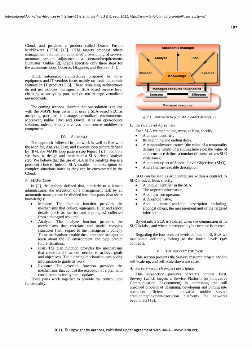
182



Cloud, and provides a product called Oracle Fusion Middleware (OFM) [13]. OFM targets amongst others management automation, automated provisioning of servers, automate system adjustments as demand/requirements fluctuates. Unlike [2], Oracle specifies only three steps for the autonomic loop: Observe, Diagnose, and Resolve [14].

Third, autonomic architectures proposed by other

equipment and IT vendors focus mainly on basic autonomic features in IT products [15]. These remaining architectures do not use policies managers or SLA-based service level checking as analyzing part, and do not manage virtualized environments.

The coming sections illustrate that our solution is in line

with the MAPE loop pattern. It uses a SLA-based SLC as analyzing part and it manages virtualized environments. Moreover, unlike IBM and Oracle, it is an open-source solution: indeed, it only involves open-source middleware components.

IV. APPROACH

The approach followed in this work is well in line with the Monitor, Analyze, Plan, and Execute loop pattern defined by IBM: the MAPE loop pattern (see Figure 1). In addition, we chose to design and implement a SLA-driven Analyze step. We believe that the use of SLA in the Analyze step is a pertinent choice, indeed, SLA enables the description of complex situations/states as they can be encountered in the Cloud.

A. MAPE Loop

In [2], the authors defined that, similarly to a human administrator, the execution of a management task by an autonomic manager can be divided into four parts (that share knowledge):

Monitor: The monitor function provides the mechanisms that collect, aggregate, filter and report details (such as metrics and topologies) collected from a managed resource.

Analyze: The analyze function provides the mechanisms that correlate and model complex situations (with regard to the management policy). These mechanisms enable the autonomic manager to learn about the IT environment and help predict future situations.

Plan: The plan function provides the mechanisms that construct the actions needed to achieve goals and objectives. The planning mechanism uses policy information to guide its work.

Execute: The execute function provides the mechanisms that control the execution of a plan with considerations for dynamic updates.

These parts work together to provide the control loop functionality.

Figure 1. Autonomic loop (or MAPE/MAPE-K loop) [2].

B. Service Level Agreement

Each SLA we manipulate, must, at least, specify: A unique identifier, Its beginning and ending dates, A temporality/occurrence (the value of a temporality

defines the length of a sliding time slot; the value of an occurrence defines a number of consecutives SLO violations),

A non-empty set of Service Level Objectives (SLO), And a human-readable description. SLO can be seen as articles/clauses within a contract. A

SLO must, at least, specify: A unique identifier in the SLA, The targeted information, A comparison operator, A threshold value, And a human-readable description including,

amongst others, the measurement unit of the targeted information.

By default, a SLA is violated when the conjunction of its

SLO is false, and when its temporality/occurrence is crossed. Regarding the four contract levels defined in [4], SLA we

manipulate definitely belong to the fourth level: QoS contracts.

V. THE SERVERY USE CASE

This section presents the Servery research project and the self-scale-up, and self-scale-down use cases.

A. Servery research project description

This sub-section presents Servery's context. First, Servery (which targets a Service Platform for Innovative Communication Environment) is addressing the still unsolved problem of designing, developing and putting into operation efficient and innovative mobile service creation/deployment/execution platforms for networks beyond 3G [16].

183



One of the main goals of Servery is to propose a services marketplace platform where Telco services can be executed, and where end users can search, browse and access the executed services. Services published in the Servery marketplace platform can also be executed in others platforms belonging, e.g., to the telecommunication operators themselves. The services targeted in Servery are stateless services.

The Figure 2 below shows the overview of Servery's

context diagram, i.e., end users that are external actors of the system use Telco services provided by the Servery Marketplace Platform.

Figure 2. Servery's context diagram.

B. Servery self-scale-up use case

This sub-section presents the Servery self-scale-up use case. The goal of this use case is to maintain the overall QoS of the services executed in the Servery marketplace platform and of the marketplace platform itself while the user load grows up. QoS is directly (and indirectly) defined via SLAs. Here, the user load is represented by the number of end users (and consequently by the number of requests sent to the services). The services targeted are Telco services, e.g., SMS services, weather forecast services, etc.

C. Servery self-scale-down use case

This sub-section presents the Servery self-scale-down use case. This use case's goal is to maintain the overall QoS of the services executed in the Servery marketplace platform and of the marketplace platform itself while the user load falls down. The idea, here, is to minimize the cost of the services execution in the Servery marketplace platform, and of the marketplace platform execution itself while preserving services' QoS (at a defined level). A positive side effect of the reduction of the overall system's size is that it also enables the system to be Greener.

VI. SOLUTION FOR SERVERY SELF-SCALING

As presented in the related works section, our proposition is well in line with the MAPE loop pattern defined in [2]. Our idea is to define SLAs between the administrators of the Servery marketplace platform and the marketplace platform itself. The whole MAPE loop proposed is based on these defined SLAs. It is named Servery marketplace management platform. Its monitoring and analyzing parts depend directly on the elements and metrics specified in the SLAs. As a

reminder, the Servery marketplace platform is a Cloud. It means that three types of entities can be distinguished: the entities belonging to the software level, the platform entities and the infrastructure entities. SLAs defined can specify information related to these three types of entities.

More precisely, the analyzing part contains two distinct

sub-parts: the SLC [17], and the JASMINe Monitoring (and its Drools module) [18]. The SLC is in charge of requesting the relevant probes and collecting the monitoring data. It is also in charge of checking the compliance of the defined SLAs with the collected monitoring data. It produces SLC results about the SLA compliance, the SLA violation, or errors occurred during the checking or information collection steps. JASMINe Monitoring takes these SLC notifications as input and checks their frequency over a configurable sliding time slot. This analysis over a sliding time slot is realized by a Drools module. Drools is a business logic integration platform which provides a unified and integrated platform for rules, workflow and event processing [19]. Using a sliding time slot analysis is interesting because it avoids launching the planning and executing steps for non-significant/non-relevant events.

JASMINe Monitoring is also in charge of the planning

part and leads the execution part. All the execution actions related to the virtual machines management is done via the mechanisms provided by JASMINe Virtual Machines Management (JASMINe VMM) [20].

The Servery marketplace platform (see Figure 3) was

designed with a front-end element (i.e., an Apache HTTP Server) and at least one services execution environment (i.e., an OW2 JOnAS open-source Java EE 5 Application Server [21]). This design enables us to be able to scale-up, and scale-down the Servery marketplace platform and the Telco services deployed in it. In short, the Apache front-end acts as a load balancer. Note that the Apache front-end and all the JOnAS server(s) are run in virtual machines themselves run over the Xen hypervisor technology - an open source industry standard for virtualization [22].

Figure 3. Servery marketplace platform architecture.

184



This marketplace platform design is interesting, because it enables to easily support the addition and/or removal of services execution environments. Its only constraint is the need to reconfigure the front-end element in order to take into account additions and/or removals.

VII. PROTOTYPE

This section presents the proposed solution. It involves two high-level modules:

The Servery marketplace platform that is in charge of providing services to the end users.

And the Servery marketplace management platform that ensures the scale-up, and scale-down autonomic properties.

The Servery marketplace management platform involves

four distinct modules: The Service level checking module is in charge of

requesting the relevant probes and collecting the monitoring data from the Servery marketplace platform. It is also in charge of checking the compliance of the defined SLAs with the monitoring data collected. It produces SLC results that are sent to JASMINe monitoring. SLC is developed by France Telecom.

JASMINe Monitoring is part of the OW2 JASMINe project. The OW2 JASMINe project aims to develop an administration tools suite dedicated to SOA middleware such as application servers (Apache, JOnAS, ...), MOM (JORAM, ...) BPM/BPEL/ESB solutions (Orchestra, Bonita, Petals, etc.) in order to facilitate the system administration [23]. JASMINe Monitoring takes SLC notifications as input and checks their frequency over a configurable sliding time slot. It is also in charge of the planning step and it leads the scale-up and scale-down execution steps. JASMINe Monitoring is developed by Bull.

Cluster scaler is in charge of transmitting execution actions to JASMINe VMM. It is also in charge of the reconfiguration of the Apache Load Balancer in order to take into account the virtual machine just added. Cluster scaler is developed by Bull.

JASMINe VMM is in charge of the management of the virtual machines created and executed over the Xen hypervisor. JASMINe VMM aims at offering a unified Java-friendly API and object model to manage virtualized servers and their associated hypervisor. In short, it provides a JMX hypervisor-agnostic façade/API in front of proprietary virtualization management protocols or APIs (such as the open-source Xen and KVM hypervisors, the VMware ESX hypervisor, the Citrix Xen Server hypervisor, and the Microsoft Hyper-V hypervisor). JASMINe VMM is developed by France Telecom.

Note that the solution we propose is a fully open-source

and Java-based solution, and that all communications are done via the Java Management eXtension technology (JMX).

A. Self-scale-up use case

We now present the nominal steps executed by our solution when the need of a scale-up action is detected, and when a scale-up action is then executed (see Figure 4).

Figure 4. Overview of the self-scale-up solution.

Here, the Servery Marketplace Platform initially contains two virtual machines (one containing the Apache LB, and one containing a JOnAS server and Telco services). The fact that end users request/interact with the (services of the) Servery marketplace platform is referred to as step number 0. A nominal execution involves 6 steps (from 1 to 6).

First, the objective of SLC is to check the compliance of

the Servery Marketplace Platform (and its Telco services) with SLAs related: to the Software As A Service (SaaS) level (i.e., Telco services level), to the PaaS level (i.e., JOnAS server level), and to the Infrastructure As A Service (IaaS) level (i.e., virtual machines level). Consequently, SLC requests probes related to the Telco services, the JOnAS server and the virtual machine with regard to the contracts wanted. Amongst all the possible probes, we have chosen to focus and collect the following Telco services (SaaS) information:

The number of requests processed during the last (configurable) time period

The total processing time during the last period The average processing time during the last period The JOnAS server information chosen was: The current server state (e.g., starting, running) The number of active HTTP sessions The number of services deployed/running in a server The virtual machine information chosen was: The virtual machine CPU load The total memory (heap and no-heap) The used memory (heap and no-heap) Second, SLC results are sent to JASMINe monitoring.

JASMINe monitoring then checks the frequency of the SLC

185



results corresponding to a violation. If the frequency of the violations is too high (e.g., more than five violations in a one minute sliding time slot), it means that a scale-up action is needed. So, JASMINe monitoring plans this scale-up action (thanks to information known about the marketplace platform) and executes it. Here, it means that JASMINe monitoring plans to introduce and configure another virtual machine containing a JOnAS server and the Telco services.

Third, the scale-up action is sent to the Cluster Scaler. Fourth, Cluster Scaler commands the JASMINe VMM to

create a new virtual machine (containing a JOnAS server and the Telco services).

Fifth, JASMINe VMM commands the Xen hypervisor in

order to introduce the specified virtual machine. By introducing a virtual machine, we mean creating, instantiating and launching the virtual machine (and its content).

Sixth, Cluster Scaler is informed that the requested

virtual machine has correctly been instantiated and is now in the running state. Then, Cluster Scaler reconfigures the Apache Load Balancer in order to take into account the new virtual machine (and its content) just introduced.

Finally, the load induced by the end users requests is now

dispatched between the two virtual machines (containing the JOnAS Servers and the services).

B. Self-scale-down use case

We now present the design of the nominal steps that should be executed when the need of a scale-down action is detected, and when a scale-down action is then executed (see Figure 5). Let's start with a Servery Marketplace Platform that initially involves three virtual machines (one containing the Apache LB, and two containing each a JOnAS server and the Telco services). The fact that end users request/interact with the (services of the) Servery marketplace platform is also referred here to as step number 0. A nominal scale-down execution involves 6 steps (from 1 to 6).

Figure 5. Overview of the self-scale-down solution.

First, SLC's objective is, here again, to check the compliance of the Servery Marketplace Platform (and its Telco services) w.r.t. the specified SLAs. Therefore, SLC requests the probes related to the Telco services, the JOnAS server and the virtual machine. It then produces SLC results.

These results are, then, sent to JASMINe monitoring.

This latter checks the frequency of the violation. Like in the scale-up steps, we chose that more than five violations in a one minute sliding time slot means that a scale-down action is required. If such a case occurs, JASMINe monitoring then plans the scale-down action, and executes it. A virtual machine containing a JOnAS server and the Telco services will therefore be selected (let's say " VM' " in Figure 5.), and removed from the Marketplace Platform.

After that, the scale-down action is sent to the Cluster

Scaler. Fourth, Cluster Scaler reconfigures the Apache Load

Balancer in order to take into account the future removal of the chosen virtual machine.

Fifth, Cluster Scaler requests the JASMINe VMM to

remove the given virtual machine. Sixth, JASMINe VMM then commands the Xen

hypervisor to remove the virtual machine. By removing, we mean stopping, and deleting the virtual machine (and its content). Cluster Scaler is then informed that the requested virtual machine has correctly been removed.

Consequently, the load induced by the end users requests

is now factorized/centered, here, on the remaining virtual machine.

VIII. VALIDATION

This section presents details, screenshots, and results about the demonstration associated to the scale-up use case.

First, our solution has been demonstrated to CELTIC and

French National Research Agency (ANR) experts during the Servery project's mid-term review.

This live demonstration and the validation were done on

three standards servers: one dedicated to the marketplace platform, one containing the marketplace management platform, and one in charge of injecting the end users load to the marketplace platform.

Over this hardware configuration, we observed that our

whole MAPE loop runs approximately in 10 minutes (this is an average value coming from ten consecutive experimentations. These 10 minutes are broken down as follows:

1 minute is taken by SLC and JASMINe monitoring in order to monitor and detect 5 consecutive SLA violations in a 1 minute sliding time slot.

186



1 minute is taken by JASMINe monitoring for the planning of the scale-up action and the execution step launching.

1 minute is spent by JASMINe VMM in order to interact with the Xen hypervisor for introducing a new virtual machine.

At least 6 minutes are consumed by the creation, the boot and the initialization steps of the (just introduced) virtual machine.

Less than 1 minute is spent by Cluster Scaler to reconfigure the marketplace platform and check its state.

Note that the creation of the virtual machine can be

reduced to a dozen seconds via the use of virtual machine templates; the boot and initialization steps are complex to shorten.

Figure 6 below is a screenshot of SLC. It shows SLC

results: here, one violation of the SLA tsla_id_3 has been detected).

Figure 6. Screenshot of SLC with a SLA violation.

Figure 7 is a screenshot of JASMINe VMM. It shows the marketplace platform after a self-scale-up. Three virtual machines are displayed: one containing the Apache LB (called apache) and two containing each a JOnAS server and the Telco services (called jonasWorker1 and jonasWorker3).

Figure 7. Screenshot of JASMINe VMM with 3 Virtual Machines.

Figure 8 below shows the number of requests, the average processing time, and the CPU load corresponding to jonasWorker1. Here, we have injected two identical loads on the Apache LB. The first load has led to a SLA violation and the marketplace platform has been self-scaled-up. The second load has been injected after the self-scale-up action; the load is now balanced amongst the two jonasWorkers.

Figure 8. Screenshot of JASMINe Monitoring graphs.

IX. CONCLUSION AND FUTURE WORK

In this paper, we have presented an innovative open-source solution for self-scaling the cloud to meet service level agreements. Our solution has been applied to the Cloud Computing context via two self-scaling use cases coming from the European CELTIC Servery cooperative research project. Applying our proposal to these use cases has led us to several conclusions.

First, according to the objectives, it enables to self-scale a

virtualized cloud depending on the compliance with SLA. It also enables separating concerns related to the monitoring, analyzing, planning and executing steps in an industrial context and in the frame of industrial use cases.

Second, our solution is functional and efficient. It has

been demonstrated in front of experts and validated. Third, an important challenge we solved with this

solution was to find, extend/modify, and integrate open-source middleware pieces with respect to industrial constraints raised by our R&D centers.

Last, but not least, this solution is well accepted by both

France Telecom and Bull project teams. As future work, we plan to introduce several other

monitoring probes in the marketplace platform, to extend the SLC module in order to check more complex SLAs, and to embed it in JASMINe monitoring in order to take advantage of its monitoring mechanisms.

We also plan to study how self-scale-up and self-scale-

down mechanisms can coexist, as well as the self-scaling of statefull services.

187



We also wish to use JASMINe VMM capabilities in order to test our solution on a VMware based marketplace platform.

Finally, it would be interesting to enhance our current

solution by adding self-scaling capability at a lower/finer grain, i.e. SaaS grain, in addition of the current PaaS grain; the OW2 Sirocco middleware can be an interesting basis to do so [24].

ACKNOWLEDGMENT

We would like to thank the European CELTIC program for co-funding the SERVERY project (project number CP5-023), as well as both France Telecom - Orange Labs and Bull. Thanks to Dr. Thierry COUPAYE for hosting this work.

REFERENCES [1] Chazalet A., Dang Tran F., Deslaugiers M., Exertier F., and Legrand

J., "Self-scaling the Cloud to meet Service Level Agreements", IARIA - Cloud Computing 2010, Lisbon, Nov. 2010, pp. 116-121.

[2] IBM, "An architectural blueprint for autonomic computing", white paper, http://www-01.ibm.com/software/tivoli/autonomic/pdfs/ AC_Blueprint_White_Paper_4th.pdf, Jun. 2006, [last accessed Nov. 2010].

[3] Horn P., "Autonomic Computing: IBM’s perspective on the State of Information Technology", in IBM corporation, http://www.research.ibm.com/autonomic/manifesto/autonomic_computing.pdf, Oct. 2001, [last accessed Nov. 2010].

[4] Beugnard A., Jezequel J.-M., Plouzeau N., and Watkins D., "Making components contract aware", IEEE Computer, vol. 32, no 7, 1999.

[5] Andrieux A., Czajkowski K., Dan A., Keahey K., Ludwig H., Kakata T., Pruyne J., Rofrano J., Tuecke S., and Xu M., "Web Services Agreement Specification (WS-Agreement)", Open Grid Forum specification, http://www.ogf.org/documents/GFD.107.pdf, 2007.

[6] Open Grid Forum, http://www.ogf.org/, [last accessed Jan. 2012].

[7] IBM, "Simplified Policy Language", http://download.boulder.ibm. com/ibmdl/pub/software/dw/autonomic/ac-spl/ac-spl-pdf.pdf, 2008, [last accessed Nov. 2010].

[8] IBM, "Virtualization Management", http://www-01.ibm.com/ software/tivoli/solutions/virtualization-management/, 2010, [last accessed Nov. 2010].

[9] Oracle, "Monitoring Performance Using the WebLogic Diagnostics Framework", http://www.oracle.com/technetwork/articles/cico-wldf-091073.html, August 2009, [last accessed Nov. 2010].

[10] Oracle, "Service Management", http://download.oracle.com/docs/cd/ B19306_01/em.102/b31949/service_management.htm, 2009, [last accessed Nov. 2010].

[11] Oracle, "Oracle Enterprise Management 11g Database Management", http://www.oracle.com/technetwork/oem/db-mgmt/index.html, 2010, [last accessed Nov. 2010].

[12] Oracle, "Oracle VM Management Pack", http://www.oracle.com/technetwork/oem/grid-control/ds-ovmp-131982.pdf, 2010, [last accessed Nov. 2010].

[13] Oracle, "Platform-as-a-Service Private Cloud with Oracle Fusion Middleware", Oracle White Paper, http://www.oracle.com/us/036500.pdf, October 2009, [last accessed Nov. 2010].

[14] K. Dias, M. Ramacher, U. Shaft, V. Venkataramani, and G. Wood, "Automatic Performance Diagnosis and Tuning in Oracle", 2nd Conference on Innovative Data Systems Research (CIDR), http://www.cidrdb.org/cidr2005/cidr05cd-rom.zip, pp. 84-94, 2005.

[15] Eurescom, " Autonomic Computing and Networking: The operators’ vision on technologies, opportunities, risks and adoption roadmaps", http://www.eurescom.eu/~pub/deliverables/documents/P1800-series/P1855/D1/, 2009, [last accessed Nov. 2010].

[16] Servery consortium, "SERVERY Celtic project", http://projects.celtic-initiative.org/servery/, 2010, [last accessed Nov. 2010].

[17] Chazalet A., "Service Level Agreements Compliance Checking in the Cloud Computing", 5th International Conference on Software Engineering Advances (ICSEA), pp. 184-189, 2010.

[18] OW2 consortium, "JASMINe Monitoring", http://wiki.jasmine.ow2.org/xwiki/bin/view/Main/Monitoring, 2010, [last accessed Nov. 2010].

[19] JBoss Community, "Drools 5 - The Business Logic integration Platform", http://www.jboss.org/drools, 2010, [last accessed Nov. 2010].

[20] OW2 consortium, "JASMINe Virtual Machine Management", http://wiki.jasmine.ow2.org/xwiki/bin/view/Main/VMM, 2010, [last accessed Nov. 2010].

[21] OW2 consortium, "OW2 JOnAS open-source Java EE 5 Application Server", http://jonas.ow2.org/, 2010, [last accessed Nov. 2010].

[22] Citrix Systems, "The Xen Hypervisor", http://www.xen.org/, 2010, [last accessed Nov. 2010].

[23] OW2 Consortium, "JASMINe: The Smart Tool for your SOA Platform Management", http://jasmine.ow2.org/, 2010, [last accessed Nov. 2010].

[24] OW2 Consortium, "Sirocco: A Multi-Cloud Infrastructure-as-a-Service Software Platform", http://www.ow2.org/view/ActivitiesDashboard/Sirocco, 2011, [last accessed Jul. 2011].

188



SERSCIS-Ont

Evaluation of a Formal Metric Model using Airport Collaborative Decision Making

Mike Surridge, Ajay Chakravarthy, Maxim Bashevoy, Joel Wright, Martin Hall-May

IT Innovation Centre University of Southampton

Southampton, UK {ms,ajc,mvb,jjw,mhm}@it-innovation.soton.ac.uk

Roman Nossal Austro Control

Österreichische Gesellschaft für Zivilluftfahrt mbH Vienna, Austria

[email protected]

Abstract— In the Future Internet, programs will run on a

dynamically changing collection of services, entailing the

consumption of a more complex set of resources including

financial resources. The von Neumann model offers no useful

abstractions for such resources, even with refinements to

address parallel and distributed computing devices. In this

paper we detail the specification for a post-von Neumann

model of metrics where program performance and resource

consumption can be quantified and encoding of the behaviour

of processes that use these resources is possible. Our approach

takes a balanced view between service provider and service

consumer requirements, supporting service management and

protection as well as non-functional specifications for service

discovery and composition. The approach is evaluated using a

case study based on an airport-based collaborative decision-

making scenario. Two experimental approaches are presented:

the first based on stochastic process simulation, the second on

discrete event-based simulation.

Keywords-adaptive metrics; SOA; measurements;

constraints; QoS; discrete event simulation.

I. INTRODUCTION

This paper presents the SERSCIS-Ont metric ontology first introduced in [11], together with an expanded evaluation section.

A (relatively) open software industry developed for non-distributed computers largely because of the von Neumann model [8], which provided the first practical uniform abstraction for devices that store and process information. Given such an abstraction, one can then devise models for describing computational processes via programming languages and for executing them on abstract resources while controlling trade-offs between performance and resource consumption. These key concepts, resource abstraction supporting rigorous yet portable process descriptions, are fundamental to the development and widespread adoption of software assets including compilers, operating systems and application programs.

In the Future Internet, programs will run on a dynamically changing collection of services, entailing the consumption of a more complex set of resources including financial resources (e.g., when services have to be paid for). The von Neumann model offers no useful abstractions for such resources, even with refinements to address parallel and distributed computing devices. In this context, we need

something like a ‘post-von Neumann’ model of the Future Internet of Services (including Grids, Clouds and other SOA), in which: program performance and consumption of resource (of all types) can be quantified, measured and managed; and programmers can encode the behaviour of processes that use these resources, including trade-offs between performance and resource consumption, in a way that is flexible and portable to a wide range of relevant resources and services.

In this paper, we describe the metric model developed within the context of the SERSCIS project. SERSCIS aims to develop adaptive service-oriented technologies for creating, monitoring and managing secure, resilient and highly available information systems underpinning critical infrastructures. The ambition is to develop technologies for such information systems to enable them to survive faults, mismanagement and cyber-attack, and automatically adapt to dynamically changing requirements arising from the direct impact of natural events, accidents and malicious attacks. The proof of concept (PoC) chosen to demonstrate the SERSCIS technologies is an airport-based collaboration and decision-making scenario. In this scenario, separate decision makers must collaborate using a number of dynamic interdependent services to deal with events such as aircraft arrival and turn-around, which includes passenger boarding, baggage loading and refuelling. The problem that decision makers face is that the operations are highly optimised, such that little slack remains in the turnaround process. If a disruptive event occurs, such as the late arrival of a passenger, then this has serious knock-on effects for the rest of the system that are typically difficult to handle.

The focus for our work is therefore to support the needs of both service providers and consumers. Our goal is to allow providers to manage and protect their services from misbehaving consumers, as well as allowing consumers to specify non-functional requirements for run-time service discovery and composition should their normal provider become unreliable. In this sense, SERSCIS-Ont combines previous approaches from the Semantic Web community focusing on service composition, and from the service engineering community focusing on quantifying and managing service performance.

The rest of the paper is organised as follows. Section II defines and clarifies the terminology used for metrics, measurements and constraints. In Section III, we present the

189



SERSCIS-Ont metric model. Here each metric is discussed in a detail along with the constraints which can be imposed upon these metrics. Section IV reviews the state of the art for related work and compares and contrasts research work done in adaptive system metrics with SERSCIS-Ont. Section V describes the scenario and experiments that are used to test the applicability of the SERSCIS metrics. Section VI presents the results of the validation experiment carried out using stochastic process modelling and simulation. Sections VIII and IX elaborate the experimental scenario by describing, respectively, Key Performance Indicators (KPI) for each actor and failure scenarios. These are then demonstrated in Section IX using the results of a discrete event-based simulation experiment. Finally, we conclude the paper in Section X.

II. METRICS MEASUREMENTS AND CONSTRAINTS

It is important to distinguish between the terminology used for metrics, measurements and constraints. In Figure 1. we show the conceptual relationships between these terms.

Figure 1. Metrics, Measurements and Constraints

Services (or sometimes the resources used to operate

them) are monitored to provide information about some feature of interest associated with their operation. The monitoring data by some measurement procedure applied to the feature of interest at some time or during some time period. Metrics are labels associated with this data, denoting what feature of interest they refer to and (if appropriate) by which measurement procedure they were obtained. Finally, monitoring data is supplied to observers of the service at some time after it was measured via monitoring reports, which are generated and communicated to observers using a reporting procedure. It is important to distinguish between monitoring data for a feature of interest, and its actual behaviour. In many situations, monitoring data provides only an approximation to the actual behaviour, either because the measurement procedure has limited accuracy or precision, or was only applied for specific times or time periods and so does not capture real-time changes in the feature of interest. Constraints define bounds on the values that monitoring data should take, and also refer to metrics so it is clear to which

data they pertain. Constraints are used in management policies, which define management actions to be taken by the service provider if the constraints are violated. They are also used in SLA terms, which define commitments between service providers and customers, and may specify actions to be taken if the constraints are violated. Note that management policies are not normally revealed outside the service provider, while SLA terms are communicated and agreed between the service provider and customer. Constraints refer to the behaviour of services or resources, but of course they can only be tested by applying some testing procedure to the relevant monitoring data. The testing procedure will involve some mathematical manipulation to extract relevant aspects of the behaviour from the monitoring data.

III. SERSCIS METRICS

In SERSCIS, we aim to support metrics which will represent the base classes that capture the physical and mathematical nature of certain kinds of service behaviours and measurements. These are described below.

A. Absolute Time

This metric signifies when (what time and date) some event occurs. It can be measured simply by checking the time when the event is observed. Subclasses of this metric would be used to refer to particular events, e.g., the time at which a service is made available, the time it is withdrawn from service, etc. There are two types of constraints imposed on this metric. (1) a lower limit on the absolute time, encoding “not before” condition on the event. (2) an upper limit on the absolute, encoding a “deadline” by which an event should occur.

B. Elapsed Time

This metric just signifies how long it takes for some event to occur in response to some stimulus. It can be measured by recording the time when the stimulus arises, then checking the time when the subsequent event is observed and finding the difference. Subclasses of this metric would be used to refer to particular responses, e.g., the time taken to process and respond to each type of request supported by each type of service, or the time taken for some internal resourcing action such as the time for cleaners to reach an aircraft after it was scheduled and available. In the SERSCIS PoC, it should be possible to ask a consumer task for the elapsed times of all responses corresponding to the metric, and possibly to ask for the same thing in a wider context (e.g., from a service or service container). Constraints placed on elapsed time are (1) an upper limit on the elapsed time which encodes a lower limit on the performance of a service. (2) a lower limit which is typically used only in management policies to trigger actions to reduce the resource available if a service over-performs. If there are many events of the same type, one may wish to define a single constraint that applies to all the responses, so if any breaches the constraint the whole set is considered to do so. This allows one to test the constraint more efficiently by checking only the fastest and slowest response in the set.

Service

(or resource)

ObserverMonitoring

Report

Monitoring

Data Value

Measurement

ProcedureMetric

Feature

of Interest

Reporting

Procedure

Obtained

by

Denoted

by

Denoted

by

Reflects

Obtains

reports via

Provided

via

Provided

to

Observes

Contains

Applied

to

Associated

with

Constraint

Bounds

Has

Behaviour

Has

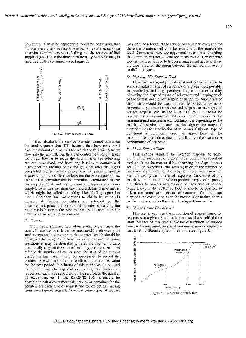
190



Sometimes it may be appropriate to define constraints that include more than one response time. For example, suppose a service supports aircraft refuelling but the amount of fuel supplied (and hence the time spent actually pumping fuel) is specified by the consumer – see Figure 2.

Figure 2. Service response times

In this situation, the service provider cannot guarantee the total response time T(i), because they have no control over the amount of time C(i) for which the fuel will actually flow into the aircraft. But they can control how long it takes for a fuel bowser to reach the aircraft after the refuelling request is received, and how long it takes to connect and disconnect the fuelling hoses and get clear after fuelling is completed, etc. So the service provider may prefer to specify a constraint on the difference between the two elapsed times. In SERSCIS, anything that is constrained should be a metric (to keep the SLA and policy constraint logic and schema simple), so in this situation one should define a new metric which might be called something like ‘fuelling operation time’. One then has two options to obtain its value (1) measure it directly so values are returned by the measurement procedure; or (2) define rules specifying the relationship between the new metric’s value and the other metrics whose values are measured.

C. Counter

This metric signifies how often events occurs since the start of measurement. It can be measured by observing all such events and adding one to the counter (which should be initialised to zero) each time an event occurs. In some situations it may be desirable to reset the counter to zero periodically (e.g., at the start of each day), so the metric can refer to the number of events since the start of the current period. In this case it may be appropriate to record the counter for each period before resetting it the retained value for the next period. Subclasses of this metric would be used to refer to particular types of events, e.g., the number of requests of each type supported by the service, or the number of exceptions, etc. In the SERSCIS PoC, it should be possible to ask a consumer task, service or container for the counters for each type of request and for exceptions arising from each type of request. Note that some types of request

may only be relevant at the service or container level, and for these the counters will only be available at the appropriate level. Constraints here are upper and lower limits encoding the commitments not to send too many requests or generate too many exceptions or to trigger management actions. There are also limits on the ration between the numbers of events of different types.

D. Max and Min Elapsed Time

These metrics signify the slowest and fastest response to some stimulus in a set of responses of a given type, possibly in specified periods (e.g., per day). They can be measured by observing the elapsed times of all events and keeping track of the fastest and slowest responses in the set. Subclasses of this metric would be used to refer to particular types of response, e.g., times to process and respond to each type of service request, etc. In the SERSCIS PoC, it should be possible to ask a consumer task, service or container for the minimum and maximum elapsed times corresponding to the metric. Constraints on such metrics signify the range of elapsed times for a collection of responses. Only one type of constraint is commonly used: an upper limit on the maximum elapsed time, encoding a limit on the worst case performance of a service.

E. Mean Elapsed Time

This metrics signifies the average response to some stimulus for responses of a given type, possibly in specified periods. It can be measured by observing the elapsed times for all such responses, and keeping track of the number of responses and the sum of their elapsed times: the mean is this sum divided by the number of responses. Subclasses of this metric would be used to refer to particular types of response, e.g., times to process and respond to each type of service request, etc. In the SERSCIS PoC, it should be possible to ask a consumer task, service or container for the mean elapsed time corresponding to the metric. Constraints on this metric are the same as those for the elapsed time metric.

F. Elapsed Time Compliance

This metric captures the proportion of elapsed times for responses of a given type that do not exceed a specified time limit. Metrics of this type allow the distribution of elapsed times to be measured, by specifying one or more compliance metrics for different elapsed time limits (see Figure 3. ).

Figure 3. Elapsed time distribution

Triggering event (i-th

refuelling request received)

Fuel starts flowing

Fuel stops flowing

Refuelling completed

C(i)

T(i)

1.0

Elapsed time (T)

Fraction F(T) of responses with elapsed time up to T

3 mins 6 mins 7.5 mins

Fraction taking

up to 3 m

Fraction taking

up to 6 m

Fraction taking

up to 7.5 m

191



When measuring elapsed time compliance, it is convenient to make measurements for all the metrics associated with a distribution like Figure 3. One has to observe the elapsed times for all relevant responses, and keep track of the number of responses that were within each elapsed time limit, and also the total number of responses. The value of the elapsed time compliance metric at each limit is then the ratio between the number of responses that did not exceed that limit and the total number of responses. Subclasses of this metric would be used to refer to particular types of responses and time limits. For example, one might define multiple elapsed time compliance metrics for different time limits for responses to each type of request supported by the service, and for some internal process time. In the SERSCIS PoC, it should be possible to ask a consumer task, service or container for the elapsed time compliance for responses corresponding to the metric. It may also be useful to support requests for all elapsed time compliance metrics for a given type of response, allowing the compliance of the entire distribution function to be obtained at once. Note that some types of request may only be relevant at the service or container level, and for these the elapsed time distribution function will only be available at the appropriate level. Constraints for this metric are normally expressed as lower (and sometimes upper) bounds on the value of the metric for specific responses and time limits. SLA commitments typically involve the use of lower bounds (e.g., 90% of responses within 10 mins, 99% within 15 mins, etc.), but both upper and lower bounds may appear in management policies (e.g., if less than 95% of aircraft are cleaned within 10 mins, call for an extra cleaning team).

G. Non-recoverable resource usage and usage rate

These metrics capture the notion that services consume resources, which once consumed cannot be got back again (this is what we mean by non-recoverable). In most cases, non-recoverable usage is linked to how long a resource was used, times the intensity (or rate) of usage over that period. It can be measured by observing when a resource is used, and measuring either the rate of usage or the total amount of usage at each observation. Subclasses of the non-recoverable usage metric would be used to refer to the usage of particular types of resources, for example on CPU usage, communication channel usage, data storage usage etc. In the SERSCIS PoC, it should be possible to ask a consumer task, service or container for the usage rate at the last observation, and the total usage up to that point. Ideally this should trigger a new observation whose result will be included in the response. The response should include the absolute time of the last observation so it is clear whether how out of date the values in the response may be. Non-recoverable resource usage is characterized by functions of the form:

�(�, �) ≥ 0 (1)

�(�, �)

�≥ 0

(2)

U represents the total usage of the non-recoverable resource by a set of activities S up to time t. The range of U

is therefore all non-negative numbers, while the domain spans all possible sets of activities using the resource, over all times. In fact, U is zero for all times before the start of the first activity in S (whenever that may have been), and its time derivative is also zero for all times after the last activity has finished. The time derivative of U represents the rate of usage of the non-recoverable resource. This must be well-defined and non-negative, implying that U itself must be smooth (continuously differentiable) with respect to time, i.e., it cannot have any instantaneous changes in value.

Constraints for non-recoverable usage and usage rate are typically simple bounds on their values. Both upper and lower bounds often appear in management policies to regulate actions to decrease as well as increase resources depending on the load on the service:

� ≤ �(�, ��) − �(�, ��) ≤ � (3)

represents a constraint on the minimum and maximum total usage for a collection of activities S in a time period from t0 to t1, while:

�� ≤

�(�, �)

�≤ ��, ∀�: �� ≤ � ≤ ��

(4)

represents a constraint on the maximum and minimum total usage rate for a collection of activities S during a time period from t0 to t1. Note that it is possible to have a rate constraint (4) that allows a relatively high usage rate, in combination with a total usage constraint (3) that enforces a much lower average usage rate over some period. Alternatively, a contention ration could be introduced for usage rate constraints to handle cases where a resource is shared between multiple users but may support a high usage rate if used by only one at a time.

H. Maximum and Minimum Usage Rate

These metrics capture the range of variation in the usage rate (possibly in specified periods, which is described above. They can be measured by simply retaining the maximum and minimum values of the usage rate whenever it is observed by the measurement procedure. Subclasses of these metrics would be used to refer to maximum and minimum usage for particular types of resources. Constraints on maximum and minimum usage rate take the form of simple bounds on their values. Note that if we constrain maximum usage rate to be up to some limit, and the usage rate ever breaches that limit, then the constraint is violated however the usage rate changes later.

I. State

This metric captures the current state of a service, with reference to a (usually finite) state model of the service’s internal situation (e.g., the value of stored data, the status of

192



supplier resources, etc). The value of the metric at any time must be a state within a well-defined state model of the service, usually represented as a string signifying that state and no other. It can be measured by observing the internal situation of the service and mapping this to the relevant state from the state model. In the SERSCIS PoC implementation, it should be possible to ask a task, service or container for its current state. Note that the state model of a service will normally be different from the state model of tasks provided by the service, and different from the state model of the container providing the service. State is an instantaneous metric – a measurement of state gives the state at the time of observation only. To obtain a measure of the history of state changes one should use state occupancy metrics or possibly non-recoverable usage metrics for each possible state of the service. Subclasses of the state metric will be needed to refer to particular state models and/or services. Constraints can be used to specify which state a service should be in, or (if the state model includes an ordering of states, e.g., security alert levels), what range of states are acceptable.

J. State Occupancy

This metric captures the amount of time spent by a task in a particular state (possibly in specified periods). It can be measured by observing state transitions and keeping track of the amount of time spent in each state between transitions. Note that for this to be practical one must predefine a state model for the task encompassing all its possible states, in which the first transition is to enter an initial state when the task is created.

The state of a resource on a service is a function of time:

��(�) ∈ Σ, ∀� ≥ �� (5)

where Si(t) is the state of resource i at time t, ∑ is the set of possible states (from the resource state model) and t0 is the time resource i was created. Constraints on state occupancy are bounds on the proportion of time spent in a particular state, or the ratio between the time spent in one state and time spent in one or more other states.

K. Data Accuracy

This metric captures the amount of error in (numerical) data supplied to or from a service, compared with a reference value from the thing the data is supposed to describe. The two main aspects of interest with this particular metric are the precision of the data (how close to the reference value is the data supposed to be) and the accuracy of the data (how close to the reference value the data is, compared to how close it was supposed to be). Subclasses of data accuracy may be needed to distinguish between different types of data used to describe the thing of interest (single values, arrays etc), and different ways of specifying precision (precision in terms of standard deviation, confidence limit etc), as well as to distinguish between things described by the data (e.g., aircraft landing times, fuel levels or prices). In the SERSCIS PoC, we are only really interested in the accuracy of

predictions for the absolute time of future events, including the point when an aircraft will be available so turnaround can start (an input to the ground handler), the point when the aircraft will be ready to leave, and various milestones between these two points (e.g., the start and end of aircraft cleaning, etc). Constraints on accuracy are typically just upper bounds on the accuracy measure, e.g., accuracy should be less than 2.0. Such constraints apply individually to each data value relating to a given reference value.

L. Data Precision

This is a simple metric associated with the precision bands for data supplied to or from a service. Data that describes some reference value should always come with a specified precision, so measuring the precision is easy – one just has to check the precision as specified by whoever supplied the data. The reason it is useful to associate a metric with this is so one can specify constraints on data precision in SLA, to prevent data suppliers evading accuracy commitments by supplying data very poor (wide) precision bands. Subclasses of data precision are typically needed for different kinds of things described by data, and different sources of that data. For example, one might define different metrics to describe the precision in scheduled arrival times (taken from an airline timetable) and predicted arrival times (supplied by Air Traffic Control when the aircraft is en-route). Note that precision (unlike accuracy) is not a dimensionless number – it has the same units as the data it refers to, so metric subclasses should specify this. In the SERSCIS PoC testbed, it should be possible to ask a consumer task for the precision of data supplied to or by it. The response should ideally give the best, worst and latest precision estimates for the data corresponding to the metric. Constraints on data precision are simple bounds on its value. Typically they will appear in SLA, and define the worst-case precision that is acceptable to both parties. If data is provided with worse precision than this, the constraint is breached. This type of constraint is normally used as a conditional clause in compound constraint for data accuracy or accuracy distribution.

M. Data Error

This is a simple metric associated with the error in a data item relative to the reference value to which it relates. In some situations we may wish to specify and measure commitments for this ‘raw’ measure of accuracy, independently of its supposed precision. Subclasses of data error are typically needed for different kinds of things described by data, and different sources of data. In the SERSCIS PoC testbed, it should be possible to ask a consumer task for the error in data supplied to or by it once the reference value is known to the service. The response should ideally give the best, worst and latest error for data sent/received corresponding to the metric. Constraints on data error are simple bounds on its value. Typically, they will appear in SLA, and define the worst-case error that is acceptable to both parties. If data is provided and turns out to have an error worse than this, the constraint is breached.

193



N. Data Accuracy Compliance

This metric captures the proportion of data items in a data set provided to or from a service whose accuracy is not worse than a specified limit. This metric is mathematically similar to the elapsed time compliance metric, and as before we may wish to use several accuracy compliance metrics for the same data at different accuracy levels, to approximate a data accuracy distribution function. Accuracy compliance can be measured by keeping track of the total number of data items, and how many of these had accuracy up to each specified level. The value of the metric is then the fraction of data items whose accuracy is within the specified level. In the SERSCIS PoC testbed, subclasses of accuracy compliance are typically used to distinguish between different accuracy levels, types of data and methods for defining precision, for data forecasting the time of events. To construct accuracy distributions it is necessary to classify those events so we know which forecasts to include in each distribution function. It should be possible to ask consumer tasks, services or service containers for the value of these compliance metrics. Constraints on accuracy compliance just specify bounds on the metrics; thus, specifying what proportion of data items can have accuracy worse than the corresponding accuracy limit.

O. Auditable Properties

Auditable property metrics are used to express whether a service satisfies some criterion that cannot be measured, but can only be verified through an audit of the service implementation and behaviour. An auditable property will normally be asserted by the service provider, who may also provide proof in the form of accreditation based on previous audits in which this property was independently verified. Auditable properties are usually represented as State metrics: a state model is devised in which the desired property is associated with one or more states, which are related (out of band) to some audit and if necessary accreditation process. Subclasses are used to indicate different auditable properties and state models. Auditable property constraints typically denote restrictions on the resources (i.e., supplier services) used to provide the service. For example, they may specify that only in-house resources will be used, that staff will be security vetted, or that data backups will be held off site, etc. In SERSCIS, such terms are also referred to as Quality of Resourcing (QoR) terms. As with other state-based descriptions, auditable properties may be binary (true or false), or they may be ordered (e.g., to describe staff with different security clearance levels). It is also possible to treat Data Precision (and other data characteristics) as an auditable property which does not correspond to a state model.

IV. RELATED WORK

Characterizing the performance of adaptive real-time systems is very difficult because it is difficult to predict the exact run-time workload of such systems. Transient and steady state behaviour metrics of adaptive systems were initially drafted in [4], where the performance of an adaptive was evaluated by its response to a single variation in the

application behaviour that increased the risk of violating a performance requirement. A very simple set of metrics are used: reaction time which is the time difference between a critical variation and the compensating resource allocation, recovery time by which system performance returns to an acceptable level, and performance laxity which is the difference between the expected and actual performance after the system returns to a steady state. These metrics are further specialized in [1] by the introduction of load profiles to characterize the types of variation considered including step-load (instant) and ramp-load (linear) changes, and a miss-ratio metric which is the fraction of tasks submitted in a time window for which the system missed a completion deadline. System performance is characterized by a set of miss-ratio profiles with respect to transient and steady state profiles. A system is said to be stable in response to a load profile if the system output converges as the time goes to infinity, while transient profiles can measure responsiveness and efficiency when reacting to changes in run-time conditions. The SERSCIS-Ont metrics provide a superset of these concepts, appropriate to a wider range of situations where accuracy and reliability may be as important as performance and stability.

A more recent alternative approach to defining adaptive system metrics is given by [6,7]. Here the focus is on the system engineering concerns for adaptivity, and metrics are categorized into four types: architectural metrics which deal with the separation of concerns and architectural growth for adaptive systems [2], structural metrics which provide information about the role of adaptation in the overall functionality of a system (and vice versa), interaction metrics which measure the changes in user interactions imposed by adaptation, and performance metrics which deal with the impact of adaptation on system performance, such as its response time, performance latency, etc. [2]. The focus of SERSCIS-Ont is to provide concrete and mathematically precise metrics covering performance and some aspects of interactivity, which can be used in such a wider engineering framework.

The most closely related work is found in the WSMO initiative [3], which has also formalized metrics for resource dependability. This was done with the intention of providing QoS aware service oriented infrastructures. Semantic SLA modelling using WSMO focuses principally on automated service mediation and on the service execution infrastructure [3]. By adding semantic descriptions for service parameters it is possible for agents to discover and rank services automatically by applying semantic reasoning. The WSMO initiative focused its modelling efforts on capturing service consumer requirements, which can then be used for service discovery. Work in [5] extends the WSMO ontology to include QoS and non-functional properties. This includes providing formal specifications for service level agreements including the units for measurement, price, CPU usage, etc. However, the focus is still to support the description of services for orchestration purposes (service discovery and selection). SERSCIS-Ont is more even-handed. It can be used for service discovery and selection, but it is also designed to support service operators by introducing service

194



protection measures from a provider’s perspective such as the usage limits, service access and control decisions, as well as workflow adaption, etc.

SERSCIS-Ont is thus also related to the development and service management specifications such as WSDM. The WSDM-MOWS specification [9] defines 10 metrics which are used to measure the use and performance of a general Web Service. These include NumberOfRequests, NumberOfFailedRequests and NumberOfSucessfulRequests which count the messages received by the Web Service end point, and whether the service handles them successfully. In SERSCIS-Ont we have a more general Counter metric, of which these WSDM-MOWS metrics can be regarded as subclasses specifically for Web Service management. WSDM-MOWS also defines ServiceTime (the time taken by the Web Service to process all its requests), and MaxResponseTime and LatestResponseTime. In SERSCIS-Ont these would be modelled as subclasses of usage and elapsed time, and SERSCIS-Ont then provides additional metrics such as min/max/mean responses and response time compliance metrics. WSDM-MOWS specifies a state model for Web Service operation with states {UpState, DownState, IdleState, BusyState, StoppedState, CrashedState, SaturatedState}, and metrics CurrentOperationalState and LastOperationStateTransition all of which can be handled easily by SERSCIS-Ont. The one area where WSDM-MOWS goes beyond SERSCIS-Ont is in providing metrics for the size of Web Service request and response messages: MaxRequestSize, LastRequestSize and MaxResponseSize. These can be modelled with difficulty using SERSCIS-Ont usage metrics, but if SERSCIS-Ont were applied to Web Service management, some extensions would be desirable.

V. VALIDATION EXPERIMENTS

To verify that SERSCIS-Ont really is applicable to the management of service performance and dependability, the project is conducting two types of experiments: the first involving stochastic process simulation and the second extends to discrete event simulation. In the latter case, a testbed has been developed which comprises SERSCIS dependability management tools along with emulated application services based on air-side operations at Vienna Airport. This is a discrete event simulation in which realistic application-level requests and responses are produced, and the full (not emulated) management tools are tested using SERSCIS-Ont metrics in service level agreements and monitoring and management policies.

A. Scenario Description

The scenario used to validate the metric model is based on Airport Collaborative Decision Making (A-CDM). A-CDM is an approach to optimizing resource usage and improving timeliness at an airport. It is about all partners at an airport working together, openly sharing accurate information and – based on the information – making decisions together. Through the use of A-CDM predictability of airport operations is improved. All actions involved in turning around an aircraft can be planned more accurately

and the plans can more easily be controlled with respect to the actual operation.

A-CDM also has a European, network-wide perspective. The Central Flow Management Unit (CFMU) of Eurocontrol monitors the capacity of airspace sectors and imposes restrictions by issuing so-called slots in case congestion might arise. Currently, this planning is mainly based on flight plan information that is filed up to three hours before the actual flight. Changes, in particular last minute changes e.g., due to late passengers, are not taken into account. Hence, everyday a huge amount of airspace capacity is wasted due to inaccurate information. The Airports applying A-CDM can more accurately determine the take-off time of departing flights. CFMU can then update their network planning based on information that closely reflects the real traffic to be expected. Hence, slot wastage is minimized for the benefit of all airspace users.

The testbed scenario for the evaluation is based on the workflow that is executed during an aircraft turn-around. The workflow represents the interaction of the main actors in a turn-around, i.e., the ANSP, a ground handler and ramp service providers. Each step in the workflow uses a service to perform the step. Services are provided by different actors. Most services can be provided by more than one service provider. In this case the service user has the choice of the service provider, for which he has to take into account several Quality-of-Service criteria.

The workflow, which is shown in Figure 4. consists of three sub-workflows being executed in parallel. After the aircraft goes in-block passenger disembarkation starts. At the same time a baggage handler starts to offload the luggage from the aircraft. The third sub-workflow deals with refuelling the aircraft. It can only be started after disembarkation of passengers is finished. Going back to the first sub-workflow, when disembarkation is finished an optional security check of the plane for left items can be performed by either the crew or a security company under the crew’s supervision. When this is done the crew leaves the aircraft. Cleaning of the aircraft and catering commence in parallel. For the latter to be released the new crew is required as they have to check the number of meals provided. Upon completion of cleaning and release of catering another optional security check can be performed given that refuelling has completed as well. After the security check embarkation of passengers can begin if the landside workflow is ready for boarding.

The second sub-workflow is concerned with offloading the luggage and loading the new luggage. It is completely independent of the passenger and cabin-related workflow. Finally, the third sub-workflow has the purpose of refuelling the aircraft. As mentioned above, it can only commence once disembarkation has completed. In turn, completion of refuelling is a precondition for passenger embarkation.

195



Figure 4. Airside Workflow for Aircraft Turnaround

B. Validation Objectives

This evaluation is done by validation, which applies the system to a chosen scenario. From the results of validation one can derive the usefulness of the system for the given application.

In the chosen A-CDM scenario the SERSCIS mechanisms and tools must demonstrate two characteristics:

• They must be able to implement and execute the real-world scenario in the fault-free case. This property ensures that the SERSCIS tools capture the scenario requirements and are able to accompany the execution of the processes. Note that in order to gain acceptance with the potential users, the tools and mechanisms must adapt to the real-world processes, not the other way round.

• They must be able to handle failure cases and improve the execution of the processes in these cases. While the above fault-free case shows the possibility to execute the processes with SERSCIS support, this validation aims at proving the added value of SERSCIS. The tools and mechanisms must improve the handling of failure cases.

Several test runs were conducted to demonstrate the above characteristics. The properties of the SERSCIS tools and mechanisms were evaluated by use of so-called Key

Performance Indicators (KPIs), which are described in Section VII.

VI. STOCHASTIC PROCESS SIMULATION EXPERIMENTS

SERSCIS validation work initially focused on the use of stochastic process simulation based on queuing theory [10]. A simplified Markov chain model was developed for a single aircraft refuelling service, and the resulting equations solved numerically to compute the expected behaviour. This approach is faster and easier to interpret than a discrete event simulation, though it uses simpler and less realistic models of services and their interactions.

The basic model of the refuelling service assumes that around 20 aircraft arrive per hour and need to be refuelled. The service provider has 3 bowsers (fuel tankers), which can supply fuel to aircraft at a certain rate. The time taken for refuelling varies randomly between aircraft depending on their needs and how much fuel they still have on landing, but the average time is 7.5 minutes. However, with only 3 bowsers, aircraft may have to wait until one becomes available before refuelling can start. The SERSCIS-Ont metrics used to describe this service are:

• a counter metric for the number of aircraft refuelled, and an associated usage rate metric for the number of aircraft refuelled per hour;

• a non-recoverable usage rate metric for the time the bowsers spend actually refuelling aircraft, from which we can also obtain the resource utilization percentage;

• an elapsed time metric for the amount of time spent by aircraft waiting for a bowser (the refuelling service cannot control how long the refuelling takes, so QoS is defined in terms of the waiting time only); and

• elapsed time compliance metrics for the proportion of aircraft that have to wait for different lengths of time between 0 and 20 minutes.

We also assume that the service will refuse an aircraft, i.e., tell it to use another refuelling company rather than wait, if it would become the 10th aircraft in the queue. This is captured by a further counter metric, which is used to find the proportion of arriving aircraft that are refused service.

The first simulation considered an unmanaged service (no SLAs), and produced the following behaviour (See Table I):

TABLE I. UNMANAGED SERVICE SIMULATION

Metric Value

Service load 20 aircraft / hour Service throughput 19.5 aircraft / hour Percentage of aircraft that do not have to wait 33.6% Percentage that do not have to wait more than 10 mins

74.6%

Percentage that do not have to wait more than 20 mins

94.4%

Percentage of aircraft refused service 2.6% Mean waiting time 6.1 mins Resource utilization 81.2%

196



The QoS is relatively poor because the random variation in aircraft arrival and refuelling times means queues can build up, leading to a high proportion of aircraft having to wait, and some having to wait for a long time or even being sent to other service providers.

To investigate how the metrics could be used to manage the service, the simulation was extended so airlines must have an SLA with the service provider before they can use the service. Each SLA lasts on average 1 week, and allows an airline to refuel an average of 3 aircraft per hour. The extended model assumed about one new SLA per day would be signed, giving an average load roughly similar to the total load in the first simulation. We also assumed the service provider would refuse to agree more than 12 SLA at a time, so the load could temporarily rise up to 50% higher than the capacity of its resources. We wished to investigate how well the use of SLA as a pre-requisite for service access allowed such overloads to be managed. The results of this second simulation were as follows (See Table II):

TABLE II. MANAGED SERVICE SIMULATION

Metric Value

Service load 0-36 aircraft / hour Service throughput 21.1 aircraft / hour Percentage of aircraft that do not have to wait 22.4% Percentage that do not have to wait more than 10 mins

60.4%


89.7%

Percentage of aircraft refused service 4.9% Mean waiting time 9.4 mins Resource utilization 87.8%

While the use of this SLA allowed the service provider to

anticipate the load from a pool of potential consumers, it could not improve QoS with a fixed set of resources. In fact, the compliance metrics are now much worse than before, with only a small increase in the total throughput because the load exceeds the resource capacity around 25% of the time. Further tests showed that reducing the number of SLA the service accepts does not help much as this only lowers the long term average load, whereas overloads and long queues arise from shorter-term fluctuations. The limit would have to be much lower (and the throughput substantially lower) before the compliance metrics were good enough to be of interest to customers.

The final experiment used a different type of SLA in which each customer can still have 3 aircraft serviced per hour on average, but only one at a time. To handle this, we used a non-recoverable usage rate metric for the number of aircraft in the system and specified in the SLA that this could not exceed 1. This simulation produced the following (See Table 3):

TABLE III. CONSTRAINED SLA SERVICE SIMULATION

Metric Value

Service load 0-36 aircraft / hour Service throughput 17.9 aircraft / hour Percentage of aircraft that do not have to wait 50.6%

Metric Value


96.0%


99.9%

Percentage of aircraft refused service 0% Mean waiting time 3.4 mins Resource utilization 74.7%

Evidently, if this last type of SLA were enforced by a

suitable management procedure, it would allow the service to protect itself from overloads, without a huge drop in the service throughput. Further experiments showed that if the permitted long-term load per SLA were pushed up to 3.5 aircraft per hour, the throughput would reach 19.7 aircraft per hour (more than the original unmanaged service), yet the compliance metrics would stay above 90%. This provides a good indication that the SERSCIS-Ont metrics can be used to describe service management and protection constraints, as well as consumer QoS measurements and guarantees.

VII. BUSINESS-LEVEL OBJECTIVES AND KEY

PERFORMANCE INDICATORS

While the above-mentioned description set the framework for the scenario, the identification of failure and threat scenarios requires a more in–depth look. In order to determine relevant service disruptions two additional pieces of information are required:

• A definition of the business-level objectives for each player in the scenario.

• An identification of the Key Performance Indicators (KPIs) used to measure the objective achievement.

Starting from the top-level CDM system business-level objectives are identified for each stakeholder in the scenario. These describe why the stakeholders participate in the CDM system and what they want to achieve. Each stakeholder’s objectives determine the individual goals as well as the contribution to the higher-level goals of CDM overall.

A similar picture is drawn for the KPIs. At each level and stakeholder the KPIs should be usable to measure the achievement of the business-level objectives. At the same time they are grouped according to their contribution to the higher-level KPIs. The use of KPI enables SERSCIS to focus on system behaviour that is directly related to business performance, both of the A-CDM cell (i.e., the system as a whole), and of the individual stakeholders that contribute to it. This helps to ensure that SERSCIS only takes action when a problem really is a problem.

See Figure 5. for the concrete business-level objectives and KPIs for the Airport CDM scenario.

197



Figure 5. Business-level Objectives and Key Performance Indicators

The following sections describe the objectives and KPIs for the individual stakeholders. Please note that these sections only list KPIs that are of relevance to the overall A-CDM objectives and KPIs. Naturally there are several additional KPIs for each stakeholder, which they may use to assess their own performance. It was considered sufficient to use a few individual stakeholder KPIs in this evaluation. This ensures that SERSCIS can handle situations where individual and community goals may differ, but without needing to emulate the individual actors in excessive detail.

A. CDM Cell

The objective at this highest level is to make optimal use of the available resources. Note that this does not mean to increase any capacity, but to increase the usage of existing capacity.

The achievement level of this goal is measured by two KPIs. 1) Percentage of wasted slots (slots allocated but not

used) (K1) This will be measured on a monthly basis by measuring

the wasted slots and dividing this figure by the number of totally allocated slots. Total allocated slots is given by the number of CTOTs issued by CFMU for flights departing from the airport. Wasted slots are defined as allocated slots (CTOTs) that passed without the aircraft departure or allocated slots (CTOTs) that have been changed within 15 minutes before the CTOT1.

This KPI indirectly includes external requirements from the CFMU. It is the objective of the CFMU to reduce congestions and to reduce the number of wasted slots. 2) Accuracy of EIBT (K2)

This parameter is the basis for optimal resource scheduling and dispatching for ground handling and ramp services. The EIBT is the estimated time when the aircraft

1 This assumes that a slot changed within the last 15 minutes

before CTOT cannot be re-used for another flight by CFMU.

goes in-block at the stand. Hence this is the time when ground handling should start.

Measurement is done by mean square deviation between EIBT and AIBT for all flights of one day. EIBT is taken at FIR entry and at commencement of final approach for measurement purposes. The suggested goal is to achieve an accuracy of +/- 3 minutes at FIR entry and +/-1 minute on final approach.

EIBT accuracy is determined by: • The accuracy of the landing time prediction (ELDT)

and the updates to this and • The accuracy of the taxi time prediction (EXIT). While the latter factor originates from within the CDM

cell (being provided by the ACISP), the first is provided either by the CDM actor ATC or externally by CFMU. Neither this input factor not EIBT accuracy itself are emulated in the current (proof of concept) testbed. The KPI is therefore listed here for completeness purpose only. The testbed and its evaluation at this stage focused on K1.

B. Central Flow Management Unit

The objective for this unit is to reduce congestions in the European air-traffic system and to avoid slotting2 wherever possible.

The CFMU is not further detailed as it only acts as a value provider in the simulation. Beyond this CFMU’s real functionality is not simulated.

C. A-CDM Information Sharing Platform

The objective for the ACISP is to deliver a performance that allows all stakeholders and the entire A-CDM system to achieve their goals. This performance goal also includes certain quality criteria with regard to data handling, in particular data consistency and data accuracy.

This is measured by the ACISP performance, i.e., the delay in forwarding values the CISP has received. This is simply measured by the sum of differences between reception and according sending time of a value divided by the number of such forwarding operations. This KPI also contributes to K1 and K2.

The ACISP as central data repository must meet high security requirements. Some of the data it stores are sensitive with respect to competition; others might influence physical security if exposed to the wrong person or if data from a wrong source are incorporated. It is also important that the data is accessible to those who have a right to use it.

To deal with this, a wide variety of metrics can be used, including:

• the accuracy of data retrieved by another actor: inaccuracy may indicate it is forged or corrupted (insecure update), in the absence of other explanations; or

2 “Slotting” is the process of issuing departure slots for flights if

the calculation by CFMU shows a potential congestion anywhere in the enroute part. In other words, if the combined flight trajectories of all flights result in a capacity demand exceeding the capacity of any sector along the route, slots are issued for all flight passing this sector.

198



• the timeliness of data retrieved by another actor: if data updates are not available soon after they are made, or in the worst case, not available until after they are needed, this may indicate an availability problem.

Data confidentiality is difficult to monitor, as it is impossible to prove the null hypothesis that the data has NOT been accessed by an authorised party. One could seek to measure the number of known confidentiality breaches, which may be an indicator (albeit imperfect) of the number of actual breaches. A more common option is to ensure the data service has access control in place and to check the integrity of its implementation, e.g., through the use of vetted staff and accredited software.

Access control to ACISP data is implemented in the PoC testbed, but confidentiality breaches are not simulated yet, as they cannot directly cause a degradation of the infrastructure. However, data accuracy and timeliness are measures that can be used in the PoC evaluation.

D. Air Traffic Control

For ATC representing the Air Navigation Service Provider (ANSP) the business level is to maximize runway capacity and to reduce congestion of the European air traffic system while at the same time limiting or reducing the air-traffic controller workload. The second goal is not A-CDM specific and will not be regarded any further here.

For measuring the first objective two KPIs are devised. The first KPI helps to ensure that the European air traffic system makes best use of the available capacity by measuring the percentage of take-offs outside the so called slot tolerance window (STW, -5/+10 minutes around the Calculated Take-Off Time CTOT). This is performed by counting take-offs outside the STW and dividing this by the number of take-offs of regulated flights, i.e., flights that have a CTOT assigned. This directly contributes to K1.

Secondly the accuracy of the landing time prediction is measured, which reflects the ATC contribution to turn-around optimisation. For this the ELDT is compared to the ALDT. The concrete measurement is done by calculating the mean square deviation between ELDT and ALDT for all flights of one day. ELDT is taken at FIR entry and at commencement of final approach for measurement purposes. The suggested goal is to achieve an accuracy of +/- 3 minutes at FIR entry and +/-1 minute on final approach. In the PoC testbed, the ATC is not represented by an explicit service emulator, so any error in the landing time prediction forms part of the simulation input. For this reason, it is not used here, as already explained in section VII.A.

E. Ground Handler

The ground handler strives to optimize resource usage of his own and indirectly of the ramp services’ resources. This involves human resources as well as equipment.

For the evaluation of this business level objective two internal KPIs are devised, which do not contribute to K1 nor to K2. They solely reflect the resource usage. Indicator 1 averages the usage of a type of resource over the period of a day, where usage is defined as percentage of resources

occupied in comparison to resources available. One indicator is required for each type of resource.

The second indicator aims at avoiding overbooking. Per type of resource the number of occasions during a day are counted, when the service consumer tries to obtain resources beyond the available. Again, one indicator is required for each type of resource.

With respect to the overall A-CDM goals the ground handler contributes by accurately predicting the aircraft’s TOBT. This is evaluated by two KPIs, TOBT accuracy and TOBT stability. The first KPI is derived from comparing the TOBT with the ARDT. Again the mean square deviation between TOBT and ARDT is calculated for all flight of a day, where TOBT is taken at TOBT freeze time, i.e., 30 minutes before TOBT.

In the PoC testbed the estimate given by the ground handler will be a constant. The actual delivery time of the ramp services, however, will include some variation, e.g., dictated by the actual service requirements or by the service provider’s resource trade-offs. Hence this parameter will be of interest.

The second parameter measures how stable the prediction mechanism of the ground handler is. For this purpose the average number of TOBT updates per flight is calculated.

Both parameters contribute directly to K1.

F. Ramp Service

Like the ground handler each ramp service provider wants to optimize his resource usage of both human resources as well as equipment.

For the evaluation of this business level objective two internal KPIs are devised, which do not contribute to K1 or to K2. They solely reflect the resource usage. Indicator 1 averages the usage of a type of resource over the period of a day, where usage is defined as percentage of resources occupied in comparison to resources available. One indicator is required for each type of resource.

The second indicator aims at avoiding overbooking. Per type of resource the number of occasions during a day are counted, when the service consumer tries to obtain resources beyond the available. Again, one indicator is required for each type of resource.

With regard to the overall A-CDM objectives two KPIs are required to evaluate the ramp service provider’s performance: the arrival reliability and the service delivery duration. Both parameters contribute to K1.

VIII. FAILURE SCENARIOS

This section describes a number of cases that represent failures caused by malfunctions, performance shortcomings or security breaches that can affect the operation of A-CDM in an adverse manner. The SERSCIS tools and mechanisms are expected to handle these failure cases and improve the process performance of A-CDM even in the existence of failure conditions. The evaluation of these cases and thus the full validation of the SERSCIS results will be undertaken in project year 3.

The evaluation studies described in the deliverable at hand have a different purpose. Apart from proving the ability

199



to implement and reflect the process as described in chapter II), they should demonstrate that the testbed can actually perform failure cases and that meaningful KPIs have been chosen. The KPIs must enable the user to identify the effects of failures and to assess the impact of the SERSCIS mechanisms in handling the failure. Thus, the purpose of this is not to apply a huge number of failure scenarios but to focus on one or two cases that yield a representative assessment of the SERSCIS mechanisms and tools.

In order to cover the SERSCIS mechanisms as comprehensively as possible, mainly two distinctions of failure scenarios should be taken into account, the recurrence of threats and the phase when they occur along with the countermeasures provided by SERSCIS on the one hand and the type of security issue causing these on the other hand.

There are three basic types of threats or failures to be evaluated according to their recurrence and the countermeasure SERSCIS supports:

(M1) One-off threats or failures, for which SERSCIS can help to mitigate the effects.

(M2) Recurring failures, for which SERSCIS can support the mitigation by systematic adaptation.

(M3) System problems identified in modelling and prevented from happening by redesigning the system.

From a phenomenal cause point of view, failures can be induced by physical (C1) or by ICT related compromises (C2). The use case validation will cover both types. But in both cases the primary concern is the impact on and the usage of the ICT facilities to mitigate the threats.

A. Compromise of ramp service availability

In this scenario, the ramp service provider fails to respond to service requests in a timely manner or does not show up at all. In this case, the ground handler’s request is not met with a reply containing the estimated completion time from the ramp service. After a timeout the ground handler could try to invoke the service a second time. If this does not succeed either, he would have to schedule and invoke the ramp service with an alternative provider. Once this provider replies to the service invocation with an estimated completion time, the workflow continues as described in Section V.A.

This event can be handled in two ways: • As a one-off event that requires the selection of an

alternative service provider • From the point of view of a recurring event, which is

counteracted by either blacklisting the specific service provider or by adapting the workflow such that it has more slack for late service delivery.

This scenario covers recurrence and countermeasures M1 and M2 and cause C1. It was used in the evaluation of both the run-time and off line SERSCIS components.

B. Passenger No-Show

A passenger who has checked in luggage does not show up for boarding. Consequently, his luggage needs to be unloaded. In its simple form, this is a scenario handled by

countermeasure M1 (alternative workflow applied). It is caused by type C1.

This failure scheme could also be used for a massive distributed DoS attack if a huge number of passengers in coordination and on purpose do not show for boarding. Beyond the description above, that should also be detected by means of SERSCIS mechanisms.

This scenario was represented in all run-time tests (there is a passenger no-show in one flight in all scenarios used), leading to a small deviation from perfect KPI even in the ‘sunny day’ scenario.

In the off-line evaluation, the idea of an organised mass passenger no-show was also considered (creating a physical denial of service attack). This mass no-show could not be used in the run-time evaluation without a substantial extension of the PoC emulators for the Ground Handler and the Baggage Handler services. This is because the possible mitigation strategies involve changing the strategy for managing resources and computing the predicted TOBT (algorithmic adaptation), rather than at the agile SOA level.

C. ACISP Communication Delays

ACISP communication delays, caused by a denial of service (DoS) attack, can arise if the ACISP can be addressed from a sufficiently public network (e.g. the Internet), so an attacker can send too many requests (or possible a smaller number of malformed requests) in order to tie up the ACISP service’s resources. It is caused by type C2.

To mitigate this threat, the ACISP can ensure their software stack is up to date, therefore reducing the opportunity for small numbers of malformed packets to cause a problem. They can also use a private network limited to the other airport stakeholders, although this may not be possible depending on how many stakeholders need access. Or they can deploy multiple redundant end points, and switch frequently so the attacker(s) will not know which endpoint to flood with malicious requests. These are all instances of M3.

This scenario with no mitigation was included in the evaluation of run-time SERSCIS components, to show how the KPI can be used to detect cyber-attacks as well as physical effects. The mitigation using redundant end-points could also have been implemented using the PoC testbed, but this was not done as it uses the same fail-over mechanism demonstrated in the compromised ramp service case. Other mitigation strategies could not be included in the PoC testbed as they would require explicit emulation of private/redundant communication networks, which was not yet implemented. In practice, these have to be included by design, so the vulnerability would need to be detected at the design stage via system modelling. However, the use of alternate networks (as well as endpoints) would need to be activated at run-time. So, even though prior modelling of the system is required (treating the threat as type M3), once this is done we then have to treat the threat as type M1/M2 in deciding when to activate the use of alternate networks or endpoints if a compromise is detected.

200



IX. DISCRETE EVENT SIMULATION EXPERIMENTS

The evaluation using discrete event simulation used the testbed to emulate a subset of the previously identified failure scenarios including types M1 and M2 above. The impact on identified KPI was measured (relative to a ‘normal’ or ‘sunny day’ scenario), thereby verifying that the testbed is able to emulate adverse behaviour, and that the impact can be characterised using the chosen KPI. Where the PoC testbed already provides an appropriate countermeasure based on the use of agile SOA, a further simulation was run to determine how this affects (improves) the emulated outcome and KPI.

This section lists the results obtained during the simulation runs. It describes the types of tests performed, shows the KPI values resulting from these runs and provides an interpretation of those. Several runs of the testbed were conducted for the evaluation. The runs represented different cases, one no-failure case and several degraded scenarios.

The simulation driver provides an interface (see Figure 6. ) showing the progress of flights, and it is possible to inspect monitoring data for various application services (e.g., performance metrics) and SERSCIS components (e.g., SLA usage, etc.). Only if something goes wrong does the user receive any feedback through the DST interface (from WP5), after which the user must inspect the corresponding monitoring data to discover the cause, possibly aided by queries to a system-of-systems model. However, the emulation is designed to run in accelerated time (so each run does not take a whole day), and when this feature is used, there is very limited opportunity for user interactivity.

Figure 6. SERSCIS Graphical User Interface

The evaluation started with a ‘sunny day’ case, in which all service providers had a sufficient number of workers and hence always delivered. This was used to provide a starting point for further experimentation, and represents a best case scenario, although even the ‘sunny day’ case included a single passenger no-show to provide a ‘background’ signal in the measured KPI.

In the first approach to simulating a failure, the number of workers of one of the ramp services, specifically the

baggage handler, was reduced step by step. Different runs were performed with ever-smaller number of workers until a threshold was reached when turn-around processes took a substantial time to complete. Once the threshold value was obtained, the policy of the resource manager was changed such that it could select an alternative service provider once the main provider failed. Specifically, once the baggage handler failed to respond to a service perform request due to a lack of workers it was considered failed. In this case it was replaced by another baggage handler with a sufficient number of workers.

The second approach to simulating a failure affected the communications of the ACISP. Similarly to above, the delay in communications to and from the ACISP was increased step-by-step until degradation in the simulation KPIs was observed. This experiment was used to model a denial of service attack on the airport network.

A. KPIs used in the evaluation

In section VII.F, two KPIs to evaluate the performance on a ramp service provider level are listed, his arrival reliability and his service delivery duration. In the proof-of-concept evaluation the second KPI is a constant and disregarded. The first KPI on the other hand is taken into account to show the effect of a reduced number of workers. It is assumed that the reliability decreases if the number of workers available at a service provider is reduced. In the testbed this is measured by the number of “perform attempts” issued to the service provider. If a service provider has sufficient resources, every flight requires exactly one perform attempt that is honoured by the service provider; i.e., the number of perform attempts must be equal to the number of flights. If the provider cannot immediately honour a perform attempt due to a lack of workers, the perform attempts will be repeated. Thus the number increases beyond the number of flights.

The ramp service performance also has an effect on the ground handler’s KPIs. As described in section VII.E, two KPIs characterize this performance, TOBT accuracy and TOBT stability. Since the actual delivery time of the ramp services is a distribution with a certain variation, e.g., dictated by the actual service requirements or by the service provider’s resource trade-offs, TOBT accuracy will decrease with a reduction in the number of workers at the ramp service provider. TOBT stability expresses the number of updates to the TOBT required for each flight. In a sunny day scenario this number should be 1 or close to it, i.e., once a TOBT is issued it will not be changed. In degraded scenarios, however, a ramp service will deliver late due to a lack of workers. In the testbed the ground handler re-issues a TOBT whenever the estimate deviates from the previous value by more than 10 minutes. Hence the longer the ramp service delays its service delivery the more TOBT values need to be issued for a flight.

Both above-mentioned KPIs affect the number of take-offs outside the slot-tolerance windows (STW), an overall CDM KPI (K1 as listed in Section VII.A). The value will increase in a ripple on effect of the ramp service provider’s inaccuracy. If the ramp service provider fails to show up on

201



the initial perform request, there is a risk that he delays the turn-around of a flight and causes it to miss its slot. This effect, however, might be countered in part by an available slack in the turn-around process.

A policy change that allows to replace the service provider with an alternate in case he fails to respond to a perform request must reverse the above effect. Choosing an alternative service provider when the primary provider failed, will replace the overall service delivery reliability and thus result in less take-offs outside the STW.

Another KPI is applied to evaluate the overall CDM system’s performance, the average number of slots issued per flight. Obviously, in the ideal case one slot is issued for a flight and this one is used subsequently. In less ideal situations delays in the turn-around prevent a flight from meeting its slot. Thus a new slot has to be issued, potentially wasting the previous one if it cannot be claimed by another flight. The longer the delay of a turn-around, e.g., induced by a lack of workers at a ramp service providers, the more slots must be issued for a flight3.

B. Applied scenarios

In the beginning of this section, a general description of the scenarios was given. This section provides more details on the various scenarios and the changes for the different failure cases.

All scenarios use a schedule of 124 flights to be turned around during a day. All of those are regulated flights, i.e., all require a slot.

Apart from the non-failure case, three degraded mode cases are listed and assessed below.

The first case, the ‘sunny day’, provides sufficient resources for all ramp service providers. Hence none of the flights experiences a delay in turn-around.

Case 2 is characterized by a reduction in the number of workers of the baggage handler to 23. In this case the baggage handler fails to honour several perform attempts and the flights experience substantial delays.

In case 3 the number of workers is further reduced to 18. Hence even fewer perform attempts are honoured.

In case 4, a second baggage handling resource was introduced (i.e., the Ground Handler starts with two SLAs for the provision of baggage handling services with different suppliers). Now if the primary baggage handler fails, an alternative service provider can replace it. If this arises as a one-off problem it can be handled by the service orchestrator component (mitigation type M1 as defined in Section IV), though some delay will still be experienced. If the primary supplier persistently fails, it is better to manage the situation by excluding it from further use (mitigation type M2). This was done by attaching the policy shown below to the

3 In the testbed the ground handler uses a simple strategy to update

the TOBT. A new estimate for TOBT is calculated, and the TOBT is updated if the new estimate is more than 10 minutes after the previous TOBT. Note that in the current simulation every TOBT change automatically results in the issuance of a new slot. For this reason, currently the number of slots per flight is equal to the number of TOBT updates. The implementation of this behaviour will be re-assessed for the final validation.

individual baggage handler resources (as seen by the Ground Handler). This policy sets the condition of the service to ‘failed’ if there is more than one failure, and deregisters the service so preventing it being offered to the orchestrator:

This addresses the immediate problem of a failing supplier, but it reduces the number of available options for baggage handling to one. A further policy is therefore needed, attached to the resource manager, causing the resource manager to procure a new SLA with a replacement baggage service provider (referred to by the SLA template provided).

Finally, case 5 implements a simulation of communication delays to demonstrate the effects of a denial of service attack on the ACISP. Due to the slow rate of communications, a number of flights take off outside their slot windows. No mitigation for this was considered in the run-time tests, as the only one that could be handled by the PoC emulators was to have redundant ACISP endpoints, which duplicates the mechanisms tested in Cases 1-4.

C. KPI results

TABLE IV. KPI RESULTS

KPI Case 1 Case 2 Case 3 Case 4 Case 5

Baggage perform attempts

249 556 961 266 249

Average TOBT error

4 min 14 min 49 min 4 min 4 min

Average TOBT updates per flight

1 1,5 2,7 1 1

Average number of slots issued

1 1,5 2,7 1 1

Take-offs outside STW

0% 15% 31% 0% 13%

The results shown in Table IV clearly indicate that the

chosen KPIs are meaningful for the testbed and the scenario and that verification and validation of the testbed succeeded.

The KPI “Perform attempts” was expected to increase if a service provider does not have sufficient resources to honour all requests in parallel. In this case some of the requests must be repeated, which means a larger figure. When introducing the possibility to choose an alternative provider in case the first one fails to honour requests, the total number of perform attempts should decrease again.

This is exactly the behaviour of the testbed. Case 2 and also case 3 exhibit a significantly larger number of perform attempts than the sunny day case 1. With the introduction of an alternative service provider in case 4, the number of request drops close to the value of the sunny day case again. Note that it is still slightly larger than in the sunny day case, because additional perform requests are issued (and not honoured) while the alternative provider is being set up. Hence the KPI provides meaningful characteristics of the testbed and the testbed shows the expected behaviour.

The TOBT-related KPIs reflect the quality of service delivery by a ramp service provider. With a decreasing

202



number of workers in cases 2 and 3, the TOBT accuracy decreases as well and the required number of updates to this value per flight increases accordingly. When the ground handler has the option to choose an alternative service provider in case 4, the trend reverses and case 4 delivers the same performance as the sunny day case 1.

Similarly, the number of slots issued per flight increases with the number of TOBT updates per flight. In case 4, in which TOBT does not get updated, only one slot is required as in case 1.

The last KPI, which was assesses in the testbed evaluation, is the percentage of take-offs outside the slot-tolerance window (STW). In the case of a sufficient number of workers at all service providers (case 1), none of the flights should miss its slot4. Hence the KPI must be 0%. With turn-arounds being delayed due to an insufficient number of workers at one of the service providers, flights will miss their slots and take off outside the STW. For this reason the value increases to 19% in case 2. When an alternative service provider steps in to take over the tasks from a failed provider as in case 3, turn-arounds are on time again. The percentage of missed slots falls back to 0% again.

In the event of communication delays with the ACISP we see the percentage of takeoffs outside the slot tolerance window increase in proportion to the delay. This is caused by delays in communications resulting in windows of opportunity to be missed.

The KPI reflects these behaviours as expected and thus also indicates a correct behaviour of the testbed.

X. CONCLUSIONS

This paper describes a base metric model that provides a uniform abstraction for describing service behaviour in an adaptive environment. Such an abstraction allows services to be composed into value chains, in which consumers and providers understand and can manage their use of services according to these metrics.

A service provider, having analysed the application service that it is offering, defines a metric ontology to describe measurements of the relevant service behaviour. This ontology should refer to the SERSCIS base ontology, and provide subclasses of the base metrics to describe each relevant aspect of service behaviour. Note that while each service provider can in principle define their own metrics ontology, it is may be advantageous to establish ‘standard’ ontologies in particular domains – this reduces the need for translation of reported QoS as it crosses organizational boundaries.

Validation simulations provide a good indication that the SERSCIS-Ont metrics are useful for describing both service management and protection constraints, and service dependability and QoS guarantees.

The evaluation of SERSCIS using discrete event-based simulation and KPI-based definition of behavior also proved to be a good indicator of the approach. KPIs were used as a

4 The limited capacity of taxiways and runways might cause flights

to miss their slots despite a timely turn-around, but this is not modelled in the testbed.

starting point for run-time monitoring and mitigation strategies. Using an appropriate set of KPIs the behaviour of the system can be monitored effectively and efficiently. Failures of individual services can be detected and – given that mitigation strategies are implemented – their effectiveness can be observed as well.

ACKNOWLEDGMENT

The research leading to these results has received funding from the European Community’s Seventh Framework Programme under grant agreement no. 225336, SERSCIS.

REFERENCES

[1] C. Lu, J.A. Stankovic, T.F. Abdelzaher, G.Tao, S.H. Son and M.Marley, “Performance Specifications and Metrics for Adaptive Real-Time Systems,”In Real-Time Systems Symposium 2000.

[2] C. Raibulet and L. Masciadri. "Evaluation of Dynamic Adaptivity Through Metrics: an Achievable Target?". In the paper proceedings of the 8th working IEEE/IFIP Conference on Software Architecture. WICSA 2009.

[3] D. Roman, U. Keller, H. Lausen, R.L.J. de Bruijn, M. Stolberg, A. Polleres, C. Feier, C. Bussler and D. Fensel. “Web service modelling ontology”. Applied Ontology. I (1):77-106, 2005.

[4] D. Rosu, K. Schwan, S. Yalamanchili and R. Jha, "On Adaptive Resource Allocation for Complex Real-Time Applications," 18th IEEE Real-Time Systems Symposium, Dec., 1997. J. Clerk Maxwell, A Treatise on Electricity and Magnetism, 3rd ed., vol. 2. Oxford: Clarendon, 1892, pp.68 73.

[5] I. Toma, D. Foxvog, and M.C. Jaeger. “Modelling QoS characterists in WSMO”. In: Proceedings of the 1st workshop on Middleware for Service Oriented Computing. November 27-December 01, 2006.

[6] L. Masciadri, “A Design and Evaluation Framework for Adaptive Systems”, MSc Thesis, University of Milano-Bicocca, Italy, 2009.

[7] L. Masciadri, and C. Raibulet, “Frameworks for the Development of Adaptive Systems: Evaluation of Their Adaptability Feature Software Metrics”, Proceedings of the 4th International Conference on Software Engineering Advances, 2009..

[8] Collected Works of John von Neumann, 6 Volumes. Pergamon Press, 1963.

[9] WSDM-MOWS Specification. www: http://docs.oasis-open.org/wsdm/wsdm-mows-1.1-spec-os-01.htm (Last accessed Feb 2012).

[10] D. Gross and C.M. Harris. Fundamentals of Queueing Theory. Wiley, 1998.

[11] M. Surridge, A. Chakravarthy, M .Bashevoy and M. Hall-May. “Serscis-Ont: A Formal Metrics Model for Adaptive Service Oriented Frameworks”. In: Second International Conference on Adaptive and Self-adaptive Systems and Applications (ADAPTIVE), 2010.

203



Financial Business Cloud for High-Frequency Trading

A Research on Financial Trading Operations with Cloud Computing

Arden Agopyan Software Group

IBM Central & Eastern Europe Istanbul, TURKEY [email protected]

Emrah Şener Center for Computational Finance

Özyeğin University Istanbul, TURKEY

[email protected]

Ali Beklen Software Group

IBM Turkey Istanbul, TURKEY [email protected]

Abstract — This paper defines a new business cloud model to create an efficient high-frequency trading platform while validating the portability and also cost-efficiency of cloud execution environments for financial operations. High-frequency trading systems, built to analyze trends in tick-by-tick financial data and thus to inform buying and selling decisions, imply speed and computing power. They also require high availability and scalability of back-end systems which, require high cost investments. The defined model uses cloud computing architecture to fulfill these requirements, boosting availability and scalability while reducing costs and raising profitability. It incorporates data collection, analytics, trading, and risk management modules in the same cloud, all of which, are the main components of a high-frequency trading platform.

Keywords — high-frequency trading, cloud computing, portability, cost-efficiency, financial business cloud.

I. INTRODUCTION Financial markets are broad and complex systems in

which, market players interact with each other to determine the prices of different assets.

Advances and innovations in computer technologies have changed the nature of trading in financial markets [1]. As a result of these innovations, transmission and execution of orders are now faster than ever, while the holding periods required for investments are compressed. For this reason a new investment discipline, high-frequency trading, was born [2].

In very broad terms, high-frequency trading refers to analyzing trends in tick-by-tick data and basing buying and selling decisions on it.

Exchanges supporting high-speed low-latency information exchange have facilitated the emergence of high-frequency trading in the markets. In 2009, in the United States, high-frequency equity trading was 61% of equity share volume and generated $8 billion per year (Figure 1) [3]. Again in the United States, high-frequency trading also accounted for up to 40% of trading volume in futures, up to 20% in options, and 10% in foreign exchange [5]. It has already become popular in Europe and is also manifesting itself in some emerging markets, like Latin America and Brazil [5]. It is estimated that about

30% of Japanese equity trading is high-frequency [5]. This compares with up to 10% in all of Asia, up to 10% in Brazil, about 20% in Canada, and up to 40% in Europe [5].

Hong Kong Stock Exchanges is building a data centre where traders can place their computers next to Hong Kong Exchanges’ own systems [3]. The National Stock Exchange of India has rented out racks of computer space for traders, and the Australian Securities Exchange plans a centre offering co-location by August 2011 [3]. The speed with which, exchanges are building such facilities is a sign of the global spread of the High-Frequency Trading phenomenon [3].

High-frequency trading platforms incorporate trading, data collection, analytics, and run-time risk management modules to create systems which, search for signals in markets, such as price changes and movements in rates. This helps to spot trends before other investors can blink. Then finally orders and strategies are executed or changed within milliseconds on the exchanges. The trading module hosts trading algorithms built on top of the statistical models, and executes orders on electronic execution platforms like exchanges. The data collection module collects tick-by-tick data from data providers and feeds trading and analytics modules. This data can also be exported to external data analysis tools. The analytics module is used to analyze historical financial data, to generate automated reports and to help creating new trading algorithms.

Figure 1. High-frequency trading in the United States and Europe [3].

204



Finally, the run-time risk management module is responsible for maintaining the whole system within pre-specified behavioral and profit and loss boundaries. These modules can be accessed via web and rich mobile applications which, enhance management capabilities and increase the speed of user interactivity and control.

High-frequency trading systems imply speed, as high-frequency trades are done in milliseconds, and also require high availability and readiness to trade at anytime. The speed of execution is secured by powerful hardware and co-location of the systems with the electronic execution platforms to minimize the network latency [2][6]. High availability is achieved by adding more resources to the system and by clustering the datacenters. All of these necessitate high cost investments.

Cloud computing refers to both the applications delivered as services with Software as a Service (SaaS) model over the Internet, and the hardware and systems software in the datacenters that provide those services [7]. A cloud is the ensemble of applications delivered as services and datacenter hardware, software and networking.

From the cloud user and consumer perspective, in the cloud, computing resources are available on demand from anywhere via the Internet and are capable of scaling up or down with near instant availability. This eliminates the need for forward planning forecasts for new resources [8]. Users can pay for use of computing resources as needed (e.g., processors by the hour and storage by the day) and release them as needed, thereby rewarding conservation by letting machines and storage go when they are no longer useful [7]. The cost impact of over-provisioning and under-provisioning is eliminated [8] and consumers no longer need to invest heavily or encounter difficulties in building and maintaining complex IT infrastructures [9]. Cost elements like power, cooling, and datacenter hardware and software are eliminated, as well as labor and operations costs associated with these. Using computing as a utility [8] with infinite and near instant availability and low entry costs gives enterprises the opportunity to concentrate on business rather than IT in order to enter and exploit new markets. There is also no cost for unexpectedly scaling down (disposing of temporarily underutilized equipment), for example due to a business slowdown [7]. In our world, where estimates of server utilization in datacenters range from 5% to 20% [7], elastic provisioning to scale up and down to actual demand creates a new way for enterprises to scale their IT to enable business to expand [8].

In cloud computing, business process as a service is a new model for sharing best practices and business processes among cloud clients and partners in the value chain [10]. A business cloud covers all scenarios of business process as a service in the cloud computing environment [10].

This paper presents a financial business cloud model for high-frequency trading to create an efficient trading platform and IT infrastructure using cloud computing architecture for financial institutions. In this model,

trading, data collection, analytics, and run-time risk management modules are deployed to the cloud. An Enterprise Service Bus, a standard-based integration platform [11], integrates these modules and handles routing, data transformations, mediations and messaging between them. Cloud Manager is responsible for essential tasks like policy management, account management, authorization & access, security, application management, scheduling, routing, monitoring, auditing, billing and metering [10]. It exposes modules as high availability financial cloud services accessible from anywhere in the world via the Internet. The whole cloud is co-located in datacenters close to the electronic execution platforms to avoid data movement costs and network latency, and to assure the speed of execution [6][7].

Cloud computing is a unique opportunity for batch-processing and analytics jobs which, analyze terabytes of data and take hours to finish, as well as automated tasks responsible for responding as quickly as possible to real-time information [7]. As these are essential jobs in high-frequency trading operations, and require high computing power, high-frequency trading platforms are ideal candidates for cloud computing.

Total cost of ownership can be reduced by using high-frequency trading platforms as financial business clouds instead of deploying capital intensive on-premise infrastructure. Adopting this model reduces the IT dependence of high-frequency trading while increasing profitability. Existing systems can be designed to exist in a cloud, as portability can be achieved while moving to cloud environments [12].

Cloud computing gives financial institutions the opportunity to outsource their IT infrastructure and operations, and to concentrate on business rather than IT. It also helps to reduce their operational risk and risk management costs because, availability and service delivery are assured by cloud providers via Service Level Agreements (SLAs) [9]. Cloud computing has a big future for high-frequency trading clients, and can be used increasingly to allow firms to implement strategies that previously might have been considered too short-term to justify implementation [13].

Section 2 of this paper, presents work related to this subject. Section 3 discusses why high-frequency trading requires the adoption of cloud computing as Information Technology (IT) infrastructure. This section also includes the reference component architecture of a contemporary on-premise high-frequency trading platform. Section 4 reveals the proposed model with a research which, helped to determine the requirements of the model and also its feasibility and portability. Section 5 presents the conclusion and future work.

II. RELATED WORK There are many published studies to assist in

understanding high-frequency trading and cloud computing individually. Irene Aldridge published a book exploring various aspects of high-frequency trading [2], and references [7] [8] [9] [10] are valuable studies on

205



cloud computing. Regarding financial cloud applications, V. Chang, G. Wills and D. De Roure proposed the Financial Cloud Framework [12]. This study demonstrates how portability, speed, accuracy and reliability can be achieved while moving financial modeling from desktop to cloud environments.

This study proposes a financial business cloud model and addresses high-frequency trading. It proposes cloud reference architecture for efficient high-frequency operations.

III. HIGH-FREQUENCY TRAD NG AND CLOUD COMPUT NG

This section examines why high-frequency trading requires the adoption of cloud computing as IT infrastructure. The reference component architecture of a contemporary on-premise high-frequency trading platform is also presented.

A. High-Frequency Trading In time, masters of physics and statistics, quants, gave

birth to quantitative trading. This is a new trading style using innovative and advanced mathematical trading models which, make portfolio allocation decisions based on scientific principles. The objective of high-frequency trading is to run the quant model (the model developed after quantitative analysis) faster, and to capture the gain from the market, as high-frequency generation of orders leaves very little time for traders to make subjective non-quantitative decisions and input them into the system.

Figure 2. Reference component architecture of a contemporary on-

premise high-frequency trading platform [1].

Many high-frequency traders collect tiny gains, often measured in pennies, on short-term market gyrations [14]. They look for temporary "inefficiencies" in the market and trade in ways that can make them money before the brief distortions go away [14].

The need for speed, to make and execute trading decisions and strategies, requires investment in fast computers. These strategies are established by designing algorithms including generation of high-frequency trading signals and optimization of trading execution decisions. The need to be ready to trade at anytime requires high availability of the trading and execution systems. This high availability is assured by adding more resources to the system and by clustering the datacenters. With all of these aspects, high-frequency trading operations are IT dependent.

This IT dependence of high-frequency trading generates two drawbacks from a cost perspective:

Profitability: Trading itself already entails a transaction cost, and high-frequency trading generates a large number of transactions, leading to exorbitant trading costs. As high-frequency traders look for tiny gains, the combination of trading and IT infrastructure costs reduces profitability.

Lead time to deploy trading algorithms and strategies: Implementing high-frequency trading platforms to deploy algorithms and strategies created by quants and traders requires experienced IT labor and this adds another layer to the operation, costing time and money.

B. Contemporary High-Frequency Trading Platforms Contemporary high-frequency trading platforms

incorporate trading, data collection, analytics, and run-time risk management modules. They may also be accessed via web and rich mobile applications to provide user control and enhanced management capabilities.

Figure 2 shows the reference component architecture of a contemporary on-premise high-frequency trading platform [1]. In this architecture:

The trading module incorporates optimal execution algorithms to achieve the best execution within a given time interval, and the sizing of orders into optimal lots while scanning multiple public and private marketplaces simultaneously. These algorithms are generally academic researches and proprietary extensions which, are coded and embedded into the software. This module accepts and processes data from data providers via the data collection module and real-time data coming from exchanges. It generates portfolio allocation and trade signals, and records profit and loss while automating trading operations.

The data collection module is responsible for collecting real-time and historical financial data coming from data providers. High-frequency financial data are observations on financial

206



variables taken daily, or on a finer time scale, and this time stamped transaction-by-transaction data is called tick-by-tick data [13]. Data providers (or aggregators) are companies who generally provide 24-hour financial news and information including this high-frequency real-time and historical price data, financial data, trading news and analyst coverage, as well as general news. Collected tick-by-tick data and financial news in machine readable format are distributed to trading and analytics modules to feed trading algorithms, to support decision making processes, and to generate reports. This data can be exported to external data analysis software to be used in algorithmic research.

The analytics module is responsible for automated report generation from historical financial data as well as providing multi-dimensional analytics.

The run-time risk management module ensures that the system stays within pre-specified behavioral and profit and loss bounds using pre-defined metrics. Such applications may also be known as system-monitoring and fault-tolerance software [2].

The electronic execution platform is the exchange or market facilitating electronic trading (preferably in high-speed and low-latency) which, is a must for high-frequency trading operations. Platform independent high-frequency systems can connect to multiple electronic execution platforms. Intermediary languages like Financial Information eXchange (FIX), a special sequence of codes optimized for the exchange of financial trading data, helps organizations to change the trading routing from one executing platform to another, or to several platforms simultaneously [15].

Web and rich mobile applications are channels developed to enhance management capabilities, and increase the speed of user interactivity and control. They may also incorporate modules under the same interface to create a single point of control.

Modules can be developed in-house, or alternatively proprietary software sold by major software vendors can be used. Modules are deployed on-premise following high investments in expensive datacenters including hardware, software and network connectivity [7]. Generally, each module is deployed on-premise to separate hardware with very low or no virtualization. They interact with each other independently with different communication protocols and data types. Development, deployment, operation and maintenance of these systems require experienced IT labor which, is expensive and drives costs upwards.

C. Cloud Computing as Infrastructure for High-Frequency Trading The adoption of cloud computing as infrastructure for

high-frequency trading addresses the IT dependency of high-frequency trading platforms as follows:

Investing in building and maintaining complex IT infrastructure is no longer necessary. Computing resources are billed on a usage basis.

Computing resources are infinitely available on demand from anywhere via the Internet.

The cloud provider is responsible for maintaining and operating the IT infrastructure.

Most of the tasks in high-frequency trading operations are automated based on algorithms. The whole system is responsible for responding as quickly as possible to real-time information coming from markets. Cloud computing provides the availability, speed and computing power required for these automated operations.

High-frequency trading operations include batch-processing and analytics jobs requiring high computing power. Cloud computing provides a unique opportunity in this regard [7].

Total cost of ownership can be reduced by adopting cloud computing as a high-frequency trading infrastructure instead of deploying capital-intensive on-premise infrastructures. Buyers can move from a capital expenditure (CAPEX) model to an operational expenditure (OPEX) one by purchasing the use of the service, rather than having to own and manage the assets of that service [6]. Adopting this model reduces the IT dependency of high-frequency trading while increasing profitability.

Nowadays, trading firms and hedge funds are already outsourcing their accounting and back-office operations. Cloud computing gives financial institutions the opportunity to outsource their IT infrastructure and operations, and concentrate on business rather than IT. It also helps to reduce their operational risk and risk management costs because availability and service delivery are assured by cloud providers via SLAs [9]. As high-frequency trading operations are already running in many countries, this model will facilitate the entry of other participants to the market at a low entry cost. Cloud computing has a big future for high-frequency trading clients and can be used increasingly to allow firms to implement strategies that previously might have been considered too short-term to justify implementation [13].

IV. FINANCIAL BUSINESS CLOUD FOR HIGH-FREQUENCY TRADING (FBC-HFT)

This section presents the Financial Business Cloud for High-Frequency Trading (FBC-HFT) to create an efficient trading platform and IT infrastructure for financial institutions using cloud computing architecture. A research which, helped to determine the requirements of FBC-HFT and to validate its feasibility is also exposed in this section.

A. A Research to Determine Requirements and to Validate the Feasibility of FBC-HFT Implementation of a high-frequency trading platform

consists of many components such as identified statistical models, coded algorithms using these models to analyze and clean the tick data, installations of hardware and software, and connections with exchanges and data

207



providers as well as whole risk management structure of the platform. The objective of this research is to analyze historical high-frequency data using statistical models and algorithms to determine the main requirements of FBC-HFT for the data analysis phase, the most critical part of the operation affecting the autonomous decision making process. Our aim is also to execute these operations in a cloud environment as well as in on-premise hardware to confirm the feasibility of the model while simulating the autonomous decision making process. Implementation of other components required to build a complete high-frequency trading platform is subject to future work.

1) Data

High-frequency tick data is different from low-frequency data with its own properties. Utilization of tick data creates opportunities which, are not available at lower frequencies.

High-frequency Istanbul Stock Exchange 30 Index (XU030) tick data for 10-minute intervals between April 1st 2007 and June 30th 2010 are used for this application.

The Istanbul Stock Exchange (ISE) was established for the purpose of ensuring that securities are traded in a secure and stable environment, and commenced operating in January 1986 [16]. The ISE has contributed greatly to the development of Turkish capital markets and the Turkish economy since the date of its establishment [16]. The ISE 30 Index consists of 30 stocks which, are selected among the stocks of companies listed on the National Market, and the stocks of real estate investment trusts and venture capital investment trusts listed on the Corporate Products Market [16].

Data was obtained directly from the Turkish Derivatives Exchange (TURKDEX) as part of an exclusive research agreement between TURKDEX and Özyeğin University – Center for Computational Finance (CCF). TURKDEX, the first private exchange in Turkey, designs and develops markets where derivative contracts of assets, liabilities and indicators are traded in a competitive and secure environment [17].

High-frequency data may contain erroneous observations, data gaps and even disordered sequences [18]. These may result from human input errors, such as typing errors leading to data outliers; computer system errors, such as transmission failures leading to data gaps, and database bugs leading to mis-ordered time series observations [18]. Data problems may bring about misleading results from the analysis. To obtain a clean data set, we identified and discarded the records which, are not of interest using available information. The raw data is re-ordered, filtered and cleaned for mis-ordered ticks, repeated ticks and erroneous test ticks using Microsoft Excel functions. Business week and exchange operating hour restrictions are also applied to the data as the analysis is region specific.

The time series created from these data sets have following fields:

A timestamp (ex: 01.04.2007 09:00:09) Last index value (ex: 48546.63)

A financial identification code (ex: XU030)

2) Statistical Models and Analytical Methods

Experiments include the following analyses and calculations for ten-minute tick data:

a) Basic descriptive statistics: Mean: The weighted average of all possible values

that a random variable can take on, or simply the expected value ( )(XE ). The larger the sample size, the more reliable is the mean [19]. For a data set, the mean ( X ) is the sum of the values divided by the number of values:

nxxxxX n++++

=...321 (1)

Variance: A measure of how far numbers of a set

are spread out from each other. It also describes how far the numbers lie from the mean (expected value). The variance is the expected value of the squared difference between the variable's value and the variable's mean:

[ ]2)()( XXEXVar −= (2)

Standard deviation: Shows how much variation there is from the mean. A low standard deviation indicates that the data points tend to be very close to the mean. A high standard deviation indicates that the data are spread out over a large range of values. Standard deviation is the square-root of the variance:

[ ]2)( XXE −=σ (3)

Skewness and kurtosis: Practitioners use skewness and kurtosis of returns when describing the shape of the distributions. Skewness measures the deviation of the distribution from symmetry. If the skewness is clearly different from 0, then that distribution is asymmetrical, while normal distributions are perfectly symmetrical [19]. Skewness illustrates the position of the distribution relative to the return average; positive skewness indicates prevalence of positive returns, while negative skewness indicates that a large proportion of returns are negative [2]. Skewness is calculated as follows [20]:

3

3)(σXXESkew −

= (4)

Kurtosis measures the "peakedness" of a distribution [18]. Distributions with values of less than 3 are called platykurtic, and those with values greater than 3 are called leptokurtic [20]. A

208



distribution with a kurtosis value of 3 is known as mesokurtic, of which, the normal distribution is the prime example [20]. Kurtosis indicates whether the tails of the distribution are normal; high kurtosis signifies “fat tails,” a higher than normal probability of extreme positive or negative events [2]. Kurtosis is calculated as follows [20]:

[ ]224

)()(

XXEXXEKurt

−

−= (5)

Extreme negative returns can be particularly damaging to a trading strategy, potentially wiping out all previous profits and even equity capital [2].

b) Technical analysis: Z-Score: A statistical measure that quantifies the

distance a data point is from the mean of a data set. This distance is measured in standard deviations. Z-Score is also called z-value, normal score, standard score and standardized variable. Z-Score is calculated as follows:

σXXz −

= (6)

Moving Average Convergence/Divergence

(MACD): MACD is a technical momentum indicator that belongs to a family of indicators called oscillators. An oscillator gets its name from the fact that it moves or oscillates between two fixed values based on the price movement of a security or index. Here, taking the difference between two exponential moving averages (EMAs) with different periods, MACD produces an oscillator because the resulting curve swings back and forth across a zero line [21]. The MACD is calculated by subtracting the 26-day EMA from the 12-day EMA. A 9-day EMA of the MACD, called the "signal line" or “trigger line”, is then plotted on top of the MACD, functioning as a trigger for buy and sell signals [22].

The MACD Indicator mathematical formulae are as follows [22]:

[ ] [ ]

[ ] ))%1.(().%(

1

00

MACD

MACD

MACDCMACD−+

= (7)

)1

2(%+

=IntervalMACD (8)

where:

[ ]0C = Closing price of the most recent period.

MACD% = Percentage used to determine the exponential moving average length.

[ ]1MACD = The MACD value from one period previous. Interval = Exponential moving average length in periods.

There are three popular ways to interpret the MACD indicator:

o Crossovers: The basic trading rule is to sell when the indicator falls below the trigger line [22]. Similarly, a buy signal occurs when it rises above the trigger line [22].

o Overbought / Oversold: When the shorter moving average pulls away dramatically from the longer moving average (i.e., it rises), it is likely that the price is overextending and will soon return to more realistic levels [22].

o Divergence: A bearish divergence occurs when it is making new lows while prices fail to reach new lows [22]. A bullish divergence occurs when it is making new highs while prices fail to reach new highs [22].

Relative Strength Index (RSI): Another technical momentum indicator that belongs to the oscillators’ family. An RSI ranges between 0 and 100 and compares the magnitude of recent gains to recent losses in an attempt to determine overbought and oversold conditions of an asset [23]. RSI is calculated using the following formula:

RSRSI

+−=1100100 (9)

where:

closesdown days' of Average closes up days' of Average

=RS (10)

When the RSI turns up, developing a trough below 30, it suggests the price is oversold and likely to rally [23]. Conversely, when the RSI turns down, reaching a peak above 70, it suggests that the price is overbought and likely to drop [23].

3) Development and Execution Environments

Comparative analysis methodologies are used for this research. Basic descriptive statistics and technical analysis methods are developed as executable algorithms. These algorithms are deployed and executed on an on-premise hardware system and on a cloud system to determine the feasibility and effectiveness of cloud versus on-premise deployments.

209



a) Development: Basic descriptive statistics and technical analysis

methods are developed as executable algorithms in The R Project for Statistical Computing. R is a language and environment for statistical computing and graphics [24]. Similar to the S language and environment which, was developed at Bell Laboratories (formerly AT&T, now Lucent Technologies) by John Chambers and colleagues, R provides a wide variety of statistical (linear and nonlinear modeling, classical statistical tests, time-series analysis, classification, clustering etc.) and graphical techniques, and is highly extensible [24]. R is an integrated suite of software facilities for data manipulation, calculation and graphical display, available as Free Software under the terms of the Free Software Foundation's GNU General Public License in source code form [24]. It includes:

An effective data handling and storage facility. A suite of operators for calculations on arrays, in

particular matrices. A large, coherent, integrated collection of

intermediate tools for data analysis. Graphical facilities for data analysis and display,

either on-screen or on hardcopy. A well-developed, simple and effective

programming language which, includes conditional, loops, user-defined recursive functions and input and output facilities.

In order to implement the desired high frequency trading algorithms, the Trade Analytics project under the R-Forge and Moments package is leveraged.

The Trade Analytics project is a transaction-oriented infrastructure for defining instruments, transactions, portfolios and accounts for trading systems and simulation. It intends to provide portfolio support for multi-asset class and multi-currency portfolios [25]. The Trade Analytics project consists of four contributory packages [26]:

Blotter: Tools for transaction-oriented trading systems development.

Financial Instrument: Infrastructure for defining instruments` meta-data and relationships.

Quantstrat: Specifies build, and back-test quantitative financial trading and portfolio strategies.

RTAQ: Contains a collection of R functions to carefully clean and match the trades and quotes data, calculate ex post liquidity and volatility measures and detect price jumps in the data.

Last index values are not meaningful in isolation while calculating the Basic Descriptive Statistics, so calculation of delta (Δ ) value change series from the data sets is required. Changes are expressed as percentages and are calculated using the following formula:

⎟⎟⎠

⎞⎜⎜⎝

⎛=Δ

−1

lnt

t

PP (11)

Tables 3, 4, 5 and 6 show R execution codes for Basic Descriptive Statistics, Z-Score, MACD and RSI respectively. Figures 4 and 5 show MACD and RSI graphs of XU030 for two months period respectively.

b) Execution Environments Developed algorithms are deployed on an on-premise

hardware system and on a cloud system. The on-premise hardware is provided by IBM Istanbul

Innovation Center (IIC). IBM IIC offers ISVs, business partners and customers, trainings on cloud technologies, expertise of local subject matter experts, and leverages IIC capabilities for local business [27]. IBM IIC aims to help IBM customers & partners provision their VMs in a cloud environment or port their applications (SaaS) and databases as a service (DBaaS) in a cloud environment [27].

Amazon Elastic Compute Cloud (EC2) and Biocep-R Project are used as the cloud system. Amazon EC2 is a web service that provides resizable computing capacity in the cloud [28]. Amazon EC2 presents a true virtual computing environment, allowing you to use web service interfaces to launch instances with a variety of operating systems, load them with your custom application environment, manage your network’s access permissions, and run your image using as many or as few systems as you desire [28]. In Amazon EC2, customers pay only for the resources that they actually consume, like instance-hours or data transfer. Biocep, a universal open-source computing platform that enhances the accessibility of mathematical and statistical computing, creates an open environment for the production, sharing and reuse of all the artifacts of computing [29]. With Biocep, R/Scilab computational engines are abstracted with URLs and can run at any location [29]. They can be interactively controlled from the user's laptop either programmatically, or via an extensible, highly productive data analysis workbench, or from highly programmable spreadsheets [29]. The Biocep-R software platform makes it possible to use mainstream statistical/scientific computing environments such as R, Scilab, SciPy, Sage and Root as a service in the cloud [29]. The full capabilities of the environments are exposed to the end user from within a simple browser. Users can issue commands, install and use new packages, generate and interact with graphics, upload and process files, download results, etc. using high-capacity virtual machines that can be started and stopped on-demand. The computational engines can be used as clusters on Grids and Clouds to solve computationally intensive problems, to build scalable analytical web applications, or to expose functions as web services or nodes for workflow workbenches [29]. Biocep-R virtual machine is available as Amazon Machine Image (AMI). An AMI is a special type of pre-configured operating system and virtual application software which, is used to create a virtual machine within the Amazon Elastic Compute Cloud (EC2) [30]. It serves as the basic unit of deployment for services delivered using EC2 [30]. Biocep-R AMI can be controlled via Elasticfox, Mozilla Firefox

210



TABLE I. TEST ENV RONMENTS AND CONF GURAT ONS

IBM IIC [31] Amazon EC2 [28] Type On-premise Virtual / Cloud Model IBM BladeCenter

LS21 Standard Instances – Large

Memory 7.5 GB 7.5 GB Computing Units AMD Opteron 2.6

GHz - 2 cores 4 EC2 Compute Units (2 virtual cores- 2 EC2 Compute Units each)

Architecture 64-bit 64-bit Operating System Ubuntu Linux – Server Ubuntu Linux – Server

TABLE II. COST ANALYSIS

IBM IIC Amazon EC2 Initial Price $11400a $0 Hourly Operating Cost Unestimated $0.34 Execution Time (hours) 2400 2400 Total Cost of Ownership (TCO) > $12400 $816

a. Price quoted by IBM Turkey. b. 2 years equal 2400 execution hours based on exchange operating hours.

TABLE III. EXECUT ON RESULTS

IBM IIC Amazon EC2 Execution Time (s) Execution Time (s)

Basic Descriptive Statistics

1.351 1.267

Z-Score 0.040 0.036 MACD 7.323 6.953 RSI 837.365 807.678 extension for interacting with Amazon EC2. [29] Figure 6 shows the technology environment of Biocep-R.

Near-identical computer configurations are used for tests. Used IBM IIC hardware and Amazon EC2 virtual environment configurations are shown in Table 1.

1) Cost Analysis

Table 2 shows the Total Cost of Ownership (TCO) of on-premise and cloud systems for 2 years.

Considering the execution hours based on exchange operating hours, and leveraging cloud’s pay-as-you-go model, we concluded that cloud usage reduces the Total Cost of Ownership (TCO) compared to the usage of on-premise hardware systems, while not sacrificing execution time and performance.

2) Execution Results

Table 3 shows the execution times of the algorithms.

This research presents an essential part of high-frequency trading operations which, includes:

Cleansing of the data coming from data providers. Conversion and manipulation of the data for

different analysis software and tools. Routing the data to the tools. Analyzing the data for high-frequency

characteristics Execution of financial algorithms and calculations. Decision-making based on the analysis.

Regarding this research, the following outputs are observed:

Portability can be achieved while moving financial calculation environments from on-premise to cloud environments.

Development of data conversions and transformations is time consuming and hampers the implementation.

There is a need for integration between different tools and systems.

Analyzing high-frequency data is computing power intensive.

Usage of cloud systems reduces the TCO. These outputs show that the adoption of cloud

computing can address the computing power need. An Enterprise Service Bus (ESB), a standards-based integration platform combining messaging, web services, data transformation and intelligent routing in a highly distributed, event driven Service Oriented Architecture [11] can facilitate the development of data transformation and the integration of different systems.

B. The Model The proposed reference model in this research

incorporates high-frequency trading modules in short running; routing, data and protocol conversion based processes and reveals them as a business cloud.

Figure 3 shows the reference component architecture of the proposed Financial Business Cloud for High-Frequency Trading [1].

In this architecture, trading, data collection, analytics, and run-time risk management modules are deployed to the cloud. Existing systems can be designed to exist in a cloud as portability can be secured while moving to cloud environments [12]. Their functionalities and roles in the operation are the same as in contemporary high-frequency trading platforms. However, the integration of these modules, routing and data, and protocol conversions between them, are now handled with an ESB. Modules provide standardized interfaces to be accessed and managed in the cloud.

Cloud Manager (CM) is the common management system which, also manages request and response flows in the cloud. CM is directly connected to electronic execution platforms and data providers. Modules which, need interaction with electronic execution platforms and data providers use CM to access outside the cloud. All routing, data and protocol transformations, mediations and messaging between modules and CM are done via ESB. This provides flexibility and standardized integration of the system components.

CM provides web and rich mobile application channels as single points of control for the cloud, boosting the speed of user interactivity and control. Data for external data analysis software can be exported via Cloud Manager.

CM is also responsible for cloud specific management tasks:

Account management for cloud users and consumers.

211



Authorization and access control of users for modules and resources.

Scheduling of jobs and tasks as well as selecting and provisioning suitable resources in the cloud.

Routing of incoming requests from outside the cloud to the ESB to run associated processes, and vice versa.

Application management for deployed applications (modules) including application specific configurations.

Policy management for cloud resources and configuration of SLAs guaranteeing service availability and delivery.

Monitoring of the entire cloud including users, tasks, processes, modules and resources.

Security of the cloud. Providing audit records of the cloud. Metering, usage-based billing and billing

management. The whole cloud is co-located in datacenters close to

the electronic execution platforms to avoid data movement costs and network latency, and to assure speed of execution [4][6][7]. The Financial Business Cloud for High-Frequency Trading is a model to adopt cloud computing as an IT for infrastructure financial institutions running high-frequency operations. It brings the benefits of cloud computing to high-frequency trading and addresses business specific issues explained in the previous sections.

I. CONCLUS ON AND FUTURE WORK This research presents a new business cloud model to

create an efficient high-frequency trading platform. Portability can be achieved while moving financial calculation environments from on-premise to cloud environments. The adoption of cloud computing can address the computing power need while reducing the TCO.

These outputs show that current drawbacks and needs of high-frequency trading are addressed by the proposed reference model.

High-frequency trading has had three key effects on markets. First, it has meant ever-larger volumes of trading have been compressed into ever-smaller chunks of time. Second, it has meant strategic behavior among traders is occurring at ever-higher frequencies. Third, it is not just that the speed of strategic interaction has changed but also its nature. Yesterday, interaction was human-to-human. Today, it is machine-to-machine, algorithm-to-algorithm. For algorithms with the lifespan of a ladybird, this makes for rapid evolutionary adaptation.

Bid-ask spreads have fallen by an order of magnitude since 2004, from around 0.023 to 0.002 percentage points. On this metric, market liquidity and efficiency appear to have improved. High-frequency trading has greased the wheels of modern finance [32].

As it continues increasing importance of high-frequency in financial markets, it is obvious that cloud based models would be evolving accordingly.

Future research and work on this study will implement a complete real life prototype of this reference model to test performance benefits and the efficiency of the system, from both cloud consumer and cloud provider perspectives. The implementation and development of each component of the proposed model, and the development of security and management approaches are also subject to future work.

ACKNOWLEDGMENT The authors would like to sincerely thank Prof. Dr.

Vedat Akgiray (Capital Board of Turkey), Dr. Çetin Ali Dönmez (TURKDEX), Sayad R. Baronyan (Center for Computational Finance, Özyeğin University) and İbrahim Demir (Istanbul Innovation Center, IBM Turkey) for their cooperation with and contributions to this research. Also, special thanks go to IBM Turkey and the Turkish Derivatives Exchange (TURKDEX) for their material and data support for this research.

Figure 3. Reference component architecture of Financial Business

Cloud for High-Frequency Trading [1].

212



REFERENCES [1] A. Agopyan, E. Şener, and A.Beklen, “Financial Business Cloud

for High-Frequency trading”, CLOUD COMPUTING 2010 (CC2010): The First International Conference on Cloud Computing, GRIDs, and Virtualization, November 2010.

[2] I. Aldridge, High-Frequency Trading. New Jersey: Wiley, 2010. [3] L. Tabb, R. Iati, and A. Sussman, “US Equity High Frequency

Trading: Strategies, Sizing and Market Structure”, 2009, Report by TABB Group.

[4] Internet: High-frequency trading: Up against a bandsaw. Available on WWW at URL: http://www.ft.com/cms/s/0/b2373a36-b6c2-11df-b3dd-00144feabdc0.html (Last access date: June 2011).

[5] Internet: High-frequency trading surges across the globe. Available on WWW at URL: http://www.dnaindia.com/money/report_high-frequency-trading-surges-across-the-globe_1319167 (Last access date: June 2010).

[6] Internet: High-frequency trading. Available on WWW at URL:http://www.vimeo.com/6056298 (Last access date: June 2010).

[7] M. Armbrust et al., “Above the Clouds: A Berkeley View of Cloud Computing”, Technical Report, 2009. Electrical Engineering and Computer Sciences, University of California at Berkeley, February 2009.

[8] M. Skilton et al., “Building Return on Investment from Cloud Computing”, White Paper, The Open Group, April 2010.

[9] R. Buyyaa, C. S. Yeoa, S. Venugopala, J. Broberg, and I. Brandic, “Cloud computing and emerging IT platforms: Vision, hype, and reality for delivering computing as the 5th utility”, Future Generation Computer Systems, December 2008.

[10] L. Zhang and Q. Zhou, “CCOA: Cloud Computing Open Architecture”, IEEE International Conference on Web Services, 2009

[11] D. A. Chappell, Enterprise Service Bus, O'Reilly Media, June 2004, p.1.

[12] V. Chang, G. Wills, and D. De Roure, “Towards Financial Cloud Framework - Modelling and Benchmarking of Financial Assets in Public and Private Clouds”, University of Southampton.

[13] Internet: New wave of high-frequency traders to target European markets. Available on WWW at URL:http://www.thetradenews.com/node/4395 (Last access date: June 2010).

[14] Internet: What's Behind High-Frequency Trading. Available on WWW at URL: http://online.wsj.com/article/SB124908601669298293.html (Last access date: June 2010).

[15] Internet: What is FIX? Available on WWW at URL: http://www.fixprotocol.org/what-is-fix.shtml (Last access date: June 2010).

[16] Internet: Istanbul Stock Exchange. Available on WWW at URL: http://www.ise.org (Last access date: June 2011).

[17] Internet: Turkish Derivatives Exchange. Available on WWW at URL: http://www.turkdex.org.tr (Last access date: June 2011).

[18] B. Yan, and E. Zivot, “Analysis of High-Frequency Financial Data with S-Plus”, 2003, White Paper

[19] T. Hill, and P. Lewicki, STATISTICS Methods and Applications. Tulsa:StatSoft, 2007.

[20] D. Gujarati, and D. Porter, Basis Econometrics (4th Ed.). New York: McGraw-Hill/Irwin, 2004.

[21] Hills Capital Management, “An Analysis of the Moving Average Convergence / Divergence Indicator”, Darren Brothers - Hills Capital Management.

[22] Internet: MACD (Moving Average Convergence/Divergence). Available on WWW at URL: http://www.investopedia.com/terms/m/macd.asp (Last access date: June 2011).

[23] J. W. Wilder, New Concepts in Trading Systems. Trend Research, 1978.

[24] Internet: The R Project for Statistical Computing. Available on WWW at URL: http://www.r-project.org (Last access date: June 2011).

[25] Internet: R-Forge: TradeAnalytics. Available on WWW at URL: https://r-forge.r-project.org/projects/blotter (Last access date: June 2011).

[26] Internet: R-Forge: TradeAnalytics – Contributed Packages. Available on WWW at URL: https://r-forge.r-project.org/R/?group_id=316 (Last access date: June 2011).

[27] Internet: IBM Istanbul Innovation Center. Available on WWW at URL: http://www.ibm.com/isv/spc/istanbul.html (Last access date: June 2011).

[28] Internet: Amazon Elastic Compute Cloud. Available on WWW at URL: http://aws.amazon.com/ec2 (Last access date: June 2011).

[29] Internet: Biocep-R, Statistical Analysis Tools for the Cloud Computing Age. Available on WWW at URL: http://biocep-distrib.r-forge.r-project.org/(Last access date: June 2011).

[30] Internet: Amazon Machine Images (AMIs).Available on WWW at URL: http://aws.amazon.com/amis (Last access date: June 2011).

[31] Internet: IBM BladeCenter LS21.Available on WWW at URL: http://publib.boulder.ibm.com/infocenter/bladectr/documentation/topic/com.ibm.bladecenter.ls21.doc/bls_ls21_product_page.html (Last access date: June 2011).

[32] Internet: More on High Frequency Trading and Liquidity. Available on WWW at URL: http://marginalrevolution.com/marginalrevolution/2011/10/more-on-high-frequency-trading-and-liquidity.html (Last access date: January 2012).

213



TABLE IV. R EXECUT ON CODE FOR BAS C DESCR PT VE STAT ST CS

## HFTBasicStatistics calculates the mean, median, variance, standart deviation, kurtosis and skewness of the xu30 high-frequency ## data. HFTBasicStatistics <- function() { x = data.matrix(data.frame((my.csv.data))) for (i in 1:length(x)){ if (i>1){ a[i-1] = x[i]/x[i-1] a[i-1]= log(a[i-1]) } } print(mean(a)) print(median(a)) print(var(a)) print(sd(a)) print(kurtosis(a)) print(skewness(a)) } ## "System.time" provides execution time of HFTBasicStatistics function. system.time(HFTBasicStatistics())

TABLE V. R EXECUT ON CODE FOR Z-SCORE

## CalcZscore function calculates zscore of new fictional record by using real XU30 data in the recordset. CalcZscore <- function() { x = data.matrix(data.frame((my.csv.data))) m <- mean(x) print(m) s <- sd(x,na.rm=TRUE) z = (72000-m)/s print(z) } ## "System.time" provides execution time of CalcZscore function. system.time(CalcZscore())

214



TABLE VI. R EXECUT ON CODE FOR MACD

## XU30macd function provides to implement Exit, Entry and Risk strategy based on Moving Average Convergence-Divergence ##(MACD) of XU30 high frequency data. It also draws final MACD graphic. XU30macd = function(){ stock.str='XU30_matrix' data(XU30_matrix) XU30_matrix<-as.xts(XU30_matrix) initDate='2007-04-01' initEq=60000 portfolio.st='macd' account.st='macd' initPortf(portfolio.st,symbols=stock.str, initDate=initDate) initAcct(account.st,portfolios=portfolio.st, initDate=initDate) initOrders(portfolio=portfolio.st,initDate=initDate) maType="EMA" signalMA = 9 fastMA = 12 slowMA = 26 currency('TL') stock(stock.str,currency='TL',multiplier=1) stratMACD <- strategy(portfolio.st) stratMACD <- add.indicator(strategy = stratMACD, name = "MACD", arguments = list(x=quote(Cl(XU30_matrix))) ) ## Enter to market strategy stratMACD <- add.rule(strategy = stratMACD,name='ruleSignal', arguments = list(sigcol="signal.gt.zero",sigval=TRUE, orderqty=70, ordertype='market', orderside='long', threshold=NULL),type='enter') ## Stop to buy strategy stratMACD <- add.rule(strategy = stratMACD,name='ruleSignal', arguments = list(sigcol="signal.gt.zero",sigval=TRUE, orderqty=-70, ordertype='stoplimit', orderside='long', threshold=.60,tmult=TRUE),type='risk') ## Exit strategy stratMACD <- add.rule(strategy = stratMACD,name='ruleSignal', arguments = list(sigcol="signal.lt.zero",sigval=TRUE, orderqty='all', ordertype='market', orderside='long', threshold=NULL),type='exit') stratMACD <- add.signal(strategy = stratMACD,name="sigThreshold",arguments = list(column="signal",relationship="gt",threshold=0,cross=TRUE),label="signal.gt.zero") stratMACD <- add.signal(strategy = stratMACD,name="sigThreshold",arguments = list(column="signal",relationship="lt",threshold=0,cross=TRUE),label="signal.lt.zero") getSymbols(stock.str,from=initDate) start_t<-Sys.time() out<-try(applyStrategy(strategy=stratMACD , portfolios=portfolio.st,parameters=list(nFast=fastMA, nSlow=slowMA, nSig=signalMA,maType=maType))) end_t<-Sys.time() print(end_t-start_t) start_t<-Sys.time() updatePortf(Portfolio=portfolio.st,Dates=paste('::',as.Date(Sys.time()),sep='')) end_t<-Sys.time() print(end_t-start_t) chart.Posn(Portfolio=portfolio.st,Symbol=stock.str) plot(add_MACD(fast=fastMA, slow=slowMA, signal=signalMA,maType="EMA")) } ## "System.time" provides execution time of XU30macd function. system.time(XU30macd())

215



TABLE VII. R EXECUT ON CODE FOR RSI

## XU30rsi provides to implement Relative Strength Index (RSI) based entry / exit trading strategy. ##It uses xu30 high frequency data. It also helps to add thresholds, rules and signals. XU30rsi = function(){ # Strategy object stratRSI <- strategy("RSI") # Indicator stratRSI <- add.indicator(strategy = stratRSI, name = "RSI", arguments = list(price = quote(getPrice(XU30_matrix))), label="RSI") # RSI is greater than 70 stratRSI <- add.signal(strategy = stratRSI, name="sigThreshold",arguments = list(threshold=70, column="RSI",relationship="gt", cross=TRUE),label="RSI.gt.70") # RSI is less than 30 stratRSI <- add.signal(strategy = stratRSI, name="sigThreshold",arguments = list(threshold=30, column="RSI",relationship="lt",cross=TRUE),label="RSI.lt.30") # Buy when the RSI crosses below the threshold 30 stratRSI <- add.rule(strategy = stratRSI, name='ruleSignal', arguments = list(sigcol="RSI.lt.30", sigval=TRUE, orderqty= 500, ordertype='market', orderside='long', pricemethod='market', replace=FALSE), type='enter', path.dep=TRUE) stratRSI <- add.rule(strategy = stratRSI, name='ruleSignal', arguments = list(sigcol="RSI.gt.70", sigval=TRUE, orderqty='all', ordertype='market', orderside='long', pricemethod='market', replace=FALSE), type='exit', path.dep=TRUE) # Sell when the RSI crosses above the threshold 70 stratRSI <- add.rule(strategy = stratRSI, name='ruleSignal', arguments = list(sigcol="RSI.gt.70", sigval=TRUE, orderqty=-500, ordertype='market', orderside='short', pricemethod='market', replace=FALSE), type='enter', path.dep=TRUE) stratRSI <- add.rule(strategy = stratRSI, name='ruleSignal', arguments = list(sigcol="RSI.lt.30", sigval=TRUE, orderqty='all', ordertype='market', orderside='short', pricemethod='market', replace=FALSE), type='exit', path.dep=TRUE) currency("TL") symbols = c("XU30") for(symbol in symbols){ stock(symbol, currency="TL",multiplier=1) getSymbols(symbol) } applySignals(strategy=stratRSI, xu30_matrix=applyIndicators(strategy=stratRSI, xu30_matrix=symbols[1])) initEq=60000 port.st<-'RSI' initDate='2007-04-01' initOrders(portfolio=port.st, initDate=initDate) initAcct(port.st, portfolios=port.st, initDate=initDate) initPortf(port.st, symbols=symbols, initDate=initDate) start_t<-Sys.time() out<-try(applyStrategy(strategy=stratRSI , portfolios=port.st, parameters=list(n=2) ) ) end_t<-Sys.time() start_t<-Sys.time() updatePortf(Portfolio=port.st,Dates=paste('::',as.Date(Sys.time()),sep='')) end_t<-Sys.time() } ## "System.time" provides execution time of XU30rsi function. system.time(xu30rsi())

216



Figure 4. MACD graph for 2 months data.

Figure 5. RSI graph for 2 months data.

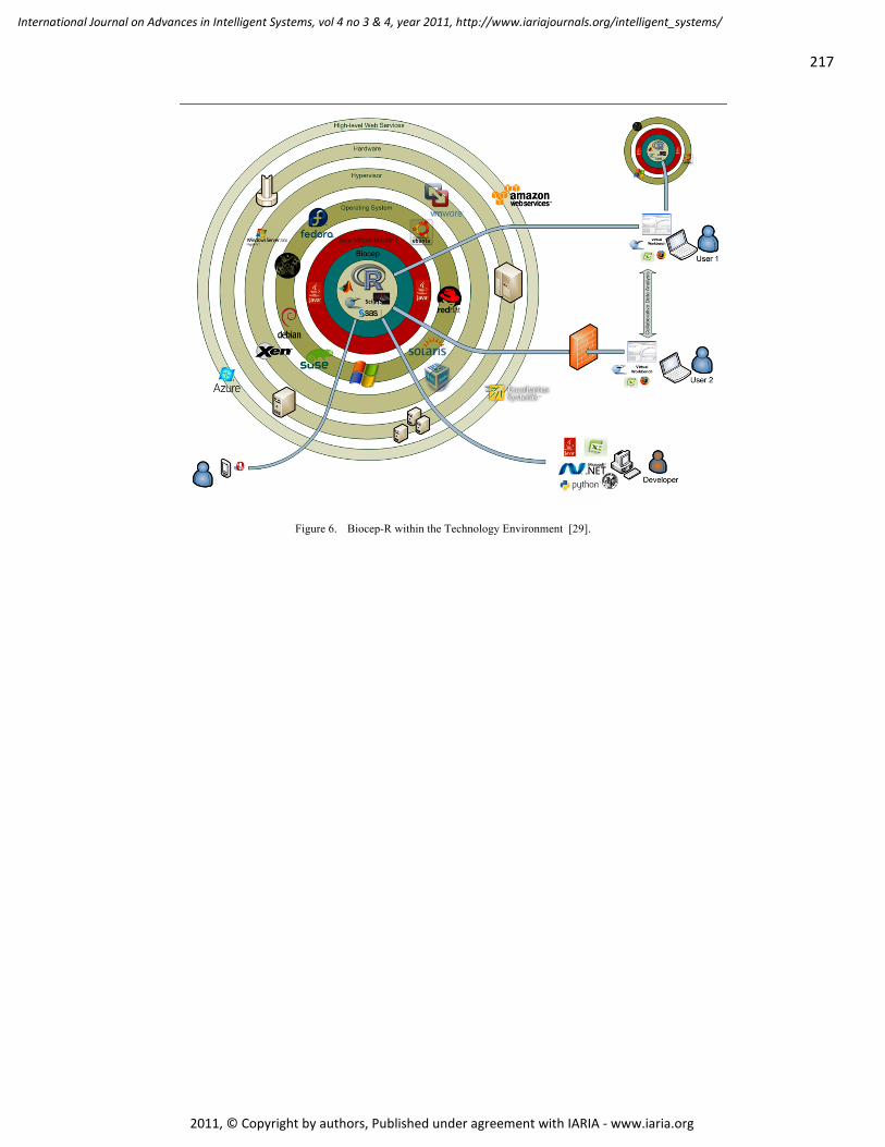
217



Figure 6. Biocep-R within the Technology Environment [29].

218



Design and Evaluation of Description Logics based Recognition and Understanding

of Situations and Activities for Safe Human-Robot Cooperation

Stephan Puls, Jürgen Graf and Heinz Wörn

Institute of Process Control and Robotics (IPR)

Karlsruhe Institute of Technology (KIT)

Karlsruhe, Germany

{stephan.puls, juergen.graf, woern}@kit.edu

Abstract—Recognition of human activities and situation

awareness is a premise for advanced safe human-robot-

cooperation. In this paper, a recognition module and its

advancements based on previous work is presented and

discussed. The usage of Description Logics allows for

knowledge based representation of activities and situations.

Furthermore, reasoning about context dependent actions

enables conclusions about expectations for robot behavior.

This work is extensively tested and benchmarked. The

presented approach represents a significant step towards a

full-fledged cognitive industrial robotic framework.

Keywords – cognitive robotics, Description Logics, situation

and action recognition, evaluation, human-robot cooperation.

I. INTRODUCTION

Industrial robotics is a challenging domain for cognitive systems, especially, when human intelligence meets solid machinery with certain degrees of freedom like most of today’s industrial robots.

Hence, guaranteeing safety for human workers, safety fences are installed to separate humans and robots. As consequence no time and space sharing interaction or cooperation can be found in industrial robotics.

Some progress has gained in the past so that some modern working cells are equipped with laser scanners performing foreground detection. But with these systems one is not able to know what is going on in the scene and, therefore, could not contribute something meaningful for challenging tasks like safe human-robot cooperation.

We are conducting research on recognition of and reasoning about actions and situations in a human centered production environment, in order to enable interactive and cooperative scenarios.

In [1], we presented a first approach for using Description Logics (DLs) [9] as means for representation of knowledge and as reasoning facilities for inference about activities and situations. Furthermore, conclusions about user expectations about robotic behavior can be drawn. This paper focuses on presenting applied techniques and the advancements on previous work [1]. Also, there are further investigations taking into account effectiveness and runtime behavior of the presented recognition module.

In Section II, selected research work on reasoning about scenes and situations will be presented. In Section III, a framework is introduced, which enables the sensor data processing and subsequent knowledge based reasoning. In

Section IV, DLs are briefly introduced and the module realizing the communication with a Description Logics reasoner, knowledge base management and reasoner result management is presented in detail. Also the modeled situations and activities are explained. Section V discusses experimental results which have been carried out for both, predetermined test cases and under real-life conditions. In Section VI, a summary is given. Finally, some hints for future work are mentioned.

II. RELATED WORKS

There are a lot of approaches for action recognition systems based on probabilistic methods, e.g., hidden Markov Models (HMMs) [17, 18, 19], as their theoretic foundation is well understood and applications in speech recognition and other domains have shown their capabilities.

Based on arguments, that HMMs are not suitable for recognition of parallel activities, propagation networks [20] have been introduced. The propagation network approach associates each node of the network with an action primitive, which incorporates a probabilistic duration model. Also conditional joint probabilities are used to enforce temporal and logical constraints. In analogy to HMMs, many propagation networks are evaluated, in order to approximate the observation probability.

In [21], Minnen et al. put forward arguments that recognition of prolonged activities is not feasible based on purely probabilistic methods. Thus, an approach is presented which uses parameterized stochastic grammars.

The application of knowledge based methods for action recognition tasks is scarce, but work on scene interpretation using DLs has been conducted.

In [10], Hummel et al. use DLs for reasoning about traffic situations and understanding of intersections. Deductive inference services are used to reduce the intersection hypotheses space and to retrieve useful information for the driver.

In [24], Tenorth and Beetz present a system, which uses Prolog in order to process knowledge in the context of robotic control. It is especially designed for use with personal robots. Knowledge representation is based on DLs and processed via a Web Ontology Language (OWL) Prolog plug-in. In contrast to our approach, the Prolog based reasoning system is not used to recognize activities or reason about situations. Instead, it is used to query on its environmental model. Actions and events are observed by

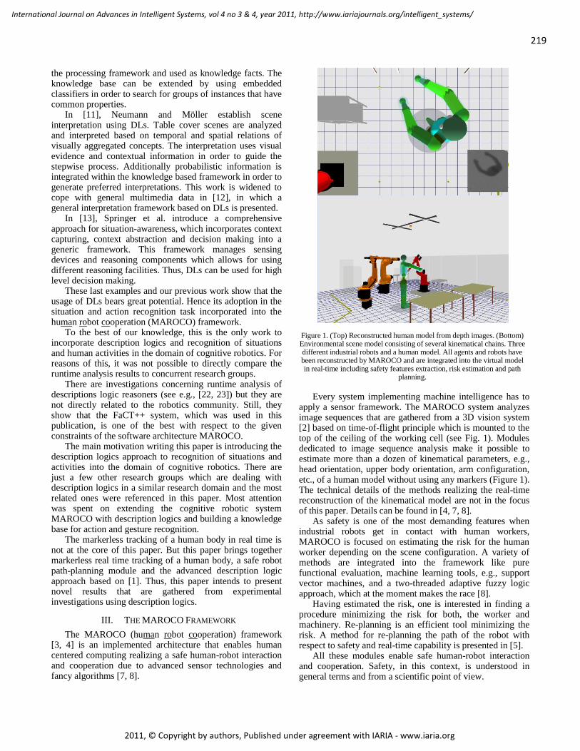
219



the processing framework and used as knowledge facts. The knowledge base can be extended by using embedded classifiers in order to search for groups of instances that have common properties.

In [11], Neumann and Möller establish scene interpretation using DLs. Table cover scenes are analyzed and interpreted based on temporal and spatial relations of visually aggregated concepts. The interpretation uses visual evidence and contextual information in order to guide the stepwise process. Additionally probabilistic information is integrated within the knowledge based framework in order to generate preferred interpretations. This work is widened to cope with general multimedia data in [12], in which a general interpretation framework based on DLs is presented.

In [13], Springer et al. introduce a comprehensive approach for situation-awareness, which incorporates context capturing, context abstraction and decision making into a generic framework. This framework manages sensing devices and reasoning components which allows for using different reasoning facilities. Thus, DLs can be used for high level decision making.

These last examples and our previous work show that the usage of DLs bears great potential. Hence its adoption in the situation and action recognition task incorporated into the human robot cooperation (MAROCO) framework.

To the best of our knowledge, this is the only work to incorporate description logics and recognition of situations and human activities in the domain of cognitive robotics. For reasons of this, it was not possible to directly compare the runtime analysis results to concurrent research groups.

There are investigations concerning runtime analysis of descriptions logic reasoners (see e.g., [22, 23]) but they are not directly related to the robotics community. Still, they show that the FaCT++ system, which was used in this publication, is one of the best with respect to the given constraints of the software architecture MAROCO.

The main motivation writing this paper is introducing the description logics approach to recognition of situations and activities into the domain of cognitive robotics. There are just a few other research groups which are dealing with description logics in a similar research domain and the most related ones were referenced in this paper. Most attention was spent on extending the cognitive robotic system MAROCO with description logics and building a knowledge base for action and gesture recognition.

The markerless tracking of a human body in real time is not at the core of this paper. But this paper brings together markerless real time tracking of a human body, a safe robot path-planning module and the advanced description logic approach based on [1]. Thus, this paper intends to present novel results that are gathered from experimental investigations using description logics.

III. THE MAROCO FRAMEWORK

The MAROCO (human robot cooperation) framework [3, 4] is an implemented architecture that enables human centered computing realizing a safe human-robot interaction and cooperation due to advanced sensor technologies and fancy algorithms [7, 8].

Figure 1. (Top) Reconstructed human model from depth images. (Bottom) Environmental scene model consisting of several kinematical chains. Three different industrial robots and a human model. All agents and robots have been reconstructed by MAROCO and are integrated into the virtual model in real-time including safety features extraction, risk estimation and path

planning.

Every system implementing machine intelligence has to

apply a sensor framework. The MAROCO system analyzes image sequences that are gathered from a 3D vision system [2] based on time-of-flight principle which is mounted to the top of the ceiling of the working cell (see Fig. 1). Modules dedicated to image sequence analysis make it possible to estimate more than a dozen of kinematical parameters, e.g., head orientation, upper body orientation, arm configuration, etc., of a human model without using any markers (Figure 1). The technical details of the methods realizing the real-time reconstruction of the kinematical model are not in the focus of this paper. Details can be found in [4, 7, 8].

As safety is one of the most demanding features when industrial robots get in contact with human workers, MAROCO is focused on estimating the risk for the human worker depending on the scene configuration. A variety of methods are integrated into the framework like pure functional evaluation, machine learning tools, e.g., support vector machines, and a two-threaded adaptive fuzzy logic approach, which at the moment makes the race [8].

Having estimated the risk, one is interested in finding a procedure minimizing the risk for both, the worker and machinery. Re-planning is an efficient tool minimizing the risk. A method for re-planning the path of the robot with respect to safety and real-time capability is presented in [5].

All these modules enable safe human-robot interaction and cooperation. Safety, in this context, is understood in general terms and from a scientific point of view.

220



The kinematical model also allows for recognition of human activities and situations inside the robot working area. Using DL reasoning facilities, conclusions about occurring situations, actions, their temporal relations and expectations about robot behavior can be drawn. This is presented in the following sections.

IV. THE RECOGNITION MODULE

This section is dedicated to discuss the recognition module including its components and modeled knowledge base after a very brief introduction to DLs.

A. Description Logics

In this paper, DLs [9] are used to formalize knowledge about situations, actions and expectations. DL is a 2-variable fragment of First Order Logic and most DLs are decidable. Thus, sound, complete and terminating reasoning algorithms exist. Due to this reason, different efficient algorithms have been engineered and implemented into diverse reasoning systems.

A DL knowledge base is divided distinctly into general

knowledge and knowledge about individuals in a domain. The former defines the terminology of the domain and its axioms are declared in the terminology box, hence TBox. The latter defines assertions about individuals and, therefore, is declared in the assertion box, hence ABox. This allows for modular and reusable knowledge bases and thus for more efficient coding of knowledge [10].

Due to DL’s open world assumption, it can deal naturally with incomplete information, which is essential in reasoning taking sensor data into account.

B. Reasoner Systems and Interfaces

By progress in the development of the semantic web, many reasoning systems were engineered in order to implement efficient algorithms, e.g., RacerPro [14], FaCT++ [15] or Pellet [16]. These systems can be interfaced by different means. In [1], we used the Pellet system and the DIG-interface. Pellet allows for efficient reasoning [22, 23]. The DIG-interface, on one side, has the advantage of its separation of application and reasoner by the means of programming language and execution place, because it implements communication via TCP and XML messages. On the other side, this interface is superseded by more recent developments which incorporate more features of recent web ontology languages, e.g., OWL API [25]. These new interfaces are based on Java implementations.

Because the MAROCO framework is implemented in C++, a Java based implementation of an interface was not feasible. The FaCT++ reasoning system, though, is written in C++. Furthermore, as shown in [15, 22, 23], FaCT++ uses very efficient algorithms. Thus, it is used as reasoning facility for the recognition module.

FaCT++ uses a tableaux decision procedure which includes optimization techniques that exploits structural features of typical ontologies [15]. Due to its architecture, it allows for a wide range of heuristic optimizations.

In this work, version 1.5.1 of FaCT++ was used. Besides the introduction of a new volatile axiom type, described in Section IV C, there are no further optimizations implemented into the reasoner system. Furthermore, FaCT++ does not allow for incremental reasoning after assertions have been retracted, added, or changed.

C. The Module Design

The recognition module needs to fulfill at least the tasks of

instantiating a Description Logics reasoner, managing the

knowledge base and managing the reasoner results.

The recognition module is embedded in the MAROCO

Framework and is executed in parallel to the sensor data

analysis module. This allows for fast computations for the

safety relevant robot control and, with less priority,

computations for higher cognitive processes, e.g., situation

and activity recognition.

The recognition module consists of different

subcomponents (see Figure 2).

Figure 2. Components of the recognition module.

The knowledge base management follows a functional

approach called Tell&Ask [9]. After defining a knowledge base – the tell operation – reasoner results and information can be retrieved – the ask operation. The modification of an existing knowledge base after using an ask operation can be achieved by using the retract-functionality of FaCT++. It allows single axioms to be marked as unused and flags the knowledge base as changed. In a subsequent processing cycle new axioms can be added. The retraction of axioms in FaCT++ does not actually delete these axioms due to its inner data management. Thus, by repeated retraction and addition of axioms, memory requirements increase.

In the realm of sensor data processing, it is advisable having an update functionality rather than retraction and addition. Thus, we augmented the FaCT++ reasoning system with a new volatile axiom. This allows updating the DL knowledge base without increasing its memory usage (see Figure 3).

As a consequence the recognition module needs to manage an up-to-date model of the knowledge base, which consists of domain specific knowledge and assertions dependent on the current kinematical human model and robot specific parameters. This distinction corresponds in Description Logics with TBoxes and ABoxes. The domain specific knowledge is modeled a priori; the assertional knowledge is updated in each runtime cycle. The modeled

221



knowledge base will be explained in more detail in Section IV D.

As the assertional knowledge depends on kinematical parameters a feature extraction component is applied in order to fill the attribute values of the assertions. The following features are important w.r.t. the component Human:

Angles of both elbows,

Angles of both shoulder joints,

Angle difference between head orientation and robot,

Walking velocity, and

Used tool. The feature used tool is not supported by existing sensors

at the moment and is therefore simulated. It can have one of the following values: none, measurement tool or working tool. The simulation of this parameter can be influenced directly by user input using standard human machine interfaces. As a result, complex working scenarios can be modeled and analyzed.

The component Robot provides the parameters for: gripper status, which can be empty or full, and movement status, which can be one of

Stopped,

Following predefined path, or

Follow user given task. During feature vector creation, extracted values are

mapped onto sharp sets. The knowledge base is then populated with corresponding set strings which can be used for comparative operations during reasoning.

One major aspect of understanding human activity is modeling temporal relations between different actions. In this work, these relations are introduced by defining an after-role. Hence a certain action can only be recognized if certain other actions occurred prior. This after-role can be regarded as defining preconditions onto actions. Previously recognized actions need to be included in the knowledge base in order to allow for correct recognition of current actions. All recognized actions are stored by the reasoner

result management component and are retrieved during updating of the knowledge base. Each occurred action is included in the DL knowledge base as an ABox instance.

The after-role is defined as a transitive role. Thus, in order to relate a new action instance to all past ones, only the relation to the previous action needs to be defined in the ABox update step.

D. The Knowledge Base

In Figure 4, the ontology about situations which is modeled by the knowledge base is presented. The concept Situation has the attribute Number Humans to distinguish between the concepts Robot alone and Human present.

In addition to the described situation ontology in [1], a new sub-concept Partially Attentive is introduced. It allows for a more detailed differentiation if observed actions and instructions need to be complied by the robot.

Depending on the Activity, which is done by the Human, different sub-concepts can be distinguished. In order to relate the concepts Situation, Activity and Human, the roles done by and takes place are defined.

In Figure 5, the concept Activity with its sub-concepts is depicted. In the line of the extension of the situation ontology, the concept Paying Partially Attention is introduced to the activity ontology. The concept Human, its properties and the defined roles are not shown for clarity reasons.

In Figure 6, the ontology concerning Actions and

complex Actions is shown. As pointed out above, actions can

Figure 3. Interaction between recognition module and FaCT++.

Figure 4. ER model of the situation ontology.

Figure 5. ER model of the activity ontology.

222



have a temporal relation expressed as after-role. The action Put Tool Away can only happen after occurrence of the action Take Tool. This role is also exploited in complex actions, e.g., Continue Robot Motion can only be signaled after Stop Robot was recognized.

Actions can be regarded as atomic concepts, whereas complex actions consist of other actions, regardless of atomicity. The concepts Take Tool and Put Tool Away are considered atomic, because they are defined by and based on a single attribute Used Tool. This attribute is directly altered by user input, therefore, does not result from sensor data analysis. The role doneBy which is defined for activities is also modeled for actions. For reasons of readability this relation is not depicted.

The occurrence of the situation Cooperation implies that there are expectations towards the robot behavior. Moreover, an expectation can be triggered by an action (see Figure 7). This allows for reasoning about expectations without necessarily recognizing a triggering action. This implicit relation is also exploited between the activities Monitor, Hold Tool and Actions.

The resulting expectations can be used as input to a task planning module. The scope of each possible expectation is

variable. Position TCP and Get Work Piece are concrete commands. Complying Follow Instructions, on the other side, needs also the information about recognized actions.

V. EXPERIMENTAL RESULTS

For reasons of experimental analysis of the implemented activity and situation recognition different courses of action were executed and the recognition results were recorded.

In order to analyze different scenarios efficiently, means of automated feature value presetting have been implemented. The overall analysis is based on these presets and on actual sensor data processing. Hence natural movements and transitions between actions can be tested and special use cases can be investigated.

In this section, recorded recognition results will be illustrated and discussed. Due to the advancements and changes to the recognition system compared to the presented work in [1], all experimental investigations were repeated and have to stand up to comparison. During result analysis special emphasis was put on efficiency and elapsed processing time.

A. Exemplary Result Records

The recorded experimental results contain a timestamp which indicates the starting time of the recognition cycle in milliseconds since program start. This timestamp is then followed by the extracted feature values if there is a human worker in the supervised area. The components of the feature vector are listed in following order: Angle arm left, angle arm right, angle elbow left, angle elbow right, walking velocity, angle difference between head orientation and robot, holding tool, gripper status and robot movement status.

The next number is the timestamp of the final result message from the DL reasoner (see Table I). Results will be recorded whenever there are new insights. Thus, the last two lines of Table I have no special entries past the last return timestamp.

TABLE I. EXAMPLE RECORD BASED ON SENSOR DATA

34942 34980 RobotAlone FollowPathPlanning

34980 0 0 0 0 3 105 0 0 0 35082 Distraction Ignore

35082 0 0 0 0 1 125 0 0 0 35240

35240 0 7 0 9 2 117 0 0 0 35408 Table II demonstrates the recognition of different

situations and activities. Furthermore, an additional action and expectation are reasoned and recognized.

TABLE II. EXAMPLE RECORD BASED ON PRESETS

75041 90 0 0 0 20 0 0 0 1 75141 WalkingBy Walking

. . .

79949 90 0 0 0 20 0 0 0 1 80109

80109 0 0 0 0 0 0 1 0 1 80164 Cooperation

HoldTool TakeTool getWorkPiece During a recognition cycle all recognized concepts are

returned from the DL reasoner in a single flush, therefore,

Figure 6. ER model of the action ontology.

Figure 7. ER model of the expectation ontology.

223



the number of lines in the records represents the number of returned responses.

Table I and II also depict the different feature values achieved by either using processed sensor data – Table I – or presets – Table II respectively. Assuming the recognition is fast enough, natural movement and action transitions can be observed. In the next section, this will be investigated.

B. Results

Tables I and II already indicate that the processing time of a recognition cycle varies between 100 ms and 200 ms. By analysis of a large amount of processing cycles, this indication needs to be corrected only slightly upwards.

TABLE III. RESULTS FROM EVALUATION (PRESETS)

# Recognition cycles 2830

# > 500 ms 441

(15.58%)

Ø Response time [ms] 263.19

# > 1000 ms 100

(3.53%)

Min [ms] 54

# > 1200 ms 100

(3.53%)

Max [ms] 1221 # > 1220 ms 1 (0.03%)

Standard Deviation [ms] 284.17

In Table III, the results of 2830 recognition cycles are

summarized. Feature value presets were used and it shows that the average processing time is approximately 263 ms. The lower bound is 54 ms. The casual outliers take up to 1.2 seconds in worst case scenarios. The number of cycles taking more than 1 second reaches 3.53% of all cycles. Almost all of these outliers are situated between 1.2 and 1.22 seconds.

In Table IV, corresponding results are shown using actual processed sensor data during recognition. Recorded were 2680 cycles with an average processing time of approximately 237 ms. This seems faster than using value presets. Interestingly, the maximal outliers and the standard deviation are worse.

TABLE IV. RESULTS FROM EVALUATION (SENSOR DATA)

# Recognition cycles 2680

# > 500 ms 381

(13.46%)

Ø Response time [ms] 236.68

# > 1000 ms 112

(3.96%)

Min [ms] 37 # > 1200 ms 79 (2.79%)

Max [ms] 1543 # > 1500 ms 41 (1.45%)

Standard Deviation [ms] 320.24

In Figure 8, the processing time of some cycles using

presets are shown. The reoccurring nature of the feature value presets can clearly be recognized. It can also be seen, that the outliers are systematic and presumably dependent on feature values.

In Figure 9, the cycle processing time and the corresponding returned number of recognized concepts are depicted. It can be seen, that the number of resulting concepts is not directly related to the cycle time.

In order to investigate the difference in runtime behavior further, the evident change in cycle times, marked by a red

rectangle in Figure 9, is examined in Table V. The first number in each row marks the cycle index. The first two rows enumerate the used feature values during those cycles. The bottom rows present the recognized concepts. The only difference is the occurrence of the concepts Monitor (Monitoring) and Ignore (Distraction) respectively. This change is triggered solely by the change of the angle difference between viewing angle and robot, namely changing from 0 to 60.

In the knowledge base the definition of these concepts only differs in the evaluation of this angle difference. Thus, the change in runtime duration cannot be directly related to the character of declaration of these concepts.

It is noticeable, that the increase in cycle times occurs with the recognition of a Distraction. This is counterintuitive, as the possibilities of interaction decrease with distraction and increase with an attentive human worker.

Figure 8. Runtime analysis with reoccurring feature value presets.

Figure 9. The bottom line (green) shows the number of returned concepts. The upper line (blue) shows the corresponding cycle processing time. For

recognition, feature value presets were used. The red rectangle highlights the examined feature value change.

224



The repeatable and counterintuitive observation will need further investigation in order to optimize the DL knowledge base and achieve better performance.

TABLE V. EXAMINATION OF FEATURE VALUE CHANGE AND CYCLE

TIME

303 0 0 0 0 0 0 0 0 1 used feature

304 0 0 0 0 0 60 0 0 0 values

303 TOP HumanPresent Monitoring TOP Standing

Monitor ArmsDown FollowPathPlanning

304 TOP HumanPresent Distraction TOP Standing

Ignore ArmsDown FollowPathPlanning

In Figure 10, the cycle processing time is shown, when

using processed sensor data. As expected, the repeatability of the preset feature values cannot be achieved. Peaks of more than 1000 ms are not a rare coincidence. Thus, further investigations about runtime durations are necessary. Nevertheless, most processing cycles have shorter durations than 800 ms, and as Table IV shows, the average processing time is below 237 ms. This allows for recognition frame rates of about 4.2 Hz on average.

In Figure 11, the frame rates of the MAROCO

framework are shown. In each frame sensor data is processed, risk is evaluated and the robot motion and path planning are adapted accordingly. The frame rates reach occasional lows with 15.9 Hz and average out around 33.8 Hz. Recorded sensor streams were used for playback during these tests in order to be independent on a possible bottleneck due to sensor restrictions. The repeating sensor input can clearly be recognized in Figure 11.

The peaks in performance are reached when there is no human worker in the supervised working area of the robot. These peaks reach up to 126 Hz. When the human reenters this area, the data shows noticeable performance decrease. The circles in Figure 11 mark obvious examples. In these cases, the performance drops to a low and recovers afterwards to converge with the average frame rate. This indicates the adaption of the path planning [5] to the human

presents. Though, this data is not sufficient to allow profound analysis. Thus, the recognition module might cause these performance decreases.

By using the kinematical human model, recognition of

gestures and human motion can be analyzed. In Figure 12, different examples of recognized situations and actions are depicted. The topmost picture shows a human watching the robot. The icons to the right symbolize the recognition results. Thus, the identified situation is Monitoring. No specified action is recognized. The robot is expected to carry on with its task of following its preplanned path.

In the second image of Figure 12, a human is communicating with the robot. The complex action to signal a stop of robot movement is recognized. Thus, the resulting situation is identified as Communication. The robot is expected to comply with the users instructions.

The bottommost picture also shows a human communicating. The complex action to signal a right turning movement is recognized. The robot is expected to comply accordingly.

TABLE VI. EXAMPLE RECORD FOR NATURAL MOVEMENT

342000 0 0 1 0 7 4 0 1 1 342111 Monitoring Monitor

followPathPlanning

. . .

342779 0 0 1 0 7 3 0 1 1 342890

342890 14 13 10 11 3 4 0 1 1 342952

342952 20 26 13 16 3 4 0 1 1 343012

343012 35 39 16 22 4 4 0 1 1 343073

343073 47 46 19 28 0 5 0 1 1 343134

343134 47 46 19 28 0 5 0 1 1 343195

343195 54 51 21 31 0 5 0 1 1 343428 Comm. MoveArms

StopRobot followInstructions

Table VI shows an example in which a human first

watches the robot. This concludes the expectation, that the robot shell follow a planned path. After some time the

Figure 10. Runtime analysis with processed sensor data.

Figure 11. Frame rates of the MAROCO sensor data processing and robot control cycle running in parallel to the recognition module. The circles mark the reentrance of the human into the work area of the robot with noticeable

decrease of performance.

225



human moves his arms which results in a communicative situation. The reasoning results in the expectation that the robot shell comply with the instructions. It can be seen, that both arms are moved upwards at the same time. The value changes are observable over some cycles.

Consequently natural movements and actions can be recognized despite the average cycle processing time of approx. 250 ms.

Tables II and VI demonstrate that depending on situation and actions expectations are generated. The generation of expectation is also dependent on the robot movement status. Table VII shows that at first a cooperative situation is recognized and a generated expectation get Work Piece. At this moment the robot was following a planned path, which is signaled as 1 in the feature vector. In the simulation incorporated in MAROCO, this generated expectation leads to a change of the robot movement status which sets the

corresponding feature value to 2, meaning the robot is obeying instructions. This change allows the reasoning to conclude the new expectation to position the robot’s tool center point in order to ease the work that the user is about to do with the work piece.

TABLE VII. EXAMPLE FOR DYNAMIC EXPECTATION REASONING

96795 75 0 21 0 0 3 1 0 1 97287 Coop. HoldTool

TakeTool getWorkPiece

97289 75 0 22 0 0 0 1 1 2 97799 positionTCP This process of interaction between reasoner results and

robotic behavior demonstrates the dynamic abilities of the presented approach to recognize and understand situations and actions.

C. Evaluation of Results

The results demonstrate that the capabilities of the presented approach reach beyond sole activity and situation recognition. By generating expectations towards robot behavior, an understanding of the situation can be achieved. This induction of relations between concepts can hardly be realized by purely probabilistic methods.

The achieved processing cycle time of approx. 250 ms does not allow for safe cooperation based only on the recognition module. Thus, the MAROCO framework uses its implemented techniques and algorithms to enforce safety and real-time capabilities during robot motion. Nevertheless, the measured results will be used to quantify improvements of later developments.

In comparison with presented results in [1], an increase of performance was achieved. The recognition module executes its processing cycle more than two times faster on average. Due to the incorporation of the DLs reasoning system into the MAROCO framework, these speedups are gained. It avoids the overhead of the DIG-interface and allows for a more thorough investigation concerning runtime and cycle duration.

Having a closer look at the results, there are still outliers that take more than a second. All cycle times were faster than 5 seconds, which was observed in [1]. Investigation in concept dependent runtime is needed in order to optimize the dependencies between concepts and the overall recognition performance.

In Table VI, it is demonstrated, that the rates of changes of actions can be captured. Still, to the best of our knowledge, there are no investigations concerning the rate of change of human actions in human-robot cooperative scenarios. During the experiments conducted for this publication, the subjective impression of the MAROCO system was responsive and accurate. Nevertheless, it can be assumed that repetitive work can be carried out faster by an experienced human worker than the current module is capable of recognizing. More effort has to be spent to be able to evaluate the real-time capabilities of the recognition module accurately.

To the best of our knowledge, there are no other such time related results made available in the field of industrial

Figure 12. Different examples of recognized situations and actions. The icons on the right in each image symbolize the recognition results.

226



human-robot cooperation or another related field close to it so far.

VI. SUMMARY AND FUTURE WORK

In this paper, a situation and action recognition module was presented, which is capable of generating expectations towards robotic behavior.

A knowledge base containing domain and assertional knowledge is modeled. It defines concepts about situations, activities, actions and expectations. These concepts are linked and related by role definitions. Temporal associations of actions are modeled by an after-role, which allows preconditioning the recognition of certain actions.

Description Logics are used to define the knowledge base. The Description Logics reasoner FaCT++ was incorporated into the MAROCO framework. A volatile axiom definition was introduced to the reasoner to avoid increasing memory requirements due to repeated updates to the assertional knowledge.

In order to express value constraints on concept attributes, the feature extraction process maps feature values onto sets, which can be represented as strings in the knowledge base. This allows additionally for support of future development in regards to symbol based classifiers. This might ease the load on DL reasoning and achieve further increase of performance.

During evaluation the effectiveness was shown. Situations, activities and naturally conducted actions are recognized. Expectations are generated and can influence dynamically subsequent processing cycles.

Compared to previous work, an increase of recognition performance was achieved. The recognition cycle requires less than half the processing time on average. Extreme outliers of over 1.5 seconds duration do not occur.

The here presented experimental results are promising for further research in the field of cognitive industrial robotics.

The next steps will be modeling a broader knowledge base in order to incorporate multi-robot setups and more complex cooperation scenarios. Also, the implementation of action plan recognition will deepen the understanding of situations and enable the analysis of complex cooperation scenarios.

Optimizations to the reasoning system FaCT++ matched to the structure of the implemented ontology might increase recognition performance. Thus, further investigation of concept dependent cycle time durations is needed. Also, implementation of incremental reasoning can avoid processing of unchanged knowledge.

Moreover, investigations concerning rate of changes of human actions will allow better evaluation of real-time constraints and capabilities of the recognition module.

Using generated expectations towards robotic behavior as input for subsequent task planning will augment the cooperative experience and will allow research on system responsiveness and accuracy. It will also enable investigations concerning interaction of reasoner results and robotic behavior.

It was taken a stand against the probabilistic way of estimating actions from image sequences in the beginning of

the related work section. But it is suggested to evaluate different approaches in the near future which also take probabilistic methods into account or maybe apply different methods in a boosting like manner bringing together the best of both worlds.

ACKNOWLEDGMENT

We would like to thank Dmitry Tsarkov for his support during development regarding the incorporation of FaCT++ into the MAROCO framework.

REFERENCES

[1] J. Graf, S. Puls, and H. Wörn, “Recognition and Understanding Situations and Activities with Description Logics for Safe Human-Robot Cooperation”, in Proc. of Cognitive 2010, pp.90-96, 2010.

[2] http://www.pmdtec.com/products-services/pmdvisionr-cameras/pmdvisionr-camcube-30/ [Last visited on 2012-01-19]

[3] J. Graf and H. Wörn, “An Image Sequence Analysis System with Focus on Human-Robot-Cooperation using PMD-Camera”, in VDI Proc. of Robotik 2008, June 2008, pp. 223-226.

[4] J. Graf and H. Wörn, “Safe Human-Robot Interaction using 3D Sensor”, in Proc. of VDI Automation 2009, June 2009, pp. 445-456.

[5] J. Graf, S. Puls, and H. Wörn, “Incorporating Novel Path Planning Method into Cognitive Vision System for Safe Human-Robot Interaction”, in Proc. of Computation World, pp. 443-447, 2009.

[6] S. Bechhofer, “The DIG Description Logic Interface: DIG/1.1.”, in Proc. of the 2003 Description Logic Workshop, 2003.

[7] J. Graf, F. Dittrich, and H. Wörn, „High Performance Optical Flow Serves Bayesian Filtering for SafeHuman-Robot Cooperation”, in Proc. of the Joint 41th Int. Symp. on Robotics and 6th German Conf. on Robotics, pp. 325-332, Munich, 2010.

[8] J. Graf, P. Czapiewski, and H. Wörn, “Evaluating Risk Estimation Methods and Path Planning for Safe Human-Robot Cooperation”, in Proc. of the Joint 41th Int. Symp. on Robotics and 6th German Conf. on Robotics, pp. 579-585, Munich, 2010

[9] F. Baader, D. Calvanese, D. McGuinness, D. Nardi, and P. Patel-Schneider, “The Description Logic Handbook”, 2nd Edition, Cambridge University Press, 2010.

[10] B. Hummel, W. Thiemann, and I. Lulcheva, “Description Logic for Vision-Based Intersection Understanding”, in Proc. of Cognitive Systems with Interactive Sensors (COGIS), Stanford University, CA, 2007.

[11] B. Neumann and R. Möller, “On Scene Interpretation with Description Logics”, in Image and Vision Computing, vol. 26, pp. 81-101, 2008.

[12] R. Möller and B. Neumann, “Ontology-Based Reasoning Techniques for Multimedia Interpretation and Retrieval”, in Semantic Multimedia and Ontologies, part 2, pp. 55-98, Springer London, 2008.

[13] T. Springer, P. Wustmann, I. Braun, W. Dargie, and M. Berger, „A Comprehensive Approach for Situation-Awareness Based on Sensing and Reasoning about Context“, in Lecture Notes in Computer Science, vol. 5061, pp. 143-157, Springer, Berlin, 2010.

[14] V. Haarslev, R. Möller, and M. Wessel, “RacerPro User’s Guide and Reference Manual”, Version 1.9.1, May 2007.

[15] D. Tsarkov and I. Horrocks, “FaCT++ Description Logic Reasoner: System Description”, in Lecture Notes in Computer Science (LNCS), vol. 4273, pp. 654-667, 2006.

[16] E. Sirin, B. Parsia, B. Grau, A. Kalyanpur, and Y. Katz, “Pellet: A practical OWL-DL reasoner”, in Web Semantics: Science, Services and Agents on the World Wide Web, vol.5 (2), pp. 51-53, 2007.

[17] V. Krüger, D. Kragic, A. Ude, and C. Geib, „The Meaning of Action: A Review on action recognition and mapping“, in Proc. of Advanced Robotics, Vol. 21, pp. 1473-1501, 2007.

227



[18] P. Raamana, D. Grest, and V. Krueger „Human Action Recognition in Table-Top Scenarios : An HMM-Based Analysis to Optimize the Performance”, in Lecture Notes in Computer Science (LNCS), Vol. 4673, pp. 101-108, 2007.

[19] Y. Wu, H. Chen, W. Tsai, S. Lee, and J. Yu, „Human action recognition based on layered-HMM”, in IEEE Inter. Conf. on Multimedia and Expo (ICME), pp.1453-1456, 2008.

[20] Y. Shi, Y. Huang, D. Minnen, A. Bobick, and I. Essa, „Propagation Networks for Recognition of Partially Ordered Sequential Action”, in Proc. of Computer Vision and Pattern Recognition (CVPR), Vol. 2, pp. 862-869, 2004.

[21] D. Minnen, I. Essa, and T. Starner, „Expectation Grammars: Leveraging High-Level Expectations for Activity Recognition”, in Proc. of Computer Vision and Pattern Recognition (CVPR), Vol. 2, pp. 626-632, 2003.

[22] T. Gardiner, I. Horrocks, and D. Tsarkov, “Automated Benchmarking of Description Logic Reasoners”, in Proc. of the 2006 Intern. Workshop on Description Logics (DL2006), Windermere, Lake Districrt, UK, 8 pages, June 2006.

[23] Z. Pan, “Benchmarking DL Reasoners Using Realistic Ontologies”, in Proc. of the First OWL Experiences and Directions Workshop, 2005.

[24] M. Tenorth and M. Beetz, “KNOWROB – Knowledge processing for Autonomous Personal Robots”, in IEEE Inter. Conf. on Intelligent Robots and Systems (IROS), 2009.

[25] M. Horridge and S. Bechhofer, “The OWL API: A Java API for Working with OWL 2 Ontologies”, in Proc. of OWL: Experiences and Directions, 2009.

228



Adaptable Interfaces [1]

Ken Krechmer Lecturer, University of Colorado

Boulder, CO, USA e-mail: [email protected]

Abstract––Adaptable interfaces offer the possibility of more maintainable and reliable systems. This paper defines the four ways interfaces can change and develops the concept of adaptability using communications theory. Adaptability is a complex process, which requires a number of supporting processes. Together these process automatically negotiate possible capabilities across an interface. The concept of state-pairs is used to define communicating entities, inter-face, comparison, measured information, communications, flexibility and finally adaptability.

Keywords-adaptable; interface; communications structure; measured information; etiquette

I. INTRODUCTION As systems become programmable at lower layers of

the OSI model, the interfaces in such systems can become more versatile. Prior to programmable systems, interfaces were known to be fixed or at most modifiable using an external adaptor. Programmable systems change this inter-face paradigm. This paper defines the four ways interfaces can change and develops the concept of adaptability using communications theory. Adaptability is a complex proc-ess, which requires a number of supporting processes. To-gether these process automatically negotiate possible ca-pabilities across an interface. Adaptability requires com-munications across an interface between at least two enti-ties. First the structure of a communications system is de-veloped. From this structure all the processes supporting adaptability are derived. With a more complete under-standing of these processes, a more rigorous understanding of adaptability, and the advantages of adaptable interfaces, emerges.

II. A COMMUNICATIONS STRUCTURE Fig. 1 models communications for the purpose of un-

derstanding its structure rather than its performance. Fig. 1 is similar to the Shannon model of a communications sys-tem [2] except that the communications channel is re-placed by an interface and the probability of the output message being the same as the input message is fixed to one. The transmitter (T) and receiver (R) are independent communicating entities connected via an interface. The purpose of this model is to analyze the structure of the relationship between T and R.

From communications theory, T and R support all the state-pairs ti - ri, where i represents the set of all t or r states 1 to n in Fig. 1. A state-pair includes a specific input part (tx) associated with T, which is related to the output part (rx) associated with R. An interface describes the one-

one relationships between the related parts of two or more state-pairs. "A relation is said to be one-one when, if t has the relation in question to r, no other term t' has the same relation to r, and t does not have the same relation to any other term r' other than r" [3]. All the state-pairs associated with T and R form the interface between T and R. A single set of ti or ri states is usually considered a specific parame-ter (e.g., data rate) of the transmitter or receiver. Commu-nications (information transfer) is possible only when mul-tiple state-pairs form an interface between independent entities. An interface does not exist independently, it is formed by the common parameters of the communicating entities. Most interfaces include multiple parameters.

A one-one relation is in some way a relationship be-tween equal elements. As example in Fig. 1, state tx may be seen as the equal of state rx. However, it is not possible to define such equality without specifying other sets of state-pairs. For state tx to be equal to rx for example, the boundary conditions, tolerances, and measurement appara-tus all must be equal. Such equality is possible in theory but difficult in practice. In practice, the relationship be-tween each state tx and rx is more easily described as one-one.

The concept of state-pairs may be applied to any inter-face, even a physical interface. Examine a perfectly com-patible (zero tolerance) physical plug and socket. The out-side diameter of the plug and the inside diameter of the socket are the same. The length of the plug and the socket are the same. The physical interface between the plug and socket consists of all the common pairs of points on the plug and socket. These common points are the state-pairs, which form a physically compatible interface. Even in this simple physical interface, multiple layers of sets of state-pairs are needed to completely define the interface. Other parameters that need to be defined include: the physical dimension system used, the tolerances applied, even con-cepts such as diameter and length have to be "agreed" at each communicating entity.

III. COMMUNICATIONS PROCESS The ability to pass information across state-pairs re-

quires two comparisons. Each comparison is associated with a part of a state-pair. The fundamental nature of these comparisons is suggested by I. Kant who states that a comparison is necessary for understanding [4].

229



The simplest communications process may be six op-

erations, three in the transmitter and three in the receiver (Table 1). Operations 2 and 5 in Table 1 demonstrate how a state-pair relates to the communications process. The number of operations is not critical to this analysis. What is critical is that the communications process consists of symmetric transmit and receive processes, each of which includes a comparison. This symmetry of a communica-tions process also appears in the Venn diagram in Fig. 3, below.

Consider a binary amplitude-modulated communica-tions system with two state-pairs (t1 - r1 and t2 - r2) and without time domain or tolerance effects. The input mes-sage to T is compared with the decision boundary between t1 and t2 determining which state causes a T signal output. T encodes +V signals for t1 and -V signals for t2, which are received as signals in R. The received signal is compared with the decision boundary between r1 and r2 determining which state causes a R output message. The decision boundaries, both threshold and maximum, are lower level parameters (formed by other parameters created in the implementation of T and R). These boundaries implement the relationship between each part of the t1 - r1 and t2 - r2 state-pairs and determine the operational characteristics of the signal path. A more complex communications system has more sets of transmitter and receiver state-pairs (pa-rameters) and more complex boundaries.

Example: In the course of reading, a word appears of unknown meaning. The reader refers to a dictionary. A dictionary relates words (states) to their meanings (mes-sage). The author and reader select words from similar dictionaries (first and second comparisons). The author's and reader's dictionaries together are the state-pairs of equal words with a common meaning in each dictionary.

TABLE I. COMMUNICATIONS PROCESS

For the transmitter (T): 1 Select an input message 2 Compare this input and determine state (ti) 3 Output a signal

For the receiver (R): 4 Select the signal received 5 Compare this signal and determine related state (ri) 6 Output message

The state-pairs in a communications system may be created by chemical bonds (A-C, G-T in DNA), pre-exist-ing written or spoken alphabets, pre-existing dictionaries or syntax, the specifications or standards defining a trans-mitter, receiver or protocol (electronic communications) or a physical implementation of a transmitter, transmission link, or receiver. Different forms of state-pairs are divided into layers in the Open System Interconnect model (OSI) where each reference layer provides the interface(s) used by the next layer. Layer one includes physical aspects of the interface and higher layers include successively more abstract functionality. All the state-pairs used for a specific functional relationship between two or more entities create an interface.

A. Interfaces There are four broad catagories that describe how the

state-pairs that define an interface may change - fixed (state-pairs are unchangeable), flexible (state-pairs changed by external action), adaptable (state-pairs are se-lected by negotiation across the interface) and evolutionary (state-pairs change by internal action). These four interface variations are not mutually exclusive and may exist in dif-ferent combinations at different layers of the OSI model. A mechanical plug and socket is an example of a fixed inter-face. Using adapters to convert AC power connectors to different countries' power outlets is an example of a way to implement flexibility. Adaptable interfaces are necessary for true peer-to-peer operation. An Internet Engineering Task Force (IETF) protocol Session Initiation Protocol (SIP) used to negotiate capabilities between two commu-nicating ends is an example of an adaptable protocol. An example of an evolutionary interface would be a system that autonomously accesses independent web sites to ac-quire additional interface capabilities. Enabling automatic upgrades of personal computer software is an example of evolutionary software. An evolutionary interface is yet more complex, as the independent software defining each side of the interface must be upgraded.

Other examples of flexible interfaces include: an Edi-son light bulb socket that supports many different types of lamps. While the mechanical aspects of the light bulb and socket are fixed, the load can be changed. A human user manually identifies and selects the specific lamp and the

Figure 1. Communications structure.

Transmitter (T) Receiver (R)

r1 r2 r3 . rn

t1 t2 t3 . tn

Interface)

signal path

input

output

230



Edison light bulb plug/socket (the physical interface) makes this flexibility possible. A protocol example of a fixed interface that supports flexibility is the use of the Internet protocols TCP/IP as the interface with which each lower physical network or higher layer protocol is de-signed to interoperate. XML (eXtensible Markup Lan-guage) is an example of an interface protocol that supports flexibility and can reduce fixed state-pairs.

IV. MEASUREMENT PROCESS After defining communications and interfaces, next an

understanding of the measurement process is required to understand adaptability. A measurement is a quantified selection of an observable. The process of making a quan-tified selection is similar to the transmitter or receiver process shown in Table 1 (select signal, compare signal and determine state, output signal). In a measurement process there is a measurement apparatus that compares an observable with a predefined set of states. The states of the measurement apparatus must be related to the observable for a measurement to be practical. A measurement and a communications transmitter or receiver, as described above, are quite similar. This similarity supports the use of communication theory to analyze the measurement proc-ess. With a measurement process understood, communi-cating entities may be defined. Then adaptability can be defined for communicating entities.

N. Campbell defines a measurement (the concept) as "the assignment of numerals to represent properties" [5]. A measurement process assigns the numerals by utilizing one or more comparisons with states of the measurement appa-ratus. Each of these states of the measurement apparatus, and its associated boundary conditions, acts to quantify the measurement. Any observable that may be quantized, e.g., weight, length, color, hardness, texture, transfer rate, ca-pacity, spin, etc., may be measured. The observable de-fines the property to be measured and the range of states of the property in the receiver quantifies the measured pa-rameter.

The choice of the receiver states and boundary condi-tions actually selects the parameter and quantification of the entity to be measured. That is, if a length scale is used, distance is measured; if a weight scale is used, weight is measured; if a voltmeter is used, voltage is measured, etc. A measurement is not absolute; it is always relative to the parameter measured by the receiver, the states of that pa-rameter in the receiver and the boundary conditions be-tween states. A measurement requires that the states of the receiver be represented in a definition of measured infor-mation.

Equation (1) is Shannon's equation for entropy [2, page 50]. D (2) is defined in T. Cover and J. Thomas as the en-tropy relative to log n [6, page 27]. This section of the pa-per develops the theory that D represents the information contained in the measurement of a parameter (T) of an entity A receiver (for ti) with n discrete states is applied (represented by the first term [log n] in (2)). The entropy distribution (H(T)) of the measurement process is calcu-lated by the second term. p indicates a probability. The

output from the measurement process is one or more spe-cific states tx, ty, tz. This measured information is equal to

D. As example, a voltmeter (used to measure volts) with a

3 volt full scale (parameter of the voltmeter) and the minimum measurable increment (boundary condition) of 0.1 V, has 30 (= n) possible states of vi and produces a single output measurement vx, then D = log 30. The greater the number of states n, the greater the information from the measurement process. The narrower the distribu-tion of the entropy term (H(T)), the greater the informa-tion. A perfect measurement (zero H(T)) produces the maximum information, log n. The first term of (2) effec-tively includes the concept of tolerance (minimum meas-urable increment) in the measured information calculation.

Fig. 2 expresses (2) as a Venn diagram. Fig. 2 shows how the limit of the entropy distribution (log n) is related to the entropy distribution (H(X)). (3) is Cover and Tho-mas' equation for Mutual Information (MI), the relative entropy between related entropy distributions. Replacing H(R) in (3) [6, page 19] with log n calculates the mutual information of H(T) and log n (4).

MI = I(T;R) = H(R) – H(R|T) (3)

MI = log n - (log n – H(T)) (4)

MI = H(T)= I (T; log n) (5)

Equation (5) shows that H(T) when referenced to its

limit is equal to the mutual information as the log n terms cancel in (4). Thus, using D (2) provides a rigorous de-scription of measured information without changing mu-tual information (MI).

Figure 2. Venn diagram of H(T) and its limit.

log n

H(T)

D = log n - H(T)

231



A related result to (5) substitutes H(T) for H(R) in (3) and is noted as self-information [5, page 20]. Equation (5) and self-information indicate that the reference may be either log n or H(T) itself. If the reference is not log n or H(T) itself, then there are additional parameters (not T). A single parameter entropy distribution should be referenced to its limit (i.e., log n), as applying H(T) to reference H(T) is self-referential. The measured information related to a single parameter entropy distribution only exists in relation to a reference and the only logical reference is the limit of the entropy distribution. This provides a proof of D (2) as the definition of measured information.

The different observables of an entity are acquired by multiple measurements. The multiple measurements nec-essary to define an entity may each be represented by a Di. With a model of an entity, communications between two entities can be defined by relating the Venn diagrams of the transmitter and receiver versions of Fig. 2 in Fig. 3.

V. COMMUNICATIONS Communications exist when the six operations in Ta-

ble 1 occur. The comparisons necessary for communica-tions require the existence of common state-pairs between two distinct entities. A communications system may be modeled by using two overlapping Venn diagrams from Fig. 2 as shown in Fig. 3. Fig. 3 is derived from Shannon's model of a communications system, where the receiver output is related to the transmitter input by a probability less than one. In Fig. 3, log nt is the bound of H(T) and log nr is the bound of H(R). The intersection of log nt and log nr is shown as a dotted lens shape. This space represents the interface (I) made up of all the state-pairs of T and R. I limits the mutual information (MI, overlap of the solid circles, solid lens shape) possible between the transmitter and the receiver.

Fig. 3 identifies that a communications system creates mutual information by comparing the transmitter and re-ceiver inputs to the respective parts of state-pairs, not by H(T) to H(R) interaction.

Summarizing the communications structure and proc-ess developed thus far: Comparisons are necessary for communications and measurement. A measurement, using a comparison, quantifies an element of a set in relation to a reference. A group of measurements defines the observ-ables of an entity. State-pairs form the interface between

Figure 3. Venn diagram of a communication system.

two compatible entities. An interface allows communica-tions by supporting comparisons between sets of state-pairs Communications between programmable entities can support adaptability. Using this model it is now possible to define adaptability.

VI. ADAPTABILITY Each parameter presented across an interface consists

of a number of state-pairs (n). However, the number of states in T may not be the same as the number of states in R for some parameters. Such unpaired states occur when parameters, by virtue of options, special features, differing revisions or just non-selection in the transmitter or re-ceiver, are not available or not used. For instance, tele-phone modems may offer six different modulations rang-ing from 300 bit/s to near 56 kbit/s. Usually only the 56 kbit/s modulation is in operation and the five other modu-lations are unused.

Fig. 3 shows unpaired states within each dotted circle areas (log nt and log nr) and outside the dotted lens shape (I). The communications structure is more efficient when unpaired states don't exist. Older communications systems, which tended to be single provider (e.g., telegraph and telephony) tried to avoid unpaired states. Newer commu-nications systems tend to have more and more unpaired states as communications becomes more complex and variation increases. Interconnected systems have become larger, multi-vendor and may include many revision levels and multiple technologies. These increasing trends cause more and more unpaired states.

At least two approaches have been used to avoid un-paired states: 1) the selection of other capabilities has been treated as vendor-specific and not defined (e.g., the 3G cellular IMT-2000 standards); 2) a protocol is defined to determine which of the available capabilities in the T or R should be employed in a specific situation. As example, telephone modems prior to V.32 (circa 1984) selected the modulation to be used based on convention and vendor-specific decision boundaries. After V.32, the identifica-tion, negotiation and selection of a specific modulation was defined by an independent protocol, V.8.

The process of automatically negotiating possible ca-pabilities is termed adaptability as it makes a system more adaptable. As defined here, adaptability requires three spe-cific functions: identification of the capabilities available at each end, negotiation to determine the desired state-pairs (the interface), and selection of the desired state-pairs (which may require accessing software from elsewhere). These three functions are more complex versions of the basic functions required for any communications: select input, compare input to reference (with adaptability mechanisms each end is compared to the other), and create output (select state-pairs). After these adaptable processes are completed, then information or control communica-tions can begin across the negotiated interface.

Fully flexible interfaces such as XML are the current state-of-the-art. By definition, an XML relationship is not peer-to-peer. Only when the two communicating entities can negotiate any change independently can they be peers.

H(R)

H(T)

MI

log nt log nr

I

232



Adaptability, the means to support such negotiation, may be created by a software program (often termed agent soft-ware) that can identify, negotiate and select the state-pairs across an interface. Or an independent communications protocol may be used for the purposes of identification, negotiation and selection. When such a protocol is used only for these purposes, it is termed an etiquette [7]. It seems likely that other approaches to implement adapt-ability may be identified.

Etiquettes are already used in some communications systems, e.g., ITU V.8 for telephone modems, ITU T.30 for G3 fax, ITU G.994.1 for digital subscriber line trans-ceivers, and IETF Session Initiation Protocol (SIP); their properties have been explored previously [7]. In a future 4G cellular architecture, an etiquette could allow the serv-ice provider to negotiate the protocol that optimizes sys-tem loading or maximizes geographic coverage, or allow a user to select the protocol (and related service provider) that offers the best economic performance for that user. Troubleshooting of incompatibilities using an etiquette is also easier as each end can identify the available and com-patible parameter sets of the other end. The use of adapt-ability mechanisms is a system architecture choice that significantly enhances the long term performance of pro-grammable heterogeneous communications systems.

When systems are programmable, adaptability is pos-sible. An etiquette transmitter presents the range of possi-ble compatible parameters to an etiquette receiver. The etiquette receiver responds with its range of possible com-patible parameters. Using heuristics local to the transmitter and receiver (e.g., largest parameter is best [pels, bits, col-ors, data rate, etc.]) or remote heuristics accessed by both the transmitter and the receiver (e.g., using a remote data base to determine which common parameters are to be utilized), the etiquette transmitter and receiver negotiate and select the desired interface for compatibility and fol-low-on communications.

Communications interfaces are layered. Adaptability may be employed at each layer of the OSI model or par-tially in one or more layers. Adaptability could be useful in communications entities such as software defined radios. A software defined radio that includes the physical layer, perhaps others, is not defined as adaptable but has the properties - programmable and a radio interface (non-mechanical) - that allow it to be adaptable. The ability to change the software in a system is sometimes termed re-configurability or changeability. But these terms do not necessarily denote adaptability. Currently discussions of adaptability do not define which layer or how many layers are adaptable and may confuse the concept of flexibility with adaptability. One purpose of this paper is to better define terms such as "flexible" and "adaptable”.

Compatible systems have state-pairs. If there are transmitter states (at any OSI layer) that do not have re-lated receiver states, such inconsistencies cause "bugs”. Adaptability mechanisms offer a means to negotiate and select a specific interface and thus reduce such bugs.

For this unique functionality of etiquettes to operate consistently, any addition to an etiquette must be a proper

super-set of the previous version. As long as the etiquette is a logical single tree structure, where each branch refers to a single parameter set and no deletions are allowed, a correctly modified etiquette will always be backward compatible. Following this model an etiquette may be ex-panded whenever desired independently in the transmitter and the receiver. This allows new capabilities, and the parameters in the etiquette that identify them, to be added to a communications system at any time. If both ends can support the new parameters they can be employed. If one end supports a parameter and the other end does not, either this parameter will not be used or it may be practical for the deficient end to download the needed software from a known Internet web site.

Adaptability mechanisms also can support the use and charging for proprietary technology in public standards. If one or more parameters in the logical tree are identified as proprietary (e.g., identified by a trademark), the use of such parameters would legally require the trademark owner's approval. All the other parameters identified in the etiquette remain in the public standard. Such approval might require some form of payment to the trademark owner. If the proprietary technology is valuable, implementers or users will have reason to pay the trade-mark owner for the use of their proprietary technology. Many different procedures are possible to compensate the trademark owner: charge for downloads, per implementa-tion fees, usage fees, periodic maintenance/support fees, or simply the sales advantages of proprietary implementa-tions offering improved operation over the public sections of the standard.

VII. EVOLVABLE INTERFACES Looking further into the future: evolvable interfaces

have not yet been developed. Such interfaces could enable a new level of system openness. Consider a future open cell phone system where new features may be added to the system by uploading operating software to a specific web site. An independent developer defines and creates soft-ware for a new cell phone functionality and the related software for the cell phone system base station. This soft-ware is uploaded to a specific web site. When any other cell phone users anywhere finds this capability desirable they could download this new capability to their mobile as well as any necessary base stations either automatically or as desired. Consider what could happen when a developer creates a new video or voice compression algorithm. Us-ing the process described, the new algorithm could be used throughout the cell phone system wherever it was desired. It is also possible to imagine that there is a charging sys-tem that allows the developer to charge each user for download or usage of the new algorithm. Then the new capability would be tested in the market to see if users will bear the required charges, rather than being forced on the users by the original system designers' decisions.

233



VIII. CONCLUSION Adaptable interfaces makes it possible to automatically

negotiate the rising complexity of communications, intro-duce new technology into communications channels at will, simplify communications troubleshooting, better support multi-mode operation, avoid identified communi-cations channel bugs, and support incentives to developers and implementers without forcing all users of public inter-faces to pay private fees. The advantages of making all programmable interfaces adaptability are significant enough to suggest that adaptability should be a require-ment for future programmable interfaces in communica-tions systems.

REFERENCES [1] An earlier version, titled Quantifing Adaptability, was

presented at IARIA ADAPTIVE 2010, The Second

International Conference on Adaptive and Self-adaptive Systems and Applications, November 25, 2010, Lisbon, Portugal.

[2] C. E. Shannon and W. Weaver, The Mathematical Theory of Communications, Fig. 1 p. 34. Urbana and Chicago IL, USA: University of Illinois Press, 1963.

[3] B. Russell, Introduction to Mathematical Philosophy. New York: Simon and Schuster, 1971, page 15.

[4] I. Kant, Logic (General Doctrine of Elements, Para. 6, Logical Acts of Comparison, Reflection and Abstraction), Library of Liberal Arts, trans. R.S. Hartman and W. Schwarz. Indianapolis and New York: The Bobbs-Merrill Company, Inc., 1974.

[5] N. Campbell, Foundations of Science, p. 267, Dover Publications, New York, NY, 1957.

[6] T. M. Cover and J. A. Thomas, Elements of Information Theory, New York: John Wiley & Sons, Inc., 1991.

[7] K. Krechmer, "Fundamental nature of standards: technical perspective," IEEE Communications Magazine, 38(6), p. 70, June, 2000. Available at http://www.csrstds.com/fundtec.html

234



Interactive Rule Learning for Access Control: Concepts and Design

Matthias Beckerle, Leonardo A. Martucci, Sebastian Ries, Max Mühlhäuser

Telecooperation Group (TK), Technische Universität DarmstadtDE-64293 Darmstadt, Germany

{beckerle, leonardo, ries, max}@tk.informatik.tu-darmstadt.de

Abstract—Nowadays the majority of users are unable toproperly configure security mechanisms mostly because theyare not usable for them. To reach the goal of having usablesecurity mechanisms, the best solution is to minimize theamount of user interactions and simplify configuration tasks.Automation is a proper solution for minimizing the amountof user interaction. Fully automated security systems arepossible for most security objectives, with the exception ofthe access control policy generation. Fully automated accesscontrol policy generation is currently not possible becauseindividual preferences must be taken into account and, thus,requires user interaction. To address this problem we proposea mechanism that assists users to generate proper accesscontrol rule sets that reflect their individual preferences. Wename this mechanism Interactive Rule Learning for AccessControl (IRL). IRL is designed to generate concise rule setsfor Attribute-Based Access Control (ABAC). The resultingapproach leads to adaptive access control rule sets that can beused for so called smart products. Therefore, we first describethe requirements and metrics for usable access control rulesets for smart products. Moreover, we present the design of asecurity component which implements, among other securityfunctionalities, our proposed IRL on ABAC. This design iscurrently being implemented as part of the ICT 7th FrameworkProgramme SmartProducts of the European Commission.

Keywords-adaptivity, usability, access control, rule learning.

I. INTRODUCTION

Smart products are a new class of upcoming devices that iscurrently been developed to bridge the gap between the realand the virtual world. They provide a natural and purposefulproduct-to-human interaction and context-aware adaptivity.Smart products need knowledge about the application, theenvironment that they are immersed in, and confidential userdata, such as user’s preferences and behavioral information,to fulfill their tasks. Moreover, smart products often needto exchange private / confidential information between eachother to complete collaborative tasks that require data frommultiple sources, such as booking flight tickets or hotelrooms. Smart products can be part of highly dynamicenvironments.

However, the amount of possible security breaches isproportional with the sheer number and variety of smartproducts. Equally, the variety of devices with different userinterfaces also increase the complexity of administrativetasks for the end-users. Therefore, one of the main chal-

lenges of IT-security regarding smart products is the designof mechanisms that combine a customizable level of securityand usability [1]–[3].

Current IT-security solutions tend to overstrain non-expertusers. In home and enterprise environments, users are fre-quently forced to choose passwords for local and remoteauthentication and also define rules for access control,e.g., file sharing access rights. However, the imposition ofsuch security features often lead to insecure or unpracticalmeasures, such as written passwords and access control rulesthat are often too general. In addition, users tend to deac-tivate security mechanisms or render them useless by: notchanging default passwords or leaving them blank; grantingaccess to everyone; or turning off basic security mechanisms.This kind of behavior is very common nowadays, especiallyregarding login passwords, browser cookies, virus scanners,and file access controls [4].

The administration of secure features in computationalsystems by non-expert end-users is already a challenge.Such a fact can be easily shown by the massive number ofcomputers that are part of bot nets [5], which is, in most ofcases, caused by inability of such users to keep their systemsup-to-date or to change default settings. Smart productsadd more complexity to such scenarios by increasing theadministrative burden to the end-users.

In this paper, the usability aspects of security solutionsare first analyzed. This initial analysis is used to identifyusability gaps in basic security mechanisms that can beapplied for smart products. It shows that there are alreadysufficient solutions that can applied for confidentiality, in-tegrity, and authentication services, but it also concludes thatno appropriate access control solutions exist nowadays thattake user preferences into account.

We define security and usability requirements for accesscontrol rule sets that can be implemented in smart products.We then propose a mechanism that allows more user-friendlyaccess control rule generation and provide a design for asecurity architecture for implementing it. The architectureis presented as a component that is integrated to a largersoftware platform being implemented as part of the ICT7th Framework Programme SmartProducts of the EuropeanCommission.

This paper is organized as follows. In Section II, some

235



key terms are defined. Section III brief outlines the state-of-the-art solutions for maintaining confidentiality, integrity,authentication, and authorization in highly dynamic envi-ronments. In particular, authorization and access controlmechanisms are analyzed in Section III-E. An access controlmodel suitable for smart products is presented in Section IVand security and usability requirements for access controlrule set are introduced in Section V. In Section VI, wepresent a solution that helps users to generate proper accesscontrol rule sets using a combination of automated rulelearning and user interaction. The related work is shown inSection VII. The design of a security architecture for smartproducts and its underlaying building blocks are presentedin Sections VIII, IX and X. Finally, the concluding remarksare presented in Section XI.

II. DEFINITION OF SECURITY TERMS

In this section, we define the some key security terms thatare going to be use throughout this paper: reliability, usabil-ity, confidentiality, integrity, authenticity and authorization.

• Reliability: in this paper we define reliable securityas a set of security mechanisms that is able to fulfillthe security expectations of an end-user regarding theirsecurity requirements.

• Usability: in this paper usability means that securitymechanisms demand minimum user interference to bedeployed. A smart product should stay as usable as itwould be without security mechanisms. Thus, the in-troduction of security should be preferably automated.

• Confidentiality: means that the assets of a computingsystem are accessible only by authorized parties. Con-fidentiality is usually implemented using cryptographicalgorithms.

• Integrity: means that assets can be modified only byauthorized parties or only in authorized ways. Integrityis mostly implemented using one-way functions incombination with cryptographic algorithms.

• Authenticity: means that an entity can prove who orwhat they claim to be. Authentication services areusually implemented by a proof of knowledge, a proofof ownership, or a proof of biometric trait.

• Authorization: means that policies are used and en-forced to specify access rights. Authorization is im-plemented through access rules that are used by accesscontrol mechanisms to determine if an entity is allowedto access information or not.

The aforementioned terms reliability and usability areoften seen as contradicting goals, especially regarding accesscontrol rules. Such contradiction is usually resulting from thehuge amount of rules that are required to secure a system,which makes them unintelligible for end-users. Usability inmost cases is simply neglected, what can result in insecuresystems in the long-term since users tend to turn suchsecurity features off or use them in improper ways, as

UsabilityReliability

Reliable and

usable security

Security

usable security

Figure 1. Dependencies for reliable and usable security

mentioned in Section I. These dependencies are shown inFigure 1.

III. SECURITY SERVICES FOR SMART PRODUCTS

To achieve reliable and usable security, an analysis ofexisting security services in the context of smart productsand highly dynamic environments is needed first. Thissection presents such an analysis. In such a context, weshow that confidentiality, integrity and authenticity can beautomated quite well, but authorization cannot. Confidential-ity is presented in Section III-A, integrity in Section III-B,authenticity in Section III-C, and authorization in SectionIII-D.

A. Confidentiality

For a reliable secure system it is important to secure notonly the access to the data, but also to secure the data itself,whereas stored or in transit. Confidentiality can be achievedusing encryption to protect data.

There are symmetric, such as AES, and asymmetricencryption mechanisms like RSA. Symmetric key encryp-tion demand the distribution of cryptographic keys amongparticipating devices. Asymmetric key encryption performsworse than symmetric key encryption. Hence, large chunksof data are rarely encrypted using asymmetric keys, but onlyselected data, such as symmetric keys. In smart products, theprocess of symmetric key distribution is a potential challengebecause if a unique key is demanded for every pair ofcommunicating entities, the number of required keys equals(n2

), where n is the total number of communicating devices.

Nonetheless, it is feasible to embed public-private key pairsinto them, which would reduce the number of total numberof keys to 2n. Such an approach is sufficient in principle andimplements confidentiality into high dynamic environmentsusing existing and standard cryptographic systems.

B. Integrity

Integrity has to assure that any unauthorized change ofdata is recognized. Data integrity is usually accomplishedusing one-way hash functions and public key encryption orwith just symmetric keys. Message Authentication Codes(MAC) [6] are implemented using symmetric keys and

236



digital signatures with public-private key pairs. Since suchcryptographic tools are expected to be embedded into smartproducts (as seen in Section III-A), there are going tobe enough cryptographic tools available for securing dataintegrity.

C. Authenticity

Authentication is required to obtain a proof of correctnessover an identity claim. In smart product scenarios thereare basically three types of authentication: device–to–device,device–to–user, and user–to–user. There are sufficient mech-anisms based on digital certificates that can carry out device–to–device authentication automatically. Device–to–user anduser–to–user authentication can also be realized using proofsof knowledge, biometric traits or digital tokens together withpublic-key encryption. In such a case, after users authenti-cate themselves to smart products, such devices might beused to automatize other authentication procedures betweenusers and other devices.

D. Authorization

Authorization is needed to specify access rights andenforce them. It is implemented through access rules, andthe collection of such rules is referred to as a rule set. Thereare mechanisms that allows fully automated generation ofrule sets for smart products. Such approaches, however,disregard adaptivity to the end-user. The general problemis resulting from the diversity of user preferences, so moreinformation regarding the users is required. Authorizationproblems regarding adaptivity and user in smart products arediscussed in Section III-E, where the existing access controlmodels are outlined and evaluated regarding their suitabilityto smart product scenarios.

E. Access Control

This section provides an overview of different accesscontrol models and provides an evaluation of such modelsregarding their suitability to smart product scenarios. Inthis section, we describe the following access control (AC)models: Blacklists, Mandatory AC (MAC), DiscretionaryAC (DAC), Role-Based AC (RBAC), and Attribute-BasedAC (ABAC). This section concludes with a set of recom-mendations for an AC models suitable for smart productscenarios. It concludes that ABAC models together withBlacklists is the most suitable solution for such scenarios.

The role of AC mechanisms, which are implemented afterAC models, is to ensure that only authorized entities are ableto access the information and functions of a computer system(principle of authorization) [7].

1) Blacklist: A Blacklist AC is a very simple AC thatblocks all requests from entities that are included in aBlacklist. It is used to thwart known or recurrent attackers.Blacklists have to be configured manually or, sometimes,they can be updated automatically according to predefined

rules, e.g., multiple unauthorized requests, or a series offailed authentication procedures. Blacklists usually outper-form other AC mechanisms because their complexity classis lower than those, and its performance can be O(1) with avery small constant factor for the blacklist lookup. Blacklistsare a rather simple to use AC, but also rather inflexible, sincethere no conditional access policies can be defined.

2) MAC / DAC: MAC and DAC are two early AC models[8]. MAC and DAC can be seen as complementary ap-proaches, but both link access rights directly to the relatedentities.

In MAC, a central administrator controls the access rightsof each entity of the system. No other entity is able tochange the access rights. In such a context, MultiLevelSecurity (MLS) (such as Bell-La Padula [9]) is an often usedapproach. In MLS, each entity or object of the system has asecurity level given by a central authority. Each entity is onlyable to access other entities or objects that have the same or alower security levels. Mandatory Integrity Control (MIC) isa similar approach and is used in Microsoft Windows Vista(and later). Processes can only write or delete other objectswith an security level lower or equal to their own.

DAC differs from these approaches as each entity canhand its rights over to other entities. That way, users are ableto share objects among each other. DAC is used in UNIXand Windows-based systems for sharing data and resources.

3) RBAC: RBAC [10] introduced a new way by settingroles between the entity and the related rights. That way,each entity can have several roles and each role can beheld by multiple entities. For administrative purposes, rolesare established first, and afterwards they are assigned toentities. Since roles usually rarely change, this reducesthe complexity for administrating RBAC significantly afterthe first setup. If only those entities change that inherit arole, this can be simply addressed by adding or deletingentities (in form of the name or a unique identifier) thatare associated with the regarding role. Roles can changedynamically and in that way the user might gain and loseroles automatically when doing special tasks.

4) ABAC: One of the newest models is ABAC [11].ABAC uses attributes instead of roles to link rights toentities. This procedure allows the use of dynamic conditionsencoded in attributes, such as the location of an entity, todecide whether to grant access or not. Since the role as wellas the security level of an entity can be seen as an attribute,it is possible to integrate concepts known from other ACmodels like DAC or RBAC.

5) Hybrid approaches: In reality, the distinction betweendifferent AC models is not as strict as shown in this section.There are hybrid models like the Location-Aware Role-Based Access Control (LRBAC) [12], which allows the useof a geographical location as a “role”. It is often possibleto derive a less complex AC model from a more complexone, e.g., it is possible to create an MAC mechanism from

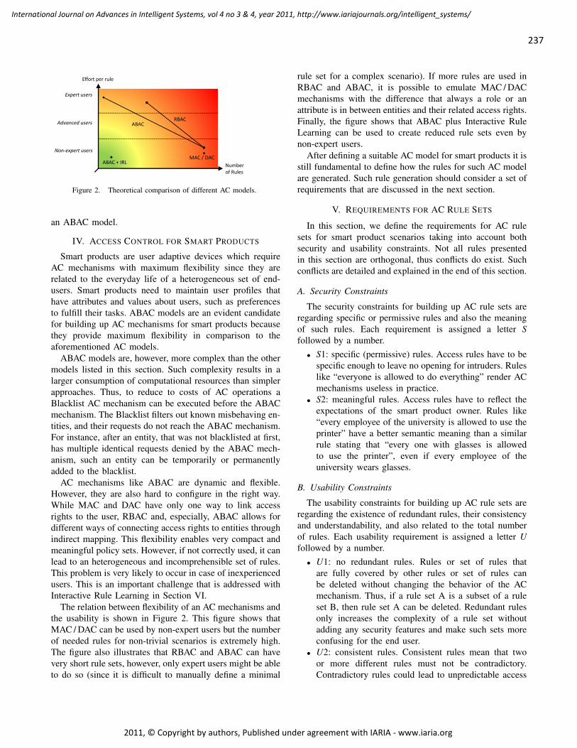
237



Effort per rule

Expert users

Number

of Rules

MAC / DAC

RBACABAC

ABAC + IRL

Non-expert users

Advanced users

Figure 2. Theoretical comparison of different AC models.

an ABAC model.

IV. ACCESS CONTROL FOR SMART PRODUCTS

Smart products are user adaptive devices which requireAC mechanisms with maximum flexibility since they arerelated to the everyday life of a heterogeneous set of end-users. Smart products need to maintain user profiles thathave attributes and values about users, such as preferencesto fulfill their tasks. ABAC models are an evident candidatefor building up AC mechanisms for smart products becausethey provide maximum flexibility in comparison to theaforementioned AC models.

ABAC models are, however, more complex than the othermodels listed in this section. Such complexity results in alarger consumption of computational resources than simplerapproaches. Thus, to reduce to costs of AC operations aBlacklist AC mechanism can be executed before the ABACmechanism. The Blacklist filters out known misbehaving en-tities, and their requests do not reach the ABAC mechanism.For instance, after an entity, that was not blacklisted at first,has multiple identical requests denied by the ABAC mech-anism, such an entity can be temporarily or permanentlyadded to the blacklist.

AC mechanisms like ABAC are dynamic and flexible.However, they are also hard to configure in the right way.While MAC and DAC have only one way to link accessrights to the user, RBAC and, especially, ABAC allows fordifferent ways of connecting access rights to entities throughindirect mapping. This flexibility enables very compact andmeaningful policy sets. However, if not correctly used, it canlead to an heterogeneous and incomprehensible set of rules.This problem is very likely to occur in case of inexperiencedusers. This is an important challenge that is addressed withInteractive Rule Learning in Section VI.

The relation between flexibility of an AC mechanisms andthe usability is shown in Figure 2. This figure shows thatMAC / DAC can be used by non-expert users but the numberof needed rules for non-trivial scenarios is extremely high.The figure also illustrates that RBAC and ABAC can havevery short rule sets, however, only expert users might be ableto do so (since it is difficult to manually define a minimal

rule set for a complex scenario). If more rules are used inRBAC and ABAC, it is possible to emulate MAC / DACmechanisms with the difference that always a role or anattribute is in between entities and their related access rights.Finally, the figure shows that ABAC plus Interactive RuleLearning can be used to create reduced rule sets even bynon-expert users.

After defining a suitable AC model for smart products it isstill fundamental to define how the rules for such AC modelare generated. Such rule generation should consider a set ofrequirements that are discussed in the next section.

V. REQUIREMENTS FOR AC RULE SETS

In this section, we define the requirements for AC rulesets for smart product scenarios taking into account bothsecurity and usability constraints. Not all rules presentedin this section are orthogonal, thus conflicts do exist. Suchconflicts are detailed and explained in the end of this section.

A. Security Constraints

The security constraints for building up AC rule sets areregarding specific or permissive rules and also the meaningof such rules. Each requirement is assigned a letter Sfollowed by a number.

• S1: specific (permissive) rules. Access rules have to bespecific enough to leave no opening for intruders. Ruleslike “everyone is allowed to do everything” render ACmechanisms useless in practice.

• S2: meaningful rules. Access rules have to reflect theexpectations of the smart product owner. Rules like“every employee of the university is allowed to use theprinter” have a better semantic meaning than a similarrule stating that “every one with glasses is allowedto use the printer”, even if every employee of theuniversity wears glasses.

B. Usability Constraints

The usability constraints for building up AC rule sets areregarding the existence of redundant rules, their consistencyand understandability, and also related to the total numberof rules. Each usability requirement is assigned a letter Ufollowed by a number.

• U1: no redundant rules. Rules or set of rules thatare fully covered by other rules or set of rules canbe deleted without changing the behavior of the ACmechanism. Thus, if a rule set A is a subset of a ruleset B, then rule set A can be deleted. Redundant rulesonly increases the complexity of a rule set withoutadding any security features and make such sets moreconfusing for the end user.

• U2: consistent rules. Consistent rules mean that twoor more different rules must not be contradictory.Contradictory rules could lead to unpredictable access

238



usability

Security Authorization(attribute based access control, anomaly based intrusion detection)

Interactive Rule Learning(machine rule learning, user interaction)

Level of

automation

reliability

Confidentiality(encryption)

Integrity(MAC, digital signatures)

Authentication(challenge-response)

(attribute based access control, anomaly based intrusion detection) automation

Figure 3. Reliable and Usable CIA + Authorization

decisions or worsen the usability by unnecessarilyincreasing the complexity of the rule set.

• U3: general, understandable and manageable rule sets.AC rules need to be general enough for users tounderstand and manage.

• U4: minimum number of rules. The number of rulesthat describes the scenario should be minimal to makethe rule set understandable and manageable.

The use of general rules in requirement U3 contradictsthe requirement S1 regarding specific rules. Thus, the bestcompromise between specific and general rules need to bereached. The best compromise is, however, connected to theusers preferences and it is, therefore, individual.

Rule U2 is not only a usability requirement, since itcan also impact the security level obtained by the ACmechanism. An inconsistent rule set can lead to a non-expected behavior that can compromise the security of thesmart product.

In the next section, we develop a rule generation pro-cedure that takes the aforementioned requirements into ac-count. Such procedure combines automatic rule generationwith user interaction.

VI. RULE GENERATION

Nowadays, the common procedure for rule generation is todo it manually. Therefore, the requirements listed in SectionV need to be considered by the owner of the smart product.The manually generation of rules by inexperienced userswill likely result in misconfigured access rule sets (or themanual deactivation of security mechanisms), which even-tually end up into security vulnerabilities. Therefore, the rulegeneration process should be automated as much as possible.Learning algorithms, from the Artificial Intelligence researchfield, are able to accomplish this goal [13].

A. Automatic Rule Learning

Extracting knowledge out of data by using a rule-learningalgorithm is a well-known topic. However, for defininggood access rules, a fully automated rule generation isunfortunately not worth most of the time. It is very difficult

to determine automatically what kind of information needsto be protected. The whereabouts of a person, for instance.Taxi drivers may have their geographical position publicavailable, but for lawyers or doctors on their way to clients orpatients must keep their location information strictly private.

It could be possible to decide which information shouldbe public and private by analyzing the user profile. Thus,automatic rule set generation is possible, but it is expectedthat errors would also be a commonplace. However, ifrelated information for automatic rule generation is missing,automatic processes are not possible. Hence, the smartproduct owners have to decide by their own regarding theaccess rules.

Therefore, a proper solution is to use automatic rulegeneration to create an initial rule set that is later presentedto the user. Such a solution is presented in Section VI-B.

B. Interactive Rule Learning

Learning algorithms can generate a set of rule sets andpresent them to users that decide which specific rule setsuits best to their context. A rule learner can be used toanalyze the set of access rules of a smart product regardingthe actual behavior of entities [14].

Such an analysis disclose whether rules are shadowed,redundant, or correlative, and which exceptions exist fol-lowing the definition and classification presented in [15].Furthermore, in interaction with users, the number of rulesis minimized by analysing, pruning, and rebuilding the setof access rules. This procedure is called Interactive RuleLearning (IRL) [16].

Combined with the ABAC, the IRL helps the user tobuild a secure and usable set of access rules. The expectedoutcome of ABAC+IRL is shown in Figure 3. This conceptrepresents an important step towards usable security.

An automated rule learning algorithm can fulfill thefollowing requirements: S1, U1, U2 and U4. Users have toverify the compliance of requirement S2, since it dependson the context and also on the smart product owner prefer-ences. To satisfy requirement U3, regarding general rules,interaction between the smart product owner and the ruleleaner is required.

VII. RELATED WORK

Over the years, a variety of learning algorithms havebeen developed that try to imitate natural learning or usea more technical approach as a starting point. Some ap-proaches try to reproduce the functioning of a brain atthe level of neurons [17], [18]. Other mechanisms, suchas support vector machines, are based on a more abstractmathematical concept by finding an optimal border betweenpositive and negative examples (like access and deny for anaccess request) by maximizing the distance between them[19]. Existing algorithms further differ with respect to theirapplicability, speed, and accuracy [20], [21].

239



Rule learners use a very intuitive approach in relation tothe aforementioned algorithms. They try to find causalitiesin recorded databases and express them with simple rules.For example, in a database that describes the attributes ofdifferent animals like ravens, sparrows and pigs such a rulecould be as follows: “If an animal can fly and has feathers,it is a bird”. This approach has the particular advantage ofbeing relatively easy to understand for humans as opposed tothe classification of a support vector machine, for instance.This is both a psychological and a practical advantage. Froma psychological perspective people tend to accept somethingmore likely if they are able to understand it. From a practicalpoint of view, potential errors can be more easily detectedand extended [16].

VIII. DESIGNING SECURITY FOR SMART PRODUCTS

Usable access control mechanism for smart productsis currently being implemented as a component of theSmartProducts software platform [22] being implemented aspart of the SmartProducts project funded by the EuropeanCommission’s 7th Framework Programme. In this sectionwe describe the design overview of the Access Managercomponent in the SmartProducts software platform. Theobjective of this platform is to provide an open frameworkfor developers to design hardware and implement applica-tions for smart products. The Access Manager componentis mainly responsible for the authentication, access controland security administration in smart products. Figure 4depicts the architecture of the Access Manager component.This diagram and the following diagrams in this paper arepresented using the FMC notation [23].

The Access Manager has interfaces to the CommunicationMiddleware, which handles all communications outside thedevice, and to the Ubiquitous Data Store, which implementsan interface to one or more databases. The Access Managerhas three subcomponents: the Authentication, the AccessHandling, and the Security Administration. The functionalityof the aforementioned subcomponents are summarized next:

• The Authentication subcomponent handles multiple au-thentication mechanisms, such as biometric data (BD).Itis responsible for authenticating entities, such as usersand devices. The authentication component is out ofthe scope of this paper and it is not going to befurther detailed and it is only mentioned for the sakeof completeness. Anyhow, it is a fundamental buildingblock of the security architecture for smart products.

• The Access Handling (AH) manages the blacklist andthe ABAC as deducted in Sections III-E and IV. TheAH is described in details in section IX.

• The Security Administration (SA) is the componentwhere the Interactive Rule Learning (see Section VI-A)takes place. The SA is described in details in sectionX.

IX. ACCESS HANDLING

The Access Handling assures that only authorized entitiesare able to access the proactive knowledge (PaK), which isbasically a secure distributed database for RDF (ResourceDescription Framework) data and key-value pairs1. It filtersevery request through a set of rules and forwards onlythose requests that are legitimated. The Access Handling ispictured in Figure 5. This section is divided into two parts:the first part describes the access handling components, andan use case is illustrated in the second part.

The Access Handling is composed by the Access Handler(AH), the Blacklist Handler (BH), the Access Control (AC),and the Intrusion Detection System (IDS), which are detailednext.

A. Access Handling Components1) Access Handler: The AH is the interface for access

requests. It forwards requests to the BH and informs therequesting entity about the outcome of the request. If anaccess request was authorized by the security system it willbe forwarded to the Ubiquitous Data Store. If it is necessaryto send data back to the requesting entity to fulfill therequest, the data goes through the AH.

2) Blacklist Handler: The BH is the first of the three rule-based access control mechanisms. It blocks every requestfrom entities which are listed in the General Blacklistdatabase. If the requesting entity is not blocked the requestis forwarded to AC for further examination.

3) Access Control: The AC checks if a request corre-sponds with the access rights of the requesting entity. Allaccess rights are read from the AC Rules database. If anaccess is refused, the ID of the requesting entity will likelybe added to the General Blacklist database for a period oftime. If an entity often tries to access a resource it has noauthorization for it will be added to the General Blacklistdatabase. In all cases a blocked request will be sent to theAH to inform the requesting entity that it was blocked. Ifa rule exists that allows the requesting entity to access therequested resource the request is forwarded to the IDS.

4) IDS: The IDS verifies that an access request does notdeviate from the expected behavior of the requesting entity.The expected behavior is stored in the Behavior Whitelistdatabase. If an access request is determined as abnormalthe IDS asks the IDS of other smart products around forhelp. The IDSs around combine their knowledge about therequesting entity to determine if the entity is the one it claimsto be. The outcome will be used to update the databasefor better future results and is also forwarded to the AH.The IDS should ideally be able to exchange informationwith IDSs on other smart products in order to cooperativelydetect intrusions. The design and implementation of the IDScomponent is out of the scope of this paper.

1More information regarding PaK is available on the SmartProductsproject website: www.smartproducts-project.eu.

240



�

Figure 4. Access Manager architecture.

B. Use Case

In this use case, an user request information from theUbiquitous Data Store. To decide whether a data accessmay take place or not, the respective request must passthrough all mechanisms of the Access Handling. Only whenall instances approve the right to access the data, the requestwill be forwarded from the AH to the Ubiquitous Data Store.This use case is depicted in Figure 6.

X. SECURITY ADMINISTRATION

The Security Administration contains the Rule Handler(RH) – a bidirectional interface for the owner, the manu-facturer and the Access Handling of the smart product toupdate the access rules. The RH maintains three Databasesfor the different Access Handling mechanisms. Every smartproduct in the same Trusted Network [24] of the owner hasthe same owner specific access rules for redundancy andagainst easy manipulations. To help the user define suitablerules a new research topic called Interactive Rule Learningwill be investigated. The Security Administration Moduleis depicted in Figure 7. This section is divided into twoparts: the first part describes the Security Administrationcomponents, and an use case is presented in the second part.

A. Security Administration Components

The Security Administration is composed by the RuleHandler (RH), the set of access control rules, the blacklistand the whitelist. The RH exchanges information with theMinimum Entity (ME). A description of the RH and the MEare provided below.

1) Rule Handler: The RH manages the three databasesGeneral Blacklist, AC Rules, and Behavior Whitelist. TheGeneral Blacklist contains the identities of blocked entitiesused by the BH. Moreover, there are two different databasesfor AC rules: The first database contains access rules definedby the user, the second database consists of access rulesof the manufacturer, which are required for maintainingthe smart product (e.g., firmware updates). The BehaviorWhitelist has rules that describe the normal behavior ofentities interacting with the smart product and is needed forthe IDS.

The RH communicates to the Minimal Entity (ME) orequivalent device to support the user managing the differentdatabases. This is done with the support of Interactive Rule-Learning (see [24]). The manufacturer of the smart productis only able to update the manufacturer AC Rules database.

2) ME: The ME is a device that represents the owner inthe digital world. It is used to easy authenticate the ownerand as a user interface for configuring the RH. Alternativelythe functionality can be integrated in a smart product. MEsare described in detail in [24].

B. Use Case

In our scenario, we consider a family of four. Alice(A), Bob (B), and their children Charlie (C), a 17-yearold, and Denise (D), an 8-year old. The set with elements{A,B,C,D} is the family, and the subset with elements{A,B} are the parents. In the family’s kitchen there are 3new smart products: a smart coffee machine (X), a smartblender (Y), and a smart oven (Z).

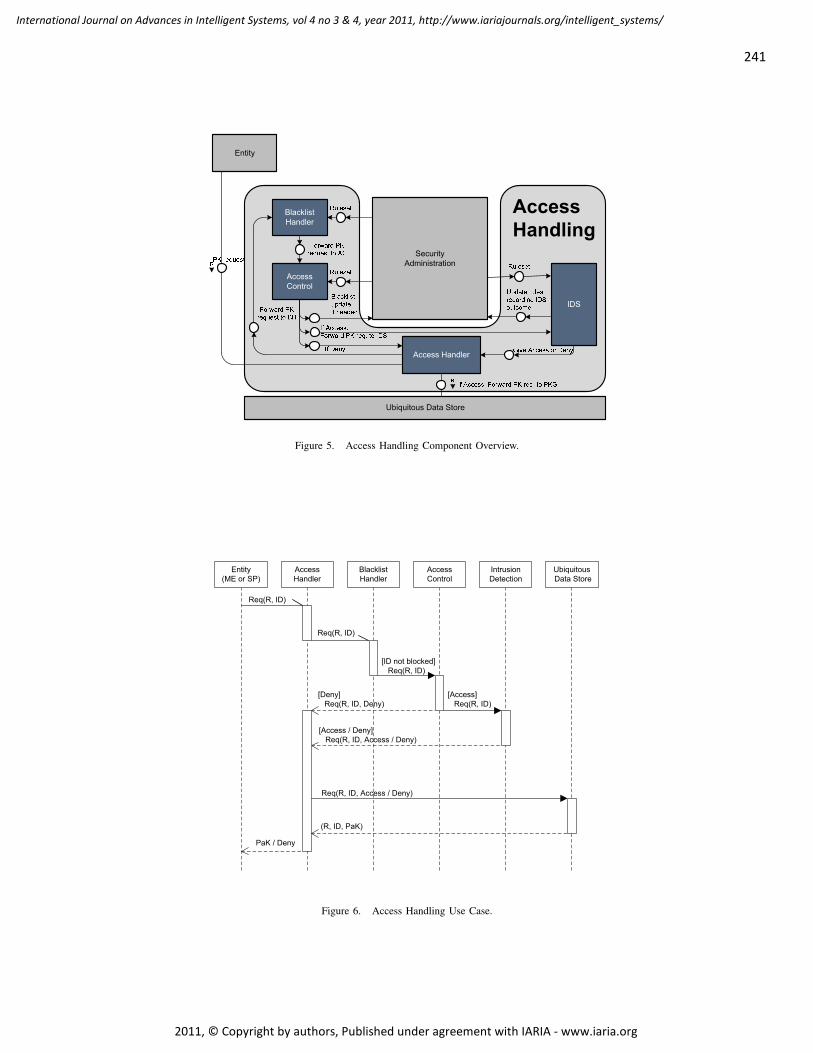
241



�

Figure 5. Access Handling Component Overview.

�

Figure 6. Access Handling Use Case.

242



�

Figure 7. Security Administration Module.

We assume that newly bought devices come with a defaultset of access rules, which are defined by the smart productmanufacturers. Since the manufactures cannot predict inwhich way smart products are going to be used, the factorysettings for the access control rules are basically general.They follow the usage rules of similar non-smart products,i.e., everyone that physically interacts with a device isallowed to use up to its full-functionality. For instance,everyone locally interacting with the coffee machine isallowed to brew coffee.

The full control of a smart product is given to the onewho first activates it. A smart product might be remotelycontrolled by its users (through smart devices) after it hasbeen integrated into the home environment. A wants toconfigure and generates access rules for the 3 newly boughtsmart products (X, Y, Z), so that her family can best profitfrom them. Three classes of access rights are preloaded insmart devices (those classes can later be reconfigured orchanged):

1) Full access: the right to locally or remotely access asmart product and to manage its access rights.

2) Remote and local access: the right to locally andremotely access a smart product.

3) Local access: the right to locally access the smartproducts.

A wants to grant B with full control over all the smartproducts. C shall get access to the full functionality (locallyand remotely), but shall not have administrative rights overthe smart products. D shall not have any access to thedevices, even by local interaction. Since the family often

have guests, A wants them to be able to locally interact withthe smart products, just as in a non-smart kitchen. The initialmanually generated rule set is:Rule Set 11: If (owner) -> full access2: If (any) -> local access3: If (A) -> full access4: If (B) -> full access5: If (C) -> remote and local access6: If (D) -> no access to X7: If (D) -> no access to Y8: If (A) -> no access to Z9: If (guest) -> local access

There are a few mistakes in A’s manually generated ruleset. They are:

• The first two rules are residues from the preloadedfactory default rule set. The fact that A ignored themleads to two implications regarding requirements U1and U2. Rule 2 is a superset of rule 9, and it alsocontradicts rules 6, 7, and 8. Moreover, since there areredundant rules, their number is surely not minimum,which contradicts U4.

• Rule 9 is misconfigured since it does not reflect A’sexpectation. Instead of denying D, she denied herselfto access Z. It contradicts requirements S2 and U2.

• The rules were generated taking into account specificfamily members instead of more general attributes, suchas age. The use of attributes for generating small andunderstandable rule sets is recommended and one of thereasons why ABAC is better suited for smart products,as mentioned in Section III-E. Therefore, there is acontradiction with U3.

243



Table IUSABILITY OVERVIEW TO CIA AND AUTHORIZATION.

Confidentiality Integrity Authenticity AuthorizationUsability Yes, transparent Yes, transparent Yes, transparent Partially,

fully automation not possibleAdequate Method Encryption Digital Signatures Proofs of knowledge, biometric traits

or digital tokens + public-key enc.ABAC and

Interactive Rule Learning

The smart products analyze the manually generated ruleset taking the usability and security constraints presented inSection V and produce new rule sets that are free of conflicts.In our example, the smart products present to the user A twoautomatically generated rule set options:

Rule Set 21: If (age > 40) -> full access2: If (family & age > 16) -> remote and local acc3: If (age > 9) -> local access

and,

Rule Set 31: If (parents) -> full access2: If (family & age > 16) -> remote and local acc3: If (age > 16) -> local access

It is up to A to decide which rule set suits her needsthe best. Both rule sets look much better and concise thanthe manually generated rule set. However, the first ruleof the Rule Set 2 is way too general (an infringement torequirement S1), since it gives full access rights for everyoneabove 40, which would include eventual guests. The last ruleof Rule Set 2 is also not of her likes, since A would not trusta 9-year old to operate kitchen appliances (but she wouldtrust a 12-year old). Thus, A picks Rule Set 3, but manuallychanges rules 2 and 3 to better fits her expectations. Themodified rule set, Rule Set 4, is:

Rule Set 41: If (parents) -> full access2: If (family & age > 12) -> remote and local acc3: If (age > 12) -> local access

A comparison between the manually generated Rule Set1 and the interactive generated Rule Set 4 demonstrates agreat improvement of the latter regarding the usability andsecurity requirements presented in Section V. Rule Set 4addresses the security requirements S1 and S2 since therules are specific and meaningful. Usability requirementsU1, U2, U3, and U4 are also fulfilled since there are noredundant rules, and the rules are consistent, understandable,meaningful, manageable and provide a minimum amount ofrules to express the owner’s security expectations.

XI. CONCLUSION

In this paper, we showed that generation of access con-trol rule sets is the most challenging aspect for obtainingboth usability and security in a smart product scenario.Other security services, such as confidentiality, integrity,and authenticity can be automated and, therefore, made

fully transparent for end-users. In Table I we summarizethe usability aspects and security mechanisms regarding theaforementioned security services. Based on analysis of thedifferent AC mechanisms, the combination of a blacklistwith an attribute based access control (ABAC) approachcombined with an interactive rule learning (IRL) is proposedto comply with today and future needs for smart products.Hence, we first listed a series of security and usabilityrequirements for access control rule sets. We concludedthat the combination of automated rule learning with userinteraction is able to meet such requirements to a secure andusable system. A design description based on FMC diagramsshowed the integration of the proposed security solutionin the SmartProducts framework. The design componentsAccess Handler and Security Administration directly corre-late to the aforementioned concepts of ABAC and IRL. Forboth components use cases were provided to demonstratethe dynamic structure of the smart products security design.

Future work is going to exploit how IRL for ABACcan be implemented to achieve the best possible results ingenerating usable and secure rule sets for smart products.Initially, data needs to be collected for the automated rulegeneration from two different sources. The first data sourceis composed of rules that are already pre-loaded or addedby users to smart products. The second source is the actualbehavior of users of smart products that can be observedby the intrusion detection component. The combined data isgoing to be used by the automatic rule learner to define anew set of rules that are submitted to the user for approval.

We are also going to address the processing of hierarchicaldata in automatic rule learning in the near future. Rulelearning on hierarchical data is important to allow the usersto define natural access rules. Hierarchical data providescrucial contextual information. They are commonplace inmany aspects of our daily lives. For instance, businessstructures are mostly hierarchical, with directors, managers,and secretaries. Current automatic rule learners are not ableto process hierarchical data and, therefore, they need to beextended to accept such data2. A final aspect is the con-version of automated generated rules to rules that are user-friendly, i.e. rules that are simple and easy to understand.

2There are indeed already proposals of rule learning on hierarchicaldata [25]. However, those are still very limited regarding the use of thehierarchical structures.

244



ACKNOWLEDGEMENTS

This research paper is part of research conducted bythe ICT 7th Framework Programme SmartProducts of theEuropean Commission (grant n◦ 231204) and supportedby the Center for Advanced Security Research Darmstadt(CASED).

REFERENCES

[1] M. Beckerle, L. A. Martucci, and S. Ries, “Interactive ac-cess rule learning: Generating adapted access rule sets,” inADAPTIVE 2010 : The Second International Conference onAdaptive and Self-Adaptive Systems and Applications, ser.ComputationWorld 2010. IARIA, Nov 2010, pp. 104–110.

[2] M. Beckerle, “Towards Smart Security for Smart Products,” inAmI-Blocks’09: 3rd European Workshop on Smart Products,2009.

[3] L. Cranor and S. Garfinkel, Security and Usability. O’ReillyMedia, Inc., 2005.

[4] A. Herzog and N. Shahmehri, New Approaches for Security,Privacy and Trust in Complex Environments, 232nd ed.Springer Boston, 2007, pp. 37–48.

[5] V. Reding, The Future of the Internet - A conference heldunder the Czech Presidency of the EU. Belgium: EuropeanCommission - Information Society and Media, 2009, ch. Whatpolicies to make it happen?, pp. 2–5.

[6] H. Krawczyk, M. Bellare, and R. Canetti, “HMAC: Keyed-hashing for message authentication,” 1997.

[7] F. Stajano, Security for ubiquitous computing. John Wileyand Sons, 2002.

[8] S. Brand, “DoD 5200.28-STD Department of Defense TrustedComputer System Evaluation Criteria (Orange Book),” Na-tional Computer Security Center, 1985.

[9] D. Bell and L. La Padula, “Secure computer system: Unifiedexposition and Multics interpretation,” MTR-2997, 1976.

[10] D. Ferraiolo, D. Kuhn, and R. Chandramouli, Role-basedaccess control. Artech House Publishers, 2003.

[11] E. Yuan and J. Tong, “Attributed based access control (ABAC)for Web services,” in IEEE International Conference on WebServices ICWS 2005. Proceedings, 2005.

[12] I. Ray, M. Kumar, and L. Yu, LRBAC: A location-aware role-based access control model. Springer, 2006.

[13] J. Carbonell, R. Michalski, and T. Mitchell, An overview ofmachine learning. Tioga Publishing Company, Palo Alto,1983.

[14] J. Fuernkranz, “Separate-and-conquer rule learning,” ArtificialIntelligence Review, vol. 13, no. 1, pp. 3–54, 1999.

[15] H. Hamed and E. Al-Shaer, “Taxonomy of conflicts in net-work security policies,” IEEE Communications Magazine,vol. 44, no. 3, pp. 134–141, 2006.

[16] M. Beckerle, “Interaktives Regellernen,” Master Thesis, Tech-nische Universität Darmstadt, 2009.

[17] M. Riedmiller, “Advanced supervised learning in multi-layerperceptrons-from backpropagation to adaptive learning algo-rithms,” Computer Standards and Interfaces, vol. 16, pp. 265–278, 1994.

[18] E. Yair and A. Gersho, “The Boltzmann perceptron network:A soft classifier,” Neural networks, vol. 3, no. 2, pp. 203–221,1990.

[19] B. Schoelkopf, C. Burges, and A. Smola, Introduction tosupport vector learning. MIT Press Cambridge, MA, USA,1999.

[20] Y. Jin, “A comprehensive survey of fitness approximationin evolutionary computation,” Soft Computing-A Fusion of

Foundations, Methodologies and Applications, vol. 9, no. 1,pp. 3–12, 2005.

[21] S. Haykin, Neural networks: a comprehensive foundation,3rd ed. Prentice Hall, 2008.

[22] D. Schreiber, Ed., SmartProducts Public deliverableD.6.2.2: Final Architecture and Specification ofPlatform Core Services, Jan 2011, retrieved: Jan 2012,from http://www.smartproducts-project.eu/media/stories/smartproducts/publications/SmartProducts_D6.2.2_Final.pdf.

[23] F. Keller and S. Wendt, “Fmc: An approach towardsarchitecture-centric system development,” in ECBS. IEEEComputer Society, 2003, pp. 173–182.

[24] M. Beckerle, Ed., SmartProducts Public deliverableD4.2.2: Final Concept for Security and Privacy ofProactive Knowledge, Feb 2011, retrieved: Jan 2012,from http://www.smartproducts-project.eu/media/stories/smartproducts/publications/SmartProducts_D4.2.2_Final.pdf.

[25] W. Cohen, “Fast effective rule induction,” in Proceedings ofthe Twelfth International Conference on Machine Learning,1995, pp. 115–123.

245



A Universal Model for Hidden State Observation in Adaptive Process Controls

Melanie Senn, Norbert LinkInstitute of Computational Engineering at IAF

Karlsruhe University of Applied SciencesMoltkestrasse 30, Karlsruhe, Germany

Email: [email protected], [email protected]

Abstract—In many manufacturing processes it is not possibleto measure on-line the state variable values that describe thesystem state and are essential for process control. Instead,only quantities related to the state variables can be observed.Machine learning approaches are applied to model the relationbetween observed quantities and state variables. The charac-terization of a process by its state variables at any point in timecan then be used to adequately adjust the process parametersto obtain a desired final state. This paper proposes a generalmethod to extract state variables from observable quantitiesby modeling their relations from experimental data with datamining methods. After transforming the data to a space ofde-correlated variables, the relation is estimated via regressionmethods. Using Principal Component Analysis and ArtificialNeural Networks we obtain a system capable of estimatingthe process state in real time. The general method features ahigh flexibility in adjusting the complexity of the regressionrelation by an adaptive history and by a variable determinacyin terms of degrees of freedom in the model parameters.The universal model is applied to data from numerical deepdrawing simulations to show the feasibility of our approach.The application to the two sample processes, which are ofdifferent complexity confirms the generalizability of the model.

Keywords-universal statistical process model; state predic-tion; regression analysis; dimension reduction; deep drawing.

I. INTRODUCTION

In our previous work [1], we have presented a statisticalmodel for hidden state observation based on data from anelementary deep drawing process. In this paper, we extendthe observation to a complex deep drawing process withanisotropic plastic material behavior. It is shown that theuniversal statistical process model is capable of generatingmodel instances for both complexity categories of the deepdrawing process with good prediction results.

Closed-loop controls are capable of reaching desired finalstates by compensating disturbances in individual processesor by adapting to varying input in a process chain. Feedbackabout the system state is essential for this purpose. Themeasurement of the real state variables usually requireslarge efforts and cannot be executed in process real time.Only few process-related quantities can be measured byreal production machines during process execution. If theseobservables can be related to state variables with sufficientunambiguity and accuracy, a state-based closed-loop controlcan be created. The final state can then be estimated as

well and the information be transferred to the control ofthe next step in a process chain. Multiple process controlsof a process chain can be linked together using standardizedtransfer state variables between the single processes. Thisallows the optimization of the entire process chain withrespect to the desired properties of the final workpiece. Someapproaches follow this idea by observing such quantities,which are directly correlated to the controlled variables. Thisholds usually true only for one specific process.

In deep drawing, observables such as forces and displace-ments in the tools and in the workpiece are accessible withreasonable measurement effort during process execution.Mechanical stress distributions reflecting the state of thesheet material can be used as the controlled variable asapplied in [2] to find optimal values for the blank holderforce of an experimental deep drawing environment. Acontrol system for deep drawing is presented in [3], basedon the identification of static material properties in [4].

Data mining methods for regression analysis such asArtificial Neural Networks (ANNs) or Support Vector Re-gression (SVR) are widely used in material science forthe prediction of time-invariant process quantities. In [5],thickness strains in different directions of the sheet arecomputed from material parameters, and [4] presents amodel to predict material properties from process parametersand conditions. These both affect the final result, however,conditions are constant during execution and cannot be usedfor on-line closed-loop state control. The texture of coldrolled steels is predicted from process conditions in [6]. Ageneral overview for the use of ANNs in material scienceis given in [7] considering model uncertainties and noise.

In our approach, a generic state estimator is proposed,which represents the functional dependence of state vari-ables on observable quantities, by adapting its structure andparameters to the specific process under consideration. Theestimator consists of a feedforward, completely connectedANN, which is used due to its capability of modelingthe nonlinear relation between observable quantities andthe process state. Principal Component Analysis (PCA) isapplied for dimension reduction in observables and statevariables to decrease the complexity of their relations. Anadaptive history of observable quantities allows an additionaladjustment of the complexity of the regression relation.

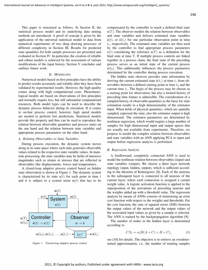
246



This paper is structured as follows. In Section II, thestatistical process model and its underlying data miningmethods are introduced. A proof of concept is given by theapplication of the universal statistical model to data fromnumerical experiments of two deep drawing processes ofdifferent complexity in Section III. Results for predictedstate quantities for both sample processes are presented andevaluated in Section IV. In particular, the creation of reliableand robust models is achieved by the assessment of variousmodifications of the input history. Section V concludes andoutlines future work.

II. MODELING

Numerical models based on first principles have the abilityto predict results accurately and reliably after they have beenvalidated by experimental results. However, the high qualitycomes along with high computational costs. Phenomeno-logical models are based on observations of first principlesand normally require less, but still substantial computationalresources. Both model types can be used to describe thedynamic process behavior during its execution. If it comesto on-line process control, however, high speed modelsare needed to perform fast predictions. Statistical modelsprovide this property and thus can be used to reproduce therelation between observable quantities and process states onthe one hand and the relation between state variables andappropriate process parameters on the other hand.

A. Relating Observables to State Variables

During process execution, the dynamic system movesalong in its state space where each state generates observablevalues related to the respective state variable values. In mate-rials processing, the state variables may be fields of intensivemagnitudes such as strains or stresses that are reflected inobservables like displacements, forces and temperatures.

A closed-loop adaptive process control based on hiddenstate observation is shown in Figure 1. The dynamic systemis characterized by its state s(t) for each point in time tand it is subject to a system noise n(t) that has to be

Controller Observer

System

Figure 1. Closed-loop adaptive process control

compensated by the controller to reach a defined final states(T ). The observer models the relation between observablesand state variables and delivers estimated state variabless(t), or s(tc) for one particular observation point in timetc, respectively. The estimated state variables are then usedby the controller to find appropriate process parametersc(t) considering the reference s(T ) as a definition for thefinal state at time T . If multiple process controls are linkedtogether in a process chain, the final state of the precedingprocess serves as an initial state of the current processs(t0). This additionally influences the process parametersdetermined by the controller during process execution.

The hidden state observer provides state information byderiving the current estimated state s(tc) at time tc from ob-servables between a defined starting point at time t0 and thecurrent time tc. The begin of the process may be chosen asa starting point for observation, but also a limited history ofpreceding time frames is admissible. The consideration of asampled history of observable quantities as the basis for stateestimation results in a high dimensionality of the estimatorinput. When fields of physical quantities, which are spatiallysampled, represent the state, also the estimator output is highdimensional. The estimator parameters are determined bynonlinear regression, which would require a large number ofsamples for high dimensional input and output spaces thatare usually not available from experiments. Therefore, wepropose to model the complex relation between observablesand state variables with an ANN applying PCA to input andoutput before regression analysis is performed.

B. Regression Analysis

A feedforward, completely connected ANN is used tomodel the nonlinear relation between observables (input) andstate variables (output). We choose a three layer networktopology (input, hidden, output), which is sufficient accord-ing to the theorem of Kolmogorov [8]. Each of the neuronsin the subsequent layer is connected to all neurons of thecurrent layer, where each connection is assigned a certainweight value. A logistic activation function is applied to thesuperposition of the activations of preceding neurons andthe weights added up with a threshold value. The regressionanalysis by means of ANNs consists of minimizing an errorcost function with respect to the weights and thresholds. Forthe cost function, the sum of squared errors (SSE) betweenthe output values of the network and the output values ofthe associated input values as given by a sample is selected.The ANN is trained by the backpropagation algorithm [9].

The number of nodes in the hidden layer is determinedaccording to

CNt = α(B(A+ C) +B + C), (1)

see [10] for details. The objective is to retrieve an overdeter-mined approximation, i.e., the number of training samples

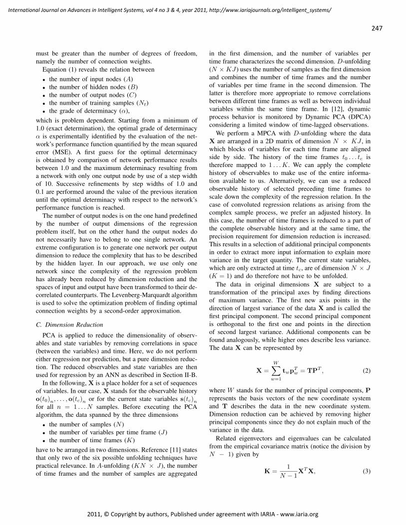
247



must be greater than the number of degrees of freedom,namely the number of connection weights.

Equation (1) reveals the relation between• the number of input nodes (A)• the number of hidden nodes (B)• the number of output nodes (C)• the number of training samples (Nt)• the grade of determinacy (α),

which is problem dependent. Starting from a minimum of1.0 (exact determination), the optimal grade of determinacyα is experimentally identified by the evaluation of the net-work’s performance function quantified by the mean squarederror (MSE). A first guess for the optimal determinacyis obtained by comparison of network performance resultsbetween 1.0 and the maximum determinacy resulting froma network with only one output node by use of a step widthof 10. Successive refinements by step widths of 1.0 and0.1 are performed around the value of the previous iterationuntil the optimal determinacy with respect to the network’sperformance function is reached.

The number of output nodes is on the one hand predefinedby the number of output dimensions of the regressionproblem itself, but on the other hand the output nodes donot necessarily have to belong to one single network. Anextreme configuration is to generate one network per outputdimension to reduce the complexity that has to be describedby the hidden layer. In our approach, we use only onenetwork since the complexity of the regression problemhas already been reduced by dimension reduction and thespaces of input and output have been transformed to their de-correlated counterparts. The Levenberg-Marquardt algorithmis used to solve the optimization problem of finding optimalconnection weights by a second-order approximation.

C. Dimension Reduction

PCA is applied to reduce the dimensionality of observ-ables and state variables by removing correlations in space(between the variables) and time. Here, we do not performeither regression nor prediction, but a pure dimension reduc-tion. The reduced observables and state variables are thenused for regression by an ANN as described in Section II-B.

In the following, X is a place holder for a set of sequencesof variables. In our case, X stands for the observable historyo(t0)n, . . . ,o(tc)n or for the current state variables s(tc)nfor all n = 1 . . . N samples. Before executing the PCAalgorithm, the data spanned by the three dimensions

• the number of samples (N )• the number of variables per time frame (J)• the number of time frames (K)

have to be arranged in two dimensions. Reference [11] statesthat only two of the six possible unfolding techniques havepractical relevance. In A-unfolding (KN × J), the numberof time frames and the number of samples are aggregated

in the first dimension, and the number of variables pertime frame characterizes the second dimension. D-unfolding(N ×KJ) uses the number of samples as the first dimensionand combines the number of time frames and the numberof variables per time frame in the second dimension. Thelatter is therefore more appropriate to remove correlationsbetween different time frames as well as between individualvariables within the same time frame. In [12], dynamicprocess behavior is monitored by Dynamic PCA (DPCA)considering a limited window of time-lagged observations.

We perform a MPCA with D-unfolding where the dataX are arranged in a 2D matrix of dimension N × KJ , inwhich blocks of variables for each time frame are alignedside by side. The history of the time frames t0 . . . tc istherefore mapped to 1 . . .K. We can apply the completehistory of observables to make use of the entire informa-tion available to us. Alternatively, we can use a reducedobservable history of selected preceding time frames toscale down the complexity of the regression relation. In thecase of convoluted regression relations as arising from thecomplex sample process, we prefer an adjusted history. Inthis case, the number of time frames is reduced to a part ofthe complete observable history and at the same time, theprecision requirement for dimension reduction is increased.This results in a selection of additional principal componentsin order to extract more input information to explain morevariance in the target quantity. The current state variables,which are only extracted at time tc, are of dimension N × J(K = 1) and do therefore not have to be unfolded.

The data in original dimensions X are subject to atransformation of the principal axes by finding directionsof maximum variance. The first new axis points in thedirection of largest variance of the data X and is called thefirst principal component. The second principal componentis orthogonal to the first one and points in the directionof second largest variance. Additional components can befound analogously, while higher ones describe less variance.The data X can be represented by

X =

W∑w=1

twpTw = TPT , (2)

where W stands for the number of principal components, Prepresents the basis vectors of the new coordinate systemand T describes the data in the new coordinate system.Dimension reduction can be achieved by removing higherprincipal components since they do not explain much of thevariance in the data.

Related eigenvectors and eigenvalues can be calculatedfrom the empirical covariance matrix (notice the division byN − 1) given by

K =1

N − 1XTX, (3)

248



where X has been mean-centered before and N correspondsto the number of samples in X. Pairs of eigenvalues andeigenvectors are then sorted such that the largest eigenvalueis associated with the first principal component explainingthe most variance [13]. The covariance matrix can be seenas a description of the rotation in the transformation ofthe principal axes, the data centroid corresponds to thedisplacement of the origin of the new coordinate systemwith respect to the initial one.

If the number of variables is much higher than the numberof samples, which might apply to observables, [14] advisesto use Singular Value Decomposition (SVD) according to

X = USVT (4)

to determine the eigenvalues and eigenvectors efficiently.The N eigenvalues of XTX can then be extracted fromthe diagonal matrix STS by

λn =1

N − 1(STS)nn, (5)

and the orthonormal matrix V contains the associated eigen-vectors P of XTX. The data in the new coordinate systemT can finally be determined by a matrix multiplication ofU and S.

D. Statistical Process Model

For each requested observation point in time tcd,the system collects previously sampled observableso(t0d), . . . ,o(tcd) and current state variables s(tcd) asshown in Figure 2. Thereby, either the complete history(t01 = t02) or an adjusted history of selected preceding timeframes (t01 6= t02) is used as a basis for state estimation.

The statistical process model for hidden state observationat one particular observation point in time tc is divided into atraining and a prediction block as indicated in Figure 3. First,PCA is applied to both observables o and state variables s,of which a subset is used to train the ANN as input co andtarget cs, respectively. After successful training, the ANNcan predict state variables in reduced dimensions cs(tc) frompreviously unseen observables o(t0), . . . ,o(tc), reduced toco(t0, . . . , tc), that have not been included in training. The

Figure 2. State observation by observable histories for different observationpoints in time tcd (for d = 1, 2)

Observables State variables

Training

ANN

Prediction

ANN

Sample process On-line process

PCAO PCAS PCAO

PCA-1

S

Observables

Estimated state variables

Figure 3. Architecture of the statistical process model

predicted state quantities cs(tc) are subject to an inversedimension transformation to obtain their counterparts s(tc)in the original, high dimensional space for visualization andvalidation.

III. APPLICATION TO DEEP DRAWING

The feasibility of the proposed approach is tested withtwo sample processes for the cup deep drawing of a metalsheet. In cup deep drawing, a metal sheet is clamped betweena die and a blank holder. A punch presses the sheet thatundergoes a traction-compression transformation into the dieopening to obtain a cup-shaped workpiece. An axisymmetric2D deep drawing model (Figure 4 left) represents an ele-mentary sample process, whereas a 3D deep drawing modelwith anisotropic plastic material behavior (Figure 4 right)describes a complex sample process. Anisotropic plasticityis expressed by a direction-dependent forming resistance inthe material resulting in an earing profile in deep drawing.This material behavior might be induced by a precedingrolling process and is undesired in this context, but may becompensated by process control. Details about the processesof deep drawing and rolling are contained in [15].

Statistical samples are generated by experiments per-formed in a numerical simulation environment. For thispurpose, two finite element deep drawing models have beenimplemented in ABAQUS (finite element analysis software).

sheet

punch

blank

holder

die

radial (1)

axial (2)

sheet

Figure 4. Workpiece and tools in cup deep drawing for the elementarysample process (left) and the complex sample process (right)

249



A. Elementary Sample Process

Observable quantities are displacements and forces, whiletemperature behavior is neglected. Displacements in the cupbottom in direction of the moving punch are recorded as wellas displacements in the sheet edge in orthogonal directionto reflect the sheet retraction. Additional displacements inpunch and blank holder are acquired. Reaction forces in thetools are recorded in both radial and axial direction. Arisingpartial correlations in observables are removed by PCA. Thestate of the deep drawing process is characterized by the vonMises stress distribution within the entire workpiece.

In the performed parametric study, the blank holder forcehas been varied in the range of [70, 100] kN, whereasprocess conditions such as drawing height or lubricationhave been kept constant. For each sample, observables andstate variables have been collected for all time frames. Atime frame equalization ensures common time frames for allsamples. 200 samples have been generated, each consistingof 131 time frames, which in turn contain 9 observablesand 400 state variables. The extracted data are randomlypartitioned into a training set (80%) and a test set (20%).Dimension reduction is applied to all samples, where thetraining data are split again randomly into a training set(80%) and a validation set (20%) for the following regressionanalysis. The test set is used for an overall validation of thestatistical model. Resampling and subsequent remodeling isperformed to select the best model and to prove indepen-dence of specific data sets.

B. Complex Sample Process

Displacements in the sheet edge in different directions(0◦, 45◦, 90◦ with reference to the rolling direction) areselected as observable quantities. Also, reaction forces in thepunch and logarithmic strains reflecting the minimum andmaximum forming grade in selected sheet wall locations areobserved during deep drawing. Altogether, 12 observablesare recorded for each of the common 368 time frames.The process state is again given by the von Mises stressdistribution, this time in 960 elements. 499 experiments havebeen executed under variation of the blank holder forcein the range of [4000, 6000] N with otherwise constantprocess conditions. The partition of the data into a trainingset, a validation set and a test set is performed as for theelementary sample process. Again, multiple resampling runsare accomplished and evaluated by their obtained results.

IV. DISCUSSION OF THE RESULTS

The state prediction results of the statistical model, whichhas been applied to the two sample processes are analyzed.The common underlying prediction characteristics are de-fined in Section IV-A. Results for the particular instancesare given in Section IV-B for the elementary sample processand in Section IV-C for the complex sample process.

A. Prediction Characteristics

The prediction characteristics are computed over all sam-ples from the test set for multiple resampling runs withdifferent random initial conditions to show the independenceof specific data sets. Random initial conditions appear in theselection of data (training, validation and test sets) and inthe initialization of the ANN weights before training starts.The best results are then presented in the following sections.

The quality of the statistical model is quantified by thecoefficient of determination by

R2 = 1− SSE

SST, (6)

which can be applied to nonlinear regression analysis [16].The sum of squared errors given by

SSE =

N∑n=1

L∑l=1

(yl − yl)n2 (7)

describes the sum of the squared deviations between theoriginal data in the test set yl and the associated predictedresults yl. The SSE is calculated over all dimensions in thepredicted quantity l, i.e., the number of state variables, andall samples n. It is divided by the SST , which quantifiesthe total variation in the test set calculated by the summedsquared deviations of the original data from their means. TheR2 lies between 0.0 and 1.0, where a high value indicatesa good model fit and and a low value reveals a poor fit.

The root mean square error according to

RMSE =√MSE =

√SSE

N(8)

is a further measure of model quality, where MSE standsfor the mean squared error, and N corresponds to thenumber of samples in the test data set. The RMSE can beused to compare different models in the same complexitycategory, i.e.., in order to select the best model from multipleresampling runs.

The relative prediction error for each variable dimensionl defined by

REl =

∣∣∣∣Targetl − PredictionlTarget l

∣∣∣∣ for l = 1 . . . L, (9)

quantifies the error percentage, where L is the numberof variable dimensions in the predicted quantity and thetarget quantity comes from the training data. The resultingdistribution can be characterized by the mean relative errorREµ and the maximum relative error REmax with respectto L and the number of samples N.

In order to compare the variation of the predicted resultsto the variance of the generated data, we have defined themodel uncertainty by

U =1

L

L∑l=1

MSE l

Var l, (10)

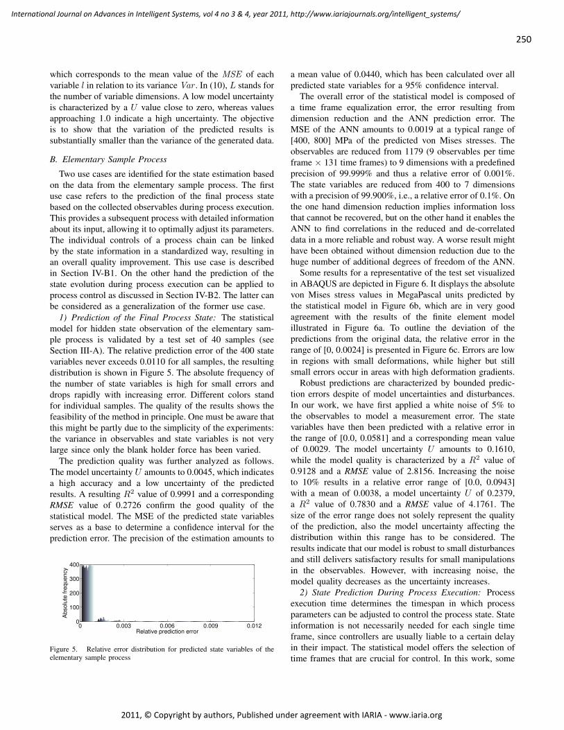
250



which corresponds to the mean value of the MSE of eachvariable l in relation to its variance Var . In (10), L stands forthe number of variable dimensions. A low model uncertaintyis characterized by a U value close to zero, whereas valuesapproaching 1.0 indicate a high uncertainty. The objectiveis to show that the variation of the predicted results issubstantially smaller than the variance of the generated data.

B. Elementary Sample Process

Two use cases are identified for the state estimation basedon the data from the elementary sample process. The firstuse case refers to the prediction of the final process statebased on the collected observables during process execution.This provides a subsequent process with detailed informationabout its input, allowing it to optimally adjust its parameters.The individual controls of a process chain can be linkedby the state information in a standardized way, resulting inan overall quality improvement. This use case is describedin Section IV-B1. On the other hand the prediction of thestate evolution during process execution can be applied toprocess control as discussed in Section IV-B2. The latter canbe considered as a generalization of the former use case.

1) Prediction of the Final Process State: The statisticalmodel for hidden state observation of the elementary sam-ple process is validated by a test set of 40 samples (seeSection III-A). The relative prediction error of the 400 statevariables never exceeds 0.0110 for all samples, the resultingdistribution is shown in Figure 5. The absolute frequency ofthe number of state variables is high for small errors anddrops rapidly with increasing error. Different colors standfor individual samples. The quality of the results shows thefeasibility of the method in principle. One must be aware thatthis might be partly due to the simplicity of the experiments:the variance in observables and state variables is not verylarge since only the blank holder force has been varied.

The prediction quality was further analyzed as follows.The model uncertainty U amounts to 0.0045, which indicatesa high accuracy and a low uncertainty of the predictedresults. A resulting R2 value of 0.9991 and a correspondingRMSE value of 0.2726 confirm the good quality of thestatistical model. The MSE of the predicted state variablesserves as a base to determine a confidence interval for theprediction error. The precision of the estimation amounts to

0 0.003 0.006 0.009 0.0120

100

200

300

400

Relative prediction error

Absolu

te fre

quency

Figure 5. Relative error distribution for predicted state variables of theelementary sample process

a mean value of 0.0440, which has been calculated over allpredicted state variables for a 95% confidence interval.

The overall error of the statistical model is composed ofa time frame equalization error, the error resulting fromdimension reduction and the ANN prediction error. TheMSE of the ANN amounts to 0.0019 at a typical range of[400, 800] MPa of the predicted von Mises stresses. Theobservables are reduced from 1179 (9 observables per timeframe × 131 time frames) to 9 dimensions with a predefinedprecision of 99.999% and thus a relative error of 0.001%.The state variables are reduced from 400 to 7 dimensionswith a precision of 99.900%, i.e., a relative error of 0.1%. Onthe one hand dimension reduction implies information lossthat cannot be recovered, but on the other hand it enables theANN to find correlations in the reduced and de-correlateddata in a more reliable and robust way. A worse result mighthave been obtained without dimension reduction due to thehuge number of additional degrees of freedom of the ANN.

Some results for a representative of the test set visualizedin ABAQUS are depicted in Figure 6. It displays the absolutevon Mises stress values in MegaPascal units predicted bythe statistical model in Figure 6b, which are in very goodagreement with the results of the finite element modelillustrated in Figure 6a. To outline the deviation of thepredictions from the original data, the relative error in therange of [0, 0.0024] is presented in Figure 6c. Errors are lowin regions with small deformations, while higher but stillsmall errors occur in areas with high deformation gradients.

Robust predictions are characterized by bounded predic-tion errors despite of model uncertainties and disturbances.In our work, we have first applied a white noise of 5% tothe observables to model a measurement error. The statevariables have then been predicted with a relative error inthe range of [0.0, 0.0581] and a corresponding mean valueof 0.0029. The model uncertainty U amounts to 0.1610,while the model quality is characterized by a R2 value of0.9128 and a RMSE value of 2.8156. Increasing the noiseto 10% results in a relative error range of [0.0, 0.0943]with a mean of 0.0038, a model uncertainty U of 0.2379,a R2 value of 0.7830 and a RMSE value of 4.1761. Thesize of the error range does not solely represent the qualityof the prediction, also the model uncertainty affecting thedistribution within this range has to be considered. Theresults indicate that our model is robust to small disturbancesand still delivers satisfactory results for small manipulationsin the observables. However, with increasing noise, themodel quality decreases as the uncertainty increases.

2) State Prediction During Process Execution: Processexecution time determines the timespan in which processparameters can be adjusted to control the process state. Stateinformation is not necessarily needed for each single timeframe, since controllers are usually liable to a certain delayin their impact. The statistical model offers the selection oftime frames that are crucial for control. In this work, some

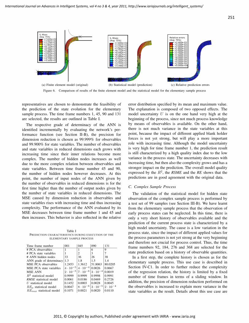
251



(Avg: 75%)S, Mises

+4.500e+02+4.778e+02+5.056e+02+5.334e+02+5.612e+02+5.890e+02+6.168e+02+6.445e+02+6.723e+02+7.001e+02+7.279e+02+7.557e+02+7.835e+02

(a) Finite element model (original)

(Avg: 75%)S, Mises

+4.499e+02+4.777e+02+5.055e+02+5.333e+02+5.611e+02+5.889e+02+6.167e+02+6.445e+02+6.723e+02+7.001e+02+7.279e+02+7.557e+02+7.835e+02

(b) Statistical model (prediction)

(Avg: 75%)Relative errors

+0.000e+00+2.000e-04+4.000e-04+6.000e-04+8.000e-04+1.000e-03+1.200e-03+1.400e-03+1.600e-03+1.800e-03+2.000e-03+2.200e-03+2.400e-03

(c) Relative prediction errors

Figure 6. Comparison of results of the finite element model and the statistical model for the elementary sample process

representatives are chosen to demonstrate the feasibility ofthe prediction of the state evolution for the elementarysample process. The time frame numbers 1, 45, 90 and 131are selected, the results are outlined in Table I.

The respective grade of determinacy of the ANN isidentified incrementally by evaluating the network’s per-formance function (see Section II-B), the precision fordimension reduction is chosen as 99.999% for observablesand 99.900% for state variables. The number of observablesand state variables in reduced dimensions each grows withincreasing time since their inner relations become morecomplex. The number of hidden nodes increases as welldue to the more complex relation between observables andstate variables. Between time frame number 45 and 90,the number of hidden nodes however decreases. At thispoint, the number of input nodes of the ANN given bythe number of observables in reduced dimensions is for thefirst time higher than the number of output nodes given bythe number of state variables in reduced dimensions. TheMSE caused by dimension reduction in observables andstate variables rises with increasing time and thus increasingcomplexity. The performance of the ANN evaluated by itsMSE decreases between time frame number 1 and 45 andthen increases. This behavior is also reflected in the relative

Table IPREDICTION CHARACTERISTICS DURING EXECUTION OF THE

ELEMENTARY SAMPLE PROCESS

Time frame number 001 045 090 131# PCA observables 1 1 6 9# PCA state variables 1 2 3 7# ANN hidden nodes 33 36 26 38ANN grade of determinacy 1.3 1.8 1.5 1.4MSE PCA observables 1.2453 1.3612 51.8063 80.0205MSE PCA state variables 4 · 10−5 4 · 10−4 0.0026 0.0667MSE ANN 2 · 10−5 7 · 10−6 3 · 10−4 0.0019R2 statistical model 0.9999 0.9999 0.9998 0.9991RMSE statistical model 0.0061 0.0186 0.0469 0.2726U statistical model 0.1452 0.0003 0.0028 0.0045REµ statistical model 0.0047 8 · 10−6 3 · 10−5 2 · 10−4

REmax statistical model 0.1071 0.0021 0.0020 0.0110

error distribution specified by its mean and maximum value.The explanation is composed of two opposed effects. Themodel uncertainty U is on the one hand very high at thebeginning of the process, since not much process knowledgeby means of observables is available. On the other hand,there is not much variance in the state variables at thispoint, because the impact of different applied blank holderforces is not yet strong, but will play a more importantrole with increasing time. Although the model uncertaintyis very high for time frame number 1, the prediction resultis still characterized by a high quality index due to the lowvariance in the process state. The uncertainty decreases withincreasing time, but then also the complexity grows and has astronger impact on the prediction. The overall model qualityexpressed by the R2, the RSME and the RE shows that thepredictions are in good agreement with the original data.

C. Complex Sample Process

The validation of the statistical model for hidden stateobservation of the complex sample process is performed bya test set of 99 samples (see Section III-B). We have learntfrom the elementary sample process that the observation ofearly process states can be neglected. In this time, there isonly a very short history of observables available and theprediction of the current process state is characterized by ahigh model uncertainty. The cause is a low variation in theprocess state, since the impact of different applied values forthe process parameters is not yet strong at the very beginningand therefore not crucial for process control. Thus, the timeframe numbers 92, 184, 276 and 368 are selected for thestate prediction based on a history of observable quantities.

In a first step, the complete history is chosen as for theelementary sample process. This use case is described inSection IV-C1. In order to further reduce the complexityof the regression relation, the history is limited by a fixednumber of time frames in terms of a sliding window. Inaddition, the precision of dimension reduction performed onthe observables is increased to explain more variance in thestate variables as the result. Details about this use case are

252



outlined in Section IV-C2. In Section IV-C3, the results ofthe two history variants are compared to each other withrespect to the sensitivity to random initial conditions.

1) State Prediction with Complete History: For the stateprediction based on the complete history of observables, thepredefined precision of dimension reduction in observablesand state variables is chosen as 99.90% and 99.00%, re-spectively. The results are presented in Table II. The MSEinduced by PCA in observables and state variables growswith increasing time. In the case of time frame number 276,both values are greater than the ones of the last time framewith number 368. The number of reduced dimensions inobservables does not change between time frame number276 and 368. This means that a longer history leads to asmaller MSE with the same number of reduced dimensions.The complete history of 368 time frames in fact entirelycontains the selected history for the prediction of time framenumber 276. As a consequence, the MSE proportion in theremaining 92 time frames must be smaller than the ones ofthe common history interval. The increasing confidence inthe prediction is also indicated by a lower model uncertaintyU for time frame number 368. Compared to the elementarysample process, the MSE induced by PCA in observablesis much smaller, which is the result of a generally smallervariance in the observables of the complex sample process.The complexity of the regression relation in terms of thehidden ANN nodes increases with time. Time frame number184 represents an exception, since the number of reduceddimensions in observables is smaller than the number ofreduced dimensions in state variables.

The model quality expressed by the R2 is lower comparedto the predictions performed on data from the elementarysample process. Additionally, the upper bounds of the rela-tive error distribution are much higher for predictions basedon the complex sample process. A possible reason might bethe high complexity of the regression relation in terms ofANN nodes. On the one hand, a more sophisticated modelis necessary to describe complex material behavior as plasticanisotropy. But on the other hand, the high complexity

Table IIPREDICTION CHARACTERISTICS DURING EXECUTION OF THE COMPLEX

SAMPLE PROCESS WITH COMPLETE HISTORY OF OBSERVABLES

Time frame numbers 001-092 001-184 001-276 001-368# PCA observables 7 6 11 11# PCA state variables 3 7 7 10# ANN hidden nodes 73 114 98 121ANN grade of determinacy 1.2 1.4 1.2 1.2MSE PCA observables 0.0337 0.1103 0.5211 0.4539MSE PCA state variables 0.0066 0.0213 0.0802 0.0713MSE ANN 8 · 10−6 0.0049 0.0044 0.0076R2 statistical model 0.9918 0.9914 0.9844 0.9822RMSE statistical model 0.0829 0.1455 0.3694 0.3699U statistical model 0.0781 0.0319 0.0656 0.0409REµ statistical model 0.0001 0.0003 0.0013 0.0021REmax statistical model 0.0130 0.0338 0.3295 0.4194

needs to be reduced to the crucial characteristics to obtain ageneralizable model. This can be achieved by adapting thehistory of observables by use of the following procedure.

2) State Prediction with Adjusted History: In this usecase, we adjust the history of observables by limiting thenumber of time frames in terms of a sliding window. Avariable history length makes the approach very flexible.At the same time, the question arises what might be theminimum history length to describe the current processstate unambiguously? Further efforts may be investigated torealize a self-adaptive history with reference to performanceand accuracy criteria. The sliding window is set to a fixedlength of 92 times frames, which is one quarter of thecomplete history length and seems to be sufficient for stateprediction in this case. That means that the process state forthe currently selected time frame is predicted by a historyof the preceding 92 time frames. This adaptation indeedreduces the complexity, but does not yield better predictionresults. Furthermore, this reduced history approach is sen-sitive to random initial conditions as it is also observed forpredictions based on the complete history in Section IV-C1.

In order to explain more variance in the state variablesas the regression output, the precision of the dimensionreduction procedure performed on the observables is in-creased to 99.99%. The combination of reducing the numberof time frames in the history and inflating the remainingobservables by a higher precision represents the adjustedhistory approach. This procedure yields similar or evenbetter prediction results with a lower complexity in termsof number of ANN nodes. It also reduces the sensitivity torandom initial conditions as demonstrated in Section IV-C3.

The prediction results with adjusted history and data fromthe complex sample process are summarized in Table III.Note that the history is not adjusted for early predictions upto time frame number 92. Despite of a shorter history, thenumber of dimensions in the reduced observable space isabout twice the size of the number of principal componentswith lower precision in the complete history variant. Theincrease in the precision seems to have a stronger effect

Table IIIPREDICTION CHARACTERISTICS DURING EXECUTION OF THE COMPLEX

SAMPLE PROCESS WITH ADJUSTED HISTORY OF OBSERVABLES

Time frame numbers 001-092 092-184 184-276 276-368# PCA observables 7 10 20 24# PCA state variables 3 7 7 10# ANN hidden nodes 73 89 62 76ANN grade of determinacy 1.2 1.4 1.3 1.2MSE PCA observables 0.0337 0.0220 0.1472 0.0126MSE PCA state variables 0.0066 0.0213 0.0802 0.0713MSE ANN 8 · 10−6 0.0004 0.0068 0.0036R2 statistical model 0.9918 0.9911 0.9882 0.9840RMSE statistical model 0.0829 0.1554 0.3524 0.3395U statistical model 0.0781 0.0350 0.0519 0.0458REµ statistical model 0.0001 0.0003 0.0012 0.0025REmax statistical model 0.0130 0.0350 0.1342 0.2860

253



on the number of reduced dimensions than the decrease inthe history to one quarter of its entire length. The MSEinduced by dimension reduction in observables is muchsmaller due to the higher requested precision. For timeframe number 276, this quantity is still higher comparedto the other time frames, even though 20 components areextracted to describe the reduced space. There might besome nonlinear behavior in dominant observables aroundthis point, which cannot be explained adequately by lineardimension reduction methods. The adjustment in the historyleads to a kind of linearization by limiting the number oftime frames and thus yields more reliable prediction results.

The prediction characteristics of the statistical model,namely the R2, the RMSE and the uncertainty U are similarto the results of the complete history variant. Indeed, themaximum of the relative prediction error REmax is reducedsubstantially by the adjusted history variant. The relativeerror distribution based on 960 state variables and 99 testsamples with an upper bound of 0.2860 is depicted inFigure 7. The absolute frequency is high for small errors anddecreases rapidly for higher errors. The individual samplescan be distinguished by the different colors in the histogram.

A representative is selected from the test set for predictedstate variables at the end of the complex sample processwith an adjusted history of observables. The obtained resultsare visualized in ABAQUS as presented in Figure 8. Theabsolute von Mises stress values at a typical range of[1, 300] MPa, which are calculated by the finite elementmodel are depicted in Figure 8a. The predicted von Misesstresses are displayed in 8b. They are in good agreementwith the original results. The relative error in the range of [0,0.0449] is illustrated in Figure 8c to compare the predictionwith the original results. As also observed for the elementarysample process, the largest errors occur in the area of highdeformation gradients as in the rounding of the sheet wall.

3) Sensitivity to Random Initial Conditions: The twovariants with complete and adjusted history are comparedwith reference to their sensitivity to random initial condi-tions. Random initial conditions appear in the selection oftraining, validation and test data and in the initialization

0 0.1 0.2 0.3 0.350

200

400

600

800

1000

Absolu

te fre

quency

Relative prediction error

Figure 7. Relative error distribution for predicted state variables of thecomplex sample process with adjusted history of observables

of the ANN weights before training. Figure 9 visualizesthe sensitivity to random initial conditions observed on theRMSE over 10 resampling runs for both history variants.On the left, the error intervals are illustrated for the com-plete history, whereas the ones for the adjusted historyare depicted on the right. The intervals are the same forthe predicted state variables up to time frame number 92,since the history has not been adjusted at the early stageof prediction. For all other time frames, the error intervalsdecrease substantially in case of the adjusted history variant.This means that the sensitivity to random conditions is muchless and yields a higher reliability in the prediction.

The distribution characteristics RMSEµ,RMSEσ andRMSEmax for the corresponding time frame numbers 184,276 and 368 are compared in Table IV for the completeand the adjusted history. The RMSEµ is minimized up toone half with an adjusted history. An improvement is alsoachieved in a reduced variation RMSEσ (≈ up to one forth)and a reduced maximum RMSEmax (≈ up to one forth).In particular, the RMSE for the prediction of time framenumber 276 is characterized by much lower error bounds.The adjusted history of observables used for prediction atthis point in time has already attracted attention by highererrors in context of its reduced space in Section IV-C2.

0.5

1

1.5

2

001−092

001−184

001−276

001−368

Time Frames

Complete History

RMSE

0.5

1

1.5

2

001−092

092−184

184−276

276−368

Time Frames

Adjusted History

RMSE

Figure 9. RMSE sensitivity w.r.t. random initial conditions for differenttime frames with complete history (left) and adjusted history (right)

Table IVDISTRIBUTION CHARACTERISTICS OF RMSE SENSITIVITY W.R.T.

RANDOM INITIAL CONDITIONS FOR DIFFERENT TIME FRAMES

Distribution characteristics RMSEµ RMSEσ RMSEmax

Time frames 001-092 0.1156 0.0419 0.1983Time frames 001-184 (complete) 0.3313 0.2851 0.8845Time frames 092-184 (adjusted) 0.1727 0.0168 0.2032Time frames 001-276 (complete) 0.9129 0.5572 2.3296Time frames 184-276 (adjusted) 0.5034 0.0966 0.6631Time frames 001-368 (complete) 0.4948 0.1282 0.7395Time frames 276-368 (adjusted) 0.3857 0.0362 0.4722

254



(a) Finite element model (original) (b) Statistical model (prediction)

(Avg: 75%)

Relative errors

+0.000e+00+3.742e−03+7.483e−03+1.123e−02+1.497e−02+1.871e−02+2.245e−02+2.619e−02+2.993e−02+3.368e−02+3.742e−02+4.116e−02+4.490e−02

(c) Relative prediction errors

Figure 8. Comparison of results of the finite element model and the statistical model for the complex sample process with adjusted history of observables

V. CONCLUSION AND FUTURE WORK

A universal statistical process model for hidden stateobservation based on the nonlinear regression analysis ofa history of observables and the current state by meansof an ANN has been created. PCA as a linear dimensionreduction method is applied to input and output separatelybefore performing the regression analysis. The complexityof the relation between observables and state variables canbe adjusted by the grade of determinacy of the ANN and byan adaptive history of observables. This makes the approachvery flexible with reference to performance and accuracy.

The presented statistical process model has been appliedto two deep drawing processes of different complexity. Ithas been shown that the universal model adapts well tothe specific data of the different sample processes. Theresulting model instances can be successfully used for stateprediction based on observations. For the complex sampleprocess, the sensitivity to random initial conditions has beenreduced by an adjusted history of observables, such thatmore reliable prediction results are achieved. The resultsoutlined in Section IV are very promising and can thereforebe taken as a solid base for process control. Process param-eters can thereon be adjusted by observing the evolution ofthe process state implementing a suitable control law. Thecontrol of one single process can be extended to processchain optimization by multiple linked process controls. Forthis purpose, workpiece properties are to be deduced fromthe final state of the final process. The predefined state canthen serve as set value for the optimization procedure.

One drawback of the statistical process model for hiddenstate observation is the high uncertainty in state predictionat the beginning of the process. This can be overcome bynot considering those early predictions with high uncertaintyin process control. By observing an entire process chain,the final state information of the preceding process canbe used as reliable characterization at the begin of thecurrent process. Significant time frames for the observationof the process state evolution have to be identified to enableprocess control. The proposed universal approach for the

observation of hidden states in adaptive process controls maybe transferred to any process characterized by state variablesthat can be derived from related observable quantities.

Future work includes the extension of the statistical pro-cess model for hidden state observation to a local processcontrol based on extracted features. For this purpose, dimen-sion reduction shall be integrated into the regression analy-sis, such that the resulting compact feature space representsthe relation between observables and state variables. Theextracted features may then serve as a base for an efficientprocess control. Therefore, nonlinear dimension reductionmethods are taken into account to obtain a more generaldescription with a feature space as small as possible.

ACKNOWLEDGMENT

This work has been supported by the DFG ResearchTraining Group 1483 ”Process chains in manufacturing”.The authors would like to thank the ITM at the KIT forproviding the finite element deep drawing models.

REFERENCES

[1] M. Senn and N. Link, “Hidden state observation for adaptiveprocess controls,” in Proceedings of the Second InternationalConference on Adaptive and Self-adaptive Systems and Ap-plications, ADAPTIVE 2010, pp. 52 – 57.

[2] C. Blaich and M. Liewald, “Detection and closed-loop controlof local part wall stresses for optimisation of deep drawingprocesses,” in Proceedings of the International Conferenceon New Developments in Sheet Metal Forming Technology,Fellbach, Germany, 2010, pp. 381 – 414.

[3] Y. Song and X. Li, “Intelligent control technology for thedeep drawing of sheet metal,” in Proceedings of the Inter-national Conference on Intelligent Computation Technologyand Automation, Los Alamitos, CA, USA, 2009, pp. 797 –801.

[4] J. Zhao and F. Wang, “Parameter identification by neuralnetwork for intelligent deep drawing of axisymmetric work-pieces,” Journal of Materials Processing Technology, vol.166, pp. 387 – 391, 2005.

255



[5] S. K. Singh and D. R. Kumar, “Application of a neuralnetwork to predict thickness strains and finite element simu-lation of hydro-mechanical deep drawing,” The InternationalJournal of Advanced Manufacturing Technology, vol. 25,no. 1, pp. 101 – 107, 2005.

[6] A. Brahme, M. Winning, and D. Raabe, “Prediction of coldrolling texture of steels using an artificial neural network,”Computational Materials Science, vol. 46, pp. 800 – 804,2009.

[7] H. K. D. H. Bhadeshia, “Neural networks and informationin materials science,” Statistical Analysis and Data Mining,vol. 1, no. 5, pp. 296 – 305, 2009.

[8] R. Hecht-Nielsen, “Theory of the backpropagation neural net-work,” in Proceedings of the International Joint Conferenceon Neural Networks, Washington D.C., USA, 1989, pp. 593– 605.

[9] M. T. Hagan, H. B. Demuth, and M. H. Beale, Neural networkdesign. University of Boulder, Colorado, USA: CampusPublication Service, 2002.

[10] W. C. Carpenter and M. E. Hoffman, “Selecting the ar-chitecture of a class of back-propagation neural networksused as approximators,” Artificial Intelligence for EngineeringDesign, Analysis and Manufacturing, vol. 11, pp. 33 – 44,1997.

[11] C. Zhao, F. Wang, N. Lu, and M. Jia, “Stage-based soft-transition multiple PCA modeling and on-line monitoringstrategy for batch processes,” Journal of Process Control,vol. 17, no. 9, pp. 728 – 741, 2007.

[12] J. Chen and K.-C. Liu, “On-line batch process monitoringusing dynamic PCA and dynamic PLS models,” ChemicalEngineering Science, vol. 57, no. 1, pp. 63 – 75, 2002.

[13] C. M. Bishop, Pattern recognition and machine learning,2nd ed. Springer, 2007.

[14] T. Hastie, R. Tibshirani, and J. H. Friedman, The elements ofstatistical learning: data mining, inference, and prediction,2nd ed. Springer, 2009.

[15] W. F. Hosford and R. Caddell, Metal Forming: Mechanicsand Metallurgy, 4th ed. Cambridge University Press, 2011.

[16] H. Motulsky and A. Christopoulos, Fitting Models to Biologi-cal Data using Linear and Nonlinear Regression - A practicalguide to curve fitting. GraphPad Software Inc., San DiegoCA, 2003.

256



Behaviour-inspired Data Management in the Cloud

Dariusz Król, Renata Słota, Włodzimierz Funika

AGH University of Science and Technology, Faculty of Electrical Engineering, Automatics, Computer Science and Electronics, Department of Computer Science,

al. Mickiewicza 30, 30-059 Krakow, Poland {dkrol, rena, funika}@agh.edu.pl

Abstract — Open source cloud computing solutions are still not mature enough to handle data-intensive applications, e.g., scientific simulations. Thus, it is crucial to propose appropriate algorithms and procedures to the data management problem in order to adjust Cloud-based infrastructures to scientific community requirements. This paper presents an approach inspired by the observation of the Cloud user behaviour: the intensity of data access operations, their nature, etc. We also describe how the proposed approach influences the architecture of a typical Cloud solution and how it can be implemented based on the Eucalyptus system, which is a successful open source Cloud solution.

Keywords-cloud computing; data management; monitoring; behaviour patterns.

I. INTRODUCTION Cloud computing is arguably the most popular buzzword

in the tech world today. It promises to reduce the total cost of maintenance of an IT infrastructure with providing better scalability and reliability at the same time. Apart from “unlimited” computational power, the Cloud provides also "unlimited" storage capacity which can be accessed from every device which is connected to the Internet. Therefore, this is not a surprise that many commercial companies along with academic facilities are very interested in this paradigm. As with other paradigms, various research centers test it in a variety of ways in order to unveil its strengths and weaknesses. What makes the Cloud computing special in comparison to other, more academic-related approaches to distributed computing, e.g., Grid computing [2], is the support and investment made by the largest IT companies [3], e.g., Google, IBM, Microsoft and many others. These million dollars investments can be treated as a good omen that Cloud computing can be widely adopted and will not disappear after few years.

From a few years now, Clouds are evolving into a number of different forms but with a common goal, i.e., providing computational power and storage capacity on premise. Existing Clouds can be classified in a few ways each of which relates to one feature from the following list:

• accessibility of the Cloud for users, • abstraction level on which Cloud users operate, • resources provided by the Cloud, • openness of the source code of the Cloud.

The first taxonomy includes public, private and hybrid Clouds. Today, the most popular are public clouds which can be used by anyone. Potential customer needs only to obtain an account on the providers site. This category includes Amazon Elastic Compute Cloud (Amazon EC2) [5], Microsoft Azure [6], Google AppEngine [7] and many others. On the other hand, there are private clouds. In most cases, they are limited to resources and members of a single organization. Also, their accessibility is limited to the organization's intranet. The third group, called hybrid Clouds, concerns a special type of private Clouds whose computation power and storage capacity can be extended by resources of public Clouds. Hybrid Clouds exploit the scalability feature of the Cloud to provide required resources by utilizing publicly accessible Clouds when the in-house infrastructure is not enough.

The second taxonomy concerns the style in which the customers use Clouds. This taxonomy includes:

• Infrastructure as a Service (IaaS) Clouds which provide access to a virtualized pool of resources using which customers assemble Virtual Machines (VMs) on which customers install any technology stack and any applications they need. Probably the most well known example of this group is Amazon EC2,

• Platform as a Service (PaaS) Clouds expose a well defined runtime environment, e.g., Java Virtual Machine or Microsoft .NET and programming services which are used to develop applications without troubling with virtual machines, e.g., queuing systems, (non-)relational databases and more. This group includes Google AppEngine among many other,

• Software as a Service (SaaS) Clouds are about delivering applications which are deployed at the providers infrastructure, e.g., Google Apps [8]. Applications which are exposed with SaaS model are accessible mostly often via a web browser and are provided in the pay-per-use model. This group focuses on customers rather than developers.

The third taxonomy of Clouds focuses on the type of resources provided. Today, this taxonomy includes two elements: compute Clouds and storage Clouds. The first group comprises Clouds which provide access to computational power by running VMs or applications on a

257



specified virtualized hardware, e.g., in Amazon EC2 the user can choose the size of a virtual machine to use in terms of the available number of virtual CPUs and RAM memory [9]. To mention just a few examples, the customer can choose a small instance of a virtual machine which can be defined as a single, normalized, virtual CPU, 512 MB of RAM and 10 GB of hard drive capacity while a big instance can consist of 8 virtual CPU, 4 GB of RAM and 50 GB of hard drive capacity. On the other hand, the storage Clouds enable users to store data sets in a number of ways, i.e., in files, (non-)relational databases or block devices. In theory, the storage clouds can provide an infinity storage capacity on demand.

The last taxonomy divides Clouds into two groups: open-source Clouds and proprietary Clouds. This classification is important especially from a developer point of view. Open-source Clouds can be modified and analyzed by anyone while proprietary Clouds are commercial solutions mostly often with a closed source code. Hence, their internals are hidden from customers or developers from outside the Cloud provider’s company. Thus, in many situations, it is difficult or even impossible to compare these two types of Clouds.

Todays Cloud computing solutions, especially the open source ones, are not mature enough in terms of storage capabilities to handle data-intensive applications which need to store results in Cloud-based storage. One of the issues is the lack of adaptability of data management strategy, e.g., to dynamically changing user requirements or location from where the user access the Cloud storage. Each of these aspects influences the access time to data especially when considering geographically distributed resources which constitute a single Cloud installation, e.g., a user who lived in Europe can download his data from a data center in US instead of a closer data center located in Europe. Therefore, we propose a novel approach, based on autonomic systems (similar to situation-aware systems - [4]) and behaviour observation whose main goal is to adapt data location to the user needs which will result in decreasing data access time and higher utilization factor of resources. We introduce a “Usage profile” concept which describes a piece of data stored in the Cloud storage. The usage profile contains information how the described data is used by Cloud clients. To create such a profile, storage-related operations performed by Cloud users are monitored and analyzed. The approach is designed to be an additional element of the Cloud installation rather than being mandatory. Thus, it can be treated as a plugin for a Cloud solution. Moreover, it is transparent from the Cloud user point of view because it operates on the Cloud provider’s side where various management actions can improve the storage performance.

The commercial clouds, e.g., Amazon EC2 which is an IaaS solution, i.e., it allows to manage a computational environment consisting of virtual machines, cannot be easily studied due to proprietary source code, thus in this paper they will not be taken into consideration.

This article is an extended version of the work presented in [1]. The rest of the paper is organized as follows.In Section II, a number of the existing Cloud solutions and Cloud-based storage services are presented. In Section III, we describe a data management algorithm which is based on

behaviour analysis. Parameters of the usage profile along with behaviour which is analyzed to create usage profiles are described in Section IV. A prototype implementation of the algorithm is presented in Section V. Directions for future work are discussed in Section VII. The paper is concluded in Section VIII.

II. RELATED WORK Cloud computing has been already widely adopted by

various commercial companies and academic facilities. While many commercial companies develop their own solutions, e.g., Amazon EC2, Microsoft Azure or Google AppEngine, others use and invest in open source solutions which are especially well suited for situations where the environment has to be adapted to some specific requirements. This feature is very important for scientific community which would like to implement new concepts and approaches, e.g., to optimize data access time or other parameters. In this section, we focus on three well known IaaS environments: Eucalyptus, Nimbus, OpenNebula and OpenStack. We also consider a few commercial products for data management. In addition, two data management systems which are based on the Grid computing paradigm are presented. Hence, we will be able to compare Cloud-based solutions with Grid-based solutions which is valuable for readers with a Grid computing background but who are not familiar with Clouds yet.

A. Eucalyptus Eucalyptus system [10] is an example of an open source

project which became very popular outside the scientific community and is exploited by many commercial companies to create their own private clouds. It was started as a research project in the Computer Science Department at the University of California, Santa Barbara in 2007 and today it is often treated as a model solution of an IaaS Cloud. Eucalyptus aims at providing an open source counterpart of the Amazon EC2 Cloud in terms of interface and available functionality. There are two versions of the Eucalyptus Cloud: Community and Enterprise.

Each Eucalyptus installation consists of a few loosely coupled components each of which can run on a separate physical machine to increase scalability. The frontend of such a Cloud is “Cloud controller” element which is an access point to the virtual machines related features. While “Cloud controller” is responsible for computation, the “Walrus” component is responsible for data storage. It allows to store virtual machine images along with any other files which are organized into a hierarchy of buckets and can be treated as a counterpart of Amazon Simple Storage Service (S3) [11] in the Eucalyptus system. Amazon S3 is a Cloud storage service which allows to store any type of data in form of files in a number of buckets (each with a unique name within a bucket) using a simple Application Programming Interface (API), i.e., put, get, list, del operations are supported. Each virtual machine is run on a physical host which is controlled by the “Node controller” element. A group of nodes can be gathered into a cluster which exposes a single access point, namely “Cluster

258



controller” from the virtual machine management side and “Storage controller” from the virtual machine images repository side.

Eucalyptus is based on the Java technology stack and its source code is freely accessible and can be modified as necessary. To mention a few, the current implementation uses web services (Apache Axis [12]) to expose the provided functionality to the external clients, and exposes a web-based user interface developed with Google Web Toolkit (GWT) [13]. It also supports the Xen [14] and Kernel-based Virtual Machine (KVM) [15] hypervisors to run virtual machines on the supervised resources.

The open version of the Eucalyptus system stores data into a single directory on the host on which the Walrus component is installed. Therefore, the only way to distribute the data is to exploit a distributed file system, e.g., Lustre [16] or Oracle Cluster File System 2 [17], which will be mounted to the directory used by the Eucalyptus installation. However, this file system is orthogonal to the Cloud solution, i.e., it does not have access to any information about the Cloud. Thus, it can manage data based on some basic information only, e.g., size of stored files or capacity of available storage resources. Such strategies are very limited and are not customizable for the Cloud computing paradigm.

On the other hand, we have the Enterprise version of Eucalyptus. Among other features, the Enterprise version of Eucalyptus provides an adapter for direct integration with Storage Area Networks (SANs) [18], e.g., Dell Equallogic or NetApp. With this adapter, you can easily configure Eucalyptus to exploit SAN [19] directly as a data storage back end. However, to our best knowledge, this integration does not allow to combine different types of storage systems within a single Cloud installation. Also, a Cloud administrator can`t provide policy for data distribution among available storage resources. The data management is left entirely to the SAN solution which knows nothing about the Cloud, its users or the type of data stored in the Cloud. Though, SANs are enterprise-class solutions for data storage, they do not provide any Cloud-specific storage strategies which would regard, e.g., information about Cloud customers.

B. Nimbus Nimbus [20] is a toolkit for turning a cluster into an IaaS

Cloud computing solution. It is developed by the Globus Alliance [21]. A Nimbus client can lease remote resources by deploying virtual machines on these resources and configure them to fulfil the user requirements. What makes it attractive is support for a communication interface known from the Grid computing, namely Web Services Resource Framework (WSRF) [22]. As in other popular solutions, Nimbus provides an Amazon EC2 compatible interface for Cloud clients, which is de facto a standard of IaaS environment due to its wide adoption in a number of solutions.

A Nimbus installation consists of a number of loosely coupled elements. The center point of the Nimbus architecture is the “Workspace service” component which is a coordinator of the whole installation. It is invoked through

different remote protocol frontends, e.g., WSRF or EC2 – compatible services. Another important component is “Workspace resource manager” which runs on each host within the Cloud and is responsible for controlling a hypervisor on the host machine. The current version fully supports the Xen hypervisor and most of the operations on the KVM hypervisor. It is also worth of mentioning that Nimbus installation can be easily connected to a public commercial Cloud, e.g., Amazon EC2 in order to achieve even greater computer power when the in-house infrastructure is not enough.

In terms of data management, the Nimbus project is limited to the virtual machine image repository. There is no component which would provide a functionality similar to that of the Amazon S3. The user can only upload virtual machine images to the Nimbus cloud and store the data stemming from computation on storage devices connected directly to a virtual machine.

The Nimbus project is based on open source tools and frameworks, e.g., Apache Axis, the Spring framework [28] or JavaDB [29]. Therefore, everyone can download its sources from a public repository and modify its functionality as desired.

C. OpenNebula OpenNebula [30] is a Virtual Infrastructure Manager for building cloud infrastructures based on Xen, KVM and VMWare virtualization platforms [31]. It was designed and developed as part of the EU project RESERVOIR [32], whose main goal is to provide open source technologies to enable deployment and management of complete IT services across different administrative domains. OpenNebula aims to overcome the shortcomings of existing virtual infrastructure solutions, e.g., inability to scale to external clouds, a limited choice of interfaces with the existing storage and network management solutions, few preconfigured placement policies or lack of support for scheduling, deploying and configuring groups of virtual machines (apart from the VMWare vApp solution [34]). Like other of the presented solutions, OpenNebula is fully open source and its source code can freely be downloaded from a public repository.

OpenNebula architecture was designed with modularity in mind. Therefore, it can be extended to seamlessly support a new virtualization platform e.g., in terms of virtual image or service managers. For instance, a procedure of setting up a VM disk image consists of well-defined hooks whose implementation can be easily replaced to interface with the third-party software. To manage an OpenNebula installation, the user can use a simple, dedicated command line interface or Amazon EC2 query interface. Therefore, it can be accessed with the tools originally developed to work with the Amazon EC2 cloud.

In terms of storage mechanisms, it is limited to repository of VM images only. The repository can be shared between available nodes with the Network File System (NFS) [35]. It is also possible to take advantage of block devices, e.g.,

259



Logical Volume Management 2 (LVM2) [36] to create snapshots of images in order to decrease time needed to run a new image instance.

D. OpenStack

OpenStack is a joint effort of NASA and RackSpace. NASA contributed to the project by releasing its middleware, called Nebula [23], for managing virtual machines at physical infrastructure. RackSpace contributed with its storage solution known as Cloud Files [24]. OpenStack [25] is a collection of tools for managing data centers resources to build a virtual infrastructure. In terms of computations, OpenStack provides OpenStack Compute (Nova) solution which is responsible for managing instances of virtual machines. In terms of storage, OpenStack provides OpenStack Object Storage (Swift) which is an object storage solution with built-in redundancy and failover mechanisms. There is also a separate subsystem, called OpenStack Imaging Service, which can be used to lookup and retrieving virtual machine images. Since the first release of OpenStack was in October 2010, there is no evidence about production deployments of the toolkit in either industry or scientific area yet. Thus, there is no information about the performance and stability of OpenStack. Also, OpenStack lacks of an interface that would be compatible with the Amazon clouds which is a de facto standard in the Cloud ecosystem.

E. Flash Cloud “Flash Cloud” [27] is a commercial service for storing

data using the Cloud paradigm. After creating an account, the user gets access to a certain storage capacity which can be scaled up depending on your requirements. Your data can be managed using the following methods:

• Web 2.0 interface, • native desktop software for PC or Mac and mobile

devices including IPhone and BlackBerry, • Web Distributed Authoring and Versioning

(WebDAV)-based [38] API. The data are stored using industry leading solutions such

as Internet Small Computer Interface (iSCSI) [37], File Transfer Protocol (FTP)/Network Attached Storage (NAS) and EVault [39]. However, “Flash Cloud” does not provide any mechanism for integrating with popular computing Clouds, e.g. Eucalyptus, Nimbus, OpenStack. Moreover, the storage capacity limits (250GB for a normal customer and 2000 GB for an enterprise customer) are rather low comparing to the requirements for a Cloud which can be measured in TeraBytes or even PetaBytes. The last drawback is the programming interface which is proprietary and does not follow any popular solutions, though it is based on open WebDAV protocol.

F. EMC Atmos Another commercial product is EMC2 Atmos which is a

complete Cloud Storage-as-a-Service solution [17]. It

provides massive scalability by allowing to manage and attach new storage resources from a single control center. Atmos features policy-based information management which allows to define bussiness level policies how the stored information should be distributed among available resources. It also reduces effort required for administration by implementing auto-configuring, auto-managing and auto-healing capabilities. In the newest version 2.0, it also provides a Representational State Transfer (REST)-based API which is compatible with Amazon S3. Although, Atmos provides many interesting features and capabilities, it does not provide integration with existing Clouds, to our best knowledge. It is rather a separate solution oriented to the storage only, i.e., it does not support any functionality related to running virtual machines. Thus, to provide your users with a fully functional Cloud you will need to use a computing Cloud solution besides EMC Atmos. However, the data management within EMC Atmos does not take into account specific information about the computing Cloud part and its users, e.g., access frequency to users data.

G. XtreemOS XtreemFS [33] is a cluster-oriented, distributed file

system developed within the XtreemOS European project. The main goal of the project is to develop an easy to use and administrate, grid operating system which provides an abstraction layer on top of available resources, both computational and storage ones. From the data management point of view, the project provides a modern file system which is optimized to run in a Grid environment. It focuses on such features as: scalability, parallel Input/Output (IO), replication and extendibility. Like many other distributed file systems, XtreemFS separates metadata information from the actual data in order to provide a coherent logical namespace on the one hand and to distribute actual data among available resources, on the other hand. The replication mechanism is introduced to provide high availability of the stored data. While this behaviour is appropriate for crucial data which may not be lost in any case, in other cases the replication mechanism generates only overhead in terms of time necessary to write a single file in many locations. Also, there is no Web Service interface available to access the XtreemFS remotely.

H. dCache DCache [26] is a data management system which

implements all the requirements for a Storage Element in the Grid. It was developed at CERN to fulfil the requirements of the Large Hadron Collider for data storage. One of its main features is the separation of the logical namespace of its data repository from the actual physical location of the data. DCache exposes a coherent namespace built from files stored on different physical devices. Moreover, dCache autonomously distributes data among available devices according to the currently available space on devices, workload and the Least Recently Used

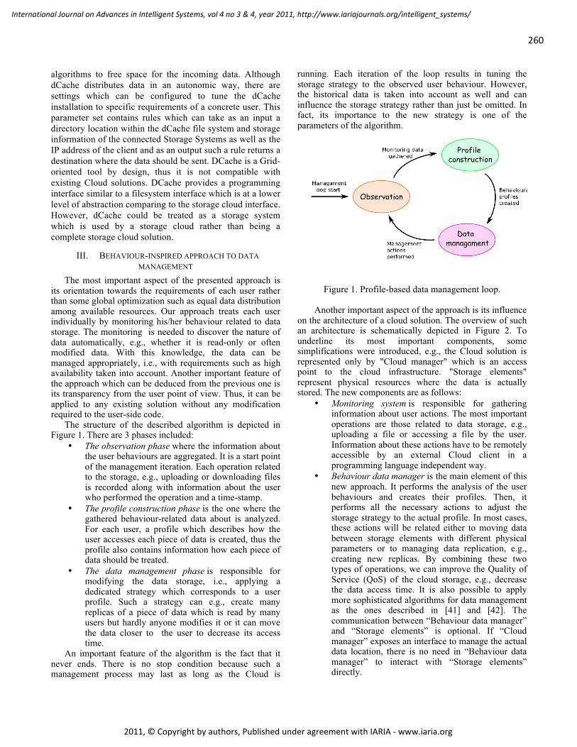
260



algorithms to free space for the incoming data. Although dCache distributes data in an autonomic way, there are settings which can be configured to tune the dCache installation to specific requirements of a concrete user. This parameter set contains rules which can take as an input a directory location within the dCache file system and storage information of the connected Storage Systems as well as the IP address of the client and as an output such a rule returns a destination where the data should be sent. DCache is a Grid-oriented tool by design, thus it is not compatible with existing Cloud solutions. DCache provides a programming interface similar to a filesystem interface which is at a lower level of abstraction comparing to the storage cloud interface. However, dCache could be treated as a storage system which is used by a storage cloud rather than being a complete storage cloud solution.

III. BEHAVIOUR-INSPIRED APPROACH TO DATA MANAGEMENT

The most important aspect of the presented approach is its orientation towards the requirements of each user rather than some global optimization such as equal data distribution among available resources. Our approach treats each user individually by monitoring his/her behaviour related to data storage. The monitoring is needed to discover the nature of data automatically, e.g., whether it is read-only or often modified data. With this knowledge, the data can be managed appropriately, i.e., with requirements such as high availability taken into account. Another important feature of the approach which can be deduced from the previous one is its transparency from the user point of view. Thus, it can be applied to any existing solution without any modification required to the user-side code.

The structure of the described algorithm is depicted in Figure 1. There are 3 phases included:

• The observation phase where the information about the user behaviours are aggregated. It is a start point of the management iteration. Each operation related to the storage, e.g., uploading or downloading files is recorded along with information about the user who performed the operation and a time-stamp.

• The profile construction phase is the one where the gathered behaviour-related data about is analyzed. For each user, a profile which describes how the user accesses each piece of data is created, thus the profile also contains information how each piece of data should be treated.

• The data management phase is responsible for modifying the data storage, i.e., applying a dedicated strategy which corresponds to a user profile. Such a strategy can e.g., create many replicas of a piece of data which is read by many users but hardly anyone modifies it or it can move the data closer to the user to decrease its access time.

An important feature of the algorithm is the fact that it never ends. There is no stop condition because such a management process may last as long as the Cloud is

running. Each iteration of the loop results in tuning the storage strategy to the observed user behaviour. However, the historical data is taken into account as well and can influence the storage strategy rather than just be omitted. In fact, its importance to the new strategy is one of the parameters of the algorithm.

Figure 1. Profile-based data management loop.

Another important aspect of the approach is its influence

on the architecture of a cloud solution. The overview of such an architecture is schematically depicted in Figure 2. To underline its most important components, some simplifications were introduced, e.g., the Cloud solution is represented only by "Cloud manager" which is an access point to the cloud infrastructure. "Storage elements" represent physical resources where the data is actually stored. The new components are as follows:

• Monitoring system is responsible for gathering information about user actions. The most important operations are those related to data storage, e.g., uploading a file or accessing a file by the user. Information about these actions have to be remotely accessible by an external Cloud client in a programming language independent way.

• Behaviour data manager is the main element of this new approach. It performs the analysis of the user behaviours and creates their profiles. Then, it performs all the necessary actions to adjust the storage strategy to the actual profile. In most cases, these actions will be related either to moving data between storage elements with different physical parameters or to managing data replication, e.g., creating new replicas. By combining these two types of operations, we can improve the Quality of Service (QoS) of the cloud storage, e.g., decrease the data access time. It is also possible to apply more sophisticated algorithms for data management as the ones described in [41] and [42]. The communication between “Behaviour data manager” and “Storage elements” is optional. If “Cloud manager” exposes an interface to manage the actual data location, there is no need in “Behaviour data manager” to interact with “Storage elements” directly.

261



• Profile knowledge base is a repository where the historical profiles for each piece of data are stored along with a record of each performed action. Thus, it can be used by the "Behaviour data manager" to take into account not only the most recent information but also the previous actions.

As we can see, the approach can be easily integrated with any Cloud solution which can be monitored, i.e., each performed operation related to the storage is registered, and the stored data can be moved between available physical resources, either indirectly with an exposed programming interface or directly with accessing storage elements and moving raw data. These requirements are rather easy to meet and in the next section we are presenting an example implementation based on a popular open source Cloud solution. It is also worth mentioning that in most cases the original source code of such a Cloud solution may stay untouched.

IV. USAGE PROFILE The presented approach highly exploits usage profiles

which are based on the observation of the actions performs by Cloud users. In our approach, a usage profile describes how a concrete piece of data in the Cloud is used by customers within a specified period of time in a quantitative way. The quantitative nature of usage profiles is a must in order to enable comparison of usage profiles. We would like to represent each usage profile as an element of a N-dimensional space where N denotes the number of usage profile parameters. By doing so, we can determine the relationship between each two profiles, e.g., whether they are similar, i.e., close to each other or not.

Such a profile aims at describing a behaviour pattern for a piece of data to which the profile is assigned. Thus, it can be treated as a kind of metadata for the actual data stored in a

Cloud storage. The necessary data for creating usage profiles is obtained with a dedicated monitoring system. On the other hand, we have a set of behaviour classes which define typical usage patterns in the domain of data storage, e.g., read-only data. In our representation in an N-dimensional space, each behaviour class will be represented by distinct subspaces of the entire space. Thus, we will be able to easily determine to which subspace each usage profile belongs.

The behaviour classes should be defined either by experts of the data storage domain or experienced administrators of storage solutions. To each behaviour class, a set of proper actions is assigned concerning the usage pattern which is described by the class. After creating a usage profile for a given data object, the nearest behaviour class is chosen. Then, the assigned set of data management actions is performed in order to increase desired quality parameters of the Cloud, e.g., throughput, data availability or data access time. Which quality parameters will be increased depends on the behaviour classes and data management actions assigned to the behaviour classes. This algorithm is performed periodically in a loop with a configurable interval between iterations.

For a system prototype, we defined the following parameters which will be included in usage profiles:

• frequency of access to an object, e.g., per hour or per iteration of the algorithm loop,

• number of read/write operations, • number of different users accessing to the object

(separately for read/write operations), • number of different places (e.g., IP addresses) from

which the object was accessed (separately for read/write operations).

Based on these parameters a set of predefined behaviour

Figure 2. Architecture overview of a cloud solution with “Behaviour data manager” involved.

262



classes can be created. They should correspond to the well known storage management patterns, e.g., when an object is always read, it should be replicated to multiple physical locations to decrease the access time.

Such a profile is created for each piece of data in the cloud storage (e.g., file) after the first iteration of the algorithm and updated on each subsequent iteration. In each “Data management” phase, for each profile a similarity function to each defined profile type is calculated. Then, the actions related to the most similar profile type are performed.

Therefore, the approach can be easily extended in terms of recognized behaviour, simply by defining new behaviour classes along with related actions.

V. IMPLEMENTATION To present a sample implementation of the approach, we

chose the Eucalyptus system as a basis. This choice was motivated by the large popularity of Eucalyptus and its functionality in terms of storage which is very similar to the Amazon S3 offer, a de facto standard in the Cloud industry.

The Eucalyptus architecture contains a component called "Walrus" which is responsible for the storage-related functionality. "Walrus" exposes an API which comprises

methods for creating, updating, and removing objects and buckets from the Cloud storage.

The open version of Eucalyptus implements cloud storage as a designated directory on the local file system. It is rather a minimalistic solution of the Cloud storage, due to very limited ways of data distribution. A feasible way is to mount a distributed file system at the designated directory which will transparently distribute data among a number of storage elements. Unfortunately such a solution does not allow to control data manipulation which cannot be accepted in our situation. Therefore, we extended the storage system in Eucalyptus by an ability to store data in several directories instead of one only, each of which can point to a different physical location, e.g., via NFS. With this extension, the location of the data can be easily controlled, simply by moving files between directories.

As mentioned above, there are a few components to add to the Eucalyptus architecture in order to implement the approach under discussion. Such an extended architecture is depicted in Figure 3. There is the "Walrus" component which exposes an API to external users for storing data in the Cloud. Apart from storing the custom data, e.g., results coming from a running simulation, "Walrus" stores two other types of objects. The first one is a VM image which is uploaded by the user and then is run on the Eucalyptus

Figure 3. Eucalyptus system architecture extended by “Behaviour Data Manager”, “Profile KnowledgeBase”, “Monitoring system”, and “Distributed storage component”.

263



infrastructure. Although, the user communicates with another component, called "Cloud controller", the images are actually stored with "Walrus". The second type of objects is "Block storage". It is used as a mountable partition to store data during a VM run, similarly to a local file system. Moreover, a "Block storage" object can store data between two subsequent runs of a VM and as opposed to a VM virtual disk, the data is not erased after a VM shutdown. Such a partition is stored within the Cloud storage with "Walrus". All these three types of objects are stored with "Walrus" on the same rules and thus can be uniformly managed with our system.

In the following subsections, we describe the implementation of the previously mentioned components, i.e. a monitoring system, the behaviour data manager and the profile knowledge base. However, in order to implement these components we had to extend the Eucalyptus implementation to support the distributed storage and to provide some additional information about storage-related operations when they occur.

When designing the extension to Eucalyptus, we focused on making it as non-intrusive as possible. Thus, we decided to replace an existing implementation of a Java class responsible for storing the data to the storage resources. By doing so, we can activate this functionality with few modifications to the Eucalyptus source code.

A. Storage-related operation monitoring The first of the additional elements added to the

architecture is a dedicated “Monitoring system”. It consists of “Log analyzer” which periodically reads the Walrus log where each storage-related operation is recorded and a relational database where information who and which operation performed are stored. Thus all the necessary data to create usage profiles is prepared in a technology neutral form.

The Walrus component logs an occurrence of each storage-related operation to a common log file, i.e., create and delete buckets, put, get and delete objects from buckets. A log entry which corresponds to a storage-related operation contains information about the type of operation, the user who performs the operation and information about the subject of the operation. A sample entry describing a putObject operation is depicted below:

07:53:32 INFO 342 WalrusRESTBinding | <?xml version="1.0" encoding="UTF-8"?> | <euca:PutObjectType xmlns:euca="http://msgs.eucalyptus.com"> | <euca:WalrusDataRequestType> | <euca:WalrusRequestType> | <euca:EucalyptusMessage> | <euca:correlationId>58b85aeb-29f4-4125-8f60-da95baa4422e</euca:correlationId> | <euca:_return>true</euca:_return> | </euca:EucalyptusMessage> | <euca:accessKeyID>WKy3rMzOWPouVOxK1p3Ar1C2uRBwa2FBXnCw</euca:accessKeyID> |<euca:timeStamp>2011-06-11T05:53:32.006Z</euca:timeStamp>

| <euca:bucket>testing_bucket_1</euca:bucket> | <euca:key>file_1024_5</euca:key> | </euca:WalrusRequestType> | <euca:randomKey>testing_bucket_1.file_1024_5.Dpq-OXrOgNtjnQ..</euca:randomKey> | </euca:WalrusDataRequestType> | <euca:contentLength>1024000000</euca:contentLength> | <euca:metaData/> | <euca:accessControlList> | <euca:grants/> | </euca:accessControlList> | <euca:contentType>binary/octet-stream</euca:contentType> | </euca:PutObjectType>

Every entry has a structure similar to an XML document

where data is put within tags which describe the semantic of the data, e.g., <euca:timeStamp>2011-06-11T05:53:32.006Z</euca:timeStamp>.

The monitoring system is implemented with the Python programming language. It uses mainly the standard library of Python to parse and retrieve relevant information from Cloud log files. The monitoring system analyzes the size of a log file in a loop to find out whether or not the file contains new information. If the size of the file grows between two iterations, the monitoring system analyzes only this additional data. Using a regular expression, the storage-related operations are extracted.

Whenever the monitoring system parses a log entry which describes a storage-related operation, it inserts information about this fact to a shared relational database which acts as the Profile Knowledge base. To connect with the database, the MySQLdb Python connector is used. The schema of the knowledge base is depicted in Figure 4. There are several tables which are filled with monitoring information. Most of them are self-explanatory. The “Users”, “Buckets” and “Objects” tables contain information on the elements, i.e., buckets and objects, stored in Eucalyptus Cloud and on the users of the cloud. The information about the performed storage-related operations are stored in the “BucketOperationHistory” and “ObjectOperationHistory” tables. The “Operations” table contains information about possible types of operations.

B. Behaviour-inspired Data Manager While the monitoring system gathers information about

the state of a Cloud, another component called “Behaviour-inspired Data Manager” analyzes this information and manages the data stored in the Cloud.

The Data Manager performs the following actions periodically on the information gathered by the monitoring system:

• create usage profiles for each stored object, • classify the usage profiles to one of the defined

behaviour classes, • manage stored objects based on actions which are

assigned to behaviour classes.

264



The procedure of creating usage profiles is in counting different types of operations performed on each stored object by different users. Currently, a usage profile consists of information about the performed puts and gets operations and the number of different users who have accessed the object over a period of time. Each created usage profile is stored in the “UsageProfile” table in Profile Knowledge Base with information about the time period to which the profile refers. The second step of the management process is the classification. Each usage profile created in the previous step is assigned to one of the defined behaviour class. In the presented prototype, behaviour classes are defined manually by a Cloud administrator. Each behaviour class refers to a management pattern which will be exploited in the next phase. For testing purposes, we defined three sample classes for describing three main behaviour patterns:

• “Read-only” class which describes objects which are mostly read,

• “Write-only” class which describes objects which are often changed,

• “Nothing-do” class which describes objects which

are hardly used. Each class is defined in the Profile Knowledge base as a

tuple <typical_number_of_gets, typical_number_of_puts, typical_number_of_users>. Based on the created usage profiles and behaviour classs, the Data Manager calculates Euclidian distances between profiles and classes and assigns the nearest class to each stored object.

The last phase is the phase where the actual management actions take place. After the classification phase, each object stored in the Cloud has a behaviour class assigned. Each behaviour class refers to a management pattern which is a set of actions which should be performed in a situation described by the behaviour class. To present the idea, we provided sample actions for each of the previously defined behaviour classes:

• Create a new replica of a “read-only” object, • Remove one of the existing replicas of a “write-

only” object. Also if the user number is equal to one then move the “write-only” object closer to the client.

• Do nothing for a “nothing-do” object. The replication is a common mechanism for increasing

Figure 4. Data model schema of a relational database which constitutes the Profile Knowledge base.

265



read performance for files which are often read. By changing the replication level of a stored object dynamically, we can respond to changes in the object usage.

To implement the Behaviour-inspired Data Manager we used the Ruby programming language along with a few common Ruby libraries (called Ruby Gems) such as:

• ActiveRecord for Object-Relation mapping, • YAML for reading configuration files, • ftools for manipulating files in a file system.

C. Profile Knowledge Base The Profile Knowledge Base provides a shared data

model for the monitoring system and the data manager components. It is implemented as a relational database whose schema is depicted in Figure 4.

By sharing a common data model, the monitoring system and the data manager can be implemented as loosely coupled components. Also, the shared data model allows to easily attach new components to the system in the future. The presented prototype of the system is based on the MySQL database [40].

VI. EXPERIMENTAL EVALUATION In order to evaluate the implemented prototype, a proper testing infrastructure has been configured and a number of tests were performed. The evaluation aimed at finding how the proposed system influences Cloud performance.

A. Testing environment Testing environment is a very important aspect of the

experimental evaluation. Thus, we prepared a sample configuration for building a small Cloud installation based on a blade-class cluster nodes and a disk array. As a base server for an extended version of the Eucalyptus cloud we use a worker node with the following parameters:

• 2x Intel Xeon CPU L5420 @ 2.50GHz (4 cores each)

• 16 GB RAM • 120 GB hard drive (5400 RPM) • Ubuntu Linux 10.04.1 LTS

Apart from the Cloud front end where the Cloud controller and Walrus components were installed, we also have three similar nodes for running virtual machines connected with the front end by Gigabit Ethernet. However, a more interesting part of the environment is the storage. As the main storage resource for our Cloud installation we used part of a disk array accessible via iSCSI protocol, of 6 TB capacity. Such a disk array, however, with a greater storage capacity available, could be used in a production cloud. As an additional storage, we decided to use hard drives from additional worker nodes which are exposed via the NFS protocol. To summarize, we depicted a map of the testing environment in Figure 5. In our opinion, the presented environment can be effectively used to evaluate different storage strategies because it contains heterogeneous storage resources such as hard drives and disk array distributed

among a few machines all being connected with open protocols and a commodity network fabric.

Figure 5. A map of physical resources which constitute a

testing environment.

B. Testing scenario Due to the limited throughput of the network interface

from each worker node (1 GbE) which is lower than the overall throughput of the available storage devices, we had to configure the Cloud in a specific way. We decided to use the three storage nodes as a Cloud storage back end and the disk array as a user device, i.e., a device to which users download data. Using this configuration we were able to show the positive influence of the “Behaviour-inspired Data Manager” on the data access time stored in the Cloud despite the limited network throughput. It is worth mentioning that such a configuration was feasible to prepare using our extension to the Eucalyptus Cloud which supports distributed storage.

To compare a standard Eucalyptus installation with an installation supported with the behaviour-inspired Data Manager, we prepared a test case which focused on the read operation to check the dynamically increasing replication feature. In this scenario, we assume there are three files stored in the Cloud of the same size which equals 5 GB. The number and size of the files were selected to obviate the cache mechanism of the storage resources. The files were downloaded several times by a number of users simultaneously. We ran the test case starting with 1 user and ending with 10 users. Also, each test case was performed three times and a mean value was calculated to abate possible noises within the infrastructure during tests.

C. Evaluation results The results obtained from the above described test case

are presented in Figure 6. The chart in this figure presents overall data read time for each number of users. As long as

266



the number of users is less than 5, the overall data read time is similar for both Cloud installations: with and without support from the Behaviour-inspired Data Manager. This similarity is anticipated since the Data Manager reacts only in the situations described by behaviour classes. In our case, we only defined behaviour classes for read-only and write-only data objects. Since the number of users, less than 5, do not generate enough workload, the Data Manager was virtually idle. . Then, for 5 users and more, the observed usage of each data object is classified as relevant to the read-only object. Thus, the Data Manager replicated data objects among available storage resources. This operation reduces data read time.

The mean gain from using the Behaviour-inspired Data Manager for more than 5 users is about 10% which is pretty high due to the limited throughput of physical network interfaces in the Cloud installation. Moreover, the measurements from different series for the same number of users were very similar and repeatable which implies that both presented solutions: support for distributed storage and the Behaviour-inspired Data Manager are stable.

VII. FUTURE WORK While the presented prototype is fully functional, there is

still some place for enhancements. From the conceptual point of view, the approach lacks of a well-defined set of behaviour classes along with related actions. However, these classes will be crystallized during real life tests when the behaviour of the real users will be observed and analyzed.

Also, the implementation of the described components can be improved. The monitoring system will be extended with analysis of semantic relationship between observed

storage-related operations. Such an analysis will lead to detection of different performance issues. The Data Manager will be extended by analysis of trends in storage-related operations. An analysis of such trends will enable the Data Manager to perform more suitable management actions. Additionally, we plan to include some AI-based mechanisms to discover new management actions based on the observed behaviour.

VIII. CONCLUSIONS Although, there are several open source Cloud solutions

available today, none of them provide a storage system which would be able to adapt to the user needs automatically. Instead, only basic functionality, e.g., storing VM images or custom objects is supported. The approach presented in the paper aims at providing a sophisticated data management functionality which would be flexible enough to be applicable to different Cloud solutions and which would manage data according to observed behaviour of Cloud users. We have presented the main assumptions of the approach along with phases of the management process. As an example of its implementation a prototype version of the system based on Eucalyptus is described. Due to the limited functionality of the Eucalyptus system, an extension which provides a real distributed data storage to multiple locations has been implemented.

The performed tests show positive influence of the described components on the performance of the Cloud in common use cases. The tests prove also the stability of the implemented prototype.

Figure 6. Summary read time of 3 files (5 GB each) for each user for different number of users.

267



ACKNOWLEDGMENTS This research is supported partly by the European

Regional Development Fund program no. POIG.02.03.00-00-007/08-00 as part of the PL-Grid Project. The authors are grateful to prof. Jacek Kitowski for valuable discussions.

REFERENCES [1] Krol, D., Slota, R., Funika, W., „Behaviour-inspired Data

Management in the Cloud“, in: Proc. of CLOUD COMPUTING 2010 The First International Conference on Cloud Computing, GRIDs, and Virtualization November 21-26, 2010 - Lisbon, Portugal, IARIA, 2010, pp. 98-103.

[2] Foster, I., and Kesselman, C. (Eds.), “The Grid: Blueprint for a New Computing Infrastructure”. Morgan Kaufmann Publishers Inc., San Francisco, CA, USA, 1998.

[3] Cloud Computing – Google: The Best Cloud Computing Investment. [on-line: http://www.cloudtweaks.com/2010/02/cloud-computing-google-the-best-cloud-computing-investment/, as of June 13, 2011].

[4] Han, J.H., Lee, D.H., Kim, H., In, H. P., Chae, H.S., and Eom Y.I., “A situation-aware cross-platform architecture for ubiquitous game”, Computing and Informatics, vol. 28(5) (2009) 619- 633.

[5] Amazon Elastic Compute Cloud (Amazon EC2). Amazon Inc., 2008, [on-line: http://aws.amazon.com/ec2, as of June 13, 2011].

[6] Microsoft Windows Azure Platform (Windows Azure). Microsoft, 2010 [on-line: http://www.microsoft.com/windowsazure/, as of June 13, 2010].

[7] Google AppEngine. Google Inc., 2008 [on-line: http://code.google.com/intl/pl-PL/appengine/, as of June 13, 2011].

[8] Google Apps website [online: http://www.google.com/apps/intl/en-GB/business/index.html, as of June 13, 2011].

[9] Amazon EC2 instances [on-line: http://aws.amazon.com/ec2/instance-types/, as of June 13, 2011].

[10] Eucalyptus Systems Inc. [on-line: http://www.eucalyptus.com/, as of July 24, 2010]/

[11] Amazon Simple Storage Service (Amazon S3). Amazon Inc. [on-line: http://aws.amazon.com/s3/, as of June 13, 2011].

[12] Apache Axis website [on-line: http://ws.apache.org/axis/, as of June 13, 2011].

[13] Google Web Toolkit website [on-line: http://code.google.com/intl/pl-PL/webtoolkit/, as of June 13, 2011].

[14] P. Barham, B. Dragovic, K. Fraser, S. Hand, T. Harris, and A. Warfield, "Xen and the art of virtualization," in SOSP '03: Proceedings of the nineteenth ACM symposium on Operating systems principles. New York, NY, USA: ACM, 2003, pp. 164-177 [on-line: http://dx.doi.org/10.1145/945445.945462, as of June 13, 2011]

[15] Kernel-based Virtual Machine project wiki [on-line: http://www.linux-kvm.org/page/Main_Page, as of June 13, 2011].

[16] Lustre filesystem wiki [on-line: http://wiki.lustre.org/index.php/Main_Page, as of June 13, 2011].

[17] Oracle Cluster File System 2 (OCFS2) project website [on-line: http://oss.oracle.com/projects/ocfs2/, as of June 13, 2011].

[18] Eucalyptus Enterprise version website [on-line: http://www.eucalyptus.com/products/eee, as of June 13, 2011].

[19] Introduction to Storage Area Networks, IBM redbook, [online: http://www.redbooks.ibm.com/abstracts/sg245470.html? Open, as of April 16, 2011].

[20] Kielmann, T., “Cloud computing with Nimbus”, March 2009, EGEE User Forum/OGF25 & OGF Europe's 2nd International Event.

[21] Globus Alliance website [on-line: http://www.globus.org/, as of June 13, 2010].

[22] Foster, I., Frey, J., Graham, S., Tuecke, S., Czajkowski, K., and Weerawarana, S., “Modeling Stateful Resources with Web Services”, 2004 [on-line: http://www.ibm.com/developerworks/library/ws-resource/ws-modelingresources.pdf, as of June 13, 2010].

[23] NASA Nebula website [on-line: http://nebula.nasa.gov/, as of April 16, 2011].

[24] RackSpace CloudFiles solution website [on-line: http://www.rackspace.com/cloud/cloud_hosting_products/files/, as of April 16, 2011].

[25] OpenStack project website [on-line: http://www.openstack.org, as of April 16, 2011].

[26] G. Behrmann, P. Fuhrmann, M. Gronager, and J. Kleist, “A distributed storage system with dCache”, in G .Behrmann et al Journal of Physics: Conference Series, 2008.

[27] Flash Cloud web. [on-line: http://www.flashcloudstorage.com/, as of June 13, 2010]

[28] Spring Framework website [on-line: http://www.springsource.org/, as of June 13, 2010].

[29] Java database website [on-line: http://developers.sun.com/javadb/, as of June 13, 2010].

[30] B. Sotomayor, R. S. Montero, I. M. Llorente, and I. Foster, "Capacity Leasing in Cloud Systems using the OpenNebula Engine." Cloud Computing and Applications 2008 (CCA08), 2009.

[31] VMware website [on-line: http://www.vmware.com, as of June 13, 2010].

[32] RESERVOIR project website [on-line: http://62.149.240.97/, as of June 13, 2010].

[33] F. Hupfeld, T. Cortes, B. Kolbeck, E. Focht, M. Hess, J. Malo, J. Marti, J. Stender, and E. Cesario. “XtreemFS - a case for object-based file systems in Grids.”, In: Concurrency and Computation: Practice and Experience. vol. 20(8) (2008).

[34] VMware Virtual Appliances website [on-line: http://www.vmware.com/appliances/getting-started/learn/, as of June 13, 2010].

[35] Network File System version 4 protocol specification [on-line: http://tools.ietf.org/html/rfc3530, as of June 13, 2010].

[36] Logical Volume Management 2 (LVM2) website [on-line: http://sourceware.org/lvm2/, as of June 13, 2011].

[37] Internet Small Computer Interface (iSCSI) RFC document [on-line: http://www.ietf.org/rfc/rfc3720.txt, as of June 13, 2011].

[38] Web Distributed Authoring and Versioning (WebDAV) RFC document [on-line: http://www.ietf.org/rfc/rfc3744.txt, as of June 13, 2011].

[39] EVault Data Backup Software website [on-line: http://www.i365.com/products/data-backup-software/evault-backup-software/, as of June 13, 2011].

[40] The MySQL database website [on-line: http://www.mysql.com/]. [41] Slota, R., Nikolow, D., Kuta, M., Kapanowski, M., Skalkowski, K.,

and Kitowski, J., “Replica Management for National Data Storage”, Proceedings PPAM09, LNCS6068, Springer, 2010, in print.

[42] Slota, R., Nikolow D., Polak, S., Kuta, M., Kapanowski, M. , and Kitowski, J., "Prediction and Load Balancing System for Distributed Storage", Scalable Computing Practice and Experience, 2010, in print.

268



Business-Policy driven Service Provisioning in HPC

Eugen Volk

High Performance Computing Center Stuttgart (HLRS)

Stuttgart, Germany

volk @ hlrs.de

Abstract—Service provisioning in High Performance

Computing (HPC) is typically defined in the way that

implicitly corresponds to business policies of the HPC

provider. Business policies, represented by business rules,

objectives or directives, form means to guide and control the

business of HPC service provisioning, affecting

interdependently resource-management, SLA-management,

contracting, security, accounting, and other domains. As

business policies in HPC domain exist mostly implicitly,

administrators configure resource management systems mostly

intuitively and subjectively. This makes it hard for business

people to assess whether business polices are consistent, and

resource management behavior corresponds to business

policies (and vice versa), as no linkage between business

policies and scheduling policies is defined yet. In this paper we

analyze relationships between business policies and resource

management behavior, (1) presenting approach allowing to

investigate how business policies and scheduling policies relate

together, (2) identifying sources and key-factors influencing

scheduling behavior, (3) describing relationships between those

key-factors, and (4) using Semantics of Business Vocabulary

and Business Rules (SBVR) for definition of business policies

and transformation rules, capable to translate business policies

into scheduling policies.

Keywords - Business-Policy; Job-Scheduling; Policy-based

Management; Policy-refinement; Business-Driven IT

Management; SBVR.

I. INTRODUCTION

Service provisioning in High Performance Computing (HPC), reflected mostly by Job-Scheduling behavior, is typically defined in the way that implicitly corresponds to business policies of the HPC provider [1]. Business policies represented by business objectives, rules, or directives, form means to guide and control provisioning of HPC resources and services managed by a resource management system (RMS), which is responsible for resource management, job queuing, job scheduling and job execution. Business policies affect interdependently several domains involved in HPC service provisioning, such as SLA-management, contracting, resource-management, security, accounting, and others, and, might have direct or indirect influences on job-scheduling. For instance, a business policy, such as “all jobs of premium customers have to be started within 4 hours” has direct influence on scheduling, by determining the latest start of the job. In contrast, a business policy that demands “no violation

of Quality of Services for platinum customers” may lead to higher priority of jobs of platinum customers, or to pre-allocation of resources dedicated to this customer’s group. However, business-policies in HPC domain exist in most cases not explicitly, i.e., written by using domain specific language or natural language, but implicitly in the mind of the business people, whereas the configuration of resource-management-systems, in particular job-scheduler, is done by administrators.

The range of existing schedulers used for job scheduling in HPC varies from time based scheduler like Cron [4] to advanced policy-based schedulers like Moab [3] or its open-source variant Maui [2], which support large array of scheduling policies. Scheduling policies define thereby behavior of the scheduler by, i.e., assigning priority to a job depending on job-size (number of CPUs or cores required), estimated job-duration, user’s priority and other factors. However, schedulers have a big amount of parameters and different scheduling policies which need to be selected and adjusted in order to meet business policies in different situations.

A problem occurs when administrators are configuring resource management systems, especially job-schedulers. The configuration of schedulers is done in most cases intuitively and subjectively, because of implicit business policies, system administrators unaware of them, or in general, because of missing link or mapping between business policies and selection and configuration of scheduling policies. This makes it hard for business people to assess whether current resource management behavior corresponds to business policies and vice versa, as no link between business policies and resource management is defined yet.

In our previous work [1] we presented approach allowing investigate how business policies influence scheduling policies. In this paper we apply this approach analyzing relationships between business policies and resource management system, (1) identifying sources and key-factors influencing scheduling behavior, (3) describing relationships between business policies, those key-factors and scheduling policies, and (4) using Semantics of Business Vocabulary and Business Rules (SBVR) for definition of business policies and transformation rules, capable to translate business policies into scheduling policies.

This paper is structured as follows. Section II presents

related work in the area of job scheduling in HPC, SLA

269



based scheduling, policy-based management, business

driven IT management, and semantics for description of

business policies and business rules. Section III provides

background information on job-scheduling in HPC. In

Section IV we discuss the problem related to alignment of

scheduling behavior with the business policies, showing the

need for business-policy-based job-scheduling in HPC.

Section V presents approach allowing investigating how

business-policies relate to the job-scheduling in HPC and

solve the problem described in previous section. Section VI

analyzes influence of job-scheduling behavior on business

metrics, identifying key-factors and relationships between

scheduling policies, scheduling objectives, performance

metrics and business metrics. In Section VII we analyze

relationships between business metrics and business

policies, identifying influences of business policies on job-

scheduling, including relationships between different

domains, such as SLA-management, Security, Accounting,

etc. Finally, in Section VIII we present approach allowing

expressing business policies in HPC using Semantics of

Business Vocabulary and Business Rules (SBVR),

providing examples for description of business policies. The

last section summarizes this paper and outlines work in

progress and future work.

II. STATE OF THE ART

In the target-area of “business-policy based resource-management/scheduling in HPC” currently no work is known to the author. However, there exists work in related areas, presented in the subsequent paragraphs.

Much research was done in job-scheduling in HPC domain, concerned on development and investigation of scheduling policies characterized by performance metrics, such as utilization, response-time, job-throughput, QoS violation, etc.. Feitelson et al. assessing several scheduling policies for parallel jobs, elaborating/identifying scheduling criteria and performance metrics [25][26]. Iqbal, Gupta and Fang [6] offer an overview about scheduling algorithms used for job-scheduling in HPC clusters. In [7], Casavant and Kuhl provide taxonomy of scheduling strategies in general-purpose distributed computing systems. In [8], Yeo and Buyya provide taxonomy of market-based resource management system, citing over 79 references. In [9], Abawajy describes recent advances in efficient adaptive scheduling policies. Achim Streit [27][28] investigated several job-scheduling policies for HPC dolmans, assessing their influence on utilization and response-time and developing adaptive-scheduling dynP algorithm which selects different scheduling policies, based on mean duration of all jobs in the job-queue. Proposed approach to “business policy based resource-management in HPC” uses scheduling criteria and performance metrics from job-scheduling in HPC area to elaborate linkage between scheduling policies, performance metrics and business level objectives.

In the area of SLA-based job-scheduling many papers have been published. SLA is part of a mostly short term service contract where the level of services or quality of

services (QoS) is formally defined and agreed between service providers and customers. SLA contains usually rewards, for successful fulfillment of SLA, and penalties in case of SLA violations. SLAs are contracted in accordance with business-policies. Business-Policies prescribe kind of services and QoS which can be offered principally to the customer. Hence, SLAs can be considered as service level objectives contracted in accordance with the business-policies. On the other hand, business-policies are more prescriptive than SLAs, as SLA might be violated due to various reasons, but the behavior in a company must follow provider's business-policy. In [12][13][14][15], QoS and SLAs are used to find and allocate desired resources in quantity and quality, and determine priority and order of jobs for scheduling, among others, based on rewards and penalties declared in SLAs. In [13], authors describe how to derive IT management policies from SLAs, which in general follows autonomic computing approach (management by objectives).

Policy based management (PBM) aims at separation of rules and objectives governing the behavior of a system from its functionality [10]. Today, PBM is part of several management architectures and paradigms, including SLA-driven and business-driven management [10]. Many solutions in the area of policy-based management have been proposed since 1960 to present. In [10], Boutaba and Aib provide history of policy-based management, referencing over 118 papers. In IBM’s autonomic computing reference architecture [11], the authors drafted the principle on how policies on high level might be used to express business needs/objectives that govern IT infrastructure operations. In IBM's Whitepaper [16] authors provide most recent definitions of policies and rules in business area, relating them to IT.

OMG’s Semantics of Business Vocabulary and Business Rules (SBVR) [30] in its version 1.0, is recent (2008) standard intended to define “the vocabulary and rules for documenting the semantics of business vocabularies, business facts, and business rules” [30], used for the description of complex compliance rules. SBVR is interpretable in predicate logic with a small extension in modal logic, enabling consistency checking between rules. The proposed approach to “business policy based resource-management/job-scheduling in HPC” uses SBVR for the description of business vocabularies, facts, and policies.

Business Driven IT Management (BDIM) aims at a holistic management of enterprise IT infrastructure and services efficiently from business perspective [21], i.e., by aligning IT management decisions with business level objectives coming from the providers themselves, and their users [22]. Methods as used in BDIM are “based on mappings between IT technical performance metrics and business relevant metrics and exploit the linkage to provide decision support to IT management so as to maximize business value and IT-Business alignment” [21]. Existing work in this area [21][22][23][25] relates mostly to alignment of business requirements coming from business processes, with the management of IT-infrastructure of the enterprise systems, thus, addressing non HPC environment.

270



Moura et al. [21] provide a research agenda for BDIM, reviewing BDIM concepts and proposing a framework to assist in defining and describing BDIM usage domains. Sauvé et al. [25] present approach allowing to calculate business loss due to unavailability and high response time of web-services, aiming at minimizing costs and loss. In contrast to mentioned work in BDIM, the proposed approach to “business-policy based resource-management in HPC” is focusing on resource-management in HPC domain, in particular on job-scheduling. Whereas BDIM approach is mostly oriented on optimization of IT-Infrastructure to achieve business goals, proposed approach to “business policy based resource-management in HPC” is aiming at checking consistency between business policies themselves, and, between business policies and selection of job-scheduling policies in HPC domain.

III. BACKGROUND

Computing center infrastructure consists of several

clusters used to provide computing resources to users. The

cluster infrastructure of computing centers can be divided in

two classes: high-throughput computing clusters and high

performance computing clusters [6]. Nodes in high

throughput computing clusters are usually connected by

low-end interconnections. In contrast, more powerful nodes

in high performance computing (HPC) cluster are

interconnected by faster interconnection with higher

bandwidth and lower latency. The application profile of

high-throughput computing clusters includes loosely

coupled parallel, distributed or embarrassingly parallel

applications, requiring less communication and

synchronization between nodes during the calculation. In

contrast, the application profile of HPC clusters consists

mainly of tightly coupled parallel applications, with high

communication and synchronization requirements.

The computing nodes in cluster are managed by a

resource management system (RMS), which is responsible

for resource management, job queuing, job scheduling and

job execution. Firstly, users who are willing to submit their

applications or programs to resource management system

need to express their applications as computational jobs,

specifying requirements using, i.e., Job Submission

Description Language (JSDL). Job specification contains

usually number of nodes/CPUs/cores required, estimated

maximum job-runtime, target architecture type (i.e., vector

or scalar), specific I/O requirements (i.e., tools and files

required for job execution) and other application- or

platform specific parameters. After expressing application

as a job, user submits the job in batch to queue of the

resource management system, where it waits in the queue

with the jobs of other users, until it is scheduled and

executed. The wait time of the job depends on job-priority,

system load, availability of requested resources and other

factors [6]. Typically, a resource management system is

comprised of a resource manager and a job scheduler [6].

Most resource managers have an internal, built-in job

scheduler, which can be substantiated by external scheduler

with enhanced capabilities [6], i.e., with support for various

scheduling policies like Maui [2]. Resource manager

provides scheduler with information about job-queues, loads

on compute nodes, and resource availability. Based on that

information, scheduler decides on how and when to allocate

resources for job execution. The decision of the scheduler

follows scheduling policy that determines the order in which

the competing users’ jobs are executed. The order of jobs

typically depends on job-size (amount of resources, i.e.,

processors/cores required), estimated maximum job-runtime

(indicated by user), resource access permission (established

by administrator), resources available, and might depend

additionally on QoS parameters (i.e., response time)

expressed in contracts or SLAs.

The assessment of scheduling behavior is typically done

according to various performance metrics

[6][8][18][27][28], the most well known are:

• Wait time: the time a job has to wait before the

execution of the job starts

• Response time: total time between when the job is

submitted and when the job is completed. It includes

wait time and execution time of the job.

• Resource Utilization: reflects the usage level of the

cluster system - what percentage of available

resources is used by jobs. Average resource

utilization is calculated by total amount of

resources/nodes used by all jobs within considered

time period, divided by that time period.

A good scheduling policy is aiming at high resource

utilization and short response times for the jobs, which are

two conflicting goals. Typical performance criteria for users

who expect minimal response time is the mean response

time [6]. In contrast, administrators are typically trying to

achieve maximum overall resource utilization, as that

maximizes profit. Improving overall resource utilization and

at the same time decreasing mean response time are two

conflicting goals, as short waiting times are achievable only

with low utilization [26]. Typically, scheduling policies that

optimize resource utilization prefer those jobs which need

many resources (large jobs) over long time period (long

jobs) [26]. However, this causes that short jobs requesting

few resources need to wait longer until long and large jobs

are finished. Contrary, scheduling policies preferring short

and small jobs would reduce the average response time [26].

Because job-size and job-length are varying from job to job,

as well as the job-submission rate, gaps in schedule occurs,

which are reflected by utilization drop [30]. The challenge

in design of scheduling policies is to find tradeoff between

optimizing these two (and other) mostly contradicting

performance metrics [26]. This tradeoff should be derived

from the business demands or business level objectives,

expressed in business policies. Hence, there is a need for a

preference specification, making tradeoff between

contradicting performance metrics, derived from business

objectives or demands.

271



IV. NEED FOR BUSINESS-POLICY-BASED JOB-SCHEDULING

Business policies are control statements that guide behavior in a company and control the business. Business policies are defined usually at an overall strategic level influencing and controlling various areas participating in business provisioning by setting business level objectives, rules and other constraints. In HPC domain, these areas are: security, contracts and SLAs, resource management, accounting, and others. Business policies, which relate to security, contain statements governing the access to HPC resources, i.e. prescribing the process of obtaining permission to HPC resources, granting, restricting or refusing the access, taking external regulation into account. Contract and SLA business policies describe the spectrum of HPC services offered principally, including Quality of Services (QoS) and capacity capabilities. Resource management business policies contain statements influencing resource allocation and scheduling behavior on a high level, by, i.e., prescribing the preferences between users-groups, tradeoffs between different performance metrics, scheduling optimization criteria, resource allocation strategies, and others.

As already mentioned, scheduling behavior is typically defined in the way that it implicitly adheres to business policies of the HPC providers, while taking users' job requirements, available resources, existing SLAs, long term contracts and other factors into account [1]. Advanced policy-based schedulers like Maui [2] have a big amount of parameters and different scheduling policies which need to be selected and adjusted in order to meet all business policies in different situations. As business policies exist mostly implicitly in the mind of people, or, because administrators are not really aware of all of them and their interrelationship with site-effects, administrators configure schedulers mostly intuitively and possibly subjectively. This makes it hard for business people to assess whether the actual scheduling behavior is correct and corresponds to current business policies, as there is no linkage between business policies and scheduling policies defined. Additionally, there might be new business policies, or a fast switch between different business policies required, affecting job-scheduling. Hence, for right configuration of job-scheduling behavior it is essential to understand:

• What are the business requirements that affect job-scheduling?

• Where are these requirements coming from?

• How are they influencing job-scheduling?

• Are there any conflicting requirements?

• What is/should be the tradeoff between conflicting requirements?

• On what is this tradeoff dependent? For instance, in profit oriented organizations, managers

try to achieve maximum profit, which often means that they deliver various quality of services (with specified expected response-time) to various users and groups [2], aiming at increasing system utilization at specified expected response time level. In contrast, nonprofit organizations, like computing centers at universities are delivering HPC

resources to various users and groups on best effort basis, neglecting response time, thus, focusing only on the overall resource utilization to increase amount of jobs completed. Some of the national computing centers affiliated to universities have joint collaboration with scientific and industrial partners through common joint cooperation company, offering HPC services with certain QoS level. That means the scheduling behavior in clusters of such computing centers needs to be adapted to various business needs, even at the same time, leading to differentiation between at least two different QoS service classes, e.g., silver class with specified expected response time, and, bronze class with best effort. Such requirement could lead to a higher prioritization of jobs of industrial users, comparing to jobs of students or scientific users. In addition to silver, and bronze, there might be gold service class offered for urgent computing, whose jobs are scheduled immediately preempting other jobs.

Furthermore, there are cases where the usual job-scheduling behavior must be adapted to changing situations and require evaluation of several business polices. Assuming there are at least two separated clusters – one for industrial users and, one for research users and students. In case of fall-out of the cluster on which jobs of industrial users are executed, these could be shifted to another cluster, if allowed. The answer on the question whether the jobs of industrial users might be shifted, e.g., to research cluster, on which jobs of students or researchers are executed, depends thereby on evaluation of several business policies and constraints. Research and educational clusters are typically financed by federal authority, whereas clusters used for industrial calculations are financed through common joint cooperation company. In case of the business policies, which prescribe that (1) industrial partners have higher importance than students or researchers, (2) only the owner (who has financed it) of the cluster decides on permissions, and (3) current federal land policy that impose to use research clusters only by researchers or students, then the shifting of industrial jobs to a research cluster is not allowed. Alternatively, if a business policy prescribes that (1) industrial partners have higher importance than students or researchers, (2) only the service provider decides on permissions, then shifting of industrial jobs to research cluster is allowed, it is even an obligation.

As stated, there are many different business policies from different areas, which need to be considered when configuring schedulers. Furthermore, there might be a fast switch between different business policies required, and a fast adaptation of the scheduling behavior dependent on evaluation of several business policies from different domains. Because of implicit existence of business policies and missing link between business policies and scheduling policies, there is a risk of resulting incorrect scheduling behavior.

V. APPROACH

An approach to handle problems described in previous section, induced by changing business objectives or altering situations, might follow IBM’s autonomic computing

272



reference architecture [11]. Autonomic computing is thereby defined “as a computing environment with the ability to manage itself and dynamically adapt to changes in accordance with business policies and objectives” [11]. Following this approach, there must be (1) business policies defined, capable to express business requirements influencing scheduling behavior on high level. Once, there are business policies defined, the next step (2) consist then of transforming these business policies with other sources (as SLA, Contracts, Accounting, etc.) influencing scheduling behavior into scheduling policies to configure advanced policy-based schedulers like Maui or Moab. In order to define business-policies explicitly, there must be HPC business policy specification language elaborated, capable to express business needs for various situations. In order to address this problem, we will follow a bottom-up process:

The first step (1) consists of the analysis of existing scheduling policies in HPC in order to identify: scheduling criteria used by scheduling policies, scheduling objective function which is approximated by scheduling policies, and performance metrics/indicators characterizing costs of scheduling. The first step includes also identification of relationships between the elements of scheduling. The results of the first step are described in Section VI.A. The next step (2) involves the analysis of performance metrics and their influence on business, metered by business metrics. Section VI.B presents results of the second step, describing business metrics and relationship to scheduling performance metrics. The outcomes of the first and second step are summarized in third step (3) as a model, presented in Section VI.C, identifying key-factors and their relationships influencing scheduling behavior, taking business metrics, scheduling performance metrics, scheduling policies, user-requirements, SLAs/contracts and resource-capacities into account. In the next step (4) we identify influence of business policies on business metrics and scheduling behavior, considering various sources of influence. The outcomes of the fourth step are summarized in Sections VII.A and VII.B, presenting relationships between business metrics and business policies, identifying sources of influence on job-scheduling behavior coming from various domains, including SLA-Management, Resource-Management, Security/License Management, etc. Especially the relationship between existing business policies, business metrics and scheduling policies will provide an overview on how policy refinement process of transforming business policies to scheduling policies might principally looks like. In the fifth step (5) we propose usage of Semantics of Business Vocabulary and Business Rules (SBVR) for description of business policies and transformational rules, capable to provide semantic framework for definition of vocabulary and business policies/rules (including business policy schema) used to describe business policies, consistence checking rules and transformational rules. Results of the fifth step are described in Section VIII, presenting examples describing business policy schema and transformation of business policies into scheduling policies using SBVR. Thereby we present examples for business policy schema, enabling description of business policies.

Finally, in order to evaluate results achieved in previously steps, the last step consists of the reference implementation, enabling mapping of reference business policies together with other key factors to scheduling policy configuration for advanced schedulers such as Moab [3] or Maui [2].

VI. FROM JOB-SCHEDULING-POLICIES TO BUSINESS-

METRICS, AND BACK

In this section we analyze the influence of job-

scheduling behavior on business. Firstly, we analyze job-

scheduling policies to identify relationship between

scheduling criteria, such as job-size, job-length, etc., and

scheduling performance metrics, such as utilization,

response-time, and others. In the second section, we analyze

influence of scheduling performance metrics on business,

identifying business metrics and their relationship to

performance metrics.

A. Analysis on Job-scheduling in HPC

Job-Scheduling algorithms can be divided in two

classes: time-sharing and space-sharing [6]. Time sharing

algorithms divide time on a processor into several slots,

each time-slot is assigned to unique job then. In contrast,

space-sharing algorithms assign requested resources

exclusively to unique job, until job is completed. In all HPC

clusters is space-sharing approach used, as time-sharing

approach increases synchronization overhead between nodes

of the same job.

According to Streit [28], Resource Management Systems

can be divided into queuing and planning systems,

depending on their planned time frame. Queuing systems try

to utilize currently free resources; in contrast planning

systems are not restricted to present time, but take also

future into account assigning resource-reservation to future

jobs. According to Feitelson and Rudolph [26], queuing

systems can be classified into on-line vs. offline, with online

subdivided into closed and open models. Off-line model

assumes that all jobs are available from the closed set of

jobs, with no later arrivals. In contrast, on-line model

assumes that jobs arrive over period of time. A closed on-

line model expects fixed set of jobs to be handled; in

contrast, open on-line model is characterized by endless

stream of jobs [26]. In HPC centers, open online model is

most commonly used, as it reflects real user-behavior –

continuous submission of jobs as a stream. Offline models

are used as well, for the processing of batch jobs during the

night or weekends.

Massive parallel systems as used in HPC are typically

operated in following way [25][28]: The system is divided

in partitions on which parallel jobs are executed. Thereby, a

partition consists of several nodes assigned to one or several

job-queues. The partitioning can be done according to job-

characteristics (i.e., job-size, job-length) and priorities (i.e.,

high-priority, best effort) [28]. Within a job-queue several

273



scheduling policies can be applied, FCFS is the most

commonly used scheduling-policy. Nodes of a partition are

assigned to different possible prioritized queues. Jobs in

prioritized queue are taken first to be executed on free

resources. Once a job is started with the requested number

of nodes, it is running until the job is completed [28].

According to Feitelson et al. [25] in [28], jobs can be

classified into rigid, moldable, evolving and malleable jobs.

Rigid and moldable jobs are depending on whether the

number of assigned resources to a job is decided by the

scheduler (moldable) or is fixed by the user at start-time

(rigid). Evolving jobs arise when applications go through

distinct execution-phases with changing amount of

resources, resulting in allocation of required resources in

each execution step [25]. Malleable jobs are those which are

capable to deal with changing system capacities, resulting in

an increase of decrease of resources to be used by a job. The

rigid jobs with fixed amount of required resources are the

most difficult for scheduling. In HPC, rigid jobs are mostly

used. As mentioned before, jobs have various requirements,

differing on quality (Memory, CPU-speed, IO-

bandwidth/latency), quantity (amount of resources –

typically number of cores/nodes) of resources and expected

run-time. However, the job-runtime is only estimated, as the

actual job-run-time depends on application-characteristics

such as number of nodes-used, speedup-factor, whether the

job is memory, CPU or IO bounded, and machine

characteristic on which jobs are executed.

According to Krallmann, Schwiegelshohn, and

Yahyapour [32] in [28], scheduler can be divided in three

parts: a scheduling policy determining allocation of

resources to jobs; objective function describing the cost of

the complete schedule, such as response-time, utilization,

job-throughput, etc., scheduling algorithm generating valid

schedule according to objective function. As optimal scheduling is NP hard problem, it requires

high computational effort to calculate perfect schedule. Approximation to optimal scheduling can be found in polynomial time, i.e., using specific heuristics as outlined below.

Job scheduling policies have two important phases [28]: 1. Putting jobs in the queue at submit time 2. Taking jobs out of the queue at start time

Putting jobs in the queue can be done by sorting jobs according to:

• Arrival time (FCFS) – the most known scheduling policy with fairness. The jobs that arrive later start later.

• Increasing estimated job-runtime (SJF). This strategy is aiming at minimizing mean response time. However, SJF is not fair strategy as longer job may be starved - failed to be scheduled.

• Decreasing estimated job-runtime (LJF). This strategy is aiming at resource utilization, as it acquires resources for longest possible time period hence for longest job. LJF is not fair, as shorter jobs may be starved.

• Increasing or decreasing number of requested resources. Decreasing strategy is aiming at maximizing resource utilization, as it acquires as much resources as possible, as required by the largest job. Increasing strategy is aiming at minimizing

• Increasing or decreasing used area of the job (estimated runtime * requested resources). Decreasing strategy is aiming at maximizing utilization, as it tries to allocate as much cpu-time for job as possible. Increasing strategy is aiming at minimizing mean response time while maximizing utilization.

• Increasing time to deadlines (EJF). This strategy is aiming at satisfying deadlines, to prevent any violation of contracts or SLAs.

• Given Job-weights: the higher the weight the higher the priority of the job is. Higher prioritized jobs are executed before the lower jobs. The job-weight can be based on customer importance, granting important customers’ shorter response-time.

• By the Smith ratio, that is defined as a ratio between job-weight and its area (run-time * required resources).

• And many other scheduling policies based on other criteria, and their mathematical or logical combination.

Taking jobs out of the queue can follow different strategies – here some examples [28]:

• “Always start the head of the queue.” Lack of resources to serve head job leads to delay of the other jobs, even if there are enough resources available. This approach is called front.

• “Search the queue from the beginning and take the first job that can be started immediately fitting given constraints” [28] - that fits into current schedule. This strategy is called FF – fist fit. It tries to optimize resource utilization, but has a drawback that in worst case a job can wait forever.

• Search the queue from the beginning and take the job that can be started immediately and leaves latest resources free. This strategy is called BF - best fit.

• Combination of several of these and other strategies is used to optimize and improve scheduling.

During the schedule there might be gaps between jobs– reflecting idleness of resources and indicating drop in resource utilization. In order to fill out these gaps and optimize utilization, two backfilling strategies exist [28]:

• Conservative backfilling selects only those jobs to fill out the gap, that are not delaying other waiting jobs in the queue. This is a predictive strategy that ensures fairness and increases utilization.

274



• EASY backfilling is more aggressive and selects those jobs to fill-out the gap that are not delaying the waiting-queue head. This is less predictive strategy, since only the scheduling of the head jobs is assured. In worst case, jobs may be starved.

Hence, simple scheduling algorithms might be enhanced by combining them with the use of advanced reservation and backfill techniques. Advanced reservation algorithms, as used in planning system, use estimated job-runtime to make reservation on resources for particular jobs and create time-schedule for certain time period. The problem thereby is that schedule is based on estimated job-runtime, which is in most cases much longer than the real one. That means the schedule needs to be adapted as soon as jobs are completed earlier than expected. The backfilling strategy improves basic strategies by combining them with additional iteration to fill out the gaps, as outlined previously. Given schedule on high priority jobs i.e., by applying LJF strategy, the scheduler use in second iteration lower priority jobs to fill out the gaps (free time slots on unused resources) between higher priority jobs.

As mentioned, the assessment of scheduling behavior is done according to various performance metrics. However the selection of right performance metrics depends on system type: open online/offline and closed. In addition to metrics presented in Section III, such as wait-time, response-time and resource-utilization, there exists various other metrics, depending on type of queuing system [26]:

• Makespan: total time for the completion of all jobs. It is a metric for offline queuing systems, since the number of jobs in an online open model is assumed as infinitely.

• Throughput: number of jobs completed in a

period of time. It is a good metric for closed

systems, with fixed number of jobs.

• Average Response Time: is ratio between the

sum of all jobs’ response-time and the number

of jobs (or total time for waiting and execution

of all jobs divided by the number of jobs). It is

widely used for open online systems. However,

this metrics seems to make emphasis on long

jobs, as opposed to shorter jobs which are most

common [26]. A possible solution is

normalization of the response time by

slowdown.

• Slowdown: ration between response time

(wait-time + running time) and running time.

Hence, the slowdown is the response time

normalized by the running time. The problem

with slowdown is that extremely short jobs with

even acceptable wait-time lead to high

slowdown. Hence there is a need for

boundaries.

• Bounded Slowdown: is slowdown by applying

lower bound to job-runtime.

• Loss of capacity: as opposite to utilization,

loss of capacity determines how much percent

of all resources were idle despite of jobs

waiting in the queue.

Additional metric, which play essential role on rewards or

penalties is the missed deadline metric for each job. As in

case of SLAs, not meeting deadline for a job may result in

penalties, thus influencing the profit function of the provider

directly.

As mentioned previously, performance metrics can be

divided into user centric metrics, and provider centric

metrics. Provider centric metrics are focusing on resource

utilization, throughput, makespan etc. In contract, user-

centric metrics refer to actual job-performance, relating

mostly to wait-time, response-time, average-response-time,

slow-down, etc.. However, providers are interested in user-

specific metrics as well, to ensure that the level of quality of

services as requested by users is achieved, to satisfy users.

At the same time, users are interested in utilization metrics

as well, as they know that underutilized system has typically

short response time, as presented in Figure 1.

Hence, performance-metrics are trying to formalize

scheduling goals [25]: 1. Satisfy the user 2. Maximize profit

User satisfaction can be achieved by reducing the

response time [25], however at the price of reduced load, as

shown in Figure 1. Using open online queuing model implies

that the scheduler has to deal in worst case with extreme

situation [26]. The analysis on scheduling policies metered

by, i.e., response-time and utilization, tries to find out when

the utilization breaks down, because of high system load

[26], as shown in Figure 1.

Figure 1. Response time vs. load [26].

In order to achieve certain QoS level, advanced

reservation protocol may be used, that reserves and allocates required amount of resources for certain time period, ensuring meeting latest deadline of the job-execution [27].

275



The scheduling of other jobs arriving at allocated time-period has to deal with the reminder of available resources.

In addition to scheduling policies, that determine the priority of jobs based on objective, there are fairness policies that are managing usage on resources between different user-groups and jobs. Fairness implies giving all users equal access to resources [2]. However, different concepts incorporating historical resource usage, political issues, and job value are equally valid, depending on the preferences of the provider; as example, here a list of fairness policies supported by Maui [2]:

• Throttling polices specify limits on resource usage for a jobs, a user-group or a project.

• Job-Prioritization policies allow to balance between different performance metrics such as response-time, utilization and other, by assigning weighting factors or base priority to different service classes.

• Fairshare policies are used for job feasibility and priority decisions, by limiting resource access or adjust priority based on historical resource usage by users/groups/QoS-classes/queues [2].

• Allocation policies specify long term, credential-based resource usage limits. Resource allocation policies grant a job a right to use a particular amount of resources at particular time-period. Limits might be applied to particular machines, or globally usage, containing activation and expiration date, as well the amount of granted resources [2].

To summarize, scheduling policies determine priority of jobs based on various criteria, such as arrival-time, job-runtime, job-size, selected level of quality of services (QoS), taking limitations such as fairness, fairshare and allocation policies into account. The assessment of schedulers is done according to performance indicators. The performance of scheduling is reflected by several performance indicators, such as response-time, system-utilization, missing deadlines, etc. The selection of right performance indicators depends on the queuing model, and, in particular on objectives given by the provider derived from its business demand. Providers have usually multiple goals which may include maximizing resource utilization, ensuring certain level of QoS reflected by response-time, giving preference to certain customer/user-groups/project, etc.. However these goals are mostly conflicting and require tradeoffs, claiming their relative importance to each other, while taking certain constraints into account. In next section we describe relationship between scheduling and business.

B. Scheduling and its Influence on Business

As mentioned in the previous section, scheduling

performance-metrics are trying to formalize business goals,

which might be, i.e., maximize profit, satisfy the user,

increase own reputation, etc. In this section we analyze

influence of scheduling performance metrics/indicators on

business goals such as profit and user-satisfaction,

identifying relationship between business-goals, business

metrics and performance metrics. Following subsections

provide mathematical definition of business metrics. Profit is defined as a difference between total revenue

and total costs:

(F1) A Revenue for executing a job j on computing

resources of type i (homogenous cluster with machines of

type i) with required number of nodes , execution time

and deadline d can be defined as follow (based on notation as used in [33]):

(F2)

with - execution time (hours) of job j on resource of type i

reflects different execution time of the same job on different machines, dependent on capabilities provided by resources (CPU-speed, memory, IO-interconnect)

– number of CPUs required for job j reflects

requirements of the rigid (fixed amount of CPUs) job – QoS class of job j with deadline d, reflecting expected

response time – price per CPU-hour of machine-type i for QoS class

with deadline d, reflecting different prices for different machine-types and different QoS classes (expected response-time). In reality, even the same QoS class on the same machine can have different prices for different customer groups. For example, some national supercomputing centers have two different prices – one for researchers and one for industrial users, due to government grant aiming at supporting researchers.

Considering the revenue formula, it must be noted that the product of indicates resource-usage of job j on

cluster i, while meeting QoS requirements d. Hence, contribution of job j to utilization on cluster i is: utilization = divided by total number of resources

in cluster i. Total revenue can be defined for: various QoS

classes d (1…D), jobs j (1,..,J), and clusters i (1,..,N) as follow:

(F3) with

276



Costs for executing a job j on a resource-type i can be obtained as follow:

(F4)

with: – costs (€ per hour) for executing a job on machine-

type i . This function contains electricity costs per hour, as

well as machine specific hardware and software costs averaged by usage period (which is in HPC domain usually 3 – 5 years). Thereby, costs for the job-complexity, as a result of job behavior reflecting CPU, IO and memory usage are implicitly covered as average values.

– number of CPUs required for job j

- execution time (hours) of job j on resource-type i Total costs can be defined as a combination of variable

costs and fixed costs , containing maintenance,

software, facility, and other fixed costs.

(F5) The profit model presented reflects mainly long term

contracts, where rewards for meeting QoS requirements are defined as Revenues. Penalties in long term contracts are usually not reflected monetary, but may lead to customers leaving providers, resulting in lower load and system utilization. In contrast, short term contracts expressed as SLA use monetary rewards and penalties associated with fulfillment and violation of SLAs demanding certain level of QoS (response-time or deadline).

Rewards may be defined in a similar way as Revenues for executing job j on machine i while meeting deadline. Although, other price models exists, where fixed rewards are paid, independent on used cpu-time, or, are proportional to difference between actual response-time and contracted response-time, as presented by Abraho et al. [34].

Penalties in SLAs are reflected monetary, expressing the price as a fixed value (per cpu-time) or as a function of violation degree. The higher the excess between contracted and actual QoS level (response-time or deadline) is, the higher the penalty (per CPU-hour or fixed) is paid, as presented by Abraho et al. [34] in Internet data center service domain, where requests for same application class of QoS have same capacity demands, but variable arrival rate.

The influence of Rewards (Rew) Penalties (Pen) on Profit can be expressed simplified as follow:

(F6) with:

(F7)

as a Reward function expressing monetary value

for meeting contracted QoS, as declared in SLAs, see [34]

for details.

(F8)

as a penalty function expressing monetary value of violating contracted QoS, as declared in SLAs, see [34] for details.

In order to minimize violation on SLAs, it is necessary to determine available capacities for each level of QoS offered. Existing work on capacity planning in Grid, as presented by M Siddiqui, A. Vallization, T. Fahringer in [35] introduced new mechanism, based on advanced co-reservation, that optimizes resource utilization and QoS constraints among grid resources. In order to achieve certain QoS level, advanced reservation approach reserves and allocates required amount of resources for certain time period, ensuring latest deadline and implicitly start of the job-execution.

The presented profit function provided simplified linkage between utilization and profit function, reflecting response time as rewards and penalties, depending on violation of contracted QoS levels. In addition to profit business metric, other finance metrics such Return on Investment (ROI) can be used to measure value of the HPC system:

(F9) Traditionally, HPC systems have been valued according

their utilization; but this lead to equal treating of problems, jobs of different complexity and purpose, independent of their business value for the organization, and possibly not optimizing users’ needs [36]. Without considering these issues, the investments on hardware, software, and other upgrades, i.e., aiming at energy-efficiency, appear to be blindly, not aiming at optimizing users’ need and productivity of the system [36]. To overcome these issues, ROI, expressed by Benefit-Cost Ratio (BCR) calculation, can be used to value system according their benefit. BCR is defined as “profit or cost savings divided by the sum of the investment over a given time period” [36]. Thereby, the time period for renewing of hardware/software etc. in HPC domain is usually 3-5 years.

[36] (F10) BCR is similar to classical definition of productivity, as

ratio between utility and costs [36]:

277



(F11) However, the definition of benefits/utility and costs

depends on organization type, that uses HPC. For example for a research-oriented institution like a university or national laboratory, HPCS productivity model [36] defines utility/benefit as a function on “time saved by engineers or researchers in solving advanced problems”, taking into account not only the system costs, but also time on parallelization, training, launching and administration [36]:

(F12) For industrial organization, where HPC systems are used

mostly for solving product design and development challenges, industrial users are concerned mostly on value of the product, its market-share, resulting profits generated, etc., leading to assessment of importance of jobs or projects associated that value. Hence, the BCR can be defined as follow [36]:

(F13) This definition is valid as well for HPC provisioning,

where importance of different projects is equivalent to importance of different customers (users-groups), or in general to importance of jobs in scope of job-streams (with varying job-size, job-length and job-complexity) of different QoS classes executed on different machines.

As costs and speed varies from machine to machine, how does a faster machine influence on user-behavior, profit and price?

The answer on this question can be explained by Amdahl’s Law:

(F14) With: q Sequential fraction of the program (1-q) parallel fraction of the program p number on processor-cores T(N,1) – Time for sequential execution for a problem size

N using best sequential algorithm T(N,p) – Time it takes to solve a problem of size N on p

processors using best parallel algorithm This is equivalent to

with Speedup expressed as:

(F15) This leads to following conclusion:

1. The faster a machine is, the faster a job can be executed on it. Doubling the computing-speed on each core (on CPU), leads to halving the computing time (assuming the same Speedup). At the same time this leads to halving the response-time, as more jobs can be processed.

2. The longer a job is, the greater is its time-saving potential on faster machine.

3. The larger a job is, the shorter is its response-time (wait-time and execution-time) on faster machine, as the capacity of the machine increases with its speed.

Thus, a user would rather prefer a faster machine for long and large jobs, even if the prices are higher.

The next question arises on prices (per core/CPU hour) between two machines-types A and B. To calculate possible price-range on different machines, we need to calculate:

a) the lowest price per CPU-core-hour, the provider can offer to cover the exploitation-period of the machines, with particular assumption on average utilization for planned time-period

b) the highest price per CPU-hour, reflecting the value for the user.

The lowest price per CPU-core-hour can be calculated by dividing TCO (Total cost of ownership), including costs for software, maintenance, administration, and systems, by exploitation-period, number of CPU-cores and expected utilization:

(F16) The highest price per CPU-hour depends on its value for

the user. We calculate the price relative to the slower machine. We define initially, the value of the job j as the Revenue obtained by executing job j on p cores of machine-type i, with job duration and price :

(F17)

For simplification, we demand:

(F18)

Thereby, the value of the time-savings from the user-perspective is not taken into account.

(F19)

278



(F20)

(F21) Hence, the price per core-hour on the machine-type A is

in ideal case (neglecting the effect of time-saving) proportional to the speed factor on the machine-type B. Taking the time saving on job-execution into account, the value on time saving can be adapted as follow:

(F22)

However, value of time-saving is rather subjective and hard to reflect monetary; it depends on the purpose of the job as mentioned previously.

To summarize, increasing the speed on a CPU-core, leads to higher preference of the cluster for users with large and long jobs, despite to higher CPU-core-prices. This leads to better utilization-potential of the cluster. At the same time, increasing CPU-core speed, leads to higher capacity of the cluster, assuming the number of cores is at least the same. However, current trend on CPU design is focusing increasingly on energy efficiency, leading to increasing number of cores per CPU, in contrast to increasing CPU-core-speed consuming more energy.

In conclusion, in this section we defined business metrics and described relationship between performance metrics, such as utilization, response-time, and business metrics, including productivity, profit, revenue, costs, rewards, penalties and prices, taking CPU-core-speed and user behavior into account.

C. Identifying Key-Factors and Relationships

Analyzing the scheduling algorithms and policies leads to identification of key-factors, characterizing (and determining) scheduling behavior and influencing business. In this section we identify Key-Factors and summarize their relationships, as shown in Figure 2, according to explanation provided in previous sections.

Scheduling is a function which is aiming at optimizing

resource-allocation (assigning available resources to jobs),

while ensuring that requirements of users/customers are

satisfied according to objectives of the provider.

Customer requirements are expressed as capacity

requirements, jobs specifying job-size (amount of resources)

and job-length (runtime of the job), and as QoS

requirements, called also as Service Level Objectives

(SLO), metered by customer specific metrics such as

response-time, deadline-missed, etc. However, capacity

requirements as contracted in contracts or SLAs between the

provider and a customer specify mostly the estimated total

capacity (CPU or core hours) to be used within a period of

time, thus hiding the nature of jobs, in particular job-size,

job-length, job-submission-time, job-submission-rate,

making it impossible to create optimal scheduling-plan for

resource-allocation before the arrival of jobs. This makes it

hard for providers meeting required QoS level, in case there

are not enough resources available to satisfy demand of all

jobs waiting in the job-queue.

Profit

Revenue Costs

Productivity ROI

Rewards Penalties

Financial Aspect / Business Metrics

SLAs

QoS Req.Capacity

Contracts

User Requirements

Jobs

Utilization

Performance Metrics

Scheduling

Scheduling

criteria

Price

Profit = 0

NPO Constrain

Response-Time Deadline Missed

Capacity Management

Free

Capacity

QoS Class

Gold

(Urgent)

QoS Class

Silver

(Industry)

QoS Class

Bronze

(Students)

Total

Capacity

Used

Capacity

20% 70%

50% 50%

Usage Constrain

100%

Resource

Request

Resource

Availability

Figure 2. Scheduling and its influence on HPC service

provisioning. The objectives of the provider (Business Level

Objectives) are depending on the purpose of the

organization (his/her mission), his/her preference on profit-

orientation or user-satisfaction, external influence of

regulations and policies, and other factors. The profit-

orientation of the provider and customer-satisfaction are

metered by business metrics presented in previous section,

using profit, ROI, productivity, revenue, costs, rewards,

penalties.

The relationship between business metrics and

scheduling performance metrics was explained in previous

section. As pointed out, the profit is dependent on revenue,

279



costs, rewards and penalties. Revenue is dependent on

system utilization (the higher usage of resource, the higher

is the revenue) and price (per cpu-hour), which is dependent

at least on system capacity and capability. Penalties are

dependent on fulfillment of contracts and SLAs, as metered

by performance metrics – exceeded response-time and

missed deadlines. Penalties may result not only in monetary

payment, but also in loss of customers/users, leading to

decrease on utilization. The loss of customers might lead to

loss of company-image, resulting in further decrease on

utilization for a long time-period. In order to minimize the

risk on violating contracts or SLAs, the provider needs to

make planning on capacities.

In order to realize capacity management which purpose

is to plan allocation of capacities to different QoS levels, a

provider has to know the saturation point of the system.

This saturation point is determined by system-load (system-

utilization), scheduling policies, and accepted response-

time, as pointed out by Feitelson et al. [26], and Streit [28],

shown in Figure 1. However, the system load is hard to

predict, as job-stream is varying in job-size, job-length, job-

submission-time, job-arrival-rate, and is based on user-

behavior. To meet QoS requirements, it’s necessary: to

make prioritization between jobs of different QoS levels, to

use fair-share policies, regulating the usage of capacity

between several customers and QoS levels, by adjusting

priority according to the usage-history, or to partition the

system according to capacity allocated for each QoS level.

However, there is still a danger of not meeting QoS,

resulting in penalties to be paid by provider. Using

advanced reservation mechanisms enables to guarantee QoS

level, by allocating desired amount of capacity, specified by

number of nodes and usage-time-period, within the nodes

are allocated exclusively. However, the customer has to pay

the full price on allocated cpu-hours, independent on the

actual usage.

As mentioned in previous section, scheduling policies

determine (optimal) allocation of resources to jobs

according to objective function describing the costs of

complete schedule preferably as a single value [32][28]. The

simple objective functions are utilization, average response-

time, job-throughput etc. However, as optimal scheduling is

NP hard problem, approximation algorithms determine

scheduling in polynomial time, using heuristics by (1)

sorting jobs in the queue at submit time according

scheduling-criteria such as job-size, job-length, job-arrival-

time, etc., and, (2) putting jobs out of the queue at start time,

using first fit or best fit methods. In order to optimize

scheduling, in the sense of leaving as less resources

unassigned as possible, backfilling strategies such as EASY

backfilling or conservative backfilling are used to fill out the

gaps in the schedule. The quality of scheduling, expressed

as scheduling costs, are measured by performance metrics,

such as utilization, average response-time, job-throughput,

etc. which influence business metrics, as already motioned.

In conclusion, in this section we presented key-factors and their relationships describing:

1. influence of business-metrics on scheduling behavior, by setting scheduling-objective function, such as utilization, response-time, etc. derived from the business requirements

2. influence of performance metrics on business metrics, by expressing a profit function and their dependency on performance metric and capacity management

3. influence of scheduling objective function on selection of right scheduling policies and scheduling criteria, approximating scheduling objective

4. influence of scheduling policies on performance metrics

In the next section, we identify business policies, affecting key-factors presented in this section.

VII. BUSINESS POLICIES AND THEIR INFLUECE ON JOB-

SCHEDULING

As mentioned in Section IV, for the right configuration of job-scheduling behavior it is essential to understand:

(1) What are the business requirements, expressed by business policies, that influencing job-scheduling?

(2) Where are these requirements/business policies coming from?

(3) How are they influencing job-scheduling?

In this section we investigate these questions, relating them to identified Key-Factors, relationships, and business policies.

A. Business Policies and Business Metrics

As stated in earlier work [38], business policies are control statements that guide behavior in a company and control business processes that manage resources (HPC resources, licenses, and people) [37]. The purpose of business policies is to ensure the alignment of business processes with business goals that respond to business requirements [37]. Following OMG’s Business Motivation Model (BMM) [37], business policies can define what can be done, what must not be done, and may indicate how, or set limits on how it should be done. Business policies exist to guarantee that the course of action (what has to be done in terms of channeled effort to achieve desired results using resources, skills, competency etc.) will be applied intelligently and within the boundaries of what is acceptable or optimal [37] for the HPC provider. Business policies are not directly enforceable, they require interpretation (e.g. in business rules) and serve as basis for definition of business rules [37]. As noted by Weigand et al. [39] “application of business policies in specific contexts leads to business rules, i.e., highly structured, discrete, atomic statements carefully expressed in terms of a vocabulary to enforce constraints (integrity rules), to deduce new information (derivation rules) or to trigger actions on satisfied conditions (reaction

280



rules)”. Constraints are usually expressed in terms of deontic logic, stating permission/prohibition/obligation/omission, whereas definition rules are expressed typically in form of derivation rules [39]. According to Weiden et al. in [39], business rules can be classified according their semantic properties into: structural, behavioral and managerial rules. Structural and behavioral rules correspond to constraints and definition rules, whereas managerial rules refer to goal-statements. In order to quantify achievement of goals, these are expressed in terms of metered objectives. These objectives are metered (but are not limited) by business metrics, as defined in Section VI.B. For example, managerial rule might be: “The number of violated SLAs for class silver must be lower than 5%”. Thereby, “number of violated SLAs” refer to metric for SLA violations in particular QoS class “silver”, as noted in Section VI.B, whereas “must be lower than 5 %” prescribes a constraint using obligation (“must”), with comparative operator “lower than” and value of “5%”. The corresponding behavioral rule to achieve this objective could demand to increase priority of jobs of the QoS class silver, or to allocate more capacities in advance to silver class.

Hence, business policies are to be considered as a set of highly structured business rules (integrity rules, derivation rules, reaction rules), expressed in terms of vocabulary to be applied in specific contexts to achieve goals quantified by measurements and business metrics, as described in Section VI.B. The following subsections provide examples of business policies, relating to different sources influencing scheduling behavior.

B. Sources of Business Policies and their Influece on Job-

Scheduling

As mentioned in earlier work [38], business policies in

the context of HPC come from different sources and affect

several domains. They might have direct or indirect

influences on job-scheduling. Following sources of business

policies have been identified to influence job-scheduling:

• Contract Management

• SLA Management

• License Management

• Security Management

• Resource Management

• Accounting Management

The following sub-sections, published in earlier work [38],

explain these relationships in detail, showing the scope of

business policies that influence job scheduling behavior.

1) Contract Management

Contract Management refers to establishing long-term

agreements between a provider and a customer, business

partner, (financial) stakeholder, or a third party. Contracts

between provider and customer define scope and level of

services to be delivered, including agreement on Quality of

Services: time (execution time, deadline), costs (rewards,

penalties), level of reliability, level of trust/security etc. [8].

Contracts between provider and business partners or

stakeholders define constraints, or references to external

regulations and policies, that influence scheduling by, e.g.,

prescribing the usage of HPC resources in a certain way. For

instance a contract between a HPC provider and a federal

authority that co-financed a HPC cluster could contain

regulations prescribing to “use 50 % of the cluster for

industrial users and 50 % for researchers for each month”.

This means that a job scheduler has to limit the CPU time

budget for each user group to 50 % of the total CPU time

within a period. Another contract between the HPC provider

and a federal authority may prescribe to use a HPC cluster

in such a way that justifies its huge size. A job scheduler can

satisfy such a demand by preferencing large jobs, i.e., using

Large Job First scheduling strategy.

Thus, contracting identifies and defines business policies

which influence and control job scheduling by setting

constraints (i.e. limiting time budget, restricted access to

particular resources), by prescribing criteria (job size) and

possibly strategy (largest job first) for job scheduling. In

addition, contracted QoS between customer and provider

define scheduling criteria (i.e. deadline) and constraints that

need to be satisfied by scheduling. Business policies in

scope of contracting define and constrain the spectrum of

HPC service provisioning. They can contain legal

statements and references to external regulations and

policies.

2) SLA Management

As stated [38], SLA based job-scheduling has been

investigated in various fields from different perspectives. In

general, SLAs are contracts containing rewards in case of

successful execution of job, and penalties in case of

violation of QoS, contracted in SLA. SLAs are typically

contracted on per-job basis, which means a unique SLA is

established for each job to be submitted [38]. SLAs provide

more flexibility, enabling provider to offer free capacities in

short time-period, thus enabling to increase resource

utilization and to fulfill a large number of requests [12][13]

[38]. The parameters in SLAs reflect usually job parameters,

such as job start and finish times, expected run times,

number of requested CPU nodes [40], required processor,

time, required disk space etc [38]. However, in case of using

SLAs as long term contracts, service levels have to be

defined in different way, relating not to particular jobs, but

to bundle of jobs or service classes with particular QoS

requirements. SLA might then define not only the average

response-time for particular job-bundle or service class, but

also, i.e., feasible number of violations, such as “the number

of violated SLAs for class silver must be lower than 5%”.

Requirements for particular services classes will force

provider to plan carefully available capacities, to reduce

potential of SLA violations that affects profit directly.

Hence, adherence to QoS levels as defined in SLAs [38]

will play major importance for capacity planning and

configuration of schedulers, as stated in Section VI.C. “HPC

providers nowadays still provide mostly best-effort service

without sophisticated QoS levels, but urgent computing, for

281



example, already calls for a prioritization of customers”

[38]. Thus, there is a need for creating different service

classes, i.e., “bronze class” for best-effort and “silver class”

for jobs which are prioritized [38]. However, this simple

distinction on prioritization opens already questions that

need to be answered when deciding the scheduling of an

individual job which was submitted in reference to an SLA

[38]:

• How are jobs in the same service level prioritized

against each other?

• If many jobs from a higher service level are being

queued, how will jobs from lower service levels be

handled?

• How many service levels can be offered (only

”bronze” and ”silver”, or maybe a ”gold” service

level corresponding to urgent computing)?

• Is profit a key target? In how far is customer

satisfaction accounted for?

• How many SLAs can be contracted so that profit

and/or customer satisfaction are still satisfying?

• Will lower service levels possibly be starved?

Increasing spectrum of offered service levels (timed

access, guaranteed environments, even exclusive access

etc.) constrain the provider even more, increasing demand

for capacity planning [38], as handled in Section VI.

Widening the spectrum of various service levels by offering

new service levels, including urgent computing, will

potentially attract new customers [38].

3) Accounting

Accounting stores and maintains information about

executed jobs, containing number and type of CPUs,

duration of the job-execution, and total CPU time spent for

the job execution. This information is processed for

charging a customer, checking his/her account balance for

limits, or for planning future resource allocation decisions

[8]. In case of using , i.e., a fairs-hare policies, a job-

scheduler might use accounting data to determine total

consumed CPU time spent by a user for calculation of

his/her jobs in the past, to adjust (increase/decrease) priority

of his/her current jobs.

As an example, a business rule might state to “decrease

priority of jobs if user has spent more than 95% of his time-

budget”. Other business rule might state to “allow

processing of jobs, only if current accounting balance is

greater than 0”. Further business rule might state “50% of

cpu-time on cluster X must be granted to user-group

researchers”, and “50% of cpu-time on cluster X must be

granted to user-group industrial users”. Thus, accounting

can be used to check aggregated usage of resources to

monitor fair-share, relating to users, projects, customers etc.

4) Security

Security Management is responsible for planning and

managing a defined level of security for HPC resources and

services. Security policies manage access to HPC resources

[8]. They ensure that jobs with requested security level are

executed on HPC resources with corresponding security

level. For instance, jobs with highly sensitive and

confidential information (i.e. crash simulations of a new car

model) are executed on HPC resources with high security

level. This could be realized by partitioning cluster and

allocating resources in dedicated manner for particular jobs,

preventing other users from access. A corresponding

business rule might demand “jobs of service class gold,

must be executed on dedicated partition of the cluster X”.

Hence security regulate access to HPC resources while

meeting requirements of HPC provider and its users.

5) Licencse Management

License Management is responsible for monitoring the

availability of licenses and only permits the initiation of a

new job if enough licenses are available for its execution.

Hence, job schedulers need to take availability of license

into account, to create an optimal scheduling. In order to

distinguish between different service levels, a corresponding

license rule might state to reserve xx licenses of software

YZ to service class gold.

6) Resource Management

A resource management system (RMS) is responsible for

resource management, job queuing, job scheduling and job

execution. Resource management system consists of a

resource manager and a job scheduler [13]. Most resource

managers have an internal, built-in job scheduler, which can

be substantiated by external scheduler with enhanced

capabilities, i.e., with support for various scheduling

policies like Maui [14]. Resource managers provide

schedulers with information about job queues, loads on

compute nodes, resource availability etc. Based on that

information, a scheduler decides on how and when to

allocate resources for job execution. The decision of the

scheduler follows a scheduling policy that determines the

order in which the competing users’ jobs are executed. For

example a business rule stating “jobs of industrial users

have higher priority than jobs of researchers”, would

directly influence scheduling by prioritizing corresponding

jobs. In addition, a business rule stating “jobs of researchers

might be preempted by jobs of industrial users” would lead

to immediate preemption of jobs submitted by researchers.

C. Summarizing Influence on Scheduling

As stated [38], License, Security and Resource

Management provide the job scheduler with the information

on available licenses and resources (quantity and quality),

with corresponding security level. In addition, Resource

Management provides information on submitted jobs

waiting in the job queue. The identified key-factors, as

presented in Section VI.C, are to be considered as the

282



information on job requirements and available capacities

(resources, supported security level, licenses).

Accounting Management provides the job scheduler

with information on job submission and resource

consumption history, indicating used resources and

consumed CPU time per user, user group, or project.

Identified key factors (data-history and remaining budget)

are to be considered as information to the job scheduler,

allowing to control fair-share policies, identifying and

predicting workload behavior of users, and adapting

scheduling behavior to achieve the best possible scheduling

performance or fairness between users.

In scope of contracting identified Stakeholder

Management comprise contracts between the HPC provider

and its stakeholders. These contracts, containing legal

statements, define boundary conditions on job scheduling.

Identified key factors regulate the usage on HPC resources

on high level, constraining directly or indirectly (by deriving

from the legal statements) high level scheduling behavior by

characterizing a range of possible scheduling criteria. The

definition of the utility function (for the provider),

calculating utility and benefit for each job, must take these

constraints into account, determining range of permissible

scheduling criteria and objective functions. In case of

conflicting constraints of different stakeholders, conflict

resolution strategies are required to resolve conflicts, i.e.,

according to validity of constraint or

importance/prioritization of stakeholder.

Customer Relationship Management (CRM) comprises

SLA Management and Contract Management. Identified key

factors from these domains involve QoS parameters, such as

time (job wait time, latest job deadline, estimated job run

time, etc.), type and amount of required resources, requested

security level, and costs (rewards and penalties). In addition

to these key factors, which are reflected in SLAs and

contracts, there is a key factor called ”importance” which

expresses how important a customer or a project is for the

provider. The ”importance” key factor expresses the

preferences between different customers, and might be

based on contracted service level, rewards/penalties,

strategically long term partnership, and on other subjective

criteria. These key factors are to be considered as

parameters for the job scheduling policies. A job scheduling

policy can be defined by selecting one or combining several

of these key factors into scheduling criteria. The question, in

how far the scheduling behavior must adhere to QoS (as

contracted in SLAs or contracts), is outside of the CRM

view, as well as the control (in the sense of the definition of

the scheduling function) on the job scheduling behavior.

Contracted rewards and penalties provide only a financial

assessment on fulfillment or violation of SLAs/contracts,

they don’t form 100 % guarantees. On the other hand,

service providers exist on basis of quality of the customer

services. Hence the provider should not violate

SLAs/contracts, if possible. However, in case of

overloading situations, where existing HPC resources are

not sufficient to fulfill all SLAs and contracts, the provider

has to make prioritization between customer’s jobs, which

can be based on ”job deadline” (urgency), ”customer

importance” and on other business objectives of the

provider.

The business objectives of the HPC provider are

determined by its mission and vision statements. Dependent

whether the provider is profit-oriented or not, there are

different business objectives. A profit-oriented HPC

provider, could define the high level objective as ”maximum

profit”. Hence, the job scheduling strategy would be to

maximize the overall sum of rewards, obtained by fulfilling

SLAs. A possible scheduling policy would be to sort jobs in

the queue according to their deadlines (earliest deadline

first) and rewards (maximum reward). A non-profit oriented

HPC provider (a university, for example) has typically a

mission to ”promote research” by providing students and

researchers access to HPC resources. As researchers’ jobs

are equally important, the overall goal of the provider is to

”maximize number of completed jobs”. A possible

scheduling policy would be FCFS with FF (First Fit)

strategy, which ensures fairness and increases the number of

jobs completed.

VIII. USING SBVR FOR DEFINITION OF BUSINESS POLICIES

In this section we introduce Semantics of Business Vocabulary and Business Rules (SBVR) intended to describe business policies. We provide examples describing business policies, consistence checking rules and transformational rules, allowing to translate business policies into scheduling policies.

A. Semantics of Business Vocabulary and Business Rules

As stated, OMG’s Semantics of Business Vocabulary and Business Rules (SBVR) [31] in its version 1.0, is recent (2008) standard intended to define “the vocabulary and rules for documenting the semantics of business vocabularies, business facts, and business rules” [31], serving as basis for the natural language declarative description of complex entities and rules. In SBVR, business facts and business rules may be expressed either informally or formally, capable to be interpreted and used by humans and computer systems [31]. Formal statements are “expressed purely in terms of fact types (verb concept) in the pre-declared schema of the business domain, as well as certain logical and mathematical operators, including quantifiers” [31]. Terms or vocabularies in SBVR are used to describe the formal semantic structures of discourse domain, using semantic formulations based on logical composition of meaning [31]. Only formal statements may be transformed to logical representation in first order predicate logic with a small extension in modal logic, enabling consistency checking between rules.

SBVR follows business rule mantra, where “Rules are based on facts, and facts are based on terms” [31]. Thereby, “a fact is a proposition taken to be true by the business” [31], and serves as a basis of communication [39].

283



Figure 3. SBVR Metamodel and Vocabulary [31].

Terms and vocabularies (concepts) in SBVR, as shown in

Figure 3, are defined by noun concepts and fact-types (or verb concept). Noun concepts express individual concepts (instance of a concept that corresponds to only one object), object-types (general concept class), and roles (concepts that correspond to things based on their role). Noun concepts form class hierarchies via subtype relationships, such as specialization and generalization providing the basis for subsumption reasoning [41]. Fact types (also called verb concepts) describe relationships among concepts, including unary (describing characteristic of a concept), binary (relationship between two concepts) and n-ary (relationships among roles, with fixed number of roles) relationships [41]. Attributive fact types capture mereological relationships, such as relationships between parts and a whole [41]. For example, a rule stating “Scheduling policy has scheduling criteria” defines fact-type, describing that every scheduling policy has a property called scheduling criteria. Scheduling criteria can be defined as a value used for sorting of jobs according to particular job-characteristics.

Rule statements in SBVR, as shown in Figure 4, can be divided into Structural Business Rules and Operative Business Rules. Structural rules are definitional rules, proposing necessary characteristics of concepts or models, being always true for each instance of the concept. Structural rule statements often facilitate a deeper understanding of concepts, but a structural rule never changes a concept [31]. Structural rules use two alethic modalities, expressing logical necessity (“it is necessary that…”) and logical possibility (“it is possible that…”). For example, “It is possible that a scheduling policy has more than one scheduling criteria”, expresses that several criteria might be used for job-scheduling. Behavioral rules describe guidance specifying expectations that can be violated by people or systems by not following them [41]. Behavioral rules are described using deontic modalities, expressing obligation (“It is obligatory that …”) and permissions (“It is permitted that…”). For example, “It is obligatory that jobs of gold customers are started within 5 hours”.

Figure 4. Rule statements in SBVR [31].

The examples of SBVR rules in subsequent sections are

given in “Structured English”, using format and font styles as suggested by Linehan [41]:

nouns are underlined verbs are given in italics literal values and instance names are double underlined keywords are shown in bold font uninterpreted text is shown in normal font style

B. Using SBVR to describe Business Policies for Job-

Scheduling

The proposed approach to “business policy based resource-management/job-scheduling in HPC” uses SBVR for the description of business vocabularies, facts, and rules, to ensure compliance between business policies and scheduling policies. Following sections provide simple examples for definition of vocabularies and rules, which are used for the transformation and consistency checking between business objectives, scheduling objectives and scheduling policies.

1) Defining Vocabulary As mentioned before, vocabularies and terms in SBVR

are defined using noun concepts and fact types. Firstly, we start with the definition of concepts that are central for scheduling, describing concepts and relationships between “scheduler”, “scheduling objective”, “scheduling policy” and corresponding characteristics of particular “scheduling policies” as instances of fact types:

Scheduler has scheduling policy (R1) Scheduling policy has scheduling criteria (R2) Scheduling policy has performance indicators (R3)

Utilization is a performance indicator (R4)

Response-time is a performance indicator (R5)

Scheduling policy has scheduling objective function (R6)

284



minimize response time is a scheduling objective function

(R7)

maximize utilization is a scheduling objective function (R8)

2) Expressing Scheduling Policies

In the next step, we define scheduling policies, explaining

their meaning based on their kind of sorting of jobs (up or

down) according to specific scheduling criteria. For this

purpose we define a corresponding fact type as follow:

A Scheduling Policy sort (up or down) jobs in the waiting

queue according to specific scheduling criteria

For simplicity, we reformulate it as follow:

A Scheduling Policy sort (up or down) according to specific

scheduling criteria (R9)

Consequently, the definition of scheduling policies is to be

considered as instances of previously defined fact type:

LJF is a scheduling policy that sort down according to

scheduling criteria job-length. (R10)

SJF is a scheduling policy that sort up according to

scheduling criteria job-length. (R11)

LSJF is a scheduling policy that sorts down according to

scheduling criteria job-size. (R12)

SSJF is a scheduling policy that sorts up according to

scheduling criteria job-size. (R13)

In order to enable detection of inconsistence and

contradictions between various policies, we define up as

opposites of down, and vice verse:

up is not down (R14)

down is not up (R15)

3) From Scheduling Policies to Scheduling Objectives

As mentioned before, scheduling policies are

approximations of the scheduling objective functions. For

example, LJF and LSJF are greedy strategies aiming at

maximizing utilization, as they acquire as long/much

resources as possible, according to maximum job-

length/job-size. In contrast, SJF and SSJF are greedy

strategies aiming at minimizing average response-time, as

they acquire as short/little resources to jobs as possible,

according to minimum job-length/job-size.

We can specify simplified (and idealized) rules that

describe these relationships in different way, as

transformation rule and as a compliance rule. We start with

the definition of compliance rules. As there are many

scheduling policies aiming at, i.e., maximizing utilization,

we can define a compliance rule that checks whether the

actual scheduling policy is compliant with current

scheduling objective:

Scheduling policy that sort down for any scheduling

criteria, has objective function maximize utilization (R16)

Scheduling policy that sort up for any scheduling criteria,

has objective function minimize response-time (R17)

A transformational rule defines how to translate from

objective function to scheduling policy. As there are

different degrees of enforcement or advice existing

(permission, obligation,…), we define a transformation rule

as an permission, allowing selection of several alternatives -

corresponding to “1 to n” mapping (from scheduling

objective to scheduling policy):

It is permitted that scheduling objective function that

maximize utilization may use scheduling policy that sort

down for any scheduling criteria. (R18)

It is permitted that scheduling objective function that

minimize response-time may use scheduling policy that sort

up for any scheduling criteria. (R19)

Alternatively it can be reformulated as follow:

Administrator may use scheduling policy that sort up for

any scheduling criteria, only if scheduling objective

function is minimize response-time (R20)

Administrator may use scheduling policy that sort down

for any scheduling criteria, only if scheduling objective

function is maximize utilization (R21)

Using deontic equivalence rules, these rules can be

reformulated as:

Administrator must not use scheduling policy that sort

down for any scheduling criteria, if scheduling objective

function is not maximize utilization

Correspondingly:

Administrator must not use scheduling policy that sort

up for any scheduling criteria, if scheduling objective

function is not minimize response-time

A “permission” (with may statement) expresses optional

selection of particular action for particular condition,

whereas “prohibition” with “must not” statement prohibits

the selection of particular option/action on inverted

condition. It should be noted that in case of using

“obligation” instead of “permission”, it restricts the

transformation space to “1 to 1” mapping. However, in

general case, “permission” should be used instead of

“obligation”, to allow selection of several alternative

scheduling polices, thus enabling “1 to n” mapping.

4) From Scheduling Objectives to Business Goals

As described in VI.B, relationship between profit

function and utilization can be described in the following

way:

Profit is a difference between revenue and costs (R22)

Profit = revenue – costs (– penalty ) (R22)

Revenue is a product of utilization and price (R23)

Revenue = utilization* price (R23)

With fixed price:

Price is fixed (R24)

and fixed costs:

Cost is fixed (R25)

Thereby we assume, semantic of functions, such as sum,

difference, product, maximization and minimization are

defined using mathematical functions. Alternatively,

285



maximize can be defined, dependent on variable and fixed

parameters, semantically in the following way:

If maximize difference of variable X and fixed Y then

maximize X (R26)

If maximize product of variable X and fixed Y then

maximize X (R27)

To allow transformation between fact-type and its

nominalization, we define following rules:

maximize utilization is maximize utilization (R28)

maximize utilization is scheduling objective function

(R29)

Before we start with the definition of business goals, we

need to define terms that are used for description of these

business goals. For example, “maximizing profit” as a

business goal can be expressed as a fact type that maximizes

profit:

Maximum profit is a business goal that maximize profit

(R30)

To indicate which/what goal should be pursued by HPC

provider, we define operational rule, prescribing obligatory

to use “maximum profit” as a business goal:

It is obligatory to use business goal maximum profit

(R31)

In the next section we describe the full cycle of

transformation and consistency checking, using pre-defined

rules.

5) From Busines-Goal to Scheduling Policies

Using previously defined rules allows transformation

from business goal to scheduling policies, allowing at the

same time checking consistency between rules. It is clearly

to see, that following the business goal “Maximum Profit”

implies:

(R31)� Maximum profit

(R30) � maximize profit

(R22), (R25), (R26) � maximize revenue

(R23), (R24), (R27) � maximize utilization

(R28), (R29) � scheduling objective function maximize

utilization

(R18) � scheduling policy that sort down for any

scheduling criteria.

(R10) � use LJF

or

(R12)� use LSJF

Thus, LJF or LSJF scheduling policies can be used for

configuration of job-scheduler, to achieve “maximum

profit”.

However, as new scheduling policies might be defined

using various scheduling criteria, it is necessary to analyze

these policies to identify corresponding scheduling

objective function, approximated by scheduling policy. A

possible approach allowing identifying relationship between

scheduling policies and scheduling objective function can be

based on greedy heuristics, as explained previously. Other

heuristics might be used as well.

SBVR approach presented in this section allows by

definition of vocabularies and rules, transformation of

business goals and business policies into scheduling

policies. Nonetheless, as a transformation is “1 to n”

mapping (from business policies to scheduling policies)

where several scheduling policies are possible for the same

goal, and selection of the right scheduling policy might

depend on additional job-characteristics, such as job-

submission-time, job-arrival rate, variance on job-size and

job-length, etc., the transformation rules may be refined

using additional criteria or experience made in the past. The

definition of policies described in VII can be defined in a

similar way, starting with the definition of terms and

concepts used in these business policies, continuing with

definition of fact-types – serving as schema, and resulting in

definition of business policies and rules, prescribing a goal,

a constraint or a behavior (condition – action rule).

However, examples presented in this section covered

only idealized basic approach, not considering internal /

external influences from various sources, as presented in

VI.B. These aspects will be covered in future work,

enabling evaluation of various (internal/external) influencers

of business policies and goals.

IX. SUMARY AND FUTURE WORK

In this paper we outlined why business policy based jobs-scheduling is needed, presenting an approach allowing to investigate how much influence business policies have on job-scheduling in HPC domain. The proposed bottom-up process explains identification of relationships between scheduling policies and business policies in several steps, including scheduling-performance-indicators, and key-factors. Following this approach we analyzed in Section VI.A scheduling policies, indentifying scheduling criteria used by scheduling policies, scheduling objective function approximated by scheduling policies, and performance metrics/indicators characterizing costs of scheduling. In Section VI.B, we identified relationships between performance metrics and business metrics, providing corresponding definition of business metrics. The results of the first two steps were summarized in Section VI.C into a model, described by key-factors and relationships influencing scheduling behavior. In Section VII, we described influence of business policies on business metrics and scheduling behavior, considering various sources of influence. Finally, in Section VIII, we described usage of SBVR as business policy language, for definition of business vocabularies, business rules, facts and business policies related to job-scheduling in HPC domain, capable to check consistency between rules or to describe transformation between business policies and scheduling polices. The

286



general aim of the proposed approach to realize hierarchical policy refinement, allowing transformation of business policies together with other constraints into selection and configuration of parameters and policies needed to configure policy based schedulers was demonstrated on few examples presented in Section VIII.B.

Results presented in this paper described theoretical basis of the proposed approach on “business policy based resource-management/job-scheduling in HPC”, and require implementation of all policies, rules and terms, to be covered in future work. Future work will also comprise evaluation of policies on various levels, including business-policies, business-metrics, scheduling-performance-metrics and scheduling criteria, to detect inconsistencies and conflicts between business policies. In the next step, detected conflicts will be assessed according to their influence on resource-usage and business-impact. The purpose of resulting tool is to support business people in design and definition of business policies, allowing assessing impact of varying business policies and possible conflicts on service provisioning in HPC.

ACKNOWLEDGMENT

The results presented in this paper are partially funded by Federal Ministry of Education and Research (BMBF) through the TIMaCS project [17].

REFERENCES

[1] Volk, E.: Approach to Business-Policy based Job-Scheduling in HPC,

Cloud Computing 2010, Lisbon, November 2010, pp. 20-25.

[2] Maui Scheduler Administrator's Guide, version 3.2 from http://www.adaptivecomputing.com/resources/docs/maui/, [Last access January 23, 2012]

[3] Moab Workload Manager Website. http://www.adaptivecomputing.com/products/moab-hpc.php, [Last access January 23, 2012]

[4] Cron Wikipedia description, from http://en.wikipedia.org/wiki/Cron, access date 17.06.2010

[5] IBM, “Policies and Rules improving business agility”, IBM website, http://www.ibm.com/developerworks/webservices/library/ws-policyandrules/index.html, [Last access January 23, 2012]

[6] S. Iqbal, R. Gupta, Y. Fang, Planning Considerations for Job

Scheduling in HPC Clusters. Dell PowerSolutions, Feb 2005

[7] T. L. Casavant, G. J. Kuhl, “A taxonomy of scheduling in general-purpose distributed computing systems”. IEEE Transactions on

Software Engineering 1988; 14(2):141–154.

[8] C. S. Yeo, R. Buyya, “A taxonomy of market-based resource management systems for utility-driven cluster computing.” in Software-practice and experiences 2006; 36:1381–1419, Published online 8 June 2006 in Wiley InterScience

[9] J. H. Abawajy, “An efficient adaptive scheduling policy for high-performance computing”, in Future Generation Computer Systems, Volume 25, Issue 3, March 2009, Pages 364-370.

[10] R. Boutaba, I. Aib, “Policy-based Management: A Historical Perspective”, Journal of Network and Systems Management, pp 447-480, Springer, 2007

[11] IBM, “An architectural blueprint for autonomic computing.”, IBM

Whitepaper, June 2005, http://www-03.ibm.com/autonomic/pdfs/AC%20Blueprint%20White%20Paper%20V7.pdf, [Last access January 23, 2012]

[12] R. Sakellarioiu, V. Yarmolenko, “Job Scheduling on the Grid: Towards SLA-Based Scheduling.” in High Performance Computing

and Grids in Action, pages 207–222. IOS, 2008.

[13] V. Yarmolenko, R. Sakellariou, “An Evaluation of Heuristics for SLA Based Parallel Job Scheduling.” 3rd High Performance Grid

Computing Workshop (in conjunction with IPDPS 2006), 2006.

[14] J. Sherwani, N. Ali, N. Lotia, Z. Hayat, R. Buyya, “Libra: Economy-Driven Job Scheduling System for Clusters.”, in Software: Practice

and Experience 2004; 34(6):573–590.

[15] L. Tang, Z. Yang, Z. Yu, Y. Wang, “A Quality-Driven Algorithm for Resource Scheduling Based on Market Model on Grid.”, 2007 International Conference on Parallel Processing Workshops (ICPPW 2007)

[16] M. Hondo, J. Boyer, A. Ritchie, “Policies and Rules – Improving business agility: Part 1: Support for business agility”, IBM Whitepaper, 16. March 2010

[17] TIMaCS - Tools for Intelligent Management for Very Large Computing Systems, Web site: www.timacs.de, [Last access January 23, 2012]

[18] Scheduling Wikipedia description, from http://en.wikipedia.org/wiki/Scheduling_(computing), [Last access January 23, 2012]

[19] W. T. Greenwood, “Business Policy-Case Method Forum: A Rejoinder”, in The Academy of Management Journal, Vol. 10, No. 2 (Jun., 1967), pp. 199-204

[20] C. Kandagatla, Survey and Taxonomy of Grid Resource Management Systems, University of Texas, Austin. [Online] Available:http://www.cs.utexas.edu/users/browne/cs395f2003/projects/KandagatlaReport.pdf.

[21] A. Moura, J. Sauve, C Bartolini „Research Challenges fo Business-Driven IT Management“, in Business-Driven IT Management, 2007. BDIM '07. 2nd IEEE/IFIP International Workshop on BDIM

[22] J. Oriol Fito and J. Guitart, "Initial Thoughts on Business-driven IT Management Challenges in Cloud Computing Providers", 6th IFIP/IEEE International Workshop on Business Driven IT Management, 2010

[23] J. P. Sauvé, J A. Moura, M. C. Sampaio, J. Jornada, E. Radziuk, "An Introductory Overview And Survey Of Business Driven It Management”, 1st IEEE / IFIP International Workshop On Business-Driven Management, IT Management

[24] J. P. Sauvé, R.R. Almeida, J A. Moura,J. A. Belträo, C. Bartolini, A. Boulmakoul, D. Trastour, "Business-Driven Decision Support for Change Management: Planning and Scheduling of Changes." In: 17th IFIP/IEEE International Workshop on Distributed Systems: Operations and Management, DSOM 2006, 2006, Dublin, Irlanda. Large Scale Management of Distributed Systems. Heidelberg : Springer Berlin, 2006. v. 4269. p. 173-184.

[25] D. G. Feitelson, L. Rudolph, U. Schwiegelshohn, and K. C. Sevcik, "Theory and Practice in Parallel Job Scheduling." In D. G. Feitelson and L. Rudolph, editor, Proc. of 3rd Workshop on Job Scheduling Strategies for Parallel Processing, volume 1291 of Lecture Notes in Computer Science, pages 1–34. Springer Verlag, 1997.

[26] D. G. Feitelson and L. Rudolph. "Metrics and Benchmarking for Parallel Job Scheduling." In D. G. Feitelson and L. Rudolph, editor, Proc. of 4th Workshop on Job Scheduling Strategies for Parallel Processing, volume 1459, pages 1–24. Springer Verlag, 1998.

[27] A. Streit, “On Job Scheduling in HPC-Clusters and the and the dynP Scheduler”, In High Performance Computing — HiPC 2001, Vol. 2228 (4 December 2001), pp. 58-67.

[28] A. Streit, “Self-Tuning Job Scheduling Strategies for the Resource Management of HPC Systems and Computational Grids”, Dissertation, 2003, online http://digital.ub.uni-paderborn.de/ubpb/urn/urn:nbn:de:hbz:466-20030101378, [Last access January 23, 2012]

[29] M. Hovestadt, O. Kao, A. Keller, A. Streit, "Scheduling in HPC Resource Management Systems: Queuing vs. Planning". In Job

287



Scheduling Strategies for Parallel Processing, Vol. 2862 (2003), pp. 1-20.

[30] D. G. Feitelson. “A Survey of Scheduling in Multiprogrammed Parallel Systems.” Research, report rc 19790 (87657), IBM T.J. Watson Research Center, Yorktown Heights, NY, 1995.

[31] OMG group, “Semantics of Business Vocabulary and Business Rules” (SBVR), version 1, January 2008, online http://www.omg.org/spec/SBVR/1.0/, [Last access January 23, 2012].

[32] J. Krallmann, U. Schwiegelshohn, and R. Yahyapour. On the Design and Evaluation of Job Scheduling Algorithms. In D. G. Feitelson and L. Rudolph, editor, Proc. of 5th Workshop on Job Scheduling Strategies for Parallel Processing, volume 1659 of Lectures Notes in Computer Science, pp. 17–42. Springer, 1999.

[33] S. K. Garg, C. S. Yeo, A. Anandasivam, R. Buyya, "Energy-Efficient Scheduling of HPC Applications in Cloud Computing Environments", 2009, url: http://www.cloudbus.org/reports/EE-SchedulingAcrossClouds-2009.pdf, [Last access January 23, 2012]

[34] B. Abrahao, V. Almeida, J. Almeida, A. Zhang, D. Beyer F. Safai, "Self-Adaptive SLA-Driven Capacity Management for Internet Services", 2006, in 17th IFIP/IEEE International Workshop on Distributed Systems: Operations and Management, DSOM.

[35] M. Siddiqui, A. Villazion, T. Fahringer, "Grid capacity planning with negotiation-based advance reservation for optimized QoS", in SC'06

Proceedings of the 2006 ACM/IEEE conference on Supercomputing, 2006

[36] S. Tichenor, A. Reuther: "Making the Business Case for High Performance Computing: A Benefit-Cost Analysis Methodology", in CTWatch Quarterly, Volume 2 Number 4a, November 2006

[37] OMG: Business Motivation Model, Version 1.1, Release May 2010, http://www.omg.org/spec/BMM/1.1/, [Last access January 23, 2012]

[38] E. Volk, R. Kübert (2010) "Towards Business-Policy based Job-Scheduling in HPC", pp 126 - 135, in Proceedings of Cracow Grid Workshop 2010.

[39] H. Weigand, W.J. van den Heuvel, M. Hiel, "Business policy compliance in service-oriented systems", 2011, in Information Systems, v.36 n.4, p.791-807, June, 2011

[40] C. S. Yeo, R. Buyya: "Managing Risk of Inaccurate Runtime Estimates for Deadline Constrained Job Admission Control in Clusters." In Proceedings of the 2006 International Conference on Parallel Processing (ICPP ’06). IEEE Computer Society, Washington, DC, USA, 451-458. DOI=10.1109/ICPP.2006.52 http://dx.doi.org/10.1109/ICPP.2006.52, [Last access January 23, 2012]

[41] M. H. Linehan: “SBVR Use Cases”, Advancement of Artificial Intelligence (AAAI), 2008

288



Online Evolution in Dynamic Environmentsusing Neural Networks in Autonomous Robots

Christopher SchwarzerNico K. Michiels

Institute for Evolution and EcologyUniversity of Tuebingen

Tuebingen, GermanyEmail: [email protected]

Florian SchlachterInstitute for Parallel and Distributed Systems

University of StuttgartStuttgart, Germany

Email: [email protected]

Abstract—Online evolution is adaptation of agents while theyare deployed in their task. The agents adapt autonomouslyand continuously to changing environmental conditions andnew challenges. Such changes are also a topic in incrementalevolution, where the difficulty of a task is gradually increased inan attempt to increase adaptation success. Here we investigatean online evolutionary process in simulated swarm robotsusing recurrent neural networks as controllers. In order tocope with dynamic environments, we present a distributedonline evolutionary algorithm that uses structural evolutionand adaptive fitness. Using an experiment about incrementalevolution as a test case, we show that our approach is capable ofadapting to a change that requires new recurrent connections.

Keywords-online evolution; incremental evolution; recurrentneural networks; swarm robotics; evolutionary robotics.

I. INTRODUCTION

The design of adaptive robotic systems is a big challenge.Much research is being done to increase the flexibility ofrobot behaviour so they are able to adapt to changes inthe environment. One big approach to solve this problemis evolutionary robotics, where the design of the robotcontrollers is driven by bio-inspired approaches [2], [3], [4].Many of them are evolved offline on an external computerwhere the controller candidates are tested repeatedly withthe same problem and the best solutions advance. After thecontrollers are optimized, the best ones are deployed to therobots in their actual task but the adaptive process is stopped.However in many environments, the conditions can changecontinuously and chaotically and it would be too inefficientor impossible to manually update the robots’ behaviour.Such changes can be random or hard to predict and canmake control structures obsolete or inefficient for the task.To deal with a dynamic environment, where the conditionsof the task or even the task itself can change after therobotic system has been deployed, a process of continuousadaptation is needed that is running on the robots. Onlineevolution is such a process where the robots continuouslyevaluate their behaviour and change it to find improvements.A lot of research has been done in recent years about

online evolution; it has been used successfully with neuralnetworks [5] and it is often applied to robots [6], [7], [8].

One major aspect of evolution is that the evolutionaryengine is flexible enough to adapt to a wide variety ofchanges. This is particularly important for online evolutionbecause it would be ideal if our evolutionary algorithm andgenome can adapt to a wide variety of a priori unknownsituations. In offline evolution this is less of an issue as theentire evolutionary system can be tailored towards the knownproblem. Our main motivation is to come closer to theexample given by natural evolution, by being able to createan evolutionary process in artificial agents that continuouslyevolve into increasingly sophisticated solutions. This can beon the organism level by evolving more complex organisms,for example multicellular robots, and also on species levelby evolving different, interacting and coevolving roboticspecies [9].

In this paper, we investigate how online evolution can dealwith a dynamic, changing environment. Our model systemis swarm robots that are simulated in a 2D environment. Weuse artificial neural networks as robot controllers, which isa state-of-the-art approach for evolving robot behaviour [4].In Section II, we give an overview of the state of the art inthe evolution of artificial neural networks and incrementalevolution. In Section III, we describe our proposal of anevolutionary algorithm that allows evolution of the genomestructure. While having state-of-the-art capabilities, it hasthe novelty that it also runs online and distributed. Becausethere is no other comparable online and distributed approach,we use an experiment about incremental evolution to testour algorithm in Section IV. We show that our approachcan effectively deal with a strong environmental change thatrequires structural evolution to achieve best performance. Inan experiment that ends in a certain difficult environment,we compare treatments that have different intermediate stepsand find no differences in the end performance. Section Vprovides a conclusion to our findings.

289



Figure 1. Experimental setup of our previous work [1] about incrementalevolution with island evolution on a single robot. First populations evolvedfor 100 evaluations in two types of arenas, empty and boxes. Thenarenas were changed (treatments empty-boxes and boxes-empty) or kept thesame (empty-empty and boxes-boxes) for a second period of evolutionaryadaptation with 100 evaluations.

II. RELATED WORK

In several approaches, it has been shown that the evolutionof neural networks can be improved by structural evolutionof the networks. One of the early works in this field is theGeneralized Acquisition of Recurrent Links (GNARL) [10].In this work, they developed algorithms for the evolutionof neural networks with recurrent links. The networks arerandomly initialized (random hidden neurons and links)and evaluated. Afterwards, fifty percent of the populationare allowed to create offspring (two children) for the nextgeneration and so on. In the NeuroEvolution of Augment-ing Topologies (NEAT) [11] the structural evolution startswith empty neural networks and develops over time. Theyalso introduced a cross-over mechanism based on historicinformation and showed mechanisms for innovation pro-tection (speciation). The improvements to the Hypercube-based NeuroEvolution of Augmenting Topologies (Hyper-NEAT) [12] extend the algorithms with a generative encod-ing and inclusion of sensors and output geometries [13].

The alternative to structural evolution is to use a fixedamount of structural genetic elements and just evolving con-nections between those elements. We call this here parameterevolution because the entire genome is a fixed set of param-eters whose values are evolved. For example in a neuralnetwork, the neurons can be considered structural elementsand the adjacency matrix of the network as the parameters.In this conceptual model, structural evolution does not onlyevolve the values of the parameters, but also the numberof parameters. Consider that for a given problem a certainamount of structure is optimal: one that is large enough tobe able to solve the problem but as small as possible tominimize search space. Thus for a known and static problem,a fixed approach will likely outperform structural evolutionif the starting structure is optimal for this problem. Howeverin dynamic environments, the optimal amount of structureis dynamic as well and possibly unpredictable. Structural

(a) (b)

Figure 2. The collection performance at the end of each evolutionary phaseof our previous experiment [1]. Shown is the summed performance of thelast 10 evaluations (n = 40). (a) After the first phase, the performance islower in the arena with boxes (Wilcoxon test z = −5.2 p < 0.0001). (b)After the second phase, the treatments that evolved first in the empty arenahave a better final performance in the empty arena (Wilcoxon test z = 5.6p < 0.0001) as well as in the boxes arena (Wilcoxon test z = −3.9p < 0.0001).

evolution can then adaptively increase structural complexityto increase computational capabilities or reduce structure toreduce search space.

Structural evolution has one additional problem com-pared to parameter evolution; it complicates recombination.Structural, and functional, elements of two genomes mustroughly match for recombination to be efficient, otherwisesimilar elements can be duplicated or omitted completelyin the resulting recombinant genome. This can make re-combination very disruptive and reduce overall offspringperformance. An outstanding feature of NEAT is that ituses structural evolution and tackles this problem by track-ing structural elements with innovation numbers. By com-paring the innovation numbers of two networks, similarand dissimilar structural elements can be recognized andrecombined accordingly. Furthermore, the recognition ofsimilarity is used in forming speciation by only recombiningindividuals of certain similarity [11]. However, NEAT usesa central database that contains all known innovations andthis database is needed for the matching algorithm. ThusNEAT cannot run truly distributed with a separate instanceof the evolutionary algorithm running in each robot and withan exchange of genomes between instances. Because eachinstance would have its own innovation database, foreigngenomes would contain innovations that are not known tothis instance.

In this work, we propose an evolutionary algorithm that iscomparable in features to NEAT, using structural evolutionof neural networks and recombination based on networksimilarity, but it has the notable extension that it can runfully distributed and it is especially tailored for onlineevolution. Because there is no other comparable frameworkpresent that runs both online and distributed, we showcasethe capabilities of our approach in several experiments and

290



especially in the context of incremental evolution.With incremental evolution, the difficulty of an evo-

lutionary challenge is gradually increased by introducingintermediate steps of relaxed difficulty. The theory is thatevolution works better in smooth fitness landscapes [14].For a population to evolve towards a challenging task, anincrease in fitness must be possible within the neighbour-hood of solutions that can be reached with the evolutionaryoperators like mutation and recombination. The more likelyit is to reach a fitness increase, the quicker the evolutionaryprocess can proceed. This is important for artificial evolutionin robotics, where fitness evaluations are particularly costlyon real hardware. An early work that used incrementalevolution on a real robot was in 1994 by Harvey et al. [15].

There has been some work with different kinds of experi-ments that tried to show advantages of incremental evolutioncompared to direct evolution that has no intermediate stepsbut results have been mixed. For example, Gomez and Mi-ikkulainen [16] evolved robots for a capture-prey scenario,where an agent has to capture a prey in a grid world andthe evasiveness of the prey is gradually increased. Theyshow that direct evolution could not solve the problem inthe same time as incremental evolution. Similarly, Barlow etal. [17] found that it increases the chance to find a successfulcontroller.

In our previous work [1], we have also found a positiveeffect of incremental evolution. In the experiment that wasa precursor to the one described later in this work, wecompared a plain empty environment with one with severallarge obstacles in a search and collection task. Populationswere first adapted on one arena type and then arenas werechanged as illustrated in Figure 1. In Figure 2, the collectionperformance at the end of each evolutionary phase is shownfor 40 replicates. Notable is that the performance of thetreatment empty-boxes is significantly higher than boxes-boxes. The incremental evolution treatment that first evolvedin the empty arena adapted better to the boxes arena thanthe direct evolution treatment that spent the same total timein the boxes arena.

But there are also contradicting results like the one fromChristensen and Dorigo [18], who experimented with thetask of finding a light source while avoiding holes in theground. They gradually increased the challenge by increas-ing the complexity of the fitness function and by addingmore holes to the arena. They conclude that the incrementalstrategies do not perform better than direct evolution whengiven equal computational time.

Based on these mixed results, we want to provide moreinsight if incremental evolution is beneficial for evolvingrobot controllers. Because incremental evolution providesan environment with explicit changes, it also provides adynamic environment to test our framework for distributedonline evolution, which we present in the following section.

Figure 3. Example of a genome and its neural network. The genome isa set of link genes and node genes that produce the respective elements inthe neural network. Input and output neurons are fixed and not part of thegenome.

III. DISTRIBUTED ONLINE EVOLUTION FRAMEWORK

The genome of our evolutionary framework encodes aneural network as a set of genes with two types of genes:node genes and link genes. The neural network model issimilar to NEAT: there are no layers and recurrent con-nections are allowed. We use a piecewise linear activationfunction with a variable bias value (Formula 1). The useof bias values replaces the bias neuron, common to manyother neural network models. No learning mechanisms areemployed.

ϕpwl(v) =

1 if v ≥ 1 + b

v − b if b < v < 1 + b

0 if v ≤ b

(1)

A node gene contains an id and a bias value for a neuron.A link gene contains a source and destination neuron idand a link weight value. The first step of producing aneural network from the genome is creating the input andoutput neurons. These have fixed ids and parameters andare not part of the genome. Then the hidden neurons arecreated and finally the neural links between neurons. Eachnode gene produces one hidden neuron, using the id andbias values stored in each gene. In the same fashion, eachlink gene produces one neural link, making a connectionbetween the source neuron to the destination neuron withthe weight value of the gene. An example of a genome withthe corresponding neural network is displayed in Figure 3.

The template of our online evolutionary algorithm is an(µ+1) algorithm [19]. On each robot, there is a populationof µ genomes and one extra genome is active, controlling therobot. One robot is considered an island population and onesuch algorithm instance is independent and unaffected by theother islands except of genome exchange between islands,called genome migration. An overview of the concepts ofour approach is shown in Figure 4.

The island population of genomes serves as parental genepool from which offspring genomes are created. First, onegenome of the population is selected to be a parent (parentselection). Then, the parent may choose another genomefrom the population for recombination (mate selection). This

291



Figure 4. Overview of the distributed online evolution algorithm. It isbased on a (µ + 1) algorithm with an island population of genomes ineach robot and one active genome serving as controller. The active genomeis an offspring genome of members of the island population.

selection is based on the similarity of the parent genomeand the potential mates. If a suitable mate is found, arecombinant genome is produced from the two parents andthe recombinant is mutated. Otherwise, a clone of the singleparent undergoes mutation instead. The parent genomes arenot modified. The resulting offspring genome is set as activegenome and a neural network is produced from the genome,acting as controller of the robot for a fixed amount oftime. This time is the evaluation period of the offspringgenome and a performance score is accumulated. After theevaluation period has elapsed, a decision is made whether amember of the population is replaced or if the evaluateeis discarded (survivor selection). At this point, the cycleof online evolution starts anew by picking a parent andproducing an offspring genome to control the robot.

Asynchronously to this cycle, the population of a robotcan change by migration with other robot populations.For this process, we assume range limited communicationmechanisms of real robots like infrared communication.When two robots are in close proximity and no migrationhas happened within a grace period, one random genome ofeach population is exchanged with the other. An overviewof terms of our evolutionary algorithm and their implemen-tation details is given in Table I.

The fitness score f of a population member x is calculatedas the weighted average between its original performancescore sx and the performance scores of all its offspring O(x)according to Formula 2. The weight w of an offspring is 0.5for recombinant offspring and 1.0 otherwise.

f(x) =2 sx +

∑i∈O(x)wi si

2 +∑i∈O(x)

wi

(2)

The combination of offspring performance with originalperformance of an individual is a major source of the

Table IKEY TERMS OF THE EVOLUTIONARY ALGORITHM

Term DescriptionIsland Population Set of genomes within one robot. A population

is initialized fully at start and the size is alwaysconstant.

Parent Selection Uniform random selection of one genome of thepopulation.

Mate Selection Parent genome compares similarity with theother genomes of the population with its desiredmate similarity. If there are genomes withina desired similarity window, one of those israndomly picked as mate.

Survivor Selection Evaluated genome replaces the genome of thepopulation with the lowest fitness score, if theperformance score is better.

Migration If two robots are in close proximity and theyhave not had a migration in a delay period, onerandom genome of each population is exchangedwith the other.

Evaluation Offspring genome is active and controls therobot for a fixed period of time. During this timeit accumulates a performance score.

Fitness Score A combination of a genome’s performance scoreand the performance scores of its offspring.

adaptiveness of our approach. It can be considered as anadaptive fitness function because the comparative fitnessof an individual changes as more offspring is producedand evaluated. If the environment changes and the individ-ual becomes maladapted, its average offspring performancedrops and so does the individual’s fitness score. In this way,once dominating individuals can be purged from the systemif they become maladapted in a changing environment. Asecond effect of this approach deals with the inherent errorof performance evaluations in online evolution. A singleevaluation can be affected heavily by chance as the currentsituation of the dynamic environment can vary heavily indifficulty. One way to tackle this problem is by performingrepeated evaluations of the same individual to reduce theerror [8]. However, these re-evaluations cost time and inour approach every genome is only evaluated a single time.We argue that offspring performance is highly correlated toparent performance and thus offspring evaluations are in factpartial re-evaluations of the parent.

The mutation operator is implemented for each gene type.There is a probability of 0.2 per gene for a point mutationchanging the gene itself and a separate probability of 0.2 formaking a structural mutation. The point mutation of a linkgene changes the link weight by applying a uniform randomchange in the range from -0.2 to 0.2. In the same way, thebias value of a node gene is mutated. Structural mutationof a link gene cane either delete the gene or produce a newlink gene with random link weight, source and destinationneurons. Structural mutation of a node gene can also eitherdelete the gene or produce a new node gene with a randomidentifier and random bias value. Deleting a node does notremove link genes that connect to this neuron. Such dangling

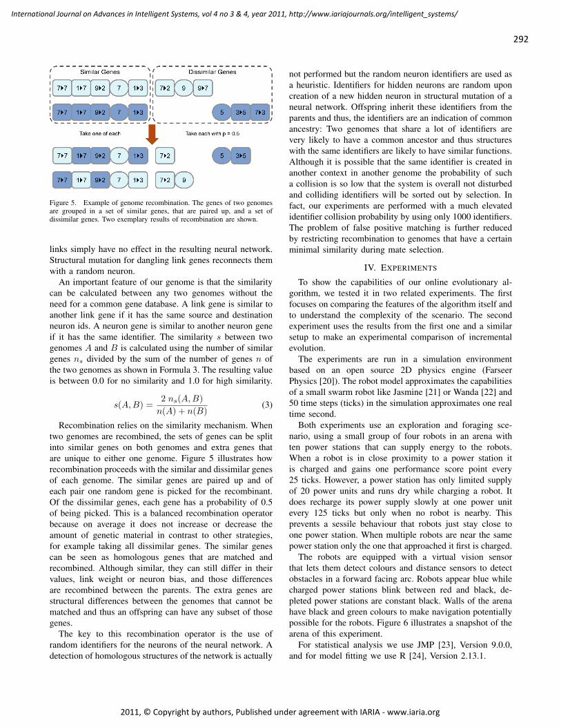
292



Figure 5. Example of genome recombination. The genes of two genomesare grouped in a set of similar genes, that are paired up, and a set ofdissimilar genes. Two exemplary results of recombination are shown.

links simply have no effect in the resulting neural network.Structural mutation for dangling link genes reconnects themwith a random neuron.

An important feature of our genome is that the similaritycan be calculated between any two genomes without theneed for a common gene database. A link gene is similar toanother link gene if it has the same source and destinationneuron ids. A neuron gene is similar to another neuron geneif it has the same identifier. The similarity s between twogenomes A and B is calculated using the number of similargenes ns divided by the sum of the number of genes n ofthe two genomes as shown in Formula 3. The resulting valueis between 0.0 for no similarity and 1.0 for high similarity.

s(A,B) =2 ns(A,B)

n(A) + n(B)(3)

Recombination relies on the similarity mechanism. Whentwo genomes are recombined, the sets of genes can be splitinto similar genes on both genomes and extra genes thatare unique to either one genome. Figure 5 illustrates howrecombination proceeds with the similar and dissimilar genesof each genome. The similar genes are paired up and ofeach pair one random gene is picked for the recombinant.Of the dissimilar genes, each gene has a probability of 0.5of being picked. This is a balanced recombination operatorbecause on average it does not increase or decrease theamount of genetic material in contrast to other strategies,for example taking all dissimilar genes. The similar genescan be seen as homologous genes that are matched andrecombined. Although similar, they can still differ in theirvalues, link weight or neuron bias, and those differencesare recombined between the parents. The extra genes arestructural differences between the genomes that cannot bematched and thus an offspring can have any subset of thosegenes.

The key to this recombination operator is the use ofrandom identifiers for the neurons of the neural network. Adetection of homologous structures of the network is actually

not performed but the random neuron identifiers are used asa heuristic. Identifiers for hidden neurons are random uponcreation of a new hidden neuron in structural mutation of aneural network. Offspring inherit these identifiers from theparents and thus, the identifiers are an indication of commonancestry: Two genomes that share a lot of identifiers arevery likely to have a common ancestor and thus structureswith the same identifiers are likely to have similar functions.Although it is possible that the same identifier is created inanother context in another genome the probability of sucha collision is so low that the system is overall not disturbedand colliding identifiers will be sorted out by selection. Infact, our experiments are performed with a much elevatedidentifier collision probability by using only 1000 identifiers.The problem of false positive matching is further reducedby restricting recombination to genomes that have a certainminimal similarity during mate selection.

IV. EXPERIMENTS

To show the capabilities of our online evolutionary al-gorithm, we tested it in two related experiments. The firstfocuses on comparing the features of the algorithm itself andto understand the complexity of the scenario. The secondexperiment uses the results from the first one and a similarsetup to make an experimental comparison of incrementalevolution.

The experiments are run in a simulation environmentbased on an open source 2D physics engine (FarseerPhysics [20]). The robot model approximates the capabilitiesof a small swarm robot like Jasmine [21] or Wanda [22] and50 time steps (ticks) in the simulation approximates one realtime second.

Both experiments use an exploration and foraging sce-nario, using a small group of four robots in an arena withten power stations that can supply energy to the robots.When a robot is in close proximity to a power station itis charged and gains one performance score point every25 ticks. However, a power station has only limited supplyof 20 power units and runs dry while charging a robot. Itdoes recharge its power supply slowly at one power unitevery 125 ticks but only when no robot is nearby. Thisprevents a sessile behaviour that robots just stay close toone power station. When multiple robots are near the samepower station only the one that approached it first is charged.

The robots are equipped with a virtual vision sensorthat lets them detect colours and distance sensors to detectobstacles in a forward facing arc. Robots appear blue whilecharged power stations blink between red and black, de-pleted power stations are constant black. Walls of the arenahave black and green colours to make navigation potentiallypossible for the robots. Figure 6 illustrates a snapshot of thearena of this experiment.

For statistical analysis we use JMP [23], Version 9.0.0,and for model fitting we use R [24], Version 2.13.1.

293



Figure 6. Snapshot of the simulation experiment. In the arena are four bluecoloured robots with the view area of their sensors shown and ten powerstations. The colour of the power stations is alternating between black andeither red or blue. At this point, half the power stations blink in red, theother half in blue. The arena is also occupied by some larger obstacles withwalls in different shades of green.

A. Structural Evolution

In this experiment, there is one large change in theenvironment that requires a complex adaptation and wecompare different mechanisms of the evolutionary algorithm.Our hypothesis is that in face of a complex adaptationchallenge, structural evolution and recombination are ben-eficial. We define here a complex challenge as one wherehidden neurons and recurrent connections are needed and,thus, a perceptron without hidden neurons should performsignificantly worse.

The evolutionary challenge for the robots is a change inthe appearance of the power stations. The experiment startswith a genome population that is adapted to collecting powerstations that blink in red (the colour alternates between blackfor 5 ticks and red for 5 ticks). The ten power stations startwith red blinking and every 100.000 ticks, one power stationchanges its appearance to blinking in blue (same frequency).During the blue phase such power stations appear identicalto other robots to the colour vision sensors of a robot andduring the black phase they appear like walls and depletedpower stations. Neural networks must perform temporalsensor fusion to detect the alternation between black andblue. They must infer the blinking to recognize a blueblinking power stations and distinguish them from the robotsand walls. After one million ticks, all power stations blinkin blue. The experiment continues for another one millionticks without further changes for a total of two million ticks.

Each robot is controlled by an artificial neural networkproduced by our evolutionary framework described in Sec-tion III. The neural network performs five update steps at

Figure 7. Sensor model of the simulated robot. In the 2D simulationenvironment, a 2D-to-1D perspective projection is used to create an arrayof nine RGB colour values. These values are combined into three averagedvalues for left, middle and right view area. Each RGB channel of thosethree colour values is fed into one input neuron of the neural network inaddition to three proximity values of simulated distance sensors.

each simulation time tick. There are twelve input neurons(three colour sensors each with a red green and blue channeland three proximity sensors) and two output neurons tocontrol the differential drive of the robot. All inputs aremapped to values from 0 to 1, the output neurons providevalues from -1 to 1.

The colour vision sensors are simulated using a 2D-to-1D perspective projection in the 2D simulation environmentwith an opening angle of 72◦ which returns an array of ninecolour pixels. Every three of these nine pixels are averagedinto three colour values. Each RGB colour channel of thesevalues is fed into one input neuron of the neural network.A visual example of this procedure is given in Figure 7.The result is a simple colour vision input for the neuralnetwork with three virtual colour sensors, fanned out in aforward facing arc. A comparable sensor is feasible on actualrobots using RGB sensors or downsampling a camera image.The simulated robot is also equipped with three proximitysensors, one facing ahead, one 24◦ to the right and one 24◦ tothe left. These sensors behave similar to infrared proximitysensors.

Three factors of the evolutionary process are investigated:• Network type: A perceptron with no hidden layer (P)

and a recurrent network with hidden neurons (H).• Structural evolution: Enables mutation to delete and

create genes for both links and neurons of the network.Note that here, the perceptrons never evolve hiddenneurons but can still add an remove links with struc-tural evolution. Without structural evolution, only linkweights and bias values of existing genes are mutated.

294



Figure 8. The development of foraging performance over time for each treatment. Shown is the average of 50 replicates, standarderror is omitted for clarity. Dashed lines belong to the perceptron treatments (P), solid lines to the treatments with hidden neurons(H). The performance overall drops until 1 million ticks as the power stations change to blue blinking appearance. Some treatmentsare better able to adapt and recover from this change than others.

• Recombination: Enables mate selection and recombi-nation in the evolutionary algorithm. Genomes try tofind another genome that falls within a certain similaritywindow for producing a recombinant offspring. Withoutrecombination, all offspring is mutated clones.

With these three factors, each with two levels, we dida full factorial setup for a total of eight treatments with50 replicates. For preparation, initial populations of randomperceptrons and random recurrent networks with five hiddenneurons were evolved for three million ticks to adapt to thered blinking power stations. Of those runs, one population ofrecurrent networks and one population of perceptrons wereselected for the experiment proper. Both populations havethe same performance and the highest performing pair wasselected out of 10 runs.

The response variable of the experiment is the totalforaging performance of all four robots over a time periodof 100.000 ticks. This foraging performance is the sumof all performance score points dispensed by all powerstations in that period. With an evaluation time of theevolutionary algorithm of 2.500 ticks per individual, 160individual evaluations contribute to this value. This measurerepresents the effective system performance and underlinesthe online nature of the scenario because every singleevaluation contributes to the system performance rather thanfew peak performing individuals.

B. Results

The development over time of the average performanceof the replicates is shown in Figure 8. Every treatment is

affected by the environmental change and the performancedrops. The perceptron treatments without structural evolu-tion drop the lowest and are unable adapt much to thechange. The treatments with hidden neurons and structuralevolution do not drop as low, show a clear recovery andadapt better to the new situation.

Figure 9 presents the performance of each treatment atthe end of the experiment. Confirming our expecetations,the treatments with perceptrons (P) perform worse than theones with hidden neurons at every treatment. The treatmentwith the highest final performance uses hidden neurons, re-combination and structural mutation (H-Rec-Struct), thoughthe difference to the next best treatment H-Rec is slim andthe statistical difference only borderline significant. Though,these two treatments are significantly different and superiorto all others.

We fitted a general linear model to the endpoint per-formance results. After data exploration, we used log-transformed performance values to equalize distributions ofresiduals and two outliers with a value of 0.0 were excluded.Starting with a full-factorial model, the three-way interactionwas removed, lowering the AIC value. Our final model canbe seen in Table II. The residuals of this model appear linearin a Q-Q plot and can be considered normal distributed. Thebiggest influencing factors are network type and structuralevolution (estimates of 0.754 and 1.07 respectively) withsmaller interactions between all factors. Recombination asprimary factor has no influence but in interaction with thehidden network type it acts positively (0.317) and slightlynegatively together with structural evolution (-0.186).

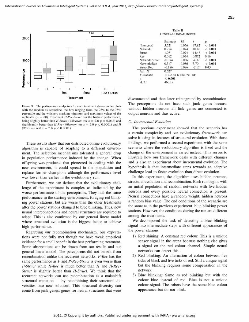
295



Figure 9. The performance endpoints for each treatment shown as boxplotswith the median as centreline, the box ranging from the 25% to the 75%percentile and the whiskers marking minimum and maximum values of thereplicates (n = 50). Treatment H-Rec-Struct has the highest performance,being slightly better than H-Struct (Wilcoxon test z = 2.0 p = 0.045) andsignificantly better than H-Rec (Wilcoxon test z = 5.0 p < 0.0001) and H(Wilcoxon test z = 7.6 p < 0.0001).

These results show that our distributed online evolutionaryalgorithm is capable of adapting to a different environ-ment. The selection mechanisms tolerated a general dropin population performance induced by the change. Whenoffspring was produced that pioneered in dealing with thenew environment, it could spread in the population andreplace former champions although the performance levelwas lower than earlier in the evolutionary run.

Furthermore, we can deduce that the evolutionary chal-lenge of the experiment is complex as indicated by theworse performance of the perceptrons. They had the sameperformance in the starting environment, foraging red blink-ing power stations, but are worse than the other treatmentsafter the power stations changed to blue blinking. Thus, newneural interconnections and neural structures are required toadapt. This is also confirmed by our general linear modelwhere structural evolution is the biggest factor to achievehigh performance.

Regarding our recombination mechanism, our expecta-tions were not fully met though we have weak empiricalevidence for a small benefit in the best performing treatment.Some observations can be drawn from our results and ourgeneral linear model. The perceptrons did not benefit fromrecombination unlike the recurrent networks. P-Rec has thesame performance as P and P-Rec-Struct is even worse thanP-Struct while H-Rec is much better than H and H-Rec-Struct is slightly better than H-Struct. We think that therecurrent networks can use recombination as a makeshiftstructural mutation — by recombining their structural di-versities into new solutions. This structural diversity cancome from junk genes: genes for neural structures that were

Table IIGENERAL LINEAR MODEL

Estimate SE t p(Intercept) 5.521 0.056 97.82 < 0.001Network 0.754 0.074 10.16 < 0.001Struct 1.07 0.074 14.47 < 0.001Rec 0.012 0.074 0.872 0.16Network:Struct -0.374 0.086 -4.37 < 0.001Network:Rec 0.317 0.086 3.70 < 0.001Struct:Rec -0.186 0.086 -2.17 0.03Adj. R2 0.627F -statistic 112.2 on 6 and 391 DFp < 0.001AIC 460.19

disconnected and then later reintegrated by recombination.The perceptrons do not have such junk genes becausewithout hidden neurons all link genes are connected tooutput neurons and thus active.

C. Incremental Evolution

The previous experiment showed that the scenario hasa certain complexity and our evolutionary framework cansolve it using its features of structural evolution. With thosefindings, we performed a second experiment with the samescenario where the evolutionary algorithm is fixed and thechange of the environment is varied instead. This serves toillustrate how our framework deals with different changesand is also an experiment about incremental evolution. Thehypothesis is that intermediate steps towards an adaptivechallenge lead to faster evolution than direct evolution.

In this experiment, the algorithm uses hidden neurons,structural evolution and recombination. Each run begins withan initial population of random networks with five hiddenneurons and every possible neural connection is present.Neural connections have a random weight, hidden neuronsa random bias value. The end conditions of the scenario arethe same as in the previous experiment, blue blinking powerstations. However, the conditions during the run are differentamong the treatments.

We decomposed the task of detecting a blue blinkingsignal into intermediate steps with different appearances ofthe power stations.

1) Red shining: A constant red colour. This is a uniquesensor signal in the arena because nothing else givesa signal on the red colour channel. Simple neuralnetworks can detect this.

2) Red blinking: An alternation of colour between fiveticks of black and five ticks of red. Still a unique signalbut the blinking requires some compensation in thenetwork.

3) Blue blinking: Same as red blinking but with thecolour blue instead of red. Blue is not a uniquecolour signal. The robots have the same blue colourappearance but do not blink.

296



Figure 10. The four treatments of the incremental evolution experiment.A: Starting with red shining, gradual transition to red blinking, followedby another gradual transition to blue blinking. B: Same as A but thetransitions happen instantly. C: Starting with red blinking and only oneinstant transition to blue blinking. D: Starting with blue blinking directlywithout any transitions.

This experiment has four treatments that are illustrated inFigure 10. Each treatment has a total of five million ticks toadapt from a random starting population to harvest the blueblinking power stations at the end.

• A: Starting with red shining, after 1 million ticks thepower stations change one after the other to red blink-ing. The transition is complete after 2 million ticks. At3 million ticks, there is another gradual transition fromred blinking to blue blinking, which is finished after4 million ticks. This is the treatment with the mostincrements.

• B: This starts similar to A with red shining but allpower stations change to red blinking at 1.5 millionticks simultaneously. At 3.5 million ticks happens thesimultaneous change to blue blinking.

• C: Here the phase of red shining is omitted and itstarts with red blinking right away. The change to blueblinking happens at 3.5 million ticks like in B. Thistreatment serves also as comparison to direct evolutionto the red blinking environment.

• D: The appearance of the power stations is blue blink-ing from the start with no changes in the environment.This is the direct evolution treatment for the blueblinking environment.

It is expected that the final performance is higher in thetreatments with more increments: treatment A having highestperformance and D lowest. For the treatments A, B and Cwe can make a similar comparison at 3 million ticks foradaptation to the red blinking environment.

(a) (b)

Figure 11. The performance of the incremental evolution experiment at3 million ticks and 5 million ticks (n = 50). Treatment D is omittedat 3 million ticks because it is not comparable. (a) At 3 million ticks,treatments A and B have the same performance (Wilcoxon test z = 0.6p = 0.556) but C is significantly lower than A (Wilcoxon test z = −2.1p = 0.036) and than B (Wilcoxon test z = −2.5 p = 0.011). (b) At5 million ticks there are not differences between the treatments (Kruskal-Wallis test χ2 = 3.1 p = 0.380).

D. Results

Surprisingly, the performance at the end of the 5 millionticks is the same across all treatments (Figure 11(b)). Thereare no significant differences between the direct evolutiontreatment D and the the incremental evolution treatments.However, a slightly different picture can be seen for thered blinking environment at 3 million ticks (Figure 11(a)).Here, treatment C is the direct evolution treatment withsignificantly lower performance than treatments A and B,though there is no difference between them.

An overview of the development of mean performanceover time of all four treatments is displayed in Figure 12.The treatments with intermediate steps climb to high valuesduring their relaxed conditions but then drop back when theenvironment changes. When comparing treatment A and B,we see that the gradual transitions of A carry no benefit andthe instant transitions of B result in the same performanceat 2 and 4 million ticks respectively. However, we see incomparison with C that they are able to leverage someadvantage of first evolving with red shining power stationsto the next phase of red blinking power stations, resulting inan increased performance at 3 million ticks. The transitionaround 4 million ticks to blue blinking affects treatmentsA, B and C equally hard. They all drop below the baselineof the direct evolution treatment D but recover quickly andreach the same performance level of D by the end of theexperiment.

These results show that incremental evolution is notuniversally beneficial and give support to the conclusionof Christensen and Dorigo [18]. Each previous works onincremental evolution uses different experimental scenarioswith a different approach to realizing the increments, whichis a likely explanation for the mixed results. In our ownprevious experiment [1], we used different arenas and found

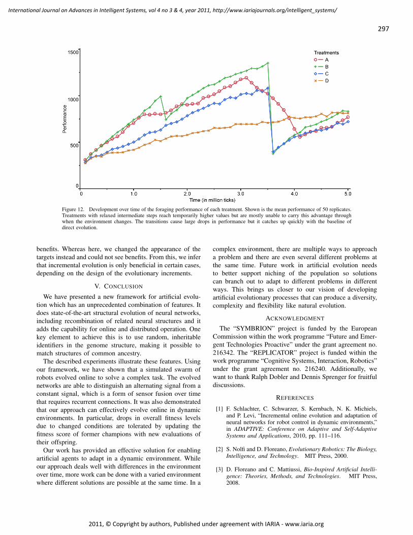
297



Figure 12. Development over time of the foraging performance of each treatment. Shown is the mean performance of 50 replicates.Treatments with relaxed intermediate steps reach temporarily higher values but are mostly unable to carry this advantage throughwhen the environment changes. The transitions cause large drops in performance but it catches up quickly with the baseline ofdirect evolution.

benefits. Whereas here, we changed the appearance of thetargets instead and could not see benefits. From this, we inferthat incremental evolution is only beneficial in certain cases,depending on the design of the evolutionary increments.

V. CONCLUSION

We have presented a new framework for artificial evolu-tion which has an unprecedented combination of features. Itdoes state-of-the-art structural evolution of neural networks,including recombination of related neural structures and itadds the capability for online and distributed operation. Onekey element to achieve this is to use random, inheritableidentifiers in the genome structure, making it possible tomatch structures of common ancestry.

The described experiments illustrate these features. Usingour framework, we have shown that a simulated swarm ofrobots evolved online to solve a complex task. The evolvednetworks are able to distinguish an alternating signal from aconstant signal, which is a form of sensor fusion over timethat requires recurrent connections. It was also demonstratedthat our approach can effectively evolve online in dynamicenvironments. In particular, drops in overall fitness levelsdue to changed conditions are tolerated by updating thefitness score of former champions with new evaluations oftheir offspring.

Our work has provided an effective solution for enablingartificial agents to adapt in a dynamic environment. Whileour approach deals well with differences in the environmentover time, more work can be done with a varied environmentwhere different solutions are possible at the same time. In a

complex environment, there are multiple ways to approacha problem and there are even several different problems atthe same time. Future work in artificial evolution needsto better support niching of the population so solutionscan branch out to adapt to different problems in differentways. This brings us closer to our vision of developingartificial evolutionary processes that can produce a diversity,complexity and flexibility like natural evolution.

ACKNOWLEDGMENT

The “SYMBRION” project is funded by the EuropeanCommission within the work programme “Future and Emer-gent Technologies Proactive” under the grant agreement no.216342. The “REPLICATOR” project is funded within thework programme “Cognitive Systems, Interaction, Robotics”under the grant agreement no. 216240. Additionally, wewant to thank Ralph Dobler and Dennis Sprenger for fruitfuldiscussions.

REFERENCES

[1] F. Schlachter, C. Schwarzer, S. Kernbach, N. K. Michiels,and P. Levi, “Incremental online evolution and adaptation ofneural networks for robot control in dynamic environments,”in ADAPTIVE: Conference on Adaptive and Self-AdaptiveSystems and Applications, 2010, pp. 111–116.

[2] S. Nolfi and D. Floreano, Evolutionary Robotics: The Biology,Intelligence, and Technology. MIT Press, 2000.

[3] D. Floreano and C. Mattiussi, Bio-Inspired Artificial Intelli-gence: Theories, Methods, and Technologies. MIT Press,2008.

298



[4] D. Floreano and L. Keller, “Evolution of adaptive behaviourin robots by means of darwinian selection,” PLoS Biology,vol. 8, no. 1, January 2010.

[5] A. Agogino, K. Stanley, and R. Miikkulainen, “Online inter-active neuro-evolution,” Neural Process. Lett., vol. 11, no. 1,pp. 29–38, 2000.

[6] J. Walker, S. Garrett, and M. Wilson, “Evolving controllersfor real robots: A survey of the literature,” Adaptive Behavior,vol. 11, no. 3, pp. 179–203, September 2003.

[7] J.-M. Montanier and N. Bredeche, “Embedded EvolutionaryRobotics: The (1+1)-Restart-Online Adaptation Algorithm,”in Workshop on Exploring new horizons in EvolutionaryDesign of Robots at IROS 2009, 2009, pp. 37–43.

[8] N. Bredeche, E. Haasdijk, and A. Eiben, “On-line, on-boardevolution of robot controllers,” in Artifical Evolution, ser.Lecture Notes in Computer Science. Springer, 2010, vol.5975, pp. 110–121.

[9] C. Schwarzer, C. Hosler, and N. Michiels, “Artificial sexualityand reproduction of robot organisms,” in Symbiotic Multi-Robot Organisms: Reliability, Adaptability, Evolution, P. Leviand S. Kernbach, Eds. Springer-Verlag, 2010, pp. 389–408.

[10] P. J. Angeline, G. M. Saunders, and J. P. Pollack, “An evolu-tionary algorithm that constructs recurrent neural networks,”IEEE Transactions on Neural Networks, vol. 5, no. 1, pp.54–65, January 1994.

[11] K. O. Stanley and R. Miikkulainen, “Evolving neural networkthrough augmenting topologies,” Evolutionary Computation,vol. 10, no. 2, pp. 99–127, 2002.

[12] K. O. Stanley, D. B. D’Ambrosio, and J. Gauci, “Ahypercube-based encoding for evolving large-scale neuralnetworks,” Artificial Life, vol. 15, no. 2, pp. 185–212, 2009.

[13] D. B. D’Ambrosio and K. O. Stanley, “A novel generativeencoding for exploiting neural network sensor and outputgeometry,” in GECCO: Conference on Genetic and Evolu-tionary Computation. ACM, 2007, pp. 974–981.

[14] P. Stadler and S. Institute, “Towards a theory of landscapes,”in Complex Systems and Binary Networks, ser. Lecture Notesin Physics. Springer, 1995, vol. 461-461, pp. 78–163.

[15] I. Harvey, P. Husbands, and D. Cliff, “Seeing the light:artificial evolution, real vision,” in Conference on Simulationof adaptive behavior: From Animals to Animats. MIT Press,1994, pp. 392–401.

[16] F. Gomez and R. Miikkulainen, “Incremental evolution ofcomplex general behavior,” Adaptive Behavior, vol. 5, pp. 5–317, 1996.

[17] G. J. Barlow, C. K. Oh, and E. Grant, “Incremental evolutionof autonomous controllers for unmanned aerial vehicles usingmulti-objective genetic programming,” in CIS: Conferenceon Cybernetics and Intelligent Systems, December 2004, pp.688–693.

[18] A. L. Christensen and M. Dorigo, “Incremental evolutionof robot controllers for a highly integrated task,” in SAB:Conference on the Simulation of Adaptive Behavior, 2006,pp. 473–484.

[19] A. Eiben, E. Haasdijk, and N. Bredeche, “Embodied, on-line, on-board evolution for autonmous robotics,” in SymbioticMulti-Robot Organisms: Reliability, Adaptability, Evolution,P. Levi and S. Kernbach, Eds. Springer-Verlag, 2010, pp.367–388.

[20] (2011, Aug.) Farseer physics engine. [Online]. Available:http://farseerphysics.codeplex.com/

[21] (2011, Aug.) Open-source micro-robotic project. [Online].Available: http://www.swarmrobot.org/

[22] A. Kettler, M. Szymanski, J. Liedke, and H. Worn, “Introduc-ing wanda - a new robot for research, education, and arts,” inIROS: Conference on Intelligent Robots and Systems, 2010,pp. 4181–4186.

[23] Using JMP 9, SAS Institute Inc., Cary, NC, USA, Oct. 2010.

[24] R Development Core Team, R: A Language and Environmentfor Statistical Computing, R Foundation for StatisticalComputing, Vienna, Austria, 2011. [Online]. Available:http://www.R-project.org

299



Animated Virtual Agents to Cue User Attention Comparison of static and dynamic deictic cues on gaze and touch responses

Santiago Martinez, Robin J.S. Sloan, Andrea Szymkowiak and Ken Scott-Brown University of Abertay Dundee

Dundee, DD1 1HG. UK [email protected], [email protected], [email protected], [email protected]

Abstract — This paper describes an experiment developed to study the performance of virtual agent animated cues within digital interfaces. Increasingly, agents are used in virtual environments as part of the branding process and to guide user interaction. However, the level of agent detail required to establish and enhance efficient allocation of attention remains unclear. Although complex agent motion is now possible, it is costly to implement and so should only be routinely implemented if a clear benefit can be shown. Previous methods of assessing the effect of gaze-cueing as a solution to scene complexity have relied principally on two-dimensional static scenes and manual peripheral inputs. Two experiments were run to address the question of agent cues on human-computer interfaces. Both experiments measured the efficiency of agent cues analyzing participant responses either by gaze or by touch respectively. In the first experiment, an eye-movement recorder was used to directly assess the immediate overt allocation of attention by capturing the participant’s eye-fixations following presentation of a cueing stimulus. We found that a fully animated agent could speed up user interaction with the interface. When user attention was directed using a fully animated agent cue, users responded 35% faster when compared with stepped 2-image agent cues, and 42% faster when compared with a static 1-image cue. The second experiment recorded participant responses on a touch screen using same agent cues. Analysis of touch inputs confirmed the results of gaze-experiment, where fully animated agent made shortest time response with a slight decrease on the time difference comparisons. Responses to fully animated agent were 17% and 20% faster when compared with 2-image and 1-image cue severally. These results inform techniques aimed at engaging users’ attention in complex scenes such as computer games and digital transactions within public or social interaction contexts by demonstrating the benefits of dynamic gaze and head cueing directly on the users’ eye movements and touch responses.

Keywords-agents; digital interface; touch interface; computer animation; reaction time; eyetracking.

I. INTRODUCTION The allocation of attention by a human observer is a

critical yet ubiquitous aspect of human behaviour. For the designer of human-computer interfaces, the efficient allocation of user attention is critical to the uptake and continued use of their interface designs. Historically, many human-computer interfaces have relied on static textual or

pictorial cues, or a very limited sequence of frames loosely interconnected over time (for example, on automated teller device menus, or on websites). More recently, the increased power of computer graphics at more cost effective prices has allowed for the introduction of high resolution motion graphics in human computer interfaces. Until now, psychological insights on attention and the associated cognitive processes have mirrored Human-Computer Interaction’s (HCI) reliance on either static or stepped pictorial stimuli, where stepped pictorial stimuli consist of a few static frames displayed over time to imply basic motion. Again, this legacy can be attributed to limitations in affordable and deployable computer graphics.

This paper extends previous work from CONTENT 2010 Martinez et al. [1] and is centered on the evaluation of fully animated (25 frames per second) virtual agents, where both the head and eye-movements of the agent are animated to allocate user attention. In contrast to most previous studies that have relied on manual inputs, using peripheral devices in response to agent cues, this research explores the possibility of two different ways of interaction. The first study uses the captured eye-gaze of participants as a response mechanism, following on from the work of Ware and Mikaelian [2], while the second study explores the suitability of attention allocation involving small amount/range of locomotion (i.e., touch action) on the same task.

Where observers look in any given scene is determined primarily by where information critical to the observer’s next action is likely to be found. The visual system can easily be directed to guide and inform the motor system during the execution of information searching. Consequently, a record of the path that observer gaze takes during a task provides researchers with what amounts to a running commentary on the changing information requirements of the motor system as the task unfolds [3]. This is the underlying principle of the reported experiment, which is an expansion of the cognitive ethology concept expressed by Eastwood et al. [4] to virtual agents. The experiments are based on the deictic gaze cue – the concept that the gaze of others acts like a signal that is subconsciously interpreted by an observer’s brain, and that it can transmit “information on the world” [5]. The gaze of another human agent is inherently difficult to avoid, and it can be used as a specific pointer to direct an observer’s attention [6]. The incorporation of this concept can be easily implemented into an agent-based interface.

300



Another aspect this study evaluates is how locomotion can influence the effectiveness of cueing. Most research has been focused on response using peripheral devices. It is important to assess the validity of cues on a wider range of modalities. In this study we analyze gaze and touch inputs in order to assess the suitability of agent cues in these kind of interfaces and their applicability in upcoming interface design.

The efficiency of interfaces such as these can be assessed based on the speed of observer response to cues. In both studies, the cues are presented as fully animated (dynamic) agents, stepped agents (two images), or static agent images (one image). Coupled with appropriate software, a virtual agent can anticipate a user’s goals, and point (using gaze) to the area where the next action has to be performed. An agent with animated gaze may therefore be useful to adopt in digital interfaces to guide user attention and potentially increase the speed of attention allocation, or where the work space of human physical action may have many possible choices; and the possibility of not selecting the right one is high.

In the following sections, we will explain in detail the application of the virtual agent to cue user attention. In Section 2 we will describe the existing literature reviews from two different research fields. In Section 3, we will explain the method used to develop a gaze experiment. Gaze input results will be presented in Section 4. In Section 5, we will describe the method of a touch experiment and in Section 6 its results. Finally, in Section 7, we will discuss the overall conclusions of both experiments: dynamic versus static cues, the differences observed between the interaction modalities (e.g., gaze and touch) and the impact on user engagement and agent animation on real world interfaces.

II. LITERATURE REVIEW Previous studies belong to two different but related

research fields: namely cognitive psychology and computer interface design. Psychological studies have reviewed attention and its relationship with the cues. Posner [7] describes the process of orienting attention. Relative to neutral cue trials, participants were faster and/or more accurate at detecting a target given a valid cue, and they were slower and/or less accurate given an invalid cue. Friesen and Kingstone [8] worked with faces and lines drawn following the gaze direction towards the target area. They found that subjects were faster to respond when gaze was directed towards the intended target. This effect was reliable for three different types of target response: detection, localization and identification. Langton and Bruce [9], and more recently Langton et al. [10], investigated the case of attention in natural scene viewing. They concluded that facial stimuli, that indicate direction by virtue of their head and eye position, produce a reflexive orienting response in the observer. Eastwood et al. [4] produced experimental findings leading to the conclusion that facial stimuli are perceived even when observers are unaware of the stimuli. In 2006, Smilek et al. [11] focused on isolating specific processes underlying everyday cognitive failures. They developed a measure for attention-related cognitive failures with some

success, and introduced the term of cognitive ethology. Studies in HCI and computing are mostly focused on proving the validity of eye-gaze as an input channel for machine control. One exception was Peters et al. [12] in 2009, who tested shared attention behaviours during virtual agent interaction. The method was based on a head direction mapping metric (directedness) using their own algorithm and recorded by a common and cheap available equipment, a webcam. They demonstrated, with some success, the importance of participant head motion directed to an object in the interface to infer the level of engagement. However, the absence of gaze tracking disabled the analysis of peripheral eye movements and covert attention. Also, the use of a gaze-contingent moving cross-hair was an important distractor on the tasks, becoming intrusive.

Concerning the study of the eye-gaze as an input modality, Ware and Mikaelian [2] used an eye-tracker to compare the efficacy of gaze with other more usual inputs, such as manual using physical devices. They found that the gaze input was faster with a sufficient size of target. Sibert and Jacob [13] studied the effectiveness of eye gaze in object selection using their own algorithm and compared gaze selection with a traditional input – a hand operated mouse. They found that gaze selection was 60% faster than mouse selection. They concluded that the eye-gaze interaction is convenient in workspaces where the hands are busy and another input channel is required.

The above research shows how eye-gaze can be used to assess the response of a user when accurate tracking is possible. In addition, it has been demonstrated that the eye-gaze of an agent can effectively allocate attention. However, the interplay between pictorial cues to gaze allocated attention (and subsequent assessment of allocated attention) is still to be fully explored. Specifically regarding this point, for the reported experiment, two goals were set by the authors; to assess the extent to which the gaze of the observer can be used to record their selection of targets and response time to agent cues, and to determine whether fully animated agents would offer an advantage over standard static (1-image) or stepped (2-image basic motion) agents when directing attention using gaze. By focusing on gaze as a means of target selection, this removes as much motor response as possible from the observer. Manual responses operated through any device inevitably introduce uncertainty in establishing the true response time since they are an indirect response to the gaze cue (requiring over allocation of attention and eye-gaze, followed by translation of the response signal to the input modality of device). Therefore, when it comes to assessing the effectiveness of animated versus static and stepped agent cues, directly recording the eye-movements of observers and using this data to determine the speed of their response and their selection of objects offers a significant advantage.

Nevertheless, touch inputs are increasingly appearing in our daily lives on screens, via smartphones, kiosks or Automated Teller Machines (ATMs). In this context, touch is considered a natural way of interaction [14]. It rapidly evolved from places where there was no space for peripherals (i.e., factory environment), such mouse or

301



keyboard, to be included in portable devices, desktop PCs, and home entertainment.

Originally, use of touch screens was limited by a lack of precision, high error rates of selections [15] and absence of ergonomic standards in their physical design. Although touch calibrations are still required in some devices such as eye-trackers and large touch-sensitive display screens, the evolution of screen technologies (i.e., capacitive, resistive, surface acoustic wave [16]) has largely solved the precision and errors in selection problems. At the same time, advances in hardware design have tackled the ergonomic standards problem by allowing the user to adjust screen position by independent rotations on two axes for fixed monitors and three axes for tablet screens. Touch screen applications are beginning to be found in many different contexts, such as information kiosks, airports, education, museums, amusement parks, and very widely on self-service technologies (e.g. Schreder et al. cite the railways usage [17]). Attributes of touch screens are: fast response time [14] (especially in most recent generation of hardware), contribution to user satisfaction [18] [19] and above all direct manipulation of elements (an important advantage for infrequent users of interfaces [20]).

Previous research states that directly touching the screen provides a more direct approach to elements on the interface, conferring a more natural way of handling objects than with a mouse or other pointer device [21]. Ever since Jef Hann’s TED talk [22] (which has since clocked up over 5million views), the repertoire of touch screen modality has been evolving towards a standard for user input. Wobbrock (2009) outlines a multitude of gestures available for the Microsoft Surface, but in the meantime a more reduced selection of gestures is becoming apparent through the development of hardware and associated applications. This is most obvious in the form of multi-touch mass produced items such as iPod Touch and more recently iPad (with 15 million sales at time of writing). The sales of touch screen computers are testament to the engaging qualities of the interface possibilities. However, how the direct physical action affects the interface elements’ performance compared to interactions with external buttons, track pads, trackballs or mice remains uncertain. In the context of public space touch screens, this uncertainty comes from two areas. Firstly from the influence of layout: when there are no peripheral buttons required to be used (e.g. keyboard or mouse) the keys get you around an ATM [18]. The second uncertainty comes from the use of fingers to touch the screen, fingers and hands that can occlude large parts of the screen and thus change the layout requirements of a display. In this work, we evaluate whether the touch task constrains or interferes to some extent with how cues allocate the attention of user and whether these agent cues are as effective on a touch screen as in a non-contact, gaze, interface.

III. GAZE-RESPONSE EXPERIMENT: METHOD The experiment method was as follows below.

A. Task description In this experiment, participants were asked to perform an

object selection task (using their eye gaze alone) on a series of twenty-four different agent animations, presented on a monitor at a resolution of 1024 x 768. Each of the videos showed a virtual agent’s head in the centre of the screen surrounded by eight different possible target areas (see Fig. 1). Each agent was displayed on screen for 3000 ms. Over the course of the video, the agent would orient its head and eyes to aim at a particular target square. The point at which the agent oriented its head and gaze (and the nature of the agent’s movement) was determined by the type of agent cue (see below). Of the eight target areas in each video, only one was the right choice in each trial – the one that was specifically indicated by the agent. If the participants selected that specific area with their eye-gaze, it was counted as a success. If the participant selected any of the other seven areas, it was counted as incorrect. Fixations to areas outside the 8 target areas were coded as no target selected. The target areas were red squares approximately 150 x 150 pixels in size, and were all equidistant from the center of the screen.

B. Agent Cues There were three different types of agent cues (see Fig.

2): a) Static cue: A single image of an agent. The agent’s

head and eyes were aimed at the target area for the duration that the stimulus is displayed. The orientation cue was therefore presented from 0 ms till 3000 ms.

b) Stepped cue: Two images of an agent, sequenced to imply movement. The agent’s head and eyes were looking straight forward from 0 ms, before the second image was displayed from 960 ms. In the second image, the agent’s head and eyes were aimed at the target from 960 ms till 3000 ms.

Figure 1: The appearance of the virtual agent, surrounded by eight target squares, arranged on both the cardinal and oblique axes.

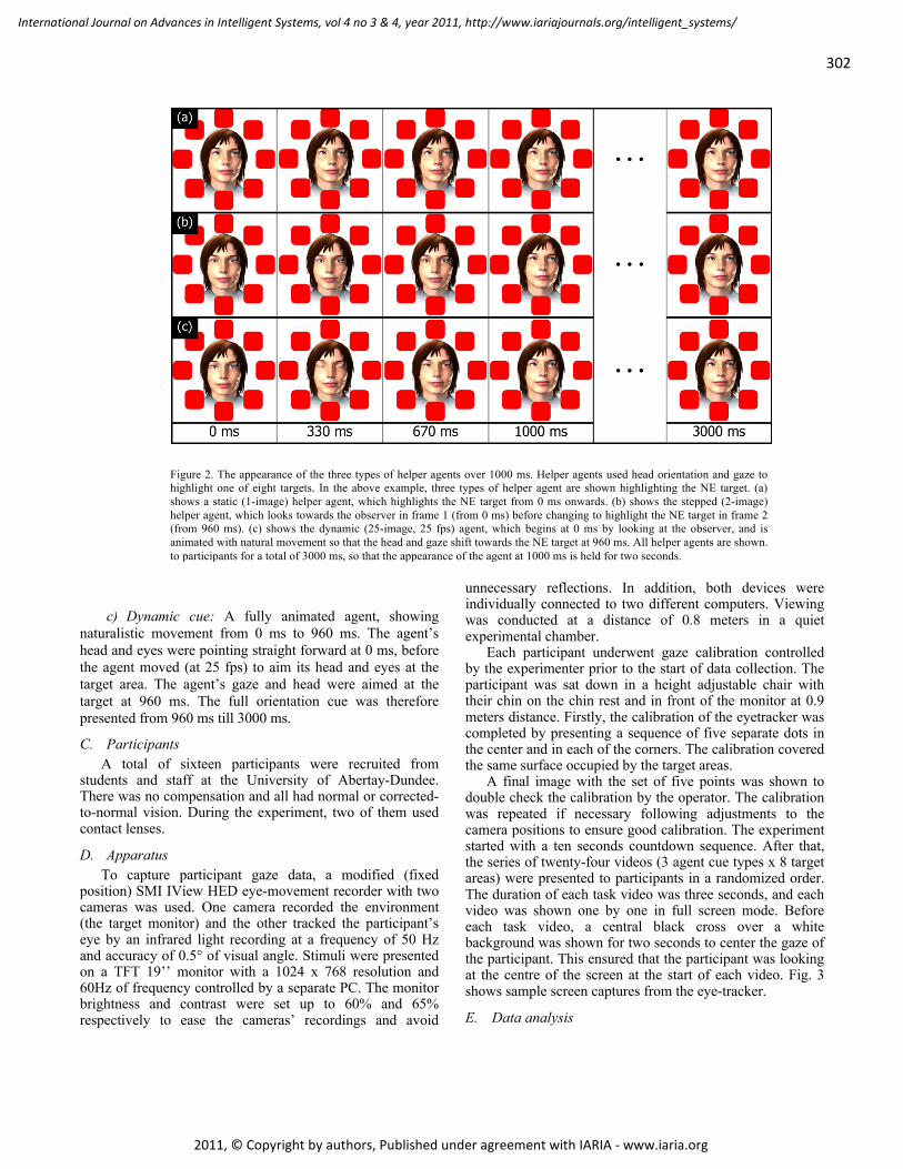
302



c) Dynamic cue: A fully animated agent, showing

naturalistic movement from 0 ms to 960 ms. The agent’s head and eyes were pointing straight forward at 0 ms, before the agent moved (at 25 fps) to aim its head and eyes at the target area. The agent’s gaze and head were aimed at the target at 960 ms. The full orientation cue was therefore presented from 960 ms till 3000 ms.

C. Participants A total of sixteen participants were recruited from

students and staff at the University of Abertay-Dundee. There was no compensation and all had normal or corrected-to-normal vision. During the experiment, two of them used contact lenses.

D. Apparatus To capture participant gaze data, a modified (fixed

position) SMI IView HED eye-movement recorder with two cameras was used. One camera recorded the environment (the target monitor) and the other tracked the participant’s eye by an infrared light recording at a frequency of 50 Hz and accuracy of 0.5° of visual angle. Stimuli were presented on a TFT 19’’ monitor with a 1024 x 768 resolution and 60Hz of frequency controlled by a separate PC. The monitor brightness and contrast were set up to 60% and 65% respectively to ease the cameras’ recordings and avoid

unnecessary reflections. In addition, both devices were individually connected to two different computers. Viewing was conducted at a distance of 0.8 meters in a quiet experimental chamber.

Each participant underwent gaze calibration controlled by the experimenter prior to the start of data collection. The participant was sat down in a height adjustable chair with their chin on the chin rest and in front of the monitor at 0.9 meters distance. Firstly, the calibration of the eyetracker was completed by presenting a sequence of five separate dots in the center and in each of the corners. The calibration covered the same surface occupied by the target areas.

A final image with the set of five points was shown to double check the calibration by the operator. The calibration was repeated if necessary following adjustments to the camera positions to ensure good calibration. The experiment started with a ten seconds countdown sequence. After that, the series of twenty-four videos (3 agent cue types x 8 target areas) were presented to participants in a randomized order. The duration of each task video was three seconds, and each video was shown one by one in full screen mode. Before each task video, a central black cross over a white background was shown for two seconds to center the gaze of the participant. This ensured that the participant was looking at the centre of the screen at the start of each video. Fig. 3 shows sample screen captures from the eye-tracker.

E. Data analysis

Figure 2. The appearance of the three types of helper agents over 1000 ms. Helper agents used head orientation and gaze to highlight one of eight targets. In the above example, three types of helper agent are shown highlighting the NE target. (a) shows a static (1-image) helper agent, which highlights the NE target from 0 ms onwards. (b) shows the stepped (2-image) helper agent, which looks towards the observer in frame 1 (from 0 ms) before changing to highlight the NE target in frame 2 (from 960 ms). (c) shows the dynamic (25-image, 25 fps) agent, which begins at 0 ms by looking at the observer, and is animated with natural movement so that the head and gaze shift towards the NE target at 960 ms. All helper agents are shown. to participants for a total of 3000 ms, so that the appearance of the agent at 1000 ms is held for two seconds.

303



The participant gaze data was analyzed using the software BeGaze 2.3. The data stored in BeGaze contained all the fixations’ timestamps. Only trials where the participant’s gaze started on the cross in the center of the screen were considered valid. Target selection was defined by the first full-gaze fixation occurring in the eight predefined areas of interest overlying the 8 target destinations. The fixation duration criterion for an observer response is defined in the light of previous literature. Ware and Mikaelian in 1987 used 400 ms; Sibert and Jacob in 2000 considered 150 ms. Because extended forced fixation (400 ms) can become laborious, we established a criterion for successful cognitive response to fixation as equal as or greater than to 250 ms, i.e., a fixation that locates on the target area at least for 250 ms.

Based on this concept, of the total number of possible cognitive responses, 92.18% were successfully tracked. Of the successfully tracked data, correct responses accounted for 95.2% of the total and mismatches accounted for 4.9%. The definition of a mismatch was when there was a fixation of 250 ms or more inside an incorrect target area. In 8.47% of the total mismatches, no clear target was selected – i.e., there was no fixation of 250 ms or more in any of the target areas.

IV. GAZE-RESPONSE EXPERIMENT: RESULTS Only one participant presented problems during the

tracking because of the unexpected movement of her contact lens in the tracked eye. This resulted in four non-tracked responses in the same participant.

For each agent type a total of 128 eye tracking recordings were made. Recordings were then evaluated and allocated to one of four categories: Correct (where the observer clearly selected the intended target), Incorrect (where the observer clearly selected an unintended target), No Target (where it was not clear which target the observer had selected), and Corrupted (where the eye tracking data had been disrupted

resulting in lost data, for instance when a participant’s head moved in a trial). After excluding the corrupted recordings, it was clear that observers were able to accurately select the intended target regardless of whether the virtual agent was static (95%), stepped (92.5%), or dynamic (94.2%) (see Table I). This would suggest that, in general, the type of virtual agent (in terms whether it was static, stepped, or fully animated) did not substantially impact upon how effective it was at communicating what the intended target was.

A repeated measures analysis of variance (ANOVA) was used to determine whether agent type had an effect on how long it took participants to look at and select the intended target square. The response times for static agent cues - which contained agents that were oriented towards the target 960 ms earlier than both stepped and dynamic cues – were corrected to account for this difference. The analysis showed that the type of agent did have a significant effect on participant response time, F(2, 30) = 52.73, p < .001.

Participants responded most quickly to the dynamic (fully animated) agent type (M = 1220, SE 95) than they did to either the stepped (2 frame) agent type (M = 1874, SE 61) or the static (1 frame) agent type (M = 2091, SE 59) (see Fig. 4).

Comparisons between agent types were assessed using a Bonferroni post-hoc test. The results showed that participants responded to the dynamic agent type significantly more quickly than both the static (Mean Deviation (MD) = 870, p < .001) and the stepped (MD = 654, p < .005) agent types. Furthermore, participants also responded to the stepped agent type significantly more quickly than the static agent type

Figure 3: The eye tracking data of one participant, where the blue circles represent fixations. In image (a), the participant looks towards the cross before the agent appears in image (b). In image (c), the agent highlights the East target, at which point the participant looks towards this target, before fixating on the cross again in image (d).

Figure 4: The mean gaze response times for static, stepped, and dynamic agents indicate that participants reacted most quickly to the fully animated, dynamic agents

TABLE I. PARTICIPANT GAZE SELECTION OF TARGETS

Type Correct Incorrect No Target selected

Corrupt (Exclusions)

Static 93.5 % 5.7 % 0.8 % 7 / 128

Stepped 92.5 % 5.8 % 1.7 % 8 / 128

Dynamic 94.2 % 5 % 0.8 % 7 / 128

304



(MD = 217, p < .005) (see Table II). These results not onlyunderline that static agent types are significantly less effective at cueing observer attention than either stepped or dynamic agents, but also that stepped agent types are significantly less effective than fully animated, dynamic agents.

V. TOUCH-RESPONSE EXPERIMENT: METHOD The experiment method was as follows below.

A. Task description The task to perform in this experiment was analogous to

the described above (see Section 3 Gaze-Response Experiment), except this time hand-touch was the input modality instead of eye-gaze. Participants had to perform the object selection task using the same hand for all trials, on a series of twenty-four different agent animations. Agent animations were presented on a monitor at a resolution of 1280 x 720. Each of the videos showed a virtual agent’s head in the centre of the screen, surrounded by eight different touchable square areas (see Fig. 5). Each agent was displayed on screen for 3000 ms and remained on the screen with the last frame shown till a target selection was made by participant. Orientation cues timing, type of agents and type of choices are identical as previously described in gaze experiment.

Over the course of the video, the agent would orient its

head and eyes aim at a particular target square. The point at

which the agent oriented its head and gaze (and the nature of the agent’s movement) was determined by the type of agent cue. Of the eight possible target areas in each video, only one was the right choice in each trial – the one that was specifically indicated by the agent. If the participants selected that specific area, it was counted as a success. If the participant selected any of the other seven areas, it was counted as incorrect.

The target areas were red squares of exactly 150 x 150 pixels in size, and were all equidistant from the center of the screen. In comparison with gaze experiment, targets have the same area but with the slight difference in the layout, a grey border around the border to create a button similarity –giving a ‘push-able’ notion to the eight square items.

B. Agent Cues The agent cues described in section III.B were also used

in the current experiment.

C. Participants A total of thirty-two participants were recruited from

students and staff at the University of Abertay-Dundee. 4 participants already participated in the gaze experiment. There was no compensation and all had normal or corrected-to-normal vision and were able to use hands correctly for the purpose of this experiment. There were 29 right-handed, 1 left handed and 2 ambidextrous. Both ambidextrous participants chose right hand to run the experiment. In one case choice was the participant’s dominant-hand and in the other it was their non-dominant hand. They were asked to use the same hand across all trials and all participants did so.

D. Apparatus The trials were run in a Sony VAIO® L Series

Touchscreen. It is an All-In-One PC multi-touch (two point) capacity on the screen (dimensions of 24 inches at 60 Hz; resolution of 1280x720; bright and contrast at 62%, graphic card default levels). Computer specifications were memory of 4 GB DDR2 SDRAM, processor Intel® Core™ 2 Duo CPU E7500@, 2.93 GHz and 2.94 GHZ. The OS was Microsoft® Windows 7 Home Premium 64 bits. The video card was an integrated GeForce G210M with a total graphics memory of 2271 MB (512 MB dedicated). The PC was securely placed on an office table and participants were seated on a chair with adjustable height. The PC was at a distance of approximately 25 cm from participant’s head and 12 cm from participant’s hands, well within arm’s reach. All the trials were run in a quiet chamber in the Usability Lab of the University of Abertay-Dundee. During the experimental trials, the experimenter was observing the experiment in a separate twin room through a one-way mirror to minimize the disturbance or possible noises on participants. Participants were told they could raise their hand in any moment to request presence of the researcher. During the thirty-two runs, the researcher’s assistance was required only once due to equipment failure. All of this participant’s trials were removed from the analysis and all their response data discarded.

Figure 5: The appearance of the virtual agent, surrounded by eight target squares, arranged on both the cardinal and oblique axes.

TABLE II. MULTIPLE COMPARISON BETWENN AGENT TYPES (GAZE)

Type Comparison Mean Deviation

Std. Error

Sig.

Static Stepped

Dynamic

217 ms

870 ms 54.3

85.8 .004

.000

Stepped Static

Dynamic

-217 ms

654 ms 54.3

114.3 .004

.000

Dynamic Static

Stepped

-870 ms

-654 ms 85,8

114.3 .000

.000

305



After the participant was comfortably sat in the chair and contented with the distance of PC, button-feedback training was run to make them confident with the button touch feedback. It was recommended to make at least one touch per target area (n = eight) to feel how the buttons worked. The experiment started with a ten second countdown video. Before each trial, a text indicated to participant to push space bar key to start. This assured that the participant was resting their hand at the same point before the start of each trial. The series of twenty-four videos (3 agent cue types x 8 target areas) were presented to participants in a randomized order and counter-balanced. The duration of each video was three seconds, and each video was shown one by one. Preceding each stimulus trial, a central black cross over a white background was shown for two seconds (similarly as seen in Fig. 3.a) to mirror gaze experiment task preamble. The last video frame from each trial remained on screen until the participant selected one of the eight touchable areas.

E. Data analysis The participant response time data was stored using

Adobe Flash CS5 (version 11.0.0.485). The data contained all the participants time responses (24 per participant) counted from the starting point of showed cue (video with the agent) till the participant selected a target area on the screen by their finger touch. Successful target selection was defined by the touch on the target area cued specifically by the agent. A touch in any of the other seven areas not cued by the agent was considered a mismatch. No responses outside the eight target areas were recorded during the experimental trials.

The choice of Adobe Flash to measure Reaction Time (RT) was intentional. First, it gave a desired degree of freedom in the design of the interface layout. In contrast with gaze experiment where all elements on the interface where passive, here the touchable areas or buttons are external to the video and now become functional components themselves. Second, the decision was based on studies proving the validity of Flash as reliable software to measure RT, once that specific conditions were accomplished in the experiment. One condition is related with the device used in the time measurement, in this case the PC. The smaller the difference in RTs, the more critical it is to know the properties of the timing device used. Neath et al. [23] showed that the smallest difference in magnitude that a stock iMac 8.1 (April, 2008-March, 2009) using Flash (version 10.0 r42) could detect under realistic conditions is approximately 5–10 ms, and this dictates the types of research that should use these systems: if a researcher tests all subjects using the exact same hardware, if the focus is on relative rather than absolute RTs, if the differences in RTs in the conditions to be examined are expected to be fairly large (e.g., at least 20–40 ms), if only certain software is used, and if many properties of the visual display are not of critical importance, then the conclusions drawn from RT data collected on a stock iMac are likely to be the same as those drawn from RT data collected on custom or high-end hardware.

Reimers et al. [24] in 2007 studied on PC (processor 1.4 MHz AMD Athlon, 256 MB of RAM, graphic card PCI NVidia GeForce 2MX and 32 MB of video RAM) the estimation of the average and the spread of RTs in the different conditions stating that RTs recorded with Flash are between 10 and 40 ms longer than those recorded in the Baseline condition (application on programming language C using the X Window System to display stimuli and a parallel port button box). Flash did not appear to add significant random error to RT measurements.

VI. TOUCH-RESPONSE EXPERIMENT: RESULTS An unexpected operating system error resulted in data

loss of one participant, due to a sudden failure of OS that invalidated the participant’s session. All of the participant’s trials were removed from the analysis and all his times discarded. Thus, 94.8% of the total number of responses were successfully stored. Of these stored answers, correct responses accounted for 98.48% and mismatches accounted for 1.51%.

For each agent type a total of 24 time response recordings were made per participant. Recordings were then analyzed and allocated to one of three categories: Correct (where the observer selected the intended target), Incorrect (where the observer selected an unintended target), and Corrupted (where the file writing was corrupted or non-existent). After excluding the corrupted recordings, it was clear that users were able to accurately select the intended target regardless of whether the virtual agent was static (99%), stepped (99.7%), or dynamic (99.7%) (see Table III). This would suggest that, analogously as in the previous case of gaze-interaction, the type of virtual agent (in terms whether it was static, stepped, or fully animated) did not substantially impact upon how effective it was at communicating what the intended target was.

A repeated measures analysis of variance (ANOVA) was used to determine whether agent type had an effect on how long it took participants to select by touch the intended target square. The response times for static agent cues - which contained agents oriented towards the target 960 ms earlier than both stepped and dynamic cues – were corrected to account for this difference. The analysis showed that the type of agent did have a significant effect on participant response time, F(2, 724) = 50.38, p < .001. Participants responded most quickly to the dynamic (fully animated) agent type (M

TABLE III. PARTICIPANT TOUCH SELECTION OF TARGETS

Type Correct Incorrect

Corrupt (Exclusions)

Static 99% 1 % 24 / 256

Stepped 99.7% 0.3% 24 / 256

Dynamic 99.7% 0.3% 24 / 256

306



= 2423, SE 32) than they did to either the stepped (2 frame) agent type (M = 2900, SE 40) or the static (1 frame) agent type (M = 3007, SE 57) (see Fig. 6).

Comparisons between agent types were assessed using

the Bonferroni post-hoc test. The results showed that participants responded to the dynamic agent type significantly more quickly than both the static (Mean

Deviation (MD) = 584, p < .001) and the stepped (MD = 476, p < .001) agent types. In contrast to gaze case, participants responded to the stepped agent type not significantly faster than the static agent type (MD = 108, p >.005) (see Table IV). These results corroborate the gaze experiment results where static agent types are significantly less effective at cueing observer attention than dynamic agents, but also that stepped agent types are significantly less effective than fully animated, dynamic agents.

VII. GAZE- AND TOUCH-RESPONSE EXPERIMENT: DISCUSSION AND FUTURE WORK

Using a paradigm where the criterion for correct response to pictorial or animated agent gaze is the eye-gaze of the participant we found that the presence of full-motion in the gaze and head inducing agent drives the observer’s attention the fastest. Gaze recorded responses for 25 frame stimuli were 35% faster than stepped and 42% faster than static stimuli. This result is consistent with previous research on gaze cueing [10]. The current paradigm provides the most direct route to the establishment of the overt allocation of gaze location since it subverts the need for a translation to a device manual response. This confirms Ware and Mikaelian’s [2] assertion that participants eye-gaze itself can be used to indicate responses.

By modifying the gaze cue paradigm from experiment to a touch-based target selection paradigm, we demonstrated that fully animated agent gaze and head cues drive user attention faster than static and 2-image agent cues. Touch recorded responses for 25 frame stimuli were 17% faster than stepped and 20% faster than static stimuli, confirming those obtained in eye-gaze interface experiments. Compared with the gaze response results, the decrease on the time differences suggests that the touch selection method alters, to some extent, the delay from when the participant correctly

follows the cue to when the target selection is executed. It seems that the motor response reduces the time advantages gained with the fastest cue, suggesting that eye responses are much more rapid than hand responses. There is an aspect, clearly observed, of longer reaction times in touch modality, probably due to the translation of response into the sense of touch. This fact reinforces the idea of the complex process of motor response that reduces the time saved by the motion cue. Such a process should be greater in magnitude in order to explain those time save absorptions. Confirming that the introduction of hand locomotion does not invalidate the effectiveness of dynamic cue, results also showed that it was the difference on time response between 2-stepped and static was non-significant.

Regarding whether the 2-image agent could be considered not completely a motion cue, this suggests that motion cues with a sufficient number of frames (25 tested in the experiment) are more necessary in context where human locomotion is involved. Probably the presence of touch involves more factors than those that we could control and include in the study, but at least one of them should be the higher impermeability to attention cues. The presence of movement in gaze cueing stimuli seems to drive the user’s attention more quickly. One prediction arising from this is that, when compared with 2D agents, 3D agents create an expectation of more believable behaviour. The combination of additional pictorial cues and natural motion may make the appearance of the agent more akin to that of a human conversation partner. The additional realism possible with modern computer animation techniques may make agents more believable and engaging [25].

The present study indicates how the animation of an agent can be linked to the sequencing of the social ‘script’ or ‘narrative’ of a HCI interface experience. Previous investigators such as Kendon [26] observed a hierarchy of body movements in human speakers; while the head and hands tend to move during each sentence, shifts in the trunk and lower limbs occur primarily at topic shifts. They discovered the body and its movements as an additional part of the communication, participating in the timing and meaning of the dialogue. Argyle and Cook [27] discuss the use of deictic gaze in human conversation. They argued that during a conversation the eye gaze serves for information seeking, to send signals and to control the flow of the conversation. They explained how listeners look at the speaker to supplement the auditory information. Speakers on

Figure 6: The mean touch response times for static, stepped, and dynamic agents indicate that participants reacted most quickly to the fully animated, dynamic agents

TABLE IV. MULTIPLE COMPARISONS BETWEEN AGENT TYPES (TOUCH)

Type Comparison Mean Deviation

Std. Error

Sig.

Static Stepped

Dynamic

108 ms

584 ms 62.1

62.1 .249

.000

Stepped Static

Dynamic

-108 ms

476 ms 62.1

61.6 .249

.000

Dynamic Static

Stepped

-584 ms

-476 ms 62.1

61.6 .000

.000

307



the other hand spend much less time looking at the listener, partially because they need to attend to planning and do not want to load their senses while doing so. Preliminary work from our laboratory suggests that experience in the gaze task over time may lead to a learning effect whereby extended exposure to these stimuli leads to improved gaze allocation. This analysis will form part of a wider study including a sequence of guided navigation prompts in a naturalistic setting. Only by creating a natural sequence of user choices with a combination of gaze cues and items competing for attention (including distractors) can we fully confirm the efficacy of an agent-based cue in human computer transactions in the natural environment.

The research presented here is consistent with the wider conclusions of other investigators [25], which indicate that vivid, animated emotional cues may be used as a tool to motivate and engage users of computers, when navigating complex interfaces. The results of this experiment provide guidance for agent design in consumer electronics such as computer games or animation. In order to avoid an unpleasant robotic awareness, natural motion and the correct presentation of the cue contribute to increase the deictic believability of the agent. Deictic believability in animated agents requires design that considers the physical properties of the environment where the transaction occurs. The agent design must take account of the positions of elements in and around the interface. The agent’s relative location with respect to these objects, as well as social rules known from daily life, are critical to create deictic gestures, motions, and speech that are both effective, efficient and unambiguous. All these aspects have an effect in addition to the core the response time measure. They easily trigger natural and social interaction of human users, reaching the right level of expectations. Furthermore, they make the system errors, human mistakes and interaction barriers more acceptable and navigable to the user [28].

Fully animated agents have the potential to be a key new component into the assistive characteristic of interfaces, where an appropriate animated performance demonstrating a solution to a problem can be delivered. In principle, this study has demonstrated that agent guidance would be suitable both with gaze and touch interfaces, but its use could be extendable to general interfaces, where searching and selection tasks are dominant. Animated agents could become a new component in the salience characteristic of interfaces, where a synchronized movement can reinforce the perceptibility of relevant elements inside the interface.

The concept of natural interfaces has been extensively discussed in the HCI literature [29]. The ‘naturalness’ is explained in terms of more familiarity, intuitive and predictable use, information retrieval and behaviour of the interface and the machine. In this context, the findings of the current study could be used to propose that more human-like interface components would be of practical use, particularly with agent behaviour synchronized with cues. The combination has a potential role in attention conflict situations, influencing significantly the overt allocation of user attention and, consequently, his responses and the interaction in general. In considering the graphical fidelity of

agents, it is worth noting that natural realism can cause problems within interface design. Research examining expression animation by Zamitto et al. [30], highlights a valuable distinction between realism and believability. One of their conclusions was that the pursuit of realism in expression animation may risk falling into the ‘uncanny valley’ where increasing photo-realism results in a perception of falseness [31]. In the context of user interaction, we predict that such prioritization of realism on the agent could result in an inappropriate user disengagement. Instead, believability, suitability of the context and usefulness in their assigned task (i.e., timing regards the cues) should be the premises for the representation of the interface agent.

In future work, it is planned to extend this study with a wide range of emotions on the agent cues, to evaluate their suitability on these interfaces, and compare with the results already obtained with fully animated non-emotional agents. With these set of studies, it is intended to draw a better and more complete picture of new ways of implementing guidance in interface design. This guidance strategy attempts to cover the ‘what to do next?’ situation for new or infrequent users, and it is specifically designed to resolve attention conflicts on environments with many distractors in number and type, such as those typically found in public space interaction.

As an ultimate goal, this and future related work pursues the intention to effectively design methods of allocation of the attention of users to improve the interaction flow. It is crucial that we evaluate the cues used in a guidance system based on the principle of cueing that can anticipate user actions and help in ‘what to do next’ problems.

ACKNOWLEDGMENT Martinez is grateful for support from the Alison

Armstrong Studentship. Sloan is grateful for support from a University funded studentship. The authors gratefully acknowledge the supportive interdisciplinary research environment provided by Abertay’s Whitespace Research Group, Institute for Arts Media and Computer Games and Centre for Psychology.

REFERENCES [1] S. Martinez, R. J. S. Sloan, A. Szymkowiak, and K. C. Scott-

Brown, “Using virtual agents to cue observer attention,” in CONTENT 2010, The Second International Conference on Creative Content Technologies, 21-26 November 2010, Lisbon, Portugal, 2010.

[2] C. Ware and H. H. Mikaelian, “An evaluation of an eye tracker as a device for computer input”, SIGCHI Bull., 17, May. 1986, pp. 183-188, doi:10.1145/30851.275627.

[3] J. M. Findlay and I. D. Gilchrist, “Active vision: the psychology of looking and seeing”, Oxford University Press, Oxford. 2003.S. R. H.

[4] J. D. Eastwood, D. Smilek, and P. M. Merikle, “Differential attentional guidance by unattended faces expressing positive and negative emotion”, Perception & Psychophysics, vol. 63, 2001, pp. 1004-1013.

[5] I. Poggi and C. Pelachaud, “Signals and meanings of gaze in animated faces,”. In: S. Nuallain, C. Muhlvihill and P.

308



McKevitt, eds, Language, Vision and Music. Amsterdam: John Benjamins, 2001

[6] S. R. H. Langton and V. Bruce, “Reflexive visual orienting in response to the social attention of others”, Visual Cognition, vol. 6, 1999, pp. 541-567., doi:10.1080/135062899394939

[7] M. I. Posner, “Orienting of attention”, Quarterly Journal of Experimental Psychology, vol. 32, 1980, pp. 3–25.

[8] C. K. Friesen and A. Kingstone, “The eyes have it! reflexive orienting is triggered by nonpredictive gaze”, Psychonomic Bulletin and Review, vol. 5, 1998, pp. 490-495.

[9] S. R. Langton, R. J. Watt, and V. Bruce, “Do the eyes have it? Cues to the direction of social attention”, Attention And Performance, vol. 4(2), 2000, pp. 50-59, ISSN 1364-6613, DOI: 10.1016/S1364-6613(99)01436-9

[10] S. R. Langton, C. O’Donnell, D. M. Riby, and C. J. Ballantyne, “Gaze cues influence the allocation of attention in natural scene viewing”, Experimental Psychology, vol. 59(12), 2006, pp. 2056- 2064, doi: 10.1080/17470210600917884.

[11] D. Smilek, E. Birmingham, D. Cameron, W. Bischof, and A. Kingstone, “Cognitive ethology and exploring attention in real world scenes,” Brain Research, vol. 1080, Issue 1, Attention, Awareness, and the Brain in Conscious Experience, 2006, pp. 101–119.

[12] C. Peters, S. Asteriadis, and K. Karpouzis, “Investigating shared attention with a virtual agent using a gaze-based interface”, Journal on Multimodal User Interfaces, vol. 3, Dec. 2009, pp. 119-130.

[13] L. E. Sibert and R. J. Jacob, “Evaluation of eye gaze interaction”, In Proceedings of the SIGCHI Conference on Human Factors in Computing Systems (CHI 00), ACM, 2000, pp. 281-288, doi: 10.1145/332040.332445.

[14] A. Sears, “High precision touchscreens: design strategies and comparisons with a mouse”, International Journal of Man-Machine Studies, vol. 34, Apr. 1991, pp. 593-613.

[15] J. Pickering, “Touch-sensitive screens: the technologies and their application”, International Journal of Man-Machine Studies, vol. 25, Sep. 1986, pp. 249-269.

[16] M. Platshon, "Acoustic touch technology adds a new input dimension", Computer Design, Mar. 1988, pp 89-93.

[17] G. Schreder, K. Siebenhandl, E. Mayr, & M. Smuc, “The ticket machine challenge? Social inclusion by barrier-free ticket vending machines”. In Proceedings of the The good, the bad and the challenging: The user and the future of information and communication technologies (pp. 780-790), 2009

[18] N. P. Marcous, M. J. Brant, and M. J. Rosenzweig, System and method for electronic transfer of funds using an automated teller machine to dispense the transferred funds. Google Patents, 1997.

[19] M.D. Stone, “Touch-Screens for Intuitive Input”, PC Magazine, 1986, 183-192.

[20] R.L. Potter, L.J. Weldon, and B. Shneiderman, “Improving the accuracy of touch screens: an experimental evaluation of three strategies”, Proceedings of the SIGCHI conference on Human factors in computing systems - CHI ’88, 1988, pp. 27-32.

[21] C. Forlines, D. Wigdor, C. Shen, and R. Balakrishnan, “Direct-touch vs. mouse input for tabletop displays”, Proceedings of the SIGCHI conference on Human factors in computing systems - CHI ’07, 2007, p. 647.

[22] J. Hann’s TED talk http://www.ted.com/talks/jeff_han_demos_his_breakthrough_touchscreen.html <retrieved: June, 2011>

[23] I. Neath, A. Earle, D. Hallett, and A.M. Surprenant, “Response time accuracy in Apple Macintosh computers”, Behavior research methods, Mar. 2011, pp. 1-10-10.

[24] S. Reimers and N. Stewart, “Adobe Flash as a medium for online experimentation: A test of reaction time measurement capabilities”, Behavior Research Methods, vol. 39, Aug. 2007, pp. 365-370.

[25] T. Vanhala, V. Surakka, H. Siirtola, K. Raiha, B. Morel, and L. Ach, “Virtual proximity and facial expressions of computer agents regulate human emotions and attention”, Computer Animation And Virtual Worlds, vol 21(3-4), 2010, pp. 215-224, doi: 10.1002/cav.336.

[26] A. Kendon, “Some relationships between body motion and speech: ana anlysis of an example”, In: A. Siegman and B. Pope, eds, Studies in Dyadic Communication, pp. 177-210, Elmsfor, NY: Pergamon Press, 1972.

[27] M. Argyle and M. Cook, “Gaze and mutual gaze”, New York: Cambridge University Press, 1976, 221 pages, ISBN-13: 978-0521208659.

[28] E. M. Diederiks, “Buddies in a box: animated characters in consumer electronics”,IUI '03, 2003, pp. 34-38, doi: http://doi.acm.org/10.1145/604045.604055.

[29] W. Buxton, “Lexical and pragmatic considerations of input structures”, ACM SIGGRAPH Computer Graphics, vol. 17, no. 1, p. 31–37, 1983.

[30] V. Zammitto, S. DiPaola, and A. Arya, 2008, “A methodology for incorporating personality modeling in believable game characters”, Arya, 1(613.520), p.2600.

[31] M. Mori, “The uncanny valley”, Energy, vol. 7, no. 4, p. 33–35, 1970.

309



A System-On-Chip Platform for HRTF-Based Realtime Spatial Audio RenderingWith an Improved Realtime Filter Interpolation

Wolfgang Fohl, Jürgen Reichardt, Jan KuhrHAW Hamburg

University of Applied SciencesHamburg, Germany

Email: [email protected], [email protected], [email protected]

Abstract—A system-on-chip platform for realtime renderingof spatial audio signals is presented. The system is based ona Xilinx Virtex-6 FPGA platform. On the chip an embeddedµBlaze microprocessor core and FIR filters are configured.Filtering is carried out in the FPGA hardware for performancereasons whereas the signal management is performed on theembedded processor. The azimuth and elevation angles of avirtual audio source relative to the listener’s head can bemodified in real time. The system is equipped with a compasssensor to track the head orientation. This data is used totransform the room related coordinates of the virtual audiosource to the head related coordinates of the listener, so that afixed position of the virtual sound source relative to the roomcan be attained regardless of the listener’s head rotation. Headrelated transfer functions (HRTF) were sampled in steps of30◦ for azimuth and elevation. Interpolation for intermediateangles is done by either interpolating between the coefficientsof the measured HRTFs at the four adjacent angles (azimuthand elevation), or by feeding the audio signal through thecorresponding four filters, and mixing the outputs together.In the latter case the required four filter processes per outputstereo channel do not result in longer computing time becauseof the true parallel operation of the FPGA system. In order toachieve a constant loudness level for all interpolated angles it isnecessary to decompose the HRTF filters in two components,one for the amplitude response and the other for the delay.The system output is identical to the output of a correspondingMatlab prototype.

Keywords- Mixed-reality audio; realtime HRTF interpolation;filter decomposition; system-on-chip.

I. INTRODUCTION

Spatial sound rendering is important for audio playback,and for creating realistic virtual environments for simula-tions and games. For headphone-playback devices, tech-niques based on Head Related Transfer Functions (HRTF)are widely used, not only in virtual reality applications, butalso for stereo enhancements in home audio systems andmobile audio players [1]–[4]. There are already consumerproducts available that use HRTF-based audio spatialisationwith head tracking [5], [6].

For a realistic spatial impression of a virtual sound source,the perceived source location must stay fixed relative to theroom when the listener’s head is turned, so a headphone-based system will have to perform a coordinate transforma-

tion between head-related and room-related coordinates. Aquick update of head position data is necessary to preventa perceivable delay between head movement and HRTFadjustment.

The system described here was first presented as anconference article in [7]. It is aimed at mixed-reality audioapplications, which require a mobile device with realtimebehaviour. For such applications, systems-on-chip consistingof a Field Programmable Gate Array (FPGA) with anembedded microprocessor on it are versatile and flexibleplatforms. The application of the time-variant HRTFs to theaudio signal is done on the FPGA hardware. The filtersare configured in the VHDL language (VHDL stands forVery High Speed Integrated Circuit Hardware DescriptionLanguage [8]). The tasks of signal routing and signal man-agement are performed by the C program running on theembedded µBlaze-Processor.

Since the first publication the software has been portedfrom the Virtex-5 to the Virtex-6 platform, and the realtimeinterpolation of HRTF filters has been improved

In the next sections an overview of related work is given,and the fundamentals of audio spatialisation with HRTFs areoutlined. Then the design of our system is described withemphasis on the partitioning of the application to hardwareand software, and on the interface between the embeddedµBlaze processor and the surrounding FPGA chip. Resultsare presented and the paper finishes with the discussion ofresults, summary, and outlook to future work.

II. THEORETICAL BACKGROUND

A. Related Work

Since its beginnings in the mid-1970’s, dummy headstereophony has found continuous research and developmentinterest [9]. With increasing computing power of audioworkstations it has become feasible to perform realtimerendering of a virtual audio environment [1]. The problem ofproper out-of-head localisation has been addressed by manyauthors. It turns out, that a HRTF-based solution combinedwith a room reverberation model yields the best results [10].HRTF rendering algorithms will always have to interpolatebetween the stored filter coefficients for measured angles.

310



In a recent investigation the threshold of spatial resolutionin a virtual acoustic environment has been investigated [3].The reported result is, that the auditory localization has aresolution of 4◦ to 18◦, depending of the source direction.In PC-based realtime systems an effective way of designingHRTF filters is to perform a minimum phase plus allpassdecomposition, where the minimum phase part models thefrequency response of the HRTF, and the allpass part, whichis usually replaced by a delay, models the phase response [2].

In this work, we introduce a similar approach, but insteadof an minimum phase filter, we are designing an FIR filterwith a group delay of half the filter length. This means,that the centroid of the filter coefficients is located in thecenter of the filter coefficient array. Crossfading algorithmsfor HRTF filter interpolations are described in [2] and [3].FPGA systems turn out to be suitable platforms for mobileaudio processing [11], [12].

B. Basic Concepts

1) Spatial Audio Rendering: The human auditory systemuses (at least) three binaural properties of a sound signalto determine the direction of the source: Inter-aural Inten-sity Differences (IID), Inter-aural Time Differences (ITD),and the angular variation of the spectral properties of thesound. Concerning only the inter-aural time and intensitydifferences leaves an ambiguity, the “cone of confusion”:All source locations on this cone yield the same ITDand IID. This ambiguity is partly removed by the angle-dependent spectral properties of the perceived sound, whichresult from the transmission properties of the signal pathfrom the source to the eardrums. These three propertiesare completely represented by the Head Related TransferFunctions (HRTF) for given azimuth and elevation angles.

Figure 1 shows the impulse response of the HRTF at0◦ elevation and 30◦ azimuth angle, where the time and leveldifferences can clearly be seen. As the right ear is closer tothe source, the absolute values of the right impulse responsesamples are larger. The sound reaches the right ear earlierwhich causes the shift of the maximum of the right channelto shorter delays.

The spatial rendering is done by filtering the source soundwith the HRTFs of the corresponding angle and playing theresulting stereo signal back by a set of headphones.

In dynamic listening situations, listeners resolve the ambi-guity of the cone of confusion by slightly turning their heads:the resulting changes in ITD, IID and sound spectrum allowa proper localization of the source. Especially the front-backambiguity is immediately resolved by the variation of theincident angle relative to the head, as can be seen in Fig. 2:When turning the head to the left, a source in front of thelitener will move to the right, whereas a source behind thelistener will move to the left.

The third dimension that has to be modeled for a realistic3D audio system is the distance of the sound source. In

-1

-0.5

0

0.5

1

200 220 240 260 280 300 320

Val

ue

Sample index

-1

-0.5

0

0.5

1

200 220 240 260 280 300 320

Val

ue

Sample index

Figure 1. HRTF impulse responses for 0◦ elevation and 30◦ azimuthangle. Top: left ear, bottom: right ear

Figure 2. Resolving the front-back-confusion by head movements: Whenthe listener turns the head to the left, the perceived position of a source infront will move to the right, and for a source in the back it moves to theleft.

this work we do not address distance, because the relatedpsychoacoustical effects are much more involved than forthe azimuth and elevation angles [13].

2) FPGA System-On-Chip: The low-level FPGA archi-tecture consists of a pool of logic blocks for combinationaland registered logic, RAM-memory and DSP slices. DSPslices consist of a MAC block (Multiply-Accumulate) andregisters of appropriate width to perform the multiply-accumulate operations in digital signal processing. Thelogic cells and DSP slices are interconnected by a userprogrammable switch matrix. By programming this switchmatrix the user defined functionality of the system is ob-tained.

To handle the complexity of larger systems, the designtools for the FPGA system support a block structuredapproach by defining Intellectual Property blocks (IP cores),that implement special functions like FIR filters or evenmicroprocessors (in our case the emulation of a µBlazeprocessor, see section III-C). Once these IP cores have beendeveloped or purchased, the high-level design task is toproperly interconnect these cores and to supply the necessaryglue logic.

With the availability of a microprocessor core on theFPGA chip, it is possible to design a complete soft-ware/hardware system, where the software part is writtenin C and executed on the processor core, and the hardware

311



part is specified in the VHDL language and is performingtime-critical and hardware-related tasks. Systems with thisarchitecture are called System-on-Chip (SoC).

C. HRTF coefficients

In preliminary measurements, HRTFs were measured witha dummy head measuring system and an audio spectrumanalyser. Attenuation and phase differences were measuredfor 500 logarithmically spaced sine wave frequencies. Theresults are in good conjunction with other HRTF measure-ments [14], [15].

From the frequency response data the FIR filters mod-elling the angle dependent sound properties were designedusing standard frequency-domain design techniques, withthe special feature of considering the measured phase byadding it to the linear base phase. This directly introduces theinteraural time delays to the FIR coefficients as can be seenin Figure 1, which is actually a plot of the FIR coefficientvalues over coefficient index.

D. HRTF interpolation techniques

Two approaches of interpolating HRTFs for angles be-tween the sampled positions are considered: the first ap-proach is the interpolation of the filter coefficients, thesecond approach is the crossfading (mixing) of appropriatefilter outputs. In the stationary case (no variation of sourceangle) these two approaches are equivalent. In the nexttwo paragraphs the two techniques are explained for thecase of constant elevation. If also the elevation angle is tobe interpolated, the interpolation of four filters has to beperformed (see section III-D5).

1) Coefficient Interpolation: The coefficient interpolationfor an angle ϕ that lies in the interval [ϕk, ϕk+1] is done bylinear interpolation of each of the FIR parameters bi. Theimplementation of Equation 1 requires 2L additions and Lmultiplications per filter, where L is the FIR filter length.

bi(ϕ) = bi(ϕk) +ϕ− ϕk

ϕk+1 − ϕk·(bi(ϕk+1)− bi(ϕk)

)i ∈ {0 . . . L− 1}

(1)

It should be noted that this approach is not applicable toIIR filters.

2) Crossfade Interpolation: The crossfading approachaccording to Equation 2 obtains the output signal yϕ bymixing the filter outputs of the two filters corresponding tothe interval limits ϕk and ϕk+1. The relative contribution ofthe two outputs is controlled by the parameter m.

yϕ = (1−m)·yϕk+m·yϕk+1

with m =ϕ− ϕk

ϕk+1 − ϕk(2)

This interpolation is also suited for IIR filters. It requiresonly three multiplications and three additions per audiosample at the extra expense of running the audio materialthrough two filters simultaneously, if only variations of the

azimuth shall be rendered, and four filters, if also variouselevations shall be rendered.

3) Decomposition Into Amplitude Response and Delay:There is a problem with the interpolation of FIR coefficientsets, when the filters are designed in a way that they producethe amplitude response and the delay at the same time. Fig. 3illustrates the problem.

Figure 3. Interpolation of FIR coefficients with incorporated time delays.The average value of the interpolated FIR coefficients is substantially lowerthan the average values of its constituting components.

The incorporation of the delay time into the filters leadsto a shift of the centroid of the filter coefficients away fromthe center of the coefficient array. For the ear closer to thesource, the centroid of the corresponding filter coefficientsis shifted towards lower indexes, for the ear away fromthe source, the centroid is shifted towards higher indexes.When two sets of filter coefficients are superposed by theinterpolation algorithm, the coefficients will partly level outeach other, as can be seen in the bottom plot of Fig. 3. Thiseffect leads to a decay in loudness at intermediate anglepositions.

To overcome this problem, the HRTF filters are decom-posed into two parts, one for the amplitude response, theother for the delay, as shown in Fig. 4.

Amplitude Response

DelayInput

SignalOutputSignal

FIR 1 FIR 2

Figure 4. Decomposition of the HRTF Filter into Amplitude Responseand Delay

The interpolation is performed separately on the ampli-tude response filter and on the delay. For the amplituderesponse, the filter coefficients for intermediate angles areagain computed by linear interpolation. Figure 5 again showsthe designed filter coefficients for 30◦ and 60◦, and the

312



interpolated coefficients for 45◦. As can be seen, there isno decrease in the average amplitude of the coefficients forthe interpolated filter, so no degradation of loudness is to beexpected for the interpolated angle.

The delay is implemented as an FIR filter with all zerocomponents, except one component with a value of oneat the interpolated delay time. The delay filter is the lastprocessing stage, and it is only one delay filter required foreach stereo channel.

Figure 5. Interpolation of FIR coefficients without incorporated timedelays. The average value of the FIR components of the interpolated filteris in the same range as the average values of its constituting components.

4) Computational Efficiency: A key feature of FPGAsystems is the ability of true simultaneous execution ofthe filtering: The parallel operation of multiple filters doesnot require more processing time, instead it requires moreFPGA resources, in particular, it requires at least one DSPslice per filter. The maximum filter length per DSP sliceis given by the ratio of system clock frequency and audiosampling rate [12], [16]. The device presented here workswith 125 MHz processor clock frequency and 44.1 kHzaudio sampling rate, allowing a maximum filter length of125·106 Hz44.1·103 Hz ≈ 2800.

5) Computational Cost on FPGA Hardware: The compu-tational costs of multiple parallel filtering is entirely differenton FPGA hardware. Here the filtering is performed inhardware as a genuine parallel operation, so on a FPGAsystem the parallel operation of multiple filters does notrequire more processing time, but it requires more FPGAresources. The crucial resources in this case are the DSPslices on the FPGA chip. A FIR filter operating with lowsampling rates can be implemented as a processing pipelineusing only one DSP slice per filter [12], [16]. Since onemultiply-accumulate operation per clock cycle is executed,the maximum filter length is given by the ratio of clockfrequency to audio sampling rate. The device presentedhere works with 125 MHz processor clock frequency and

Figure 6. Head Related Coordinates r, ϑ, φ and Room Related Coordinatesx, y, z

44.1 kHz audio sampling rate, allowing a maximum filterlength of 125·106

44.1·103 ≈ 2800. Under these conditions a FIRfilter length of 512 can be implemented with only one DSPslice per filter.

E. Head tracking

For a realistic spatial impression of headphone-based 3D-audio the transformation from head-related to room-relatedcoordinates according to Figure 6 is necessary. For a virtualaudio source that is supposed to remain fixed in the room,the orientation of the listener’s has to be continuouslymeasured and a corresponding correction of the apparentsource direction has to be applied.

III. SYSTEM DESIGN AND IMPLEMENTATION

A. Requirements

The requirements listed here are a consequence of theintended use of the system as a mobile device for spatialaudio rendering in mixed-reality environments.

• Low power consumption, small and light system.• Audio signals in CD quality: 44.1 kHz sampling rate,

16 Bit word length, 2 channels.• Multiple parallel FIR filters with ≥ 512 coefficients.• Tracking of the head azimuth and pitch (forward)

angle. For future developments also the roll (sideways)angle and the acceleration data for three axes must bemeasured.

• Sufficient memory to hold the filter coefficient sets.• Audio latency ≤ 10 ms to avoid perceivable delay.• Architecture must be extensible to multiple indepen-

dently moving virtual audio objects.

B. System Components

Our system is based on a Xilinx Virtex-6 FPGA evaluationboard. In addition to the FPGA chip this board provides alarge number of resources and interfaces, the most importantones being an AC97 audio interface, a RS 232 serial inter-face, a Compact Flash (CF) memory interface, for which a

313



FPGA

FIR Filter

μBlaze

main()

ISR

Compass

sensor

RS232

RS232

UART

AC97

AC97

Interface

Audio out Audio in

Data

Buffer

IRQ

FSL Bus

FSL Bus

Audio

Samples

AudioAudio

Filter CoeffsCoefficient

DPRAM

CF Card

(FAT12-FS)

DDR2

RAM

Figure 7. FPGA Components and Interfaces

file system driver is provided, and a DDR2 RAM interface.In addition there is a DIP-switch interface for simple userinteraction (e.g., switching of operating modes).

The azimuth and elevation angles of the listener’s head areprovided by a compass sensor (Ocean Server OS5000 [17]),that is mounted on the headphone clip and is connected tothe system via the RS 232 link.

C. Hardware Architecture

On the FPGA chip is the embedded µBlaze processor IPcore for signal and data management, the FIR filter blocks,and the block interconnection logic. The µBlaze is a 32-bit big-endian RISC processor with a library to access theFPGA chip hardware and a runtime environment for a Cmain() routine. The processor was configured without afloating-point coprocessor to save FPGA resources for theHRTF filters. The FPGA chip is configured with 64 kBon-chip RAM for the µBlaze processor, Dual-ported RAMblocks for the FIR filter coefficients, 256 MB of externalDDR2 memory and a 512 MB CF card with a FAT12filesystem, which can be accessed by the standard C file I/Oroutines. Figure 7 gives an overview of the relevant systemcomponents and interfaces.

External devices like the AC97 and the RS 232 can beaccessed by the µBlaze program with library functions pro-vided by Xilinx. The interconnection with the on-chip FIRblocks is established via the Fast Simplex Link (FSL) bus.The FSL bus is an unidirectional bus which also performsthe synchronisation of sender and receiver to the systemclock. Three FSL bus instances per filter were implementedfor parameter transfer, audio input, and audio output.

Incoming audio samples generate an interrupt which willbe served by the Interrupt Service Routine (ISR) on theµBlaze.

The FIR filters for the HRTF filtering are implemented ina direct form I (DF1) structure as a sequential processingpipeline utilising only one DSP slice per filter block [16].

The active FIR filter coefficients are stored in a dual-ported RAM (DPRAM), so the coefficient update and thefiltering may be executed asynchronously.

D. Software Architecture

1) Operating Modes: Two basic modes were imple-mented: a realtime mode, and an offline mode. In realtimemode, spatial audio rendering is triggered by the interruptsof the AC97 interface. Each incoming sample raises aninterrupt, the ISR takes the input sample, transfers it tothe filters, receives the filtered audio sample, performs themixing if required, and sends it to the AC97 interface forplayback.

In offline mode, audio data is read from wav-files storedon the CF memory card. Audio samples are processed inthe same way as in realtime mode, but in offline mode, thewhole program is executed at maximum speed in the cyclicalmain() program, and the output is stored in a wav-file onthe CF card for further evaluation.

In realtime mode, the timing and latency of the twointerpolation techniques are investigated; in offline mode, thecorrectness of implementation is checked by comparing theoutput wav-files with the results of corresponding MATLABcomputations.

For both modes, either of the two interpolation techniques,coefficient interpolation or crossfading may be selected asinterpolation mode. In coefficient interpolation mode, eachdata update from the compass sensor triggers the calculationof a new interpolated coefficient set for the filters for left andright audio channel according to Equation 1. The coefficientsets are then transferred via the FSL bus to the coefficientDPRAM on the hardware. In crossfading interpolation modeaccording to Equation 2, each update of the compass sensordata triggers the computation of a new mixing factor and anew delay time, which is written to the global data spacewhere the ISR can access it.

2) Filter Implementation: The FIR filter coefficients ofthe HRTFs were calculated in MATLAB from measurementdata. The normalisation of the filter coefficients was done inan empirical way, starting with L1− normalized coefficients.These coefficients lead to very low output amplitudes andthus a poor S/N ratio. For typical input signals a normali-sation factor was determined experimentally, that led to noaudible overflow.

Data have been converted to 16-bit Q15 integer formatusing the MATLAB fixed-point toolbox, and stored in binaryformat on the CF card. Intermediate results in the filter blockare stored in 32 bit wide registers.

Filter coefficients are loaded from CF memory by themain() routine of the µBlaze C program, and are trans-ferred to the hardware filters via the FSL bus connections

314



Embedded System FIR_FSL_STEREO

putfsl(data)FSL BusMaster

32 BitFSL Bus

Slave

32 BitCoefficient Pair COEFFS

RAM

SAMPLESRAM

16 Bit Coefficients Left

16 Bit Samples Right

32 BitSample Pair

16 Bit Sample Left16 Bit Sample Right

16 Bit ResultLeft

16 Bit ResultRight

32 Bit Output Sample Pair

32 BitFSL BusMaster

FSL BusSlave

data=getfsl()

MAC Unit Left

MAC UnitRight

combine

Figure 8. Data Flow for the Filtering Process

of the filters.3) Head Tracking: The azimuth and elevation (pitch)

angles of the compass sensor are read in the main()routine, and are used for calculating the audio source anglesin head-related coordinates. The compass sensor provides athird angle, giving the sideways bend of the head (roll angle).This angle is neglected because performing the necessarytrigonometrical computations in integer arithmetic on themicroprocessor would be too time-consuming.

4) Signal Routing: All audio signals are processed by theµBlaze ISR and transferred to the filters via the FSL bus.To minimize overhead, the 16 bit samples for left and rightchannel are combined to a 32 bit word and transferred as oneitem to the filters. The filter connection logic then extractsthe two samples from the transferred word. Figure 8 showsthe interconnection between the µBlaze processor and thehardware filters.

Filter coefficients are transferred from processor to hard-ware from within the processor’s main() function usingthe same technique of transferring two 16 bit coefficients atonce.

5) Implementation of Crossfading: Figure 9 shows theprinciple of crossfading interpolation for azimuth and el-evation. The mono input signal is fed to four stereo FIRfilter pairs, for the top left, top right, bottom left, andbottom right position of the interpolation interval. Fromthe compass sensor data the azimuth and elevation mixingparameters mϕ and mϑ are computed, and the filter outputsare superposed according to the two mixing parameters.When the azimuth and elevation data from the compass dataindicate that the current interpolation interval has been left,the FIR coefficient sets are reloaded according to the newinterval.

IV. RESULTS AND DISCUSSION

A. Verification of the Static Filtering Algorithms

The filtering algorithms for both interpolation techniqueshave also been implemented in Matlab using the fixed-point toolbox, and the results have been compared with thewav-files that are produced by the FPGA system in offlinemode. Test cases were filtering at the measured HRTF angles

FIR TL FIR TR

FIR BL FIR BR

Mono AudioIn

mφ 1 - mφ+

mφ 1 - mφ+

+

mϑ

1 - mϑ2 2

22

2

Stereo AudioOut

CompassData

ParameterUpdate

mφ mϑSelect FIR Coeff. Sets

FIR Delay

Figure 9. Signal Crossfading Interpolation between Top Left (TL), TopRight (TR), Bottom Left (BL), and Bottom Right (BR) Filter Outputs. Notethat there is only one pair of delay filters required.

and at different constant interpolated azimuth and elevationpositions.

In these measurements, the outputs of the FPGA systemand the Matlab implementation were bit-wise identical.

Both interpolation algorithms produced identical outputsignals.

B. Signal Processing Latencies

To assess and optimize system performance, and to ex-amine, if the data transfer times will limit the maximumnumber of audio objects (i.e., independent filter processes),detailed timing measurements have been carried out.

Table of System Latencies:tAC97 : AC 97 audio subsystem (Note 1) 1 mstFSL: FSL transfer (round-trip)

of one 32 bit word 300 nstFIR: FIR processing L=512 4.2µstParm : Parameter transfer

for 512 32-bit parameter pairs 120µstgd : Filter group delay ≤ 7 mstCS: Compass sensor sampling time 25 mstCT : Compass sensor data transfer

(Note 2) 2.4 . . . 22 mstAL: System audio latency for N audio objects (Note 3)tAL = tAC97 +N · tFSL + tFIR + tgd 8 ms

tHLI : Head tracking latencytHLI = tAL + tCS + tCT + tParm 35 . . . 55 ms

Notes:1) This value has been measured in a previous work [12].

It is the time for transferring a stereo audio samplefrom the AC97 to the FPGA, decode it in hardware,re-code and pass it back to the AC97 output withoutrouting the audio signal through the µBlaze processor.

315



Codec C Audio ISR C Driver FSL Bus FIR Filter

Codec Interrupt putfsl(sample0) sample0sample0

returnreturnreturn

getfsl(...)

sample0'sample0'sample0'return

ISR

Pro

cess

ing

Tim

e

Filt

erin

g

FSL Transfer 1

FSL Transfer 2

Figure 10. Blocking Filtering Process Sequence Diagram

Codec C Audio ISR C Driver FSL Bus FIR Filter

Codec Interrupt nputfsl(sample1) sample1sample1

returnreturnreturn

ngetfsl(...)sample0'sample0'

return sample0'ISR

Pro

cess

ing

Tim

e

Filt

erin

g

FSL Transfer 1

FSL Transfer 2

Figure 11. Non-Blocking Filtering Process Sequence Diagram

2) The compass data is transferred in ASCII. Smallvalues have less digits and thus need less transfer timethen large values.

3) Delay between audio input and audio output.The table shows that the filtering of one audio sample

takes much longer time than the FSL bus transfer, sothe ISR can be substantially sped up by replacing thestandard blocking data transfer routines putfsl() andgetfsl() by their nonblocking counterparts nputfsl()and ngetfsl(). In the case of blocking transfer as shownin Figure 10, the getfsl() routine has to wait until thefiltering process has finished, whereas in the nonblockingcase as shown in Figure 11 the ngetfsl() routine returnsimmediately. In the latter case, the ISR gets the result of theprevious filtering process, adding an extra latency of 1 audiosampling time to the system, which is negligible comparedto the group delay of the filter.

The limiting factor for the number of audio objects isthe fact, that each audio object will require one FSL bustransfer that is executed sequentially in the C program ofthe µBlaze processor. An upper limit can be estimated bythe requirement, that all the FSL bus transfers must becompleted within one audio sampling period tS :

N · tFSL < tS (3)

For tS = 1/44100 s, the upper limit for N is 75 audioobjects.

C. Filtering With Compensation of Head Movement

At the moment of writing, only qualitative listeningtests have been performed. The compensation of the headmovement drastically increases the spatial impression of

the rendered audio material. No front-back ambiguity wasnoticed. A much better externalization of the sound wasperceived, even in the case of source locations directly infront of the listener, where externalization is known to bemost difficult to obtain [10].

The latency of approximately 40 ms for the compensationof the head movements by evaluating the compass data isperceivable only at fast and abrupt head movements, whereit causes a slight irritation. For head movements at moderatespeed no latencies are perceivable. This is due to the limitedangle resolution (4◦ to 18◦) of the human auditory system[3].

The latencies summarized in section IV-B show that thelargest latency contribution arises from the compass sensor.For lower system latency a replacement for this componentwill have to be found.

1) Coefficient Interpolation: The coefficient interpolationalgorithm according to Equation 1 leads to artifacts at fasthead movements or fast moving sources. This is due tothe fact, that the coefficient modification is asynchronouswith the filtering, so for fast moving sources the coefficientsets may be inconsistent during the parameter transfer. Asshown in section IV-B, this transfer takes 120µs, which isapproximately 5 audio sampling times, so 5 audio sampleswill be filtered with inconsistent filter coefficients, whichwill cause the audible artifacts.

2) Crossfading: With the crossfading interpolation algo-rithm according to Equation 2 and Figure 9, no noise was au-dible in our listening tests, as long as the source azimuth andelevation angles remain in the same interpolation interval. Inthe moment, where the interval boundaries are crossed, thereis the risk of artifacts which arise from the same reason asin the parameter interpolation case: The parameter updateof the four involved filter pairs takes longer than one audiosample, so the filter coefficients are inconsistent during thisupdate.

With the FIR filters containing the delay, the variations ofloudness with head rotation according to the interpolationeffect discussed in section II-D3 could clearly be perceived.

3) Crossfading With Separate Filters for Amplitude Re-sponse and Delay: In our last implementation of the cross-fading algorithm the FIR filters were decomposed into theamplitude response filter for each angle on the interpolationgrid and one delay FIR filter per stereo output channel. Thissetup removed the loudness variations for angles betweenthe points of the interpolation grid.

V. CONCLUSION

A. Summary

The system-on-chip platform presented in this paperturned out to be well suited as a mobile component of amixed-reality audio system. The maximum number of virtualaudio sources is limited by the 126 DSP slices on the FPGAchip. Two slices are needed for the headphone compensation,

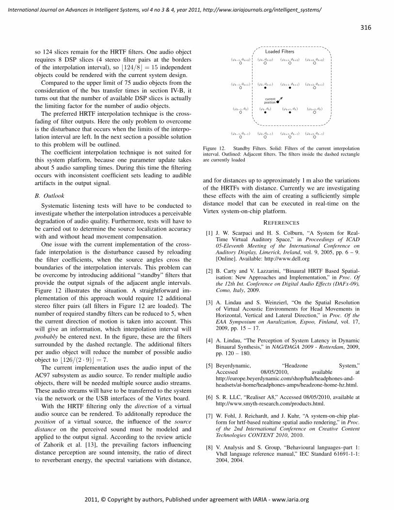
316



so 124 slices remain for the HRTF filters. One audio objectrequires 8 DSP slices (4 stereo filter pairs at the bordersof the interpolation interval), so b124/8c = 15 independentobjects could be rendered with the current system design.

Compared to the upper limit of 75 audio objects from theconsideration of the bus transfer times in section IV-B, itturns out that the number of available DSP slices is actuallythe limiting factor for the number of audio objects.

The preferred HRTF interpolation technique is the cross-fading of filter outputs. Here the only problem to overcomeis the disturbance that occurs when the limits of the interpo-lation interval are left. In the next section a possible solutionto this problem will be outlined.

The coefficient interpolation technique is not suited forthis system platform, because one parameter update takesabout 5 audio sampling times. During this time the filteringoccurs with inconsistent coefficient sets leading to audibleartifacts in the output signal.

B. Outlook

Systematic listening tests will have to be conducted toinvestigate whether the interpolation introduces a perceivabledegradation of audio quality. Furthermore, tests will have tobe carried out to determine the source localization accuracywith and without head movement compensation.

One issue with the current implementation of the cross-fade interpolation is the disturbance caused by reloadingthe filter coefficients, when the source angles cross theboundaries of the interpolation intervals. This problem canbe overcome by introducing additional “standby” filters thatprovide the output signals of the adjacent angle intervals.Figure 12 illustrates the situation. A straightforward im-plementation of this approach would require 12 additionalstereo filter pairs (all filters in Figure 12 are loaded). Thenumber of required standby filters can be reduced to 5, whenthe current direction of motion is taken into account. Thiswill give an information, which interpolation interval willprobably be entered next. In the figure, these are the filterssurrounded by the dashed rectangle. The additional filtersper audio object will reduce the number of possible audioobject to b126/(2 · 9)c = 7.

The current implementation uses the audio input of theAC97 subsystem as audio source. To render multiple audioobjects, there will be needed multiple source audio streams.These audio streams will have to be transferred to the systemvia the network or the USB interfaces of the Virtex board.

With the HRTF filtering only the direction of a virtualaudio source can be rendered. To additonally reproduce theposition of a virtual source, the influence of the sourcedistance on the perceived sound must be modeled andapplied to the output signal. According to the review articleof Zahorik et al. [13], the prevailing factors influencingdistance perception are sound intensity, the ratio of directto reverberant energy, the spectral variations with distance,

(ϕk−1, ϑk−1) (ϕk, ϑk−1) (ϕk+1, ϑk−1) (ϕk+2, ϑk−1)

(ϕk−1, ϑk) (ϕk, ϑk) (ϕk+1, ϑk) (ϕk+2, ϑk)

(ϕk−1, ϑk+1) (ϕk, ϑk+1) (ϕk+1, ϑk+1) (ϕk+2, ϑk+1)

(ϕk−1, ϑk+2) (ϕk, ϑk+2) (ϕk+1, ϑk+2) (ϕk+2, ϑk+2)

Loaded Filters

qPcurrentposition

Figure 12. Standby Filters. Solid: Filters of the current interpolationinterval. Outlined: Adjacent filters. The filters inside the dashed rectangleare currently loaded

and for distances up to approximately 1 m also the variationsof the HRTFs with distance. Currently we are investigatingthese effects with the aim of creating a sufficiently simpledistance model that can be executed in real-time on theVirtex system-on-chip platform.

REFERENCES

[1] J. W. Scarpaci and H. S. Colburn, “A System for Real-Time Virtual Auditory Space,” in Proceedings of ICAD05-Eleventh Meeting of the International Conference onAuditory Display, Limerick, Ireland, vol. 9, 2005, pp. 6 – 9.[Online]. Available: http://www.dell.org

[2] B. Carty and V. Lazzarini, “Binaural HRTF Based Spatial-isation: New Approaches and Implementation,” in Proc. Ofthe 12th Int. Conference on Digital Audio Effects (DAFx-09),Como, Italy, 2009.

[3] A. Lindau and S. Weinzierl, “On the Spatial Resolutionof Virtual Acoustic Environments for Head Movements inHorizontal, Vertical and Lateral Direction,” in Proc. Of theEAA Symposium on Auralization, Espoo, Finland, vol. 17,2009, pp. 15 – 17.

[4] A. Lindau, “The Perception of System Latency in DynamicBinaural Synthesis,” in NAG/DAGA 2009 - Rotterdam, 2009,pp. 120 – 180.

[5] Beyerdynamic, “Headzone System,”Accessed 08/05/2010, available athttp://europe.beyerdynamic.com/shop/hah/headphones-and-headsets/at-home/headphones-amps/headzone-home-hz.html.

[6] S. R. LLC, “Realiser A8,” Accessed 08/05/2010, available athttp://www.smyth-research.com/products.html.

[7] W. Fohl, J. Reichardt, and J. Kuhr, “A system-on-chip plat-form for hrtf-based realtime spatial audio rendering,” in Proc.of the 2nd International Conference on Creative ContentTechnologies CONTENT 2010, 2010.

[8] V. Analysis and S. Group, “Behavioural languages–part 1:Vhdl language reference manual,” IEC Standard 61691-1-1:2004, 2004.

317



[9] J. Blauert, Spatial Hearing The Psychophysics of HumanSound Localization. MIT Press, 1983, vol. 9.

[10] T. Liitola, “Headphone Sound Externalization,” Master’s the-sis, Helsinki University of Technology, Department of Elec-trical and Communications, 2006.

[11] S. Kurotaki, N. Suzuki, K. Nakadai, H. G. Okuno, andH. Amano, “Implementation of Active Direction-Pass Filteron Dynamically Reconfigur able Processor,” in IEEE/RSJInternational Conference on Intelligent Robots and Systems,2005, pp. 8912 – 8913.

[12] W. Fohl, J. Matthies, and B. Schwarz, “A FPGA-basedAdaptive Noise Cancelling System,” in Proc. of the 12th Int.Conference on Digital Audio Effects (DAFx-09), Como, Italy,2009.

[13] P. Zahorik, D. S. Brungart, and A. W. Bonkhorst, “Audi-tory Distance Perception in Humans: A Summary of Pastand Present Research,” Acta Acustica United with Acustica,vol. 91, pp. 409 – 420, 2005.

[14] B. Gardner and K. Martin, “HRTF Measurements of a KE-MAR Dummy-Head Microphone,” MIT Media Lab, Cam-bridge, MA 02139, MIT Media Lab Perceptual ComputingTechnical Report No.280, 1994.

[15] O. Warusfel, “LISTEN HRTF Database,”Accessed 08/05/2010, available athttp://recherche.ircam.fr/equipes/salles/listen/index.html.

[16] J. Reichardt and B. Schwarz, VHDL-Synthese Entwurf digi-taler Schaltungen und Systeme, 5th ed. München: Olden-bourg Wissenschaftsverlag, 2009.

[17] O. S. T. Inc., “Digital Compass Users Guide, OS5000 Se-ries,” Accessed 08/05/2010, available at http://www.ocean-server.com/download/OS5000_Compass_Manual.pdf.

318



An Integrated Approach for Data- and Compute-intensive Mining of Large DataSets in the GRID

Matthias Rohm, Matthias Grabert and Franz SchweiggertInstitute of Applied Information Processing

Ulm UniversityUlm, Germany

[email protected], [email protected], [email protected]

Abstract—The growing computerization in modern academicand industrial sectors is generating huge volumes of electronicdata. Data mining is considered the key technology to extractknowledge from these data. Grid and Cloud technologiespromise to meet the tremendously rising resource requirementsof heterogeneous, large-scale and distributed data mining ap-plications. While most projects addressing these new challengeshave a strong focus on compute-intensive applications, weintroduce a new paradigm to support the development ofboth compute- and data-intensive applications in heterogeneousenvironments. Combined storage and compute resources formthe basis of this new approach as they allow programs to beexecuted on resources storing the data sets and thus are thekey to avoid data transfer. A data-aware scheduling algorithmwas developed to efficiently utilize all available resourcesand reduce data transfer of global data-intensive applicationsas well as support compute-intensive applications. Based onthe results of the DataMiningGrid project we developed theDataMiningGrid-Divide&Conquer system that combines thisapproach with current Grid and Cloud technologies into ageneral-purpose data mining system suited for the differentaspects of today’s data analysis challenges. The system formsthe core of the Fleet Data Acquisition Miner for analyzing thedata generated by the Daimler fuel cell vehicle fleet.

Keywords- data-intensive; data mining; Grid; MapReduce;scheduling.

I. INTRODUCTION

Increasing data volumes in many industrial and academicsectors are fueling the need for novel data analysis solutions[1]. The effective and efficient management and transforma-tion of these data into information and knowledge is con-sidered a key requirement for success in knowledge-drivensectors. Data mining is the key methodology to addressthese information needs through automated extraction ofpotentially useful information from large volumes of data.In the last decade there have been multitudes of effortsto scale data mining algorithms for solving more complextasks, including peer-to-peer data mining, distributed datastream mining and parallel data mining [2] [3].

Recently, data mining research and development has puta focus on highly data-intensive applications. Google’s pub-lications on MapReduce [4][5], a special incarnation of thedivide&conquer paradigm, inspired many projects working

on large data sets. MapReduce frameworks, like Hadoop[6], simplify the development and deployment of peta-scaledata mining applications leveraging thousands of machines.MapReduce frameworks are highly scalable because theyavoid data movement and rather send the algorithms to thedata. In contrast to other data mining environments theseframeworks restrict themselves to a certain programmingmodel, loosing some of the functionality provided by fullyfeatured distributed data mining systems.

Another branch of modern distributed data mining ismotivated by the sharing of heterogeneous, geographic dis-tributed resources from multiple administrative domains tosupport global organizations [7] [8] [9]. This field of activeresearch and development is generally referred to as datamining in Grid computing environments. The DataMining-Grid project addresses the requirements of modern datamining application scenarios arising in Grid environments,in particular those which involve sophisticated resourcesharing. The DataMiningGrid system is a service-oriented,scalable, high performance computing system that supportsGrid interoperability standards and technology. It meets theneeds of a wide range of users, who may flexibly andeasily grid-enable existing data mining applications and de-velop new grip-based approaches. The DataMiningGrid, likemost related Grid systems, focused on compute-intensiveapplications following design principles that are correct forcompute-intensive, but not for data-intensive applications.For compute-intensive application scenarios the main re-source and the limiting factor is CPU-power and the focus ofthe system is to provide a transparent integration of multiplecompute clusters. In these scenarios it is commonly assumedthat the time needed to transfer the input and output datais relatively small compared to the overall execution time.These assumptions lead to an architecture build on threemain components:(1) Specialized storage servers to store input and output dataas well as executables. (2) A set of compute clusters fromdifferent organizations each composed of multiple computenodes for running the algorithms. To provide a high levelof transparency, these clusters are treated as one multi-CPUresource. (3) Grid management servers for accessing and

319



managing the storage and compute clusters of the localorganization.In such environments data is stored on dedicated storageservers and has to be transferred to the compute nodes priorto execution. Though different scheduling algorithms havebeen proposed to optimize the relation between data transferand execution time [10][11], for data-intensive applicationswhere the limiting factor is not CPU-power but ratherstorage and network speed, data should not be moved atall [12].

To bring the advantages of the MapReduce paradigm intoworldwide, heterogeneous computing environments we de-veloped the DataMiningGrid-Divide&Conquer (DMG-DC)[1] system based on the concepts and services of theDataMiningGrid project. This article covers a detailed de-scription of the scheduling algorithm and the Grid compo-nents to implement this new approach that combines differ-ent current data mining technologies into a single system.This article is organized as follows: First, we briefly reviseMapReduce frameworks and introduce the more generaldivide&conquer paradigm for data-intensive applications inGrid environments. Then we describe the DataMiningGridand its successor, the DMG-DC system. We also introducea real-world data mining application based on the DMG-DC: The Fleet Data Acquisition Miner (FDA-Miner) foranalyzing the data generated by the Daimler fuel cell vehiclefleet. Finally, we present system evaluation results from theFDA-Miner and discuss related technologies.

II. MAPREDUCE AND DATA-INTENSIVEDIVIDE&CONQUER

The tremendous amount of data generated in modernscience and business applications require new strategies forstoring and analyzing. As the amount of data increases,data can not be efficiently stored on a single storage serverbut has to be distributed over multiple machines. Google’sMapReduce[4] and its open-source implementations provideframeworks to mine these distributed data sets.

The name MapReduce refers to the map and reduce func-tions of functional programming languages. In the contextof a MapReduce framework, all applications consist of amap and a reduce function [4]. The map function reads akey/value pair and produces a set of new key/value pairs.In an intermediate step all pairs are grouped by their keyvalues. A key and its values are presented to the reducefunction which produces a list of result values.These functions are supposed to produce the same resultwhen applied to the whole data set or to the parts of thedata set.

MapReduce frameworks build an environment for execut-ing these map and reduce functions on a cluster. Data is splitup into small chunks and stored in a distributed file systemcomprised of multiple standard machines acting as storageand compute nodes [5]. A special manager node keeps

track of all data chunks and their locations in the cluster.A master process manages the execution and minimizesdata movement by executing the functions on the nodescontaining the data to be mined. The master identifies thenodes to use for execution by asking the distributed filesystem manager for the location of the data chunks. Ifmultiple copies of a chunk are available the master schedulesthe execution to the least used node.

Executing the functions on the nodes that contain thedata is the key to the high performance and scalability ofMapReduce frameworks. As not data, but algorithms aretransferred, MapReduce frameworks are perfectly suited forClouds because they do not require information about serverlocation and network bandwidth as traditional systems needfor data scheduling.

Restricting themselves to only two functions, MapReduceframeworks are easy to program and simple to set up.However, not all data-intensive applications can be decom-posed into map and reduce functions. Especially the integra-tion of existing data mining programs including compute-intensive applications is sometimes impossible. In addition,current MapReduce-Frameworks are implemented for clus-ters within a single organization and are not suitable forloosely-coupled environments comprised of heterogeneous,geographic distributed resources from multiple administra-tive domains.

A. Divide&Conquer for data-intensive Grid applications

Recent Grid implementations provide an ideal infrastruc-ture for inter-domain resource sharing but, as mentionedabove, are geared towards compute-intensive applications.To utilize Grid systems for a wide range of data- andcompute-intensive applications in such environments a dif-ferent distributed computing paradigm is needed.

MapReduce can be viewed as a special form of thedivide&conquer paradigm, where a problem is split intosmaller sub problems that are easier to solve. Compute-intensive applications also use a divide&conquer techniqueto leverage the performance of compute clusters by split-ting compute-intensive problems into smaller sub problemsand compute these sub problems on multiple resourcessimultaneously. Compared to MapReduce, the general di-vide&conquer paradigm does not impose any restrictionson the functions or the number of processing steps andis therefore more suitable for a general purpose distributeddata mining system. A data-intensive Divide&Conquer Gridprocessing model DCG might be defined as follows:(1) The data set D to be processed can be decomposedinto m subsets d1, . . . , dm (

⋃i≤m di = D) and stored on

multiple storage resources.(2) An arbitrary function ϕ is applied to all m subsets ofD in parallel. The execution of ϕ on resource r is denotedwith ϕr.(3) Assuming that data transfer is expensive, the function ϕ

320



is executed on a resource r which is closest to the storageof di

ϕr(di) = ei, di ∈ D, r ∈ R, r closest to di

and the results E may be processed by another function ϕ′,

ϕ′q(ei, ej , ...) = hi, ei, ej , ... ∈ E, q ∈ R, q close to ei, ej , ...

generating the result set H , which again may be processedby another function.(4) A series of such execution steps can be represented by adirect acyclic graph, where each node is a function and thevertices symbolize the data flow between the functions.

We identified the need for three major conceptual en-hancements to traditional Grids when applying the DCG ap-proach to data-intensive applications in Grid environments:

1) Any storage or computational resource may becomea combined storage/compute resource. This resourcetype forms the basis of scalable data-intensive applica-tions as data can be processed directly on the storagelocation. To increase storage capacity and speed, com-putational resources of compute clusters may becomecombined resources by storing data on their localdisks. It is important to point out that the combinedresources are suitable for data- and compute-intensiveapplications as only new functionality is added. Com-bined resources fundamentally differ from currentGrid concepts which impose a strict differentiationbetween storage and compute resources.

2) A combined resource may provide Grid data transfermechanisms. As combined resource will mostly beorganized within a cluster, data transfer out of the clus-ter is often not desired or not supported. This, again,differs from traditional Grids where each Grid storagehas to implement Grid data transfer mechanisms (e.g.,GridFTP).

3) A data processing methodology avoiding input datato be transferred. The scalability of data-intensiveapplications is mainly limited by two factors: thestorage and network speed. Combined resources arethe key to increase the overall storage speed of thesystem as each combined resources contributes itslocal storage. Avoiding input data transfer through pro-cessing the data directly on the resources storing thedata, minimizes network traffic and therefore increasesthe scalability for data-intensive applicaitons [12].

To illustrate the benefits of these concepts for data-intensiveapplications, consider the example depicted in Figure 1where a common Grid setup is shown on the left andthe new concepts on the right. In a traditional Grid setupmultiple clusters from different organisations are connectedthrough Grid servers hosting the Grid middleware. Eachcompute cluster is treated as one single resource by the Gridmiddleware and is managed by a local cluster management

Org A

Org B

S21

60 TB4 GB/s

200 nodes1800 CPUs

Grid2

C21

S11

40 TB2 GB/s

100 nodes800 CPUs

Grid1

C11

10 MB/s? Cloud C

(a) Common Grid setup

Org A

Org B

S21

60 TB4 GB/s

200 nodes1800 CPUs200 TB,20 GB/s

Grid2

C21

S11

40 TB2 GB/s

100 nodes800 CPUs100 TB,10 GB/s

Grid1

C11

10 MB/sCloud C ?

(b) DCG setup

Figure 1. A traditional Grid setup compared to the Divide&Conquerconcepts.

system like Condor, LSF or SGE. Dedicated storage systemsare used to store the input and output data of the computeclusters. These storage systems are optimized to supportmany concurrent connections for reading and writing to asingle large file. Cloud resources may also be integrated intothe local clusters to increase storage or compute capacity.A setup like this fits the needs of many compute-intensiveapplications: First an input file, or a part of it, is read byeach compute resource, then a model is computed for longtime and finally each compute resource writes its part of theoverall solution into the output file.

The situation changes in a Grid environment with multi-ple compute clusters from different organisations or Cloudproviders. When a compute-intensive application should beexecuted on a compute cluster in organisation A - or in theCloud C - and the input data is stored in organisation Bthe data has to be transferred from the storage system inB to the one in A or C because a cluster can not directlyaccess data on a storage system of another Grid site. Therequired data input and output transfers are often handled viaspecial pre- and post-processing steps. As it is commonlyassumed that the data transfer time is small compared to theexecution time the transfer overhead is accepted. For mostdata-intensive applications this assumption can not be hold.In contrary, not CPU-power but storage speed is the limitingfactor of many data-intensive applications. When applyingthe divide&conquer technique to data-intensive problems,large data sets are split into smaller subsets and distributedover multiple storage systems. An application may thenprocess all subsets in parallel and the overall processingspeed scales with the number of storage resources. In aGrid environment with a strict distinction between computeand storage resources, the only way of implementing this

321



approach is to add new storage resources. New dedicatedstorage resources not only increases costs but also thenetwork bandwidth becomes a limiting factor - especiallywhen resources from other Grid sites or the Cloud are used- because data always have to be transferred from a storageto a compute resource.

Here the combined resources of the DCG come into thepicture. As shown on the right of Figure 1, storing datasubsets on the compute nodes of a cluster saves costs,because existing resources are utilized, and increases storagespace as well as the overall storage speed. In addition,data can be processed and stored on a single resourcemaking data transfer superfluous. The combined resourcesare still managed by the grid middleware and the localcluster management system so that both data- and compute-intensive applications may run simultaneously on the samecluster.

The following example illustrates the differences betweena setup with separated storage and compute resources (1)and with combined resources (2): An application needs toscan through 20TB to find special patterns in the data.(1) The data is stored on storage resource S11. So the inputdata has to be transferred to one of the compute clusters C11,C21 or the Cloud. The scheduler decides to use the localcluster C11 as the connections to the other Grid instanceand the Cloud have limited bandwidth and the networkload is not known exactly. The cluster management systemstarts the data analysis program on all available resourcesof C11. At best all 100 compute resources start reading aportion (200GB) of the input data. As the storage systemS11 provides a maximum speed of 2GB/s, each resourceprocesses about 20MB/s. The overall time for processingthe 20TB is roughly 2.8 hours.(2) The data was split into 20GB chunks and distributed overthe 300 combined resources of the cluster C11 and C21 eachnow providing 1TB of storage with a speed of 100MB/s. Forredundancy each chunk is stored on at least two differentresources halving the overall storage space to about 150TB.To scan through the 20TB the scheduler advices the clustermanagement system to start the analysis program for eachdata chunk on a resource of C11 or C21 storing the datasubset. In this setup the scheduler can choose resourcesfrom different Grid sites or the Cloud for processing asthe input data has not to be transferred at all. At best 100combined resources immediately start processing the locallystored data chunk at a speed of 100MB/s each and a totalspeed of 10GB/s. The overall time for processing the 20TBwith combined resources comes down to about 0.6 hours.

B. A scheduling algorithm for DCG

The described data-intensive divide&conquer processingmodel requires not only new functionality to manage com-bined resources but also a method to schedule the executionof a program to a resource that is closest to the data. As

there was no algorithm available to schedule programs closeto data sets within a Grid, we developed the flexible DCGscheduling algorithm, which only needs information aboutthe compute and storage power of the combined resources.

The inputs of the DCG scheduling algorithm depicted inFigure 2 are the set of input data D, the program p, thedata locality weights λ1, λ2, the data transfer schedulingweights α1 to α4 and the data to compute ratio weightsβ1, β2. First, the scheduler obtains the current grid status andsorts the data sets of D in descending order. The orderingof D assures that the larger data sets are scheduled firstand the scheduler may therefore choose among more freeresources. After this init phase, the algorithm schedules eachdata subset d of the ordered input data D′. The main goal ofthe scheduler is to find a resource tuple (r, s) where: r ∈ Ris the best (highest compute speed gc) available executionresource that is able to execute p; and s ∈ Rd is the storageresource storing d with a minimal data transfer overheadto r. Due to the special properties of the Data DistanceFunction fs used to compute the data transfer overhead, thealgorithm only needs to consider four execution resourcesper storage resource s. These four execution resources are:the storage resource s itself, the best resource within thesame cluster rc, the best resource within the same grid rgand the best resource outside the local grid instance ra.From the resulting 4 · |Rd| candidate (r, s) resource tuplesthe scheduler chooses the one with the highest priority ascomputed by the Normed Priority Function fp.

The algorithm and functions are based on the followingdefinitions:P := all programs available in the Grid;R := {r1, . . . , rn} is the set of all n resources of the grid;D := {d1, ..., dm} is the m data sets of the job;Q := {(r, s)|r, s ∈ R, r and s can exchange data directly};Rd := { r | r ∈ R stores d ∈ D };Dr := { d | d ∈ D is stored on r ∈ R };δc : R → {1, . . . , nc} assigns a unique number to each ofthe nc clusters;δg : R → {1, . . . , ng} assigns a unique number to each ofthe ng grid sites;gs(Z, d, r) is the storage speed of resources r with respectto d defined as gs(Z, d, r) ≥ 0 if d is stored on r;and gc(Z, p, r) is the compute power of resource r withrespect to program p defined as gc(Z, p, r) ≥ 0 if r fulfillsall requirements of p. Different properties of a resource maybe used to define the computing and storage power of aresource, but at least the current usage - included in theoverall system state Z - has to be taken into account.

The data transfer overhead of a candidate resource tupler, s is computed by the Data Distance Function fs whichassigns the weights α1 to α4 to the storage power of saccording to the distance between s and r: α1 if d isstored on the resource itself r = s; α2 if d is storedon a resource on the same cluster δc(r) = δc(s); α3 if

322



FUNCTION DCG (p ∈ P , D, α1−4, β1−2, λ1−2)Z ← current state of the gridD′ ← D ordered by sizeC ← ∅for all d ∈ D′ doC

′ ← ∅for all s ∈ Rd dorc with gc(Z, p, rc) = max{gc(Z, p, r) | r ∈ R ∧ δc(rc) = δc(r)}rg with gc(Z, p, rg) = max{gc(Z, p, r) | r ∈ R ∧ δg(rg) = δg(r)}ra with gc(Z, p, ra) = max{gc(Z, p, r) | r ∈ R ∧ δg(ra) 6= δg(r)}C ← C ∪ { (s, s, fs(Z, d, s, s), gc(Z, p, s)),

(s, rc, fs(Z, d, s, rc), gc(Z, p, rc)),(s, rg, fs(Z, d, s, rg), gc(Z, p, rg)),(s, ra, fs(Z, d, s, ra), gc(Z, p, ra)) }

end forFind c ∈ C with fp(c) = max{fp(c) | c ∈ C}if fp(c) ≤ 0 then

print Could not schedule delseC ← C ∪ {c}Z ← current State of Z after choosing c

end ifend forreturn C #Return schedule C containing the choices c for each scheduled data set

END FUNCTION

Figure 2. DCG algorithm for scheduling a program for each data set

d is on the same Grid instance δg(r) = δg(s); and α4

if d is on another Grid instance δg(r) 6= δg(s). In caseboth resources are not able to exchange data directly, eachresource needed to transfer the data set d from s to r is alsoconsidered.FUNCTION fs(Z, d ∈ D, s ∈ Rd, r ∈ R)t ← t∞if (r, s) ∈ Q thent ← |d|/gs(Z, s)

else if ∃ s1, . . . , sp with (s, s1), . . ., (sp−1, sp), (sp, r)∈ Q then

Choose shortest s1, . . . , sq with (s, s1), . . . (sq, r) ∈ Qt ← |d|/gs(Z, s) +

∑qi=1 |d|/gs(Z, si)

end ifif r = s thent ← α1 · t

else if δc(r) = δc(s) thent ← α2 · t

else if δg(r) = δg(s) thent ← α3 · t

elset ← α4 · t

end ifreturn t

END FUNCTIONAs can easily be seen the data transfer scheduling weights α1

to α4 may be used to enforce specific data transfer policies:

• α1 > 0, α2 = α3 = α4 = t∞ forces the scheduler tochoose a resource storing the data set d regardless ofits speed.

• α1 ≤ α2, α3 = α4 = t∞ forces the scheduler tochoose a resource storing the data set d or a resourcein the same cluster.

• α1 ≤ α2 ≤ α3, α4 = t∞ forces the scheduler tochoose a resource belonging to the same Grid instancefavoring resources storing the data or resources in thesame cluster.

• With α1 ≤ α2 ≤ α3 ≤ α4 the scheduler may chooseany resource in the Grid, but prefers resources close tothe data storage location d.

The Normed Priority Function is used to compute thepriority of each resource as its data transfer overhead andits compute power. In addition, a data locality may beincluded into the priority calculation. The priority of each

323



tuple (s, r) is the linear combinaton of the weighted transfertime (fs(Z, d, s, r)), the compute speed (gc(Z, p, r)) and thecluster and grid data locality factors (uclu, ugrid). To controlthe influence of each value on the scheduling the values arenormed to [0 : 1] using a non-linear norming function gn andmultiplied with a weight, where β1 describes the importanceof the data, β2 the weight of the compute power and λ1, λ2control the influence of the data locality in the schedulingprocess. The data locality factors uclu, ugrid describe howmuch of the input data D is stored within the cluster orgrid of the resource r and how fast the storage is. Thefactors are especially useful if the results of the executionwill be combined by a subsequent step of the executiongraph.FUNCTION fp(r ∈ R,Sr ∈ RD, tr ∈ <, vr ∈ <)

if tr ≥ t∞ ∨ vr ≤ 0 thenreturn 0

end ifuclu ←

∑d∈D

∑s∈Rd∧δc(r)=δc(s)

|d||D| · gs(Z, s)

ugrid ←∑d∈D

∑s∈Rd∧δg(r)=δg(s)

|d||D| · gs(Z, s)

q ← β1 ·gn(tr)+β2 ·gn(vr)+λ1 ·gn(uclu)+λ2 ·gn(ugrid)return q

END FUNCTIONFigure 3 shows the more general DCG-MD scheduling

algorithm for applications requiring multiple input data sets.In this scenario all data sets have to be available on oneexecution resource. First, the algorithm produces the set ofcandidate execution resources as the best (highest computespeed gc) resources from all nc clusters in the Grid and allresources storing one of the data sets d ∈ D. For each ofthese resources the set of storage resources with minimaltransfer overhead with regard to D is generated. From allcandidates the scheduler chooses the one with the highestpriority fp.

In order to support a wide range of data- and compute-intensive Grid applications without re-implementing every-thing from scratch it was decided to integrate the developedDCG approach into an existing grid-based data miningsystem. As the DataMiningGrid system described in the nextsection already provides many functionalities for grid-baseddata mining it was chosen as a basis for the DMG-DCsystem. Because of the missing support for data-intensiveDCG applications it had to be enhanced with: (1) A dis-tributed data registry to store, manage and locate all datasubsets. (2) A resource broker implementing the schedulingalgorithm described in this section. (3) A workflow managerto coordinate multiple dependant execution steps.

III. DATA MINING IN THE GRID: DATAMININGGRID

In general, a grid-enabled data mining system should sup-port the seamless and efficient sharing of data, data miningapplication programs, processing units and storage devices in

heterogeneous, multi-organizational environments. As datamining is used by a wide variety of users and organiza-tions such a system should not only address the technicalissues but also pay attention to the unique constraints andrequirements of data mining users and applications. In theDataMiningGrid[7] project, use case scenarios from a widerange of application areas were analyzed to identify thekey requirements of grid-based data mining that can besummarized as follows:

• A grid-based data mining environment should offerbenefits like increased performance, high scalability toserve more users and more demanding applications,possibilities for creation of novel data mining appli-cations and improved exploitation of existing hardwareand software resources.

• Grid-enabling data mining applications should not re-quire modification of their source code. The systemshould not be restricted to specific data mining pro-grams, tools, techniques, algorithms or application do-mains and should support various types of data sources,including database management systems (relational andXML) and data sets stored in flat files and directories.

• To support the different user groups, intricate tech-nological details of the Grid should be hidden fromdomain-oriented users, but at the same time users witha deep knowledge of Grid and data mining technologyshould be able to define, configure and parameterizedetails of the data mining application and the Gridenvironment.

In order to address these requirements, the DataMiningGridsystem was designed according to three principles: services-oriented architecture (SOA), standardization and open tech-nology. The early adoption of two important distributed com-puting standards, the Open Grid Service Architecture[13](OGSA) and the Web Services Resource Framework[14](WSRF)were essential for succeeding projects, like theone presented in this article. The OGSA is a distributedinteraction and computing architecture based on the conceptof a Grid computing service, assuring interoperability onheterogeneous systems so that different types of resourcescan communicate and share information. The WSRF refersto a collection of standards which endorse the SOA andproposes a standard way of associating Grid resources withweb services to build stateful web services required by theOGSA.

Following these principles, the DataMiningGrid projectimplemented various components based on existing opentechnology: Data management, security mechanisms, exe-cution management and other services commonly needed inGrid systems are provided by the Globus Toolkit 4 (GT 4)Grid middleware.

Three higher-level components for data, information andexecution management form the core of the DataMiningGrid

324



FUNCTION DCG-MD (p ∈ P , R, D, α1−4, β1−2, λ1−2)Z ← current state of the gridRmax ← {ri |∀i ≤ nc : ri ∈ R ∧ δc(ri) = i ∧ gc(Z, p, ri) = max{gc(Z, p, r)|r ∈ R ∧ δc(r) = i} }Rsp ← { r | ∀d ∈ D : r ∈ Rd ∧ gc(Z, p, r) > 0 }C ← ∅for all r ∈ Rmax ∪Rsp doZ ′ ← Z , td ← 0 , S ← ∅for all d ∈ D do

Find s ∈ Rd with fs(Z ′, d, s, r) = min{fs(Z ′, d, s, r)|s ∈ Rd}td ← td + fs(Z

′, d, s, r)S ← S ∪ {s}Z ′ ← current State of Z ′ after choosing s

end forC ← C ∪ {( r, S, td, gc(Z ′, p, r) )}

end forFind c ∈ C with fp(c) = max{fp(c) | c ∈ C}return c

END FUNCTION

Figure 3. DCG algorithm for scheduling a program with multiple data sets

system. The data components offer several data transforma-tion and transportation capabilities to support typical dataoperations for data mining applications based on OGSA-DAI[15] and the Globus Toolkit data management com-ponents. The Information Service collects and manages allinformation about the data mining programs available in thesystem. The Resource Broker is responsible for matchingavailable resources to job requests, global scheduling of thematched jobs and executing, managing and monitoring ofjobs, including data stage in and out operations.

The main user interface of the system is the Trianaworkflow environment [16]. Triana provides a workfloweditor and manager to design and execute complex work-flows. Several DataMiningGrid workflow components buildthe interface to the GT 4 Grid infrastructure services aswell as the DataMiningGrid services. The most importantcomponents allow the users to search for an application,configure its parameters, select and transform the input datasets and finally execute the configured task on the Grid.

The DataMiningGrid Application Description Schema(ADS) is the link between these DataMiningGrid compo-nents. An ADS instance covers the complete life-cycle ofa data mining task. The XML document is devided intofour parts: A description, information about the executable,requirements as well as monitoring and accounting informa-tion. The description contains data mining specific informa-tion about the implemented algorithm following the CRISP-DM standard and is mainly used for discovering. The nextsection contains all information regarding the executables

implementing the algorithm, including the required libraries,options and parameters for configuring the executables.The requirements section holds the hardware and softwarerestrictions imposed by the implementation of the executableor the user. Throughout the execution the ADS containsmonitoring information and after the execution is finished,the ADS instance also stores all information related to theexecution environment.

Although the necessity to address data-intensive applica-tions was recognized in the DataMiningGrid project, dueto time constraints, the project focused more on compute-intensive applications. Hence, three functionalities neededfor DCG jobs are not available in the DataMiningGrid andrelated systems:

1) There is no server-side workflow execution componentto coordinate the steps of DCG jobs.

2) There is no specialized data registry that could be usedfor scheduling data-intensive applications.

3) The Resource Broker [17], like other Grid resourcebrokers, does not provide a scheduling mechanism forcombined resources and is only able to schedule andexecute jobs on a clusters level. As a consequence,jobs can not be placed directly on combined stor-age/compute resources inside a cluster, as required byDCG jobs.

The following section describes the changes made to theDataMiningGrid system as well as the new components andfeatures of the DMG-DC system to natively support data-intensive applications in Grid environments.

325



IV. DATAMININGGRID DIVIDE&CONQUER SYSTEM

The DMG-DC system is designed to support the differ-ent aspects of today’s data analysis challenges, includingcompute- and data-intensive applications. Combined storageand compute resources form the basis of the DMG-DCsystem, allowing data to be stored and processed on anymachine in a Grid. With this approach there is no need totransfer the input data from a storage server to a computenode prior to execution, which can significantly speed updata-intensive applications.

V. DMG-DC

Unfortunately, as discussed in the previous sections, cur-rent grid-based systems do not provide the functionalityto support these combined resources because of the focuson compute-intensive applications. As a consequence, thereare two different approaches to design a Grid system forcombined resources that supports both, compute- and data-intensive applications: (1) Implement all needed functional-ity as a set of new services from scratch; (2) use or enhanceexisting systems and services where possible.The architecture proposed in this article follows the laterapproach and builds on the DataMiningGrid system incombination with standard Grid infrastructure services. Thisnot only reduces the implementation time but also ensuresthe compatibility of the system with newer versions of theGrid infrastructure.

The DataMiningGrid project already implements manyfeatures needed for grid-based data mining. The flexibleand extendable design of the DataMiningGrid system madeit easy to integrate the missing functionality to supportdata-intensive applications. Consequently, the architectureof the DMG-DC, depicted in Figure 4, does not differsignificantly from the DataMiningGrid architecture [7]. Theclient components, the Triana workflow environment andtwo web-based applications, are build on top of the DMG-DC services and may also directly interact with the Gridinfrastructure services. The DMG-DC services, the Infor-mation Integrator Service (IIS), the Data Registry Service(DRS) and the Workflow Resource Broker (WRB), provideall additional functionality to support DCG jobs in a standardGrid environment. The IIS manages all available data-miningalgorithms as ADS instances and provides an interface toadd and remove ADS descriptions. The DRS and the WRBservices are the main building blocks to execute DCG jobs.The DRS manages all information about each data set in theGrid, including the storage location, and provides powerfulfunctions to search for data sets. The WRB schedules andmanages multiple Grid jobs in the correct sequence. Incombination with the DRS the matchmaking and schedulingfunctions of the WRB are able to execute data-intensive jobsdirectly on the Grid nodes storing the data. The DRS andWRB are build on top of the Grid layer and use various

DataService

DataService

MDS4

ObjectDatabases

ObjectDatabases

Applications SystemServices

DataService

ObjectDatabases

Figure 5. The DMG-DC Data Registry Service architecture

GT 4 Grid services like the MDS4, the RFT or the WS-GRAM [18]. The Grid layer also provides all functionalityto integrate the resources of the different organisations into asingle virtual organisation. In most setups all resources of anorganisation are managed by one Grid server instance that isconnected to the grid servers of all other organisations. Mul-tiple compute or combined resources within an organisationare typically controlled by a cluster management system likeCondor, Sun Grig Enging or LSF.

A. Data Registry Service

The data registry is the central component for executingDCG jobs in a Grid, as it provides the locations of all datasets to the Resource Broker. Without this information theResource Broker would not be able to schedule jobs tothe nodes containing the data to be mined. The developeddistributed registry consists of a number of WSRF-compliantData Registry Services that store user-defined metadatadescribing the data sets available in the Grid. In contrastto the distributed file system of a MapReduce framework,the DRS only stores information about the data, leavingthe actual storage to database management or file systems.Therefore, DCG jobs can process data stored in any storagesystem and are not limited to a specific distributed filesystem.

The DRS stores metadata in user-defined categories whichspecify a list of logical and physical attributes describing thedata. Logical attributes hold information about the content orcreation process of the data set, whereas physical attributesinclude storage location, size or data format information.When a new data set is registered with a category, a logicaland a physical object is created with unique object names.These objects contain the logical/physical attributes of thatdata set and are used to model replication: A logical objectreferences one or more physical objects.

A single DRS may store the metadata information of alldata sets in the Grid. To improve reliability and performanceseveral DRS may run on different sites in the Grid. Asdepicted in figure 5 multiple DRS automatically form apeer-to-peer network, forwarding client search requests andcategory information to the appropriate DRS.

326



Data MiningActivities

InformationIntegrator

Execution Management

OGSA-DAI

WorkflowRessource Broker

ApplicationExplorer

DataComponents

RFT

/G

ridFT

P

LocalCluster

Managment

Legend:

Grid-Middleware Software Ressource

Components developed by DataMiningGrid or FDA Hardware Ressource

Security

CommonRuntime

InformationServices(MDS4)

Executionand Monitor

CredentialGenerator

DMG WebApplication

ApplicationEnabler

EnhancedCondorAdapter

EnhancedFork

Adapter

Triana Workflow Editor and Manager DMG-DC Web-Client

DMG-DC and FDAClient Components

DMG-DC High Level Service

Globus Toolkit 4

Hard and Software Ressources

Processing Units, Networks, Storage

Data Mining Programs, Files, DirectoriesDatabase Management Systems

Data RegistryServices

Online Reporting

FDA Web-Client

Data Analysis Composer

Figure 4. The DMG-DC architecture

As many data analysis applications need mechanisms toselect and process arbitrary subsets of the data stored in theGrid, the DRS provides an advanced search enabling clientsto search for data using multiple attributes within a singlequery. This distinctive feature of the DRS is not availablein other Grid data registries like the Globus Toolkit ReplicaLocation Service [19].

B. Workflow Resource Broker

The new requirements arising from DCG jobs led to thedevelopment of the DMG-DC Workflow Resource Broker.The WRB was designed not only to support DCG jobs butalso to include all features of current Grid resource brokerslike the DataMiningGrid Resource Broker [17]. The two

central new features of the WRB are the workflow executionmanager and the advanced job scheduler, able to schedulejobs close to the data.

As depicted in Figure 6, the WRB consist of 5 componentscommunicating through well-defined interfaces:Clients connect to the workflow manager to submit work-flows, monitor and manage workflow execution. A work-flow consists of one or more jobs, each described by anADS instance, and dependencies between these jobs. Theworkflow manager is responsible for executing all jobs asspecified in the workflow. To start the execution of a singlejob, the workflow manager sends the corresponding ADSinstance to the ADS execution component. The execution

327



DRS

MDS4

Clients

WS-GRAM

Workflow Ressource Broker

InformationManager Condor-G

WorkflowManager

ADSExecution

LocalCluster

Management

DataLocater

Figure 6. The components of the Workflow Resource Broker.

component analyzes the ADS instance and connects to thedata locator to get the locations of all data sets specifiedin the ADS instance. The data locator acts as an interfaceto different data registries, although currently only DRSis supported. The execution component combines the datalocations with the ADS definitions and generates a Condor-G job description. In addition to the standard job descriptionparameters, like executable and arguments, the generateddescription also contains a Condor-G representation of thedeveloped scheduling algorithm enabling DCG jobs to runon nodes storing the selected data sets.

Condor-G [20] is a powerful Grid task broker providingadvanced scheduling, execution and managing capabilitiesas well as an uniform interface to different Grid executionmanagement systems. A key feature of Condor-G is itsClassAd mechanism to describe jobs and compute resourceswith specific ClassAd attributes for jobs and compute re-sources. Based on these descriptions jobs can be matchedand scheduled to suitable compute resources. ClassAds canalso be used to implement various different scheduling poli-cies through defining requirements and rank expressions.As current Grid implementations do not provide resourceinformation as ClassAds we developed the informationmanager. The information manager collects all informationfor each computational resource from the Grid informa-tion system - currently only an interface to the GlobusToolkit Monitoring and Discovery System (MDS4) is im-plemented - and translates it into ClassAds. To implementthe Divide&Conquer scheduling algorithm the informationmanager adds two new ClassAds for combined resources:the ClusterInstance and the GridInstance. With thesenew ClassAds, each combined resource can be uniquelyidentified and directly used for scheduling.When receiving a job, Condor-G matches the job with allavailable resources, as defined by the respective resourceand job ClassAds. DCG jobs contain special requirementsand rank expressions that configure the Condor-G scheduleraccording to the scheduling algorithm described above. Afterthe matchmaking step, the job is submitted to the executionmanagement service - in case of the Globus Toolkit, theWS-GRAM - of the Grid instance providing the best match.

The job submitted to the WS-GRAM contains an elementinstructing the WS-GRAM to produce a job descriptionfor the local cluster management system - currently onlyCondor is supported - that insures the job is only startedon the chosen resource. The WS-GRAM of this instancethen submits the job to the cluster management system thatmanages the chosen resource. Figure 7 shows the interactionof all components while executing a single DCG job: (1)A client searches for suitable algorithms in the MDS4 andreceives an ADS description. (2) The client configures thealgorithm parameters, the input/ouptut data and optionallythe scheduler parameters αx and λ. Input data can bespecified by logical object names or a search query. Steps(1) and (2) may be repeated several times to compose acomplex workflow. (3) The client submits a single ADS ora workflow description to the WRB. (4) The WRB parses theworkflow and starts processing of the root ADS descriptionsof the workflow. First it retrieves the current status of allcompute resources from the MDS4. Then it queries the DRSfor the physical attributes, including the storage location,of all input data. Based on this information it configuresa Condor-G job description implementing the developedscheduling algorithm and starts the scheduling. For each ofthe 4 data subsets the scheduler initiates the execution onone of the combined resources storing the data. (5) As the4 chosen resources are located in the organisations A and BCondor-G creates WS-GRAM job descriptions and submitsthem to the WS-GRAMs. (6-7) The WS-GRAMs parses thedescription and initiates the transfer of the executables fromorganisation D to the local storage. (8) The WS-GRAMtranslates the job description to the format of the localcluster management system and submits it. (9-10) The localcluster management system parses the job description withthe restriction to only use the chosen resources and startsthe execution on these resources. (11a - 11c) The localcluster management system monitors the execution. TheWS-GRAM periodically polls the status of the job from thelocal cluster management system. Condor-G in turn polls theWS-GRAMs and provides the information to the WRB. (12-13) As the user specified a storage resource in organisationC as the output data location, the WS-GRAM initiates thetransfer of the results.

VI. FDA-MINER

The presented DMG-DC system forms the basis of theFleet Data Acquisition Miner (FDA-Miner) for analyzingthe data generated by the Daimler fuel cell vehicle fleet.The Daimler AG has been involved in fuel cell technologyfor more than 15 years and has released the largest fleetof zero emission fuel cell vehicles in the world with morethan 100 vehicles [21]. The purpose of these operations isto test these vehicles in the hands of selected customersin everyday operations under varying climatic conditions,traffic conditions and driving styles in different locations

328



Org C

ApplicationService

MDS4

Application

WRB

Client

RFT/GridFTP

Org D

RFT/GridFTP WS-GRAM

LocalCluster

Managemt

Org B

RFT/GridFTPWS-GRAM

LocalCluster

Managemt

Org A

WS-GRAM

LocalCluster

Managemt

RFT/GridFTP

Legend: Organisation

Middleware Component: GT4, Condor... Software Resource

DC-DMG-Service / Component Management and informationcommunication

Data and data managementcommunication

Storage Resource

CPU Resource

54

3

21

6

11a

713

128

11b

11cData

Service

5

7

11a8

6

12

Results

13

910 109 9

Figure 7. Interaction of the different components while running a Divide&Conquer job.

worldwide. In order to gain the most experience for futurefuel cell vehicle development, a fleet data acquisition systemhas been developed which continuously records all relevantparameters of vehicle operation, such as the fuel cell voltage,current and temperatures. The enormous amount of world-wide distributed data produced by the fleet - over 4 millionkilometers have been recorded - and the needs for compute-intensive data analysis methods were the key drivers behindthe development of the DMG-DC system [22].

The FDA-Miner provides a user friendly web-based dataanalysis application for mining the fuel cell data. In additionto specialized visualization and reporting features, it offersa flexible front end to configure customized data miningtasks. The application uses the services of the DMG-DCto retrieve information about the available data and analysisprograms. For each user defined task, the application createsthe appropriate ADS instances and workflow definitions andsubmits it to the WRB.

The FDA-Miner programming toolbox supports usersimplementing specialized DCG data mining algorithms. Thetoolbox provides Perl and C modules to read the fuel celldata sets and templates for parallel data processing andcombination steps.

A common usage scenario of the FDA-Miner is the gener-ation and testing of models for different key components ofthe fuel cell system. First the user defines a model, e.g., anArtificial Neural Network, to analyze or simulate a specificcomponent then the data to train the model is selected. Inmost cases only data points with special properties are ofinterest. In a first data-intensive processing step these datapoints have to be filtered out of all available data by aDCG job. The resulting training data is relatively small andis transferred to a fast machine for the compute-intensivemodel training. In the next step the model is applied to asubset or the complete data set to evaluate the model.As model definition - model training - model evaluation is

329



an iterative process and new data is recorded constantly,this process is repeated frequently. With its ability to ef-ficiently execute data- and compute-intensive programs theFDA-Miner helps reducing the overall processing time ofsuch applications and therefore enables shorter developmentcycles of fuel cell vehicle components.

VII. EVALUATION

The FDA-Miner has been already heavily used in pro-duction and successfully computed thousands of data- andcompute-intensive jobs. The following evaluation thereforefocuses on the advantages of the DCG functionality of theDMG-DC system compared to traditional Grid systems, likethe DataMiningGrid, with dedicated storage servers. Theevaluation setup consisted of 9 dual quad core machines withdirect attached storage connected over a 1 GBit Ethernetnetwork. To measure the performance of the DCG function-ality, a subset of the fuel cell data was randomly distributedover all 9 machines and each file was placed on at least twomachines. Traditional Grid systems were represented by arepresentative scenario with 1 storage server serving the datato 8 compute nodes.

A typical FDA-Miner data-intensive analysis job - filteringthe data and computing various statistical properties - wasexecuted on both setups. Figure 8 shows the overall timefor performing this job while varying the number of CPUsand the size of the data set. The results demonstrate that theDMG-DC (blue curve), like MapReduce systems, scales wellfor data-intensive analysis jobs. When the number of CPUsis increased more machines and their storage are utilized,leading to a higher overall data throughput. As no input datais transferred, there is no transfer overhead and the CPUscan leverage the complete storage speed of the machine.

Traditional Grid systems (orange curve) on the otherhand have to send the data to the compute nodes first.This not only introduces an additional overhead but alsolimits the processing performance to the storage speed ofthe file server. Depending on the network bandwidth andthe storage speed the transfer time may, for simple datafiltering operations, even exceed the time for data processing.Scaling of these systems is also limited by the number ofconcurrent connections the storage server can handle withoutdropping network throughput. In the presented evaluationsetup a single storage server can only deliver enough data toserver about 20 CPUs and therefore does not scale above thatpoint. Adding additional dedicated storage servers is the onlyway to increase the system performance. Then distributedfile systems like Lustre[23] have to be used if a single filesystem is required.

VIII. RELATED WORK

Recently, various systems and approaches to grid-baseddata mining and MapReduce have been reported in the

0,00

5,00

10,00

15,00

20,00

10 20 40 60CPUs

Tim

e

Send

D&C

(a) 11694 data sets

0

100

200

300

400

500

10 20 40 60CPUs

Tim

e

Send

D&C

(b) 256530 data sets

Figure 8. Execution time of a job in Send and Divide&Conquermode.

literature. Some of those, that are particularly relevant tothe DMG-DC system, are briefly reviewed here.

The GridBus resource broker [24] provides functionsfor scheduling data- and compute-intensive applications. Incombination with the Storage Resource Broker[25] GridBusis able schedule data-intensive jobs based on various dif-ferent metrics, including network bandwidth and utilization.As GridBus follows the common separation between storageand compute resources, data has to be transferred prior toexecution and therefore it does not provide DCG or similarfunctionality at the moment. In addition GridBus is notcompatible with current grid standards, in particular WSRF.

The Cactus [26] broker was developed to supportcompute-intensive numerical calculations in Grid environ-ments. It is based on MPICH-G and the Globus Toolkit andrequires that applications have to be written in MPI. Thisrestriction makes it almost impossible to integrate existingdata mining applications. In addition Cactus is not WSRF-compliant and does not provide any notion of data aware

330



scheduling to support data-intensive DCG applications.The GridWay Meta-Scheduler [27] is the built in resource

broker of the Globus Toolkit. GridWay provides common re-source brokering functions including data aware scheduling.Storage and compute resources are treated separately so thatdata has to be transferred prior to execution and there is nosupport for DCG processing.

Data Mining Grid Architecture (DMGA) [28] focuses onthe main phases of a data mining process: pre-processing,data analysis and post-processing. The proposed architectureis composed of generic data Grid and specific data miningservices. WekaG is an implementation of DMGA based onthe data mining toolkit Weka and the Globus Toolkit 4. TheDMGA itself is a flexible architecture to build grid-baseddata mining system. But its only implementation WekaG isrestricted to Weka. The service based approach offers highflexibility but implies resource utilization issues as a servicecan only use the local resources and WekaG provides noDCG or similar functionality at the moment.

Anteater [2] is a web-service-based system to handle largedata sets and high computational loads. Anteater applicationshave to be implemented in a filter-stream structure. Thisprocessing concept and its capability to distribute fine-grained parallel task make it a highly scalable system. Dueto the restriction on a filter-stream structure Anteater sharessome downsides of MapReduce frameworks: Applicationshave to be ported to this platform which makes it almostimpossible to integrate existing applications.

GridMiner [9] is designed to support data mining andonline-analytical processing in distributed computing envi-ronments. GridMiner implements a number of common datamining algorithms, some as parallel versions, and supportsvarious text mining tasks. Two major differences betweenGridMiner and DMG-DC are the DCG functionality and thatthe latter complies with the recent trend towards WSRF.

Knowledge Grid (K-Grid) [8] is a service-oriented systemproviding grid-based data mining tools and services. The K-Grid system can be used for a wide range of data miningand related tasks such as data management and knowledgerepresentation. The system architecture is organized into ahigh-level K-Grid services and a core-level K-Grid servicelayer, which are built on top of a basic Grid services layer.K-Grid incorporates some interesting features for distributeddata mining but no DCG or similar functionality is availableat the moment.

Hadoop [6] is the most well known open source im-plementation of Google’s MapReduce paradigm. Hadoop’sMapReduce framework is build on top of the Hadoopdistributed file system (HDFS) containing all data to bemined. The map and reduce functions are typically written inJava, but also executables can be integrated via a streamingmechanism. MapReduce frameworks like Hadoop do not of-fer the functionality to efficiently execute compute-intensiveapplications on a cluster, making them unsuitable for a

general-purpose data mining system. Hadoop On Demandin combination with the SUN Grid Engine try to overcomethese limitations by running Hadoop on top of a clustermanagement system, thus adding another layer of complex-ity. Still, the resources to use for MapReduce are reservedexclusively for Hadoop and can not be used by other jobs.Hadoop and similar MapReduce frameworks simplify thedevelopment and deployment of data-intensive applicationson local clusters and cloud resources but, in contrast to theDMG-DC system, these frameworks are currently not suitedfor large-scale, heterogeneous environments comprised ofmultiple independent organizations.

IX. CONCLUSION

In this article, we introduced the DCG, a divide&conquerapproach for data-intensive applications in Grid environ-ments. The new concept of combined Grid resources in com-bination with the developed data location aware schedulingalgorithm provides an infrastructure to build scalable data-intensive applications in worldwide, heterogeneous environ-ments. The scheduling algorithm and the implemented Re-source Broker also support compute-intensive applicationsso that both data- and compute-intensive applications canbe implemented in one single system. The developed DMG-DC system not only provides the functionality to run diversedata- and compute-intensive data mining applications butalso supports the complete data mining process end-to-end.

The FDA-Miner, a real world data analysis application,uses the distinct features of the DMG-DC system to ef-ficiently mine the data of the whole Daimler fuel cellvehicle fleet. The FDA-Miner evaluation results highlightthe advantages of the DMG-DC compared to traditional Gridsystems.

Future work may include the integration of other datamanagement systems like the Globus Toolkit Data Replica-tion Service[29] or the Storage Resource Broker, adding sup-port for other local cluster management system than Condorand a generalized version of the FDA-Miner programmingtoolbox.

REFERENCES

[1] M. Rohm, M. Grabert, and F. Schweiggert, “A generalizedmapreduce approach for efficient mining of large data sets inthe grid,” in 1. International Conference on Cloud Computing,GRIDs, and Virtualization, CLOUD COMPUTING 2010,Lisbon, Portugal, 2010, pp. 14–19.

[2] D. Guedes, W. Meira, and R. Ferreira, “Anteater: A service-oriented architecture for high-performance data mining,”IEEE Internet Computing, vol. 10, no. 4, pp. 36–43, 2006.

[3] S. Datta, K. Bhaduri, C. Giannella, and H. Kargupta, “Dis-tributed data mining in peer-to-peer networks,” IEEE InternetComputing, vol. 10, no. 4, pp. 18–26, 2006.

331



[4] J. Dean and S. Ghemawat, “Mapreduce: Simplified data pro-cessing on large clusters,” 2004, pp. 137–150. [Online]. Avail-able: http://www.usenix.org/events/osdi04/tech/dean.html

[5] S. Ghemawat, H. Gobioff, and S. T. Leung, “The google filesystem,” SIGOPS Oper. Syst. Rev., vol. 37, no. 5, pp. 29–43,2003.

[6] T. White, Hadoop: The Definitive Guide, 1st ed. O’ReillyMedia, 2009.

[7] V. Stankovski, M. Swain, V. Kravtsov, T. Niessen, D. We-gener, M. Rohm, J. Trnkoczy, M. May, J. Franke, A. Schuster,and W. Dubitzky, “Digging deep into the data mine withdatamininggrid,” IEEE Internet Computing, vol. 12, no. 6,pp. 69–76, 2008.

[8] A. Congiusta, D. Talia, and P. Trunfio, “Distributed data min-ing services leveraging wsrf,” Future Generation ComputerSystems, vol. 23, no. 1, pp. 34–41, 2007.

[9] B. Peter and W. Alexander, “Grid-aware approach to datastatistics, data understanding and data preprocessing,” In-ternational Journal of High performance Computing andNetworking, vol. 1, no. 6, pp. 15–24, 2009.

[10] R. McClatchey, A. Anjum, H. Stockinger, A. Ali, I. Willers,and M. Thomas, “Data intensive and network aware (diana)grid scheduling,” Journal of Grid Computing, vol. 5, pp. 43–64, 2007.

[11] S. Venugopal and R. Buyya, “A set coverage-based mappingheuristic for scheduling distributed data-intensive applicationson global grids,” in In proceedings of the 7th IEEE/ACMInternational Conference on Grid Computing(Grid06. IEEECS press, 2006.

[12] K. Ranganathan and I. Foster, “Decoupling computation anddata scheduling in distributed data-intensive applications,”in HPDC ’02: Proceedings of the 11th IEEE InternationalSymposium on High Performance Distributed Computing.IEEE Computer Society, 2002, pp. 352–358.

[13] I. Foster, C. Kesselman, J. M. Nick, and S. Tuecke,“The physiology of the grid: An open gridservices architecture for distributed systems integration,”Global Grid Forum, 2002. [Online]. Available:http://www.globus.org/alliance/publications/papers/ogsa.pdf

[14] K. Czajkowski, D. F. Ferguson, I. Foster, J. Frey, S. Graham,I. Sedukhin, D. Snelling, S. Tuecke, and W. Vambenepe,“The ws-resource framework,” 2005. [Online]. Available:http://www.globus.org/wsrf/specs/ws-wsrf.pdf

[15] A. Mario, K. Amy, P. N. W., E. Andrew, L. Simon, M. Susan,M. Jim, and P. Dave, “The ws-dai family of specificationsfor web service data access and integration,” SIGMOD Rec.,vol. 35, no. 1, pp. 48–55, 2006.

[16] I. Taylor, M. Shields, I. Wang, and A. Harrison, “The trianaworkflow environment: Architecture and applications,” inWorkflows for e-Science, I. Taylor, E. Deelman, D. Gannon,and M. Shields, Eds. Secaucus, NJ, USA: Springer, NewYork, 2007, pp. 320–339.

[17] V. Kravtsov, T. Niessen, V. Stankovski, and A. Schuster,“Service-based resource brokering for grid-based data min-ing,” in Proceedings of The 2006 International Conference onGrid Computing and Applications, Las-Vegas, USA, 2006.

[18] I. T. Foster, “Globus toolkit version 4: Software for service-oriented systems.” in NPC, ser. Lecture Notes in ComputerScience, H. Jin, D. A. Reed, and W. Jiang, Eds., vol. 3779.Springer, 2005, pp. 2–13.

[19] M. Ripeanu and I. Foster, “A decentralized, adaptive replicalocation mechanism,” in HPDC ’02: Proceedings of the 11thIEEE International Symposium on High Performance Dis-tributed Computing. Washington, DC, USA: IEEE ComputerSociety, 2002, p. 24.

[20] J. Frey, T. Tannenbaum, M. Livny, I. Foster, and S. Tuecke,“Condor-g: A computation management agent for multi-institutional grids,” Cluster Computing, vol. 5, no. 3, pp. 237–246, July 2002.

[21] J. Friedrich, R. Schamm, C. Nitsche, J. Keller, B. Rehfus,T. Frisch, and M. Rohm, “Advanced on-/offboard diagnosticsfor a fuel cell vehicle fleet,” in Society of Automotive Engi-neers SAE World Congress 2008, 2008.

[22] M. Rohm, J. Keller, and T. Hrycej, “Data mining fuel cell fleetdata for stack degradation analysis,” in Fuel Cell Seminar, SanAntonio, 2007.

[23] S. C. Simms, G. G. Pike, and D. Balog, “Wide area filesystemperformance using lustre on the teragrid,” in in Proceedingsof the TeraGrid 2007 Conference, 2007.

[24] S. Venugopal, R. Buyya, and L. Winton, “A grid servicebroker for scheduling e-science applications on global datagrids,” Concurrency and Computation: Practice and Experi-ence, vol. 18, pp. 685–699, 2006.

[25] A. Rajasekar, M. Wan, and R. Moore, “Mysrb & srb: Com-ponents of a data grid,” in HPDC, 2002, pp. 301–310.

[26] G. Allen, W. Benger, T. Dramlitsch, T. Goodale, H.-C. Hege,G. Lanfermann, A. Merzky, T. Radke, and E. Seidel, “Cactusgrid computing: Review of current development,” in Euro-Par 2001 Parallel Processing, ser. Lecture Notes in ComputerScience, R. Sakellariou, J. Gurd, L. Freeman, and J. Keane,Eds. Springer Berlin / Heidelberg, 2001, vol. 2150, pp. 817–824.

[27] E. Huedo, R. S. Montero, and I. M. Llorente, “A frameworkfor adaptive execution in grids,” Softw. Pract. Exper., vol. 34,no. 7, pp. 631–651, 2004.

[28] M. Perz, A. Sanchez, V. Robles, and P. Herrero, “Designand implementation of a data mining gridaware architecture,”Future Generation Computer Systems, vol. 23, no. 1, pp. 42–47, 2007.

[29] A. Chervenak, R. Schuler, and C. Kesselman, “Wide area datareplication for scientific collaborations,” in In In Proceedingsof the 6th International Workshop on Grid Computing, 2005.

332



Towards an Approach of Formal Verification of Web Service Composition

Mohamed GraietMIRACL,ISIMS

Sfax, [email protected]

Mourad KmimechMIRACL,ISIMS


Lazhar HamelMIRACL,ISIMS


Mohamed Tahar BhiriMIRACL,ISIMS

Sfax, Tunisiatahar [email protected]

Raoudha MaraouiMIRACL,ISIMS


Walid GaaloulComputer Science Department Telecom SudParis

Paris, [email protected]

Abstract—Web services can be defined as self-containedmodular programs that can be discovered and invoked acrossthe Internet. Web services are defined independently fromany execution context. A key challenge of Web Service (WS)composition is how to ensure reliable execution. Due to theirinherent autonomy and heterogeneity, it is difficult to reasonabout the behavior of service compositions especially in case offailures. Therefore, there is a growing interest for verificationtechniques which help to prevent service composition executionfailures. In this paper, we present a proof and refinementbased approach for the formal representation, verification andvalidation of Web Services transactional compositions using theEvent-B method.

Keywords-Web service; transactional; composition; Event-B;verification; proof;

I. INTRODUCTION

Web services are emergent and promising technologies forthe development, deployment and integration of applicationson the internet. One interesting feature is the possibility todynamically create a new added value service by composingexisting web services, eventually offered by several compa-nies. Due to the inherent autonomy and heterogeneity ofweb services, the guarantee of correct composite servicesexecutions remains a fundamental problem issue. An exe-cution is correct if it reaches its objectives or fails properlyaccording to the designer’s requirement or users needs. Todeal with the web services heterogeneity we proposed in[1] a formalisation of web service composition mediationwith the ACME ADL( Architecture Description Language).The problem, which we are interested in, is how to ensurereliable web services compositions. By reliable, we mean acomposition for which all executions are correct.

Our work deals with the formal verification of the transac-tional behavior of web services composition. In this paper,we propose to address this issue using proof and refine-ment based techniques, in particular the Event-B method[2] [3] used in the RODIN platform [4]. Our approachconsists on a formalism based on Event-B for specifyingcomposite service (CS) failure handling policies. This formal

specification is used to formally validate the consistency ofthe transactional behavior of the composite service modelat design time, according to users’ needs. We proposeto formally specify with Event-B the transactional servicepatterns. These patterns are formally specified as events andinvariants rule to check and ensure the transactional consis-tency of composite service at design time. Most previouswork is based on the model checking technique and doesnot support the full description of transactional web services.Refinement and proof techniques offered by Event-B methodare used to explore it and in Section 6 we discuss thisapproach.

This paper is organized as follows. Section 2 presents asummary of related work on this topic, i.e. on approachesfor modeling the behavior of web services. In Section 3we introduce a motivating example. Section 4 presentsthe Event-B method, its formal semantics and its proofprocedure and introduces our transactional CS model. InSection 5, we present how we specify a pattern-based ofthe transactional behavior using the Event-B. An overviewof the validation methodology is given in Section 6.

II. RELATED WORKS

Some web services are used in a transactional context,for example, reservation in a hotel, banking, etc.; thetransactional properties of these services can be exploitedin order to answer their composition constraints and thepreferences made by designers and users. However, currenttools and languages do not provide high-level concepts forexpress transactional composite services properties [5]. Theexecution of composite service with transactional propertiesis based on the execution of complex distributed transactionswhich eventually implements compensation mechanisms. Acompensation is an operation which goal is to cancel theeffect of another transaction that failed to be successfullycompleted. Several transactions models previously proposedin databases, distributed systems and collaborative environ-ments but these models face problems of integration and

333



transaction management. When a service is integrated intothe composition, it is probable that its transaction manage-ment system does not meet the needs of the composition.In order to manage with this focus many specificationsproposed to response to this aspects. Many research in thisfield, WS-Coordination [6], WS-AtomicTransaction [7] andWS-BusinessActivity [8]. ), aiming for instance to guaranteethat an activity is cancelable and / or compensable. The veri-fication step will help ensure a certain level of confidence inthe internal behavior of an orchestration. Several approacheshave been proposed in this direction, based on work relatedto the transition system [9], process algebras [10], or thetemporal theories [11].

LTSA-WS [12] is an approach allowing the comparisonof two models, the specification model (design) and im-plementation model in order to specify and verify the webservice composition. In case of no coherence (consistency)of executions traces of the model generated by the visualtool LTSA , the implementation is fully resume: as a weakpoint in this approach is the verification phase is too late.

The approach presented in [9] formalizes some operatorsused for orchestration of Web services as a Petri net andenabling some checks. Petri nets provide mechanisms foranalyzing simulation process but do not allow execution.The temporal theories have emerged through the applicationof logic in Artificial Intelligence. The work presented in[11] is based on one of these theories: Event Calculus. First,the approach allows the verification of functional and non-functional properties. Second, it allows the verification ofBPEL4WS orchestration at a static level (prior to execu-tion) and all along the execution of an orchestration. Thetranslation phase between BPEL4WS and its formalizationlanguage is presented as in other approaches, which leads tothe same restrictions, namely the potential loss of semantics.

In last work [1] [13], SOA (Service Oriented Architecture)defines a new Web Services cooperation paradigm in orderto develop distributed applications using reusable services.The handling of such collaboration has different problemsthat lead to many research efforts. We addresses in theseworks the problem of Web service composition. Indeed,various heterogeneities can arise during the composition.The resolution of these heterogeneities, called mediation, isneeded to achieve a service composition. Then, we propose asound approach to formalize Web services composition me-diation with the ADL (Architecture Description Language)ACME [14]. To do so, we, first, model the meta-model ofcomposite service manager and mediation. Then we specifya semi formal properties associated with this meta-modelusing OCL (Object Constraint Language) [15]. Afterwards,we formalize the mediation protocol using Armani [16],which provides a powerful predicate language in order toensure service execution reliability.

The approach presented in [17] consists in extracting anEvent-B model from models expressing service composi-

tions and description. These models expressed with BPEL.This approach consists in transforming a BPEL process intoan Event-B model in order to check the relevant propertiesdefined in the Event-B models by the services designersThe verification of an orchestration before its executioncan theoretically limit any undesired behavior, or currentwork introduces one or more phases of translation betweenthe description and formalization of the orchestration. It istherefore not possible to affirm that what is verified is exactlywhat is described. In addition, BPEL4WS has no formallydefined operational semantics, it is not possible to affirmthat what is executed is exactly what is described. That isessentially what we will try to solve in our approach ofverifying services compositions.

III. MOTIVATING EXAMPLE

In this section, we present a scenario to illustrate ourapproach we consider a travel agency scenario (Figure 1).The client specifies its requirement in terms of destinationsand hotels via the activity ”Specification of Client Needs”(SCN). After SCN termination, the application launchessimultaneously two tasks ”Flight Booking” (FB) and ”HotelReservation” (HR) according to customer’s choice. Oncebooked, the ”Online Payment” (OP) allows customers tomake payments. Finally travel documents (air ticket andhotel reservations are sent to the client via one of theservices ”Sending Document by Fedex” (SDF) ,”SendingDocument by DHL” (SDD) or ” Sending Document byTNT” (SDT). To guarantee outstanding reliability of theservice the designers specify that services FB, OP andSDT will terminate with success. Whereas on failure of theHR service, we must cancel or compensate the FB service(according to his current state) and in case of failure of theSDF, we have to activate the SDD service as an alternative.

Figure 1. Motivating example

The problem that arises at this level is how to check /ensure that the specification of a composite service ensuresreliable execution in accordance with the designer’s require-ments. To do so, the verification process should cover the

334



composite service lifecycle. Basically, at design time thedesigner should respect the transactional consistency rules.For instance, one has to verify that there is no cancel-lations dependencies between no concurrent services (forinstance, SDD, SDT, SDF), as a cancellation dependencycan intrinsically exist only between services executed at thesame time. Indeed, discovering and correcting such kindof senseless and potentially costly behavior improve thecomposite service design. In the other side, after runtimeone can discover that in reality the users express the needto cancel or compensate the FB service in failure of the HRservice. Starting from this observation, we should proposea technique to discover these discrepancies between theinitially designed model and users’ evolution needs. Indeed,taking in account this new transactional behavior improvescomposite service reliability.

IV. FORMALIZING TRANSACTIONAL COMPOSITESERVICE WITH EVENT-B

To better express the behavior of web services we haveenriched the description of web services with transactionalproperties. Then we developed a model of Web servicescomposition. In our model, a service describes both acoordination aspect and a transactional aspect. On the onehand it can be considered as a workflow services. On theother hand, it can be considered as a structured transactionwhen the services components are sub-transactions and inter-actions are transactional dependencies. The originality of ourapproach is the flexibility that we provide to the designersto specify their requirements in terms of structure of controland correction. Contrary to the ATMs [18] [19], we startfrom designers specifications to determine the transactionalmechanisms to ensure reliable compositions according totheir requirements. We show how we combine a set oftransactional service to formally specify the transactional CSmodel in Event-B.

The work presented in [20] uses Event Calculus to specifymodels of web services. Event calculus uses a languages ofpredicates that requires verification. However Event Calculusare not backed by verification tools. Therefore verificationand validation of these models become more complex.

Compared to [20] the big advantage of Event-B is theRODIN platform, which is based on Eclipse. RODIN storestemplates in a database and provides new powerful proverswhich can be manipulated using a graphical interface.Another interesting aspect is the possibility of extendingRODIN using plug-ins. Another advantage is ProB tool [21]which, allows the animation and model checking of Event-B specifications. In other words, ProB can visualize thedynamic behavior of a machine B and one can systematicallyexplore all accessible states of an Event-B machine. Withthis plug-ins RODIN becomes a platform where the usercan edit, animate and proving models.

Event-B uses successive refinement to verify that a systemsatisfies the requirements of a specification; it can repairerrors during the development. The complexity of the systemis distributed; the step by step proofs are easier. Event-B offers more flexibility and expressivity than the inputlanguages of model checkers.

A. Event-BB is a formal method based on he theory of sets, enabling

incremental development of software through sequentialrefinement. Event-B is a variant of B method introducedby Abrial to deal with reactive system. An Event-B modelcontains the complete mathematical development of a dis-crete system. A model uses two types of entities to describea system: machines and contexts. A machine represents thedynamic parts of a model. Machine may contain variables,invariants, theorems, variants and events whereas contextsrepresent the static parts of a model .It may contain car-rier sets, constants, axioms and theorems. Those constructsappear on Figure 2.

Figure 2. Event-B constructs and their relationships

A machine is organized in clauses:• VARIABLES represent the state variable of the model.• INVARIANTS represents the invariance properties of

the system, must allow at least the typing of variablesdeclared in the VARIABLES clause.

• THEOREMS contain properties that can be derivedfrom properties invariance.

• EVENTS clause contains the list of events of the model.An event is modeled with a guarded substitution, isfired when its guards evaluated to true. The eventsoccurring in an Event-B model affect the state describedin VARIABLES clause.

Each event in the EVENTS clause is a substitution, and itssemantics is the calculation of Dijkstra’s weakest precon-ditions. An event consists of a guard and a body. Whenthe guard is satisfied, the event can be activated. When theguards of several events are satisfied at the same time, thechoice of the event is to enable deterministic. An Event-Bmodel may refer to a context.

335



A context consists on the following clauses:• SETS describe a set of abstract and enumerated types.• CONSTANTS represent the constants of the model.• AXIOMS contain all the properties of the constants and

their types.• THEOREMS contains properties deduced from the

properties present in the clause AXIOMS.Refinement: The concept of refinement is the main featureof Event-B. it allows incremental design of systems. In anylevel of abstraction we introduce a detail of the system mod-elled. A series of proof obligations must be discharged toensure the correction of refinement as the proof obligationsof the concrete initialization, the refinement of events, thevariant and the prove that no deadlock in the concrete andthe abstract machine.

Correctness checking: Correctness of Event-B machinesis ensured by proving proof obligations (POs); they aregenerated by RODIN to check the consistency of the model.For example: the initialization should establish the invariant,each event should be feasible (FIS), each given event shouldmaintain the invariant of its machine (INV), and the systemshould ensure deadlock freeness (DLKF). The guard andthe action of an event define a before-after predicate forthis event. It describes relation between variables before theevent holds and after this. Proof obligations are producedfrom events in order to state that the invariant condition ispreserved.

Let M be an Event-B model with v being variables, carriersets or constants. The properties of constants are denoted byP(v), which are predicates over constants, and the invariantby I(v). Let E be an event of M with guard G(v) andbefore-after predicate R(v, v’). The initialization event is ageneralized substitution of the form v : init(v). Initial proofobligation guarantees that the initialization of the machinemust satisfy its invariant: Init(v)⇒ I(v). The second proofobligation is related to events. Each event E, if it holds, ithas to preserve invariant. The feasibility statement and theinvariant preservation are given in these two statements [22][23].• I(v) ∧G(v) ∧ P (v)⇒ ∃v′R(v, v′)• I(v) ∧G(v) ∧ P (v) ∧R(v, v′)⇒ I(v′)

An Event-B model M with invariants I is well-formed,denoted by M � I only if M satisfies all proof obligations.

B. Transactional web service modelBy Web service we mean a self-contained modular pro-

gram that can be discovered and invoked across the Internet.Each service can be associated to a life cycle or a statechart.A set of states (initial, active, cancelled, failed, compen-sated, completed) and a set of transitions (activate(), cancel(), fail(), compensate (), complete()) are used to describe theservice status and the service behavior.

A service ts is said to be retriable(r) if it is sure tocomplete after finite number of activations. ts is said to

be compensatable(cp) if it offers compensation policies tosemantically undo its effects. ts is said to be pivot(p) ifonce it successfully completes, its effects remain and cannotbe semantically undone. Naturally, a service can combineproperties, and the set of all possible combinations is r; cp;p; (r; cp); (r; p)[24].

The initial model includes the context ServiceContext andthe machine ServiceMachine. The context ServiceContextdescribes the concepts SWT which represents all transac-tional web services and STATES represents all the states ofa given SWT. These states are expressed as constants.• A set named STATES is defined in the SETS clause

which represents the states that describe the behaviorof such a service.

• A set named SWT is defined in the SETS clause whichrepresents all transactional web services.

• A subset named SWT C is defined in the VARIABLESclause which represents the compensable transactionalservices.

• A subset named SWT R is defined in the VARIABLESclause which represents the retriable transactional ser-vices.

• A subset named SWT P is defined in the VARIABLESclause which represents the transactional services pivot.

• The service state which is represented by a functionalrelation service state defined in VARIABLES clausegives the current state of such a service.

CONTEXT ServiceContextSETSSWTSTATESCONSTANTSactiveinitialabortedcancelledfailedcompletedcompensatedAXIOMSAxm1:STATES = {active, initial, aborted,cancelled, failed, completed, compensated}END

The transactional behavior of a transactional web serviceis modeled by a machine. Inv1 the invariant specifies thatservice state is a total function, and that each service has astate.

In our model, transitions are described by the event. Forinstance the activate event changes the status of a service andpass it from initial status to active. The compensate eventenables to compensate semantically the work of a serviceand pass it from completed status to compensated. The retryevent changes the status of a service and activate it after his

336



failure and pass it from failed status to active. The completeevent enables to finite the execution of a service with successand pass it from active status to completed.

MACHINE ServiceMachineSEES ServiceContextVARIABLESservice stateSWT CSWT PSWT RINVARIANTSInv1: service state ∈ SWT → STATESInv2: SWT C ⊂ SWTInv3: SWT R ⊂ SWTInv4: SWT P ⊂ SWTEVENTSactivate ,ANYsWHEREgrd1 : s ∈ SWTgrd2 : service state(s) = initialTHENact1 : service state(s) := activeENDcompensate ,ANYsWHEREgrd1 : s ∈ SWTgrd2 : service state(s) = completedTHENact1 : service state(s) := compensatedENDRetry ,ANYsWHEREgrd1 : s ∈ SWT Rgrd2 : service state(s) = failedTHENact1 : service state(s) := activeENDcomplete ,ANYsWHEREgrd1 : s ∈ SWTgrd2 : service state(s) = activeTHENact1 : service state(s) := completedEND

C. Transactional composite serviceA composite service is a conglomeration of existing Web

services working in tandem to offer a new value-addedservice [25]. It orchestrates a set of services, as a compositeservice to achieve a common goal. A transactional composite(Web) service (TCS) is a composite service composed oftransactional services. Such a service takes advantage of thetransactional properties of component services to specifyfailure handling and recovery mechanisms. Concretely, aTCS implies several transactional services and describes theorder of their invocation, and the conditions under whichthese services are invoked.

To formally specify in Event-B the orchestration we intro-duced a new context CompositionContext which extends thecontext ServiceContext that we have previously introduced.

The first refinement includes the context Composition-Context and the machine CompositionMachine which refinethe machine introduced at the initial model. In this sectionwe show how formally the interactions between CS aremodeled. We introduce the concept of dependencies(depA,depANL, depCOMP, etc.).

Dependencies are specified using Relations concept. It issimply a set of couples of services. For example depA rep-resents the set of couples of services that have an activationdependency.

CONTEXT CompositionContextEXTENDS ServiceContextCONSTANTSdepAdepALdepANLdepABDdepCOMPAXIOMSAxm1 : depA ∈ SWT ↔ SWTAxm2 : depAL ∈ SWT ↔ SWTAxm3 : depANL ∈ SWT ↔ SWTAxm4 : depABD ∈ SWT ↔ SWTAxm5 : depCOMP ∈ SWT ↔ SWTEND

These dependencies express how services are coupled andhow the behavior of certain services influences the behaviorof other services. Dependencies can express different kindsof relationships (inheritance, alternative, compensation, etc.)that may exist between the services. We distinguish be-tween ”normal” execution dependencies and ”exceptional”or ”transactional” execution dependencies which expressthe control flow and the transactional flow respectively.The control flow defines a partial services activations orderwithin a composite service instance where all services areexecuted without failing cancelled or suspended. Formally,we define a control flow as TCS whose dependencies areonly ”normal” execution dependencies.

337



The transactional flow describes the transactional de-pendencies which specify the recovery mechanisms ap-plied following services failures (i.e. after fail() event).We distinguish between different transactional dependenciestypes(compensation, cancelation and alternative dependen-cies). Alternative dependencies (depAL) allow us to de-fine forward recovery mechanisms. A compensation depen-dency (depCOMP) allows us to define a backward recoverymechanism by compensation. A cancellation dependency(depANL) allows us to signal a service execution failureto other service(s) being executed in parallel by cancelingtheir execution. It exists an abortion dependency (depABD)between a service s1 and a service s2 if the failure, thecancellation or the abortion of s1 can fire the abortion ofs2.

MACHINE CompositionMachineREFINES ServiceMachineSEES CompositionContextactivate, REFINES activateANYsWHEREgrd1 : s ∈ SWTgrd2 : service state(s) = initialgrd3 : (∀s0.s0 ∈ SWT ∧ s0 7→ s ∈ depA ⇒service state(s0) = completed)∨(∃s0.s0 ∈ SWT ∧ s0 7→ s ∈ depAL⇒service state(s0) = failed)THENact1 : service state(s) := activeENDcompensate, REFINES compensateANYsWHEREgrd1 : s ∈ SWT Cgrd2 : service state(s) = completedgrd3: ∃s0.s0 ∈ SWT ∧ s0 7→ s ∈ depCOMP⇒ ((service state(s0) = failed)∨(service state(s0) = compensated))THENact1 : service state(s) := compensatedEND

Activation dependencies (depA) express a succession re-lationship between two services s1 and s2. But it does notspecify when s2 will be activated after the termination ofs1. The guard added to the activate event which refines theactivate event of the initial model expresses when the servicewill be active as a successor to other (s) service (s) (onlyafter the termination of these services).

For example, our motivating example defines an activationdependency from HR and FB; to OP such that OP will beactivated after the completion of HR and FB. That means

there are two normal dependencies: from HR to OP and fromFB to OP. At this level the refinement of the compensateevent is a strengthening of the event guard to take intoconsideration the condition of compensation of a servicewhen a service will be compensated.

The guard grd4 in the compensate event expresses thatthe compensation of a service s is triggered when a services0 failed or was compensated and there is a compensationdependency from s to s0. Therefore compensate allows tocompensate the work of a service after its termination, thedependency defines the mechanism for backward recoveryby compensation, the condition added as a guard specifieswhen the service will be compensated.

The guard grd4 in the activate event expresses when aservice will it be activated as a successor of other (s) service(s) (i.e. only after termination of these services) or when willbe activated as an alternative to other (s) service (s) (i.e. onlyafter the failure other (s) service (s)).

V. TRANSACTIONAL SERVICE PATTERNS

The use of workflow patterns [26] appears to be aninteresting idea to compose Web services. However, currentworkflow patterns do not take into account the transactionalproperties (except the very simple cancellation patterns cat-egory [27] ). It is now well established that the transactionalmanagement is needed for both composition and coordina-tion of Web services. That is the reason why the originalworkflow patterns were augmented with transactional de-pendencies, in order to provide a reliable composition [28].In this section, we use workflow patterns to describe TCS’scontrol flow model as a composition pattern. Afterwards, weextend them in order to specify TCS’s transactional flow, inaddition to the control flow they are considering by default.Indeed, the transactional flow is tightly related to the controlflow. The recovery mechanisms (defined by the transactionalflow) depend on the execution process logic (defined by thecontrol flow).

The use of the recovery mechanisms described throw thetransactional behavior varies from one pattern to another.Thus, the transactional behavior flow should respect someconsistency rules(INVARIANT) given a pattern. These rulesdescribe the appropriate way to apply the recovery mecha-nisms within the specified patterns. Recovering properly afailed composite service means: trying first an alternative tothe failed component service, otherwise canceling ongoingexecutions parallel to the failed component service, andcompensating the partial work already done. The trans-actional consistency rules ensure transactional consistencyaccording to the context of the used pattern. In the followingwe formally specify these patterns and related transactionalconsistency rules using Event-B.

Our model introduces a new context And-patternContextwhich extends the context CompositionContext and a ma-chine transactionalpatterns which refines the machine Com-

338



Figure 3. Studied patterns

positionMachine. To extend these patterns we introducenew events that can describe them. For example, to extendthe pattern AND-split the machine introduces a new eventAND-split which defines the pattern AND-split. Due to thelack of space, we put emphasis on the following threepatterns AND-split, AND-join and XOR-split to explain andillustrate our approach, but the concepts presented here canbe applied to other patterns.

An AND-split pattern defines a point in the process wherea single thread of control splits into multiple threads ofcontrol which can be executed in parallel, thus allowingservices to be executed simultaneously or in any order. TheSWToutside represent the set of services (s1,..,sn) and s0 isrepresented by S0.

AND-split ,ANYS0SWToutsideWHEREgrd1 : SWToutside ⊂ SWT ASgrd2 : S0 ∈ SWT AS \ SWToutsidegrd3 : service state(S0) = completedTHENact1 : SWToutstate := activatedEND

The Event-B formalization of this pattern indicates that allSWToutside services will be activated when S0 is success-fully completed and this is ensured by adding a theoremindicating that SWToutstate is activated is equal to all theservices from this subset is in the active state. The SWT ASsubset represents the AND-split services and covers allSWToutside and S0 services.

To verify the transactional consistency of these patternswe add predicates in the INVARIANT clauses. These in-variants ensure transactional consistency according to thecontext of use. These rules are inspired from [29] whichspecifies and proves the potential transactional dependenciesof workflow patterns. The transactional consistency rules ofthe AND-split pattern support only compensation dependen-cies from SWToutside (Inv 23).• Inv 23: ∀s.s ∈ SWToutside ⇒ sAS 7→ s 6∈

depCOMP

The compensation dependencies can be applied only overalready activated services. The transactional consistencyrules supports only cancellation dependencies between onlythe concurrent services. Any other cancellation or alternativeor compensation dependencies between the pattern’s services(Inv 11, 12) are forbidden.• Inv 11: ∀s.s ∈ SWT AS ⇒ s 7→ sAS 6∈ depANL• Inv12: ∀s, s1.s ∈ SWT AS∧s1 ∈ SWT AS ⇒ s 7→

s1 6∈ depAL

Our example illustrates the application of AND-split patternto the set of services (SCN, HR, FB) and specifies thatexist a dependency of compensation from HR to FB and acancellation dependency also from HR to FB. The guard ofthe AND-split event represents the conditions of activationof the pattern. In our example SCN must terminates its workbefore activating the pattern. In order to ensure a normalexecution of the event an invariant must be preserved byAND-split event that express that all SWToutside serviceshave an activation dependency from S0• Inv 13: ∀s.s ∈ SWToutside⇒ sAS 7→ s ∈ depA

An AND-join pattern defines a point in the process wheremultiple parallel subprocesses/services converge into onesingle thread of control, thus synchronizing multiple threads.To extend the pattern AND-join, the machine introduces anew event AND-join which defines the control flow of theAND-join pattern.

AND-join ,ANYS0SWToutsideWHEREgrd1 : SWToutside ⊂ SWT AJgrd2 : S0 ∈ SWT AJ \ SWToutsidegrd3 : ∀s.s ∈ SWToutside⇒ service state(s) =completedTHENact1 : service state(S0) := activeEND

The Event-B formalisation of this pattern indicates thatS0 will be activated after the termination with successof all SWToutside services. The SWT AJ subset representsthe AND-join services and covers all SWToutside and S0services.

The transactional consistency rules of the AND-join pat-tern supports only compensation dependencies for SWTout-side, S0 can not be compensated by SWToutside services asthey are executed after (inv 24).• Inv 24: ∀s.s ∈ SWToutside ⇒ s 7→ S0 ∈

depCOMP

The transactional consistency rules of the AND-join patternsupport also cancellation dependencies between only the

339



concurrent services. Any other cancellation or alternative orcompensation dependencies between the pattern’s servicesare forbidden.

• Inv25: ∀s.s ∈ SWToutside⇒ s 7→ S0 ∈ depANL

Our example illustrates the application of AND-join pat-tern to the set of services (HR, FB, OP). The guard of theAND-join event represents the conditions of activation ofthe pattern. HR and FB must terminates its work beforeactivating the pattern. The termination of HR is necessaryand not efficient to activate the pattern. All SWToutside , HRand FB, services must complete their work.

An XOR-split pattern defines a point in the process where,based on a decision or control data, one of several branchesis chosen. To extend the pattern XOR-split, the machineintroduces a new event XOR-split which defines the patternXOR-split.

XOR-split ,ANYS0SWToutsideswWHEREgrd1 : SWToutside ⊂ SWT XSgrd2 : S0 ∈ SWT XS \ SWToutsidegrd3 : service state(S0) = completedgrd4 : sw ∈ SWToutsideTHENact1 : service state(sw) := activeEND

The Event-B formalization of this pattern indicates that swwill be activated after the termination of S0. The SWT XSsubset represents the XOR-split services and covers allSWToutside and S0 services.

The XOR-split pattern supports alternative dependenciesbetween only the services SWToutside, as the alternative de-pendencies can exist only between parallel and non concur-rent flows. The XOR-split pattern support also compensationdependencies from SWToutside to sXS.

• Inv18: ∀s.s ∈ SWT XS \ sXS ⇒ s 7→ s0 ∈depCOMP

Any other cancellation or alternative or compensation de-pendencies between the pattern’s services are forbidden.

• Inv15: ∀s.s ∈ SWT XS ⇒ s 7→ s0 6∈ depAL• Inv22: ∀s.s ∈ SWT XS \ sXS ⇒ s0 7→ s ∈

depCOMP

Our example illustrates the application of XOR-split patternto the set of services (OP, SDD, SDF, SDF) and specifiesthat exist an alternative dependency from HR to FB. Theguard of the XOR-split event represents the conditionsof activation of the pattern. The execution of OP service

must be completed for activate XOR-split pattern. After theactivation one service from (SDD, SDF, SDF) will be active.

VI. VALIDATION

The hierarchy of web services model obtained by thedevelopment process described in the last two sectionscontains the different contexts and specific machine model.We present it in three levels:• The first level expresses the transactional behavior of

web services in terms of events and states.• The second level represents the combinations of a

set of services to offer a new value-added service. Itintroduces the dependency concept between servicesto express the relation that can exist between servicesand expresses how the behavior of certain servicesinfluences the behavior of other services.

• The third level presents the concept of compositionpatterns and introduces two machines and contexts. Weextend them in order to specify TCS’s transactionalflow. We add transactional consistency rules in IN-VARIANTS clause to check the consistency of usedpatterns.

In the previous section, we showed how to formally specify aTCS using Event-B. The objective of this section is to showhow we verify and validate our model using proof and ProBanimator.

In the abstract model the desired properties of the systemare expressed in a predicate called invariant, it has to provethe consistency of this invariant compared to system eventsby a proof. We find many proof obligations (Figure 4).Each of them has got a compound name for example, ”evt/ inv / INV”. A green logo situated on the left of the proofobligation name states that it has been proved (an A meansit has been proved automatically).

Axm1: SWT ={SCN,HR,FB,OP, SDD,SDF, SDT}

INITIALISATION ,service state = {SCN 7→ initial,HR 7→initial, FB 7→ initial, OP 7→ initial, SDF 7→initial, SDD 7→ initial, SDT 7→ initial}SWT C = {SCN,FB}SWT P = {OP, SDT}SWT AS = {SCN,HR,FB}SWT AJ = {HR,FB,OP}SWT XS = {OP, SDD,SDF, SDT}depA = {SCN 7→ FB, SCN 7→ HR,HR 7→OP,FB 7→ OP,OP 7→ SDF,OP 7→SDD,OP 7→ SDT}depCOMP = {HR 7→ FB,HR 7→ SCN}depAL = {SDF 7→ SDD}depANL = {HR 7→ FB}END

340



In our case shown in Figure 4 the tool generates thefollowing proof obligations ”activate / inv1 / INV” and”compensate / inv1 / INV”. This proof obligation ruleensures that the invariant inv1 in the CompositionMachine ispreserved by events activate and compensate. Figure 4 showalso the proof obligations ”compensate / grd2 / WD”. Thisproof obligation rule ensures that a potentially ill-definedguard is indeed well defined.

Figure 4. Proof obligations

Our work is proof oriented and covers the transactionalweb services. All the Event-B models presented in this paperhave been checked within the RODIN platform. The proofbased approaches do not suffer from the growing numberof explored states. However, the proof obligations producedby the Event-B provers could require an interactive proofinstead of automatic proofs.

Concerning the proof process within the Event-B method,the refinement of transactional web services Event-B modelscan be performed. This refinement allows the developer toexpress the relevant properties at the refinement level wherethey are expressible. The refinement is a solution to reducethe complexity of proof obligations.

In our example the designer can initially specify, asCS transactional behavior, that FB will be compensated orcancelled if HR fails, SDD is executed as alternative ofSDF failure. The Event-B formalization of our motivatingexample defines a cancellation dependency and compensa-tion dependency from HR to FB and alternative dependencyfrom SDF to SDD.

For example, by checking the compensation dependencybetween SCN and HR the RODIN platform mentioned thatthe proof obligations has not been discharged (Figure 5).

As HR is executed after, it can not exist a compensationdependency from SCN to HR. A red logo with a ”?” appearin the proof tree and it means that is not discharged. Thisbasic example shows how it is possible to formally checkthe consistency of transactional flow using Event-B. Torepair this error we can refer to the initialization of themachine and verify the compensation dependencies. After

Figure 5. A red logo indicates that the proof obligations is not discharged

the initialization of the ServiceMachine the compensateevent is disabled and after the termination of the executionof a service the event will be enabled. ProB offer to thedeveloper which parameter is used in the animation byclicking right on the event (Figure 6). In the development

Figure 6. Animation with the ProB animator

of our model some proof obligations are not discharged butthe specifications is correct according to our work in [20]which is specified and validated using Event Calculus. Todo so, we use ProB animator to verify our specification of

341



transactional web services. This case study has shown thatthe animation and model-checking are complementary to theproof, essential to the validation of Event-B models. In othercase, many proved models (proof obligations are discharged)still contain behavioral faults, which are identified with theanimators. The main advantage of Event-B develop that canrepair errors during the development. It allows the backwardto correct specification. With refinement, the complexity ofthe system is distributed; the step by step proofs are morereadily. Event-B offers more flexibility and expressivity thanthe input languages of model checkers.

VII. CONCLUSION

The paper addresses the formal specification, verificationand validation of the transactional behavior of servicescompositions within a refinement and proof based approach.The described work uses Event-B method, refinement forestablishing proprieties. This paper presented our model ofWeb service, enriched by transactional properties to betterexpress the transactional behavior of web services and toensure reliable compositions. Then we describe how wecombine a set of services to establish transactional compos-ite service by specifying the order of execution of composedservices and recovery mechanisms in case of failure. Finallywe introduced the concept of composition pattern and howwe uses it to specify a transactional composite service.

In our future works we are considering the followingperspectives:• Using automation approach of MDE type to verify

transactional behavior of services compositions.• We extend this work to consider the dynamic evolution

of a composite service. By controlling the dynamic ofa composition, we preserve the architectural and com-portemental properties of a composite service during itsevolution and not lead configurations that may damagethe operation of the composite service.

REFERENCES

[1] R. Maraoui, M. Graiet, M. Kmimech, M.T. Bhiri andB. Elayeb, Formalisation of protocol mediation for web servicecomposition with ACME/ARMANI ADL, Service ComputationIARIA 2010-Lisbon-Portugal, Nov 2010.

[2] J.R. Abrial, The B Book: Assigning programs to meanings,Cambridge University Press, 1996.

[3] J.R. Abrial, Modeling in Event-B: System and Software Engi-neering, cambridge edn. Cambridge University Press, 2010.

[4] J.R. Abrial, M. Butler and S. Hallerstede, An open exten-sible tool environment for Event-B, ICFEM06, LNCS 4260,Springer, p. 588-605, 2006.

[5] M. Dumas and M.C. Fauvet, Les services web. intergiciel etconstruction d’applications reparties, ICAR, 2006.

[6] L.P. Cabrera, G. Copeland, M. Feingold, R.W. Freund, T. Fre-und, J. Johnson,S. Joyce, C. Kaler, J. Klein, D. Langworthy,M. Little, A. Nadalin, E. Newcomer, D. Orchard, I. Robinson,J. Shewchuk, and T. Storey. Web servicescoordination(ws-coordination), 2005.

[7] L.P. Cabrera, G. Copeland, M. Feingold, R.W. Freund, T. Fre-und, J. Johnson,S. Joyce, C. Kaler, J. Klein, D. Langworthy,M. Little, A. Nadalin, E. Newcomer, D. Orchard, I. Robinson,T. Storey, and S. Thatte. Web services atomic transaction(wsatomictransaction), 2003.

[8] L.P. Cabrera, G. Copeland, M. Feingold, R.W. Freund, T. Fre-und, S. Joyce, J. Klein, D. Langworthy, M. Little, F. Ley-mann, E. Newcomer, D. Orchard, I. Robinson, T. Storey,and S. Thatte. Web services business activity framework(ws-businessactivity), 2003.

[9] R. Hamadi and B. Benatallah, A petri net-based model forweb service composition. Fourteenth Australasian DatabaseConference (ADC2003), 2003.

[10] G. Salaun, A. Ferrara, and A. Chirichiello, Negotiationamong web services using lotos/cadp. European Conferenceon Web Services (ECOWS 04), 2004.

[11] M. Rouached, W. Gaaloul, W.M.P. van der Aalst, S. Bhiri, andC. Godart, Web service mining and verification of properties:An approach based on event calculus. OTM ConfederatedInternational Conferences, 2006.

[12] H. Foster, S. Uchitel, J. Magee, and J. Kramer. Model-basedverification of web service compositions, IEEE AutomatedSoftware Engineering (ASE), 2003.

[13] M. Graiet, R. Maraoui, M. Kmimech, M.T. Bhiri andW. Gaaloul, Towards an approach of formal verification ofmediation protocol based on Web services, 12th InternationalConference on Information Integration and Web-based Ap-plications & Services (iiWAS2010), Paris-France, November2010.

[14] D. Garlan, R. Monroe and D. Wile, ACME: ArchitecturalDescription of Component-Based Systems. Foundations ofComponent-Based Systems, Leavens G.T, and Sitaraman M.(Eds.), Cambridge University, Press, 2000.

[15] J. Warmer and A. Kleppe. The Object Constraint Language:Precise Modeling with UML, Addison-Wesley, 1998.

[16] D. Garlan, R. Monroe and D. Wile, ACME: ArchitecturalDescription of Component-Based Systems. Capturing softwarearchitecture design expertise with Armani, Technical ReportCMU-CS-98–163, Carnegie Mellon University School of Com-puter Science, 2001.

[17] I. Ait-Sadoune and Y. Ait-Ameur, From BPEL to Event-B,International Workshop on Integration of Model-based Meth-ods and Tools IM FMT’09 at IFM’09 Conference, DsseldorfGermany, Fevruary , 2009.

[18] A. K. Elmagarmid, Ed., Database transaction models foradvanced applications, San Francisco, CA, USA. MorganKaufmann Publishers Inc., 1992.

342



[19] W. M. P. van der Aalst and K. M. van Hee, Workflow Manage-ment: models, methods and tools, ser. Cooperative InformationSystems, J. W. S. M. Papazoglou and J. Mylopoulos, Eds.MIT Press, 2002.

[20] W. Gaaloul, S. Bhiri and M. Rouached, Event-Based Designand Runtime Verification of Composite Service TransactionalBehavior, IEEE Transactions on Services Computing, 02 Feb.2010, IEEE computer Society Digital Library, IEEE Com-puter Society.

[21] M. Leuschel and M. Butler, ProB: A Model Checker for B ,in K. Araki, S. Gnesi, D. Mandrioli (eds), FME 2003: FormalMethods, LNCS 2805, Springer-Verlag, pp. 855-874, 2003.

[22] C. Metayer, J. Abrial, and L. Voisin , Event-B Language.Technical Report D7, RODIN Project Deliverable, 2005.

[23] L. Jemni Ben Ayed and F. Siala, Event-B based Verificationof Interaction Properties In Multi-Agent Systems, in Journal ofSoftware, Vol 4, No 4 (2009), pp.357-364, Jun 2009.

[24] S. Mehrotra, R. Rastogi, H. F. Korth, and A. Silberschatz, Atransaction model for multidatabase systems, in ICDCS, pp.56-63, 1992.

[25] B. Medjahed, B. Benatallah, A. Bouguettaya, A. H. H. Nguand A. K. Elmagarmid, Business-to-business interactions: is-sues and enabling technologies, The VLDB Journal, vol. 12,no. 1, pp. 59-85, 2003.

[26] W. M. P. van der Aalst, A. P. Barros, A. H. M. ter Hof-stede and B. Kiepuszewski, Advanced Workflow Patterns in5th IFCIS Int. Conf. on Cooperative Information Systems(CoopIS’00), ser. LNCS, O. Etzionand P. Scheuermann, Eds.,no. 1901. Eilat, Israel: Springer-Verlag, September 6-8, pp. 18-29, 2000.

[27] W. M. P. van der Aalst and A. H. M. ter Hofstede,Yawl: yetanother workflow language Inf. Syst., vol. 30, no. 4, pp. 245-275, 2005.

[28] S. Bhiri, C. Godart and O. Perrin, Transactional patterns forreliable web services compositions, in ICWE, D. Wolber, N.Calder, C. Brooks, and A. Ginige, Eds. ACM, pp. 137-144,2006.

[29] S. Bhiri, O. Perrin and C. Godart, Extending workflow pat-terns with transactional dependencies to define reliable com-posite web services, in AICT/ICIW. IEEE Computer Society,p. 145, 2006.

343



Virtual Reality Technologies: A Way to Verify and Design Dismantling

Operations First application case in a highly radioactive cell

Caroline Chabal, Jean-François Mante, Jean-Marc Idasiak CEA, DEN, SDTC, LSTD

30207 Bagnols-sur-Cèze, France. [email protected], [email protected], [email protected]

Abstract - The CEA must manage the end of its nuclear fuel cycle facilities’ lifetime. Cleansing and dismantling actions are among its priorities. In order to address these issues, the CEA has created a dismantling division, which runs an R&D program to provide innovative tools. Intervention scenario simulation is one of these R&D projects, enabling defined scenarios to be run, their suitability for the environment or scenario key points to be verified, taking into account unexpected situations and providing technical answers. Simulation is a good means of visualizing and therefore understanding constraints, of testing different alternatives, and is a way to train workers prior to interventions. This paper describes an application of such a technology: dismantling a chemical cell in the APM (Marcoule Pilot Workshop) facility at Marcoule (France). This highly radioactive cell will be dismantled by a remote handling system using the Maestro slave arm. An immersive room has helped to design the dismantling scenarios. The article presents all the pieces of equipment in detail. Then, we focus on the processes of building the 3D model, especially the photogrammetric study step. Next, the software development we have done to couple the Maestro with a haptic interface and its carrier with game joysticks is described. All the remote handling is controlled in real time and with interactivity and detection collision. Thanks to force feedback and visual immersion, accessibility, operational trajectories and maintainability on the carrier have been verified. The overall scenario has been tested and problems have been found, which have meant modifications and updates of the final scenario to guarantee the system will work properly. The results are very encouraging. Finally, the perspectives for the project are mentioned, especially worker training and radioactive dose rate simulation.

Keywords-virtual reality; dismantling operation; haptic interface; accessibility study; remote handling; collision detection; interactivity; real-time

I. INTRODUCTION

The CEA is the French Atomic and Alternative Energies Commission. A leader in research, development and innovation, the CEA is active in four main fields: low carbon energies (including nuclear energy), IT and health technologies, very large Research Infrastructures (TGIR), defense and global security. It is part of the European

research community, and its international presence is growing.

Among other activities, it must manage the end of its nuclear fuel cycle facilities’ lifetime. Cleansing and dismantling actions are a CEA priority [2]. It has the objective of managing its legacy through exemplary Decommissioning & Decontamination programs for its old nuclear plants, in order to better prepare the future. The stakes are high. It must be shown that the nuclear industry is able to control the complete lifecycle of first generation facilities (built 1950-1960), from their construction, commissioning, operation, and shut down through to dismantling and site release. In parallel, the 2nd generation facility lifecycle must be managed, the 3rd generation started up and the 4th prepared for.

The Marcoule site (Gard, France) is one of the biggest cleansing and dismantling worksite in the world. It was created in the 1960s, as part of France’s atomic energy program. Today, the D&D operations are dealing with G1, G2 and G3 shutdown reactors, workshops used to develop reprocessing and vitrification processes (APM), the first French spent fuel reprocessing plant (UP1) and the fast breeder demonstration reactor (Phenix).

The CEA must carry out these operations while respecting three vital issues: worker protection by dose rate limitation, environment protection by research into lowering nuclear waste volume and activity, and financial management, which combines costs efficiency and respect of the regulations and ever-stricter safety requirements [3].

In order to address these three issues, the CEA has created a dismantling division, which runs an R&D program to provide innovative tools. This program focuses on development and industrialization of measurement tools and techniques to better characterize in situ radiological conditions, of remote handling and cutting tools, designed for highly radioactive environments, and of intervention scenarios simulation. The latter involves running defined scenarios and verifying their suitability for the environment.

This simulation is possible thanks to Virtual Reality (VR) technologies, which enable a user to interact with a computer-simulated environment, whether that environment is a simulation of the real world or of an imaginary world. VR environments mostly based on visual immersion and displayed either on a computer screen or through

344



stereoscopic displays, can also include additional sensory information, such as sound or touch.

This paper describes how VR technologies, adapted to the nuclear decommissioning context, can provide useful support to engineers in charge of scenario design [1]. Before beginning the actual operations, such a set of tools is also well adapted to communicating and sharing information during project reviews, or to training workers and ensuring they are aware of the risks they could be exposed to.

First, the chosen VR technologies will be presented. Secondly, the first application case will be presented and explained as well as the nuclear environment and the remote handling system used for dismantling. Then, we will describe the simulator developed to validate scenarios.

In the last section, we will describe our first results and the perspectives.

II. VIRTUAL REALITY AND DISMANTLING: THE STATE OF

THE ART

Virtual reality (VR) is a technology widely used in various fields. For instance, in medicine, the primary use of VR in a therapeutic role is its application to various forms of exposure therapy, from phobia treatments to newer approaches to treating Posttraumatic stress disorder [4]. Other research fields in which the use of virtual reality is being explored are physical medicine, pediatrics or surgery training [5]. In industry, VR can be applied to new product design (electronics, CAD, Computer Aided Manufacturing, naval, automotive or aerospace design, etc.), for urban regeneration and planning or in Archeology to rebuild destroyed monuments. Applied to the nuclear industry, VR provides an intuitive and immersive human-computer interface, to verify intervention scenarios and train future operators. Some research has led to development of applications for maintenance training [6], or to new methodologies for disassembly evaluation of CAD models designs for maintenance [7]. Some works have also focused on using VR as a training program for simulating refueling operations while reducing the doses received by workers [8]. Lastly, some studies target decommissioning assistance thanks to VR, in the Chernobyl NPP dismantling, for example [9]. Our work is slightly different because it is the first time that a whole dismantling scenario has been simulated via VR technologies and especially with force feedback, which gives more confidence, reliability and reality to the simulated scenario.

III. THE MARCOULE IMMERSIVE ROOM

The CEA created the Marcoule immersive room (Fig. 1) at the end of 2008 in order to validate maintenance or dismantling operations. It is a resource shared by all the CEA decommissioning projects described in the introduction (APM, Phenix, UP1), and can be used for project reviews, for accessibility, ergonomics or scenario feasibility studies, and for training workers.

The team works on new plant design as well as dismantling projects.

Figure 1. Marcoule immersive room.

The CEA Marcoule immersive room groups all the technologies enabling user immersion in a virtual environment and interaction. The figure below shows the immersive room configuration (Fig. 2). The main pieces of equipment will be described hereafter.

Figure 2. Marcoule immersive room configuration.

A. The hardware

The Marcoule immersive room is equiped with VR pieces of equipment based on the following technologies.

1) Screen The immersive room is equipped with a stereoscopic

visualization system with a 3.7m x 2.3m image wall, giving the user a 3D vision of the virtual environment. The two Projection Design video-projectors (resolution 1920x1200) create the images and are each controlled by a separate PC (slaves 1 and 2 above). The result is a definition of 2 mm pixels. The size of the screen means it is very comfortable to work on life-size simulations.

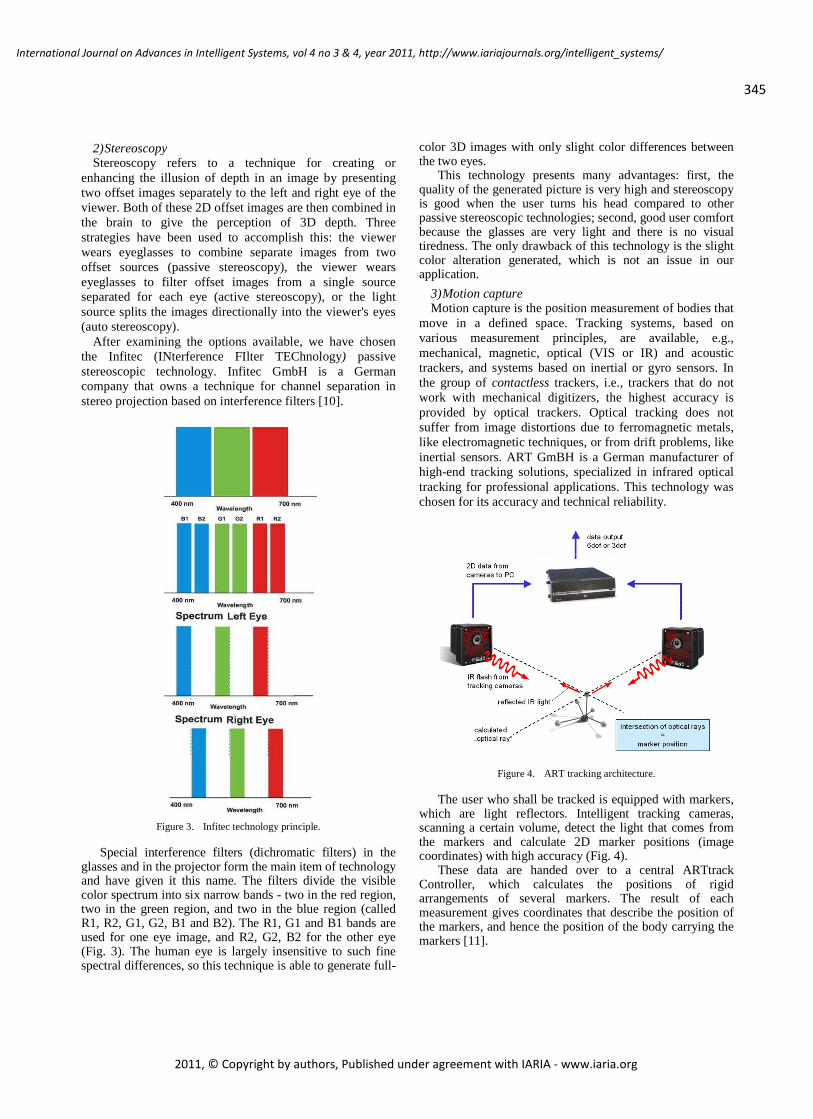
345



2) Stereoscopy Stereoscopy refers to a technique for creating or

enhancing the illusion of depth in an image by presenting two offset images separately to the left and right eye of the viewer. Both of these 2D offset images are then combined in the brain to give the perception of 3D depth. Three strategies have been used to accomplish this: the viewer wears eyeglasses to combine separate images from two offset sources (passive stereoscopy), the viewer wears eyeglasses to filter offset images from a single source separated for each eye (active stereoscopy), or the light source splits the images directionally into the viewer's eyes (auto stereoscopy).

After examining the options available, we have chosen the Infitec (INterference FIlter TEChnology) passive stereoscopic technology. Infitec GmbH is a German company that owns a technique for channel separation in stereo projection based on interference filters [10].

Figure 3. Infitec technology principle.

Special interference filters (dichromatic filters) in the glasses and in the projector form the main item of technology and have given it this name. The filters divide the visible color spectrum into six narrow bands - two in the red region, two in the green region, and two in the blue region (called R1, R2, G1, G2, B1 and B2). The R1, G1 and B1 bands are used for one eye image, and R2, G2, B2 for the other eye (Fig. 3). The human eye is largely insensitive to such fine spectral differences, so this technique is able to generate full-

color 3D images with only slight color differences between the two eyes.

This technology presents many advantages: first, the quality of the generated picture is very high and stereoscopy is good when the user turns his head compared to other passive stereoscopic technologies; second, good user comfort because the glasses are very light and there is no visual tiredness. The only drawback of this technology is the slight color alteration generated, which is not an issue in our application.

3) Motion capture Motion capture is the position measurement of bodies that

move in a defined space. Tracking systems, based on various measurement principles, are available, e.g., mechanical, magnetic, optical (VIS or IR) and acoustic trackers, and systems based on inertial or gyro sensors. In the group of contactless trackers, i.e., trackers that do not work with mechanical digitizers, the highest accuracy is provided by optical trackers. Optical tracking does not suffer from image distortions due to ferromagnetic metals, like electromagnetic techniques, or from drift problems, like inertial sensors. ART GmBH is a German manufacturer of high-end tracking solutions, specialized in infrared optical tracking for professional applications. This technology was chosen for its accuracy and technical reliability.

Figure 4. ART tracking architecture.

The user who shall be tracked is equipped with markers, which are light reflectors. Intelligent tracking cameras, scanning a certain volume, detect the light that comes from the markers and calculate 2D marker positions (image coordinates) with high accuracy (Fig. 4).

These data are handed over to a central ARTtrack Controller, which calculates the positions of rigid arrangements of several markers. The result of each measurement gives coordinates that describe the position of the markers, and hence the position of the body carrying the markers [11].

346



Figure 5. Flystick (left) and tracked glasses (right).

A flystick (Fig. 5) is a wireless interaction device for virtual reality (VR) applications. DTrack software takes up the flystick button and joystick events and correlates them with the 6DOF output data. This makes the matching of all data very user-friendly.

For head tracking in passive stereo systems, tracking targets must be attached to the stereo glasses (Fig. 6). As a result, when the user moves his head, the point of view of the simulation changes as if a genuine movement had taken place within the VR surroundings.

4) Haptic device A haptic system reproduces the sensations of touch and

of effort applied to an object in a VR application. The device enables greater possibilities of immersion in handling virtual objects in 3D. Force-feedback interfaces are substituted for the traditional keyboard and mouse during tasks such as ergonomic studies or the simulation of maintenance or mechanical assembly operations. Actions involving the insertion of mechanical parts within a cluttered space can therefore be carried out very quickly and naturally, whereas they would require a lot more time and user skill with a keyboard and mouse.

We chose to equip the room with a haptic interface, the Virtuose 6D35-45 (Fig. 6). This device has been developed by Haption, a CEA spin-off, and is the only product on the market today, which offers force feedback on all six degrees of freedom (DOF) (three translations and three rotations), together with a large workspace and high torques [12] (the volume is equivalent to a 40 cm side cube). It is especially recommended for scale 1 manipulation of virtual objects such as assembly/disassembly simulations, ergonomic studies, or maintenance training.

Figure 6. Virtuose 6D35-45.

B. The software

In order to run the simulation, the Marcoule immersive room is equipped with specific software, described below.

1) Techviz We use TechViz XL, developed by the French company

TechViz, in order to capture the OpenGL flow from an application, generate stereoscopic images and send them to both projectors. It works especially well with 3DSMax, SolidWorks or Virtools. It is used to display 3D models on any display solution (CAVE, HMD, visualization wall …). TechViz XL offers the ability to work directly within 3D applications and to see 3D model displays in real-time on an immersive room [13].

2) 3DVIA Virtools 3DVIA Virtools produced by Dassault Systèmes is used

to manage a simulation. It is a complete development and deployment platform with an innovative approach to interactive 3D content creation. The 3DVIA Virtools production process facilitates prototyping and robust development up to large-scale, immersive or online, lifelike experience delivery. Thanks to its development environment and its Software Development Kit (SDK), we can create 3D real-time applications and add our own functionalities [14].

3) The IPSI physics engine A physics engine is an independent software library

applied to classical mechanics problem resolution (collisions, falls, forces, kinematics...). The purpose is to give a « physical » existence to graphical objects. One of the most robust and reliable principles is based on 3D model voxelisation. The word voxel means volume element (by analogy with "pixel") and voxelize an object means finding all the voxels ("small cubes"), which are inside the object. We can move from a surface representation to a volume [15]. The figure below shows that depending on the voxel size, model voxelisation is more or less faithful to the graphical object (Fig. 7).

Figure 7. Examples of voxellistion with 2 different voxel sizes.

In this voxelized environment, the physics engine generates the forces to be applied to avoid objects inter-penetration. IPSI is a physics engine provided by Haption, based on voxelisation, and enables the testing of

347



intersections between volumetric solids, in order to calculate trajectories and impact points. The real-time collision detection disables penetration between objects. It also offers kinematic chains creation and haptic interface plug-in with force feedback [16].

IV. FIRST APPLICATION: CELL 414

We chose to implement the first application case on the Cell 414 decommissioning project.

A. Presentation of the project

The vitrification process currently used in La Hague was developed by the CEA in the Marcoule Pilot Workshop (APM facility). It was a prototype plant for reprocessing spent fuel, first commissioned in 1962, with production activities shut down in 1997. The plant is currently undergoing clean-up and dismantling.

Cell 414 is one of the 760 places in APM and one of the

30 very high radioactive cells. It was a chemical unit used to process liquids from irradiated fuel dissolution operations. It is a particularly large cell: 20m long, 4m wide and 6m high. There are approximately 5km of pipes to remove (Fig. 8). The total weight is estimated to be 18 tons of waste. The present high level of radioactivity rules out direct manual dismantling, so the choice of a remote handling system called Maestro has been made.

Figure 8. Very complex cell interior seen from a porthole.

The first step of decommissioning is to remove high level radioactivity. Data was gathered from an initial inventory: hot spots were identified with a gamma camera. These hot spots like the dosing wheels, the centrifuges, the pulsed filter and some parts of the pipes have to be removed first in order to reduce cell radioactivity (Fig. 9):

Figure 9. Pieces of equipment to be dismantled.

B. The remote handling system

The remote handling system is made up with the Maestro system and a carrier specifically designed for the dismantling.

1) The Maestro system The Maestro system is the result of 10 years of

collaboration between the CEA and Cybernetix, in charge of its manufacturing [17]. This advanced remote manipulator is used when human intervention is not possible, as in nuclear or offshore hostile environments. Maestro is dedicated to many tasks like inspection, maintenance, dismantling, cleaning, etc. Dexterity, accuracy and strength are its main advantages. It can be used in either robotic mode (automatic sequence) or in manual remote control mode with or without force feedback management.

Figure 10. The Maestro slave arm (left) and the Maestro master arm

(right).

This system is made up of two parts: the master arm and the slave arm. The master arm is a device allowing the control of the slave arm end-effecter in Cartesian mode with a complete force feedback. This device is a Virtuose 6D40-40 from Haption Erreur ! Source du renvoi introuvable..

348



The slave arm is a hydraulic robot with six degrees of freedom (Fig. 10).

The Cell 414 dismantling project will be the first worksite where Maestro will be used to dismantle a whole cell.

2) The carrier The carrier was especially designed for Cell 414

dismantling, and will enable the Maestro system to reach all parts of the cell.

It works on three axes, using existing rails to move along the cell (20m), with vertical (3m) and rotating movements. A crane-type handling bracket is also set up on the carrier to hold parts during dismantling and for other handling operations. This carrier is currently undergoing tests (Fig. 11).

Figure 11. The carrier.

3) The surrounding rooms Corridor 417, which is adjacent to Cell 414, will be used

to assemble, maintain and disassemble remote handling pieces of equipment and will be the parking and transfer zone. A radiation-proof safety door between Cell 414 and Corridor 417 provides radioactivity containment (Fig. 12).

Figure 12. Control room and maintenance corridor.

During the dismantling, operations will be realized with indirect vision from the control room located in Room 245

(Fig. 12), via audio and video equipment installed inside Cell 414 and on the remote handling system. The control room includes four control screens, which display the images from the six in situ video cameras, two set up in the cell and four on the carrier.

V. FROM REAL TO VIRTUAL: THE STEPS TO BUILD THE

SIMULATION

In order to verify accessibility and maintainability on the carrier and to validate technical choices, it was decided to design the dismantling scenarios using a simulator and the VR technologies available in Marcoule.

A. Step one: build the 3D models

1) Cell 414 and surroundings First, 3D models of the environment had to be built. As

the 2D facility plans available were not sufficiently up-to-date to design a precise digital mock-up, a photogrammetric technique was used.

The photogrammetic reconstruction enabled a 3D model to be built up, using the parallax obtained between the images acquired depending on the different points of view. It implements the correlation calculation between the digital images to give a 3D reconstruction of the model. After an in situ photo campaign, processing consisted of identifying and digitalizing the points with common physical details on the photos, as well as the apparent contours of lines and cylinders. This reconstruction is semi-automatic, and is carried out from basing trade elements (tube valve, nut, screw, elbow…).

The Cell 414 photogrammetric study was carried out by the subcontractor ESIC SN [18], as the model obtained is compatible with standard CAD software (Microstation, SolidWorks). It consisted in taking 700 photos along the existing rails (Fig. 13), for one week. The 3D reconstruction lasted four weeks. The model obtained is accurate to about 5 cm. Nevertheless, the photos taken do not allow all the pipes to be seen, especially those located behind other elements.

349



Figure 13. 6 of 700 photos taken during the measurement campaign.

To import 3D models into 3DVIA Virtools, they must be in a specific format, .NMO. Therefore 3DSMax was used, as it provides an exporter from .MAX format to .NMO format used by Virtools.

Next, the modeling of the building containing Cell 414 was made based on the plans of construction in SolidWorks. We also designed Cell 417 and Control Room 245.

Finally, we merged these parts to obtain a whole model in 3DSMax software. The images below enable the comparison between a real photo and a VR view of the same scene. We can see that the 3D simulation is very close to reality (Fig. 14).

Figure 14. A real photo (left) and 3D view (right).

2) The robots Concerning the robots previously described, we obtained

the CAD model made by Cybernetix, the manufacturer. The modeling is in SolidWorks format and we did the necessary conversions to use it in 3DSMax (Fig. 15).

Figure 15. Carrier 3D model.

3) Simplification of the complete model When all the models were merged, the result proved to be

too big to manage easily and generated performance slowness in the 3D rendering. This first model contained more than 10 million faces. It had to be simplified to reach correct display performances. Whereas the civil engineering and Cell 414 internals could not be simplified, the reduction of the remote handling model was not complicated. It was the manufacturer’s model and included modeling of all the elements down to screws and nuts. For accessibility studies, it is not necessary to have such accuracy. It is therefore possible to remove fastenings (screws, nuts, washers…), fill holes by deleting drilling or simplifying extrusion profiles, and suppressing non visible, hidden objects or those contained in others.

4) Results The example below (Fig. 16) illustrates the simplification

of a part: screws, grooves, rounded edges and holes have been removed. The overall shape is respected and the number of faces decreases from 2693 to 98.

Figure 16. Example of part simplication

This step was very useful because without distorting the model, the simplification of every part of the carrier model leads to 180 000 faces, instead of 2.5 million. As a result, the final 3D model has 1.2 million faces, compared to 10 million before simplification.

B. Step two: develop the simulator

In order to verify accessibility, we need to be able to pilot kinematics chains and detect collisions with the

350



environment in real time. We have developed a physics module, integrating IPSI in 3DVIA Virtools, by using a specific script language and functions called Building Block (BB).

1) Kinematics creation A robot is shown by 3D objects linked by father-child

kinematic links. Objects called “axes” make up the robot skeleton. There are two types of 1DOF motion that can be applied on these axes: rotation around x, y or z and translation (in the direction of x, y or z). These movements can be used on a single axis and are limited by minimal and maximal end stops, applied on the object pivot. Virtual robots can then be manipulated with their constraints as in reality.

The Maestro arm has 6 rotation DOF, as shown in the figure below (Fig. 17):

Figure 17. Maestro kinematics

The carrier can move all along the cell (20 m). The lifting mechanism enables the support platform to be raised. This platform has one rotation axis (±90°). The carrier therefore has three DOF, two translations and one rotation, as illustrated below (Fig. 18):

Figure 18. Carrier kinematics

Lastly, the handling bracket, which holds parts being dismantled, has three DOF; one rotation (±90°), one translation (extension of the bracket arm) and one other translation enabling the pulley to be lowered (see Fig. 19):

Figure 19. Handling bracket crane kinematics

Each robot has its own object hierarchy and they are attached to each other: The Maestro base is fastened to the carrier’s object #5 (the support platform) and the bracket crane base is on the carrier’s object #3 (Figure 20. 20). A Maestro tool is attached to Maestro object #6.

Figure 20. Robots’ hierarchies

2) Maestro tools All the tools below can be connected to the Maestro end-

effecter. They are all used in the dismantling scenarios either to cut, like the saw or the grinder, or to grasp pieces of equipment, like the clamp. Collisions and contacts with the environment can be felt on each of them (Figure 21. ).

Clamp Shears Nibbler

Hydraulic saw Grinder Drill

351



Figure 21. Tools to be used to dismantle

3) The simulator The simulator was created with Virtools for the graphical

part and IPSI for the physical part., with a Dynamic Link Library (DLL) to interface IPSI functions.

In the simulation initialization, all the 3D objects we want to add to the physical simulation are sent to IPSI as well as the information about robots (hierarchies, degrees of freedom, end stops etc.). The kinematics of the Maestro arm and the carrier were then created.

The graphical representation of the objects is updated in Virtools by IPSI, which calculates the new position in real-time. During the simulation life, we use a callback function to match graphical and physical objects (Figure 22. ).

Figure 22. graphics and physical simulation coupling

C. Step three: control the simulation

To control the robots, two gaming joysticks are used to pilot the carrier and the crane (Figure 23. ). The first one controls the carrier’s three DOF and the second those of the crane. These controls are very similar to the interface, which will be used for the final dismantling system. Each robot is controlled axis by axis (the articular mode).

Figure 23. Gaming joysticks used to pilot the carrier and the crane.

The Maestro arm has been coupled to the Virtuose 6D 35-45 haptic interface. The Virtuose enables manipulation of the Maestro end-effecter, and thus control of the Maestro extremity, while respecting the kinematics chain and all the end-stops. The Maestro arm is not piloted axis by axis like the carrier and the handling bracket crane, but it is used in the Cartesian mode via the Virtuose, as it will be during the actual dismantling operation. The Virtuose sends force-feedback when the Maestro is in collision with a « voxelized » element of the environment. The operator can

also feel when one or several axes reaches end stop: the user manipulation is blocked on the axis concerned.

D. Step four: add interactive functionalities

An interactive real-time simulator was developed into which the whole cell, the Maestro slave arm and the carrier are loaded. The Maestro arm and its carrier can be maneuvered using the joysticks and the Virtuose. Any of the six available tools can be connected to the Maestro arm or changed, as necessary.

The points of view of the six cameras can also be displayed in the simulator. It has been checked that every part of the cell is visible and controllable. Sound simulation has been added, to reproduce the sound received by the in situ microphone: the operator will be able to hear the sound of collisions in the monitoring room. This sense will be very useful to operators when piloting the system; therefore a specific sound has been associated with each tool and collision, to enhance the information sent to the user.

Figure 24. MMI

The current value of each robot’s axis is displayed and written in red if it corresponds to the end stop value. The axis is also highlighted and a sound is heard.

A menu enables specific functions to be launched, such as tool grasping, MMI configuration or automatic scenarios; the carrier entry in the cell for example (Fig. 24).

VI. FIRST RESULTS

This part describes the first results, coming from the simulation of the dismantling scenarios.

A. Gamma-3D superimposition

This consists in superimposing radiological imaging data and 3D environment (Fig. 25 and 26). An in situ measurement campaign was carried out in 2006 and enabled identification of about twenty radioactive hot spots in the cell, with ambient dose between 15 and 25mGy/h. The dominant radioelement is 137Cs (80%). The image of each gamma hot spot has been superimposed on the corresponding 3D object.

3D rendering

Robots’ axis position

Menu

Cameras’ points of view

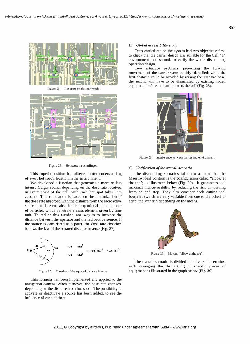
352



Figure 25. Hot spots on dosing wheels

Figure 26. Hot spots on centrifuges.

This superimposition has allowed better understanding of every hot spot’s location in the environment.

We developed a function that generates a more or less intense Geiger sound, depending on the dose rate received in every point of the cell, with each hot spot taken into account. This calculation is based on the minimization of the dose rate absorbed with the distance from the radioactive source: the dose rate absorbed is proportional to the number of particles, which penetrate a mass element given by time unit. To reduce this number, one way is to increase the distance between the operator and the radioactive source. If the source is considered as a point, the dose rate absorbed follows the law of the squared distance inverse (Fig. 27).

Figure 27. Equation of the squared distance inverse.

This formula has been implemented and applied to the navigation camera. When it moves, the dose rate changes, depending on the distance from hot spots. The possibility to activate or deactivate a source has been added, to see the influence of each of them.

B. Global accessibility study

Tests carried out on the system had two objectives: first, to check that the carrier design was suitable for the Cell 414 environment, and second, to verify the whole dismantling operation design.

Two interface problems preventing the forward movement of the carrier were quickly identified: while the first obstacle could be avoided by raising the Maestro base, the second will have to be dismantled by existing in-cell equipment before the carrier enters the cell (Fig. 28).

Figure 28. Interference between carrier and environment.

C. Verification of the overall scenario

The dismantling scenarios take into account that the Maestro ideal position is the configuration called “elbow at the top”; as illustrated below (Fig. 29). It guarantees tool maximal maneuverability by reducing the risk of working from an end stop. They also consider each cutting tool footprint (which are very variable from one to the other) to adapt the scenario depending on the means.

Figure 29. Maestro “elbow at the top”.

The overall scenario is divided into five sub-scenarios, each managing the dismantling of specific pieces of equipment as illustrated in the graph below (Fig. 30):

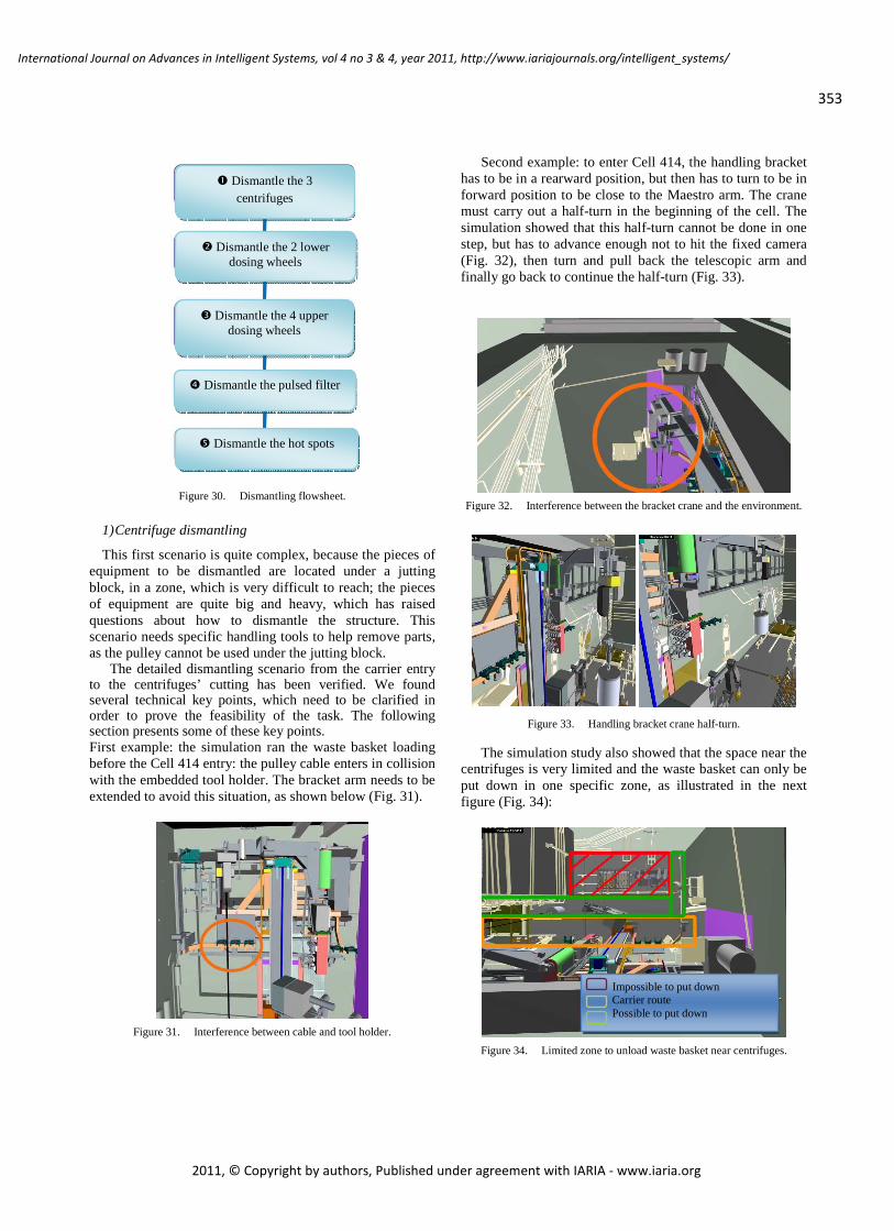
353



Figure 30. Dismantling flowsheet.

1) Centrifuge dismantling

This first scenario is quite complex, because the pieces of equipment to be dismantled are located under a jutting block, in a zone, which is very difficult to reach; the pieces of equipment are quite big and heavy, which has raised questions about how to dismantle the structure. This scenario needs specific handling tools to help remove parts, as the pulley cannot be used under the jutting block.

The detailed dismantling scenario from the carrier entry to the centrifuges’ cutting has been verified. We found several technical key points, which need to be clarified in order to prove the feasibility of the task. The following section presents some of these key points. First example: the simulation ran the waste basket loading before the Cell 414 entry: the pulley cable enters in collision with the embedded tool holder. The bracket arm needs to be extended to avoid this situation, as shown below (Fig. 31).

Figure 31. Interference between cable and tool holder.

Second example: to enter Cell 414, the handling bracket has to be in a rearward position, but then has to turn to be in forward position to be close to the Maestro arm. The crane must carry out a half-turn in the beginning of the cell. The simulation showed that this half-turn cannot be done in one step, but has to advance enough not to hit the fixed camera (Fig. 32), then turn and pull back the telescopic arm and finally go back to continue the half-turn (Fig. 33).

Figure 32. Interference between the bracket crane and the environment.

Figure 33. Handling bracket crane half-turn.

The simulation study also showed that the space near the centrifuges is very limited and the waste basket can only be put down in one specific zone, as illustrated in the next figure (Fig. 34):

Figure 34. Limited zone to unload waste basket near centrifuges.

� Dismantle the 4 upper dosing wheels

� Dismantle the pulsed filter

� Dismantle the hot spots

Impossible to put down Carrier route Possible to put down

� Dismantle the 2 lower dosing wheels

� Dismantle the 3 centrifuges

354



We have also proved that dismantling the centrifuges in situ with the hydraulic shears would not be feasible as originally planned. In fact, the shears footprint is too big and it cannot access the centrifuges. A new scenario was proposed, consisting in removing the centrifuges from under the jutting block, bringing them close to the cutting table, where there is more space and cutting them up with the hydraulic shears. This scenario has been validated and approved by the dismantling project engineers.

Another example: the simulation enables Maestro configuration during tool grasping on the embedded tool holder to be shown. To grasp tools, the arm must have “the elbow at the bottom”, two axes must be close to end stops and the support platform must have a 45 degree orientation (Fig. 35). This configuration is not optimal and needs a large footprint in the cell. While it is not an issue in the half-turn zone, it causes interferences with an embedded camera near the cutting table: the camera orientation needs to be modified in order not to touch the table (Fig. 36).

Figure 35. The tool grasping

Figure 36. Interference between camera and cutting table.

Other such situations have been found and embedded tool grasping is not possible in some parts of the cell. This kind of problem had not been identified before, and the manufacturer has had to take these issues into account.

Thus, from the first simulation runs, the project has already provided vital information to implement in its dismantling scenarios. The chosen VR technologies have proved their worth, and the various capabilities of the

Maestro system and carrier will continue to be tested as the dismantling project enters its next phase.

VII. LIMITS AND PERSPECTIVES

The results are quite satisfying, but some limits exist and some developments can be made to use the simulation to train the future operators.

A. Current limits

First, the mismatch of information relevant to reality can affect safety and performance. For instance, if the modeling accuracy for the robot or the cell is not high enough, we cannot be sure that the scenarios that have to be tested with the simulator are reproducible in practice. The robot model comes directly from the manufacturer’s CAD model, so it can be considered as identical to the actual robot. The modeling uncertainty comes from 3D reconstruction. It is known that photogrammetry is accurate with 5cm precision. The most difficult task is to obtain a true model of the cell. The present model created by photogrammetry is accurate enough for the first steps of scenario study, but because of the layout of the cell, the complete model of the pipes could not be rebuilt with this technique. Only the first row of pipes was modeled, so the cell modeling will have to be updated after the first steps of dismantling if we want to match the reality.

Next, we are limited by the physics engine, which is directly dependent on the computing power. With the current hardware, we cannot physicalize the robots and the whole cell with a high precision for collision detection and get a real-time simulation. Therefore, only the robots and some key parts of the cell have been physicalized. These parts depend on the scenario being tested. Collision detection precision has to be inferior or equal to 10mm, so that the accessibility studies can be realistic.

B. Add the radioactivity dose rate information

The CEA, in collaboration with Euriware, a French company, has developed an application called NARVEOS [20] capable of calculating the radioactivity dose rate. It is specifically used to simulate scenarios in nuclear environments. In NARVEOS, we can import a 3D model of a nuclear facility, specify the kinds of materials (steel, lead, concrete …) of each 3D object and add radioactive pieces of information to the 3D model: sources coming from the in situ measurement campaign mentioned earlier in this article, protection screens defined by the material of each object, and measurement points where we want to have the calculation done. From this data, NARVEOS is able to calculate the radioactive dose rate received by the measurement points in real-time and interactively. In the following figure (Fig. 37), sources and protection screens have been added and the measurement point has been located on the operator’s chest. It is controlled interactively via mouse and keyboard. The curve below displays the changes to the dose rate received by the operator depending on the motion he makes.

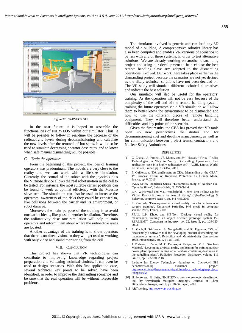
355



Figure 37. NARVEOS GUI

In the near future, it is hoped to assemble the functionalities of NARVEOS within our simulator. Thus, it will be possible to follow in real-time the decrease of the radioactivity levels during decommissioning and calculate the new levels after the removal of hot spots. It will also be used to simulate decreasing operator dose rates, and to know when safe manual dismantling will be possible.

C. Train the operators

From the beginning of this project, the idea of training operators was predominant. The models are very close to the reality and we can work with a life-size simulation. Currently, the control of the robots with the joysticks plus the Virtuose device allows the real robot motion in the cell to be tested. For instance, the most suitable carrier positions can be found to work at optimal efficiency with the Maestro slave arm. The simulation can also be used to increase the operators’ awareness of the risks they could be exposed to, like collisions between the carrier and its environment, or robot damage.

Moreover, the main purpose of the training is to avoid nuclear incidents, like possible worker irradiation. Therefore, the radioactivity dose rate simulation will help to train operators and inform them about where the radioactive areas are located.

Another advantage of the training is to show operators that there is no direct vision, so they will get used to working with only video and sound monitoring from the cell.

VIII. CONCLUSION

This project has shown that VR technologies can contribute to improving knowledge regarding project preparation and validating technical choices. It can even be used to design scenarios. With this first application case, several technical key points to be solved have been identified, in order to improve the dismantling scenarios and be sure that the real operation will be without foreseeable problems.

The simulator involved is generic and can load any 3D model of a building. A comprehensive robotics library has also been compiled and enables VR versions of scenarios to be run with any of these systems, in order to test alternative solutions. We are already working on another dismantling project and using our development to help choose the best remote handling slave arm adapted to the dismantling operations involved. Our work there takes place earlier in the dismantling project because the scenarios are not yet defined as the likely technical solutions have not been decided on. The VR study will simulate different technical alternatives and indicate the best solution.

Our simulator will also be useful for the operators’ training. As the operation will not be easy because of the complexity of the cell and of the remote handling system, training the future operators via a VR simulation will allow them to better know the environment to be dismantled and how to use the different pieces of remote handling equipment. They will therefore better understand the difficulties and key points of the scenario.

Given the first results, the CEA has proved that VR tools open up new perspectives for studies and for decommissioning cost and deadline management, as well as for communication between project teams, contractors and Nuclear Safety Authorities.

REFERENCES [1] C. Chabal, A. Proietti, JF. Mante, and JM. Idasiak, “Virtual Reality

Technologies: a Way to Verify Dismantling Operations, First application case in a highly radioactive cell”, ACHI, Digital World, Le Gosier, France, pp. 153-157, 2011.

[2] P. Guiberteau, “Démantèlement au CEA. Dismantling at the CEA.”, 4th European Forum on Radiation Protection, La Grande Motte, France, pp. 8, 2010.

[3] IAEA Safety Standards Series, “Decommissioning of Nuclear Fuel Cycle Facilities”, Safety Guide, No WS-G-2.4.

[4] B.K. Wiederhold and M.D. Wiederhold. “Three-Year Follow-Up for Virtual Reality Exposure for Fear of Flying” CyberPsychology & Behavior, volume 6 issue 4, pp. 441-445, 2003.

[5] F. Yaacoub, “Development of virtual reality tools for arthroscopic surgery training”, Université Paris-Est, Phd thesis in computer science, Paris, France, 2008.

[6] J.R.Li, L.P. Khoo, and S.B.Tor, “Desktop virtual reality for maintenance training: an object oriented prototype system (V-REALISM)”, Computers in Industry, vol 52, issue 2, pp. 109-125, 2003.

[7] R. Gadh,H. Srinivasan, S. Nuggehalli, and R. Figueroa, “Virtual disassembly-a software tool for developing product dismantling and maintenance systems”, Reliability and Maintainability Symposium, 1998. Proceedings., pp. 120-125, 1988.

[8] J. Ródenas, I. Zarza, M. C. Burgos, A. Felipe, and M. L. Sánchez-Mayoral, “Developing a virtual reality application for training nuclear power plant operators: setting up a database containing dose rates in the refuelling plant”, Radiation Protection Dosimetry, volume 111 issue 2, pp. 173-180, 2004.

[9] Institute for Energy Technology, datasheet on Chernobyl NPP decommissioning assistance project, http://www.ife.no/departments/visual_interface_technologies/projects/chnpp/view .

[10] H. Jorke and M. Fritz, “INFITEC- a new stereoscopic visualisation tool by wavelength multiplex imaging”, Journal of Three Dimensional Images, vol.19, pp. 50-56, Japan, 2005.

[11] ARTracking, http://www.ar-tracking.de

356



[12] F. Gosselin, C. Andriot, J. Savall, and J. Martin, “Large workspace Haptic Devices for Human-Scale Interaction: A Survey”, EuroHaptics, LNCS 5024, pp.523-528, 2008.

[13] C. Limousin, J. Sebot, A. Vartanian, and N. Drach, “Architecture optimization for multimedia application exploiting data and thread-level parallelism”, Journal of Systems Architecture, vol. 51, issue 1, pp. 15-27, 2005.

[14] 3DVIA, http://www.3ds.com/products/3dvia/3dvia-virtools/welcome/

[15] M.W. Jones and R. Satherley, “Voxelisation: Modelling for Volume Graphics”, proceedings VMV’2000, pp. 319-326, 2000.

[16] Haption, IPSI datasheet. Available from http://www.haption.com/site/eng/images/pdf_download/Datasheet_IPSI.pdf.

[17] O. David, Y. Measson, C. Rotinat, F-X. Russotto, and C. Bidard, “Maestro, a Hydraulic Manipulator for Maintenance and Decommissioning Application”, ENC, Bruxelles, Belgium, pp. 54-61, 2007.

[18] Haption, Virtuose 6D35-45 datasheet, Available from http://www.haption.com/site/pdf/Datasheet_Virtuose_6D35-45.pdf.

[19] ESIC SN, MEEX datasheet, Available from http://www.esic-sn.fr/spip.php?article14.

[20] J-B. Thevenon, L. Lopez, C. Chabal, and J-M. Idasiak, “Using simulation for intervention design in radiating environment: first evaluation of NARVEOS”, GLOBAL, Paris, France, pp.153-157, 2009.

357



An Event-based Communication Concept forHuman Supervision of Autonomous Robot Teams

Karen Petersen and Oskar von StrykDepartment of Computer Science

Simulation, Systems Optimization and Robotics GroupTechnische Universitat Darmstadt, Darmstadt, Germany

{petersen|stryk}@sim.tu-darmstadt.de

Abstract—The supervisor’s understanding about the statusof the robots and the mission is a crucial factor in supervisorycontrol, because it influences all decisions and actions of thehuman in charge. In this paper, the concept of situationoverview (SO) is presented as an adequate knowledge base fora human supervisor of an autonomous robot team. SO consistsof knowledge about each individual robot (robot SO) andoverview of team coordination and the actions towards missionachievement (mission SO). It provides the human with relevantinformation to control a robot team with high-level commands,e. g., by adapting mission details and influencing task allocationin a manner that is applicable to different task allocationmethods in general. The presented communication concept toobtain SO is based on events, that are detected using methodsfrom complex event processing. These events are dynamicallytagged to different semantical or functional topics, and are sentto the supervisor either as notifications of different levels, toinform the supervisor about the mission progress, unexpectedevents and errors, or as queries, to transfer decisions to thesupervisor, to make use of implicit knowledge and the human’sexperience in critical situations. The robots’ level of autonomycan be adapted using policies, that allow to take decisions eitherautonomously by the robots, or with support by the supervisor,using different query modes. The concept can be applied tofundamentally different problem classes involving autonomousrobot teams and a remote human supervisor. The applicationof the concept is discussed for the two example scenarios ofurban search and rescue and robot soccer.

Keywords-human-robot team interaction; supervisory con-trol; situation overview; complex event processing; policies

I. INTRODUCTION

Teams of autonomous robots have the potential to solvecomplex missions such as urban search and rescue (USAR),but are not yet sufficiently reliable and powerful to op-erate without any human supervision. However, humansand robots have many complementary capabilities, whichcan contribute significantly to a successful and efficientmission achievement if utilized properly in combination.For example, humans are very good at cognitive tasks suchas visual perception, coping with unfamiliar or unexpectedsituations, and prediction of future states of the world basedon incomplete knowledge of the current state. Robots, incontrast, have their strengths, for example, in fast executionof well-defined or repetitive tasks, evaluation and storage

of large amounts of data, or operation in areas inaccessibleto humans, like narrow spaces, in the air, or contaminatedareas. This complementarity has already been observedwhen comparing humans and machines almost 60 years ago(c. f. Section IV-A), which leads to the assumption that thissituation will not change significantly in the near futuredespite tremendous technological developments. Therefore,these specific strengths should be used efficiently for humansupervision of autonomous robot teams.

The proposed communication concept has first been pre-sented in [1]. This article is a revised and extended versionof [1], providing more details about the applied methods andthe underlying concept of situation overview. In particular,a detailed definition of situation overview is provided and iscontrasted with situation awareness, which is usually appliedas a knowledge base for robot teleoperation. Furthermore,the applied tagging and policy concept is specified in moredetail. Additionally, more detailed examples for event-basedcommunication are provided.

A. Abilities and Scenarios for Team Interaction

The proposed concept addresses scenarios, where a teamof autonomous robots can be supported by a human supervi-sor with high-level instructions. The main goal of the robots(called mission) can be subdivided into tasks, that may beknown prior to the mission start or can emerge during themission. Each task can be fulfilled by a single robot, but notevery robot is able to achieve each task. A task allocationmethod is used to decide which robot works on which task.This can be either a centralized planner for the whole team,or a distributed algorithm, where the robots negotiate thetasks among each other. The choice of an appropriate taskallocation algorithm depends on the concrete mission setup,robots and environmental conditions.

Common teleoperation interfaces require one operator perrobot, which implies that having a team of robots also re-quires a team of operators. If a single human supervisor shallbe enabled to control a whole robot team, a fundamentallydifferent approach is needed.

Following the definition of supervisor and operator fromScholtz [2], the main difference between these two in-

358



teraction roles is, that the supervisor usually interacts byspecifying goals and intentions, while the operator interactsat the action level. Due to an increased robot autonomy, thesupervisor has a lower workload per robot, and can thereforehandle more robots simultaneously than an operator. High-level commands from the supervisor in a USAR missionmay be used, e. g., to confirm or discard a robot’s objecthypotheses (e. g., victims or fire), to classify terrain traffica-bility, or to specify regions that are to be searched first or fora second time by a specific robot. In a robot soccer scenario,supervisor interactions may include changing or adapting ateam’s tactic, or allocating specific roles to individual robots.Common for all applications is, that the supervisor should beenabled to modify the tasks’ parameters and the allocationof tasks to robots, and to act as decision support for therobots, e. g., in case they are not granted sufficient authorityor do not have sufficient information for good autonomousdecisions.

B. General Concept

The goal of the presented concept is on the one handto enable the supervisor to modify the mission’s and tasks’details (including task allocation), and on the other handto allow robots to transfer decisions to the supervisor, ifthey are not allowed or not able to decide autonomously.Mission and task allocation adaptations can be realized byintroducing a layer between the task allocation and thetask cost calculation, that modifies the cost calculated forexecuting a task. It should be noted that this approach can beapplied to very different task allocation methods. However,to be able to take such decisions, the supervisor needs to beaware of the team’s progress towards mission achievementand the current state of the world and the robots.

In this paper, we propose a method to create a basis forsupervisor-initiated interactions with the robot team. Theactual interactions are not covered here. Instead, we focuson the event-based communication between the human andthe robot team, which provides the supervisor with relevantinformation about the robots and the environment, andenables robot-initiated interactions using queries to transferdecisions from the robots to the supervisor.

In the next section, we introduce the term situationoverview (SO), which includes more general knowledgeabout the world and the robots’ status, compared to situationawareness (SA), which is usually applied for teleoperationtasks. SO is a basis for all supervisor actions. Achieving SOis a nontrivial task, especially when dealing with a robotteam instead of a single robot.

For obtaining SO, discrete events instead of continuousdata streams are used as communication basis betweenrobots and supervisor. The information required for obtain-ing SO is usually not fixed, instead, the communicationhas to be adopted during runtime to the specific needs ofdifferent missions and supervisors. For this purpose, we

propose to control the amount of information using policies,which define the events to be detected by the robots usingcomplex event processing. These events are then classifiedaccording to their priority and are sent to the supervisor asnotifications (to provide information) or queries (to ask fordecision support).

A main advantage of SO over SA is the reduction of datathat has to be communicated. This is an important factor inreal-world applications where the available communicationbandwidth is usually limited. Additionally, it addresses robotteams, not just single robots. SO, obtained with the presentedmethods, gives a human supervisor a basis for high-levelteam interactions, without overburdening the human withtoo specific information of each robot.

This procedure follows the same idea as teamwork inhuman teams, where a common approach is to let a teamleader maintain an overview of the project’s progress [3].For example, the rescue personnel at a rescue site informsthe task force leader about their progress (e. g., an area hasbeen searched) and the search team’s status (the team isavailable again). This concept is ”simple, reliable, and re-duces information overloading and distractions to decision-makers” [4]. In contrast to the concept provided here, inhuman teams the leader obtains the information from otherhumans, who can reason about the value of an information,to decide if it is relevant for the team leader. However, ifinstead a team of robots shall inform a leader about theirprogress to support the leader’s SO, they cannot judge asituation in the same way as a human, and therefore needsome rules about what information they have to send to thesupervisor and in which context. This problem is addressedby the presented communication concept.

The rest of this paper is organized as follows: In SectionII, the term situation overview is introduced and contrastedwith other widespread notions for describing a human’sknowledge about a semi-autonomous system. Related workis discussed in Section III. In Section IV, first the inter-actions among humans in loosely coupled teamwork areobserved. Second, inspired by these findings, the methodsenabling the robots to send notifications and queries to thehuman supervisor are described. For detecting the impor-tant incidents, methods from complex event processing areapplied. The events are classified with different levels toallow filtering and discriminative representations at a userinterface. The amount of messages can be controlled usingpolicies, which can be adapted either manually or auto-matically, depending on the supervisor’s workload. Someapplication examples, for general robot team applicationsand for concrete scenarios of USAR and robot soccer, aregiven in Section V. The methods are discussed and futurework is described in Section VI.

359



II. SITUATION OVERVIEW

In research on robot teleoperation, the operator’s requiredknowledge about the robot’s state and the environment iscalled situation awareness (SA), which is adopted from pilotsituation awareness and is usually measured with the sametools [5].

The term SA was defined by Endsley as ”the perceptionof the elements in the environment within a volume of timeand space, the comprehension of their meaning, and theprojection of their status in the near future” [6]. To achieveSA, a human has to pass three levels:

• Level 1 SA is the perception of status, attributes, anddynamics of relevant elements in the environment,

• Level 2 SA is the understanding of the meaning and thecorrelation of the perceived level 1 elements,

• Level 3 SA is the projection of the current state into thefuture.

Level 2 and 3 can usually be achieved easier by experiencedusers than by novices, because they can base their knowledgeon previous experiences and already have developed detailedmental models of the system [6].

Because this definition is derived from the egocentricSA of a pilot in an aircraft, also SA for a robot operatoris egocentric from the point of view of a single robot. Ageneralization to a whole team of robots is difficult, becauseusually a human cannot track such detailed information formany robots simultaneously. Instead, the presentation of allSA elements of many different robots to a single operatorcan quickly lead to information overflow [4].

In the USAR domain, good SA is usually associatedwith a complete knowledge of the status of a robot andits surrounding. This includes the robot’s health (e. g., thefunctionality of all sensors, the battery level, software fail-ures, mechanical breakdowns), the robot’s direct surrounding(e. g., the structure of the terrain, nearby obstacles, objects ofinterest such as victims or hazards, other robots or humansin the vicinity), and the relation between the robot and theenvironment (e. g., the robot’s position and 3D orientationwith respect to a fixed coordinate system, the distancebetween the robot and the obstacles, maneuverability ofthe robot on the given terrain). This information is usuallygathered by full video streams of the cameras or live map-data, which produce a large data volume.

Obviously, a problem occurs if SA is applied to super-visory control of semi-autonomous robot teams: A singlehuman is not able to obtain SA for several robots simulta-neously and maintain SA for a long time. However, a super-visor does not need to obtain such a detailed SA, becausethe tasks of a supervisor, and therefore also the interactionswith the robots, are fundamentally different compared to theinteractions between an operator and a teleoperated robot.This shows, that supervisory control demands for a differentdefinition of the human’s required knowledge about the

system, that is more specifically designed for multi-robotteams, instead of single robots.

Drury et al. [7] use the term Humans’ overall missionawareness to describes the humans’ overview of the activi-ties in the team and the teams’ progress towards the missiongoal. However, this definition is rather loose, and it seemsthat it only includes the teams activities, but not the statusof the individual robots, or the reasonable teamwork amongthe robots.

Hence, both definitions (situation awareness and missionawareness) do not provide an adequate basis for high-levelinteractions between a human supervisor and a robot team.To overcome this, we introduce the notion of situationoverview (SO).

SO consists on the one hand of information related tothe mission progress, and on the other hand of informationconcerning each robot in the team.

• Mission SO is the supervisor’s knowledge about themission progress in general, and the knowledge aboutwhich robot contributes to the mission progress bytaking which actions, and the reasonable coordinationamong the team members.

• Robot SO describes the understanding the supervisorhas about a robot’s location and status, its current andplanned actions, including the robot’s ability to ac-complish the current task. This includes the knowledgeabout a robot’s health, i. e., if the robot is working cor-rectly or if it needs support from either the supervisoror from an operator.

Robot SO is related to each robot’s individual perfor-mance, whereas mission SO is related to the team perfor-mance, which is not necessarily the sum of the individual’sperformance. As an example, consider a team of robots,that has the task to explore and map an office building.On the one hand, in case all robots cluster in the sameroom and all follow the same exploration pattern, instead ofcoordinating and distributing to different rooms, the overallteam performance is poor, even though each individual robotshows a good performance. On the other hand, if the teamperformance is good, a malfunctioning robot would notbe recognized if the individual robot performance is dis-regarded. Therefore, mission SO and robot SO complementeach other and should usually be treated together as situationoverview.

A supervisor, who has obtained mission SO, should beable to answer the following questions:

• Is the mission advancement as planned? Are there anycomplications? Is it expected that all deadlines are met?Is there anything that cannot be achieved?

• Which tasks still have to be done to accomplish thewhole mission? Are any problems expected for theexecution of these tasks?

• Do the robots coordinate properly? Are they (as a team)working efficiently towards the mission goal? Are the

360



tasks allocated to the robots in a way that matches therobots’ capabilities and current status?

With a good robot SO, the supervisor should be able toanswer the following questions for each robot:

• Are all sensors and actuators of the robot functioningcorrectly? Is the battery level high enough? Which partsare not functioning? Can it be repaired?

• Is the robot idle? If yes: why?• Can the robot fulfill its current task satisfactorily? Does

it need any support, or should it even be releasedfrom this task? In which way does the current activityadvance the mission goal?

Generally spoken, the supervisor should have an overview ofthe team’s and robots’ activities and status, but does not needto know specific details. The important part is to quicklyrecognize deviations from the ”normal” status, that requiresupervisor interaction.

Good SO includes on the one hand knowledge about thecurrent state of the robots and the mission, which requiresknowledge about the past developing to know how thecurrent state has to be interpreted, and on the other handassumptions about the future state of robots and mission, toenable the supervisor to interact with the robots and correctthe team’s behavior as early as possible.

Compared to Drury’s mission awareness, mission SOincludes additional information about team coordinationand overall team progress. Compared to Endsley’s situationawareness, robot SO includes less details about an individualrobot, which accounts for the different requirements of asupervisor and an operator, and allows a single human tomaintain information of a whole robot team. However, be-cause SO is, like SA, based on the perception and projectionof information, many research results from SA can also betransferred to SO. The following results from [6] also applyto SO:

• It cannot be defined in general, for different applica-tions and robots, which information the human needsto receive to achieve SA (SO).

• SA (SO) is influenced by several human factors, likeattention, working memory, workload and stress.

• The possibility to obtain SA (SO) is dependent onwhich information the system provides, and how thisinformation is presented.

• Trained or experienced users can achieve a high SA(SO) easier than novices. Furthermore, some people arein general better in obtaining SA (SO) than others.

• Achieving SA (SO) is a process over time, not a discreteaction.

• Good SA (SO) can increase system performance, butbad performance does not necessarily indicate bad SA(SO).

Endsley concludes, that there are two factors in a system,that influence how good a human can obtain SA: 1) which

information does the system provide, and 2) how the avail-able information is presented to the human. This also appliesto SO. In this paper, a method is presented, that addressesthe first factor: Which information shall the robots send tothe supervisor, while on the one hand providing all relevantinformation, but on the other hand not sending informationthat does not advance the human’s SO to prevent informationoverflow and reduce the required network bandwidth.

III. RELATED WORK

Especially in the USAR domain, much research hasbeen done on teleoperation interfaces, e. g., [8], [9]. Thesestrongly rely on video and map data, that need to be sentfrom the robot to the user interface in real-time. On theone hand, this allows to accurately control a robot evenin unstructured and complicated environments, but on theother hand, those interfaces cannot be extended easily tocontrol more than one robot simultaneously, and requirehigh bandwidth, which is often not permanently available inreal-world scenarios. Further, most teleoperation interfacesrequire extensive operator training and continuously demandmaximum concentration of the operator, hence quickly lead-ing to task overload and operator fatigue.

Approaches that allow a single supervisor to deal withrobot teams and do not require continuous high bandwidthcommunication can be found in the area of sliding autonomyor mixed initiative. In [10], Markov models are used todecide whether a robot works on a task autonomously or isbeing teleoperated by an operator. This requires continuouscommunication connection only during the teleoperationphases. The mixed initiative system presented in [11] allowsthe operator to manually switch between autonomy modes,where the operator input varies from goal input to fullteleoperation. Similarly, in [12], the operator can assignwaypoints, move the camera, or completely teleoperate arobot. With the augmented autonomy approach used in [13],the robots in an exploration scenario can either select theirnext waypoints autonomously, or the operator can assignwaypoints. Results show, that these methods are appropriateto deal with a larger number of robots and can produce muchbetter results than fully autonomous or purely teleoperatedsystems. However, they still require periods of continuoushigh-bandwidth connection, and can hardly be extended tofundamentally different scenarios, where the main focus isnot on search or exploration.

A completely different approach is described in [14],where the robots can ask questions to the human super-visor. Similarly, in [15], the human is treated as a sourceof information for the robots. The level of autonomy iscontrolled by adjusting the costs to contact the supervisoras decision support. The teleautonomous system presentedin [16] enables the robots to detect situations where humanintervention is helpful, which are in this context the statesof robot stuck, robot lost or victim found. Human supported

361



decision taking is presented in [17], here two variants areproposed: management-by-exception, where the operator canveto against an autonomous decision, and management-by-consent, where the operator needs to confirm an autonomousdecision before execution. In [18], policies are used torestrict the autonomy bounds of the robots, in this contextalso rules are defined about which messages the robotsare required to send to the human. These approaches arepromising to be applicable to larger robot teams in real-world environments, because they do not require continuoushuman attention to a single robot and require less bandwidthas they do not rely on video streams. However, they arestill not very flexible to be adapted to fundamentally dif-ferent scenarios or for on-line adaption to different operatorpreferences. Furthermore, the events that require operatorintervention are detected manually, and yet no method hasbeen provided to flexibly detect complex events in arbitrarycomplex situations.

IV. CONTROL OF COMMUNICATION BETWEEN ROBOTSAND A SUPERVISOR

In this section, the teamwork among humans, that in-spired the new communication concept, is described briefly.Afterwards, the specific strengths of humans and robots,that contribute to these kinds of scenarios and interactionsare revised. Finally, the methods used to realize a flexiblecommunication between the robots and the supervisor arepresented and discussed.

A. Interactions in Team Work Among Humans

When observing interactions in loosely coupled work-groups [19], some commonalities can be observed regardlessof the scenario, e. g., home care, knowledge work, firemenin a search and rescue scenario, soccer players coordinatingwith each other and getting instructions from a coach, orpeople in an office preparing an exhibition at a fair: Inall these situations, the overall mission is subdivided intotasks, that are assigned to the team members. Everyoneworks on his own tasks, and reports the progress to theteammates or the leader, either explicitly by verbal or writtencommunication, or the progress can be directly observed bythe others. If someone has problems in fulfilling a task, hecan ask somebody else (who is expected to be more capablefor this specific problem) for support.

To understand the benefits of supervisory control, it isimportant to be aware of some fundamental differencesbetween humans and robots. In [20], the superiorities ofhumans over machines and vice versa are discussed. Oneof the main outcomes is that machines are good in fastroutine work, computational power and data storage, whilehumans’ strengths are perception, reasoning, and flexibility.These findings (although almost 60 years old!) are in mostpoints still valid and can be transferred to a large extent frommachines to robots. Especially the superiority of humans

over robots in problem solving and situation overview iscrucial, and is not likely to change in the near future.Further, although there are several sensors that allow robotsto perceive data that humans cannot sense directly (e. g.,distance sensors, infrared sensors), humans are much morecapable in interpreting data, especially images.

As a conclusion, if a human supervisor is aware of theoverall situation, but not necessarily of all details, it makessense to leave some high-level decisions to the human, whocan be expected to decide based on implicit knowledge,situation overview and experience, that cannot easily beadded to the robots’ world model. Due to the complementarycapabilities of robots and humans, it can be expected thathumans can cope well with the problems that robots cannotsolve autonomously.

If this model of human teamwork is applied to human-robot interaction, with the human taking the role of a su-pervisor, the robots are required to report their progress andunforeseen events to the human, and ask for support if theycannot solve their tasks sufficiently well autonomously. Thisis enabled by the proposed communication concept usingthe following methodologies: First, important or criticalevents are detected using complex event processing (SectionIV-B). These events are dynamically mapped to semantictags (Section IV-C), and are classified to message classes,which are different levels of notifications and different querymodes, according to their criticality (Section IV-D). Finally,the message flow is controlled by policies, that define whichmessages need (not) to be sent to the supervisor (SectionIV-E).

B. Complex Event Processing

The events to be detected by the robots can be very diverseto many aspects. Some are just special variables exceedingthresholds, others are patterns that have to be detected,or several occurrences of different events simultaneously.Certainly, the detection of every single event could beprogrammed manually, but this is very time consuming, canlead to many failures, and usually duplicates lots of code.

The research field of Complex Event Processing (CEP)deals with such questions, of how to detect events in commu-nication systems [21], for example in databases or WirelessSensor Networks (WSNs). In WSNs, the challenge is to useseveral hundreds of distributed sensor nodes to detect events,e. g., human presence or fire, and combine simpler events todetect complex events, that are aggregations or patterns ofseveral events. Simple events are discrete events, that canbe directly detected without aggregating more information,e. g., a variable exceeding a threshold, or a sensor (not) deliv-ering data. Complex events are events that are composed oftwo or more (simple or complex) events, or events enhancedwith external information. These compositions can be twoevents occurring simultaneously, an event chain, patterns,etc. To describe those aggregations, event algebras are used,

362



e. g., HiPAC [22], SNOOP [23], REACH [24]. Those alge-bras provide operators as conjunction, disjunction, sequence,etc., to combine two or more events to a complex event.They vary in complexity and versatility. Depending on theapplication, an appropriate algebra needs to be chosen, thatsatisfies all needs, but is not too complex, hence being moredifficult to understand and leading to higher implementationefforts.

The analogy between CEP as used in WSNs and roboticsis, that there are several sensors and pre-processed dataavailable, based on this information certain events or statesof the robot or the world have to be detected. The key dif-ferences are, that a robot has less, but more reliable sensorsthan in a typical WSN, the sensors are more complex anddeliver not only scalar values. Furthermore, the ”network”is more static, apart from sensor failure, because a robot’ssensors are physically connected and not entirely distributed.Therefore issues like time synchronization and timelinesscan be disregarded for CEP on robots. However, the tasksand capabilities of a robot team are fundamentally differentfrom those of a WSN: robots can physically interact withthe environment in time and space, while a WSN can onlymonitor the state of the environment over time. This allowsto base expectations about changes in the environment onthe actions of the robots. Furthermore, the robots’ mobilityallows to systematically collect data at locations where ahigh information gain is estimated. In case also events haveto be detected that involve more than one robot, also theWSN aspects of synchronization and timeliness have to beconsidered, which is usually done by the robots’ middleware.Overall, CEP provides good methodologies, that can be usedefficiently not only in databases and WSNs, but also onrobots.

CEP allows to detect events on different semantical lev-els, corresponding to the three SA levels: perception ofthe current status, interpretation of the current status, andprojection of the current and past events into the future. Thesemantically most basic events correspond the the currentstate of each robot, and help the supervisor to obtain SOcorresponding to the first level of SA. Correlations betweenthese events can be modeled, e. g., the simultaneous occur-rence of two different events, using CEP. This supports thesupervisor in understanding the meaning of the more basicevent, which enhances the SO corresponding to the secondlevel of SA. If the correlations and the meaning of the eventsare modeled carefully, the supervisor usually does not needto perceive the underlying basic events separately, whichallows on the one hand to save communication bandwidth,and on the other hand to reduce the risk of informationoverload. Finally, complex event operations can be definedto model the future state of different components. Dependingon the input data, for example stochastic models, regressionfunctions, or more sophisticated models can be applied asprediction tools. This is usually not done in WSNs, because

the sensor nodes typically don’t have enough computationalpower for extensive calculations.

For the supervisor’s robot SO, each robot can individuallydetect relevant events, report the current state and makepredictions about the future state. Events that are relevantfor the supervisor’s mission SO are based on the one handon the modeling of the robots’ current mission, and on theother hand on each robot’s current and past activities andplans. Therefore, events from different sources have to becombined for enhancing the supervisor’s mission SO. Thiscan either be done locally by one of the robots, or anevent detection module has to be active at the supervisor’scomputer. The former scales better for large teams, becauseall calculations can be distributed over all team members.However, with the second possibility, the events are detectedat the location where they are needed, and the required datavolume is still low, because the events for mission SO arecompositions of SO events from different robots, and do notrely on raw data.

Some examples of important events in a USAR missionare of course if a robot has detected a potential victim or afire, but also reports about the status of the exploration, e. g.,if a room has been explored completely without finding avictim. All these examples are relevant for robot SO as wellas for mission SO. In a humanoid robot soccer match, arobot can monitor the frequency of falling when walking orkicking, taking into account disturbances by teammates oropponents (e. g., by pushing), and can deduce if it is stillcapable of playing efficiently. This information is primaryrelevant for robot SO. The goalkeeper can monitor its benefitto the match, if it observes the frequency of jumping to catchthe ball, compared to the number of goals scored by theopponent, i. e., if the goalkeeper jumps for the ball, and nogoal is scored directly afterwards by the opponents, the teampresumably benefits from the goalkeeper. If the opponentsscore, regardless of the goalkeeper jumping or not, therobot can potentially contribute more to the team’s successwhen acting as a further field player. This information isrelevant for mission SO, because it affects the teams overallperformance, but it is not relevant for robot SO.

C. Event Tagging

For allowing a human supervisor to quickly manage, sortand access groups of events by topic, events can be tagged.These tags can, for example, reflect the different tasks therobots are working on, functional or mechanical componentsof the robots, or more high-level topics like a robot’s statusor goals. Therefore, the tagging allows to match eventsto the two components of SO, namely mission SO androbot SO. Because the tags can describe different levels oroverlapping topics, it becomes clear that one tag per eventis not sufficient, hence, each event can have several tags.

As examples in a search and rescue mission, there couldbe events related to victim detection, events related to simul-

363



taneous localization and mapping (SLAM), events related tothe vehicle’s health, or event related to the vehicle’s generalmission progress. In this scope, the event that a robot hasfound a potential victim is on the one hand tagged as victimdetection, but on the other hand also as mission progress.Likewise, a defect of a laser range finder is related in generalto robot health, but also affects the performance of theSLAM, and is therefore tagged to both topics.

To guarantee a high flexibility, the tags are not definedstatically offline, but can be adapted during runtime. Thisallows the supervisor to define new categories on the fly,add event types to existing categories, or remove event typesfrom single categories.

In addition to the manual tagging, some tags can also begenerated and mapped automatically using name prefixes.This can be used if some events clearly belong to a maintopic. For example, events related to victim detection in aUSAR mission all have names of the form victim.* (e. g.,victim.found, victim.exploreHypothesis,victim.discarded, etc.).

The mapping of events to tags is stored in a configurationfile, so that it does not have to be repeated manually at everysystem restart. Only manually defined tags and mappingshave to be stored, because the automatically generated tagscan be reconstructed easily at every system start.

D. Event Classification

The supervisor shall be supported – and not confused– by the messages from the robots. To enable the userinterface to prominently present critical messages and showother information when needed to obtain SO, the events areclassified according to their importance and criticality. Thequeries are graded with different modes of action selection,depending on the desired degree of robot autonomy.

Proposed Levels of Notifications: The most prominentnotification levels are the five stages as used, for example, forsoftware development: debug, information, warning, error,and fatal. The concept provided here targets users unfa-miliar with the implementation details of the robot controlsoftware, hence the debug-level can be omitted here, asthese notifications would confuse the supervisor, insteadof advancing the SO. Fatal are usually those errors, thatcannot be handled properly and lead to program termination.Because these notifications can often not be communicatedanymore, or can not be handled properly by the supervisor,also the fatal-level is omitted here.

In summary, there remain three notification levels, to beused by the robots: information, representing regular events(e. g., start or termination of execution of a task), warning,representing unexpected but noncritical events (e. g., task ex-ecution takes longer than expected), and error, representingcritical events (e. g., sensor failures).

As examples for notifications, an information can be sentby a USAR robot, informing the supervisor that it has

finished exploring a room without finding any victims. Awarning can be sent by a soccer robot, that detects thatit falls frequently without external influence and thereforecannot play properly. An error should be sent by a robotthat detects that an important sensor, e. g., the camera orthe laser range finder, does not deliver any or sufficientlymeaningful data.

Types of queries: Robot-initiated interactions are en-abled using queries based on the detected events. Recall, thatsupervisor-initiated interactions are realized with differentmethods, which are not covered in this paper. Dependingon the desired degree of robot autonomy, there are sev-eral possibilities to take decisions. Besides deciding andexecuting everything autonomously, the supervisor can beintegrated for confirming or vetoing decisions, or even forselecting the appropriate answer. Decisions that allow orrequire supervisor intervention are formulated as queries.

Three query classes are proposed:(1) Autonomous decision with veto: The robot selects amongseveral solutions, and does not start execution before aspecific time texec has elapsed. The supervisor is given atime tveto to contradict this decision. texec and tveto areindependent of each other, which means, if texec < tveto,the supervisor can veto a decision even after the robot startedexecution.(2) Autonomous decision with confirmation: The robot se-lects among several solutions and presents the selectedsolution and the alternatives to the supervisor. Executiondoes not start before the supervisor confirms or contradictsthe selection.(3) Supervisor decision: The robot provides several solutionsto the supervisor, but does not preselect a solution. Executionstarts after the supervisor selects and confirms a solution.

The robots are granted more autonomy in the first class,and less autonomy if confirmation by the supervisor isrequired. The second and third query classes make nodifference for the robots, but for the human there is apsychological difference if a selection is proposed or not.

As an example, consider the goalkeeper from the examplein Section IV-B. If this robot detects that it is either notneeded (because the opponents do not shoot on the goal)or is not beneficial (because it cannot block the goal shots),the robot could instead act as an additional field player, topotentially contribute more to the team’s success. Dependingon how much autonomy is granted to the robot, this tacticchange could either be autonomous with veto, or (to givethe human more control) autonomous with confirmation.

E. Control of the Message Flow

The amount of messages that are sent to the supervisorneeds to be controlled carefully. On the one hand, too manymessages can result in information overflow and supervisorstress, or in complacency if most of the robot decisionsare trivial, which brings the danger of overseeing wrong

364



decisions [25]. On the other hand, too few messages lead toa loss of SO. In general, there should not be any static rulesabout which events shall be communicated to the supervisor,and which decisions the robot should take autonomouslyor with some support by the supervisor. Rather, this ishighly dependent on the current mission, the supervisor’spreferences, and the supervisor’s trust in the system.

In [18], policies are used to define the bounds of an agent’sautonomy. Policies are positive and negative authorizations,that define what an agent is (not) allowed to do (A+ andA-), and positive and negative obligations, that define whatan agent is (not) required to do (O+ and O-). Policies areapplied to actions as well as to communication, e. g., sendingacknowledgments when receiving new instructions. Withinthe scope of this paper, the only bound on autonomy isdecision taking, and the communicativeness of the robots hasto be controlled. Therefore it is sufficient to apply similarrules to regulate the amount of notifications and queries ofthe previous section.

By means of the tagged events (Section IV-C) and thedifferent messages classes (Section IV-D), policies can bedefined for groups of messages, according to their impor-tance, according to a topic, or for single event types. Becauseonly binary decisions have to be taken (send an event to thesupervisor or not), only two different types of policies areused: send (S+) and do not send (S-). Compared to [18],S+ corresponds to an O+ policy, and S- to an A- policy.S+/- policies can be defined for single event types, tags, orimportance levels.

Each event can have one of three different policy states:S+, S-, or D (default). If no policies are defined, all statesare set to D. The default value can be defined centrally,and allows the supervisor to decide if the system behavesgenerally communicative or silent.

If a policy P is defined for a tag or a priority, the statusof all events that are mapped to this property is set to P.In that way, the system behavior always complies with themost recent policies. Conflicting policies are resolved eitherby heuristics, or manually by the supervisor. If the old statusof an event is D, no conflict occurs, and the status is simplyoverwritten. In case an event already has a policy S+ orS-, which is different to the new policy P, the status of thisevent is marked as conflicting. Table I shows an example forresulting event policies after defining policies for some tags.An ”x” in the table indicates the mapping of an event to atag. Initially, all event policies are set to the default valueD. Two policies are defined sequentially. First, a policy S+is defined for tag T1. Because E1 and E3 are mapped to T1,also the corresponding event policies are set to S+. Second,a policy S- is defined for tag T2, therefore, also the eventpolicy of E2 is set to S-. For event E3 a conflict occurs,because this event policy has been set to S+ because of T1,and is now overwritten because of T2. As described above,the event policy is preliminarily set to the most recent policy

(S-), but is marked as a conflict (indicated by a * in the table)that has to be resolved by the supervisor.

If desired, the conflicts are sent to the supervisor asqueries (autonomous decision with veto, with texec = 0 andtveto = ∞). The first query allows the supervisor to decideto a) set all conflicted states to S+, b) set all conflicting statesto S-, c) set all conflicting states to D, d) set all conflictingstates to the most recent policy, e) set all conflicting states tothe older policy, or f) decide individually for each event type.In the last case, a new query is generated for every event withconflicting state, allowing the supervisor to a) set the stateto S+, b) set the state to S-, c) set the state to D. The pre-selection for all these queries is to set all conflicting statesto the most recent policy (which caused the conflict). If noqueries are sent, the events with conflicting states have tobe highlighted at the user interface, to indicate the conflictsfor the supervisor.

Different custom sets of policies can be stored, allowing toload specific settings for different supervisors, or dependenton the current scope of a mission. For example, if a humanin a USAR mission has to supervise the victim detection,while other humans are monitoring the robots’ health, apolicy set can be loaded, that shows only events relatedto victim detection, and concerning the sensors used forvictim detection. All other events, even critical events,can be disregarded, because they are outside the currentscope. However, if the supervisor has to take over othertasks in addition, like monitoring the robots’ health or thelocalization, the policies do not have to be adapted manually,instead another stored setting can be loaded.

In addition to manual policy settings, policies can alsobe adapted automatically, depending on the supervisor’scurrent workload. For example, if there is a number ofpending queries, only queries with supervisor selection orsupervisor confirmation should be sent, because those withsupervisor veto are expected to expire before the supervisornotices them. More sophisticated models, that involve otherinformation like the mouse clicks, eye movements, or otherstress indicators, could also be used here.

To illustrate the importance of user-dependent or auto-matically adapting policy sets, consider two examples ofdifferent applications: In the USAR scenario, a supervisorwithout trust in the robots’ autonomous victim detectionmight want to get informed every time human-like temper-ature is detected with a thermal sensor, while a supervisorwith more trust might be satisfied getting just the hypothesesthat are positively verified by the robots. For the soccerscenario, if the supervisor is occupied with notificationsabout malfunctioning sensors or instable walking abilities,the queries about tactics changes can be omitted, becausethey are just of secondary importance if so many otherproblems have to be handled.

365



Tag Policy S+ S- . . . D ResultingT1 T2 . . . TM Event Policy

E1 x - . . . - S+E2 - x . . . x S-E3 x x . . . - S-*. . .EN - - . . . x D

Table IRESULTING EVENT POLICIES AFTER SEQUENTIAL DEFINITION OF TAG

POLICIES.

RobotCEP Events Classification

Notificationsand Queries

Policy Manager

Supervisor

Subset of Notificationsand Queries

Requested Events

PoliciesMappingEvents → Tags

Figure 1. Visualization of the interactions among the different componentsof the proposed general communication concept

F. Discussion

All four methods applied here have been well establishedin entirely different fields. The new concept is, to combinethem, and to use them to enable a human supervisor to obtainsituation overview on a high level.

Overall, the four components are connected in a loop withexternal feedback from the supervisor, as shown in Figure 1:CEP detects important events, which are then classified tonotification levels or query types. Based on the mappingof events to tags and the policies, the policy manager thendecides which of those events are sent to the supervisoras messages or queries. For closing the loop, both themapping between events and tags, and the policies can beadapted during runtime, either manually by the human orautomatically, and therefore it changes dynamically, whichevents have to be detected by the CEP system. Comparedto other approaches, the presented concept supports a moreflexible communication, that allows to control on the onehand the supervisor’s workload and the robots’ autonomy,and on the other hand also the use of network capacity, iflow bandwidth is an issue.

V. APPLICATION EXAMPLES

In this section it is demonstrated how the proposedapproach can be applied to different scenarios from differentapplications. First, some general examples are given, thatapply to arbitrary robot missions in general. Second, firststeps of the integration of the concept into our USAR robotand our humanoid soccer robots are outlined.

(a) (b)

Figure 2. (a) Hector UGV. (b) Example of a hazmat sign.

A. Mission-independent Examples

With most robot user interfaces, the supervisor needs to befamiliar with the system for deciding which system functionsneed to be monitored, and how they can be monitored.With the methods proposed in this paper, the robots providemethods to monitor themselves and can on the one handinform the human about the status, and on the other handsend warnings if the status changes or is critical.

Before the start of a mission, all important sensors have tobe checked for functionality. Instead of doing every checkby hand – which is often omitted or only done for somesamples to save time – this can be done automatically usingCEP. A successful check results in an event of the typesensor.check, which is sent as information message. If acheck fails, an event of the type sensor.failure is sentas error message, accompanied with an error description.

The battery status of every robot should be monitoredcontinuously, to prevent malfunctions because of too lowvoltage or damaged batteries. Battery displays for each robotcan be overlooked, especially if a single human has to mon-itor the battery status of many robots in parallel to severalother monitoring or coordination tasks. With the methodspresented in this paper, each robot can monitor its batterystatus individually, and can send a warning notificationbefore the battery runs empty. The methods of complex eventprocessing further allow to warn not before the voltage isconstantly below a threshold for some seconds, and thereforeis able to filter voltage peaks or faulty measurements.

As a general proposal, an unexperienced supervisorshould start with no restricting policies, and then graduallyconstrain the messages, if they are not needed. On the onehand, this leads to lots of messages at the beginning, but onthe other hand, the supervisor learns, which types of eventsare provided by the robots and can decide on this basis whichmessages are important for the current setup.

B. Example: Urban Search and Rescue

In the USAR setup, a team of heterogeneous, autonomousrobots has to search for trapped victims in a partiallycollapsed building, e. g., after an earthquake, and to locate

366



Event Relevant for Notification PayloadRobot SO Mission SO Level

Battery voltage, estimated remaining runtimeLevel x infoLow x warnEmpty x errorTooLowForTask x x warn + estimated task execution time

Sensor sensor typeCheck x infoFailure x error + error message

Task task nameStart x x info + estimated execution timeFinish x x info + resultAbort x x warn + error messageLongExecution x warn + initially estimated execution time and actual time required so farNoneSuitable x x warn + reasons for not being able to execute remaining tasks

Victim supporting sensor data (e. g. camera image)ExploreHypothesis x x info + location of victim and robotFound x x info + detailed sensor data and victim locationDiscarded x x warn + reason for discardingSeeEvidence x x info + evidence type, reliability

Localization robot poseMove x info + path and traveled distanceLost x warn + potential alternative robot poses

Exploration current map and frontiersFinished x info + reason for remaining frontiers (e. g. not reachable)NewGoal x info + position of exploration goal

Terrain (Simplified) 3D point cloudOk x x infoDifficult x x warn + problem description (high inclination, steps, ...)Impassable x x warn + reason and marking in point cloud

Progress mapEnterRoom x x info + room identificationLeaveRoom x x info + room identificationTravel x info + distance traveledNoProgress x warn

Table IISUBSET OF THE EVENTS IN A USAR MISSION, WITH ASSOCIATED NOTIFICATION LEVELS AND PAYLOAD.

potential hazards like gas leaks or fire. The methodologiesproposed in this paper apply to robot behavior that can beobserved for example at a RoboCup Rescue competition,because in current real-world deployments the robots are notyet autonomous at all, while the proposed concept requiresrobot autonomy as a starting point.

The results are discussed for the unmanned ground vehicle(UGV) of Team Hector Darmstadt [26] (Figure 2(a)). Thisrobot can autonomously explore an environment, build amap based on 2D laser scans, detect uneven terrain likesteps or holes using an RGB-D camera, and search for po-tential victims and markers that indicate hazardous material(hazmat signs, see Figure 2(b)) using an RGB camera anda thermal camera. A sensor fusion algorithm is applied thatcombines victim hypotheses from the daylight camera andthe thermal camera with information from the laser rangefinder to build up a semantic map [27]. This algorithm isalso suitable for more realistic conditions than RoboCup,i. e., to reliably find real people in environments that containother heat sources than humans or shapes similar to humans.

Many user interfaces require the supervisor to requestall relevant information from the robots manually, and only

alert the supervisor when a robot has found a victim. Theother extreme is, that an interface displays all informationthat could be of interest by default. In both cases, eithersome important data is potentially not monitored, or muchinformation is sent continuously, even if it is not needed.For example, the operator requests the map generated bythe robot and the camera images, but does not have a lookat the output of the thermal sensor. If this sensor has amalfunction, it is potentially never noticed. We proposeinstead, to automatically provide the operator with relevantinformation, but filtering data that does not enhance thesupervisor’s SO.

Mission progress is usually monitored by looking at thecamera images and the map in real-time. However, as therobots usually do not proceed very fast, not all informationis needed all the time. With the methods provided here, it ispossible to send an image of the map every time a progress isobserved. Progress can be, for example, every time the robottraveled more than 3 meters, or every time a robot enters orleaves a room, which results in an event of, e. g., the typeenterRoom, labeled to the general topic progress, andis published as information message. In addition, every time

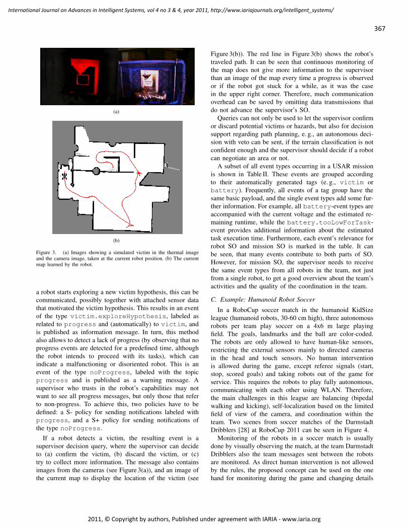
367



(a)

(b)

Figure 3. (a) Images showing a simulated victim in the thermal imageand the camera image, taken at the current robot position. (b) The currentmap learned by the robot.

a robot starts exploring a new victim hypothesis, this can becommunicated, possibly together with attached sensor datathat motivated the victim hypothesis. This results in an eventof the type victim.exploreHypothesis, labeled asrelated to progress and (automatically) to victim, andis published as information message. In turn, this methodalso allows to detect a lack of progress (by observing that noprogress events are detected for a predefined time, althoughthe robot intends to proceed with its tasks), which canindicate a malfunctioning or disoriented robot. This is anevent of the type noProgress, labeled with the topicprogress and is published as a warning message. Asupervisor who trusts in the robot’s capabilities may notwant to see all progress messages, but only those that referto non-progress. To achieve this, two policies have to bedefined: a S- policy for sending notifications labeled withprogress, and a S+ policy for sending notifications ofthe type noProgress.

If a robot detects a victim, the resulting event is asupervisor decision query, where the supervisor can decideto (a) confirm the victim, (b) discard the victim, or (c)try to collect more information. The message also containsimages from the cameras (see Figure 3(a)), and an image ofthe current map to display the location of the victim (see

Figure 3(b)). The red line in Figure 3(b) shows the robot’straveled path. It can be seen that continuous monitoring ofthe map does not give more information to the supervisorthan an image of the map every time a progress is observedor if the robot got stuck for a while, as it was the casein the upper right corner. Therefore, much communicationoverhead can be saved by omitting data transmissions thatdo not advance the supervisor’s SO.

Queries can not only be used to let the supervisor confirmor discard potential victims or hazards, but also for decisionsupport regarding path planning, e. g., an autonomous deci-sion with veto can be sent, if the terrain classification is notconfident enough and the supervisor should decide if a robotcan negotiate an area or not.

A subset of all event types occurring in a USAR missionis shown in Table II. These events are grouped accordingto their automatically generated tags (e. g., victim orbattery). Frequently, all events of a tag group have thesame basic payload, and the single event types add some fur-ther information. For example, all battery-event types areaccompanied with the current voltage and the estimated re-maining runtime, while the battery.tooLowForTask-event provides additional information about the estimatedtask execution time. Furthermore, each event’s relevance forrobot SO and mission SO is marked in the table. It canbe seen, that many events contribute to both parts of SO.However, for mission SO, the supervisor needs to receivethe same event types from all robots in the team, not justfrom a single robot, to get a good overview about the team’sactivities and the quality of the coordination in the team.

C. Example: Humanoid Robot Soccer

In a RoboCup soccer match in the humanoid KidSizeleague (humanoid robots, 30-60 cm high), three autonomousrobots per team play soccer on a 4x6 m large playingfield. The goals, landmarks and the ball are color-coded.The robots are only allowed to have human-like sensors,restricting the external sensors mainly to directed camerasin the head and touch sensors. No human interventionis allowed during the game, except referee signals (start,stop, scored goals) and taking robots out of the game forservice. This requires the robots to play fully autonomous,communicating with each other using WLAN. Therefore,the main challenges in this league are balancing (bipedalwalking and kicking), self-localization based on the limitedfield of view of the camera, and coordination within theteam. Two scenes from soccer matches of the DarmstadtDribblers [28] at RoboCup 2011 can be seen in Figure 4.

Monitoring of the robots in a soccer match is usuallydone by visually observing the match, at the team DarmstadtDribblers also the team messages sent between the robotsare monitored. As direct human intervention is not allowedby the rules, the proposed concept can be used on the onehand for monitoring during the game and changing details

368



Figure 4. Two scenes from robot soccer matches in the RoboCup KidSize league, Darmstadt Dribblers are playing in cyan.

during game breaks, or on the other hand for tuning therobots during tests or practice games.

Monitoring the health of each robot could also be donevisually, but with three or more robots on the field it isdifficult to keep track of each robot’s performance. WithCEP, it is possible to monitor the falling frequency of eachrobot for different motions like walking or kicking, and itscorrelation with other factors like the vicinity of opponentsor teammates (which could indicate that the fall was due toa collision), or motor temperature and battery status, whichcould be a reason to switch to a more robust behavior, e. g.,dribbling instead of kicking the ball.

Further, the benefit of the specific roles can be monitored,like already proposed for the goalie in Section IV. Thisallows on the one hand to tune the parameters during teststo maximize each role’s benefit, and on the other hand toquickly change tactics or preserve hardware during a match.

VI. CONCLUSION AND OUTLOOK

The communication concept presented in this paper isdesigned for interactions between a human supervisor anda team of autonomous robots. To make use of the specificcomplimentary strengths of humans and robots, supervisorinteractions are focusing on high-level commands. BecauseSA is not an adequate knowledge base for a human super-visor of a whole robot team, the notion of SO is introduced,which consists of robot SO and mission SO, to enable thehuman to detect on the one hand problems related to indi-vidual robots an on the other hand performance decrementsrelated to suboptimal team coordination. SO can be flexiblyachieved for several fundamentally different scenarios usingthe presented methods, which are complex event processing,message tagging, message classification, and policies. Thiscommunication concept is inspired by loosely coupled hu-man teamwork and requires a low communication overheadcompared to standard teleoperation methods, because onlydata needed for SO are sent, while omitting details only usedfor exact teleoperation. The methods enable a human super-visor to gain a general SO of a whole robot team, withoutrequiring the supervisor to be familiar with implementationdetails. The performance of the team can be enhanced bytransferring critical decisions to the supervisor, because inthis case the decision is based on SO, human experience and

implicit knowledge, and is therefore expected to be morereliable and efficient for achieving the mission goal.

In general, an interface that is based on this new com-munication concept can provide a higher SO than standardinterfaces, because the robots can send information thatthe supervisor would probably not request, hence problemsand errors can potentially be noticed earlier. SO gives thesupervisor a basis to take high-level decisions, e. g., foradapting task allocation or mission details. Preliminary re-sults in USAR and robot soccer indicate the potential of thedeveloped concept. These two fundamentally different setupsdemonstrate, that the proposed concept can be applied to alarge variety of problem classes. It is furthermore planned toimplement the whole concept, including the communicationconcept as well as high-level commands by the supervisor,for different scenarios with heterogeneous robot teams.

Future work includes experiments in simulation and withreal robots to support the hypotheses and approach of thispaper. It is planned to conduct user studies in differentapplication scenarios to show the wide applicability ofthe proposed methods. Furthermore, the possibilities of thesupervisor to coordinate robot teams based on the proposedsituation overview will be examined. For dealing with largerrobot teams, a basis for a large-scale interface is providedby the presented concept, as it offers the data for SO andsupports efficient filtering.

ACKNOWLEDGMENTS

This research has been supported by the German ResearchFoundation (DFG) within the Research Training Group 1362“Cooperative, adaptive and responsive monitoring in mixedmode environments”.

REFERENCES

[1] K. Petersen and O. von Stryk, “Towards a general commu-nication concept for human supervision of autonomous robotteams,” in Proceedings of the Fourth International Conferenceon Advances in Computer-Human Interactions (ACHI), 2011,pp. 228 – 235.

[2] J. Scholtz, “Theory and evaluation of human robot interac-tions,” in Proceedings of the 36th Annual Hawaii Interna-tional Conference on System Sciences, 2003.

369



[3] D. H. Fernald and C. W. Duclos, “Enhance your team-basedqualitative research,” Annals of Family Medicine, vol. 3, no. 4,pp. 360 – 364, July/August 2005.

[4] R. R. Murphy, “Human-robot interaction in rescue robotics,”IEEE Transactions on Systems, Man, And Cybernetics – PartC: Applications and Reviews, vol. 34, no. 2, pp. 138 – 153,May 2004.

[5] M. R. Endsley, “Situation awareness global assessment tech-nique (sagat),” in Proceedings of the IEEE 1988 NationalAerospace and Electronics Conference, vol. 3, 1988, pp. 789– 795.

[6] ——, “Toward a theory of situation awareness in dynamicsystems,” Human factors, vol. 37, no. 1, pp. 32–64, 1995.

[7] J. Drury, J. Scholtz, and H. Yanco, “Awareness in human-robot interactions,” in Systems, Man and Cybernetics, 2003.IEEE International Conference on, vol. 1, 2003, pp. 912 –918 vol.1.

[8] M. W. Kadous, R. K.-M. Sheh, and C. Sammut, “Effec-tive user interface design for rescue robotics,” in HRI ’06:Proceedings of the 1st ACM SIGCHI/SIGART conference onHuman-robot interaction. ACM, 2006, pp. 250–257.

[9] C. W. Nielsen, M. A. Goodrich, and R. W. Ricks, “Ecologicalinterfaces for improving mobile robot teleoperation,” IEEETransactions on Robotics and Automation, vol. 23, no. 5, pp.927–941, October 2007.

[10] B. P. Sellner, F. Heger, L. Hiatt, R. Simmons, and S. Singh,“Coordinated multi-agent teams and sliding autonomy forlarge-scale assembly,” Proceedings of the IEEE - SpecialIssue on Multi-Robot Systems, vol. 94, no. 7, pp. 1425 – 1444,July 2006.

[11] J. W. Crandall and M. A. Goodrich, “Experiments in ad-justable autonomy,” in IEEE International Conference onSystems, Man, and Cybernetics, vol. 3, 2001, pp. 1624 –1629.

[12] J. Wang and M. Lewis, “Human control for cooperatingrobot teams,” in HRI ’07: Proceedings of the ACM/IEEEinternational conference on Human-robot interaction. ACM,2007, pp. 9 – 16.

[13] Y. Nevatia, T. Stoyanov, R. Rathnam, M. Pfingsthorn,S. Markov, R. Ambrus, and A. Birk, “Augmented autonomy:Improving human-robot team performance in urban searchand rescue,” in Proceedings of the 2008 IEEE/RSJ Interna-tional Conference on Intelligent Robots and Systems (IROS),Nice, France, Sept, 22-26 2008, pp. 2103 – 2108.

[14] T. Fong, C. Thorpe, and C. Baur, “Robot, asker of questions,”Robotics and Autonomous Systems, vol. 42, pp. 235 – 243,2003.

[15] T. Kaupp and A. Makarenko, “Measuring human-robot teameffectiveness to determine an appropriate autonomy level,” inProceedings of the 2008 IEEE International Conference onRobotics and Automation, Pasadena, CA, USA, May 19 - 232008, pp. 2146 – 2151.

[16] R. Wegner and J. Anderson, “Balancing robotic teleoperationand autonomy for urban search and rescue environments,”in Advances in Artificial Intelligence, 17th Conference of theCanadian Society for Computational Studies of Intelligence,ser. Lecture Notes in Computer Science. Springer, 2004, pp.16–30.

[17] M. L. Cummings, S. Bruni, S. Mercier, and P. J. Mitchell,“Automation architecture for single operator-multiple uavcommand and control,” International Command and ControlJournal, vol. 1, no. 2, pp. 1 – 24, 2007.

[18] M. Johnson, P. J. Feltovich, J. M. Bradshaw, and L. Bunch,“Human-robot coordination through dynamic regulation,” inProceedings of the 2008 IEEE International Conference onRobotics and Automation, Pasadena, CA, May 19 - 23 2008,pp. 2159 – 2164.

[19] D. Pinelle and C. Gutwin, “A groupware design frameworkfor loosely coupled workgroups,” in Proceedings of the NinthEuropean Conference on Computer-Supported CooperativeWork, Paris, France, 18-22 September 2005, pp. 65 – 82.

[20] P. M. Fitts, Ed., Human engineering for an effective air-navigation and traffic control system. Washington, DC:National Academy of Sciences Archives, 1951.

[21] A. Hinze, K. Sachs, and A. Buchmann, “Event-based applica-tions and enabling technologies,” in Proceedings of the ThirdACM International Conference on Distributed Event-BasedSystems, 1:1–1:15, July 2009.

[22] U. Dayal, A. Buchmann, and D. McCarthy, “Rules areobjects too: A knowledge model for an active, object-orienteddatabase system,” in Advances in Object-Oriented DatabaseSystems, ser. Lecture Notes in Computer Science, K. Dittrich,Ed. Springer Berlin / Heidelberg, 1988, vol. 334, pp. 129–143.

[23] S. Chakravarthy and D. Mishra, “Snoop: an expressive eventspecification language for active databases,” IEEE Data andKnowledge Engineering, vol. 14, no. 10, pp. 1 – 26, 1994.

[24] H. Branding, A. P. Buchmann, T. Kudrass, and J. Zimmer-mann, “Rules in an open system: the REACH Rule System,”in Proc. 1st Intl. Workshop on Rules in Database Systems,Edinburgh, Scotland, September 1993, pp. 111 – 126.

[25] D. B. Kaber and M. R. Endsley, “The effects of level ofautomation and adaptive automation on human performance,situation awareness and workload in a dynamic control task,”Theoretical Issues in Ergonomics Science, vol. 5, no. 2, pp.113 – 153, 2004.

[26] “Team Hector Darmstadt website,” January 2012. [Online].Available: http://www.gkmm.tu-darmstadt.de/rescue/

[27] J. Meyer, P. Schnitzspan, S. Kohlbrecher, K. Petersen,O. Schwahn, M. Andriluka, U. Klingauf, S. Roth, B. Schiele,and O. von Stryk, “A semantic world model for urban searchand rescue based on heterogeneous sensors,” in RoboCup2010: Robot Soccer World Cup XIV, 2010.

[28] “Team Darmstadt Dribblers website,” January 2012. [Online].Available: http://www.dribblers.de/

370



A Virtual Navigation in a Reconstruction of the Town of Otranto in the Middle Ages for Playing and Education

Lucio Tommaso De Paolis, Giovanni Aloisio Department of Innovation Engineering

University of Salento Lecce, Italy

[email protected] [email protected]

Maria G. Celentano, Luigi Oliva, Pietro Vecchio Scuola Superiore ISUFI

University of Salento Lecce, Italy

[email protected] [email protected]

[email protected]

Abstract— The aim of the MediaEvo Project is to develop a multi-sensory platform for the edutainment in Cultural Heritage towards integration of human sciences and new data processing technologies, for the realization of a digital didactic game oriented to the knowledge of medieval history and society. The developing of the project has enhanced interactions among historical, pedagogical and ICT researches, by means of the definition of a virtual immersive platform for playing and educating and has permitted to investigate some navigation and interaction modalities among players for education purposes. In this paper we present some results of the MediaEvo Project that has led the researchers to use the reconstruction of the city of Otranto in the Middle Ages in order to determine the conditions for testing more elements of interaction in a virtual environment and a multisensory mediation in which merge objects, subjects and experiential context. With the aim to make interaction easier for users without any experience of navigation in a virtual world and more efficient for trained users, we use the Wiimote and the Balance Board of Nintendo in order to increase the sense of immersion in the virtual environment.

Keywords - simulation; edutainment; Virtual Cultural Heritage; navigation; virtual treasure hunt

I. INTRODUCTION Edutainment, a neologism created from the combination

of the words education and entertainment, refers to any form of entertainment aimed at an educational role. The videogame is one of the most exciting and immediate media of the edutainment applications because the game enables a type of multisensory and immersive relationship of the user through its interactive interface; moreover, the cyberspace of the videogame is a privileged point of sharing and socializing among players.

Edutainment is an up-and-coming field that combines education with entertainment aspects; thus, it enhances the learning environment and makes it much more engaging and fun-filled.

One of the most important applications of edutainment is undoubtedly the reconstruction of 3D environments aimed at the study of cultural heritage; the use of Virtual Reality in this field makes it possible to examine the three-dimensional high-resolution environments reconstructed by using information retrieved from the archaeological and historical studies and to navigate in these in order to test new methodologies or to practically evaluate the assessment. Virtual Reality (VR) technology makes it also possible to create applications for edutainment purposes for the general public and to integrate different learning approaches.

The building of three-dimensional renderings is an efficient way of storing information, a means to communicate a large amount of visual information and a tool for constructing collaborative worlds with a combination of different media and methods. By recreating or simulating something concerning an ancient culture, virtual heritage applications are a bridge between people of the ancient culture and modern users.

One of the best uses of the virtual models is that of creating a mental tool to help students learn about things and explore ancient cultures and places that no longer exist or that might be too dangerous or too expensive to visit. In addition, it allows students to interact in a new way, using many possibilities for collaboration. A very effective way to use VR to teach students about ancient cultures is to make them enter the virtual environment as a shared social space and allow them to play as members of that society.

The development technologies of video games are today driven by strong and ever-increasing request, but there are very few investments related to teaching usage of such technologies, they are still restricted to the entertainment context. Several VR applications in Cultural Heritage have been developed, but only very few of these with an edutainment aim.

The Human-Computer Interaction (HCI) technology is concerned with methodologies and methods for designing

371



new interfaces and interaction techniques, for evaluating and comparing interfaces and developing descriptive and predictive models and theories of interaction.

The HCIs improve interactions between users and computers by making computers more usable and receptive to the user's needs.

Researches in HCI field focus on the developing of new design methodologies and new hardware devices and on exploring new paradigms and theories for the interaction. The end point in the interface design would then lead to a paradigm in which the interaction with computers becomes similar to the one between human beings.

This paper presents some results of the MediaEvo Project that has led the researchers to use the reconstruction of the city of Otranto in the Middle Ages in order to determine the conditions for testing more elements of interaction in a virtual environment and to develop a multi-channel and multi-sensory platform for the edutainment in Cultural Heritage.

In the following is reported the virtual reconstruction of the town of Otranto in the Middle Ages, the interaction modalities and rules of the navigation in the virtual town and has been also tested the possibility to navigate in a complex virtual environment by means of the Nintendo Wiimote and Balance Board [1] and the idea of the use of the Augmented Reality technology in a treasure hunt.

II. PREVIOUS WORKS ON THE NAVIGATION WITHIN VIRTUAL ENVIRONMENTS

The techniques for navigation within virtual environments have covered a broad kind of approaches ranging from directly manipulating the environment with gestures of the hands, to indirectly navigating using hand-held widgets, to identifying some body gestures and to recognizing speech commands. Perhaps the most prevalent style of navigation control for virtual environments is directly manipulating the environment with gestures or movements of part of the user’s body.

Some developed systems are based on a head-directed navigation technique in which the orientation of the users head determines the direction and speed of navigation [2]. This technique has the advantage of requiring no additional hardware besides a head tracker, but has the disadvantage that casual head motions when viewing a scene can be misinterpreted as navigation commands. In addition, a severe drawback of this and other head-based techniques is that it is impossible to perform the common and desirable real-world operation of moving in one direction while looking in another.

Another direct body-based navigation technique is found in some systems that use sensors to measure the tilt of the user’s spine or the orientation of the user’s torso in order to determine the direction of the motion and to enable the

decoupling of the user’s head orientation from their direction of movement [3].

Another category of techniques for motion control is based on speech recognition. Speech allows a user to indicate parameters of navigation and can often be used in conjunction with gestures to provide rich, natural immersive navigation controls [4]. Speech controls should play a role in virtual environment navigation, but it is also critical to support an effective navigation based on speech-free techniques.

In the last few years, systems based on locomotion interfaces and on control navigation by walking in place for the navigation in a virtual environment have also been developed.

String Walker [5]is a locomotion interface that uses eight strings actuated by motor-pulley mechanisms mounted on a turntable in order to cancel the displacement of the walker. String Walker enables users to maintain their positions while walking in various directions in virtual environments because, when the shoes move, the strings pull them in the opposite direction and cancel the step. The position of the walker is fixed in the real world by this computer-controlled tension of the strings that can pull the shoes in any direction, so the walker can perform a variety of gaits, including side-walking or backward walking

The CirculaFloor [6] locomotion interface uses a group of movable floors that employ a holonomic mechanism in order to achieve omni-directional motion. The circulation of the floors enables users to walk in arbitrary directions in a virtual environment while their positions are maintained. The CirculaFloor creates an infinite omni-directional surface using a set of movable tiles that provide a sufficient area for walking and a precision tracing of the foot position is not required. This method has the potential to create an uneven surface by mounting an up-and-down mechanism on each tile.

Powered Shoes [7] employs roller skates actuated by motors and flexible shafts and supports omni-directional walking, but the walker cannot perform a variety of gaits. Powered Shoes is a revolutionary advance for entertainment and simulation applications, because it provides the proprioceptive feedback of walking.

III. IMPROVING KNOWLEDGE THROUGH THE VIRTUAL REPRESENTATION

Evolution in research methodology corresponds to a general debate on communication and education closely linked to the characteristics of a changing perception of teaching, oscillating between experimental impulses and conservative attitudes.

The improvement in technological capabilities enriches the possibilities for research and protection and enhances the value of cultural heritage, thus halting their demise.

372



Firstly, the increased speed of communication and data exchange within the research community offers the dimension of real time interconnectivity.

Secondly, the overall amount of information originating from both qualitative and quantitative exploration with the support of technologically advanced equipment, compared with that of a few decades ago, leads to the possibility of an extremely detailed description of reality.

The ancient town, as an information unit made up of ontological entities [8], can be defined as a cultural unit code which locates and describes the process of territorialisation of human society. It represents the space-time relation between man and environment at a certain time [9]. Apart from this assertion of uniqueness of space and time the educational purpose of the work requires a perceivable synthesis of culture, civilization and place referred to a perceivable and sufficiently extended phase of civilization [10].

Until recently, "historic vision" was limited to only a few professionals, scholars and researchers, who shared the interpretation codes for extracting the ancient landscape from the actual one. In this new stream of experimentation, geared towards interaction and edutainment, the researcher becomes part of a larger system through which to study and interpret space. In a virtual interactive town, the possibilities of information exchange increase dramatically, moving from static reconstruction to simulation.

Simulation permits the construction of a platform that adds the definition of game rules and plots to interaction and immersion. The final goal of the definition of the historic landscape is a cybernetic world that will create infinite possible simulations, not necessarily bonded to physical reality, based on the algorithms that encode the understanding of ancient situations [11].

At present, many experiences of interactive reconstruction take place on the net or have been presented during the course of international conferences. These primarily concern the elaboration of algorithmic models in order to better comprehend and reconstruct the sites, technological applications for Augmented Reality on cultural heritage and ontological systems and data management.

Other applications facilitate access to and reading of the cultural patrimony both within the museum and online, for example:

• The reconstruction of the site of Faragola (Foggia) by the University of Foggia, undertaken as part of the Itinera Time Machine Project, fits within the trend of an experiential relationship within an archaeological context [12];

• Appia Antica Project, a digital archive of the monuments of the park, employing many different technologies for 3D representation of the landscape

and integrating instruments for topographic relief and methodologies of surveying on site [13];

• Virtual Rome Project [14]; • Ancient Rome on Google Earth [15]; • Medieval Dublin [16]; • Nu.M.E. Project, a virtual museum concerned with

the city of Bologna [17]. On a strongly interactive level and related specifically to

multichannel edutainment, examples of applications utilizing Virtual Collaborative Environments are:

• City Cluster [18]; • The Quest Atlantis Project [19]; • Integrated Technologies of Robotics and Virtual

Environment in Archaeology Project [20].

IV. THE MEDIAEVO PROJECT: LEARNING ABOUT THE MIDDLE AGES IN OTRANTO

The MediaEvo Project aims to develop a multi-channel and multi-sensory platform in Cultural Heritage and to test new data processing technologies for the realization of a digital didactic game oriented to the knowledge of medieval history and society [21], [22].

The framework has features of strategy games, in which the decision-making capacities of a user have a big impact on the result, which in our case is the achievement of a learning target. The idea is to create competition between the players, during the learning process.

The game is intended as a means to experience a loyal representation of the possible scenarios (environments, characters and social roles) in the historic-geographical context of Otranto during Frederick Age (XIII century).

We chose Otranto as an example town; Otranto is located in the easternmost tip of the Italian peninsula, in Puglia, in the so-called Italy’s heel. Due to its geographical position, Otranto was like a bridge between East and West and it played an important connective role in the Middle Ages from a historical and cultural point of view. For these reasons many publications and lectures have looked at and partly explained the ancient role of this town by focusing on the historical happenings and on the development of urban institutions within it [23].

Otranto was a Byzantine and a Gothic centre, later ruled by the Normans, Swabians, the Anjou and the Aragonese. After a long siege, on 14 August 1480 the town was caught and the inhabitants were massacred by the Turkish army. This mix of history can be seen in the enigmatic mosaic of the Cathedral, a Romanesque church built during the Norman domination in the 10th century on the axis that joined Rome to Byzantium. The mosaic, done by the monk Pantaleone in the 12th century, covers almost the entire floor of the Cathedral, for over 16 metres; its size is nothing compared to the complexity of images and references that mixes Biblical narration from the Old and New Testaments

373



with some pagan elements and others of Eastern derivation. The implementation of an edutainment platform is

strongly influenced by the definition of the scenery that is the world in which the framework is placed with the related learning objects and learning path, the characters, the scene’s objects, the logic, hence, the rules of the game, the audio content, the texts and anything related to its use.

The framework will have features of strategy games, in which the decision capabilities of a user have a big impact on the result, which in our case is the achievement of a learning target. Nevertheless, the strategy and tactics are in general opposed by unforeseeable factors (provided by the game), connected with the edutainment modules, in order to provide a higher level of participation, which is expressed in terms of the ease with which it is learnt. The idea is to provide a competition between the players, during their learning.

The system, on the basis of a well-defined learning target and eventually based on the knowledge of the user, will continuously propose a learning path (learning path composed by a sequence of learning objects), in order to allow the achievement of particular learning results.

The use of digital entertainment and performance media, then, can enhance the communication of cultural heritage and history in order to increase our knowledge of such a relevant part of our history.

Given the knowledge we have of the town in the Middle Ages, it may be almost impossible to carry out a full reconstruction, what could be experienced in the game is the immersion in a virtual environment that can easily enhance the communication of historical research and understanding of the birth and life of cultural heritage.

During its definition, the platform that has been planned for educational purposes has proved to be useful for testing researchers’ hypotheses about the ancient town and its everyday life.

Figure 1. Scheme of project work organization for MediaEvo Project

At the end of project, other application fields have been tested on the game: new peripherals for motion and interaction, virtual treasure hunts, Augmented Reality and evaluation of the scheme for territorial marketing and touristic promotion.

The scheme of the MediaEvo Project work organization is reported in Fig. 1.

V. RECONSTRUCTION OF THE VIRTUAL TOWN For reconstructing the natural place and its surroundings a

Digital Terrain Model (DTM) of the site was produced using ESRI ArcGIS and imported in the game engine Torque Game Engine of GarageGames. Characters and animation are made using 3ds Max.

Figure 2. The reconstruction of defensive wall and its surroundings.

Architectural contents were modelled using the Torque Constructor editor of the Torque 3D engine. The first dwelling consists of a unit cell surrounded by a rectangular court, this is considered the initial settlement model for all ancient towns; the second one is the terraced house unit. Composing and varying those units on the particular scheme leads to the reconstruction of the urban medieval space in the game. The modular elementary residential units have been designed according to the local medieval unit system. They have been used as bricks for composing the urban landscape in which monuments, infrastructures and playing are located. In Fig. 2 the reconstruction of the defensive wall and its surroundings is shown.

Torque Constructor has proved to be an efficient tool for the direct implementation of basic 3D graphics models but we found some difficulties in modelling complex buildings because of the lack of many useful features implemented in professional 3D software. For this reason, the reconstruction of big monuments has been carried out using a CAM in order to obtain a more accurate definition of the architectural structures. All the models have been imported into the Torque 3D engine.

St. Peter's Church was found to be useful for testing the

374



importing system both for its characteristic modularity and for its historical relevance as a single byzantine building located in a medieval context.

In Fig. 3 is shown the internal and external reconstruction of the Otranto Cathedral.

Figure 3. The reconstruction of the Otranto Cathedral.

Other parts, walls and external structures such as towers or gates, complete the original landscape for the game.

For the context of edutainment for cultural heritage, in this issue various virtual interactions into the Torque Game Engine platform have been produced.

A new algorithm has been implemented to realize a preliminary Artificial Intelligence with the ability to establish stable textual or vocal connections between the different virtual players placed in the game mission.

Interactions have been placed into some checkpoints of the Torque virtual environment; these checkpoints make it possible to trigger particular audio or/and video events

during the navigation of the game player. It is also possible to implement the interactions in the

Torque platform, allowing developers to bind appropriate actions to a given event. Each event manages a particular action in the game mission and in this sense the events can be used for controlling textual or multimedia mode.

It is possible to control the movements of each game player in the game mission in the collisions with game objects placed in the virtual environment.

VI. INTERACTION MODALITIES AND RULES In Fig. 4 is shown a diagram of interactions of the avatar-

player. There are 2 levels, as it is described below: A. Level I. Educational

When the game starts, the player sees a multimedia presentation (a videoclip developed by experts in medieval history/art) with a short introduction to the history of Otranto; s/he can then choose the possible destinations (Cathedral, St. Peter’s Church, Castle and Town Walls) and see the corresponding videoclips or skip the presentation and start the application. Here s/he goes to the second level. B. Level II. Interaction and surfing

This is an interactive level where the player enters the virtual world. S/he will meet a guide and could choose to navigate with him/her - surfing with a guide (level II.1) - or free surfing without the guide (level II.2).

Figure 4. Access and interaction levels of the avatar-player

In the definition of the interaction with the 3D environment in the case of level II.1, two possible scenarios were created and, therefore, two possible tasks for the avatar-guide:

a) 1st choice: Facilitator Guide (F-Guide) The guide is a facilitator and gives the player suggestions

to follow a specific navigation path. The player can start multiple paths with the F-Guide and select among four different Interest Points (IPs): the Cathedral (IP1), St. Peter’s Church (IP2), the Castle (IP3) and the Town Walls (IP4). Fig. 5 shows the Interest Points of the game.

In the journey from the starting point (Ø) to the selected

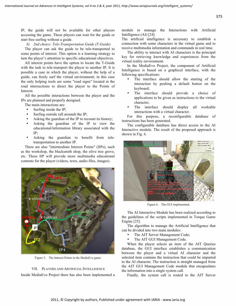
375



IP, the guide will not be available for other players accessing the game. These players can wait for the guide or start free surfing without a guide.

b) 2nd choice: Tele-Transportation Guide (T-Guide) The player can ask the guide to be tele-transported to

some points of interest. This option is a learning strategy to turn the player’s attention to specific educational objectives.

All interest points have the option to locate the T-Guide with the task to tele-transport the player to another IP. It is possible a case in which the player, without the help of a guide, can freely surf the virtual environment; in this case the only helping tools are some "road signs" located at the road intersections to direct the player to the Points of Interest.

All the possible interactions between the player and the IPs are planned and properly designed.

The main interactions are: • Surfing inside the IP; • Surfing outside (all around) the IP; • Asking the guardian of the IP to recount its history; • Asking the guardian of the IP to view the

educational/information library associated with the IP;

• Asking the guardian to benefit from tele-transportation to another IP.

There are also "intermediate Interest Points" (IIPs), such as the workshop, the blacksmith shop, the olive tree grove, etc. These IIP will provide more multimedia educational contents for the player (videos, texts, audio files, images).

Figure 5. The Interest Points in the MediaEvo game

VII. PLAYERS AND ARTIFICIAL INTELLIGENCE Inside MediaEvo Project there has also been implemented a

module to manage the Interactions with Artificial Intelligence (AI) [24]. The artificial intelligence is necessary to establish a connection with some characters in the virtual game and to receive multimedia information and commands in real time.

The ability to interact with AI characters is the principal key for retrieving knowledge and experiences from the virtual reality environment.

In the MediaEvo Project, the component of Artificial Intelligence is based on a graphical interface, with the following specifications:

• The interface should allow the starting of the interaction by pushing a default button on the keyboard;

• The interface should provide a choice of applications to be given as instructions to the virtual character;

• The interface should display all workable interactions with a virtual character.

For this purpose, a reconfigurable database of instructions has been generated.

The configurable database has direct access to the AI Interactive module. The result of the proposed approach is shown in Fig. 6.

Figure 6. The GUI implemented.

The AI Interactive Module has been realized according to the guidelines of the scripts implemented in Torque Game Engine [25].

The algorithm to manage the Artificial Intelligence that can be divided into two main modules:

• The AIT Server Management Code; • The AIT GUI Management Code. When the player selects an item of the AIT Queries

database, the GUI interface establishes a communication between the player and a virtual AI character and the selected item contains the instruction that could be imparted to the AI character. The instruction is straight managed from the AIT GUI Management Code module that encapsulates the information into a single system call.

Finally, the system call is routed to the AIT Server

376



Management Code module and then it is interpreted to identify the corresponding action, into the AIT Actions database.

Figure 7. The opening of a multimedia clip video.

The game has been designed for enabling multi-playing in order to provide the real-time ability to interact with other game sessions localized in different places of the reconstructed virtual environment.

In the MediaEvo platform are available some multimedia elements; in particular, it is possible to insert audio elements and to run video clips when the player reaches some checkpoint.

In Fig. 7 is shown the opening of a multimedia clip video when the character reaches the S.Peter’s church. In addition it is visualized a virtual radar in order to know the positions of the other players in the virtual environment.

VIII. TESTING INPUT PERIPHERALS: THE NINTENDO WIIMOTE AND BALANCE BOARD

In recent years some systems based on the control of the navigation in a virtual environment by walking have been also developed.

We present an application of navigation and interaction in a virtual environment using the Wiimote (word obtained as a combination of "Wii" and "Remote") and the Balance Board of Nintendo [26].

The aim is to make interaction easier for users without any experience of navigation in a virtual world and more efficient for trained users; for this reason we need to use some intuitive input devices oriented to its purpose and that can increase the sense of immersion.

Wii is the last console produced by Nintendo; it was released in October 2006 and, according to official data of 2010, has surpassed 70 million units sold. The reasons for this success can be undoubtedly found in the new approach that the gaming console gives the user in terms of interaction that effectively makes it usable and enjoyable by a large part of users. The secret of this usability is the innovative interaction system; the Wiimote replaces the

traditional gamepad controller type (with cross directional stick and several buttons) with a common object: the remote control.

The Wiimote is provided with an infrared camera that can sense the infrared LED of a special bar (Sensor Bar) and it can interpret, by means of a built-in accelerometer, the movements of translation, rotation and tilt.

Figure 8. Interaction modalities of Wiimote and Balance Board.

The Wiimote has been equipped with a series of accessories that increase its potential, such as the Balance Board, that, by means of four pressure sensors at each corner, is able to interpret the movements of the body in order to control the actions of the user in a videogame.

Because we walk on our feet, controlling walking in Virtual Reality could be felt as more natural when done with the feet rather than with other modes of input. For this reason we used the Nintendo Balance Board as an input device for navigation that offers a new and accessible way to gain input. It is a low-cost interface that transmits the sensor data via Bluetooth to the computer and enables the calculation of the direction the user is leaning to.

Fig. 8 shows the interaction modalities of Wiimote and Balance Board.

In addition, in order to implement the control of different views and to change the point of view of the user, in our application we use the Nintendo Wiimote and the interaction by means of this device has the aim to simulate the use of the mouse.

Figure 9. Use of Wiimote and Balance Board in the MediaEvo game.

377



Fig. 9 shows the use of Wiimote and Balance Board in the MediaEvo game.

Since the frequency of communication between the Wii console and the Wiimote/Balance Board is that of the standard Bluetooth, these devices can be used as tools to interact with any computer equipped with the same technology. Appropriate libraries have been realized in order to allow the interfacing between these devices and a computer.

A software layer that allows the Balance Board and the Wiimote to be used as input devices for any application that runs on a computer has been realized. The aim is to make it possible to receive signals and commands from the Wiimote and the Balance Board and to translate these into commands for the computer in order to emulate the keyboard and the mouse.

The application, created to provide a new system of interaction in the virtual world of the MediaEvo Project, can be coupled to any application of navigation in a virtual world.

The modalities of interaction provided by the application involve the use of the Wiimote and Balance Board simultaneously. In particular, the user is able to move the avatar in the virtual environment by tipping the scales in the direction in which he wants to obtain the move; an imbalance in forward or reverse leads to a movement forward or backward of the virtual character, while the lateral imbalance corresponds to the so-called "strafe" in video games, where the movement is made on the horizontal axis while maintaining a fixed pointing direction of the gaze.

Figure 10. Configuration interface of the Wiimote and Balance Board.

To run the application, it is first necessary to configure the keys able to emulate any type of movement, to set the sensitivity of the Balance Board and then to connect the device; the information on the data received from the device are displayed in real time.

The interface that visualize the data received from the Wiimote and Balance Board is divided into two main

sections: the left panels contain the control with all the data received via Bluetooth from the devices, whereas in the right side it is possible to set the associations among the command given to the device and the equivalent command simulated from the computer, the levels of sensitivity and threshold beyond which the interactions occur.

For these operations the software uses two open-source libraries in C# and the WiimoteLib InputSimulator; the WiimoteLib is a library for interfacing the Nintendo Wiimote and other devices (such as the Balance Board) in an environment .NET [27]. The purpose of this library within the application is to simulate the use of a mouse and a keyboard starting from the properly interpreted and translated inputs received from the Wiimote and Balance Board.

Regarding the interaction by means of the Wiimote, the aim is to simulate the mouse using two modalities of interaction.

"Mode 1" uses the movement on the X and Y axes of the accelerometer to move the mouse (and, in the 3D environment, the user’s point of view) on the longitudinal and latitudinal axes; the value provided by the accelerometer is compared with the sensitivity set during configuration.

"Mode 2", that is the default mode, allows to move the mouse (and, then, the user’s point of view) using the direction arrows of the Wiimote.

Fig. 10 shows the configuration interface of the Wiimote and Balance Board devices.

Figure 11. Navigation in the MediaEvo virtual environment.

378



Fig. 11 shows a user during the navigation in the MediaEvo virtual environment using the Wiimote and the Balance Board.

IX. VIRTUAL TREASURE HUNT Within the MediaEvo Project it has been also developed a

“virtual treasure hunt” placed in the old town of Otranto using an iPhone as a device to find and read the clues of the game.

The Augmented Reality [28] has been used as an edutainment-oriented technology for geo-locating the points of interest (POI) and the visualization of useful and interesting data that are overlapped on the video stream of the iPhone camera.

The working modalities of the virtual treasure hunt are shown in Fig. 12.

Figure 12. Working modalities of the virtual treasure hunt.

The main components of the developed application are: • The management of the treasure hunt guides the

logic of the game in every aspect and. It also has the task of interfacing with the database to retrieve the information that helps players during the treasure hunt. It is possible to obtain additional data through Internet on a specific POI.

• Augmented Reality manages the information regarding the user geo-location and the visualization of the information associated with the POI.

These components take advantage of the GPS and compass interfaces and provide the user with a map of the city in order to facilitate moving in the town and easy reaching the clues.

The user menu allows visualizing the last clue or a map where are shown the location of the player in the town and the location of the next point to be reached.

The tools that the player can use during the treasure hunt are the following:

• A radar that provides the location of the POI during the player's walk;

• A GPS signal display; • A user menu; • A radius that shows the distance within which the

radar can detect the POIs. In Fig. 13 is shown the graphic interface with the tools. During the treasure hunt the player can use radar that

provides the location of the POI, and a menu with the possibility to increase or decrease the distance within which the radar can detect the POIs.

Figure 13. Visualization of the POI.

Once the player is close to a POI, a marker that indicates the presence of a clue is visualized on the on the iPhone screen and superimposed on the images captured by the camera; this is a typical visualization in Augmented Reality.

Touching the marker in the screen, a brief description of the stage is shown and two new buttons appear in the toolbar:

• The first one is a link to the resources available through Internet if the POI has an associated web page;

• The second gives more detailed information (in terms of text, move or audio) to reach the next stage.

In Fig. 14 are shown some video and audio clues.

Figure 14. Visualization of video and audio clues.

379



X. CONCLUSIONS AND FUTURE WORK The aim of the MediaEvo Project is the development of a

multi-channel and multi-sensory platform for the edutainment in Cultural Heritage.

This paper presents some results of the project that has led the researchers to use the reconstruction of the city of Otranto in the Middle Ages in order to determine the conditions for testing more elements of interaction in a virtual environment and a multisensory mediation in which merge objects, subjects and experiential context.

Taking into account the potential of a virtual scenario, a series of properties have been defined to give the game platform an effective educational value.

By incorporating historical, technical and educational considerations, the final product presents itself as a “complete-open-interactive” environment for the acquisition of knowledge, the enhancement and safeguarding of cultural heritage.

In the MediaEvo Project has been also tested the possibility to navigate in a complex virtual environment by means of the Nintendo Wiimote and Balance Board and the idea of the use of the Augmented Reality technology in a treasure hunt.

Possible future developments could include the conversion of the application in external library, by adding specific methods and attributes to be directly integrated into other applications, and the porting of the developed application in a multi-platform language in order to be used in different development environments.

REFERENCES [1] L. T. De Paolis, M. Manco, and G. Aloisio, “Navigation and

Interaction in the Virtual Reconstruction of the Town of Otranto in the Middle Ages”, The 4th International Conference on Advances in Computer-Human Interactions (ACHI 2011), February 23-28, 2011, Gosier, Guadeloupe, France, pp. 120-124.

[2] A. Fuhrmann , D. Schmalstieg, and M. Gervautz, “Strolling through Cyberspace with Your Hands in Your Pockets: Head Directed Navigation in Virtual Environments”, the 4th Eurographics Workshop on Virtual Environments, Springer-Verlag, 1998, pp. 216-227.

[3] P. R. Cohen, M. Johnston, D. McGee, S. Oviatt, J. Pittman, I. Smith, L. Chen, and J. Clow, “QuickSet: Multimodal interaction for distributed applications”, the Fifth International Multimedia Conference (Multimedia ’97), ACM Press, 1997, pp. 31-40.

[4] D.A. Bowman, S. Coquillart, B. Froehlich, M. Hirose, and Y. Kitamura, “3D User Interfaces: Theory and Practice”, Boston, MA, Addison-Wesley, Pearson Education, 2005, pp. 342-344.

[5] H. Iwata, H. Yano, and M. Tomiyoshi, “String Walker”, International Conference on Computer Graphics and

Interactive Techniques ACM SIGGRAPH 2007, August 2007, San Diego, California.

[6] H. Iwata, H. Yano, M., H. Fukushima, and H. Noma, “CirculaFloor”, IEEE Computer Graphics and Applications, Jan-Feb. 2005, Vol. 25 pp. 64 – 67.

[7] H. Iwata, H. Yano, M., and H. Tomioka, “Powered Shoes”, International Conference on Computer Graphics and Interactive Techniques ACM SIGGRAPH 2006, Boston, Massachusetts.

[8] G. Kassel, "A formal ontology of artefacts", Applied Ontology, vol. 5, no. 3-4 / 2010, IOS Press, pp. 223-246.

[9] S. Pescarin and L. Valentini, "Databases and Virtual Environments: a Good Match for Communicating Complex Cultural Sites", ACM SIGGRAPH 2004, Los Angeles, 2004.

[10] M. Forte, “Mindscape: ecological thinking, cyber-anthropology, and virtual archaeological landscapes”, The reconstruction of Archaeological Landscapes through Digital Technologies, M. Forte and P. R. Williams, Eds., Boston, 2003, pp. 95-108.

[11] S. Pescarin, “Reconstructing Ancient Landscape”, Budapest: Archaeolingua, 2009, pp. 21-23.

[12] Itinera Time Machine Project. Available: http://www.itinera.puglia.it

[13] Appia Antica Project. Available: http://www.appia.itabc.cnr.it [14] Virtual Rome Project. Available: http://3d.cineca.it/storage [15] Ancient Rome. Available: http://earth.google.it/rome [16] Medieval Dublin. Available: http://www.medievaldublin.ie [17] F. Bocchi, "The city in four dimensions: the Nu.M.E.

Project", J. of Digital Information Management, vol. II(4), 2004, pp. 161-163.

[18] City Cluster. Available: http://www.fabricat.com [19] Quest Atlantis Project. Available:

http://atlantis.crlt.indiana.edu [20] Integrated Technologies of Robotics and Virtual Environment

in Archaeology Project. Available: http://www.vhlab.itabc.cnr.it

[21] L.T. De Paolis, M.G. Celentano, P. Vecchio, L. Oliva, and G. Aloisio, "Otranto in the Middle Ages: a Virtual Cultural Heritage Application", 10th VAST International Symposium on Virtual Reality, Archaeology and Cultural Heritage (VAST 2009), September 22-25, 2009, Malta.

[22] L.T. De Paolis, M.G. Celentano, P. Vecchio, L. Oliva, and G. Aloisio, " A Multi-Channel and Multi-Sensorial Platform for the Edutainment in Cultural Heritage", IADIS International Conference Web Virtual Reality and Three-Dimensional Worlds 2010, July 27-29, 2010, Freiburg, Germany.

[23] H. Houben, “Otranto nel Medioevo: tra Bisanzio e l'Occidente”, Congedo, Galatina , Italy, 2007.

[24] K. C. Finney, “Advanced 3D game programming all in one”, Thomson Course Technology, 2005.

[25] K. C. Finney, “3D game programming all in one”, Thomson Course Technology, Boston, USA, 2004.

[26] Nintendo WiiMote and Balance Board. Available: http://www.nintendo.com

[27] WiimoteLib - Managed Library for Nintendo Wii Remote, November 2008. Available: http://www.brianpeek.com

[28] R. Azuma, “A Survey of Augmented Reality”, Presence: Tele-operators and Virtual Environments, 1997, 4(6), pp. 355-385.

380



A Novel Graphical Interface for User Authentication on Mobile Phones and Handheld

Devices

Abstract — Mobile phones are rapidly becoming an important

tool to carry out financial transactions besides the normal

communication. They are increasingly being used to make

payments, access bank accounts and facilitate other commercial

transactions. In view of their increased importance there is a

compelling need to establish ways to authenticate people on the

mobile phones. For the last several decades the popular method

of authentication on computers has been text based. Both the

username and password are alphanumeric. The textual password

scheme though convenient to use suffers from various

drawbacks. Alphanumeric passwords are most of the times easy

to guess, vulnerable to brute force attacks, prone to shoulder-

surfing, and are easily forgotten. With financial transactions at

stake, the need of the hour is to have a secure, robust, and usable

scheme for authentication. Graphical passwords are one of such

schemes that offer a plethora of options and combinations. In this

paper we are proposing a scheme which is simple, secure and

robust. The proposed graphical password scheme will provide a

large password space and at the same time will facilitate

memorability. It is suitable to implement on all touch sensitive

mobile phones as well as PDAs and Tablet PCs.

Keywords- User authentication, graphical password, mobile

phone security, usability, security

I. INTRODUCTION

Mobile phones have made their presence felt in different

walks of human life. Today's technically advanced mobile

phones are capable of not only receiving and making phone

calls, but can very conveniently store data, take pictures and

connect to the internet. They have also become a powerful

tool to conduct commercial and financial transactions. They

are increasingly being used to make payments, such as at

retail shops, public transport, paid parking areas and also to

access the bank accounts via internet. In view of this the

security and safety of mobile phones have become paramount

to prevent unauthorized persons from conducting any

unwarranted transactions through the phones. Conventional

method of authentication remains mainly text based as it has

been around for several decades and also because of ease of

implementation. However, text based passwords suffer from

various drawbacks such as they are easy to crack through

dictionary attacks, brute force, shoulder surfing, social

engineering etc.

The “small dictionary” attack is so successful that in

Klein‟s case study [2], about 25% of 14,000 passwords were

cracked by a dictionary with only 3 million entries. Following

the same method used by Van Oorschot and Thorpe [12], such

a dictionary can be exhausted by a 3.2 GHz PentiumTM

4

machine in only 0.22 second. Graphical passwords, which

require a user to remember and repeat visual information,

have been proposed to offer better resistance to dictionary

attack. Psychological studies support the hypothesis that

humans have a better capability to recognize and to recall

visual images than alphanumeric strings [3], [4] and [5]. If

users are able to remember more complex graphical

passwords (i.e., from a larger password space), an attacker has

to build a bigger dictionary, thus spend more time or deploy

more computational power to achieve the same success as for

textual passwords.

In this paper, we will demonstrate a graphical grid-based

password scheme which will aim at providing a huge

password space along with ease of use. We will also analyze

its strength by examining the success of brute force technique.

In this scheme we will try to make it easy for the user to

remember and more complex for the attacker. In Section II we

describe the recent work done in the area of graphical

password schemes. Sections III to VI describe the proposed

scheme in detail. Security analysis of the proposed scheme is

illustrated in the Section VII. This is followed by a case study

described in the Section VIII.

II. RELATED WORK

Many papers have been published in recent years with a

vision to have a graphical technique for user authentication.

Primarily there are two methods, having recall and

recognition-based approach respectively. Traditionally both

the methods have been realized through the textual password

space, which makes it easy to implement and at the same time

easy to crack.

The study shows that there are 90% recognition rates for

few seconds for 2560 pictures [24]. Clearly the human mind is

best suited to respond to a visual image. A number of Recall-

Based approaches have been proposed and some of the

significant ones based on their security and usability features

are presented in this section [23].

Mohammad Sarosh Umar Department of Computer Engineering,

Aligarh Muslim University, Aligarh,

India

[email protected]

Mohammad Qasim Rafiq Department of Computer Engineering,

Aligarh Muslim University, Aligarh,

India

[email protected]

381



Passdoodle is a graphical password comprised of

handwritten designs or text, usually drawn with a stylus onto a

touch sensitive screen [23]. In their 1999 paper, Jermyn et al.

[10] prove that doodles are harder to crack due to a

theoretically much larger number of possible doodle

passwords than text passwords: while there are only 2.08 x

1011

8 letter passwords, there are 10400

different 100-point

doodles in a 100 x 100 grid. Figure 1 shows a sample of

Passdoodle password.

Figure 1: An Example of a Passdoodle

The issue of recognition prevents widespread use of the

Passdoodle. The length and identifiable features of the doodle

set the limits of the system. Only a finite amount of computer

differentiable doodles can be made. To maintain security the

system cannot simply authenticate a user as the user whose

recorded doodle is most similar, a minimum threshold of

likeliness and similarity must be set. This prevents the use of

blatant guessing to authenticate as a random user. However

speed and accuracy remain top priorities for the system. A

complicated recognition design requiring a hundred training

samples and a minute of computation to authenticate negates

the purpose of the original pervasive design. Often, the

authentication schemes based on the doodles uses a

combination of doodle velocity and distribution mapping to

recognize and authenticate a doodle [21]. Goldberg and his

colleagues [21] developed a Passdoodle algorithm, which was

a graphical password comprised of handwritten designs or

text, usually drawn with a stylus onto a touch sensitive screen.

Their study concluded that users were able to remember

complete doodle images as accurately as alphanumeric

passwords. They found that people could remember complete

doodle images as accurately as alphanumeric passwords, but

they were less likely to recall the order in which they drew a

doodle than the resulting image. In the other research [22],

users were fascinated by the doodles drawn by other users,

and frequently entered other users‟ login details merely to see

a different set of doodles from their own.

Another recall-based password approach is VisKey [6],

which is designed for PDAs. In this scheme, users have to tap

spot in sequence to make a password. As PDAs have a smaller

screen, it is difficult to point exact location of spot.

Theoretically, it provides a large password space but not

enough to face a brute force attack if number of spots is less

than seven [7].

A scheme like Passfaces in which user chooses the

different relevant pictures that describes a story [8] is an

image recognition-based password scheme. Recent study of

graphical password [9], says that people are more comfortable

with graphical password which is easier to remember. In

Recall-based password, user has to remember the password.

Figure 2: VisKey SFR

Figure 3: DAS scheme.

Jermyn et al. [10], proposed a technique, called “Draw- a-

secret (DAS)”, which allows the user to draw their unique

password (Figure 3). In the DAS scheme, stylus strokes of the

user-defined drawing are recorded and the users have to draw

the same to authenticate themselves. DAS scheme also allows

for the dots as well as shown in one of the examples in Figure

4.

382



Figure 4: Example of a password in DAS has only dots.

But research shows that people optimally recall only 6 to

8 points in pattern [11], and also successful number of recalls

decreases drastically after 3 or 4 dots [12]. Our main

motivation will be to increase password space. The user can

choose the geometrical shape of their choice for the device

like PDA having graphical user interface that will also

optimize that password storage space. In our scheme, we will

allow users to draw some geometrical shape with some fixed

end points and by putting dots at different location but it will

give some filed triangle in such a way that chances of

remembering those positions will be better.

M. Sarosh Umar and M.Q. Rafiq [1] proposed a technique

for mobile devices and PDAs that uses a grid on which the

users can authenticate using a password composed of lines

and dots.

III. DRAWING GEOMETRY

Drawing geometry is a graphical password scheme in

which the user draws some geometrical object on the screen.

Through this scheme we are targeting devices like mobile

phones, notebook computers and hand-held devices such as

Personal Digital Assistants (PDAs) which have graphical user

interface. Since these devices are graphical input enabled we

can draw some interesting geometries using stylus.

In this scheme there will be mxn grids and each grid is

further divide into four parts by diagonal lines as shown in

Figure 5. We have considered 4x5 grid keeping in mind the

typical screen size of the PDAs these days and its width height

ratio. Depending on the screen size it can be changed with

justifiable number of rows and columns.

On taking the size (4x5) we have total of 5x4 = 20 blocks

and each block has four triangles so total number of possible

triangles is: (20 blocks) x (4 triangle/block) = 80 triangles.

Similarly each block has 4 small diagonal lines so total lines

in that way (20 blocks) x (4 lines/block) = 80 lines. Also we

do have some lines which are a result of joining adjacent

points horizontally and vertically. That will give 4x6=24

(horizontal) and 5x5=25 vertical lines which makes a total of

24+25 = 49 (horizontal and vertical) lines.

Figure 5: Grid provided to user and some simple geometrical shape drawn by

user.

In that way we will have total of

p (5,4) => 80 + 80 + 49 = 209 (1)

These 209 objects can be used to choose password by drawing

some of these objects in an easy and efficient manner. A

password is considered to be the selection of certain lines and

triangles. When a triangle is selected it is filled with some

color and when a line is selected the color of that line changes

(gets highlighted). Any combination of the selection of lines

and triangles will form a password as shown in Figure 6. In

this way, highlighted lines and filled triangle will provide us

larger password space. Filling triangle and highlighting work

can be done by using stylus of PDAs either by putting dot in

triangle or by dragging the stylus crossing that line. As

research shows that if the number of dots increases to difficult

to remember those it is also increases. In this scheme we fill

the triangle highlighted lines makes geometric shape which is

to be recalled not the dots. More over we give another option

which converts all highlighted lines to un-highlighted and

vice-versa and the same for filling triangle by single click a

button “Invert” a button which at least double the password

space within practical limit of password length. A line which

is not inclined at an angle of 45° or 0° or 90° i.e. the line

which is not parallel to diagonal, horizontal as well as vertical

lines. (Let‟s call them non-parallel lines) These non-parallel

lines can also be drawn by joining two points after enabling

those drawing by clicking the button given labeled line “Line”

which enables user to draw non-parallel lines. As we can see

that crossing the same lines again cancels the effect of

highlighting, Figure 7, in general we can say that crossing

even number of times the same line will cancel the

highlighting effect. The users don‟t need to recall the strokes

but the resulting geometry. By using inversion operation as

shown in Figure 8 the user can deselect all currently

highlighted lines and triangles and select all the unselected

lines and triangles.

383



Figure 6: Drawing solid triangle

Note that the inversion does not take place for non-parallel

lines. Figure 9 shows a password made by using parallel and

non-parallel lines. To draw that we have button stylus able to

draw those lines by dragging stylus from one point to another.

The start point and end point of such line will be decided by

actually where stylus touches the screen and where it leaves it.

As illustrated in Figure 9 if stylus touches the screen at any

location say coordinate (x,y) where two vertical line va and vb

(nearest vertical lines from point P at a distance half cell

width) such that va _ x < vb and ha_ y < hb the nearest point

of region P will be considered. Same strategy will be adopted

for end point where stylus release screen. If lines drawn by

user are parallel but procedure adopted by user to draw is as of

nonparallel, in that case the scheme will automatically detect

that and even if parallel lines are drawn by non-parallel

method of drawing it will be considered as parallel lines.

Figure 7: Drawing lines

Figure 8: Inversion of drawn geometry

Figure 9: Example of non-parallel lines

The grid shown on screen is for the user‟s convenience.

Password drawn on invisible grids is shown in Figure 8 also

illustrates the inversion.

IV. TEXT SIMULATION

Interestingly, the above proposed technique can also be

used to write any textual password in graphical manner [1]. In

the example shown the word “IMAGINE” is written vertically

to accommodate more letters on the screen, still letter E is

missing (purposely) as shown in Figure 10. If the password

contains more words then multiple screens (say frames) can

be used to accommodate them.

384



Figure 10: Example of textual password

This can allow users to use textual passwords in graphical

way. The letter(s) can be drawn in any direction and any letter

can be entered at any position on the screen as per the user‟s

convenience. Thus this method of entering text based

passwords has the convenience of the alphanumeric

passwords and enjoys the security and robustness of graphical

passwords.

V. EXTENSION FOR POSITION INDEPENDENCE

AND MULTISTAGE

As of now we have considered that the shapes as well as

its location constitute the password, together. If the user has

written letter „A‟ but fails to recall the position of the „A‟ even

then the password will be incorrect. This scheme can be

extended to accommodate such cases. The location of the

figure can be ignored if the shape is correct (as illustrated in

Figure 11). The same shape pattern at two different location

circled should be treated as same. Obviously doing so the

password space decreases but by increasing number of grid

this can be compensated. As we have seen that text can be

drawn but size of the PDAs limits the grid size. We can have

multiple stages for drawing shapes i.e. one shape in first frame

followed by next frame and so on.

The user can select the more button provided (not shown

any where) to go into next fresh blank frame on which more

letters or shape can be drawn. As we could not write full word

IMAGINE but by doing so (multistage) we can write first few

letters say IMA in first frame and rest GINE in second frame.

Multistage increases the time required to enter the password

but also it gives us huge password space like my password

word GRAPH is simulated in geometry the way it can be

entered or chosen by user increased like GR and APH or GRA

and PH etc for two stage, though stages will be less normally

but by not fixing the number of stage we get advantage of

high password space.

Figure 11: Example of position independence

VI. STORAGE OF PASSWORD

Since there is no need to store any image therefore only

password need to be stored as we have seen in case of grid

size (4x5) there are 209 possible objects if non-parallel lines

are not considered, if we numbered every object from number

0, 1, 2,… , 208 then 209 bits are sufficient to store such

password. An extra bit should be kept for inversion whether

the password is inverted or not to avoid more calculation

while entering the password. For including non-parallel lines,

each non-parallel line can be stored by storing the coordinates

of two points (start point and end point). The first fix number

of bits will represent how many such lines are there and then

the coordinates of end points of each line (10 bits for each).

So if number of non-parallel lines is np then total password

length by taking 10 bits for representing each non-parallel line

is given in Figure 12.

Required number of bits to store password;

= 209 + 1 + 10 + np * 10;

= 220 + np * 10.

So this scheme does not take much space to store the

password as many other graphical schemes take [10].

VII. SECURITY ANALYSIS

As we have seen in eqn.(1) that we have 209 objects each

can be either highlighted or unselected, individually.

Considering only the 209 objects and excluding the non-

parallel lines then we have a total of 2209

= 8.2275X1062

possibilities which is huge in terms of password space.

385



So it is very robust from security point of view even after

excluding non-parallel lines. If we consider non-parallel lines

also the additional 220 lines will be added which will be also

either highlighted or unselected so in that case total password

possible 2(209+220)

= 2429

= 1.386X10129

. It is clear that the

password space will increase exponentially with increase in

rows or columns as shown in table above. It will be possible

for device with a bigger screen (like ATM) to have many

more columns and rows.

Due to this larger password space it is very difficult to

carry out brute force attack on this password. With this

scheme even if user decides to have the graphical

representation of the text, he will not be susceptible to

dictionary attacks. We have computed above password space

in simple case with only 4x5 grids and single stage password

entry. Since we have not made any special assumption for text

simulation in this scheme, the password space remains same

even if we use it as textual password scheme.

VIII. CASE STUDY

A case study was conducted and twenty five users were

chosen randomly comprising undergraduate and graduate

students of engineering discipline. A short questionnaire was

developed and the users were requested to try this scheme and

share their experience with us. Interestingly, the users rated it

8.5 on a scale of 10.0 on ease of use which demonstrates the

acceptable usability of the scheme. 80% of the users (20)

found it easier to remember passwords in the form of

graphical figures. Twenty one users out of twenty five could

reproduce their passwords after an interval of one week. A

rigorous study may be conducted to further explore the

proposed scheme.

IX. CONCLUSION AND FUTURE WORK

In this paper, we have proposed a graphical password

scheme in which the user can draw simple geometrical shapes

consisting of lines and solid triangles. The user need not

remember the way in which the password is drawn but only

the final geometrical shape.

This scheme gives large password space and is competent

in resisting brute force attack. Moreover, the way of storing

the password requires less memory space as compared to the

space required by other existing graphical authentication

schemes.

This scheme is less susceptible to shoulder surfing as the

screen of the hand held device is visible to the user only.

However, when employed on PCs and ATM machines it is

susceptible to shoulder surfing. To make it more robust and

handle the problem of shoulder surfing, the geometrical shape

will have to be drawn by assigning an order to the various

components i.e. triangles and lines. This consideration will

limit the scheme‟s vulnerability to shoulder surfing and will

further expand the password space. Moreover, a background

image on the grid may be chosen by the user to aid the process

of inputting the geometry of the password. This would further

enhance the memorability of the graphical password.

REFERENCES

[1] M. Sarosh Umar and M. Q. Rafiq, “A Graphical Interface

for User Authentication on Mobile Phones”, in Proceedings

of The Fourth International Conference on Advances in

Computer-Human Interactions (ACHI 2011), IARIA,

ISBN: 978-1-61208-117-5, pp. 69-74, 2011.

[2] D. Klein, “Foiling the Cracker”, A Survey of, and

Improvements to, Password Security in The 2nd USENIX

Security Workshop, pp. 5-14, 1990. [3] A. Paivio, T. B. Rogers, and P. C. Smythe, “Why are

pictures easier to recall than words?”, Psychonomic

Science, 11: 137-138, 1968.

[4] G. H. Bower, M. B. Karlin, and A. Dueck,

“Comprehension and memory for pictures”. Memory and

Cognition, 3, 216-220, 1975.

[5] L. Standing, “Learning 10,000 Pictures”. Quarterly Journal

of Experimental Psychology, 25: 207-222, 1973.

[6] SFR-IT-Engineering, http://www.sfr-

software.de/cms/EN/pocketpc/viskey/, Accessed on

January 2011. [7] M. D. Hafiz, A. H. Abdullah, N. Ithnin, and H. K. Mammi,

“Towards Identifying Usability and Security Features of

Graphical Password in Knowledge Based Authentication

Technique”, in Proceedings of the Second Asia

International Conference on Modelling & Simulation,

IEEE Computer Society, pp. 396-403, 2008. [8] D. Davis, F. Monrose, and M. Reiter, “On User Choice in

Graphical Password Schemes”, in Proceedings of 13th

USENIX Security Symposium, pp. 151–164, 2004.

[9] J. Thorpe and P. C. van Oorschot, “Graphical Dictionaries

and the Memorable Space of Graphical Passwords”, in

Proceedings of 13th USENIX Security Symposium, pp.

135–150, 2004. [10] I. Jermyn, A. Mayer, F. Monrose, M. Reiter, and A. Rubin,

“The Design and Analysis of Graphical Passwords”, in

Proceedings of 8th USENIX Security Symposium, pp. 1-14,

1999. [11] R. S. French, “Identification of Dot Patterns From Memory

as a Function of Complexity”, Journal of Experimental

Psychology, 47: 22–26, 1954.

[12] S. I. Ichikawa, “Measurement of Visual Memory Span by

Means of the Recall of Dot-in-Matrix Patterns”, Behavior

Research Methods and Instrumentation, 14(3):309–313,

1982. [13] X. Suo, Y. Zhu, and G. S. Owen, “Graphical Passwords: A

Survey”, in Proceedings of the 21st Annual Computer

386



Security Applications Conference (ACSAC 2005), IEEE

Computer Society, pp. 463-472, 2005. [14] K. Chalkias, A. Alexiadis, and G. Stephanides, “A Multi-

Grid Graphical Password Scheme”, in 6th International

Conference on Artificial Intelligence and Digital

Communications (AIDC 2006), Greece, pp. 80-90, 2006.

[15] J. Thorpe and P. C. van Oorschot, “Towards Secure Design

Choices for Implementing Graphical Passwords”, in

Proceedings of the 20th Annual Computer Security

Applications Conference (ACSAC‟04), IEEE Computer

Society.

[16] J. Thorpe, P.C. van Oorschot, and A. Somayaji, “Pass-

thoughts: Authenticating With Our Minds”, Proceedings of

Workshop on New security paradigms, Lake Arrowhead,

California, pp. 45 – 56, 2005

[17] P. L. Lin, L. T. Weng, and P. W. Huang, “Graphical

Passwords Using Images with Random Tracks of

Geometric Shapes”, in Proceedings of 2008 Congress on

Image and Signal Processing, IEEE Computer Society, pp.

27-31, 2008.

[18] S. Chiasson, P. C. van Oorschot, and R. Biddle, “Graphical

Password Authentication Using Cued Click Points”,

ESORICS 2007, 12th European Symposium on Research

in Computer Security, Dresden, Germany, September, pp.

24-26, 2007.

[19] M. W. Calkins, “Short studies in memory and association”

from the Wellesley College Laboratory. Psychological

Review, 5:451-462, 1898.

[20] M. A. Borges, M. A. Stepnowsky, and L. H. Holt, “Recall

and Recognition of Words and Pictures by Adults and

Children”. Bulletin of the Psychonomic Society, 9:113-

114, 1977.

[21] C. Varenhorst, “Passdoodles: a Lightweight Authentication

Method”, Massachusetts Institute of Technology,

Research Science Institute, July 27,2004.

[22] K. Renaud, “On User Involvement in Production of Images

Used in Visual Authentication”; Elsevier, Journal of Visual

Languages and Computing, pp. 1-15, 2009.

[23] A. H. Lashkari, R. Saleh, F. Towhidi and S. Farmand, “A

complete comparison on Pure and Cued Recall-Based

Graphical User Authentication Algorithm”, IEEE - ICCEE

'09: Proceedings of the Second International Conference on

Computer and Electrical Engineering - December 2009,

Volume 01, pp. 527-532, 2009.

[24] L Standing, J. Conezio, and R. N. Haber, “Perception and

Memory for Pictures: Single-trial Learning of 2500 Visual

Stimuli”. Psychonomic Science, 19(2): 73-74, 1970.

387



Figure 12: Variation of password space with increase in the number of grids

388



Specification and Application of a Taxonomy for Task Models in Model-Based User

Interface Development Environments

Gerrit Meixner

German Research Center for

Artificial Intelligence (DFKI)

Kaiserslautern, Germany

[email protected]

Marc Seissler




[email protected]

Marius Orfgen




[email protected]

Abstract—This paper presents a taxonomy allowing for the

evaluation of task models with a focus on their applicability in

model-based user interface development processes. Task

models are explicit representations of all user tasks which can

be achieved through a user interface. It further supports the

verification and improvement of existing task models, and

provides developers with a decision-making aid for the

selection of the most suitable task model for their development

process or project. The taxonomy is applied on the Useware

Markup Language 1.0, the ConcurTaskTrees notation and the

AMBOSS notation. The results of the application are briefly

described in this paper which led to the identification of

substantial improvement potentials for the Useware Markup

Language.

Keywords-Task model; Taxonomy; useML; CTT; AMBOSS;

Model-based User Interface Development; MBUID.

I. INTRODUCTION

This contribution is a revised and extended version of our ACHI 2011 paper [22].

The improvement of human-machine-interaction is an important field of research reaching far back into the past [26]. Yet, for almost two decades, graphical user interfaces have dominated their interaction in most cases. In the future, a broader range of paradigms will emerge, allowing for multi-modal interaction incorporating e.g., visual, acoustic, and haptic input and output in parallel [46]. But also the growing number of heterogeneous platforms and devices utilized complementarily (e.g., PC’s, smartphones, PDA) demand for the development of congeneric user interfaces for a plethora of target platforms; their consistency ensures their intuitive use and their users’ satisfaction [18].

To meet the consistency requirement, factors such as reusability, flexibility, and platform-independence play an important role for the development of user interfaces [7]. Further, the recurring development effort for every single platform, single device or even use context solution is way too high, so that a model-based approach to the abstract development of user interfaces appears to be favorable [35].

The purpose of a model-based approach is to identify high-level models, which allow developers to specify and analyze interactive software applications from a more semantic oriented level rather than starting immediately to address the implementation level [20][40]. This allows them to concentrate on more important aspects without being

immediately confused by many implementation details and then to have tools, which update the implementation in order to be consistent with high-level choices. Thus, by using models, which capture semantically meaningful aspects, developers can more easily manage the increasing complexity of interactive applications and analyze them both during their development and when they have to be modified [32]. After having identified relevant abstractions for models, the next issue is specifying them with suitable languages that enable integration within development environments.

The pivotal model of a user-centric model-based development process is the task model [21]. Task models—developed during a user and use context analysis—are explicit representations of all user tasks [34]. Recently, several task modeling languages have been developed, which differ, for example, in their degree of formalization, and their range of applications. To make the selection of a suitable task modeling language simpler, this paper introduces a task model taxonomy that enables all participants involved in an integrated model-based user interface development (MBUID) process, to evaluate and compare task modeling languages.

The rest of this paper is structured as follows: Section II explains the proposed taxonomy for task models in detail. Section III gives a short introduction on the Useware Markup Language (useML) 1.0 and shows the application of the taxonomy. Section IV evaluates the ConcurTaskTrees (CTT) notation, Section V the AMBOSS notation. The paper finishes with Section VI, which gives a brief summary and an outlook on future activities.

II. THE TAXONOMY AND ITS CRITERIA

The proposed taxonomy focuses on the integration of task models into architectures for model-based development of user interfaces allowing for consistent and intuitive user interfaces for different modalities and platforms. For the evaluation of different task models, criteria describing relevant properties of these task models are needed. The criteria employed herein are based on initial work of [1] and [43], and are extended by additional criteria for task models with their application in MBUID. A summary of the criteria and their values are given in TABLE I.

389



A. Criterion 1: Mightiness

The most important criterion in the taxonomy is the

mightiness of the task model. Therefore it is divided into 8

sub criteria.

According to [30], a task model must help the developer

to concentrate on tasks, activities, and actions. It must focus

on the relevant aspects of task-oriented user interface

specifications, without distracting by complexity. Yet, the

granularity of the task definition is highly relevant. For the

application of a task model in a MBUID process, the task

model must comprise different levels of abstraction [17],

describing the whole range of interactions from abstract top-

level tasks to concrete low-level actions. According to [38],

it is commonly accepted that every person has her own

mental representations (mental models) of task hierarchies.

The hierarchical structure thereby constitutes the human’s

intuitive approach to the solution of complex tasks and

problems. Consequently, complex tasks are divided into less

complex sub-tasks [11] until a level is reached where sub-

tasks can be performed easily. Normally, task models are

divided into two levels of abstraction. With abstract tasks the

user is able to model more complex tasks, e.g., “Edit a file.”

On the other hand a concrete task is an elemental or atomic

task, e.g., “Enter a value.” Tasks should not be modeled too

detailed, e.g., like in GOMS [8] at least at development time

[10].

Tasks can also be modeled from different perspectives. A

task model should differentiate at least between interactive

user tasks and pure system tasks [4]. Pure system tasks

encapsulate only tasks, which are executed by the computer

(e.g., database queries). This differentiation is preferable,

because it allows for deducting when to create a user

interface for an interactive system, and when to let the

system perform a task automatically.

A further aspect determining the mightiness of a task

model is its degree of formalization. Oftentimes, task

modeling relies on informal descriptions, e.g., use cases [10]

or instructional text [9]. According to [31], however, these

informal descriptions do rarely sufficiently specify the

semantics of single operators as well as the concatenation of

multiple operators (i.e., to model complex expressions).

These task models therefore lack a formal basis [37], which

impedes their seamless integration into the model-based

development of user interfaces [29]. On the one hand,

developers need a clear syntax for specifying user interfaces,

and on the other hand, they need an expressive semantic.

Furthermore, the specification of a task model should be

checked for correctness, e.g., with a compiler. For these

reasons a task model should rather employ at least semi-

formal semantics [28].

By using temporal operators (sometimes called

qualitative temporal operators [16]) tasks can be put into

clearly defined temporal orders [12]. The temporal order of

sub-tasks is essential for task modeling [31] and opens up the

road to a completely model-based development of user

interfaces [17].

The attribution of optionality to tasks is another important feature of a task modeling language [1]. By itemizing a task as either optional or required, the automatic generation of appropriate user interfaces can be simplified. Similarly, the specification of cardinalities for tasks [30] allows for the automatic generation of loops and iterations. Several types of conditions can further specify when exactly tasks can, must, or should be performed. For example, logical [36] or temporal [16] conditions can be applied. Temporal conditions are also called quantitative temporal operators [16].

B. Criterion 2: Integratability

Due to the purpose of this taxonomy, the ease of a task model’s integration into a consistent (or even already given) development process, tool-chain or software architecture [17], is an important basic criterion. Therefore it is necessary to have a complete model-based view, e.g., to integrate different other models (dialog model, presentation model, etc.) in the development process [41]. Among others, the unambiguity of tasks is essential, because every task must be identified unequivocally, in order to match tasks with interaction objects, and to perform automatic model transformations [45].

C. Criterion 3: Communicability

Although task modeling languages were not explicitly

developed for communicating within certain projects, they

are suitable means for improving the communication within

a development team, and towards the users [33]. Task

models can be employed to formalize [1], evaluate [36],

simulate [31] and interactively validate [3] user

requirements. A task model should therefore be easily,

preferably intuitively understandable, and a task modeling

language must be easy to learn and interpret. Semi-formal

notations have shown to be optimally communicable [28] in

heterogeneous development teams.

D. Criterion 4: Editability

This criterion defines how easy or difficult the creation

and manipulation of a task model appears to the developer

[6]. In general, we can distinguish between plain-text

descriptions like e.g., GOMS [8] and graphical notations like

e.g., CTT [30] or GTA [43]. For the creation of task models,

graphical notations are better utilizable than textual notations

[12]. For example, graphical notations depict hierarchical

structures more intuitively understandable. Here, one can

further distinguish between top-down approaches like CTT,

and left-right orders such as in GTA. Although this fourth criterion is correlated to the third

one (communicability), they put different emphases. For every graphical notation, obviously, dedicated task model editors are essential [31].

E. Criterion 5: Adaptability

This criterion quantifies how easily a task model can be adapted to new situations and domains of applications. This applies especially to the development of user interfaces for

390



different platforms and modalities of interaction. The adaptability criterion is correlated to the mightiness criterion. Especially while using task models in the development process of user interfaces for ubiquitous computing applications [44], run-time adaptability is an important criterion [5], which must be considered.

F. Criterion 6: Extensibility

The extensibility of a task modeling language is correlated to its mightiness and adaptability. This criterion reveals the ease or complicacy of extending the semantics and the graphical notation of the task modeling language. This criterion is highly significant, because it is commonly agreed that there is no universal task modeling language, which can be applied to all domains and use cases [6]. In general, semi-formal notations are more easily extendable than fully formal ones. Formal notations are usually based on well-founded mathematical theories, which rarely allow for fast extensions.

G. Criterion 7: Computability

Computability quantifies the degree of automatable processing of task models. This criterion evaluates, among others, the data management, including the use of well-established and open standards like XML as data storage format. Proprietary formats should be avoided, because they significantly hinder the automatic processing of task models.

H. Summary

Some of the criteria are partly correlated, e.g., the Editability criterion is aiming in the same direction as the Communicability criterion, but their focus in terms of usability is quite different (see Figure 1). The Adaptability criterion is correlating with the Mightiness and the Extensibility criteria. Furthermore the Extensibility criterion is correlated to the Mightiness criterion.

Figure 1: Correlating criteria

Table 1 shows all criteria and their possible values. All

these possible values are more or less subjective. According to [6], the definition of more precise values is not possible, because there are no suitable metrics for value quantification.

TABLE I. CRITERIA AND VALUES

Criterion Values

1. Mightiness

a. Granularity

b. Hierarchy c. User- and system task

d. Degree of formalization

e. Temporal operators f. Optionality

g. Cardinality

h. Conditions

High, Medium, Low

High, Medium, Low

Yes, No Yes, No

High, Medium, Low

Yes, No Yes, No

Yes, No

High, Medium, Low

2. Integratability High, Medium, Low

3. Communicability High, Medium, Low

4. Editability High, Medium, Low

5. Adaptability High, Medium, Low

6. Extensibility High, Low

7. Computability High, Low

III. EVALUATION OF USEWARE MARKUP LANGUAGE 1.0

This section gives a short introduction on the Useware Markup Language (useML) 1.0 and shows the application of the taxonomy.

A. Overview of useML 1.0

The Useware Markup Language (useML) 1.0 has been developed by Achim Reuther [36] to support the user- and task-oriented Useware Engineering Process [46] with a modeling language that could integrate, harmonize and represent the results of an initial analysis phase in one use model in the domain of production automation. Figure 2 visualizes the structure of useML 1.0. Accordingly, the use model abstracts platform-independent tasks, actions, activities, and operations into use objects that make up a hierarchically ordered structure. Each element of this structure can be annotated by attributes such as eligible user groups, access rights, importance. Use objects can be further structured into other use objects or elementary use objects. Elementary use objects represent the most basic, atomic activities of a user, such as entering a value or selecting an option. Currently, five types of elementary use objects exist [25]:

Inform: the user gathers information from the user interface

Trigger: starting, calling, or executing a certain function of the underlying technical device (e.g., a computer or field device)

Select: choosing one or more items from a range of given ones

Enter: entering an absolute value, overwriting previous values

Change: making relative changes to an existing value or item

391



Figure 2: Schematic of useML 1.0

B. Mightiness of useML 1.0

a) Granularity

useML 1.0’s differentiation between use objects and five

types of elementary use objects is sufficiently granular. With

the classification of these elementary use objects types,

corresponding, abstract interaction objects can be determined

[36]—which the rougher differentiation of task types in the

de facto standard CTT does not allow [2] [18] [39].

b) Hierarchy

The hierarchical structure of the use model satisfies the Hierarchy sub-criterion of this taxonomy. Beside hierarchical structures, useML 1.0 also supports other structures, e.g., net structures.

c) User and System Task

The use model by [36] focuses on the users’ tasks, while those tasks, which are fulfilled solely by the (computer) system, cannot be specified. Yet, for subsequently linking the use model to the application logic of a user interface, this task type is also required [2]. Querying a database might be such a pure system task, which however, might require that the query results are being presented to the user in an appropriate way. Pure system tasks can obviously be a part of a more complex, interactive action.

d) Degree of formalization

The use model or the useML 1.0 language can be categorized as semi-formal. Though useML 1.0 is not based on formal mathematical fundamentals as e.g., Petri Nets [13], its structure is clearly defined by its XML schema. It allows, among others, for syntax and consistency checks, which ensure that only valid and correct use models can be created.

e) Temporal Operators

For the current useML 1.0 specification, no temporal operators were specified, which constitutes a substantial limitation for the later integration of useML 1.0 into a fully model-based development process.

In [36], Reuther himself admits that useML 1.0 does not possess temporal interdependencies between tasks. Task interdependencies must therefore be specified with other notations such as, e.g., activity diagrams. Such a semantic break, however, impedes developers in modeling the dynamics of a system, because they need to learn and use different notations and tools, whose results must then be

consolidated manually. This further broadens the gap between Software- and Useware Engineering [46].

f) Optionality

The current useML 1.0 version cannot indicate that certain use objects or elementary use objects are optional or required, respectively. Although there is a similar attribute, which can be set to a project-specific, relative value (between 1 and 10, for example), this is not an adequate mean for formally representing the optionality of a task.

g) Cardinality

There are no language elements in useML 1.0 that specify the cardinality (repetitiveness) of a task’s execution.

h) Conditions

Although use models allow for specifying logical pre- and post-conditions, they don’t support quantitative temporal conditions. Also, they lack means for specifying invariant conditions that must be fulfilled at any time during the accomplishment of the respective task.

C. Integratability of useML 1.0

Since no other models or modeling languages instead of

use models or useML 1.0, respectively, have been applied

and evaluated within projects pursuing the Useware

Engineering Process, it is difficult to assess the applicability

of use models into an integrated MBUID architecture.

Luyten mainly criticized the lack of dialog and presentation

models complementing useML 1.0 [18].

Further, no unambiguous identifiers exist in useML 1.0,

which however, are required for linking (elementary) use

objects to abstract or concrete interaction objects of a user

interface—currently, use objects and elementary use objects

can only be identified by their names that, of course, don’t

need to be unique. UseML 1.0 must therefore be extended to

arrange for unique identifiers for (elementary) use objects,

before it can be integrated into a complex architecture

comprising multiple models representing relevant

perspectives on the interaction between humans and

machines. Until then, the integratability of useML 1.0 into

such a model-based architecture must be rated low.

D. Communicability of useML 1.0

Since Useware Engineering demands for an

interdisciplinary, cooperative approach [25], use models and

useML 1.0 should be easily learnable and understandable.

Being an XML dialect, in principal, useML 1.0 models can

be viewed and edited with simple text or XML editors. Yet,

these representations are difficult to read, understand, and

validate. Readers with little knowledge in XML will have

problems handling use models this way. Much better

readability is achieved with the web-browser-like

presentation of use models in the useML-Viewer by Reuther

[36] (see Figure 3).

392



Figure 3: Excerpts of a use model as presented by the useML-Viewer

This HTML-based viewer allows for easily reading,

understanding, and evaluating use models even without any

knowledge in XML. It also prints use models using the web

browsers’ printer functions. However, the quality of the

print is rather bad, among other reasons, because use models

cannot be scaled to preferred paper sizes. Finally, the

useML-Viewer can only display and print static use models,

but does not provide means for interactive simulations or for

the validation and evaluation of use models. Therefore, the

communicability of useML 1.0 can only be rated medium.

E. Editability of useML 1.0

Though a simple editor may be sufficient for editing

useML 1.0 models, XML editors are much more

comfortable tools, especially those XML editors that run

validity checks. Naturally, however, common versatile

XML editors from third party developers are not explicitly

adapted to the specific needs of useML 1.0. Therefore, they

cannot provide adequate means to simply and intuitively

edit use models. The editability criterion of useML 1.0 must

be rated low.

F. Adaptability of useML 1.0

useML 1.0 had been developed with the goal of

supporting the systematic development of user interfaces for

machines in the field of production automation. It focuses

on the data acquisition and processing during the early

phases of the Useware Engineering Process. Tasks, actions,

and activities of a user are modeled in an abstract and

platform-independent way. Thereby, the use model can be

created already before the target platform has been

specified. useML 1.0 provides for the incorporation of the

final users and customers during the whole process, by

allowing for the automatic generation of structure

prototypes.

The project-specific attributes (e.g., user groups,

locations, device types) can be assigned as needed, which

means that useML 1.0 can be employed for a huge variety

of modalities, platforms, user groups, and projects. Among

others, useML 1.0 has already been applied successfully,

e.g., in the domain of clinical information system

development [19]. In conclusion the adaptability criterion

can be rated high.

G. Extensibility of useML 1.0

The fact that useML 1.0 is not strictly based upon well-

grounded mathematical theories, actually simplifies its

enhancement and semantic extension. This can simply be

done by modifying the XML schema of useML 1.0.

In most cases, however, not even this is necessary,

because useML 1.0 comprises a separate XML schema

containing project-specific attributes (e.g., user groups,

locations, device types), which can easily be adjusted

without changing the useML 1.0’s core schema. Since this

allows for storing an unlimited number of use-case or

domain-specific useML 1.0 schemes, the extensibility of

useML 1.0 can be rated high.

H. Computability of useML 1.0

Since useML 1.0 is a XML dialect, use models can be

further processed automatically. Employing dedicated

transformations (e.g., XSLT style sheet transformations)

prototypes can be generated directly from use models [25].

I. Summary of the evaluation of useML 1.0

The subsequently depicted table summarizes the

evaluation of useML 1.0. Those criteria that were rated

“No” or “Low”, highlight severe deficits of the language.

Figure 4 visualizes the results of the evaluation in a radar

chart that reveals these deficits: They identify starting points

for the upcoming, and for future improvements of the

useML 1.0.

TABLE II. CRITERIA AND VALUES OF USEML 1.0

Criterion Values

1. Mightiness

a. Granularity b. Hierarchy

c. User- and system task

d. Degree of formalization e. Temporal operators

f. Optionality

g. Cardinality h. Conditions

Low

High Yes

No

Medium

No

No

No

Medium

2. Integratability Low

3. Communicability Medium

4. Editability Low

5. Adaptability High

6. Extensibility High

7. Computability High

393



Figure 4: Results of the evaluation of useML 1.0

IV. EVALUATION OF CTT

This section gives a short introduction on CTT and

shows the application of the taxonomy.

A. Overview of CTT

The notation of CTT was developed by Fabio Paternò in 1995. CTT can be seen as an extension of notations like LOTOS [15] with a graphical syntax. In difference to other graphical notations like GTA [42] it features the temporal operators Interruption and Optionality. It is used in the description of task models and one of the most common notations, which is aided further through support with different tools, e.g. CTTE (ConcurTaskTree Environment).

CTTs form a hierarchic tree structure and provide several operations to model temporal relationships in tasks. It focuses on “the activities that the users aim to perform” [31], thereby abstracting from low-level application tasks.

B. Mightiness of CTT

a) Granularity

CTT differentiates between four task categories: User tasks, which are performed by the user alone, “usually [...] important cognitive activities” [30], application tasks, which are “completely executed by the application” [30], interaction tasks, where user and application interact and abstract tasks, “which require complex activities whose performance cannot be universally allocated, for example, a user session with a system.” [30]. The categories can be used at every abstraction level, from very high-level tasks to very concrete ones.

Although the differentiation into four types of tasks and further information in form of task relations has been provided, it is not sufficient to specify all user tasks clearly and efficiently. For example, the abstract task type can contain tasks like using an application (which involves physical movement, cognitive activities, interaction and application tasks). The whole structure has a higher granularity than other task models, which might provide a possibility of defining the structure with better classification for tasks enabling easier identification.

b) Hierarchy

CTT has a hierarchical tree structure. “It provides a wide range of granularity, allowing large and small task structures to be reused, and it enables reusable task structures to be defined at both low and high semantic levels.” [30].

In contrast to useML 1.0, CTT has no explicit concept of primitive or atomic tasks.

c) User and System Task

With CTT it is possible to specify interactive user tasks as well as system tasks. It further differentiates between user tasks that involve interaction and those that do not (e.g. mental processes) [30].


The CTTE tool can save CTTs as “… XML format. To this end, the DTD format for task models specified by CTTs has been developed. Its purpose is to indicate the syntax for XML expressions that correctly represent task models.” [31].

However, the task descriptions are given as informal text, which can only be further processed manually.

Therefore the degree of formalization can be rated as semi-formal.

e) Temporal Operators

CTT supports several temporal operators [31] (see TABLE III. ).

TABLE III. TEMPORAL OPERATORS OF CTT

Operator Description

Hierarchy This operator is used for decomposing tasks into less abstract subtasks. A subset of the subtasks has to be performed to perform the decomposed task.

Enabling Specifies that a “second task cannot begin until [the] first task has been performed.” [31]

Enabling with information passing

Like Enabling, but information that is produced in the first task is provided as input to the second one.

Choice With this operator, starting one task disables the other.

Concurrent tasks This operator specifies that two tasks “can be performed in any order, or at the same time, including the possibility of starting a task before the other one has been completed” [31].

Concurrent Communicating Tasks

With this operator, it is possible to specify concurrent tasks that also exchange information while being performed.

Task independence Specifies that “Tasks can be performed in any order, but when one starts then it has to finish before the other can start” [31]

Disabling With the “disabling” operator, a “task is completely interrupted by the

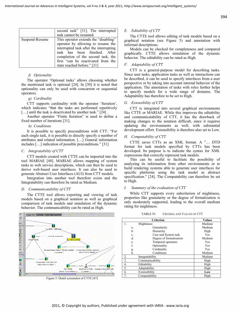
394



second task” [31]. The interrupted task cannot be resumed.

Suspend-Resume This operator extends the “disabling” operator by allowing to resume the interrupted task after the interrupting task has been finished. After completion of the second task, the first “can be reactivated from the state reached before.” [31]

f) Optionality

The operator ‘Optional tasks’ allows choosing whether the mentioned task is optional [24]. In [30] it is noted that optionality can only be used with concurrent or sequential operators.

g) Cardinality

CTT supports cardinality with the operator ‘Iteration’, which indicates “that the tasks are performed repetitively […] until the task is deactivated by another task.” [24] .

Another operator “Finite Iteration” is used to define a fixed number of iterations [31].

h) Conditions

It is possible to specify preconditions with CTT: “For each single task, it is possible to directly specify a number of attributes and related information. […] General information includes […] indication of possible preconditions.” [31]

C. Integratability of CTT

CTT models created with CTTE can be imported into the tool MARIAE [48]. MARIAE allows mapping of system tasks to web service descriptions, which can then be used to derive web-based user interfaces. It can also be used to generate Abstract User Interfaces (AUI) from CTT models.

Integration into another tool therefore exists and the Integratability can therefore be rated as Medium.

D. Communicatability of CTT

The CTTE tool allows exporting and viewing of task models based on a graphical notation as well as graphical comparison of task models and simulation of the dynamic behavior. The communicability can be rated as High.

Figure 5: Detail screenshot of CTTE [47]

E. Editability of CTT

The CTTE tool allows editing of task models based on a graphical notation (see Figure 5) and annotation with informal descriptions.

Models can be checked for completeness and compared graphically. CTTE allows simulation of the dynamic behavior. The editability can be rated as High.

F. Adaptability of CTT

CTT is a general-purpose model for describing tasks. Since user tasks, application tasks as well as interactions can be described, it can be used to specify interfaces from a user perspective or by taking into account internal behavior of the application. The annotation of tasks with roles further helps to specify models for a wide range of domains. The Adaptability has therefore to be set to High.

G. Extensibility of CTT

CTT is integrated into several graphical environments like CTTE or MARIAE. While this improves the editability and communicatability of CTT, it has the drawback of making changes to the notation difficult, since it requires updating the environments as well, with substantial development effort. Extensibility is therefore also set to Low.

H. Computability of CTT

CTTE saves CTTs as an XML format. A ”… DTD format for task models specified by CTTs has been developed. Its purpose is to indicate the syntax for XML expressions that correctly represent task models.

This can be useful to facilitate the possibility of analyzing its information from other environments or to build rendering systems able to generate user interfaces for specific platforms using the task model as abstract specification.” [24]. The Computability can therefore be set to High.

I. Summary of the evaluation of CTT

While CTT supports every subcriterion of mightiness, properties like granularity or the degree of formalization is only moderately supported, leading to the overall medium rating for mightiness.

TABLE IV. CRITERIA AND VALUES OF CTT

Criterion Values

1. Mightiness a. Granularity

b. Hierarchy

c. User and System task d. Degree of formalization

e. Temporal operators

f. Optionality g. Cardinality

h. Conditions

Medium Medium

High

Yes Medium

Yes

Yes Yes

Medium

2. Integratability Medium

3. Communicability High

4. Editability High


6. Extensibility Low

7. Computability High

395



Figure 6: Results of the evaluation of CTTE

V. EVALUATION OF AMBOSS

This section gives a short introduction on AMBOSS and

shows the application of the taxonomy.

A. Overview of AMBOSS

AMBOSS [14] is a graphical editing tool for the task model approach of the same name. The model and the environment are tightly integrated, resulting in good editability but drawbacks on the extensibility.

The tool was developed from 2005 to 2006 at the University of Paderborn. While it can be used for general-purpose task modeling, its focus lies in the support for modeling of properties for safety-critical systems. Additionally to task objects and roles, it supports barriers and risk factors.

B. Mightiness of AMBOSS

a) Granularity

With AMBOSS, tasks of different abstraction levels can be defined. The tool allows high flexibility for creating task models and consistency checkers for validating the correct structure afterwards. Its granularity can therefore be set to high.

b) Hierarchy

Tasks can be abstract or concrete and can be refined into more concrete subtasks. It therefore supports hierarchy.

c) User- and system task

AMBOSS has three basic types of actors: human, system and abstract [14]. Abstract tasks are “tasks performed in co-operation between”[14] human and system. Human tasks are performed just by the human, similar to CTT. System tasks are also similar to CTT. AMBOSS therefore supports user- and system tasks.


The AMBOSS environment contains checkers that test for cycles other constraints. The resulting task model is formal enough so it can be simulated. Its formalization is therefore high.

e) Temporal operators

“AMBOSS contains six different temporal relations” [14] (see TABLE V. ).

TABLE V. AMBOSS TEMPORAL RELATIONS

Operator Description Fixed Sequence Subtasks have to be performed in a

fixed sequence.

Sequence with arbitrary order

Subtasks can be performed in any order.

Parallel Subtask can be started and stopped independently.

Simultaneous “All subtasks have to start before any subtask may stop.” [14]

Alternative “Exactly one subtask is performed.” [14]

Atomic This task has no further subtasks.

f) Optionality

AMBOSS allows a temporal relationship called “ALT” (for alternative), which means that exactly one subtask is being performed. There exist different temporal relationships for defining, which tasks can or must run parallel or separate. It therefore supports optionality.

g) Cardinality

There are no language elements to define how many times a task has to be executed.

h) Conditions

AMBOSS supports “two different types of preconditions. Message preconditions” [14] and barriers. There seems to be no support for postconditions or invariants. Conditions are therefore rated as medium.

C. Integratability of AMBOSS

The AMBOSS environment provides an API for linking other analysis tools to it. It also uses a XML-based storage format. While a plug-in mechanism allows extension of AMBOSS with new functionality, the storage format is not standardized, resulting only in a medium integratability.

D. Communicatability of AMBOSS

The language features the refinement of tasks into subtasks as well as temporal operators. Task models are created and viewed using the AMBOSS environment, which is a graphical application based on the Eclipse Rich Client Platform [50]. Besides creation and viewing, the environment allows simulation and validation of models. Communicability can therefore be set to High.

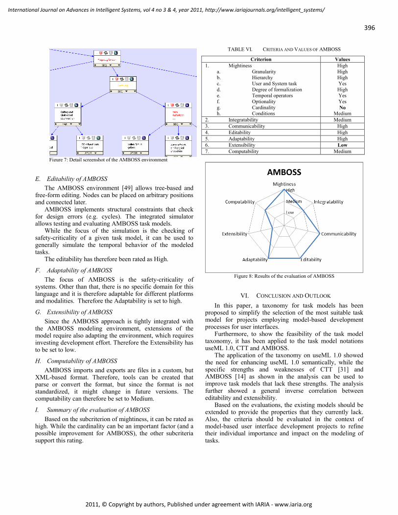
396



E. Editability of AMBOSS

The AMBOSS environment [49] allows tree-based and free-form editing. Nodes can be placed on arbitrary positions and connected later.

AMBOSS implements structural constraints that check for design errors (e.g. cycles). The integrated simulator allows testing and evaluating AMBOSS task models.

While the focus of the simulation is the checking of safety-criticality of a given task model, it can be used to generally simulate the temporal behavior of the modeled tasks.

The editability has therefore been rated as High.

F. Adaptability of AMBOSS

The focus of AMBOSS is the safety-criticality of systems. Other than that, there is no specific domain for this language and it is therefore adaptable for different platforms and modalities. Therefore the Adaptability is set to high.

G. Extensibility of AMBOSS

Since the AMBOSS approach is tightly integrated with the AMBOSS modeling environment, extensions of the model require also adapting the environment, which requires investing development effort. Therefore the Extensibility has to be set to low.

H. Computability of AMBOSS

AMBOSS imports and exports are files in a custom, but XML-based format. Therefore, tools can be created that parse or convert the format, but since the format is not standardized, it might change in future versions. The computability can therefore be set to Medium.

I. Summary of the evaluation of AMBOSS

Based on the subcriterion of mightiness, it can be rated as high. While the cardinality can be an important factor (and a possible improvement for AMBOSS), the other subcriteria support this rating.

TABLE VI. CRITERIA AND VALUES OF AMBOSS

Criterion Values

1. Mightiness

a. Granularity b. Hierarchy

c. User and System task

d. Degree of formalization e. Temporal operators

f. Optionality

g. Cardinality h. Conditions

High

High High

Yes

High Yes

Yes

No

Medium

2. Integratability Medium

3. Communicability High

4. Editability High


6. Extensibility Low

7. Computability Medium

Figure 8: Results of the evaluation of AMBOSS

VI. CONCLUSION AND OUTLOOK

In this paper, a taxonomy for task models has been proposed to simplify the selection of the most suitable task model for projects employing model-based development processes for user interfaces.

Furthermore, to show the feasibility of the task model taxonomy, it has been applied to the task model notations useML 1.0, CTT and AMBOSS.

The application of the taxonomy on useML 1.0 showed the need for enhancing useML 1.0 semantically, while the specific strengths and weaknesses of CTT [31] and AMBOSS [14] as shown in the analysis can be used to improve task models that lack these strengths. The analysis further showed a general inverse correlation between editability and extensibility.

Based on the evaluations, the existing models should be extended to provide the properties that they currently lack. Also, the criteria should be evaluated in the context of model-based user interface development projects to refine their individual importance and impact on the modeling of tasks.

Figure 7: Detail screenshot of the AMBOSS environment

397



REFERENCES

[1] S. Balbo, N. Ozkan, and C. Paris, “Choosing the right task modelling notation: A Taxonomy” in the Handbook of Task Analysis for Human-Computer Interaction, D. Diaper and N. Stanton, Eds., Lawrence Erlbaum Associates, pp. 445–466, 2003.

[2] M. Baron and P. Girard, “SUIDT: A task model based GUI-Builder”, Proc. of the 1st International Workshop on Task Models and Diagrams for User Interface Design, 2002.

[3] M. Biere, B. Bomsdorf, and G. Szwillus, „Specification and Simulation of Task Models with VTMB”, Proc. of the 17th Annual CHI Conference on Human Factors in Computing Systems, ACM Press, New York, pp. 1–2, 1999.

[4] B. Bomsdorf and G. Szwillus, “From task to dialogue: Task based user interface design”, SIGCHI Bulletin, vol. 30, nr. 4, pp. 40–42, 1998.

[5] K. Breiner, O. Maschino, D. Görlich, G. Meixner, and D. Zühlke, “Run-Time Adaptation of a Universal User Interface for Ambient Intelligent Production Environments”, Proc. of the 13th International Conference on Human-Computer Interaction (HCII) 2009, LNCS 5613, pp. 663–672, 2009.

[6] P. Brun and M. Beaudouin-Lafon, “A taxonomy and evaluation of formalism for the specification of interactive systems”, Proc. of the Conference on People and Computers, 1995.

[7] G. Calvary, J. Coutaz, J., and D. Thevenin, “A Unifying Reference Framework for the Development of Plastic User Interfaces”, Proc. of the Eng. Human-Computer-Interaction Conference, pp. 173-191, 2001.

[8] S. K. Card, T. P. Moran, and A. Newell, “The psychology of human-computer interaction”, Lawrence Erlbaum Associates, 1983.

[9] J. Carroll, “The Nurnberg Funnel: Designing Mini-malist Instruction for Practical Computer Skill”, MIT Press, 1990.

[10] L. Constantine and L. Lockwood, “Software for Use: A Practical Guide to the Models and Methods of Usage-Centered Design”. Addison-Wesley, 1999.

[11] A. Dittmar, “More precise descriptions of temporal relations within task models”, Proc. of the 7th International Workshop on Interactive Systems: Design, Specification and Verification, pp. 151–168, 2000.

[12] A. Dix, J. Finlay, G. D. Abowd, and R. Beale, ”Human-Computer Interaction, 3rd ed., Prentice Hall, 2003.

[13] C. Girault and R. Valk, “Petri Nets for Systems Engineering”, Springer, 2003.

[14] M. Giese, T. Mistrzyk, A. Pfau, G. Szwillus, and M. Detten, „AMBOSS: A Task Modeling Approach for Safety-Critical Systems”, Proc. of the 2nd Conference on Human-Centered Software Engineering and 7th international Workshop on Task Models and Diagrams, Pisa, Italy, pp. 98–109, 2008.

[15] ISO/IS 8807: LOTOS – A Formal Description Based on Temporal Ordering of Observational Behaviour

[16] X. Lacaze and P. Palanque, “Comprehensive Handling of Temporal Issues in Task Models: What is needed and How to Support it?”, Proc. of the 22th Annual CHI Conference on Human Factors in Computing Systems, 2004.

[17] Q. Limbourg, C. Pribeanu, and J. Vanderdonckt, “Towards Uniformed Task Models in a Model-Based Approach”, Proc. of the 8th International Workshop on Interactive Systems: Design, Specification and Verification, pp. 164–182, 2001.

[18] K. Luyten, “Dynamic User Interface Generation for Mobile and Embedded Systems with Model-Based User Interface Development”, PhD thesis, Transnationale Universiteit Limburg, 2004.

[19] G. Meixner, N. Thiels, and U. Klein, “SmartTransplantation – Allogeneic Stem Cell Transplantation as a Model for a Medical Expert System”, Proc. of Usability & HCI for Medicine and Health Care, Graz, Austria, pp. 306–317, 2007.

[20] G. Meixner, D. Görlich, K. Breiner, H. Hußmann, A. Pleuß, S. Sauer, and J. Van den Bergh, “4th International Workshop on Model Driven

Development of Advanced User Interfaces”, CEUR Workshop Proceedings, Vol-439, 2009.

[21] G. Meixner, “Model-based Useware Engineering”, W3C Workshop on Future Standards for Model-Based User Interfaces, Rome, Italy, 2010.

[22] G. Meixner, M. Seissler, “Selecting the Right Task Model for Model-based User Interface Development”, Proc. of the 4th International Conference on Advances in Computer-Human Interactions, pp. 5–11, 2011.

[23] T. Mistrzyk and G. Szwillus: Modellierung sicherheitskritischer Kommunikation in Aufgabenmodellen, i-com, vol. 7, nr. 1, pp. 39–42, 2008.

[24] G. Mori, F. Paternó , and C. Santoro: CTTE: Support for Developing and Analyzing Task Models for Interactive System Design, IEEE Transactions on Software Engineering, vol. 28, nr. 8, pp. 797–813, 2002.

[25] K. S. Mukasa and A. Reuther, “The Useware Markup Language (useML) - Development of User-Centered Interface Using XML”, Proc. Of the 9th IFAC Symposium on Analysis, Design and Evaluation of Human-Machine-Systems, Atlanta, USA, 2004.

[26] B. Myers, “A brief history of human-computer interaction technology”, interactions, vol. 5, nr. 2, pp. 44–54, 1998.

[27] H. Oberquelle, “Useware Design and Evolution: Bridging Social Thinking and Software Construction”, in Social Thinking – Software Practice, Y. Dittrich, C. Floyd, and R. Klischewski Eds., MIT-Press, Cambridge, London, pp. 391–408, 2002.

[28] N. Ozkan, C. Paris, and S. Balbo, “Understanding a Task Model: An Experiment”, Proc. of HCI on People and Computers, pp. 123–137, 1998.

[29] P. Palanque, R. Bastide, and V. Sengès, “Validating interactive system design through the verification of formal task and system models”, Proc. of the IFIP Working Conference on Engineering for Human-Computer Interaction, pp. 189–212, 1995.

[30] F. Paternò, “Model-based design and evaluation of interactive applications”, Springer, 1999.

[31] F. Paternò, “ConcurTaskTrees: An Engineered Notation for Task Models” in the Handbook of Task Analysis for Human-Computer Interaction, D. Diaper and N. Stanton, Eds., Lawrence Erlbaum Associates, pp. 483–501, 2003.

[32] F. Paternò, “Model-based Tools for Pervasive Usability”, Interacting with Computers, Elsevier, vol. 17, nr. 3, pp. 291–315, 2005.

[33] C. Paris, S. Balbo, and N. Ozkan, “Novel use of task models: Two case studies”, in Cognitive task analysis, J. M. Schraagen, S. F. Chipmann and V. L. Shalin, Eds., Lawrence Erlbaum Associates, pp. 261–274, 2000.

[34] C. Paris, S. Lu, and K. Vander Linden, ”Environments for the Construction and Use of Task Models” in the Handbook of Task Analysis for Human-Computer Interaction, D. Diaper and N. Stanton, Eds., Lawrence Erlbaum Associates, pp. 467–482, 2003.

[35] A. Puerta, “A Model-Based Interface Development Environment”, IEEE Software, vol. 14, nr. 4, pp. 40–47, 1997.

[36] A. Reuther, “useML – systematische Entwicklung von Maschinenbediensystemen mit XML“, Fortschritt-Berichte pak, nr. 8, Kaiserslautern, TU Kaiserslautern, PhD thesis, 2003.

[37] D. Scapin and C. Pierret-Golbreich, “Towards a method for task description: MAD”, Proc. of the Conference on Work with DisplayUnits, pp. 27–34, 1989.

[38] S. Sebillotte, “Hierarchical planning as a method for task analysis: The example of office task analysis”, Behavior and Information Technology, vol. 7, nr. 3, pp. 275–293, 1988.

[39] J. Tarby, “One Goal, Many Tasks, Many Devices: From Abstract User Task Specification to User Interfaces” in the Handbook of Task Analysis for Human-Computer Interaction, D. Diaper and N. Stanton, Eds., Lawrence Erlbaum Associates, pp. 531–550, 2003.

[40] J. Van den Bergh, G. Meixner, K. Breiner, A. Pleuß, S. Sauer, and H. Hußmann, “5th International Workshop on Model Driven

398



Development of Advanced User Interfaces”, CEUR Workshop Proceedings, Vol-617, 2010.

[41] J. Van den Bergh, G. Meixner, and S. Sauer, „MDDAUI 2010 workshop report“, Proc. of the 5th International Workshop on Model Driven Development of Advanced User Interfaces, 2010.

[42] G. Van der Veer, B. Lenting, and B. Bergevoet: GTA: Groupware task analysis - modeling complexity. In: Acta Psychologica, Heft 91, S. 297-322, 1996

[43] M. Van Welie, G. Van der Veer, and A. Eliens, “An ontology for task world models”, Proc. of the 5th International Workshop on Interactive Systems: Design, Specification and Verification, pp. 57–70, 1998.

[44] M. Weiser, “The computer for the 21st century”, Scientific American, vol. 265, nr. 3, pp. 94–104, 1991.

[45] A. Wolff, P. Forbrig, A. Dittmar, and D. Reichart, „Linking GUI Elements to Tasks – Supporting an Evolutionary Design Process”, Proc. of the 4th International Workshop on Task Models and Diagrams for User Interface Design, pp. 27–34, 2005.

[46] D. Zuehlke and N. Thiels, „Useware engineering: a methodology for the development of user-friendly interfaces”, Library Hi Tech, vol. 26, nr. 1, pp. 126–140, 2008.

[47] http://giove.isti.cnr.it/ctte.html, Retrieved at January 13, 2012.

[48] http://giove.isti.cnr.it/tools/MARIAE/home, Retrieved at January 13, 2012.

[49] http://mci.cs.uni-paderborn.de/pg/amboss/, Retrieved at January 13, 2012.

[50] http://www.eclipse.org/home/categories/rcp.php, Retrieved at January 13, 2012.

399



Personality and Mental Health Assessment

A sensor-based approach to estimate personality and mental health

Javier Eguez Guevara, Ryohei Onishi,

Hiroyuki Umemuro Department of Industrial Engineering and Management

Tokyo Institute of Technology

Tokyo, Japan

[email protected], [email protected],

[email protected]

Kazuo Yano, Koji Ara

Central Research Laboratory

Hitachi, Ltd.

Tokyo, Japan [email protected], [email protected]

Abstract - The purpose of this study was to estimate personality

and mental health through behavior data measured by

acceleration and voice intensity sensors. Traditionally

measuring methodologies require huge amount of time and

resources for its operation. Techniques that attempt to classify

and measure psychological states require acknowledgment of

its dynamic behavior, and the issues intrinsic to the use of self

report inventories. This research conducted experiments in

real-life settings, minimizing intrusiveness to participants. A

methodology for estimating personality and mental health in

the work place was proposed. Sensor-based behavior analysis

provided an unobtrusive and time-efficient mechanism to

estimate psychological states through measurement of a

selected set of behaviors. This methodology’s objective was to

demonstrate existing correlations between estimated behavior

and assessed personality and mental health. The results

showed significant correlations between behavior and all

personality and mental health states studied except for

openness. This research provides insights into the analysis of

personality and mental health states in the working settings.

More broadly, the methodology proposed in this research

provides implications for the development of recognition

systems that will facilitate the attainment of personal and

collective goals, which proves highly useful in today’s increasingly technicized societies.

Keywords - human behavior; sensory technology; mental

health; personality

I. INTRODUCTION

The wide study of personality theory and mental health

has opened new research directions through the use of

sensorial technology to better understand personnel psychology [1]. Companies are increasingly aiming to

develop their human workforce performance by studying

their employees‟ individual characteristics. Robbins [2]

identified four individual-level variables, i.e. biographical

characteristics, ability, personality, and learning, which have

effects on employee performance and satisfaction.

Since the use of questionnaire-based objective tests for

both personality and mental health has been widely

established [3], the time required for employers and

employees to carry out such questionnaires has increasingly

become wasteful and troublesome. On the other hand, recent

technology enables to visualize office workers‟ interactions

[4], identify human behavior within organizational

situations and obtain associated tacit knowledge [5][6]

without privacy intrusion or major burden.

The purpose of this study was to propose a sensor-based methodology to estimate behavior, and to further

demonstrate existing correlations between employee‟s

estimated behavior and mental health and personality traits.

Building on the aforementioned findings, this study

provides conclusions involving personality traits and mental

health in the working setting with a minimum required

burden from both employers and employees.

This paper is organized as follows. Section II contains an

overview of related personality and mental health studies in

the workplace. In Section III, it is proposed a methodology

to estimate behavior based on sensory data, which was used in Section IV to analyze the relationship with personality

and mental health. Section V includes some discussion

points, and finally, Section VI presents conclusions, a

summary of the paper, and future work.

II. RESEARCH ON PERSONALITY AND MENTAL HEALTH

Personality has been defined as the characteristic manner

in which one thinks, feels, behaves, and relates to others [7].

Robbins [2] claimed that all our behavior is at some extent

explained by our personalities and experiences. Traits in

personality psychology have been used to describe

consistent inter-correlated behavior patterns [8]. The study

of personality traits has increased the understanding of the differences between people‟s behavior in order to explain

how certain personality traits better adapt for certain job

types [2][9], how personality relates to the effective

performance of teams [9][10][11], and how personality is a

component of motivation [12].

With similar attention, mental health in the workplace

has also been studied. A study has concluded that adverse

psychosocial work conditions are predictors of depression

worsening [13]. This result was independent from

personality traits analyses, and demonstrated the importance

of the study of mental health alone. Also, the impact of job stress and working conditions on mental health problems

400



[14], and the relation between job satisfaction and the Five

Factor model [15][16] has been studied.

A. Personality traits in this study

Although there is a general consensus over the Big Five

being a general framework for assessing personality traits,

this study has included in addition to those in the Big Five,

the Locus of Causality, the General Causality Orientation,

the Self Monitoring, and the Type A traits in order to

present a more comprehensive assessment of personality.

The Five Factor Model (FFM) is a taxonomy, or

descriptive model of personality traits organized at the

broadest level of abstraction in five factors or dimensions named: extraversion or surgency, agreeableness,

conscientiousness, emotional stability versus neuroticism,

and intellect or openness [8]. These traits became eventually

known as the Big Five [17]. Extraversion describes traits

relating energy, dominance, sociability, and positive

emotions. Agreeableness includes traits such as altruism,

tender-mindness, trust and modesty, defining a prosocial

orientation towards others. Conscientiousness summarizes

traits which facilitate goal-directed behavior. Neuroticism

describes anxiety, sadness or irritability, contrasting

emotional stability. Finally, openness describes the depth of an individual‟s mental and experiential life [18].

Locus of Causality traits are related to the motivation

factor of an individual and it examines the source of the

motivation when engaging on an activity. Locus of

Causality‟s intrinsic motivation refers to doing something

because it is inherently interesting, fun, or enjoyable. On the

other hand, extrinsic motivation refers to doing something

because it leads to a separable outcome, or because it

responds to external demands. Each motivation trait has two

secondary scales. Secondary scales for intrinsic motivation

are enjoyment and challenge. Challenge orientation is

related to problem-solving, while enjoyment orientation is related to writing and art involvement. Secondary scales for

extrinsic motivation are outward and compensation scales.

Outward motivation entails personal endorsement and a

feeling of choice. Compensation, on the other hand, merely

involves compliance with an external control [19][20].

General Causality Orientation is referred as the

individual differences that can be characterized in terms of

people‟s understanding of the nature of causation of

behavior [21]. In other words, these traits characterize the

degree to which human behaviors are volitional or self-

determined. There are three causality orientations, namely, autonomy, control, and impersonal orientation. Autonomy

orientation trait involves a high degree of experienced

choice related to the initiation and regulation of one‟s own

behavior. Control orientation trait involves people‟s

behavior following controls either in the environment or

inside themselves. Impersonal orientation trait involves

people experiencing their behavior as being beyond their

intentional control [21].

Self-Monitoring people are described as showing

considerable adaptability and behavior flexibility to external

factors, being capable of behave differently in different

situations [2].

Type A personality is the trait describing people which is

aggressively involved to achieve more in less time. Highly rated Type A people are highly competitive, cannot cope

with leisure time, and are continuously measuring their

success [2].

B. Mental health in this study

The mental health states considered for this study were

depression and happiness. Although these states could be related to a general happiness scale, in this study the term

mental health was used to describe each of them. The

viewpoint from which these traits were analyzed was to

relate depression, and stress, against job satisfaction

characterized by happiness in the workplace.

C. Personality and mental health measurement

Objective tests have been firmly established as the

preferred personality measuring method [3], and it has also

been used to assess mental health. However, it has been

pointed out that several issues relating to this method may

jeopardize its efficacy. Measuring methods have failed to

accurately reflect the dynamics of personality and mental

health [22][23]. As individuals‟ behavior is not constant

from situation to situation, the associated personality and

mental health will also be continuously shaped by

experiences. Another concern is the increasing number of

inventories and scales offered, for which a huge amount of time and effort would be required for its completion [8].

On the other hand, recent technology enables to make

inferences about office workers‟ interactions [4], and obtain

associated tacit knowledge [5][6], without privacy intrusion

or major burden. The use of these approaches may be a

mechanism to cope with issues regarding the use of

objective tests [8][22][24] in the assessment of mental

health and personality traits.

III. STUDY 1: ESTIMATION OF BEHAVIOR BASED ON

SENSORY DATA

This first study proposed a methodology to estimate

human behavior at the workplace based on objective data measured by sensors. An experiment was done in order to

investigate the possibility of identifying certain human

behavioral expressions based on sensory data.

A. Participants

Two male participants volunteered for this experiment. Participants were aged 25 and 44, and were all capable of

moving freely.

B. Apparatus

Business Microscope (BM) [6] developed by Hitachi

Corporation was used in this experiment. BM, shown in

Figure 1 being worn as a name tag, records data from the

401



user‟s acceleration, face-to-face (IR), temperature, and voice

intensity sensors.

Figure 1. Hitachi‟s Business Microscope.

C. Procedure

Each participant wore a BM device and acted out

different behaviors switching them from one to another for 2

hours as if they were engaging in daily office working

activities. The characterized behavior categories were desk

working, talking, walking, and not-working related

behaviors like sleeping, eating-drinking, or simply being

unoccupied. These last were grouped into a single category

hereafter referred as idle.

D. Measurements

For the purpose of this study, this experiment only used

acceleration and voice intensity sensory raw data with a

sampling frequency of 50 Hz. Due to privacy concerns and

to a limitation of energy consumption, each datum was

observed for 2s long and was acquired once every 10s. The

data captured by the device was wirelessly transferred to a

server where it was stored for later use.

While acting out behavior categories, participants

marked the time, the location, the posture, and the behavior

being acted.

E. Results

Sensor data chosen from each behavior category was

plotted for analysis to reveal distinctive characteristics

representing each acted behavior. This information served to

build a method with which behavior was estimated. The

estimated behavior was compared with the participants‟

actual behavior by finding out hit and false alarm rates. A hit was defined by corresponding predicted and actual

behaviors. False alarm on the contrary was defined by a

mismatch between them.

A graphic method, the Receiver Operating Characteristic

(ROC), was used to evaluate and compare the performances

of signal-noise discrimination [25]. ROC was used to

portray the optimal criteria to detect behaviors and to select

the most effective prediction thresholds.

1) Behavior detection criteria For the walking category, the amplitude and the

frequency of the oscillations of acceleration data were calculated. The amplitude of the curve was calculated by

subtracting the curve‟s minimum data value from the

maximum data value. As for the number of oscillations of

the curve, it was used the zero crossing method. The zero

cross line was determined as the data‟s average line. The

number of times the curve crossed the zero-crossing line

were added up to obtain the curve‟s frequency.

Sound intensity curve was represented by temporal

changes of sound volume. The data‟s mean and the standard

deviation were calculated and used to obtain thresholds for

data characterized by sound representing a talking behavior.

For desk working behavior, back and forth acceleration data was investigated. It was found that the mean of

acceleration data at time t, and the mean of acceleration data

at time t-10s, tended to be comparable. As differences in

mean values of these succeeding two time points were

limited in range, it was assumed that such behavior

corresponded to small posture changes as those displayed by

desk working behavior. Upper and lower limits were

calculated, and data found within this range was regarded as

describing desk working behavior category.

As for the idle behavior category, the acceleration data‟s

frequency of vibration was analyzed. The most suitable data for analysis was found along the vertical direction; therefore

402



the zero crossing number was used to calculate this

behavior‟s data frequency along that axis.

2) Sequential detection method The hit rates and false alarm rates for each behavior

category are shown in Table I. Also, ROC curves for each

behavior category are shown in Figure 2. The variance of dots in each graph represents the performance of criteria

using various threshold combinations. The results showed

that the best detection performance (represented by a red

dot) was found in the following order: walking behavior

category, followed by talking, desk working, and idle

behavior. Consequently, it was considered a sequential

detection order through which the sensitivity of each

detection method was set as the detection order priority [25].

Thus, walking behavior was the first category to be detected

from the entire sensor data set. From the remaining data,

talking behavior was detected, then desk working, and

finally idle behavior category.

TABLE I. HIT AND FALSE ALARM RATES FOR BEHAVIOR DETECTION

Behavior category hit rate false alarm

rate

Walking 0.78 0.12

Speaking 0.82 0.19

Desk working 0.69 0.48

Idle 0.59 0.28

Figure 2. ROC curve: (a) walking detection, (b) talking detection, (c) desk working detection, (d) idle detection.

(a)

(b)

(c)

(d)

403



IV. STUDY 2: STUDY OF PERSONALITY AND MENTAL

HEALTH BASED ON BEHAVIOR DATA

The purpose of this study was to analyze the

relationships among behavior estimated through the method

proposed in Section III, and personality and mental health.

An experiment was conducted, and a correlation analysis was done in order to validate that sensory data can be used

to assess personality and mental health.

A. Participants

Ninety two Japanese participants, 77 males and 15

females, ranging between 21 and 61 years old (M = 35.93,

SD = 8.50), who worked as software developers at a certain company volunteered for the experiment. They were all

capable of moving freely and perform routine office

activities. The participants of this experiment were not

familiar with what kind of measurements were being

executed, and further agreed to provide individual

psychological states information.

B. Apparatus

The apparatus for this study were the same as those used

in study one. Refer to Section III.

C. Procedure

Participants wore individual BM devices every working day for 71 days, time in which they engaged in normal daily

working activities. Participants‟ behavior was detected

according to the procedure explained in Section III. Also

participants conducted 8 sets of questionnaires, 5 relating

personality, and 3 more relating mental health.

D. Measurements

To assess the big five personality, the Big Five Inventory

[18], which consisted of 44 items, was used. The Work

Preference Inventory (WPI) which consists of 30 items was

used to assess Locus of Causality [20]. The 12-item General

Causality Orientation Scale Questionnaire (GCOS) was

used to assess General Causality Orientation [21]. It was

also used the Self-Monitoring trait questionnaire developed

by Lennox and Wolfe [26], and the Type A questionnaire

developed by Bortner [27]. As for mental health, two scales for depression and one

for happiness were used. The Center for Epidemiology

Studies Depression Scale (CES-D) was developed by

Radloff [28], and consisted of 20 items. Also the Beck

Depression Inventory Second Edition (BDI-II) was used.

The BDI-II is a 21 items self-administered questionnaire

assessing the severity of depression in adults and

adolescents [29]. The last mental health state studied was

satisfaction. The Oxford Happiness Questionnaire (OHQ)

was used to assess this state [30].

E. Results

This study considered unitary behavior samples and

behavior events as measurement units. A behavior sample

was defined as each datum in a set of data corresponding to

an estimated behavior category (one sample per 10s). A

behavior event was defined as the sequential group of two

or more samples under the same behavior category. A chronological summary showing the time series of estimated

behavior samples and events was prepared for each

participant. This summary indicated what type of behavior

category a participant engaged in and for how long.

1) Detected behavior Basic statistics of the behavior data collected are shown

in Table II. After analyzing the number of behavior samples

of the 92 participants, three outlier participants were

excluded as they provided significantly less number of

samples (< M – 2 x SD) due to their absence in the

experimentation settings.

TABLE II. BEHAVIOR SAMPLES AND EVENTS DETECTED PER PARTICIPANT

Average Standard Deviation Median Minimum Maximum Sum

Total samples 147031.63 33345.42 152837 50633 203825 13085815

Behavior Samples (number of samples)

Walking 41229.87 18198.27 37405 6538 94410 3669458

Talking 22147.24 9796.56 20431 6469 51626 1971104

Desk working 44192.09 13258.58 43589 13845 75012 3933096

Idle 31643.84 9933.78 30054 9989 63565 2816302

Behavior events (number of events)

Walking 9129.35 2854.07 9186 1527 15844 812512

Talking 7996.57 2749.70 7576 2662 15795 711695

Desk working 11446.83 2861.78 11457 3457 17209 1018768

Idle 13471.34 3707.78 13750 3769 21119 1198949

404



The results hereafter report data from the remaining 89

participants, 74 males and 15 females (M = 36.07, SD =

8.56). From the total number of detected samples, 28% were

detected as walking, 15% as talking, 30% as desk working,

and 21% were detected as idle behavior. There was a 5% of

samples which could not be detected as any of the proposed behaviors.

2) Personality and mental health results The results presented in Table III show the participants

scores obtained through personality and mental health

questionnaires.

3) Behavior characteristic variables Characteristic variables were obtained for the behavior

samples and events of individual participants. The behavior

characteristic variables (BCVs) were represented by letters

triplets and are summarized in Table IV. The first letter of

each triplet represented the behavior categories. This is W,

T, D, and I represented walking, talking, desk working, and idle behaviors, respectively. The second letters in a triplet

were A, T, E, and D, and represented time instances. A as a

triplet‟s second letter represented the entire time span. T as a

triplet‟s second letter represented the time ratio per day.

This ratio was obtained by dividing a given behavior

total time over the total time in a day. The letter E as a

triplet‟s second letter represented the number of events per day. The letter D as the second letter in a triplet represented

the behavior events duration. If the second letter of the

triplet was A, the third letters of a triplet were T or E. In this

case T represented the time ratio, and E represented an event.

However if the second letter of the triplet was T, E, or D,

the third letter of a triplet could be A, D, or M, which stood

for average, standard deviation, and median.

Personalities like intrinsic or extrinsic motivation are

estimated to be related to the variation of behavior. In order

to assess this variation, the percentage of behavior-engaged

time over all the experiment‟s time span and the number of

events per day was calculated. It was also calculated the average, standard deviation and median of behavior-

engaged time (time ratio T and number of events E) per day.

TABLE III. PERSONALITY AND MENTAL HEALTH SCORES

Average Standard Deviation Median Minimum Maximum

Big Five

Extraversion 22.88 4.98 23.00 10.00 37.00

Agreeableness 28.81 3.70 28.00 20.00 37.00

Neuroticism 26.82 4.62 27.00 10.00 38.00

Conscientiousness 26.94 4.27 27.00 15.00 40.00

Openness 30.78 4.42 31.00 21.00 42.00

Locus of Causality

Intrinsic M 39.02 6.05 39.00 24.00 52.00

Enjoyment 20.93 3.59 21.00 13.00 29.00

Challenge 18.94 2.94 19.00 10.00 27.00

Extrinsic M 35.46 5.31 35.00 24.00 51.00

Outward 18.52 3.89 18.00 9.00 30.00

Compensation 11.94 2.47 12.00 6.00 19.00

General Causality Orientation

Autonomy 56.77 10.65 56.00 36.00 83.00

Control 37.12 8.47 37.00 17.00 61.00

Impersonal 43.87 11.54 44.00 23.00 84.00

Additional traits

Type A 9.35 3.10 9.00 3.00 18.00

Self-Monitoring 7.39 3.37 7.00 0.00 15.00

Mental health

CES-D 9.33 8.14 7.00 0.00 43.00

BDI-II 21.11 9.90 20.00 3.00 51.00

OHQ 100.29 23.16 102.00 24.00 147.00

405



TABLE IV. BEHAVIOR CHARACTERISTIC VARIABLES USED IN STUDY 2

Variable Definition

WAT, TAT, DAT, IAT percent of walking (W), talking (T), desk working (D), and idle (I) time (T) over all

investigation time (A)

WAE, TAE, DAE, IAE percent of walking (W), talking (T), desk working (D), and idle (I) events (E) over all

investigation time (A)

WTA-WTD-WTM, TTA-TTD-TTM, DTA-DTD-

DTM, ITA-ITD-ITM

average (A), standard deviation (D) and median (M) of the percent of daily walking (W),

talking (T), desk working (D) and idle (I) time (T)

WEA-WED-WEM, TEA-TED-TEM, DEA-DED-

DEM, IEA-IED-IEM

average (A), standard deviation (D) and median (M) of the percent of daily walking (W),

talking (T), desk working (D) and idle (I) events (E)

WDA-WDD-WDM, TDA-TDD-TDM, DDA-DDD-

DDM, IDA-IDD-IDM

average (A), standard deviation (D) and median (M) of walking (W), talking (T), desk

working (D) and idle (I) events duration (D)

The concept of absorption is important for some

personality traits and it is considered to be strongly related with uninterrupted behavior engagement. Therefore the

average, standard deviation and median of the time

continuance of each behavior were also calculated (triplets

with “D” as the second letter).

4) Correlation among personality traits, mental health,

and BCVs

a) Big Five personality scores

Big Five personality scores and BCVs combinations

whose correlations were significant are shown in Table V.

Extraversion showed positive correlation with walking

behavior variables. It was also found negatively correlated with talking events (TEA, TEM) and desk working related

variables (DAE, DAT, DEA, DTA, DTM). These results

suggested that people who often walk, and often spent their

time away from their desks were likely to be extraverted.

b) Locus of Causality and subscales personality scores

Intrinsic and extrinsic Locus of Causality personality

scores and BCVs combinations whose correlations were significant are shown in Table VI and Table VII,

respectively.

TABLE V. PEARSON‟S CORRELATION BETWEEN BIG FIVE PERSONALITY SCORES AND BCVS

Extraversion Agreeableness Conscientiousness Neuroticism Openness

WAT 0.212 * 0.082 -0.142 0.006 0.076

WED 0.235 * 0.089 -0.109 0.118 0.147

WTA 0.216 * 0.091 -0.141 0.009 0.078

WTD 0.255 * 0.221 * 0.015 -0.010 0.181

WTM 0.239 * 0.096 -0.130 0.010 0.081

WDA 0.238 * 0.120 -0.081 -0.102 0.059

WDM 0.226 * 0.128 -0.089 -0.039 0.104

TEA -0.216 * -0.164 0.032 0.129 0.018

TEM -0.213 * -0.140 0.043 0.110 0.027

TDD -0.131 0.064 0.209 * -0.041 -0.071

DAE -0.298 ** -0.029 -0.111 0.184 -0.002

DAT -0.285 ** 0.000 -0.039 0.058 -0.142

DEA -0.210 * 0.048 -0.132 0.216 * 0.077

DEM -0.204 0.099 -0.118 0.233 * 0.078

DTA -0.284 ** -0.008 -0.036 0.059 -0.158

DTM -0.273 ** -0.007 -0.039 0.056 -0.154

n=89; **p<.01; *p<.05

Locus of Causality variables were both positively and

negatively correlated with BCVs. Talking related variables

were negatively correlated with intrinsic Locus of Causality,

and both of its subscales, enjoyment and challenge. It can be

argued that intrinsically motivated people have a strong

preference for working individually without talking or interacting with people around. However, as it is shown in

Table VI, idle behavior variables were found positively

correlated with challenge subscale alone. It might be argued

that the nature of intrinsic Locus of Causality and challenge

orientation, motivate these people to find time to think and

reflect about their own initiatives.

Intrinsic Locus of Causality and the challenge subscale

correlated positively with idle BCVs IAT, ITA, ITD, ITM,

IDA. It may be argued that the nature of intrinsic Locus of Causality and challenge-motivated people drives them to

find time to think and reflect about their own initiatives.

406



TABLE VI. PEARSON‟S CORRELATION BETWEEN INTRINSIC LOCUS OF

CAUSALITY AND SUBSCALES PERSONALITY SCORES AND BCVS

Intrinsic Enjoyment Challenge

WTD 0.203 0.126 0.209 *

TEA -0.254 * -0.216 * -0.230 *

TEM -0.220 * -0.174 -0.214 *

TTA -0.211 * -0.210 * -0.173

TTM -0.212 * -0.222 * -0.166

TDM -0.226 * -0.231 * -0.174

DEA -0.217 * -0.048 -0.283 **

DEM -0.168 0.005 -0.246 *

IAT 0.280 ** 0.157 0.298 **

ITA 0.285 ** 0.169 0.298 **

ITD 0.209 * 0.136 0.225 *

ITM 0.264 * 0.151 0.272 *

IDA 0.239 * 0.119 0.277 **

n=89; **p<.01; *p<.05

TABLE VII. PEARSON‟S CORRELATION BETWEEN EXTRINSIC LOCUS OF

CAUSALITY AND SUBSCALES PERSONALITY SCORES AND BCVS

Extrinsic Outward Compensation

WED 0.275 ** 0.217 * 0.250 *

DAT -0.221 * -0.148 -0.241 *

DTA -0.213 * -0.136 -0.243 *

DTM -0.237 * -0.144 -0.282 **

DDA -0.223 * -0.174 -0.205

DDM -0.249 * -0.186 -0.242 *

IEM 0.179 0.232 * 0.019

ITD 0.209 * 0.183 0.161

n=89; **p<.01; *p<.05

The variation of the percentage of daily walking events

(WED) showed a positive correlation with extrinsic

personalities, and both of its subscales (extrinsic, r=.275,

p<.01; outward, r=.217, p<.05; compensation, r=.250, p<.01). Also, walking variable WTD which referred to the

variation of walking time in a day, correlated with challenge

subscale. Building from these findings, it can be argued that

intrinsic motivated participants walked longer by their

challenging determination; however, although extrinsic

participants walked more times, they tend to do it for shorter

periods.

Other results showed that extrinsic motivated people did

not tend to stay in their desks or focus on their work for

long periods as desk working related variables (DAT, DTA,

DTM, DDM) were all negatively correlated with extrinsic

Locus of Causality and compensation subscale.

c) General Causality Orientation personality scores

General Causality Orientation personality scores and

BCVs combinations whose correlations were significant are

shown in Table VIII. Talking related variables correlated

negatively with the autonomy trait. On the other hand,

impersonal trait correlated positively with desk working and idle behavior related variables. It can be argued that people

who do not actively engage or face external circumstances

tend to spend more time at their desks.

TABLE VIII. PEARSON‟S CORRELATION BETWEEN GENERAL CAUSALITY

ORIENTATION PERSONALITY SCORES AND BCVS

Autonomy Control Impersonal

WED 0.163 0.233 * 0.085

WTD 0.231 * 0.133 -0.041

WDA 0.175 -0.120 -0.240 *

WDD 0.148 -0.244 * -0.182

TAE -0.238 * 0.000 0.101

TAT -0.273 ** -0.016 0.065

TTA -0.278 ** -0.029 0.060

TTD -0.305 ** -0.034 0.054

TTM -0.254 * -0.032 0.051

TDA -0.216 * -0.029 0.009

TDM -0.292 ** -0.096 0.034

DAE -0.016 0.059 0.304 **

DEA 0.041 0.054 0.331 **

DEM 0.083 0.087 0.323 **

IEA 0.077 0.117 0.296 **

IED 0.148 0.222 * 0.165

IEM 0.100 0.147 0.301 **

n=89; **p<.01; *p<.05

These results implied that people with high impersonal score, whose behavior is marked by decisions beyond their

control, tend to follow directions as they are told. In other

words, these people might not leave their desks or stop

working. These findings are comparable to idle behavior

variables being positively correlated with impersonal trait. It

can be argued that as these people tend to stay at their desks,

they might be able to loosen up, even in front of their desks.

d) Self-Monitoring and Type A personality scores

Self-Monitoring and Type A personality scores and

BCVs combinations whose correlation were significant are

shown in Table IX. Self-Monitoring personality was

positively correlated with walking related variables (WAT,

WTA, WTM, WDA, WDM). This suggested that people

with high sociability skills, or those rating high in Self-

Monitoring, engage for longer periods in walking behavior.

High Self-Monitoring rated people are able to show striking

contradictions between their public persona and their private

self [2]. Thus, by the fact that Self-Monitoring correlated negatively with talking related variables (TEA, TEM) it can

be argued that even though these people regulate their

behavior by walking or interacting with others, they might

be reluctant to show their opinions by an apprehension of

social disapproval.

Type A trait correlated positively with the number of

walking events per day (WEM). This suggested that people

who tended to walk more often are likely to be competitive

or involved in achieving more in less time. It might be

argued that these people are often walking around, looking

for self-improving opportunities.

407



TABLE IX. PEARSON‟S CORRELATION BETWEEN SELF-MONITORING

AND TYPE A PERSONALITY SCORES AND BCVS

Self-Monitoring Type A

WAT 0.271 * 0.055

WEM 0.080 0.236 *

WTA 0.268 * 0.060

WTM 0.281 ** 0.069

WDA 0.266 * -0.031

WDM 0.225 * -0.003

TEA -0.232 * 0.013

TEM -0.221 * 0.009

n=89; **p<.01; *p<.05

e) Mental health scores

Mental health scores and BCVs combinations whose

correlations were significant are shown in Table X. Both

depression scales utilized in this study presented similar

results which highlighted positive correlation with talking,

desk working, and idle behavior related variables (TEA,

TEM, DAE, DEA, DEM, IEA). These results suggested that

people who more often engaged in talking, desk working,

and idle behaviors present higher depression or stress scores.

Given that BDI-II depression scale positively correlated with walking idle events related variables (WEA, IEM) it

can be argued that both, unoccupied behavior people or

persistently walking people, might display high work

depression or stress.

TABLE X. PEARSON‟S CORRELATION BETWEEN MENTAL HEALTH SCORES

AND BCVS

CES-D BDI-II OHQ

WEA 0.103 0.221 * -0.083

WDA -0.174 -0.139 0.237 *

TAE 0.204 0.144 -0.215 *

TAT 0.191 0.166 -0.235 *

TEA 0.282 ** 0.267 * -0.287 **

TEM 0.250 * 0.271 * -0.267 *

TTA 0.188 0.158 -0.228 *

TTM 0.176 0.151 -0.211 *

TDM 0.072 0.152 -0.270 *

DAE 0.239 * 0.254 * -0.255 *

DEA 0.283 ** 0.371 ** -0.283 **

DEM 0.211 * 0.355 ** -0.255 *

IEA 0.223 * 0.264 * -0.156

IEM 0.173 0.246 * -0.119

n=89; **p<.01; *p<.05

The OHQ results showed that participants who highly engaged in walking behavior rated high in satisfaction

(WDA). On the contrary, results also showed that high

talking, and desk working behavior people often showed

frustration or discontent (TAE, TAT, TEA, TEM, TTA,

TTM, TDM, DAE, DEA, DEM). It can be argued that

people who talked for longer periods, would be able to cope

with dissatisfaction.

V. DISCUSSION

Personality information is important for managers as they can make more educated decisions on how to conform

teams, based on their members‟ characteristics. This

research provided a methodology that provides up-to-date

personality information. This is most important since the

evaluation of such teams can be tracked along time. Until

now, this was only possible through a pervasive policy of

personality assessment that would demand great effort and

time for both employers and employees.

Mental health information is also of great importance for

managers as provides a clear sight of the mental condition

of their workforce. The methodology proposed in this study

presented a real-time assessment of mental health which is most important for immediate actions can be taken in order

to prevent the worsening of the condition, and the potential

dissemination to nearby environments.

This study used the personality and mental health

questionnaires as the affect ascertaining method. As it has

been discussed, the use of questionnaires describes a

number of concerns. Nevertheless, what has been argued as

a benefit of the use of questionnaires (greater choice) is a

major weakness; the use of questionnaires allows for

questionnaire items' omission or misrepresentation, thus

affecting the overall effectiveness and goals of the assessment. This limitation affects the informant him/herself

who is the ultimate beneficiary of the research efforts. In

addition, the subjective nature of these questionnaires

impedes the elucidation of an individual‟s self perception of

personality, as opposed to the external perception of an

individual‟s personality. The improvement of the

methodology for assessing personality and mental health

described in this research is essential, as it meliorates theses

psychological states estimation and lessens the impact of the

discussed issues regarding the use of questionnaires.

The application of personality and mental health inside

an outside the working settings present various application opportunities. It has been claimed that one of the most

important issues in organizations, is to understand how the

productivity of its workforce could be improved. One reason

hindering this understanding is that interactions of

nowadays organization can be barely visualized, and

therefore it is complex to find out problems between

employees‟ relations. In this study it was presented a

methodology through which the behavior of employees

could be visualized, and further used to have a better

understanding of their psychological states.

VI. CONCLUSION AND FUTURE WORK

The present study proposed a methodology to estimate

personality from sensory data information. However studies

pertaining personality with emphasis to the workplace are

numerous, the established measuring method used by those

studies were questionnaire tests. This study built up a clear

methodology through which personality is estimated

408



unobtrusively and without the need of questionnaires,

through the use of acceleration and voice sensory

information.

In Study 1 it was effectively detected walking, talking,

desk working, and idle behaviors. In Study 2, the correlation

analysis showed significant correlations between behavior and all personality and mental health traits studied except

for openness. While some personality variables showed

significant correlation with a greater extent of behavior

variables (extraversion, intrinsic motivation, challenge, and

happiness), other personality variables showed significant

correlation with fewer (agreeableness, conscientiousness,

neuroticism, control orientation, outward, Type A). On the

other hand, the behavior category which showed significant

correlation with the greater number of personality variables

was desk working behavior category revealing 31

significant correlations; while the behavior category which

showed significant correlation with the least number of personality variables was idle category showing only 18

significant correlations.

The results in this study suggest that it is possible to

effortlessly assess personality and mental health, respecting

the privacy of employees, and without the need of

questionnaires. What has been argued as a benefit of the use

of questionnaires (greater choice) is a major weakness; the

use of questionnaires allows for questionnaire items'

omission or misrepresentation, thus affecting the overall

effectiveness and goals of the assessment. This limitation

affects the informant himself who is the ultimate beneficiary of the research efforts. Furthermore, personality is

continuously shaped by experiences, and thus questionnaires

are limited to cope with personality‟s changing nature. As

the methodology presented in this study is set by

continuously loading data, the personality and mental health

information obtained will always provide up-to-date

information. In addition, saving employers‟ and employees‟

time, is yet another benefit proposed by this study, which

opens a new behavior estimation research direction, and

thus its continuation is essential. Future studies should

deepen this study‟s findings: it should consider additional

working settings; the improvement of the behavior detection method including participants from both genders, and a

larger set of behavior categories.

ACKNOWLEDGMENT

This research was based on the data provided by the

World Signal Center, Hitachi, Ltd.

REFERENCES

[1] J. P. Eguez Guevara, H. Umemuro, R. Onishi, K. Yano, and K. Ara, “Personality and mental health assessment: A sensor-based behavior analysis,” ACHI 2011, Gosier, 2011, pp. 22-

27.

[2] S. Robbins, “Foundation of Individual Behavior,” in Organizational Behavior, 8th ed. Upper Saddle River, New Jersey: Prentice-Hall, 1998, pp. 40-87.

[3] D. G. Winter and N. B. Barenbaum, “History of modern personality theory and research,” in Handbook of Personality,

L. A. Pervin and O. P. John, Eds. New York: The Guilford Press, 1999, pp. 3-27.

[4] J. Nishimura, N. Sato, and T. Kuroda, “Speaker siglet detection for Business Microscope,” in Proc. 7th International Conference on Machine Learning and Applications, San Diego, 2008, pp. 376-381.

[5] K. Ara, N. Kanehira, D. Olguin Olguin, B. N. Waber, T. Kim, A. Mohan, P. Gloor, R. Laubacher, D. Oster, A. Pentland, and

K. Yano, “Sensible organizations: Changing our business and work styles through sensor data,” J. Information Processing, vol. 16, pp. 1-12, 2008.

[6] K. Yano and H. Kuriyama, “Human x sensor: How sensor information will change human, organization, and society,” Hitachi Hyouron, vol. 89, No. 07, pp. 62-67, 2007.

[7] T. A. Widiger, R. Verheul, and W. van den Brink, “Personality and psychopathology,” in Handbook of

Personality, L. A. Pervin and O. P. John, Eds. New York: The Guilford Press, 1999, pp. 347-366.

[8] O. P. John and S. Srivastava, “The Big Five trait taxonomy: History, measurement, and theoretical perspectives,” Handbook of Personality, L. A. Pervin and O. P. John, Eds. New York: The Guilford Press, 1999, pp. 102-138

[9] M. K. Mount and M. R. Barrick, “Five reasons why the „Big Five‟ article has been frequently cited,” Personnel Psychology,

vol. 51, pp. 849-857, 1998. [10] R. R. Reilly, G. S. Lynn, and Z. Aronson, “The role of

personality in new product development team performance,” J. Engineering and Technology Management JET-M, vol. 19, pp. 39-58. 2002.

[11] M. R. Barrick, G. L. Stewart, and M. Piotrowski, “Personality and job performance: Test of the mediating effects of motivation among sales representatives,” J. Applied Psychology, vol. 87, No. 1, pp. 1-9, 2002.

[12] A. Furnham, L. Forde, and K. Ferrari, “Personality and work motivation,” Personality and Individual Differences, vol. 26, pp. 1035-1043, 1999.

[13] S. Paterniti, T. Niedhammer, T. Lang, and S. M. Consoli, “Psychosocial factors at work, personality traits and depressive symptoms,” British Journal of Psychiatry, vol. 181, pp. 111-117, 2002.

[14] R. Tyssen, P. Vaglum, N. Grenvold, and D. Ekeberg, “The

impact of job stress and working conditions on mental health problems among junior house officers. A nationwide Norwegian prospective cohort study,” Medical Education, vol. 34, 2000, 374-384.

[15] T. A. Judge, D. Heller, and M.K. Mount, “Five-factor model of personality and job satisfaction: A meta-analysis,” Journal of Applied Psychology, vol. 87, No. 3, 2002, 530-541.

[16] A. Furnham, A. Eracleus, and T. Chamorro-Premuzic,

“Personality, motivation and job satisfaction: Hertzberg meets the Big Five,” Journal of Managerial Psychology, vol. 28, No. 8, 2009, 765-779.

[17] L. R. Goldberg, “Language and individual differences: The search for universals in personality lexicons,” in Review of personality and social psychology, vol. 2, L. Wheeler Ed. Beverly Hills, CA: Sage, 1981, pp. 141-165.

409



[18] V. Benet-Martinez and O. P. John, “Los cinco grandes across cultures and ethnic groups: Mutitrait multimethod analysis of the big five in Spanish and English,” J. Personality and Social Psychology, vol. 75, No. 3, pp. 729-750, 1998.

[19] R. M. Ryan and E. L. Deci, “Intrinsic and extrinsic

motivations: Classic definitions and new directions,” Contemporary Educational Psychology, vol. 25, pp. 54-67, 2000.

[20] T. M. Amabile, K. G. Hill, B. A. Hennessey, and E. M. Tighe, “The work preference inventory: Assessing intrinsic and extrinsic motivational orientations,” J. Personality and Social Psychology, vol. 66, pp. 950-967, 1994.

[21] E. L. Deci and R. M. Ryan, “The general causality

orientations scale: Self-determination in personality,” J. Research in Personality, vol. 19, pp. 109-134, 1985.

[22] Gendlin, E. T. “A theory of personality change,” in Personality Change, P. Worchel and D. Byrne, Eds. New York: John Wiley & Sons, 1964.

[23] W. Mischel, “Toward a cognitive social learning reconceptualization of personality,” Psychological Review, vol. 80, 1973, 252-283.

[24] P.E. Meehl, “The dynamics of “structured” personality tests. Journal of Clinical Psychology, vol. 1, 1945, 296-303.

[25] C. D. Wickens and J. G. Hollands, “Signal detection, information theory, and absolute judgement,” in Engineering Psychology and Human Performance, 3th ed. Upper Saddle

River, New Jersey: Prentice-Hall. 2000, pp. 17-44. [26] R. D. Lennox and R. N. Wolfe, “Revision of the self-

monitoring scale,” J. Personality and Social Psychology, vol. 46, pp. 1349-1364, 1984.

[27] R. W. Bortner, “A short rating scale as a potential measure of pattern A behavior,” J. Chronic Diseases, vol. 22, No. 2, pp. 87-91, 1969.

[28] L. S. Radloff, “The CES-D scale: A self-report depression

scale for research in the general population,” Applied Psychological Measurement, vol. 1, pp. 385-401, 1977.

[29] A. T. Beck, R. A. Steer, and G. K. Brown, Manual for the Beck Depression Inventory-II, San Antonio, TX: The Psychological Corporation. 1996.

[30] P. Hills and M. Argyle, “The Oxford happiness questionnaire: a compact scale for the measurement of psychological well-being,” Personality and Individual Differences, vol. 33, pp.

1073-1082, 2002.

410



A Semi-Automatic Method for Matching Schema Elements in the Integration of

Structural Pre-Design Schemata

Peter Bellström

Department of Information Systems

Karlstad University

Karlstad, Sweden

[email protected]

Jürgen Vöhringer

econob GmbH

Klagenfurt, Austria

[email protected]

Abstract—In this paper we present a semi-automatic method

for matching schema elements in the integration of structural

pre-design schemata. In doing so we describe and present how

element level matching (concept), structural level matching

(neighborhood) and taxonomy-based matching can be

combined into one workflow and method. The matching

method is a composite schema-based matching method where

several different approaches are used to receive one single

matching result. Our contributions facilitate the otherwise

complex task of matching schema elements during the

integration of pre-design schemata and they also speed up the

process due to automation of certain process steps. The

research approach used within this work can be characterized

as design science and our main contributions as a method and

an instantiation (a prototype).

Keywords-Semi-automaic Schema Integration; Pre-Design;

Schema Matching; Implementation Neutral Design

I. INTRODUCTION

In the early phases of information system development we deal with requirements that are described in natural language and suitable modeling languages, resulting in a number of documents and schemata. These schemata both illustrate structural (static) and behavioral (dynamic) aspects. The requirements, however, are not illustrated in one schema but in a set of schemata, each showing some small fraction of the information system being designed. To avoid problems and misunderstandings these schemata should be integrated into one blueprint of the information system. In other words, the source schemata are to be integrated into one global conceptual schema. The schema integration process is divided into at least four phases: it starts with a preparation phase, then moves on to a comparison phase, which is followed by a resolution phase and ends with a phase in which the schemata are superimposed and the global integrated schema is restructured. The focus of this paper is on the second of theses phases; i.e. how to recognize similarities and differences between the compared source schemata. In [1] we described a three-tier matching strategy for pre-design schema elements that facilitates the difficult task of pair-wise comparison of the source schemata while aiming to recognize similarities and differences between them. In this paper we present and describe a continuation and extension of that work. More precisely, this means that we present and describe a semi-automatic method for matching schema elements during the integration of

structural pre-design schemata. The recognition of similarities and differences is one of the integration phases that can be automated, which is something we should aim for, because, as Doan et al. [2] express it, “schema matching today remains a very difficult problem.” (p. 11).

One of the most quoted descriptions of ‘schema integration’ is given by Batini et al. [3], who state that schema integration is “the activity of integrating the schemas of existing or proposed databases into a global, unified schema.” (p. 323). Since schema integration is a very complex, error-prone and time-consuming task [4], computer-based applications and tools are needed to facilitate the process. Consequently, in this paper we present a semi-automatic method for matching schema elements in the integration of structural pre-design schemata. In this method focus is placed on automation with the main goal to consolidate different matching strategies and approaches in order to achieve semi-automatic recognition of similarities and differences between schemata. By it we always compare two source schemata since binary ladder integration is assumed [3][5]. Even though automatic schema integration is desirable, we agree with Stumptner et al. [6] who state in connection with dynamic schema integration, full automation is not feasible due to the complexity of the task. We also argue that domain experts are an important source of domain knowledge and therefore should be involved in the entire schema integration process. In this article the compared structural schemata only contain two types of primitives: concepts (including labels) and connections (dependency/relationship) between the concepts. Finally, our use of ‘pre-design’ refers to analysis and design on an implementation-independent level; i.e. focusing on describing the content (what) rather than the specific implementations of an information system (how). Besides schema integration, another application area for pre-design matching is the consolidation of project schemata during ontology engineering (see for instance [7]).

The article is structured as follows: in section two we describe the applied research approach. In section three we address related work and distinguish it from our own. In section four we present the schema integration process and in section five this article’s main contribution is discussed: the proposed semi-automatic schema matching method. Finally, the paper closes with a summary and conclusions.

411



II. RESEARCH APPROACH

The research approach used within this work can be characterized as design science. The big difference between the ‘behavioral science paradigm’ and the ‘design science paradigm’ is that behavior science “seeks to find ‘what is true’” while design science “seeks to create ‘what is effective’” [8]( p. 98). Design science in not a new research approach. It has been used for a rather long time in several disciplines such as Computer Science, Software Engineering and Information Systems [9]. In design science focus is on producing artifacts. Hevner et al. [8] describe it as follows: “The result of design-science research in IS is, by definition, a purposeful IT artifact created to address an important organizational problem.” (p. 82). In this quotation, Hevner et al. use IS as an acronym for ‘Information System.’ The produced artifacts can further be classified as constructs, models, methods and instantiations [8][10]. In Table 1, each type of artifact is briefly described quoting March & Smith [10].

TABLE I. DESIGN SCIENCE ARTIFACTS ACCORDING TO [36]

ARTIFACT DESCRIPTION

Construct Construct or concepts form the vocabulary of a domain. They constitute a conceptualization used to describe problems within the domain and to specify their solutions. (p. 256)

Model A model is a set of propositions or statements expressing relationships among constructs. In design activities, models represent situations as problem and solution statements. (p. 256)

Method A method is a set of steps (an algorithm or guideline) used to perform a task. (p. 257)

Instantiation An instantiation is the realization of an artifact in its environment. (p. 258)

Finally, it is important to evaluate design science

research contributions through one, or several, evaluation methods. In [8] Hevner et al. describe five such evaluation methods: observational, analytical, experimental, testing and descriptive. In Table 2, each evaluation method is shortly described quoting [8].

As will be addressed in section 5, our research has two types of contributions: we have developed a method and an instantiation (a prototype). To validate these research contributions several evaluation methods have been used: analytical, testing and descriptive evaluation methods.

For a more detailed discussion and description of the design science approach, please see Hevner & Chatterjee [11].

TABLE II. DESIGN SCIENCE EVALUATION METHODS ACCORDING TO

[27]

EVALUATION METHOD DESCRIPTION

1. Observational Case Study: Study artifact in depth in business environment Field Study: Monitor use of artifact in multiple projects (p. 86)

2. Analytical Static Analysis: Examine structure of artifact for static qualities (e.g., complexity) Architecture Analysis: Study fit of artifact into technical IS architecture Optimization: Demonstrate inherent optimal properties of artifact or provide optimality bounds on artifact behavior Dynamic Analysis: Study artifact in use for dynamic qualities (e.g., performance) (p. 86)

3. Experimental Controlled Experiment: Study artifact in controlled environment for qualities (e.g., usability) Simulation - Execute artifact with artificial data (p. 86)

4. Testing Functional (Black Box) Testing: Execute artifact interfaces to discover failures and identify defects Structural (White Box) Testing: Perform coverage testing of some metric (e.g., execution paths) in the artifact implementation (p. 86)

5. Descriptive Informed Argument: Use information from the knowledge base (e.g., relevant research) to build a convincing argument for the artifact’s utility Scenarios: Construct detailed scenarios around the artifact to demonstrate its utility (p. 86)

III. PREVIOUS AND RELATED WORK

In the schema integration research field several approaches and methods have been proposed during the last thirty years. These can roughly be classified into three approaches (see Bellström [12]): manual, formal and semi-automatic. Manual means that everything is done by hand, formal means that a formal modeling language is used and semi-automatic means that at least one computer-based tool (application) is used to support the manual steps in the integration process. Our research is mainly placed within semi-automatic, the last of these three approaches. Previously we have both developed automation rules (see [13][14]) and implemented a prototype (see [15][16]). Besides that, we have also consolidated several matching strategies into one applicable matching approach for pre-design schema elements (see [1]). Our research focuses on developing a modeling language-independent integration method. Some preliminary results were given [17] in which we proposed six generic integration guidelines:

• Performing schema integration on the pre-design level

• Standardizing concept notions and utilizing them during integration

• Using domain repositories for supporting the integration process

• Neighborhood-based conflict recognition • Pattern-based resolution of integration conflicts

412



• Computer supported integration with utilized user feedback

This was followed by a proposal of a method for

modeling language-independent integration of dynamic schemata (see [18]). Here we only focused on modeling language-independent constructs. This means that the focus was only on two primitives – processes and conditions – with the proposed method being comprised of four phases:

• Preparation of the source schemata • Recognition of conflicts and commonalties between

the source schemata • Resolution of conflicts and commonalties between

the source schemata • Merging the source schemata and restructuring the

global schema In [18] we also mapped the generic integration strategies

proposed in [17] to these aforementioned phases. As mentioned in the introduction, our research focused

on the implementation-neutral level; i.e. implementation-neutral schemata (pre-design schemata) and modeling-independent schema integration. In doing so the numbers of conflicts that can arise are reduced since fewer modeling concepts are needed [19]. Some specific ‘pre-design’ (user-near) modeling languages do exist today; e.g. Klagenfurt PreDesign Model (KCPM) [20] and Enterprise Modeling (EM) [21]. It is still possible, however, to use any modeling language for pre-design [17].

Looking at previous work in relation to traditional modeling languages it can be concluded that the Entity-Relationship Modeling Language (ERML) [22], or some extension of it, has dominated schema integration research [23] for a long time., Focus, lately, has shifted towards the Unified Modeling Language (UML) [24]. Both the ERML and the UML are modeling languages that are used to illustrate implementation-dependent aspects of an information system and are therefore not ideal for our research where we focus on the implementation-independent level; i.e. implementation-neutral design. This means that we do not distinguish between entities (classes) and attributes (see for instance [25] and [19]), which is something ERML and UML do. Nor are we interested in implementation-specific features, such as lists, that can be found in both UML and in many programming languages. Instead, we are interested in ‘what’ and therefore focus on content.

Having addressed previous and related work in relation to traditional modeling languages we now turn to related work in relation to semi-automatic approaches and methods. By doing so, we address some semi-automatic approaches and distinguish them from our own efforts.

Rahm & Bernstein [26] presents a survey on automatic schema-matching approaches. They differentiate schema-based and instance-based matching. Schema-based matching can be performed on the element level (concept) and on the structural level (neighborhood). Moreover, the matching can be linguistic-based (depending on the similarity of names or descriptions) or constraint-based (depending on meta-information about concepts, such as data types and

cardinalities). Furthermore, Rahm & Bernstein [26] classify combined approaches as either hybrid or composite matchers. The difference between these two is that hybrid matchers use different matching approaches independently, whereas composite matchers use different approaches to receive one single result.

Following the terminology of Rahm & Bernstein [26], our own matching method can be classified as a composite schema-based matching approach because we apply element-level matching, structural-level matching and taxonomy-based matching with the goal of receiving one single result. Later on the results presented in [26] were adapted, refined and modified by Shvaiko & Euzenat [27].

In Lee & Ling [28] and He & Ling [29], the authors present algorithms for resolving different structural conflicts. These are the conflicts between entity types and attributes, as well as schematic discrepancy. He & Ling [29] express schematic discrepancy as follows: “the same information is modeled as data in one database, but metadata in another.” (p. 245). In both [28] and [29] the authors work towards an (semi-) automatic method in which structural conflicts and schematic discrepancy are both resolved by transforming attributes and metadata to entity types.

Our method does not distinguish between entity types (classes) and attributes (properties) because our focus is on implementation-neutral design.

Several algorithms for calculating concept similarity have also been proposed. The Wu and Palmer [30] similarity value is one such algorithm, which is calculated using formula 1:

)2()1(

))2,1((*2

conceptdepthconceptdepth

conceptconceptLCSdepthwup

In a first step the so called LCS (the Least Common

Subsumer) is determined; i.e. the first common parent of the compared concepts in the taxonomy. The Wu and Palmer similarity score is then derived from dividing the double of the taxonomy depth of the LCS by the sum of the taxonomy depths of the compared concepts. Further separation of the concepts from their first common father concept means a lower similarity score.

The Hirst and St Onge [31] similarity value allows us to measure the similarity between two concepts by determining the length of the taxonomy path between them. The paths for connecting concepts can be distinguished based on their strength: extra-strong, strong and medium paths. Extra-strong paths exist between two equivalent concepts; strong paths are identified by a direct connection between two concepts while medium-strong paths finally mean that two concepts are indirectly connected. In the latter case the number of path direction changes is relevant for determining the concept similarity. Direction changes occur every time a medium-strong connection switches between upwards-paths, downward-paths and horizontal paths. More precisely, this means generalization, specialization and other relationships exist between the concepts. Frequent direction changes lower the similarity score as shown by formula 2:

esctionChangnumberDirekpathLengthChso *

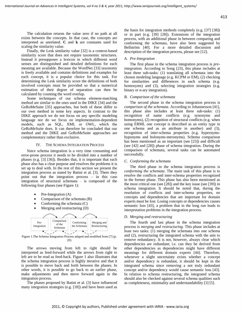
413



The calculation returns the value zero if no path at all exists between the concepts. In that case, the concepts are interpreted as unrelated. C and k are constants used for scaling the similarity value.

Finally, the Lesk similarity value [32] is a context-based similarity score that does not require taxonomic structures. Instead it presupposes a lexicon in which different word senses are distinguished and detailed definitions for each meaning are available. Because the WordNet [33] taxonomy is freely available and contains definitions and examples for each concept, it is a popular choice for this task. For determining the Lesk similarity score the definitions of both involved concepts must be provided so that a numerical estimation of their degree of separation can then be calculated by counting the word overlap.

Some techniques of our schema element-matching method are similar to the ones used in the DIKE [34] and the GeRoMeSuite [35] approaches, but both of these differ to our own method in some key aspects. In contrast to the DIKE approach we do not focus on any specific modeling language nor do we focus on implementation-dependent models, such as SQL, XML or OWL, which the GeRoMeSuite does. It can therefore be concluded that our method and the DIKE and GeRoMeSuite approaches are complementary rather than exclusive.

IV. THE SCHEMA INTEGRATION PROCESS

Since schema integration is a very time consuming and error-prone process it needs to be divided into a number of phases (e.g. [3] [36]). Besides that, it is important that each phase also has a clear purpose and resolves the problems it is set up to deal with. In the rest of this section we present the integration process as stated by Batini et al. [3]. There they point out that the integration process – in this case integration of structural schemata – is composed of the following four phases (see Figure 1):

Pre-Integration (A)

Comparison of the schemata (B)

Conforming the schemata (C)

Merging and restructuring (D)

Figure 1.The Schema Integration Process adaped and modified from [7] (p.

20)

The arrows moving from left to right should be interpreted as feed-forward while the arrows from right to left are to be read as feed-back. Figure 1 also illustrates that the schema integration process is highly iterative and that it is possible to move back and forth between the phases. In other words, it is possible to go back to an earlier phase, make adjustments and then move forward again in the integration process.

The phases proposed by Batini et al. [3] have influenced many integration strategies (e.g. [18]) and have been used as

the basis for integration methods completely (e.g. [37] [38]) or in part (e.g. [39] [28]). Extensions of the integration process, with an additional phase in between comparing and conforming the schemata, have also been suggested by Bellström [40]. For a more detailed discussion and description of the integration process, please see [12].

A. Pre-Integration

The first phase in the schema integration process is pre-integration. According to Song [23], this phase includes at least three sub-tasks: (1) translating all schemata into the chosen modeling language (e.g. KCPM or EM), (2) checking for similarities and differences in each schema (e.g. homonyms) and (3), selecting integration strategies (e.g. binary or n-ary integration).

B. Comparison of the schemata

The second phase in the schema integration process is comparison of the schemata. According to Johannesson [41], this phase also includes at least three sub-tasks: (1) recognition of name conflicts (e.g. synonyms and homonyms), (2) recognition of structural conflicts (e.g. when using ERML one concept is described as an entity type in one schema and as an attribute in another) and (3), recognition of inter-schema properties (e.g. hypernyms-hyponyms and holonyms-meronyms). Schema comparison has been mentioned as an important (see [23]) and difficult (see [42] and [28]) phase of schema integration. During the comparison of schemata, several tasks can be automated successfully.

C. Conforming the schemata

The third phase in the schema integration process is conforming the schemata. The main task of this phase is to resolve the conflicts and inter-schema properties recognized in the former phase. This phase has also been mentioned as the most critical one (see [28]) and the key issue (see [39]) in schema integration. It should be noted that, during the resolution of conflicts and inter-schema properties, no concepts and dependencies that are important for domain experts must be lost. Losing concepts or dependencies causes semantic loss [43], a problem that in the long run leads to interpretation problems in the integration process.

D. Merging and restructuring

The fourth and last phase in the schema integration process is merging and restructuring. This phase includes at least two tasks: (1) merging the schemata into one schema and (2), restructuring the integrated schema with the aim to remove redundancy. It is not, however, always clear which dependencies are redundant; i.e. can they be derived from other dependencies as dependencies might have different meanings for different domain experts [44]. Therefore, whenever a slight uncertainty exists whether a concept and/or dependency is redundant, it should be kept in the integrated schema since removing a not truly redundant concept and/or dependency would cause semantic loss [43]. In relation to schema restructuring, the integrated schema should also be checked against several schema qualities such as completeness, minimality and understandability [3] [5].

Pre-

Integration

Comparison

of the

Schemata

Conforming

the Schemata

Merging and

Restructuring

414



V. A SEMI-AUTOMATIC METHOD FOR MATCHING PRE-

DESIGN SCHEMA ELEMENTS

As indicated in the former section, the schema integration process includes several phases starting with schema preprocessing (pre-integration) moving on to schema matching (comparison and conforming the schemata) and finally ending with schema consolidation (merging and restructuring) (cf. with section IV).

In this article, we view schema preprocessing as a phase in which six activities are carried out:

Translate the schemata into the chosen modeling language

Schema element name adaption

Schema element disambiguation

Recognition and resolution of inner-schema conflicts

Introduction of missing relationships

Selecting the integration strategy Translate the schemata into the chosen modeling

language is the first activity to perform within the preprocessing phase. This activity is applicable when the information system is modeled using several modeling languages. It is, however, very important that the chosen modeling languages “have an expressiveness which is equal to or greater than that of any of the native models” [41](p. 15). For integration of structural pre-design schemata this should not be a problem since concepts and connections between concepts are the only modeling constituents that are used.

Schema element name adaption is the second activity to perform within schema preprocessing. It is a mandatory activity at least in its basic form; i.e. the reduction of words to their base forms using stemmers or lemmatizers. The use of naming guidelines (e.g. [17]) for its modeling elements can further improve a schema. This step is optional because it presupposes an individual set of naming guidelines, which depend at least on the used language.

Schema element disambiguation is an optional, but recommended, step. It constitutes an easy way of improving schema matching and integration on the pre-design level. Word senses are either assigned manually by domain experts or automated suggestions are made based on domain ontologies and general-purpose lexicons.

Recognition and resolution of inner-schema conflicts is mandatory in its basic form; i.e. the same designations are not allowed for different schema elements in static pre-design schemata. It is also recommended to perform an enhanced search for potential homonym and synonym conflicts by using context matching (cf. with section V.B.).

Introduction of missing relationships is optional provided domain ontology, or taxonomy, is available for identifying possible gaps in the schema.

Selecting the integration strategy is the final activity to perform in schema preprocessing and it is a mandatory one. In this activity it must be decided whether binary or n-ary integration should be used [5]. If binary integration is chosen then a further decision must be made whether binary ladder or binary balanced integration (see [3][45]) should be used.

For n-ary integration the two options n-ary one-shot, or n-ary iterative (see [3][46]), integration exist. For our method, we have decided to use binary ladder integration.

After schema preprocessing the matching phase starts, which itself consists of several sub phases. We first discussed in detail [25] how the several matching techniques are utilized in a common workflow. An extended and updated version of this process is structured as follows:

Step 1: Preparation for schema element-matching

Step 1.1: Find linguistic base form of schema elements

Step 1.2: Find schema element pairs to be matched

Step 2: Matching on the element level

Step 2.1: Direct element name matching

Step 2.2: Application of linguistic rules

Step 2.3: Domain ontology-based comparison

Step 3: Matching on the structural level

Step 3.1: Determine schema element neighborhood

Step 3.2: Domain ontology-based comparison for all pairs of neighbors

Step 3.3: Rule-based comparison for all pairs of neighbors

Step 4: Taxonomy-based matching Step 5: Decision on matching results

Step 5.1: Present matching proposals

Step 5.2: Get user feedback

Step 5.3: Finalize matching decisions In the first schema matching step – preparation for

schema element-matching – all combinations of schema element pairs from the two source schemata are prepared for comparison. The eventual goal in schema matching is to decide whether an element pair matches. The possible outcomes are:

Matching

Related

Dissimilar

The matching method and workflow are as follows: every schema element pair is first matched on the element level using the direct comparison of the base form and the application of linguistic rules. This step results in a preliminary matching decision. If the result is “dissimilar” and domain ontology is available, then information about potential connections between the elements can be looked up in the ontology. Schema element pairs that are classified as “dissimilar” or “matching” then undergo structural matching, which aims to identify potential conflicts based on the neighbors of the compared elements. If such conflicts are identified, a respective warning is added to the preliminary matching decisions. Finally, taxonomy-based matching – in our case the Lesk algorithm – can be optionally performed for schema element pairs, which are assumed “dissimilar,” in

415



order to detect hidden relatedness. This is especially recommended if at least one of the compared schema elements is as yet unknown in the domain ontology. The final matching proposals, including any warnings, are presented to domain experts who then have the chance to accept the proposals or override them. For instance, they can decide if and how potential differences and similarities, such as homonyms and synonyms, should be resolved. If no domain expert is available the default proposals are pursued. Based on the matching results specific integration proposals are made in the schema consolidation phase. The three different matching steps, which our method is comprised of, are discussed in more detail in the following sections (V.A – V.C).

A. Matching on the element level

A.1 Element name comparison (Step 2.1 and 2.2) In our matching method element-level matching (concept

matching) is the first activity. In element-level matching static schema elements are directly compared via their names (direct element name matching). Two elements which have matching names are automatically interpreted as equal for the moment although this decision can be amended later when matching on the structure level is performed. For example, let’s assume that schema A and schema B both come from the university domain. The static elements “students” in schema A and “student” in schema B have the same base form: “student.” Therefore, the elements match on the element-level; they supposedly describe the same concept.

If one, or both, of the compared schema element names consist of compound words the compounds are deconstructed. For endocentric compounds – the most common ones in the English language according to Bloomfield [47] – the rightmost element of the word is its head. Thus the following two percolative rules (application of linguistic rules) are applicable:

a. If the compared schema elements have names in the

form of A and AB (i.e. A corresponds to the compound AB minus the head B), then the relationship “AB belongs/related to A” can be assumed between the elements.

b. If the compared schema elements have names in the

form B and AB (i.e. A is the head of the compound AB), then the relationship “AB is a B” can be assumed between the elements.

To exemplify the first rule (a), an element named “car

manufacturer” is identified as a potential attribute of an element named “car” (“car manufacturer” belongs to “car”) while an element “student social security number” is identified as an attribute candidate for the element “student” (“student social security number” belongs to “student”). However the relationship “belongs to” is usually interpreted as an inverse aggregation, which is not always the intended meaning. For instance “blood pressure” is defined as “the pressure of the circulating blood against the walls of [a person’s] blood vessels.” Thus it can be preferable to

interpret “blood pressure” as an attribute of “person” rather than an attribute of “blood.” A more general association named “related to” is preferable in such cases; e.g. blood pressure” related to “blood.”

Regarding (b), the second rule, the exemplary element-pair “patient” and “dialysis patient” is interpreted as “dialysis patient” is a “patient,” while the concepts “blood pressure measurement” and “measurement” have the relationship “blood pressure measurement” is a (specific form of) “measurement.” The “is a” relationship obviously applies to all endocentric compounds, because their head is modified by the rest of the composite (consequently called the modifier) per definition. A.2 Domain ontology-based comparison (Step 2.3)

The strategy to perform schema element-matching solely based on their names and definitions is not always sufficient. While correlations of element names might indicate a possible matching, the meanings of the involved words might still differ. Moreover, in practice sufficient concept definitions are not always available. Lastly, even if definitions are available for both compared elements they might not be detailed enough to decide whether the schema elements actually match or not. Thus it is optimal to have ontology of the domain at one’s disposal.

On the supposition that the compared schema element pair has been preliminarily identified as dissimilar in the prior element-level matching step, the matching process proceeds by looking up concepts that fit to the schema element pair in the domain ontology. If both schema elements correspond to concepts in the domain ontology these are again compared on the element-level with the typical outcomes related and dissimilar. If one of the schema elements is missing no additional information about the elements’ relationship can be derived. Nevertheless, the missing elements can still be candidates for new ontology concepts. On the other hand, if both schema elements are found in the domain ontology, then the ontology can be utilized to recognize additional similarity as follows:

If the elements are directly related by an association in the domain ontology, then their relationship is assumed as “related” and this new relationship is introduced into the integrated schema. If, according to the ontology, both elements are synonymous this is denoted by the special relationship “is synonym of” or “mutual inheritance.”

If the elements are connected indirectly via relationships up to a certain restrictable degree of separation, they may also be assumed as “related.” Besides path length, relationship type is also a criterion for whether an indirect connection is interpreted as relatedness. The criteria of path length and relationship type may also be combined when evaluating indirect relationships. In order to correctly depict the connection between the indirectly connected schema elements the missing concepts and relationships from the ontology need to be introduced to the integrated schema.

416



If no direct relationship, or indirect path, of the required length and/or type is found in the domain ontology between the compared schema elements, then they are assumed to be dissimilar or independent.

B. Matching on the structural level

B.1 Determine schema element neighborhood (Step 3.1) The previously described element-based schema

matching techniques only take into account the names and definitions of the compared concepts. Matching results obtained in such a way might still be erroneous, however, as both synonym and homonym conflicts are possible (see also Figure 2 and Figure 3).

Matching on the structure level (see [26]) is likely to improve the outcome of element-level matching namely by taking the schema elements’ neighborhood into account. Using neighborhood for deriving concept meanings isn’t a new approach (e.g. [34]), although it usually is utilized for word-disambiguation in full texts instead of schema element-matching. For instance, Koeling & McCarthy et al. [48] suggest word sense disambiguation based on context and give an example: if the word “plant” has the sense ’industrial plant,’ it tends to occur in the neighborhood of words like “factory,” “industry,” “facility,” “business,” “company” and “engine.” Its other meaning, ’flora,’ is often hinted at by neighbors like “tree,” “crop,” “flower,” “leaf,” “species,” “garden,” “field,” “seed” and “shrub.” Heylen et al. [49] describe similar word matching techniques where 1

st and 2

nd

order bag-of-word-models are used for context-based word matching; i.e. it is determined whether words in the close proximity of the compared target words match. In 1

st order

models the target words are identified as similar if their neighbors match to a certain degree while in 2

nd order

models a two-level matching process takes place as the context of the neighbor words themselves are again compared. Context-based word disambiguation techniques, which are applied on natural language texts, usually aim at finding the meaning of single words in the text. Based on context a decision is derived, which out of several possible word definitions is the correct, or most likely, one. This is slightly different from schema matching where word pairs are compared with the goal of identifying possible conflicts. Finding the meaning of each involved concept is the first step towards identifying conflicts and commonalities.

Regarding the notion of neighborhood in natural language text documents, the relevant neighborhood is typically defined by context windows that span a defined number of (content) words before and after the disambiguated word. Additional boundaries are provided by sentence delimiters. When adapting structure-based matching techniques on conceptual schemata, different definitions for the notions of “neighborhood” and “context” are needed. Typically, the context, or neighborhood, of a static schema element encompasses all surrounding directly connected elements. Sometimes it is helpful for the sake of matching and integration algorithms to extend the notion of context so that it also encompasses indirectly connected schema elements up to a certain level of separation.

B.2 Domain Ontology-Based Neighborhood Comparison (Step 3.2)

Essentially neighborhood matching acts as a security check whether the preliminary results from the element level are trustworthy, or if conflicts, such as homonyms or synonyms, are likely. If the neighborhood comparison supports the result of the element-level matching then the integration process continues. But when the neighborhood comparison yields different results than the element-level comparison, however, a contradiction is at hand and the domain experts must be notified by displaying a warning that the current schema element pair has a potential conflict. For the purpose of recognizing conflict candidates two threshold values are defined: the homonymy threshold and the synonymy threshold. These thresholds are reference values and adaptable so that they can fit the needs of different projects. It is possible for the two thresholds to congregate on the same value, but the homonymy threshold must not be greater than the synonymy threshold.

In order to calculate a matching result that can be compared against the threshold values the structure-level matching of neighbor schema elements is itself performed on the element level. The neighbor elements are counted as matching if one of the following conditions is fulfilled:

They have the same name and/or definitions

A synonymy relationship exists between them according to the domain ontology

The schema element pair has a taxonomy-based similarity score above a certain threshold

Including more than just the direct neighbors in the

decision process achieves a more thorough matching, but it is slower due to several more elements to compare. To determine the neighborhood matching of schema element-pairs the percentage of corresponding neighbors is calculated using the matching criteria listed above. For this purpose the following intuitive formula (subsequently referenced as Degree of Neighborhood Matching (DNM)) can be used:

2/1*ma2))ntFromScheount(Eleme(NeighborCma1)ntFromScheount(eleme(NeighborC

ountmaElementCighborScheMatchingNe

Formula 3 calculates the percentage of matches among

the average neighbor count. The resulting DNM value is compared against the thresholds. Schema elements that have been classified as “matching” on the element level must have a DNM above the defined homonymy threshold. If the DNM is below the threshold a homonym warning is issued by the matching application. Similarly, an element pair that has been classified as “dissimilar” on the element level should be below the provided synonymy threshold. If that isn’t the case a synonymy warning is issued by the matching application.

Figures 2 and 3 give examples how analyses of the compared schema elements’ context may point towards hidden homonym and synonym conflicts in static pre-design schemata. In Figure 2 the element “course” occurs in both source schemata, but upon nearer inspection of the neighbors

417



it becomes apparent that the two elements have disjunctive neighborhoods.

Figure 2. Recognition of homonym conflict [11] (p.113)

Figure 3. Recognition synonym conflict [11] (p. 114)

This raises the suspicion of homonymy. Indeed, the left schema describes a course served during a meal while the right hand schema describes a university course. It must be noted that severe homonym conflicts as shown in Figure 2 are unlikely to occur if the source schemata come from the same domain. Most remaining homonym conflicts occur between concepts that have less pronounced semantic differences; e.g. see the more extensive example in Figure 4 when the vocabulary of terms is small [3] and when incomplete concept names are used [50].

A synonym conflict is shown in Figure 3. The schema elements “registration” and “participation” have been classified as dissimilar on the element level, but several neighbors match: two of two adjacent elements for the schema element “registration” and two of three neighbors for the schema element “participation.” In spite of the small number of neighbors this implies that the elements “participation” and “registration” are used synonymously here. In actuality a student’s participation in an exam is modeled in both cases. Synonym conflicts frequently occur when different groups, or departments, are involved who might use different nomenclature for the same concept that’s specific to their point of view.

participation

student

have

assistant

lecturer

examcourse

manager

be

account

have

teaching

position

being paid

have

course

have

apply to

registration

belong to

have

belong to

subject

have

registrationexist for

have

examiner

student

make

solution

have

specification have

task

have

solution partexist for consist of

exam

certificate have

belong to

Figure 4. Homonym conflict example [49] ( p. 56)

Figure 4 shows an example of a homonym conflict. Since the element “registration” occurs in both source schemata the schema element pair is preliminarily categorized as equivalent on the element level. Comparing the immediate context of the neighborhoods of “registration” the elements show the two registrations as actually being different concepts. Students are involved in both cases, but in the left-hand schema students register to a course, while in the right-hand-schema students register to an exam. In the latter case the students’ exam solution is related to their registration too. The result value according to the default DNM formula given above is 0.4, which, depending on the threshold, might be enough to issue a homonym conflict warning by the matching application.

A way of further refining the DNM formula and improving its results is the additional consideration of schema elements that only appear in the neighborhood of one element although they are available in both schemata. Since these elements are expected, but not actual neighbors, in one of the schemata, they could be included in that schema’s neighbor count. Naturally, however, the match count stays the same so the resulting DNM score is always lowered when missing expected neighbors are taken into consideration.

B.3 Rule-based Neighborhood Comparison (Step 3.3)

In the third and last activity in structural-level matching we use two types of “IF THEN” rules: those for equivalent element names and others for similar element names (see also [13] and [14]). For this case equivalent means that matching on the element level resulted in two equivalent element names. Size, for instance, is an element within both schema 1 and schema 2. On the other hand, similar means that the element names are not equivalent but still have something in common; e.g. Order Line in schema 1 and Order in schema 2. Our method uses at least six rules for equivalent element names and three rules for similar element names. Our rules for equivalent element names can be stated as:

IF the comparison of concept names yields equivalent

and the comparison of concept neighborhoods yields:

Equivalent, THEN equivalent concepts are most likely recognized (E1)

Different, THEN homonyms are most likely recognized (E2)

Similar, AND one concept in each schema is named differently, THEN synonyms are most likely recognized (E3)

418



Similar, AND one concept name is a composite of another concept name with a following addition AND the cardinality is indicating 1:1, THEN an association between the two concepts is most likely recognized (E4)

Similar, AND one concept name is a composite of another concept name with a prior addition, THEN a hypernym-hyponym pair is most likely recognized (E5)

Similar, AND one concept name is a composite of another concept name with a following addition AND the cardinality is indicating 1:M with or without uniqueness, THEN a holonym-meronym pair is most likely recognized (E6)

Examples of rules E5 and E6 are illustrated in Figure 5 and Figure 6.

Figure 5. Recognition of a hypernym-hyponym dependency based on rule

[10] ( p. 184)

Figure 6. Recognition of a holonym-meronym dependency based on rule

[10] (p. 185)

Our rules for similar concept names can be stated as: IF the comparison of concept names yields:

Similar, AND one concept name is a composite of another concept name with a following addition AND the comparison of concept neighborhoods yields similar or equivalent with an indication to a 1:1 cardinality, THEN an association between the two concepts is most likely recognized

Similar, AND one concept name is a composite of another concept name with a following addition AND the comparison of concept neighborhoods yields similar or equivalent with or without an indication to a unique 1:M cardinality, THEN a holonym-meronym pair is most likely recognized

Similar, AND one concept name is a composite of another concept name with a prior addition AND the comparison of concept neighborhoods yields similar or equivalent, THEN a hypernym-hyponym pair is most likely recognized

One last remark is needed before moving on to the Lesk algorithm. The rules addressed above were applied in [13]

and [14] while using the Karlstad Enterprise Modeling approach [21]. On the other hand, we do not focus here on any specific modeling language. We have therefore refined and adapted the rules to be useful for any modeling language; in other words, the rules are now modeling language-independent and can be used on the implementation -neutral level.

C. Taxonymy-based matching - The Lesk Metric (Step 4)

C.1 The Lesk approach in structure-based matching The Lesk metric [32] is a domain-independent similarity

score that doesn’t require taxonomic structures (cf. [30] [31]). Instead, it presupposes a lexicon in which different word senses are distinguished and detailed definitions for each meaning are provided. Because the WordNet [33] taxonomy contains definitions and examples for each concept it is a popular choice for this kind of task. The Lesk approach is a context-based similarity measurement strategy and requires neither the LCS (Least Common Subsumer) nor the path length unlike other WordNet-based similarity measures (cf. [30] [31]). For determining the Lesk similarity score the definitions of both involved concepts must be provided and then a numerical estimation of their degree of separation is calculated by counting the word overlap.

In Banerjee & Pederson et al. [32] and Ekedahl & Golub et al. [51] specific implementations of the Lesk-algorithm are discussed for disambiguating words in full texts using WordNet [33]. In their approach a context window containing an equal number of words on both sides of the observed word is defined after which all available definitions for the observed concept and the other content words in the context window are examined and compared. The word sense that has the greatest overlap with the definitions from the surrounding text is assumed to be the correct one. Non-content words, like pronouns or articles, are excluded from the overlap count. Although the Lesk algorithm was originally designed for word disambiguation in full texts a similar approach can be applied to schemata by comparing not only concept notions, but also the definitions of concepts and those of their neighbors. This application of the Lesk algorithm for disambiguation purposes is similar to schema matching on the structure level although concept definitions rather than concept names are matched.

C.2 Calculation and performance of the Lesk score

In our method we adopt the Lesk algorithm as presented by Vöhringer & Fliedlet al. in [15]. The following glosses are interpreted for each compared word: the examples and the definitions of the hypernyms, hyponyms, meronyms, holonyms and the word itself. Table III lists the glosses for the concept “bus#n#1” as extracted from WordNet. The underlined words are not part of the actual gloss value but added for clarity reasons because they denote the corresponding concepts of the gloss.

Permutations of the various glosses are tested for overlaps; i.e. example “car#n#1”- glos “bus#n#1,” glos “car#n#1”- glos “bus#n#1” etc. (see table IV). In order to prioritize longer matches, the score for each gloss-pair is defined as the sum of the squared word count of each

Customer

Product OrderItem

Order

Name

Product

High Priority

Order

OrderItem

Hypernym-Hyponym

Schema 1 Schema 2

Compared

Concepts

Neighbor

Match

No Neighbor

Match

Priority

Name

Product OrderItem

Order Name

Product

OrderItem

Schema 1 Schema 2

Holonym-Meronym

Compared

Concepts

Neighbor

Match

No Neighbor

Match

419



overlap. The total Lesk similarity score is defined as the accumulated score of all gloss-combinations.

TABLE III. TYPICAL WORDNET GLOSSES FOR THE CONCEPT

“BUS#N#1“

Gloss

Type

Description Gloss Value

Example Example of

usage

"he always rode the bus to work"

Glos Word sense definition

bus: a vehicle carrying many passengers; used for public transport;

Hype glos Bus is a kind

of…

public transport: conveyance for

passengers or mail or freight

Hypo glos … Is a kind of bus

minibus: a light bus (4 to 10 passengers) school bus: a bus used to transport children

to or from school

trolleybus: a passenger bus with an electric motor that draws power from overhead

wires

Holo glos Bus is a part of…

fleet: group of motor vehicles operating together under the same ownership

Mero glos … Is a part of

bus

roof: protective covering on top of a

motor vehicle

window: a transparent opening in a vehicle that allows vision out of the sides or back;

usually is capable of being opened

Table IV lists the overlaps and the resulting scores for the

word pair “car#n#“1 – “bus#n#1“; only gloss permutations with at least one overlap are shown. As for the calculation of the overlap scores, comparing the example gloss of “car#n#1” and the (descriptive) gloss of “bus#n#1” yields a single overlap of the length 1. The score for this overlap is therefore 1

2; i.e. 1. The hyponym gloss of “car#n#1” and the

(descriptive) gloss of “bus#n#1” have four overlaps. Three of them have the length 1 while one of the overlaps (“a vehicle”) consists of two words; i.e. it has the length 2. The score is thus calculated as follows: 3*1

2+1*2

2; i.e. 7. The

total similarity score for car#n#1 and bus#n#1 is 615.

TABLE IV. EXAMPLE OF STANDARD LESK OVERLAPS

Tracing Lesk Comparison car#n#1 – bus#n#1

car#n#1 Bus#n#1 Overlap Score

Example Glos 1 x "a" 1

Glos Glos 1 x "a"

1 x "vehicle"

2

Glos mero glos 1 x "usually" 1 x "a motor

vehicle"

10

hypo glos Glos 1 x "passengers"

1 x "a vehicle"

1 x "for" 1 x "used"

7

Mero glos mero glos 1 x "a

transparent opening in a

vehicle that

allows vision out of the sides

or back; usually

is capable of being opened"

1 x "protective

covering on top of a motor

vehicle"

505

Total score 615

Generally, two concepts are more closely related the

higher the Lesk score is. The Lesk metric, however, is dependent on the number and size of the available glosses. Like other similarity measures, the Lesk score needs reference values to which it can be compared. In other words, the Lesk score needs a threshold value to be meaningful.

Table V compares the Lesk scores for the three word pairs “car#n#1”-“bicycle#n#1,” “car#n#1”-“motorcycle#n#1” and “car#n#1-“bus#n#1”.

TABLE V. UNINTUITIVE RANKING OF CONCEPTS WITH THE LESK

SCORE

Pair Score Rank

car – bicycle 300 2

car – motorcycle 237 3

car – bus 739 1

Ranking the scored pairs shows that cars and buses are

identified as the most similar pair followed by cars and bicycles while cars and motorcycles are identified as the least similar pair. Furthermore, choosing a relevance threshold of 300 implies that cars and bicycles and cars and buses are similar, but cars and motorcycles are not. These results are unintuitive as, following intuition, at least cars and motorcycles should be interpreted as more similar than cars and bicycles since both are motorized vehicles. When regarding shape and function motorcycles and bicycles are similar. This example demonstrates that the Lesk score requires some optimizations to become more meaningful. Optimizations of the Lesk Algorithm are therefore addressed in the following section.

420



C.3 Optimizations of the Lesk Algorithm As discussed by Vöhringer & Fliedl et al. in [15], the

standard Lesk algorithm has optimization potential in regard to not only internal factors but also in regard to external factors. Optimization of the internal factors means that the Lesk algorithm itself is updated and improved while in the optimization of the external factors the environment is adapted but the algorithm stays unchanged. The underlying lexicon, in particular, can be optimized regarding contents and structure. Possible optimization strategies include:

Internal factors: o Partial filtering of stop words o Word reduction via stemming o Normalization based on gloss length

External factors: o Improvement of glossary quality and quantity

via completion and substitution of certain keywords

o Restructuring of taxonomy o Guidelines for gloss extension in specific

domains Stop word-based enhancements of the Lesk strategy are,

for example, discussed in [32]. A stop word list generated from WordNet can be used for filtering word grams that contain a certain empirically motivated percentage of non-content words. Gloss overlaps above a predefined percentage of stop words are ex-filtrated. Since single stop word overlaps have a 100% stop word quotient they are obligatorily filtered out. For identifying matches of inflected word variants, stemming is proposed. In a prototype implementation of the Lesk algorithm, a version of the extended Porter stemmer is used for this purpose [52].

Other Lesk optimization strategies include normalization by gloss sizes. Using the standard additive calculation of gloss overlap scores the availability of extensive glosses is naturally favored. If, in contrast, gloss size normalization was used overlap scores would yield the proportional rate of overlaps in a gloss instead of the absolute numbers.

Lesk optimizations with respect to external factors; e.g. by filling gaps in WordNet glosses or restructuring the WordNet taxonomy, are a difficult process. Although there are apparent gaps and suboptimal taxonomies in WordNet that are seemingly easy to improve one must be wary of side effects. The easiest least intrusive change on the external level is the filling of prominent gloss gaps; in particular missing hypernyms, hyponyms, meronyms and holonyms. This can be done either manually or by transferring these definitions from other related words. For instance, the two WordNet entries “motorcycle” and “bicycle” miss several fitting meronyms that exist for the related word “car.” Motorcycles, like cars, have an engine, a mirror and a horn. Likewise, “mirror” and “horn” are parts of bicycles too.

As shown in table VI, these already existing glosses are transferred to “motorcycle” and “car” by entering the respective meronyms.

TABLE VI. FILLING GAPS IN WORDNET GLOSSES

Concept Extension of WordNet standard glosses for

meronyms

Car WordNet standard glosses (not extended)

Bus WordNet standard glosses (not extended)

Motorcycle WordNet standard glosses extended by

motorcycle engine: the engine that propels a

motorcycle

motorcycle horn: a device on a motorcycle for

making a warning noise

motorcycle mirror: a mirror that the driver of a motorcycle

gasoline engine: an internal-combustion engine that burns gasoline

Bicycle WordNet standard glosses extended by

bicycle horn: a device on a bicycle for making a warning noise

bicycle mirror: a mirror that the driver of a bicycle can use

To demonstrate the effects of internal and external Lesk

optimizations the exemplary word pairs from table V (“car#n#1”-“bicycle#n#1,” “car#n#1”-“motorcycle#n#1” and “car#n#1-“bus#n#1”) have also been tested with updated versions of the Lesk algorithm (see tables VII and VIII). While the original Lesk score listed “car”-“bicycle” as more similar than “car”-“motorcycle” (a score of 300 vs. 237), the internally optimized Lesk implementation yields the scores 115 for the word pair “car”-“bicycle” and 181 for the word pair “car”-“motorcycle.” Thus the improved algorithm using the strategies discussed above better reflects the greater similarity between “car” and “motorcycle.”

TABLE VII. RESULTS OF THE INTERNALLY OPTIMIZED LESK

ALGORITHM

Pair Score Rank

Car-Bicycle 115 3

Car-Motorcycle 181 2

Car-Bus 688 1

TABLE VIII. RESULTS OF THE INTERNALLY & EXTERNALLY OPTIMIZED

LESK ALGORITHM

Pair Score Rank

Car-Bicycle 198 3

Car-Motorcycle 321 2

Car-Bus 688 1

Summarized results of the internal and external Lesk

optimizations are shown in tables VII and VIII. Obviously, the results in table V don’t adequately reflect the intuitive similarity-ranking concerning form and functionality of the involved entities. Table VII shows that internal optimization already establishes the correct ranking. Table VIII shows the scoring results after filling obvious lexicon gaps with adjusted score distances. The experiment’s results suggest that the outcomes using the optimized Lesk algorithm are more meaningful than the standard Lesk score.

D. Decision on matching results (Step 5)

In short, the following strategies are applied in step 5’s decision on matching results. Both equality and synonymy mean that the compared schema elements match. The

421



integration proposal “matching” is therefore an indication for merging these elements though semantic loss must be avoided under any circumstances. This can be done by storing the original schemata and concept names for traceability reasons. Unrelated schema elements are “dissimilar” and therefore transferred independently to the integrated schema. For (directly) “related” schema elements both elements are transferred to the integrated schema and a relationship between them is introduced. Schema elements are indirectly related when they have no direct connecting relationship in the domain, but are connected via several other concepts. For example, two elements might have a common neighbor concept with which they are connected via generalization- or aggregation-relationships. It is principally possible to also transfer such more complex relationships – including all intermediate concepts – to the integrated schema as a proper connection for the indirectly-related schema elements.

A central requirement says that the integration process should be automatized. This means that domain experts should be supported by preferably accurate proposals and the tool should generate a default-integrated schema even when no user input is made at all. For this purpose an option is provided in the integration tool that allows adjusting the preferred degree of automatization. At its most rigid setting a rough solution is automatically calculated using the matching methods as described in the previous sections if user feedback is absent? The proposals’ quality is influenced by the correctness and completeness of the available domain ontology. If ambiguity conflicts arise they are resolved by automatically choosing the most probable word meaning. While fully automatic integration without any manual input is fast and convenient the quality of the proposed solution is likely to be lower than when user feedback is available. On the other hand, the prototype also allows a setting where the matching and integration is performed stepwise and domain experts need to accept, or reject, the proposals for each schema element pair and each integration step. This setting naturally allows the most direct influence for the user, but it is also the slowest and most laborious. Our recommended strategy is to strike a balance between these two extremes. This can be done by automating the process, but asking the domain experts to provide missing definitions to resolve conflicts like word ambiguities, or contradictions, and to evaluate the end results of the integration.

VI. SUMMARY AND CONCLUSION

In this paper, we have presented a semi-automatic method for matching schema elements in the integration of structural pre-design schemata. Following Rahm & Bernstein et al. [26], our own method can be classified as a composite schema-based matching method. Our approach uses element-level (concept) matching – structural-level (neighborhood) matching and taxonomy-based matching – and combines these parts to one workflow resulting in the proposed integrated schema. The research approach used within this work can be characterized as design science and our main contributions as a method and an instantiation; i.e. a prototype application. When applied in schema integration, our matching method should facilitate the recognition of

similarities and differences between two structural source schemata.

REFERENCES

[1] P. Bellström and J. Vöhringer, “A Three-Tier Matching Strategy for Predesign Schema Elements,” Proceedings of The Third International Conference on Information, Process, and Knowledge Management (eKNOW 2011), 2011, pp. 24-29.

[2] A. Doan, F.N. Noy and A.Y. Halevy, “Introduction to the Special Issue on Semantic Integration,” SIGMOD Record, Vol. 33, No. 4, 2004, pp. 11-13.

[3] C. Batini, M.Lenzerini, and S.B. Navathe, “A Compartive Analysis of Methodologies for Database Schema Integration,” ACM Computing Surveys, vol. 18(4), 1986, pp. 323-364.

[4] S. Navathe, R. Elmasri and J. Larson, “Integrating User Views in Database Design,” IEEE Computer 19(1), 1986, 50–62.

[5] Batini, C., S. Ceri and S.B. Navathe, Conceptual Database Design An Entity-Relationship Approach, The Benjamin/Cummings Publishing Company Inc., Redwood City California, 1992.

[6] M. Stumptner, M. Schrefl and G. Grossmann, “On the Road to Behavior-Based Integration,” Proceedings of the 1st APCCM Conference, 2004, pp. 15-22.

[7] A. Bachmann, W. Hesse, A. Russ, C. Kop, H.C., Mayr, and J. Vöhringer J., “OBSE – An Approach to Ontology-Based Software Engineering in the practice,” Proceedings of EMISA, 2007, pp. 129–142.

[8] A.R. Hevner, S.T. March and J. Park, “Design Science in Information Systems Research,” MIS Quarterly, 28 (1), 2004, pp. 75-105.

[9] J. Iivari, “A Paradigmatic Analysis of Information Systems As a Design Science,” Scandinavian Journal of Information Systems, 19 (2), 2007, pp. 39-64.

[10] S.T. March and G.F. Smith “Design and Natural Science Research on Information Technology,” Decision Support Systems, 15, 1995, pp. 251-266.

[11] A. Hevner and S. Chatterjee, Design Research in Information Systems Theory and Practice, New York, Springer (2010).

[12] P. Bellström, View Integration in Conceptual Database Design – Problems, Approaches and Solutions, Licentiate Thesis, Karlstad University Studies 2006:5, 2006.

[13] P. Bellström, Schema Integration – How to Integrate Static and Dynamic Database Schemata, Dissertation, Karlstad University, Karlstad University Studies 2010:12, 2010.

[14] P. Bellström, “A Rule-Based Approach for the Recognition of Similarities and Differences in the Integration of Structural Karlstad Enterprise Modeling Schemata,” Proceedings of the 3rd IFIP WG 8.1 Working Conference on The Practice of Enterprise Modeling (PoEM 2010), 2010, pp. 177-189.

[15] J. Vöhringer and G. Fliedl, “Adapting the Lesk Algorithm for Calculating Term Similarity in the Context of Ontology Engineering,” in Information Systems DevelopmentBusiness Systems and Services: Modeling and Development, 2011, pp. 781-790.

[16] J. Vöhringer, Schema Integration on the Predesign Level, Dissertation, Alpen-Adria-Universität Klagenfurt, 2010.

[17] P. Bellström, J. Vöhringer and C. Kop, “Guidelines for Modeling Language Independent Integration of Dynamic Schemata,” Proceedings of the IASTED International Conference on Software Engineering, 2008, pp. 112-117.

[18] P. Bellström, J. Vöhringer, and C. Kop, “Towards Modeling Language Independent Integration of Dynamic Schemata,” in Information Systems Development Toward a Service Provision Socity, Heidelberg: Springer, 2009, pp. 21-29.

422



[19] P. Bellström, J. Vöhringer, and A. Salbrechter, “Recognition and Resolution of Linguistic Conflicts: The Core to a Successful View and Schema Integration,” in Advances in Information Systems Development New Methods and Practice for the Networked Society, Vol. 2, 2007, pp. 77-87.

[20] G. Fliedl, C. Kop, H.C. Mayr, W. Mayerthaler and C. Winkler, “Linguistically based requirements engineering – The NIBA project,” Data & Knowledge Engineering, 35, 2000, 111-120.

[21] R. Gustas and P. Gustiené, “Towards the Enterprise Engineering Approach for Information System Modelling Across Organisational and Technical Boundaries,” in Enterprise Information Systems V, Dordrecht: Kluwer, 2004, pp. 204-215.

[22] P. Chen, “The Entity-Relationship Model – Toward a Unified View of Data,” ACM Transactions on Database Systems, vol. 1(1), 1976, pp. 9-36.

[23] W. Song, Schema Integration – Principles, Methods, and Applications, Dissertation, Stockholm University, 1995.

[24] Object Management Group, OMG Unified Modeling Language (OMG UML), Superstructure, [Electronic], Available: http://www.omg.org/spec/UML/2.3/Superstructure/PDF/ [20120126], 2010.

[25] P. Bellström and J. Vöhringer, “Towards the Automation of Modeling Language Independent Schema Integration,” Proceedings of the International Conference on Information, Process, and Knowledge Management (eKNOW 2009), 2009, pp. 110-115.

[26] E. Rahm and P.A. Bernstein, “A Survey of Approaches to Automatic Schema Matching,” The VLDB Journal, vol. 10, 2001, pp. 334–350.

[27] P. Shvaiko and J. Euzenat, “A Survey of Schema-Based Matching Approaches,” Journal of Data Semantics, vol. 4, 2005, pp. 146-171.W.

[28] M.L., Lee and T.W. Ling, “A Methodology for Structural Conflict Resolution in the Integration of Entity-Relationship Schemas,” Knowledge and Information System. 5, 2003, 225-247.

[29] Q. He and T.W. Ling, “Resolvning Schematic Descrepancy in the Integration of Entity-Relationship Schemas,” in: Proceedings of ER 2004, Heidelberg: Springer, pp. 245-258.

[30] Z. Wu and M. Palmer, “Verb semantics and lexical selection,” in Proceedings of the 32nd Annual Meeting of the Association for Computational Linguistics, 1994, pp. 133-138.

[31] G. Hirst and D. St-Onge, “Lexical chains as representations of context for the detection and correction of malapropisms,” in WordNet: An Electronic Lexical Database (Language, Speech, and Communication), 1998.

[32] S. Banerjee and T. Pederson, “An Adapted Lesk Algorithm for Word Sense Disambiguation Using WordNet,” Proceedings of the 3rd International Conference on Intelligent Text Processing and Computational Linguistics (CICLing 2002), 2002, pp. 136–145.

[33] Wordnet, WordNet A lexical database for English [Electronic], Available: http://wordnet.princeton.edu/ [20120126]

[34] L. Palopoli, G. Terracina, and D. Ursino, “DIKE; A System Supporting the Semi-Automatic Construction of Cooperative Information Systems From Heterogeneous Databases,” Software–Practice and Experiences, vol. 33, 2003, pp. 847-884.

[35] D. Kensche, C. Quix, X. Li, and Y. Li, “GeRoMeSuite: A System for Holistic Generic Model Mangement,” Proceedings of the 33rd International Conference on Very Large Data, 2007, pp. 1322-1325.

[36] H. Frank and K. Eder, “Towards an Automatic Integration of Statecharts,” Proceedings of ER’99, Springer, 1999, pp. 430-445.

[37] P. Shoval, “A Methodology for Integration of Binary-Relationship Conceptual Schemas,” International Conference on Databases, Parallel Architectures and Their Applications, 1990, pp. 435–437.

[38] T.J. Teorey, Database Modeling & Design, Morgan Kaufmann Publishers Inc, USA, 1999.

[39] S. Spaccapietra and C. Parent, “View Integration: a Step Forward in Solving Structural Conflicts,” IEEE Transactions on Knowledge and Data Engineering, Vol. 6, No. 2, 1994, pp. 258–274.

[40] P. Bellström, “Bridging the Gap between Comparison and Conforming the Views in View Integration,” Local Proceedings of the 10th ADBIS Conference, 2006, pp. 184-199.

[41] P. Johannesson, Schema Integration, Schema Translation, and Interoperability in Federated Information Systems. Dissertation Stockholm University, Royal Institute of Technology, 1993.

[42] L. Ekenberg and P. Johannesson, “A Formal Basis for Dynamic Schema Integration,” Conceptual Modeling – ER’96, Springer, 1996, . pp. 211-226.

[43] P. Bellström, “On the Problem of Semantic Loss in View Integration,” in Information Systems Developent Challenges in Practice, Theory, and Education, Vol. 2, Heidelberg: Springer, 2009, pp. 963-974.

[44] D. Dey, V.C. Story and T.M. Barron, “Improving Database Design through the Analysis of Relationships,” ACM Transactions on Database Systems, 24 (4), 1999, pp. 453-486.

[45] C. Batini and M.Lenzerini, “A Methodology for Data Schema Integration in the Entity-Relationship Model,” IEEE Transactions on Software Engineering, 10 (6), 1984, pp. 650–664.

[46] S.B. Navathe and S.U. Gadgil, “A Methodology for View Integration in Logical Database Design,” Proceedings of the Eighth International Conference on Large Data Bases, Morgan Kaufmann, 1982, pp. 142–164.

[47] Bloomfield, L. (1933). Language. Chicago - London: The University of Chicago Press.

[48] R. Koeling and D. McCarthy, “From Predicting Predominant Sense to Local Context for Word Sense Disambiguation,” Proceedings of the 2008 Conference on Semantics in Text Processing (STEP’08), 2008, pp. 103-114.

[49] K. Heylen, Y. Peirsman, D. Geeraerts and D. Speelman, “Modelling Word Similarity: An Evaluation of Automatic Synonymy Extraction Algorithms,” Proceedings of the 6th International Conference on Language Resource and Evaluation (LREC’08), 2008, pp. 3243-3249.

[50] W. Kim and J. Seo, “Classifying Schematic and Data Heterogeneity in Multidatabase Systems,” IEEE Computer, 24, 1991, pp. 12–18.

[51] J. Ekedahl and K. Golub, Word sense disambiguation using WordNet and the Lesk algorithm. Projektarbeten 2004: Språkbehandling och datalingvistik Lunds Universitet, Institutionen för Datavetenskap, 2005, pp. 17-22.

[52] P. Willet, “The Porter stemming algorithm: then and now,” Electronic Library and Information Systems, 40 (3), 2006, pp. 219-223. ISSN 0033-0337.

www.iariajournals.org

International Journal On Advances in Intelligent Systems

ICAS, ACHI, ICCGI, UBICOMM, ADVCOMP, CENTRIC, GEOProcessing, SEMAPRO,BIOSYSCOM, BIOINFO, BIOTECHNO, FUTURE COMPUTING, SERVICE COMPUTATION,COGNITIVE, ADAPTIVE, CONTENT, PATTERNS, CLOUD COMPUTING, COMPUTATION TOOLS

issn: 1942-2679

International Journal On Advances in Internet Technology

ICDS, ICIW, CTRQ, UBICOMM, ICSNC, AFIN, INTERNET, AP2PS, EMERGING

issn: 1942-2652

International Journal On Advances in Life Sciences

eTELEMED, eKNOW, eL&mL, BIODIV, BIOENVIRONMENT, BIOGREEN, BIOSYSCOM,BIOINFO, BIOTECHNO

issn: 1942-2660

International Journal On Advances in Networks and Services

ICN, ICNS, ICIW, ICWMC, SENSORCOMM, MESH, CENTRIC, MMEDIA, SERVICECOMPUTATION

issn: 1942-2644

International Journal On Advances in Security

ICQNM, SECURWARE, MESH, DEPEND, INTERNET, CYBERLAWS

issn: 1942-2636

International Journal On Advances in Software

ICSEA, ICCGI, ADVCOMP, GEOProcessing, DBKDA, INTENSIVE, VALID, SIMUL, FUTURECOMPUTING, SERVICE COMPUTATION, COGNITIVE, ADAPTIVE, CONTENT, PATTERNS,CLOUD COMPUTING, COMPUTATION TOOLS

issn: 1942-2628

International Journal On Advances in Systems and Measurements

ICQNM, ICONS, ICIMP, SENSORCOMM, CENICS, VALID, SIMUL

issn: 1942-261x

International Journal On Advances in Telecommunications

AICT, ICDT, ICWMC, ICSNC, CTRQ, SPACOMM, MMEDIA

issn: 1942-2601

The International Journal on Advances in Intelligent Systems ...

Documents

Transcript of The International Journal on Advances in Intelligent Systems ...