arX

iv:0

705.

3335

v1 [

astr

o-ph

] 2

3 M

ay 2

007

The Infrared Ca II triplet as metallicity indicator

R. Carrera and C. Gallart

Instituto de Astrofısica de Canarias, Spain

rcarrera@iac.es

carme@iac.es

E. Pancino

Osservatorio Astronomico di Bologna, Italy

and

R. Zinn

Department of Astronomy, Yale University, USA

ABSTRACT

From observations of almost 500 RGB stars in 29 Galactic open and glob-

ular clusters, we have investigated the behaviour of the infrared Ca II triplet

(8498, 8542 and 8662 A) in the age range 13≤Age/Gyr≤0.25 and the metallicity

range −2.2 ≤ [Fe/H] ≤+0.47. These are the widest ranges of ages and metal-

licities in which the behaviour of the Ca II triplet lines has been investigated

in a homogeneous way. We report the first empirical study of the variation of

the CaII triplet lines strength, for given metallicities, with respect to luminosity.

We find that the sequence defined by each cluster in the Luminosity-ΣCa plane

is not exactly linear. However, when only stars in a small magnitude interval

are observed, the sequences can be considered as linear. We have studied the

the Ca II triplet lines on three metallicities scales. While a linear correlation

between the reduced equivalent width (W ′

V or W ′

I) versus metallicity is found in

the Carretta & Gratton (1997) and Kraft & Ivans (2003) scales, a second order

term needs to be added when the Zinn & West (1984) scale is adopted. We in-

vestigate the role of age from the wide range of ages covered by our sample. We

find that age has a weak influence on the final relationship. Finally, the rela-

tionship derived here is used to estimate the metallicities of three poorly studied

open clusters: Berkeley 39, Trumpler 5 and Collinder 110. For the latter, the

metallicity derived here is the first spectroscopic estimate available.

– 2 –

Subject headings: stars: abundances — stars: late-type — globular clusters:

general — open clusters: individual(Berkeley 39,Collinder 110, Trumpler 5)

1. Introduction

The main functions defining the star formation history of a complex stellar system

are the star formation rate, SFR(t) and the chemical enrichment law, Z(t), both function

of time. The SFR(t) can be derived in detail from deep color–magnitude diagrams. Z(t)

has been traditionally constrained by the color distribution of RGB stars. However, this

method of deriving metallicities from photometry is a very crude one because in the RGB

there is a degeneracy between age and metallicity. To break this degeneracy we may obtain

metallicities from another source and then derive the age from the positions of stars in the

color–magnitude diagram. Of course, the best way to obtain stellar metallicities is high-

resolution spectroscopy, which also provides abundances of key chemical elements. However,

a lot of telescope time is necessary to measure a suitable number of stars. The alternative is

low-resolution spectroscopy, which allows us to observe a large number of stars in a reasonable

time using modern multi-object spectrographs. At low resolution, the metallicity is obtained

from a spectroscopic line strength index. The Mg2, Ca II H & K and Ca II infrared triplet

lines, the Fe lines, etc., are the most widely used indexes for obtaining stellar metallicities.

Different indexes are adequate for different types of stars. For example, Fe lines are useful

for stars at the base of the RGB or in the main sequence turn-off. Observation of these stars,

however, is only possible for the closest systems and even those require 8 m-class telescopes

and long integration times. Thus, for external galaxies, the only stars that can be observed

with modern multi-object spectrographs and reasonable amounts of telescope time are those

near the tip of the RGB. A good spectroscopic index to obtain metallicities for these stars is

the infrared Ca II triplet (CaT), whose lines are the strongest features in the infrared spectra

of red giant stars.

Armandroff & Zinn (1988) demonstrated that in the integrated spectra of Galactic glob-

ular clusters, the equivalent widths of CaT lines are strongly correlated with metallicity.

As the near-infrared light of globular clusters, where the CaT lines are, is dominated by

the red giant contribution, this relation may be also true in these stars individually. Sub-

sequent studies focused on the analysis of individual red giants in globular clusters (e.g.

Armandroff & Da Costa 1991). These studies demonstrated that the strength of the CaT

lines changes systematically with luminosity along the RGB. Moveover, for a given lumi-

nosity, the strength of these lines is correlated with the cluster metallicity. Many authors

have obtained empirical relationships between the combined equivalent width of the CaT

– 3 –

lines and cluster metallicity. A very comprehensive work in this field was published by

Rutledge et al. (1997a), based on 52 Galactic globular clusters covering a metallicity range

of −2 ≤ [Fe/H] ≤ −0.7. They compared the resulting calibration in the Zinn & West (1984)

and Carretta & Gratton (1997) metallicity scales. While in the Carretta & Gratton (1997)

scale a linear correlation between metallicity and equivalent width of the CaT lines at the

level of the horizontal-branch (HB) V-VHB=0 (known as reduced equivalent width) was

found for all clusters, this relationship was not linear when the Zinn & West (1984) scale

was used. In most studies, the run of CaT lines with metallicity has been investigated in

globular clusters only, which have all similar ages. If we wish to derive stellar metallicities in

systems in which star formation has taken place in the last few Gyr, such as dwarf irregular

galaxies or open clusters, it is necessary to address the role of age on the CaT strength.

Some authors have used (a few) young open clusters to study the behaviour of the CaT with

metallicity (e.g. Suntzeff et al. 1992), using the Zinn & West (1984) metallicity scale as ref-

erence. Cole et al. (2004) very recently obtained a new relationship, using open and globular

clusters covering −2 ≤ [Fe/H] ≤ −0.2 and 2.5 ≤ (age/Gyr) ≤ 13 in the Carretta & Gratton

(1997) scale. They found a linear correlation among the reduced equivalent width and metal-

licity. This indicates a weak influence of age in the range of ages investigated (age ≥ 2.5

Gyr). However, to apply this relationship to systems with star formation over the last Gyr

and/or with stars more metal-rich than the solar metallicity, it is necessary to investigate its

behaviour further for younger ages and higher metallicities.

The purpose of this paper is to obtain a new relationship between the equivalent width

of the CaT lines and metallicity, covering a range as wide as possible of age and metallicity.

Our sample covers −2.2 ≤ [Fe/H] ≤+0.47 and 0.25 ≤ Age/Gyr ≤ 13. The influence of age

and the variation of the CaT lines along the RGB are investigated. In Section 2, we present

the cluster sample. In Section 3, the observations and data reduction are described. The

way in which the equivalent width of the the CaT lines has been computed is described in

Section 4, where the behaviour of the CaT with luminosity is also investigated. In Section

5 we obtain the relationship between the equivalent width of the CaT lines and metallicity,

and we discuss the influence of age and the [Ca/Fe] ratio in them. Finally, the derived

relationships are used in Section 6 to obtain the metallicities of the open clusters Berkeley

39, Trumpler 5 and Collinder 110.

2. Clusters Sample

To study the behaviour of the CaT lines with metallicity, we have observed individual

stars, with available V magnitudes, in 29 stellar clusters (15 open and 14 globular). Of

– 4 –

the 29 clusters in this sample, 27 also have I magnitudes available. This sample covers the

widest range of ages (0.25 ≤ Age/Gyr ≤1 3) and metallicities (2.2 ≤ [Fe/H] ≤ +0.47) in

which the CaT lines have been observed in a homogeneous way. The main parameters of

the observed clusters are listed in Table 1. Our sample covers most of the open clusters

visible from the northern hemisphere with enough stars above the red clump to get a good

sampling of the RGB, and with magnitudes easily reachable with the INT, WHT and 2.2

m CAHA telescopes. In particular, the sample contains NGC 6705 (M11), a very young

open cluster (0.25 Gyr) with a well populated RGB, and NGC 6791, one of the oldest open

clusters (∼9 Gyr), which is among the most metal-rich clusters in our Galaxy ([Fe/H] ∼

+0.47). From the south, using the VLT1 and CTIO 4 m telescope, we observed four globular

clusters, including NGC 5927 and NGC 6528, which are among the most metal-rich globular

clusters in our Galaxy. The sample also includes the observations of 9 globular and 3 open

clusters available at the ESO archive, whose observations were carried out with the same

instrumental configurations as our own. With the purpose of investigating the behaviour of

the CaT lines with luminosity, we have observed stars along the RGB in 5 clusters spanning

our whole range of metallicities.

Table 1 presents a list of all the clusters in our sample, together with their main char-

acteristics: age, distance modulus, reddening, reference metallicities in 3 scales (see Section

) and [Ca/H]. In total, 26 of the 29 observed clusters have metallicities in at least one of

the three scales. For the other 3 clusters (Collinder 110, Trumpler 5 and Berkeley 39), we

calculate their metallicities with the relationships obtained here.

3. Observations and Data Reduction

About 500 stars have been observed in the 29 clusters of our sample in 6 different runs

from 2002 to 2005, using the William Herschel Telescope (WHT) and Isaac Newton Telescope

(INT), both at Roque de los Muchachos Observatory (La Palma, Spain), the 4 m telescope

at CTIO (La Serena, Chile), the 2.2 m at the Calar Alto Observatory (Almeria, Spain) and

the VLT at Paranal Observatory (Chile). The dates, instruments and spectral resolution for

each run are listed in Table 2. The instrumental configurations have been chosen in order

to ensure that the resolution was similar in each run. The exposure times were selected as

a function of the magnitude of the stars in order to obtain a good S/N, which in most cases

was greater than 20. We have rejected from the analysis those stars with S/N lower than

1Based on observations made with ESO telescopes at Paranal observatories under programme 074.B-

0446(B).

– 5 –

20 (see below). In each run we have observed a few stars in common with other runs in

order to ensure the homogeneity of our sample. Equivalent widths obtained for each star

observed in two or more runs have been plotted in Figure 1. The differences between runs are

< 0.1 ± 0.1 A. The calculated equivalent widths, together with the obtained radial velocity

and the utilized V and I magnitudes, are listed in Table 3.

The data taken with slit spectrographs, i.e., all except the observations with HY-

DRA@CTIO and WYFFOS@WHT, were reduced following the procedure described by

Massey et al. (1992) using the IRAF2 packages but with some small differences described

by Pont et al. (2004). We obtained two images of each object, with the star shifted along

the slit. First, we subtracted the bias and overscan, and corrected by the flat-field. Then,

since the star is in a different physical position in the two images, we subtracted one from

the other, obtaining a positive and a negative spectrum in the same image. With this pro-

cedure the sky is subtracted in the same physical pixel in which the star was observed, thus

minimizing the effects of pixel to pixel sensitivity variations. Of course, a time dependency

remains since the two spectra have not been taken simultaneously. These sky residues are

eliminated in the following step, when the spectrum is extracted in the traditional way and

the remaining sky background is subtracted from the information on both sides of the star

aperture. As the next step, the spectrum is wavelength calibrated. We then again subtracted

the negative from the positive (so we added both spectra because one is negative) to obtain

the final spectrum. Finally, each spectrum was normalized by fitting a polynomial, exclud-

ing the strongest lines in the wavelength range such as those of the CaT. The order of the

polynomial changes among runs in order to eliminate the response of each instrument. The

wavelength calibration of the VLT data (both from the archive and from run 6) might be

less accurate than the rest because arcs are not taken at the same time and with the same

telescope pointing as the object. The effects of this on the wavelength calibration has dis-

cussed by Gallart et al. (2001), and we evaluate them in Section ??. However, since we are

not interested in obtaining precise radial velocities, this problem will not have an important

impact on our project.

HYDRA@CTIO and WYFFOS@WHT are multifibre spectrographs. The data obtained

with HYDRA has been extracted with the DOHYDRA task within IRAF in the way de-

scribed by Valdes (1992). This task was developed specially to extract data acquired with

this instrument. The procedure is described in depth by Carrera et al. (2007). Basically,

after bias, overscan subtraction and trimming, DOHYDRA traces the apertures, makes the

2IRAF is distributed by the National Optical Astronomy Observatory, which is operated by the Associa-

tion of Universities for Research in Astronomy, Inc., under cooperative agreement with the National Science

Foundation.

– 6 –

flat-field correction and calibrates in wavelength. We followed a similar procedure with the

data obtained with WYFFOS, but in this case we used the general DOFIBERS task, which

works similarly to DOHYDRA. Although both tasks allow for sky subtraction, the results

were poor, and important residuals of sky lines remained. To remove the contribution of

these sky lines, we have developed our own procedure to subtract them. Basically, it consists

in obtaining an average sky spectrum from all fibres placed on the sky in a given config-

uration. Before subtracting this average, high S/N sky, from each star spectrum, we need

to know the relation between the intensity of the sky in each fibre (which varies from fibre

to fibre due to the different fibre responses) and the average sky. This relation is a weight

(which may depend on wavelength) by which we must multiply the average sky spectra be-

fore subtracting it from each star. To calculate it, we have developed a task that finds the

weight which minimizes the sky line residuals over the whole spectral region considered. As

a result of this procedure, the sky emission lines are removed very accurately. Finally, the

normalization was carried out in the same way as previously described.

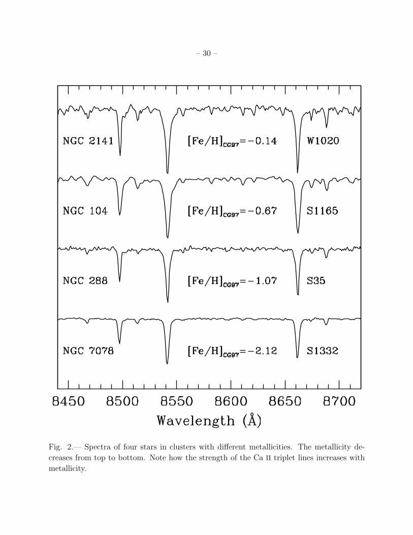
Examples of 4 stars with different metallicities are shown in Figure 2. Note how the

strength of the CaT lines increases with metallicity.

The radial velocity of each star has been calculated in order to reject cluster non-

members. We used the FXCOR task in IRAF, which performs the cross-correlation between

the target and template spectra of known radial velocity (Tonry & Davis 1979). We selected

between 8 and 10 template stars in each run that had very high S/N and covered a wide

range of radial velocities. The velocities were corrected to the heliocentric reference frame

within FXCOR. The final radial velocity for each star was obtained as the average of the

velocities obtained from each template, weighted by the width of correlation peaks.

In the case of observations with slit spectrographers, the star might not be exactly

positioned in the centre of the slit. This error means a velocity uncertainty given by ∆v =

c × ∆Θ × p/λ0, where: c is the light speed, p is the spectral resolution given in A arcsec−1;

λ0 is the wavelength of the lines (in this case ∼8600 A), and ∆Θ is the angular offset of the

star from the centre of the slit in arcsec. This effect has been described by Irwin & Tolstoy

(2002) and Harris & Zaritsky (2006). In our case, it may only be significant in the case

of the VLT observations. To estimate the offset in this case we used through-slit images

obtained at the beginning of the observation of each configuration, taken to check that the

stars were positioned in the slits. In this image we have measured the position of each stellar

centroid, which is compared with the position of the slit given in the header of the image.

The difference between both, ∆Θ, allows us to calculate the uncertainty in the measurement

of the radial velocity. This value changes from one star to another, the error being about 15

km s−1 on average.

– 7 –

The mean velocity for each cluster is listed in Table 4. Most of the values obtained

agree, within the uncertainties, with previous measurements from the literature, even in the

case of the clusters observed with the VLT, where the uncertainties are larger. In the case

of NGC 2141, we found a mean velocity similar to the value obtained by Cole et al. (2004).

Both values differ by 20 and 30 km s−1, respectively, from the value found by Friel et al.

(2002). For Collinder 110, no previous measurement of its radial velocity could be found in

the literature.

4. The Calcium Triplet

We are interested in obtaining metallicities from red giant stars, and within this group,

from the brightest ones, which are of spectral types K and M. The main features in the

infrared spectra of these stars are the CaT lines. But their spectra also contains other weak

atomic lines. The Fe I (8514.1, 8674.8, 8688.6 and 8824.2 A) and Ti I (8435.0 A) lines are

the most important. When within this range, we move to later spectral types, and hence to

cooler stars, molecular bands begin to appear that change the slope of the local continuum.

The main contribution are from the titanium oxide (TiO) bands, the strongest of which

are the triplet situated at 8432, 8442 and 8452 A and the doublet at 8859.6 and 8868.5 A.

There are other weaker bands at 8472, 8506, 8513, 8558 and 8569 A, near the bluest lines

of the CaT. There are also several vanadium oxide (VO) bands at 8521, 8538, 8574, 8597,

8605, 8624, 8649 and 8668 A. The strength of these features increases when the temperature

decreases, i.e. when we move to later spectral types. The presence of these bands complicates

the definition of the continuum, which makes it difficult to obtain the equivalent widths of

the CaT lines for stars with Teff ≤3500 K or (V-I)>2, in the most metal-rich clusters. The

description of the CaT region for other spectral types can be found in Cenarro et al. (2001).

4.1. Definition of Line and Continuum Bandpass Windows

In the literature we can find different prescriptions to measure the strength of the CaT

lines. The classical definition of a spectral index consists in establishing a central bandpass

covering a spectral feature and one or more bandpasses on both sides to trace the local

continuum reference level. Cenarro et al. (2001) have presented a description of the previous

CaT index definitions and a comparison among them. In Figure 3 we have plotted the

line and continuum bandpasses used in several reference works, Cenarro et al. (2001) (a),

Rutledge et al. (1997a) (b) and Armandroff & Zinn (1988) (c), over a metal-poor (left) and

a metal-rich (right) spectrum. The Armandroff & Zinn (1988) and Rutledge et al. (1997a)

– 8 –

indices were defined for relatively metal-poor RGB stars where the influence of the molecular

bands is not important. The index of Cenarro et al. (2001) was defined specifically to avoid

the presence of molecular bands. Also, from Figure 3, we can easily see that the wings

of the lines are larger than the line bandpasses defined by Armandroff & Zinn (1988) and

Rutledge et al. (1997a) in the case of the metal rich stars. Only the line bandpasses defined

by Cenarro et al. (2001) completely cover the line wings. Although we have selected the

bandpasses defined by Cenarro et al. (2001), which are listed in Table 5, the equivalent

width of the line will be measured in a different way, as described in the following section.

4.2. Equivalent widths

The next step is to measure the line flux from its equivalent width. The equivalent width

of a spectral line can be measured in different ways. One method is by numerical integration

of the observed spectra in a line band (e.g. Cenarro et al. 2001). However, in the wings of

the strongest lines of the CaT there are some weak lines, whose strength may change with

different stellar atmospheric parameters than the CaT lines. These lines must be excluded

when we measure the CaT equivalent width. The alternative (e.g. Rutledge et al. 1997a;

Cole et al. 2004) consists in fitting an empirical function to a line profile and calculating the

equivalent width from the integration of this fit. Many functions have been used to fit the

CaT line profiles, most commonly a Gaussian profile (e.g. Armandroff & Da Costa 1991).

However, as Cole et al. (2004) have shown, the Gaussian profile provides a good fit for weak-

line stars, but the fit is worse in strong-line stars, where the contribution of the non-Gaussian

wings of the CaT lines becomes substantial. We have to take this point into account because

the main contributors to the strength of the CaT lines are their wings, while the core is not

very sensitive to the atmosphere and stellar parameters (Erdelyi-Mendes & Barbuy 1991).

Rutledge et al. (1997a) fitted a Moffat function of exponent 2.5. As Pont et al. (2004) has

demonstrated, the behaviour of Moffat function of exponent 2.5 is similar to the Gaussian fit

for the weakest lines. However, neither provides a good fit to the strongest lines. Cole et al.

(2004) fitted the whole line profile with the sum of a Gaussian and a Lorentzian function,

which provides a better fit for the strongest lines and agrees with the single Gaussian fit

for the weakest lines (see Cole et al. 2004, for a further discussion). We have compared

the different functions in order to evaluate the quality of the fit in the whole range of line

strengths. We have chosen the sum of a Gaussian and a Lorentzian function because this

provides the best fit for the whole range of equivalent widths in this study. We have also

checked whether a simple Gaussian or Moffat function would produce a good fit in the case

of spectra obtained with lower resolution. Also in this case a Gaussian plus a Lorentzian

provides the best fit for strong-line stars.

– 9 –

A Gaussian plus a Lorentzian function has therefore been fitted to the line profiles with

a least-squares method, using the Levenberg-Marquardt algorithm. For the whole range of

equivalent widths covered in this work, the differences between the observed line and the

fit are negligible for stars with S/N ≥ 20. Stars with poorer S/N have been rejected. The

equivalent width of each line is the area limited by the fitted profile of the line and the

continuum level, defined as the linear fit to the mean values of the flux in each window

chosen to determine the continuum. Formal errors of the fit are estimated as the difference

between the equivalent width measurement for continuum displacements of ±(S/N)−1.

4.3. The CaT index

The equivalent widths of the three CaT lines are combined to form the global index

ΣCa (Armandroff & Da Costa 1991). Some authors excluded the weakest line at 8498 A on

the basis of its poor S/N (e.g. Suntzeff et al. 1993; Cole et al. 2000). Others have used all

three lines, either weighted (e.g. Rutledge et al. 1997a) or unweighted (e.g. Olszewski et al.

1991). As our spectra have high S/N ratios, we used the unweighted sum of the three lines,

ΣCa=W8498+W8542+W8662, and we calculate its error as the square root of the quadratic

sum of the errors of each line. As we have some stars in common with previous works, we can

compare the ΣCa calculated by us with values obtained in previous papers. Rutledge et al.

(1997a) compared their ΣCa with previous index definitions until 1997. Here, for simplic-

ity, we are only going to compare our index with three reference works. Stars in common

with Armandroff & Da Costa (1991); Rutledge et al. (1997a) and Cole et al. (2004) are plot-

ted in Figure 4. As mentioned before, the works of Armandroff & Da Costa (1991) and

Rutledge et al. (1997a) were focused on old and metal-poor stars. However, Olszewski et al.

(1991) and Suntzeff et al. (1993), using the same index as Armandroff & Da Costa (1991)

defined for globular cluster stars, measured the equivalent width of the CaT lines in stars of

two open clusters, M11 and M67, respectively. We are going to use these values to complete

the measurements of Armandroff & Da Costa (1991).

We find a quasilinear relation up to ΣCa ∼7 among the ΣCa values in this paper and

those obtained by Armandroff & Da Costa (1991) (see also Suntzeff et al. 1993). From this

point the relationship saturates: while our index increases by an additional ∆ΣCa ∼2, theirs

only increases by ∆ΣCa ∼1.5 (on their scale). We believe that the reason for this is that

they fitted the line profile by a Gaussian function which underestimates the contribution of

the line wings in strong lines (see Section ). Note also the zero-point difference between

both scales. The relation is not exactly one to one because they did not use the equivalent

width of the weakest CaT line. However, the slope close to one of the linear fit for the

– 10 –

metal-poor stars implies that the two indices are almost equivalent for these kind of stars.

The loss of linearity for strong-line stars partly explains why these authors found a nonlinear

relationship between the CaT index and metallicity, but, of course, the metallicity scale also

plays a role in this issue, as we discuss in Section 5.2. The linear fit for ΣCa≤7 (solid straight

line in top panel of Figure 4) is:

ΣCaAC91 = −0.88(±0.08) + 0.96(±0.01)ΣCaTP (1)

and the second order polynomial fit for the whole range of equivalent widths is

ΣCaAC91 = −1.10(±0.08) + 1.20(±0.03)ΣCaTP − 0.04(±0.01)ΣCa2TP (2)

In the case of Rutledge et al. (1997a), who only observed stars with [Fe/H] ≤ −0.7, we

find a linear correlation for the whole range of equivalent widths. In this case the slope is

less than one, meaning that their index is less sensitive to changes in the strength of the

CaT lines than ours. For the same star, our index is higher than the Rutledge et al. (1997a)

one. The linear fit is:

ΣCaR97 = −0.23(±0.06) + 0.78(±0.01)ΣCaTP . (3)

Finally, the correlation between Cole et al. (2004) index and ours is one to one (ΣCaTP −

ΣCaC04 = 0.009 ± 0.0007). As we used the same empirical function and index definition

of ΣCa as Cole et al. (2004), differences could only come from the definition of line and

continuum bandpasses. This means that, in the range of equivalent widths covered here,

both indices are equivalent. However, as the continuum in our index has been defined to

avoid the influence of TiO bands, we expect that our index would also behave well in stars

whose continuum is contaminated by TiO bands.

4.4. The reduced equivalent width

The next step is to relate the CaT index with metallicity. The strength of the absorption

lines mainly depends on the chemical abundance, stellar effective temperature (Teff) and

surface gravity (log g). Therefore, to relate the equivalent width of the CaT lines with

– 11 –

metallicity it is necessary to remove the Teff and log g dependence. Armandroff & Da Costa

(1991) and Olszewski et al. (1991) demonstrated that the cluster stars define a sequence

in the Luminosity–ΣCa plane, using luminosity measures from indicators like MI or (V-

VHB). These sequences are separated as a function of the cluster metallicity. The theoretical

explanation of this can be found in Pont et al. (2004), using Jørgensen et al. (1992) models,

which describe the behaviour of the CaT lines as a function of Teff , log g and metallicity.

It is necessary to study the morphology of the sequence defined by each cluster in

the Luminosity–ΣCa plane. From a theoretical point of view, the increment of luminos-

ity along the RGB comes with a drop in Teff and log g that decreases and increases the

strength of the lines, respectively. The result is a modest increment in ΣCa with luminosity

(δΣCa/δMI ∼0.5). Moreover, the models predict that ΣCa increases more rapidly with

luminosity in the upper part of the RGB (above the HB) than in the lower part. In other

words, the sequence defined by each cluster might not be linear and might be best described

adding a quadratic component. The Jørgensen et al. (1992) models also predict that ΣCa

increases more rapidly when log g decreases, or when the luminosity increases, for the more

metal-rich clusters than for the more metal-poor ones. Therefore, the linear and quadratic

terms, which characterize the sequence defined for each cluster in the luminosity–ΣCa plane,

increase with metallicity, as can be seen in Figure 15 of Pont et al. (2004).

Observationally, the variation in ΣCa with metallicity has traditionally been studied

from (V-VHB), which removes any dependence on distance and reddening (e.g. Armandroff & Da Costa

1991; Rutledge et al. 1997a; Cole et al. 2004). In this context, it is found that clusters define

linear sequences in the (V-VHB)–ΣCa plane, where the reduced equivalent width, W ′, is

defined as ΣCa = W ′

HB+β(V-VHB). Rutledge et al. (1997a) found that the slopes of these

sequences were the same for all clusters in their sample, independently of their metallicity.

Therefore only W ′

HB changes from one cluster to another, and its variation is directly related

to metallicity. Other studies have reached the same conclusion using open and globular clus-

ters (e.g. Olszewski et al. 1991). Pont et al. (2004) (see also Armandroff & Da Costa 1991)

have demonstrated that this also occurs in the MV -ΣCa and MI-ΣCa planes. However, no

studies have observed the theoretical predictions that cluster sequences are not exactly linear

with luminosity, or that their shape depends on metallicity.

The main objective of this study is to apply the relationships obtained to derive metal-

licities of individual stars in Local Group galaxies, which in general have had multiple star

formation epochs and do not always have a well defined HB (e.g. LMC: Carrera et al. 2007;

SMC: Noel et al. 2007; Leo A: Cole et al. 2007). For example, the Magellanic Clouds do

not have a measurable HB in the CMD, and in studies which define the reduced equivalent

width as a function of (V − VHB) ((e.g. Cole et al. 2005)), the HB position has been taken

– 12 –

as that of the red-clump. However, in the Magellanic Clouds, the position of the red-clump

is about 0.4 magnitudes brighter than the HB. This only implies underestimating the metal-

licity by ≃ 0.15 dex, which is similar to the uncertainty on the metallicity determination

itself. Distances to Local Group galaxies are in general determined with an accuracy greater

than 0.4 mag., and so, even if the error on the derived metallicity due to the uncertainty in

the position of the HB is not large, it can be minimized by defining the reduced equivalent

width as a function of absolute magnitude. This point is also important in the case of open

clusters, which hardly ever have a HB or, if they do, it is usually not well defined. For this

reason, like Pont et al. (2004), we redefine W ′ as the value of ΣCa at MV =0 (hereafter W ′

V )

or MI=0 (hereafter W ′

I).

First we will study in detail the morphology of the cluster sequences in the Luminosity–

ΣCa plane. As discussed above, from a theoretical point of view, we expect that these

sequences are not exactly linear. We have observed stars along the RGB in 5 clusters

covering the whole metallicity range. In Figure 5 we have plotted stars observed in these

clusters in the MV –ΣCa and MI–ΣCa planes. These stars have magnitudes in the ranges

-2≤MV ≤2 and -3≤MI ≤2 (or -2.3≤V-VHB ≤1.8). These ranges contain both stars brighter

and fainter than previous works (e.g. Rutledge et al. 1997a; Cole et al. 2004). Note that the

strength of the CaT lines increases more rapidly in the upper part of the RGB, as predicted

by Pont et al. (2004) using Jørgensen et al. (1992) models. These observations can be used

to obtain a new relationship between ΣCa, absolute magnitude and metallicity valid for

all the stars in the RGB, that takes into account the curvature in the Luminosity–ΣCa

plane. The sequence of each cluster has been fitted with a quadratic function such that

ΣCa=W ′

V,RGB+βMV +γM2V . We plotted the result when the stars of each cluster are fitted

independently in Figure 5. The coefficients of the fit are shown in Table 6. From this, it

seems that β tends to increase with metallicity, as predicted theoretically. In the case of γ

this increment is not observed, i.e. its variation does not show a significant dependence on

metallicity, except for the most metal-rich cluster, which also has a large uncertainty.

Using the Jørgensen et al. (1992) empirical relations and the BaSTI stellar evolution

models (Pietrinferni et al. 2004), we have calculated theoretical sequences for clusters with

[Fe/H] ≥ −1, which are plotted in Figure 6 as dashed lines. These models were obtained for

[Fe/H] = +0.5, 0, −0.5 and −1, while the clusters metallicities are [Fe/H] =+0.47, −0.14,

−0.67 and −1.07 respectively. Jørgensen et al. (1992) did not compute relationships for

more metal-poor clusters. We used BaSTI isochrones with metallicities of +0.32, −0.28,

−0.58 and −0.98, respectively, in order to estimate Teff and log g along the RGB. The

Jørgensen et al. (1992) relationships were calculated for the two strongest CaT lines. To

compare the theoretical predictions with the observational sequences we computed, using

our own data, an empirical relation between ΣCa8442+8662 obtained from these two lines

– 13 –

and the ΣCa used in this work, computed from the three CaT lines. We found is ΣCa =

0.13 + 1.21ΣCa8442+8662. Applying this correction, we find that the theoretical and observed

cluster sequences still do not match. There is a zero-point that changes from one cluster to

another, which is not surprising because the cluster metallicities are not exactly the same

as those used to compute the theoretical relationships. Therefore, the theoretical sequences

have been shifted in order to superimpose them on the cluster ones. It can be seen that

models do not exactly reproduce the behaviour of the observed cluster sequences. However,

the prediction that the shape changes from the metal-poor clusters to the metal-rich ones is

observed, although, as was mentioned before, these variations are similar to the uncertainties.

We can simplify the problem if we assume that all clusters have the same tendency, i.e.

if we calculate a single slope and quadratic term for the whole sample. So only the zero

point changes among clusters. To obtain these coefficients, we have performed an iterative

least-squares fit as described by Rutledge et al. (1997a). From a set of reference values, we

obtained the quadratic and linear terms of the fit in iterative steps, until they converged

to a single value within the errors and allow only the zero point to change among clusters.

The values are: βV = −0.647 ± 0.005 and γV = 0.085 ± 0.006. In the same way, for MI

we obtained βI = −0.618 ± 0.005 and γI = 0.046 ± 0.001. In Figure 6 we have plotted

the individual fit for each cluster (solid line) and that when the linear and quadratic terms

do not change among clusters (dashed lines). In both cases, the dotted lines represent the

region where there are no cluster stars and the fits have therefore been extrapolated. As we

can see in Figure 6, in the magnitude interval covered by cluster stars, both fits are similar

and give very similar values of W ′ within the uncertainties. For example, for NGC 7078,

where the discrepancy is larger, we obtained 2.79 ± 0.06 and 2.79 ± 0.01 in V ; and 2.64

± 0.08 and 2.31 ± 0.01 in I, when the linear and quadratic terms change among clusters

or they are fixed, respectively. Larger differences between both fits are found in the regions

where the relationships are extrapolated.

Moreover, in our case we are interested in measuring the strength of the CaT lines

in galaxies where we can observe only the upper part of the RGB with a good S/N. The

quadratic behaviour of the cluster sequences in the Luminosity–ΣCa plane is not significant

when we observe stars with MI ≤0 only (or MV ≤1.25; this magnitude limit has been selected

in order to sample in both filters the same number of stars in each cluster). For example,

when we repeat the previous procedure, but only for stars with MV ≤ 1.25, we find that the

quadratic term is γV = 0.004 ± 0.003, which is negligible within the uncertainty. In the same

way, when we only observe stars with MV ≥ 1.25 we obtain a similar result: γV = 0.002±0.01.

The same happens in the MI–ΣCa plane, but here the quadratic terms are even smaller.

According to this, the cluster sequence can be considered linear above and below MV =1.25

and MI=0, and we can fit it as ΣCa = W ′

V +βV MV or ΣCa = W ′

I +βIMI on each side of this

– 14 –

point. Following the same iterative procedure as in the case of the quadratic fit, we calculated

the values of the slope β for MV ≤ 1.25 and for MI ≤ 0, obtaining βV = −0.74 ± 0.01 and

βI = −0.60± 0.01, respectively. The linear fits for MV ≤1.25 and MI ≤ 0 are represented in

Figure 6, by dotted–dashed lines. In all cases, within the ranges covered by the cluster stars,

the linear fit to the bright stars is equivalent, within the uncertainties, to the quadratic ones.

Finally, for clusters where we have observed a wide range of magnitudes we find that

the slope (β) increases, although within the uncertainties, with metallicity. We might check

this point using now all clusters in our sample. A total of 27 clusters in I and 29 in V

have stars brighter than MI=0 and MV = 1.25. We have fitted the sequence to each cluster

independently in the linear form ΣCa = W ′

V,I + βV,IMV,I . The values obtained from the

slope have been plotted against W ′, which is directly correlated with metallicity, for each

cluster in Figure 7. From this figure it is seen that there is no significant relation between

the cluster slope and W ′ (or [Fe/H]). Therefore, from here on, we consider the slope of the

fit to be the same for the whole range of [Fe/H] and, hence, for all objects.

In summary, as we are specially interested in obtaining metallicities for stars in the

upper part of the RGB with the CaT, where the quadratic term is not significant and the

slope can be fixed independently of metallicity, we are going to use a linear fit with a single

slope for the calibration using the whole cluster sample. This is what has been done in all

previous calibrations of the CaT.

Figures 8 and 9 represent the clusters in our sample in the MV –ΣCa and MI–ΣCa

planes respectively, together with the linear fit to each of them. Using the same procedure

as in the case of the quadratic fit discussed above, we have obtained βV = −0.677 ± 0.004

and βI = −0.611 ± 0.002A mag−1 in the MV –ΣCa and MI–ΣCa planes, respectively. The

value found in the MI–ΣCa plane is slightly larger than that obtained by Pont et al. (2004),

βI = −0.48±0.02 A mag−1. Although these authors used a different method to calculate the

metallicity (they fitted each cluster individually and obtained the mean of the slopes of all

of them), this is not the reason for the discrepancy because if we follow the same procedure

with our own data, again we find βI = −0.61. There are no previous determinations of βV .

The values obtained for W ′

V and W ′

I are listed in Table 7.

5. The Ca II Triplet metallicity scale

An important point in this study is the reference metallicities. It would be ideal to use

the same metallicity scale for both open and globular clusters, and that this would have

been obtained from high-resolution spectroscopy. In the literature we can find two globular

– 15 –

cluster metallicity scales obtained from high resolution spectroscopy: Carretta & Gratton

(1997, hereafter CG97) and Kraft & Ivans (2003, hereafter KI03). There is a third metallicity

scale obtained from low-resolution data: Zinn & West (1984, hereafter ZW84). There are

systematic differences among these three scales, but there is no reason to prefer any particular

one of them. For this reason, here we are going to study the behaviour of the CaT lines with

metallicity in these three scales. Lamentably, there is not a homogeneous metallicity scale

obtained from high-resolution spectroscopy for open clusters. However, the metallicities of

some of them have been obtained directly in the CG97 scale by some authors: NGC 6819

(Bragaglia et al. 2001); NGC 2506 (Carretta et al. 2004); NGC 6791 (Gratton et al. 2006)

and Berkeley 32 (Sestito et al. 2006). These metallicities were obtained using Fe I and Fe II

lines. For the other 8 open clusters in our sample there are also metallicities obtained from

high-resolution spectroscopy in RGB stars and using Fe I and Fe II lines in a similar way to

CG97. Even though some discrepancies could exist because the procedures are not exactly

the same, we are considering these metallicities also to be on the CG97 scale. The reference

values in this scale are listed in column 2 of Table 1 and the sources for each of them are

listed in column 3. The reference metallicities in the ZW84 and KI03 are listed in columns

4 and 5 respectively. In both cases, we have used only values obtained directly by these

authors.

5.1. Calibration in the CG97 metallicity scale

Figures 10 and 11 show the run of W ′

V and W ′

I with metallicity. In most cases, the

errors are smaller than the size of the points. The circles indicate clusters younger than

4 Gyr. The solid line shows the best fit to the data. The dashed lines represent the 90%

confidence level. Note that in both cases there is a linear correlation. The bottom panels

show the residuals of the linear fit. We have used 22 clusters for the calibration in V and 20

for that in I. There are three clusters that differ from the fit by more than 0.2 dex in both

filters. These clusters are NGC 2420, NGC 2506 and Berkeley 32. They have been excluded

from the analysis. In the case of NGC 2420, only 6 stars in V and 4 in I are radial velocity

members. This, together with a relatively large uncertainty in its metallicity (Gratton 2000),

contributes to its large error bar. In the case of NGC 2506 and Berkeley 32, there are only 3

and 4 stars respectively with membership confirmed by their radial velocities. Thus, slight

differences in the ΣCa value of one of them could change the derived W ′ significantly. Two

of the three very deviant clusters (NGC 2420 and NGC 2506) have ages less than 4 Gyrs,

but 5 other young clusters fit the mean relationships in Figures 10 and 11 to better than 0.2

dex. We doubt therefore that cluster age is the major cause of the large deviations.

– 16 –

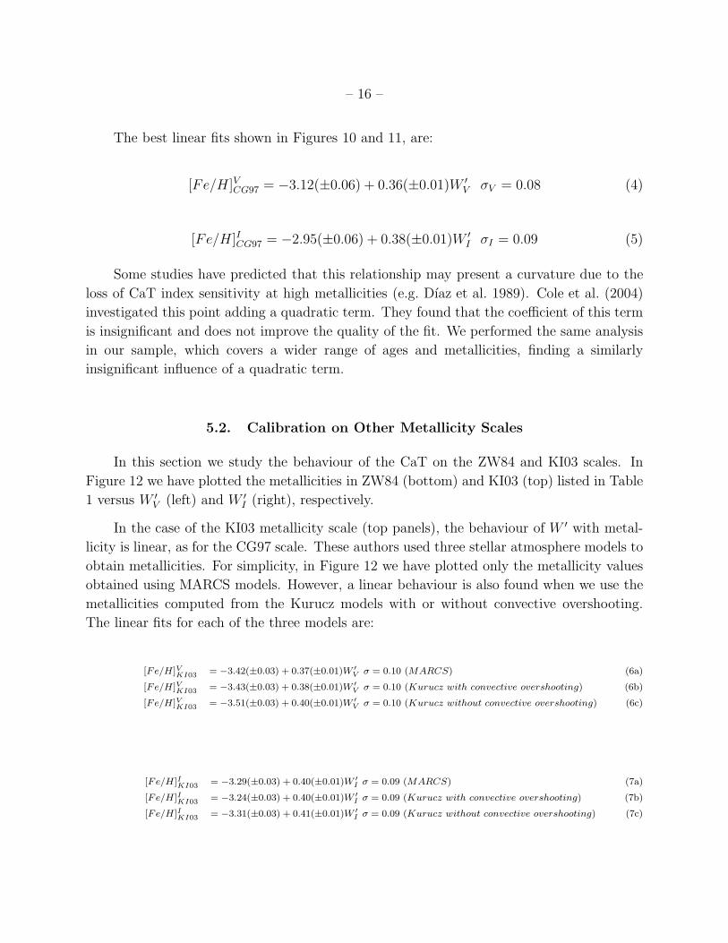
The best linear fits shown in Figures 10 and 11, are:

[Fe/H]VCG97 = −3.12(±0.06) + 0.36(±0.01)W ′

V σV = 0.08 (4)

[Fe/H]ICG97 = −2.95(±0.06) + 0.38(±0.01)W ′

I σI = 0.09 (5)

Some studies have predicted that this relationship may present a curvature due to the

loss of CaT index sensitivity at high metallicities (e.g. Dıaz et al. 1989). Cole et al. (2004)

investigated this point adding a quadratic term. They found that the coefficient of this term

is insignificant and does not improve the quality of the fit. We performed the same analysis

in our sample, which covers a wider range of ages and metallicities, finding a similarly

insignificant influence of a quadratic term.

5.2. Calibration on Other Metallicity Scales

In this section we study the behaviour of the CaT on the ZW84 and KI03 scales. In

Figure 12 we have plotted the metallicities in ZW84 (bottom) and KI03 (top) listed in Table

1 versus W ′

V (left) and W ′

I (right), respectively.

In the case of the KI03 metallicity scale (top panels), the behaviour of W ′ with metal-

licity is linear, as for the CG97 scale. These authors used three stellar atmosphere models to

obtain metallicities. For simplicity, in Figure 12 we have plotted only the metallicity values

obtained using MARCS models. However, a linear behaviour is also found when we use the

metallicities computed from the Kurucz models with or without convective overshooting.

The linear fits for each of the three models are:

[Fe/H]VKI03

= −3.42(±0.03) + 0.37(±0.01)W ′

Vσ = 0.10 (MARCS) (6a)

[Fe/H]VKI03

= −3.43(±0.03) + 0.38(±0.01)W ′

V σ = 0.10 (Kurucz with convective overshooting) (6b)

[Fe/H]VKI03

= −3.51(±0.03) + 0.40(±0.01)W ′

V σ = 0.10 (Kurucz without convective overshooting) (6c)

[Fe/H]IKI03

= −3.29(±0.03) + 0.40(±0.01)W ′

Iσ = 0.09 (MARCS) (7a)

[Fe/H]IKI03

= −3.24(±0.03) + 0.40(±0.01)W ′

Iσ = 0.09 (Kurucz with convective overshooting) (7b)

[Fe/H]IKI03

= −3.31(±0.03) + 0.41(±0.01)W ′

I σ = 0.09 (Kurucz without convective overshooting) (7c)

– 17 –

Differences between metallicities derived with the MARCS model and the models of

Kurucz with or without overshooting are negligible.

This linear behaviour is not surprising because, as KI03 demonstrated, their metallicities

are linearly correlated with the CG97 values, which are, at the same time, linearly correlated

with our W ′. However, the metallicities calculated by KI03 are systematically lower than

the CG97 ones. KI03 studied this point and concluded that the difference could be explained

because they used different Teff and log g values, as well as different atmosphere models. The

combination of all these can easily introduce systematic differences in the globular cluster

abundance scales.

In the case of ZW84, we have found that the data are best fitted by a second-degree

polynomial (solid line):

[Fe/H]VZW84 = −1.98(±0.07) − 0.18(±0.02)W ′

V + 0.05(±0.01)W ′2V σV = 0.10 (8a)

[Fe/H]IZW84 = −2.07(±0.07) − 0.12(±0.03)W ′

I + 0.05(±0.01)W ′2I σI = 0.09 (8b)

In Section 4.3, we discussed several previous definitions and measurement procedures

of the CaT lines, and noted the loss of sensitivity to the CaT lines strength in some cases

(e.g. Armandroff and Da Costa 1991) which also found a non-linear relationship between the

CaT index and metallicity. We mentioned that this non-linearity was probably the result

of the combination of a non-accurate measurement of the CaT on strong-line stars and the

particular metallicity scale in use. In order to assess the relative importance each factor, we

will now compare the effects on the derived abundances of alternatively i) assuming a linear

relationship between W ′ and metallicity on the ZW84 metallicity scale and ii) adopting

a Gaussian to fit the CaT lines, which provides a poorer fit. When a linear relationship

between W ′

I and [Fe/H]ZW84 is assumed, the derived metallicity of a strong-line star, W ′

I=8.5,

is underestimated in 0.3 dex. In the case of a weak-line star, W ′

I=2, again the metallicity is

underestimated in 0.2 dex. Similar results are obtained when lines are not properly fitted.

For example, as we saw in Section 4.3, Armandroff & Da Costa (1991) fitted the line profile

with a Gaussian, resulting in that their index saturated for strong-line stars. The relation

between the reduced equivalent width obtained from their index and metallicities in the

CG97 scale is a second-degree polynomial. If we then assume a linear relationship between

this index and [Fe/H]CG97 for a strong-line star, its metallicity would be underestimated in

0.3 dex. Similar result is obtained for a weak-line star. We conclude therefore, that the

effects on the derived metallicity due to a poor fit to the line or the non-linearity of the

metallicity scale are comparable.

– 18 –

5.3. The role of Age in the W ′

V (W ′

I) versus [Fe/H] relationship

Pont et al. (2004) investigated the influence of age in the W ′

V (W ′

I) versus [Fe/H] re-

lationship from a theoretical point of view. They used the theoretical calculations of CaT

equivalent widths for different values of log g, Teff and metallicity calculated by Jørgensen et al.

(1992) together with the Padova stellar evolution models (Girardi et al. 2002). They con-

cluded that the variation of W ′ with age for a fixed metallicity would be negligible for

clusters older than 4 Gyr. However, this was not the case for the younger clusters. This is

observed clearly in Figure 15 by Pont et al. (2004). For a given metallicity, the sequences

in the MV –ΣCa and MI -ΣCa planes are separated as a function of their ages for clusters

younger than ∼4 Gyr. According to this calculation, for the same metallicity, W ′ decreases

with age. Thus, metallicities for clusters younger than 4 Gyr, calculated from calibrations

computed from old stars, will be underestimated. This age dependence is more important

in the MV –ΣCa plane than in the MI–ΣCa one. This means that W ′

I would be less sensitive

to age than W ′

V .

Using the Jørgensen et al. (1992) models and the BaSTI stellar evolution models (Pietrinferni et al.

2004), we have estimated the expected W ′ differences as a function of age. From these cal-

culations, for two clusters with the same metallicity and age 10.5 and 0.6 Gyr respectively,

the youngest cluster W ′

V would be approximately 0.7 A lower than that of the oldest one.

This implies that the metallicity obtained for young clusters using this calibration would be

0.25 dex more metal-poor than the actual metallicity. In the case of W ′

I , the difference would

be 0.4 A, so the metallicity obtained for young clusters would be 0.15 dex more metal-poor

than the actual one. As we can see in Figure 15 by Pont et al. (2004), the difference would

be similar for different metallicities.

From our data, we confirm that the influence of age is weak. In Figure 13 we plot

W ′

I versus age for clusters with −0.17 ≤ [Fe/H]CG97 ≤ +0.07. We have selected this range

because it contains clusters with a wide range of ages and is small enough for the metallicity

differences to be within the uncertainties. We can see that clusters with ages younger than

5 Gyr (NGC 2141, NGC 2682, NGC 6819 and NGC 7789) have similar W ′

I than the oldest

one (NGC 6528). There are only two clusters that deviate widely from the behaviour of the

others. One of these is the youngest cluster, NGC 6705, which has a larger W ′

I than the oldest

clusters. This is contrary to the theoretical prediction that it should be smaller. However,

we have to take into account that differences of 0.5 A in W ′

I mean differences of ∼0.1 dex

in [Fe/H]. So the observed variations are similar to the uncertainty in the determination

of [Fe/H]. Our data are not accurate enough to detect the influence of age because the

uncertainty in the metallicity determination of clusters is similar to the expected variations

due to age.

– 19 –

5.4. The influence of [Ca/Fe] abundance

The CaT has traditionally been used to infer Iron abundances from Ca lines, and we

also do so in this paper. But, the CaT lines strength should also be sensitive to the Ca

abundances. In fact, the relationships obtained in this work and those found in the literature

have been obtained assuming implicitly the specific relationship between Ca and Fe followed

by clusters used in the calibration (see Figure 14 for the relationship of the clusters used

in this work). Using these relationships to derive Fe abundances in stellar systems with a

different chemical evolution than the Milky Way, reflected in the calibrating cluster sample,

could give wrong results.

In general, the relationship between the reduced equivalent width of an atomic line and

the chemical abundance of the corresponding element is described by the curve of growth.

This is only linear for very weak and unsaturated lines. This is not the case for the CaT.

As we can find the [Ca/H] ratio for most of the clusters in our sample from the literature,

in Figure 14 we have plotted W ′

V and W ′

I versus [Ca/H]. The relationship between both is

equivalent to the curve of growth. The relations obtained are:

[Ca/H]V = −2.51(±0.08) + 0.30(±0.01)W ′

V σ = 0.11 (9)

[Ca/H]I = −2.36(±0.08) + 0.31(±0.01)W ′

I σ = 0.11 (10)

As in the case of the [Fe/H] relationship, we obtain a linear dependence. However, note

that in this case the errors of the fit are larger. This may be related to the inhomogeneity

of the [Ca/H] abundances, which were obtained from different sources.

In any case, even though [Ca/H] changes linearly with W ′, [Fe/H] does not have to

do likewise. However, as we see in Figures 10 and 11, the relationship between [Fe/H] and

W ′ is also linear. On the other hand, since the [Ca/H] and [Ca/Fe] abundances are related

according to [Fe/H] = [Ca/H] − [Ca/Fe], we can expect that [Ca/Fe] also changes linearly

with W ′ (and with [Fe/H]), if the relation with [Ca/H] is linear. In fact, in Figure 14 we

can check that this is the case over the whole range of [Fe/H] except for the most metal-

poor clusters. Note however that the linear behaviour of W ′ with [Ca/H] and [Ca/Fe] is a

characteristic of our particular sample, but this would not have to be the rule.

The problem of the relation between the CaT, [Ca/H] and [Fe/H] has been addressed

by Idiart et al. (1997) from an empirical point of view. For their sample of late-type stars

(G and K), they found that the dominant stellar parameter controlling the behaviour of

the CaT lines is metallicity, and contrary to what would be expected, the [Ca/Fe] ratio has

practically no effect on the CaT index. However, all the stars in their sample follow the

– 20 –

same relationship between Ca and Fe, so they cannot check in a general way the influence

of the [Ca/Fe] ratio.

To properly investigate the influence of the [Ca/Fe] ratio, it is necessary to have objects

with the same metallicities and different [Ca/H] ratios. In our sample, most of the metal-

poor clusters have high α-element abundances relative to Fe, as is the case for Ca. On the

other hand, open clusters are metal-rich and have low α-element abundances. To study the

influence of the [Ca/Fe] ratio on the CaT calibration as a function of metallicity it would

be necessary to include metal-rich objects with high α-element abundances (i.e. stars in the

Milky Way bulge) and metal-poor objects with low α-element abundances (i.e. perhaps stars

in dwarf galaxies). This sort of work would need a huge observational effort, which explains

why it has not been done until now.

6. Derived cluster Metallicities

We will use the relationships derived in previous sections to estimate the metallicities

in the three observed clusters without previous determinations. In fact, we have observed

Collinder 110, a poorly studied cluster with no previous spectroscopic metallicity deter-

minations. For Berkeley 39, only Friel et al. (2002) have determined its metallicity from

low-resolution spectroscopy. The sequences of these clusters in the MI–ΣCa plane have been

plotted in Figure 16.

6.1. Berkeley 39

The first colour–magnitude diagram of this open cluster was published by Kaluzny & Richtler

(1989). These authors calculated a distance modulus of (m-M)V = 13.4 and E(B−V ) = 0.12.

These values agree with the determinations of Carraro et al. (1994), who also used colour–

magnitude diagrams. The age of this cluster is 7 ± 1 Gyr (Salaris et al. 2004).

There are few determinations of its metallicity. From photometric data Twarog et al.

(1997) estimated [Fe/H] = −0.18±0.03, while from low-resolution spectroscopy, Friel & Janes

(1993) and Friel et al. (2002) obtained [Fe/H] = −0.32 ± 0.08 and [Fe/H] = −0.26 ± 0.09

respectively. In our case we have 10 RGB stars which are cluster members from their radial

velocity, although only 5 stars have I magnitudes available. Moreover, only 2 are brighter

than MI = 0; nevertheless, the other 3 have magnitudes close to this value. We therefore

used all 5 stars. From Equation 5 we obtain [Fe/H]CG97 = −0.14 ± 0.02. We have used

the relationship as a function of MI because the RGB is more resolved in the I filter, and

– 21 –

this relation is less sensitive to age. The calculated value is slightly more metal-rich than

previous spectroscopic determinations. In the KI03 and ZW84 scales we obtain [Fe/H]KI03

= −0.33± 0.14 and [Fe/H]ZW84 = −0.23± 0.25 respectively from Equations 7a and 8b. On

these scales we have no young and/or metal-rich reference clusters, but, as we have checked

before, the influence of age is weak.

We have also calculated the radial velocity of this cluster. We find Vr = 59 ±5 km s−1,

which is similar to values found previously (i.e. Friel et al. 2002, Vr=55±7 Km s−1).

6.2. Trumpler 5

Trumpler 5, also named Collinder 105, is also a poorly studied cluster, even though it

was discovered about 75 yr ago. It is located towards the Galactic anticentre in a rich star

field in Monoceros, and in a region of variable interstellar reddening. This has complicated

the studies of this cluster. In fact, only photometric studies could be found in the literature

(e.g. Kaluzny 1998; Kim & Sung 2003; Piatti et al. 2004) with the exception of the work by

Cole et al. (2004), who observed the CaT lines in a few stars on the RGB and derived the

first spectroscopic determination of its metallicity. The distance modulus and reddening of

this cluster have been derived from isochrone fitting. Most studies converge on a reddening

of E(B − V ) = 0.6 (e.g. Kim & Sung 2003). However, this does not happen in the case

of the distance, where the values lie between (m-M)0 = 12.25 (Piatti et al. 2004) and 12.64

(Kim & Sung 2003), corresponding to a distance from the Sun of 2.4 or 3.4 kpc respectively.

Also, the age and metallicity have traditionally been estimated from isochrones. The age of

this cluster is estimated between 2.4 ± 0.2 (Kim & Sung 2003) and 5.0 ± 05 Gyr (Piatti et al.

2004), while the derived metallicity is [Fe/H] = −0.30 ± 0.15 dex (e.g. Kim & Sung 2003;

Piatti et al. 2004).

We have observed 21 stars in the field of Trumpler 5, 17 of which are radial velocity

members (Table 3). The metallicity derived from Equation 5 is [Fe/H]CG97 = −0.36 ±

0.05, which is more metal-rich (although within the error) than the previous spectroscopic

determination, [Fe/H] = −0.56±0.11, by Cole et al. (2004). The alternative determination of

the metallicity on the KI03 and ZW84 scales gives [Fe/H]KI03 = −0.56±0.09 and [Fe/H]ZW84

= −0.48 ± 0.20 respectively from Equations 7a and 8b

From our data we have also calculated the radial velocity of this cluster, Vr = 44 ± 10

km s−1, which is similar to the value derived by Cole et al. (2004, Vr=54±5 Km s−1).

– 22 –

6.3. Collinder 110

Collinder 110 is a poorly populated cluster, even less studied than Trumpler 5. Only

two photometric studies can be found in the literature for the last three decades. Using

synthetic colour–magnitude diagrams, Bragaglia & Tosi (2003) have estimated a reddening

of 0.38 ≤ E(B − V ) ≤ 0.45 and distance modulus (m-M)0 between 11.8 and 11.9. From

these values they derived an age between 1.1 and 1.5 Gyr. Similar values were found by

Dawson & Ianna (1998). There are no metallicity determinations for this cluster in the

literature. Bragaglia & Tosi (2003) tried to derive the metallicity of this cluster from different

stellar evolution models, but concluded that the final result vary widely depending on the

models.

The metallicity derived from Equation 5 is [Fe/H]CG97 = −0.01± 0.07. If we use Equa-

tions 7a and 8b on KI03 and ZW84 metallicity scales we find [Fe/H]KI03 = −0.19±0.21 and

[Fe/H]ZW84 = 0.00 ± 0.30. From our data we can also provide the first determination of its

radial velocity, Vr = 45 ± 8 km sec−1.

7. Summary

We have observed the CaT lines in RGB stars in a sample of 29 clusters of the Milky

Way. This sample covers an age range of (13 ≤ Age/Gyr ≤ 0.25) and metallicity range of

(−2.2 ≤ [Fe/H] ≤ +0.47). These are the widest ranges of ages and metallicities in which

the behaviour of the CaT has been investigated in a homogeneous way until now. We have

obtained relationships between the CaT equivalent widths and metallicities on the scales of

Zinn & West (1984), Carretta & Gratton (1997) and Kraft & Ivans (2003). The influence of

other parameters, such as age and [Ca/Fe] ratio, has been investigated. Moreover, for the

first time, the behaviour of the CaT lines as a function of luminosity along the RGB has

been studied for the whole range of metallicities in our sample.

The main results of this work are:

• Theoretically, it has been predicted that the sequences of clusters in the Luminosity–

ΣCa plane may not be linear, and that the slope should change with metallicity. In this

article we have demonstrated that the nonlinear tendency and the change of the slope

can be (marginally) detected if a wide range of magnitudes in the RGB is observed.

• However, this behaviour is not significant if only the usual range of 3-4 magnitudes

below the tip of the RGB is observed. For this reason, for stars with MV ≤ 1.25 or

– 23 –

MI ≤ 0, we have considered that the sequences of the clusters in the MV –ΣCa and

MI–ΣCa planes are linear, and share a common slope, independently of metallicity.

• We have obtained relationships between the reduced equivalent width (W ′

V and W ′

I) and

metallicity on the Zinn & West (1984), Carretta & Gratton (1997) and Kraft & Ivans

(2003) scales. While on the Carretta & Gratton (1997) and Kraft & Ivans (2003)

scales these relationships are linear, in the case of the Zinn & West (1984) scale, it

is quadratic.

• Theory predicts that the relationship between the CaT line equivalent widths and

metallicity might be dependent on age, mainly for clusters younger than 4 Gyr. We

have studied the influence of age and found that the expected differences due to age

are similar to the metallicity resolution of our work.

• We have also investigated the influence of Ca abundances on the relationships between

W ′

V and W ′

I and metallicity. We have found that [Ca/H] also changes linearly with

W ′

V and W ′

I .

• Finally, the relationships obtained have been used to compute the metallicity of 3

clusters in our sample: Berkeley 39, Trumpler 5 and Collinder 110. For the last one,

there are no previous determinations of its metallicity in the literature.

We warmly thank Dr. Antonio Aparicio for many fruitful discussions on this paper, and

a careful and critical reading of the manuscript. Extensive use was made of the WEBDA

database, maintained at the university of Geneva, Switzerland. C.G. and R.C. acknowl-

edge the support from the Spanish Ministry of Science and Technology (Plan Nacional de

Investigacion Cientıfica, Desarrollo, e Investigacion Tecnologica, AYA2004-06343). E. P. ac-

knowledge support from the Italian MIUR (Ministero dell’Universita e della Ricerca) under

PRIN 2003029437 entitled ”Continuities and discontinuites in the formation of the galaxy”.

R.Z. acknowledges the support of the NSF under grant AST05-07364.

Facilities: VLT(FORS2), CAHA2.2m(CAFOS), CTIO4m(HYDRA), WHT(WYFFOS),

WHT(ISIS), INT(IDS).

REFERENCES

Alcaino, G., 1974, A&AS, 13, 55

Alcaino, G., & Liller, W. 1980, AJ, 96, 92

– 24 –

Alcaino, G., & Liller, W. 1986, A&A, 161, 61

Armandroff, T. E., & Zinn, R. 1988, AJ, 96, 92

Armandroff, T. E. & Da Costa, G. S. 1991, AJ, 101, 1329

Bragaglia, A., Carretta, E., Gratton, R. G., Tosi, M., Bonanno, G., Bruno, P., Calı, A.,

Claudi, R., Cosentino, R., Desidera, S., Farisato, G., Rebeschini, M. & Scuderi, S.

2001, AJ, 121, 327

Bragaglia, A., & Tosi, M. 2003, MNRAS, 343, 306

Brown, J. A., Wallerstain, G., & Gonzalez, G. 1999, AJ, 118, 1245

Buonanno, R., Buscema, G., Corsi, C. E., Iannicola, M. & Fusi Pecci, F. 1983, A&AS, 51,

83

Burkhead, M. S., Burgess, R. D., & Haisch, B. M. 1972, AJ, 77, 661

Carraro, G. Chiosi, C., Bressan, A., & Bertelli, G. 1994, A&AS, 103, 375

Carraro, G. Hassan, S. M., Ortolani, S., & Vallerini, A. 2001, A&A, 372, 879

Carrera, R., Gallart, C., Hardy, E., Aparicio, A., Zinn, R. 2007, AJ, In preparation

Carretta, E., & Gratton, R. G. 1997, A&AS, 121, 95 (CG97)

Carretta, E., Cohen, J. G., Gratton, R. G. & Behr, B. B. 2001, AJ, 122, 1469

Carretta, E., Bragaglia, A., Gratton, R. G. & Tosi, M. 2004, A&A, 422, 951

Cenarro, A. J., Cardiel, N., Gorgas, J., Peletier, R. F., Vazdekis, A., & Prada, F. 2001,

MNRAS, 326, 959

Cole, A. A., Smecker-Hane, T. A., & Gallagher III, J. S. 2000, AJ, 120, 1808

Cole, A. A., Smecker-Hane, T. A., Tolstoy, E., Bosler, T. L., & Gallagher III, J. S. 2004,

MNRAS, 347, 367

Cole, A. A., Tolstoy, E., Gallagher III, J. S., & Smecker-Hane, T. A., 2005, AJ, 129, 1465

Dıaz, A. I., Terlevich, E. & Terlevich R. 1989, MNRAS, 239, 325

Dawson, D. W., & Ianna, P. A. 1998, AJ, 115, 1076

Erdelyi-Mendes, M., & Barbuy, B. 1991, A&A, 241, 176

– 25 –

Feltzing, S., & Johnson, R. A. 2002, A&A, 385, 67

Friel, E. D. 1989, PASP, 101, 244

Friel, E. D., & Janes, K. A. 1993, A&A, 267, 75

Friel, E. D., Janes, K. A., Tavarez, M., Scott, J., Katsanis, R., Lotz, J., Hong, L., & Miller,

N. 2002, AJ, 124, 2693

Fullton, L. K. 1996, PASP, 108, 545

Gallart, C., Martınez-Delgado, D., Gomez-Flechoso, M. A., & Mateo, M. 2001, AJ, 121,

2572

Gim, M., Vanderverg, D. A., Stetson, P. B., Hesser, J. E., & Zurek, D. R. 1998, PASP, 110,

1318

Girardi, L., Bertelli, G., Bressan. A., Chiosi, C., Groenewegen, M: A. T., Marigo, P., Salas-

nich, B., & Weiss, A. 2002, A&A, 391, 195

Gonzalez, G., & Wallerstein, G. 2000, PASP, 112, 1081

Gratton, R. G. 1987, A&A, 179, 181

Gratton, R. G. 2000, on ASP Conf. Ser. 198, Stellar Clusters and Associations, ed. R.

Pallavicini, G. Micela & S. Sciortino (San Francisco: ASP), 225

Gratton, R. G., & Contarini, G. 1994, A&A, 283, 911

Gratton, R. G., Bragaglia, A., Carretta, E., & Tosi, M. 2006, ApJ, 642, 462

Gratton, R. G., & Ortolami, S. 1989, A&A, 211,41 ApJ, 642, 462

Harris, J. & Zaritsky, D. 2006, AJ, 131, 2514

Harris, W. E. 1975a, AJ, 82, 954

Harris, W. E. 1975b, ApJS, 29, 397

Harris, W. E. 1982, ApJS, 50, 573

Harris, W. E. 1996, AJ, 112, 1487

Hubbs, L. M., Thorburn, J. A. & Rodriguez-Bell, T. 1990, AJ, 100, 710

Idiart, T. P., Thevenin, F. & de Freitas Pacheco, J. A.. 1997, AJ, 113, 1066

– 26 –

Irwin, M., & Tolstoy, E. 2002, MNRAS, 336, 643

Jørgersen, U. G., Carlsson, M., & Johnson, H. R. 1992, A&A, 254, 258

Kaluzny, J., & Richtler, T. 1989, Acta Astron., 39, 139

Kaluzny, J., 1998, Astron. Astrophys. Suppl. Ser. 133, 25

Kassis, M., Janes, K. A., Friel, E. D., & Phelps, R. L. 1997, AJ, 113, 1723

Kim, S. C., & Sung, H., 2003, J. Korean Astron. Soc., 36, 13

Kraft, R. P., & Ivans, I. I. 2003, PASP, 115, 143 (KI03)

Layden, A. C., & Sarajedini, A. 1997, ApJ, 486, L110

Lee, S. W. 1977, A&AS, 27, 381

Lee, S. K., Kang, Y. W., & Ann, H. B. 1999, PKAS, 14, 61

Marconi, G., Hamilton, D., Tosi, M., & Bragaglia, A. 1997, MNRAS, 291, 763

Massey, P., Valdes, F., & Barnes, J. 1992, A User’s Guide to Reducing Slit Spectra with

IRAF

Mathieu, R. D. 1985, IAUS, 113, 427

Mathieu, R. D., Latham, D. W., Griffin, R. F., & Gunn, J. E. 1986, AJ, 92, 1100

McWilliam, A., Geisler, D., & Rich, R. M. 1992, PASP, 104, 1193

Mermilliod, J. C. 1995 on ”Information and On-line Data in Astronomy”, Eds.

D. Egret & M. A. Albrecht (Kluwer Academic Press, Dordrecht) p. 127

(http://obswww.unige.ch/webda)

Noel, N., Gallart, C., Costa, E. & Mendez, R.A. 2007, AJ, accepted.

Olszewski, E. W., Schommer, R. A., Suntzeff, N. B., & Harris, H., C. 1991, AJ, 101, 515

Origlia, L., Valenti, E., & Rich, R. M. 2005, A&A, 356, 1276

Ortolani, S., Bica, E., & Barbuy, B. 1992, A&AS, 92, 441

Piatti, A. E., Calria, J. J., & Ahumada, A. V. 2004, MNRAS, 349, 641

Pietrinferni, A., Cassisi, S., Salaris, M., & Castelli, F. 2004, ApJ, 612, 168

– 27 –

Pont, F., Zinn, F., Gallart, C., Hardy, E., & Winnick, R. 2004, AJ, 127, 840

Richtler, T., & Sagar, R. 2001, Bull. Astr. Soc. India, 29, 53

Rosenberg, A., Saviane, I., Piotto, G., & Aparicio, A. 1999, AJ, 118, 2306

Rosenberg, A., Piotto, G., Saviane, I., & Aparicio, A. 2000, A&AS, 144, 5

Rosenberg, A., Recio-Blanco, A., & Garcıa-Marın, M. 2004, ApJ, 603, 135

Rosvick, J. M. 1995, MNRAS, 277, 1379

Rosvick, J. M. & Vandenverg, D. A. 1998, AJ, 115, 1516

Rutledge, G. A., Hesser, J. E., Stetson, P. B., Mateo, M., Simard, L., Bolte, M., Friel, E.

D., & Copin, Y. 1997a, PASP, 109, 883

Rutledge, G. A., Hesser, J. E., & Stetson, P. B. 1997b, PASP, 109, 907

Salaris, M., & Weiss, A. 2002, A&A, 388, 492

Salaris, M., Weiss, A., & Percival, S. M. 2004, A&A, 414, 163

Sarajedini, A., von Hippel, T., Kozhurina-Platais, V., & Demarque, P. 1999, AJ, 118, 2294

Sestito. P., Bragaglia, A., Randich, R., Carretta, E., Prisinzano, L. & Tosi, M. 2006, A&A,

456, 121

Shetrone, M. D., & Keane, M. J. 2000, AJ, 119, 840

Sneden, C., Kraft, R. P., Shetrone, M. D., Smith, G. H., Langer, G. E., & Prosser, C. F.

1997, AJ, 114, 1964

Stetson, P. B. 1981, AJ, 86, 687

Stetson, P. B. 2000, PASP, 112, 925

Stetson, P. B., & Harris, W. E. 1977, AJ, 82, 954

Stetson, P. B., Bruntt, H., & Grundahl, F. 2003, PASP, 115, 413

Sung, H., Bessel, M. S., Lee, H. W., Kang, Y. H., Lee, S. W. 1999 MNRAS, 310, 982

Suntzeff, N. B., Schommer, R. A., Olszewski, E. W., & Walker, A. R. 1992, AJ, 104, 1743

– 28 –

Suntzeff, N. B., Mateo, M., Terndrup, D. M., Olszewski, E. W., Geisler, D., & Weller, W.

1993, ApJ, 418, 208

Tautvaisiene, G., Edvardsson, B., Puzeras, E., & Ilyin, I. 2005, A&A, 431, 933

Tonry, J., & Davis, M. 1979, AJ, 84, 1511

Twarog, B. A., Ashman, K. M., Anthony-Twarog, B. J. 1997, AJ, 114, 2556

Valdes, F. 1992, Guide to the HYDRA Reduction task DOHYDRA

Yong, D., Carney, B. W., & Texeira de Almeida, M. L. 2005 AJ, 130, 597

Zinn, R., & West, M. J. 1984 ApJS, 55, 45 (ZW84)

Zoccali, M., Barbuy, B., Hill, V., Ortolani, S., Renzini, A., Bica, E., Monany, Y., Pasquini,

L., Minniti, D., & Rich, R. M. 2004 A&A, 423, 507

This preprint was prepared with the AAS LATEX macros v5.2.

– 29 –

Fig. 1.— Comparison between equivalent widths for stars observed with different telescopes.

Small differences are within the uncertainties.

– 30 –

Fig. 2.— Spectra of four stars in clusters with different metallicities. The metallicity de-

creases from top to bottom. Note how the strength of the Ca II triplet lines increases with

metallicity.

– 31 –

[Fe/H]=-2.12 [Fe/H]=-0.14

[Fe/H]=-2.12 [Fe/H]=-0.14

[Fe/H]=-2.12 [Fe/H]=-0.14

Fig. 3.— Continuum (clear) and line (dark) bandpasses defined by (a) Cenarro et al. (2001),

(b) Rutledge et al. (1997a) and (c) Armandroff & Zinn (1988). They have been overplotted

on to metal-poor (left) and metal-rich (right) stars. The bands of Cenarro et al. (2001) are

wider in the lines to cover the wings fully and narrower in the continuum in order to avoid

the most prominent molecular features for metal-rich stars.

– 32 –

Fig. 4.— Comparison between ΣCa, as defined by Armandroff & Da Costa (1991),

Rutledge et al. (1997b) and Cole et al. (2004), and the values obtained in this paper. The

dashed lines represent the one-to-one equivalence. Solid lines are best fits to the data.

– 33 –

Fig. 5.— Stars in the MV –ΣCa and MI–ΣCa planes for the clusters in which we have

observed stars along the RGB: NGC 7078 (open circles), NGC 288 (hexagons), NGC 104

(triangles), NGC 2141 (crosses) and NGC 6791 (filled circles). The individual quadratic fit

to each cluster is plotted (solid lines). Dotted lines represent the extrapolation of the fit in

the magnitude range where there are no calibration stars. We also plotted the theoretical

predictions for each of them (dashed lines). The models have been shifted to match approxi-

mately the cluster sequences (see text for details). Errorbars are omitted for clarity, but the

typical error is shown on the lower rigth corner.

– 34 –

Fig. 6.— Different fits to the sequences of the clusters in which we have observed stars

along the RGB in the MV –ΣCa and MI–ΣCa planes. Solid lines are the quadratic fit to

each cluster independently. Dashed lines are the quadratic fit when the linear and quadratic

terms are the same for all clusters. Finally, dotted–dashed lines are the linear fits for stars

brighter than MV ≤ 1.25 and MI ≤ 0, assuming the same slope for all clusters. Dotted lines

are the regions in which the fits are extrapolated.

– 35 –

Fig. 7.— Values of the slopes obtained from the individual fit for each cluster, versus W ′.

Solid lines are the linear fit, which is given at the bottom. Note that there is no correlation

between slope and W ′ (and therefore [Fe/H]) in any of the filters.

– 36 –

Fig. 8.— Cluster sample in the MV –ΣCa plane. Solid lines are the linear fit to the stars in

each cluster when we assume that the slope is the same for all of them. The typical error is

shown on the lower rigth corner.

– 37 –

Fig. 9.— Same as Figure 8 but in the MI–ΣCa plane.

– 38 –

Fig. 10.— Top panel: [Fe/H] versus W ′

V . The solid lines are the best linear fit to the data.

Dashed lines define the confidence band of the fit. Open circles are clusters younger than 4

Gyr. The residuals of the linear fit are shown in the bottom panel. Note that the W ′

V errors

are smaller that the size of points in most cases. The clusters excluded from the analysis

(NGC 2420, NGC 2506 and Berkeley 32) have not been plotted.

– 39 –

Fig. 11.— Same as Figure 10 but with W ′

I .

– 40 –

Fig. 12.— W ′

V (left) and W ′

I (right) versus [Fe/H] on the KI03 (top) and the ZW84 (bottom)

metallicity scales. The lines are the best fit to the data. In the case of the ZW84 metallicity

scale, a second-order polynomial results in an improvement of the fit.

– 41 –

Fig. 13.— W ′

I versus age for clusters with −0.17 ≤ [Fe/H] ≤ +0.07. Independently of their

ages, all clusters have similar W ′

I , with the exception of the youngest cluster, NGC 6705

(0.25 Gyr).

– 42 –

Fig. 14.— [Ca/Fe] versus W ′

V (left) and W ′

I (right) for the clusters in our sample with Ca

abundances available.

– 43 –

Fig. 15.— W ′

V (left) and W ′

I (right) versus [Ca/H] ratio. The solid line is the best linear fit

to the data. As before, open circles are clusters younger than 4 Gyr. The residuals of the

linear fit are shown in the bottom panel.

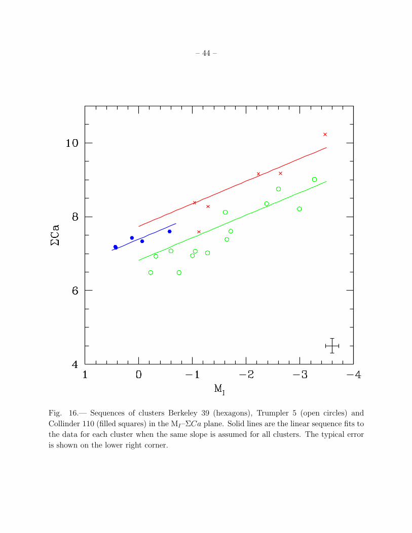
– 44 –

Fig. 16.— Sequences of clusters Berkeley 39 (hexagons), Trumpler 5 (open circles) and

Collinder 110 (filled squares) in the MI–ΣCa plane. Solid lines are the linear sequence fits to

the data for each cluster when the same slope is assumed for all clusters. The typical error

is shown on the lower right corner.

–45

–

Table 1. Cluster sample.

Cluster [Fe/H]CG97 Ref. [Fe/H]ZW84 [Fe/H]KI03 [Ca/H] Ref. Age(Gyr) Ref. (m − M)V E(B − V ) Ref. Run

shetrone00 NGC 104 (47 Tuc) −0.67 ± 0.03 31 −0.71 −0.70 0.47 ± 0.02 31 10.7 ± 1.0 8 13.32 0.05 13 7

NGC 188 −0.07 ± 0.04 2 · · · · · · · · · · · · 6.30 ± 0.3 9 11.44 0.09 17 3

NGC 288 −1.07 ± 0.03 1 −1.40 −1.41 −0.79 ± 0.02 33 11.3 ± 1.1 8 14.64 0.03 13 7

NGC 362 −1.09 ± 0.03 1 −1.27 −1.34 −0.91 ± 0.01 33 8.7 ± 1.5 8 14.75 0.05 13 7

NGC 1851 · · · · · · −1.36 · · · · · · · · · 9.2 ± 1.5 8 15.49 0.02 13 7

NGC 1904 (M79) −1.37 ± 0.05 1 −1.69 −1.64 −1.07 ± 0.02 32 11.7 ± 1.3 8 15.53 0.01 13 7

Berkeley 20 −0.49 ± 0.05 22 · · · · · · −0.42 ± 0.05 22 4.05 ± 0.7 9 15.84 0.38 22 7

NGC 2141 −0.14 ± 0.05 22 · · · · · · −0.04 ± 0.04 22 2.45 ± 0.9 9 14.15 0.40 14 3,7

Collinder 110 · · · · · · · · · · · · · · · · · · 1.3 ± 0.2 24 13.04 0.40 24 3

Trumpler 5 · · · · · · · · · · · · · · · · · · 5.7 ± 2.3 9 14.50 0.60 23 3,7

NGC 2298 −1.74 ± 0.04 1 −1.85 −1.64 −1.35 ± 0.03 35 12.6 ± 1.4 8 15.54 0.13 13 7

Berkeley 32 −0.29 ± 0.04 32 · · · · · · · · · · · · 5.9 ± 1.6 9 12.85 0.08 25 3

Melote 66 −0.38 ± 0.06 3 · · · · · · −0.29 ± 0.10 40 5.3 ± 1.4 9 13.63 0.14 26 7

Berkeley 39 · · · · · · · · · · · · · · · · · · 7.0 ± 1.0 9 13.24 0.11 26 7

NGC 2420 −0.44 ± 0.15 3 · · · · · · · · · · · · 2.2 ± 0.3 9 12.0 0.05 15 3

NGC 2506 −0.20 ± 0.01 31 · · · · · · · · · · · · 2.1 ± 0.3 9 12.60 0.09 16 3,7

NGC 2682 (M 67) −0.03 ± 0.03 4 · · · · · · +0.01 ± 0.06 4 4.3 ± 0.5 9 9.65 0.04 17 3,7

NGC 3201 −1.24 ± 0.12 1 −1.61 −1.48 −1.11 ± 0.02 34 11.3 ± 1.1 8 14.17 0.21 13 4

NGC 4590 (M 68) −2.00 ± 0.03 1 −2.09 −2.43 −1.68 ± 0.02 34 11.2 ± 0.9 8 15.14 0.04 13 3,4,6,7

NGC 5927 · · · · · · −0.30 · · · · · · · · · 10.9 ± 2.2 30 15.81 0.47 13 6

NGC 6352 −0.64 ± 0.02 1 −0.51 · · · −0.63 ± 0.14 36 9.9 ± 1.4 8 14.39 0.21 13 6

NGC 6528 −0.17 ± 0.02 28,29 +0.12 · · · −0.03 ± 0.01 37 11.2 ± 2.0 10 16.16 0.55 18 7

NGC 6681 (M 70) −1.35 ± 0.03 1 −1.51 · · · · · · · · · 11.5 ± 1.4 8 14.93 0.07 13 7

NGC 6705 (M 11) +0.07 ± 0.05 5 · · · · · · −0.12 ± 0.06 5 0.25 ± 0.1 11 12.88 0.43 11 2,5

NGC 6715 (M 54) · · · · · · −1.42 −1.47 −0.98 ± 0.04 39 12 ± 1.5 27 17.77 0.16 19 7

NGC 6791 +0.47 ± 0.04 6 · · · · · · · · · · · · 12.0 ± 1.0 12 13.07 0.09 12 5

NGC 6819 +0.07 ± 0.03 7 · · · · · · +0.03 ± 0.06 7 2.9 ± 0.7 9 12.35 0.14 20,7 1,5

NGC 7078 (M 15) −2.12 ± 0.04 1 −2.15 −2.42 −1.88 ± 0.02 38 11.7 ± 0.8 8 15.31 0.09 13 7

NGC 7789 −0.04 ± 0.05 4 · · · · · · +0.10 ± 0.08 4 1.3 ± 0.3 9 12.20 0.28 4,21 1,3

References. — (1) Carretta & Gratton (1997); (2) Hubbs et al. (1990); (3) Gratton (2000) (4) Tautvaisiene et al. (2005); (5) Gonzalez & Wallerstein (2000); (6) Gratton et al.

(2006); (7) Bragaglia et al. (2001); (8) Salaris & Weiss (2002); (9) Salaris et al. (2004); (10) Feltzing & Johnson (2002); (11) Sung et al. (1999); (12) Stetson et al. (2003); (13)

Rosenberg et al. (1999); (14) Carraro et al. (2001); (15) Lee et al. (1999); (16) Marconi et al. (1997); (17) Sarajedini et al. (1999); (18) Ortolani et al. (1992); (19) Rosenberg et al.

(2004); (20) Rosvick & Vandenverg (1998); (21) Gim et al. (1998); (22) Yong et al. (2005); (23) Kim & Sung (2003); (24) Bragaglia & Tosi (2003); (25) Richtler & Sagar (2001);

–46

–(26) Kassis et al. (1997); (27) Layden & Sarajedini (1997) (28) Zoccali et al. (2004); (29) Origlia et al. (2005); (30) Fullton (1996); (31) Carretta et al. (2004); (32) Sestito et al.

(2006); (33) Shetrone & Keane (2000); (34) Gratton & Ortolami (1989); (35) McWilliam et al. (1992); (36) Gratton (1987); (37) Carretta et al. (2001); (38) Sneden et al. (1997);

(39) Brown et al. (1999); (40) Gratton & Contarini (1994).

– 47 –

Table 2. Observing runs

Run Date Telescope Instrument Resolution A/pix

1 May 2002 WHT ISIS 7000 0.41

2 April 2002 WHT WYFFOS 4000 1.5

3 December 2002 INT IDS 6000 0.45

4 January 2005 CTIO 4m HYDRA 6000 0.9

5 June 2005 CAHA 2.2m CAFOS 2000 2.0

6 2005 VLT FORS2 MXU 5000 0.85

7 ESO Archive VLT FORS2 MXU/MOS 5000 0.85

– 48 –

Table 3. Star sample.

Cluster Id ΣCa σΣCa V I Vr σVrComments

ngc104 S2701 6.18 0.13 14.07 99.99 2.22 4.90 Member?

ngc104 S2703 6.55 0.07 12.99 99.99 4.44 4.34 No member

ngc104 S2705 7.27 0.02 12.08 99.99 -13.24 3.68

ngc104 S2707 6.96 0.07 13.35 99.99 -2.71 5.46

ngc104 S2712 7.34 0.05 12.89 99.99 9.46 5.25 No member

References. — NGC 104 Lee (1977) [L], Stetson (2000) [S]; NGC 188

Webda http://obswww.unige.ch/webda/ (Mermilliod 1995) [W]; NGC 288

Alcaino & Liller (1980) [A]; NGC 362 Harris (1982) [H]; NGC 1851 Stetson

(1981) [S]; NGC 1904 Stetson & Harris (1977) [S]; Berkeley 20 Webda

[W]; NGC 2141 Burkhead et al. (1972) [B]; Rosvick (1995) [R]; Webda

[W]; Collinder 110 Webda [W]; Trumpler 5 Webda [W]; NGC 2298

Alcaino & Liller (1986) [A], Alcaino (1974) [A]; Berkeley 32 Webda [W];

Melotte 66 Webda [W]; Berkeley 39 Webda [W]; NGC 2420 Webda

[W]; NGC 2506 Webda [W]; NGC 2682 Webda [W]; NGC 3201 Stetson

(2000) [S]; NGC 4590 Harris (1975a) [H], Stetson (2000) [S]; NGC 5927

Zoccali (private communication); NGC 6352 Zoccali (private communica-

tion); NGC 6528 Ortolani et al. (1992) [O]; NGC 6681 Harris (1975b) [H]

Rosenberg et al. (2000) [R]; NGC 6705 Sung et al. (1999) [S]; NGC 6715

Rosenberg et al. (2004) [R]; NGC 6791 Stetson et al. (2003) [S]; NGC 6819

Webda [W]; NGC 7078 Buonanno et al. (1983) [B]; Stetson (2000) [S]; NGC

7789 Webda [W];

Note. — Table 3 is published in its enterety in the electronic edition of

Astronomical Journal. A portion is shown here for guidance regarding its form

and content.

– 49 –

Table 4. Radial velocities of the cluster sample.

Cluster Vr σ(Vr) Stars Vr (ref.) Ref.

NGC 104 (47 Tuc) -16 11 32 -18.7 1

NGC 188 -44 20 8 -45 2

NGC 288 -50 11 19 -46.6 1

NGC 362 213 7 16 223.5 1

NGC 1851 321 9 14 320.5 1

NGC 1904 (M79) 227 5 16 206 1

Berkeley 20 80 7 4 70 2

NGC 2141 44 10 21 33/64 3,4

Collinder 110 45 11 8 · · · · · ·

Trumpler 5 44 10 15 54 4

NGC 2298 153 15 6 148.9 1

Berkeley 32 98 12 3 101 2

Melote 66 18 10 11 23 5

Berkeley 39 59 6 5 55 2

NGC 2420 69 5 5 67 2

NGC 2506 76 5 3 84 6

NGC 2682 (M 67) 36 6 9 33 2

NGC 3201 491 3 10 494 1

NGC 4590 (M 68) -89 7 19 -93.4 1

NGC 5927 -84 5 20 -107.5 1

NGC 6352 -114 8 23 -121 1

NGC 6528 220 7 5 206 1

NGC 6681 (M 70) 199 7 4 220 1

NGC 6705 (M 11) 28 7 10 34 7

NGC 6715 (M 54) 156 8 23 142 1

NGC 6791 -46 10 10 -57 2

NGC 6819 2 5 7 -5 2

NGC 7078 (M 15) -108 10 33 -107 1

NGC 7789 -58 6 20 -64 2

References. — (1) Harris (1996); (2) Friel et al. (2002); (3)

Friel (1989); (4) Cole et al. (2004) (5) Friel & Janes (1993); (6)

Mathieu (1985); (7) Mathieu et al. (1986)

– 50 –

Table 5. Line and continuum bandpasses

Line Bandpasses (A) Continuum bandpasses (A)

8484-8513 8474-8484

8522-8562 8563-8577

8642-8682 8619-8642

· · · 8799-8725

· · · 8776-8792

– 51 –

Table 6. Coefficients of the quadratic fits in the form ΣCa=W ′+βMV,I+γM2V,I to the

sequence of each cluster individually. The clusters are ordered by metallicity.

Cluster W’ β γ σ

MV

NGC 6791 10.26±0.97 -1.64±1.28 0.38±0.35 0.72

NGC 2141 8.30±0.14 -0.91±0.13 0.02±0.15 0.44

NGC 104 6.77±0.06 -0.69±0.05 0.15±0.04 0.30

NGC 288 5.46±0.08 -0.56±0.05 0.07±0.03 0.29

NGC 7078 2.79±0.06 -0.39±0.04 0.15±0.04 0.22

MI

NGC 6791 8.49±0.24 -0.63±0.74 0.22±0.79 0.54

NGC 2141 7.52±0.11 -0.73±0.20 0.00±0.11 0.47

NGC 104 6.30±0.04 -0.42±0.05 0.06±0.02 0.14

NGC 288 5.09±0.07 -0.44±0.04 0.03±0.03 0.27

NGC 7078 2.64±0.08 -0.27±0.14 0.05±0.07 0.22

– 52 –

Table 7. Derived W ′

V and W ′

I and number of stars used.

Cluster W ′

V#Star W ′

I#Star

NGC 104 6.94 ± 0.01 34 6.23 ± 0.01 14

NGC 188 8.17 ± 0.07 6 7.27 ± 0.08 5

NGC 288 5.51 ± 0.01 19 5.04 ± 0.03 14

NGC 362 6.01 ± 0.01 16 · · · · · ·

NGC 1851 5.94 ± 0.03 14 5.24 ± 0.04 8

NGC 1904 4.91 ± 0.03 16 · · · · · ·

Berkeley 20 6.86 ± 0.03 4 6.39 ± 0.03 3

NGC 2141 8.33 ± 0.01 18 7.67 ± 0.02 15

Collinder 110 8.21 ± 0.04 11 7.74 ± 0.06 6

Trumpler 5 7.52 ± 0.04 16 6.97 ± 0.04 15

NGC 2298 3.75 ± 0.03 6 3.09 ± 0.03 5

Berkeley 32 5.90 ± 0.08 4 5.27 ± 0.08 4

Melote 66 7.69 ± 0.03 11 6.90 ± 0.03 11

Berkeley 39 8.21 ± 0.04 5 7.27 ± 0.06 3

NGC 2420 6.26 ± 0.09 6 6.15 ± 0.08 4

NGC 2506 6.96 ± 0.09 4 6.37 ± 0.09 3

NGC 2682 8.24 ± 0.01 6 7.48 ± 0.01 8

NGC 3201 5.46 ± 0.03 9 4.76 ± 0.02 6

NGC 4590 2.84 ± 0.02 19 2.19 ± 0.06 12

NGC 5927 7.81 ± 0.01 21 6.92 ± 0.01 13

NGC 6352 7.10 ± 0.01 19 6.31 ± 0.01 19

NGC 6528 8.28 ± 0.04 5 7.58 ± 0.04 5

NGC 6681 5.05 ± 0.03 4 4.49 ± 0.07 3

NGC 6705 8.95 ± 0.07 7 8.28 ± 0.12 6

NGC 6715 4.86 ± 0.03 23 4.30 ± 0.03 24

NGC 6791 9.78 ± 0.09 9 8.77 ± 0.09 8

NGC 6819 8.41 ± 0.04 7 7.64 ± 0.04 7

NGC 7078 2.78 ± 0.01 38 2.18 ± 0.01 14

NGC 7789 8.47 ± 0.02 20 7.61 ± 0.02 20

arX

iv:0

705.

3335

v1 [

astr

o-ph

] 2

3 M

ay 2

007

– 1 –

Table 1. Star sample.

Cluster Id ΣCa σΣCa V I V−r σVrComments

NGC 104 L2701 6.19 0.13 14.07 · · · 2.2 4.9 Member?

NGC 104 L2703 6.55 0.07 12.99 · · · 4.4 4.3 Member?

NGC 104 L2705 7.27 0.02 12.08 · · · -13.2 3.7

NGC 104 L2707 6.96 0.07 13.35 · · · -2.7 5.4

NGC 104 L2712 7.34 0.05 12.89 · · · 9.4 5.2 No member

NGC 104 L2720 6.51 0.11 13.95 · · · -30.7 5.4

NGC 104 L2722 6.48 0.10 13.84 · · · -1.6 5.1

NGC 104 L2730 6.20 0.12 14.04 · · · -6.2 3.4

NGC 104 L3618 5.51 0.21 14.70 · · · -11.1 5.3

NGC 104 L3703 5.66 0.21 15.40 · · · -5.8 4.1

NGC 104 L3709 7.27 0.05 12.55 · · · -20.4 4.7

NGC 104 L3712 6.09 0.13 15.06 · · · -28.1 5.6

NGC 104 L3727 5.76 0.10 14.06 · · · -25.9 5.6

NGC 104 L3730 8.05 0.02 11.85 · · · -29.3 3.8

NGC 104 L3736 8.03 0.03 11.98 · · · -22.8 4.1

NGC 104 L3740 6.22 0.10 13.92 · · · -26.4 6.4

NGC 104 L3752 5.92 0.25 14.32 · · · -28.9 3.7

NGC 104 L5309 8.03 0.05 12.20 · · · -20.8 8.2

NGC 104 L5310 6.58 0.12 13.39 · · · 4.4 7.6 Member?

NGC 104 L5311 4.62 0.30 15.07 · · · -9.9 6.2

NGC 104 L5312 8.16 0.05 12.18 · · · -17.4 9.4

– 2 –

Table 1—Continued

Cluster Id ΣCa σΣCa V I V−r σVrComments

NGC 104 L5418 5.59 0.35 15.28 · · · -30.6 7.3

NGC 104 L5419 7.03 0.09 14.02 · · · -26.9 8.5

NGC 104 L5420 5.87 0.53 15.78 · · · -104.4 5.7 No member

NGC 104 L5422 7.53 0.06 12.47 · · · -29.2 7.8

NGC 104 L5523 6.46 0.12 15.75 · · · -4.7 7.7

NGC 104 L5527 7.17 0.15 13.60 · · · -23.9 7.4

NGC 104 L5528 6.79 0.30 14.78 · · · -5.1 7.1

NGC 104 L5530 6.45 0.19 13.14 · · · -25.8 7.6

NGC 104 L6401 6.10 0.32 14.81 · · · -25.0 7.1

NGC 104 S1186 7.00 0.04 13.07 11.82 -18.1 3.0

NGC 104 S2070 6.25 0.08 14.58 13.54 -11.1 3.4 L3735

NGC 104 S2069 6.08 0.11 14.50 13.47 -23.4 3.3 L3701

NGC 104 S2073 6.70 0.06 13.69 12.59 -9.3 3.0

NGC 104 S1014 8.12 0.03 12.09 10.46 -20.1 2.3 L3708

NGC 104 S1024 3.70 0.09 14.78 13.73 8.1 1.3 L3707

NGC 104 S1096 6.88 0.05 13.58 12.40 -20.6 3.0 L3716

NGC 104 S2074 6.45 0.09 14.27 13.22 -18.0 3.2

NGC 104 S2072 5.90 0.10 14.67 13.64 -20.0 2.9

NGC 104 S1168 6.05 0.09 14.30 13.26 -32.4 3.3

NGC 104 S1153 6.06 0.15 15.40 14.42 -2.7 3.5

NGC 104 S1165 7.23 0.03 12.57 11.35 -21.3 2.9

– 3 –

Table 1—Continued

Cluster Id ΣCa σΣCa V I V−r σVrComments

NGC 104 S1019 8.01 0.03 11.87 10.13 -23.2 0.1 L2620

NGC 104 S1054 6.11 0.15 15.14 14.14 -18.2 3.0 L2719

NGC 104 S1080 7.95 0.02 12.11 10.55 -21.0 0.1 L2721

NGC 104 S1048 6.23 0.10 14.26 13.22 -29.3 3.0 L2717

NGC 104 S1059 6.37 0.09 14.20 13.14 -15.9 3.0 L2714

NGC 104 S1193 6.42 0.08 14.05 12.98 -15.5 3.1

NGC 104 S1111 5.96 0.12 15.02 14.04 -18.9 3.5 L2709

NGC 104 S1203 7.08 0.06 13.19 11.94 -17.3 3.4

NGC 104 S1181 6.91 0.05 13.41 12.23 -19.8 3.2

NGC 188 W1057 6.13 0.15 13.68 12.52 -54.4 5.7

NGC 188 W1069 7.50 0.22 12.32 11.02 -63.7 6.0

NGC 188 W1105 6.78 0.21 12.39 11.21 -63.5 6.0

NGC 188 W2051 6.61 0.12 12.97 11.78 -63.1 6.8

NGC 188 W2072 7.58 0.14 12.45 11.14 -65.4 6.5

NGC 188 W2076 7.72 0.15 12.46 11.25 -59.1 8.2

NGC 188 W3018 9.08 0.18 11.38 · · · -65.6 7.0

NGC 188 W5217 6.68 0.18 12.46 11.26 -62.7 6.1

NGC 188 W7330 7.49 0.15 12.86 11.62 -64.4 6.7

NGC 288 A0156 5.80 0.11 14.42 · · · -57.7 2.4

NGC 288 A0158 5.20 0.11 14.47 · · · -53.8 6.2

NGC 288 A0166 5.26 0.13 15.17 · · · -65.2 5.5

– 4 –

Table 1—Continued

Cluster Id ΣCa σΣCa V I V−r σVrComments

NGC 288 A0172 4.86 0.15 15.32 · · · -60.4 4.7

NGC 288 A0196 5.45 0.10 14.52 13.63 -69.2 5.6

NGC 288 A0213 6.93 0.03 13.00 11.63 -69.5 6.0

NGC 288 A0222 5.14 0.15 15.28 14.34 -70.2 5.5

NGC 288 A0245 6.55 0.06 13.39 12.24 -53.9 4.8

NGC 288 A0260 7.06 0.03 12.57 · · · -71.4 4.4

NGC 288 A0307 6.28 0.06 13.63 12.69 -56.7 5.3

NGC 288 A0096 7.39 0.03 12.74 14.21 -57.7 1.6

NGC 288 A0199 6.51 0.05 13.50 12.26 -71.2 5.9

NGC 288 S0183 5.16 0.08 15.48 14.53 -20.9 3.4 A0181, No member

NGC 288 S0188 4.80 0.22 16.87 16.00 -34.3 3.2 A0323

NGC 288 S0193 5.89 0.03 13.19 11.87 -39.7 3.0 A0077

NGC 288 S0414 4.80 0.18 17.02 16.14 -40.5 4.2 A0328

NGC 288 S0198 5.24 0.10 15.62 14.68 -38.4 4.8

NGC 288 S0028 4.94 0.26 17.39 16.57 -43.9 4.0

NGC 288 S0027 5.07 0.09 15.40 14.45 -59.5 4.1 A0217

NGC 288 S0113 4.62 0.15 16.38 15.50 -44.5 4.4

NGC 288 S0020 4.61 0.18 16.72 15.86 -53.0 4.0

NGC 288 S0017 4.80 0.16 16.51 15.66 -47.5 3.8 A0205

NGC 288 S0012 5.83 0.05 14.46 13.39 -40.9 5.7 A0181

NGC 288 S0006 3.94 0.25 17.22 16.38 -51.7 3.0

– 5 –

Table 1—Continued

Cluster Id ΣCa σΣCa V I V−r σVrComments

NGC 288 S0004 4.13 0.19 16.85 15.99 -45.1 3.7

NGC 288 S0124 6.07 0.05 14.08 12.97 -47.5 28.6 A0195

NGC 288 S0161 5.51 0.09 15.11 14.12 -34.1 3.5 A0154

NGC 288 S0107 4.83 0.12 16.18 15.28 -51.3 4.6

NGC 288 S0065 5.15 0.11 15.84 14.91 -41.9 4.3 A0129

NGC 288 S0061 5.34 0.10 15.43 14.46 -45.0 4.3 A0125

NGC 288 S0059 4.90 0.20 17.10 16.25 -46.6 4.3 A0359

NGC 288 S0058 4.75 0.11 16.06 15.15 -40.4 3.8 A0141

NGC 288 S0054 4.81 0.17 16.82 15.96 -24.7 3.2 No member

NGC 288 S0052 4.29 0.19 17.04 16.22 -42.4 4.2

NGC 288 S0047 4.44 0.16 16.73 15.87 -27.8 4.0 Member?

NGC 288 S0103 6.48 0.03 13.92 12.74 -42.3 14.9 A0251

NGC 288 S0035 4.67 0.14 16.58 15.72 -37.8 3.6

NGC 362 H1111 6.24 0.10 14.23 · · · 213.3 5.2

NGC 362 H1156 5.33 0.14 14.79 · · · 205.9 2.6

NGC 362 H1159 7.38 0.05 12.68 · · · 209.5 5.4

NGC 362 H1211 6.10 0.11 14.32 · · · 206.6 5.7

NGC 362 H1216 7.28 0.05 13.09 · · · 217.7 5.7

NGC 362 H1423 7.63 0.03 12.58 · · · 217.7 4.1

NGC 362 H1312 6.80 0.06 13.54 · · · 196.2 5.3

NGC 362 H1351 5.81 0.14 14.84 · · · 207.3 5.9

– 6 –

Table 1—Continued

Cluster Id ΣCa σΣCa V I V−r σVrComments

NGC 362 H1412 6.45 0.07 13.81 · · · 218.5 5.1

NGC 362 H1422 6.50 0.07 13.52 · · · 218.5 4.8

NGC 362 H1441 7.68 0.03 12.71 · · · 217.2 4.1

NGC 362 H2108 6.52 0.07 13.77 · · · 211.4 4.8

NGC 362 H2220 5.46 0.15 15.00 · · · 215.1 4.8

NGC 362 H2302 6.26 0.06 13.96 · · · 207.8 6.7

NGC 362 H2309 5.85 0.10 14.83 · · · 215.6 5.2

NGC 362 H2423 7.50 0.03 12.81 · · · 228.4 3.2

NGC 1851 S0160 5.75 0.21 15.51 14.51 290.1 8.4 Member?

NGC 1851 S0275 6.15 0.26 13.92 12.82 324.4 7.6

NGC 1851 S0109 6.08 0.18 14.85 13.71 321.0 14.4

NGC 1851 S0195 5.55 0.28 15.82 · · · 326.1 9.2

NGC 1851 S0095 7.42 0.09 13.57 12.09 329.0 10.2

NGC 1851 S0126 6.72 0.09 14.29 13.04 319.5 10.8

NGC 1851 S0123 5.21 0.32 16.21 15.58 328.0 7.3

NGC 1851 S0112 7.02 0.09 13.80 12.37 319.8 8.9

NGC 1851 S0003 7.25 0.07 13.60 12.16 319.8 8.9

NGC 1851 S0231 5.20 0.33 15.93 14.93 328.9 5.5

NGC 1851 S0209 6.93 0.11 14.08 12.82 317.9 7.6

NGC 1851 S0107 6.87 0.17 14.50 · · · 317.1 8.5

NGC 1851 S0179 5.45 0.32 16.45 · · · 324.6 8.9

– 7 –

Table 1—Continued

Cluster Id ΣCa σΣCa V I V−r σVrComments

NGC 1851 S0175 5.05 0.37 16.22 · · · 322.8 7.9

NGC 1851 S0065 5.45 0.27 15.75 14.75 324.9 8.0

NGC 1904 S0006 4.88 0.21 15.27 · · · 226.6 8.7

NGC 1904 S0011 4.74 0.29 15.74 · · · 228.0 8.0

NGC 1904 S0015 6.59 0.07 13.22 · · · 227.7 9.6

NGC 1904 S0045 4.91 0.26 15.58 · · · 235.1 8.0

NGC 1904 S0089 5.07 0.18 14.71 · · · 225.4 9.2

NGC 1904 S0091 4.44 0.48 16.25 · · · 228.2 6.5

NGC 1904 S0111 4.89 0.28 15.62 · · · 220.9 8.0

NGC 1904 S0115 4.47 0.45 15.97 · · · 224.8 7.4

NGC 1904 S0138 3.72 0.35 16.16 · · · 219.8 8.0

NGC 1904 S0153 6.46 0.07 13.44 · · · 213.7 9.1

NGC 1904 S0160 6.15 0.06 13.02 · · · 219.1 10.3

NGC 1904 S0161 4.23 0.36 15.86 · · · 232.0 6.8

NGC 1904 S0176 4.86 0.19 14.95 · · · 231.2 8.0

NGC 1904 S0209 5.28 0.19 15.02 · · · 233.3 7.6

NGC 1904 S0224 4.71 0.36 16.09 · · · 230.1 6.0

NGC 1904 S0237 5.86 0.17 14.19 · · · 227.5 8.0

NGC 1904 S0241 5.93 0.10 13.61 · · · 230.9 8.3

Berkeley 20 W0005 7.52 0.04 14.80 13.31 71.2 9.1

Berkeley 20 W0008 7.37 0.05 15.15 13.72 75.7 8.8

– 8 –

Table 1—Continued

Cluster Id ΣCa σΣCa V I V−r σVrComments

Berkeley 20 W0012 6.67 0.09 16.21 14.93 82.4 8.8

Berkeley 20 W0022 6.24 0.13 16.90 15.72 89.6 1.5

Berkeley 20 W0027 6.34 0.14 17.07 15.87 -6.4 7.4 No member

Berkeley 20 W0029 5.46 0.17 17.14 16.01 39.5 8.1 No member

NGC 2141 W0661 7.76 0.11 14.60 13.26 25.4 7.5

NGC 2141 W0954 7.70 0.15 14.94 13.55 25.0 7.2

NGC 2141 W1007 9.03 0.05 13.27 11.42 27.6 8.7

NGC 2141 W1809 7.87 0.15 14.85 13.50 36.7 7.9

NGC 2141 W2080 7.73 0.10 14.61 12.91 51.4 8.4

NGC 2141 W3127 9.45 0.04 13.05 · · · 35.0 7.7

NGC 2141 W9999 7.08 0.18 15.00 · · · 47.6 8.4

NGC 2141 W0069 8.75 0.15 13.25 11.24 98.6 5.7 No member

NGC 2141 W0330 7.97 0.14 14.01 12.23 17.8 6.0

NGC 2141 W0847 6.18 0.11 11.82 9.78 15.6 6.8

NGC 2141 W1401 8.12 0.21 13.25 11.31 24.6 5.9

NGC 2141 W1602 9.92 0.14 13.66 11.89 28.5 6.0

NGC 2141 W2111 9.40 0.13 13.30 11.36 41.9 6.5

NGC 2141 W2703 7.98 0.17 14.05 12.42 35.6 6.2

NGC 2141 W0514 8.26 0.04 14.09 12.48 34.9 3.1

NGC 2141 W0587 6.43 0.06 15.14 13.69 70.5 3.1 No member

NGC 2141 W0632 6.74 0.10 15.78 14.38 108.6 2.3 No member

– 9 –

Table 1—Continued

Cluster Id ΣCa σΣCa V I V−r σVrComments

NGC 2141 W0701 7.05 0.10 15.81 14.35 33.5 3.1

NGC 2141 W0714 7.16 0.08 15.46 13.95 21.5 2.9

NGC 2141 W0783 7.60 0.06 15.01 13.55 23.9 2.5

NGC 2141 W0871 6.63 0.06 15.30 13.79 33.0 2.8

NGC 2141 W1020 7.08 0.08 15.62 14.25 43.0 2.9

NGC 2141 W1093 7.47 0.06 14.97 13.46 8.0 2.9 No member

NGC 2141 W1194 7.34 0.08 14.90 13.47 12.5 2.7

NGC 2141 W1205 3.61 0.01 11.58 9.69 39.7 2.3

NGC 2141 W1267 7.56 0.04 14.53 12.96 21.9 2.7

NGC 2141 W1333 7.70 0.06 15.09 13.62 22.5 2.9

NGC 2141 W1348 8.78 0.02 13.25 11.31 0.5 2.2 No member

NGC 2141 W1470 7.73 0.06 15.00 13.56 34.0 2.9

NGC 2141 W1602 8.66 0.02 13.05 10.88 -7.1 2.3 No member

NGC 2141 W1640 7.49 0.06 15.01 13.53 58.0 2.7 Member?

NGC 2141 W1657 6.72 0.08 15.53 14.19 110.9 3.1 No member

NGC 2141 W1770 7.73 0.05 14.98 13.38 37.1 2.8

NGC 2141 W1821 8.15 0.04 14.13 12.52 10.5 2.5 No member

NGC 2141 W2066 8.52 0.04 14.18 12.56 49.6 2.7

NGC 2141 W2082 7.37 0.07 15.45 14.06 39.7 2.3

NGC 2141 W2167 7.66 0.06 14.91 13.47 30.7 3.1

Collinder 110 W1148 8.38 0.14 12.97 11.36 37.8 6.2

– 10 –

Table 1—Continued

Cluster Id ΣCa σΣCa V I V−r σVrComments

Collinder 110 W1218 10.23 0.11 11.47 8.93 56.0 6.7

Collinder 110 W1306 9.43 0.12 12.62 10.16 78.2 7.0 No member

Collinder 110 W1319 7.59 0.22 12.90 11.28 40.9 5.9

Collinder 110 W2202 9.17 0.16 11.80 9.76 54.7 7.0

Collinder 110 W4111 9.16 0.17 12.11 10.17 55.0 7.0

Collinder 110 W4204 8.28 0.15 12.70 11.11 35.9 6.1

Collinder 110 W4222 8.30 0.15 12.64 · · · 56.4 6.8

Collinder 110 W5002 8.91 0.10 11.89 · · · 39.1 5.8

Collinder 110 W5006 7.36 0.16 13.37 · · · 39.3 5.5

Collinder 110 W5007 6.87 0.16 13.47 · · · 36.9 6.1

Collinder 110 W5008 7.67 0.21 13.31 · · · 41.2 6.0

Trumpler 5 W0833 7.07 0.42 14.92 12.94 39.8 6.4

Trumpler 5 W1026 6.49 0.30 14.71 12.79 29.7 6.3

Trumpler 5 W1214 7.38 0.31 13.90 11.90 34.4 7.8

Trumpler 5 W1277 1.54 0.10 14.92 · · · 331.8 56.3 No member

Trumpler 5 W2280 6.49 0.35 15.18 14.21 35.9 8.3

Trumpler 5 W2324 6.93 0.30 15.03 13.22 41.6 7.5

Trumpler 5 W2579 6.43 0.29 16.74 13.78 40.9 7.2

Trumpler 5 W3066 6.94 0.29 14.39 12.54 37.7 8.4

Trumpler 5 W3354 7.06 0.27 14.46 12.49 29.2 7.9

Trumpler 5 W3763 7.80 0.28 14.54 12.72 -20.6 8.3 No member

– 11 –

Table 1—Continued

Cluster Id ΣCa σΣCa V I V−r σVrComments

Trumpler 5 W1063 7.02 0.17 14.46 12.56 51.8 5.8

Trumpler 5 W1305 8.12 0.21 14.24 12.20 61.0 6.7

Trumpler 5 W1378 8.35 0.09 13.36 11.38 42.9 6.8

Trumpler 5 W1935 8.21 0.09 12.87 10.78 45.9 6.9

Trumpler 5 W4219 8.18 0.12 12.55 10.31 31.4 5.7 TiO

Trumpler 5 W4811 7.61 0.32 13.71 12.00 54.0 7.0

Trumpler 5 W5099 8.89 0.20 12.35 10.27 48.7 7.0

Trumpler 5 W6075 8.55 0.19 13.24 10.94 63.2 5.3

NGC 2298 A0004 4.97 0.06 13.55 12.10 164.4 5.8

NGC 2298 A0006 4.98 0.06 13.82 12.38 158.1 6.4

NGC 2298 A0012 4.72 0.07 14.23 12.88 147.2 3.4

NGC 2298 A0015 4.07 0.10 14.86 13.53 164.3 5.7

NGC 2298 A0022 3.57 0.13 15.30 14.10 176.2 5.3

NGC 2298 A0025 3.69 0.16 15.69 14.60 171.7 4.5

NGC 2298 A0024 4.11 0.16 15.57 14.69 150.3 4.8

NGC 2298 A9999 3.80 0.18 · · · · · · 169.9 6.2

Berkeley 32 W1851 4.72 0.26 13.49 12.33 40.3 6.5

Berkeley 32 W1948 5.07 0.18 13.42 12.21 111.4 6.5

Berkeley 32 W3198 5.78 0.14 12.69 11.51 91.0 1.1

Berkeley 32 W3199 6.17 0.16 12.78 11.55 80.5 6.0

Berkeley 32 W3200 5.30 0.18 12.92 11.61 38.1 6.2 No member

– 12 –

Table 1—Continued

Cluster Id ΣCa σΣCa V I V−r σVrComments

Berkeley 32 W3201 6.32 0.17 12.90 11.47 107.5 6.1

Melotte 66 W783 6.94 0.14 14.58 13.25 15.5 8.3

Melotte 66 W797 7.39 0.10 14.01 12.65 3.8 7.9 Member?

Melotte 66 W862 7.15 0.11 14.16 12.84 29.3 9.3

Melotte 66 W968 6.57 0.22 15.48 14.29 16.2 7.9

Melotte 66 W1000 6.66 0.13 14.68 13.39 10.9 7.8

Melotte 66 W1209 7.02 0.11 14.17 12.77 15.2 8.0

Melotte 66 W1419 6.93 0.13 14.48 13.30 17.7 7.8

Melotte 66 W1615 7.68 0.10 13.66 12.33 43.9 7.6 No member

Melotte 66 W1677 8.33 0.06 13.25 11.53 16.2 8.0

Melotte 66 W1805 6.96 0.16 14.71 13.52 17.1 7.9

Melotte 66 W1941 5.19 0.20 15.29 13.95 9.2 7.2

Melotte 66 W2155 7.04 0.18 14.46 13.29 31.2 7.1

Melotte 66 W2160 7.38 0.14 14.09 12.74 7.9 6.3

Melotte 66 W2236 8.18 0.07 12.78 11.00 22.9 0.6

Berkeley 39 W1587 7.42 0.12 14.43 13.19 58.3 9.1

Berkeley 39 W1725 7.16 0.13 14.78 13.49 58.3 8.2

Berkeley 39 W1923 6.71 0.16 15.52 14.19 58.1 8.4

Berkeley 39 W2033 7.42 0.11 14.33 · · · 56.4 8.7

Berkeley 39 W2055 7.60 0.08 13.99 12.49 58.1 8.2

Berkeley 39 W2573 7.19 0.12 14.74 13.50 58.5 9.3

– 13 –

Table 1—Continued

Cluster Id ΣCa σΣCa V I V−r σVrComments

Berkeley 39 W2784 7.33 0.10 14.20 13.00 53.9 8.6

Berkeley 39 W4368 8.23 0.07 13.55 · · · 61.4 8.2

Berkeley 39 W9999 5.97 0.17 · · · · · · 73.5 7.2

NGC 2420 W0034 4.05 0.20 13.09 12.08 73.1 6.3

NGC 2420 W0041 5.70 0.17 12.67 11.59 69.1 6.3

NGC 2420 W0073 8.34 0.13 11.09 9.66 77.9 5.9

NGC 2420 W0114 5.16 0.19 13.10 12.10 67.6 6.3

NGC 2420 W0140 6.95 0.16 11.53 10.26 63.1 1.7

NGC 2420 W0188 5.62 0.32 13.48 12.54 71.8 6.0

NGC 2420 W0192 5.54 0.20 12.94 11.91 67.5 6.5

NGC 2506 W2101 8.04 0.17 11.09 9.66 79.8 7.5

NGC 2506 W2122 6.58 0.20 13.10 12.10 78.9 7.1

NGC 2506 W2212 4.78 0.20 11.53 10.26 28.9 7.0 No member

NGC 2506 W3254 6.73 0.13 12.94 11.91 76.2 6.3

NGC 2682 W0141 7.85 0.04 10.48 9.40 35.1 3.761

NGC 2682 W0105 7.55 0.03 10.30 9.07 41.0 2.507

NGC 2682 W0185 6.50 0.08 11.06 10.80 42.9 1.247

NGC 2682 W0174 6.62 0.13 12.72 12.02 34.6 2.975

NGC 2682 W0143 5.67 0.06 11.52 10.61 38.2 3.033

NGC 2682 W0103 5.81 0.18 13.17 12.52 32.3 3.108

NGC 2682 W0164 7.43 0.03 10.55 9.46 37.5 2.732

– 14 –

Table 1—Continued

Cluster Id ΣCa σΣCa V I V−r σVrComments

NGC 2682 W0104 7.17 0.05 11.20 10.12 31.7 2.903

NGC 2682 W0096 6.52 0.14 13.02 12.10 31.1 3.132

NGC 2682 W0100 6.38 0.19 13.49 12.78 37.7 2.372

NGC 2682 W0132 5.90 0.15 13.10 12.38 38.5 2.687

NGC 2682 W0108 8.51 0.02 9.72 8.36 35.0 0.694

NGC 2682 W0116 5.47 0.23 14.16 13.35 33.7 2.201

NGC 2682 W0111 6.00 0.13 12.73 12.04 41.7 3.046

NGC 2682 W0135 7.55 0.05 11.44 10.39 39.5 2.747

NGC 2682 W0130 6.30 0.14 12.89 12.30 43.4 3.098

NGC 2682 W0127 6.55 0.13 12.76 12.08 38.2 2.176

NGC 2682 W0117 5.41 0.10 12.60 11.69 37.1 2.223

NGC 2682 W0170 8.09 0.02 9.69 8.36 17.9 2.548 Member?

NGC 2682 W0173 6.38 0.31 12.11 11.08 21.0 6.466 Member?

NGC 2682 W2152 6.31 0.22 10.93 9.79 36.4 6.591

NGC 2682 W6495 8.30 0.11 9.37 7.87 34.5 6.185

NGC 3201 S0011 4.89 0.19 14.55 13.30 488.9 0.3

NGC 3201 S0082 5.16 0.17 14.60 13.31 489.5 0.2

NGC 3201 S0165 6.30 0.17 12.71 11.20 496.0 0.4

NGC 3201 S0253 8.89 0.74 16.74 15.63 35.6 0.8 No member

NGC 3201 S0272 7.30 0.24 14.90 13.64 34.8 0.8 No member

NGC 3201 S0278 5.77 0.18 12.91 11.51 495.1 0.3

– 15 –

Table 1—Continued

Cluster Id ΣCa σΣCa V I V−r σVrComments

NGC 3201 S0287 8.27 0.10 13.27 11.89 27.1 0.7 No member

NGC 3201 S0288 5.63 0.10 13.43 12.11 490.3 0.3

NGC 3201 S0296 6.42 0.05 12.64 11.08 488.1 0.4

NGC 3201 S0298 4.12 0.18 15.52 14.28 492.4 0.4

NGC 3201 S0302 4.34 0.20 14.87 13.64 490.1 0.3

NGC 3201 S0320 4.46 0.15 15.21 14.03 493.3 0.2

NGC 3201 S0323 6.93 0.05 12.39 10.68 490.7 0.4

NGC 4590 S164 6.48 0.34 15.16 16.02 -36.7 0.1 No member

NGC 4590 S174 6.17 0.61 15.95 16.64 -6.2 0.6 No member

NGC 4590 S189 6.02 0.41 15.14 15.79 -21.3 0.7 No member

NGC 4590 S190 7.26 0.39 15.31 16.05 -47.4 0.8 No member

NGC 4590 S194 5.74 0.39 15.25 16.11 -22.2 0.6 No member

NGC 4590 S195 3.55 0.16 14.20 15.11 -95.3 0.7

NGC 4590 S203 4.03 0.14 13.36 14.44 -95.3 0.1

NGC 4590 S206 3.50 0.26 14.58 15.43 -97.7 1.0

NGC 4590 S207 5.18 0.08 12.67 14.00 -99.4 0.8

NGC 4590 S208 5.58 0.53 15.98 16.71 81.1 0.7 No member

NGC 4590 S221 6.38 0.17 13.68 14.58 -24.4 0.9 No member

NGC 4590 S227 3.31 0.24 14.52 15.38 -94.2 1.1

NGC 4590 S230 5.82 0.95 16.76 17.52 27.0 0.5 No member

NGC 4590 S237 3.01 0.32 15.01 15.83 -90.5 0.8

– 16 –

Table 1—Continued

Cluster Id ΣCa σΣCa V I V−r σVrComments

NGC 4590 S250 7.16 0.24 14.52 15.46 192.6 0.6 No member

NGC 4590 S255 3.34 0.25 14.69 15.54 -95.6 0.9

NGC 4590 S259 6.23 0.45 14.69 15.54 -30.5 0.8 No member

NGC 4590 S265 3.23 0.35 14.93 15.74 -93.1 0.8

NGC 4590 S266 4.23 0.49 14.93 15.74 -22.6 0.9 No member

NGC 4590 S270 5.91 1.09 16.32 17.05 -0.2 1.0 No member

NGC 4590 S277 3.06 0.58 17.79 18.76 -4.7 0.5 No member

NGC 4590 S286 2.92 0.43 15.59 16.36 -91.5 0.7

NGC 4590 S113 6.85 0.22 15.45 · · · -21.7 3.2 No member

NGC 4590 S134 8.06 0.36 15.53 · · · -8.5 2.7 No member

NGC 4590 H2 2.77 0.21 14.95 · · · -84.6 23.7

NGC 4590 H47 2.87 0.16 15.15 · · · -87.4 24.2

NGC 4590 H49 2.97 0.20 14.62 · · · -82.0 22.6

NGC 4590 H74 3.25 0.17 14.66 · · · -89.8 26.2

NGC 4590 H119 3.74 0.07 13.66 · · · -82.3 26.8

NGC 4590 H239 3.42 0.11 14.19 · · · -84.1 24.3

NGC 4590 H256 4.44 0.05 12.64 · · · -76.9 26.8

NGC 4590 H258 3.23 0.10 14.36 · · · -75.8 27.3

NGC 4590 H260 4.61 0.04 12.52 · · · -95.6 13.8

NGC 4590 R4 2.20 0.26 14.71 13.68 -88.6 6.4

NGC 4590 R5 3.97 0.24 13.41 12.23 -40.0 6.4 No member

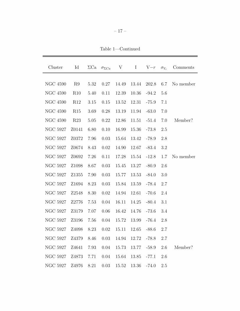
– 17 –

Table 1—Continued

Cluster Id ΣCa σΣCa V I V−r σVrComments

NGC 4590 R9 5.32 0.27 14.49 13.44 202.8 6.7 No member

NGC 4590 R10 5.40 0.11 12.39 10.36 -94.2 5.6

NGC 4590 R12 3.15 0.15 13.52 12.31 -75.9 7.1

NGC 4590 R15 3.69 0.28 13.19 11.94 -63.0 7.0

NGC 4590 R23 5.05 0.22 12.86 11.51 -51.4 7.0 Member?

NGC 5927 Z0141 6.80 0.10 16.99 15.36 -73.8 2.5

NGC 5927 Z0372 7.96 0.03 15.64 13.42 -78.9 2.8

NGC 5927 Z0674 8.43 0.02 14.90 12.67 -83.4 3.2

NGC 5927 Z0692 7.26 0.11 17.28 15.54 -12.8 1.7 No member

NGC 5927 Z1098 8.67 0.03 15.45 13.27 -80.9 2.6

NGC 5927 Z1355 7.90 0.03 15.77 13.53 -84.0 3.0

NGC 5927 Z1694 8.23 0.03 15.84 13.59 -78.4 2.7

NGC 5927 Z2548 8.30 0.02 14.94 12.61 -70.6 2.4

NGC 5927 Z2776 7.53 0.04 16.11 14.25 -80.4 3.1

NGC 5927 Z3179 7.07 0.06 16.42 14.76 -73.6 3.4

NGC 5927 Z3196 7.56 0.04 15.72 13.99 -76.4 2.8

NGC 5927 Z4098 8.23 0.02 15.11 12.65 -88.6 2.7

NGC 5927 Z4379 8.46 0.03 14.94 12.72 -78.8 2.7

NGC 5927 Z4641 7.93 0.04 15.73 13.77 -58.9 2.6 Member?

NGC 5927 Z4873 7.71 0.04 15.64 13.85 -77.1 2.6

NGC 5927 Z4976 8.21 0.03 15.52 13.36 -74.0 2.5

– 18 –

Table 1—Continued

Cluster Id ΣCa σΣCa V I V−r σVrComments

NGC 5927 Z5433 8.67 0.03 15.09 12.79 -57.5 2.2 Member?

NGC 5927 Z5642 7.85 0.03 15.48 13.34 -82.2 2.7

NGC 5927 Z6925 8.39 0.02 14.92 12.58 -97.6 3.0

NGC 5927 Z204901 8.34 0.03 15.45 13.42 -77.7 2.4

NGC 5927 Z206658 8.50 0.02 14.82 12.41 -88.8 2.9

NGC 5927 Z210840 9.76 0.02 14.89 12.74 -91.1 2.4

NGC 5927 Z211700 8.24 0.02 14.93 12.53 -92.0 2.8

NGC 5927 Z212159 8.34 0.02 15.03 12.81 -78.3 2.4

NGC 5927 Z212828 7.74 0.03 14.58 12.46 -28.6 3.0 No member

NGC 5927 Z213516 7.90 0.08 17.26 15.54 30.5 2.3 No member

NGC 6352 Z0541 6.90 0.04 14.65 13.23 -113.6 3.9

NGC 6352 Z0934 6.68 0.05 15.23 13.88 -105.8 3.4

NGC 6352 Z1346 6.65 0.04 15.20 13.83 -116.0 3.2

NGC 6352 Z1924 7.65 0.08 14.87 13.44 -87.9 2.3 Member?

NGC 6352 Z2393 6.18 0.08 16.00 14.69 -113.4 3.4

NGC 6352 Z3467 6.62 0.04 15.03 13.68 -113.5 3.6

NGC 6352 Z3925 6.13 0.07 16.05 14.79 -119.5 3.3

NGC 6352 Z4396 6.84 0.05 15.31 13.92 -114.3 3.5

NGC 6352 Z4688 7.50 0.02 14.17 12.57 -110.6 3.1

NGC 6352 Z5131 7.53 0.07 15.34 14.00 -91.5 2.5 Member?

NGC 6352 Z5424 5.84 0.07 15.21 13.89 -111.8 3.2

– 19 –

Table 1—Continued

Cluster Id ΣCa σΣCa V I V−r σVrComments

NGC 6352 Z5673 7.30 0.02 13.58 11.66 -116.6 3.1

NGC 6352 Z6343 6.90 0.05 14.81 13.32 -103.7 3.5

NGC 6352 Z6611 6.77 0.05 15.19 13.79 -114.0 3.6

NGC 6352 Z6811 7.75 0.04 14.37 13.03 -2.2 3.5 No member

NGC 6352 Z202750 4.75 0.03 14.96 13.63 -11.6 2.6 No member

NGC 6352 Z7496 6.82 0.07 15.96 14.59 -80.1 3.2

NGC 6352 Z7708 7.26 0.04 14.99 13.63 -14.2 3.9 No member

NGC 6352 z7876 7.29 0.04 14.71 13.36 -168.3 3.6 No member

NGC 6352 Z8025 6.49 0.05 15.35 13.99 -90.7 3.6

NGC 6352 Z0141 6.99 0.14 17.08 15.79 -7.9 4.9 No member

NGC 6352 Z0458 6.56 0.04 15.08 13.72 -117.9 3.8

NGC 6352 Z0657 7.16 0.08 16.10 14.84 -72.9 4.3

NGC 6352 Z0831 7.52 0.03 14.44 12.90 -116.9 1.6

NGC 6352 Z1139 6.55 0.08 15.93 14.61 -43.9 3.8 No member

NGC 6352 Z1503 6.08 0.08 15.87 14.58 -113.0 4.2

NGC 6352 Z1728 7.83 0.02 13.68 11.99 -128.6 2.7

NGC 6352 Z2023 7.58 0.02 13.38 11.63 -120.6 2.4

NGC 6352 Z2336 7.62 0.08 15.65 14.20 -166.9 2.8

NGC 6352 Z2586 7.08 0.03 14.41 12.94 -117.9 3.0

NGC 6352 Z2950 7.53 0.07 16.00 14.57 -86.8 4.1 Member?

NGC 6352 Z3302 6.81 0.04 15.08 13.69 -110.8 3.6

– 20 –

Table 1—Continued

Cluster Id ΣCa σΣCa V I V−r σVrComments

NGC 6352 Z201006 7.27 0.04 15.14 13.79 -114.7 3.3

NGC 6352 Z4171 6.09 0.10 16.58 15.36 -118.4 5.0

NGC 6352 Z4626 6.82 0.05 15.17 13.82 -123.7 6.4

NGC 6352 Z5000 6.78 0.04 15.00 13.63 -122.2 2.7

NGC 6528 O0256 7.81 0.11 16.18 2.02 219.4 4.1

NGC 6528 O0409 8.06 0.07 16.41 1.96 209.6 4.0

NGC 6528 O0572 7.19 0.05 15.90 1.90 -75.7 3.7 No member

NGC 6528 O0682 8.98 0.09 15.81 2.07 212.3 4.3

NGC 6528 O0809 8.56 0.12 16.69 3.04 -32.1 4.0 No member

NGC 6528 O0927 7.22 0.20 16.68 1.86 226.6 4.2

NGC 6528 O0986 8.38 0.10 16.08 2.14 236.1 5.0

NGC 6681 H0030 4.85 0.28 15.73 · · · 165.3 3.4

NGC 6681 H0069 6.69 0.20 15.49 · · · 204.6 2.3

NGC 6681 H0102 5.05 0.13 15.04 13.96 202.5 6.1

NGC 6681 H0119 6.20 0.13 13.79 · · · 174.7 5.1 No member

NGC 6681 H0122 5.11 0.04 14.89 · · · 179.6 5.3

NGC 6681 H0166 6.92 0.13 15.56 · · · -94.9 3.1 No member

NGC 6681 H0260 4.59 0.08 15.36 · · · 188.9 4.8

NGC 6681 R0031 6.92 0.07 15.06 14.01 93.5 6.1 No member

NGC 6681 R0202 5.56 0.16 13.98 12.80 181.2 6.0

NGC 6681 R0387 5.43 0.09 14.50 13.36 171.3 6.1

– 21 –

Table 1—Continued

Cluster Id ΣCa σΣCa V I V−r σVrComments

NGC 6705 S2441 7.54 0.21 13.40 12.05 27.8 1.1

NGC 6705 S2680 7.50 0.74 12.91 11.55 22.4 0.6

NGC 6705 S4002 9.37 0.19 11.43 9.86 35.6 0.1

NGC 6705 S4390 8.81 0.17 12.86 11.16 18.2 0.9

NGC 6705 S4509 7.51 1.30 12.83 11.51 -4.3 0.6 No member

NGC 6705 S4780 8.36 0.39 12.00 10.52 36.2 0.1

NGC 6705 S4961 8.69 0.33 12.56 10.73 -30.8 0.9 No member

NGC 6705 S5107 6.55 1.14 13.38 11.89 7.2 1.2 Member??

NGC 6705 S5527 8.71 0.23 11.62 10.12 33.3 0.0

NGC 6705 S5656 6.99 0.58 13.10 11.61 384.6 0.6 No member

NGC 6705 S5688 9.12 0.53 11.65 9.90 25.6 1.0

NGC 6705 S5866 8.92 0.47 12.45 10.55 16.3 0.8

NGC 6705 S6410 7.59 0.91 11.86 10.35 68.7 1.0

NGC 6705 S6493 9.24 0.73 11.41 9.79 30.5 0.7

NGC 6705 S6675 7.64 1.46 11.83 10.48 66.6 1.2

NGC 6705 S7099 8.57 1.09 11.46 10.08 40.7 0.7

NGC 6705 S7240 8.86 2.00 11.43 9.74 40.4 0.6

NGC 6705 S7442 7.76 2.57 11.90 10.43 53.8 0.5

NGC 6705 S8287 8.84 0.09 11.63 10.10 33.4 1.0

NGC 6705 S8354 7.87 0.59 13.22 11.63 107.3 0.7 No member

NGC 6705 S9264 8.21 1.02 13.27 11.51 8.6 0.7 No member

– 22 –

Table 1—Continued

Cluster Id ΣCa σΣCa V I V−r σVrComments

NGC 6705 S9751 7.541 0.54 11.56 9.88 81.2 0.9 No member

NGC 6715 R66 6.51 0.08 15.34 13.93 155.9 5.2

NGC 6715 R137 6.35 0.10 15.71 14.21 161.2 5.8

NGC 6715 R200 6.70 0.12 15.92 14.52 152.3 4.6

NGC 6715 R202 4.98 0.14 15.92 14.51 159.1 3.6

NGC 6715 R205 6.19 0.14 15.92 14.47 170.3 4.4

NGC 6715 R228 6.09 0.12 16.00 14.61 164.1 6.1

NGC 6715 R328 7.80 0.23 16.32 14.99 -20.0 4.0 No member

NGC 6715 R402 7.44 0.23 16.49 15.16 154.2 3.5

NGC 6715 R410 6.12 0.29 16.51 15.21 160.2 3.9

NGC 6715 R438 5.21 0.17 16.58 15.29 144.5 4.3

NGC 6715 R456 4.82 0.21 16.63 15.42 162.9 3.3

NGC 6715 R466 5.10 0.17 16.64 15.38 156.8 4.5

NGC 6715 R558 3.48 0.23 16.84 15.63 208.1 3.5 No member

NGC 6715 R591 5.53 0.28 16.90 15.65 152.0 4.1

NGC 6715 R617 5.78 0.25 16.95 15.69 155.4 4.4

NGC 6715 R618 5.79 0.26 16.95 15.70 160.4 4.0

NGC 6715 R657 6.70 0.26 17.02 15.86 156. 3.4

NGC 6715 R660 4.66 0.28 17.02 15.90 174.8 3.3

NGC 6715 R695 6.25 0.27 17.07 15.87 153.3 3.5

NGC 6715 R822 4.86 0.26 17.27 16.04 186.4 4.1 Member?

– 23 –

Table 1—Continued

Cluster Id ΣCa σΣCa V I V−r σVrComments

NGC 6715 R824 5.85 0.40 17.27 16.10 137.3 2.4

NGC 6715 R844 3.80 0.29 17.30 16.08 140.7 2.7

NGC 6715 R882 4.72 0.27 17.33 16.23 156.3 0.8

NGC 6715 R972 5.06 0.30 17.43 16.26 171.6 2.8

NGC 6715 R1026 5.59 0.25 17.51 16.34 159.8 3.1

NGC 6715 R1044 4.36 0.30 17.54 16.41 163.6 3.8

NGC 6715 R1067 5.73 0.41 17.57 16.41 180.1 3.3 Member?

NGC 6715 R1122 6.98 0.46 17.66 16.82 2.4 2.2 No member

NGC 6715 R1203 4.21 0.39 17.75 16.91 49.5 1.9 No member

NGC 6715 R9991 4.92 0.16 · · · · · · 158.6 5.0

NGC 6715 R9992 6.71 0.29 · · · · · · -38.0 3.0 No member

NGC 6715 R9994 4.51 0.29 · · · · · · -63.5 4.2 No member

NGC 6715 R9995 4.34 0.34 · · · · · · 39.2 2.4 No member

NGC 6715 R8881 3.93 0.36 · · · · · · 136.8 0.8

NGC 6715 R8882 6.64 0.40 · · · · · · 20.3 3.0

NGC 6715 R8883 6.04 0.19 · · · · · · 160.6 5.4

NGC 6791 S11539 8.37 0.27 14.21 12.58 -88.7 2.4 No member

NGC 6791 S11814 9.45 0.30 13.85 12.19 -40.0 4.2

NGC 6791 S1249 8.97 0.26 14.93 13.49 -35.4 2.7

NGC 6791 S14379 5.65 0.20 13.84 10.78 -18.8 1.7 Member?

NGC 6791 S99999 8.20 0.41 · · · · · · 7.1 2.0 No member

– 24 –

Table 1—Continued

Cluster Id ΣCa σΣCa V I V−r σVrComments

NGC 6791 S14591 8.88 0.35 13.84 10.78 -41.1 2.6

NGC 6791 S2044 7.62 0.38 14.14 12.67 -41.1 2.3

NGC 6791 S3754 8.20 0.44 14.61 13.08 -42.8 2.8

NGC 6791 S4952 8.74 0.35 14.71 13.23 -35.6 2.6

NGC 6791 S5342 9.15 0.26 14.14 12.39 -49.9 3.3

NGC 6791 S5839 9.42 0.22 13.75 11.77 -34.5 3.3

NGC 6791 S8266 9.22 0.18 13.74 11.96 -63.4 2.3

NGC 6791 S8904 8.83 0.27 13.86 11.89 -59.6 2.6

NGC 6791 S2793 9.83 0.40 14.10 12.08 -41.0 0.3

NGC 6791 S4616 9.70 0.36 16.13 14.86 -36.8 3.4

NGC 6791 S5454 8.91 0.64 14.92 13.51 -57.9 3.0

NGC 6791 S5972 7.22 0.82 15.86 14.57 -58.9 2.0

NGC 6791 S6583 9.60 0.63 16.34 15.10 -73.9 2.0

NGC 6791 S7912 8.97 0.65 15.70 14.38 -87.8 2.4 No member

NGC 6791 S7972 9.19 0.29 14.14 12.37 -48.0 0.4

NGC 6819 W390 7.67 0.16 12.76 11.56 -4.8 5.0

NGC 6819 W965 8.97 0.09 11.85 10.29 -0.9 5.9

NGC 6819 W968 9.32 0.11 11.75 10.08 -7.7 6.1

NGC 6819 W970 8.65 0.06 11.57 9.36 -38.6 3.7 No member

NGC 6819 W972 8.55 0.09 12.03 10.52 -2.0 5.8

NGC 6819 W974 7.94 0.12 12.67 11.40 3.7 5.0

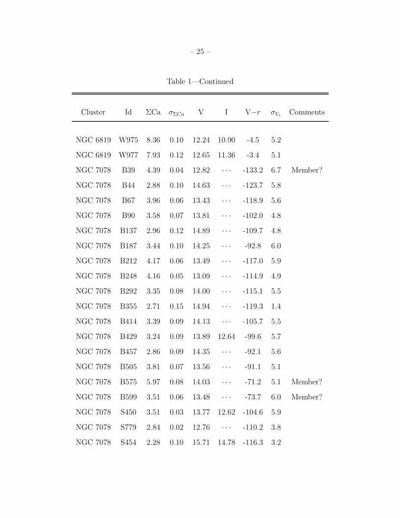
– 25 –

Table 1—Continued

Cluster Id ΣCa σΣCa V I V−r σVrComments

NGC 6819 W975 8.36 0.10 12.24 10.90 -4.5 5.2

NGC 6819 W977 7.93 0.12 12.65 11.36 -3.4 5.1

NGC 7078 B39 4.39 0.04 12.82 · · · -133.2 6.7 Member?

NGC 7078 B44 2.88 0.10 14.63 · · · -123.7 5.8

NGC 7078 B67 3.96 0.06 13.43 · · · -118.9 5.6

NGC 7078 B90 3.58 0.07 13.81 · · · -102.0 4.8

NGC 7078 B137 2.96 0.12 14.89 · · · -109.7 4.8

NGC 7078 B187 3.44 0.10 14.25 · · · -92.8 6.0

NGC 7078 B212 4.17 0.06 13.49 · · · -117.0 5.9

NGC 7078 B248 4.16 0.05 13.09 · · · -114.9 4.9

NGC 7078 B292 3.35 0.08 14.00 · · · -115.1 5.5

NGC 7078 B355 2.71 0.15 14.94 · · · -119.3 1.4

NGC 7078 B414 3.39 0.09 14.13 · · · -105.7 5.5

NGC 7078 B429 3.24 0.09 13.89 12.64 -99.6 5.7

NGC 7078 B457 2.86 0.09 14.35 · · · -92.1 5.6

NGC 7078 B505 3.81 0.07 13.56 · · · -91.1 5.1

NGC 7078 B575 5.97 0.08 14.03 · · · -71.2 5.1 Member?

NGC 7078 B599 3.51 0.06 13.48 · · · -73.7 6.0 Member?

NGC 7078 S450 3.51 0.03 13.77 12.62 -104.6 5.9

NGC 7078 S779 2.84 0.02 12.76 · · · -110.2 3.8

NGC 7078 S454 2.28 0.10 15.71 14.78 -116.3 3.2

– 26 –

Table 1—Continued

Cluster Id ΣCa σΣCa V I V−r σVrComments

NGC 7078 S478 2.27 0.13 16.42 · · · -114.1 2.9

NGC 7078 S468 6.19 0.10 15.79 · · · 28.8 2.3 No member

NGC 7078 S801 3.46 0.06 14.51 · · · -132.0 53.9

NGC 7078 S833 4.44 0.03 13.40 · · · -115.9 4.0

NGC 7078 S796 3.43 0.04 14.44 · · · -101.0 3.3

NGC 7078 S831 3.35 0.06 14.42 · · · -112.8 3.6

NGC 7078 S767 2.50 0.17 16.76 · · · -106.9 2.0

NGC 7078 S1343 3.39 0.04 14.36 13.24 -99.4 3.5

NGC 7078 S769 5.98 0.11 15.77 · · · -37.7 3.1 No member

NGC 7078 S784 3.80 0.05 14.11 · · · -110.8 3.9

NGC 7078 S1346 3.88 0.04 13.92 12.77 -111.3 5.9

NGC 7078 S154 3.58 0.04 14.16 13.07 -102.6 3.5

NGC 7078 S1354 3.40 0.04 14.17 13.09 -101.3 5.3

NGC 7078 S173 2.73 0.10 15.84 14.83 -120.9 4.1

NGC 7078 S177 3.41 0.04 14.12 13.05 -109.0 4.1

NGC 7078 S168 2.45 0.12 16.42 15.48 -111.2 3.1

NGC 7078 S448 2.43 0.17 16.76 15.83 -102.4 2.6

NGC 7078 S455 3.13 0.06 14.84 · · · -107.9 2.2

NGC 7078 S1332 3.85 0.04 13.98 12.82 -119.3 3.7

NGC 7078 S1337 3.54 0.03 13.81 12.60 -95.2 40.9

NGC 7078 S677 3.22 0.05 14.46 13.30 -95.2 5.9

– 27 –

Table 1—Continued

Cluster Id ΣCa σΣCa V I V−r σVrComments

NGC 7078 S694 3.19 0.06 14.88 13.77 -101.0 4.3

NGC 7078 S708 2.93 0.12 16.49 15.50 -101.8 3.6

NGC 7078 S109 2.10 0.08 20.35 · · · -95.9 2.1

NGC 7078 S1098 2.61 0.11 16.31 · · · -108.2 1.8

NGC 7078 S499 2.70 0.11 16.16 15.18 -109.2 3.2

NGC 7078 S434 4.05 0.03 13.68 · · · -112.6 158.6

NGC 7078 S503 3.44 0.05 14.34 13.32 -95.7 5.5

NGC 7078 S1333 5.26 0.06 14.68 13.56 -114.3 4.9

NGC 7789 W8957 8.96 0.14 11.61 10.05 -74.3 6.0

NGC 7789 W9840 9.15 0.13 11.93 10.34 -51.7 6.4

NGC 7789 W10652 8.33 0.10 11.89 10.21 -56.4 5.2

NGC 7789 W10746 9.36 0.07 11.04 8.64 -56.9 6.4

NGC 7789 W1135 8.03 0.14 12.19 10.66 -60.1 5.4

NGC 7789 W12478 8.77 0.12 11.57 9.88 -56.6 5.7

NGC 7789 W1269 8.27 0.12 11.96 10.34 -54.1 5.1

NGC 7789 W13089 8.27 0.15 11.98 10.27 -58.8 5.0

NGC 7789 W13862 9.46 0.07 10.74 8.53 -60.4 7.4

NGC 7789 W2740 9.20 0.09 11.05 9.08 -57.5 6.6

NGC 7789 W6345 9.63 0.07 10.66 8.48 -56.1 6.6

NGC 7789 W6767 8.94 0.08 11.35 9.57 -58.3 6.3

NGC 7789 W6810 9.17 0.09 11.61 9.72 -47.6 5.7

– 28 –

References:

• NGC 104 Lee (1977) [L], Stetson (2000) [S]

• NGC 188 Webda http://obswww.unige.ch/webda/ [W]

• NGC 288 Alcaino & Liller (1980) [A]

• NGC 362 Harris (1982) [H]

• NGC 1851 Stetson (1981) [S]

• NGC 1904 Stetson & Harris (1977) [S]

• Berkeley 20 Webda [W]

• NGC 2141 Burkhead y col. (1972) [B]; Rosvick (1995) [R]; Webda [W];

• Collinder 110 Webda [W]

• Trumpler 5 Webda [W]

• NGC 2298 Alcaino & Liller (1986) [A]; Alcaino (1974) [A]

• Berkeley 32 Webda [W]

• Melotte 66 Webda [W]

• Berkeley 39 Webda [W]

• NGC 2420 Webda [W]

• NGC 2506 Webda [W]

• NGC 2682 Webda [W]

• NGC 3201 Stetson (2000) [S];

– 29 –

• NGC 4590 Harris (1975a) [H]; Stetson (2000) [S]

• NGC 5927 Zoccalli (comunicacion privada)

• NGC 6352 Zoccalli (comunicacion privada); Rosenberg y cols. (2000) [R]

• NGC 6528 Ortolani y cols. (1992) [O]

• NGC 6681 Harris (1975b) [H]; Rosenberg y cols. (2000) [R]

• NGC 6705 Sung y cols. (1999) [S]

• NGC 6715 Rosenberg y cols. (2004) [R]

• NGC 6791 Stetson y cols (2003) [S]

• NGC 6819 Webda [W]

• NGC 7078 Buonanno y cols. (1983) [B]; Stetson (2000) [S]

• NGC 7789 Webda [W]

– 30 –

Table 1—Continued

Cluster Id ΣCa σΣCa V I V−r σVrComments

NGC 7789 W7013 8.78 0.09 11.32 9.66 -67.9 5.4

NGC 7789 W7029 9.41 0.07 10.74 8.59 -54.6 7.0

NGC 7789 W7091 9.22 0.09 11.20 9.36 -48.2 6.7

NGC 7789 W8293 8.75 0.10 11.46 9.74 -54.9 5.0

NGC 7789 W8400 9.58 0.08 11.18 9.07 -67.4 6.6

NGC 7789 W8799 9.46 0.06 10.88 8.77 -56.0 1.1

NGC 7789 W896 8.64 0.09 11.49 9.74 -60.9 6.2