Luo et al. Genome Biology 2014, 15:527http://genomebiology.com/2014/15/12/527

METHOD Open Access

The importance of study design for detectingdifferentially abundant features inhigh-throughput experimentsHuaien Luo1†, Juntao Li1†, Burton Kuan Hui Chia1, Paul Robson2 and Niranjan Nagarajan1*

Abstract

High-throughput assays, such as RNA-seq, to detect differential abundance are widely used. Variable performanceacross statistical tests, normalizations, and conditions leads to resource wastage and reduced sensitivity. EDDArepresents a first, general design tool for RNA-seq, Nanostring, and metagenomic analysis, that rationally selectstests, predicts performance, and plans experiments to minimize resource wastage. Case studies highlight EDDA’sability to model single-cell RNA-seq, suggesting ways to reduce sequencing costs up to five-fold and improvingmetagenomic biomarker detection through improved test selection. EDDA’s novel mode-based normalization fordetecting differential abundance improves robustness by 10% to 20% and precision by up to 140%.

BackgroundThe availability of high-throughput approaches to docounting experiments (for example, by using DNA se-quencing) has enabled scientists in diverse fields (espe-cially in Biology) to simultaneously study a large set ofentities (for example, genes or species) and quantifytheir relative abundance. These estimates are then com-pared across replicates and experimental conditions toidentify entities whose abundance is significantly altered.One of the most common scenarios for such experi-ments is in study of gene expression levels, where se-quencing (with protocols such as SAGE [1], PET [2],and RNA-Seq [3]) and probe-based approaches [4] canbe used to obtain a digital estimate of transcript abun-dance in order to identify genes whose expression is al-tered across biological conditions (for example, cancerversus normal [5]). Other popular settings where suchdifferential abundance analysis is performed include thestudy of DNA-binding proteins and histone modifica-tions (for example, using ChIP-Seq [6,7]), RNA-bindingproteins (for example, using RIP-Seq [8] and CLIP-Seq[9]), and the profiling of microbial communities (using16S rRNA amplicon [10] and shotgun sequencing [11]).

* Correspondence: nagarajann@gis.a-star.edu.sg†Equal contributors1Computational and Systems Biology, Genome Institute of Singapore,Singapore 138672, SingaporeFull list of author information is available at the end of the article

© 2014 Luo et al.; licensee BioMed Central LtdCommons Attribution License (http://creativecreproduction in any medium, provided the orDedication waiver (http://creativecommons.orunless otherwise stated.

Due to its generality, a range of software tools havebeen developed to do differential abundance tests (DATs),often with specific applications in mind, including popularprograms such as edgeR [12], DEseq [6], Cuffdiff [13,14],Metastats [11], baySeq [15], and NOISeq [16]. The di-gital nature of associated data has allowed for severalmodel-based approaches including the use of exact tests(for example, Fisher’s Exact Test [11]), Poisson [17], andNegative-Binomial [6,12] models as well as Bayesian [15]and Non-parametric [16] methods. Recent comparativeevaluations of DATs in a few different application settings(for example, for RNA-Seq [6,16,18-21] and Metage-nomics [11]) have further suggested that there is notablevariability in their performance, though a consensus onthe right DATs to be used remains elusive. In addition, itis not clear, which (if any) of the DATs are broadly applic-able across experimental settings despite the generality ofthe statistical models employed. The interaction betweenmodeling assumptions of a DAT and the applicationsetting, as defined by both experimental choices (forexample, number of sequencing reads to produce forRNA-seq) as well as intrinsic experimental characteris-tics (for example, number of genes in the organism ofinterest), could be complex and not predictable a priori.Correspondingly, only in very recent work, have experi-mental design issues been discussed in a limited setting,that is, using a t-test for RNA-seq analysis [22]. Also, as

. This is an Open Access article distributed under the terms of the Creativeommons.org/licenses/by/4.0), which permits unrestricted use, distribution, andiginal work is properly credited. The Creative Commons Public Domaing/publicdomain/zero/1.0/) applies to the data made available in this article,

Luo et al. Genome Biology 2014, 15:527 Page 2 of 17http://genomebiology.com/2014/15/12/527

experimental conditions can vary significantly and alongseveral dimensions (Table 1), a systematic assessment ofDATs under all conditions is likely to be infeasible. As aresult, the choice of DAT as well as decisions related toexperimental design (for example, number of replicatesand amount of sequencing) are still guided by rules ofthumb and likely to be far from optimal.In this study, we establish the strong and pervasive im-

pact of experimental design decisions on differentialabundance analysis, with implications for study design indiverse disciplines. In particular, we identified data nor-malization as a source of performance variability and de-signed a robust alternative (mode normalization) thatuniformly improves over existing approaches. We thenpropose a new paradigm for rational study design basedon the ability to model counting experiments in awide spectrum of applications (Figure 1). The resultinggeneral-purpose tool called EDDA (for ‘ExperimentalDesign in Differential Abundance analysis’), is the firstprogram to enable researchers to design experimentsfor single-cell RNA-seq, NanoString assays, and Meta-genomic sequencing, and we highlight its use throughcase studies. EDDA provides researchers access to anarray of popular DATs through an intuitive online inter-face [25] and answers questions such as ‘How much se-quencing should I be doing?’, ‘Does the study adequatelycapture biological variability?’, and ‘Which test should Iuse to sensitively detect differential abundance in myapplication setting?’. To provide full access to its func-tionality, EDDA is also available as a user-friendly Rpackage (on SourceForge [26] and Bioconductor [27]),and is easily extendable to new DATs and simulationmodels. The R package as well as the website providedifferent metrics to assess the performance of DATs

Table 1 Experimental conditions affecting differential abunda

Abbr. Description

Experimental choices Number of replicates NR Number of treplicates foin the test

Number of data-points ND Number of dcounting ex

Experimentalcharacteristics

Entity count EC Number of eexperiment

Sample variability SV Variability ac

Abundance profile AP Relative abufirst group

Perturbation profile PDA, FC Perturbationthe first grouthe second g

Test settings Biases in data generation Deviations fdue to biaseexperimenta

Differential abundance test DAT See Table 2

including the area under curve (AUC) of the receiveroperating characteristic (ROC) curve, precision-recallcurves, and actual versus estimated false discovery rate(FDR).

ResultsIn the following, we present and emphasize the under-appreciated impact of various experimental conditions(grouped into two categories: experimental choices andexperimental characteristics, see Table 1) and variouspopular DATs (see Table 2) on the ability to detect dif-ferential abundance. Our results highlight the import-ance of careful experimental design and the interplaybetween experimental conditions and DATs in dictatingthe success of such experiments. We first establish thatthe impact of experimental choices on performance canbe significant and in the next section explore their inter-action with various experimental characteristics. The re-sults presented here are based on synthetic datasets toallow controlled experiments and exploration of a wide-range of parameters, with no emphasis on a particularapplication. Note that these comparisons are not meantto serve as a benchmark (more sophisticated compari-sons and benchmarks can be found in other studies[6,11,16,18-21,28]) but instead to motivate the need forand the specific design decisions in EDDA. In the fol-lowing section, we discuss the validity of the modelingassumptions and parameter ranges that we investigatedand used to guide the design of EDDA. We conclude byshowcasing EDDA’s application in various settings. Forease of reference, a schematic overview of the simulationmodel in EDDA (Figure 1a) and a flowchart of how itcan be used (Figure 1b) is provided in Figure 1 with de-tailed descriptions in the Methods section.

nce tests (DATs)

Notes

echnical or non-technicalr the two groups compared

For simplicity, in many cases, we assumeNR to be the same in both groups

ata-points generated in theperiment

For example, reads generated in anRNA-seq experiment

ntities in the counting For example, number of genes in anRNA-seq experiment

ross replicates (see Methods) For example, biological variability inRNA-seq datasets

ndance of the entities in the Typically follows a power-law distribution

s to the abundance profile ofp to obtain the profile forroup (see Methods)

Used to generate the differentiallyabundant entities (PDA = Percentage ofentities, FC = fold-change distribution)

rom multinomial samplings inherent in thel protocol

These are often corrected for in apreprocessing step, for example,composition bias in RNA-seq data [23,24]

Rel

ativ

e A

bund

ance

Entities

Abundance Profile

Perturbation Profile

Variability Simulator

Sample Variability

Number of Replicates

[Negative Binomial or Model-free]

Count Simulator [Multinomial or Original]

Number of Data-pointse.g. No. of Sequencing Reads

Cou

nts

Panel of Tests [edgeR, DESeq, Cuffdiff, NOISeq, baySeq, Metastats, ...]

Characterisitics

ChoicesExperimentali.e. modifiable by user

i.e. intrinsic to experimentExperimental

Design Choices

Output: Test Recommendations, Optimal Design

1

2

3

4

Condition 1 Condition 2

a bactgaagtcagtaacggtattaatccagtgagatacacctcgcgcgcctattatcgatcgtcgtgcttgatgcgctatcgcgtacgtcaagacacatacgttttatgtcctgtaataatcaaagggctgtttt

actgaagtcagtaacggtattaatccagtgagatacacctcgcgcgcct

?

Data Availability? What performance should I expect?

Full Dataset

Pilot Dataset

How much datashould I generate?

Online Performance Evaluation ModuleNo Data

Is there a suitablesample dataset?

Yes: Set as Pilot Dataset

Online Experimental Design Module

Generate Full Dataset according to recommendations

Full EDDA functionality in R

Is the Negative Binomial Model valid here?

No: Generate Pilot Dataset

No

Are recommendations robust to changes in AP and SV?

No: Generate Pilot Dataset

Yes: Generate Full Dataset according to recommendations

Is performance satisfactory?

No

Online Differential Abundance Testing Module

Yes

Output: List of Differentially Abundant Entities

Entity Fold-Change p-Value FDR A 153 3e-20 3e-16 B 96 6e-18 6e-14 C 64 5e-16 5e-12 D 48 7e-10 7e-8

Rel

ativ

e A

bund

ance

0.05

2000

Yes: Do extensive testing with EDDA

Figure 1 A schematic overview of EDDA and its usage. (a) Overview of the simulate-and-test approach used in EDDA involving four key steps(see Methods for details). The figure also indicates the various parameters studied here, that impact the ability to predict differentially abundantentities (also see Table 1), in red and green text. (b) A flowchart describing how EDDA can be used to optimize design and performance in acounting experiment. EDDA functionality is depicted in green boxes and rhombi indicate decision nodes.

Luo et al. Genome Biology 2014, 15:527 Page 3 of 17http://genomebiology.com/2014/15/12/527

Impact of experimental choices on performanceWhile the availability of high-throughput technologies(such as massively parallel DNA sequencing) to do count-ing experiments has significantly increased the resolutionof such experiments, the cost of the experiment is often

Table 2 Description of various software packages for conduct

Name Statistical testing Nor

edgeR [12] Negative Binomial Model, Conditional MaximumLikelihood to estimate parameters, Exact Test

TMM

DESeq [6] Negative Binomial Model, local regression toestimate parameters, Exact Test

Nor

baySeq [15] Negative Binomial Model, empirical Bayes toestimate parameters

RPM

NOISeq [16] Non-parametric approach RPM

Cuffdiff [14] t-test RPM

Metastats [11] Non-parametric t-test, Fisher’s Exact Test forsmall counts

RPM

RPKM: Normalization by read count and gene length (RNA-seq) [3], RPM: NormalizaUQN: Upper Quartile Normalization [20].

still an important factor and the number of replicates anddata-points that can be afforded may be less than optimal.Furthermore, in many settings the number of replicates orthe number of data-points possible may be constraineddue to technological limitations or uniqueness of samples

ing differential abundance tests

malization approach Target application areas

, UQN SAGE [1], MPSS [29], PMAGE [30], miRAGE[31] and SACO [32] among others

malization by median RNA-seq [3], HITS-CLIP [9] and ChIP-seq[33] among others

, TMM DNA-seq, RNA-seq [3] and SAGE [1]among others

, RPKM, UQN ChIP-seq [33] and RNA-seq [3] among others

, RPKM, UQN RNA-seq [3]

Metagenomics

tion by read count (RNA-seq), TMM: Trimmed Mean of M values [34],

Luo et al. Genome Biology 2014, 15:527 Page 4 of 17http://genomebiology.com/2014/15/12/527

and conditions. In such settings, it would be ideal tounderstand and exploit the trade-off between the numberof replicates and data-points needed (for example, bydoing deeper RNA-seq for a few biological replicates) forsuch analysis. In the following, we investigate these di-mensions individually and in conjunction. For consistencyand ease of comparison, we typically use AUC as themetric for performance (with precision-recall curves beingprovided in the supplement) to highlight variability acrossconditions. In practical applications, other metrics such asthe true-positive rate and actual FDR while controlling forFDR (methods such as NOISeq would need alternativethresholds) may be more appropriate and are also sup-ported by EDDA.

Number of replicatesThe performance of DATs (measured in terms of AUC)as a function of the number of replicates (NR) in thestudy is highly non-linear, with significant improvementsobtainable until a saturation point (indicated by a largermarker size; Figure 2a). The saturation point is likely to belargely determined by the intrinsic variability of replicates

1 5 10 15 20

0.55

0.6

0.65

0.7

0.75

0.8

0.85

0.9

0.95

1

Number of Replicates (NR)

AU

C

a

4 5 6 7 8 9

0.90

0.92

0.94

0.96

0.98

1.00

DESeq edgeR baySeq

NOISeq Cuffdiff Metastats

Figure 2 Performance of DATs as a function of experimental choices.of the number of data-points with (b) one replicate, (c) two replicates, andthe average per entity. Points with large markers indicate the saturation poResults reported are based on an average over 10 simulations with the follND =1,000 per entity, AP = BP, SM = NB, and SV =0.85 (see Table 1 and Me

in an experiment. However, clear differences are also seenacross DATs as seen in Figure 2a, where edgeR and DESeqachieved AUC greater than 0.95 with five replicates, whilebaySeq required eight replicates and has substantiallylower AUC with one replicate. While all DATs seem toconverge toward optimal performance (AUC =1) in thissetting, the rate of convergence varies markedly (for ex-ample, note the curve for Cuffdiff). Note that the relativeperformance of DATs is influenced by the experimentalsetting, especially in conditions where the number of rep-licates available is small (as is typically the case), and thusthe choice of DAT is strongly dependent on the desiredprecision/recall trade-off (Additional file 1: Figure S1).

Number of data-pointsThe number of data-points (ND) generated in an appli-cation setting is often set to be the maximum possiblegiven the resources available. However, this may lead tomisallocation of resources as suggested by Figure 2b, c,and d. In this setting, increasing the number of data-pointscontinues to improve AUC over a wide range of values (formost DATs). At very high values AUC saturates, but not

10 50 100 500 1000 5000 10000

0.2

0.4

0.6

0.8

b

AU

C

NR=1

10 50 100 500 1000 5000 100000.2

0.4

0.6

0.8

1c NR=2

AU

C

10 50 100 500 1000 5000 100000.5

0.6

0.7

0.8

0.9

1

Number of Data−points

d NR=5

AU

C

(a) AUC as a function of the number of replicates. AUC as a function(d) five replicates. Note that the number of data-points reported isint where the AUC is within 5% of the maximum observed AUC.owing parameters, EC =1,000, PDA =26%, FC = Uniform (3, 5),thods for key to abbreviations used here).

Luo et al. Genome Biology 2014, 15:527 Page 5 of 17http://genomebiology.com/2014/15/12/527

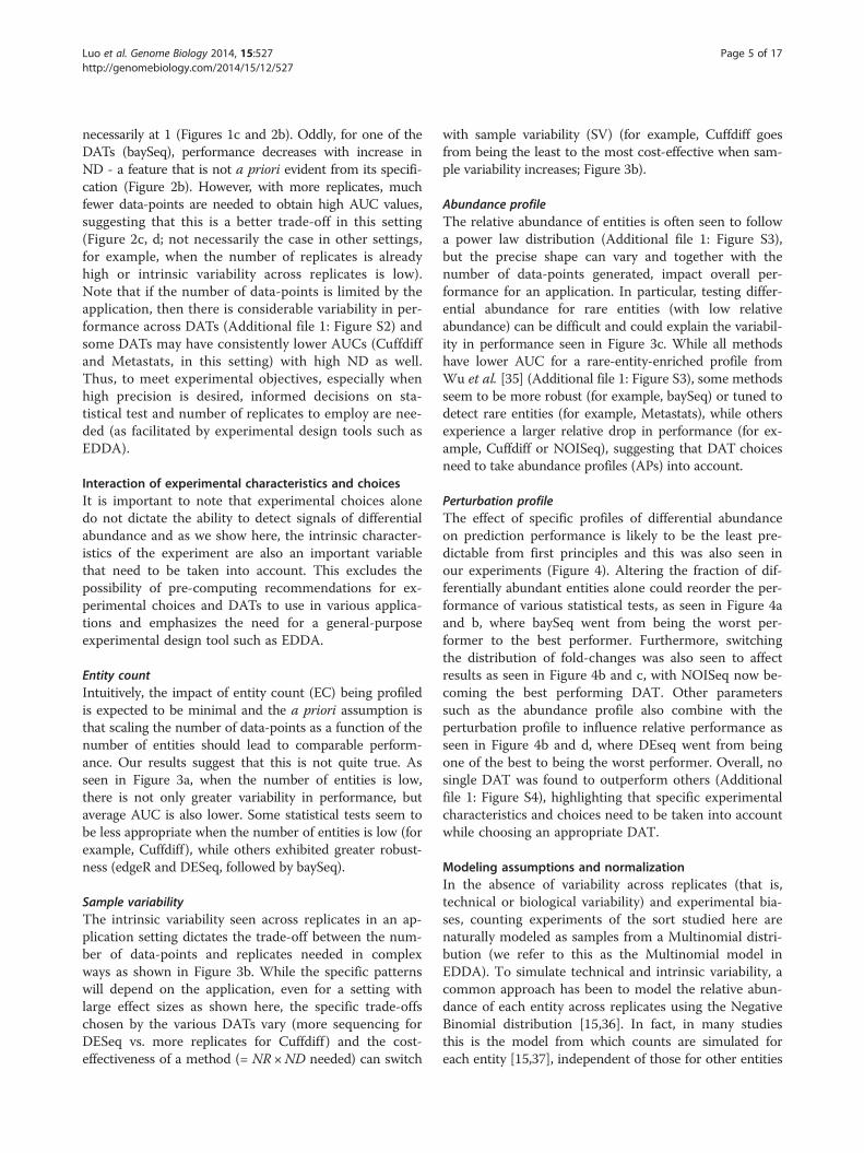
necessarily at 1 (Figures 1c and 2b). Oddly, for one of theDATs (baySeq), performance decreases with increase inND - a feature that is not a priori evident from its specifi-cation (Figure 2b). However, with more replicates, muchfewer data-points are needed to obtain high AUC values,suggesting that this is a better trade-off in this setting(Figure 2c, d; not necessarily the case in other settings,for example, when the number of replicates is alreadyhigh or intrinsic variability across replicates is low).Note that if the number of data-points is limited by theapplication, then there is considerable variability in per-formance across DATs (Additional file 1: Figure S2) andsome DATs may have consistently lower AUCs (Cuffdiffand Metastats, in this setting) with high ND as well.Thus, to meet experimental objectives, especially whenhigh precision is desired, informed decisions on sta-tistical test and number of replicates to employ are nee-ded (as facilitated by experimental design tools such asEDDA).

Interaction of experimental characteristics and choicesIt is important to note that experimental choices alonedo not dictate the ability to detect signals of differentialabundance and as we show here, the intrinsic character-istics of the experiment are also an important variablethat need to be taken into account. This excludes thepossibility of pre-computing recommendations for ex-perimental choices and DATs to use in various applica-tions and emphasizes the need for a general-purposeexperimental design tool such as EDDA.

Entity countIntuitively, the impact of entity count (EC) being profiledis expected to be minimal and the a priori assumption isthat scaling the number of data-points as a function of thenumber of entities should lead to comparable perform-ance. Our results suggest that this is not quite true. Asseen in Figure 3a, when the number of entities is low,there is not only greater variability in performance, butaverage AUC is also lower. Some statistical tests seem tobe less appropriate when the number of entities is low (forexample, Cuffdiff), while others exhibited greater robust-ness (edgeR and DESeq, followed by baySeq).

Sample variabilityThe intrinsic variability seen across replicates in an ap-plication setting dictates the trade-off between the num-ber of data-points and replicates needed in complexways as shown in Figure 3b. While the specific patternswill depend on the application, even for a setting withlarge effect sizes as shown here, the specific trade-offschosen by the various DATs vary (more sequencing forDESeq vs. more replicates for Cuffdiff ) and the cost-effectiveness of a method (= NR ×ND needed) can switch

with sample variability (SV) (for example, Cuffdiff goesfrom being the least to the most cost-effective when sam-ple variability increases; Figure 3b).

Abundance profileThe relative abundance of entities is often seen to followa power law distribution (Additional file 1: Figure S3),but the precise shape can vary and together with thenumber of data-points generated, impact overall per-formance for an application. In particular, testing differ-ential abundance for rare entities (with low relativeabundance) can be difficult and could explain the variabil-ity in performance seen in Figure 3c. While all methodshave lower AUC for a rare-entity-enriched profile fromWu et al. [35] (Additional file 1: Figure S3), some methodsseem to be more robust (for example, baySeq) or tuned todetect rare entities (for example, Metastats), while othersexperience a larger relative drop in performance (for ex-ample, Cuffdiff or NOISeq), suggesting that DAT choicesneed to take abundance profiles (APs) into account.

Perturbation profileThe effect of specific profiles of differential abundanceon prediction performance is likely to be the least pre-dictable from first principles and this was also seen inour experiments (Figure 4). Altering the fraction of dif-ferentially abundant entities alone could reorder the per-formance of various statistical tests, as seen in Figure 4aand b, where baySeq went from being the worst per-former to the best performer. Furthermore, switchingthe distribution of fold-changes was also seen to affectresults as seen in Figure 4b and c, with NOISeq now be-coming the best performing DAT. Other parameterssuch as the abundance profile also combine with theperturbation profile to influence relative performance asseen in Figure 4b and d, where DEseq went from beingone of the best to being the worst performer. Overall, nosingle DAT was found to outperform others (Additionalfile 1: Figure S4), highlighting that specific experimentalcharacteristics and choices need to be taken into accountwhile choosing an appropriate DAT.

Modeling assumptions and normalizationIn the absence of variability across replicates (that is,technical or biological variability) and experimental bia-ses, counting experiments of the sort studied here arenaturally modeled as samples from a Multinomial distri-bution (we refer to this as the Multinomial model inEDDA). To simulate technical and intrinsic variability, acommon approach has been to model the relative abun-dance of each entity across replicates using the NegativeBinomial distribution [15,36]. In fact, in many studiesthis is the model from which counts are simulated foreach entity [15,37], independent of those for other entities

Figure 3 Performance of DATs as a function of experimental characteristics. (a) AUC as a function of entity count (small =100, medium =1,000, large =30,000). Simulations were done with the same parameters as in Figure 2a, except with ND =100 per entity, AP = HBR, SM = Full, andFC = Log-normal [1,2]. (b) AUC as a function of SV (and NR, ND per entity), where low, medium, and high were set to SV =0.05, 0.5, and 0.85,respectively. Note that the plotted point shows the smallest NR and ND values (small NR was given priority in the case of ties) that achieved anAUC target of 0.95. Synthetic data were generated with EC =1,000, PDA =10%, FC = Uniform (8, 8), AP = BP, and SM = NB. (c) AUC as a function ofabundance profile. Simulations were done with the same parameters as in Figure 2a and with NR =5 and ND =500 per entity. The inset showsthe fraction of rare entities (mean count <10) in each abundance profile. Results reported are based on an average over 10 simulations and errorbars in (a) and (c) represent one standard deviation.

Luo et al. Genome Biology 2014, 15:527 Page 6 of 17http://genomebiology.com/2014/15/12/527

(we refer to this as the Negative Binomial model), andbypassing the joint simulation of counts from a Multi-nomial distribution (referred to here as the Full model).For most current high-throughput experiments, as bio-logical variation is significant, the Full Model that incor-porates multinomial sampling of counts while modelingsample-to-sample variability as a negative binomial dis-tribution is appropriate. EDDA also includes an outliersimulation model that allows users to simulate more rea-listic datasets for some settings (for example, RNA-seq[28]; see Methods). In practice, both the Full and theNegative Binomial model elicit similar performance formost experimental settings and most DATs. However,for a few DATs (baySeq, NOISeq, and Cuffdiff) we ob-served deterioration in performance on the Full modelwhen compared to a similar experiment using the Negative

Binomial model (Additional file 1: Figure S5) suggestingthat the Full model is a better measure of performanceof a DAT.By analyzing several published and in-house datasets

we established that, in general, for bulk transcriptomesequencing (confirming earlier reports [15,36]), Nano-string assays and Shotgun Metagenomic sequencing (notshown in prior work), variability in replicates can be ad-equately modeled using the negative binomial distribution(Additional file 1: Figure S6). An exception to this rulewas, however, seen in single-cell RNA-seq experiments inaccordance with observations of unusually high cell-to-cell variability in recent reports [38,39] (Additional file 1:Figure S6c, d). For cases where an appropriate modelfor variability across replicates is not available (as in thesingle-cell case), we developed a Model-Free approach,

0 0.2 0.4 0.6 0.8 1

0

0.2

0.4

0.6

0.8

1

edgeRDESeqNOISeqCuffdiffbaySeq

0 0.2 0.4 0.6 0.8 1

0

0.2

0.4

0.6

0.8

1

baySeqDESeqNOISeqedgeRCuffdiff

0 0.2 0.4 0.6 0.8 1

0

0.2

0.4

0.6

0.8

1

NOISeqedgeRDESeqbaySeqCuffdiff

0 0.2 0.4 0.6 0.8 1

0

0.2

0.4

0.6

0.8

1

False Positive Rate False Positive Rate

True

Pos

itive

Rat

eTr

ue P

ositi

ve R

ate

ba

dc

baySeqCuffdiffNOISeqedgeRDESeq

↑ ↓PDA:5% 5% ↑ ↓PDA:50% 25%

↑ ↓PDA:50% 25% +FC:logN(2,1) ↑ ↓PDA:50% 25% +AP:HBR

Figure 4 ROC plots under various perturbation profiles. Statistical tests in the legend are listed from best to worst (in terms of AUC values)for each setting. Note the striking reordering of test performance across subfigures with slight changes in experimental conditions. Simulations inEDDA were done with (a) PDA =10%, (b) PDA = (50% UP, 25% DOWN), (c) PDA = (50% UP, 25% DOWN), FC = Log-normal (2, 1), (d) PDA = (50%UP, 25% DOWN), AP = HBR. Unless stated otherwise, common parameters include NR =3, EC =1,000, FC = Uniform(3, 7), ND =500 per entity,AP = BP, SM = Full, and SV =0.5.

Luo et al. Genome Biology 2014, 15:527 Page 7 of 17http://genomebiology.com/2014/15/12/527

that uses sub-sampling (and appropriate scaling whereneeded) of existing datasets to provide simulated datasetsthat match sample-to-sample variability in real datasetsbetter (with the drawback that it relies on the availabilityof a dataset with many replicates; see Methods).To evaluate the data generation models used in this

study (either model-based or model-free), as well as es-tablish their suitability for the design of EDDA, we firstinvestigated distributional properties of real and simu-lated datasets (Additional file 1: Figure S7). The resultshere indicate that while overall both simulation approa-ches (where applicable) provide good approximationsand capture the general trend, the Model-Free approachmore closely mimics true sample variability (Additionalfile 1: Figure S7). We next tested the suitability of an ap-proach where simulated datasets are generated to mimican existing pilot dataset and employed to measure trendsin performance. Our results confirmed that simulated

data generated by our simulation models enable reliablemeasurement of true performance for DATs (relative-error in AUC <6%) and monitoring of trends as a functionof experimental choices and characteristics (Additionalfile 1: Figure S8). In addition, experimental recommen-dations from EDDA simulations were also found tomatch DAT recommendations based on benchmarkingon real datasets [40] (Additional file 1: Figure S9), sug-gesting that EDDA can help avoid this step and still reli-ably guide experimental design.In some experimental settings, variability in replicates

can be extremely low and directly simulating from theMultinomial distribution (a special case of the Full modelthat we refer to as the Multinomial model; see Methods)is sufficient. In principal, with enough data-points, sta-tistical testing under the Multinomial model should bestraightforward and we expect various DATs to performwell. The few exceptions that we noted, suggest that aspects

Luo et al. Genome Biology 2014, 15:527 Page 8 of 17http://genomebiology.com/2014/15/12/527

other than statistical testing, such as data normalization,may play a role in their reduced performance (Additionalfile 1: Figure S5).An investigation of different normalization approaches

(Table 2) under the various experimental conditions ex-plored in this study suggests that their robustness can varysignificantly as a function of the experimental setting. Inparticular, we observed a few settings under which manyof the existing approaches performed sub-optimally(Figure 5a) and to address this we designed a newmethod (mode normalization) that analyzes the distri-bution of un-normalized fold-changes of entities usingmode statistics to select a suitable normalization fac-tor (see Methods and Additional file 1: Figure S10). We

Figure 5 Comparison of different data normalization approaches. (a)normalization by the sum of counts for all non-differentially-abundant entitUpper-quartile Normalization (UQN) improved over the Default normalizatidid not we mark its performance with a solid line. Mode normalization alwnormalization for the DAT (improvement shown by the solid box). The parDOWN), AP =Wu et al.; B: PDA = (35% UP, 15% DOWN); C: PDA = (40% DOWotherwise, common parameters include NR =3, EC =1,000, FC = Log-normaComparison on real datasets, highlighting the robustness of mode normaliof the top 500 differentially abundant genes (sorted by P value using edgethose where one of the libraries is down-sampled (5% or 10% of original sione standard deviation.

compared mode normalization to the default normaliza-tion and a popular alternate (Upper-quartile Normaliza-tion), for each DAT and across all the conditions testedhere, to find that the use of mode normalization uniformlyimproved performance (on average, AUC by 9% and preci-sion by 14% at 5% FDR). Also, in cases where the perform-ance of a few DATs dipped under the Multinomial model,mode normalization was able to rescue the AUC values(Additional file 1: Figure S5d). In addition, we identifiedseveral examples where mode normalization significantlyimproved AUC values for all the DATs tested (improvingprecision to detect differential abundance by up to 140%at 5% FDR), highlighting that proper data normalization isa key step in attaining experimental goals (Figure 5a). As

On simulated benchmark datasets using EDDA. Note that we usedies (non-DA) as a measure of ideal performance here. In general,on (improvement shown by the checked box) but for cases where itays improved over the performance from UQN and the Defaultameters for the various experiments include for A: PDA = (26% UP, 10%N), SM =Mutinomial; and D: the same as in Figure 4b. Unless statedl (1.5, 1), ND =500 per entity, AP = HBR, SM = Full, and SV =0.5. (b)zation. Shown here is the overlap fraction (used to measure robustness)R) in comparisons involving both the original full-size libraries versusze). Barplots show the average of five runs and error bars represent

Luo et al. Genome Biology 2014, 15:527 Page 9 of 17http://genomebiology.com/2014/15/12/527

depicted in Figure 5a, there are often cases where thedefault normalization of a DAT or a popular alternate(Upper-quartile Normalization) lead to reduced perform-ance while calling differentially abundant entities, whilemode normalization consistently achieves optimal per-formance across DATs. Note that no normalization can beexpected to work under all conditions and simulated data-sets generated by EDDA can also be valuable to compareand choose among alternative normalization techniques.To further evaluate normalization methods on real

datasets, we studied the consistency of differential abun-dance predictions (against predictions on the full data-set) upon down-sampling of data-points, using threedeeply-sequenced RNA-seq datasets [40] (Figure 5b).These results highlight the robustness of mode normali-zation versus other popular approaches (UQN and TMM;Table 2). Mode normalization was found to improve ro-bustness by 10% to 20% across datasets and was the leastaffected by imbalances in sequencing depth across condi-tions (Figure 5b).

Applications of EDDA and mode normalizationThe observed variability in the performance of DATsacross experimental characteristics and choices, andthe demonstration that data from many kinds of high-throughput experiments can be adequately modelled insilico, motivated the use of a simulate-and-test paradigmin EDDA to guide experimental design (see Figure 1aand Methods). EDDA allows users fine-scale control ofall the variables discussed here (summarized in Table 1),but also provides the option to directly learn experi-mental parameters (and models for the model-free ap-proach) from pilot or publicly-available datasets. Someof the commonly expected modes of usage for EDDAare discussed in the Methods section ‘EDDA modules’and illustrated in Figure 1b. Furthermore, to showcasethe use of EDDA and mode normalization, we presentresults from EDDA analysis of several recently gener-ated datasets in three different experimental settings,each highlighting a different aspect of the utility of thepackage in a practical scenario.For the first case study, we analyzed data from a re-

cent single-cell RNA-seq study of circulating tumorcells (CTCs) from melanoma patients [41]. The authorsgenerated on average 1,000 data-points per entity (>20million reads) and used a one-way ANOVA test (equiva-lent to a t-test) to identify differentially abundant genesbetween CTCs and primary melanocytes. We reanalyzedthe data using EDDA to simulate synthetic datasets thatmimicked real data (with the Model-Free approach anda 96-cell dataset generated as a resource for this study)and used them to test a panel of DATs (see Methods).The availability of new micro-fluidics based systems toautomate single-cell omics has highlighted the cost of

sequencing as the major bottleneck in studying a largenumber of cells. Strikingly, EDDA analysis revealed thatthis study could have been conducted with one-fifth ofthe sequencing that was done (by reducing sequencingdepth to one-tenth and doubling the number of repli-cates) without affecting performance in terms of iden-tifying differentially abundant genes (Figure 6a). Thiswas, however, only possible if the appropriate DAT wasused (edgeR and BaySeq, in this case), with the choiceof DAT playing a more significant role than the amountof sequencing done. Using BaySeq with on average 100reads per gene (that is, 2 million reads per cell as op-posed to the 20 million reads used in this study) and in-creasing the number of replicates from five to 50 (andthus maintaining sequencing cost) would be expected toboost AUC from 0.86 (and 0.75 using the t-test) to 0.96and sensitivity from 57% to 72% at 5% FDR, in this study(Figure 6a). Note that while practical considerationscould limit the number of CTCs that can be capturedand studied, this should not be an issue for other celltypes in this study.In the second case study, we analyzed data from an in-

house project (manuscript in preparation) for the de-velopment of prognostic and predictive gene signaturesin breast cancer on the NanoString nCounter platform(NanoString, WA, USA). The NanoString platform al-lows for the digital measurement of gene expression, si-milar to RNA-seq, but is typically used to profile a small,selected set of genes in a large number of samples (107genes and 306 samples in this study), making data nor-malization a critical step for robust analysis. Using EDDA,we explored the impact of a range of normalization ap-proaches, including the one recommended in the Nano-String data analysis guide (NanoString, WA, USA). Asshown in Figure 6b, the coefficient of variation (COV) of apanel of six housekeeping genes (ACTG1, ACTB, EIF4G2,GAPDH, RPLP0, and UBE2D4) is significantly lower, asexpected, when the data are properly normalized and, inparticular, this is the case when using mode normalizationwhich produces the lowest average COV across all themethods tested. We then investigated the effect of nor-malization on the power to discriminate between ER po-sitive and negative breast cancers using a panel of eightknown ER signature genes [43]. Not surprisingly, the abil-ity to distinguish ER positive and negative breast cancersimproves significantly with proper normalization withmode normalization providing the largest F-score(see Methods) among all the approaches tested (Figure 6c).In our third case study, we critically assessed the ana-

lysis done in a recent Metagenomic study that lookedinto the association of markers in gut microflora withtype 2 diabetes in Chinese patients [42]. Due to thecomplexity of the microbial community in the gut, theauthors reported that they were able to assemble more

DESeq edgeR baySeq NOISeq Cuffdiff Metastats

5 5 5 10 20 5 10 20 30 40 501000 500 250 500 250 100 100 100 100 100 100

0.7

0.75

0.8

0.85

0.9

0.95

Raw Mode UQN

0.2

0.6

1.0

1.4

ER− ER+

24

68

ER− ER+

24

68

ER− ER+

24

68

75 75 150 150 300 30010 100 5 10 5 10

0.7

0.75

0.8

0.85

0.9

0.95

1

Wilcoxon

Single−cell

Metagenomics

Raw Mode UQN

NR:ND:

Mea

n E

xpre

ssio

n (lo

g2)

F=165 F=277 F=213

NR:ND:

Coe

ffici

ent o

f Var

iatio

n

AU

C

AU

C

a b

c d

Figure 6 Case studies of EDDA usage. (a) Predicted performance of DATs as a function of replicates (NR) and sequencing depth (ND) for asingle cell RNA-seq experiment (Ramskold et al. [41]). Note that the vertical black dashed line indicates design choices in the original study.(b) Coefficient of variation for a panel of housekeeping genes from a NanoString experiment under different normalization approaches. (c)Separability of ER positive and negative samples under different normalization approaches. (d) Predicted performance of DATs as a function ofreplicates (NR) and sequencing depth (ND) for a Metagenomics experiment (Qin et al. [42]). Note that the vertical black and red dashed linesindicate design choices in the original study and using one-fifth of the original amount of sequencing.

Luo et al. Genome Biology 2014, 15:527 Page 10 of 17http://genomebiology.com/2014/15/12/527

than 4 million microbial genes overall. Correspondingly,since on average approximately 20 million paired-endreads were generated per sample, the sequencing donehere is expected to provide shallow coverage of the geneset, on average. The study involved a large number ofcases (71) and controls (74) and the Wilcoxon test wasused to identify differentially abundant genes in a case-control comparison. Another batch of 100 cases andcontrols was then used to validate biomarkers identifiedfrom the first batch. We used EDDA to generate virtualmicrobiome profiles and assessed the performance ofthe Wilcoxon test in this setting, in addition to the de-fault panel of DATs (Table 2). EDDA analysis revealedthat the Wilcoxon test was likely to have been too con-servative in this setting and could have been improvedupon using DATs like Metastats, which was designed for

Metagenomic data and edgeR, which is commonly usedfor RNA-seq analysis (Figure 6d). In addition, while in-creased coverage is likely to improve the ability to detecttrue differences in the microbiome, the gains are ex-pected to be relatively modest (for edgeR, approximatley1% increase in AUC with 10-fold increase in sequencing;Figure 6d). Correspondingly, despite the shallow cover-age employed in this study, it is likely to have captured asignificant fraction of the biomarkers that could havebeen determined with more sequencing. In contrast, in-creasing the number of replicates is likely to have mark-edly improved the ability to detect true differences inthe microbiome, (with edgeR, approximately 7% increasein AUC by doubling the number of replicates Figure 6d).Keeping sequencing cost fixed and using 300 replicatesand five reads per gene is thus expected to boost AUC

Luo et al. Genome Biology 2014, 15:527 Page 11 of 17http://genomebiology.com/2014/15/12/527

from 0.73 (using the Wilcoxon test) in the study to 0.97(using edgeR; Figure 6d) and sensitivity from 32% to86% at 5% FDR.Based on this, we reanalyzed cases and controls from

the first batch in this study to identify an additional37,664 differentially abundant genes (17% increase) usingedgeR, of which a greater fraction (27% increase overthe original study) were also validated in the secondbatch of samples (Additional file 1: Table S2). The newlyidentified genes highlighted previously missing aspectsof the role of the microbiome in Type 2 diabetes in-cluding the identification of 24 additional gene familiesenriched in differentially abundant genes (Additionalfile 1: Table S3). In particular, this analysis detected twobacterial genes identified as multiple sugar transportsystem substrate-binding proteins as being abundant incases vs. controls (Additional file 1: Figure S11), as well asthe enrichment of two new families for multiple sugartransport system permease proteins (K02025 and K02026).Strikingly, the newly detected genes also enabled construc-tion of an improved microbiome-based predictive modelfor Type 2 diabetes (AUC of 0.96 vs. 0.81 in the originalstudy; see Methods and Additional file 1: Figure S11),based on the selection of 50 marker genes (see Methodsand Additional file 1: Table S4), highlighting the disease-relevance for the additional biomarkers that we detect andthat improved differential abundance analysis based on in-formed choices using EDDA can significantly impact majorconclusions from a study.

Discussion and ConclusionsThe case studies highlighted in the previous section arenot unique in any way and point to a general trend incurrent design of high-throughput experiments, wherecommonly used rules of thumb lead to suboptimal designsand poor utilization of precious experimental resources.Considering that the market for sequencing based experi-ments alone is currently in the billions of dollars, savingsin research budgets worldwide would be substantial witheven a modest 10% improvement in study design. On theother end, with a fixed budget, optimizing study designcan ensure that key insights are not missed. In particular,in many scenarios where either (a) effect sizes are smalland fold-changes are marginal or (b) large effects on a fewentities mask subtle effects on other entities or (c) thegoal is to understand coordinated processes such as cel-lular pathways through enrichment analysis [44], loss insensitivity or precision due to unguided experimentalchoices can be detrimental to the study. The use of apersonalized-benchmarking tool such as EDDA pro-vides a measure of insurance against this.With the recent, dramatic expansion in the number of

high-throughput applications (largely based on DNA se-quencing) as well as end-users (often non-statisticians),

differential abundance testing is now frequently done bynon-experts in settings different from the originalbenchmarks for a method. This can make it difficult todetermine if a particular analysis was appropriate or leadto incorrect results. One possible approach that couldaccount for this is to use multiple DATs to get a consen-sus set (also available as an option on the EDDA web-server) but this can result in overly conservative predic-tions. For example, in a recent analysis of RNA-seq datafrom two temporally-separated mouse brain samplesusing edgeR and DESeq (with default parameters), wefound that the intersection of differentially expressedgenes (at 10% FDR) contained less than 10% of the union.Breakdown of the results showed that while edgeR wasprimarily reporting upregulated genes (998 out of 1189),DESeq was largely reporting downregulated genes (875out of 878), with no indication as to which analysis wasmore appropriate. EDDA simulations and analysis werethen used to clarify that results from edgeR were more re-liable here (FPR of 3.8% vs. 9.2% at 10% FDR) and couldbe improved further using mode-normalization (FPR of1.5%). Furthermore, the bias towards detecting up- ordownregulated genes was intrinsic to the tests here (notaffected by normalization as we originally suspected) andhence reporting the union of results was more appropri-ate. Examples such as this are not uncommon in the ana-lysis of high-throughput datasets and experimental designtools such as EDDA can help provide informed answers toresearchers.We hope the results in this study serve to further

highlight the still under-appreciated importance of pro-per normalization for differential abundance analysiswith high-throughput datasets [20,45,46]. Normalizationbased on mode statistics provides an intuitive alternativeto existing approaches, exhibiting greater robustness toexperimental conditions in general, >20% improved AUCperformance in some conditions, as well as the ability todetect cases where proper normalization may not befeasible.EDDA was designed to provide an easy-to-use and

general-purpose platform for experimental design in thecontext of differential abundance analysis. To our know-ledge, it is the first method that allows users to plansingle-cell RNA-seq, Nanostring assays and Metagenomicsequencing experiments (as well as other high-throughputcounting experiments, for example, ChIP-seq), where thelarger number of samples involved could lead to import-ant experimental trade-offs. The combination of model-based and model-free simulations in EDDA allows forgreater flexibility and, in particular, we provide evidencethat the commonly used Negative Binomial model maynot be appropriate for single-cell RNA-seq, but a model-free approach (leveraging on a 96-cell dataset generated inthis study) is better suited. Model-free simulations using

Luo et al. Genome Biology 2014, 15:527 Page 12 of 17http://genomebiology.com/2014/15/12/527

EDDA can thus serve as a basis for refining new statisticaltests and clustering techniques for single-cell RNA-seq.Note that a common assumption in EDDA and most stat-istical testing packages is that deviations from the multi-nomial model due to experimental biases can be correctedfor and hence these issues were ignored in this study[14,23]. However, we include an outlier simulation modelthat allows users to investigate the impact of potential out-liers in their data on various DATs that are more or lesstuned to handle them [28].EDDA was developed for count-based analysis, where

its model-based simulations assume that counts fromdifferent entities are not correlated. In some applica-tions, such as transcript-level quantification using short-read RNA-sequencing, this assumption may not be validdue to technical reasons (for example, ambiguity in readmapping). Currently, this limitation can only be circum-vented by using the model-free approach in EDDA,based on sample data where entities are correlated (for ex-ample, by using transcript-level mapping for RNA-seq).Further work is needed to develop appropriate model-based approaches that adequately simulate technical ar-tefacts in count data and will necessarily have to beapplication-specific. Note that gene and exon-level quanti-fication are common applications of RNA-seq (as indi-cated by the majority of DATs being designed for this) andshould benefit from model-based analysis in EDDA. Fur-thermore, with improvements in sequencing read lengthas well as adoption of third-generation sequencing tech-nologies, issues related to ambiguous read assignment arelikely to affect a small fraction of reads. The use of EDDA’smodel-based analysis is thus expected to become increas-ingly feasible in this burgeoning application area.Recently, McMurdie et al. demonstrated the applic-

ability of normalization/detection methods designed forRNA-seq data (edgeR/DESeq) for analyzing metage-nomic count data [47]. This study supports the under-lying basis of our work that methods for normalizationand differential abundance testing should be broadly ap-plicable beyond the domains for which they were origin-ally proposed. Cross-fertilization of best practices fromvarious application areas can improve the analysis ofhigh-throughput count data and we hope that generalplatforms such as EDDA accelerate this process.The basis for EDDA is a simple simulate-and-test pa-

radigm as the diversity of statistical tests precludes moresophisticated approaches (for example, deriving closed-form or numerical bounds on expected performance).Given the simplicity of this approach, it is even moresurprising that the field has until now relied on rules ofthumb. In light of this, the main contribution of thiswork should be seen as the demonstration that signifi-cant variability can be observed across all experimentaldimensions and, therefore, lack of experimental design

tailored to a particular application setting can lead tosubstantial wastage of resources and/or loss of detec-tion power. We hope that the availability of EDDAthrough an intuitive, easy-to-use, point-and-click web-based interface will thus encourage a wide-spectrumof researchers to employ experimental design in theirstudies.

MethodsSingle-cell library preparation and sequencingATCC® CCL-243™ cells (that is, K562 cells) were thawedand maintained following vendor’s instructions usingIMDM medium (ATCC® 30-2005™) supplemented with10% FBS (GIBCO® 16000-077™). The cells were fed every2 to 3 days by dilution and maintained between 2 × 10[5] and 1 × 10 [6] cells/mL in 10 to 15 mL cultures keptin T25 flasks placed horizontally in an incubator set at37°C and 5% CO2. Cells were slowly frozen 2 days afterfeeding at a concentration of 4 million cells per mL in100 μL aliquots of complete medium supplemented with5% DMSO (ATCC® 4X). The cryo-vials containing thefrozen aliquots were kept in the vapor phase of liquid ni-trogen until ready to use. On the day of the C1™ experi-ment, a 900 μL aliquot of frozen complete medium wasthawed and brought to room temperature. The cryo-vialwas retrieved from the cryo-storage unit and placed indirect contact with dry ice until the last minute. As soonas the cryo-vial was taken out of dry ice, the cells werethawed as quickly as possible at a temperature close to37°C (in about 30 s).The room temperature complete medium was slowly

added to the thawed cells directly in the cryo-tube andmixed by pipetting four to five times with a 1,000 μLpipette tip. This cell suspension was mixed with C1™ cellsuspension reagent at the recommended ratio of 3:2 im-mediately before loading 5 μL of this final mix on theC1™ IFC. The C1 Single-Cell Auto Prep System (Fluidigm)was used to capture individual cells and to perform celllysis and cDNA amplification following the chip manufac-turer’s protocol for single-cell mRNA-seq (PN 100-5950).Briefly, chemistry provided by the SMARTer Ultra LowRNA Kit (Clontech) was used for reverse transcriptionand subsequent amplification of polyadenylated tran-scripts using the C1™ script 1772×/1773×. After harvestof the amplified cDNA from the chip, 96-way bar-codedIllumina sequencing libraries were prepared by tagmen-tation with the Nextera XT kit (Illumina) following themanufacturer’s protocol with modifications stated inFluidigm’s PN 100-5950 protocol. The 96 pooled librar-ies were 51-base single-end sequenced over three lanesof a Hi-Seq 2000.Raw reads for all libraries are available for download

from NCBI using the following link: [48].

Luo et al. Genome Biology 2014, 15:527 Page 13 of 17http://genomebiology.com/2014/15/12/527

Simulation of count data in EDDAAbundance profile (AP)When provided with sample data, EDDA uses the entitycount and the sample abundance profile from the data(when multiple samples are provided, the counts are ag-gregated to get an average frequency profile) to do si-mulations. Users can also explicitly provide a profile orchoose from among pre-defined profiles including BP(for BaySeq Profile; the profile used in simulations byHardcastle et al. [15]), HBR (a profile derived from a‘human brain reference’ dataset [49]) and the profilefrom Wu et al. [35]. In order to simulate with entitycounts that differ from the original profile, EDDA allowsusers to sample entities (without replacement for sub-sampling and with replacement for over-sampling) fromthe middle 80% (entities are ordered by relative abun-dance), top 10%, and bottom 10% independently. Thisprocedure is designed to maintain the dynamic range ofthe original profile. In addition, to avoid working withentities with very low counts, EDDA allows users to fil-ter out those with counts below a minimum thresholdfor all replicates (default of 10).

Perturbation profileIf EDDA is provided with sample data under two con-ditions then the profile of differential abundance seenthere is assigned to genes by keeping the relationship ofmean expression and fold change. Specifically, EDDAapplies a DAT (DESeq and FDR cutoff of 5% by default,after mode normalization) to the sample data to identifydifferentially abundant entities and their correspondingfold-changes (f i ¼ x2i =x

1i where x1i and x2i are the mean

relative abundance of entity i under the first and secondcondition, respectively). Given d differentially abundantentities, with fold-changes f1 to fd, a set of d entitiesfrom the first condition are perturbed by these fold-changes to obtain the abundance profile for the secondcondition (that is, x2i ¼ √f j � x1i and x1i ¼ x1i =√f j ) whileretaining the correspondence between mean expressionlevel and fold-change. In addition, to account for un-detected entities an additional fraction of entities is ran-domly selected (from those that fail the FDR cutoff andwith fold-change >1.5) and their observed fold-changesused to perturb abundance profiles as before. The frac-tion of entities was determined to ensure that the overallcount matched the expected number of differentiallyabundant entities in the dataset (estimated from the ex-pected number of true positives at each gene’s FDR level).In the absence of sample data, EDDA also allows users tospecifically set the percentage of entities with increasedand decreased entity counts (PDA), ranges for the fold-changes (FC) and the distribution to sample fold-changesfrom (for example, Log-normal, Normal, or Uniform).

Simulation model (SM)The default model for simulations in EDDA is the Fullmodel where the mean abundance for each entity (undereach condition) and the dispersion value provided (SV)is used to compute means for the replicates using aNegative Binomial distribution (this is done emulatingthe procedure in baySeq [15] where each entity has adispersion sampled from a gamma distribution). Whensample data are available, EDDA estimates dispersionvalues by using the procedure in DESeq (alternately,edgeR) to fit the empirical distribution. Entity abundan-ces for each replicate are then normalized to get a fre-quency vector (that sums to 1) to simulate count datafrom a Multinomial distribution (where the total countis sampled from Uniform(0.9 ×ND, 1.1 ×ND) and ND isthe number of data-points specified by the user). EDDAalso allows users a simpler Negative Binomial model(NB) where the counts are directly obtained from theNegative Binomial sampling described above and aMultinomial model where the abundance profile (nor-malized to 1) is used to directly simulate from the Multi-nomial distribution. EDDA also supports an outliersimulation model (turned off by default) as these are fre-quently encountered in real applications (for example, inRNA-seq data [28]). Specifically, to generate outlier data-points as in Love et al. [28], a random subset of genes(upto x% as specified by the user; default 15%) is selectedand counts for them scaled up or down in a randomlychosen sample, by a user-specified factor (100 by default).In addition, the presence of outliers in sample data canallow users to simulate more realistic datasets using theModel-Free aproach as detailed below.

Model-free approachThe Model-Free approach is based on a sub-samplingstrategy and, therefore, requires sample data (ideally withmany replicates and data-points) from which to generatethe simulated counts. For RNA-seq, single-cell RNA-seq,and Metagenomic simulations, EDDA is packaged withsample datasets discussed in this study. If enough repli-cates are available in the sample dataset (that is, greaterthan NR × desired number of simulations), EDDA sub-samples counts from the entity in the sample datasetwith the closest average count to the intended simulatedabundance level (scaling counts as needed). To simulatemore replicates than the number available in sample data,EDDA groups entities according to their average count tosub-sample entity counts. This approach was validatedusing RNA-seq data [35] where more than 90% of geneshad similar expression variability compared to the 10closest genes (in terms of average count; Kolmogorov-Smirnov test P value <0.05), as opposed to 2% of genesin the case of random groupings. After simulating vari-ability in counts across replicates using the model-free

Luo et al. Genome Biology 2014, 15:527 Page 14 of 17http://genomebiology.com/2014/15/12/527

approach, EDDA also provides users the option to con-vert counts back to a relative abundance profile formultinomial sampling of counts with a desired numberof data-points.

Mode normalizationIn principle, the ideal normalization factor for detectingdifferential abundance would be based on counts for anentity that is not differentially abundant (or the sum ofcounts for all such entities, see Figure 5). The idea be-hind mode-normalization is to identify such entitiesunder the assumption that non-differentially-abundantentities will tend to have similar un-normalized foldchanges (UFCs, computed as ratio of average countsacross conditions). In methods such as DESeq, a relatedidea is implemented using a quantity called the size-factor (= ratio of observed count to a pseudo-referencesample computed by taking the geometric mean acrosssamples) and by taking the median (or upper-quartile)size factor under the assumption that it would typicallycome from a non-differentially-abundant entity.Mode normalization in EDDA is based on calculating

UFCs for all entities and determining the approximatemodes for their empirical distribution (Additional file 1:Figure S10). Specifically, we used a kernel density esti-mation approach [50] to smooth the empirical distribu-tion and to compute local maxima for it. In cases wherethe number of maxima is not as expected (that is, 3, cor-responding to entities with decreased, unchanged andincreased relative abundance), the bandwidth for smoo-thing was decreased as needed (starting from 0.5, insteps of 0.02, till the number of maxima is as close to 3as possible). If the final smoothed distribution was uni-or tri-modal then the mode in the middle (presumablycomposed of non-differentially-abundant entities) waschosen and the normalization factor was calculated fromthe geometric mean of 10 entity counts around themode. For bimodal distributions, selecting the correctmode is potentially error-prone and we flag this to theuser, picking the mode with the narrowest peak (as givenby the width of the peak at half the maximum value)and calculating the normalization factor as before.

Parameter/DAT settings and EDDA extensionsEDDA is designed to be a general-purpose experimentaldesign tool (that is easily extendable due to its implemen-tation in R) and correspondingly it provides significantflexibility in user settings. In addition, we investigated thequestion of which parameter values are typically seen incommon applications (for example, RNA-seq, Nanostringanalysis and Metagenomics) and used these to guide theevaluations presented in this study as detailed below.For RNA-seq experiments, ECs in the range 1,000 (mi-

crobial genomes) to 30,000 (mammalian genomes) are

common with NR and ND in the range (1, 10) and (10,10,000) per entity, respectively. For Nanostring andMetagenomic experiments (species profile), EC can besignificantly lower (in the range (10, 1,000)) as well assignificantly higher (>1 million for Metagenomic geneprofile). For the RNA-seq datasets analyzed in this study,SV was found to be in the range (0.1, 0.9) (Additionalfile 1: Table S1) though much higher variability was seenin Metagenomic data (>5). Abundance profiles are bestlearnt from pilot data but in their absence, the sampleprofiles provided with EDDA should serve as a usefulrange of proxies. For RNA-seq experiments, PDA valuesin the range (5%, 30%) can be expected while Nanostringand Metagenomic experiments can have even higherpercentages. Fold change distributions were typically ob-served to be well-approximated by a Log-normal model(Log-normal(μ, σ)) but other models are also feasible inEDDA (for example, Normal(μ, σ) and Uniform(a, b)).For DATs such as DESeq, edgeR, baySeq, NOISeq, and

Metastats that are implemented in R, EDDA is set to callcorresponding R functions, running them with defaultparameters and normalization options unless otherwisespecified. The results in this study were obtained withthe following versions of the various packages: DESeq(v1.7.6), edgeR (v2.4.6), baySeq (v1.8.3), NOISeq (versionas of 20 April 2011), Metastats (version as of 14 April2009), and R (v2.14.0). For Cuffdiff, the relevant C++code was extracted from Cufflinks (v2.1.1) and incorpo-rated into EDDA as a pre-compiled dynamically-linkedlibrary using Rcpp [45,51].In its current form, EDDA installs the DATs listed in

Table 2 by default. In addition, EDDA is designed tosupport the easy integration of new DATs and a step-by-step guide to do so (with the Wilcoxon test used hereas an example) is provided as part of the package (seeAdditional file 2: Text). EDDA is also designed to beextendable in terms of simulation models and a guidefor this is also provided in the installation package (seeAdditional file 2: Text).

EDDA modulesFor expert users the full functionality of EDDA andmode normalization is available in a package written inthe statistical computing language R that can be freelydownloaded from public websites such as SourceForgeand Bioconductor. In addition, to enable easy access forthose who are unfamiliar with the R environment, wedesigned web-based modules that encapsulate typicaluse cases for EDDA [25] (also see Figure 1a) includingmodules for:

a) Differential Abundance Testing: This module ismeant to enable users to easily run a panel of DATson any given dataset, to assess the variability of

Luo et al. Genome Biology 2014, 15:527 Page 15 of 17http://genomebiology.com/2014/15/12/527

results across DATs, compute the intersection andunion of these results, and correspondingly select amore robust or comprehensive set of calls fordownstream analysis. The assumption here is that auser has already generated all their data and wouldlike a limited comparison of results from variousDATs.

b) Performance Evaluation: The purpose of this moduleis to allow users to evaluate the relative performanceof various DATs based on the characteristics of theirexperimental setting. A salient feature of thismodule is that users can adjust the stringencythresholds for the DATs and immediately assess theimpact on performance, without re-running theDATs. The expected use case for this module iswhen users have pilot data and would like to do asystematic evaluation of the DATs.

c) Experimental Design: This module allows users tospecify desired performance targets and the range ofexperimental choices that are feasible, to identifycombinations that can meet the targets as well asthe appropriate DATs that can be used to achievethem. Ideally, users in the planning stages of anexperiment would use this module to optimize theirexperimental design.

Note that the experimental design module is arguablythe most sophisticated and valuable among the threemodules and encapsulates the main intended functionfor EDDA.

Preprocessing of RNA-seq datasetsCount data for RNA-seq datasets in ENCODE (forGM12892 NR =3, MCF7 NR =3, and h1-hESC NR =4)were obtained directly from [52]. Count data for Pickrellet al. [53] (NR =69) were obtained from [54]. Readsfrom each library of the K562 single cell RNA-seq data-set were mapped uniquely and independently usingTopHat [55] (version 2.0.7) against the human referencegenome (hg19). Raw counts for each gene were thenextracted using Human Gencode 19 annotations andhtseq-count [56].

Single-cell RNA-seq and metagenomic analysisRNA-seq count data from single-cell experiments inRamskold et al. [41] were obtained from Additional file 1:Table S4 in the manuscript (15,000 genes and 10 sam-ples – six putative circulating tumor cells and four fromthe melanoma cell line SKMEL5; RPKM values wereconverted back to raw counts). Metagenomic count datafrom the study by Qin et al. [42] were obtained from[57] (1.14 million genes and 145 samples). The fit of themetagenomic count data to the Negative Binomial dis-tribution was assessed using a Kolmogorov-Smirnov

test, where <0.1% of the genes failed the test at a P valuethreshold of 0.01. Characteristics of both datasets werelearned by EDDA and used to generate simulated data-sets (Model-Free for single-cell and with the Full Modelfor metagenomic data).To build a predictive model for type 2 diabetes from

the data in Qin et al. [42], we followed the proceduredescribed there to identify 50 marker genes from the top1,000 differentially abundant genes (based on edgeR Pvalues) by employing the maximum relevance minimumredundancy (mRMR) feature selection framework [58].The identified marker genes were combined into a ‘T2Dindex’ (= mean abundance of positive markers - meanabundance of negative markers) for each sample, whichwas then used to rank samples and compute ROCcurves as in the original study.

Nanostring analysisNanostring count data were obtained from an in-housepreliminary study of prognostic and predictive gene sig-natures for breast cancer (manuscript in preparation).Briefly, expression levels of 107 genes of interest from369 patients in different stages of breast cancer and withknown estrogen receptor (ER) alpha status and clinicaloutcomes were quantified using the NanoString nCoun-ter System (NanoString, WA, USA). The raw data werenormalized by different generally applicable methods(for example, median normalization as implemented inDESeq, mode normalization from the EDDA package,and UQN as implemented in edgeR; see Table 2) as wellas the recommended standard from the NanoString dataanalysis guide (normalized by positive and negative con-trols, followed by global normalization). Note that as thisdataset has multiple categories we extended the standardtwo-condition version of mode-normalization by ran-domly labelling samples as controls or cases to identifythe top 10 genes that are consistently chosen. In orderto measure the impact of normalization on the ability toseparate patients based on their ER status a standard F-score was calculated, as the ratio of between-group vari-ance to within-group variance of mean counts for theeight ER signature genes (formally F‐score = FBetween/FWithin, where FBetween = |X1|(E(X1) - E(X))

2 + |X2|(E(X2) -E(X))2 and FWithin = (|X1|Var(X1) + |X2|Var(X2))/(|X1| + |X2| - 2) and X = X1 ∪ X2, for mean counts X1 and X2 inthe two groups).

AvailabilityAs an open-source R package at https://sourceforge.net/projects/eddanorm/ or http://www.bioconductor.org/packages/devel/bioc/html/EDDA.html and as web-modulesat http://edda.gis.a-star.edu.sg.

Luo et al. Genome Biology 2014, 15:527 Page 16 of 17http://genomebiology.com/2014/15/12/527

Additional files

Additional file 1: Supplementary Figures and Tables.

Additional file 2: Supplementary Text.

Competing interestsThe authors declare that they have no competing interests.

Authors’ contributionsNN and CKHB initiated the project. LH and CKHB implemented EDDA withadditional inputs from LJ. LH designed and implemented mode-normalizationwith inputs from NN. PR coordinated the single-cell RNA-seq data generation.LJ conducted the single-cell and metagenomic analysis. LH conducted thenanostring analysis. NN, LH, LJ, and CHKB wrote the manuscript with inputsfrom all authors. All authors read and approved the final manuscript.

AcknowledgementsWe would like to thank Shyam Prabhakar, Swaine Chen, Denis Bertrand, SunMiao, Li Yi, and Chng Kern Rei for providing valuable feedback on drafts ofthe manuscript; Christopher Wong for sharing the Nanostring dataset withus; and Lili Sun, Naveen Ramalingam, and Jay West for technical assistance ingenerating the single-cell RNA-seq dataset.

FundingThis work was done as part of the IMaGIN platform (project No. 102 1010025), supported by a grant from the Science and Engineering ResearchCouncil as well as IAF grants IAF311009 and IAF111091 from the Agency forScience, Technology and Research (A*STAR), Singapore.

Author details1Computational and Systems Biology, Genome Institute of Singapore,Singapore 138672, Singapore. 2Stem-cell and Developmental Biology,Genome Institute of Singapore, Singapore 138672, Singapore.

Received: 12 September 2014 Accepted: 3 November 2014

References1. Velculescu VE, Zhang L, Vogelstein B, Kinzler KW: Serial analysis of gene

expression. Science 1995, 270:484–487.2. Ng P, Wei CL, Sung WK, Chiu KP, Lipovich L, Ang CC, Gupta S, Shahab A,

Ridwan A, Wong CH, Liu ET, Ruan Y: Gene identification signature (GIS)analysis for transcriptome characterization and genome annotation.Nat Methods 2005, 2:105–111.

3. Mortazavi A, Williams BA, McCue K, Schaeffer L, Wold B: Mapping andquantifying mammalian transcriptomes by RNA-Seq. Nat Methods 2008,5:621–628.

4. Geiss GK, Bumgarner RE, Birditt B, Dahl T, Dowidar N, Dunaway DL, Fell HP,Ferree S, George RD, Grogan T, James JJ, Maysuria M, Mitton JD, Oliveri P,Osborn JL, Peng T, Ratcliffe AL, Webster PJ, Davidson EH, Hood L, DimitrovK: Direct multiplexed measurement of gene expression with color-codedprobe pairs. Nat Biotechnol 2008, 26:317–325.

5. Meyerson M, Gabriel S, Getz G: Advances in understanding cancergenomes through second-generation sequencing. Nat Rev Genet 2010,11:685–696.

6. Anders S, Huber W: Differential expression analysis for sequence countdata. Genome Biol 2010, 11:R106.

7. Zhang Y, Liu T, Meyer CA, Eeckhoute J, Johnson DS, Bernstein BE,Nusbaum C, Myers RM, Brown M, Li W, Liu XS: Model-based analysis ofChIP-Seq (MACS). Genome Biol 2008, 9:R137.

8. Zhao J, Ohsumi TK, Kung JT, Ogawa Y, Grau DJ, Sarma K, Song JJ,Kingston RE, Borowsky M, Lee JT: Genome-wide identification ofpolycomb-associated RNAs by RIP-seq. Mol Cell 2010, 40:939–953.

9. Licatalosi DD, Mele A, Fak JJ, Ule J, Kayikci M, Chi SW, Clark TA,Schweitzer AC, Blume JE, Wang X, Darnell JC, Darnell RB: HITS-CLIP yieldsgenome-wide insights into brain alternative RNA processing. Nature2008, 456:464–469.

10. Ong SH, Kukkillaya VU, Wilm A, Lay C, Ho EX, Low L, Hibberd ML, NagarajanN: Species identification and profiling of complex microbial communities

using shotgun Illumina sequencing of 16S rRNA amplicon sequences.PLoS One 2013, 8:e60811.

11. White JR, Nagarajan N, Pop M: Statistical methods for detectingdifferentially abundant features in clinical metagenomic samples.PLoS Comput Biol 2009, 5:e1000352.

12. Robinson MD, McCarthy DJ, Smyth GK: edgeR: a Bioconductor package fordifferential expression analysis of digital gene expression data.Bioinformatics 2010, 26:139–140.

13. Trapnell C, Williams BA, Pertea G, Mortazavi A, Kwan G, van Baren MJ,Salzburg SL, Wold BJ, Pachter L: Transcript assembly and quantification byRNA-Seq reveals unannotated transcripts and isoform switching duringcell differentiation. Nat Biotechnol 2010, 28:511–515.

14. Trapnell C, Hendrickson DG, Sauvageau M, Goff L, Rinn JL, Pachter L:Differential analysis of gene regulation at transcript resolution withRNA-seq. Nat Biotechnol 2013, 31:46–53.

15. Hardcastle TJ, Kelly KA: baySeq: empirical Bayesian methods foridentifying differential expression in sequence count data. BMCBioinformatics 2010, 11:422.

16. Tarazona S, Garcia-Alcalde F, Dopazo J, Ferrer A, Conesa A: Differentialexpression in RNA-seq: a matter of depth. Genome Res 2011, 21:2213–2223.

17. Wang L, Feng Z, Wang X, Wang X, Zhang X: DEGseq: an R package foridentifying differentially expressed genes from RNA-seq data.Bioinformatics 2010, 26:136–138.

18. Nookaew I, Papini M, Pornputtapong N, Scalcinati G, Fagerberg L, Uhlen M,Nielsen J: A comprehensive comparison of RNA-Seq-based transcriptomeanalysis from reads to differential gene expression and cross-comparisonwith microarrays: a case study in Saccharomyces cerevisiae. Nucleic AcidsRes 2012, 40:10084–10097.

19. Soneson C, Delorenzi M: A comparison of methods for differentialexpression analysis of RNA-seq data. BMC Bioinformatics 2013, 14:91.

20. Bullard JH, Purdom E, Hansen KD, Dudoit S: Evaluation of statisticalmethods for normalization and differential expression in mRNA-Seqexperiments. BMC Bioinformatics 2010, 11:94.

21. Seyednasrollah F, Laiho A, Elo LL: Comparison of software packages fordetecting differential expression in RNA-seq studies. Brief Bioinform,doi:10.1093/bib/bbt086.

22. Busby MA, Stewart C, Miller CA, Grzeda KR, Marth GT: Scotty: a web tool fordesigning RNA-Seq experiments to measure differential gene expression.Bioinformatics 2013, 29:656–657.

23. Jones DC, Ruzzo WL, Peng X, Katze MG: A new approach to biascorrection in RNA-Seq. Bioinformatics 2012, 28:921–928.

24. Roberts A, Trapnell C, Donaghey J, Rinn JL, Pachter L: Improving RNA-Seqexpression estimates by correcting for fragment bias. Genome Biol 2011,12:R22.

25. EDDA web-based modules [http://edda.gis.a-star.edu.sg]26. EDDA on SourceForge [https://sourceforge.net/projects/eddanorm/]27. EDDA on Bioconductor [http://www.bioconductor.org/packages/devel/

bioc/html/EDDA.html]28. Love MI, Huber W, Anders S: Moderated estimation of fold change and

dispersion for RNA-Seq data with DESeq2. bioRxiv, doi:10.1101/002832.29. Brenner S, Johnson M, Bridgham J, Golda G, Lloyd DH, Johnson D, Luo S,

McCurdy S, Foy M, Ewan M, Roth R, George D, Eletr S, Albrecht G, VermaasE, Williams SR, Moon K, Burcham T, Pallas M, DuBridge RB, Kirchner J, FearonK, Mao J, Corcoran K: Gene expression analysis by massively parallelsignature sequencing (MPSS) on microbead arrays. Nat Biotechnol 2000,18:630–634.

30. Kim JB, Porreca GJ, Song L, Greenway SC, Gorham JM, Church GM,Seidman CE, Seidman JG: Polony multiplex analysis of geneexpression (PMAGE) in mouse hypertrophic cardiomyopathy. Science2007, 316:1481–1484.

31. Cummins JM, He Y, Leary RJ, Pagliarini R, Diaz LA Jr, Sjoblom T, Barad O,Bentwich Z, Szafranska AE, Labourier E, Raymond CK, Roberts BS, Juhl H,Kinzler KW, Vogelstein B, Velculescu VE: The colorectal microRNAome.Proc Natl Acad Sci U S A 2006, 103:3687–3692.

32. Impey S, McCorkle SR, Cha-Molstad H, Dwyer JM, Yochum GS, Boss JM,McWeeney S, Dunn JJ, Mandel G, Goodman RH: Defining the CREBregulon: a genome-wide analysis of transcription factor regulatoryregions. Cell 2004, 119:1041–1054.

33. Robertson G, Hirst M, Bainbridge M, Bilenky M, Zhao Y, Zeng T, EuskirchenG, Bernier B, Varhol R, Delaney A, Thiessen N, Griffith OL, He A, Marra M,Snyder M, Jones S: Genome-wide profiles of STAT1 DNA association

Luo et al. Genome Biology 2014, 15:527 Page 17 of 17http://genomebiology.com/2014/15/12/527

using chromatin immunoprecipitation and massively parallelsequencing. Nat Methods 2007, 4:651–657.

34. Robinson MD, Oshlack A: A scaling normalization method for differentialexpression analysis of RNA-seq data. Genome Biol 2010, 11:R25.

35. Wu JQ, Wang X, Beveridge NJ, Tooney PA, Scott RJ, Carr VJ, Cairns MJ:Transcriptome sequencing revealed significant alteration of corticalpromoter usage and splicing in schizophrenia. PLoS One 2012,7:e36351.

36. Robinson MD, Smyth GK: Small-sample estimation of negativebinomial dispersion, with applications to SAGE data. Biostatistics 2008,9:321–332.

37. Lu J, Tomfohr JK, Kepler TB: Identifying differential expression in multipleSAGE libraries: an overdispersed log-linear model approach. BMCBioinformatics 2005, 6:165.

38. Brennecke P, Anders S, Kim JK, Kolodziejczyk AA, Zhang X, Proserpio V,Baying B, Benes V, Teichmann SA, Marioni JC, Heisler MG: Accounting fortechnical noise in single-cell RNA-seq experiments. Nat Methods 2013,10:1093–1095.

39. Deng Q, Ramskold D, Reinius B, Sandberg R: Single-cell RNA-seq revealsdynamic, random monoallelic gene expression in mammalian cells.Science 2014, 343:193–196.

40. Rapaport F, Khanin R, Liang Y, Pirun M, Krek A, Zumbo P, Mason CE,Socci ND, Betel D: Comprehensive evaluation of differential geneexpression analysis methods for RNA-seq data. Genome Biol 2013,14:R95.

41. Ramskold D, Luo S, Wang YC, Li R, Deng Q, Faridani OR, Daniels GA,Khrebtukova I, Loring JF, Laurent LC, Schroth GP, Sandberg R: Full-lengthmRNA-Seq from single-cell levels of RNA and individual circulatingtumor cells. Nat Biotechnol 2012, 30:777–782.

42. Qin J, Li Y, Cai Z, Li S, Zhu J, Zhang F, Liang S, Zhang W, Guan Y, Shen D,Peng Y, Zhang D, Jie Z, Wu W, Qin Y, Xue W, Li J, Han L, Lu D, Wu P, Dai Y,Sun X, Li Z, Tang A, Zhong S, Li X, Chen W, Xu R, Wang M, Feng Q, et al: Ametagenome-wide association study of gut microbiota in type 2 dia-betes. Nature 2012, 490:55–60.

43. Yu K, Ganesan K, Miller LD, Tan P: A modular analysis of breast cancerreveals a novel low-grade molecular signature in estrogen receptor-positive tumors. Clin Cancer Res 2006, 12:3288–3296.

44. Subramanian A, Tamayo P, Mootha VK, Mukherjee S, Ebert BL, Gillette MA,Paulovich A, Pomeroy SL, Golub TR, Lander ES, Mesirov JP: Gene setenrichment analysis: a knowledge-based approach for interpretinggenome-wide expression profiles. Proc Natl Acad Sci U S A 2005,102:15545–15550.

45. Garmire LX, Subramaniam S: Evaluation of normalization methods inmammalian microRNA-Seq data. RNA 2012, 18:1279–1288.

46. Dillies MA, Rau A, Aubert J, Hennequet-Antier C, Jeanmougin M, Servant N,Keime C, Marot G, Castel D, Estelle J, Guernec G, Jagla B, Jouneau L, Laloe D,Le Gall C, Schaeffer B, Le Crom S, Guedj M, Jaffrezic F, French StatOmiqueConsortium: A comprehensive evaluation of normalization methods forIllumina high-throughput RNA sequencing data analysis. Brief Bioinform2013, 14:671–683.

47. McMurdie PJ, Holmes S: Waste not, want not: why rarefying microbiomedata is inadmissible. PLoS Comput Biol 2014, 10:e1003531.

48. K562 Single-cell RNA-seq data [http://www.ncbi.nlm.nih.gov/bioproject/238846]

49. Au KF, Jiang H, Lin L, Xing Y, Wong WH: Detection of splice junctionsfrom paired-end RNA-seq data by SpliceMap. Nucleic Acids Res 2010,38:4570–4578.

50. Rosenblatt M: Remarks on some nonparametric estimates of a densityfunction. Ann Math Stat 1956, 27:832–837.

51. Rcpp Package [http://cran.r-project.org/web/packages/Rcpp/index.html]52. SeqQC website [http://bitbucket.org/soccin/seqc]53. Pickrell JK, Marioni JC, Pai AA, Degner JF, Engelhardt BE, Nkadori E,

Veyrieras JB, Stephens M, Gilad Y, Pritchard JK: Understanding mechanismsunderlying human gene expression variation with RNA sequencing.Nature 2010, 464:768–772.

54. ReCount website [http://bowtie-bio.sourceforge.net/recount/]55. Kim D, Pertea G, Trapnell C, Pimentel H, Kelley R, Salzberg SL: TopHat2:

accurate alignment of transcriptomes in the presence of insertions,deletions and gene fusions. Genome Biol 2013, 14:R36.

56. HTSeq website [http://www-huber.embl.de/users/anders/HTSeq/doc/overview.html]

57. GigaDB website [www.gigadb.org]58. Peng H, Long F, Ding C: Feature selection based on mutual information:

criteria of max-dependency, max-relevance, and min-redundancy.IEEE Trans Pattern Anal Mach Intell 2005, 27:1226–1238.

doi:10.1186/s13059-014-0527-7Cite this article as: Luo et al.: The importance of study design fordetecting differentially abundant features in high-throughputexperiments. Genome Biology 2014 15:527.

Submit your next manuscript to BioMed Centraland take full advantage of:

• Convenient online submission

• Thorough peer review

• No space constraints or color figure charges

• Immediate publication on acceptance

• Inclusion in PubMed, CAS, Scopus and Google Scholar

• Research which is freely available for redistribution

Submit your manuscript at www.biomedcentral.com/submit