Differentially-Private Network Trace Analysis

Frank McSherry Ratul Mahajan

Microsoft Research

Abstract– We consider the potential for network traceanalysis while providing the guarantees of “differential pri-vacy.” While differential privacy provably obscures the pres-ence or absence of individual records in a dataset, it has twomajor limitations: analyses must (presently) be expressed ina higher level declarative language; and the analysis resultsare randomized before returning to the analyst.

We report on our experiences conducting a diverse set ofanalyses in a differentially private manner. We are able toexpress all of our target analyses, though for some of theman approximate expression is required to keep the error-levellow. By running these analyses on real datasets, we findthat the error introduced for the sake of privacy is often(but not always) low even at high levels of privacy. Wefactor our learning into a toolkit that will be likely usefulfor other analyses. Overall, we conclude that differentialprivacy shows promise for a broad class of network analyses.

Categories and Subject DescriptorsC.2.m [Computer-communication networks] Miscellaneous

General TermsAlgorithms, experimentation, measurement

Keywords

Differential privacy, trace analysis

1. INTRODUCTIONAs a community, if we do not solve this problem [privacy-

compliant data sharing], we are in trouble.– Vern Paxson (HotNets-VIII, 2009)

The complexity of modern networks makes access to real-world data critical to networking research. Without thisaccess it is almost impossible to understand how the networkbehaves and how well a proposed enhancement will functionif deployed. But obtaining relevant data today is a highlyfrustrating exercise for researchers and one that can oftenend in failure.

Thus far, the community has mainly taken the social ap-proach of encouraging institutions and researchers to releasecollected data (e.g., CRAWDAD [6], ITA [11]). While ben-eficial, this approach has weaknesses. The released data isheavily sanitized (e.g., payloads are removed) and anonymized,

Permission to make digital or hard copies of all or part of this work forpersonal or classroom use is granted without fee provided that copies arenot made or distributed for profit or commercial advantage and that copiesbear this notice and the full citation on the first page. To copy otherwise, torepublish, to post on servers or to redistribute to lists, requires prior specificpermission and/or a fee.SIGCOMM’10, August 30–September 3, 2010, New Delhi, India.Copyright 2010 ACM 978-1-4503-0201-2/10/08 ...$10.00.

limiting their research value [21]. Worse, as demonstrated byresearch [5, 26, 21] and real mishaps [2, 29, 20], anonymiza-tion is vulnerable to attacks that infer sensitive information.Because of this fear, many data owners today prefer the saferoption of not releasing data at all.

Consider an alternative approach to enable data-drivennetworking research: instead of releasing sanitized data, thedata owners run analyses on behalf of the researchers; topreserve privacy, restrictions are placed on what analysesare permitted and what output is returned. This approachwas first advocated by Mogul and Arlitt [19] and recentlytermed mediated trace analysis by Mittal et al. [18].

Given the intricacies of protecting sensitive informationand past failures, we believe that strong and formal privacyguarantees are an important prerequisite for data owners toadopt this approach. Existing proposals, however, provideno guarantee. The basis for protecting privacy in Moguland Arlitt’s original proposal is human verification, which iserror-prone and hard to scale to sophisticated analyses [19].To obviate human verification, Mirkovic proposes rules thatan analysis must follow to protect privacy [17]. It is un-clear, however, what privacy properties are achieved by theserules. Mittal et al. propose that only analyses that leakfewer than a threshold number of bits (in an information-theoretic sense) be allowed [18]. However, restricting in-formation leakage and preserving privacy are not the same.An analysis that reveals if hosts A and B communicate leaksonly one bit but may represent an unacceptable privacy lossfor the hosts.

We ask if mediated trace analysis can be enabled with for-mal privacy guarantees. The definition of privacy that weconsider is differential privacy [8, 7]. Informally, differentialprivacy guarantees that the presence or absence of individualrecords is hard to infer from the analysis output. While it isunclear if differential privacy is the appropriate guarantee fornetworking analyses—or if there even exists a single defini-tion that applies to all analyses and datasets—we considerit because it provides one of the strongest known privacyguarantees. Appealingly, it is resilient to collusion, supportsmultiple interactive queries, and is also independent of anyauxiliary information that an attacker might possess; suchinformation has been shown to break anonymization [5, 26,20, 29]. As such, differential privacy has the potential toprovide a strong foundation for mediated data analysis.

However, the strong guarantees of differential privacy donot come for free. Privacy is preserved by adding noise tothe output of the analysis, imposing on its accuracy. Theadded noise is scaled to mask the presence or absence ofsmall sets of records. While the magnitude of the noise istypically small, and the distribution of the noise is known tothe analyst, it can render sensitive analyses useless. Addi-tionally, using current tools a differentially-private analysis

must be expressed using high-level operations (e.g., SQL-like) on the data, so that the privacy-preserving platformcan understand how the analysis manipulates data and addnoise accordingly.

Given limitations of accuracy and expressibility, the ques-tions of whether and which networking analyses can be fruit-fully conducted in a differentially private manner is open.The answers depend both on the nature of the analyses andthe data. Differential privacy is a recent development, andits practical utility is still unclear, even outside of network-ing. We are aware of only two concrete case studies [15, 24],and the results are mixed.

To shed light on the possibility of network trace analysiswith differential privacy guarantees, we attempt to repro-duce a spectrum of network trace analyses using PINQ [14],a differentially-private analysis platform. Our analyses in-clude multiple examples of packet-level, flow-level, and graph-level computations chosen from the networking literature.Each analysis relies on sensitive fields in the source dataand will thus be difficult to conduct for researchers that donot own the data.

We find that we are able to express all the analyses thatwe consider, though some required approximations. Cer-tain computations, such as arbitrary resolution cumulativedistribution function, are fundamentally impossible with dif-ferential privacy (independent of the platform), but can beapproximated with noisy counterparts. Certain others, suchas sliding window computations and splitting a long flow intoindividual connections, are hard to implement in a mannerthat incurs only a small amount of noise. We find that theimpact of our approximations on the results is low, however.

There are multiple ways to implement an analysis, withdifferent privacy costs (i.e., added noise). We find that some-times there is also a trade-off between algorithmic complex-ity and privacy cost. These challenges are surmountable,but they complicate (or, enrich) the task of implementingnetworking analyses. We implement a toolkit with analysisprimitives that we find common to multiple analyses. Toaid other researchers, we are releasing this toolkit and ouranalysis implementations [23].

We find that the added noise tends to not be a hindrancebecause most analyses seek only broad distributional andstatistical information about the data. They rarely dependheavily on few individual records, and differential privacy is,in principle, compatible with this use. The main challengelies in extracting sufficient aggregates from the data in aprivacy-efficient manner. For a few analyses, we achieve highaccuracy only when the privacy level is low. As we gain moreexperience at implementing privacy-preserving analyses, thissituation should only improve.

Overall, we conclude that differential privacy is a promis-ing avenue for enabling mediated trace analysis for a largeclass of analyses. Our work, however, is only the first step.Before we can start convincing data owners to share data, weneed to resolve several key issues. One is managing privacyloss due to repeat analysis of the same data. Another is pre-serving privacy, with acceptable analysis noise, for higher-level entities (e.g., hosts, subnets) that may be spread acrossmany records. Yet another issue is developing guidelinesregarding appropriate privacy levels for various situations.Building on the strong foundation that is provided by dif-ferential privacy, we hope that future work can resolve theseissues to the satisfaction of many data owners.

2. BACKGROUNDIn this section, we give a brief background on differential

privacy and contrast it with alternative privacy definitions.We also describe PINQ, the analysis platform we use in ourinvestigation.

2.1 Differential PrivacyDifferential privacy requires that a computation exhibit

essentially identical behavior on two data sets that differonly in a small number of records. Formally, let A and Bbe two datasets and A B be the set of records in exactlyone of them. Then, a randomized computation M providesε-differential privacy if for all A and B and any subset S ofthe outputs of the computation:

Pr[M(A) ∈ S] ≤ Pr[M(B) ∈ S]× exp(ε|AB|)

That is, the probability of any consequence of the compu-tation is almost independent of whether any one record ispresent in the input. For each record, it is almost as if therecord was not used in the computation, a very strong base-line for privacy. The guarantee assumes that each recordis independent of the rest and applies to all aspects of therecord. So, if each record is a packet, differential privacyprotects its IP addresses, payloads, ports, etc., as well as itsvery existence.

Differential privacy is preserved by adding “noise” to theoutputs of a computation. Intuitively, this noise introducesuncertainty about the true value of the output, which trans-lates into uncertainty about the true values of the inputs.The noise distributions that provide differential privacy varyas a function of the query, though most commonly we seeLaplace noise (a symmetric exponential distribution). Themagnitude of the noise is calibrated to the amount by whichthe output could change should a single input record arriveor depart, divided by ε. The value of a perturbed resultdepends greatly on the data, however; a count accurate towithin ±10 may be useful over a thousand records but notover ten records. The noise distribution is known to theanalyst, who can judge if the noisy results are statisticallysignificant or not without access to the actual data.

The parameter ε is a quantitative measurement of thestrength of the privacy guarantee. Lower values correspondto stronger guarantees, with ε = 0 being perfect privacy.Typically, ε ≤ 0.1 is considered strong and ε ≥ 10 is con-sidered weak. We are not advocating specific levels of dif-ferential privacy as sufficient but are instead interested inunderstanding the trade-off between accuracy and privacy.

Comparison with alternative privacy definitions Un-like differential privacy, many alternative formulations donot provide a direct guarantee or are vulnerable to auxiliaryinformation that the attacker might possess. Consider, forexample, k-anonymity, which provides guidance on releasingdata such that the identity of individual records remains pri-vate [29]. A release provides k-anonymity if the informationfor each record cannot be distinguished from at least k-1other records. However, this definition provides no guar-antee in the face of auxiliary information that may existoutside of the released dataset. Such information can breakanonymization [20, 5, 26].

As another example, consider reducing information leak-age as a way to preserve privacy [18]. The reasoning is thatthe fewer bits of information that an analysis leaks aboutspecific records, the more privacy is protected. However,

Aggregations

Count Std. deviation of added noise is√

2/ε.

Sum Std. deviation of added noise is√

2/ε.

Average Std. deviation of added noise is√

8/εn,where n is the number of records.

Median The return value partitions input into setswhose sizes differ by approx.

√2/ε

TransformationsWhere, Select No sensitivity increaseDistinctGroupBy Increases sensitivity by twoJoin, Concat No sensitivity increase for either inputIntersectPartition Privacy cost equals the maximum of the

resulting partitions

Table 1: Main data operations in PINQ.

this reasoning is indirect at best and fallacious at worst.Revealing even one bit can lead to significant loss in pri-vacy. For example, revealing if hosts A and B communicaterequires only one bit of information but may represent anunacceptable loss in privacy. Moreover, any such scheme al-ways leaks at least one bit, in response to: “did the analysisreveal too many bits?” This response bit can encode verysensitive information, and is always revealed to the analyst.

2.2 Privacy Integrated Queries (PINQ)PINQ is an analysis platform that provides differential

privacy [14]. Rather than provide direct access to the under-lying data, PINQ provides an opaque PINQueryable objectsupporting various SQL-like operations. The analyst spec-ifies queries over the data in a declarative language, and isrewarded with aggregate quantities that have been subjectedto noise. Once a noised aggregate has been extracted fromPINQ, it can be manipulated freely by the analyst, and usedin further queries. PINQ tracks the privacy implications ofsuccessive operations and ensures that the cumulative pri-vacy cost does not exceed a configured budget.

Table 1 summarizes the main data operations supportedby PINQ and their privacy implications. There are two typesof operations: aggregations and transformations. Aggrega-tions return the aggregate value after adding noise per differ-ential privacy. Transformations return a new PINQueryable

object that can be further operated upon. They can amplifythe sensitivity of subsequent queries, so that aggregationsrun with one value of ε may deplete many multiples of εfrom the privacy budget. PINQ ensures that any amplifica-tion is properly accounted. Importantly, the logic within atransformation can act arbitrarily on the sensitive records.

The semantics of the transformations are similar to SQL,with two major exceptions. First, the Join operation inPINQ is not a standard equijoin, in which one record canmatch an unbounded number of other records. Instead,records in both data set are grouped by the key they arebeing joined on, so that the Join results in a list of pairs ofgroups. This restricts each pair to have limited impact onaggregates (that of a single record) despite being arbitrar-ily large, but it does enable differential privacy guaranteeswhich would not otherwise exist.

A second difference is a Partition operation that can split

a single protected data set into multiple protected data sets,using an arbitrary key selection function. This operation isimportant because the privacy cost to the source data set isthe maximum of the costs to the multiple parts, rather thantheir sum. We can, for example, partition packets based ondestination port, and conduct independent analyses on eachpart while costing only the maximum.

As the discussion above illustrates, and will become clearerlater, the privacy cost of an analysis depends not only whatthe analysis aims to output but also on how it is expressed.PINQ is essentially a programming language, and the spaceof analyses that can be expressed is limited mainly by theanalysts creativity. One of our contributions is to deviseprivacy-efficient ways of expressing network data analyses.We will see many common tools and programming patternsthat we expect to be broadly useful, several of which weexplicitly factor out into a re-usable toolkit.

2.3 An ExampleSuppose we want to count distinct hosts that send more

than 1024 bytes to port 80. This computation, which in-volves grouping packets by source and restricting the resultbased on what we see in each group, can be expressed as:1

packets = new PINQueryable<Packet>(trace, epsilon);packets.Where(pkt => pkt.dstPort = 80)

.GroupBy(pkt => pkt.srcIP)

.Where(grp => grp.Sum(pkt => pkt.len) > 1024)

.Count(epsilon_query);

The Packet type contains fields that we might expect, in-cluding sensitive fields such as IP addresses and payloads.The raw data lies in trace. The total privacy budget for thetrace is epsilon, and the amount to be spent on this query isepsilon_query. The analyst can run multiple queries on thedata as long as the total privacy cost is less than epsilon.The expressions of the form x => f(x) are anonymous func-tions that apply f to x.

For one of our datasets (the Hotspot trace in §3), the cor-rect, noise-free answer for this analysis is 120. In a particularrun with epsilon=0.1, we get an answer of 121. Differentruns will yield different answers. The expected error for thisanalysis is ±10.

3. DIFFERENTIALLY-PRIVATENETWORK TRACE ANALYSIS

Our goal is to investigate if differential privacy can providean effective basis for mediated trace analysis. If feasible, wecan enable rich yet safe data analysis, without requiring thedata owners to expose raw, anonymized, or sanitized data.As a precursor to conducting analysis, however, the ana-lysts need to know the format of the stored data. This canbe accomplished by having the data owners release formatspecifications or release synthetic data on which an analysiscan be tested before submitting to the owner. A non-goal ofour work is investigating if new analyses can be developed ina differentially private manner. This task, which is distinctfrom conducting existing analyses (or their variants), mayrequire intimate access to raw data.

The strong and direct guarantees of differential privacyare appealing but its utility for network data analysis is

1The code fragments in this paper are stylized C# code.They will not compile or record outputs but are otherwisealmost identical to actual PINQ code.

uncertain because of two issues. First, differential privacyintroduces noise, which may incapacitate certain sensitivecomputations. Examples include arbitrary resolution CDFsand fragile statistics like minimum and maximum. Second,the analysis must (currently) be expressed in a restrictedhigh-level language. Networking analyses are not typicallyconstrained to such languages, and privacy aside it may bechallenging to express analyses in such languages. Thesetwo constraints have interplay, in that the amount of noiseintroduced depends on how the analysis is expressed. Wewill see several cases where we must exchange fidelity to theoriginal algorithm for a smaller amount of noise introduced.

The expressibility restriction could potentially be over-come by the invention of new differentially-private primitivecomputations. Although PINQ does contain mechanismsfor extending the platform, the extensions become part ofthe trusted computing base. For this reason, we restrict ourstudy to the existing operations supported by PINQ, to seehow far we can go with just those operations. While weare largely successful, our experience does point at a fewextensions that will be broadly useful.

To understand if differentially private network trace anal-ysis is feasible, we consider a wide array of real analyses.We investigate the extent to which each can be faithfullyexpressed and its accuracy loss over real data.

Analyses Table 2 shows the analyses that we considerand summarizes our results (explained later). The analysisselection process was informal and intended to maximize di-versity with a manageable number. We made a list of analy-ses that appear in recent networking literature and preferredthose with computations that are disparate from others al-ready picked. While picking an analysis, we ignore any priorexpectations about whether it would be easy to conduct ina differentially private manner.

There is no standard classification of networking analysesto let us judge if we have included an analysis from eachclass. But based on our original list, we find that set ofanalyses can be classified as operating on the granularity ofpackets, flows, or graphs. As the table shows, our chosenset includes multiple examples of each category. That wecan conduct these analyses in a differentially private mannerdoes not imply that we can conduct any analysis. But thediversity of our selected analyses gives us confidence thatif we can conduct these we can conduct a wide range ofnetwork trace analyses.

In addition to being diverse, these analyses require accessto information that data owners typically consider sensitive.For instance, worm fingerprinting [27] (a packet-level anal-ysis) requires raw packet payloads; stepping stone detec-tion [33] (a flow-level analysis) requires addresses and portsin traffic flows; and anomaly detection [13] (a graph-levelanalysis) requires information on the amount of traffic atindividual links of an ISP and how it varies across time. Be-cause of the sensitivity of such information, researchers findit difficult today to conduct these and similar analyses onreal data. If finding one data source for such analyses isdifficult, finding multiple is almost impossible.

Datasets The analysis accuracy depends on the natureof the data. We thus use real network traces in our work.Table 3 shows the datasets that we study in this paper andthe type and the number of records they contain. Differentdatasets are used by different analyses. The size of each is

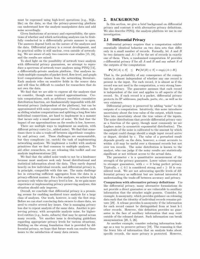
Record #recordsHotspot <timestamp, packet> 7.0MIspTraffic <timestamp,link,packet> 15.7BIPscatter <monitor, IPaddr, ttl> 3.8M

Table 3: The datasets that we consider.

comparable to what its analysis typically operates on. Wealso studied other datasets [4, 11] for several of the analysesand obtained results similar to those presented below.

Hotspot is a tcpdump trace of packets that we collected onthe wired access link of a large hotspot. It contains completepackets, including unaltered addresses and payloads.

IspTraffic is constructed from traffic at a large ISP (whoseidentity we are required to keep confidential). The ISPhas over 400 links and it provided us highly aggregatedinformation on traffic volume at each link in each 15-minwindow over a week-long period. We mimic a fine-graineddataset using this information by de-aggregating traffic vol-ume into 1500-bytes packets that are spread evenly acrossthe time window. Note that the aggregate representation ofthe source data is not itself a basis for differential privacy;the presence or absence of individual packets can still beobserved in the precise aggregates.

IPscatter is a list of IP addresses and their TTL-distancesfrom 38 monitors. It was constructed using the data col-lected by Spring et al. [28], who conducted traceroute probesfrom 38 PlanetLab sites to an IP address inside each BGPprefix. The constructed dataset includes a record for eachIP seen along each probe.

Privacy level The accuracy of a differentially pri-vate analysis depends on the desired strength of the pri-vacy guarantee (parameter ε). We consider three differentvalues of ε—0.1, 1.0, and 10.0—that correspond roughly tohigh, medium, and low privacy levels. Recall that highervalues are not necessarily unsafe but are theoretically easierto break.

Privacy principal The guarantees of differential pri-vacy are for the records of the underlying data set. Theserecords may or may not directly correspond to the higher-level privacy principal that the data owner wants to protect.Network data is interesting in that there are multiple pos-sible privacy principals such as packets, flows, hosts, andservices. If the underlying records are finer-grained thanthe intended principal (e.g., packets vs. hosts), no explicitguarantees are given for the principal.

Selecting an appropriate-granularity privacy principal isan important first step for the data owner. As a logisticalmatter, finer-grained records that share the same higher-level principal can be aggregated into one logical record us-ing SQL-like views. Using this aggregated data will thenprovide guarantees as the level of the principal. But in gen-eral, the analysis fidelity will decrease as fewer records areable to contribute to the output statistics.

In this paper, we assume that the privacy principal is atthe granularity of records in the dataset. This position isgenerous for analysis but it is also the starting point forbeginning to understand the applicability of differential pri-vacy in our context. If analysis noise is excessive even at thisgranularity, there is little hope. In the future, we intend tostudy the impact of using higher-level principals.

Packet-level analyses Expressibility High accuracyPacket size and port dist. (§5.1.1) faithful strong privacyWorm fingerprinting [27] (§5.1.2) faithful weak privacy

Flow-level analysesCommon flow properties [30] (§5.2.1) could not isolate connections in a flow strong privacyStepping stone detection [33] (§5.2.2) (one of the two) sliding windows were approximated medium privacy

Graph-level analysesAnomaly detection [13] (§5.3.1) faithful strong privacyPassive topology mapping [9] (§5.3.2) used a simpler clustering method weak privacy

Table 2: The analyses that we consider and summary results for them.

4. A PRIVATE ANALYSIS TOOLKITIn this section we present a collection of tools that im-

plement primitives that are common to many network traceanalyses. The tools are applicable to data analysis broadlyand represent the first practical implementations that aresensitive to privacy cost and added noise. We will arrive atspecific networking analyses in the next section. Our toolkitand the associated analyses are publicly available [23].

4.1 The Cumulative Density FunctionOften, in addition to simple aggregates like counts and

averages, we are interested in understanding the underly-ing distribution itself, which may have informative rangesor modes. In networking analyses, distributions are oftenstudied using the CDF: cdf(x) = number of the records withvalue ≤ x. Measuring precise empirical CDFs with arbi-trary resolution is not possible with differential privacy; asthe resolution δ decreases, cdf(x) - cdf(x-δ) depends on onlya few records in the data. We present three approaches toapproximate the CDF.

A simple approach is to partition the range into buckets ofa certain resolution and count, for each bucket, the recordsthat fall in that bucket or a previous one. Let buckets bethe set of values that represent the high end of each bucket,then:

foreach (var x in buckets)trace.Where(rec => rec.val < x).Count(epsilon);

This approach directly measures each value of cdf(x), but thestandard deviation of the error is proportional to |buckets|.

A more advanced approach is to use the Partition oper-ation to partition data into buckets:

tally = 0;parts = trace.Partition(buckets, rec => rec.value)foreach (var x in buckets)

tally += parts[x].Count(epsilon);yield tally;

This approach has the advantage that the total privacy costis independent of the number of buckets (i.e., resolution) buta limitation is that the error at each measurement accumu-lates to form the CDF. However, these errors cancel some-what, and their standard deviation is proportional only top|buckets|.An even more advanced approach takes measurements at

multiple resolutions and aggregates at most a logarithmicnumber of measurements to reproduce the full set of val-ues for the CDF. A recursive function to implement thisapproach is:

CDF3(data, epsilon, max)if (max == 0)yield return data.Count(epsilon);

else//--- partition data at max/2var parts = data.Partition(new int[] { 0, 1 },

x => x/(max/2));//--- emit counts for [0,max/2)foreach (var x in CDF3(parts[0], epsilon, max/2))

yield return x;//--- a cumulative count for [0,max/2)var count = parts[0].Count(epsilon);//--- emit frequencies for [max/2, max)parts[1] = parts[1].Select(x => x - max/2);foreach (var x in CDF3(parts[1], epsilon, max/2))

yield return x + count;

The standard deviation associated with each measurementis proportional to log(|buckets|)3/2.

Figure 1 compares these three approaches to the actualCDF for the time difference between a packet and its re-transmission in the Hotspot trace. We discretize values to1-ms granularity. The top graph shows that the error fromthe first approach is incredibly high, but the other two ap-proaches are accurate. The bottom graph zooms in to showthe distinction between the latter two approaches. We seethat in the second approach yields a smoother estimate thatmimics reality but consistently underestimates because theerror accumulates across the range. (In a different run, wemay see a consistent overestimation.) The errors with thethird approach are generally lower but could represent anover- or under-estimation at individual points. In any case,with both these approaches the errors are relatively smalland likely acceptable for most settings with modest abso-lute counts.

A natural consequence of noisy measurement is that thecomputed CDFs are not non-decreasing. If needed, theCDFs can be made non-decreasing through isotonic regres-sion. Linear time algorithms (e.g., the “pool adjacent viola-tors” algorithm [3]) can find the non-decreasing curve thatminimizes the squared error distance from the input. Suchsmoothing can also increase the accuracy in some cases (e.g.,cdf3 in Figure 1). But it is a non-reversible removal of in-formation, so we do not do it by default.

4.2 Finding Frequent (Sub)stringsMany analyses need to identify substrings or values that

occur frequently, for example, common payloads or addresses.While this may seem at odds with privacy, the presence orabsence of individual records is not necessarily at risk; if aparticular string occurs a large number of times, it is essen-

0 50 100 150 200 250

Time diff (ms)

0

50000

100000

CDF

cdf1

cdf2

cdf3

noise-free

(a) Complete view of all three methods

230 235 240 245 250

Time diff (ms)

40000

40500

41000

41500

42000

CDF

cdf2

cdf3

noise-free

(b) Zoomed in view of cdf2 and cdf3

Figure 1: Comparing three approaches for comput-ing CDFs with the actual (noise-free) CDF. (a) Thecomplete view shows that the first approach has higherror but the other two are indistinguishable fromthe actual CDF. (b) The zoomed-in view shows theerror behavior of the last two approaches.

tially a statistical trend that need not reveal the presence orabsence of one of its representatives.

As a concrete example, consider the problem of learningthe common strings of length B bytes. We might partitionour set of packets by the all possible values, of which thereare at most 256B , and measure the number of records ineach bin. Although the privacy cost is not high, the compu-tational cost is exorbitant for even small values of B.

Instead, we can reveal common strings by asking aboutstatistics of successive bytes. Initially, we partition the recordsinto 256 bins based on the first byte, and count the numberof records in each bin.

parts = data.Partition(bytes, rec => rec.str[0])foreach (var byte in bytes)

if (parts[byte].Count(epsilon) > threshold)yield return parts[byte]

All common strings contribute to the counters associatedwith their first bytes, which should be noticeably non-zero.Each byte with count greater than threshold can now be ex-tended, by each of the 256 bytes, to form prefixes of lengthtwo. Again we can partition and count, using our new can-didates and the first two bytes of each string, resulting ina set of viable prefixes of length two. This process contin-ues until length B, at which point the counts correspond tothe number of records with each distinct B byte string. Wewould have ideally culled most of the strings along the way,rather than at the very last step, as a monolithic partitionoperation would do. While we incur a higher privacy cost,due to the B rounds of interrogation, we can afford to take

string true count est. count % err2D2816FECDCAB780 3038504 3038500.005 -0.000F389B84545A38BAF 92494 92505.050 0.012E41903DCF7D86F2F 41600 41606.893 0.0176F7E03DC833D6F2F 40279 40287.970 0.022CD4F03DCE10E6F2F 40084 40087.437 0.009B68503DCCA446F2F 37431 37448.584 0.04758B403DC6C736F2F 36526 36537.877 0.03341EA03DC55A96F2F 29625 29624.397 -0.0029FBB03DCB37A6F2F 20715 20711.169 -0.0187EEEB845D1088BAF 18976 18980.823 0.025

Table 4: True and noisy counts of the top-10 strings.

measurements with less accuracy as we face relatively feweropportunities for false positives.

We used the procedure above to find the top 10 strings inthe payloads of the Hotspot trace. Table 4 shows the hashvalue of the discovered strings, true and estimated counts,and the relative error. We see that the top 10 strings arediscovered correctly, in order, and the error in the estimatedcount is low. The number 10 was an arbitrary choice forpresentation; the computation produces counts for all stringswhose counts exceed a user specified threshold with a userspecified confidence.

4.3 Frequent Itemset MiningA recurring theme in many data analyses is that com-

monly co-occurring items are a possible indication of corre-lation. The task of identifying frequently co-occurring itemsacross an input list of item sets is called frequent itemsetmining.

There are many algorithms for this task, including thepopular apriori algorithm [1]. It starts with a collection ofsingleton sets and counts the number of times each occurs.Sets that have sufficient frequency are retained, and mergedto form sets of size two, and so on.

Thus, the insight underlying this algorithm is similar towhat we used for frequent substring counting. But a keydifference from a privacy perspective is that the records,which are each essentially a set of items, must be partitionedamongst the candidate itemsets; each record can only con-tribute to the count for one candidate itemset even thoughit may support several. Consequently, if there are too manycandidate itemsets it can be hard to assemble enough evi-dence for any one candidate.

We get over this hurdle by aggressively restricting the can-didate item sets with high thresholds, focusing the supportof the records and ensuring that we do not spread the countstoo thin. Counter-intuitively, these high thresholds allow usto learn more. We omit implementation details for spaceconstraints.

As one brief example of its use, we use it to discover thecommon sets of ports that are used simultaneously by hosts.Our discovered sets were very close to reality. The top-five, which are all correct, in the Hotspot trace are (22,80),(25,22), (443,80), (445,139), and (993,22).

5. NETWORK TRACE ANALYSESWe now survey our experiences at reproducing several

analyses from the networking literature. We stress thatwhile we consider a wide range of analyses, our experiences

may not be representative. Moreover, our reproductions areeach only one of many possible ways of reproducing an anal-ysis; different ways of measuring the same quantity may leadto different results.

Table 2 summarizes our findings. “Expressibility” reflectsthe faithfulness of our implementation to the original anal-ysis, ignoring quantitative privacy constraints. That is, ifthe privacy allotment was arbitrarily high, would we recon-struct the original results or deviate from the specificationof the original algorithm? To a first order, we find that weare able to reproduce the analyses, though some flexibilityis required in reproducing the spirit of the analysis, if notthe exact letter.

“High accuracy” indicates our qualitative assessment ofwhat privacy level yielded highly accurate results; strongerprivacy levels do not necessarily yield bad results (some do)but do produce noticeably different outputs. In all cases,medium privacy (ε= 1.0) produces admirable results. Pick-ing an appropriate point in the privacy-accuracy trade-offrequires a more concrete understanding of the data’s sen-sitivity and the value of accuracy, but our results suggestseveral plausibly valuable locations on the privacy-accuracycurve.

5.1 Packet-level AnalysesWe now present our results in more detail, beginning with

packet-level analyses. Unless otherwise specified, we use theHotspot trace.

5.1.1 Packet-size and port distributionsTwo common packet-level analyses are measuring the dis-

tribution of packet sizes and ports. These are easy to repro-duce with the CDF computation methods that we describedearlier. We use the second method in our experiments.

Figure 2(a) shows the fidelity of the CDFs of packet lengthcomputed with the three values of ε that provide differentprivacy strengths. The graph also shows the real, noise-freeCDF and error bars for each noisy CDF. We see that theerror is minimal even at the strongest privacy level. As onemeasure of the overall accuracy, we compute the root mean

square error (RMSE) asq

1nΣi(1− vp[i]

vnf [i])2, where vp[i] and

vnf [i] are the private and noise-free values at index i. Atε=0.1, the RMSE is only 0.01%.

This extremely low error implies that accurate results canbe obtained even with far less data. Indeed, when we restrictour computations to only 1/10th of the data, the RMSEincreases to only 0.02%.

We also see that privately computed CDFs correctly cap-ture the interesting features of the distribution, for example,spikes at 40 and 1492 bytes. The former corresponds to TCPacknowledgments with no data, and the latter to the maxi-mum packet size with IEEE 802.3 (which is used for wirelesscommunication).

Figure 2(b) shows that similarly high-fidelity result areobtained for port distributions. At ε=0.1, the RMSE is only0.07%. With 1/10th of the data, the RMSE is 0.7%. Theerror for ports is more than that for packet lengths becausethere are more unique ports, and thus there are in generalfewer packets that contribute to port frequencies.

While packet length and port distributions may not seemthe most exciting quantities, they are simply examples ofCDFs of arbitrary packet statistics. Computations usingmore sensitive information (e.g., the CDF of the scores of

0 500 1000 1500

0

2

4

6

CDF (million)

epsilon=0.1

epsilon=1

epsilon=10

noise-free

(a) Packet length (bytes)

0 20000 40000 60000

0

2

4

6

CDF (million)

epsilon=0.1

epsilon=1

epsilon=10

noise-free

(b) Ports

Figure 2: Packet length and port CDFs computedwithout noise and with different values of ε. Thecurves (and error bars) are all indistinguishable.

a packet payload classifier) are similarly straightforward foran analyst to specify and to convince the data provider ofthe privacy guarantees.

5.1.2 Worm fingerprintingWe now consider a more complex packet-level analysis

which looks closely at packet payloads and depends criti-cally on this very sensitive data. Automated worm finger-printing [27] examines a stream of packets for frequently oc-curring payload substrings, with an additional “dispersion”requirement that the substring is originated by and destinedto many distinct IP addresses.

The PINQ fragment grouping the packets by payload andrestricting to those with the appropriate dispersion proper-ties is:

trace.GroupBy(pkt => pkt.payload).Where(grp => grp.Select(pkt => pkt.srcIP)

.Distinct()

.Count() > srcthreshold).Where(grp => grp.Select(pkt => pkt.dstIP)

.Distinct()

.Count() > dstthreshold)

These packet groups are still hidden behind the privacy cur-tain, and while we could count the groups (2739± 10, withthresholds at 5), or consider other statistics thereof, we can-not (yet) directly view them.

To read out the interesting payloads, we leverage their fre-quency in the data set. We use the frequent string findingtechnique (§4.2) to spell out payloads that appear a signif-icant number of times. This produces a list of candidatepayloads, from which we want to evaluate each to see if itmight be deemed suspicious. A simple PINQ fragment toproduce the number of distinct destinations associated witheach candidate payload is:

parts = trace.Partition(candidates, x => x.payload);foreach (var candidate in candidates)

parts[candidate].Select(x => x.dstIP).Distinct().Count(epsilon)

A similar fragment yields the distinct sources for each pay-load. The reported values for each payload are correct upto the error PINQ introduces.

With a dispersion threshold of 50 for sources and destina-tions, the noise-free computation yields 29 payloads. Search-ing for prefixes privately with ε values of 0.1, 1.0, and 10.0reveals 7, 24, and 29 of these 29, respectively. That is, wemiss 75%, 17% and 0% of the payloads. The missing pay-loads tend to correspond to payloads with low overall pres-ence but above average dispersal.

Thus, unlike packet length and port analysis, the accu-racy of worm fingerprinting is low at high privacy levels andhigh only at low privacy levels. Because the theoretical dis-tribution of analysis error is known in advance, the analystcan judge that the results have low accuracy at high privacylevels.

The approach of [27] is extended in several ways in thepaper. The extensions include reducing false positives byincorporating the destination port into the signature andsliding a window over the payloads to look for invariant con-tent. We are able to express both these extensions in PINQ.But with them, we do not find any high-dispersal signaturesin our trace, even in the absence of noise. Our monitoredenvironment likely observes little worm activity because itis behind a single public IP address.

5.1.3 SummaryWe showed results from two kinds of packet-level analyses

at the opposite ends of the spectrum. One was simple dis-tributions over packet sizes and ports, and the other was amore involved computation that considered payloads, ports,and IP addresses. We found that the both could be faith-fully reproduced and the output fidelity was high at least atlow privacy levels. Based on these results, we surmise thatmany other forms of packet-level analyses, such as variousclassification algorithms [10], can also be implemented in thedifferentially private manner.

5.2 Flow-level AnalysesWe now investigate the feasibility of conducting flow-level

analyses in a differentially private manner. These analysesdiffer from packet-level analyses as they consider propertiesacross groups of packets. Rather than aggregate directlyacross packets, we need to first apply non-trivial compu-tation across the packets to yield the derived statistics ofinterest.

5.2.1 Common flow statisticsA common operation for network analyses is to compute

flow properties such as round trip time (RTT) and loss rate.To compute these statistics, we use the techniques used bySwing [30]. A flow refers to the standard 5-tuple.

Swing measures RTT of a flow by differencing the timebetween the TCP SYN and the following SYN-ACK. Con-sidering only the handshake means that the results are notimpacted by delayed acknowledgments. To reproduce theseRTT values in PINQ, we join SYNs with SYN-ACKs, seek-ing pairs corresponding to common flows, with the ACK

0 200 400 600

0

20

40

60

CDF (thousand)

epsilon=0.1

epsilon=1

epsilon=10

noise-free

(a) RTT (ms)

0.0 0.2 0.4 0.6 0.8 1.0

0

50

100

150

CDF (thousand)

epsilon=0.1

epsilon=1

epsilon=10

noise-free

(b) Loss rate

Figure 3: The CDF of RTT and loss rate com-puted without noise and with differential privacy.All curves (and error bars) are indistinguishable.

number of the second equal to the sequence number of thefirst, plus one.

syns = packets.Where(x => x.syn)acks = packets.Where(x => x.syn && x.ack)times = syns.Join(acks,

x => x.src + x.dst + (x.seqn + 1),y => y.dst + y.src + y.ackn,(x,y) => y.time - x.time);

Swing measures flow loss rate downstream of the moni-tored link using TCP retransmissions. When a packet islost downstream, the monitor will observe a correspondingretransmission. We group packets by flow, and compare dis-tinct sequence numbers to total packets:

trace.GroupBy(pkt => pkt.flow).Select(grp => grp.Select(pkt => pkt.seq)).Select(grp => grp.Distinct().Count/grp.Count()).Select(x => 1.0 - x);

Once RTT and loss rates have been computed, we canstudy their distributions using the CDF primitive. Figure 3shows the results for these two properties with the threeprivacy levels. RTT is computed only for flows for which wesee both the SYN and its ACK. Loss rate is computed onlyfor flows with more than 10 packets. We see that for bothproperties the results are high-fidelity even at the strongestprivacy level. At ε=0.1, the RMSE for RTT is 2.8% and forloss rate is 0.2%.

We also considered other properties that Swing considers,including loss rate upstream of the monitor (computed usingout-of-order packets) and path capacity (computed using thetime difference and sizes of in-order packets). For these, theresults are similar to those shown above.

There was one class of computations in Swing that wecould not immediately reproduce in PINQ. This class oper-ates at the level of connections, e.g., computing the number

of packets per connection. A (5-tuple) flow may include mul-tiple TCP connections, and we could not isolate the connec-tions within a flow using the currently available operations.This issue is not fundamental, however. The data ownercould pre-process the traces to add a “connection id” field,or (as we are currently investigating) PINQ could be ex-tended with more flexible grouping transformations. Onceconnections are identified, the connection-level analyses arestraightforward.

5.2.2 Detecting stepping stonesWe now consider an analysis that operates across pack-

ets of different flows rather than working within individualflows. This analysis detects stepping stone relationships be-tween flows [33]. A stepping stone occurs when a computeris accessed indirectly, through a chain of one or more othercomputers. One scenario for such usage is to launch attackin a way that makes it it harder to trace back to the source.

Stepping stone detection [33] leverages the intuition that,for related interactive flows, the states of the flows are likelyto go from idle to active together, many times. It estab-lishes a time-out interval (Tidle=0.5 secs) after which a flowis considered idle, and a another time window (δ=40 ms)within which idle-to-active transitions of two flows are con-sidered correlated. It then identifies as stepping stones pairsof flows that exhibit a high ratio of correlated idle-to-activetransitions to all such transitions. To minimize false posi-tives, it also constrains the correlated flows to occur in thesame order multiple times and places a lower bound on theratio of the ordered occurrences to idle-to-active transitions.

Identifying the set of idle-to-active transitions is a slidingwindow computation that we conduct in PINQ by bucketingtime in buckets of width 2Tidle. We group packets by acombination of flow and bucket. Each group can containat most one activation in it’s second half—the last—and wehave enough context to confirm this packet as an activationor not.

packets.GroupBy(x => new {x.flow,x.time/(2*T_idle)}).Where(/* if last packet is an activation */).Select(x => x.Last())

This captures roughly half of the activations. To producethe remaining we shift each time by Tidle and apply thesame operation, moving packets from the front half of eachbucket to the rear.

Next, we need to identify correlated activations acrossflows. While we could reproduce the sliding window in thesame manner as above, the double groupings required doublethe noise we must suffer. We find that a better option is tobin the activations by time, and then run frequent itemsetmining to identify pairs of flows that are frequently acti-vated together. This trade-off between fidelity to the sourcealgorithm and privacy efficiency is one we will see again. De-signing analyses for privacy from the ground up is likely toyield better results in settings where privacy is mandatory.The pseudo code for binning flows by time is:

activations.GroupBy(x => x.time / delta).Select(x => x.Select(y => y.flow)

.Distinct())

Finally, we need to evaluate if the pairs thus producedare stepping stones by the original criteria. To evaluate agiven candidate pair, we simply count the number of binscontaining both. To evaluate many pairs, we first Parti-

tion the activations by flow, which reduces the privacy costdramatically.

ε noisy corr. noise-free corr false positives0.1 0.06± 0.07 0.03± 0.01 18/201.0 0.72± 0.10 0.76± 0.12 1/2010.0 0.78± 0.03 0.82± 0.05 2/20

Table 5: Evaluating private detection of steppingstones.

In the Hotspot trace, we find a surprising number of cor-related flows (even with non-private computations), likelybecause of the couplings between flows introduced by thewireless channel. This likely suggests that the original step-ping stone algorithm needs to be recalibrated for wirelesstraffic. For us, however, this complicates the task of fre-quent itemset mining as the data becomes too dense. Wecould tweak Tidle and δ, but that makes validation harder.

Instead, to reduce density and being able to compareagainst the original parameters, we focus on the set of flowswith [1200, 1400] activations. We compare against a faith-ful implementation (in Perl) that does not approximate thetask of identifying correlated flows. Thus, the comparisonincludes errors introduced by privacy constraints as well asalgorithmic approximation.

Table 5 shows the results. For each value of ε, it showsthe average and standard deviation of the approximate cor-relation for the top-twenty flows pairs, approximately com-puted with bucketed correlations. For those flow pairs, italso shows the actual average correlation scores (computedwith the Perl script), and what fraction had no actual corre-lation. We see that ε=0.1 has a very high false positive rate.But higher values of ε have good accuracy, suggesting thatstepping stones can be detected accurately with “medium”privacy levels. That we see accurate results at these privacylevels also indicates that the impact of algorithmic approx-imation is low. The threshold for correlation used in theoriginal analysis was 0.3, and every non-false positive can-didate for ε at 1.0 and 10.0 was above this threshold.

5.2.3 SummaryWe presented two kinds of flow-level analyses. One com-

putes statistics within flows and another that is based oncorrelations among different flows. Though there are roughedges (that are resolvable), in both cases, we are able tocapture the essence of the analysis and the output is highfidelity. Based on these, we believe that many other formsof flow-level analyses can be conducted in a differentiallyprivate manner. For instance, we are able to reproduce theassociation-rule mining based analysis of Kandula et al. [12]with a high fidelity; we omit results due to space constraints.

5.3 Graph-level AnalysesWe now turn our attention to analyses that focus on network-

wide properties rather than those of individual packets orflows. As with the previous two sections, some statisticalproperties are relatively easy to produce: distributions ofin and out degrees of nodes in the graph, restricted to vari-ous ports or protocols, distributional properties of computedquantities of edges (e.g., the distribution of loss rates acrossedges in the graph). Some useful properties, such as thediameter of the graph or the maximum degree, are difficultor impossible to compute because they rely on a handful of

0 200 400 600

Time bin

0

200

400

600

Norm (scaled bytes) epsilon=0.1

epsilon=1

epsilon=10

noise-free

Figure 4: The norm of anomalous traffic computedwith and without privacy. All four lines are indis-tinguishable.

records. We consider two complex graph-level analyses thatlie between these two extremes.

5.3.1 Anomaly detectionThe first graph-level analysis that we consider is the detec-

tion of network-wide traffic anomalies by observing link-leveltraffic volumes across time. We follow the analysis proposedby Lakhina et al. [13]. They first assemble a matrix indexedby link and time bucket, where each entry corresponds toload on the link at that time. They then apply principalcomponents analysis (PCA) to this matrix and use the firstfew factors to represent “normal” traffic. Entries not welldescribed by these factors represent substantial deviationsfrom the normal, and they are labeled as anomalies andflagged for inspection.

While the algorithm is mathematically sophisticated, wewill have little trouble adapting the approach to work withinPINQ. The first step, computing the link×time load matrixis an aggregation:

rows = trace.Partition(links, x => x.link)foreach (var link in links)

vals = rows[link].Partition(times, x => x.time);foreach (var time in times)

vals[time].Count(epsilon);

While the counts are noisy, the definition of a volumeanomaly is robust to small counting errors, and no significantanomaly should go unnoticed. This robustness can be seenin Figure 4 even at the highest privacy level. The graphshows, for the IspTraffic dataset, the volume of anomaloustraffic, i.e., bytes that are badly explained by the first fewsingular vectors of the traffic matrix. Despite the complexityof the analysis, the relatively low volume of noise addedto each measurement and the robustness of the techniquelead to results that are indistinguishable from the noise-freeversion. The anomalies in the network, e.g., at time unit of270, clearly stand out. The RMSE at ε=0.1 with respect tonoise-free results is 0.17%.

5.3.2 Passive network discoveryEriksson et al. propose a novel approach to map network

topology [9]. It takes as input a collection of hop countmeasurements between a large number of IP addresses anda few monitors. It infers network topology by clustering IPaddresses based on these measurements—two IP addressesthat have similar hop counts to most of the monitors arelikely topologically close. This work follows the clustering

0 2 4 6 8 10

Num. iteration

10

12

14

16

18

20

RMSE

epsilon=0.1

epsilon=1

epsilon=10

noise-free

Figure 5: Clustering error with and without privacy.

with small number of active measurements to each of theidentified clusters.

We focus on whether we can reproduce the clustering anal-ysis in a private manner; active measurement require non-private information by necessity. This separation is not un-common in privacy-preserving data analysis: a large volumeof protected data is analyzed to find trends, after which asmaller amount of privileged data is subjected to arbitrarycomputation involving the learned trends.

The clustering analysis starts by establishing the averagevalue of each monitor across all IP addresses, to be used inlieu of absent readings.

average = monitor.Average(epsilon, x => x.hops);

The monitors are then assembled into a collection of vectors,one for each IP address, and one coordinate per monitor.Addresses not observed at a monitor result in the averagevalue for that coordinate:

monitors.Aggregate((x,y) => x.Concat(y)).GroupBy(x => x.IP).Select( /* additional logic */)

So assembled, the set of vectors can be subjected to stan-dard clustering algorithms. We use k-means clustering ofPINQ. The original analysis uses Gaussian EM instead, anextension of k-means using covariance matrices for each clus-ter. While Gaussian EM is also expressible, it has a higherprivacy cost and is consequently less accurate for us. Thiscalls into light the trade-off between algorithmic complex-ity and accuracy; more complex algorithms can give betterresults in the absence of privacy constraints, but if their so-phistication requires looking “too closely” at the data, thenecessary noise to preserve privacy can counteract thesegains.

The data used by Eriksson et al. is hop count (inferredusing TTL) from scanning IP addresses to honeypot mon-itors. We run our analysis on the IPscatter dataset, whichis similar. It has hop count measurements from PlanetLabnodes (as monitors) to large number of IP addresses.

Figure 5 shows the results with different values of ε as wellas without privacy. It plots the objective function of the k-means optimization, the average distance from a point toits nearest cluster center, against the number of iterationsconducted. Nine centers are used, initialized to a commonrandom set of vectors for each execution. For each value of ε,each iteration of the algorithm consumes another multiple ofthe privacy cost. After 10 iterations, a value of ε=0.1 costs1. However, given the flatness of the curves, for a fixed

privacy budget, the appropriate strategy may not be to runten iterations at one-tenth the accuracy.

The curves reveal that at the strongest privacy level (ε=0.1)the RMSE is worse by 50%. The medium privacy level ismuch closer and its error may be acceptable. (The impli-cations of variation in cluster quality on the reconstructednetwork topology is beyond the scope of this paper.) Theweakest privacy level, however, is able to provide results al-most identical to the non-private computation.

5.3.3 SummaryWe considered two graph-level analyses. We were able to

reproduce the anomaly-detection analysis faithfully becausemost of its complex computations are on heavily aggregateddata that is less hindered by privacy constraints. The pas-sive network discovery analysis yielded high-fidelity resultsonly with weak privacy guarantees. It also exposed a trade-off between algorithmic complexity and privacy cost. Giventhat these two analyses are fairly involved, our experiencesuggests that many other graph-level analyses can be con-ducted in a differentially private manner.

6. RELATED WORKThe dominant method for data sharing today is trace

anonymization [16, 31, 22]. However, many researchers haveshown that anonymization is vulnerable to attacks that canextract sensitive information from the traces [5, 26, 31, 21].The utility of anonymized traces is further limited by theremoval of sensitive fields, critical for certain analyses [21].

Because of these shortcomings of anonymization, researchershave begun exploring mediated trace analysis. There arethree proposals to our knowledge, none of which match thestrong and direct privacy guarantees of differential privacy.First, Mogul and Arlitt’s SC2D relies on the use of pre-approved analysis modules and human verification to pre-serve privacy [19]. Given the complexity and diversity ofnetwork analyses, it is unclear if human verification is prac-tical and what guarantees it can provide.

Second, Mirkovic’s secure queries [17] are conceptuallysimilar to our work in that the analysis is expressed in ahigh-level language and the analysis server is tasked withensuring privacy. The privacy requirements are inspired bydifferential privacy as well. However, privacy is enforced us-ing a set of ad hoc rules whose eventual properties are poorlyunderstood. Further, while we show that a range of anal-yses can be accurately done using our methods, Mirkovicdoes not evaluate the usefulness of secure queries.

Third, Mittal et al. develop a method for quantifying theamount of information revealed by an analysis and proposethat data owners refuse to support analyses that leak morethan a threshold [18]. While intriguing, this approach is vul-nerable to targeted attacks. As previously discussed, singlebits can be arbitrarily sensitive, and the refusal reveals a bitin itself. Differential privacy reveals less than a bit abouteach record, but many bits about aggregate statistics.

Differential privacy is a recent concept and its practicalutility is an open question that can be answered only byapplying it to several domains. Along with McSherry andMironov, who study Netflix recommendations [15], and Ras-togi and Nath, who study distributed time-series [24], ourwork helps to further an understanding of this question.Reed et al [25] recently proposed an analysis language sim-ilar to PINQ to detect botnets in a differentially private

manner. While this approach has not been evaluated yet,our experience suggests that it can be effective.

7. DISCUSSION AND OPEN ISSUESOur results indicate that differential privacy has the po-

tential to be the basis for mediated trace analysis, which willenable data owners to let other analysts extract statisticalinformation in a provably private manner. The limitationsof differential privacy with respect to output fidelity and theneed to implement the analysis in a high-level language aresurmountable for a large class of analyses.

Retrospectively, the success of differential privacy in thisdomain stems from two factors. First, many analyses seekaggregate statistical trends and common patterns in thedata. For such analyses, individual records contribute only asmall fraction to each output value, which implies that onlya small amount of noise can guarantee privacy. Second, thecomputations that many analyses conduct directly over in-dividual records are rather simple and thus easy to express.Any complicated computations (e.g., clustering, PCA) areconducted only over aggregate data that can first be ex-tracted privately with a high fidelity. These properties maynot hold for all analyses but they appear to hold for largeclass of analyses.

We do not claim that implementing analysis in a differen-tially private manner is straightforward. We ran into manychallenges and counter-intuitive behaviors. Some analysesyielded low fidelity results at strong privacy levels; highoutput fidelity could be achieved only at weak privacy lev-els. Between, at medium privacy settings, the accuracy wasrarely bad, but distinguishable from the truth. Whetherthis is sufficient depends on the needs of the analyst, andthe available privacy resources. As more thought is put intoalgorithm (re-)design, we expect these trade-offs to improve.

Some computations that are easy otherwise (e.g., slidingwindows) can have a high privacy cost. Others, such as em-pirical CDFs with arbitrary resolutions, are fundamentallyimpossible to do in a differentially private manner. Fur-ther, there are multiple ways to implement the same analy-sis, some more privacy efficient than others. A worthwhiletask for the future is to educate networking researchers onthe concept of privacy efficiency, which is distinct from, andsometimes counter to, the more familiar concept of compu-tational efficiency. A related one is to develop a library withprivacy-efficient implementations of common primitives usedby networking analyses. The toolkit presented in this paperis a first step in that direction [23].2

This paper is by no means the final word on the use ofdifferential privacy for mediated trace analysis; there areseveral policy-related and practical challenges that must firstbe fully explored. One such challenge, which we mentionedin §3, is developing support for coarser-granularity privacyprincipals (e.g., flow or hosts) even when the underlying datais at a finer-granularity (e.g., packets).

Another challenge is developing guidelines for data ownerson what privacy level (parameter ε) to set for their datasets.

2Expressing analyses in high-level languages makes themeasier to debug and maintain as well. In the specific contextof PINQ, because it is based on LINQ, the analyses will alsoautomatically scale to a cluster [32]. Today, for flexibility,most networking analyses are written in low-level languages(e.g., C, Perl). Our survey provides evidence that the com-munity can afford to move to high-level languages.

While we explore a range of levels in our work, owners willhave to decide on specific levels to us for their data. There isunlikely to be a single answer for all situations. Instead, theappropriate level should be based on a combination of datasensitivity, the value of the analysis, acceptable noise-level,and the trust in the analyst.

Yet another challenge is managing the impact of repeateduse of the same data, by the same analyst or by differentanalysts. Each use leaks some private information (in the-ory) and successive uses leak more information. Differentialprivacy provides useful guidance on this issue. Two analyseswith privacy cost c1 and c2 have a total privacy cost at mostc1 + c2. Using this property, the data owners can enforcevarious policies such as limiting the total privacy cost peranalyst or across all analysts. They can also reduce privacycost (i.e., increase ε) with time such that the data is availablelonger but the added noise increases with time.

Resolving these challenges requires balancing usability andprivacy. With the strong foundation provided by differentialprivacy, we are optimistic that they can be resolved to thesatisfaction of many data owners.

Acknowledgments We are grateful to Saikat Guha,Suman Nath, Alec Wolman, the anonymous reviewers andour shepherd, Walter Willinger, for feedback on this paper.We also thank Stefan Savage for suggesting the worm fin-gerprinting and stepping s analyses early in the project.

8. REFERENCES[1] R. Agrawal and R. Srikant. Fast algorithms for mining

association rules. In VLDB, 1994.

[2] AOL search data scandal. http://en.wikipedia.org/wiki/AOL_search_data_scandal. Retrieved2010-16-01.

[3] M. Ayer, H. Brunk, G. Ewing, W. Reid, andE. Silverman. An empirical distribution function forsampling with incomplete information. The Annals ofMathematical Statistics, 26(4), 1955.

[4] R. Chandra, R. Mahajan, V. Padmanabhan, andM. Zhang. CRAWDAD data set microsoft/osdi2006(v. 2007-05-23).

[5] S. E. Coull, C. V. Wright, F. Monrose, M. P. Collins,and M. K. Reiter. Playing devilcs advocate: Inferringsensitive information from anonymized network traces.In NDSS, 2007.

[6] CRAWDAD: A community resource for archivingwireless data at Dartmouth.http://crawdad.cs.dartmouth.edu/.

[7] C. Dwork. Differential privacy. In ICALP, 2006.

[8] C. Dwork, F. Mcsherry, K. Nissim, and A. Smith.Calibrating noise to sensitivity in private dataanalysis. In Theory of Cryptography Conference, 2006.

[9] B. Eriksson, P. Barford, and R. Nowak. Networkdiscovery from passive measurements. In SIGCOMM,2008.

[10] P. Gupta and N. McKeown. Algorithms for packetclassification. IEEE Network, 15(2), 2001.

[11] The Internet traffic archive. http://ita.ee.lbl.gov/.

[12] S. Kandula, R. Chandra, and D. Katabi. What’s going

on? Learning communication rules in edge networks.In SIGCOMM, 2008.

[13] A. Lakhina, M. Crovella, and C. Diot. Diagnosingnetwork-wide traffic anomalies. In SIGCOMM, 2004.

[14] F. McSherry. Privacy integrated queries: Anextensible platform for privacy-preserving dataanalysis. In SIGMOD, 2009.

[15] F. McSherry and I. Mironov. Differentially privaterecommender systems: building privacy into theNetflix prize contenders. In KDD, 2009.

[16] G. Minshall. tcpdriv. http://ita.ee.lbl.gov/html/contrib/tcpdpriv.html.

[17] J. Mirkovic. Privacy-safe network trace sharing viasecure queries. In workshop on Network DataAnonymization, 2008.

[18] P. Mittal, V. Paxson, R. Summer, andM. Winterrowd. Securing mediated trace access usingblack-box permutation analysis. In HotNets, 2009.

[19] J. C. Mogul and M. F. Arlitt. SC2D: An alternative totrace anonymization. In MineNet workshop, 2006.

[20] A. Narayanan and V. Shmatikov. Robustde-anonymization of large sparse datasets. In Securityand Privacy, 2008.

[21] R. Pang, M. Allman, V. Paxson, and J. Lee. The deviland packet trace anonymization. SIGCOMM CCR,36(1), 2006.

[22] R. Pang and V. Paxson. A high-level programmingenvironment for packet trace anonymization andtransformation. In SIGCOMM, 2003.

[23] Network trace analysis using PINQ. http://research.microsoft.com/pinq/networking.aspx.

[24] V. Rastogi and S. Nath. Differentially privateaggregation of distributed time-series withtransformation and encryption. In SIGMOD, 2010.

[25] J. Reed, A. J. Aviv, D. Wagner, A. Haeberlen, B. C.Pierce, and J. M. Smith. Differential privacy forcollaborative security. In EuroSec, 2010.

[26] B. Ribeiro, W. Chen, G. Miklau, and D. Towsley.Analyzing privacy in enterprise packet traceanonymization. In NDSS, 2008.

[27] S. Singh, C. Estan, G. Varghese, and S. Savage.Automated worm fingerprinting. In OSDI, 2004.

[28] N. Spring, R. Mahajan, and T. Anderson. Quantifyingthe causes of path inflation. In SIGCOMM, 2003.

[29] L. Sweeney. k-anonymity: A model for protectingprivacy. Int’l Journal of Uncertainty, Fuzziness, andKnowledge-Based Systems, 10(5), 2002.

[30] K. V. Vishwanath and A. Vahdat. Swing: realistic andresponsive network traffic generation. ToN, 17(3),2009.

[31] J. Xu, J. Fan, M. Ammar, and S. Moon.Prefix-preserving IP address anonymization:Measurement-based security evaluation and a newcryptography-based scheme. In ICNP, 2002.

[32] Y. Yu, M. Isard, D. Fetterly, M. Budiu, UlfarErlingsson, P. K. Gunda, and J. Currey. DryadLINQ:A system for general-purpose distributed data-parallelcomputing using a high-level language. In OSDI, 2008.

[33] Y. Zhang and V. Paxson. Detecting stepping stones.In USENIX Security, 2000.