Chapter 1

Process analysis � The importance of mass and

energy balances

Eric S Fraga

Department of Chemical Engineering

University College London (UCL)

Torrington Place

London WC1E 7JE

United Kingdom

phone: +44 (0) 20 7679 3817

fax: +44 (0) 20 7383 2348

email: e.fraga@ucl.ac.uk

28th August 2015

Contents

I Concepts of Chemical Engineering for Chemists 3

1 Process analysis - The importance of mass and energy bal-

ances 4

1.1 Introduction . . . . . . . . . . . . . . . . . . . . . . . . . . . . 4

1.1.1 Nomenclature and units of measurement . . . . . . . . 5

1.2 Mass balances . . . . . . . . . . . . . . . . . . . . . . . . . . . 6

1.2.1 Process analysis procedure . . . . . . . . . . . . . . . . 8

1.2.2 Processes with reactions . . . . . . . . . . . . . . . . . 14

1.2.3 More complex process con�gurations . . . . . . . . . . 21

1.3 Energy balances . . . . . . . . . . . . . . . . . . . . . . . . . . 27

1.3.1 Example 3. Energy balance on distillation column: . . 33

1

1.3.2 Solution . . . . . . . . . . . . . . . . . . . . . . . . . . 35

1.4 Summary . . . . . . . . . . . . . . . . . . . . . . . . . . . . . 38

1.5 Further reading . . . . . . . . . . . . . . . . . . . . . . . . . . 39

2

Part I

Concepts of Chemical

Engineering for Chemists

3

Chapter 1

Process analysis - The

importance of mass and energy

balances

Eric S. Fraga, Department of Chemical Engineering, University College Lon-

don (UCL)

1.1 Introduction

Process engineering includes the generation, study and analysis of process

designs. All processes must obey some fundamental laws of conservation.

4

We can group these into conservation of matter and conservation of energy.1

Mass and energy balances are fundamental operations in the analysis of any

process. This chapter describes some of their basic principles.

1.1.1 Nomenclature and units of measurement

In carrying out any analysis, it is important to ensure that all units of mea-

surement used are consistent. For example, mass may be given in kg (kilo-

grammes), in lb (pounds) or in many other units. If two quantities are given

in di�erent units, one quantity must be converted to the same units as the

other quantity. Any book on chemical engineering (or physics and chemistry)

will have conversion tables for standard units.

There are 7 fundamental quantities which are typically used to describe

chemical processes, mass, length, volume, force, pressure, energy and power,

although some of these can be described in terms of others in the list. For

example, volume is length raised to the power 3; power is energy per unit

time, pressure is force per area or force per length squared, and so on.

Chemical engineering uses some standard notation for many of the quantities

we will encounter in process analysis. These are summarized in Table 1.1,

where the dimensional terms are T for time, M for mass and L for length.

In describing processes, the variables that describe the condition of a process

1These two laws are separate in non-nuclear processes. For nuclear processes, we of

course have the well known equation, E = mc2, which relates mass and energy. For this

lecture, we will consider only non-nuclear processes, but the same fundamental principles

apply to all processes.

5

Table 1.1: Some of the quantities encountered in process analysis withtypical notation and units of measurement.

Quantity Notation Dimension Units

Time t T sMass m M kgMass Flow m MT-1 kg s-1

Mole n M molMolar Flow n MT-1 mol s-1

Pressure P MT-2L-2 barEnergy H, Q, W ML2T-2 Joule

fall into two categories:

extensive variables, which depend on (are proportional to) the size of the

system, such as mass and volume, and

intensive variables, which do not depend on the size of the system, such

as temperature, pressure, density and speci�c volume, and mass and

mole fractions of individual system components.

The number of intensive variables that can be speci�ed independently for a

system at equilibrium is known as the degrees of freedom of the system.

1.2 Mass balances

Chemical processes may be classi�ed as batch, continuous or semibatch and

as either steady-state or transient. Although the procedure required for

performing mass, or material, balances depends on the type of process, most

of the concepts translate directly to all types.

6

The general rule for the mass balance in a system box (a box drawn around

the complete process or the part of the process of interest) is

input + generation− output− consumption = accumulation (1.1)

where

input: the material entering through the system box. This will include feed

and makeup streams.

generation: material produced within the system, such as the reaction

products in a reactor.

output: the material which leaves through the system boundaries. These

will typically be the product streams of the process.

consumption: material consumed within the system, such as the reactants

in a reactor.

accumulation: the amount of material that builds up within the system.

In a steady-state continuous process, the accumulation should always be

zero, which leads to a more simple mass balance equation:

input + generation = output + consumption (1.2)

In the case of systems with no reaction, where mass is neither generated nor

7

consumed, the result is even simpler:

input = output (1.3)

1.2.1 Process analysis procedure

The analysis of the mass balance of a process typically follows a number of

steps:

1. Draw and label a diagram for the process, clearly indicating the infor-

mation given by the problem de�nition and the values that have been

requested.

2. Choose a basis of calculation, if required. If no extensive variables

(e.g. amount or �ow rate of a stream) have been de�ned, a basis of

calculation is required and this must be an extensive variable.

3. Write down appropriate equations until the number of equations equals

the number of unknown variables and such that all the desired unknown

variables are referred to in the equations. Possible sources of equations

include the following:

(a) Mass balances. For a system with n species, n mass balance

equations may be written down. These mass balance equations

may be drawn from a total mass balance and from individual

species mass balances. The only exception is where the system

box contains solely a splitter, where all the streams have the same

8

composition and di�er only in extensive variables. In this case,

only one mass balance equation can be included.

(b) Process speci�cations and conditions, such as, for example, the

separation achieved by a distillation unit or the conversion in a

reactor.

(c) De�nitions, such as the relationship between density, mass and

volume or the relationship between mole fraction and total mass.

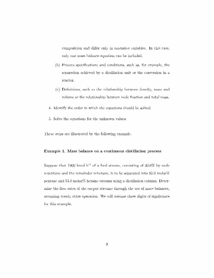
4. Identify the order in which the equations should be solved.

5. Solve the equations for the unknown values.

These steps are illustrated by the following example.

Example 1. Mass balance on a continuous distillation process

Suppose that 1000 kmol h-1 of a feed stream, consisting of 30.0% by mole

n-pentane and the remainder n-hexane, is to be separated into 95.0 molar%

pentane and 95.0 molar% hexane streams using a distillation column. Deter-

mine the �ow rates of the output streams through the use of mass balances,

assuming steady state operation. We will assume three digits of sign�cance

for this example.

9

Solution:

The �rst step is to draw and label a �owsheet diagram, indicating the process

steps and all the streams. Figure 1.1 shows the layout of the distillation

unit labelled with both the known variables and the variables we wish to

determine. The system box for this example is the whole process, i.e. the

distillation unit. The streams we wish to consider are those that intersect

this system box and consist of the feed stream and the two output streams.

All other streams can be ignored in solving this example.

System box

1n1 = 1000 kmol

h

x1,p = 0.30 kmolkmol

2n2 = ?

x2,p = 0.95 kmolkmol

3n3 = ?

x3,h = 0.95 kmolkmol

Figure 1.1: Distillation process diagram for Example 1, showing the systembox and the streams that intersect this system box.

10

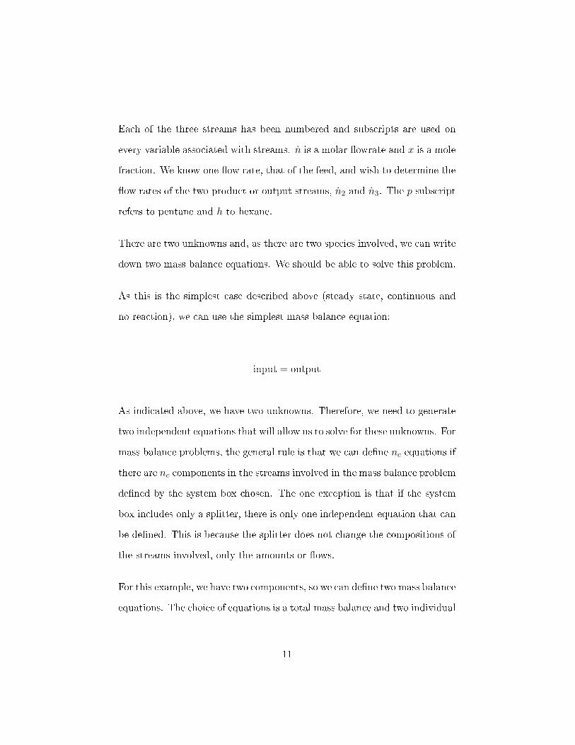
Each of the three streams has been numbered and subscripts are used on

every variable associated with streams. n is a molar �owrate and x is a mole

fraction. We know one �ow rate, that of the feed, and wish to determine the

�ow rates of the two product or output streams, n2 and n3. The p subscript

refers to pentane and h to hexane.

There are two unknowns and, as there are two species involved, we can write

down two mass balance equations. We should be able to solve this problem.

As this is the simplest case described above (steady state, continuous and

no reaction), we can use the simplest mass balance equation:

input = output

As indicated above, we have two unknowns. Therefore, we need to generate

two independent equations that will allow us to solve for these unknowns. For

mass balance problems, the general rule is that we can de�ne nc equations if

there are nc components in the streams involved in the mass balance problem

de�ned by the system box chosen. The one exception is that if the system

box includes only a splitter, there is only one independent equation that can

be de�ned. This is because the splitter does not change the compositions of

the streams involved, only the amounts or �ows.

For this example, we have two components, so we can de�ne two mass balance

equations. The choice of equations is a total mass balance and two individual

11

component balances:

n1 = n2 + n3 (1.4)

x1,pn1 = x2,pn2 + x3,pn3 (1.5)

x1,hn1 = x2,hn2 + x3,hn3 (1.6)

We can choose any two of these three equations to solve our problem. For

this example, we will choose the total mass balance, eq. (1.4), and the

pentane mass balance, eq. (1.5). Together with the mole fraction values

already labelled on the diagram, we are left with 0 degrees of freedom. The

number of degrees of freedom is de�ned as the di�erence between the number

of unknowns and the number of equations relating these unknowns.

Although it would appear that we have more than 2 unknowns, we implicitly

know the value of x3,p as mole fractions must add up to 1. We can either

consider that we know the value of x3,p or we can explictly add the equation

x3,p + x3,h = 1

Either way, we end up with 0 degrees of freedom.

We can solve the two equations, 1.4 and 1.5, by rearranging the �rst equation

to have n2 alone on one side and then replace n2 in the second equation with

12

the expression on the other side. The second equation can be solved for n3.

This value can then be used to solve the �rst equation for n2.

(1.4)⇒ n2 = n1 − n3 (1.7)

(1.5)⇒ x1,pn1 = x2,p (n1 − n3) + x3,pn3

⇒ (x3,p − x2,p) n3 = x1,pn1 − x2,pn1

⇒ n3 =x1,p − x2,px3,p − x2,p

n1

=x1,p − x2,p

(1− x3,h)− x2,pn1

=0.3− 0.95

(1− 0.95)− 0.95× 1000

kmol

h

= 722kmol

h

(1.7)⇒ n2 = 1000kmol

h− 722

kmol

h= 278

kmol

h

The example has been solved. We can now use the unused mass balance

equation, in this case being the hexane component mass balance, eq. (1.6),

to provide a check for consistency:

13

x1,hn1 = x2,hn2 + x3,hn3

∴ (1− x1,p)n1 = (1− x2,p)n2 + x3,hn3

∴ 0.7× 1000kmol

h= 0.05× 278

kmol

h+ 0.95× 722

kmol

h

X 700kmol

h= 700

kmol

h

(assuming three signi�cant digits in the calculations) so the results are at

least consistent which gives some con�dence in their correctness.

1.2.2 Processes with reactions

For processes involving reactions, the mass balance equation, eq. (1.3), used

in the �rst example, is not su�cient. Equations (1.1) or (1.2) must be used.

The presence of reactions means that the generation and consumption terms

in these equations are non-zero. The �rst key di�erence between a simple

separation process and a process involving reactions is the need to de�ne

these extra terms in terms of the amounts of the components in the sys-

tem. Extra equations are required to satisfy the extra degrees of freedom

introduced by having these extra terms present. There is another key dif-

ference: each reaction has associated with it a degree of freedom, one which

essentially describes the extent to which the reaction takes place. Therefore,

the analysis of a process involving a reaction will require extra equations to

satisfy degrees of freedom introduced by the reactions taking place.

14

Two concepts are often used to describe the behaviour of a process involving

reactions: conversion and selectivity. Conversion is de�ned with respect to a

particular reactant and describes the extent of the reaction that takes place

relative to the amount that could take place. If we consider the limiting re-

actant, the reactant that would be consumed �rst based on the stoichiometry

of the reaction, the de�nition of conversion is straightforward:

conversion ≡ amount of reactant consumed

amount of reactant fed

Selectivity is a concept that applies to processes with multiple simultaneous

reactions. It is used to quantify the relative rates of the individual reactions.

However, any discussion about multiple reactions and the analysis of these

is beyond the scope of this chapter. Refer to the further reading material

identi�ed at the end of this chapter for more information. In any case, the

speci�cation of conversion and/or selectivity will often provide the extra

information required to satisfy those extra degrees of freedom introduced by

having reactions present in the process.

Example 2: Mass balance on a process with reaction.

Suppose that an initially empty tank is �lled with 1000 mol of Ethane (C2H

6)

and the remainder air. A spark is used to ignite this mixture and the fol-

lowing combustion reaction takes place:

15

2 C2H6 + 7 O2 −−→ 4 CO2 + 6 H2O (1.8)

Assume that the amount of air provides twice the stoichiometric requirement

of oxygen for this reaction and that air is composed of 79% nitrogen and the

remainder oxygen. Suppose that the reaction reaches a 90% conversion.

What is the composition of the mixture in the tank at the end?

Solution

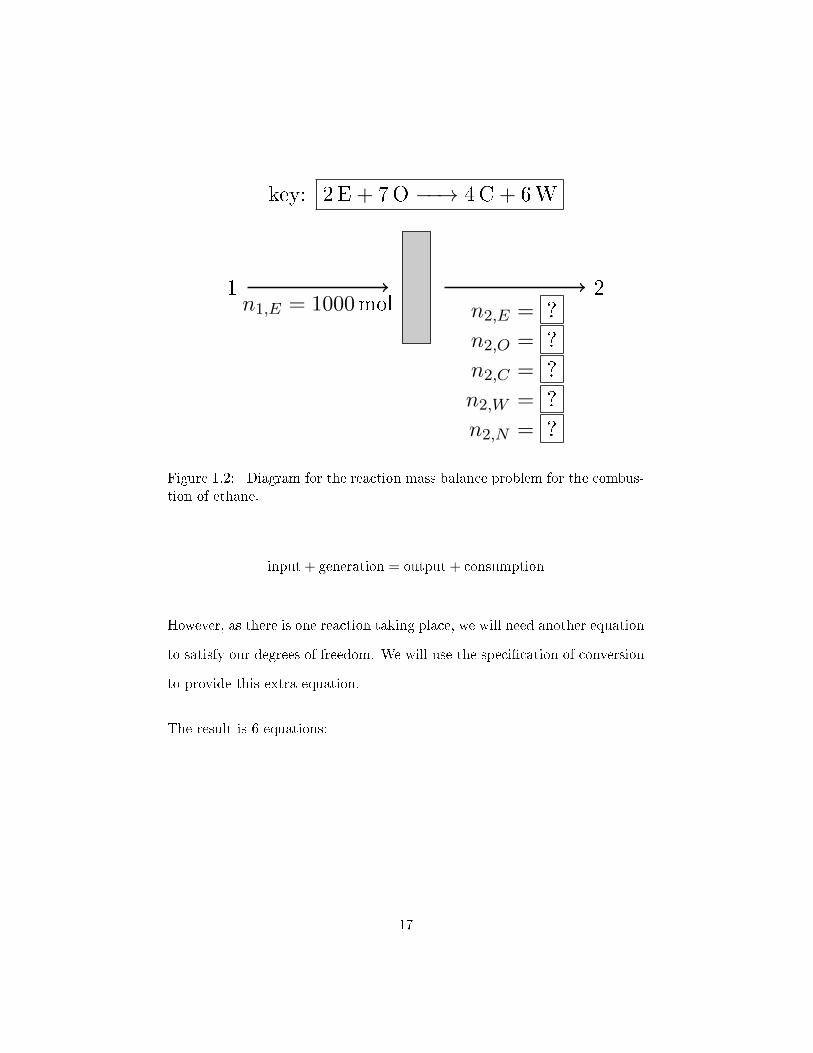
As in the �rst example, the �rst step is to draw and label a diagram, as shown

in Figure 1.2. This example is a batch problem, so arrows indicate material

�ow in the sense of loading and discharging the reactor. The subscripts for

mass amounts are the stream index (1 for the original contents of the tank

and 2 for the �nal contents after combustion) and the species involved. The

key is E for ethane, O for oxygen, N for nitrogen, C for carbon dioxide and

W for water.

As in the �rst example, the boxed question marks highlight the variables

which need to be determined. As there are �ve highlighted variables, we will

require at least �ve equations. As there are �ve species involved, �ve mass

balance equations can be de�ned. In this case, we should use eq. (1.1), but

with accumulation set to zero to indicate that the tank is empty to start

with and also empty at the end. This means that the mass balance equation

we should use is identical in form to eq. (1.2):

16

1n1,E = 1000mol

2n2,E = ?

n2,O = ?

n2,C = ?

n2,W = ?

n2,N = ?

key: 2E + 7O −−→ 4C + 6W

Figure 1.2: Diagram for the reaction mass balance problem for the combus-tion of ethane.

input + generation = output + consumption

However, as there is one reaction taking place, we will need another equation

to satisfy our degrees of freedom. We will use the speci�cation of conversion

to provide this extra equation.

The result is 6 equations:

17

n1,E + ng,E = n2,E + nc,E (ethane balance)

n1,O + ng,O = n2,O + nc,O (oxygen balance)

n1,N + ng,N = n2,N + nc,N (nitrogen balance)

n1,C + ng,C = n2,C + nc,C (carbon dioxide balance)

n1,W + ng,W = n2,W + nc,W (water balance)

conversion =n1,E−n2E

n1,E(speci�cation)

(1.9)

where the subscript g is used to indicate an amount generated and the sub-

script c indicates an amount consumed. At this point, all the variables

except for n1,E are unknown. We have 19 unknown variables. As we have

just de�ned 6 equations, we have 13 degrees of freedom remaining.

To solve this problem, therefore, it would seem that we need to de�ne at least

13 more equations. We can write down new equations relating the unknown

and known variables by making use of the stoichiometric coe�cients given by

eq. (1.8). It is helpful to write all of these in terms of one of the consumption

or generation terms. In this case, given that the key process speci�cation

is the conversion of ethane, it helps to write the equations in terms of the

amount of ethane consumed:

18

ng,E = 0 (no ethane is generated)

ng,O = 0 (no oxygen is generated)

nc,O =7

2nc,E

ng,N = 0 (no nitrogen is generated)

nc,N = 0 (no nitrogen is consumed)

ng,C =4

2nc,E

nc,C = 0 (no carbon dioxide is consumed)

ng,W =6

2nc,E

nc,W = 0 (no water is consumed)

(1.10)

This set of 9 equations reduces the degrees of freedom to 4 as no new variables

have been introduced.

Further equations can be de�ned based on the speci�cations of the feed:

n1,O = 2× 7

2n1,E (twice as much as required)

n1,N = 0.79×n1,O

0.21(nitrogen is remainder of air)

n1,C = 0 (no carbon dioxide in the feed)

n1,W = 0 (no water in the feed)

(1.11)

This set of 4 equations also introduces no new unknown variables. The

result is that we have 19 equations, comprising the three sets of equations

above, (1.9), (1.10) and (1.11). These can now be solved as follows. Given

19

n1,E = 1000mol, the initial amount of ethane, we evaluate the equations in

set (1.11):

n1,O = 2× 7

2n1,E = 7× 1000 mol = 7000 mol

n1,N = 0.79×n1,O

0.21= 0.79

7000 mol

0.21≈ 26333 mol

nc,E = 0.90× n1,E = 0.90× 1000 mol = 900 mol

Now determine the amounts generated and consumed for each species using

the set of equations (1.10):

nc,O =7

2nc,E =

7

2× 900 mol = 3150 mol

ng,C =4

2nc,E =

4

2× 900 mol = 1800 mol

ng,W =6

2nc,E =

6

2× 900 mol = 2700 mol

Finally, we use the mass balance equations, (1.9), to determine the amount

of each species in the output:

20

n2,E = n1,E + ng,E − nc,E = 1000 mol + 0− 900 mol = 100 mol

n2,O = n1,O + ng,O − nc,O = 7000 mol + 0− 3150 mol = 3850 mol

n2,N = n1,N + ng,N − nc,N = 26333 mol + 0− 0 = 26333 mol

n2,C = n1,C + ng,C − nc,C = 0 + 1800 mol− 0 = 1800 mol

n2,W = n1,W + ng,W − nc,W = 0 + 2700 mol− 0 = 2700 mol

1.2.3 More complex process con�gurations

The two examples above consist of a single processing unit or step. More

realistic problems will consist of multiple steps. When there are multiple

steps, connected to each other, we have not only input and output streams,

but also internal streams. In such a case, we have alternative system boxes

and we often need to consider more than one such box to solve a problem.

The key concept is that the input and output streams in the mass balance

equations are only those streams that enter or leave the particular system

box. Streams internal to the system box are not involved at all.

Example 3: Process with recycle

Consider the production of cyclohexane from 1-hexene, both C6H

12, but with

di�erent con�gurations of the atoms:

21

C

C

C

C

C

C

1-hexene

C

C

C

C

C

C

cyclohexane

This reaction does not achieve 100% conversion, so the e�uent (the output)

from the reactor needs to be processed to separate the reactant from the

product. This is undertaken using a distillation unit. Any unused reactant

is then recycled back to the reactor.

The feed to the continuous process, which should operate at steady state, is

10 mol s−1 pure 1-hexene. The product is to be cyclohexane at 95 molar%

purity. The reactor e�uent will be fed to a distillation unit that has two

outputs: a distillate stream and a bottoms stream. The distillate product

is to contain 90 mol% 1-hexene and the bottoms product should meet the

process requirements. The distillate is combined with the feed to the process

before the mixture is sent to the reactor. This mixture will be 95 molar%

1-hexene.

We want to �nd the composition of all streams in the process and the con-

version that is achieved in the reactor.

Solution

We start by drawing and labelling the process diagram, including all the

information we have about the process. This is shown in Figure 1.3. There

22

are 5 streams involved at this level of view.

n1 = 10 mols

x1,h = 1Mixer Reactor

n2 = ?x2,h = 0.95

Distillationn3 = ?

x3,h = ?

n4 = ?x4,h = 0.9

n5 = ?x5,c = 0.95

Figure 1.3: Process diagram for Example 3. h as a subscript refers to1-hexene and c as a subscript refers to cyclohexane.

If we take the whole process as the system box, we have one input stream,

the feed, and one output stream, the bottoms product of the distillation unit.

There are two unknowns: the amount of the output and the extent of the

reaction overall. We can write two equations, one for each species using eq.

1.2:

x1,hn1 = (1− x5,c)n5 + nc,h (1-hexene mass balance) (1.12)

(1− x1,h)n1 + ng,c = x5,cn5 (cyclohexane mass balance)

(1.13)

where nc,h is the rate at which 1-hexene is consumed and ng,c the rate at

which cyclohexane is generated. These two equations have three unknowns,

so we need at least another equation to be able to solve them. This equation

23

comes from the stoichiometry, which tells us that for each mole of 1-hexene

consumed, 1 mole of cyclohexane is generated:

nc,h = ng,c (1.14)

Solving this set of three equations, given the input �ow rate and the mole

fractions of 1-hexene in the feed stream and cyclohexane in the output

stream, we �nd that n5 = 10 mol s−1. The rate at which 1-hexene is con-

sumed and cyclohexane is generated are both 9.5 mol s−1.

To determine the �ows and compositions of the other streams in the process,

we have to consider di�erent system boxes. For instance, we can use a

system box that contains only the mixer, as shown in �gure 1.4. Given

the speci�cation on the inlet to the reactor, that the composition is 95% 1-

hexene, we have two unknowns and we can write two mass balance equations

for this system box:

n1 = 10 mols

x1,h = 1Mixer

n2 = ?x2,h = 0.95

n4 = ?x4,h = 0.9

Figure 1.4: System box containing only the mixer for the process in example3.

24

n1 + n4 = n2 (total mass balance) (1.15)

x1,hn1 + x4,hn4 = x2,hn2 (1-hexene mass balance) (1.16)

We can solve these two equations to get n2 = 20 mol s−1 and n4 = 10

mol s−1.

With stream 4 known, we can now determine stream 3 by considering a sys-

tem box around the distillation unit, as shown in Figure 1.5. We again have

two unknowns, n3 and x3,h, and we can write two mass balance equations:

n3 = n4 + n5 (total mass balance) (1.17)

x3,hn3 = x4,hn4 + (1− x5,c)n5 (1-hexene mass balance) (1.18)

which yields n3 = 20 mol s−1 and x3,h = 0.475.

We now have determined all the stream compositions and can therefore cal-

25

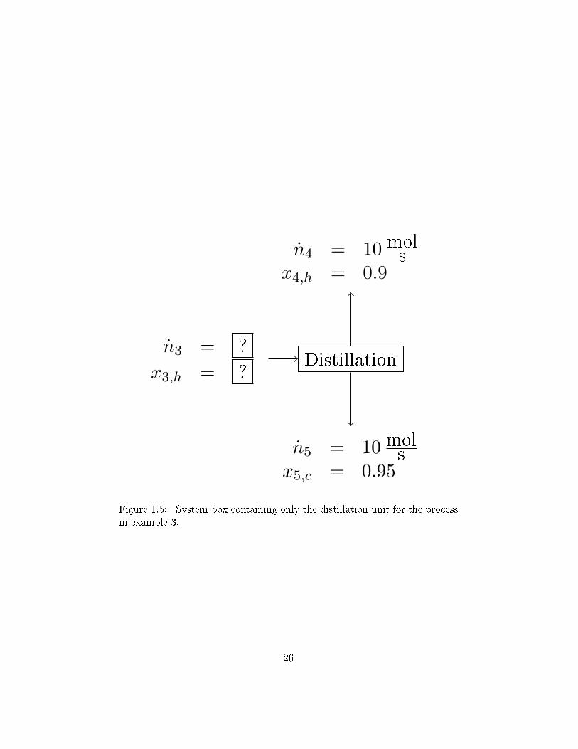
n3 = ?

x3,h = ?Distillation

n4 = 10 mols

x4,h = 0.9

n5 = 10 mols

x5,c = 0.95

Figure 1.5: System box containing only the distillation unit for the processin example 3.

26

culate the single pass conversion of the reactor:

conversion =reactant consumed

reactant fed(1.19)

=x2,hn2 − x3,hn3

x2,hn2(1.20)

=0.95× 20 mol

s − 0.475× 20 mols

0.95× 20 mols

(1.21)

= 0.5 (1.22)

which is 50%.

1.3 Energy balances

Energy balances can be treated in much the same way as material balances.

The only fundamental di�erence is that there are three types of energy (for

non-nuclear processes):

kinetic: Energy due to the translational motion of the system as a whole,

relative to some frame of reference (the earth's surface, for instance)

or to the rotation of the system about some axis.

potential: Energy due to the position of the system in a potential �eld. In

chemical engineering, the potential �eld will typically be gravitational.

internal: All energy possessed by the system other than kinetic or potential.

For example, the energy due to the motion of molecules relative to the

27

centre of mass of the system and to the motion and interactions of the

atomic and subatomic constituents of the molecules.

Energy may be transferred between a system and its surroundings in two

ways:

1. As heat, or energy that �ows as a result of a temperature di�erence

between a system and its surroundings. The direction of �ow is always

from the higher temperature to the lower. Heat is de�ned as positive

when it is transferred to the system from its surroundings.

2. As work, or energy that �ows in response to any driving force other

than a temperature di�erence. For example, if a gas in a cylinder

expands and moves a piston against a restraining force, the gas does

work on the piston. Energy is transferred as work from the gas to its

surroundings, including the piston. Positive work means work done by

the system on its surroundings, although this convention is sometimes

not followed and one should be careful to note the convention used by

other people.

In this chapter, we will deal solely with heat.

Energy and work have units of force times distance, such as a Joule (J),

which is a Newton-metre (N m). Energy is sometimes measured as the

amount of heat that must be transferred to a speci�ed mass of water to raise

the temperature of the water a speci�ed temperature interval at a speci�ed

28

pressure (e.g. 1 kcal corresponds to raising 1 kilogramme of water from 15

◦C to 16 ◦C).

As in material balances, energy must be conserved.2 We have two energy

balance equations: one for closed systems and one for open systems. A closed

system is one in which no mass comes in or goes out of the process during

its operation. An example of this would be a batch process with an initial

state and a �nal state. An open system has mass coming in and/or going

out during the operation. A continuous process is an example of an open

system. In either case, the energy balance equations are based on the �rst

law of thermodynamics.

The full energy balance equation for a closed system is

∆U + ∆Ek + ∆Ep = Q−W (1.23)

where ∆U is the di�erence in internal energy of all the streams at the end of

the process in relation to those streams at the start of the process, ∆Ek the

change in kinetic energy of the system, ∆Ep the change in potential energy

of the system, Q the amount of heat put into the system and W the amount

of work done by the system.

For continuous processes, we wish to consider rates of energy, so the equiv-

alent equation is

∆H + ∆Ek + ∆Ep = Q− W

2Noting again that we are refering only to non-nuclear processes.

29

where H is the enthalpy of the inlet and outlet streams and the changes in

kinetic and potential energies refer to the streams coming out of the process

and the streams coming into the process. Speci�c enthalpy (enthalpy per

unit mass), denoted by H, is de�ned as the combination of internal energy

and �ow work, the work that is required to move material into and out of a

process:

H = U − PV

where P is the system pressure and V the speci�c volume of the material.

The actual rate of enthalpy for a stream, H, will be calculated by nH.3 In

working with changes of enthalpy, we will use a reference state, a combina-

tion of temperature and pressure for which the enthalpy is assumed to be

zero. Enthalpy data in property tables is typically given with reference to a

speci�ed reference state.

In this chapter we will introduce some of the basic properties required to

perform energy balances on a process. Speci�cally, we will describe how to

estimate changes in the rate of enthalpy due to changes in temperature and

phase for streams. We will consider open systems and will ignore changes

in kinetic and potential energies. For systems in which kinetic and potential

energies are assumed to not change or where the changes in these energies

3This calculation assumes that the speci�c enthalpy is given in units of energy per

mole. However, many tables will have units of energy per unit mass, so a unit conversion

using molecular weights may be required.

30

are assumed to be negligible, the energy balance equation can be reduced to

∆H = Q− W

for an open system.

In working with materials, there are two types of heat:

sensible heat, which signi�es heat that must be transferred to raise or lower

the temperature of a substance, assuming no change in phase (solid,

liquid, gas), and

latent heat, which is the heat necessary to change from one phase to an-

other.

The calculation of sensible heat is based on the heat capacity (at constant

pressure) of the substance, Cp(T ), which is in units of heat (energy) per unit

mass. Heat capacity information is typically in the form of coe�cients for a

polynomial expression:

Cp(T ) = a + bT + cT 2 + dT 3

The values of the coe�cients are given in physical property tables found

in most chemical engineering reference books. To determine the change

in enthalpy in heating a substance from one temperature, T1, to another

temperature, T2, without a phase change, we integrate the polynomial over

31

the temperature range:∫T2

T1

Cp(T ) dT =

[aT + b

T 2

2+ c

T 3

3+ d

T 4

4

]T2

T1

(1.24)

We evaluate the right hand side of this equation as the di�erence of the

polynomial evaluated at T2 and at T1. The relation between the heat capacity

(integrated over a temperature interval) and the change in enthalpy is exact

for ideal gases, exact for nonideal gases only if the pressure is indeed constant,

and a close approximation for solids and liquids.

For latent heat, we look up the corresponding entry in the tables for either

the latent heat of vapourization (or simply the heat of vapourization) or the

heat of fusion, depending on the type of phase change encountered: liquid

to vapour and solid to liquid, respectively. These quantities are in units of

energy per unit mass and are given for a speci�c reference state, often the 1

atm boiling point or melting point of the substance.

The calculation of the change in enthalpy from one temperature to another

for a given substance will often be a multi-step process. The main principle

is to identify a path of pressure and temperature changes that goes from

the initial state to the �nal state, passing through states at which we have

reference data (e.g. the heat of vapourization) available. Any sections of the

path that do not involve phase changes will simply require the calculation of

sensible heat using the heat capacity equation given above. Phase changes

will then require the use of the appropriate latent heat quantity.

32

For process analysis including energy balances, the same procedure de�ned

for mass balances is followed. The only change is that the source of equa-

tions, described in step 3 of the procedure, now includes the energy balance

equation, as well as the de�nition of the di�erent energy terms. Again, this

procedure will be illustrated by an example.

1.3.1 Example 3. Energy balance on distillation column:

We again consider the distillation unit introduced in Example 1, updated

with temperature information for each of the streams, and now including

detail about the inner workings on the unit. Speci�cally, the process now

includes the total condenser, which cools the vapour coming out of the top

of the column into liquid, and the reboiler, which boils up the liquid from

the bottom of the column into vapour (see Figure 1.6). These two processing

steps were previously considered to be internal to the system box used in

solving the mass balance problem.

The temperatures noted on the diagram have been estimated using a physical

property estimation system. There are a number of computer based tools for

estimating physical properties and most simulation software systems will in-

clude appropriate methods. Figure 1.6 shows these temperatures, as well as

the results obtained earlier. As more streams have been included in this dia-

gram, we have new unknowns. Speci�cally, we now have the vapour stream,

V , from the top of the column to the condenser and the liquid re�ux stream,

L, from the condenser back into the column. Both of these streams have the

33

n1 = 1000 kmolh

x1,p = 0.30 kmolkmol

T1 = 328.1 ◦C

VTV = 312.2 ◦C

Condenser

Qc = ?

L

n2 = 278 kmolh

T2 = 310.2 ◦C

ReboilerQr = ?

n3 = 722 kmolh

T3 = 339.2 ◦C

Figure 1.6: Distillation unit including a total condenser and a partial re-boiler with streams annotated with temperatures.

same composition as the distillate product, stream 2, and their �ow rates

will be denoted by nV and nL, respectively. The relationship between the

liquid re�ux stream back into the column and the actual distillate product

stream (n2) is given by the re�ux ratio:

R =nL

n2(1.25)

For this particular con�guration, the re�ux ratio required to achieve the

separation is R = 1.6.

Neglecting the e�ect of pressure on enthalpy, we wish to estimate the rate

at which heat must be supplied to the reboiler.

34

1.3.2 Solution

Figure 1.6 is the �owsheet diagram for this problem with all the streams

labelled, both with known quantities and with an indication of what we re-

quire to estimate to solve this problem. The speci�c answer to the question

posed is the value of Qr, the rate of heat supplied to the reboiler. To deter-

mine this amount, we will need to determine the change in enthalpy of the

output streams relative to the feed stream and the amount of cooling done

in the condenser, Qc. We will consider two system boxes: one around the

whole unit, essentially the same system box as was used in solving Example

1, and one around the condenser section of the unit, shown in Figure 1.7.

The latter system box will be useful for determining Qc and will be the �rst

we consider.

nV = ?

xV,p = 0.95 kmolkmol

TV = 312.2 ◦C

Condenser Splitter

n2 = 278 kmolh

x2,p = 0.95 kmolkmol

T2 = 310.2 ◦C

nL = ?

xL,p = 0.95 kmolkmol

TL = 310.2 ◦C

Qc = ?

System box

Figure 1.7: System box containing the condenser of the distillation unit witha splitter. The input stream is vapour from the top of the distillation column.The output streams are the distillate product (indicated by subscript 2) andthe liquid re�ux. There is also a heat input, Qc, for the condenser.

For this system box, there are three streams: an input vapour stream, which

35

originates in the top of the column and two output streams, the distillate

product of the unit and the liquid re�ux going back into the column. The

system box includes a splitter and a condenser. There are three unknowns

indicated in the �gure: the amount of cooling required, Qc and the �ow rates

of the vapour, nV , and liquid streams, nL. Material and energy balances

must be addressed simultaneously. As the only step that changes stream

amounts is a splitter, we will only be able to write down one mass balance

equation for this system box. Together with the appropriate energy balance

equation, we have

nV = n2 + nL (1.26)

∆H = Qc (1.27)

As there are three unknowns in the diagram, we will need at least one more

equation. We will use eq. (1.25), which relates the �ows of the liquid re�ux

and the distillate product stream. We also need to calculate the change

enthalpy, which we do by estimating the sensible and latent heats for each of

the streams involved, relative to a reference temperature. For this problem,

we will use 0 ◦C = 273.15 K as the reference temperature.

The estimate of the speci�c enthalpy of each stream requires data, available

from a number of sources as discussed above, for the heat capacity equa-

tion and the latent heat of vapourisation. For each stream, we will have a

36

contribution for each compound present. For instance, the enthalpy of the

distillate stream will be composed of the enthalpy contribution of pentane

and of hexane:

H2 = x2,pn2H2,p + x2,hn2H2,h (1.28)

where the subscripts 2, p, for instance, indicate the pentane component in

the distillate stream.

The results of these calculations, using equation (1.24) and data from Felder

& Rousseau (2000) (see further reading section below), are shown in Table

1.2. The table presents the speci�c enthalpies for the two species before and

after the condenser. The speci�c enthalpies for the species in the liquid re�ux

stream will be the same as in the distillate output stream. The di�erence

between the enthalpies in the vapour stream and the distillate stream is

primarily due to the heats of vapourisation, but there is a small contribution

from the drop in temperature across the condenser.

Table 1.2: Speci�c enthalpies for species before and after the condenser.Note that the speci�c enthalpy HL,i is the same as H2,i, where i is either pfor pentane or h for hexane.

Species HV,i H2,i

(J mol-1) (J mol-1)

Pentane 38521 7377Hexane 38601 8013

Using the speci�c enthalpies in Table 1.2 to get the actual stream enthalpies

allows us to then solve for the remaining 3 unknowns, with the following

37

results: nV = 722 kmol h-1, nL = 444 kmol h-1 and Qc = −2.25 × 107 kJ

h-1. The negative sign on Qc indicates that the condenser is removing heat

from the process, as expected.

To determine the amount of heating required in the reboiler, we now look at

the �rst system box, the box that includes the whole distillation unit: the

column, the condenser and the reboiler. This box also has three streams, the

feed stream and the two output streams, and two heat inputs, Qc and Qr.

All mass �ow rates are known and we also know the condenser requirements,

so we have one unknown, the reboiler heat duty. We have only one equation,

the energy balance around the column

∆H = Qc + Qr (1.29)

We again need to calculate the enthalpies of the stream, noting that we

have already calculated the enthalpy of the distillate product stream. If we

calculate the enthalpies of the feed and bottom product streams and solve

eq. 1.29, we get Qr = 2.20×107 kJ h-1, a positive value indicating that heat

is being added to the process, again as expected.

1.4 Summary

This chapter has introduced the concepts of mass and energy balances. These

are essential steps in the analysis of any process. Simple examples have been

38

used to illustrate the di�erent steps, including not only mass and energy

balances, but also simultaneously solving mass and energy balances together.

The key to doing process analysis is the identi�cation of the extra equations

that it may be necessary to solve for the unknown variables. These equa-

tions will come from a number of sources, including the balance equations

themselves (eq. (1.1) and eq. (1.23)), process speci�cations (such as the pu-

rity of output streams and the re�ux ratio), physical relations (such as the

de�nition of enthalpy for liquid and vapour streams) and other constraints

imposed by the problem. Once a full set of equations has been developed,

the equations can be solved, usually with little di�culty, and the desired

results obtained.

1.5 Further reading

1. J. Coulson, J. F. Richardson, J. R. Backhurst & J. H. Harker, �Coulson

& Richardson's Chemical Engineering Volume 1: Fluid Flow, Heat

Transfer and Mass Transfer,� 5th Edition, Butterworth-Heinemann,

1997.

2. R M Felder & R W Rousseau, �Elementary principles of chemical pro-

cesses,� 3rd Edition, John Wiley & Sons (New York), 2000.

3. C. A. Heaton (Editor), �An Introduction to Industrial Chemistry,�

Leonard Hill (Glasgow), 1984.

39

4. R. H. Perry, D. W. Green & J. O. Maloney, �Perry's Chemical Engi-

neers' Handbook,� 7th Edition, McGraw-Hill, 1997.

40