The impact of Commercial Banks development on Economic ...

Univers

ity of

Cap

e Tow

n

The Impact of Commercial Banks Development on

Economic Growth in Namibia

A Dissertation

presented to

The Development Finance Centre (DEFIC)

Graduate School of Business

University of Cape Town

In partial fulfilment

of the requirements for the

Master of Commerce in Development Finance Degree

by

Elia Paavo

December 2017

Supervised by: Prof. Nicholas Biekpe

The copyright of this thesis vests in the author. No quotation from it or information derived from it is to be published without full acknowledgement of the source. The thesis is to be used for private study or non-commercial research purposes only.

Published by the University of Cape Town (UCT) in terms of the non-exclusive license granted to UCT by the author.

Univers

ity of

Cap

e Tow

n

i

PLAGIARISM DECLARATION

Declaration

1. I know that plagiarism is wrong. Plagiarism is to use another’s work and pretend that

it is one’s own.

2. I have used a recognised convention for citation and referencing. Each contribution to,

and quotation in this thesis from the work(s) of other people has been attributed, and

has been cited and referenced.

3. This project is my own work.

4. I have not allowed, and will not allow, anyone to copy my work with the intention of

passing it off as his or her own work.

5. I acknowledge that copying someone else’s assignment or essay, or part of it, is

wrong, and declare that this is my own work.

Elia Paavo

Signature removed

ii

ABSTRACT

This study sets out to investigate the impact of commercial banks development on economic

growth in Namibia. Using quarterly data on GDP as well as various commercial banks

development indicators, covering the period March 2005 to December 2016, the study

employed the Auto-Regression Distributive Lag (ARDL) methodology in determining existence

of the short-run and long-run relationships. Furthermore, the study employed the Granger

causality test in determining the causal relationship between banking sector development and

economic growth. From the ARDL results, the study concluded that there is existence of a

positive short-run relationship between banking sector development and GDP growth,

channelled through net interest income and funding liabilities of banks. The causality test

indicated a bi-directional causality between economic growth and the banking sector

development, entailing that development of the banking sector would enhance GDP growth and

vice versa. The study thus concluded that, commercial banks development has an impact on

economic growth in Namibia and recommends for reforms in the banking industry to ensure

increased lending in order to support the economy.

iii

TABLE OF CONTENTS

PLAGIARISM DECLARATION ............................................................................................... i

ABSTRACT ............................................................................................................................... ii

TABLE OF CONTENTS .......................................................................................................... iii

LIST OF TABLES ..................................................................................................................... v

GLOSSARY OF TERMS ......................................................................................................... vi

ACKNOWLEDGEMENT ....................................................................................................... vii

1 CHAPTER ONE: INTRODUCTION ................................................................................. 1

1.1 Research Area.......................................................................................................................... 1

1.2 Problem Statement .................................................................................................................. 2

1.3 Purpose and Significance of the Research ............................................................................... 3

1.4 Research Questions and Scope ................................................................................................ 4

1.5 Research Assumptions ............................................................................................................ 5

1.6 Organization of the study ........................................................................................................ 5

2 CHAPTER TWO: LITERATURE REVIEW ..................................................................... 6

2.1 Introduction ............................................................................................................................. 6

2.2 Defining Banking Sector Development................................................................................... 6

2.3 Overview of the Namibia Banking Sector ............................................................................... 7

2.4 Theoretical Framework ........................................................................................................... 8

2.4.1 Walter Bagehot ................................................................................................................ 8

2.4.2 Schumpeterian Model of Economic Growth ................................................................... 8

2.4.3 Neo-Classical Model of Growth ...................................................................................... 9

2.4.4 Endogenous Growth Model ............................................................................................. 9

2.4.5 Financial Repression Hypothesis .................................................................................. 10

2.5 Empirical Literature .............................................................................................................. 10

2.5.1 Size and Depth of the Banking Sector ........................................................................... 10

2.5.2 Efficiency of the Banking Sector .................................................................................. 13

2.5.3 Stability of the Banking Sector...................................................................................... 14

2.5.4 Empirical Studies on Namibia ....................................................................................... 17

2.6 Conclusion ............................................................................................................................. 18

3 CHAPTER THREE: RESEARCH METHODOLOGY ................................................... 19

3.1 Introduction ........................................................................................................................... 19

3.2 Research Approach and Strategy .......................................................................................... 19

3.3 Specification of the Model .................................................................................................... 19

3.4 Justification and Measurement of Variables ......................................................................... 20

iv

3.5 Data Collection, Frequency and Choice of Data ................................................................... 23

3.6 Sampling ................................................................................................................................ 24

3.7 Data Analysis Methods ......................................................................................................... 24

3.7.1 Unit Root Tests .............................................................................................................. 25

3.7.2 Bound Cointegration Test.............................................................................................. 25

3.7.3 Estimating Short-Run Coefficients ................................................................................ 26

3.7.4 Granger-Causality Tests ................................................................................................ 26

3.8 Research Reliability and Validity .......................................................................................... 26

3.9 Limitations ............................................................................................................................ 27

4 CHAPTER FOUR: RESEARCH FINDINGS, ANALYSIS AND DISCUSSION .......... 28

4.1 Introduction ........................................................................................................................... 28

4.2 Empirical Analysis ................................................................................................................ 28

4.2.1 Correlation Coefficient Test .......................................................................................... 28

4.2.2 Unit Root Test ............................................................................................................... 29

4.2.3 Determination of Optimal Lag Length .......................................................................... 29

4.2.4 Bound Test Approach to Cointegration ......................................................................... 30

4.2.5 Long-run Estimates ....................................................................................................... 31

4.2.6 Short-run ........................................................................................................................ 31

4.2.7 Bivariate Error Correction Models ................................................................................ 32

4.2.8 Model Diagnostic Test .................................................................................................. 36

4.2.9 Pairwise Granger Causality Test Results ...................................................................... 38

5 CHAPTER FIVE: RESEARCH CONCLUSIONS .......................................................... 40

5.1 Introduction ........................................................................................................................... 40

5.2 Research Conclusion ............................................................................................................. 40

5.3 Policy Implications ................................................................................................................ 41

6 CHAPTER SIX: RECOMMENDATIONS FOR FUTURE RESEARCH ....................... 43

REFERENCES ......................................................................................................................... 44

APPENDICES .......................................................................................................................... 49

v

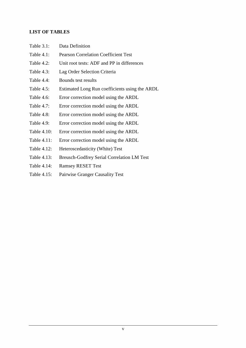
LIST OF TABLES

Table 3.1: Data Definition

Table 4.1: Pearson Correlation Coefficient Test

Table 4.2: Unit root tests: ADF and PP in differences

Table 4.3: Lag Order Selection Criteria

Table 4.4: Bounds test results

Table 4.5: Estimated Long Run coefficients using the ARDL

Table 4.6: Error correction model using the ARDL






Table 4.12: Heteroscedasticity (White) Test

Table 4.13: Breusch-Godfrey Serial Correlation LM Test

Table 4.14: Ramsey RESET Test

Table 4.15: Pairwise Granger Causality Test

vi

GLOSSARY OF TERMS

ADF: Augmented Dickey Fuller Test

ARDL: Auto-Regression Distributive Lag

ASEAN: Association of South East Asian Nations

BON: Bank of Namibia

D-SIB: Domestic Systemic Important Banks

EU: European Union

FSI: Financial Soundness Indicators

GDP: Gross Domestic Product

IMF: International Monetary Fund

M2: Broad Money Supply

NAD/ N$: Namibia Dollar

NPL: Non-Performing Loans

OECD: Organisation for Economic Co-operation and Development

OLS: Ordinary Least Square

PP: Phillips-Perron

SME: Small and Medium Enterprises

US: United States

vii

ACKNOWLEDGEMENT

Firstly, I would like to express my profound gratitude to God, the Alpha and Omega, for giving

me strength and protecting me from all troubles until I completed this project. Secondly, my

appreciation goes out to my parents for giving life to me, guiding me through this journey since

the first day and, most importantly, for believing in me (I dedicate this work to you). Thirdly,

I would like to express my gratitude to my supervisor, professor Biekpe, for providing me with

guidance on this project and ensuring that I produced quality work.

In addition, I would like to thank my best friend and confidant, Martha, for the support and for

always being there for me even when the going got tough. A special thanks goes to my

classmates and good friends for life, Mutale, Thulile, Laone, Michael and Zubair for the

motivation and for undertaking this academic journey with me, it was truly a blessing meeting

all of you. Finally, a special thanks goes out to my old friend Peyavali for invaluable support

and for the guidance provided during the drafting of this paper.

1

1 CHAPTER ONE: INTRODUCTION

1.1 Research Area

It is well acknowledged in economics literature that deposit taking banking institutions play a

major role in promoting economic development through channelling of funds from those with

excess to those in need for investment purposes. However, for banks to be effective in fostering

economic growth, it is important that they lend to the right sectors of the economy that are

essential and can act as catalysts to stimulate growth. Furthermore, it is fundamental that banks

effectively manage various risks that they are exposed to, in order to remain solvent in the long-

run and be in a position to provide long term capital which is more essential for economic

growth and development. In this regard, for an economy to grow, it should have a well-

developed and stable banking system that is resilient to external shocks to effectively play the

role of financial intermediation.

In Namibia, the common suppliers of funds for supporting domestic economic activities are

commercial banks, development banks and micro-finance institutions. However, other financial

institutions such as pension funds, unit trusts, insurance companies also play a role in providing

funds for domestic investment purposes, in that they also create a platform for raising domestic

savings. The role of non-banking financial institutions in providing funds for domestic

investment is, however, limited given the fact that they are only required by law to invest at

least 35 percent of their total assets in the domestic economy (International Monetary Fund,

2016). As such, most of these institutions have their investments off-shore, mainly invested

with South African institutions. This has even placed a larger expectation on commercial banks

in Namibia to provide domestic credit that can stimulate the growth of the economy.

While commercial banks in Namibia are expected to drive economic growth through providing

credit to the important sectors of the economy, it is not clear whether or not banks are making

a significant impact on the economy. As such, the Bank of Namibia (BON), which is the central

bank entrusted with the function of supervising commercial banks in the country, has over the

years raised concerns over the increasing household credit, that is mainly dominated by

instalment credit, overdrafts and other loans and advances, which are mostly used to finance

unproductive luxury imported vehicles (BON, 2014). This has necessitated the need for this

2

study to investigate the role that domestic banks play in terms of economic growth, also taking

into account that very few similar studies have been conducted on Namibia.

1.2 Problem Statement

The facilitation of capital formulation for private investment purposes mainly require the

availability of domestic savings and in some instances foreign assistance through aid and

borrowings. Notwithstanding this assertion, Namibia was classified, in 2009, as an upper

middle income country by the World Bank, which was an upgrade from the lower middle

income category (Republic of Namibia, 2012). This classification entailed that the country, with

now higher income per capita, will no longer qualify as a recipient of foreign aid from the

World Bank. As such Namibia had to heavily depend on the domestic financial system to play

the critical role of financial intermediation to provide funds for investment. This, has more than

ever, increased the important role that commercial banks, as dominant institutions in the

financial system in terms of credit extension, had to play in attracting funds from savers for on

lending purposes.

Despite the important role that the banking sector has to play in the Namibian economy, the

actual impact that the banking sector has on economic growth has not been thoroughly

interrogated. As such, while the total loans and advances of the banking sector have increased

by close to 400 percent over the past 10 years, and the sector has also been fairly stable and

efficient (Bank of Namibia, 2016), the Namibian economy has only grown at an average rate

of 4 percent over the same period (Trading Economics, 2017). This growth rate is below the

targeted annual growth rate of 5 percent, which the government deems appropriate to achieve

Vision 2030; a long-term national economic objective, in order to reduce the rate of

unemployment and income inequality (Republic of Namibia, 2012). Furthermore, the economic

growth rate has even declined further in recent years, with Namibia experiencing a technical

recession in 2016 and 2017 (Trading Economics, 2017).

Moreover, while the government has specifically targeted savings and investments as two

critical factors to attain the targeted economic growth rate of 5 percent, the banking sector

through which these factors are mainly channelled has demonstrated several weaknesses. As

such, the Namibian banking system is considered to be highly concentrated and lacking

competition given the fact that more than 90 percent of the total sector’s loans and advances

3

are concentrated within the big four banks (Republic of Namibia, 2011). In addition,

considering that banks are profit-driven and would most likely finance activities that increase

their profits with minimal consideration of its impact on the economy, one would wonder

whether the commercial banks’ credit has been channelled to the right sectors of the economy

that can propel economic growth. Furthermore, despite the increasingly growing total assets of

banks, 38 percent of the Namibian bankable population is reported to be excluded from the

banking system as at 2012, with no access to banking products and services (FinMark Trust,

2012).

The problem highlighted above, therefore, necessitates the conduct of this study, which will

contribute to the literature with regard to the actual impact that commercial banks development

has on economic growth. In this regard, Calderon and Liu (2002) define financial sector

development as enhancements in the quantity, quality and efficiency of financial products and

services offered by intermediate institutions. Depending on the outcome of the research, this

study will contribute to policy initiatives that can bring reform in the banking sector so that

banks are given incentives to lend to the sectors of the economy that are productive in order to

effectively promote economic growth of the country. In addition, the outcome of this study

could further lead to an improvement in the provision of financial products and services to the

unbanked population living in remote areas.

1.3 Purpose and Significance of the Research

Given the unique characteristics of the banking sector and the important role that banking

institutions can play in the Namibian economy, the extent to which their activities have

influenced economic growth has not been interrogated over the years. As such, there has been

significant transformations in the banking sector such as the number of commercial banking

institution that increased from only 4 at independence to 9 in 2016, with a number of new banks

focusing on the aspect of financial inclusion. Despite these transformations, there has been only

one credible research published on Namibia, to the author’s knowledge, pertaining to the

financial sector’s influence on the general economy. In this regard, other studies conducted on

related topics, that the author found were only academic thesis and were not published in any

credible journals. These studies could, therefore, not be relied upon as credible source of

information during this study.

4

Furthermore, with the introduction of new technology such as cell-phone banking and internet

banking, existing banks and new entrants in the market have been able to improve their

efficiency in terms of service delivery over the years and increase access to their product to

clients without bank accounts and those with limited access to branches of banks. As such, with

this technological advancements, the banks’ total funding liabilities and total loans and

advances have more than tripled over the past 10 years. The developments in the banking sector

as outlined above thus necessitate an investigation in order to establish the impact that

commercial banks have on economic growth. Depending on the findings, this study can be used

to inform policy initiatives that can assist in further developing the banking sector and creating

incentives for the banks to avail credit to the most productive sectors of the economy in order

to stimulate economic growth.

1.4 Research Questions and Scope

In light of the discussions above, the main objective of this study is to analyse the relationship

that exists between commercial banks’ development; as the largest providers of domestic credit

in the economy, and economic growth in Namibia during the period 2005:1 to 2016:4.

Furthermore, the study will try to determine the direction of causality between commercial

banks’ development indicators and economic growth over the same period in order to establish

whether commercial banks development results from the development in the real sector or

whether expansion of the banking sector precedes economic growth. As such, this study will

attempt to answer the following research questions:

1. Does commercial banks’ development lead to economic growth?

2. What is the direction of causality between banking sector development and growth of the

real sector, is it supply leading or is it demand following?

Hypothesis 1:

𝑯𝟎: There is no relationship between banking sector development and economic growth.

𝑯𝟏: There is a positive relationship between banking sector development and economic growth.

Hypothesis 2:

𝑯𝟎: There is no causal relationship between banking sector development and economic growth.

𝑯𝟏: There is causal relationship between banking sector development and economic growth.

5

1.5 Research Assumptions

The underlying assumption of this study is that, banking sector development, as characterised

by its size and depth, efficiency and stability has a positive impact on economic growth. This

assumption is based on the view that for an economy to expand, it would require funding and

most of this funding would most likely come from the banking sector as it is the largest domestic

lending sector in the economy. The second underlying assumption is that the direction of

causality runs from the banking sector development to the real sector based on the argument

that banking sector development is a necessity for economic growth.

1.6 Organization of the study

This study is divided into six (6) chapters. Following the introduction, Chapter two presents an

overview of the literature reviewed, both theoretical and empirical, pertaining to this research

topic as well as an overview of the Namibian banking sector. In this regard, the theoretical

literature covered the review of the evolution of theories on banking sector/ financial sector

development and economic growth, while the empirical literature presents the outcome of

various studies conducted on the topic in different jurisdictions. Chapter three provides a

description of the methodology employed in the study, as well as the data used, its source and

description of the choice of variables considered in the model. While Chapter four presents the

results and the detailed empirical analysis of the study on which the conclusion and

recommendations is based, Chapter five presents the conclusions of the study as well as the

policy implications. Finally, Chapter six presents the recommendations for future research.

6

2 CHAPTER TWO: LITERATURE REVIEW

2.1 Introduction

This chapter provides a summary of the literature that is available with regard to the role that

financial sector development in general and the banking sector specifically play in influencing

economic growth. In this regard, the chapter will begin by introducing the definition of banking

sector development, before presenting the overview of the Namibia banking sector and the

various theories underpinning the role of banks and credit in fostering economic growth.

Furthermore, the section will present the review of empirical studies conducted on the subject

in various countries, with specific focus on the variables examined, methodology employed and

the outcome established. Finally, the section will conclude with the review of literature

conducted on Namibia, thereby identifying gaps in literature and providing more justification

for conducting this study in the Namibian context.

2.2 Defining Banking Sector Development

Traditionally, banking sector development indicators only focused on the size and depth of the

banking system as opposed to access of banking services and products to the broader

population, efficiency in the process of financial intermediation and stability and resilience of

the banking system to negative shocks (Word Bank, 2006). As such, these conventional

measures of banking sector development only considered the ratio of broad money supply (M2)

to GDP and the ratio of private credit to GDP, which have all been used in measuring the causal

effects of financial development on economic growth (Word Bank, 2006). However, most of

the traditional measures ignored the bank’s branch and Automated Teller Machine (ATM)

network, average loans and deposits size, return on assets, net interest margin, capital adequacy

ratio (CAR), non-performing loans (NPL) and liquid assets ratio, among others. These

measures, therefore, define the size and depth, efficiency and stability of the banking sector.

For the purposes of this study, banking sector development is defined to mean an increase in

the size and depth of the banking sector services, with improved efficiency and broader access

to financial products and services that are extended by a stable banking system. This definition

is aligned to the development indicators contained in the World Bank’s Financial Sector

Operations and Policy (World Bank, 2006).

7

2.3 Overview of the Namibia Banking Sector

As at December 2016, the banking sector in Namibia consisted of 9 fully-fledged commercial

banks, one branch of a foreign banking institution and one representative office of a foreign

banking institution. The banking sector is, however, dominated by the big four banks, that are

considered to be Domestic Systematically Important Banks1 (D-SIBs) (Bank of Namibia,

2014). The D-SIBs are made up of three South African banking subsidiaries and one local bank

and share, amongst them, more than 90 percent of the market share in terms of deposits and

total loans and advances. The big four banks have been in operation since before the country

gained independence in 1990, while the other 5 banks currently in operation entered the market

only after 2012 (Bank of Namibia, 2017). The Namibian banking sector is regulated by the

central bank, the Bank of Namibia, with the objective to serve as the state principle instrument

to control money supply as well as to ensure financial stability, price stability and economic

growth, among other mandates (Bank of Namibia, 2016).

While the Namibian financial sector is said to be dominated by non-bank financial institutions,

the commercial banks are relatively large as they accounted for around 70 percent of GDP in

2016 (International Monetary Fund, 2016). In terms of credit extension to the domestic

economy, the total loans and advances of banks in Namibia amounted to N$84.9 billion as at

December 2016 (Bank of Namibia, 2016). Apart from commercial banks, the Namibian

Financial System is also comprised of two development banking institutions, a number of unit

trusts, pension funds and insurance companies. The two development banks are funded by

government and are categorised per sector of lending, namely; agriculture and infrastructure.

According to the Development Bank of Namibia (2016) and Agribank of Namibia (2015), the

two institutions had a combined total loans and advances of just below N$6 billion as at

December 2015. On the other hand, pension funds and long-term insurance companies, which

also provide a platform for private savings and investments, have most of their funds invested

off-shore as they are only required by law to invest at least 35 percent of their total assets locally

(International Monetary Fund, 2016). This further exerts pressure on the banking sector to

finance economic activities within the domestic economy.

1 D-SIB are banking institutions that are classified by the Bank of Namibia as significant in terms of size,

complexity, substitutability and interconnectedness.

8

2.4 Theoretical Framework

It is imperative to note from the onset that over the years, researchers have had opposing views

with regard to the role of banks credit extension in promoting economic growth. In this regard,

while some hold the view that finance plays a critical role in fostering economic development,

others believe that finance is an overstressed determinant of growth and as such economic

growth precedes demand for finance. This section, therefore, presents the evolution of the

theories underpinning financial development and economic growth theory over the years.

2.4.1 Walter Bagehot

In finance and economics, the role of finance in economic development is first attributed to the

work of Walter Bagehot in 1873 titled “Lombard Street: A description of the money market”.

Bagehot (1873) argues that if English traders using larger portion of borrowed funds in

comparison to their own capital can borrow at low interest rates, they can sell their commodities

at much lower prices than a trader using his own capital, and still be able to make higher returns

on their own funds after paying for the interest on their loans. In the face of competition, these

traders are able to reduce their prices further, and forego a relatively smaller profit, and can

drive out the old-fashioned traders who trade in the market using their own capital. At lower

prices, traders using borrowed capital are, thus, able to produce more and sell more of their

products, therefore inducing economic growth. Bagehot thus established that “development in

finance, such as the joint-stock company and limited liability enabled the industrial revolution

in Britain by facilitating the mobilization of capital for large-scale investments” (Driffill, 2003,

p. 363).

2.4.2 Schumpeterian Model of Economic Growth

Another pioneer of the theory on financial development and economic growth is Joseph

Schumpeter who, in his work published in 1934, recognised the role of bank credit in promoting

economic development (Schumpeter, 1934). Schumpeter argued that economic development

cannot take place naturally but would require an entrepreneur to initiate innovation to replace

the old technologies, which he termed as “creative destruction”. As such, for the entrepreneur

to carry out his function and induce economic growth, he would require technical knowledge

and banking credit to purchase goods that he will use to conduct experiments, therefore, leading

to innovations and eventually growth. Schumpeter (1934) argued that economic growth and

development would result because of new products and improvements in the old ones that

9

would come by because of innovation. Critical to Schumpeterian model is the role of bank

credit used to finance research and development in order to come up with cost effective methods

of production that eventually results in the increase of goods and services produced in the

economy.

2.4.3 Neo-Classical Model of Growth

Neo-Classical Growth theory is based on the work of Solow (1956) and Swan (1956) which is

an extension of the Harrod-Domar model, that was developed in 1946. According to Solow

(1956), economic growth is a factor of labour, capital and technology. The theory entails that a

temporary equilibrium can be achieved by varying the combination of labour, capital and

technology in the economy, thereby ignoring any specific role that finance can play with regard

to economic growth. Solow (1956) argued that economic growth is independent of the rate of

saving and investment in the economy and that capital investments resulting from increased

savings only lead to temporally growth as capital is subject to diminishing returns in a closed

economy with fixed stock of labour and no technological progress. In this regard, Solow (1956)

argued that only through technological progress can sustainable economic development be

achieved.

2.4.4 Endogenous Growth Model

The Endogenous Growth Model consists of the body of literature that opposed the Neo-

Classical Model of Growth. It entails that economic growth is determined by endogenous

factors rather than by external forces. In this regard, the theory has two folds, one that considers

economic growth to be significantly determined by investments in innovation, knowledge and

human capital and the second one that focuses on externalities and positive spill over effects

that can lead to economic growth. Central to this theory is the role that financial intermediation

plays with regard to achieving economic growth. In this regard, several authors such as Levine

(1997), Bencivenga and Smith (1991) and Saint-Paul (1992) have incorporated, in the

Endogenous Growth Model, the role of the financial system in determining economic growth.

Smith (1991) argument centers on the efficient financial intermediation that arises when

liquidity risk is adequately managed to prompt savers to invest in productive investments that

can induce economic growth. Saint-Paul (1992) argues that a well-developed and well-

functioning stock market can promote economic growth through risk sharing by

businesspersons. Similar to Saint-Paul (1992), Levine (1997) puts more emphasis on the

10

importance of stock markets in creating finance needed for investments purposes, especially in

less liquid assets.

2.4.5 Financial Repression Hypothesis

The formalization of the theory of financial intermediation is attributed, by literature, to the

work of McKinnon (1973) and Shaw (1973). In this regard, McKinnon and Shaw

acknowledged the pivotal role that financial institutions play in fostering economic growth

arguing that the variety in economic growth can be explained by the quantity and quality of

service that financial institutions provide in the economy. McKinnon (1973) and Shaw (1973)

argue that if an economy has an efficient financial system, then growth and development can

be achieved through efficient allocation of capital. They further argue that, historically, most

countries both developed and more especially developing, suppressed competition in their

financial sectors through government interventions and regulations leading to low levels of

growth. They believed this to be the case based on the notion that an uncompetitive financial

sector leads to lower levels of savings and investments than the levels that could otherwise be

achieved in a competitive market.

2.5 Empirical Literature

Empirical evidence that exist presents varying results with regard to the role of banking sector

development on economic growth in different jurisdictions examined. In this regard, while

some researchers established that financial development resulted in an increase in GDP growth

of the economies of countries they examined, other researchers found that economic growth is

the enabler for banking sector and financial sector development. In contrast, empirical evidence

also exists, indicating that other researchers have failed to prove existence of any relationship

between banking sector development and economic growth in countries they examined. Given

the above, it could safely be concluded from the available literature that there is no clear-cut

relationship between banking sector development and economic growth, but such would vary

from country to country. A review of the various papers published on the topic is presented

below.

2.5.1 Size and Depth of the Banking Sector

As the traditional measure of banking sector development, the size and depth of the banking

system and financial sector at large are the widely used indicators employed in determining the

11

relationship between financial development and economic growth as well as in establishing the

direction of this relationship. The indicators of size and depth of the financial sector include

broad money supply (M2) to GDP, private credit to GDP, central bank assets to GDP, private

credit to deposits, deposits to GDP etc. However, for the purposes of this study, only the two

commonly used indicators of M2 to GDP and private credit to GDP will be considered.

2.5.1.1 Money Supply to GDP

A number of empirical studies have examined the relationship between money supply in the

economy and economic growth with an objective to determine whether or not an increase in

money supply, which measures monetization in the economy, has any impact on economic

growth. One such study is by Tripathy and Pradhan (2014), who examined the relationship

between the banking sector development and economic growth in India. In his study, Tripathy

and Pradhan (2014) used the broad money supply as an indicator of the size of the financial

system and financial intermediary development among others. Using the correlation matrix and

the granger causality methodology, Tripathy and Pradhan (2014) established a positive bi-

directional relationship between broad money supply and economic growth, implying that

growth in GDP can cause an increase in the broad money supply and vice versa.

Unlike Tripathy and Pradhan (2014), Petkovski and Kjosevski (2014) adopted the quasi money

supply as a measure of the size of the financial sector development, which they regarded as an

adequate measure in developing nations given the predominant nature of the banking sector as

well as owing to the lack of data on other financial assets. In this regard, Petkovski and

Kjoseviski (2014) employed the dynamic panel method to estimate the regression and

determine the relationship between economic growth and quasi money supply. Similar to

Pradhan and Tripathy (2014), Petkovski and Kjosevski (2014) also found the coefficient of the

quasi money variable to be positive and statistically significant, therefore, implying that

banking sector development promotes economic growth in the selected southern and south-

eastern European countries and for period examined. These findings, thus, support the financial

repression theory hypothesis that recognises the critical role of the financial system in the

economy.

Odhiambo (2004) and Chucku and Agu (2009) are some of the other authors who used the

broad money supply to GDP as a proxy for measuring the depth of the banking sector

development in their quest to establish the impact of financial development on economic

12

growth. Odhiambo (2004) used granger causality test of the co-integration and error-correction

model in analysing the direction of causality between economic growth and financial

development for South Africa, given its effectiveness in both large and small samples. On the

other hand, Chucku and Agu (2009) employed the method of Multivariate Vector Error

Correction Model (VECM) to analyse the same for Nigeria. In this regard, both Odhiambo

(2004) and Chucku and Agu (2009) established a one direction linkage between M2 and

economic growth, running from economic growth to money supply. Contrary to the findings of

Pradhan (2014) and Petkovski and Kjosevski (2014), the findings of Odhiambo (2004), Chucku

and Agu (2009) suggest that economic growth causes the development of the financial sector,

therefore, supporting the Neo-Classical Model of Growth, which does not recognise the role of

finance towards economic growth.

2.5.1.2 Banks Credit

As discussed before, credit to the private sector is one of the most widely used measure of the

size of the banking sector development as it captures the financial resources extended to the

private sector by the banking institutions in the economy, through loans and other account

receivables. Timsina (2014) examined the relationship between bank credit extended to the

private sector and economic growth in Nepal. The study used the commonly used approach of

Co-integration and Error Correction Model and established a long run positive relationship

between bank credit extended to the private sector and economic growth in line with the

financial repression theory. This finding is also supported by the work of Ogege and Shiro

(2012), who examined the impact of depositing money in banks on economic growth in Nigeria

using a similar methodology to the one employed by Timsina (2014), establishing a positive

relationship between bank credit and economic growth.

Apergis, Fillipidis and Economidou (2007) conducted a panel integration and co-integration

techniques for a dynamic heterogeneous panel of 15 OECD and 50 non-OECD countries over

the period 1975-2000 in order to establish the causal linkages between financial deepening and

economic growth. Because of the view expressed in the finance growth nexus that the

significance of the financial development impact on economic growth depends on the level of

the country’s level of development and financial indicators’ employed, the study assessed the

impact of three different measure of financial development. Two of the three measures

employed by the study are the bank credit, measured by bank credit extension to the private

sector over GDP, and private sector credit measured by banks and financial institutions’ credit

13

extension to the private sector over GDP. The Dynamic Ordinary Least Square showed that the

estimated coefficients of both the bank credit and private credit are all positive and statistically

significant in all group of countries, therefore, implying a positive and statistically significant

relationship between financial development and economic growth. The results further indicate

a bi-causal relationship between financial deepening and economic growth entailing that

financial development caused economic growth while at the same time economic growth led to

the deepening of the financial sector.

2.5.2 Efficiency of the Banking Sector

Sufian, Kamarudin and Nassir (2016) examined the determinants of efficiency in the Malaysian

banking sector, taking into consideration the impact that origination of banks would have on

efficiency. As a measure of efficiency, Sufian et al. considered six bank specific variables in

the regression model, namely loan loss provision over total loans, non-interest income over

total assets, non-interest expenses over total assets, total loans over total assets, log of total

assets and book value of shareholders’ equity as a fraction of total assets. The authors used the

loan loss provision as a proxy measure for credit risk, non-interest income as a proxy measure

for diversification in non-traditional activities, while the non-interest expense was used to

provide data with regard to how the banks operating cost varies. Furthermore, the loans to total

assets was used as a measure of liquidity risk, log of total assets as a proxy measure for size,

and the book value of shareholders’ equity to total assets as a measure of the relationship

between the bank’s efficiency and capitalization.

Sufian et al. (2016) established from the regression analysis that productive efficiency in the

Malaysian banking sector is positively related to the size, non-interest income and

capitalisation. In terms of efficiency being determined by size, Hauner (2005) explains that it

could either relate to market power, where large banks are likely to pay less for their inputs or

it could be because of economies of scale where fixed costs are spread over a higher volume of

services or as a result of specialised labour force. Furthermore, according to Sufian et al. (2016),

the positive relationship between capitalization and efficiency could be supported by the

argument that well-capitalised banks face a lower cost of failing and hence they reduce their

cost of funding. While the positive relationship between non-interest income and efficiency

appears to suggest that Malaysian banks with a higher proportion of their income derived from

non-interest sources are likely to report higher efficiency level, this co-efficient was however

only found to be statistically significant at 10 percent confidence level.

14

Aurangzeb (2012) considered the banking sector’s efficiency in assessing the contribution of

the banks on economic growth in Pakistan. In this regard, Aurangzeb (2012) used the banking

sectors’ profit and interest earnings variables as a proxy measure for efficiency. The author

employed the method of multiple regression analysis to test for the relationship between

efficiency and economic growth and the Granger Causality Test to determine the direction of

causality. In his findings, Aurengzeb (2012) established that profitability and interest earnings

have a significant positive impact on economic growth of Pakistan. Furthermore, the causality

test indicated a bi-directional relationship between profitability and economic growth and a

unidirectional relationship between interest earnings and economic growth, running from

interest earning to economic growth.

2.5.3 Stability of the Banking Sector

In 2001, following experts consultative meeting and the surveys from member countries, the

International Monetary Fund (IMF) has endorsed a set of core and encouraged financial

soundness indicators (FSI) which have been revised and refined over the years (IMF, 2015).

The idea behind the development of the financial soundness indicators is, therefore, to provide

an idea of the soundness or stability of the financial system as a whole, as well as that of the

banking sector, given the significant role played by these sectors in an economy. The IMF has

thus developed a total of 39 indicators that are divided into two groups, with 12 main or core

set relating only to the banking sector, while the remaining set of 27 encouraged indicators

pertains to some other banking sector indicators and also to households, financial markets, non-

bank financial institution, non-financial corporations and property markets. From the 12 core

FSIs for the banking sector, this study will investigate the three indicators that are commonly

and widely used in measuring the banking sector stability in many jurisdictions, in order to

establish the relationship between these measures and economic growth. The indicators are

capital adequacy; asset quality and liquidity.

2.5.3.1 Capital Adequacy Ratio

Capital adequacy ratio measures the bank’s capital as a percentage of the risk weighted credit

exposure and is used to enhance the stability of individual banking institutions as well as the

entire system by offsetting expected and unexpected losses. It is, therefore, expected that banks

facing higher capital requirements are likely to reduce credit supply to the real sector as they

15

become more conservative and hold a significant portion of its equity and partly debt in capital

reserves to off-set losses, which may slow down economic growth. This assertion is also

supported by Joseph Ackermann, who in 2009 as the CEO of Deutsche Bank said “More equity

might increase the stability of banks. At the same time, however, it would restrict their ability

to provide loans to the rest of the economy. This reduces growth and has negative effects for

all” (Admati, 2011). However, with higher capital requirements, banks and other financial

intermediary institutions are expected to become more resilient to credit defaults and other

losses as they are able to absorb significant losses, which makes them stable and able to provide

credit to the economy in the long run, and which may also positively impact on economic

growth. However, while this remains a possibility, most empirical evidence available lean more

towards an inverse relationship between capital requirements and economic growth as

presented below.

Martynova (2015) conducted a survey in a quest to establish the effect of bank capital

requirements on economic growth by reviewing several studies that explored the relationship

between bank capital and economic growth. Martynova (2015) established little evidence of

direct effect, pointing out that research focuses rather on indirect effect such as the impact of

banks capital on credit supply, bank asset risk and cost of bank capital which in turn can affect

economic growth. He further pointed out that bank’s facing higher capital requirements are

faced with three options, (1) cutting down on lending, (2) raising equity or (3) reducing asset

risk. A study by Gross, Kok and Zochowski (2016) examined the impact of bank capital on

economic activity using a Mixed-Cross Section Global Vector Autoregressive model for the 28

European Union (EU) economies and a sample of 42 significant listed European banking

groups. The study established that raising the capital ratio requirements for banks can result in

materially reduced economic activities in the EU countries.

The findings of Gross et al. (2016) are further supported by the study conducted by the Institute

for International Finance (2011), which covers a different variety of regulatory reforms,

including new capital, in the United States (US), Eurozone, Japan, United Kingdom and

Switzerland. The study established that following the financial crisis of 2008/09, the regulatory

reforms that led to, among others, increases in capital requirements led to US bank lending rates

increasing by around 5 percentage points in 2011 to 2015, while GDP growth declined by

around 3 percent compared to the no reform level. The view that higher capital requirements in

banks will lead to reduced economic activities has, however, been dismissed by Admati (2011)

16

in his paper on the false trade-off between economic growth and bank capital. Admati (2011)

argued that higher capital requirements do not force banks to stop lending but only encourage

them to fund with relatively more equity. Despite Admati (2011) argument, there seems to be

little empirical evidence that supports his assertion.

2.5.3.2 Asset Quality

The quality of loans and advances extended by the commercial banks is measured by the

percentage of Non-Performing Loans (NPLs) to total loans. According to the International

Monetary Fund (IMF) (2005, p. 4), “a loan is non-performing when payments of interest and/or

principal are past due by 90 days or more, or interest payments equal to 90 days or more have

been capitalized, refinanced, or delayed by agreement, or payments are less than 90 days

overdue, but there are other good reasons such as a debtor filing for bankruptcy which leads to

doubt that payments will be made in full”. As such, NPLs indicate the level of credit default

incurred by the banks in carrying out their functions as credit providers. NPLs that are not

recoverable such as loans that are not adequately secured by collateral are written off against

the bank’s capital and thus impact on the bank’s profitability and stability. Banking institutions

with high NPL ratios will be required to hold high provisions for loan losses or becoming

unprofitable and unstable, eventually leading to their failure. As such, whether banks end up

with high provisions for loan losses or failing, the end result would be a decline in credit

provided to the private sector, which may negatively impact on economic growth. The empirical

literature on the relationship between NPL and economic growth is, however, inconclusive as

presented below.

Murumba (2013) assessed the relationship between Real GDP and NPL in Nigeria between the

period 1995 to 2009. Using the Pearson Product-Moment Correlation Coefficient to analyse the

time series data, the study established existence of a significant and positive relationship

between real GDP growth and NPL in the Nigerian banking sector. The findings of Murumba

(2013) is, however, contrary to popular belief that positive growth in real GDP will lead to a

decline in NPL since people are actually better off in an environment of high GDP growth and

are able to service their loans. This argument is supported by studies conducted by Jordan and

Tucker (2013) on the extent to which economic output affects NPL in the Bahamas as well as

a study by Morakinyo and Sibanda (2016) in which they assessed the long run determination

of economic growth by NPL in Nigeria. While employing different methodologies, Jordan and

Tucker (2013) using the Vector Error Correction model and Morakinyo and Sibanda (2016)

17

employing the endogenous growth model, both arrived to the conclusion that the relationship

between growth in GDP and NPL is negative.

2.5.3.3 Liquidity

As per the European Central Bank report series (Nikolaou, 2009), liquidity can be defined in

the context of funding liquidity as well as market liquidity. As such, funding liquidity is defined

by the Basel committee of banking supervision as the ability of banks to meet their liabilities,

unwind or settle their positions as they become due, while market liquidity is defined as the

ability to trade an asset at short notice, at low cost and with little impact on its price (Nikolaou,

2009). As per the above definition, holding enough liquid assets at hand plays a key role in the

stability of a banking institution as well as financial sector at large given the fact that liquidity

risk has the potential to lead to failure of even solvent institutions, which may have an impact

on economic growth. In this regard, this section provides a review of the empirical studies that

has been conducted on the relationship between liquidity of the banking sector and economic

growth in different jurisdictions.

Ojiegbe, Oladele and Makwe (2016) carried out a study to determine the effect of bank liquidity

on economic growth in Nigeria. Using data from the central bank of Nigeria statistical bulletin

covering the period between 1980 to 2013, Ojiegbe et al. (2016) employed the Ordinary Least

Square (OLS) regression analysis and the econometrics co-integration test. From the OLS test,

the study established a significant and positive relationship between total bank credit ratios and

economic growth in Nigeria, implying that high liquidity in banks leads to increases in banks

credit ratios and eventually in economic growth. This finding is also supported by a study

conducted by Fidrmuc, Fungacova and Weill (2015) on the contribution of bank liquidity

creation on economic growth in Russia. The authors used macroeconomics data and banking

sector data between the period 2004 and 2011 employing the fixed effect model with

benchmark regression. The results established a positive coefficient for liquidity creation

measures, implying that liquidity creation role of banks is beneficial for economic growth.

2.5.4 Empirical Studies on Namibia

While a few number of empirical studies have been conducted on the relationship between the

financial sector development and economic growth in Namibia, only one study on this topic

has been published in a credible journal on Namibia, at least to the author’s knowledge. As

18

such, all the other studies conducted on related topics were found to be academic thesis and

were not published in any reliable journals. In the context, these studies were deemed unreliable

for the purposes of this study. The only study considered credible in this regard is by Sunde

(2013), who investigated the nature of the nexus between financial sector development and

economic growth in Namibia. In his study, Sunde (2013) acknowledged that this study was the

first of its kind as there was no any other study conducted on the topic in Namibia before.

In his study, Sunde employed the level of real GDP, level of real GDP per capita, and the ratio

of investment to GDP as measures of economic growth. On the other hand, the study used the

lending rates, the ratio of liquid assets to GDP and the ratio of private credit to GDP as measures

of financial system development (Sunde, 2013). After conducting the unit root and co-

integration tests, Sunde (2013) employed the method of Granger causality to establish the

relationship between the financial sector indicators and economic growth indicators. The study

established a bi-directional relationship between financial sector development and economic

growth in Namibia, implying that development of the financial sector will lead to economic

growth and vice versa. The author, however, cautioned that the results of this study should be

interpreted with caution given the fact that a small sample size was used.

2.6 Conclusion

From the various studies reviewed, it could be established that there is uniformity in terms of

the proxy used to measure economic growth, which is measured by GDP. However, there are

various proxies used for measuring the banking sector development which include variables

related to the depth and size of the banking sector, the efficiency of the banking sector as well

as the stability of the banking sector. In terms of the methodology, most studies reviewed

employed the Co-integration and Error Correction Model, with a few others making use of the

multiple linear regression analysis to establish the relationship, while the granger causality test

was used in determining the direction of this relationship. What could further be deduced from

the review of the literature is that, the empirical literature is inconclusive with regard to the

relationship between banking sector development and economic growth, irrespective of the

level of development attained by the country, as this relationship has been found to be positive

in some jurisdictions, negative in others and in some cases insignificant. Considering that only

a single study on the topic has been conducted on Namibia so far, this study will thus be the

second of its kind on Namibia.

19

3 CHAPTER THREE: RESEARCH METHODOLOGY

3.1 Introduction

This chapter presents the methodology employed in the study in an effort to establish the impact

that the banking sector has on economic growth in Namibia. In this regard, the section starts

off by explaining the econometrics methodology used and presenting the model specifications,

before it goes on to explain the data used, the period covered, its source and frequency.

Furthermore, the section provides the sampling method considered, justification of variables

used as well as the methods employed to analyse the data collected. The section closes off by

highlighting the research validity and reliability as well as its limitations.

3.2 Research Approach and Strategy

According to McMillan and Schumacher (2001), research design is a plan for a study that sets

out the activities to be undertaken, such as data collection procedures and sampling strategy in

order to provide answers to the research questions. In this regard, the study makes use of a

quantitative approach, thereby employing mathematical, statistical and numerical analysis of

the data to establish the relationship among measured variables. The study is therefore of an

explanatory nature, in the sense that it employs an econometrics model to analyse the

relationship and cause factors among various bank specific variables and the macro-economic

variable. This research approach allowed for the quantitative data collection for all the variables

considered in the study in order to answer the research questions and achieve the research

objectives.

3.3 Specification of the Model

The model is specified based on the empirical literature reviewed with regard to the relationship

between banking sector development and economic growth in various jurisdictions. In this

regard, the model is specified in a similar manner to the studies that also examined the long run

relationship between banking sector development and economic growth such as Aurangzeb

(2012), Petkovski and Kjosevski (2014), Ojiegbe et al. (2016) while making minor adjustments

to suit the Namibian environment. This confirms that the specification of the model is well

aligned to similar studies conducted in different jurisdictions.

20

The regression equation’s general specification is presented below as follows:

𝐺𝐷𝑃𝑡 = 𝛽0 + 𝛽1𝐹𝑁𝐷𝑡 + 𝛽2𝐶𝑅𝐸𝑡 + 𝛽3 𝑁𝐸𝑇𝐼𝑁𝑇𝑡 + 𝛽4𝐶𝐴𝑃𝑡 + 𝛽5𝐿𝐼𝑄𝑡 + Є (1)

Where:

𝐺𝐷𝑃𝑡 – Represents Gross Domestic Product at time t;

𝐹𝑁𝐷𝑡 – Represents Total Funding Related Liabilities held by Commercial Banks at time t;

𝐶𝑅𝐸𝑡 – Denotes Total Credit Extended by Commercial Banks at time t;

𝑁𝐸𝑇𝐼𝑁𝑇𝑡 – Denotes Net Interest Income/ Expenses of Commercial Banks at time t;

𝐶𝐴𝑃𝑡 – Level of Capital held by Commercial Banks at time t;

𝐿𝐼𝑄𝑡 – Liquid Assets held by Commercial Banks at time t.

Є – Denotes the Error Term (which captures all the other variables that have an impact on

GDP but were not included in the model).

3.4 Justification and Measurement of Variables

GDP

Real GDP growth was taken into account in the model to indicate the aggregate demand in the

domestic economy. As the only macroeconomic variable considered in the model, GDP is

presented as the dependent variable in order to capture the impact that banking sector

development variables would have on economic growth. Similar studies conducted on the topic

such as Kiprop, Kalio, Kibet and Kiprop (2015), Aurengzeb (2012), Ojiegbe et al. (2016) and

many others have also used GDP growth as a proxy measure for economic growth, therefore,

providing justification for its use in this study.

Total Funding Liabilities

Total funding liabilities is one of the proxy measures of size and depth of the banking sector

development considered in the model to indicate the total funds at the bank’s disposal to provide

loans and advances to the economy. In this regard, total funding liabilities include total banks

deposits and borrowings. An increase in the banks’ total funding liabilities is, therefore, likely

to have an indirect positive impact on the economy through an increase in the amount of credit

that banks will provide to the economy leading to an increase in the demand for general goods

and services. While similar studies such as Ojiegbe et al. (2016) and Aurengzeb (2012) have

21

only considered the deposit liabilities component, this study deemed it fit to use the total

funding liabilities given the availability of the data and the fact that this measure provides a

complete picture of how banks fund their asset growth.

Banks Credit

Banks credit extension to both the private and public sector is used as another proxy measure

for size and depth of the banking sector in measuring the banking sector development. This

variable is expected to have a positive direct impact on GDP growth because banks provide

funding to various sectors of the economy that are essential for economic growth such as

infrastructure projects, SMEs and agricultural projects, among others. As such, increases in

loans and advances provided by banks would directly lead to an increase in GDP growth. The

impact of bank credit on economic growth was also tested by Tripathy and Pradhan (2014),

Aurangzeb (2012) and Ojiegbe et al. (2016) and all these studies established a positive

relationship between banks credit and economic growth.

Capital

The model also considered the amount of capital held by banks as a proxy measure of banking

sector development as it indicates the stability of the banking system. However, the relationship

between the amount of capital held by banks and GDP growth is expected to be negative since

banks facing higher capital requirements are likely to reduce credit supply which eventually

reduces the demand for goods and services. The impact of banks’ capital on GDP growth was

also considered in similar studies such as Gross, Kok and Zochowski (2016) and Institute for

International Finance (2011), therefore, establishing a negative relationship.

Net Interest Income/ Expenses

The net interest income/ expenditure indicates the banks’ profitability and efficiency and also

measures the banking sector development. This variable was considered on the basis that when

banks are profitable they are likely to increase either the amount of credit extended to the

economy or the duration of credit or both, thereby positively impacting GDP growth. This

variable was also considered by Aurengzeb (2012) and was found to have a positive impact on

GDP.

Liquid Assets

22

Finally, the model considered the amount of liquid assets held by commercial banks also as a

proxy measure for stability in banking sector development. The expectation of the study is that

banks holding high amounts of liquid assets are likely to provide long term credit, which is

ideal for economic growth, since they are able to meet their funding obligations as they become

due given their high stock of assets that easily convertible into cash. Impact of banks liquidity

on economic growth was also conducted by Fidrmuc, Fungacova and Weill (2015), thereby

establishing a positive relationship between banks liquidity and economic growth.

Given the economic justification of variables above, the overall expectation of the study is that

growth of the banking sector will lead to growth in the real economy. This expectation is in line

with the findings of Tripathy and Pradhan (2014) and Petkovski and Kjosevski (2014), among

others, and supports the financial repression hypothesis theory that recognises the role of

financial institutions in driving economic growth. Table 3.1 provides the definition of data and

the expected relationship between each independent variable and GDP.

Table 3.1: Data Definitions

Variables Descriptions Apriori

Expectation

Research Support

Dependent

Variable

Gross Domestic

Product (GDP)

Real value of Gross

Domestic Product

expressed in N$.

N/A N/A

Independent

Variables

Total Funding

related liabilities

(FND)

Value of total deposits

and borrowing available

for credit extension by

commercial banks,

expressed in N$.

+ (Positive) Ogege and Shiro (2012)

23

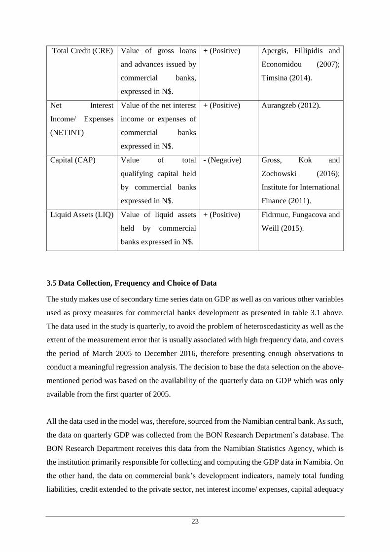
Total Credit (CRE) Value of gross loans

and advances issued by

commercial banks,

expressed in N$.

+ (Positive) Apergis, Fillipidis and

Economidou (2007);

Timsina (2014).

Net Interest

Income/ Expenses

(NETINT)

Value of the net interest

income or expenses of

commercial banks

expressed in N$.

+ (Positive) Aurangzeb (2012).

Capital (CAP) Value of total

qualifying capital held

by commercial banks

expressed in N$.

- (Negative) Gross, Kok and

Zochowski (2016);

Institute for International

Finance (2011).

Liquid Assets (LIQ) Value of liquid assets

held by commercial

banks expressed in N$.

+ (Positive) Fidrmuc, Fungacova and

Weill (2015).

3.5 Data Collection, Frequency and Choice of Data

The study makes use of secondary time series data on GDP as well as on various other variables

used as proxy measures for commercial banks development as presented in table 3.1 above.

The data used in the study is quarterly, to avoid the problem of heteroscedasticity as well as the

extent of the measurement error that is usually associated with high frequency data, and covers

the period of March 2005 to December 2016, therefore presenting enough observations to

conduct a meaningful regression analysis. The decision to base the data selection on the above-

mentioned period was based on the availability of the quarterly data on GDP which was only

available from the first quarter of 2005.

All the data used in the model was, therefore, sourced from the Namibian central bank. As such,

the data on quarterly GDP was collected from the BON Research Department’s database. The

BON Research Department receives this data from the Namibian Statistics Agency, which is

the institution primarily responsible for collecting and computing the GDP data in Namibia. On

the other hand, the data on commercial bank’s development indicators, namely total funding

liabilities, credit extended to the private sector, net interest income/ expenses, capital adequacy

24

and liquid assets of banks was computed from the various aggregated industry returns published

on the bank’s website under the Banking Supervision Department. These aggregated industry

returns include the Capital Adequacy return, Income Statement return, Liquid Assets return and

the Balance Sheet return.

3.6 Sampling

The selected sample only includes the period from 2005:1 to 2016:4 taking into consideration

that this is the period where the data was available on a quarterly basis. In terms of the number

of banks included in the sample, the data covers all commercial banks authorised by BON, to

conduct banking business in Namibia.

3.7 Data Analysis Methods

To investigate the relationship between financial development and economic growth, the study

employed the autoregression distributive lag modelling (ARDL) approach as it was also used

in a similar study by Kiprop et al. (2015). The choice of this model is justified by so many

reasons as outlined by Pesaran and Shin (1999). Firstly, this approach enables for simultaneous

estimation for both short-run and long-run coefficients. Secondly, all the variables enter the

model as endogenous. Thirdly, there is no need to pre-test for the univariate characteristics of

the series. Even though pre-testing is done, the model allows for estimation of series with

mixture of order of integration either integrated of zero I(0) or first I(1) order, with the exception

I(2). Fourthly, this technique addresses the problem of endogeneity in the model due to the fact

that causal relationship between the regressand and regressors cannot be ascertained

beforehand. Lastly, this technique is most suitable for small sample size as it has superior small

sample properties in comparison with other methods. This approach is, therefore, suitable in

analyzing the underlying relationship between economic growth and banking sector

development, as its use in empirical research has increased recently.

For ease of interpretation, equation (1) can be expressed in natural logarithms and it can be

presented as follows:

𝐿𝑁𝐺𝐷𝑃𝑡 = 𝛽0 + 𝛽1𝐿𝑁𝐹𝑁𝐷𝑡 + 𝛽2𝐿𝑁𝐶𝑅𝐸𝑡 + 𝛽3 𝐿𝑁𝑁𝐸𝑇𝐼𝑁𝑇𝑡 + 𝛽4𝐿𝑁𝐶𝐴𝑃𝑡 +

𝛽5𝐿𝑁𝐿𝐼𝑄𝑡 + Є (2)

25

The process of estimating equation (2) requires some prior steps to be performed as discussed

below.

3.7.1 Unit Root Tests

Upon collection of the data, the first step was to investigate the time series characteristics of

the data in order to establish if the data set is integrated. In case of evidence suggesting presence

of unit root the study will, similar to Aurangzeb (2012), employ the Augmented Dickey Fuller

(ADF) and Phillips-Perron (PP) Unit Root tests, to ensure that the data is stationary and ensure

that the results can be relied upon. For the ADF and PP tests, the null hypothesis entails that

there is presence of unit root in the series, while the alternative hypothesis entails that there is

no evidence of unit root and the data is stationary in level or at first difference. This step is,

thus, undertaken to ensure that none of the variables are integrated of order two or higher.

3.7.2 Bound Cointegration Test

The cointegration test is applied to ascertain whether or not there exists a long-run relationship

among the variables (Gujarati, 2004). The test is for the null hypothesis which postulates that

there is no cointegration, whilst the alternative hypothesis postulates that there is cointegration.

The presence of cointegration suggests that both long-run and short-run coefficients can be

estimated using an unrestricted error correction model (UECM) which can be expressed as

follows:

∆𝐿𝑁𝐺𝐷𝑃 = 𝛼0 + 𝜆1𝐿𝑁𝐺𝐷𝑃𝑡−1 + 𝜆2 𝐿𝑁𝐹𝑁𝐷𝑡−1 + 𝜆3 𝐿𝑁𝐶𝑅𝐸𝑡−1 + 𝜆4 𝐿𝑁𝑁𝐸𝑇𝐼𝑁𝑇𝑡−1 +

𝜆5𝐿𝑁𝐶𝐴𝑃𝑡−1 + 𝜆6𝐿𝑁𝐿𝐼𝑄𝑡−1 + ∑ 𝛾1 ∆𝐿𝑁𝐺𝐷𝑃𝑡−1 + ∑ 𝛾2 𝛥 𝐿𝑁𝐹𝑁𝐷𝑡−1 + ∑ 𝛾3 𝛥 𝐿𝑁𝐶𝑅𝐸𝑡−1 +

∑ 𝛾4Δ 𝐿𝑁𝑁𝐸𝑇𝐼𝑁𝑇𝑡−1 + Σγ5Δ𝐿𝑁𝐶𝐴𝑃𝑡−1+ Σ𝛾6𝐿𝑁𝐿𝐼𝑄𝑡−1 + 𝑈1𝑡 …………. (3)

Where; 𝜆1 − 𝜆6 are the estimated long-run coefficients and 𝛾1 − 𝛾6 are short-run coefficients.

The tests follow an F-test statistic and is then used to detect the existence of a long-run

relationship among the variables. This is done by comparing the calculated value to the critical

values in order to make a decision about the hypothesis of cointegration. The null hypothesis

of no co-integration is tested under the condition 𝐻0: 𝜆1 − 𝜆2 = 𝜆3 = 𝜆4 = 𝜆5 = 𝜆6 =

0, while the alternative hypothesis is tested under the condition 𝐻1: 𝜆1 ≠ 𝜆2 ≠ 𝜆3 ≠ 𝜆4 ≠

𝜆5 ≠ 𝜆6 ≠ 0. The decision about cointegration is arrived at by comparing the calculated F-test

statistic with the two critical bounds, the lower and the upper bounds. For example, when the

calculated value happens to be below the lower critical bound then the null hypothesis of no

26

cointegration cannot be rejected. However, should the calculated value happen to be above the

upper critical bound then the null hypothesis of no cointegration can be rejected. In cases where

the calculated F-value happens to fall between the two critical bounds then the test is

inconclusive (Pesaran, Shin & Smith, 2001).

3.7.3 Estimating Short-Run Coefficients

After conducting the cointegration test and finding its existence then this suggests an estimation

of an error correction model (ECM). This helps to determine the speed of adjustment at which

the variables adjust to their long-run equilibrium value (Gujarati and Porter, 2010). The error

correction model can be expressed in ARDL form and expressed as:

∆𝐿𝑁𝐺𝐷𝑃𝑡 = 𝛾0 + ∑ 𝛾1𝑖𝑛𝑖=1 ∆𝐿𝑁𝐺𝐷𝑃𝑡−1 + ∑ 𝛾2𝑖

𝑛𝑖=1 ∆𝐿𝑁𝐹𝑁𝐷𝑡−1 + ∑ 𝛾3𝑖

𝑛𝑖=1 𝐿𝑁𝐶𝑅𝐸𝑡−1 +

∑ 𝛾4𝑖𝑛𝑖=1 Δ 𝐿𝑁𝑁𝐸𝑇𝐼𝑁𝑇𝑡−1 + ∑ 𝛾5𝑖

𝑛𝑖=1 Δ𝐿𝑁𝐶𝐴𝑃𝑡−1+ ∑ 𝛾6𝑖

𝑛𝑖=1 ∆𝐿𝑁𝐿𝐼𝑄𝑡−1 + 𝜑𝐸𝐶𝑀𝑡−1 + 𝜀1

…………. (4)

Where:

ECM is a residual from the estimated cointegration equation 3, 𝜑 is the parameter which

represents the speed of adjustments in the long run. Ideally, the coefficient of the ECM should

have a negative sign, statistical significant and less than unity.

3.7.4 Granger-Causality Tests

The Granger causality test developed by Granger (1969) is widely used in econometric analysis

and in this case it is used to determine any causal relationship between financial development

and economic growth in Namibia. In particular, a simple pairwise Granger-causality is used in

this study. This test yields three possibilities namely, unidirectional causality (causality from

one variable to another and not the other way round). Secondly, there could be causality from

both variables (bidirectional causality). Lastly, there is a possibility of no causal relationship

among the variables.

3.8 Research Reliability and Validity

Since the study is making use of secondary data, all the data used in this study was obtained

from a credible institution in Namibia, namely BON, which is responsible for the supervision

of commercial bank activities in Namibia, among other responsibilities. BON collects data from

commercial banks on a regular basis and at different time intervals for the purposes of effective

banking supervision and this data is published on BON’s website on an aggregated level.

27

Furthermore, BON Research Department receives data on GDP from the Namibia Statistics

Agency, which is the primary custodian of GDP data. In light of the above, it could, therefore,

be concluded that this study is conducted with reliable and valid data.

3.9 Limitations

The main limitation to the study is the fact that the list of banking sector variables that could

have an impact on GDP growth is not exhaustive. Apart from the limited variables used to

measure banking sector development, there are no further limitations to the study.

28

4 CHAPTER FOUR: RESEARCH FINDINGS, ANALYSIS AND

DISCUSSION

4.1 Introduction

This chapter presents the results and the detailed empirical analysis of the study on which the

conclusion and recommendations were based. The section on empirical analysis is divided into

nine sub-sections as follows. Section 4.2.1 presents the correlation coefficient test, section 4.2.2

presents the unit root test, section 4.2.3 presents the determination of the optimal lag length,

section 4.2.4 presents the cointegration test, while section 4.2.5 and 4.2.6 presents the long term

and short term ARDL regression results, respectively. Furthermore, section 4.2.7 presents the

bivariate error correction models, section 4.2.8 presents the model diagnostic test and section

4.2.9 presents the pairwise granger causality test.

4.2 Empirical Analysis

4.2.1 Correlation Coefficient Test

In determining whether or not a linear relationship exists between the variables employed in

the model, the study made use of the Pearson correlation coefficient test. The test was also

conducted to determine the possible existence of multicollinearity within the variables, which

if present, can lead to errors in the coefficient estimates of the multiple regression. In this regard,

all coefficients between all variables as indicated in table 4.1 below were above 0.9, which

indicates possible existence of multicollinearity given that they are close to 1. This outcome

entails that, reliance cannot be placed on the estimation results of a multiple regression as

multicollinearity could severely affect these results, hence the need to run a separate model for

each banking sector development indicator.

Table 4.1: Pearson Correlation Coefficient Test

Variable LNGDP LNFND LNCRE LNNETINT LNCAP LNLIQ

LNGDP 1.000000 0.976556 0.977370 0.981389 0.972740 0.972134

LNFND 0.976556 1.000000 0.998207 0.992662 0.997044 0.995489

LNCRE 0.977370 0.998207 1.000000 0.994423 0.996691 0.991976

LNNETINT 0.981389 0.992662 0.994423 1.000000 0.989239 0.989219

LNCAP 0.972740 0.997044 0.996691 0.989239 1.000000 0.992204

29

LNLIQ 0.972134 0.995489 0.991976 0.989219 0.992204 1.000000

4.2.2 Unit Root Test

While the ARDL technique does not require the data to be tested for unit root, it is important

to conduct this test in order to make sure that the series are not integrated to an order higher

than one. As such, using an ARDL technique with data series that is integrated to an order of

more than one may lead to spurious results. Using the ADF and PP unit root tests, the results

as presented in table 4.2 below indicate that all variables are stationary either in level or after

first difference. This implies that the data is suitable to carry out an ARDL regression analysis

and the null hypothesis of unit root can be rejected at 1 percent and 5 percent significance levels,

respectively.

Table 4.2: Unit root tests: ADF and PP in differences

Variable Model Specification ADF PP

Levels

First

difference Levels

First

differenc

e

Order of

integratio

n

LNGDP

Intercept and trend -5.304** -6.316** -5.300**

-29.759**

0

Intercept -1.007 -6.365** -0.932 -27.585** 1

LNFND

Intercept and trend -3.803** -9.087** -3.734** -10.151** 0

Intercept -0.978 -9.085** -1.203 -9.803** 1

LNCRE

Intercept and trend -2.823 -6.572** -1.957 -6.909** 1

Intercept -0.594 -6.417** -0.577 -7.004** 1

LNNETINT

Intercept and trend -2.995 -7.004** -2.995 -15.430** 1

Intercept 0.261 -7.055** 1.388 -15.545** 1

LNCAP

Intercept and trend -3.612** -10.259** -3.652** -11.429** 0

Intercept -0.378 -10.370** -0.224 -11.551** 1

LNLIQ Intercept and trend -5.134** -7.609** -5.160** -13.349** 0

Intercept -0.414 -7.698** -0.156 -13.599** 1

Note: ** means the rejection of the null hypothesis at 1% and 5%.

4.2.3 Determination of Optimal Lag Length

Upon establishing the univariate characteristics of the variables and subsequently the order of

integration, the following step is undertaken to establish the optimal lag length for the model.

This was determined using the lag length criterion such as Akaike Information Criterion (AIC),

30

Schwarz Bayesian Criterion (SC) and Hannan-Quinn Criterion (HQ). This study opted to

follow the SC and HQ, the information criterion because of their powerfulness and consistency.

The two criteria suggested a lag length of one as reported in table 4.3 below.

Table 4.3: Lag Order Selection Criteria

Lag LogL LR FPE AIC SC HQ

0 402.5699 NA 3.93e-16 -18.44511 -18.19936 -18.35449

1 593.0014 318.8620 3.04e-19 -25.62797 -23.90773* -24.99360*

2 625.3152 45.08903 3.98e-19 -25.45652 -22.26178 -24.27840

3 673.8072 54.13063* 2.93e-19* -26.03754 -21.36832 -24.31568

4 714.9886 34.47746 4.23e-19 -26.27854* -20.13482 -24.01292

* indicates lag order selected by the criterion

4.2.4 Bound Test Approach to Cointegration

The bound cointegration test was performed in order to ascertain whether or not there is a long-

run relationship among the variables. Table 4.4 below reports the results of the test which show

that the calculated F-statistic value of 5.33 is greater than the critical upper bound values of

4.15 at 1 percent significance level. This implies existence of a long run relationship between

GDP and the variables used in the model, and as such, the null hypothesis of no cointegration

can be rejected.

Table 4.4: Bounds test results

Test Statistic Value K

F-statistic 5.329185 5

Critical Value Bounds

Significance I(0) Bound I(1) Bound

10% 2.08 3

5% 2.39 3.38

31

2.5% 2.7 3.73

1% 3.06 4.15

Given existence of a long-run relationship between GDP and the regressors in the model, the

study then goes further to estimate the long-run and the short-run ARDL Error Correction

equation and the results are presented below in table 4.5 and table 4.6, respectively.

4.2.5 Long-run Estimates

Table 4.5 displays the long-run coefficients from the ARDL estimation. The results show that

only the relationship between net interest income and economic growth was found to be positive

and statistically significant in the long-run, with all the other explanatory variables found to be

statistically insignificant. The positive relationship between net interest income and GDP

growth is well in line with the theoretical expectations of this study, however, given the high

correlation coefficients as depicted in table 4.1, which suggest possible existence of

multicollinearity, the multiple regression results could not be relied upon, hence the need to run

a separate model for each indicator.

Table 4.5: Estimated Long Run coefficients using the ARDL

Variable Coefficient Std. Error t-Statistic Prob.

LNFND 0.132987 0.263197 0.505275 0.6162

LNCRE -0.132348 0.243153 -0.544298 0.5893

LNCAP 0.013198 0.141236 0.093443 0.9260

LNNETINT 0.344429 0.110141 3.127160 0.0033

LNLIQ -0.019973 0.104336 -0.191432 0.8492

C 5.495557 1.002939 5.479455 0.0000

4.2.6 Short-run

Table 4.6 displays the short-run coefficients from the ARDL estimation. As it is the case with

the long-run estimates, the only variable that was found to be statistically significant in the

model is the net interest income, with a t-statistic of 3.099 which is above the value of 2, and

further confirmed by the corresponding p-value of 0.0037, which is lower than the 1 percent

32

significance value. However, similar to the long run model, these results could not be relied

upon in presence of multicollinearity, hence the need to run separate models for each

commercial bank development indicators.


Variable Coefficient Std. Error t-Statistic Prob.*

D(LNGDP(-1)) 0.002621 0.155429 0.016860 0.9866

D(LNFND) 0.398840 0.276694 1.441451 0.1579

D(LNCRE) 0.127311 0.400300 0.318039 0.7522

D(LNCAP) 0.000726 0.178407 0.004070 0.9968

D(LNNETINT) 0.350874 0.113216 3.099172 0.0037

D(LNLIQ) -0.116331 0.101617 -1.144801 0.2596

ECT(-1) -1.098665 0.220638 -4.979482 0.0000

C -0.012439 0.015782 -0.788208 0.4356

𝑅2 = 0.599, 𝐷𝑊 = 1.98, 𝑃𝑟𝑜𝑏(𝐹 − 𝑠𝑡𝑎𝑡𝑖𝑠𝑡𝑖𝑐) = 0.000007

4.2.7 Bivariate Error Correction Models

The exercise of the ARDL conducted with the comprehensive model was repeated by regressing

real gross domestic product with each banking sector development indicator. This was informed

by the fact that table 4.1 showed a high correlation coefficient among the variables, which may

have influenced the statistical significance of the regressors in the comprehensive model. The

results are presented in table 4.7 to 4.11 below.



D(LNGDP(-1)) 0.367915 0.224005 1.642442 0.1097

D(LNCRE) 0.513224 0.442943 1.158667 0.2547

D(LNCRE(-1)) -0.020565 0.408616 -0.050328 0.9602

D(LNCRE(-2)) -1.175524 0.388923 -3.022510 0.0047

D(LNCRE(-3)) 2.147860 0.461809 4.650970 0.0000

D(LNCRE(-4)) -1.190222 0.606240 -1.963286 0.0578

33

ECT01(-1) -1.083296 0.284795 -3.803780 0.0006

C -0.001302 0.026865 -0.048479 0.9616


Table 4.7 above presents the results of the bivariate error correction regression between credit

extension and economic growth. The results indicate that the relationship between commercial

banks credit extension to the private sector and economic growth is statistically significant for

the second, third and fourth lag periods at 10 percent significance value. The corresponding

coefficients are, however, negative for the second lag, positive for the third lag and negative

for the fourth lag, indicating an inconclusive outcome of the relationship between credit

extension to the private sector and economic growth. However, since credit extension to the

private sector was used as a proxy measure for the size and depth of the banking sector and its

relationship was found to be inconclusive in this regard, another indicator of banking size and

depth, namely funding liabilities, was employed in the quest to establish the impact of bank

size and depth on economic growth.

Table 4.8 below, therefore, presents the bivariate error correction results of the relationship

between funding liabilities of banks and economic growth. This relationship was found to be

positive and statistically significant at 10 percent significance value, given the p-value of

0.0573. The coefficient of 0.47 entails that any 1 percent increase in the funding liabilities of

banks will lead to 0.47 percent increment in economic growth. This finding is in line with the

theory expectation of the study as well as with the findings of Ogege and Shiro (2012) and

could be interpreted to mean that as the funding related liabilities of banks such as deposits and

borrowings increase, banks are able to fund more activities in the real sector by increasing the

amount of credit extended to that sector, thereby driving the production capacity of the economy

and eventually leading to economic growth. This finding is, thus, an indication that

advancement in the banks’ size and depth contributes to the growth of the economy in Namibia,

in line with the financial repression hypothesis.



D(LNGDP(-1)) 0.023112 0.183553 0.125917 0.9004

34

D(LNFND) 0.471177 0.240858 1.956241 0.0573

ECT05(-1) -0.974779 0.236572 -4.120436 0.0002

C -0.003331 0.009025 -0.369137 0.7139


The bivariate regression results of the short-run relationship between capital held by

commercial banks and economic growth is presented in table 4.9 below. Though positive, this

relationship was found to be statistically insignificant entailing absence of any significant

evidence that a relationship exists between banks capital and economic growth. As such, the

finding is contradictory to the theoretical expectations of this study, while it also contradicts

the findings of Gross, Kok and Zochowski (2016) and the Institute for International Finance

(2011), which all established a negative relationship in this regard.



D(LNGDP(-1)) 0.207691 0.209575 0.991009 0.3275

D(LNCAP) 0.213340 0.218807 0.975015 0.3353

ECT02(-1) -0.990589 0.270253 -3.665410 0.0007

C 0.002219 0.010069 0.220351 0.8267


Another indicator of banking sector stability, namely liquid assets held by commercial banks

was also found to have a statistically insignificant relationship with economic growth as

presented in table 4.10 below. As it was the case with capital, this finding confirms the position

that the stability of the banking system does not have any influence on the growth of the

economy. Also, this finding contradicts the theory expectation of this study, as well as the

findings of Fidrmuc, Fungacova and Weill (2015), who found a positive relationship.



35

D(LNGDP(-1)) 0.136436 0.197903 0.689409 0.4944

D(LNLIQ) 0.096210 0.090728 1.060418 0.2952

ECT04(-1) -0.977308 0.252099 -3.876690 0.0004

C 0.006395 0.006702 0.954241 0.3456


Table 4.11 below presents the findings of the bivariate regression between net interest income

of banks and economic growth. Similar to the comprehensive ARDL model for both the long

run and the short run, this relationship was found to be positive and statistically significant, as

indicated by the p-value of 0.0013 which is below the 5 percent significance value. As such,

the coefficient of 0.35 entails that any 1 percent increase in the net interest income of banks

will lead to 0.35 percent growth in the economy. Thus, as banks become more profitable, they

acquire more resources and are willing to invest more in the economy, eventually, influencing

growth.

Table 4.11 Error correction model using the ARDL


D(LNGDP(-1)) 0.060890 0.134449 0.452888 0.6530

D(LNNETINT) 0.346245 0.100475 3.446093 0.0013

ECT03(-1) -1.144704 0.208349 -5.494174 0.0000

C -0.000536 0.006007 -0.089188 0.9294


In light of the high correlation coefficient observed in table 4.1, the results of the bivariate error

correction models are adopted as the reliable findings of this study. The results of the bivariate

error correction models, therefore, indicate that there is a positive short-run relationship

between banking sector development indicators and economic growth in Namibia, and this

impact on GDP growth is mainly realised through net interest income and banks’ funding

liabilities. This is an indication that the impact that the banking sector has on economic growth

is channelled through the size and depth of the banking sector as well as through the sector’s

36

efficiency. On the contrary, the banking sector’s stability as indicated by capital and liquid

assets held by banks, does not have any influence on economic growth, as both these indicators

were found to be statistically insignificant. The null hypothesis of no impact of commercial

banks development on economic growth can therefore be rejected.

In terms of validity of the bivariate error correction models, table 4.7 to table 4.11, the Durbin-

Watson value of all of these models show that there is no problem of serial or autocorrelation

in the models, while their F-statistic test also confirms the overall significance of the models

given that their F-value probabilities are less than the 1 percent levels of significance. All these

indicators are, thus, positive and indicate reliability of the models as well as of the results.

4.2.8 Model Diagnostic Test

As per the classical assumption, a model should be normally distributed with a constant

variance and a mean of zero in order to produce the best linear unbiased estimators (Gujarati,

2004). As such, the study conducted the model efficiency test and the results are presented

below.

Table 4.12: Heteroscedasticity (White) Test

F-statistic 1.195559 Prob. F(7,37) 0.3294

Obs*R-squared 8.300859 Prob. Chi-Square(7) 0.3068

Scaled explained SS 4.250234 Prob. Chi-Square(7) 0.7505

Table 4.12 above presents the heteroscedasticity test, which was conducted in order to

determine whether the model has a constant variance or not. The statistical hypothesis for

conducting a heteroscedasticity test is formulated based on the statistic where the null

hypothesis implies that the variances are constant (i.e., Homoscedasticity) while the alternative

hypothesis implies that the variances are not constant (i.e., heteroscedasticity). The rejection

rule states that the null hypothesis can be rejected should the probability value of observation

R-square be less than 5 percent level of significance. As such, given that the probability of Chi-

Square is 0.3068 which is greater than 0.05 level of significance, the null hypothesis cannot be

rejected and concludes that the variances in the model are constant.

37

Table 4.13: Breusch-Godfrey Serial Correlation LM Test

F-statistic 0.146373 Prob. F(2,35) 0.8644

Obs*R-squared 0.373266 Prob. Chi-Square(2) 0.8297

Table 4.13 presents the results of the autocorrelation test which was conducted to determine the

absence or presence of correlation in the error terms of the model. The hypotheses for testing

for autocorrelation are, therefore, formulated in the following manner; the null hypothesis

implies that there is no autocorrelation while the alternative hypothesis implies presence of

autocorrelation among the error terms. The decision rule for the autocorrelation test, therefore,

states that the null hypothesis should be rejected if the p-value for the observed R-square is less

than the 5 percent significance value. In this regard, the observed R-square of 0.8297 is higher

than the 5 percent level of significance, implying that the null hypothesis of no autocorrelation

cannot be rejected.

Furthermore, the study conducted a model stability test using the Ramsey Reset test to

determine the stability capacity of the model. The results of test are displayed in table 4.14

below.

Table 4.14: Ramsey RESET Test

Value df Probability

t-statistic 0.197974 36 0.8442

F-statistic 0.039194 (1, 36) 0.8442

The hypothesis for the Ramsey Reset stability test is, therefore, formulated in the following

manner. The null hypothesis claims that the model is stable while the alternative hypothesis

claims that the model is not stable. The decision rule entails that the null hypothesis should not

be rejected if the probability of the F-statistic is higher than the 5 percent significance level. In

this regard, the F-statistic probability of 0.8442 is higher than the 5 percent significance value

and concludes that the null hypothesis cannot be rejected, implying that the model is stable.

38

4.2.9 Pairwise Granger Causality Test Results

The study conducted the granger causality test in order to determine the direction of causality

between GDP growth and the various banking sector development indicators considered in the

model. The results of the Pairwise Granger Causality test are presented in table 4.15 below.

Table 4.15: Pairwise Granger Causality Test

Null Hypothesis: Obs F-Statistic Prob.

D(LNFND) does not Granger Cause D(LNGDP) 44 0.18592 0.8311

D(LNGDP) does not Granger Cause D(LNFND) 6.30162 0.0043

D(LNCRE) does not Granger Cause D(LNGDP) 44 2.80524 0.0727

D(LNGDP) does not Granger Cause D(LNCRE) 0.49566 0.6130

D(LNNETINT) does not Granger Cause

D(LNGDP) 44 5.70388 0.0067

D(LNGDP) does not Granger Cause D(LNNETINT) 0.36683 0.6953

D(LNCAP) does not Granger Cause D(LNGDP) 44 0.25576 0.7756

D(LNGDP) does not Granger Cause D(LNCAP) 1.09005 0.3462

D(LNLIQ) does not Granger Cause D(LNGDP) 44 0.16941 0.8448

D(LNGDP) does not Granger Cause D(LNLIQ) 3.54214 0.0386

After differencing the data to ensure that it was stationary and the results can be relied upon,

table 4.15 presents the findings of causality test between economic growth and the other

regressors considered in the model. In this regard, the results show a unidirectional causality at

5 percent significance value, running from economic growth to banks funding liabilities, as

well as from economic growth to liquid assets held by commercial banks. Furthermore, in line

with the findings of Aurangzeb (2012), the granger causality test established a unidirectional

causality running from net interest income/expense to economic growth at 5 percent

significance value, while credit extended to the private sectors by banks granger caused

economic growth at 10 percent significance value, partially corresponding with the findings of

Apergis, Fillipidis and Economidou (2007), which discovered a bi-direction causality between

GDP growth and credit extension to the private sector.

39

Overall, the causality test results revealed a bi-directional causality between banking sector

development and economic growth, albeit through different variables. As such, the causality

test indicates that the size and depth of the banking sector and efficiency in the banking sector

caused economic growth. On the other hand, economic growth caused stability in the banking

sector as well as expansion in the size and depth of the banking sector, but through different

variables. This finding entails that the null hypothesis of no causal relationship between GDP

growth and banking sector development can be rejected, therefore, concluding that there is

existence of bi-direction causality in line with the findings of Sunde (2013), Apergis, Fillipidis

and Economidou (2007) etc. This finding supports the financial repression theory that

recognises the essential role that financial institutions play in driving economic growth.

40

5 CHAPTER FIVE: RESEARCH CONCLUSIONS

5.1 Introduction

Following the regression outcomes and analysis of the results outlined in the preceding chapter,

this chapter seeks to present the conclusion of the study.

5.2 Research Conclusion

This study set out to establish the impact that commercial banks’ development has on economic

growth in Namibia. The study employed the quantitative methodology of ARDL in order to

establish the long-run and the short-run relationship between GDP growth and banking sector

development as well as the Granger causality test in determining the direction of causality. To

this effect, the study used quarterly GDP growth rate and quarterly data on banks various

development indicators such as total credit extended by banks to the private sector, aggregate

funding liabilities, covering the period of 2005:1 to 2016:4. Prior to the regression analysis

being conducted, the data was tested for unit root using the ADF and PP unit root test to ensure

that it was stationary and could yield reliable results.

In the context of Namibia, this study is the second of its kind and follows a study conducted by

Sunde (2013) who investigated the nature of the nexus between financial sector development

and economic growth in Namibia. While covering different periods and employing different

variables and to a certain extend different methodologies, the findings of the studies are in line

with the findings of Sunde (2013). In this regard, the study concluded that there is existence of

a positive short-run relationship between banking sector development and economic growth.

The positive short run relationship is exerted through funding liabilities and net interest income

and entails that only the size and depth of the banking sector as well as the efficiency of the

sector have an impact on economic growth. On the contrary, the stability of the banking sector

was found not to have any influence on the growth of the economy.

Furthermore, the study concluded from the granger causality test that the relationship between

economic growth and banking sector development in Namibia is bi-directional, entailing that

economic growth will advance the banking sector development while at the same time

development of the banking sector will promote the growth of the economy, albeit through

different variables. As such, a unidirectional causality was established between GDP and

41

funding liabilities of banks as well as between GDP and liquid assets held by banks, with

causality running from GDP to banking sector development, while credit extended by banks to

the private sector and net interest income of banks caused the growth of the economy.

In light of the above, the study concludes that both the null hypothesis 1 of no relationship

between commercial banks development and economic growth and the null hypothesis 2 of no

causal relationship between commercial banks development and economic growth can be

rejected. As such, the conclusion of the study is in support of the findings of prior empirical

studies conducted on the subject matter by, among others, Sunde (2013), Aurengzeb (2012),

Apergis, Fillipidis and Economidou (2007) and supports the endogenous growth model and

financial repression hypothesis theories that acknowledge the role of financial institutions in

driving economic growth.

5.3 Policy Implications

In light of the study conclusions, the government of Namibia, the BON as the regulator of the

commercial banks in Namibia has a number of factors to consider in order to further drive

economic growth in the country. Firstly, in light of the study establishing a link between

banking sector development and economic growth, driven by the bank’s interest income and

funding liabilities, Namibian banks should consider increasing the absolute amounts of loans

and advances to the real sector in order to foster economic growth. This can be achieved either

through the central bank authorizing additional participants in the banking sector or through

existing banks embarking on a campaign to secure more funding liabilities, such as deposits

and borrowings, to enable them to extend more credit to the economy.

Secondly, considering an insignificant relationship between liquid assets held by commercial

banks and economic growth, banks should not be required to hold too much assets in liquid

assets as these assets are normally short term and not ideal for financing long term

developmental projects. While the minimum liquid assets requirement set by the central bank

at 10 percent liquid assets to total liabilities to the public, as per BON (2014), is not too

stringent, commercial banks tend to keep a buffer above this requirement to ensure that they

have enough liquidity to meet their funding obligations as they fall due. In this regard, the

central bank should be careful against setting the liquid assets requirements too stringent going

forward, especially in light of the more stringent liquidity requirements coming from Basel 3.

42

As such, requiring banks to hold higher liquid assets would mean that they would need to reduce

their total loans and advances to the economy which are more ideal for financing economic

growth as these are granted on a longer term as opposed to investments in liquid assets.

Thirdly, commercial banks should be incentivised to provide funding to sectors that can

contribute to the growth of the economy as opposed to providing finance for unproductive

activities. In this regard, commercial banks should increase funding to the SME sector since

banks tend to be more risk averse and have put in place stringent requirements that most SMEs

do not meet, such as collateral, high annual turnover, audited financial statements etc.

Furthermore, given that the FinScope Consumer Survey Namibia, (2012) reported that 38

percent of the Namibian bankable population is reported to be excluded from the banking

system as in 2012, with no access to banking products and services, commercial banks should

aim to provide banking products services to those in remote areas. This could be achieved

through expanding their branches or setting up mobile banks in remote areas, while their models

should also be suitable to enable people excluded from the financial system to access banking

products and services in order to contribute to the growth of the rural economies and eventually

of the general economy.

43

6 CHAPTER SIX: RECOMMENDATIONS FOR FUTURE RESEARCH

Given limited research conducted on the subject matter in Namibia, this study creates

opportunities for further research extension on the subject. In this regard, future researchers can

consider extending this research in various ways as outlined below:

a) Considering that BON might adopt Basel 3 regulatory requirements in the near future,

future researches can be based on the impact that complying with Basel 3 capital and

liquidity requirements will have on the banking sector’s ability to support economic growth.

b) This research could further be extended to investigate the role that commercial banks in

Namibia have played with regard to financial inclusion since the country’s independence in

1990, in order to recommend reforms that the government should implement to ensure

access to financial services and products to the unbanked and promote an inclusive

economic growth.

c) Future researchers may also focus on investigating the efficiency of the Namibian banking

sector given the fact that there are only few banks in the industry, with the big four usually

accused of uncompetitive practices to keep the smaller ones out of the market.

d) The commercial banks’ corporate social responsibilities and the impact it has on the

communities can also be investigated, given that banks are said to be the most profitable

institutions in Namibia yet with minimal social impact on communities.

44

REFERENCES

Admati, A. R. (2011). The false trade-off between economic growth and bank capital.

Unpublished paper. Stanford University. Retrieved from

https://www.gsb.stanford.edu/sites/gsb/files/false-tradeoff.pdf

Agribank of Namibia (2015). Annual report. Retrieved from

http://2015annualreport.agribank.com/

Apergis, N., Filippidis, J., & Economidou, C. (2007). Financial deepening and economic

growth linkages: A panel data analysis. Review of World Economics, 143(1), 179-198.

Aurangzeb, Q. (2012). Contribution of banking sector in economic growth: A case for

Pakistan. Economics and Finance Review, 2(6), 45–54.

Bagehot, W. (1873). Lombard Street: A description of the money market. London, UK: H. S.

King. Retrieved from http://www.econlib.org/library/Bagehot/bagLom1.html

Bank of Namibia (2009). Determination on Minimum Liquid Assets, (BID-6). Government

Gazette, No. 4373, 6 November. Retrieved from

https://www.bon.com.na/CMSTemplates/Bon/Files/bon.com.na/b0/b0c4c785-c327-4407-

a1c2-5541e5628608.pdf

Bank of Namibia (2014). Domestic Systemically Important Banks for the Namibian Banking

System: An Indicator-Based Measurement Approach.

Bank of Namibia, (2014, August 20). Repo rate increased to 6.0 percent. Monetary Policy

Statements, Ref: 6/9/2. Retrieved from

https://www.bon.com.na/CMSTemplates/Bon/Files/bon.com.na/32/3274d92c-8815-4cd2-

b5fb-f9c27a7178c8.pdf

Bank of Namibia, (2016). Aggregated Industry Returns: 2005 - 2016. Retrieved from:

https://www.bon.com.na/Bank/Banking-Supervision/The-Banking-System-in-

Namibia/Aggregated-industry-returns.aspx

Bank of Namibia, (2016). Annual report. Retrieved from

https://www.bon.com.na/CMSTemplates/Bon/Files/bon.com.na/0e/0e9c5d80-8203-498a-

8e07-3bb26d5657d9.pdf

Bank of Namibia. (2017). The Banking System in Namibia. Retrieved from

https://www.bon.com.na/Bank/Banking-Supervision/The-Banking-System-in-

Namibia.aspx

Bencivenga, V. R. and Smith, B. D. (1991). Financial Intermediation and Endogenous

Growth. Review of Economics Studies 58(2), 195–209.

https://www.bon.com.na/Bank/Banking-Supervision/The-Banking-System-in-Namibia/Aggregated-industry-returns.aspx

https://www.bon.com.na/Bank/Banking-Supervision/The-Banking-System-in-Namibia/Aggregated-industry-returns.aspx

https://www.bon.com.na/CMSTemplates/Bon/Files/bon.com.na/0e/0e9c5d80-8203-498a-8e07-3bb26d5657d9.pdf

https://www.bon.com.na/CMSTemplates/Bon/Files/bon.com.na/0e/0e9c5d80-8203-498a-8e07-3bb26d5657d9.pdf

https://www.bon.com.na/Bank/Banking-Supervision/The-Banking-System-in-Namibia.aspx

https://www.bon.com.na/Bank/Banking-Supervision/The-Banking-System-in-Namibia.aspx

45

Calderon С., & Liu, L. (2002). The direction of causality between financial development and

economic growth. Journal of Development Economics 72(1), 321–334.

Chukwu, J., & Agu, C. (2009). Multivariate Causality Between Financial Depth and

Economic Growth in Nigeria. African Review of Money Finance and Banking, 7-21.

Development Bank of Namibia (2016). Annual report. Retrieved from

http://www.dbn.com.na/index.php/investors-relations/annual-reports/file/115-annual-

report-2016

Driffil, J. (2003). Growth and finance. The Manchester School, 71(4), 363-380.

Fidrmuc, J., Fungacova, Z., & Weill, L. (2015). Does bank liquidity creation contribute to

economic growth? (Unpublished paper). Retrieved from

http://ies.fsv.cuni.cz/default/file/get/id/26488

FinMark Trust, (2012). FinScope consumer survey: Namibia. Retrieved from

https://www.finmark.org.za/finscope-consumer-survey-namibia-2011/

Granger, C. W. J. (1969). Investigating Causal Relations by Econometric Models and Cross-

spectral Methods. Econometrica Vol. 37, No. 3, pp. 424-438.

Gross, M., Kok, C., & Zochowski, D. (2016). The impact of bank capital on economic

activity: Evidence from a mixed-cross-sectional GVAR model. (ECB working paper, No.

1888), European Central Bank, Frankfurt am Main, Germany. Retrieved from

https://www.ecb.europa.eu/pub/pdf/scpwps/ecbwp1888.en.pdf?44a6ffdb1230bc5f5cfefffa8

c6a5a49

Gujarati, D. (2004). Basic econometrics (4th ed.). New York, NY: McGraw-Hill.

Gujarati, D. N., & Porter, D. C. (2010). Essentials of econometrics. New York, NY: McGraw-

Hill.

Hauner, D. (2005). Explaining efficiency differences among large German and Austrian

banks. Applied Economics, 37(9), 969–980.

Hicks, J. (1969). A theory of economic history. Oxford, UK: Claredon Press.

Institute for International Finance (2011). The cumulative impact on the global economy of

changes in the financial regulatory framework. Washington, DC: IIF.

International Monetary Fund. (2005). The treatment of non-performing loans. Eighteenth

Meeting of the IMF Committee on Balance of Payments Statistics, Washington, DC, June

27–July 1. Retrieved from https://www.imf.org/external/pubs/ft/bop/2005/05-29.pdf

International Monetary Fund, (2015). Financial soundness indicators and the IMF. Retrieved

from: https://www.imf.org/external/np/sta/fsi/eng/fsi.htm

https://www.imf.org/external/pubs/ft/bop/2005/05-29.pdf

https://www.imf.org/external/np/sta/fsi/eng/fsi.htm

46

International Monetary Fund, (2016). Namibia: Selected issues. (IMF Country Report No.

16/374) International Monetary Fund, Washington, DC. Retrieved from

https://www.imf.org/external/pubs/ft/scr/2016/cr16374.pdf

Jordan, A., & Tucker, C. (2013). Assessing the impact of non-performing loans on economic

growth in the Bahamas. Monetaria, 1(2), 371-400.

Kiprop, M J., Kalio, A., Kibet, L., & Kiprop, S. (2015) Effect of financial development on

economic growth in Kenya: Evidence from time series analysis. European Journal of

Business and Social Sciences, 3(11), 62-78

Levine, R. (1997). Stock markets, growth and tax policy. The Journal of Finance, 46(4),

1445-1465.

Martynova, N. (2015). Effect of bank capital requirements on economic growth: A survey.

(DNB working paper No. 467) De Nederlandsche Bank, Amsterdam, Netherlands.

Retrieved from https://www.dnb.nl/binaries/Working%20paper%20467_tcm46-

319679.pdf

McKinnon, R. (1973). Money and capital in economic development. Washington, DC:

Brookings Institute.

McMillan, J. H., & Schumacher, S. (2001). Research in education. A conceptual introduction

(5th ed.). New York, NY: Longman.

Morakinyo, A. E., & Sibanda, M. (2016). Non-performing loans and economic growth in

Nigeria: A dynamic analysis. SPOUDAI Journal of Economics and Business,66(4), 61-81.

Murumba, I. (2013). The relationship between GDP and non-performing loans: Evidence

from Nigeria (1995–2009). International Journal of Capacity Building in Education and

Management (IJCBEM), 2(1), 1-7.

Nikolaou, K. (2009). Liquidity (risk) concepts, definitions and interactions. (ECB working

paper, No. 1008), European Central Bank, Frankfurt am Main, Germany. Retrieved from

https://papers.ssrn.com/sol3/papers.cfm?abstract_id=1333568

Odhiambo, N. M. (2004). Is financial development still a spur to economic growth? A casual

evidence from South Africa. Savings and Development, 28(1), 47-62.

Ogege, S., & Shirro, A. A. (2012). Does depositing money in bank impact economic growth?

Evidence from Nigeria. African Journal of Business Management, 7(3) 196-205.

Ojiegbe, J. N., Oladele, A. O., & Makwe, E. U. (2016). Bank liquidity and economic growth

of Nigeria. Research Journal of Finance and Accounting, 7(14), 20-33.

Pesaran M. H., & Shin Y. (1999). An autoregressive distributed lag modelling approach to

cointegration analysis. In S. Strøm (ed.), Econometrics and economic theory in the

47

twentieth century: The Ragnar Frisch Centennial Symposium (pp. 371-413). Cambridge,

UK: Cambridge University Press.

Pesaran, M.H., Shin, Y. and Smith, R. (2001). Bounds Testing Approaches to the Analysis of

Level Relationships. Journal of Applied Econometrics, 16, 289-326.

Petkovski, M., & Kjosevski, J. (2014). Does banking sector development promote economic

growth? An empirical analysis for selected countries in Central and South Eastern Europe.

Economic Research-Ekonomska Istraživanja, 27(1), 55-66.

Republic of Namibia. (2011). Namibia Financial Sector Strategy 2011-2021: A sector

development document towards achieving vision 2030. Windhoek, Namibia: Ministry of

Finance. Retrieved from http://www.namfisa.com.na/wp-

content/uploads/2017/10/Namibia-Financial-Sector-Strategy.pdf

Republic of Namibia. (2012). Namibia’s Fourth National Development Plan (NDP_4.):

Changing gear towards vision 2030. Windhoek, Namibia: National Planning Commission.

Retrieved from https://www.npc.gov.na/?wpfb_dl=37

Saint-Paul, G. (1992). Technological choice, financial market and economic development.

European Economic Review, 36(4), 763-782.

Schumpeter, J. A. (1934). The theory of economic development: An inquiry into profits,

capital, credit, interest, and the business cycle. New Brunswick, NJ: Transaction

Publishers.

Shaw, E. (1973). Financial deepening in economic development. London, UK: Oxford

University Press.

Solow, R. M. (1956). A contribution to the theory of economic growth. Quarterly Journal of

Economics, 70(1), 65-94.

Sunde, T. (2013). Financial sector development and economic growth in Namibia. Journal of

Emerging Trends in Economics and Management Sciences, 1(2), 76-80.

Sufian, F., Kamarudin, F., & Nassir, A. (2016). Determinants of efficiency in the Malaysian

banking sector: Does bank origin matters? Intellectual Economics 10(1), 38–54.

Swan, T. W. (1956). Economic growth and capital accumulation. Economic Record, 32(63),

334–361.

Tang, T. (2005). An examination of the causal relationship between bank lending and

economic growth: Evidence from ASEAN. Savings and Development, 29(3), 313-343.

Timsina, N. (2014). Impact of bank credit on economic growth in Nepal. (NRB Working

Paper No. 22), Nepal Rasta Bank, Kathmandu, Nepal. Retrieved from

https://www.nrb.org.np/ecorev/pdffiles/nrbwp201422.pdf

http://www.namfisa.com.na/wp-content/uploads/2017/10/Namibia-Financial-Sector-Strategy.pdf

http://www.namfisa.com.na/wp-content/uploads/2017/10/Namibia-Financial-Sector-Strategy.pdf

https://www.npc.gov.na/?wpfb_dl=37

https://www.nrb.org.np/ecorev/pdffiles/nrbwp201422.pdf

48

Trading Economics (2017). Namibia GDP Annual Growth Rate. Retrieved from

https://tradingeconomics.com/namibia/gdp-growth-annual

Tripathy, S., & Pradhan, R. P. (2014). Banking sector development and economic growth in

India. Global Business Review, 15(4) 767–776.

World Bank, (2006). Measuring banking sector development. Financial Sector Operations

and Policy, Financial Sector Indicators, Note 1. Retrieved from

http://siteresources.worldbank.org/INTTOPACCFINSER/Resources/Banking.pdf

World Bank, (2009). Measuring banking sector development. Financial sector operations and

policy. Retrieved from

http://siteresources.worldbank.org/INTTOPACCFINSER/Resources/Banking.pdf

World Bank. (2016, September). World Bank list of Economies. Retrieved from

http://www.ispo2017.org/wp-content/uploads/2016/11/World-Bank-List-of-Economies.pdf

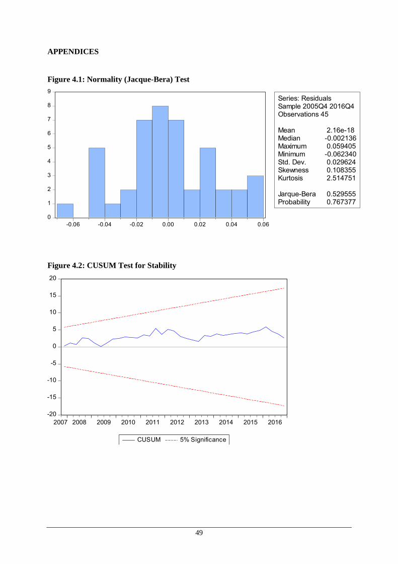
https://tradingeconomics.com/namibia/gdp-growth-annual

49

APPENDICES

Figure 4.1: Normality (Jacque-Bera) Test

0

1

2

3

4

5

6

7

8

9

-0.06 -0.04 -0.02 0.00 0.02 0.04 0.06

Series: ResidualsSample 2005Q4 2016Q4Observations 45

Mean 2.16e-18Median -0.002136Maximum 0.059405Minimum -0.062340Std. Dev. 0.029624Skewness 0.108355Kurtosis 2.514751

Jarque-Bera 0.529555Probability 0.767377

Figure 4.2: CUSUM Test for Stability

-20

-15

-10

-5

0

5

10

15

20

2007 2008 2009 2010 2011 2012 2013 2014 2015 2016

CUSUM 5% Significance

50

Figure 4.3: CUSUM Square Test for Stability

-0.4

-0.2

0.0

0.2

0.4

0.6

0.8

1.0

1.2

1.4

2007 2008 2009 2010 2011 2012 2013 2014 2015 2016

CUSUM of Squares 5% Significance

The impact of Commercial Banks development on Economic ...

Documents

Transcript of The impact of Commercial Banks development on Economic ...