Management Behaviour in Indian Commercial Banks - IRABF

IRABF 2011 Volume 3, Number 3

70

Management Behaviour in Indian Commercial Banks

Kalluru Siva Reddya

a Dept. of Finance and Economics, IBS, Dontanapalli, Hyderabad, Andhra Pradesh, India-501504, Email: [email protected]

_____________________________________________________________________ Abstract: The study explores management behavior in Indian commercial banks during the post reform period. The Granger causality approach of Berger and De Young (1997) is employed to examine four hypotheses such as bad management, bad luck, moral hazard and skimping behavior of Indian commercial banks. The empirical analysis conducted for Indian banks on its three ownership groups, viz., public sector, private domestic and foreign banks, reveal the existence of characteristics of the bad management and the bad luck in Indian banking operations. The econometric analysis for sub samples of the most cost efficient banks reveal that there is no skimping behavior, while the sub sample for the least capitalized banks supports the existence of moral hazard behavior in Indian banks. The study also finds an inverse relationship between cost efficiency and capitalization. Finally, economic effects of the four hypotheses are explored. Keywords: Non-performing loans; Capitalization; X-efficiency; Stochastic frontier approach; Granger causality; Management behaviour; Economic effects. _____________________________________________________________________

1. Introduction

ver the last two decades the Indian banking system has become increasingly

integrated. The two forces of deregulation and technological change led to the

development of financial integration and increased competition in the banking system.

As a result of the deregulatory process, there has been a remarkable stress on the role

of efficiency in the banking system. That is, it has forced banks to perform closer to

the efficient production frontier. On the other hand, the increase in competition

reduces the market power of banks which could lead to greater risk taking behaviour

in banks (Fiordelisi et al., 2011).

O

Vol 3, No.3, Fall 2011 Page 70~92


71

Principal agent problems, which imply that managers in foreign or private

enterprises are supposed to be more restrained by capital market discipline, explain

variations in x-efficiencies. On the contrary, lack of owner’s control makes

management more free to pursue a personal agenda. The principal-agent problems

exist whenever there is a break between ownership and control, and this will explain

differences in the performance of banks operating under different ownerships. The

nexus between ownership and efficiency is determined by the amount of trading of

equities and the transfer of ownership rights (William, 2004). The principal-agent

problems include but are not limited to capturing board of directors, indifferent

depositors, and the absence of shareholders which reflect the inadequate external

discipline in banks.

This issue has attracted a considerable attention in the empirical literature,

although the results are rather mixed or inconclusive. Studies such as Verbrugge and

Goldstein (1981), Verbrugge and Jahera (1981), Cebenoyan et al (1993), Mester

(1993), Berger and Humphrey (1997), Cummins and Zi (1998), and Altunbas et al.

(2001) are recent contributors to the literature explaining variations in efficiency in

terms of their ownership structure. However, the literature on ownership-performance

has certain limitations. It simply describes that banks operate under one ownership

structure are more or less efficient than the banks under another ownership structure.

The ownership approach might provide useful information for policy and regulation.

But it does not help in understanding how management behaviour could affect

performance and efficiency (William, 2004).

In addition to the above, there are a considerable number of studies that

differentiate bank efficiency levels between types of ownership. But the literature on

the link between management behaviour and efficiency is sparse. To the best of our

knowledge, even a single study does not exist with respect to Indian banks. De Young

et al. (2001) examined the management structure of small US banks and found that

management behaviour of most profit efficient banks is online with shareholder

interests. Berger and Hannan (1998) found evidence for the structure-conduct

-performance hypothesis in U.S. banks. They found that the structure of banking

markets, such as concentration and its effects on bank behavior, are positively

associated with cost inefficiency. In addition, Berger (1995) found a positive

relationship between capitalization and earnings, supporting the expected bankruptcy


72

cost hypothesis, and Mester (1996) provided evidence for the moral hazard hypothesis,

in U.S. banks.

In order to understand the different kinds of management behaviour, we need to

explore the inter-temporal relationships between cost efficiency, non-performing loans,

and capitalization. According to Berger and De Young (1997) the directions of these

relationships reveal four different kinds of management behaviour, namely: (1) bad

management (an exogenous decline in cost efficiency leads to an increase in non

performing loans); (2) bad luck management (an exogenous increase in

non-performing loans leads to a decrease in cost efficiency); (3) skimping behavior

( an exogenous increase in cost efficiency leads to increases in non-performing loans);

and (4) moral hazard behavior (an exogenous reduction in capital leads to an increase

in non-performing loans).

The above management behaviours are not mutually exclusive; sometimes banks

show characteristics of multiple behaviours. A couple of studies have investigated this

issue for developed countries. Berger and De Young (1997) is the first study in this

direction. Berger and De Young (1997) investigated causality between non performing

loans, cost efficiency and capitalization on a sample of US commercial banks using

Granger causality tests. The study found evidence of skimping behaviour among most

efficient banks, moral hazard behaviour among least capitalized banks, and also the

presence of the other two, bad management and bad luck behaviour, in U.S. banks.

William (2004) provides a robustness test for Berger and De Young (1997) on a

sample of European savings banks. The study found a strong statistical evidence to

support bad management behaviour in European savings banks and also in a

sub-sample of thinly capitalized banks. At the country level, the study found evidence

of both bad management and bad luck management in German banks. Podpiera and

Weill (2008) extended Berger and De Young’s (1997) technique to examine bad

management and bad luck management behaviour in Czech banks and found evidence

of bad management behaviour in the Czechs’ banks. Rossi et al (2009) linked banks’

management behavior to loan portfolio diversification for Austrian commercial banks

and found that diversification has a negative impact on banks’ cost efficiency, and

reduces risk. On the other hand, it has a positive impact on banks’ profit efficiency

and capitalization. In addition, recently, Fiordelisi et al. (2011) for European

commercial banks found that lower bank efficiency with respect to costs and revenues


73

Granger-causes higher bank risk. He also found that increases in bank capital

precede cost efficiency improvements. More efficient banks tend to become better

capitalized and these higher capital levels tend to have a positive effect on efficiency

levels. These studies concentrated on developed countries. There are few studies

dealing with bank management behaviour in developing countries.

The purpose of this study is to extend Berger and De Young’s (1997) technique

to examine the intertemporal relationships among non performing loans, cost

efficiency and capitalization of Indian commercial banks to identify the different

kinds of management behaviours existing in Indian banks. The explanation of the

relationships of these variables is in terms of an increase in non-performing loans,

because the increase in non-performing loans will reduce the asset quality of banks

and push the banks to an insolvency situation. The Granger causality framework

explores the intertemporal relationships between variables, and should display various

types of management behaviours in banks. Studying management behaviour is a

pertinent issue for bank management and policy makers in framing appropriate

policies for the development of banks. This analysis focuses on the sign and the

direction of lagged values of these variables.

The panel dataset consists of public, private and foreign commercial banks in

India of 1,052 observations. Excluding banks with missing data the study uses a final

unbalanced panel data of 87 commercial banks for the period 1995-2007. Data after

year 2008 are excluded, since the global financial crisis originating in the U.S. hit

almost all banking industries in the world in that year. The Indian banking industry is

no exception. Inclusion of this crisis period in the analysis could have serious

implications on the results of study as the whole banking industry is operating under

some sort of heat and pressure created by stringent regulatory measures such as tight

monetary controls and rising interest rates. To avoid any event like impact on the

operations of banks, I excluded the crisis period from the sample. The necessary

statistical information for empirical analysis was obtained from the Annual Accounts

Data of Scheduled Commercial Banks, the Statistical Tables Relating to Banks in

India, the Reports on Trend and Progress of Banking in India, published by the

Reserve Bank of India, and the Prowess data base provided by Center for Monitoring

Indian Economy (CMIE).

The remainder of this paper is organized as follows. Section II provides a brief


74

view about Indian commercial banking. Section III presents the econometric method

adopted to explore the inter-temporal relationships between the variables. The results

of the Granger causality tests are presented in Section IV. Section V discusses the

economic effects of management behaviour. Section VI presents a summary and

concluding remark for the study.

2. A brief view of Indian banking

India is one of the fastest growing countries in the world with a rich banking

system history. The Indian banking industry is the largest one in South Asia and is

predominantly dominated by public sector banks. After the independence, there was a

perception among the policy makers that unless there is direct control of the

Government over banking industry, it would be difficult to meet the financial needs

for planned economic development, such as mopping up potential savings, addressing

the credit gaps in agriculture, industry and retail trade, where the Government has had

a leading role in every economic activity. Keeping its linkages with the economic

activities in the mixed-economy framework and the economic and the social

objectives of planning, the Government of India nationalized 20 banks in two phases

in 1969 and 1980. The nationalization process led the Indian banking industry to grow

very rapidly, in terms of branch expansion, deposit mobilization and credit allocation.

On the other hand, the bank nationalization brought several regulatory measures.

Interest rates on all kinds of deposits and loans were brought under an administered

mechanism; public sector banks were asked to open branches in rural and semi urban

areas; and entry and operations of private and foreign banks were restricted. The

Government fixed credit targets to the priority sector with subsidized interest rates.

The cash reserve ratio (CRR) and the statutory liquidity ratio (SLR) were kept at very

high rates in order to meet growing fiscal deficits. As a result, the Indian banking

industry suffered with high costs and low quality financial intermediation. The

average return on assets was about 0.15 per cent, which is extremely low as per

international standards. Non- performing loans in the public sector banks accounted

for nearly 24 per cent of total loan portfolio s, and thirteen public sector banks were

earning losses of which eight banks made operating losses. Operating expenses were

increasing and half of the public sector banks had negative worth (Sarkar, 2002). On


75

identifying the growing illnesses in Indian banking, the Government of India set up a

committee on Financial Sector Reforms in 1991 to review the Indian financial system

and suggest appropriate measures to improve its profitability and efficiency. Based on

the recommendations of the committee, the Government started implementing

reforms in the banking sector. These reforms include deregulation of interest rates,

gradual reduction of CRR and SLR, branch delicensing, operational freedom to public

sector banks, introduction of capital adequacy norms and provisioning norms, etc.

Entry norms for private and foreign banks were also liberalized to induce competition

in Indian banking markets. These measures were expected to improve bank

profitability and enhance competition and efficiency (Kumbhakar and Sarkar, 2004).

These structural changes over the last several years in Indian banking will

obviously have an impact on the bank management. This study period following

major changes enables an examination of the characteristics of management

behaviour in Indian commercial banks during the post reform period. Indian banking

consists of public, private, and foreign banks. Since the objectives of the each group

are different; it is very important to examine how the management behaviour varies

across the bank groups.

3. The econometric model

Granger causality tests developed by Berger and De Young (1997) are employed

to explore management behaviour existing in Indian commercial banks. The

management behaviour is analyzed as an inter-temporal relationships between non

performing loans, cost efficiency, and capitalization that are expected to reveal four

kinds of management behaviours, namely: (1) bad management, (2) bad luck, (3)

skimping, and (4) moral hazard. The Granger causality framework for the present case

is as follows:

NPLi,t= f1 (NPL i,lag, X-EFFi,lag, CAPi,lag, LTA i,lag, Yrt) + 1i,t (1)

X-EFFi,t= f2 (NPL i,lag, X-EFFi,lag, CAPi,lag, LTA i,lag, Yrt) + 2i,t (2)

CAPi,t = f3 (NPL i,lag, X-EFFi,lag, CAPi,lag, LTA i,lag, Yrt) + 3i,t

(3)

where

NPLi,t = ratio of non performing loans to total loans for ith bank in tth year


76

X-EFFi,t = cost efficiency for ith bank in tth year

CAPi,t = ratio of equity capital to total assets for ith bank in tth year

LTAi,t= ratio of total loans to total assets for ith bank in tth year

Yrt= set of time dummy variables

The ratio of non-performing loans to total loans (NPL) is an indicator of asset

quality, which is defined as the ratio of loans which are either overdue for more than

90 days or non earning loans to total loans. Cost efficiency (X-EFF) is estimated by

using the stochastic frontier model. The details of measuring cost efficiency and

estimates are given in Appendix I. The ratio of equity capital to total assets (CAP) is a

measure of bank capitalization and reflects the financial strength of the bank for

absorbing loan losses resulting from mix of loan portfolio. The ratio of total loans to

total assets (LTA) is a proxy for risk which is included in all the three equations in

order to control risk factors1. Certain portfolio mixes usually produce more non

performing loans and give more costs and difficulties to banks to maintain loan

intensive balance sheet. This pressures banks to improve cost efficiency. Time dummy

(Yrt) for all the years, such as D1995, D1996, D1997 and so on, is included in the

model to control macroeconomic changes, such as raising inflation, increasing interest

rates, and regulatory changes as well as changes in technology. Each dummy variable

is equal to one, if the observation refers to the correspondent year and zero, if

otherwise. The D1995 variable has been dropped to avoid collinearity in the data.

Equation (1) tests the bad management hypothesis that predicts a negative

relationship between non-performing loans and x-efficiency. Because, the bad

management hypothesis considers low cost efficiency to be an indicator for poor

managerial performance, lower efficiency would be expected to result in larger

amounts of non performing loans. Poor managers may fail to control operating costs

which leads to low cost efficiency. Such managers may not follow standard loan

underwriting or monitoring practices; not be capable of credit scoring; not be

competent in assessing the value of collateral, and may often choose a relatively high

proportion of loans with negative or low net present values. Besides an immediate

reduction in cost efficiency, poor underwriting and control practices should lead to

1 The database on the ratio of risk weighted assets to total assets, suggested by Berger and De Young (1997) for measuring risk factor, is not available. Therefore, the study is constrained to use the ratio of risk weighted assets to total assets as risk controlling factor. The study considered the ratio of total loans to total assets as a proxy for risk factor.


77

high non-performing loans in the future. Therefore, under the bad management

hypothesis, reduced cost efficiency is expected to cause higher non-performing loans.

On the other hand, a positive relationship between the two variables suggests

skimping behaviour. Under the skimping behaviour hypothesis bank managers face a

trade-off between short -term operating costs and long term non-performing loans and

reduce the amount of resources spent on underwriting and monitoring bank loans.

This affects both the quality of loans and cost efficiency. Skimping behaviour gives

the misleading impression that the banks are cost efficient in the short-run, because

fewer expenses are supporting the same quantity of outputs, while non performing

loans are about to multiply. Therefore, I re-estimate the equation (1) for a sub sample

of banks with cost efficiency above the median cost efficiency. Banks that engage in

skimping behaviour should appear to be cost efficient in the short run and should have

a rise in non performing loans.

Equation (1) also tests the moral hazard hypothesis and predicts a negative

relationship between non performing loans and capital. I re-estimate equation (1) to

test the moral hazard hypothesis only for a sub sample of banks with capital below the

median capital. Because the moral hazard hypothesis assumes that managers of low

capitalized banks are less opposed to take risk, since the expected return on the risk is

positively related to the amount of the bank risk taken, and it is more attractive than

the possibility of loss on account of default risk. This may happen when bank

mangers feel that the risk is rewarding and others in the industry are resorting to the

same practice. Mangers prefer to take risk to the extent their position warrants, and

the support likely to be extended by their bosses in the event of an adverse outcome

on account of the risk taken. Thus risk taken by a bank depends not only on the risk

appetite of the managers, but also to the extent of the protective shield extended by

the Central Bank/Government. Thus, under the moral hazard hypothesis, banks with

relatively low capital may undertake more risky portfolios in response to moral hazard

incentives, which in turn results in higher non-performing assets in the future.

Equation (2) tests the bad luck hypothesis which predicts a negative relationship

between cost efficiency and non-performing loans. Under the bad luck management

hypothesis exogenous events, such as, closing a local firm or economic downtrends,

increase non-performing loans. Once the loans become past due, the management will

put extra managerial effort and expenses to deal with the adverse effect of problem


78

loans, which in turn leads to a decrease in bank cost efficiency. These extra expenses

result from various sources, including keeping more vigilance on delinquent

borrowers and their loan collateral, the cost of seizing and disposing of collateral in

cases of default, allocating extra resources to analyze and negotiate the possibility of

getting back the default amount, the extra costs associated with showing the bank’s

records as to safety and soundness to supervisors and market participants, costs on

additional precautions to protect the high quality of current loans, etc. Most of

these expenses will take place well after increases in non performing loans. Hence, the

bad luck hypothesis assumes that increases in non performing loans cause a decrease

in cost efficiency.

Equation (3) is included to complete the model but not for testing any of the

above hypotheses. However, following Berger and De Young (1997), the study wants

to see whether the estimated parameters of Equation (3) make any economic sense in

a Granger causality framework. The relationships among the variables may indicate

different unknown behaviours or hypotheses. However, the scope of the present study

is limited to the aforesaid four hypotheses.

4. Results and discussion

For the primary investigation, results of the summary statistics for the variables

in the Granger causality model are presented in Table 1. The mean of the ratio of

non-performing loans to total loans is around 7 per cent in Indian banks, and it is

slightly lower in case of public sector banks over other groups. Indian banks on

average operate at 75 per cent cost efficiency. Among the groups, public sector banks

are relatively more cost efficient over the other groups. Mean values for the ratio of

equity capital to assets for all banks indicate that Indian banks are adequately

capitalized. Public sector banks and private banks are much less capitalized than

foreign banks. The mean values for the ratio of loans to assets indicate that loans

occupy a major portion in the Indian banks asset portfolios. But foreign banks are

more loan intensive when compared to public sector banks in India. The mean values

of the variables vary across the groups. The values of the standard deviation reveal

that there is considerable variation in the dataset, and it is high in variable, such as the

ratio of capital to assets and loans to assets.


79

Using the sample of 87 commercial banks, the study estimated the Granger

causality Equations (1) to (3) for the period 1995-2007. A Breusch-Pagan test found

the presence of heteroskedasticity in the model. Using a weighted least square

technique, heteroskedasticity is corrected and the corrected results are reported.2

Specifying an optimum lag for the model, I followed an F-test procedure, which

supported a single lag for each equation. I tested the results by increasing the lags

from one to two, two to three. This exhibited the collinearity problem among the

estimated lagged coefficients. The coefficients were becoming statistically

insignificant, and the F-test value was declining. The usage of one over two, and two

over three lagged terms in the model statistically weakens the presence of several

important relationships among the variables. Hence, I included a single lag

considering it as appropriate for the model. Subsequently, the three equations were

re-estimated for each of the three bank groups.3

The OLS estimates of Granger causality tests for Equation (1) are displayed in

Table 2. The lagged coefficient of cost efficiency is negative in all banks, i.e. public

sector banks and private domestic banks. However, it is statistically significant only in

2 First an OLS regression is run and the residuals are taken. The logs of the squares of these residuals then become the dependent variable in second regression and the original independent variables plus their squares are included in the right-hand side. The fitted values from the second regression are then used to construct a weight series, and the original model is re-estimated using weighted least squares, and the final results are reported. 3 Coefficients of time dummy variables are not displayed in the tables.

Table 1 Summary statistics of mean and standard deviation for variables in the Granger causality model (after a lag)

Bank Group N Non

Performing Loans (%)

Cost Efficiency

Capital to Assets (%)

Loans to Assets (%)

PSB 330 6.695

(4.268) 0.783

(0.113) 3.35

(5.612) 87.129

(197.691)

DPB 306 7.3374

(10.382) 0.735

(0.126) 2.841

(4.628) 65.02

(93.446)

FB 329 7.444

(10.421) 0.749

(0.123) 31.969

(96.967) 242.635

(665.544)

ALL 965 7.154

(8.827) 0.756

(0.122) 13.027

(58.587) 133.535

(417.433)

Note: Values in parenthesis are standard deviation. PSB = Public Sector Banks, DPB= Domestic Private Banks, FB = Foreign Banks, and ALL = All Banks.


80

public sector banks. It reveals that public sector banks are characterized with bad

management behaviour. It indicates that a decrease in the estimated cost efficiency

tends to lead to increases in non-performing loans in public sector banks on account

of poor loan management thereby affecting the asset quality. The relationship between

the ratio of non-performing loans and loans to assets is positive, and it is statistically

significant only in all banks group. This supports the argument that banks with more

loan-intensive balance sheets will eventually yield higher non-performing loans,

which exhibit deteriorating asset quality. For instance, banks may not have

up-to-date information about the whereabouts of loan customers, and the status of

loan accounts, is such loan accounts may become non performing assets.

Table 2 OLS estimates of Granger Causality tests in non performing loans equation (1)

Variable All Indian

banks Public sector

banks Private banks Foreign banks

Constant 0.328*** (1.766)

0.664* (3.67)

0.666** (1.975)

0.266 (0.513)

NPL-1 0.275* (7.816)

0.201* (4.098)

0.151* (3.062)

0.278* (4.538)

X-EFF-1 -0.088

(-0.413) -0.389* (-3.922)

-0.121 (-0.547)

0.017 (0.038)

CAP-1 -0.033*** (-1.671)

0.005 (0.161)

0.003 (0.054)

-0.014 (-0.477)

LTA-1 0.054*** (1.879)

0.002 (0.056)

0.057 (0.972)

0.038 (1.075)

R2 (adj) 0.170 0.441 0.229 0.150

N 965 330 306 329

Note: * indicates significant at one per cent, ** indicates significant at five per cent, and *** indicates significant at ten per cent. t- values are in parenthesis.

In general, it is observed that skimping behaviour is dominated by bad

management behaviour for the overall sample, but this may not prevent the possibility

of skimping behaviour in individual banks. In order to check the possibility of

skimping behaviour in Indian commercial banks, a sub sample of the most cost

efficient banks, whose efficiencies are higher than the median cost efficiency in ever

year, are constructed. We may expect the skimping behaviour among the most

efficient banks because such banks face a trade-off between loan quality and cost

reductions and wait for the non -performing loans to multiply in future. Therefore, the

study re-estimates Equation (1) for the sub- samples of the most cost efficient banks,


81

and the results are presented in Table 3. The results do not find any statistical

evidence for skimping behaviour in the most efficient Indian banks. The relationship

between non-performing loans and the lagged coefficient of loans to assets is positive

and statistically significant which indicates that even in most cost efficient banks a

higher loan proportion tends to cause a greater volume of non-performing loans.

Table 3 OLS estimates of Granger Causality tests in non performing loans equation (1) for sub samples of the data

Variable Skimping behaviour

(in most cost efficient banks) Moral hazard hypothesis

Constant 0.235

(1.064) 0.525** (2.040)

NPL-1 0.196* (3.816)

0.037 (0.847)

X-EFF-1 -0.012

(-0.315) -0.739

(-1.572)

CAP-1 -0.065** (-2.207)

-0.036*** (-1.931)

LTA-1 0.084** (2.055)

-0.008 (-0.193)

R2 (adj) 0.203 0.118

N 481 492


Using Equation (1) the study also tested the moral hazard hypothesis for another

sub-sample of Indian banks, which consists of those banks with a ratio of equity

capital to assets below the sample median in every year. The Moral hazard hypothesis

predicts negative relationships between low capitalized banks and non-performing

loans. The results of this model are presented in the last column of Table 3. The

coefficient of the lagged capitalization is negative, and it is statistically significant

supporting the presence of moral hazard behaviour in thinly capitalized Indian banks.

Because thinly capitalized banks may take more risk by responding to moral hazard

incentives, such as negligence in business, favouritism, and nepotism in sanctioning

loans, etc., this appears to result in higher non-performing loans in the future.

Equation (2) tests the bad luck hypothesis, which predicts an increase in

non-performing loans will Granger cause a decrease in cost efficiency. Therefore,


82

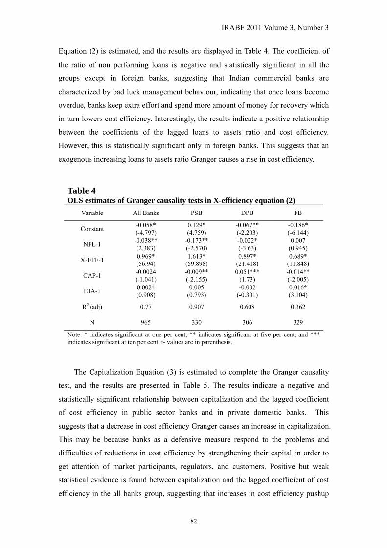
Equation (2) is estimated, and the results are displayed in Table 4. The coefficient of

the ratio of non performing loans is negative and statistically significant in all the

groups except in foreign banks, suggesting that Indian commercial banks are

characterized by bad luck management behaviour, indicating that once loans become

overdue, banks keep extra effort and spend more amount of money for recovery which

in turn lowers cost efficiency. Interestingly, the results indicate a positive relationship

between the coefficients of the lagged loans to assets ratio and cost efficiency.

However, this is statistically significant only in foreign banks. This suggests that an

exogenous increasing loans to assets ratio Granger causes a rise in cost efficiency.

Table 4 OLS estimates of Granger causality tests in X-efficiency equation (2)

Variable All Banks PSB DPB FB

Constant -0.058* (-4.797)

0.129* (4.759)

-0.067** (-2.203)

-0.186* (-6.144)

NPL-1 -0.038** (2.383)

-0.173** (-2.570)

-0.022* (-3.63)

0.007 (0.945)

X-EFF-1 0.969* (56.94)

1.613* (59.898)

0.897* (21.418)

0.689* (11.848)

CAP-1 -0.0024 (-1.041)

-0.009** (-2.155)

0.051*** (1.73)

-0.014** (-2.005)

LTA-1 0.0024 (0.908)

0.005 (0.793)

-0.002 (-0.301)

0.016* (3.104)

R2 (adj) 0.77 0.907 0.608 0.362

N 965 330 306 329


The Capitalization Equation (3) is estimated to complete the Granger causality

test, and the results are presented in Table 5. The results indicate a negative and

statistically significant relationship between capitalization and the lagged coefficient

of cost efficiency in public sector banks and in private domestic banks. This

suggests that a decrease in cost efficiency Granger causes an increase in capitalization.

This may be because banks as a defensive measure respond to the problems and

difficulties of reductions in cost efficiency by strengthening their capital in order to

get attention of market participants, regulators, and customers. Positive but weak

statistical evidence is found between capitalization and the lagged coefficient of cost

efficiency in the all banks group, suggesting that increases in cost efficiency pushup


83

bank earnings, which Granger causes increases in bank capital. This possibly happens

when a part of banks’ earnings are used to improve bank capitalization.

Table 5 OLS estimates of Granger causality tests in capitalisation equation (3)

Variable All Banks PSB DPB FB

Constant 0.199

(0.861) -0.882* (-2.765)

-0.963** (-2.163)

1.426* (3.101)

NPL-1 -0.022

(-1.053) -0.001 (0.020)

0.009 (0.187)

-0.073 (-1.549)

X-EFF-1 0.387

(1.526) -1.179* (-3.738)

-0.679*** (-1.659)

-0.035 (-0.069)

CAP-1 0.497*

(16.201) 0.654*

(14.113) 0.0442* (8.771)

0.323* (5.93)

LTA-1 -0.083* (-2.886)

-0.038 (-0.615)

0.101*** (1.821)

-0.049 (-1.171)

R2 (adj) 0.391 0.598 0.362 0.246

N 965 330 306 329


Table 6 OLS estimates of Granger causality tests in capitalization equation (3) for subsamples of the data

Variable Thinly capitalized banks Highly capitalized

banks

Constant -0.686** (-2.538)

0.789*** (1.718)

NPL-1 -0.066

(-1.582) -0.125

(-1.544)

X-EFF-1 0.254

(0.574) -0.386***

(-1.77)

CAP-1 0.0857** (2.355)

0.325* (6.885)

LTA-1 0.032

(0.834) -0.218* (-4.067)

R2 (adj) 0.231 0.231

N 492 486


Equation (3) is re-estimated for the two sub-samples to test whether highly

capitalized banks and low capitalized banks respond differently to changes in

non-performing loans. The sample is divided into two sub-samples of low capitalized

and highly capitalized banks based on annual sample medians. The results are


84

reported in Table 6. The results seem to be consistent with the results of the overall

sample. For highly capitalized banks, the study found negative and statistically

significant relationships between bank capitalization and the lagged coefficient of cost

efficiency. This suggests that decrease in cost efficiency Granger causes an increases

in bank capitalization.

5. The economic effects of management behaviour

Further, the study examines the economic effects of the aforementioned four

hypotheses, and the results are presented in Table 7. The economic effects are

calculated based on how a one standard deviation increase or decrease in a variable

leads to the cumulative decrease or increase in another variable. The economic effects

of bad management behaviour in Indian banks are measured in terms of a one

standard deviation reduction in cost efficiency (from 0.756 to 0.634) that predicts a

cumulative increase in the non performing loan ratio over a year from 7.154 to 8.308

or a rise of 16.14 per cent. The economic effects of bad management in public sector

banks are measured in a similar way. In this case also a one standard deviation

reduction in measured cost efficiency (from 0.783 to 0.670) predicts a cumulative

increase in the non performing loan ratio over a year from 6.695 to 7.662 or a rise of

14.44 per cent. Similarly, for private domestic banks it is a rise of 17.11 per cent, and

for foreign banks the reduction in the non-performing loan ratio is 16.36 per cent.

The economic impact of bad luck is measured in terms of the impact of one

standard deviation increase in non performing loans to cost efficiency. One standard

deviation increase in non performing loans (from 7.154 to 15.98) predicts a

cumulative decrease in cost efficiency over a year is 123.9 per cent in Indian banks,

which is much higher. This impact is also evident in Equation 2. This provides strong

evidence for bad luck management behaviour in Indian banks. Similarly, the

economic effect of bad luck behaviour for the different bank groups is measured. For

public sector banks, bad luck predicts a cumulative decrease in cost efficiency of

63.74 per cent; for private domestic banks it is 141 per cent; and for foreign banks it is

140 per cent.


85

Table 7 Economic effects of management behaviour

Economic effects of bad management

Sign &sig Mean

X-EFF 1std.dev NPL NPL % change

All -&ns 0.756 0.634 7.154 8.308 16.14

PSB -&sig 0.783 0.67 6.695 7.662 14.44

DPB -&ns 0.735 0.609 7.337 8.593 17.11

FB +&ns 0.749 0.627 7.444 6.226 -16.36

Economic effects of skimping behaviour

Mean

X-EFF 1std dev NPL NPL % change

Cost eff -&ns 0.8396 0.8567 7.126 6.981

Economic effects of moral hazard behaviour

Mean CAP 1std dev NPL NPL % change

Low-CAP -&sig 0.9334 0.6651 7.517 9.678 28.78

Economic effects of bad luck

Mean Mean NPL 1std dev XEFF XEFF¯ % change

ALL -&sig 7.154 15.98 0.756 0.177 -123.9

PSB -&sig 6.695 10.963 0.783 0.284 -63.74

DPB -&sig 7.337 17.719 0.735 0.305 -141.49

FB +&ns 7.444 17.865 0.749 1.798 140

Notes: 1. The economic effects of bad management are measured as one standard deviation reduction in cost efficiency tends to cause to increase in non performance loans.

2. The economic effects of skimping behaviour are measured as one standard deviation increase in cost efficiency tends to cause to increase in non performing loans. This is measured based on the two sub samples of most cost and profit efficient banks.

3. The economic effects of moral hazard behaviour are measured as one standard deviation decrease in bank capitalization tends to cause to increase in non performing loans. This is done using a sub sample of the low capital banks.

4. The economic effects of bad luck are measured as one standard deviation reduction in non performing loans tends to cause to decrease in x-eff. #sig = significant, ns = not significant, sign= direction of the coefficient. And, values in parenthesis indicate a percentage reduction in the specified variable. PSB = Public Sector Banks, DPB= Domestic Private Banks, FB = Foreign Banks, and ALL = All Banks.

Using sub samples of the most cost efficient banks the economic effects of

skimping behaviour in Indian commercial banks is measured. It was observed in the

previous section that the study has not found any statistically significant evidence for

the presence of skimping behaviour in Indian banks. Therefore, the economic impact

of skimping behavior measured in terms of a one standard deviation increase in


86

estimated cost efficiency (from 0.8396 to 0.8567) predicts a cumulative reduction in

the non performing loan ratio over a year of 2.03 percent.

Using sub-sample of low capital banks, the economic effects of moral hazard

behaviour is measured in low capitalized Indian commercial banks. It revealed that a

one standard deviation reduction in capitalization (from 0.9334 to 0.6651) results in a

cumulative change in the ratio of non-per forming loans over a year from 7.517 to

9.678 or a rise of 28.78 per cent.

6. Summary and conclusions

Using the Granger causality framework of Berger and De Young (1997), I

examine four kinds of management behaviours, namely, bad management, bad luck,

skimping, and moral hazard in Indian commercial banks during the post reform period.

They are derived based on the intertemporal relationships between non performing

loans, efficiency and capitalization. The results of the Granger causality technique are

as follows. There is strong statistical evidence for bad management behaviour

(which implies that a decrease in cost efficiency tends to increase non-performing

loans) in public sector banks. The skimping behaviour (which implies that increasing

cost efficiency leads to increase non performing loans) is tested on the sub-sample of

the most cost efficient banks. However, the study has not found any strong statistical

evidence for the presence of skimping behaviour in Indian banks. Using another sub

sample of low capitalized banks, the study tested moral hazard (low capital tends to

cause an increase in non performing loans) behaviour in Indian banks. There is strong

statistical evidence to support that Indian banks are characterized by moral hazard

behaviour. Further, the results found strong statistical evidence for bad luck

management behaviour (increasing non performing loans tend to cause decrease in

cost efficiency) in all bank groups, like public sector banks and private domestic

banks. It also found strong statistical evidence for banks response to the consequences

of decreasing cost efficiency by boosting their capital to attract the attention of market

participants and regulators.

In addition, the study also explored the economic effects of bad management,

bad luck, skimping and moral hazard behaviours in Indian commercial banks. The

results indicate that the intensity of the economic effects of bad management


87

behaviour and bad luck are higher in private domestic banks than in other banks.

The findings of the present study have several policy implications for banks. The

findings of bad management in Indian banks, particularly public sector banks, suggest

that regulators and supervisors should focus on improving cost efficiency, such as

through a better recruitment process, finding and assessing high expense areas, better

training of managers, and increasing competition, and foreign ownership (particularly

for transferring of technology know-how). The findings of bad luck behaviour suggest

that banks should concentrate on diversified loan portfolios and reduce loan

concentrations. Bank supervisors should also limit individual banks’ high risk

exposures. The findings of skimping behaviour, though they are not statistically

significant, suggest that as precautionary measure banks’ supervisors and researchers

should pay attention towards the review of loan portfolio and its performance in order

to curb the likely rise in non-performing loans, in addition to focusing on improving

efficiency. The findings of moral hazard behaviour in Indian banks suggest that

regulators and supervisors as a recovery mechanism should pay special attention on

monitoring bank capital ratios and ensuring an increase in the ratios whenever they

become low. This means that banks should maintain minimum capital ratios as per

statutory capital requirement norms, because undercapitalization is the first reason for

deteriorating asset quality, which in turn leads to bank failures. Supervisors should

also pay due attention to the attitude and performance of banks’ managers, and try to

motivate them to increase their efficacy and efficiency. Future studies can well focus

on comparing these behaviours in the Indian banking sector with those in other

emerging economies and also with developed economies in order to explore factors

that similarly and differently affect management behavior in banks, thus examining

reasons for why this is so.

References

Aigner D.J., Lovell, C.A.K. and Schmidt, P. 1977. Formulation and estimation of stochastic frontier production models. Journal of Econometrics, 6(1), 21-37.

Altunbas. Y., Evans, L. and Molyneux, P. 2001. Bank ownership and efficiency. Journal of Money, Credit and Banking, 33(4), 926-954.

Battese, G.E. and Coelli, T.J. 1992. Frontier production functions, technical efficiency and panel Data: with application to paddy formers in India. Journal of Productivity, 3, 153-169.


88

Berger, A.N. 1995. The relationship between capital and earnings. Journal of Money, Credit and Banking, 27(6), 432-456.

Berger, A.N. and De Young, R. 1997. Problem loans and cost efficiency in commercial banks. Journal of Banking and Finance, 21(6), 849-870.

Berger, A.N. and Hannan, T.H. 1998. The efficiency cost of market power in the banking industry: A test of the ‘quite life’ and related hypotheses. The Review of Economics and Statistics, 80(3), 454-465.

Berger, A.N. and Humphrey, D.B. 1997. Efficiency of financial institutions: International survey and directions for future research. European Journal of Operational Research, 9(2), 175-212.

Cebenoyan, A.S., Cooperman, E.S., Register, C.A. and Hudgins, S.C. 1993. The relative efficiency of stock versus mutual S&Ls: A stochastic cost frontier approach. Journal Financial Services Research, 7, 151-170.

Cummins, J.D. and Zi, H. 1998. Comparison of frontier efficiency methods: An application to the US life insurance industry. Journal of Productivity Analysis, 10, 135-152.

De Young, R., Spong, K. and Sullivan, R. 2001. Who’s minding the store? Motivating and monitoring hired managers at small closely held commercial banks. Journal of Banking and Finance, 25(7), 1209-1244.

Sarkar, J. 2002. India’s Banking Sector Current Status, Emerging Challenges, and Policy Imperatives in a Globalised Environment. In Hanson JA and Kathuria S (ed.), India A financial Sector for the Twenty-first Century. Oxford University Press, New Delhi.

Kumbhakar, S.C. and Sarkar, S. 2003, Deregulation, Ownership and Productivity Growth in Banking Industry: Evidence from India. Journal of Money, Credit and Banking, 35, 403-424.

Meeusen, W. and Broeck van den, J. 1977. Efficiency Estimation from Cobb-Douglas Production Functions with Composed Error. International Economic Review, 18, 435-444.

Mester, L.J. 1993. Efficiency in savings and loan industry. Journal of Banking and Finance, 17, 267-286.

Mester, L.J. 1996. A study of bank efficiency taking into account risk-preferences. Journal of Banking and Finance, 20, 1025-1045.

Podpiera, J. and Weill, L. 2008. Bad luck or bad mangement? Emerging banking market experience. Journal of Financial Stability, 4, 135-148.

Sealey, C. and Lindley, J.T. 1977. Inputs, Outputs and a Theory of Production and Cost at Depository Financial Institution. Journal of Finance, 32, 1251-1266.

Verbrugge, J.A. and Goldstein, S.J. 1981. Risk, return and managerial objectives: some evidence from savings and loan industry. Journal of Financial Research, 4, 45-58.

Verbrugge, J.A. and Jehera, J.S. 1981. Expense-preference behaviour in the savings and loan industry. Journal of Money, Credit and Banking, 13(4), 465-476.

William, J. 2004. Determining management behaviour in European banking. Journal


89

of Banking Finance, 28, 2427-2460.

Fiordelisi, F., Marques‐Ibanez, D. and Molyneux, P. 2011. Efficiency and risk in European

banking. Journal of Banking Finance, 35, 1315‐1326.

Rossi, S.P.S., Schwaiger, M.S. and Winkler, G. 2009. How loan portfolio diversification affects risk, efficiency and capitalization: A managerial behavior model for Austrian banks. Journal of Banking Finance, 33, 2218-2226.

Appendix 1

Estimating cost efficiency

Variables such as loans, assets, capital and non performing loans can directly be

culled from banks’ financial statements, but cost efficiency is required to be estimated.

Cost efficiency measures how the costs of a bank in relation to an ideal/model bank

adopting best practices when both the banks produce the same output under similar

conditions (William, 2004). More specifically, cost efficiency is the ratio between the

minimum cost C*, at which a firm can produce a given vector of output, and actual

cost C. Thus, cost efficiency CE = C* /C implies that it would be possible to produce

the same vector of outputs with a saving in costs of (1 – CE) percent. The cost

efficiency is estimated using the Battese and Coelli (1992) Stochastic Frontier

Approach, developed for an unbalanced panel data context, with a translog functional

form.4 The most important advantage of the stochastic frontier approach compared to

non-parametric methods is that the former allows random error. The random error has

two components, one represents random effects of measurement error, statistical noise,

and random shocks that are external to the firm’s control and another represents for

technical inefficiency which arises within the firm. The inefficiency may be due to

noise in the data or misspecification errors or from internal disturbances such as

operational risks. The inefficiencies follow an asymmetric half-normal distribution,

based on the logic that inefficiencies need not be negative, but invariably increase the

costs, and that random errors follow a symmetric standard normal distribution,

because random fluctuations can either increase or reduce costs. In addition, it

4 Another popular functional form is Fourier Flexible (FF), which combines a translog form with a non- parametric Fourier form i.e. trigonometric transformations of the variables and requires estimations of a larger number of coefficients than does the translog specification form. Given the limited data, therefore, the study estimate cost function using translog functional form.


90

provides point estimates of the efficiency score and allows estimating for unbalanced

panel data.

For selecting outputs and inputs of banks, the intermediation approach, proposed

by Sealey and Lindley (1977), is used. This approach considers banks as financial

intermediaries between savers and investors. Under this method the funds raised as

deposits and their costs, interest expenses, will be considered as inputs, since they

constitute raw material which is required to be transformed in to outputs such as loans

and investible funds, and all the outputs are measured in monetary terms. Our cost

function has three outputs and three inputs. The functional specification (in natural

logarithm) form in the present case is as follows:

lnTCit=α0+α1lny1+α2lny2+α3lny3+β1lnp1+β2lnp2+β3lnp3+1/2α11lny1lny1

+α12lny1lny2+α13lny1lny3+1/2α22lny2lny2+α23lny2lny3+1/2α33lny3lny3

+1/2β11lnp1lnp1+β12lnp1lnp2+β13lnp1lnp3+1/2β22lnp2lnp2+β23lnp2lnp3

+1/2β33lnp3lnp3+λ11lny1lnp1+λ12lny1lnp2+λ13lny1lnp3+λ21lny2lnp1

+λ22lny2lnp2+λ23lny2lnp3+λ31lny3lnp1+λ32lny3lnp2+λ33lny3lnp3+Vit+itUit

(4)

In the above specification, TC is total costs; y1, y2, and y3 are outputs as loans,

investments in Government and other approved securities and non interest income,

respectively, and p1, p2 and p3 are input prices of labour, physical capital and

purchased funds, respectively. The price of labour is estimated by salaries and wages

divided by number of employees.5 The price of physical capital is calculated by total

expenses of premises and fixed assets divided by total assets.6 The price of purchased

funds is estimated by interest expenses divided by total borrowings and deposits. Vit is

a random variable, which captures the effects of uncontrollable factors. It is assumed

to be independent and identically distributed with N (0, ²v) distribution and

independent of Uit. Uit is a non negative random variable associated with inefficiency

in the banks and assumed to be truncation of the N (it,²u) distribution. The α, β, λ,

and η, parameters are required to be estimated.

5 Data base on number of officers, clerks and sub staff and salaries and wages of the each group separately is not available. Therefore, the study is constrained to go in division of expenses or price of the each labour group. 6 Data base on rentals of own premises is not available. Therefore, expenses of premises consist of hiring expenses on other people’s owned premises and maintenance expenses of own premises.


91

The error term representing the inefficiency in the model is specified as:

Uit= exp (-(t-T)) (5)

The parameters of the model are estimated by using the maximum likelihood

estimation method. Under the above specification, inefficiencies in periods prior to T

depend on the parameter and number of remaining periods (t-T). The positive

indicates inefficiencies decrease overtime ,and, conversely, negative implies

increase of inefficiencies overtime. If = 0, then efficiency is time-invariant i.e.,

banks never improve their efficiency. The variances of the error terms in model (4) are

reparameterised and expressed as ² = ²u+²v and = ²u/². The value of will

lie between 0 and 1. If Uit equals zero, it indicates full technical efficiency. Then

equals zero and deviations from the frontier are entirely due to noise Vit. If equals

one, it implies that all deviations from the frontier are due to technical inefficiency.

Symmetric assumptions are imposed on all parameters as αij = αji and so on in

accordance with the economic theory. Estimates of the cost frontier follow.

Maximum likelihood estimates of stochastic cost frontier variable parameter coefficient standard-error t-ratio intercept α0 2.473 0.511 4.843*

y1 α1 -0.040 0.103 -0.390

y2 α1 0.423 0.136 3.111*

y3 α3 0.441 0.099 4.465*

p1 β1 0.083 0.107 0.781

p2 β2 0.570 0.164 3.470*

p3 β3 -0.117 0.056 -2.096**

y1y1 α11 0.047 0.011 4.126*

y1y2 α12 0.030 0.016 1.857***

y1y3 α13 -0.021 0.011 -1.967***

y2y2 α22 0.126 0.027 4.683*

y2y3 α23 -0.172 0.016 -10.914*

y3y3 α33 0.156 0.015 10.230*

p1p1 β11 -0.011 0.015 -0.733

p1p2 β12 0.024 0.020 1.230

p1p3 β13 -0.014 0.009 -1.510

p2p2 β22 0.123 0.039 3.143*

p2p3 β23 -0.030 0.013 -2.237**

p3p3 β33 -0.020 0.005 -3.713*

y1p1 λ11 -0.053 0.012 -4.295*

y1p2 λ12 0.045 0.019 2.319**

y1p3 λ13 0.016 0.008 1.884***

y2p1 λ21 0.028 0.015 1.840***

y2p2 λ22 0.091 0.027 3.421*


92

y2p3 λ23 -0.052 0.014 -3.786*

y3p1 λ31 0.022 0.014 1.576

y3p2 λ32 -0.130 0.019 -6.894*

y3p3 λ33 0.023 0.011 2.170**

sigma-squared σ2 0.108 0.008 13.712*

gamma γ 0.260 0.050 5.226*

Mu μ 0.336 0.099 3.384*

Eta η -0.083 0.016 -5.042*

log likelihood -204.673 No. of observations 1052 Note: * indicates one per cent significant, ** indicates five per cent significant, and *** indicates ten per cent significant

Management Behaviour in Indian Commercial Banks - IRABF

Documents

Transcript of Management Behaviour in Indian Commercial Banks - IRABF