Stress test of the banks' lending to commercial real estate firms

Finansinspektionen +46 8,408,980 00 [email protected] www.fi.se

FI Ref.: 20-24428

Summary Commercial real estate firms are sensitive to changes in interest expenses and income. Following a shock, vulnerable commercial real estate firms could lead to credit losses for the banks.

In this FI Analysis, we describe the stress test we have used to analyse how the commercial real estate firms’ financial position, and the banks’ credit risks related thereto, can be affected by a negative macroeconomic development. The method is based on detailed information about the banks’ lending portfolios, which are matched with other data to obtain information about the commercial real estate firms’ financial position.

We estimate the banks’ credit losses by first calculating how a change in the gross domestic product (GDP) or the interest rate affects the firms’ creditworthiness. We thereafter estimate how the changed creditworthiness affects the stage to which the firms’ loans are classified in accordance with the accounting standard IFRS 9. Finally, we calculate how the changed creditworthiness and stage classification affect the size of the banks’ provisions. The changes in the provisions then give the expected credit losses.

FI has used this method to assess the resilience of the banks to a shock on the commercial real estate market. However, this micro-based stress test method can also be applied to other parts of the banks’ portfolios. A benefit of this method is that it takes into consideration the current credit risk in the banks’ lending portfolios by starting with the counterparties’ financial position.

FI Analysis Stress test of the banks’ lending to commercial real estate firms

No. 24

11 November 2020

Ted Aranki, Carl Lönnbark and Viktor Thell * The authors work at the Economic Analysis Office at FI. The FI Analysis series is presented at an internal seminar at FI. The reports are approved for publication by an Editors’ Board. _____________________ *The authors thank Kristoffer Blomqvist, Henrik Braconier, Karl Hjert, Lars Hörngren, Magnus Karlsson, Anders Kvist, Niclas Olsén Ingefeldt, Jonas Opperud, Megan Owens and Stefan Palmqvist for valuable feedback.

mailto:[email protected]

FINANSINSPEKTIONEN STRESS TEST OF THE BANKS’ LENDING TO COMMERCIAL REAL ESTATE FIRMS

2

Stress tests are an important tool Finansinspektionen (FI) is tasked with promoting a stable financial system and counteracting financial imbalances. Therefore, FI must identify and monitor risks, vulnerabilities and resilience in the financial system on an ongoing basis. Stress tests are an important tool for understanding vulnerabilities and assessing banks’ and other market participants’ resilience to financial and economic uncertainty, but there are different ways and methods for performing stress tests when testing banks’ solvency. These tests often assume a negative economic scenario, and their objective is to assess whether the capital held by the banks is sufficient for offsetting any credit losses that could arise. If the credit losses are too high, individual banks may find their solvency threatened, which by extension could also threaten the stability of the financial system.1

In recent years, stress tests have become a more central part of supervision in order to analyse banks’ capital levels (see, for example, EBA, 2020). However, stress tests are simplified analyses and are dependent on assumptions, definitions and available data. It is therefore important that the conditions are known and the assumptions realistic. Otherwise, there is a risk that the results of the stress tests will be misleading and difficult to assess.

Over the past few years, FI has developed different methods for performing macroeconomic stress tests (see Finansinspektionen, 2020). In this analysis, we present a method where we first use detailed microdata to assess the risks in the commercial real estate sector. We then estimate how this could lead to credit losses in the financial sector based on the accounting standard International Financial Reporting Standard (IFRS) 9. In the report The Commercial Real Estate Market and Financial Stability, FI applies this microbased stress test method to assess the banks’ resilience in the event of a disruption to the commercial real estate market (see Finansinspektionen, 2019). In this FI Analysis, we describe in more detail the method and the assumptions that serve as a basis for the analysis of the commercial real estate firms’ resilience and the impact on the banks’ credit losses.

Even though we are focusing here on the commercial real estate market, the method can also be applied to other parts of the banks’ portfolios. For example, it is possible to use the same type of approach to calculate potential credit losses following a shock to other non-financial sectors.

Banks’ credit losses reflect change in risk Banks lend money knowing that some customers will not be able to pay them back. They are therefore exposed to credit risks. If a customer defaults and is not able to pay, the realised credit loss can be limited if the customer has pledged any collateral for the loan, for 1 In order for this not to occur, the banks are subject to requirements on how much capital they

should hold (see Finansinspektionen, 2014). The banks must hold enough capital to be able to cover unexpected losses as well without threatening their survival. In this way, capital gives the banks the strength to withstand stressed scenarios.


3

example in the form of a real estate. The bank can then sell the collateral and recover part of its loan receivable. Some levels of credit losses are expected and can be viewed as a regular cost for the bank. This cost is compensated for by the level of the interest rates customers pay to borrow money and is covered in the accounts by provisions for expected credit losses.2 Provisions are amounts set aside in the banks’ balance sheets to absorb losses in the future. In other words, the banks assume that they will not be able to recover a certain percentage of every loan and thereby allow for this in advance by burdening the results with a provision. The higher the credit risk, the larger the provisions.

The banks have used the accounting standard IFRS 9 since 1 January 2018 to calculate the amounts they need to set aside for expected losses.3 This new standard contains in part a new method for reporting credit losses that is based on future loss expectations. In the previous standard (IAS 39), banks made a provision first when there was clear evidence that losses would arise.

Credit losses according to IFRS 9 are based on a three-stage classification of credits:

1. Unchanged credit risk (Stage 1), loans with no significant increase in the credit risk since the first reporting occasion. The provision corresponds to the expected credit loss for a one-year period.

2. Elevated credit risk (Stage 2), loans with a significant increase in the credit risk since the first reporting occasion. The provision corresponds to the expected credit losses for the loan’s remaining lifetime.

3. Credit-impaired or In default (Stage 3). A credit-impaired or in default is when the borrower does not meet its payment commitments to the banks. The provision corresponds to the expected loss.

At each reporting occasion (for example in conjunction with quarterly reports), the bank must report if the credit risk has changed since the first reporting occasion. It must also update its provisions for expected credit losses. The banks’ provision rates are typically largest in Stage 3 and significantly larger in Stage 2 than in Stage 1 since the time horizon for calculating the expected credit loss is longer and the risk level is usually higher (see Diagram 1).4 Subsequently, provisions are made for all loans. The reported credit losses during a given period of time reflect the change in the total provisions during the period. But the final realised credit loss level is determined by the relationship between the provision and any recovery (including costs associated with it). The expected recovery is given as 1 minus the provision rate. If the recovery is lower than expected, this results in additional losses. For example, if a bank recovers 30 per cent of a loan but has made a

2 The expected loss (EL) is often formally broken down as

𝐸𝐸𝐸𝐸 = 𝐸𝐸𝐸𝐸𝐸𝐸 ∗ 𝑃𝑃𝐸𝐸 ∗ 𝐸𝐸𝐿𝐿𝐸𝐸

where EAD is the exposure at default, PD is the probability of default, and LGD is the loss given default.

3 After the global financial crisis, it became apparent that the provisions made by some banks were too small and too late. The new accounting standard was introduced in part to resolve these problems. See, for example, G20 (2009).

4 The provision rate indicates the size of the provision in relation to the size of the loan.

Diagram 1. Banks’ provision rates at different stages Per cent

Source: FI.

Note: Provision rates are calculated as total provisions

divided by total loans at each stage. The calculations refer to

the major Swedish banks (SEB, Handelsbanken and

Swedbank) for Q2 2020.

0

10

20

30

40

50

Stage 1 Stage 2 Stage 3


4

provision for 60 per cent (expected recovery of 40 per cent) of the loan, there are additional losses of 10 per cent. Similarly, the loss is reduced if the recovery is higher than expected.

A loan remains in Stage 1 as long as the credit risk has not increased significantly. The loan is moved to Stage 2 following a significant increase in the credit risk. The banks themselves determine when the credit risk has increased significantly. This decision is dependent, for example, on how the banks’ probability of default (PD) estimates for the remaining maturity have changed. Other factors that are not always included in the estimates but reflect the credit risk also play a role in practice when determining if the credit risk has increased significantly. Examples of these factors include the credit rating the bank has assigned to the borrower, the number of days after the due date for a loan payment, and forward-looking macroeconomic information. For a loan to be moved to Stage 3, the credit must be in default.5

PROVISIONS RISE DURING ECONOMIC DOWNTURNS IFRS 9 is an accounting standard that takes into account different information, including forecasts of the future macroeconomic development. The start of an economic downturn should lead to an increase in provisions. As a result, the bank's financial position is also impacted at an earlier stage than under the previous accounting standard. The state of the economy, in other words, affects both the classification of the loan and the provision rate.

When the banks calculate their provisions for their lending, they use different credit risk models.6 These models help estimate the probability of default (PD) and the loss given default (LGD). The estimates are largely based on the banks’ historical data with regard to defaults and credit losses. The banks use PD models to assess how the probabilities of default will be affected by various explanatory factors, such as the borrowers’ financial position. The provision calculation in Stage 2 and 3 also require estimates of PD and LGD at different time horizons.

In a stressed scenario, the banks’ expected losses increase since exposures are moving from Stage 1 to Stage 2 and Stage 3 and from Stage 2 to Stage 3 (see Diagram 2). The provision rates in each stage also increase since PD and LGD are higher under stress, which results in further losses.

Different types of stress tests There are different methods that can be used to estimate the banks’ provisions for credit losses following a macroeconomic shock. We focus on the provisions since they have a direct impact on banks’ financial position through the financial statements when they are made. The final realised credit losses come later and impact the banks primarily through the difference between the actual and expected 5 A credit is considered in default when the borrower is more than 90 days late with the

payment or the lender makes the assessment that it is improbable that the borrower can repay the entire credit amount without needing to sell any collateral (Article 178 of CRR).

6 As part of its supervision, FI grants authorisation and regularly reviews the banks’ internal ratings models for calculating their statutory capital requirement. Some banks have used these as a starting point for the models they use to calculate provisions for their lending. But the models are not identical.

Diagram 2. Loans and provisions following a shock Money

Source: FI.

Note: The diagram provides a schematic overview of a loan

following a shock. The relationship between loans and

provisions in each stage does not reflect the actual

conditions.

Time T Time T+1 Time T+2Loan Provision stage 1Provision stage 2 Provision stage 3

Stress scenariois "known" and the exposuremoves to stage 2

The loan starts in stage 1

The loandefaults and moves to stage 3


5

recovery. Below we use the word credit losses synonymously with changes in provisions for expected credit losses if we do not expressly write realised credit losses.

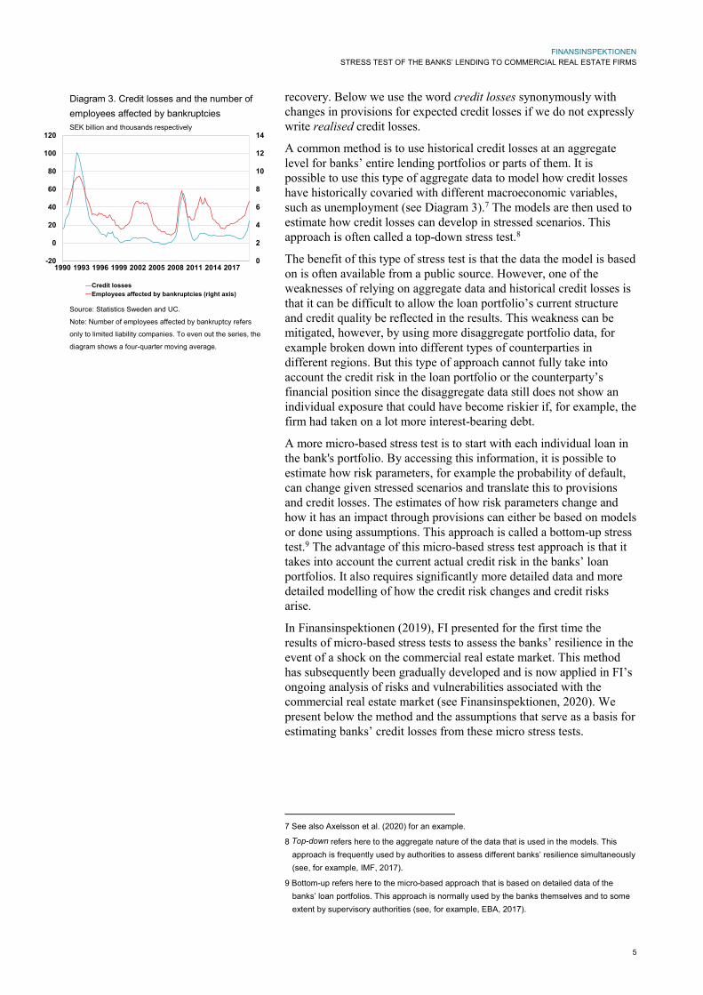
A common method is to use historical credit losses at an aggregate level for banks’ entire lending portfolios or parts of them. It is possible to use this type of aggregate data to model how credit losses have historically covaried with different macroeconomic variables, such as unemployment (see Diagram 3).7 The models are then used to estimate how credit losses can develop in stressed scenarios. This approach is often called a top-down stress test.8

The benefit of this type of stress test is that the data the model is based on is often available from a public source. However, one of the weaknesses of relying on aggregate data and historical credit losses is that it can be difficult to allow the loan portfolio’s current structure and credit quality be reflected in the results. This weakness can be mitigated, however, by using more disaggregate portfolio data, for example broken down into different types of counterparties in different regions. But this type of approach cannot fully take into account the credit risk in the loan portfolio or the counterparty’s financial position since the disaggregate data still does not show an individual exposure that could have become riskier if, for example, the firm had taken on a lot more interest-bearing debt.

A more micro-based stress test is to start with each individual loan in the bank's portfolio. By accessing this information, it is possible to estimate how risk parameters, for example the probability of default, can change given stressed scenarios and translate this to provisions and credit losses. The estimates of how risk parameters change and how it has an impact through provisions can either be based on models or done using assumptions. This approach is called a bottom-up stress test.9 The advantage of this micro-based stress test approach is that it takes into account the current actual credit risk in the banks’ loan portfolios. It also requires significantly more detailed data and more detailed modelling of how the credit risk changes and credit risks arise.

In Finansinspektionen (2019), FI presented for the first time the results of micro-based stress tests to assess the banks’ resilience in the event of a shock on the commercial real estate market. This method has subsequently been gradually developed and is now applied in FI’s ongoing analysis of risks and vulnerabilities associated with the commercial real estate market (see Finansinspektionen, 2020). We present below the method and the assumptions that serve as a basis for estimating banks’ credit losses from these micro stress tests.

7 See also Axelsson et al. (2020) for an example.

8 Top-down refers here to the aggregate nature of the data that is used in the models. This approach is frequently used by authorities to assess different banks’ resilience simultaneously (see, for example, IMF, 2017).

9 Bottom-up refers here to the micro-based approach that is based on detailed data of the banks’ loan portfolios. This approach is normally used by the banks themselves and to some extent by supervisory authorities (see, for example, EBA, 2017).

Diagram 3. Credit losses and the number of employees affected by bankruptcies SEK billion and thousands respectively

Source: Statistics Sweden and UC.

Note: Number of employees affected by bankruptcy refers

only to limited liability companies. To even out the series, the

diagram shows a four-quarter moving average.

0

2

4

6

8

10

12

14

-20

0

20

40

60

80

100

120

1990 1993 1996 1999 2002 2005 2008 2011 2014 2017

Credit lossesEmployees affected by bankruptcies (right axis)


6

Micro-based stress tests of commercial real estate firms Comprehensive data collection is required to obtain information about the banks’ loan portfolios.10 In 2020, FI collected data from seven banks that have exposures to the commercial real estate sector.11 The data included all loans to firms that are defined as commercial real estate (CRE) firms.

There is basic information for every loan, such as the outstanding amount, provisions, interest rate, transaction date and maturity, but also more detailed information about the banks’ PD and LGD estimates and risk weights. Detailed information about the property, for example the type of property, geographic location, loan-to-value ratio, valuation method and valuation date, is also provided for loans collateralised by a commercial real estate.

The banks’ PD, LGD and risk weight estimates and information about the groups they belong to are included for each borrower. The information about the parent company in the borrower’s group is matched with other information from Bisnode’s Serrano database to merge data on the firms’ financial position.12

With access to this data, we can calculate how large the banks’ credit losses could be following a shock. We estimate the banks’ credit losses by

1) estimating how a shock affects the CRE firms’ creditworthiness

2) estimating how the change in creditworthiness affects which stage the firms’ loans are assigned to

3) calculating how the change in creditworthiness and stage classification affects the banks’ provisions.

The changes in provisions generates the expected credit losses.

WE ANALYSE CRE FIRMS’ RESILIENCE The starting point for the stress test is a macro-economic scenario. A scenario refers to a description of the macroeconomic development based on assumptions of a number of important economic variables.13 CRE firms are exposed to different risks. The most important factor for the development of the real estate market is the growth in the economy. A downturn in economic activity leads to lower demand for premises and thus lower rental income and a drop in earnings. At the

10 For example, the Riksbank’s credit data base (KRITA), which contains information about

Swedish credit institutions’ credits to corporates and the public sector, credit by credit.

11 A similar data collection was conducted in 2019 as well, but since 2020 FI’s analysis of the commercial real estate market includes Danske bank, Handelsbanken, Länsförsäkringar Bank, Nordea, SBAB, SEB and Swedbank.

12 Bisnode’s database, Serrano, contains information about Swedish companies’ financial position from their annual reports (see Weidenman, 2016).

13 This is different than a forecast, which tries to predict a plausible development for a number of variables.


7

same time, CRE firms have high levels of debt, which means that they are exposed to both interest rate and refinancing risks.14

To analyse the resilience, we expose the firms to economic stress. CRE firms’ rental income is largely influenced by the activity level in the economy and thus GDP growth (see Diagram 4). There is a strong positive correlation between GDP and rent growth. GDP growth often leads rent growth since many rental contracts have long durations and changed conditions occur first when new contracts are signed or when old contracts are renegotiated. Since 1993, the rents of CRE firms have increased on average by 2.8 per cent a year, which is in line with Swedish GDP, but the variance is high.15

A decrease in GDP growth will lower CRE firms’ rental income. The impact on rental income is dependent on how sensitive the firms are to the macroeconomic development. In the crisis in the 1990s and in the economic recession at the beginning of the 2000s, office rental income fell 2–3.5 times as much as GDP (see Diagram 5). The impact thereafter gradually declined, which could be related to the commercial real estate market in Sweden not having experienced a major shock since then.

When economic growth is weakened, there is a risk that tenants will not renew or extend their rental contracts, that it will not be possible to find new tenants, or that new tenants will not be willing to pay the same rent. The sensitivity of CRE firms to weaker economic growth varies since the properties differ in terms of location, size, use and tenant composition. These factors affect stability in the demand for premises and thus rental income. Properties used for offices, retail and industrial activities are, for example, often more sensitive to a downturn in the economy than residential properties, where occupancy rates and rental income tend to be more stable over time (Finansinspektionen, 2019). Office, retail and industrial properties are associated with a higher financial risk since the tenants as a rule are firms. For these tenants, both the need for premises and their desire and ability to pay rent are dependent on the firm’s success.

Even if the sensitivity to weaker economic growth varies between different types of properties, more or less all CRE firms are exposed to interest rate risk since the firms’ financing for their property portfolios largely consist of loans. The borrowing mainly consists of interest-bearing instruments such as bank loans, bonds or commercial paper. The firms are therefore sensitive to changes in interest rate expenses for borrowings. In addition to the direct risk of higher interest rate costs due to a higher general level of interest rates, there is a risk that the banks’ and bond purchasers’ requirements on credit margins will increase, which also means higher financing costs for the firms when new loans are realised or outstanding loans will be refinanced.

14 The risk of an increase in interest rate expenses is the firm's interest rate risk. Refinancing

risk is the risk that it is difficult or costly to replace loans that have fallen due.

15 The standard deviation for rent growth is approximately 3 times as high as the standard deviation for GDP growth during the corresponding period.

Diagram 4. Office rent growth and GDP Annual percentage change

Source: Pangea and Statistics Sweden.

Note: Office rent growth refers to central, so-called prime,

locations throughout the country. Annual figures have been

extrapolated into quarterly averages. GDP is the change in

real GDP in per cent a given quarter compared to the

corresponding quarter the previous year.

Diagram 5. Estimated effect of GDP on rent growth Per cent

Source: FI.

Note: The diagram shows coefficients from a recursive

estimated model where rent growth is explained by GDP

growth. Dashed lines show a 95-per cent confidence interval.

A recursive estimated model means that we estimate the

model using an increasing number of observations. We first

estimate the model for the period Q1 1993–Q4 1998 (shaded

area) and then expand the observation period one quarter at

a time.

-20

-15

-10

-5

0

5

10

15

1993 1996 1999 2002 2005 2008 2011 2014 2017 2020

GDP Rent

0

1

2

3

4

1993 1996 1999 2002 2005 2008 2011 2014 2017


8

The firms’ financial position are the starting point when calculating their resilience. The firms’ interest coverage ratio and loan-to-value ratio are two key figures that we use to gain an understanding of how sensitive CRE firms are to changes in interest expenses and income.16 The interest coverage ratio is a measure of how well the current net operating income (rental income minus operating expenses) covers the firm’s interest expenses. The loan-to-value ratio measures how much debt a CRE firm has in relation to the value of its property assets. We define these two key figures as follows:

𝐼𝐼𝐼𝐼𝐼𝐼𝐼𝐼𝐼𝐼𝐼𝐼𝐼𝐼𝐼𝐼 𝐶𝐶𝐶𝐶𝐶𝐶𝐼𝐼𝐼𝐼𝐶𝐶𝐶𝐶𝐼𝐼 𝑅𝑅𝐶𝐶𝐼𝐼𝑅𝑅𝐶𝐶 =(𝐼𝐼𝐼𝐼𝐼𝐼𝐼𝐼𝐶𝐶𝑟𝑟 𝑅𝑅𝐼𝐼𝑖𝑖𝐶𝐶𝑖𝑖𝐼𝐼 − 𝐶𝐶𝑜𝑜𝐼𝐼𝐼𝐼𝐶𝐶𝐼𝐼𝑅𝑅𝐼𝐼𝐶𝐶 𝑖𝑖𝐶𝐶𝐼𝐼𝐼𝐼)

𝑅𝑅𝐼𝐼𝐼𝐼𝐼𝐼𝐼𝐼𝐼𝐼𝐼𝐼𝐼𝐼 𝐼𝐼𝐶𝐶𝐼𝐼𝐼𝐼 ∗ 𝑑𝑑𝐼𝐼𝑑𝑑𝐼𝐼

= 𝐼𝐼𝐼𝐼𝐼𝐼 𝐶𝐶𝑜𝑜𝐼𝐼𝐼𝐼𝐶𝐶𝐼𝐼𝑅𝑅𝐼𝐼𝐶𝐶 𝑅𝑅𝐼𝐼𝑖𝑖𝐶𝐶𝑖𝑖𝐼𝐼𝑅𝑅𝐼𝐼𝐼𝐼𝐼𝐼𝐼𝐼𝐼𝐼𝐼𝐼𝐼𝐼 𝐼𝐼𝑒𝑒𝑜𝑜𝐼𝐼𝐼𝐼𝐼𝐼𝐼𝐼

𝐸𝐸𝐶𝐶𝐶𝐶𝐼𝐼 − 𝐼𝐼𝐶𝐶 − 𝑉𝑉𝐶𝐶𝑟𝑟𝑉𝑉𝐼𝐼 =𝑑𝑑𝐼𝐼𝑑𝑑𝐼𝐼

𝑖𝑖𝐶𝐶𝐼𝐼𝑚𝑚𝐼𝐼𝐼𝐼 𝐶𝐶𝐶𝐶𝑟𝑟𝑉𝑉𝐼𝐼=

𝑑𝑑𝐼𝐼𝑑𝑑𝐼𝐼

�𝐼𝐼𝐼𝐼𝐼𝐼 𝐶𝐶𝑜𝑜𝐼𝐼𝐼𝐼𝐶𝐶𝐼𝐼𝑅𝑅𝐼𝐼𝐶𝐶 𝑅𝑅𝐼𝐼𝑖𝑖𝐶𝐶𝑖𝑖𝐼𝐼𝑦𝑦𝑅𝑅𝐼𝐼𝑟𝑟𝑑𝑑 𝐼𝐼𝐼𝐼𝑟𝑟𝑉𝑉𝑅𝑅𝐼𝐼𝐼𝐼𝑖𝑖𝐼𝐼𝐼𝐼𝐼𝐼 �

The market value of a property can be given in a simplified manner as the discounted value of future net operating income that is expected to be generated over time. We can thus calculate the market value by dividing the net operating income by the yield requirement. 17 The yield requirement is defined as the risk-free interest rate plus the risk premium that investors demand when investing in properties. This means that investors’ yield requirements are influenced by the general level of interest rate, which is closely linked to the risk-free rate. Thus, both the interest coverage ratio and the loan-to-value ratio of CRE firms are influenced by changes in income and interest rates.

We shock the firms’ net operating income in the stress tests.18 The operating expenses are assumed to remain constant, and therefore the impact of GDP growth on the net operating income will be larger than the impact on rental income. We assume that the CRE firms’ net operating income is affected three times as much as GDP (see Table 1).19 When it comes to net operating income for CRE firms that are

16 These two key figures are two common financial conditions (covenants) that the banks apply

in their contracts.

17 This is a version of Gordon's formula, where the market value is expressed as

𝑉𝑉𝐶𝐶𝑟𝑟𝑉𝑉𝐼𝐼 = 𝐼𝐼𝐼𝐼𝐼𝐼 𝐶𝐶𝑜𝑜𝐼𝐼𝐼𝐼𝐶𝐶𝐼𝐼𝑅𝑅𝐶𝐶𝐼𝐼𝐶𝐶 𝑅𝑅𝐼𝐼𝑖𝑖𝐶𝐶𝑖𝑖𝐼𝐼/(𝐼𝐼 − 𝐶𝐶),

where r is a representative discount rate, i.e. the sum of a risk-free rate and a risk add-on that reflects the uncertainty in the future net operating income and g is the growth rate in the net operating income. All else equal, higher expected net operating income generates a higher value on the property, while a higher discount rate (higher risk-free rate or risk add-on) generates a lower value of the property (see Geltner and Miller, 2001).

18 This is because the data underlying the net operating income is greater than the underlying data for rental income and operating cost.

19 In the crisis of the 1990s and the IT crisis, rental income for offices declined by approximately three times as much as GDP.

Table 1. Assumed elasticities in FI’s stress test Per cent

Commercial properties

Commercial residential properties

ε (net operating income, GDP)

3 1

ε (yield requirement, interest rate)

0.5 0.25

Source: FI.

Note: The table shows the assumed elasticities in FI’s stress

test between GDP growth and the growth in the net operating

income, as well as the interest rate and the yield requirement.


9

less dependent on the business cycle, we assume that it is affected in line with GDP.20

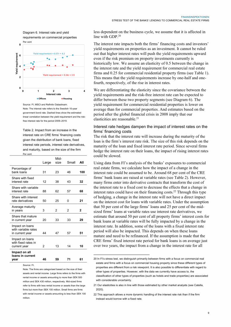
The interest rate impacts both the firms’ financing costs and investors’ yield requirements on properties as an investment. It cannot be ruled out that higher interest rates will push the yield requirements upward even if the risk premium on property investments currently is historically low. We assume an elasticity of 0.5 between the change in the interest rate and the yield requirement for commercial real estate firms and 0.25 for commercial residential property firms (see Table 1). This means that the yield requirements increase by one-half and one-fourth, respectively, of the rise in interest rates.

We are differentiating the elasticity since the covariance between the yield requirements and the risk-free interest rate can be expected to differ between these two property segments (see Diagram 6). The yield requirement for commercial residential properties is lower on average than for commercial properties. And estimates based on the period after the global financial crisis in 2008 imply that our elasticities are reasonable.21

Interest rate hedges dampen the impact of interest rates on the firms’ financing costs The risk that the interest rate will increase during the maturity of the loan is the firm’s interest rate risk. The size of this risk depends on the maturity of the loan and fixed interest rate period. Since several firms hedge the interest rate on their loans, the impact of rising interest rates could be slowed.

Using data from FI’s analysis of the banks’ exposures to commercial real estate firms, we calculate how the impact of a change in the interest rate could be assumed to be. Around 68 per cent of the CRE firms’ bank loans are raised at variable rates (see Table 2). However, many firms enter into derivative contracts that transform the cost of the interest rate to a fixed cost to decrease the effects that a change in interest rates could have on their financing costs.22 Through this type of hedging, a change in the interest rate will not have a direct impact on the interest cost for loans with variable rates. Under the assumption that 50 per cent of the large firms’ loans and 25 per cent of the mid-sized firms’ loans at variable rates use interest rate derivatives, we estimate that around 50 per cent of all property firms’ interest costs for bank loans at variable rates will be fully impacted by a change in the interest rate. In addition, some of the loans with a fixed interest rate period will also be impacted. This depends on when these loans mature and need to be refinanced. If the assumption is made that the CRE firms’ fixed interest rate period for bank loans is on average just over two years, the impact from a change in the interest rate for all

20 In FI’s stress test, we distinguish primarily between firms with a focus on commercial real

estate and firms with a focus on commercial housing property since these different types of properties are different from a risk viewpoint. It is also possible to differentiate with regard to other types of properties. However, with the data we currently have access to, the classification of other types of properties (such as hotels and trade properties) are associated with considerable uncertainty.

21 Our elasticities is also in line with those estimated by other market analysts (see Catella, 2020).

22 This approach allows a more dynamic handling of the interest rate risk than if the firm instead would borrow with a fixed rate.

Diagram 6. Interest rate and yield requirements on commercial properties Per cent

Source: FI, MSCI and Refinitiv Datastream.

Note: The interest rate refers to the Swedish 10-year

government bond rate. Dashed lines show the estimated

linear correlation between the yield requirement and the risk-

free interest rate for the period 2009–2019.

Table 2. Impact from an increase in the interest rate on CRE firms’ financing costs given the distribution of bank loans, fixed interest rate periods, interest rate derivatives, and maturity, based on the size of the firm Per cent

Large Mid-size Small All

Percentage of bank loans 31 23 46 100

Share with fixed interest rate 12 38 43 32

Share with variable interest rate 88 62 57 68

Share with interest rate derivatives 50 25 0 21

Average maturity in years 3 2 2 2

Share that mature in current year 20 33 33 29

Impact on loans with variable rates in current year 44 47 57 51

Impact on loans with fixed rates in current year 2 13 14 10

Impact on all loans in current year 46 59 71 61

Source: FI.

Note: The firms are categorised based on the size of their

assets and rental income. Large firms refers to the firms with

rental income or assets amounting to more than SEK 500

million and SEK 430 million, respectively. Mid-sized firms

refer to firms with less rental income or assets than the large

firms but more than SEK 100 million. Small firms are firms

with rental income or assets amounting to less than SEK 100

million.

Yield requirement = 0.57r + 4.2

Yield requirement = 0.24r + 3.5

0

2

4

6

8

0 1 2 3 4

Yiel

d re

quire

men

t

Interest rateOffices Housing


10

loans is estimated to be around 60 per cent. This is also what we use in the stress test.

Firms’ loan-to-value ratio and interest coverage ratio are used to identify vulnerable CRE firms We use FI’s analysis of the banks’ exposures to commercial real estate firms to identify the CRE firms. We then match these firms with information from their annual reports to estimate the firms’ financial position at the outset. Given the underlying assumptions, we then calculate how the CRE firms’ interest coverage ratio and loan-to-value ratio could be impacted by a macroeconomic shock.23 This is a statistical and simplified calculation to illustrate the effect of one or a few factors.

Using the stress tests, we analyse how the firms’ interest rate coverage and loan-to-value ratio could be affected if the interest rate were to rise or the net operating income were to fall sharply. The interest coverage ratio under stress provides an indication of whether the firm could experience problems handling its interest rate payment or even find itself in default.

There are no absolute measures of when a firm's interest coverage ratio is so low that it will experience financial difficulties. If the interest coverage ratio is lower than 1, this means that the firm cannot make its interest payment with income from its operating activities. 24 The firm will then need to instead use existing equity, sell assets, or increase its financial cash flow through new borrowings in order to avoid default. The possibilities the firm faces to sell its assets or raise new financing varies from case to case and are difficult to determine in general. But a firm with a low loan-to-value ratio in general faces better possibilities for selling assets or raising new financing to manage an interest coverage ratio of less than one. This is why we use a combination of a low interest coverage ratio and a high loan-to-value ratio to identify vulnerable CRE firms.

We define CRE firms as vulnerable if they demonstrate an interest coverage ratio of less than 1 and a loan-to-value ratio of more than 70 per cent. Loan-to-value ratios of between 60 and 70 per cent are often applied by the banks as internal ceilings when they lend money to CRE firms.25 Lending to firms with these characteristics (interest coverage ratio of less than 1 and loan-to-value ratio of more than 70 per cent) could subsequently be viewed as an indicator of elevated credit risk for the commercial real estate sector’s lenders.

In other words, we perform the calculations for all CRE firms individually and study how the distribution of vulnerable CRE firms

23 FI has previously shown that CRE firms’ high level of debt primarily makes them vulnerable

to rising financing costs, and that rising interest costs affect CRE firms more than variations in their income (see Finansinspektionen, 2019). See also the calculations in Appendix 1.

24 An interest coverage ratio that is this low can be assumed to be a signal that the firm may be financially strained. But higher values have also been used to capture early signals of potential problems (see Chow, 2015).

25 Loans to commercial residential properties are usually granted to the higher loan-to-value ratios.

Diagram 7. Cumulative distribution of CRE firms’ interest coverage ratios Per cent

Source: FI.

Note: Threshold refers to the value that we assume in our

calculations to identify vulnerable CRE firms. Firms to the left

of the threshold have an interest coverage ratio less than 1.

Diagram 8. Cumulative distribution of CRE firms’ loan-to-value ratios Per cent

Source: FI.

Note: Threshold refers to the value that we assume in our

calculations to identify vulnerable real estate firms. Firms to

the right of the threshold have a loan-to-value ratio of more

than 70 per cent.

0

20

40

60

80

100

0 2 4 6 8 10

Outset Threshold

0

20

40

60

80

100

0 10 20 30 40 50 60 70 80 90 100 110

Outset Threshold


11

shifts given our assumptions on correlation, stress and threshold values (see Diagram 7 and Diagram 8).26

WE CALCULATE HOW VULNERABLE CRE FIRMS IMPACT THE BANKS Vulnerable CRE firms can cause credit losses for the banks. The size of the credit losses that could arise in these situations is dependent on how much of a need there is to increase the provisions for expected credit losses. To estimate this, we need to know the distribution of the credit risk in the banks’ lending portfolios and the major banks’ provision rates in each provision stage.

To calculate the provisions, we start with the banks’ own provision rates for loans in each category at the outset. Following a stress, the provisions will increase. This is because more loans will be classified as Stage 2, and more loans will be past due (Stage 3). A key determination in the size of the credit losses is thus how we classify the loan given a stress. We use the following assumptions to classify the vulnerable CRE firms’ loans in Stage 2 and 3:

• We classify loans to firms with an interest coverage ratio of less than 1 and a loan-to-value ratio of between 70 and 100 per cent as having an elevated credit risk (Stage 2).27

• Loans to firms with an interest coverage ratio of less than 1 and a loan-to-value ratio of more than 100 per cent are past due (Stage 3).

These assumptions have some support in the data. In FI’s data, the median value of the interest coverage ratio for CRE firms – with all loans in Stage 2 and 3 – is close to 1 (see Table 3). The loan-to-value ratio is on average lower than what we assume in the classification, but there is large variation. And the loan-to-value ratio is higher in Stage 3 than in Stage 2.

With these assumptions, we estimate how the credit risk in the banks’ lending portfolios is distributed. Our calculations show that 4.2 per cent of the lending to the CRE firms is categorised at the outset as an elevated credit risk and in default (Stage 2 and Stage 3, respectively). This is marginally higher than what we observe in the banks’ lending portfolio at the outset (see Table 4). Our classification generates a higher value than what the banks have at the outset in primarily Stage 3. Since there are very few CRE firms that have loans in Stage 3 at the outset, we keep the assumed thresholds.

The credit losses that arise in the event of a shock are dependent on how the lending portfolio’s credit risk is distributed after the shock and how large the banks’ provision rates are in each stage. The credit losses are primarily the result of defaulted loans (Stage 3) since the provision rate for this category is significantly higher than for loans with elevated credit risk (Stage 2).

26 Table B1 of Appendix 2 presents our calculations of how different scenarios impact the CRE

firms’ loan-to-value ratios and interest coverage ratios and the share of firms and debt with elevated credit risk according to the definition FI uses.

27 According to IFRS 9, an assessment of whether a credit risk is elevated is conducted in relation to what the credit risk was when the loan was issued. Naturally, loans may have already been issued at the outset to firms with elevated credit risk according to these conditions. But we consider this to be a reasonable indicator for our purpose.

Table 3. CRE firms’ key ratios by loan category Ratio, per cent and number

Stage 1

Stage 2

Stage 3

Interest rate coverage ratio

3.0 1.3 0.7

Loan-to-value ratio

57 61 84

Number of firms 10,020 663 23

Source: FI.

Note: The table shows the CRE firms’ interest coverage ratio

(median) and loan-to-value ratio (average). Only firms that

have more than 80 per cent of their loans in the same loan

category are included in each stage.

Table 4. Distribution of credit risk in the banks’ lending portfolio and applied provision rate Per cent

Banks’ lending portfolio

FI’s estimate

Provision rate

Stage 1 96.1 95.8 0.0

Stage 2 3.8 3.6 1.5

Stage 3 0.1 0.6 30.0

Source: FI.

Note: The table shows the percentage of the bank loans in

each risk category at the outset (according to FI’s data on

exposures to CRE firms) and given FI’s assumptions for risk

classification in relation to the total loans to CRE firms and the

provision rate that the banks apply on average in each stage.


12

In the calculations, we start with the banks’ average provision rates at the outset for loans in each category (see Table 4). But the variation in the banks’ provisions rates is large, particularly in Stage 3 (see Diagram 9). Since the banks’ provision rates will probably be higher following a shock than they are at the outset, this could mean that we are underestimating the credit losses. At the same time, this is offset by the probability that we are overestimating the percentage of loans that are classified as in default. This is because not all firms will default even if they have an interest coverage ratio of less than 1 and a loan-to-value ratio of more than 100 following a shock.28 For example, it is in the banks’ own interests to prevent a loan from defaulting even when firms are demonstrating poor key ratios.

Concluding remarks In this FI Analysis, we present a method for stress testing CRE firms and banks. We also present the assumptions that serve as the basis for the analysis of the CRE firms’ resilience and their impact on the banks’ credit losses. The advantage of this micro-based stress test approach is that it takes into account the current actual credit risk in the banks’ loan portfolios. For example, the credit expansion and structural changes to the banks’ lending in recent years – combined with the sharp increase in property prices – may have changed the banks’ vulnerabilities over time. Micro-based stress tests of the banks’ lending portfolios have the flexibility to consider such changes.

Even if we have focused here on the commercial real estate market, the method is also applicable to other segments. For example, it is possible to use the same type of general approach to analyse how a shock to other types of non-financial firms could impact the banks’ credit losses. However, it is key to have a good understanding about the sector in question since the method requires detailed modelling of how the credit risk changes and how credit losses occur.

28 Table B2 in Appendix 2 presents calculations of how large the banks’ credit losses could be

given different scenarios.

Diagram 9. Distribution of provision rates in each stage Per cent

Source: FI.

Note: The diagram shows how the banks’ provision rates vary

in each stage. The X-axis specifies the provision rate in per

cent.

0

20

40

60

80

100

Und

er 1

1—5

6—10

11—

20

21—

30

31—

40

41—

50

51—

60

61—

70

71—

80

81—

90

Ove

r 90

Stage 1 Stage 2 Stage 3


13

References Axelsson, P., Å. David, K. Kamath, C. Lönnbark and V. Thell, (2020). En makrobaserad kreditförlustmodell för de svenska storbankerna, Pending FI Analysis, Finansinspektionen.

Chow, J. (2015). Stress Testing Corporate Balance Sheets in Emerging Economies, IMF Working Paper WP/15/216.

Catella 2020. Catella Property Forecast, 16 June 2020, Catella.

EBA (2017). 2018 EU-wide stress test: Methodological Note, European Banking Authority.

EBA (2020). On the future changes to the EU-wide stress test, European Banking Authority Discussion Paper, EBA/DP/2020/01.

Finansinspektionen (2014). Kapitalkrav för svenska banker, Memorandum, FI Ref. 14-6258. An English translation is available at www.fi.se.

Finansinspektionen (2019). Den kommersiella fastighetsmarknaden och finansiell stabilitet, May 2019, Övriga rapporter, FI. Ref. 18-20931. An English translation is available at www.fi.se.

Finansinspektionen (2020). Stabiliteten i det finansiella systemet, June 2020, Stabilitetsrapporter, FI Ref. 20-9224. An English translation is available at www.fi.se.

G20 (2009). Declaration on strengthening the financial system, provided by the G20 Research Group, London.

Geltner, D., and Miller, N. G., (2001). Commercial Real Estate Analysis and Investment, South Western Publishing.

IMF (2017). Sweden: Financial Sector Assessment Program: Technical Note – Stress testing, IMF Country Report No. 17/309.

Weidenman, P., (2016). The Serrano Database for analysis and register-based statistics, Bisnode.


14

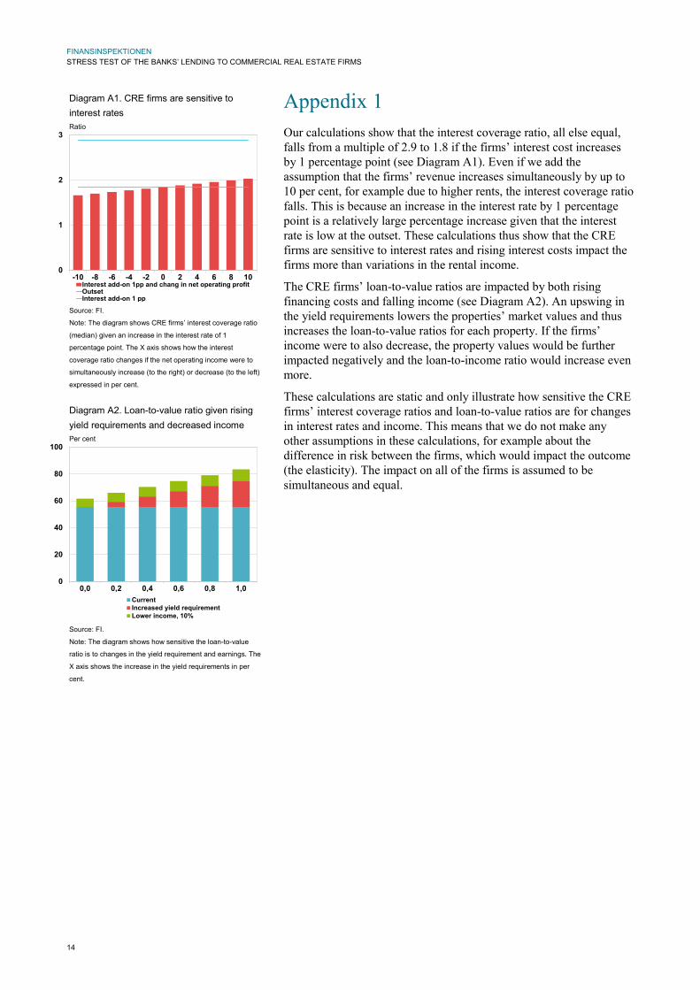
Appendix 1 Our calculations show that the interest coverage ratio, all else equal, falls from a multiple of 2.9 to 1.8 if the firms’ interest cost increases by 1 percentage point (see Diagram A1). Even if we add the assumption that the firms’ revenue increases simultaneously by up to 10 per cent, for example due to higher rents, the interest coverage ratio falls. This is because an increase in the interest rate by 1 percentage point is a relatively large percentage increase given that the interest rate is low at the outset. These calculations thus show that the CRE firms are sensitive to interest rates and rising interest costs impact the firms more than variations in the rental income.

The CRE firms’ loan-to-value ratios are impacted by both rising financing costs and falling income (see Diagram A2). An upswing in the yield requirements lowers the properties’ market values and thus increases the loan-to-value ratios for each property. If the firms’ income were to also decrease, the property values would be further impacted negatively and the loan-to-income ratio would increase even more.

These calculations are static and only illustrate how sensitive the CRE firms’ interest coverage ratios and loan-to-value ratios are for changes in interest rates and income. This means that we do not make any other assumptions in these calculations, for example about the difference in risk between the firms, which would impact the outcome (the elasticity). The impact on all of the firms is assumed to be simultaneous and equal.

Diagram A1. CRE firms are sensitive to interest rates Ratio

Source: FI.

Note: The diagram shows CRE firms’ interest coverage ratio

(median) given an increase in the interest rate of 1

percentage point. The X axis shows how the interest

coverage ratio changes if the net operating income were to

simultaneously increase (to the right) or decrease (to the left)

expressed in per cent.

Diagram A2. Loan-to-value ratio given rising yield requirements and decreased income Per cent

Source: FI.

Note: The diagram shows how sensitive the loan-to-value

ratio is to changes in the yield requirement and earnings. The

X axis shows the increase in the yield requirements in per

cent.

0

1

2

3

-10 -8 -6 -4 -2 0 2 4 6 8 10Interest add-on 1pp and chang in net operating profitOutsetInterest add-on 1 pp

0

20

40

60

80

100

0,0 0,2 0,4 0,6 0,8 1,0CurrentIncreased yield requirementLower income, 10%


15

Appendix 2 Table A1. CRE firms’ loan-to-value ratios, interest coverage ratios, and the share of vulnerable firms (loans) given different scenarios and at the outset

GDP Interest ICR LTV

Percentage vulnerable

firms

Share of loans with vulnerable

firms GDP shock -2 - 2.8 59.6 9.4 5.0

-4 - 2.6 62.4 11.1 6.4 -8 - 2.4 68.2 15.5 9.0 -10 - 2.3 71.6 17.4 10.3

Interest rate shock - 0.5 2.5 58.7 9.9 5.6 - 1.0 2.2 62.1 12.8 7.8 - 1.5 1.9 65.4 15.7 10.2 - 2.0 1.7 68.8 19.2 13.7

Combined shock -2 0.5 2.4 61.4 11.5 6.7 -4 1.0 2.0 67.9 16.9 10.2 -8 1.5 1.6 78.3 24.6 18.3 -10 2.0 1.4 86.4 29.9 23.5

Outset - - 2.9 57.0 7.7 4.2

Source: FI. Note: The GDP column shows the percentage change in GDP that is assumed in each scenario. The Interest rate column shows the change in interest rate in percentage points. An increase in the interest rate is assumed to also entail an increase in the average yield requirement (see Table 1). LTV and ICR are the CRE firms’ loan-to-value ratio and interest coverage ratio (median). The Percentage vulnerable firms column shows the percentage of all CRE firms that have an interest coverage ratio of less than 1 and a loan-to-value ratio of more than 70 per cent given each scenario and at the outset. The Share of loans with vulnerable firms shows how large the loans with the vulnerable firms are in relation to all CRE firms. Table A2. Estimated credit losses given different scenarios GDP Interest Credit losses

GDP shock -2 - 0.4

-4 - 0.5

-8 - 0.8

-10 - 1.0

Interest rate shock - 0.5 0.4

- 1.0 0.6

- 1.5 1.0

- 2.0 1.4

Combined shock -2 0.5 0.5

-4 1.0 0.9

-8 1.5 2.1

-10 2.0 3.6 Source: FI.

Note: The table shows the banks’ estimated credit losses as a per cent of

outstanding exposures to the commercial real estate sector.

Stress test of the banks' lending to commercial real estate firms

Documents

Transcript of Stress test of the banks' lending to commercial real estate firms