The hillslope-storage Boussinesq model

for non-constant bedrock slope

A.G.J. Hilbertsa,*, E.E. van Loona, P.A. Trocha, C. Paniconib,c

aHydrology and Quantitative Water Management Group, Department of Environmental Sciences,

Wageningen University, Nieuwe Kanaal 11, 6709 PA Wageningen, The NetherlandsbCenter for Advanced Studies, Research and Development in Sardinia (CRS4), Cagliari, Italy

cINRS-ETE, University of Quebec, Sainte-Foy, Que., Canada

Accepted 23 December 2003

Abstract

In this study the recently introduced hillslope-storage Boussinesq (hsB) model is cast in a generalized formulation enabling

the model to handle non-constant bedrock slopes (i.e. bedrock profile curvature). This generalization extends the analysis of

hydrological behavior to hillslopes of arbitrary geometrical shape, including hillslopes having curved profile shapes. The

generalized hsB model performance for a free drainage scenario is evaluated by comparison to a full three-dimensional

Richards equation (RE) based model. The model results are presented in the form of dimensionless storage profiles and

dimensionless outflow hydrographs. In addition, comparison of both models to a storage based kinematic wave (KW) model

enables us to assess the relative importance of diffusion processes for different hillslope shapes, and to analyze the influence of

profile curvature on storage and flow patterns specifically. The comparison setup consists of a set of nine gentle (5% bedrock

slope) and nine steep (30% bedrock slope) hillslopes of varying plan shape and profile curvature. Interpretation of the results

shows that for highly conductive soils the simulated storage profiles and outflow hydrographs of the generalized hsB model and

RE model match remarkably for 5% bedrock slope and for all plan and profile curvatures. The match is slightly poorer on

average for 30% bedrock slope, in particular, on divergently shaped hillslopes. In the assessment of the influence of hydraulic

diffusion, we find good agreement in simulation results for the KW model compared to results from the generalized hsB model

and the RE model for steep divergent and uniform hillslopes, due to a relatively low ratio between water table gradient and

bedrock slope compared to convergent or gentle hillslopes. Overall, we demonstrate that, in addition to bedrock slope, hillslope

shape as represented by plan and profile curvature is an important control on subsurface flow response.

q 2004 Elsevier B.V. All rights reserved.

Keywords: Hillslope hydrology; Subsurface flow; Boussinesq equation; Richards equation; Kinematic wave equation

1. Introduction

Landscape geometry influences hydrological

response, thus, clear insight into the effects of the

shape and characteristics of landscape elements is

required to further our understanding of and our

Journal of Hydrology 291 (2004) 160–173

www.elsevier.com/locate/jhydrol

0022-1694/$ - see front matter q 2004 Elsevier B.V. All rights reserved.

doi:10.1016/j.jhydrol.2003.12.043

* Corresponding author. Tel.: þ31-317-484017; fax: þ31-317-

484885.

E-mail addresses: arno.hilberts@wur.nl (A.G.J. Hilberts),

emiel.vanloon@wur.nl (E.E. van Loon), peter.troch@wur.nl (P.A.

Troch), cxpanico@crs4.it (C. Paniconi).

ability to model hydrological processes. For some

time research has focused on identifying and quanti-

fying hillslope processes as a first step towards

assessment of (sub)catchment response. In catchment

hydrology the importance of subsurface flow pro-

cesses in generating variable source areas was first

addressed by Dunne and Black (1970) and Freeze

(1972a,b). Later Kirkby (1988) reported that almost

all of the water in streamflow has passed over or

through a hillside and its soils before reaching the

channel, thereby emphasizing the role of hillslope

hydrological processes. These references indicate a

need for quantifying the hydrological processes on

hillslopes and for the development of appropriate

models to describe these processes. Many models

have been developed over the past 30 years. Pikul et al.

(1974) formulated a coupled model based on the

Richards and Boussinesq equations and evaluated it

by comparison to a two-dimensional Richards based

model. Sloan and Moore (1984) compared Richards

equation (RE) based models of Nieber and Walter

(1981) and Nieber (1982), a kinematic wave (KW)

model of Beven (1981) and a storage discharge model

to measurements on a hillslope with a uniform width

function. Other examples include Fipps and Skaggs

(1989), who applied a two-dimensional Richards

based model to a unit-width hillslope with a constant

slope inclination; Verhoest and Troch (2000), who

determined the analytical solution to the Boussinesq

equation applied to a non-curved unit-width aquifer;

and Ogden and Watts (2000), who analyzed the

behavior of a numerically solved two-dimensional

model for steady and unsteady flow types on a unit-

width non-curved hillslope. None of these studies

presents models that account for the effect of the

three-dimensional hillslope shape on storage and flow

patterns, although other recent research has begun to

address these issues. For example, Paniconi and Wood

(1993) presented a three-dimensional Richards based

model for subsurface flow on complex hillslopes;

Duffy (1996) formulated a volume-weighted integral-

balance model for complex terrain types and applied it

to steep slightly curved hillslope to analyze subsur-

face flow, overland flow and variable source areas;

and Woods et al. (1997) modeled subsurface flow

processes using a topographic index and compared

results to extensive field measurements on 30 steep

inclined shallow troughs of various shapes (conver-

gent, planar and divergent).

To overcome difficulties associated with three-

dimensional models, a series of new low-dimensional

hillslope models have been developed (Troch et al.,

2002, 2004). These models are able to treat geometric

complexity in a simple way based on a concept

presented by Fan and Bras (1998), resulting in a

significant reduction in model complexity, and they

can cope with varying hillslope width functions and

bedrock slope. In Troch et al. (2002) the analytical

solutions to a KW equation that is expressed in terms

of storage using the mapping method of Fan and Bras

(1998) are evaluated by applying them to nine

hillslopes with different plan and profile curvature.

The resulting hillslope-storage KW model shows

quite different dynamic behavior during a free

drainage and a recharge experiment. The authors

conclude that the KW assumption is limited to

moderate to steep slopes, and that for more gentle

slopes a new model formulation based on the

Boussinesq equation would be necessary. In Troch

et al. (2004) the hillslope-storage Boussinesq (hsB)

model together with several simplified versions (e.g.

linearized) are derived and evaluated under free

drainage and recharge scenarios. The evaluation is

conducted on a subset of the nine hillslopes presented

in Troch et al. (2002). Results are compared to those

of the KW model and the authors find that dynamic

response of the hillslopes is strongly dependent on

plan shape and bedrock slope, and that convergent

hillslopes tend to drain much more slowly than

divergent ones due to a reduced flow domain near

the outlet. Concerning the several simplified versions

of the hsB model it is concluded that for gentle slopes

(5% bedrock slope) none of these simpler models is

able to fully capture the dynamics of the full hsB

model, while for steep slopes (30% bedrock slope) the

performance is better. In Paniconi et al. (2003) the

hsB model is compared to a three-dimensional RE

based model on the same subset of hillslopes, in order

to identify the circumstances under which the

different models generate comparable responses. In

this work the RE model is regarded as the benchmark.

The overall conclusion is that the hsB model is able to

capture the general features of storage and outflow

response. Overall, a closer match between the hsB and

RE models was observed for convergent hillslopes

A.G.J. Hilberts et al. / Journal of Hydrology 291 (2004) 160–173 161

than divergent, and the match was quite independent

of slope steepness. A poorer match was observed in

case of the recharge simulations compared to the free

drainage scenario, most likely due to absence of a

description of the unsaturated zone in the hsB model,

important in the transmission of water through a

hillslope soil during a rainfall or recharge event. The

absence of an unsaturated zone component in the hsB

model also causes the water table heights for the hsB

model to be slightly higher and the flow values to be

slightly lower than the RE model in almost all cases.

These previous papers on the hsB model suggested

several extensions of the model to make it more

representative of complex hillslopes, including the

capability to handle non-constant bedrock slope in

order to more accurately account for hillslope profile

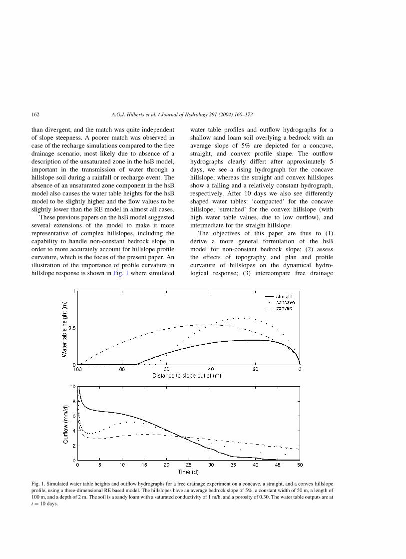
curvature, which is the focus of the present paper. An

illustration of the importance of profile curvature in

hillslope response is shown in Fig. 1 where simulated

water table profiles and outflow hydrographs for a

shallow sand loam soil overlying a bedrock with an

average slope of 5% are depicted for a concave,

straight, and convex profile shape. The outflow

hydrographs clearly differ: after approximately 5

days, we see a rising hydrograph for the concave

hillslope, whereas the straight and convex hillslopes

show a falling and a relatively constant hydrograph,

respectively. After 10 days we also see differently

shaped water tables: ‘compacted’ for the concave

hillslope, ‘stretched’ for the convex hillslope (with

high water table values, due to low outflow), and

intermediate for the straight hillslope.

The objectives of this paper are thus to (1)

derive a more general formulation of the hsB

model for non-constant bedrock slope; (2) assess

the effects of topography and plan and profile

curvature of hillslopes on the dynamical hydro-

logical response; (3) intercompare free drainage

Fig. 1. Simulated water table heights and outflow hydrographs for a free drainage experiment on a concave, a straight, and a convex hillslope

profile, using a three-dimensional RE based model. The hillslopes have an average bedrock slope of 5%, a constant width of 50 m, a length of

100 m, and a depth of 2 m. The soil is a sandy loam with a saturated conductivity of 1 m/h, and a porosity of 0.30. The water table outputs are at

t ¼ 10 days.

A.G.J. Hilberts et al. / Journal of Hydrology 291 (2004) 160–173162

simulation of the hsB, KW and RE models for

hillslopes with varying plan and profile curvature.

The generalized hsB model allows a quantitative

analysis of water tables and hydrographs, and

thereby enables us to conduct a very accurate

analysis of the effects of topography and geometry

on hydrological processes on these hillslopes, since

it allows simulations for virtually any hillslope

shape and bedrock slope. The generalized hsB

model will be compared to the full three-dimen-

sional RE model that was also applied in Paniconi

et al. (2003). The behavior of the models will be

analyzed for the nine hillslopes of varying plan and

profile curvature that are described in Troch et al.

(2002), and model results will be presented in

dimensionless variables. In addition, the relative

influence of diffusion processes in both models will

be evaluated by comparison to the hillslope-storage

KW model of Troch et al. (2002).

2. Development of the generalized hillslope-storage

Boussinesq model

The mass balance equation for describing subsur-

face flow along a unit-width hillslope reads

›

›tðfhÞ ¼ 2

›q

›xþ N ð1Þ

where h ¼ hðx; tÞ is the elevation of the groundwater

table measured perpendicular to the underlying

impermeable layer, f is drainable porosity, x is

distance to the outlet measured parallel to the

impermeable layer, q ¼ qðx; tÞ is subsurface flux

along the hillslope bedrock, t is time, and N is a

source term, representing rainfall recharge to the

groundwater table. Eq. (1) is derived for a unit-width

hillslope and therefore does not account for the three-

dimensional shape of a hillslope. Investigating the

effect of geometry on hydrological response thus

requires a more general form of Eq. (1). This is

obtained by first expressing the equation in terms of

storage by using the relationship of Fan and Bras

(1998) to map the three-dimensional soil mantle onto

a one-dimensional soil pore space: S ¼ fw�h; where

S ¼ Sðx; tÞ is actual storage, w ¼ wðxÞ is hillslope

width at position x; and �h ¼ �hðx; tÞ is the width

averaged water table height

�hðx; tÞ ¼1

wðxÞ

ðw

hðx; y; tÞdy ð2Þ

where y is the perpendicular direction to x: Including

hillslope width as an integral part of Eq. (1) allows

description of subsurface flow within a hillslope of

arbitrary plan geometry

›

›tðfw�hÞ ¼ 2

›

›xðwqÞ þ Nw ð3Þ

Subsurface flux q ¼ qðx; tÞ is formulated by Boussi-

nesq (1877) as

q ¼ 2k �h›�h

›xcos i þ sin i

� �ð4Þ

where k is hydraulic conductivity, and i is bedrock

slope. Combining Eqs. (3) and (4) yields the hsB

equation as formulated by Troch et al. (2004),

f›S

›t¼

k cos i

f

›

›x

S

w

›S

›x2

S

w

›w

›x

� �� �

þ k sin i›S

›xþ fNw ð5Þ

Eq. (5) allows us to investigate the hydrological

behavior of the original Boussinesq equation on

hillslopes of variable plan geometry. In order to

analyze the effect of non-constant profile curvature,

we need to define the bedrock slope as being non-

constant (i.e. i ¼ iðxÞ). Treating the bedrock slope

parameter as such, upon combining Eqs. (3) and (4)

we obtain the generalized hsB equation

f›S

›t¼

›

›x

kS

fcos iðxÞ

›ðS=wÞ

›x

� �þ

›

›xðkS sin iðxÞÞ

þ fNw ð6Þ

which when expanded yields the governing equation

of the hsB model for non-constant bedrock slope

f›S

›t¼

k

fcos iðxÞ B

›S

›xþ S

›B

›xþ fS

›iðxÞ

›x

� �

þk

fsin iðxÞ f

›S

›x2 SB

›iðxÞ

›x

� �þ fNw ð7Þ

where

B ¼›

›x

S

w

� �

A.G.J. Hilberts et al. / Journal of Hydrology 291 (2004) 160–173 163

Note that the flow lines for Eqs. (5) and (7) are

assumed to be parallel to the bedrock. For the original

hsB Eq. (5) this implies uncurved flowlines; the

flowlines for the generalized hsB model of Eq. (7)

allow a curved flow path. For constant bedrock slope

iðxÞ ¼ i; Eq. (7) reduces to the hsB equation (Eq. (5)).

For convenience we will henceforth refer to the

extended model described by Eq. (7) as the hsB

model.

3. The hillslope-storage kinematic wave model

and the Richards equation based model

In Troch et al. (2002) a KW model is presented that

is also based on the principle of Fan and Bras (1998)

for collapsing a three-dimensional soil mantle into a

one-dimensional pore space. The governing equation

for the KW model reads

f›S

›t¼ k

›S

›x0›z

›x0þ kS

›2z

›x02

þ fNwðx0Þ ð8Þ

in which z is elevation of the impervious layer above a

given datum and x0 is the horizontal distance to the

hillslope crest. The third model to be evaluated is fully

three-dimensional, and is based on Richards’ equation

hðcÞ›c

›t¼ 7ðKsKrðcÞð7cþ ezÞÞ ð9Þ

where h ¼ SwSs þ usðdSw=dcÞ is the general storage

term, Sw is the water saturation defined as u=us; u is the

volumetric moisture content, us is the saturated

moisture content, Ss is the aquifer specific storage

coefficient, c is pressure head, ez is the vector

ð0; 0; 1ÞT (positive upward), and the hydraulic con-

ductivity tensor is expressed as a product of the

saturated conductivity Ks and the relative conductivity

KrðcÞ: Ks corresponds to hydraulic conductivity k of

the hsB and KW models. The non-linear unsaturated

zone characteristics are described using the Brooks–

Corey relationships (Brooks and Corey, 1964)

SeðcÞ ¼ ðcc=cÞb; c , cc

SeðcÞ ¼ 1; c $ cc

ð10Þ

and

KrðcÞ ¼ ðcc=cÞ2þ3b

; c , cc

KrðcÞ ¼ 1; c $ cc

ð11Þ

where Se is the effective saturation, defined as

ðu2 urÞ=ðus 2 urÞ; ur is the residual moisture content,

b is a constant representing the pore size distribution

index, and cc represents the capillary fringe height.

The RE model used in this work is the subsurface

module of a coupled surface–subsurface numerical

model (Bixio et al., 2000) using a tetrahedral finite

element discretization in space, a weighted finite

difference scheme in time, and Newton or Picard

iteration to resolve the non-linearity (Paniconi and

Putti, 1994). It can be applied to hillslopes and

subcatchments of arbitrary geometry, and handles

heterogeneous parameters and boundary conditions,

including atmospheric forcing and seepage faces.

4. Experiment setup

4.1. Nine characteristic hillslopes

To evaluate hillslope hydrologic response as a

function of profile and plan curvature we apply the

hsB, KW, and RE models to a set of nine

characteristic hillslopes. The nine characteristic

hillslopes consist of three divergent, straight and

convergent hillslopes with profile curvature varying

from convex to straight to concave. The same

hillslope parameterization as in Troch et al. (2002)

is used, with the exception that slope length is

measured parallel to the bedrock and is set at L ¼ 100

m for all slopes.

It has been reported in the literature that for high

slope inclination the KW assumption becomes valid

(Henderson and Wooding, 1964; Woolhiser and

Liggett, 1967; Beven, 1981) and that the Boussinesq

equation is applicable for settings in which there are

relatively shallow highly conductive soils (Childs,

1971; Freeze, 1972a; Sloan and Moore, 1984). To

thoroughly test the different approaches and to assess

the limits within which they are valid, simulations on

the nine hillslopes are carried out for gentle (5%

bedrock slope) and steep slope types (30% bedrock

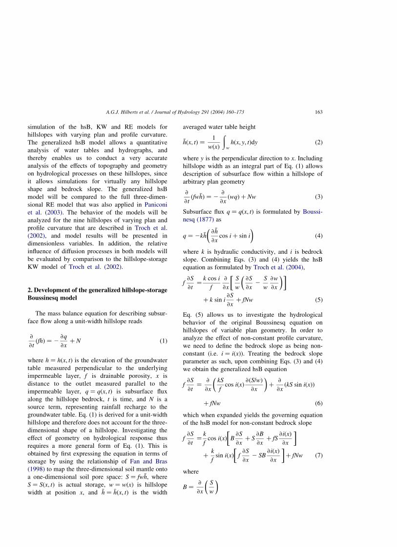
slope). A three-dimensional view of the nine

A.G.J. Hilberts et al. / Journal of Hydrology 291 (2004) 160–173164

hillslopes and the two-dimensional plot of contour

lines and slope divides is given in Fig. 2. The

hillslopes have a flow path of length L ¼ 100 m and

soil depth is set at d ¼ 2 m; corresponding to a

relatively shallow unconfined aquifer. Hillslope

response can be studied by performing either free

drainage experiments after initial (partial) saturation,

or constant recharge experiments to equilibrium. In

Troch et al. (2002) it is noted that for a KW model,

drainage response and recharge experiments contain

the same information of the hydrological model, since

outflow and storage changes in both cases can be

converted to overlapping functions in space and time

by means of dimensional analysis. In this work

we have, therefore, selected drainage response

experiments for a first assessment of the characteristic

response of the three different hydrological models.

4.2. Discretization

In this study for the RE simulations the

hillslopes were discretized using Dx ¼ L=200 ¼ 0:5

m and Dy ¼ wðxÞ=6 m; giving a surface mesh of

2400 triangles. The vertical coordinate was dis-

cretized with Dz ¼ d=40 ¼ 0:05 m yielding a total

of 288,000 tetrahedra. For the hsB simulations Eq.

(7) is discretized in the spatial coordinate

(Dx ¼ 0:5 m) and then solved using a variable-

order ordinary differential equation solver based on

the numerical differentiation formulas. For the KW

Fig. 2. Three-dimensional view (top), and a two-dimensional plot of the contour lines and slope divides (bottom) of the nine hillslopes

considered in this study.

A.G.J. Hilberts et al. / Journal of Hydrology 291 (2004) 160–173 165

model analytical solutions obtained by Troch et al.

(2002) were used.

4.3. Initial and boundary conditions

For all models we impose as an initial condition a

uniformly distributed water table height along the

hillslopes. Water table height is set to �h ¼ 0:40 m

(20% of the storage capacity), for all models. We

selected these initial conditions in order to avoid

occurrence of saturation on the hillslopes, enabling us

to investigate subsurface processes alone in almost all

cases. For the RE model an initial condition of vertical

hydrostatic pressure distribution was used, with a

water table height at 0.40 m vertically above bedrock

level, giving a pressure head value of 21.6 m at the

hillslope surface and 0.40 m at the bedrock. Note that

for the RE model the water table is at 0.40 m above

the bedrock, whereas, the boundary of the saturated

zone is at a higher level, due to the water bound in the

capillary fringe zone.

For all models the bedrock, hillslope crest and

lateral hillslope divides are treated as zero-flux

boundaries. At the outlet free drainage conditions

apply for all models: storage and consequently water

table height is assigned a fixed value of zero

(Dirichlet-type boundary condition) for the hsB and

the KW models. For the RE model the bottom layer

of nodes at the outlet have a constant head boundary

of zero pressure head. To keep the boundary

conditions as close to those of the hsB and KW

model, the nodes in the layers above are assigned a

zero-flux condition. Consequently, only the most

downslope node(s) form an outlet for soil moisture

for all three models.

4.4. Parameterization

In the simulations presented in this paper par-

ameters are used that correspond to those of a highly

conductive sandy loam soil (Bras, 1990): k ¼ Ks ¼ 1

m=h; us ¼ 0:30; ur ¼ 0; b ¼ 3:3; cc ¼ 20:12 m; and

Ss ¼ 0:01 m21: The drainable porosity parameter f in

the hsB and KW models is an ambiguously defined

parameter that in most cases serves the purpose of

representing some of the effects of the unsaturated

zone. This parameter may be interpreted as the

fraction of the total soil volume (matrix and pore

space) that is available for transport of soil moisture.

Typically, drainable porosity is estimated as the

volume of water that an unconfined aquifer releases

from or takes into storage per unit aquifer area per unit

change in water table depth (Bear, 1972). In this study

the drainable porosity is fitted as (Paniconi et al.,

2003)

f ¼ usVtfinal=Vi ð12Þ

where us is saturated moisture content (which is

treated as being equal to porosity), Vtfinal is the

cumulative volume of water drained from the

hillslope in a steady state situation at the end of

simulation and Vi is the initial volume of water

present in the soil calculated on the basis of the results

of the RE model. The drainable porosity is a

dynamical parameter that is dependent on hillslope

shape, initial conditions and other factors, and,

therefore, values for f are different for all hillslopes

and simulation settings. In Table 1 the values for f that

were used to run the hsB and KW models are listed for

the nine hillslopes, and we note that all porosity values

are in the range [0.25, 0.30] except for the 30%

hillslope number 1, for which a lower value is likely

due to the extremely slow subsurface drainage of the

hillslope.

4.5. Dimensional analysis

Differences exist in hydrological system behavior

(i.e. hydrographs, storage profiles) on gently sloping

hillslopes compared to steep slopes. The same holds

for hillslopes with differences in conductivity, soil

depth, hillslope length and for simulations with

different initial conditions. In order to generalize the

results a dimensional analysis is conducted. A

dimensionless representation will lead to model

Table 1

Drainable porosity values (in %) for the nine characteristic

hillslopes used in this study

126, 22 227, 26 325, 26428, 26 528, 27 628, 29728, 27 828, 28 928, 30

The superscript indicates hillslope number. The left number

within a cell corresponds to results obtained on the 5% slopes, and

right number corresponds to the 30% results.

A.G.J. Hilberts et al. / Journal of Hydrology 291 (2004) 160–173166

results that are ‘scaled’ for the parameters mentioned

above. The work of Troch et al. (2002) shows that for

the KW case, simulation results under different

conditions (i.e. varying slope angle, recharge rate,

soil properties, etc.) all collapse into a single

characteristic response function, when the appropriate

dimensionless variables are selected. We define the

following dimensionless variables

t ¼tk�ı

fL

x ¼ 1 2x

L

x ¼x0

L

f ¼QcumðtÞ

Vi

s ¼Sðx; tÞ

ScðxÞ¼

�hðx; tÞ

d

where �ı is the average bedrock slope (in this work 5 or

30%), defined as

�ı ¼1

L

ðL

0iðxÞdx

QcumðtÞ is cumulative flow volume up to time t

QcumðtÞ ¼ðt

0QðtÞdt

where QðtÞ is the outflow at the outlet, and ScðxÞ ¼

fwðxÞd is the storage capacity at a given position on

the hillslope. The variable t defines kinematic time

(Ogden and Watts, 2000) generalized for varying

values for f as in Beven (1981), x defines flow

distance as a fraction of the total length of the

flow path L; and f and s are the new dimensionless

flow and storage variables, respectively. Note that the

variable x is defined differently for the KW model,

when compared to the hsB and RE models, since the

x0-axis of the KW model differs from the x-axis of the

hsB and RE models: the x0-axis is horizontal,

originates from the hillslope crest, and is positive in

the direction of the outlet, whereas the hsB and RE

x-axes originate from the outlet and are positive slope

upward. To intercompare the results the hsB and RE

x-axes have been reversed by using the relationships

above.

As the values of saturated conductivity k and

average bedrock slope �ı increase, and the values of

drainable porosity f and hillslope length along the

flow path L decrease, the hydrological system will

drain more rapidly. Mapping the variables onto a

dimensionless time space using time variable t causes

a scaling (‘compression’ or ‘stretching’) of the time

axis, which facilitates comparison of the results

obtained, since results are scaled for convective

processes and consequently also scaled for the

kinematic component in the flow process. If no

overland flow occurs, differences between dimension-

less outflow hydrographs fðtÞ and dimensionless

storage plots sðx; tÞ can thus be ascribed to diffusion

processes. The flow variable f can be regarded as the

fraction of the total initial soil water storage that has

drained from the hillslope up to kinematic time t; and

the storage variable s is the saturation fraction for a

given time and point on the hillslope. Note that for the

hsB and KW models initial volume of stored water is

defined as Vi ¼ Af �hðx; 0Þ; where A is the slope surface

area, whereas for the RE model it is defined as Vi ¼

Vtfinal: The rationale behind using total cumulative

flow volume instead of Vi as a basis for calculating the

dimensionless flow value for the RE model is that for

the RE model, a fraction of the initial storage will be

retained in the hillslope as residual unsaturated

storage. Values for Vtfinal are slope and simulation

dependent and are directly related to drainable

porosity values through Eq. (12).

5. Drainage response

5.1. Introduction

We will analyze the spatio-temporal behavior of

the three models using pseudocolor plots of (dimen-

sionless) storage patterns sðx; tÞ and dimensionless

hydrographs fðtÞ: In these figures the value of sðx; tÞ

is indicated by color: low values tend towards the blue

end of the spectrum whereas the higher values tend

towards the red end. A scaling bar is depicted next to

all plots. Note that for maximum detail three different

types of scaling are applied: for the convergent slopes

(i.e. slope numbers 1, 4, and 7) the values for s range

up to 0.6, for the straight slopes (i.e. 2, 5, and 8) up to

0.4 and for the divergent slopes (i.e. 3, 6, and 9) up to

A.G.J. Hilberts et al. / Journal of Hydrology 291 (2004) 160–173 167

0.2. Looking at an individual figure, a horizontal

transect for a given kinematic time t will show a

saturation fraction s over the hillslope length fraction

x: A vertical transect of the figures for a given x shows

a dimensionless stage hydrograph: the variation of

saturation fraction in kinematic time t at a given

location x on the hillslope. In all the plots the outlet of

the hillslopes is at x ¼ 1; and the top at x ¼ 0:

An important note on the different coordinate

systems for the models was made in Paniconi et al.

(2003), where it was shown that despite some

differences in hillslope configuration for the hsB and

RE models, the models are fully comparable. This

also holds for the comparison of the hsB and RE

models with the KW model. The KW model has no

diffusion dynamics, making the outflow hydrograph

and storage patterns solely dependent on hillslope

geometry once the appropriate dimensionless vari-

ables have been selected.

5.2. Interpretation of the KW storage profiles for

5 and 30% bedrock slope

In Fig. 3a the dimensionless storage patterns of the

KW models are depicted for all nine hillslopes for a

bedrock slope of both 5 and 30% and different

drainable porosity values. Due to the selection of

appropriate (kinematic) dimensionless variables, sto-

rage patterns for the 5 and 30% bedrock slopes and for

different drainable porosity values all can be collapsed

into one s profile. On all nine slopes we see a clear

propagation of a discontinuity in s in the x; t-domain

without any diffusion characteristics. After initiation

of the simulation, we can trace the tail of the wave by

looking at the line that divides the blue area (zero

storage) from the rest (non-zero values). Note that the

inverse of the tangent to this divide in the x; t-domain

is a measure of dimensionless wave velocity (cel-

erity). Also, note that for equal profile curvature the

propagation of the tail of the wave is identical. For

slope numbers 1, 2 and 3 we see that the tail velocity

decreases as t and x increase, since the slope

steepness decreases near the outlet (i.e. concave

slope profile). For the straight profile shapes (i.e. 4,

5 and 6) we see a constant tail velocity and for the

convex profiles (i.e. 7, 8 and 9) we get an increase in

tail velocity as x and t increase. Note that for the

convex profile shapes, the wave shape tends to

disperse and the s profiles tend to flatten out, as can

be seen for slopes 8 and 9. For slope 7, however, we

see an accumulation, especially in the middle segment

of the hillslope, due to a convergent slope shape.

Whereas the velocity of the wave is determined by

bedrock slope, the storage values are determined by

both plan curvature (through the width function) and

profile curvature.

5.3. Interpretation of storage profiles for 5% bedrock

slope

In Fig. 3b the dimensionless storage profiles for the

hsB model when applied to a 5% bedrock slope are

depicted. Foremost, we notice that the wave front is

less pronounced than for the KW model. Due to

diffusion, strong gradients in storage values (and

consequently in s values) tend to smoothen out. This

effect is clearest for hillslopes 1, 2, 3, 4 and 7 where s

values are significantly lower than for the KW model.

For slopes 1–3 concavity of profile shape causes

strong gradients in storage value (and consequently

large effect of diffusion) and for slopes 1, 4 and 7 the

effect is caused by convergence of plan shape.

Consequently, the diffusive effect of profile curvature

on s profiles is amplified on slope number 1. Slopes 5,

6, 8 and 9 show a relatively good resemblance to the

KW results due to low gradients and, consequently, a

marginal effect of diffusion. This is best illustrated

looking at hillslope 5, where results are very similar to

the KW results except for the front and rear end of the

wave where strong gradients cause diffusion in the

hsB results, whereas, the KW model shows the

expected ramp function during drainage. Note that

for the front end (at the outlet), gradients are a result

of the imposed boundary condition sð1; tÞ ¼ 0:

It is interesting to compare the results of these

relatively simple one-dimensional models (Fig. 3a

and b) to the results of the more complex three-

dimensional RE model when applied to 5% hillslopes

(Fig. 3c). The RE results show a remarkable match

with the results obtained with the hsB model for all

hillslope shapes. On the convergent slopes (1, 4 and 7)

we notice slightly higher s values and a small delay in

drainage for the RE model compared to the hsB

results. On the divergent slopes (3, 6 and 9) the hsB

model produces slightly higher s values and a

somewhat faster drainage. Some irregularities for

A.G.J. Hilberts et al. / Journal of Hydrology 291 (2004) 160–173168

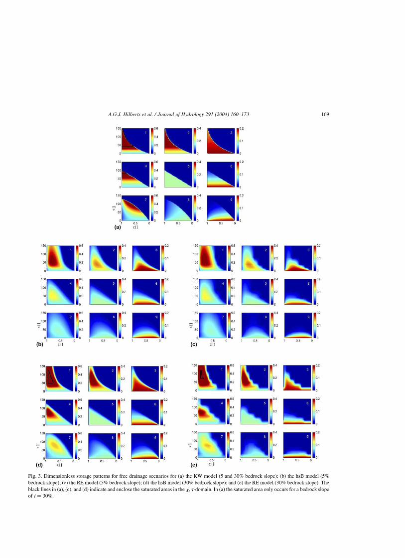
Fig. 3. Dimensionless storage patterns for free drainage scenarios for (a) the KW model (5 and 30% bedrock slope); (b) the hsB model (5%

bedrock slope); (c) the RE model (5% bedrock slope); (d) the hsB model (30% bedrock slope); and (e) the RE model (30% bedrock slope). The

black lines in (a), (c), and (d) indicate and enclose the saturated areas in the x; t-domain. In (a) the saturated area only occurs for a bedrock slope

of i ¼ 30%:

A.G.J. Hilberts et al. / Journal of Hydrology 291 (2004) 160–173 169

low s values are visible in Fig. 3c on slopes 2 and 3, in

particular. They are caused by numerical difficulties

in solving the strong non-linearity in the Brooks–

Corey relations for small pressure head values. This

implies that a finer spatio-temporal discretization is

required for the RE simulations, especially for the

steeper slopes discussed next.

5.4. Interpretation of storage profiles for 30% bedrock

slope

The drainage response on the 30% hillslopes using

the hsB model and the RE model is depicted in Fig. 3d

and e, respectively. Fig. 3e displays numerical

irregularities more clearly than for the 5% RE

hillslopes: practically all slopes now show small

wiggles in the s values. When Fig. 3d and e are

compared, we again see a very good agreement in the

shape of storage profiles in the spatial as well as the

temporal dimension (ignoring the numerical oscil-

lations). Unlike for the 5% hillslopes we now obtain

the best match for the convergent and straight

hillslopes, although the RE model shows a slightly

more diffused pattern. On the divergent slopes the hsB

model has structurally higher storage values than the

RE model, but the shape of the storage profiles and the

timing of the storage peaks in the x; t-domain are in

good agreement. This was also ascertained in

Paniconi et al. (2003), for simulations on slopes

with a straight profile shape (i.e. no profile curvature).

This behavior may be caused by the relatively large

effect of the unsaturated zone on these slopes due to

low storage values.

5.5. Comparison of storage profiles for 5 and 30%

bedrock slope

When Fig. 3d and e (30% hillslopes) are compared

to Fig. 3b and c (5% hillslopes), we notice that the

former two show overall higher s values. This is

caused by the fact that on all 30% hillslopes despite

high gradients in storage values the effect of diffusion

on storage and flow is relatively small when compared

to the effect of increased convection due to high

values for bedrock slope. The small response times on

the 30% hillslopes do not allow for diffusion to take

full effect. This results in an increased accumulation

of storage in the 30% case. On the 5% hillslopes,

however, these counter-balancing processes of con-

vection and diffusion are more dominated by diffu-

sion. A clear indication thereof is that hillslope 1 for

30% bedrock slope generates overland flow, whereas

no overland flow occurs on the 5% hillslopes (see Fig.

3d and e: the saturated area is enclosed by a black

line). The hsB model generates overland flow for

46 # t # 125; the RE model for 72 # t # 122; and

the KW model for 42 # t # 166: The KW results

also show a small saturated area on hillslope 4 for

30% bedrock slope for 81 # t # 100: The large

saturated area in the KW simulations is caused by the

low flow values at the outlet. Due to the absence of a

flow component driven by gradients in water tables in

the KW model, water accumulates at the outlet when

the plan shape is convergent or when the local

bedrock slope is small. In general, the effect of an

increased storage accumulation is clearest for the

convergent slopes where the width function intensifies

the accumulation process, and less pronounced for the

divergent slopes where also due to the width function

diffusion remains a relatively important process.

Thus, the resemblance of the s profiles of both

models for the 5% compared to the 30% slopes is

clearest for divergent slopes. When the storage

profiles of the 5% slopes (Fig. 3b and c) are compared

to those of the 30% slopes (Fig. 3d and e) and the KW

results (Fig. 3a), we notice that the profiles for the

steep slopes show a better match to the KW profiles

than the 5% profiles. Illustrative of this is the

comparison of slope numbers 2, 3 and 4 in Fig. 3a,

b, and d, also indicating that diffusion on the 30%

slopes has less impact on flow and storage of soil

water than on the 5% slopes, as expected.

5.6. Comparison of hydrographs for 5 and 30%

bedrock slope

In Fig. 4 we analyze the (dimensionless) hydro-

graphs of both simulation settings (i.e. 5 and 30%

bedrock slope) and three models (i.e. KW, hsB and

RE) for the nine characteristic hillslopes. We note that

the KW model has the fastest response for all hillslope

types and all bedrock slopes. The hsB hydrograph

shows a fast initial climb for hillslope 1, in particular,

which originates from the fact that the hsB model

produces more overland flow than the RE model on

the 30% slopes, thus draining more rapidly initially.

A.G.J. Hilberts et al. / Journal of Hydrology 291 (2004) 160–173170

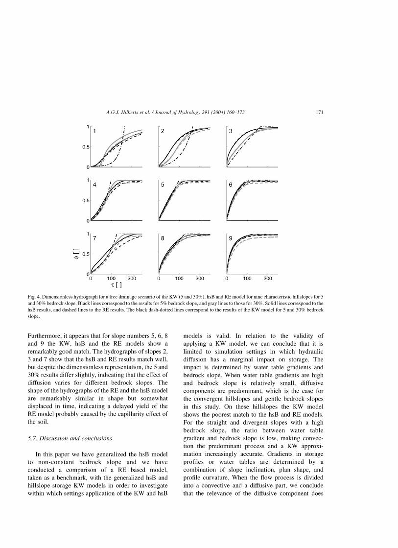
Furthermore, it appears that for slope numbers 5, 6, 8

and 9 the KW, hsB and the RE models show a

remarkably good match. The hydrographs of slopes 2,

3 and 7 show that the hsB and RE results match well,

but despite the dimensionless representation, the 5 and

30% results differ slightly, indicating that the effect of

diffusion varies for different bedrock slopes. The

shape of the hydrographs of the RE and the hsB model

are remarkably similar in shape but somewhat

displaced in time, indicating a delayed yield of the

RE model probably caused by the capillarity effect of

the soil.

5.7. Discussion and conclusions

In this paper we have generalized the hsB model

to non-constant bedrock slope and we have

conducted a comparison of a RE based model,

taken as a benchmark, with the generalized hsB and

hillslope-storage KW models in order to investigate

within which settings application of the KW and hsB

models is valid. In relation to the validity of

applying a KW model, we can conclude that it is

limited to simulation settings in which hydraulic

diffusion has a marginal impact on storage. The

impact is determined by water table gradients and

bedrock slope. When water table gradients are high

and bedrock slope is relatively small, diffusive

components are predominant, which is the case for

the convergent hillslopes and gentle bedrock slopes

in this study. On these hillslopes the KW model

shows the poorest match to the hsB and RE models.

For the straight and divergent slopes with a high

bedrock slope, the ratio between water table

gradient and bedrock slope is low, making convec-

tion the predominant process and a KW approxi-

mation increasingly accurate. Gradients in storage

profiles or water tables are determined by a

combination of slope inclination, plan shape, and

profile curvature. When the flow process is divided

into a convective and a diffusive part, we conclude

that the relevance of the diffusive component does

Fig. 4. Dimensionless hydrograph for a free drainage scenario of the KW (5 and 30%), hsB and RE model for nine characteristic hillslopes for 5

and 30% bedrock slope. Black lines correspond to the results for 5% bedrock slope, and gray lines to those for 30%. Solid lines correspond to the

hsB results, and dashed lines to the RE results. The black dash-dotted lines correspond to the results of the KW model for 5 and 30% bedrock

slope.

A.G.J. Hilberts et al. / Journal of Hydrology 291 (2004) 160–173 171

not solely depend on slope steepness, but also on

water table gradients. The importance of this last

conclusion is that it refutes a widespread belief that

has been based on analyses of straight, unit-width

slopes, namely that bedrock slope alone determines

the validity of the KW assumption. A new criterion

to determine validity of the KW assumption should

therefore be developed.

The most general conclusion with respect to the

validity of the hsB model is that it provides a broadly

accurate description of subsurface storage profiles

and subsurface flow in a hillslope of arbitrary

geometrical shape, in the same way as the hsB

equation for straight slopes was found to be accurate

(Paniconi et al., 2003).

On a more specific case by case basis, a

dimensionless representation enabled us to investi-

gate the influence of diffusion in different simulation

settings. We conclude that the results of the three

models on the 5 and 30% slopes in dimensionless

representation show the best agreement in terms of

storage profiles as well as hydrographs on divergent

slope types due to a relatively low influence of

diffusion, and the poorest agreement on convergent

slopes because of high diffusivity. For convergent

slope forms the KW model loses its ability to

accurately describe water tables and hydrographs,

whereas the hsB model remains close to the RE

solution in all simulations. Analyzing the shape of

the RE and hsB hydrographs, in particular, we see

that the shapes are very similar but the RE

hydrograph is delayed. This is caused by capillarity

effects of the soil. An extension of the hsB and KW

model with a component describing the unsaturated

zone is expected to improve model results

significantly.

A basic assumption underlying the hillslope-

storage concept is that subsurface flow can be

described by saturated flow processes only. This

implies that the unsaturated zone is not expected to

have a large influence on the flow process. A second

assumption is that movement of water through the soil

down the hillslope is parallel to the underlying

impervious layer (i.e. second Depuit–Forcheimer

assumption). This requires marginal head differences

perpendicular to the hillslope bedrock. Both assump-

tions are only valid for relatively shallow, highly

conductive soils. This limits the application of models

based on the Boussinesq equation to these settings.

When the application of the hsB or KW model is

valid, the advantages of these models compared to RE

models are significant, and include computational

efficiency, numerical robustness, scope for analytical

or other simplified formulations, and low-dimension-

ality (implying easier parameterization and cali-

bration).

For the model simulations presented in this

paper, soil properties (e.g. hydraulic conductivity,

soil depth, drainable porosity) are considered to be

spatially uniform over the hillslope domain and

constant in time. Ongoing research is focused on

investigating the impact of spatio-temporal variation

of the model parameters and extension of the model

to incorporate processes as overland flow and

macropore flow.

Acknowledgements

This work has been supported by Delft Cluster

(project DC-030604) and in part by the European

Commission (contract EVK1-CT-2000-00082) and

the Italian Ministry of the University (project ISR8,

C11-B).

References

Bear, J., 1972. Dynamics of Fluids in Porous Media. Dover,

Mineola, NY.

Beven, K., 1981. Kinematic subsurface stormflow. Water Resour.

Res. 17 (5), 1419–1424.

Bixio, A., Orlandini, S., Paniconi, C., Putti, M., 2000. Physically-

based distributed model for coupled surface runoff and subsur-

face flow simulation at the catchment scale. In: Bentley, L.,

(Ed.), Computational Methods in Water Resources, 2. Balkema,

Rotterdam, The Netherlands, pp. 1115–1122.

Boussinesq, J., 1877. Essai sur la theorie des eaux courantes. Mem.

Acad. Sci. Inst. Fr. 23 (1), 252–260.

Bras, R.L., 1990. Hydrology: An Introduction to Hydrologic

Science. Addison-Wesley, Reading, MA.

Brooks, R.H., Corey, A.T., 1964. Hydraulic Properties of Porous

Media, Hydrology Paper 3, Colorado State University, Fort

Collins, CO.

Childs, E., 1971. Drainage of groundwater resting on a sloping bed.

Water Resour. Res. 7 (5), 1256–1263.

Duffy, C., 1996. A two-state integral-balance model for soil

moisture and groundwater dynamics in complex terrain. Water

Resour. Res. 32 (8), 2421–2434.

A.G.J. Hilberts et al. / Journal of Hydrology 291 (2004) 160–173172

Dunne, T., Black, R., 1970. Partial area contributions to storm

runoff in a small New England watershed. Water Resour. Res. 6,

1296–1311.

Fan, Y., Bras, R., 1998. Analytical solutions to hillslope subsurface

storm flow and saturation overland flow. Water Resour. Res.

34 (4), 921–927.

Fipps, G., Skaggs, R.W., 1989. Influence of slope on subsurface

drainage of hillsides. Water Resour. Res. 25 (7), 1717–1726.

Freeze, R.A., 1972a. Role of subsurface flow in generating surface

runoff, 1, base flow contributions to channel flow. Water Resour.

Res. 8 (3), 609–623.

Freeze, R.A., 1972b. Role of subsurface flow in generating surface

runoff, 2, upstream source areas. Water Resour. Res. 8 (5),

1272–1283.

Henderson, F., Wooding, R., 1964. Overland flow and groundwater

flow from a steady rainfall of finite duration. J. Geophys. Res.

69 (8), 1531–1540.

Kirkby, M., 1988. Hillslope runoff processes and models. J. Hydrol.

100, 315–339.

Nieber, J., 1982. Hillslope soil moisture flow, approximation by a

one-dimensional formulation. Pap. Am. Soc. Agric. Engng 82-

2026, 1–28.

Nieber, J., Walter, M., 1981. Two-dimensional soil moisture flow in

a sloping rectangular region: experimental and numerical

studies. Water Resour. Res. 17 (6), 1722–1730.

Ogden, F., Watts, B., 2000. Saturated area formation on convergent

hillslope topography with shallow soils: a numerical investi-

gation. Water Resour. Res. 36 (7), 1795–1804.

Paniconi, C., Putti, M., 1994. A comparison of Picard and Newton

iteration in the numerical solution of multidimensional variably

saturated flow problems. Water Resour. Res. 30 (12),

3357–3374.

Paniconi, C., Wood, E., 1993. A detailed model for simulation of

catchment scale subsurface hydrologic processes. Water

Resour. Res. 29 (6), 1601–1620.

Paniconi, C., Troch, P., van Loon, E., Hilberts, A., 2003. The

hillslope-storage Boussinesq model for subsurface flow and

variable source areas along complex hillslopes: 2. Numerical

testing. Water Resour. Res. 39 (11), 1317.

Pikul, M., Street, R., Remson, I., 1974. A numerical model based on

coupled one-dimensional Richards and Boussinesq equations.

Water Resour. Res. 10 (2), 295–302.

Sloan, P.G., Moore, I.D., 1984. Modeling subsurface stormflow on

steeply sloping forested watersheds. Water Resour. Res. 20 (12),

1815–1822.

Troch, P., van Loon, E., Hilberts, A., 2002. Analytical solutions to a

hillslope-storage kinematic wave equation for subsurface flow.

Adv. Water Resour. 25, 637–649.

Troch, P., Paniconi, C., van Loon, E., 2003. The hillslope-storage

Boussinesq model for subsurface flow and variable source areas

along complex hillslopes: 1. Formulation and characteristic

response. Water. Resour. Res 39 (11), 1316.

Verhoest, N., Troch, P., 2000. Some analytical solutions of the

linearized Boussinesq equation with recharge for a sloping

aquifer. Water Resour. Res. 36 (3), 793–800.

Woods, R., Sivapalan, M., Robinson, J., 1997. Modeling the spatial

variability of subsurface runoff using a topographic index.

Water Resour. Res. 33 (5), 1061–1073.

Woolhiser, D., Liggett, J., 1967. Unsteady one-dimensional flow

over a plane—the rising hydrograph. Water Resour. Res. 3 (3),

753–771.

A.G.J. Hilberts et al. / Journal of Hydrology 291 (2004) 160–173 173