THE GRAVITY FIELD IN NEW GUINEA

by

V. P. St JOHN, B.Sc. (Hons).

Submitted inpartial fulfilment of the requirements

for the Degree Of

Doctor of Philosophy.

UNIVERSITY OF TASMANIA

HOBART

1967

-3_e„4,77 ST, To HA/

OD lilt 63 A 7002 24873606

This thesis contains no material which has been accepted for

the award.of any other degree or diploma in any University and,to the

best of my knowledge and.belief, contains no copy or paraphrase of

material previously published or written by another person, except where

due reference is made in the text of the thesis.

V. P. St JOHN,

University of Tasmania,

October, 1967.

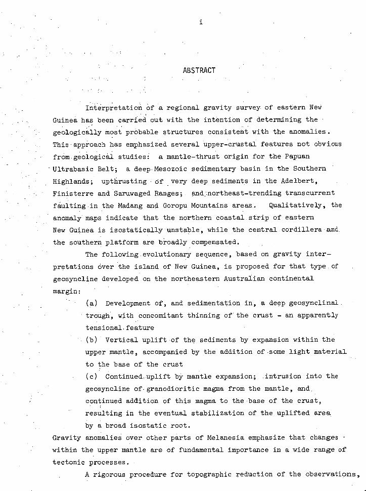
ABSTRACT

Interpretation of a regional gravity survey, of eastern Nevi

Guinea has been carried out with the intention of determining the -

geologically Most probable. structures consistent.with the anomalies.

This-approach has emphasized several Upper-crustal features not obvious

from.geological studies: a mantle-thrust origin for the Papuan

- Ultrabasic Belt; a deep Mesozoic sedimentary basin in the Southern

Highlands; upthrusting Of , very deep sediments in the Adelbert,

Finisterre and Saruwaged Ranges; and:northeast-trendingtranscurrent

faulting in the Madang and Goropu Mountains areas. Qualitatively, the

anomaly maps indicate that the northern coastal.strip of eastern

New. Guinea is isostatically unstable, while the central cordillera and.

the southern platform are broadly compensated.

The following:evolutionary sequence, based on gravity inter-

pretations over the island of New Guinea, is proposed for that type of

geosyncline developed on the northeastern Australian continental

margin:

(a) Development of, and sedimentation in, a deep geosynclinal.

trough, with concomitant thinning of the crust - an apparently

tensional feature

(b) Vertical uplift of the sediments by expansion within the

upper mantle, accompanied by the addition of some light material

to the base of-the crust

(c) Continued,uplift by mantle expansion; .intrusion into the

geosyncline of-granodioritic magma from the'mantle, and.

continued addition of this magma to the base of the crust, - 1

resulting in the eventual stabilization of the uplifted area

by a broad isostatic root.

Gravity anomalies over other parts of Melanesia emphasize that changes -

within the upper mantle are of fundamental importance in a wide range of

tectonic processes.

A rigorous procedure for topographic reduction of the observations,

demanded by the mountainous nature of the region, involves the expression

of the topography as vertical square prisms of the correct density, and

the aggregation of their gravitational effects at the observation point;

the computation being carried out to a distance of 540 kilometres on a

spheroidal earth. Pratt and Airy isostatic anomalies are computed on

the basis of local compensation-of each topographic prism, and the

topographic and isostatic correction procedures . are . combined in a

comprehensive computer program. A running-means smoothing technique

enhances the low-spatial-frequency components of free-air, Bouguer and

isostatic anomaly fields.

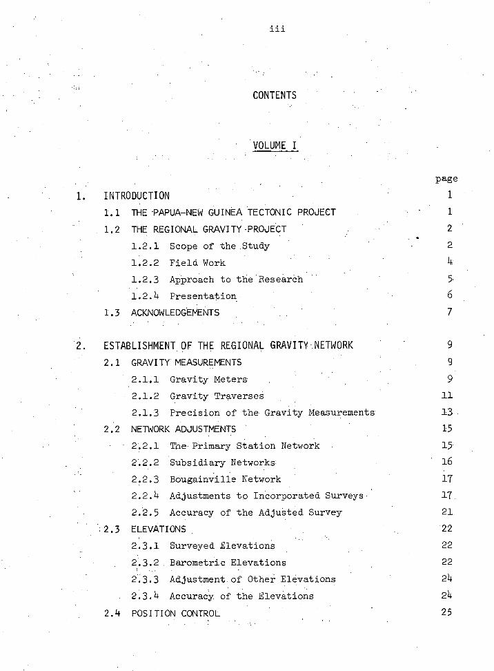
CONTENTS

VOLUME I

I. INTRODUCTION

1.1 THE PAPUA-NEW GUINEA TECTONIC PROJECT

1.2 THE REGIONAL GRAVITY PROJECT

page.

1

2

1.2.1 Scope of the .Study 2

1.2,2 Field Work 4

1.2.3 Approach to the Research 5 , 1.2.4 Presentation. 6

1.3 ACKNOWLEDGEMENTS 7

2. ESTABLISHMENT OF THE REGIONAL GRAVITY - NETWORK 9

2.1 GRAVITY . MEASUREMENTS 9

2.1,1 Gravity Meters 9

2.1.2 Gravity Traverses 11

2.1.3 Precision of the Gravity Measurements 13

2.2 NETWORK ADJUSTMENTS 15

2.2.1 The Primary Station Network 15

2.2.2 Subsidiary Networks 16

2.2.3 Bougainville Network S 17

2.2.4 Adjustments to Incorporated Surveys. 17.

• 2.2.5 Accuracy of the Adjusted Survey 21

:2.3 ELEVATIONS . 22.

2.3.1 Surveyed Elevation's 22

2.3.2 Barometric Elevations 22 •

2.3.3 Adjustment.ofOther Elevations 24

2.3.4 Accuracy of the Elevations 24

2.4 POSITION CONTROL 25

iv

3. REDUCTION OF THE GRAVITY VALUES 26 3.1 GENERAL CONSIDERATIONS 26

3.2 LATITUDE CORRECTION 30 3.3 FREE-AIR CORRECTION 30

3.4 BOUGUER ANOMALIES 31

_3.4.1 The Calculation of a Complete Topographic 34

Effect

3.4.2 Digitization of the Topography 38

3•4.3 Errors in the Bouguer Anomalies 4o

3.4.4 The Bouguer Anomaly Map •41

3.5 ISOSTATIC ANOMALIES 42

3.5.1 General Discussion 42

3.5.2 Calculation of Isostatic Anomalies 45

3.5.3 Errors in the Isostatic Anomalies 49

3.5.4 Contour Maps of Isostatic Anomalies 51

3.5.5 Geological Corrections to Isostatic Anomalies 51

3.6 THE REDUCTION PROGRAM 52

3.6.1 Input 53

3.6.2 Subroutines 55

3.6.3 Output 55 3.7 SMOOTHING THE ANOMALIES 56

3.7.1 Operation of the Smoothing Filter 57

3.7.2 The Three-Dimensional Means Program 61

4. INTERPRETATION OF THE GRAVITY ANOMALIES 65 4.1 DENSITIES OF CRUSTAL MATERIALS 65

4.1.1 Crystalline Rocks 65

4.1.2 Sedimentary Rocks 69

4.2 DIRECT INTERPRETATIONAL METHODS 72

4.3 INDIRECT INTERPRETATIONAL METHODS 74

4.3.1 The Two-Dimensional Computation Program 78

4.4 BROAD SIGNIFICANCE OF THE ANOMALIES 80

4.4.1 Geodetic Implications 80

4.4.2 Structural and Isostatic Implications 86

4.5 DETAILED INTERPRETATION OF THE BOUGUER ANOMALIES 97

4.5.1 Regional Geology of New Guinea 97

4.5.2 The Thickness of the Standard Crust 97

4.5.3 The Bouguer Anomaly Profiles aol 4.6 SYNTHESIS OF THE GRAVITY. INTERPRETATIONAL MODELS :144

4:6.1 Structures Within the Upper Crust 145

4.6.2 Structure of the Crust-Mantle Interface 149

4.7 EXAMINATION OF THE GRAVITY FIELD THROUGHOUT MELANESIA 150

4.7.1 West Irian 150

4.7.2 Banda Sea. 152

4.7:3 'S'alomon Iblands 152

4.7.4 Oceanic Areas North and East of New Guinea 155

5. TECTONIC IMPLICATIONS OF THE GRAVITY INTERPRETATIONS 157

5.1 THE TECTONIC EVOLUTION OF EASTERN NEW GUINEA 157

5.2 SOME TECTONIC PROBLEMS IN MELANESIA DEFINED BY

GRAVITY INTERPRETATIONS, AND SOME SUGGESTED

SOLUTIONS 170

5.2.1 The Apparent Orogenic Sequence on the Island

of New Guinea 170

5.2.2 The Causes of the Orogenic Sequence 176

5.2.3 Further Problems and Possible Solutions 181

POSTSCRIPT 185

REFERENCES 485

APPENDIX I. ELLIOTT 503 COMPUTER•PROGRAMS (503 ALGOL) 193

APPENDED REPRINT (In hard-cover thesis copies only) following p.200

St JOHN,. V.P. and GREEN, R., ,1967 - Topographic and

isostatic corrections to gravity surveys in

mountainous areas. Geophys. Prospect. 15:

151-162.

vi

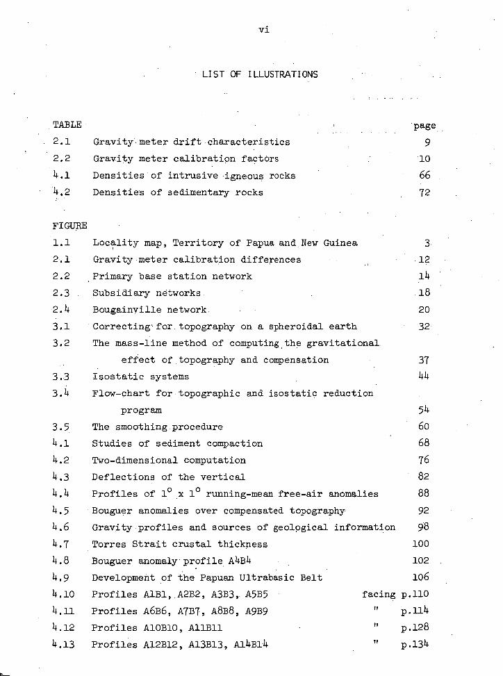
• LIST OF ILLUSTRATIONS

TABLE page

2.1 Gravity meter drift characteristics 9 2.2 Gravity meter calibration factors 10

4.1 Densities of intrusive igneous rocks 66

4.2 Densities of sedimentary rocks 72

FIGURE

1.1 Locality map, Territory of Papua and New Guinea 3

2.1 Gravity meter calibration differences 12

2.2 Primary base station network 14

2.3 Subsidiary networks 18

2.4 Bougainville network 20

3.1 Correcting for topography on a spheroidal earth 32

3.2 The mass-line method of computing the gravitational

effect of topography and compensation 37

3.3 Isostatic systems 44

3.4 Flow-chart for topographic and isostatic reduction

program 54

3.5 The smoothing procedure 60

4.1 Studies of sediment compaction 68

4.2 Two-dimensional computation 76

4.3 Deflections of the vertical 82

4.4 Profiles of 1 0 x 10 running-mean free-air anomalies 88

4.5 Bouguer anomalies over compensated topography 92

4.6 Gravity profiles and sources of geological information 98

4.7 Torres Strait crustal thickness 100

4.8 Bouguer anomaly profile A4B4 102

4.9 Development of the Papuan Ultrabasic Belt 106

4.10 Profiles A1B1, A2B2, A3B3, A5B5 facing p.110

4.11 Profiles A6B6, A7B7, A8B8, A9B9 tt p.114

4.12 Profiles A10B10, A11B11 p.128

4.13 Profiles Al2B12, A13B13, Al4B14 rt p.134

vii

page

4.14 Profiles A15B15,- A16B16 142

4.15 Structures within the upper crust of eastern New Guinea 146

4.16 Structure of the Mohorovicic discontinuity in eastern

New Guinea 148

4.17 Bathymetry of the Solomon Sea 154

5.1 (a) Triassic, Jurassic palaeotectonic map 160

(b) Cretaceous palaeotectonic map

5.2 (a) Palaeogene palaeotectonic map 162

(b) Lower and Middle Miocene palaeotectonic map

5.3 (a) Upper Miocene palaeotectonic map 166

(b) Pliocene palaeotectonic map

5.4 The orogenic sequence in New Guinea 174

FOLDOUT MAPS facing page

Regional gravity stations 24

Smoothed free-air anomalies 64

Extended Bouguer anomalies. 64

Smoothed extended Bouguer anomalies 64.

Pratt isostatic anomalies 64

Airy isostatic , anomalies 64

.Smoothed Airy isostatic anomalies_ 64

Regional geology map 100

New Guinea-Solomon Islands region; generalized Bouguer

'anomalies. 150

VOLUME 2

APPENDIX II. GRAVITY DATA AND COMPUTED ANOMALIES 3 Figures, 15 Maps, 147 pp.

I. INTRODUCTION

Gravity exploration for oil has been carried out in eastern

New Guinea Since 1937, but the various surveys were: unconnected, and of

too limited a coverage to delineate the major structural features of the '

island. This thesis is the record of a study involving

(a) the establishment of a precise regional gravity network over eastern

New Guinea,

(b) incorporation in the regional network of the detailed oil surveys,

with the values reduced on a common datum, and

(c) interpretation of the gravity anomalies in terms , of crustal structure,

providing a basis for a tectonic study of the area.

1.1 THE PAPUA-NEW GUINEA TECTONIC PROJECT

The gravity study is one phase of the Papua-New Guinea Tectonic

Project, established by Professor S. Marren Carey at the University of

Tasmania in 1961. Conceived as a plan to obtain a better understanding

of the tectonic processes previously and presently active in New Guinea,

the project required the synthesis of all available geological and

geophysical data, and its supplementation by further investigations.

Cooperation was given by those organizations in possession of the bulk of

unpublished information accumulated as a result of oil exploration since

1911; viz., Australasian Petroleum Co. Pty Ltd, Island Exploration Co.

Pty Ltd, Papuan Apinaipi Petroleum Co. Ltd, and the Bureau of Mineral

Resources, Geology and Geophysics.

The geological phase - of the project has been concerned mainly with

the area of Papua to the west of Port Moresby, and adjacent parts of the

New Guinea Highlands. J. G. Smith eihesis, 1964), R.P.B. Pitt (thesis,

1966) and A. Kugler (thesis in preparation) have studied three

subdivisions composing this area. J. E. Shirley (B. Sc, Hons thesis,

2

1964) commenced the geophysical phase of the project by connecting to a

common datum several detailed oil company gravity surveys in the Fly River

basin and around the Gulf of Papua (see Appendix II). He also carried

out gravity observations on roads and at some airstrips within Papua and

New Guinea, a total of 180 stations. A Seismic investigation of the

region is at present being carried out by J. A. Brooks, who is studying

crustal structure by Rayleigh wave dispersion.

1.2. THE REGIONAL GRAVITY PROJECT

Following on from the work of Shirley (1964) it became apparent

that the opportunity existed to complete and interpret a.regional gravity

survey of Papua and New Guinea.

1.2.1 Scope of the Study

The project was - resolved - into three studies on - different scales:

First, gravity data extracted by Shirley from oil company files

were to be recomputed on a common datum, and the Bouguer anomalies

contoured on a scale of 1:100,000. Secondly, enough gravity stations

were to be established with a suitable areal distribution to enable

meaningful regional contours to be drawn over all parts of mainland Papua

and New Guinea, on a scale sufficient to delimit all major tectonic

features. The gravity anomalies thus defined were to be interpreted in

some detail in terms of crustal structure, and hence tectonic processes,

in the area. Thirdly, this regional survey was to be combined with

existing observations in West Irian, the Solomon Islands and the adjacent

and intervening ocean areas to obtain a general picture of the tectonic .

state of the Melanesian region.

As the potential source of a real contribution to knowledge of

New Guinea structure the second of these-studies ranked far above the

others, and has accordingly received the most attention.

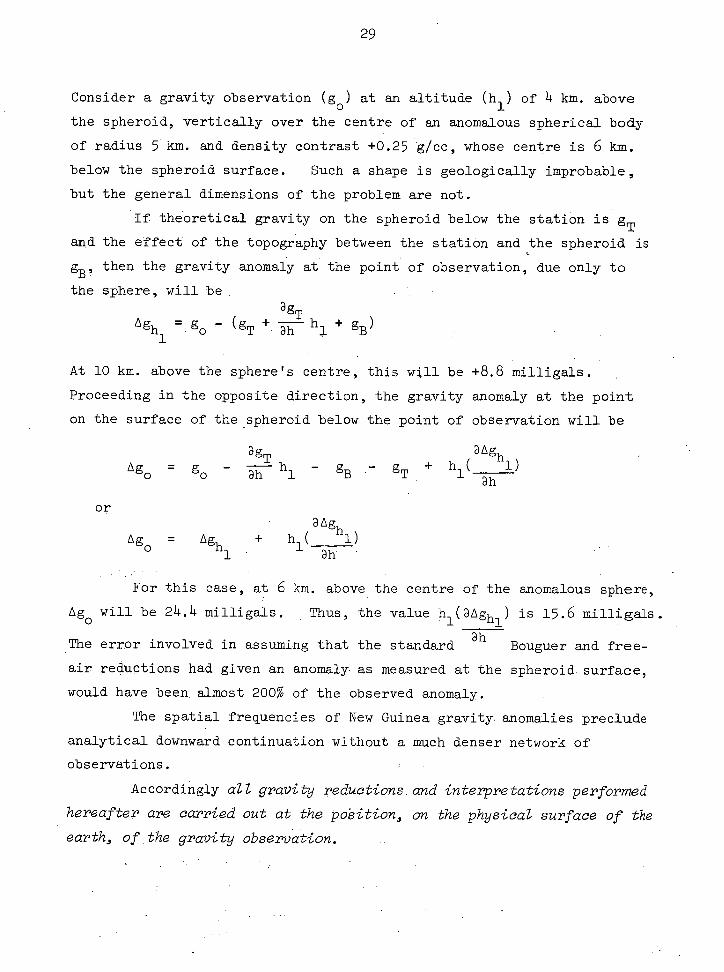
Pa.

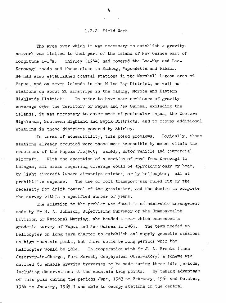
I

ens

\.SOUT E •

,..)HIGH ANDS

era"

'4444,

s

Delta E boymen

WES ERN

Ara

SOLOMON SEA

MOROSE o OU *

10

Marshall °Qs CENTRAL

a Pi

Callingorood Bay'

Co, 'y el Pon. '0

Al/ L NE SAY

••••—•... ADMINISTRATIVE DISTRICT

PAPUA A '.ZZ2 •

I OU/S

g%,44/7c, LOCALITY MAP TP&NG

(>4

Sep i R. MA DA IV G

- • (STERN

,s

NEW

no BRITAIN

c5.

OU

New

'anise Madong

•5,

'WV Kain.•

LAND.!

• • • Lae

41, ' HUON ", PENINSUL

Solo 0 u o

.,

t CIA 7.,.. s- .. ! l'f , \ 0

3 an ..• 4'

a \

TO Popondetti, % 0

e \ k

'3

.i,,

.1, s-i

PORT MORESBY

TORRES STRAIT No,

Vanimo

NEW GUINEA SEPIK

Pio 44,...,0, 4, ak

GULF

GULF OF PAPUA

bad us n id=e

O ISL

NORTHERN Trobrlo nd

Islands

4

1.2.2 Field Work

The area over which it was necessary - to establish a gravity.

network was limited to that part of the island of New Guinea east of

longitude 141 °E. Shirley (1964) had covered the Lae-Wau and Lae-

Kerowagi roads and those.close to Madang, Popondetta and Rabaul.

He had also established coastal stations in the Marshall Lagoon area of

Papua, and on seven islands in the Milne Bay , District, as well as

stations Ion about 20 airstrips in the Madang, Morobe and Eastern

Highlands Districts. In order to have some semblance of gravity

coverage over the Territory of Papua and New Guinea, excluding the

islands, it- :was necessary to cover most of peninsular Papua, the Western

Highlands, Southern Highland and Sepik Districts, and to occupy additional

stations - in'those - districts covered by Shirley.

In terms . of accessibility, this posed problems. Logically, those

stations already occupied were those mostaccessible by means within the

resources of the Papuan Project; namely, motor vehicle and commercial

aircraft. With the exception of a section of road from Kerowagi to

Laiagam, all areas requiring coverage could.be approached onlyby boat,

by light aircraft (where airstrips existed)or by helicopter; all at

prohibitive - expense. The use of foot transport . was ruled out by the

necessity for drift control of the gravimeter, and the desire to complete

the survey within a specified number of years.

The solution to the problem was found in an admirable arrangement

made by Mr H. A. Johnson, Supervising Surveyor of the Commonwealth

Division of National Mapping, who headed a team which commenced a

geodetic survey of Papua and New Guinea in 1963. The team needed an

helicopter on long term charter to establish and supply geodetic stations

on high mountain peaks, - but there would be long periods when the

helicopter would be idle. In cooperation with Mr J. A. Brooks (then

Observer-in-Charge, Port Moresby Geophysical Observatory) a scheme was

devised to enable gravity traverses to be made during these idle periods,

including observationsat the mountain trig points. By taking advantage

of this plan during the periods June, 1963 to February, 1964 and October,

1964 to January, 1965 I was able to occupy stations in the central

5

mountain ranges of New Guinea from Milne Bay to the West Irian border, at

Australian Army survey points around most of the coastline, and at many

points in between. Major J. Hillier, the Officer Commanding the A.H.Q.

Survey Regiment unit engaged at the time in a geodetic survey along the

north coast of New Guinea, gave his cooperation to the project and enabled

me to occupy, by helicopter, stations, on the coast and inland, between

Wewak and the West Irian border. In addition he made a Land Rover and

driver available to enable survey points between Lae and Kainantu to be

occupied, and stations to be established in the highlands between Kerowagi

and the Tomba Pass (west of Mt Hagen). The District Commissioner of the

Western Highlands District, Mr T. Ellis, allowed me to travel on supply

flights from Mt Hagen, and so to make observations at remote airstrips in

the Western and Southern Highlands Districts. The District Commissioner

of the Sepik District, Mr Cole, gave similar assistance with flights out

of Wewak. Survey points accessible by vehicle and foot were occupied

with the help of the Department of Lands at Mt Hagen. To the limit of

the finance available further stations were occupied by sharing charters,

by commercial or mission flights, or by hired vehicle.

During much of both field seasons I was fortunate in having the

cooperation of PFC (later SP)4) Peter S. Lepisto, a gravity meter observer

with the United Station Army Map Service, Far East. He accompanied me

on many traverses, which resulted in a large number of stations having

the double-check of observation by two gravimeters. Further, when

working in separate areas, the pooling of results was of benefit to both.

In this way, I obtained gravity data for the islands off Cape York, and

the coast of Milne Bay.

1.2.3 Approach to the Research

The Field Survey This was approached with one aim in mind:

To have a network of gravity observations distributed as evenly as

possible over the area to be studied. The position, rather than the

number, of stations was regarded as of prime importance during the field

work described above. Hence, the possibility of detailed surveys in small,

6

accessible areas was neglected at times in favour of a few scattered •

stations obtained by aerially hitch-hiking around.remote . areas.. The

philosophy was, and is, that further workers can fill in the detail where

the broad reconnaissance shows-that it is necessary. •

Gravity Reductions Since improper assumptions, which may pass

unnoticed in a low-level survey, could cause large errors in a rugged area

such as New Guinea, the problem of reducing.the observations in a meaning,.

ful way was taken back to first principles. On these lines a program was

developed for complete topographic . and ,. isostatic corrections.

Interpretation . The ambiguity inherent in the inverseproblem of

postulating the unknown scarce or sources Of the observed gravitational

potential field is well known. Except for qualitative estimates by direct

methods, the indirect method of-gravity interpretation has been used, as

is dictated by the scattered nature of the observations. To reduce the

number of variables to be deduced from the gravity field anomalies, it

was necessary to take into account all existing sources of independent -

information. With the exception of. a few seismic and Magnetic investigations,

the independent information comprised the geological mapping accomplished

by workers in the territory, and the hypothesesr based on - their observations.

. Accordingly, I have compiled all available geological information, and

interpretational methods have been directed toward finding in. all cases

the most geologically probable structure consistent with the observed gravity anomalies and any other independent evidence.

1.2.4 Presentation

The thesis is' presented in two volumes'. VOlume One is- the

development of my structural and.tectonic hypotheses, based mainly on the

regional survey of mainland Papua and New Guinea. The investigation is

traced through four stages:

(a) Establishment and precision of the network of gravity observations.

(b) The design and application of a system of - gravity reductions to

produce the gravity anomalies most useful as a source of information on

crustal structure.

(c) The significance of the anomalies, and.detailed interpretation of

the Bouguer. anomaly map in the light of the regional geology.

(d) Postulation of the origin of the deduced structures; and extension of

the tectonic thesis to throw some light on the sources of gravity

anomalies throughout Melanesia.

Volume Two (Appendix II) contains all observed and computed

gravity information, and the contoured'Bouguer anomaly maps, on a scale of

1:400,000, of the recomputed oil surveys in western Papua. Since the

appendix is designed to be complete in itself, for the convenience of any

future worker desiring to commence an investigation from the original

data, there is some reiteration of basic reduction techniques discussed in

Volume One. The oil survey maps are not interpreted in detail, but all

the main anomalies are represented on the regional map, and the inter-

pretation of this takes into accountthe subsidiary anomalies apparent on

the larger scale sheets.

1.3 ACKNOWLEDGEMENTS

I wish to acknowledge the interested and tireless supervision of

Dr. Ronald Green (now Professor of Geophysics, University of New England)

whose inquiring mind was constantly called upon to reactivate my flagging

ingenuity. Professor S. Warren Carey's originality in tectonic thinking

has done much to shape my ideas on New Guinea and elsewhere. He also

gave very considerable financial assistance in the production of this

thesis. The contribution of various organisations and people in making

the field survey possible is obvious from the narrative above (1.2.2).

For assistance then, and subsequently, in the form of survey data, maps

and photos, I must thank Mr H. A. Johnson and the Commonwealth Division of

National Mapping; Colonel Buckland, Majors J. Hillier and E. Anderson

and the AHQ Survey Regiment of the Royal Australian Survey Corps;

Mr J. Cavell and the staff of the TP & NG Department of Lands and Surveys

in Port Moresby, Lae and Mt Hagen.

Members of the Papuan and New Guinea administration . assisted with

air.transport and accommodation,as well as base microbarometer readings.

Mr T. Ellis and Mr L. D. LeFevre, and Pat, were of great assistance in

Mt Hagen. The number of Patrol Officers who put me up for varying

periods in remote outposts is too great to list, but to them I extend my

thanks. The Bureau of Mineral Resources and. Professor J. C. Jaeger

(Australian National University) lent me geodetic gravimeters, and

Mr J. A. Brooks (Bureau of Mineral Resources) gave me office space in

Port Moresby, and his continued cooperation.

The contribution of these people maybe more striking when it is

considered that a regional . gravity survey of more than 300 new stations

covering some 400,000 sq. km . of the territory, and taking a total time

of twelve months, was accomplished for a cost to project funds (apart

from fares to and from Tasmania) of less than eleven hundred dollars.

I am also grateful for the cheerful assistance of.a host of .

Papuans and New Guineans.during the field work, and to Angela Loftus-Hills

for typing. The development of my ideas was - encouraged by discussion

with mycolleagues of the Papuan Project and by Professor Edgar W. Spencer

(Washington and Lee University, Lexington, Va.), who was sceptical.

9

2. ESTABLISHMENT OF THE REGIONAL GRAVITY NETWORK

2.1 GRAVITY MEASUREMENTS

Gravity observations were-made during the periods June 1st, 1963

to January 25th, 1964, and 3rd November, 1964 to 18th January, 1965.

SP4 Lepisto worked in conjunction with me during approximately five months

of the first period, and three weeks of the second. The measurements on

Bougainville were made.by - A. Kugler (University of Tasmania) and SP4.

Dodini of USAMSFE, during September and October, 1963.

2.1.1 Gravity Meters

Drift - The gravity meters used - during the .various surveys, and their

generalized drift characteristics, are summqrized below.

Table 2.1 GRAVITY METER - DRIFT - CHARACTERISTICS

Survey Observer Meter Drift

NG 1963-64 St John Warden Master 548 +O. 03 to 0.08 mgal/hr

NG 1963-64 Lepisto LaCoste & Romberg G24 ±0. 01 mgal/hr

NG 1964-65 St John Worden (geodetic) 201 +O. 02 to 0.07 mgal/hr

NG 1964-65 Lepisto LaCoste & Romberg G23 ±0. 02 mgal/hr

Bougainville Kugler Worden 273 +O. 2 to 0.4 mgal/hr 1963

Dodini LaCoste & RoMberg G12 +O. 02 mga1/hr,

The excessive drift of Worden 273 (a-non-geodetic - instrument) is

undoubtedly due to the number of resets necessary during the boat traverses

on the Bougainville coast, which involved up to 40 hours travelling time

between base readings.

The LaCosteAc Romberg instruments - became - unreadable if internal

temperature compensation was lost'dueto - flat batteries. The Worden

Master, - a similarly-compensated - meter, merely exhibited - negative drift

10

(-0.02 mgal/hr) under the same conditions.

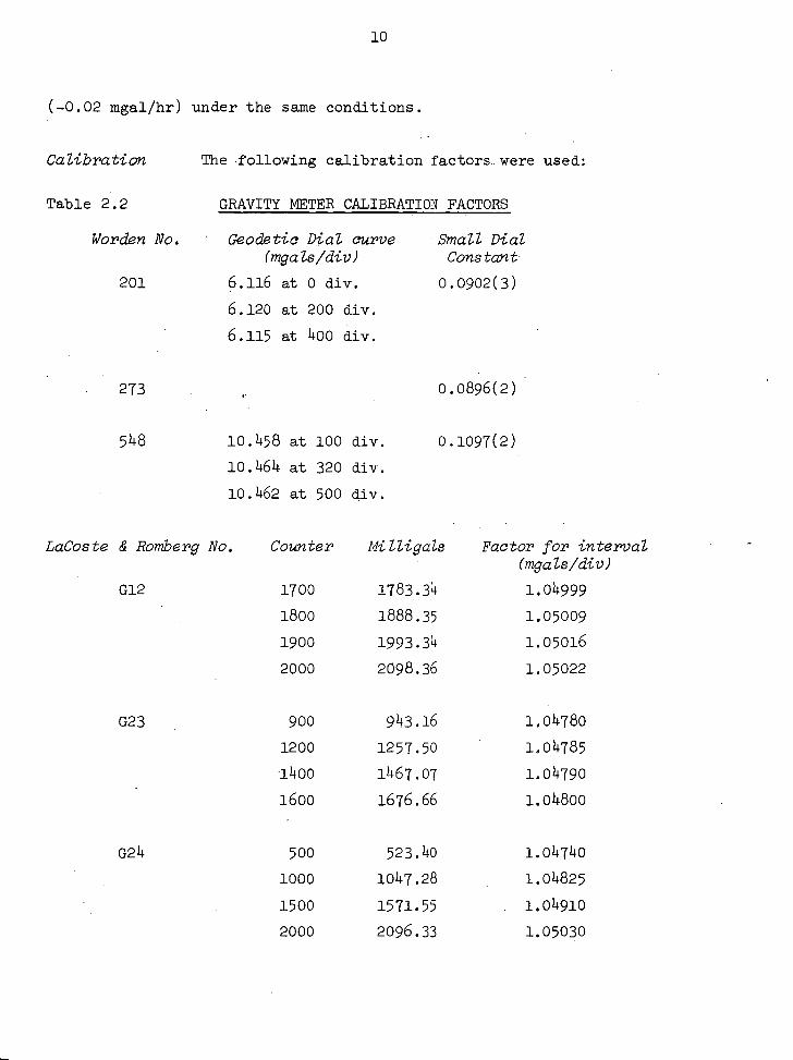
Calibration The following calibration factors_ were used:

Table 2.2 GRAVITY METER CALIBRATION FACTORS

Worden No. Geodetic Dial curve Small Dial (mgals/div) Constant

201 6.116 at 0 div. 0.0902(3)

6.120 at 200 div.

6.115 at 400 div.

273 0.0896(2)

548 10.458 at 100 div. 0.1097(2)

10.464 at 320 div.

10.462 at 500 div.

LaCoste & Romberg No. Counter MiZligals Factor for interval (mgals/div)

G12 1700 1783.34 1.04999

1800 1888.35 1.05009

1900 1993.34 1.05016

2000 2098.36 1.05022

G23 900 943.16 1.04780

1200 1257.50 1.04785

1400 1467.07 1.04790

1600 1676.66 1.04800

G24 500 523.40 1.04740

1000 1047.28 1.04825

1500 1571.55 1.04910

2000 2096.33 1.05030

11

For large gravity differences the meters showed calibration

discrepancies, probably because-none had been calibrated over a range with

intervals between adjacent stations of up to 1000 milligals, as was

sometimes the case in New Guinea. There also exists the possibility

that, although they had been originally calibrated identically, the

variation with time of the calibration factors for different meters was

not uniform. For Worden gravity meters Inghilleri (1959) shows that the

calibration factor decreases with age, with the greatest rate of decrease

occurring directly after construction or repairs. Estimates of the

decrease during the first year range from 0.13% to 0.5%. The LaCoste &

Romberg.meter may have a smaller decrease,.of calibration factor.

Fig.2.1(a) shows comparisons between W548 and L & R G24 and between

W201 and L & R G23. The calibration - of W548 has a non-linear variation

from that of L & R G24, to the extent ofabout +2 milligals per 1000

milligal interval in this range, and both of these meters had been

calibrated by the makers during the preceding year. The comparison of

W201 and L & R G23 carries much less weight, being based on two common

measurements. It indicates a variation of the Worden from the LaCoste

of about -1.8 milligals per 1000 milligal interval. When W201 was read

at stations established previously by W548 the reoccupation error was

smaller than +0.1 milligals for intervals up to .200 milligals, while for

intervals .of 500 to 550 milligals the difference W201-W548 was -0.8 to

-1.0 milligals.

The situation was not, however, as crippling - as might appear from

these comparisons. Most - of the intervals measured were less than 200

milligals, and within this range all four meters-gave values within a

few tenths - of a'milligal. For greater intervals; since it was not known

which meter, if any, was correctly calibrated, the mean values were

taken.

2.1.2 Gravity Traverses

During the gravity traverses layover drift readings were always

taken, thus restricting the effective time between base readings to the

.■•■■ 0

W548 - L & R G24 (mgals) -e 9

••■••

ADJUSTED— D-C•A. ELEVATIONS (metres) o

0

000 • cr) oo

s- CO 0 8 s 0 0 0 e

• •• • • • • • •

8 o

I W201- L&R G23 (mgols) 9

•

•

13

actual travel time. With most traverses by aircraft this wasunder three

hours, although a few helicopter runs were of longer duration. Motor

vehicle traverses often involved from ten to twenty hours travel between

readings at a specified base, but in these cases there was ample

opportunity to re-read previous stations, and establish cross-ties.

This "ladder-loop" method of traversing provided drift control as

effectively as did single two or three'hour traverses. In all cases,

previously-observed stations were reoccupied as often as they were

encountered.

Tidal. Corrections The earth tide effect within the latitudes of

New Guinea can:vary by more . .than 0,3 milligal/hour. Prior to drift

calculations, therefore, it was essential that the tidal effect be.

eliminated. The corrections were obtained from the Tidal Gravity

--Correction tables publishedannually in "Geophysical Prospecting" by the

Service Hydrographique de'la,Marine and Compagnie Generale de Geophysique.

2.1.3 Precision of the Gravity Measurements

Corrected for drift and earth tides, all intervals (mean intervals

if measured by more than one meter) gave reoccupation errors of less than

+0.3 milligal, and usually less then +0.2 milligal. Shirley (196)-)

assigned his survey a possible error of 1 to 2 milligals. This may be

the case for coastal stations in eastern Papua, where the traverses were

not closed. However, with the exception of Kokoda (which was 60

milligals too low) all Shirley's intervals which I have remeasured were

within +0.4 milligal.

In general, the internal precision of the survey, before adjusting

to other surveys, is estimated to be +0.4 milligal.

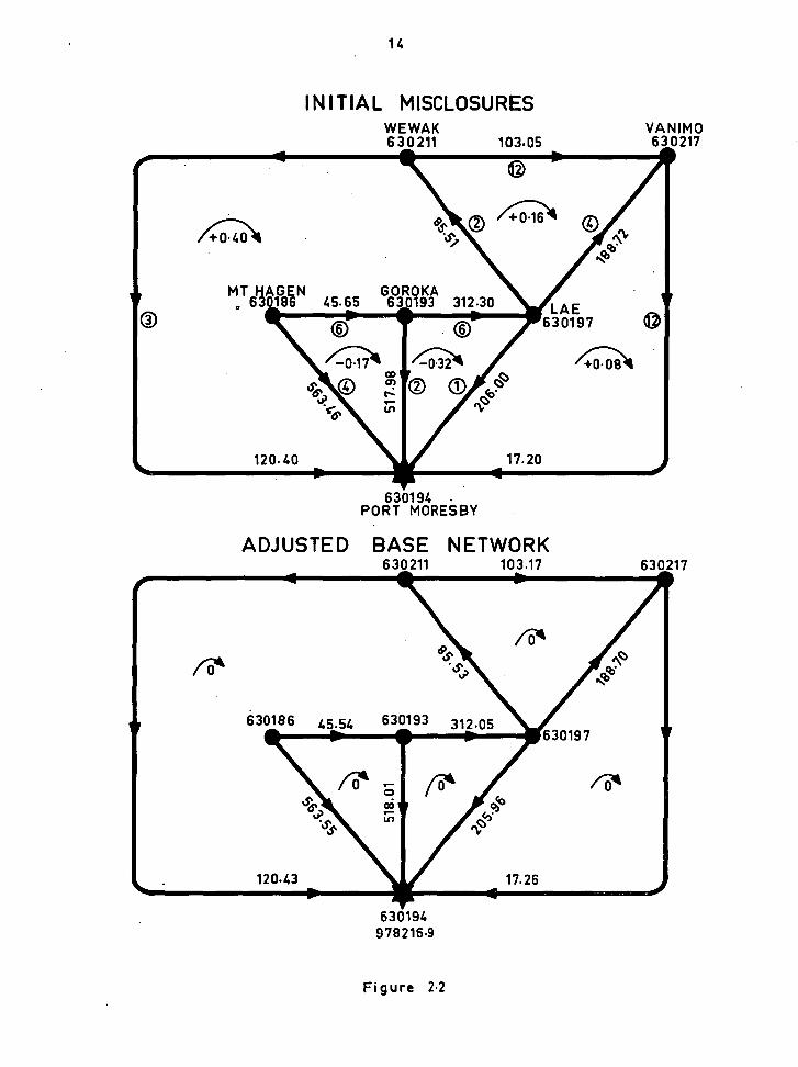
103.05

INITIAL MISCLOSURES WEWAK 630 211

14

MT HAGEN GOROKA „ 630186 45.65 630193 312.30 LAE

•

630197

VANIMO 630217

630194 - PORT MORESBY

ADJUSTED BASE NETWORK 630211 103.17

• •

aik 630186 45.54 630193 312.05

• • 630197

120.43 17.26 • 4

630194 978216.9

630217

71-11.1 1

•

Figure 2•2

15

2.2 -NETWORK ADJUSTMENTS

Owing to a very large number of independent measurements over a

series of stations at major airports, used as base stations for various

sections of the survey, it was decided to adjust these as a primarY

network, and to consider the intervals as fixed when adjusting the

secondary networks.

2.2.1 The Primary Station Network

This is based on the gravity value for the Port Moresby Geo-

physical Observatory (Station 63019)4), given by Woollard and Rose (1963)

as 978,216.9 milligals. The base stations adjusted in this network are

630197 (Lae), 630193 (Goroka), 630186 '(Mt Hagen), 630211 (WeWak), and

630217 .(Vanimo). Apart from observations by Lepisto and' myself in

1963 and 1964, all stations except Mt Hagen (630186) were "observedby

Dr T. Laudon (University of Wisconsin) in 1961, and quoted by Woollard

and Rose (1963). Laudon (pers comm.) also - made observations at

_Moresby (63019)4), Lae and Wewak during a survey from Brisbane to the'

Solomon'ISiandSin 1963. Brewer and Bierig of USAMSFE . (pers. comm.)

made observations at Moresby; Lae-and Wewak during a Southeast Pacific

survey in 1963.

The primary network is shown in Fig. 2.2 . The initial value

for any side is the mean of all observations along that side. As can be

seen from the figure, the combination of observations by eight different

meters Over various sections of the network resulted in a maximum

misclosure of 0.40 milligal.

Following Gibson (19)41), each side of the network is assigned an

adjustability (a) which is defined as

number of stations observed in interval

'number of separate observations of the interval

In the'netwOrk under conSideration the numerator is always unity, since

the observations are direct ties by aircraft. The Moresby-Lae interval,

16

with twelve separate observations, has the lowest adjustability of 1/12 .

Assigning this a unit adjustability the other links receive the values

shown.

Each circuit (i), having a misclosure (q i ), is assigned a

correlate (x.), and the adjustment is made by solving_the simultaneous

equations for n circuits:

a11

x1

*000 +,a x + . j 00•O a x + lii of.16 x +a = q + al2x2 + lj ln n 1

a .. + + a .x + + a x 2nn

= q2 21x 1 a22x2 a2j x j 21 i

ailx, + ai2x2 + + a..x. + + aiixi n n + + ai x =q i lj j

• •••0

a x a x + a .x + + a .x. + + a x = qn nil n22 nj j nil nn n

where a.. is the adjustability.of the side common to circuits i and j, and i

aii is the sum of all adjustabilities.around circuit i.

The five equations representing the primary network were solved,

giving a weighted distribution of misclosures and resulting in the

accepted intervals for the base station network.

Although it was not used as a base, station'630202 at Madang,

having been occupied by Laudon, USAMSFE and many times by myself, was

adjusted in a three-junction circuit involving 630197 and 630194, and

considered as a fixed value in subsequent adjustments. The mis-

closure in this loop was only 0.03 milidgaL

In 1964 the Mt Hagen airstrip base (630186) was tied to a new

base (640600) at the District Office owing to the proposed move to a new

airstrip at Kagimuga.

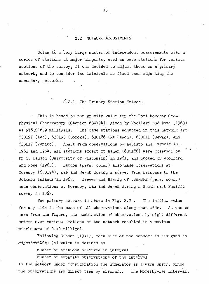
2.2.2 Subsidiary Networks

Networks based on the primary network are shown in Fig. 2.3 .

Heavy lines are used to indicate fixed links, and initial misclosures and

assigned adjustabilities are given. The final values for the stations,

and hence the - accepted intervals, are listed in Appendix II. Any stations

17

not included in the diagrams are those linked to the nearest base by a

straight-line traverse.

Since no network had more than eight circuits the adjustments

were made by manually solving the equations, set up as described in

2.2.1 , either directly or by Gibson's (1941) method of iteration.

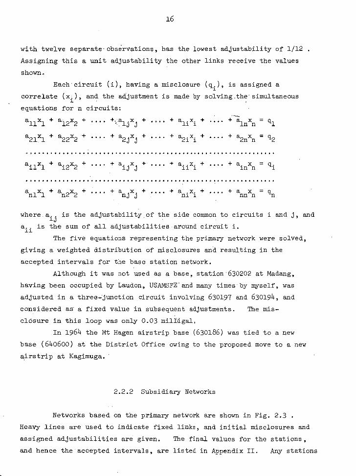
2.2.3 Bougainville Network

Kugler's and Dodini's (1963, pers. comm.) coastal survey of

Bougainville was based on station 630207 (Buka Airstrip). Woollard and

Rose (1963) quote Laudon's 1961 value of 978301.6 milligals for the

station. In reducing the data I have used the value 978302.0 milligals,

based on Laudon's 1963 (pers. comm.) interval measured from 630194 with

the LaCoste & Romberg meter Gl, an instrument with an allegedly near-

perfect calibration.

Traverses on Bougainville formed two networks (Fig. 2.4), one

of four circuits and one of thirty one. The equations for the latter

case were solved by using the Algol Library matrix-inversion procedure

SOLVEQ, incorporated in Program U362 (Appendix I).

2.2.4 Adjustments to Incorporated Surveys

Sections of Shirley's (1964) survey were based on the values of

Woollard and Rose (1963), which have, except for the initial base

(630194), been adjusted as part of the Primary Network. The adjust-

ments, -0.2 milligal for 630197 and -0.5 milligal for 630193, were not

considered sufficiently large to warrant a change in the overall internal

• adjustment of Shirley's survey, and his observed gravity values have, in

most cases, been directly incorporated. Exceptions include those

stations reobserved and adjusted within secondary networks; station

630116 (Kokoda) which was increased by 59.7 milligals after reoccupation

by three meters, and the Wau Road loop (630070 to 630078) which was

decreased by 60.0 milligals after recomputing the original field data.

18

REGIONAL SURVEY SUBSIDIARY NETWORKS

630648 630715 717 714 713 630710

630116 630630 630632

770 0.15

630059

771

630735

630059

PORT MORESBY CALIBRATION LOOP 630219 630614

61

630194 630612 611 610 607

630197

685

681.

683

682

681

6 3 0194 63 019 7

630688 687 686 63 0194 624 626 630601 604 605 606

630659 630674

658 673 630000 630694

630700

630670

669

680

63069

698

696

111

630080 6307 63019

714 620032 630033 .0 630626

630185 630187 630,731

630768

7

-0.06

630774

630733 /6775-*

0732

G. 729

640908 907 630780 630186

640906

905

92

640913 912 911 910 909 630783

640900

40904

640901

630210 630742

630193 630725

630767

640961

630766

903

630755 630211

630186

630756

640955 640953

630752 630750

757 630754 6409

630758 759

760 640959 640957 630211

640902

.730 630728

Figure 2.3

19

Stations from the oil surveys in western Papua were incorporated

in the regional compilation after the observed gravity values had been

recomputed on the Port Moresby datum. Accordingly, no adjustment was

necessary. Chosen on a basis of one per five-minute square, 440 such

stations were used.

The only other survey used was that of Paterson (1958) in the

Upper Sepik - August River area. There is some confusion inherent in the

description by Paterson of the tie between Wewak and the August River

gravity base (station 630809). Information regarding the Wewak station,

supplied to Paterson by the Australasian Petroleum Company, stated that

"The base was located under a solitary thatch hut at the edge of the strip

and the gravity value was 978,099.8 milligals The figures are

based on an absolute value of 978227.7 milligals, outside the Badili

Geological Office, established by Mr Muckenfuss."

There are two airstrips at Wewak, Boram and Wirui, neither of

which possesses a solitary thatch hut. Paterson (pers. comm.) thought

that the strip in question was probably the one now used by the missions

at Wirui. Laudon's measurement (Woollard and Rose, 1963) at the

Catholic Mission Hanger, Wirui, is 978099.9 milligals, which is close to

the base value given above. The interval of -36.4 milligals to the

August River Base was therefore assumed to be from that station, giving

station 630809 an observed value of 978063.4 milligals, which is the

value used in this compilation.

An accurate tie by two meters between the Badili Geological

Office (station 630190) and 630194 introduces an element of doubt into

the above argument. The adjusted value of 630190 is 978224.2, a

difference of 3.5 milligals from the value used as a base for the Wewak

tie, Assuming that the interval 630190- Wewak was measured correctly,

the adjusted Wewak value would be 978099.8 - 3.5 = 978096.3 milligals.

My value for the Boram airstrip station (630211) of the primary

network is 978096.5, which reopens the possibility of the original base

being the Boram strip. There is, therefore, the possibility of an

error of +3.5 milligals in incorporating Paterson's survey. In view of

the size of the anomalies in the area, this error is not excessive.

Twenty four stations of the survey were used, only one of which

OSLLE9

170 610

LLZLI

012 1

ELLLE9

800

600

LOZ

ZZO

000 SOZ BOLL

9L 0

LI LOZOE9

VLOOLE9 LOOLE9

970LE 9 870

OSO

ry.z ain6u

LLLOE9 0 . Z0E8L6 LOZOE9

S7OLE9 SSL

770 E0•0-

E70 ZSL

070

761

ESL

9L •

EL .0 DEL

070

700 LEL

6LtLE9

ULLE9

ELLLE9

900 000

9000E9

700 lE9

9001E9

LO

LEO

LEO LEO

900

SZO

700

EEL

EEL

EL

ZEOLE9

L0.0-

'EL

SEL

9EL

® LEL

BEL 6EL 07LLE9

LOLC9

0E0

LEO

EOOLE9

700LE9

EL

671

6L0- 77L

E00 LEO

0El

6ZLLE9

OLLC9

8000E9 0

600 LEO

8E0

LEO

9E0

SE0

7E0

EECILE9 LOO E9

BL 0

000

600LE9 8100E9

80.0- 7001E9

ZLO

000

890

990

790LE9

OLOLE9 OLL

601

ZBO

780

sou , LOL SOL COL LOL 660 _ L60_ _ 760 _ 060 OtO EIBOLE9

0

E9 ZELL

060, 99L EOZ Nk...L..."'" SO.0 09 SO

t 8 L %...Ofl2/ 7 1. 081- ....2.3., L90 SO ® 0 0 L60 © ® C8L L81.

„\..9.1...0../ 090LE9 NQILy01 ' 19I 06L 7BL

k.I.) ZOZ 000 L6 661. 0 09L

®• Z9L 68L SBL

891 981

LO0LE9

881

69LLE9 09LLE9 961409 . LEILLE9 08L1E9

S>180MAN 3111ANIV91108

0 Z

900 LEO © 7S0

• d) • 80

0801E9

6011E9

21

(630809) was used in anomaly calculations and recorded in Appendix II.

Since the survey was a detailed one over a very restricted area (3 °57'S

to 4 026S and 140 °52.5'E to 141 °14'E) the corrections computed for

630809 were applied to the Bouguer anomalies at all stations.

2.2.5 Accuracy of the Adjusted Survey

Only three misclosures were more than 0.5 milligal, all of them

in circuits involving high mountain traverses. The vast majority of

misclosures were less than 0.2 milligal. Considering the initial

survey precision of +0.4 milligal and assuming that the least squares

adjustment is one close to reality, the adjusted section of the regional

survey is assigned an internal accuracy of +0.6 milligal. • This is also

considered to be a realistic accuracy for the adjusted Bougainville

survey.

The recomputed oil company stations are on the same gravity

datum as the regional survey, and have an accuracy of +0.5 milligals.

Shirley's survey could have a base error of -0.5 milligals for stations

based on 630193. Based on the reoccupation of his stations, the

accuracy of that survey, apart from a few coastal stations in eastern

' Papua, is reliably estimated at +0.5 milligal.

For two small areas, then, the Marshall Lagoon area of eastern

Papua, and the area of Paterson's (1958) survey, the possible survey

error is large; +2 milligals and +3.5 milligals respectively.

For the total regional compilation, apart from these areas, the

accuracy is certainly within +1.0 milligal.

22

2.3 ELEVATIONS

2.3.1 Surveyed Elevations

In the regional survey 171 stations were observed at points with

surveyed elevations, mostly first- and third-order geodetic points, as

listed in Appendix II. Surveyed elevations were also used in the oil

company surveys in Western Papua,

2.3.2 Barometric Elevations

Measurement Where no surveyed elevations were available, heights were

determined by the barometric method° Two Askania Microbarometers were

used, having a reading accuracy of +0.1 m. During a traverse the base was

read at intervals sufficient to define the daily pressure variation.

Pressure variations were converted separately to apparent altitude

variations at the base and at the gravity station. The non-linear

variation of pressure with elevation was accounted for by using the

formula

Ah = 02 -.1 k 1/2 [ 2-] 2 / c.g.s.u. a po ' po

a = gd c.g.s.u. Po

where d = density of moist air in g/cc, at pressure p o .

g = gravitational acceleration.

In practice, the density of moist air was calculated, and

calibration curves constructed, for barometer bases in the two differing

environments of the highlands and coastal lowland or foothill regions.

Ah was assigned a value of zero at p o = 750.00 Torrs in the first case,

and at po = 600.00 Torrs in the second. Corresponding meteorological

data and values of d were:

23

Lowlands: Av. Temp. 29 °C; Av. Rel. Humidity 75%;

Dew Point 23 °C; d = 1.1411 g/litre

Highlands: Av. Temp. 22 °C; Av. Rel. Humidity 60%;

Dew Point 14 °C .; d = 0.93746 g/litre.

The initial values of Ah at base and station were multiplied by a

further correcting, factor to account for the variation of actual

temperature from the assumed average on which 4 had been calculated.

Finally, drift between base readings was distributed as in gravity

traversing.

Adjustment Barometric traverses in lowland areas were always based on

a coastal town, where the initial point of the survey could be tied to sea

level. In highland areas, in the 1963 survey, the barometric bases were _ . _ at Goroka,

one survey

2248.8m.).

KI.3.naJ_ 41qa. and Mt . Hagen, which were barometrically tied to only

point, the National Mapping trig on Mt Murray (Station 630728,

. In both highland and lowland areas internal misclosures were •

less than 5, metres, and were adjusted by the least squares method, the

adjustability of a side, being proportional to the measured interval.

Barometric elevations measured at airstrips differed com.siderably

from altimeter heights given. by the Department of Civil Aviation. In

highland areas, where Shirley (196)-) based his barometric elevations on

airstrip heights, the discrepancy was up to 100 metres..

Prior to the 1964 survey the TP & NG Department of Lands and

Surveys established a third-order surveyed network in the Western and

Southern Highlands, based on National Mapping trig points. Of 19 of my

1.963 barometric stations surveyed, 11 were within 10 m. of the surveyed

value, and two each within 20, 30, and 40 m. The whole network, including

1964 observations, was adjusted to the third order survey, which provided

very good control,and . it is considered that the highland barometric

network, and the (relatively restricted) lowland one both possess an

accuracy of .+10 metres.

24

2.3,3 Adjustment of Other Elevations

The airstrip elevations given by DCA proved to have large dis-

crepancies from those surveyed in by the Lands Department. In Fig. 2.1(b)

the differences between DCA elevations and those surveyed, or tied by

microbarometer to nearby survey points, are plotted as a function of the

elevation given by DCA. As can be expected, the discrepancy is basically

a function of elevation, but there is a very large scatter of results.

Most of Shirley's (196)4) highland stations are based on 630042

(Kainantu) which has been subsequently linked to a Commonwealth Dept of

Works road survey in the Markham Valley. The resulting correction

required 35.0 metres to be added to the elevation of all barometer

stations based on Kainantu. Following the final 1964 adjustments, all

Shirley's stations based on Goroka (630193) were corrected for elevation

by +45.0 metres.

Both in my own and Shirley's surveys, stations were observed in

some cases at airstrips which were not included in barometer traverses.

In these cases, the average correction for the particular DCA elevation

was read from Fig. 2.1(b), and applied.

The elevation of the August River Base Station (630809) was

increased by 20 metres from Paterson's (1958) value after measuring the

elevation of the Sepik River in the vicinity.

2.3.4 Accuracy of Elevations

All surveyed elevations are accurate to +0.3 metre at the outside.

Microbarometer elevations, as finally adjusted, are estimated accurate to

+10 metres. Elevations at airfields, corrected only for the average

probable error, cannot be considered more accurate than +25 metres.

In my survey there are only about five such stations, and less than ten at

any considerable elevation in Shirley's survey.

3 °

1

. 630217

.3.• 60216

. •

' 0

0

,.6Z.

0

silos.,

.140155 '

4.0911

64095" "''''

.30797

',sass

40 630 739 -,..„,,..".

° lin

• 600

63070 •

766

•6.7.0r6'0"

6408 7

0 ,

70742

d.7., 0.61

007

•::::::, 610732 .'"".16

. 0207. • •

•

PAPUA and REGION-AL GRAVITY

STATION BASE STATION

LAMBERT CONFORMAL

NEW GUINEA .

SURVEY

MAP Kr

CONIC PROJECTION

I , I I

CV: - 6409

s 101

26 10069

9 4•6•011S4

.

1.i.°3 •

toss*

640949

8 39

0 .60959 '

• •640901

. . 409117

60926 030700

.64005 C121.3,,,

67001.

a

•

• • ,..,.0 4,60910

•610917

•"" 640941.

.'""' .

14.,2•"lit.,..4:::

,

....2

moos

N. 07091.

•

•00000 ' 6 401129• ...2.7.

•6 40920 •640924

•660927. •00910 014092

.6307611 640915. .670760 .

• „ 1340731 1005 • 6 347 - • 1530772 •• 070

1510110•130 • ••,..,,, 027. •

""6 4016: 5'4 -Aten ' .it- '

"0. 63020

1170017.....,)

svials •S' •6700116

300117

0,0o,

630091

.0064 • 11301001 7020 2

0 70311.

6 620719 •

..,..,,, •."3.

•"•'''' 0170776

.27:0140 720 27

,7 6 0717.6"..027

STANDARD PARALLELS 040. 3.20 , 4-40..7 . 20. 8-40.11-20. •

10 0 SO 100 150 200 260 300

1

I,

I

i

1 N

301117

nem 3017:

610102

•63111 0

, •

67010

08310

• .

a

0

00. . 640912 • 0965

640 967.

•670666

(3 0

• 63055

6306540

6

811.01487186

1 ' 4000000 .

O M

0

070

32403

241

1009•7:'4' •"°' 69 43

. .040150

• 712464 •232470

•212 475

2

27210 4

777170

.20409

• 770.4

•;0•01 •

230460, 10•41040

:"7'3 '2°722 "0 ' 3'

71222 5

• 270411

j,. .q9 7.1q ".2 7 270 5...4,a15,14201'1.

' 070497 •

030407 230Y .30462

01001 • 270427 • 270425 •

• •770427 •270471

•";,*,•:„, • .3001 470 471,20•,.

. •7703111 '3°•"

•...'

64090

• 210211

220252

A •270 207

23020 • 640903

30291 100902

30300

10316

.2222:10.70.771v..

.

.630792 ssons • .•

.

2

•

0300 004027

0,70711

....I...11. 670036

• 6307 27

.00728

630036. 0 70192 „ 02, 12 5 07

6 7 0 1:01 • • V:7:030 4 3

670050 . • 0 7.01502.,0.10211222222 ...1

''" 07004: 1;:t02.25r 67006;

000730

..056

630057 •

' 0630061 0301.8 0670063 11

l0.777" ' .570716

• 0054

' tillili 6 7 .6700. •630005

spans. .67070:21202

67071% 208•••.3°'" 2 „.• „ 1711: 67071

630722 • 63 0 070 0107

0.3 • .67070 630077 •

.6 700711

• 0055 7

.670 662

•00561

5.

,

.

I 332" ."•37137:5 'sass,

2"'•13 r , . 2 • 07271012101912 70776

23220 230370 70 I • 232250 70776

2./5121361 270359

I 237760 210776 1030

I 717136 2.22

2302

I 0201,1.,

I • . 27074

I 73012

702499 • ". 7024

302484.

3007

•33.°33

71F017

7700:

.710064 •31°.

30046 31005

71005 4 270736

6 • :r07191 407775"

r.. .'23: ."‘ 2 6307712

.102472 " 01513

•303100 .103740 33,1,33•

103005. 301763• 003013

poo,

,.. 1025 , _ 7160

2 2.1221 .2 T.,, c ., ?NW; 0,D Pr,,

0715 3 ,81112.1 sas 2 .

' 910115

• 'AT 4 130 " _,•• 7 411;15ueS 1 74‘ a ”000 2219

11104 71707 19 06 •111•12 „sfilias

1112% • 11 0.0.710.0V0767 .4E5 11

*-2}7 ": \gt, 1 ,

VI ..

206 • 122329 ,,,..• 7,,,‘ 0

1, 74issi. • •posso •Inss• ' '"11 1/4-

670010 6 120100

I sum .. :170/SS

.120745 1 2

112070 21101

.1701711 1 1165

021113 ,2,080 0,0,7.

000610 ,., ,., Istr.al.,

670611 276

0630072 ••• 670646

• 67007 7 04

svosl 030074

•670765 ° .30667

0636 •224225

630607 • 224 731

.120370 • 114225 60216. 6706

• 630 660

463108i

60646 .621047

II

I 20270

230 721.

I 7=10 •

• •770211 270674

I 230167* .2 .;110190

' .11111,/,.. •2301517

I • „..iir. •210150

, • 712277 02377 • 21709 1 •Sassss 70 • 2701. . •20267 232741 0 I • 27207 272272

' 2'2"• " 33' 272050

1 0, • 232231 2 n

ss

10274 3 11 31 =24

270272

'

• •

2 77101• ,,,,,, 7

212101 •

. 0020 0 • 230022 ' 02 j12,020 ,;volle .,.. 2330773

f 20091

<;' 0007 7

- •:.

• 0

"3 ,34,3'"0" , •sos.”

710007 IS

Cs %

222117

272 011

• , • 230074

; °... 2...2 .,,

-

. 1 745

it 31 111

01224 301074

1999 297 2

P 13

.

612256 22. kt

•6.70 492 ''''' . .

630/93 • 670

070601 •

61451 • 212 776

•224 253 • 630629

....•

spo rs(c:;:,:,, •::. 26 2 •,,,,„ 7 •630639 09•

410500 27/1111 ."•''' • 630630

222 :11,1 „ 2:6....2.2 4 211 9630673

.224221 •0 200 0 07000 •

20121

610519 • 3•32f2r1 •670 671

670620 • 0630609

ssossr .1.111 6010 • 670577. 24 070524 •

.00175 20

* 706. 111116/

2201:1108 P...

00.0

• 0641

, 2022,,

170.6 3.;,,,,,

670126

630111. ....

°2 •4291.771„. 30120

030644

•

•

.

701 7 5

•

030546

<2 s •

*

400.0 solso

607 •

.21E°:Ii 110706 22 6 07 •670705

.630 605 630601

° 4 l' is'otlir' spooOs .6701150 30704

60693 .630703

1129195

p 01567

70666

• 670661

• 630 0 75 •sposs.

• 610013

'43..3 .

63060 30669

030670

70113

.,...

.70157 0.0 .....,

1 .3°

-

00051

411111 '

•

•

0

0.793 .

2

rail 63

141 ° . 142° 143 ° 144 °

Compiled by: V.P.St John

Geology Department University of Tasmania

1966

145°

.

• 146 ° 147 * , 148 °

2006 292.

222. 6670697

oln° 0201110

1.19 °

03/712 71

I

.. 6700

..150 °

,

6 2

.

610076•

3060 . •

. /10177

,,,, •.423. 2M6Z;y

• 151 .. .

1

• 152.° 08,8,.•

0

.2,2• • . AM.

. 1 °

6'

• 5 37174

277179 27205

272195 232122

232207

272206 . 232 21

272212

7

2324

25

2.4 POSITION CONTROL

Surveyed positions are given to fractions of a second, but can be

considered accurate to within +1 second. All other positions were

obtained from the National Mapping 1:1,000,000 Aeronautical Approach

Charts, which cover New Guinea, the 1:100,000 Border Run series or the

1-mile series covering the Lae-Mt Hagen road area; all published by the

same organization. Locations scaled from these maps are accurate to

better than 0.5 minute.

26

3. REDUCTION OF THE GRAVITY VALUES

3.1 GENERAL CONSIDERATIONS

Implied in the term "gravity reduction" is the concept that the

gravity measured on the physical surface of the earth is converted to the

value which would have been measured at apoint on some reference surface

vertically above or below the actual measurement. The magnitude of the

reduction is dependent upon whether the mass between the measurement and

the reference surface is assumed to have been retained or removed.

It is indeed desirable that such a process should be operative

when a gravity reduction is made. For geodetic investigations it is

essential for the applications of Clairaut's and Stokes' formulae that the

values of gravity be known over the surface of a spheroid and geoid

respectively, inside which all external masses have been transferred.

In investigations of the earth's crust the location of disturbing masses

is simplified if the gravity is known over a theoretical equipotential

surface of an homogeneous earth.

The fact that the classical types of gravity reduction do not give

a theoretical point of observation on the spheroid or geoid, is either not

emphasized or completely neglected by many authors. Dobrin (1960 sect.

11.4) states that the combined Bouguer and free-air reductions, applied to

two observations at different levels on flat terrain, will mathematically

remove the material between the observation points and the datum plane so

that both instruments (the meters making the observations) are effectively

placed on the datum surface. Grushinsk:sr (1963, sect. 11.5) describes

(correctly) the effect of the combined Bouguer and terrain correction as

the flattening and removal of the nearby masses projecting above the geoid.

However, he then says a correction for height (the free-air correction) is

introduced which acts as though the point sank to the geoid. (translation,

pers. comm. from Professor D. A. Brown, Australian National University).

Garland (1965, p. 50) also implies that the combination of Bouguer and

free-air reductions corrects the gravity to sea level.

27

The correct sequence of events is, of course, as follows:

(a) The theoretical value of gravity on a theoretical spheroid

is continued upwards to the elevation of the point of observation; a

perfectly legitimate mathematical procedure since all parameters of this

theoretical body are known. The "indirect effect" can be added to account

for the possible departure of geoid from spheroid, if this is known.

(b) The effect, at the observation point, of all masses outside

the geoid, is calculated and subtracted from the observed value.

The difference between the resulting value and the . theoretical

value is then the gravity anomaly at the point of observation due to

deviations from the theoretical homogeneous density distribution below

the surface of the ,geoidor spheroid. Further reductions, such as

isostatic corrections, are again made by calculating at the point of

observation, the effect of some hypothesized subsurface density distribution,

and subtracting the effect from the observed anomaly.

All or any of these processes, then, leave us with a gravity

anomaly where it was measured, at the physical surface of the earth.

That this is not equivalent to the inverse procedure of projecting. the

observed gravity down (or up) to the geoid.is evident when it is

considered that, after the elimination of the topographic effect, the

observed gravity consists of two parts:

(a) the theoretical gravitational attraction, which can be

projected from the observation point to the geoid, or

inversely, with equal validity, and

(b) the gravity anomaly caused by mass excesses or defects

within the theoretical body.

This second quantity can not be continued up or down unless

its source is known, or tacitly assumed as in analytic continuation

methods.

.Grant and West (1965, p. 269) stress that there exists the

problem of reducing the residual (Bouguer) Values to some level surface

if interpretational methods require the knowledge of such a distribution

of potential. They show that the Bouguer anomalies (Ag)z=h' at the

observation point, can be projected a distance (h) downward by applying the

relation

28

= ( °g ) z.11 - h{} az z=0

(equation 10.1)

which has no counterpart in the reduction of the anomalies at the

observation point.

This distinction between "correcting up" and "correcting down" is

not newly realized. Hayford and Bowie (1912) maintained that the gravity

anomalies, corrected for free-air, Bouguer or isostatic effects, were at

the point of observation. According to Daly (1940, p. 121) "The

officers of the United States Coast and Geodetic Survey calculate the

theoretical value (g c ) of gravity at the level of the station, and express

the isostatic anomaly as g-g." He draws the erroneous conclusion that

this is equivalent to the inverse procedure, as, surprisingly, do

Heiskanen and Vening Meinesz (1958, p. 165). They discuss the difference

between the concepts of reducing theoretical gravity (on the spheroid) to

the observation point and reducing observed gravity to sea level, and

conclude "Naturally, the gravity anomalies will be the same in both cases."

It would be presumption to accuse the several notable geodesists

mentioned above of being unaware of the distinction here discussed.*

Rather, the reason for their apparent lack of concern is undoubtedly due

to the fact that the errors involved are not usually large, since

(a) most of the gravity observations in the world are at

elevations under one or two kilometres, which would combine

with the usual run of geological conditions to give a rather

small continuation effect, and,

(b) for geodetic calculations anomalies are averaged over broad

areas, which would minimize the sum of positive and negative

discrepancies.

However, for surveys involving high altitudes and many large

anomalies originating in the upper crust, as is the case for the New Guinea

survey, large errors could be involved in neglecting the distinction.

In a book just published Heiskanen and Moritz (1967) discuss continuation down from the physical surface of the earth (Chapter 8 - "Modern methods for determining the figure of the earth").

29

Consider a gravity observation (go ) at an altitude (h 1 ) of 4 km. above

the spheroid, vertically over the centre of an anomalous spherical body

of radius 5 km. and density contrast +0.25 g/cc, whose centre is 6 km. below the spheroid surface. Such a shape is geologically improbable,

but the general dimensions of the problem are not.

If theoretical gravity on the spheroid below the station is g T

and the effect of the topography between the station and the spheroid is

gB' then the gravity anomaly at the point of observation, due only to

the sphere, will be

agT Aghi = - go (gT an —

h gB )

At 10 km. above the sphere's centre, this will be +8.8 milligals.

Proceeding in the opposite direction, the gravity anomaly at the point

on the surface of the spheroid below the point of observation will be

agT Ago = go an -1 — gB

+ h (Agh

1) 1 an

or

= + h (aAgh

1 Ag Aghl 1 an

For this case, at 6 km. above the centre of the anomalous sphere, Ago will be 24.4 milligals. Thus, the value hi (aAghl ) is 15.6 milligals.

an The error involved in assuming that the standard Bouguer and free-

air reductions had given an anomaly as measured at the spheroid. surface,

would have been, almost 200% of the observed anomaly.

The spatial frequencies of New Guinea gravity, anomalies preclude

analytical downward continuation without a much denser network of

observations.

Accordingly all gravity reductions, and interpretations performed

hereafter are carried out at the poition, on the physical surface of the

earth, of the gravity observation.

30

3.2 LATITUDE CORRECTION

The basic gravity formula used is that based on the 1930

International Spheroid (Heiskanen and Vening Meinesz, 1958, p. 53).

For theoretical gravity (gT ) as a function of latitude (B)

gT = 978049.0 (1 + 0.0052884 sin2B - 0.0000059 sin

22B) milligals.

The maximum error in latitude has been quoted (section 2.5) as +0.5

minute, which corresponds, in the latitudes of New Guinea, to about

+0.2 milligal.

3.3 FREE-AIR CORRECTION

The free-air correction is based upon the decrease of theoretical

gravity with increasing elevation above the spheroid surface. Although

the departure from constancy of the rate of decrease is small, it is

dependent upon distance from the earth's centre, and therefore upon

elevation and latitude. Since the survey to be corrected ranges over

five kilometres elevation and ten degrees of latitude, it is necessary to

take the variation of the free-air correction factor into account.

The formula of Vyskocil (1960) has been used:

Rf = -0.308772 (1 - 0.001422 sin

2(1)) h + 0.72 X 10

-7h2

where Rf = free-air correction (milligals)

h = elevation (metres)

The accuracy of the free-air anomalies so calculated is dependent

upon the accuracy of elevations. As discussed in 2.3 the vast majority

of elevations used are accurate to +10 metres, while rare stations are

accurate to +25 metres. These correspond to a precision of +3.1 and

+7.8 milligals respectively. Taking the positioning error into account

it is safe to assume an accuracy of +3.5 milligals for free-air anomalies,

31

excepting - those at airstrips . not independently checked for elevation.

As expected; the free-air anomalies correlate very significantly

with local topography, which makes it impossible to contour a rather

sparse survey with stations on many mountain peaks. These anomalies

have therefore been contoured only after a smoothing process has been

applied .(Section 3.7).

3.4 BOUGUER ANOMALIES

3.4.1 The Approach to a true Topographic Correction

Since the topography above the geoid is visible it is logical

that its effect at a gravity station should be removed if one is seeking

to isolate the gravitational effect of hidden subsurface bodies. The

classical reduction of Bouguer (1749) : approximates the effect of

topography to that of an infinite horizontal plate of uniform density (p),

occupying the vertical interval (h) between the reference surface and the

station. This simple Bouguer correction has the value 27Gph, where G is the gravitational constant. The resulting anomaly is the simple

Bouguer anomaly. In order to reconcile this infinite slab with the true topography,

several corrections are usually applied° These include the effect of the

earth's curvature, the effect of terrain . (i.e. masses above the station

level and mass deficiencies below it), and the effect of horizontal

density variations. The resulting anomaly is the extended Bouguer anomaly.

The deficiencies of this "two-step" topographic reduction have

been enumerated by St John and Green (1967), and the arguments will be

reiterated within this discussion. For a local survey in gentle

topography the corrections to the simple BoUguer anomaly will be almost

the same for each station. Accordingly, the simple anomalies may be •

compared with each other within the local survey, although they should not

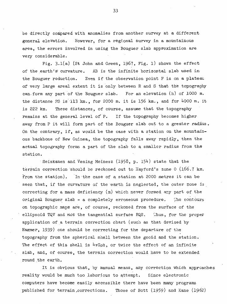
Outer limit of zone 0 where h = zoo° m

A

daidillion

Fr"- II (a)

PRATT

AIRY

Figure 3•1

33

be directly compared with anomalies from another survey at a different

general elevation. However, for a regional survey in a mountainous

area, the errors involved in using the Bouguer slab approximation are

very considerable.

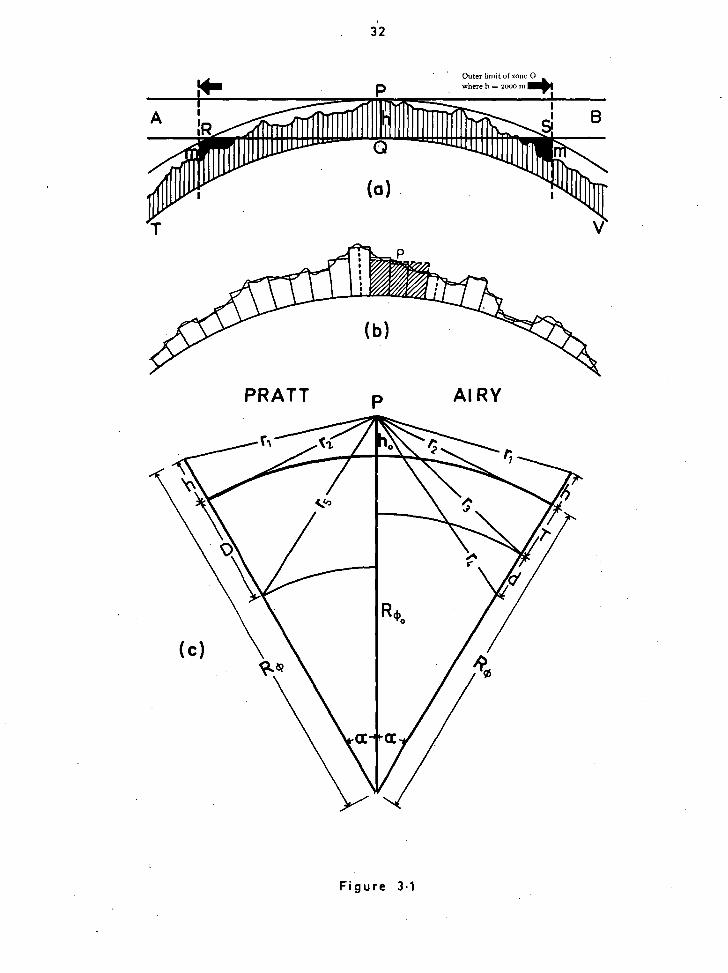
Fig. 3.1(a) (St John and Green, 1967, Fig. 1) shows the effect

of the earth's curvature. AB is the infinite horizontal slab used in

the Bouguer reduction. Even if the observation point P is on a plateau

of very large areal extent it is only between R and S that the topography

can. form any part of the Bouguer slab. For an elevation (h) of 1000 m.

the distance PS is 113 km., for 2000 m. it is 156 km., and for 4000 m. it

is 222 km. These distances, of course, assume that the topography

remains at the general level of P. If the topography becomes higher

away from P it will form part of the Bouguer slab out to a greater radius.

On the contrary, if, as would be the case with a station on the mountain-

ous backbone of New Guinea, the topography falls away rapidly, then the

actual topography forms a part of the slab to a smaller radius from the

station. '

'Heiskanen and Vening Meinesz (1958, p. 154) state that the

terrain correction should be reckoned out to Hayford's zone 0 (166.7 km.

from the station). In the Case of a station at 2000 metres it can be

seen that, if the curvature of the earth is neglected, the outer zone is

correcting for a mass deficiency (m) which never formed any part of the

original Bouguer slab - a completely erroneous procedure. The contours

on topographic maps are, of course, reckoned from the surface of the

ellipsoid TQV and not the tangential surface RQS. Thus, for the proper

application of a terrain correction chart (such as that devised by

Hammer, 1939) one should be correcting for the departure of the

topography from the spherical shell between the geoid and the station.

The effect of this shell is 47Gph, or twice the effect of an infinite

slab, and, of course, the terrain correction would have to be extended

round the earth.

It is obvious that, by manual means, any correction which approaches

reality would be much too laborious to attempt. Since electronic

computers have become easily accessible there have been many programs

published for terrain corrections. Those of Bott (1959) and Kane (1962)

34

have in common the fact that the terrain is digitized and the gravitational

attraction of each compartment is summed at the station. Gimlett (196)4) .

has published a program which lays stress upon the correction for horizontal

density variations due to geological conditions. However these programs,

and other similar ones, merely take the place of conventional terrain

correction charts, by calculating a correction to be applied to the

simple Bouguer anomaly. Consequently, for a regional survey in a rugged

area, they retain all the inadequacies enumerated above.

The "infinite slab" approximation is a crude model that was used

only because of the previous lack of facilities for the computation of a

true topographic effect.

3.4.1 The Calculation of a Complete Topographic Effect

The topographic effect is obviously what was defined at the

beginning of Sect. 3.4 : the effect, at the station, of topography above

the geoid. In other words, it is the gravitational attraction (g) given

by the integration of the effects of all the mass elements [p (cp,x,r) d0Adr]

over a specified section of the spheroid, centred on the observation point

+ ho)], taken out to any desired angular distance (a) from the

station, a.:Cia bounded radially by the geoid and the irregular topographic

surface. (I) is latitude, A longitude and r the radius of the spheroid,

which is a function of latitude. Since the elevation (h) and density (p)

of the topography cannot be expressed as anything but exceedingly complicated

functions of (I) and A , the integral cannot be directly evaluated and must

be reduced to a 'summation.

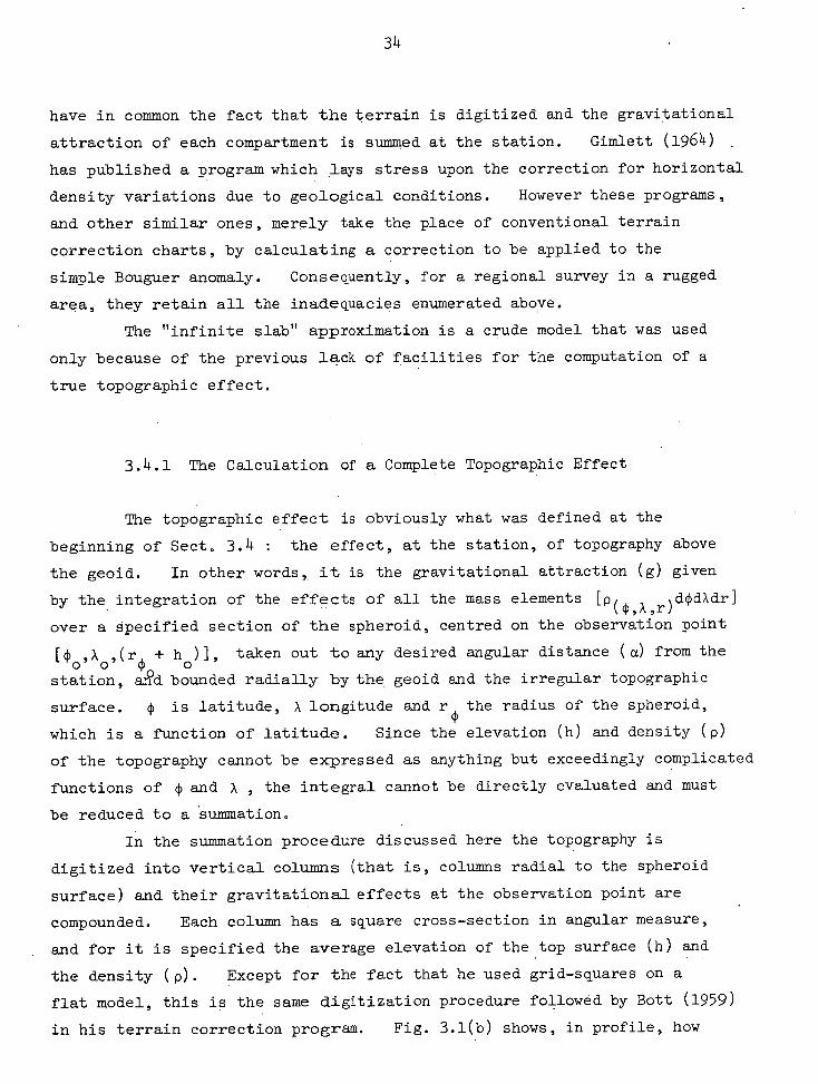
In the summation procedure discussed here the topography is

digitized into vertical columns (that is, columns radial to the spheroid

surface) and their gravitational effects at the observation point are

compounded. Each column has a square cross-section in angular measure,

and for it is specified the average elevation of the top surface (h) and

the density (p). Except for the fact that he used grid-squares on a

flat model, this is the same digitization procedure followed by Bott (1959)

in his terrain correction program. Fig. 3.1(b) shows, in profile, how

35

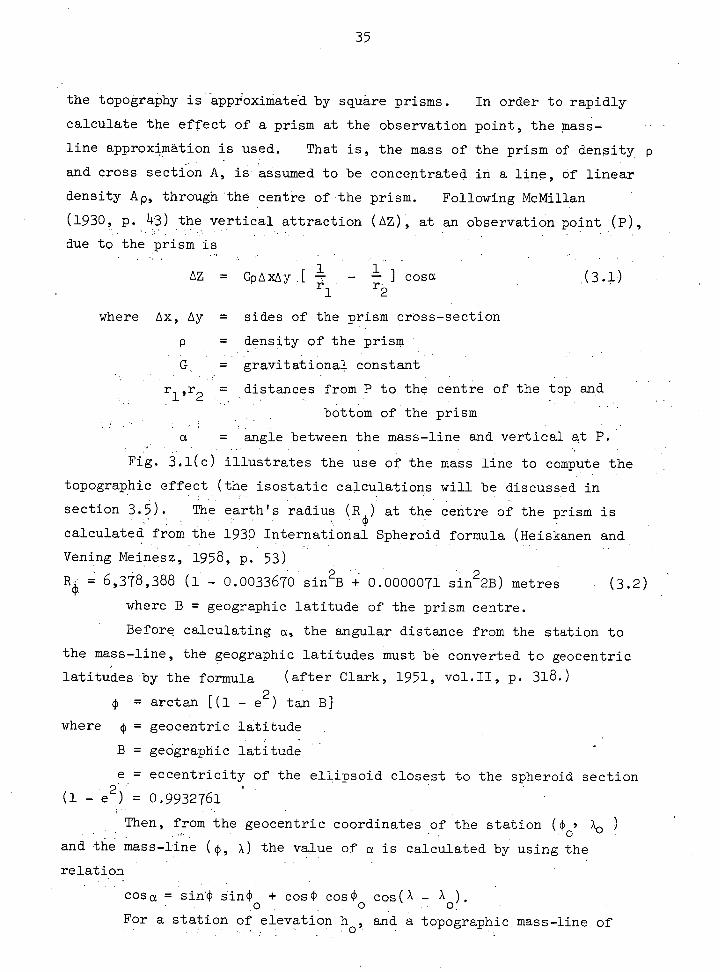
the topography is approximated by square prisms. In order to rapidly

calculate the effect of a prism at the observation point, the mass-

line approximation is used. That is, the mass of the prism of density p

and cross section A, is assumedto be concentrated it a line, of linear

density Ap, through the .centre of the prism. Following McMillan

(1930, p. 43) the vertical attraction (AZ), at an observation point (P),

due to the prism is

(3 .1)

where Ax, Ay = sides of the prism cross-section

density of the prism

= gravitational constant

rr2 = distances from P to the centre of the top and

bottom of the prism

a = angle between the mass-line and vertical at P.

Fig. 3.1(c) illustrates the use of the mass line to compute the

topographic effect (the isostatic calculations will be discussed in

section 3.5). The earth's radius (R) at the centre of the prism is (1)

calculated from the 1930 International Spheroid formula (Heiskanen and

Vening Meinesz, 1958, p. 53) .

= 6 5 378 388 (1 - 0.0033670 sin2B + 0.0000071 sin22B) metres 4), where B = geographic latitude of the prism centre.

Before calculating a, the angular distance from the station to

the mass-line, the geographic latitudes must be converted to geocentric

latitudes by the formula (after Clark, 1951, vol.II, p. 318.)

= arctan [(1 - e 2 ) tan B]

where 0 = geocentric latitude

B = geographic latitude

e = eccentricity of the ellipsoid closest to the spheroid section

(1 - = 0.9932761

Then, from the geocentric coordinates of the station (4) ) .0

and the mass-line (0, x) the value of a is calculated by using the

relation

( 3 . 2 )

cosa = sin' sin 0 + cos cP cos $o cos(A - A ).

For a station of elevation h, and a topographic mass-line of

36*

elevation h, the values of r 1 and r

2 can be obtained by simple trig-

onometrical relations:

2 , • r1

= (R + h)2 + (R + h)2 - 2(R + h )(R + h)cosa

(I) (I) 0 (I)

R2

2(R + h )R cosa r2 2 = (RA, + h )2

° (I)

The linear values of Ax and Ay in formula (3.1) above, are dependent on

latitude if they are initially expressed in angular measure Ayb and AX.

Using the value of R from formula (3.2), the values become: (1)

Ax = R sinAci)

Ay = R sinAcpcosq,

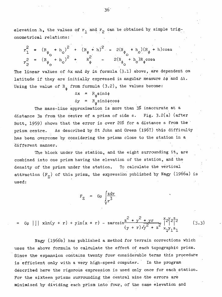
The mass-line approximation is more than 3% inaccurate at a

distance 3s from the centre of a prism of side s. Fig. 3.2(a) (after

Bott, 1959) shows that the error is over 20% for a distance s from the

prism centre. As described by St John and Green (1967) this difficulty

has been overcome by considering the prisms close to the station in a

different manner.

The block under the station, and the eight surrounding it, are

combined into one prism hexing the elevation of the station, and the

density of the prism under the station. To calculate the vertical

attraction (F z ) of this prism, the expression published by Nagy (1966a) is used:

jzdv FZ = Gp 3

Vr

2 2 = GP III xln(y + r) + yln(x + r) - zarcsinz y+ Yr x2Y2 z2

I I I

(y r)/y2 , z2

-r xlylz1

(3.3)

Nagy (1966b) has published a method for terrain corrections which

uses the above formula to calculate the effect of each topographic prism.

Since the expansion contains twenty four considerable terms this procedure

is efficient only with a very high-speed computer. In the program

described here the rigorous expression is used only once for each station.

For the sixteen prisms surrounding the central nine the errors are

minimized by dividing each prism into four, of the same elevation and

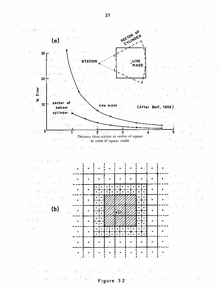
(a)

37

1 • 1

LINE MASS I

(After Bott, 1959 )

2 3 Distance from station to centre of square

in units of square width

• I • • • a •

I • • • •• I • . . . . • a •

• • . • ..

•

• 1 •

•, • —•-.---,f---,t--- • ; •

•, • • 1 • •,- • •

• i • + - •, •

• 1 • - - I.- - •1 • •

_ . 1111Wje

• I

•

•

. I •

11111WX7

•

I •

•

• .

TI■

17

--t -

•

•

I 4.-. ILL I • _

.

•

1 •

•

I •

•, : •, • . - i----t--

•, • •, •

•

a. • :"

. 1 . - + - •, • •

•_ . • . . .

I _ _ I I _ . . I I • I I •

- - -

•

•

Figure 3.2

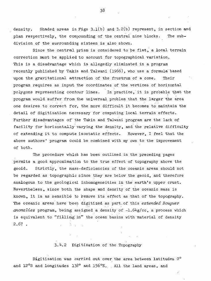
38

density. Shaded areas in Figs 3.1(b) and 3.2(b) represent, in section and

plan respectively, the compounding of the central nine blocks. The sub-

division of the surrounding sixteen is also shown.

Since the central prism is considered to be flat, a local terrain

correction must be applied to account for topographical variation.

This is a disadvantage which is allegedly eliminated in a program

recently published by Takin and Talwani (1966), who use a formula . based

upon the gravitational attraction of the frustrum of a cone. Their

program requires as input the coordinates of the vertices of horizontal

polygons representing contour lines. In practice, it is probable that the

program would suffer from the universal problem that the larger the area

one desires to correct for, the more difficult it becomes to maintain the

detail of digitization necessary for computing local terrain effects.

Further disadvantages of the Takin and Talwani program are the lack of

facility for horizontally varying the density, and the relative difficulty

of extending it to compute isostatic effects. However, I feel that the

above authors' program could be combined with my own to the improvement

of both.

The procedure which has been outlined in the preceding pages

permits a good approximation to the true effect of topography above the

geoid. Strictly, the mass-deficiencies of the oceanic areas should not

be regarded as topographic since they are below the geoid, and therefore

analogous to the geological inhomogeneities in the earth's upper crust.

Nevertheless, since both the shape and density of the oceanic mass is

known, it is as sensible to remove its effect as that of the topography.

The oceanic areas have been digitized as part,of this extendedBouguer anomalies program, being assigned a density of -1.64g/cc, a process which is equivalent to "filling in" the ocean basins with material of density

2.67

3.4.2 Digitization of the Topography

Digitization was carried out over the area between latitudes 00

and 12 °S and longitudes 138 ° and 156 °E.. All the land areas, and

39

adjacent parts of the. sea, were divided into 10' x 10' blocks - 2349 in

all. The New Britain Trench area was divided into 286 15' x 1,5' blocks,

and the remaining sea areas, remote from land stations, were covered by

554 blocks of 0.5° x .0.5° .

Topography and bathymetry Since the gravity survey of New Guinea was

carried out in conjunction with the first geodetic survey it is not

surprising that there are no really well-controlled topographic maps.

There are a number of USAF 1:250,000 maps for the central section of . ,

TP & NG, which have good contours hazed on air photography. The errors

in absolute eleVatiohs On these maps are not large, and the contours are

especially useful in Calculating the local terrain correction . . Apart

from a few wartime 1-mile maps of limited areas the rest of the

topographic information was obtained from "form-lines" on USAF and

National Mapping 1:1,000,000 series maps. It could hardly be said,

therefore, that there is not room for improvement in digitizing New Guinea

topography. HOWever, the shape digitized is certainly a better approx-

imation than a flat plate to the true topography.

Bathymetry of the area was obtained from two sources: the map of

the .southwest Pacific' published by Hess and Maxwell (1949) and the

Monaco bathyMetry map of the south Pacific and Indian Oceans.

Density The densities chosen for the topographic columns were those

most appropriate to the surface geology as depicted on the regional

geological 'Map (p.'100'). Naturally, there are some regions 'where the

surface geology dOes:not account for the whole topographical column.

These include the highland volcanoes, based at least 1000 metres above

sea-level on Tertiary and Mesozoic sediments, and the alluvium-covered

highland flobd-plains of dome rivers. In such cases a weighted average

was taken.

Since few fresh sample's were obtained, the correlation of density

and geology was largely on'a theoretical basis. This is discussed in

considerable 'detail in section '4.1, and the average surface densities

used will merely be stated here:

14o

Quaternary Alluvium 2.1-2.2 g/cc Metamorphics 2.7

"Continental" Volcanics 2.5-2.7 Granite-Granodiorite 2.6-2.75

Pliocene Pelites 2.3 ' Gabbro-DOlerite 2.9-3.0

Pliocene Volcanics 2.7-2.8 Ultrabasics 3.2

Miocene Limestone 2.5-2.6 Unknown "Basement" 2.7

Miocene. "Aure w rocks 2.3-2.4 Basaltic islands 2.7-2.8

Lower Tertiary undiff. seds. 2.5

Mesozoic sediments 2.5

Usually, of course, any one 10' x 10' square would contain more

than one density category. An estimated average was used when this

situation occurred.

3.4.3 Errors in Bouguer Anomalies

The accuracy of the Bouguer anomalies is dependent upon several

factors:

Errors introduced in computation: These are discussed in some detail

by St John and Green (1967), who agree with Bott (1959) that the main

sources of error are

(a) the departure of a mass-line from the true attraction of a

prism, and,

(b) the use of a mean elevation for the top surface of the block.

The actual error varies with the elevation of the prisms proximate

to the station, and has been estimated by the above authors as

(a) negligible for stations near sea level;

(b) less than +1% for stations at the average highland valley

level of 1500 metres; and

(c) less than +2% for the highest stations at 4500 metres.

Errors due to station elevations: For all but a few stations the

elevation is - estimated correct to +10 metres (sect. 2.3). This

corresponds to approximately +2 milligals in the Bouguer anomaly.

Error due_toprismelevations: The central nine prisms are accounted

for, since they have the elevation of the station. Therefore this error

applies only to the prisms outside these (which never contribute more

than ,40% of the total effect). Since accurately-contoured topographic

maps are not _yet available it is difficult to estimate how. wrong the

existing onesare,J, The onlycomment which can be made here is that the

gravity_ values- are corrected for a model based on the known topography -

and all anomalies are self 7consistent.in this.

Error due to wrong densities: The main error here would occur in

assuming the central nine prisms to have the density of the one under the

station, the size of the error depending upon the departure of that

density from the weighted mean of the nine. Again, estimation is

difficult, but a tentative error of +1.5 milligals is assumed.

Error due to local terrain correction: The effect of local terrain

was estimated by.the use of a Hammer-type template and the tables of

Bible (.1962):, The error is again dependent, upon map, accuracy (though

only with respect toa station positioned on the map) but is. certainly .

under 0.5.,milligal0:

When these errors, plus the original observed gravity error, are

compounded it can be.assumed that the topography, as it is known, has

been corrected for to a precision of +5,milligals,

3,4.4 The Bouguer Anomaly Map

About 1000 stations on mainland ,Papua and New Guinea, in addition

to the Bougainville : ones, were, corrected for 'topography out to 5 ° (5)-0 km.)

from the station. The program (U172) is discussed in section 3.6 .

For a station at sea-level the extended and simple Bouguer

anomalies are similar.. For stations in :highland valleys,, at 1500 to

2000 metres, : theextended anomalies are from 10 to 20 milligals algebraically

above. the.,simpqe- anomalies, with the difference becoming 30, to 70 milligals

on mountains over .3000 metres high. Fig. 7 of St.John and Green (1967)

42

shows the great improvement of extended over simple Bouguer anomalies in

removing local elevation correlations.

Contouring has been carried out on an interval of 10 milligals,

the smallest interval commensurate with the precision of the anomalies..

The map is presented on a scale of l: 4,000,000 (p. 64). Naturally, all

topographically-corrected anomalies are on the -physical surface of the

earth, so the map 'must be seen as the projection to a horizontal plane

(sea level) of gravity contours on the earth's surface.

3.5 ISOSTATIC ANOMALIES

3.5.1 General Discussion

An isostatic anomaly is simply the difference between an observed

Bouguer anomaly and one calculated for a subsurface mass-distribution

which compensates for the topographic mass according to some postulated

mechanism of isostasy. Every isostatic mechanism so far postulated

belongs to one of three -hypothetical systems, or is a combination of two

or more of them.

The Pratt hypothesis assumes that, below a depth D, the earth is

laterally uniform. Above that depth adjacent columns of equal cross-

section may have different average densities, but equal masses. . Thus,

the lower-density column will have a greater length than the higher_

density one. On the principle of Pratt compensation, then, a high range

of mountains would be compensated by a column of material, extending to

depth D, of a lower density than a column underlying a sea-level plain

(Fig. 3.3a).

The Airy hypothesis assumes that the earth's crust has a constant

density (d1 ) and constant sea-level-thickness (T), and may - be considered

as a number of columns of equal cross-section floating in a vitreous

substratum of a higher density (d 2 ). - Iceberg-like, the longer columns

stand higher above sea-level and project deeper into the substratum than

do their shorter neighbours. Mountains are therefore compensated by a

43

deep "root" projecting below the Standard sea-level thickness (T)

(Fig. 3.3b).

The Vening MeinesZ regional isostatic system (Heiskahen and

Vening Meinesz,.1958, p. 137) assumes that a topographic load is

compensated for by the elastic bending of a standard thickness - crust

resting on an higher density substratum. What would have been normal

Airy compensation is thus spread out over a wide area, and part of the

load is kept in an equilibrium position purely by'the elasticity of the

crust (Fig. 3.3(c); . Heiskanen and Vening Meinesz, 1958, Fig..5 - 6).

The essential.:difference.between the hypotheses of local and

regional compensation is that the former tacitly assumes that adjacent .

crustalblockeof.different average elevation are separated by zones of

plastic or viscous flow, while the latter does not. The earth's crust,

oi''COUrSe.; - does wt15ehave.as an elastic plate for stresses applied over

an.extended,period_of time. It has a finite viscosity„eStimated by 3 Heiskanen and Vening Meinesz (1958, Ch. 10) to be between 10 2 . and 10

24 7 '

poises, and it also has a definite elastic limit, beyond which deformation

will be plastic The combination of stress-dependent plasticity and

time-dependent viscous flow will first become effective at the planes Al

and A2 of Maxitum vertical stress difference, shown in Fig. .3.3(c)..

The result will be that the central part of the elastically buckled plate

will sink down, and the outer parts will move up, so that the model

approximates the locall'cOMpensated Airy model. Thus, the only real

difference between the two models (Airy and Vening Meinest) is that the

former is time-indetiendent.and the latter is time-dependent; a fact which

follows from the discussiOn,by Carey (1962a) of the time-dependence of

geologic phendmena.

As previously mentioned,: many combinations of the above hypotheses ,

have been advanced as representing more closely the true state of the

earth's.upper layers. 'Hayford and Bowie (1912) used a.Pratt-type system

with 4 depth of Compensation (D) of 113.7 km., measured from the physical

surface of the earth (Fig.. 3.3d) - . In'a later study,'Heiskanen

(in Heiskanen and Vening Meinesz, 1958,.P. 135) assumes a direct

Airy model (Fig. 3.3b) with T . = 30 km., d1 = 2.67 g/cc, and d 2 = 3.27 g/cc.

The same author also suggests (p. 143) a model combining elements of both

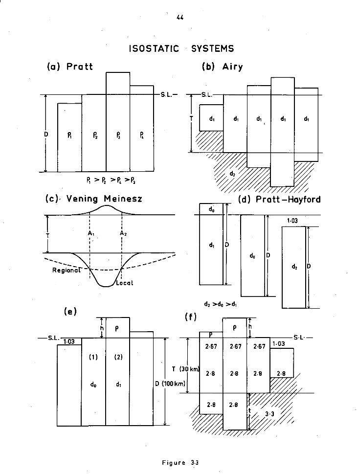
d2

(b) Airy (a) Pratt

P3 P2

> P2 >P4 >P3

(c). Vening Meinesz ) Pratt—Hayford

44

ISOSTATIC SYSTEMS

S. L.

A1 A2

do

1.03

d2 >do > d 1 (e)

—S.L 1.03

(2)

D(

Figure 3.3

45

the Pratt and Airy models, in which 37% of the compensation occurs by

lateral density changes in the crust above the root formations

(Heiskanen and Vening Meinesz, 1958, Fig. 5 - 8.

3.5.2 Calculation of Isbstatic Anomalies

For the New Guinea survey the effects of compensating masses

according to both Pratt- and Airy-type models were compared with

observed Bouguer anomalies.

Pratt isostatic anomalies These are based on an hypothesis of local

compensation of the topographic blocks as digitized for the Bouguer

correction (sect. 3.4). The depth of compensation (D) has been chosen

as 100 km., on the assumption that much of the Pratt-type compensation

must occur within the upper mantle (Hayford and Bowie's (1912) value of

113.7 km. is a little too precise in view of the generalized nature of

the problem).. As shown in Fig. 3.3(e) a column (1) of length D has an

average density do . An adjacent column (2) which supports a

topographic prism of height h and density p, has a smaller average density

d1

. Based upon the principle of equality of mass, rather than equality

of pressure, the following relation holds:

hp + Dd1 = Dd

o

The isostatic effect is, however, independent of the actual

values of d and do

. It is due to the density deficiency

-Ad = d1

- do

of the column supporting the topography.

Thus,

The density difference is assumed to be evenly spread through the

column between the level of compensation and the geoid surface. If a

layered earth, with density increasing downwards, is assumed, every layer

of density d z in column 1 has a density d z - Ad in column 2.

For computing the isostatic anomaly the mass-line approximation is

-Ad = d - d = -11a 1

46

used, as described in Heiskanen and Vening Meinesz (1958, set. 6-3B).

Fig. 3.1(c) shows the geometrical parameters, most of which will have been

previously calculated in obtaining the Bouguer anomaly. The values of r2 ,

a and li (1) are known, and

2 \ 2 r5 = (R D) + (R + h

o) 2 - 2(R - D)(R A, + h )cosa

gbo Po °

As shown above, the density deficiency -Ad is very simply calculated,

depending only upon the topographic mass, and D.

Thus, the Pratt compensation model is very rapidly set up, the

gravitational effect of the compensating column being (from Fig. 3.1(c),

and following equation 3.1),

g -Gn.e-AxAv(1 - 1 )cosa D - r2

r5

The effects at P of all the compensating columns are accumulated,

and subtracted from the extended Bouguer anomaly to give the Pratt

isostatic anomaly.

The model used here is not exactly the same as either the Pratt or

Pratt-Hayford systems. The main distinguishing features are:

(a) The depth of compensation (D) is measured from sea-level; not

the earth's surface, as by Hayford and Bowie (1912).

(b) The actual mass above Sea-level is used. That is, high

topography is not assumed to have a density deficiency in common with its

compensating column.

(c) A layered earth, with density increasing downwards, is quite

in accordance with the hypothesis, provided the required density difference

between adjacent columns is maintained.

Airy isostatic anomalies The system used to. set up the Airy-type

model is again not, to my knowledge, exactly the same as any previous one,

but the differences are minor. It differs from Heiskanen's first

assumption (described above) in that the crustal density is not everywhere

2.67 g/cc., and it differs from his second in that no element of Pratt-

type compensation is assumed. The system is shown diagrammatically in

Fig. 3.3(f). As with the Pratt model, the topographic blocks themselves

play no part in the compensation, being assigned their true density (p).

47

Below the geoid (sea-level) the crust has a density of 2.67, which

increases downwards towards the crust-mantle interface, at which there is

a density increment of 0.5. Standard crustal thickness is assumed to be

30 km,. The actual densities of the crust and mantle are not critical,

the only proviso being that in any horizontal section from the mantle

(considered equivalent to the Airy "substratum") into a crustal root the

density change at the interface will be 0.5 g/cc.

This is equivalent to the concept of an horizontally-layered crust

and mantle, with an interface at 30 km. As long as there are no horizontal

density discontinuities there will be no gravity anomalies. If any

density interface becomes other than horizontal an anomaly will result.

Thus, one might postulate a mountain root, of density 2.9 at depth 50 km.,

adjoining mantle material of density 3.4, while a mantle antiroot at 25 km.

might be of density 3.25, and abut upon crustal material of density 2.75 .

In practice, the density assumedfor the lower crustal layers is dependent

upon vertical density variations in the uppermost mantle. Brooks (1962)

showed that for the New Guinea-Solomon Islands region the average

compressional-wave velocity varied from 7.93 km/sec at 31 km, to 7.88 km/sec

at 65 km. depth. Comparing these velocities with the velocity-density

relationships of Nafe,and Drake (1957) and Woollard (1959) it would seem

that, within the accuracy of the curves, a density of 3.3 g/cc can be -

assumed for the mantle over the whole range of likely crust-mantle

interface depths. Over this range of depths, then, the crust must be

assumed to have a density of 2.8 g/cc, as shown in Fig. 3.3(f).

A crustal configuration such as this Airy model assumes is

certainly not without precedent in the literature. Daly (1940)

postulated a crust consisting of "sial", with a density increasing from

2.70 at the top to 2.90 at the bottom, overlying "sima" of density 2.95

to 3.06 . Seismologists have long explained crustal velocity distributions

by vertical density discontinuities in the crust. Gutenberg (1959,

table 3,4) lists about 50 determinations, in various parts of the world,

of velocities forr;upper "granitic" and lower "gabbro" layers.

Velocities of about 6 km/sec in the upper layer and 6.6 km/sec in the

lower layer correspond approximately to densities of 2.6-2.7 g/cc and

2.8-2.9 g/cc respectively. Other seismic models postulate several

density layers, but it must be remembered that these are purely

mathematical models which fit the pattern of seismic arrivals for some

area. The pattern of seismic layers suggested by Andreev (1959),

based mainly on data for parts of the Soviet Union, Woollard (1959) opines

to be ".... very suggestive of an exponential increase (of density) with

depth".

The crust-mantle density increment which I have assumed is in

accord with the opinion of Gutenberg (1959, p. 51), who finds " .... that

in most regions the difference in average densities above and below the

Mohorovicic discontinuity is probably closer to 0.5 than to 0.6 g/cm3fl

(the latter value being that assumed in the Airy-Heiskanen model).

This last- argument notwithstanding, it might be concluded from the

preceding discussion that the proposed model may have been more realistic

if the density increment at the crust-mantle interface were from 2.9 g/cc

to 3.3 g/cc, or 0.4 ecc. It will transpire, however, in the succeeding

sections of this dissertation, that such a controversy is purely academic,

since the gravity effects of the two equal compensating masses of different

density would be practically the same.

As with the computation of the Pratt anomaly, the Airy system'

assumes local compensation of the topographic columns as digitized for

the Bouguer reduction. The geometry of Fig. 3.1(c) is simply set up.

A topographic column of height h and density p is compensated by a crustal

root of the same cross-section projecting a distance d below a standard'

crust of thickness T, into subjacent material of density contrast +Ap

from the root material. T is specified, and

d--

The chords r3 and /•4 are then calculated:

2 , r3 = (RA + h) 2 + (R - T)

2 - 2(R + h )(R - T)cosa

2 r4 (R h) 2 + (R - T - d)

2 - 2(R + h )(R - T - d)cosa

° (I) °

The effect at P of the Airy compensating column is then

1 1 ,

gA -GApAxAy

/— )cos r3

49

It can be seenthat if h. is negative the expression will have the opposite

sign, being the positive effect of an antiroot. To obtain the Airy

isostatic anomaly the gravitational effects of all the compensating

columns are accumulated at the station, and the result is subtracted from

the extended Bouguer anomaly.

Minimizationerrors due to the mass - line approximation, . As discussed

in section :3.4-1 . the retention of the mass-line approximation for large

cross-section. prisms close to.the computation point could introduce large

errors.. , The vertical quartering of the sixteen prisms outside the central

nine, shown for the. topographic case Fig. 3.2(b), is retained for

isostatic anomalies. However, the rigorous prism formula, used for the

central nine blocks in the topographic correction, is not used in the

isostatic case. , Instead,, the central prism is divided into 10 x 10

vertical prisms, and each of the eight surrounding it into 5 x 5 vertical

prisms . . This is a defensible procedure since the Airy compensating

prisms . are,well below the station (unless it happens to be.on . the . ocean .

floor, which none of mine are). Similarly, the central Pratt compensating

columns are either several kilometres below the computation point or they

are not significantly anomalous.

3.5.3 Errors in,the Isostatic Anomalies

Errors introduced, in computation In the calculation of isostatic

effects the errors due to the mass-line approximation are less critical

than in the topographic case. As calculated by St John and Green (1967)

for the topographic case; the effect of the central 30' x 30' combination

of blocks varies from almost 100% of the total effect at sea,level, to

about 60% at. 4500 metres. To compare this with the isostatic effect

consider.a compensated topographic column 3 km. high. The centre of

gravity of the Pratt. 'compensating column will be . at 50 km. depth, and that

of the Airy at about, 40 km. Taking the simplest approximation of a point

massi- if the gravitational attraction, at a point in the centre of the

top surface .ofthe.topographic column, of .the Airy compensation is 1 unit,

50

then at 40 km. horizontally from the station it will be 0.5 unit and.at

80 km. it will be 0.2 unit. Thus, if we consider the effect of the central

9-block complex as 1 unit, the total effect of the eight similar complexes

around it will be approximately 3 units, that of the sixteen surrounding

them approximately 2 units, and so on. It is obvious, therefore, that

the compensating prisms subject to any considerable mass-line error, those

close to the computation point, contribute no more than 15% of the

isostatic• effect. Because of the subdivision of these prisms, discussed

in the previous section, the error in computing their effect would be

largely due to the innermost subdivisions, and certainly less than 2%.

The total error in using this method for isostatic anomalies is thus less

than

There is a second source of error in the computational method,

which stems from neglecting the convergence towards the centre of the earth

of the bounding planes of the compensating prisms. . The cross-sectional

area of a pyramid with its apex at the centre of the earth is proportional

to the square of the distance from that point. The difference between

the average cross-section of a topographic mass 4 km. high (corresponding to a radius of 6380 km.), and that of its Pratt compensating column (whose

. mid-point is 6330 km. from the earth's centre) is under 1.5%, and would be

slightly less for the Airy case.

The total computation error is the sum of that introduced by the

mass-line approximation and that just discussed. Since the former will

always give a positive error, and the latter a negative one, the total

error caused by computational approximations is less than about 1.2%.

The actual value depends, of course, on the actual isostatic correction at

any point, but should always be less than about 3 milligals.

Errors due to topographic information These have been discussed for

Bouguer anomalies in section 3• 24•3• Since the isostatic correction is

subtracted from the extended Bouguer anomaly one might expect to compound

the errors. This is certainly true of basic observational random errors.

However, errors of topography, density etc., are largely neutralized

since the program works out the effect of compensation only of topographic

blocks as specified: That is, an increment on the Bouguer anomaly due to

51

wrong 'topographic information is accompanied by a similar increment on

the isostatiC effect which is subtracted from.the Bouguer value.

The total possible error in the isostatic anomalies is therefore

about ±5 milligals.

3.5.4 Contour Maps of Isostatic Anomalies

Both Pratt and Airy.isostatic anomalies have been computed for

all stations of the regional survey. They are contoured at 10 milligal

intervals on a scale of 1:4,000,000 (0:). 64 ), A

3.5.5 Geological Corrections to Isostatic Anomalies

It may be argued that the isostatic anomalies computed as

described above are more likely to deviate from zero because of local

geological effects than lack orsurfeit of isostatic compensation.

This_iS'indeed true. In order to better :investigate the isostatic

state of the' crust Evans and Crompton (1946), introduced geological

corrections to isostatic anomalies. For the case of, for example, a

sedimentary basin the correction will consist of two steps:

(a) A correction to the Bouguer anomaly (before the isostatic

effect is subtracted from it) which; removes the negative anomaly

associated with the low density sediments below the geoid; and

('p) 'A correction to the ,computed isostatic effect to account

for the possible self-compensating effect of a sedimentary column.

This second effect can be visualized if.one considers a standard

crustal column of density 2.67 g/cc, from sea-level to 6 km. depth, and

an adjoining sedimentary column, part of a sedimentary basin extending ,

to 6 km..below,sea-level, of.density,,2.2g/ccc A column of the latter ,

density 7.3 km. long is equivalent in mass to - 6 km. of standard crust.

Therefore, the sedimentary basin is complete compensation for topography

1.3 km. high. If the topography were 4.3 km-: high, the second

correction of Evans and Crompton (19)-6) would have the effect of

52

reducing it to 3 km. before setting up the isostatic model.

In the reductions which I have computed, these corrections were

not applied. The reason for this omission is that such 'a correction

could well give a distorted picture of the isostatid state of the crust,

since the application of the geological isostatic correction requires an

even further assumption than those already made in topographic and iso-

static reductions. And the assumption is one with even less basis:

that the subsurface geology is well-enough known to remove its effect

without distorting the true effect of isostatic compensation.

Accordingly, the isostatic anomalies as they stand are examined

with regard to the causation of individual maxima or minima, be it

geological or isostatic. In addition, the detailed interpretation of

the Bouguer anomalies (Ch. 4) takes into account the most probable nature

of upper crustal geology, in Order to deduce the most likely configuration

of the base of the crust, assuming an Airy-type.model.

5:6 THE REDUCTION PROGRAM

The flow chart for the gravity reduction program is given in

Fig. 3.4. Essentially, it is the same as that published by St John and

Green (1967, Fig. 6), except that the subroutine DIVIDE applies only to

the eight blocks surrounding the central one. An additional subroutine

SPLIT is introduced to subdivide the central block for isostatic computations.

The subroutine previously called SPLIT becomes CHOP.

Formulae used, and computational techniques have been explained in

some detail in this chapter, and the Algol program (U172, ISOSTATIC

CORRECTIONS) is reproduced in Appendix I, so the flow chart should need

little amplification. Input and output, and the operation Of sub-

routines will be explained here.

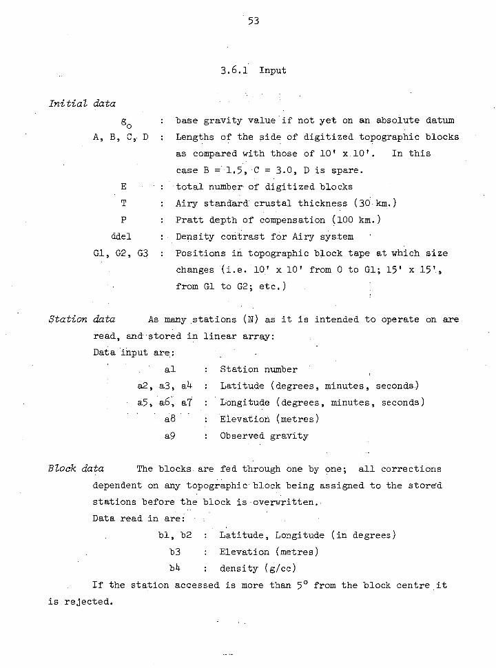
53

3.6.1 Input

Initial data g base gravity value if not yet on an absolute datum

A, B, C, D : Lengths of the side of digitized topographic blocks

as compared with those of 10' x 10'. In this

case B = . 1.5,.0 = . 3.0, D is spare.

.total number of digitized blocks

: Airy standard crustal thickness (30 . km.)

: Pratt depth of compensation (100 km-)

ddel :- Density contrast for Airy system

Gl, G2, G3 : Positions in topographic block tape at which size

changes (i.e. 10' x 10' from 0 to Gl; 15' x 15',

from G1 to G2; etc.)

Station data As many stations (N) as it is intended to operate on are

read, and storedin linear array:

Data input are. :

al : Station number

a2, a3, a4 : Latitude (degrees, minutes, seconds)

a5, a6, at : Longitude (degrees, minutes, seconds)

a8 : Elevation (metres)

a9 : Observed gravity

Block data The blocks are fed through one by one; all corrections

dependent on any topographic block being assigned to the stored

stations before the block is overwritten.

Data read in are:

bl, b2 : Latitude, Longitude (in degrees)

b3 : Elevation (metres)

b4 : density (g/cc)

If the station accessed is more than 5 0 from the block centre it

is rejected.

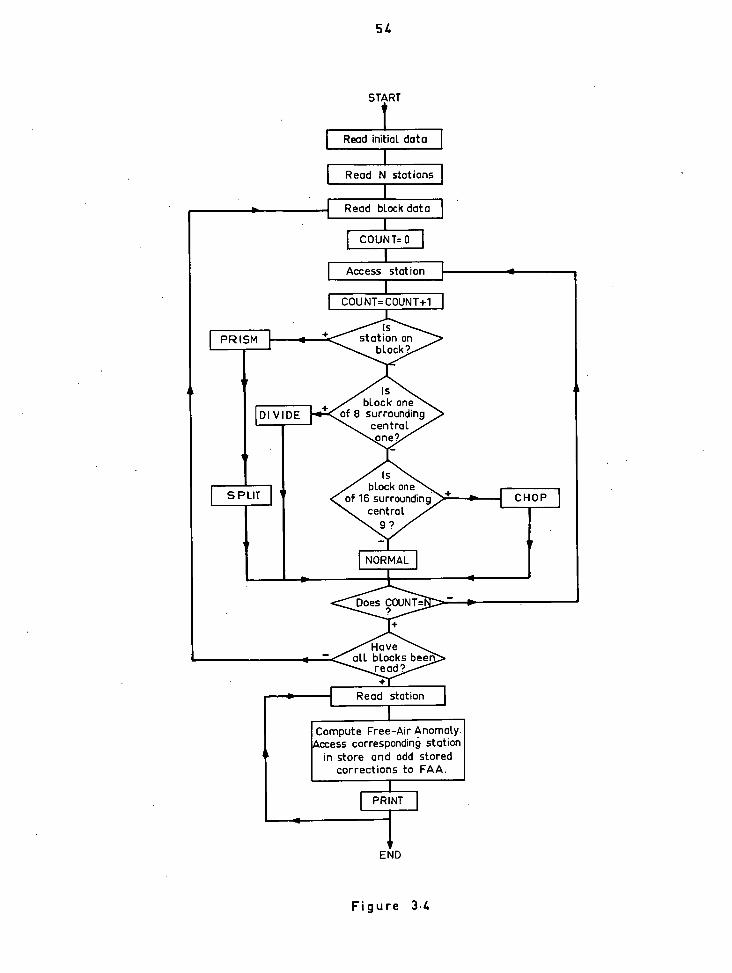
I Read N stations I

Is block one

of 8 surrounding central one?

Is block one

of 16 surrounding central

Compute Free-Air Anomaly. Access corresponding station

in store and add stored corrections to FAA.

PRINT

Read station

54

START

Read initial data

END

Figure 3.4

55

3.6.2 Subroutines

PRISM : If the station accessed is on the block, the topographic

effect is computed by the rigorous formula '(3.3).

SPLIT' : The topographic prism is subdivided 10 x 10 times, Pratt and

Airy models are set up for each sub-prism, and the isoStatib -

effects of these models are summed at the Station.

DIVIDE : If the block is one of eight surrounding the central block its

topographic effect has been overruled by PRISM. It is . Sub

divided 5 x 5 times, Pratt and Airy models are set up for each

sub-prism, and the isostatic effects are summed at the station.

CHOP If the block is one of the sixteen surrounding the central

nine it is subdivided 2 x 2 times. The topographic and

isostatic effects Corresponding to each sub-block are

calculated and summed at the station.

NORMAL : This is the normal routine for all blocks except the 25 closest

to the accessed station. Using the mass-line the topographic - „

and isoStatic effect's are Calculated at the station.

3.6.3 Output'

After all the blocks have been read through, the topographic,

Pratt and Airy effects of each will have been acCumulated in the three

store locations set aside for each station:

aa[j+5] Topographic effect

• aa[j+6] . Pratt isostatic effect

aa[j+7] Airy isostatic effect.

• The station tape is then read through again. Each static:in

locates the corresponding station in the Store -, and the following steps

result: •

(a) Theoretical gravity ., free-air anomaly and simple 136 .11g-der

anomaly for the station are Calculated.

(b) The total stared topographic cOrrection is subtracted from

the free-air anomaly to give the extended '8Ouguer anomaly.

56

(c) The total stored Pratt and Airy corrections are separately

subtracted from the extended Bouguer anomaly to give the Pratt and Airy

isostatic anomalies.

(d) The following parameters are then output: station number,

latitude, longitude, elevation, observed gravity, theoretical gravity, free-

air, simple Bouguer, extended Bouguer, Pratt and Airy anomalies.

The process is repeated for each station.

The computer output for the regional survey is resented in

Appendix II, pp. 111-127. The station numbering is also explained in that

Appendix (section 11.2).

3.7 SMOOTHING THE ANOMALIES

Techniques of smoothing, filtering, regional-residual separation,

and so on, have been used for some time in the treatment of geophysical

data (e.g. Peters, 1949; Elkins, 1951; Dean, 1958). The purpose of such

techniques is essentially the same as that of the original gravity

reduction - to remove the gravitational disturbance due to one source, in

order to reveal or enhance other gravity anomalies which may have been

masked by it. Whether these techniques do, in fact, achieve their

objective is a matter Of some debate.

As the gravity reduction becomes more specialized, so does the

number of assumptions become greater. Free-air anomalies involve only the

assumption that the geoid is the spheroid, and even this can be eliminated

by the indirect correction. Bouguer anomalies involve the further

assumption that the shape and mass of the topography is known, and rightly

corrected for. Both these assumptions can, however, be justified to an

ever-increasing degree by careful observation and detailed calculation.

The isostatic anomaly involves the assumption that isostasy, if operative,

is consistent with some particular system. It also assumes that either

there is no super-isostatic . inhomogeneity in the crust, or that these are

correctly allowed for (the geologicalcorrection).

57

Smoothing techniques (if they are intended to provide

information about some particular level within the earth), need

not follow all the above assumptions, since they can be applied to

any type of anomaly. However, they do involve the further assumption

that low-spatial-frequency anomalies can be correlated with deep sources,

and high-frequency anomalies with shallow. The latter correlation

is usually fairly well justified, the more so the higher the frequency.

On the other hand, the rejection or retention of low frequencies as

being due to deep crustal or upper mantle sources is often rather

dangerous. For example, a broad sedimentary basin can give an anomaly

identical to one produced by an isostatic root. Upper-crustal geological

features of large areal extent, and unknown depth and density, are

undoubtedly present in the New Guinea region. Thus, unless independent

corroborative evidence were available, it would be unwise to assume that

the low-frequency anomalies revealed by smoothing techniques were

directly interpretable as being due to deep sources.

On the other hand, a proper smoothing of an anomaly field can be

of value in revealing major tectonic trends in an area. For a given

station density there is a maximum frequency in the spectrum of the

gravity field about which one can obtain valid information. If the

spectrum contains frequencies higher than this maximum they must be

removed before interpretation of the data. Since gravity observations

in New Guinea were made on high mountain peaks, as well as in adjacent

valleys, the strong topographic correlation inherent in free-air anomalies

resulted in gradients of some hundreds of milligals within very short

horizontal distances. If the free-air anomaly field was to be inter-

preted at all it was essential that such high frequencies be eliminated

from its spectrum. Extended Bouguer anomalies and Airy isostatic

anomalies were also subjected to smoothing in order to remove the sharper

anomalies due to geological causes. Naturally, all indirect inter-

pretation was carried out using the original anomalies.

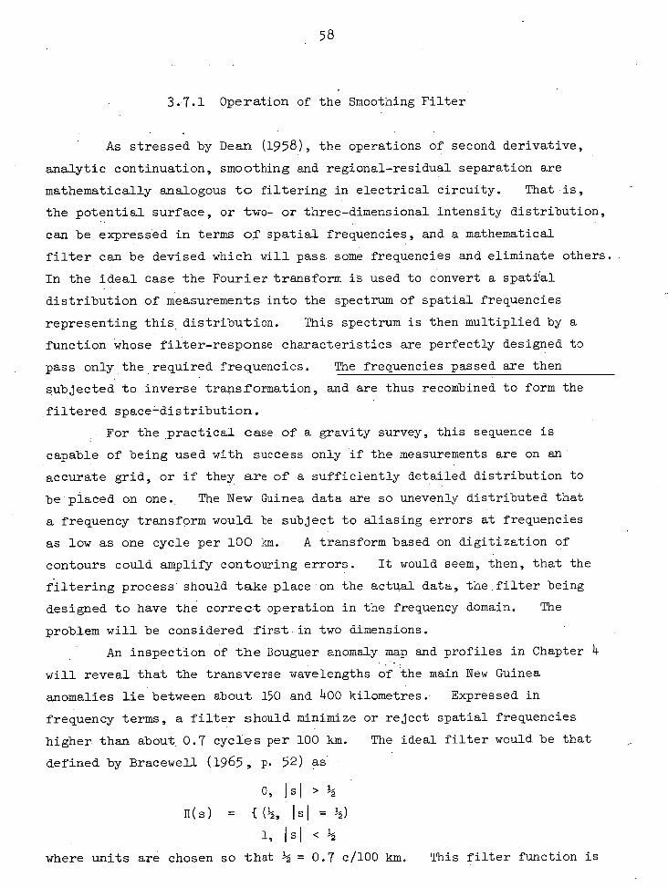
58

3.7.1 Operation of the Smoothing Filter

As stressed by Dean (1958), the operations of second derivative,

analytic continuation, smoothing and regional-residual separation are

mathematically analogous to filtering in electrical circuity. That is,

the potential surface, or two- or three-dimensional intensity distribution,

can be expressed in terms of spatial frequencies, and a mathematical

filter can be devised which will pass some frequencies and eliminate others.

In the ideal case the Fourier transform is used to convert a spatial

distribution of measurements into the spectrum of spatial frequencies

representing this distribution. This spectrum is then multiplied by a

function whose filter-response characteristics are perfectly designed to

pass only the required frequencies. The frequencies passed are then

subjected to inverse transformation, and are thus recombined to form the

filtered space-distribution.

For the practical case of a gravity survey, this sequence is

capable of being used with success only if the measurements are on an

accurate grid, or if they are of a sufficiently detailed distribution to

be placed on one. The New Guinea data are so unevenly distributed that

a frequency transform would be subject to aliasing errors at frequencies

as low as one cycle per 100 km. A transform based on digitization of

contours could amplify contouring errors. It would seem, then, that the

filtering process should take place on the actual data, the filter being

designed to have the correct operation in the frequency domain. The

problem will be considered first in two dimensions.

An inspection of the Bouguer anomaly map and profiles in Chapter 4

will reveal that the transverse wavelengths of the main New Guinea

anomalies lie between about 150 and 400 kilometres. Expressed in

frequency terms, a filter should minimize or reject spatial frequencies

higher than about 0.7 cycles per 100 km. The ideal filter would be that

defined by Bracewell (1965, . p. 52) as

0, Isl > 1/2

11(s) = 01/2, Isl = 1/2) 1, Is' <

where units are chosen so that 1/2 = 0.7 c/100 km. This filter function is

59

multiplied by the transform of the data distribution

f(x) = 0(s)

to give the filtered spectrum 0(s)11(s). However, since the process

must take place in the space domain we must make use of the convolution

theorem that

0 (s)11(s) = f(x) * g(x)

If ( u ) g(x-u)du

where g(x) is the inverse transform of 11(s).

This operation is equivalent to taking a weighted running mean of

data spaced at an interval du, the weighting function being g(x-u).

The transform of 11(s) is sinc(x)", defined by Bracewell (1965, p. 62) as

sinc( ) - sinnx nx

(= g(x). )

Such a weighting function would be simple enough to apply to a running

mean. But for 1000 or more stations the computing time on the machine

available would have been prohibitive.

The reverse case was therefore considered. The function H(x)

convoluted with f(x) is equivalent to taking an uhweighted running mean

of the data. In:the frequency domain the transform 0(s) is multiplied by

- the filter:

sinc( sinns

TTS

This is a reasonable approximation to a low-pass filter, with the

complication that a negative filter response of. up to 0.21 times the

. maximum occurs for frequencies betwee,11sc and 2s, , between 3s c and 4s c,

- c and so on; where s - is the cutoff frequency '(Fig. 3.5b). Because

of the simplicity of operation in the space domain this complication was

not considered damning.

The aperture of the H function was chosen as 11 0 (= 112 km:).

In order to avoid distorting the true amplitude of the running mean, it

is necessary that the area under the II function be unity. Using units

of 100 km., Fig. 3.5(a) shows theditensions of the function; having an

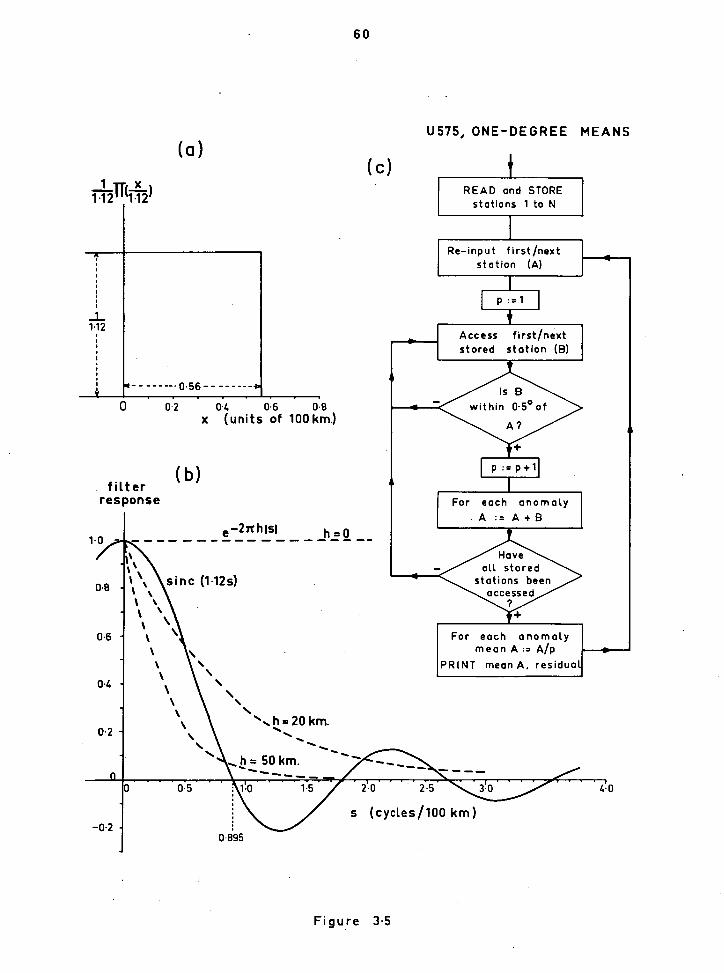
(a) (c)

•

•

(b) filter

response

READ and STORE stations 1 to N

Re—input first/next station (A)

Access first/next stored station (B)

0.2 04 0-6 0-8 x (units of 100km.)

0

1.0 e -2nhIsl

p := p+1

For each anomaly A := A + B

h =0

Have all stored

stations been accessed

For each anomaly mean A := A/p

PRINT mean A, residual

0.6

0.4

■ h=20 km. 0.2

= 50 km.

s (cycles/100 km)

0-895

p :=1

nix 1.12 1.12'

112

4-0

U575, ONE-DEGREE MEANS

60

Figure 3•5

half-width of 0.56 and height. of 1/1,12 . The function is.then expressed

as

1 x 1.12 '1.12

The frequency transform' of this function - is-

sinc(1.12s)

.sin(1:12fs)

which is plotted in Fig. 3:5(b).' Since sinc(x) = 0 where x = 1, therefore

sinc(1.12s)-will:be zero at S' = 0.895Cycles/100.km. , 111hiS ishigher than

the 0.7 cycle cutoff-required,.but - 4t must., be remeMbered thatthecutoff.'

is not sharp. . The applitudesof all.frequencies"greater than:02.7"are: . •

multiplied by less than 0.3 ,- The , negative.MultiplierAmaxiMum.'-0.21) of

frequencies .above 0.895 should.besuffidiently:small'to•ensure.that.the.•

resulting amplitudesare masked:by-those of•the,low•frequenciesl. The

dashed , lines:on , Fig.-3.5(b) are'the.upward continuation:filterresponse:

curves for various. heights.. (in, units of 100 -km.) calculatedfrom ,-Deanis -

(1958) theoretical.filterresponse expression:,

filter . response

can.be seen. that this sinc(s)filter.corresponds.vaguely in the lower ,• . _ •frequencies to upward continuation to between 20 and. 50 km„ but is

completely out towards the higher frequencies„

.3,7..2 The Three-dimensional Means Program

The two-dimensional functions II(x)and sinc(s),. discussed above,

have rotational symmetry about the vertical axis. Thus, their,

mathematical filtering operations are valid for the three-dimensional

case.

The running mean was computed for every station, using only the

anomalies observed. That is, an imaginary circle of angular radius

0.5 0 was drawn arOund each station and Observed anomalies for all stations

within that circle were . Meaned at the Central statiOn:' ' Fig. 3.5(C) is a

62

flow chart for the program.which operates in two steps: . . . '(a) All observed statiOn data as output from the reduction

program .(with local terrain corrections added) are read and stored in

linear array.

(b) The stations are input again one by one. Each reinput

station accesses in order each station in the' store, and the angular

distance (a) between them is computed'uSing the relation

cos,a = sinybsino

0 + cosOCOSOocos(A-A0 )

. •

where (0 .0) and( 00 ) are the coordinates of the two stations. o

(Geographic rather than the correct geocentric coordinates are used; the

error involved in an arc distance of . 0:5' being negligible.) If a is

less than 0:5 ° the five anomalies(free-air, simple and extended BOuguer,

Pratt and Airy isOStatic) and the elevation are added to the corresponding

valueS for the operating Station, and a counter is incremented by unity.

If a is greater than the next stored station is accessed immediately

and the process repeated.. When all stored stations have been accessed

and tested the accumulated anomalies and elevations are averaged . (using

the counter), residuals are computed; and the next Operating station is

input.

This program 'Was'ilsed for the Bougainville survey (which could be

considered separately since the radius of averaging didinot , overlap with

any of the rest of the regional survey). From the time taken for

operations on About 200 x200 stations it was obvious that a similar

operation involving More than11000 x 1000 stations for the other part of -

the survey would be most wasteful of computer title. Accordingly the

program was modified to t*.e a running mean over a 10 x I ° square rather

. than the 0.59 radius circle. That is, the parameters to be computed.

became simply

A-A

When.tested on-the B.ougainville survey, the mean .anomalies using this „ method were within 0.1 ndlligal of those using the circle method.

63

Both the 1 0 circle and the 10 x 10 square means programs are

given in Appendix I (U575, ONE DEGREE MEANS). The length of the

programs is due to the use of core backing store transfer procedures for

the Elliott 503 computer, which has a main store too small to accommodate

all the data which formed the array for the main body of gravity

stations. The flow-chart (Fig. 3.5c) is for the 10 circle case only.

Errors in the smoothing process The first important. source of error

is general to both programs, and results from the uneven station

distribution. That is, the theory discussed in 3.7.1 does not strictly

hold, since the sampling interval (du) for the space domain convolution

is not constant. To put it in another way, the width and height of the II

function (Fig. 3.5a) vary in terms of units of station-spacing. The

mean is not always taken by summing 1.12/du anomaly values and multiplying

by du/l.12 . In the extreme case of a station more than 0.5 ° away from

its nearest neighbour all frequencies would be retained. This happens

in one or two cases of island stations, but in general the frequency

cutoff operates to some extent. In .addition to this is the fact that

the integration is not over the interval -co to +co . There will be a

definite edge effect for stations at the boundaries of the survey.

Again, this operates toward retention of the high-spatial-frequencies.

The second error is found in the 1 ° x 1 ° square approximation

only. This has the effect of retaining higher frequencies in the

diagonal directions, or introducing a direction into the smoothed

anomalies. As stated above, this was negligible in the Bougainville

survey, and it is considered that it would not significantly affect

ten-milligal contours for the mainland Papua and New Guinea survey.

Output and results The outputof the means program is reproduced in

Appendix II (pp. 128-147) and the headings are explained on p.14 of that

Appendix. The residual at a station is, of course, the original

anomaly minus the mean anomaly.

Mean anomaly maps have been contoured for free-air, extended

Bouguer and Airy isbstatic anomalies, and are presented in the next

chapter on a scale of 1:4,000,000.

64

It is obvious from an inspection of these maps that the effect

of high frequency anomalies has indeed been minimized.

KEY TO FOLDOUT GRAVITY MAPS

The sequence of gravity maps opposite is as follows:

Smoothed Free-Air Anomalies

Extended Bouguer Anomalies

Smoothed Extended Bouguer Anomalies

Pratt Isostatic Anomalies

Airy Isostatic Anomalies

Smoothed Airy Isostatic Anomalies

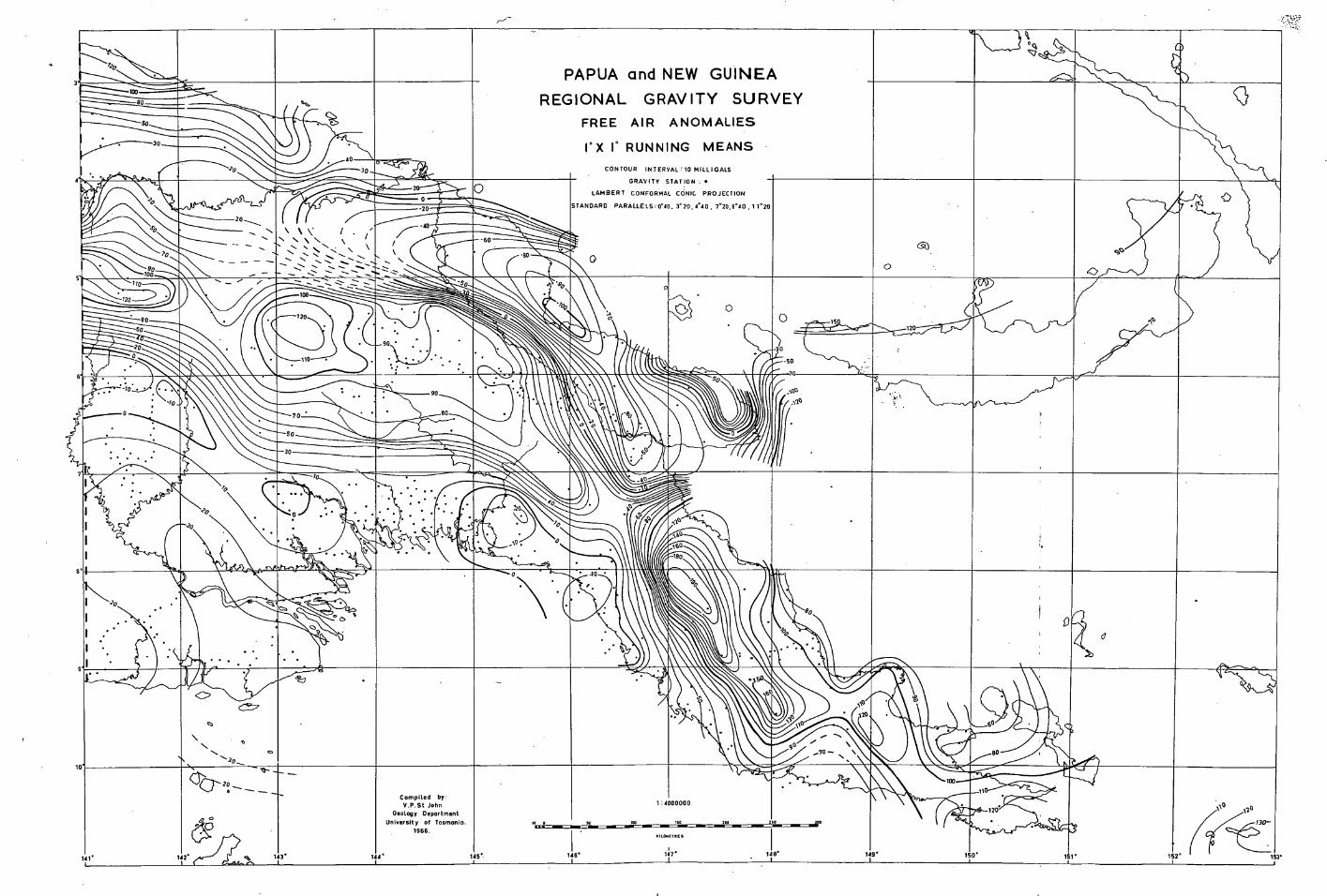
PAPUA and NEW GUINEA

‘0 q 111

.

e•a.

0 4 30 . ..-

REGIONAL GRAVITY SURVEY FREE AIR ANOMALIES

I ° X 1 ° RUNNING MEANS - CONTOUR INTERVAL : 10 MILL I GALS

thilli&sh____41 100

80

so

., , ,.... driam'i jIP% •

1

0

, 20 GRAVITY STAT ION : •

0 LAMBERT CONFORMAL CONIC PROJECTION

63,

6 ■

... - I

I / / 1 /

_.

(

/7 /// / )

/ // / / ti

., / //I '

/1/

I —

II

/ / / ,

I

0 immak m 3° STANDARD PARALLELS , ONO. r20. 440 7 ° 20,8 ° 40 .1 1 • 20 -20

, •

/

1 \

) ' 1

1

7--- -40

/ \

--.. ....

•••:•. -60 AK,

PVC

li.

616.

100

120

______5 .

••••_, ■

o

e

„ 4

,

• 0 0 wr rir

Air 1

111111111111,,,.........120 .

90 • .•• . . ..: . .. • .1i

80

...15

x. •

LIIIL

_90

•

• -‘,"

MIL 1IIIIIIIIIMIlli,. 50

1

I

, •,„ .• • • . , . .• • . . • , .

141 ° 142

30

St11111IIN. . Mir

•

1(%

NM

.

•■•

....2.4

.

r

-1.1117 1113 :,,

70

'''''. • ° %

I. 11......*,... ■

i '6° ' 4 11 •

,

i • 1

,

/

1

111 • .0

.........

,

, , a

.

...,

ro °

• 0

c7 c:t7.

\ .:. ..... . -' 30......

..,.° °

143. -

P

Compiled by V.P.St John

Geology Deportment University of Tasmania. , 1966.

10 0 sa v•

1:4000000

' Ropy

Ili • ,,No „ ..... , .....

L

r -

1111

.4"

O1

1

/----.8 . ......a

,20

° 153.

iso 200 250

—..*W1101b- IIIh1! -

• 151° 152 145 °- 145

KILOMETRE S

• 147° - 149 • 149

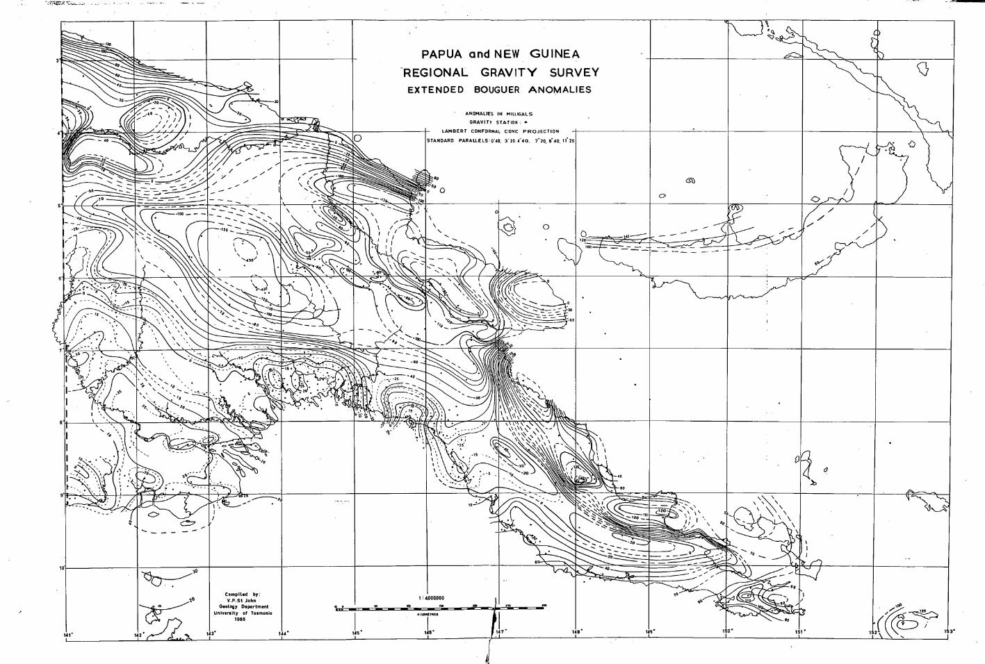
3

• , . •

- PAPUA and NEW GUINEA .

EXTENDED BOUGUER ANOMALIES

ANOMALIES IN MILLIGALS GRAVITY STATION : •

11.

su.

.,,.

-REGIONAL GRAVITY SURVEY iiiig.,..,.......

2.

'...1.

1.• I

....,..-•,,--,

..--• 1 1 i , , •

, ... "area. isralred 1■111Woll.._ • \

LAMBERT CONFORMAL CONIC PROJECTION

STANDARD PARALLELS:0'40. 320 eao. 7°20. 6. 40.11 20

0

P

Iii //

/1

/ I

•

/ I

.\

' ' ' ' ' ' - - - - - - - - - . „ , , , ..„, — , • . . . _'' '', , , . .. . :: . . , , ..,.,.,: „ ..ki 9 0

_ s o

- 0o •

, `... • ,

"

g,

7 ,

. ..-.9,'

A A

.--Ai.

• .•,74 I /

.

/ ,

/7

• /

.

_--. //:)

(p

/ }

I /

/ 'r• .

1 1 1 (

/ ./'

, / .

!

•

\ _..upormr........1161111111r

1

/

a'

1111W%

r0pr •

,

, •

/

,

•

/ .-

8L17

,

0

/

/

I /

/

/ ///

\

'

/ , /

I / I I . I ....

pf 20. ■■■■■ ■........,.....,11,

- -

• .1\,.1,..., .., ...,....,, , 8 \ ‘

•

\ \ \ \

V f'?

\ I

I/

I /

.

•

, I. .,..

1 • / /

\ \ \ \ '1,.....

• \ ...... •

'DO ' "°° `..- ,

..■-...../.- .Z - , 30

I.

i_ e ..,..

I :

.1 /

•

1 • 41

. ./// -/

• ^

•

,`•"" •

/,'

.--** •

"/

•

. /

•

•

.0,,o

\ ,s \

\

\ N.' •

ISSW\,-

.

.

.

.1.1 11.1

II

I 1 el. iAN\ t■

4 '' 40

....

_,...,..,

. , , • ,. - swum ..-.. '

7/2 \

\ •••..

I .,,,,

,

I

.

fruf

'01re -

0 .(

ve, \ \ \ , N1,1•,....., , \ \ \ \ \-`

. • \ • \\. I,

I

. F . 40

I '0 •

.• ..

' . I . - - - - .. -

,......',

. • \\

- I .

1 \ , : - -5 va . ■ i

1 \

... • .

.4111111111b■ 'lliii 60 ,F‘ ....4......C7,26.... a

I 1

/ ,. i

'"*Ir i .

1 5 \

III

& 0

\ — •••.' \\ \ ow ■ III

\ as. \ 4,14

•• . . ._ i !.....,

-

' ---. 1111114k ) ,

//

do 7o _

\ IFIA7

1

/

gwe

riliWill0%.'°

152\

op

CIL,) , 1 53

10

141 ° 1

Compiled by: V.P.St John

Geology Deportment I :

. ea

r-1t:31.07—.3°

4009000 no roo soy

•. _ jpr. 4.....1 ..)

., I.- 491114. y

---- rag:

•

• 149 °

....-- .... _--.■ . 00111100011:a ...v.v..- o .,...

CD wir A,

eir

150 ° 171 .

.Unlversity of Tasmania 611.416411146 .

1966

I 2 • •i, 143. 144 . 145 ° 18 J147 ° 149

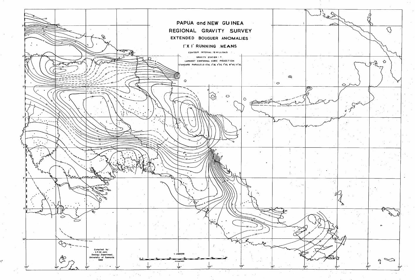
111 PAPUA and NEW GUINEA

...-

REGIONAL GRAVITY SURVEY EXTENDED BOUGUER ANOMALIES '-

rx I ° RUNNING .MEANS CONTOUR INTERVAL:10 MILLI6ALS

eifiA:l%M;Mlair

I.L. IL All ■■■•■1111aLke-44' . GRAVITY STATION I •

l LAMBERT CONFORMAL CONIC PROJECTION

lii

•w I I

— \

\ ■

, .. —•

, \

— •\

\\

1 s,

—..... ..., \

0\\

— . ■•

\ l'

.-1,

\\\ 1 1 1 1 ).r

. .`

\ litl

I II

,, \ .

HI c

,11

r 0 ,

i . \,. \\II. 1\ i

*-401

411)

STANDARD PARALLELS: 040, 3° 20, 4 •40, 7 .20, 8 °30. 11 . 20.

So

_ Too

70

._4.1.,....

-

/ fd

/

I 0•

$

y0 4 1

.77 • •

..•

......

Ml .\\ _s

ir illilli

•

.•.•

/

•

/ /

,/ r

••

• / /

o

/ //

1 o

.

.

.

;

•.•••.• . \.....______t/ ___

e

s------ 60

„, . \

-30

•

. •1-31 41

•

. , .,. ,....,

lb

1 1

r • . •

.. • z /

, 1

. 1 ...?

, ,

ri

bti ,

PI

' --- 4 j

0 ,,e y

,,

0

-

1

•

IP • •

.

A O

ff .

gl • • .

•

. - a

. 70

.

,

0 ,/

-.....01,

• • , -

1111 11 / 60

/ / / ,

t.

at

,..400111110 41040

141 ° . 142° c43 143 °

Compited by: . V.P.St John

Geology Deportment University of Toernonio.

• 1966' 10 0

:

SO 00 1 4000000

. no 200 -, 100

119°.

.40000volir

-

150 ° i

,

1 , Alb

171 °

saw

rti. 9

152 ° 153° 144 ° I • I

145 ° 16° 147° i

148°

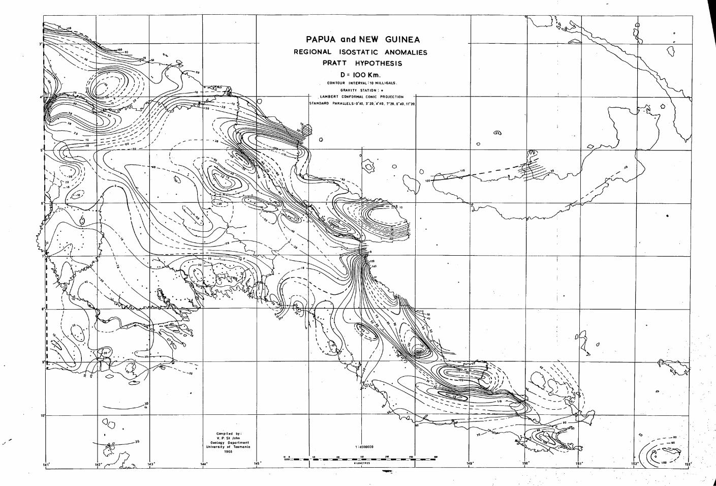
_•••,....______z.'""%ki...._ „. ... •

PAPUA and NEW GUINEA

11. . ...

112..._ 0

. ........ . .......„

., .3...

---- .

REGIONAL ISOSTAT IC ANOMALIES

PRATT HYPOTHESIS

D = 100 Km. CONTOUR INTERVAL :10 MILL IGALS .

.c.1

(

r__, ,,

t \

‘,

•

\‘..,.s.

\‘.....,_v,

,,,

,.....„........ ,

(, ,

•

i - I'''. .1, — '17441111111....

I..... 30 _ •2° .- .... ‘IIIIk

( \ \ ge"----

\ •

- . , 0 \ • ' 0 lr--'"•--,__-

0

a, Ilk ...-_,.._„.. . _. . . _-■..............." -.'''''',, . ' o .,,,,:z...„,..24

..E.

GRAVITY STATION : •

\\.\\

\

\ \ \ tt. \ R V.,(C

. LAMBERT CONFCIRMAL CONIC PROJECTION

STANDARD PARALLELS;13'40, 3' 20:4'40, 720. 9 . 40.1120.

0 0

( 1

I \ \ \ .

.. , S

. s.

' •••• s

,

-1 0

. .

I —

/ l .

•

• . t•tc,

• • • .

:

7

.

. • : • .

,

1 / //,

/ .3P

-at

.

._•1111....,

.

t .

‘0

,00 0014

I

:S.

..

p• ./

,- -- --

I \

•••. .... / / ,

••6",

\ •

.....

,

■••■.- .

lowls.. N

r".•"---"..4-......—Aar-- ""IIMIV

-

%

I /

•

/Y,/

/ y

•

i

I

Phi i . . 45

vo

.,

/ -7 A

(4,6)

— • • ;

-

*:: ::-::----------- -20

7;

• ,

•

_

. ../

..... ....to ".

/

1111. L.

.

A•I,I

_

• . •

7.

I

•

O

I ,

▪

, , A

•

Ai

20 •

/ 40

I% •\

% •

kA:\:‘ ' IVAU \ —

.

I

I

.

.0 , - ,114

.-,..-

.... 0_;:p ■

No/

+ft( 30 4

••... \

4

— —

—

11111ie" II

• '

or/ ,4

;

•

L.

•

•

•

/ •

00P 1 . v

CC

-.... ••••••-/-.6772-7":2• ■ .... .

'".• -30

..

r

•

\ \

\

••■

„:Eul 6 di

,

/

/ / —

4 /

•

Irk

4

--......_____ 20

114

Compiled by: V. P. St John

Geology Deportment University of Tasmania

1966

" 145' la= ■ .-.-- Em

•

149

....pi oh& _ 0

10 (

4 '...-.... /ark

' 150 151

..,4

152

0 ...-

0

' 1 00 -;"...' 153.

OP

Ill 142 % 113 .-......NI e"..

04

1 , 4000000

-1'm-7. _

RilOMEIRES

I

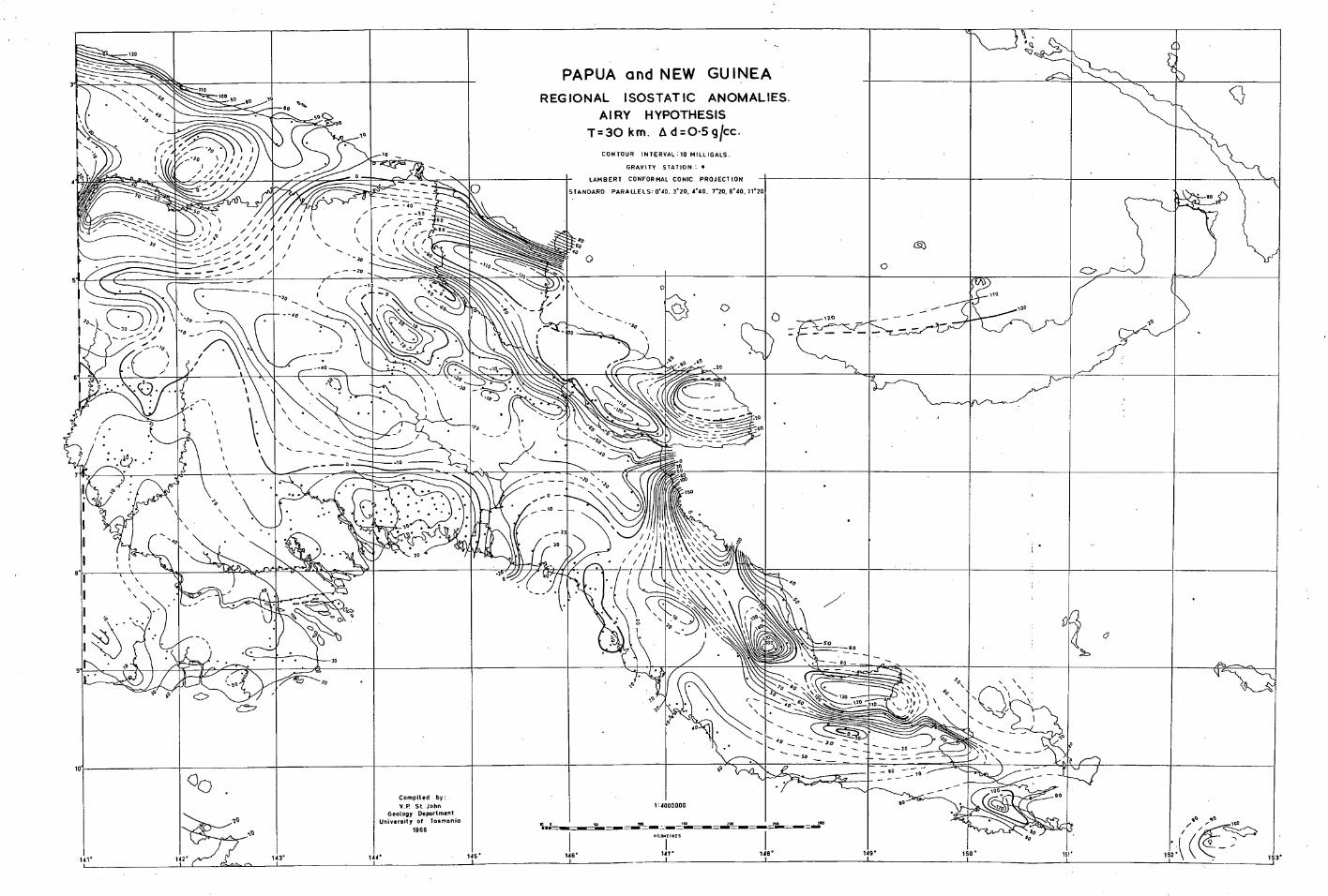
.......■.. ,.... .... ___,,......:4........_ _.;_-__-_--------_-------"-\

.

PAPUA and NEW GUINEA

mo q .,..i ii a

REGIONAL ISOSTAT IC ANOMALIES. AIRY HYPOTHESIS

T=30 km. A d=0-5gicc. CONTOUR INTERVAL :10 MILL IGALS.

GRAVITY STATION : •

1111N:L

1

1 1 ,

• /

- -

•

/

•

„. n %

0 0 .0

'`.

'•-• ---. -.,„ • i

1 1 / I / / , / /

/ / /

...,.. • / LAMBERT CONFORMAL

STANDARD PARALLELS: 0'40.

CONIC PROJECT ION

320, 440. 720, r40,11.20

r ...I

fir,

,

Ilk\

\ '

.

\

\ s \ \ \ \ \

1-1,..,\\ \\ \ \ 1\ 1

% ' / - • \

' \

1

\))) 1

11.

)

,,_,4 , ,Ftw- , , ,

,

, , ,

„ ,

,

/

_ -__ ti,--'-\00

.

.--

/

- - -- ,

,

, .

78„,"

. •

•

I .

r___ .-_.....,

I I

\

I •

a

_

1 \

0

\ ■

......

, \

•

•

•-

V _

c/

1 /

.-- -- "'" -----' .o• /

\

I

.( / O p,(.)

. ..

.. :.

.

..(

- - -

/ I

/

/

/

/

I

.•••••

. s -,, , ' -20

\ ■ I I

• .. .• i4

-20 t

. .

• •• , _

- - . I

''''''

• "so

..,

o

•

•

- -

o _ - _o

3o

..„ H„,,fi t.

.... k '

.-', • ......40- ....., 0,

4, ,. .,

•

OA

/ 7

)9' d'e

... ,

•

(

•

.11 _

-).41111 1111.-

. r 7

. • • 1

• • ,

• a

.... - \

. l'

•

• 4

4 • -10 -

imaa.,/ ..

IOW -- -

. , / /

• / i

P la 150

o .

.

,

i •

2

\\•\\ \ .. . , •

.,

a . ...

1 ..

,

6 50

e„

. s \'` • \

1111114 \ \ \ X \ \ ''' \ 1), 1 i \ • '- ',/,/ ‘ \ .

•

•

60

- 90 -

..111•••••■...41 11.1F-""111114.! . )0 6. '6 ..‘ \\ •

\ * 130

, ' ...____2-_n • ,

.

I WI I -r9 a ,.."---45—=3 -----"- 3o •

C:7.

.. • \ •

\ \ •

. Ilk . •- \ -■

, •-, c.......... --, ..) , - - ,...

--. -■ ._.._

...... -,,,, ,..4...,.., 4

--■•••••

112

/ .1.0 •,, iao

' ' 173'

10

141 . 112 .

0 •

......\..0,(25...____„.A0

143' 114' ,, ,,,.

Compiled by:

V.P. St John Geology Department

University of Tasmania

-- 115 °

la •

1:1000000

' 1.11141

- '1.

150 •

00 A

a

111• I

146' 117' 1413 . 149'

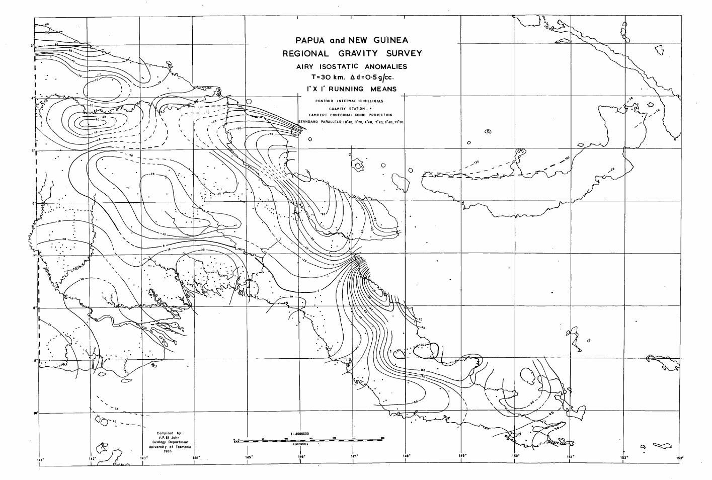
PAPUA and NEW GUINEA

NIIII • di 10 lb

- REGIONAL GRAVITY SURVEY

AIRY ISOSTAT IC ANOMALIES T=30 km. Li dO.5g/cc.

-..1111111\L ,.----:-

, } . I° X I' RUNNING MEANS

#10"1.14.4."

‘ I

1 1

-.- \ ■ /

- - --

:30

. •

.

.

...mirr,.. •

_. --

— — -- ...- --

CONTOUR INTERVAL :10 MILLIGALS.

GRAVITY STATION : •

LAMBERT CONFORMAL CONIC PROJECTION

.15

• \ \ ‘‘ \

-- ,... ■ \

STANDARD PARALLELS :0 °40, 3 ° 20, 4 °40, 7 °20, 8°40,11 °20.

7 0 NV 0

4 .

.

.....__ , ,..\\,..\, , \ ‘ \

4111/4,,\

\ ,\ \ \

i

\\ \ \ \

•

.

.

• II. ...A.

0 .„. ._.sto _ --

-- --

-- .....•

./'

1

,,,

10'

.

0

F0 .

• . • . . . . •

-20

0 10 70

• i • : •

I

• . •. .

..* • .

• • . • . . .

11. . '116_

41113

, ". --..ra10111b --....

o

•. • . , .. ' 1111 . • . •

\

W

.

• • to

a.

•

. I

.• ... ik

• .. •

• • •

--742 .._......,b'I'Ll

irk

so

I L

w....m -wr- ii io.

-4111,1111,01141

.

• _I

Iwo limi,

dm,

41°

C)

142 ° 143 °

Cornpited by: V.P.St John

Geology Department University of Tasmanio

1956

NO

1: 4000000 iSO zee 170 30,

150°

00 ''-• - A owir

151 ° I

152 ° I

a}

• 153 I

1

KILONEIRES

I 145 • 146 ° 147 ° 149 ° 149 °

!I I I

65

4. INTERPRETATION OF THE GRAVITY ANOMALIES

Any gravity anomaly is the result of actual departures from the

assumed mass-distribution within the earth. The purpose of any inter-

pretational method is to determine, the most likely distribution of the

anomalous mass causing a gravity anomaly. ,Thus, -.from one observed

quantity, gravitational accelleration, must be induced the four causative

variables; position of the anomalous body, and its volute, shape and

density. As stressed in section 1.2.3 it is only by considering all

independent geological and geophysical evidence that some of these

variables may be either eliminated or confined within limits. Geological

mapping can define the surface shape of a body, and seismic studies can

give . a reliable indication of its subsurface shape and elastic properties

(which can,be related to density):. Where there exist no seismic surveys

or density measurements the density of a body can be confined within

limits by a careful consideration-of its zeologicalmature.. Accordingly,

the bases of subsequent .density postulations will be discussed in some detail here.

4 1 1 DENSITIES OF CRUSTAL MATERIALS

4.1.1 Crystalline Rocks

• The. likely densities of lower-crustal and upper mantle materials

have been discussed in connection with the Airy isostatic model (3.5.2),

the conclusions being based purely on relations between seismic velocity

and density.

• Densities used for upper crustal crystalline rocks are averages

of actual measurements made on rocks of specified mineralogy and texture.

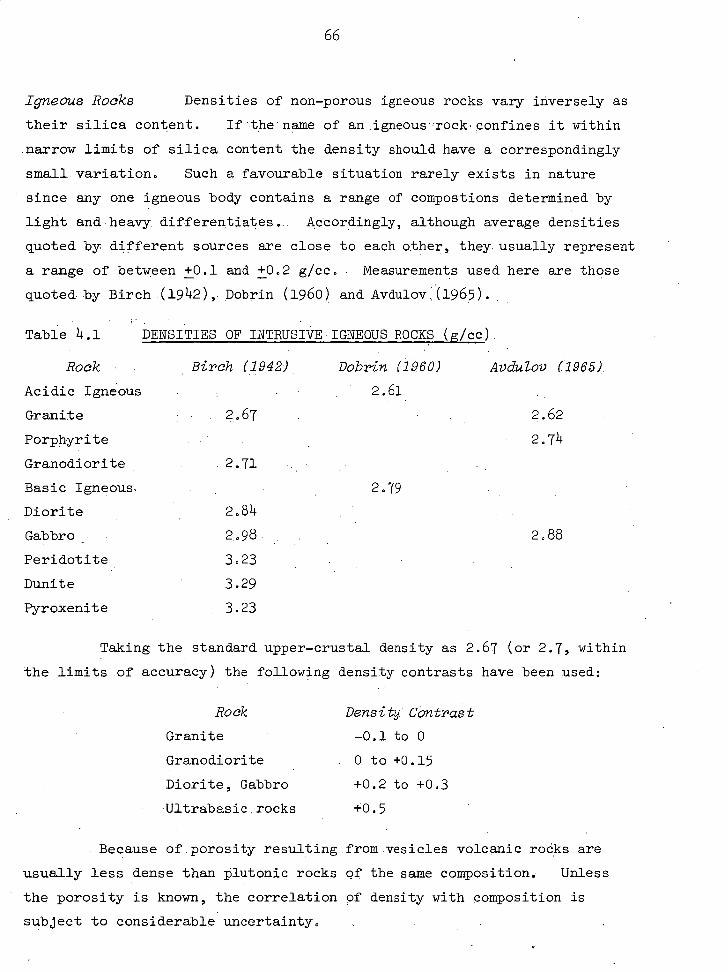
66

Igneous Rocks Densities of non-porous igneous rocks vary inversely as

their silica content. If•the'name of an.igneous-rock , onfines it within

narrow limits of silica content the density should have a correspondingly

small variation. Such a favourable situation rarely exists in nature

since any one igneous body contains a range of compostions determined by

light and heavy, differentiates. Accordingly, although average densities

quoted by different sources are close to each other, they. usually represent

a range of between +0.1 and 1-0.2 g/cc. Measurements used here are those

quoted by Birch (19)-2),- Dobrin (1960) and Avdulov(1965).

Table 4.1

Rock Acidic Igneous

DENSITIES OF INTRUSIVE IGNEOUS ROCKS (g/cc)

AvduZov (1965) Birch (1942) Dobrin (1960) 2.61

Granite 2.67 2.62

Porphyrite 2.74

Granodiorite 2.71

Basic Igneous, 2.79

Diorite 2.84

Gabbro 2.98 2.88

Peridotite 3.23

Dunite 3.29

Pyroxenite 3.23

Taking the standard upper-crustal density as 2.67 (or 2.7, within

the limits of accuracy) the following density contrasts have been used:

Rock Density Contrast Granite -0.1 to 0

Granodiorite 0 to +0.15

Diorite, Gabbro +0.2 to +0.3

Ultrabasic rocks +0.5

- Because of porosity resulting from vesicles volcanic roaks are

usually less dense than plutonic rocks of the same composition. Unless

the porosity is known, the correlation of density with composition is

subject to considerable uncertainty.

67

There are three main volcanic associations represented by the

Quaternary volcanoes of New Guinea. Morgan (1966) describes the lavas

erupted by the north coast volcanic islands as pyroxene andesites,

andesitic basalts and basalts.; many with accessory olivine. He has

found the strato-volcanoes, Mts Lamington, Yelia and Victory, to be

composed of more acid hornblende and lamprobolite andesites, and has

described peralkaline obsidian and rhyolite from Fergusson and Dobu

Islands. The alkaline association can be extended to the Managalase

Plateau, following the work of Ruxton (1966), and the "orogenic andesite"

association can be extended to the strato-volcanoes of the Southern, and

the southern parts of the Eastern and Western, Highlands.. This latter

association includes some basalt flows.

. I have measured the (wet) densities of two samples of lava from

strato-volcanoes in the Southern. Highlands.. They are:

Hornblende Andesite (Mt Murray) 2.63g/cc

Dacite (Doma Peaks) 2.52g/cc

Comparing these densities with those of the plutonic equivalents,

Diorite and Granodiorite respectively, one has some indication of the

density change which can be caused by vesicularity. The volcanic rocks

have been assigned the following contrasts with the standard upper-

crustal density:

Acid and Alkaline lavas -0.2 to 0

Andesites -a.15 to 0

Basalts 40.1 to +0.2

Pyroclastics. and "volcanics" consisting of interbedded lavas and

pyroclasiics are ., during interpretation, assigned densities based on

their petrological descriptions.

Metamorphic rocks Most of the metamorphic rocks in New Guinea are of

,greenschist or lower amphibolite.facies.. Dobrin (1961 P. 251) quotes

an average density of 2.T4 for metamorphic rocks. Avdulov (1964) gives

an average of 2.74 for Palaeozoic schist of the Caucasian region.

Measurement of the. wet density of a sample of quartz-muscovite schist

from Mt Albert Edward yielded a value of. 2.63g/cc.

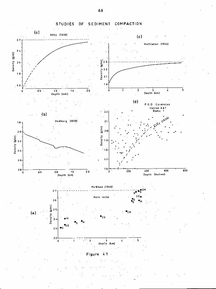
(c) (a)

At hy (1930)

2-7

// cn

‘7,

ca

2-5 '

2-3

2.1

1-9

Nettleton (1934)

. 0-5 1.0 Dept h (km.)

1.5 21, 0 0 1

(d)

3 4 Depth (km.)

P.O. D. Coreholes

Conrad 667

5

' 2.2 Bamu 1

(b)

Hedberg (1936) 2-1

7.; • •

• •

• • • <P r •

-- 2.0 •• • •

• • / 0,

• • • • • •

1-9 ./

8 • •S•

/

• )

•

1-7 7 • / .

1.6 0-5 1-0 1-5 2-0 0 200 400 obo 800

Depth (km) Depth (metres)

McWhae (1948)

2-4

De

nsity (

g/c

c)

2.1

1-8

1-5

2.0 ,

-T. 2 2-

2-4

2-6

2-8 0

68

STUDIES OF SEDIMENT COMPACTION

2.7 • CM GO °S

Aure rocks • Cdo

2-6 - • • G M

(e) °cm

• `2 2.4- • M 'CO

• .CG

2-3- • G

2 2 0 3 5

Dept h (km)

Figure 4.1

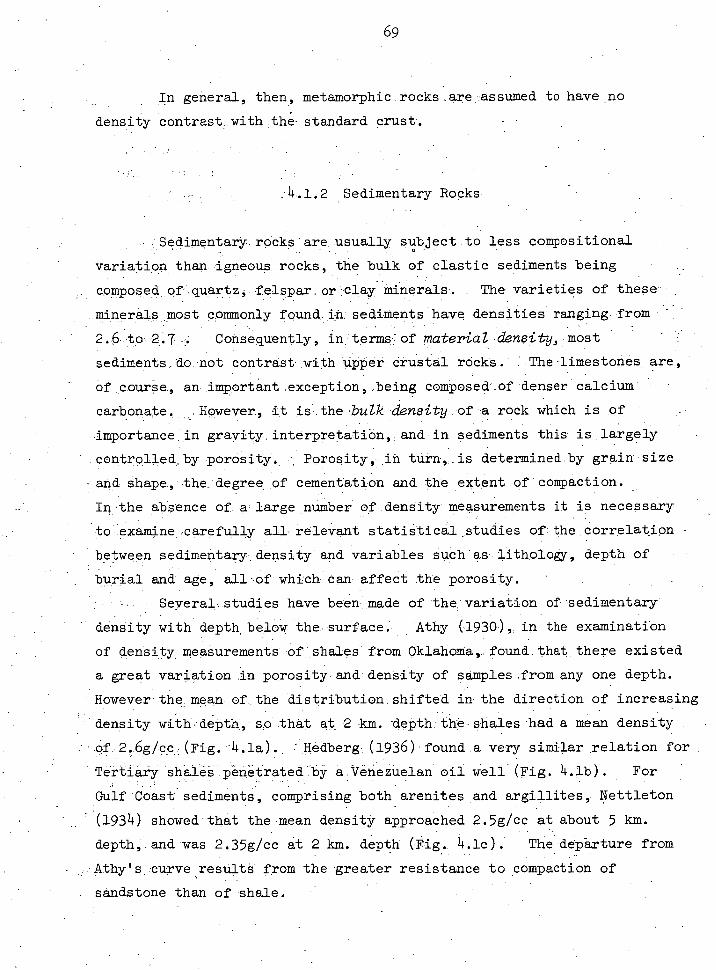
69

In general, then, metamorphic.rocks.are . ,assumed to have no

density contrast_with the standard crust.

.1.2 Sedimentary Rocks

- Sedimentary.rocks: are :.usually subject to less compositional

variation than igneous, rocks,. the bulk of.clastic sediments being _ . . . • .

composed,of.quartzi.felsparorclay minerals. . The varieties of these- .

minerals _most commonly found,in - sediMents have :densities ranging-from •

•Consequently, intermsjof'material-density,.most

sediments,:donot•contrast.With . Upper crustal rOckt..:.The - limestones are,

ofcourse, animportantexception,.:being composed -_of•denser calcium•

carbonate, : „However, it is..the ,bulk density of a-rock which is of

importance in gravity.interpretatiOn, : and in sediments this is largely

controlled by porosity, Porosity, in turn, is determined by grain size

and shape, .the. degree cementation and the extent of - compaction.

In the absence of a large number of .density measurements it is necessary

:examine carefully all relevant statistical studies of the correlation

between sedimentary density and variables such aslitholoky, depth of

burial and age, all ,of which can affect the porosity.

Several studies have been made of the variation ofizedimentary - ,

density with depth, below the surface. Athy (1930),. in the examination

of 4ensity . measurements of: shales from OklahoMa,found_that there existed

a great variation in porosity and density of samples from any one depth.

However the meanofthe.distribution shifted in the direction of increasing

- density withdepth, so that at 2 km. dePth:the-shales had 4 mean density

Hedberg (1936) . fOund.a very similar relation for

TertieryShalea4enetratedbY 4.lb). For

Gulf Coast sediments, comprising' both arenites :and argillites, Nettleton •

(1934) showed - that the mean density approached 2.5g/cc at about 5 km.

depth; and was 2.35g/cc at 2 km. depth (Fig. 4.1c). The departure from

Athy's..cqrve , restat . from the greater resistance to compaction of

sandstone than of shale.

70

All these measurements are made with the pores of the specimen filled

with water. If the specimen is measured.dry the bulk density will be

considerably less than that of the rock in its subsurface environment,

since saturation is complete below the water table. For a rock of 20%

porosity the wet and dry densities differ by 0.2g/cc (refer graph by

Ozerskaya, 1965).

There are no density logs available for.the deeper boreholes in

New Guinea,, and attempts to make measurements on core cuttings proved

unsuccessful, because of the small size of the chips and their contamination

by.drilling mud. There are, however, density logs for some of the shallow

coreholes drilled by the Papua Oil Development Company in the Bamu River

and .Purari River areas. These are the Conrah Coreholes nos 6 and 7

(Purari River), and the Bamu no: 1 Corehole The information used has

been obtained from the compilation of P.O.D.* reports by : Montgomery,

'Osborne and Glaessner (1946). The Purari River- Corehole no. 6 penetrated

780 metres of Pliocene carbonaceous, sandy; . calcareous and tuffaceous clays

of alternating estuarine' and terrigenbus facies. , No. 7 corehole in the

same area penetrated 308 metres of estuarine clays of.the.same age. The

densities measured .in the BamU no. 1 hole are of terrigenous and estuarine

clays and mudstones, extending to the base of the Pliocene' at430 metres.

All_ measured densities are plotted.against depth in Fig. 4.1(d). It can

be seen that the pointa . are widely scattered ; but they bracket the portion -

of Athy!s (1930) Curve. Corresponding to the same depths.

The only other systematic series of density measurements in New

Guinea is that carried-out by McWhae. (1948)-on the M'Bwei Sa section

through the Middle and Lower Miocene Aure Group. This group is a

monotonous .sequence of greywackes andAmidstones, some calcareous. The

density measurements wereof surface samples, the depths being stratigraphic

Several organization's are referred to in this thesis by their initial :letters. . They-are:

P.O.D. Papua Oil Development Co. Ltd. . APC Australasian Petroleum Co. Pty Ltd. IEC Island Exploration COmpany Pty BMR : : Commonwealth Bureau of Mineral Resources, Geology and Geophysics APOC Anglo,Persian Oil Company,

the western Caucasus:

:Age. Cainozçic

Palaeozoic,i

• :Range •

1.69; -,.2.33.

.2.26 2.50 '

Mean

24V-

:71

thickness from the top of the Aure Group., The wet densities are plotted

against this stratigraphic depth in Fig. 4.1(e), the abbreviations being:

G - greywacke; M•- mudstone; S - siltstone; ,C - calcareous.

In common with_the other curves of Fig. 4.1_ihe density - increases with

depth, the maximum in this case being 2.7g/cC at 5 km. depth. Some

uncertainty in applying this study to presently buried rOcks would arise

from the conditions that:-

(a) the top of the Aure Group may not be overlain by the same

thickness of rocks in all cases, and -

(b) there may be a relaxation- of compaction as erosion and

uplift bring deeply buried rocks to the surface. ,

As well as a correlation with depth, there is an apparent increase

of sedimentary density With age:- This is Tartly because older rocks have

usually, at some stage, been more deeply buried than younger Ones; and

partly because the process of cementation has been active fora,.longer

period in filling the Tore space of the older sediment. Aydulov(1965) -

quotes the following density ranges and weighted means for sediments in

Such a- StUdY'18 MUck-Ltoo general,to apidy -r direCtly io NeV Guinea.. . .

However, it is necessary to have sone guide in estimating the densities

of Mesozoic sediments underlying the Tertiary ones so far discussed.

The mean, values of densities of various Mesozoic sediments quoted by

Birch (1942) are given below.

Table 4.2 DENSITIES OF SEDIMENTARY ROCKS

Sediment 'Cretaceous• .8ancl6torie . 2...30(g/cc)

Calcareous sandstone .

Shale ,

Black ,Shale 2.65,

Siltstone 2.54

Limestone .2.60

2,56,

Conglomerate 2.41

The general impression given by these:,values;is that they are

somewhat higher than the range given by Avdniov : (1965). . , , - It would seem, then that the Mesozoic:-Sedimentary rocks in the

area can be assumed to bave densities, at'depth,-' of at least 2,4g/co.

Limestones have been considered .according to well-log descriptions,

the.reef-shoaI.iimestoneS'being assumed to have higher porosity . than

"dense argillaceous •limestones".

On the basis of the preceding discussion, and the curves of

Fig. 4.1, densities have been chosen for interpretational models, and for

the topographic corrections as discussed in 3.4.2. It is apparent that,

below a depth of 6 or 7 kilometres, any sediment will have a very small,

and often negligible, density Contrast with the standard crust. As will

be seen in section 4.5 this fact makes it difficult to postulate the

depth of a deep sedimentary basin purely on gravimetric evidence,

4,,.2 DIRECT INTERPRETATIONAL METHODS

Downward continuation Dean :(1958) shows that'it iapOssible to

estimate the position of anomalous bodies._by.contnUing the surface

'gravity anomalieS:downWard'until.the erratic behaviour of the filtered.

data indidates the body has been passed. 'AadisouSaed'in.4ecti9n:3.72:

73

the unevenly spaced sampling of the New Guinea data introduces considerable . . variation into the mathematical operation of a filter function at

different points.. While this is allowable in anoperation designed

simply to remove as many high frequency anomalies as possible, without

being unduly concerned with a variable cutoff frequency, it makes any

analytical upward or downward cpntinuation..procedures . impossible.

Derivative. Methods - -First and higher .derivative : methods have,.in

common with downward continuation, the property of: amplifying high,

frequency errors in the data. ThUs„..derivative r methods .in three dimensions

would be virtually-impossibleand :oould be.?used in two. dimensions only in

therare.easesof fairly straight.Iines.of - closely7spaced:stations.

Accordingly, formulaehased,on : derprative :methods, such as .those of Smith

(1959),which estimate'maximum,depth.or.density contrast directly from the

anomalies:,.cannot he ,rigorously applied.

Gauses.neorem.. The only direct interpretationalrmethod capable of -

being applied with_some_success in this type 'of survey .involves the use of

Gauss's theorem to estimate. the. anomalous mass. Hammer (1945) was

the. first to draw attention tothe.direct analogy,of.the gravitational, and

'electrostatic case. Thus, the..magnitudeof the anomalous.mass can be

determined, but not its location.. . The anomalous mass is assumed to be

- .bounded:below ; hya.n,infinite,surface;and above by the, earth's surface.,

so:that Ahese:two Jaurfaces,meeting.at,infinitenclose the body.

Half..tl.W...totalflux , would:.VAP4:Pass through:theearth!s surface, and the

total anbmalOumassiwoUld—be --

1/1 : = . gn ds • 21rG f 6.- .

where G = gravitational constant

.S = surface of the earth

.Ag = gravity anomaly normalto the surface. •n. . .

In praotice .,•the ,'1.infinite" : ,surface—must extend well:beyond the_

limitsOf.the.anomaly.being,inyestigated..

In:the-two7dimensionalcase the mass per -unit . .lehgth of. 841

infinitely'longrbody :isrgiyen,by

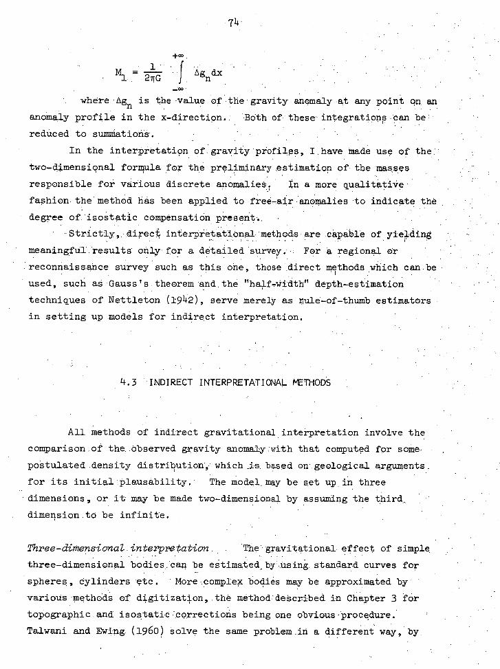
+03

- M1 27TG. 1

nax

where-Agn is the value or the gravity anomaly at any point qn an

anomaly profile in the x-direction. Both of these integrations can be

reduced to summations.

In the interpretation of gravity profiles, I have bade use of

two-dimensional formula for the preliminary estimation of the masses

responsible for various discrete anomalies. In a more qualitative

fashion the method has been applied to free-air anomalies to indicate the

degree of isostatic compensation present.

Strictly, direct interpretational methods are capable of yielding

meaningful.results only for a detailed survey. For a regional or

reconnaissance survey such as this one, those direct methods which can be

used, such as Gauss's theorem and the "half-Width" depth-estimation

techniques of Nettleton (1942), serve merely as rule-of-thumb estimators

in setting up models for indirect interpretation.

4.3 INDIRECT INTERPRETATIONAL METHODS

All methods of indirect gravitational interpretation involve the

comparison_of the:Observed gravity anomaly:with that computed for some-• •

postulated .density distribution, .• which _is based on' geological arguments.

for its initialplausability. The model_ may be set up in three

. dimensions, or it may be made two-dimensional by .assuming the third_

dimension AO be infinite. .

Three-dimensional interpretation The gravitational effect of simple

three-dimensional bodiescan be eStimated_by 'using standard curves for

spheres, cylinders etc. More complex bodies may be approximated by

various -methods of digitization, the method'described in Chapter 3 for

topographic and isostatiq-corrections being one obvious 'procedure.

Talwani and Ewing (1960) solve the same problem _in a different way, by

dividing the body Into horizontal polygonal lamellae, and compounding the

gravitational effects of these at the computation point. But, although

the computationof the effect of_athree-dimensional body presents no

problems, the construction ofa:realisticthree-dimensional model does.

It is not possible to divide a survey into small sections and set up .a

threedimensionalmodel for.each, since the gravity-field-in any section

will be affected by anomalous masses in an adjacent section. For any

survey, then, all the - anomalous masses within its limits, and for some '

distance outside them, must, be modelled and computed simultaneously.

For the New Guinea surveythis would involve

(a) setting up a different model for each likely horizontal

density change;

(b) setting up a different model for each likely vertical

density change below. the above models; and

(0_ iterating-the boundaries.of each. -model.in three-dimensions -

to obtain correspondence of calculated and observed anomalies.

Considering the number of surface geological boundaries in

New_Guinea -(map,.p.100) it is apparent that either the-models would be

'too simple to approach.realityor the labour involved in producing and

:iterating the Models would. be prohibitive.. There' is also the

consideration that a survey, of this nature should .not be over-interpreted.

'Too-dimensional interpretation The dimension of

any natural structure is of- infinitelength.is obviously unjustified.

Of•concern_to the'gravity-interpreter, however, is the extent to which

the structure can .depart from-true , twodimensionality-before,the

approximation, becomes untenablo Grant_and.f4eat (1965,-p.. 282), in

discussing "ribbon models", are: of the opinion that "a ribbon model must

have a strike length that is twenty times its width before the ends can be

safely disregarded in-the calculations". 'In a quantitative study of the

problem; Nettleton (1940, 1: 117) discusses.the."end correction", which

must be applied to_gravity-values . computed for.two-dimensional . bodies of

circular or polygonal cross-section,.tb account:Tor their' finite length.

For a traverse across the-centre of a body of-length 2y, Whose centre of

gravity (considered- as an horizontal, mass-line) is at a distance r from the

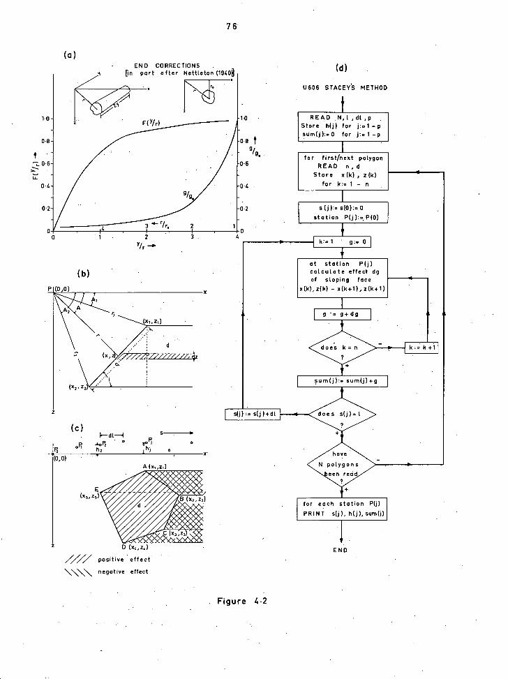
s(j :=• s( j)+d does s(j)=L

(a)

76

END CORRECTIONS . [in part after Nettleton (1940g

(d)

U606 STACEY'S METHOD

READ ,N o l o f:1Lp Store h(j) for j:.1 —p

aum(j):= 0 for j:= 1 —p

for first/next polygon READ n o d

Store x (k) z(k)

for k:= 1 — n

0.8

i. 0•6 ;:- •

0.4

F(Y/r)

0.6

0.4 •

08 t g/g.

1.0'

s(j):. s(0):. 0

station P(j ):=, P(0)

0.2 0.2

0

k 1 g:= 0 2 4

at station P(j) calculate effect dg of sloping face

x(k), z(k) — x(k+1), z(k+1)

surn(j):= sum(j)+g

(b)

have

N polygons

een read

for each station P(j)

PRINT s(j), h(j)sum(j)

D (x4 , z, ) END

/ positive effect

\\"\\X negative effect

Figure 4-2

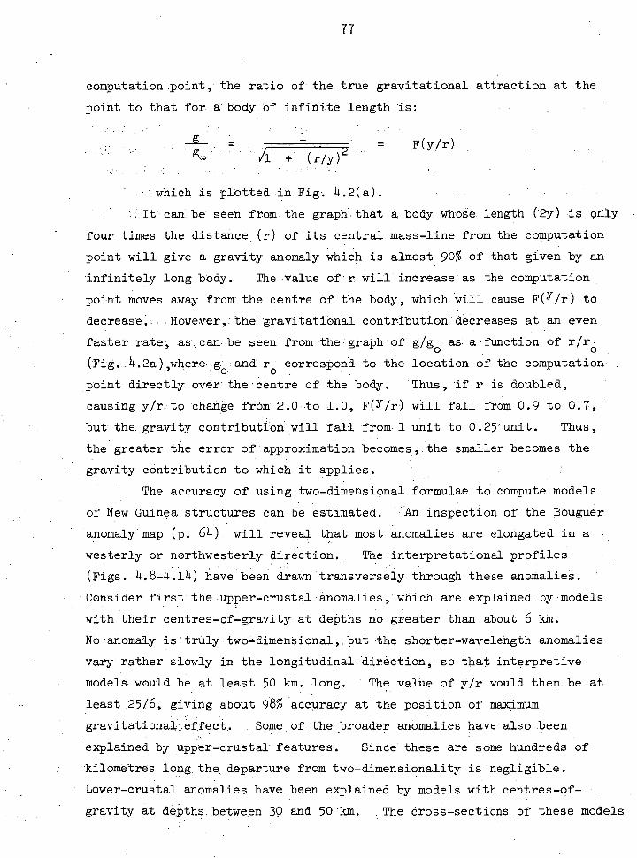
77

computation . :point, - the ratio of the true gravitational attraction at the

poiht to that for a-body of infinite length is:

1 F(y/r)

1/1 (r/y) 2

:which is plotted in Fig 4.2(a).

H It can be been from the graphthat a body whose length -(2y) is only

four times the distance . (r) of its central mass-line from the computation

point will give a gravity anomaly which is almost 90% of that given by an

infinitely long body. The value of . r Will increase asthe computation

point moves away from the centre of the body, which Will cause F(Y/r) to

decrease.,.:However,:the'gravitatiOnal -contribution"decreases at an even

faster rate; as,can be seen: from the graph of g/go as a-function of r/ro

(Fig...4.2a),wheregoand r o correspond to the location of the computation-

point directly over - the , centre of the body. Thus, if r is doubled,

causing y/r to. change from 2.0 to 1.0, F(Y/r) will fall from 0.9 to 0.7 ;

but the. gravity contribution willfall from-1 unit to 0.25 unit. Thus,

the greater the error of approximation becomes,.the smaller-becomes the

gravity contribution to which it applies.

The accuracy of using two-dimensional formulae to compute models

of New Guinea structures can be estimated. An inspection of the Bouguer

anomaly map (p. 64) will reveal that most anomalies are elongated in a

westerly or northwesterly direction. The interpretational profiles

(Figs. 4.8-4.14) have been drawn transversely through these anomalies.

Consider first the-upper-crustal.anomalies, which are explained by models

with their centres-of-gravity at depths no greater than about 6 km.

NO , anomaly is truly twodimenaional, but the shorter-wavelength anomalies

vary ratherslowly in the longitudinal-direction,. so that interpretive

models would be at least 50 km. long. The value Of yin would then be at

least .25/6, giving about 98% accuracy at the position of maximum

gravitationaleffeci, Some_of:thebroader anomalies have . also been

explained by upper-crustal features'. Since these are some hundreds of

kilometres long the, departure from two-dimensionality is negligible.

Lower-crustal anomalies have been explained by models with centres-of-

gravity at depths between 30 and 50 km. The cross-sections of these models

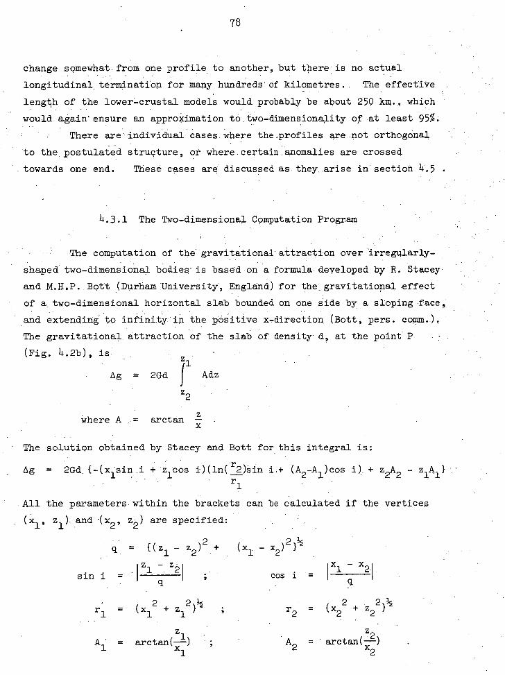
78

change somewhat from one profile to another, but there is no actual

longitudinal, termination for many hundreds of kilometres.. The effective

length of the lower-crustal models would probably be about 2(:) km., which

would again ensurean approximation ta.two-dimensionality of at least 95%,;

• There are-individual cases.where the.profiles are not orthogonal

'to the postulated structure, or where.certain.anomaIies are crossed

.towards one end. These cases are discussed as.theyarise in section .

4.3.1 The Two-dimensional Computation Program

The computation of the' gravitational attraction over irregularly-

shaped two-dimensional bodies is based on a formula developed by R. Stacey.

and M.H.P..Bott (DurharalUniversity, England) for the, gravitational effect

of a, two-dimensional horizontal slab bounded on one side by a sloping face;

and extending to infinity:in the positive x-direction (Bott, pers. comm.). •

The gravitational attraction. of the slab of density . d, at the pointP

(Fig. )4.2b), is

Ag = 2Gd f Adz

z2

Where A arctan

The solution obtained by Stacey and Bott for this integral is:

Ag = 2Gd.{-(x1sin.i + z1'cos i)(1n(r2)Sin i.+ (A2

-A1 )cos + z2A2 - ziA • 1

All the parameters. within the brackets can be calculated if the vertices

(x1, z1 ). and -(x2' z2.) are specified:

= {(z1 - z2 ) 2 +

sin i = d zi

= (x12 + z1.2 )

1/2

z i = arctan( xl

- x2 )2 } 1/2

cos i =

22 % r2

= (x2 + z2 ) 2

Z2

= • arctan( —) x2

- x2

•

79

Fig. . formula can be applied . to --the, computation of

gravity,: over: a . - .-polygonal• :..body..- : If . .the. • total . effect .. of , the infinite

- sheets bounded. by AB -, BC and cp is subtracted from the total effect of

those . .bounded by •DE and .EA and : all...sheets have ,a - .•density.d,. then the

'resultant will. he , the effect. 3 of the polygon ABODE, of ..density. d. Thus ,..

the ..effect polygon. of. any ,number. :of. sides . can ., be calculated from . .

the,, , initial- .,.specification, F.only,.. of ..its . ..vertices .,. and density.,

The :comp-ute.r-•program •• for this operation is presented in

Appendix I..(T.J.60,6., ..STACEYS . -. METHOD) , an.d. a . flow chart is given . in Fig. 4.2(d) .•

A theoretical •gravity •profile of ,length • 1 and Station separation • dl is

calculated ; ..over„a number . (N) : :of.•,polygons .:of :different .density. contrasts-. .

As stated in section.:.3;•1., all . Observed- anomalies are at the point of

observation on the earth's physical surface. . • Since the calculated

•anoMalies . .are • to be compared with the observed, the topographic height

.(h ) is specified: for . each theoretical station on the :profile. Each •

station (Po , PI, P2 , • Pn ) is • in 'turn assumed .to be the •origin of co-

ordinates, and the ;coordinates: of the polygon are adjusted accordingly

before its effect is computed. • • The program operates in the following

sequence:

. (a) The initial ; data are .input:

number of polygons N;

•,,length of traverse, ,

;station interval dl ;-

number of -stations .p:;

,...station,•heights, 1-1(.1);. • (b- ) „ Data : for. the „first- polygon are input:

number. of ,vertices + 1 n;

de .nsity - oontrast d;

.the coordin.ates 'Of , the vertices (x1 , z_) , read in a

clockwise,-direction.,, and with the first vertex.

•':repeated at the end; - ...e.g. • polygon ABCDEA; . with the

vertices • ,:zif)•• declared-, as -(x1 , z1.), (x2 , z2 ) ,

.z 5 ), zi);.. •(c) The ,effect of this -polygon : is., computed for all theoretical

stations ;.•

80

• (d) The next polygon is input, and its effeCtis calculated.at

each station and added to the contribution of the previous

polygon;

This program makes possible the.rapid computation of gravity over

two-dimensional bodies . .haVing realistic gedlogical -shaPes. The Only

'extra - labour required for a more complex body is that a.greater number of

vertices mUst.be'specified for the polygon approximating its continuous

boundary. Up to fifty vertices have been used in some cases.

The operation of this program is very similar to that of one

proposed by Talwati, Worzel.and Landisman .(1959) Their solution to the -

problem is expressed in a different form to that of Bott and Stacey ,

(pers.comm.,aboVe) but the two expressions would probably be of comparable

efficiency in computing:

4.4 BROAD SIGNIFICANCE OF THE ANOMALIES

4.4.1 Geodetic Implications

It is beyond the scope of this study to utilize the gravity

observations for a detailed qUantitative examination of either the

undulations of -the'geoid'or deflections of the vertical. To study the

former gravimetrically it is necessary to integrate the effect of gravity

anomalies, weighted by the Stokes' function, over the whole-earth. - If , the

integration is carried out to 20 ° from the station there Will be a

standard-error of 13 metres in:the determined undulation (Kaula, 1957).

Obviously,the mOst.usefUl contribution in this field would be that the

data contained in Appendix II be added to that available for existing

physical-geodesy programs, such as that of the Ohio State University.

For-the gravimetric computation of the deflections of the vertical

Heiskanen and Vening Meinesz (1958,1p. 277) : give = the requirements that

'(a) - the neighbourhood of the Oomputatidn.point have a rather

smooth gravitational field and be Covered by a network - of up -to 30

81

stations in a circle of 20 km. radius, and up to 100 stations within

100 km. radius; and

(b) an adequate regional survey exists out to about 2000 km.

from the station.

With only a,partial fulfilment of the Second requirement such conditions

are-apPrbached in. regions of the detailed oil surveys in the Gulf of

Papua. However, it is of interest to examine in a qualitative way the •

gravity anomalies: ofthe area, in, the,light of present knowledge of

geodetic parameters..

SateTlite geodesy Since the advent of artificial satellites the

perturbations of their orbits have been-used to determine the large-

scale undulations of thegeoid. W.M. Kaula has published several -

successive geoids, the latest based purely on satellite observations

being that of Kaula .(1966a).. Parameters of the ellipsoid approximating

- most closely to .this geoid differ considerably from those of the 1930

International Spheroid,

Kaula Y1966a)

1930 Spheroid

-Equatorial radius (R e 6,378,160+5 m. 6,378,388 m.

Flattening (a)

1/298.25

1/297.0

- Equatorial gravity (y e )

978,926.2 mgal. 978,049 mgal.

Thus, because the New Guinea survey iSclose to the equator, the

. gravity anomalies calculated on the 1930 - Spheroidare some 23 milligals

less than those which would be - calculated using a theoretical gravity

formula based on,Kaula's ellipsoid. However, i it is essential that all

- published gravity anomalies be based on the 1930 Spheroid until a new

gravity formula be internationally accepted.

On all satellite -determined geoids .a strong maximum has appeared

in the 'NewGuinea - Solomon Islands region. Kaula (1966a, Fig. 1) shows

the maximum deviation of +67 metres from.the ellipsoid described above

(with an equatorial-radius of 6,378,165 m.) to occur. off the northeast

coast of New Guinea. A subsequent - study by Kaula combining both

gravimetric and satellite data, gives a maximum.deviation of +76 metres

from the same ellipsoid, slightly- to-the.northeast of the previous maximum

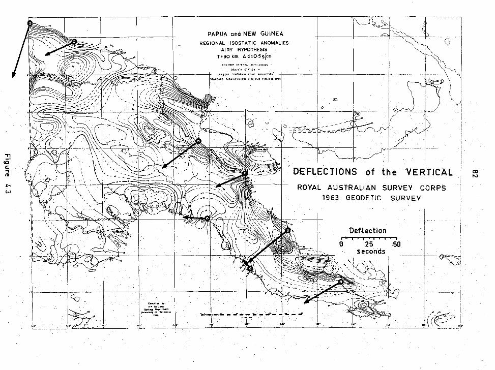
PAPUA and NEW GUINEA REGIONAL ISOSTAT IC ANOMALIES.

AIRY HYPOTHESIS T=30 km c1:0-5gicc

CONTOUR INTERVAL MIL .LIGALS •

GRAVITY ET•TION •

LAMBERT CONFORMAL CONIC PROJECTION .

STANDARD PARALLELS 0 • 40. 3 • 20, en. 710. 240.11.70

DEFLECTIONS of the VERTICAL ROYAL AUSTRALIAN SURVEY CORPS

1963 GEODETIC SURVEY

Deflection

Cornoilsd 02: 0.0. ft Joh*

<WO.

' Iria

'sr

83

(Kaula, 1966b, Fig. 1). The long.axes of the maxima in both cases have

a northwest-southeast orientation.

Vertical Deflections : The AHQ Survey-Regiment of the Royal Australian Survey Corps has made available to me the preliminary astronomical and

- - - geodetic coordinateS'at - Laplace:points'of the 1963 survey. Vertical

deflections computed from these arePlOttedin.Fig:" 4.3 on the background.

of Airy isottatio anomalies.. Sin. these deflectionsare s measured at

different elevation's* it is necessary to introduce reductions, analogous

to those for gravity, in order that they may be compared with each other.

Heiskanen and.Vening Meinesz . (1958, Sect-8.3B) consider that corrections

must be applied for topography and iscistaty, for elevation and for

horizontal gradients of gravity anomalies in the vicinity of the station, :

The effect of these corrections on . the.highebt station (630736) will be

considered, using the exact or approximate_numericalcoefficients given by

Heiskanen and Vening Meinesz ..' The height of the station is ,537 metres .,.

and the maximum gradient of any gravity anomaly is about .4 mgal/km.. for

the free-air anomaly . taken. in a- N-S direction between the stations 630736

and 630101. "

Topographic correction:

Maximum for

0.00033 h

= metres.

..seconds N-S 1

(Aln") 2 1 1/2 ' < 0,26"

reostatic 'correction: this is smaller than. the topographic correction, and

. - of.the oPPb'Pite sign', and to will reduce the above

value

Elevation correction (for changein equipotential slope): , Applied N-S

component only.

A ft -0.000171 h sin 24) seconds

-0.00006 h" (h = metres)

-o.4"

8)4

- Correction for horizontal gravity gradient;

AV i = dO •=. 0.210 2AE h seconds 3x

3Ag . '. An"- ----• 'dX = 0.210 h secO seconds 3y

3Ag 4.mga1/km (= maximum gradient)

• - 3x hence. AV 0.45" ; Ann. < 0.45"J

• The. total for•this correction will be less than 1"i

Thus; for the station requiring the greatest reduction, the total

correction is less than 1.5". Scime uncertainty is introdUced into the

gravity gradient correction, .since there is not a dense net of observations

close to any station. It is Safe to assume, however, that no observed

deflection would require a reduction of more than 3".. The deflections "on.

Fig, 4•3, then, can be compared directly if one assumes an accuracy no

greater than +3", with the consequent directional imprecision. Considering

the magnitude of the observed - deflections such an error is unlikely to

introduce'erroneous conclusions in a qualitative examination.

As stated above, the immediate observation toloe made is that the

deflections are very large. The values are relative since they depend on

the dimensions of the reference ellipsoid being used and on the deflection

values assumed at the initial point of the survey (Heiskanen and Vening

Meinesz, 1958, p. 250). These errors affect all the observed values by

almost the same amount over an area Of this size, so the fact remains that

the meridional component of vertical deflection 'changes by up to 50" from

the south to the north side of the island.. Such a variation is an

expression of geoidal undulations of a much higher order than those shown

in Kaula's (1966a,b) maps, which have wavelengths of over 90°. The

component of vertical deflection introduced by the New Guinea - Solomon

-Islands geoidal high.is a constant 2" - 3" NE' Over the whole area being

considered. The actual wavelengths bf -undulatiohs responsible for the

observed deflections - are - almost certain to vary from one station to another,

depending upon whetherthe deflection is of local or regional origin.

The deflections.are plotted on 'the backgroUnd of regional isostatic

anomalies sci - that this might be discussed.

85

The horizontal variation in the earth's gravitational field is a

direct expression of -the variation in vertical separation of adjacent

potential-surfaces of the earth. In general, for a gravitating earth,

an increase in the gravitational field represents a ripe-of the potential

surfaces and a decrease-, a fall :A graVitational - .anomOly-field - results

from the removal of some background component of the total gravitational

field; and-is:therefore expressive of Some m residualcomponent of

potential-Surface undulation. By analogy with the casefor the total

field,_d-positive-gravity anomaly represents-a rise in the corresponding

component of the potential surface and a negative anomaly, a falL

Thus, in-the : limit, d:4roperreduced gravity-anomaly map expresses

directly some high-frequency, low -amplitude component of geoidal

undulation. Differenttypes of gravity anomaly are expressive of •

different components of this undulation. _ The highest frequency is.

expressed-by free -air anomalies, and can be mountainous areas

only by measuring the anomalies Over a very dense net. A broader

component Of the undulation is expressedby free-air anomalies, sampled

over the total height range', and - smoothed. Isostatic anomalies express

that - component of geoidal undulation observed - at a station sufficiently .

removed from the topography that the effects of topography and compensation

are similar.

All - the Components- are -of, low amplitude compared with the primary

geoidal undulatiOns, but they can produce large geoidal_gradients over _

small distances, and hence large deflectiOns. Looking at Fig. 4.3 (and

bearing in Mind that the deflections•:are merely relative) it can be seen

that . 1, 4 and 6 have ttrong comikments'in the direction of the maximum local gradient of the isostatib anomaly. The deflection at Station 5 is

to the west of the maximum local gradient of-the iSostatic anomaly,

possibly resulting from an east-west gebdetie gradient in this-location,

due to the - New Britain Trench:. Such a regional potential-surface.

gradient- need not be the cause of observable gravity anomalies on the

of this survey Station 3 has a deflection in the direction of

maximum gradientof the mean free -air anomalies (p. 64), Station 2'

-shows a small deflection in the direction of negative isostatib anomaly

gradient and zero free-air- anomaly gradient - probably .resulting from

local causes not evident in the regional gravity coverage Stations 7

86

and 8 have deflections in the direction of negative gradient of all regional anomalies. This points to the existence of strong positive isostatic

'anomalies associated with the Bewani and_Torricelli Mountains, over which

there is no gravity, coverage.. Station 8 could also be strongly affected. by the ultrabasic Bougainville massif, on the northern,of which it

is located.

It is very likely that the overall. correction, accounting for the

dimensions of the reference ellipsoid used and the Initial point assumptions,

would add to all stations a.northeasterly deflection component. Yet there

will remain, though perhaps predictably, a residual system of northeast-

southwest deflections which indicate a longitudinal geoidal high through

central New Guinea and Papua,

4.4.2 Structural and Isostatic Implications

Before carrying out a detailed indirect interpretation it is of

value to examine the significance of the patterns exhibited by anomalies

reduced according to different assumptions.

Mean free -air anomalies Neglecting the effect of upper-crustal

inhomogeneities, the free-air. anomaly can be said to comprise the

gravitational effects of topography and its isostatic compensation.

Even if the topography is perfectly compensated the inverse square law

ensures that its effect is much greater than that of the compensation.

Hence the usual correlation of positive free-air anomalies and elevation.

Before this correlation is examined quantitatively the exact nature of

observed and mean free-air anomalies must be understood.

Consider a sawtooth-shaped - cross-section . of a mountain range

having two-dimensional symmetry, and with the valleys at a common

plateau-level. The topographic attraction at .a vAlley -station will

consist of the downward attraction of the plateau below the valley,

reduced by a component of upwardattraction due to the mountains. Thus

the free-air anomaly at a valley station represents the downward attraction

of Less than the material underneath it. At a mountain-top station all

87

components of attraction will be downwards, and the free-air anomaly

will truthfully represent the downward attraction of all material lower

than the station. All stations between mountain-top and valley floor

will have a component of upward attraction. To make a free-air anomaly

truly representative only of the material belowthe . station level, then,

there must be a terrain correction applied to neutralize the gravitational

effect of material above station level. This terrain correction is

• largest in the valleys, and zero on mountain peaks, and thus differs from

- the terrain, correction applied in topographic reduction, which is largest

on mountain peaks, but also finite invalleys-. If the free-air anomaly

is evenly sampled over hill and dale, the mean anomaly will be less than

the attraction of the mean topography by the value of the mean terrain

correction. If the free-air - anomaly is sampled only in valleys the mean

will be, as shown above, less than the attraction of the mean minimum

topography. If mountain-peak stations predominate, 'the mean anomaly will

be greater than that caused by the mean topography.

The tendency in most_gravity surveys is for the more accessible

valley areas to be more densely sampled than the mountains.. The survey

under.consideration has the advantage that almost 20% of the stations are

at survey points, located on high points of the topography and accessible

only hy helicopter.. Such a proportion approximates the distribution of

actual high and low ground in the mountainous areas.

The bean topography has been taken simply as the running mean of

station elevations, calculated'by the smoothing program (sect. 3.7).

_ This is considered to be most representative of the mean elevation

corresponding to any mean anomaly, and it tallies well with mean topographic

elevation_from the digitized topographic blocks. No terrain correction

has been applied to the free-air anomalies before orafter smoothing.

However, as discussed above, the correction is purely for the upward

attraction of mountain areas, and is likely to be more than one or two

milligals only in verysteep, narrow valleys (and where they were common

stations were usually situated on the heights).' The major part of the

terrain correction' in the topographic reduction is due to the lack of.'

attraction of valley areas, which. represent a much .larger proportion of

a mountain cross-section than the peaks.

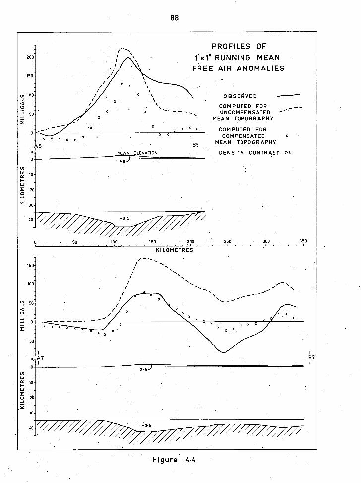
40- -0-5

X X

85

PROFILES OF rxl ° RUNNING MEAN FREE AIR ANOMALIES

200

150

OBSERVED

COMPUTED FOR UNCOMPENSATED

'MEAN TOPOGRAPHY

COMPUTED FOR COMPENSATED

MEAN TOPOGRAPHY

50

x x x

AS

X X X X X

5 - MEAN ELEVATION DENSITY CONTRAST 2.5

0

- 1° - _ 2o-

30-

2.5

40- -13.5

50

100

150

200

250 300 350

KILOMETRES

150

■ ■ 100

.... / \ ■ /

\ /

\ ...■ ."' /".. N ....

\ ..."

X X

/•—

/

MIL

LIG

ALS 50

-50

I I 5 A7 B7

I I o

KILO

MET

RES

7

10

20-

30-

9

2.5

88

Figure 4.4

89

• On further question must be asked before interpreting these mean

anomalies: - Where does one assume the stations to be? It has been

reiterated in this thesis that no classical reduction changes the

position Of the observation point. This is indeed the most rigorous

Iay of interpreting all other anomalies, both observed and smoothed.

HOWeVer, in. this case the smoothed topography is above the level of the

valley stations while the increased anomalies at these stations indicate

that there has been•a - (mathematical) thickening of material below them.

Since the free-air anomalies are not used in any detailed interpretation

it has been adjudged reasonable to consider them as observations on the

surface defined by the mean elevations.

Two profiles across the free-air anomaly map are shown in Fig. 4.4,

the pOsitiOns of the profiles being given in Fig. 4.6 . In both cases

the effect has been calculatedOf "local" Airy compensation of the

ambothed topography, with a standard crustal thickness of 35 ipa. This,

'of course, correaponds to regional compensation of the Vening Meinesz

type.

Profile . A5B5, across the -Owen Stanley Range, indicates that the

observed anomaly is closer to the theoretical curve for the uncompensated

than for the compensated case. However, the high value of the observed

mean, especially towards B5,. is undoubtedly due partly to the smoothing

out of the large positive anomaly over the Papuan Ultrabasic Belt (a

feature discussed in some detail later). Removal of this effect would

cause the smoothed anomaly to assume a position somewhat closer to that

calculated for the compensated Case.

'Profile A7B7, across the Eastern Highlands and Huon Peninsula,

shows that the observed curve; in the central part, fits well with that

- calculated as suming complete compensation. The apparent overcompensation

to the right of this Is more likely to be a geological effect, caused by

• thick sediments.

In both these cases the regional compensation could be considered

to 'be a smoothed local compensation.

The contours of the free-air anOmaly map (p. 64) define a series

of trends which are certainly related to the first-order tectonic

features of the region'. A broadly sinuous positive anomaly trending WNW

90

through the central highlands indicates a degree of isostatic compensation

lessening to the. west of profile A7B7. . The mass-excess appears to be

greatest in the Star Mountains (5 ° ,1)41° ) and probably continues into

West Irian. Flanking this anomaly on the .south side is a small negative

anomaly which is especially pronounced in areas of Pliocene sedimentation,

the youngest (exposed) development of the Papuan Geosyncline. A saddle

in this anomaly corresponds to the Upper Miocene Darai.swell (71/2° ,1)44° )

(see geological map, p. 100). On the north side of the central positive

there is another'flanking low which trends, ESE through the Sepik Valley

(4°, 1)42°) to reach a minimum of -100 milligals near Madang (51/2°, 1)46 ° ),

and then swings SE through the Finisterre Range to end on a saddle to the

south and west of the Watut River. This low saddle (71/20 , 1)461/20 ) links

the northern and southern negative areas through the uplifted Middle and

Lower Miocene Aure Trough, and.is of tectonic significance in that it

distinctly separates the pre-Tertiary blocks of the central highlands and

the Owen Stanley Range. The northern negative area marks the position of

Upper Tertiary geosynclinal sedimentation, and is itself bounded on the

north by positive, anomalies consistent with a crust thinning towards the

ocean.

The Owen Stanley Block and Papuan Ultrabasic Belt (81/20 1471/2°) are

encompassed by a SE-trending anomaly which shows that the mass-excess

indicated by profile A5B5 is typical of the. region. On the western side

of the Goropu Mountains (91/20 , 1 )49° ) the anomaly has a pronounced sinistral

offset of some 70 km. in a NE direction. The appearance of this offset

on the map may be partly a function of 'sampling, and indeed the mean

elevations show some tendency in the same direction. However, the offset

cannot be completely . explained by the mean elevations, and it will be

shown in subsequent .sections that both the geological and detailed Bouguer

'interpretations are consistent with the probability of transcurrent

faulting in this region.

In the southwest of the area the positive anomalies over the "

essentially sea-level Fly River Platform indicate a crust slightly thinner.

than normal. The,gentle,high in the centre of the region . 0° , 142° )

'correlates with the area of thinnest sedimentation.

91

Bouguer anomalies It is generally - accepted that, if isostatic

compensation exists, Bouguer anomalies in a mountainous area will be

negative, - at least with respect to the adjoining low-level platform.

The extent. to Which this appliesin a local sense is dependent upon the

level at which the - isostatic compensation is located. A more rigorous

and generalized form of the principle is to be found in Gauss's theorem

where

= 2TrGM .

gB = Bouguer anomaly;

M = total compensating mass, or anti-mass;

S = surface of the earth.

If the integral. could be evaluated over an extensive, area including only

mountains and sea-level plain, then any compensating mass would be

negative (anti-mass), SO that the integral would be negative. The test

that a - mountainous area-is to some.degree compensated is not that

immediate Bouguer anomalies be negative, but that their sum over a wide

area be negative,. Fig. 4.5(a) illustrates this point. A zone in the

upper mantle, between 70 and 190 km., is assumed to have expanded, with

lateral. constraints restricting the volume increase to the vertical

direction. An increase corresponding to 2 km. uplift of the top

surface of the expanded zone requires a density change of -0.05 g/cc

in material of original density 3.3 ecc. 'Thus, on the surface of the

earth, there 2 km. topographic uplift without any change in crustal

thickness. However, the "normal" and "expanded" columns have identical

masses above the level of 190 km., so isostatic compensation (of a

modified Pratt type) prevails. The resultanti3ouguer anomaly over the

80 km. wide uplift. is More positive than that over the surrounding

"normal" area., but it is apparent that the integral of the anomaly over

a wide area will be - negative.

Where Airy-type compensation exists the compensation is usually

less than 50 km, from the surface, which results In a direct negative

correlation of Bouguer anomaly with topography. The distinction between

local and regional compensation is usually beyond the resolving power of

gravity anomalies. In Fig. 4.5(h) computed-profiles are shown for a

two-dimensional topographic mass compensated locally and regionally, the

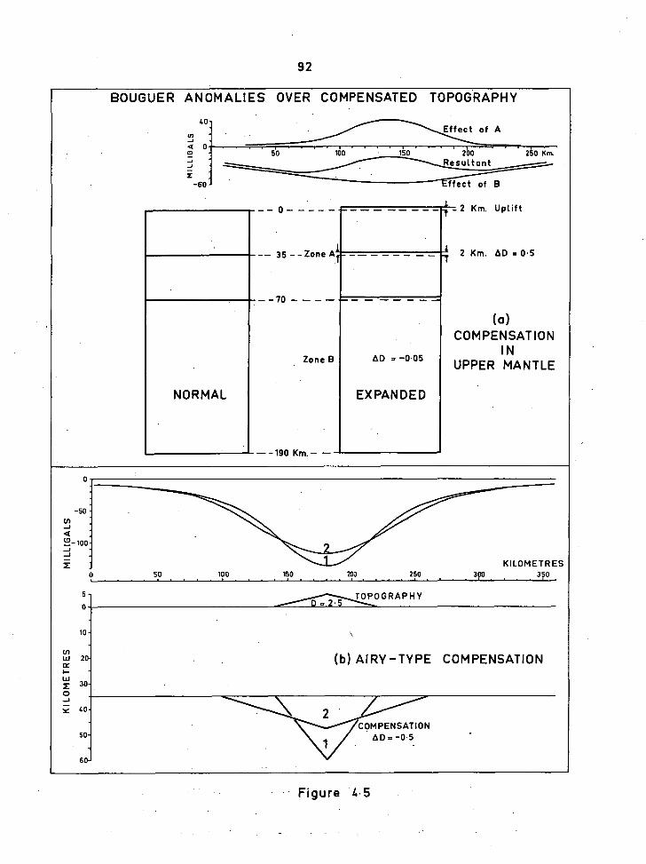
92

BOUGUER

•

40

u) - _• .

ANOMALIES OVER COMPENSATED TOPOGRAPHY

Effect of A

4 0 ED _,— '

-60

50 100 150 200 250 Km Resultant

Effect of B

_2 Km. Uplift

I 4 2 Km. AD = 0.5

(a) COMPENSATION

IN UPPER MANTLE

o _____ 4 _2

------

NORMAL

Zone B

190 Km.

AD = —0.05

EXPANDED

o

-50

4 cn

0 -100 -L- _t E

0

5

o

_

190 N44MMIIV KILOMETRES

mo no 300 350

------

50 150

TOPOGRAPHY

10 -

tn W 20- ce ,- - w x 30- 0

\

(b) AIRY-TYPE COMPENSATION

—, 40-

60-

50-

/ COMPENSATION

Figure 4.5

9 3

crdsa2-seational - areas of:structures 1 and 2 being equal. With very

little- interference from geological sources the two . Bouguer anomaly

profile' would be indistinguishable.

: - The'broad configuration of , the - BOuguer anomalies is most readily

seen-on-the tap of smoothed data (p..64) A large negative anomaly

encompasses the . whole Central highlands area— The most negative.

anomalies are-in the Southern Highlands low (6° , 1431/2° ), - and the

Finiaterre lOW'(6° 1461/4P). Following a detailed examinatiOn (4.5.3)

I consider that both of these lows.aredue-more to thickened sediments .

than to an espeCially ,-thick crust.' -Between these two IoW areas is':a -

relatiVe high (though still as low-as 90' milligais) which correlate's'

broadly with the KubOrand" Bismarck Ranges and which appears to be a •

• continuation Of the West Range . high (41/20 142° ).. The Bouguer anomalies

Ofthe , Central 'highlands become less negative to the west, being

algebraically greater than 750 milligals in the Star Mountains (50, 11410).

To the east' the anomalies becomé . positive in the OwenStanley Block,

althoUghthey-are negative relatiye . to the flanking anomalies. As with

the 'mean freeair anOtalieS, the mean Bouguer:anomaly loses its correlation

with topographyin the Goropu Mts region (91/2 0 , 149° ), and swings to the

- northeast, lending support to.the idea of some structural offset in the

region. - Other similarities to the mean free-air anomalies are to be

fbund.in'the:relatiVe low in the Sepik Valley (4°,. 1421/2°) trending' into

the Finisterre low, and in the•gentle'high•trending northwest through the'

'Fly Platform

-In general, both mean' free-air and mean Bouguer anomalies show an

'apparent interaction of northerly,- and easterly-trending tectonic features.

Since' individual anomalies are "smeared out". the' smoothed anomalies

cannot be interpreted too literally in terms *of underlying' structures.

•The extended Bouguer anomalies mai:y-(p. -64) - adds some detail to the

smbOthed ve rsion .: Finisterre low is not entirely continuous, but

aPPears to be' Subject -to an offset in the Madang region (51/2 0 , 1451/2° ).

The western part Of 'the 'anomaly is not correlated with' any- considerable

Mouniaina;-but with - deep seditenta Of the' Madang basin (5 0 , 1451/2° ).

Although' at"- elevation -,the eastern end of the Huon Peninsula -

(61/2° , 147h° ) has a positive anomaly, indicating uplift not directly

9 )4

compensated on the Airy, system. In the Sepik area the negative values

are especially pronounced in two basins, the August River Basin (4 ° , 1419 )

and the Nuku Basin (4°, 14°). Strong positive gradients on the north

coast indicate rapid thinning or the crust. A relative high appears

over the .Bismarck Range (60 , 1451/49) and is separated from'an indefinite

high over the Kubor Range (61/2°, 1)459 .),,- by a low over the Wahgi Valley

(6° ,.145° ). In the east, the Owen Stanley Block is a region of small

negative anomalies, bounded on the northeast by a very strong positive

gradient over the edge of the Papuan Ultrabasic Belt (9 0 , 148° ). The

large positive anomalies over the belt form an arc more . than 400 km. long,

from Salamaua. 147° )-to CollingWood Bay.(91/2P, 1491/29). The Bouguer

anomalies lose any correlation with the trend of the Eastern Cordillera

at about 9½°S, 14 WW, while the D'Entrecasteaux Islands (AP, 1501/2°) become the locus of a Bouguer anomaly low. As will be discussed in some

detail in profile interpretation, this pattern is consistent with a

northeasterly sinistral offset. Around:the.Gulf of. Papua (99 , 1)45 ° ) a

series of negative anomalies is correlated with areas'of deep Pliocene

and Upper Miocene pelitic sedimentation,•,with intervening. positive anomalies

being 'overuplifted Middle and Lower Miocene Aure Group rocks (8 ° , 1451/20 )

or Miocene limestone (71/29, - 14)4° ).

Isostatic anomalies The isostatic• anomalies calculated according to

Pratt or Airy models have a very similar distribution, as can be seen

from the contour maps (p. 64). Where the anomaly values differ, those on

the .Airy hypothesis are.up to 20 milligals higher than those on the Pratt'

hypothesis. This, is due' to the somewhat larger degree of regionality of .

the gravitational - effect of the Pratt-type compensation, which is centred

on a greater' depth than the Airy.

When a - fairly narrow topographic feature, (say 30-40 km. wide) is

assumed to be locally compensated, the isOstatic correction on the Pratt

hypothesis will be of lower maximumamplitude and broader than that on the

Airy. hypothesis. Consequently, for a Bouguer anomaly located on or near

the abovementioned narrow topographic feature,. the algebraic value will be

increased more by the subtraction of the larger:(negative)-Airy correction

than the smaller Pratt correction,- A. broad topographic feature will

95

occasion Much the same correction bn both Airy and Pratt' hypotheses.''

Following thiS argument, at a cOnsiderablediStande from any -

toPograPhic feature the'Pratt'correction'shoUld be ofa,larger amplitude .

than the Ai ri (to . maintain - the conditions of'GdUsS's Theorem).' In this

area; .- then;the -algebrait'valUes . of . the isostatio anbmalies should be

larger tOr'thelpratt than therAiry Model. This iS Seen to be the case

on the rsostatic maps, where the Pratt 'anomalies over the FlY'Platform-

are slightly larger - than the . Airy; ' Theeffect, Of course, -is not as

pronounted'as . the excess of the -Airy' anomalies' in the 'axial part bi" -•,, • .

isostatiC-model; bUtit - is spread over 'a more ektensive'area.

"A mentionedin sectibn 3.5.5, iSOStatic : anomalies (without 'a'

geological correction) can be caused either by departures from complete

topOgraphiccoMpensation or' by upper crustal geological features.

AnotaiieS'reSuiting'from the latteareldentifiableif of high spatial'

frequency, but it is' notpossible, on-graVimetric evidence alone, to'*

diStingdish between a broad upper-crustal anomaly and an isOsiatic effect.

.Apart froma- positive anotaly . at 'the eastern end of the Bismarck

'Range andSepikWahgiTivide'(51/2 °-,. 1441/2°) the Pratt and Airy . anomalies

are negativethroughbUt'the central'Cordilleran However, the

isostatia'anomalieS . are Up'to.80: milligals'aboVe the BOuguer anomalies

thiS region, afgood'indiaation that much 'Of' the' negatiVe Bouguer anomaly

results froth the'isostatic compensation of the . mbuntarns. Most of the

anomalous:structures - defined by the'Bouguer anoMaIies are still evident On

the isostatic anomaly map:' The . 'Sepik area retains the anomaly configur-

ation of to distinct basins within -a- ESt7trending . low, bounded on the

north and south by positive anomalies . . The West, and Central, Range area

(41/2° ,1429)'haVing p6sitiv'e .Boilgver anomalies, naturally has More -

positive isostatic anomalies.' The trending through the Middle Ramu o o riS -s .tiIIWell-defined; . with the apparent offset in the

Madang s area being . acCentuated'on - both Pratt and Airy Maps.- . Although -

iscistatic 'eanbraalies'olie -r the Western FiniSterre Mts ar'e very negative; the

largestnegative anomalies are.cOnfined to the northern 'margin Of the '

Markham Va1ley, - (61/2° , 1461/2° )'; .1-11'hi8 is - understandable in View Of' the fact

that an isostatic compensation model is'set up for the mountains, but not

for the low-lying valley. Thus, the Bouguer 'anomalies over the mountains

96

are subject to a much larger positive isostatic correction than are those

in the valley4 Distortion, in this way, of 13ouguer anomalies which

probably have a common origin (deep sediments) indicates 'that it is

essential to carry out detailed interpretation at the Bouguer anomaly

stage. This northwesterly-trending . Finisterre low is separated from the

Southern Highlands low (6° , 1431/20 ) by a series of small, similarly..

trending, apparently geological anomalies in the Bismarck Range-Wahgi Valley'

area.. lsostatic corrections, on both hypotheses, reduce the Southern

Highlands Bouguer anomaly of . -130 .milligals to an isostatic anomaly of

-50 milligals. As will be shown in detailed interpretation, this

isostatic anomaly may well be due to a broad sedimentary basin instead of

overcompensation.

To the east, the Owen Stanley BloOk has low isostatic anomalies,

and again appears to be dissociated from that part of Papua .east of.the

Goropu Mts, where isostatic anomalies rise to a maximum of over 100

milligals in the Milne Bay'region..(101/2 c.) , 1501/2°). The Papuan Ultrabasic

Belt, having large positive Bouguer anomalies, has even larger isostatic

anomalies., the Airy being higher than the Pratt owing to the proximity of

the Ultrabasics to the hypothesized compensation 'of the Owen Stanley Range.

The Fly River Platform has positive isostatic anomalies reaching

a maximum of 50 milligals, and which are probably the result of under-

compensation combined with upwarping,Of the crystalline basement. If the

Airy hypothesis is assumed to be correct, the crust under the platform is

a few kilometresthinner than the standard sea-level crust.

Airy isostatic anmalies,. subjected to the smoothing technique

discussed in 3.7, show that large (apparent) departures from equilibrium

are confined toa northern coastal strip, generally less than 150 km, wide,

extending the length of the eastern part of the island (p. 64). The

central, southern and western regions Of the map area, and the Owen Stanley

Block, would appear to have reached a mOre'stable condition. This

distribution of stable and unstable regions lends support to the concept

of successive . orogenic zones developing On, and becoming . indorporated in,

the northeastern margin of the Australian continent.

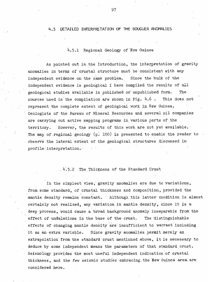
97

4.5 DETAILED INTERPRETATION OF THE BOUGUER ANOMALIES

4.5.1 Regional Geology of NewGuinea

As pointed out in the Introduction, the interpretation of gravity

anomalies in terms of crustal structure must be consistent with any

independent evidence on 'the same problem. Since the bulk of the

independent evidence is geological I have Compiled the results of all

geological studies available in published or unpublished form. The

sources used in the compilation are shown in Fig. 4.6 . This does not

represent the complete extent of geological work in New Guinea.

Geologists of the Bureau of Mineral Resources and several oil companies

are carrying out active mapping programs in various parts of the

territory. However, 'the results of this work are not yet available.

The map of.regional.geology (p. 100) is presented to enable the reader - to

observe the lateral extent of the geological structures discussed in

profile -interpretation.•

4.5.2 The Thickness of the Standard Crust

In the simplest view, gravity anomalies are due to variations,

from some standard, of crustal thickness and composition, provided the

mantle density retains constant. Although this latter condition is almost

certainly not realized, any variation in mantle density, since it.is a

deep process, would cause a broad.background anomaly inseparable from the

effect of undulations in the base of the crust. The distinguishable

effects of changing mantle density are" insufficient to warrant including

it as an extra variable. Since gravity anomalies permit merely an

extrapolation from the standard crust mentioned above, it is necessary to

deduce by some independent means the parameters of that standard crust.

Seismology provides the most useful independent indication of crustal

thickness; and the few seismic studfes. - embracing_the New Guinea area are

considered here.

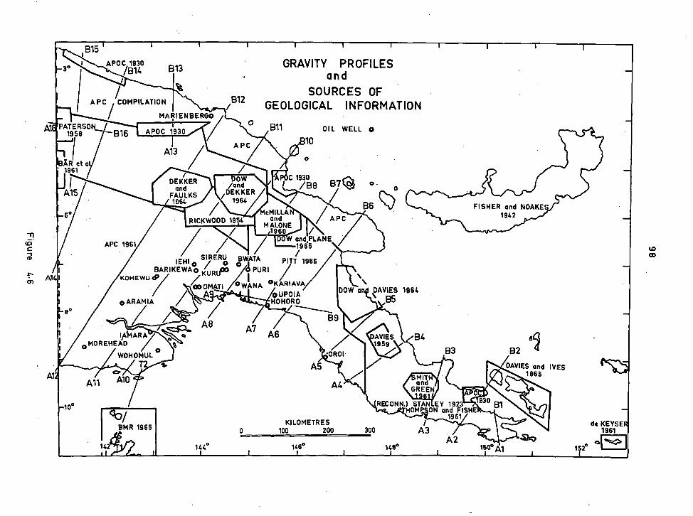
B15 APOC 1930

/B14

APC / COMPILATION

MARIENBERGO

GRAVITY PROFILES and

SOURCES OF B12 GEOLOGICAL INFORMATION

B13

GO OMATI A •

BMR 1965

42

•OR01 . •

Ag

A2 146° 146° 144°

de KEYSER 1961

152° 41'

a PATERSON 1958 — B16 —1/

BAR et a 1961

JA115

APOC 1930

413

DEKKER and

FAULKS 1964.

RICKWOOD 1954

OIL WELL 0

10

6 A P

APC 1961

SIRERU IEHI 0 / 0 . BARIKEWAo K'URU°C1

KOMEWU

o ARAMIA

48 I,AV4 AR A

o MOREHEAD

WOHOMU o

L 1.

All A10

BWATA 0 1

0 PURI

„ WAN I

A OKARIAVA w OUPOIA HOHORO

B9 47

AVIES B4 I959

44

RECONN.) STAN EY 1923 • HOMP ON and FISHE

1961 KILOMETRES

100 200 300 43

150° 41

I I and.PLANE 1965

PITT 1966

6

B3

OW /and

/DEKKER

1964

A PC trdi

C 1930 /B8

eMILLA and

MALONE 1960

412

DAVIES 1964 B5

DOW a

B2

DAVIES and IVES

al 1965

7

•Elc?

30

99

Santo (1963), in his division of the Pacific into regions of

different crustal thickness, based on Rayleigh wave dispersion, assigned

the whole of the New Guinea - Bismarck Sea area to the Same "Continental"

subdivision as Australia. Bolt and Niazi (1964) found that Rayleigh

wave dispersion curves fora - Solomon Is earthquake recorded at Charter's

Towers (CUT) and Mundaring (MUN) indicated an average crustal thickness,

between the two observatories, of 30 to 35 km. (Fig-4.7). Wave paths

from New Guinea and the Aru Is to Mundaring indicated that the crust

thickened to the north of the CHT-MUN line. Brooks and Ripper (1966), in

a study of the group velocities of Rayleigh waves recorded at Port

Moresby (POW . , find that the crust is "normal continental" along paths A,

3 and C, and thicker along D and E (Fig. 4.7). From a consideration of

these studies it has been decided, for the northeastern Australian region, .

to assume a standard crustal thickness. of 35 km. where zero Bouguer -

anomaly is recorded, at sea-level, on exposed crystalline sialic rocks.

Granite of the Lower Palaeozoic Tasman Geosyncline is exposed on

Cape York Peninsula (northeastern Australia), on islands across Torres

Strait', and at Mabaduan in southern Papua, Profile T1T2 (Figs 4.6 and

4.7) shows the sea-level Bouguer anomalies on the granites of Prince of

Wales Island.and Mabaduan. Assuming a density contrast.of 0.5 g/cc at

the base of the crust the anomalies correspond to.a northward thinning

of the crust across Torres Strait, from 34 km. to 33 km. From this

crustal thickness of 33 km. at Mabaduan, with no geological anomaly, the

interpretations of all gravity profiles are extrapolated. The low

Bouguer anomalies in the Port Moresby area (30 40 milligals), although

crystalline basement is not exposed, are assumed to correlate with a

crustal thickness, similar to that at Mabaduan. From a study of arrivals

at POM from Bikini . and Eniwetok explosions, Doyle and Webb (1963) conclude

that the crust under the station is continental..

It will be noted that the standard crust chosen (35 km.) is

different from the standard crust (T = 30 km.) assumed in the calculation

of Airy isostatic.anomalies. The imprecision of the seismic evidence used

makes it impossible to choose between the two. Indeed, the question is

largely academic since the gravitational effect of compensation disposed

about the 30 km: level Would be, owing to other perturbations, indistin-

guishable from that disposed about the 35 km. level.

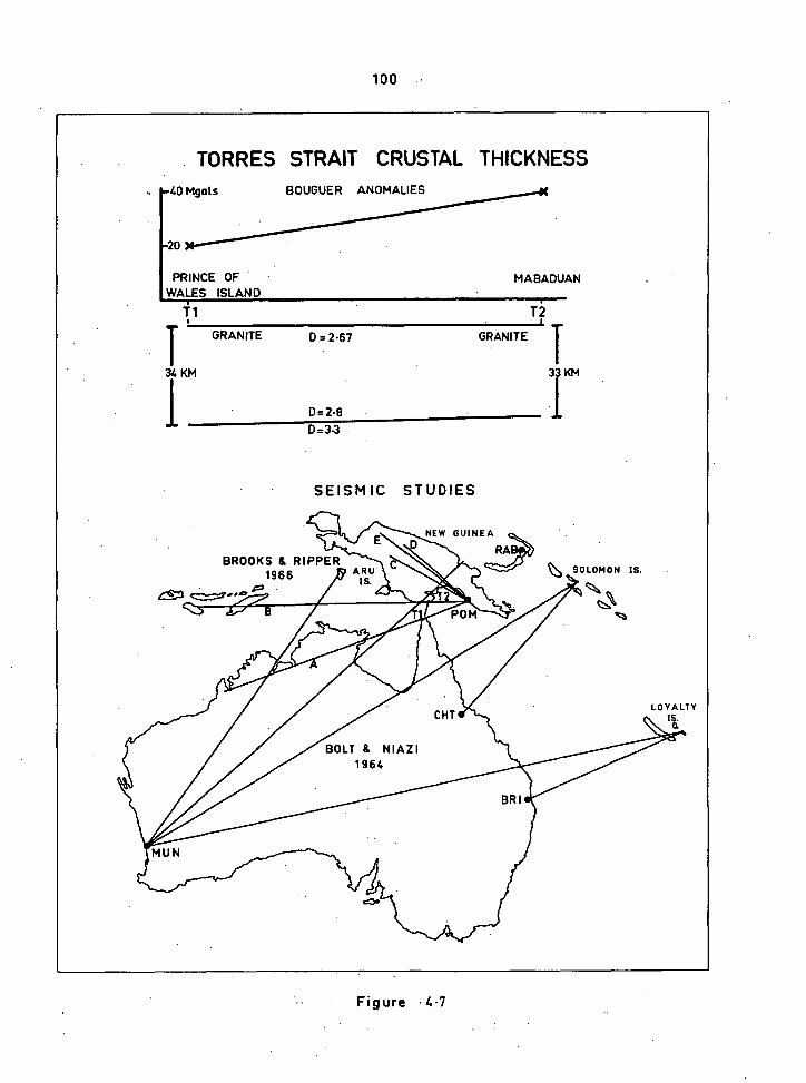
BROOKS & RIPPER 1966

4'2 CS;:l

NEW GUINEA

4A7

SOLOMON IS.

LOYALTY IS.

100

TORRES STRAIT CRUSTAL THICKNESS 40 MgaEs BOUGUER ANOMALIES

PRINCE OF WALES ISLAND

ti GRANITE 0 = 2•67

MABADUAN

GRANITE

33 KM

D= D = 3.3

SEISMIC STUDIES

Figure •4•7

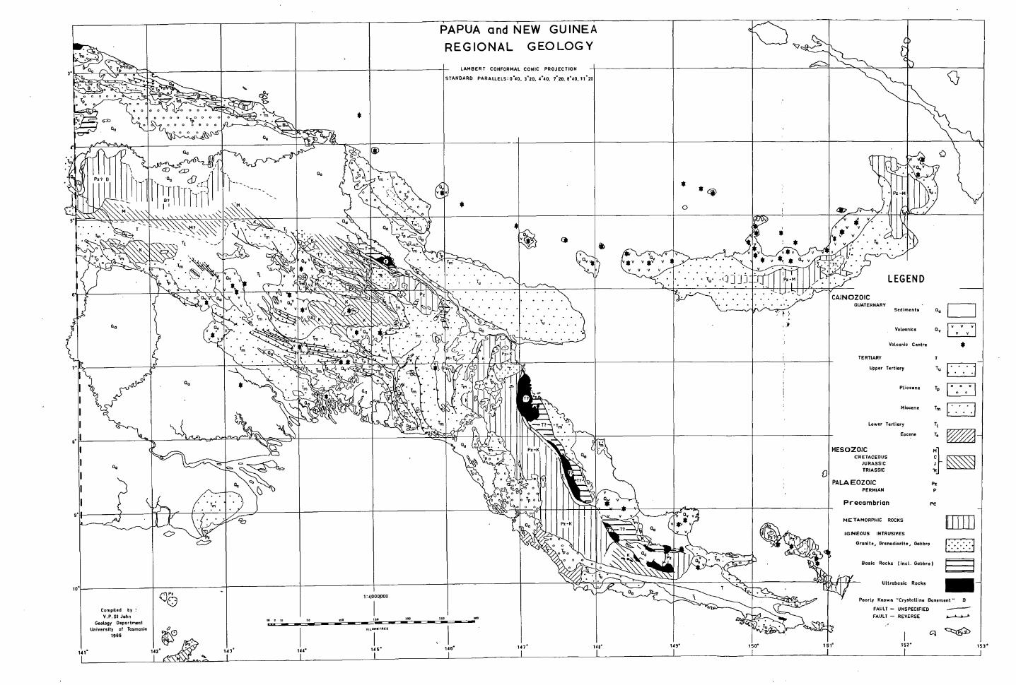
PAPUA and NEW GUINEA

REGIONAL GEOLOGY a.

0 ■

arc 913 •

•

I 4,

LAMBERT CONFORMAL CONIC PROJECTION

STANDARD PARALLELS. 0 °40, 3 °20, 4 °40, 7° 20, 6 ° 40, 11 ° 20

,

C3

Ilk

allpilopligNioNimi.,

.31iihee. .-.:.°'.....r. . I. 111.. : ■sh....... ai --vg.....- ----0r- e. Frigirr':

j? a )

•

• .-

.) .

•:-:

.

Of

. , Pz? B

1•1\\ \\

, ao

B? I

CD

I I 1

./

I 1

, r

\‘t•I

. • T,e .

..-7 • y

v v TI v v

av, v

* v v

(2

)

•

°

(4) •

•

*

* ....

0

,

47

\••

•

. .

• I. •

, 4

\

\

•

\

•

1 if P

M

„

4 1

. . .

, •

• A A • e

Pr e .14

, . •

•

•EAV

',1 •

.

Oa

It GO

> >

v

• • • • a • . (:) i 1 j :_,--i T • • • . • . . .

81

*

4 y*y v ,h.v ! * i v y

v vv i v .. • .

//1 V • •

.

v ,.

. . .

.

ir •

411

-.'. '''441111-...061W. .

\ ,,, NN.,,,*, v * a v v v

ILO 0 Tr,' . • . . .

....I-I-ANN .

• • • Tu • • • ,...A111ki ■ •

• . .

' ' • ' • v v ..

gill .

• .

. .

• LEGEND . • •

. . • . • , • . .

• • . . . . •

. . . . . .

. . • . • . . . . . • • -

. . .. .

, .

CAINOZOIC v v %v ovv

.....,:,.. • . v

, .Tro .. .

',..

, . . . • '" er•

• ' • • . . .

• .

A „.,,..)4)1\.....

--....- \-.Ri,

. ' n . .

NIC . ,

' .

. • • • . , . QUATERNARY Sediments Cie

T • • 4\

>

_

' ‘. • . Volcanics 0„

v v . • . .

I 6? Pz- K

Volcanic Centre

TERTIARY T

*

. ip...

.• *

, %•,4:1 0 ‘j4r.IC:3

• • • e "vgi• i PI

K

I

I

I

I

I A.....1 ...._........

. Upper Tertiary Tu . . . .

' • • '

I. . Tp

I 1 C3 :2,44

wai 01 JI =

Pliocene Tp ° 0 ° .°

• it

1 Miocene Tp,

. . . .

,IttapriN 44 o& Lower Tertiary T, i■\:-.. Eocene Te ,V

I s...,

c. .:Op

o ..,e, c

0

P. -K '111‘‘INik a°

MESOZOIC

I Oa

I

I ( \ ivirc%

c=.

. . .

. . . .

. %0

. .

o o

ifif, . . .

•i lav

MI

CRETACEOUS C

JURASSIC J Nillik

.

riMik

v v C14/ v

TRIASSIC

PALAEOZOIC PERMIAN

Pz P

Precambrian pe •

' 9:3

-.Pam ley- -Nelc

.

rid

7601 r `1 Pz-K

v v

v Cl v v * *v v o.

. METAMORPHIC ROCKS 4 a. IGNEOUS INTRUSIVES tit

Granite, Granodiorite, Gabbro ' • ' • .,.__.--,...........

....... , Pz

N. 111,.. N * NW,

Basic Rocks ( incl. Gabbro) \

'1411111 Ilia dillt Ultrabasic Rocks

Poorly Known "Crystalline Basement " B

FAULT — UNSPECIFIED FAULT — REVERSE e..--L-A--1.

OAF 10

Compiled by : V.P. St John

Geology Department

University of Tasmania 1966

1:4.000P00

Iortrir -mos

150°

••vr,104

•

• Me' "T. ..,

151

10 so 000 so io o loo Ir

I 152 ° 151

. . KILOMETRES

I 117 ° 149 ° 149° 141. 142

143

144

101

Since the completion of interpretation Mr D. Finlayson, of the

Bureau of Mineral Resources, Geology and Geophysics, has communicated to

me the preliminary, results of the CRUMP Seismic Experiment (Carpentaria

Region Upper Mantle Project). His calculations put the depth of the

Mohorovicic discontinuity under Torres Strait at 29 km. As stated

above, the change of 5 km. in absolute depth of the hypothesized crust-

mantle interface will not observably affect computed gravitational effects,

the relative depth of the interface being the operative factor. However,

to bring the following.interpretational profiles into agreement with the

seismic case one can assume the standard crustal-base line to be at 30,

rather than 35 kilometres.

4.5.3 The Bouguer Anomaly Profiles

Apart from the "definitive" profile T1T2, sixteen Bouguer anomaly

profiles, have been interpreted by the.indirect method of comparing

observed anomalies with those calculatedfor two-dimensional models by the

program discussed in section 4.3. . Computation points in the theoretical

profiles are assumed to be on the physical surface of the earth,, and.the

effect of all geological structure's above sea-level is assumed to have

been removed in the extended Bouguer reduction. Because of the irregular

station distribution the "observed" profiles are not purely observational,

, but are taken from contours. In all cases where there exists a good,

approximately linear, -station distribution transverse to anomalies the

profiles have been p1acedso'as4-to minimite:the effect of any contouring

- error. Those Tarts of a.profile . which are determined by contours based on

sketchy information are; by broken,lines. The profile positions

are indicated in Fig. 4.6 , Excepting the first, profiles will be

discussed . in numerical order, and the geological evidence for upper-

crustal structures will be presented where it is incorporated. To

eliminate' edgeeffects, the. terminating vertices.of_all models are

projected out. horizontally :for 1000 km.

Profile A4B4 (Fig. 4.8) This profile is discussed first since it

150

73. OBSERVED

COMPUTED 100

tn DENSITY A , cu

Z.— CONTRAST

E0 oc 50

X

7

7

00 CO

-20 A4

B4

5 - I OWEN STANLEY RA.

0

KILOMETRES 50 100 150 200 250

in 150

too

E 0

X

102

Figure 4.8

103

incorporates-. the most closely-spaced traverse across the Papuan Ultrabasic

Belt„-pne of,themost:enigmatio .structures in New Guinea.. The . observed

profile. has been, matched by. theoretical profiles calculated for two

Anodels,r based.on ; surface geology, but significantly different, in sub 7 .

surface,00nfiguration, Only for,thisprofile .have.alternative inter :7

pretationsL been. calculated,but . the procedure should emphasize that. the

interp fretations : of.allsubsequent .profiles are. based entirely on my own_

conception of the most probable geological structure . consistent : .witn the

„One,nould, ofcourse .,•go•on for evercomputing_likely :. %

alternativestructure.P-sror_aiw profile.

In both models, .he,low7gradp.metaMorphics exposed:dn,the

OwenStanley,jiange :areassumed,to. have zero density contrast, and to.:

comprisethezupper7crustal . "bAsement!!. throughout the. area,. , The surface

•geology . inthe.:portMoresby , ,area.has been described by,Glaessner (1952),

the maimunits,Jbeing:

Pliocene - (up to se.beral-hudred.metres)

-"'Nrrestrial'baSid valCanics'.

'OtigOoene - 1200 r7.4

-Tuffs,'4glamerates andlimestones, thickening'tothe'

northeast'

EoCene 1700 rri..

Cherts, calcareous sandstone, siliceous limestone

Cretaceous '

(about '100 m.)

Marine sediments , •

The pre-Pliocene sequence is cut by SE-striking reverse faults, and the

area is intruded by Late Palaeogene gabbroic rocks, and by small' _

Serpentinite bodies.'

In Model 1, Glaessner's section is used, with the siliceous Eocene

material:at Port Moresby being assigned zero density contrast. The

thickening Palaeogene tuffaceous material to the northeast, the under-

lying Cretacebus sediments, and - the asSociated - gabbros and serpentinites,

are assumed to constitute a bulk density with a positive .contrast of 0.1 . . ,

The thickness of the pile, 7 km., is based on. a.combination of the extrap-

olatiOn of Glaessner s measured section, and the shape of the positive

anomaly.

1o4

Model:2 incorporates Pitt's (1966) reconstructionbaSed on

Glaessner's and other Work. Following his 'section D-D' eastwards from

Port Moresby; the "Palaeogene deep-water marine sedimente have -been

assigned a density contrast of -0.15,_the underlying Mesozoic, sediments and'

metamorphics have been assumed of standard density, and the intruding rocks

have been - given a contrast of +0.15 . In this model the positive anomaly

results Prom :a basic magma-chamber and. the More rapid seaward crustal

thinning than in Model 1.

• The Papuan Ultrabasic belt - as synthesized.by Dow and Davies (l964)

is shown on the geological map (p. 100).. .It Is separated from the Owen

Stanley Metamorphics by a near,vertioal fault, and.in some areas by a

fault-bounded topographic trough containing sediments of indeterminate -

age. . Where basic and ultrabasic rocks occur,'theAlltrabasics are

generally closer to the bounding fault. on the coastal side Of the ultra-

basic belt there outcrops a sequence of intrusive and extrusive rocks

(including pillow lavas) of "basic, intermediate and possibly acid

composition". Dow and Davies postulate :* fault-contact with the ultra-

basic belt of these "Mageri Volcanics", and infer a possible Lower Miocene

age. The Quaternary Mt Lamington and Hydrographers volcanics, and

alluvium, obscure much of the geology west of the central part of the

ultrabasic belt. Dow and Davies think that the alluvium "may be of the

order. of 2000 feet".

Model 1 attempts to explain the ultrabasic belt as an intrusion,

in accordance with Dow and Davies' (1964) hypothesis, with the basic rocks

.being light differentiates. The small trough of density contrast -0.4

represents the "fine,:grained.sediments and metadolerite" of the Lasa,BedS,

outcropping in the fault-?bounded Matbare valley between ,the ultrabasics

and the Owen_ . Stanley Metamorphics. The effect of this on the regional

observed or computed profile - is apparently insignificant. On the

assumption that the very large positive anomaly over the ultrabasic belt :

is purely the result of a shallow, bounded intrusive body, - Gauss's theorem

was employe&to arrive at a preliminary cross-sectional area for the body.

Using the formulae of section4.2, the total mass per' unit length was

obtained as

M1 ' 2.387 x.66142 x 10 8 g/cm

105

For a maximum density contrast of +0.6 g/cc, a minimum _cross-section of

264 sq. km , is indicated. Using this as a guide the initial structure

of Model 1 was set up, basic rocks being assigned a contrast of +0.25,

ultrabasics +0.5 . After some iteration the str-u.ctur of Model 1

presented here was arrived at, the bulk of the intrusion being some

distance northeast of the contact, in accordance with the position of

maximum gradient of the anomaly. The Mageri .Volcanics , of bulk density

contrast +0.1, are shown overlying the basic rocks. A thick wedge of

sediments of contrast -0.2 is considered to be the compounded detrita

of Tertiary and Quaternary sedimentary and volcanic action. This

structure is indicated by the shape of the decreasing anomaly. The shape

of the crust-mantle interface on this model shows the 0 -wen Stanley Range

to be somewhat undercompensated.

This model, although consistent with gravity and surface geology- ,

fails to account satisfactorily for an important feature of the Papuan

Ultrabasic Belt; namely, that it is, for several hundred kilometres,

bounded on one side by a fault. Dow and Davies (1964) suggest that the

magmatically emplaced pluton may have been raised by subsequent faulting

to its present position. Quite apart from the fact th.at a magmatic

ultrabasic body of the cross-sectional area and length required by

Model 1 is geologically horrifying, it would seem much more probable that

the faulting and the ultrabasic complex are genetically re1a,ted.

Thompson and Fisher (1965, Fig. 5) suggest that the ultrabasic belt is a

segment of oceanic floor and subjacent mantle thrust from the northeast

over the acidic Owen Stanley Metamorphics. In this view the fault

contact with the metamorphics is presumably due to the subsequent differ-

ential movement resulting in the Owen Stanley Range. I see some

difficulties in Thompson... and Fisher's suggestion. First, if the belt

is continuous towards the northeast, it must have a considerable dip in

that direction to account for, the falling off of the observed anomaly.

Consequently, since the overthrust sea-floor formed th land-surface when

emplaced, there would now be an enormous sedimentary thickness, of some

20 km. ,above it. Secondly, a map published by R-u.xton (1966, Fig. 1)

shows clearly the detailed intersecting-arc outcrop of the fault-boundary

of the ultrabasic belt. This is very indicative of the spoon-shaped

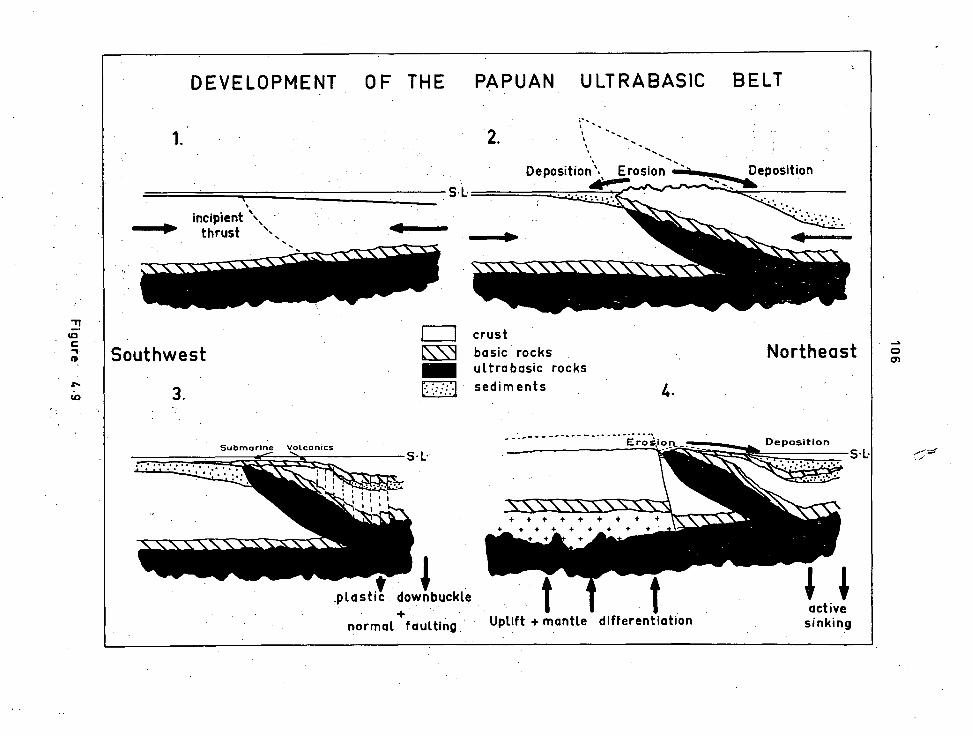
DEVELOPMENT OF THE PAPUAN ULTRABASIC BELT

4.

Northeast Southwest

3.

crust basic rocks ultra basic rocks sediments

Deposition %, Erosion Deposition 4600.„,

incipient \, a"."41111. thrust \

VOICligiblooloweewleoggehm•■■•■■••■■.110■•••

*1 active

sinking Uplift + mantle differentiation

S

"It•

plastic downbuckle

normal faulting

Submarine Volcanics

Nve,N,

Eros,ion_ Deposition

S.L

lbzioweolov■-■■■•■■

107

.surface.of - geolOgical - thrusts,.which may be vertical at outcrop but will

• assute a - lower.angle at)depth,(Sherbon•Hills, 1963, p,, 195).

Neither - of the:above arguments - condemns the view•cfThompson and

ViSher,_but I feel thatsomemodification is needed. , -The viewwhich,I.:

take is that there is.•sialic•material both above and below the•ultra,.

basicirand:basic rocks,,a consequenceof the method-of-emplacement_

viz:.

.(1)-Y:The,initial state is assumed to be that,of seaward-thinning

upper-.andlower-crustal'rocks overlying the mantle. would .seem:

likely-that; atthei_nterface, - .there would be complex:intrusive : relations

of mantle rocks, and lighter differentiates and crustal adtixtures,:in

which thelighterrOcks would generally overly the heavier.

:(2)* Probably , duringthe - lateCretaceoUs, &northeasterly-

diPping::thrUSt. shallOwing at depth, - isasSumed-to have developed through

thethinnin&sialia wedge:. With thrusting.from-the northeast occured

the 'Steep Uplift-:andconcurrent-erosion of the Mesozoic and older meta-. :

Thiohi-cs Above the basic-ultrabasic rocks-. . .As will - -be discussed in some

detail laterauchanYupliftwbuld provide the required:source-for deep

Palaeogeneand yoUnger ,sediments•to thesouthwest; - :: During the thrusting,

which , iSaSsUmedjto have been steadily active%until well: into the-Upper.

Tertiary, the-hanging .-wall block would - be distorted to accommodate to the

shabeofthe ,, thrust surface, and thefoOtwall sialic material, would be

depessed:by the Weight of ultrabasic rock abovelt;

( ..3) With the:telaxatianof the - thrusting force (providing .a

dyn'amicequilibritmwhile operativeYthat part Of the upthrust block

HunSupported'by:underthruat sial would -tend to sink towards its . isostatic

position : by'acbMbination of normal faulting and plastic bending. A deep

sedimentary-basin would thus - be formed, and filled -as the remaining ,

uplifted area- were - eroded toWarda-sealevel.. By this stage it i8 considered

thatUPlift-and erosion had resulted in the exposure of - parts .of: the basic

and-Ultrabasic-loWer - and- Subcruatal material,- Since no -partofthe

upthrUt'-bloCk could be considered tompletelY:supported*isostatically the

'Wl‘ible . belt may have been submerged during the eruption of the basal pillow

lavas and Subseqbent extrUsionS of the Mageri'Volcanics..

'

108

(4) During the Pliocene the whole area is assumed to •aVe been

Subjected to uplift,.. followed by the addition of light material to the

base of 'the crust: Due to the greater Weight of the ultrabasic belt the

Owen Stanley Mountains were differentially uplifted along a normal fault,

which in most places coincided with the upper part of the old thrust

surface . . Where, this was not the case there remains,. between the thrust

and the normal fault, a remnant of earlier westward sedimentation:from the '

upthrust block. The sediments of indeterminate age in the Waria and

Mambare Valleys, described by Dow and Davies (1964) ,are examples of this.

The uplift of both the Owen Stanley block' andthe ultrabasic belt would

. seem to be presently active.

Based on this concept. the structure of the.ultrabasic belt,

proposed in Model 2 was set up. The sediments between the belt and the

metamorphics, having a rather dubious density contrast, are neglected in

this - model. The ultrabasic rocks have;a density contrast of 0.5, the

basic rocks 0.2 . 'Overlying these are sediments (developed over the

sinking part of the'belt) of density contrast -0.25, which are overlain by

the Mageri Volcanics (contrast +0.1) followed by recent alluvium (-0.6).

Although the computed gradient over the front of the ultrabasic

belt differs slightly from the observed one, yet it is apparent that 'a

structure of. the type shown in Model 2 can account for the observed anomaly -

as well as can. Model 1. Nonetheless, this can hardly be considered to

prove the reality of Model 2. No metamorphics of the Owen Stanley type

have been found overlying the belt, but Model - .2 assumes that they are

deeply buried. No age has been obtained, for any material conformably

overlying the ultrabasics, a.fact which adds to the difficulty of choosing

between Model 2 and an oceanic overthrust. As Dow and Davies (1964)

state "the north-eastern margin is everywhere concealed by volcanics and

sediments of Middle Tertiary age, 'or younger". On.new evidence Davies

(1967) states "The .(probably overlying) basalt is locally intruded by the

gabbro-and diorite of the belt The volcanics and (associated)

limestone are thought to represent the pre-emplacement oceanic crust;

they are, at least in part,.Upper Cretaceous." This is quoted in support

of Thompson and Fisher's , (1965). "oceanic' overthrust" suggestion. The

objection to this as conclusive evidence is that the material of the

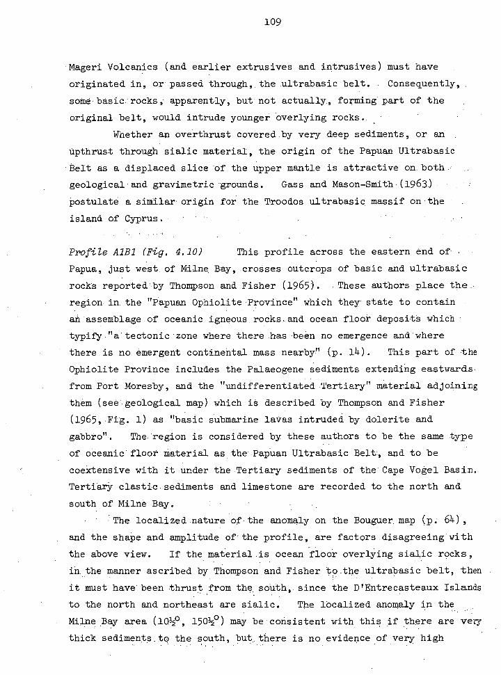
109

- Mageri Volcanics (and earlier extrusives and intrusives) must have

originated in, or passed through, the ultrabasic belt. . Consequently,

somebasic:rocks,. apparently, but not actually, forming part of the

original belt, would intrude younger Overlying rocks. .

Whether an overthrust covered.by very deep sediments, or an

Upthrust through sialic material, the• origin of the Papuan Ultrabasic

.Belt asa displaced slice of the upper mantle is attractive-on_both.•

geological . and gravimetric .grounds. Gass and Mason-Smith(l963).

Postulate a similar originfor the Troodos ultrabasic massif on the .

island of Cyprus. •

Profile A1B1 (Fig. 4.10) This profile across the eastern end of

Papua, just west of Milne Bay, crosses outcrops of basic and ultrabasic

rocks reportedly Thompson and Fisher (1965). These authors place the..

regionin the "Papuan Ophiolite 'Province" which they state to contain .

an - assemblage.of oceanic igneous.rocks-and ocean floor deposits which

typify,"a:tectonic . zone where there .has been no emergence and'where

there is no emergent continental mass nearby" (p. 14). This part of the

Ophiolite Province includes the Palaeogene sediments extending eastwards.

from Port Moresby, and the "undifferentiated .Tertiary" material adjoining

them (see geological map) which is described by Thompson and Fisher

(1965,•Fig. 1) as "basic submarine laVas intruded by dolerite and

gabbro". The• region is considered by these authors to be the same type

of oceanic floor material as the Papuan Ultrabasic Belt, and to be

coextensive With it under the Tertiary sediments of the CapeVogel Basin.

Tertiary clastic-sediments and limestone are recorded to the north and

south of Milne Bay.

- The localized nature of the anomaly on the Bouguer. map (p: 64),

and the shape and amplitude of'the profile, are factors .disagreeing with

the above view. If the material.is ocean floor overlying sialic rocks,

in the manner ascribed by Thompson and Fisher to.the ultrabasic belt, then

it must have been thrust from the rn south,. since the D'Entrecasteaux Islands

to the north and northeast are sialic. The localized anomaly in the

Milne .Bay area (10.1/2P, 1501/20 ) may be . consistent with this if there are very

thick sediments,to the south, but there is no evidence of very high , .

110

gravity anomalies over the "ocean floor" lavas to the northwest, which are

supposedly underlain by ultrabasics.. A more detailed gravity survey of this area, at present being undertaken by the Bureau of Mineral Resources,

Geology and Geophysics, has not yet indicated - the presence of large

anomalies localized in the centre of the;peninsula..

If the material is ocean, floor in situ then, the gravity anomalies

can be explained by- assuming either. that is underlain by.a continental-

thickness crust .of light Material (perhaps serpentine), or that it is

crust of oceanic thickness underlain by mantle material of very localized

low density. This is a dilemma which is discussed later in this thesis

in connection with gravity anomalies in northern New Guinea and the

Solomon Islands.

_The model set up for the profile interpretation is perhaps the

simplest, and involves the assumption that the ultrabasic and basic rocks

are outcrops of a localized intrusion into material of sialic density.

A general density contrast of 0.3 is assigned to the intrusive,,since its

basic/ultrabasic.ratio is link/10MM. Similarly, the flanking sediments

are given a formalized contrast of -0.2 . Those on the north side are

probably of the Cape Vogel Basin.

Profile_A2B2 , (Fig. 4.10) -:,Although contours.are.poorly controlled to the

south the obse'rved anomalies present useful information in the region of

the Cape Vogel Basin and D'Entrecasteaux Islands.. The southern part of

the profile is over Thompsbn and Fisher's "Papuan Ophiolite Province"

mentioned in connection with A1B1, and which' is represented on the model

by material of density contrast +0.1 . The' Cape Vogel_Basin is defined

mainly by the work of Papp and Nason-Jones (1928, in APOC, 1930) on the

actual Cape Vogel Peninsula. They describe a section of about 4500 - m.,

comprising

Mio-Pliocene

Upper Arenaceous Group.

Mainly non-marine sandstones, marls and grits

Upper Miocene

Lower Arenaceous Group _

Meanly non-marine sandstones, marls, tuff's. and breccias

4,500 m.

3000 m.

/a

100 -

50-

30 - 0

//////// ///// 50 100 150 200

100 -

MIL

LIG

ALS

50-

0 /

co 50 —/

0

-J °

A5 B5

100

• x a

a

Papuan u/b belt

5- Mt Victory

-0.25 0.2

10

20-

KILO

ME

TRES

30-

BOUGUER ANOMALY PROFILES 150 -

_ M

ILLI

GA

LS

OBSERVED

COMPUTED

DENSITY CONTRAST

50-

100-

0.3

MIL

LIG

AL

S

a-

0

A2 5 7

0

B2

10 - U)

Mt Simpson

0'l

C. Vogel Basin Cope Vogel

•2

0.5

Goodenough I.

Al

B1

0 .

10 - LLJ

Goodenough Bay

-0-2

-0-2

1— w X 20 - 0

30

/ 0-5 ././

////////////////////77/// 50 100

150

40-

0 200

250 I

M W MEM E S KILOMETRES

A3

5 Mt

SuckLing Oral

C . (Pitt) Galley Reach

Basin

C - Papuan u/b beLt

-crr 0111111111111111111 11111

0- 5 02

0•5 -0-25

7// 1 5/

//1/////71////7 0.5

-0-5 40 -

-0.5 40-

Figure 4-10

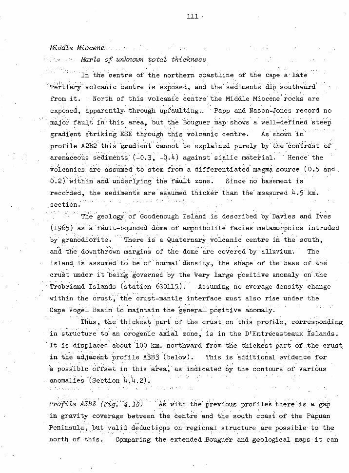
111

Middle Miocene. - ...:

Marls.of unknown: total thickness

In the centre of the northern Coastline of the Cape a' late

'Tertiary volcanic centre is e-kpbSed, and the sediments diPabuthward

from it. • North of this volcanic centre the Middle MioceneroCks are

exposed, apparently through upfaulting. Papp and Nason-Jones record no

major fault in this area, but the Bouguer map shows a well-defined steep

gradient striking ESE through this volcanic centre. As shown in'

profile A2B2 this gradient cannot be explained purely by the contrast of ,

arenaceous sediments (-0.3, -0.4) against'sialic material. Hence the

volcanics are assumed to stem from a differentiated magma source (0.5 and

0.2) within and underlying the fault zone. Since no basement is - . .

recorded, • the sediments are assuMed thicker than the measured4.5 kth.

section.

The geology: Of Goodenough Island is described by Davies and Ives

(1965)' as:a 'fault-bounded'dbme of amphibblite faCies metamorphics intruded

by granodiorite. - There 16 a Quaternary volcanic centre in the south,

and the dOwnthrOwn margins of the doe are coVeredhy'alluvium The

island is asSuthecl...tb of normal density, the shape of the base of the . .

crust under it Meing.governed by the Very large positive anomaly on'the

Trobriand Islands (station 630115). AsSuming.to average density change

within the orust . the Crust-mantle interface must also rise under the

Cape Vogel Basin to maintain the general positive anomaly.

Thus, the - thickest part Of the crnat.on this profile, corresponding

in atructure to an orogenibaxial zone,' is in the D'Entrecasteaux Islands.

It is 'displaced abOut -100 km. northward from the thickest Part Of the Crust.

in the adjacent Profile A3B3 (below). This is 'additional eVidence for

a possible offset in this area, as 'indicated by the contours of various

anomalies '(SectiOn

PrOfile A3B3(Fig.4.10) AS With the'Previbus profile's there is a gaP

in gravity coverage between the Centre - and the south coast: of the Papuan

Peninsula,..but.valid deductions . on regional structure are possible to the

north of this. Comparing the extended .BougUer- and geological maps it can

112

be seen that in this area the most strongly positive anomaly occurs more

than 60 km. to the north of the southernmost mapped uitrabasic rocks, which

are in a region of low negative anomalies. The surface appearance of the

Papuan Ultrabasic Belt, which is fairly simple to the north,. becomes quite

complicated and lacking of a simple. explanation.

In the area shown in Fig. 4.6 as Mapped by Smith and Green (1961)

bodies of ultrabasic rock appear in faulted, as well as apparently intrusive,

contacts with Mesozoic sediments (Urere "Metamorphics") and the older

Goropu Metamorphics. Some appear as fault-bounded blocks emerging

vertically through Pleistocene cover. Many of the important contacts

are, however, concealed beneath Quaternary sediments and volcanics in the

Musa Valley. No continuous fault is mapped as bounding the ultrabasics

to the east of the fault between the Sibium Range and the Owen Stanley

Metamorphics 1481/4°). H. L. Davies (pers. comm.) has recently

mapped a southerly-dipping thrust fault separating the southernmost ultra-

basic body and the Goropu Metamorphics on Mt Suckling*

(south of 91/20 ,.149° )-

Observed gravity anomalies in the Musa Valley indicate that there

are no large ultrabasic bodies beneath the Quaternary cover. Anomalies

on the 'south coast are inconsistent with an interpretation of the

Mt Suckling thrust as the outcrop of an extensive sheet thrust from the

south. But the elongate positive anomaly of 110 milligals over the swamps

and volcanics south of Mt Victory appears to be a continuation of the

anomaly associated with the northern part of the ultrabasic belt.

Accordingly, in setting up model A3B3 -, the contact of the ultrabasics with

the northern edge of the Goropu Metamorphics (91/2 0 , 149° ) is assumed to be -

the southern boundary of the main part of the ultrabasic belt. The

observed anomalies are consistent with a mantle-thrust structure similar

to that of model_A4B4, and of the same origin. The Mt Victory volcanics

(no density contrast) are assumed to overlie sediments of formalized

density contrast -0.25 and -0.1 . In the south, a structure of contrast

+0.2 represents the "basic intrusions and submarine lavas" which should

underlie the Upper Tertiary sediments (-0.25) . .

* The National Mapping - Trig named' "Mt Suckling" is actually some distance to._..the - north of this...

113

The presence of fault-bounded ultrabasics south of the postulated

belt is a problem. The answer may lie in the previously mentioned

occurrence, that the thickest part of the crust (underlying metamorphics)

in A3B3 is 100 km to the south of the thickest crust (also under metamOrphic:

in profile A2B2. Transcurrent faulting in the area could be responsible

for the tectonic movement of previously-intruded small ultrabasic bodies.

Another suggestion is that the ultrabasics on the southern side of the

Goropu Mts are remnants of a surfaced overthrust from the north which

became "draped' over" the Goropu Mts during their uplift, and subsequently

eroded off the top. Applying this suggestion to the whole area one can

see that the only thick subsurface ultrabasics will be under deep

sediments in the position shown on model A3B3. All other ultrabasic out-

crops represent thin remnants of the overthrust sheet, with their faulted

boundaries being an accompaniment of Plio-Pleistocene uplift movements.

Profile- A5B5 (Fig. 4.10) The southern half of this profile is fairlY

well controlled but in the northern part the gradient over-the contact of

the ultrabasic belt is not well defined. The only value of inter-

pretation'in the latter region is. to show that the amplitude of the anomaly

is consistent with a northwesterly continuation Of. the ultrabasic belt

structure as proposed for A4B4, Mode1 . 2.

Geological information in the southern part of the area is taken , .• " from APC (1961). The Oroi bore (Fig. .6) commenced 250 m.

below the top of theLower MiOcene and penetrated 1500 m. of siltstone,

mudstone and conglomerate without reaching the base of the Miocene.

Sections measured inland frOm OrOi 'show that there are up to 3000 m. of

terrestrial basic volcanics in the LOwer Miocene. In model A5B5 the

argillaceous Lower Miocene (-0.3) is assumed to be underlain by thinner

basic ,voicanics (+0.15) which thicken northwards to occupy the whole

Lower Miocene section." Based on isopachs (APC, 1961, Fig. 12) about

1200 m. of Eocene siliceous limestone, shales and tuff, with a bulk

density 'contrast Of'-0.1, are assumed to underlie the Lower Miocene.

in the Galley Reach Basin sections of more than 3000 m. of Pliocene

volcanics have been measured, including basic lapilli, tuffs and

agglomerates, interbedded basalt and tuffaceous sandstone and siltstone.

This section is assigned zero density contrast, and the dense Pliocene

agglomerate to the northeast is assigned a contrast of 0.1 .

The faulted contact with the Owen Stanley. Metamorphics . (zero

contrast) is suggested to explain the sharp negative anomaly over the

metamarphics in the central part of the profile (81/2 ° , 1)471/2° ). That is,

the negative is assumed.to be a normal isostatic effect.with the sharp

rise to the southwest being caused.by the presence of dense volcanics in

the Upper crust . .

An alternative explanation may be the presence of dense intrusions

in the area where the fault is assumed, as shown by Pitt (1966, structure .

section C'C").

. It could be reiterated here .that the geological structure in the

southern part of the profile is not deduced from the rather meagre

gravity data; but rather, the geological information is extrapolated

within the bounds dictated by the gravity information. This procedure

allows a larger probability of success in deducing the structure of the

base of the crust..

Profile A6B6 (Fig. 4..11) As can be seen on the Bouguer anomalies map,

profile A6B6 crosses an area where N-S trends apparently interfere with the

normal NW-SE trends. .Consequently, most of the anomalies crossed by this

NE-SW profile depart very considerably from two-dimensionality, and any

model consistent with the observed profile.is but an approximation to that

consistent with the three-dimensional anomaly.

The southern part of the profile crosses the KukukUku Lobe (71/2 ° ,

l 4 5½° ) ,an area of uplifted Miocene sediments in which the structural

grain swings from almost N-S in the north towards a NW-SE trend in the

south. The Middle and Lower Miocene sediments form a monotonous

succession of greywackes, mudstones, conglomerates and silts, referred to

as the "Aure FacieS", and which has a maximum thickness of at least 7000 m.

Upper Miocene, where present, is generally developed in an argillaceous

facies, and is up to 2500 m. thick. Pliocene rocks are generally marine

and transitional arenites and argillites, up to 300 m. thick in the deeper

synclines. The succession is cut by a large number of reverse faults,

dipping easterly and northeasterly, and apparently of Pliocene or younger

age. On the geological map (p. 100) the main faults only are shown.

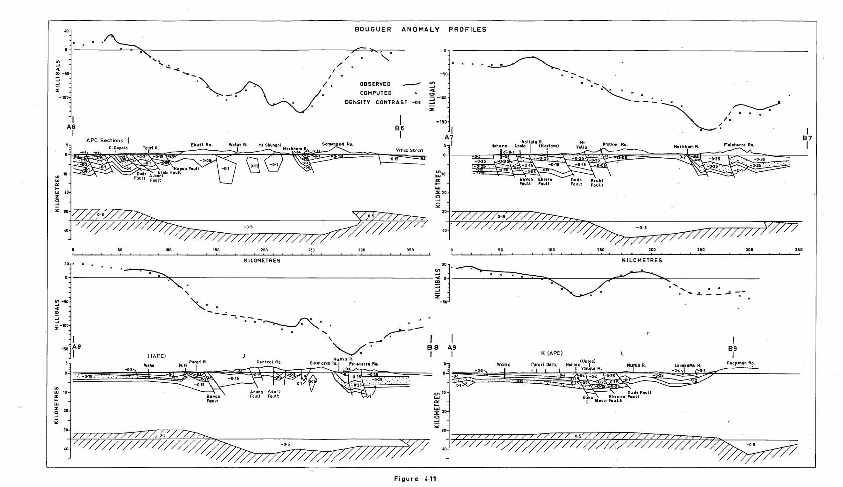
-150-

/ / 0 OBSERVED cr)

<lc COMPUTED 7, -100 -

DENSITY CONTRAST -0-3 —1

-50- a

•

Vallala R. Hohoro Upola I (Ka

1riava)

Mt Vella

Bevan Eklere Fault Fault

Dude Fault

Eruki Fault

Kratk• Ra. Markham R.

0

A7 5 - I

B7 F1n1sterre Ra. Ekutl Ra. Watut R. Mt Shungol

Markham -04

86

Vitlaz Strait C. Cupola Tauri R.

APC Sections

Kapau Fault mbeErtruki Fault

Fault FaultFault -

Saruwaged Ra.

20-

30- 30-

- ///////V///////// ///////// 40-

111 -50 -s

-150

B•van Fault

40: BOUGUER ANOMALY PROFILES

0

0

\

• •

/ a a

x

KILO

ME

TR

ES

-100- -

0 SO 100 150 200 250 300 350 50 100 150 200 250 300 350

KILOMETRES KILOMETRES •

X X X

X X X

X X

X

X

I AR B8 A9

5 -7 Wano Murua R. -0-3 -0-3

I (APC) Purari R.

Warm Purl Central Ra.

Ramu R. Bismarck Ra.I Finisterre Ra.

K (APC)

Purari Delta Hohoro(Upo

lla)

Vallala R.

B9

Chapman Ra.

-0.15 0•

Anuna Asaro Fault Fault

Dude Fault Kuku Ekuere Fault

Bevan Fault

KILO

ME

TR

ES

10-

20-

30-

///////// ///// //////////// 0.5 A.301/■•■■■■••

40- ////////// -0-5

/// Figure 4-11

115

Although cognizance is taken of the described lithology in

individual sections Used, there are some generalizations which may be

made with regard to the densities of sediments in the Kukukuku Lobe.

.The'Aure facies - mudstones and.greywackes are likelyto.beaess dense •

than the upperMiocene argillaceous sediments (often. developed as blue ,

- mudstones) for reasons of lithology,. depth and age. Similarly-,the

Pliocene fine sandstones and' siltstones are likely:to have a: smaller

bulkA.Onsity than the. Upper Miocene. : The density section through Aure

rocks measured by:McWhae ..(1948) has - beenpreviouslyquoted'.(Sect..

Combining thiswith, the theoretical studies of argillaceous:,and , ! 1 Gulf

Coast" sediments of. various depths (Fig. 4.1) the following minimum

density contrasts can be assumed: ,

Aure'Rotk6:. -0.25 at top (if not very deeply buried) decreasing

downwards to terb density contrastbelow about 10 km.

Upper Miocene: -0 ..3 to .-0J+'

Pliocene: -0.4 to -05

.Sections- described for the region east of Kerema (APC,.1961,

p. 91) have been used in constructing the model inland from.Cape Cupola.

TheCupola gravity high, a . prominent feature on the Bouguer map (8° ,

1451/20 ) is explained by the upthrusting of denser Aure rocks in a region

of predominantly Upper . Miocene argillites... As stated by APC (1961,

p. 91) the exposure at Cape Cupola of rocks 2000 m. below the top of the

Middle Miocene constitutes the oldest coastal exposure for sixty miles

to the east of Kerema.

The measured section near the coast is:

Pliocene 1000 rtt.

Fine grey sand, silt, mudstone, lignite

Upper Miocene 1600 m.•

- :• . Argillaceous

Middle. Miocene - 2000.m.+ -

: . Greywacke,: mudetone,cOnglomerate.

Based on inland sections, at least 5000 M. of Aure rocks can be assumed

to underlie this' section (APC, p. 92). 'Further to this, Apc,(1961,

Fig. 9) infer that: at'leaSt 7000 m. of MesOzoic geosynclinal-sediments

116

underlie, the. Tertiary in this region..

. 'Based on ,the style of folding and faulting inferred in the

geological cross-section of APC (1961, plate 2) thesouthern part of the

model has been constructed:. 'The projection of the structure southwestwards

into the Gulf of Papua is . justified on the _grounds of recent submarine

seismic work. This indicates that the sediments beneath the gulf are Irr,Y

thick, and subjected to the same type of diapiric thrusting observed in

the Kukukuku Lobe (Paper presented at A.P.E.A.Conference, Sydney, March,

1967 by N. Tallis of Phillips Petroleum Co:). Taking conservative

density contrasts, the Ireaues.used_are; Pliocene, 70.4; Upper Miocene,

-0.35; VpperAure,. -0.25; Middle Aure, 70.2; J.Jower Aure, -0.1 or

-0.15; Uppermost Cretaceous to Lowermost Aure, -0.05 . Only under very

exceptional circumstances could sediments at a depth of more than 10 km.

be assumed to have a.density less than 2,67 . Hence, the supposedly very

thick Mesozoic section here would not be gravimetrically. observable.

The rocks are progressively upfaulted towards the northeast, SO that the

older rocks are exposed. Pitt '(1966) considers that the rocks in the

Upper Tauri River area are of "undifferentiated Mesozoic-Upper Tertiary"

age, with an exposed core of'Palaebtoic met'atorphics (70 , 146° ) which is

well to the north of this profile. The sediments which are between the

Eruki and Kapau Faults in this section are.correlated with the Lower lure

and Upper Cretaceous density subdivisions, and are assigned contrasts of

-40.15 and -0.05 .

'Comparison of observation and computation in this southern section

indicates that the Cupola high is capable of being explained by the up-

faulting of high-density sedimenta. . Indeed, the contrast would seem to -

be too extreme, or the structure. of too large an amplitude, since the

residual anomaly over the model is too large. . Perhaps the most striking

feature of this part of the profile is. that there is a positive gravity

anomaly over well-recorded, and extremely thick, sediments. ..though I

consider the. chosen -sedimentary densities tip be maximal, it is still .

necessary to have a crust some 6 km. thinner than normal to neutralize the

negative anomaly caused by the sediments.

The central part of the profile, between the. Ekuti Range and the

Markham Valley, passes through a complicated_region-on the Bouguer map.

117

The geology, also, is quite complicated. Fisher (1944) mapped three

units within the metamorphics shown on the regional map:

(a) "Cretaceous" greywacke and sericite schist,

(b) "Palaeozoic" phyllite,.. schist and marble;:

(c). High grade amphibolites, gneisses and migmatite, just. south

of the Markham Valley.-

These rocks are intruded by the - granodioritic-Morobe ,Batholith

(7° , 1470 ),andthere , dre deposits of explosive agglomerates of supposedly

Pliocene age (7140 , 146V). . (Recent newsworthy volcanic activity in the

Wau atea indicates a:yoUnger age for these agglomerates.).

'I consider that the three rather shamefully non-geological-

looking structures 'in the Central part of the model are probably a too

simple explanation of the observed gravity. It is more likely that the. -

irregular anomaly is the result of juxtaposition of high and low grade.

metamorphics Of different density. llowever, the structure of. these is

not well enough known.to justify any complex model. The southernmost

structure (-0.1) Under the northern Ekuti Range could be replaced by a

deeper basin of Tertiary.and Cretaceous sediments and low-grade . meta-

motphics, perhaps of' greater density contrast than the -0.05 assigned to

them. :The central:StructUre . (+0.I5) represents the non-outcropping part

of the granodioritic Morobe Batholith, which can be seen from a comparison

of the geological and BoUguer maps' to coincide to a large degree :with a

gravity high trending NNW from 71/4PS, 147°E. This structure ; then, is •

considered geologically likely. The northernmost structure - (-0,1)

Coincides with surface outcrops of granitic intrusives ., and represents an

intrusive body 'lighter than the metamorphics. Since this.is the area of

higher-grade metamorphics mapped by Fisher.(1944) -, the gravity would be

equally compatible with an higher density body under the adjaCent gravity

maximum.

'The northern part of the profile passes over the Markham Valley

and the Saruwaged Range. From information obtained in reconnaissance

surveys, 'Thompson and Fisher (1965, p. 18) report that "The Finisterre

and Saruwaged Ranges are composed 'of a 'very rapidly deposited thick

accumulation oflMiocene%Clastib 'sediments, basaltic Arolcarlibs and limestone,

the 'basal-Part:Of Which has been intruded by gabbto - ; particularly Oh the

118

Huon Peninsula. This succession has been broadly folded, extensively

faulted, and elevated . along marginal,. steeply dipping„ fault zones,

represented by the . Markham-Ramu Valley.system on the south and relatively

straight coastline to the north. • Upper Miocene limestones cap the

Saruwaged Range at elevations exceeding 10,000 feet above sea level".

They also state that thick, dark shale,. deep-water sequences dominate the .

Finisterre-Saruwaged sedimentary succession Little is directly known of

rocks under the-alluVium,of the Markham Valley. However, Pliocene

elastics are exposed, against the fault bounding the mountains on the

north-side - of . the valley.. On the southern side,in the Aroha area (61/2°,

1461/40 ),Dow and Plane (1965) show Lower Miocene sediments, intruded by

porphyries and dolerites, dipping towards the Markham Valley. This

succession (the Omoura Greywacke) consists of almost 3000 m. of greywacke,

siltstone, limestone,. arkose and pebble conglomerate. To the west of

this, McMillan and Malone (1960) show Lower Miocene limestone, shale,

slate, greywacke and conglomer4te.unconformably overlying Palaeozoic

metamorphics, and dipping northeasterly . at 400-500 . The sediments are

intruded by late Tertiary dolerite, diorite aro, gabbro. These occurrences

indicate that the Finisterre-Saruwaged Mountains' represent the upfaulted

northern part of a deep 'sedimentarysequence overlying a metamorphic base-

ment in the Markham Valley.

In setting up this part of the model it was necessary to explain

the large gradient towards the eastern end of the Huon Peninsula

1471/20 ). The gradient may be partly an effect of the gabbroic intrusions

mentioned by Thompson and Fisher (1965, above), but its appearance on the

regional profile suggests a deep-seated cause. The suggestion advanced

in model A6B6 is that the thrust surface, along which the mountains are . •

being elevated, extends through the earth's crust. The addition of a

broad gabbroic intrusion beneath the sediments Of the range would bring

the observed and calculated curves into A better The sediments of

the basin are assigned a similar range of densities to those of the Aure

Trough.

The profile again suffers from lack of two-dimensionality here, at

least with-regard to lower-crustal structures, and the suggested structure

is but one of many alternatives. .A gabbroic mass could undoubtedly be

119

shaped to fit the anomaly, without any significant. lower-crustal perturb-

ations. However, I regard this model as consistent with a thrust origin

of the Finisterre-Saruwaged uplift, and the concept will be pursued in

subsequent profiles.

Finally, there may be mentioned in connection with this profile a

condition applying to most others. Namely, the Airy compensation

accounting for the regional part of the gravity profile is assumed to be of

the simplest structure - broadly regional. As shown in Fig. 4.5(b), a

local type of compensation could fit the observed curve equally well.

There is no reason to favour regional over local compensation (provided

"local" is not taken as meaning point-for-point compensation). Indeed,

recent studies of Rayleigh wave dispersion along paths through the axial

zone of the Swiss Alps, not significantly higher than large areas of the

Bismarck, Kubor or Owen Stanley Ranges, are interpreted as showing that the

depth to the Mohorovicic discontinuity increases from 30 to 60 km. in an

horizontal distance of less than 50 km. (Knopoff, Mueller and Pliant,

1966).

PPoP12.e A7B7 (Fig. 4.11) The structures crossed by this profile are

quite similar to those crossed by A6B6, but the gravity anomalies in this

case approach more closely to two-dimensionality.

Lithological and structural information in, the southern part of the

. profile (over the Kukukuku Lobe) has been obtained from the ,surface mapping

and borehole data of APC (1961). The Pliocene has its thickest present

development to the northwest and west of the . A7B7 section, along which it

has been largely removed by .faulting and.erosion. Penetration by the

Hohoro wells, and measurement:of the . section_on the.northern flank of the

Hohoro Anticline, gives a Pliocene section of more than 1000 in., consisting

of a . 200 m. argillaceous section. .(mudstone, calcareous mudstone, silt-

stone) sandwiched between upper and .1Ower, arenaceous sections (sandstone,

- grit, conglomerate, with minor mudstone and siltstone). There are coal

seams in the upper arenaceous section (APC. , 1961,, p, 90). As shown in

A7B7, the. Pliocene is terminated to the northeast of Hohoro by a fault

(the Kuku Fault).

120

The Upper Miocene is calculated by APC to have been thickest in the

Hohoro area, where a stratigraphic thickness of about 2500m. of light

blue and grey mudstone, calcareous and silty in part and occasionaly

carbonaceous, was penetrated without bottoming in the Hohoro no.2 bore.

APC estimates a total Upper. Miocene section of 3300 m. (APC, 1961, Fig. 15),

which thins to the east and-west.

The Middle and Lower Miocene Aure .fades is thickly developed in

the area. In the Kariava well (projected along strike .t9 A7B7) more than

3500 m. of alternating greywacke and mudstone were penetrated without

reaching the base. To the northeast of Kariava more than 5 km. of Aure

rocks have been measured in the M'bwei Sa section (APC, p. 85). The total

thickness of the Aure fades is not known, but APC estimates it at 6 or 7 km. in isopach construction (APC, Figs. 13, 14). Mesozoic sediments of

geosynclinal thickness are believed to underlie the Aure Fades.

In keeping with section A6B6, the structure of the Kukukuku Lobe

along this section is based mainly on the APC interpretation; that is,

progressive upfaulting to the northeast of rocks lower in the Aure

section. , As stated earlier, Pitt (1966, p. 121) assigns the sediments to

the east of the Eruk.i fault to the range ''undifferentiated Mesozoic to

Upper Tertiary''. The rocks within this range, and in this region, are

those in the stratigraphic divisions 5 and 6 of Carey (1941), viz:

5) Hard tuffs, hardened mudstones and calcareous sandstones 800 m.

6) Sandstones (which may or may not be tuffaceous) and 3000t m.

shales

Pitt assigns a Palaeozoic age to metamorphics reported to underlie this

section (7° , 146° ).

From the geological map it can be seen that the exposure of older

rocks in this area is almost certainly due to a combination of two causes;

the north-south striking reverse faults of the Kukukuku Lobe, and the

arching, along a NW-SE axis, of the central mountain backbbne of New

Guinea. Because of this,- profile A7B7 is approximately orthogonal to the

thinning of the .sediments, but not to the strike of faults east of the

Dude fault. The latter condition should not introduce large errors,

since the regional gravity gradient in that area seems to be largely due

to the NW-SE structures.

121

The profile does not intersect any actual metamorphic exposures,

but the.(probably . metamorphic) gravimetric basement is assumed to

approach the surface in the Kratke Range and to the north ot it.

Mt YeIia, 4 Quaternary andesitic volcano (just east of 7 ° , 1466 ), is

intersected by. the profile, and is shown in,thisAnterpretation to lie on

a northern extension of the.Eruki fault. The fault. in the Kratke

Range, to the northeat of the Eruki,is purely hypothetical,

Densities used for the southern part of this model correspond.to

those used for A606. . As with that model, although the maximum Tertiary

and,Mesozoic , sedi,mentarr,section .is estimated by APC .(1961) to loamuch . ,

greater, : no density contrast. is. likely at_depths.of over 10 or,l1 km. .

As before-, to: account for the, anomaly observed over deep sediments it is

necessary to _assume a.crust some. 5 km—thinner than the standard.

The northern part of the. profile crosses : the Markham Valley and .

Finisterre Range,- the known : geology of which .has been discussed with

respect to the previous profile., . A sudden steepening, in the Markham

area, of. the observed . gravity gradient indicates that the. large negative

anomaly is due, at least in part, to a shallow Structure... The structure

hypothesized_isHoasedon the same premises as the A6B6 structure, with

the modification that two reverse faults are assumed to be , present.to

account for the steepened. positive gradient to the north of the present

mountain.front. In plan, these. reverse faults are assumed to be

arcuate and to converge, to the east, being jointly the upper-crustal

expression of a dynamic rise in the base of the crust.

Profile'. A8138 (Fig. 4.11) In its southern part, this profile passes

through the low-lying Delta,Embayment, encompassing areas to the north

and west of the Purari Delta (71/20 , 145 ° ). Where the profile enters the

southern foothills of the central cordillera (7 ° , 145 ° ) it crosses a

zone of WNW-striking folds and faults which represent the north-striking

Kukukuku Lobe structures after westward deflection around the "Purari

Bending Axis" (Carey, 1941, p. 116).

The model in this southern sector follows the geology as mapped

by APC (1961, sect. 3.324), and is based largely on their profile IJ.

The Pliocene in the area (-0.14), is. developed in,a transitional facies

122

which grades upward from marine to terrestrial. tower beds include

sandstones, siltstones and mudstOnes, sometimes calcareous, and upper

beds comprise cross-bedded sandstone's, carbonaceous mudstoneS and coal

seams. About 1 km. of Pliocene is present in theWana bore, and this

thins to the southwest and thickens to the northeast.' A maximuM thickness

of 2 km, is reached to the south of 1puti, and that thickneas is also

approached in the Pide Basin, which in this profile straddles the Purari

River.

UpperMiocene marine and estuarine mudstones and sandstones (-0.3)

are about 1200 m. thick at Wana; about 2000 m: thick south of Puri, and

become thinner towards their northern termination.by the Bevan fault.

The Middle and. Lower Miocene is developed in a calcareous facies

to the south of the Purari-River, where it grades into northward-thickening

greywaCkes and mudstones of the Aure facies (Smith, 1964, Figs. 6, 8).

Lower Miocene argillaceous limestone thins from about3 km. near A8 (in

the southerly extension of the: Omati Trough) to about 0.6 km. at Wana -

and 0.5 km. at Puri. At Wana and Puri this is overlain by thin (100-

200 -m,) Middle Mdocene Marls. The calcareous fades is assigned a density

contrast of -0.1 . The Aure facies to the north of the Purari River is

assigned a,bulk contrast of -0.2

Although they have not been completely penetrated anywhere in the

southern part of the Section, Mesozoic sediments are shown by isopachs

(APC, 1961, Fig. 9) to be about 1.5 km, thick at Wana,'with little variation

to the south or north until a sudden northward-thickening in the Puri area.

The lithology, according to Smith (1964, Fig. 14), is of geosynclinal

facies, being mainly greywackes, shales and mwdstones. , Glauconitic

siltstone has been encountered in the Puri bore The Mesozoic is

assigned an overall density contrast of -0,15 . The geological structure

follows APC.'S section IJ, with the exception that the pre--Mesozoic base,'

ment is not considered to rise so rapidly to. the north of the Purari

Fault. Although not very well controlled, the steep gradient of the

contours south of 7 °S, 145°E is not explicable purelyin terms of deep -

crustalstructures, and.deepened 'Mesozoic Would seem to be the most likely

explanation. The Puri Anticline produces a considerable geological

anomaly in the computed profile, which is not matched onthe observed

123

section. However, there are no actual observations in the area, so the

observed section is purely the interpolated regional. •This might be

construed as over-interpretation, but I feel that the justification for

including the Puri Anticline, in the model.lies in the fact that it is

there. As in the previous two profiles, some crustal thinning-is.,

indicated in the southern section, reaching a maximum of 5 km. beneath

the front of the Aure structures.

„In. - its central section, profile A8B8crosses •the area mapped by..

McMillanAnd Malone (1960).. The oldest:exposed:rocks:here are, the pre- : -

-Triassic metamorphics of the HenaBenaand Goroka_Formations (.6 . 0 ,145h0 ),:

They are overlainunConformably , by Lower.Miocene.limestone,.shale, slate,

greyWackeiuld.:Conglomerate an essentially Aure.Facies:assemblage

:Cretaceous sediments (soft calcareous :grey shale and:mudstone i ,

someIimestone) are exposed-on the Kubor.Anticline :(here known as the

Central_Range).and underlie the Miocene and thin Palaeocene, but

apparently:thinHoutAcwards the , Bismarck Range .(-0.15)- The two .

synclines shownbetween:the , Central and.Bismarck Ranges are modelled on

the:sections measured by-McMillanHand Maloneforthe yaveufa (southern)

and OrIowa-tSynclines: HThesteep positivezravity,gradient'over.the .

southern fall of the .Bismarck. Range'- that the contact of. .

sediments with metamorphicS'mustbesteeply dippingif not faulted.- .

I have assumed that the Tertiary, mainly basic, intrusives (+0.1) and

the Triassic Bismarck Granoriorite (+0.05) are also.instrumental in

causing the positive residual anomaly.

The northern section of the profile crosses the Ramu Valley, and

the western end of the Finisterre Range. . As mentioned previously,

'McMillan and Malone (1960) show the Lower Miocene rocks observed to the

south :,tobe dipping at 40° to 50° off the northern edge of the Bismarck

Range. In constructing a model for the area after the nature of A7B7,

older sediments (-0.1) are assumed to underlie the Lower Miocene (-0.25)

but to -be:Concealed by a Lower Miocene' transgression. It can be seen

that the'Observed and calcUlated'profiles haVe'Very different gradients'

in :the - Ram Valleiare, the nature of the deViation indicatingthat a:

too-steep edge haS been asSUmed to - bOund the sedimentary basin. This may

be the 'case; but it is an unfortunate fact that" theobserved gradient' in.

124

the critical , area is uncontrolled (6 ° , 145;n.

Lower-crustal structure in this model is similar to that of A7B7,

maintaining consistency of the implicit tectonic hypothesis that the

initial uplift of the deep sediments of the area is due to a rise in the

base of the crust.

Profile A.9B9 (Fig. 4.11) This profile runs in an approximately east- 7,

west direction across the southern sections of profiles 6, 7 and 8, and, is

designed to'exhibit the main gravitational. features associated with the

different sedimentary and structural regimes around the head of the Gulf.

of Papua. Since twodimensionality ib dependent only on the ratio of

depth to horizontal extent Orthogonal to the profile ; the broader'basinal

features will be adequately approximated, as will most of the structural .

features in the upper crust. The base of the crust, which dips almost at

right angles to the line of section, Is not, approximated by a two-

dimensional model, and its shape On this section can be neglected.

Sections drilled in the Wana and Hohbro bores have been projected

along strike to 49B9. The Upoia. bore is . separated from the profile by

faulting, but lithological information has been projected. West of

Hohoro the profile crosses the Delta.Embayment The Wana section,

discussed in connection 'with the previous profile, consists of:

Pliocene . 1000 m.

mudstone, silt, sand, coal (-0.4)

U. Miocene 1200 m,

marine and estuarine mudstone and sandstone (-0.35)

M. and L. Miocene (less than 1000 m.)

argillaceous limestone (-0,1)

Mesozoic (about 1500 m.)

greywackes, shales, mudstones (-0.15)

To the west of Wana the Upper Miocene and Pliocene sections thin,

while the Lower Miocene thickens toward the Omati Trough. • closed

positive gravity .anomaly near A9 is correlated with an hypothetical inter-

mediate intrusion associated with the Aird Hills volcanic'centre (7 1P,

144V). To the. east of Wana the Pliocene thickens, the section in the

125

Kuku Syncline (west of. the Kuku fault) .being given as:

Sandstone, conglOme24atealcareoud sandstone', 66'ea Seams 1250 m.

Muds tdne, sandy muds tone 1250 tn.

(APC, 1961, p. 91)

In the region of the Purari Delta the Upper Miocene is assumed to change

from the marine and estuarine mudstone and sandstone of the Wana bore, to

the blue-grey mudstones of the Hohoro bore, accompanied by a decrease in

density, from a contrast of -0.3 to one of -0.35 . In the same region

the calcareous Middle and Lower Miocene (-0.1) grades into the arenaceous

and argillaceous Aure facies (-0.25, at this level) (Smith, 1964,

Figs 6, 8).

From the .PurariDelta eastwards . across the. Kukukuku Lobe, the

model is based to some_extent on APC,'s. profile .KL„ . .The Eravity . feature _

most demanding of explanation in this area is the.prominent north-

trending low between the Purari and Vailala Rivers (71/20 , 1451/49, and Map 32,

Appendix The Pliocene and Upper Miocene'isopachmaps (APC,,1961,

Figs 15, 16) show sedimentation maxima in this..area,.and it has been

previously noted, that the 'Upper . Miocene. was.not completely penetrated in

the Hohoro bore.. Even assuming: that the .Upper Miocene east of Hohoro'is

of still lower .density (contrast —0.4) it is not possible to explain the

observed low by adherence . to ,APC's sectionaL (APd,..1961.,. plate .2).

To maintain the axis of the gravitational low in its observed position,

two alternative Modifications. cah.be made to that section:

In the modification shown.on.the computed model.the_assumption is

made that presently thick Upper Miocene.mudstones continue as far as the

Ekiere Fault, 'rather than the.Revan•Fault as shown.by APC. This fits

the gravitational picture, but it requires. that the thin ,(less than

:1 km.) Upoia :section of Upper Miocene (as modelled in A7 .137) be due to a

very . localized:and . steep anticline. That this may be possible is evident

from the yery. rapid. variations in thickness of the Upper. Miocene in the

• area.(APd, 1961, p. 88)..

An alternative modification is that the_upper:Aure sediments

(0.25) be considerably thickerlin:the zone beneath the Vailala River,

extending to the Ekiere. Fault. This is perhaps pc)Fp likelysolution,

since .there is no direct geological.evidence.for the. assumed Aure thickness

126

here. Such a modification would conflict with model A7B7 in , the Vailala

River region, but since profile A9B9 in that region is much.closer to,

orthogonality to the contours it can be considered the more precise.

In the Mnrua River area, A9B9 trends across the structure modelled

in A6B6 as responsible for the Cape.Cupola gravity high. Twodimensional-

ity is not well-approximated here by the A9B9 section, but it can be seen,

at least semi-quantitatively, that the high can be explained by a closer

. approach to the surface.of lower Aure rocks and (gravitational) basement.

The exposed upper and middle Aure rocks are not differentiated as in A6B6,

but assigned a bulk contrast of -0.25 .

To the east of the Kukukuku Lobe the profile passes across the .

northern part of the Lakekamu Embayment. The Pliocene to the west of the

Lakekamu River consists of.up to 2000 m. of conglomerate, sandstones,

siltstones and clays (-0.).) while that to the east '(in the Kunimaipa

Basin) is of similar thickness and lithology .(-0.3), With the addition of

some volcanic detritus (Pitt, 1966, p. 21).

The Upper Miocene is exposed at the western edge of the Lakekamu

Embayment as more. than 1500 m. of marine and terrestrial conglomerates

and sandstones composed of volcanic detritus, and silty clays. It is

also Present in the Kurai Anticline to the south of the profile (8 ° , 1461/20 )

(Pitt, 1966, p. 38);

The Middle Miocene sediments of the Lakekamu Embayment are thin,

shallow-water sandstones and conglomerates whiCh grade into upper Aure

deep-water sediments towards the Murua River (Pitt, 1966, p. 49).

The Lower Miocene is not certainly identified in the Lakekamu

Embayment, but Pitt (1966, Enclosure 7) assigns basal volcanics, exposed

on the eastern side of the basin, to the interval "Miocene to Eocene

undifferentiated".

In the model; the Middle and Upper Miocene volcanic -,derived rocks

(-0.25) have been assumed to grade into the upper Aure without Significant

density change. The underlying volcanics in this area are likely to be

transitional to clastic Aure sediments, and are assumed to have a density

contrast of' -0.2 Below these the lower Aure (..,0.1) is shown to lens

out, in accordance with the position of the eastern border of the thick

Aure rocks deduced by APC (1961, Fig. 13).

127

' As explained. PKPYiously.,. this: , interpretational profile is purely

of upper-crustal significance , the. position of the base of the-crust

is: correct only in that it maintains :.the same sense of undulation as

that indicated by the transverse. Iprofilea::

Profile A101310 (Fig. 4.12) From -the. south, this section passes

from exposed -granitic basement near . Mabaduan (the starting : ,pdint for,.

Anterpretation,.discuesed_ in , 4,5,2) over sediments gradually deepenng.to

the northeast, Sj_nce' :several other 'profiles .:cross the,:e.rea the _geology

of the Southwestern and western central Foothills Regions .(APC 1961,

Fig. 74-.)Will• be . first „discussed in •general. and :later , it applies to

each particular, profile.

•Recent, and ,F,Ieistocene deposits conceal, older ..rocics.. throughout -

most of the Southwestern Region Fly.. Platform. _They are apparently, .

-quite thin•overthe scuthernpart of the: area,. and are Mentions

in. but one borehole Aramia where. 50 metres. offFleistocene blue

mudstones.. are recorded,... $mitla 20) estimates . a . • greater: thick-

. nesstowaras :the:. mountains, Gravimetrically Quaternary .argillaceous

rocks can reasonably, :be :lumped- with.the-Pliocene,

• Pliocene. rocks are quite thin-where; they,occur AIL this ,area.

The maximum, recorded_thickne0 iS 430 m, carbonaceous mudstones with

. . bands of lignitic material,. and , rare marine 'bands., intersected in . the

Bamu no,l'Corehole of -P 0 J21: . (Montgomery et ca.„. 19)46,-p. 123 • . Three

other :Coreholes:near. the. J3amu estuary. ( l)43½9) recorde& less than 350 m.

of the same, material. At Ar9.miaabout 150:m. , of .micaceous AAa ilty .

marls, With-calcareous siltstne. and. mudstones,were. assigned' to the

. Pliocene. (APG., A.961, T„.. , 58) . similar' 'argillaceous section -was.

encountered. at J<Omewu.' , Less. than 100 m. of carbonaceous •mudstone of

Pliocene age is present- . in. the. Morehead .:section,, Smith .(196)4,. Fig. 2)

shows maximum offsPIiocehedeposition -centre on' the Bamu estuary. •

In ,the. headwateraLof!sthe) FIT River. ,(the' Fly7Strickland,Headwaters -

-Region of.AP0)...More than 1 Ipql,of- -Pliocene ._clastics .and pyroclastics

are presentin. a. closed. basin • ( : - -The Miocene over the entire Fly PlatforM-.region; and extending- -

( except, tor °the: Upper. Vdocene) - to. the, zone inside the right-angle bend

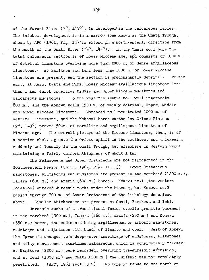
12 8

of the Purari River (7° , 145 ° ), is developed; in the calcareous . facies.

The thickest development is in a narrow. zone known as the Omati Trough,

shown by APC (1961, Fig. 13) to extend in amorthwesterly direction from

the mouth of . the , Omati River (71/2o. ,.. 14)4o) . . In the;Omati no.1 bore the

total Calcareous section is of Lower Miocene age, and consists of 1000 m.

of detrital. limestone overlying more than 2000 131 of dense argillaceouS

limestone.- At Barikewa and Iehi less than 1000 m. of Lower Miocene

limestone are present, and the 'section is predominantly detrital. To the

east, at Kuru, Bwata and Puri,' Lower MiOcene argillaceous limestone less'

than 1 km. thick underlies Middle and Upper Miocene mudstones and

calcareous mudstohes. To the west 'the Aramia no.1 well intersects

800 m., and the Komewu wells 1500 m. of mainly detrital, Upper, Middle

and Lower Miocene limestone. Morehead no.1 penetrated 1000 m. of

detrital limestone, And the Wohomul bores on the low Oriomo Plateau

(9° ,. 1)43° ) proved 500m.; of coralline and argillaceous limestone of

Miocene age. The overall picture of the Miocene limestone, then, is of

a.section shelving onto the Oriomo uplift in the southwest and thickening

suddenly and locally in the Omati Trough, but elsewhere in Western Papua

maintaining a fairly uniform thickness of about 1 km.

The Palaeogene and Upper Cretaceous.. are not represented in the

Southwestern Region (Smith, 196)4, Figs 11, 13)- Lower Cretaceous

sandstones, siltstones and mudstones are present lathe Morehead (1200 m.),

Iamara (600 m.) and Axam.ia (600 .m.)rbores.; Komewu no,1 (the western

location) entered Jurassic rocks.undexthe Miocene, but Komewu no:2

passed through 700 m. of Lower cretaceous_of the lithology described

above. Similar thicknesses are. .present at Omati, Baxikewa and Iehi.

Jurassic rocks of -a transitional facies:overlie granitic basement

in the Morehead (300. m.), IaMara (260 m.), Aran a.(290 ra.) and Komewu

(350 m.)- bores, the sediments being argillaceous_or arkosic sandstones ;

mudstones and. siltstones with bands Of lignite and coal. West- of Komewu

the Jurassic changes to'd deep-water assemblage of mudstones, siltstones

and silty sandstones, sometimes:calCareOus,which is considerably thicker.

- At Barikewa 2200 m.r were recorded, overlying pre-Jurassic aXenities,

and at Iehi (1000-t.)-and.Omati .(500 m.);the Jurassic was'not completely

penetrated. ; (APC, 1961 sect. 3 ..?).. 'No bore in Papua to the* north or

100

50

-100

Komewu Fault

(seismic) Gogol Fault

(APOC)

KILO

ME

TRE

S

MIL

LIG

ALS

All 5 -

0

Mt lalibu B11 Sepik-Wohgi

Kubor Ra. Divide Bismarck Re. Kauget R. Wahgi R. Jimi R.

Adelbert Re. Wassi Mai Kussa Kussa

Ramu R.

(Ararnio) (Komewu)

I Aramia R. Wawoi R. Bamu R. Ill

1w_

Hawoi R. Turam a R.I K r Er._t.v.:.L-2. • Fly R

i-/ -0-2 -0-2 -0-25

10-

_ •

0-15

20-

30-

BOUGUER ANOMALY PROFILES

OBSERVED

COMPUTED

DENSITY CONTRAST 0-25

a se.

a

r

A10 5-

0

G (APC)

larnara Omati (Barikewa)(Iah))

Fly R. Bamu R. Turama R. Omati R. KikoIri R. Sirebi R.

I/ -0-4 J. I

G (Rickwood) G'

Purari R.

Kubor Ra. Bismarck Ra. Wahgi R. lmbrum R . Ramu R.

Adel. brat R a. Gaga). R.

B10 Kar Kar I.

-0-15 0-4 -015

10-

05

20-

30-

40- ////// /// // / //// //// /////////

50

0 50 100 150 200 250 300 350 400 450 500 . 550 600 650 .

KILOMETRES

0

-50-

\a

'to

/a

N. a /

-100-

offset (APC) i■ (Dow &Dekker)B

KILO

ME

TRE

S

40- ///// // /////// /7-

7//. -anaf Anoro now.-o■awaraearwowo•-- _

Figure 4-12

129

east.of:Barikewa has reached-the base of the Mesozoic section.

:There are, no density , measurement - available for any boreholes -

apart-from,the shallow : Bamu . coreholes previously discussed (Fig.. 4.1.-).

However,•Bliaux (1957) records seismic velocities -for several . ..areas;

thesecan.be loosely . correlated.with bulk densities (Grant and West,

. The MioCene. Limestone-in the .Omati areahad . velocities -

rangingom 4.3 to.5:8-km/sec . ., the latter-velocity being correlated.

withHthedense argillaceous.phase.. Elsewhere, limestone velocities •

nged,fram-4.2to 5. km/sec., : the . higher velodity_beingcorrelated-by.

Bliawcwith.a.larger..proportion of argillaceousbasinar . limestone.

This.indicates, that the densest liMestones.would.be about 2.7. g/cc„

whilethe,reswouldrange between 2.4.: and ::For_the Southwestern .

Region a.contrast of.-(1.1 .5 is assumed for limestones in general, with

the argillaceous - Omati Trough limestone being. accorded.-standard density.

The'Mesozoiais characterised by lower velocities than the limestone,

varying from 3.3?to.k.3 .km/sec:. in the upper. layers. . Taking the:

lithology and depth' into account,,the Mesozoic is assigned, in--this area,

bulk Contrasts of -0.2 and -0.15, which are probably on the conservative

side:

':.'A stated previously,. A10 is close toexposed granitic basement,

onithe . north side . of Torres Strait: The regional Bouguer map, and the •

detailed-maps. in -Appendix II,. show a .number of.open and, closed negative ' . . 'anomalies in.thisarea, superimposed on an otherwise flat .gradient.

Since these anomalies. are near-surface in origin.- the only known altern-

atives are that they represent , a thickening of either thelimestone,ar

the . Mespzoiasediments.' By analogy with the Morehead Basin (9 0 ,. 1411/20 ),

where asimilar.gravity law, is :correlated with deepened Mesozoic, these , ,

.small lows,.andjmost other gravityfluctuations.over -the area of thin

Mioceneflimestone, are correlated with thicker Mesozoic sedimentation.

In this waTis.explained the first small low north of . A10, and- the second

decrease in. the .Iamara region. The step,like nature of the basement

• from thence towards Omati is indicated by several different lines of

evidence. .,Regional Bouger andmore:especially,.the detailed gravity

maps(AppendixIIJ•show a , sequence of northwesttrending anomalies in the .

area.:' 'The pre.-MiOcene : Komekau,Tault inferred:between. the-two Komewu

f3o

wells has been seismically- traced to the southeast; intersecting AIOBi0

just estóf the Turama- RiVer (BliauX -,- 1957). : addition to this the

seismib baseinent deepens to aboiit-7kii. under the' , Turania River (Bliauk! s

"Turama Deep") :and Shallows again under Omati. A,eromagnetic Work shows

that the Koniewu Fau:It accounts -for' 'only- one 'of seireral , NW-SE' trend:ing

magnetio' :features -; 'and is-' quoted as'indieating' "an undulating interior.

between 'the' Fly and Turaina' Rivers ! ' , (APC, p':' 113) Combining . -these

lines -of 'evidence - ; . suggest that the Komewu feature is one of several

northwest- tb"Westtrending tens iorial-type basenient flexures, each of which

may be reScilVed intO a in.unber Of step-faialta.' The' graben=endhorst

development naay , have been contemporenedus! with -depositi6n in the depressed

areaS ' Of- thidker CretaCedu.s Shallow=Water 'sediments-,- provided the ,

rate of- differential , mcivementWere- slow.' -If the' faulting is Of post- ;

Lower- Cretaceous ,S.ge' the .fcirnier presence is indibatecl of thick Lower

Cretaceads sedinients 'oVer mi.lch . Of the SonthweStern- Region, the 'clOwn-

faulted 'reinnantS 'Ibeing', indicative: of , -the original thickness. , This,

congiderls` the'' -less: -Iikely' alternative.. . 3 - • ;

' Eadtr of -the-thick Mesozoic Sediment's in the Turania Deep: (-0.15) 'is

a sharp gravitational high over _the Onaati Trough, reaching a maximum very

cl&Ser•-to' the Oinati , trending- northwest,. This correlates with the

highvelocity- , argiiIaceads • limestones (0) mentioned earlier. The basement

under' .0Mati determined' by' •Bliaux- (1957), In-the 8irebi River area

the negative , gravitY gradient - becomes qUite' steep. .Although this gradient

is - cantrolled, by only a few stations, the direct gradient between

controlling - points Would still seem too steep td be due pUrely to isostatic

compensation. APC I's profile Gil (1961, plate 2) shows the Mesozoic as

thickening -slightly - to the , north of lehi, but the basement actually

apprciach-ing-' closer to sea-level as a- 'result of repeated thrusting. Snch a

struCturei WOUld - be :the. ,calise , 'of a Positive graVity; gradient; and:. 'require

Sucice,' large AsoStatib; effect - to- reCoficile; 'with-the.' total Obsetved'

patters:to render -inexplicable many Other. gravity- features on, the- map - . ; There 're -xiste;;-- fortunately; room for an- alternative interpretation: ,

BetWeen.-- BarikeWa and the Kubor Range, and extending- some hUndredb,

of * kilometres' -to' the-nOrthwest, , there' is:'absolutely—nO basis for depths.

pre-JurassiC basement t'postulated APC- ( -1961; Indeed; APC -

131

stress : the : scattered nature of the evidence for the Mesozoic isopach

; mapOp. 35)._ Accordingly, purely on the gravitational evidence, I

postulateconsiderable thickening. of existing Mesozoic sediments to . the

north of the .Sirebi . River. The . actualthickening shown on the model±

is probably, a r maximum-interpretation.since the' chosen densitiesof,upper

and lower::Mesozoic rocks .( 70.2:and, 70,.15) are minimum contrasts. : -, Also, ,

the modelled basin 4s_merely:an . overall shape,.the,actualthinning,Of the

sedimentstowards the Kubor Anticline being due to the type of repeated

thrusting.postulatedby-APC,

In the i Centralj.11ighlands:the profile passes through areas mapped,

byRickwood 0-954)andDay. and-Dekker (1964). According to Rickwood, the

oldest rocks in the area are the low7grade, argillaceous Omung Metamorphics;

intruded,by the Kubor Granodiorite (+0.05) which:is unconformatly overlain

by thin Pertian,l#estone .(less than 300,m.); thick Jurassic shales (-0.1).

and thicker Cretaceous tuffs, shales, - mudstones,and greywackes

Thesubsurface-sedimentary structure :on the model follows Rickwood's.

section- W, but the structure of the Kubor Granodiorite is one ofmany

alternatives, none of - which is especially important . .

To the -north of.theWahgi Valley the sediments are interrupted by

faulting (the Bismarck Fault). ,Though sediments are; present above sea

level,to,the northof the fault their effect . is• assumed to, have been

,largely,remoyed in the topographic correction. The oldest rocks the

BismarckRange are Palaeozoic to Lower Triassic metamorphics . which are,.

intruded by the. Upper Triassic .Bismarck Granodiprite . (+0.1) ,which contains

gabbroic phases(Dow and Dekker, .1964): Tertiary acidic intrusives are

also present, and,are:.assumed to .have a standard density.

On the north-side. of the Bismarck Range Dow and Dekker, show Lower

Tertiary.sediments-(-0.35) in faulted, contact with,, and partly overlying,

ultrabasio,rocksin the. Imbrum River area ,(the Marum Ultrabasic Belt)..

The existenceofHa,fault-bounded trough.ofJ.,ower Tertiary sediments

separating-upliftedmetamorphics.from-ultrabasicsis reminiscent of the

structure of the Papuanjatrabasic Belt (ProfileA.4B4. However,. there

is . no:anomaly:tO indicate a structure of any such magnitude. There are

no measurements.across the Marup Ultrabasic Belt closeyto:this profile,

and_the,existenceofthe beltjs . not :expressedin the observed gravity.

132

From the Ramu River to the Adelbert Range the regional gravity is

fairly constant, but between the range and the north side of Kar Kar Island

is •a sustained positive gradient of 200 milligalsin.50 kiloMetres

gradient is'well-controlleI and bustte due,.at.least partly; to anomalies

of Upper-crustal origin. The area to the south of the Adelbert Range

was mapped as part Of the . Barum RiverOil Concession' 'by APOC

The oldest rocks (The Gum Series) consist of mudstones, sandstones,

'conglomerates, red clays and shales; and:are overlain by the -(barely

differentiated) Mebu Series of crushed marine greywackeaand argillites -

which includes outcrops of Oligocene limestone. UncOnformably overlying

the Mebu is the Mena Series (Middle to Upper Miocene) of micaceous shales,

With leaser thicknesses of Conglomerate; and' sandstone which includes

carbonaceous-banda. 'Separated by another unconformity is the Upper

Miocene to Pliocene Ouba Series of conglomerates, grit, sandstone,

foraminiferal limestone, marl and mUdstone. In an unpublished compilation

map of' northern Guinea geology, APT assigns the Ouba Series to the

Pliocene; and the Mena Series to the Upper Miocene. This convention has -

been followed in the compilation of the regional geology .100). The

dotted areas . within the Miocene of the Adelbert Range .(5 0 -;'1451/29 ) represent

outcrops of the partly pre-Miocene MebU Series:

In the interpretational model several factors' lead me to postulate

a Finisterretype structure. A fault, zeparatingthe:Pliocene Ouba Series .

from the older Mebu and Mena to the north, has been traced in a north-

westerly direction along the:Gogbi River - a similaraituation to that on

the north side of . the Ramu-Markham Valley. Gray (1939); n a compilation

map of Exploration Permit 2, traces the Barum RiveraUccession'into the

Finisterre Range- -As well as these lines of,evidencathere is the fact

that both gravity and geologidal maps suggest a continuation in the'Madang

area, though displaced to the north, of the Finisterre structure.

The two-dimenaiOnal model is Undoubtedly much-simplified but '

maintains_the essentially synclinal structure of the Ouba'Series .(-0.35)

flanking the older uplifted sediments:(-0.25).• Since 10 km. of Sediments

of this density could not completely explain-the . gravity gradient a"basic .

magma chatber (+0.25) has been'postulated under . the baSaltic volcano Of

Kar KAT Island; WhiChA.6 assumed - to'bagenetically connected , with'a steep,

133

perhapsthrnst,like;.risein the base of the crust. .

, Elsewhere in model A10B10 the base of the crust undulates

_ . gently:, maintaining broadlTregional . Adry,equilibrium under.theceptral

cordillerdand,being • -4.kilometres less:than : standardsouth:: Of the .

Sirebi River.

Profile A111311 (Pig. 4,12) Mostofthe .geological arguments upon....

which mode1LA1OBWis s based,apply .also to the adjacent,profile_Al1B11, : ,

In thesouthern part :the, undulating gravity anomaly. is adequately

explained hi :a step-like variation,in.the thickness of the IVISOZIP.ic

(70..0, underlying the mainly detrital Miocene limestone .(-.0.15), The

Komewnand TAramiabores,:projected p,short.distance along,the gravitational

strikegive some control over, sedimentary thicknesses :A3ased onthe ,

isopachs . pf-, Smith1964,,Fig. 2.Ltheyliocene ( 70.4) is assumed to. be,,

aboUt.500..m. thick. between theAramiaiand WawoiRivers. :; The detailed .

grayityy picture intheKomewu-Hawoi, River Area (maps 29, 30,35, 36;,

Appendixillis explicable in terms of step-like variations in :Mesozoic-

thicknessombined with probable tacies.variations,of the overlying

limestone.

,N.0.7h of the Hawoi_Riverthe :gravity gradient steepens suddenly

AlthoUghuncontrolled-between the-Hawoi and Erave,Rivers the direct .

gradient between these , points is difficult to explain purely on.iso-

; staticground, especially as.,, the well-controlled positive gradient -

between the-Eraveand Jimi River .swouldcall for' deep isostatic compensation

under the. ,ow Southern YbothillSregion. The north. part of APc's :

section EF. show..sthebasement, as deepening quite insignificantly between

the,gawoi and Er4lre Rivers:(APC,:196i, plate-2). However, as 'mentioned,

in connection :with profile A10B10, thereiS,.in this area, no, geological

evidence bearing on the total thickness of the Mesozoic.

Aswith,thedorevious profile I . postulate deep Mesozoic sediments.

in thearea,assigning,them.kbu1k,-density of -0.2 in. the simplified

model. The andesitic volCanic . cone : of-Mt_IaliW(of purely topographic

density significance) is shown On :the model to be associated with deep

thrusting,- entirely on the basis that. the area has 'been. mappeda . zone

of repeated thrusting.. iihisdeep basin, postulated . in .4101310 and-A11B11,

134

is seen on the Bouguer map to be expressed by -a negative anomaly of very

large extent (6?, 1431/20). There is,..Of 'Course, the possibility that the

anomaly is due more to isostatic causes than:I believe, and there is - also

the possibility of soMe . coMpletely unknown cause such as a deeply-

penetrative basement density deficienty. Bearing in mind these possibilities,

there remains the fact that the base of the Mesozoic has not been recorded

within any Part of the anomaly inside the -100 milligal contour. This

hypothesized deep basin is termed the "Southern Highlands Basin". It

includes, but overlaps; the "Kutubu Trough" defined by .APC (1961, Fig. 9).

-To- the' north, —the profile passes through the-par of the central

cordillera mapped by Rickwood (1954) And Do,./ and Dekker - As in

Al0B10, Jurassic and Cretaceous shalea,greywackes and tUffSoverlie the

thin Permian limestone above the Kubor Granodiorite. 'These Mesozoic,

or older, underlying sediments must be .nom.ch thicker under Mt Talibu than

hypothesized by Rickwood (195 )-t, section' C-C). The lack of a residual

negative anomaly over the Wahgi Valley is consistent with RiCkwood's

mapping, which indicates that the sediments of the valley, along this

line of section, are .purely topographic. . A large gravity high over the

Sepik-Wahgi Divide is correlated with the, assumed Tertiary., basic Timun

Intrusives shown by Dow (1961) to oUtCrOp along the Bismarck Fault Zone.

The very large body, assigned a contrast of +0.15; could be-replaced by a

flatter or deeper body of higher density. As mapped by Dow and Dekker

(1964) the Main body of the Bismarck Granbdiorite is not present where the

profile intersects the Bismarck Range, and no large feature is shown on

the gravity profile. North of this, Observations have been made in the

region of the MarUm Ultrabasic Belt (+0.4) and .are consistent with a wedge-

like structure dipping to the north. Obviously ; this belt is on a much

smaller scale than the Papuan Ultrabasio-Belt, conforming in size with

ultrabasic belts found-in many other Orogenic.'areas. The Control of the

contours to the north of. the.RAmu River ig sketchybut:they indicate,

fairly unambiguously, that the Adelbert Range-Madang Basin - Structureis

similar to that in'the adjoining -profile A10B10.

Profile Al2B12 (F1.4,- 4.13) - Because of the Areal-persistence of-

gravimetric and geologidaLfeatureeon the 'Fly River PlatfOrM the principles,

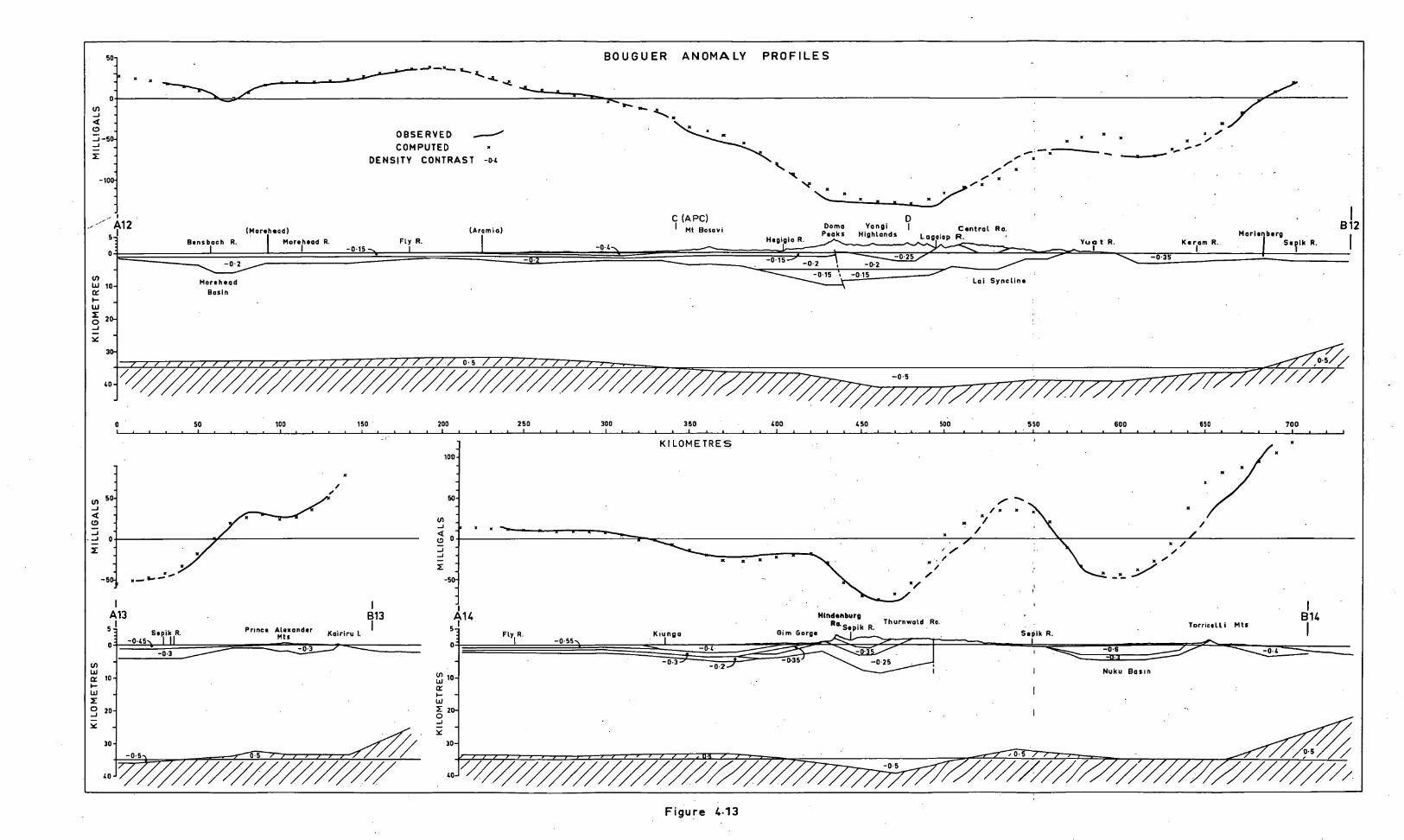
-100-

-50- -

KI L

OM

ETR

ES

—J .jt 0

—J

KIL

OM

ETR

ES

B13 A13 5 -

0

Kairiru I. Sepik R. -0.45-‘ I

Prince Alexander kits

-0.3

10-

B14 Torric ell. i Mts

Nuku Basin

o.5

/ // 5

—s

OBSERVED ■' COMPUTED

DENSITY CONTRAST -0.4

BOUGUER ANOMALY PROFILES

X

•

X K

X.,

50

0

—21 —50 —J

41. x

Yua t R. Karam R.

Do ma Peaks

Hegigio R.

C (A PC) (Moreh•ad) (Aramia) Mt Bosavi

Bensbach R. Morehead R. -0.15 FLy R.

-0.4

Yangi I Central Ra. Highlands Lagolap R.

B 112 Marl. berg

Serk R.

-0.35

10

-0.15 ■ -0-15 Lai Syncline

20-

-0-15 -0.2 -0.2 -0-2 .

Morehead

Basin

30-

0.5

-0.5 40-

50 100 150 200 250 300 1 a

350

K I LOME TRES

100

20-

30-

-

Hindenburg Ra. Sepi

. k R. Thurnwald Ra.

Gim Gorge

-0.4

-0.3 -0-2 -0.25

./MIYM .■rmme■■WIIMairn% 0,1■41NrImm■

///

A14 5-

:

Fly R. !Clung° -0.55

Sepik R.

400

450

500

550 600

850

700 .t.• • . •

.0"

/e x

• /

K

-0.5 IIIIIMMINVA■mamreirair

Figure 4-13

135

of : interpretation:elaborated in discussing A10B10 are_valid for the

southern part:of - this profile.

Or the regional Bouguer map the-Morehead - area.is - characterized by.

a northwest-trending low which is open only.to:the northwest .,SinCe. the -

anomaly-ia_notapparentim-gravity surveys over the southern:platform - of -

West-Irian it must eventually close in that direction,also (Compilation -

Map,_p.150). On.detailed - gravity maps the northwest-trending low is

interrupted by. a: transverse: saddle midway-along it, and-there_is - some

indication that. there is: another: gravity low south:, of the .Coast

:A.AppendixJI,.maps The Morehead-n°..1 bore (APG, - 1961, ry.12)

:penetrated a section composed of: .

Pliodene. 70 m. clays, carbonaCeous_mudstones

Miocene 1050 m. detrital limestone

. Cretaceous. 'alternating sandstone and muds one 700 m.

hard, brittle muds tone

500 m.'

JithaaSic 300 M. recrystallised arkosic[.sandstones

- On seismic evidence the basement was placed at 2500 m. When it is'

projected-along the gravity contours; to this section the-Morehead :bore

can be' seen to be located on thenorthern flank of the gravity low.

Assuming that the anomaly is caused by deepened Mesozoic, sediments

(-0.2), the maximum depth of the Morehead basin'is:5 to 6 kilometres.

APC ,(1961, p. 114) states that in the deepest partof - the Morehead Basin

the sedimentsare alpout.A km. thiàk. Trovided'that this thickness is

based on seismic.measurementsn the axis of the gravitylow,.it indicates

the choice of too small a bulk density contrast for the Mesozoic

sediments,. That this may well be the case is -indicated by.th&low

seismic velocity_of the upper layers of Mesozoic sedimentain.this basin,

given'by, Bliaux (1957) as 3.31m/sec, which corresponds to a density of

about 2.3 g/cc. The bulk density contrast of the whole Mesozoic section

would thus be closer to -0.3 than -0.2 .

Over the rest of the - platform section the anomalies are consistent'

with variations in the thickness of'MeSOzoic rOcks . Underlying a Miocene'

136

detrital . limestone layer (-0.15) of fairly constant thickness. The high

over the Fly River (80 , 142° ) indicates that the present Mesozoic thickness

in . that area is small or.zera. . Based on. the isopachs of Smith (1964,

Fig. 2) a shallow basinal.stru.cture in Pliocene'argillites (-0 1 4) is

situated northeast of Aratia is projected. to this section along

the anomaly. contours)..

Along this profile., the gradient towards the Southern Highlands

graVity low is apparently quite gentle, and could be explained largely by

depression of the base' of the crust ? •' But it is equally well explained

by the' type of deep 'sedimentary structure which was more strongly suggested,

by the previous two profiles, and which is hypothesized on this computational

model. This structure does not agree with that.depicted in APC's parallel

profile CD (1961, plate 2) which is projected onto this section. However,

as stressed earlier, there is no 'geological evidence for the thickness of

the Mesozoic in the area. South of the Lagaiap River, Dekker and Faulks

(1964) mapped 1000 m. of Lower Kiocene.limestone . overlying and inter-'

fingering with the Yangi Beds,a Palaeocene to Upper. Miocene succession, up.

to 5 km. thick ., of mudstone, limestone and pandstOne. The:Lai Syncline,

to the north, showed the following' succession:

Middle Miocene

greywacke, tuffaceous sandstone 2500+ m.

tuff, 'agglomerate,, pillow lava 1000+ m.

Lower Miocene 4000+ m.

greywacke, conglomerate, shale

Upper Cretaceous to Lower Miocene

2000+ m.

siltstone, shale, limestone, marl, calcarenite

(Lagaiap Beds)

Upper Cretaceous

(unknown)

mudstone

The Lagaiap beds also appear tO underlie, or grade into, the

Yangi Beds. The Mesozoic succession north of the Bismarck Fault Zone

(5140 , 144° ) is:

Lower Cretaceous basalt, agglomerate, tuff

Jurassic sandstone, shale, siZtstone

137

The thickness 'of the successionje unknown

The model structure in the area-follows• that interpreted by

Dekker and.Faulks (1964), only the sub-sea-level succession being:

considered. A contrast of -0.25 is assigned to the lami Beds, and

70.2totheLagaiap Beds and the upper part.of the Mesozoic. ,: The..

deeper Mesozoic beds are given a contrastof--0-15. The Lagaiap and

Bismarck Faults,.respectiyelyto.the'south . and,north of the . Central-

Range, are shown as .step-,like rises in basement level, and the Quaternary

volcano, Doma Peaks ;• isalso'_assumed,to be associated with an abrupt .

basement . rise.

There4s: :virtually . no. control on the contours, or .geology,

between the Central..Rangeand Marienberg„ SO little significance can be

attached . to:that_partof : the model„ :APOC. (1930,jol.II)..reports :Upper

Tertiary sediments overlying metamorphic rocks to the west of the Yuat

River in this profile, ancl.papp.,(in..APOCi . 1930, vol.II) estimated about

1500 m. ,of Miocene overlying basement in the Marienberg area. In the

Marienberg of..mm.dstoneS„ Shales, , sandstones_and conglomerates

were.encountered„.including_thin ses .ms of lignite. The base, of the

Miocenewas . notreached.... (In the geological map.(p.100) . this age has

been,altered.to:Pliooene, following the unpublished compilation of APC).

There is nothing ‘ inthe gravity, pattern, defined by a.,few observations in

the north of the area, to indicate more:than . two or three .kilometres of

light sediments (-0.35).

Profile A13B13 (Fig. 4.13) - This short profile is examined in order

to obtain some indication of,geological structure between the Sepik

River and the north coast, in a region where there is some control on the

regional gravity contours ? Geological mapping along the north coastal

strip by APOC (1930, vol.III) and in a few inland areas by AC geologists

(refer Carey,1938a) has been connected by reconnaissance traverses and

compiled by APC. The general sedimentary succession, as defined for the

Aitape area by Nason-Jones (in APOC, 1930, vol.III) is:

Pleistocene Yalingi Series 200 m.

gravel, conglomerate, clay, mudstone

138

Plio-Miocene Finsch Coast Series 1500-3000 m.

argillaceous blue marls, sandstone

Upper Middle Miocene Upper . Aitape Group 500 m..

marls, limestone, calcareous sandstone

Middle Miocene Lower Aitape Group 1000-2000 m.

tuffs; marls, conglomerate

In the APC compilation, which I have followed, the Finsch Coast Series is

shown as Pliocene. Where the basement is exposed in the northern

mountain ranges it consists of basic intrusions and volcanics or meta-

volcanics, and in most early reports is referred to generally as "diorite".

To the north of the Bewani, Torricelli and Prince Alexander Mountains the

sediments are folded and flatly overthrust towards the north. South of

the mountains the sediments are folded about W- to NNW-trending axes

. (Carey, 1938a).

Basement is not exposed along A13B13, but it is present' to

either' side of the PrOfile. The only' sedithents exposed .tO the north

the 'Prince Alexander MOUntains are Miocene (-0.3'), with,the Pliocene

Finsch "Coast Series (-0.45), south of the mountains,' dipping gently south-

wards - Under the alluvium o' Valley. The steep northward rise

of gravity alOng the north coast west of Wewak (3ko , 143340) is interpreted

as the etfect of a rapidly thinning crust, as this model demonstrates:

Under the Sepik - Basin, the crust would' appear to be close to standard

thickness.

Profile A14B14 (Fig. 4.13) The gently undulating nature of the gravity

anomalies over the southern part of the area traversed by Al4B14 indicates

that the geological structure is likely to differ little "from other parts

of the Southwestern Region of Papua. ' Control is difficult, since 434 is

200 km. from the nearest Papuan oil bore, and about the same distance

from surface exposures to the north.' the nearest geological control

location is - th Aripoe no.1 bore, ab6ut 100 to the northeast, in West

Irian, in which the section penetrated was

Pliocene 500 m: sandstone, siltstane, clay •

139

Upper.jvliocene . sandy limestone

Upper Cambrian limestone

500 pp.-

500+ m.

(Visser and Hermes, 1962, encl:'8) - •

Since no pre-Mesozoic sediments have been identified in the - Southwestern Region of.Papua,the.Cambrian limestOne.is not assumed. to be

present in the 'section.at A14. If it werepresent it would probably be

lacking in density contrast, • and gravimetrically.indiatinguishable from - basement.

From observations in' the headwaters of the Fly and Strickland _ .

Rivers the Pliocene is known to thicken to the north, and to have a'

lithology indicating:a.non-Marine origin under volcanic cOnditions.

Along this line of section a maximum of about 2500 m..is present, -

Consisting of current-bedded tuffaceous sandstones and tuffs, With. bands

of conglomerate and agglomerate '(APC, 1961, .seat. 3.322);

The Middle and Upper Miocene section Consists of limestOnes,

mudstones and siltstones and has a thickness of about 1000 m. Where

exposed in the foothills -. This section may thin to the south. — From a

thickness of about 500 in. at the Gim Gorge the Lower Miocene, developed

entirelyA.n-,the:limestone fades, thickens to more than 1500 m. in the

Hindenberg'Range,

In the'Gim Gorge Osborne'(195) measured a Mesozoic section

beneath the Lower Miocene, comprising:

Cretaceous 1100 m. mudstone, calcareous thuds tone, silt, sandstone

Jurassic 1300 m.• sandstone, micaceous shales, conglomerate

• From the nature of the basal conglomerates, Osborne deduces

that "in all probability uanite basement underlies the4uabgen

conglomerates at no great depth!'.'''. the upper Sepik River near.

Telefomin (50 , 1411/20 ) more than 3 km. of Jurassic black shales (with

minor sandstone) are exposed, overlain by.500 m. of Cretaceous sandstones

and shales.-

The structure of the model south of the upper Sepik River is

based to.some extent on section AB of .APC (1961) and Sections I and II of

140

Smith (1964), which are parallel to Al4B14 but about 100 km. away from it.

These sections all show a basement anticline in the foothills, separating

deepened sediments under the main range from a deepened basin to the south.

Further to the south the sediments shallow onto the platform. Such an

interpretation is consistent with both gravity and geology along this

profile. The regional gravity gradient is not indicative of a large

isostatic root under the mountains. Basement is considered to be

shallow under the head of the Gim Gorge, and the sediments thicken to

both the south and north. Density contrasts chosen for this model are

greater than those for similar sedimentary successions in other models.

They are, nonetheless, within the range of probable density contrasts, and

are used to demonstrate the effect of using maximum, rather than minimum,

contrasts. The densities used in the southern part of the model are:

Pliocene argillites -0.55

Pliocene tuffs and tuffaceous sandstones —0.4

Miocene (mainly limestone) -0.2

Cretaceous -0.35

Jurassic -0.25

Mesozoic undifferentiated -0.3

The effect of using smaller contrasts would be to increase either the

depth of the basins or the amplitude of undulation of the base of the

crust, but it is apparent that the' interpretation of the nature of the

structures is unaffected.

The northern boundary of the deep Mesozoic is shown as a faulted

contact with crystalline rocks, after Smith (1964). Thompson and

Fisher (1965, p.8) state that the Cretaceous and Jurassic sediments dip to

the south unconformably . off the basement 'block. However, it is not known

whether this statement is the result of observation orinference.

Whichever is correct, the gravity to the north is too sparsely observed

to distinguish. 'The postulated deep Mesozoic can be seen, on the

Bouguer:Map, to be located on the narrowing western continuation of the

Southern Highlands Low-(5° , 1411/20 ). As it is - interpreted here,, the

gravity indicates that the zone of deepened Mesozoic becomes more narrow,

but perhaps not less deep, towards the west. ' The southern lip Of the

deep basin, shown on this profile at Gim Gorge, extends at least 80 km.

ila

to the east, where granitic basement has been reported'by APC (1961,

p:20) to underlie the Mesozoic at Strickland Gorge .(51/2 0 , 142 ° ).

To the west, in the Star Mountains of West Irian,_Visser and Hermes

(1962, encl. 9) show a belt of thickened Mesozoic, and possibly

-older, sediments with a width, of 25 to 40 km. between a southern

bounding anticline s(exposing Cambrian rocks).and.a faulted contact

with. schists in the north (Visser. and Hermes, sections 26, 27).

I therefore think it probable that the narrowness .of the Mesozoic

basin in the west is due to the truncation, by faulting in the north,

of.an originally much wider basin.

North of the Thurftwald_Range is - a - gravitational high defined.

by a few. observations. This high appears .to exist: over the uplifted

area to the south of the Sepik plains (We, 1411/20 ), which Smith (1964)

calls the "Behrmann Massif". Metamorphics have been recorded at

several localities on the northern edge of the area by APOC . (1930),

and along the western edge by Paterson and Perry (1964), but the

interior geology is unknown. Assuming the area to consist of meta-

morphics of standard density the crust must be thinner_than normal to

explain the observed anomaly, a8.shown on the model. However,

Paterson and Perry (1964) have recorded boulders of granodiorite,

diorite and gabbro in streams issuing . from the metamorphics. -A large

basic intrusion in the area would certainly explain the gravity anomalies

more satisfactorily.

. South of the Torricelli Mountains, in which the basement is

exposed, the Pliocene Finsch Coast Series (-0.6) is known to thicken

considerably. Assigning maximum contrasts to this, and to the under-

lying Miocene, a depth of at least 50,00 m. in the Nuku Basin is consistent -

with the rather sparse gravity observations. There is sufficient

. control on the southern side of the basin to indicate that the basement

is-quite shallow under the Sepik River. No observations exist over the

.Torricelli Mountains, which would.probably be found to represent a

** : A recent reconnaissance survey by the Bureau of Mineral Resources has

confirmed the existence of large bodies of serpentinized peridotite and pyroxenite in the eastern part Of the southern watershed of the Sepik

- River (Dow, 1967).

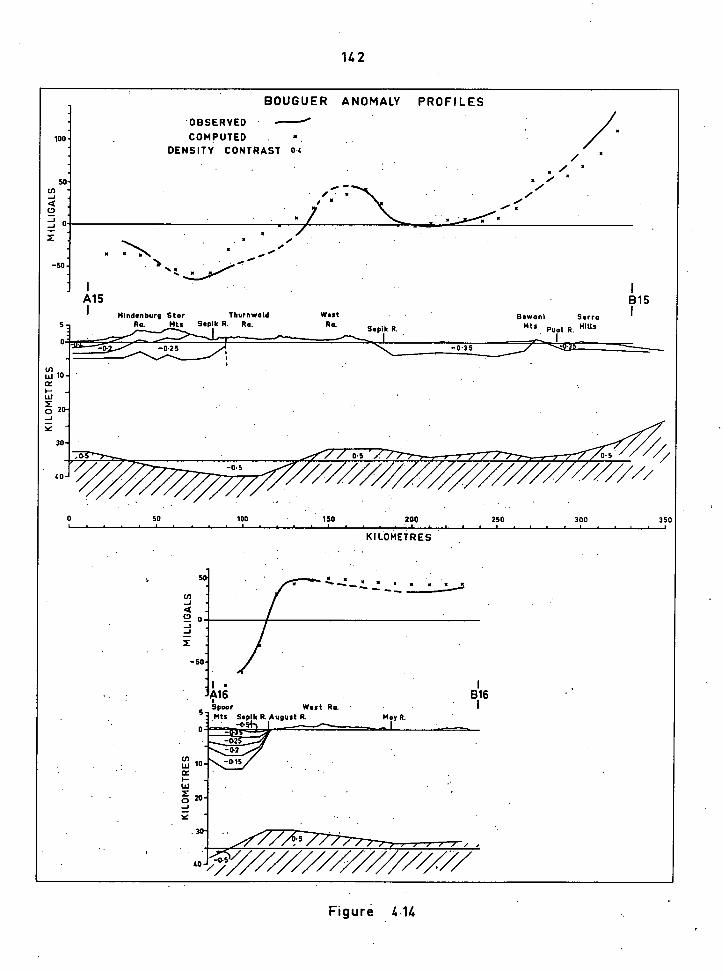
OBSERVED COMPUTED •

DENSITY CONTRAST 0.4

-50-

57

•

•

A15 B15

-0.35 "."•CA21.. -0.25

0 50 100 150 200 250 ... 300 350 . . ..

B11

6 I •

Spoor West Pa. Mts Sepik R. August R.

BOUGUER ANOMALY PROFILES

KILOMETRES

•

-50

M I L

LIG

ALS

May R.

100

•

Thurnwald West Pa.

Sepik R.

// /4/

........oior/BarrArAIZIWAw•-....orAIVANKAIK/z/0 5

/// / /

Hindenburg Star Pa. Mts Sepik R. Ra.

Bewani S•rra Mts Hills Pual R.

0.5

40 -0.5

142

Figure 4.14

1)43

residual gravity high. Taking into account the sedimentary Vsection

north of the mountains, discussed in connection with Al3B13, the

regional positive gradient is explicable by a rapid thinning of the crust

under the rapidly deepening sea.

Profile 41015 (Fig. 4.14) . As with the northern part of the

previous profile A15B15 suffers from the poor coverage, both geological

and gravimetric, of the area. The only purpose.of this model is to

indicate a few probable parameters to associate with qualitative inter-

pretation of the anomalies, and_no attempt has been made to match

precisely the computed anomalies With the observed:. Over the Star

Mountains the amplitude of the anomaly indicates that the pre-Mesozoic

basement is closer to the surface here than to the east._ Alternatively,

the more positive anomaly may be due to the presence, at depth, Of the

Antarei GranOdiorite Which intrudes Mesozoic and Tertiary sediments in the

Sta MoUntainS West of the border (ITISSer and He/ties, 1962, bection:.27).H

- ' The positive anomaly over the West Range (or Behrmann Massif)

Is again indicative of an UppercrUStal basic intrusion rather than, as

here . , ageneral. high 'due to lower crustal source's, With the

sharp gradient being the effect of : light'sediments adjoining the meta- - .

morphids: - .1f basic intrusions were present; the basement Would be -

closer to:the SUrface . tO the north ofAhe . ..(abwer) Sepik River,: in the -

area Which- appears aS a graVitetric saddle to the west-of•the NUku

Basin. (31/29,' 1511/29 ) . ESSehtiallY- , the anOtalY' indicates a considerable

uppecrUstal , densiti contrast:riear . theSepik River, be it sediments

againstmetamorphiasor-metamarphicS'against basic' igneous rocks.. - North

of the Bewani Mountains Osborne (1956) reports about 11 km. of Miocene

and Pliocene geosynclinal sediments "upfaulted and eroded to expose

granitic and metamorphic basement". There is no indication given by the

observed anomalies that any considerable remnant of these sediments is . . _

presently existing,-- -• VV • .-

Profile A16B16 (Fig. 4.14) This profile, trending from the West

Range aCross . the4pper 'Sepik:-August River area , is basecron'the detailed gravity:surVey of PatersOn (1958):, which 1 haVe*converted'to: the absolute

144

datum (section 2.2.4), plus the feV . regional observatiOns in the area.

Paterson and Perry . (1964) have measured, the following sections, in areas

not covered by Alluvium:

Pliocene 300 m.

calcareous pebbly greyumcke

Middle and, Upper Miocene, , 1000 m.

calcareous siltstone, sandstone, conglomerate,

carbonaceous muds tone

Lofder Miocene . . 700, m.

calcareous greyzdacke, 'detrital limestone,

interbedded voleanies

Upper Cretaceous 1000 m.

greywacke, muds tone, sandstone, conglomerate -

The very steep westerly negative gravity gradient must be largely

due to upper-crustal features . . Paterson' and Perry (1964) believe that the,

gradient is due to the.effect of about 5000m. of sediments, superimposed

on a regional effect However,-, the regional gradient is not in an east-

west direction, except for that part of-it obviously caused by the

'structure in this area. As shown on the model, if Aure fades densities

are used for these similar sediments, it . is necessary - that at least 10

kilometres be present, even assuming a thickened crust under the basin.

If, as suggested previously, a.large basic igneous intrusion were present

in the West Range area : the sediments in the model would not need to be so

thick and the base of the crust could be flatter. Even so, the anomaly

would almost certainly require a thickness of sediments greater than 5 .

kilometres.

4.6 SYNTHESIS OF THE GRAVITY INTERPRETATIONAL MODELS

The preceding discussion of Bouguer . anomaly profileS has outlined

a - crustal Structure of the . eastern part ofthe : island of New Guinea which

1145

is consistent with. gravimetric and known seismic.data, and which I

consider to be the most likely structure in view of the observed

geology.. By . interPolating.betweenprofiles the boundaries ofthe

major upper- and lower-crustal structural features have been,defined. -

4.6.1 Structures Within the Upper Crust

. Structural features which are.. defined by gravity represent

only the situation as now existing, without regard to causation..

Therefore, in the compilation of interpreted features (Fig. 4,15), the

structural terms used refer to the present depth of basement, regardless

of the age of overlying sediments or any palaeotectonic'features defined

by isbpachs'. "Basement exposed or close to surface" refers to those

areas where basement exposures are recorded, and where there -is no

gravity evidence to indicate significant deepening of sediments, between

exposures. "Platform" areas : are those where all available evidence

points to the existence of flat-lying sediments .,..up to a few kilometres

thick, overlying basement. The term "Basin" is applied. to an area of

. sediments significantly deeper than.those_surrounding it, and bounded by

the zone of steepening negative basement gradient. Thus., the actual

depth of basement can vary considerably from one basin, to another.

The zone of sediments between the Fly River Platform and the Aure Trough -

Southern Highlands Basin does not fit.into any of the.aboVe . categories,

and is referred to simply as an "Intermediate Zone".

With reference to the profiles„the structures outlined in

Fig. 4.15 should need little further explanation... .The.transcurrent

faults in the Madang (5 ° , 146° ) and C011ingwood Bay (91/40 , 1149½0) areas,

which were suggested by the gravity interpretations, are indicated.

Thompson and Fisher (1965) suggest the possibility of the former, and

Davies and Ives (1965), the latter, on topographic and geological grounds . .

In addition, it is suggested that the Papuan.Ultrabasic Belt. is bounded

to the northwest by a transcurrent fault.in . the Salamaua area - (7° , 147° ),

as would be a logical consequence of emplacement. by thrusting. The Owen

Stanley 'Fault, and those fronting the Finisterre and Adelbert Ranges and

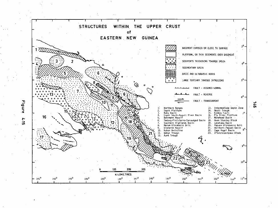
O 0

BASEMENT EXPOSED OR CLOSE TO SURFACE

PLATFORM; OR THIN SEDIMENTS OVER BASEMENT

SEDIMENTS THICKENING TOWARDS BASIN •

: SEDIMENTARY BASIN

•BASIC AND ULTRABASIC ROCKS

LARGE TERTIARY IGNEOUS INTRUSIONS

FAULT - ASSUMED NORMAL

-41--A—A- FAULT - REVERSE

■•■■••••

FAULT - TRANSCURRENT .11.■■■

. • . . . 000 '0 0

O 0 0 0 0

0 0 0 0 0 0 0 0

o n000 13. o 0 0 0 0 000

0 0 0 0 0 0

O 0 0 0 0

•

30_

4°-

so_

6°-

O 00 ,

4 0 0 .

0 100 200 300

KILOMETRES 145 0 146° 147 0

1: Northern Ranges 13.

2. Sepik Platform 14.

3. Nuku Basin

15. 4. Upper Sepik-August River Basin

16.

5. Behrmann Massif

17. 6. Madang-Finisterre-Saruwaged Basin 18. 7. Southern Highlands Basin 19. 8. Marum Ultrabasic Belt

20. 9. Bismarck Massif

21. 10. Kubor Anticline

22. 11. Wahgi Trough

23. 12. Aure Trough

•

/,

23

149 0

Intermediate Depth Zone Omati Trough Komewu Fault 70 . Fly River Platform

Morehead Basin Owen Stanley Block Lakekamu Basin Papuan Ultrabasic Belt Northern Papuan Basin

80- Cape Vogel Basin

D'Entrecasteaux Block

153°

16 Nst

:: • . .•.17 *.*:4 .‘

:•::: • . A

— 141 °

1420

143 °

1440 1480 150 0

151 °

152°

..

I+ + + ++

I I

STRUCTURES WITHIN THE UPPER CRUST 2°-

of EASTERN NEW GUINEA

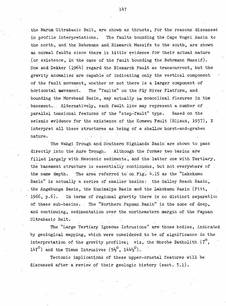
1147

the Marum Ultrabasic Belt, are shown as thrusts, for the reasons discussed

in profile interpretations. The faults bounding the .Cape Vogel Basin to

the north, and the Behrmann and. Bismarck Massifs to the south, are shown

as normal faults since there is little'evidence.for their actual nature

(or existence, in the case of the fault bounding the Behrmann Massif).

Dow and Dekker (196).i.) regard the Bismarck Fault as transcurrent, but the

gravity anomalies are capable of indicating only the vertical component

of the fault movement, whether or not there is a larger component of -

horizontal movement. The "faults" on the Fly River Platform, and.

bounding the Morehead.Basin, may actually be monoclinal.flexures in the

basement-. Alternatively, each fault. line.may represent a number of

. parallel tensional features of the "step-fault" type. Based on the

seismic evidence for the existence.of the Komewu Fault (Bliaux,. 1957), I

interpret all these structures as being of a shallow horst-and-graben

nature.:

The Wahgi Trough and Southern Highlands Basin are shown to pass

directly into the Aure Trough. Although the former two basins are

filled largely with Mesozoic sediments,. and the latter one with Tertiary,

the basement structure is essentially -continuous, but not everywhere of

the same depth. The area referred to . on.Fig'.. 4..15 as the "Lakekamu

Basin" is actually a series of smaller basins: the Galley Reach Basin,

the Angabunga Basin, the Kunimaipa Basin and the Lakekamu Basin (Pitt,

' 1966, p.6). In terms ofregional gravity there is no distinct separation

of these sub-basins. The "Northern Papuan Basin" is the zone of deep,

and continuing, sedimentation over the northeastern margin of the Papuan

Ultrabasic Belt.

The "Large Tertiary Igneous Intrusions" are those bodies, indicated

by geological mapping, which were considered to be. of significance in the

interpretation of the gravity profiles; Viz, the . Morobe Batholith (7° ,

147° ) and the TiMun Intrusives (51/2° , 1441/2° ).

Tectonic implications of these upper-crustal features will be

discussed after a review of their geologic history (sect. 5.1).

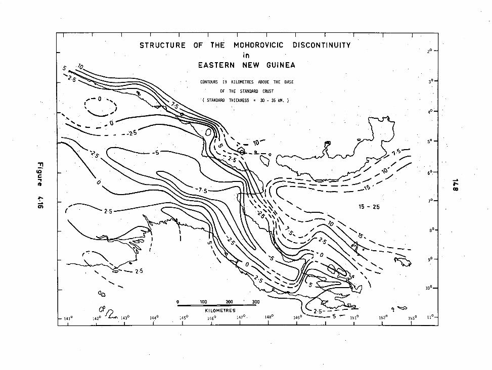
••-"' 0 % f \

— \ % ..■ \

\ ... .....

4° —

ezis --- 2.5 ■ **,

1 1 I I I I I I I I

STRUCTURE OF THE MOHOROVICIC DISCONTINUITY in

EASTERN NEW GUINEA

2° —

CONTOURS IN KILOMETRES ABOVE THE BASE

OF THE STANDARD CRUST

( STANDARD THICKNESS = 30 - 35 KM. )

3o _

61)

143 0 142 0 — 1410 153 0 11°- 152°

5o _

6°—

—

2.5 15 -25

70_

8°— 76-,

90 _

10°—

300

2.5- — 148° 147 0 149 0

100 200

KILOMETRES

146° .7— 1510 145 0 9440

J_)49

4.6.2 Structure of the Crust-mantle Interface

The authenticity of the interpreted structure of the base of the

crust is dependent upon the precision with which. upper-crustal structures

have been deterinined„ - and the validity of the assumption , that.there are no

mass.-anomalies within the lower.crust. Accordingly, the contours of the

base of the gravimetricbrust, which I correlate with the Mohorovicic

discontinuity, in this region, are subject to indeterminate errors.

Within the mainland of eastern New Guinea the area where crustal

thickness is.subject . to'the most doubt is the.Southern Highlands Basin,

for which the relative merits of deep sediments and thicker crust have . . _

been previously ,discussed. The position of the Mohorovicic- discontinuity

under the ocean to the north of eastern Papua is indicated by very

generalized contours. The derivation of the crustal thickness in this

region is discussed in section 4.7.4, following an examination of the

BougUer'anomalies compilation map (p.150).

Since the regional type of Airy compensation was assumed in the

computation of the profiles, the undulations of the Moho.are rather

gentle, . Absolute crustal. thicknesses are not given, but rather

deviations from a standard thickness which, following the discussion in

can be assumed: to be.in , 'or close to, the range 30-35 kilometres.

The thickest part of the crust is under the central cordillera to the

south .of the Markham Valley, which is also the position of a pronounced

change in the trend of the thick crust, from NW-SE to.WNW-ESE. South-

eastwards along the Owen Stanley Range, and westwards along the. central

ranges . the crust becomes thinner- . As discussed in the interpretations

of profiles A2B2_and A3B3, the thick crust under the Owen Stanley Block

is sinistrally offset.in the Collingwood Bay region. . The areas of

thinnest crust underlying the mainland are under the Cape Vogel Basin and

the Aure Trough. . The tectonic eignificance of the crustal undulations in

relation, to , upper-crustal features will be . examined in section 5.2 .

150

•.7 EXAMINATION OF THE GRAVITY FIELD THROUGHOUT MELANESIA

Before embarking on any tectonic discussion based on gravity work

within an artificial subdivision of the Melanesian area: it is essential

that the subdivision be regarded in its setting, as part of a wider

distribution of gravity anomalies. Therefore, all available gravity

information for areas surrounding eastern New Guinea has been cotpiled as

a Bouguer anomaly map (p.150). Apart from:the Bougainville island .

survey, reduced by the methods described in Chapter 3, all incorporated

data were :acquired as simple Bouguer . anomalies, and thus are not strictly

comparable with the extended BoUguer anomalies Of eastern New Guinea.

However, the West Irian survey, especially near the junction with

eastern New Guinea, consists painly ,of . the near-sea-level observations of

oil surveys, for which the topographic correction would be small. For

both this and the sea areas the contour interval is so large 4s to obviate

any likely junction errors... A Contour interval of 25 milligals is used for land areas, and intervals of 50 or 100 milligals are used for sea

areas. Brief and qualitative interpretations of the incorporated

surveys are given here.

4.7:1 West Irian

The gravity data compiled, by Visser and Hermes (1962), from oil

company surveys, did not include a coverage of the 66ntral mountain

ranges, apart from those on the Vogelkop (2 ° , 134° ). However, the'

anomaly values to the north and south of the cordillera indidate that if

there is a regional gravity low over the mountains it isof muCh smaller

magnitude than that observed in the central part of eastern New Guinea.

From the known gravity field, it would appear that the small negative

anomaly (-50 milligals) observed in the Star Mountains to the east of the

border (5° , 141° ) increases little in amplitude in a westerly direction

along the cordillera, which is much higher in west than that in east

New Guinea.

141 ° 139 ° 135 ° 137 ° 131° 133°

NEW GUINEA- SOLOMON ISLANDS REGION GENERALISED BOUGUER ANOMALIES

MILLIGALS 175

775

NEGATIVE ANOMALIES 100 7

LAND ° NE

250 -)

TERRITORY OF NEW GUINEA

50 700 10

-5 °

100

,g- :50

‘,.)2 BRITISH SOLOMON

ISLANDS

•BOUGAI N VILLE / C 200

• •

\

Compiled by V. P.St John

Geology Dept. University of Tasmania (1966) from the following sources :

West Irian : Visser and Hermes (1962)

Bougainville Is. :.Kugler and Dodini (1963) ( pers. comm.)

British Solomon Is. : Woollard, Hawaii Institute of Geophysics (1965) (pers. comm.) -11 ° Seaborne Gravity Data :Woollard,Hawaii Institute of Geophysics (1965) (pers. comm.) Preliminary Map

Dooley (1963) , Vening Meinesz (1934)

- 7 °

-<,

, —•;—— , (—)1 I' _ s -'--

--- 50 - 350 3.0 -,-- --- \------, ---=--- — r -3T---

-

"1111411 - , --..........._

: SO ... .. .. Se/A I\ II, a

■ ■

‘krikt

GEORGIA • s s .

0'- '°-- . •s .

---. '*V SO- _ s •s :.

-72e , ss ss

• s '"-

SANTA ISOBEL

15,J

QUEEN S LAND 0 50 250 500

125

.125

25

-25 /

100

25

•reLon

25

50

750

'143 ° 145 ° KILOMETRES

147 • 149 ° 751° 157 °

161 ° 159 ° 155 ° 153 ° aso

250 -

25 0

15 1

. A11, -the larger negativeanothalies in the West Irian survey can be

correlated with deepaedithentarY taaina.' - That of- -75 thilligals, in the

southeast . VOge/koi; : (22,' '1340), is centred on the Bintoeni - Baein, Where

Visser and-Hermes (1962, p.1)45) report'up t 9 kilometres of Miocene and

Pliocene sediments. On the eastern side of Geelvink Bay (30 , 136° )

the "Waipoga Minimum" occurs over a very thick development of the

. Pliocene Mamberamo Formation, and the' underlying Miocene. This is. also

the cause of the gravity low in the northern Meervlakte (30 , 138° ).

South -Of'thabordillera aithinimUM of "-;75 . niiiligalS oVer'the foothills and-

part'of'the'bbastal plain . ( 41/20 ;'•1384I) • dile to- thick Plibbehe and'

MiOcene'Sediment8 in the Akimeugah Basin. The basin is truncatedto the

north' 14- the-upthrust "central . ranges.

'Mott of the pOSitive'anothalies ocbur Over areas of uplifted'

This is the case with the gravity highs near the - Mamberamo Mouth

( 20 ; '138 ° , ) on the 6:.clOpsoun tains

Meervlakteic%" - 137°) and:onthe islands of Biak and:japen (11/2° ,'136° );

In all these areas exposed basement 'is cOmPosedof greenschist facies

metamorhics," enéra1Ir intruded' by basic. or Ultrabasid:rocks. Basement 13 ' o,) . is not exPoted in the" rn northe' Vogelkop (1/20 ' , 21/2 but - the presence of.

Silurian rocks containing igneous intruSions indicates that it is - at 'a

shallow depth. The,positiveanomaly in the Onin.Peninsular - Koemawa

Mts. region (4° , 133° ) may. be partly due to an anticlinal structure

(Visser and Hermes, 1962,-section 13)- but is probably largely a result of

crustal thinning in the "Southwestern Arc" . Of the Banda Sea structures.

As a qualitative interpretation : of the regional gravity Visser

and HermeS transverse Section from Frederik

Hendrik'island Cape &Urvilie (11/2°, - 138° ). The' southern

part of- he seCtion 'depicts a StructUre"sithilar"to that of the Southwestern

Region Of -Papua -- thin tediments'Oveing a crustsiightly thinner . than

normal. The Cruat it Shown as thibkening under the southern Part of the

central' ranges;' but "Only by abOut..7 kiibtheireS, WhiCh is insufficient for

Airy isostatic'equilibriuth. " A positive over the northern part of the . , . .

central raniesj_S -Interpreted as'auetOthinning;cruti, and an adjacent . . . . .

negative "oiler -the Mee'rViaktetd thickening bru't'. From the observed

geology E.bonaider it likely- that the 'jii:xtSpbsiiidn . of these pcisitive - - .

and' riegatlye graliitY Snonlalies at"least Partly an effect Of the

underlying juxtaposition of metamorphicand basic igneous basement, and

( - 21/2° ,'1)401/20); in the -southern

152

deep sediments. As with my interpretation of the anomalies on the north

coast of east New Guinea, so Visser and Hermes see the positive anomalies

on the north coast of. the western section as resulting from a crust

thinning rapidly away from the land. .

4.7.2 Banda Sea

• The area south and west of the Vogelkbp is pert of the. regional

Indonesian survey described .by Vening Meinesz (1954):.. He interpretedthe

regional isostatic-anOmalies as' indicating a . cruStaLdownbuckle under the

ocean trench However,. Wodllard and - Strange (1962) show that, for a.

profile across Java, while the regional.isostatic anomalies indicate a

downbuckle under the trench, the Bouguer anomalies areconsistent with

crustal thinning under the trench and . thickening under the ridge. on the

landward side of the trench. In shape, this type of cross-section

suggests an .approach to local Airy equilibrium. Similarly, for. the

Banda Sea, the negative anomaly shows a crust slightly thicker than

normal in an arc which include the Kei Islands (6°, 133 ° ), while the

positive anomalies indicate a considerable thinning of the crust Under the

deep ocean trench to.the west-

4.7.3 Solomon Islands

. The Bouguer anomali es over the Solomon Islands range from 20 to

250 milligals, By comparison of the anomalies with the geology of the

Solomons, as described by Coleman et al.. (1962), it is evident that the

gravitational highs correspond to areas.of uplifted Mesozoic basement,

and the lows to deep sediments. The basement is similar to that of

northern New Guinea, being composed of ,greenschist and lower amphibolite

facies metamorphics derived from volcanics and pelagic sediments.

Coleman (1966) . states that the high, positive gravity anomalies

over the Solomon Islands indicate acrustal . thickness of less than 15 km.

Such a view is based, as it must be, on the assumption that a . Bouguer

anomalyof-zero attends a crust which extends to -a standard depth below

153

sea-level, and which has sufficient horizontal extent to be considered

infinite.. Should any part of the crust be replaced.by denser substratum,

by virtue of the former's thinning,.then - the.Bouguer anomaly will

become positive, even at points below, which there is no thinning. This

is well illustrated in the computed profile A2B2 (Fig. 4.10), where the -

crust under the north of-Goodenough Island is of .standard thickness, yet

the horizontal effect of'adjacent deep anti-roots produces a positive

anomaly of 50 milligals.

To examine the gravity evidence for crustal thickness under the

Solomons consider them initially to form part of.an infinite crustal

plate which thickens or thins uniformly over its area, which has a

standard thickness, of 30 km.; and at the base of which there is a density

contrast of 0.4 g/cc with the mantle. Under these conditions a rise of

1 km. in the base of the Crust would produce an increase of 16 milligals .

in the. Bouguer anomaly at the surface. The maximum observed Solomon

Islands Bouguer anomaly (250 milligals) would 'correspondto a rise of

151/2 km. in the base of the infinite crust, giving a crust 141/2 - km. .thick.

However, the crust does not extend infinitely as a flat plate. The

anomalies of .300 to 400 milligals indicate a very thin crust immediately

to the south of the' Solomon chain. The horizontal effect of this thin

crust.(of almost zero thickness under the simplified standard conditions

chosen above) would make a considerable contribution to the anomalies on

the islands; a deduction which is borne out by the fact that the highest

anomalies of the Solomon chain are on' its southern or southeastern margins.

Thus, the high gravity anomalies over the Solomon Islands can be considered

to be derived only partly from crustal thinning directly under the islands.

It follows that, for a standard crust of 30 km., with a subcrustal density

contrast of 0.4, the crust under the Solomons must be considerably

thicker than the 141/2 km. minimum derived above; Taking into consideration

other factors, such as the quantity of .dense volcanic material within the

crust, and the possibilities of a thicker standard crust or an higher.sub-

crustal density contrast,. the gravity evidence, in the absence of any

other, is consistent with a crustal thickness of at least 20 to 25

kilometres under the Solomon Islands..

This view is entirely dependent upon initial assumptions, which

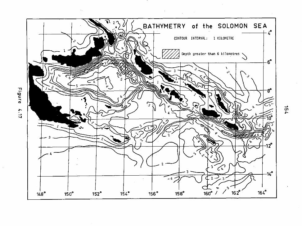
11 BATHYMETRY of the SOLOMON SEA

---,cle

■ \I-J9r.„,i ( b‘ ) t

CONTOUR INTERVAL: 1 KILOMETRE

_5-

1 0 3

1,......

V .. Depth greater than 6 kilometres Arl'..1.1'-'....-;?:.""

t---.....j." - ,Pe sAt4 '1k i•••. .•-•41* "lt.40.•

■

A 1 b a _

1.-

.1 61 I I

‘1111111111Nr4

I I ■ .K:

■

W 1 k ,b ill _ ...

ofr (D 6 5 4 5

..„;„„,.....1, 11. _ ___......—_,Iiiti.

A • 1 , 4

imi tsa.tiire

r i N 9 4

i _..., i

t wegt b, L 4

"ItiA irecal44'""b ii!!1•• 3 1...r.di

‘ 111111'''' 1

IN, `s-Nli..„0144•11,_ \ dri.

litt ,.. 20 s 70,,

4°

148 0 150° 152 0 154 ° 156 0

-4

1580

I

el

1600 a- cp

í / 162 164°

155

do not. take into account the likelihood of varying mantle density.

In the.absence of any seismic evidence for mantle.density or crustal

thickness the simplest structure consistent with gravity _must be considered

,the., most probable.. Some, seismic , work has been recently undertaken in the

Solomon , Islands, but , an . abstract published by Furumoto et al: ( 1967)

reported merely that "The results of the survey raised more geological

questions ,instead of providing answers." Some of the geological

questions raised by the Solomon Islands are discussed in 5.2.3.

4.7.4 Oceanic Areas North and East of New Guinea

data used- in ,cOmpiling , the.anomalies. over these areas -were'

derivedrfromtwo sources... - Most: .ofthe.material. is.derive&from United

States Navy shipboard gravity observations 'contoured andhadeavailable to

me by. Hawaii.Institute of Geophysics -(Professor G.P...Woollard,pers. comm.

to-Professor SIAICarey.)...'With these data have been notbined theresults

of two :submarine traverses 'acrossthe New Britain Trench, recorded-by-

Dooley'.(1963).

,.An approximate interpretation -of the gravity pattern can

if• one, considers that-airise'in . the base , of the crust of. 1: km. will

increasethesurfaceBougueratomaly. by. an amount. varying from about 10' to

20'milligals,depending upon the 'density -contrast.. 'The axis of an

'elongate zone ,of crustal thinning will lie along, the axis of the associated

Bouguer.anomaly. of. interest to compare the Bouguer, anomalies on

the-compilation, map .(p:150) with the , bathymetry of the Solomon Sea (Fig.

4.17); bearing in mind that the, bathymetry.is -„to'date, observed in more

detail thanthe,gravity.

IIihe ,:trapezoidal - gravity.high southeastof-NewBritain coincides .

with a similarly-shaped:lsedtion.. of ocean over deep. , Although

%possiblyLa:resUltM_insufficient gravity'observations,;'there 18 no

indication that:theanotalies are especially' large' over the deep trench:.

(up to '8500:- ,mwhich.formb the northwestern and;northeaatern boundaries

of the trapezoid, or over a minor troUgh,:deeperthan' 5000 . m.„, which.

156

forms the, southern boundary.. A bathymetric ridge, running east, then

northeast, from the Trobriand Islands (81/2 9 , 1519 ); isoharacterized by

lower .gravity anomalies than the deeper Sea flanking it. . South. of this

'ridge, and extending to the west and southwest of.Guadalcanal, is a series

of narrow ridges and.troughs defined by recent bathymetric observations,

and which vary.in. depth from more than 4 kilometres to.less than 1.

(J. Grover, - British Solomon Islands Geological Survey, pers. comm. to

Professor S.W. Carey). This area is encompassed by a broad gravity high

trending west from Guadalcanal, and which has almost as great an

amplitude (400 milligals) as the anomaly over the deep .ocean south of.

New Britain.

In terms of-Crustal thickness, then, it would appear that the

deep ocean south 'of New Britain, and the x.dag.e, to the South of that are

characterized by broad subcrustal undulations negatively imaging the"

'regional undulations of. the .ocean floor.. Such an association of

deepening ocean and .thinning crust. accords with the statistical. studies

of.Woollard and' Strange (1962, Fig. 6), At apparent Variance with this

correlation is the area to the 'west of .Guadalcanal, where a rise in the

base of the crust does not correspond to a regional depression of the

ocean floor. There is a 'possibility that this lack of correlation is a

function of inadequate gravity sampling over the area of rugged bathymetry,

but if the contoured anomaly is real it indicates that the ocean-floor

ridges and troughs are neither locally nor regionally compensated on an

Airy system. '

It is not possible to assign precise values to the depth fromsea-

level to the bas e of the crust without•knowing - the thickness, and hence

the gravitational effect, of sea-floor sediments. Recent sparker

profile work suggests considerable sedimentary thickness near the Solomon

Islands (J. Grover, pers. comm. to Professor S.W. Carey). .D.ren neglecting

the negative effect of sediments, the high positive Bouguer anomalies

indicate a thin, or oceanic, crust over the whole Solomon Sea area.

Using the rule-of-thumb interpretation, mentioned above (10-,20 milligals per

kilometre of 'crustalthinning) it is obvious that in the deeper trenches

the, base of theoceanic crust (the Mbhorovicic discontinuity) must be

within. a few kilometres of the sea-floor..,

15.7

5. TECTONIC IMPLICATIONS OF THE GRAVITY INTERPRETATION

Any tectonic hypothesis is built Upoh . the presently-ObServed -

disposition of geological'features'on'the'earthiS -surfaCeiand'ihe inferred _ .

disposition Of theS6 featUres ai depth. - There are waregions of -

uncertainty in the formulation of such'an.hipothesis. -Firstly, the

projection' of obaerved . geology into the-thirddimension is open to

'COnSiderable imprecision, - especially if the observations are sparse.

SeeOndlY,Ahe inferred geological structures MayWell . :be consistent with

a -number Of different tectOnio'hypOtheses„an ineradicable consequence of

the a posteriori reasoning which geologists must employ.

Neither the first nor the second source of error has been

eliminated - bythe gravity survey,' bUt . the necessity to be consistent

with observed.gravitY has; at least, piabed firmer limits on inferred sub

Surface:geological structures. This tectonic discussion emphasizes the

significance of those featuresof the upper and lower crust which . the

gravity pattern has shown to be Of Major importance.

5.1 THE TECTONIC EVOLUTION OF EASTERN NEW GUINEA

Since the eastern- half of . the island of New Guinea has received

most attention in the 'gravity interpretation its tectbniC evolution is

discussed in more detail than that of the rest of Melanesia. The

geologicalliistory of part or whOle.of eastern New Guineajlas'been

discussed in some detail - by'Carei -(198a), -APC .(1961), SMith (1964) and

Pitt (1966); and - summarized by Thomi;sOnA1967). These authors are -

generally in agreement - With,regaretolthe Sequence of geological events

and the differentiatibt Of tedtbnic regimes. In the following summary'

the palaeotectonic maps embOdy the recOnstruCtiona of' theie authors,

158

modified in. accordance with the interpretations which I have discussed in

detail in the previous chapterand summarized in Fig. 4.15 7 %

The palaeotectonic maps are drawn, and referred to, according to

the present orientation of geological features. It seems probable,

however, that the disposition of the main structural units of New Guinea

has not. been constant throughout.geological time. Pitt (1966) considers

that .the successive sedimentation belts represented by the Orating,

Bismarck and Owen Stanley Metamorphics were oriented north-south. Smith

(1964), supporting a . view advanced by Carey (1938a), believes that the

belts of metamorphics were parallel or collinear:until the Upper Miocene,

or Pliocene. . The subsequent clockwise rotation of the Owen Stanley Block

with respect to the Bismarck and olderAnetamorphics is reflected in the

deflection of Tertiary structural trends around the "Purari Bending Axis"

(71/4°., 1145¼0 ).

Palaeozoic Permian limestone overlying the granodiorite intruded

into the Omung.Metamorphics of the Kubor Range represents the only .

fossiliferous.occurrenceof Palaeozoic.rocks in eastern New Guinea. , Pitt

(1966) considers the Bismarck.Metamorphics to overlie the Omung Meta,

morphics to the north of the Kubor Anticline, and assigns the lower part

of them to the Palaeozoic. The metamorphic and.granitic basement under

the sediments of the Southwestern Region of Papua is probably of Palaeozoic

age.

Structurally, little is known of the Upper Palaeozoic. The

Southwestern Region was probably emergent,.with_a shallowly-submerged

area to the north, in the Kubor region. During the Permian, part of the

submerged area must have been uplifted to provide a provenance for

sediments now forming the lower part of the Bismarck Metamorphics.

Triassic . ( Fig , 5.1a) Clasticsediments, including. tuffs, continued

to be deposited in the,trough north. of the Kubor Range. In the Upper

Triassic the lower part of the sequence became metamorphosed at the time

of emplacement of the Bismarck Granodiorite . (Dow and Dekker, 1965). No

other Triassic .sediments are known . from eastern New Guinea, but some of

the Owen Stanley Metamorphica May.1)e of this age,

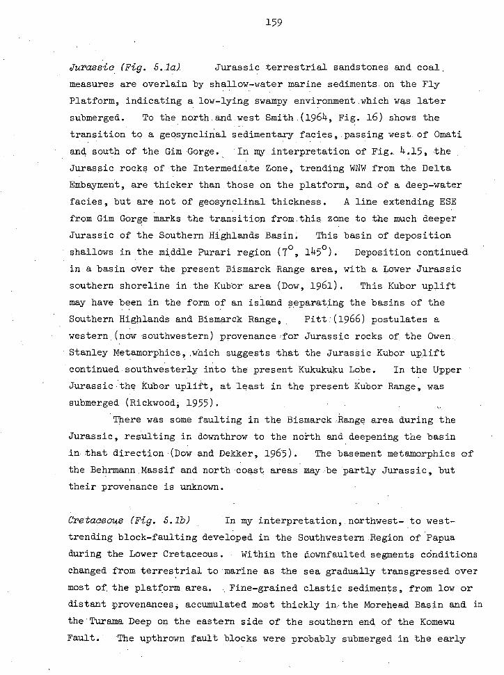
159

Jurassic (Fig. 5.1a) Jurassic terrestrial sandstones and coal,

measures are overlain by shallow-water marine sediments on the Fly

Platform, indicating a low-lying swampy environment which was later

submerged. To the north.and.west Smith.(196)4, Fig. 16) shows the

transition to a geosynclinal sedimentary facies,,passing west. of Omati

and south of the Gim Gorge. In my interpretation of Fig. 4.15, the

Jurassic rocks of the Intermediate Zone, trending WNW from the Delta

Embayment, are thicker than those on the platform, and.of a deep-water

facies, but are not of geosynclinal thickness. A line extending ESE

from Gim Gorge marks the transition from.this zone to the much deeper

Jurassic of the Southern Highlands. Basin. This basin of deposition

' shallows in the middle Purari region •(7° , 145° ). Deposition continued

in a basin over the present Bismarck Range area, with a Lower Jurassic

southern shoreline inthe Kubbr area (Dow, 1961). This Kubor uplift

may have been in the form of an island separating the basins Of the

Southern Highlands and Bismarck Range,. Pittr..(1966) postulates a

western (now southwestern) provenance for Jurassic rocks of. the Owen

Stanley Metamorphichich suggests that the Jurassic Kubor uplift

continued southwesterly into the present Kukukuku Lobe. In the Upper

Jurassic the Kubor uplift, at least in the present Kubor Range, was

submerged (Rickwoodi. 1955).

There was Some faulting in the Bismarck .Range area during the

Jurassic, resulting in dawnthrow to the north and deepening the basin

in that direction -(Dow and Dekker, 1965). The basement metamorphics of

the Behrmann.Massif and north coast areas maybe partly Jurassic, but

their provenance is unknown.

Cretaceous (Fig. 5.1b) In my interpretation,,northwest- . to west-

trending block-faulting developed in the Southwestern Region of Papua

during the Lower Cretaceous. Within the downfaulted segments cOnditions

changed from terrestrial to marine as the sea gradually transgressed over

most of the platform area. Fine-grained clastic sediments, from low or

distant provenances; accumulated most thickly in. the Morehead Basin and in

the Turama Deep on the eastern side of the southern end of the Komewu

Fault. The upthrown fault blocks were probably submerged in the early

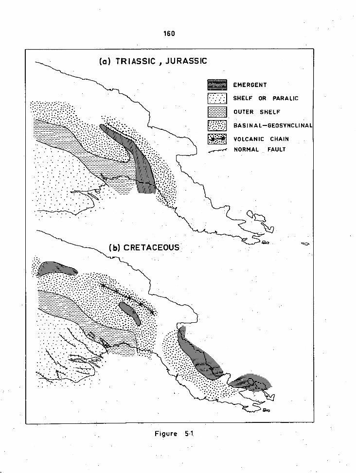
161

Lower Cretaceous, but general emergence of the whole shelf area towards

the Upper Cretaceous would have resulted in the rapid removal of thin

Cretaceous sediments from these topographically high blocks. The Lower

Cretaceous basin deepened through an intermediate zone into the. Southern

Highlands Basin. At this time the latter extended to the Middle Purari:

region (70 , 1450 ), where greywackes and conglomerates suggest a nearby

provenance, perhaps an uplifted part of the Kubor structure. , Combining

the investigations of Pitt (1966) and APC_(1961) it would appear that the

Cretaceous basin was also deep in the regions . of the present Kukukuku Lobe

and Owen Stanley Range. Pitt favours an easterly provenance for the

sediments here. In the Bismarck Range sedimentation and vuloanism were'

active throughout the .Cretaceous, with the..Kubor Range being either ,

emergent or shallowly submerged. • Dow (1961) postulates an upper

Cretaceous . "volcanic island arc" extending.in.a WNW direction' along the -

present Bismarck Range, Deep-water sedimentation had also commenced in

the restricted trough of the Upper Sepik - August River.

The succession, from southwest to northeast, of' Cretaceous

depositional- environments embodies

(1) . a continental platform, with generally NW,-SE trending - horst-

and-graben- and block-faulting, shallowly submerged,

(2) a more deeply submerged region,- trending in the same direction

aa the faulting,

(3) a parallel zone with a considerable thickness of deep-water

sediments and

(4) a probable shallowing . in the Kubor area succeeded to the north

by• a volcanic island chain.

This sequence typifies a fringing geosyncline, and the presence of ,

tensional structures on the platform point to the probability of its

tensional development, after the model proposed by Carey (1958, p.

In the late Cretaceous, zones 1 and 2 (above), and the middle Purari

section of)3, were apparently emergent (Smith-, .1964, Fig. 13).

According to the interpretation discussed in 4.5.3 (A4B4)-, at the

end of the Cretaceous the northeastern side of the Owen Stanley Block

began to be uplifted along a reverse fault zone penetrating through the

crust, the Owen Stanley Fault.

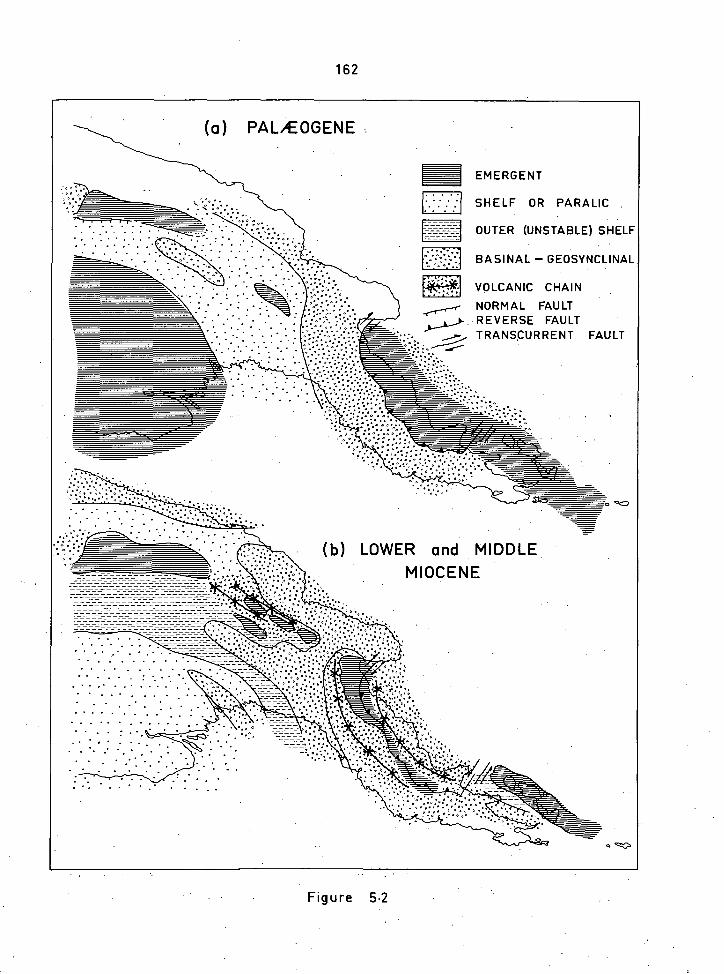
(a) PALiEOGENE

EMERGENT

SHELF OR PARALIC

OUTER (UNSTABLE) SHELF

BASINAL - GEOSYNCLINAL

VOLCANIC CHAIN

NORMAL FAULT REVERSE FAULT TRANS,CURRENT FAULT

• • - • • • . • • • . ... •

• . • • • • . • . . • • • • . • .

• . .

e °CD

(b) LOWER and MIDDLE MIOCENE

• • . • . • • .

. • • .• • . • . • • .

• • • • • . . . . • • • . • . . . • . . .. ...

. . . • .

. . •• • .

• •• • . .•

162

Figure 5-2

163

Palaeogene::(Fig. 5..2a) • During the Palaeogene.the -Fly Platform was

emergent, -aswell as the eastern part of the Intermediate Zone. The

Southern Highlands Basin was represented at this time by a deep northwest-

trending:basin'in.the Lagaiap River area (51/2 ° , 1431/29 ), in which:limestones

are interbedded with argillites, flanked by shelf environments' of

limestone and elastic deposition.' (Dekker and:.Faulks,.196)4). ..To the

southeast in theAure-Puratiregion,.a thin shelf sequence, mainly of

limestone; was deposited. Pitt .(1966)postulates:an,axis of thick.

Palaeogene.depOsition extending in a.northwesterly direction along the-

eastern fIankYof the Owen Stanley Block. , Most of the detritus he

considers to.have beenderivedfrom the east,- where, in my reconstruction,

metamorphics overlying hasic.and.ultrabasic rocks were.being - slowly up-

lifted along the Owen Stanley Fault.

'According to'Thompson (1967):theSalaeogene - northern continental

slope --was'to . the north of the Bismarck Range , Beyond that,. pelagic .

limestones and submarine volcanics represent the early stageS'of depos-

ition in the.basins.of northern New Guinea, The Morobe :Granodioriteis

thought'tO havelpeen intruded during the Lower Tertiary'into'Cretaceous

rOcks of the. Owen Stanley:Metamorphics'.(Dow and'Davies,'1964):.

Lower and-Middle Miocene (Fi g . 5.2b) During this interval the TIT

Platform was submerged and limestone was deposited over the: entire shelf

area, with deposition extending . eastand north to the - Purari andLagaiap

Aiivers, and'the'headwatereof the Sepik. The:limestone was deposited

in shallow water over most of the shelf, with.the . exception of the 300.0.

'metres deposited in the Lower Miocene'Omati'Trough. To the north and.

east the shelf limestone ls , succeededlpy limestone, with some.argilliteS,

deposited under -deep-water basinal conditions.

Bounding-the.basinal'limestone belt there existed a series Of-

deep, interconnected.troughs:which received' thick accumulations of

elastic sediments;generally'mudstones, greywackeS'-and'tuffaceous

sandstonesi . 'during.the Middleand,LoWer . Miocene.- . For:those'basins to

the nOrth of ;the limestone belt the sediments were derived, from 6rogenic

islands of the :Bismarck and Kubor Ranges;.'andto .the north of the Lagaiap

River. Vulcanism was prevalent along the Bismarck. Fault Zone; and'was-

164

accompanied-by basic intrusions. , The basic and, ultrabasic rocks of the

Marum Vltrabasic.Belt (Dow and Dekker, 1964) may have been magmatically .

emplaced at thisstage, later to be faulted into their present position.

By far the deepest basin,wa.s the Aure Trough, which received as much as

10 km. of Middle and Lower Miocene elastic sediments from an easterly

provenance. AccOrding,to.Pitt (1966) this accounted for the erosion.of

most of the Palaeogene sediments from the uplifted.trough of that age to

the east. In my opinion the metamorphics being uplifted northeast.of

the Owen Stanley Fault also . shed much material into the Aure Trough.

The troughshallowed:to the north, but continued across the eastern end of

the Bismarck and Kubor Ranges. A volcanic, belt extended around, the

western and southwestern flanks of the Owen Stanley Metamorphics, on the

landward side of the Aure Trough.

Clastic sediments and limestones were deposited in the Madang-

Finisterre-Saruwaged Trough in the Lower Miocene, and were succeeded by

very thick elastic deposition in the Middle Miocene, as a greater part.

of the Bismarck Range emerged by block-faulting. Thick Middle Miocene.

deposition also occurred in the northern basins of the Bewani, Toricelli .

and Prince Alexander Mountains, the provenance for which is. assumed to be

the emergent parts of the central-ranges. The Upper Sepik - August

River Basin continued to receive elastic sediments and volcanics through-

out the Middle and Lower Miocene.

By the Middle'Miocene, according to my interpretation, the

continued, thrusting from the northeast had brought : subcrustal rocks close

to the surface along the Owen Stanley Fault.. As shown in Fig. 4.9,

subsidence must occur to the northeast of the thrust surface. During the

Middle . Miocene, and probably earlier, thick sediments, as well as

volcanics, accumulated in such a subsidence behind the thrust surface.

The.Goropu Mts . - D'Entrecasteaux Islands transcurrent fault was in

existenceby the Middle Miocene, resulting largely from the necessity for

a thrust sheet to be laterally bounded by zones of strike-slip faulting.

There is one pressing tectonic, problem .in the postulated thrust-

origin .of-the ultrabasic•belt: Was the Aure Trough of tensional.origin?

If so, how can this be reconciled with contemporaneous compression from.

the northeast.?

165

On all counts it is most probable. that the Aure Trough is of

tensional origin, If Pitt (1966) is correct in supposing that Mesozoic

sediments of the Owen Stanley Metamorphics were derived from uplifted

older rocks in the region of the later Aure Trough, then the, trough* could

be formed either by downbuckling of those older rocks or by their tensional

thinning. From the gravity interpretational models for the region it

can be seen that the former process is as unlikely as the latter is likely.

Northeast-southwest tension in the Aure Trough can be reconciled

with northeast-southwest compression on the northern side of the Owen

Stanley Block, if it is assumed that the block was the active structural

unit in the tectonic process. That is, if some.subcrustal force were

dragging the' Owen Stanley Block towards the northeast, while disturbing

neither the crust behind the moving block nor that in front of it, then

it would be natural to expect compressional structures in front of the

block and tensional ones behind. An interesting corollary to this view

is the distribution of structures to the east of the GoropuD'Entrecasteaux,

Fault. Here, the Owen Stanley Block, represented by the D'Entrecasteaux

Islands, has not met the same resistance to its northeast motion as it

has. to the west. The Trobriand Islands to the north may exist as a

result of compression, 'since they have an isostatic anomaly of 180

milligala. To the south of the D'Entrecasteaux Islands the Cape Vogel

Basin appears from the interpretational model (A2B2) to be a tensional

structure, and its earlier sedimentation is Middle Miocene in age.

The synthesis by Pitt (1966, IIC) of the tectonic sequence in

Central Papua throws some doubt on the requirement that tension in the

Aure Trough be contemporaneous with compression north of the Owen Stanley

Block. He shows that northerly-dipping thrusting, and accompanying

folding, occurred in zones which migrated from east to west across the

Aure Trough from the late Lower Miocene until the Pliocene. Therefore,

although it is very likely that the original development of the Aure

Trough were tensional, it is not necessary, in this view, that the tension

be assumed to exist after the late Lower Miocene. The folding and

'faulting could be due either to compression from the northeast while

sedimentation still continued to the 'west, or.to direct vertical uplift

of the trough.sediments, commencing at the eastern,edge of the trough and

VOLCANIC ZONE

NORMAL FAULT y-A-> REVERSE FAULT

TRANSCURRENT FAULT

166

Figure 5-3

167

migrating towards the west.

The formation of the New Britain Trench had probably .commenced

by the Middle Miocene ,. As discussed previously the highly positive .

Bouguer anomalies indicate that the trench and adjacent ocean is a region

of very thin crust, a feature which is consistent with a tensional origin

of the trench. Carey (1958, Fig. )40b) postulates a tensional origin for

the trench,(the.Planet Sphenochasm) due'to.the movement of, New Britain

away, from the Owen Stanley Block. .

Upper : .Miocene ‘ (Fig 5, 3a) . Limestone:deposition_.continued.over the

SouthwesternRegion of .Papua throughout the Upper.Miocene.,... Thin mud--

stonesfringedthiszone to the north and.east,•although, much .of the . •

central-highlandsarea•was emergent. -.The mudstones.were deposited most,.

thickly. in,a trough betweenthe.Vailala and Purari Rivers ; being derived

partly from the.uplifted.eections of the AUre.Trough tathe'east and.north-

east._ : In . theJ,4kekamuEmbayment fluviatile.and.lacustrine elastic

sediments were, deposited in the northeast and marine mudstones and sand-

..stones-in.the southwest.

Thick..clastic sedimentation' continued in the northern New Guinea.

babinsduring:theUpper.Miocene;•.although.the base of the succession is„

of terrestrial or, transitional origin. ,The thickest existing sediments:

are in,theMadang-Finisterre-Saruwaged.Trough, but ; according to Osborne..

(1956);_those in theBewaniGeosyncline may have been thicker at the time

of deposition. Marine mudstones and conglomerates were- deposited in the

upper Sepik—August River. Basin . ;„ the . CapeVogel Basin a mainly

freshwaterclastic'successionwas deposited, with some.of.the material

derived from vulcanism, intermittently active,through the Upper Miocene..

Reverse movement on the Owen. Stanley- Fault surface continued

during the Upper. Miocene, exposing the subcrustal - rocks in many places. .

In the Goropu Mountains:region the:exposed.ultrabasics continued to be,

thrust southwards overtheGoropu:Metamorphics,:.and.younger, sediments. and

metasediments.. It. "is possible thatshallow,submergenceof this area'

enabled the thrusting.to excee&the.rate:of-erosion; Sedimentation.

perststed.An the:subsiding:trough- to:the-nortbeast of . the- uplifted

;Section:-:

168

In the Kukukuku Lobe north-trending reverse faults and asymmetric

folds developed further to the west than previously (Pitt, 1966).

According to Smith (1964) the orogeny .culminating in the present central

ranges of eastern New Guinea commenced in.the Upper Miocene.

Pliocene tO Recent . (Fig, 5.3b.and Regional Geology Map) Thin marine

and transitional argillaceous sediments were deposited over the South-

western Region in the Pliocene, a fairly important delta being in the lower '

Bamu River area. A slowly-deepening basin in the middle Purari area

was filled with marine and transitional arenites and argillites, derived

from the rising Kukukuku Lobe to the. edst. Pliocene vulcanism to the

south of the rising central ranges contributed volcanics and . volcanic-,

derived sediments to a deep basin in the Fly-Strickland Headwaters

Region. The•orogenic uplift of the central ranges had attained a

'considerable intensity in the Pliocene, and thick terrestrial basic

volcanics occur along the southwestern Side of the Owen Stanley Block in

the Lakekamu Embayment and the Port Moresby area. Clastic'sediments were

deposited under generally transitional conditions in the southwestern part

of the Lakekamu Embayment. Freshwater sedimentation continued in the

Cape Vogel Basin. In the northern New Guinealpasins marine Pliocene

sedimentation occurred universally before.the commencement of orogenic

uplift in the Middle or Upper Pliocene. From this time onwards sediment-

ation continued in the synclinal areas such as the Ramu-Markham Trough,

the north coast and the local basins in the Sepik Valley.

During the interval from the Middle Pliocene to Recent east New

Guinea assumed its present morphology. The whole central axis was up- •

lifted; those areas such as the Bismarck, Kubor and Owen Stanley Blocks,

which had been intermittently emergent since the Mesozoic, forming the •

highest parts of the central ranges. The Papuan Ultrabasic-Belt was

uplifted with the Owen Stanley Block, but its weight caused normal faulting

to develop between the two units, with the Owen. Stanley Block being

differentially uplifted. In most places the upper part of the normal

fault Coincided with the upper part of the thrust fault, but where this

was not the case narrow graben developed between the ultrabasics and

metamorphics, and became the sites of lake sedimentation.. The differential

169

rise of the eastern end of the Owen: Stanley .Block, accompanied by

considerabIenormal faulting,..causecipartof the, overthrust ultrabasics

to become '!draped over'! the rising. Goropu Metamorphicsleaving.southerly-

dipping erosional remnants. - . :Part.ofthe:Cape_Vogel'Basin,:and.the

eastern end of the Papuan_Peninsula, were:aIso elevated at this time.

Subsidence of the basin to the north of. the Papuan : Ultrabasic Belt is..

-still continuing:, as is: shOwn.by Carey's (1938b):observation that there

is no evidence of Recent or: :Pleistocene raised Coral reefs -between

Salamaua and CapeTogel, while such reefs,; .uplifted some hundreds of..

Ametres, are present elsewhere along the north coast-of eastern New Guinea.

-'Uplift of the.AdeIbert, Finisterre and_Saruwaged Ranges occurred_

along steep, northerly-dipping thrust-surfaces, which.have been interpreted

as penetrating through the crust in much the same way as the original

Owen Stanley Fault (Fig. 4.9). . In this interpretation the transcurrent

fault in the Madang!area,' proposedj_n order'tO 'explain morphological,

structural anT.graVitatiOnaLoffset.features, is simply thezone of

'horizontal movement separating -two differentially-moving thrust-sheets.

As. shown in the gravity interpretational profiles„and as is evidenced .

by the:topography,' the thrusting has proceeded further - ih the.Finisterre-

Saruwaged Ranges than in the Adelbertange. The“northerly:cbmpression

_on this,section of eastern - New. Guinea may_havebeen instrumental in its

counterclockwise rotation with respect'to the Owen. Stanley Block, with .

the subsequent' bending - of the Structural trends of the Kukukuku Lobe and

the intensifying of imbrication and folding: in the Southern Highlands

Basin and areas to the south.

The mode of upliftofthe northern ranges to_thewest of the

Sepik mouth is not clear. .South-dipping overthrusts_irLthe sediments

north - of the mountainsecorded tylAPOC'.(1930)could- indicate . uplift of

the mountains by steep, southerly-dipping, basement thrusts. . Alternatively,

the mountain - cores could be block-faulted basement,.as-recorded:by Visser

and Hermes (1962)for the similar northern ranges of West. Irian. ' In. this

case the sedimentary'overthruststruCtureswould_bedue to gravity

sliding off the rising basement..

Vulcanism has- been'Widespread_durifti'the.Quaternary'phase of the

orogeny, the centres being Shown on the geo1ogica1 - map(p-.100. The

northern basaltic volcanic arc,, from the Sepik mouth to Rabaul, coincides

170

with a.region of present.cOmpressive forces, if one accepts the thrust-

origin of the mountains east of the Sepik mouth and the northward move-.

'tent of New Britain away from the trench. ; Andesitic Vulcanism has a

less well-defined pattern. The majority of the'known_centres is located

within, or close to, the gxavimetrically low Southern Highlands Basin,

In a more detailed examination it can be seen that most of- the centres

are on zones of thrust-faulting, which. lendS weight to the hypothesis

that these' faults are of a deep crustal origin. Most other centres

west of the 'Owen Stanley Block are located on thrust-faults. East of

the Owen Stanley Block the volcanic centres are usually on zones of major ,

or minor transcurrent faulting associated , with the Olien Stanley Fault,

5.2 SOME TECTONIC PROBLEMS IN MELANESIA DEFINED BY GRAVITY

INTERPRETATIONS AND SOME SUGGESTED SOLUTIONS

In the foregoing discussion of the evolution Of eastern' New Guinea

no attempt has been made to define the configuration of the base of the

crust, or the iSostatic state of the various crustal elements, during:the

successive stages of each orogenic :phase. However, by adopting a.

uniformitarian approach, one can reconstruct an orogenic sequence from

presently-existing structural features assumed to represent different:

stages of that sequence..

5.41 The Apparent Orogenic Sequence , on the Island.of New Guinea

The classical.geosynclinal.concept . of orogenesis embodies the

following stages;

(a) Accumulation, usually rapid, ofa great thickness of sediments in a

geosyncline;

.(b) The commencementOf folding and.thrust,faulting of the sediments,

and metamorphism of 'the deeper layers;

17,1

( c ) Injection of , granite into the. metamorphic .and: sedimentary*pile, with

strong Uplift :then or subsequently.

In most orogenic Zones , the: Metatorphita, 'injected:by granodiorite,

eventually become the highest part ' of the mountain. range by - a combination

of block :faulting- Arid - resistance to -erosion..

There: are many mountain ranges where the -above beqUence of , events

has been by hO means' faithfully followed.: Indeed, in some cases the '

region -which, becomes-mdst :-StrOnglyAlplifted- is the' exposed basement .

which-formed the ptovenanc for, Itlfe• deepsediments ! Thi8 lack . -

conformity to perhaps, As • evident in New GUinea ' as -anywhere

else. , NOnetheleSs',-• it is' Tossible to draw some inferences'from the

observed and .interpreted etructures;. as slimniarized In Figs 4.l5 and 4.16 .

• Firstly, it is apparent • that deep sedimentary basins are not

formed-by simple depression of the Whole crust Under geologically well-

defined basins: such as the Aure • Trough and the Cape . Vogel . Basin the

gravity anoMalies requite that there be A. -Mass-ekcesS . at depth, to

compensate for 'the negative -effect of • the sediments. This mass-excess

is 'mosteimply explained , byr. a rise in "the base of the crust. - 'It has

been mentioned • previously (:Section. 4 7 that: most of the • negative

Bouguer anomalies recorded in West. Irian are over deep sediMeritary

basins. • In- the ,Biritoehi Basin, for 'exaMpie, • at least 9 km. of - Miocene .

and .Pliocene sediments' are present and the observed anomaly' is --75

milligals. If these sediments, , neglecting _older underlying ones, were

accommodated - by a' depresSidn Of 9 km. in the base Of the crust the

negative .anotaly wouId.:be greater' than 100 milligals even before the

graVitatiOnal effect of : the sediments . is Considered.' The same' . argument

applies . to the Other deep West Irian' basinS ; which have comparable ,

sediMentary. thicknesses and gl,altity . anomalies. The argument' uSed in

demonstrating-the- general' , rule, that thick sediments are Correlated with

thin cruet', ' lackS the usual' •ambiguity of :gravity • interpretations'.

That iA , the -gravity anomkTies observed in the' area leave but two •

alternatives: ' Either the: crust is not thin, or the - sediments are not

deep.

The setond stage in the orogenic 'prOcess: is' the- foldin , thrusting

and initial uplift !of the deep sediments .., This -stage would Seem to be

172

represented by the northern and eastern (older) sections of the Aure

Trough, by the Madang-Finisterre-Saruwaged Trough and by the Southern

Highlands Basin. From the interpretational profiles it is not

immediately.obvious,what.configuration of the base of the .crust .corres-

ponds to these uplifted basins ; since they have distinct asymmetry.

For those structures south of the central ranges it would appear that the

crust is, somewhat thicker than at the depositional stage, yet the up-

lift is certainly not caused by the restoration of local isostatic -

equilibrium. For the Finisterre structure, to the north of the central

ranges', the uplift is interpreted as haying been accompanied by a rise,

north of the mountains, in the base of the crust. The uplift and

thrusting might be completely due to the horizontal and vertical strain

distribution . resulting from a mantle upthrust well to the north of the

initial basin, as shown in profile A10B10. There is the possibility

that the crust may be slightly thicker than at the depositional stage,.

although the thickness of crust underlying the sediments is very much

thinner than the standard crust: As with the Kukukuku Lobe and the

Southern Highlands basin, the uplift and deformation of deep sediments

here has not been due to readjustment of local isostatic equilibrium,

since in all cases the movements are essentially anti-isostatic. For

this are the initial. deformation and uplift of deep sediments

have been accompanied neither.by appreciable thickening of the gravi-

metric crust, nor by any appreciable thinning.

The final orogenic stage is represented by the uplifted meta-'

morphics.intruded by granodiorite, of areas such as the.Bismarck and

Kubor Ranges. There is no doubt that these regions are.underlainby.a

gravimetric crust much' thicker than the standard. Within this general-

ization it is possible to discern further detail.. The Kubor Range has

had a much longer,orogenic history than the Bismarck, forming a distinct

nucleus at least as early as the Upper Palaeozoic. In most inter-

pretational profiles. the crust is thicker under the Kubor-Central Range

area than under the Bismarck Range, where metamorphism and intrusion

are of Triassic age. The same trend can be followed into the Owen

Stanley Block, where Pitt (1966) suggests an Upper Mesozoic, possibly

Cretaceous, age of metamorphism, and where uplift.' is unlikely to have

173

commenced before the early Tertiary. The crust underlying the Owen

Stanley Block is thicker than the standard, but it is thinner than that

underlying the Bismarck Metamorphics. Even further along this trend are

the central ranges of West Irian, which have more affinities with the

• uplifted miogeosyncline of . the . Southern Highlands Basin than the eugeo-

synclinal Bismarck Range area. Although Cambrian sediments are exposed

in the core of the central ranges, and there are minor acid intrusions,

yet there.was no uplift or deformation of the rocks before the Pliocene

'(Visser and Hermes, 1962, Encl. 12). According to.Visser and Hermes'.

interpretation of the gravity anomalies over the central ranges of West

Irian, to which I, see no serious .objection, the crust thickens slightly,.

but less than it does under the central ranges of eastern New Guinea.

There are no gravimetric indications of significant crustal thickening.

under the northern ranges west of the Sepik mouth, which probably

represent the second -, rather than the third, stage:of orogenic development.

The orogenic.sequence, therefore, which is indicated•by the

structures of mainland New Guinea, is as follows (Fig. 5.4):

(1) The development of a. deep baSin of deposition is accompanied by a

rise in the base of the crust: This is best explained by the tensional

theory of geosyncline origin (Carey,'1958).' • Thick sedimentation in the

basin may depress the crust so that the base becomes approximately level,

again., • Isostatic equilibrium is maintained.

(2) Tension isrelaxed; - the sedimentary pile.begins to be uplifted,

folded and faulted by mainly vertical forces, possibly asymmetrically

directed. At this stage there is no local isostatibequilibrium;

rather, the - equilibrium - is . dynamic. It is likely that a small amount

of ligh -Lmaterial is added to the base of the crust during this process.

(3) The basal - sedimentaare- metamorphosed, and, intruded by large

granodiorite plutons. Uplift continues until the tetamorphics are

exposed. At this stage the base of the gravimetric crust is well

below its original position.

This sequence of events obviously poses a dilemma: A geosyncline

.commences with a thinning of the underlying crust. After sedimentation

is complete the geosyncline, and therefore the underlying crust, is

uplifted by . vertical forces, and yet the position of the base of the crust

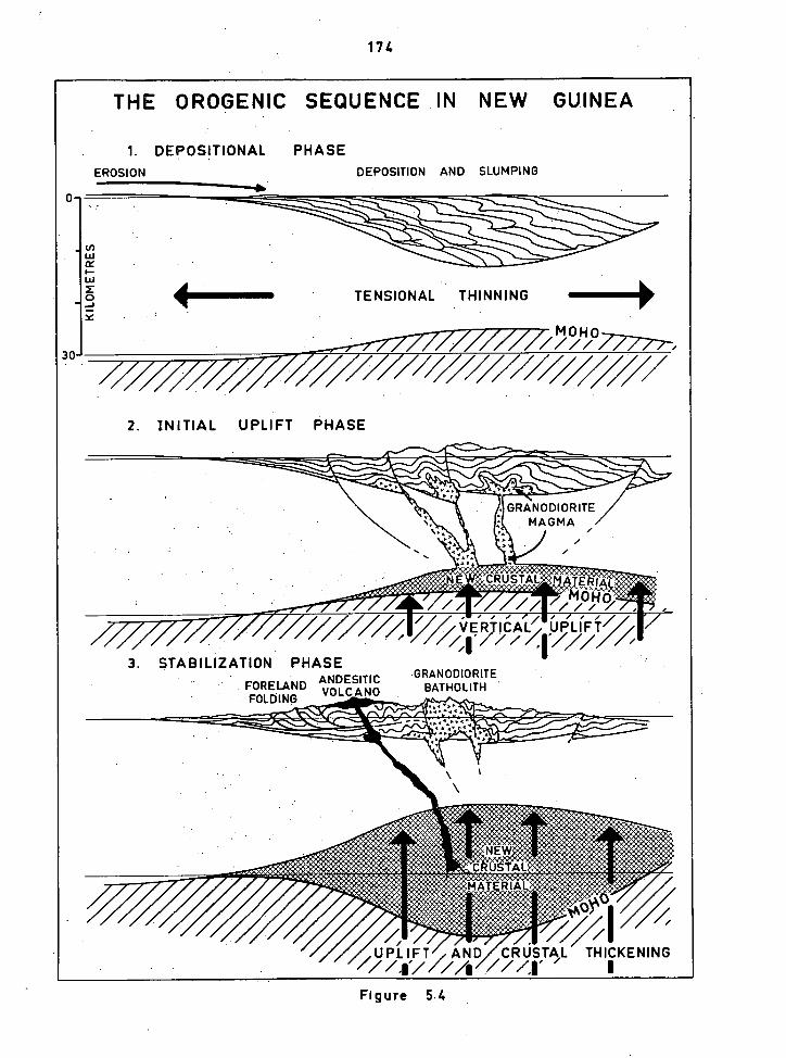
174

0

30

THE

1.

EROSION

OROGENIC SEQUENCE

DEPOSITIONAL PHASE

DEPOSITION

IN NEW GUINEA

AND SLUMPING

tn w ce w X o ..J -- Y

- - - — " • ` • • • • • NM , ,,,,, i i i . .1 .ftk..,.‘---ThIMmmi

41111■ID TENSIONAL

ii. . . . .11.111,_ipiwiiiii ,i

IL-."IliNlow.--

THINNING oo.......4

MOHO // 77-777".

2.

// / // /

INITIAL UPLIFT PHASE

swillnill111■0111 -..■•••■•■-- '11.1ei/A."111. 4„., -------■---..----111 --

_ - \ .....7. -- ■.,,..."0.. _ k'N"....s.._. ob.

ANit GRANODIORITE

, MAGMA

/ . .

..-,•:;:a ...c... Y S Th.(7;: M VP

• / /

3.

//7 //// /

STABILIZATION PHASE ANDESMC FORELAND VOLCANO FOLDING

•-,....4k a,-,. Takv m_.,t..1.1.,‘

, / ,/ 7 VERJICAL, ,UPLIFT'

//

•GRANODIORITE BATHOLITH

_ ..M.M.or,•0...---

.

---•■--■-■,.--1-11W•1 l'rf

...

-.•:* ........

. - ---veiil ..

, ar■d °".°1' ..-_•-

•• ,;434:1:§:: ::-:::•:•:•:•:•:-:•:•:•* *****::::::""

•:::::::ri*:**)):::•;•:: .:::$2;:w.;...... * .."' ••:•• •

• 4+:3§:Airtti:ii:::••••••

.. '• ••• 3:10:::-.• .... 0.:•:+:44.:::4:44.:::,:.:. "-•••?*** -4.***••••• • .4:::::::::

.. •':416afant::$: ::*** , ., ... •

-.1.VC ......

/ . UPLIFT

// /-17///11

:::$;:ex-:-.•.-.•.-.-.-.-.-42::. 2 . .NIX,SMKiiip:? . *0-:•:•:•;

. ..**?::::::IV::: v. ' A, • . .., .:P• I i / AND CRUSTAL THICKENING

/ /I' /

*?:-

I

Figure 5.4

175

is.little. Changed. Finally,..by stage 3 ..(above), the - base.of.the

original geosyncline is close to the : surface.,:so that:the base:of the

crust should be:,onan higher level than at the . earliest geosynclinal

stage..- But instead., the crust is thicker :than at any-previous stage.

An explanation which might be advanced is that , the , crust, •

thickens by compressional crumpling into a root which .creates the uplift

in its rise to isostatic equilibrium. I am convinced that this process

is most unlikely. :.:The rising mountains of West Irian, for example, are

.far above Airy isostatic.equilibrium, and sufficient evidence has been

quoted to.show- that the initial uplift of stage 2"(above) is anti-

-.SAnceTthe rootwhich stabilizes mountains during ; or after, .

their final, stage of uplift-cannot be-derived from the.pre 7existing crust,

it is obviousthat new material, having the seismic and.gravimetric

. properties•ofthe lower cruSt,-is added. to the base of the crust.-

Carey (1962b) suggests that the orogenic root is formed.by the alteration

Of upper mantle materialijpossibly.to serpentine.. .• However, this would

result in a. large proportion of.the,crust.in•an orogenic area being

composed of serpentine, On the assumption that continents grow by the

incorporation•ofstabiized orogenic zones,. the process .would eventually

.result in a continental shield. incorporating a.considerable.proportion of

serpentine, • Geological observation shows that serpentine is 4 sub--

ordinate:.constituent,.not only of,dontinents,.but also of orogenic zones.

.There is, however, 4 component introduced into an orogenic zone

which is •also , a.very-important constituent of continental shields,.and -

that As. the granodiorite•magma.H In the.intermediate stages of . an.

orogenicc - cycle the - magma:begins. to be intruded deep . in-the geosyncline.

In the late stages, as the.granodiorite and:metamorphics are uplifted, :I

postulate.a.massive addition-of.granodioritic material to the base of the

crust, forming - a broad rootwhich..,eventually stabilizes the uplifted.

orogen,:-The widespreadPleAstoceneandesitic Nulcanism.could well be

the.surfaceexpression of such a.process, occurring:An the late etages,

of . the:Plio-Pleistocene:orogenyin New Guinea..

•f'flthe•uniformitarianapproach usedebove -As regarded •as.valid, •

then.theAnduced:sequence of events. mnst.be , regarded,as-real; at least

176

for the evolution of the fringing type of geosyncline developed on main,

land.New Guinea.. It is necessary, then, to find causes for the developr

ment of the deep basin and its subsequent anti.,isostatic uplift, and a

source 'for the material, having a negative density contrast with mantle

rocks, which eventually stabilizes the orogen.

5:2.2 The Causes of the Orogenic Sequence

As mentioned before, the crustal structure beneath a deepening

basin, or an oceanic trench, is consistent with Carey's (1958) hypothesis

of tensional origin: The. search for the basic cause of separation of two

blocks, of the earth's -crust must extend further into the realms of

speculation. Convection currents are .á possibility, but for the New

Guinea area, the above author's Tethyan Shear System has more observational,

basis.

The upward force on the isostatically stable : geosyncline must

originate in the earth's 11.1)lier mantle, since it is applied in too

discriminatory a fashion to be acting from greater depths. By the same

token, the commencement of the upward force from,the-mantle would seem to

be genetically connected with the existence of a deep geosynclinal trough.

Carey's (1958, P.325) view is that the rising isotherms under a thinning

crust,cause.differential expansion of the mantle prism beneath the geo-

syncline.. In my interpretation of the gravity profiles, the base of the

crust underlying a sediment-filled geosyncline is rarely more than 5'km:

above the base of the standard crust. This figure is admittedly dependent

upon the chosen crust-mantle density difference, but if the value chosen

were 0.3 g/cc instead of 0.5 g/cc the crust would need to be only 8 km.

above the standard level; that is, there would be a' rise of only 8 km. -

in the isotherms. According to Gutenberg.(1959, Fig. 6.1) this would

mean a.temperature excess of about 16 °C of the subgeosynclinal over the

adjacent prism.(and.this only to the depth at which the disturbed iso-

therms flatten out): It is doubtful if any direct expansion resulting

from this- situation would be.sufficient to produce the observed uplifts.

Nonetheless, there must be expansion of some part of the upper

177

mantle_ at he uplift stage : of-geosynclinal evolution... Based:on seismic

results-it-is evident that , : the low velocity zone of the upper mantle is

subjeCt-to:-considerable:horizontal . velocity i and therefore density,

variations (Gutenberg, 1959; For compressional waves in

fouractiveseismic - areas Gutenberg . derived an average velocity-depth

curve, which-indicated a-P-velocity of 8.1 km/sec at the Mohorovicic A

discontinuity, 'decreasing to anainimum,of 7.85 km/sec'at about 120 km.

depth.Increasingly . precise seismic measurements over the last few

-years haveShownYthat the - parameters of the low-velocity zone vary widely

fromthese average values ..... For-example ; in the : Western Mediterranean-

Basin and- adjacent alpine : areas, Berry and Knopoff - (1967) have defined a

"lower-crustal compressional velocity of7.7..km/sec,•,with an increase to

8.15 km/sec-at depths:varying from 20-•-30 km. under the sea,to 4o-6o km.

under the land. , .Below this zone is a low-velocity channel which, under

the centre of-the basin,- has an ultra-low shear-velocity•of , 4.10 km/sec,.

and,extends from 50.to:200 km. depth.. At the margins of the basin the.

channel hasa - shear velocityof 4.43•km/seC ancLa"depth extent of from

100 to 250 km.

For:the New -Solomon Islands region, Brooks (1962,

Fig. 4) obtained a sub-Moho compreSsionalveloCity of 7.95 km/Sec,

decreasing to - a.minimum -of 7.6 km/sec at about'130 km. - depth. Related

to..the,density-velocity curve of Nafe.andlDrake (1957) this means that

the sub,Mohodensity is 0.05•g/cc, and.the - velocity-minimum density

0.08 g/cc,. less than- the corresponding average-values of Gutenberg

(1959). • These values are,:.of course, averaged over ,the,Vhole Solomon

Islands' ,- New Guinea-belt, extending 4000 km.from east to weSt. The

scatters- of - points in Brooks! (1962) travel-time curves indicate that

there - is very-likely to:be a:considerable Variation' of the properties

of the low-velocity zone within the - area studied..

It has been shown theoretically (Fig. 4,5a) that a density ,

change-of 0.05 g/ccin'a vertical zone of the-mantle - between 70 and

190 km. depth would be auffiCient to -upliftthe crust ty , 2 km. Thus,

if larger. density changes - could—be produced overlimited.areas, the' amount

.of . upTift necessary for the second stage of geosynelinal evolution would

baproduced. . It is obvious from.Fig.j[:5(a) that, although isostatic

178

compensatiOn'is maintained-at the base of the expanding column, yet the

Airy isostatic anomaly would be positive. Thick sediments would, of •

course, modify the theoretical gravityyrofiles over, the rising zone.

However, as discussed in 5.2.1, there is no evidence.that the second or

third stages of orogenic development correspond exactly.to:the structure

portrayed in Fig. 4.5(a), the base of the light crust apparently either

remaining at the same level or deepening, rather than approaching closer

to sea-level. At least for the third stage of development, represented

by parts of the central cordillera, present seismic evidence is in agree-

ment with the gravity interpretation of a thickened, crust (Brooks and

, Ripper, 1966.; J.A. Brooks, Department of Geology, University of Tasmania,

\ pers. comm.). To reconcile the' anti-isostatic uplift of the second,

\stage with a lack of uplift at the base of the crust I propose that .\ mantle expansion does act as shown in Fig. 4.5(a), bUt that simultaneous

addition of light material to, the base of the, crust produces the

gx4vitational and seismic effects of slight crustal thickening.

\ The actual changes in mantle material which could produce the low-

velocity zone have been investigated by Ringwood (1966).• He has

determined the stability of several different mineral assemblages having \

the tot chemical composition of a rock which : he calls "Pyrolite".

Below continents, in his view, a peridotite layer (theoretical velocity.

8.32 km/se0 is underlain by pyroxene . pyrolite.(8.18) followed bygarnet

pyrolite (8138). The' effect of high temperature is to lower these

theoretical velocities, while retaining their differences. In the

oceanic case Ringwood believes that•increasing•temperature causes the

decrease towards a minimum -velocity in pyroxene pyrolite, with underlying

garnet pyrolite\causing the subsequent velocity increase. In localized

regions of high Aeat-flow Ringwood. (1966) believes that the stable sub-

Moho assemblage cduld be plagioclase pyrolite, which has a velocity,

0.17 km/sec less than pyroxene pyrolite. •

The.stability fields of thevarious mineral assemblages are

controlled by.temperature if the depth be constant: From Ringwood's

Fig. 3 it . appears that the only transition which shows any promise of

providing local differential expansion in the upper-mantle - is that between

pyroxene and garnet pyrolite. A downward Shift, by about 150 oC, of the

179

oceanic geotherm towards the-Precambrian shield .geotherm•would permit a

. transition from the:lighter to.tne:heavier-pyrolite over a vertical

distance, withinthe:mantle, of about 80-km. Under the intermediate

type of crust of.a developing orogenic zone, the geotherm might lie

: ..sufficiently close , to,thetransition between stability.fields that the

fluctuation of heat rlowovershort periods of geological:time would

cause.expansion, or contractionof-part of the upper mantle. .Thus,.the

blanketing effect.,of deep sediments might raise:the.temperature of the.

upper mantle by :an amount sufficient:to transform garnet pyrolite to

pyroxenepyrolite, producing expansion, and hence uplift,

:The aboVediscussionshows that- it is possible , to explain some,

if notall,of . the initial Uplift of .a geosyncline without invoking

processes which.haye noexperimental-verification(e.g. convection

currents or tectogenes).. The weak link -in the argument is the lack of , .

any,detailed . knowledge:of temperatures. in the upper.mantle. Geotherms- -

are extrapolated.fromsurface'heat-flow observations and involve

.assumptions as to theconductivity of.the.mantle-and core, and.the •

source ofJleat

The third stageof geosynclinaLdevelopment remains to be

explained; continuation of uplift, metamorphism of basal sediments and

emplacement 'of granodiorite tetholiths, and final stabilization by

addition to the base of-the crust of large volumes of material lighter

than thejnantle.'

Uplift can be assumed to proceed by .mantle expansion, although

the actual quantities consistent with present experimental data, quoted

above, scannot explain the whole uplift.. One possible.alternative is

that the addition of the root of light material does .contribute to the

uplift;intheIate stages.... .Another, more likely; alternative 'is that

there are stone things about the.mantle.which are.not yet . known.

. Metamorphismis:the result of temperatures and pressures developed

low in the geosynclinal pile, and due respectively tothe thermal-. -

blanketing effect of the sediments and their weight The phenomena

most demanding of an explanation are.the origins of the granodiorite.

intrusions. and.the• light rootmaterial._

The mantle must be the source of any material added to, or intruded

180

into, the lower crust. , On the. basis . of experimental data,. Green and

Ringwood (1966), proposed .a mechanism for the derivation, from the mantle,

of the ca1c-alkaline igneous rock suite. - , Since quartz-bearing magma

cannot be evolved directly from . a pyrolite mantle, the postulated process

is a two-stage one. Undersaturated basaltic magma, produced by fractional

melting of the pyrolite.mantle, rises towards the base of the crust.

Fractionation of this magma will occur at depths of less than 20 km.,

producing large volumes of quartz-normative basalt, which will become

transformed into the more stable eclogite if the temperature is low

enough. The second stage of the process involves the sinking of the

heavy (3.45 g/cc) eclogite into the mantle and its fractional melting

to yield andesitic and more acid magmas of the. calc-alkaline series.

If the first stage of the above process occurred in the early

geosynclinal phase, the magma would be able to rise to within 20 km. of

the sea floor.. This magma would also provide a source for the basaltic

volcanics associated with early geosynclinal sedimentation. The

second stage of the process would yield the andesitic (i.e. granadioritic);

magma which intrudes the base of the geosyncline at the end of the first

phase of uplift and deformation. The continued rise of andesitic magma

would gradually increase the thickness of the crust, .which may explain

the apparent lack of uplift in the base of the crust during the initial

geosynclinal uplift. Eventually, as the uplift,ing force from the mantle

relaxes, the rising orogen would become stabilized by the accumulation

of a broad granodioritic root.

The eruption of basalts from late-orogenic andesitic volcanoes

indicates that primary basalt magma may also form part of the mountain

root.

Evidence bearing on the role of the upper mantle in tectonic

processes is contained-in the recent seismic studies of Evison (1967).

In a study of first motions of P-waves from 68 earthquakes, he found the

following polarity distribution:

(1) First motions are compressional for shallow sources in

general (depth less than 70 km.)

(2) They are dilatationai_for shallow sources beneath deep ocean

trenches.

181

(3). -For, deep-sources..(greater than 300 km.) first motions are

-dilatational:

The change An: polarity can be placed at•approxiMately . :200 km.

depth.: As Evison•.(1967)...points . but,, this distribution indicates an

-.expansion within and' the-loW7velocity, zone under rising , orogenic

areas -:.

The zone, would appear to be contracting.under:oceanic trenches.

These results are .quite in accordance with the mechanism of geo-

synclinal. evolution discussed aboVe,

.5.2..3 Further Problems and-Possible ;Solutions

Oceanic Basement • 'It has been stressed . bymany geologists' concerned•

with New Guinea .that :a distinction mUst be made.between ."continental •t

basement". in the..south and,"oceanic.basement"underlying sedimenta in the

north and east(e. ,g,ThompsonJand,Fisher, 1965;. Thompson, 1967).... This

"oceanic basement" is exposed in' the ranges of east New Guinea,

and WeStIrian,-and,is usually stated. to consist of "schists.and basic

igneous intrusives". In the'interpretation.of the gravity profiles the

"oceanic basement" has ..not been differentiated from the southern

"continental basement".;' .and, indeed, from the gravity, • anomalies and what .

is known ofthe•thickness-of sediments', a vertical section'through the. -

crust.in.the-middle Sepik -aretL could - well .be . the same asone on the Fly

Platform., If the - term "oceanic basement" - isaupposedto mean "oceanic -

crust"..(i.e.: about 10 km...of•basaltic material) then either the mantle

under northern New Guinea4s -of very. low density, or 'low •density material

has. been added to the base of the crust.

It is, in fact, almost certain that the so called "oceanic base-

ment"-is very different. from.the.presentoCeanic crust. . The gravity,

gradients on. the coast-indicate:that the.- crust thins- rapidly towards

the true oceanic crust,. . Preliminary:results-from Rayleigh. Nave dispersion

studies by,J.„A: Brooks °Department of Geology, University of Tasmania,

comm:)-indicate.a crust' of COntinental.thickness throughout the

inland areasof-northern.New-GUinea.In short,.whatever.its surface

geology may.:beasa - geophysical-andtectonicAlnit.the:'oceanic basement"

182

of northern New Guinea is very similar to the southern basement. If it

represents a type of intermediate crust, which had.not previously been

sufficiently thick to be isostatically emergent, it may have an analogy in

the crustal Plate of the Bismarck Sea. This plate, with water depths

generally less than 2000 m., should be about 20 km. thick to maintain

isostasy.- The basaltic vulcanism at present active around its perimeter

could: well build up its thickness to continental dimensions.

Asymmetry The tectonic hypothesis outlined in 5.2.2 is essentially

symmetrical. That is, uplift of the geosyncline is vertical and

thrusting should proceed towards each flank. The structures of New

Guinea are not symmetrical. Two factors.are likely to contribute to

this. Firstly, since,the geosynclines are of the fringing type ; the

rigid craton ensures. that the initial structure is asymmetrical, and the

reaction to stress of the craton is likely to be different to that of the

weaker sediments. , Secondly, many Melanesian structures are simply

explained by Carey's (1958) -Zone of Tethyan Shear ,: . On New Guinea

structures south of this zone the effects of the intense sinistral shear

must be asymmetrical.

The Papuan Intrabasic Belt The hypothesized development of the

Papuan Ultrabasic Belt has been outlined in 4.5.3 (Profile A4B4). The

processes which would cause such. a large-scale thrust are problematical.

One possible answer to the problem is that the initial upthrust developed

as a result of upper-mantle expansion, and the overthrusting'process. was .

maintained by compressive forces associated with the. abovementioned

Tethyan Shear System.

The Solomon Islands Chain The orogenic sequence proposed for the

development of the New Guinea structures does not apply directly- . to - the

Solomon Islands. Coleman (1966) presents good evidence for considering

the Solomons chain to be an oceanic island, arc, a tectonic feature which .

Donnelly (1964) stresses must not "be thought of as a mountain chain

in statu nascendi".. This categorical statement is open to some

qualification, since the sediments of many uplifted eugeosynclines must

1.83:

have.been. derived; from provenances' similar to present-day island arcs,

and in this ,capacity : the arcs play an important : part . in , the birth of

some ,mountainranges, .A . more . correct statementof the:positionwould be

that island arcs are invOlved in.theearliest stage.of'an Orogenic .

evolutionary-sequence-which-is, more complicated than. that of fringing

geosynclines.- .Donnelly (l96) gives the opinion, based ona.study of

the: Greater.Antilles, : that - The -island arc is a structure whose

relative simplicity results from the direct. interaction,of its thin,

volcanic-rich. and sediment-poor stratigraphic . section,withprimary

orogenic forces." This stratigraphic section does not exactly

correspond_tothat.of the Solomon Islands, where_ sediments upto 5000

metresthichave beenrecorded, but,. as these sediments have been_

locally derived, the, lack of. correspondence is, not significant, .The

qualitative Interpretation.of the, gravity anomalies. . .(4..7..3). indicates:

that the islands of. the Solomons chain are standing well., above their

local isostatic position, especially if the fairly thin crust (20-25 km.).

is of basic composition. This would indicate that the upper mantle is

again playing an important role, in supporting the uplift of the

islands by its expansion. An alternative view to this is that the up-

lift of the islands is supported by the strength of the crust. However,

according to Carey .(1962a), crustal blocks the size of the Solomon

Islandsshould.be subject to., significant isostatic adjustment within

years, : .and :Pleistocene reef-limestone , exposed-on all the Islands

shows,that they.are.still rising..

It is also necessary. to .explain why the crust.under the Solomons,. - ..

although thinner than continental, is shown by gravity tole considerably

thicker than that-under the adjacent ocean. . For the Antillean chain,

Donnelly, (1964) °postulates the crustal thickening tobe due-to a

compressional.downwarping of hydrated oceanic crust. I am of the opinion

that a . plastic downbuckle of the:type shown In stage 2,(Fig. of

Donnelly's sequence has yet to.be geophysically proved anywhere_on the

earth. As 'mentioned in 4.7, even . the classical "downbuckline inter-

pretation of the Indonesian' Arcs is open to serious doubt, following the .

reassessment by Woollard and Strange (1962) of the original gravity data.

Gravity and seismic work across several oceanic-trench areas has tended to

184

show crustal thickening towards the adjacent landmass, with no apparent

downbuckle under the trench. This is true of the Puerto Rico Trench

(Ewing and Worzel, 19.54), the Tonga Trench (TalWani, Worzel and Ewing,

1961) and the Peru-Chile Trench (Fisher and Raitt, 1962).

Arising from the discussion of the derivation of lower-crustal

material from the mantle. (5.2.2), it would' seem likely . that the thickened

Solomon 'IslandScruSt be the result of addition of andesitic and basaltic

magma to the base of the crust. This would also provide a magma source ,

for the predominantly andeSitic volcanoes of.the - Volcanic. Province

(Coleman; 1966).

As with other Melanesian structures, primary vertical forces

originating in the mantle can explain.only part of the observed structure

of the Solomon Islands, Large-scale horizontal forces, certainly

consistent with crustal shearing, must also be operative on this south-

western. Pacific margin.

POSTSCRIPT

It is perhapS inevitable that any attempt to define basic

tectonic processes will succeed in revealing at least as many new problems

as it .set out to solve,. and.in the present state or advancement of earth

science this can only be a favorable situation. Since' many of the facts

are yet.to-be discovered, any.tectonic.theory which claims to have all

the answers must be suspect. This dissertation does not claim to

have all the answers, nor even to have defined all the problems which'

exist in Melanesia. If it can be construed-as representing an.

increase.in the sum.of knowledge, I shall confess to a certain

satisfaction.

185-

REFERENCES

ANDREEV, B.A., 1959 - Relation between etructural relief. and gravity

•anomalies fo'r the case of some 'density layer . boundaries . : .

Dokl. .(Proc.) -Acad. Sc1:V.S.S.1124): 111-313.

ANGLO-PERSIAN OIL COMPANY; 1930 - The'oil eXPloratiOn work in Papua and

New Guinea .cOnduCteCby the Ang16-Persian Oil Company on behalf

of the Government of the Commonwealth of Australia, 1920-1929.

4.vols:(H.M.S.0., London).

ATHY, L.F,, 1930 - Density, porosity and compaction of sedimentary

'ro'cks- . Bull. Am. Ass. Petra. Geol. 14: 1-24..

AUSTRAfiASIANTROLEUM COMPANy, 1961 - Geologicai ' resuits.Of Petroleum

- exploration in Western Papua, 1937-1961. J. 'geol. ,50C. AUSt.

• 8: . 1-133.

AVDULOV; M.V„ 1965'- Gravimetric data.on structure of the crust in

central 'and western Caucasus.. Mt. Geol. Rev. 7: 1550-1561.

BAR, C.B., CORTEL, H.J. and ESCHER,:A.E., 1961 - Geological results of

the Star Mountains (Sterrengebergte) . expedition. Nova'Guinea

(Geology Ser..) (4):.39-99.

BERRY, M.J. and KNOPOFF, L„ 1967 - Structure of the upper mantle under , - the Western Mediterranean Basin. J. geophys. Res. 72: 3613-

3626.

J.L., 1962 - Terrain correction tables for gravity. • Geophysics 27: 715-718.

BIRCH, F., 1942 (Ed„) - Handbook of physical constants. Spec. Pap.

, geol.. Soc. Am. 36.

BLIAUX, L.P., 1957 - The Turama Deep in relation to the Komewu and Omati

areas. Is land EXplOratiOn'bompan'Rep. PL .(unpubl..)

BOLT, B.A. and NIAZI i M., 1964 - Dispersion of Rayleigh We.Ves across

• Australia. GeophYs. J..R. astr..Sqp. - 9: 21-35.

BOTT, M.H.P., 1959 - The use of electronic digital computer's for the

eValuation of gravimetric terrain corrections.. Geophys.

Prospect. 7: 46-54.

BOUGUER, P. 1749 -La figure de la terre. (Paris).

186

BRACEWELL, R., 1965 - The Fourier transform and its applications.

(McGraw-Hill, New York).

BROOKS,.J.A., 1962 -. Seismic wave velocities in the New Guinea-Solomon

Islands region. Geophys. Monogr. 6: 2-10.

• . and.RIPPER, I.D., 1966 - Proposed investigations of crustal

structure in New Guinea. Rec. Bur, Winer. Resour.

•Geophys. Aust. 1966/33 (unpubl.)

BUREAU OF MINERAL RESOURCES, 1965 - Geological Map of the World;

. Australia and Oceania, Sheet 7.

CAREY, S.W., 1938a - Tectonic evolution of New - Guinea and Melanesia.

•Univ. of Sydney, Doctoral Thesis (unpubl.)

, 1938b 7 The morphology of New Guinea. Austr. Geogr. 3: 3-31._

, 1941 Report on the geology of the Purari River region,

Permit 5, Papua. Australasian Petroleum Company Rep. LI

(unpubl.)

, 1958 - The tectonic approach to continental drift. in

Continental Drift, A Symposium (Univ. of Tasmania, Hobart):

177-355 . .

, 1962a - Scale of geotectonic phenomena. J. geol. Soc. India

3: 97-105.

,19.62b - Folding._ J. Alberta.$oc. : :Petrol. _Geol. 10: 95-144.

CLARK, D., 1951 - Plane and geodetic surveying, 4th Ed. (Constable and

Co., London).

COLEMAN P.J., 1966 - The Solomon Islands as an island arc, ,Nature, Lond.

211 (5055): 1249-1251.

, GROITER,.J.C.„ STANTON, R.L. and THOMpSON, -

A first geological map.of the British Solomon Islands. Br.

Solomon Isl. geol. Rec. 1959-62: 16-33.

DALY, R.A., 1940 7. Strength and structure of. the earth. (Prentice-Hall,

Inc., New York).

DAVIES, H:L., 1959 - The geology of the Ajurb. Kujara Range. Rec. Bur.

Miner. Resour. Geol. Geophys. Aust. 1959/32 (unpubl.)

, 1967 - Papuan Ultramafic Belt. Aust. N. Z. Ass. Adv. Sci.

Melbourne. Abstract M6 (unpubl.)

and IVES, D.J., 1965 .7 The geology of Fergusson and. Goodenough

Islands, Papua. Rep. Bur. Miner. Resour. Geol. Geophys. Aust. 82.

187

DEAN, .W.C.; 1958 --Frequency analysis for gravity'and magnetic .inter-'

pretation. Geophysics 23: 97-127.

de KEYSER, F., 1961- -Misima -Island,.geology and gold Mineralization.

Rep. Bur. Miner. Reàour. GâolGeophys', - Aust; . 57.

DEKKER, F.E; , 'andlEAULKS; IG196l - - The 'geology of'the Wabag.area,

New Guinea. ,Rec. Bur.-Miner. ResourGeol. Geophys; _Aust.

1964/137 (unpubl.) '

DOBRIN, M:B., - 1960 - Introduction to geophysical prospecting,'2nd Ed.

(McGraw-Hill, New York)...

DONNELLY,.T.W. - ,-1964,- Evolution .of-the'eastern:Greater Antillean

island . arc. Am- Ass— Petrol: Geol. 48:.680-696.

DOOLEY, J.C., 1963 - Results 'of southwest Pacific submarine gravity

survey, 1956. Rec. Bur. Miner. Resour. Geol. Geophys. Aust..

1963/43 (unpubl.).

DOW; D.B., 1961., The geology of the Sau River and environs, New Guinea.

Rec. Bur. Miner.iResour. GeoZ. .Geophys. Aust. 1961/73 (unpubl.)

,, - 1967 = Regional Mapping in New Guinea. Int. Council

Scientific Unions', U. Mantle Rep. 2nd Aust. Prog. Rep.

• 1965-67: 131 (unpubl.) ;

and DAVIES; 1964 - The geology of the Bowutu Mountains,

New Guinea.. Rep Bur. Miner. Resour. ; Geol. Geophys:. Aust. 75. and DEKKER, F.E., , 1964 - The geology.of.the.Bismarck.Mountains,

New Guinea. Rep, Bur. Miner. Resour.',Geol. Geophys:' Aust. 76.

• and.PLANE, M.D., 1965 - :The geology of the Kainantu Goldfields.

Rep. Bur. Miner, Resour. Geol. Geophys: Aust. 79. .

ELKINS,. T.A., 1951.. The second derivative method Of gravity inter-

pretation. ,Geophysics 16: 29-50.

EVANS, P. and CROMPTON, W., 1946 - Geological factors in gravity inter-

.pretation illustrated' by evidence. from India :and Burma.

Q. JZ geol. Soc. Lond. 102: 211-249.

EVISON, -1967 = On the Occurrence of volume_change at the earth-

quake source. Bull. seism. Soc. Am, 57: 9-25

EWING, M. and WORZEL; J.L-, 1954 .- Gravity anomalies and structure of .the

West Indies, Bull. geol. Soc. Am.% 65::165-174 ,, 195-200.

- ,

188

FISHER, N.H., 1944 - Outline of the geology of the Morobe Goldfields.

Proc. R. Soc. Qd 55: 51- 58.

and NOAKES, L.C., 1942 - Geological reports on New Britain,

Terr. New Guinea Geol. Bull. no. 3.

FISHER, R.L. and.RAITT, R.14,, 1962 - Topography and structure of the

. Peru-Chile Trench. Peep Sea Res. 9:.423 -443

FURUMOTO, A.S.:, SUTTON, G.H. and ROSE, J.C., 1967- Results of the

seismic. refraction survey in the-Solomon.Ialands group.

Trans. Am. geophys. Un 48: 217.

GARLAND,,G.D., 1965 - The earth's shape and gravity.. (Pergamon, Oxford).

GASS, I.G. and MASON -SMITH, p., 1963 - The geology and gravity anomalies

of the Troodos Massif7, Cyprus. Phil., Trans. R. Soc..255: 417-

467.

GIBSON, M.0:, 1941.- Network adjustment by least squares - Alternative

formulation and solution by iteration. Geophysics 6:168-179.

GIMLETT, 1J:A., 1964 7 A computer Method for calculating complete Bouguer

corrections with varying surface density. in Computers in the

Mineral Industries, Stanford - Univ: Pubis - Geological Sciences

9, pt 1: 429-463 . .

GLAESSNER, M.F., 1952 7 Geology of Port Moresby, Papua in Sir Douglas

Mawson Anniversary Volume (Univ. of Adelaide): 6386.

GRANT, .F.S. and WEST, G.F., 1965 - Interpretation theory in applied

geophysics. (McGraw-Hill, New York).

K.W., 1939 - Geological map, Permit no.2, M.T.N.G, Island

Exploration Company (unpubl.).

GREEN, T.H. and RINGWOOD, A.E., 1966 - Origin Of the calc -alkaline

igneous rock suite. Earth and Planetary Science . .Letters

307-316i

GRUSHINSKy, N.P.,.1963 - Teoria Figuri Zemli. (State Publishing House,

Physical-Mathematical Literature, Moscow).

GUTENBERG,.B., 1959 - Physics of the earth's interior. (Academic Press,

New York).

HAMMER, S., 1939 - Terrain corrections for gravimeter stations.

Geophysics 4: 184-194.

, 1945 - 'Estimating ore masses in gravity prospecting.

GOphysics 10: 50-62.

189

HAYFORD, J.F. and BOWIE, W., 1912 - The effect of - topography and

isostatic compensation upon the intensity of gravity.

• Spec. PUbls U.S. Cst geod. Surv.. 10...

HEDBERG, H.D., :i936- .Gravitational compaction of clays and, shales.

Am: j.'Sci. 31: 2/1-287.

HEISKANEN, W.A. and MORITZ, H., 1967 - Physical .geodesy, (W.H. Freeman

and Co., San Francisco),-

and VENING .1958 - _The earth and, its

gravity field. (McGra.w-Hilli New York)

HESS, H.H. and MAXWELL, J.C., 1949 - Major structural, features of the

, southwest Pacific. Proc...7th Pacif. .Sci. Congr. 2: 14-17.

INGHILLERI, G., 1959 - Time variations -of: the calibration of the

Worden gravity meter. Geophys. Prospect. 7: 141-145.

KANE, M.F., 1962 - A comprehensive -system of terrain corrections using

a digital computer. Geophysics 27: 455-462.

KAULA, W.M., 1959 -. Accuracy of gravimetrically computed,deflections of

the vertical. Trans. Am. geophys. .Un. 38: 297-305..

, 1966a - Tesseral harmonics of the earth's gravitational

field from camera tracking of satellites. J. geophys. 'Res.

7l:.. )4377)4388.

, 1966b - Tests and. combination of satellite determinations

of the gravity field with gravimetry. J. geophys. Res.

71: 5303-531)4.

KNOPOFF, MUELLER, S. and PILANT, .W.L., 1966 -. Structure of the crust

and upper mantle in the Alps from the phase velocity of Rayleigh

waves. Bull. seism.-Soc.. Am. 56: 1009-1044,

McMILLAN, N.J. and MALONE, E.J. 1960 - The geology of the eastern

central highlands of New Guinea. Rep. Bur. Miner. Resour.

Geol. Geophys. Aust. 48.

McMILLAN, W.D. , 1930 - The ,theory of the potential. - (Dover, New York).

McWHAE, J.R.H. , 1948 - Report on - the upper .Vailala surVey, Permits 5

and 13, Papua. Australasian Petroleum Company Rep. T..JR

(unpubl. )

MONTGOMERY, J.N. , OSBORNE, N. and GLAESSNER, .M.F., 1946 - Extracts from

P.O.D. statutory reports. Australasian Petroleum Company. Rep.

WK (unpubl.)

190

MORGAN, W.R., 1966 - A note on'the petrology of some lava types from

east New Guinea. J. geol. Soc..Aust., 13: 583-591..

NAFE, J.E. and DRAKE, 1957 .Physical properties of crustal

'materials . as related to compreSsiona1 wave velocities. Paper

delivered to Soc. Explor. Geophysicists, Ann. Meeting, Dallas.

(unpubl,) -

NAGY, D., .1966a - The gravitational attraction of a right rectangular

Prism. Geophysics 31: 362-371.

, 1966b - The prism method for terrain corrections using digital

computers. Geofis. puraappl. 63: 31-39.

NETTLETON, -L.L,, 1934 7 .Fluid mechanics of salt domes: Bull, Am. Ass.

Petrol. Geol..18: 1175-1204,

, 1940 - Geophysical,proapecting for oil. (McGraw-Hill,

New York),

1942 - Gravity and magnetic calculations. Geophysics

293310.

OSBORNE, N., 1945— The Mesozoic stratigraphy of the Fly River headwaters,

Papua. Proc. R. Soc. Vict. 56: 131-149.'

, 1956 - The sedimentary basins of the Australian Territory

of Papua and New Guinea. Proc. XX Int. geol. Congr, (Mexico,

1956); Symp.,Yac. Petr.' y Gas 2: 227-235. .

OZERSKAYA, M.L., 1965 - Influence of structural factors on density and

elastic properties of sedimentary rocks. Izv. Acad. Sci.

USSR,.. earth phys.. Ser. (1): 103 -108.

PATERSON, Z.J., 1958 - Report on geophysical and geological investigations

carried out. inand adjacent to Permit Area no.21 in . 1957.

Enterprise of New Guinea. Gold. and -Petroleum Development N.L.

Rep. (unpubl.)

and PERRY,. W.J.,.1964.- The geology of the Upper Sepik -

August River Area, New Guinea. J. geol. Soc. Aust.11:'199-211.

PETERS, L.J., 1949 - direct approach to magnetic interpretation and.

its practical applications. Geophysics 14:.290-320.

PITT, R.T.B., 1966- Tectonicsin central-Papua and the Adjoining part

of New Guinea. Univ. of Tasmania, Ph.D. thesis (unpubl.)

191

RICKWOOD, F.K., .1954 - The geologY of the Western Highlands of.New

Guinea. J. geol. Soc. Aust.' 2: 63 -82.

RINGWOOD, A.E., 1966 - Mineralogy , of the Mantle. in Advances in earth

science. - (M.I.T. Press, Cambridge): 357-399..

RUXTON, .P., 1966- late Pleistocene to Recent rhyodacite-. ,

trachybasalt-basaltic latite ,volcanic%association in.northeast

Papua.. Bull.: volcan.. 29,: 3 147374. •

SANTO, T., 1963 - Division. 'of' the Pacific:":intp: evrx..regions., - n each of

which. Rayleigh Waves. have.thesame, group.

Earthq.

SHERBON HILLS, E.., 1963 Elements. of -structural,geologT:- (Menthuen &

SHIRLEY, J.E., 1964 . - • A gravitY.survey . of Papua 'arid New Guinea. Univ.

. of Tasmania, -, R.Sc : Hons - npubl, )

SMITH,. J. G. , 1964 I).iastrophic: .evolution of, westernPapua. and- s New

Quinea.- ..Univ, of .Tasmania, Ph.D. thesis (unpubl.,) •

- SMITH, J.W. and GREEN., 1961The geology,of the NusaxRiyer area,

. .1?apua Rep... Bur. Miner. Resour, Geol... Geophys. Aust _ 52.

SMITH, R. A. „ - . SOme, depth formulae' for local magnetic: and. gravity

anomalies. Geophys. Prospect. 7.: 55-63.

St JOHN, V.P.and GREEN, 1967 - Topographic, and isostatic corrections

to gravity surveys in. mountainous areas. Geophys.. Prospect.

15: 151-162.

TAKIN, M. and , TALWANI, M., 1966 .- Rapid computation of the gravitation

attraction of topography on.a spherical earth, Geophys..

Prospect. 14: 119-142. •

TALWANI,.,M. and EWING, M., 1960 - Rapid,computation.of gravitational

attraction of three-dimensional bodies of arbitrary shape.

Geophysics 25: 203-225._

WORZEL, J.L. and EWING, M., 1961 - Gravity anomalies and

crustal section across the Tonga Trench.. J..geophys„ Res.

66: 1265-1278.

, WORZEL, J.L. and LANDISMAN, M., 1959 - Rapid gravity

computations for two-dimensional bodies, with application to

the Mendocino submarine fracture zone. J. geophys. Res. 64:

49-59.

192

THOMPSON, J.E., 1967 - Stunntary or a geological history of eastern

New Guinea. Paper presented at Aust. Petrol. Extol. ,Ass.

Conference, Sydney, 11967. (unpubl.)

. and FISHER, 1965 - Mineral deposits of New•Guinea,

and Papua and their tectonic Setting. Rec. Bur. Miner. Resour.

GeoZ..Geophys. Aust. 1965/10 (unpubl.)

VENING MEINESZ, P.A., 1954 - Indonesian Archipelago: A geophysical

study. -Bull. geol. Soc. Am. 65: 143-164.. VISSER, W.A.. and HERMES, J.J. , 1962 Geological results: of the

exploration, for oil in Netherlands New. .Guinea. Verh. K. ned.

Genoot.,.geolog. ser. 20,(sp. no'.)

VYSKOCIL, V. 1960 7 Anomaly field of gravity in gravimetric prospecting.

• Pr. geOfys. (1st. cal. Akaci. Ved. (131): 175 -23)4. . •

WOOLLARD, .G.P., 1959.5- Crustal strUcture - from gravity and seismic :

Measurements. J. geophys. Res. 64: 1521-1544. and ROSE', J.C. , 1963 - international gravity measurements,

(Society of Exploration .Geophysicists, Tulsa).

and STRANGE, W.E., 1962_ - .Gravity _anomalies . .and the crust

of the earth in the Pacific Basin. Geophys. MonOgr. 6: 60-80.

193 • -•-•-•

.

-

4

:APPENDP(..., a ,

:ELLIOTT 503: , C0MPUTER-H ,PROGRAMS:,-

:

,

IN..

•

'

(5037 . ALGOL)

-

•

%- NETWORK ADJUSTMNT .,.U362; . '

begin

L:

end;

integer i,j; , real array•a(1:314:32); • .' . !. . procedure SOLVEQ(a,n); 'value- n; integer' h;' real array a; begin integer i,j,k,piv,ri,rk,n1; ,;.•ealqiivot,-arki; '

integer array r(1:n); switch P - LF14; • ' for i:=1 step 1 until n do-r(i):Fi; n1:=n+1; for i:=1 step 1 until.n do ',••.- - -L: - '

begin piv:-=i; ri:=r(i); . pivot4=a(ri',d) , ..:.,oz' : for.,.k„: .=i+lst6P. ,1-iihti172,n do -

- if abs(a(r(k);i)) .>abs('PiVot)_than;- ,j-fd• begin 'OI:=ki'clOirot:=aCt:(mi)..et -T;

ri:=r(piv); r(piv):=r(i); "r(i):7-ii; - ' rfor-rj:=i+i-:step . 1).intil;n1 do a(-riTt=a(ri,jRpivot; '- :,, ,

for k:1. step.1 until IT-1,i+1 stepj until n do begin rik:=r(k); - arki:=a(rk,i); . for jr=i1-1 step- 1-until n1 cibatrk,j):=a(rk,j)-arki*a(ri,j; end -tcY k;.:...4„i.. —7—. ■:' c. ..

•0 . ., • • ••

1:,' end reductibn; ill,.-• 'fOri=n step -1.until 2'do ' '

if ki- then'-: -- • .

. .. begin if R>i then begin k:=r(k) goto L . end;• . 1 , - _ pivot:=a(i,nl); a(i,n1):=a(k,n1); a(k,nI) . :=pivOt

end ' end

end SOLVEQ; for i:=1 step 1 until 31 do for j:=1 step 1 until 32 do read a(i,j).; _ SOLVEQ(a,31); for i:=1 step 1 until 31 do print aligned(1,3), a(i32)

• . . In this Appendix- round brackets are used in array addressing instead

of the correct square brackets..

19 4

ISOSTATIC CORRECTIONS, U172;

• begin real gO,g1,g2,g3,A,B,C,E,T,P,ddel iM4a2,a3,a4;a5,a6,a7,a8,a9,b1,b2, b3,b4,t3,t4,t5,t6,r1,wsl,b110)22,e1,1,x2,y1,y2,z,x11,x22,y11, y22,z11,d1,d2,d3,d4,05,d6,47,d8,d9,d10 -,d11,d12,d13,d14,R,ws2, •

• ws3,ws4,ws5,ws6,w67,ws8,ws9,wal0,ws11,ws12,f,wssl,r2,a,b,c,e,

integer N,a1,i,j,btally,GI,G2,G3,E,ns,u,v,w,h; real array aa(1:3507),xxl(1:4),xx2(1: )4),yy1(1:4),yy2(1:4),abl(1:10),

• ab2(1:10); switch S:=ekit,next,prism,start,aplit,divide,bypass,skip,chop; read gO,A,B .,C,D,E,T,P,ddel,GliG2,G3; for j:=0 step 7 witil,3500 begin read al,a2,a3,a4,a5,a6,a7,a8,a9;

a2:=(a2+a3/600+a4/3600.0)*0.0174532925; a5:=(a5+a6/60.+0+a7/3600.0)*°.0174532925; aa(j+1):=a1; aa(j+2):=a2; aa(j+3):=a5;

• aa(j+4):=a8 aa(j+5):=aa(j+6):=aa(j+7).:=°; N:=N+7;

if_al<0..0 then gata,:exit end; .

exit: btally:=0; next: read reader(2),b1,b2,b3,b4;

btally:=btally+1; na:=1; if btally<G1 then M:=A else if btally<G2 then 14:=B else if btally<G3 then M:=C else M:=D; bl:=b1*0.0174532925; b2:=b2*0.0174532925; . for j:=0 step 7 until N do begin if abs(b1-aa(j+0)>0.08726646 or abs(b2-aa(j+3))>0.08726646

. then goto,skip; t3:=0.002908882*M; t4:=t3*2; t5:=t3*3; t6:=0.007272221*M; rl.:=sin(aa(j+2)); r1:=rl*r1; r1:=6378388*(1.0-0.003367*r1+0.0000284*r1*(1.0-r1)); ws1:=arctan(0.9932761*tan(aa(j+2).)); b11:=b1; b22:=b2;

if-abs(bl-aa(j+2))<t3 and abs(b3-aa(j+3))<t3 then goto prism else if t3<abs(bl,aa(j+2)) and abs(bl-aa(j+2))<t5 and , t3<abs(b2-aa(j+3)) and abs(b2-aa(j+3))<t5 then goto . divide else if t5<abs(bl-aa(j+2)) and abs(bl-aa(j+2))<t6 and t5<abs(b2,aa(j+3)) and abs(b2-aa(j+3)).<t6 then goto chop gasg.goto bypass; comment. subroutine to calculate effect of composite block

under station; prism: el:=r1*cos(b1); comment the effect of the four blocks in

the quadrants around thestation is computed; xx1(1):=xxi():=xxl(3):=xxl(4):=0.0001; xx2(1):=xx2(3):=e1*(Abs(b2t3-aa(j+3))-1-t4); if xx2(1)<0.00I than xx2(1):=Xx2(3):=0.001; xx2(2):=xx2(4):=e1*(abs(b2-t3+aa(j+3))+t4; if xx2(2)<0.001 then xx2(2):=xx2(4):=0.001; yyl(1):=yy1(2):=yy1(3):=yyl(4):=-0.0001;,

ws2:=arctan(0.9932761*tan(b11)); wss1:=abs(b22-aa(j+3)); ws3:=sin(ws2)*sin(ws1)+cos(ws2)*cos(ws1)*cos(wss1):; r2:=sin(b11); a:=r1+aa(j+4); b:=a*a., r2:=r2*r2; r2:=6378388*(1.0-0.003367*r2+0.000028 );*r2*(1.0-r2)); q:=r2*r2*cos(ws2); p:=a*ws3; ws6:=sqrt(b+r2*r2-2.0*p*r2); k:=r2-T; 1:=k-b3*b4/dde1; m:=r2-P; ws7:=sqrt(b+k*k-2.0*p*k); ws8:=sqrt(b+1*1-2.0*p*1); ws9:=sqrt(b+m*m-2.0*p*m);

195

yy2(1):=yy2(2):=r1*(abs(bl-t3-aa(j+2))+ -04; if yy2(1)<0.001 then yy2(1):=yy2(2):=0.001; yy2(3):=yy2(4):=r1*(abs.(b1+t3-aa(j+2))+t4; if , yy2(3)<0.001 then Yy2(3):=YY2(4):=0.001; i:=0; ws10:=0.0; -

.start: i:=i+1; xl:=xxl(i); x2:=xx2(i); - :Y1:=yy1(I); y2:•=yy2(i);, z:=aa(j+4); x22:=x2*x2;:x111=xl*xl; y22:=y2*y2; yll:Fyl*y1; z11:=z*z; dl:=sqrt(x22+y22); d2:=Sqrt(x11+y22), - l' d3:=sqrt(x22+y11); d4:=sqrt(x11+y11);'d5:=s4rt(X224722+41) . ; d6:=sqrt(x11+y22+t11); d7i=sqri(y22+Z11); d8:=sqrt(x22+ylli-z11); d9:=sqrt(x11+yll+z11); d10:=sqrt(yll+z11); d11:=(d7*d7+y2*d.6)/((y2+.d6)*d7); . if abs(di1:)>1.0 then'd11:=sign(d11); - d12:=(d7 *d7+y2*d5)/((y2+d5)/d7) . ;- '• ' if abs(d12)>1.0 then d12:=sign(d12); d13:=(d10*d1O+ygT.817((Y1+d8)*d10); if abs(dI3)>1.0 then d13:=sign(d13); d14:=(110*d10+yl*d9)/((y1+d9)*410); if abs(d1)4)>1.0 then d14:=sign(414);

RT:6.67* 1,-6*b4*(x2*1n((y2+d1)*(y1+d8)/((y1+d3) (Y 24-d5))) +xl*ln((g+d4)*:(y2+d6)/((y2+d2)*(yl+d9))) • . +y2*ln((x2+d1)*(xl+d6)/((x1+d2)*(x2+d5)) . ) +y1*1n((x1+d4) * (x2td8)/((x2+d3)*(x1+d9))) - +z*(arcsin(d11)-arcsin(d12)+arcsin(d13)-arcsill(d14)M ws10:=ws1O+R; if i<4 then goto start; 2 .

aa(j+5):=aa(j+5).+ws10;

comment this subroutine calculates the 'isostatic andmalies forythe•hlock under the statioiq

split: . for .u:1 step 1 until 10 do - begin w:.=0.000290888*u*M70.001159988*Mi,

abl(u):=b1+w; ab2(11): .=b2+w end. , .,

for u:=1 step i unti1,10 do 2 . begin for v:=1 step :1 unt4:-1. 10 do. .

begin b11:=abl(u); • b22:=ab2(7).;-

ROUTINE

ws11:=56.4149*10-12*q*b3*b4/P*ws3*(1.0/ws6-1.0/ws9); ws12:=56.4149 *10-12,eddel*ws3* (1.0/w87-1.0/ws8); t : =0.01*m*m ; .

196

aa(j+6):=aa(j+6)+ws11*t; aa(j+7):=aa(j+7)+ws12*t end

end; goto skip; comment this subroutine subdivides the eight blocks closest

to the central block; divide: for u:=1 step 1.until 5 do

begin w:=0.0005817761-41u*M-0.0017453292*M; abl(u):=b1+w; alo(u):=b2+w;

end; for u:=1 step 1 until 5 do begin for v:=1 step 1 until 5 do

begin—b11:=ab1(u); b22:=ab-frv);

INSERT ROUTINE

ws 11: =56.4149* 10-12 4eq*b3*bil/P*ws3*,(1.0/ws6-1.0/ws9 ) ; ws12:=56.4149* 1 0-124eq*dde1*ws3*(1-.0/ws7-1.0/ws8) ;

. t:=0.04*M*M; aa( j+6 ) :=aa(j+6 )+wsll*t; aa(j+7) :=aa( j+7 )+ws12 41t end

end; goto skip; comment this subroutine :subdivides the sixteen blocks

surrounding the central' nine; chop: for u:=1 step 1 until 2 do

begin w:=0.00145447.u*M-0.002181.66*M;

abl(U) :=b1-Fw; ab2(u):=b2+w end;

for u:=1 step 1 until 2 do begin for v:=1 step 1 until 2 do

begin b11:=abl(u); b22:=ab2(v);

INSERT ROUTINE

ws10:=56. 14149* 10-12*q*b 14*ws3*( 1.0/ws 5-1.0/ws 6)*( -1 ) ; ws11:=56.4149* 10-12*eb4*b3/P*ws3*(1.0/ws6-1.0/ws9); ws12 : =56.4149* 10-12*eddel*ws3* ( 1.0/ws7-1.0/ws 8 ) ; t:=0.25*M*M; aa(j+5):=aa(j+5)+ws10*t; aa(j+6):=aa( j+6 )+ws1.1*t; aa(j+7) :=aa(j+7 )+ws 12*t end

end; goto skip; comment this is the normal routine for blocks well-removed

from the station; bypass:

INSERT ROUTINE

ws10:=-56.4149* 0-12 4eq*b44ews3*( 1.0/ws 5-1.0/ws 6) ; 1 ws11:= 56.41 149* 10-12*q*b3*b 14/P*ws3*(1.0/ws6-1.0/ws9);

ws12:= 56.4149 46 10-12*eddel*ws3*(1.0/ws7-1.0/w58); t:=M*M;

E3:7g3*.m3; ws3:=(eaa(j+5)) 46 1,3; ws4:=13-1-aa(j+6)*

10 ' ws5:=ws3+aa(j+7)*10

3; g2:=g2*

103;

priht digitsk6),a1,same1ine,aligned(2,0),a2,a1igned(2,1),a3,a4, aligned(3,0),a5,aligned(2,1),a6,a7,aligned(4,1);a8, aligned(3,5),a9,g1,aligned(3,2),g2,g3,ws3,i,m4;Ws5; goto check;

fault: prin-Cf.217 non matching station results?; check: ws3:=ws4:=ws5:=0.0

end- end;

if btally<E then goto next; for j:=0 step 7 until N dO begin .switch SS:=check,fault;

read reader(2),al,a2,a3,a4,a5,a6,a7,a8,a9; : . ws3:=ws4:=ws5-:•0;

• if abs(aa(j+1)-a1)> 1n-4 then goto fault; . a:=sin((a2+a3/60.0+a4/3600.0)*0:0174532925;

• a:=0.94 a9:=(g0+a9) 46 .10-3; ' - g1:=978.049+5.172314381ta-G.02308196*a*(1.0-0; - g2:=0.000308772*a8*(1A-0.001)422*a)-.7.2*

10' -11*a8*a8+a9-gl; - g3:=g2-6.283185*a8*2 .67*6.67* • .10

197

skip:

aa(j+5):=aa(j+5)+ws10*t; aa(j+6):=aa(j+6)+wsll*t; aa(j+7):=aa(j+7)+ws12*t;

ws10:=ws11:=ws12:=0.0 end;

ONE DEGREE MEANS, u575; (0.50 RADIUS CIRCLE)

begin real a2,a3,a4,a5,A6,a70.8,a9,a10,a11,a12,a13,a14,a15,r11,r12, r13,r14,r15,WS2; integer al,j,N,p,R,adr;

real array aa(2:8); switch s:=next,neXtw,start,loop;

comment Standard procedures to facilitate use Of core backing store with ALGOL.;

•procedure CBSERR(j,k,l,t); comment Error testing.and output procedure used by 6

following procedures.;

procedure ajktobs(a) array elements:(j) t :(k) to location . in CBS:(1); . • •v. •

comment Writes .element,s.aC1):,to_ a(lafintp location 1 et seq of C13$;

198

procedure ajkfrobs(a) array elements:(j) to:(k) from location in CBS:(1);

comment Reads elements a(j) to a(k) from location 1 et seq of CBS;

N:=0; adr:=16377; start: read al,a2,a3,9.4,a5,a6,a7,a8,a9,a10,a11,a12,a13,a14,a15;.

a2:=(a2ta3/60.0+a4/3600.0)*0.0174532925; a5:=(a5+a6/60.0+a7/3600.0)*0.0174532925; aa(2):=a2; aa(3):=a5; aa(4):=a11; aa(5):=a12; aa(6):=a13; aa(7):=a14; aa(8):=a15; N:=N+1; ajktobs4aa,2,8,adr4 if al>1000000 then goto nextw; adr:=adr-7; goto start;

nextw: print punch(3),E insert data tape in reader 1 again? ; wait; next: read al,a2,a3,a4,a5,a6,a7,a8,a9,a10,a11,a12,a13,a14,a15;

r11:=a11; r12:=a12; r13:•=a13; r14:=a14; r15:=a15; p:=1; a2:=(a2+a3/60.0+a4/3600.0)*0.0174532925; a5:=(a5+a6/60.0+a7/3600.0)*0.0174532925; adr:=16377; R:=0;

loop: ajkfrobs(aa,2,8,adr); WS2:=sin(aa(2))*sin(a2)+cos(aa(2))*cos(a2) *cos(abs(a5-aa(3))); if WS2>0.999964 then

begin a11:=all+aa(4); a12:=a12+aa(5); a13:=a13+aa(6); al4:=a14+aa(7); al5:=a15+aa(8);

p:=p+1 end;

adr:=adr-7; R:=R+1; if R<N then goto loop; all:=all/p; r11:=r11-all; a12:=a12/p; r12:=r12-a12; a13:=a13/p; r13:=r13-a13; a14:=a14/p; r14:=r14-a14; a15:=a15/p; r15:=r15-a15; print digits(6),al,sameline,aligned(3,2),all,r11,a12,r12,

al3,r13,a14,r14,a15,r15; al1:=a12:=a13:=a14:=a15:=0.0; goto next

end•

ONE DEGREE MEANS, U575;

:(1° *X 10 SQUARES)

begin real a2,a3,a4,a5,a6,a7,a8,a9,a10,a11,a12,a13,a14,a15, r11,r12,r13,r14,r15,WS2;

integer al,j,N,p,R,adr,count; real array aa(2:8); switch s:=next,nextw,start,loop;

INSERT BACKING STORE PROCEDURES

CBSERR(j,k,l,t); ajktobs(a,j,k,1); ajkfrobs(a,j,k,1);

199

adr:=16377;. count:=0; start: read al,a2,a3,a4;a5,a6,4,a8;a9,a10,a11,a12;a13 -,a14,a15;

a2:=a2+a3/60.0+8.4/3600,0;,: a5:=a5+a6/60.0+a7/360.0.0; aa(2):=a2; aa(3):=a5; aa(4):=a11;. aa(5): .=a12; aa(6):=a13; aa(7):=a14. aa(8):=a15; N.:=Ntl; ajktobs(aa,2,8,adr); if al>1000000then goto-nextw;.- adr:=adr-7; .goto.,start;

nextw:. print punch(3),'L insert tape in reader 1 .againY; next: read al,a2,a3,a4,a5,a6;a7,a8,a9 .,a1G,a11,a12,a13,414 - ,a15;

r11:=a11; r12:=a12; r13:=a13; r14:=a14i:r15:=a15; p:=1; a2:=a2+a3/60.0+a4/3600.0; a5.:=a5+a6/60:0+a7/3600..0.;

adr:=16377; R:=0; loop: ajkfrobs(aa,2,8,adr);

if abs(a2-aa(2)),< 0:50000 and.alis(a5-aa(3)) <'-'0:5(moo then a117=a11+aa(4); a12:=a12+aa(5);

a13:=a13+aa(6); al4:=a14+aa(7); . a15:=a15+aa(8); P:=10t 37

end;. adr:=adr-7; R:=R+1; if.R<. N then goto lopp: . all:=all/p; r11:=r1lall; 412:=a12/p; r12 :=r128.12;_ a13:=a13/p; r13:=r13a13; al4:=a14/p; r14.:=r146,14.; a15:=a15/p; r15:=r15La15; print digits(6), al,sameline,aligned(4,2),all,r11,a12,r12,

_ al3,r13;a14,r14,a15;r15;. all :=a12:=a13:=a14:=a15:=0.0; - CoUnt:=count+1; if. count=55 then print'a 111??

else &AO, next; cdunt:=O;

goto next end;

STACEYS METHOD, U606;

begin real 1,d1,s,a,b,dg,g,d,r1,r2,r3,r,axl,ax2,azl,az2,A1,A2,sini,cosi; integer N,n,p,co,k,j; real array x(1:100),z(1:100),sum(1:100),h(1:100); switch S:=loop, nowt; procedure marctn(x,y,theta); value x,y4 real x,y,theta;

begin real pi; pi:=3.14159265; if x=0 then

begin if y>0 then theta:=pi/2.0 else if y=0 then theta:=0.0 else if y<0 then .theta: ,-pi/2.O

end else

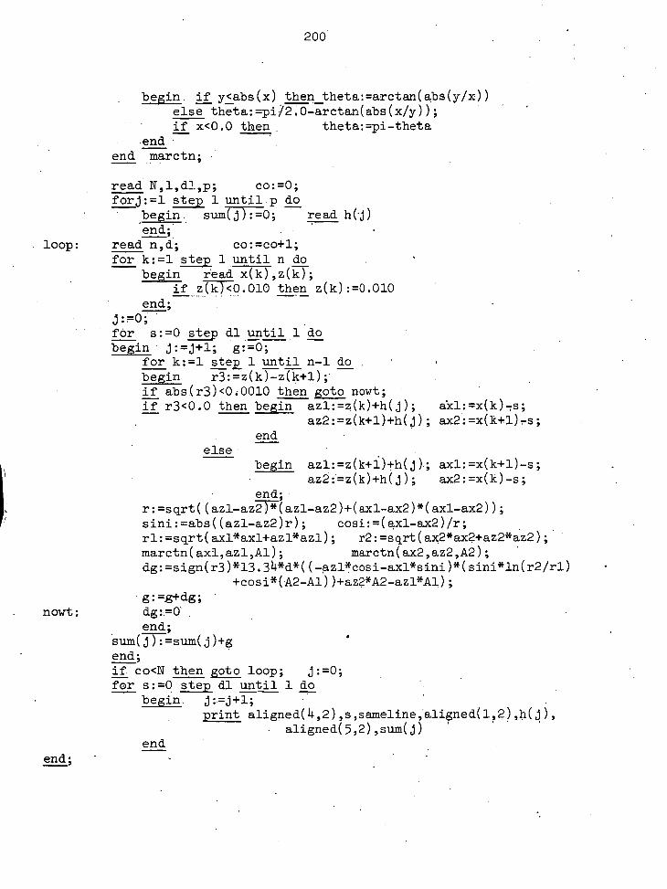
200

• begin. if y<abs(x) then theta:=arctan(abs(y/x)) else theta:=pi/2.0-arctan(abs(x/y));

• if x<0.0 then theta:=pi-theta end'

end marctn;

read N,1,d1,p; co:=0; forj:=1 step 1 until p do

begin sum(j):=0; read h(j) end;

loop: read n,d; co:=co+1; for k:=1 step 1 until n do

begin read x(k),z(0-; if i5.70.010 then z(k):=0.010

end;

for s:=0 step dl until 1 do begin j:=j+1; g:=0;

for k:=1 steg 1 until n-1 do begin r3:=z(k)-z(k+1); if abs(r3)<0:0010 then goto nowt; if r3<0.0 then begin az1:=z(k)+h(j); akl:=x(k) 7s;

az2:=z(k+1)+h(j); ax2:=x(k+1),s; end

else

nowt:

begin az1:=z(k+i)+11.(j).; axl:=x(k+1)-s; az2:=z(k)+h(j); ax2:=x(k)-s;

end; r:=sqrt((azl-azTF(az1,az2)+(axl-ax2)*(ax1-ax2)); sini:=abs((azl-az2)r); cosi:=(axl-ax2)/r; r1:=sqrt(axl*axl+azl*az1); r2:=sqrt(ax2*ax2+az2*az2); marctn(axl,az1,A1); marctn(ax2,az2,A2); dg:=sign(r3)*13.34*d*((,azl*cosi-axl*sini)*(sini*ln(r2/r1)

+cosi*(A2-A1))+az2*A2-azl*A1); - g:=,g+dg; dg :0

sum(j):=sum(j)+g end; if co<N then goto loop; j:=0; for s:=0 step dl until I do

begin j:.=j+1; print aligned(4,2),s,sameline,aligned(1,2),h(j),

aligned(5,2),sum(j)

end

end;

TOPOGRAPHIC AND ISOSTATIC CORRECTIONS TO GRAVITY SURVEYS IN MOUNTAINOUS AREAS

BY

V. P. St JOHN and RONALD GREEN

Reprinted from:

GEOPHYSICAL PROSPECTING, Volume XV, No. t, 1967

TOPOGRAPHIC AND• ISOSTATIC CORRECTIONS TO GRAVITY SURVEYS IN MOUNTAINOUS AREAS *

BY

V. P. St JOHN ** and RONALD GREEN **

ABSTRACT In mountainous areas it is an inadequate procedure to reduce gravity observations by

merely subtracting the effect of an infinite flat slab of material between the station and sea-level, and adding a terrain correction. A programme is described which directly computes the effect of masses above sea-level, and mass-deficiencies below it; as well as the effect of compensating masses under the Pratt and Airy isostatic systems. As an example, the method has been applied to a regional gravity survey of Papua and New Guinea where it is seen to remove the usually high correlation of the Bouguer anomaly with local topography.

INTRODUCTION The purpose of any gravity reduction is to compare with each other, on a

reference surface such as the ellipsoid or geoid, gravity observations made at different positions and elevations. Towards this end, the Bouguer reduction purports to remove the effect of masses above the reference surface, and mass deficiencies below it. This is achieved, in the classical reduction, by two steps:

1) Removal of the effect of an infinite horizontal plate of uniform density, assumed to be between the station and the reference surface. This resulting anomaly is termed the "simple Bouguer anomaly" ;

2) A correction occasioned by the departure of the true topography from the infinite slab. This must include the effect of the earth's curvature, the terrain effect, and the effect of horizontal density variations. The resulting anomaly is termed the "extended Bouguer anomaly."

The importance of applying these corrections to the simple Bouguer anomaly varies with the scale of the survey and the nature of the topography. For a local survey in gentle topography the corrections will be almost the same for every station, which means that the simple Bouguer anomalies are comparable, although they may be in error by a constant amount. However, for a regional survey in a mountainous area, each of the corrections can be appreciable. • In Fig. i the effect of the earth's curvature is shown. P is a station of height, "h" above sea-level and AB represents the infinite slab used in the Bouguer

* Manuscript received by the Editor, July, 1966. ** Department of Geology, University of Tasmania, Hobart, Tasmania, Australia.

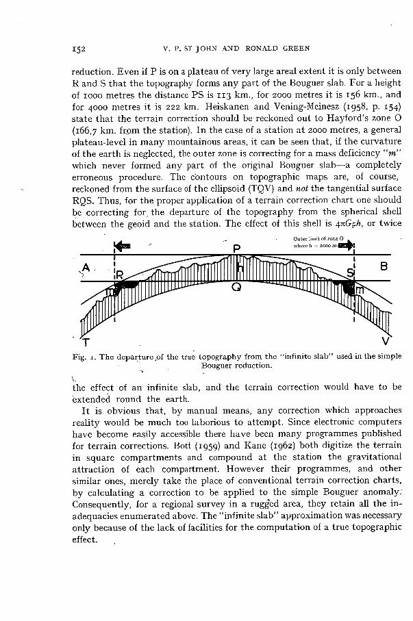
152 V. P. ST JOHN AND RONALD GREEN

reduction. Even if P is on a plateau of very large areal extent it is only between R and S that the topography forms any part of the Bouguer slab. For a height of i000 metres the distance PS is 113 km., for 2000 metres it is 156 km., and for 4000 metres it is 222 km. Heiskanen and Vening-Meinesz (1958, p. 154) state that the terrain correction should be reckoned out to Hayford's zone 0 (166,7 km. from the station). In the case of a station at 2000 metres, a general plateau-level in many mountainous areas, it can be seen that, if the curvature of the earth is neglected, the outer zone is correcting for a mass deficiency "m" which never formed any part of the original Bouguer slab—a completely erroneous procedure. The contours on topographic maps are, of course, reckoned from the surface of the ellipsoid (TQV) and not the tangential surface RQS. Thus, for the proper application of a terrain correction chart one should be correcting for the departure of the topography from the spherical shell between the geoid and the station. The effect of this shell is 47Gph, or twice

Outer limit of zone 0 where h = z000 m 1411

:41211

_..e.girs' opt low"

1111iL-N.■ -' 1•11

V Fig. r. The departure ,of the true topography from the "infinite slab" used in the simple

Bouguer reduction.

the effect of an infinite slab, and the terrain correction would have to be extended round the earth.

It is obvious that, by manual means, any correction which approaches reality would be much too laborious to attempt. Since electronic computers have become easily accessible there have been many programmes published for terrain corrections. Bott (1959) and Kane (1962) both digitize the terrain in square compartments and compound at the station the gravitational attraction of each compartment. However their programmes, and other similar ones, merely take the place of conventional terrain correction charts, by calculating a correction to be applied to the simple Bouguer anomaly. Consequently, for a regional survey in a rugged area, they retain all the in-adequacies enumerated above. The "infinite slab" approximation was necessary only because of the lack of facilities for the computation of a true topographic effect.

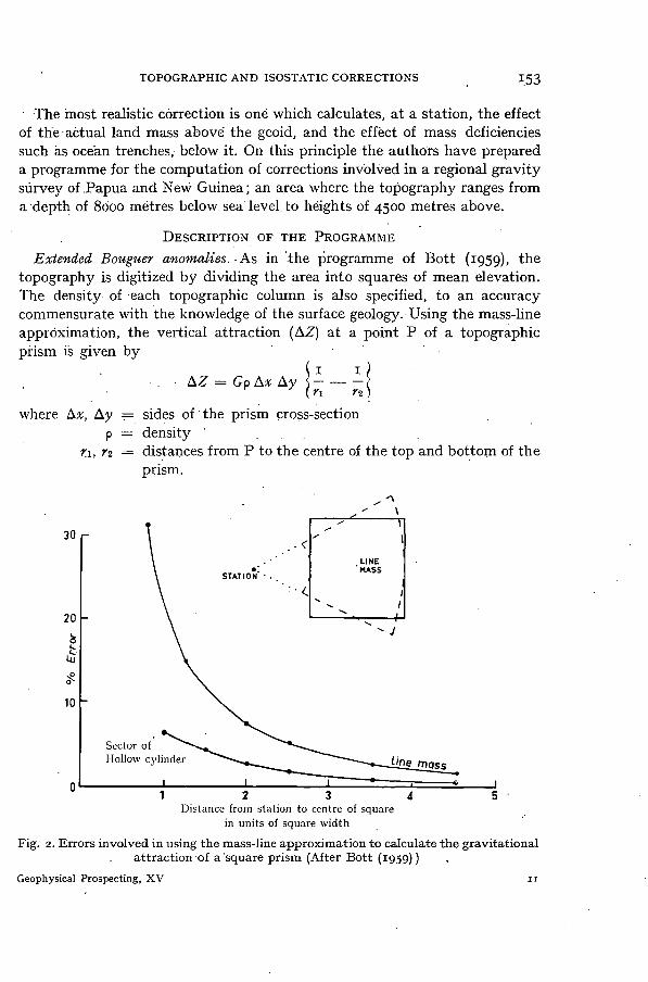
LINE MASS

TOPOGRAPHIC AND ISOSTATIC CORRECTIONS 153

The Most realistic cOrrection is one which calculates, at a station, the effect of the actual land mass above the geoid, and the effect of mass deficiencies such as ocean trenches, below it. On this principle the authors have prepared a programme for the computation of corrections involved in a regional gravity survey of Papua and New Guinea; an area where the topography ranges from a depth of 8000 metres below sea level to heights of 4500 metres above.

DESCRIPTION OF THE PROGRAMME

Extended Bouguer anomalies. As in the programme of Bott (D959), the topography is digitized by dividing the area into squares of mean elevation. The density of each topographic column is also specified, to an accuracy commensurate with the knowledge of the surface geology. Using the mass-line apprOximation, the vertical attraction (AZ) at a point P of a topographic prism is given by

AZ = Gp Ax Ay — — 72

where Ax, Ay -= sides of the prism cross-section p = density '

7.1, 72 = distances from P to the centre of the top and bottom of the prism.

30

20

e. STATION • ..

" : •

j

Sector of Hollow cylinder line mass

1 2 3 4 5 Distance from station to centre of square

in units of square width

Fig. 2. Errors involved in using the mass-line approximation to calculate the gravitational attraction .of a 'square prism (After Bott (i959))

Geophysical Prospecting, XV

10

0

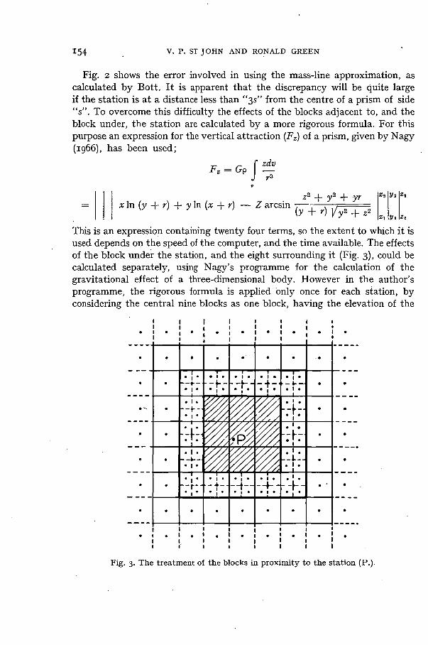
154 V. P. ST JOHN AND RONALD GREEN

Fig. 2 shows the error involved in using the mass-line approximation, as calculated by Bott. It is apparent that the discrepancy will be quite large if the station is at a distance less than "3s" from the centre of a prism of side "s". To overcome this difficulty the effects of the blocks adjacent to, and the block under, the station are calculated by a more rigorous formula. For this purpose an expression for the vertical attraction (Fe) of a prism, given by Nagy (1966), has been used;

Fe = Gp zdv r3

•

x ln (y r) y In (x r) Z arcsin

z2 ± y2 ± yr

X2 Y2 Z2

(y r) 42 + 2'2

y1 Z1

This is an expression containing twenty four terms, so the extent to which it is used depends on the speed of the computer, and the time available. The effects of the block under the station, and the eight surrounding it (Fig. 3), could be calculated separately, using Nagy's programme for the calculation of the gravitational effect of a three-dimensional body. However in the author's programme, the rigorous formula is applied only once for each station, by considering the central nine blocks as one block, having the elevation of the

1

• 1 • • 1 • 1 . 2 .

• • • • •

• I • • 1 •

• •

; • •-•

i •

, .:

1:_,

,

•

•

• 1 • • •

I • I

• 1 •

• _ •

• I • • , •

1r A

r • ree A

• •

•

• • • • •

r A r

PA I • A

• • •

• .

• , . • 1 • A! AirA.

porj, •

_.

_

• 1 •

• 1 •

. , . 1

•

_ , .

• ,

•

, .

• • • •

• —

• • .

— • • • • • • •

I I I I • • I • • • • •

•

•

•

Fig. 3. The treatment of the blocks in proximity to the station (P.).

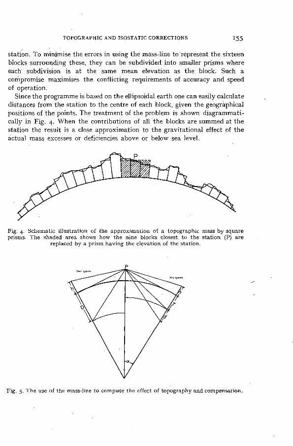
TOPOGRAPHIC AND ISOSTATIC CORRECTIONS 155

station. To minimise the errors in using the mass-line to represent the sixteen blocks surrounding these, they can be subdivided into smaller prisms where each subdivision is at the same mean elevation as the block. Such a compromise maximises the conflicting requirements of accuracy and speed of operation.

Since the programme is based on the ellipsoidal earth one can easily calculate distances from the station to the centre of each block, given the geographical positions of the points. The treatment of the problem is shown diagrammati-cally in Fig. 4. When the contributions of all the blocks are summed at the station the result is a close approximation to the gravitational effect of the actual mass excesses or deficiencies above or below sea level.

Fig. 4. Schematic illustration of the approximation of a topographic mass by square prisms. The shaded area shows how the nine blocks closest to the station (P) are

replaced by a prism having the elevation of the station.

Fig. 5. The use of the mass-line to compute the effect of topography and compensation.

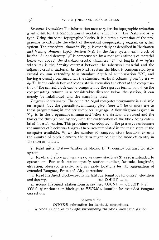
156 V. P. ST JOHN AND RONALD GREEN

Isostatic Anomalies: The information necessary for the topographic reduction is sufficient for the computation of isostatic reductions of the Pratt and Airy type. Using the same topographic blocks, it is a simple extension of the pro-gramme to calculate the effect of theoretical compensating masses, on either system. The procedure, shown in Fig. 5, is essentially as described in Heiskanen and Vening Meinesz (1958, Section 6-3). In the Airy system each block of height "h" and density "p" is compensated by a root (or antiroot) of material below (or above) the standard crustal thickness "T", of length d = hpl where Ap is the density contrast between the subcrustal material and the adjacent crustal material. In the Pratt system the block is compensated by a crustal column extending to a standard depth of compensation "D", and having a density contrast from the standard sea-level column, given by Ap = hp ID. In the calculation of these isostatic anomalies the effect of the compensa-tion ;of the central block can be computed by the rigorous formula or, since the compensating column is a considerable distance below the station, it can merely be subdivided and the mass-line used.

Programme summary: The complete Algol computer programme is available on request, but the generalized summary given here will be of more use to those programming in another computer language. A flow diagram is given in Fig. 6. In the programme summarized below the stations are stored and the blocks fed through one by one, with the contribution of the block being calcu-lated for each station. This procedure was adopted in the present case because the number of blocks was too great to be accommodated in the main store of the computer available. Where the number of computer store locations exceeds the number of block elements the data might be handled more efficiently in the reverse manner.

1. Read initial Data—Number of blocks, D, T, density contrast for Airy system.

2. Read, and store in linear array, as many stations (N) as it is intended to operate on. For each station specify station number, latitude, longitude, elevation, observed gravity; and set aside locations for the aggregation of extended Bouguer, Pratt and Airy corrections.

3. Read first/next block—specifying latitude, longitude (of centre), elevation and density. set COUNT = o.

4. Access first/next station from array; set COUNT . = COUNT + 1. TEST: if station is on block go to PRISM subroutine for extended Bouguer corrections

followed by DIVIDE subroutine for isostatic corrections.

if block is one of the eight surrounding the block under the station

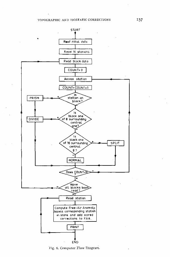
Access station

Is block one

of 16 surrounding central

?

Compute Free-Air Anomaly. Access corresponding station

in store and add stored corrections to FAA.

PRINT

Read station

TOPOGRAPHIC AND ISOSTATIC CORRECTIONS 157

START

Read initial data

Read N stations

END

Fig. 6. Computer Flow Diagram.

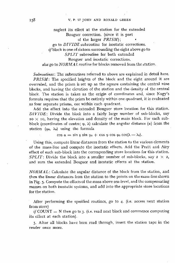
158 V. P. ST JOHN AND RONALD GREEN

neglect its effect at the station for the extended Bouguer correction. (since it is part

of the larger PRISM); go to DIVIDE subroutine for isostatic corrections.

if block is one of sixteen surrounding the eight above go to SPLIT subroutine for both extended

Bouguer and isostatic corrections. else go to NORMAL routine for blocks removed from the station.

Subroutines: The subroutines referred to above are explained in detail here. PRISM: The specified heights of the block and the eight around it are

overruled, and the prism is set up as the square containing the central nine blocks, and having the elevation of the station and the density of the central block. The station is taken as the origin of coordinates and, since Nagy's formula requires that the prism be entirely within one quadrant, it is evaluated as four separate prisms, one within each quadrant.

Add the effect into the extended Bouguer store location for this station. DIVIDE: Divide the block into a fairly large number of sub-blocks, say 10 x io, having the elevation and density of the main block. For each sub-block (coordinates of centre; co, X) calculate the angular distance (a) from the station (cpo, Xo) using the formula

cos oc = sin co sin cpo + cos cp cos yo cos(A — AO.

Using this, compute linear distances from the station to the various elements of the mass-line and compute the isostatic effects. Add the Pratt and Airy effect of each sub-block into the corresponding store locations for this station. SPLIT: Divide the block into a smaller number of sub-blocks, say 2 X 2,

and sum the extended Bouguer and isostatic effects at the station.

NORMAL: Calculate the angular distance of the block from the station, and then the linear distances from the station to the points on the mass-line shown in Fig. 5. Compute the effects of the mass above sea-level, and the compensating masses on both isostatic systems, and add into the appropriate store locations for the station.

After performing the specified routines, go to 4. (i.e. access next station from store)

if COUNT = N then go to 3. (i.e. read next block and commence computing its effect at each station).

5. After all blocks have been read through, insert the station tape in the reader once more.

TOPOGRAPHIC AND ISOSTATIC CORRECTIONS 159

6. Read first/next station, and locate corresponding station in the store. 7. Compute theoretical gravity, free-air anomaly and simple Bouguer anom-

aly for this station. 8. Subtract the total stored extended Bouguer correction from the free-air

anomaly to give the extended Bouguer anomaly. 9. Add the total stored Pratt and Airy corrections separately to the extended

Bouguer anomaly to give these two isostatic anomalies. io. Print station number, latitude, longitude, elevation, observed gravity,

theoretical gravity, free-air, simple Bouguer, extended Bouguer, Pratt and Airy anomalies.

1. Go to 6—until all stations have been read through. End of programme.

It is possible to introduce a large number of variations within the basic framework of this programme, after weighing the precision required against the calculating speed of the computer. The size of the topographic blocks depends on the area over which it is intended to calculate the topographic effect. Since the basic idea of this programme is to examine the effect over a wide area it will be necessary to have fairly large blocks to keep the number within reasonable bounds. For the New Guinea survey the area digitized was between latitudes o° and 12°S, and longitudes 138° and 156°E. The land, with the submarine areas adjacent to it, was divided into 10' x 10' blocks. Further out, the sea floor was divided into 15' x 15' blocks, while those submarine areas most remote from any station were divided into blocks of 0.5° x 0.5°. In all, about 3200 blocks were specified. A restraint in the programme caused it to neglect blocks farther than 5° from the station, giving a radius of computa-tion of about 540 kilometres. The terrain correction for the central block was estimated, using the tables of Bible (1962). Using the Elliott 503 computer, the time taken to compute the extended Bouguer and two isostatic anomalies for 1500 stations was just over 40 hours.

ERRORS

The errors introduced in this method have been adequately discussed by Bott (1959). We are in agreement with him that the main sources of error are:

(a) The departure of the mass-line approximation from the true attraction of a prism. As seen in Fig. 2 this is appreciable only for blocks closer to the station than about four times the side of the square. The error for each block immediately adjacent to the central 25 will be 4 %; for each block in the next zone out it will be 2 %, and will diminish further with distance from the station.

(b) The use of a mean elevation to represent the topography of the top

160 V. P. ST JOHN AND RONALD GREEN

.surface of the block. If the height difference from the station to the top of the block is "h", and the range of height within it is "2h", Bott estimates the error in the terrain correction to be 25 %. That is, the error in estimating the effect "t" of the departure of the block from the Bouguer slab height is 25 %. This error will be diminished by two factors :

i. "t" will be considerable only if "h" is large, in which case there is a small probability that the range of height within the block will remotely approach

ii. Even if there is a large error in "t", it must still be spread over the attraction of the whole topographic block, which will greatly reduce the percentage error.

As well as this, the further the block is from the station, the more closely will the effect of a block of mean elevation approach the true topographic effect. - -

These errors are in the calculation of the effects of individual blocks, and hence their /importance depends upon the size of the contribution of the indi-vidual block compared to the total topographic effect. Depending on the eleva-tion of the station, from slightly above sea-level to 4500 metres, the effect of the central 30' x 30' block varies from ioo % to about 6o % of the total effect. Since there should be no error in the computation of this, it follows that the errors discussed above always affect less than 40 % of the summation. In the extreme case of a station at 4500 metres, and assuming that the zone of blocks surrounding the central 25 contributes all of this 40 %, the total error due to the mass-line summation is still only 40 % of 4 %—or 1.6 %. In practice; of course, even quite remote blocks with negligible errors will

/ contribute to the effect, and the total error will be considerably less than 1.6 %. There will be a small, but inestimable, error in the terrain correction of the central block, but since the terrain correction itself is usually very small the error is not important.

From this discussion it is evident that the total error in the computation of the effect of the topography will vary with the height of the station, but even for the highest station it should not exceed 2 %, and for average highland stations at 15oo metres it will be under i %.

RESULTS This programme was used to apply topographic and isostatic corrections

to some 1500 gravity stations of a regional survey of Papua and New Guinea. In general, the extended Bouguer anomalies were little different from simple Bouguer anomalies for sea-level stations. For stations in highland valleys at 1500 to 2000 metres they were io to 20 milligals higher (algebraically), while for

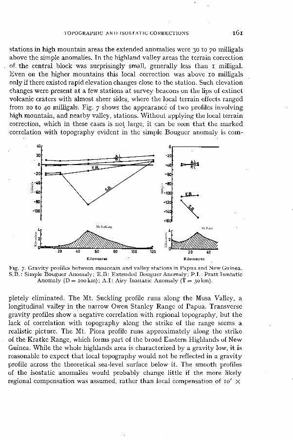
Mt SockTing

20 40 100 60 80 120 Kilometres

-20

-40

-so 4, -80

Mt nom

20 40 Kilometres

40

2

TOPOGRAPHIC AND ISOSTATIC CORRECTIONS r6r

stations in high mountain areas the extended anomalies were 30 to 70 milligals above the simple anomalies. In the highland valley areas the terrain correction of. the central block was surprisingly small, generally less than r milligal. Even on the higher mountains this local correction was above ro milligals only if there existed rapid elevation changes close to the station. Such elevation changes were present at a few stations at survey beacons on the lips of extinct volcanic craters with almost sheer sides, where the local terrain effects ranged from 20 to 40 milligals. Fig. 7 shows the appearance of two profiles involving high mountain, and nearby valley, stations. Without applying the local terrain correction, which in these cases is not large, it can be seen that the marked 'correlation with topography evident in the simple Bouguer anomaly is corn-

Fig. 7. Gravity profiles between mountain and valley stations in Papua and New Guinea. S.B. : Simple Bouguer Anomaly; E.B: Extended Bouguer Anomaly; P.1.: Pratt Isostatic

Anomaly (D= 100 km); Al: Airy Isostatic Anomaly (T= 3o km).

pletely eliminated. The Mt. Suckling profile runs along the Musa Valley, a longitudinal valley in the narrow Owen Stanley Range of Papua. Transverse gravity profiles show a negative correlation with regional topography, but the lack of correlation with topography along the strike of the range seems a realistic picture. The Mt. Piora profile runs approximately along the strike of the Kratke Range, which forms part of the broad Eastern Highlands of New Guinea. While the whole highlands area is characterized by a gravity low, it is reasonable to expect that local topography would not be reflected in a gravity profile across the theoretical sea-level surface below it. The smooth profiles of the isostatic anomalies would probably change little if the more likely regional compensation was assumed, rather than local compensation of ro' x

162 ST JOHN AND GREEN, TOPOGRAPHIC AND ISOSTATIC CORRECTIONS

10' blocks. This is due to lack of resolution at the surface of deep isostatic effects.

A detailed interpretation being prepared for the accompanying map (Fig. 8) shows that the extended Bouguer anomalies are explained by subsurface crustal, and upper mantle, variations rather than by local topography.

The removal of the effect of masses above sea-level, without introducing spurious topographic correlation, seems to indicate that this method of gravity reduction has achieved its objective.

REFERENCES BIBLE, J. L., 1962: Terrain correction tables for gravity. Geophysics 27, pp. 715-718. BOTT, M. H. P., 1959: The use of electronic digital computers for the evaluation of gra-

vimetric terrain corrections. Geophysical Prospecting 7, pp. 46-54. HEISKANEN, W. A., and VENING MEINESZ, F. A., 1958: "The Earth and its Gravity Field".

(McGraw-Hill: New York). KANE, M. F., 1962: A comprehensive system of terrain corrections using a digital com-

puter. Geophysics 27, pp. 455-462. NAGY, D., 1966: The gravitational attraction of a right rectangular prism. Geophysics 31,

pp. 362-371.

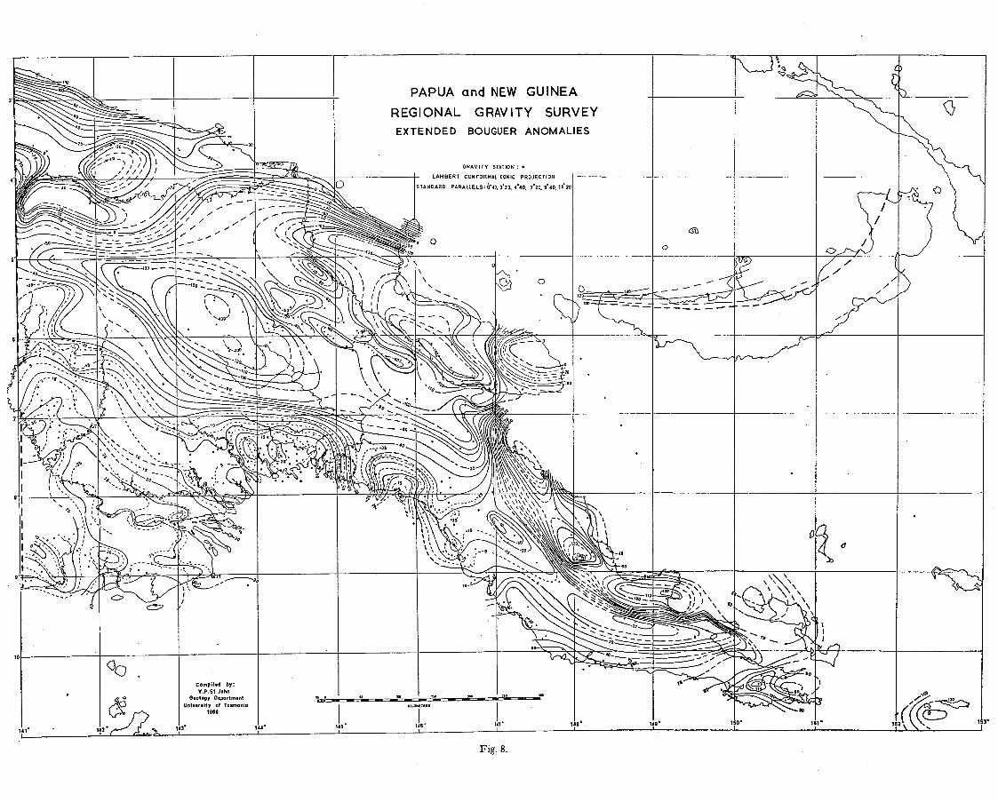
Mill PAPUA and NEW GUINEA

% ....

REGIONAL GRAVITY SURVEY EXTENDED BOUGUER ANOMALIES

GRAVITY STATION : •

LAMBERT CONFORMAL

Cil

- ) ) )

I ./. ....... iir,...„ -.1-Qtrp, vt,

,' . / 1 1 it,

- \\\\\\0

\\ , ,,

,,_\,,,,

1IA

11101 1

1,.. tr %,,,- /)//, i

/

11 :

1

' t

.??

z..,. k

.. rkg..-----

.III 'I Q

__ _--. N.......,

CONIC PROJECTION

STANDARD PARALLELS' 0 . 19 3.20. 4 .40. 7•20, ..40,11* 20

,

-Ally

t

\ \

.■

\

\

\

,..........„

11111 •••••

J. _.,...

/ •

it li

f —

I /

trit 0 • &

r,.. iiic

, .... ,... ..... .

- . , ..

, \

/ \ ...

S. • ■

•

NO.

\

\

.... ,Nik

oo

`,.. \ ••■ ..... .... ..... "AI" 1110

". ■ • ,......

61 .

/,' • . . , \ • \ •

•43.0 . s. lz,

.... ... --

% 1114 \ \

,,.-

-, S

, -- -,-: - ...1 ,

s , \

r ( 7 . , ...

/7 211

-11,1 11111wirpo--

'7,

IMIlipmel l' .., I „ s,.. I .. .. • \ S , ... S

r 4" 1/` \ . S •••• ,(1 ..., •

\ ... . .... • . •7,

I `• ...... , ,

I

--..,,... .

•

•

• ,o , --- NOPISIC

0 : . ..

14- ,•••

, b

I ,

•

,

‘ \ \

, ‘ ‘,\ 11

8 ' •,

r, ..

• , I

tvati....W

- ko

At7

0

0 .44

•

ocs

„:-; • _ t35.

. • I ' . ,•13 --.....‘.

1 . •

‘ ‘, • \

11...- -Ad

I

\ \ ‘ s \ \ N..", ‘‘, _ ‘

M\ I, 1

\ . \\\ 1

I a . 40 .....

. • So ' • -..

.

. 9 ••--- ....414wfir .------. Jo

I.

/

.

...11101 . \ — — \ \ \ 0 \ ; , 120 ..., 414.3 1 1 , ‘ o...,

. i , e, III ‘ 14. • • , e, ..• ., ,

■

...—.—

\ t

7 (1 . f 1.7. I!)

i i il i

/ .

ii

( , •....1

•

142. 143

Compiled by: V.P.St John

Geology Deportment University of Tasmania

1960

• 144.

so m •

ICED 153

10

•

141 •

71.1% --.......

11111•716/

. .:-...-:,

`,....-my ..... .....

MI

OD ,Ilirlitif,

• r''' —7" .44,.... .0.)

F.14,7110

INN . 145- 117 • 146

SO •

• 149 . 150 . 151 152‘

Fig. 8.