The global abundance and size distribution of lakes, ponds, and impoundments

J. A. DowningDepartment of Ecology, Evolution, and Organismal Biology, Iowa State University, 253 Bessey Hall, Ames, Iowa 50011

Y. T. PrairieDepartement des Sciences Biologiques, Universite du Quebec a Montreal, P. O. Box 8888, station Centre-Ville, Montreal,Quebec H3C 3P8, Canada

J. J. ColeInstitute of Ecosystem Studies, Box AB, Millbrook, New York 12545

C. M. DuarteInstitut Mediterrani d’Estudis Avancats (Consejo Superior de Investigaciones Cientıficas, Universitat de les Illes Belears),Miquel Marques 21, Esporles, Islas Baleares, Spain

L. J. TranvikLimnology, Department of Ecology and Evolution, Evolutionary Biology Centre, Norbyv. 20, SE-75 236 Uppsala, Sweden

R. G. StrieglUnited States Geological Survey, National Research Program, Box 25046 MS 413, Denver, Colorado 80025

W. H. McDowellDepartment of Natural Resources, University of New Hampshire, Durham, New Hampshire 03824

P. KortelainenFinnish Environment Institute, P. O. Box 140, 00251 Helsinki, Finland

N. F. CaracoInstitute of Ecosystem Studies, Box AB, Millbrook, New York 12545

J. M. MelackBren School of Environmental Sciences and Management, University of California, Santa Barbara, California 93106

J. J. MiddelburgNetherlands Institute of Ecology, Korinaweg 7, Yerseke, 4401 NT, Netherlands

Abstract

One of the major impediments to the integration of lentic ecosystems into global environmental analyses hasbeen fragmentary data on the extent and size distribution of lakes, ponds, and impoundments. We use new datasources, enhanced spatial resolution, and new analytical approaches to provide new estimates of the globalabundance of surface-water bodies. A global model based on the Pareto distribution shows that the global extentof natural lakes is twice as large as previously known (304 million lakes; 4.2 million km2 in area) and isdominated in area by millions of water bodies smaller than 1 km2. Similar analyses of impoundments based oninventories of large, engineered dams show that impounded waters cover approximately 0.26 million km2.However, construction of low-tech farm impoundments is estimated to be between 0.1% and 6% of farm areaworldwide, dependent upon precipitation, and represents .77,000 km2 globally, at present. Overall, about4.6 million km2 of the earth’s continental ‘‘land’’ surface (.3%) is covered by water. These analyses underscorethe importance of explicitly considering lakes, ponds, and impoundments, especially small ones, in global analysesof rates and processes.

Although lakes are of global importance, most analyses offunctional processes in freshwater ecosystems have eitheremphasized regional similarities (Thienemann 1925; Nau-mann 1929; Kalff 2001) or have adopted an ecosystem-

specific emphasis. The few global analyses of lacustrineprocesses have been limited because knowledge of thenumber and size distribution of lakes has been incomplete(Alsdorf et al. 2003; Lehner and Doll 2004). Further,

Limnol. Oceanogr., 51(5), 2006, 2388–2397

E 2006, by the American Society of Limnology and Oceanography, Inc.

2388

freshwater ecosystems are generally considered to cover onlya small portion of the earth’s surface. Previous assessments ofthe global area covered by lakes and ponds are probablyunderestimates (Kalff 2001) and have ranged from 2–2.8 3106 km2 (Meybeck 1995; Kalff 2001; Shiklomanov andRodda 2003). The literature suggests that lakes and pondsconstitute only 1.3–1.8% of the earth’s non-oceanic area, andthat lakes are numerically dominated by small systems, butthat global lake area is dominated by a few, large lakes(Schuiling 1977; Wetzel 1990; Meybeck 1995).

Because many consider continental waters to be a minorcomponent of the biosphere, the activity of inland waters iscommonly ignored in global estimates of ecosystem pro-cesses such as elemental budgets (e.g., IPCC 2001). Recentevidence points to the significant role of freshwaterecosystems in many key processes, for example, carbondioxide (CO2) and methane (CH4) efflux and organiccarbon storage in sediments (Cole and Caraco 2001; Sobeket al. 2003; Pace and Prairie 2004). There are two majoruncertainties in these global estimates. Both the total areaoccupied by lakes is poorly known, and the size distributionof lakes is not well described. Because many key processesscale with lake size (Hakanson 2004), both issues createa great deal of uncertainty in global estimates. Hence, thereis a need to ascertain the global extent and the sizedistribution of freshwater lentic ecosystems.

Present estimates of the global extent and size distribu-tion of freshwater ecosystems are subject to great un-certainty (Kalff 2001; Lehner and Doll 2004). Here, weestimate the global extent and size distribution of lakes,ponds, and impoundments by exploring the size-depen-dence of the abundance of lakes, ponds, and impound-ments to formulate scaling laws, which are tested acrossdifferent regions and scales. These scaling laws are thenintegrated to provide estimates of the total global extent offreshwater ecosystems.

Methods

Historical analyses and models of natural lake abun-dance—One of the first attempts to characterize the globalabundance and frequency distribution of lentic waterbodies was performed by Schuiling (1977). Schuilinginventoried the most complete list of large lakes available(Halbfass 1922), supplementing it with 800 planimeteredlake maps, to determine the number of lakes in Europe and

the world within size ranges of area. This size–frequencyapproach significantly undersampled lake areas less than3 km2 for the European lakes and 800 km2 for world lakes.Normalizing data per unit land area, however, enables datafrom different regions to be plotted together and compared.Such graphical analyses suggest that small lakes arenumerically dominant (Fig. 1). In an analysis of land–water interfaces, Wetzel (1990) designed a graphicalrepresentation of the relationship between the number oflakes on Earth and their areas and depths, suggesting thatthe earth contains so many small, shallow lakes that smalllacustrine ecosystems may cover more area than large ones.Meybeck (1995) collected data on dL (the number of lakesin given size categories, per unit area) for lakes in manygeographical regions that also indicated consistent de-creases in the areal frequency of lakes with increasing size(Fig. 1). Taken together, orthogonal regression of theseearly data suggests that dL varies as

dL ~ 1,186 A{0:961 ð1Þ

where dL is the number of lakes per 106 km2 in a size rangeof one log-unit of width, and A is the area in km2 (Fig. 1; r2

5 0.77; 95% slope confidence interval is 21.05 to 20.88).The exponent of this relationship indicates that each sizecategory contains approximately the same total surfacearea of lakes. The relationship postulated by Wetzel (1990)tracks just beneath Eq. 1 for large lakes (.1 km2) andslightly above it for smaller ones.

There are three important limitations to these data.First, they consider only lake counts and sizes obtainedusing samples of regional lake densities that do not coverall lakes found in a region. Second, the data underrepresentsmall waterbodies (e.g., ,0.1 km2) because these do notappear on most printed maps. Third, the regional datacover a limited number of geographic areas. Because ofthese limitations, we used fine-resolution geographicalinformation systems (GIS) and some modern data toextend the dL approach to new areas and smaller lakes thanhave been analyzed elsewhere (e.g., Lehner and Doll 2004).

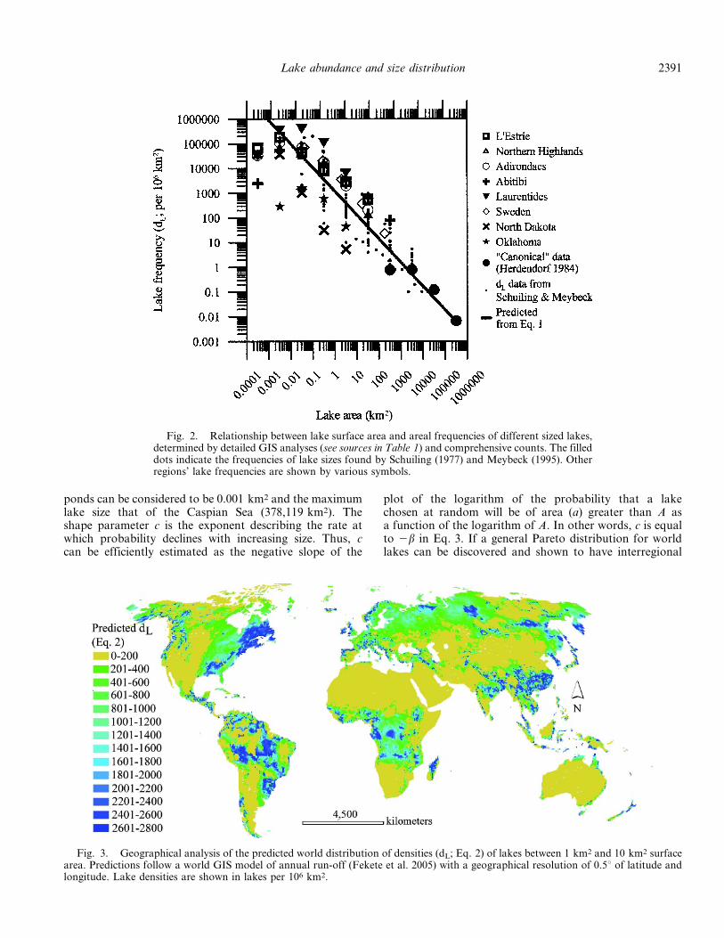
New data for several geographically dissimilar regions fitwell within the range of dL values observed in past analyses(Fig. 2) and track Eq. 1. This suggests that the relationshipsbetween lake densities and lake area are similar amongregions and can be extended to smaller lake sizes than wereoriginally analyzed in worldwide data. That is, traditionalsize–frequency relationships appear to extend to waterbodiesas small as 0.001–0.0001 km2. Inspection suggests, however,that some arid to semi-arid regions (e.g., North Dakota andOklahoma) may have lower dL for a given size category oflakes than those in areas with greater run-off (e.g., L’Estrie,Laurentides, regions of Canada; Fig. 2). Multiple regressionanalysis of the logarithm of dL (lakes per 106 km2) showsthat lake densities within size classes vary predictably asfunctions of lake area (A; km2) and average annual run-off(V; mm yr21) (Fekete et al. 2005):

log dL ~ 2:08 { 0:800 log10 Að Þz 0:004 V

{ 2:8 | 10{6 V2� � ð2Þ

AcknowledgmentsThis contribution is dedicated to Robert G. Wetzel whose global

understanding of aquatic ecosystems has inspired a generation oflimnologists. We also acknowledge the many aquatic scientistswho have counted, measured, and explored the earth’s lakes,ponds, and impoundments. We thank Dan Canfield and RogerBachmann for sharing data on Florida lakes, Steve Hamiltonfor sharing data on Amazonian lakes, and Daelyn Woolnoughfor help with geographical information system analyses.

This work was conducted as a part of the ITAC WorkingGroup supported by the National Center for Ecological Analysisand Synthesis, a center funded by the National ScienceFoundation (grant DEB-94-21535), the University of Californiaat Santa Barbara, and the State of California.

Lake abundance and size distribution 2389

(R2 5 0.83, n 5 139, p , 0.001), where dL is the density of

lakes in a log10 bin range with an upper bound of A, and

partial effects of all variables are statistically significant ( p ,

0.001). The polynomial effect is highly significant ( p , 0.001)

and indicates that lake density increases with run-off up to

about 1,000 mm yr21, then declines in the erosional land-

forms that are subject to extremely high run-off. Variation

around this relationship is likely the result of differences in

regional hypsometry (Strahler 1952) and average landscape

slope (Schumm 1956). Application of Eq. 2 using a GIS of

global run-off data (Fekete et al. 2005) models many of theworld’s regions with abundant lakes and ponds (Fig. 3).

The calculation of the global extent of area covered by lakesis complicated by the influence of regional climate on dL (Eq. 2).The worldwide or ‘‘canonical’’ data of Herdendorf (1984;Fig. 2) consist of counts of all of the world’s large lakes. Onecannot use dL data (e.g., Figs. 1 and 2) to accurately estimatethe worldwide area of smaller lakes without making some boldassumptions about the influence of climate and hypsometryon dL for geographically diverse regions of the world. Theproblem is that we can count the large lakes of the world butunderstanding the role of small lakes in global budgets andprocesses requires extrapolation from known, canonical cen-suses of large lakes to the global extent of lakes of all sizes.

Results and Discussion

The distributional properties of lake number versussize relationships—The power-function fit of the relation-

ship between dL and A in Eqs. 1 and 2 suggests that lakesize distributions share some fundamental distributionalproperties with other size class data. In fact, lake size datahave been recently shown (Lehner and Doll 2004) to havean excellent fit to a size–frequency function of the form

Na §A ~ aAb ð3Þ

where Na$A is the number of lakes of greater or equal area(a) than a threshold area (A), and a and b are fittedparameters describing the total number of lakes in the dataset that would be of one unit area in size and thelogarithmic rate of decline in number of lakes with lakearea, respectively. The model above corresponds well toa Pareto distribution (Pareto 1897). The Pareto distributionis particularly versatile and is widely used in fields asdisparate as semiotics and engineering (Vidondo et al.1997). It has also been found useful in describing lake size–frequency distributions (Hamilton et al. 1992), as long asthe data are complete and accurate (i.e., not truncated orcensored).

The Pareto distribution has a probability densityfunction ( pdf ) described by:

pdf að Þ~ ckca{ c z 1ð Þ ð4Þ

where a is the size of the object, and k and c are the locationand shape parameters, respectively (Evans et al. 1993).Because lakes cannot be of infinitesimal or infinite sizes, krepresents a compound measure of the actual range of lakesizes observed on Earth. The minimum size of lakes and

Fig. 1. Relationship between lake surface area and areal frequencies of different sized lakes.The filled circles and open squares indicate the frequencies of lake sizes digitized from Schuiling(1976). The dashed line represents the hypothesis advanced by Wetzel (1990), digitized from hisfig. 5. All other data are from Meybeck (1995).

2390 Downing et al.

ponds can be considered to be 0.001 km2 and the maximumlake size that of the Caspian Sea (378,119 km2). Theshape parameter c is the exponent describing the rate atwhich probability declines with increasing size. Thus, ccan be efficiently estimated as the negative slope of the

plot of the logarithm of the probability that a lakechosen at random will be of area (a) greater than A asa function of the logarithm of A. In other words, c is equalto 2b in Eq. 3. If a general Pareto distribution for worldlakes can be discovered and shown to have interregional

Fig. 2. Relationship between lake surface area and areal frequencies of different sized lakes,determined by detailed GIS analyses (see sources in Table 1) and comprehensive counts. The filleddots indicate the frequencies of lake sizes found by Schuiling (1977) and Meybeck (1995). Otherregions’ lake frequencies are shown by various symbols.

Fig. 3. Geographical analysis of the predicted world distribution of densities (dL; Eq. 2) of lakes between 1 km2 and 10 km2 surfacearea. Predictions follow a world GIS model of annual run-off (Fekete et al. 2005) with a geographical resolution of 0.5u of latitude andlongitude. Lake densities are shown in lakes per 106 km2.

Lake abundance and size distribution 2391

generality, then we can calculate the global extent of allsizes of lakes.

Fit of lake area frequencies to the Pareto distribution—Totest lake size distributions for general fit to the Paretodistribution, we collected inventories of all lakes withina variety of geographical settings representing divergenttopography and geology. Data not derived from publishedsources (Table 1) were determined from regional GISanalyses using ARCView (ESRI). Data were scrutinizedfor evidence of undersampling at small lake sizes to includeonly untruncated, uncensored data (Hamilton et al. 1992).Figure 4 and Table 1 show strong interregional similarityin the slopes of these distributional curves. Becausedifferent regions hold differing total numbers of lakesand their largest lakes differ in size, curves are located atdifferent points along the abscissa. The Pareto distributionshows a similar rate of decline in abundance with increasedlake size, regardless of the region of the earth examined.

Given that the size–frequency distributions of lakesfollow a Pareto distribution in many regions down to verysmall lake sizes (Fig. 4), canonical data on the abundanceof the world’s largest lakes should enable the anchoring ofEq. 3 and the calculation of the worldwide abundance oflakes. Herdendorf (1984) inventoried the world’s largestlakes to document the dominance of the 251 largest lakes inthe world’s freshwater supply (Fig. 4). He concluded thatthe greatest impediment to this work was the paucity ofaccurate maps. Lehner and Doll (2004) have recently usedGIS analysis to develop and validate a global lakedatabase. They combined analog and digital maps withdatabases, registers, and inventories of lakes to present a listof .250,000 waterbodies. Considering only the 17,357natural lakes .10 km2 in area included in their analysis, we

calculate Eq. 3 by least squares regression:

Na §A ~ 195,560A{1:06079 ð5Þ

(r2 5 0.998; n 5 17,357; SEb 5 0.0003). The exponent ofthis relationship (b, Eq. 3; –c, Eq. 4) is near the middle ofthose seen in regional analyses (Table 1) and the twocanonical lake area data sets describe an identical lake sizedistribution (Fig. 4). Orthogonal regression yielded a 99.9%confidence interval of the estimated b from 21.06245 to21.06056. The accuracy and precision of the estimate ofb is very important because calculated lake size distribu-tions and areas are very sensitive to this parameter. Becausethe shape of Pareto distributions is similar among diverseregions of the earth (Table 1; cf., Lehner and Doll 2004)and the parameters of this distribution are estimable fromthe canonical data sets, we can thus calculate the globalextent of ponds and lakes.

The number of lakes in the world can be calculatedfollowing the approach of Vidondo et al. (1997). FromEq. 5, c of the Pareto distribution is 1.06. Given that wedefine the range of lake sizes as 0.001 to 378,119 km2 (theCaspian Sea), integration of Eq. 4 will indicate the fractionof all the world’s lakes and ponds that is contained withinany range of areas. A good estimate of k is 0.001 km2

because this is the smallest size of pond practicallyrecognizable in landscapes. The fraction of all world lakesthat are represented by those in the canonical data set ( fc)can be calculated as follows:

fc ~ { kc | A{cc max { A{c

c min

� �ð6Þ

where Ac min and Ac max are the minimum and maximumareas of lakes found in the canonical data set (i.e., 10 and378,119) and c is the negative of the exponent (Eq. 5) found

Table 1. Coefficients of Eq. 3 fitted by least squares regression. GIS data were derived from original GIS analyzed by the authors ofthis study. Data sources for original GIS analyses are noted if the data were not the property of the authors.

Data setExponent

(b, Eq. 3; c, Eq. 4)Smallest reliable

size (km2)Number of lakes

analyzed (a) Source

L’Estrie (Quebec, Canada) 20.66 0.001 3,398 GIS (Y. T. Prairie unpubl. data)Abitibi (Quebec, Canada) 20.67 0.001 1,020 GIS (Y. T. Prairie unpubl. data)Finland 20.69 0.009 57,205 (Raatikainen and Kuusisto 1988)Eastern Lakes Survey (U.S.A.) 20.76 0.1 1,264 (Linthurst et al. 1986; Landers et al.

1988)Western Europe 20.77 5 751 (Schuiling 1977)Western Lakes Survey (U.S.A.) 20.78 0.01 752 (Clow et al. 2003)Amazon basin (South America) 20.79 0.1 4,482 (Sippel et al. 1992; Hamilton et al. 1992)Adirondacks (U.S.A.) 20.79 0.01 2,125 GIS (J. J. Cole unpubl. data)Median of regional estimates 20.79World’s large lakes 20.83 – 251 (Herdendorf 1984)Florida (U.S.A.) 20.88 0.05 5,346 (Shafer et al. 1986)Mean of regional estimates 20.89Laurentides (Quebec, Canada) 20.90 0.001 562 GIS (Y. T. Prairie unpubl. data)World’s largest lakes 21.06 10 17,357 (Lehner and Doll 2004)Oklahoma (U.S.A.) 21.19 0.1 444 GIS (Oklahoma Center for Geospatial

Information 2004)Orinoco basin (South America) 21.22 0.1 956 (Hamilton and Lewis 1990; Hamilton et

al. 1992)North Dakota (U.S.A.) 21.334 0.001 7,239 GIS (North Dakota State Water

Commission 2003)

2392 Downing et al.

for the canonical data set. Solving Eq. 6 indicates that thecanonical lake data set contained a fraction of the world’slakes equal to 5.712 3 1025. Division of the number ofcanonical lakes used to calculate Eq. 5 by this fractionestimates that there are in the neighborhood of 304 millionponds and lakes ($0.001 km2) in the world. This totalnumber of world lakes is defined as Nt.

Further, because Eq. 3 fits consistently over a wide rangeof lake areas (Fig. 4 and Table 1) and because Eq. 5anchors this canonical frequency distribution to the knownsizes of the world’s largest lakes, the number of world lakescan be approximated over any size range. If Amin and Amax

are the minimum and maximum sizes of lakes in a givensize range, the number of lakes over a size range can becalculated:

NAmax { Amin~ { Ntk

c A{cmax { A{c

min

� �ð7Þ

(see Table 2). Because c is greater than unity, Eq. 7 shows

that there are many small lakes and few large lakes.Likewise, the average size and total area covered by lakes

in a given size range can be calculated using the Paretodistribution (Vidondo et al. 1997). After simplification, theaverage area of lakes over a size range of Amin to Amax canbe calculated:

�AAAmin { Amax~ c |

{ AmaxAcmin z Ac

maxAmin

c { 1ð Þ Acmax { Ac

min

� � ð8Þ

The total land area covered by lakes of any size range canbe calculated as the product of Eqs. 7 and 8.

Analyses of canonical lake data and the exponents ofPareto distributions of lake sizes derived by regional GISreveal some surprises. Contrary to previous predictions(Schuiling 1977; Wetzel 1990; Meybeck 1995; Kalff 2001),small lakes, not large ones, appear to represent the mostlacustrine area. Although lakes $10,000 km2 in individuallake area constitute nearly 1 3 106 km2, these lakes make uponly about 25% of the world lake area. Together, the twosmallest size categories of lakes in Table 2 comprise morearea than the three largest size categories. When converted todL units (number per 106 km2 of Earth’s surface; Table 2),extension of canonical lake data to small lakes using thePareto distribution tracks Robert Wetzel’s concept (Wetzel1990) of the likely abundance of small lakes (see Fig. 1).

Undercounting small lakes has led to significant under-estimates of the world lake and pond area. World lakes andponds account for roughly 4.2 3 106 km2 of the land areaof the earth. This more than doubles most quantitativehistoric estimates (Kalff 2001; Wetzel 2001; Shiklomanovand Rodda 2003). Natural lakes and ponds $0.001 km2

comprise roughly 2.8% of the non-oceanic land area; not1.3–1.8% as previously supposed.

Reservoirs and impoundments—The foregoing analysismade every attempt to exclude consideration of anthropo-genic impoundments of water. Artificial waterbodies can,however, be of great importance in many processes (Deanand Gorham 1998; St. Louis et al. 2000) and should beincluded in global analyses. The size distributions ofnatural lakes and impoundments are both extensions of

Fig. 4. Plots of data on the axes implied by Eq. 3. Statistical fits of Eq. 3 to these data areshown in Table 1. Data are only plotted throughout the range of lake sizes that could bereasonably expected to be comprehensively censused using the resolution of GIS coveragesavailable (see Table 1). The black lines represent canonical (complete) censuses of world lakes(Herdendorf 1984; Lehner and Doll 2004).

Lake abundance and size distribution 2393

the earth’s hypsometry (Strahler 1952), which is funda-mentally influenced by the erosional force of the watersupply. As landscapes are covered with impounded water,however, small depressions are aggregated into larger lakes.Expressed in terms of an effect on the Pareto distribution,this could lead c (Eq. 4) to be larger.

Because the earth clearly has more small depressionsthan large ones (both dry and wet), it is likely that a Paretodistribution could fit for impoundments as well as fornatural lakes. In fact, Eq. 2 suggests that there are water-rich regions of the earth that are underserved by naturallakes owing to their tilted, erosional, river-dominatedtopography caused by very high run-off (Fig. 3). Ashumans install impoundments in more of the depressionsthat will hold water, impounded waters could cover evenmore area than natural lakes, while following similar sizedistributions. If more large impoundments are built thansmall ones, however, there could be differences in theexponents of the relationships of the type shown in Eq. 3for natural and impounded waterbodies.

The area impounded by large dams is increasingworldwide. It has been estimated that the volume of waterin impoundments increased by an order of magnitudebetween the 1950s and the present (Shiklomanov andRodda 2003). As an example, Fig. 5 shows the trend in thearea covered by impoundments in the United States. Thesemi-log trend is approximately linear from 1700 topresent, but decelerated around 1960. The annual averagerate of increase in impounded area during this term wasabout 4%. The rate of increase since 1960 has slowed toabout 1% per year perhaps because of the increasing rarityof vacant land.

The International Commission on Large Dams (ICOLD;www.icold-cigb.org) tracks data on dams around the worldthat are of safety, engineering, or resource concern. Thesedata are purposefully biased toward large dams, mostnotably those .15 m height. The data are thus likely toprovide the best estimate of impoundments with the largestimpounded areas and progressively less exhaustive cover-

age of smaller impoundments. Restricting an analysis ofEq. 3 to the 41 largest impoundments from the Inguriimpoundment (13,500 km2) down to 1,000 km2 yields

Na §A ~ 2,922,123A{1:4919 ð9Þ

(r2 5 0.97; n 5 41; SEb 5 0.0435). The strongly negativeexponent of this equation indicates that the smallest of thelarge impoundments comprise more surface area than the

Table 2. The numbers, average sizes, and areas of world lakes calculated from Eqs. 7 and 8. The total area of lakes in the size rangeis calculated as the product of calculations from Eqs. 7 and 8. Values are inclusive of lower bounds but exclusive of upper bounds.

Amin (km2) Amax (km2) Number of lakesAverage lake

area (km2)Total area oflakes (km2)

dL (lakes per106 km2) Source

0.001 0.01 277,400,000 0.0025 692,600 1,849,333 Eqs. 7, 80.01 0.1 24,120,000 0.025 602,100 160,800 Eqs. 7, 80.1 1 2,097,000 0.25 523,400 13,980 Eqs. 7, 81 10 182,300 2.50 455,100 1,215 Eqs. 7, 810 100 15,905 24.7 392,362 106 Lehner and

Doll (2004)100 1,000 1,330 248 329,816 9 Lehner and

Doll (2004)1,000 10,000 105 2,456 257,856 0.7 Lehner and

Doll (2004)10,000 100,000 16 37,978 607,650 0.1 Lehner and

Doll (2004).100,000 1 378,119 378,119 0.007 Lehner and

Doll (2004)All lakes 304,000,000 0.012 4,200,000

Fig. 5. Rate of change in impounded area in the UnitedStates for all water impoundments with dams listed as potentialhazards or low hazard dams that are either taller than 8 m,impounding at least 18,500 m3, or taller than 2 m, impounding atleast 61,675 m3 of water (USACOE 1999). All data were ignoredwhere the date of dam construction was unknown (ca. 12% ofimpounded area) or natural lakes (e.g., Lake Superior) were listedas impoundments. The dashed line shows a semi-log regression(r2 5 0.95).

2394 Downing et al.

largest of them. The intentional bias of this data set towardlarge dams progressively increases the exponent of thisequation as smaller impoundments are included. Theaverage relationship, considering all of the ICOLDimpoundments down to 1 km2, is

Na §A ~ 20,107A{0:8647 ð10Þ

(r2 5 0.97; n 5 9,604; SEb 5 0.0154). Integration of thisequation certainly results in an underestimate of the areacovered by impoundments (cf., Eqs. 9 and 10) because itignores many impoundments formed by small dams.Calculations following Eqs. 6–8 (Table 3) show, however,that there are at least 0.5 million impoundments$0.01 km2 in the world, and they cover .0.25 million km2

of the earth’s land surface. This is a smaller area thanestimates based on extrapolation (Dean and Gorham 1998;St. Louis et al. 2000; Shiklomanov and Rodda 2003) butnearly identical to GIS-based estimates (Lehner and Doll2004). Large impoundment data sets (e.g., Smith et al.2002) suggest that small impoundments cover less area thanlarge ones (Table 3).

The preceding analysis includes only those impound-ments with large, engineered dams and ignores smallimpoundments created using small-scale technologies. Thearea covered by small impoundments has largely beena matter of speculation (St. Louis et al. 2000). Farm andagricultural ponds are a growing and globally uninventor-ied resource. They are constructed as sources of water forlivestock, sources of irrigation water, fish culture ponds,recreational activities, sedimentation ponds, and waterquality control structures.

Figure 6 shows the area of water impounded byagricultural ponds in several political units. There isclimatic regularity in the fraction of farm land that isconverted to pond structures. Under dry conditions, farmponds are rare, owing to the difficulty of collection andconservation of sufficient standing water. Up to about1,600 mm of annual precipitation, farm ponds are anincreasing fraction of the agricultural landscape. In moistclimates such as Great Britain, Tennessee, and Mississippi,farm ponds make up 3–4% of agricultural land.

The statistical–climate relationship shown in Fig. 6 wasused with data on area under farming practice, pond size,and estimates of annual average precipitation (FAO 2003)

to estimate the global area covered by farm pondimpoundments. This area sums to 76,830 km2 worldwide.The accuracy of predictions of farm pond area were verifiedusing published data on farm land areas (USDA 2004) andnormal precipitation averages (NOAA 2000) for the UnitedStates. This method estimates the area of farm ponds in thecontiguous United States to be 21,600 km2, remarkablyclose to the 21,000 km2 estimated by GIS (Smith et al.2002). The predicted world area of farm ponds is more thansix times the area predicted by extrapolation of the largedams database and nearly double the total area covered byimpoundments between 100 km2 and 1,000 km2 in area(Table 3). Such small impoundments are growing inimportance at annual rates of increase from 0.7% in GreatBritain, to 1–2% in the agricultural parts of the United

Table 3. The numbers, average sizes, and areas of world water impoundments calculated from Eqs. 7, 8, and 10. The total area ofimpoundments in the size range is calculated as the product of calculations from Eqs. 7 and 8. Values are inclusive of lower bounds butexclusive of upper bounds.

Amin (km2) Amax (km2)Number of

impoundmentsAverage impoundment

area (km2)Total area of

impoundments (km2)dL (impoundments

per 106 km2)

0.01 0.1 444,800 0.027 12,040 2,9650.1 1 60,740 0.271 16,430 4051 10 8,295 2.71 22,440 55.310 100 1,133 27.1 30,640 7.55100 1,000 157 271 41,850 1.051,000 10,000 21 2,706 57,140 0.1410,000 100,000 3 27,060 78,030 0.02All impoundments 515,149 0.502 258,570

Fig. 6. Relationship between the surface area of farm pondsand the annual average precipitation in several political units.Data sources for farm pond numbers are given in Web Appendix1. The line is a least squares regression (r2 5 0.80, n 5 13) wherethe area of farm ponds expressed as a percentage of the area offarm land (FP) rises with annual average precipitation (P; mm) asFP 5 0.019 e 0.0036P.

Lake abundance and size distribution 2395

States, to .60% in dry agricultural regions of India (seereferences in Web Appendix 1, http://www.aslo.org/lo/toc/vol_51/issue_5/2388a1.pdf ).

Consistent regional hypsometry permits calculation ofthe size distribution and area covered by lakes by anchoringa Pareto distribution function to a canonical size distribu-tion of the earth’s largest lakes. Natural lakes andponds are estimated to cover about 4.2 million km2 of theearth’s surface (Table 2), whereas impoundments cover260,000 km2 (Table 3), and farm ponds cover about77,000 km2. These data, taken together, indicate that lakes,ponds, and impoundments cover .3% of the earth’ssurface. This is more than twice as much as indicated byprevious inventories because small lakes have been under-censused.

On a global scale, rates of material processing (e.g.,carbon, nitrogen, water, sediment, nutrients) by aquaticecosystems are likely to be at least twice as important ashad been previously supposed. Since the numerical andareal cover of small waterbodies is much greater than waspreviously assumed, processes that are most active in smalllakes and ponds may assume global significance. On a localscale, previous analyses had indicated that small aquaticsystems were spatially unimportant, yet small waterbodiesdominate the global area covered by continental waters.Because studies of small aquatic systems have beenunderemphasized, future work should emphasize the globalrole and contribution of small waterbodies.

References

ALSDORF, D., D. LETTENMAIER, AND C. VOROSMARTY. 2003. Theneed for global, satellite-based observations of terrestrialsurface waters. EOS 84: 269, 275–276.

CLOW, D. W., AND oTHERS. 2003. Changes in the chemistry of lakesand precipitation in high-elevation national parks in thewestern United States, 1985–1999. Water Resour. Res. 39,1171, [doi: 10.1029/2002WR001533].

COLE, J. J., AND N. F. CARACO. 2001. Carbon in catchments:Connecting terrestrial carbon losses with aquatic metabolism.Mar. Freshwat. Res. 52: 101–110.

DEAN, W. E., AND E. GORHAM. 1998. Magnitude and significanceof carbon burial in lakes, reservoirs, and peatlands. Geology26: 535–538.

EVANS, M., N. HASTINGS, AND B. PEACOCK. 1993. Statisticaldistributions. 2nd ed. John Wiley and Sons.

FAO. 2003. Aquastat database. Food and Agriculture Organiza-tion of the United Nations.

FEKETE, B. M., C. J. VOROSMARTY, AND W. GRABS. 2005. UNH/GRDC composite runoff fields. V 1.0. University of NewHampshire and Global Runoff Data Centre.

HAKANSON, L. 2004. Lakes: Form and function. The BlackburnPress.

HALBFASS, W. 1922. Die Seen der Erde. Peterm. Mitteilungen,Ergangzungsheft 185: 1–169. [In German.]

HAMILTON, S. K., AND W. M. LEWIS, JR. 1990. Physicalcharacteristics of the fringing floodplain of the OrinocoRiver, Venezuela. Interciencia 15: 491–500. [In Spanish.]

———, J. M. MELACK, M. F. GOODCHILD, AND W. M. LEWIS. JR.1992. Estimation of the fractal dimension of terrain from lakesize distributions, p. 145–164. In G. E. Petts and P. A. Carling[eds.], Lowland floodplain rivers: A geomorphological per-spective. Wiley.

HERDENDORF, C. E. 1984. Inventory of the morphopmetricand limnologic characteristics of the large lakes of theworld, technical bulletin. The Ohio State Univ. Sea GrantProgram.

IPCC. 2001. The carbon cycle and atmospheric carbon dioxide,p. 183–237. In IPCC, Climate Change 2001. Cambridge Univ.Press.

KALFF, J. 2001. Limnology: Inland water ecosystems. PrenticeHall.

LANDERS, D. H., W. S. OVERTON, R. A. LINTHURST, AND D. A.BRAKKE. 1988. Eastern lake survey: Regional estimates of lakechemistry. Environ. Sci. Tech. 22: 128–135.

LEHNER, B., AND P. DOLL. 2004. Development and validation ofa global database of lakes, reservoirs and wetlands. J. Hydrol.296: 1–22.

LINTHURST, R. A., D. H. LANDERS, J. M. EILERS, D. F. BRAKKE, W.S. OVERTON, E. P. MEIER, AND R. E. CROWE. 1986. Populationdescriptions and physico-chemical relationships, p. 136. InCharacteristics of lakes of the eastern United States. V. 1.U.S. Environmental Protection Agency.

MEYBECK, M. 1995. Global distribution of lakes, p. 1–35. In A.Lerman, D. M. Imboden and J. R. Gat [eds.], Physics andchemistry of lakes. Springer-Verlag.

NAUMANN, E. 1929. The scope and chief problems of regionallimnology. International Revue der gesamten Hydrobiologie22: 423–444.

NOAA. 2000. State, regional and national monthly precipitationweighted by area; 1971–2000 (and previous normals periods),Historical Climatology Series, p. 17. National Oceanic andAtmospheric Administration, National Environmental Satel-lite, Data, and Information Service, National Climatic DataCenter.

NORTH DAKOTA STATE WATER COMMISSION. 2003. North Dakotastate-wide areal hydrologic features [Internet]. Bismarck(ND): North Dakota State Water Commission; [accessed2004 March]. Available from http://www.state.nd.us/gis/mapsdata/

OKLAHOMA CENTER FOR GEOSPATIAL INFORMATION. 2004. Inlandwater resources: All Oklahoma lakes [Internet]. Stillwater(OK): Oklahoma State University/Strategic Consulting In-ternational; [accessed 2004 March]. Available from http://www.ocgi.okstate.edu/zipped/

PACE, M. L., AND Y. T. PRAIRIE. 2004. Respiration in lakes. In P.A. del Giorgio and P. J. L. Williams [eds.], Respiration inaquatic systems. Oxford Univ. Press.

PARETO, V. 1897. Cours d’economie politique. Lausanne.RAATIKAINEN, M., AND E. KUUSISTO. 1988. Suomen jarvien

lukumaara ja pinta-ala. Terra 102: 97–110.SCHUILING, R. D. 1977. Source and composition of lake sediments,

p. 12–18. In H. L. Golterman [ed.], Interaction between sedimentsand fresh water. Proceedings of an international symposium heldat Amsterdam, the Netherlands, September 6–10, 1976. Dr. W.Junk B.V.

SCHUMM, S. A. 1956. Evolution of drainage systems and slopes inbadlands at Perth Amboy, New Jersey. Bull. Geol. Soc. Amer.67: 597–646.

SHAFER, M. D., R. E. DICKINSON, J. P. HEANEY, AND W. C. HUBER.1986. Gazetteer of Florida lakes. Water Resources ResearchCenter of Florida.

SHIKLOMANOV, I. A., AND J. C. RODDA. 2003. World water resources atthe beginning of the twenty-first century. Cambridge Univ. Press.

SIPPEL, S. J., S. K. HAMILTON, AND J. M. MELACK. 1992.Inundation area and morphometry of lakes on the AmazonRiver floodplain, Brazil. Arch. Hydrobiol. 123: 385–400. [InGerman.]

2396 Downing et al.

SMITH, S. V., W. H. RENWICK, J. D. BARTLEY, AND R. W.BUDDEMEIER. 2002. Distribution and significance of small,artificial water bodies across the United States landscape. Sci.Total Environ. 299: 21–36.

SOBEK, S., G. ALGESTEN, A.-K. BERGSTROM, M. JANSSON, AND L. J.TRANVIK. 2003. The catchment and climate regulation ofpCO2 in boreal lakes. Global Change Biol 9: 630–641.

St. LOUIS, V. L., C. A. KELLY, E. DUCHEMIN, J. W. RUDD, AND D.M. ROSENBERG. 2000. Reservoir surfaces as sources ofgreenhouse gases to the atmosphere: A global estimate.BioScience 50: 766–775.

STRAHLER, A. N. 1952. Hypsometric (area-altitude) analysis oferosional topography. Bull. Geol. Soc. Amer. 63: 1117–1142.

THIENEMANN, A. 1925. Die Binnengewasser Mitteleuropas: EineLimnologische Einfuhrung. E. Schweizerbart’sche Verlags-buchhandlung. [In German.]

USCOE. 1999. National inventory of dams. United States ArmyCorps of Engineers. [Available online at http://crunch.tec.army.mil/nid/webpages/nid.html].

USDA. 2004. 2002 Census of agriculture; summary and statedata, Geographic Area Series. United States Department ofAgriculture, National Agricultural Statistics Service.

VIDONDO, B., Y. T. PRAIRIE, J. M. BLANCO, AND C. M. DUARTE.1997. Some aspects of the analysis of size spectra in aquaticecology. Limnol. Oceanogr. 42: 184–192.

WETZEL, R. W. 1990. Land-water interfaces: Metabolic andlimnological regulators. Int. Verein. Theor. Limnol. Verh.24: 6–24. [In German.]

———. 2001. Limnology: lake and river ecosystems. AcademicPress.

Received: 10 July 2005Accepted: 5 March 2006

Amended: 6 April 2006

Lake abundance and size distribution 2397