The Gambler's Ruin Problem, Genetic Algorithms, and the Sizing of Populations

The Gambler’s Ruin Problem, GeneticAlgorithms, and the Sizing of Populations

George HarikIllinois Genetic Algorithms LaboratoryUniversity of IllinoisUrbana, IL 61801 [email protected]

Erick Cantu-PazIllinois Genetic Algorithms LaboratoryUniversity of IllinoisUrbana, IL 61801 [email protected]

David E. GoldbergIllinois Genetic Algorithms LaboratoryUniversity of IllinoisUrbana, IL 61801 [email protected]

Brad L. MillerI2 TechnologiesBoston, MA 02139 [email protected]

Abstract

This paper presents a model to predict the convergence quality of genetic algorithms basedon the size of the population. The model is based on an analogy between selection inGAs and one-dimensional random walks. Using the solution to a classic random walkproblem—the gambler’s ruin—the model naturally incorporates previous knowledge aboutthe initial supply of building blocks (BBs) and correct selection of the best BB over itscompetitors. The result is an equation that relates the size of the population with thedesired quality of the solution, as well as the problem size and difficulty. The accuracy ofthe model is verified with experiments using additively decomposable functions of varyingdifficulty. The paper demonstrates how to adjust the model to account for noise present inthe fitness evaluation and for different tournament sizes.

Keywords

Population size, noise, decision making, building block supply.

1 Introduction

The question of how to choose an adequate population size for a particular domain isdifficult and has puzzled practitioners for a long time. If the population is too small, itis not likely that the genetic algorithm (GA) will find a good solution for the problem athand. Therefore, it may appear reasonable that to find solutions of high quality, the sizeof the populations must be increased as much as possible. However, if the population istoo large, the GA will waste time processing unnecessary individuals, and this may resultin unacceptably slow performance. The problem consists of finding a population sizethat is large enough to permit a correct exploration of the search space without wastingcomputational resources. The goal of this study is to provide a practical answer to theproblem of finding suitable population sizes for particular domains.

Hard questions are better approached using a divide-and-conquer strategy, and thepopulation sizing issue is no exception. This paper identifies two factors which depend onthe population size and that influence the quality of the solutions that the GA may reach: the

c 1999 by the Massachusetts Institute of Technology Evolutionary Computation 7(3): 231-253

G. Harik, E. Cantu-Paz, D. Goldberg and B. Miller

initial supply of building blocks (BBs), and the selection of the best BB over its competitors.One way of approaching the population-sizing problem would be to study these two factorsin isolation, and indeed useful models may be found. However, considering only one factormay result in predictions that are too inaccurate to be practical.

The approach used in this study incorporates previous knowledge about the initialsupply and the correct selection of BBs in a natural way. The critical point in the modelingis to create an analogy between selection in GAs and simple one-dimensional random walks.Once the analogy is established, the analysis may use well-known results from the literatureon stochastic processes to make progress on the population sizing issue. The result is amodel that accurately predicts the quality of the solution reached when the GA converges,and from which a population sizing equation can be derived.

The paper begins with a review of the facetwise decomposition that guides this workand a discussion of some previous studies on population sizing. Section 3 revisits in detail amodel describing the probability of choosing correctly between two competing individuals.This pairwise decision probability is then used as an integral part of the population sizingmodel presented in section 4. Section 5 verifies the accuracy of the model with results ofexperiments using additively decomposable functions of varying difficulty. Next, section 6discusses how the model is extended to account for explicit noise in the fitness of theindividuals. Section 7 further extends the model to consider different tournament sizes.The paper concludes with a summary of results and suggestions for extending this work.

2 Background

Over the years, researchers and practitioners have noticed that population size is stronglyrelated to the convergence quality of GAs and the duration of their run. Large populationsusually result in better solutions, but also in increasing computational costs. The challengeis to find adequate population sizes, so that the GA can be designed to reach the desiredsolution as fast as possible.

Unfortunately, the question of how large the population has to be to reach a solutionof certain quality has been largely ignored; there are only a handful of studies that guideusers to choose adequate population sizes (Goldberg, 1989b; Goldberg et al., 1992). Thissection reviews some of these studies, but first describes the decomposition that guides ourstudy of GAs.

2.1 Decomposing the Problem

Despite their operational simplicity, GAs are complex non-linear algorithms. To have anyhope of understanding and designing GAs we need to approach them similarly to otherdifficult engineering tasks: decompose the problem into tractable sub-problems, solve thesub-problems, and integrate the partial solutions. For some time, we have used the followingdecomposition as a guide in our study of GAs (Goldberg and Liepins, 1991; Goldberg et al.,1992):

1. Know what the GA is processing: building blocks (BBs).

2. Solve problems tractable by BBs.

3. Supply enough BBs in the initial population.

232 Evolutionary Computation Volume 7, Number 3

The Gambler’s Ruin Problem & Population Size

4. Ensure the growth of necessary BBs.

5. Mix the BBs properly.

6. Decide well among competing BBs.

We restrict the notion of building blocks to the minimal-order schemata that contributeto the global optimum (Thierens and Goldberg, 1993). In this view, when crossoverjuxtaposes two BBs of order k at a particular string it does not lead to a single BB of order2k but instead to two separate BBs. In addition, we assume that the only source of BBs is therandom initialization of the population: mutation and crossover do not create or destroytoo many BBs.

This study addresses two of the six points listed above: the initial supply and the decisionprocess between competing BBs. The model described later in this paper incorporatesthese two issues in what elsewhere (Goldberg, 1996) has been called a little model; it doesnot attempt to describe the effect of all possible parameters on the search. Instead, themodel focuses only on the supply and decision issues and describes many practical relationsbetween them. We found that, although the model excludes the effects of mixing andgrowth of BBs, the result is extremely accurate and can be used as a guideline to designfaster and more reliable GAs.

Previous estimates of adequate population sizes fall into two categories: models con-cerned with the initial supply of BBs and models that involve decision-making betweencompeting BBs. The remainder of this section reviews some of these previous studies.

2.2 Supply Models

A basic premise in this study is that GAs work by propagating and combining BBs. However,before selection and recombination can act on the BBs, the GA must have an adequate supplyof them. When BBs are abundant, it is likely that the GA will choose and combine themcorrectly; conversely, when BBs are scarce the chances of the GA converging to a goodsolution are small.

The first supply model simply considers the number of BBs present in the initial randompopulation. The probability that a single building block of size k is generated randomly is1=2k for binary domains, and therefore the initial supply of BBs can be estimated as

x0 =n

2k(1)

This simple supply equation suggests that domains with short BBs, and thus with moreBBs in the initial population, need smaller population sizes than domains with longer BBs.A later section presents empirical results using functions with BBs of different lengths tocorroborate this notion.

Another way of relating the size of the population with the expected performance ofthe GA is to count the number of schemata processed by the GA. Holland (1975) estimatedthat a randomly initialized population of size n contains O(n3) schemata. Holland used theterm implicit parallelism to denote this fact, and it has become one of the common argumentson why GAs work well. Goldberg (1989a) rederived this estimate in two steps: (1) computethe number of schemata in one string, and then (2) multiply it by the population size.

Evolutionary Computation Volume 7, Number 3 233


The number of schemata of length ls or less in one random binary string of length l is2ls�1(l � ls + 1). The schema length ls is chosen such that the schemata survive crossoverand mutation with a given constant probability. It is likely that low-order schemata will beduplicated in large populations, so to avoid overestimating the number of schemata, pick apopulation size n = 2ls=2 so that on average half of the schemata are of higher order thanls=2 and half are of smaller order. Counting only the higher order ones gives a lower boundon the number of schemata in the population as ns � n(l � ls + 1)2ls�2. Since n = 2ls=2

this becomes ns = (l�ls+1)n3

4; which is O(n3).

In a different study, Goldberg (1989b) computed the expected number of uniqueschemata in a random population and used this quantity together with an estimate of theconvergence time to find the optimal population size that maximizes the rate of schemaprocessing. Goldberg considered serial and parallel fitness evaluations, and his resultssuggest that high schema turnover is promoted with small populations in serial GAs andwith large populations in parallel GAs.

More recently, Muhlenbein and Schlierkamp-Voosen (1994) derived an expression forthe minimum population size needed to converge to the optimum with high probability.Their analysis is based on additive fitness functions, and their study focuses on the simplestfunction of this type: the onemax, which we also use in our investigation. They conjecturedthat the optimal population size depends on the initial supply of the desired alleles, thesize of the problem, and the selection intensity. Our study also considers the effect ofthese variables on the population size. Later, Cvetkovic and Muhlenbein (1994) empiricallydetermined that for the onemax the population size is directly proportional to the squareroot of the size of the problem, and it is inversely proportional to the square root of theproportion of correct alleles in the initial population. Our results are also based on additivefitness functions and are consistent with their experimental fit on the problem size butindicate that, in general, the population size is inversely proportional to the proportion ofcorrect BBs present initially (not to the square root).

2.3 Decision Models

The second aspect of population sizing involves selecting better partial solutions. Holland(1973, 1975) recognized that the issue of choosing between BBs (and not between completestrings) can be recast as a two-armed bandit problem, a well-known problem in statisticaldecision theory. The problem consists of choosing the arm with the highest payoff of atwo-armed slot machine at the same time the information needed to make this decision iscollected. This classic problem is a concrete example of the tradeoff between exploring thesample space and exploiting the information already gathered. Holland’s work assumes anidealization of the GA as a cluster of interconnected 2-armed bandits, so his result relatingthe expected loss and the number of trials can be directly applied to schema processing.Although Holland’s calculations are based on an idealization, his results give an optimisticbound on the allocation of trials on a real GA.

De Jong (1975) recognized the importance of noise in the decision process and proposedan estimate of the population size based on the signal and noise characteristics of theproblem. Unfortunately, he did not use his estimate in the remainder of his ground-breaking empirical study and the result was unverified and ignored by many.

Goldberg and Rudnick (1991) gave the first population sizing estimate based on thevariance of fitness. Later, Goldberg et al. (1992) developed a conservative bound on the



* * * * * * * * * * * * * * * * * * * * * * * ** * * * 0000

* * * * * * * * * * * * * * * * * * * * * * * ** * * * 1111

m Partitions

H1

H2

Figure 1: Two competing building blocks of order four.

convergence quality of GAs. Their model is based on deciding correctly between thebest BB in a partition and its closest competitor, while the decision process is clouded bycollateral noise coming from the other partitions.

The result of that investigation is a population sizing equation which for binary alpha-bets and ignoring external sources of noise is

n = 2c(�)2km0�2

bb

d2; (2)

where c(�) is the square of the ordinate of a unit normal distribution where the probabilityequals �; � is the probability of failure; k is the order of the BB; m0 is one less than thenumber of BBs in a string (m); �2bb is the root mean square (RMS) fitness variance of thepartition that is being considered; and d is the fitness difference between the best and secondbest BBs.

Their model conservatively approximates the behavior of the GA by considering thatif the wrong BBs were selected in the first generation, the GA would be unable to recoverfrom the error. Likewise, if the decisions were correct in the first generation, the modelassumes that the GA would converge to the right solution. Our study is a direct extensionof the work by Goldberg, Deb, and Clark. The main difference between our model andtheirs is that we do not approximate the behavior of the GA by the outcome of the firstgeneration.

3 Deciding Well Between Two BBs

The role of selection in GAs is to decide which individuals survive to form the next gener-ation. The selection mechanism is supposed to choose those individuals having the correctBBs and to eliminate the others, but sometimes the wrong individuals are chosen. To un-derstand why this may occur this section reviews the calculations by Goldberg et al. (1992)of the probability of deciding well between an individual with the best BB and anotherindividual with the second best BB. Their idea is to focus on one partition and to considerthe fitness contributions from the other partitions as noise that interferes in the decisionprocess.

Consider a competition between an individual i1 that containing the optimal BB ina partition H1, and an individual i2 with the second best BB H2. This is illustrated inFigure 1. Ideally, the selection mechanism should choose i1, but there is a chance oferroneously choosing i2. This may occur because the contribution of the other partitions



d

f fH2H1

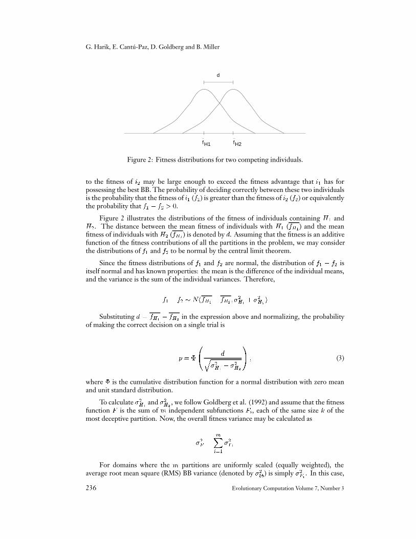
Figure 2: Fitness distributions for two competing individuals.

to the fitness of i2 may be large enough to exceed the fitness advantage that i1 has forpossessing the best BB. The probability of deciding correctly between these two individualsis the probability that the fitness of i1 (f1) is greater than the fitness of i2 (f2) or equivalentlythe probability that f1 � f2 > 0.

Figure 2 illustrates the distributions of the fitness of individuals containing H1 andH2. The distance between the mean fitness of individuals with H1 (fH1

) and the meanfitness of individuals with H2 (fH2

) is denoted by d. Assuming that the fitness is an additivefunction of the fitness contributions of all the partitions in the problem, we may considerthe distributions of f1 and f2 to be normal by the central limit theorem.

Since the fitness distributions of f1 and f2 are normal, the distribution of f1 � f2 isitself normal and has known properties: the mean is the difference of the individual means,and the variance is the sum of the individual variances. Therefore,

f1 � f2 � N(fH1� fH2

; �2H1+ �2H2

)

Substituting d = fH1� fH2

in the expression above and normalizing, the probabilityof making the correct decision on a single trial is

p = �

0@ dq

�2H1+ �2H2

1A ; (3)

where � is the cumulative distribution function for a normal distribution with zero meanand unit standard distribution.

To calculate �2H1and �2H2

, we follow Goldberg et al. (1992) and assume that the fitnessfunction F is the sum of m independent subfunctions Fi, each of the same size k of themost deceptive partition. Now, the overall fitness variance may be calculated as

�2F =

mXi=1

�2Fi

For domains where the m partitions are uniformly scaled (equally weighted), theaverage root mean square (RMS) BB variance (denoted by �2bb) is simply �2Fi . In this case,



x=n/2^kx=0 x=n

pq

Figure 3: The bounded one-dimensional space of the gambler’s ruin problem.

the total noise coming from the m0 = m � 1 partitions that are not competing directly is�2 = m0�2bb. Therefore, the probability of making the right choice in a single trial in aproblem with m independent and equally-scaled partitions becomes

p = �

�dp

2m0�bb

�(4)

Goldberg et al. (1992) used this probability to create the first model relating the size ofthe population with the quality of decisions. Their model showed how to incorporate theeffect of the collateral noise into the population-sizing question, and their paper describeshow to estimate the parameters necessary to calculate p. In the next section, the knowledgeabout noise and decision-making at the BB level is unified with the estimate of the initialsupply of BBs.

4 The Gambler’s Ruin Model

The gambler’s ruin problem is a classical example of random walks, which are mathematicaltools used to predict the outcome of certain stochastic processes. The most basic randomwalk deals with a particle that moves randomly on a one-dimensional space. The probabilitythat the particle moves to the left or to the right is known, and it remains constant for theentire experiment. The size of the step is also constant, and sometimes the movement ofthe particle is restricted by placing barriers at some points in the space. For our purposes,we consider a one-dimensional space bounded by two absorbing barriers that capture theparticle once it reaches them.

In the gambler’s ruin problem, the capital of a gambler is represented by the position,x, of a particle on a one-dimensional space, as depicted in Figure 3. Initially, the particle ispositioned at x0 = a where a represents the gambler’s starting capital. The gambler playsagainst an opponent that has an initial capital of n� a, and there are absorbing boundariesat x = 0 (representing bankruptcy) and at x = n (representing winning all the opponent’smoney). At each step in the game, the gambler has a chance p of increasing his capital byone unit and a probability q = 1� p of loosing one unit. The object of the game is to reachthe boundary at x = n, and the probability of success depends on the initial capital and onthe probability of winning a particular trial.

The analogy between selection in GAs and the gambler’s ruin problem appears naturallyif we assume that partitions are independent and we concentrate on only one of them. Theparticle’s position on the one-dimensional space, x, represents the number of copies ofthe correct BBs in the population. The absorbing barriers at x = 0 and x = n represent



convergence to the wrong and right solutions, respectively. The initial position of theparticle, x0, is the expected number of copies of the BB in a randomly initialized population,which in a binary domain and considering BBs of order k is x0 = n

2k.

There are a number of assumptions that we need to make to use the gambler’s ruinproblem to predict the quality of the solutions of the GA. First, the gambler’s ruin modelconsiders that decisions in a GA occur one at a time until all then individuals in its populationconverge to the same value. In other words, in the model there is no explicit notion ofgenerations, and the outcome of each decision is to win or lose one copy of the optimal BB.Assuming conservatively that all competitions occur between strings that represent the bestand the second best BBs in a partition, the probability of gaining a copy of the global BBis given by the correct decision-making probability p, which was calculated in the previoussection for additively-decomposable fitness functions (see Equation 4).

The calculation of p implicitly assumes that the GA uses pairwise tournament selection(two strings compete), but adjustments for other selection schemes are possible, as we seein a later section. The analogy between GAs and the gambler’s ruin problem also assumesthat the only source of BBs is the random initialization of the population. This assumptionimplies that mutation and crossover do not create or destroy significant numbers of BBs.The boundaries of the random walk are absorbing; this means that once a partition containsn copies of the correct BB it cannot lose one, and likewise, when the correct BB disappearsfrom a partition there is no way of recovering it. We recognize that this is a simplification,but experimental results suggest that is it a reasonable one.

As we discussed above, the GA succeeds when there are n copies of the correct BBin the partition of interest. A well-known result in the random walk literature is that theprobability that the particle will eventually be captured by the absorbing barrier at x = n is:

Pbb =1��qp

�x01��qp

�n ; (5)

where q = 1 � p is the probability of losing a copy of the BB in a particular competi-tion (Feller, 1966). From this equation, it is relatively easy to find an expression for thepopulation size. First, note p > 1 � p (because the mean fitness of the best BB is greaterthan the mean fitness of the second best), and x0 is usually small compared to the populationsize. Therefore, for increasing values of n, the denominator in Equation 5 approaches 1very quickly and can be ignored in the calculations. Substituting the initial supply of BBs(x0 = n=2k), Pbb may be approximated as

Pbb � 1��1� p

p

�n=2k(6)

Since we assume that the BBs are independent of each other, the expected number ofpartitions with the correct BB at the end of a run is E(BBs) = mPbb. Assuming that weare interested in finding a solution with an average of Q BBs correct, we can solve Pbb = Q

m

for n to obtain the following population sizing equation:



n =2k ln(�)

ln�1�pp

� ; (7)

where � = 1 � Qm

is the probability of GA failure. To observe more clearly the relationsbetween the population size and the domain-dependent variables involved, we may expandp and write the last equation in terms of the signal (d), the noise (�bb), and the number ofpartitions in the problem (m). First, approximate p using the first two terms of the powerseries expansion for the normal distribution as:

p =1

2+

1p2�

z;

where z = d=(�bbp2m0) (Abramowitz and Stegun, 1972). Substituting this approximation

for p into Equation 7 results in

n = 2k ln(�)= ln

0@1� z

p2p�

1 + zp2p�

1A (8)

Since z tends to be a small number, ln(1� zp2p�) may be approximated as� z

p2p�

. Usingthese approximations and substituting the value of z into the equation above gives

n = �2k�1 ln(�)�bbp�m0

d(9)

This rough approximation makes more clear the relations between some of the variablesthat determine when a problem is harder than others. It quantifies many intuitive notionsthat practitioners have about problem difficulty for GAs. For example, problems with longBBs (large k) are more difficult to solve than problems with short BBs, because long BBsare scarcer in a randomly initialized population. The equation shows that the requiredpopulation size is inversely proportional to the signal-to-noise ratio. Problems with a highvariability are hard because it is difficult to detect the signal coming from the good solutionswhen the interference from not-so-good solutions is high. Longer problems (larger m) aremore difficult than problems with a few partitions because there are more sources of noise.However, the GA scales very well to the problem size; the equation shows that the requiredpopulation grows with the square root of the size of the problem.

5 Experimental Verification

This section verifies that the gambler’s ruin model accurately predicts the quality of thesolutions reached by simple GAs. The experiments reported in this section use test functionsof varying difficulty. First, a simple one-max function is used, and later the experimentsuse fully deceptive trap functions. The population sizes required to solve the test problemsvary from a few tens to a few thousands, demonstrating that the predictions of the modelscale well to problem difficulty.



20 40 60 80 100 Pop Size

0.6

0.7

0.8

0.9

1Proportion BBs

Figure 4: Experimental and theoretical results of the proportion of correct BBs on a 100-bitone max function. The prediction of the gambler’s ruin model (Equation 5) is in bold, theexperimental results are the dotted line, and the previous decision-based model is the thinline.

All the results in this paper are the average over 100 independent runs of a simplegenerational GA. The GA uses pairwise tournament selection without replacement. Thecrossover operator was chosen according to the order of the BBs of each problem and isspecified in each subsection below. In all the experiments, the mutation probability is setto zero, because the model considers that the only source of diversity is the initial randompopulation. Also, mutation would make it possible to escape the absorbing boundaries ofthe random walk. Each run was terminated when the population had converged completely(which is possible because the mutation rate is zero), and we report the percentage ofpartitions that converged to the correct value. The theoretical predictions of the gambler’sruin model were calculated using Equation 5.

5.1 One-max

The one-max problem is one of the most frequently used fitness function in genetic algo-rithms research because of its simplicity. The fitness of an individual is equal to the numberof bits set to one in its chromosome. This is an easy problem for GAs since there is noisolation or deception and the BBs are short. The supply of BBs is no problem either,because a randomly initialized population has on average 50% of the correct BBs.

In this function the order of the BBs is k = 1. The fitness difference is d = 1 becausea correct partition contributes one to the fitness and an incorrect partition contributesnothing. The variance may be calculated as �2bb = (1 � 0)=4 = 0:25 (see Goldberg et al.(1992) for a discussion on how to approximate or bound �2bb). The first set of experimentsconsiders strings with 100 bits, so m = 100. Substituting these values into Equation 4 givesthe probability of choosing correctly between two competing BBs as p = 0:5565.

Since the length of the BBs is one, crossover cannot disrupt them, and uniformcrossover was chosen for this function as it mixes BBs quite effectively. The probabil-ity of exchanging each bit was set to 0.5.

In Figure 4 the bold line is the theoretical prediction of the gambler’s ruin model(Equation 5) and the dotted line is the experimental results for a 100-bit function. The thin



20 40 60 80 100 Pop Size

0.6

0.7

0.8

0.9

1Proportion BBs

Figure 5: Experimental and theoretical results of the proportion of correct BBs on a 500-bitone-max function. The bold line is the prediction of the gambler’s ruin model (Equation 5),the dotted line is the experimental results, and the thin line is the previous decision-onlymodel.

line in the figure is the theoretical prediction of the population sizing model of Goldberget al. (1992). The results of a second set of experiments with a 500-bit onemax problem(p = 0:5252) are shown in Figure 5.

The gambler’s ruin model predicts the outcome of the experiments for the 100 and500-bit functions quite accurately. However, in the 500-bit function the match is not asclose as in the 100-bit case. The reason for this small discrepancy may be that the theoryonly considers one partition at a time and that decisions for one partition are independentof all the others. In order to achieve this independence, crossover must distribute BBscompletely at random across all the individuals in the population. The goal of crossover inthis case is to smooth the distribution of BBs in the different alleles to avoid hitchhiking.However, it would not be practical to reach this perfect distribution, because many roundsof crossover would be necessary in every generation.

5.2 Scaled Problems

The next set of experiments tests the predictions of the model on scaled subfunctions. Thefitness function is similar to a one-max except that the contribution of every tenth bit to thefitness is reduced. In particular, the first scaled function is

Fsc =

mXi=0

cixi;

where xi 2 f0; 1g, and ci = 0:8 when i 2 f0; 10; 20; :::; 90g and ci = 1 otherwise.

The signal of the scaled partitions is smaller than before (d = 0:8), and the noiseis reduced slightly (�2bb = 0:245). The reduction of the signal makes it harder to decidecorrectly between the right and wrong BBs, and therefore larger populations are requiredto reach the correct solution (in this case p = 0:5457). The parameters for the experimentsare the same as for the one-max functions, but the results reported are the proportion ofbadly scaled bits that converged correctly. The stronger bits converge more easily, andincluding them in the results would paint an overly optimistic picture.



0.4 0.6 0.8 1Signal

0.6

0.7

0.8

0.9

1Proportion BBs

(a) n = 20

0.4 0.6 0.8 1Signal

0.6

0.7

0.8

0.9

1Proportion BBs

(b) n = 40

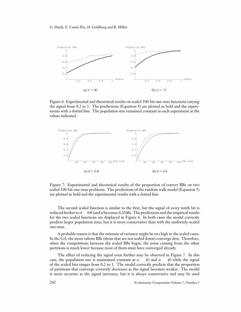
Figure 6: Experimental and theoretical results on scaled 100-bit one-max functions varyingthe signal from 0.2 to 1. The predictions (Equation 5) are plotted in bold and the experi-ments with a dotted line. The population size remained constant in each experiment at thevalues indicated.

20 40 60 80 100 Pop size

0.6

0.7

0.8

0.9

1Proportion BBs

(a) d = 0:8

20 40 60 80 100 Pop size

0.6

0.7

0.8

0.9

1Proportion BBs

(b) d = 0:6

Figure 7: Experimental and theoretical results of the proportion of correct BBs on twoscaled 100-bit one-max problems. The predictions of the random walk model (Equation 5)are plotted in bold and the experimental results with a dotted line.

The second scaled function is similar to the first, but the signal of every tenth bit isreduced further tod = 0:6 (and p becomes 0:5346). The predictions and the empirical resultsfor the two scaled functions are displayed in Figure 6. In both cases the model correctlypredicts larger population sizes, but it is more conservative than with the uniformly-scaledone-max.

A probable reason is that the estimate of variance might be too high in the scaled cases.In the GA, the more salient BBs (those that are not scaled down) converge first. Therefore,when the competitions between the scaled BBs begin, the noise coming from the otherpartitions is much lower because most of them must have converged already.

The effect of reducing the signal even further may be observed in Figure 7. In thiscase, the population size is maintained constant at n = 20 and n = 40 while the signalof the scaled bits ranges from 0.2 to 1. The model correctly predicts that the proportionof partitions that converge correctly decreases as the signal becomes weaker. The modelis more accurate as the signal increases, but it is always conservative and may be used



1 2 3 4Ones

1

2

3

4

Fitness

Figure 8: A 4-bit deceptive function of unity.

confidently to determine the population size required to find the desired solution.

5.3 Deceptive Functions

The next three sets of experiments use deceptive trap functions. Fully deceptive trapfunctions are used in many studies of GAs because their difficulty is well understood andthey can be regulated easily (Deb and Goldberg, 1993).

Trap functions are hard for traditional optimizers because they will tend to climb to thedeceptive peak, but GAs with properly sized populations can solve them satisfactorily. Weexpect to use larger population sizes than before to solve these functions for two reasons:(1) the BBs are much scarcer in the initial population because they are longer; and (2) thesignal to noise ratio is lower, making the decision between the best and the second best BBsmore difficult.

To solve the trap functions, tight linkage was used (i.e., the bits that define the trap func-tion are next to each other in the chromosome), although there are algorithms such as themessy GA (Goldberg and Bridges, 1990) and its relatives (Goldberg et al., 1993; Kargupta,1996; Harik and Goldberg, 1996) that are able to find tight linkages autonomously.

The first deceptive test function is based on the 4-bit trap function depicted in Figure 8,which was also used by Goldberg et al. (1992) in their study of population sizing. As inthe one-max, the value of this function depends on the number of bits set to one, but inthis case the fitness increases with more bits set to zero until it reaches a local (deceptive)optimum. The global maximum of the function occurs precisely at the opposite extremewhere all four bits are set to one, so an algorithm cannot use any partial information to findit. The signal difference d (the difference between the global and the deceptive maxima)is 1 and the fitness variance (�2bb) is 1.215. The test function is formed by concatenatingm = 20 copies of the trap function for a total string length of 80 bits. The probability ofmaking the right decision between two individuals with the best and the second best BBsis p = 0:5585. The experiments with this function use two-point crossover to avoid theexcessive disruption that uniform crossover would cause on the longer BBs. The crossoverprobability is set to 1.0 and, as before, there is no mutation.

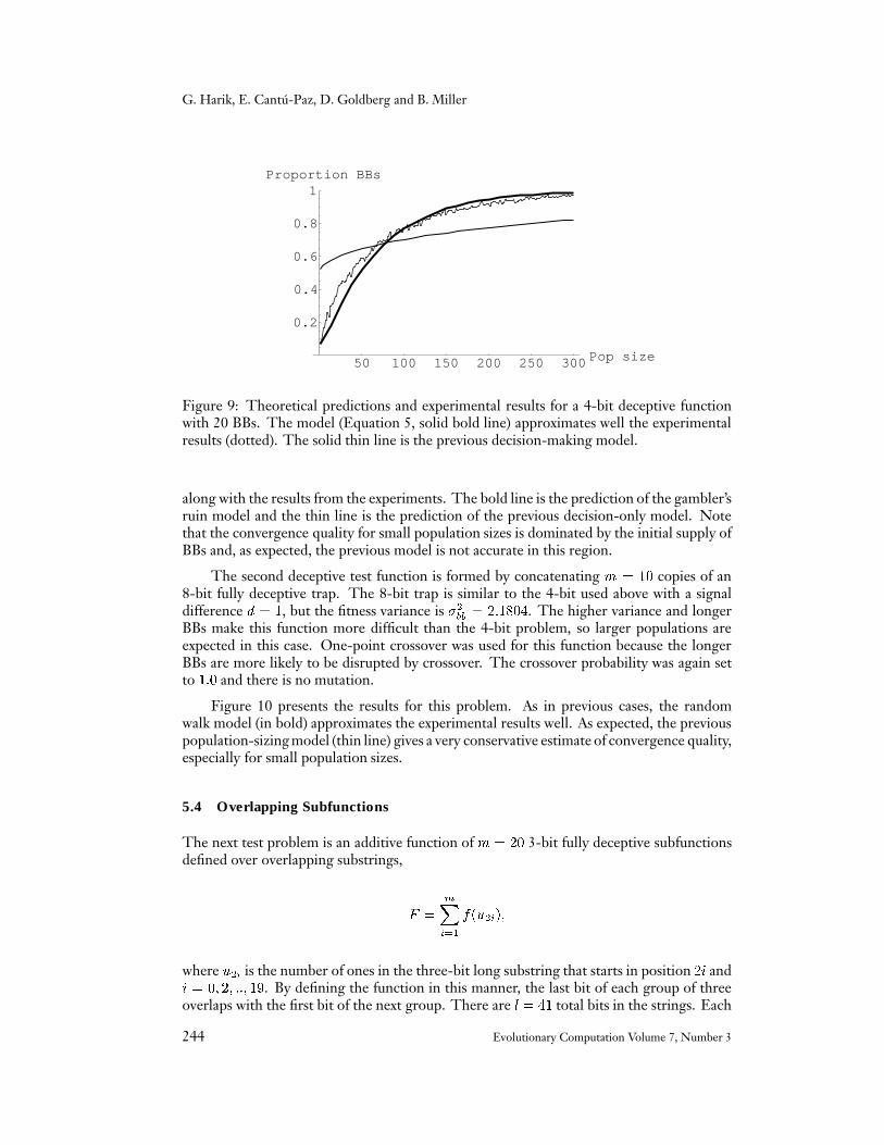
Figure 9 presents the prediction of the percentage of BBs correct at the end of the run



50 100 150 200 250 300 Pop size

0.2

0.4

0.6

0.8

1Proportion BBs

Figure 9: Theoretical predictions and experimental results for a 4-bit deceptive functionwith 20 BBs. The model (Equation 5, solid bold line) approximates well the experimentalresults (dotted). The solid thin line is the previous decision-making model.

along with the results from the experiments. The bold line is the prediction of the gambler’sruin model and the thin line is the prediction of the previous decision-only model. Notethat the convergence quality for small population sizes is dominated by the initial supply ofBBs and, as expected, the previous model is not accurate in this region.

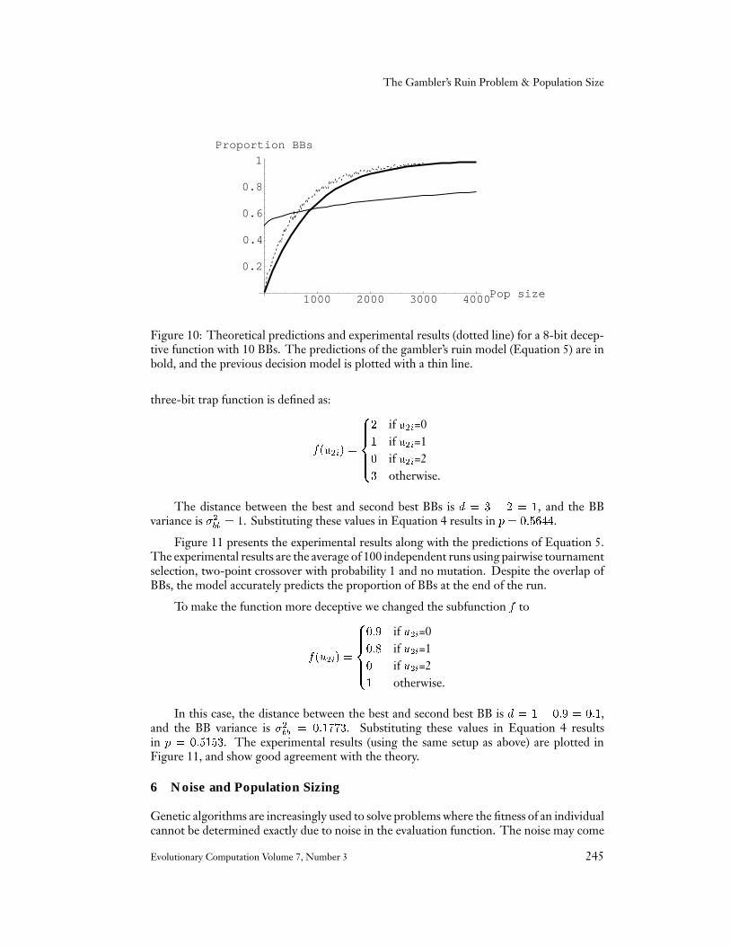
The second deceptive test function is formed by concatenating m = 10 copies of an8-bit fully deceptive trap. The 8-bit trap is similar to the 4-bit used above with a signaldifference d = 1, but the fitness variance is �2bb = 2:1804. The higher variance and longerBBs make this function more difficult than the 4-bit problem, so larger populations areexpected in this case. One-point crossover was used for this function because the longerBBs are more likely to be disrupted by crossover. The crossover probability was again setto 1:0 and there is no mutation.

Figure 10 presents the results for this problem. As in previous cases, the randomwalk model (in bold) approximates the experimental results well. As expected, the previouspopulation-sizing model (thin line) gives a very conservative estimate of convergence quality,especially for small population sizes.

5.4 Overlapping Subfunctions

The next test problem is an additive function of m = 20 3-bit fully deceptive subfunctionsdefined over overlapping substrings,

F =

mXi=1

f(u2i);

where u2i is the number of ones in the three-bit long substring that starts in position 2i andi = 0; 2; ::; 19. By defining the function in this manner, the last bit of each group of threeoverlaps with the first bit of the next group. There are l = 41 total bits in the strings. Each



1000 2000 3000 4000Pop size

0.2

0.4

0.6

0.8

1

Proportion BBs

Figure 10: Theoretical predictions and experimental results (dotted line) for a 8-bit decep-tive function with 10 BBs. The predictions of the gambler’s ruin model (Equation 5) are inbold, and the previous decision model is plotted with a thin line.

three-bit trap function is defined as:

f(u2i) =

8>>><>>>:

2 if u2i=01 if u2i=10 if u2i=23 otherwise.

The distance between the best and second best BBs is d = 3 � 2 = 1, and the BBvariance is �2bb = 1. Substituting these values in Equation 4 results in p = 0:5644.

Figure 11 presents the experimental results along with the predictions of Equation 5.The experimental results are the average of 100 independent runs using pairwise tournamentselection, two-point crossover with probability 1 and no mutation. Despite the overlap ofBBs, the model accurately predicts the proportion of BBs at the end of the run.

To make the function more deceptive we changed the subfunction f to

f(u2i) =

8>>><>>>:

0:9 if u2i=00:8 if u2i=10 if u2i=21 otherwise.

In this case, the distance between the best and second best BB is d = 1 � 0:9 = 0:1,and the BB variance is �2bb = 0:1773. Substituting these values in Equation 4 resultsin p = 0:5153. The experimental results (using the same setup as above) are plotted inFigure 11, and show good agreement with the theory.

6 Noise and Population Sizing

Genetic algorithms are increasingly used to solve problems where the fitness of an individualcannot be determined exactly due to noise in the evaluation function. The noise may come



100 200 300 400 500Pop size

0.2

0.4

0.6

0.8

1Proportion BBs

(a) d = 1

100 200 300 400 500Pop size

0.2

0.4

0.6

0.8

1Proportion BBs

(b) d = 0:1

Figure 11: Experimental and theoretical results of the proportion of correct BBs on afunction with overlapping 3-bit traps. The solid line plots the predictions of the randomwalk model (Equation 5) and the experimental results are plotted with the dotted line.

from an inherently noisy domain or from a noisy approximation of an excessively expensivefitness function. This section examines how this explicit fitness noise affects the size of thepopulation.

Following Goldberg et al. (1992) the noisy fitness F 0 of an individual may be modeledas

F 0 = F +N;

where F is the true fitness of an individual and N is the noise present in the evaluation.The effect of the added noise is to increase the fitness variance of the population, makingit more difficult to choose correctly between two competing individuals. Therefore, theone-on-one decision-making probability (Equation 4) has to be modified to include theeffect of explicit noise; then, it may be used to find the required population size as was donein Section 4.

Assuming that the noise is normally distributed as N(0; �2N ), the fitness variance be-comes �2F+�

2

N . Therefore, the probability of choosing correctly between an individual withthe optimal building block and an individual with the second best BB in a noisy environmentis

p = �

�dq

�2H1+ �2H2

+ 2�2N

�

In the case of uniformly scaled problems, this becomes (Miller, 1997):

p = �

�dp

2(m0�2bb + �2N )

�(10)

Using this form of p and the same procedure used to obtain Equation 9 results in thefollowing population sizing equation for noisy domains:

n = �2k�1 ln(�)p�m0�2bb + �2N

d(11)



The one-max domain was used to test the predictions of the gambler’s ruin model(Equation 5) using the decision probability given by Equation 10. The experiments con-sidered a 100-bit problem and used the same GA as the previous one-max experiments(pairwise tournament selection, uniform crossover and no mutation).

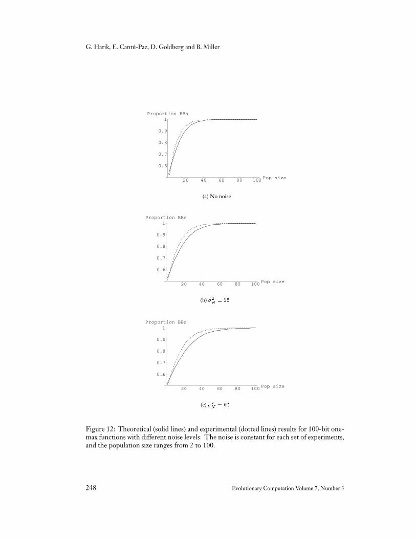
For this function, the fitness variance is �2F = m�2bb = 25, and the experiments wererun for �2N values of �2F � (0; 1; 2). Figure 12 displays the average proportion of partitionsthat converge correctly (taken over 100 independent runs at each population size) for eachnoise level. Note that the experiments with �F = 0 are equivalent to those presented inFigure 4, and are included here to facilitate comparisons.

The effect of increasing the noise in the quality of convergence may be observed veryclearly in Figure 13. In this set of experiments, the population size was held constant atn = 20 and n = 40 while the noise increased. The gambler’s ruin model correctly predictsthat additional noise causes the GA to reach solutions of lower quality, and although thepredictions are not exact, the model is conservative and may be used as a guideline tocalculate the required population size.

7 Effect of the Selection Type

Besides the population size, an important factor in the convergence quality of GAs is theselection scheme. After all, the selection mechanism is the part of the GA making thedecisions we have discussed in the previous sections. The goal of any selection method is tofavor the proliferation of good individuals in the population. However, selection methodsdiffer in how much pressure they exert on the population.

Muhlenbein and Schlierkamp-Voosen (1993) introduced the concept of selection inten-sity to measure the pressure of selection schemes. The selection intensity is the expectedaverage fitness of the population after selection. The selection pressure of tournamentselection increases as the tournament size, s, becomes larger. Only tournament selection isconsidered here, but the results can be extrapolated to other selection methods with knownconstant selection intensities (see Back, 1994; Miller and Goldberg, 1996). A differentanalysis would be necessary for schemes such as proportional selection that do not have aconstant selection pressure.

Assume conservatively that the correct BB competes against s� 1 copies of the secondbest BB. As larger tournaments are considered, the probability of making the wrong decisionincreases proportionately to s; thus, we approximate the probability of making the rightdecision as 1=s. In reality, this probability is higher than 1=s since a tournament mightinvolve more than one copy of the best BB—especially as the run progresses and theproportion of correct BBs increases. However, 1=s is a good initial approximation as theexperiments suggest.

The increasing difficulty of decision-making as the tournament size increases can beaccounted for as a contraction in the signal that the GA is trying to detect. Setting the newsignal to

d0 = d+��1�1

s

��bb; (12)

where ��1(1=s) is the ordinate of a unit normal distribution where the CDF equals 1=s,



20 40 60 80 100 Pop size

0.6

0.7

0.8

0.9

1Proportion BBs

(a) No noise

20 40 60 80 100 Pop size

0.6

0.7

0.8

0.9

1Proportion BBs

(b) �2N

= 25

20 40 60 80 100 Pop size

0.6

0.7

0.8

0.9

1Proportion BBs

(c) �2N

= 50

Figure 12: Theoretical (solid lines) and experimental (dotted lines) results for 100-bit one-max functions with different noise levels. The noise is constant for each set of experiments,and the population size ranges from 2 to 100.



20 40 60 80 100Noise

0.6

0.7

0.8

0.9

1Proportion BBs

(a) n = 20

20 40 60 80 100Noise

0.6

0.7

0.8

0.9

1Proportion BBs

(b) n = 40

Figure 13: Theoretical (solid lines) and experimental (dotted lines) results for 100-bit one-max functions varying the noise levels from �2N = 0 to 100. The population size remainedconstant for each set of experiments at the values indicated.



20 40 60 80 100 Pop size

0.6

0.7

0.8

0.9

1Proportion BBs

Figure 14: Predictions and experimental results for a 100-bit one-max function varying theselection intensity. From left to right: s = 2; 4; 8.

we can compute a new probability of deciding well using d0 instead of d in Equation 4.

Experiments were performed using a 100-bit one-max function and tournament sizesof 2, 4, and 8. The experimental results are plotted in Figure 14 with dotted lines alongwith the theoretical predictions obtained with Equation 5 using the appropriate value of pfor each case. The leftmost plot corresponds to a tournament size s = 2, the next to s = 4,and the rightmost to s = 8. Once again, the model is a good predictor of the proportion ofBBs correct at the end of the run.

8 Extensions

The gambler’s ruin model integrates two facets that influence the convergence of GAs: theinitial supply of BBs (x0) and correct decision making between competing BBs (p). Thesuccess of the integration of two facetwise models is evidence that the divide-and-conquerstrategy can have good results. Following this notion of integrating small models, theresults of this paper may be extended to include other facets of GA efficiency. Previoussections hinted at some possible extensions; here they are treated in more detail and otherpossibilities are presented.

Probably the most important extension to the model is to incorporate the effects ofcrossover and mutation. In its current state, the model assumes that all the BBs in a stringare independent of each other and that the correct BBs are evenly distributed along thewhole population. This assumption implies that BBs are mixed properly and that stringshave on average the same number of correct BBs. In reality, some strings may contain morecopies of the correct BB and they may reproduce faster, impeding the crossover operator tomix the BBs evenly.

Furthermore, crossover presents a tradeoff: we want to distribute BBs throughout thepopulation, but we do not want to disrupt those BBs that have been found already. Moreaggressive crossover operators (e.g., 5-point or uniform) would increase the chances thatBBs mix, but more BBs would be disrupted. We need to model both of these effects to finda balance between mixing and disruption.



Another fundamental assumption of the model is that crossover and mutation do notcreate or destroy many BBs. Extending the model to consider that BBs can be created ordestroyed by the operators implies that the boundaries of the gambler’s ruin random walkwould not be absorbing anymore. However, the idea of modeling selection in the GA as abiased random walk can still be used. Instead of calculating the probability of absorption,we may calculate the probability of hitting the barrier that denotes success (x = n) beforehitting the barrier that represents failure (x = 0).

Another extension is the sizing of populations for parallel GAs. Parallel implemen-tations are important because they open opportunities to solve harder or larger problemsthan is possible with single processors. Work is underway to quantify the effect of somerelevant parameters of parallel GAs on the size of the populations, and there are alreadysome results for cases that bound the interactions between multiple populations (Cantu-Pazand Goldberg, 1997).

9 Summary and Conclusions

This paper presented a model that permits users to determine an adequate population sizeto reach a solution of a particular quality. The model is based on an analogy between theselection mechanism of GAs and a biased random walk. The position of a particle on thebounded one-dimensional space of the random walk represents the number of copies of thecorrect BBs present in the population. The probability that the particle will be absorbedby the boundaries of the space is well known, and is used to derive an equation thatrelates the population size with the required solution quality and several domain-dependentparameters.

The accuracy of the model was verified with experiments using test problems thatranged from the very simple to the moderately hard. The results showed that the predictionsof the model are accurate for the functions tested, and that the predictions scale well withthe difficulty of the domain.

The investigation was influenced by a facetwise decomposition of GAs. This methodof integrating small models opens opportunities to develop models for other facets of GAperformance. For instance, the basic model was extended to consider non-uniformly scaledfitness functions, explicit noise in the fitness evaluation and different selection schemes.Other extensions may require different adjustments, but we have shown that the facetwisedecomposition of tasks that guided this investigation is appropriate.

Acknowledgments

The work was sponsored by the Air Force Office of Scientific Research, Air Force MaterielCommand, USAF, under grant number F49620-97-1-0050. Research funding for thisproject was also provided by a grant from the US Army Research Laboratory Program, Co-operative Agreement DAAL01-96-2-003. The US Government is authorized to reproduceand distribute reprints for governmental purposes notwithstanding any copyright notationthereon. The views and conclusions contained herein are those of the authors and shouldnot be interpreted as necessarily representing the official policies and endorsements, eitherexpressed or implied, of the Air Force Office of Scientific Research or the US Government.



Erick Cantu-Paz was partially supported by a Fulbright-Garcıa Robles Fellowship.

Brad Miller was supported by NASA under grant number NGT-9-4.

References

Abramowitz, M. and Stegun, I. (1972). Handbook of mathematical functions with formulas, graphs, andmathematical tables. Dover Publications, Mineola, New York.

Back, T. (1994). Selective pressure in evolutionary algorithms: A characterization of selection mech-anisms. In Proceedings of the First IEEE Conference on Evolutionary Computation, Volume 1, pages57–62, IEEE Service Center, Piscataway, New Jersey.

Cantu-Paz, E. and Goldberg, D. E. (1997). Modeling idealized bounding cases of parallel geneticalgorithms. In Koza, J., Deb, K., Dorigo, M., Fogel, D., Garzon, M., Iba, H. and Riolo, R.,editors, Genetic Programming 1997: Proceedings of the Second Annual Conference, pages 353–361,Morgan Kaufmann, San Francisco, California.

Cvetkovic, D. and Muhlenbein, H. (1994). The optimal population size for uniform crossover and truncationselection. Technical Report No. GMD AS GA 94-11. German National Reseach Center forComputer Science (GMD), Germany.

De Jong, K. A. (1975). An analysis of the behavior of a class of genetic adaptive systems. Doctoral dissertation,(University Microfilms No. 76-9381), Department of Computer and Communication Sciences,University of Michigan, Ann Arbor, Michigan.

Deb, K. and Goldberg, D. E. (1993). Analyzing deception in trap functions. In Whitley, L. D., editor,Foundations of Genetic Algorithms 2, pages 93–108, Morgan Kaufmann, San Mateo, California.

Feller, W. (1966). An introduction to probability theory and its applications(2nd ed.), Volume 1, John Wileyand Sons, New York, New York.

Goldberg, D. E. (1989a). Genetic algorithms in search, optimization, and machine learning. Addison-Wesley, Reading, Massachusetts.

Goldberg, D. E. (1989b). Sizing populations for serial and parallel genetic algorithms. In Schaffer,J. D., editor, Proceedings of the Third International Conference on Genetic Algorithms, pages 70–79,Morgan Kaufmann, San Mateo, California, (Also TCGA Report 88004).

Goldberg, D. E. (1996). The design of innovating machines: Lessons from genetic algorithms.Computational Methods in Applied Sciences ’96, pages 100–104.

Goldberg, D. E. and Liepins, G. (1991). A tutorial on genetic algorithm theory. A presentation givenat the Fourth International Conference on Genetic Algorithms, University of California at SanDiego, La Jolla, California.

Goldberg, D. E. and Bridges, C. L. (1990). An analysis of a reordering operator on a GA-hardproblem. Biological Cybernetics, 62:397–405, (Also TCGA Report No. 88005).

Goldberg, D. E., Deb, K. and Clark, J. H. (1992). Genetic algorithms, noise, and the sizing ofpopulations. Complex Systems, 6:333–362.

Goldberg, D. E., Deb, K., Kargupta, H. and Harik, G. (1993). Rapid, accurate optimization ofdifficult problems using fast messy genetic algorithms. In Forrest, S., editor, Proceedings of theFifth International Conference on Genetic Algorithms, pages 56–64, Morgan Kaufmann, San Mateo,California.

Goldberg, D. E. and Rudnick, M. (1991). Genetic algorithms and the variance of fitness. ComplexSystems, 5(3):265–278. (Also IlliGAL Report No. 91001).

Harik, G. R. and Goldberg, D. E. (1996). Learning linkage. In Belew, R. K. and Vose, M. D.,editors, Foundations of Genetic Algorithms 4, pages 247–262, Morgan Kaufmann, San Francisco,California.



Holland, J. H. (1973). Genetic algorithms and the optimal allocation of trials. SIAM Journal onComputing, 2(2):88–105.

Holland, J. H. (1975). Adaptation in natural and artificial systems. University of Michigan Press, AnnArbor, Michigan.

Kargupta, H. (1996). The gene expression messy genetic algorithm. In Back, T., Kitano, H. andMichalewicz, Z., editors, Proceedings of 1996 IEEE International Conference on Evolutionary Com-putation, pages 814–819, IEEE Service Center, Piscataway, New Jersey.

Miller, B. L. (1997). Noise, sampling, and efficient genetic algorithms. Doctoral dissertation, Depart-ment of Computer Science, University of Illinois at Urbana-Champaign, Urbana, Illinois. Alsoavailable as IlliGAL tech report No. 97001.

Miller, B. L. and Goldberg, D. E. (1996). Genetic algorithms, selection schemes, and the varyingeffects of noise. Evolutionary Computation, 4(2):113-131.

Muhlenbein, H. and Schlierkamp-Voosen, D. (1993). Predictive models for the breeder geneticalgorithm: I. Continuous parameter optimization. Evolutionary Computation, 1(1):25–49.

Muhlenbein, H. and Schlierkamp-Voosen, D. (1994). The science of breeding and its application tothe breeder genetic algorithm (BGA). Evolutionary Computation, 1(4):335–360.

Thierens, D. and Goldberg, D. E. (1993). Mixing in genetic algorithms. In Forrest, S., editor, Proceed-ings of the Fifth International Conference on Genetic Algorithms, pages 38–45, Morgan Kaufmann,San Mateo, California.


The Gambler's Ruin Problem, Genetic Algorithms, and the Sizing of Populations

Documents

Transcript of The Gambler's Ruin Problem, Genetic Algorithms, and the Sizing of Populations