Lot Sizing with Carbon Emission Constraints

Nabil Absia, Stephane Dauzere-Peresa, Safia Kedad-Sidhoumb, Bernard Penzc, Christophe Rapined

aDepartment of Manufacturing Sciences and Logistics, CMP - Site Georges Charpak, Ecole des Mines de Saint-Etienne, 13541 Gardanne, FrancebLaboratoire d’Informatique de Paris 6, 75252 Paris Cedex 05, France

cLaboratoire G-SCOP, Grenoble INP / UJF Grenoble 1 / CNRS, 38031 Grenoble Cedex 1, FrancedUniversite de Lorraine, Laboratoire LGIPM, ıle du Saulcy, Metz, F-57045, France

Abstract

This paper introduces new environmental constraints, namely carbon emission constraints, in multi-sourcing lot-sizingproblems. These constraints aim at limiting the carbon emission per unit of product supplied with different modes. Amode corresponds to the combination of a production facility and a transportation mode and is characterized by itseconomical costs and its unitary carbon emission. Four types of constraints are proposed and analyzed in the single-item uncapacitated lot-sizing problem. The periodic case is shown to be polynomially solvable, while the cumulative,global and rolling cases are NP-hard. Perspectives to extend this work are discussed.

Keywords: Lot sizing, carbon emission, dynamic programming, complexity

1. Introduction

Legislations are evolving in order to enforce control on carbon emissions. This will probably be done by constrain-ing companies to emit less than a given amount of carbon dioxide by product unit that is produced and transported.Along with legislation and norms, some companies may volunteer in this direction for marketing reasons and to geta competitive advantage. The amount of carbon emission will probably appear on item packages in the near future.Companies will face new constraints that will force them to reduce carbon emissions while still minimizing produc-tion and transportation costs. There are few papers addressing production planning and transportation problems thattake into account environmental constraints. Generally, environmental issues are integrated as cost components inthe objective function, and resulting problems are solved using multi-criteria approaches (see Handfield et al. (2002)and Aissaoui et al. (2007)). Note that classical cost components (production and transportation costs) have the samebehavior as environmental cost components (e.g. reducing the number of vehicles or the total distance).

One of the main objectives of green logistics is to evaluate the environmental impact of different distribution andproduction strategies to reduce the energy usage in logistics activities. Although the interests in green logistics grew inthe last decades, current logistics practices still rarely comply with environmental constraints. One of the objectives ofthe Kyoto protocol is to stabilize and then reduce greenhouse gas emissions in order to limit global warming. Carbondioxide being one of the most important greenhouse gases, countries will have to reduce their carbon emissions, andwill impose companies to trim down their carbon emissions. A quota of carbon emission per company will probablybe fixed (e.g. California). As a result, some companies have already started to monitor their carbon footprint toevaluate the environmental impact of their activities. The classical production and distribution models focus on theminimization of costs subject to operational constraints. Considering green logistics objectives and constraints willlead to new problems resulting in novel combinatorial optimization models.

Green supply chain management (see Srivastava (2007)) has been extended to include green inventory modelsthat link the inventory and ordering behaviors and emissions. Sbihi and Eglese (2007) present a short state-of-the-arton green logistics and combinatorial optimization. They describe some of the problems that arise in green logistics

Email addresses: absi@emse.fr (Nabil Absi), dauzere-peres@emse.fr (Stephane Dauzere-Peres), safia.kedad-sidhoum@lip6.fr(Safia Kedad-Sidhoum), bernard.penz@grenoble-inp.fr (Bernard Penz), christophe.rapine@univ-lorraine.fr (Christophe Rapine)

Preprint submitted to Elsevier April 12, 2013

which can be formulated as combinatorial optimization problems. They focus on the topics of reverse logistics,waste management and vehicle routing and scheduling. Dekker et al. (2012) provides a recent overview of issuesand challenges in green logistics and operations research, focusing on supply chain management and design fortransportation, inventory and production. Reverse logistics is an important part of Green supply chain managementand a lot of research has been conducted in this field. Teunter et al. (2006) address this issue for lot-sizing problems,and propose two models. In the first model, they assume that manufacturing and remanufacturing operations arecarried out in the same factory. They model these operations with a joint setup cost. In the second model, they assumethat manufacturing and remanufacturing operations are done on two separate lines. Several works on the integrationof remanufacturing in a closed loop supply chain can be found in the literature (Pan et al. (2009), Li et al. (2009),Quariguasi Frota Neto et al. (2010)).

Depending on the objectives of a company, the integration of carbon emission constraints can be considered atdifferent decision levels (strategic, tactical and operational). At the strategic level, designing supply chain flows orlocating a factory or a warehouse impact green constraints and objectives (Chaabane et al. (2012), Wang et al. (2011),Pishvaee and Razmi (2011)). At the tactical level, carbon emissions can be considered in production and distributionplanning decisions. Recently, some authors (Hua et al. (2011), Bouchery et al. (2011)) study the integration of carbonemission constraints in classical inventory management models. At the operational level, carbon emission constraintscan be related to vehicle routing or production scheduling decisions (Bektas and Laporte (2011), Fang et al. (2011)).Our paper focuses on the tactical decision level of a supply chain.

There are few research works addressing the introduction of carbon emission constraints in production and/ordistribution planning models. In lot-sizing, we only found the work of Benjaafar et al. (2010) that integrates carbonemission constraints. The authors insist on the potential impact of operational decisions on carbon emissions and theneed for Operations Management research that incorporates carbon emission concerns. The authors also point outthat the contribution of operational research in this area is almost absent. Benjaafar et al. (2010) add a new capacityconstraint that links and limits all carbon emissions related to production and storage over the planning horizon. Theweakness of this constraint is that producers can create large carbon emissions at the beginning of the horizon byproducing large quantities, and balance the total carbon emission by producing nothing at the end of the horizon.

As previously mentioned, the need of companies to monitor their carbon emissions is growing. This monitoringmust be consistent with production and distribution planning models that must take into account carbon emissionconstraints. More precisely, if the monitoring of the carbon footprint is aggregated according to the type of vehiclesand their consumption, there is no need to consider more detailed information on each vehicle in production anddistribution planning models.

There are several methodologies to calculate carbon emissions (Greenhouse Gas protocol GHG (2012), ARTEMIS(2004), ECOTransIT (2012), etc.). Greenhouse Gas protocol is the most commonly used, since it is easy to use andits scope is worldwide. The unitary carbon emission of a product can be calculated using a linear function thatdepends on the traveled distance (in kilometers) and on the carbon emission of the used vehicle (in grams of CO2per kilometer). This carbon emission model is adopted in this paper where, for a given supplying mode, the carbonemission is proportional to the amount of units that are shipped. We define a supplying mode as a combination of atransportation mode (combining one or more types of vehicles) and a production facility.

In this paper, we study multi-sourcing lot-sizing problems with carbon emission constraints. These new constraintsare induced from a maximum allowed carbon dioxide emission coming from legislation, green taxes or the initiativesof companies. Contrary to Benjaafar et al. (2010), where a global limit of carbon emission is studied, we consider amaximum environmental impact allowed on average per item. We study four types of carbon emission constraints:(1) Periodic carbon emission constraints, (2) Cumulative carbon emission constraints, (3) Global carbon emissionconstraint and (4) Rolling carbon emission constraints. The global carbon emission constraint has similar drawbacksas the constraint introduced in (Benjaafar et al., 2010).

The main contribution of this paper is twofold. First, we propose new lot-sizing models that take into accountdifferent carbon emission constraints. Second, we determine the complexity status of these new models. We proposea polynomial dynamic programming algorithm for the problem with periodic carbon emission constraint, and showthat the three other problems are NP-hard. The outline of the paper is as follows. In Section 2, we provide differentmathematical formulations to model the four types of carbon emission constraints. In Section 3, we show that theuncapacitated multi-sourcing lot-sizing problem with the periodic carbon emission constraint can be solved using apolynomial dynamic programming algorithm. In Sections 4 and 5, we show that the uncapacitated multi-sourcing lot-

2

sizing problem with the cumulative carbon emission constraint, global carbon emission constraint or rolling carbonemission constraint is NP-hard. We conclude and discuss some perspectives of this work in Section 6.

2. Mathematical programming models

Consider a multi-sourcing lot-sizing problem faced by a company that must determine, over a planning horizonof T periods, when, where and how much to produce of an item to satisfy a deterministic time-dependent demand.Different production locations and transportation modes are available to satisfy a given demand. Let us consider Mdifferent supplying modes, where a mode corresponds to the combination of a production facility and a transportationmode. To each mode are associated classical (fixed and variable) supplying costs together with an environmentalimpact modeling the carbon emission of the mode. As previously discussed, we assume that this carbon emission isproportional to the amount of units supplied with the mode, and can be expressed as a unitary environmental impact.We study four types of carbon emission constraints: (1) Periodic carbon emission constraint, (2) Cumulative carbonemission constraint, (3) Global carbon emission constraint and (4) Rolling carbon emission constraint. We shall seethat the first and third constraint types are actually special cases of the fourth one. To model these new constraints, wedefine the following parameters and variables.Parameters:dt: Demand at period t,ht(s): Cost of holding s units at the end of period t,pm

t : Unitary supplying cost of mode m at period t,f mt : Supplying setup cost of mode m in period t,

emt : Environmental impact (carbon emission) related to supplying one unit using mode m at period t,

Emaxt : Maximum unitary environmental impact allowed at period t.

Variablesxm

t : Quantity supplied at period t using mode m,ym

t : Binary variable which is equal to 1 if mode m is used at period t, and 0 otherwise,st: Inventory carried from period t to period t + 1.

Note that Emaxt depends on period t, since carbon emissions will probably be forced to be decreased by stages

and not to a specific level right away. The variations of Emaxt depend on the level (strategic, tactical or operational)

at which the lot-sizing models are used. We consider in the following either the stationary case or the general casewithout any assumption on the time dependency of Emax. The classical formulation for the multi-sourcing lot-sizingproblem, without carbon emission constraint, is given below:

minM∑

m=1

T∑t=1

(pmt xm

t + f mt ym

t ) +

T∑t=1

ht(st) (1)

s.t.∑M

m=1 xmt − st + st−1 = dt t = 1, . . . ,T (2)

xmt ≤

(∑Tt′=t dt′

)ym

t t = 1, . . . ,T,m = 1, . . . ,M (3)xm

t ∈ R+, ymt ∈ {0, 1} t = 1, . . . ,T,m = 1, . . . ,M (4)

st ∈ R+, t = 1, . . . ,T

The objective function (1) minimizes the fixed and variable production and transportation costs and holding costs.Constraint (2) models flow conservation, and Constraint (3) ensures that no item can be supplied with mode m atperiod t if this mode is not selected. We add to this formulation the carbon emission constraint (6), (7), (9) or (10),introduced in the following sections.

2.1. Periodic carbon emission constraint

This constraint is very tight, and assumes that the amount of carbon emission that is not used in a given periodis lost. This constraint is useful if the company must ensure that it meets periodically its carbon emission objectives,

3

and can be formulated as follows: ∑Mm=1 em

t xmt∑M

m=1 xmt

≤ Emaxt , t = 1, . . . ,T. (5)

This constraint forces the average amount of carbon emission at any period t to be lower or equal than the maxi-mum unitary environmental impact allowed. This constraint can be rewritten:

M∑m=1

(emt − Emax

t )xmt ≤ 0, t = 1, . . . ,T. (6)

At first sight, Constraint (6) looks like a capacity constraint but is actually very different, since the coefficients(em

t −Emaxt ) of the xm

t variables in Constraint (6) can be positive or negative. This creates a compensation phenomenon,with no limitation on the quantity which can be ordered. Note that, in any feasible solution, at least one mode with anon-positive coefficient must be chosen if a positive quantity is ordered. To ensure feasibility, we assume that, for afirst demand occurring at period t, there is at least one mode m such that em

t′ ≤ Emaxt′ in some period t′ ≤ t.

2.2. Cumulative carbon emission constraint

Constraint (7) below is weaker than Constraint (6). The amount of unused carbon emission of a given period canbe used in future periods without exceeding the cumulative capacities.

t∑t′=1

M∑m=1

(emt′ − Emax

t′ )xmt′ ≤ 0, t = 1, . . . ,T. (7)

This constraint can be modeled using inventory variables Jt (with Jt ≥ 0 and J0 = 0), representing the amount ofunused carbon emission that can be used in future periods.

Jt = Jt−1 −

M∑m=1

(emt − Emax

t )xmt , t = 1, . . . ,T. (8)

2.3. Global carbon emission constraint

This constraint extends Constraint (7) on the whole horizon, and is thus weaker. In Constraint (9), the unitarycarbon emission over the whole horizon cannot be larger than the maximum unitary environmental impact allowed.In this case, the maximum unitary environmental impact Emax

t does no longer depend on the horizon and is stationary,i.e. Emax

t = Emax ∀t = 1, . . . ,T .

T∑t=1

M∑m=1

(emt − Emax)xm

t ≤ 0. (9)

One of the main limitations of Constraint (9) is that the solution strongly depends on the horizon length T . Gen-erally speaking, this constraint has similar drawbacks, discussed in Section 1, as the ones of the constraint introducedin (Benjaafar et al., 2010).

2.4. Rolling carbon emission constraint

Constraint (7) assumes, at each period t, that the horizon from 1 to t can be used to compensate carbon emissionsbetween periods. In Constraint (10) below, we suppose that this is only possible on a rolling horizon of R periods.This seems more realistic, and makes the problem less dependent on the planning horizon T . Note that the periodic

4

carbon emission constraint (6) is equivalent to Constraint (10) when R = 1, and that the global emission constraint (9)is equivalent to Constraint (10) when R = T .

t∑t′=t−R+1

M∑m=1

(emt′ − Emax

t′ )xmt′ ≤ 0, t = R, . . . ,T. (10)

Inventory variables Jt can still be used, but constraints on perishable inventories must be introduced, since unusedcarbon emission in period t cannot compensate carbon emission in periods after t + R.

3. The uncapacitated single-item lot-sizing problem with the periodic carbon emission constraint

We want to establish that the multi-sourcing Uncapacitated Lot-Sizing problem with the Periodic Carbon emissionconstraint (ULS-PC) problem can be solved in polynomial time. More precisely, we show that we can reformulate theULS-PC problem as a standard lot-sizing problem, i.e. without carbon emission constraints, using a pre-computationstep in O(M2T ). Thus, standard lot-sizing combinatorial algorithms can be used to solve the problem.

3.1. ULS-PC problem analysis

Recall that the periodic carbon emission constraint (6) ensures that, in each period t, the average amount of carbonemission per product ordered does not exceed the impact limit Emax

t . For the sake of conciseness, we denote byem

t the value (emt − Emax

t ), and a mode m is called ecological in period t if emt ≤ 0. For a period t, we denote by

Ft = {m ∈ 1, . . . ,M|emt ≤ 0} the subset of its ecological modes. The following dominance properties can be stated.

Property 1 Consider a solution of the ULS-PC problem using two modes m1 and m2 in a given period t. If pm1t ≤ pm2

tand em1

t ≤ em2t , then mode m1 dominates mode m2 (i.e. a solution using modes m1 and m2 can be improved by removing

the quantity xm2t produced using mode m2 and by producing xm2

t using mode m1).

Property 2 Any solution of the ULS-PC problem uses at least one ecological mode in each period with an order, i.e.∑Tm=1 xm

t > 0 ⇒∑

m∈Ftxm

t > 0.

Proof: The proof is straightforward, since a solution with an order in a given period t, i.e. xmt > 0, and which does

not contain a mode m′ such that em′t ≤ Emax

t cannot be feasible since Constraint (6) is violated. �

Theorem 1 There exists an optimal solution for the ULS-PC problem that uses at most two modes in each period:One ecological mode and possibly one non-ecological mode.

Proof: Let us introduce variables Xt =∑

m xmt , representing the total amount of products ordered at period t in a solu-

tion. The ULS-PC problem decomposes, using a Bender’s approach, into a master problem (MP) and T independentsubproblems IPt(Xt), with:

(MP)

min

T∑t=1

z∗t (Xt) +

T∑t=1

ht(st)

s.t. Xt − st + st−1 = dt t = 1, . . . ,TXt = 0 t = 1, . . . ,T such that Ft = ∅

Xt ∈ R+ t = 1, . . . ,T

5

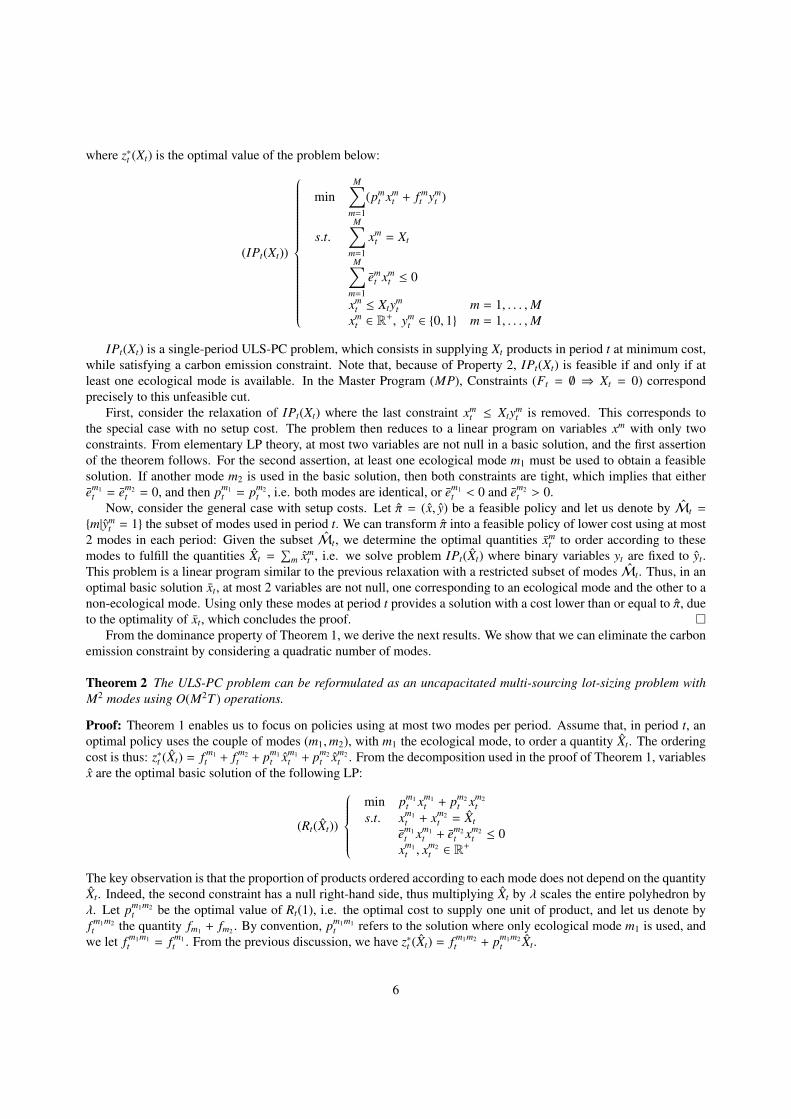
where z∗t (Xt) is the optimal value of the problem below:

(IPt(Xt))

minM∑

m=1

(pmt xm

t + f mt ym

t )

s.t.M∑

m=1

xmt = Xt

M∑m=1

emt xm

t ≤ 0

xmt ≤ Xtym

t m = 1, . . . ,Mxm

t ∈ R+, ymt ∈ {0, 1} m = 1, . . . ,M

IPt(Xt) is a single-period ULS-PC problem, which consists in supplying Xt products in period t at minimum cost,while satisfying a carbon emission constraint. Note that, because of Property 2, IPt(Xt) is feasible if and only if atleast one ecological mode is available. In the Master Program (MP), Constraints (Ft = ∅ ⇒ Xt = 0) correspondprecisely to this unfeasible cut.

First, consider the relaxation of IPt(Xt) where the last constraint xmt ≤ Xtym

t is removed. This corresponds tothe special case with no setup cost. The problem then reduces to a linear program on variables xm with only twoconstraints. From elementary LP theory, at most two variables are not null in a basic solution, and the first assertionof the theorem follows. For the second assertion, at least one ecological mode m1 must be used to obtain a feasiblesolution. If another mode m2 is used in the basic solution, then both constraints are tight, which implies that eitherem1

t = em2t = 0, and then pm1

t = pm2t , i.e. both modes are identical, or em1

t < 0 and em2t > 0.

Now, consider the general case with setup costs. Let π = (x, y) be a feasible policy and let us denote by Mt =

{m|ymt = 1} the subset of modes used in period t. We can transform π into a feasible policy of lower cost using at most

2 modes in each period: Given the subset Mt, we determine the optimal quantities xmt to order according to these

modes to fulfill the quantities Xt =∑

m xmt , i.e. we solve problem IPt(Xt) where binary variables yt are fixed to yt.

This problem is a linear program similar to the previous relaxation with a restricted subset of modes Mt. Thus, in anoptimal basic solution xt, at most 2 variables are not null, one corresponding to an ecological mode and the other to anon-ecological mode. Using only these modes at period t provides a solution with a cost lower than or equal to π, dueto the optimality of xt, which concludes the proof. �

From the dominance property of Theorem 1, we derive the next results. We show that we can eliminate the carbonemission constraint by considering a quadratic number of modes.

Theorem 2 The ULS-PC problem can be reformulated as an uncapacitated multi-sourcing lot-sizing problem withM2 modes using O(M2T ) operations.

Proof: Theorem 1 enables us to focus on policies using at most two modes per period. Assume that, in period t, anoptimal policy uses the couple of modes (m1,m2), with m1 the ecological mode, to order a quantity Xt. The orderingcost is thus: z∗t (Xt) = f m1

t + f m2t + pm1

t xm1t + pm2

t xm2t . From the decomposition used in the proof of Theorem 1, variables

x are the optimal basic solution of the following LP:

(Rt(Xt))

min pm1

t xm1t + pm2

t xm2t

s.t. xm1t + xm2

t = Xt

em1t xm1

t + em2t xm2

t ≤ 0xm1

t , xm2t ∈ R

+

The key observation is that the proportion of products ordered according to each mode does not depend on the quantityXt. Indeed, the second constraint has a null right-hand side, thus multiplying Xt by λ scales the entire polyhedron byλ. Let pm1m2

t be the optimal value of Rt(1), i.e. the optimal cost to supply one unit of product, and let us denote byf m1m2t the quantity fm1 + fm2 . By convention, pm1m1

t refers to the solution where only ecological mode m1 is used, andwe let f m1m1

t = f m1t . From the previous discussion, we have z∗t (Xt) = f m1m2

t + pm1m2t Xt.

6

Clearly, we do not know a priori which couple of modes (u, v) is used in an optimal policy but, due to Theorem 1,we can replace program IPt(Xt) by the following optimization problem:

z∗t (Xt) = min{ f uvt + puv

t Xt | u, v = 1, . . . ,M and eut ≤ 0}

This is exactly the supplying cost of the uncapacitated multi-sourcing lot-sizing problem where, at each period, O(M2)modes are available. Each mode corresponds to a couple (u, v) with a setup cost f uv

t and a unitary production cost puvt .

The holding cost function h remains unchanged. This reformulation requires the computation of all costs puvt , which

can be done in time O(M2) for each period. The theorem follows. �As a corollary of Theorem 2, the lot-sizing problem with the periodic carbon emission constraint is polynomial

if and only if the corresponding lot-sizing problem without the periodic carbon emission constraint is polynomial.Hence, Constraint (6) does not modify the complexity status of the problem, but only increases (in a reasonableamount) the computation time, due to the pre-computation step and the increase of the number of modes. Roughlyspeaking, the algorithmic complexity of the lot-sizing problem is increased by a factor M2 due to Constraint (6).However, note that our result is restricted to linear supplying costs. We show, in the following sections, that thesituation is different for the other carbon emission constraints, as the corresponding ULS problems become NP-hard.

3.2. A dynamic programming for the USL-PC problem

In this section, we assume that the holding costs ht are linear, i.e. ht(st) = ht st in the objective function (1).We explicitly show how the dynamic programming algorithm of Wagelmans et al. (1992) can be adapted to solvethe ULS-PC problem in O(T M2 log M + T 2). To formalize the algorithm, the following theorem is required, whichfollows from Theorem 2 since the multi-sourcing lot-sizing problem satisfies the zero inventory ordering (ZIO) policy(i.e. It−1.

∑Mm=1 xm

t = 0 for t = 1, . . . ,T ).

Theorem 3 Zero inventory ordering (ZIO) policies are dominant for the ULS-PC problem.

Using the previous properties, we derive a dynamic programming algorithm to solve the ULS-PC problem. Therationale is mainly based on the following:

• Each demand is entirely produced in a single period (see Theorem 3),

• At each period t and for each couple of modes (m1,m2), a dominant solution Xm1t + Xm2

t must cover a demandof type dtt′ =

∑t′k=t dk (see Theorem 3),

• At most two modes are used in the same period (see Theorem 1).

In the following, a backward dynamic programming algorithm is proposed to solve the ULS-PC problem basedon recursion formulas that use the principles described above and the dynamic programming proposed by Wagelmanset al. (1992). The dynamic programming algorithm uses the following new cost and parameter definitions.

• Let dtt′ define the cumulative demand such that dtt′ =∑t′

k=t dk.

• Inventory variables can be eliminated from the initial formulation since they can be expressed using productionvariables and demands (st =

∑tt′=1

∑Mm=1 xm

t′ −∑t

t′=1 dt′ ). The objective function is reformulated as follows:∑Mm=1

∑Tt=1(cm

t xmt + f m

t ymt ) +

∑Tt=1 ht

∑tt′=1 dt with cm

t = pmt +

∑tt′=1 ht′ . This reformulation is useful because

holding costs can be ignored.

• Let G(t) be the value of an optimal solution to the instance of ULS-PC with a planning horizon from t to T witht = 1, . . . ,T . G(T + 1) is equal to zero.

• Let H(t, t′) be the function that provides the best total cost (fixed and variable costs) for producing dtt′ at periodt. According to Theorem 1, at most two modes can be used to produce dtt′ at period t.

7

Because of the ZIO policy, the following recursion holds:

G(t) =

min

t<t′≤T+1{G(t′) + H(t, t′ − 1)} , if dt > 0

min{G(t + 1), min

t+1<t′≤T+1{G(t′) + H(t, t′ − 1)}

}, if dt = 0

(11)

The optimal value is given by G(1).We first want to analyze the time complexity for calculating H(t, t′) for any t and t′. Let al + blX be the cost

function associated to l, where l denotes either one ecological mode or a combination of two modes. Parameter al

corresponds to f uvt and parameter bl depends on cu

t , cvt , eu

t and evt . Let z∗t (X) be the optimal cost to supply a quantity

X at period t. As observed in the proof of Theorem 2, function z∗t is the lower envelope of the set of cost functionsal + blX, and is thus concave and piecewise linear. Hence, z∗t can be defined by a series of breakpoints and slopesassociated to the allowed combinations of modes. Since there are at most M2 possible combinations, there are at mostM2 − 1 breakpoints.

First, note that if these breakpoints and slopes are known and sorted, computing all values H(t, t′) for a fixedperiod t can be done in O(T + M2). Indeed to evaluate z∗t (X) for a quantity X, it is sufficient to find an interval oftwo consecutive breakpoints where it belongs. For a given period t, we must evaluate z∗t (X) for at most T differentvalues of X, namely Xt = {dt,t, dt,t+1, . . . , dt,T }. Since both the values of Xt and the breakpoints are sorted, we can usea merge procedure to go only once through the set of breakpoints and thus compute all z∗t (dtt′ ) in time proportionalto the number of breakpoints and the number of values to evaluate. Holding costs can be computed by accumulationduring the merge, without increasing the time complexity, due to the linearity of h.

Hence, before starting the dynamic program, we propose to use a pretreatment procedure to determine the break-points and slopes for each period t. This corresponds to finding the extreme points of the 2-dimensional polyhedrondefined by the inequalities Y ≤ al +blX. The problem of finding the extreme points of a polyhedron defined by s linearconstraints in the plane can be solved in time O(s log s) using the result of Shamos and Hoey (1976). As a consequencefor each period t, we can find all the breakpoints and their optimal costs in time O(M2 log M), and thus determine allvalues of H(t, t′) for t ≤ t′ ≤ T in time complexity O(T M2 log M + T (T + M2)) which is in O(T M2 log M + T 2).

Finally let us analyze the time complexity of the dynamic programming algorithm. The values H(t, t′) beingcalculated, quantity G(t) can be determined in time O(T ) for each period t. Thus determining G(1) can be done intime O(T 2). The overall complexity of the dynamic programming algorithm, including precomputations, is thus inO(T M2 log M + T 2). Note that this complexity cannot be easily reduced using the geometric techniques describedin Wagelmans et al. (1992) since the production cost (H(t, t′)) is concave and piecewise linear. A key element of theproof in Wagelmans et al. (1992) is that the production cost is linear in t.

4. The uncapacitated single-item lot-sizing problem with the cumulative carbon emission constraint

In this section, we study the multi-sourcing Uncapacitated Lot-Sizing problem with the Cumulative Carbonemission constraint (ULS-CC): For each period t, the average amount of carbon emission per product ordered fromthe first period up to t should not exceed an impact limit Emax

t . As in the case of the periodic carbon emissionconstraint, it is dominant to use at most two modes per period.

Theorem 4 There exists an optimal solution for the ULS-CC problem that uses at most two modes in each period:One ecological mode and possibly one non-ecological mode.

Proof: As in Theorem 1, consider variables Xt =∑

m xmt and let us introduce variables Et =

∑m em

t xmt , which represent

the algebraic carbon impact of period t. The mathematical formulation of ULS-CC then decomposes into one masterproblem (MP′) and T independent subproblems IP′t(Xt, Et), consisting in supplying quantity Xt at the cheapest costwhile ensuring that the emission impact does not exceed Et. Program IPt(Xt) corresponds to the special case Et = 0.Program IP′t(Xt, Et) still has only two constraints, and Theorem 4 follows in a way analogous to Theorem 1. �

We apparently are in a situation very similar to the periodic carbon emission constraint. It turns out that problemULS-CC is far more difficult to solve than the ULS-PC problem. Contrary to Theorem 3, we first show that the ZIOproperty is not dominant for the ULS-CC problem, and that the best ZIO policy may perform arbitrarily bad.

8

Lemma 1 For the ULS-CC problem, the cost of the best ZIO policy may be arbitrary large compared to the cost ofan optimal policy.

Proof: The proof is done by construction on an instance with two periods and two modes u and v. Setup costs andholding costs are null, while the other parameters are given in Table 1. The optimal policy consists in ordering 2 units

Parameters demand eu ev Emax pu pv

Period 1 1 0 D+1 D 1 ∞

Period 2 2D+1 0 D+1 D ∞ 0

Table 1: Parameters of the instance with a non-ZIO optimal solution

at period 1 using mode u, and 2D units at period 2 using mode v. The resulting cost is 2. Observe that any finite costpolicy must order 2 units using mode u at period 1. Thus the only finite cost ZIO policy consists in ordering all thedemands at period 1 using mode u, for a total cost of 2D + 2, which concludes the proof. �

We now show that the ULS-CC problem is NP-hard. We reduce from a special version of the Subset Sum problemwith an additional cardinality constraint on the size of the selected set: There are n items, each one associated witha weight wi, together with a knapsack capacity W and an integer k. The problem consists in deciding if a subset ofexactly k objects exists, allowing multiple copies of items, such that the total weight equals W. That is, is there an-integer vector (α1, . . . , αn) such that

∑i wiαi = W and

∑i αi = k? Without the cardinality constraint on the number

k of objects to select, the problem is known as the Money Changing Problem (MCP) which is NP-hard (see Lueker(1975), Bocker and Liptak (2007) and Ramırez-Alfonsın (1996)). Adding the cardinality constraint on the numberof objects, Caprara et al. (2000) introduce the problem in its {0, 1} version, i.e. when each item can be picked atmost once, under the name Exact k-item Subset Sum Problem (E-kSSP), and show that it is NP-hard. By analogy, wecall our problem Exact-kMCP for Exact k-item Money Changing Problem. We establish below that Exact-kMCP isNP-complete.

Lemma 2 The Exact-kMCP problem is NP-complete.

Proof: First notice that the problem k-MCP, where the cardinality constraint is relaxed to select at most k objects, isNP-complete, since problem MCP is a special case (set k ≥ W/mini wi). We use the same argument as Caprara et al.(2000) to reduce problem Exact-kMCP from k-MCP. Consider any instance I of k-MCP, with n items of weights wi,a value W and an integer k. We transform instance I into an instance I′ of Exact-kMCP in the following way. Let usconsider n + k items:

• The first n items (original items) have weights w′i = kwi + 1,

• The last k items (dummy items) have unitary weights.

The question is whether there exists k objects summing exactly to W ′ = k(W + 1).We show that there exists a solution for instance I if and only if there exists a solution for instance I′. Instance I is

positive if and only if there exists (αi)1,n such that∑n

i=1 wiαi = W and∑n

i=1 αi ≤ k. Denoting by k′ =∑n

i=1 αi, we canextend α to a (n + k)-vector α′ by setting to one the first k − k′ dummy items such that

∑n+ki=1 α

′i = k. Similarly, from a

(n + k)-vector α′ whose components sum up to k, we can define a n-vector α by keeping only original items. We have:∑ni=1 wiαi = W ⇔ k

∑ni=1 wiαi + k′ = kW + k′

⇔∑n

i=1(kwi + 1)αi = kW + k′

⇔∑n

i=1 w′iα′i +

∑n+ki=n+1 α

′i = kW + k′ + (k − k′)

⇔∑n+k

i=1 w′iα′i = W ′

The result follows. �

Theorem 5 The ULS-CC Problem is NP-hard, even on stationary instances with unit demands.

9

Proof: We perform the reduction from the Exact-kMCP problem using the result of Lemma 1. We can restrict toinstances with k ≥ 2 and thus we can assume that W > wi for all items. Without loss of generality, we can also assumethat wi ≥ 1 for all items (otherwise add 1 to all weights and increase W by k). We transform an instance I of theExact-kMCP into a stationary instance of ULS-CC in the following way:

• There are M = n + 1 different modes. Modes 1 to n are associated to the Exact-kMCP items and have algebraicimpacts ei = W − wi and setup costs f i = wi. Mode M is the only ecological mode, with eM = −(k − 1)W andsetup cost f M = W + 1.

• There are T = k + 1 periods, each one with a unitary demand to satisfy.

• The holding cost is set to h = kW and the production costs are null for all modes.

• It is asked if a solution of cost at most 2W + 1 exists.

Assume first that instance I is positive: Let S = (i1, . . . , ik) be a valid list of items. We can build a valid solutionfor the ULS-CC instance by ordering one unit at period 1 using mode M, and then ordering one unit at period t usingmode it−1. The cost of this solution is (W + 1) + w(S ) = 2W + 1 (w(S ) is the cost incurred by items in S ). Thissolution is feasible since

∑i∈S ei = kW −W = −eM .

Conversely, assume that all the demands can be satisfied at cost at most 2W + 1. First, observe that it is necessaryto use mode M at the first period to satisfy the constraint carbon emission for t = 1. Since the total cost cannot exceed(2W + 1), a valid policy orders using mode M exactly once. Secondly, the value of the holding cost imposes thatε =

∑t st does not exceed 1/k < 1. It implies that a valid policy has to order in every period to satisfy the unitary

demands. Thus, since production costs are null and only mode M is ecological, exactly one mode is used in eachperiod. Let S be the list of the modes used from period 2 up to period T = k+1. We claim that S is a valid solution forinstance I. From the previous discussion, S exactly contains k elements. Its total weight is equal to the total setup costfrom period 2 to period T . Thus we have fM + hε + w(S ) ≤ 2W + 1, which implies that w(S ) ≤ W − hε = W(1 − kε).

To conclude, we now show that a valid policy does not carry any inventory (ε = 0), which will imply thatw(S ) = W. Observe that the only interest to supply more than 1 unit in a period using mode m is that m has a smallcarbon emission impact. By an interchange argument, it is possible to see that it is dominant to carry all the inventoryε from period 1 to 2. If xt is the amount of products supplied at each period, then we have x1 = 1+ε and

∑T2 xt = k−ε.

It results that:w(S ) =

∑Tt=2 wit =

∑Tt=2 wit xt +

∑Tt=2 wit (1 − xt)

≥∑T

t=2 wit xt +∑T

t=2(1 − xt) ≥∑T

t=2 wit xt + ε

Satisfying the carbon emission constraint at period T implies that −(1 + ε)(k − 1)W +∑T

t=2 eit xt ≤ 0. Replacing eit byits value W − wit , we obtain the inequality

∑Tt=2 wit xt ≥

∑Tt=2 xtW − (1 + ε)(k − 1)W. It follows that:

w(S ) ≥∑T

t=2 wit xt + ε≥ [(k − ε) − (1 + ε)(k − 1)] W + ε≥ (1 − kε)W + ε

The second inequality is due to the fact that∑T

2 xt = k − ε. As we established that w(S ) ≤ W(1 − kε), we necessarilyhave ε = 0: A valid policy orders one unit at each period. The previous inequality immediately implies that w(S ) = W,which concludes the proof. �

5. The uncapacitated single-item lot-sizing problem with the global carbon emission constraint or rolling car-bon emission constraint

The multi-sourcing Uncapacitated Lot-Sizing problem with the Global Carbon emission constraint (ULS-GC) isa relaxation of the ULS-CC problem, where (T −1) constraints are removed to only keep Constraint (9). Although theULS-GC problem is simpler, it remains NP-hard. The proof uses the same reduction as Theorem 5 and is omitted.

Recall that Constraint (10) imposes a maximum per unit carbon emission Emaxt on every interval of R consec-

utive periods. It is still dominant to use at most 2 modes per period since, in the decomposition, the subproblems

10

IPt(Xt, Emaxt ) are unchanged. The special case R = 1 of the Uncapacitated Lot-Sizing problem with the Rolling Car-

bon emission constraint (ULS-RC) corresponds to the ULS-PC problem, which is polynomial. On the contrary, thecase R = T of the ULS-RC problem is equivalent to the ULS-GC problem, and thus the ULS-RC problem is alsoNP-hard.

6. Conclusion and further research directions

We believe the integration of carbon emission constraints in lot-sizing problems leads to relevant and originalproblems. This paper is a first step to model such problems from which several new academic lot-sizing problemscould arise. We tried to define and categorize these new constraints. We proposed and studied four types of carbonemission constraints: (1) Periodic carbon emission constraint, (2) Cumulative carbon emission constraint, (3) Globalcarbon emission constraint and (4) Rolling carbon emission constraint. We showed that the multi-sourcing uncapaci-tated lot-sizing problem (ULS) with periodic carbon emission can be solved optimally using a dynamic programmingalgorithm. We also proved that, when considering one of the other three constraints, the ULS problem becomesNP-hard. For future research, it would be interesting to propose exact methods to solve the NP-hard problems orapproximation algorithms for some special cases.

Different sensitivity analysis can also be conducted by different actors. In fact, the impact of introducing carbonemission constraints in a supply chain can be analyzed from different points of view. Local authorities or governmentscould be interested in conducting some analysis to determine the best way to introduce new legislations or a successionof legislations on carbon emission without excessively penalizing manufacturers. Companies could also be interestedin conducting some analysis to find out which carbon emission constraint is more relevant for them. They may beinterested in displaying carbon footprints on their products while keeping their competitiveness.

In this paper, carbon emissions are aggregated in each supplying mode, which is a combination of a productionlocation and a transportation mode (requiring one or more types of vehicles). The carbon emission of each supplyingmode is modeled using a linear function of the delivered quantity. This model could be detailed by considering fixedand variable carbon emissions. The variable carbon emission would still be a linear function of the delivered quantityand the fixed carbon emission could depend on the number of required “vehicles” (e.g. containers). It would beinteresting to study the added value of a more detailed carbon emission constraint and the complexity of the resultingproblems.

References

Aggarwal, A., Park, J.K., Improved algorithms for economic lot size problems, Operations Research 41 (3) (1993), 549–571.Aissaoui, N., Haouari, M., Hassini, E., Supplier selection and order lot sizing modeling: A review, Computers & Operations Research 34 (12)

(2007), 3516–3540.ARTEMIS, Assessment and Reliability of Transport Emission Models and Inventory Systems, (2004), http://www.trl.co.uk/artemis.Bektas, T., Laporte, G., The Pollution-Routing Problem, Transportation Research Part B 45 (2011), 1232–1250.Benjaafar, S., Li, Y., Daskin, M., Carbon Footprint and the Management of Supply Chains: Insights from Simple Models, Working Paper, University

of Minnesota, USA (2012).Bocker, S., Liptak, Z., A Fast and Simple Algorithm for the Money Changing Problem, Algorithmica 48 (2007), 413–432Bouchery, Y., Ghaffari, A., Jemai, Z., Dallery, Y., Including Sustainability Criteria into Inventory Models, Working Paper CER 11-11, Ecole

Centrale de Paris, France (2011).Caprara, A., Kellerer, H., Pferschy, U., Pisinger, D., Approximation algorithms for knapsack problems with cardinality constraints, European

Journal of Operational Research 123 (2) (2000), 333–345.Chaabane, A., Ramudhin, A., Paquet, M., Design of sustainable supply chains under the emission trading scheme, International Journal of Produc-

tion Economics 135 (1) (2012), 37–49.Dekker, R., Bloemhof, J., Mallidis, I., Operations Research for Green Logistics - An Overview of Aspects, Issues, Contributions and Challenges,

European Journal of Operational Research 219 (3) (2012), 671–679.EcoTransIT, Ecological Transport Information Tool (2012), http://www.ecotransit.org.Fang, K., Uhan, N., Zhao, F., Sutherland, J.W., A new approach to scheduling in manufacturing for power consumption and carbon footprint

reduction, Journal of Manufacturing Systems 30 (2011), 234–240Greenhouse Gas Protocol (2012), http://www.ghgprotocol.org.Handfield, R., Walton, S.V., Sroufe, R., Melnyk, S.A., Applying environmental criteria to supplier assessment: A study in the application of the

Analytical Hierarchy Process, European Journal of Operational Research 141 (1) (2002), 70–87.Hua, G., Cheng, T.C.E., Wang, S., Managing carbon footprints in inventory management, International Journal of Production Economics 132

(2) (2011), 178–158.

11

Li, C., Liu, F., Cao, H., Wang, Q., A stochastic dynamic programming based model for uncertain production planning of re-manufacturing system,International Journal of Production Research 47 (13) (2009), 3657–3668.

Lueker, G. S., Two NP-Complete Problems in Nonnegative Integer Programming, Technical Report TR-178, Department of Electrical Engineering,Princeton University (1975).

Pan, Z., Tang, J., Liu, O., Capacitated dynamic lot sizing problems in closed-loop supply chain, European Journal of Operational Research 198(3) (2009), 810–821.

Pishvaee, M.S., Razmi, J., Environmental supply chain network design using multi-objective fuzzy mathematical programming. Applied Mathe-matical Modelling 135 (1) (2011), 37–49.

Quariguasi Frota Neto, J., Walther, G., Bloemhof, J., van Nunen, J.A.E.E., Spengler, T., From closed-loop to sustainable supply chains: the WEEEcase. International Journal of Production Research 48 (15) (2012), 4463–4481.

Ramırez-Alfonsın, J.L., Complexity of the Frobenius problem, Combinatorica 16 (1) (1996), 143–147.Sbihi, A., Eglese, R.W., Combinatorial optimization and Green Logistics, 4OR: A Quarterly Journal of Operations Research 5 (2) (2007), 99–116.Shamos, M.I., Hoey, D., Geometric intersection problems, Proc. of the 17th Symp. on Found. of Comput. Sci., Houston (1976), 208-215.Srivastava, S.K., Green supply-chain management: A state-of-the-art literature review, International Journal of Management Reviews 9 (2007),

53–80.Teunter, R.H., Pelin Bayindir, Z., Van Den Heuvel, W., Dynamic lot sizing with product returns and remanufacturing, International Journal of

Production Research 44 (20) (2006), 4377–4400.Wagelmans, A., Van Hoesel, C.P.M., Kolen, A., Economic lot sizing: an O(n log n) that runs in linear time in the Wagner-Whitin case, Operations

Research 40 (1992), S145–S156.Wang, F., Lai, X., Shi, N., A multi-objective optimization for green supply chain network design, Decision Support Systems 51 (2) (2011), 262–269.

12