i

OPTIMAL PLACEMENT AND SIZING OF SOLAR

PHOTOVOLTAIC SYSTEM IN RADIAL DISTRIBUTION

NETWORK FOR ACTIVE POWER LOSS REDUCTION

BY

MADJISSEMBAYE Nanghoguina

A thesis submitted to Pan African University Institute for Basic Sciences, Technology, and

Innovation in partial fulfillment of requirement for the award of the Master of Science degree in

Electrical Engineering - Power option

FEBRUARY, 2016

i

DECLARATION This thesis is my original work, and I am the sole author of this work. It has not been presented

for a degree in any other university and all the previous works used in this work were properly

referred in the provided reference list.

Signature Date C

Name: Madjissembaye Nanghoguina

Reg. Num.: EE300-0011/15

This thesis report is submitted for examination with our approval as University Supervisors

Signature Date C

Dr Christopher Maina Muriithi

Signature Date C

Dr Cyrus Wekesa Wabuge

ii

ACKNOWLEDGEMENT

I would like to apreciate the invaluable guidance and inputs of my supervisors and mentors Dr

Christopher Maina Muriithi and Dr Cyrus Wekesa Wabuge in this research work. I would

also like to express my gratitude to Prof. Thiaw Lamine who has provided useful and constructive

comments during this research. I thank the outstanding lecturers who helped us during the two

semesters of coursework which enabled us to undertake this research successfully.

My sincere thanks go to the African Union and all partners for the full financial support to this

research work. I also thank the PAUISTI administration that ensures the well-being of Pan African

students. I thank my family for prayers and support. I really thank my friends and my colleagues

for their great ideas and sharing, their inputs added value to this research. Finally, I thank you for

taking your precious time to read this work, and I hope it will be relevant, educative, and useful to

you.

iii

ABSTRACT

The integration of Distributed Generation into electric power systems has considerably increased

to meet the increasing load requirements and provide environmental benefits. More attention has

been given to Solar Photovoltaic (SPV) energy in the last decade because SPV technology provides

the most direct way to convert solar energy into electrical energy without carbon dioxide

emissions, or greenhouse effects; it also provides reliable, clean, efficient and continuous source

of electrical energy to consumers. Optimal placement of SPV in the radial distribution system

considerably reduces the active power loss and also improves the voltage profile. However, a

limited study has been carried out on this. Therefore, the analysis of the optimal placement of SPV

becomes mandatory to maximise the benefits of the DG integration. In this thesis, strategically

siting and sizing of the SPV for loss reduction in a radial distribution network (RDN) were studied

with various loading cases and tested on a standard IEEE 33-bus test RDN system, while

considering constraints on the power generation capacity and the voltage limits of the SPV

penetration. The technique used the branch current loss formula to evaluate the power loss and the

size of the DG to be placed to reduce the power loss. The initial total power loss of the system was

evaluated through the load flow analysis using Backward/Forward sweep method. The total power

loss with the DGs injected was subtracted from the total initial losses to get the total loss saving

for each DG placed at each node and the candidate node with the highest power loss saving was

identified for the optimal placement of the DG. Furthermore, the optimal DG size was evaluated

using the branch current injected at the optimal node. Results obtained in this analysis show a

power loss reduction of 49% and a voltage improvement from 0.9134 p.u to 0.9507 p.u when

injecting the SPV of 2.4752 MW at node 6. Clearly, optimal placement and sizing of SPV leads

to reduced power losses and improved voltage profile.

iv

TABLE OF CONTENTS DECLARATION ................................................................................................................................................ i

ACKNOWLEDGEMENT .................................................................................................................................. ii

ABSTRACT .................................................................................................................................................... iii

TABLE OF CONTENTS ................................................................................................................................... iv

LIST OF FIGURES .......................................................................................................................................... vi

LIST OF TABLES ........................................................................................................................................... vii

LIST OF ABBREVIATIONS AND ACRONYMS .............................................................................................. viii

NOMENCLATURE ......................................................................................................................................... ix

CHAPTER ONE: INTRODUCTION ....................................................................................................... 1

1.1 BACKGROUND ......................................................................................................................... 1

1.2 PROBLEM STATEMENT .............................................................................................................. 3

1.3 JUSTIFICATION ............................................................................................................................. 4

1.4 OBJECTIVES OF THE STUDY ..................................................................................................... 4

1.4.1 MAIN OBJECTIVE .................................................................................................................. 4

1.4.2 SPECIFIC OBJECTIVES ......................................................................................................... 4

1.5 SCOPE OF THE STUDY ................................................................................................................. 5

1.6 THESIS OUTLINE ........................................................................................................................... 5

CHAPTER TWO: LITERATURE REVIEW .......................................................................................................... 7

2.1 INTRODUCTION ............................................................................................................................. 7

2.2 POWER SYSTEM TOPOLOGY AND POWER LOSSES ........................................................................... 7

2.2.1 THE CHALLENGES OF RADIAL DISTRIBUTION NETWORKS ......................................................... 9

2.2.2. OVERVIEW OF THE LOSSES IN ELECTRIC POWER SYSTEM ...................................................... 10

2.2.3 OVERVIEW OF THE LOSSES REDUCTION APPROACHES ........................................................... 11

2.2.4 TYPES OF THE DISTRIBUTED GENERATIONS ............................................................................. 12

2.3 THE EFFECT OF INTEGRATING SPV IN THE POWER SYSTEM. .......................................................... 13

2.4 DIFFERENT APPROACHES USED IN SOLVING THE SITING AND SIZING OF DG. ............................... 15

2.4.1 REVIEW ON THE OBJECTIVE FUNCTION FORMULATION .................................... 17

2. 5 REVIEW OF LOAD FLOW ANALYSIS METHODS .............................................................. 23

2.6 SUMMARY OF THE LITERATURE REVIEW ........................................................................ 24

CHAPTER THREE: METHODOLOGY ............................................................................................................. 26

3.1 INTRODUCTION ........................................................................................................................... 26

3.2 FORMULATION OF THE OBJECTIVE FUNCTION ............................................................................... 26

v

3.2.1 Objective function .................................................................................................................... 28

3.2.2 Constraints ................................................................................................................................. 28

3.3 BACKWARD AND FORWARD SWEEP METHOD ................................................................. 29

Pseudo code of Backward/forward sweep algorithm ..................................................................... 30

3.4 MAXIMUM POWER LOSS SAVING TECHNIQUE ............................................................................... 32

CHAPTER FOUR: RESULTS AND DISCUSSIONS ........................................................................................... 36

4.1 INTRODUCTION .......................................................................................................................... 36

4.2 LOAD FLOW ANALYSIS WITH THE BACKWARD AND FORWARD SWEEP ALGORITHM ................... 36

4.2 MAXIMUM LOSS SAVING TECHNIQUE RESULTS ....................................................................... 41

4.2.1 OPTIMAL PLACEMENT OF SINGLE DG WITH UNITY POWER FACTOR ...................................... 41

4.2.2 PLACEMENT OF TWO DG WITH VARIATION OF POWER FACTOR ............................................ 48

CHAPTER FIVE: CONCLUSION AND RECOMMANDATIONS ....................................................................... 52

5.1 CONCLUSION ............................................................................................................................... 52

5.2 CONTRIBUTION ........................................................................................................................... 52

5.3 RECOMMENDATIONS ................................................................................................................ 53

Appendix A ................................................................................................................................................. 54

Table A.1. System data of 33-bus test radial distribution system [56] ................................................. 54

REFERENCES ................................................................................................................................................ 56

LIST OF PUBLICATIONS ............................................................................................................................... 61

vi

LIST OF FIGURES Figure 2.1 Traditional power topology ........................................................................................... 8

Figure 2.2 Smart grid power system topology ................................................................................ 9

Figure 2.3. Current direction along the distribution line .............................................................. 20

Figure 3.1 Two buses network configuration ............................................................................... 26

Figure 3.2 Flowchart of Backward and forward sweep method ................................................... 31

Figure 3.3 Radial distribution network with SPV integrated ........................................................ 32

Figure 3.4 Flowchart of load flow for DG analytical allocation ................................................... 35

Figure 4.1 IEEE 33 bus radial distribution network ..................................................................... 36

Figure 4.2 Voltage profile for different loading of 33 bus ........................................................... 38

Figure 4.3 Active power loss in different branches for three scenarios........................................ 38

Figure 4.4 Reactive power loss in different branches for the three scenarios. ............................. 39

Figure 4.5. Active power loss comparison for the minimum loading .......................................... 42

Figure 4.6. Active power loss comparison for the medium loading ............................................. 43

Figure 4.7. Active power loss comparison for the maximum loading .......................................... 43

Figure 4.8 Comparison of the voltage profile with and without SPV for minimum loading ....... 46

Figure 4.9 Comparison of the voltage profile with and without SPV for Medium loading ......... 47

Figure 4.10 Comparison of the voltage profile with and without SPV for maximum loading..... 47

Figure 4.11 Comparison of the voltage profile for different loadings with and without SPV

penetration at unity PF .................................................................................................................. 48

Figure 4.12 Comparison of the voltage profile for base load flow, with one DG, and two DGs

injected. ......................................................................................................................................... 50

vii

LIST OF TABLES

Table 4.1 Based load flow result of the test systems .................................................................... 37

Table 4.2 Voltage profile (p.u) for IEEE 33 bus Radial Distribution system and the total power 39

Table 4.3 Numerical results of the active and reactive power losses in the IEEE 33 bus RDN ... 40

Table 4.4 Summary of SPV placement impact on loss and voltage improvement ....................... 42

Table 4.5 Real and Reactive power loss at each branch with the SPV integration for the 33 bus

RDN .............................................................................................................................................. 44

Table 4.6 Voltage profile with and without SPV for the three cases of 33 bus RDN .................. 45

Table 4.7. Results of the DG injected at node 6 with different power factor for the three cases . 49

Table 4. 8. Optimal placement of two DGs in the radial distribution system ............................... 49

Table 4.9 Comparison of different approaches for optimal DGs in IEEE 33-bus RDN .............. 51

viii

LIST OF ABBREVIATIONS AND ACRONYMS

ABC Artificial bee colony algorithm

BFO Bacterial Foraging Optimization

BFSM Backward/Forward Sweep method

CAIDI Customer average interruption duration index

CH4 Methane

CO2 Carbon dioxide

DG Distributed Generation

ELF Exhaustive Load Flow

FACTS Flexible AC transmission systems

GA Genetic Algorithm

IA Improved Analytic method

LSF Loss Sensitive Factor index

NOx Nitrogen oxide

p.u per unit

PCC point of common coupling

PF Power factor

PFDG Distributed Generation Power Factor

PSO Particle Swarm Optimization

PV Photovoltaic

RDN Radial Distribution Network

RES Renewable Energy Sources

SAIDI System Average Interruption duration index

SNE Societe Nationale d’Electricite

SO2 Sulphur dioxide

SPV Solar Photovoltaics

THD Total Harmonic Distortion

TS Tabu Search

ix

NOMENCLATURE

A cross-sectional area (m2)

Iay, Iry real and imaginary components of current at branch y (A)

IDGk The active component of injected DG current (A)

Iy current magnitude in branch y (A)

kWh/m2/d Kilowatthour per square meter per day

m/s meter per second

PDGk active power injected at node k (MW)

PLDGk, QLDGk total active and reactive power loss with DG injected (KW and KVAr)

PTL, QTL total active and reactive power loss of the system (KW and KVAr)

Py, Qy active and reactive power flowing in branch y (KW and KVAr)

Ry, Xy Resistance and reactance of branch y (Ω)

Price/E The US dollars per kilowatt-hour ($/kWh)

SSk total saving with DG injected at node k (MW)

Vy voltage magnitude at node y (V)

Vymax, Vymin maximum and minimum voltage magnitude at node y (V)

1

CHAPTER ONE: INTRODUCTION

1.1 BACKGROUND

Electricity is an ingredient for the development of any nation, and it has become a crucial

commodity while the fossil fuels which are sources of conventional energy supply for several

centuries are limited or exhauting. The fossils have also contributed to the pollution of the

environment by the emission of carbon dioxide (CO2), methane (CH4) and other greenhouse gases

(NOx and SO2) [1]. These gases are causing the earth’s temperature to rise, and this increase in

greenhouse gases emission will lead to even greater global warming during this century, at the

same time to meet the fast growth of the electric power demands of the world needs. To continually

satisfy the electric power loads and to reduce the environmental pollution, many countries have

invested in the renewable energy sources (RES) such as Photovoltaic systems, wind turbines,

geothermal, biomass and hydropower as they are considered clean and environment-friendly [1].

Distributed Generation (DG) is a small source of electric power generation in the range from less

than a kW to several tens of MW, which is not located in the central power plants but it is connected

along the distribution network or directly connected to the loads. DG can be renewable or non-

renewable energy sources. The non-renewable energy sources comprise of the combustion

turbines, steam turbine, micro-turbines and fuel cell using the natural gases or petrol while the

renewable DG energy sources are solar, wind turbine, small-hydro, biomass and the geothermal.

DGs penetration into the power system has increased in the last decades because of some

advantages namely power losses reduction, power quality enhancement, voltage deviation

improvement, power generation cost reduction, reducing Total Harmonic Distortion (THD), and

increasing the efficiency, with less pollution. The DGs are modular systems; their planning and

time required for installation are shorter than other centralised power plants. Furthermore, it is easy

to implement them in remote areas to supply electricity without requiring long transmission and

distribution lines [2-3].

The losses in radial distribution networks are considered to be the highest in the electric power

networks due to load unbalances and the losses in the conductors as the current is flowing through

them. These losses can affect the operating conditions of the power system and may even lead to

voltage collapse, thus the power blackout or the frequency instability which may destroy the users’

2

equipment. The integration of DGs in the distribution systems enhances the power reliability by

reducing the power losses if properly located in the system, the study of DGs allocation in the

distribution networks becomes necessary as the penetration of DGs is increased in the power

systems to achieve all the benefits above and also to mitigate the power loss and voltage profile

challenges in the grid.

This research is an approach applied to standard radial distribution networks, to address the actual

problem of electrification of Chad Republic, a country located in central Africa, with the mass land

of 1,284,000 square kilometres, a distance of 2000 kilometres from South to the North; 1000

kilometres from East to West and a population of about 12 million people. The country is

landlocked, and the total percentage of electrification is about 4% which consists of 80% electric

power consumption in the capital city, the electric power source is exclusively thermal. The

National Society of Electricity (SNE) which has a total integrated monopoly over electricity

market, has a capacity less than 200MW of production.

The cost of electricity is very high despite the low income of an average Chadian; the electric bill

is 0.15$/KWh for the consumption below 150KWh and 0.21$/KWh above 150KWh [32]. Apart

from the cost, the reliability of the power supply is very low, and few people have access to this

basic commodity considered to be sole of the development in the present era. The country has a

good potential in the renewable energy especially the solar energy all over the country because it

is located in the sub-Sahara. The research has shown that from South to North, the solar intensity

varies between 4.5 to 6.5KWh/m2/d, a wind speed lies between 2.5 to 5m/s from South to North

and a good potential of biomass in the South [33]. Therefore, there is a need to carry out research

on the penetration of the SPV in the existing weak grid and the possible extension of the

electrification of the country using the potential of solar which is uniformly distributed across the

country and considered to be God given resources [33].

Several researches have been conducted to evaluate the effect of DG on the electric power system,

and several methods were proposed to mitigate the losses and at the same time increasing the

penetration of the DGs in the power system. Among these solutions, there is the strategic location

and sizing of the DG sources in the distribution system. Although, many approaches were

suggested to determine the optimal placement of the DG yet DG-units still have technical

challenges to be effectively integrated into the electric power systems [4]. These methods namely,

3

classical approaches, analytic approaches and meta-heuristic approaches, have their advantages,

disadvantages and efficiency. In this research, an analytical approach was used for optimal

placement and sizing of SPV in the RDN for maximum power loss reduction. An analytical method

based on maximum power loss saving using the backwards/forward sweep method was employed

for the optimal siting and sizing of the SPV in RDN. The current flowing in each branch was

computed using the backwards/forward sweep method, and the branch current loss formula was

adopted to optimally place and size the SPV.

1.2 PROBLEM STATEMENT

SPV systems integration in the distribution networks has led to some technical challenges such as

reverse power flow and overvoltage as the power flows through the less resistible path. Moreover,

keeping the voltage in the desired range has become a real challenge to the Distribution Network

Operators (DNO) because the violation of the voltage profile may lead to the instability of the

electric system [5]. The life span of the distribution equipment can also be shortened due to

overvoltage operating conditions. On the other hand, the power losses in the distribution network

which are reality because of the physics associated with various power system components, have

to be reduced as well. Losses in the distribution systems are mainly due to low voltage feeders

overloading and unbalanced loads connected to the lines. Therefore it is mandatory to contrive

remedies to address these challenges mentioned above by increasing the integration of the SPV [3,

5, and 6].

Different methods were proposed to solve these challenges; some examples are the system level,

plant level and interactive level [7]. The system level mainly deals with the grid side rather than

PV plants or loads side. The interactive level includes solutions in-between, it has the

communication facilities, fitted at different positions in the network. Plant level remedies focus on

PV plants and are connected just before the point of common coupling (PCC). The voltage profile

and power losses reductions management using these measures has shown efficiency but they are

very expensive to implement, and they cannot reduce the global pollution challenges. Furthermore,

research on the optimal location of the SPV in the distribution network is very crucial to minimise

the power losses, to know the size of SPV to be integrated as they also provide sources of

alternative power generation. Different objective functions were formulated based on active and

4

reactive power branch loss formula to optimally place and size SPV in the radial distribution

networks for voltage improvement and power loss reduction. Therefore, there is need to also

evaluate the sizing and placement of SPV using the current branch loss formula and observe what

is the voltage profile and the power loss reduction percentage.

1.3 JUSTIFICATION

The losses in the power system have led to the increasing cost of supplying electricity, the shortage

of fuel with the ever-increasing cost to generate more power, and the global warming problems.

Distribution losses also have a lot of effect on the power generation and consumers’ equipment by

reducing the life span and the stability of the power system is compromised. This research was

intended to propose a solution to reduce these power losses. The reduction in the power losses

leads to a real financial gain in energy production and reduced capital-intensive investments. This

reduction will also encourage the increment in the penetration of the renewable energy resources

hence improving the power quality and reducing the pollution of the environment. The results

presented here may help the energy planners and Distribution Operator Networks to optimally

place the SPV in the existing distribution system to reduce the losses. It provides a reliable power

supply and relieves the transmission and distribution lines from the overloading during the peak

load demand thus the results of the research can be used as a guideline for DG-units penetration.

1.4 OBJECTIVES OF THE STUDY

This section highlights the main objective and specific objectives of the study as follow.

1.4.1 MAIN OBJECTIVE

The objective of this research work is mainly to investigate the optimal placement and sizing of

the solar Photovoltaic system in the radial distribution network for the active power losses

reduction and to improve the voltage profile.

1.4.2 SPECIFIC OBJECTIVES

To achieve the main objective, the following specific objectives of the research are developed and

outlined briefly.

1. Model the power distribution system with the solar PV at suitable bus,

5

2. Formulate the objective function and determine the constraints,

3. Determine the location, size of the SPV and the minimum active power losses,

4. Evaluate the performance of the proposed approach with the existing methods.

1.5 SCOPE OF THE STUDY

This research is limited to the following points:

1. Only the integration of the SPV is considered

2. The number of SPV integrated in the radial system is limited to 2;

3. Voltage constraints are within ±5% of the nominal value and the SPV capacity is limited

between 20 to 80% of the total power load demands of the radial distribution networks to

avoid the reverse power flow in the network.

4. Only three cases of the power factor variation were considered for the analysis namely

0.85PF lagging, 0.95PF lagging and unity PF respectively

1.6 THESIS OUTLINE

The chapter one gives the general view of the power loss problem in the radial distribution and

the pollution challenges. The problem statement and the objective of the study was formulated

with the specific objectives outlined. The scope of the study was described and finally the

organization of the thesis was highlighted.

In chapter two, the background of the study on the integration of the DG in the radial distribution

was discussed. The general topology of the grid was introduced followed by the power losses and

their causes in the power systems were examined before naming the challenges of the radial

distribution networks compared to the ring systems. Furthermore, the advantages and

disadvantages of injecting DGs in the radial distribution systems were briefly mentioned before

discussing the various techniques used for the power loss reduction including various algorithms.

The survey on the objective function formulation for the placement of DGs and finally the load

flow analysis methods were reviewed before the summary of the literature.

Chapter three started with the description of the proposed backwards/forward sweep method used

for the load flow analysis of the radial distribution networks; this approach is a bridge over the

formulation of the Jacobian matrix which leads to time and space consumption. The formulation

6

of the power loss reduction problem for the optimisation purpose was related to the voltage and

generation capacity constraints. The formula for evaluating the current flowing in each branch and

the associated power losses were discussed, and this chapter lastly described the proposed

maximum power loss saving technique used for the optimal placement and sizing of the SPV in

the RDN.

Results from the basic load flow and integration of the SPV were discussed in chapter four. The

analysis started with the various loadings of the IEEE 33 bus RDN for the initial load flow before

injecting single SPV at the optimal nodes, and the power flow was carried out again to record the

change in the total power losses and the voltage profile of the system. The effectiveness and

performance of the proposed analytical method was compared with the existing methods found in

the literature. Furthermore, the study went far by varying the power factor from 0.85 lag, 0.95 lag

to unity PF and the results compared, and finally, the system with two DGs injected at various

power factors was also studied at the end of this chapter.

Chapter five deals with the general conclusion of the study followed by the contribution of the

research to the field and finally the the recommendation from the study. This section is followed

by the appendix and the reference lists.

7

CHAPTER TWO: LITERATURE REVIEW

2.1 INTRODUCTION

This chapter highlights the overview of the DG placement and sizing in the radial distribution

networks. It introduces the challenges of the distribution systems due to power losses and the

impact of DG penetration in these systems. Then the overview of the research background on

different approaches used for optimal siting of DG and the formulated objective functions to solve

the optimisation problems are presented. Finally, the identification of gaps and limitations from

the literature reviews are also highlighted in this chapter.

2.2 POWER SYSTEM TOPOLOGY AND POWER LOSSES

The losses in the distribution system have compromised the efficiency and the reliability of the

power system while the electricity is a crucial commodity for the development and the

improvement of the lifestyle of humanity [63]. Engineers and energy planners have investigated

with different approaches to quantify the effect of the losses, and how to mitigate them, therefore,

numerous tools and methods have been used to mitigate these challenges while considering the

reduction of the pollution at the same time. Among the suggested solutions comes the penetration

of the Distributed Generations (DG) to solve these power losses in the distribution network, to

reduce the greenhouse gases emission and to provide alternative sources of electric energy [5-7].

The power system comprises of the generation, transmission, distribution and loads interconnected

through the transformers and other ancillary and control services as shown in Figure 2.1 [7].

The centralized systems based on fossil fuels generate bulk electric power and transmit it through

long distance lines to the consumers. These systems face the high power losses and pollution of

the nature. The remedies to both problems have been the development of the techniques to integrate

renewable energies namely wind turbines, PV modules, thermal concentrators, biomass, mini-

hydro, and geothermal to provide an alternative power source to meet the exponential increasing

load demands [64]. They generate power at a low or medium voltage rating which is stepped up

by the transformers to high voltages for transmission lines.

8

Figure 2.1 Traditional power topology

The lines and cables provide the means for the transmission and distribution from the generation

point to the consumers’ premises or load centres. They can be overhead lines and underground

cables used in the transmission and distribution of the power system according to the rating they

can carry high, medium or low voltages [13]. The knowledge of their characteristics helps in the

design of the system to avoid overloading and heating which leads to further power losses in the

power flow. The cross-sectional area of the conductors is a very important parameter in the

selection of the transmission and distribution lines to avoid the power losses and overheating in

the lines [7].

Transformers are essential elements in the power system because they enable to raise the voltage

at a given sufficient level for the transmission and reduce it to a suitable level for the distribution

purpose. They are static elements in the power system with fewer losses if properly selected and

installed [10].

The consumers are end users of the power generated and the power system always has to be

balanced that is the power generated has to be consumed [66]. There are different types of loads

such as large consumers and small consumers; there are resistive, inductive and capacitive loads.

The power loads connection and disconnection have an impact considerable on the operation of

9

the power system, but they are difficult to predict or control [65]. The ancillary services and the

control units are associated with the grid to have more control over the system operation and

reliability. The compensating services such as capacitor banks, Flexible AC Transmission Systems

(FACTS) and the integration of renewable energy resources are used to ensure the power flow runs

smoothly in the required frequency and voltage profile ranges [36, 68].

With the penetration of intermittent energy sources, the configuration of the classical power system

has changed, and the means of communication are incorporated in such a way that the consumers

can also interact with the system [69-70]. The consumers can inject the excess of the small scale

power generated into the grid during pick of their production. This system is called the Smart Grid

which is the configuration of the future grid as shown in Figure 2 [5, 36-69].

Figure 2.2 Smart grid power system topology

2.2.1 THE CHALLENGES OF RADIAL DISTRIBUTION NETWORKS

The distribution system is characterised by the primary distribution lines which supply power to

heavy loads and the secondary distribution system which provides electricity to the low voltage

consumers. Cabling can be overhead or underground depending on the area of the distribution.

The distribution system configuration can be ring distribution systems which have different

sources of electric power generation connected to the feeders, and they form a closed loop [5]. On

the other hand, the radial distribution system is an open loop, and it depends only on the single

10

feeder and single source of power generation for the simplicity of the coordination and control

[37-43].

The latter configuration is mainly used in the existing centralised power generation system, and

has many disadvantages [37-45]:

1. The consumers are dependent on the single feeder and single distribution line thus any fault

found on the feeder or distributor failure, the consumers who are on the side of the fault

away from the substation experience blackout,

2. The consumers very far from the supply feeder would be subjected to voltage fluctuation

when the load changes and they also suffer low voltage profile,

3. No communication means for the control of the power flow and for the fault identification

thus it takes time to fix any small fault in the lines.

2.2.2. OVERVIEW OF THE LOSSES IN ELECTRIC POWER SYSTEM

The increase in the loads changes the structure of the electric power system to be very complex,

the complexity of the electric power systems has brought some technical challenges in operation

especially the power losses due to the equipment used in transporting the bulk power from

generation to the load centres [15]. The system power losses cause a voltage instability and

disturbance in the power system; the losses occur in the transmission and distribution systems,

substation transformers [10], and the connection extension of the power system [70].

The losses in the transmission lines are mainly due to electric energy dissipation in the conductor

used for the transmission caused by the high current flowing through the conductors. The

transmission line losses include conductor loss, radiation loss, dielectric heating, coupling loss and

the corona [9]. Thus reducing the current from the sending end will reduce the power losses in the

transmission lines and at the same time it is important to prevent the corona discharges losses due

to high voltage that may also offset the lower resistance losses.

Distribution power losses can be subdivided into two groups: technical and non-technical power

losses [2]. The technical losses in the distribution systems are mainly caused by the aluminium

used in the overhead lines and cables, the current flowing through the line causes heat or power

dissipation. Another factor of losses in the distribution network is unbalanced loadings when the

three-phase current are not balanced, the neutral line can be affected, and more leakage current is

11

produced thus the losses become severe in unbalanced loads. The research has shown that the

temperature rise also participates to the increase in power consumption, where the loading can rise

by 3.75% for 1ºC temperature rise [7].

The challenge is that the power losses in the system are unavoidable because of some factors such

as electric energy cannot be stored thus the generated power must match with the load at any time.

Moreover, the integration of DGs-units in the grid is one of the solution of reducing the system

power losses as described in the next section [2].

2.2.3 OVERVIEW OF THE LOSSES REDUCTION APPROACHES

The power losses from the generations to the consumer’s premises are estimated to be 13% of the

total power generated [3], [11] and the researchers have tried different approaches to address the

power loss issues, and some of the techniques are outlined below:

According to the approach given in [3], to reduce or eliminate the non-technical losses in the

distribution, the following measures can be taken:

1. Regular inspection can be carried out randomly to check any suspected connected load,

2. Provide and install new meters at the primary substation to control the internal consumption

to avoid considering substation consumption as losses,

3. Appraise and locate the default-meters and replace them for the accuracy of measurement,

4. Awareness and power factor penalties should be increased to the consumers for the

efficient use of electricity.

For the technical losses, the following approaches were suggested for the effective operation of

the power system [3], [5], [8], [12], [16].

1. Install capacitor banks to support the voltage profile in RDN [5], [9].

2. Replace overloaded lines with new bigger conductors, avoid any overloading of the system

and monitor the progress in losses reduction.

3. Remove unloaded transformers to avoid no-load losses and balancing the loading of the

transformer to reduce the neutral current flowing thus reducing the power losses [10], [11].

4. Upgrade transformers to match the load and the installed capacity, and to replace

old/damaged transformers.

12

5. Perform regular preventive maintenance and ensure the frequent live-line washing to

reduce the leakage current.

6. The most effective are the placement of the DG optimally in the distribution network and

the network reconfiguration

The other loss reduction techniques used are feeder reconfiguration, VAR compensation,

Distributed Generation Integration and the installation of the smart metering for non-technical

losses [8, 34, and 48]

Wu, Y.K. et al. [8] developed the reconfiguration method used for the loss reduction by using

optimisation techniques and heuristics to determine the configuration with minimal loss power.

From their result, many other techniques have been suggested such as Baran and Wu’s method [2,

8] on feeder reconfigurations for loss reduction based on branch exchange. This approach started

with a feasible configuration of the network; then one of the switches was closed, and others were

opened based on heuristics and approximate formulas for change in system losses. Zhu, Ji Ngong

[3] presented another heuristic approach for the reconfiguration using genetic algorithm, but this

search technique also did not necessarily guarantee global optimisation. These techniques suffer

the different optimisation issues, but they were efficient in reducing the power losses in the electric

system. The main challenge is that the system still depends on a single source of power supply

also the transmission and distribution lines are not relieved from overloading.

VAR compensation or shunt compensators are in the family of Flexible AC Transmission Systems

and they are used mainly to control reactive power and provide support to the voltage profile by

injecting or absorbing the reactive power to/from the power system [16]. The challenge is when

there is voltage collapse, instead of compensating they tend to worsen the situation because the

voltage profile further decreased and they require harmonic filters to inject the current into the

power system [19]. Another approach for the losses reduction is integration of the Distributed

Generation which will be described in the next section.

2.2.4 TYPES OF THE DISTRIBUTED GENERATIONS

Distributed or embedded Generations are small-scale electric power sources connected near the

load centre or across the distribution systems to support the centralised power plants by supplying

13

electric power near the consumers [2, 14]. They effectively participate to the power loss reduction

and the voltage profile improvement. Furthermore, they provide an alternative source of energy

with considerable pollution reduction. They can be subdivided into renewable or non-renewable

sources. There are different types of the DGs according to the power they feed into the grid and

the role they play in compensation [16]:

First type: DGs that can only supply reactive power (PF=0) such as synchronous condensers which

mainly support the voltage profile in the network.

Second type: they can only generate and supply active power (PF=1). The solar energy sources are

most popular in this category along with their battery backup.

Third type: in this category, DGs generate and supply both active and reactive power to the system

(0 ≤ PF ≤ 1). The induction machines/generators are used to produce electric power including wind

turbines.

Fourth type: DGs act like the slack bus regulating the voltage at the bus, thus they generate and

absorb reactive power in/from the network to maintain the balance in the voltage buses (-1 < PF <

1).

In this research work, the second and third type will be used for investigation of optimal placement

of the DG in the Distribution systems for active power loss reduction, the improvement of voltage

profile and environmental pollution reduction as well [58]. The types 2 and 3 have direct impact

on the active power loss improvement and also they provide an alternative power supply to the

consumers [14-16].

2.3 THE EFFECT OF INTEGRATING SPV IN THE POWER SYSTEM. The climate change or the global warming has become a real problem faced by the humankind,

and the technological revolution has made humanity, to be quasi-dependent of the electricity for

the improved lifestyle. The clean energy has become part of the political debate i.e. conference of

parties (COP21-Paris) [71]. Moreover, the increase in the integration of renewable energy

resources has introduced some technical challenges which slow down or prevent the efficient

injection or deployment of these resources along with the availability and intermittency of these

resources which are located in privileged areas. The integrations of the distributed energies are

14

considered in this thesis with a particular focus on the solar photovoltaic in the radial distribution

networks for the ultimate aim of maximum active power loss reduction and improved voltage

profile [14, 15].

The integration of the Solar Photovoltaics (SPV) to the grid has its pros and cons on the existing

power systems since the traditional power systems were designed without taking into account the

penetration of the intermittent energy resources [20]. Apart from the fact that SPV provides clean

and interminable power to the consumers, the systems can lead to the maximum reduction of the

power losses and improvement of the voltage profile in the system. The proper placement of the

PV can also free the transmission lines, and they impact both the active and reactive power unlike

the capacitor banks which only affect the reactive power flow [2, 12, 13]. Distributed generators

are beneficial in reducing the power losses effectively compared to other methods employed for

the power loss reduction.

On the other hand, the integration of the PV systems can lead to some unexpected conditions such

as voltage and power fluctuation issues, harmonic distortions, high transmission and distribution

losses, over/under loading of the feeders and the malfunctioning of the protection systems.

Therefore, there is a need to critically investigate the effects of SPV systems integration level

which is increasing daily to meet the demand of the consumers [13].

Researchers have evaluated the effect of SPV and have shown that small scale of SPV is considered

as negative load and may not affect the operation of the power system while the large penetration

of SPV into the grid can affect the stability of the power system [14]. In [15], the authors showed

that the SPV penetration beyond 20% of the total power generated will degrade the frequency

stability of the power system but they have not considered the optimal placement of the PSV in

their study. The dynamic analysis of SPV integration showed that change in the temperature and

irradiance can affect the performance of the grid and may lead to the voltage collapse due to the

sudden change or fluctuation if there is no proper reserve to peak up the load [13-15]. So many

works have proved that the non-optimal and sizing of the SPV or non-sizing and optimal placement

of the SPV can degrade the quality of the power system thus it is important to study the optimal

placement under the constraints of active power capacity and voltage limits of the SPV in the

distribution system [21].

15

Facing these two challenges namely, the power losses in the distribution systems, and the effect of

the DG penetration into the electric system, some research works have been conducted to mitigate

them [12-21]. Different approaches and algorithms investigating the penetration of the renewable

energy sources into the power system are increasing daily with these challenges mentioned above

[15-29]. Some of the techniques used in analysing the optimal placement of the DGs are

highlighted in the following section.

2.4 DIFFERENT APPROACHES USED IN SOLVING THE SITING AND SIZING OF DG. The challenges due to the integration of DG have received considerable attention and many works

have been done up to now to mitigate the effect of DG penetration. These techniques include

classical approach, the analytical approach and the meta-heuristics approach such as the Genetic

Algorithm (GA), Tabu Search (TS), Simulated Annealing, Particle Swarm Optimization (PSO),

Bacterial Foraging Optimization (BFO) [15-20]. These methods have their pros and cons given

the estimate of how the power losses can be minimised. The results showed different voltage

profile improvement and level of DG integration.

The metaheuristic approaches are mainly based on the systematic random exploration of the space

solutions augmenting the probability of getting the global optimal and avoiding the premature

convergence. The optimisation technique in heuristic methods are the Genetic Algorithm which

uses the strings instead of manipulating the objects themselves to get the results, but the principal

challenge is coding of these objects into strings which may take a long time [17]. Many techniques

were applied to place the DGs in the power system to reduce the losses, and besides, many

optimisation tools including the artificial intelligence approaches like a Genetic Algorithm, Direct

Search Algorithm, Tabu Search, particle swarm optimisation (PSO) were also used to achieve the

same objective.

N. Acharya et al. in [18,] suggested the analytical method for minimising the power loss in the

primary distribution system. In [16] S.A.H. Zadeh et al. have suggested the smart method

comprising of Binary Genetic Algorithm (BGA) and Bacteria Foraging Algorithm (BFA) for DG

placement in the distribution network, their approach was the bridge by combining two different

algorithms. In [22], the thumb rule technique was presented for the optimal location of the

capacitor for reactive power support. This method is easy and efficient, but it failed to analyse the

16

other types of loads or the unbalanced loading systems. In [23], the authors used Direct Search

Algorithm for optimal placement of SPV in the distribution systems with three DGs connected.

In [24] optimal placement and sizing of DGs for active loss and total harmonics distortion (THD),

reduction and voltage profile improvement using sensitivity analysis and PSO have been

presented. The authors in [25] presented based on the heuristic approaches, a novel optimal

placement of Photovoltaic system for loss reduction and the improvement of voltage profile.

Srinivasa R. et al. [26] have proposed ABC algorithm for the reconfiguration of the system power

loss reduction. The results were compared with the existing algorithm, and they concluded that the

ABC had a better performance than others such as Tabu search, GA and Simulated Annealing

(SA). In [27], the authors used the metaheuristic method ABC for the optimal placement and sizing

of DG for power loss reduction and improved voltage profile. The power branch loss formula was

used to formulate the objective function, and the results were compared to the grid search method.

The maximum power loss saving technique was introduced in [43] to identify the placement and

optimal sizing of the DG. Although the results were satisfactory, only the unity power factor was

considered throughout the study. The authors in [44] proposed a simple analytical method based

on iterative search technique and Newton-Raphson method for the optimal sizing and allocation

of DG in a network to lower the cost and loss effectively. They used the weight factors between

the loss and cost in the study. In [61], the authors also proposed an analytical method to place and

size DG in the RDN based on sensitivity index which was the combination of the exact loss

formula and voltage sensitivity coefficient to achieve the active power loss reduction and improved

voltage profile.

As mentioned earlier, different researchers have investigated on the optimal placement of DG with

different algorithms but the main difference is how those problems were formulated and the

assumptions made with the constraints. Moreover, each approach has its efficiency, advantages

and limitations in solving the effect of the integration of the Distributed Generation in the electric

systems. The metaheuristic population-based algorithms are to be fast and required less storage,

but they are probability based so their results can not be guaranteed due to so many manipulations

of parameters and they depend on the analytical equations. They used the analytical methods as

benchmark methods. The analytical methods are more accurate than the meta-heuristic methods

17

for the smooth objective functions. The next section will deal briefly with the formulation of the

objective functions used in the location of the DG in the distribution systems.

2.4.1 REVIEW ON THE OBJECTIVE FUNCTION FORMULATION

Many approaches have been used to quantify the power losses in the distribution systems which

are due to the current flowing through the conductors. Some of the formulations are highlighted

briefly below:

In [31], the consideration of the characteristics of the resistance due to the temperature was

investigated as factor of losses, the power loss formulated considering the current flowing in the

conductors, and the objective function of the study was:

Ploss = I2 × R ……………………………………..…..…….……………………………….. (2.1)

The line resistance R depends on many factors, including the length of the line, the effective cross-

sectional area A, and the resistivity of the metal of which the line is made.

𝑅 = 𝜌𝐿

𝐴………………..……………………………………….……………………………. (2.2)

The current can be expressed in terms of the apparent power.

I2 =P2+jQ2

|V|2………..…………………………………………………………….………...… (2.3)

where I is current flowing in the branch, P is active power, Q is reactive power and V is the

magnitude of the voltage at the node.

Parizad et al. in [17] used the Harmony Search heuristic algorithm to optimally site and size DG

to reduce losses, improve voltage profile, improve system security and reduce THD. The objective

function they used is described as follow:

F = a1. JP + a2. JV + a3. JLOSSES + a4. JTHD……………………………………..……………. (2.4)

The trial and error optimisation coefficients a1 to a4. The objective functions are given by

JV = ∑ wii |Vi − Vref,i|2…………….………………………………………………………… (2.5)

Jp = ∑ wjj ⟨Sj

Sj,max⟩2……………………………………………………………...…………. (2.6)

Where Vi is the voltage amplitude at bus i, Sj is the apparent power for line j, Vref, i is the nominal

voltage, Sj, max is the apparent nominal power of the line jth and wi, wj are weighting factors.

18

Jlosses = ∑ aj. Max(0, (PjDG −nb

j=1 PjBase)) ………...………………………………………..… (2.7)

where PjDG is the loss in jth branch after DG installation, 𝑃𝑗

𝐵𝑎𝑠𝑒 is the loss in the jth branch without

DG connected and nb is the total number of nodes. The power loss is calculated in terms of the

bus current injection as described below:

JTHD = ∑ aj. Max(0, (THDj −nbj=1 THDmax)) ……………..…………………………………. (2.8)

where THDj is the total harmonic distortion in the jth bus with DG and THDmax without DG injected

and aj is the trial and error optimisation coefficients. The loads consist of the harmonic current

sources and the impedance using the backwards and forward sweep method to compute the load

flow; the limitation is that the current absorbed by the shunt capacitor were not known [17, 20].

Hung et al. in [27] proposed the improved analytical (AI) method to size all the four types of the

DGs optimally, and the results of their work were compared to the Exhaustive Load Flow (ELF)

method and the Loss Sensitivity Factor (LSF). The results showed that AI method achieved a loss

reduction of 61.62% which is less that of the ELF at 64.83% while the LSF is said to be the worst

of the three methods with 59.72% of power reduction. [20, 27]. The test was carried on the IEEE

test systems (16, 33, 69 bus). Different types of objective functions to fit each category of DGs are

summarised below:

1. Type 1 DG (0<PFDG<1) it injects active and reactive power and the size of DG is defined

by:

PDGi =∝ii(PDi+aQDi)−Xi−aYi

a2∝ii+∝ii…………..…………...………………………...…… (2.9)

QDGi = aPDGi…………………………………………...…..……………………….… (2.10)

Where 𝑎 = (𝑠𝑖𝑔𝑛)tan (cos−1 𝑃𝐹𝐷𝐺) and sign = +1 (DG injecting reactive power), PDGi is

the total active power generated by the distributed generator at node i; PDi and QDi are active

and reactive power demands at node i respectively.

Xi = ∑ (∝ij Pj −nj=1j≠i

βijQj) ………………………………….………………..…………….… (2.11)

19

Yi = ∑ (∝ij Qj +nj=1j≠i

βijPj) ………………………………………………..…………….…..... (2.12)

The loss coefficients ∝ and 𝛽 are obtained from the base case load flow and they are updated at

each load flow step. Pj and Qj are active and reactive power flowing in node j.

2. Type 2 DG (0<PFDG<1) which inject the active power but absorb reactive power (sign =

-1) and they have the same formula as type 1.

3. Type 3 DG (PFDG=1) DG injects only the active power sign=0, thus the optimal DG size

at bus i is given by:

PDGi = PDi −1

∝ii∑ (∝ij Pj −n

j=1j≠i

βijQj) …………..…………………………..… (2.13)

4. Type 4 DG (PFDG=0) DGs inject only the reactive power in the system with sign = ∞ ,

and the optimal DG size is calculated as follow:

QDGi = QDi −1

∝ii∑ (∝ij Qj +n

j=1j≠i

βijPj) …………...………………………….. (2.14)

∝𝑖𝑗=𝑅𝑖𝑗

|𝑉𝑖||𝑉𝑗|𝑐𝑜𝑠(𝛿𝑖 − 𝛿𝑗) ; 𝛽𝑖𝑗 =

𝑅𝑖𝑗

|𝑉𝑖||𝑉𝑗|𝑠𝑖𝑛(𝛿𝑖 − 𝛿𝑗)

where Pi and Pj are active power injected at ith and jth buses respectively; Qi and Qj are reactive

power injected at ith and jth buses. 𝑉𝑖 < 𝛿𝑖 𝑎𝑛𝑑 𝑉𝑗 < 𝛿𝑗, they are complex voltages at buses ith

and jth; 𝑅𝑖𝑗 + 𝑗𝑋𝑖𝑗 is the ijth element of the impedance matrix [Zbus] and n is the total number of

the buses.

The challenge is the need of means of communication for the control of reactive power, yet the

small DG are not equipped with these means, and the combination of the four types of DG in the

same network is practically difficult to be implemented in reality. Furthermore, the authors run the

type 1 and type 3 only for the analysis with the software they developed. Thus the unity power

factor is best practice for the DG penetration [20, 27].

Paliwal et al. in [28] proposed the analytical method for the distributed generator placement for

loss reduction and improvement in reliability based on the reliability indices: SAIDI, CAIDI and

EANS, which are defined as follow:

SAIDI defines the System Average Interruption Duration Index i.e. the customers’ downtime

20

SAIDI =∑ Vi.Ni

∑ Ni ……………………….…….………………………..……………..… (2.15)

Where Vi is the annual outage time and Ni is the number of customer of lateral i.

CAIDI stands for the Customer Average Interruption Duration Index i.e. average time needed to

restore service to the average customers per sustained interruption defined by

CAIDI =∑ Vi.Ni

∑ βiNi………………………….…………………………………………….. (2.16)

AENS is the Average Energy Not Supplied which is the total energy not supplied to the total

number of the customers

AENS =∑ Vi.Lai

∑ Ni……………………………………………………………………….. (2.17)

where La(i) is the average load connected at load point i; this analysis was based on the

consumer side and the effect of not supplying power to the consumers. The authors considered

the consumers’ downtime to size the DG. Therefore, the generator capacity was studied in this

case, the power loss experienced by the lines during the operation was not taken into

consideration.

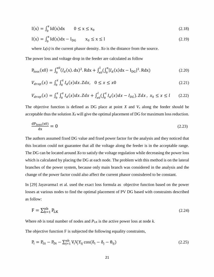
The authors used the current phasor to formulate the objective function considering the distance

Xo to place the DG optimally as illustrated in Figure 3 below.

Figure 2.3. Current direction along the distribution line

Considering one DG is injected into the distribution feeder at the distance Xo, the feeder phasor

current is derived as:

21

I(x) = ∫ Id(x)dx 0 ≤ x ≤ x0x

0 ………...……...………………………………… (2.18)

I(x) = ∫ Id(x)dx − IDG x0 ≤ x ≤ lx

0……….………………………………….... (2.19)

where Id(x) is the current phasor density. Xo is the distance from the source.

The power loss and voltage drop in the feeder are calculated as follow

Ploss(x0) = ∫ (𝐼𝑑(x). dx)2. Rdxx0

0+ ∫ (∫ |𝐼𝑑(x)dx − IDG|2. Rdx)

x

0

l

x0………...……... (2.20)

𝑉𝑑𝑟𝑜𝑝(𝑥) = ∫ ∫ 𝐼𝑑(𝑥)𝑑𝑥. 𝑍𝑑𝑥, 0 ≤ 𝑥 ≤ 𝑥0𝑥

0

𝑥

0 …………..……………………….... (2.21)

𝑉𝑑𝑟𝑜𝑝(𝑥) = ∫ ∫ 𝐼𝑑(𝑥)𝑑𝑥. 𝑍𝑑𝑥 + ∫ (∫ 𝐼𝑑(𝑥)𝑑𝑥 − 𝐼𝐷𝐺). 𝑍𝑑𝑥𝑥

0

𝑙

𝑥0, 𝑥0 ≤ 𝑥 ≤ 𝑙

𝑥

0

𝑥

0…... (2.22)

The objective function is defined as DG place at point X and Vx along the feeder should be

acceptable thus the solution X0 will give the optimal placement of DG for maximum loss reduction.

dPloss(x0)

dx= 0……………..…………………..………………………………………. (2.23)

The authors assumed fixed DG value and fixed power factor for the analysis and they noticed that

this location could not guarantee that all the voltage along the feeder is in the acceptable range.

The DG can be located around Xo to satisfy the voltage regulation while decreasing the power loss

which is calculated by placing the DG at each node. The problem with this method is on the lateral

branches of the power system, because only main branch was considered in the analysis and the

change of the power factor could also affect the current phasor consisdered to be constant.

In [29] Jayavarma1 et al. used the exact loss formula as objective function based on the power

losses at various nodes to find the optimal placement of PV DG based with constraints described

as follow:

F = ∑ PLKnbk=1 ………………………………………..………………………………… (2.24)

Where nb is total number of nodes and PLK is the active power loss at node k.

The objective function F is subjected the following equality constraints,

Pi = PGi − PDi − ∑ ViVjYij cos(δi − δj − θij)nbj=1 …….………………………...….… (2.25)

22

Qi = QGi − QDi − ∑ ViVjYij sin(δi − δj − θij)nbj=1 …………………..……….…….... (2.26)

Also the inequality constraints

QGi,min ≤ QGi ≤ QGi,max i = 1,2 … … … … NG

Vi,min ≤ V ≤ Vi,max i = 1,2 … … … … Nb

|Pij| ≤ Pijmax , ij = 1,2 … … … … … … … … Nl

Where Pi and Qi are active and reactive power flowing in branch i, PGi and QGi are active and

reactive power generated at node i, Vi, Vj are voltages magnitude at node i and j respectively. Yij

is the admittance of the line between node i and j. δi δj and θij are phase angles of the voltage at

node i, j, and the admittance respectively.

This study was intended to investigate the losses improvement and the effect of high-level

penetration of the SPV using the heuristic algorithm. This objective function was tested on

standard IEEE 14 bus non-radial network and the active power loss minimization was 34.46%.

Another research presented by H. Nasiraghdam [30], using the Bacterial Foraging optimisation

(BFO) algorithm has proposed the following objective function for the power loss reduction

PLRI =𝑃𝑙𝑜𝑠𝑠−𝐵𝑎𝑠𝑒−PlossDGi

𝑃𝑙𝑜𝑠𝑠−𝐵𝑎𝑠𝑒 ….……..……………………………………….…...……. (2.27)

where PLRI is the Power Loss Reduction Index, Ploss Base is the power loss without DG and PlossDG

is the power loss with the DG integrated. The complex power loss between bus i and j is computed

as follow:

𝑆𝑖𝑗 = Vi. Iij∗ …………………………………………………….…...…………………….… (2.28)

𝑆𝑗𝑖 = Vj. Iji∗ …………………………...……………………….…...………….…….….…… (2.29)

Where Sij is the complex power loss from node i to j and Sji is the complex power loss from node

j to i. Vi and Vj are voltage magnitude at node i and j respectively. Iij and Iji is the current value at

each node. Re is the equivalent resistance of the lines.

The total power loss is the summation of all power losses in different lines.

Ploss = ∑ ∑ Re(Sij +Nj=1 Sji)

Ni=1 …………………………………………….…...………… (2.30)

23

Along with the BFO, the optimisation equation was tested on the IEEE 33-bus test system, and the

results are satisfactory. Thus various objective functions were formulated to fit with the algorithm

used for the optimisation, and each approach has its merits and limitations.

2. 5 REVIEW OF LOAD FLOW ANALYSIS METHODS

The power flow or load flow analysis is essential for planning, operation, optimisation and control

of power systems. It is called the heart of decision making in the electric power systems [46]. The

information provided by the load flow analysis consists of the active and reactive power flow in

each branch and associated line losses, the magnitude and phase angles of voltages at each bus and

the current magnitude in the various branches under steady state condition. The load flow analysis

is highly complex, and it involves hundreds of buses and several distribution links, therefore

resulting in the extensive calculations [35, 47].

The load flow analysis in the electric power systems consists of primary evaluating the voltage

magnitudes and phase angles at each node. Using the obtained values to compute the current at

each branch and also the power flowing in various branches along with the system power losses

associated with the current flowing in these lines [2]. The same principle is applied to the single

wire earth return analysis, underground cables or overhead distribution systems for the

optimisation, upgrading the existing system equipment or installing a new distribution system.

There are mainly two topologies of the electric power distribution systems namely the ring loop

and the radial distribution systems. The ring distribution systems are more reliable and robust but

very expensive thus many existing electric grids adopted the radial distribution systems which

have the following characteristics [48]:

Radial or weakly meshed networks (source supplied at one side only),

Low X/R ratios, due to high resistance and low reactance of the line,

Unbalanced operation, Unbalanced distributed load and multi-phase,

Distributed generation not easily dispatchable,

Less expensive but least reliable network configuration.

24

These features make the radial distribution networks to be known as ill-conditioned systems, and

they become challenging for the conventional, Gauss-Seidel method, Newton-Raphson, Fast

Decoupled and their variants to effectively analyse them [47].

The Newton-Raphson algorithm is the most widely used methods in the electric power industries

for the strongly meshed transmission lines with several redundant paths and parallel lines. But it

failed in the radial distribution network due to the reasons mentioned above and the convergence

challenges though it could be effective and robust in the voltage convergence [47]. It could not be

effective for the optimal power flow computation due to the time consumption, and large storage

memory required [35, 48].

Authors in [49] proposed a Newton-Raphson method for solving ill-conditioned power systems.

Their work demonstrated voltage convergence but could not be effectively applied for large power

flow calculations.

In this thesis, the proposed backwards and forward sweep method is used to calculate branch

currents, nodal voltages and power losses in each branch using the Kirchhoff’s current and voltage

laws [43, 50, and 51].

The backwards and forward sweep method is used to solve the power flow analysis of the radial

distribution systems with recursive equations. W.H. Kersting et al. proposed the method known as

the modified Ladder iterative technique [52, 53] and R. Berg et al. [54], the convergence of the

method explained in [51,55]. The backwards and forward sweep method is based on the

Kirchhoff’s voltage and current laws and in each iteration, two computation stages occur, the

forward path and the backwards walk. The BFSM has the advantage over the counterpart methods

in the load flow analysis due to the fast convergence and taking into account each branch of the

network thus more accurate. Unlike other methods that used the admittance matrix and the

Jacobean inverse matrix to evaluate the power losses, the BFSM used each branch resistance and

reactance to evaluate the power losses in that specific branch.

2.6 SUMMARY OF THE LITERATURE REVIEW

Each of the methods described in this review has its merits and gaps. Moreover, there is still need

to emphasize more on technical effects of DGs especially the solar photovoltaic integration in the

25

radial distribution systems characterized by the high R/X ratio and the unbalanced loads connected

[43]. It was observed from the litterature review that metaheuristic methods are fast, robust, and

reliable but they are probabilistic approaches and their control parameters required expertise.

Therefore, any mistake in the manipulation can compromise the final output, and they are all based

on the analytic formula.

All these methods have a common point which is the problem formulation; they used the exact

loss formula or the power branch formula to define the objective functions and apply different

optimization techniques [62]. From the review on the objective functions, it is clear and obvious

that active and reactive power components were mainly used to formulate the objective functions

and other optimization tools were used to allocate and size the DG to reduce the power losses and

improve the voltage profile of the radial distribution networks. Moreover, the power loss in the

system can be also evaluated using the branch current components i.e. I2R. The current flowing

through the distribution lines causes the power loss in the system. Therefore the optimal placement

and sizing of the DG in RDN using this approach is mandatory and necessary. However, the

current branch loss used as objective function for the optimal placement is quasi-inexistent.

Furthermore, the purpose and the novelty of this research is to propose a simple and effective

analytical method based on the current branch loss formula and equivalent current injection to

optimally place and size DG in the radial distribution systems. The current flowing in various

branches and the equivalent current injected at different nodes were explored to evaluate the total

power loss, the power saving for the current injected at each node, and the size of the SPV

associated to these power savings. The backward and forward sweep method was proposed to run

the load flow analysis to achieve the bridge over high R/X ratio and unbalanced loadings of the

systems [47]. The method did not use the admittance matrix, the Jacobian matrix which is shown

to be problematic for the radial distribution systems.

26

CHAPTER THREE: METHODOLOGY

3.1 INTRODUCTION

This chapter highlights the methodology proposed for the optimal placement and sizing of SPV

in RDN. The chapter introduces the formulation of the objective function along with different

constraints followed by the proposed method used for the load flow analysis. Finally, the

proposed optimization algorithm named maximum power loss saving technique is discussed

in details at the end of this chapter.

3.2 FORMULATION OF THE OBJECTIVE FUNCTION This part deals with the analytical method of formulating the optimisation problem and defines the

constraints attached to the objective function to achieve the optimal siting and sizing of the SPV

for maximum loss reduction and voltage improvement.

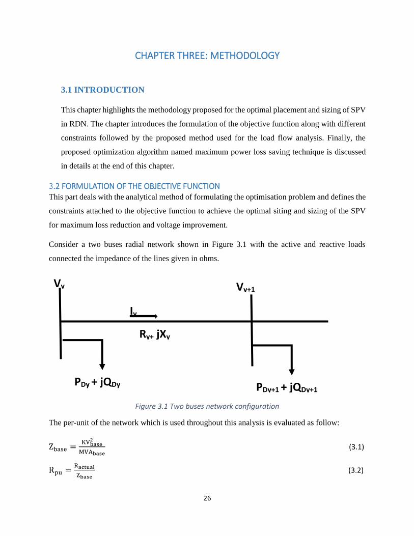
Consider a two buses radial network shown in Figure 3.1 with the active and reactive loads

connected the impedance of the lines given in ohms.

Figure 3.1 Two buses network configuration

The per-unit of the network which is used throughout this analysis is evaluated as follow:

Zbase =KVbase

2

MVAbase……………………………………….……………………………………………………………………….. (3.1)

Rpu =Ractual

Zbase ……………………………………….……………………………………………….………………………….. (3.2)

PDy + jQDy

Vy

Iy

Vy+1

Ry+ jXy

PDy+1 + jQDy+1

27

Xpu =Xactual

Zbase ……………………………………….……………………………………………………………………………. (3.3)

Ppu =Pactual

1000×MVAbase ……………………………………….…………………………………………………………………. (3.4)

Qpu =Qactual

1000×MVAbase ……………………………….……………………………………………… ……………………….. (3.5)

Where Zbase is the base impedance of the line;

Rpu is the per unit value of the resistance; Ractual is the actual value of the resistance;

Xpu is the per unit value of the resistance; Xactual is the actual value of the reactance;

Ppu is the per unit value of the active power; Pactual is the actual value of the active power;

Qpu is the per unit value of the reactive power; Qactual is the actual value of the reactive power;

MVAbase is the base value of the Megawatt; KVbase is the base value of kilovolt.

The initial current flowing through each branch of the network can be obtained using the active

and reactive power and assuming 1.0 p.u. voltage at node 1 as shown in Equation (3.6).

Iy = conj Py+jQy

Vy………………….…….………..………………….…....…………...…… (3.6)

where Py and Qy are the active and reactive power flowing from bus y to bus y+1 respectively.

Updating the voltage at every node, the value of the current flowing in each branch can be

evaluated using the following formula;

Iy = 𝐕𝐲<𝛅𝐲−𝐕𝐲+𝟏<𝛅𝐲+𝟏

𝐑𝐲+𝐗𝐲 ………… … …....…… …… …….………..….………....… ………. (3.7)

Where Vy, Vy+1 voltage magnitude at node y and y+1 respectively. δy, δy+1 voltage angle at node y

and y+1. Ry and Xy are the resistance and reactance of the line.

Similarly, the voltage at each node is calculated using the value of the branch current obtained

previously.

Vy+1 = Vy − Iy(Ry + jXy)……………………………………………………… …….….... (3.8)

where Vy and Vy+1 are the voltage magnitude at node y and y+1 respectively, Iy is the current

flowing the branch y and the impedance of the line is Ry+jXy .

28

The equations 3.7 and 3.8 are repeated and the convergence conditions are checked with an

accuracy of ε=0.001 between the previous voltage calculated and the value of voltage in the current

iteration.

𝜺 = 𝑽𝒚_𝒐𝒍𝒅 − 𝑽𝒚_𝒏𝒆𝒘 …………...……………………………………………..…………… (3.9)

Where Vy_old is the voltage magnitude in the previous iteration, Vy_new is the actual voltage

magnitude, and ε is the accuracy set for the stopping criteria.

After the convergence, the current values obtained are used to evaluate the power losses in the

network as described in the next section.

3.2.1 Objective function

The objective function of this study is formulated based on the current branch loss formula as

follows [36]

PTL = ∑ Iy2N

y=1 × Ry…………...………………………………………………..…….…… (3.10)

QTL = ∑ Iy2N

y=1 × Xy…………………………………………..……….....…..…….……… (3.11)

Where PTL and QTL are total active and reactive power losses in the system respectively,

Iy is the current magnitude flowing from node y to node y+1.

Ry and Xy are the resistance and reactance of the line respectively with N number of branches.

The current magnitude in Equations (3.10) and (3.11) has two components which are active

component Ia and imaginary component Ir, therefore the total active and reactive power loss in

the system in Equations (3.10) and (3.11) can be rewritten as:

PTL = ∑ Iay2 × Ry

Ny=1 + ∑ Iry

2 × RyNy=1 …....……………….....….……….…....……….... (3.12)

𝑄𝑇𝐿 = ∑ 𝐼𝑎𝑦2 × 𝑋𝑦

𝑁𝑦=1 + ∑ 𝐼𝑟𝑦

2 × 𝑋𝑦𝑁𝑦=1 …………………………………......………….. (3.13)

Where Iay, Iry are real and imaginary components of current at node y

3.2.2 Constraints

The main objective function is subjected to equality constraints and inequality constraints

described below:

1. Bus Voltage constraints

The voltage at each node must be within its operating conditions of ±5% of the nominal value [43].

29

| Vy min | ≤ | Vy | ≤ | Vy max |

2. Feeder capacity limits

The current flowing through each branch must be less than its maximum capacity rating to avoid

overloading of the feeder lines [5].

| Iy | ≤ | Iymax, | y=1, 2, 3…….N

3. Power flow equation constraints

The total active power generated (Py Gen) must be equal to the sum of total real power losses in

the line (Ploss) and the total active nodal loads (Py loads).

∑ 𝑃𝑦𝐺𝑒𝑛 = 𝑃𝐿𝑜𝑠𝑠 + ∑ 𝑃𝑦𝑙𝑜𝑎𝑑𝑠 ………………………………….………………….…….… (3.14)

Where PyGen active power injected at node y, Ploss is the total real power loss, and Pyload is the active

load connected to bus y.

3.3 BACKWARD AND FORWARD SWEEP METHOD

Power flow analysis is a necessary basic tool for any electrical power system under steady state

condition for determining the exact electrical performance. It helps to determine the real and

reactive power losses, the amount of current flowing through the lines, and the voltage magnitude

and phase angle at different nodes. It is important in the planning of the new power installation

and upgrading or extension of the existing power system. The stability analysis and protection

designs based on the load flow calculation, similarly the selection of the equipment and their rating

such as generator capacity, switch gear for protection, transformers and the cable sizes; thus the

results of the load flow is the starting point for other analyses of the electric power system. In this

section, the backwards/forward sweep method for radial distribution system load flow analysis is

explained and the flowchart is provided in Figure 3.2.

The Backward/Forward Sweep method (BFSM) for load flow computation is an iterative method

in which, at each iteration two calculation steps are performed. The first set of equations for

calculating the power flow through the branches starting from the last branch and proceeding in

the backwards direction towards the root node. The other set of equations is for calculating the

voltage magnitude and angle at each node starting from the root node and continuing in the forward

direction till the last node [34, 35, 43, 51]. This method is useful in the radial distribution network

30

where the classical methods for load flow analysis failed to compute the power losses in each

branch accurately.

Backwards path: the purpose is to find the current flowing in each branch in the tree by

considering the constant value of voltages found in the previous iteration while a flat voltage value

assumed at the initial iteration. The backwards path starts from the last node to the source node.

The forward path which starts from the source node to the far end node aims to calculate the

voltages at each bus while keeping the current obtained from the previous walk constant meaning

that the current obtained in the backwards walk will be held constant during the forward

propagation. The calculated voltages are compared with specified voltages, and if the error is

within tolerance limits, the process is stopped, and the power line losses are computed otherwise;

the process is repeated until criteria conditions are met. The pseudo code and the flowchart of the

backwards /forward sweep method are shown below.

Pseudo code of Backward/forward sweep algorithm

Step 1: Read bus data, line resistance and reactance data,

Step 2: Read base MVA and base KV and calculate the per unit values of the data loaded using

Equations (3.1) to (3.5).

Step 3: Backwards walk from end node to source node to find all branch currents by using

Equation (3.6) while keeping constant flat initial voltages for the initial walk else Equation (3.7)

Step 4: Forward walk from the source node to the far end node, to find all voltages using Equation

(3.8) while updating the constant current values obtained in the previous iteration and check for

convergence criterion.

Step 5: Check if the mismatch of the specified and calculated voltages at the substation is less than

the convergence tolerance using equation (3.9). If yes, go to next step. Otherwise, repeat step 3

and step 4.

Step 6: calculate the total active and reactive line losses using Equations (3.10) and (3.11) with

the currents and voltages obtained from the backwards and forward sweep method.

Step 7: Print the results of all bus voltage, branch currents and total power losses in the system,

Step 9: Stop.

31

start

Read data

Evaluate the per unit

values

Backward path

Find current at each branch

Forward path

Find voltage at each node

Convergence?

Print all results

Calculate the active and

reactive power losses

stop

NO

YES

Figure 3.2 Flowchart of Backward and forward sweep method

32

3.4 MAXIMUM POWER LOSS SAVING TECHNIQUE Now let consider a network of N branches, if DG is placed at node k and β set branches are

branches located between the source node and the node at which DG is placed as illustrated in

Figure 3.3.

Figure 3.3 Radial distribution network with SPV integrated

The current flow in β branch set will be uttered by the DG current injected while the current

flowing in the rest of the network remains unaffected. Furthermore, the total loss in the system

with the integration of the DG in the radial distribution network can be evaluated as follow:

PLDGk = ∑ [(Iay + IDGk)2

× Ry] + ∑ (Iay2 × Ry)N

y=k+1 + ∑ [(Iry + akIDGk)2 ×ky=1

ky=1

Ry] + ∑ (Iry2 × Ry)N

y=k+1 ………………….…….…………………………………………………………………………. . (3.15)

QLDGk = ∑ [(Iay + IDGk)2

× Xy] + ∑ (Iay2 × Xy

Ny=k+1 ) + ∑ [(Iry + akIDGk)2 ×k

y=1ky=1

Xy] + ∑ (Iry2 × Xy

Ny=k+1 ) ……………………………………………………………………………………..….. (3.16)

Where PLDGk, QLDGk are active and reactive power loss with DG injected in the network.

Iay, Iry are the real and imaginary components of the current obtained from the initial load flow

analysis and IDGk is the active current component injected by the SPV at node k. Ry, Xy are resistance

and reactance of the lines respectively.

The imaginary part of the injected current is 𝑰𝒓𝒌 = 𝒂𝒌𝑰𝑫𝑮𝒌 , IDGk is the SPV real current injected

at node k. 𝑎𝑘 = (𝑠𝑖𝑔𝑛) tan(cos−1(𝑃𝐹𝑑𝑔)), sign =+1 if DG producing the reactive power and sign=

-1 if DG is absorbing the reactive power from the network.

33

The maximum power loss saving technique evaluates the current injected at each node and

calculates the power losses when this current is injected at that node. The saving for each DG

injected is saved and compared, the bus with the maximum power loss saving is identified as the

optimal node for the placement of the DG and the size of the DG is evaluated accordingly.

The power loss saving is the subtraction of the total losses with DG integrated from the initial

power loss; we consider integrating the real current component from the solar photovoltaic i.e. ak

= 0. Thus subtracting Equation (3.15) from Equation (3.12), we will have:

SSk = −2IDGk × ∑ (Iay × Ryky=1 ) − IDGk

2 × ∑ Ryky=1 − 2ak × IDGk × ∑ (Iry × Ry) −k

y=1

ak2 × IDGk

2 × ∑ Ryky=1 ……….……………………………………..………………..…..…. (3.17)

Where SSk is the power saving for DG current injected at each node.

Differentiating the Equation (3.17) with respect to the current injected at node k, and equating the

result to zero will give the maximum power loss saving for the DG integrated at each node.

∂SSk

∂IDGk= 0 ≅ −2 ∑ Iay × Ry

ky=1 − 2IDGk ∑ Ry

ky=1 ………………………………………….....… (3.18)

The Equation (3.18) will allow the computation of the current injected at each node.

Therefore this equation is used to compute the value of the current to be injected at each candidate

node for the maximum power loss reduction. Furthermore, the computed current values are

replaced in Equation (3.17) for all the nodes to evaluate the saving for the injected current at each

node respectively. The results are compared, then the node with highest power loss saving is

identified and selected as a candidate for SPV placement. The expression for the SPV current

injected at each node is given by:

IDGk = −∑ Iay×Ry

ky=1

∑ Ryky=1

……………………..……..………...….…………………………. (3.19)

In the analytical method, the identification of the node with maximum power loss saving defined

the optimal location of the DG in the radial system and once the optimal node is identified. The

size of the DG injected at that node can be evaluated using constant voltage values obtained in the

initial load flow analysis multiplied by the value of current injected. The optimal size of power

injected at selected node k will be the optimal branch current from Equation (3.19) with its

corresponding nodal voltage magnitude as given by:

34

PDGk = IDGk × |Vk| = −|Vk|∑ Iay×Ry

ky=1

∑ Ryky=1

…………..….……………………………......… (3.20)

Where PDGk is the optimal active power injected at node k, IDGk is the current magnitude, and the

DG voltage magnitude is Vk. This process is repeated for multiple integrations of the DG in the

systems till power loss becomes negligible as specified in Equation (3.9). The flowchart of

maximum power loss saving method is shown in figure 3.4 below.

The comparison was done based on the percentage reduction of the active power loss reduction

for each method and also the voltage profile improvement of the proposed method was compared

with the results found in the provided literatures.

35

Read line and load data

start

Set a flat voltage at 1.0 p.u

Calculate current branch using backward walk using Eq. (3.7)

Calculate bus voltage using forward walk using Eq.(3.8)

Is convergence satisfied?

Compute line losses using current and voltage calculated using Eq.(3.10 & 3.11)

yes

Compute DG current injected using Equation (3.18) for each node

Compute the saving (Eq. (3.17)) and select the maximum saving as siting candidate

Calculate optimal DG size and new power loss using Eq. (3.20 & 3.15)

No

Compute the new load flow with DG injected

Is voltage criteria met?

Print results and stop

Yes

No

Figure 3.4 Flowchart of load flow for DG analytical allocation

36

CHAPTER FOUR: RESULTS AND DISCUSSIONS

4.1 INTRODUCTION The maximum power loss saving was tested on IEEE 33-bus with different loading scenarios and

results were reported in this chapter. The analysis starts with the based load flow with 90%, 100%,

and 130% of the total real and reactive power demands, and initial power losses and voltage

profiles of the system were reported respectively. The results analysis of single SPV optimal

placement and sizing were carried out, and the comparisons were made with the existing methods.

Finally, the power factor variation was considered in the DG-units penetration in the radial

distribution systems before concluding with the integration of two DGs for maximum power loss

reduction and improved voltage profile using the same technique. Similarly, the results were also

compared to the existing methods in the provided references.

4.2 LOAD FLOW ANALYSIS WITH THE BACKWARD AND FORWARD SWEEP ALGORITHM In this section, the performance and validity of the proposed methods were tested on IEEE 33-bus

radial distribution networks [36, 41], the data of the test system is shown in Appendix A, and

Figure 4.1 shows the network structure. Different peak loadings were studies from the minimum

loading to the medium loading then the maximum peak demand as shown in the data.

Figure 4.1 IEEE 33 bus radial distribution network

37

The test system fed on a single side, and it has a serially connected active and reactive power loads

at different scenarios which are minimum, medium and maximum loading. The characteristics of

the test system are given below:

Total number of nodes: 33 and Total number of branches: 32,

Kilovolt base: 12.66 KV and MVA base are 100MVA,

In this simulation, three case scenarios with different power demands corresponding to different

peak loads are considered as described below:

Case 1 Minimum Loading: The total minimum active and reactive power loadings connected to

the system are 3343.5 KW and 2070 KVAr which represent 90% of normal system loading.

Case 2 Medium loading: The total medium active and reactive power loadings are 3715 KW and

2300 KVAr respectively which represent the normal system loading or 100%.

Case 3 Maximum loading: The total maximum active and reactive power loadings are 4829.5

KW and 2990 KVAr respectively which represent 130% of the normal system loading.

The initial load flow simulation was carried out under MATLAB using the backwards and forward

sweep method, and the summary of the result was presented in Table 4.1 below. The active and

reactive power losses in the system represent 4.82%, and 5.19% of the total load demands

respectively for the low loading, 5.44% and 5.86% of the demand for the medium loading while

for the maximum loading, it represents 7.41% and 7.99% respectively thus the system losses

increase proportionally with the increase in the loading.

Table 4.1 Based load flow result of the test systems

Loading Minimum Medium Maximum

Total load (KVA) 3343.5+j2070 3715+j2300 4829.5 +j2990

Total active loss (KW) 161.1077 201.9057 357.8295

Total reactive loss (kVAr) 107.4235 134.6618 238.8545

Min voltage (p.u) 0.9227 0.9134 0.8845

Bus 18 18 18

38

Figures 4.2, 4.3 and 4.4 illustrate the nodal voltage profile, active and reactive power losses for

the different loading scenarios using the backwards and forward sweep algorithm based on the

branch current loss formula given in Equations (3.10) and (3.11). RDN are supplied from a single

side which is the centralized generation, and the end users receive power through this passive

network making the direction of the power flow to be unidirectional, thus a large amount of current

flowing. The high resistance to reactance ratio explains the high power loss and the large voltage

drop across the lines. Under heavy loading, the voltage is degraded further which explain a very

low voltage profile of the maximum loading shown in Figures 4.2 and 4.3.

Figure 4.2 Voltage profile for different loading of 33 bus

Figure 4.3 Active power loss in different branches for three scenarios.

0.86

0.88

0.9

0.92

0.94

0.96

0.98

1

1.02

1 3 5 7 9 1 1 1 3 1 5 1 7 1 9 2 1 2 3 2 5 2 7 2 9 3 1 3 3

VO

LTA

GE

MA

GN

ITU

DE

(PU

)

NODES|V|min loading without |V|medium Loading without

39

Figure 4.4 Reactive power loss in different branches for the three scenarios.

Table 4.2 shows the voltage profile for the three scenarios with the comparison with the result

obtained in the provided references, for the three cases, the minimum voltage occurs at node 18

i.e. 0.9038 p.u. 0.9134 p.u. 0.9227 p.u and 0.8845 p.u. for the minimum, medium and maximum

loadings respectively. The results of the medium loading were compared to existing results [56],

but the proposed method has shown better results; the total power loss for the proposed method is

201.91 KW and 134.66 KVAr.

Table 4.2 Voltage profile (p.u) for IEEE 33 bus Radial Distribution system and the total power

Medium Loading Min Loading Max Loading

nodes ref [56] Proposed method

proposed method

1 1 1 1 1

2 0.997 0.997 0.9974 0.9961

3 0.9829 0.983 0.9848 0.9774

4 0.9754 0.9755 0.9781 0.9675

5 0.968 0.9682 0.9715 0.9577

6 0.9495 0.9498 0.9552 0.9332

7 0.946 0.9463 0.9521 0.9286

8 0.9323 0.9415 0.9477 0.9221

9 0.926 0.9352 0.9422 0.9137

10 0.9201 0.9294 0.937 0.906

11 0.9192 0.9286 0.9362 0.9048

12 0.9177 0.9271 0.9349 0.9028

13 0.9115 0.921 0.9295 0.8947

40

14 0.9092 0.9187 0.9275 0.8917

15 0.9078 0.9173 0.9262 0.8898

16 0.9064 0.916 0.925 0.888

17 0.9044 0.914 0.9232 0.8853

18 0.9038 0.9134 0.9227 0.8845

19 0.9965 0.9965 0.9969 0.9954

20 0.9929 0.9929 0.9937 0.9907

21 0.9922 0.9922 0.993 0.9898

22 0.9916 0.9916 0.9925 0.989

23 0.9793 0.9794 0.9816 0.9727

24 0.9726 0.9727 0.9756 0.964

25 0.9693 0.9694 0.9726 0.9596

26 0.9476 0.9479 0.9534 0.9306

27 0.945 0.9453 0.9512 0.9272

28 0.9335 0.9339 0.941 0.912

29 0.9253 0.9257 0.9337 0.901

30 0.9218 0.9222 0.9305 0.8963

31 0.9176 0.918 0.9268 0.8907

32 0.9167 0.9171 0.926 0.8895

33 0.9164 0.9168 0.9258 0.8891

Minimum voltage 0.9038 0.9134 0.9227 0.8845

bus 18 18 18 18

PTL (KW) 210.9824 201.91 161.108 357.8295

QTL (KVAr) 143.0219 134.66 107.424 238.8545

Table 4.3 shows the branch active and reactive power loss of the system. The maximum active

loss occurs at branch 2 for the three scenarios 41.2383 KW, 51.5711 KW, and 90.7723 KW

respectively while the maximum reactive power loss occurs at branch 5 which are 26.1544 KVAr,

32.826 KVAr, and 58.442 KVAr for the three scenarios respectively.

Table 4.3 Numerical results of the active and reactive power losses in the IEEE 33 bus RDN

branches Active power loss in KW Reactive power loss in KVAr

Min load Med load Max load Min load Med load Max load

1--2 9.7625 12.1927 21.3729 4.9766 6.2154 10.8951

2--3 41.2383 51.5711 90.7723 21.004 26.267 46.2331

3--4 15.7831 19.7934 35.1528 8.0382 10.081 17.903

4--5 14.8178 18.5931 33.0784 7.5469 9.4697 16.8473

5--6 30.2977 38.0256 67.7001 26.1544 32.826 58.442

6--7 1.5248 1.9131 3.4027 5.0402 6.3238 11.2478

41

7--8 3.8493 4.8342 8.6241 1.2721 1.5976 2.85

8--9 3.3225 4.1773 7.4799 2.387 3.0012 5.3739

9--10 2.8287 3.5575 6.3764 2.005 2.5216 4.5197

10--11 0.4397 0.5531 0.992 0.1454 0.1829 0.328

11--12 0.6996 0.8802 1.5801 0.2313 0.2911 0.5225

12--13 2.1163 2.6638 4.7866 1.6651 2.0958 3.766

13--14 0.5787 0.7286 1.3099 0.7618 0.959 1.7242

14--15 0.2834 0.3569 0.6424 0.2522 0.3176 0.5717

15--16 0.2234 0.2813 0.5066 0.1631 0.2054 0.37

16--17 0.1996 0.2515 0.4532 0.2665 0.3358 0.605

17--18 0.0422 0.0531 0.0957 0.0331 0.0416 0.075

2--19 0.1302 0.161 0.2732 0.1242 0.1536 0.2607

19--20 0.673 0.8322 1.4132 0.6064 0.7498 1.2734

20--21 0.0815 0.1008 0.1711 0.0952 0.1177 0.1999

21--22 0.0353 0.0436 0.0741 0.0466 0.0577 0.098

3--23 2.5613 3.1812 5.4774 1.7501 2.1737 3.7426

23--24 4.1402 5.1432 8.8605 3.2693 4.0613 6.9966

24--25 1.0359 1.2873 2.2202 0.8106 1.0073 1.7373

6--26 2.0646 2.594 4.6342 1.0516 1.3213 2.3605

26--27 2.6425 3.3211 5.9387 1.3454 1.6909 3.0237

27--28 8.9701 11.2766 20.1834 7.9088 9.9424 17.7953

28--29 6.2179 7.818 14.00 5.4169 6.8108 12.1965

29--30 3.0919 3.8881 6.9661 1.5749 1.9805 3.5482

30--31 1.2656 1.5928 2.8611 1.2508 1.5742 2.8277

31--32 0.1693 0.2131 0.3829 0.1973 0.2484 0.4462

32--33 0.0105 0.0132 0.0237 0.0163 0.0205 0.0368

4.2 MAXIMUM LOSS SAVING TECHNIQUE RESULTS This section discusses the results of the maximum power loss saving in the identification of optimal

location and calculation of the size of SPV to reduce losses in the system. The single SPV and two

DG are discussed respectively considering different loading conditions.

4.2.1 OPTIMAL PLACEMENT OF SINGLE DG WITH UNITY POWER FACTOR

The validity of the proposed method discussed in section 3.3 was tested on the standard IEEE 33-

bus RDN considering different scenarios of the loadings using results obtained from the basic load

flow calculation above. It is assumed that all nodes in the network are candidates for the SPV

placement except slack bus. The currents flowing in each branch were calculated first with the

nodal voltage then the algorithm was used to identify the node with maximum power loss saving

which becomes the optimal candidate for SPV placement, and the optimal SPV size was calculated

42

using the injected current value. In this study, node six is identified as the optimal SPV location

for maximum active power loss reduction as shown in Table 4.4. The active power reduction

percentage of the medium loading, was compared to references [41, 57 and 58] but the results of

the proposed method gave a better result of 48.99% of loss reduction compared to a decrease of

48.19%, 47.33% and 44.83% for [41, 57 and 58] respectively.

Table 4.4 Summary of SPV placement impact on loss and voltage improvement

Loading low Medium

Maximum [57] proposed method

optimal siting 6 6 6 6

optimal size (MW) at 1PF 2.2243 2.601 2.4752 3.2337

Initial Active losses (KW) 161.1077 211.2 201.9057 357.8295

Total active loss (KW) 82.8181 111.1 102.9785 177.83

% of MW loss reduction 48.60% 47.33% 48.99% 50.30%

Total reactive loss (KVAr) 59.6041 -- 74.1179 128.05

Min voltage (p.u) at node 18 0.9558 0.9425 0.9507 0.9352

Figures 4.5, 4.6, and 4.7 show the comparison of the real power branch losses with and without

SPV integration for the minimum, medium and maximum loading scenarios respectively. The

active power losses in the branches located between the source node and the optimal node at which

the SPV was placed have drastically reduced. It is three times lesser than the initial losses.

However, beyond the optimal node, there was only a slight power loss reduction.

Figure 4.5. Active power loss comparison for the minimum loading

0

5

10

15

20

25

30

35

40

1 4 7 10 13 16 19 22 25 28 31

Avt

ive

po

we

r lo

ss (

KW

)

Nodes

without SPV with SPV

43

The drastic power loss reduction is caused by the active power injected at the optimal node 6, the

injected power supplied part of the total loads thus reducing the amount of current flowing in the

line between the source and node 6.

Figure 4.6. Active power loss comparison for the medium loading

Figure 4.7. Active power loss comparison for the maximum loading

Table 4.5 provides the branch active and reactive power losses with solar photovoltaic system

penetration for the different loading scenarios. The maximum branch loss occurs at the same

branch 2 for the real power loss and branch 5 for the reactive power loss, but the loss values have

drastically reduced with the integration of SPV. The percentage of active power loss reduction are

0

10

20

30

40

50

1 4 7 10 13 16 19 22 25 28 31

Avt

ive

po

wer

loss

(K

W)

NODES

without SPV with SPV

0

10

20

30

40

50

60

70

80

90

1 4 7 10 13 16 19 22 25 28 31

Act

ive

po

wer

loss

(K

W)

NODES

without SPV with SPV

44

48.60% for case 1, 48.99% for case 2 and 50.66% for case 3 respectively. The SPV integrated has

supplied the total or part of that particular zone load demand, hence reducing the current flow from

the source to a load of a given location.

Table 4.5 Real and Reactive power loss at each branch with the SPV integration for the 33 bus RDN

branch Active power loss in KW Reactive power loss KVAr

case 1 case 2 case 3 case 1 case 2 case 3

1--2 3.3202 4.1214 7.0429 1.6925 2.1009 3.5902

2--3 12.9281 16.0621 27.5398 6.5847 8.1809 14.0269

3--4 5.0467 6.2715 10.8364 2.5702 3.194 5.5189

4--5 4.893 6.0796 10.5165 2.4921 3.0965 5.3562

5--6 10.3155 12.8149 22.1729 8.9049 11.0624 19.1407

6--7 1.4234 1.77 3.0566 4.7052 5.8509 10.1037

7--8 3.5919 4.4701 7.7386 1.187 1.4773 2.5574

8--9 3.0987 3.8601 6.7034 2.2262 2.7733 4.816

9--10 2.6378 3.2869 5.7128 1.8697 2.3298 4.0493

10--11 0.4099 0.5109 0.8886 0.1355 0.1689 0.2938

11--12 0.6522 0.813 1.4149 0.2157 0.2688 0.4679

12--13 1.9728 2.46 4.2849 1.5522 1.9355 3.3713

13-14 0.5395 0.6728 1.1724 0.7101 0.8856 1.5432

14-15 0.2641 0.3295 0.5747 0.235 0.2932 0.5115

15-16 0.2082 0.2597 0.4532 0.152 0.1897 0.331

16-17 0.186 0.2321 0.4053 0.2484 0.3099 0.5412

17-18 0.0393 0.049 0.0856 0.0308 0.0384 0.0671

2--19 0.1298 0.1604 0.272 0.1239 0.1531 0.2596

19-20 0.6711 0.8296 1.4073 0.6047 0.7475 1.268

20-21 0.0812 0.1004 0.1704 0.0949 0.1173 0.1991

21-22 0.0352 0.0435 0.0738 0.0465 0.0575 0.0976

3--23 2.5155 3.1173 5.3283 1.7188 2.13 3.6408

23-24 4.066 5.0397 8.6188 3.2107 3.9795 6.8057

24-25 1.0173 1.2613 2.1594 0.796 0.987 1.6897

6--26 1.9243 2.395 4.147 0.9801 1.2199 2.1123

26-27 2.4625 3.0658 5.3126 1.2538 1.561 2.7049

27-28 8.3581 10.4083 18.0501 7.3692 9.1768 15.9144

28-29 5.7934 7.2154 12.5184 5.047 6.2859 10.9057

29-30 2.8806 3.5881 6.2278 1.4673 1.8276 3.1722

30-31 1.1786 1.4691 2.5553 1.1648 1.4519 2.5254

31-32 0.1577 0.1965 0.3419 0.1838 0.2291 0.3985

32-33 0.0097 0.0121 0.0211 0.0151 0.0189 0.0328

45

The voltage profile of the three cases with the integration of SPV is given in Table 4.6, and Figures

4.8, 4.9, and 4.10 provide the voltage profile before and after the SPV integration for the three

cases respectively.

Table 4.6 Voltage profile with and without SPV for the three cases of 33 bus RDN

without SPV injected with SPV injected at node 6

Buses |V| min

loading

|V| medium

Loading

|V| Max

Loading

|V| min

loading

|V| medium

Loading

|V| Max

Loading

1 1 1 1 1 1 1

2 0.9974 0.997 0.9961 0.9987 0.9986 0.9982

3 0.9848 0.983 0.9774 0.9935 0.9928 0.9906

4 0.9781 0.9755 0.9675 0.9924 0.9915 0.989

5 0.9715 0.9682 0.9577 0.9915 0.9905 0.9877

6 0.9552 0.9498 0.9332 0.9875 0.9861 0.9821

7 0.9521 0.9463 0.9286 0.9844 0.9826 0.9775

8 0.9477 0.9415 0.9221 0.9803 0.978 0.9714

9 0.9422 0.9352 0.9137 0.9748 0.9719 0.9634

10 0.937 0.9294 0.906 0.9698 0.9663 0.956

11 0.9362 0.9286 0.9048 0.9691 0.9655 0.9549

12 0.9349 0.9271 0.9028 0.9678 0.9641 0.953

13 0.9295 0.921 0.8947 0.9625 0.9582 0.9452

14 0.9275 0.9187 0.8917 0.9605 0.9559 0.9422

15 0.9262 0.9173 0.8898 0.9593 0.9546 0.9404

16 0.925 0.916 0.888 0.9581 0.9532 0.9386

17 0.9232 0.914 0.8853 0.9563 0.9513 0.936

18 0.9227 0.9134 0.8845 0.9558 0.9507 0.9352

19 0.9969 0.9965 0.9954 0.9983 0.9981 0.9975

20 0.9937 0.9929 0.9907 0.995 0.9945 0.9928

21 0.993 0.9922 0.9898 0.9944 0.9938 0.9919

22 0.9925 0.9916 0.989 0.9938 0.9931 0.9911

23 0.9816 0.9794 0.9727 0.9903 0.9893 0.986

24 0.9756 0.9727 0.964 0.9844 0.9826 0.9773

25 0.9726 0.9694 0.9596 0.9814 0.9793 0.973

26 0.9534 0.9479 0.9306 0.9859 0.9843 0.9798

27 0.9512 0.9453 0.9272 0.9838 0.9819 0.9766

28 0.941 0.9339 0.912 0.974 0.971 0.9623

29 0.9337 0.9257 0.901 0.967 0.9632 0.9521

30 0.9305 0.9222 0.8963 0.964 0.9599 0.9478

31 0.9268 0.918 0.8907 0.9604 0.9559 0.9424

32 0.926 0.9171 0.8895 0.9596 0.955 0.9412

33 0.9258 0.9168 0.8891 0.9593 0.9547 0.9409

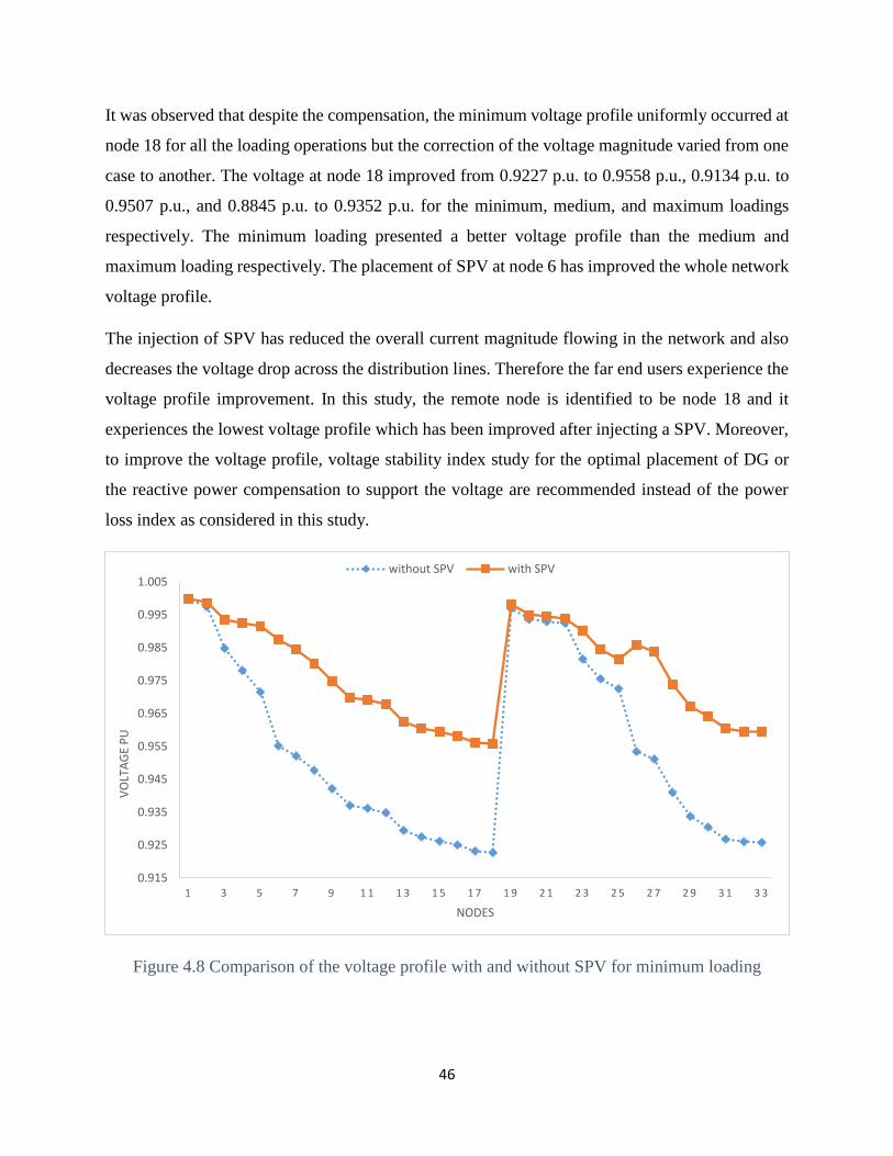
46

It was observed that despite the compensation, the minimum voltage profile uniformly occurred at

node 18 for all the loading operations but the correction of the voltage magnitude varied from one

case to another. The voltage at node 18 improved from 0.9227 p.u. to 0.9558 p.u., 0.9134 p.u. to

0.9507 p.u., and 0.8845 p.u. to 0.9352 p.u. for the minimum, medium, and maximum loadings

respectively. The minimum loading presented a better voltage profile than the medium and

maximum loading respectively. The placement of SPV at node 6 has improved the whole network

voltage profile.

The injection of SPV has reduced the overall current magnitude flowing in the network and also

decreases the voltage drop across the distribution lines. Therefore the far end users experience the

voltage profile improvement. In this study, the remote node is identified to be node 18 and it

experiences the lowest voltage profile which has been improved after injecting a SPV. Moreover,

to improve the voltage profile, voltage stability index study for the optimal placement of DG or

the reactive power compensation to support the voltage are recommended instead of the power

loss index as considered in this study.

Figure 4.8 Comparison of the voltage profile with and without SPV for minimum loading

0.915

0.925

0.935

0.945

0.955

0.965

0.975

0.985

0.995

1.005

1 3 5 7 9 1 1 1 3 1 5 1 7 1 9 2 1 2 3 2 5 2 7 2 9 3 1 3 3

VO

LTA

GE

PU

NODES

without SPV with SPV

47

Figure 4.9 Comparison of the voltage profile with and without SPV for Medium loading

Figure 4.10 Comparison of the voltage profile with and without SPV for maximum loading

The variation of the voltage profile due to the effect of SPV penetration was compared to the

Firefly Algorithm [59], and the proposed method gives a better voltage profile. It is observed that

the size of the SPV integrated increases with the increase in loading but the location remains the

0.91

0.92

0.93

0.94

0.95

0.96

0.97

0.98

0.99

1

1.01

1 3 5 7 9 1 1 1 3 1 5 1 7 1 9 2 1 2 3 2 5 2 7 2 9 3 1 3 3

VO

LTA

GE

MA

GN

ITU

DE

(P.U

)

NODES

without SPV with 1 SPV

0.88

0.9

0.92

0.94

0.96

0.98

1

1.02

1 3 5 7 9 11 13 15 17 19 21 23 25 27 29 31 33

VO

LTA

GE

MA

GN

ITU

DE

(P.U

)

NODES

without SPV with SPV

48

same despite the loading variations. Similarly, the node at which the minimum voltage occurs is

the same for the different cases and even after compensation. Figure 4.11 gives the comparison of

the voltage profile for the three cases with and without SPV injected. The minimum voltage profile

at 18, had improved by 0.0331pu, 0.0373pu and 0.0507pu when the SPV was optimally inserted

at node 6 for low, medium, and maximum loadings respectively.

Figure 4.11 Comparison of the voltage profile for different loadings with and without SPV

penetration at unity PF

4.2.2 PLACEMENT OF TWO DG WITH VARIATION OF POWER FACTOR

Table 4.7 shows the DG integration at different power factor and the effect on real power loss and

voltage profile were observed for the three cases. The power factor set at 0.95 lagging has shown

better active power loss reduction compared to unity PF and 0.85 lagging while the best voltage

profile was found with unity power factor for all the cases followed by 0.95 PF lagging and 0.85

PF lagging respectively. The role of the power factor is vital in the stability of the electric power

system. Therefore, a careful design is required when injecting SPV in the grid at a power factor

different from unity.

0.88

0.9

0.92

0.94

0.96

0.98

1

1.02

1 2 3 4 5 6 7 8 9 10 11 12 13 14 15 16 17 18 19 20 21 22 23 24 25 26 27 28 29 30 31 32 33

Vo

ltag

e m

agn

itu

de

(p.u

)

Nodes

|V|min loading without |V|medium Loading without |V|max Loading without

|V|min loading with SPV |V|medium Loading with SPV |V|max Loading with SPV

49

Table 4.7. Results of the DG injected at node 6 with different power factor for the three cases

Power factor 0.85 PF lagging 0.95 PF lagging unity PF

Loading low Mediu

m

Maximu

m low

Mediu

m

Maximu

m low

Mediu

m

Maximu

m

Optimal size

(MW) 0.91845 1.0213 1.3311 1.5512 1.7257 2.2524 2.2243 2.4752 3.2337

Initial Active

loss (KW)

161.107

7

201.905

7

357.829

5

161.10

8

201.905

7

357.829

5

161.107

7

201.905

7

357.829

5

Total active

loss (KW) 92.4154 115.89

205.844

7

75.735

1 94.9765

168.701

6 82.8181

102.978

5 177.83

% of MW

loss reduction 42.64% 42.60% 42.47% 52.99 52.96% 52.85% 48.60% 48.99% 50.30%

Total reactive

loss (KVAr) 107.424 134.662 238.855 107.43 134.662 238.855 59.6041 74.1179 128.05

Min voltage

(p.u) at bus18 0.9418 0.935 0.9139 0.9504 0.9446 0.9253 0.9558 0.9507 0.9352

The medium loading in case 2 was used for the optimal successive placement of DGs using the

maximum power loss saving technique with different power factors. The placement of two DGs

in the radial distribution networks allows the maximum reduction of real power loss and a net

improvement of voltage profile as shown in Table 4.8. The results compared to the Exhaustive

load flow [57], and it was observed that the locations are different. Furthermore, the power loss

reduction of the proposed method was better than that of [57] and [60].

Table 4. 8. Optimal placement of two DGs in the radial distribution system

Power factor unity PF 0.95 PF lag 0.85 PF lag

comparison [57] Proposed method Proposed method Proposed method

Number of DG First

DG second DG

First

DG

second

DG

First

DG

second

DG

First

DG

second

DG

Optimal location 6 14 6 32 6 32 6 31

Optimal size

(KW) 1800 720 2475.2 41.9487 1725.7 336.674 1.0213 247.052

Initial Active loss - 211.2 201.91 201.906 201.91 201.906 201.91 201.906

Total active loss

(KW) after - 91.63 102.979 78.806 94.9765 47.79 115.89 66.355

% of MW loss

reduction - 56.61% 48.99% 60.97% 52.96% 76.33% 42.61% 67.13%

Min voltage (p.u)

at bus 18 -

0.9539 at 33

0.9507 0.9515 0.9446 0.9465 0.935 0.9403

50

Figure 4.12 shows a comparison between the voltage profile before and after injecting two DGs in

the radial distribution network for normal loading. The minimum voltage which occurred at node

18 was 0.9134 p.u. for base load flow of the medium loading, and it had improved to 0.9507 p.u.

when single DG was integrated at unity power factor. There was a further voltage improvement

for the second DG injected in the system to 0.9515 p.u. Furthermore, there was a significant

improvement in voltage profile of 0.0311 p.u, 0.0373 p.u, and 0.0507 p.u for low, medium, and

maximum loading conditions at the minimum node when a single SPV was optimally injected at

node 6. After integrating the second SPV, there was a slight voltage improvement from the single

SPV penetration as shown in Figure 4.12 and Table 4.8.

Figure 4.12 Comparison of the voltage profile for base load flow, with one DG, and two DGs

injected.

The performance of the proposed method in optimally placing single DG in the radial distribution

system for effective active power loss reduction and improved voltage profile on IEEE 33-bus test

system was compared to metaheuristic methods [45, 59], and improved analytical method [57].

The method has optimally identified the same location of DG in RDN as other methods and the

size of the placed DG varied from one method to another. The maximum active power reduction

of the proposed analytical method has outperformed those methods provided in the reference as

shown in Table 4.9. The minimum voltage magnitude occurred at the same node 18 for all the

0.89

0.91

0.93

0.95

0.97

0.99

1.01

1 4 7 10 13 16 19 22 25 28 31

Vo

ltag

e m

agn

itu

de

Nodes

without SPV with 1 SPV with 2 SPV

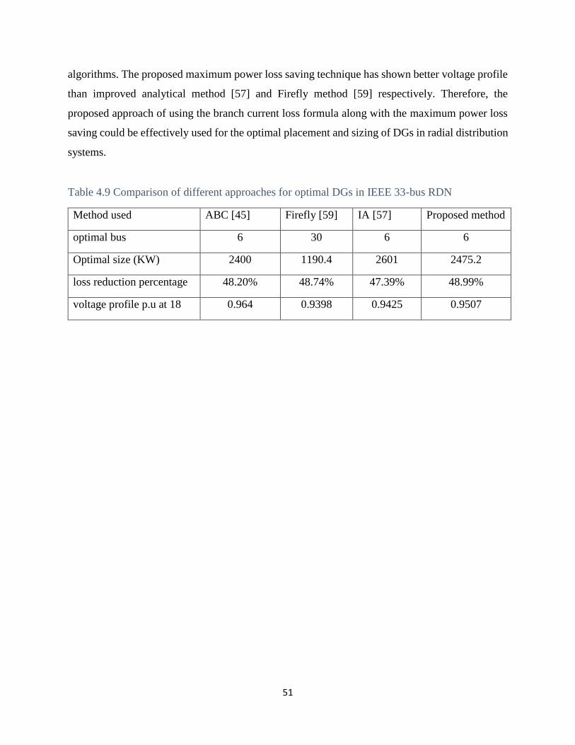
51

algorithms. The proposed maximum power loss saving technique has shown better voltage profile

than improved analytical method [57] and Firefly method [59] respectively. Therefore, the

proposed approach of using the branch current loss formula along with the maximum power loss

saving could be effectively used for the optimal placement and sizing of DGs in radial distribution

systems.

Table 4.9 Comparison of different approaches for optimal DGs in IEEE 33-bus RDN

Method used ABC [45] Firefly [59] IA [57] Proposed method

optimal bus 6 30 6 6

Optimal size (KW) 2400 1190.4 2601 2475.2

loss reduction percentage 48.20% 48.74% 47.39% 48.99%

voltage profile p.u at 18 0.964 0.9398 0.9425 0.9507

52

CHAPTER FIVE: CONCLUSION AND RECOMMANDATIONS

5.1 CONCLUSION

The impact of power losses and the low voltage profile in the radial distribution networks are

among the critical issues in the electric power systems. It affects especially the planning and

operation conditions of the distribution networks. Numerous approaches have been used to address

the power loss reduction including the network reconfiguration, capacitor banks and FACTs to

support the voltage profile, and DGs integration. Each approach has specific techniques for the

integration with their merits and disadvantages. The integration of SPV has both advantages of

power loss reduction and the greenhouse gases reduction.

Maximum power loss saving technique was proposed to optimally place and size SPV in the RDN

and it has been tested on the standard IEEE 33 bus and from the results discussed, the proposed

method has given better results in terms of power loss reduction and voltage profile improvement.

The proposed analytical method has been used to identify the optimal node candidate for the SPV

placement and to compute the size of the SPV at that node to achieve the maximum power loss

reduction. Further investigation was done on 3 different discrete power factor to achieve the

maximum power loss reduction follow by the placement of 2 DGs which has further improved the

voltage profile and also maximum power loss reduction.

5.2 CONTRIBUTION

This research has proposed a simple, easy and efficient analytical method based on branch current

loss formula for optimal location and sizing of DG in the Radial distribution networks for

maximum loss reduction.

The proposed method could be used as a guideline by the power planners and distribution system

operators to optimally place and size the DGs in the radial distribution systems for the reliable and

stable power systems.

This research work has provided a clear impact of the solar photovoltaic penetration in improving

the voltage profile and drastically reducing the system real power loss.

53

This research work suggests the use of current branch loss formula to explore the optimal location

and sizing of DG in the radial system or weakly meshed systems as an alternative option to the

common exact loss formula and power branch formula.

5.3 RECOMMENDATIONS

Following points are worthy of further research to optimally reduce the losses and improve the

voltage profile:

1. This research work suggests the use of current branch loss formula to explore the optimal

location and sizing of DG in the radial system or weakly meshed systems as an alternative

option to the common exact loss formula and power branch formula. Furthermore, other

optimization techniques can be applied for the loss reduction and the method can be applied

to a large network to test its robustness and efficiency.

2. The study done on the uniformly distributed loads, but the allocation of the SPV could be

done with the network reconfiguration simultaneously using the same technique.

3. The study has been carried out on balanced distribution networks. The DGs placement

problem could be extended to unbalanced distribution systems.

4. The economic dispatch of SPV injection could be included in the study to establish the

impact of the cost function in the penetration of the SPV.

5. Study considering the intermittency of the solar irradiance and the load's variation

uncertainties.

54

Appendix A

Table A.1. System data of 33-bus test radial distribution system [56]

Serial

Number

Sending

Node

Receiving

Node

Low loading Medium

loading Maximum loading

R(ohms) X(ohms) P

(KW)

Q

(KVAr)

P

(KW)

Q

KVAr

P

(KW)

Q

(KVAr)

1 1 2 90 54 100 60 130 78 0.0922 0.047

2 2 3 81 36 90 40 117 52 0.493 0.2511

3 3 4 108 72 120 80 156 104 0.366 0.1864

4 4 5 54 27 60 30 78 39 0.3811 0.1941

5 5 6 54 18 60 20 78 26 0.819 0.707

6 6 7 180 90 200 100 260 130 0.1872 0.6188

7 7 8 180 90 200 100 260 130 0.7114 0.2351

8 8 9 54 18 60 20 78 26 1.03 0.74

9 9 10 54 18 60 20 78 26 1.044 0.74

10 10 11 40.5 27 45 30 58.5 39 0.1966 0.065

11 11 12 54 31.5 60 35 78 45.5 0.3744 0.1238

12 12 13 54 31.5 60 35 78 45.5 1.468 1.155

13 13 14 108 72 120 80 156 104 0.5416 0.7129

14 14 15 54 9 60 10 78 13 0.591 0.526

15 15 16 54 18 60 20 78 26 0.7463 0.545

16 16 17 54 18 60 20 78 26 1.289 1.721

17 17 18 81 36 90 40 117 52 0.732 0.574

18 2 19 81 36 90 40 117 52 0.164 0.1565

19 19 20 81 36 90 40 117 52 1.5042 1.3554

20 20 21 81 36 90 40 117 52 0.4095 0.4784

21 21 22 81 36 90 40 117 52 0.7089 0.9373

22 3 23 81 45 90 50 117 65 0.4512 0.3083

23 23 24 378 180 420 200 546 260 0.898 0.7091

24 24 25 378 180 420 200 546 260 0.896 0.7011

25 6 26 54 22.5 60 25 78 32.5 0.203 0.1034

26 26 27 54 22.5 60 25 78 32.5 0.2842 0.1447

27 27 28 54 18 60 20 78 26 1.059 0.9337

28 28 29 108 63 120 70 156 91 0.8042 0.7006

29 29 30 180 540 200 600 260 780 0.5075 0.2585

30 30 31 135 63 150 70 195 91 0.9744 0.963

31 31 32 189 90 210 100 273 130 0.3105 0.3619

32 32 33 54 36 60 40 78 52 0.341 0.5302

Total loading 3344 2070 3715 2300 4830 2990

Substation voltage KV base= 12.66 KV and MVA base = 100 MVA.

55

Per unit values calculation.

𝑍𝑏𝑎𝑠𝑒 =𝐾𝑉𝑏𝑎𝑠𝑒

2

𝑀𝑉𝐴𝑏𝑎𝑠𝑒 ;

𝑅𝑝𝑢 =𝑅𝑎𝑐𝑡𝑢𝑎𝑙

𝑍𝑏𝑎𝑠𝑒 ;

𝑋𝑝𝑢 =𝑋𝑎𝑐𝑡𝑢𝑎𝑙

𝑍𝑏𝑎𝑠𝑒 ;

𝑃𝑝𝑢 =𝑃𝑎𝑐𝑡𝑢𝑎𝑙

1000×𝑀𝑉𝐴𝑏𝑎𝑠𝑒 ;

𝑄𝑝𝑢 =𝑄𝑎𝑐𝑡𝑢𝑎𝑙

1000×𝑀𝑉𝐴𝑏𝑎𝑠𝑒.

Where Zbase is the base impedance of the line;

Rpu is the per unit value of the resistance;

Ractual is the actual value of the resistance;

Xpu is the per unit value of the resistance;

Xactual is the actual value of the reactance;

Ppu is the per unit value of the active power;

Pactual is the actual value of the active power;

Qpu is the per unit value of the reactive power;

Qactual is the actual value of the reactive power;

MVAbase is the base value of the Megawatt;

KV base is the base value of kilovolt.

56

REFERENCES

[1] P. N. Hrisheekesha and J. Sharma. “AI Applications to Distribution System with Distributed

Generation”, International Journal of Computer Applications 1(14):38–42, February 2010.

[2] Kamaruzzaman, Z. A., A. Mohamed, and H. Shareef. "Effect of grid-connected photovoltaic systems

on static and dynamic voltage stability with analysis techniques–a review." Przegląd Elektrotechniczny 91

(2015): 134-138.

[3] Zhu, Ji Zhong. "Optimal reconfiguration of electrical distribution network using the refined genetic

algorithm." Electric Power Systems Research 62.1 (2002): 37-42.

[4] A.R. Jha, “Solar Cell Technology and Applications”, Auerbach Publications. 2010 pp. 72-245

[5] D.Q. Hung, “Smart Integration of Distributed Renewable Generations and Battery Energy Storages.”

Retrieved from http://espace.library.uq.edu.au/view/UQ:342027/s4250093_phd_submission.pdf. (2014).

[6] A. Samadi, “Large Scale Solar Power Integration in Distribution Grids,” Doctoral Thesis Stockholm,

Sweden 2014

[7] M. Vandenbergh, D. Craciun, V. Helmbrecht, R. Hermes, R. Lama, P. Michele Sevilla, M. Redinger,

and G. Concas, “Prioritisation of technical solutions available for the integration of PV into the distribution

grid,” tech. rep., DERlab, European Distributed Energy Resources Laboratories e. V., June 2013.

[8] Wu, Y. K., Lee, C. Y., Liu, L. C., & Tsai, S. H. “Study of reconfiguration for the distribution system

with distributed generators.” Power Delivery, IEEE Transactions on, (2010). 25(3), pp. 1678-1685.

[9] Castillo, Alejandro, and Dennice F. Gayme. "Profit-maximizing storage allocation in power

grids." Decision and Control (CDC), 2013 IEEE 52nd Annual Conference. IEEE, 2013.

[10] Gupta, Amit, and Ranjana Singh. "Computation of transformer loss under the effects of non-sinusoidal

currents." Advanced Computing: An International Journal (ACIJ) 2.6 (2011): 91-104.

[11] M.S. Dalila, M. Shah and M.N. Khalid. “Distribution Transformer Losses Evaluation under Non-

Linear Load,” Australasian Universities Power Engineering Conference, Adelaide, SA, pp. 1-6, 27-

30. Sept. 2009

[12] Da Silva Filho et al. “Electric Power System-Operation Decision-Support by Expert System-Built with

Paraconsistent Annotated Logic.” INTECH Open Access Publisher. 2012.

[13] Baldwin, E., Brass, J. N., Carley, S., & MacLean, L. M. “Electrification and Rural development: issues

of scale in distributed generation.” Wiley Interdisciplinary Reviews: Energy and Environment, Pp. 4(2),

196-211 2015

[14] Y. T. Tan, D. S. Kirschen, & N. Jenkins. “Impact of aLarge Penetration of Photovoltaic-Generation

on the Power System.” In CIRED 17th International-Conference on Electricity-Distribution Barcelona,

May 2003. pp. 12-15.

[15] Alquthami, Thamer, et al. "Study of photovoltaic integration impact on system stability using the

custom model of SPV arrays integrated with PSS/E." North American Power Symposium (NAPS), 2010.

IEEE, 2010.

[16] S.A.Hashemi Zadeh, et al., “Optimal DG Placement for Power Loss Reduction and Improvement

Voltage Profile Using Smart Methods.” International Journals of Smart Electrical-Engineerings, Vol.1,

No.3, fall 2012, pp.141:147

57

[17] A. Parizad, A.H. Khazali and M. Kalantar, “Siting and sizing of DG through Harmony-Search-

Algorithm for improving voltage profile and reduction of THD and losses,” in 23rd Canadian Conference,

Electrical and Computer Engineering (CCECE), Calgary, Canada, pp. 1-6, May 2-5, 2010.

[18] N. Acharya, P. Mahat and N. Mithulananthan, “An analytical approach for DG allocation in primary

distribution network”, Int. J. Electr. Power Energy Syst., 2006, 28, (10), pp. 669–746.

[19] O. Gavasheli, “Optimal Placement of Reactive Power Supports for Loss Minimization: The Case of a

Georgian Regional Power Grid”, Master’s Thesis, 2007, Chalmer’s University of Technology, Division of

Electric Power Engineering, Göteborg, Sweden.

[20] M. Mukerji, “Optimal Siting and Sizing of Solar Photovoltaic Distributed-Generation to Minimize

Loss, Present Value of Future Asset Upgrades and Peak-Demand Costs on aReal Distribution Feeder”,

master’s thesis, University of Waterloo, Electrical and Computer Engineering, Ontario, Canada, 2011

[21] Shahzad, Mohsin, et al. "Analytical approach for simultaneous optimal sizing and placement of

multiple Distributed Generators in primary distribution networks." 2014 IEEE 23rd (ISIE). IEEE, 2014.

[22] H. L. Willis, “Analytical methods and rules of thumb for modelling DG distribution interaction,” in

Proc. IEEE Power Eng. Soc. Summer Meet., 2000, vol.3, pp.1643–1644.

[23] Nagaraju, B., K. Sri Padmini, and J. Viswanatha Rao. "Optimal Placement of SPV-based DG for

LossReduction in RDS Using Direct Search Algorithm.", Vol. 3, Issue. 1, ISSN: 2345 – 9603, April 2015

[24] O. Amanifar, M.E. Hamedani Golshan, “Optimal Distributed Generation Placement and Sizing for

Loss and THD Reduction and Voltage ProfileImprovement in Distribution Systems Using Particle Swarm

Optimization and Sensitivity Analysis”, IJTPE, Vol. 3. Issue 7, No. 2, pp. 47-53, June 2011.

[25] E. Mohammadi & S. Esmaeili, “A Novel Optimal Placement of SPV System for Loss Reduction and

Voltage Profile Improvement”, IJTPE, Issue 13, Vol. 4, No. 4, Pp 11-16, December 2012

[26] R. Srinivasa Rao, S.V.L. Narasimham, & M. Ramalingaraju, “Optimization of Distribution Network

Configuration for Loss Reduction Using Artificial Bee Colony Algorithm.” International Journal of

Electrical, Computer. Vol: 2, No: 9, 2008

[27] Hung D. Q. and Nadarajah M., "Multiple distributed generator placement in primary distribution

systems for loss reduction." IEEE Transactions Industrial Electronics 60.4 (2013): 1700-1708.

[28] P. Paliwal & N.P. Patidar, “Distributed Generator Placement for Loss-Reduction andImprovement in

Reliability”, (IJTPE), Vol:4, No:9, 2010

[29] A. Jayavarma1, & T. Joseph, “Optimal Placement of Solar PV in Distribution System using Particle

Swarm Optimization”, (IJTPE), Vol. 2, Special Issue 1, December 2013.

[30] H. Nasiraghdam, “Bacterial Foraging Optimization for Dispersed Energy Resources Placement

Considering Reliability Enhancement and Power Loss Reduction of Distribution Systems”, World Applied

Sciences Journal 20 (10): 1426-1432, 2012, ISSN 1818-4952

[31] Benedict E., et al., "LOSSES IN ELECTRIC POWER SYSTEMS", ECE Technical Reports. Paper

266. (1992).

[32] SNE, [Online]. Available at http://snetchad.com/

[33] AFRIQUINFOS, “Tchad-gouvernement-fait-efforts-pour-electrifier-tout-pays” [Online]. Available at

http://www.afriquinfos.com/articles/2012/9/21/

58

[34] M.N. Muhtazaruddin, M.A. Baharudin, M.W. Wazir, J.J. Jamian, G. Fujita, and H. Mokhlis

“Distribution Network Loss Minimization via Simultaneous DG Coordination with Network-

Reconfiguration”, Arabian Journal forScience and Engineering, Springer, Vol. 39, No. 6, pp. 4923-4933,

June 2014.

[35 Rupa, JA Micheline, and S. Ganesh. "Power Flow Analysis for Radial Distribution Networks Using

Backward/Forward Sweep Method." World Academy of Science, Engineering and Technology,

International Journal of Electrical, Computer, Energetic, Electronic and Communication Engineering8.10

(2014): 1621-1625.

[36] Gungor, V. C., et al. "Smart grid technologies: Communication technologies and standards." IEEE

transactions on Industrial informatics 7.4 (2011): 529-539.

[37] S.I. Kumar and N. K. Prema, “A novel approach to identify optimal access point and capacity of

multiple DGs in a small, medium and large-scale RDS”, Electrical Power and Energy Systems, vol. 45,

(2013), pp. 142–151.

[38] Abu-Mouti, Fahad S., and Mohamed E. El-Hawary. "A new and fast power flow solution algorithm

for radial distribution feeders including distributed generations." 2007 IEEE International-Conference on

Systems, Man &Cybernetics. IEEE, 2007.

[39] Nagaraju, B., K. Sri Padmini, and J. Viswanatha Rao. "Optimal Placement of SPV based DG for

LossReduction in RDS Using Direct Search Algorithm.", Vol. 3, Issue. 1, ISSN: 2345 – 9603, April 2015

[40] X. Weidong, W. G. Dunford, and A. Capel, "A novel modelling method for photovoltaic cells, in PESC

2004 IEEE 35th Annual, 2004, pp. 1950-1956 Vol.3

[41] Abu-Mouti, F.S. and M.E. El-Hawary, “Optimal Distributed Generation Location and Sizing in

Distribution Systems via Artificial Bee Colony Algorithm.” Power Delivery, IEEE Transactions on, 2011.

26(4): p. 2090- 2101.

[42] M. A. Kashem and G. Ledwich, “DG impact on rural lines: Voltage control and line protection issues,”

in Proc. Int. Symp. Distributed Gen.: Power Syst. Market Aspects, Stockholm, Sweden. June 11–13, 2001.

[43] N. Madjissembaye, et al., “Optimal siting and sizing of single SPV system in radial distribution

systems for loss reduction based on maximum power saving technique.” IJMER. Retrieved from

http://www.ijmer.com/papers/Vol6_Issue7/Version-1/E6713036.pdf (2016)

[44] Ghosh S., Sakti P. G., and Sardined G. "Optimal sizing and placement of distributed generation in a

network system." International Journal of Electrical Power & Energy Systems 32.8 (2010): 849-856.

[45] Abu-Mouti, F. S., and M. E. El-Hawary. "Modified artificial bee colony algorithm for optimally

distributed generation is sizing and allocation in distribution systems." Electrical Power & Energy

Conference (EPEC), 2009 IEEE. IEEE, 2009.

[46] Kothari, Dwarkadas Pralhaddas, and I. J. Nagrath. Modern power system analysis. Tata McGraw-Hill

Education, 2003. Pp. 184-239

[47] S. C. Tripathy, G. D. Prasad, O. P. Malik and G. S. Hope, "Late discussion and closure to Load-Flow

Solutions for Ill-Conditioned PowerSystems by aNewton-Like Method", in IEEE Transactions on Power

Apparatus and Systems, vol. PAS-103, no. 8, pp. 2368-2368, Aug. 1984.

[48] Balamurugan, K., and Dipti Srinivasan. "Review of the power flow studies on distribution network

with distributed generation." Power Electronics and Drive Systems (PEDS), 2011 IEEE Ninth International

Conference. IEEE, 2011. [49] S.C.Tripathy, G.Durga Prasad, O.P.Malik and G.S.Hope, “Load Flow for ill-

59

ConditionedPower Systems by a Newton-like Method”, IEEE Trans., PAS-101, October 1982, pp.3648-

365.

[50] Bhutad, A. G., S. V. Kulkarni, and S. A. Khaparde. "Three-phase load flow methods for radial

distribution networks." TENCON 2003. Conference on Convergent Technologies for the Asia-Pacific

Region. Vol. 2. IEEE, 2003.

[51] Bompard, E., et al. "Convergence of the backwards-forward sweep method for the load-flow analysis

of radial distribution systems." International Journal of Electricalpower and energy systems. 22.7 (2000):

521-530.

[52] W.H.Kersting, W.H.:’Distribution System Modeling and Analysis’, CRC Press,2002

[53] Kersting, W. H., Mendive, D. L.: ‘An application of Ladder Network theory to thesolution of three

phase Radial Load Flow Problem’, IEEE PAS Winter Meeting, New York, 1976, IEEE Paper No. A76 044-

8.

[54] Berg, R.,Hawkins,E.S., and Plelines, W.W. ’Mechanised Calculation of Unbalanced Load Flow on

Radial Distribution Circuits’, IEEE Trans. onPower Apparatus andSystems,1967, 86, (4), pp.415-421

[55] Michael McAsey and Libi Mou,” Convergence of the Forward-Backward Sweep Method in Optimal

Control” IL 61625.

[56] Teja, B. Ravi, V. V. S. N. Murty, and Ashwani Kumar. "An Efficient and Simple Load Flow Approach

for Radial and Meshed Distribution Networks." International Journal of Grid andDistributed Computing 9.2

(2016): 85-102.

[57] Hung D. Q. and Nadarajah M., "Multiple distributed generator placement in primary distribution

systems for loss reduction." IEEE Transactions Industrial Electronics 60.4 (2013): 1700-1708.

[58] T. N. Shukla, S. P. Singh, V. Srinivasarao, and K. B. Naik, “Optimal sizing of distributed generation

placed on radial distribution systems,” Elect. Power Company. Syst., vol. 38, no. 3, pp. 260–274, 2010.

[59] N. Ketfi, D. Chabane, and B. Tarek. "Distributed generation location and size determination to reduce

power losses of a distribution feeder by Firefly Algorithm." International Journal of advancedscience and

technology 56 (2013): 61-72.

[60] N. Acharya, P. Mahal, and N. Mithulananthan, “An analytical approach for DG allocation in the

primary distribution network,” Elect. Power Syst. Res., vol. 28, no. 10, pp. 669–678, Dec. 2006.

[61] M. Shaaban, J.O. Petinrin, “Sizing and siting of DG in distribution system for voltage profile

improvement and loss reduction.” International Journal of smart grid and clean energy. Vol 8. No.1 pp.1-

7, 2013

[62] Elgerd, O.I.: ‘Electric energy systems theory: an introduction’ (McGraw-Hill, 1971).

[63] I. El-Samahy and E. El-Saadany, “The effect of DG on power quality in a deregulated environment,”

in Proc. IEEE Power Eng. Soc. Gen. Meet., 2005, vol. 3, pp. 2969–2976.

[64] W. Li, G. Joos, and J. Belanger, “Real-time simulation of a wind turbine generator coupled with a

battery supercapacitor energy storage system,” IEEE Trans. Ind. Electron., vol. 57, no. 4, pp. 1137–1145,

Apr. 2010.

[65] O. Henry, J. Volschenk, and E. Smit. "Residential consumers in the Cape Peninsula’s willingness to

pay for premium priced green electricity." Energy Policy 39.2 (2011): 544-550.

60

[66] J. J. Antonio, et al. "Daily load profiles for residential, commercial and industrial low voltage

consumers." IEEE Transactions on power delivery 15.1 (2000): 375-380.

[67] Dixon, Juan, et al. "Reactive power compensation technologies: State-of-the-art review." Proceedings

of the IEEE 93.12 (2005): 2144-2164.

[68] Luo, An, et al. "Combined system for harmonic suppression and reactive power compensation." IEEE

Transactions on Industrial Electronics 56.2 (2009): 418-428.

[69] Farhangi, Hassan. "The path of the smart grid." IEEE power and energy magazine 8.1 (2010).

[70] Al-Mahroqi, Y., Metwally, I. A., Al-Hinai, A., & Al-Badi, A. “Reduction of power losses in

distribution systems”. World Academy of Science, Engineering and Technology, 6, 498-505. 2012

[71] Christoff, Peter. "The promissory note: COP 21 and the Paris Climate Agreement." Environmental

Politics 25.5 (2016): 765-787

61

LIST OF PUBLICATIONS

1. N. Madjissembaye, L. Thiaw, C. M. Muriithi, C. W. Wekesa, “Optimal siting and

sizing of single SPV system in radial distribution systems for loss reduction based on

maximum power saving technique.” International Journal of Modern Engineering

Research (IJMER) Vol 6, Issue 7, July 2016.

2. N. Madjissembaye, C. M. Muriithi, C. W. Wekesa, “Load Flow Analysis for Radial

Distribution Networks Using Backward/Forward Sweep Method” Journal of

Sustainable Research in Engineering (SRI) (pending)

3. N. Madjissembaye, V.Siyoi, C. M. Muriithi, C. W. Wekesa, “Optimal Siting and Sizing

of Distributed Generation in Radial Distribution System for Active Power Loss

Reduction.” Journal of Sustainable Research in Engineering (SRI) (pending)

62

MATLAB CODE %======ESSAY FOR THE RADIAL DISTRIBUTION NETWORK LOAD FLOW USING BFSM=====% %********* LOAD CALCULATION WITH ACTIVE POWER DG PENETRATION********* clc; clear all; format short; tic sn=load('loaddata33bus2.m'); ln=load('linedata33bus.m'); %------------------------------------------------------------------------% je=length(ln); tu=length(sn); MVAb=100; KVb=12.66; ak=tan(acos(1)); Zb=(KVb^2)/MVAb; % Per unit Values for i=1:je R(i,1)=(ln(i,4))/Zb; X(i,1)=(ln(i,5))/Zb; end for i=1:tu P(i,1)=((sn(i,4))/(1000*MVAb)); Q(i,1)=((sn(i,5))/(1000*MVAb)); end %------------------------------------------------------------------------% R; X; P; Q; D=zeros(je,tu); for i=1:je f=ln(i,2); g=ln(i,3); for j=1:tu if f==j D(i,j)=-1; end if g==j D(i,j)=1; end end end D; b=1; for i=1:tu a=0; for j=1:je if D(j,i)==-1 a=1; end end if a==0 endnote(b,1)=i; b=b+1; end

63

end endnote; %------------------------------------------------------------------------% c=length(endnote); for j=1:c b=2;

d=endnote(j,1); % while (f~=1) for s=1:tu if (d~=1) k=1; for i=1:je if ((D(i,d)==1)&&(k==1)) d=i; k=2; end end k=1; for i=1:tu if ((D(d,i)==-1)&&(k==1)); d=i; e(j,b)=i; b=b+1; k=3; end end end end end for i=1:c e(i,1)=endnote(i,1); end e; h=length(e(1,:)); for i=1:c j=1; for k=1:tu for l=1:h if e(i,l)==k e(i,l)=e(i,j); e(i,j)=k; j=j+1; end end end end e; %------------------------------------------------------------------------% for k=1:je b=1; for i=1:c for j=1:h-1 if (e(i,j)==k) if e(i,j+1)~=0 Sam(k,b)=e(i,j+1); b=b+1;

64

else Sam(k,1)=0; end end end end end Sam; for i=1:je-1 for j=c:-1:1 for k=j:-1:2 if Sam(i,j)==Sam(i,k-1) Sam(i,j)=0; end end end end Sam; m=length(Sam(:,1)); n=length(Sam(1,:)); for i=1:m for j=1:n if Sam(i,j)==0 && j~=n if Sam(i,j+1)~=0 Sam(i,j)=Sam(i,j+1); Sam(i,j+1)=0; end end if Sam(i,j)~=0 Sam(i,j)=Sam(i,j)-1; end end end Sam; for i=1:m-1 for j=1:n samy(i,j)=Sam(i+1,j); end end g=length(samy); %-----------------------------------------------------------------------% %evaluation of the branche currents and the node voltages for i=1:tu vb(i,1)=1; end for s=1:10 for i=1:tu Icp(i,1)=conj(complex(P(i,1),Q(i,1)))/(vb(i,1)); end Icp; for i=1:je Ibr(i,1)=Icp(i+1,1); end Ibr; xx=length(samy(1,:)); for i=je-1:-1:1 for k=1:xx

65

if samy(i,k)~=0 xy=samy(i,k); Ibr(i,1)=Ibr(i,1)+Ibr(xy,1); %Ibr(i,1)=Icp(i+1,1)+Ibr(k,1); end end end Ibr; for i=2:tu e=0; for f=1:g if xy>1 if samy(f,2)==i-1 xy=samy(f,1); vb(i,1)=((vb(xy,1))-((Ibr(i-1,1))*(complex((R(i-1,1)),X(i-

1,1))))); e=1; end if samy(f,3)==i-1 xy=samy(f,1); vb(i,1)=((vb(xy,1))-((Ibr(i-1,1))*(complex((R(i-1,1)),X(i-

1,1))))); e=1; end end end if e==0 vb(i,1)=((vb(i-1,1))-((Ibr(i-1,1))*(complex((R(i-1,1)),X(i-1,1))))); end end s=s+1; end Icp; Ibr vb; Vbp=[abs(vb) angle(vb)*180/pi]

%toc; for i=1:tu va(i,2:3)=Vbp(i,1:2); end for i=1:tu va(i,1)=i; end va; Ibrp=[abs(Ibr) angle(Ibr)*180/pi]; PL(1,1)=0; QL(1,1)=0; %------------------------------------------------------------------------% %evaluation of the line losses for d=1:je Pl(d,1)=(Ibrp(d,1)^2)*R(d,1); Ql(d,1)=(Ibrp(d,1)^2)*X(d,1); PL=PL(1,1)+Pl(d,1); QL=QL(1,1)+ Ql(d,1); end %print the answers

66

Pkwloss=(Pl)*1e5; Qkvarloss=(Ql)*1e5; PTL=(PL)*1e5; QTL=(QL)*1e5; voltage=Vbp(:,1); angle=Vbp(:,2)*(pi/180); %------------------------------------------------------------------------% %evaluating the power losses using the current real and imaginary component Ibrr=real(Ibr);Ibri=imag(Ibr); IL=[Ibrr Ibri]; for d=1:je PLL(d,1)=(Ibrr(d,1)^2)*R(d,1)+(Ibri(d,1)^2)*R(d,1); QLL(d,1)=(Ibrr(d,1)^2)*X(d,1)+(Ibri(d,1)^2)*X(d,1); Ptl=PL(1,1)+PLL(d,1); Qtl=QL(1,1)+QLL(d,1); end PTl=Ptl*1e5 QTl=Qtl*1e5 %=========================================================================% %in this portion, we will calculate the value of the DG current injected %at each node and evaluate the power saving using these values once the bus %with highest power savingis loacated it will be candidate to the DG

penetration thus the %load flow will be done using these node to minimize the loss. for i=1:je Iy(i,1)=IL(i,1)*R(i,1);%Evaluating the I^2.R of the branches/active cpmt Ir(i,1)=IL(i,2)*R(i,1);%Evaluating the I^2.R of the branches/reactive

cpmt end for j=1:je Ipv(j,1)=-(sum(Iy(1:j,1))-ak*sum(Ir(1:j,1)))/((ak^2+1)*sum(R(1:j,1)));%DG

current for maximum saving end for i=2:je SS(i,1)= -2*Ipv(i,1)*sum(Iy(1:i,1))-(Ipv(i,1)^2)*sum(R(1:i,1))-

2*ak*Ipv(i,1)*sum(Ir(1:i,1))-(Ipv(i,1)^2)*ak^2*sum(R(1:i,1));%the saving.... %calculated using the maximum value of the Pv current end

[sav,branch]= max(abs(SS(1:i,1))) %selecting the maximum saving branch

which will be %the candidate for the DG placement % for j=1:je %

PDDloss=sum((IL(1:6,1)+Ipv(6,1)).^2)*sum(R(1:6,1))+(sum(IL(7:je,1).^2))... % *sum(R(7:je,1))+(sum(IL(1:je,2)))*sum(R(1:je,1)); % end % % %the power loss can be calculated using the Ploss without DG minus the %maximum saving when injecting the DG. PLDG=Ptl-max(abs(SS));PLDG61=PLDG*1e5, PDG=-

Vbp(branch+1,1)*Ipv(branch,1)*1e5, QDG=ak*PDG toc

% toc;