The Cryosphere, 6, 1445–1461, 2012www.the-cryosphere.net/6/1445/2012/doi:10.5194/tc-6-1445-2012© Author(s) 2012. CC Attribution 3.0 License.

The Cryosphere

The footprint of Asian monsoon dynamics in the mass and energybalance of a Tibetan glacier

T. M olg1, F. Maussion1, W. Yang2, and D. Scherer1

1Chair of Climatology, Technische Universitat Berlin, Berlin, Germany2Key Laboratory of Tibetan Environment Changes and Land Surface Processes, Institute of Tibetan Plateau Research,Chinese Academy of Sciences, Beijing, China

Correspondence to:T. Molg (thomas.moelg@campus.tu-berlin.de)

Received: 26 June 2012 – Published in The Cryosphere Discuss.: 8 August 2012Revised: 15 October 2012 – Accepted: 3 November 2012 – Published: 6 December 2012

Abstract. Determinations of glacier-wide mass and energybalance are still scarce for the remote mountains of the Ti-betan Plateau, where field measurements are challenging.Here we run and evaluate a physical, distributed mass bal-ance model for Zhadang Glacier (central Tibet, 30◦ N) basedon in-situ measurements over 2009–2011 and an uncertaintyestimate by Monte Carlo and ensemble strategies. The modelapplication aims to provide the first quantification of how theIndian Summer Monsoon (ISM) impacts an entire glacierover the various stages of the monsoon’s annual cycle. Wefind a strong and systematic ISM footprint on the interannualscale. Early (late) monsoon onset causes higher (lower) ac-cumulation, and reduces (increases) the available energy forablation primarily through changes in absorbed shortwave ra-diation. By contrast, only a weak footprint exists in the ISMcessation phase. Most striking though is the core monsoonseason: local mass and energy balance variability is fully de-coupled from the active/break cycle that defines large-scaleatmospheric variability during the ISM. Our results demon-strate quantitatively that monsoon onset strongly affects theablation season of glaciers in Tibet. However, we find no di-rect ISM impact on the glacier in the main monsoon sea-son, which has not been acknowledged so far. This resultalso adds cryospheric evidence that, once the monsoon is infull swing, regional atmospheric variability prevails on theTibetan Plateau in summer.

1 Introduction

Changes in the Asian monsoon climate and associated glacierresponses have become predominant topics of climate re-search. Their importance is founded on, e.g. (i) the effect ofmonsoon activity on the livelihood of millions of people (e.g.Tao et al., 2004), (ii) the effect of glacier change on regionalwater supply and global sea level rise (Kaser et al., 2006,2010), and (iii) the role of the monsoon in gobal telecon-nections, which was discussed by Webster et al. (1998) andcontinues to be a research focus (e.g. Li et al., 2010; Park etal., 2010).

Understanding the direct influence of atmospheric condi-tions on glacier mass requires quantitative knowledge of thesurface energy balance (SEB) and its relation to the mass bal-ance (MB) of a glacier. Compared to mid and high latitudes,there are few detailed SEB/MB studies for the high Asianmountains. This scarcity was emphasized more than a decadeago by Fujita and Ageta (2000) and it has only slightly im-proved due to the difficulty of field data collection. A numberof such studies are available for the Himalaya at the borderregion of Nepal and China (Kayastha et al., 1999; Aizen etal., 2002), including glacier-wide analyses. Other examinedregions are the interior of the Tibetan Plateau in the TanggulaMountains (Fujita and Ageta, 2000) and the plateau’s northmargin (Jiang et al., 2010), where distributed quantificationshave been conducted, and the maritime southeast of the Ti-betan Plateau, where point SEB studies were performed (Xie,1994; Yang et al., 2011).

In the Nyainqentanglha Mountains on the south-centralplateau section, Caidong and Sorteberg (2010) modeled the

Published by Copernicus Publications on behalf of the European Geosciences Union.

1446 T. Molg et al.: Monsoon impact on a Tibetan glacier

SEB/MB of Xibu Glacier. However, the authors themselvesnoted that their study only revealed basic features, sinceno direct measurements from the glacier were available.For Zhadang Glacier in the same mountain chain, Zhou etal. (2010) investigated the runoff variability in relation to lo-cal air temperature and precipitation and made conceptualSEB considerations. In this paper we calculate the glacier-wide SEB/MB of Zhadang Glacier in detail with the help ofin-situ measurements. We therefore extend the knowledge ofSEB/MB processes on the Tibetan Plateau, which meets theneed to better understand the heterogeneous glacier changeson the plateau (e.g. Yao et al., 2012). However, we also pur-sue a specific application: to investigate the SEB/MB link toAsian monsoon dynamics. The study goals are therefore (i) toreveal the SEB/MB terms and their space–time variability;and (ii) to analyze these terms in relation to specific periodsthat reflect both intra- and interannual monsoon variability(the “monsoon footprint” on the glacier), since glacier fluc-tuations in the high Asian mountains have traditionally beenlinked to Asian summer monsoon conditions (e.g. Fujita andAgeta, 2000; Yang et al., 2011).

Our study is unique due to thecombinationof a multi-year data set (vs. single-season investigations), the use ofdistributed analysis (vs. point studies), and, most especially,the focus on the linkage of SEB/MB to multi-temporal mon-soon dynamics (vs. focus on the monsoon onset, i.e. on inter-annual variability alone). Despite the heterogeneous glacierchanges on the Tibetan Plateau, which result from interact-ing large-scale atmospheric flows and local relief factors (Heet al., 2003; Fujita and Nuimura, 2011; Scherler et al., 2011),a common feature is the strong sensitivity to climatic condi-tions in summer (wet season). This was found by all previousSEB studies and stems from the regional climatic conditions,which show peaks in the annual air temperature and precip-itation cycle at the same time. Of particular importance isthe precipitation phase in response to air temperature vari-ations (e.g. Kayastha et al., 1999; Fujita and Ageta, 2000;Caidong and Sorteberg, 2010), which has a double effect onMB through changes in accumulation by solid precipitation,and through changes in ablation by albedo. Thus, our goalsbuild on the working hypothesis that local conditions in themonsoon season (boreal summer) govern the mass variabilityof Zhadang Glacier, which was also postulated from runoffobservations downstream of the glacier (Kang et al., 2009;Zhou et al., 2010).

2 Methods, data basis and climatic setting

A physically-based SEB/MB model (Sect.2.3) is the maintool employed in this study. The forcing data are mainly pro-vided by on-site measurements (Sect.2.1) and also partly byatmospheric model output (Sect.2.2), while measurementsnot used for forcing serve to evaluate the MB model’s per-formance. We rely on large-scale reanalysis and satellite data

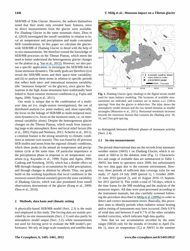
Fig. 1. Zhadang Glacier (grey shading) in the digital terrain modelused for mass balance modeling. The locations of available mea-surements are indicated, and contours are in meters a.s.l. (100 mspacing). Note that the glacier is debris-free. The inlay shows theatmospheric model domain and the two nested domains as smallerrectangles (Maussion et al., 2011). Horizontal resolution increasestowards the innermost domain that contains the Zhadang area: 30,10, and 2 km grid spacing.

to distinguish between different phases of monsoon activity(Sect.2.4).

2.1 In-situ measurements

The pivotal observational data are the records from automaticweather station (AWS) 1 on Zhadang Glacier, which is sit-uated at 5665 m in the ablation zone (Fig. 1). Characteris-tics and usage of available data are summarized in Table 1.AWS1 has been in operation since 2009, but unfortunatelyhas two data gaps due to the extreme environment. How-ever, three periods of sufficient data coverage exist for ourstudy: 27 April–14 July 2009 (period 1), 1 October 2009–25 June 2010 (period 2), and 16 August 2010–15 Septem-ber 2011 (period 3). This yields a total of 743 days, which isthe time frame for the MB modeling and the analysis of themonsoon impact. All data were post-processed according tothe instrument manuals, but also carefully screened follow-ing the procedure described in Molg et al. (2009a) in order todetect and correct measurement errors. Basically, this proce-dure aims to identify periods when radiative sensor heatingand/or riming of instruments may have occurred. Only 0.9 %of wind data and between 0 and 0.7 % of the other variablesneeded correction, which indicates high data quality.

Note that we use accumulation recorded by the sonicranger (SR50) only for the months of October to April (Ta-ble 1), since air temperature (Ta) at AWS1 in the summer

The Cryosphere, 6, 1445–1461, 2012 www.the-cryosphere.net/6/1445/2012/

T. M olg et al.: Monsoon impact on a Tibetan glacier 1447

Table 1.Measurement specifications for AWS1 located at 5665 m a.s.l. The height (depth) values refer to the initial distances to the surfaceon 27 April 2009. Last column indicates the usage for the mass balance modeling: forcing (F), parameter setting (P), or model evaluation(E). The two radiation components yield the measured albedo.

Variable Instrument Nominal accuracy Usage

Air temperature (1.9 m) Campbell CS215a 0.9◦C (−40◦C to+70◦C) FRelative humidity (1.9 m) Campbell CS215a 4 % (0–100 %) FWind speed (3.4 m) Young 05103-45 0.3 m s−1 FAir pressure TH Friedrichs DPI 740 0.15 hPa FWinter accumulationb Campbell SR50 1 cm or 0.4 % to target FIncoming and reflected shortwave radiation Campbell CS300 5 % (daily totals) PSurface height change Campbell SR50 1 cm or 0.4 % to target EGlacier surface temperature Campbell IRTS-Pc 0.3◦C ESubsurface temperature (5.6 m) Campbell TP107 0.3◦C ESubsurface temperature (9.6 m) Campbell TP107 0.3◦C P

a With ventilated radiation shield.b The months October to April.c Uses the principle of emitted radiation.

months clearly exceeds the melting point and therefore theSR50 does not capture the liquid fraction of precipitation.However, total precipitation is a required input for the model(Sect.2.3). Further, subsurface temperature measurementsat AWS1 were also performed at depths less than 5 m, butwere obviously affected by radiative heating. Thus, we onlyuse data from the initial depths of≈ 5.6 and≈ 9.6 m forMB model evaluation and lower boundary condition defini-tion, respectively (Table 1). Regarding the latter, data from≈

9.6 m depth show an almost constant temperature of 268.6 K(standard deviation 0.06 K). We initialize the MB model aftermidnight on the first day of each of the three periods, and in-clude measured surface temperature as well as data from thesensors at≈ 3 and≈ 1.5 m depth since the heating problemduring night is minimal.

The time-dependent height of theTa/relative humidity(RH) and wind speed sensors, as well as the depth of subsur-face sensors, can be estimated from the SR50 record. Withinperiod 3, however, surface height change is not availablefrom 4 October 2010 to 30 June 2011 (68 % of period 3). Thisgap was filled with SR50 data from nearby AWS2 (Fig. 1),which has been operated since 2 October 2010 at 5566 m al-titude (wind instrument from 21 May 2011 onward). AWS2does not record ice ablation, as it is located slightly off theglacier margin on a moraine. Nevertheless, the data gap co-incides with a period of weak ablation, which will be shownin the results section. Thus, we deem this correction to bea reasonable alternative to assuming a random sensor height.Wind speed andTa/RH from AWS2 (same instruments asat AWS1) were also used to examine vertical gradients, butonly for intervals when AWS1 and AWS2 sensor heightsagreed within 0.2 m and when there was high enough windspeed for sufficient natural ventilation of theTa/RH sensor(Georges and Kaser, 2002;n = 1629 h for wind;n = 1340 hfor Ta/RH). We find no gradients in wind speed and RH, asdifferences are within the instrument accuracy. TypicalTa

gradients were considered for defining MB model parame-ters (Sect.2.3).

Finally, data from a precipitation gauge (Geonor T-200B;sensitivity≤ 0.1 mm) at AWS2 between 22 May 2010 and15 September 2011 are used to (i) constrain atmosphericmodel output (Sect.2.2) and (ii) obtain winter precipitationfor period 3 when SR50 data at AWS1 are unavailable. Also,several ablation stakes on Zhadang Glacier serve in the MBmodel evaluation. The locations of these measurement sitesare presented in Fig. 1. Stake readings performed by per-sonnel from the Institute of Tibetan Plateau Research areavailable for three intervals that overlap with each of thethree model simulation periods once, as will be detailed inSect.3.1.

2.2 Atmospheric modeling

We run the Advanced Weather Research and Forecast-ing (WRF) numerical atmospheric model (Skamarock andKlemp, 2008) with a domain that covers a large part ofAsia and the Northern Indian Ocean (Fig. 1) for the years2009–2011. Multiple grid nesting in the parent domain yieldsa local-scale spatial resolution over Zhadang Glacier of 2 km(Fig. 1), which reproduces the real terrain altitude well (seebelow). All details of the model configuration are presentedin Maussion et al. (2011), e.g. the grid structure (their Fig. 1)and the chosen model options and forcing strategy (their Ta-ble 1). We initialize WRF every day from the Global Fore-cast System’s final analysis (Maussion et al., 2011), whichdiffers from the traditional regional climate model approachwhere the model fields evolve over the entire simulation time.WRF output here, by contrast, is strongly constrained by theobserved synoptic weather patterns and thus represents a re-gional atmospheric reanalysis.

Running WRF and producing a high-resolution reanalysisdata set are part of a larger project, but for the present studywe are only interested in the simulation of two variables that

www.the-cryosphere.net/6/1445/2012/ The Cryosphere, 6, 1445–1461, 2012

1448 T. Molg et al.: Monsoon impact on a Tibetan glacier

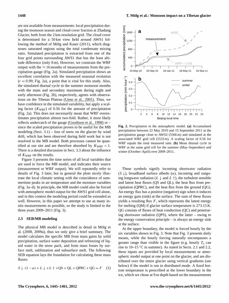
are not available from measurements: local precipitation dur-ing the monsoon season and cloud cover fraction at ZhadangGlacier, both from the 2 km-resolution grid. The cloud coveris determined for a 50 km view field around AWS1 fol-lowing the method of Molg and Kaser (2011), which diag-noses saturated regions using the total condensate mixingratio. Simulated precipitation is extracted from one of thefour grid points surrounding AWS1 that has the least alti-tude difference (only 8 m). However, we constrain the WRFoutput with the≈ 16 months of measurements from the pre-cipitation gauge (Fig. 2a). Simulated precipitation shows anexcellent correlation with the measured seasonal evolution(r = 0.99; Fig. 2a), a point that is vital for this study. Also,the simulated diurnal cycle in the summer monsoon monthswith the main and secondary maximum during night andearly afternoon (Fig. 2b), respectively, agrees with observa-tions on the Tibetan Plateau (Ueno et al., 2001). Thus, wehave confidence in the simulated variability, but apply a scal-ing factor (KWRF) of 0.56 for the amount of precipitation(Fig. 2a). This does not necessarily mean that WRF overes-timates precipitation almost two-fold. Rather, it most likelyreflects undercatch of the gauge (Goodison et al., 1998) or –since the scaled precipitation proves to be useful for the MBmodeling (Sect.3.1) – loss of snow on the glacier by winddrift, which has been observed during field work but is notresolved in the MB model. Both processes cannot be quan-tified at our site and are therefore absorbed byKWRF < 1.There is a detailed discussion in Sect.3.3about the influenceof KWRF on the results.

Figure 3 presents the time series of all local variables thatare used to force the MB model, and indicates their source(measurement or WRF output). We will repeatedly refer todetails of Fig. 3 later, but in general the plots nicely illus-trate the local climatic setting with the coincidence of sum-mertime peaks in air temperature and the moisture variables(Fig. 3a–d). In principle, the MB model could also be forcedwith atmospheric model output for the AWS1 grid cell alone,and in this context the modeling period could be extended aswell. However, in this paper we attempt to use as many in-situ measurements as possible, so the study is limited to thethree years 2009–2011 (Fig. 3).

2.3 SEB/MB modeling

The physical MB model is described in detail in Molg etal. (2008, 2009a), thus we only give a brief summary. Themodel calculates the specific MB from mass gains by solidprecipitation, surface water deposition and refreezing of liq-uid water in the snow pack, and from mass losses by sur-face melt, sublimation and subsurface melt. The followingSEB equation lays the foundation for calculating these massfluxes:

S ↓ ·(1− α) + L ↓ +L ↑ +QS+ QL + QPRC+ QG= F (1)

2 4 6 8 10 12 14 16 18 20 22 24

Beijing local time

0

0.1

0.2

0.3

0.4

prec

ipita

tion

(mm

hou

r−1)

summer

winter

23-May-10 20-Sep-10 18-Jan-11 18-May-11 15-Sep-11

0

400

800

1200

1600

accu

mul

ated

pre

cipi

tatio

n (m

m)

a WRF

measurement

WRF × 0.56

b

Fig. 2. Precipitation in the atmospheric model.(a) Accumulatedprecipitation between 22 May 2010 and 15 September 2011 at theprecipitation gauge close to AWS2 (5566 m) and simulated at theassociated WRF grid cell (5533 m). A scaling factor of 0.56 forWRF equals the total measured sum.(b) Mean diurnal cycle inWRF at the same grid cell for the summer (May–September) andwinter (October–April) over 2009–2011.

These symbols signify incoming shortwave radiation(S ↓), broadband surface albedo (α), incoming and outgo-ing longwave radiation (L ↓ andL ↑), the turbulent sensibleand latent heat fluxes (QS and QL), the heat flux from pre-cipitation (QPRC), and the heat flux from the ground (QG).An energy flux has a positive (negative) sign when it inducesan energy gain (sink) at the surface. The sum of these fluxesyields a resulting fluxF , which represents the latent energyfor melting (QM) if glacier surface temperature is 273.15 K.QG consists of fluxes of heat conduction (QC) and penetrat-ing shortwave radiation (QPS), where the latter – owing tothe energy conservation principle – is always an energy sinkat the surface.

At the upper boundary, the model is forced hourly by thesix variables shown in Fig. 3. Note that Fig. 3 presents dailymeans, while the hourly forcing naturally encompasses agreater range than visible in the figure (e.g. hourlyTa canrise to 10–15◦C in summer). As stated in Sects.2.1and2.2,these inputs are provided by local measurements or atmo-spheric model output at one point on the glacier, and are dis-tributed over the entire glacier using vertical gradients (seebelow) if the model is run in distributed mode. A fixed bot-tom temperature is prescribed at the lower boundary in theice, which we chose at 9 m depth based on the measurements

The Cryosphere, 6, 1445–1461, 2012 www.the-cryosphere.net/6/1445/2012/

T. M olg et al.: Monsoon impact on a Tibetan glacier 1449

M J J OND J FMAM J SOND J FMAM J J A S

-25

-20

-15

-10

-5

0

5

air

tem

pera

ture

(°C

)

2009 2010 2011M J J OND J FMAM J SOND J FMAM J J A S

0

20

40

60

80

100

rela

tive

hum

idity

(%

)

2009 2010 2011

0

0.2

0.4

0.6

0.8

clou

d co

ver

frac

tion

M J J OND J FMAM J SOND J FMAM J J A S2009 2010 2011

0

5

10

15

20

25

prec

ipita

tion

(mm

day

−1)

M J J OND J FMAM J SOND J FMAM J J A S2009 2010 2011

M J J OND J FMAM J SOND J FMAM J J A S

4

8

12

win

d sp

eed

(m s

−1)

2009 2010 2011M J J OND J FMAM J SOND J FMAM J J A S

485

490

495

500

505

510

air

pres

sure

(hP

a)

2009 2010 2011

GAP GAP

a

c

e

b

d

f

SR50 gauge

Fig. 3.Daily means of(a) air temperature,(b) relative humidity,(c) cloud cover fraction,(e)wind speed,(f) air pressure, and(d) daily sumsof all-phase precipitation at AWS1 between 27 April 2009 and 15 September 2011. Ticks on the x-axes indicate the first day of the respectivemonth, and black (blue) signifies measurements (atmospheric model output). In panel(d), the data gaps due the measurement failure areindicated to distinguish them from zero precipitation, and the measurement source for surface accumulation in winter is indicated as well(SR50 or gauge). For consistency, SR50 derived precipitation (actual height) has been converted to w.e. values by a density of 200 kg m−3.

in this region (Sect.2.1). The remaining subsurface layers areat 0.1, 0.2, 0.3, 0.4, 0.5, 0.8, 1.4, 2, 3, 5, and 7 m depth, whichyielded a stable solution in all runs. For these model layersthe initial temperature profile is specified from the availablesubsurface measurements (Sect.2.1) by linear interpolation.A digital terrain model at 60 m resolution (re-sampled fromthe Shuttle Radar Topography Mission; Rabus et al., 2003)and the 2009 glacier extent (Bolch et al., 2010) constitute thetopographic boundary (Fig. 1). A concise overview of theMB model, to illustrate which atmospheric forcing variablesaffect each energy and mass flux in the model, is provided inTable 1 in Molg et al. (2009a).

Since the last model version (Molg et al., 2009a) weadded a few new features based on published work: (i) thelocal air temperature gradient can vary between day andnight/morning to better capture the effect of katabatic winddevelopment (Petersen and Pellicciotti, 2011); (ii) snow set-tling and compaction is simulated from the viscous fluid as-sumption (Sturm and Holmgren, 1998), and together with re-freezing can contribute to snow densification. Specifically,we use Eqs. (5)–(8) in Vionnet et al. (2012); (iii) the tran-sition solid–liquid precipitation is specified by a tempera-ture range using linear interpolation (e.g. Molg and Scherer,

2012), instead of abruptly by one air temperature thresh-old; (iv) a second stability correction for stable conditions isavailable so the turbulence damping factor can be calculatedfrom either equation 11 or 12 in Braithwaite (1995); (v) theenergy flux from precipitation may be included in the SEB(standard equation; e.g. Bogan et al., 2003); and (vi) a sec-ond parameterization ofL ↓ from air temperature, water va-por pressure and cloud cover (Klok and Oerlemans, 2002)provides an alternative to the original formulation (Molg etal., 2009b).

In light of the main goal to unravel the “monsoon foot-print” in the glacier SEB/MB, we also attempt to quantify themodel uncertainty. Thus, we perform a Monte Carlo simula-tion consisting of 1000 realizations, in which all importantmodel parameters, including the vertical gradients for ex-trapolation of meteorological conditions, as well as selectedstructural uncertainties, are varied (Appendix A). This sim-ulation is conducted for one point at the location of AWS 1,since the computational expense for the distributed model istoo large. From the point results we select three combinationsof parameter settings that are maintained for running the fulldistributed MB model (Appendix A), i.e. the final ensem-ble size is 3. One of these combinations, henceforth called

www.the-cryosphere.net/6/1445/2012/ The Cryosphere, 6, 1445–1461, 2012

1450 T. Molg et al.: Monsoon impact on a Tibetan glacier

reference run (REF), reflects the best match with the mea-sured surface height change. The other two settings are usedto spread the uncertainty range around REF (Appendix A).All error estimates in the remainder of the text are based onthis method, unless otherwise noted. One advantage of themethod is that the uncertainty does not simply increase withprogressive simulation time like in classical sensitivity ex-periments where one parameter is changed and all others areheld constant. Instead, in the present method the uncertaintyrange is mainly dependent on surface conditions (snow vs.ice), which is shown later in the model evaluation (Sect.3.1)and in Appendix A.

2.4 Characterization of monsoon dynamics

The specific component of the Asian monsoon system thataffects the Tibetan Plateau is the Indian Summer Monsoon(ISM) (Ding, 2007). To relate glacier energy/mass fluxes tothe ISM we focus on (i) interannual variability associatedwith the monsoon onset and cessation, and (ii) intra-seasonalvariability tied to the active/break cycle – both of which aretypical oscillations in the monsoon dynamics (Webster etal., 1998; Ding, 2007). To characterize these dynamics wefollow Prasad and Hayashi (2007) in identifying active andbreak periods of the ISM, since the authors showed that theirmethod satisfies both precipitation- and circulation-based in-dices used in previous research. A horizontal wind shearindex (HWSI) is defined as the difference in the 850 hPazonal wind (from NCEP/NCAR reanalysis data: Kalnay etal., 1996) between a southern (5–15◦ N, 40–80◦ E) and north-ern region (20–30◦ N, 70–90◦ E). Active periods are definedas days with HWSI> 1σ over 2009–2011, and break peri-ods as days> 1.5σ in the northern region’s zonal wind (i.e.strong westerlies).

Figure 4a shows that establishment of the ISM circulationin the examined years occurred between 1 June (2011) and21 June (2009), when the curves start to rise. The ISM ceasedbetween 16 September (2011) and 19 October (2010), whenthe curves flatten. The former interval contains the mean on-set date in terms of convection and rainfall in the Zhadangregion (Webster et al., 1998). Thus, we define the yearly pe-riod of monsoon onset(monsoon cessation) from 1–21 June(16 September–19 October), which comprises the time win-dows used in the subsequent analysis (Sect.3.4). Only twoyears are available for the analysis of the cessation period,as AWS data in 2011 ends before 16 September. However,both 2009 and 2010 contain the interval 1–19 October andcover the respective cessation dates (6 October in 2009 and19 October in 2010).

Between 22 June and 15 September (ISM core season) thesuccession of active periods and the remaining non-active(weak and break) periods characterizes the intra-seasonalISM variability (Prasad and Hayashi, 2007). Consequently,we have 105 active days and 39 non-active (weak/break)days during the core season in our data set. Amongst the

0102030405060708090

accu

mul

ated

day

s

0 30 60 90 120 150 180 210 240 270 300 330 360

-700-600-500-400-300-200-100

0100

accu

mul

ated

spe

ed (

m s

−1)

0 30 60 90 120 150 180 210 240 270 300 330 360

2009

2010

2011

cessation16 Sep-19 Oct

onset1-21 June

a

b

180

200

220

240

260

280

ener

gy fl

ux d

ensi

ty (

W m

−2)

0 30 60 90 120 150 180 210 240 270 300 330 360day of year

c

Fig. 4. (a)Accumulated active monsoon days,(b) accumulated hor-izontal wind shear index, and(c) top-of-atmosphere outgoing long-wave radiation (14-day smooth) in the ISM region (65–105◦ E, 5–27.5◦ N; Ding, 2007) for 2009, 2010, and 2011.

non-active periods, 10 days can be classified as break days,which will also be considered in the analysis (Sect.3.4).These amounts of days are typical of the active/break cyclein the monsoon region (Webster et al., 1998).

Late monsoon onset and few active periods in 2009(Fig. 4a) are in agreement with the weak cumulative strengthof the ISM circulation in this year, as seen in Fig. 4b. Todraw robust conclusions about monsoon activity, it is desir-able to supplement the circulation index with a convectionindicator (Wang and Fan, 1999), for which we extract top-of-atmosphere outgoing longwave radiation (Liebmann andSmith, 1996) over the ISM precipitation region. This secondindicator yields the same result (Fig. 4c): 2010 and 2011 ex-ceed 2009 in terms of ISM strength, which is particularly ob-vious from day 200–270 (ca. July–September) where 2009shows markedly reduced convection (i.e. higher values inFig. 4c than other years).

The Cryosphere, 6, 1445–1461, 2012 www.the-cryosphere.net/6/1445/2012/

T. M olg et al.: Monsoon impact on a Tibetan glacier 1451

1-May-09 1-Sep-09 2-Jan-10 5-May-10 5-Sep-10 6-Jan-11 9-May-11 9-Sep-11-300

-200

-100

0

surf

ace

heig

ht (

cm)

measurement

model (REF)

250

260

270

tem

pera

ture

(K

)

r = 0.99RMSD = 7.3 cm

r = 0.98RMSD = 1.69 K

1-May-09 1-Sep-09 2-Jan-10 5-May-10 5-Sep-10 6-Jan-11 9-May-11 9-Sep-11265

270

1-May-09 1-Sep-09 2-Jan-10 5-May-10 5-Sep-10 6-Jan-11 9-May-11 9-Sep-11

100

200

300

400

ener

gy fl

ux d

ensi

ty (

W m

−2)

r = 0.83RMSD = 39 W m−2

r = 0.86, RMSD = 0.59 K

a

b

c

d

Fig. 5.Measurements versus MB model (REF run) at AWS1 with correlation and root-mean-square statistics.(a) Accumulated surface heightchange (error bars reflect model uncertainty as defined in Sect.2.3), where every curve starts at 0 at the beginning of the periods;(b) glaciersurface temperature;(c) subsurface temperature, whereas observed depth varies between start and end from 5.6–3.2 m in period 1, 5.3–5.1 min period 2, and 4.4–4.1 m in period 3 (model values found by linear interpolation between layers; note a measurement gap within period 2in May 2010);(d) global radiation. All data are daily mean values.

3 Results and discussion

3.1 MB model performance

We first evaluate the model at the point scale against obser-vations at AWS1 in Fig. 5. The observations of a rather stablesurface height during the winter months and surface lower-ing in summer are well reproduced (Fig. 5a). Regarding thelatter, the model also captures the differential ablation be-tween 2009 (strong) and 2011 (weak) well. Figure 5a alsoillustrates that the model uncertainty is greatest when snowcover is removed during periods of strong ablation (first halfof the 2009 curve). This is a reasonable finding since mod-eling snow ablation, which is complicated by variable snowdensity and refreezing processes, is more difficult than mod-eling ice loss (e.g. Molg et al., 2009a). The root-mean-squaredifference (RMSD) in Fig. 5a is only a tiny fraction of the ob-served amplitude (≈ 3 m), and the explained variance is veryhigh.

A similarly-good performance is evident for glacier sur-face temperature (Tsfc), where the model captures the vari-ability between 245–250 K mean dailyTsfc in winter andmelting point in peak summer well (Fig. 5b). MeasuredTsfcis based on emitted radiation (Table 1), which typically leads

to uncertainties over glacier surface on the order of 2–2.5 K(e.g. Greuell and Smeets, 2001; Molg et al., 2008). TheRMSD in Fig. 5b, however, is below 2 K and corroboratesthe model. Moreover, the temperature variability in the sub-surface (Fig. 5c) indicates that penetrating shortwave radia-tion is simulated reasonably well, since no systematic modelbias is evident (Hoffman et al., 2008; Molg et al., 2008). Fi-nally we consider global radiation (an important driver ofthe SEB) in Fig. 5d, which shows good agreement for vari-ability but a rather high RMSD. As soon as the two curvesare a 5-day smooth, however, the RMSD drops below 10 %of the mean measured global radiation, and 10 % is indeeda more realistic estimate for measurement uncertainty in re-mote field places than the nominal accuracy (e.g. Michel etal., 2008). Thus, incoming shortwave radiation generated bythe MB model can be interpreted reliably for means over fiveor more days, an averaging period always used in this studyfor the monsoon analysis.

To evaluate the distributed output of the model, we calcu-late the mean MB over the available ablation stakes as well asthe associated gradient of the vertical balance profile (VBP)in Fig. 6a. Stake readings are available for three intervals,where the first one (June–July 2009) is contained in simu-lation period 1, and the third one (August–September 2010)

www.the-cryosphere.net/6/1445/2012/ The Cryosphere, 6, 1445–1461, 2012

1452 T. Molg et al.: Monsoon impact on a Tibetan glacier

0

2

4

6

VB

P g

radi

ent (

kg m

−2 m

−1)

-1800

-1600

-1400

-1200

-1000

-800

-600

-400

-200

0

200

mas

s ba

lanc

e (k

g m

−2)

stakes

model

20092 Jun-13 Jul

2009-20103 Sep-17 May

201016 Aug-28 Sep -6000 -4000 -2000 0

mass balance (kg m−2)

5500

5600

5700

5800

5900

6000

altit

ude

(m a

.s.l.

)

2009-2011 (all cells)

2009-2011 (50 m bands)

period 3 (50 m bands)

a b

Fig. 6. (a)Mean mass balance (black) and vertical balance profile (VBP) gradient (grey) over the available ablation stakes (see Fig. 1) andthe associated model locations (found by bi-linear interpolation) for the three intervals indicated at the bottom. Error bars are defined as 1σ

for mass balance, and as 95 % confidence interval of the least-squares regression coefficient for the VBP gradient.(b) Modeled VBP over theentire simulation period (743 days) and period 3 (16 August 2010–15 September 2011). Model data in(a) and(b) are from the mean model(REF and two uncertainty settings, see Sect.2.3).

in simulation period 3 except for the last 13 days in Septem-ber 2010 (which are missing in the model). Since ablationlate in September is usually small, we neglect these days.However, for the second interval of stake readings (3 Septem-ber 2009–17 May 2010) the model is missing the entiremonth of September, since AWS data in period 2 starts on1 October 2009. As ablation in early September can still belarge, we run the MB model for September 2009 with onlyatmospheric model output as MB model forcing in order tobetter evaluate the results for the second interval (withoutSeptember 2009, modeled MB has a positive bias). The onlydiscrepancy in Fig. 6a concerns the VBP in the 2010 interval,where the model shows a higher gradient. However, there isagreement for the net mass flux in the same interval, whichis most important as the area-integrated mass is of primaryinterest in this study. In all other cases, model and measure-ments agree within the error bounds (Fig. 6a), which gives usconfidence that ablation processes are well simulated. Corre-lation coefficients between the single stakes and the associ-ated model locations range between 0.5 and 0.81 in the threeintervals of Fig. 6a (significant at 5 % based on a two-sidedt-test), so the model also captures the basic structure of ob-served spatial variability. Note that strong mass loss in sum-mer 2009 affected the entire ablation area (Fig. 6a), not onlythe AWS1 site (Fig. 5a).

3.2 SEB/MB characteristics

The altitudinal dependence of MB is shown in Fig. 6b,where areas of positive modeled MB are confined to ele-vations> 5750 m. The most notable feature of the VBP isthe change in slope between 5600 and 5700 m. The onlyother distributed MB model study for a nearby region, whichwas also checked against stake measurements, is for XiaoDongkemadi Glacier in the Tanggula Mountains for Octo-ber 1992–September 1993. There, Fujita and Ageta (2000)also found steepening of the VBP around 5600 m; however,it occurs above the equilibrium-line altitude (ELA). If we

examine only period 3, when ablation on Zhadang Glacierwas rather weak (Figs. 5a and 6a), the “knee” in the VBP isalso shifted along the x-axis and above the ELA (Fig. 6b).The single year studied by Fujita and Ageta (2000) wasalso characterized by weak ablation and a slightly positiveglacier-wide MB. In the pure modeling study by Caidongand Sorteberg (2010), the steepening of the VBP occurs at≈ 5800 m. These findings suggest that a dual VBP gradient isa robust feature of glaciers in the central Tibetan Plateau, andis more determined by altitude (weak above 5600–5800 m)than by the MB in a specific year. The result also fits withtheoretical work, as the shape/gradient in Fig. 6b is almosta perfect mixture of the typical mid-latitude and subtropi-cal VBP (Kaser, 2001). The explanation of the shape can befound in the energy fluxes: the VBP in Fig. 6b mimics theprofile of QM (not shown), i.e. the energy available for melt-ing diminishes clearly above 5700 m.

What processes drive the variability of the glacier-wideMB? In general (Fig. 7a; unit is W m−2), S ↓ (260.4) andL ↓ (200.9) dominate energy input, followed by QS (17.9),QC (4.5), and very small QPRC (0.2). Reflected shortwaveradiation S ↑ (−187.7), L ↑ (−268.2), and QL (−10.9),QPS (−3.4), and QM (−13.7) are the energy sinks at thesurface. A salient feature of the variability is the period ofApril–June both in 2010 and 2011, whenS ↑ developed intoan equally strong energy sink asL ↑ (i.e. when the two lowercurves converge in Fig. 7a). The pattern was completelydifferent in 2009, when anomalously low albedo weakenedthis process of energy removal. This, in combination withthe highestL ↓ in the record, resulted in exceptionally highavailability of melt energy in June–July 2009. Also note-worthy is a continuously negative QL on the monthly scale(Fig. 7a), which is not unexpected owing to the generally dryconditions in the central Tibetan Plateau.

The low reflectance of solar radiation in summer 2009 isclearly manifested in the MB components (Fig. 7b). First,surface melt is much higher than in the simulated months of

The Cryosphere, 6, 1445–1461, 2012 www.the-cryosphere.net/6/1445/2012/

T. M olg et al.: Monsoon impact on a Tibetan glacier 1453

-300

-200

-100

0

100

200

300

ener

gy fl

ux d

ensi

ty (

W m

−2)

Apr-09 Aug-09 Dec-09 Apr-10 Aug-10 Dec-10 Apr-11 Aug-11

0.6

0.8

1

QC

QS

QL

QP

S

QM

Apr-09 Aug-09 Dec-09 Apr-10 Aug-10 Dec-10 Apr-11 Aug-11

-40-30-20

-10

0

mas

s flu

x de

nsity

(kg

m−2

day

−1)

refreezing

deposition

solid precipitation

sublimation

subsurface melt

surface melt

Alb

edo

S↓

L↓

L↑

S↑

QC QS QL QPSQMa

b

-2

-4

-6

-8

2

4

Fig. 7.Glacier-wide mean monthly(a) SEB components with surface radiation terms shown as lines, albedo as dots, and the remaining fluxesas bars (see Sect.2.3 for abbreviations; precipitation heat flux is not shown as it is negligibly small) and(b) MB components from April2009 to September 2011 in the REF run. Note the y-axis break and variable scaling in(b) due to large melt amounts in 2009.

the ablation seasons 2010 and 2011. Second, the high en-ergy availability at the surface also caused more penetrat-ing shortwave radiation and thus subsurface melt in 2009,which hardly occurs at other times. Due to the negativeQL discussed above, sublimation is also evident in the MBrecord. It peaks in the months prior to monsoon onset (e.g.February–April 2010) when (i)Tsfc rises after the winterminimum (Fig. 5b) but the atmosphere remains rather dry,which favors a large surface-air vapor pressure gradient, and(ii) higher wind speeds (Fig. 3e) drive turbulence. Meltingis absent from November–March, and in total 3.7 % of themodeled grid cell-scale melt happens at air temperatures be-low 0◦C. The latter was previously detected as a typical fea-ture of glaciers in High Asia (e.g. Aizen et al., 2002). Re-freezing of liquid water can occasionally be larger than ac-cumulation by solid precipitation, generally in spring/earlysummer (Fig. 7b). This feature affirms previous statementsthat refreezing in the snow is an evident process on Asianhigh-altitude glaciers (Ageta and Fujita, 1996; Fujita andAgeta, 2000). On average, 13 % of surface melt refreezes,which is less than the 20 % obtained for Xiao DongkemadiGlacier (Fujita and Ageta, 2000). The glacier-wide MB esti-mate from the REF run over the 743 modeled days (−1.63×

103 kg m−2) is composed as follows (same unit): solid pre-cipitation (1.02), refreezing (0.32), deposition (0.03), sur-face melt (−2.52), sublimation (−0.28), and subsurface melt(−0.20). The dominance of melt over sublimation at this

site fits into the regional-scale pattern of ablation characteris-tics suggested by simplified MB modeling (Rupper and Roe,2008).

We can also give two annual MB estimates for ZhadangGlacier, from 1 October to 30 September of the subse-quent year for consistency with previous studies (Kang et al.,2009). Glacier-wide MB based on the model for 2009/2010(2010/2011) is−154± 43 (−382± 41) kg m−2. The modeldata gap from 26 June to 15 August 2010 can be accountedfor fairly reasonably, since the initial condition for period 3on 16 August 2010 (based on observations) is a snow-freeglacier (i.e. all the snow at the end of period 2 is assumed tobe lost in the gap for the MB estimate). Still, 2009/2010 ismore likely an over- rather than under-estimation, since icemay have also ablated in this gap. For 2010/2011, the modelends 15 days earlier in September 2011, which must be ne-glected. The values found here are within the range measuredfrom 2005–2008,−1099 to 223 kg m−2 per year (Kang et al.,2009).

3.3 Sensitivity to processes and forcing

We performed sensitivity runs for the REF configuration inTable 2 because little is known about the importance of par-ticular physical processes for the Tibetan glaciers. For theseruns, certain structural components of the MB model (phys-ical parameterizations) are deactivated, thus they differ from

www.the-cryosphere.net/6/1445/2012/ The Cryosphere, 6, 1445–1461, 2012

1454 T. Molg et al.: Monsoon impact on a Tibetan glacier

Table 2.Sensitivity of glacier-wide MB over the entire simulation period (with respect to REF settings:−1.63× 103 kg m−2) to particularprocesses or (last four lines) changes in the forcing. Relative changes in parentheses. Winter (W) and summer (S) half years are defined asOctober–March and April–September, respectively.

Process MB change (103 kg m−2)

no topographic shading −0.193 (−12 %)no stability correction for turbulence −0.788 (−48 %)no variation in surface roughness −0.141 (−9 %)no snow compaction/settling −0.421 (−26 %)no refreezing in snow −0.199 (−12 %)no subsurface melt +0.339 (+21 %)no penetrating shortwave radiation −0.185 (−10 %)1Ta = +1◦C −1.140 (−70 %); W:−0.053 (−3 %), S:−1.087 (−67 %)1Ta = −1◦C +0.789 (+48 %); W:+0.034 (+2 %), S:+0.755 (+46 %)precipitation:+10 % +0.248 (+15 %); W:+0.015 (+1 %), S:+0.233 (+14 %)precipitation:−10 % −0.303 (−19 %); W:−0.017 (−1 %), S:−0.286 (−18 %)

usual sensitivity studies that change the value of one inter-nal model parameter. From the calculations, we find littleinfluence of using variable surface roughness lengths, whileQPS, topographic shading and refreezing are on the orderof the model uncertainty (0.21× 103 kg m−2). Also impor-tant are snow compaction/settling due to the resultant effectson snow density and subsurface melt. Suppressing the lat-ter in the model leads to a saving of 0.34× 103 kg m−2 inthe MB, which is a higher absolute value than the subsur-face melt term in the MB budget (−0.20× 103 kg m−2; seeSect.3.2). This result indicates that the absence of subsurfacemelt has a feedback potential (mostly through the influenceon snow depth and thus albedo). The strongest impact on MBis clearly from the stability correction of turbulent fluxes (Ta-ble 2). A strong feedback process also operates here, sincethe increase in absorbed shortwave radiation (5.3 W m−2)from the initially turbulence-driven acceleration of snow ab-lation is eventually larger than the increase in the turbulentflux itself (1QS +1QL = 3.6 W m−2). The stratification ofthe surface layer, on the other hand, reduces the strength ofQS and QL to 54 % of their value in neutral conditions. Thus,not accounting for stability effects can lead to a strong neg-ative MB bias, and Table 2 suggests that any physical MBmodel for Tibetan glaciers must include stability correction.Also, empirically-based models driven byTa and precipita-tion alone should incorporate parameterizations of refreezing(e.g. Gardner et al., 2011) for Tibetan glaciers. Refreezingonly shows an intermediate effect in Table 2, but due to thesystematic seasonal importance in the MB (Fig. 7b) its ne-glect seems unwarranted as soon as seasonal variations aremodeled and interpreted.

Furthermore we present in Table 2 classical, static MBsensitivity to constant changes in the two atmospheric forc-ings Ta and precipitation, using the typical perturbations of1◦C and 10 %. First, in bothTa and precipitation perturba-tions, the MB change is hardly affected by conditions in win-ter. Hence, our study complements other evidence that the

“summer accumulation type glaciers” of Asia are extremelysensitive to atmospheric conditions in the warm season, asdiscussed in the introduction. Second, the general MB sen-sitivity is calculated from Table 2 as the mean of absolute1MB for negative and positive perturbations before beingconverted to an annual value by multiplying with the fac-tor 365/743, i.e. the number of days per year/days in modelrecord. The annual value then amounts to (all units in the re-maining paragraph in 103 kg m−2

= m w.e.) 0.47 per◦C fortheTa perturbations, and to 0.14 per 10 % for the precipita-tion perturbations. These numbers can be compared to thefew available studies that also employed identical perturba-tions to a glacier-wide, SEB-based MB model run over atleast one year. A typical glacier in the European Alps (Klokand Oerlemans, 2002) seems to respond slightly stronger (≈

0.67 per◦C and≈ 0.17 per 10 %), while the extremely mar-itime and high-precipitation glaciers in New Zealand (An-derson et al., 2010) show a clearly higher sensitivity in theorder of 2.0 per◦C and 0.4 per 10 %. On the other hand, thehigh-altitude equatorial glaciers on Kilimanjaro (Molg et al.,2009a) show a lower response in their dry climatic environ-ment (0.24 per◦C and 0.09 per 10 %) than Zhadang Glacier.Our calculations therefore support the generally accepted re-lation of increasing MB sensitivity as the climatic conditionsbecome wetter and warmer (e.g. Fujita and Ageta, 2000).

Finally, we varyKWRF, which is the only parameter usedto scale MB model input (Sect.2.2). This is done for period1 as it relies entirely on scaled summer precipitation as input(Fig. 3d), shows the highest mass amplitude (Fig. 5a), andhence is most sensitive to the scaling. In concert withKWRFwe vary the density of solid precipitation, because (i) it is afree model parameter (Appendix A) and together withKWRFdetermines the actual precipitation height, i.e. the variablethat enters the MB model (Molg and Scherer, 2012), and(ii) this procedure helps to explore the physically meaningfulrange of the scaling (see below). Multiplication ofKWRF by1.25, 1.5 and 1.75 changes the glacier-wide MB in period 1

The Cryosphere, 6, 1445–1461, 2012 www.the-cryosphere.net/6/1445/2012/

T. M olg et al.: Monsoon impact on a Tibetan glacier 1455

-300

-200

-100

0

100

200

300

400

ener

gy fl

ux d

ensi

ty (

W m

−2)

or a

lbed

o (%

)

-80

-60

-40

-20

0

20

40

60

80

L↓L↑ α

QS

QL

QCQM

QPS

monsoon onset

-20

-18

-16

-14

-12

-10

-8

-6

-4

-2

0

2m

ass

flux

dens

ity (

kg m

−2 d

ay−1

)

2009 (late)

2010 (early)

2011 (earliest)

solid prec.

surfacemelt

sublimation

refreezing

subsurfacemelt

deposition

a

b

S↑S↓

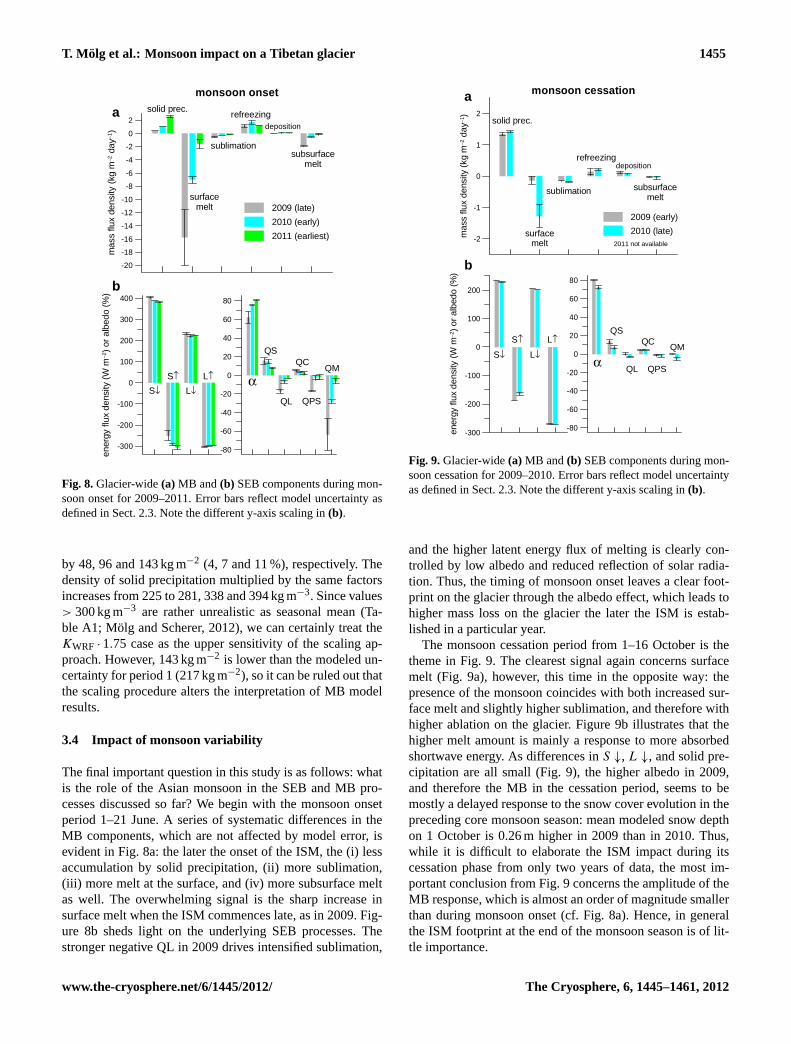
Fig. 8. Glacier-wide(a) MB and(b) SEB components during mon-soon onset for 2009–2011. Error bars reflect model uncertainty asdefined in Sect.2.3. Note the different y-axis scaling in(b).

by 48, 96 and 143 kg m−2 (4, 7 and 11 %), respectively. Thedensity of solid precipitation multiplied by the same factorsincreases from 225 to 281, 338 and 394 kg m−3. Since values> 300 kg m−3 are rather unrealistic as seasonal mean (Ta-ble A1; Molg and Scherer, 2012), we can certainly treat theKWRF · 1.75 case as the upper sensitivity of the scaling ap-proach. However, 143 kg m−2 is lower than the modeled un-certainty for period 1 (217 kg m−2), so it can be ruled out thatthe scaling procedure alters the interpretation of MB modelresults.

3.4 Impact of monsoon variability

The final important question in this study is as follows: whatis the role of the Asian monsoon in the SEB and MB pro-cesses discussed so far? We begin with the monsoon onsetperiod 1–21 June. A series of systematic differences in theMB components, which are not affected by model error, isevident in Fig. 8a: the later the onset of the ISM, the (i) lessaccumulation by solid precipitation, (ii) more sublimation,(iii) more melt at the surface, and (iv) more subsurface meltas well. The overwhelming signal is the sharp increase insurface melt when the ISM commences late, as in 2009. Fig-ure 8b sheds light on the underlying SEB processes. Thestronger negative QL in 2009 drives intensified sublimation,

-300

-200

-100

0

100

200

ener

gy fl

ux d

ensi

ty (

W m

−2)

or a

lbed

o (%

)

-80

-60

-40

-20

0

20

40

60

80

L↓

L↑

α

QS

QL

QCQM

QPS

monsoon cessation

2011 not available-2

-1

0

1

2

mas

s flu

x de

nsity

(kg

m−2

day

−1)

2009 (early)

2010 (late)

solid prec.

surfacemelt

sublimation

refreezingdeposition

subsurfacemelt

S↓

S↑

a

b

Fig. 9. Glacier-wide(a) MB and(b) SEB components during mon-soon cessation for 2009–2010. Error bars reflect model uncertaintyas defined in Sect.2.3. Note the different y-axis scaling in(b).

and the higher latent energy flux of melting is clearly con-trolled by low albedo and reduced reflection of solar radia-tion. Thus, the timing of monsoon onset leaves a clear foot-print on the glacier through the albedo effect, which leads tohigher mass loss on the glacier the later the ISM is estab-lished in a particular year.

The monsoon cessation period from 1–16 October is thetheme in Fig. 9. The clearest signal again concerns surfacemelt (Fig. 9a), however, this time in the opposite way: thepresence of the monsoon coincides with both increased sur-face melt and slightly higher sublimation, and therefore withhigher ablation on the glacier. Figure 9b illustrates that thehigher melt amount is mainly a response to more absorbedshortwave energy. As differences inS ↓, L ↓, and solid pre-cipitation are all small (Fig. 9), the higher albedo in 2009,and therefore the MB in the cessation period, seems to bemostly a delayed response to the snow cover evolution in thepreceding core monsoon season: mean modeled snow depthon 1 October is 0.26 m higher in 2009 than in 2010. Thus,while it is difficult to elaborate the ISM impact during itscessation phase from only two years of data, the most im-portant conclusion from Fig. 9 concerns the amplitude of theMB response, which is almost an order of magnitude smallerthan during monsoon onset (cf. Fig. 8a). Hence, in generalthe ISM footprint at the end of the monsoon season is of lit-tle importance.

www.the-cryosphere.net/6/1445/2012/ The Cryosphere, 6, 1445–1461, 2012

1456 T. Molg et al.: Monsoon impact on a Tibetan glacier

Figure 10 finally turns to the monsoon core season. Theamplitude of mass fluxes (Fig. 10a) is comparable to themonsoon onset phase (Fig. 8a), but a series of systematicdifferences between active and non-active ISM days is notevident. Surface melt is higher during break periods than dur-ing active periods, but this difference does not hold for activeversus non-active days (Fig. 10a). Solid precipitation, albedoandL ↓ are higher during non-active and break periods thanon active monsoon days (Fig. 10), a surprising finding in thecontext of the core season given that monsoon air massescarry abundant moisture. We discuss this result in the para-graph below from three angles, but wish to first note that in-troducing a lead/lag of one or two days to the analysis inFig. 10 for the monsoon/local SEB and MB relation does notchange the results, since active and non-active periods occuras clusters of several consecutive rather than isolated days(Fig. 4a).

First, Prasad and Hayashi (2007) analyzed the synop-tic structure of the intra-seasonal ISM variability in de-tail. Their Fig. 4 shows that convective centers are clearlyshifted away from the main ISM precipitation region (de-fined by Ding, 2007, as 65–105◦ E, 5–27.5◦ N) during non-active periods, but little difference is evident over the Ti-betan Plateau. An analysis of WRF output as well as satellite-based data (Fig. 11) supports the idea that the expected in-crease in precipitation during active monsoon days existsfor the large-scale ISM area, but not for the Zhadang re-gion. Thus, atmospheric variability over the ISM area doesnot seem to directly influence the Zhadang region. Second,Ueno et al. (2001) highlighted that precipitation on the Ti-betan Plateau is dominated by weak but frequent events inthe monsoon season that typically originate from mesoscalesystems or local deep convective cells. Hence, the monsooncan be understood as the “background trigger”, but local tomesoscale processes forced by the complex relief structure,as well as by the numerous lakes (e.g. Lake Nam Co closeto the investigation site: Haginoya et al., 2009), modify thelarge-scale flow and cause a unique precipitation regime overthe Tibetan Plateau. A recent study (Chen et al., 2012) alsoshows that one of the moisture source regions for the TibetanPlateau in summer is situated on the plateau itself, and thatlocal water recycling is evident in the same season. Third,it is well appreciated that mid-latitude flow impacts HighAsia in the non-monsoon season, but less is known aboutmid-latitude intrusions during the monsoon. For instance,Ueno (2005) shows that mid-latitude flow anomalies affectthe Tibetan Plateau as late as in mid May, so it cannot beruled out that mid-latitude circulation also modifies ISM ac-tivity in the core season, especially when the monsoon onsetoccurs early. This should be investigated in more detail infuture studies in the context of cryospheric changes in HighAsia.

In summary, the moisture regime on the Tibetan Plateauduring the ISM core season seems to be controlled by localand regional circulations, and/or by the fact that large-scale

-300

-200

-100

0

100

200

300

ener

gy fl

ux d

ensi

ty (

W m

−2)

or a

lbed

o (%

)-80

-60

-40

-20

0

20

40

60

80

L↓

L↑

α

QS

QL

QC QM

QPS

monsoon core season

-20

-18

-16

-14

-12

-10

-8

-6

-4

-2

0

2

4

mas

s flu

x de

nsity

(kg

m−2

day

−1)

active

non-active

break

solid prec.

surfacemelt

sublimation

refreezingdeposition

subsurfacemelt

S↓

S↑

a

b

Fig. 10. Glacier-wide (a) MB and (b) SEB components in themonsoon core season for active, non-active, and break compositesin 2009–2011. Error bars reflect model uncertainty as defined inSect.2.3. Note the different y-axis scaling in(b).

ISM variability does not advance as far north as onto the cen-tral Tibetan Plateau. Therefore, local conditions may showa poor correlation to large-scale flow at this time of the year,e.g. as also found for measured precipitation at Lhasa fromMay to September (Caidong and Sorteberg, 2010). In thisvein, local SEB and MB on Zhadang Glacier do not followa systematic pattern in relation to large-scale ISM variabilityduring the monsoon core season (Fig. 10).

4 Conclusions

Our state-of-the-art, distributed and physical mass balancemodel (Molg et al., 2009a) reproduces the available measure-ments on Zhadang Glacier well, and a novel combination ofthe Monte Carlo and ensemble approaches allows for a rea-sonable time-varying estimate of model uncertainty. Modelforcing is mainly based on field measurements, but also onoutput from high-resolution atmospheric modeling – a strat-egy that should become more common for data-sparse re-gions (e.g. Van Pelt et al., 2012). From the glacier model’soutput it is evident that interannual variability in mass bal-ance has its physical origin in late spring/early summer, whenthe energy sink by reflected shortwave radiation is muchweaker in high-ablation years than in other years. Affected

The Cryosphere, 6, 1445–1461, 2012 www.the-cryosphere.net/6/1445/2012/

T. M olg et al.: Monsoon impact on a Tibetan glacier 1457

0 4 8 12

0

0.1

0.2

0.3

0.4

rela

tive

freq

uenc

y

0 4 8 12precipitation (mm day−1)

0

0.1

0.2

0.3

0.4

rela

tive

freq

uenc

y

ISM region (TRMM)

Zhadang region (TRMM)

0 4 8 12

0

0.1

0.2

0.3

0.4ISM region (WRF)

0 4 8 12precipitation (mm day−1)

0

0.1

0.2

0.3

0.4

break

active

Zhadang region (WRF)

Fig. 11.Precipitation histograms in the ISM region (65–105◦ E, 5–27.5◦ N) and the region of Zhadang Glacier (90–91◦ E, 30–31◦ N)in the monsoon core season for active and break composites 2009–2011. Data are from (left) the Tropical Rainfall Measuring Missionsatellite, product 3B42 (Huffman et al., 2007) and from (right) theWRF simulation (Sect.2.2).

mass and energy fluxes can differ by almost one order ofmagnitude between such contrasting circumstances.

This strong mechanism is closely linked to the onsetperiod of the Indian Summer Monsoon from 1–21 June.Early (late) monsoon onset not only results in increased (de-creased) accumulation, but through the albedo effect pro-vides less (more) energy for surface melt, sublimation, andsubsurface melt. This local footprint shows that ZhadangGlacier senses the monsoon dynamics in the onset period,which has a profound impact on interannual mass balancevariability as well. In the monsoon cessation period duringfall, however, the footprint on the glacier is relatively weakand also seems to be impacted by the snow cover evolution inthe preceding core monsoon season. During the core season,we do not find any systematic relation in our data betweenmonsoon dynamics and glacier mass/energy fluxes.

Coming back to the hypothesis from the introduction sec-tion, our results do confirm that the Asian monsoon has a vi-tal impact on the glaciers of the Tibetan Plateau. However, re-sults also demonstrate the need to differentiate in any hypoth-esis/research question between the phase of the monsoon,onset vs. intraseasonal variability. The present results showthat in the core season of the monsoon, at least for 2009–2011, the glacier mass and energy budgets obey local-scaleweather that is not related to large-scale circulation variabil-ity. Thus, local and regional meteorological systems seem tocontrol atmospheric variability on the Tibetan Plateau from

Fig. A1. Surface height change at AWS1 from 27 April to14 July 2009, measurement versus 1000 model realizations.

July to mid September (e.g. Ueno et al., 2001), which is cor-roborated here from a cryospheric viewpoint.

Appendix A

MB model uncertainty

For the free MB model parameters, values are assignedpseudo-randomly from either published ranges or rangesconstrained by on-site measurements and atmospheric sim-ulations (Table A1). Figure A1 shows the result for the firstperiod of forcing data coverage. A total 450 of 1000 pa-rameter combinations yield a root-mean-square difference(RMSD)< 10 % of the measured amplitude and a devia-tion < 10 % from the measurement at the final data point inthe time series. These runs pass the test and therefore are“accepted” (dark grey in Fig. A1). Amongst them, the runwith minimum RMSD (blue in Fig. A1) is the reference run(REF), while the two combinations that result in the largestpositive and negative sum of the deviation from the measure-ment define the uncertainty (red). It is evident (Fig. A1) thatuncertainty is larger for the first part of the period when snowis present (until day 51 in REF) and decreases afterwards. Forthe second and third period of data coverage, the criterionof 10 % is increased to 20 %, since the measured amplitudeof surface height change is clearly smaller (see Fig. 5a); 65and 62 parameter combinations pass the test in period 2 and3, respectively. The 10–20 % criterions are greater than thenominal accuracy of the SR50, but in order to detect a robustmonsoon footprint the aim is to avoid an underestimation ofmodel uncertainty (thus we chose these rather large percent-age criterions), and also provide space for uncertainty/errorin the meteorological forcing data. Errors in the forcing datahave been minimized as much as possible (Sects.2.1and2.2)and are absorbed by the model parameters in our case. Even

www.the-cryosphere.net/6/1445/2012/ The Cryosphere, 6, 1445–1461, 2012

1458 T. Molg et al.: Monsoon impact on a Tibetan glacier

Table A1. Free parameters in the MB model. Base value (V) and uncertainty (U) are from the literature, or constrained by on-site fieldmeasurements (meas. – Sect.2.1) and atmospheric model output (atmo. – Sect.2.2). For assumptions (assum.), the uncertainty is chosen tobe relatively large (20 %). Bold parameters indicate structural uncertainty, others parametric uncertainty (e.g. Tatang et al., 1997). For theMonte Carlo simulation, values are assigned randomly from a uniform distribution, except for case 13 (normal distribution) since the authorsprovide uncertainty as one standard deviation (Gromke et al., 2011).

Parameter(ization) Value References Note

1 vertical air temperature gradient (night/morning:> 21:00–13:00 local time)

−0.0035 K m−1±10 % V+ U: meas., Petersen and Pellicciotti (2011) a

2 vertical air temperature gradient (day:> 13:00–21:00 local time)

−0.0095 K m−1±10 % V+ U: meas., Petersen and Pellicciotti (2011) a

3 vertical precipitation gradient +0.038±0.026 % m−1 V: Li (1986), atmo.; U: atmo. b

4 upper threshold for precipitation phase (all liquid above) 6.5± 0.5◦C V+U: Fujita and Ageta (2000), Zhou et al. (2010),atmo.

5 lower threshold for precipitation phase (all solid below) 1± 1◦C V+U: Fujita and Ageta (2000), Zhou et al. (2010),atmo.

6 parameterization of L ↓ n.a. Molg et al. (2009b) or Klok and Oerlemans (2002)

7 layer thickness for surface temperature scheme 0.5 m±10 % V+ U: Molg et al. (2008)

8 parameterization of stable condition effect on turbu-lence

n.a. Eqs. (11) or (12) in Braithwaite (1995)

9 clear-sky diffuse radiation fraction 0.046± 20 % V: Molg et al. (2009b); U: assum.

10 cloud effect in radiation scheme 0.55± 10 % V+ U: Molg et al. (2009b), meas.

11 roughness length ice (momentum) 1.7± 1 mm V: Cullen et al. (2007); U: Brock et al. (2006) c

12 roughness length ice (scalars) 1.7± 1 mm V: Cullen et al. (2007); U: Brock et al. (2006) c

13 roughness length fresh snow 0.24± 0.05 mm V+ U: Gromke et al. (2011) c

14 roughness length aged snow (momentum) 4± 2.5 mm V+ U: Brock et al. (2006) c

15 roughness length aged snow (scalars) 4± 2.5 mm V+ U: Brock et al. (2006) c

16 density of solid precipitation 250± 50 kg m−3 V+U: Sicart et al. (2002), Molg and Scherer (2012)

17 initial snow depth two- or threefoldincrease towards peak

V + U: assum. d

18 initial snow density 300 kg m−3± 20 % V+ U: assum.

19 superimposed ice constant 0.3± 20 % V: Molg et al. (2009a); U: assum.

20 fraction ofS ↓ ·(1− α) absorbed in surface layer (ice) 0.8± 10 % V+ U: Bintanja and van den Broeke (1995), Molget al. (2008)

21 fraction ofS ↓ ·(1− α) absorbed in surface layer (snow) 0.9± 10 % V+U: Bintanja and van den Broeke (1995), Van Aset al. (2005)

22 extinction of penetrating shortwave radiation (ice) 2.5 m−1± 20 % V: Bintanja and van den Broeke (1995); U: assum.

23 extinction of penetrating shortwave radiation (snow) 17.1 m−1± 20 % V: Bintanja and van den Broeke (1995); U: assum.

24 fixed bottom temperature 268.6± 0.2 K V + U: meas. e

25 ice albedo 0.3± 0.1 V + U: meas.

26 fresh snow albedo 0.85± 0.03 V+ U: meas.

27 firn albedo 0.55± 0.05 V+ U: meas. f

28 albedo time scale 6± 3 days V+ U: meas. f

29 albedo depth scale 8± 6 cm V+ U: meas. f

a Determined from AWS1 vs. AWS2 data (Sect.2.1). b The value 3.8 % per 100m in the atmospheric model agrees well with the observations of Li (1986): 5 % per 100m.Uncertainty is the 95 % confidence interval of the gradient in the atmospheric model output.c Several roughness lengths are specified because the MB model uses a schemefor space/time-varying roughness, which is described in Molg et al. (2009a).d Between the measured initial snow depth at AWS1 and the highest altitude on the glacier inthe digital terrain model; there are no measurements other than at AWS1, but field experience clearly suggests increasing snow depth with altitude.e 0.2K is the amplitudeof the measurements at that level (Sect.2.1). f Optimal values of these three albedo scheme parameters are determined from measurements over period 2 (the only periodwith a reliable snow depth record), as described in Oerlemans and Knap (1998). The uncertainty reflects varying choice of the parameters that are held constant in theoptimization procedure.

The Cryosphere, 6, 1445–1461, 2012 www.the-cryosphere.net/6/1445/2012/

T. M olg et al.: Monsoon impact on a Tibetan glacier 1459

if the Monte Carlo simulation is done with the point model,vertical gradients influence the result due to the altitude dif-ference between AWS1 and the associated grid cell in thedigital terrain model (≈ 20 m). Also, these gradients clearlydiffer between the three chosen parameter combinations forthe distributed runs (i.e. REF and two uncertainty settings),which allows us to capture uncertainty for the higher glacierreaches as well.

Acknowledgements.This work was supported by the Alexandervon Humboldt Foundation (Thomas Molg), by the GermanResearch Foundation (DFG) Priority Programme 1372, “TibetanPlateau: Formation – Climate – Ecosystems” within the DynRG-TiP (“Dynamic Response of Glaciers on the Tibetan Plateau toClimate Change”) project under the codes SCHE 750/4-1, SCHE750/4-2, SCHE 750/4-3, and by the German Federal Ministry ofEducation and Research (BMBF) Programme “Central Asia –Monsoon Dynamics and Geo-Ecosystems” (CAME) within theWET project (“Variability and Trends in Water Balance Compo-nents of Benchmark Drainage Basins on the Tibetan Plateau”)under the code 03G0804A. We thank Eva Huintjes and ChristophSchneider, RWTH Aachen, for their active participation in fieldwork and in AWS design questions, and for providing DEM andAWS2 data. We thank Tandong Yao, Shichang Kang, GuoshuaiZhang and the staff of the Nam Co monitoring station fromthe Institute of Tibetan Plateau Research, Chinese Academy ofSciences, for leading the glaciological measurements on Zhadangand for providing ablation stake and rain gauge data. We alsothank the local Tibetan people for their assistance during field work.

Edited by: V. Radic

References

Ageta, Y. and Fujita, K.: Characteristics of mass balance of summer-accumulation type glaciers in the Himalayas and Tibetan Plateau,Z. Gletscherk. Glazialgeol., 32, 61–65, 1996.

Aizen, V. B., Aizen, E. M., and Nikitin, S. A.: Glacier regime on thenorthern slope of the Himalaya (Xixibangma glaciers), Quatern.Int., 97–98, 27–39, 2002.

Anderson, B., Mackintosh, A., Stumm, D., George, L., Kerr, T.,Winter-Billington, A., and Fitzsimmons, S.: Climate sensitivityof a high-precipitation glacier in New Zealand, J. Glaciol., 56,114–128, 2010.

Bintanja, R. and van den Broeke, M.: The surface energy balanceof Antarctic snow and blue ice, J. Appl. Meteorol., 34, 902–926,1995.

Bogan, T., Mohseni, O., and Stefan, H. G.: Stream temperature–equilibrium temperature relationship, Water Resour. Res., 39,1245, doi:10.1029/2003WR002034, 2003.

Bolch, T., Yao, T., Kang, S., Buchroithner, M. F., Scherer, D., Maus-sion, F., Huintjes, E., and Schneider, C.: A glacier inventory forthe western Nyainqentanglha Range and the Nam Co Basin, Ti-bet, and glacier changes 1976–2009, The Cryosphere, 4, 419–433, doi:10.5194/tc-4-419-2010, 2010.

Braithwaite, R. J.: Aerodynamic stability and turbulent sensible-heat flux over a melting ice surface, the Greenland ice sheet, J.Glaciol., 41, 562–571, 1995.

Brock, B. W., Willis, I. C., and Martin, M. J.: Measurement andparameterization of aerodynamic roughness length variations atHaut Glacier d’Arolla, Switzerland, J. Glaciol., 52, 281–297,2006.

Caidong, C. and Sorteberg, A.: Modelled mass balance of Xibuglacier, Tibetan Plateau: sensitivity to climate change, J. Glaciol.,56, 235–248, 2010.

Chen, B., Xu, X. D., Yang, S., and Zhang, W.: On the ori-gin and destination of atmospheric moisture and air mass overthe Tibetan Plateau, Theoret. Appl. Climatol., 110, 423–435,doi:10.1007/s00704-012-0641y, 2012.

Cullen, N. J., Molg, T., Kaser, G., Steffen, K., and Hardy, D. R.:Energy-balance model validation on the top of Kilimanjaro, Tan-zania, using eddy covariance data, Ann. Glaciol., 46, 227–233,2007.

Ding, Y.: The variability of the Asian Summer Monsoon, J. Meteo-rol. Soc. Jpn., 85B, 21–54, 2007.

Fujita, K. and Ageta, Y.: Effect of summer accumulation on glaciermass balance on the Tibetan Plateau revealed by mass-balancemodel, J. Glaciol., 46, 244–252, 2000.

Fujita, K. and Nuimura, T.: Spatially heterogeneous wastage of Hi-malayan glaciers, P. Natl. Acad. Sci. USA, 108, 14011–14014,2011.

Gardner, A. S., Moholdt, G., Wouters, B., Wolken, G. J.,Burgess, D. O., Sharp, M. J., Cogley, J. G., Braun, C., andLabine, C.: Sharply increased mass loss from glaciers and icecaps in the Canadian Arctic Archipelago, Nature, 473, 357–360,2011.

Georges, C. and Kaser, G.: Ventilated and unventilated air tem-perature measurements for glacier-climate studies on a trop-ical high mountain site, J. Geophys. Res., 107, 4775,doi:10.1029/2002JD002503, 2002.

Greuell, W. and Smeets, P.: Variations with elevation in the surfaceenergy balance on the Pasterze (Austria), J. Geophys. Res., 106,31717–31727, 2001.

Goodison, B., Louie, P., and Yang, D.: WMO solid precipitationmeasurement intercomparison, 1998.

Gromke, C., Manes, C., Walter, B., Lehning, M., and Guala, M.:Aerodynamic roughness length of fresh snow, Bound.-Lay. Me-teorol., 141, 21–34, 2011.

Haginoya, S., Fujii, H., Kuwagata, T., Xu, J., Ishigooka, Y.,Kang, S., and Zhang, Y.: Air-lake interaction features found inheat and water exchanges over Nam Co on the Tibetan Plateau,SOLA, 5, 172–175, 2009.

He, Y., Zhang, Z., Theakstone, W. H., Chen, T., Yao, T., andPang, H.: Changing features of the climate and glaciers inChina’s monsoonal temperate glacier region, J. Geophys. Res.,108, 4530, doi:10.1029/2002JD003365, 2003.

Hoffman, M. J., Fountain, A. G., and Liston, G. E.: Sur-face energy balance and melt thresholds over 11 years atTaylor Glacier, Antarctica, J. Geophys. Res., 113, F04014,doi:10.1029/2008JF001029, 2008.

Huffman, G. J., Adler, R. F., Bolvin, D. T., Gu, G., Nelkin, E. J.,Bowman, K. P., Hong, Y., Stocker, E. F., and Wolff, D. B.:The TRMM Multi-satellite precipitation analysis: quasi-global,multi-year, combined-sensor precipitation estimates at fine scale,

www.the-cryosphere.net/6/1445/2012/ The Cryosphere, 6, 1445–1461, 2012

1460 T. Molg et al.: Monsoon impact on a Tibetan glacier

J. Hydrometeorol., 8, 38–55, 2007.Jiang, X., Wang, N. L., He, J. Q., Wu, X. B., and Song, G. J.: A dis-

tributed surface energy and mass balance model and its appli-cation to a mountain glacier in China, Chinese Sci. Bull., 55,2079–2087, 2010.

Kalnay, E., Kanamitsu, M., Kistler, R., Collins, W., Deaven, D.,Gandin, L., Iredell, M., Saha, S., White, G., Woollen, J., Zhu, Y.,Leetmaa, A., Reynolds, R., Chelliah, M., Ebisuzaki, W., Higgins,W., Janowiak, J., Mo, K. C., Ropelewski, C., Wang, J., Jenne,R., and Joseph, D.: The NCEP/NCAR 40-year reanalysis project,Bull. Am. Meteorol. Soc., 77, 437–471, 1996.

Kang, S., Chen, F., Gao, T., Zhang, Y., Yang, W., Yu, W., andYao, T.: Early onset of rainy season suppresses glacier melt:a case study on Zhadang glacier, Tibetan Plateau, J. Glaciol., 55,755–758, 2009.

Kaser, G.: Glacier-climate interaction at low latitudes, J. Glaciol.,47, 195–204, 2001.

Kaser, G., Cogley, J. G., Dyurgerov, M. B., Meier, M. F., andOhmura, A.: Mass balance of glaciers and ice caps: consen-sus estimates for 1961–2004, Geophys. Res. Lett., 33, L19501,doi:10.1029/2006GL027511, 2006.

Kaser, G., Großhauser, M., Marzeion, B.: Contribution potential ofglaciers to water availability in different climate regimes, P. Natl.Acad. Sci. USA, 107, 20223–20227, 2010.

Kayastha, R. B., Ohata, T., and Ageta, Y.: Application of a massbalance model to a Himalayan glacier, J. Glaciol., 45, 559–567,1999.

Klok, E. J. and Oerlemans, J.: Model study of the spatial distri-bution of the energy and mass balance of Morteratschgletscher,Switzerland, J. Glaciol., 48, 505–518, 2002.

Li, J.: The glaciers of Tibet, Science Press, Beijing, China, 1986.Li, J., Wu, Z., Jiang, Z., and He, J.: Can global warming strengthen

the East Asian Summer Monsoon?, J. Climate, 23, 6696–6705,2010.

Liebmann, B. and Smith, C. A.: Description of a complete (interpo-lated) outgoing longwave radiation dataset, Bull. Am. Meteorol.Soc., 77, 1275–1277, 1996.

Maussion, F., Scherer, D., Finkelnburg, R., Richters, J., Yang, W.,and Yao, T.: WRF simulation of a precipitation event over theTibetan Plateau, China – an assessment using remote sensing andground observations, Hydrol. Earth Syst. Sci., 15, 1795–1817,doi:10.5194/hess-15-1795-2011, 2011.

Michel, D., Philipona, R., Ruckstuhl, C., Vogt, R., and Vuilleu-mier, L.: Performance and uncertainty of CNR1 Net Radiometersduring a one-year field comparison, J. Atmos. Ocean. Technol.,25, 442–451, 2008.

Molg, T. and Kaser, G.: A new approach to resolving climate-cryosphere relations: downscaling climate dynamics to glacier-scale mass and energy balance without statistical scale linking, J.Geophys. Res., 116, D16101, doi:10.1029/2011JD015669, 2011.

Molg, T. and Scherer, D.: Retrieving important mass-balancemodel parameters from AWS measurements and high-resolutionmesoscale atmospheric modeling, J. Glaciol., 58, 625–628, 2012.

Molg, T., Cullen, N. J., Hardy, D. R., Kaser, G., and Klok, E. J.:Mass balance of a slope glacier on Kilimanjaro and its sensitivityto climate, Int. J. Climatol., 28, 881–892, 2008.

Molg, T., Cullen, N. J., Hardy, D. R., Winkler, M., and Kaser, G.:Quantifying climate change in the tropical midtroposphere overEast Africa from glacier shrinkage on Kilimanjaro, J. Climate,

22, 4162–4181, 2009a.Molg, T., Cullen, N. J., and Kaser, G.: Solar radiation, cloudiness

and longwave radiation over low-latitude glaciers: implicationsfor mass balance modeling, J. Glaciol., 55, 292–302, 2009b.

Oerlemans, J. and Knap, W. H.: A 1 year record of global radiationand albedo in the ablation zone of Morteratschgletscher, Switzer-land, J. Glaciol., 44, 231–238, 1998.

Park, H. S., Chiang, J. C. H., Lintner, B., and Zhang, G. J.: The de-layed effect of major El Nino events on Indian Monsoon Rainfall,J. Climate, 23, 932–946, 2010.

Petersen, L. and Pellicciotti, F.: Spatial and temporal variabil-ity of air temperature on a melting glacier: atmospheric con-trols, extrapolation methods and their effect on melt modeling,Juncal Norte Glacier, Chile, J. Geophys. Res., 116, D23109,doi:10.1029/2011JD015842, 2011.

Prasad, V. S. and Hayashi, T.: Active, weak and break spells in theIndian summer monsoon, Meteorol. Atmos. Phys., 95, 53–61,2007.

Rabus, B., Eineder, M., Roth, A., and Bamler, R.: The shuttle radartopography mission – a new class of digital elevation models ac-quired by spaceborne radar, J. Photogramm. Remote Sens., 57,241–262, 2003.

Rupper, S. and Roe, G.: Glacier changes and regional climate: Amass and energy balance approach, J. Climate, 21, 5384–5401,2008.

Scherler, D., Bookhagen, B., and Strecker, M. R.: Spatially variableresponse of Himalayan glaciers to climate change affected bydebris cover, Nat. Geosci., 4, 156–159, 2011.

Sicart, J. E., Ribstein, P., Chazarin, J. P., and Berthier, E.:Solid precipitation on a tropical glacier in Bolivia measuredwith an ultrasonic depth gauge, Water Res. Res., 38, 1189,doi:10.1029/2002WR001402, 2002.

Skamarock, W. C. and Klemp, J. B.: A time-split nonhydrostaticatmospheric model for weather research and forecasting applica-tions, J. Comput. Phys., 227, 3465–3485, 2008.

Sturm, M. and Holmgren, J.: Differences in compaction behavior ofthree climate classes of snow, Ann. Glaciol., 26, 125–130, 1998.

Tao, F., Yokozawa, M., Zhang, Z., Hayashi, Y., Grassl, H., andFu, C.: Variability in climatology and agricultural production inChina in association with the East Asian summer monsoon andEl Nino Southern Oscillation, Clim. Res., 28, 23–30, 2004.

Tatang, M. A., Pan, W., Prinn, R. G., and McRae, G. J.: An ef-ficient method for parametric uncertainty analysis of numericalgeophysical models, J. Geophys. Res., 102, 21925–21932, 1997.

Ueno, K.: Synoptic conditions causing nonmonsoon snowfallsin the Tibetan Plateau, Geophys. Res. Lett., 32, L01811,doi:10.1029/2004GL021421, 2005.

Ueno, K., Fujii, H., Yamada, H., and Liu, L.: Weak and frequentmonsoon precipitation over the Tibetan Plateau, J. Meteorol. Soc.Jpn., 79, 419–434, 2001.

Van As, D., van den Broeke, M. R., Reijmer, C., and van deWal, R.: The summer surface energy balance of the high Antarc-tic plateau, Bound.-Lay. Meteorol., 115, 289–317, 2005.

van Pelt, W. J. J., Oerlemans, J., Reijmer, C. H., Pohjola, V. A.,Pettersson, R., and van Angelen, J. H.: Simulating melt, runoffand refreezing on Nordenskioldbreen, Svalbard, using a coupledsnow and energy balance model, The Cryosphere, 6, 641–659,doi:10.5194/tc-6-641-2012, 2012.

The Cryosphere, 6, 1445–1461, 2012 www.the-cryosphere.net/6/1445/2012/

T. M olg et al.: Monsoon impact on a Tibetan glacier 1461

Vionnet, V., Brun, E., Morin, S., Boone, A., Faroux, S.,Le Moigne, P., Martin, E., and Willemet, J.-M.: The detailedsnowpack scheme Crocus and its implementation in SURFEXv7.2, Geosci. Model Dev., 5, 773–791, doi:10.5194/gmd-5-773-2012, 2012.

Wang, B. and Fan, Z.: Choice of South Asian summer monsoonindices, Bull. Am. Meteorol. Soc., 80, 629–638, 1999.

Webster, P. J., Magana, V. O., Palmer, T. N., Shukla, J.,Tomas, R. A., Yanai, M., and Yasunari, T.: Monsoons: processes,predictability, and the prospects for prediction, J. Geophys. Res.,103, 14451–14510, 1998.

Xie, Y.: Autumn heat balance in the ablation area of HailuogouGlacier, in: Glaciers and Environment on the Tibet Plateau (1),the Gongga Mountain, edited by: Xie, Z. and Kotlyakov, V. M.,Science Press, Beijing, China, 1994.

Yang, W., Guo, X., Yao, T., Yang, K., Zhao, L., Li, S., and Zhu, M.:Summertime surface energy budget and ablation modeling in theablation zone of a maritime Tibetan glacier, J. Geophys. Res.,116, D14116, doi:10.1029/2010JD015183, 2011.

Yao, T., Thompson, L., Yang, W., Yu, W., Gao, Y., Guo, X.,Yang, X., Duan, K., Zhao, H., Xu, B., Pu, J., Lu, A., Xiang, Y.,Kattel, D. B., and Joswiak, D.: Different glacier status with atmo-spheric circulations in Tibetan Plateau and surroundings, NatureClim. Change, 2, 663–667, 2012.

Zhou, S., Kang, S., Gao, T., and Zhang, G.: Response of ZhadangGlacier runoff in Nam Co Basin, Tibet, to changes in air temper-ature and precipitation form, Chinese Sci. Bull., 55, 2103–2110,2010.

www.the-cryosphere.net/6/1445/2012/ The Cryosphere, 6, 1445–1461, 2012