water

Article

The Flow Pattern Transition and Water Holdup of Gas–LiquidFlow in the Horizontal and Vertical Sections of a ContinuousTransportation Pipe

Guishan Ren 1, Dangke Ge 1, Peng Li 2,* , Xuemei Chen 1, Xuhui Zhang 2,3 , Xiaobing Lu 2,3, Kai Sun 1,Rui Fang 1, Lifei Mi 1 and Feng Su 1

�����������������

Citation: Ren, G.; Ge, D.; Li, P.; Chen,

X.; Zhang, X.; Lu, X.; Sun, K.; Fang, R.;

Mi, L.; Su, F. The Flow Pattern

Transition and Water Holdup of

Gas–Liquid Flow in the Horizontal

and Vertical Sections of a Continuous

Transportation Pipe. Water 2021, 13,

2077. https://doi.org/10.3390/

w13152077

Academic Editors:

Maksim Pakhomov and

Pavel Lobanov

Received: 19 June 2021

Accepted: 26 July 2021

Published: 30 July 2021

Publisher’s Note: MDPI stays neutral

with regard to jurisdictional claims in

published maps and institutional affil-

iations.

Copyright: © 2021 by the authors.

Licensee MDPI, Basel, Switzerland.

This article is an open access article

distributed under the terms and

conditions of the Creative Commons

Attribution (CC BY) license (https://

creativecommons.org/licenses/by/

4.0/).

1 Oil Production Technology Institute, Dagang Oilfield, Tianjin 300280, China;rengshan@petrochina.com.cn (G.R.); gedke@petrochina.com.cn (D.G.); chenxmei@petrochina.com.cn (X.C.);sunkai18@petrochina.com.cn (K.S.); fangr@petrochina.com.cn (R.F.); milfei@petrochina.com.cn (L.M.);sufeng@petrochina.com.cn (F.S.)

2 Institute of Mechanics, Chinese Academy of Sciences, Beijing 100190, China; zhangxuhui@imech.ac.cn (X.Z.);xblu@imech.ac.cn (X.L.)

3 School of Engineering Science, University of Chinese Academy of Sciences, Beijing 100049, China* Correspondence: lipeng@imech.ac.cn

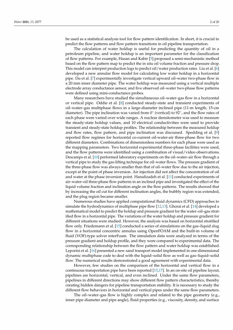
Abstract: A series of experiments were conducted to investigate the flow pattern transitions andwater holdup during oil–water–gas three-phase flow considering both a horizontal section and avertical section of a transportation pipe simultaneously. The flowing media were white mineral oil,distilled water, and air. Dimensionless numbers controlling the multiphase flow were deduced tounderstand the scaling law of the flow process. The oil–water–gas three-phase flow was simplified asthe two-phase flow of a gas and liquid mixture. Based on the experimental data, flow pattern mapswere constructed in terms of the Reynolds number and the ratio of the superficial velocity of the gasto that of the liquid mixture for different Froude numbers. The original contributions of this work arethat the relationship between the transient water holdup and the changes of the flow patterns in atransportation pipe with horizontal and vertical sections is established, providing a basis for judgingthe flow patterns in pipes in engineering practice. A dimensionless power-law correlation for thewater holdup in the vertical section is presented based on the experimental data. The correlation canprovide theoretical support for the design of oil and gas transport pipelines in industrial applications.

Keywords: oil–water–gas flow; flow pattern; water holdup; dimensionless analysis

1. Introduction

The pipe transportation of oil–water–gas three-phase systems is a crucial process in oiland natural gas production and provides vital information for interpreting the productionstages. A deep understanding of the flow characteristics, such as the flow patterns andwater holdup (the volume fraction of water in a pipe section), of the three-phase flow isbeneficial to the proper design and operation of pipelines [1]. The different flow patternsdirectly determine the different flow characteristics of multiphase flows. This is a notablefeature of multiphase flows in pipes, and it is an essential topic in multiphase flow research.The change of the flow pattern has a vital impact on the pressure drop (reflected in theenergy consumption of transportation), spatial phase distribution, and safety of pipelinetransportation [2]. For example, in the churn flow of gas–liquid flow, the bubbles havedifferent sizes and shapes, and the liquid film attached to the pipe wall becomes an up–down vibrating flow, which affects the stability of the pipeline flow. To estimate thefrictional pressure gradient accurately in a transparent vertical pipe, Xu et al. [3] studiedthe actual flow pattern under specific flow conditions. The flow patterns can be used todeduce the concentration distribution of each phase. Jones and Zuber [4] demonstratedthat the probability density function (PDF) of the fluctuations in the volume fraction could

Water 2021, 13, 2077. https://doi.org/10.3390/w13152077 https://www.mdpi.com/journal/water

Water 2021, 13, 2077 2 of 20

be used as a statistical analysis tool for flow pattern identification. In short, it is crucial topredict the flow patterns and flow pattern transitions in oil pipeline transportation.

The calculation of water holdup is useful for predicting the quantity of oil in apetroleum pipeline, and water holdup is an important parameter for the classificationof flow patterns. For example, Hasan and Kabir [5] proposed a semi-mechanistic methodbased on the flow pattern map to predict the in situ oil volume fraction and pressure drop.This model can interpret production logs to predict oil/water production rates. Liu et al. [6]developed a new annular flow model for calculating low water holdup in a horizontalpipe. Du et al. [7] experimentally investigate vertical upward oil–water two-phase flow ina 20 mm inner diameter pipe. The water holdup was measured using a vertical multipleelectrode array conductance sensor, and five observed oil–water two-phase flow patternswere defined using mini-conductance probes.

Many researchers have studied the simultaneous oil–water–gas flow in a horizontalor vertical pipe. Oddie et al. [8] conducted steady-state and transient experiments ofoil–water–gas multiphase flows in a large-diameter inclined pipe (11-m length, 15-cmdiameter). The pipe inclination was varied from 0◦ (vertical) to 92◦, and the flow rates ofeach phase were varied over wide ranges. A nuclear densitometer was used to measurethe steady-state holdup values, and 10 electrical conductivities were used to providetransient and steady-state holdup profiles. The relationship between the measured holdupand flow rates, flow pattern, and pipe inclination was discussed. Spedding et al. [9]reported flow regimes for horizontal co-current oil-water-air three-phase flow for twodifferent diameters. Combinations of dimensionless numbers for each phase were used asthe mapping parameters. Two horizontal experimental three-phase facilities were used,and the flow patterns were identified using a combination of visual/video observations.Descamps et al. [10] performed laboratory experiments on the oil–water–air flow through avertical pipe to study the gas-lifting technique for oil–water flows. The pressure gradient ofthe three-phase flow was always smaller than that of oil–water flow due to the air injection,except at the point of phase inversion. Air injection did not affect the concentration of oiland water at the phase inversion point. Hanafizadeh et al. [11] conducted experiments ofair–water–oil three-phase flow patterns in an inclined pipe and investigated the effect of theliquid volume fraction and inclination angle on the flow patterns. The results showed thatby increasing the oil cut for different inclination angles, the bubbly region was extended,and the plug region became smaller.

Numerous studies have applied computational fluid dynamics (CFD) approaches tosimulate the hydrodynamics of multiphase pipe flow [12,13]. Ghorai et al. [14] developed amathematical model to predict the holdup and pressure gradient for the water–oil–gas strat-ified flow in a horizontal pipe. The variations of the water holdup and pressure gradient fordifferent situations were studied. However, the analysis was based on horizontal stratifiedflow only. Friedemann et al. [15] conducted a series of simulations on the gas–liquid slugflow in a horizontal concentric annulus using OpenFOAM and the built-in volume offluid (VOF)-type solver interFoam. The simulation data were analyzed in terms of thepressure gradient and holdup profile, and they were compared to experimental data. Thecorresponding relationship between the flow pattern and water holdup was established.Leporini et al. [16] presented a new sand transport model implemented in one-dimensionaldynamic multiphase code to deal with the liquid–solid flow as well as gas–liquid–solidflow. The numerical results demonstrated a good agreement with experimental data.

However, few studies on the comparison of the horizontal and vertical flow in acontinuous transportation pipe have been reported [15,17]. In an on-site oil pipeline layout,pipelines are horizontal, vertical, and even inclined. Under the same flow parameters,pipelines in different directions may show different flow pattern characteristics, therebycreating hidden dangers for pipeline transportation stability. It is necessary to study thedifferent flow behaviors in horizontal and vertical pipes under the same flow parameters.

The oil–water–gas flow is highly complex and related to the pipe geometry (e.g.,inner pipe diameter and pipe angle), fluid properties (e.g., viscosity, density, and surface

Water 2021, 13, 2077 3 of 20

tension), and boundary conditions (e.g., superficial input velocities) [18]. Previous studiesmainly focused on the effect of a single parameter, but the coupled effect of the controllingparameters on the flow is not well understood. Hence, to understand the fundamentalmechanisms of oil–water–gas flows, the controlling dimensionless parameters were derivedby dimensional analysis first. In a three-phase flow, it is difficult to distinguish the boundarybetween oil and water, especially at high flow rates. Thus, the oil–water–gas three-phaseflow can be simplified as the two-phase flow of a gas and liquid mixture considering, as thedensities of oil and water are much higher than that of gas and the oil and water velocitiesare sufficiently high to obtain a mixture [11].

Thus, the objective of this work was to investigate the flow patterns and water holdupfor a simplified gas–liquid flow in horizontal and vertical sections through a comparativestudy of the flow behaviors in a pipe loop considering different superficial input velocities.In particular, a series of experiments were conducted to investigate the flow patterntransition and the water holdup, considering both the horizontal and vertical sections ofa transportation pipe. In addition, the relationship between the transient water holdupand the change of the flow pattern in a transportation pipe with horizontal and verticalsections was established, which provides a basis for judging the flow pattern in a pipe inengineering practice. A dimensionless power-law correlation for the water holdup in thevertical section is presented based on the experimental data.

The current paper is structured as follows. The experimental setup is described inSection 2. In Section 3, the dimensionless numbers are derived based on the physicalanalysis and the proper choice of the units for the problem. In Section 4, the relationshipbetween the transient water holdup and the change of the flow pattern in a transportationpipe with horizontal and vertical sections is established, and a dimensionless power-lawcorrelation for the water holdup in the vertical section is presented. Finally, Section 5presents the conclusions of this study.

2. Description of Experiments

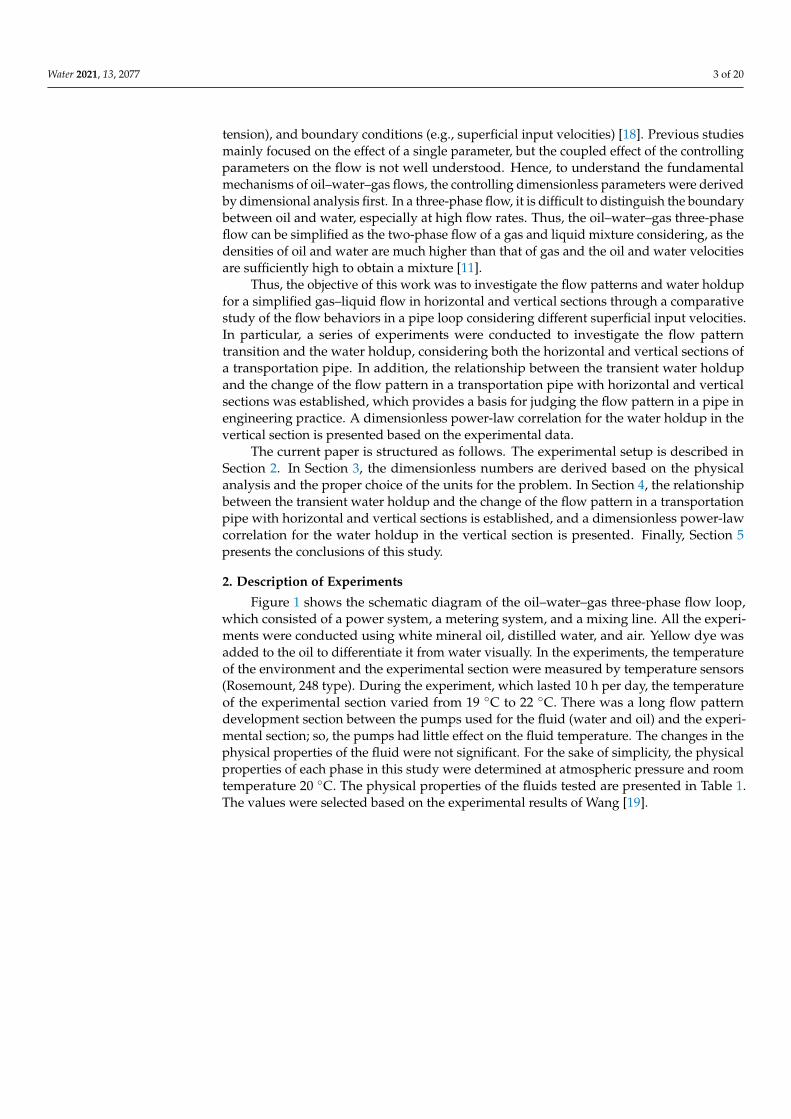
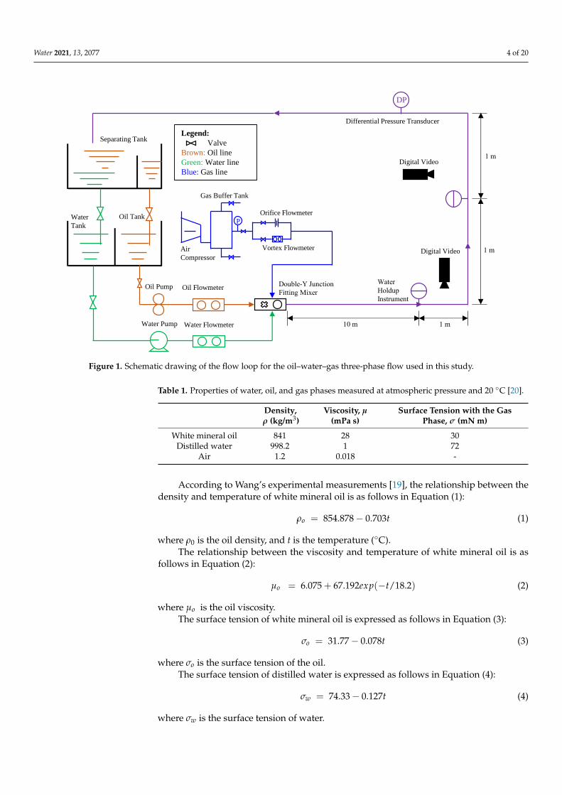
Figure 1 shows the schematic diagram of the oil–water–gas three-phase flow loop,which consisted of a power system, a metering system, and a mixing line. All the experi-ments were conducted using white mineral oil, distilled water, and air. Yellow dye wasadded to the oil to differentiate it from water visually. In the experiments, the temperatureof the environment and the experimental section were measured by temperature sensors(Rosemount, 248 type). During the experiment, which lasted 10 h per day, the temperatureof the experimental section varied from 19 ◦C to 22 ◦C. There was a long flow patterndevelopment section between the pumps used for the fluid (water and oil) and the experi-mental section; so, the pumps had little effect on the fluid temperature. The changes in thephysical properties of the fluid were not significant. For the sake of simplicity, the physicalproperties of each phase in this study were determined at atmospheric pressure and roomtemperature 20 ◦C. The physical properties of the fluids tested are presented in Table 1.The values were selected based on the experimental results of Wang [19].

Water 2021, 13, 2077 4 of 20Water 2021, 13, x FOR PEER REVIEW 4 of 20

Figure 1. Schematic drawing of the flow loop for the oil–water–gas three-phase flow used in this study.

Table 1. Properties of water, oil, and gas phases measured at atmospheric pressure and 20 °C [20].

Density,

𝝆 (𝐤𝐠/𝐦𝟑)

Viscosity, µ

(mPa s)

Surface Tension with the Gas Phase,

σ (mN m)

White mineral oil 841 28 30

Distilled water 998.2 1 72

Air 1.2 0.018 -

According to Wang’s experimental measurements [19], the relationship between the

density and temperature of white mineral oil is as follows in Equation (1):

𝜌𝑜 = 854.878 − 0.703𝑡 (1)

where 𝜌0 is the oil density, and t is the temperature (°C).

The relationship between the viscosity and temperature of white mineral oil is as

follows in Equation (2):

𝜇𝑜 = 6.075 + 67.192𝑒𝑥𝑝 (−𝑡/18.2) (2)

where 𝜇𝑜 is the oil viscosity.

The surface tension of white mineral oil is expressed as follows in Equation (3):

𝜎𝑜 = 31.77 − 0.078𝑡 (3)

where 𝜎𝑜 is the surface tension of the oil.

The surface tension of distilled water is expressed as follows in Equation (4):

𝜎𝑤 = 74.33 − 0.127𝑡 (4)

where 𝜎𝑤 is the surface tension of water.

The power system pumped gas, oil, and water into the pipe. The system consisted of

oil and water pumps, an oil tank, a water tank, an air compressor, and a double-Y junction

fitting mixer. The metering system was composed of flowmeters and a water holdup in-

strument. The mixing line comprised a stainless-steel pipe section and a plexiglass pipe

section with an inner diameter of 50 mm. The flow pattern development section was a

DP

Digital Video

Separating Tank

Water

Tank

Oil Tank

Oil Pump

Water Pump

Oil Flowmeter

Water Flowmeter

Differential Pressure Transducer

Water

Holdup

Instrument

Double-Y Junction

Fitting Mixer

Legend:

Valve

Brown: Oil line

Green: Water line

Blue: Gas line

P

Air

Compressor

Gas Buffer Tank

Vortex Flowmeter

Orifice Flowmeter

10 m 1 m

1 mDigital Video

1 m

Figure 1. Schematic drawing of the flow loop for the oil–water–gas three-phase flow used in this study.

Table 1. Properties of water, oil, and gas phases measured at atmospheric pressure and 20 ◦C [20].

Density,ρ (kg/m3)

Viscosity, µ(mPa s)

Surface Tension with the GasPhase, σ (mN m)

White mineral oil 841 28 30Distilled water 998.2 1 72

Air 1.2 0.018 -

According to Wang’s experimental measurements [19], the relationship between thedensity and temperature of white mineral oil is as follows in Equation (1):

ρo = 854.878− 0.703t (1)

where ρ0 is the oil density, and t is the temperature (◦C).The relationship between the viscosity and temperature of white mineral oil is as

follows in Equation (2):

µo = 6.075 + 67.192exp(−t/18.2) (2)

where µo is the oil viscosity.The surface tension of white mineral oil is expressed as follows in Equation (3):

σo = 31.77− 0.078t (3)

where σo is the surface tension of the oil.The surface tension of distilled water is expressed as follows in Equation (4):

σw = 74.33− 0.127t (4)

where σw is the surface tension of water.

Water 2021, 13, 2077 5 of 20

The power system pumped gas, oil, and water into the pipe. The system consisted ofoil and water pumps, an oil tank, a water tank, an air compressor, and a double-Y junctionfitting mixer. The metering system was composed of flowmeters and a water holdupinstrument. The mixing line comprised a stainless-steel pipe section and a plexiglass pipesection with an inner diameter of 50 mm. The flow pattern development section was ahorizontal stainless-steel pipe with a length of 10 m, which was convenient for the fulldevelopment of the multiphase flow pattern in the pipe. The flow pattern observationsection was installed at the end of the flow pattern development section, which was aplexiglass pipe, so that the flow pattern in the pipe could be easily observed. The flowobservation sections were a 1-m-long horizontal transparent pipe and a 2-m-long verticaltransparent pipe. Through this arrangement, the horizontal and vertical flow experimentscould be carried out simultaneously.

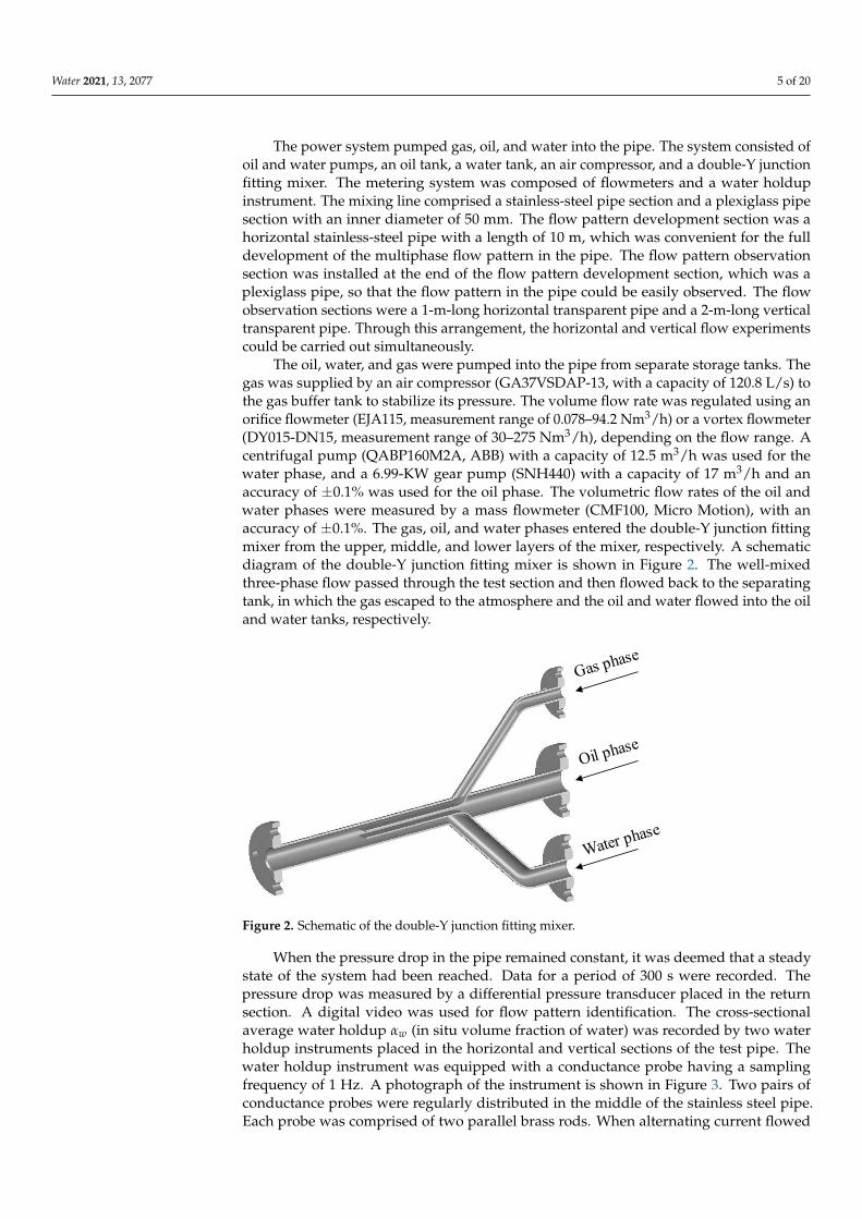
The oil, water, and gas were pumped into the pipe from separate storage tanks. Thegas was supplied by an air compressor (GA37VSDAP-13, with a capacity of 120.8 L/s) tothe gas buffer tank to stabilize its pressure. The volume flow rate was regulated using anorifice flowmeter (EJA115, measurement range of 0.078–94.2 Nm3/h) or a vortex flowmeter(DY015-DN15, measurement range of 30–275 Nm3/h), depending on the flow range. Acentrifugal pump (QABP160M2A, ABB) with a capacity of 12.5 m3/h was used for thewater phase, and a 6.99-KW gear pump (SNH440) with a capacity of 17 m3/h and anaccuracy of ±0.1% was used for the oil phase. The volumetric flow rates of the oil andwater phases were measured by a mass flowmeter (CMF100, Micro Motion), with anaccuracy of ±0.1%. The gas, oil, and water phases entered the double-Y junction fittingmixer from the upper, middle, and lower layers of the mixer, respectively. A schematicdiagram of the double-Y junction fitting mixer is shown in Figure 2. The well-mixedthree-phase flow passed through the test section and then flowed back to the separatingtank, in which the gas escaped to the atmosphere and the oil and water flowed into the oiland water tanks, respectively.

Water 2021, 13, x FOR PEER REVIEW 5 of 20

horizontal stainless-steel pipe with a length of 10 m, which was convenient for the full

development of the multiphase flow pattern in the pipe. The flow pattern observation

section was installed at the end of the flow pattern development section, which was a

plexiglass pipe, so that the flow pattern in the pipe could be easily observed. The flow

observation sections were a 1-m-long horizontal transparent pipe and a 2-m-long vertical

transparent pipe. Through this arrangement, the horizontal and vertical flow experiments

could be carried out simultaneously.

The oil, water, and gas were pumped into the pipe from separate storage tanks. The

gas was supplied by an air compressor (GA37VSDAP-13, with a capacity of 120.8 L/s) to

the gas buffer tank to stabilize its pressure. The volume flow rate was regulated using an

orifice flowmeter (EJA115, measurement range of 0.078–94.2 Nm3/h) or a vortex flowmeter

(DY015-DN15, measurement range of 30–275 Nm3/h), depending on the flow range. A

centrifugal pump (QABP160M2A, ABB) with a capacity of 12.5 m3/h was used for the wa-

ter phase, and a 6.99-KW gear pump (SNH440) with a capacity of 17 m3/h and an accuracy

of ±0.1% was used for the oil phase. The volumetric flow rates of the oil and water phases

were measured by a mass flowmeter (CMF100, Micro Motion), with an accuracy of ±0.1%.

The gas, oil, and water phases entered the double-Y junction fitting mixer from the upper,

middle, and lower layers of the mixer, respectively. A schematic diagram of the double-Y

junction fitting mixer is shown in Figure 2. The well-mixed three-phase flow passed

through the test section and then flowed back to the separating tank, in which the gas

escaped to the atmosphere and the oil and water flowed into the oil and water tanks, re-

spectively.

Figure 2. Schematic of the double-Y junction fitting mixer.

When the pressure drop in the pipe remained constant, it was deemed that a steady

state of the system had been reached. Data for a period of 300 s were recorded. The pres-

sure drop was measured by a differential pressure transducer placed in the return section.

A digital video was used for flow pattern identification. The cross-sectional average water

holdup 𝛼𝑤(in situ volume fraction of water) was recorded by two water holdup instru-

ments placed in the horizontal and vertical sections of the test pipe. The water holdup

instrument was equipped with a conductance probe having a sampling frequency of 1 Hz.

A photograph of the instrument is shown in Figure 3. Two pairs of conductance probes

were regularly distributed in the middle of the stainless steel pipe. Each probe was com-

prised of two parallel brass rods. When alternating current flowed between two probes,

the conductance probe measured the voltage between the two ends of the conductor,

which reflects the mean conductivity of the mixture in the pipe [20]. Because the conduc-

tivities of oil and gas are weak, the voltage values measured when the pipe was filled with

pure oil or gas were basically the same. Calibration of the water holdup instrument was

performed by measuring the transmitted conductivity for single-phase gas, oil, and water.

气相

油相

水相

Figure 2. Schematic of the double-Y junction fitting mixer.

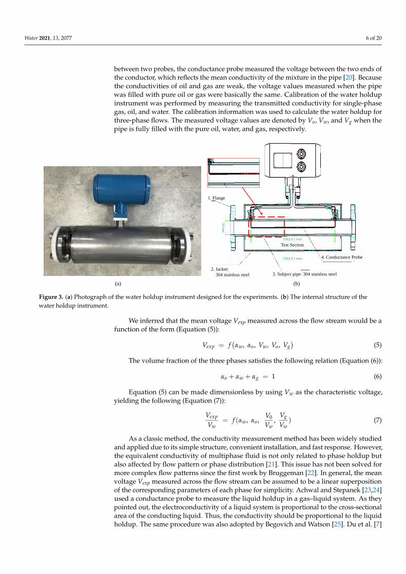
When the pressure drop in the pipe remained constant, it was deemed that a steadystate of the system had been reached. Data for a period of 300 s were recorded. Thepressure drop was measured by a differential pressure transducer placed in the returnsection. A digital video was used for flow pattern identification. The cross-sectionalaverage water holdup αw (in situ volume fraction of water) was recorded by two waterholdup instruments placed in the horizontal and vertical sections of the test pipe. Thewater holdup instrument was equipped with a conductance probe having a samplingfrequency of 1 Hz. A photograph of the instrument is shown in Figure 3. Two pairs ofconductance probes were regularly distributed in the middle of the stainless steel pipe.Each probe was comprised of two parallel brass rods. When alternating current flowed

Water 2021, 13, 2077 6 of 20

between two probes, the conductance probe measured the voltage between the two ends ofthe conductor, which reflects the mean conductivity of the mixture in the pipe [20]. Becausethe conductivities of oil and gas are weak, the voltage values measured when the pipewas filled with pure oil or gas were basically the same. Calibration of the water holdupinstrument was performed by measuring the transmitted conductivity for single-phasegas, oil, and water. The calibration information was used to calculate the water holdup forthree-phase flows. The measured voltage values are denoted by Vo, Vw, and Vg when thepipe is fully filled with the pure oil, water, and gas, respectively.

Water 2021, 13, x FOR PEER REVIEW 6 of 20

The calibration information was used to calculate the water holdup for three-phase flows.

The measured voltage values are denoted by Vo, Vw, and Vg when the pipe is fully filled

with the pure oil, water, and gas, respectively.

Figure 3. (a) Photograph of the water holdup instrument designed for the experiments. (b) The internal structure of the

water holdup instrument.

We inferred that the mean voltage Vexp measured across the flow stream would be a

function of the form (Equation (5)):

𝑉𝑒𝑥𝑝 = 𝑓(𝛼𝑤 , 𝛼𝑜, 𝑉𝑤 , 𝑉𝑜 , 𝑉𝑔) (5)

The volume fraction of the three phases satisfies the following relation (Equation (6)):

𝛼𝑜 + 𝛼𝑤 + 𝛼𝑔 = 1 (6)

Equation (5) can be made dimensionless by using Vw as the characteristic voltage,

yielding the following (Equation (7)):

𝑉𝑒𝑥𝑝

𝑉𝑤= 𝑓(𝛼𝑤 , 𝛼𝑜,

𝑉0

𝑉𝑤,𝑉𝑔

𝑉𝑤) (7)

As a classic method, the conductivity measurement method has been widely studied

and applied due to its simple structure, convenient installation, and fast response. How-

ever, the equivalent conductivity of multiphase fluid is not only related to phase holdup

but also affected by flow pattern or phase distribution [21]. This issue has not been solved

for more complex flow patterns since the first work by Bruggeman [22]. In general, the

mean voltage Vexp measured across the flow stream can be assumed to be a linear super-

position of the corresponding parameters of each phase for simplicity. Achwal and Ste-

panek [23,24] used a conductance probe to measure the liquid holdup in a gas–liquid sys-

tem. As they pointed out, the electroconductivity of a liquid system is proportional to the

cross-sectional area of the conducting liquid. Thus, the conductivity should be propor-

tional to the liquid holdup. The same procedure was also adopted by Begovich and Wat-

son [25]. Du et al. [7] measured the water holdup using a vertical multiple electrode array

conductance sensor in vertical upward oil–water flow. According to the experiments, the

mean voltage for mixed fluid and oil holdup showed a good linear relationship. Based on

the above considerations, the mean voltage Vexp can be expressed as follows in Equation

(8):

1. Flange

2. Jacket:

304 stainless steel 3. Subject pipe: 304 stainless steel

4. Conductance Probe

50

mm

350

520

Test Section

(a) (b)

Figure 3. (a) Photograph of the water holdup instrument designed for the experiments. (b) The internal structure of thewater holdup instrument.

We inferred that the mean voltage Vexp measured across the flow stream would be afunction of the form (Equation (5)):

Vexp = f(αw, αo, Vw, Vo, Vg

)(5)

The volume fraction of the three phases satisfies the following relation (Equation (6)):

αo + αw + αg = 1 (6)

Equation (5) can be made dimensionless by using Vw as the characteristic voltage,yielding the following (Equation (7)):

Vexp

Vw= f (αw, αo,

V0

Vw,

Vg

Vw) (7)

As a classic method, the conductivity measurement method has been widely studiedand applied due to its simple structure, convenient installation, and fast response. However,the equivalent conductivity of multiphase fluid is not only related to phase holdup butalso affected by flow pattern or phase distribution [21]. This issue has not been solved formore complex flow patterns since the first work by Bruggeman [22]. In general, the meanvoltage Vexp measured across the flow stream can be assumed to be a linear superpositionof the corresponding parameters of each phase for simplicity. Achwal and Stepanek [23,24]used a conductance probe to measure the liquid holdup in a gas–liquid system. As theypointed out, the electroconductivity of a liquid system is proportional to the cross-sectionalarea of the conducting liquid. Thus, the conductivity should be proportional to the liquidholdup. The same procedure was also adopted by Begovich and Watson [25]. Du et al. [7]

Water 2021, 13, 2077 7 of 20

measured the water holdup using a vertical multiple electrode array conductance sensor invertical upward oil–water flow. According to the experiments, the mean voltage for mixedfluid and oil holdup showed a good linear relationship. Based on the above considerations,the mean voltage Vexp can be expressed as follows in Equation (8):

Vexp

Vw= α0

V0

Vw+ (1− αw − αo)

Vg

Vw+ αw (8)

Since the voltage Vo is equal to Vg, the above formula can be further simplified asfollows in Equation (9):

Vexp

Vw= (1− αw)

Vo

Vw+ αw (9)

Thus, the relationship between the water holdup αw and the mean voltage Vexp can beexpressed as follows:

αw =V0 −Vexp

Vo −Vw(10)

The measured voltage values when the pipe is fully filled with the pure water andpure oil in each group of experiments were different. Therefore, Vo and Vw were measuredfor each set of experimental conditions when the voltage signal was converted into a waterholdup using Equation (10). The dimensionless electrical signal of the water holdup instru-ment ensured that the measured data of the horizontal and vertical devices in the samegroup of experiments could be compared, which was also convenient for the comparisonof experimental data of different groups.

3. Analysis of Oil–Water–Gas Three-Phase Flow

An oil–water–gas three-phase flow is highly complex and related to pipe geometry,fluid properties, and fluid flow rates. An oil–water–gas three-phase flow can be regardedas a special kind of gas–liquid two-phase flow, especially at high flow rates, where the oiland water are well mixed and form a homogeneous dispersion. The clear identificationof the oil and the water phases is difficult in these cases [8]. The methods and theoriesdeveloped for gas–liquid two-phase flows can be used as the basis for the investigation ofoil–water–gas three-phase flows [14]. The liquid mixture properties, such as the viscosityand density, depend on the ratio of the superficial velocity of oil to that of water. Themixture density is defined as follows in Equation (11):

ρm = εwρw + εoρo (11)

where ρw is the water density. εw and εo are the input water and oil cuts, respectively, definedas the ratio of each phase flow rate to the mixture flow rate (Equations (12) and (13)):

εw =Qw

Qw + Qo=

usw

usm(12)

εo =Qo

Qw + Qo=

uso

usm(13)

where Q is the volume flow rate of each phase, and us is the superficial velocity, which isdefined as us = Q/A, A is the cross-sectional area of the pipe, A = πD2/4, and D is the innerpipe diameter.

An oil–water mixture is a non-Newtonian fluid, and its viscosity is called the apparentviscosity. In general, the viscosity of a liquid mixture varies significantly with the spatialdistribution of the two phases, the viscosity of each phase, the temperature, and thepressure. It is difficult to include all these factors in any theoretical expression of theapparent viscosity. Some scholars have suggested using a calculation method similar tothat for the densities of oil–water mixtures to calculate the apparent viscosity [11,26,27].Over the range of superficial velocities considered here, the oil and water were well mixed,

Water 2021, 13, 2077 8 of 20

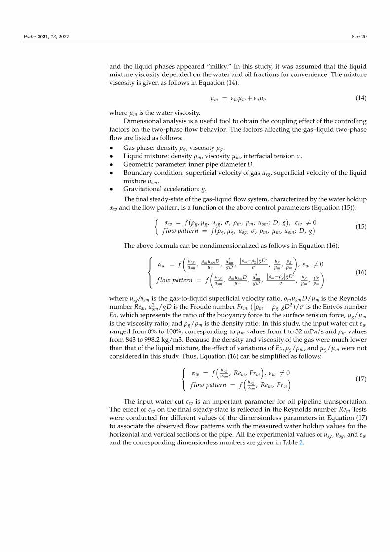
and the liquid phases appeared “milky.” In this study, it was assumed that the liquidmixture viscosity depended on the water and oil fractions for convenience. The mixtureviscosity is given as follows in Equation (14):

µm = εwµw + εoµo (14)

where µm is the water viscosity.Dimensional analysis is a useful tool to obtain the coupling effect of the controlling

factors on the two-phase flow behavior. The factors affecting the gas–liquid two-phaseflow are listed as follows:

• Gas phase: density ρg, viscosity µg.• Liquid mixture: density ρm, viscosity µm, interfacial tension σ.• Geometric parameter: inner pipe diameter D.• Boundary condition: superficial velocity of gas usg, superficial velocity of the liquid

mixture usm.• Gravitational acceleration: g.

The final steady-state of the gas–liquid flow system, characterized by the water holdupαw and the flow pattern, is a function of the above control parameters (Equation (15)):{

αw = f(ρg, µg, usg, σ, ρm, µm, usm; D, g

), εw 6= 0

f low pattern = f(ρg, µg, usg, σ, ρm, µm, usm; D, g

) (15)

The above formula can be nondimensionalized as follows in Equation (16):αw = f

(usgusm

, ρmusmDµm

, u2sm

gD , |ρm−ρg|gD2

σ , µgµm

, ρgρm

), εw 6= 0

f low pattern = f(

usgusm

, ρmusmDµm

, u2sm

gD , |ρm−ρg|gD2

σ , µgµm

, ρgρm

) (16)

where usg/usm is the gas-to-liquid superficial velocity ratio, ρmusmD/µm is the Reynoldsnumber Rem, u2

sm/gD is the Froude number Frm, (∣∣ρm − ρg

∣∣gD2)/σ is the Eötvös numberEo, which represents the ratio of the buoyancy force to the surface tension force, µg/µmis the viscosity ratio, and ρg/ρm is the density ratio. In this study, the input water cut εwranged from 0% to 100%, corresponding to µm values from 1 to 32 mPa/s and ρm valuesfrom 843 to 998.2 kg/m3. Because the density and viscosity of the gas were much lowerthan that of the liquid mixture, the effect of variations of Eo, ρg/ρm, and µg/µm were notconsidered in this study. Thus, Equation (16) can be simplified as follows: αw = f

(usgusm

, Rem, Frm

), εw 6= 0

f low pattern = f(

usgusm

, Rem, Frm

) (17)

The input water cut εw is an important parameter for oil pipeline transportation.The effect of εw on the final steady-state is reflected in the Reynolds number Rem Testswere conducted for different values of the dimensionless parameters in Equation (17)to associate the observed flow patterns with the measured water holdup values for thehorizontal and vertical sections of the pipe. All the experimental values of usg, usg, and εwand the corresponding dimensionless numbers are given in Table 2.

Water 2021, 13, 2077 9 of 20

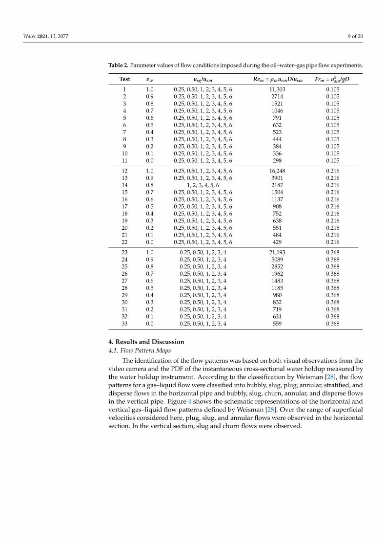
Table 2. Parameter values of flow conditions imposed during the oil–water–gas pipe flow experiments.

Test εw usg/usm Rem = ρmusmD/usm Frm = u2sm/gD

1 1.0 0.25, 0.50, 1, 2, 3, 4, 5, 6 11,303 0.1052 0.9 0.25, 0.50, 1, 2, 3, 4, 5, 6 2714 0.1053 0.8 0.25, 0.50, 1, 2, 3, 4, 5, 6 1521 0.1054 0.7 0.25, 0.50, 1, 2, 3, 4, 5, 6 1046 0.1055 0.6 0.25, 0.50, 1, 2, 3, 4, 5, 6 791 0.1056 0.5 0.25, 0.50, 1, 2, 3, 4, 5, 6 632 0.1057 0.4 0.25, 0.50, 1, 2, 3, 4, 5, 6 523 0.1058 0.3 0.25, 0.50, 1, 2, 3, 4, 5, 6 444 0.1059 0.2 0.25, 0.50, 1, 2, 3, 4, 5, 6 384 0.10510 0.1 0.25, 0.50, 1, 2, 3, 4, 5, 6 336 0.10511 0.0 0.25, 0.50, 1, 2, 3, 4, 5, 6 298 0.105

12 1.0 0.25, 0.50, 1, 2, 3, 4, 5, 6 16,248 0.21613 0.9 0.25, 0.50, 1, 2, 3, 4, 5, 6 3901 0.21614 0.8 1, 2, 3, 4, 5, 6 2187 0.21615 0.7 0.25, 0.50, 1, 2, 3, 4, 5, 6 1504 0.21616 0.6 0.25, 0.50, 1, 2, 3, 4, 5, 6 1137 0.21617 0.5 0.25, 0.50, 1, 2, 3, 4, 5, 6 908 0.21618 0.4 0.25, 0.50, 1, 2, 3, 4, 5, 6 752 0.21619 0.3 0.25, 0.50, 1, 2, 3, 4, 5, 6 638 0.21620 0.2 0.25, 0.50, 1, 2, 3, 4, 5, 6 551 0.21621 0.1 0.25, 0.50, 1, 2, 3, 4, 5, 6 484 0.21622 0.0 0.25, 0.50, 1, 2, 3, 4, 5, 6 429 0.216

23 1.0 0.25, 0.50, 1, 2, 3, 4 21,193 0.36824 0.9 0.25, 0.50, 1, 2, 3, 4 5089 0.36825 0.8 0.25, 0.50, 1, 2, 3, 4 2852 0.36826 0.7 0.25, 0.50, 1, 2, 3, 4 1962 0.36827 0.6 0.25, 0.50, 1, 2, 3, 4 1483 0.36828 0.5 0.25, 0.50, 1, 2, 3, 4 1185 0.36829 0.4 0.25, 0.50, 1, 2, 3, 4 980 0.36830 0.3 0.25, 0.50, 1, 2, 3, 4 832 0.36831 0.2 0.25, 0.50, 1, 2, 3, 4 719 0.36832 0.1 0.25, 0.50, 1, 2, 3, 4 631 0.36833 0.0 0.25, 0.50, 1, 2, 3, 4 559 0.368

4. Results and Discussion4.1. Flow Pattern Maps

The identification of the flow patterns was based on both visual observations from thevideo camera and the PDF of the instantaneous cross-sectional water holdup measured bythe water holdup instrument. According to the classification by Weisman [28], the flowpatterns for a gas–liquid flow were classified into bubbly, slug, plug, annular, stratified, anddisperse flows in the horizontal pipe and bubbly, slug, churn, annular, and disperse flowsin the vertical pipe. Figure 4 shows the schematic representations of the horizontal andvertical gas–liquid flow patterns defined by Weisman [28]. Over the range of superficialvelocities considered here, plug, slug, and annular flows were observed in the horizontalsection. In the vertical section, slug and churn flows were observed.

Water 2021, 13, 2077 10 of 20Water 2021, 13, x FOR PEER REVIEW 10 of 20

Figure 4. Schematic representation of the (a) horizontal and (b) vertical gas–liquid flow patterns defined by Weisman [28].

Figure 5 shows examples of the four main flow patterns that were observed in this

study in both the horizontal and vertical sections in a continuous transportation pipe. Fig-

ure 5a presents the plug flow pattern, where small bubbles gathered in the upper part of

the pipe and formed large bubbles, and there were almost no small bubbles between the

large bubbles. Figure 5b shows the annular flow pattern, where a liquid film with a certain

thickness formed between the gas column and the pipe wall. Figure 5c shows the slug

flow pattern, where gas pockets were separated by slugs of liquid with dispersed small

bubbles. Figure 5d shows the churn flow pattern; the flow was similar to the slug flow but

without clear phase separation or structure. Figure 5 shows that the oil and water phases

were well mixed with each other. Based on the experimental observations, the assumption

that the oil–water phase was simplified as a liquid mixture was reasonable.

Figure 5. Instantaneous flow patterns observed in the experiments in the horizontal and vertical

sections: (a) plug flow, Frm = 0.368, usg/usm = 0.25, 𝜀𝑤 = 0.5; (b) annular flow Frm = 0.105, usg/usm = 0.50,

𝜀𝑤 = 0.5; (c) slug flow, Frm = 0.216, usg/usm = 6, 𝜀𝑤 = 0.1; (d) churn flow, Frm = 0.368, usg/usm = 4, 𝜀𝑤 =

0.1

Figures 6 and 7 show the typical time-series data of the cross-sectional average water

holdup αw and the corresponding PDF as a function of the water holdup for different

superficial velocities in both the horizontal and vertical sections [4]. Figure 6 shows the

data for Frm = 0.368, usg/usm = 0.50, and 𝜀𝑤 = 0.8. In the horizontal section, plug flow was

(a) (b)

(a) Plug flow

(b) Annular flow (c) Slug flow (d) Churn flow

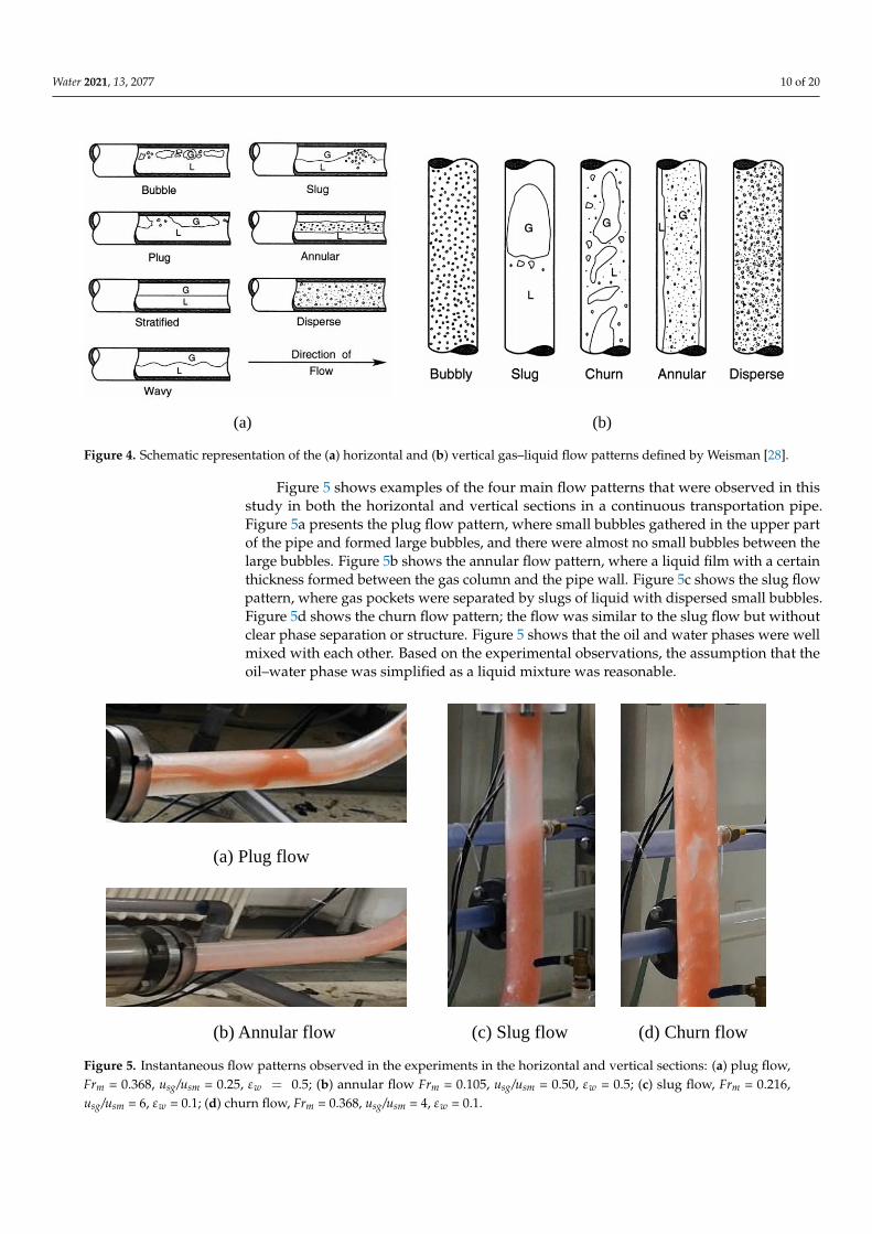
Figure 4. Schematic representation of the (a) horizontal and (b) vertical gas–liquid flow patterns defined by Weisman [28].

Figure 5 shows examples of the four main flow patterns that were observed in thisstudy in both the horizontal and vertical sections in a continuous transportation pipe.Figure 5a presents the plug flow pattern, where small bubbles gathered in the upper partof the pipe and formed large bubbles, and there were almost no small bubbles between thelarge bubbles. Figure 5b shows the annular flow pattern, where a liquid film with a certainthickness formed between the gas column and the pipe wall. Figure 5c shows the slug flowpattern, where gas pockets were separated by slugs of liquid with dispersed small bubbles.Figure 5d shows the churn flow pattern; the flow was similar to the slug flow but withoutclear phase separation or structure. Figure 5 shows that the oil and water phases were wellmixed with each other. Based on the experimental observations, the assumption that theoil–water phase was simplified as a liquid mixture was reasonable.

Water 2021, 13, x FOR PEER REVIEW 10 of 20

Figure 4. Schematic representation of the (a) horizontal and (b) vertical gas–liquid flow patterns defined by Weisman [28].

Figure 5 shows examples of the four main flow patterns that were observed in this

study in both the horizontal and vertical sections in a continuous transportation pipe. Fig-

ure 5a presents the plug flow pattern, where small bubbles gathered in the upper part of

the pipe and formed large bubbles, and there were almost no small bubbles between the

large bubbles. Figure 5b shows the annular flow pattern, where a liquid film with a certain

thickness formed between the gas column and the pipe wall. Figure 5c shows the slug

flow pattern, where gas pockets were separated by slugs of liquid with dispersed small

bubbles. Figure 5d shows the churn flow pattern; the flow was similar to the slug flow but

without clear phase separation or structure. Figure 5 shows that the oil and water phases

were well mixed with each other. Based on the experimental observations, the assumption

that the oil–water phase was simplified as a liquid mixture was reasonable.

Figure 5. Instantaneous flow patterns observed in the experiments in the horizontal and vertical

sections: (a) plug flow, Frm = 0.368, usg/usm = 0.25, 𝜀𝑤 = 0.5; (b) annular flow Frm = 0.105, usg/usm = 0.50,

𝜀𝑤 = 0.5; (c) slug flow, Frm = 0.216, usg/usm = 6, 𝜀𝑤 = 0.1; (d) churn flow, Frm = 0.368, usg/usm = 4, 𝜀𝑤 =

0.1

Figures 6 and 7 show the typical time-series data of the cross-sectional average water

holdup αw and the corresponding PDF as a function of the water holdup for different

superficial velocities in both the horizontal and vertical sections [4]. Figure 6 shows the

data for Frm = 0.368, usg/usm = 0.50, and 𝜀𝑤 = 0.8. In the horizontal section, plug flow was

(a) (b)

(a) Plug flow

(b) Annular flow (c) Slug flow (d) Churn flow

Figure 5. Instantaneous flow patterns observed in the experiments in the horizontal and vertical sections: (a) plug flow,Frm = 0.368, usg/usm = 0.25, εw = 0.5; (b) annular flow Frm = 0.105, usg/usm = 0.50, εw = 0.5; (c) slug flow, Frm = 0.216,usg/usm = 6, εw = 0.1; (d) churn flow, Frm = 0.368, usg/usm = 4, εw = 0.1.

Water 2021, 13, 2077 11 of 20

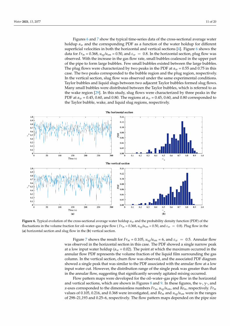
Figures 6 and 7 show the typical time-series data of the cross-sectional average waterholdup αw and the corresponding PDF as a function of the water holdup for differentsuperficial velocities in both the horizontal and vertical sections [4]. Figure 6 shows thedata for Frm = 0.368, usg/usm = 0.50, and εw = 0.8. In the horizontal section, plug flow wasobserved. With the increase in the gas flow rate, small bubbles coalesced in the upper partof the pipe to form large bubbles. Few small bubbles existed between the large bubbles.The plug flows were characterized by two peaks in the PDF at αw = 0.55 and 0.75 in thiscase. The two peaks corresponded to the bubble region and the plug region, respectively.In the vertical section, slug flow was observed under the same experimental conditions.Taylor bubbles and liquid slugs between two adjacent Taylor bubbles formed slug flows.Many small bubbles were distributed between the Taylor bubbles, which is referred to asthe wake region [29]. In this study, slug flows were characterized by three peaks in thePDF at αw = 0.45, 0.60, and 0.80. The regions at αw = 0.45, 0.60, and 0.80 corresponded tothe Taylor bubble, wake, and liquid slug regions, respectively.

Water 2021, 13, x FOR PEER REVIEW 11 of 20

observed. With the increase in the gas flow rate, small bubbles coalesced in the upper part

of the pipe to form large bubbles. Few small bubbles existed between the large bubbles.

The plug flows were characterized by two peaks in the PDF at αw = 0.55 and 0.75 in this

case. The two peaks corresponded to the bubble region and the plug region, respectively.

In the vertical section, slug flow was observed under the same experimental conditions.

Taylor bubbles and liquid slugs between two adjacent Taylor bubbles formed slug flows.

Many small bubbles were distributed between the Taylor bubbles, which is referred to as

the wake region [29]. In this study, slug flows were characterized by three peaks in the

PDF at αw = 0.45, 0.60, and 0.80. The regions at αw = 0.45, 0.60, and 0.80 corresponded to

the Taylor bubble, wake, and liquid slug regions, respectively.

Figure 7 shows the result for Frm = 0.105, usg/usm = 6, and 𝜀𝑤 = 0.5. Annular flow was

observed in the horizontal section in this case. The PDF showed a single narrow peak at a

low input water holdup (αw = 0.02). The point at which the maximum occurred in the an-

nular flow PDF represents the volume fraction of the liquid film surrounding the gas col-

umn. In the vertical section, churn flow was observed, and the associated PDF diagram

showed a single peak that was similar to the PDF associated with the annular flow at a

low input water cut. However, the distribution range of the single peak was greater than

that in the annular flow, suggesting that significantly severely agitated mixing occurred.

Flow pattern maps were developed for the oil–water–gas pipe flow in the horizontal

and vertical sections, which are shown in Figures 8 and 9. In these figures, the x-, y-, and

z-axes corresponded to the dimensionless numbers Frm, usg/usm, and Rem, respectively. Frm

values of 0.105, 0.216, and 0.368 were investigated, and Rem and usg/usm were in the ranges

of 298–21,193 and 0.25–6, respectively. The flow pattern maps depended on the pipe size

and the size of the gas inclusions. The flow pattern maps in this study were constructed

for D = 50 mm.

Figure 6. Typical evolution of the cross-sectional average water holdup αw and the probability density function (PDF) of

the fluctuations in the volume fraction for oil–water–gas pipe flow ( Frm = 0.368, usg/usm = 0.50, and 𝜀𝑤 = 0.8). Plug flow in

the (a) horizontal section and slug flow in the (b) vertical section.

Figure 6. Typical evolution of the cross-sectional average water holdup αw and the probability density function (PDF) of thefluctuations in the volume fraction for oil–water–gas pipe flow ( Frm = 0.368, usg/usm = 0.50, and εw = 0.8). Plug flow in the(a) horizontal section and slug flow in the (b) vertical section.

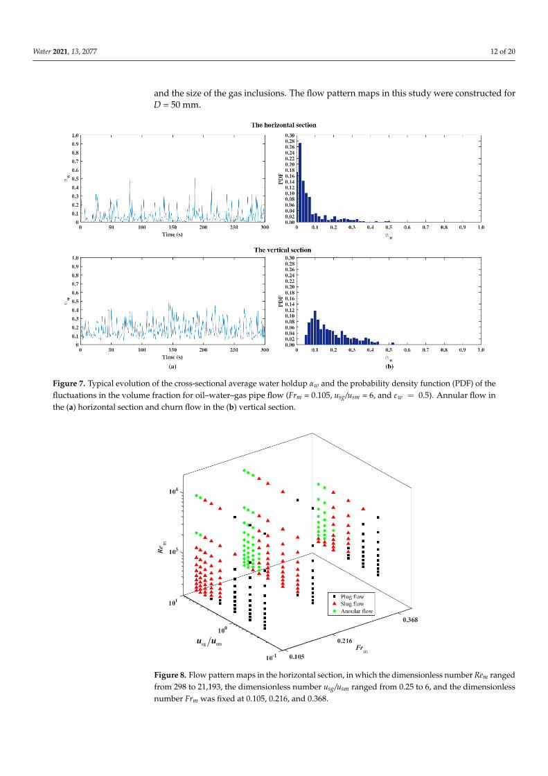
Figure 7 shows the result for Frm = 0.105, usg/usm = 6, and εw = 0.5. Annular flowwas observed in the horizontal section in this case. The PDF showed a single narrow peakat a low input water holdup (αw = 0.02). The point at which the maximum occurred in theannular flow PDF represents the volume fraction of the liquid film surrounding the gascolumn. In the vertical section, churn flow was observed, and the associated PDF diagramshowed a single peak that was similar to the PDF associated with the annular flow at a lowinput water cut. However, the distribution range of the single peak was greater than thatin the annular flow, suggesting that significantly severely agitated mixing occurred.

Flow pattern maps were developed for the oil–water–gas pipe flow in the horizontaland vertical sections, which are shown in Figures 8 and 9. In these figures, the x-, y-, andz-axes corresponded to the dimensionless numbers Frm, usg/usm, and Rem, respectively. Frmvalues of 0.105, 0.216, and 0.368 were investigated, and Rem and usg/usm were in the rangesof 298–21,193 and 0.25–6, respectively. The flow pattern maps depended on the pipe size

Water 2021, 13, 2077 12 of 20

and the size of the gas inclusions. The flow pattern maps in this study were constructed forD = 50 mm.

Water 2021, 13, x FOR PEER REVIEW 12 of 20

Figure 7. Typical evolution of the cross-sectional average water holdup αw and the probability density function (PDF) of

the fluctuations in the volume fraction for oil–water–gas pipe flow (Frm = 0.105, usg/usm = 6, and 𝜀𝑤 = 0.5). Annular flow in

the (a) horizontal section and churn flow in the (b) vertical section.

Figure 8. Flow pattern maps in the horizontal section, in which the dimensionless number Rem

ranged from 298 to 21,193, the dimensionless number usg/usm ranged from 0.25 to 6, and the dimen-

sionless number Frm was fixed at 0.105, 0.216, and 0.368.

g ms su u

Figure 7. Typical evolution of the cross-sectional average water holdup αw and the probability density function (PDF) of thefluctuations in the volume fraction for oil–water–gas pipe flow (Frm = 0.105, usg/usm = 6, and εw = 0.5). Annular flow inthe (a) horizontal section and churn flow in the (b) vertical section.

Water 2021, 13, x FOR PEER REVIEW 12 of 20

Figure 7. Typical evolution of the cross-sectional average water holdup αw and the probability density function (PDF) of

the fluctuations in the volume fraction for oil–water–gas pipe flow (Frm = 0.105, usg/usm = 6, and 𝜀𝑤 = 0.5). Annular flow in

the (a) horizontal section and churn flow in the (b) vertical section.

Figure 8. Flow pattern maps in the horizontal section, in which the dimensionless number Rem

ranged from 298 to 21,193, the dimensionless number usg/usm ranged from 0.25 to 6, and the dimen-

sionless number Frm was fixed at 0.105, 0.216, and 0.368.

g ms su u

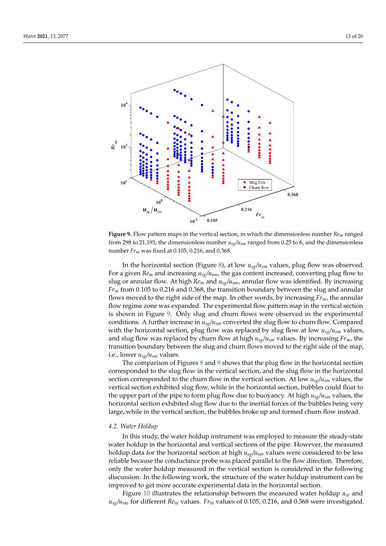
Figure 8. Flow pattern maps in the horizontal section, in which the dimensionless number Rem rangedfrom 298 to 21,193, the dimensionless number usg/usm ranged from 0.25 to 6, and the dimensionlessnumber Frm was fixed at 0.105, 0.216, and 0.368.

Water 2021, 13, 2077 13 of 20Water 2021, 13, x FOR PEER REVIEW 13 of 20

Figure 9. Flow pattern maps in the vertical section, in which the dimensionless number Rem ranged

from 298 to 21,193, the dimensionless number usg/usm ranged from 0.25 to 6, and the dimensionless

number Frm was fixed at 0.105, 0.216, and 0.368.

In the horizontal section (Figure 8), at low usg/usm values, plug flow was observed. For

a given Rem and increasing usg/usm, the gas content increased, converting plug flow to slug

or annular flow. At high Rem and usg/usm, annular flow was identified. By increasing Frm

from 0.105 to 0.216 and 0.368, the transition boundary between the slug and annular flows

moved to the right side of the map. In other words, by increasing Frm, the annular flow

regime zone was expanded. The experimental flow pattern map in the vertical section is

shown in Figure 9. Only slug and churn flows were observed in the experimental condi-

tions. A further increase in usg/usm converted the slug flow to churn flow. Compared with

the horizontal section, plug flow was replaced by slug flow at low usg/usm values, and slug

flow was replaced by churn flow at high usg/usm values. By increasing Frm, the transition

boundary between the slug and churn flows moved to the right side of the map, i.e., lower

usg/usm values.

The comparison of Figures 8 and 9 shows that the plug flow in the horizontal section

corresponded to the slug flow in the vertical section, and the slug flow in the horizontal

section corresponded to the churn flow in the vertical section. At low usg/usm values, the

vertical section exhibited slug flow, while in the horizontal section, bubbles could float to

the upper part of the pipe to form plug flow due to buoyancy. At high usg/usm values, the

horizontal section exhibited slug flow due to the inertial forces of the bubbles being very

large, while in the vertical section, the bubbles broke up and formed churn flow instead.

4.2. Water Holdup

In this study, the water holdup instrument was employed to measure the steady-

state water holdup in the horizontal and vertical sections of the pipe. However, the meas-

ured holdup data for the horizontal section at high usg/usm values were considered to be

less reliable because the conductance probe was placed parallel to the flow direction.

Therefore, only the water holdup measured in the vertical section is considered in the

following discussion. In the following work, the structure of the water holdup instrument

can be improved to get more accurate experimental data in the horizontal section.

Figure 10 illustrates the relationship between the measured water holdup αw and

usg/usm for different Rem values. Frm values of 0.105, 0.216, and 0.368 were investigated. The

g ms su u

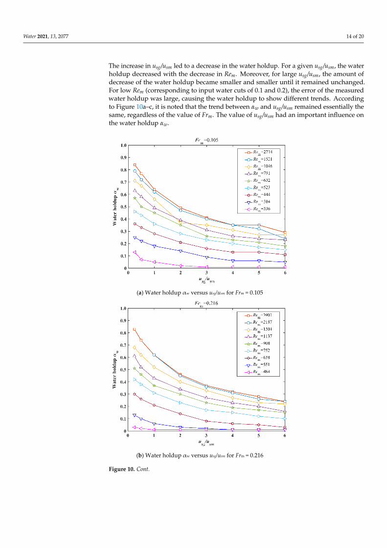
Figure 9. Flow pattern maps in the vertical section, in which the dimensionless number Rem rangedfrom 298 to 21,193, the dimensionless number usg/usm ranged from 0.25 to 6, and the dimensionlessnumber Frm was fixed at 0.105, 0.216, and 0.368.

In the horizontal section (Figure 8), at low usg/usm values, plug flow was observed.For a given Rem and increasing usg/usm, the gas content increased, converting plug flow toslug or annular flow. At high Rem and usg/usm, annular flow was identified. By increasingFrm from 0.105 to 0.216 and 0.368, the transition boundary between the slug and annularflows moved to the right side of the map. In other words, by increasing Frm, the annularflow regime zone was expanded. The experimental flow pattern map in the vertical sectionis shown in Figure 9. Only slug and churn flows were observed in the experimentalconditions. A further increase in usg/usm converted the slug flow to churn flow. Comparedwith the horizontal section, plug flow was replaced by slug flow at low usg/usm values,and slug flow was replaced by churn flow at high usg/usm values. By increasing Frm, thetransition boundary between the slug and churn flows moved to the right side of the map,i.e., lower usg/usm values.

The comparison of Figures 8 and 9 shows that the plug flow in the horizontal sectioncorresponded to the slug flow in the vertical section, and the slug flow in the horizontalsection corresponded to the churn flow in the vertical section. At low usg/usm values, thevertical section exhibited slug flow, while in the horizontal section, bubbles could float tothe upper part of the pipe to form plug flow due to buoyancy. At high usg/usm values, thehorizontal section exhibited slug flow due to the inertial forces of the bubbles being verylarge, while in the vertical section, the bubbles broke up and formed churn flow instead.

4.2. Water Holdup

In this study, the water holdup instrument was employed to measure the steady-statewater holdup in the horizontal and vertical sections of the pipe. However, the measuredholdup data for the horizontal section at high usg/usm values were considered to be lessreliable because the conductance probe was placed parallel to the flow direction. Therefore,only the water holdup measured in the vertical section is considered in the followingdiscussion. In the following work, the structure of the water holdup instrument can beimproved to get more accurate experimental data in the horizontal section.

Figure 10 illustrates the relationship between the measured water holdup αw andusg/usm for different Rem values. Frm values of 0.105, 0.216, and 0.368 were investigated.

Water 2021, 13, 2077 14 of 20

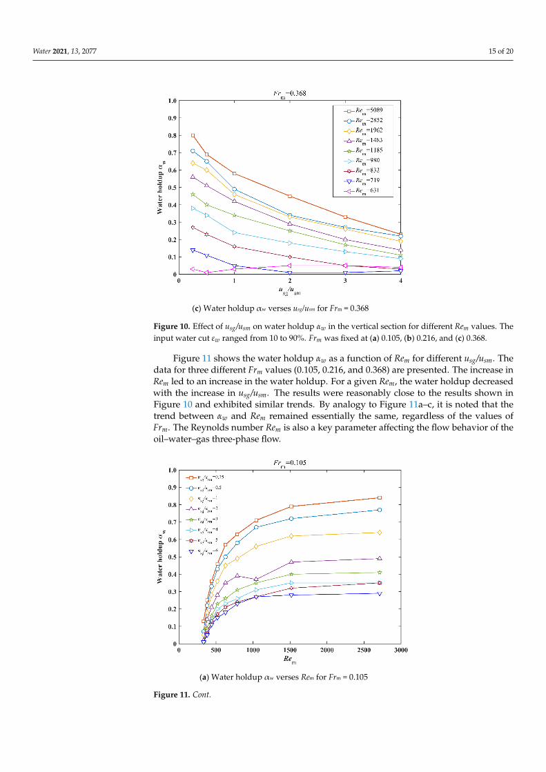
The increase in usg/usm led to a decrease in the water holdup. For a given usg/usm, the waterholdup decreased with the decrease in Rem. Moreover, for large usg/usm, the amount ofdecrease of the water holdup became smaller and smaller until it remained unchanged.For low Rem (corresponding to input water cuts of 0.1 and 0.2), the error of the measuredwater holdup was large, causing the water holdup to show different trends. Accordingto Figure 10a–c, it is noted that the trend between αw and usg/usm remained essentially thesame, regardless of the value of Frm. The value of usg/usm had an important influence onthe water holdup αw.

Water 2021, 13, x FOR PEER REVIEW 14 of 20

increase in usg/usm led to a decrease in the water holdup. For a given usg/usm, the water

holdup decreased with the decrease in Rem. Moreover, for large usg/usm, the amount of de-

crease of the water holdup became smaller and smaller until it remained unchanged. For

low Rem (corresponding to input water cuts of 0.1 and 0.2), the error of the measured water

holdup was large, causing the water holdup to show different trends. According to Figure

10a–c, it is noted that the trend between αw and usg/usm remained essentially the same, re-

gardless of the value of Frm. The value of usg/usm had an important influence on the water

holdup αw.

(a) Water holdup αw versus usg/usm for Frm = 0.105

(b) Water holdup αw versus usg/usm for Frm = 0.216

Figure 10. Cont.

Water 2021, 13, 2077 15 of 20Water 2021, 13, x FOR PEER REVIEW 15 of 20

(c) Water holdup αw verses usg/usm for Frm = 0.368

Figure 10. Effect of usg/usm on water holdup αw in the vertical section for different Rem values. The

input water cut εw ranged from 10% to 90%. Frm was fixed at (a) 0.105, (b) 0.216, and (c) 0.368.

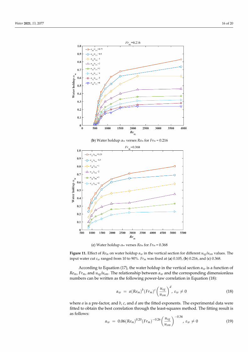
Figure 11 shows the water holdup αw as a function of Rem for different usg/usm. The

data for three different Frm values (0.105, 0.216, and 0.368) are presented. The increase in

Rem led to an increase in the water holdup. For a given Rem, the water holdup decreased

with the increase in usg/usm. The results were reasonably close to the results shown in Fig-

ure 10 and exhibited similar trends. By analogy to Figure 11a–c, it is noted that the trend

between αw and Rem remained essentially the same, regardless of the values of Frm. The

Reynolds number Rem is also a key parameter affecting the flow behavior of the oil–water–

gas three-phase flow.

(a) Water holdup αw verses Rem for Frm = 0.105

Figure 10. Effect of usg/usm on water holdup αw in the vertical section for different Rem values. Theinput water cut εw ranged from 10 to 90%. Frm was fixed at (a) 0.105, (b) 0.216, and (c) 0.368.

Figure 11 shows the water holdup αw as a function of Rem for different usg/usm. Thedata for three different Frm values (0.105, 0.216, and 0.368) are presented. The increase inRem led to an increase in the water holdup. For a given Rem, the water holdup decreasedwith the increase in usg/usm. The results were reasonably close to the results shown inFigure 10 and exhibited similar trends. By analogy to Figure 11a–c, it is noted that thetrend between αw and Rem remained essentially the same, regardless of the values ofFrm. The Reynolds number Rem is also a key parameter affecting the flow behavior of theoil–water–gas three-phase flow.

Water 2021, 13, x FOR PEER REVIEW 15 of 20

(c) Water holdup αw verses usg/usm for Frm = 0.368

Figure 10. Effect of usg/usm on water holdup αw in the vertical section for different Rem values. The

input water cut εw ranged from 10% to 90%. Frm was fixed at (a) 0.105, (b) 0.216, and (c) 0.368.

Figure 11 shows the water holdup αw as a function of Rem for different usg/usm. The

data for three different Frm values (0.105, 0.216, and 0.368) are presented. The increase in

Rem led to an increase in the water holdup. For a given Rem, the water holdup decreased

with the increase in usg/usm. The results were reasonably close to the results shown in Fig-

ure 10 and exhibited similar trends. By analogy to Figure 11a–c, it is noted that the trend

between αw and Rem remained essentially the same, regardless of the values of Frm. The

Reynolds number Rem is also a key parameter affecting the flow behavior of the oil–water–

gas three-phase flow.

(a) Water holdup αw verses Rem for Frm = 0.105

Figure 11. Cont.

Water 2021, 13, 2077 16 of 20Water 2021, 13, x FOR PEER REVIEW 16 of 20

(b) Water holdup αw verses Rem for Frm = 0.216

(c) Water holdup αw verses Rem for Frm = 0.368

Figure 11. Effect of Rem on water holdup αw in the vertical section for different usg/usm values. The

input water cut εw ranged from 10% to 90%. Frm was fixed at (a) 0.105, (b) 0.216, and (c) 0.368.

According to Equation (17), the water holdup in the vertical section αw is a function

of Rem, Frm, and usg/usm. The relationship between αw and the corresponding dimensionless

numbers can be written as the following power-law correlation in Equation (18):

𝛼𝑤 = 𝑎(𝑅𝑒𝑚)𝑏(𝐹𝑟𝑚)𝑐 (

𝑢𝑠𝑔

𝑢𝑠𝑚)𝑑

, 𝜀𝑤 ≠ 0 (18)

where a is a pre-factor, and b, c, and d are the fitted exponents. The experimental data were

fitted to obtain the best correlation through the least-squares method. The fitting result is

as follows:

𝛼𝑤 = 0.06(𝑅𝑒𝑚)0.20(𝐹𝑟𝑚)−0.26 (

𝑢𝑠𝑔

𝑢𝑠𝑚)−0.34

, 𝜀𝑤 ≠ 0 (19)

Figure 11. Effect of Rem on water holdup αw in the vertical section for different usg/usm values. Theinput water cut εw ranged from 10 to 90%. Frm was fixed at (a) 0.105, (b) 0.216, and (c) 0.368.

According to Equation (17), the water holdup in the vertical section αw is a function ofRem, Frm, and usg/usm. The relationship between αw and the corresponding dimensionlessnumbers can be written as the following power-law correlation in Equation (18):

αw = a(Rem)b(Frm)

c(

usg

usm

)d, εw 6= 0 (18)

where a is a pre-factor, and b, c, and d are the fitted exponents. The experimental data werefitted to obtain the best correlation through the least-squares method. The fitting result isas follows:

αw = 0.06(Rem)0.20(Frm)

−0.26(

usg

usm

)−0.34, εw 6= 0 (19)

Water 2021, 13, 2077 17 of 20

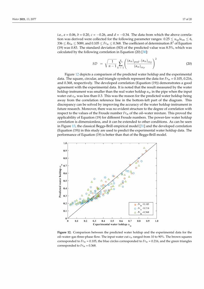
i.e., a = 0.06, b = 0.20, c = −0.26, and d = −0.34. The data from which the above correla-tion was derived were collected for the following parameter ranges: 0.25 ≤ usg/usm ≤ 6,336≤ Rem ≤ 5089, and 0.105≤ Frm ≤ 0.368. The coefficient of determination R2 of Equation(19) was 0.83. The standard deviation (SD) of the predicted value was 8.5%, which wascalculated by the following correlation in Equation (20) [30]:

SD =

√1

n− 1

n

∑k = 1

((αw)pred−(αw)exP

(αw)exP

)2

(20)

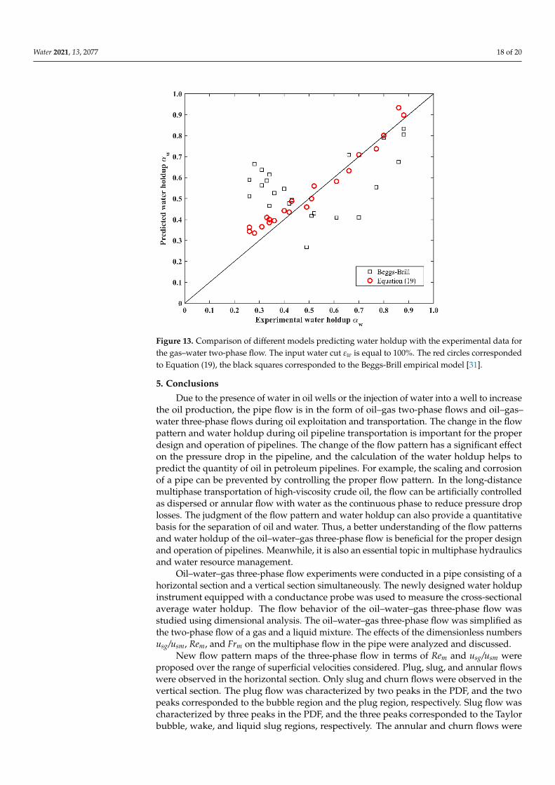
Figure 12 depicts a comparison of the predicted water holdup and the experimentaldata. The square, circular, and triangle symbols represent the data for Frm = 0.105, 0.216,and 0.368, respectively. The developed correlation (Equation (19)) demonstrates a goodagreement with the experimental data. It is noted that the result measured by the waterholdup instrument was smaller than the real water holdup αw in the pipe when the inputwater cut εw was less than 0.3. This was the reason for the predicted water holdup beingaway from the correlation reference line in the bottom-left part of the diagram. Thisdiscrepancy can be solved by improving the accuracy of the water holdup instrument infuture research. Moreover, there was no evident structure to the degree of correlation withrespect to the values of the Froude number Frm of the oil–water mixture. This proved theapplicability of Equation (19) for different Froude numbers. The power-law water holdupcorrelation is dimensionless, and it can be extended to other conditions. As can be seenin Figure 13, the classical Beggs-Brill empirical model [31] and the developed correlation(Equation (19)) in this study are used to predict the experimental water holdup data. Theperformance of Equation (19) is better than that of the Beggs-Brill model.

Water 2021, 13, x FOR PEER REVIEW 17 of 20

i.e., a = 0.06, b = 0.20, c = −0.26, and d = −0.34. The data from which the above correlation

was derived were collected for the following parameter ranges: 0.25 ≤ usg/usm ≤ 6, 336 ≤ Rem

≤ 5089, and 0.105 ≤ Frm ≤ 0.368. The coefficient of determination R2 of Equation (19) was

0.83. The standard deviation (SD) of the predicted value was 8.5%, which was calculated

by the following correlation in Equation (20) [30]:

𝑆𝐷 = √1

𝑛 − 1∑(

(𝛼𝑤)𝑝𝑟𝑒𝑑−(𝛼𝑤)𝑒𝑥𝑃(𝛼𝑤)𝑒𝑥𝑃

)

2𝑛

𝑘=1

(20)

Figure 12 depicts a comparison of the predicted water holdup and the experimental

data. The square, circular, and triangle symbols represent the data for Frm = 0.105, 0.216,

and 0.368, respectively. The developed correlation (Equation (19)) demonstrates a good

agreement with the experimental data. It is noted that the result measured by the water

holdup instrument was smaller than the real water holdup αw in the pipe when the input

water cut εw was less than 0.3. This was the reason for the predicted water holdup being

away from the correlation reference line in the bottom-left part of the diagram. This dis-

crepancy can be solved by improving the accuracy of the water holdup instrument in fu-

ture research. Moreover, there was no evident structure to the degree of correlation with

respect to the values of the Froude number Frm of the oil–water mixture. This proved the

applicability of Equation (19) for different Froude numbers. The power-law water holdup

correlation is dimensionless, and it can be extended to other conditions. As can be seen in

Figure 13, the classical Beggs-Brill empirical model [31] and the developed correlation

(Equation (19)) in this study are used to predict the experimental water holdup data. The

performance of Equation (19) is better than that of the Beggs-Brill model.

Figure 12. Comparison between the predicted water holdup and the experimental data for the oil–

water–gas three-phase flow. The input water cut εw ranged from 10% to 90%. The brown squares

corresponded to Frm = 0.105, the blue circles corresponded to Frm = 0.216, and the green triangles

corresponded to Frm = 0.368.

Figure 12. Comparison between the predicted water holdup and the experimental data for theoil–water–gas three-phase flow. The input water cut εw ranged from 10 to 90%. The brown squarescorresponded to Frm = 0.105, the blue circles corresponded to Frm = 0.216, and the green trianglescorresponded to Frm = 0.368.

Water 2021, 13, 2077 18 of 20Water 2021, 13, x FOR PEER REVIEW 18 of 20

Figure 13. Comparison of different models predicting water holdup with the experimental data for

the gas–water two-phase flow. The input water cut εw is equal to 100%. The red circles corresponded

to Equation (19), the black squares corresponded to the Beggs-Brill empirical model [31].

5. Conclusions

Due to the presence of water in oil wells or the injection of water into a well to in-

crease the oil production, the pipe flow is in the form of oil–gas two-phase flows and oil–

gas–water three-phase flows during oil exploitation and transportation. The change in the

flow pattern and water holdup during oil pipeline transportation is important for the

proper design and operation of pipelines. The change of the flow pattern has a significant

effect on the pressure drop in the pipeline, and the calculation of the water holdup helps

to predict the quantity of oil in petroleum pipelines. For example, the scaling and corro-

sion of a pipe can be prevented by controlling the proper flow pattern. In the long-distance

multiphase transportation of high-viscosity crude oil, the flow can be artificially con-

trolled as dispersed or annular flow with water as the continuous phase to reduce pres-

sure drop losses. The judgment of the flow pattern and water holdup can also provide a

quantitative basis for the separation of oil and water. Thus, a better understanding of the

flow patterns and water holdup of the oil–water–gas three-phase flow is beneficial for the

proper design and operation of pipelines. Meanwhile, it is also an essential topic in mul-

tiphase hydraulics and water resource management.

Oil–water–gas three-phase flow experiments were conducted in a pipe consisting of

a horizontal section and a vertical section simultaneously. The newly designed water

holdup instrument equipped with a conductance probe was used to measure the cross-

sectional average water holdup. The flow behavior of the oil–water–gas three-phase flow

was studied using dimensional analysis. The oil–water–gas three-phase flow was simpli-

fied as the two-phase flow of a gas and a liquid mixture. The effects of the dimensionless

numbers usg/usm, Rem, and Frm on the multiphase flow in the pipe were analyzed and dis-

cussed.

New flow pattern maps of the three-phase flow in terms of Rem and usg/usm were pro-

posed over the range of superficial velocities considered. Plug, slug, and annular flows

were observed in the horizontal section. Only slug and churn flows were observed in the

vertical section. The plug flow was characterized by two peaks in the PDF, and the two

Figure 13. Comparison of different models predicting water holdup with the experimental data forthe gas–water two-phase flow. The input water cut εw is equal to 100%. The red circles correspondedto Equation (19), the black squares corresponded to the Beggs-Brill empirical model [31].

5. Conclusions

Due to the presence of water in oil wells or the injection of water into a well to increasethe oil production, the pipe flow is in the form of oil–gas two-phase flows and oil–gas–water three-phase flows during oil exploitation and transportation. The change in the flowpattern and water holdup during oil pipeline transportation is important for the properdesign and operation of pipelines. The change of the flow pattern has a significant effecton the pressure drop in the pipeline, and the calculation of the water holdup helps topredict the quantity of oil in petroleum pipelines. For example, the scaling and corrosionof a pipe can be prevented by controlling the proper flow pattern. In the long-distancemultiphase transportation of high-viscosity crude oil, the flow can be artificially controlledas dispersed or annular flow with water as the continuous phase to reduce pressure droplosses. The judgment of the flow pattern and water holdup can also provide a quantitativebasis for the separation of oil and water. Thus, a better understanding of the flow patternsand water holdup of the oil–water–gas three-phase flow is beneficial for the proper designand operation of pipelines. Meanwhile, it is also an essential topic in multiphase hydraulicsand water resource management.

Oil–water–gas three-phase flow experiments were conducted in a pipe consisting of ahorizontal section and a vertical section simultaneously. The newly designed water holdupinstrument equipped with a conductance probe was used to measure the cross-sectionalaverage water holdup. The flow behavior of the oil–water–gas three-phase flow wasstudied using dimensional analysis. The oil–water–gas three-phase flow was simplified asthe two-phase flow of a gas and a liquid mixture. The effects of the dimensionless numbersusg/usm, Rem, and Frm on the multiphase flow in the pipe were analyzed and discussed.

New flow pattern maps of the three-phase flow in terms of Rem and usg/usm wereproposed over the range of superficial velocities considered. Plug, slug, and annular flowswere observed in the horizontal section. Only slug and churn flows were observed in thevertical section. The plug flow was characterized by two peaks in the PDF, and the twopeaks corresponded to the bubble region and the plug region, respectively. Slug flow wascharacterized by three peaks in the PDF, and the three peaks corresponded to the Taylorbubble, wake, and liquid slug regions, respectively. The annular and churn flows were

Water 2021, 13, 2077 19 of 20

characterized by a single peak in the PDF, and the distribution range of the single peak inthe churn flow was greater than that in the annular flow. Moreover, the flow pattern mapsdescribed using dimensionless numbers may also be applied to other pipe sizes. Basedon the experimental data, a dimensionless power-law water holdup correlation for theoil–water–gas three-phase flow in the vertical section was developed. The predicted waterholdup agreed reasonably well with the experimental results.

Author Contributions: Conceptualization: G.R., D.G. and P.L.; Formal analysis: G.R., D.G., P.L., X.Z.and X.L.; Investigation: G.R., P.L., X.Z. and X.L.; Methodology: G.R., X.C., K.S., R.F., L.M. and F.S.;Project administration: G.R., X.C., K.S., R.F., L.M. and F.S.; Supervision: G.R. and D.G.; Validation:P.L.; Visualization: P.L.; Writing—original draft: P.L.; Writing—review and editing: P.L., X.Z. and X.L.All authors have read and agreed to the published version of the manuscript.

Funding: This research received no external funding.

Institutional Review Board Statement: Not applicable.

Informed Consent Statement: Not applicable.

Data Availability Statement: Not applicable.

Conflicts of Interest: The authors declare no conflict of interest.

References1. Brauner, N. The prediction of dispersed flows boundaries in liquid–liquid and gas–liquid systems. Int. J. Multiph. Flow 2001, 27,

885–910. [CrossRef]2. Ibarra, R.; Nossen, J.; Tutkun, M. Two-phase gas–liquid flow in concentric and fully eccentric annuli. Part I: Flow patterns, holdup,

slip ratio and pressure gradient. Chem. Eng. Sci. 2019, 203, 489–500. [CrossRef]3. Xu, J.Y.; Li, D.H.; Guo, J.; Wu, Y.X. Investigations of phase inversion and frictional pressure gradients in upward and downward

oil–water flow in vertical pipes. Int. J. Multiph. Flow 2010, 36, 930–939. [CrossRef]4. Jones, O.C.; Zuber, N. The interrelation between void fraction fluctuations and flow patterns in two-phase flow. Int. J. Multiph.

Flow 1975, 2, 273–306. [CrossRef]5. Hasan, A.; Kabir, C.S. A new model for two-phase oil/water flow: Production log interpretation and tubular calculations. SPE

Prod. Eng. 1990, 5, 193–199. [CrossRef]6. Liu, Z.; Liao, R.; Luo, W.; Riberio, J.X.F. A new model for predicting liquid holdup in two-phase flow under high gas and liquid

velocities. Sci. Iran. 2019, 26, 1529–1539.7. Du, M.; Jin, N.D.; Gao, Z.K.; Wang, Z.Y.; Zhai, L.S. Flow pattern and water holdup measurements of vertical upward oil–water

two-phase flow in small diameter pipes. Int. J. Multiph. Flow 2012, 41, 91–105. [CrossRef]8. Oddie, G.; Shi, H.; Durlofsky, L.J.; Aziz, K.; Pfeffer, B.; Holmes, J.A. Experimental study of two and three phase flows in large

diameter inclined pipes. Int. J. Multiph. Flow 2003, 29, 527–558. [CrossRef]9. Spedding, P.L.; Donnelly, G.F.; Cole, J.S. Three phase oil–water–gas horizontal co-current flow. Chem. Eng. Res. Des. 2005, 83,

401–411. [CrossRef]10. Descamps, M.N.; Oliemans, R.V.A.; Ooms, G.; Mudde, R.F. Experimental investigation of three-phase flow in a vertical pipe:

Local characteristics of the gas phase for gas-lift conditions. Int. J. Multiph. Flow 2007, 33, 1205–1221. [CrossRef]11. Hanafizadeh, P.; Shahani, A.; Ghanavati, A.; Akhavan-Behabadi, M.A. Experimental investigation of air–water–oil three-phase

flow patterns in inclined pipes. Exp. Therm. Fluid Sci. 2017, 84, 286–298. [CrossRef]12. Tunstall, R.; Skillen, A. Large eddy simulation of a t-junction with upstream elbow: The role of dean vortices in thermal fatigue.

Appl. Therm. Eng. 2016, 107, 672–680. [CrossRef]13. Xing, L.; Yeung, H.; Shen, J.; Cao, Y. Numerical study on mitigating severe slugging in pipeline/riser system with wavy pipe. Int.

J. Multiph. Flow 2013, 53, 1–10. [CrossRef]14. Ghorai, S.; Suri, V.; Nigam, K.D.P. Numerical modeling of three-phase stratified flow in pipes. Chem. Eng. Sci. 2005, 60,

6637–6648. [CrossRef]15. Friedemann, C.; Mortensen, M.; Nossen, J. Gas–liquid slug flow in a horizontal concentric annulus, a comparison of numerical

simulations and experimental data. Int. J. Heat Fluid Flow 2019, 78, 108437. [CrossRef]16. Leporini, M.; Terenzi, A.; Marchetti, B.; Corvaro, F.; Polonara, F. On the numerical simulation of sand transport in liquid and

multiphase pipelines. J. Pet. Sci. Eng. 2019, 175, 519–535. [CrossRef]17. Pietrzak, M.; Witczak, S. Flow patterns and void fractions of phases during gas–liquid two-phase and gas–liquid–liquid three-

phase flow in U-bends. Int. J. Heat Fluid Flow 2013, 44, 700–710. [CrossRef]18. Liu, W.; Bai, B. Transition from bubble flow to slug flow along the streamwise direction in a gas–liquid swirling flow. Chem. Eng.

Sci. 2019, 202, 392–402. [CrossRef]

Water 2021, 13, 2077 20 of 20

19. Wang, H.Q. Investigation on Flow Characteristics of Oil–Water Two-Phase Flow and Gas–Oil–Water Three-Phase Flow inHorizontal Pipelines. Ph.D. Thesis, China University of Petroleum (East China), Qingdao, China, 2008.

20. Flores, J.G. Characterization of oil-water flow patterns in vertical and deviated wells. Soc. Pet. Eng. 1997, 14, 102–109.21. Ji, H.F.; Chang, Y.; Huang, Z.Y.; Wang, B.L.; Li, H.Q. Voidage measurement of gas–liquid two-phase flow based on Capacitively

Coupled Contactless Conductivity Detection. Flow Meas. Instrum. 2014, 40, 199–205. [CrossRef]22. Bruggeman, D.A.G. Berechnung verschiedener physikalischer Konstanten von heterogenen Substanzen. I. Dielektrizitätskonstan-

ten und Leitfähigkeiten der Mischkörper aus isotropen Substanzen. Ann. Phys. 1935, 416, 636–664. [CrossRef]23. Achwal, S.K.; Stepanek, J.B. An alternative method of determining hold-up in gas–liquid systems. Chem. Eng. Sci. 1975, 30,

1443–1444. [CrossRef]24. Achwal, S.K.; Stepanek, J.B. Holdup profiles in packed beds. Chem. Eng. J. 1976, 12, 69–75. [CrossRef]25. Begovich, J.M.; Watson, J.S. An electroconductivity technique for the measurement of axial variation of holdups in three-phase

fluidized beds. AIChE J. 1978, 24, 351–354. [CrossRef]26. Huang, S.F.; Zhang, B.D.; Lu, J.; Wang, D. Study on flow pattern maps in hilly-terrain air–water–oil three-phase flows. Exp. Therm.

Fluid Sci. 2013, 47, 158–171. [CrossRef]27. Hapanowicz, J.; Troniewski, L. Two-phase flow of liquid–liquid mixture in the range of the water droplet pattern. Chem. Eng.

Process. 2002, 41, 165–172. [CrossRef]28. Weisman, J. Two-phase flow patterns. In Handbook of Fluids in Motion; Cheremisinoff, N.P., Gupta, R., Eds.; Chapter 15; Ann Arbor

Science Publishers: Ann Arbor, Michigan, USA, 1983; pp. 409–425.29. Zhang, S.; Wang, Z.; Sun, B.; Yuan, K. Pattern transition of a gas–liquid flow with zero liquid superficial velocity in a vertical tube.

Int. J. Multiph. Flow 2019, 118, 270–282. [CrossRef]30. Al-Wahaibi, T. Pressure gradient correlation for oil–water separated flow in horizontal pipes. Exp. Therm. Fluid Sci. 2012, 42,

196–203. [CrossRef]31. Beggs, D.H.; Brill, J.P. An experimental study of two-phase flow in inclined pipes. J. Pet. Technol. 1973, 25, 607–617. [CrossRef]