Medical Image Analysis xxx (2012) xxx–xxx

Contents lists available at SciVerse ScienceDirect

Medical Image Analysis

journal homepage: www.elsevier .com/locate /media

The estimation of patient-specific cardiac diastolic functions fromclinical measurements

Jiahe Xi a,b, Pablo Lamata a,b, Steven Niederer a,b, Sander Land a,b, Wenzhe Shi c, Xiahai Zhuang d,Sebastien Ourselin d, Simon G. Duckett b, Anoop K. Shetty b, C. Aldo Rinaldi b, Daniel Rueckert c,Reza Razavi b, Nic P. Smith a,b,⇑a Department of Computer Science, University of Oxford, United Kingdomb Department of Biomedical Engineering, Kings College London, Kings Health Partners, St. Thomas Hospital, London SE1 7EH, United Kingdomc Department of Computing, Imperial College London, United Kingdomd Centre for Medical Image Computing, University College London, United Kingdom

a r t i c l e i n f o a b s t r a c t

Article history:Received 26 September 2011Received in revised form 26 July 2012Accepted 14 August 2012Available online xxxx

Keywords:Constitutive material parameter estimationLeft ventricular (LV) mechanicsDiastolic heart failure

1361-8415/$ - see front matter � 2012 Elsevier B.V. Ahttp://dx.doi.org/10.1016/j.media.2012.08.001

⇑ Corresponding author at: Department of BiomedicLondon, Kings Health Partners, St. Thomas HospitaKingdom. Tel.: +44 020 718882451.

E-mail address: nicolas.smith@kcl.ac.uk (N.P. Smit

Please cite this article in press as: Xi, J., et al. Th(2012), http://dx.doi.org/10.1016/j.media.2012.0

An unresolved issue in patients with diastolic dysfunction is that the estimation of myocardial stiffnesscannot be decoupled from diastolic residual active tension (AT) because of the impaired ventricular relax-ation during diastole. To address this problem, this paper presents a method for estimating diastolicmechanical parameters of the left ventricle (LV) from cine and tagged MRI measurements and LV cavitypressure recordings, separating the passive myocardial constitutive properties and diastolic residual AT.Dynamic C1-continuous meshes are automatically built from the anatomy and deformation capturedfrom dynamic MRI sequences. Diastolic deformation is simulated using a mechanical model that com-bines passive and active material properties. The problem of non-uniqueness of constitutive parameterestimation using the well known Guccione law is characterized by reformulation of this law. Using thisreformulated form, and by constraining the constitutive parameters to be constant across time pointsduring diastole, we separate the effects of passive constitutive properties and the residual AT during dia-stolic relaxation. Finally, the method is applied to two clinical cases and one control, demonstrating thatincreased residual AT during diastole provides a potential novel index for delineating healthy and path-ological cases.

� 2012 Elsevier B.V. All rights reserved.

1. Introduction

The quantification of diastolic dysfunction is vital for the diag-nosis and assessment of heart disease, enabling improved selectionand treatment of individuals with pathological myocardialmechanics for further therapy (Nagel and Schuster, 2010).Patient-specific cardiac models, parameterized from clinical mea-surements on an individual basis, provide a powerful approachfor this purpose (Smith et al., 2011). Accordingly, model-basedparameter estimation from clinical measurements of cardiac func-tion has been an active research area.

Parameters in organ-level cardiac mechanical models can bebroadly classified as passive and active. Typically within computa-tional models, passive constitutive parameters have been used tocharacterize the diastolic function, and with the addition of active

ll rights reserved.

al Engineering, Kings Collegel, London SE1 7EH, United

h).

e estimation of patient-specific8.001

contraction models simulate systole (Nash and Hunter, 2000;Nordsletten et al., 2011). Various frameworks and methods havebeen proposed to estimate these parameters (Sermesant et al.,2006, in press; Chabiniok et al., 2011; Delingette et al., 2012;Moireau and Chapelle, 2011; Wang et al., 2009, 2010). In Sermesantet al. (2006), a variational data assimilation method was developedto estimate the contractility parameters of an electromechanicalmodel from clinical cine MRI. Focusing on passive parameters,Wang et al. (2009) have described a workflow to estimate theGuccione constitutive parameters using high-resolution MRI dataacquired from a canine heart. An approach which these authorsfurther extended in Wang et al. (2010) to estimate the activetension (AT) during the isovolumetric contraction, systole andisovolumetric relaxation using the constitutive parameters pre-estimated during diastole.

However, an unsolved problem in patients with diastolic dys-function is that the estimation of myocardial stiffness cannot bedecoupled from impaired ventricular relaxation (one of the lusi-tropic abnormalities commonly present in heart failure, Katz,2010). For this reason, the development of methods which can ro-bustly estimate both the stiffness and residual AT during diastole

cardiac diastolic functions from clinical measurements. Med. Image Anal.

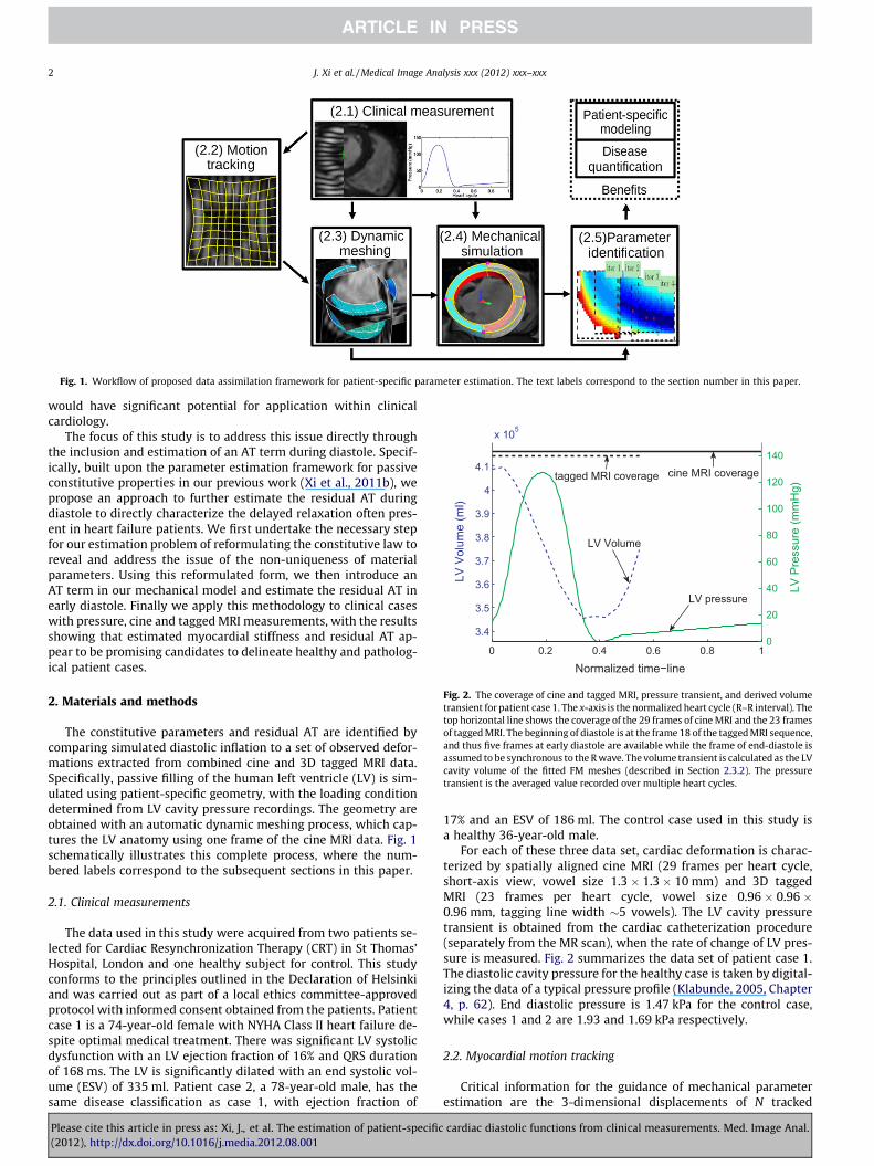
Fig. 1. Workflow of proposed data assimilation framework for patient-specific parameter estimation. The text labels correspond to the section number in this paper.

3.4

3.5

3.6

3.7

3.8

3.9

4

4.1

x 105

Normalized time−line

LV V

olum

e (m

l)

0 0.2 0.4 0.6 0.8 10

20

40

60

80

100

120

140

LV P

ress

ure

(mm

Hg)

LV pressure

tagged MRI coverage cine MRI coverage

LV Volume

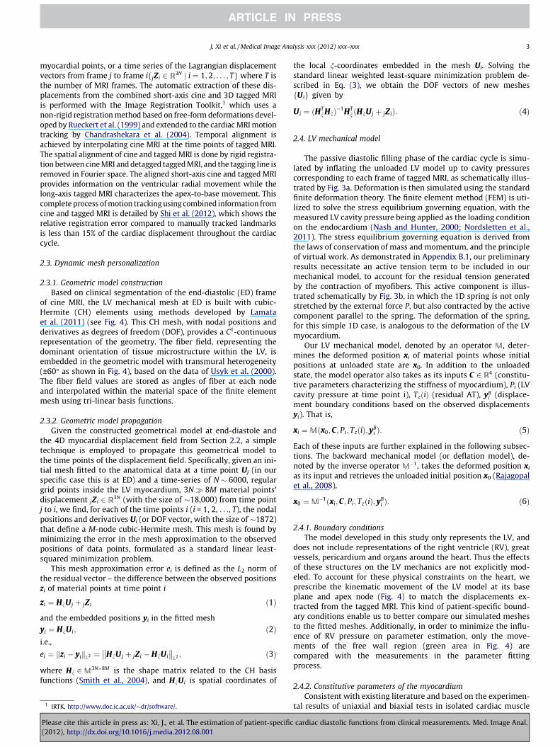
Fig. 2. The coverage of cine and tagged MRI, pressure transient, and derived volumetransient for patient case 1. The x-axis is the normalized heart cycle (R–R interval). Thetop horizontal line shows the coverage of the 29 frames of cine MRI and the 23 framesof tagged MRI. The beginning of diastole is at the frame 18 of the tagged MRI sequence,and thus five frames at early diastole are available while the frame of end-diastole isassumed to be synchronous to the R wave. The volume transient is calculated as the LVcavity volume of the fitted FM meshes (described in Section 2.3.2). The pressuretransient is the averaged value recorded over multiple heart cycles.

2 J. Xi et al. / Medical Image Analysis xxx (2012) xxx–xxx

would have significant potential for application within clinicalcardiology.

The focus of this study is to address this issue directly throughthe inclusion and estimation of an AT term during diastole. Specif-ically, built upon the parameter estimation framework for passiveconstitutive properties in our previous work (Xi et al., 2011b), wepropose an approach to further estimate the residual AT duringdiastole to directly characterize the delayed relaxation often pres-ent in heart failure patients. We first undertake the necessary stepfor our estimation problem of reformulating the constitutive law toreveal and address the issue of the non-uniqueness of materialparameters. Using this reformulated form, we then introduce anAT term in our mechanical model and estimate the residual AT inearly diastole. Finally we apply this methodology to clinical caseswith pressure, cine and tagged MRI measurements, with the resultsshowing that estimated myocardial stiffness and residual AT ap-pear to be promising candidates to delineate healthy and patholog-ical patient cases.

2. Materials and methods

The constitutive parameters and residual AT are identified bycomparing simulated diastolic inflation to a set of observed defor-mations extracted from combined cine and 3D tagged MRI data.Specifically, passive filling of the human left ventricle (LV) is sim-ulated using patient-specific geometry, with the loading conditiondetermined from LV cavity pressure recordings. The geometry areobtained with an automatic dynamic meshing process, which cap-tures the LV anatomy using one frame of the cine MRI data. Fig. 1schematically illustrates this complete process, where the num-bered labels correspond to the subsequent sections in this paper.

2.1. Clinical measurements

The data used in this study were acquired from two patients se-lected for Cardiac Resynchronization Therapy (CRT) in St Thomas’Hospital, London and one healthy subject for control. This studyconforms to the principles outlined in the Declaration of Helsinkiand was carried out as part of a local ethics committee-approvedprotocol with informed consent obtained from the patients. Patientcase 1 is a 74-year-old female with NYHA Class II heart failure de-spite optimal medical treatment. There was significant LV systolicdysfunction with an LV ejection fraction of 16% and QRS durationof 168 ms. The LV is significantly dilated with an end systolic vol-ume (ESV) of 335 ml. Patient case 2, a 78-year-old male, has thesame disease classification as case 1, with ejection fraction of

Please cite this article in press as: Xi, J., et al. The estimation of patient-specific(2012), http://dx.doi.org/10.1016/j.media.2012.08.001

17% and an ESV of 186 ml. The control case used in this study isa healthy 36-year-old male.

For each of these three data set, cardiac deformation is charac-terized by spatially aligned cine MRI (29 frames per heart cycle,short-axis view, vowel size 1.3 � 1.3 � 10 mm) and 3D taggedMRI (23 frames per heart cycle, vowel size 0.96 � 0.96 �0.96 mm, tagging line width �5 vowels). The LV cavity pressuretransient is obtained from the cardiac catheterization procedure(separately from the MR scan), when the rate of change of LV pres-sure is measured. Fig. 2 summarizes the data set of patient case 1.The diastolic cavity pressure for the healthy case is taken by digital-izing the data of a typical pressure profile (Klabunde, 2005, Chapter4, p. 62). End diastolic pressure is 1.47 kPa for the control case,while cases 1 and 2 are 1.93 and 1.69 kPa respectively.

2.2. Myocardial motion tracking

Critical information for the guidance of mechanical parameterestimation are the 3-dimensional displacements of N tracked

cardiac diastolic functions from clinical measurements. Med. Image Anal.

J. Xi et al. / Medical Image Analysis xxx (2012) xxx–xxx 3

myocardial points, or a time series of the Lagrangian displacementvectors from frame j to frame ifjZi 2 R3N j i ¼ 1;2; . . . ; Tg where T isthe number of MRI frames. The automatic extraction of these dis-placements from the combined short-axis cine and 3D tagged MRIis performed with the Image Registration Toolkit,1 which uses anon-rigid registration method based on free-form deformations devel-oped by Rueckert et al. (1999) and extended to the cardiac MRI motiontracking by Chandrashekara et al. (2004). Temporal alignment isachieved by interpolating cine MRI at the time points of tagged MRI.The spatial alignment of cine and tagged MRI is done by rigid registra-tion between cine MRI and detagged tagged MRI, and the tagging line isremoved in Fourier space. The aligned short-axis cine and tagged MRIprovides information on the ventricular radial movement while thelong-axis tagged MRI characterizes the apex-to-base movement. Thiscomplete process of motion tracking using combined information fromcine and tagged MRI is detailed by Shi et al. (2012), which shows therelative registration error compared to manually tracked landmarksis less than 15% of the cardiac displacement throughout the cardiaccycle.

2.3. Dynamic mesh personalization

2.3.1. Geometric model constructionBased on clinical segmentation of the end-diastolic (ED) frame

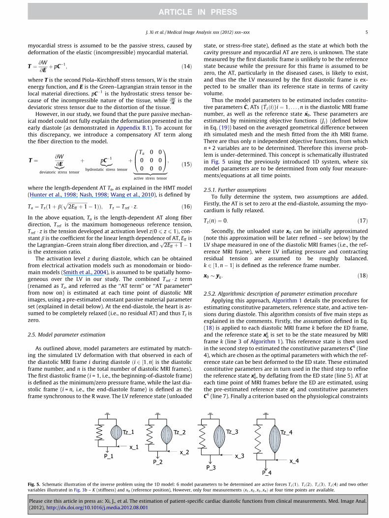
of cine MRI, the LV mechanical mesh at ED is built with cubic-Hermite (CH) elements using methods developed by Lamataet al. (2011) (see Fig. 4). This CH mesh, with nodal positions andderivatives as degrees of freedom (DOF), provides a C1-continuousrepresentation of the geometry. The fiber field, representing thedominant orientation of tissue microstructure within the LV, isembedded in the geometric model with transmural heterogeneity(±60� as shown in Fig. 4), based on the data of Usyk et al. (2000).The fiber field values are stored as angles of fiber at each nodeand interpolated within the material space of the finite elementmesh using tri-linear basis functions.

2.3.2. Geometric model propagationGiven the constructed geometrical model at end-diastole and

the 4D myocardial displacement field from Section 2.2, a simpletechnique is employed to propagate this geometrical model tothe time points of the displacement field. Specifically, given an ini-tial mesh fitted to the anatomical data at a time point Uj (in ourspecific case this is at ED) and a time-series of N � 6000, regulargrid points inside the LV myocardium, 3N� 8M material points’displacement jZi 2 R3N (with the size of �18,000) from time pointj to i, we find, for each of the time points i (i = 1, 2, . . ., T), the nodalpositions and derivatives Ui (or DOF vector, with the size of �1872)that define a M-node cubic-Hermite mesh. This mesh is found byminimizing the error in the mesh approximation to the observedpositions of data points, formulated as a standard linear least-squared minimization problem.

This mesh approximation error ei is defined as the L2 norm ofthe residual vector – the difference between the observed positionszi of material points at time point i

zi ¼ HnU j þ jZi ð1Þ

and the embedded positions yi in the fitted meshyi ¼ HnU i; ð2Þi.e.,

ei ¼ zi � yik kL2 ¼ HnU j þ jZi � HnU i

�� ��L2 ; ð3Þ

where Hn 2M3N�8M is the shape matrix related to the CH basisfunctions (Smith et al., 2004), and HnU i is spatial coordinates of

1 IRTK, http://www.doc.ic.ac.uk/�dr/software/.

Please cite this article in press as: Xi, J., et al. The estimation of patient-specific(2012), http://dx.doi.org/10.1016/j.media.2012.08.001

the local n-coordinates embedded in the mesh Ui. Solving thestandard linear weighted least-square minimization problem de-scribed in Eq. (3), we obtain the DOF vectors of new meshesfU ig given by

U i ¼ ðHTnHnÞ�1HT

n ðHnU j þ jZiÞ: ð4Þ

2.4. LV mechanical model

The passive diastolic filling phase of the cardiac cycle is simu-lated by inflating the unloaded LV model up to cavity pressurescorresponding to each frame of tagged MRI, as schematically illus-trated by Fig. 3a. Deformation is then simulated using the standardfinite deformation theory. The finite element method (FEM) is uti-lized to solve the stress equilibrium governing equation, with themeasured LV cavity pressure being applied as the loading conditionon the endocardium (Nash and Hunter, 2000; Nordsletten et al.,2011). The stress equilibrium governing equation is derived fromthe laws of conservation of mass and momentum, and the principleof virtual work. As demonstrated in Appendix B.1, our preliminaryresults necessitate an active tension term to be included in ourmechanical model, to account for the residual tension generatedby the contraction of myofibers. This active component is illus-trated schematically by Fig. 3b, in which the 1D spring is not onlystretched by the external force P, but also contracted by the activecomponent parallel to the spring. The deformation of the spring,for this simple 1D case, is analogous to the deformation of the LVmyocardium.

Our LV mechanical model, denoted by an operator M, deter-mines the deformed position xi of material points whose initialpositions at unloaded state are x0. In addition to the unloadedstate, the model operator also takes as its inputs C 2 R4 (constitu-tive parameters characterizing the stiffness of myocardium), Pi (LVcavity pressure at time point i), TzðiÞ (residual AT), yB

i (displace-ment boundary conditions based on the observed displacementsyi). That is,

xi ¼Mðx0;C; Pi; TzðiÞ; yBi Þ: ð5Þ

Each of these inputs are further explained in the following subsec-tions. The backward mechanical model (or deflation model), de-noted by the inverse operator M�1, takes the deformed position xi

as its input and retrieves the unloaded initial position x0 (Rajagopalet al., 2008).

x0 ¼M�1ðxi;C; Pi; TzðiÞ; yBi Þ: ð6Þ

2.4.1. Boundary conditionsThe model developed in this study only represents the LV, and

does not include representations of the right ventricle (RV), greatvessels, pericardium and organs around the heart. Thus the effectsof these structures on the LV mechanics are not explicitly mod-eled. To account for these physical constraints on the heart, weprescribe the kinematic movement of the LV model at its baseplane and apex node (Fig. 4) to match the displacements ex-tracted from the tagged MRI. This kind of patient-specific bound-ary conditions enable us to better compare our simulated meshesto the fitted meshes. Additionally, in order to minimize the influ-ence of RV pressure on parameter estimation, only the move-ments of the free wall region (green area in Fig. 4) arecompared with the measurements in the parameter fittingprocess.

2.4.2. Constitutive parameters of the myocardiumConsistent with existing literature and based on the experimen-

tal results of uniaxial and biaxial tests in isolated cardiac muscle

cardiac diastolic functions from clinical measurements. Med. Image Anal.

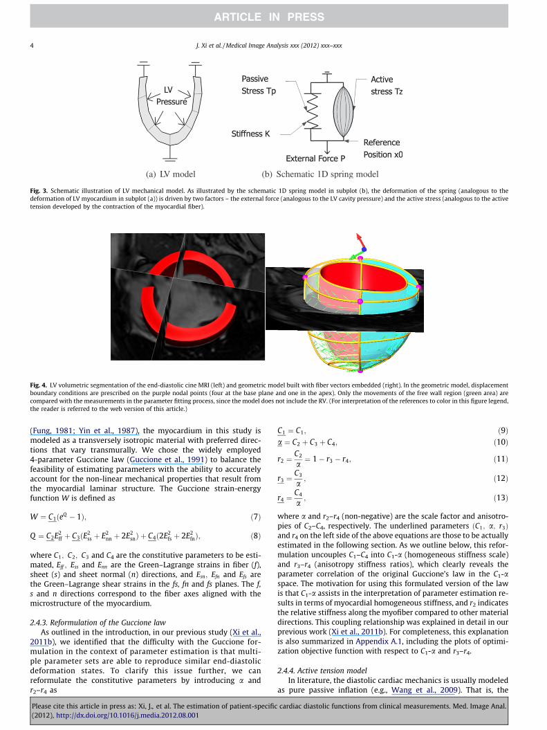
(a) LV model (b) Schematic 1D spring model

Fig. 3. Schematic illustration of LV mechanical model. As illustrated by the schematic 1D spring model in subplot (b), the deformation of the spring (analogous to thedeformation of LV myocardium in subplot (a)) is driven by two factors – the external force (analogous to the LV cavity pressure) and the active stress (analogous to the activetension developed by the contraction of the myocardial fiber).

Fig. 4. LV volumetric segmentation of the end-diastolic cine MRI (left) and geometric model built with fiber vectors embedded (right). In the geometric model, displacementboundary conditions are prescribed on the purple nodal points (four at the base plane and one in the apex). Only the movements of the free wall region (green area) arecompared with the measurements in the parameter fitting process, since the model does not include the RV. (For interpretation of the references to color in this figure legend,the reader is referred to the web version of this article.)

4 J. Xi et al. / Medical Image Analysis xxx (2012) xxx–xxx

(Fung, 1981; Yin et al., 1987), the myocardium in this study ismodeled as a transversely isotropic material with preferred direc-tions that vary transmurally. We chose the widely employed4-parameter Guccione law (Guccione et al., 1991) to balance thefeasibility of estimating parameters with the ability to accuratelyaccount for the non-linear mechanical properties that result fromthe myocardial laminar structure. The Guccione strain-energyfunction W is defined as

W ¼ C1ðeQ � 1Þ; ð7Þ

Q ¼ C2E2ff þ C3ðE2

ss þ E2nn þ 2E2

snÞ þ C4ð2E2fs þ 2E2

fnÞ; ð8Þ

where C1; C2; C3 and C4 are the constitutive parameters to be esti-mated, Eff ; Ess and Enn are the Green–Lagrange strains in fiber (f),sheet (s) and sheet normal (n) directions, and Esn; Efn and Efs arethe Green–Lagrange shear strains in the fs, fn and fs planes. The f,s and n directions correspond to the fiber axes aligned with themicrostructure of the myocardium.

2.4.3. Reformulation of the Guccione lawAs outlined in the introduction, in our previous study (Xi et al.,

2011b), we identified that the difficulty with the Guccione for-mulation in the context of parameter estimation is that multi-ple parameter sets are able to reproduce similar end-diastolicdeformation states. To clarify this issue further, we canreformulate the constitutive parameters by introducing a andr2–r4 as

Please cite this article in press as: Xi, J., et al. The estimation of patient-specific(2012), http://dx.doi.org/10.1016/j.media.2012.08.001

C1 ¼ C1; ð9Þa ¼ C2 þ C3 þ C4; ð10Þ

r2 ¼C2

a¼ 1� r3 � r4; ð11Þ

r3 ¼C3

a; ð12Þ

r4 ¼C4

a; ð13Þ

where a and r2–r4 (non-negative) are the scale factor and anisotro-pies of C2–C4, respectively. The underlined parameters ðC1; a; r3Þand r4 on the left side of the above equations are those to be actuallyestimated in the following section. As we outline below, this refor-mulation uncouples C1–C4 into C1-a (homogeneous stiffness scale)and r3–r4 (anisotropy stiffness ratios), which clearly reveals theparameter correlation of the original Guccione’s law in the C1-aspace. The motivation for using this formulated version of the lawis that C1-a assists in the interpretation of parameter estimation re-sults in terms of myocardial homogeneous stiffness, and r2 indicatesthe relative stiffness along the myofiber compared to other materialdirections. This coupling relationship was explained in detail in ourprevious work (Xi et al., 2011b). For completeness, this explanationis also summarized in Appendix A.1, including the plots of optimi-zation objective function with respect to C1-a and r3–r4.

2.4.4. Active tension modelIn literature, the diastolic cardiac mechanics is usually modeled

as pure passive inflation (e.g., Wang et al., 2009). That is, the

cardiac diastolic functions from clinical measurements. Med. Image Anal.

J. Xi et al. / Medical Image Analysis xxx (2012) xxx–xxx 5

myocardial stress is assumed to be the passive stress, caused bydeformation of the elastic (incompressible) myocardial material.

T ¼ @W@Eþ pC�1; ð14Þ

where T is the second Piola–Kirchhoff stress tensors, W is the strainenergy function, and E is the Green–Lagrangian strain tensor in thelocal material directions. pC�1 is the hydrostatic stress tensor be-cause of the incompressible nature of the tissue, while @W

@E is thedeviatoric stress tensor due to the distortion of the tissue.

However, in our study, we found that the pure passive mechan-ical model could not fully explain the deformation presented in theearly diastole (as demonstrated in Appendix B.1). To account forthis discrepancy, we introduce a compensatory AT term alongthe fiber direction to the model.

T ¼ @W@E|{z}

deviatoric stress tensor

þ pC�1|ffl{zffl}hydrostatic stress tensor

þTa 0 00 0 00 0 0

0B@

1CA

|fflfflfflfflfflfflfflfflfflfflffl{zfflfflfflfflfflfflfflfflfflfflffl}active stress tensor

; ð15Þ

where the length-dependent AT Ta, as explained in the HMT model(Hunter et al., 1998; Nash, 1998; Wang et al., 2010), is defined by

Ta ¼ Tzð1þ bðffiffiffiffiffiffiffiffiffiffiffiffiffiffiffiffiffi2Eff þ 1

p� 1ÞÞ; Tz ¼ Tref � z: ð16Þ

In the above equation, Ta is the length-dependent AT along fiberdirection, Tref is the maximum homogeneous reference tension,Tref � z is the tension developed at activation level zð0 6 z 6 1Þ, con-stant b is the coefficient for the linear length dependence of AT, Eff isthe Lagrangian–Green strain along fiber direction, and

ffiffiffiffiffiffiffiffiffiffiffiffiffiffiffiffiffi2Eff þ 1p

� 1is the extension ratio.

The activation level z during diastole, which can be obtainedfrom electrical activation models such as monodomain or biodo-main models (Smith et al., 2004), is assumed to be spatially homo-geneous over the LV in our study. The combined Tref � z term(renamed as Tz, and referred as the ‘‘AT term’’ or ‘‘AT parameter’’from now on) is estimated at each time point of diastolic MRimages, using a pre-estimated constant passive material parameterset (explained in detail below). At the end-diastole, the heart is as-sumed to be completely relaxed (i.e., no residual AT) and thus Tz iszero.

2.5. Model parameter estimation

As outlined above, model parameters are estimated by match-ing the simulated LV deformation with that observed in each ofthe diastolic MRI frame i during diastole ði 2 ½1;n� is the diastolicframe number, and n is the total number of diastolic MRI frames).The first diastolic frame (i = 1, i.e., the beginning-of-diastole frame)is defined as the minimum/zero pressure frame, while the last dia-stolic frame (i = n, i.e., the end-diastole frame) is defined as theframe synchronous to the R wave. The LV reference state (unloaded

Fig. 5. Schematic illustration of the inverse problem using the 1D model: 6 model paravariables illustrated in Fig. 3b – K (stiffness) and x0 (reference position), However, only

Please cite this article in press as: Xi, J., et al. The estimation of patient-specific(2012), http://dx.doi.org/10.1016/j.media.2012.08.001

state, or stress-free state), defined as the state at which both thecavity pressure and myocardial AT are zero, is unknown. The statemeasured by the first diastolic frame is unlikely to be the referencestate because while the pressure for this frame is assumed to bezero, the AT, particularly in the diseased cases, is likely to exist,and thus the the LV measured by the first diastolic frame is ex-pected to be smaller than its reference state in terms of cavityvolume.

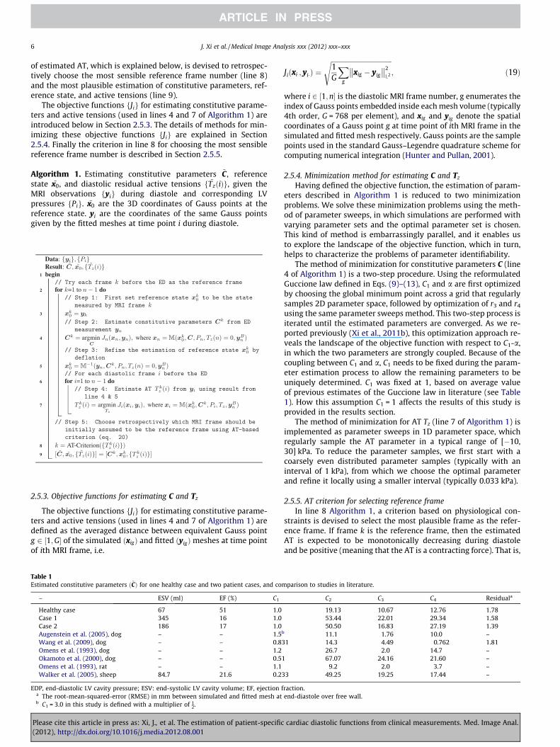
Thus the model parameters to be estimated includes constitu-tive parameters ~C, ATs f ~TzðiÞgi ¼ 1; . . . ;n is the diastolic MRI framenumber, as well as the reference state ~x0. These parameters areestimated by minimizing objective functions fJig (defined belowin Eq. (19)) based on the averaged geometrical difference betweenith simulated mesh and the mesh fitted from the ith MRI frame.There are thus only n independent objective functions, from whichn + 2 variables are to be determined. Therefore this inverse prob-lem is under-determined. This concept is schematically illustratedin Fig. 5 using the previously introduced 1D system, where sixmodel parameters are to be determined from only four measure-ments/equations at all time points.

2.5.1. Further assumptionsTo fully determine the system, two assumptions are added.

Firstly, the AT is set to zero at the end-diastole, assuming the myo-cardium is fully relaxed.

TzðnÞ ¼ 0: ð17Þ

Secondly, the unloaded state x0 can be initially approximated(note this approximation will be later refined – see below) by theLV shape measured in one of the diastolic MRI frames (i.e., the ref-erence MRI frame), where LV inflating pressure and contractingresidual tension are assumed to be roughly balanced.k 2 ½1;n� 1� is defined as the reference frame number.

x0 � yk: ð18Þ

2.5.2. Algorithmic description of parameter estimation procedureApplying this approach, Algorithm 1 details the procedures for

estimating constitutive parameters, reference state, and active ten-sions during diastole. This algorithm consists of five main steps asexplained in the comments. Firstly, the assumption defined in Eq.(18) is applied to each diastolic MRI frame k before the ED frame,and the reference state xk

0 is set to be the state measured by MRIframe k (line 3 of Algorithm 1). This reference state is then usedin the second step to estimated the constitutive parameters Ck (line4), which are chosen as the optimal parameters with which the ref-erence state can be best deformed to the ED state. These estimatedconstitutive parameters are in turn used in the third step to refinethe reference state xk

0, by deflating from the ED state (line 5). AT ateach time point of MRI frames before the ED are estimated, usingthe pre-estimated reference state xk

0 and constitutive parametersCk (line 7). Finally a criterion based on the physiological constraints

meters to be determined are active forces Tzð1Þ; Tzð2Þ; Tzð3Þ; Tzð4Þ and two otherfour measurements ðx1; x2; x3; x4Þ at four time points are available.

cardiac diastolic functions from clinical measurements. Med. Image Anal.

6 J. Xi et al. / Medical Image Analysis xxx (2012) xxx–xxx

of estimated AT, which is explained below, is devised to retrospec-tively choose the most sensible reference frame number (line 8)and the most plausible estimation of constitutive parameters, ref-erence state, and active tensions (line 9).

The objective functions fJig for estimating constitutive parame-ters and active tensions (used in lines 4 and 7 of Algorithm 1) areintroduced below in Section 2.5.3. The details of methods for min-imizing these objective functions fJig are explained in Section2.5.4. Finally the criterion in line 8 for choosing the most sensiblereference frame number is described in Section 2.5.5.

Algorithm 1. Estimating constitutive parameters ~C, referencestate ~x0, and diastolic residual active tensions f ~TzðiÞg, given theMRI observations fyig during diastole and corresponding LVpressures fPig. ~x0 are the 3D coordinates of Gauss points at thereference state. yi are the coordinates of the same Gauss pointsgiven by the fitted meshes at time point i during diastole.

TaEs

ED

P(2

ble 1timated constitutive parameters ð~CÞ for one healthy case and two patient case

– ESV (ml) EF (%)

Healthy case 67 51Case 1 345 16Case 2 186 17Augenstein et al. (2005), dog – –Wang et al. (2009), dog – –Omens et al. (1993), dog – –Okamoto et al. (2000), dog – –Omens et al. (1993), rat – –Walker et al. (2005), sheep 84.7 21.6

P, end-diastolic LV cavity pressure; ESV: end-systolic LV cavity volume; EF,a The root-mean-squared-error (RMSE) in mm between simulated and fittedb C1 = 3.0 in this study is defined with a multiplier of 1

2.

lease cite this article in press as: Xi, J., et al. The estimation of patien012), http://dx.doi.org/10.1016/j.media.2012.08.001

2.5.3. Objective functions for estimating C and Tz

The objective functions fJig for estimating constitutive parame-ters and active tensions (used in lines 4 and 7 of Algorithm 1) aredefined as the averaged distance between equivalent Gauss pointg 2 ½1;G� of the simulated ðxigÞ and fitted ðyigÞmeshes at time pointof ith MRI frame, i.e.

s, and com

C1

1.01.01.01.50.81.20.51.10.2

ejection fmesh at

t-specific

Jiðxi�; yi�Þ ¼ffiffiffiffiffiffiffiffiffiffiffiffiffiffiffiffiffiffiffiffiffiffiffiffiffiffiffiffiffiffiffiffiffiffiffiffiffi1G

Xg

xig � yig

�� ��2

L2

s; ð19Þ

where i 2 ½1;n� is the diastolic MRI frame number, g enumerates theindex of Gauss points embedded inside each mesh volume (typically4th order, G = 768 per element), and xig and yig denote the spatialcoordinates of a Gauss point g at time point of ith MRI frame in thesimulated and fitted mesh respectively. Gauss points are the samplepoints used in the standard Gauss–Legendre quadrature scheme forcomputing numerical integration (Hunter and Pullan, 2001).

2.5.4. Minimization method for estimating C and Tz

Having defined the objective function, the estimation of param-eters described in Algorithm 1 is reduced to two minimizationproblems. We solve these minimization problems using the meth-od of parameter sweeps, in which simulations are performed withvarying parameter sets and the optimal parameter set is chosen.This kind of method is embarrassingly parallel, and it enables usto explore the landscape of the objective function, which in turn,helps to characterize the problems of parameter identifiability.

The method of minimization for constitutive parameters C (line4 of Algorithm 1) is a two-step procedure. Using the reformulatedGuccione law defined in Eqs. (9)–(13), C1 and a are first optimizedby choosing the global minimum point across a grid that regularlysamples 2D parameter space, followed by optimization of r3 and r4

using the same parameter sweeps method. This two-step process isiterated until the estimated parameters are converged. As we re-ported previously (Xi et al., 2011b), this optimization approach re-veals the landscape of the objective function with respect to C1-a,in which the two parameters are strongly coupled. Because of thecoupling between C1 and a, C1 needs to be fixed during the param-eter estimation process to allow the remaining parameters to beuniquely determined. C1 was fixed at 1, based on average valueof previous estimates of the Guccione law in literature (see Table1). How this assumption C1 = 1 affects the results of this study isprovided in the results section.

The method of minimization for AT Tz (line 7 of Algorithm 1) isimplemented as parameter sweeps in 1D parameter space, whichregularly sample the AT parameter in a typical range of [�10,30] kPa. To reduce the parameter samples, we first start with acoarsely even distributed parameter samples (typically with aninterval of 1 kPa), from which we choose the optimal parameterand refine it locally using a smaller interval (typically 0.033 kPa).

2.5.5. AT criterion for selecting reference frameIn line 8 Algorithm 1, a criterion based on physiological con-

straints is devised to select the most plausible frame as the refer-ence frame. If frame k is the reference frame, then the estimatedAT is expected to be monotonically decreasing during diastoleand be positive (meaning that the AT is a contracting force). That is,

parison to studies in literature.

C2 C3 C4 Residuala

19.13 10.67 12.76 1.7853.44 22.01 29.34 1.5850.50 16.83 27.19 1.39

b 11.1 1.76 10.0 –31 14.3 4.49 0.762 1.81

26.7 2.0 14.7 –1 67.07 24.16 21.60 –

9.2 2.0 3.7 –33 49.25 19.25 17.44 –

raction.end-diastole over free wall.

cardiac diastolic functions from clinical measurements. Med. Image Anal.

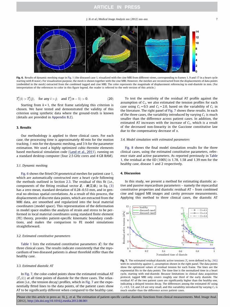
Fig. 6. Results of dynamic meshing stage in Fig. 1 (the diseased case 1, visualized with the cine MRI from different views, corresponding to frames 1, 9 and 17 in a heart cyclestarting with R wave). For visualization purpose, the mesh is shown together with the cine MRI. However, the meshes are reconstructed from the displacements of data points(embedded in the mesh) extracted from the combined tagged and cine MRI. The color represents the magnitude of displacement referencing to end-diastole in mm. (Forinterpretation of the references to color in this figure legend, the reader is referred to the web version of this article.)

J. Xi et al. / Medical Image Analysis xxx (2012) xxx–xxx 7

TkzðiÞ > Tk

zðjÞ; for any i > j; and Tkzðn� 1Þ > 0: ð20Þ

Starting from k = 1, the first frame satisfying this criterion ischosen. We have tested and demonstrated the validity of thiscriterion using synthetic data where the ground-truth is known(details are provided in Appendix B.2).

3. Results

Our methodology is applied to three clinical cases. For eachcase, the processing time is approximately 40 min for the motiontracking, 1 min for the dynamic meshing, and 3 h for the parameterestimation. We used a highly optimized cubic-Hermite elementsbased mechanical simulation code (Land et al., 2011), running ona standard desktop computer (four 2.5 GHz cores and 4 GB RAM).

3.1. Dynamic meshing

Fig. 6 shows the fitted CH geometrical meshes for patient case 1,which are automatically constructed over a heart cycle followingthe methods outlined in Section 2.3. The residual of this fit (i.e.,components of the fitting residual vector Zi � HðNÞU iÞ in Eq. (3)has a zero mean, standard deviation of 0.28–0.53 mm, and in gen-eral no obvious spatial correlations. As a result of this process, thedisplacements of discrete data points, which are extracted from theMRI data, are smoothed and regularized into the local materialcoordinates (model space). This representation of the deformationin model space enables the analysis of strain and stress to be per-formed in local material coordinates using standard finite element(FE) theory, provides patient-specific kinematic boundary condi-tions, and makes the comparison to FE model simulationsstraightforward.

3.2. Estimated constitutive parameters

Table 1 lists the estimated constitutive parameters ð~CÞ for thethree clinical cases. The results indicate consistently that the myo-cardium of two diseased patients is about threefold stiffer than thehealthy case.

Fig. 7. The estimated residual diastolic active tensions (Tz term defined in Eq. (16))with its sensitivity against C1 assumption shown in the right panel. The data pointsshow the optimized values of residual tension for each frame. The lines are theexponential fits to the data points. The time-line is the normalized time in a heartcycle, starting with end-diastole. Because limitations in clinical data acquisitionprotocol, tagged MRI only covers roughly one third of the early diastole. Theresidual AT of the two patient cases are significantly higher than the healthy one,indicating a delayed tension decay. The differences among the estimated AT usingC1 = 0.5, 1.0, and 2.0 are very small, and this variability introduced by varying C1 ismuch smaller than the difference across patient cases.

3.3. Estimated diastolic AT

In Fig. 7, the color-coded points show the estimated residual ATf ~TzðiÞg at all time points of diastole for the three cases. The relax-ation (i.e., the tension decay) profiles, which in Fig. 7 are the expo-nentially fitted lines to the data points, of the patient cases showAT to be significantly different when compared to the healthy case.

Please cite this article in press as: Xi, J., et al. The estimation of patient-specific(2012), http://dx.doi.org/10.1016/j.media.2012.08.001

To test the sensitivity of the residual AT profile against theassumption of C1, we also estimated the tension profiles for eachcase using C1 = 0.5 and C1 = 2.0, based on the variability of C1 inthe literature. The right panel of Fig. 7 shows these results. In eachof the three cases, the variability introduced by varying C1 is muchsmaller than the difference across patient cases. In addition, theestimated AT increases with the increase of C1, which is a resultof the decreased non-linearity in the Guccione constitutive lawdue to the compensatory decrease of a.

3.4. Model simulation with estimated parameters

Fig. 8 shows the final model simulation results for the threeclinical cases, using the estimated constitutive parameters, refer-ence state and active parameters. As reported previously in Table1, the residual at the ED (100%) is 1.78, 1.58 and 1.39 mm for thehealthy case, disease 1 and 2 respectively.

4. Discussion

In this study, we present a method for estimating diastolic ac-tive and passive myocardium parameters – namely the myocardialconstitutive properties and diastolic residual AT – from combinedcine and tagged MR images and cavity pressure measurements.Applying this method to three clinical cases, the diastolic AT

cardiac diastolic functions from clinical measurements. Med. Image Anal.

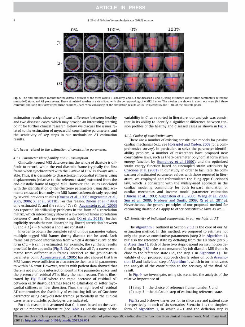
Fig. 8. The final simulated meshes for the diastole process of the three cases (1 is healthy, and 2, 3 are diseased 1 and 2), using estimated constitutive parameters, reference(unloaded) state, and AT parameters. These simulated meshes are visualized with the corresponding cine MRI frames. The meshes are shown in short axis view (left threecolumns) and long axis view (right three columns), each view consisting of the simulation results at 0%, 15%/24%/16% and 100% of the diastole phase.

8 J. Xi et al. / Medical Image Analysis xxx (2012) xxx–xxx

estimation results show a significant difference between healthyand two diseased cases, which may provide an interesting startingpoint for further clinical research. Below we discuss the issues re-lated to the estimation of myocardial constitutive parameters, andthe sensitivity of key steps in our methods on AT estimationresults.

4.1. Issues related to the estimation of constitutive parameters

4.1.1. Parameter identifiability and C1 assumptionClinically, tagged MRI data covering the whole of diastole is dif-

ficult to record, while the end-diastolic frame (typically the firstframe when synchronized with the R-wave of ECG) is always avail-able. Thus, it is desirable to characterize myocardial stiffness usingdisplacements (relative to the reference state) extracted from theend-diastolic frame of tagged MRI. However, the issues associatedwith the identification of the Guccione parameters using displace-ments extracted from only one MRI frame has been already reportedby several previous studies (Omens et al., 1993; Augenstein et al.,2005, 2006; Xi et al., 2011b). For this reason, Omens et al. (1993)only estimated C1 and the ratio of C2 : C3. Augenstein et al. (2006)has reported identifiability problems in the form of a correlationmatrix, which interestingly showed a low level of linear correlationbetween C1 and a. Our previous study (Xi et al., 2011b) furtherexplicitly reveals the non-linear (or log-linear) correlation betweenC1 and aðCa

1a ¼ b, where a and b are constant).In order to obtain the complete set of unique parameter values,

multiple tagged MRI frames during diastole can be used. Eachframe can provide information from which a distinct curve of theform Ca

1a ¼ b can be estimated. For example, the synthetic resultsprovided in the appendix (Fig. B.13a) show that all C1-a curves esti-mated from different MRI frames intersect at the ground-truthparameter point. Augenstein et al. (2005) has also showed that fiveMRI frames were sufficient to characterize the material parametersto within 5% error. However, results with patient data showed thatthere is not a unique intersection point in the parameter space, andthe presence of residual AT is likely the main reason. This is illus-trated by Fig. B.13f where the rapid decrease of residual ATbetween early diastolic frames leads to estimation of softer myo-cardial stiffness in fiber direction. Thus, the high level of residualAT compromises the feasibility of estimating full set of Guccioneparameter using early-diastole frames, particularly in the clinicalcases where diastolic pathologies are indicated.

For this reason, it is assumed that C1 is one, based on the aver-age value reported in literature (see Table 1). For the range of the

Please cite this article in press as: Xi, J., et al. The estimation of patient-specific(2012), http://dx.doi.org/10.1016/j.media.2012.08.001

variability in C1 as reported in literature, our analysis was consis-tent in its ability to identify a significant difference between ten-sion profiles of the healthy and diseased cases as shown in Fig. 7.

4.1.2. Choice of constitutive lawsThere are a number of existing constitutive models for passive

cardiac mechanics (e.g., see Holzapfel and Ogden, 2009 for a com-prehensive survey). In particular, to solve the parameter identifi-ability problem, a number of researchers have proposed newconstitutive laws, such as the 5-parameter polynomial form strainenergy function by Humphrey et al. (1990), and the optimizedstrain energy function based on uncoupled strain attributes byCriscione et al. (2001). In our study, in order to facilitate the com-parison of estimated parameter values with those reported in liter-ature, we employed and reformulated the Fung-type Guccione’slaw, which is consistent with the widely-used approach in thecardiac modeling community for both forward simulation ofcardiac mechanics and inverse model parameter estimation(Omens et al., 1993; Augenstein et al., 2006; Wang et al., 2009;Sun et al., 2009; Niederer and Smith, 2009; Xi et al., 2011a).Nevertheless, the general principles of our proposed method forestimating diastolic AT apply to other constitutive laws as well.

4.2. Sensitivity of individual components in our methods on AT

The Algorithm 1 outlined in Section 2.5.2 is the core of our ATestimation method. In this method, we proposed to estimate notonly the passive constitutive parameters (step 2 in Algorithm 1),but also the reference state by deflating from the ED state (step 3in Algorithm 1). Both of these two steps depend on assumption de-fined in Eq. (18) – the state measured by kth diastolic MRI frame isclose to the reference state (i.e., the step 1 in Algorithm 1). Thevalidity of our proposed approach clearly relies on both Assump-tion 18 and individual step of Algorithm 1, which in turn motivatesthe analysis of the contribution to the accuracy of the final ATresult.

In Fig. 9, we investigate, using six scenarios, the analysis of therelative importance of

(1) step 1 – the choice of reference frame number k and(2) step 3 – the deflation step of estimating reference state.

Fig. 9a and b shows the errors for in silico case and patient case1 respectively in each of six scenarios. Scenario 1 is the simplestform of Algorithm 1, in which k = 1 and the deflation step is

cardiac diastolic functions from clinical measurements. Med. Image Anal.

Senario ID

Err

orin

AT

(kPa

)

0

0.5

1

1.5

2

2.5

3

3.5

4

4.5

(a) In-silico case.Senario ID

Err

orin

AT

(kPa

)

1 2 3 4 5 6 1 2 3 4 5 60

1

2

3

4

5

6

7

(b) Patient case 1.

Scenario ID Explanation

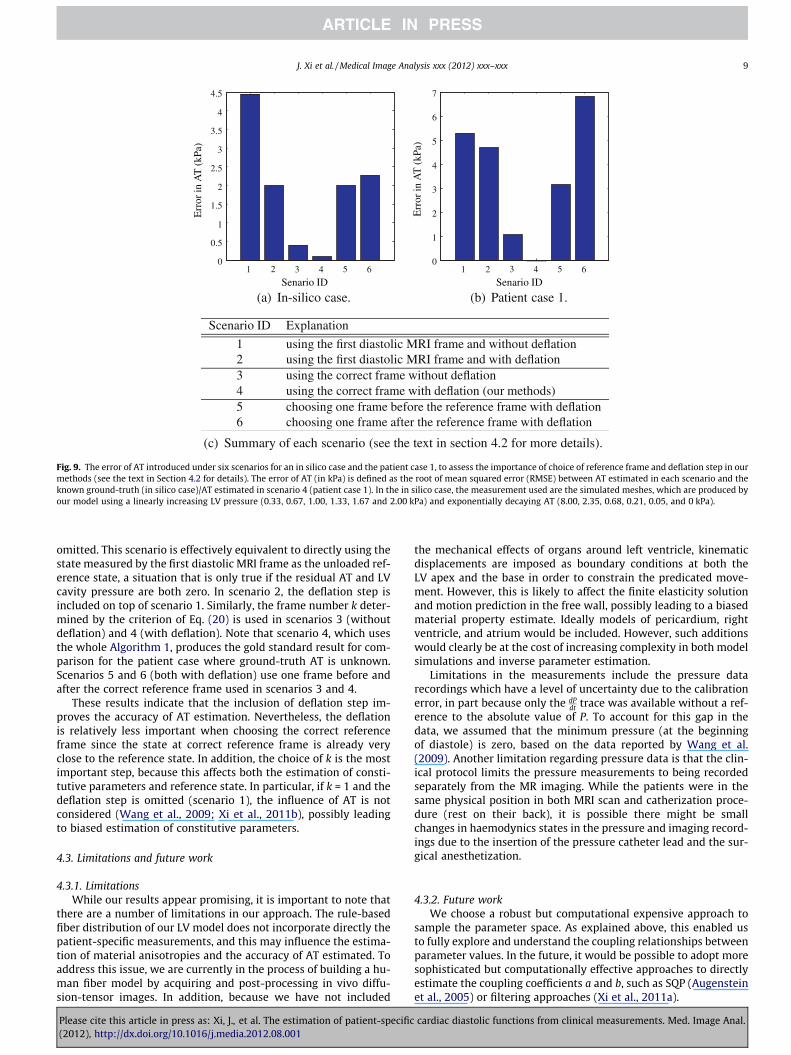
1 using the first diastolic MRI frame and without deflation2 using the first diastolic MRI frame and with deflation3 using the correct frame without deflation4 using the correct frame with deflation (our methods)5 choosing one frame before the reference frame with deflation6 choosing one frame after the reference frame with deflation

(c) Summary of each scenario (see the text in section 4.2 for more details).

Fig. 9. The error of AT introduced under six scenarios for an in silico case and the patient case 1, to assess the importance of choice of reference frame and deflation step in ourmethods (see the text in Section 4.2 for details). The error of AT (in kPa) is defined as the root of mean squared error (RMSE) between AT estimated in each scenario and theknown ground-truth (in silico case)/AT estimated in scenario 4 (patient case 1). In the in silico case, the measurement used are the simulated meshes, which are produced byour model using a linearly increasing LV pressure (0.33, 0.67, 1.00, 1.33, 1.67 and 2.00 kPa) and exponentially decaying AT (8.00, 2.35, 0.68, 0.21, 0.05, and 0 kPa).

J. Xi et al. / Medical Image Analysis xxx (2012) xxx–xxx 9

omitted. This scenario is effectively equivalent to directly using thestate measured by the first diastolic MRI frame as the unloaded ref-erence state, a situation that is only true if the residual AT and LVcavity pressure are both zero. In scenario 2, the deflation step isincluded on top of scenario 1. Similarly, the frame number k deter-mined by the criterion of Eq. (20) is used in scenarios 3 (withoutdeflation) and 4 (with deflation). Note that scenario 4, which usesthe whole Algorithm 1, produces the gold standard result for com-parison for the patient case where ground-truth AT is unknown.Scenarios 5 and 6 (both with deflation) use one frame before andafter the correct reference frame used in scenarios 3 and 4.

These results indicate that the inclusion of deflation step im-proves the accuracy of AT estimation. Nevertheless, the deflationis relatively less important when choosing the correct referenceframe since the state at correct reference frame is already veryclose to the reference state. In addition, the choice of k is the mostimportant step, because this affects both the estimation of consti-tutive parameters and reference state. In particular, if k = 1 and thedeflation step is omitted (scenario 1), the influence of AT is notconsidered (Wang et al., 2009; Xi et al., 2011b), possibly leadingto biased estimation of constitutive parameters.

4.3. Limitations and future work

4.3.1. LimitationsWhile our results appear promising, it is important to note that

there are a number of limitations in our approach. The rule-basedfiber distribution of our LV model does not incorporate directly thepatient-specific measurements, and this may influence the estima-tion of material anisotropies and the accuracy of AT estimated. Toaddress this issue, we are currently in the process of building a hu-man fiber model by acquiring and post-processing in vivo diffu-sion-tensor images. In addition, because we have not included

Please cite this article in press as: Xi, J., et al. The estimation of patient-specific(2012), http://dx.doi.org/10.1016/j.media.2012.08.001

the mechanical effects of organs around left ventricle, kinematicdisplacements are imposed as boundary conditions at both theLV apex and the base in order to constrain the predicated move-ment. However, this is likely to affect the finite elasticity solutionand motion prediction in the free wall, possibly leading to a biasedmaterial property estimate. Ideally models of pericardium, rightventricle, and atrium would be included. However, such additionswould clearly be at the cost of increasing complexity in both modelsimulations and inverse parameter estimation.

Limitations in the measurements include the pressure datarecordings which have a level of uncertainty due to the calibrationerror, in part because only the dP

dt trace was available without a ref-erence to the absolute value of P. To account for this gap in thedata, we assumed that the minimum pressure (at the beginningof diastole) is zero, based on the data reported by Wang et al.(2009). Another limitation regarding pressure data is that the clin-ical protocol limits the pressure measurements to being recordedseparately from the MR imaging. While the patients were in thesame physical position in both MRI scan and catherization proce-dure (rest on their back), it is possible there might be smallchanges in haemodynics states in the pressure and imaging record-ings due to the insertion of the pressure catheter lead and the sur-gical anesthetization.

4.3.2. Future workWe choose a robust but computational expensive approach to

sample the parameter space. As explained above, this enabled usto fully explore and understand the coupling relationships betweenparameter values. In the future, it would be possible to adopt moresophisticated but computationally effective approaches to directlyestimate the coupling coefficients a and b, such as SQP (Augensteinet al., 2005) or filtering approaches (Xi et al., 2011a).

cardiac diastolic functions from clinical measurements. Med. Image Anal.

10 J. Xi et al. / Medical Image Analysis xxx (2012) xxx–xxx

Finally, this study brings about a significant requirement on thecompleteness and accuracy of various clinical data. Limitations ofthe patient data used in this study restrict the analysis to earlyfilling, in which passive diastolic recoil is combined with the relax-ation of AT. Since the tagged MRI measurements do not cover theperiod of pure passive filling, passive material properties are con-founded with active relaxation. In the future, we plan to acquireadditional clinical data sets with optimized protocols (e.g.,whole-heart-cycle tagged MRI coverage, diffusion-tensor imagingfor the patient-specific fiber distribution), in order to further inves-tigate and correlate our new indices with clinical diagnosis.

5. Conclusion

Our methods of integrating the clinical MRI and LV cavity pres-sure data across multiple measurement points in the diastole en-abled us to provide, to our knowledge, the first attempt toestimate the diastolic residual active tension profile in human sub-jects, which has significant potential to provide an important met-ric characterizing diastolic heart failure. The results from ourpreliminary application of this method indicates that early dia-stolic residual AT in the two diseased cases are significantly higherthan the normal cases, which may well indicate that myocardialrelaxation (i.e., lusitropy) is impaired in those two patient cases.

Acknowledgements

The authors would also like to acknowledge funding from theEPSRC as part of the Intelligent Imaging Program (EP/H046410/1)and Leadership Fellowship (EP/G007527/2) grants.

Appendix A. Constitutive parameter coupling

A.1. Derivations of the C1-a coupling

The Guccione parameters are identified by matching the simu-lated deformed mesh(s) to the fitted mesh(s) from the MRIframe(s). However, from the current clinical data, the Guccioneparameters cannot be reliably identified using only the ED framein the sense that an increase of C1 can be compensated for by a de-crease of C2–C4 or a.

To explicit reveal this problem, our goal is to find the couplingdirection d in C1-a space (if any) along which two sets of differentparameters would render the same (or very similar) mechanicalsimulation. In the following analysis, the hydrostatic tensor termcan be safely eliminated. From the numerical solution perspective,given the same external loading conditions (external forces) andtemporary trial solution of a strain tensor (displacement DOF),the whole stress tensor (deviatoric plus hydrostatic) should be al-ways the same as long as the deviatoric stress tensors are the same.This is because the solver for the hydrostatic term is only con-cerned with the strain and residual stress, not the materialparameters.

For notations, T is the deviatoric second Piola–Kirchhoff stresstensors. E is the Green–Lagrangian strain tensor.

T ¼ @W@E¼ 2C1eQ

C2 C4 C4

C4 C3 C3

C4 C3 C3

0BBB@

1CCCA � E; ðA:1Þ

where � is the operator for element-wise product (or Hadamardproduct).

The material elastic tensor K for Guccione’s constitutive law isdefined as:

Please cite this article in press as: Xi, J., et al. The estimation of patient-specific(2012), http://dx.doi.org/10.1016/j.media.2012.08.001

K ¼ 2C1eQ

C2 C4 C4

C4 C3 C3

C4 C3 C3

0BBB@

1CCCA ¼ 2C1aeQ

r2 r4 r4

r4 r3 r3

r4 r3 r3

0BBB@

1CCCA: ðA:2Þ

The coupling direction d in C1-a space (if it exits) is definedwhere the directional gradient of K along d is a zero-tensor. Intui-tively the material response (stress–strain relationship) is the samealong this (local) direction.

@Ki@C1

@Ki@a

!� d ¼ 0; i ¼ 1; . . . ;9: ðA:3Þ

These nine conditions from the above equations are combined to beone constraint independent of r2–r4:

aeQ

C1eQ þ C1a @eQ

@a

!� d ¼ eQ a

C1ð1þ a @Q@aÞ

!� d ¼ 0: ðA:4Þ

A.1.1. The existence of the coupling directionThe coupling direction d exists if and only if Eq. (A.4) has a solu-

tion. The term @Q@a in Eq. (A.4) can be further expanded by using Eqs.

(8) and (13), i.e.

@Q@a¼@P

i;jarijE2ij

� �@a

ðA:5Þ

¼ QaþXi;j¼1

a 2rijEij@Eij

@a

� �; i; j ¼ 1;2;3; ðA:6Þ

where rij denotes the corresponding elements of rightmost matrixin Eq. (A.2), and Eij are the Green–Lagrange strains in fiber (f :¼ 1),sheet (s :¼ 2) and sheet normal (n :¼ 3) directions. The second term@Eij

@a is varying at different ðC1;aÞ points, and thus dependent on thecoupling direction d which we are solving for. Therefore Eq. (A.4)is non-linear.

The solution of a non-linear equation does not necessarily exist.Thus the ‘‘zero-coupling direction’’ (the direction along which thedeformation is exactly the same) may not exist. However, as evi-denced by Fig. A.10 and reported by Xi et al. (2011a), there does ex-ist a ‘‘principle-coupling direction’’ – the direction along which thechange is very close to zero and significantly smaller than otherdirections.

A.1.2. The approximated exponential coupling curveIf we ignore the second non-linear term in @Q

@a, that is,

@Q@a Q

a;

Eq. (A.4) can be simplified as

eQ aC1ð1þ QÞ

� �� d ¼ 0: ðA:7Þ

Therefore the coupling curve in ðC1;aÞ space roughly has the tan-gent direction d ¼ ðC1

a � 11þQ Þ

T , which indicates the curve is

C1

1þQ1 a ¼ b; ðA:8Þ

where b is a constant.Note that we ignored the second non-linear term in Eq. (A.6)

and use the assumption that the slope of the curve 11þQ is constant

when we derive the approximated yet simple curve expression (Eq.(A.8)). While these are mathematical approximations, in practice italready provides a good agreement with the coupling curves fittednumerically (see Fig. A.10).

cardiac diastolic functions from clinical measurements. Med. Image Anal.

0 510

20

30

40

50

C1

α

bC1a*α =

Stiffness increasing

(a) (b)

2

4

6

8

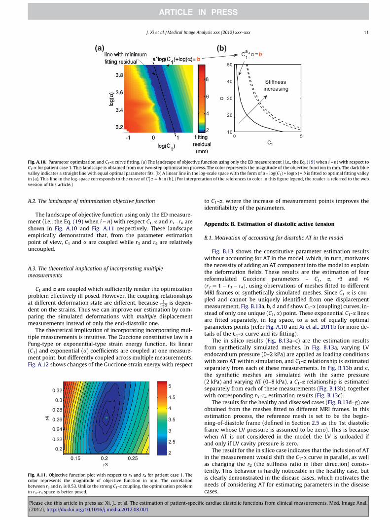
Fig. A.10. Parameter optimization and C1-a curve fitting. (a) The landscape of objective function using only the ED measurement (i.e., the Eq. (19) when i = n) with respect toC1-a for patient case 1. This landscape is obtained from our two-step optimization process. The color represents the magnitude of the objective function in mm. The dark bluevalley indicates a straight line with equal optimal parameter fits. (b) A linear line in the log-scale space with the form of a log(C1) + log(a) = b is fitted to optimal fitting valleyin (a). This line in the log-space corresponds to the curve of Ca

1a ¼ b in (b). (For interpretation of the references to color in this figure legend, the reader is referred to the webversion of this article.)

J. Xi et al. / Medical Image Analysis xxx (2012) xxx–xxx 11

A.2. The landscape of minimization objective function

The landscape of objective function using only the ED measure-ment (i.e., the Eq. (19) when i = n) with respect C1-a and r3—r4 areshown in Fig. A.10 and Fig. A.11 respectively. These landscapeempirically demonstrated that, from the parameter estimationpoint of view, C1 and a are coupled while r3 and r4 are relativelyuncoupled.

A.3. The theoretical implication of incorporating multiplemeasurements

C1 and a are coupled which sufficiently render the optimizationproblem effectively ill posed. However, the coupling relationshipsat different deformation state are different, because 1

1þQ is depen-dent on the strains. Thus we can improve our estimation by com-paring the simulated deformations with multiple displacementmeasurements instead of only the end-diastolic one.

The theoretical implication of incorporating incorporating mul-tiple measurements is intuitive. The Guccione constitutive law is aFung-type or exponential-type strain energy function. Its linear(C1) and exponential (a) coefficients are coupled at one measure-ment point, but differently coupled across multiple measurements.Fig. A.12 shows changes of the Guccione strain energy with respect

Fig. A.11. Objective function plot with respect to r3 and r4 for patient case 1. Thecolor represents the magnitude of objective function in mm. The correlationbetween r3 and r4 is 0.53. Unlike the strong C1-a coupling, the optimization problemin r3–r4 space is better posed.

Please cite this article in press as: Xi, J., et al. The estimation of patient-specific(2012), http://dx.doi.org/10.1016/j.media.2012.08.001

to C1-a, where the increase of measurement points improves theidentifiability of the parameters.

Appendix B. Estimation of diastolic active tension

B.1. Motivation of accounting for diastolic AT in the model

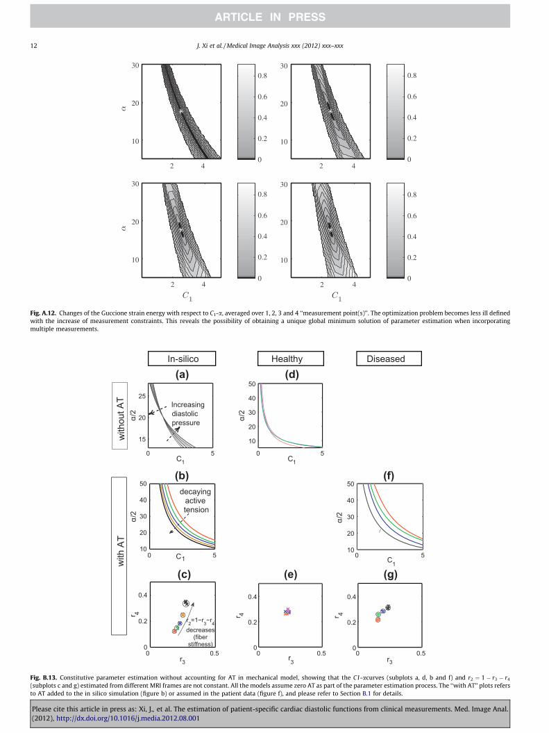
Fig. B.13 shows the constitutive parameter estimation resultswithout accounting for AT in the model, which, in turn, motivatesthe necessity of adding an AT component into the model to explainthe deformation fields. These results are the estimation of fourreformulated Guccione parameters – C1, a, r3 and r4ðr2 ¼ 1� r3 � r4Þ, using observations of meshes fitted to differentMRI frames or synthetically simulated meshes. Since C1-a is cou-pled and cannot be uniquely identified from one displacementmeasurement, Fig. B.13a, b, d and f show C1-a (coupling) curves, in-stead of only one unique (C1, a) point. These exponential C1-a linesare fitted separately, in log space, to a set of equally optimalparameters points (refer Fig. A.10 and Xi et al., 2011b for more de-tails of the C1-a curve and its fitting).

The in silico results (Fig. B.13a–c) are the estimation resultsfrom synthetically simulated meshes. In Fig. B.13a, varying LVendocardium pressure (0–2 kPa) are applied as loading conditionswith zero AT within simulation, and C1-a relationship is estimatedseparately from each of these measurements. In Fig. B.13b and c,the synthetic meshes are simulated with the same pressure(2 kPa) and varying AT (0–8 kPa), a C1-a relationship is estimatedseparately from each of these measurements (Fig. B.13b), togetherwith corresponding r3–r4 estimation results (Fig. B.13c).

The results for the healthy and diseased cases (Fig. B.13d–g) areobtained from the meshes fitted to different MRI frames. In thisestimation process, the reference mesh is set to be the begin-ning-of-diastole frame (defined in Section 2.5 as the 1st diastolicframe whose LV pressure is assumed to be zero). This is becausewhen AT is not considered in the model, the LV is unloaded ifand only if LV cavity pressure is zero.

The result for the in silico case indicates that the inclusion of ATin the measurement would shift the C1-a curve in parallel, as wellas changing the r2 (the stiffness ratio in fiber direction) consis-tently. This behavior is hardly noticeable in the healthy case, butis clearly demonstrated in the disease cases, which motivates theneeds of considering AT for estimating parameters in the diseasecases.

cardiac diastolic functions from clinical measurements. Med. Image Anal.

2 42 4

2 42 4

0

0.2

0.4

0.6

0.8

10

20

30

0

0.2

0.4

0.6

0.8

10

20

30

0

0.2

0.4

0.6

0.8

10

20

30

0

0.2

0.4

0.6

0.8

10

20

30

Fig. A.12. Changes of the Guccione strain energy with respect to C1-a, averaged over 1, 2, 3 and 4 ‘‘measurement point(s)’’. The optimization problem becomes less ill definedwith the increase of measurement constraints. This reveals the possibility of obtaining a unique global minimum solution of parameter estimation when incorporatingmultiple measurements.

In-silico Healthy Diseased

with

out A

T

0 0.50

0.2

0.4

r3

r 4

r2=1−r3−r4decreases

(fiberstiffness)

0 510

20

30

40

50

C1

α/2

decayingactivetension

with

AT

0 0.50

0.2

0.4

r3

r 4

(e)

0 0.50

0.2

0.4

r3

r 4

0 510

20

30

40

50

C1

α/2

(g)

0 5

10

20

30

40

50

C1

α/2

(d)

0 5

15

20

25

C1

α/2

Increasingdiastolicpressure

(a)

(b)

(c)

(f)

Fig. B.13. Constitutive parameter estimation without accounting for AT in mechanical model, showing that the C1-acurves (subplots a, d, b and f) and r2 ¼ 1� r3 � r4

(subplots c and g) estimated from different MRI frames are not constant. All the models assume zero AT as part of the parameter estimation process. The ‘‘with AT’’ plots refersto AT added to the in silico simulation (figure b) or assumed in the patient data (figure f), and please refer to Section B.1 for details.

12 J. Xi et al. / Medical Image Analysis xxx (2012) xxx–xxx

Please cite this article in press as: Xi, J., et al. The estimation of patient-specific cardiac diastolic functions from clinical measurements. Med. Image Anal.(2012), http://dx.doi.org/10.1016/j.media.2012.08.001

Synthetic measurement number

AT

(kP

a)

AT1AT2AT3AT4

truthGround

1 2 3 4 5 6−5

0

5

10

15

20

25

(a) In-silico AT estimation

Synthetic measurement number

AT

(kP

a)

1 2 3 4 5

-0.5

0

0.5

1

1.5

2

2.5

(b) Enlargement of (a)

LV Pressure (kPa)

LV

Vol

ume

(ml)

PV1PV2PV3PV4

truth

Referencestate

Grouth

0 0.5 1 1.5 2120

125

130

135

140

145

150

155

(c) PV curves (PV1-4) of the in-silico purely LV inflation simulations without AT.

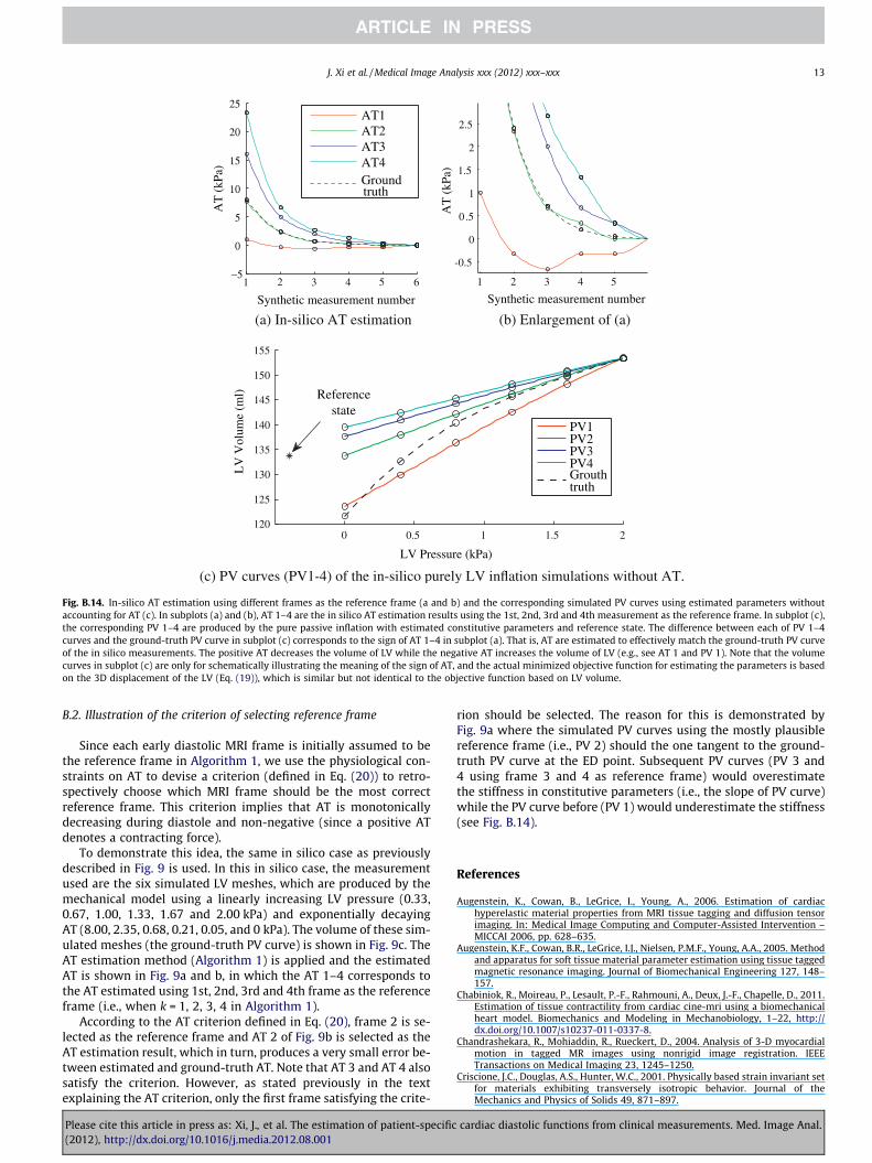
Fig. B.14. In-silico AT estimation using different frames as the reference frame (a and b) and the corresponding simulated PV curves using estimated parameters withoutaccounting for AT (c). In subplots (a) and (b), AT 1–4 are the in silico AT estimation results using the 1st, 2nd, 3rd and 4th measurement as the reference frame. In subplot (c),the corresponding PV 1–4 are produced by the pure passive inflation with estimated constitutive parameters and reference state. The difference between each of PV 1–4curves and the ground-truth PV curve in subplot (c) corresponds to the sign of AT 1–4 in subplot (a). That is, AT are estimated to effectively match the ground-truth PV curveof the in silico measurements. The positive AT decreases the volume of LV while the negative AT increases the volume of LV (e.g., see AT 1 and PV 1). Note that the volumecurves in subplot (c) are only for schematically illustrating the meaning of the sign of AT, and the actual minimized objective function for estimating the parameters is basedon the 3D displacement of the LV (Eq. (19)), which is similar but not identical to the objective function based on LV volume.

J. Xi et al. / Medical Image Analysis xxx (2012) xxx–xxx 13

B.2. Illustration of the criterion of selecting reference frame

Since each early diastolic MRI frame is initially assumed to bethe reference frame in Algorithm 1, we use the physiological con-straints on AT to devise a criterion (defined in Eq. (20)) to retro-spectively choose which MRI frame should be the most correctreference frame. This criterion implies that AT is monotonicallydecreasing during diastole and non-negative (since a positive ATdenotes a contracting force).

To demonstrate this idea, the same in silico case as previouslydescribed in Fig. 9 is used. In this in silico case, the measurementused are the six simulated LV meshes, which are produced by themechanical model using a linearly increasing LV pressure (0.33,0.67, 1.00, 1.33, 1.67 and 2.00 kPa) and exponentially decayingAT (8.00, 2.35, 0.68, 0.21, 0.05, and 0 kPa). The volume of these sim-ulated meshes (the ground-truth PV curve) is shown in Fig. 9c. TheAT estimation method (Algorithm 1) is applied and the estimatedAT is shown in Fig. 9a and b, in which the AT 1–4 corresponds tothe AT estimated using 1st, 2nd, 3rd and 4th frame as the referenceframe (i.e., when k = 1, 2, 3, 4 in Algorithm 1).

According to the AT criterion defined in Eq. (20), frame 2 is se-lected as the reference frame and AT 2 of Fig. 9b is selected as theAT estimation result, which in turn, produces a very small error be-tween estimated and ground-truth AT. Note that AT 3 and AT 4 alsosatisfy the criterion. However, as stated previously in the textexplaining the AT criterion, only the first frame satisfying the crite-

Please cite this article in press as: Xi, J., et al. The estimation of patient-specific(2012), http://dx.doi.org/10.1016/j.media.2012.08.001

rion should be selected. The reason for this is demonstrated byFig. 9a where the simulated PV curves using the mostly plausiblereference frame (i.e., PV 2) should the one tangent to the ground-truth PV curve at the ED point. Subsequent PV curves (PV 3 and4 using frame 3 and 4 as reference frame) would overestimatethe stiffness in constitutive parameters (i.e., the slope of PV curve)while the PV curve before (PV 1) would underestimate the stiffness(see Fig. B.14).

References

Augenstein, K., Cowan, B., LeGrice, I., Young, A., 2006. Estimation of cardiachyperelastic material properties from MRI tissue tagging and diffusion tensorimaging. In: Medical Image Computing and Computer-Assisted Intervention –MICCAI 2006, pp. 628–635.

Augenstein, K.F., Cowan, B.R., LeGrice, I.J., Nielsen, P.M.F., Young, A.A., 2005. Methodand apparatus for soft tissue material parameter estimation using tissue taggedmagnetic resonance imaging. Journal of Biomechanical Engineering 127, 148–157.

Chabiniok, R., Moireau, P., Lesault, P.-F., Rahmouni, A., Deux, J.-F., Chapelle, D., 2011.Estimation of tissue contractility from cardiac cine-mri using a biomechanicalheart model. Biomechanics and Modeling in Mechanobiology, 1–22, http://dx.doi.org/10.1007/s10237-011-0337-8.

Chandrashekara, R., Mohiaddin, R., Rueckert, D., 2004. Analysis of 3-D myocardialmotion in tagged MR images using nonrigid image registration. IEEETransactions on Medical Imaging 23, 1245–1250.

Criscione, J.C., Douglas, A.S., Hunter, W.C., 2001. Physically based strain invariant setfor materials exhibiting transversely isotropic behavior. Journal of theMechanics and Physics of Solids 49, 871–897.

cardiac diastolic functions from clinical measurements. Med. Image Anal.

14 J. Xi et al. / Medical Image Analysis xxx (2012) xxx–xxx

Delingette, H., Billet, F., Wong, K.C.L., Sermesant, M., Rhode, K.S., Ginks, M., Rinaldi,C.A., Razavi, R., Ayache, N., 2012. Personalization of cardiac motion andcontractility from images using variational data assimilation. IEEETransactions on Biomedical Engineering 59, 20–24.

Fung, Y., 1981. Biomechanics: Mechanical Properties of Living Tissues. Springer.Guccione, J., McCulloch, A., Waldman, L., 1991. Passive material properties of intact

ventricular myocardium determined from a cylindrical model. Journal ofBiomechanical Engineering 113, 42–55.

Holzapfel, G., Ogden, R., 2009. Constitutive modelling of passive myocardium: astructurally based framework for material characterization. PhilosophicalTransactions of the Royal Society A: Mathematical, Physical and EngineeringSciences 367, 3445–3475.

Humphrey, J., Strumpf, R., Yin, F., 1990. Determination of a constitutive relation forpassive myocardium: I. A new functional form. Journal of BiomechanicalEngineering 112, 333.

Hunter, P., McCulloch, A., Ter Keurs, H., 1998. Modelling the mechanical propertiesof cardiac muscle. Progress in Biophysics and Molecular Biology 69, 289–331.

Hunter, P., Pullan, A., 2001. FEM BEM Notes. The University of Auckland, NewZealand, Departament of Engineering Science.

Katz, A., 2010. Physiology of the Heart. Lippincott Williams & Wilkins.Klabunde, R., 2005. Cardiovascular Physiology Concepts. Lippincott Williams &

Wilkins.Lamata, P., Niederer, S., Nordsletten, D., Barber, D.C., Roy, I., Hose, D.R., Smith, N.,

2011. An accurate, fast and robust method to generate patient-specific cubichermite meshes. Medical Image Analysis 15, 801–813.

Land, S., Niederer, S., Smith, N., 2011. Efficient computational methods for stronglycoupled cardiac electromechanics. IEEE Transactions on Biomedical Engineering25, 1.

Moireau, P., Chapelle, D., 2011. Reduced-order unscented Kalman filtering withapplication to parameter identification in large-dimensional systems. ESAIM:Control, Optimisation and Calculus of Variations (COCV) 17, 380–405. http://dx.doi.org/10.1051/cocv/2010006.

Nagel, E., Schuster, A., 2010. Shortening without contraction: new insights intohibernating myocardium. JACC Cardiovascular Imaging 3, 731.

Nash, M., 1998. Mechanics and material properties of the heart using ananatomically accurate mathematical model. PhD thesis, University of Auckland.

Nash, M., Hunter, P., 2000. Computational mechanics of the heart. Journal ofElasticity 61, 113–141.

Niederer, S., Smith, N., 2009. The role of the Frank–Starling law in the transductionof cellular work to whole organ pump function: a computational modelinganalysis. PLoS Computational Biology 5.

Nordsletten, D., Niederer, S., Nash, M., Hunter, P., Smith, N., 2011. Coupling multi-physics models to cardiac mechanics. Progress in Biophysics and MolecularBiology 104, 77–88.

Okamoto, R., Moulton, M., Peterson, S., Li, D., Pasque, M., Guccione, J., 2000.Epicardial suction: a new approach to mechanical testing of the passiveventricular wall. Journal of Biomechanical Engineering 122, 479.

Omens, J., MacKenna, D., McCulloch, A., 1993. Measurement of strain and analysis ofstress in resting rat left ventricular myocardium. Journal of Biomechanics 26,665–676.

Rajagopal, V., Nash, M., Highnam, R., Nielsen, P., 2008. The breast biomechanicsreference state for multi-modal image analysis. Digital Mammography, 385–392.

Please cite this article in press as: Xi, J., et al. The estimation of patient-specific(2012), http://dx.doi.org/10.1016/j.media.2012.08.001

Rueckert, D., Sonoda, L., Hayes, C., Hill, D., Leach, M., Hawkes, D., 1999. Nonrigidregistration using free-form deformations: application to breast MR images.IEEE Transactions on Medical Imaging 18, 712–721.

Sermesant, M., Chabiniok, R., Chinchapatnam, P., Mansi, T., Billet, F., Moireau, P.,Peyrat, J., Wong, K., Relan, J., Rhode, K., Ginks, M., Lambiase, P., Delingette, H.,Sorine, M., Rinaldi, C., Chapelle, D., Razavi, R., Ayache, N., in press. Patient-specific electromechanical models of the heart for the prediction of pacing acuteeffects in crt: a preliminary clinical validation. Medical Image Analysis. http://dx.doi.org/10.1016/j.media.2011.07.003.

Sermesant, M., Moireau, P., Camara, O., Sainte-Marie, J., Andriantsimiavona, R.,Cimrman, R., Hill, D., Chapelle, D., Razavi, R., 2006. Cardiac function estimationfrom MRI using a heart model and data assimilation: advances and difficulties.Medical Image Analysis, 642–656.

Shi, W., Zhuang, X., Wang, H., Luong, D., Tobon-Gomez, C., Edwards, P., Rhode, K.,Razavi, R., Ourselin, S., Rueckert, D., 2012. A comprehensive cardiac motionestimation framework using both untagged and 3d tagged mr images based onnon-rigid registration. IEEE Transactions on Medical Imaging, 1.

Smith, N., Nickerson, D., Crampin, E., Hunter, P., 2004. Multiscale computationalmodelling of the heart. Acta Numerica, 371–431.

Smith, N., de Vecchi, A., McCormick, M., Nordsletten, D., Camara, O., Frangi, A.,Delingette, H., Sermesant, M., Relan, J., Ayache, N., et al., 2011. Euheart:personalized and integrated cardiac care using patient-specific cardiovascularmodelling. Interface Focus 1, 349.

Sun, K., Stander, N., Jhun, C., Zhang, Z., Suzuki, T., Wang, G., Saeed, M., Wallace, A.,Tseng, E., Baker, A., et al., 2009. A computationally efficient formal optimizationof regional myocardial contractility in a sheep with left ventricular aneurysm.Journal of Biomechanical Engineering 131, 111001.

Usyk, T., Mazhari, R., McCulloch, A., 2000. Effect of laminar orthotropic myofiberarchitecture on regional stress and strain in the canine left ventricle. Journal ofElasticity 61, 143–164.

Walker, J., Ratcliffe, M., Zhang, P., Wallace, A., Fata, B., Hsu, E., Saloner, D., Guccione,J., 2005. MRI-based finite-element analysis of left ventricular aneurysm.American Journal of Physiology – Heart and Circulatory Physiology 289, H692.

Wang, V., Lam, H., Ennis, D., Cowan, B., Young, A., Nash, M., 2009. Modelling passivediastolic mechanics with quantitative MRI of cardiac structure and function.Medical Image Analysis 13, 773–784.

Wang, V., Lam, H., Ennis, D., Cowan, B., Young, A., Nash, M., 2010. Cardiac activecontraction parameters estimated from magnetic resonance imaging. StatisticalAtlases and Computational Models of the Heart, 194–203.

Xi, J., Lamata, P., Lee, J., Moireau, P., Chapelle, D., Smith, N., 2011a. Myocardialtransversely isotropic material parameter estimation from in-silicomeasurements based on a reduced-order unscented Kalman filter. Journal ofthe Mechanical Behavior of Biomedical Materials 4, 1090–1102.

Xi, J., Lamata, P., Shi, W., Niederer, S., Rueckert, D., Duckett, S.G., Shetty, A.K., Rinald,C.A., Razavi, R., Smith, N., 2011b. An automatic data assimilation framework forpatient-specific myocardial mechanical parameter estimation. FunctionalImaging and Modeling of the Heart, LNCS 6666, 392–400.

Yin, F., Strumpf, R., Chew, P., Zeger, S., 1987. Quantification of the mechanicalproperties of noncontracting canine myocardium under simultaneous biaxialloading. Journal of Biomechanics 20, 577–589.

cardiac diastolic functions from clinical measurements. Med. Image Anal.