International Review of Environmental and Resource Economics, 2012, 6: 195–224

The Environmental Kuznets Curve:A Survey of the Theoretical Literature

Roberto Pasten1 and Eugenio Figueroa B.2

1Department of Economics and Finance, Universidad de Talca,Talca, Chile; rpasten@utalca.cl2Department of Economics, Universidad de Chile, Santiago, Chile

ABSTRACT

This paper reviews and summarizes most of the literature on theenvironmental Kuznets curve (EKC), focusing mainly on disentanglingand clarifying the key concepts underlying the two classes of existingtheoretical explanations for the EKC occurrence — those driven bytechnology and those driven by preferences — as well as the technicalformalization of such concepts. To do this, we develop a model whichallows the analysis of the two types of theoretical explanations under acommon theoretical framework. Using this analytical setting, we firstreview models with technology as the main driver of the EKC, and thenwe study those with preferences as the fundamental driver. Finally, wepresent a closed form solution for the EKC which, on the one hand, issimpler and less restrictive than previous ones in the literature and, onthe other hand, helps us to highlight some of the remaining theoreticalgaps and to propose some possibilities for future research.

Keywords: Environmental Kuznets curve; elasticity of substitution;economic growth.

JEL Codes: C23, Q53, Q58

ISSN 1932-1465; DOI 10.1561/101.00000051c© 2012 R. Pasten and E. Figueroa

196 Pasten and Figueroa

1 Introduction

Since the seminal paper by Grossman and Krueger (1992), the Environmen-tal Kuznets curve (EKC), which illustrates a particular form of the relation-ship between pollution and income per capita, has been studied in differentcontexts due to its potentially promising implications attaining sustainableeconomic growth in the future. According to the EKC, the emissions or theconcentration of a particular contaminant in the environment initially risesas the income per capita of a country or a city increases over time, reachesa maximum and then declines even though income per capita keeps growing(see Barbier, 1997; Suri and Chapman, 1998; Dinda, 2004; Yandle et al.,2004 for empirical illustrations). If this finding is supported by empiricalevidence, it is possible to expect, according to some authors, that economicgrowth contains the mechanisms for reversing the initial upward trend inpollution emissions or concentrations observed in several countries and forseveral pollutants (Beckerman, 1992; Selden and Song, 1994; Grossman andKrueger, 1995). However, all initial optimism about the implications forsustained development arisen from the EKC was soon challenged by someauthors skeptic of the existence of an automatism built into the EKC rela-tionship (Panayotou, 1997; Figueroa and Pasten, 2000; Stern, 2004).

After Grossman and Krueger (1992, 1995), the literature concerning theEKC developed rapidly. Selden and Song (1994) found an EKC for severalindicators of urban air pollution emissions. Different authors have madeestimations for different pollutants and in most cases they found similarrelationships when they analyzed local pollutants with cheap abatementcosts. A few examples are sulphur dioxide (Shafik and Bandyopadhyay,1992; Shafik, 1994; Cole et al., 1997; Panayotou, 1997; Kaufmann et al.,1997); carbon dioxide, nitrates, energy, traffic volumes (Holtz-Eakin andSelden, 1995); water quality (Beede and Wheeler, 1992; Hettige et al., 2000).Nevertheless the EKC relationship is not undisputed, especially as a generalempirical phenomenon expected to occur with all pollutants. A report of theWorld Bank (1992) found monotonically increasing relationships (municipalwaste) and monotonically decreasing relationships (lack of clean water, lackof urban sanitation).

In this paper our focus is on the theory underlying the EKC; we sur-vey the theoretical literature that explains the arising of an EKC and weprovide a general framework (based in Lopez, 1994) to characterize theEKC theoretically and therefore, our revision of the empirical literature

The Environmental Kuznets Curve: A Survey of the Theoretical Literature 197

concerning this phenomenon is rather limited; however it is possible tosummarize some of the stylized facts regarding the empirical analysis ofthe EKC1:

(i) An inverted U relationship between GDP per capita and environmentaldamage seems to be present only for a constrained set of pollutants(Dinda, 2004; World Bank, 1992; Harbaught et al., 2002; Roca et al.,2001).

(ii) The EKC seems to apply to local pollutants with cheap abatementcosts and short run effects (i.e., sulfur and carbon dioxide) but not forCO2, municipal waste, energy consumption, etc. (Arrow et al., 1995;Cole et al., 1997; John et al., 1995; Gangadharan and Valenzuela, 2001;Dinda, 2001, 2004; Holt-Eakin and Selden, 1995; Roberts and Grimes,1997; Horvath, 1997). Particularly Khanna and Plassmann (2004) showempirical evidence of an EKC curve for pollutants with local effects.

(iii) Additionally to the EKC, several other shapes have been foundfor the relationship between pollution and income, i.e., monotonicincreasing and monotonic decreasing relationships (Lucas et al., 1992;Hettige et al., 2000; Shafik, 1994) together with forward falling rela-tionships (see particularly Kauffman et al., 1997 for forward fallingrelationships).

(iv) The EKC seems to apply to high-income countries and not to low-income countries (Stern et al., 1996; Stern and Common, 2001;Figueroa and Pasten, 2009).

(v) In general rich-resource endowed countries display monotonicallyincreasing rather than backward bending relationships (most of thosecountries are located in Latin-America, sub-Sahara Africa and the ArabWorld (Auty, 2003; Auty and Gelb, 2001; specially Krueger, 1993 forSubsaharan countries)).

(vi) Those rich resource endowed countries where the EKC fails to appearare in general, characterized by inefficient and distorting public poli-cies, not only from an environmental point of view but also from aneconomic, social and political point of view (Sachs and Warner, 1995;Karl, 1997; Ascher, 1999; Ross, 2001; Auty, 2003; Auty and Gelb, 2001).

1 An entire issue of Environment and Development Economics edited by Barbier (1997) analyzedthe empirics of the EKC. Other papers surveying the subject are Stern (1998, 2003), Yandleet al. (2004), Dinda (2004) and Nahman and Antrobus (2005).

198 Pasten and Figueroa

(vii) It is possible to find in some of the poorest endowed countries asustainable use of resources (Tiffen and Mortimore (1994) show howdue to population density, improved information and market opportu-nities, Kenya was able to increase rural income and achieved better lev-els of conservation) in addition to an effective and efficient macroeco-nomic administration (i.e., China since late 1970s, South Korea, HongKong and more recently India) (Woolcock et al., 2001; Auty, 2003).

Every model of the environmental Kuznets curve should address at leastthe empirical evidence outlined before. In what follows we develop a frame-work that attempt to explain the stylized facts described above and, at thesame time, encompasses most of the theoretical models developed so far.

In the following section a general framework for the analysis of the EKCis presented. In Section 3, the most prominent models in the literature inwhich technology is the main driver of the EKC are presented. Section 4presents those models in the literature in which the EKC is driven by pref-erences. As a contribution to the current theoretical development, Section 5proposes a closed form of the EKC which has two central features: (1) it is amore general, less restrictive characterization of the EKC than those of theprevious models in the literature (and presented in Sections 3 and 4); and,(2) it provides a more adequate framework for empirical analysis. Finally,Section 6 concludes.

2 A General Theoretical Framework for the EKC

The current state of the art analysis of the environmental Kuznets curvecan be characterized as based on the following theoretical framework: astatic general equilibrium model with a representative agent who maximizesa utility function increasing in consumption C and decreasing in pollu-tion P . In general, intra- and inter-generational aspects are not addressed.Technological progress is assumed to be exogenous, as in Lopez (1994) andStokey (1998). Another assumption is that pollution levels are optimal anddetermined by an efficient price system, i.e., there is always a price thatequals pollution demand with pollution supply. This assumption is quiteextreme, in particular in environmental analysis where, in most of the cases,there exist no prices. Nevertheless it is worth to point out that very oftenother institutional arrangements resemble the functioning of a price systemsuch as a transparent political process that follows the changes in people’s

The Environmental Kuznets Curve: A Survey of the Theoretical Literature 199

preferences and translate them into environmental regulations which thefirms must comply. The increasing regulation stringency acts very often asan implicit (virtual) price that induces firms to invest in better environmen-tal practices. On the other hand, models which assume that competitiveprices do exist are used in the literature as a benchmark against which morerealistic policies are contrasted. For example, Lopez and Mitra (2000) usethe framework presented below to show that corruption distorts prices andinduces less than optimal levels of pollution throughout all the economicprocesses.

To establish a general framework to analyze the existing EKC theoreticalliterature in a comprehensive and concise way, here we assume that therepresentative agent preferences are given by the following utility function:

U = U(C, P ) (1)

U(·) depends on consumption C and on pollution P . It is increasing in C anddecreasing in P and it is assumed to be strictly concave in both arguments.Therefore we assume UC > 0, UP < 0 and UCC < 0, UPP > 0, wheresubscripts denote differentiation.

The production function f(·) is kept deliberately simple in order to isolatepreferences from technology and it is given by:

C = f = f(K, P ) (2)

where aggregate consumption (C) is identical to aggregate income f , K is abroad definition of capital that includes both physical and human capitals;and P is the flow of pollution generated and used in the productive pro-cess. The production function complies with the usual assumptions (increas-ing and concave in factors, Inada conditions, etc). In this model, followingTahvonen and Kuuluvainen (1993) and Lopez (1994), pollution plays a roleas a factor of production. It is assumed that environmental quality Q isa linear function of pollution such that Q = D − P , where D is the bestenvironmental quality attainable.

When the representative agent optimally chooses P we obtain:

h(C, P ) ≡ −UP (C, P )UC(C, P )

= fP (K, P ) (3)

i.e., marginal rate of substitution between pollution and consumptionh(C, P ) is equal to marginal product of pollution given by fP = ∂f/∂P .

200 Pasten and Figueroa

For a given level of capital K, h(C, P ) is pollution supply and fP (K, P )is pollution demand. It can be noted that this setting is similar to the anal-ysis of labor supply and labor demand where pollution plays the role of afactor of production similar to the role played by labor in labor market anal-yses. The equilibrium level of pollution is given by the intersection of twocurves. The height to pollution supply h(C, P ) is the willingness to pay fora marginal reduction in pollution (or the willingness to pay for a marginalimprovement in environmental quality). The height to the pollution demandis the marginal product of pollution (the opportunity cost of a marginalimprovement in environmental quality). If the willingness to pay for a bet-ter environment grows slower than its opportunity cost as income grows,then equilibrium pollution increases as income grows, otherwise equilibriumpollution decreases.

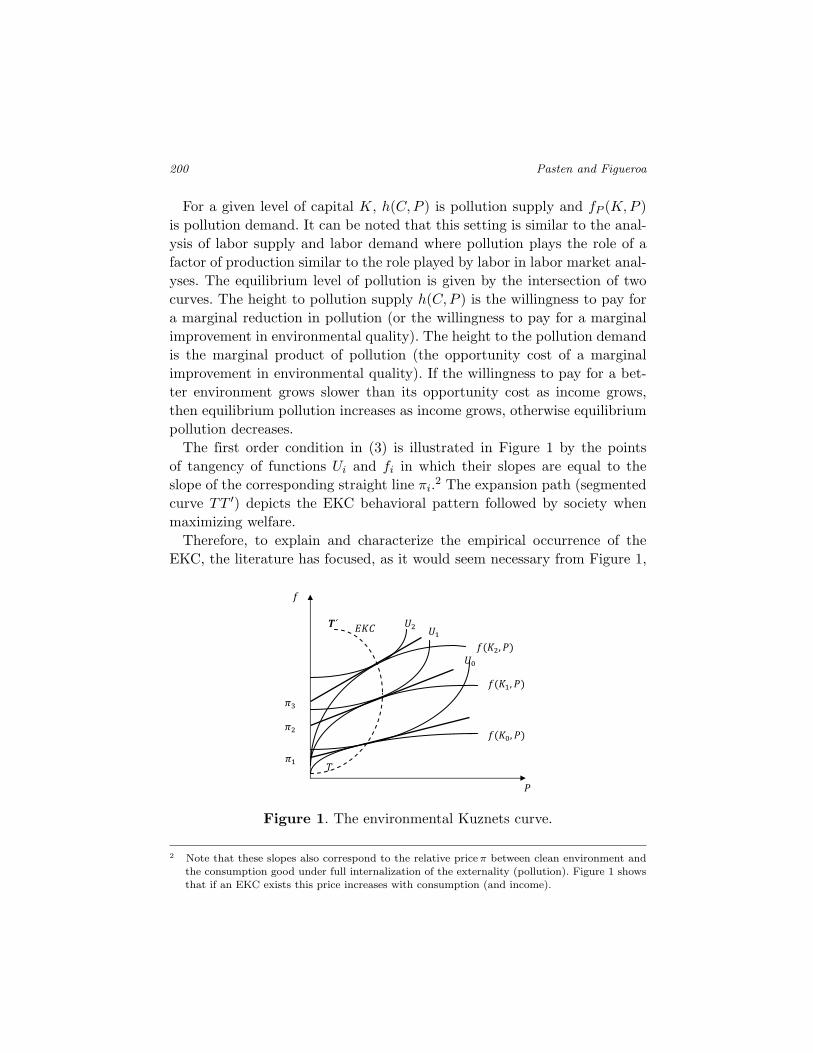
The first order condition in (3) is illustrated in Figure 1 by the pointsof tangency of functions Ui and fi in which their slopes are equal to theslope of the corresponding straight line πi.2 The expansion path (segmentedcurve TT ′) depicts the EKC behavioral pattern followed by society whenmaximizing welfare.

Therefore, to explain and characterize the empirical occurrence of theEKC, the literature has focused, as it would seem necessary from Figure 1,

Figure 1. The environmental Kuznets curve.

2 Note that these slopes also correspond to the relative price π between clean environment andthe consumption good under full internalization of the externality (pollution). Figure 1 showsthat if an EKC exists this price increases with consumption (and income).

The Environmental Kuznets Curve: A Survey of the Theoretical Literature 201

on describing the conditions under which the segmented expansion path TT ′

is a consequence of economic growth (i.e., as income increases).If h(·) in Equation (3) is positive and differentiable and preferences exhibit

a diminishing marginal rate of substitution between consumption and envi-ronmental quality, indifference curves between consumption and pollutionare convex and thus the following expression holds:

d2C

dP 2 U=U= h(C, P )hC(C, P ) + hP (C, P ) > 0 (4)

In Equation (4) hC and hP are the partial derivatives of the marginal rateof substitution h with respect to C and P , respectively.

The slope for the consumption path can be found by differentiating (2)and (3) with respect to K,

dC

dK=

fPKfP + fK(hP − fPP )fP hC + hP − fPP

Second order conditions and fPK > 0 (i.e., both production factors arecomplements) is sufficient for dC/dK > 0. However, the sign of the pollutionpath,

dP

dK= − fKhC − fPK

fP hC + hP − fPP

is ambiguous and depends on fKhC being greater, equal or lower than fPK ,i.e., (dP/dK) >

< 0 if and only if:

hCfK − fPK<

>0 (5)

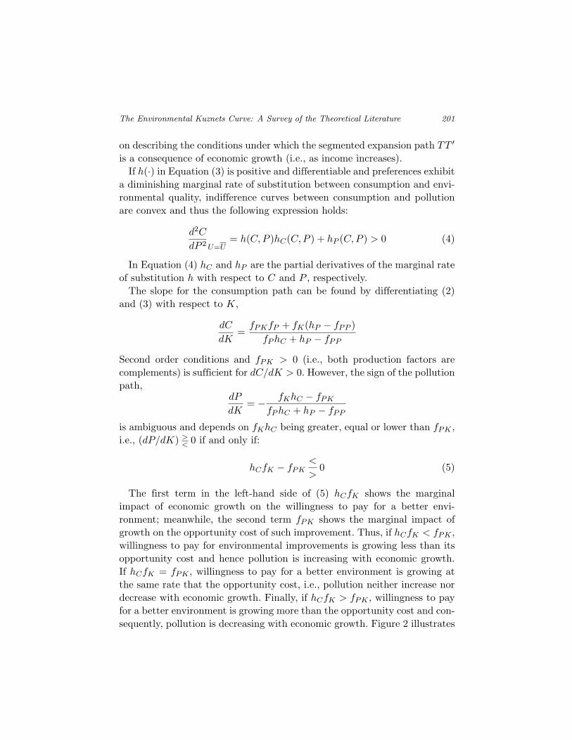
The first term in the left-hand side of (5) hCfK shows the marginalimpact of economic growth on the willingness to pay for a better envi-ronment; meanwhile, the second term fPK shows the marginal impact ofgrowth on the opportunity cost of such improvement. Thus, if hCfK < fPK ,willingness to pay for environmental improvements is growing less than itsopportunity cost and hence pollution is increasing with economic growth.If hCfK = fPK , willingness to pay for a better environment is growing atthe same rate that the opportunity cost, i.e., pollution neither increase nordecrease with economic growth. Finally, if hCfK > fPK , willingness to payfor a better environment is growing more than the opportunity cost and con-sequently, pollution is decreasing with economic growth. Figure 2 illustrates

202 Pasten and Figueroa

Figure 2. hCfK < fPK .

the hCfK < fPK case, while the analysis for the other two cases hCfK = fPK

and hCfK > fPK is straightforward and therefore it is not illustrated here.In Figure 2, hCfK<fPK , i.e., as the economy grows, the willingness to

pay for a better environment grows slower than the opportunity cost ofthis environmental improvement and thus, the optimal level of pollutionincreases as the economy grows. This is illustrated in Figure 2 by a largershift in pollution demand fP induced by economic growth than the shift inpollution supply h(·) induced by economic growth. So, even though the priceof pollution is increasing, it is not increasing enough to induce a substitutionof pollution for cleaner factors of production and thus pollution increasesfrom P0 to P1.

In the Appendix it is shown that under additive preferences

hCfK − fPK = −fKfP

C

(1ρ

− a

)(6)

and thereforedP

dK

>

<0 if and only if

1ρ

>

<a (7)

where fKfP /fPKf = ρ corresponds to the elasticity of substitution (ES)in production between pollution and capital and a = (−UCCC)/UC is theincome elasticity of the marginal utility of consumption or Frisch Coeffi-cient (FC) which is conceptually possible to assimilate to the well-knowncoefficient of relative risk aversion (RRA) in the literature on risk anduncertainty.3

3 In the context of the economics of risk and uncertainty this elasticity is known as the coefficientof relative risk aversion. However in the context of certainty, in which the EKC models are

The Environmental Kuznets Curve: A Survey of the Theoretical Literature 203

It is important here to strength the point that the result in (7) it isrestricted to the case of additive preferences and therefore it is assumedthat the cross derivative UCQ = −UCP is equal to zero. This is a commonassumption in the EKC literature focusing on the role of preferences (see forexample Lopez, 1994; Stokey, 1998; Lieb, 2002; Copeland and Taylor, 2003).McConell (1997) analyses the possibility of cross derivatives different fromzero and show what are the conditions in this cross derivatives than can leadto a decreasing in income pollution path. Figueroa and Pasten (2012) derivean EKC without the restriction of additive preferences. In spite of thesemodels, however, most of the literature on the preference-based theoreticalexplanations of the EKC relies on additive preferences. The framework wepresent below retains this assumption; however, it is important to mentionthat the study of the EKC without the assumption of additive preferencessurely impose additional restrictions that are worth to study.

Given the importance of the two parameters inside brackets in expression(6) — the elasticity of substitution in production between factors (ES) andthe income elasticity of marginal utility of consumption (the Frisch coeffi-cient, FC for short) — in our analysis of the existing literature on the EKCwe will label this framework as the ‘ES–FC model’. According to (7), if boththe ES and the FC are constants, the relationship between pollution andincome is monotonic rather than U inverted and the slope is positive, zero ornegative depending of 1/ρ being either greater, equal, or less than a. There-fore, in order for the income-pollution path to display the non-monotonicrelation described by the EKC, either a must grow or 1/ρ, must decline asincome grows.

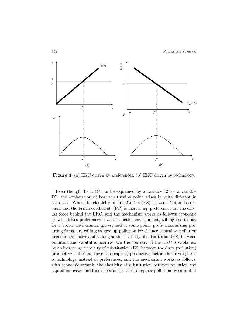
If a grows with income for a constant ρ or ρ grows with income for aconstant a or both, a and ρ, increase as income increases such that therewill be at least one point where the two functions cross in a single point, anEKC exists with a unique turning point. Figure 3a shows an example wherea grows with income while Figure 3b shows the case where ρ grows withincome.

proposed, this coefficient has more than one name: relative degree of curvature of utility (Lopez,1994), elasticity of marginal damage (Copeland and Taylor, 2003) and elasticity of marginalutility (Layard et al., 2008). Pasten and Figueroa (2012) demonstrates that in the case ofadditive preferences, this coefficient is equal to the inverse of the elasticity of substitution inpreferences between consumption and environmental quality, but it is not necessarily equal inthe more general setting of nonadditive preferences.

204 Pasten and Figueroa

11

(a) (b)

Figure 3. (a) EKC driven by preferences, (b) EKC driven by technology.

Even though the EKC can be explained by a variable ES or a variableFC, the explanation of how the turning point arises is quite different ineach case. When the elasticity of substitution (ES) between factors is con-stant and the Frisch coefficient, (FC) is increasing, preferences are the driv-ing force behind the EKC, and the mechanism works as follows: economicgrowth drives preferences toward a better environment, willingness to payfor a better environment grows, and at some point, profit-maximizing pol-luting firms, are willing to give up pollution for cleaner capital as pollutionbecomes expensive and as long as the elasticity of substitution (ES) betweenpollution and capital is positive. On the contrary, if the EKC is explainedby an increasing elasticity of substitution (ES) between the dirty (pollution)productive factor and the clean (capital) productive factor, the driving forceis technology instead of preferences, and the mechanism works as follows:with economic growth, the elasticity of substitution between pollution andcapital increases and thus it becomes easier to replace pollution by capital. If

The Environmental Kuznets Curve: A Survey of the Theoretical Literature 205

people are willing to pay a positive price for the environment, at some point,clean technologies turns out to be cheaper than pollution and people (soci-ety) are willing to buy them. However, we believe that it seems unlikely thatcleaner technologies develop without a change in preferences toward them.It seems more consistent to think that economic growth affects preferencesmaking better environment more desirable (ceteris paribus), and this changein social preferences drives technological improvements. The clarification ofthis point is an empirical endeavor that deserves attention.

The ES–FC model was pioneered by Lopez (1994) where he assumes a(f) isan increasing function of income such that a′(f) > 0 and thus his model cor-responds to Figure 3a. This leads us to think of Lopez’s model as a particularspecification of a more general ES–FC model. For example, Andreoni andLevison (2001) present a model where — contrary to Lopez model — tech-nology is the driving force behind the EKC. We formally show in Section 3,that implicit in Andreoni and Levinson’s model there is an increasing elas-ticity of substitution (ES) between pollution and capital, i.e., ρ′(f) > 0 andthus their model corresponds to Figure 3b.

As we have pointed out above, even though it is possible to impose somerestrictions on technology and still to obtain an inverted U relationship,the mechanism is likely to be weak (Lopez and Mitra, 2000). Nevertheless,several current theoretical models of the EKC use technology rather thanpreferences as the driven force behind the EKC.

In the following section we revise some of the models driven by technologybefore focusing on the main object of this review: models where preferencesare the driving force behind the EKC. As we will show shortly, all the alreadyknown models of the EKC have implicit either an increasing elasticity ofsubstitution between factors (an increasing ES) or an increasing Frisch Coef-ficient (FC), but as we have pointed out before, a constant ES along with aconstant FC cannot explain the existence of the EKC.

3 EKC Driven by Technology (With Abatement Expenditures)

McConnell (1997) is a good example of how most of the models in theEKC literature can be framed within the ES–FC model. McConnell (1997)develops a static model which differs from the models of the literature ana-lyzed in the previous section because it does not treat pollution as a fac-tor of production but as a byproduct of consumption which is reduced by

206 Pasten and Figueroa

abatement spending. In this kind of models, in addition to pollution P andconsumption C, abatement expenditures are described by the variable A

(measured in the same units that consumption), thus pollution is charac-terized as P = P (CA) where PC > 0, PA < 0, PCC > 0, PAA > 0 and,for simplicity it is assumed that PAC = 0. Moreover, in McConnell’s modelincome M is allocated between abatement spending and consumption, suchthat M = C + A.

Maximizing U(C, P ) subject to the budget constraint M = C + A turnsinto a problem of maximizing U(C, P (C, M − C)) with respect to C.

If it is assumed that A is strictly positive, an interior solution occurs withthe first-order condition given by:

UC + UP PC = UP PA

Note that this expression can be rewritten as:

−UP

UC=

1PC − PA

(8)

Expression (8) is equivalent to expression (3) because fP = 1/(∂P/∂C) =1/(PC − PA). Differentiation of (8) with respect to P and M allowsMcConnell to express the income-pollution path as:

dP

dM= − 1

∆[PC(−UP PAA) + PA(−UCC − UP PCC)] (9)

where ∆ is the negative determinant of the comparative statics matrix.Thus pollution decreases with income if the negative second term at theright side outweighs the positive first term. McConnell’s model is thebenchmark for models with abatement efforts and pollution being a by-product of consumption. These models assume that abatement spendingis zero below an income threshold and consequently pollution increases asincome increases up to that income. For income levels greater than incomethreshold, abatement spending is positive and pollution decreases as incomeincreases if the right-hand side in Equation (9) is negative. The incomethreshold is given by the solution to (8) assuming A = 0, i.e., Uc(M∗) =−UP (P (M, 0))(PC(M) − PA(0)).

It is possible to show that the ES–FC model initiated by Lopez (1994)encompasses McConnell’s model. In the following we show that McConnellmodel is a particular case of the more general ES–FC model.

The Environmental Kuznets Curve: A Survey of the Theoretical Literature 207

If dPdM < 0 rearrange (9) to obtain

−UCC

UC>

UP

UC

PCPAA + PAPCC

PA(10)

Using the first-order condition in (8), multiplying both sides of (10) by C

and remembering that the left side of (10) times C defines the income elas-ticity of marginal utility or Frisch Coefficient a(C) it is possible to showthat:

a > − C

PC − PA

PCPAA + PAPCC

PA(11)

Now consider the definition of elasticity of substitution in productionbetween factors as, (fKfP )/(fPKf) = ρ.

Given the form of the pollution function in McConnell’s model and notingthat the role of the scale variable K is assumed by the variable M , it ispossible to show:

fP =1

PC − PA, fK = − PA

PC − PA, fPK =

PCPAA + PAPCC

(PC − PA)3,

and the resulting elasticity of substitution between factors is given by:

ρ = − PA(PC − PA)( PCPAA + PAPCC)C

And therefore (11) collapses to:

a >1ρ

(11′)

This inequality is the same condition for the ES–FC model to generate thedecreasing part of the EKC. This shows that to obtain an EKC from thetypes of models analyzed here it is not necessary to assume corner solutionsor an exogenous income threshold. It is enough to assume that either a or ρ

increases as income increases.Another interesting model of technology-driven EKC is Stockey (1998)

which includes abatement spending A. In Stokey’s model, the consumptiongood is produced according to the production function C = zM , wherez ∈ [0, 1] is an index of technology and M is the representative agent’sincome, M = C + A. This budget constraint reflects a common approach inthe EKC literature that assumes consumption C and A abatement spending

208 Pasten and Figueroa

are measured in the same unit (McConnell, 1997; Andreoni and Levinson,2001; Lieb, 2002, 2004). The choice of z translates into a choice of abatementspending via A = (1 − z)M and Stokey’s pollution function is given by:

P = zδM = CδM1−δ (12)

with δ > 1 and thus higher z leads to more consumption and more pollution.From (12) it is possible to recover a production function of the type:

C = PαM1−α with α = 1/δ < 1

This is indeed a production function as long as M plays the role of a statevariable similar to the role of K in the implicit production function in (2),we adopt this approach in what follows. Thus it is possible to express Equa-tion (12) as a conventional production function in terms of pollution andcapital:

C = PαK1−α (12′)

Stokey assumes a utility function of the form:

U(C, P ) =1

1 − a(C1−a − 1) − B

γ(P )γ (13)

with B > 0, a > 0 and γ > 1. Maximizing (13) subject to (12′) with P as thedecision variable shows that the consumer uses the most pollution intensivetechnology (z = 1) and therefore pollution grows monotonically with K aslong as K ≤ (B/α)− 1

a+γ−1 which yields a corner solution with C = K = P

and dP/dK = 1 > 0.For an interior solution (that is, for K > (B/α)− 1

a+γ−1 ), the condition foran optimum is

K(1−a)(β−1)/βP (1−a−β)/β = βBP γ−1 (14)

The right-hand side of Equation (14) is the marginal cost of pollution —which does not depend on K — and the left-hand side is the marginal ben-efits of higher pollution which does change with K. Pollution is increasingin K if a < 1, is decreasing in K if a > 1 and is independent of K ifa = 1. Thus for a > 1 the model is compatible with an EKC because forK ≤ (B

α )−1/(a+γ−1) pollution is increasing in K; and, for K > (Bα )−1/(a+γ−1)

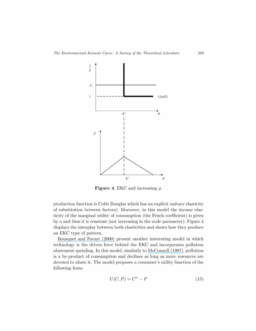
pollution is decreasing in K as long as a > 1. The Stokey’s model is compat-ible with the ES–FC model because the elasticity of substitution betweenfactors ρ is zero for K ≤ (B

α )−1/(a+γ−1) and it is one otherwise (because the

The Environmental Kuznets Curve: A Survey of the Theoretical Literature 209

1

1

Figure 4. EKC and increasing ρ.

production function is Cobb Douglas which has an explicit unitary elasticityof substitution between factors). Moreover, in this model the income elas-ticity of the marginal utility of consumption (the Frisch coefficient) is givenby a and thus it is constant (not increasing in the scale parameter). Figure 4displays the interplay between both elasticities and shows how they producean EKC type of pattern.

Bousquet and Favart (2000) present another interesting model in whichtechnology is the driven force behind the EKC and incorporates pollutionabatement spending. In this model, similarly to McConnell (1997), pollutionis a by-product of consumption and declines as long as more resources aredevoted to abate it. The model proposes a consumer’s utility function of thefollowing form:

U(C, P ) = Cα − P (15)

210 Pasten and Figueroa

As before, C denotes consumption and P aggregate emissions. In thiskind of models, consumer is endowed with an exogenous level of income, M .Pollution increases with income and decreases with abatement spending A

which requires to be financed by exogenous income such that A = M − C.Pollution is given by the following function:

P = aC − b(A)β = aC − b(M − C)β (16)

The consumer has to find the optimal level of pollution that maximizesutility given by:

maxC

Cα − aC + b(M − C)β

subject to 0 ≤ C ≤ M .Assuming that β = 1, the first-order condition is given by;

αCα−1 − (a + b) ≥ 0

It is possible to show that a corner solution with C = M holds for anyM ≤ (a+b

α )1/(α−1); consequently, P = aM , i.e., pollution grows monoton-ically with income. In addition for income levels M > (a+b

α )1/(α−1) thefirst-order condition holds with equality and the pollution path is givenby P = (a + b)(a+b

α )1/(α−1) − bM which is a decreasing function of income.Therefore pollution describes a first increasing and then decreasing charac-teristic of the EKC (in fact the curve depicts a break point rather than aturning point). As we will see, this model can also be framed within theES–FC framework. Note from (15) that the income-elasticity of marginalutility (the Frisch coefficient) is given by the constant 1−α, with α ∈ [0, 1].In addition, for income levels below the turning point, and assuming againthat the state variable M is associated to the state variable K (see pre-vious discussion about Stockey’s model) the production function can beexpressed as f = min(K, 1

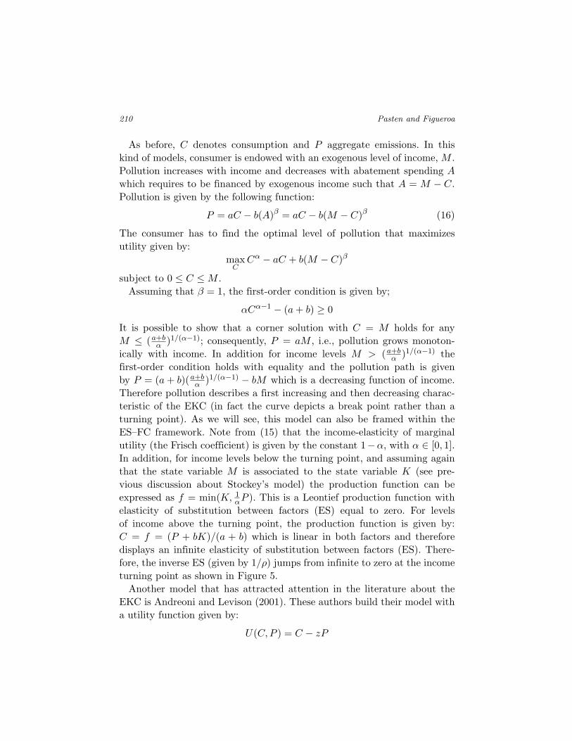
αP ). This is a Leontief production function withelasticity of substitution between factors (ES) equal to zero. For levelsof income above the turning point, the production function is given by:C = f = (P + bK)/(a + b) which is linear in both factors and thereforedisplays an infinite elasticity of substitution between factors (ES). There-fore, the inverse ES (given by 1/ρ) jumps from infinite to zero at the incometurning point as shown in Figure 5.

Another model that has attracted attention in the literature about theEKC is Andreoni and Levison (2001). These authors build their model witha utility function given by:

U(C, P ) = C − zP

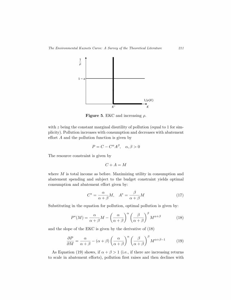
The Environmental Kuznets Curve: A Survey of the Theoretical Literature 211

1

Figure 5. EKC and increasing ρ.

with z being the constant marginal disutility of pollution (equal to 1 for sim-plicity). Pollution increases with consumption and decreases with abatementeffort A and the pollution function is given by

P = C − CαAβ, α, β > 0

The resource constraint is given by

C + A = M

where M is total income as before. Maximizing utility in consumption andabatement spending and subject to the budget constraint yields optimalconsumption and abatement effort given by:

C∗ =α

α + βM, A∗ =

β

α + βM (17)

Substituting in the equation for pollution, optimal pollution is given by:

P ∗(M) =α

α + βM −

(α

α + β

)α (β

α + β

)β

Mα+β (18)

and the slope of the EKC is given by the derivative of (18)

∂P

∂M=

α

α + β− (α + β)

(α

α + β

)α (β

α + β

)β

Mα+β−1 (19)

As Equation (19) shows, if α + β > 1 (i.e., if there are increasing returnsto scale in abatement efforts), pollution first raises and then declines with

212 Pasten and Figueroa

income, describing the EKC pattern. The intuition behind the model is asfollows: at low levels of income, the cost of abating pollution is excessivelyhigh and pollution grows with income. As income grows, however, and givenincreasing returns to scale in the abatement function, the cost of abatingpollution declines and, at some point, it becomes less expensive for firms togrow out of pollution.

The model proposed by Andreoni and Levinson can also be understoodas a special case of the ES–FC model. In Andreoni and Levinson’s model,utility is linear in both arguments; consequently, the Frisch Coefficient iszero i.e., a = 0. From (17) it is possible to show that

A =β

αC

Thus the pollution function can be expressed as a function of consumptionalone

P = C −(

β

α

)β

Cα+β,

Then, it is possible to show that the parameter 1/ρ in (7) is given by

1ρ(C)

= 1 −(

β

α

)β

(α + β)Cα+β−1

It is easy to show that 1/ρ(C) is decreasing in C as long as α+β > 1. ThusAndreoni and Levinson’s model corresponds to Figure 3b for the specificcase of a = 0.

All the examples presented in this section have highlighted the role tech-nology plays in determining the occurrence of the EKC. In the next sectionwe present a model where preferences are the driven force behind the EKC.

4 EKC Driven by Preferences (The Income Effect)

Lopez (1994) was the first to propose an EKC explained by changing pref-erences. In Lopez’s model, revenue R is a function of income f , pollution P

and the price vector w, such that

df

dP= −UP (R, P, w)

Uf (R, P, w)=

∂R

∂P(P, f, w)

The Environmental Kuznets Curve: A Survey of the Theoretical Literature 213

If the production function is a CES production function, with the constantelasticity of substitution represented by ρ, it is possible to show that

dP

df

>

<0 if and only if

1ρ

>

<a(f)

which is equivalent to condition (7) where a(f) = −fUff/Uf is the FrischCoefficient or the degree of curvature of the utility function in income, whichLopez assumes it is increasing in income such that da/df > 0. He makes thisassumption because it is a ‘‘plausible’’ condition necessary for his results;therefore, according to Equation (7) the income turning point f∗ solves thefollowing equation ρa(f∗) = 1.

If f < f∗, given that a′(f) > 0, ρa(f) < 1 and according to (7), pollutionincreases with income. On the contrary, if f > f∗, pollution decreases withincome.

In an extension to the previous model, Lopez and Mitra (2000) studiedthe implications of corruption and rent-seeking behavior from the part of thegovernment for the relation between pollution and growth. In their modelthe condition for the occurrence of the EKC when income increases is:

dP

df

>

<0 if and only if

1ρ

>

<

a(f)(1 + ϑ)

(20)

where ϑ indicates the degree of corruption of the government, and ϑ = 0indicates zero government corruption. In the no corruption case, the con-dition in (20) collapse to (7), i.e., to the case of a social optimal level ofpollution. However, if the government is corrupt (ϑ > 0) and it can be shownthat 1 > (ρa(f∗))/(1+ϑ) and f∗ is the turning point associated to zero cor-ruption. Thus, when there is corruption, at f∗ pollution is increasing withincome rather than being constant and as a result the income turning pointwith corruption is higher than the turning point f∗ without corruption.4

Lieb (2002) shows that satiation in consumption is a sufficient conditionfor an EKC to emerge. He uses the following explicit form of the utilityfunction U(C, P )

U(C, P ) =C1−a

1 − a− B(P + ε)γ

γ(21)

where B > 0, a > 0, γ > 1 and satiation in consumption implies that a > 1.This model can be restated in the context of a Cobb–Douglas production

4 See Figure 1 in Lopez and Mitra (2000, p. 144).

214 Pasten and Figueroa

function with an elasticity of substitution between factors ES constant andequal to 1. In Lieb’s model the interplay between the ES and the incomeelasticity of the marginal utility of consumption (the Frisch coefficient, FC)is the same as in the Stokey’s model; therefore, Figure 4 applies. As canbe seen in Figure 4 a condition for the EKC to emerge is a > 1 both inStokey and Lieb models. The contribution of Lieb was to show that a > 1is equivalent to satiation in consumption, which is a necessary condition foran EKC to emerge.

Copeland and Taylor (2003) (C&T hereafter) develop a model where envi-ronmental demand changes with economic growth. One assumption of theirmodel is that government translates the changes in society’s preferences intoefficient environmental regulations under neutral economic growth. In thesecircumstances, a sufficient condition for the EKC to arise is an increasingin income elasticity of willingness to pay ε. If ε < 1 pollution grows withincome otherwise pollution decreases with economic growth.

As an example, C&T used the following indirect utility function:

V (p, I, Z) = α1 − α2 exp(

−C

λ

)− dP (22)

where, V (·) is an indirect utility function; λ, α1, α2 and d are positive con-stants; C is consumption which is equal to real income, and P is pollutionemissions. Population N is indexed to be equal to 1. The marginal rate ofsubstitution between pollution and consumption is given by:

h(C, P ) =dλ

C2exp

(C

λ

)

Given a Cobb–Douglas production function, fp = β(C/P ) optimal pollutionis given by:

P ∗ =(

αβ

dλ

)C exp

(C

λ

)

According to this result, pollution raises with economic growth if C < λ

and declines with economic growth if C > λ. According to (22), the Frischcoefficient is given by C/λ which is increasing in income while the elasticityof substitution between factors is a constant equal to one (because the pro-duction function is a Cobb–Douglas function) so the Copeland and Taylormodel is also an special case of the FC–ES model presented above.

The Environmental Kuznets Curve: A Survey of the Theoretical Literature 215

5 Deriving the Environmental Kuznets Curve

5.1 A Closed Form of the EKC

To gain more insights about the EKC, we replace the implicit welfare func-tion in (1) by the following explicit form:

U(C, P ) = − µ

1 + µ

(λ − C

µ

)1+µ

− P 1+µ

1 + µ, λ ≥ 0 (23)

where µ and λ are parameters. Note that no restrictions are imposed on thesigns of the parameters in (23) other than λ being non-negative. The firstterm on the right-hand side of (23) is social utility in income, with a formsimilar to an hyperbolic absolute risk aversion (HARA) class of preferencesbroadly used in the economics of risk and uncertainty (see, for example,Eeckhoudt et al., 2005). The HARA system of preferences encompasses themost commonly used forms of utility functions depending on the valuesassigned to the underlying parameters µ and λ.5

To have a well-behaved utility function, if µ ≥ 0 (23) is defined for c ≤ µλ

such that µλ is an upper bound on consumption. On the contrary, if µ ≤ 0the welfare function is defined in the domain c ≥ µλ, such that µλ is alower bound in consumption.6 If λ = 0 and µ < 0, (23) collapses to theconstant elasticity of substitution (CES) utility function with elasticity ofsubstitution −1/µ. Furthermore, the parameter µ reflects the weight givento pollution in the welfare function, and thus it is possible to associate theparameter µ with the level of perceived harmfulness of the contaminant,with a higher value of µ implying a less harmful pollutant.

According to (23) the marginal rate of substitution between consumptionand pollution is given by:

h(C, P ) =(

µP

µλ − c

)µ

And if we assume that the production function is given by the followingconstant elasticity of substitution production function (CES):

C = [αKρ−1

ρ + βPρ−1

ρ ]ρ

ρ−1

5 See Feigenbaum (2003) for a comprehensive description of HARA utility functions.6 When µ = 0, consumption is unbounded.

216 Pasten and Figueroa

where α and β are parameters and ρ is the elasticity of substitution betweenfactors. Then, marginal product of pollution is given by

fP = β

(C

P

) 1ρ

Equalization between the marginal rate of substitution h(·) and themarginal product of pollution fP yields:

(µP

µλ − c

)µ

= π = β

(C

P

) 1ρ

(24)

where π corresponds to the equilibrium relative price of pollution in terms ofconsumption. The left-hand side of (24) can be interpreted as the marginaldamage caused by pollution while the right-hand side is pollution’s marginalbenefit. If the marginal damage is fully internalized by society, the EKCincome–pollution relationship can be derived in a straightforward fashionfrom (24):

P =(

β

µµ

) ρ

µρ+1

(µλ − C)µρ

µρ+1 C1

µρ+1 (25)

From (25) it is possible to derive the corresponding turning point CT asgiven by:

CT (µ, λ, ρ) =µλ

1 + µρ≥ 0 (26)

This general model with this general utility function encompasses mostmodels of the EKC based on preferences. In fact, in this model the Frischcoefficient is given by a(C) = µC/(µλ − C) which is increasing in incomeda(C)/dC = µ2λ/(µλ − C)2 > 0 for C ≤ µλ as long as λ > 0, i.e., aslong as the utility function is bounded from above. Therefore, as long as theutility function is bounded from above, the Frisch coefficient is increasing inincome while the elasticity of substitution between factors ρ is constant, sothis model subsumes the Lopez’s model.

On the other hand, Lieb (2002) uses graphic explanations to show that anEKC arises when there is an upper bound in the utility function. However,in our model utility is bounded because consumption is bounded as long asµ > 0, with an explicit bliss point in consumption equal to CA = µλ whichcould possibly be infinite.

Regarding the model proposed by Stokey (1998), it is worth noting herethat in Equation (23) if λ = 0 and µ < 0, (27) collapses to a power utility

The Environmental Kuznets Curve: A Survey of the Theoretical Literature 217

function in consumption and 1/a corresponds to the constant elasticity ofsubstitution between consumption and environment where a = −µ. More-over, in this particular case it is possible to express the income elasticity ofenvironment as:

η =1

1 + µ(a − 1)

(D − Q

Q

)(27)

and environmental quality increases monotonically with income if a > 1,decreases with income if a < 1 and is constant when a = 1. These arethe same conditions highlighted by Stokey (1998) in analyzing the shapeof the EKC. However, the constant elasticity of substitution, as seen inEquation (7), does not yield an inverted U curve; rather, it simply explainsmonotonic relationships between pollution and growth. In threshold modelslike Stokey’s, an additional mechanism must be imposed to describe an EKC.This ad-hoc mechanism implicitly assumes that the elasticity of substitutionbetween factors is zero below the income threshold and is one beyond thatthreshold and the Frisch coefficient is greater than 1 and consequently theEKC is an inverted V-shaped relationship (see Figure 4). However, as wehave pointed out before, we believe that the EKC is better explained by thechanging and smooth adaptive character of preferences as described in themodel presented in this section than by ad-hoc thresholds mechanisms.

Finally, Copeland and Taylor (2003, p. 84) present a closed structuralform for the EKC based on a constant absolute risk aversion (CARA). Asexplained above, the HARA class of preferences includes all of the best-known types of preferences. In particular, the consumption component ofutility in expression (23) collapses to Copeland and Taylor’s CARA prefer-ences as long as µ → ∞; therefore, Copeland and Taylor is a quite specificand restricted case of our more general closed form of an EKC. Moreover,it is possible to show that the elasticity of marginal damage in our model isgiven by:

εMD,C =µC

µλ − C

and becomes the particular form on page 85 of Copeland and Taylor (2003)when µ → ∞,

εMD,C =C

λ

Therefore, Copeland and Taylor’s model is also embedded within our moregeneral model.

218 Pasten and Figueroa

5.2 Comparative Static of the Turning Point

To study the comparative static of the turning point it is possible todifferentiate (26) with respect to the main parameters of our model, i.e., inµ, λ, and ρ

CTµ (µ, λ, ρ) =

λ

(1 + µρ)2≥ 0

CTλ (µ, λ, ρ) =

11 + µρ

≥ 0

CTρ (µ, λ, ρ) = − µ2λ

1 + µρ≤ 0

An increase in either µ or λ or a decrease in ρ would increase the incomelevel at which the turning point CT occurs. An increase in µ — associatedwith a less harmful pollutant — reduces the Frisch coefficient for each levelof income, implying that the impact of economic growth on the marginaldamage of pollution is lower and the turning point is reached at higher lev-els of income. An increase in λ increases the level of income at which themarginal utility of consumption becomes zero (i.e., satiation occurs) lead-ing to a higher turning point and therefore implying that societies become‘‘greener’’ at higher levels of income in comparison to societies with lowervalues of λ. This is consistent with recent empirical studies showing differentturning points for different countries (Koop and Tole, 1999; List and Gallet,1999; Markandya et al., 2006) and particularly with Figueroa and Pasten(2009) which found that for a given pollutant, Canada and the United Stateshave higher turning points than European countries. Finally, a decrease inρ implies that for firms it is more difficult to substitute polluting factorswith non-polluting factors and therefore a turning point would be reachedat higher levels of income.

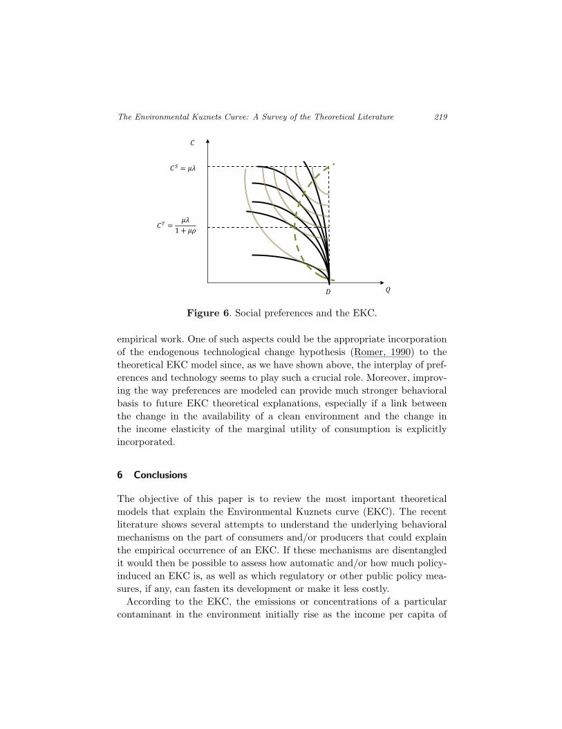
The consumption–environment (income–pollution) relationship derivedfrom Equation (25) is represented by the segmented curve in Figure 6.

The closed form for the EKC we have presented here highlights someresearch avenues to be explored in the future. Even though it is clear thatboth preferences and technology may play a role in determining the EKCoccurrence, it seems interesting to analyze and disentangle their relativeimportance. To answer this question not only empirical work will needto be carried out in the future but also theoretical analysis could shedlight on some crucial aspects that may provide some leads for the required

The Environmental Kuznets Curve: A Survey of the Theoretical Literature 219

Figure 6. Social preferences and the EKC.

empirical work. One of such aspects could be the appropriate incorporationof the endogenous technological change hypothesis (Romer, 1990) to thetheoretical EKC model since, as we have shown above, the interplay of pref-erences and technology seems to play such a crucial role. Moreover, improv-ing the way preferences are modeled can provide much stronger behavioralbasis to future EKC theoretical explanations, especially if a link betweenthe change in the availability of a clean environment and the change inthe income elasticity of the marginal utility of consumption is explicitlyincorporated.

6 Conclusions

The objective of this paper is to review the most important theoreticalmodels that explain the Environmental Kuznets curve (EKC). The recentliterature shows several attempts to understand the underlying behavioralmechanisms on the part of consumers and/or producers that could explainthe empirical occurrence of an EKC. If these mechanisms are disentangledit would then be possible to assess how automatic and/or how much policy-induced an EKC is, as well as which regulatory or other public policy mea-sures, if any, can fasten its development or make it less costly.

According to the EKC, the emissions or concentrations of a particularcontaminant in the environment initially rise as the income per capita of

220 Pasten and Figueroa

a country or city increases over time, reach a maximum and then declineeven though income per capita keeps growing. If these presumptions aresupported by empirical evidence, it would then be possible to expect that,economic growth would contain the mechanisms for reversing the initialupward trend in pollution emissions or concentrations observed in severalcountries and for several pollutants. However, it is important to point outthat all initial optimism about the implications for sustained developmentof the EKC was soon challenged by some authors skeptics of the existence ofan automatism built into the EKC relationship (Panayotou, 1997; Figueroaand Pasten, 2000; Stern, 2004).

Here we have reviewed the EKC models of the literature driven by tech-nology or/and preferences. A useful feature of our review is that all thesemodels are presented in a common theoretical framework that allows a bet-ter understanding of the underlying mechanisms theoretically driving theEKC occurrence in each type of model.

Moreover, our main contribution is the more general model we propose,which uses a closed form of the social welfare function and does not imposeany ad hoc behavioral restrictions on preferences and technology. The modelwe propose here has two specially attractive features: (1) it encompasses asspecial cases all the EKC models in the literature for which the income effectsover preferences as well as their interplay with the factor of production’selasticity of substitution are the driving forces explaining the occurrence ofthe EKC; and, (2) it is suitable to empirical testing. As a result of its spec-ification, in our model the income turning point of the EKC is determinedby how harmful is the contaminant at stake, how green or environmentallyconscious is the society, and by the elasticity of substitution between factorsin the production functions.

The closed form social welfare function we present is similar in structureto the well-known hyperbolic absolute risk aversion (HARA) preferences. Itrequires no ad hoc, additional restrictions on the demand or supply side ofindividuals’ behavior for society to follow a development path which exhibitsthe shape of the environmental Kuznets curve as income increases. Someadditional restrictions, for example, on the degree of the curvature of pref-erences or the point in time at which pollution abatement technologies areincorporated that are imposed in the existing literature to generate theEKC, can be treated as special cases of the social preference-driven modelwe proposed here.

The Environmental Kuznets Curve: A Survey of the Theoretical Literature 221

Acknowledgements

We are thankful for the very useful comments provided by Ramon Lopez,an anonymous referee and several colleagues attending our seminars inChile, Germany, The Netherlands and USA. Any error remains of our soleresponsibility.

Appendix A

Remembering that h = fp, the left hand side in (6) can be rewritten as:

fkh

(hc

h− fpk

fkfp

)

Dividing and multiplying by c = f , this equation becomes

fkh

C

(hcC

h− fpkf

fkfp

)(A1)

The second term inside brackets is the inverse of the elasticity of substitutionbetween factors ρ = (fkfp)/(fpkf) (see Lopez, 2004) h is the marginal rateof substitution between consumption and pollution thus h = −(UP /UC),assuming non-separable preferences (i.e., UPC = 0) as is usual in this typeof literature,

hC =UP

UC

UCC

UC

And the first term inside brackets in (A1) becomes (hcC/h) = −(UCCC/

UC) = a, finally,

hCfK − fPK = −fkh

C

(1ρ

− a

)

As required in Equation (6)

References

Andreoni, J. and A. Levinson. 2001. “The Simple Analytics of the Environmental KuznetsCurve.” Journal of Public Economics 80: 269–286.

Arrow, K., B. Bolin, R. Constanza, P. Dasgupta, C. Folke, C. Holling, B. O. Jansson,S. Levin, K. G. Maler, C. Perring, and D. Pimentel. 1995. “Economic Growth, CarryingCapacity and the Environment.” Science 268: 520–521.

222 Pasten and Figueroa

Ascher, W. 1999. Why Governments Waste Natural Resources: Policy Failures in Devel-oping Countries. Baltimore: The John Hopkins University Press.

Auty, R. M. 2003. “Natural Resources, Development Models and Sustainable Devel-opment.” Discussion Papers 24136, International Institute for Environment andDevelopment, Environmental Economics Programme.

Auty, R. M. and A. H Gelb. 2001. “Political Economy of Resource-abundant States.”In Resource Abundance and Economic Development, R. M. Auty, ed., Oxford UniversityPress, Oxford.

Beckerman, W. 1992. “Economic Growth and the Environment. Whose Growth? WhoseEnvironment?” World Development 20: 481–496.

Barbier, E. B. (ed.). 1997. “Special Issue: ‘The Environmental Kuznets curve.”’ Environ-ment and Development Economics 2: Part 4.

Beede, D. and D. Wheeler. 1992. “Measuring and Explaining Cross-establishment Varia-tion in the Generation and Management of Industrial Waste.” World Bank mimeo.

Bousquet, A. and P. Favart. 2000. “Does Kuznets’s Belief Question the EnvironmentalKuznets Curve?” IDEI Working Paper No. 107.

Cole, M. A., A. J. Rayner, and M. Bates. 1997. “The Environmental Kuznets Curve: AnEmpirical Analysis.” Environment and Development Economics 2(4): 401–416.

Copeland, B. R. and M. S. Taylor. 2003. Trade and the Environment: Theory and Evidence.Princeton, New Jersey: Princeton University Press.

Dinda, S. 2001. “A Note on Global EKC in Case of CO2 Emission.” Kolkata: EconomicResearch Unit, Indian Statistical Institute, Mimeo.

Dinda, S. 2004. “Environmental Kuznets Curve Hypothesis: A Survey.” Ecological Eco-nomics 49: 431–455.

Eeckhoudt, L., C. Gollier, and H. Schlesinger. 2005. Economic and Financial DecisionsUnder Risk. Princeton, New Jersey: Princeton University Press.

Feigenbaum, J. 2003. Symmetries of the HARA Class. Department of Economics,University of Pittsburgh.

Figueroa, E. and R. Pasten. 2000. “Crecimiento y medio ambiente: Existe automatismoen la U invertida?” In Comercio e Integracion de las Americas, eds., J. M. Villasusoand R. Trejos, Banco Interamericano de Desarrollo. BID. “Instituto Interamericano deCooperacion para la Agricultura (IICA). pp. 43–49.

Figueroa, E. and R. Pasten. 2009. “Country-specific Environmental Kuznets Curves:A Random Coefficient Approach Applied to High-Income Countries.” Estudios deEconomıa 36: 5–32.

Figueroa, E. and R. Pasten. 2012. “Income and the Pollution Path: Update and Exten-sions.” Working Paper, Economics Department, Universidad de Chile.

Gangadharan, L. and M. Valenzuela. 2001. “Interrelationship Between Income, Health andthe Environment: Extending the Environmental Kuznets Curve hypothesis.” EcologicalEconomics 36: 513–531.

Grossman, G. and A. Krueger. 1992. “Environmental Impacts of a North American FreeTrade Agreement.” Discussion Papers in Economics No. 158, Princeton, NJ: WoodrowWilson School of Public and International Affairs.

Grossman, G. and A. Krueger. 1995. “Economic Growth and the Environment.” QuarterlyJournal of Economics 110(2): 352–377.

Harbaugh W., A. Levinson, and D. Wilson. August 2002. “Reexamining the Empirical Evi-dence for an Environmental Kuznets Curve.” The Review of Economics and Statistics84(3): 541–551.

Hettige, H., M. Mani, and D. Wheeler. 2000. “Industrial Pollution in Economic Develop-ment: The Environmental Kuznets Curve Revisited.” Journal of Environmental Eco-nomics and Management 62: 445–476.

Holtz-Eakin, D. and T. M. Selden. 1995. “Stoking the Fires? CO2 Emissions and EconomicGrowth.” Journal of Public Economics 57: 85–101.

Horvath, R. J. 1997. Energy Consumption and the Environmental Kuznets Curve Debate.Australia: Department of Geography, University of Sydney, Mimeo.

The Environmental Kuznets Curve: A Survey of the Theoretical Literature 223

John, A., R. Pecchenino, D. Schimmelpfennig, and S. Schreft. 1995. “Shortlived Agentsand the Long-lived Environment.” Journal of Public Economics 58: 127–141.

Karl, T. L. 1997. The Paradox of Plenty, ‘Oil Booms and Petro-States. Berkeley: Universityof California Press.

Kaufmann, R. K., B. Davidsdottir, S. Garnham, and P. Pauly. 1997. “The Determinants ofAtmospheric SO2 Concentrations: Reconsidering the Environmental Kuznets Curve.”Ecological Economics 25: 209–220.

Khanna, N and F. Plassmann. 2004. “The Demand for Environmental Qualityand the Environmental Kuznets Curve Hypothesis.” Ecological Economics, 51:225–236.

Koop, G. and L. Tole. 1999. “Is There an Environmental Kuznets Curve for Deforesta-tion?” Journal of Development Economics 58: 231–244.

Krueger, A. 1993. Political Economy of Policy Reform in Developing Countries. CambridgeMA: MIT Press.

Layard, R., S. Nickell, and G. Mayraz. 2008. “The Marginal Utility of Income.” Journalof Public Economics 92: 1846–1857.

Lieb, C. M. 2002. “’The Environmental Kuznets Curve and Satiation: A Simple StaticModel.” Environment and Development Economics 7: 429–448.

Lieb, C. M.. 2004. “The Environmental Kuznets Curve and Flow versus Stock Pollu-tion: The Neglect of Future Damages.” Environmental and Resource Economics 29:483–506.

List, J. A. and C. A. Gallet. 1999. “The Environmental Kuznets Curve: Does One SizeFit All?” Ecological Economics 31: 409–423.

Lopez, R. 1994. “The Environment as A Factor of Production: The Effects of EconomicGrowth and Trade Liberalization.” Journal of Environmental Economics and Manage-ment 27: 163–184.

Lopez, R. and S. Mitra. 2000. “Corruption, Pollution and the Kuznets EnvironmentCurve.” Journal of Environmental Economics and Management 40: 137–150.

Lucas, R. E. B., D. Wheeler, and H. Hettige. 1992. “Economic Development, Envi-ronmental Regulation and the International Migration of Toxic Industrial Pollution:1960–1988.” In International Trade and the Environment, World Bank DiscussionPaper 159, ed. P. Low, pp. 67–87.

Markandya, A., A. Golub, and S. Pedroso-Galinato. 2006. “Empirical Analysis ofNational Income and SO2 Emissions in Selected European Countries.” Environmental& Resources Economics 35: 221–257.

McConnell, K. E. 1997. “Income and the Demand for Environmental Quality.” Environ-ment and Development Economics 2: 383–399.

Nahman, A. and G. Antrobus. 2005. “The Environmental Kuznets Curve: A LiteratureSurvey.” South African Journal of Economics 73: 105–120.

Panayotou, T. 1997. “Demystifying the Environmental Kuznets Curve: Turning ABlack Box into a Policy Tool.” Environment and Development Economics 2:465–484.

Pasten, R. and E. Figueroa. 2012. “Nonadditive Preferences and the EnvironmentalKuznets Curve.” Working Paper, Economics Department, Universidad de Chile.

Roberts, J. T. and P. E. Grimes. 1997. “Carbon Intensity and Economic Development1962–1991: A Brief Exploration of the Environmental Kuznets Curve.” World Devel-opment 25: 191–198.

Roca, J., E. Padilla, M. Farre, and V. Galletto. 2001. “Economic Growth and Atmo-spheric Pollution in Spain: Discussing the Environmental Kuznets Curve Hypothesis.”Ecological Economics 39(1): 85–99.

Romer, P. M. 1990. “Endogenous Technical Change.” Journal of Political Economy 98(5)Part 2: 71–102.

Ross, M. L. 2001. “Does Oil Hinder Democracy?” World Politics 53: 325–361.Sachs, J. D. and A. Warner. 1995. “Economic Reform and the Process of Globalization.”

Brookings Papers on Economic Activity 1: 1–118.

224 Pasten and Figueroa

Selden, T. M. and D. Song. 1994. “Environmental Quality and Development: Is There AKuznets Curve for Air Pollution Emissions?” Journal of Environmental Economics andManagement 27: 147, 162.

Shafik, N. 1994. “Economic Development and the Environmental Quality: An EconometricAnalysis.” Oxford Economic Papers.

Shafik, N. and S. Bandyopadhyay. 1992. “Economic Growth and Environmental Quality:Time Series and Cross-Country Evidence.” Background Paper for the World Develop-ment Report 1992 Washington DC: The World Bank.

Stern, D. I. 1998. “Progress on the Environmental Kuznets Curve.” Environment andDevelopment Economics 3: 173–196.

Stern, D. I. 2003. “The Environmental Kuznets Curve.” Paper presented to the Interna-tional Society for Ecological Economics.

Stern, D. I. 2004. “The Rise and Fall of the Environmental Kuznets Curve.” World Devel-opment 32(8): 1419–1439.

Stern, D. I., M. S. Common, and E. B. Barbier. 1996. “Economic Growth and Environmen-tal Degradation: The Environmental Kuznets Curve and Sustainable Development.”World Development 24: 1151–1160.

Stern, D. I. and M. S. Common. 2001. “Is There an Environmental Kuznets Curve forSulfur?” Journal of Environmental Economics and Management 41(2): 162–178.

Stokey, N. L. 1998. “Are There Limits to Growth?” International Economic Review 39(1):1–31.

Suri, V. and D. Chapman. 1998. “Economic Growth, Trade and Energy: Implications forthe Environmental Kuznets Curve.” Ecological Economics 25(2): 195–208.

Tahvonen, O. and J. Kuuluvainen. 1993. “Economic Growth, Pollution and Renew-able Resources.” Journal of Environmental Economics and Management 24:101–118.

Tiffen, M. and M. Mortimore. 1994. “Malthus Controverted: The Role of Capital andTechnology in Growth and Environment Recovery in Kenya.” World Development 22:997–1010.

Woolcock, M., L. Pritchett, and J. Isham. 2001. “The Social Foundations of Poor Eco-nomic Growth in Resource-rich Economies.” In Resource Abundance and EconomicDevelopment, ed. R. M. Auty, New York: Oxford University Press.

World Bank. 1992. “Development and the Environment.” World Development Report1992, Development and the Environment. NY: Oxford University Press, p. 11.

Yandle, B., M. Bhattarai and M. Vijayaraghavan. 2004. “Environmental Kuznets Curves:A Review of Findings, Methods, and Policy Implications.” PERC. Research Study 02-1.